mapping oil palm density at country scale: an active
TRANSCRIPT

Mapping oil palm density at country scale: An active learning approach
Andres C. Rodrıgueza, Stefano D’Aroncoa, Konrad Schindlera, Jan D. Wegnera,b
aEcoVision Lab - Photogrammetry and Remote Sensing, ETH Zurich, SwitzerlandbInstitute for Computational Science, University of Zurich, Switzerland
Abstract
Accurate mapping of oil palm is important for understanding its past and future impact on the environment. We propose to map andcount oil palms by estimating tree densities per pixel for large-scale analysis. This allows for fine-grained analysis, for exampleregarding different planting patterns. To that end, we propose a new, active deep learning method to estimate oil palm densityat large scale from Sentinel-2 satellite images, and apply it to generate complete maps for Malaysia and Indonesia. What makesthe regression of oil palm density challenging is the need for representative reference data that covers all relevant geographicalconditions across a large territory. Specifically for density estimation, generating reference data involves counting individual trees.To keep the associated labelling effort low we propose an active learning (AL) approach that automatically chooses the mostrelevant samples to be labelled. Our method relies on estimates of the epistemic model uncertainty and of the diversity amongsamples, making it possible to retrieve an entire batch of relevant samples in a single iteration. Moreover, our algorithm has linearcomputational complexity and is easily parallelisable to cover large areas. We use our method to compute the first oil palm densitymap with 10 m Ground Sampling Distance (GSD) , for all of Indonesia and Malaysia and for two different years, 2017 and 2019.The maps have a mean absolute error of ±7.3 trees/ha, estimated from an independent validation set. We also analyse densityvariations between different states within a country and compare them to official estimates. According to our estimates there are, intotal, >1.2 billion oil palms in Indonesia covering >15 million ha, and >0.5 billion oil palms in Malaysia covering >6 million ha.
Keywords: Palm oil, Tree density, Large-scale mapping, Active learning, Sentinel-2, Deep learning
1. Introduction
Oil palm is the third largest oil crop in the world by plantedarea, and accounted for 35% of the vegetable oil productionin the world in 2019 [1]. With the highest yield per hectareof any fat oil it is an attractive economic alternative in manytropical countries [2]. However, large-scale oil palm produc-tion in Malaysia and Indonesia is a potential driver of defor-estation [3, 4]. Several works relate oil palm development withlong-lasting effects on the environment, including loss of bio-diversity [5], poor air quality and high greenhouse gas emis-sions [6, 7]. On the other hand, it plays an important role forseveral aspects of the socio-economical life in producer coun-tries, including positive impacts on the welfare of smallholderproducers [8]. Balancing the economic and social benefits ofoil palm plantations with the impact it has on the environmentis a challenging task. We refer the reader to [9] for a thoroughanalysis of the ethics around the palm oil industry.
Transparent, evidence-based policies for sustainable palmoil production are only possible with accurate maps at country-scale and beyond. Besides, to assess long-term impacts theyshall be frequently updated. This calls for a highly automated,objective mapping process. Several authors have studied waysto map oil palm plantations with remote sensing data, e.g., [10,11, 12]. They mostly focus on classifying the land cover intooil palms vs. background. Such a binary approach implicitly
assumes that oil palms occur only as predominant land cover,in closed-canopy plantations with a certain minimum density,and is prone to missing smaller or less dense plantings. Thismay be a reason for the large variation between different esti-mates of planting area. We argue that a map of oil palm density(respectively, tree count per pixel) is preferable, as it is morerobust to non-uniform densities and at the same time allows fora more detailed analysis.
A general bottleneck of land cover mapping with supervisedmachine learning is the need for accurate, manually collectedlabels [13]. Although for some applications public online datacan be used, for instance from openstreetmap.org [14], nosuch data is available for more specific mapping tasks, includ-ing oil palm density. The standard procedure to ensure that thelearned models generalise across large, geographically diverseregions is to collect a large and diverse set of manually anno-tated reference labels, but that brute-force approach is labori-ous, and therefore time-consuming and costly.
Active learning (AL) offers a possible solution, by focusingthe (manual) labelling effort on a much smaller set of train-ing examples that optimally represent the data distribution [15],thus reducing the total annotation effort required to achieve agiven mapping accuracy. The starting point for AL is the obser-vation that naively selected training samples usually are highlyredundant, such that the marginal utility of each additional sam-ple is low. The goal of AL is to accumulate the same evidence
May 25, 2021
arX
iv:2
105.
1120
7v1
[cs
.CV
] 2
4 M
ay 2
021

with a much smaller number of samples, by gradually addingnew samples that are selected in an informed manner, so asto maximise their utility. The active construction of the train-ing set is guided by the assumption that, in order to improve a(preliminary) prediction function, one must supply it with thecorrect answers for those inputs that it has not yet learned tohandle. This leads to the following principles:
1. to decide which additional samples to label, predictionuncertainty is a useful indicator to identify samples withhigh marginal utility, respectively low redundancy withrespect to the training data used so far.
2. if, for efficiency reasons, multiple samples are added ineach round, then they should be as different from eachother as possible, to avoid redundancy within the newlyadded batch.
The function that combines uncertainty and diversity into a scorefor selecting new samples is commonly termed the acquisitionfunction.
In the context of mapping, the set of unlabelled samplescorresponds to the entire target region, in our case more than106 km2 at 10 m ground sampling distance (GSD). Most exist-ing AL methods were not designed for such extremely largedatasets and do not scale well enough. For instance, manymethods require that the model be retrained multiple times, andeach time, it must predict the output for the entire unlabelleddata set to pick new samples, which is extremely costly forlarge regions. Another strategy that makes it possible to ex-tract a large and varied training set in a single shot requires thepre-computation of all pairwise similarities between candidatesone may want to add in the next round [16] – the computationalcomplexity of that operation is obviously quadratic in the dataset size. To leverage AL for country-scale mapping, in our caseof oil palms, one must design a strategy that remains viable withmillions of pixels, which in practice means its computationalcomplexity should scale (approximately) linearly with the areaof the region (respectively, the number of pixels) and require asfew active learning iterations as possible.
In this work we produce a country-scale map of oil palmdensity, by devising an active learning procedure that scales tolarge remote sensing datasets. The contribution of our paper istwofold:
• We design a practical AL methodology for large-scale ap-plications in remote sensing. The method relies on animplicit ensemble of randomly perturbed convolutionalnetworks to estimate model uncertainty, together with anefficient core-set construction that uses distances betweenthe data points’ learned feature embeddings to efficientlyassemble a representative and diverse training set. OurAL approach scales linearly with the number of unla-belled samples and requires only 2 processing cycles overthe area of interest.
• By applying our AL system to Sentinel-2 imagery of Ma-laysia and Indonesia, we produce a 10 m GSD, wall-to-wall map of oil palm density for those two countries,which together account for 84% of the world’s palm oil
production1. In contrast to other oil palm mapping effortssuch as [12, 17, 10] we map not only the presence/absenceof oil palm plantations, but the tree density (oil palms per100 m2 pixel). The map thus provides richer informationfor further geo-spatial analysis. For instance, it can reveallocal variations in planting patterns, production intensity,and potentially relations to yield. 2
2. Related work
2.1. Oil palm mapping
Several authors have created maps of oil palm plantationsfrom remote sensing data. Some use only Synthetic ApertureRadar (SAR) [18, 11], which is unaffected by the frequent cloudcoverage in tropical regions [10]. Perhaps even more popu-lar is the combination of optical and Radar images [19, 20,21, 22, 23, 12, 17, 24]. Only a few works map oil palmsat country-wide or continental scales. [10] provide a oil palmmap over 15 countries from around the world using, ALOS-2/PALSAR-2 data from 2016 at a 25 m GSD. [17] use ALOS-2/PALSAR-2 and MODIS to generate a map of palm oil plan-tations in Malaysia and Indonesia at 100 m GSD, for the years2001-2016. Recently, [12] provided a map that distinguishesbetween industrial and small-holder plantations. This map cov-ers all areas suitable for palm oil production at a GSD of 10 mand was derived from Sentinel-1 (SAR) and Sentinel-2 (Opti-cal) images from 2019.
2.2. Density estimation
Density estimation is a recurrent task in remote sensing, in-cluding for instance the estimation of population density [25,26] and canopy density [27, 28]. Still, land cover is in mostcases mapped only as a presence/absence label. Apparentlyspecies-specific tree density estimation has rarely been con-sidered as an alternative. Most authors prefer to only detecttrees (respectively forest or plantation areas), presumably be-cause the size of individual trees is below the pixel footprintof wide-area satellite sensors. However, earlier work [29] hasdemonstrated that density estimation for sub-pixel trees is fea-sible. In agricultural applications in particular, density maps al-low for a more advanced analysis than binary land-cover mapsof the crop. This is potentially important for oil palm planta-tions, where the distance between trees is known to correlatewith the yield per tree [30, 31].
2.3. Active learning in remote sensing
A fairly large body of literature exists about active learn-ing methods for remote sensing. Early works often relied onSupport Vector Machines (SVM) [32, 33, 34, 35]. Uncertainsamples are identified as those that fall within the margin of theSVM classifier (and thus also have a high likelihood to become
1Figure for the year 2019, according to [1]210m resolution maps for 2017 and 2019 are available on request.
2

0
Oilpalmdensity
0.75 1.5
Figure 1: Oil Palm Density Map over South-east Asia in 2017 using our proposed method. We estimate a total of 1.7 billion oil palms in Indonesia and Malaysia.We present the average density over 10m pixels for illustration.
support vectors). Those works already recognised the impor-tance of diversity and proposed measures to avoid that mul-tiple similar training samples are added in the same iterationof the active learning loop [32]. In [33], the authors analysedifferences and similarities between active learning and semi-supervised learning and propose a method that combines them,leveraging the distance from a training sample to the supportvectors as a measure of uncertainty to select new samples. In[36] Gaussian Processes were used for classification, since theyoffer a natural mechanism to represent model uncertainty and,thereby, select informative samples.
Active learning with neural networks dates back to at least[37] in the remote sensing literature. While neural networksachieve excellent predictions in many image analysis tasks, theysuffer from a well-known limitation that is critical in the con-text of AL, namely that their estimates of uncertainty are poorlycalibrated. The standard work-around, already used by [37],is to employ stochastic ensembles of models to quantify pre-diction uncertainty. To reduce the computational cost, recentactive learning schemes tend to avoid explicit multi-model en-sembles and instead use more efficient approximations. For in-stance, [38] use Monte Carlo (MC) dropout [39] to estimatemodel uncertainty. Moreover, that paper compares different ac-quisition functions, and confirms that significant performancegains can be achieved with active (rather than random) selec-tion of samples. [40] combine AL with domain adaptationto detect which samples of a new target domain need to be
labelled to improve the performance of a pre-trained modelon the target domain. They propose a method based on opti-mal transport that, however, relies on having a fully labelledtraining set in the source domain. [41] use AL for binarychange detection between co-registered image pairs. To repre-sent model uncertainty they use Monte Carlo Batch Normalisa-tion (MCBN) [42], another form of randomisation within thenetwork to approximate an ensemble. Besides showing thatMCBN can indeed substitute an explicit ensemble without per-formance penalty, the authors also show that AL tends to bal-ance the training examples if the class distribution is highly im-balanced – which is often the case in remote sensing when somecomparatively rare target class should be separated from a dom-inant “background”. [16] proposes a single shot active learningapproach where a relatively large and diverse core-set of sam-ples is extracted from the unlabelled dataset. The main charac-teristic of the method is that the active learning is not iterative:the core-set is extracted only once and neglects prediction un-certainty. The limitation with this approach is that the cost ofbuilding such a core-set is quadratic in the size of the unlabelleddataset.
A main challenge, without an accepted standard solution,remains the question how to scale AL to large-scale scenarios.The typical scenario in remote sensing is that the “unlabelleddata”, from which one has to select the samples to be anno-tated, is the entire area of interest with hundreds of millionsof pixels. But most AL methods either are iterative, requir-
3

ing a new prediction pass over the unlabelled set each time themodel is retrained, or, in order to build larger effective sets forlabelling, have a quadratic complexity with respect to the un-labelled dataset (i.e., at least implicitly they form and examineall possible pairs of samples in the unlabelled set). To remaintractable one would therefore have to limit them to a tiny por-tion of the mapping area, which, if done naively, runs the riskof missing important parts of the data distribution. We aim tosolve these problems with an approximate measure of samplediversity that has computational complexity linear in the sizeof the unlabelled dataset, yet makes it possible to extract a di-verse set of samples with few (in practice even a single) activelearning iterations.
3. Data
3.1. Area of study
This study focuses on a geographical area that comprisesthe countries of Malaysia and Indonesia. We produce a 10 mGSD, wall-to-wall map of oil palm density for those two coun-tries, which together account for 84% of the world’s palm oilproduction. This covers a land area of 1.3 · 106km2 or 1.3 ·109 Sentinel-2 pixels. See Figure 1 for an overview of the oilpalm density map. According to our estimates there are, in to-tal, >1.2 billion oil palms in Indonesia covering >15 million ha,and >0.5 billion oil palms in Malaysia covering >6 million ha.See more details in Section 5.
3.2. Sentinel-2 imagery
As input to our model, we use Sentinel-2 Level-2 bottom-of-atmosphere reflectance images acquired in 2017 and 2019.The Level-2 images were obtained using sen2cor [43]. Allchannels are re-sampled to a common pixel size of 10 m withbicubic interpolation and stacked into 13-channel images. First,we filter out all pixels that are labelled as cloud, cloud shadow,water or snow in the scene classification layer provided by sen-2cor [43]. Moreover, we use only pixels with <50% cloud prob-ability for training (according to the cloud mask from sen2cor),and only pixels with <10% cloud probability for validation andinference. We use a different cloud probability for training tobe more robust to different cloud conditions. At test time, thestricter cloud threshold yields a cleaner estimate less influencedby clouds.
To create a dense map without gaps, we process each im-age separately and then average all predictions at each locationover the entire year. Instead of directly mosaicing images intoa single composite before processing, we process all imagesand perform a late fusion of results. Major advantages are thatwe avoid radiometric distortions from composite images withdifferent atmospheric conditions and, more importantly, we en-sure that the model learns to process images with a great vari-ety of atmospheric conditions, such that it can be applied to anySentinel-2 image without retraining.
We download and process Sentinel-2 images for the entireyears 2017 and 2019. Using all available images allows us tocompute dense, wall-to-wall maps without holes that provide
an oil palm density estimate at every land pixel across Malaysiaand Indonesia, despite the high cloud coverage that is commonin tropical South-east Asia.
3.3. Reference data
To obtain reference oil palm density maps to train and eval-uate our method, we rely on very high-resolution overhead im-agery (GSD < 30cm). At that resolution, individual trees areclearly visible and we thus manually annotated a total of 3.4·106
oil palms. All annotations were made with images acquired in2017. A 30-min training was required for students to learn toidentify oil palm plantations and not confuse them with othercrops such as coconut or sugar palms that are also present inthe area of the study. Only general notions of suitable areasof oil palm plantations were required for labelling (e.g., tropi-cal areas and elevations below 1500m [44]). We aimed at la-belling blocks of at least 250 ha each spanning large geographi-cal areas. Manual annotators were asked to label oil palm plan-tations and to include as background examples other types ofland cover, such as coconut plantations and forests. Inside eachblock, we obtained the centre location of each oil palm as ob-served on the very-high resolution imagery; to obtain a smoothdensity map at Sentinel-2 resolution (GSD 10m) we applied asmoothing operation with a squared kernel of 20 × 20 meterson a high-resolution grid (GSD 0.625 m) of the oil palm lo-cations and then summed the densities under each Sentinel-2pixel. This results in local oil palm density maps that can beused for training and validation of our proposed method. Seemore details in Section 5.2 about the geographical split of trainand validation areas.
4. Methods
4.1. Estimation of oil palm density
Following [29], instead of attempting to predict the loca-tions of individual oil palms, which are smaller than the GSDof the input images, we predicted the count of oil palms perpixel. This way, the estimation of oil palm density can besolved as a supervised regression task. We used a Convolu-tional Neural Network (CNN), F(x), that predicts the count ofoil palms per pixel, y, using the raw intensities of Sentinel-2image x. The architecture of the CNN (i.e., layers, hyperpa-rameters) is based on our previous work [29]. F(x) consistsof an input convolutional layer, and 15 residual layers of theform xout = h(xin) + xin. The residual layers [45] learn additiveupdates to the input features, which has emerged as a particu-larly successful strategy for many computer vision and imageanalysis tasks. In our case, each function h(x) has three se-quential convolutional layers. After every layer we include(i) batch normalisation [46], and (ii) a Rectified Linear Unit(ReLU) as activation function. Batch normalisation tracks thesecond-order statistics in each batch and uses them to standard-ise the values between different layers so as to reduce the sen-sitivity of the network to small changes between the batchesof samples that are fed during training. ReLU is an element-wise non-linear transformation of the form xout = max(0, xin) (it
4

3. Solve k-means with Bcentres using .
1. Train base model
2. For each region in compute
Base labelled dataset
Unlabelled dataset
4. Create with the B centroids
6. Train improved model using .
Algorithm 1
7. Use for inference
5. Obtain labels for sample in
Figure 2: Active Learning method overview: F0(x) is the model trained onlywith the base labelled dataset L. The acquisition function g(x) can be com-puted in parallel for each region in the unlabelled dataset U and computed asdescribed in Equation 2. g(x) is based on an estimate of the Epistemic Uncer-tainty and the distance to the centre of gravity of all data points in U. Theset A is the actively selected samples chosen using the Algorithm 1 in SectionAppendix A.1
is a basic principle of neural networks to interleave linear lay-ers with element-wise non-linearities to approximate complexfunctions [47]). Furthermore, we have two different branches asoutput: (i) y for the predicted count, and (i) ycl for a binary clas-sification task between pixel with oil palms and the background.Note that at each layer we kept the same resolution of the imagefrom input to output, different from other architectures that re-duce the resolution of the input image with an encoder and thenup-sample the resolution with a decoder [48, 49, 50] . Thisallowed us to retain the input resolution and map at the originalGSD without upsampling issues. See Section Appendix A.1for more details on the architecture in the supplementary mate-rial.
To train the model parameters of F(x) we used a refer-ence density map that was obtained by identifying individualoil palms in high-resolution imagery as described in Section3.3. The loss function to train the model is a sum over the twobranches,
Loss = (y − y)2 + CE(ycl, [y > 0]) . (1)
The right-most part of Eq. 1 is the cross-entropy (CE) be-tween the predicted class and a binary indicator that separatesbackground pixels with density 0 from oil palms. Specifically,we used F(x) to perform a regression for each pixel in theimage, where we only predicted the number of oil palms perpixel in the image. For further details, refer to Rodriguez et al.(2018) [29]. For simplicity, from now on we do not distinguishbetween the density prediction and the auxiliary classificationoutput and simply denote the network output as y.
4.2. Active learning
To start with, we defined our interest region X made up of avery large number N of samples x. In our case, each individual10m pixel from Sentinel-2 Images in the area of study is onesample x. We created an Active setA for which we annotateda subset of x (i.e., Sentinel-2 pixel) with the desired outputs y(i.e., oil palm density) using an annotation budget B, such thatwe can fit the model parameters θ and then apply the modelto all the remaining (unlabelled) samples. The goal of activelearning is to cleverly pick the most informative training datapoints until exhausting the budget B, such that we capture themost relevant correlations between radiometric input patternsin x and output densities y.
Base initial training F0(x)This leads to a chicken-and-egg problem: in the absence of
any information about the model F we cannot measure howimportant a sample x is for fitting it, except for the general intu-ition that the sample set should be diverse, so as to capture thevariability of the inputs. Hence, one has to annotate an (ideally,small) initial training set L = {xl, yl} and train a preliminarymodel F0. That function can now be applied to the setU = {xu}
of unlabelled samples to obtain estimates yu = F0(xu).
Acquisition functionThe fundamental assumption of active learning is that one
can determine from yu which samples should be labelled to im-prove the model, even without having access to the true val-ues yu (and thus to the correctness of yu). To that end the esti-mates are scored with an acquisition function g(y), and the oneswith the highest scores are used to construct A = {x∗}, theircorresponding labels y∗ are obtained with manual annotators,and a new model F1 is obtained using L and the new samples{x∗, y∗} The function g(x) is typically based on the estimateduncertainty of the prediction, often in the form of a predictedvariance σ2(y). Following the reasoning that the model must beimproved in those regions of the data space where it is uncer-tain [51, 38, 41].
Even if g(y) is an effective proxy for the actual objective todecrease the prediction error, the described procedure is onlyoptimal if new samples are added one by one until the avail-able annotation budget B is exhausted at iteration FB
θ . Unfor-tunately, it is not practically viable to run the computationallyexpensive model fitting every time a sample has been added, soone has to add multiple samples at a time to the training set –ideally one could add all B samples in one shot and retrain onlyonce. This leads to a new problem: the set A containing the Bhighest scoring samples can (and often will) contain redundantpatterns, i.e., the scores g(yi), g(y j) are similarly high becausetheir corresponding image observations xi, x j are also similar.But showing the same pattern to the model multiple times atthe cost of excluding other, yet unseen ones is wasteful and willundermine the idea of active learning.
Consequently, the acquisition function, in this case, shouldbe a set function that evaluates the benefit of adding an entireset of training data points, rather than individual points.
5

(a) Active selection of 15 samples (b) Manual selection of 15 samples (c) Naive selection of 15 samples
Figure 3: Comparison of different sampling strategies from the available samples
5 15 30 50Samples
0.36
0.38
0.40
0.42
0.44
RMSE
[Oil
palm
s / p
ixel
]
Comparison Active Learning vs Randomized labelling
BaseActiveManualNaïve
Figure 4: Comparison of active learning approach vs. two baselines. Error barsare standard deviations from 5 different runs of naıve and manual selection.
Core-set approachesA core-set is a smaller subset that summarises a large data
collection in terms of the relevant properties for some task –for instance in the case of clustering, a good core-set is onethat yields clusters similar to the ones obtained by clusteringthe complete (usually much larger) data set [52]. In our case,a good core-set is a training set that leads to predicted out-puts similar to those that would be learned if annotations wereavailable for all data points. The use of core-sets for activelearning was pioneered by [16]. However, their work has twomajor drawbacks: (i) it ignores the model uncertainty; and (ii) itdoes not scale to large data sets, as it requires an exhaustive setof pairwise (dis-)similarities between data points to assess di-versity. This second point highlights a more general principle:set functions are in general more expensive to compute thanper-point scores, so we need to design our acquisition functioncarefully to ensure it remains tractable even for large values ofN and B.
Proposed acquisition functionTo address the two limitations previously mentioned, we
propose to construct A with samples to be labelled by usingthe following acquisition function:
g(xi) =σ2(yi)∑
j∈Uσ2(y j)︸ ︷︷ ︸
Uncertainty
+dz(xi, µ)2∑
j∈Udz(x j, µ)2︸ ︷︷ ︸
Diversity
, (2)
where µ is the centre of gravity (mean value) of the projecteddata points x j ∈ U in a suitable feature space z, and dz is thecorresponding distance measure. Instead of computing dis-tances directly in the input space of image intensities, we com-pute them in a space z that provides meaningful distances withrespect to our task at hand. In our case the natural choice isto compute the (Euclidean) distances between deep activationmaps in the deep network, see Section 4.3 below.
The first term is simply the variance of the prediction (nor-malised over the unlabelled set) and corresponds to the standardassumption in active learning, that points with high uncertaintyshould be added to the training set. The price to pay is that theg(x) is no longer a true set function, and does not prevent theselected samples from lying far from the mean but close to eachother in the data space.
Active learning setA constructionOur solution to re-introduce pairwise dissimilarity is to se-
lect a larger set of q candidate points (in our implementation,q = 1 · 105) with the highest scores g(xi), then cluster theminto B clusters with weighted k-means, assigning each samplethe weight 1
q·g(xi). To constructA, from each cluster we retained
only the candidate that lies nearest to the cluster centre. Thissimple trick ensures that no two training samples are closer toeach other than the cluster radius. Note that, moreover, the clus-tering makes the selection more robust against outliers, whichmight otherwise dominate the core-set selection, as they tend tolie far from the mean µ. See Figure 2 for an overview of ourentire workflow.
6

Figure 5: Full dataset with 30 active samples
30 20 10 0 10 20 30
30
20
10
0
10
20
30
Figure 6: 2-D tSNE visualisation of the deep features from the core-set selectedfor the area of study. In red the selected areas for labelling.
4.3. Implementation
After introducing the general framework, we go on to dis-cuss practical details of the technical implementation, with aparticular focus on large-scale deployment with images totallinghundreds of giga-pixels.
Uncertainty EstimationTo select informative samples, we must estimate the predic-
tion uncertainty σ2(y) (first term in eq.(2)). More specifically,we are looking for samples with high epistemic uncertainty [53], i.e. the uncertainty that arises from the model parameters dueto limited training data. A standard way to represent epistemicuncertainty numerically, if the model fitting includes stochas-tic elements, is to learn multiple instances of the model andview their predictions as Monte-Carlo samples from the poste-rior distribution of the output y. For the case of neural networks,random initialisation and stochastic gradient descent providethe basis for such an ensemble strategy. A more efficient alter-native is Monte-Carlo dropout [39], where the model ensembleis approximated by multiple runs of the same model, where ineach run a given proportion of the model parameters is sup-pressed. In this way one avoids having to train multiple mod-
els, at the cost of potentially less well-calibrated uncertaintyestimates [54]. With an ensemble of T model predictions it isstraight-forward to derive an ensemble prediction y = 1
T∑T
t=1 yt
and and uncertainty estimate
σ2(y) =1T
T∑t=1
(yt − y)2 (3)
Distance function and deep feature embeddingTo quantify the distance dz(xi, x j) between two samples we
used the learned feature representation in the second-last layerof the neural network F. To achieve a meaningful embeddingthat is representative across the complete area of study, we alsoincluded a pixel’s location, such that the distance function canadapt to geographical variations. To inject the geographical lo-cation into the network we used Space2Vec encoding [55],which relies on a grid representation of relative and absolutepositions and allows the model to learn correlations at differentscales. Intuitively, Space2Vec uses each pixel (longitude andlatitude) location and computes its angle with respect to differ-ent directions in space, relative distances from each directionsare computed at different scales, this allows our model to in-corporate information from other pixels at different scales. Formore details refer to [55].
Overall, the following transformation is applied to an inputx at location (xlat,lon):
location encoding: r = Space2Vec(xlat,lon) (4)CNN activations: e = Fe(x) (5)
attention: a = A([r, e]) (6)final embedding: Fz(x) = a · [r, e] (7)
where [r, e] denotes concatenation along the channel dimen-sion. Space2Vec is trained on our small, initial training set L.The function Fe just reads out the activations (i.e. the outputa specific layer in the CNN) from the density prediction net-work F. The simple attention mechanism A consists of a 1 × 1convolution followed by a sigmoid function and determines therelative importance (weight) of the features from each pixel inthe image. The final embedding Fz(x) is the product of the CNNactivations and the location encoding; since the latter is a valuebetween [0, 1], it can be interpreted as a re-weighting value forCNN activations. The similarity between two data samplesis then defined as the squared Euclidean distance between theirembeddings, dz(xi, x j) = ‖zi − z j‖
22.
4.4. Large scale implementation
The second term of Eq. (2) is the distance from a samplex to the dataset mean µ. Computing each individual distancedz(x, µ)2 as well as the cumulative distance can easily be par-allelised across multiple machines for large-scale deployment.To do this one simply splits the area of interest into Q mutuallyexclusive regions and processes each of them on a different ma-chine. We first computed the number of samples n, the sum vand sum of squares w of the deep embedding z, for all samples
7
0 25 50 75 100 125 150 175 200Predicted Density (Trees/ha)
0
25
50
75
100
125
150
175
200
Grou
nd T
ruth
(Tre
es/h
a)
MAE 7.30 Trees/ha
100
101
102
Freq
uenc
y
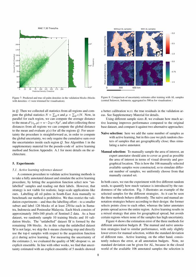
Figure 7: Predicted and true oil palm densities in the validation blocks (blockswith densities <1 were trimmed for visualisation).
in Q. Then we collected all statistics from all regions and com-pute the global statistics N =
∑Q n and µ =
∑Q v/N. Now, in
parallel for each region, we can compute the average distanceto the mean dz(xq, µ) = w−2vµ+Nµ2, and after collecting thosedistances from all regions we can compute the global distanceto the mean and evaluate g(x) for all the regions Q. For uncer-tainty the procedure is straightforward as, in order to computethe global uncertainty, we only require the cumulative sum overthe uncertainties inside each region Q. See Algorithm 1 in thesupplementary material for the pseudo-code of active learningmethod and Section Appendix A.1 for more details on the ar-chitecture.
5. Experiments
5.1. Active learning reference datasetA common procedure to validate active learning methods is
to take a fully annotated dataset and simulate the active learningprocedure, by letting the acquisition function select new “un-labelled” samples and reading out their labels. However, thatstrategy is not viable for realistic, large-scale applications likeours. Labelling all oil palms in South-East Asia manually tobenchmark our method is prohibitive. We thus restrict the vali-dation experiments – and thus the labelling effort – to a smallersubset and label 126 blocks of at least 250 ha each in Suma-tra, Indonesia and Peninsular Malaysia. Each block consists ofapproximately 160×160 pixels of Sentinel-2 data. As a basedataset, we randomly sample 10 training blocks and 10 vali-dation blocks. The “unlabelled” dataset U is formed by theremaining 106 blocks. As in this setup the unlabelled datasetU is not large, we skip the k-means clustering step and directlyuse the top-k samples with respect to the acquisition functiong(x) during active learning. For measuring the uncertainty ofthe estimates y, we evaluated the quality of MC-dropout vs. anexplicit ensemble. In line with other works, we find that uncer-tainty estimated with an explicit ensemble of 5 models showed
WithALsamples
-0.0
-0.5
-1.0
WithoutALsamples
-0.0
-0.75
-1.5
Epistem
icUn
certa
inty
Mea
npred
icted
den
sity
Figure 8: Comparison of uncertainty estimates after training with AL samples(central Sulawesi, Indonesia; aggregated to 500 m for visualisation )
a better calibration w.r.t. the true residuals in the validation ar-eas. See Supplementary Material for details.
Using different sample sizes B, we evaluate how much ac-tive learning improves performance compared to the originalbase dataset, and compare it against two alternative approaches:
Naıve selection: here we add the same number of samples aswith active learning, but in this case we pick random clus-ters of samples that are geographically close; thus simu-lating a naıve annotator.
Manual selection: To manually sample the area of interest, anexpert annotator should aim to cover as good as possiblethe area of interest in terms of visual diversity and geo-graphical location. This is how the 106 manually selectedavailable samples were constructed, so to simulate differ-ent number of samples, we uniformly choose from thatmanually curated set.
In both cases, we run the experiment with five different randomseeds, to quantify how much variance is introduced by the ran-domness of the selection. Fig. 3 illustrates an example of theselected samples for the different strategies. As it can be seenthe three methods behave differently. The naıve and manual an-notation strategies behave according to their design: the formerselects points close to each other, whereas the latter annotatespoints spread across the entire region. Active learning results ina mixed strategy that aims for geographical spread, but avoidscertain regions where none of the samples has high uncertainty.
Figure 4 shows the estimation error of the three methods fordifferent annotation budgets B. The manual and naıve annota-tion strategies lead to similar performance, with only slightlylower errors for manual selection, within the standard deviationof different runs. Active learning, on the other hand, consis-tently reduces the error, at all annotation budgets. Note, nostandard deviation can be given for AL, because in the closedworld of the available 106 annotated samples the selection is
8

1.90km
2.1
0km
GT 17896.57
1.90km
Prediction 17927.61
0.00 0.25 0.50 0.75 1.00 1.25 1.50 1.75 2.00Trees/0.01ha
Error [ha]
40 20 0 20 40Trees/ha
2.10km
1.5
0km
GT 5882.63
2.10km
Prediction 5620.96
0.00 0.25 0.50 0.75 1.00 1.25 1.50 1.75 2.00Trees/0.01ha
Error [ha]
40 20 0 20 40Trees/ha
Figure 9: Qualitative Results density estimation with manually annotated data. Left: densities per 0.01 ha block. Right: errors in Trees/ha
deterministic, and the same points will be picked in each run.We further note that the advantage of AL is smaller with veryfew samples and increases with the sample size B, a behaviouralso observed in [16].
5.2. Large-scale mappingWe start with a manually labelled base dataset of 250 re-
gions (each with at least 250 ha), out of which which we use166 for training, and 84 for validation. After training a modelon the base training dataset, we aim to predict and label 50 new
active samples. We define each region q to have size 144 ha,which in Sentinel-2 pixels represents an image patch of 1202 pixels.This results in 2 million different regions, after removing re-gions completely covered by water. We calculate the globalmean µ of the z(x) embedding from all regions in the area ofstudy, to compute the acquisition function g(x) for each region.The complete region, covering 48◦ longitude, is divided intostrips of 12◦. For each strip we draw 105 samples and use thek-means algorithm to find 50 cluster centres to be annotated asadditional training samples. The cluster centres are distributed
9

0.25 0.50 0.75 1.00 1.25 1.50 1.75Trees/pixel
0.000
0.002
0.004
0.006
0.008
0.010
Prob
abilit
y
Johor (1.005)Pahang (1.045)Perak (1.005)Sabah (0.915)Sarawak (0.865)
0.25 0.50 0.75 1.00 1.25 1.50 1.75Trees/pixel
0.000
0.001
0.002
0.003
0.004
0.005
0.006
0.007
Prob
abilit
y
W. Kalimantan (0.815)C. Kalimantan (1.035)Riau (0.905)S. Sumatera (0.845)N. Sumatera (0.925)
Figure 10: Histogram of pixel densities, for the five states with most oil palms in Malaysia and Indonesia for 2017
Saba
h
Sara
wak
Joho
r
Paha
ng
Pera
k
Nege
ri Se
mbi
lan
Tren
ggan
u
Sela
ngor
Kela
ntan
Keda
h
Mel
aka
Pula
u Pi
nang
Perli
s0
20
40
60
80
100
120
140
Tota
l Tre
es [m
]
0.0
0.2
0.4
0.6
0.8
1.0
1.2
1.4
1.6
Area
[ha]
1e6Count (2017)Count (2019)Area (2017)Area (2019)
Figure 11: Total number of oil palms vs. total planted area for the top-10 statesin Malaysia for 2017 and 2019. Only pixels with density >0.2 were counted asoil palms.
Riau
North
Sum
ater
a
Cent
ral K
alim
anta
n
Wes
t Kal
iman
tan
Sout
h Su
mat
era
East
Kal
iman
tan
Jam
bi
Wes
t Sum
ater
a
Aceh
Sout
h Ka
liman
tan
Lam
pung
Beng
kulu
Bang
ka-B
elitu
ng
Cent
ral S
ulaw
esi
Jawa
Tim
ur
0
50
100
150
200
250
300
Tota
l Tre
es [m
]
0.0
0.5
1.0
1.5
2.0
2.5
3.0
3.5
Area
[ha]
1e6Count (2017)Count (2019)Area (2017)Area (2019)
Figure 12: Total number of oil palms vs. total planted area for the top-10 statesin Indonesia for 2017 and 2019. Only pixels with density >0.2 were counted asoil palms.
across the 12◦ strips proportional to their land area. The active
learning samples were then manually annotated, resulting in thefinal dataset shown in Figure 5. To visualise how diverse ourchosen samples are compared to the rest of the dataset, we con-struct a t-SNE visualisation [56]. t-SNE non-linearly projectshigh-dimensional vectors (in our case the deep features Fz(x)from each sample) down to a low-dimensional vector (in ourcase 2-D vectors) while minimally distorting their distances.Figure 6 shows the t-SNE visualisation of our core-set sam-ples. The actively selected samples (shown as red points) arewell distributed across all deep features (blue), which indicatesa high diversity among the selected samples. Furthermore, notethat the selected samples are not only on oil palm plantationsas the model may also be uncertain about other types of veg-etation. We therefore added many samples on forest or cropsthat do not contain any oil palm trees. In practice, we ended upwith 46 labelled areas; this difference arose because our methodchose samples in areas where no cloud-free high-resolution im-ages were available for labelling.
5.3. Quantitative validation of oil palm densitiesWe quantitatively evaluate our oil palm density estimates
using validation regions not shown to the model during train-ing. All reference data was obtained by manually annotatingindividual trees in very high resolution overhead images (GSD<30cm). At the Sentinel-2 pixel size of 10 m the number oftrees per pixel is low (generally <2), and the definition un-certainty of plantation boundaries is larger than the pixel size.Thus, we aggregate both ground truth counts and predict den-sities into tree counts per 10×10 pixel block (1 ha) for the vali-dation3. Evaluating our error on 1 ha blocks allows us to com-pare if the method manages to retrieve the density for mean-ingful numbers of trees and avoid random fluctuations at pixellevel. As shown in Fig. 7, the Mean Absolute Error (MAE)
3Note that in Section 5.1, to avoid computational overhead for the differentexperiments, we evaluated directly on a 10 m pixel level in contrast to a 1 halevel.
10

Trees/pixel Descalset.al2020Industrial
Smallholder0.0 1.50.75
Figure 13: Predicted oil palm densities in smallholder and large-scale plantations
over all validation sites is 7.30 trees/ha. For comparison, us-ing only the base training dataset, the MAE was 10.14 trees/ha,in other words the error without AL samples would be 39%higher. Fig. 8 illustrates how the additional samples improve theprediction and reduce its uncertainty, in particular suppressingspurious low-density predictions in regions without oil palms.
Fig. 9 shows the true and predicted densities for two exam-ple blocks, and the corresponding errors at ha level. Althoughsome extreme density values are underestimated, the overallcounts and structure of the plantations are retrieved with highcorrectness.
Since it is not feasible to manually label several billion indi-vidual oil palm trees of all Malaysia and Indonesia, the evalua-tion of oil palm density maps beyond the manually labelled val-idation samples has to remain limited to visual inspection and aqualitative analysis. We find that extending our initial trainingset of 166 blocks with just 46 additional blocks selected by ALgreatly improves the map (Fig. 8).
5.4. Analysis of oil palm densities
To the best of our knowledge, we provide the first map ofhigh-resolution oil palm densities across the major planting re-gions of South-East Asia. According to our estimate, therewere 0.55 · 109 oil palms in Malaysia and 1.28 · 109 oil palmsin Indonesia in 2017. Assuming a cut-off threshold of >0.2trees/pixel for planted crop areas, we estimate the total area ofpalm oil plantations in 2017 to be 6.24 · 106 ha in Malaysia,respectively 16.18 · 106 ha in Indonesia. For 2019, we esti-mate 0.54 · 109 oil palms covering 6.17 · 106 ha in Malaysiaand 1.23 · 109 oil palms covering 15.29 · 106 ha in Indonesia.
Per-pixel tree counts allow us to evaluate how the tree den-sity varies across different locations, or in function of other ge-ographical factors. We show densities for individual states ofMalaysia and Indonesia in Fig. 10 for 2017 and total estimatedoil palms and covered areas for Malaysia in Fig. 11 and Indone-sia in Fig. 12.
Smallholder vs. large-scale plantations. By combining our 2019oil palm density map with the classification of [12] from the
11

0.5 1.0 1.5Trees/pixel
0.0
0.5
1.0
1.5
2.0
Freq
uenc
y
1e6 Sabah
0.5 1.0 1.5Trees/pixel
Sarawak
0.5 1.0 1.5Trees/pixel
Johor
0.5 1.0 1.5Trees/pixel
Pahang20172019
(a) Malaysia
0.5 1.0 1.5Trees/pixel
0
1
2
3
4
Freq
uenc
y
1e6 Riau
0.5 1.0 1.5Trees/pixel
N. Sumatera
0.5 1.0 1.5Trees/pixel
C. Kalimantan
0.5 1.0 1.5Trees/pixel
W. Kalimantan20172019
(b) Indonesia
Figure 14: Changes of oil palm density from 2017 vs 2019 in top-4 states bytotal area covered.
same year, we can compare the density distributions in small-holder plots versus large-scale plantations. By the definitionof [12], smallholder oil palm plantations are smaller than 25 ha,have heterogeneous tree age, and are less structured in terms ofshape and layout. Some of these features correlate with density.In Fig. 13 (top row), we can see industrial and smallholder plan-tations as mapped by [12]. Our findings support those empiricalfindings of [12]: smallholder plantations exhibit lower tree den-sities and strong, local density variations. Nonetheless, distin-guishing smallholder plantations from large-scale plantations isdifficult from Sentinel-2 satellite imagery. For example, thereis no clear threshold to distinguish smallholder from industrialplantations based solely on density, because tree density insideindustrial plantations can vary significantly, too (Fig. 13 (bot-tom row)). On our maps one can also see density predictionhighlights detailed structures inside individual plantations. Inindustrial plantations, for example, much lower densities areobserved on the access roads between blocks of oil palms.
5.5. Comparison between 2017 and 2019 oil palm density maps
We did not observe systematic density shifts from 2017 to2019, which indicates that our model generalises well acrossdifferent years.This allows us to evaluate density changes be-tween 2017 and 2019 as shown in Fig. 14. In Central Kaliman-tan, for example, the median increased from 1.035 to 1.055,which is most likely caused by new plantings with higher densi-ties, as can be observed in the histogram. A detailed view of anexample area with a large density shift is displayed in Fig. 15a,where higher density areas appear to correspond mostly to newplantations in 2019. Furthermore, in Malaysia some areas showeda decline in the amount of planted oil palms, correspondingmostly to replanting schemes (Fig. 15b).
2017
1 2Trees/Pixel
05
10152025303540
Freq
uenc
y (in
thou
sand
s)
2019
1 2Trees/Pixel
05
10152025303540
Freq
uenc
y (in
thou
sand
s)
(a) Central Kalimantan, Indonesia2017
1 2Trees/Pixel
05
10152025303540
Freq
uenc
y (in
thou
sand
s)
2019
1 2Trees/Pixel
05
10152025303540
Freq
uenc
y (in
thou
sand
s)
(b) Sabah, Malaysia
Figure 15: Detail of changes of oil palm density from 2017 vs 2019 in selectedareas
5.6. Validation of predicted land-cover
Although our primary goal is density estimation, we canalso compare our approach with land cover maps that only showbinary presence/absence of oil palms. Recently [12] publisheda worldwide map that focuses on classifying smallholder vs. in-dustrial plantations. See Figure 16 for a comparison in selectedareas.
The Malaysian Palm Oil Board (MPOB) [58] provides monthlystatistics about the area planted with mature oil palms in everystate. In Figure 17 we compare their estimates, [12] and ours.For Indonesia, we obtain official reports for 2019 from the Min-istry of Agriculture [59]. We compare in Table 1 those to areaestimates from our map, with cut-off thresholds of >0.2 and>0.4 trees/pixel. The lower threshold yields estimates closerto the official statistics in Indonesia, where the area has appar-ently been over-estimated, both with respect to our estimatesand to [12]. On the other hand, thresholding our estimates at0.4 aligns better with [12]. These large differences in Indone-sia could possibly be explained by the way the plantations aredelineated for the official statistics.
Overall, we observed a slight reduction of total planted areaof 1.15% for the whole country. For example, in Sabah, Malaysiawe found a decrease of 6.95% (in contrast to official statisticsreporting a decrease of only 1.9%). As illustrated in Fig. 15bchanges can be due to replanting schemes on previously denselyplanted areas.
6. Discussion
Our experiments indicate that oil palm density can be effi-ciently retrieved at large scale from Sentinel-2 imagery. Per-pixel tree density has a number of potential advantages overconventional presence/absence land cover maps. One advan-tage of density maps, compared to conventional land cover maps,is additional evidence about changes in palm tree density across
12

0 50 100 150 200
0
25
50
75
100
1.20km
2.4
0km
GT 21.1 103 Trees
1.20km
2.4
0km
Pred 20.2 103 Trees
1.20km
2.4
0km
Area GT 199.9 ha
1.20km
2.4
0km
Area Pred 201.2 ha
1.20km
2.4
0km
Area Descals 220.7 ha
0 100 200
0
50
100
150
1.90km
2.1
0km
GT 17.9 103 Trees
1.90km
2.1
0km
Pred 19.5 103 Trees
1.90km
2.1
0km
Area GT 170.7 ha
1.90km
2.1
0km
Area Pred 166.8 ha
1.90km
2.1
0km
Area Descals 170.5 ha
0 50 100 150
0
50
100
150
1.80km
1.9
0km
GT 11.1 103 Trees
1.80km
1.9
0km
Pred 10.1 103 Trees
1.80km
1.9
0km
Area GT 105.5 ha
1.80km
1.9
0km
Area Pred 81.1 ha
1.80km
1.9
0km
Area Descals 52.9 ha
Figure 16: Comparison with [57] for 2019 selected areas. In Descals maps, Dark and light green denote industrial and small-holder plantations respectively
13

Saba
hSa
rawa
kJo
hor
Paha
ngPe
rak
Nege
ri Se
mbi
lan
Tren
ggan
uSe
lang
orKe
lant
anKe
dah
0.0
0.2
0.4
0.6
0.8
1.0
1.2
1.4
Area
[ha]
1e6Ours (0.2)Ours (0.4)Descals2019Official
(a) Malaysia
Riau
N. S
umat
era
C. K
alim
anta
nW
. Kal
iman
tan
S. S
umat
era
E. K
alim
anta
nJa
mbi
W. S
umat
era
Aceh
S. K
alim
anta
n
0.0
0.5
1.0
1.5
2.0
2.5
3.0
3.5
Area
[ha]
1e6Ours (0.2)Ours (0.4)Descals2019Official
(b) Indonesia
Figure 17: Predicted area of oil palm per state/country for 2019. Ours(t) in-dicates estimated area with different minimum density thresholds per pixel t ∈{0.2, 0.4}. Official statistics from Malaysia and Indonesia are from MPOB[58]and the Indonesian Ministry of Agriculture [59], respectively
Ours (0.2) OfficialState 2017 2019 ∆% 2017 2019 ∆%
Sabah 1569.88 1460.79 -6.95 1380.04 1353.81 -1.90Sarawak 1391.65 1419.54 2.00 1342.10 1419.30 5.75Johor 965.78 941.99 -2.46 682.62 694.10 1.68Pahang 857.21 866.48 1.08 641.88 668.24 4.11Perak 470.62 523.39 11.21 360.50 363.81 0.92Negeri Sembilan 216.32 216.77 0.21 162.63 170.97 5.13Trengganu 215.72 205.22 -4.87 146.56 153.66 4.84Selangor 206.25 195.80 -5.07 128.06 117.56 -8.20Kelantan 144.90 147.30 1.66 118.09 127.22 7.73Kedah 118.75 115.25 -2.95 82.42 81.79 -0.76Melaka 68.57 64.88 -5.38 52.32 52.08 -0.46Pulau Pinang 16.13 14.44 -10.49 12.87 13.45 4.47Perlis 4.72 2.84 -39.86 0.62 0.84 36.47
Malaysia 6246.50 6174.68 -1.15 5110.71 5216.82 2.08
Table 1: Predicted area of oil palm (103ha) per state in Malaysia, in 2017 and2019. Official statistics taken from MPOB[58]
different geographical regions (Fig. 10). Such variations in den-sity distributions can largely be attributed to different plantationpatterns. For instance, in the Malaysian state of Sarawak, weobserve the lowest median density among the compared states;this translates to a larger planted area for the same numberof trees. According to official statistics of Fresh Fruit Bunch(FFB) yield in Malaysia4, the yield in Sarawak was 16.12 t/ha,compared to a national yield of 17.90, and values of 18.34 forSabah, 20.64 for Johor and 17.91 for Pahang, respectively. Wehypothesise that a lower tree density could have an impact onthe lower yield per area in Sarawak. However, this is a complexprocess that requires long term studies to asses how exactly itis influencing the yield [30, 31].
Our work presented in this paper is limited to Malaysia andIndonesia, which produce over 80% of global palm oil. In orderto inform at global level, we need to expand to further grow-
4Figures for the total FFB yield of 2017, according to [58]
ing regions like West Africa. We are currently using multi-spectral satellite images from the two Sentinel-2 satellites asdata source. The major disadvantage of optical sensors is thatthey cannot see through the frequent cloud cover in tropical re-gions. We circumnavigate this shortcoming by computing den-sity across stacks of Sentinel-2 images per location, in the hopethat any point on the ground will be visible at least once peryear. However, this incurs a substantial computational burden.Like [12] we will thus explore the possibility to add Sentinel-1SAR imagery to our approach, to be more robust against densecloud cover.
In Indonesia, official estimates were almost always higherthan our estimates and those from [12]. In fact, different cut-off
thresholds between oil palms and background for our methodyield different estimates that range between the two sources.This could be an indication that the methodology used to reportthe official planted area differs from what we define as oil palmareas. For example, at a density threshold of 0.4, roads insidelarge-scale plantations would be excluded in our map, which isalmost certainly not the case for the official statistics and for[12].
We will make all 10 m resolution maps for 2017 and 2019available upon publication of this paper.
7. Conclusions
We have proposed an active deep learning approach with acomputationally lightweight acquisition function g(x) that se-lects large datasets for labelling very efficiently. Our activelearning strategy allows to iteratively chose an optimal set ofsamples for interactive labelling, striking a balance betweenhigh diversity and high uncertainty of the selected samples.Approach and algorithm are designed to scale to entire worldregions with billions of individual object instances. We hopeto have shown that active (deep) learning is an excellent toolfor remote sensing applications to environmental problems atvery large scale, where manual annotation of sufficiently largeground truth is prohibitive.
We have applied our AL method to compute the first dense,10-meter resolution map of oil palm densities of the world’s twomain producers, Malaysia and Indonesia, with a Mean AbsoluteError of ±7.30 trees/ha. According to our maps, in 2019 therewere 0.54 billion oil palms covering 6.17 × 10⁶ ha in Malaysiaand 1.23 billion oil palms covering 15.29×10⁶ ha in Indonesia.
Credit author statement
A.C.R was responsible for the design and development ofthe methods, running experiments and writing the paper. S.D.,K.S. and J.D.W. were responsible for creating the research de-sign, writing and editing. All authors discussed the results andcontributed to the final manuscript
Acknowledgments
The project received funding from Barry Callebaut Sourc-ing AG, as a part of a Research Project Agreement.
14

Appendix A. Supplementary
Appendix A.1. Implementation and Architecture DetailsPseudo-code for Active Learning in Large scale datasets
See Algorithm 1 for details on the large scale implementa-tion of our proposed method.
Algorithm 1 Large-scale Active Learning ImplementationRequire: ensemble of T trained models Ft, M machines, anno-tation budget B, Unlabelled datasetUOutput: SetA = {x∗} with B samples to be labelled by humanexperts.
1: SplitU in Q regions.2: for each region q ∈ Q do . In parallel on M machines3: for each sample x ∈ q do4: Obtain predictions y =
∑t Ft(x)/T
5: Compute uncertainty s =∑
t(y − Ft(x))2
6: Obtain pixel count in nx
7: Obtain deep embedding statisticsv =∑
t Fzt (x) and w =
∑t Fz
t (x)8: Compute region statistics
sq =∑
x∈q s, nq =∑
x∈q nx, vq =∑
x∈q v,wq =∑
x∈q w
9: From each region, retrieve sq, nq, vq and wq
10: Compute total pixel count and global meanN =∑
nq, µ =∑
vq/N11: for each region q ∈ Q do12: Compute total distance to the global mean
dz(xq, µ) = wq − 2vqµ + Nµ2
13: For each region g(xh) =sq∑q sq
+dz(xq, µ)∑q dz(xq, µ)
14: Construct set C with the q · B regions with highest g score15: Cluster set C into B clusters with weighted k-means,
where each region has weight 1/(q · B · g(xi))16: Construct setA = {x∗} by obtaining the samples x∗ closest
toeach of the B centroids.
Architecture detailsWe implement all our experiments in Tensorflow using Python,
see Tab. A.2 for the specific architecture details of our networkF. For training we use a patch size of 16 × 16 pixels, a batchsize of 128, trained for 100 epochs and used ADAM optimiser 5
with a learning rate of 1 · 10−4. From all labeled areas we ran-domly extracted a total of 1·106 patches proportional to the areaof each labeled area.
Appendix A.2. Quality of uncertainty estimatesUncertainty estimates are only useful if they are reasonably
well calibrated with respect to the validation error we might ex-pect. In Figure A.18, we constructed a precision-recall curve
5Kingma D.P., Ba J., Adam: A method for stochastic optimization BengioY., LeCun Y., 3rd International Conference on Learning Representations, ICLR2015, San Diego, CA, USA, May 7–9, 2015, Conference Track Proceedings2015
Network F(x) 7→ yInput 7→ BlockIn 7→ ResNetBlocks(15) 7→ BlockOut 7→ (outputsem, outputreg)
BlockInInput 7→ Block(64,64,128) 7→ Conv2D(128,3) 7→ Conv3D(256,3)
ResNetBlocks(N)Input 7→ ReLU(Input + Block(64,64,256)) 7→ output (N times)
Block(n1, n2, n3)Input 7→ Conv2D(n1,3) 7→ Conv2D(n2,3) 7→ Conv2D(n3,3) 7→ output
BlockOutInput 7→ Conv2D(2,3) 7→ outputclInput 7→ Conv2D(1,3) 7→ outputreg
Table A.2: Architecture F(x) used in our method. x represents an input imagefrom Sentinel-2, the output y is the estimated density for the correspondinginput image x, ycl is the output of the auxiliary classification task, used only fortraining. Conv2D(n, k) is a convolutional operations with n filters and a filter ofsize k, before every Conv2D(n, k) a BatchNorm Layer is applied [46]. RectifiedLinear Units (ReLU) has the form xout = max(0, xin)
0.0 0.2 0.4 0.6 0.8 1.0Recall
0.00
0.02
0.04
0.06
0.08
0.10
0.12
Prec
ision
(mse
)
Quality of the Uncertainty EstimatesMC-dropoutEnsemble
Figure A.18: Calibration of MC-dropout and explicit model ensemble. Un-certainty was estimated from an ensemble of 5 models, respectively 5 forwardpasses.
based on the predicted uncertainty and the residual values fromvalidation data. The curve shows how the average MSE re-duces by removing samples with predicted uncertainty abovepercentile thresholds. Aligned with the related works, we cansee that the estimates of an ensemble of 5 models yield muchbetter calibrated estimates for the uncertainty than a MC-dropout.
15

References
[1] Unite States Department of Agriculture, Foreign Agriculture Service:Oilseeds: world markets and trade, https://www.fas.usda.gov/
data/oilseeds-world-markets-and-trade, accessed 2020-09-11.[2] E. Meijaard, J. Garcia-Ulloa, D. Sheil, S. Wich, K. Carlson, D. Juffe-
Bignoli, T. Brooks, Oil palm and biodiversity: A situation analysis by theIUCN oil palm task force, International Union for Conservation of Natureand Natural Resources (IUCN) (2018).
[3] K. G. Austin, A. Schwantes, Y. Gu, P. S. Kasibhatla, What causes de-forestation in indonesia?, Environmental Research Letters 14 (2) (2019)024007.
[4] D. L. Gaveau, B. Locatelli, M. A. Salim, H. Yaen, P. Pacheco, D. Sheil,Rise and fall of forest loss and industrial plantations in Borneo (2000–2017), Conservation Letters 12 (3) (2019) e12622.
[5] B. A. Margono, P. V. Potapov, S. Turubanova, F. Stolle, M. C. Hansen,Primary forest cover loss in Indonesia over 2000–2012, Nature ClimateChange 4 (8) (2014) 730–735.
[6] P. Noojipady, C. D. Morton, N. M. Macedo, C. D. Victoria, C. Huang,K. H. Gibbs, L. E. Bolfe, Forest carbon emissions from cropland ex-pansion in the Brazilian Cerrado biome, Environmental Research Letters12 (2) (2017) 025004.
[7] G. R. Van der Werf, D. C. Morton, R. S. DeFries, J. G. Olivier, P. S.Kasibhatla, R. B. Jackson, G. J. Collatz, J. T. Randerson, CO2 emissionsfrom forest loss, Nature Geoscience 2 (11) (2009) 737–738.
[8] L. Feintrenie, W. K. Chong, P. Levang, Why do farmers prefer oil palm?lessons learnt from Bungo district, Indonesia, Small-scale Forestry 9 (3)(2010) 379–396.
[9] E. Meijaard, D. Sheil, The moral minefield of ethical oil palm and sus-tainable development, Frontiers in Forests and Global Change 2 (2019)22. doi:10.3389/ffgc.2019.00022.
[10] Y. Cheng, L. Yu, Y. Xu, X. Liu, H. Lu, A. P. Cracknell, K. Kanniah,P. Gong, Towards global oil palm plantation mapping using remote-sensing data, International Journal of Remote Sensing 39 (18) (2018)5891–5906.
[11] A. Oon, K. D. Ngo, R. Azhar, A. Ashton-Butt, A. M. Lechner, B. Azhar,Assessment of ALOS-2 PALSAR-2L-band and Sentinel-1 C-band SARbackscatter for discriminating between large-scale oil palm plantationsand smallholdings on tropical peatlands, Remote Sensing Applications:Society and Environment 13 (2019) 183–190.
[12] A. Descals, S. Wich, E. Meijaard, D. L. A. Gaveau, S. Peedell, Z. Szantoi,High-resolution global map of smallholder and industrial closed-canopyoil palm plantations, Earth System Science Data Discussions 2020 (2020)1–22. doi:10.5194/essd-2020-159.
[13] D. Marmanis, K. Schindler, J. Wegner, S. Galliani, M. Datcu, U. Stilla,Classification with an edge: improving semantic image segmentation withboundary detection, ISPRS Journal of Photogrammetry and Remote Sens-ing 135 (2018) 158–172.
[14] P. Kaiser, J. Wegner, A. Lucchi, M. Jaggi, T. Hofmann, K. Schindler,Learning aerial image segmentation from online maps, IEEE Transactionson Geoscience and Remote Sensing 55 (11) (2017) 6054–6068.
[15] B. Settles, Active learning literature survey, Tech. rep., University ofWisconsin-Madison Department of Computer Sciences (2009).
[16] O. Sener, S. Savarese, Active learning for convolutional neural networks:A core-set approach, arXiv preprint arXiv:1708.00489 (2017).
[17] Y. Xu, L. Yu, W. Li, P. Ciais, Y. Cheng, P. Gong, Annual oil palm plan-tation maps in Malaysia and Indonesia from 2001 to 2016, Earth SystemScience Data 12 (2) (2020) 847–867.
[18] Y. Cheng, L. Yu, Y. Xu, H. Lu, A. P. Cracknell, K. Kanniah, P. Gong,Mapping oil palm extent in Malaysia using ALOS-2 PALSAR-2 data,International Journal of Remote Sensing 39 (2) (2018) 432–452.
[19] G. V. Laurin, V. Liesenberg, Q. Chen, L. Guerriero, F. Del Frate, A. Bar-tolini, D. Coomes, B. Wilebore, J. Lindsell, R. Valentini, Optical andSAR sensor synergies for forest and land cover mapping in a tropical sitein West Africa, International Journal of Applied Earth Observation andGeoinformation 21 (2013) 7–16.
[20] C. Pohl, Mapping palm oil expansion using SAR to study the impact onthe CO2 cycle, in: IOP Conference Series: Earth and Environmental Sci-ence, Vol. 20(1), IOP Publishing, 2014, p. 012012.
[21] Y. Cheng, L. Yu, A. P. Cracknell, P. Gong, Oil palm mapping using Land-sat and PALSAR: A case study in Malaysia, International Journal of Re-mote Sensing 37 (22) (2016) 5431–5442.
[22] K. Nomura, E. T. Mitchard, G. Patenaude, J. Bastide, P. Oswald, T. Nwe,Oil palm concessions in southern Myanmar consist mostly of unconvertedforest, Scientific reports 9 (1) (2019) 1–9.
[23] T. Sarzynski, X. Giam, L. Carrasco, J. S. H. Lee, Combining radar andoptical imagery to map oil palm plantations in Sumatra, Indonesia, usingthe Google Earth Engine, Remote Sensing 12 (7) (2020) 1220.
[24] V. H. Gutierrez-Velez, R. DeFries, Annual multi-resolution de-tection of land cover conversion to oil palm in the peruvianamazon, Remote Sensing of Environment 129 (2013) 154 – 167.doi:https://doi.org/10.1016/j.rse.2012.10.033.URL http://www.sciencedirect.com/science/article/pii/
S003442571200421X
[25] C. Robinson, F. Hohman, B. Dilkina, A deep learning approach for popu-lation estimation from satellite imagery, in: Proceedings of the 1st ACMSIGSPATIAL Workshop on Geospatial Humanities, 2017, pp. 47–54.
[26] P. Doupe, E. Bruzelius, J. Faghmous, S. G. Ruchman, Equitable develop-ment through deep learning: The case of sub-national population densityestimation, in: Proceedings of the 7th Annual Symposium on Computingfor Development, 2016, pp. 1–10.
[27] C. Joshi, J. De Leeuw, A. K. Skidmore, I. C. Van Duren, H. Van Oosten,Remotely sensed estimation of forest canopy density: A comparison ofthe performance of four methods, International Journal of Applied EarthObservation and Geoinformation 8 (2) (2006) 84–95.
[28] A. Rikimaru, P. Roy, S. Miyatake, Tropical forest cover density mapping,Tropical ecology 43 (1) (2002) 39–47.
[29] A. C. Rodriguez, J. D. Wegner, Counting the uncountable: Deep semanticdensity estimation from space, in: T. Brox, A. Bruhn, M. Fritz (Eds.),Pattern Recognition – German Conference on Pattern Recognition, 2019,pp. 351–362.
[30] X. Bonneau, R. Impens, M. Buabeng, Optimum oil palm planting densityin West Africa, OCL – Oilseeds and Fats, Crops and Lipids 25 (2) (2018).
[31] M. Rafii, Z. Isa, A. Kushairi, G. Saleh, M. Latif, Variation in yield compo-nents and vegetative traits in Malaysian oil palm (elaeis guineensis jacq.)dura× pisifera hybrids under various planting densities, Industrial Cropsand Products 46 (2013) 147–157.
[32] D. Tuia, F. Ratle, F. Pacifici, M. F. Kanevski, W. J. Emery, Active learningmethods for remote sensing image classification, IEEE Transactions onGeoscience and Remote Sensing 47 (7) (2009) 2218–2232.
[33] C. Persello, L. Bruzzone, Active and semisupervised learning for the clas-sification of remote sensing images, IEEE Transactions on Geoscienceand Remote Sensing 52 (11) (2014) 6937–6956.
[34] Z. Wang, B. Du, L. Zhang, L. Zhang, X. Jia, A novel semisupervisedactive-learning algorithm for hyperspectral image classification, IEEETransactions on Geoscience and Remote Sensing 55 (6) (2017) 3071–3083.
[35] Q. Shi, X. Liu, X. Huang, An active relearning framework for remotesensing image classification, IEEE Transactions on Geoscience and Re-mote Sensing 56 (6) (2018) 3468–3486.
[36] S. Sun, P. Zhong, H. Xiao, R. Wang, Active learning with Gaussian pro-cess classifier for hyperspectral image classification, IEEE Transactionson Geoscience and Remote Sensing 53 (4) (2014) 1746–1760.
[37] M. Roy, S. Ghosh, A. Ghosh, A neural approach under active learningmode for change detection in remotely sensed images, IEEE Journal ofSelected Topics in Applied Earth Observations and Remote Sensing 7 (4)(2013) 1200–1206.
[38] J. M. Haut, M. E. Paoletti, J. Plaza, J. Li, A. Plaza, Active learning withconvolutional neural networks for hyperspectral image classification us-ing a new bayesian approach, IEEE Transactions on Geoscience and Re-mote Sensing 56 (11) (2018) 6440–6461.
[39] Y. Gal, Z. Ghahramani, Dropout as a bayesian approximation: Represent-ing model uncertainty in deep learning, in: International Conference onMachine Learning, 2016, pp. 1050–1059.
[40] B. Kellenberger, D. Marcos, S. Lobry, D. Tuia, Half a percent of labels isenough: Efficient animal detection in UAV imagery using deep CNNs andactive learning, IEEE Transactions on Geoscience and Remote Sensing57 (12) (2019) 9524–9533.
[41] V. Ruzicka, S. D’Aronco, J. D. Wegner, K. Schindler, Deep activelearning in remote sensing for data efficient change detection, in:ECML/PKDD Workshop on Machine Learning for Earth Observation,2020.
[42] M. Teye, H. Azizpour, K. Smith, Bayesian uncertainty estimation for
16

batch normalized deep networks, in: International Conference on Ma-chine Learning, 2018, pp. 4907–4916.
[43] J. Louis, V. Debaecker, B. Pflug, M. Main-Knorn, J. Bieniarz, U. Mueller-Wilm, E. Cadau, F. Gascon, Sentinel-2 sen2cor: L2a processor for users,in: Living Planet Symposium 2016, 2016, pp. 1–8.
[44] J. Pirker, A. Mosnier, F. Kraxner, P. Havlık, M. Obersteiner, What are thelimits to oil palm expansion?, Global Environmental Change 40 (2016)73–81. doi:https://doi.org/10.1016/j.gloenvcha.2016.06.
007.URL https://www.sciencedirect.com/science/article/pii/
S0959378016300814
[45] K. He, X. Zhang, S. Ren, J. Sun, Deep residual learning for image recog-nition, in: Proceedings of the IEEE conference on computer vision andpattern recognition, 2016, pp. 770–778.
[46] S. Ioffe, C. Szegedy, Batch normalization: Accelerating deep networktraining by reducing internal covariate shift, in: International conferenceon machine learning, PMLR, 2015, pp. 448–456.
[47] S. Haykin, Neural networks and learning machines, 3/E, Pearson Educa-tion India, 2010.
[48] O. Ronneberger, P. Fischer, T. Brox, U-net: Convolutional networks forbiomedical image segmentation, in: International Conference on Medicalimage computing and computer-assisted intervention, Springer, 2015, pp.234–241.
[49] L. Chen, G. Papandreou, I. Kokkinos, K. Murphy, A. L. Yuille, Deeplab:Semantic image segmentation with deep convolutional nets, atrous con-volution, and fully connected crfs, IEEE Transactions on Pattern Analysisand Machine Intelligence 40 (4) (2018) 834–848. doi:10.1109/TPAMI.2017.2699184.
[50] V. Badrinarayanan, A. Kendall, R. Cipolla, Segnet: A deep convolutionalencoder-decoder architecture for image segmentation, IEEE transactionson pattern analysis and machine intelligence 39 (12) (2017) 2481–2495.
[51] Y. Gal, R. Islam, Z. Ghahramani, Deep bayesian active learning with im-age data, in: International Conference on Machine Learning, 2017, pp.1183–1192.
[52] O. Bachem, M. Lucic, A. Krause, Scalable k-means clustering vialightweight coresets, in: Proceedings of the 24th ACM SIGKDD Inter-national Conference on Knowledge Discovery & Data Mining, 2018, pp.1119–1127.
[53] A. Kendall, Y. Gal, What uncertainties do we need in bayesian deep learn-ing for computer vision?, in: Advances in Neural Information ProcessingSystems, 2017, pp. 5574–5584.
[54] Y. Ovadia, E. Fertig, J. Ren, Z. Nado, D. Sculley, S. Nowozin, J. Dillon,B. Lakshminarayanan, J. Snoek, Can you trust your model’s uncertainty?Evaluating predictive uncertainty under dataset shift, in: Advances inNeural Information Processing Systems, 2019, pp. 13991–14002.
[55] G. Mai, K. Janowicz, B. Yan, R. Zhu, L. Cai, N. Lao, Multi-scale rep-resentation learning for spatial feature distributions using grid cells, in:International Conference on Learning Representations, 2020.
[56] L. van der Maaten, G. Hinton, Visualizing data using t-SNE, Journal ofMachine Learning Research 9 (2008) 2579–2605.
[57] A. Descals, Z. Szantoi, E. Meijaard, H. Sutikno, G. Rindanata, S. Wich,Oil palm (elaeis guineensis) mapping with details: Smallholder versusindustrial plantations and their extent in Riau, Sumatra, Remote Sensing11 (21) (2019) 2590.
[58] Malasian Palm Oil Board: Yield and area estimates 2017 and 2019,http://bepi.mpob.gov.my/index.php/en/yield/yield-2017/
yield-2017.html, accessed 2020-10-01.[59] Indonesian Ministry of Agriculture, http://agriexchange.apeda.
gov.in/MarketReport/Reports/Oilseeds_and_Products_
Update_Jakarta_Indonesia_02-01-2020.pdf, accessed 2020-11-01.
[60] D. P. Kingma, J. Ba, Adam: A method for stochastic optimization, in:Y. Bengio, Y. LeCun (Eds.), 3rd International Conference on LearningRepresentations, ICLR 2015, San Diego, CA, USA, May 7-9, 2015, Con-ference Track Proceedings, 2015.URL http://arxiv.org/abs/1412.6980
17