mapping of indoor environments by robots using low...
TRANSCRIPT

Mapping of Indoor Environments
by Robots using Low-cost Vision Sensors
Trevor Taylor B.E. (Hons Chem), M.S.Ch.E., M.S.E.E.
Submitted in fulfilment of the requirements for the degree of
Doctor of Philosophy
Faculty of Science and Technology
Queensland University of Technology
2009

Dedicated to my sister, Lyndal, who lost her battle with cancer before I could finish
this thesis. Thanks for all the encouragement. I’ll miss you sis.
Mapping of Indoor Environments by Robots using Low-Cost Vision Sensors Trevor Taylor
KEYWORDS
Computer Vision; Simultaneous Localization and Mapping (SLAM); Concurrent
Mapping and Localization (CML); Mobile Robots
ABSTRACT
For robots to operate in human environments they must be able to make their own
maps because it is unrealistic to expect a user to enter a map into the robot’s
memory; existing floorplans are often incorrect; and human environments tend to
change. Traditionally robots have used sonar, infra-red or laser range finders to
perform the mapping task. Digital cameras have become very cheap in recent years
and they have opened up new possibilities as a sensor for robot perception. Any
robot that must interact with humans can reasonably be expected to have a camera
for tasks such as face recognition, so it makes sense to also use the camera for
navigation. Cameras have advantages over other sensors such as colour information
(not available with any other sensor), better immunity to noise (compared to sonar),
and not being restricted to operating in a plane (like laser range finders). However,
there are disadvantages too, with the principal one being the effect of perspective.
This research investigated ways to use a single colour camera as a range sensor to
guide an autonomous robot and allow it to build a map of its environment, a process
referred to as Simultaneous Localization and Mapping (SLAM). An experimental
system was built using a robot controlled via a wireless network connection. Using
the on-board camera as the only sensor, the robot successfully explored and mapped
indoor office environments. The quality of the resulting maps is comparable to those
that have been reported in the literature for sonar or infra-red sensors. Although the
maps are not as accurate as ones created with a laser range finder, the solution using
a camera is significantly cheaper and is more appropriate for toys and early domestic
robots.
iv Faculty of Science and Technology QUT
Trevor Taylor Mapping of Indoor Environments by Robots using Low-cost Vision Sensors
TABLE OF CONTENTS
Introduction 1
1.1 Problem Statement ......................................................................................... 1
1.2 Aim ................................................................................................................ 2
1.3 Purpose........................................................................................................... 2
1.4 Scope.............................................................................................................. 3
1.5 Original Contributions ................................................................................... 4
1.6 Overview of the Thesis .................................................................................. 9
Background and Literature Review 13
2.1 Background .................................................................................................. 13
2.1.1 Brief history of Vision-based Robots ............................................ 14
2.1.2 Robot Motion................................................................................. 15
2.2 Computer Vision.......................................................................................... 18
2.2.1 Stereo versus Monocular Vision.................................................... 18
2.2.2 Digital Cameras ............................................................................. 18
2.2.3 Pinhole Camera Approximation .................................................... 20
2.2.4 Focal Length .................................................................................. 21
2.2.5 Perspective..................................................................................... 22
2.2.6 Range Estimation........................................................................... 22
2.2.7 Effects of Camera Resolution........................................................ 22
2.2.8 Field of View (FOV) Limitations .................................................. 23
2.2.9 Focus.............................................................................................. 24
2.2.10 Camera Distortion and Calibration................................................ 24
2.2.11 Uneven Illumination ...................................................................... 25
2.2.12 Image Preprocessing...................................................................... 26
2.3 Navigation.................................................................................................... 26
2.3.1 Obstacle Detection and Avoidance................................................ 27
2.3.2 Reactive Navigation....................................................................... 27
2.3.3 Visual Navigation .......................................................................... 28
2.3.4 Early Work in Visual Navigation .................................................. 29
2.3.5 The Polly Family of Vision-based Robots..................................... 30
QUT Faculty of Science and Technology v
Mapping of Indoor Environments by Robots using Low-Cost Vision Sensors Trevor Taylor
2.3.6 The ‘Horswill Constraints’ .............................................................33
2.3.7 Floor Detection...............................................................................34
2.3.8 Image Segmentation .......................................................................35
2.3.9 Using Sensor Fusion.......................................................................36
2.4 Mapping........................................................................................................36
2.4.1 Types of Maps ................................................................................37
2.4.2 Topological Maps ...........................................................................37
2.4.3 Metric Maps....................................................................................39
2.4.4 Map Building..................................................................................42
2.4.5 Instantaneous Maps ........................................................................43
2.4.6 Inverse Perspective Mapping (IPM)...............................................43
2.4.7 Occupancy Grids ............................................................................45
2.4.8 Ideal Sensor Model.........................................................................48
2.5 Probabilistic Filters.......................................................................................50
2.5.1 Kalman Filters ................................................................................50
2.5.2 The Kalman Filter Algorithm.........................................................50
2.5.3 Particle Filters.................................................................................53
2.5.4 Particle Weights..............................................................................55
2.5.5 Resampling .....................................................................................55
2.5.6 Particle Diversity ............................................................................57
2.5.7 Number of Particles Required ........................................................57
2.5.8 Particle Deprivation........................................................................58
2.6 Localization ..................................................................................................59
2.6.1 Levels of Localization ....................................................................60
2.6.2 Localization Approaches ................................................................62
2.6.3 Behaviour-Based Localization .......................................................63
2.6.4 Landmark-Based Localization........................................................63
2.6.5 Dense Sensor Matching for Localization .......................................64
2.6.6 Scan Matching ................................................................................64
2.6.7 Improving the Proposal Distribution ..............................................65
2.7 Simultaneous Localization and Mapping (SLAM).......................................65
2.7.1 SLAM Approaches.........................................................................67
2.7.2 Map Features for Kalman Filtering ................................................68
2.7.3 Extensions to the Kalman Filter .....................................................69
vi Faculty of Science and Technology QUT
Trevor Taylor Mapping of Indoor Environments by Robots using Low-cost Vision Sensors
2.7.4 Examples of Kalman Filter-based SLAM ..................................... 70
2.7.5 Particle Filter SLAM ..................................................................... 71
2.7.6 A Particle Filter SLAM Algorithm................................................ 72
2.7.7 Sample Motion Model ................................................................... 75
2.7.8 Measurement Model Map.............................................................. 76
2.7.9 Update Occupancy Grid ................................................................ 77
2.7.10 Stability of SLAM Algorithms ...................................................... 77
2.8 Visual SLAM............................................................................................... 79
2.8.1 Visual Localization........................................................................ 79
2.8.2 Appearance-based Localization..................................................... 79
2.8.3 Feature Tracking............................................................................ 81
2.8.4 Visual Odometry............................................................................ 85
2.8.5 Other Approaches .......................................................................... 85
2.9 Exploration................................................................................................... 86
2.9.1 Overview of Available Methods.................................................... 87
2.9.2 Configuration Space ...................................................................... 90
2.9.3 Complete Coverage ....................................................................... 91
2.9.4 The Distance Transform (DT) ....................................................... 91
2.9.5 DT Algorithm Example ................................................................. 92
2.10 Summary ...................................................................................................... 95
Design and Experimentation 97
3.1 Methodology used in this Research ............................................................. 97
3.2 Research Areas Investigated ........................................................................ 97
3.3 The Robots ................................................................................................... 98
3.3.1 Hemisson Robot............................................................................. 99
3.3.2 Yujin Robot ................................................................................. 100
3.3.3 Simulation.................................................................................... 101
3.3.4 X80 Robot.................................................................................... 103
3.4 Robot Motion ............................................................................................. 104
3.4.1 Piecewise Linear Motion ............................................................. 104
3.4.2 Odometry Errors .......................................................................... 106
3.4.3 Effect of Motion on Images......................................................... 106
3.5 Computer Vision........................................................................................ 107
3.5.1 Vision as the Only Sensor............................................................ 107
QUT Faculty of Science and Technology vii

Mapping of Indoor Environments by Robots using Low-Cost Vision Sensors Trevor Taylor
3.5.2 Experimental Environments .........................................................108
3.5.3 Monocular Vision.........................................................................110
3.5.4 Cheap Colour Cameras.................................................................110
3.5.5 Narrow Field of View...................................................................111
3.5.6 Removing Camera Distortion.......................................................113
3.5.7 Uneven Illumination.....................................................................116
3.5.8 Compensating for Vignetting .......................................................118
3.5.9 Camera Adaptation.......................................................................118
3.6 Navigation...................................................................................................119
3.6.1 Reactive Navigation .....................................................................120
3.6.2 Floor Segmentation Approaches ..................................................122
3.6.3 Colour Spaces ...............................................................................123
3.6.4 k-means Clustering.......................................................................123
3.6.5 EDISON .......................................................................................126
3.6.6 Other Image Processing Operations .............................................126
3.6.7 Implementing Floor Detection .....................................................129
3.7 Mapping......................................................................................................131
3.7.1 Occupancy Grids ..........................................................................131
3.7.2 Inverse Perspective Mapping (IPM).............................................133
3.7.3 Simplistic Sensor Model...............................................................139
3.7.4 Effect of Range Errors..................................................................141
3.7.5 Vision Sensor Noise Characteristics ............................................142
3.7.6 More Realistic Sensor Model .......................................................145
3.7.7 The Radial Obstacle Profile (ROP) ..............................................148
3.7.8 Angular Resolution of the ROP....................................................150
3.7.9 Calculating the ROP .....................................................................150
3.7.10 Effects of Camera Tilt ..................................................................151
3.7.11 Mapping the Local Environment..................................................153
3.7.12 Creating a Global Map .................................................................154
3.8 Localization ................................................................................................155
3.8.1 Odometry ......................................................................................155
3.8.2 Tracking Image Features ..............................................................156
3.8.3 Scan Matching of ROPs ...............................................................158
3.8.4 Using Hough Lines in the Map.....................................................161
viii Faculty of Science and Technology QUT

Trevor Taylor Mapping of Indoor Environments by Robots using Low-cost Vision Sensors
3.8.5 Orthogonality Constraint ............................................................. 162
3.9 Simultaneous Localization and Mapping (SLAM).................................... 163
3.9.1 Implementation ............................................................................ 163
3.9.2 Incremental Localization ............................................................. 164
3.9.3 Motion Model .............................................................................. 165
3.9.4 Calculating Weights..................................................................... 167
3.9.5 Resampling .................................................................................. 169
3.9.6 Updating the Global Map ............................................................ 171
3.9.7 Experimental Verification of Localization .................................. 171
3.9.8 Quality of Generated Maps.......................................................... 174
3.10 Other SLAM Implementations .................................................................. 178
3.10.1 DP-SLAM.................................................................................... 179
3.10.2 GMapping .................................................................................... 180
3.10.3 MonoSLAM................................................................................. 181
3.11 Exploration Process ................................................................................... 183
3.12 Summary .................................................................................................... 184
Results and Discussion 185
4.1 Hardware.................................................................................................... 185
4.1.1 The Robots................................................................................... 185
4.1.2 Computational Requirements ...................................................... 186
4.2 Navigation.................................................................................................. 187
4.2.1 Final Floor Detection Algorithm ................................................. 187
4.3 Mapping ..................................................................................................... 191
4.3.1 Inverse Perspective Mapping (IPM)............................................ 191
4.3.2 The Radial Obstacle Profile (ROP) ............................................. 192
4.3.3 Pirouettes ..................................................................................... 193
4.3.4 Discrete Cosine Transform (DCT) of the ROP ........................... 193
4.3.5 Floor Boundary Detection for Creating Local Maps................... 196
4.3.6 Ignoring Vertical Edges............................................................... 198
4.3.7 Handling Detection Errors ........................................................... 198
4.3.8 Warping Camera Images to show Rotations ............................... 200
4.3.9 Creating a Global Map................................................................. 202
4.4 Incremental Localization ........................................................................... 203
4.4.1 Odometry Errors .......................................................................... 203
QUT Faculty of Science and Technology ix

Mapping of Indoor Environments by Robots using Low-Cost Vision Sensors Trevor Taylor
4.4.2 Using High-Level Features...........................................................204
4.4.3 Vertical Edges ..............................................................................204
4.4.4 Horizontal Edges ..........................................................................209
4.5 Difficulties with GridSLAM.......................................................................213
4.5.1 Failures in Simulation...................................................................214
4.5.2 Sensor Model................................................................................215
4.5.3 Particle Filter Issues .....................................................................217
4.5.4 Maintaining Particle Diversity .....................................................218
4.5.5 Determining the Number of Particles Required ...........................219
4.5.6 Improving the Proposal Distribution ............................................219
4.5.7 Avoiding Particle Depletion .........................................................220
4.5.8 Defining the Motion Model..........................................................221
4.5.9 Calculating Importance Weights using Map Correlation.............222
4.5.10 Resampling Issues ........................................................................224
4.5.11 Retaining Importance Weights to Improve Stability....................225
4.5.12 Adjusting Resampling Frequency ................................................225
4.6 Comparison with Other SLAM Algorithms ...............................................226
4.6.1 DP-SLAM.....................................................................................226
4.6.2 GMapping.....................................................................................228
4.7 Information Content Requirements for Stable SLAM................................230
4.8 Exploration .................................................................................................233
4.9 Experimental Results ..................................................................................236
4.10 Areas for Further Research.........................................................................243
4.10.1 Using Colour in the ROP..............................................................243
4.10.2 Floor Segmentation ......................................................................243
4.10.3 Map Correlation versus Scan Matching .......................................245
4.10.4 Information Content Required for Localization ...........................245
4.10.5 Closing Loops and Revisiting Explored Areas.............................246
4.10.6 Microsoft Robotics Developer Studio ..........................................246
4.11 Summary.....................................................................................................246
Conclusions 247
5.1 Motivation for the Research .......................................................................247
5.2 Mapping Indoor Environments Using Only Vision....................................248
5.3 Using Vision as a Range Sensor.................................................................248
x Faculty of Science and Technology QUT

Trevor Taylor Mapping of Indoor Environments by Robots using Low-cost Vision Sensors
5.4 Mapping and Exploration for Indoor Environments.................................. 249
5.5 Simultaneous Localization And Mapping (SLAM) for use with Vision... 250
5.6 General Recommendations ........................................................................ 251
5.6.1 Adapting the Environment for Robots......................................... 251
5.6.2 Additional Sensors....................................................................... 252
5.7 Contributions.............................................................................................. 253
5.7.1 Theoretical Contributions ............................................................ 253
5.7.2 Practical Contributions ................................................................ 254
5.8 Future Research ......................................................................................... 255
5.9 Summary .................................................................................................... 256
Glossary 257
References 269
QUT Faculty of Science and Technology xi

Mapping of Indoor Environments by Robots using Low-Cost Vision Sensors Trevor Taylor
LIST OF TABLES
Table 1 – Sample Data from a Distance Transform 93
Table 2 – Intrinsic Parameters for X80 robot 114
Table 3 – Effect of perspective on distance measurements 160
Table 4 – Comparison of Map Quality 178
Table 5 – Comparison of calculated rotation angles 209
Table 6 – Technical Specifications for SICK LMS 200 231
xii Faculty of Science and Technology QUT
Trevor Taylor Mapping of Indoor Environments by Robots using Low-cost Vision Sensors
LIST OF FIGURES
Figure 1 – Sample occupancy grid map (Level 7) 5
Figure 2 – Sample occupancy grid map (Level 8) 6
Figure 3 – Screenshot of the Experimental Computer Vision program (ExCV) 9
Figure 4 – Two-Wheeled Differential Drive 16
Figure 5 – Camera Orientation and Vertical Field of View 19
Figure 6 – Pinhole Camera 20
Figure 7 – Example of a topological map 38
Figure 8 – Example of a metric map 39
Figure 9 – Metric map based on a square grid 41
Figure 10 – Occupancy grid created by a simulated robot 46
Figure 11 – Ideal sensor model 49
Figure 12 – Hypothetical example showing sonar rays 59
Figure 13 – EKF SLAM example in Matlab 70
Figure 14 – UKF SLAM example in Matlab 71
Figure 15 – Example of particle trajectories 72
Figure 16 – Configuration Space: (a) Actual map; and (b) C-Space map 91
Figure 17 – 3D view of a Distance Transform 94
Figure 18 – Hemisson robot with Swann Microcam 99
Figure 19 – Playing field showing Hemisson robot and obstacles 100
Figure 20 – Yujin robot with Swann Microcam 100
Figure 21 – Playing field using Lego Duplo obstacles 101
Figure 22 – Simulator view: (a) From robot, and (b) Top-down view 102
Figure 23 – Simulated environment using Microsoft Robotics Developer Studio: (a)
Robot view, and (b) Top-down view 103
Figure 24 – Tobor the X80 robot 103
Figure 25 – Environment showing floor, wall, door and ‘kick strip’ 109
Figure 26 – Sequence of images from a robot rotating on the spot (turning left by 30°
per image from top-left to bottom-right) 112
Figure 27 – Sample calibration images for X80 robot 114
Figure 28 – Complete distortion model for X80 camera 115
QUT Faculty of Science and Technology xiii
Mapping of Indoor Environments by Robots using Low-Cost Vision Sensors Trevor Taylor
Figure 29 – Correcting for Radial Distortion: (a) Original image; and (b) Undistorted
image 116
Figure 30 – Examples of uneven illumination in corridors 116
Figure 31 – Correcting for Vignetting: (a) Original image; and (b) Corrected image
118
Figure 32 – Using vision to detect the floor: (a) Camera image; and (b) Extracted
floor region and steering direction 120
Figure 33 – Segmentation using k-means Clustering 124
Figure 34 – k-means Clustering using pixel location and colour 125
Figure 35 – Segmentation using EDISON: (a) Original image from X80 robot; and
(b) EDISON output 126
Figure 36 – Basic image processing: (a) Source image; (b) Morphological closing;
and (c) Pyramid segmentation 127
Figure 37 – Texture removal: (a) Original edges; (b) Textured area based on edgels;
and (c) Edges removed 127
Figure 38 – Effects of pre-filtering: (a) Image filtered with a 9x9 Gaussian; (b) Edges
obtained after filtering; and (c) Pyramid segmentation after filtering 128
Figure 39 – Flood Filling: (a) Fill with one seed point; (b) Fill from a different seed
point; and (c) Fill after pre-filtering 128
Figure 40 – Camera Field of View (FOV) showing coordinate system and parameters
for Inverse Perspective Mapping (IPM) 134
Figure 41 – Extrinsic parameters (Camera view) 137
Figure 42 – Extrinsic parameters (World view) 137
Figure 43 – Test image for Inverse Perspective Mapping 138
Figure 44 – Verification of Inverse Perspective Mapping 139
Figure 45 – Radial range as a function of pixel coordinates 141
Figure 46 – Corrected Floor Image: (a) Original; and (b) Hand-edited 142
Figure 47 – Frequency of edges in sample data set by scanline 143
Figure 48 – Mean of vision errors by scanline 144
Figure 49 – Standard Deviation of vision errors by scanline 144
Figure 50 – Range errors by scanline 145
Figure 51 – Complex sensor model for errors in range measurement 146
Figure 52 – Complex sensor model (with errors) for shorter range 147
Figure 53 – Typical Radial Obstacle Profile (ROP) Sweep 149
xiv Faculty of Science and Technology QUT
Trevor Taylor Mapping of Indoor Environments by Robots using Low-cost Vision Sensors
Figure 54 – ROP overlaid on a playing field 150
Figure 55 – Naïve local map showing extraneous walls 152
Figure 56 – Detecting vertical edges: (a) Simulated camera image; (b) Detected
floor; and (c) Detected vertical edges 152
Figure 57 – Corrected local map without walls due to vertical edges 153
Figure 58 – Matching SIFT features between images: (a) Small rotation; and (b)
Large rotation 157
Figure 59 – Overlap in field of view between rotations 159
Figure 60 – Hough Transform of a grid map: (a) Standard; and (b) Probabilistic 161
Figure 61 – Map Correlation for Particle 31: (a) Mask; (b) Global map segment; and
(c) Local map 168
Figure 62 – Map Correlation for Particle 48: (a) Mask; (b) Global map segment; and
(c) Local map 169
Figure 63 – Particle progression during localization and final path on map (from top-
left to bottom-right) 172
Figure 64 – Map Correlations versus map displacement 175
Figure 65 – Normalized SSD versus map displacement 176
Figure 66 – Ground truth for Level 8 176
Figure 67 – Sample SLAM maps for Level 8 177
Figure 68 – Validation of Windows version of DP-SLAM: (a) Map from the
Internet; and (b) Map produced for this Thesis 180
Figure 69 – Validation of Windows version of GMapping: (a) Map from the Internet;
and (b) Map produced for this Thesis 181
Figure 70 – Path to nearest unknown space 184
Figure 72 – Floor detected using Flood Fill and Edges 188
Figure 73 – Floor edges not detected 188
Figure 74 – Shadows detected as walls 189
Figure 75 – Enlarged image showing JPEG artefacts 190
Figure 76 – ROP sweep smoothed using DCT 193
Figure 77 – DCT Coefficients of ROP Data 195
Figure 78 – Floor detection: (a) Camera image; (b) Floor; (c) Contour; and (d) Local
map 198
Figure 79 – Examples of problems with images: (a) Interference; (b) Poor
illumination; (c) Too bright; and (d) Shadows 200
QUT Faculty of Science and Technology xv
Mapping of Indoor Environments by Robots using Low-Cost Vision Sensors Trevor Taylor
Figure 80 – Overlap between successive images: Top row – simulated camera
images; and Bottom row – warped images 201
Figure 81 – Map generated in simulation overlaid with the actual model 202
Figure 82 – Verticals in an image with a tilted camera 205
Figure 83 – Vertical edges in successive images for rotations on the spot 208
Figure 84 – Obtaining a local map from an image: (a) Image; (b) Floor; (c) Contour;
and (d) Local map 210
Figure 85 – Map created from odometry data: (a) Without incremental localization;
and (b) With incremental localization 211
Figure 86 – Map from simulation with random motion errors (50 particles): (a)
GridSLAM output; and (b) Ground Truth 214
Figure 87 – Map from simulation with no motion errors 215
Figure 88 – Local map created with complex sensor model: (a) Camera image; and
(b) Map showing uncertain range values 216
Figure 89 – Maps created with: (a) Simple sensor model; and (b) Complex sensor
model 217
Figure 90 – Particle trajectories: (a) Before; and (b) After closing a loop 218
Figure 91 – Divergent particle 224
Figure 92 – Ground truth map for simulation 226
Figure 93 – Test 1 with DP-SLAM: (a) Initial test run; and (b) After learning the
motion model 227
Figure 94 – Test 2 with DP-SLAM: (a) 50 Particles; and (b) 100 Particles 228
Figure 95 – Test 1 – GridSLAM compared to GMapping: (a) GridSLAM; and (b)
GMapping 229
Figure 96 – Test 2 – GridSLAM compared to GMapping: (a) GridSLAM; and (b)
GMapping 229
Figure 97 – GMapping with 50 Particles and 5cm grid size 230
Figure 98 – Comparison of vision and laser range finder fields of view 232
Figure 99 – Map produced by GMapping with truncated data 233
Figure 100 – Path generated by Distance Transform: (a) Original map; and (b)
Configuration space showing path 235
Figure 101 – Maps generated by: (a) Simulation; and (b) Yujin Robot 236
Figure 102 – Map of Level 7 produced using raw data 238
Figure 103 – Map of Level 7 using SLAM with 4m vision range 239
xvi Faculty of Science and Technology QUT
Trevor Taylor Mapping of Indoor Environments by Robots using Low-cost Vision Sensors
Figure 104 – Map of Level 7 using SLAM with 2m vision range 240
Figure 105 – Second map of Level 7 using SLAM 241
Figure 106 – Map of Level 8 using SLAM 242
QUT Faculty of Science and Technology xvii
Mapping of Indoor Environments by Robots using Low-Cost Vision Sensors Trevor Taylor
PUBLICATIONS ARISING FROM THIS RESEARCH
The following publications resulted from work on this PhD. Some of this
material has been incorporated into this thesis. The list is in chronological order.
Taylor, T., Geva, S., & Boles, W. W. (2004, Jul). Monocular Vision as a Range
Sensor. Paper presented at the International Conference on Computational
Intelligence for Modelling, Control & Automation (CIMCA), Gold Coast, Australia.
Taylor, T., Geva, S., & Boles, W. W. (2004, Dec). Vision-based Pirouettes using the
Radial Obstacle Profile. Paper presented at the IEEE Conference on Robotics,
Automation and Mechatronics (RAM), Singapore.
Taylor, T., Geva, S., & Boles, W. W. (2005, Sep). Early Results in Vision-based
Map Building. Paper presented at the 3rd International Symposium on Autonomous
Minirobots for Research and Edutainment (AMiRE), Awara-Spa, Fukui, Japan.
Taylor, T., Geva, S., & Boles, W. W. (2005, Dec). Directed Exploration using a
Modified Distance Transform. Paper presented at the Digital Image Computing
Techniques and Applications (DICTA), Cairns, Australia.
Taylor, T., Geva, S., & Boles, W. W. (2006, Dec). Using Camera Tilt to Assist with
Localisation. Paper presented at the 3rd International Conference on Autonomous
Robots and Agents, Palmerston North, New Zealand.
Taylor, T. (2007). Applying High-Level Understanding to Visual Localisation for
Mapping. In S. C. Mukhopadhyay & G. Sen Gupta (Eds.), Autonomous Robots and
Agents (Vol. 76, pp. 35-42): Springer-Verlag.
Taylor, T., Boles, W. W., & Geva, S. (2007, Dec). Map Building using Cheap
Digital Cameras. Paper presented at the Digital Image Computing Techniques and
Applications (DICTA), Adelaide, Australia.
Johns, K., & Taylor, T. (2008). Professional Microsoft Robotics Developer Studio:
Wrox (Wiley Publishing).
xviii Faculty of Science and Technology QUT
Trevor Taylor Mapping of Indoor Environments by Robots using Low-cost Vision Sensors
ABBREVIATIONS
CCD – Charge Coupled Device (a type of image sensor for digital cameras)
CML – Concurrent Mapping and Localization (also called. SLAM)
DCT – Discrete Cosine Transform
DT – Distance Transform
EKF – Extended Kalman Filter
FOV – Field Of View (of a camera)
HSI/L/V – Hue, Saturation and Intensity/Lightness/Value colour spaces
HVS – Human Visual System
LRF – Laser Range Finder
MCL – Monte Carlo Localization
IPM – Inverse Perspective Mapping
IR – Infra-red
PF – Particle Filter
RGB – Red, Green and Blue colour space
ROP – Radial Obstacle Profile
SIFT – Scale-Invariant Feature Transform
SLAM – Simultaneous Localization And Mapping
NOTE: There is also a Glossary at the end of this thesis.
QUT Faculty of Science and Technology xix

Mapping of Indoor Environments by Robots using Low-Cost Vision Sensors Trevor Taylor
STATEMENT OF ORIGINAL AUTHORSHIP
The work contained in this thesis has not been previously submitted to meet
requirements for an award at this or any other higher education institution. To the
best of my knowledge and belief, the thesis contains no material previously
published or written by another person except where due reference is made.
Signature:
Date: 6th March, 2009
xx Faculty of Science and Technology QUT

Trevor Taylor Mapping of Indoor Environments by Robots using Low-cost Vision Sensors
ACKNOWLEDGEMENTS
After spending over seven years working part-time on a PhD, there is a
plethora of people who deserve thanks. I hope that I have not missed anyone.
I would like to thank my thesis supervisors, Dr. Shlomo Geva and Dr. Wageeh
Boles. They have both been very understanding, especially during the times when I
was making little progress due to my workload.
In the final stages, after some serious distractions including writing a book, the
death of my sister and getting a job in the Microsoft Robotics Group, Dr. Kerry
Raymond came to my aid in rewriting my thesis into a more conventional format. I
am deeply indebted to her for her positive attitude, pragmatic approach and for
pushing me to complete the work.
Several other colleagues at QUT have assisted me in various ways, including
innumerable discussions on topics related to my PhD. At the risk of leaving
somebody out, I will just say thank you to all the academic staff and graduate
students at QUT.
In 2006, I took a sabbatical at the Heinz Nixdorf Institute in Paderborn,
Germany, to work on my PhD. I would like to thank Prof. Ulrich Rückert for his
hospitality in providing me with accommodation and a stimulating research
environment.
The Faculty of IT (now Science and Technology) deserves thanks for the
financial support that enabled me to attend numerous conferences to present papers.
Thanks also to my previous Heads of School, Dr. Alan Underwood and Dr. Alan
Tickle, who supported my endeavours.
I would like to acknowledge the input received from a number of SLAM
researchers. In particular, Prof. Wolfram Burgard and Dr. Giorgio Grisetti from the
University of Freiburg were very helpful in diagnosing problems with the system
used in this thesis due to its unique characteristics.
QUT Faculty of Science and Technology xxi
Mapping of Indoor Environments by Robots using Low-Cost Vision Sensors Trevor Taylor
Other researchers who have taken the time to discuss various SLAM problems
include: Dr. Andrew Davison (Imperial College London); Dr. Ronald Parr (Duke
University); and Dr. Tim Bailey (Australian Centre for Field Robotics).
In 2007, Kyle Johns in the Microsoft Robotics Group invited me to co-author a
book on Microsoft Robotics Developer Studio. This proved to be much more work
than I had anticipated. However, it was a key factor in my getting a job with
Microsoft in Seattle. Thank you Kyle. Thanks also to the editors at Wiley Publishing.
Most importantly, I would like to thank my wife, Denise, for putting up with
me through the trials and tribulations of working on a PhD part-time whilst teaching
full-time. Without her support and constant supply of nourishment, both physical and
emotional, I would literally not be here today.
And finally, to my parents, Geoff and Cynthia, I would like to say thank you
for providing me with a sound education – the best gift parents can give to a child.
xxii Faculty of Science and Technology QUT
Chapter One Introduction
1 Introduction
‘Map generation is a requirement for many
realistic mobile robotics applications.’
– G. Dudek and M. Jenkin,
Computational Principles of Robotics, 2005, Page 214.
Rodney Brooks, Head of the Artificial Intelligence Lab at MIT, wrote a book
about the future of robotics [Brooks 2002]. In it he stated (page 74):
Although their vision has improved drastically over the last two to
three years, today’s robots are still extraordinarily bad at vision
compared to animals and humans.
He claimed that Artificial Intelligence researchers had historically
underestimated the difficulty of computer vision because humans find it so easy. He
went on to say:
Those hard, unsolved problems include such simple visual tasks as
… being able to patch together a stable worldview when walking
through a room.
Brooks’ statement provided the principal inspiration for this research. The
objective has therefore been to build maps using only vision – a very complex task.
1.1 Problem Statement
With aging populations in many countries, there is an increasing need to care
for the elderly. This takes place in health care facilities, such as hospitals, or in
communal living areas like nursing homes. At the same time, work is underway to
QUT Faculty of Science and Technology 1
Mapping of Indoor Environments by Robots using Low-cost Vision Sensors Trevor Taylor
automate mundane tasks such as delivering the mail in office buildings and vacuum
cleaning homes.
One solution is autonomous mobile robots that can operate in indoor
environments and perform tasks without human intervention. Invariably, these robots
need maps of their environment so that they can find their way around. Robots
should be able to build their own maps so that consumers – relatively
unsophisticated end-users – can set them up with as little effort as possible. Indeed, if
robots are going to make major inroads into the home market it will not be
acceptable to require the consumer to enter a map into the robot’s memory.
Although sonar and infra-red sensors have been widely used in the past, vision
is a much richer sensory medium. Even robotic toys, such as the WowWee
Robosapien RS Media [WowWee 2006], include a camera because it permits a much
wider range of tasks to be performed than would be possible with simple range
sensors. Tasks such as locating specific objects and face recognition, for instance,
become feasible using vision.
Given the requirement to build maps for homes, hospitals, offices and so on,
and the assumption that future robots will have cameras, it makes sense to
investigate the use of vision for mapping. This is an active area of research, but a
field that is still in its infancy with numerous different approaches currently being
developed.
1.2 Aim
The aim of this research was to investigate the use of computer vision using
cheap digital cameras by autonomous mobile robots for the mapping of indoor
environments.
1.3 Purpose
The main research question of this thesis can be inferred directly from the title:
How can an autonomous robot build maps of indoor environments using vision as its
only sensor?
2 Faculty of Science and Technology QUT

Chapter One Introduction
Subsidiary questions arise naturally in breaking down the task into manageable
components. In particular:
• How can vision be used as a range sensor?
• What mapping and exploration techniques are appropriate for indoor
environments?
• Are existing SLAM (Simultaneous Localization and Mapping)
approaches applicable to visual information?
As this was applied research, one key purpose of this thesis is to document the
problems encountered. It is important to record both what did work and what did not.
This should help future researchers and warn them against travelling down the same
paths only to find that they are dead ends. Negative results are not always reported in
the literature, and instead the problem scope is narrowed down until a solution is
found. Failed experiments might sometimes be thrown away, but there can be
valuable information embodied in these failures. Therefore this thesis includes
details of failures as well as successes.
1.4 Scope
The robots used in this study all had a single colour camera (monocular vision)
as their sole sensory input device. This presents a severe limitation, and consequently
a significant challenge. (Strictly speaking, the camera was the only exteroceptive
sensor. The X80 robot used in the final experiments also used wheel encoders which
are an interoceptive sensor. The Hemisson and Yujin robots, however, did not use
any other sensors.)
To develop a commercial system, considerable effort would have to be put into
addressing the safety aspects of robots operating in human workspaces. One of the
best ways to ensure safety and reliability is to use multiple sensing modes. For
example, both infra-red and vision could be used together. These different sensors
complement each other and can ensure that a single sensor failure will not result in
an accident. The emphasis in this thesis, however, is only on vision.
QUT Faculty of Science and Technology 3
Mapping of Indoor Environments by Robots using Low-cost Vision Sensors Trevor Taylor
This research was specifically limited to indoor environments with flat floors
and reasonably uniform lighting. The floor also needed to be fairly uniform in
colour, and in particular it could not have a pattern so tiled floors were excluded.
Although this might seem like a strong restriction, it has often been assumed in the
literature that the floor is a uniform colour [Horswill 1993], [Howard & Kitchen
1997], [Cheng & Zelinsky 1998], [Lenser & Veloso 2003]. It is very common in
practice for the floors of offices to be painted a single colour, or carpet to be
primarily of one colour with a small amount of texture that can easily be filtered out
of the images.
The primary objective of this thesis was to build maps autonomously. This
involved developing an effective exploration algorithm and the use of SLAM based
on visual information. Although SLAM can be studied independently of exploration
by driving a robot manually, autonomous operation is highly desirable. Therefore
exploration was included in the scope.
One of the common research topics in localization is the ‘kidnapped robot’
problem, also referred to as global localization, where the robot must determine
where it is on a map with no initial knowledge of its position. Given that the focus
was on building maps of unknown environments using SLAM, global localization
was outside the scope.
These assumptions and constraints are further elaborated in Chapter 2 –
Background and Literature Review.
1.5 Original Contributions
There are no robots on the market today (2008) that can reliably operate
autonomously in an unstructured environment solely using vision. Even in research
environments, the robots reported in the literature invariably used sonar or laser
range finders as their primary range sensors. Vision tends to be used as an additional
sensor for identifying objects, people, or locations, but not primarily for navigation
and especially not for mapping.
This project, which began in January 2002, has contributed to the body of
knowledge by demonstrating mapping of unknown indoor environments using only
4 Faculty of Science and Technology QUT

Chapter One Introduction
vision. The principal contribution of this thesis is the confluence of range estimation
from visual floor segmentation with SLAM to produce maps from a single forward-
facing camera mounted on an autonomous robot. During the external review of this
thesis, contemporaneous work came to light [Stuckler & Benhke 2008] which
demonstrates that other researchers see value in the approach taken in this thesis.
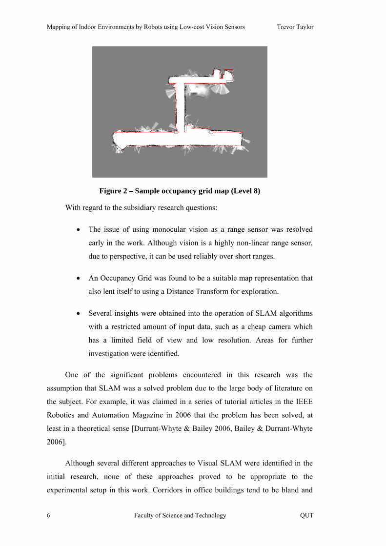
The primary output of this project was a method of producing occupancy grid
maps that can be generated using only vision, which addresses the major research
question. The feasibility of vision-only mapping is confirmed by Figure 1 and Figure
2 which show examples of maps covering areas roughly 20 metres square for floors
7 and 8 in QUT S Block. (The ground truth is shown in red). These maps use the
standard convention for an occupancy grid in which white represents free space,
black cells are obstacles and shades of grey correspond to the (inverse) certainty that
a cell is occupied. They were produced by an X80 robot with a low-resolution colour
camera.
Figure 1 – Sample occupancy grid map (Level 7)
QUT Faculty of Science and Technology 5
Mapping of Indoor Environments by Robots using Low-cost Vision Sensors Trevor Taylor
Figure 2 – Sample occupancy grid map (Level 8)
With regard to the subsidiary research questions:
• The issue of using monocular vision as a range sensor was resolved
early in the work. Although vision is a highly non-linear range sensor,
due to perspective, it can be used reliably over short ranges.
• An Occupancy Grid was found to be a suitable map representation that
also lent itself to using a Distance Transform for exploration.
• Several insights were obtained into the operation of SLAM algorithms
with a restricted amount of input data, such as a cheap camera which
has a limited field of view and low resolution. Areas for further
investigation were identified.
One of the significant problems encountered in this research was the
assumption that SLAM was a solved problem due to the large body of literature on
the subject. For example, it was claimed in a series of tutorial articles in the IEEE
Robotics and Automation Magazine in 2006 that the problem has been solved, at
least in a theoretical sense [Durrant-Whyte & Bailey 2006, Bailey & Durrant-Whyte
2006].
Although several different approaches to Visual SLAM were identified in the
initial research, none of these approaches proved to be appropriate to the
experimental setup in this work. Corridors in office buildings tend to be bland and
6 Faculty of Science and Technology QUT

Chapter One Introduction
featureless. Also, the robot had only a single camera and images were captured at a
very low frame rate (due to hardware limitations) and exhibited motion blur during
moves. Significant pose changes between images made feature tracking almost
impossible.
Despite the challenges of SLAM and the limitations inherent in using vision,
the final system was able to build maps of acceptable quality for navigating around a
building. This was the most significant output of the research. Many of the practical
problems encountered in using vision are also addressed.
In detail, the following areas are original work (with relevant citations for
published papers where applicable):
• Development of an efficient system of equations for performing Inverse
Perspective Mapping (IPM) to enable monocular vision to be used as a
range sensor [Taylor et al. 2004a] (see sections 3.7.2 and 4.3.1);
• A new approach to mapping using Radial Obstacle Profiles (ROPs) to
represent surrounding obstacles. ROPs are obtained by instructing the
robot to perform a pirouette (spin on the spot) and are used for creating
local maps [Taylor et al. 2004b, Taylor et al. 2005a] (see section 3.7.7
and 4.3.2);
• Extensions to the use of the Distance Transform for use in autonomous
exploration [Taylor et al. 2005a, Taylor et al. 2005b]. See sections 3.11
and 4.8. These extensions include modifications to the Distance
Transform for collaborative and/or directed exploration [Taylor et al.
2005b] (although most of this material is omitted from this thesis
because it is not directly relevant);
• Development of a simple method for detecting vertical edges in an
image when the camera is tilted [Taylor et al. 2006, Taylor 2007] (see
sections 3.7.10 and 4.4.3); and
• Development of methods for incremental localization based on
knowledge of the structure of the environment [Taylor et al. 2006,
QUT Faculty of Science and Technology 7
Mapping of Indoor Environments by Robots using Low-cost Vision Sensors Trevor Taylor
Taylor 2007, Taylor et al. 2007]. This constraint-based localization
improves the stability of the GridSLAM algorithm and allows
operation with fewer particles than would otherwise be required. See
sections 4.5.
In addition, this thesis contains details of previously unpublished work:
• Use of the Discrete Cosine Transform to compactly describe Radial
Obstacle Profiles for comparison purposes (see section 4.3.4).
This research produced a substantial amount of software, including:
• An OpenGL simulator for computer vision experiments, called the
SimBot_W32 program;
• A simulation environment built using the Microsoft Robotics
Developer Studio (MRDS) and sample code for producing occupancy
grid maps [Taylor 2006a, Johns & Taylor 2008];
• A library for controlling X80 robots including a version that runs on a
PDA allowing remote teleoperation of an X80 from a hand-held device
[Taylor 2006b]; and
• A complete working system based on X80 robots for map building in
indoor environments, known as ExCV.
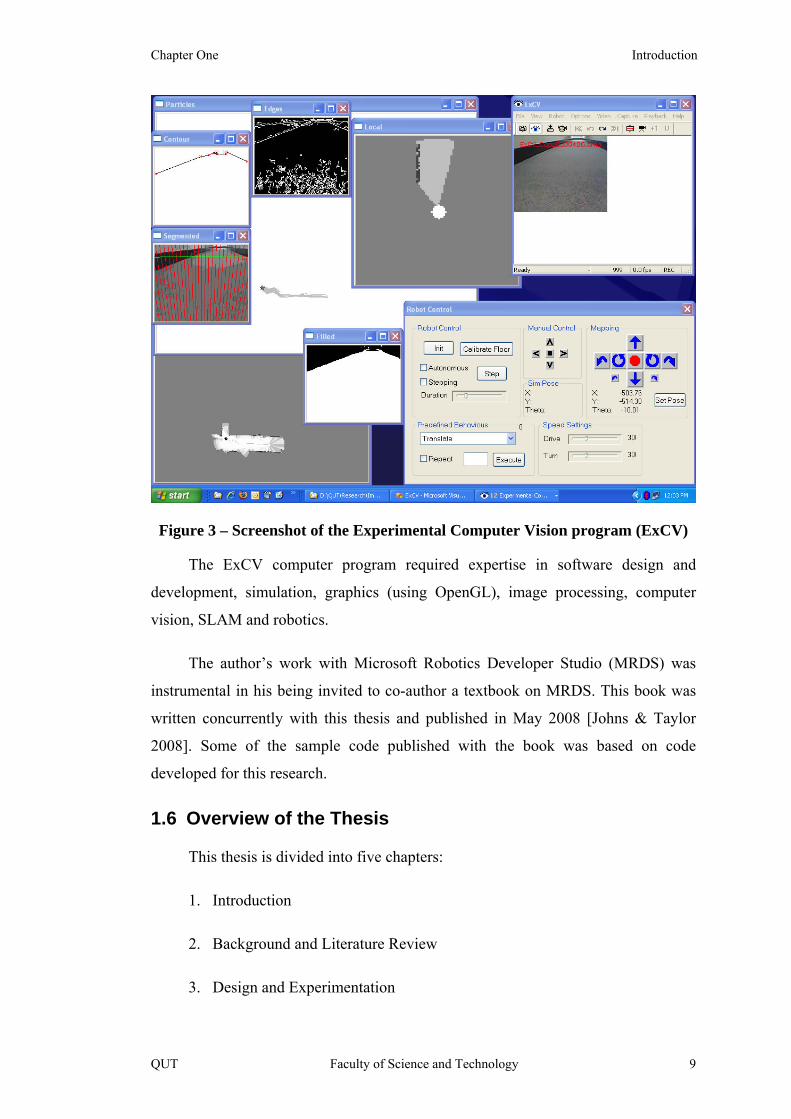
A screenshot of the program for building maps using vision, called ExCV
(Experimental Computer Vision), is shown below in Figure 3. This diagram only
shows about half of the available windows that the program can display for
diagnostic purposes.
8 Faculty of Science and Technology QUT
Chapter One Introduction
Figure 3 – Screenshot of the Experimental Computer Vision program (ExCV)
The ExCV computer program required expertise in software design and
development, simulation, graphics (using OpenGL), image processing, computer
vision, SLAM and robotics.
The author’s work with Microsoft Robotics Developer Studio (MRDS) was
instrumental in his being invited to co-author a textbook on MRDS. This book was
written concurrently with this thesis and published in May 2008 [Johns & Taylor
2008]. Some of the sample code published with the book was based on code
developed for this research.
1.6 Overview of the Thesis
This thesis is divided into five chapters:
1. Introduction
2. Background and Literature Review
3. Design and Experimentation
QUT Faculty of Science and Technology 9
Mapping of Indoor Environments by Robots using Low-cost Vision Sensors Trevor Taylor
4. Results and Discussion
5. Conclusions
Chapters 2, 3 and 4 are organised according to the following logical structure.
(The terms in italics are defined in the following paragraphs). These topics cover all
the major aspects of visual map building, each of which has to be addressed when
developing a complete system.
• Robots and Robot Motion;
• Computer Vision;
• Navigation, including Floor Detection using Vision;
• Map Building from visual data using Inverse Perspective Mapping and
the Radial Obstacle Profile;
• Exploring unknown environments using the Distance Transform;
• Localization, and in particular Incremental Localization; and
• Simultaneous Localization and Mapping.
Chapter 2 (Background and Literature Review) provides background
information as well as a review of the applicable literature. The research covered a
broad range of topics, as should be evident from the bullet points above.
The design and development process is discussed in Chapter 3 (Design and
Experimentation). The nature of the research meant that the design evolved over
time based on experimental prototypes. Therefore the chapter incorporates some
results of the research which were fed back into the design.
Chapter 3 discusses using vision as a range sensor by identifying the floor
boundary and then applying Inverse Perspective Mapping to determine the real-
world coordinates of the boundary points from pixel coordinates in the image.
Converting to a real-world reference frame is necessary in order to perform basic
navigation, exploration, and map building.
10 Faculty of Science and Technology QUT
Chapter One Introduction
Building a map does not happen automatically just by wandering around at
random – the robot must perform some sort of directed exploration. Chapter 3
therefore discusses the algorithm that was developed to explore the environment and
how it ensured that the whole area was covered.
Once basic exploration and map building were proven to work in simulation, it
was necessary to move out of the artificial environment of the simulator and on to a
real robot. This immediately introduced one of the inherent complexities of the real
world – tracking the robot’s pose (position and orientation).
Robots can quickly get lost if they are not constantly monitoring the effects of
their own movements because commands to the wheels rarely produce exactly the
desired motions. Discovering where you are with respect to a map is a process called
localization, and it is also covered in Chapter 3.
There is a basic conundrum in robotics: building an accurate map requires
accurate localization, but localization requires a map. This can be resolved through a
process called Simultaneous Localization and Mapping (SLAM), sometimes also
referred to as Concurrent Mapping and Localization (CML). Chapter 3 covers the
basic principles of SLAM.
Chapter 4 (Results and Discussion) presents the results of the study and
discusses these outcomes. SLAM is not yet an exact science and there are still many
practical issues to be resolved. Chapter 4 covers some problems encountered in
implementing SLAM using only vision.
Existing SLAM algorithms proved to be unstable with the experimental
hardware used in this project due to insufficient information content in the input data
stream. However, by applying additional constraints and performing incremental
localization (in addition to the localization embedded in the SLAM algorithm), it
was possible to develop a stable system that successfully built maps of office
corridors. The chapter finishes with a list of areas for further investigation.
Finally, Chapter 5 (Conclusions) draws conclusions from the research and
reiterates the contributions made by this work. It directly addresses the original
research questions.
QUT Faculty of Science and Technology 11

Mapping of Indoor Environments by Robots using Low-cost Vision Sensors Trevor Taylor
Note that there is a Glossary at the end of this thesis. Terms that are in the
Glossary appear in italics the first time they are used, and also to reinforce the fact
that explicit definitions are available. This saves having to include definitions or
footnotes in the main body of the text. There is some overlap between the Glossary
and the list of abbreviations in the front of the thesis.
12 Faculty of Science and Technology QUT

Chapter Two Design and Experimentation
2 Background and Literature Review
‘Vision is our most powerful sense.
Vision is also our most complicated sense.’
– B.K.P. Horn,
Robot Vision, 1986, page 1.
2.1 Background
All robots need maps to achieve useful tasks [Thrun 1998], and it is a
fundamental task for mobile robots [Grisetti et al. 2005]. The objective of this
research was therefore to achieve the task of mapping of indoor environments using
vision. In order to complete this task, the robot required the ability to:
• Measure distances to obstacles using images from a camera;
• Build maps based on what it saw;
• Explore its environment in a systematic and thorough way; and
• Keep track of its location and orientation in the presence of real-world
problems like wheel slippage.
Endowing a robot with these skills required research into a diverse range of
topics including computer vision, robot motion, inverse perspective mapping (IPM),
mapping algorithms, and exploration methods. Putting it all together required a
Simultaneous Localization and Mapping (SLAM) algorithm because mapping had to
be performed at the same time as exploration which in turn required localization to
ensure that the robot did not get lost. All of these topics are addressed in this chapter.
QUT Faculty of Science and Technology 13
Mapping of Indoor Environments by Robots using Low-cost Vision Sensors Trevor Taylor
2.1.1 Brief history of Vision-based Robots
Robots have used vision for navigation to a greater or lesser extent for many
years. This section presents a few examples that are indicative of the types of
approaches that have been used. A more detailed review can be found in [DeSouza
& Kak 2002].
The earliest attempt at using computer vision was probably Shakey the robot at
Stanford, which operated in an artificial environment with coloured blocks. A
detailed history of Shakey is available in [Nilsson 1984]. It was called Shakey
because of the way it vibrated when it moved.
Shakey was followed by the Stanford Cart [Moravec 1977] which used two
cameras, one of which could be moved to provide different viewpoints for stereo
vision. It was very slow and test runs took hours with the available computing power
at the time. Image processing took so long that the shadows during outdoor test runs
became a problem because they would actually move noticeably between images.
Moravec moved to Carnegie-Mellon University (CMU) in 1980 where he
developed the CMU Rover [Moravec 1983]. This launched a long history of robotics
and vision at CMU, including the well-known CMUcam [CMU 2006]. Moravec’s
work gave us the Moravec Interest Operator [Moravec 1980], which was an early
attempt to select significant features from an image. Moravec is also famous for
formulating occupancy grids for mapping [Moravec & Elfes 1985], although these
were created using sonar, not vision.
In the late 1980s, one of the best known robots was Polly, which was built by
Ian Horswill [Horswill 1993]. This used a low resolution black and white camera to
detect the floor and people. To attract the robot’s attention it was literally necessary
to ‘shake a leg at it’. This robot had a built-in map of part of a building at MIT,
including the place where the carpet changed colour so it could navigate across this
apparent ‘boundary’. Polly was known to have several deficiencies, including
stopping when it saw shafts of light coming in through the windows.
Polly was the first in a long family of robots that operated by detecting the
floor, and thereby identifying the surrounding obstacles. These include [Lorigo et al.
14 Faculty of Science and Technology QUT
Chapter Two Design and Experimentation
1997, Howard & Kitchen 1997, Maja et al. 2000, Murray 2000]. This research
therefore followed in the Polly tradition and adopted what are referred to here as the
‘Horswill Constraints’ (explained later in this chapter in section 2.3.6). These are
constraints on the environment that simplify the task of locating the floor.
The ER-1 robot [Evolution Robotics 2005] (now discontinued) used a web
camera to perform what Evolution Robotics called Visual Simultaneous Localization
and Mapping (vSLAM). This was basically place recognition based on building a
large database of unique image features. These features were obtained using the
SIFT (Scale Invariant Feature Transform) algorithm [Lowe 2004]. It is common for
SIFT-based systems to use several thousand features in an image.
Andrew Davison [Davison & Murray 1998, Davison 1999] used features to
create what he refers to as MonoSLAM. This system built maps by tracking
hundreds of features from one image to the next and eventually determining their
physical location in the world by applying an Extended Kalman Filter (EKF).
Further discussion of Visual SLAM can be found in section 2.8.
2.1.2 Robot Motion
To construct accurate maps, the robot must know where it is with a high degree
of certainty. This pose consists of a 2D position and an orientation, which is a total
of three variables.
A common configuration for robots used both in research and industry is the
differential drive. This consists of two wheels that can be driven independently,
either forward or backward. There might also be a castor (or jockey) wheel for
balance, but it can be ignored as far as the robot’s motion is concerned. This drive
configuration is non-holonomic because the robot cannot instantaneously move in
any direction, although a combination of translations and rotations does allow the
robot to reach any point on a 2D plane.
The kinematics of this type of robot have been studied extensively, and the
generalised equations of motion are readily available from textbooks [Dudek &
Jenkin 2000, Choset et al. 2005].
QUT Faculty of Science and Technology 15

Mapping of Indoor Environments by Robots using Low-cost Vision Sensors Trevor Taylor
Figure 4 – Two-Wheeled Differential Drive
Consider Figure 4 which shows a two-wheeled differential drive viewed from
above. This type of robot can drive forwards or backwards, rotate on the spot or
drive in arbitrary arcs.
If the robot motions are constrained to only translations or rotations, then the
equations of motion become trivial and are related directly to the geometry of the
robot and the resolution of the wheel encoders. Three parameters must be known
(refer to Figure 4):
• Number of ticks of the wheel encoders per wheel revolution, n
• Radius of the wheels, r
• Wheelbase or distance between the wheels, w.
For a translation (forward motion) both wheels must turn by the same amount.
Due to the way that the motors are mounted, this usually results in the wheel encoder
values changing in opposite directions, but both values should change by the same
absolute amount, ∆e. The distance travelled, d, is therefore:
nerd ∆
⋅= π2 (1)
Expressed in this form it is clear that the distance is equal to the perimeter of
the wheel times the ratio of the number of ticks moved to the number of ticks per
revolution.
16 Faculty of Science and Technology QUT
Chapter Two Design and Experimentation
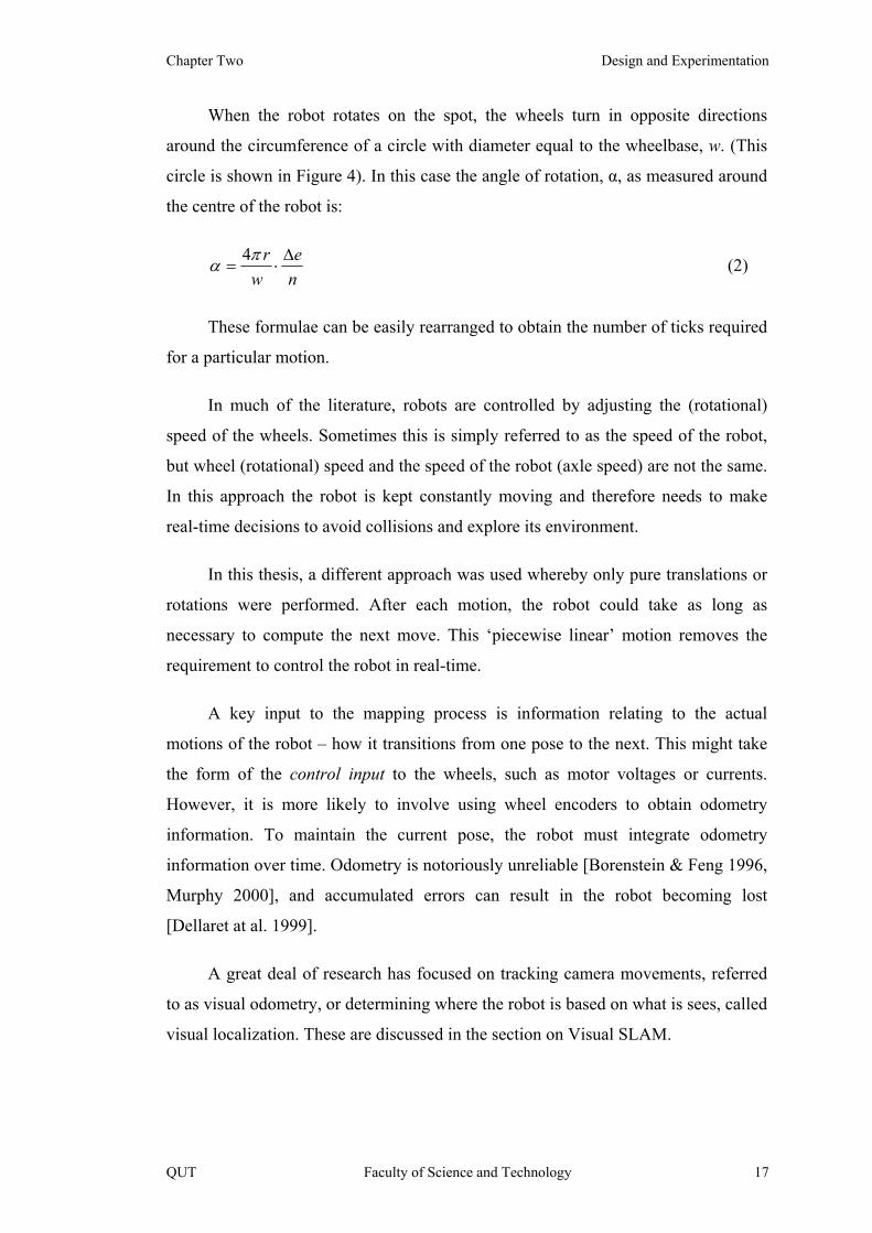
When the robot rotates on the spot, the wheels turn in opposite directions
around the circumference of a circle with diameter equal to the wheelbase, w. (This
circle is shown in Figure 4). In this case the angle of rotation, α, as measured around
the centre of the robot is:
nwer ∆
⋅=πα 4 (2)
These formulae can be easily rearranged to obtain the number of ticks required
for a particular motion.
In much of the literature, robots are controlled by adjusting the (rotational)
speed of the wheels. Sometimes this is simply referred to as the speed of the robot,
but wheel (rotational) speed and the speed of the robot (axle speed) are not the same.
In this approach the robot is kept constantly moving and therefore needs to make
real-time decisions to avoid collisions and explore its environment.
In this thesis, a different approach was used whereby only pure translations or
rotations were performed. After each motion, the robot could take as long as
necessary to compute the next move. This ‘piecewise linear’ motion removes the
requirement to control the robot in real-time.
A key input to the mapping process is information relating to the actual
motions of the robot – how it transitions from one pose to the next. This might take
the form of the control input to the wheels, such as motor voltages or currents.
However, it is more likely to involve using wheel encoders to obtain odometry
information. To maintain the current pose, the robot must integrate odometry
information over time. Odometry is notoriously unreliable [Borenstein & Feng 1996,
Murphy 2000], and accumulated errors can result in the robot becoming lost
[Dellaret at al. 1999].
A great deal of research has focused on tracking camera movements, referred
to as visual odometry, or determining where the robot is based on what is sees, called
visual localization. These are discussed in the section on Visual SLAM.
QUT Faculty of Science and Technology 17

Mapping of Indoor Environments by Robots using Low-cost Vision Sensors Trevor Taylor
2.2 Computer Vision
The primary objective of a computer vision system is to segment images to
obtain useful information about the surrounding environment. If software were
available that could perfectly segment an image and reliably identify all of the
distinct objects that it contained, a significant portion of the vision problem would
have been solved. Segmentation is still an active area of research as a topic in its
own right. For further elaboration, see the sections on floor detection (3.6.2 and
onwards) which outline various methods of segmentation that were trialled.
2.2.1 Stereo versus Monocular Vision
Stereo vision is a common configuration in the literature as well as in nature.
Using two cameras with a reasonable distance between them allows the stereo
disparity to be calculated, and hence depth or distance to objects in the field of view
established.
To extract depth information using stereo vision the correspondence between
pixels in the two images must be established unambiguously. This ‘data
correspondence’ problem is a recurring theme in computer vision. It is often
necessary to match points in two images. Optic flow, for instance, has exactly the
same problem as stereo disparity matching, but it is a temporal rather than a spatial
problem.
In addition to calibrating the individual cameras, a stereo ‘head’ also needs to
have the two cameras accurately calibrated so that their distance apart and vergence
angle is precisely known.
Stereo vision is not a pre-requisite for making range estimates. If the camera
parameters are known and the floor can be segmented in the image, then the range to
obstacles can be obtained using Inverse Perspective Mapping (see section 2.4.6)
applied to a single image, i.e. monocular vision.
2.2.2 Digital Cameras
Because digital cameras create images consisting of picture elements (pixels)
there are quantization effects when a digital image is created.
18 Faculty of Science and Technology QUT
Chapter Two Design and Experimentation
The number of pixels across the image is known as the horizontal resolution.
The vertical resolution is the number of rows or scanlines in the image. The ratio
between the horizontal and vertical resolutions is the aspect ratio of the camera.
Typical cameras have an aspect ratio of 4:3.
The cameras used in computer vision vary considerably in their specifications.
In this work cheap colour cameras (commonly referred to as web cameras) were
used. They have fairly low resolution (discussed below) which ensures that the
amount of computation involved in processing images is not excessive.
The intrinsic parameters of a camera describe its internal properties. The
extrinsic parameters define the configuration of the camera, and in particular its
orientation in terms of a real-world coordinate system.
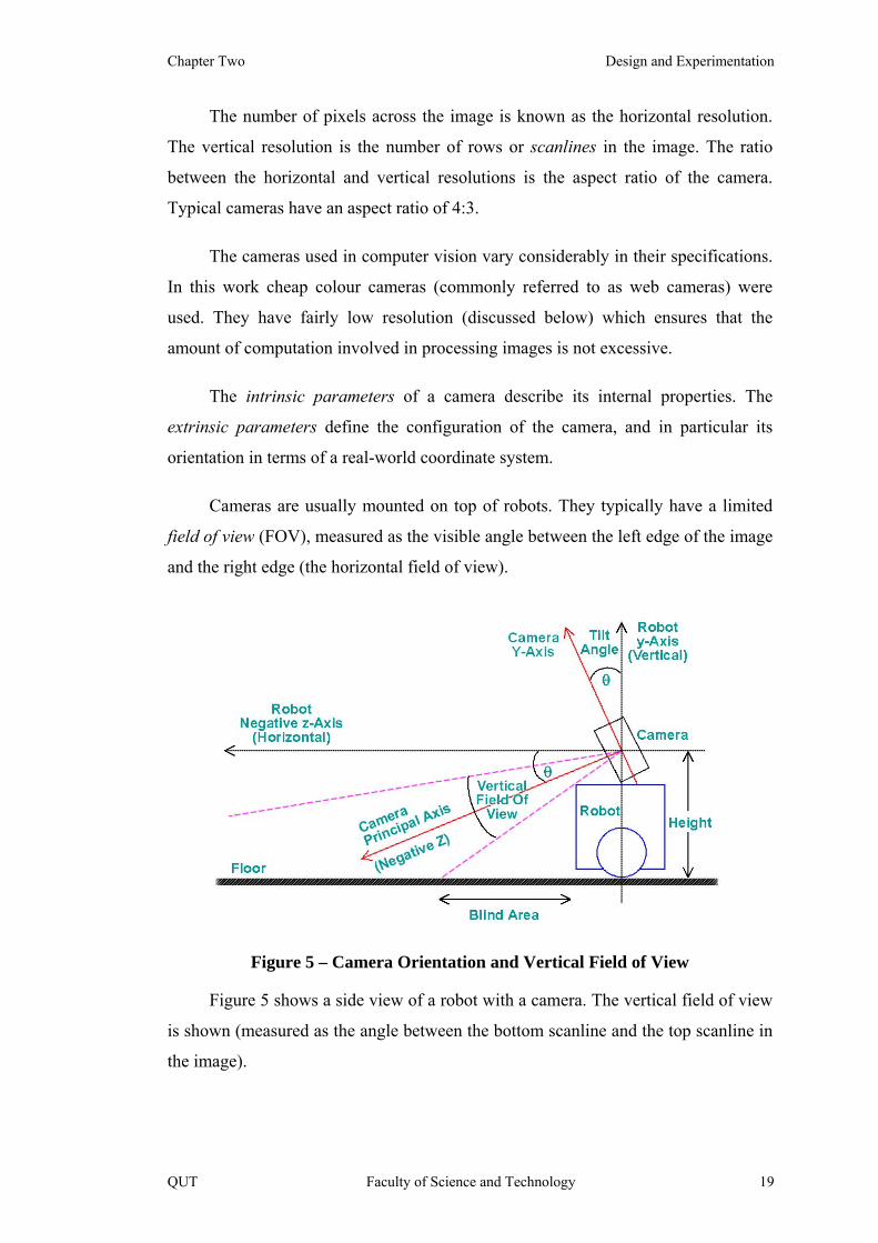
Cameras are usually mounted on top of robots. They typically have a limited
field of view (FOV), measured as the visible angle between the left edge of the image
and the right edge (the horizontal field of view).
Figure 5 – Camera Orientation and Vertical Field of View
Figure 5 shows a side view of a robot with a camera. The vertical field of view
is shown (measured as the angle between the bottom scanline and the top scanline in
the image).
QUT Faculty of Science and Technology 19

Mapping of Indoor Environments by Robots using Low-cost Vision Sensors Trevor Taylor
Notice that the camera in Figure 5 is tilted to make best use of the limited
FOV. Even with this tilt, there is still a blind area in front of the robot that cannot be
seen in the camera view.
2.2.3 Pinhole Camera Approximation
This work uses the pinhole camera approximation as a mathematical model of
the camera. The formulae for a pinhole camera are well known and usually covered
in the early chapters of textbooks on computer vision. Refer to [Horn 1986] page 20
for instance, which is one of the classic texts on computer vision. However, the same
equations can be found in many other textbooks with much more detailed coverage,
such as [Faugeras 1993, Hartley & Zisserman 2003].
Figure 6 – Pinhole Camera
In Figure 6 the ‘pinhole’ is at the origin of the camera coordinate system,
labelled O. A light ray from a point in the real world, P (x, y, z), passes through the
pinhole and hits the image plane at P' (x', y', z').
Note that the image is created on a plane at right angles to the camera’s
principal (optical) axis. To maintain a right-hand coordinate system, the z-Axis
points from the pinhole (the origin) towards the image plane. Therefore the distance
along the z-Axis to the image plane remains constant and is shown as f in the
diagram.
The equations relating the coordinates of P' to P can be obtained using simple
geometry and presented here without derivation:
20 Faculty of Science and Technology QUT

Chapter Two Design and Experimentation
zx
fx=
' (3)
zy
fy=
' (4)
Notice in these equations that the pixel coordinates vary inversely with the
distance of a point in the real world from the camera.
If the lens in the camera is perfect, then the same equations apply. However,
real lenses are not perfect so some amount of distortion occurs which complicates
the equations.
2.2.4 Focal Length
The distance from the origin to the image plane in Figure 6, labelled f, is the
focal length. In a conventional camera, the lens is located at the origin and it can be
moved backwards and forwards along the optical axis to change the focus. This
involves changing the focal length.
Light passing through the camera lens will only be in focus if it comes from a
single plane in the real world parallel to the image plane. However, over a certain
range, called the depth of field, points in the real world will converge to
approximately the same place on the image plane. This is easy to understand in terms
of a digital camera because the image plane is broken up into picture elements, or
pixels, which correspond to a small area on the image plane.
For digital cameras the focal length is expressed in units of pixels because the
coordinates on the image plane are measured in pixels. (The ratios in equations 3 and
4 are dimensionless).
Note that the classical treatment of pinhole cameras relies on knowing the
camera’s focal length. This information is not always available for a camera.
QUT Faculty of Science and Technology 21
Mapping of Indoor Environments by Robots using Low-cost Vision Sensors Trevor Taylor
2.2.5 Perspective
A key feature of pinhole cameras (as opposed to fish-eye or wide angle lenses)
is that straight lines remain straight in the image. The camera, however, introduces a
perspective transformation.
The point at which ‘parallel’ lines in an image appear to converge is called a
vanishing point. In general, there can be multiple vanishing points for an image
depending on the geometry of the objects in view.
The primary problem with perspective is that depth information is lost in the
transformation from the 3D world to a 2D image. Referring back to Figure 6, the
pixel in the image could result from any point in the real world between the camera
origin and infinity along the light ray shown as (P'-O-P).
2.2.6 Range Estimation
Clearly, to build metric maps (maps that are drawn to scale) it is necessary to
measure distances. In this research vision was used as the range sensor. Recovering
depth information from images is one of the key areas of vision research. There are
many different ways to do this.
If the pixels in the image can be classified as either floor or non-floor, this
eliminates one degree of freedom in the 3D locations of the real-world points that
correspond to the floor pixels, which must be on the ground plane (floor). Simple
geometry can then be used to obtain range estimates assuming that the camera
configuration is known.
2.2.7 Effects of Camera Resolution
Consider for example one of the earliest digital cameras that only had a
resolution of 64x48 pixels. Each horizontal scanline (one of the 48 rows of pixels)
corresponds to a large distance across the floor in the real world. Now imagine a
camera with a resolution of 640x480 (VGA resolution) that captures exactly the
same scene. Obviously the higher resolution means that the distances to obstacles
can be resolved more accurately.
22 Faculty of Science and Technology QUT

Chapter Two Design and Experimentation
Side Note:
Due to perspective effects, it is not possible to say that a resolution of 640x480
is 10 times more ‘accurate’ than 64x48. Distances in an image vary non-linearly.
Furthermore, the tilt angle of the camera has an effect as well. It is only
necessary to consider two cases to illustrate this – a camera oriented parallel to the
ground and one facing directly down at the ground.
For the horizontal camera, the centre scanline corresponds to the horizon,
which is at infinity. One scanline below this is still a long way away, but
significantly less than infinity, and so forth until the bottom scanline which is right in
front of the robot.
On the other hand for a camera oriented vertically, the distance from the
camera (measured across the floor) is zero at the centre scanline and only varies by
some small amount from the top scanline to the bottom scanline of the image.
Higher resolution for the horizontal camera will obviously result in much finer
granularity for the real-world distances between scanlines in the image. However, for
the vertical camera it might only make differences of fractions of a centimetre – not
enough to be significant on a scale that is the size of a robot.
Detecting edges in images is also affected by the resolution. Edges are
important features in image analysis. With a very low resolution an edge will be
subject to very bad ‘jaggies’ – a stair-step effect caused by the quantization of an
edge that does not align with one the horizontal or vertical axes. These jaggies might
disguise the existence of an edge.
2.2.8 Field of View (FOV) Limitations
One of the significant problems of many cheap digital cameras is a limited
field of view (FOV). A typical web camera has a FOV of 40-60°. In contrast,
humans have a FOV of up to 200°. (The exact range depends on multiple factors
including age, race and sex.)
A restricted FOV means that the robot must ‘look around’ to get a good view
of the surrounding environment when building a map. Also, to make the best use of
QUT Faculty of Science and Technology 23

Mapping of Indoor Environments by Robots using Low-cost Vision Sensors Trevor Taylor
the available FOV, the cameras on robots are often tilted downwards as in Figure 5.
Even with this tilt, there might be an area in front of the robot that cannot be seen,
labelled as the Blind Area in Figure 5.
Panoramic cameras have been widely used to overcome FOV limitations
[Yamazawa et al. 1995, Baker & Nayar 1998, Ishiguro 1998]. There are various
types of special-purpose cameras: omnidirectional cameras (360° FOV); panoramic
cameras (around 180° FOV) and cameras with wide-angle or fish-eye lenses.
The common factor in all of these is significant distortion of the image. In
these cases, standard perspective no longer applies and straight lines no longer
appear straight in the image. Nayar specifically developed a catadioptic camera (one
that uses mirrors) so that he could extract true perspective images from the
omnidirectional image [Nayar 1997].
2.2.9 Focus
Cheap cameras usually have a fixed focus, unlike the plethora of digital
cameras now on the market for consumer use which usually have an autofocus
mechanism. Autofocus can be an advantage as far as the quality of the image is
concerned, especially when attempting to extract edge information. However, if the
camera automatically changes the focus there is no way to obtain feedback from the
camera to determine the new focal length, which is one of the camera’s intrinsic
parameters.
The problem with fixed focus is that some part of the image will invariably be
out of focus. Typically cheap cameras are focussed at ‘infinity’. This leads to
blurring in the foreground and can make it harder to detect edges.
2.2.10 Camera Distortion and Calibration
A significant problem with many cameras is lens distortion. The effects are
highly non-linear. The primary effect is radial distortion. This results in straight lines
becoming increasingly curved towards the edges of the image. Clearly, when
building a map, it is important to perceive walls as being straight.
24 Faculty of Science and Technology QUT
Chapter Two Design and Experimentation
By taking pictures of a ‘calibration target’ (usually a checkerboard pattern)
from various different positions, it is possible to calculate the intrinsic parameters of
the camera, which include the focal length and various distortion parameters
[Bouguet 2006]. These parameters allow images to be undistorted by applying an
appropriate algorithm [Intel 2005]. See section 3.5.6 for details.
Given the intrinsic parameters, it is also possible to calculate the extrinsic
parameters for a given image using the same software. The extrinsic parameters
consist of a rotation matrix and a translation vector that transform camera
coordinates to real-world coordinates aligned with the calibration target. These
parameters can be used to obtain the camera tilt angle.
Another common problem with cheap cameras is vignetting which appears as a
darkening of the image towards the corners. This problem arises because the
camera’s CCD array is rectangular but the lens is round, which restricts light from
reaching the corners of the CCD. Although this problem is mentioned in textbooks
on computer vision, such as [Forsyth & Ponce 2003], no solutions are offered.
2.2.11 Uneven Illumination
If the lighting in the environment is not uniform, as in corridors where the
lighting levels vary, it might be necessary to adjust the brightness of the images in
the software to provide a more uniform range of values for floor pixels. This is a
different issue from vignetting.
Many cameras have difficulty when operating in low light conditions, resulting
in images of poor quality with many pixels approaching dark grey or black. The
HVS achieves a large dynamic range by gradually switching from cones (which
detect colour) to rods (which detect only intensity, i.e. greyscale). This is why human
‘night vision’ is black and white. However, digital cameras have not yet achieved
similar levels of performance.
The problem of poor and/or uneven illumination has plagued computer vision
for many years [Funt & Finlayson 1995, Funt et al. 1998]. The issue is referred to as
colour constancy – maintaining stable colour values despite differences in
illumination. A related problem is dealing with shadows which might be interpreted
QUT Faculty of Science and Technology 25
Mapping of Indoor Environments by Robots using Low-cost Vision Sensors Trevor Taylor
as edges in the image where there are no real edges. These are still open research
problems.
2.2.12 Image Preprocessing
Given several of the issues discussed in this chapter, most computer vision
systems perform a preprocessing step on images prior to applying computer vision
algorithms. It is common practice to use a Gaussian blur or other smoothing filter to
reduce the effects of noise. Video signals frequently contain speckles which can be
reduced via filtering.
In addition, some compensation for illumination (brightness and contrast)
might be applied. These are fundamental image processing operations. See for
instance [Forsyth & Ponce 2003].
2.3 Navigation
[Murphy 2000] proposes four questions1 related to robot navigation:
1. Where am I going?
2. What’s the best way there?
3. Where have I been?
4. Where am I?
These questions relate to different areas of the overall problem of navigating in
an unknown environment. The first two are basically path planning – a task that
cannot be performed without a goal (or multiple goals) and some sort of map. In an
unknown environment, however, the robot does not have a map to begin with. The
third question clearly requires some form of memory, i.e. building a map and a past
history of positions, called a trajectory or a trail. The last question is probably the
most important and is referred to as localization.
When all of these questions are combined, they require both an exploration
algorithm and a Simultaneous Localization and Mapping (SLAM) algorithm
1 These questions are in the order listed by Murphy. The logical order depends on the application.
26 Faculty of Science and Technology QUT
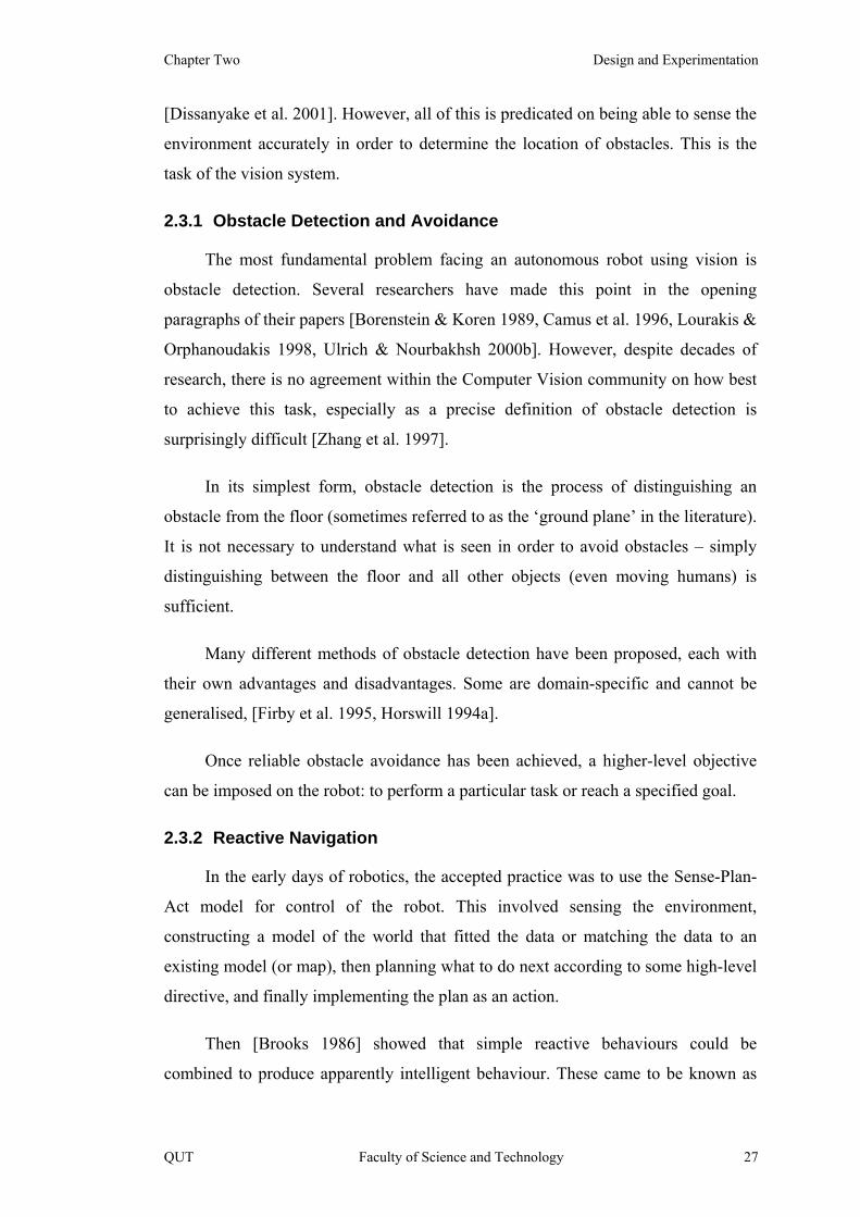
Chapter Two Design and Experimentation
[Dissanyake et al. 2001]. However, all of this is predicated on being able to sense the
environment accurately in order to determine the location of obstacles. This is the
task of the vision system.
2.3.1 Obstacle Detection and Avoidance
The most fundamental problem facing an autonomous robot using vision is
obstacle detection. Several researchers have made this point in the opening
paragraphs of their papers [Borenstein & Koren 1989, Camus et al. 1996, Lourakis &
Orphanoudakis 1998, Ulrich & Nourbakhsh 2000b]. However, despite decades of
research, there is no agreement within the Computer Vision community on how best
to achieve this task, especially as a precise definition of obstacle detection is
surprisingly difficult [Zhang et al. 1997].
In its simplest form, obstacle detection is the process of distinguishing an
obstacle from the floor (sometimes referred to as the ‘ground plane’ in the literature).
It is not necessary to understand what is seen in order to avoid obstacles – simply
distinguishing between the floor and all other objects (even moving humans) is
sufficient.
Many different methods of obstacle detection have been proposed, each with
their own advantages and disadvantages. Some are domain-specific and cannot be
generalised, [Firby et al. 1995, Horswill 1994a].
Once reliable obstacle avoidance has been achieved, a higher-level objective
can be imposed on the robot: to perform a particular task or reach a specified goal.
2.3.2 Reactive Navigation
In the early days of robotics, the accepted practice was to use the Sense-Plan-
Act model for control of the robot. This involved sensing the environment,
constructing a model of the world that fitted the data or matching the data to an
existing model (or map), then planning what to do next according to some high-level
directive, and finally implementing the plan as an action.
Then [Brooks 1986] showed that simple reactive behaviours could be
combined to produce apparently intelligent behaviour. These came to be known as
QUT Faculty of Science and Technology 27
Mapping of Indoor Environments by Robots using Low-cost Vision Sensors Trevor Taylor
‘emergent behaviours’ because they were not explicitly programmed, but emerged
from the combination of several simpler behaviours. Brooks challenged the
traditional wisdom of building a world model, saying that ‘the world is its own best
model’.
[Arkin 1998] developed this approach further and proposed robot architectures
based on combinations of behaviours. His book on behaviour-based robotics has
become a classic text in the field of robotics and it provides an excellent overview of
research in the field up to the late 1990s.
Navigation is independent of the sensor(s) used to obtain information about
obstacles. However, the focus in this research was on using vision.
2.3.3 Visual Navigation
Robots have been navigating using vision since the days of the Stanford Cart
[Moravec 1977]. However, this does not mean that the problem of navigation using
vision has been solved; far from it. Many robots today still use sensors such as sonar,
infra-red or laser range finders, and do not have cameras at all. Even those that do
have cameras often rely on them only to identify places or objects that they are
searching for, but use sonar or lasers for actual navigation.
Author after author has pointed out how complex a task vision is, and just as
importantly, how easily humans accomplish it: [Wandell 1995, Hoffman 1998,
Brooks 2002]. In their survey paper, [DeSouza & Kak 2002] also point out the lack
of progress in the field of visual navigation over the previous 30 years.
A wide range of image processing algorithms is available today as open source
code, such as the Intel Open Computer Vision Library [Intel 2005]. However,
processing steps such as edge detection, segmentation, line detection etc. do not
constitute vision on their own. Computer vision requires analysis of the scene and
high-level understanding. Complete scene interpretation is not always necessary to
achieve useful tasks [Dudek & Jenkin 2000]. In fact, [Horswill 1997] introduced the
idea of lightweight vision tasks.
28 Faculty of Science and Technology QUT
Chapter Two Design and Experimentation
2.3.4 Early Work in Visual Navigation
Some of the earliest work on visual obstacle avoidance was done by [Moravec
1977]. One legacy of his work was the Moravec Interest Operator. This was a way to
find points of interest in an image, where ‘interest’ was defined as an area that had
large changes in pixel values (using a simple sum of squared differences). These
tended to be corners. Features can then be used to track objects or for stereo
correlation.
Side Note:
Feature detection is still an active area of research. Various methods have been
developed over the years, such as the well-known Canny Edge Detector [Canny
1986], Harris Corner Detector [Harris & Stephens 1988], and the generalised Hough
Transform (for lines and curves) [Duda & Hart 1972].
The importance of features and establishing the correspondences between
features in multiple images was explained by Ullman [Ullman 1996] whose concepts
of high-level vision were built on underlying low-level features extracted from the
image.
In their classic paper, Shi and Tomasi [Shi & Tomasi 1994] identified a set of
‘good features to track’.
A more recent algorithm which has been widely applied is the Scale-Invariant
Feature Transform (SIFT) [Lowe 2004]. SIFT creates unique descriptors (128 bytes
long) for features of interest which are called keypoints. Sometimes thousands of
keypoints are obtained from a single image.
Extracted point features are usually used for tracking, not for identifying the
floor. Edges and segmentation (blob extraction) are more useful for finding floors.
Moravec developed the Stanford Cart, which later became the CMU Rover
[Moravec 1980, 1983]. The Cart moved at only 4 metres per hour. It ran outdoors
and it could become confused by changes in shadows between images because it
took so long to perform image processing. This was primarily a reflection of the
QUT Faculty of Science and Technology 29
Mapping of Indoor Environments by Robots using Low-cost Vision Sensors Trevor Taylor
computer technology available at the time, which was a DEC KL-10 processor.
However, for its time, the Cart was a triumph of engineering.
2.3.5 The Polly Family of Vision-based Robots
In the late 1980s and early 1990s, Horswill [Horswill & Brooks 1988, Horswill
1993, Horswill 1994a] developed a robot, called Polly, which navigated mostly by
means of vision. It actually had ‘bump’ and sonar sensors and did not rely totally on
vision.
Polly operated in a restricted environment with a constant floor colour, except
for a particular boundary that was specifically programmed into the built-in map.
The robot had a monochrome camera, and used a resolution of only 64 x 48 pixels.
Although this might sound low, sometimes too much information is actually a
disadvantage, both in terms of processing power requirements and because
additional detail can tend to obscure the similarity of floor pixels.
There is evidence that humans operate at multiple resolutions precisely
because segmentation is quicker and more reliable on a smaller image [Wandell
1995]. In fact, one method of segmenting an image uses so-called Gaussian or
Laplacian Pyramids where the image resolution is successively reduced so that the
principal features stand out.
Horswill’s approach was as follows:
• Smooth the image.
• Look at a trapezium in the immediate foreground and determine the
average pixel value.
• Use this as ‘floor’ and then label every pixel, starting from the bottom
of the image and scanning up each column until there was a mismatch.
• The height of the columns indicated the distance to obstacles in what
Horswill referred to as a ‘Radial Depth Map’.
Polly’s floor recognition process failed on any sort of texture like tile or carpet
patterns. It could not handle shiny floors or shadows. The robot would brake for
30 Faculty of Science and Technology QUT

Chapter Two Design and Experimentation
shafts of sunlight coming through doors. It also had a problem with obstacles of a
similar colour to the floor because it could not distinguish these ‘isoluminant edges’.
In addition, Horswill had to add a special condition for the carpet boundary on the
floor of the building where he worked.
Horswill went on to develop a second-generation robot called Frankie
[Horswill 1994b]. The constraint of a uniform colour for the floor was relaxed
somewhat and turned into a constraint on the frequency components of the floor
texture. An edge detector was also used to identify obstacles. Frankie could therefore
handle some small degree of texture, but there were still problems with shiny floors,
where the robot treated reflections as obstacles.
[Cheng & Zelinsky 1996] took the concept of the Polly vision system, but used
a very large grid size so that carpet texture would be averaged out. The robot was
given a goal, and so had competing behaviours: obstacle avoidance and driving
towards the goal. They noted that it is possible for the competition between
behaviours to result in stagnation or oscillation. To resolve this problem, it was
necessary to introduce some state information – in effect the robot needed a memory.
A subsequent paper [Cheng & Zelinsky 1998] explained how they added
Lighting Adaptation in an attempt to overcome variations in illumination. The
system used a Fujitsu vision processor to handle up to 100 template correlations at a
frame rate of 30 Hz, where the base template used for matching was updated using
the average intensity.
In another similar approach to Polly, [Howard & Kitchen 1997] developed
Robot J. Edgar which used simple edge detection to detect the first non-floor pixel in
each of several vertical image columns. The robot used a wide-angle lens and could
run at up to 30 cm/sec. The process was as follows:
• For each pixel column, apply a one dimensional edge filter starting
from the bottom of the image;
• Record the image location of the first edge; and
• Convert the image location into world coordinates using a lookup table.
QUT Faculty of Science and Technology 31
Mapping of Indoor Environments by Robots using Low-cost Vision Sensors Trevor Taylor
The resulting map of boundary points exhibited error rates of 10% because of
noise. Consequently, the measurements from three frames were combined to produce
reliable obstacle maps.
However, this approach suffered from the same problems as Polly and Frankie,
and requireed camera calibration in order to construct the lookup table for
transformations back into real world coordinates.
[Lorigo et al. 1997] extended Horswill’s work and refined the method for
segmenting the floor pixels from obstacle pixels by using a colour image and a sum
of absolute differences between histograms of a reference area and the rest of the
pixels in the image.
The robot, called Pebbles, was run both indoors and outdoors in the simulated
Mars environment at the Jet Propulsion Laboratories (JPL) in California. The system
achieved speeds of up to 30 cm/sec with 4 frames per second being processed.
The approach used three ‘vision modules’ – brightness gradients (edges), Red
and Green (from RGB) and Hue and Saturation (from HSV). An obstacle boundary
map was constructed by each of these modules, and the results fused together using
smoothing and median values. However, the image was still only 64 x 64 pixels, and
a sliding window of 20 x 10 pixels was used in computing the obstacle boundaries.
One of the limitations of this system was that it always assumed that the
reference area immediately in front of the robot was free of obstacles, and therefore
could be used as a template for the floor. Also, the robot’s only goal was to move
safely within cluttered environments – it did not do any mapping or localisation.
[Martin 2001] extended the original Polly system using Genetic Programming.
The objective was to show the use of Evolutionary Computing, rather than to
improve the performance of Polly.
Martin used a very limited set of examples – only 20 test runs. The robot had a
black and white camera and the available operations included the Sobel gradient
magnitude, Median filters and the Moravec Interest Operator. According to [Martin
2002], the best-of-run individuals had essentially the structure of Horswill’s and
32 Faculty of Science and Technology QUT

Chapter Two Design and Experimentation
Lorigo’s systems, although the window size was reduced to 8 x 8 and the process
essentially used only the Sobel operator. The resulting algorithm ran at about 10 Hz
on a 333 MHz Pentium II at a resolution of 320 x 240.
In summary, these Polly-derived systems failed if the floor was textured. In
contrast, [Lourakis & Orphanoudakis 1998] developed a system that used texture to
advantage to extract the floor from successive images. The system was based on a
ground reference, and detected obstacles that protruded from the ground using a
registration process.
2.3.6 The ‘Horswill Constraints’
In his work, Horswill [Horswill 1994a, 1994b] defined a series of constraints
on the environment in which Polly operated. These have been adopted by numerous
researchers who have continued working in the area.
In honour of Horswill’s work, the following constraints are referred to as the
‘Horswill Constraints’. Note that they have been reformulated by the author.
Ground-Plane Constraint – All obstacles rest on the ground plane and their
projections are contained within the interiors of their regions of contact with the
ground plane, i.e. no overhangs.
Background Texture Constraint – The environment is uniformly illuminated
and the ground plane has no significant texture. (Horswill expressed this in terms of
a minimum spatial frequency that would allow the texture to be removed by
smoothing the image.)
These constraints can be rephrased as follows:
1. The ground is flat so the floor is a plane, which simplifies the
geometry.
2. All obstacles sit on the floor and there is an edge where an obstacle
makes contact with the floor.
3. Obstacles differ in appearance from the ground in a way that is visually
easy to detect.
QUT Faculty of Science and Technology 33

Mapping of Indoor Environments by Robots using Low-cost Vision Sensors Trevor Taylor
4. There are no overhanging obstacles (which are likely to decapitate the
robot).
These constraints have been applied by independent researchers over a period
of many years: [Lorigo et al. 1997, Howard & Kitchen 1997, Thau 1997, Ulrich &
Nourbakhsh 2000a, 2000b, Martin 2001].
Although these constraints represent significant limitations on the environment
the robot can operate in, they are still applied today because many indoor
environments meet these constraints. There are however some obvious exceptions:
steps and ramps; floors with coverings that have a substantial texture, e.g. multi-
coloured tiles; or carpet with significant patterns.
Many indoor environments have skirting boards, or kick boards, along the
walls. These are generally a different colour from the floor and the wall. They
provide a clear visual boundary between the floor and the wall. Even if there are no
skirting boards, black linoleum strips are often stuck along the walls to make the
edges of the corridors stand out. This is common practice in hospitals, for instance.
2.3.7 Floor Detection
The basic principle behind floor detection is to segment the image so that the
floor appears as a single segment. Segmentation depends to a large extent on colour
constancy which is affected by illumination. Both of these are active fields of
research.
One of the driving forces behind research into colour object recognition has
been robot soccer. In this scenario there is only a small range of distinct colours, but
the illumination can vary considerably between the test environment and the
competition environment. Many attempts have been made to develop colour
classification systems to handle this problem. These systems have relied on
techniques such as transformations to specialised colour spaces, training of a
classifier, and fuzzy logic [Reyes et al. 2006]. The key point to note here is that the
research is ongoing and this is far from being a solved problem, even though it is
highly constrained.
34 Faculty of Science and Technology QUT
Chapter Two Design and Experimentation
2.3.8 Image Segmentation
One approach to image segmentation is to use clustering whereby pixels that
are similar (according to some measure of similarity) are grouped together. A
popular clustering algorithm is k-means [Duda et al. 2001].
[Ulrich & Nourbakhsh 2000b] developed a system that was intended to be used
in a variety of environments. The system used a resolution of 320 x 240 in colour
and ran at up to 10 Hz, which was deemed to be good enough for real-time use.
The floor detection process was as follows:
• Filter the image using a 5 x 5 Gaussian;
• Transform into HSI (Hue Saturation Intensity) colour space;
• Construct histograms of the Reference Area (Hue and Intensity) and
smooth them using a low-pass filter; and
• Compare pixels to the histograms to classify them as obstacle pixels if
either the hue histogram bin value or the intensity histogram bin value
was below a threshold. Otherwise they were floor pixels.
The primary objective was to relax the constraint that the reference area must
be free of obstacles. The reference area was only assumed to be the ground if the
robot had just travelled through it. A ‘Reference Queue’ was kept to ‘remember’ the
past reference areas.
Some of the innovations by Ulrich and Nourbakhsh were: a trapezoidal area
was taken as the reference to account for perspective effects (instead of a rectangle);
and ‘invalid’ values of Hue and Saturation (where Intensity was low) were ignored.
An additional feature of their work was an ‘assistive’ mode where the robot
could be manually driven for a period of time so that it could learn the appearance of
the ground. (This was referred to as ‘appearance-based navigation’ in the paper, but
this is not the common usage of the term in the vision community.)
QUT Faculty of Science and Technology 35

Mapping of Indoor Environments by Robots using Low-cost Vision Sensors Trevor Taylor
Detecting the floor has also been a common topic in the Robot Soccer
literature. [Bruce et al. 2000] presented a scheme using the YUV colour space that
allowed them to track several hundred regions of 32 distinct colours at a resolution
of 640 x 480 at a frame rate of 30 Hz using a 700 MHz PC. The obvious
disadvantage of this method was that it uses 32 predefined colours. [Das et al. 2001]
claimed that YUV works better than RGB for segmentation for robot soccer.
[Lenser & Veloso 2003] trained a robot to recognise the difference between the
floor and other obstacles. Their ‘visual sonar’ approach was therefore specific to the
particular environment where the robot was trained.
2.3.9 Using Sensor Fusion
Quite recently, the winning team in the DARPA Grand Challenge in 2005 used
a mixture of Gaussians to extract the road surface from camera images [Dahlkamp et
al. 2006]. However, in this case they had the benefit of a laser range finder which
allowed them to obtain training samples for recognizing the colour of the roadway
which was often dirt, but actually varied across the challenge course.
By identifying the clear area in front of their car as ‘road’, the Stanford team
could use this portion of the image to obtain a set of key pixel values using k-means
clustering. Then by applying a mixture of Gaussian around these key pixel values
they marked the whole of the image as either road or non-road pixels. For an
entertaining explanation, see the Google video [Thrun 2006].
In this case, the vision processing was used to extend knowledge of the
environment beyond the limitations of the laser range finder, thereby enabling the
vehicle to travel faster. The important point to note, however, is that the process still
used a laser range finder as the primary sensor. This was not, therefore, an example
of vision-only processing.
2.4 Mapping
Map building by autonomous robots has been done in the past in a variety of
different ways and with a wide range of different sensors. The combination of
algorithms described here includes some new methods specifically for mapping
using vision.
36 Faculty of Science and Technology QUT

Chapter Two Design and Experimentation
One obvious function of a map is to enable the robot to remember the terrain
that it has driven over. This provides positive proof of free space. The robot might
use this prior information (in its memory) to predict what a new view should look
like for comparison with actual sensor information. It can adjust its pose in the
previous ‘obstacle map’ according to its own motion and then compare what it sees
with what is already in the map.
Before mapping can be done using vision, it is necessary to transform the
camera images back to representations of the real world. This is done by segmenting
out the floor and then using Inverse Perspective Mapping on the floor boundary
points, as explained below in section 2.4.6.
To draw maps correctly, the robot must always know precisely where it is. In
simulation this is not a problem because the robot’s motions are always perfect.
However, in the real world the robot’s pose can only be estimated because there are
random errors in motions. Determining the robot’s pose is a localization problem. As
should already be apparent, in practice it is not possible to completely separate
localization from mapping.
2.4.1 Types of Maps
For a comprehensive overview of mapping algorithms, see [Thrun 2002]. The
topic is also covered in several robotics textbooks, but Thrun is acknowledged as one
of the foremost experts in the world in this area.
There are two fundamentally different types of maps: Topological and Metric.
A third approach is also possible by combining topological and metric maps to
create a hybrid [Thrun 1998, Ulrich & Nourbakhsh 2000b, Tomatis et al. 2001,
2002]. These hybrid maps use a high-level topological map with local metric maps.
In effect, the map consists of a series of smaller maps linked together.
2.4.2 Topological Maps
Topological maps are directed graphs, i.e. a set of nodes containing
information about significant objects or places connected by lines. Figure 7 shows a
QUT Faculty of Science and Technology 37

Mapping of Indoor Environments by Robots using Low-cost Vision Sensors Trevor Taylor
sample topological map. The nodes in the map have been labelled in the order that
the robot visited them.
Figure 7 – Example of a topological map
Topological maps can have information attached to the ‘edges’ that join the
nodes together, such as distance estimates and the directions (headings) between
nodes. For example, [Egido et al. 2002] created a system for mapping corridors.
Corridors have various types of features, such as corners and T-junctions, which can
be used to identify nodes.
Many of the so-called ‘appearance based’ exploration and mapping strategies
have relied on recognising previously visited places using photos attached to the map
nodes.
Strictly speaking, a topological map does not have to record exact locations for
the nodes. Also, because they do not record empty space, topological maps tend to
be more compact than metric maps.
Note that the mental maps that humans build are basically topological. For
instance, when giving directions people often use phrases like ‘turn right at the post
office’. Humans do not record exact distances because they do not have the
appropriate sensors to do this. Instead, measured distances are relative, such as ‘next
38 Faculty of Science and Technology QUT

Chapter Two Design and Experimentation
door’ (near) versus ‘a few blocks away’ (far). Everyone, for example, has heard of
the so-called ‘country mile’ that is generally much longer than a mile.
2.4.3 Metric Maps
Metric maps are exact representations of the world. These are precisely what
most people think of in relation to the word ‘map’ – a street directory or floor plan.
These maps can be drawn to scale and they have a specified orientation, or ‘north
point’.
Figure 8 – Example of a metric map
Figure 8 shows a metric map in which the significant junctions have been
labelled with the letters A to J. It is quite apparent how the robot traversed the map
simply by following the labels in order. Compare this with Figure 7 which is a
topological representation of the same map. Clearly, Figure 8 is much easier for a
human to understand and interpret. The physical arrangement of the topological
nodes on the page in Figure 7 does not correspond directly to that shown in Figure 8
because there is no requirement for a topological map to preserve spatial
relationships.
Metric maps can be either feature-based or tessellated. It is not clear from
Figure 8 what type of map it is. Because it consists only of line segments, it could be
either feature-based or tessellated.
QUT Faculty of Science and Technology 39
Mapping of Indoor Environments by Robots using Low-cost Vision Sensors Trevor Taylor
Feature-based maps record the positions of significant ‘features’, like the
corners and intersections in Figure 8. Therefore they are generally maintained in
program memory as some form of tree structure. However, it is quite easy to draw a
2D representation of these maps because exact spatial information is available. The
resulting map would have a series of marked points, like drawing pins pushed into a
sheet of paper. In the example above these are the letters A to J. However, the walls
that are visible in this map would require additional information to describe them.
Features do not have to be limited to points. For instance, in Figure 8 it would
be possible to dispense with the labels A to J and instead record each of the line
segments that make up the walls. A wall, however, is not a point feature, and it takes
some time for the robot to observe; hence it has to infer walls from a succession of
observations (sensor readings).
In deriving their SPmap approach, [Castellanos et al. 1999] presented explicit
methods for the probabilistic modelling of various types of features, including line
segments. This allowed them to incorporate features other than simple points into a
Kalman Filter-based SLAM algorithm.
One of the difficulties with feature-based maps is defining what constitutes a
feature. If the criteria are too lax, there will be an inordinate number of features
recorded and this will quickly become a problem with memory capacity. On the
other hand, if the criteria for features are too stringent, then the features will be
sparse and they might not adequately describe the environment.
In the case of ‘appearance based’ mapping using images, it is quite common
for several thousand features to be selected from each image. These are usually
corners or other areas of the image that are highly distinctive. Probably the most
well-known method for selecting these features is the SIFT (Scale Invariant Feature
Transform) algorithm [Lowe 2004].
An alternative to using features is tessellation (dividing a plane into a set of
non-overlapping figures according to specific rules). Various types of tessellation are
possible: regular lattices or grids; Voronoi diagrams which use polygons; or
Delaunay triangulation which uses only triangles. Even for a regular grid, Quadtrees
can be used to create cells of differing sizes in order to reduce the total number of
40 Faculty of Science and Technology QUT
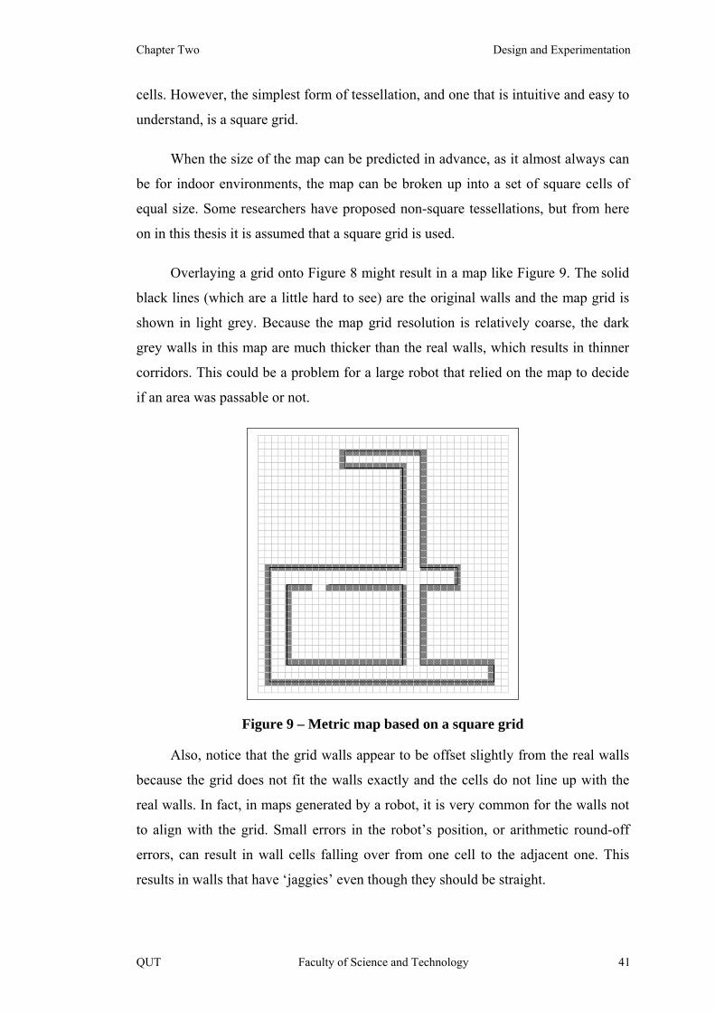
Chapter Two Design and Experimentation
cells. However, the simplest form of tessellation, and one that is intuitive and easy to
understand, is a square grid.
When the size of the map can be predicted in advance, as it almost always can
be for indoor environments, the map can be broken up into a set of square cells of
equal size. Some researchers have proposed non-square tessellations, but from here
on in this thesis it is assumed that a square grid is used.
Overlaying a grid onto Figure 8 might result in a map like Figure 9. The solid
black lines (which are a little hard to see) are the original walls and the map grid is
shown in light grey. Because the map grid resolution is relatively coarse, the dark
grey walls in this map are much thicker than the real walls, which results in thinner
corridors. This could be a problem for a large robot that relied on the map to decide
if an area was passable or not.
Figure 9 – Metric map based on a square grid
Also, notice that the grid walls appear to be offset slightly from the real walls
because the grid does not fit the walls exactly and the cells do not line up with the
real walls. In fact, in maps generated by a robot, it is very common for the walls not
to align with the grid. Small errors in the robot’s position, or arithmetic round-off
errors, can result in wall cells falling over from one cell to the adjacent one. This
results in walls that have ‘jaggies’ even though they should be straight.
QUT Faculty of Science and Technology 41
Mapping of Indoor Environments by Robots using Low-cost Vision Sensors Trevor Taylor
There is a large amount of wasted space in the map above. The robot cannot
reach the area outside the building walls. These cells can therefore never be
populated and their contents will always remain ‘unknown’. However, this approach
is simple to implement, easy to understand, and has been in widespread use in the
research community for many years.
2.4.4 Map Building
Building a map is a complex task, especially when the spatial information is
inaccurate. Several approaches have been taken, most of them probabilistic in nature,
such as Maximum Likelihood [Simmons et al. 2000] and Bayesian Filtering
[Dellaert et al. 1999].
Hidden Markov Models (HMMs) have been used [Filliat & Meyer 2000, 2001]
in an attempt to overcome the inherent uncertainty in the robot’s location.
Probabilistic methods using Markov processes (so-called Markov Localization) have
also been widely used and are well documented in a long succession of papers by a
key group of researchers including Thrun, Fox, and Burgard. For examples, see
[Thrun & Bucken 1996, Thrun 1998, Thrun et al. 2000] and in particular the
textbook Probabilistic Robotics [Thrun et al. 2005].
Note that a first-order Markov assumption is almost always made when
building a map. In other words, it is assumed that new information to be added to a
map does not depend on the previous motions of the robot (only the immediately
prior pose), or on the information in cells previously updated in the map. Put
differently, this means that past and future data are considered to be independent in a
statistical sense.
In general this is not true, especially in indoor environments. For instance, if
the robot identifies part of a wall and can determine which direction the wall is
heading in, then it is a fair assumption that it will continue in the same direction. The
robot can actually predict future map information based on prior information. This
prediction uses domain knowledge – knowing that humans build walls that tend to be
long (relative to the size of the robot). Of course the wall must eventually end, but
over much of the length of the wall there is a higher likelihood of finding another
piece of wall than of finding empty space as the robot moves along the wall.
42 Faculty of Science and Technology QUT
Chapter Two Design and Experimentation
[Pérez Lorenzo et al. 2004] explicitly used walls. A Hough transform of the
map was used to obtain a set of straight lines. If they were sufficiently long, these
lines were likely to correspond to walls. When adding new information to the map,
the data was checked to see if it contained extensions to existing walls, and this fact
was used to help localize the robot.
2.4.5 Instantaneous Maps
Assuming that the floor can be extracted from the camera image by some
algorithm (or combination of algorithms), the boundary of the resulting floor
segment in the image can be used to obtain an approximate top-down map of the
floor in front of the robot. The higher a pixel scanline is in the image the further it is
away from the camera. If an accurate metric map is not required, then the pixel
height might be sufficient information.
Badal [Badal et al. 1994] introduced the Instantaneous Obstacle Map (IOM)
which mapped the detected obstacles to a Polar Occupancy Grid and used it to
determine a steering direction. The IOM was not intended for building maps, but for
reactive navigation. Therefore the resolution was fairly coarse.
Horswill used a ‘Radial Depth Map’, but it was neither radial nor a true depth
map. For each pixel column in the image, Horswill used the height of the scanline
(row) where an obstacle was first encountered as a measure of distance but he did
not attempt to obtain real-world coordinates.
The relationship between a scanline in the image and the distance from the
robot of the corresponding point on the floor is highly non-linear due to perspective.
This is one of the challenges of visual mapping.
2.4.6 Inverse Perspective Mapping (IPM)
Knowledge of where obstacles are in the real world is essential in order to
navigate successfully. However, the required accuracy and resolution of this
information will depend on several factors, such as the speed of the robot and its
size.
QUT Faculty of Science and Technology 43
Mapping of Indoor Environments by Robots using Low-cost Vision Sensors Trevor Taylor
When images are created inside a camera, the 3D information from the real
world undergoes a perspective transformation that converts it to a 2D representation.
Unfortunately, this transformation cannot be reversed using the image alone –
additional information is required.
Consider a ray of light travelling from a point in the real world to the camera.
Every point (3D coordinate) that it passes through along the way will be mapped to
the same pixel in the resulting image. Therefore, an inverse perspective
transformation from an image pixel back to a 3D world coordinate can only be
correct up to some arbitrary scale factor.
With the ground-plane constraint, however, it is possible to use one additional
piece of information for mapping out the location of obstacles: they rest on the floor.
This ignores the possibility of an overhang, such as the top of a desk which might
stick out beyond the legs. It also assumes that the intersection of the obstacle with
the floor has been correctly identified.
The floor is a plane, and this imposes a constraint on the 3D coordinates of
points that lie on the floor, which is sufficient to allow Inverse Perspective Mapping
(IPM) to produce unique coordinates for each floor pixel in the image. A simple
lookup table can be calculated for the entire image given the necessary geometric
information. This approach has been used in conjunction with optic flow [Mallot et
al. 1991], and for stereo vision [Bertozzi et al. 1998].
Side Note:
Strictly speaking this is not correct. If the camera can see above the horizon,
then the pixels in the image that are above the horizon cannot be on the ground and
therefore there is no unique solution for their real-world locations. However, the
camera on a robot is often tilted downwards. In any case, when operating in indoor
environments the robot cannot see to the horizon because the walls get in the way.
The classical method for turning an image back into a three dimensional map
involves an analysis based on homogeneous coordinates and the perspective
transformation matrix. The transformation matrix can be determined via analysis
using an idealised pinhole camera and knowledge of the focal length of the camera
44 Faculty of Science and Technology QUT
Chapter Two Design and Experimentation
lens. In general, the focal length might be unknown. It therefore has to be obtained
via camera calibration as noted in section 2.3.10. The relevant transformations are
discussed in detail in textbooks such as [Faugeras 1993] and [Hartley and Zisserman
2003].
In the case of a digital camera, the pixel grid can be used to advantage.
[Bertozzi et al. 1998] derived formulae for use with a stereo system, but their result
was fairly complex.
Tilting the camera makes sense when it has a limited Field of View (FOV).
However, this seems to be largely ignored in the literature, with most cameras being
mounted horizontally with their principal axis parallel to the ground. In this simple
case, the ‘horizon’ is the centre scanline of the image. Anything above the horizon
cannot be part of the floor, which in a sense ‘wastes’ half of the image.
[Cheng & Zelinsky 1996] presented an analysis for a monocular camera where
the camera was tilted to the extent that the entire FOV of the camera intersected the
floor.
2.4.7 Occupancy Grids
Occupancy grids were first developed for use with sonar scans [Moravec &
Elfes 1985, Elfes 1989]. The basic idea was to break the world up into a set of grid
cells of a fixed size and assign a probability to each cell as to whether or not it was
occupied. Viewing these cells as a 2D image resulted in what would intuitively be
regarded as a top-down map. By using a single byte for the probability value, a
greyscale image could be used as a map where each pixel represents a grid cell.
This approach to building a metric map using sonar information was described
well in [Lee 1996]. The method has been used for many years for ranging devices
where the measurements are noisy or where there is significant uncertainty (as in the
case of sonar which is not highly focused).
More recently, Laser Range Finders (LRFs) have been used to obtain range
information. These have an enormous range compared to sonar, with very high
accuracy. For instance, some LRF models have a range of 80 metres with an error of
QUT Faculty of Science and Technology 45

Mapping of Indoor Environments by Robots using Low-cost Vision Sensors Trevor Taylor
no more than 2cm across the entire range. However, compared to cheap web
cameras, LRFs are very expensive devices.
Figure 10 shows a typical occupancy grid created using a simulated robot.
According to the convention for occupancy grids, white indicates free space and
black cells are obstacles. Shades of grey represent different certainties about whether
a cell is occupied or not. The map is initially filled with grey (which is still visible
around the outside), which means no prior knowledge of the cell state, or a 50/50
chance of being occupied.
Figure 10 – Occupancy grid created by a simulated robot
In a strictly numerical sense, the map is really a Free Space grid, not an
Occupancy grid. Cells in the map of Figure 10 were represented using an 8-bit value
with an obstacle having a value of zero and free space a value of 255. This is why
the obstacles appear black and the free space is white.
Note that in reality the initial probability of a cell being occupied should not be
50%. The actual probability depends on how cluttered the environment is. If a map
was available to begin with, the average ‘density’ of obstacles could be calculated. In
many environments it is far less than 50%. For example, in the map above only
about 12% of the space is occupied by obstacles. This suggests that the map should
initially be filled with some value lower than 50%. However, it was left at 50%
which is actually more conservative than the ‘sparse’ value of 12%.
In the early papers on occupancy grids, the cells in the map contained what
was called a ‘certainty factor’ which related to the probability of a cell being
occupied and ranged from -1 to +1. (The original paper did not give a name to this
type of map and referred to it simply as a sonar map). An explicit algorithm was
46 Faculty of Science and Technology QUT

Chapter Two Design and Experimentation
given for combining successive sonar readings. Later the approach was put on a
more sound footing by introducing Bayes Rule as a means of updating cell values.
Bayes Rule relates conditional probabilities. In the case of mapping, the
objective is to calculate the probability that a cell is occupied based on a sensor
reading. Assume that, by some means, an estimate is already available of the
probability that a cell, m, is occupied. This is the prior probability (sometimes
simply called the prior), denoted as p(m).
When a new sensor reading, z, arrives and this new information must be
incorporated into the map. This new posterior probability (also just called the
posterior) can be calculated as follows:
)()()(
zpmpmzp
)( zmp = (5)
The value p(m|z) is sometimes read as the ‘conditional probability of m given
z’, or in other words, the updated estimate of the map occupancy conditioned on the
new sensor reading. On the right-hand side of equation 5, p(z|m) is the probability of
getting a particular sensor reading given the actual occupancy associated with the
cell. This is usually called the inverse sensor model, and is a probability distribution
that allows translation from sensor readings to occupancy probabilities, usually in
two dimensions. (See section 2.4.8 Ideal Sensor Model below for more information.)
Notice that the denominator, p(z), does not depend on m and therefore is
effectively just a normalizing constant that will be the same for all values of m in the
posterior.
The derivation of occupancy grid mapping using Bayes Rule can be found in a
variety of papers and textbooks [Murphy 2000, Thrun 2003, Thrun et al. 2005].
Therefore the derivation is not included here. Details of the particular calculations
used in this thesis can be found in Chapter 3 – Design and Experimentation.
[Howard & Kitchen 1997] used the Log-likelihood to represent the probability
of a cell being occupied. This had a computational advantage because combining
new sensor information with the existing map required only additions, not
QUT Faculty of Science and Technology 47

Mapping of Indoor Environments by Robots using Low-cost Vision Sensors Trevor Taylor
multiplications. Given the processing power available at the time the paper was
written, this was an important issue.
Further refinements to occupancy grids have been proposed since the original
development, [Murray & Little 2000], and they have been called by other names
such as Certainty Grids or Evidence Grids (with subtle differences), but the principle
remains the same.
[Choi et al. 1999] used occupancy grids, but then applied morphological
open/close operations to the grids in order to clean them up. They pointed out that
odometry was not a reliable method for localization because of wheel slip, a theme
that has occurred repeatedly in the literature, for example [Gaussier et al. 2000].
In an interesting twist, [Hähnel 2004] showed that using a counting approach,
rather than Bayes Rule, produced results that were qualitatively the same but much
easier to calculate. The idea of the ‘counting model’ was to increment hit and miss
counters for a cell each time that it occurred in a range scan. If there were more hits
than misses, then the cell was probably occupied.
Taking this a step further, Hähnel only recorded the end-points of laser range
scans in order to avoid ray-casting to draw the laser information into the map. In this
case, the map effectively consisted just of obstacles – the free space and unknown
space were not represented explicitly. The robot did not need information about the
unknown space for exploration because Hähnel drove his robot manually.
Furthermore, Hähnel suggested that some amount of blurring of the map was
desirable for comparing maps because it resulted in a fitness measure that was
smoother.
2.4.8 Ideal Sensor Model
A key concept from the original work on occupancy grids was the sensor
model. Because sonar senses obstacles inside a cone, or beam, extending outward
from the sensor, it is not possible to determine exactly where an obstacle is located.
Consequently, a probability of occupancy is assigned to each of the cells that fall
inside the cone.
48 Faculty of Science and Technology QUT
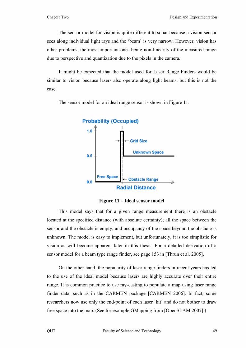
Chapter Two Design and Experimentation
The sensor model for vision is quite different to sonar because a vision sensor
sees along individual light rays and the ‘beam’ is very narrow. However, vision has
other problems, the most important ones being non-linearity of the measured range
due to perspective and quantization due to the pixels in the camera.
It might be expected that the model used for Laser Range Finders would be
similar to vision because lasers also operate along light beams, but this is not the
case.
The sensor model for an ideal range sensor is shown in Figure 11.
Figure 11 – Ideal sensor model
This model says that for a given range measurement there is an obstacle
located at the specified distance (with absolute certainty); all the space between the
sensor and the obstacle is empty; and occupancy of the space beyond the obstacle is
unknown. The model is easy to implement, but unfortunately, it is too simplistic for
vision as will become apparent later in this thesis. For a detailed derivation of a
sensor model for a beam type range finder, see page 153 in [Thrun et al. 2005].
On the other hand, the popularity of laser range finders in recent years has led
to the use of the ideal model because lasers are highly accurate over their entire
range. It is common practice to use ray-casting to populate a map using laser range
finder data, such as in the CARMEN package [CARMEN 2006]. In fact, some
researchers now use only the end-point of each laser ‘hit’ and do not bother to draw
free space into the map. (See for example GMapping from [OpenSLAM 2007].)
QUT Faculty of Science and Technology 49
Mapping of Indoor Environments by Robots using Low-cost Vision Sensors Trevor Taylor
2.5 Probabilistic Filters
Most modern SLAM algorithms rely on the use of probabilistic filters. The
most commonly used forms of filters are Kalman Filters and Particle Filters. These
are discussed below.
2.5.1 Kalman Filters
Kalman Filters are discussed here for completeness. For a good explanation of
Kalman Filtering see [Choset et al. 2005]. The description in [Thrun et al. 2005]
follows a different approach with quite different notation. [Andrade-Cetto &
Sanfeliu 2006] provide extensive discussion of the stability of the Kalman Filter.
It is only in the last decade that the stability of Kalman Filter-based SLAM has
been proven [Newman 1999, Dissanayake et al. 2001]. However, it must be noted
that stability is only proven in the limit as the number of observations approaches
infinity.
A Kalman Filter is basically a recursive state estimator [Kalman 1960]. The
‘state’ consists of a set of ‘features’ observed in the environment plus the robot’s
pose. Estimating the location of the features effectively builds a map.
The reason for the early popularity the Kalman Filter is that it is analytically
tractable and the update equations can be expressed in closed form. Being a recursive
filter, it is also computationally efficient.
2.5.2 The Kalman Filter Algorithm
The following is a brief definition of the Kalman Filter. The derivation can be
found in Probabilistic Robotics starting on page 40. The notation is as shown below
which differs slightly from the textbook:
At State Transition matrix from prior state at time t
Bt State Transition matrix from control input at time t
Ct State to Measurement Transformation matrix at time t
Kt Kalman Gain at time t
50 Faculty of Science and Technology QUT
Chapter Two Design and Experimentation
Qt Measurement noise covariance at time t
Rt System noise covariance at time t
St Estimated covariance of the state at time t
ut Control input at time t
xt Current state at time t (location of features plus the robot pose)
zt Sensor measurements at time t
δt Measurement noise at time t
εt System noise at time t
µt Estimate of the state at time t
The system is assumed to be described by equation 6:
xt = At xt-1 + Bt ut + εt (6)
This equation says that the new state is a linear combination of the previous
state plus the control input with additive zero-mean Gaussian noise, εt, with a
covariance of Rt. There are three assumptions here: linear system dynamics; first-
order Markov process; and noise that is both zero-mean and Gaussian.
The system state can only be observed indirectly through measurements, zt,
which are described by the following equation:
zt = Ct xt + δt (7)
Equation 7 states that the measurements are linearly related to the system state
plus some measurement noise, δt, that is zero-mean and has a covariance of Qt.
It is further assumed that the initial state is normally distributed with mean µ0
and covariance and S0.
QUT Faculty of Science and Technology 51
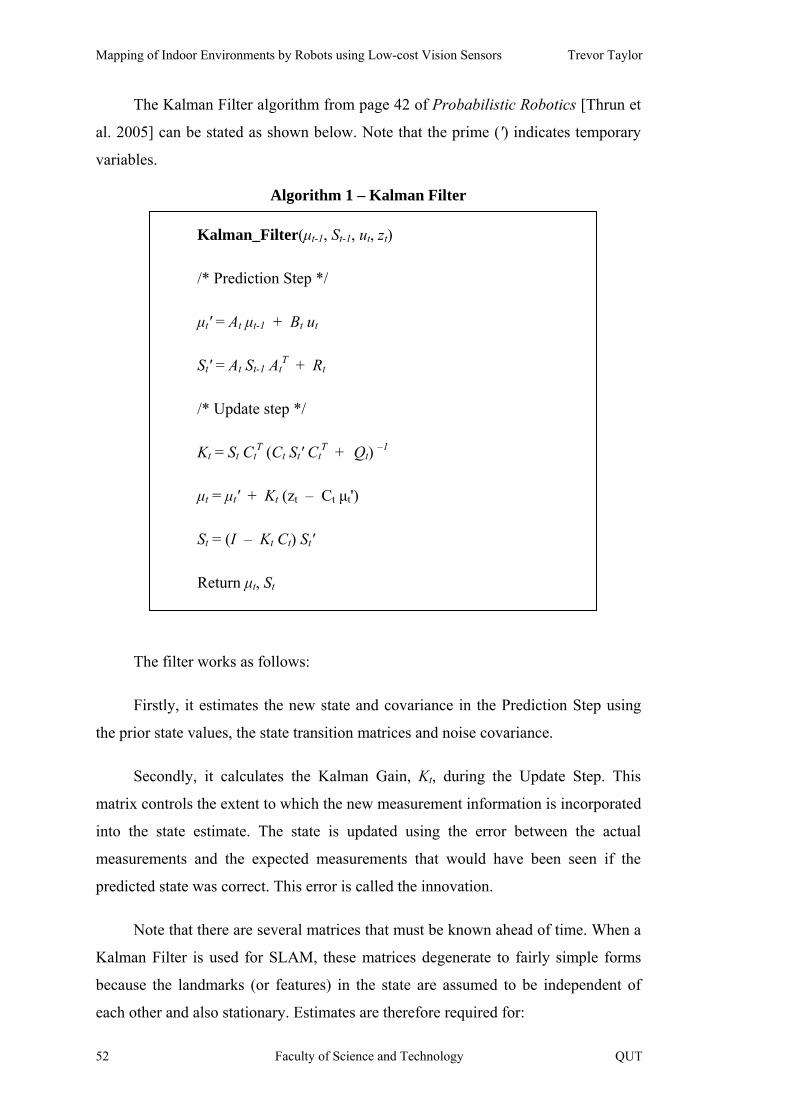
Mapping of Indoor Environments by Robots using Low-cost Vision Sensors Trevor Taylor
The Kalman Filter algorithm from page 42 of Probabilistic Robotics [Thrun et
al. 2005] can be stated as shown below. Note that the prime (') indicates temporary
variables.
Algorithm 1 – Kalman Filter
Kalman_Filter(µt-1, St-1, ut, zt)
/* Prediction Step */
µt' = At µt-1 + Bt ut
St' = At St-1 AtT + Rt
/* Update step */
Kt = St CtT (Ct St' Ct
T + Qt) –1
µt = µt' + Kt (zt – Ct µt')
St = (I – Kt Ct) St'
Return µt, St
The filter works as follows:
Firstly, it estimates the new state and covariance in the Prediction Step using
the prior state values, the state transition matrices and noise covariance.
Secondly, it calculates the Kalman Gain, Kt, during the Update Step. This
matrix controls the extent to which the new measurement information is incorporated
into the state estimate. The state is updated using the error between the actual
measurements and the expected measurements that would have been seen if the
predicted state was correct. This error is called the innovation.
Note that there are several matrices that must be known ahead of time. When a
Kalman Filter is used for SLAM, these matrices degenerate to fairly simple forms
because the landmarks (or features) in the state are assumed to be independent of
each other and also stationary. Estimates are therefore required for:
52 Faculty of Science and Technology QUT
Chapter Two Design and Experimentation
• the motion model, which is how the robot’s pose changes in response
to the control input (elements of At and Bt);
• the measurement model, which is how the sensor responds to a given
feature (Ct); and
• the system and measurement noise covariances (Rt and Qt).
Furthermore, it is usually assumed that the system and sensor dynamics do not
change over time, so the relevant matrices are fixed so the subscript, t, can be
dropped.
2.5.3 Particle Filters
A popular form of localization is called Monte Carlo Localization (MCL).
There is an enormous amount of literature on the subject, although sometimes under
other names. Much of the work has been done by the trio of Thrun, Burgard and Fox.
In particular, Probabilistic Robotics by these authors is the definitive textbook in this
area.
MCL represents the belief in the current pose of the robot as a set of particles.
In simple terms, a particle consists of a pose estimate and any necessary state
information that is required to perform updates to the pose. As the robot moves,
these particles trace out trajectories (or paths) on the map.
If the set of particles is sufficiently large and has an appropriate distribution
that adequately represents the true posterior probability distribution, then the average
of the particles should be near to the actual pose of the robot. Ideally, one of the
particles should be very close to correct. If there is no such particle, then there are
insufficient particles in the set and the filter is likely to diverge.
A particle filter (for localization) operates as follows:
QUT Faculty of Science and Technology 53

Mapping of Indoor Environments by Robots using Low-cost Vision Sensors Trevor Taylor
Algorithm 2 – Particle Filter
1. Perform a motion (based on the control input).
2. Obtain a new range scan (the measurement).
3. For each particle in the set calculate the new pose:
a. Apply the motion model to the existing (particle) pose using
the control input; and
b. For the new pose, compare the measurement to the global map
to obtain a weight (the importance factor).
4. Resample with probability proportional to the weights.
5. Decide where to go next and calculate the new control input.
6. Repeat from Step 1.
Note that there is an interesting issue here. With hundreds of particles
providing different poses there are several ways to determine the best estimate of the
pose. Taking an average seems intuitively correct, but the distribution might not be
anything like a Gaussian and could even be multi-modal. Selecting the particle that
has the best match to the existing map (highest importance factor) is another possible
approach.
Applying the motion model is referred to as sampling from the proposal
distribution. It can be considered to be adding to the tree of all possible particle
trajectories. Calculating the importance weights and then applying resampling results
in a pruning of the tree because some particles are thrown away and others are
duplicated.
Clearly this process is a compromise. It is desirable to maintain particle
diversity so that the particle set adequately represents the true posterior distribution
over the robot’s pose, but at the same time it is important to eliminate trajectories
54 Faculty of Science and Technology QUT

Chapter Two Design and Experimentation
that are obviously incorrect because they simply distort the resulting distribution and
ultimately would cause the filter to fail. Simplistically, the objective is to keep the
‘good’ particles and throw away the ‘bad’ ones. The difficulty is determining which
particles are good or bad, which is the responsibility of the map comparison step.
2.5.4 Particle Weights
An important step in a particle filter is to rank particles based on their weights.
The weights are calculated by comparing the local map information generated by
each particle against a global map. For localization only, the correct map is available
and there is no ambiguity in calculating the weights. However, in SLAM the map is
being constructed at the same time as the localization is taking place.
In SLAM each particle constructs its own map. Some of the maps will be
closer to the ground truth than others. However, the ground truth is unknown, by
definition. If a ‘bad’ particle survives for long enough, it will construct its own map
variant which fits the data and therefore its weight compared to its own map can
remain relatively high. One possibility is to compare each particle map against the
average of all maps, thereby ensuring that an individual particle cannot construct its
own version of reality and maintain its weight.
2.5.5 Resampling
Resampling is necessary because there is a finite number of particles in the set.
The objective is to retain the best particles and eliminate particles that have poor
weights. Some of the particles are ‘cloned’ to replace the bad particles.
Note that resampling should not necessarily occur after every new input
sample is received, although this is what Algorithm 2 suggests. It is common
practice to perform resampling after a small number of consecutive sensor
measurements (and motions) have been made. This provides more information for
use in the calculation of the weights and is acceptable if the variance in the pose is
not too great over the small number of motions.
There are several different ways to perform resampling. The Low Variance
Sampler from page 110 of Probabilistic Robotics can be stated as follows:
QUT Faculty of Science and Technology 55

Mapping of Indoor Environments by Robots using Low-cost Vision Sensors Trevor Taylor
Algorithm 3 – Low Variance Sampler
Low_Variance_Sampler(Pt)
Tt = Ø
r = random(0..1) / M
c = wtk
i = 1
For k = 1 to M
U = r + (k – 1) / M
While U > c
i = i + 1
c = c + wtk
End While
Add ptk to Tt
End For
Return Tt
Resampling is a stochastic process. The objective is to select particles with a
probability proportional to their importance weights. Particles are replaced after
selection, which means that the same particle can be selected more than once if it has
a high weight. However, because it is stochastic, it is possible to select a particle
with a very low weight – ‘good’ particles can be replaced by ‘bad’ ones.
Although resampling algorithms are designed to be unlikely to propagate bad
particles, it is not impossible. The author observed bad particles being propagated
during several test runs over multiple iterations. Consider for instance the case where
56 Faculty of Science and Technology QUT

Chapter Two Design and Experimentation
there is very little input information, i.e. few obstacles are visible such as in the
middle of a large open space. In this case the particles will all have very similar
weights and the stochastic nature of the resampling process can select bad particles.
The problem known as Particle Deprivation (discussed below) is symptomatic of the
propagation of bad particles.
2.5.6 Particle Diversity
A significant issue related to Particle Filters is the diversity of the particle set.
Particle Filters cannot propagate new information backwards in time – the
trajectories of particles cannot be updated retrospectively.
It is possible to think of particles in terms of their ancestry. Tracing back in
time, eventually all particles might have a single common ancestor. Looking at the
number of steps backward in time to reach this common ancestor gives some
indication of how well the filter can tolerate errors. In particular, for the filter to
‘close a loop’, some particle diversity must remain at the point where the loop closes.
Put simply, this means that the more particles there are, the larger the loop that can
be closed.
2.5.7 Number of Particles Required
Selection of the number of particles for a particle filter is difficult. Too few
particles can result in the filter failing, whereas too many particles will adversely
affect performance. Clearly, the lower bound is one particle which is not a particle
filter at all. The chance of one particle following the correct trajectory is quite small,
although not zero. On the other hand, it is impossible in practice to have an infinite
number of particles.
There is no formal procedure or theoretical foundation for selecting the number
of particles. Usually researchers establish the number of particles required by trial
and error. The process might simply be to start with a very large number of particles
and keep reducing the number until the filter fails.
Some algorithms reported in the literature have used thousands of particles,
such as DP-SLAM [Eliazar & Parr 2003]. Examples on the web site for DP-SLAM
(see the link from [OpenSLAM 2007]) used between 1,000 and 9,000 particles.
QUT Faculty of Science and Technology 57
Mapping of Indoor Environments by Robots using Low-cost Vision Sensors Trevor Taylor
One of the objectives of GMapping [Grisetti et al. 2005, Grisetti et al. 2007]
was specifically to reduce the number of particles required because each particle
contained an occupancy grid map. Some examples used as few as 30 particles.
P-SLAM [Chang et al. 2007] predicted the structure of the environment based
on features already in the map. This worked well in indoor environments. However,
the authors showed a real-life example where 1,000 particles were required with a
Rao-Blackwellized Particle Filter in order to produce a good map. The minimum
number of particles quoted for P-SLAM was 200, but in this case the map was
distorted.
A recent paper [Stuckler & Benhke 2008] that applied the environmental
assumption of orthogonal walls showed that acceptable quality maps could be
produced using only 50 particles. (NOTE: This paper was published concurrently
with this thesis. The concept of incremental localization developed in this thesis is
similar, but not derived from this paper.)
2.5.8 Particle Deprivation
One of the well-known problems with Particle Filters is referred to as particle
deprivation or depletion [Thrun et al. 2005, p122] or sample impoverishment
[Montemerlo & Thrun 2007, p63]. This happens when the particle set becomes
dominated by a few particles, leading to a dramatic reduction in diversity. If the
remaining particles do not properly represent the posterior distribution over the
robot’s pose, then the filter will diverge. This occurs in practice because there can
only be a finite number of particles.
Montemerlo and Thrun suggest that this problem occurs when there is a
mismatch between the proposal and posterior distributions due to the motion model
being very noisy, but the measurements being quite accurate. A substantial portion of
the particle set will therefore be thrown away.
The problem can be aggravated by resampling too frequently or a poor
objective function for calculating the weights.
58 Faculty of Science and Technology QUT
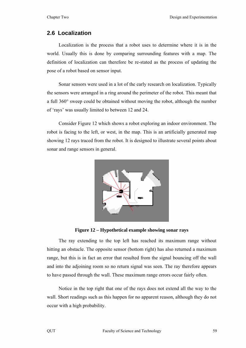
Chapter Two Design and Experimentation
2.6 Localization
Localization is the process that a robot uses to determine where it is in the
world. Usually this is done by comparing surrounding features with a map. The
definition of localization can therefore be re-stated as the process of updating the
pose of a robot based on sensor input.
Sonar sensors were used in a lot of the early research on localization. Typically
the sensors were arranged in a ring around the perimeter of the robot. This meant that
a full 360° sweep could be obtained without moving the robot, although the number
of ‘rays’ was usually limited to between 12 and 24.
Consider Figure 12 which shows a robot exploring an indoor environment. The
robot is facing to the left, or west, in the map. This is an artificially generated map
showing 12 rays traced from the robot. It is designed to illustrate several points about
sonar and range sensors in general.
Figure 12 – Hypothetical example showing sonar rays
The ray extending to the top left has reached its maximum range without
hitting an obstacle. The opposite sensor (bottom right) has also returned a maximum
range, but this is in fact an error that resulted from the signal bouncing off the wall
and into the adjoining room so no return signal was seen. The ray therefore appears
to have passed through the wall. These maximum range errors occur fairly often.
Notice in the top right that one of the rays does not extend all the way to the
wall. Short readings such as this happen for no apparent reason, although they do not
occur with a high probability.
QUT Faculty of Science and Technology 59

Mapping of Indoor Environments by Robots using Low-cost Vision Sensors Trevor Taylor
Now consider if the robot were to move forward. The ray towards the upper
left that narrowly misses the obstacle would then intersect with the obstacle and be
much shorter.
Alternatively, if the robot turned to its left, the ray from the front sensor of the
robot, which hits the very corner of an obstacle in the diagram, would miss the
obstacle and travel all the way to the wall at the left.
Small changes in position can therefore have a significant effect on the range
values. This clearly illustrates how matching the rays to a map can be used for
localization.
This explanation is based on using only a small number of range-bearing
measurements. (The bearings are implicit in the arrangement of the sensors around
the robot.) For a sensor that generates significantly denser range data, such as a laser
range finder or vision, other approaches are possible.
In this project, the visual component of the system generates a floor boundary,
which is analogous to a laser range finder’s range scan. This ROP, as it is called, is
used to create a local map. By overlaying the local map on the existing global map
and comparing the two it is possible to obtain a measure of fit. This might be thought
of as the logical extension of Figure 12 to a very large number of rays. Similar
problems with overshooting and short range measurements also apply to vision, but
the reasons are quite different to sonar and lasers.
The biggest challenge to Localization is erroneous odometry information. The
background to odometers is discussed in the classic textbook Sensors for Mobile
Robots [Everett 1995]. According to Murphy [Murphy 2000], ‘shaft encoders are
notoriously inaccurate’. Odometry errors are discussed at length in [Borenstein &
Feng 1996].
2.6.1 Levels of Localization
A common thread in the literature is the ‘Kidnapped Robot’ problem. This is
different from simply getting lost while exploring. A kidnapped robot ‘wakes up’ in
unfamiliar surroundings and has to determine where it is. Clearly this is the most
60 Faculty of Science and Technology QUT
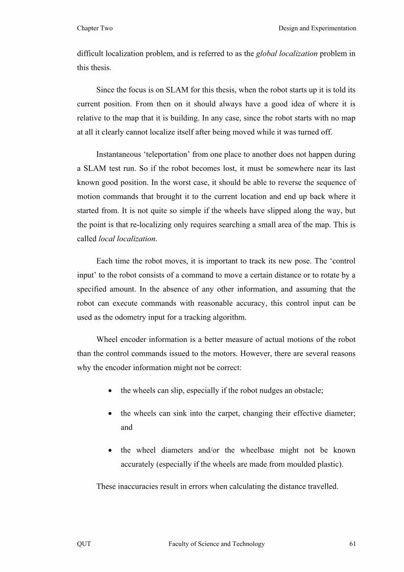
Chapter Two Design and Experimentation
difficult localization problem, and is referred to as the global localization problem in
this thesis.
Since the focus is on SLAM for this thesis, when the robot starts up it is told its
current position. From then on it should always have a good idea of where it is
relative to the map that it is building. In any case, since the robot starts with no map
at all it clearly cannot localize itself after being moved while it was turned off.
Instantaneous ‘teleportation’ from one place to another does not happen during
a SLAM test run. So if the robot becomes lost, it must be somewhere near its last
known good position. In the worst case, it should be able to reverse the sequence of
motion commands that brought it to the current location and end up back where it
started from. It is not quite so simple if the wheels have slipped along the way, but
the point is that re-localizing only requires searching a small area of the map. This is
called local localization.
Each time the robot moves, it is important to track its new pose. The ‘control
input’ to the robot consists of a command to move a certain distance or to rotate by a
specified amount. In the absence of any other information, and assuming that the
robot can execute commands with reasonable accuracy, this control input can be
used as the odometry input for a tracking algorithm.
Wheel encoder information is a better measure of actual motions of the robot
than the control commands issued to the motors. However, there are several reasons
why the encoder information might not be correct:
• the wheels can slip, especially if the robot nudges an obstacle;
• the wheels can sink into the carpet, changing their effective diameter;
and
• the wheel diameters and/or the wheelbase might not be known
accurately (especially if the wheels are made from moulded plastic).
These inaccuracies result in errors when calculating the distance travelled.
QUT Faculty of Science and Technology 61
Mapping of Indoor Environments by Robots using Low-cost Vision Sensors Trevor Taylor
Other information must therefore be used to refine estimated motions. This is
referred to as incremental localization because it incrementally adjusts the robot’s
pose between motions. The purpose is to improve the pose estimate prior to
executing the localization algorithm.
2.6.2 Localization Approaches
Localization methods fall into two broad categories:
• Kalman Filters which track features (also called landmarks or beacons)
using normal distributions to estimate errors in feature locations; and
• Markov localization methods, also called Monte Carlo Localization
(MCL) or Particle Filters, which approximate an arbitrary probability
distribution using a set of particles and operate on a grid-based map.
These techniques do not have to be mutually exclusive. For example,
probabilistic methods like MCL can use Kalman Filters in their particles instead of
occupancy grids.
It is important to note that most popular localization methods make the
assumption that the system can be represented as a first-order Markov process. In
terms of localization, this means that the robot’s pose at a particular time, t, depends
only on its pose at the previous time step, (t-1), and the control input applied to the
robot’s motors in the intervening time interval. In general, the pose at time t might
depend on a finite number of previous poses, but this is ignored.
Localization with a known map has been studied for many years. [Gutmann et
al. 1998] compared several methods, and suggested that there are three basic
approaches to localization:
1. Behaviour-based;
2. Landmark-based; and
3. Dense sensor matching.
62 Faculty of Science and Technology QUT
Chapter Two Design and Experimentation
The last two subsections discuss how to improve the quality of the pose
estimates prior to applying a localization algorithm.
2.6.3 Behaviour-Based Localization
Behaviour-based approaches usually generate topological maps. They might
involve behaviours such as wall following and recording features such as doorways.
It can therefore be difficult for these approaches to recognise places that have been
previously visited, and they cannot localize a robot accurately in a metric sense.
2.6.4 Landmark-Based Localization
There is a large body of literature that deals with using known landmarks
and/or man-made beacons for localization. Obviously, if the robot is building a map
then there cannot be any known landmarks to begin with.
Artificial landmarks were deliberately avoided in this project because
introducing them into the environment is not possible in many situations.
Furthermore, artificial landmarks introduce additional costs and maintenance
overhead.
An alternative is to choose natural landmarks, or ‘features’. It is important to
select only significant features because an excessive number of features will not
necessarily help localization. However, when operating in a corridor environment
many of the images might not show any obvious visible landmarks. This is discussed
further under Tracking Features.
There are other problems with this approach as well. In particular, landmarks
can look different from different directions or even be unidentifiable from a different
viewpoint. For instance, the front and back of a chair look quite different, but it is the
same object.
The Symmetries and Perturbations Map (SPMap) uses corners and
‘semiplanes’ as the principal features [Castellanos et al. 1999]. A ‘semiplane’ is a
line segment obtained from a laser range scan and typically represents a wall. They
developed probabilistic models for matching and tracking these distinguishing
features.
QUT Faculty of Science and Technology 63
Mapping of Indoor Environments by Robots using Low-cost Vision Sensors Trevor Taylor
[Castellanos & Tardós 1999] addressed sensor fusion between laser range
finders and monocular vision. In the case of vision, they used vertical edges as
landmarks. However, the camera was horizontal which makes detecting vertical
edges trivial. The general case where the camera is tilted is discussed below.
2.6.5 Dense Sensor Matching for Localization
Two variants of dense sensor matching were compared empirically in
[Gutmann et al. 1998]: Markov localization (based on a grid); and scan matching
using a Kalman filter (which was feature-based). In essence, these are the two
primary methods still in use today, although Gutmann et al. suggested combining the
two techniques. In particular, it was concluded that scan matching was more accurate
than Markov localization, but was less robust as the noise level increased.
‘Catastrophic failures’ were observed by Gutmann et al. in some cases,
meaning that the localization algorithm diverged. It is interesting to note that even in
this early work there was mention of a requirement for ‘sufficient information’ for
scan matching to be successful.
[Gutmann & Konolige 1999] addressed the problem of large cyclic
environments which are known to present problems for localization algorithms. They
combined three different techniques (scan matching, consistent pose estimation and
map correlation) to create the LRGC (Local Registration / Global Correlation)
algorithm.
Some of the early papers on the subject of localization did not provide
experimental results for long test runs. Examples were given from simulations, or
quite short runs. It was only with work such as [Thrun et al. 2000] that evidence
started to appear to show that localization worked reliably over long periods of time
and long distances travelled.
2.6.6 Scan Matching
In recent years there has been a lot of work done on scan matching which
involves comparing two successive laser range scans. The original work dates back
to [Lu & Milios 1994, 1997] who applied various techniques to matching sonar
sweeps in order to determine the amount of a rotation and/or translation.
64 Faculty of Science and Technology QUT
Chapter Two Design and Experimentation
[Hähnel 2004] used scan matching of laser range scans to improve pose
estimates before performing SLAM updates. He attributes the quality of his maps to
this extra step. [Grisetti et al. 2005] continued with this approach in the GMapping
algorithm.
[Nieto et al. 2005] introduced an approach called Scan-SLAM that
incorporated scan matching into an EKF SLAM algorithm.
Scan matching is not directly applicable to vision. Information must first be
extracted from an image that is similar to a laser range scan.
2.6.7 Improving the Proposal Distribution
The objective of improving the proposal distribution is to enhance the stability
of the filter by providing better pose estimates before performing the update step.
This is sometimes referred to as incremental localization. Scan matching (discussed
in the previous section) is one of the common approaches.
An alternative to scan matching is to compare features in the input data against
known features in the map and update the robot’s pose estimate prior to applying the
filter. The selected features must be significant such as walls or corners.
2.7 Simultaneous Localization and Mapping (SLAM)
For autonomous mobile robots to operate in human environments they need
SLAM (Simultaneous Localization and Mapping), also referred to as CML
(Concurrent Mapping and Localization). As domestic robots begin to appear in our
homes, it will simply not be acceptable for users to have to program maps into their
robots. Quite apart from the fact that most people do not have a map of their home,
they will not want to be bothered with the tedious process of entering a map into the
robot’s memory.
Leading researchers in the field have suggested that SLAM is now a ‘solved’
problem [Durrant-Whyte & Bailey 2006]. However, they go on to discuss the many
practical problems that still remain.
The primary problems that SLAM has to solve are:
QUT Faculty of Science and Technology 65

Mapping of Indoor Environments by Robots using Low-cost Vision Sensors Trevor Taylor
• Determining the robot’s pose from uncertain input data; and
• Estimating the relative position of observed features from
measurements containing noise.
Building a map is not one of the significant problems if the input data is
accurate. Also, the exploration algorithm does not have a strong effect.
However, if the robot’s pose is not correct, or the observations contain gross
errors, then features will be inserted into the map in the wrong locations. These
errors accumulate, resulting in distortions of the map. It is even possible for the robot
to become completely lost.
It is generally acknowledged that the field of SLAM began with a paper by
[Smith & Cheesman 1986] in which they addressed the issue of representing spatial
uncertainty in a systematic way. In a revised version [Smith et al. 1990], which is
also widely cited, they introduced the term ‘stochastic map’ which reflects the fact
that the input information is stochastic in nature.
This ground-breaking work discussed the use of a Kalman Filter and also
applied Monte Carlo simulation to robot pose estimation. Even at this preliminary
stage, the authors pointed out two of the most fundamental problems with SLAM:
non-Gaussian distributions; and non-linearities in the system.
Soon after the Smith & Cheeseman paper, another early researcher used a
geometric approach to develop a theoretical framework for SLAM [Durrant-Whyte
1988]. No experimental data was provided in this paper.
Various researchers under the tutelage of Durrant-Whyte have worked on
SLAM for close to two decades. Newman’s PhD thesis [Newman 1999] provided a
detailed theoretical background, including proofs that existing SLAM algorithms
converged (in the limit as time goes to infinity) and also a new algorithm that used
the relationships between map features rather than their absolute positions. The
general solution to the SLAM problem was published by [Dissanayake at al. 2001].
66 Faculty of Science and Technology QUT
Chapter Two Design and Experimentation
Most of the early work on SLAM was done using sonar sensors, such as [Lee
1996]. These are noisy and not very accurate. Therefore it made sense to use a
probabilistic approach.
More recently, Laser Range Finders (LRFs) have become popular. These
devices have a much greater range than sonar, and are extremely accurate by
comparison. However, LRFs cost significantly more than sonar sensors.
Vision is the most recent sensor to be used and there is a great deal of research
currently in progress on using vision for SLAM. One of the key advantages of
vision, which was part of the initial impetus for this research, is that cameras are now
very cheap. The disadvantage is that vision is a very complex sensor to use.
Consequently, many different approaches have been used for visual SLAM, as
explained later in this chapter in section 2.8.
2.7.1 SLAM Approaches
SLAM is basically a ‘chicken and the egg’ problem. To localize itself, the
robot needs a map. However, the robot does not have a map initially because
building a map is the objective of SLAM (and an appropriate exploration algorithm).
One of the implicit assumptions in SLAM is that the process can be
represented by a first-order Markov model. In other words, the current state depends
only on the previous state.
In broad terms, there are two basic approaches to SLAM:
• Kalman Filtering; and
• Probabilistic methods.
It is also possible to merge the two approaches. For instance, a set of Kalman
Filters can be used in the particles of a Particle Filter.
This section briefly outlines these two different approaches. The key point is
that all SLAM methods use stochastic models – they allow for uncertainty in the
estimated locations of objects in the environment and in the estimated pose of the
robot.
QUT Faculty of Science and Technology 67

Mapping of Indoor Environments by Robots using Low-cost Vision Sensors Trevor Taylor
2.7.2 Map Features for Kalman Filtering
Kalman Filters work with features in their state vectors and therefore are not
normally applied to grid-based maps because each grid cell would become a variable
in the state vector. The size of the filter covariance matrix grows at the rate of N2,
where N is the number of features. This can rapidly become unmanageable for large
environments or if the system is over-zealous in selecting features. As the number of
features increases, it starts to detract from the computational efficiency.
Although it is tempting to consider features to be ‘points’ in space, there are
implementations using the Kalman Filter to track other types of features. For
example, [Castellanos & Tardós 1999] used what they referred to as corners,
segments and semiplanes. As long as the features can be described parametrically
and there are methods to unambiguously determine matches between features, then
the Kalman Filter can be applied.
This simplified discussion ignores the requirement to add new features to the
state vector as they are discovered, and also to remove features if they later prove to
be inappropriate or mistakes or just to prune the state vector.
Some research has been directed towards minimizing the impact of the
expanding state matrix by breaking the map into a series of sub-maps or ignoring
features that are out of sensor range during updates. This can significantly reduce the
computational burden. However, it assumes that the sub-maps are all correctly
correlated with each other.
The nature of the Kalman Filter algorithm is such that the landmarks are fully
correlated. Therefore over time the correlation matrix will become static and the
Kalman gain will approach zero. This can happen very quickly according to
[Andrade-Cetto & Sanfeliu 2006]. In other words, no further updates to existing
landmark locations will occur – only the robot’s pose will be updated.
In theory, all landmarks must be observable at every step in order to perform a
full update. Furthermore, it must be possible to match each of the landmarks to the
corresponding one in the new observations, a process called data association. Clearly
this will never be the case in practice.
68 Faculty of Science and Technology QUT

Chapter Two Design and Experimentation
One significant problem with Kalman Filters is data association, which is the
process of matching the observed features between iterations of the filter. Any
textbook on SLAM will have a reference to this problem. See for example [Thrun et
al. 2005, Choset et al. 2005].
In order to update the state, it is necessary to know which feature corresponds
to which measurement. If a feature is associated with the wrong measurement, it can
cause the filter to become unstable. Other factors can also affect the quality of data
association such as the selection of spurious features or ambiguous features. Methods
have been developed to prune features that exhibit a large variance on the
assumption that they have resulted from a mismatch.
Features also must be invariant. In other words, they must not move around. In
theory the Kalman Filter can handle non-stationary environments. However, data
association errors resulting from moving objects can have drastic effects on the
correlation matrix.
2.7.3 Extensions to the Kalman Filter
As noted above, Kalman Filters assume that the system is linear and that any
signal noise has a Gaussian distribution. Real-world systems do not fit these
assumptions. To try to resolve this problem, the Extended Kalman Filter (EKF)
linearises the system around the current point using the first term of a Taylor
expansion. Calculating the required Jacobians increases the complexity and
computational load.
The EKF has been one of the most popular methods for SLAM in recent years.
However, in an invited paper [Julier & Uhlmann 2004] state that the EKF has several
deficiencies and that ‘more than 35 years of experience in the estimation community
has shown that it is difficult to implement, difficult to tune, and only reliable for
systems that are almost linear on the time scale of the updates.’ This is a serious
concern.
To try to overcome the linear Gaussian restriction, the Unscented Kalman
Filter (UKF) was developed [Julier & Uhlmann 1997]. UKFs combine some of the
features of probabilistic estimation with the traditional EKF, so that rather than
QUT Faculty of Science and Technology 69

Mapping of Indoor Environments by Robots using Low-cost Vision Sensors Trevor Taylor
linearizing using a Taylor expansion, the probability distribution is represented using
‘sigma points’.
2.7.4 Examples of Kalman Filter-based SLAM
The following diagrams for EKF SLAM (Figure 13) and UKF SLAM (Figure
14) were generated by the author by running sample code provided by Dr. Bailey on
the OpenSLAM web site [OpenSLAM 2007]. They are used to illustrate a couple of
key points, not to show any deficiencies in these approaches.
Figure 13 – EKF SLAM example in Matlab
In Figure 13, the actual trajectory of the robot and the estimated trajectory do
not match exactly. Furthermore, towards the end (bottom left) many of the estimated
feature locations (shown as error ellipses with a ‘+’ in the centre) are wrong.
70 Faculty of Science and Technology QUT

Chapter Two Design and Experimentation
Figure 14 – UKF SLAM example in Matlab
Figure 14 shows UKF SLAM where the robot has traversed the loop twice.
The second trajectory tracks the actual trajectory much more closely. Also, the
estimated errors in the feature locations have reduced significantly. However, the
estimated locations are still incorrect for many of the features.
The main point is that these are state-of-the-art algorithms, but they still cannot
produce good results. The importance of revisiting areas that have been seen
previously is also quite clear – as shown by trajectory improvements in Figure 14.
2.7.5 Particle Filter SLAM
[Thrun et al. 1998] were one of the first groups to apply particle filter methods
to SLAM. They formulated the problem using probability distributions and applied
Expectation Maximization (EM) to solve the problem.
The particle filter approach to SLAM is relatively recent, but it has gained
considerable attention in the literature [Doucet et al. 2001]. There are many different
names and algorithms. One basic approach, known as Monte Carlo SLAM, or
Particle Filters, can be described as follows:
QUT Faculty of Science and Technology 71

Mapping of Indoor Environments by Robots using Low-cost Vision Sensors Trevor Taylor
Maintain a large collection of pose estimates and maps with associated
certainty estimates, and update these at each step so that the distribution of these
estimates eventually approximates the real probability distribution. The idea is to
keep enough ‘guesses’ that one of them will actually turn out to be correct.
Particle Filters can be applied to either feature or grid-based maps. For
instance, a Particle Filter might use a separate Kalman Filter for each particle. In the
case of occupancy grids, each particle must maintain a separate copy of the grid. The
result is that Particle Filters can be very memory and computationally intensive.
One way to view the output of a Particle Filter is by plotting the trajectories of
all of the particles. Figure 15 shows the trajectories of particles during an exploration
run.
Figure 15 – Example of particle trajectories
In Figure 15 the robot started at the bottom centre of the map. The locations of
the particles are shown as black dots at the ends of the grey trajectories. As it
progressed, the robot became increasingly uncertain about its pose. This is reflected
in the spreading of the particles trajectories. In this 2D representation it is not
possible to show the orientations of the particles, which also have some variation.
2.7.6 A Particle Filter SLAM Algorithm
Several SLAM algorithms are provided in pseudo-code in Probabilistic
Robotics [Thrun et al. 2005]. More recently, open source code has begun to appear
[OpenSLAM 2007].
72 Faculty of Science and Technology QUT

Chapter Two Design and Experimentation
FastSLAM is a popular form of particle filter, and FastSLAM 2.0 [Montemerlo
et al. 2003, Montemerlo & Thrun 2007] is the most recent incarnation. When applied
to an occupancy grid it is called GridSLAM.
The GridSLAM algorithm is discussed below based on the description in
[Thrun et al. 2005] which is the definitive textbook on the subject. The algorithm is
reproduced below for ease of reference, with some small notational changes. The
algorithm is expressed at a high level. The derivation is not discussed here because it
was given in [Thrun et al. 2005].
In the algorithm below, the following notation is used:
M Number of particles
mtk Map (global) associated with particle number k at time t
ptk Particle number k at time t (which contains xt
k, mtk, wt
k)
Pt Particle set at time t (which contains all particles for k=1..M)
Tt Temporary particle set
ut Control input at time t
wtk Weight of particle number k at time t
xtk Robot pose for particle number k at time t
zt Sensor measurements at time t
The GridSLAM algorithm from page 478 of Probabilistic Robotics [Thrun et
al. 2005] can be stated as shown below.
QUT Faculty of Science and Technology 73

Mapping of Indoor Environments by Robots using Low-cost Vision Sensors Trevor Taylor
Algorithm 4 – FastSLAM Occupancy Grids
FastSLAM_Occupancy_Grids(Pt-1, ut, zt)
Tt = Ø /* Empty temporary Particle Set */
For k = 1 to M /* For each particle … */
xtk = Sample_Motion_Model(ut, xt-1
k)
wtk = Measurement_Model_Map(zt, xt
k, mt-1k)
mtk = Update_Occupancy_Grid(zt, xt
k, mt-1k)
Add particle ‹xtk, mt
k, wtk› to Tt
End For
/* Select new Particle Set based on Weights */
Pt = Resample(Tt)
Return Pt
This algorithm in turn uses several other algorithms. These are explained
below. However, some notes are appropriate at this point.
Each particle contains its own global map, mtk. Depending on the particle
trajectories, these maps can be substantially different. However, the same
measurement data, zt, is applied to all maps.
Particles also have a current pose, xtk, which is used when updating the map.
However, there is no trajectory maintained by the particle. The map implicitly
records the trajectory. This is a key point. It is a consequence of the Markov
assumption which states that the current pose depends only on the previous pose and
the control input, so there is no need to maintain a trajectory.
74 Faculty of Science and Technology QUT
Chapter Two Design and Experimentation
The control input, ut, could be either the command issued to the robot or the
odometry data from the robot’s wheel encoders. In either case, it represents the
amount by which the robot has moved. Clearly, ut is noisy, and this is one reason
why localization is required.
Sensor measurements (also called observations), zt, can take many forms.
Usually they will be an array of range measurements, also referred to as a range
scan. For sonar sensors or a laser range finder it is quite obvious how this is derived.
For the vision system a simulated range scan is obtained from the floor boundary as
is explained above in the section on Inverse Perspective Mapping.
The importance weights, wtk, are normalized so that they sum to 1.0 and they
are therefore equivalent to the probability of a match between the current sensor
measurement (observation) and the global map.
FastSLAM 2.0, which is an improved version of FastSLAM, applies the most
recent measurement to pose prediction prior to calculating the new proposal
distribution. The result is improved performance and stability, and might be viewed
as a form of incremental localization.
2.7.7 Sample Motion Model
The motion model should represent the physical process that the robot
undertakes as it moves through the environment. There are many different motion
models that can be used.
The mechanics of robot motion are covered extensively in [Choset et al. 2005],
with a similar model in [Thrun et al. 2005]. The kinematics of various different
methods of robot locomotion, including the differential drive, were derived in
[Dudek & Jenkin 2000]. Estimation of the odometric error for a differential drive
was discussed in [Siegwart & Nourbakhsh 2004].
Note that whether the motion model has a plausible physical interpretation or
not is not the issue, but rather the fact that it adequately covers the possible range of
motions. This means that the proposed distribution of poses will encompass the
actual pose. If the parameters of the motion model are too narrow, then the particle
filter will be unable to track the robot’s actual motion. Conversely, if the motion
QUT Faculty of Science and Technology 75
Mapping of Indoor Environments by Robots using Low-cost Vision Sensors Trevor Taylor
model results in a distribution that is very broad then particles might ‘wander’ too
much.
Applying the motion model consists of calculating the new pose based on the
control input and then adding the noise.
2.7.8 Measurement Model Map
In the particle filter algorithm above, there is a step where the importance
weights of the particles must be calculated to select the best particles. With an
occupancy grid for the map representation, the obvious way to compare new
measurements against the map is using map correlation. This involves comparing the
values of corresponding cells between the local map (new observations) and the
global map.
[Schultz & Adams 1996] applied two different search algorithms (centre-of-
mass and hillclimber) to finding the best match between the long-term (global) map
and a short-term (local) map. They combined the inputs from a ring of sonar sensors
and a laser range finder with a narrow field of view. Several scans were combined to
produce a short-term map with sufficient ‘maturity’ to instigate a search.
To provide an objective function for comparing maps, Schultz & Adams used
two different methods: Binary match and Product match. The binary match simply
allocates a 1 or 0 depending on whether the cells in the two maps match or not. The
product match takes the product of the occupancy grid values for the two
corresponding cells. However, they did not find any significant difference in the
results produced using these two methods.
They did note that the search space had large regions in which many
registration poses resulted in the same match scores. In other words, there are many
ambiguous poses and the robot could not determine its pose uniquely. This is a
common problem, and it is aggravated by using small local maps. Unfortunately, the
size of the local map is primarily determined by the sensor range.
Direct comparison of the grid cells in the local and global map can be
performed using the map correlation function defined in Probabilistic Robotics, page
174 to calculate weights. This can be expressed by the following equation:
76 Faculty of Science and Technology QUT

Chapter Two Design and Experimentation
∑ ∑
∑
−−
−−=
yx yxlocalyxyx
yxlocalyxyx
mmmm
mmmm
, ,
2_
,,2
_
,
,
_
,,
_
,
)(.)(
)).((ρ (8)
where the average map value is:
)(21
,,,,
_
∑ +=yx
localyxyx mmN
m (9)
In this notation mx,y denotes a particular cell in the global map in real-world
coordinates. The corresponding value in the local map, mx,y,local depends on the
current pose of the robot. The pose has not been shown explicitly in the formula.
The value of ρ ranges from -1.0 to +1.0 and is calculated only in the area of
overlap. In particular, the values should only be compared in the region that the
sensor might actually observe. However, in some situations such as when the robot is
facing a nearby wall, this can result in a very small number of cells being included in
the calculation.
2.7.9 Update Occupancy Grid
The process for updating an occupancy grid given a local map involves the
application of Bayes Rule to combine the probabilities of occupancy from the local
map with the existing probabilities in the global map. Refer back to section 2.4.7 on
Occupancy Grids.
2.7.10 Stability of SLAM Algorithms
The various proofs that exist for the solution of the SLAM problem
[Dissanayke et al. 2001, Montemerlo et al. 2003] apply in the limit as time, or
equivalently the number of observations goes to infinity. Additionally, for a particle
filter, the number of particles must go to infinity. In other words, these algorithms
are asymptotically stable, but this says nothing about their behaviour in the short to
medium term.
The author previously encountered numerical problems with provably stable
adaptive filter algorithms which are conceptually similar to SLAM [Johnson &
QUT Faculty of Science and Technology 77
Mapping of Indoor Environments by Robots using Low-cost Vision Sensors Trevor Taylor
Taylor 1980]. Problems such as round-off errors for floating-point numbers can
result in the failure of an algorithm if it is only marginally stable.
Only recently has information started to appear in the literature that suggests
SLAM is not as reliable as has been reported in the past. For instance, [Chang et al.
2007] showed a map that was produced using a Rao-Blackwellised Particle Filter
which was grossly distorted and would have to be classified as a SLAM failure.
These types of maps rarely appear in SLAM papers because there is a tendency to
only report positive results.
Other researchers have begun to challenge the stability of established SLAM
algorithms. In [Julier & Uhlmann 2001], it was shown that full-covariance SLAM
produced inconsistent maps after several hundred updates.
[Castellanos et al. 2004] analysed the consistency of EKF-SLAM and found
that it could fail under certain circumstances. They suggested breaking the map into
smaller sub-maps to avoid possible failures. This approach was extended further in
[Martinez-Cantin & Castellanos 2006] in what they called ‘robocentric local maps’.
Data association is a significant problem for Kalman Filter based SLAM
because incorrect associations can cause the filter to fail. This is well known and has
been mentioned in textbooks [Thrun et al. 2005, Choset et al. 2005] and was
discussed in detail in [Andrade-Cetto & Sanfeliu 2006].
The need for additional localization to improve pose estimates has become
apparent in recent years and has been reported by several researchers. For instance,
[Hähnel 2004] reported that using scan matching was crucial to producing maps that
did not contain inconsistencies.
[Bailey et al. 2006b] investigated the consistency of FastSLAM and came to
the somewhat startling conclusion that ‘FastSLAM in its current form cannot
produce consistent estimates in the long-term.’ They noted, however, that FastSLAM
might work effectively in the short term. This was at odds with [Hähnel et al. 2003],
where FastSLAM was proven to converge.
78 Faculty of Science and Technology QUT

Chapter Two Design and Experimentation
In a similar paper on EKF-SLAM [Bailey et al. 2006a], the researchers noted
that in their experiments EKF-SLAM would diverge if the true heading uncertainty
exceeded as little as 1.7 degrees. In circumstances where there is a large true heading
variance, the filter can fail suddenly and irretrievably – a catastrophic failure.
These recent papers suggest that the SLAM problem has not been solved in a
practical sense.
2.8 Visual SLAM
Visual SLAM is not a new concept. Many different methods have been applied
to using vision for SLAM.
There are several research threads running through the field of Visual SLAM,
including visual localization and visual odometry. Also, some researchers have
attempted to reconstruct 3D maps, whereas others assumed that the robot moved in
2D on a ground plane and used the homography of the ground plane as a constraint.
2.8.1 Visual Localization
Various approaches to vision-based localization have been reported in the
literature. Two fundamentally different methods are discussed below that rely on
information obtained directly from images:
• Appearance-based; and
• Feature Tracking.
Visual odometry, which is an application of feature tracking, is also discussed
briefly.
2.8.2 Appearance-based Localization
In appearance-based localization the robot captures images of various locations
and then determines where it is later by comparing images. The exact mechanism for
comparing images varies amongst researchers.
QUT Faculty of Science and Technology 79

Mapping of Indoor Environments by Robots using Low-cost Vision Sensors Trevor Taylor
[Ulrich & Nourbakhsh 2000a] developed an appearance-based localization
system using an omni-directional camera. However, this was for topological
localization, not metric.
To complicate matters, the term ‘appearance based’ is also used in [Ulrich &
Nourbakhsh 2000b], but in this case they used a monocular colour camera and the
appearance that they refer to is the appearance of the floor. This later paper deals
solely with obstacle avoidance, and does not address localization.
In a widely-cited paper, [Thrun et al. 2000], the robot Minerva used a camera
pointed upwards at the ceiling, plus other sensors. The robot operated in a museum
for two weeks using a map of the ceiling to avoid getting lost. Images from the
camera were matched to the map using Monte Carlo Localization. Note that in this
case the robot had already traversed the environment and taken all of the necessary
pictures before it was required to localize itself.
[Wolf et al. 2005] used an image retrieval system for storing and retrieving the
closest matching images. MCL was also used in this case to select the best match.
Matching images is not a robust approach because it is not possible to match
different viewpoints. In particular, the view of a location from a substantially
different direction, such as looking up or down a corridor, can be completely
different.
Using a catadioptric or omni-directional lens [Nayar 1998] to obtain a full 360°
view can eliminate the problem of differing viewpoints. However, it introduces the
complex operation of matching images that might have been rotated.
One disadvantage of appearance based approaches is that they require a large
amount of storage for the images and then finding the best match. They can also
have problems if the environment is dynamic or even if the illumination changes
significantly such as between day and night.
Variations on this approach might not require storage of entire images, but are
still based on what a scene looks like from a particular pose. For example, [Prasser,
Wyeth & Milford 2004] used the complex cell model where input images were
processed through Gabor filters to extract salient features. Template matching was
80 Faculty of Science and Technology QUT
Chapter Two Design and Experimentation
used to identify previously seen locations. The data was fed into a RatSLAM system
[Milford, Wyeth & Prasser 2004] which produced a topological map.
2.8.3 Feature Tracking
Tracking features in images is an area that has received a considerable amount
of attention.
At the macro level, the features used for tracking are usually corners or other
‘good features to track’ [Shi & Tomasi 1994]. Several other feature detectors have
been invented, such as the Moravec Interest Operator, SUSAN [Smith & Brady
1995] and the Harris Corner Detector [Harris & Stephens 1988].
As early as 1988, [Ayache & Faugeras 1988] developed methods for
combining multiple stereo images using depth information and an Extended Kalman
Filter to determine the 3D motion of a robot in a static environment. The matching
was based on horizontal and vertical edge segments extracted from the images.
Stereo imaging is a common approach to SLAM.
Monocular vision was used in [Bouguet & Perona 1995] with a recursive
motion estimator called the Essential Filter applied to features in image sequences of
around 2000 frames. They discuss how sampling frequency and the number of
features for tracking affect the accuracy of estimated motions. It is interesting that
they assumed a measurement noise of 1 pixel.
MonoSLAM [Davison 1999, Davison 2003] used features in the images from a
monocular camera which it tracked with an Extended Kalman Filter (EKF). The
examples showed how a smoothly-moving hand-held camera could have its ego-
motion tracked and build a 3D map. Test runs were only short – 20 seconds. The Shi
and Tomasi interest operator was used to select features, and then these were tracked
using a normalized Sum of Squared Differences correlation between frames in order
to estimate their 3D locations. No ground truth information was presented. Note that
the reported examples of MonoSLAM have not been for robots exploring
autonomously.
Davison noted that the selected features can often be poor choices, such as
depth discontinuities or shadows and reflections which move as the robot changes its
QUT Faculty of Science and Technology 81

Mapping of Indoor Environments by Robots using Low-cost Vision Sensors Trevor Taylor
vantage point. The solution was simple: leave these ‘bad’ features alone and let the
tracking algorithm discard them when suitable matches could not be found in
subsequent images.
MonoSLAM requires a high frame rate, or correspondingly small motions
between frames, in order to be able to track features. A wide-angle lens also helped
MonoSLAM by allowing features to remain in view for longer [Davison et al. 2004].
In feature-based SLAM the features are normally points. MonoSLAM has been
extended to use straight lines as well as point features [Smith et al. 2006]. Their main
contribution was a fast straight line detector.
One of the popular feature extraction algorithms in recent years has been SIFT
(Scale-Invariant Feature Transform) [Lowe 2004]. Sample code for SIFT can be
downloaded from Lowe’s web site at http://www.cs.ubc.ca/~lowe, but the
algorithm is the subject of a patent.
SIFT produces 128-byte ‘keypoints’ which should be unique. They are
typically corner-type features and therefore SIFT works best in cluttered
environments. In empty corridors, SIFT might not detect many features.
[Se et al. 2001, Se et al. 2002] applied the SIFT algorithm to the problem of
determining 3D motion by using a ‘Triclops’ stereo system with three cameras.
Localization was accomplished by a least-squares minimization of the errors
between matched landmarks. Again, a Kalman filter was used to handle the noise.
Hundreds of match points were used per image, with the database eventually
containing many thousands of match points. The example given was for a very small
area.
The V-GPS system [Burschka & Hager 2003] used a set of landmarks along a
path that were manually selected by the user during a ‘teaching step’. This database
of known image locations was used to triangulate and determine the camera’s
position. The authors pointed out that the tracking ability of the system was limited
by the frame rate and suggested that 30 Hz was desirable.
82 Faculty of Science and Technology QUT

Chapter Two Design and Experimentation
In a subsequent paper [Burschka & Hager 2004], the V-GPS system was
extended to perform SLAM as well. Features were automatically selected by the
system. The authors claimed that the system could operate on as few as three tracked
features and show the convergence for pure translations and rotations. In effect, the
system implemented vision-based odometry. No results were presented for large test
runs.
[Miro, Dissanayake & Zhou 2005] developed a vision-based SLAM system
that used a stereo camera where SIFT was used for data association between the
landmarks used to determine range and bearing information.
The vSLAM system developed by Evolution Robotics was based on SIFT for
feature detection. It was discussed in a two-part paper [Karlsson et al. 2005] and
[Goncalves et al. 2005]. vSLAM was one of the first commercial applications of
Visual SLAM and combined both vision and odometry based SLAM. The robot built
a map consisting of landmarks in a typical home environment, but made no attempt
to build a metric map.
The paper contains several useful pointers for feature-based Visual SLAM. It
was noted that the environment must contain ‘sufficient amount of visual features’,
although this was not quantified. It was also pointed out that more than one camera is
advantageous because of the different viewpoints which increase the chance of
reliably locating features from any given pose. A Landmark Database Manager was
required to manage the large amount of data obtained from features and prune poor
landmarks to save space.
One interesting point was the statement that the basic particle filter performs
poorly if the motion model generates too few hypothetical paths in regions where the
probability of a particular pose based on the current sensor reading is large. In other
words, if the filter generates motions that are basically random and do not fit the
observed features, then many of the particles will be ineffective. The paper suggests
using 200 particles and splitting them into 180 based on the motion model and 20
using the measurement model.
The system was tested in an indoor environment and shown to produce
reasonably accurate results. An interesting aspect of this work was that a SICK Laser
QUT Faculty of Science and Technology 83
Mapping of Indoor Environments by Robots using Low-cost Vision Sensors Trevor Taylor
Range Finder was also used to gather data and perform SLAM. The vision system
did not perform as well as the LRF, although the differences are not clearly
quantified.
The paper stated that ‘monocular sensors can not directly retrieve depth
information from the scene’. However, if there are some constraints on the geometry
such as a known (and correctly observable) ground-plane, or if multiple frames are
combined then depth information can be recovered for certain points in the image
such as the intersection of the floor with obstacles.
[Sim et al. 2006] used a Rao-Blackwellised Particle Filter (RBPF) on SIFT
features obtained using a stereo camera to obtain 3D maps. In one experiment, two
rooms of a laboratory were mapped. The resulting map contained 184,211 3D
landmarks and was constructed in real-time using only 100 particles on a 3.2GHz PC
with 4GB of memory. However, up to 2,000 particles could be used in real-time.
It is important to note that Sim et al. used weight normalization and adaptive
resampling to avoid starvation of the filter. They also found that visual odometry
outperformed dead reckoning.
In [Eade & Drummond 2006] the authors claim to be the first to apply a
FastSLAM-type particle filter to single-camera SLAM. They point out that, in
general, a single camera is a bearing-only sensor. However, Structure From Motion
(SFM) techniques allow the recovery of distance information as well. The selected
features were based solely on how distinctive they were, not on their significance in
the real world. They noted that a very large number of features were selected in a
short space of time. The system was tested with 50, 250 and 1,000 particles and it
was found that using more than 50 particles did not produce significant
improvements. Very limited testing was performed in the paper, and the
experimental data provided was for a small area which was feature-rich. Loop
closing over large trajectories was not evaluated.
A similar approach using SIFT and Monte Carlo Localization (MCL) was used
in [Bennewitz et al. 2006]. From each image they extracted 150-500 SIFT keypoints,
resulting in hundreds of thousands of points in the course of an experiment. The
authors discuss the use of the ‘number of effective particles’ to avoid flushing good
84 Faculty of Science and Technology QUT

Chapter Two Design and Experimentation
particles due to spurious observations. A total of 800 particles were used. The
experiments reported were for both a wheeled robot and a humanoid robot, although
the distances travelled were only short (20m and 7m respectively).
2.8.4 Visual Odometry
The concept of visual odometry occurs frequently in the literature. In this case
the motions of the robot are tracked accurately and integrated over time to obtain
pose information.
On the micro level (small patches of pixels), tracking is used to determine
optic flow [Beauchemin & Barron 1995]. The optic flow field describes the motion
of pixel patches in the image. The changes in the image can result either from the
ego-motion of the camera or from moving objects, but it is generally assumed that
the environment is static. Reliable optic flow requires either small motions between
frames or a high frame rate.
Visual odometry using a cheap monocular camera was addressed in [Campbell
et al. 2005]. Basically, the camera looked at the ground and tracked texture features.
The odometry system was tested on different robots in a very wide variety of indoor
and outdoor environments using commercial web cameras. Motions included
simultaneous translation and rotation. The key component was optic flow field
estimation which was performed from 2 to 10 times per second. One of the
advantages of this approach was that precipice detection could also be performed.
No attempt was made in this paper to perform localization or mapping.
However, it is significant because of the quality of the odometry and its robustness to
illumination.
2.8.5 Other Approaches
As early as 1999, researchers were comparing vision and lasers for localization
[Perez et al. 1999]. They noted that maps provide plenty of information for lasers to
correlate against, such as walls, but little information for vision. This is because they
only used vertical features such as door frames for visual comparisons.
QUT Faculty of Science and Technology 85
Mapping of Indoor Environments by Robots using Low-cost Vision Sensors Trevor Taylor
In order to obtain range information from vision, Perez et al. used a trinocular
system which had a complicated calibration procedure. They also noted that laser
range information was more accurate than vision, and required virtually no overhead
to compute. However, laser range scans are limited in that they cannot provide any
additional information for matching, such as colour.
Visual Sonar [Lenser & Veloso 2003] detected obstacles by observing
occlusions of the floor on the assumption of a small set of consistent floor colours. In
particular, the system was designed for robot soccer where the playing field is well
defined. It was a purely reactive system and did not attempt to build maps.
Active vision, where the robot seeks to maximize the information gained, was
used by [Davison & Murray 2002]. The robot used a stereo head to obtain depth
information for selected features. The head could swivel to locate good features.
They noted two failure modes in their SLAM system which was based on an
Extended Kalman Filter: Data association errors and nonlinearities in the system.
The reported results were for very short test runs with a tethered robot.
The use of colour from video images was a key aspect of work on increasing
the resolution of 3D laser-generated maps [Andreasson et al. 2006]. Visual
information was used to interpolate between laser range scans because laser
information is relatively sparse compared to images.
2.9 Exploration
To build a complete map of the surrounding environment, as discussed above,
requires a better approach than simply wandering around at random. A random walk
will eventually cover the entire environment, but it is not an efficient method of
exploration.
Note that the exploration algorithm is an entirely separate issue from SLAM,
although certain exploration approaches can improve the quality of SLAM by
revisiting areas previously explored. This helps to increase the certainty of the map.
Selecting an ‘optimal’ path depends on the goal which, by definition, is
unknown during exploration. Therefore all exploration algorithms are a compromise
and can never be truly optimal.
86 Faculty of Science and Technology QUT
Chapter Two Design and Experimentation
Exploration requires two basic tasks to be performed:
• Path Planning; and
• Remembering what has been explored (mapping).
There is a multiplicity of path planning algorithms and this chapter reviews
them briefly, with more detail on the selected algorithm. Note that once exploration
is complete, path planning is also required for performing useful tasks.
Obstacle avoidance is also a key requirement for any robot motion, including
exploration. Exploration algorithms invariably include obstacles in their path
planning, so obstacle avoidance is a natural consequence – at least for static
obstacles, not necessarily dynamic obstacles.
The robot cannot plan paths inside unknown (unexplored) space, so it must
periodically re-evaluate its trajectory. The frequency of re-planning can be a
parameter of the algorithm and will be affected by the range of the sensors.
Autonomous exploration is an important capability for a robot. However, in
much of the literature the robot has been teleoperated, even for work dealing with
SLAM [Hähnel 2004]. SLAM research on its own does not require autonomous
exploration.
Note that many of the log files provided on Radish [Radish 2001], an online
repository for mapping log files, were created by manually driving the robots around.
In other words, some of the robots did not use an exploration algorithm even though
they might have been doing SLAM in real time. The key point here is that SLAM
does not imply exploration, or vice versa.
2.9.1 Overview of Available Methods
Many exploration algorithms consider the problem as one of determining the
optimal path from the robot’s current location to unknown space, where optimal is
generally considered to be the shortest distance. For a grid or lattice map
representation, this can be done using the classic Dijkstra or A* [Hart et al. 1968]
search algorithms. These treat the grid as a graph and determine the minimum
distance path by building a search tree. The search can be either depth-first or
QUT Faculty of Science and Technology 87
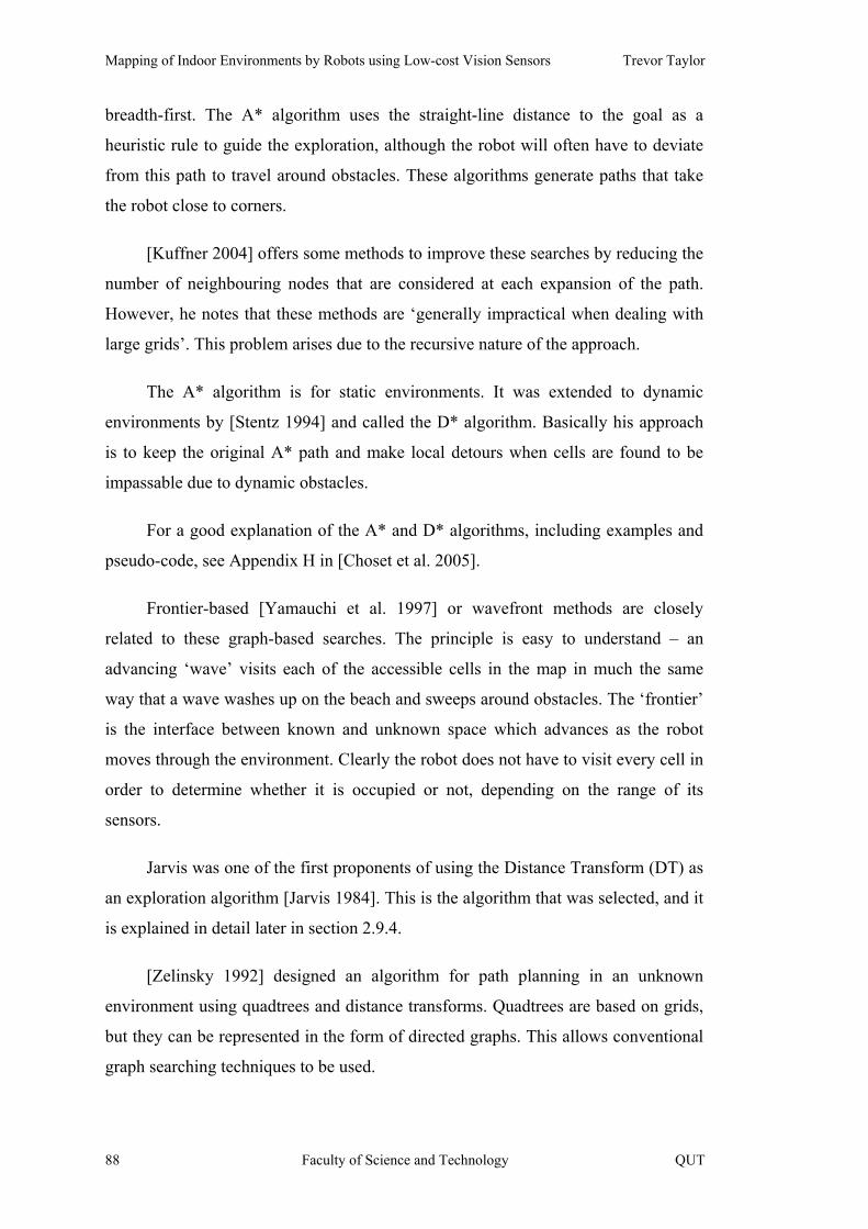
Mapping of Indoor Environments by Robots using Low-cost Vision Sensors Trevor Taylor
breadth-first. The A* algorithm uses the straight-line distance to the goal as a
heuristic rule to guide the exploration, although the robot will often have to deviate
from this path to travel around obstacles. These algorithms generate paths that take
the robot close to corners.
[Kuffner 2004] offers some methods to improve these searches by reducing the
number of neighbouring nodes that are considered at each expansion of the path.
However, he notes that these methods are ‘generally impractical when dealing with
large grids’. This problem arises due to the recursive nature of the approach.
The A* algorithm is for static environments. It was extended to dynamic
environments by [Stentz 1994] and called the D* algorithm. Basically his approach
is to keep the original A* path and make local detours when cells are found to be
impassable due to dynamic obstacles.
For a good explanation of the A* and D* algorithms, including examples and
pseudo-code, see Appendix H in [Choset et al. 2005].
Frontier-based [Yamauchi et al. 1997] or wavefront methods are closely
related to these graph-based searches. The principle is easy to understand – an
advancing ‘wave’ visits each of the accessible cells in the map in much the same
way that a wave washes up on the beach and sweeps around obstacles. The ‘frontier’
is the interface between known and unknown space which advances as the robot
moves through the environment. Clearly the robot does not have to visit every cell in
order to determine whether it is occupied or not, depending on the range of its
sensors.
Jarvis was one of the first proponents of using the Distance Transform (DT) as
an exploration algorithm [Jarvis 1984]. This is the algorithm that was selected, and it
is explained in detail later in section 2.9.4.
[Zelinsky 1992] designed an algorithm for path planning in an unknown
environment using quadtrees and distance transforms. Quadtrees are based on grids,
but they can be represented in the form of directed graphs. This allows conventional
graph searching techniques to be used.
88 Faculty of Science and Technology QUT
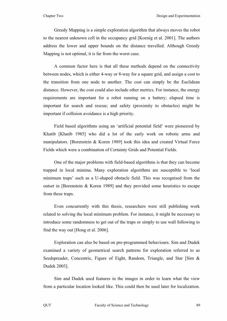
Chapter Two Design and Experimentation
Greedy Mapping is a simple exploration algorithm that always moves the robot
to the nearest unknown cell in the occupancy grid [Koenig et al. 2001]. The authors
address the lower and upper bounds on the distance travelled. Although Greedy
Mapping is not optimal, it is far from the worst case.
A common factor here is that all these methods depend on the connectivity
between nodes, which is either 4-way or 8-way for a square grid, and assign a cost to
the transition from one node to another. The cost can simply be the Euclidean
distance. However, the cost could also include other metrics. For instance, the energy
requirements are important for a robot running on a battery; elapsed time is
important for search and rescue; and safety (proximity to obstacles) might be
important if collision avoidance is a high priority.
Field based algorithms using an ‘artificial potential field’ were pioneered by
Khatib [Khatib 1985] who did a lot of the early work on robotic arms and
manipulators. [Borenstein & Koren 1989] took this idea and created Virtual Force
Fields which were a combination of Certainty Grids and Potential Fields.
One of the major problems with field-based algorithms is that they can become
trapped in local minima. Many exploration algorithms are susceptible to ‘local
minimum traps’ such as a U-shaped obstacle field. This was recognised from the
outset in [Borenstein & Koren 1989] and they provided some heuristics to escape
from these traps.
Even concurrently with this thesis, researchers were still publishing work
related to solving the local minimum problem. For instance, it might be necessary to
introduce some randomness to get out of the traps or simply to use wall following to
find the way out [Hong et al. 2006].
Exploration can also be based on pre-programmed behaviours. Sim and Dudek
examined a variety of geometrical search patterns for exploration referred to as
Seedspreader, Concentric, Figure of Eight, Random, Triangle, and Star [Sim &
Dudek 2003].
Sim and Dudek used features in the images in order to learn what the view
from a particular location looked like. This could then be used later for localization.
QUT Faculty of Science and Technology 89
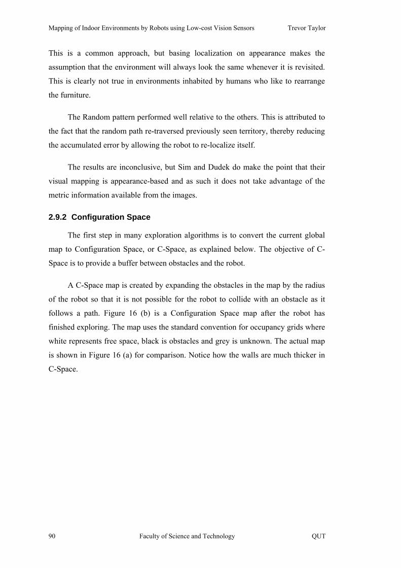
Mapping of Indoor Environments by Robots using Low-cost Vision Sensors Trevor Taylor
This is a common approach, but basing localization on appearance makes the
assumption that the environment will always look the same whenever it is revisited.
This is clearly not true in environments inhabited by humans who like to rearrange
the furniture.
The Random pattern performed well relative to the others. This is attributed to
the fact that the random path re-traversed previously seen territory, thereby reducing
the accumulated error by allowing the robot to re-localize itself.
The results are inconclusive, but Sim and Dudek do make the point that their
visual mapping is appearance-based and as such it does not take advantage of the
metric information available from the images.
2.9.2 Configuration Space
The first step in many exploration algorithms is to convert the current global
map to Configuration Space, or C-Space, as explained below. The objective of C-
Space is to provide a buffer between obstacles and the robot.
A C-Space map is created by expanding the obstacles in the map by the radius
of the robot so that it is not possible for the robot to collide with an obstacle as it
follows a path. Figure 16 (b) is a Configuration Space map after the robot has
finished exploring. The map uses the standard convention for occupancy grids where
white represents free space, black is obstacles and grey is unknown. The actual map
is shown in Figure 16 (a) for comparison. Notice how the walls are much thicker in
C-Space.
90 Faculty of Science and Technology QUT

Chapter Two Design and Experimentation
Figure 16 – Configuration Space: (a) Actual map; and (b) C-Space map
2.9.3 Complete Coverage
In certain situations it is important to visit every free cell in the map, called
paths of complete coverage. These have been developed using distance transforms
[Zelinsky et al. 1993]. Applications such as vacuum cleaning [Oh et al. 2004] or
lawn mowing require the robots to traverse every accessible cell in the map to
complete their task.
However, complete coverage is not necessary when simply building a map.
Using vision as a range sensor allows the robot to see areas of the map without
physically visiting them, thereby avoiding the need to traverse large areas of the
map. A good range sensor can also avoid many potential traps and much wasted time
by allowing the robot to see dead ends before entering them. Furthermore, the robot
might also be able to see into cells that are not physically accessible because it is too
large to fit through a gap.
2.9.4 The Distance Transform (DT)
The Distance Transform (DT) was originally designed for use in image
processing [Rosenfeld & Pflatz 1966] where the ‘distance’ between areas of the
image needed to be calculated and an image is defined as a regular grid of pixel
values.
The basic concept of a Distance Transform is simple. Consider the map as a
pool of water with the obstacles sticking out of it. Throw a pebble into the pool and
take snapshots as the ripples spread out. The advancing wave front will wrap around
obstacles. Ignore any ‘reflections’ that occur. As time progresses the wave front
moves further away from its origin – the distance increases. All points on the wave
front at any given instant in time are equidistant from the origin in the distance
QUT Faculty of Science and Technology 91
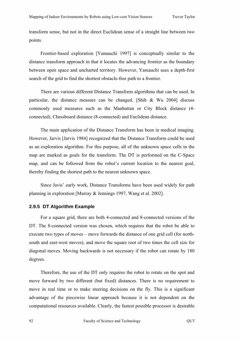
Mapping of Indoor Environments by Robots using Low-cost Vision Sensors Trevor Taylor
transform sense, but not in the direct Euclidean sense of a straight line between two
points.
Frontier-based exploration [Yamauchi 1997] is conceptually similar to the
distance transform approach in that it locates the advancing frontier as the boundary
between open space and uncharted territory. However, Yamauchi uses a depth-first
search of the grid to find the shortest obstacle-free path to a frontier.
There are various different Distance Transform algorithms that can be used. In
particular, the distance measure can be changed. [Shih & Wu 2004] discuss
commonly used measures such as the Manhattan or City Block distance (4-
connected), Chessboard distance (8-connected) and Euclidean distance.
The main application of the Distance Transform has been in medical imaging.
However, Jarvis [Jarvis 1984] recognized that the Distance Transform could be used
as an exploration algorithm. For this purpose, all of the unknown space cells in the
map are marked as goals for the transform. The DT is performed on the C-Space
map, and can be followed from the robot’s current location to the nearest goal,
thereby finding the shortest path to the nearest unknown space.
Since Javis’ early work, Distance Transforms have been used widely for path
planning in exploration [Murray & Jennings 1997, Wang et al. 2002].
2.9.5 DT Algorithm Example
For a square grid, there are both 4-connected and 8-connected versions of the
DT. The 8-connected version was chosen, which requires that the robot be able to
execute two types of moves – move forwards the distance of one grid cell (for north-
south and east-west moves), and move the square root of two times the cell size for
diagonal moves. Moving backwards is not necessary if the robot can rotate by 180
degrees.
Therefore, the use of the DT only requires the robot to rotate on the spot and
move forward by two different (but fixed) distances. There is no requirement to
move in real time or to make steering decisions on the fly. This is a significant
advantage of the piecewise linear approach because it is not dependent on the
computational resources available. Clearly, the fastest possible processor is desirable
92 Faculty of Science and Technology QUT

Chapter Two Design and Experimentation
QUT Faculty of Science and Technology 93
so that the robot does not spend too much time ‘thinking’, but it is not essential to
the task.
To perform the DT, obstacles in the map are set to ‘infinity’, and hence
ignored as possible nodes on the path during the calculations. Free space is filled in
with a ‘big’ value, which is necessary so that the transform will correctly update the
cells. It is assumed that the total cost (distance) in a cell can never reach ‘big’, but
this is a fair assumption for practical purposes even when using a 32-bit integer for
the distance. Unknown space, which is the goal, is filled in with zeros.
Table 1 – Sample Data from a Distance Transform
Consider the data shown in Table 1 which is a section from a DT (and
corresponds to the outlined region in Figure 17). The values in the cells are the
‘distance’ measure. The hash signs (##) indicate a numeric overflow because these
cells contain very large values which are obstacles.
0
##
0
0
0
0
0
1
0
2
0
3
0
4
0
5
0
4
0
3
0
2
0
##
0
0
0
0
0
0
0
0
0
0
0 0
##
0
##
0
0
0
0
0
1
0
2
0
3
0
4
0
4
0
3
0
2
0
1
0
0
0
0
0
0
0
0
0
0
##
0
## ##
0
0
##
0
0
0
0
0
0
0
1
0
2
0
3
0
4
1
3
0
2
0
1
1
0
0
0
0
0
0
0
1
0
##
0
## ##
0
0
0
0
0
0
0
0
0
0
0
0
##
1
##
1
##
2
##
1
##
0
##
0
0
0
0
0
0
0
0
0
0
##
0
## ##
0 0 0 0 1 1 2 2 3 ## ## ## 0 0 0 0 0 ## ##
## ## ## ## 2 2 3 3 4 ## ## ## 0 0 0 0 0 0 1
## ## ## ## 3 3 4 4 5 ## ## ## 0 0 0 0 0 0 0
## ## ## ## 3 4 5 5 6 7 ## ## ## ## ## 0 0 ## 0
## ## ## ## 2 3 4 5 6 7 8 ## ## ## ## ## ## ## ##
0 ## ## ## 1 2 3 4 5 6 7 ## ## ## ## ## ## ## ##
0 0 0 0 0 1 2 3 4 5 6 ## ## ## ## ## ## ## ##
0 0 0 0 0 0 ## ## ## 6 7 8 9 10 11 12 13 14 ##
0 0 0 0 0 0 ## ## ## 7 8 9 10 11 12 13 14 15 ##
0 ## ## 0 ## ## ## ## ## 8 9 10 11 12 13 14 15 16 ##
## ## ## ## ## ## ## ## ## 9 10 11 12 13 14 15 16 17 ##
## ## ## ## ## ## ## ## ## 10 11 12 13 14 15 16 16 17 ##
## ## ## ## ## ## ## ## ## 11 12 ## 14 15 ## 16 15 16 ##
## ## ## ## 12 11 10 11 12 12 ## ## ## ## ## ## 14 15 ##
## ## ## ## 11 10 9 10 11 12 ## ## ## ## ## ## 13 14 ##
## ## ## ## 10 9 8 9 10 11 ## ## ## ## ## ## 12 13 ##
## ## ## ## 9 8 7 8 9 10 ## ## ## ## ## 10 11 12 ##
## ## ## ## ## 7 6 7 8 9 8 7 6 7 8 9 10 11 12
## ## ## ## ## ## 5 6 7 8 7 6 5 6 7 8 9 10 11
0 ## ## ## ## ## 4 5 6 7 6 5 4 ## ## ## ## ## ##
0 ## ## ## ## ## 3 4 5 6 5 4 3 ## ## ## ## ## ##
## ##
##
##
0

Mapping of Indoor Environments by Robots using Low-cost Vision Sensors Trevor Taylor
The DT ‘wave’ emanates from the zero cells (unknown space) and travels
‘uphill’ until it encounters an obstacle and has nowhere else to go. This is easy to see
– look down diagonally from the top left-hand corner of the table. In the top left, the
values are zero. There is a ‘channel’ between two obstacles where the values start to
increase 1, 2, 3.
To help visualise the DT, Figure 17 shows a 3D view of the cell values. The
area inside the (red) rectangle in the top left corner corresponds to the data shown in
Table 1. Valleys and ridges are quite apparent. The obstacles are the flat areas that
are highlighted in a darker colour.
Figure 17 – 3D view of a Distance Transform
Following a steepest descent path through the DT from the robot’s current
location (or in fact starting from any non-obstacle cell) will lead to the nearest goal,
which is unknown space. To reiterate, from a single DT it is possible to create a path
from anywhere (except inside an obstacle) to the nearest unknown space just by
‘rolling downhill’.
94 Faculty of Science and Technology QUT

Chapter Two Design and Experimentation
2.10 Summary
This chapter has outlined a wide range of different subject areas that must be
addressed in order to perform mapping using vision. Although there has been a lot of
work on mapping using sonar and laser range finders, there is comparatively little
work in the literature on using only monocular vision to produce metric maps of
unknown environments.
QUT Faculty of Science and Technology 95


Chapter Three Design and Experimentation
3 Design and Experimentation
‘Vision is the process of discovering from images
what is present in the world, and where it is.’
– David Marr,
Vision, 1982, page 3
3.1 Methodology used in this Research
The basic research methodology used in this thesis was iterative
experimentation, a process sometimes referred to as action research. The design was
developed by a process of successive refinement based on prototypes using both real
robots and simulation. In principle this is similar to the approaches used today in
some software design methodologies.
A consequence of this methodology was that preliminary results were
incorporated into subsequent designs. Therefore this chapter includes some
intermediate results, but Chapter 4 – Results and Discussion includes the complete
list of significant results.
3.2 Research Areas Investigated
As outlined in Chapter 1, there were several areas that required investigation in
order to build a complete system for visual mapping. In brief, the main areas were
controlling the robot; extracting range information from the video stream; building
local maps; exploring the environment; and putting this all together with
simultaneous localization and mapping.
This chapter discusses each of the research areas in addition to outlining the
experimental environment. Due to the wide range of topics that must be covered, the
discussion might appear to be disjointed at first glance. However, they follow a
QUT Faculty of Science and Technology 97
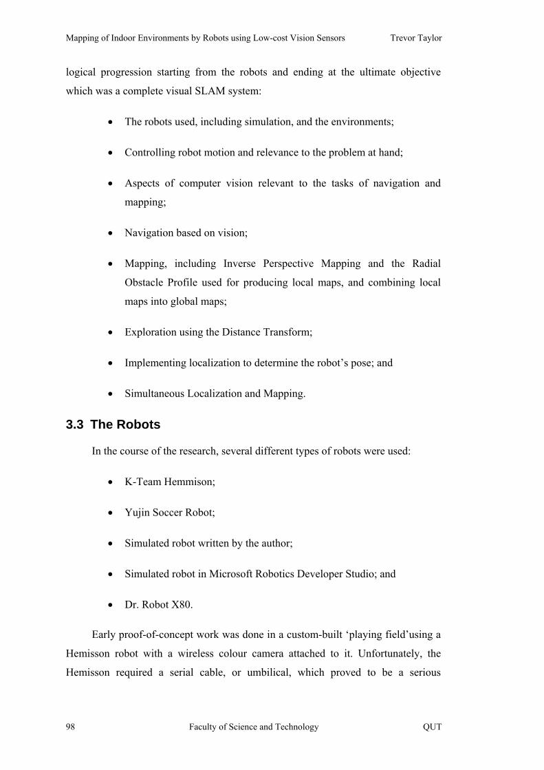
Mapping of Indoor Environments by Robots using Low-cost Vision Sensors Trevor Taylor
logical progression starting from the robots and ending at the ultimate objective
which was a complete visual SLAM system:
• The robots used, including simulation, and the environments;
• Controlling robot motion and relevance to the problem at hand;
• Aspects of computer vision relevant to the tasks of navigation and
mapping;
• Navigation based on vision;
• Mapping, including Inverse Perspective Mapping and the Radial
Obstacle Profile used for producing local maps, and combining local
maps into global maps;
• Exploration using the Distance Transform;
• Implementing localization to determine the robot’s pose; and
• Simultaneous Localization and Mapping.
3.3 The Robots
In the course of the research, several different types of robots were used:
• K-Team Hemmison;
• Yujin Soccer Robot;
• Simulated robot written by the author;
• Simulated robot in Microsoft Robotics Developer Studio; and
• Dr. Robot X80.
Early proof-of-concept work was done in a custom-built ‘playing field’using a
Hemisson robot with a wireless colour camera attached to it. Unfortunately, the
Hemisson required a serial cable, or umbilical, which proved to be a serious
98 Faculty of Science and Technology QUT

Chapter Three Design and Experimentation
drawback. Later the research moved to a Yujin robot because it had a wireless
connection.
A simulation was developed in order to speed up experiments and provide
more strict control over the environment. If an algorithm does not work in
simulation, it is unlikely to work in the real world. A simulator can therefore save a
significant amount of time.
The X80 robot was roughly 35cm in diameter and ‘human sized’ in the sense
that it could operate in the corridors of typical office buildings.
3.3.1 Hemisson Robot
Hemisson robots are manufactured by K-Team in Switzerland [K-Team 2006],
the same company that makes the popular Khepera robot. It was intended to be a
cheap robot for the education market. This robot was selected for its low price and
size, making it suitable for use in a prototype. The robot is shown in Figure 18.
Figure 18 – Hemisson robot with Swann Microcam
The Hemisson was roughly 10cm in diameter and powered by a 9V battery.
Figure 18 also shows the wireless Swann Microcam, which was smaller than the 9V
battery that it ran off. Notice the serial cable attached to the back of the robot (left-
hand side of the photo).
For testing purposes, two ‘playing fields’ were built using 120cm x 90cm
sheets of blackboard Masonite for the floor. The intention was that the floor would
be matte black in colour. The walls around the playing fields were painted white.
These playing fields could be populated with various objects to represent obstacles.
Figure 19 shows one of the playing fields with the Hemisson and some obstacles.
(The curvature of the walls in the photo was due to the camera lens).
QUT Faculty of Science and Technology 99
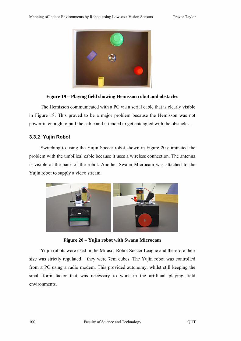
Mapping of Indoor Environments by Robots using Low-cost Vision Sensors Trevor Taylor
Figure 19 – Playing field showing Hemisson robot and obstacles
The Hemisson communicated with a PC via a serial cable that is clearly visible
in Figure 18. This proved to be a major problem because the Hemisson was not
powerful enough to pull the cable and it tended to get entangled with the obstacles.
3.3.2 Yujin Robot
Switching to using the Yujin Soccer robot shown in Figure 20 eliminated the
problem with the umbilical cable because it uses a wireless connection. The antenna
is visible at the back of the robot. Another Swann Microcam was attached to the
Yujin robot to supply a video stream.
Figure 20 – Yujin robot with Swann Microcam
Yujin robots were used in the Mirasot Robot Soccer League and therefore their
size was strictly regulated – they were 7cm cubes. The Yujin robot was controlled
from a PC using a radio modem. This provided autonomy, whilst still keeping the
small form factor that was necessary to work in the artificial playing field
environments.
100 Faculty of Science and Technology QUT
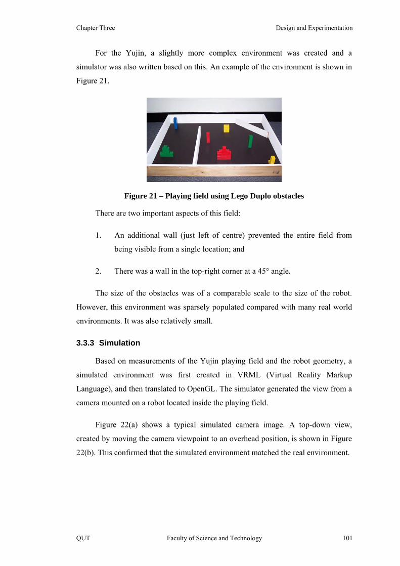
Chapter Three Design and Experimentation
For the Yujin, a slightly more complex environment was created and a
simulator was also written based on this. An example of the environment is shown in
Figure 21.
Figure 21 – Playing field using Lego Duplo obstacles
There are two important aspects of this field:
1. An additional wall (just left of centre) prevented the entire field from
being visible from a single location; and
2. There was a wall in the top-right corner at a 45° angle.
The size of the obstacles was of a comparable scale to the size of the robot.
However, this environment was sparsely populated compared with many real world
environments. It was also relatively small.
3.3.3 Simulation
Based on measurements of the Yujin playing field and the robot geometry, a
simulated environment was first created in VRML (Virtual Reality Markup
Language), and then translated to OpenGL. The simulator generated the view from a
camera mounted on a robot located inside the playing field.
Figure 22(a) shows a typical simulated camera image. A top-down view,
created by moving the camera viewpoint to an overhead position, is shown in Figure
22(b). This confirmed that the simulated environment matched the real environment.
QUT Faculty of Science and Technology 101
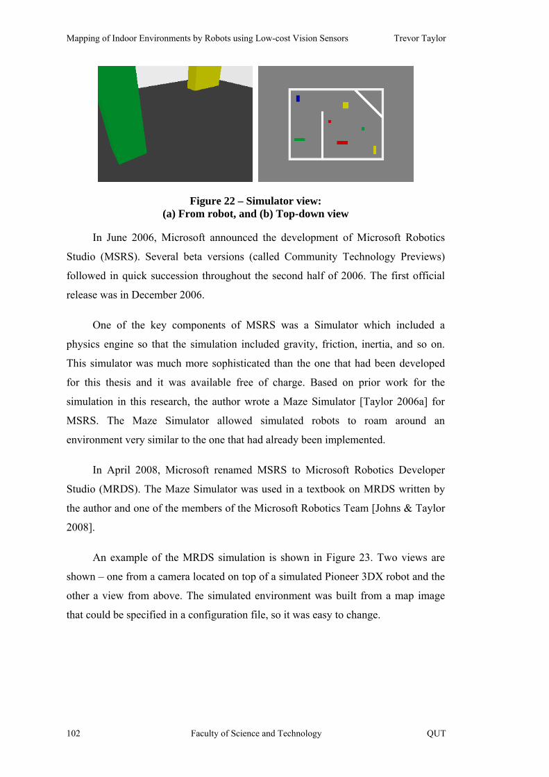
Mapping of Indoor Environments by Robots using Low-cost Vision Sensors Trevor Taylor
Figure 22 – Simulator view: (a) From robot, and (b) Top-down view
In June 2006, Microsoft announced the development of Microsoft Robotics
Studio (MSRS). Several beta versions (called Community Technology Previews)
followed in quick succession throughout the second half of 2006. The first official
release was in December 2006.
One of the key components of MSRS was a Simulator which included a
physics engine so that the simulation included gravity, friction, inertia, and so on.
This simulator was much more sophisticated than the one that had been developed
for this thesis and it was available free of charge. Based on prior work for the
simulation in this research, the author wrote a Maze Simulator [Taylor 2006a] for
MSRS. The Maze Simulator allowed simulated robots to roam around an
environment very similar to the one that had already been implemented.
In April 2008, Microsoft renamed MSRS to Microsoft Robotics Developer
Studio (MRDS). The Maze Simulator was used in a textbook on MRDS written by
the author and one of the members of the Microsoft Robotics Team [Johns & Taylor
2008].
An example of the MRDS simulation is shown in Figure 23. Two views are
shown – one from a camera located on top of a simulated Pioneer 3DX robot and the
other a view from above. The simulated environment was built from a map image
that could be specified in a configuration file, so it was easy to change.
102 Faculty of Science and Technology QUT

Chapter Three Design and Experimentation
Figure 23 – Simulated environment using Microsoft Robotics Developer Studio: (a) Robot view, and (b) Top-down view
The Pioneer 3DX in the simulation has a webcam and a Laser Range Finder.
Further work was also done on a simple example that explored the environment,
called ExplorerSim, and created maps using the LRF. This was released with the
textbook as well.
3.3.4 X80 Robot
In the final phase of the research, it was necessary to move from the playing
fields to a real human environment. For this purpose the author purchased an X80
robot from Dr. Robot Inc. in Canada [Dr Robot Inc. 2008b]. This robot was selected
because it had a built-in pan and tilt camera and a wireless Ethernet interface.
Figure 24 shows the original X80 robot, called Tobor. The pan and tilt camera
is visible at the front of the robot. Sonar and infrared sensors are also located across
the front of the robot. The WiFi antenna is located at the back of the robot but is not
visible in this photo.
Figure 24 – Tobor the X80 robot
The X80 was roughly 35cm in diameter with wheels 17cm in diameter and
wheel encoders with a resolution of 1200 ticks per revolution.
QUT Faculty of Science and Technology 103
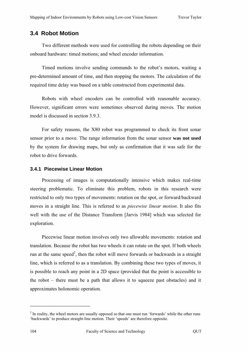
Mapping of Indoor Environments by Robots using Low-cost Vision Sensors Trevor Taylor
3.4 Robot Motion
Two different methods were used for controlling the robots depending on their
onboard hardware: timed motions; and wheel encoder information.
Timed motions involve sending commands to the robot’s motors, waiting a
pre-determined amount of time, and then stopping the motors. The calculation of the
required time delay was based on a table constructed from experimental data.
Robots with wheel encoders can be controlled with reasonable accuracy.
However, significant errors were sometimes observed during moves. The motion
model is discussed in section 3.9.3.
For safety reasons, the X80 robot was programmed to check its front sonar
sensor prior to a move. The range information from the sonar sensor was not used
by the system for drawing maps, but only as confirmation that it was safe for the
robot to drive forwards.
3.4.1 Piecewise Linear Motion
Processing of images is computationally intensive which makes real-time
steering problematic. To eliminate this problem, robots in this research were
restricted to only two types of movements: rotation on the spot, or forward/backward
moves in a straight line. This is referred to as piecewise linear motion. It also fits
well with the use of the Distance Transform [Jarvis 1984] which was selected for
exploration.
Piecewise linear motion involves only two allowable movements: rotation and
translation. Because the robot has two wheels it can rotate on the spot. If both wheels
run at the same speed2, then the robot will move forwards or backwards in a straight
line, which is referred to as a translation. By combining these two types of moves, it
is possible to reach any point in a 2D space (provided that the point is accessible to
the robot – there must be a path that allows it to squeeze past obstacles) and it
approximates holonomic operation.
2 In reality, the wheel motors are usually opposed so that one must run ‘forwards’ while the other runs ‘backwards’ to produce straight-line motion. Their ‘speeds’ are therefore opposite.
104 Faculty of Science and Technology QUT

Chapter Three Design and Experimentation
Piecewise linear motion has rarely been used in the literature. The emphasis in
the literature has instead been on building fast algorithms that can control the robot’s
motion in real-time. As CPU speeds increase every year, eventually piecewise linear
motion will be equivalent to continuous motion. In the meantime, this approach
allowed the robots to take as long as necessary to process camera images before
making their next moves – there were no real-time considerations.
Another advantage of piecewise linear motion was that the equations
governing the motion of the robot were extremely simple. This was important in
developing the SLAM algorithm because a motion model was required for the robot,
i.e. how it responded to inputs (where inputs were commands to move).
The primary disadvantage of the piecewise linear approach to robot motion
became evident early in the research – it was not possible to use optic flow.
Extracting the optic flow field from a sequence of images requires, ideally, that the
images correspond to small motions. By processing images only after significant
motions have completed, the differences between images were too great for typical
optic flow algorithms to recognise the changes. However, the camera images from
the X80 robot suffered from a significant amount of motion blur and so they would
not have been suitable for optic flow.
Some vision-based SLAM algorithms also required images with small
incremental motions in order to make reliable estimates of the positions of features
in the images. MonoSLAM [Davison 1999] was reported to work best when the
camera was waved around, thereby providing a large number of different views of
the same objects.
Because the video stream was ignored during motions, if a human walked into
the path of a robot while it was moving, the robot could collide with the human.
Further work is required to eliminate this problem. For example, the X80 robot had
sonar sensors that could have been monitored continuously as a safety measure to
avoid such collisions, rather than just checking the sonar prior to a move.
Despite these drawbacks, piecewise linear motion was a good approach.
QUT Faculty of Science and Technology 105

Mapping of Indoor Environments by Robots using Low-cost Vision Sensors Trevor Taylor
3.4.2 Odometry Errors
Odometry is notoriously unreliable, and it was not expected to be perfect.
However, the large errors that sometimes occurred were not anticipated.
For timed motions, as used on the Hemisson and Yujin robots, it proved to be
impossible to reliably time an operation under Windows. Even so-called ‘high
precision’ timer code [Wheeler 2003, Manko 2003] would randomly fail to produce
the correct result. The problem had to do with the way that Windows implements
multi-tasking, and that occasionally it would get bogged down in some internal
housekeeping, such as flushing the disk cache. This caused the timer to overrun
significantly and resulted in the robot making moves that were significantly different
from what was expected.
Because the X80 robots had wheel encoders with 1200 ticks per revolution it
was expected that it would be possible to control the movement of the robots with
reasonable accuracy. However, large variations were occasionally observed during
experiments. Dropped network packets (because the robot used UDP which is not a
reliable transport) could result in the complete loss of a command, but no
explanation was found for the unusual movements.
The full impact of poor odometry only became apparent towards the end of the
work during the implementation of SLAM on an X80. In fact, there was literature
emerging concurrent with this thesis, [Hähnel 2004; Grisetti et al. 2005, Nieto et al.
2005], that pointed to the importance of improving pose estimates before
incorporating new sensor data into a SLAM algorithm.
3.4.3 Effect of Motion on Images
There are advantages to having the robot stationary when it captures images.
Firstly, there was no vibration to affect the position of the camera. If the camera
moved up or down slightly, the pixel locations of the obstacle edges in the image
would also change, resulting in errors in the Inverse Perspective Mapping.
Secondly, the shutter speed of the camera could not be controlled on the cheap
cameras and it was fairly slow. This means that images were blurred if the robot was
moving when they were captured. Blurring tends to suppress edges, making it harder
106 Faculty of Science and Technology QUT

Chapter Three Design and Experimentation
to detect obstacles. With piecewise linear motion, however, the robot was not
moving when images were captured.
At intermediate points during a move, it was not possible to accurately
determine the pose of the robot. The pose was only known with any certainty at the
beginning and end of moves.
Therefore, the ExCV program disabled image capture during motions. It was
also found that a short delay was required after completing a motion before re-
enabling the camera, otherwise the images were still blurred while the robot ‘settled’.
In effect, this approach meant that the robot was blind during moves. This was
not a problem for rotations because the robot only turned on the spot and could not
collide with an obstacle. However, for translations there was a strong assumption
that the environment remained static, at least for a short period of time.
3.5 Computer Vision
The Horswill Constraints listed in Chapter 2 were taken as the basis for the
design of the vision system.
The vision system produced range data that was sufficient to create workable
maps. However, it still had some deficiencies. Some recommendations for future
work are discussed in the last section of Chapter 4.
The primary conclusion from the vision system was that several different
modalities should be used – as many as possible. The Human Visual System uses
many different modalities: texture, shading, edges, segmentation, pattern matching,
optic flow, occlusion, etc. In contrast, the vision system in this thesis only used edges
and colour-based segmentation.
Expanding the vision system to support other modalities might also involve
changing the camera hardware.
3.5.1 Vision as the Only Sensor
It was an objective of this research to use only vision for navigation and
mapping. Clearly, there was an implicit assumption that this was possible.
QUT Faculty of Science and Technology 107

Mapping of Indoor Environments by Robots using Low-cost Vision Sensors Trevor Taylor
There was one subtle issue that had to do with odometry. For the X80 robots
that had wheel encoders to control motions, there was inherently another sensor
besides vision. Therefore the vision-only assumption was not entirely correct.
However, in the case of the Hemisson and Yujin robots there were no wheel
encoders and motions were controlled using timers, so the vision-only assumption
held true.
As noted above, a sonar sensor on the X80 was used for safety, but not for
mapping or exploration.
3.5.2 Experimental Environments
Two playing fields were originally built for use with the Hemisson and Yujin
robots. However, these proved to be too small for adequate experimentation because
the robots could see the entire environment during a single pirouette.
The playing field environment was broken up using additional walls. However,
even then the time required to explore the entire playing field was quite short, and so
it was not a good experimental environment except for the initial prototypes. This
limitation was one of the driving factors in moving away from the playing fields to a
human-scale environment.
In the final phase of the project an X80 robot was used to map corridors in an
office building. This environment had its own particular limitations too. For
example, the corridor illumination was extremely variable causing problems with
shadows and colour variations. However, the environment was representative of
many office buildings.
The office environments used in this research were challenging due to the
colours of the carpets, walls and doors – refer to Figure 25.
108 Faculty of Science and Technology QUT
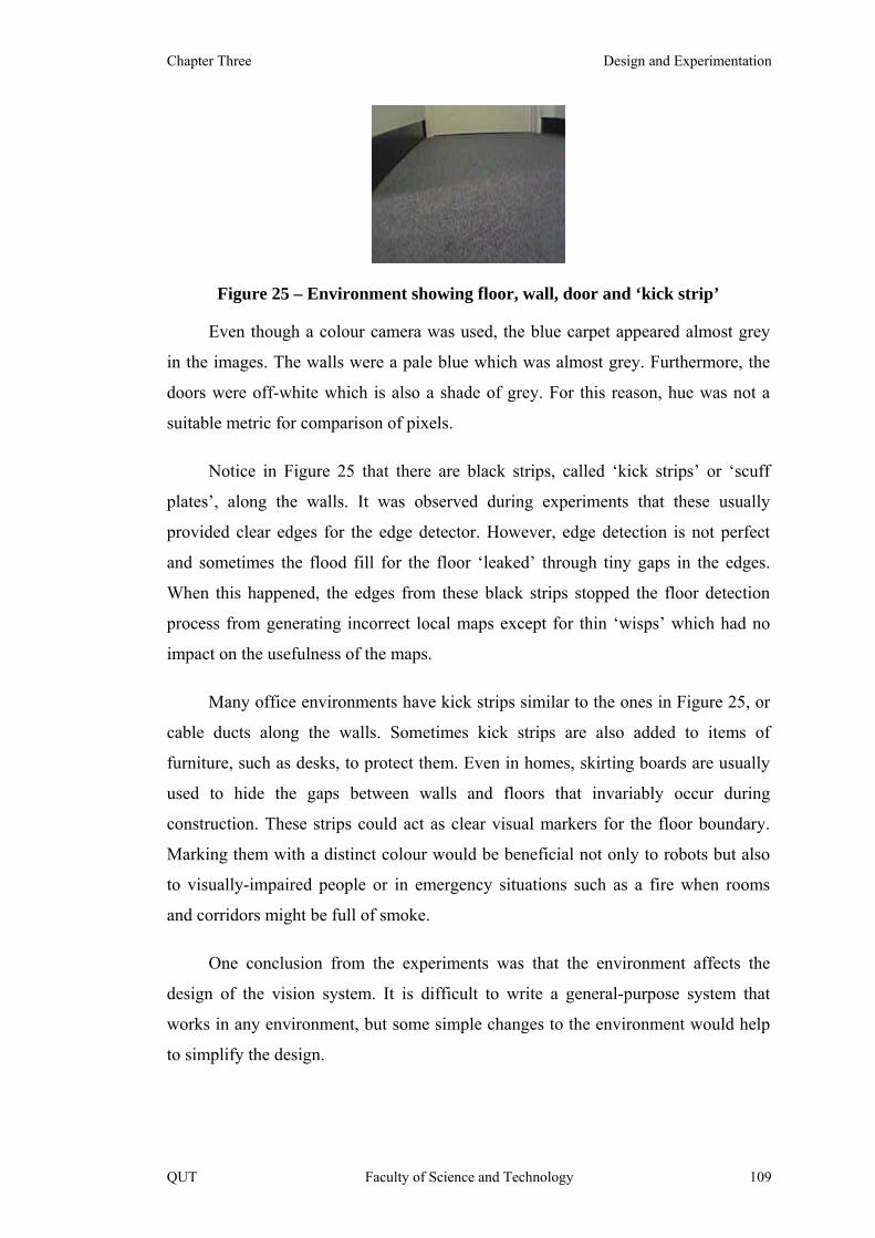
Chapter Three Design and Experimentation
Figure 25 – Environment showing floor, wall, door and ‘kick strip’
Even though a colour camera was used, the blue carpet appeared almost grey
in the images. The walls were a pale blue which was almost grey. Furthermore, the
doors were off-white which is also a shade of grey. For this reason, hue was not a
suitable metric for comparison of pixels.
Notice in Figure 25 that there are black strips, called ‘kick strips’ or ‘scuff
plates’, along the walls. It was observed during experiments that these usually
provided clear edges for the edge detector. However, edge detection is not perfect
and sometimes the flood fill for the floor ‘leaked’ through tiny gaps in the edges.
When this happened, the edges from these black strips stopped the floor detection
process from generating incorrect local maps except for thin ‘wisps’ which had no
impact on the usefulness of the maps.
Many office environments have kick strips similar to the ones in Figure 25, or
cable ducts along the walls. Sometimes kick strips are also added to items of
furniture, such as desks, to protect them. Even in homes, skirting boards are usually
used to hide the gaps between walls and floors that invariably occur during
construction. These strips could act as clear visual markers for the floor boundary.
Marking them with a distinct colour would be beneficial not only to robots but also
to visually-impaired people or in emergency situations such as a fire when rooms
and corridors might be full of smoke.
One conclusion from the experiments was that the environment affects the
design of the vision system. It is difficult to write a general-purpose system that
works in any environment, but some simple changes to the environment would help
to simplify the design.
QUT Faculty of Science and Technology 109

Mapping of Indoor Environments by Robots using Low-cost Vision Sensors Trevor Taylor
As domestic robots become more widely used, interior designers might have to
take them into account in the designs of offices, hospitals and even homes. In
particular, the colours of walls and doors should be distinctly different from the
floor.
Consideration should be given to making human environments ‘robot friendly’
in future buildings. It should also be feasible to retro-fit existing buildings at little
additional cost during routine renovations. These changes could also prove helpful
for humans who are vision impaired. In fact, many buildings already have strips of
one kind or another along the edges of the walls.
3.5.3 Monocular Vision
Preliminary work by the author showed that it was possible to use a single
camera to obtain range information based on certain assumptions about the
environment and knowledge of the camera geometry [Taylor et al. 2004a]. (See
section 3.7.2 for details). It was not necessary, therefore, to use stereo vision which
had been used in the past to obtain range information.
Due to the complexity of de-warping the images from panoramic cameras, the
cost of these specialised cameras (requiring highly accurate mirrors/lenses), and their
large size, it was decided not to use them.
3.5.4 Cheap Colour Cameras
The reason for the choice of a low-resolution colour camera was to keep the
cost as low as possible on the assumption that for robots to be successful in the
domestic and office environments they would need to be attractively priced.
Web cameras with 320x240 pixel resolution are very cheap. The original
wireless camera used on the Hemisson and Yujin robots had this resolution and so
the simulation was designed to use this same resolution.
The original documentation for the X80 robot was misleading on the subject of
camera resolution. Although the camera was capable of higher resolution (352 x
288), the on-board firmware in the robot only used 176x144 pixels. Furthermore, the
throughput of 15fps (frames per second) claimed for the camera was not achievable.
110 Faculty of Science and Technology QUT

Chapter Three Design and Experimentation
Dr. Robot, Inc. has since amended the online specifications to state that the video
can achieve “up to 4 fps”.
These problems were discussed with the manufacturer at length, but the final
outcome was that the resolution could not be changed and remained set at 176x144.
The maximum frame rate obtained during experiments was about 2fps due to the
internal bottlenecks in the hardware architecture.
Lower than anticipated resolution might have contributed to difficulties with
the map building process. However, it also highlighted an important point about
SLAM algorithms, namely that they require reasonably accurate input data.
The focal length of a web camera is generally not known. The equations
derived for Inverse Perspective Mapping (explained below in section 3.7.2)
effectively eliminated the focal length. Therefore it was not necessary to know the
focal length for the cameras used in this research. However, as shown below, the
intrinsic parameters for the cameras include the focal length.
3.5.5 Narrow Field of View
Cheap cameras typically have a narrow field of view. The Swann wireless
camera (used on the Hemisson and Yujin robots) only had a 60º Field of View
(FOV), which is fairly typical of such cameras. For the X80, the FOV was
determined to be 50.8º from the intrinsic parameters obtained via camera calibration
(explained below in section 3.5.6).
The cameras were therefore tilted downwards to see the floor in front of the
robots, but even then there were blind areas in front of the robots. Tilting the camera
also introduces a complication due to perspective effects because vertical edges do
not remain vertical in the image, which is discussed in the next section.
Because the robot could only see a small area in front of it, drawing a map was
difficult. Therefore an approach was developed whereby the robot rotates on the
spot, called a pirouette. During a pirouette the robot turns through a full 360° in 12
steps of 30° each. The choice of 30° increments was a compromise that allowed for
overlap between images, but minimised the number of turns because each turn has
the potential to introduce odometry errors. This approach of ‘looking around’ is a
QUT Faculty of Science and Technology 111

Mapping of Indoor Environments by Robots using Low-cost Vision Sensors Trevor Taylor
form of active vision – making deliberate moves in order to obtain an improved view
of the world.
Consider the sequence of images shown in Figure 26. These show what the
robot sees as it performs a pirouette. However, this image sequence only shows half
of the pirouette.
a b cd e f
Figure 26 – Sequence of images from a robot rotating on the spot (turning left by 30° per image from top-left to bottom-right)
To a human, it is apparent that the robot was rotating on the spot. It is also
obvious that it was not aligned perfectly with the corridor walls. Despite changes in
illumination between images and even across an image, the floor is immediately
obvious to a human.
On closer inspection, it is also apparent that there are very few distinguishing
features in some of the images. Such is the nature of corridors. These examples are
raw images which exhibit radial distortion, although many people do not even notice
this until it is pointed out to them. As noted earlier, radial distortion was removed
before processing the images.
Note that this process was a major source of odometry errors because, with
each individual rotation, there was a chance that the robot would turn by the wrong
112 Faculty of Science and Technology QUT

Chapter Three Design and Experimentation
amount. This problem does not exist for some other sensor configurations. Sonar
sensors, for instance, are typically used in a ring around the circumference of the
robot, so the robot does not need to turn at all to obtain a sweep. LRFs usually have a
180 degree field of view, so again they do not usually turn to ‘look around’.
3.5.6 Removing Camera Distortion
A disadvantage of cheap cameras is that they tend to have poor quality lenses
(often made of moulded plastic). The most obvious effect is radial distortion, which
causes problems with the Inverse Perspective Mapping (IPM). (IPM is explained
below in section 3.7.2).
Camera calibration can be performed using software available from [Bouguet
2006] which was based on the work in [Bouguet & Perona 1995]. Once the camera
intrinsic parameters are known, the distortion can be removed from the images using
routines included in the OpenCV Library [Intel 2005].
The calibration procedure was clearly documented. It involved taking photos
of a calibration target from a variety of different positions and angles. Some
examples are shown in Figure 27. There is no significance in this particular set of
images. This camera, on an X80 robot, had a resolution of 176 x 144 pixels.
QUT Faculty of Science and Technology 113
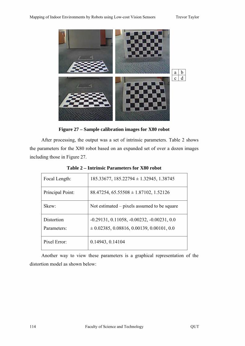
Mapping of Indoor Environments by Robots using Low-cost Vision Sensors Trevor Taylor
a b c d
Figure 27 – Sample calibration images for X80 robot
After processing, the output was a set of intrinsic parameters. Table 2 shows
the parameters for the X80 robot based on an expanded set of over a dozen images
including those in Figure 27.
Table 2 – Intrinsic Parameters for X80 robot
Focal Length: 185.33677, 185.22794 ± 1.32945, 1.38745
Principal Point: 88.47254, 65.55508 ± 1.87102, 1.52126
Skew: Not estimated – pixels assumed to be square
Distortion
Parameters:
-0.29131, 0.11058, -0.00232, -0.00231, 0.0
± 0.02385, 0.08816, 0.00139, 0.00101, 0.0
Pixel Error: 0.14943, 0.14104
Another way to view these parameters is a graphical representation of the
distortion model as shown below:
114 Faculty of Science and Technology QUT
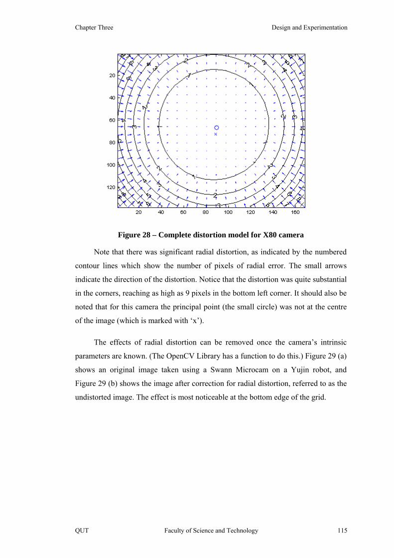
Chapter Three Design and Experimentation
Figure 28 – Complete distortion model for X80 camera
Note that there was significant radial distortion, as indicated by the numbered
contour lines which show the number of pixels of radial error. The small arrows
indicate the direction of the distortion. Notice that the distortion was quite substantial
in the corners, reaching as high as 9 pixels in the bottom left corner. It should also be
noted that for this camera the principal point (the small circle) was not at the centre
of the image (which is marked with ‘x’).
The effects of radial distortion can be removed once the camera’s intrinsic
parameters are known. (The OpenCV Library has a function to do this.) Figure 29 (a)
shows an original image taken using a Swann Microcam on a Yujin robot, and
Figure 29 (b) shows the image after correction for radial distortion, referred to as the
undistorted image. The effect is most noticeable at the bottom edge of the grid.
QUT Faculty of Science and Technology 115

Mapping of Indoor Environments by Robots using Low-cost Vision Sensors Trevor Taylor
Figure 29 – Correcting for Radial Distortion: (a) Original image; and (b) Undistorted image
In further discussion of this research, especially map building, images are
assumed to be undistorted before being processed but this is not explicitly
mentioned.
3.5.7 Uneven Illumination
In the initial work the illumination was reasonably uniform because the
‘playing fields’ were relatively small. In simulation, illumination was not an issue
because the images were artificially generated.
However, in real corridors the effects of uneven illumination were quite
apparent. Figure 30 shows three images from the same test run. The first image (top
left) shows ideal illumination which was present in most areas of the corridors.
Figure 30 – Examples of uneven illumination in corridors
‘Hard’ shadows, such as in Figure 30 (b), could result in the vision system
detecting an edge that did not exist and consequently drawing a fictitious wall in the
116 Faculty of Science and Technology QUT

Chapter Three Design and Experimentation
map. Applying a Gaussian blur before processing the images helped to reduce the
incidence of phantom edges without significantly affecting the detection of real
walls.
Wide variations in illumination like Figure 30 (c) sometimes caused the vision
system to incorrectly segment the image and reduce the amount of floor that was
detected. In the worst case, the robot concluded that the corridor was impassable. To
attempt to mitigate this problem, the vision system used a moving average for the
floor pixel values. As it progressed around the building, the current value of an
average floor pixel was changed. However, there was a threshold on the amount of
variation and it was still possible for the floor to be too dark to be reliably detected.
In order to minimise these effects, the brightness of camera images was
automatically adjusted during a test run. When the robot was first started, it used a
patch of floor immediately in front of it as a template. The parameters of this floor
patch, minimum, maximum and average RGB values, were compared to new images
as the robot moved around.
If there was a noticeable difference in the average intensity, then the intensity
of the entire image was adjusted to match the initial template. This was done by
multiplying all pixel values by an appropriate amount. In other words, the brightness
of the image was adjusted proportionally so that the average intensity of the template
floor patch was the same as the initial patch.
Even when the system adjusted the image intensity to try to average out the
changes in illumination, it was not possible to entirely eliminate the problem of sharp
shadow edges. Clearly, adjusting the average intensity to match one side of the
shadow or the other will still leave a shadow.
A different approach to shadows proposed in the literature was switching to a
different colour space where the shadows should disappear. However, attempts to
use hue were not successful. The main problem with hue is that it is very unreliable
in low-light situations. It has no representation for shades of grey which were
prevalent in the experimental environments, and this causes the hue values to
fluctuate wildly. Furthermore, the environment turned out to contain a lot of colours
with a similar hue. This is discussed below under Colour Spaces.
QUT Faculty of Science and Technology 117

Mapping of Indoor Environments by Robots using Low-cost Vision Sensors Trevor Taylor
Comprehensive image normalization was also found to be ineffective in
removing shadows. Therefore, shadows are still an open research topic.
3.5.8 Compensating for Vignetting
Vignetting makes the outer edges, especially the corners, of an image appear
darker than the centre of the image. This makes segmentation more difficult because
pixel values can vary considerably across the image.
A very simple approach was adopted in this project that improves image
quality, but cannot completely remove the vignetting effects. It was loosely based on
the work of Yu [Yu et al. 2004].
To reduce the effects of vignetting, pixel values in the image were adjusted by
a factor that was proportional to the square of the distance from the centre of the
image. This was done independently for each of the Red, Green and Blue
components, which also allows compensation for incorrect colour tint to be applied
at the same time. The resulting improvement can be seen by comparing Figure 31 (a)
and (b).
Figure 31 – Correcting for Vignetting: (a) Original image; and (b) Corrected image
Note that uniform illumination has an indirect effect on vignetting. The impact
of vignetting is worse in low-light situations, so good illumination helps to reduce
vignetting.
3.5.9 Camera Adaptation
Most cameras have automatic gain control – they adjust for the amount of light
entering the lens. This is desirable for obtaining the best possible images, but it can
also have adverse effects. Images were observed to get progressively brighter while
the robot stood still viewing the same scene.
118 Faculty of Science and Technology QUT

Chapter Three Design and Experimentation
Firstly, when the camera readjusts itself, the RGB values of pixels in the image
change. This means that colours seem to change. Any algorithm that relies on colour
matching in the RGB space will therefore have a problem because colours become
moving targets. One approach that was examined was to use a different colour space
to try to eliminate the effects of changing brightness, and to apply some ‘colour
constancy’ algorithms. Attempts to do this, for example using Comprehensive
Colour Image Normalization [Finlayson et al. 1998], proved unsuccessful.
The second problem was adaptation. If the camera remained stationary for a
significant amount of time, it adjusted itself to the point where the colours were
actually distorted. For instance, if there was a large red object in the camera’s field
of view, the image would take on a definite reddish hue over time. This effect was
very noticeable and could not be compensated for by changing to a different colour
space.
3.6 Navigation
This section discusses various aspects of navigation. Primarily the term
navigation in this research refers obstacle detection for collision-free motion.
Much of the literature assumes static environments where the obstacles stay
put and do not move around. In a human environment this is not true, but the
additional complexity involved in handling a dynamic environment makes it a much
more difficult problem. Therefore it was assumed in this research that the
environment was static.
Feature extraction was not used in the vision system for this project. In other
words, no attempt was made to recognise objects. The floor was assumed to be of a
uniform colour and therefore, by definition, it contained no features. Therefore this
work relied on detecting edges and performing segmentation to locate obstacles.
A simple approach to floor segmentation was used initially. It involved a
moving-average flood fill whereby an initial pixel value was selected at the bottom
of the image, and the pixel value to be matched varied continuously based on the
pixels previously seen while scanning vertically up an image column.
QUT Faculty of Science and Technology 119

Mapping of Indoor Environments by Robots using Low-cost Vision Sensors Trevor Taylor
3.6.1 Reactive Navigation
The first prototype, based on a Hemisson robot, used a reactive approach for
steering the robot to enable it to wander around. While purely reactive behaviours
are simple and therefore easy to implement, they have significant drawbacks. For
instance, the simple algorithm on the Hemisson robot aimed to move towards the
area of greatest free space. In order to do this, the robot segmented the images into
floor and non-floor pixels by starting at the bottom centre of the image and using a
moving-average flood fill.
Note that the reactive navigation system made no attempt to remember where
the robot had been or build a map. It just made instantaneous decisions about the
steering direction for the robot and was a proof of concept for the intended approach
to floor detection.
Figure 32 (a) is an image captured using an early version of the ExCV
program. It shows the view from the camera mounted on top of the robot.
Figure 32 – Using vision to detect the floor: (a) Camera image; and (b) Extracted floor region and steering direction
In Figure 32 (b), the floor has been segmented from the rest of the objects
(shown as a light grey area) and a direction has been selected for the next move, as
shown by the thick solid white line.
A couple of notes are appropriate at this point. Firstly, narrow margins around
the outside edges of the image were ignored as far as detecting the floor was
concerned because of the significant vignetting effect which could not be completely
eliminated.
120 Faculty of Science and Technology QUT

Chapter Three Design and Experimentation
Secondly, notice the importance of the detected obstacle edges in limiting the
spread of the floor (light grey) area. Also, the floor in this artificial environment is
reasonably uniform in colour. These factors made segmentation reliable.
Lastly, the selected direction was chosen from a small set of fixed directions
(which is why it did not align exactly with the corner of the floor in the top-right).
These directions were based on knowing the distance and direction to several points
in the image – a coarse grid overlaid on the image that corresponded to real-world
locations relative to the robot. This grid is not shown in the figure, but it was the
predecessor of the full Inverse Perspective Mapping.
The robot could wander around without bumping into obstacles. By seeking
the maximum free space, the robot avoided obstacles in its immediate vicinity.
However, the algorithm has a fundamental flaw: it drives the robot into corners. As
the robot approached a corner, the point that was farthest from the robot was the
corner itself. It, therefore, adjusted its steering direction to aim directly towards the
corner.
A behaviour was added to the program for the situation where the robot found
itself boxed in. This consisted of backing up for a pre-defined distance, turning to the
left by 90 degrees, and then starting again. In most cases this allowed the robot to
escape from corners, but it did not work in all situations. Oscillations could then
ensue.
Another common behaviour is wall following. Simple obstacle avoidance
behaviour suggests immediately turning away from a wall as soon as the robot
senses it. In contrast, wall following requires the robot to move towards a wall until
it reaches a certain specified distance from the wall and then turn to a direction
parallel to the wall. The distance from the wall should be maintained as the robot
moves forward. However, if the robot moves parallel to the wall using vision, the
limited field of view of the camera means that it actually cannot see the wall
immediately beside it – it can only see the wall some distance in front. Therefore
wall following could not be implemented successfully.
QUT Faculty of Science and Technology 121

Mapping of Indoor Environments by Robots using Low-cost Vision Sensors Trevor Taylor
These simplistic behaviours were inefficient and vulnerable to infinite loops.
This was a good reason for producing a map – the map provided a ‘memory’ for the
robot so that it could avoid exploring areas that it had already visited.
3.6.2 Floor Segmentation Approaches
The primary purpose of navigation was to locate the floor to detect obstacles
which was a segmentation problem. Several different methods were investigated for
this task, both alone and in combination. Examples are given below.
The following is a summary of some of the various methods that were trialled
for use in floor segmentation:
• Conversion to various other colour spaces before applying a flood fill,
including the Farnsworth ‘Perceptually Uniform Color Space’
[Wyszecki & Stiles 1967], the Improved HLS space [Hanbury 2002],
the ‘Color Invariance’ space [Geusebroek et al. 2001];
• Performing a Flood Fill independently on the Red, Green and Blue
image planes, as well as the Hue, and taking a majority vote;
• Converting to HLS colour space and then quantizing the values for
‘fuzzy’ colour matching;
• Using ‘Comprehensive Normalization’ [Finlayson et al. 1998] to pre-
process the RGB image before flood fill;
• Selecting the principal RGB pixel values for the floor using k-means
clustering [Duda et al. 2001];
• Applying the Mean Shift Algorithm [Comanicu & Meer 2002] using
the EDISON package [Rutgers 2004].
A wide variety of different image processing operations were applied to the
images, but none of them worked reliably on their own.
122 Faculty of Science and Technology QUT

Chapter Three Design and Experimentation
3.6.3 Colour Spaces
Changing colour spaces did not have a significant benefit, possibly because
several spaces are just linear combinations of the others. There have been conflicting
reports in the literature as to the benefits of one colour space over another.
The Improved HLS system (IHLS) [Hanbury 2002] is claimed to be more
robust than HLS, but in practice little difference was found during this research. HLS
is known to have several problems. For instance, hue is a cyclic function and hue
also has no representation for black and white or shades of grey. In an environment
such as the one shown in Figure 25 and Figure 30 the hue values fluctuated wildly
across the image due to the proximity of the colours to shades of grey.
Methods such as ‘Color Invariance’ showed spectacular results in the examples
used in the literature. However, these were generally based on contrived images. As
soon as the algorithms were applied to real-world images from a robot’s camera,
they failed to produce good results. It should be borne in mind that the purpose of
many of these algorithms was to assist with object recognition or retrieval from
image databases. The test images, therefore, tended to be of high quality.
3.6.4 k-means Clustering
The k-means clustering algorithm was tested and it was found that the main
colours in the image could be determined. Some additional information was still
required to decide which of the clusters corresponded to the floor and which colours
were obstacles. The obvious assumption was that a reference area in the image
immediately in front of the robot was the floor.
Figure 33 (a) shows a camera image after smoothing with a Gaussian filter. In
(b) the image was segmented using k-means clustering with 16 means. The
contouring effect is typical of clustering and is a consequence of variations in
illumination across the image.
QUT Faculty of Science and Technology 123

Mapping of Indoor Environments by Robots using Low-cost Vision Sensors Trevor Taylor
a b c d
Figure 33 – Segmentation using k-means Clustering
With the classical approach to k-means clustering the number of clusters is
fixed and must be known in advance, which is a serious disadvantage when
developing general-purpose algorithms for unknown environments.
An attempt was made to circumvent this problem by adaptively changing the
number of clusters. The algorithm began with a relatively large number of clusters
(16). By examining the number of pixels in each cluster and throwing away clusters
with less than 5% of the total number of pixels, the number of clusters could be
reduced iteratively. Typically, an image could be represented by half a dozen
clusters. An example is shown in Figure 33 (c). It is difficult to see the difference
compared to (b), but there are fewer colours present in (c) as evidenced by the
reduction in speckling.
However, for carpet containing small flecks of different colours the extra
colours did not appear in sufficient quantity to be represented by a mean. Therefore,
at the pixel level, it was not possible to distinguish these flecks as part of the floor
because they were incorporated into other clusters. Applying a smoothing filter prior
to clustering reduced the impact of these flecks but did not eliminate them and they
are still visible in (c).
124 Faculty of Science and Technology QUT
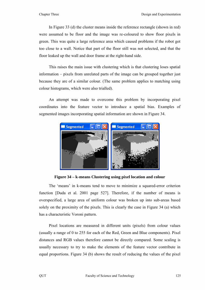
Chapter Three Design and Experimentation
In Figure 33 (d) the cluster means inside the reference rectangle (shown in red)
were assumed to be floor and the image was re-coloured to show floor pixels in
green. This was quite a large reference area which caused problems if the robot got
too close to a wall. Notice that part of the floor still was not selected, and that the
floor leaked up the wall and door frame at the right-hand side.
This raises the main issue with clustering which is that clustering loses spatial
information – pixels from unrelated parts of the image can be grouped together just
because they are of a similar colour. (The same problem applies to matching using
colour histograms, which were also trialled).
An attempt was made to overcome this problem by incorporating pixel
coordinates into the feature vector to introduce a spatial bias. Examples of
segmented images incorporating spatial information are shown in Figure 34.
Figure 34 – k-means Clustering using pixel location and colour
The ‘means’ in k-means tend to move to minimize a squared-error criterion
function [Duda et al. 2001 page 527]. Therefore, if the number of means is
overspecified, a large area of uniform colour was broken up into sub-areas based
solely on the proximity of the pixels. This is clearly the case in Figure 34 (a) which
has a characteristic Voroni pattern.
Pixel locations are measured in different units (pixels) from colour values
(usually a range of 0 to 255 for each of the Red, Green and Blue components). Pixel
distances and RGB values therefore cannot be directly compared. Some scaling is
usually necessary to try to make the elements of the feature vector contribute in
equal proportions. Figure 34 (b) shows the result of reducing the values of the pixel
QUT Faculty of Science and Technology 125
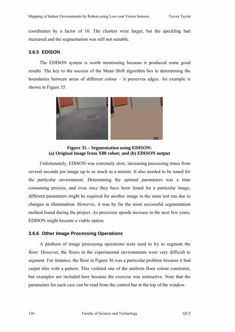
Mapping of Indoor Environments by Robots using Low-cost Vision Sensors Trevor Taylor
coordinates by a factor of 10. The clusters were larger, but the speckling had
increased and the segmentation was still not suitable.
3.6.5 EDISON
The EDISON system is worth mentioning because it produced some good
results. The key to the success of the Mean Shift algorithm lies in determining the
boundaries between areas of different colour – it preserves edges. An example is
shown in Figure 35.
Figure 35 – Segmentation using EDISON: (a) Original image from X80 robot; and (b) EDISON output
Unfortunately, EDISON was extremely slow, increasing processing times from
several seconds per image up to as much as a minute. It also needed to be tuned for
the particular environment. Determining the optimal parameters was a time
consuming process, and even once they have been found for a particular image,
different parameters might be required for another image in the same test run due to
changes in illumination. However, it was by far the most successful segmentation
method found during the project. As processor speeds increase in the next few years,
EDISON might become a viable option.
3.6.6 Other Image Processing Operations
A plethora of image processing operations were used to try to segment the
floor. However, the floors in the experimental environments were very difficult to
segment. For instance, the floor in Figure 36 was a particular problem because it had
carpet tiles with a pattern. This violated one of the uniform floor colour constraint,
but examples are included here because the exercise was instructive. Note that the
parameters for each case can be read from the control bar at the top of the window.
126 Faculty of Science and Technology QUT
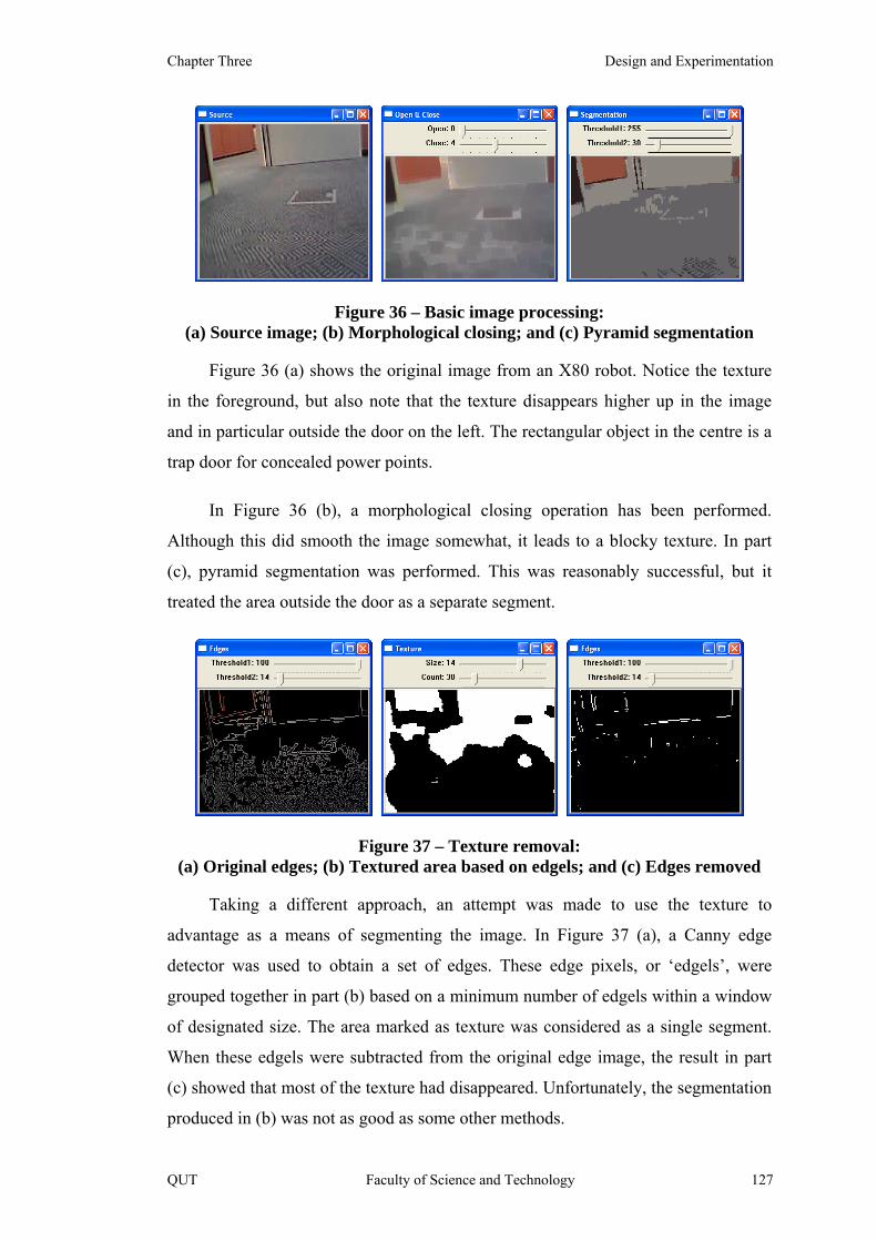
Chapter Three Design and Experimentation
Figure 36 – Basic image processing: (a) Source image; (b) Morphological closing; and (c) Pyramid segmentation
Figure 36 (a) shows the original image from an X80 robot. Notice the texture
in the foreground, but also note that the texture disappears higher up in the image
and in particular outside the door on the left. The rectangular object in the centre is a
trap door for concealed power points.
In Figure 36 (b), a morphological closing operation has been performed.
Although this did smooth the image somewhat, it leads to a blocky texture. In part
(c), pyramid segmentation was performed. This was reasonably successful, but it
treated the area outside the door as a separate segment.
Figure 37 – Texture removal: (a) Original edges; (b) Textured area based on edgels; and (c) Edges removed
Taking a different approach, an attempt was made to use the texture to
advantage as a means of segmenting the image. In Figure 37 (a), a Canny edge
detector was used to obtain a set of edges. These edge pixels, or ‘edgels’, were
grouped together in part (b) based on a minimum number of edgels within a window
of designated size. The area marked as texture was considered as a single segment.
When these edgels were subtracted from the original edge image, the result in part
(c) showed that most of the texture had disappeared. Unfortunately, the segmentation
produced in (b) was not as good as some other methods.
QUT Faculty of Science and Technology 127

Mapping of Indoor Environments by Robots using Low-cost Vision Sensors Trevor Taylor
Figure 38 – Effects of pre-filtering: (a) Image filtered with a 9x9 Gaussian; (b) Edges obtained after filtering; and (c) Pyramid segmentation after filtering
It is common practice in image processing to filter (smooth) the image prior to
performing other operations. Figure 38 (a) shows the original image filtered by a 9x9
Gaussian. Even though it was obviously blurred, solid edges could still be obtained.
In fact, they corresponded to the main features in the image as shown in (b),
although there are extraneous edges across the door due to shadows. In part (c),
pyramid segmentation was once again applied. It was questionable whether this was
better or worse than previous attempts.
Figure 39 – Flood Filling: (a) Fill with one seed point; (b) Fill from a different seed point; and (c) Fill after pre-filtering
Another method for segmenting an image was to use an adaptive flood fill
where the matching pixel value varied across the image within a defined range. As
can be seen in Figure 39 (a) and (b), the initial starting point for the fill had a
significant effect on the result. In Figure 39 (c) the image was pre-filtered, which
resulted in a much smoother flood fill. However, the fill also tended to ‘leak’ out of
the floor area.
Some of these approaches showed promise, but none of them worked on their
own and yet a human can look at the original image and immediately determine
which parts of it are floor. Furthermore, they all required parameters and a
128 Faculty of Science and Technology QUT
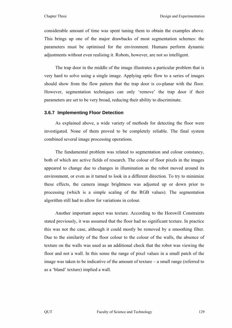
Chapter Three Design and Experimentation
considerable amount of time was spent tuning them to obtain the examples above.
This brings up one of the major drawbacks of most segmentation schemes: the
parameters must be optimised for the environment. Humans perform dynamic
adjustments without even realising it. Robots, however, are not so intelligent.
The trap door in the middle of the image illustrates a particular problem that is
very hard to solve using a single image. Applying optic flow to a series of images
should show from the flow pattern that the trap door is co-planar with the floor.
However, segmentation techniques can only ‘remove’ the trap door if their
parameters are set to be very broad, reducing their ability to discriminate.
3.6.7 Implementing Floor Detection
As explained above, a wide variety of methods for detecting the floor were
investigated. None of them proved to be completely reliable. The final system
combined several image processing operations.
The fundamental problem was related to segmentation and colour constancy,
both of which are active fields of research. The colour of floor pixels in the images
appeared to change due to changes in illumination as the robot moved around its
environment, or even as it turned to look in a different direction. To try to minimize
these effects, the camera image brightness was adjusted up or down prior to
processing (which is a simple scaling of the RGB values). The segmentation
algorithm still had to allow for variations in colour.
Another important aspect was texture. According to the Horswill Constraints
stated previously, it was assumed that the floor had no significant texture. In practice
this was not the case, although it could mostly be removed by a smoothing filter.
Due to the similarity of the floor colour to the colour of the walls, the absence of
texture on the walls was used as an additional check that the robot was viewing the
floor and not a wall. In this sense the range of pixel values in a small patch of the
image was taken to be indicative of the amount of texture – a small range (referred to
as a ‘bland’ texture) implied a wall.
QUT Faculty of Science and Technology 129

Mapping of Indoor Environments by Robots using Low-cost Vision Sensors Trevor Taylor
Edges detected in the image were found to be the best indication of the floor
outline. Therefore the most prominent edges were incorporated into the floor
detection procedure.
In the final version of the system, the process was simplified to using a Flood
Fill as follows:
• Smooth the image using a 9x9 Gaussian;
• Obtain the strongest edges in the image using a Canny Edge Detector;
• Create a mask image to prevent filling beyond the detected edges;
• Apply the adaptive FloodFill function from the OpenCV Library with
the edge mask.
There were two main problems with this approach – the flood fill could ‘leak’
through gaps in the edges, and the fill could stop prematurely if there was a wide
range of illumination across the image.
To perform a flood fill, it was necessary to supply a ‘seed’ value for the pixels
to match. The robot determined the colour of the floor when it first started up using
an average of a reference patch in the bottom centre of the image. This assumed that
the area in front of the robot was clear initially. This was only a minor constraint and
it makes sense to do this in any case.
Care had to be taken to ensure that the fill was not initiated inside an obstacle.
Therefore the colour of the seed pixel was first checked against the known floor
colour. If it differed significantly from the floor, or if the texture was bland, then a
search was performed across the bottom of the image until the floor was found.
Based on the seed colour, the floor was detected using an adaptive flood fill where
the search value varied across the image.
The range limits for the flood fill and the parameters for the edge detector were
determined by the researcher by experimentation using images captured by the robot
during test runs. Automatically selecting these parameters is a possible area for
future research.
130 Faculty of Science and Technology QUT
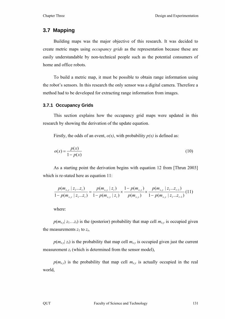
Chapter Three Design and Experimentation
3.7 Mapping
Building maps was the major objective of this research. It was decided to
create metric maps using occupancy grids as the representation because these are
easily understandable by non-technical people such as the potential consumers of
home and office robots.
To build a metric map, it must be possible to obtain range information using
the robot’s sensors. In this research the only sensor was a digital camera. Therefore a
method had to be developed for extracting range information from images.
3.7.1 Occupancy Grids
This section explains how the occupancy grid maps were updated in this
research by showing the derivation of the update equation.
Firstly, the odds of an event, o(x), with probability p(x) is defined as:
)(1)()(xp
xpxo−
= (10)
As a starting point the derivation begins with equation 12 from [Thrun 2003]
which is re-stated here as equation 11:
)...|(1)...|(
)()(1
)|(1)|(
)...|(1)...|(
11,
11,
,
,
,
,
1,
1,
−
−
−×
−×
−=
− tyx
tyx
yx
yx
tyx
tyx
tyx
tyx
zzmpzzmp
mpmp
zmpzmp
zzmpzzmp
(11)
where:
p(mx,y| z1…zt) is the (posterior) probability that map cell mx,y is occupied given
the measurements z1 to zt,
p(mx,y| zt) is the probability that map cell mx,y is occupied given just the current
measurement zt (which is determined from the sensor model),
p(mx,y) is the probability that map cell mx,y is actually occupied in the real
world,
QUT Faculty of Science and Technology 131

Mapping of Indoor Environments by Robots using Low-cost Vision Sensors Trevor Taylor
p(mx,y| z1…zt-1) is the (prior) probability that map cell mx,y is occupied given the
measurements z1 to zt-1.
In words, equation 11 says that the odds of a map cell being occupied at time t
are equal to the odds of the latest measurement times the odds of it being occupied at
time t-1 divided by the odds that the cell is actually occupied in the real world
(which is the middle factor inverted). This equation can be derived using Bayes
Rule, as shown by Thrun.
Equation 11 can be simplified by making an assumption that is common in the
literature of occupancy grids (and also mentioned in [Thrun 2003]), namely that the
initial value for the occupancy probability of all map cells is 0.5. In other words,
because the actual probability of occupancy of all the grid cells in the real world is
unknown, just assume a 50/50 chance.
Substituting 0.5 for p(mx,y) in equation 11 eliminates the middle term because
the numerator and denominator both become 0.5.
To simplify the notation, drop the subscript x,y which refers to the location of a
cell in the grid.
Define P as follows:
)...|(1)...|(
)|(1)|(
11
11
−
−
−×
−=
t
t
t
t
zzmpzzmp
zmpzmp
P (12)
This is equivalent to the right-hand side of equation 11 after substituting 0.5
for p(mx,y). The two factors in P above are the odds of the cell being occupied based
on the latest sensor reading and the previous odds for the map cell.
So equation 11 can now be re-written as:
Pzzmp
zzmp
t
t =− )...|(1
)...|(
1
1 (13)
After a small amount of rearrangement the new occupancy value for a map cell
at time t can be calculated as follows:
132 Faculty of Science and Technology QUT
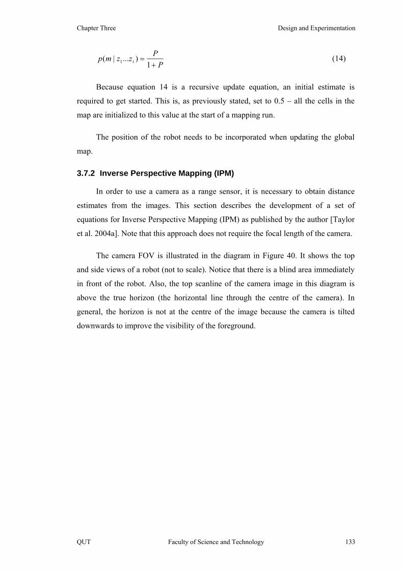
Chapter Three Design and Experimentation
PPzzmp t +
=1
)...|( 1 (14)
Because equation 14 is a recursive update equation, an initial estimate is
required to get started. This is, as previously stated, set to 0.5 – all the cells in the
map are initialized to this value at the start of a mapping run.
The position of the robot needs to be incorporated when updating the global
map.
3.7.2 Inverse Perspective Mapping (IPM)
In order to use a camera as a range sensor, it is necessary to obtain distance
estimates from the images. This section describes the development of a set of
equations for Inverse Perspective Mapping (IPM) as published by the author [Taylor
et al. 2004a]. Note that this approach does not require the focal length of the camera.
The camera FOV is illustrated in the diagram in Figure 40. It shows the top
and side views of a robot (not to scale). Notice that there is a blind area immediately
in front of the robot. Also, the top scanline of the camera image in this diagram is
above the true horizon (the horizontal line through the centre of the camera). In
general, the horizon is not at the centre of the image because the camera is tilted
downwards to improve the visibility of the foreground.
QUT Faculty of Science and Technology 133

Mapping of Indoor Environments by Robots using Low-cost Vision Sensors Trevor Taylor
Figure 40 – Camera Field of View (FOV) showing coordinate system and parameters for Inverse Perspective Mapping (IPM)
In the FOV diagram, γ is one-half of the horizontal FOV; α is one-half of the
vertical FOV; and δ is the camera tilt angle. (γ and α are related through the aspect
ratio of the camera, which is usually 4:3 for conventional video cameras.)
Image pixel coordinates are represented by (u, v) in the horizontal and vertical
directions respectively. Note that, by convention, v is measured downwards from the
top of the image. If the image resolution is m by n pixels, then the values of the
image coordinates (u, v) will range from 0 to (m-1) and 0 to (n-1) respectively.
Consider rays from the camera to points on the ground corresponding to
successive scanlines in the camera image. Each pixel in this vertical column of the
image corresponds to an angle of 2α/(n-1). Similarly, pixels in the horizontal
direction correspond to an arc of 2 γ/(m-1).
Four parameters must be measured for the IPM calculation:
134 Faculty of Science and Technology QUT
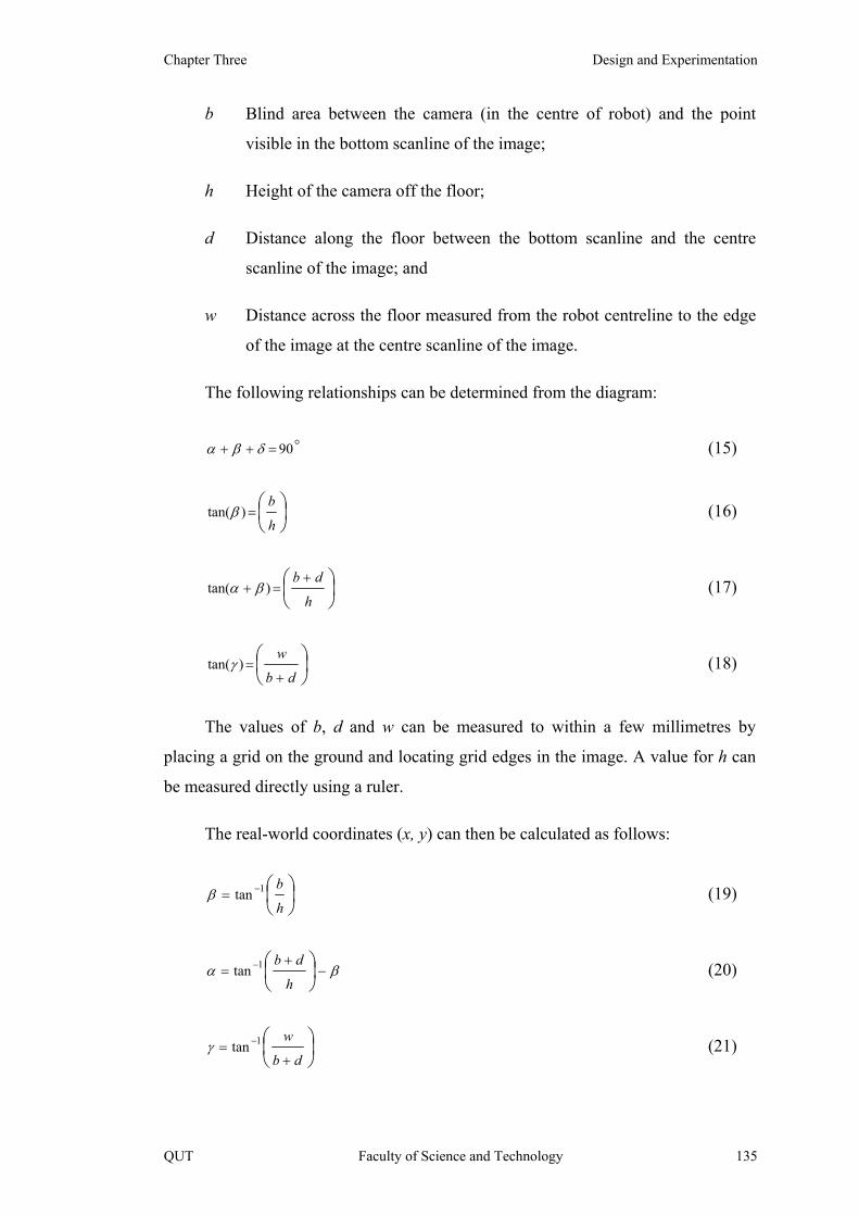
Chapter Three Design and Experimentation
b Blind area between the camera (in the centre of robot) and the point
visible in the bottom scanline of the image;
h Height of the camera off the floor;
d Distance along the floor between the bottom scanline and the centre
scanline of the image; and
w Distance across the floor measured from the robot centreline to the edge
of the image at the centre scanline of the image.
The following relationships can be determined from the diagram:
o90=++ δβα (15)
⎟⎠⎞
⎜⎝⎛
=h
b)tan(β (16)
⎟⎠⎞
⎜⎝⎛ +
=+h
db)tan( βα (17)
⎟⎠⎞
⎜⎝⎛
+=
db
w)tan(γ (18)
The values of b, d and w can be measured to within a few millimetres by
placing a grid on the ground and locating grid edges in the image. A value for h can
be measured directly using a ruler.
The real-world coordinates (x, y) can then be calculated as follows:
⎟⎠⎞
⎜⎝⎛−=
h
b1tanβ (19)
βα −+
= ⎟⎠⎞
⎜⎝⎛−
h
db1tan (20)
⎟⎠⎞
⎜⎝⎛
+= −
db
w1tanγ (21)
QUT Faculty of Science and Technology 135
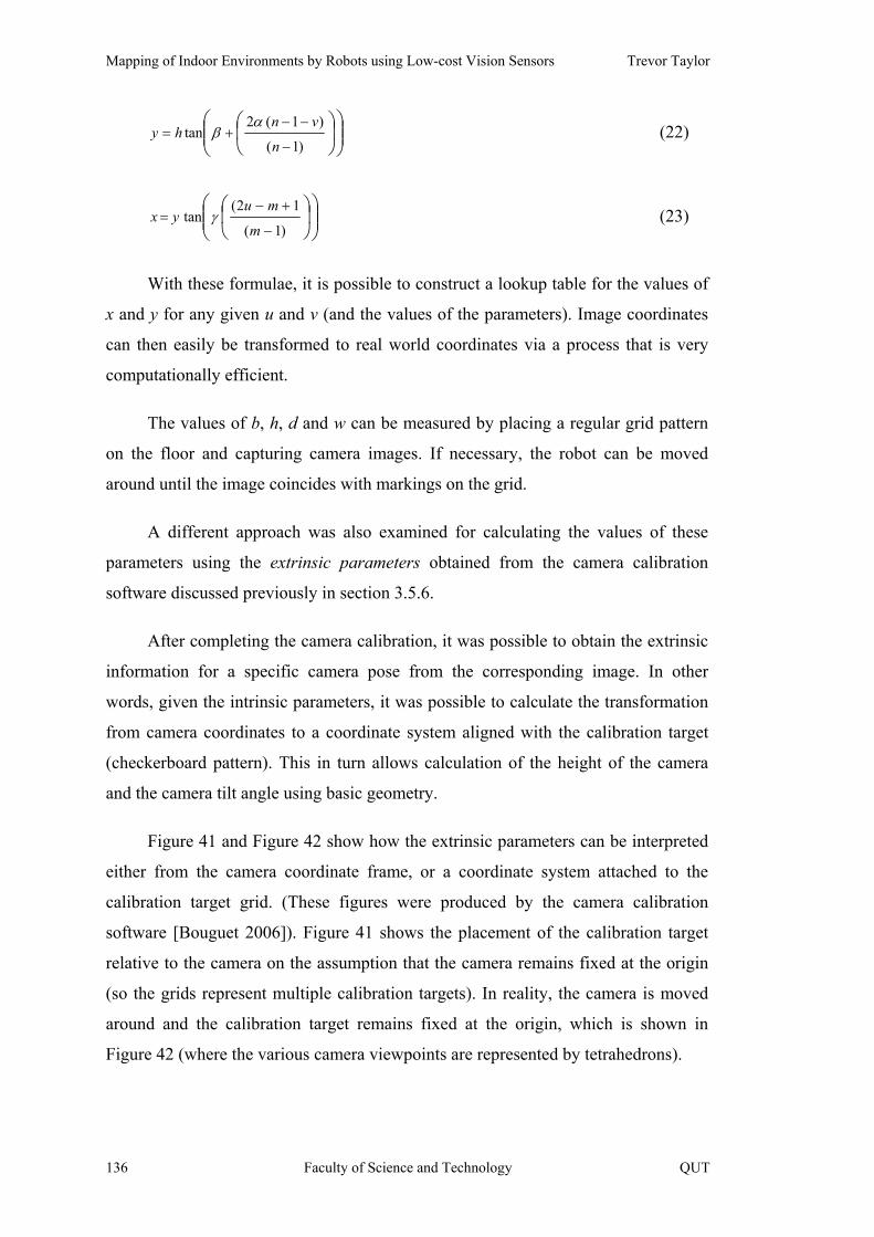
Mapping of Indoor Environments by Robots using Low-cost Vision Sensors Trevor Taylor
⎟⎟⎠
⎞⎜⎜⎝
⎛⎟⎠
⎞⎜⎝
⎛−
−−+=
)1(
)1(2tan
n
vnhy
αβ (22)
⎟⎟⎠
⎞⎜⎜⎝
⎛⎟⎠
⎞⎜⎝
⎛−
+−=
)1(
12(tan
m
muyx γ (23)
With these formulae, it is possible to construct a lookup table for the values of
x and y for any given u and v (and the values of the parameters). Image coordinates
can then easily be transformed to real world coordinates via a process that is very
computationally efficient.
The values of b, h, d and w can be measured by placing a regular grid pattern
on the floor and capturing camera images. If necessary, the robot can be moved
around until the image coincides with markings on the grid.
A different approach was also examined for calculating the values of these
parameters using the extrinsic parameters obtained from the camera calibration
software discussed previously in section 3.5.6.
After completing the camera calibration, it was possible to obtain the extrinsic
information for a specific camera pose from the corresponding image. In other
words, given the intrinsic parameters, it was possible to calculate the transformation
from camera coordinates to a coordinate system aligned with the calibration target
(checkerboard pattern). This in turn allows calculation of the height of the camera
and the camera tilt angle using basic geometry.
Figure 41 and Figure 42 show how the extrinsic parameters can be interpreted
either from the camera coordinate frame, or a coordinate system attached to the
calibration target grid. (These figures were produced by the camera calibration
software [Bouguet 2006]). Figure 41 shows the placement of the calibration target
relative to the camera on the assumption that the camera remains fixed at the origin
(so the grids represent multiple calibration targets). In reality, the camera is moved
around and the calibration target remains fixed at the origin, which is shown in
Figure 42 (where the various camera viewpoints are represented by tetrahedrons).
136 Faculty of Science and Technology QUT
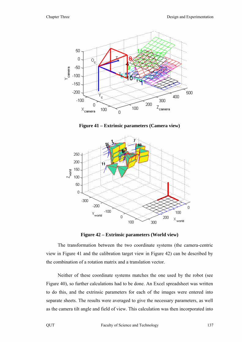
Chapter Three Design and Experimentation
Figure 41 – Extrinsic parameters (Camera view)
Figure 42 – Extrinsic parameters (World view)
The transformation between the two coordinate systems (the camera-centric
view in Figure 41 and the calibration target view in Figure 42) can be described by
the combination of a rotation matrix and a translation vector.
Neither of these coordinate systems matches the one used by the robot (see
Figure 40), so further calculations had to be done. An Excel spreadsheet was written
to do this, and the extrinsic parameters for each of the images were entered into
separate sheets. The results were averaged to give the necessary parameters, as well
as the camera tilt angle and field of view. This calculation was then incorporated into
QUT Faculty of Science and Technology 137
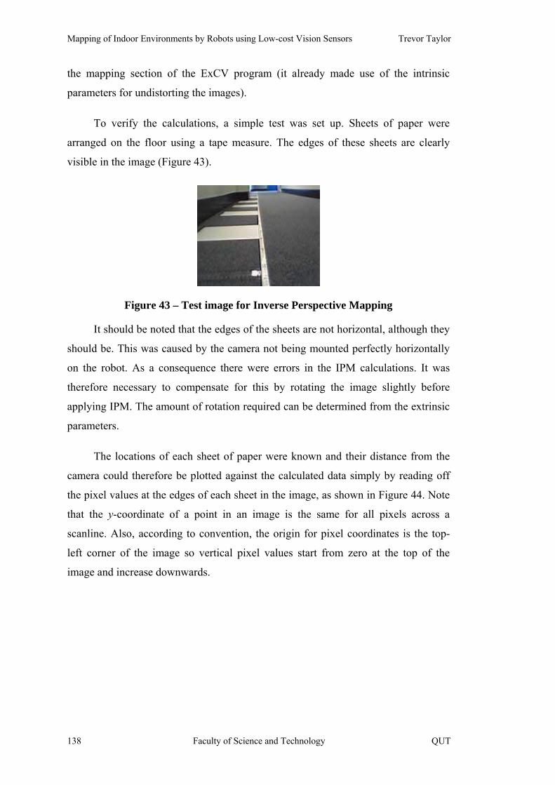
Mapping of Indoor Environments by Robots using Low-cost Vision Sensors Trevor Taylor
the mapping section of the ExCV program (it already made use of the intrinsic
parameters for undistorting the images).
To verify the calculations, a simple test was set up. Sheets of paper were
arranged on the floor using a tape measure. The edges of these sheets are clearly
visible in the image (Figure 43).
Figure 43 – Test image for Inverse Perspective Mapping
It should be noted that the edges of the sheets are not horizontal, although they
should be. This was caused by the camera not being mounted perfectly horizontally
on the robot. As a consequence there were errors in the IPM calculations. It was
therefore necessary to compensate for this by rotating the image slightly before
applying IPM. The amount of rotation required can be determined from the extrinsic
parameters.
The locations of each sheet of paper were known and their distance from the
camera could therefore be plotted against the calculated data simply by reading off
the pixel values at the edges of each sheet in the image, as shown in Figure 44. Note
that the y-coordinate of a point in an image is the same for all pixels across a
scanline. Also, according to convention, the origin for pixel coordinates is the top-
left corner of the image so vertical pixel values start from zero at the top of the
image and increase downwards.
138 Faculty of Science and Technology QUT
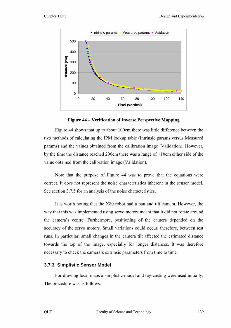
Chapter Three Design and Experimentation
0
100
200
300
400
500
0 20 40 60 80 100 120 140
Pixel (vertical)
Dis
tanc
e (c
m)
Intrinsic params Measured params Validation
Figure 44 – Verification of Inverse Perspective Mapping
Figure 44 shows that up to about 100cm there was little difference between the
two methods of calculating the IPM lookup table (Intrinsic params versus Measured
params) and the values obtained from the calibration image (Validation). However,
by the time the distance reached 200cm there was a range of ±10cm either side of the
value obtained from the calibration image (Validation).
Note that the purpose of Figure 44 was to prove that the equations were
correct. It does not represent the noise characteristics inherent in the sensor model.
See section 3.7.5 for an analysis of the noise characteristics.
It is worth noting that the X80 robot had a pan and tilt camera. However, the
way that this was implemented using servo motors meant that it did not rotate around
the camera’s centre. Furthermore, positioning of the camera depended on the
accuracy of the servo motors. Small variations could occur, therefore, between test
runs. In particular, small changes in the camera tilt affected the estimated distance
towards the top of the image, especially for longer distances. It was therefore
necessary to check the camera’s extrinsic parameters from time to time.
3.7.3 Simplistic Sensor Model
For drawing local maps a simplistic model and ray-casting were used initially.
The procedure was as follows:
QUT Faculty of Science and Technology 139
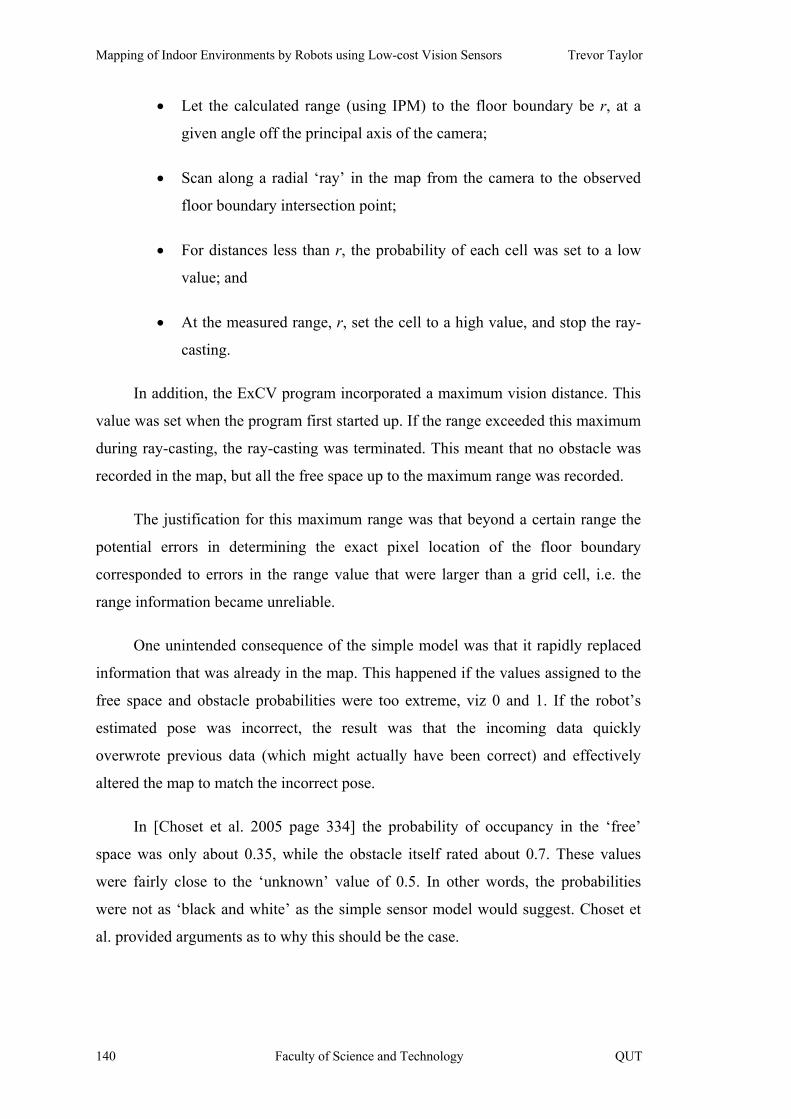
Mapping of Indoor Environments by Robots using Low-cost Vision Sensors Trevor Taylor
• Let the calculated range (using IPM) to the floor boundary be r, at a
given angle off the principal axis of the camera;
• Scan along a radial ‘ray’ in the map from the camera to the observed
floor boundary intersection point;
• For distances less than r, the probability of each cell was set to a low
value; and
• At the measured range, r, set the cell to a high value, and stop the ray-
casting.
In addition, the ExCV program incorporated a maximum vision distance. This
value was set when the program first started up. If the range exceeded this maximum
during ray-casting, the ray-casting was terminated. This meant that no obstacle was
recorded in the map, but all the free space up to the maximum range was recorded.
The justification for this maximum range was that beyond a certain range the
potential errors in determining the exact pixel location of the floor boundary
corresponded to errors in the range value that were larger than a grid cell, i.e. the
range information became unreliable.
One unintended consequence of the simple model was that it rapidly replaced
information that was already in the map. This happened if the values assigned to the
free space and obstacle probabilities were too extreme, viz 0 and 1. If the robot’s
estimated pose was incorrect, the result was that the incoming data quickly
overwrote previous data (which might actually have been correct) and effectively
altered the map to match the incorrect pose.
In [Choset et al. 2005 page 334] the probability of occupancy in the ‘free’
space was only about 0.35, while the obstacle itself rated about 0.7. These values
were fairly close to the ‘unknown’ value of 0.5. In other words, the probabilities
were not as ‘black and white’ as the simple sensor model would suggest. Choset et
al. provided arguments as to why this should be the case.
140 Faculty of Science and Technology QUT
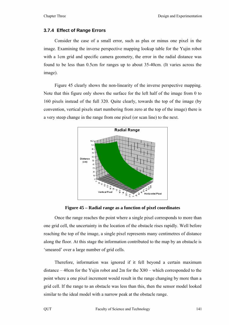
Chapter Three Design and Experimentation
3.7.4 Effect of Range Errors
Consider the case of a small error, such as plus or minus one pixel in the
image. Examining the inverse perspective mapping lookup table for the Yujin robot
with a 1cm grid and specific camera geometry, the error in the radial distance was
found to be less than 0.5cm for ranges up to about 35-40cm. (It varies across the
image).
Figure 45 clearly shows the non-linearity of the inverse perspective mapping.
Note that this figure only shows the surface for the left half of the image from 0 to
160 pixels instead of the full 320. Quite clearly, towards the top of the image (by
convention, vertical pixels start numbering from zero at the top of the image) there is
a very steep change in the range from one pixel (or scan line) to the next.
Figure 45 – Radial range as a function of pixel coordinates
Once the range reaches the point where a single pixel corresponds to more than
one grid cell, the uncertainty in the location of the obstacle rises rapidly. Well before
reaching the top of the image, a single pixel represents many centimetres of distance
along the floor. At this stage the information contributed to the map by an obstacle is
‘smeared’ over a large number of grid cells.
Therefore, information was ignored if it fell beyond a certain maximum
distance – 40cm for the Yujin robot and 2m for the X80 – which corresponded to the
point where a one pixel increment would result in the range changing by more than a
grid cell. If the range to an obstacle was less than this, then the sensor model looked
similar to the ideal model with a narrow peak at the obstacle range.
QUT Faculty of Science and Technology 141

Mapping of Indoor Environments by Robots using Low-cost Vision Sensors Trevor Taylor
With this constraint, known as the maximum vision distance, the simple sensor
model was used initially.
3.7.5 Vision Sensor Noise Characteristics
The simple sensor model assumed no noise. However, this was clearly not true
because the vision system was not perfect.
To assess the noise characteristics of the vision sensor, the output from the
vision system’s floor detector was captured. These ‘floor’ images were then edited
by hand to correct any errors in the locations of the obstacles. A total of 100 images
were corrected and used to generate statistics for the noise.
To compare them against the vision system output, images were scanned
column by column looking up from the bottom of the image to find the first edge
pixel, i.e. the nearest obstacle. This resulted in a total of 17,600 data points.
Consider the sample floor image and the corrected image in Figure 46.
Figure 46 – Corrected Floor Image: (a) Original; and (b) Hand-edited
Small gaps occurred in the edges for a variety of reasons. This was the primary
failure mode of the floor detector. Figure 46 (b) shows how these mistakes were
corrected by hand for the statistical analysis. Although it was possible to close these
gaps by increasing the sensitivity of the edge detector, this also enhanced shadows
and extracted carpet texture from the floor. The values used were a compromise.
In the initial statistics, the errors due to these gaps were included but they
resulted in very large standard deviations (to accommodate the large differences
from the correct scanline to the top of the image) and they also biased the means.
Usually these problems corrected themselves as the robot got closer to the obstacles,
142 Faculty of Science and Technology QUT
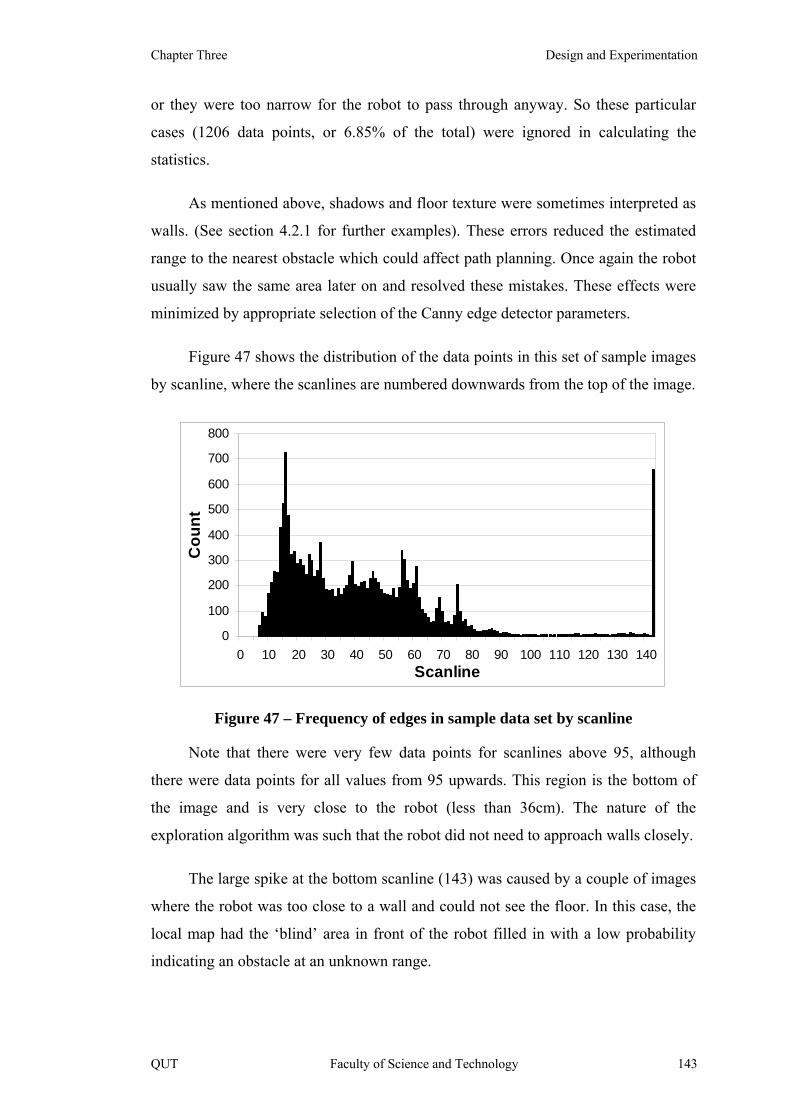
Chapter Three Design and Experimentation
or they were too narrow for the robot to pass through anyway. So these particular
cases (1206 data points, or 6.85% of the total) were ignored in calculating the
statistics.
As mentioned above, shadows and floor texture were sometimes interpreted as
walls. (See section 4.2.1 for further examples). These errors reduced the estimated
range to the nearest obstacle which could affect path planning. Once again the robot
usually saw the same area later on and resolved these mistakes. These effects were
minimized by appropriate selection of the Canny edge detector parameters.
Figure 47 shows the distribution of the data points in this set of sample images
by scanline, where the scanlines are numbered downwards from the top of the image.
0
100
200
300
400
500
600
700
800
0 10 20 30 40 50 60 70 80 90 100 110 120 130 140Scanline
Cou
nt
Figure 47 – Frequency of edges in sample data set by scanline
Note that there were very few data points for scanlines above 95, although
there were data points for all values from 95 upwards. This region is the bottom of
the image and is very close to the robot (less than 36cm). The nature of the
exploration algorithm was such that the robot did not need to approach walls closely.
The large spike at the bottom scanline (143) was caused by a couple of images
where the robot was too close to a wall and could not see the floor. In this case, the
local map had the ‘blind’ area in front of the robot filled in with a low probability
indicating an obstacle at an unknown range.
QUT Faculty of Science and Technology 143
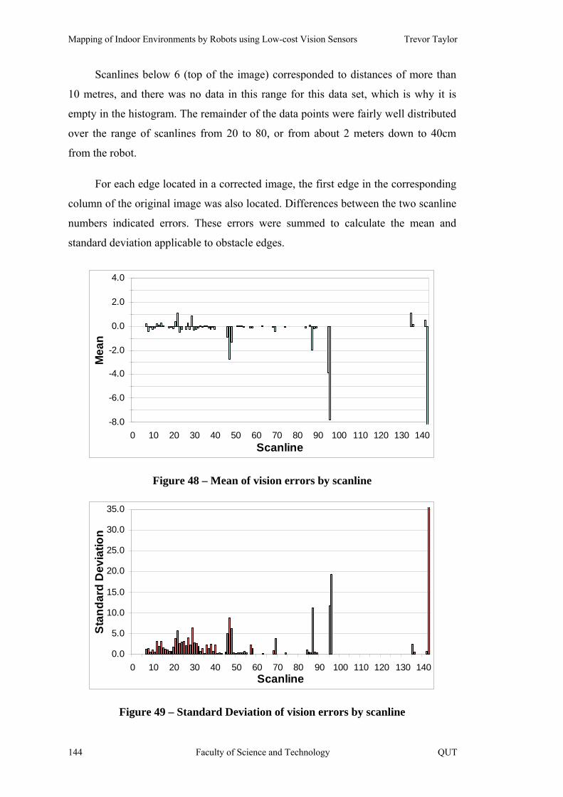
Mapping of Indoor Environments by Robots using Low-cost Vision Sensors Trevor Taylor
Scanlines below 6 (top of the image) corresponded to distances of more than
10 metres, and there was no data in this range for this data set, which is why it is
empty in the histogram. The remainder of the data points were fairly well distributed
over the range of scanlines from 20 to 80, or from about 2 meters down to 40cm
from the robot.
For each edge located in a corrected image, the first edge in the corresponding
column of the original image was also located. Differences between the two scanline
numbers indicated errors. These errors were summed to calculate the mean and
standard deviation applicable to obstacle edges.
-8.0
-6.0
-4.0
-2.0
0.0
2.0
4.0
0 10 20 30 40 50 60 70 80 90 100 110 120 130 140Scanline
Mea
n
Figure 48 – Mean of vision errors by scanline
0.0
5.0
10.0
15.0
20.0
25.0
30.0
35.0
0 10 20 30 40 50 60 70 80 90 100 110 120 130 140Scanline
Stan
dard
Dev
iatio
n
Figure 49 – Standard Deviation of vision errors by scanline
144 Faculty of Science and Technology QUT
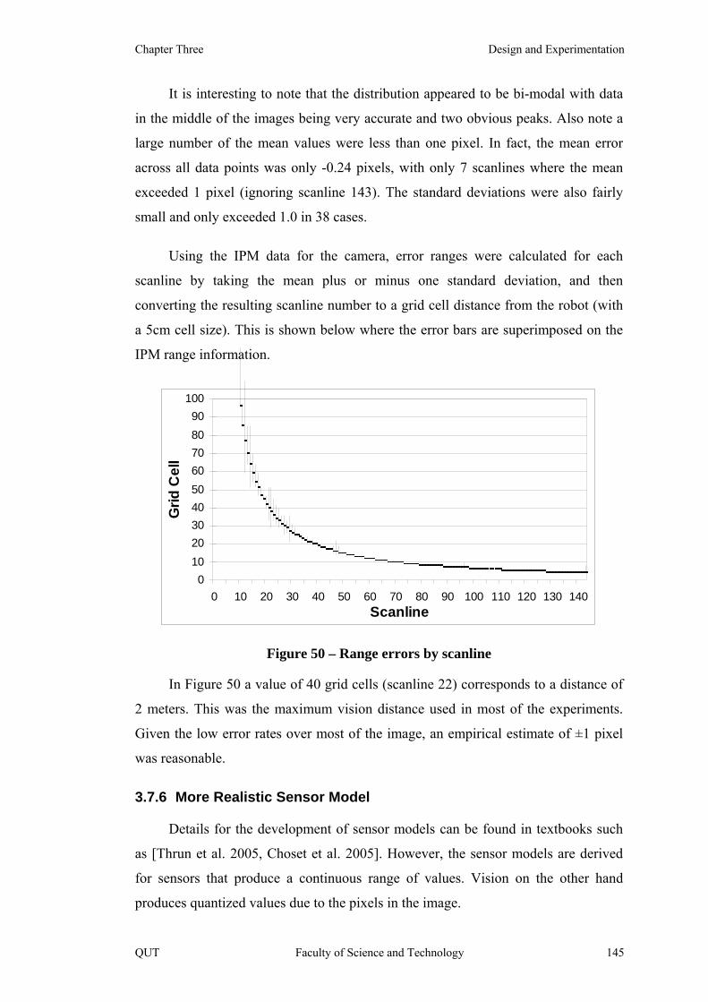
Chapter Three Design and Experimentation
It is interesting to note that the distribution appeared to be bi-modal with data
in the middle of the images being very accurate and two obvious peaks. Also note a
large number of the mean values were less than one pixel. In fact, the mean error
across all data points was only -0.24 pixels, with only 7 scanlines where the mean
exceeded 1 pixel (ignoring scanline 143). The standard deviations were also fairly
small and only exceeded 1.0 in 38 cases.
Using the IPM data for the camera, error ranges were calculated for each
scanline by taking the mean plus or minus one standard deviation, and then
converting the resulting scanline number to a grid cell distance from the robot (with
a 5cm cell size). This is shown below where the error bars are superimposed on the
IPM range information.
0102030405060708090
100
0 10 20 30 40 50 60 70 80 90 100 110 120 130 140Scanline
Grid
Cel
l
Figure 50 – Range errors by scanline
In Figure 50 a value of 40 grid cells (scanline 22) corresponds to a distance of
2 meters. This was the maximum vision distance used in most of the experiments.
Given the low error rates over most of the image, an empirical estimate of ±1 pixel
was reasonable.
3.7.6 More Realistic Sensor Model
Details for the development of sensor models can be found in textbooks such
as [Thrun et al. 2005, Choset et al. 2005]. However, the sensor models are derived
for sensors that produce a continuous range of values. Vision on the other hand
produces quantized values due to the pixels in the image.
QUT Faculty of Science and Technology 145

Mapping of Indoor Environments by Robots using Low-cost Vision Sensors Trevor Taylor
Furthermore, the textbook derivations assume that the range error has a
Gaussian distribution. This is clearly not the case for vision because each successive
scanline (pixel row) moving up towards the top of the image represents a larger and
larger distance due to perspective, so an error of as little as ±1 pixel results in an
error distribution that not only changes across the image, but is also significantly lop-
sided.
Single pixel errors in edge detection would barely be noticed by a human and
this is generally accepted as a typical error in image processing. Although edge
detectors do exist with sub-pixel resolution, ultimately the resolution of the camera
comes into play. When the edge corresponding to an obstacle is towards the top of
the image, perspective can make a significant difference to the estimated range. In
the development of the sensor model for vision a possible error of ±1 pixel was
assumed for the accuracy of edge detection.
However the key point is that errors in edge detection affect the map and the
primary purpose of this research was to produce maps. To account for range
uncertainty due to errors in the location of the floor boundary, a more sophisticated
model was developed that was similar to Figure 51. Note that the diagram is
exaggerated. The peak is not symmetrical because the distance from the camera does
not increase linearly for higher scanlines.
Figure 51 – Complex sensor model for errors in range measurement
Formulae are not provided for the sensor model because it was determined
using table lookup based on IPM (explained below). The peak of the curve in Figure
146 Faculty of Science and Technology QUT

Chapter Three Design and Experimentation
51 corresponds to the estimated range. The ‘spread’ of the peak is based the
differences between the range to successive scanlines. Although it might not be
immediately apparent from Figure 51, the curve is not symmetrical about the peak
because an error of one pixel upwards in the image corresponds to a much larger
distance then an error of one pixel downwards due to perspective.
Also note that the shape of the distribution changes with the estimated distance
from the camera, so that the spread of the peak decreases for scanlines further down
the image. Figure 52 is for an obstacle that is closer to the camera than Figure 51,
and therefore the obstacle appears closer to the bottom of the image. Notice that the
peak is much sharper.
Figure 52 – Complex sensor model (with errors) for shorter range
Near the bottom of the image, the range difference between successive
scanlines was very small – less than a centimetre. With a grid size of several
centimetres, the peak in the distribution was therefore only a single cell wide (even
for errors of several pixels in determining the floor boundary) and the distribution
was essentially the same as for the simple sensor model as shown in Chapter 2.
Eventually, the range difference between successive scanlines exceeded the
size of a map grid cell and ‘shoulders’ appeared on the curve as shown in Figure 51
and Figure 52 above. For the X80, the grid size was usually set to 5cm. By the time
that the range had reached 2m, the difference was around 10 grid cells, or 50cm
which was more than the diameter of an X80 robot.
QUT Faculty of Science and Technology 147

Mapping of Indoor Environments by Robots using Low-cost Vision Sensors Trevor Taylor
Note that the value for free space in this model was not set to zero and the peak
did not reach 1. These changes from the simple sensor model reflected the fact that
there was a small probability of bad sensor readings which gave entirely incorrect
ranges. They also prevented a single sensor update from immediately overwriting the
data in the map. Ideally, each cell in the map should be observed multiple times in
order to verify its occupancy state.
To implement this sensor model, the ExCV program built a table when it
started that contained the relevant values. The way that the values for this model
were obtained was as follows:
For each value of radial distance (measured in the centre of a cell):
1. Find the scanline corresponding to this range in the image;
2. Calculate the average change in range for the scanlines above and below, i.e.
±1 pixel; and
3. Convert this change in the range value into the equivalent number of map
grid cells and store this in the table. (This is referred to as the ‘spread’.)
When drawing the local map, if this spread was zero, then the obstacle was
simply drawn into the map at the specified range. However, if the spread was greater
than zero, then the values either side of the obstacle range needed to be calculated to
determine the starting and ending range values. The occupancy values were then
increased along the ‘ray’ from the robot from the starting range up to the estimated
range, and then decrease again on the other side out to the ending range.
3.7.7 The Radial Obstacle Profile (ROP)
A Radial Obstacle Profile (ROP) is an array of distances to the obstacles in the
vicinity of the robot. It might be considered to be similar to a traditional sonar, radar
or laser range finder scan.
The term ROP was introduced to the literature by the author [Taylor et al.
2004b]. It is similar to a range scan but represents the information from a single
image.
148 Faculty of Science and Technology QUT
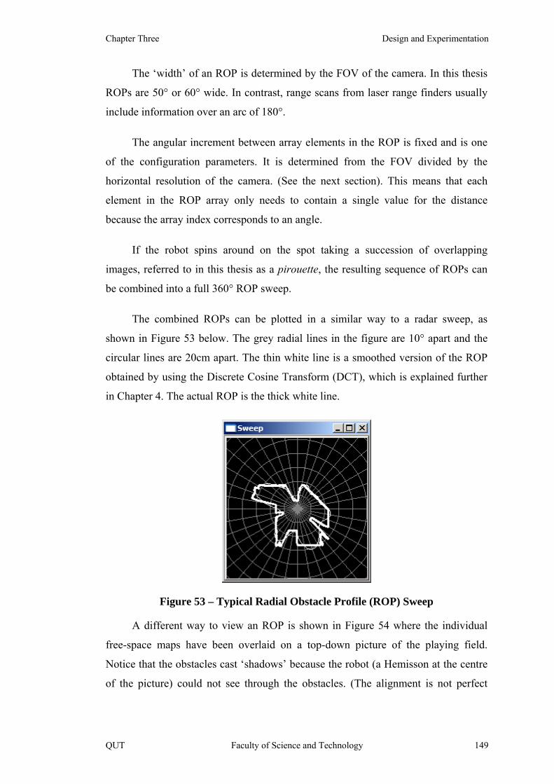
Chapter Three Design and Experimentation
The ‘width’ of an ROP is determined by the FOV of the camera. In this thesis
ROPs are 50° or 60° wide. In contrast, range scans from laser range finders usually
include information over an arc of 180°.
The angular increment between array elements in the ROP is fixed and is one
of the configuration parameters. It is determined from the FOV divided by the
horizontal resolution of the camera. (See the next section). This means that each
element in the ROP array only needs to contain a single value for the distance
because the array index corresponds to an angle.
If the robot spins around on the spot taking a succession of overlapping
images, referred to in this thesis as a pirouette, the resulting sequence of ROPs can
be combined into a full 360° ROP sweep.
The combined ROPs can be plotted in a similar way to a radar sweep, as
shown in Figure 53 below. The grey radial lines in the figure are 10° apart and the
circular lines are 20cm apart. The thin white line is a smoothed version of the ROP
obtained by using the Discrete Cosine Transform (DCT), which is explained further
in Chapter 4. The actual ROP is the thick white line.
Figure 53 – Typical Radial Obstacle Profile (ROP) Sweep
A different way to view an ROP is shown in Figure 54 where the individual
free-space maps have been overlaid on a top-down picture of the playing field.
Notice that the obstacles cast ‘shadows’ because the robot (a Hemisson at the centre
of the picture) could not see through the obstacles. (The alignment is not perfect
QUT Faculty of Science and Technology 149

Mapping of Indoor Environments by Robots using Low-cost Vision Sensors Trevor Taylor
because the scale of the photograph was unknown and so the map had to be re-scaled
and overlaid by eye. However, the principle is nonetheless clearly illustrated.)
Figure 54 – ROP overlaid on a playing field
Note that the robot in Figure 54 can see the whole of its environment in a
single sweep. Additional walls were introduced in later experiments to force it to
explore.
3.7.8 Angular Resolution of the ROP
There is a limit on the angular resolution that is possible with the ROP. The
maximum angular resolution, i, can be calculated as follows:
)1( −=
mFOVi (24)
Note that this is not exact because it is calculated at the centre of the image and
the actual angle varies with the height in the image.
For example, a typical web camera has a FOV of 60° and a horizontal
resolution of 320 pixels. This means that the best possible ROP increment is 0.188
degrees. For most of the work either 0.5 or 0.25 of a degree has been used.
3.7.9 Calculating the ROP
In the initial implementation, the ROP was approximated as follows:
• Scan across the bottom of the floor map image one pixel at a time;
• For each pixel column, scan upwards until a non-floor pixel is found;
150 Faculty of Science and Technology QUT
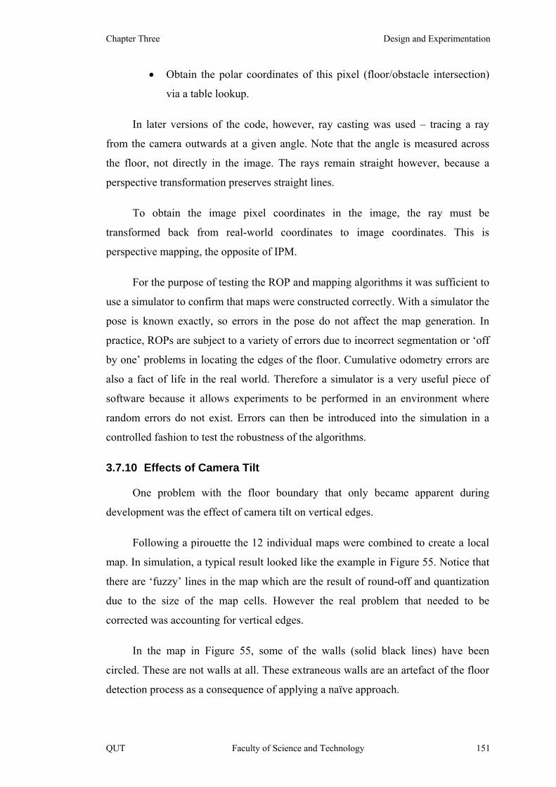
Chapter Three Design and Experimentation
• Obtain the polar coordinates of this pixel (floor/obstacle intersection)
via a table lookup.
In later versions of the code, however, ray casting was used – tracing a ray
from the camera outwards at a given angle. Note that the angle is measured across
the floor, not directly in the image. The rays remain straight however, because a
perspective transformation preserves straight lines.
To obtain the image pixel coordinates in the image, the ray must be
transformed back from real-world coordinates to image coordinates. This is
perspective mapping, the opposite of IPM.
For the purpose of testing the ROP and mapping algorithms it was sufficient to
use a simulator to confirm that maps were constructed correctly. With a simulator the
pose is known exactly, so errors in the pose do not affect the map generation. In
practice, ROPs are subject to a variety of errors due to incorrect segmentation or ‘off
by one’ problems in locating the edges of the floor. Cumulative odometry errors are
also a fact of life in the real world. Therefore a simulator is a very useful piece of
software because it allows experiments to be performed in an environment where
random errors do not exist. Errors can then be introduced into the simulation in a
controlled fashion to test the robustness of the algorithms.
3.7.10 Effects of Camera Tilt
One problem with the floor boundary that only became apparent during
development was the effect of camera tilt on vertical edges.
Following a pirouette the 12 individual maps were combined to create a local
map. In simulation, a typical result looked like the example in Figure 55. Notice that
there are ‘fuzzy’ lines in the map which are the result of round-off and quantization
due to the size of the map cells. However the real problem that needed to be
corrected was accounting for vertical edges.
In the map in Figure 55, some of the walls (solid black lines) have been
circled. These are not walls at all. These extraneous walls are an artefact of the floor
detection process as a consequence of applying a naïve approach.
QUT Faculty of Science and Technology 151

Mapping of Indoor Environments by Robots using Low-cost Vision Sensors Trevor Taylor
Figure 55 – Naïve local map showing extraneous walls
Consider the view from the robot and the proposed floor outline shown in
Figure 56 (a) and (b) respectively. These figures correspond to the view inside the
top (larger) ellipse in Figure 55. If the outline in Figure 56 (b) was used to mark the
floor boundary in the local map using IPM then incorrect walls would result.
Humans recognise that the large (yellow) object near the middle of the image has
two vertical edges even though the vertical edges do not appear vertical in the image
due to the camera tilt.
Figure 56 – Detecting vertical edges: (a) Simulated camera image; (b) Detected floor; and (c) Detected vertical edges
A naïve approach would treat all of the edges of the floor contour, Figure 56
(c), as physical boundaries (walls). However, in Figure 56 (c), the vertical edges
have been detected in the floor contour and are marked with thicker (green) lines as
explained in [Taylor et al. 2006, Taylor 2007]. When drawing the local map the
robot knows not to mark these edges as walls.
After removing vertical edges from the floor contour, the local map looks like
Figure 57, which no longer has the extraneous walls.
152 Faculty of Science and Technology QUT
Chapter Three Design and Experimentation
Figure 57 – Corrected local map without walls due to vertical edges
A couple of additional points need to be made about this map. Firstly, the
simulator was constantly ‘taking photos’, just as a real camera would. Once the robot
had stood still for a while, the map became quite black and white – literally. (See the
circled area at the top of Figure 57). This was a result of the same data being added
to the map continuously and reinforcing what was already there.
On the other hand, as the robot does its pirouette, it takes a photo after each
turn and then immediately turns again. The result appears as a star pattern that shows
where the overlaps have occurred between photos. If the robot had taken several
photos after each turn and integrated them all into the map, then this pattern would
not be visible.
3.7.11 Mapping the Local Environment
The first stage in creating a global map is to produce a map of the immediately
surrounding environment, which is a local map. This local map can then be
combined with the global map using Bayes Rule.
Note that that local map is relative to the robot, so the robot is always at the
centre (origin) of the local map. Before incorporating the new information into the
global map, the local map has to be positioned relative to the global map. The local
map can be generated with the correct rotation using the robot’s current pose
information and it is then only a matter of applying the appropriate translation in
order to overlay it onto the global map.
Selecting an appropriate grid size for an occupancy grid map is dependent on
several factors, including:
QUT Faculty of Science and Technology 153

Mapping of Indoor Environments by Robots using Low-cost Vision Sensors Trevor Taylor
• Memory limitations;
• Size of the robot; and
• Degree of clutter in the environment.
The author proposes as a general rule of thumb that the cell size should be
roughly an order of magnitude smaller than the size of the robot. Obviously the cell
size should not be larger than the size of the robot because it could get ‘lost’ inside a
cell. Conversely, a very small cell size increases the computational overhead. As the
cell size decreases, the number of cells increases quadratically – reducing the cell
size by a factor of two results in four times as many cells in the map.
Another consideration in the selection of the map grid size is the environment.
For instance, the narrowest corridors still need to be several grid cells wide in the
map. Otherwise errors in the map might squeeze a corridor to the point where it
appears to the robot that it is blocked.
When using the Hemisson robot (roughly an oval shape 12cm by 10cm) and
Yujin robot (a 7cm cube), a cell size of 1cm was used. There were no narrow
openings in the playing fields that the robot needed to pass through.
For the X80 robots (roughly 30cm in diameter) cell size of 5cm and 10cm was
used in the experiments. The narrowest corridor was just under 1m in width, or about
10 map cells wide even at the 10cm grid size.
3.7.12 Creating a Global Map
To create the global map, each new local map must be integrated into the
existing global map. This is done by registering the local map to the global map
based on the robot’s estimated pose, and then applying Bayes Rule for each
corresponding cell from the local map which does not have a value of ‘unknown’.
Values of ‘unknown’ (0.5) in the local map correspond to areas where no
information was obtained from the vision system. If Bayes Rule were applied to
these areas as well they would incorrectly affect existing information in the global
map.
154 Faculty of Science and Technology QUT
Chapter Three Design and Experimentation
3.8 Localization
Reliable localization is essential for producing an accurate map. Localization
presented several challenges which are discussed below.
Various methods of visual localization were tested in the experiments. These
are discussed in the following sections, but first some remarks about odometry are
appropriate because it is the source of errors in pose estimation.
3.8.1 Odometry
In the initial work using the Yujin robot, there was no odometry information
available from the robot. Although it does have wheel encoders, which are used by
the on-board controller to control wheel speed, the encoder information cannot be
obtained from the robot because the communication is one-way via a radio modem.
Therefore the ‘odometry’ consisted of timing the motions of the robot. This is
extremely unreliable because Windows is not a real-time operating system and
cannot accurately execute timed delays.
Each wheel encoder on an X80 robot generates 1200 ‘ticks’ for a complete
revolution of the wheel. An encoder counts upwards when the wheel rotates in one
direction, and counts down for rotations in the opposite direction. The tick count is a
16-bit value so it wraps around (back to zero) at 32767. The resolution of the
encoders equates to 0.3° in terms of wheel rotation. This is a fairly good resolution,
but the usual odometry problems still apply.
The wheel diameter for the X80 robots is nominally 165mm according to the
manufacturer. This gives a perimeter of 518.36mm. In the case where the robot is
moving forward (both wheels turning at the same speed) one tick corresponds to
travelling 0.43mm, assuming no slippage between the wheel and the ground.
It is of course impossible to move the robot by only a single tick. The
mechanical backlash in the motor/gear/axel assembly amounts to several ticks. Even
with the on-board PID controller operating in position mode (driving the motors to
make the wheel encoder tick count match a specified value), it is not possible to
position the robot to closer than 10 ticks from the desired position.
QUT Faculty of Science and Technology 155

Mapping of Indoor Environments by Robots using Low-cost Vision Sensors Trevor Taylor
If the robot is driven to turn on the spot by turning the wheels in opposite
directions, then the distance travelled per tick is around the perimeter of a circle with
a diameter equal to the wheelbase (spacing between the wheels). The manufacturer
says that the wheelbase is 272mm, giving a perimeter of 854.51mm. Therefore a
single tick corresponds to 0.18° in terms of the orientation of the robot.
3.8.2 Tracking Image Features
Many visual SLAM approaches use features, particularly if they are based on a
Kalman Filter. Therefore extracting features from the images was investigated.
Due to hardware limitations, the X80 robots did not produce frames fast
enough to allow optic flow to be calculated because optic flow requires a high frame
rate. Furthermore, the images were affected by motion blur while the robot was
moving. The hardware therefore precluded the use of optic flow.
Some experiments were carried out using SIFT as a possible method for
tracking the robot’s motion. Sample code for SIFT was downloaded from Lowe’s
web site at http://www.cs.ubc.ca/~lowe.
It was found that in most of the camera images there were very few SIFT
keypoints detected, and many cases they were not useful. This was primarily because
SIFT looked for corner-type features. Even a ‘good’ image containing doorways
rarely produced matches between successive images during a rotation.
Figure 58 shows two examples of SIFT feature matching between successive
images when the robot rotated on the spot. Each diagram consists of two images, one
above the other, with corresponding keypoints connected by white lines.
156 Faculty of Science and Technology QUT
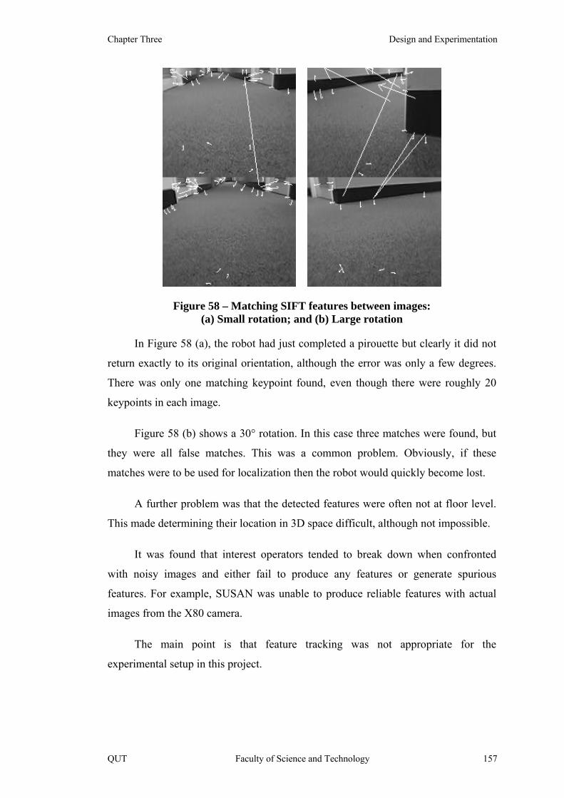
Chapter Three Design and Experimentation
Figure 58 – Matching SIFT features between images: (a) Small rotation; and (b) Large rotation
In Figure 58 (a), the robot had just completed a pirouette but clearly it did not
return exactly to its original orientation, although the error was only a few degrees.
There was only one matching keypoint found, even though there were roughly 20
keypoints in each image.
Figure 58 (b) shows a 30° rotation. In this case three matches were found, but
they were all false matches. This was a common problem. Obviously, if these
matches were to be used for localization then the robot would quickly become lost.
A further problem was that the detected features were often not at floor level.
This made determining their location in 3D space difficult, although not impossible.
It was found that interest operators tended to break down when confronted
with noisy images and either fail to produce any features or generate spurious
features. For example, SUSAN was unable to produce reliable features with actual
images from the X80 camera.
The main point is that feature tracking was not appropriate for the
experimental setup in this project.
QUT Faculty of Science and Technology 157

Mapping of Indoor Environments by Robots using Low-cost Vision Sensors Trevor Taylor
3.8.3 Scan Matching of ROPs
Scan matching is not directly relevant to vision. However, the approach taken
in this thesis was to generate a Radial Obstacle Profile which is similar to a laser
range scan. Laser scans have been used with scan matching in the literature.
Early in the project, an attempt was made to use the Lu & Milios approach, but
it was not successful. There were two distinctly different reasons for this. They are
quite easy to understand in retrospect.
In their work, Lu & Milios had data for a full 360° scan at 1° intervals. The
algorithm for determining rotations slid one set of data over the other looking for the
best match. Because they had a full circle, there were no problems with boundary
conditions because the data sets could be wrapped around. Furthermore, they had a
lot of data points to work with.
However, in this research, when a robot rotated on the spot, the overlap
between camera images was only half of the field of view, or about 30 degrees. As
one data set was moved with respect to the second data, the area of overlap reduced
until there was nothing to match. The algorithm had to ignore points with no
corresponding point. Consequently, the best match could often be found by sliding
the data until only a couple of points remained and they were a perfect match. The
resulting rotation estimates could therefore be grossly incorrect.
The diagram in Figure 59 shows a top-down view of a robot rotating on the
spot. The field of view of the robot is shown before and after a rotation. (It does not
matter which is which). Clearly, the amount of overlap is not large, so there is very
little data for comparison.
158 Faculty of Science and Technology QUT

Chapter Three Design and Experimentation
Figure 59 – Overlap in field of view between rotations
Reducing the amount of the rotation to increase the overlap would increase the
amount of data available for matching, but it would also mean that more rotations
would be required to complete a pirouette. As previously mentioned, the more times
the robot rotated the more opportunities there were for it to become disoriented
because motions were never exact. In fact, the error in rotations increased
significantly, sometimes to as much as 50%, when they were less than 10 degrees.
Note too that the camera is not in the centre of the robot in Figure 59, so the
vantage points for each of the views are separated in space. This makes comparisons
difficult because the effect is a combination of rotation and translation. It can also
have undesirable effects due to occlusion and it leaves a small area unseen, but these
effects are just noted in passing and are not addressed here.
For translations, there are entirely different problems – perspective combined
with the quantization effects involved in capturing a digital image. The result is that
successive scanlines higher up in an image equate to significant changes in the
corresponding locations of points on the floor.
For example, consider two points in successive images that are only one
scanline apart (a single pixel). Some typical values from the IPM (Inverse
Perspective Mapping) data for a robot are shown in the following table. Note that
scanlines count downwards from the top of the image, which is why the range
decreases with increasing scanline numbers.
QUT Faculty of Science and Technology 159

Mapping of Indoor Environments by Robots using Low-cost Vision Sensors Trevor Taylor
Table 3 – Effect of perspective on distance measurements
Scanline
(pixels)
Range from camera
(cm)
Difference
(cm)
Percentage
Difference
21 201.17 (Reference 1) (Reference 1)
22 190.84 10.33 5.41%
110 30.12 (Reference 2) (Reference 2)
111 29.79 0.33 1.11%
At a range of around 2m, a difference of one scanline represents 10.33cm
across the floor. Near the bottom of the image, at a range of 30cm, the difference is
only 0.33cm.
Expressing differences as a percentage disguises the impact, but cannot
entirely eliminate it (as shown in the final column of Table 3). Besides, there could
be cases where one data point was an outlier or there was a sudden discontinuity.
Penalising or, just as importantly, failing to penalise a data point in these situations
would not help to obtain the correct alignment between the scans.
The problem is that the Lu & Milios approach implicitly assumed that the
range measurements were linearly distributed and that the measurement error was
constant regardless of distance. For a laser range finder, this is a valid assumption.
However, for a perspective image, this is simply not true. Not only are the distances
restricted to a set of discrete values, but the separation between them increases non-
linearly further up the image. The associated error in the estimated position also
increases dramatically at the same time so the significance of a single pixel error in
detecting an edge in the image becomes larger for scanlines higher up the image.
It was found that although the standard Iterative Closest Point (ICP) algorithm
applied to pure translations (forward moves) would converge; the result would often
be offset by some amount from the real distance travelled.
160 Faculty of Science and Technology QUT
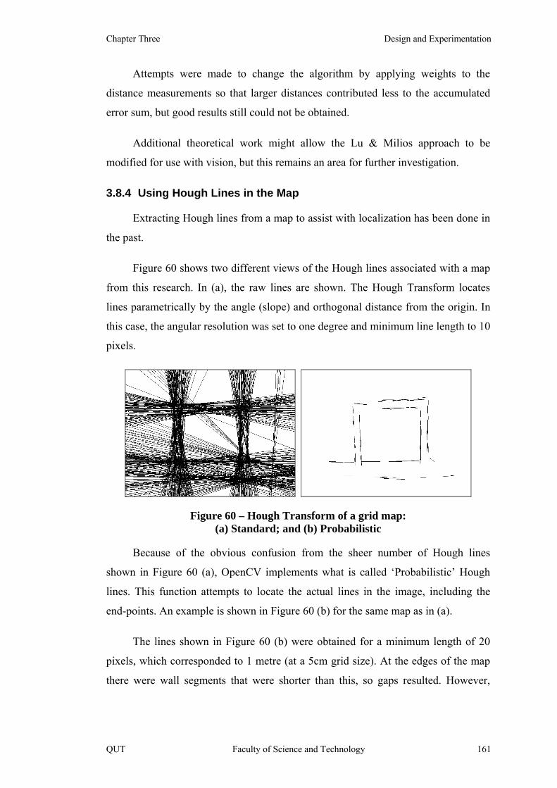
Chapter Three Design and Experimentation
Attempts were made to change the algorithm by applying weights to the
distance measurements so that larger distances contributed less to the accumulated
error sum, but good results still could not be obtained.
Additional theoretical work might allow the Lu & Milios approach to be
modified for use with vision, but this remains an area for further investigation.
3.8.4 Using Hough Lines in the Map
Extracting Hough lines from a map to assist with localization has been done in
the past.
Figure 60 shows two different views of the Hough lines associated with a map
from this research. In (a), the raw lines are shown. The Hough Transform locates
lines parametrically by the angle (slope) and orthogonal distance from the origin. In
this case, the angular resolution was set to one degree and minimum line length to 10
pixels.
Figure 60 – Hough Transform of a grid map: (a) Standard; and (b) Probabilistic
Because of the obvious confusion from the sheer number of Hough lines
shown in Figure 60 (a), OpenCV implements what is called ‘Probabilistic’ Hough
lines. This function attempts to locate the actual lines in the image, including the
end-points. An example is shown in Figure 60 (b) for the same map as in (a).
The lines shown in Figure 60 (b) were obtained for a minimum length of 20
pixels, which corresponded to 1 metre (at a 5cm grid size). At the edges of the map
there were wall segments that were shorter than this, so gaps resulted. However,
QUT Faculty of Science and Technology 161
Mapping of Indoor Environments by Robots using Low-cost Vision Sensors Trevor Taylor
reducing the minimum length of the Hough lines produced more extraneous lines. In
other words, the minimum line length is a compromise.
This approach was not pursued further due to the difficulties explained above
but it warrants more investigation.
3.8.5 Orthogonality Constraint
Based on the concepts of scan matching and using Hough lines in the map, an
approach was developed for localization, referred to as Incremental Localization.
This involved assuming that the walls were orthogonal. In most buildings, walls are
built parallel or at right-angles to each other. If the robot can identify a wall in an
image, then it can use this information to determine its orientation provided that it
has a reasonable estimate of its current orientation.
In the simplest case, a robot can follow a corridor by aligning with the walls.
However, if the walls run either North-South or East-West (which are arbitrary
directions related to the orientation of the map, not real compass directions) then the
robot also knows to the nearest 90 degrees which direction it is travelling and can
‘snap to’ one of the primary directions.
Because this is one of the main contributions of this thesis, it is discussed in
detail in Chapter 4 rather than here. A brief description of the algorithm is as
follows:
• Apply the Douglas-Peucker algorithm to the ROP to find straight lines;
• Select lines longer than a specified threshold to ignore noise and small
objects;
• Check if any of these lines correspond to walls close to North-South or
East-West in the map; and
• If the difference between the direction of a wall and one of the primary
directions is small enough, then update the robot’s orientation to be
consistent with the wall.
162 Faculty of Science and Technology QUT

Chapter Three Design and Experimentation
More than one wall might be visible. In this case, the adjustment to the robot’s
orientation is a weighted average of the adjustments indicated by each wall based on
the length of the wall segment, i.e. longer walls carry a larger weight because they
are more likely to be correct.
The effect of applying this constraint was to improve the SLAM results
significantly because it improved the motion estimates.
3.9 Simultaneous Localization and Mapping (SLAM)
The GridSLAM algorithm was selected from a recent textbook, Probabilistic
Robotics [Thrun et al. 2005], which is one of the definitive texts in the field of
SLAM. A Particle Filter algorithm was selected because it is more suitable for use
with occupancy grids than a Kalman Filter approach.
Because SLAM was well documented in the literature, a fundamental
assumption was made that reliable algorithms were available. However, this proved
not to be the case when using visual data from the hardware in this research.
Recently, several researchers created the OpenSLAM web site [OpenSLAM
2007]. Some of the SLAM packages from this web site were used for comparison
when problems were encountered with GridSLAM in order to verify that the
problems were generic and not restricted to a particular algorithm.
3.9.1 Implementation
In the algorithm below, the notation is the same as in Chapter 2 with the
addition of:
ut' Corrected control input at time t after Incremental Localization
The GridSLAM algorithm was modified slightly to incorporate incremental
localization, which is one of the innovations of this work. The new algorithm is
shown below.
QUT Faculty of Science and Technology 163
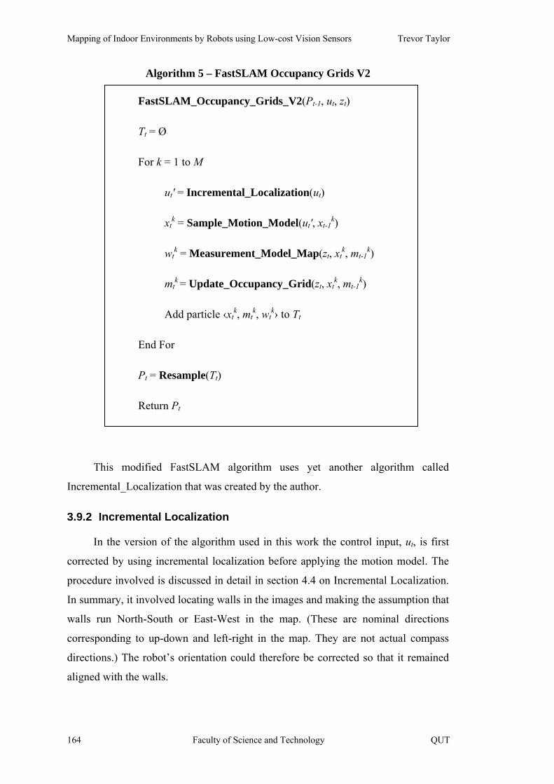
Mapping of Indoor Environments by Robots using Low-cost Vision Sensors Trevor Taylor
Algorithm 5 – FastSLAM Occupancy Grids V2
FastSLAM_Occupancy_Grids_V2(Pt-1, ut, zt)
Tt = Ø
For k = 1 to M
ut' = Incremental_Localization(ut)
xtk = Sample_Motion_Model(ut', xt-1
k)
wtk = Measurement_Model_Map(zt, xt
k, mt-1k)
mtk = Update_Occupancy_Grid(zt, xt
k, mt-1k)
Add particle ‹xtk, mt
k, wtk› to Tt
End For
Pt = Resample(Tt)
Return Pt
This modified FastSLAM algorithm uses yet another algorithm called
Incremental_Localization that was created by the author.
3.9.2 Incremental Localization
In the version of the algorithm used in this work the control input, ut, is first
corrected by using incremental localization before applying the motion model. The
procedure involved is discussed in detail in section 4.4 on Incremental Localization.
In summary, it involved locating walls in the images and making the assumption that
walls run North-South or East-West in the map. (These are nominal directions
corresponding to up-down and left-right in the map. They are not actual compass
directions.) The robot’s orientation could therefore be corrected so that it remained
aligned with the walls.
164 Faculty of Science and Technology QUT

Chapter Three Design and Experimentation
It is important to note that without the incremental localization step GridSLAM
was found to be only marginally stable and would often fail.
3.9.3 Motion Model
It was decided to use a simplified motion model similar to the approach used in
GMapping [OpenSLAM 2007]. It has no physical significance, but it is plausible
based on experience with the X80 robots. The model involves adding random errors
with a Gaussian distribution to the pose.
There were two basic types of motion that the robot performed during
exploration: forward moves and rotations on the spot. For each of these a Gaussian
noise component was applied to the robot position and the orientation. The variances
for position and orientation were maintained separately.
The equations relating the motions of the robot are shown below. These are
expressed in the 2D coordinate frame of the robot where the robot begins at the
origin facing along the positive x axis.
ηζ
=+=
ydx
(25)
ξθα += (26)
Where:
x, y = Components of the actual translation
d = Requested distance to translate
ζ = Translation error in x direction as a Gaussian
η = Translation error in y direction as a Gaussian
α = Actual angle of rotation
θ = Requested angle of rotation
ξ = Rotation error as a Gaussian
QUT Faculty of Science and Technology 165
Mapping of Indoor Environments by Robots using Low-cost Vision Sensors Trevor Taylor
To apply the motion model to the robot’s pose, the translation vector, (x,y),
was first calculated and then transformed to the world coordinate system using the
robot’s current estimated orientation. The coordinates could then be added to the
current position.
The rotation was easier to apply because it was simply a matter of adding the
new rotation value to the current orientation.
Before determining the parameters for the motion noise, the parameters of the
encoder calculations (see section 2.1.2, Equations 1 and 2) were confirmed. The
manufacturer, Dr. Robot Inc, supplied the following information:
Wheel diameter = 165mm = 2r
Wheel base = 272mm = w
Ticks per revolution = 1200 = n
The robot was set up facing a wall and commanded to move backwards by
20cm five times in a row. The sonar measurement from the front sonar was recorded
in each case, and it was seen to increase by 20cm except in the last case where it
oscillated between 20 and 21cm. However, the sonar could only be read to the
nearest centimetre so this was not a significant error (less than 1cm in 100).
This was followed by five forwards movements of 20cm. The sonar readings in
these cases decreased by 20cm each time. Although this was not an accurate
assessment, it provided quick validation that the parameters were correct.
By trial and error, values were established for the standard deviation for the
position and orientation noise components. The motion model parameters (see the
equations above) were obtained by driving the robot manually and measuring the
resulting movements.
When commanded to move forward, X80 robots rarely move by exactly the
correct amount. They also tend to rotate slightly in the process. This probably
happens because the wheels do not start and stop simultaneously, resulting in a small
166 Faculty of Science and Technology QUT
Chapter Three Design and Experimentation
amount of torque being applied around the central axis of the robot. Other factors
such as wheel slip and unevenness of the floor can also contribute.
For a rotation, the robots do not always turn by exactly the desired amount. To
complicate matters, after a full pirouette the robots had often drifted slightly from
their starting position. This drift was more likely to be sideways than forwards or
backwards.
Two types of experiment were performed:
• Drive a fixed translate distance (30cm) and record the actual distance
travelled; and
• Rotate by the ‘sweep’ amount (30 degrees) and record the actual angle.
These experiments were repeated 20 times, and the variances were obtained
from the data.
A zero mean was found in all cases. A non-zero mean would indicate a
systemic error, such as an incorrect value for the wheel diameter or distance between
wheels. This type of error could have been corrected by adjusting the commands to
the wheel motors. However, no consistent errors were observed that would indicate
such systemic errors.
The variances found in the experiments were rounded up slightly for use in the
SLAM algorithm so that the particles would propagate across the full variance of
motions. The values used were 3.0cm and 0.1cm for the x and y variances
respectively, and 2.0 degrees for the rotation variance.
3.9.4 Calculating Weights
The measurement (sensor) model is discussed in detail in sections 3.7.6 and
3.7.2. The first step is to take an image and extract a range scan from it. This must
then be used to draw a local map.
There are parameters required for the measurement model. In particular, a
maximum visual range was set. There are also several parameters involved in
extracting the floor boundary from the video images. An incorrect choice for any of
QUT Faculty of Science and Technology 167

Mapping of Indoor Environments by Robots using Low-cost Vision Sensors Trevor Taylor
these parameters can adversely affect the output of the measurement model. There is
no methodology for choosing these parameters other than trial and error.
After creating a local map using the sensor model, the map correlation
algorithm was used to obtain the particle weights. (This was discussed in section
2.7.8). The algorithm produces correlation values in the range -1.0 to +1.0.
The basic map correlation algorithm compares the entire local map to the
global map. However, the camera can only see a portion of the space in front of it
due to the limited field of view. Therefore the algorithm was modified to include
only those grid cells that were potentially visible, rather than the full square region of
the map. To do this, a mask was created as shown in Figure 61 (a).
Figure 61 – Map Correlation for Particle 31: (a) Mask; (b) Global map segment; and (c) Local map
In Figure 61 (a), the mask shows the area the camera could potentially see.
Clearly, a comparison of the entire map would be incorrect because the black area is
outside the visual range of the sensor and any comparison would be meaningless.
Notice that there is a round area at the centre of the map which represents the robot.
This area must be free space because it is occupied by the robot.
The second map, Figure 61 (b), shows the result of overlaying the mask on the
current global map maintained by the particle. Only this area is included in the
calculation of the map correlation. The last map (c) shows the local map that was
generated from the vision system. (The background appears grey because this
indicates unknown space). The local map was compared against the global map and
the resulting correlation coefficient was 0.508773, which was the best particle
weight at this time step.
168 Faculty of Science and Technology QUT
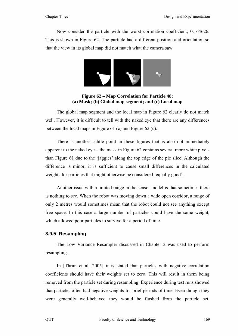
Chapter Three Design and Experimentation
Now consider the particle with the worst correlation coefficient, 0.164626.
This is shown in Figure 62. The particle had a different position and orientation so
that the view in its global map did not match what the camera saw.
Figure 62 – Map Correlation for Particle 48: (a) Mask; (b) Global map segment; and (c) Local map
The global map segment and the local map in Figure 62 clearly do not match
well. However, it is difficult to tell with the naked eye that there are any differences
between the local maps in Figure 61 (c) and Figure 62 (c).
There is another subtle point in these figures that is also not immediately
apparent to the naked eye – the mask in Figure 62 contains several more white pixels
than Figure 61 due to the ‘jaggies’ along the top edge of the pie slice. Although the
difference is minor, it is sufficient to cause small differences in the calculated
weights for particles that might otherwise be considered ‘equally good’.
Another issue with a limited range in the sensor model is that sometimes there
is nothing to see. When the robot was moving down a wide open corridor, a range of
only 2 metres would sometimes mean that the robot could not see anything except
free space. In this case a large number of particles could have the same weight,
which allowed poor particles to survive for a period of time.
3.9.5 Resampling
The Low Variance Resampler discussed in Chapter 2 was used to perform
resampling.
In [Thrun et al. 2005] it is stated that particles with negative correlation
coefficients should have their weights set to zero. This will result in them being
removed from the particle set during resampling. Experience during test runs showed
that particles often had negative weights for brief periods of time. Even though they
were generally well-behaved they would be flushed from the particle set.
QUT Faculty of Science and Technology 169
Mapping of Indoor Environments by Robots using Low-cost Vision Sensors Trevor Taylor
Consequently, a change was made to the algorithm so that if more than 50% of the
particles had a zero weight, the weights were redistributed rather than throwing away
particles that might have had a single bad result. Bad particles that continually had
poor weights would still be removed from the set eventually.
Another way to prevent particles from being unexpectedly flushed was also
used. It was based on advice from Dr. Grisetti, at the University of Freiberg and
involves what amounts to a ‘moving average’ of the particle weights to smooth out
changes. The moving average was calculated by adding successive weights together.
During resampling, all weights are normalized so that they sum to one. This is also
discussed in Chapter 4.
The resampling frequency is an important factor in the stability of the SLAM
algorithm, which is discussed in Chapter 4. It was decided that resampling would
occur only in one of two situations:
• After completing a pirouette; or
• After making a specified number of steps (translations or rotations).
A pirouette should not change the pose of the robot. However, it obtains
information about the surrounding environment for a full 360 degrees which should
provide good information for updating the map. Therefore it seemed sensible to
update the particle set after a pirouette.
Conversely, the first and last images in a pirouette sequence are the same view.
If the first image results in changes to the global map, then the last view will
reinforce this and is likely to give the particle a high weight. This could be the wrong
time to use the particle weight for a decision on resampling.
In most test runs, the number of steps before resampling was set to 5. This
value was selected using trial and error by comparing maps produced using saved
data sets.
For more discussion, see sections 4.5.10, 11 and 12.
170 Faculty of Science and Technology QUT

Chapter Three Design and Experimentation
3.9.6 Updating the Global Map
Each particle in a Particle Filter has its own global map. Updates to the global
maps are made using the pose for each particle and its local map. The update
equation was developed in section 3.7.1.
There are some design issues related to how to apply the local map information
to the global map, but these are discussed in Chapter 4 – Results and Discussion.
3.9.7 Experimental Verification of Localization
Because SLAM used a particle filter, it was important to test the localization
ability of the filter. A portion of a saved log file from a test run was re-run using the
filter for localization only. To do this, the final map (produced using SLAM) was
loaded into the ExCV program when it started up and updating of the map was
turned off. This effectively ensured that only the localization was performed.
Fifty particles were initialized at random around an approximate starting
location of the robot (not the true location of the robot). The program was then run to
see what the trajectories of the particles would be.
NOTE: If SLAM had not worked successfully to produce the map in the first
place, then this experiment could not have been performed. This example is intended
as an illustration of localization.
QUT Faculty of Science and Technology 171

Mapping of Indoor Environments by Robots using Low-cost Vision Sensors Trevor Taylor
a b cd e f
Figure 63 – Particle progression during localization and final path on map (from top-left to bottom-right)
The particles were initially scattered at random around the estimated location,
which is shown with a red ‘X’ in Figure 63 (a). Note that it is not possible to tell
from this 2D map that the orientations of the particles also varied. The particles were
distributed according to a Gaussian distribution with a zero mean and variance, σ, of
50cm in the x and y directions, and 20° for the orientation. Given that 2σ covers 95%
of a Gaussian distribution, this results in an effective range of about ±1m and ±40°.
After a few steps and updates to the particle set, the paths had already started
to coalesce as shown in Figure 63 (b) (top row in the centre). However, one aberrant
particle headed off in the wrong direction as can be seen more clearly in (c).
This ‘bad’ particle received an initial orientation that was way off the true
value. This can happen when randomly initializing particles with a Gaussian
distribution due to the long ‘tail’ in the distribution. The initial random poses can
have a significant effect on the filter performance with a small number of particles.
The results were quite reproducible, however, because the random number seed was
172 Faculty of Science and Technology QUT
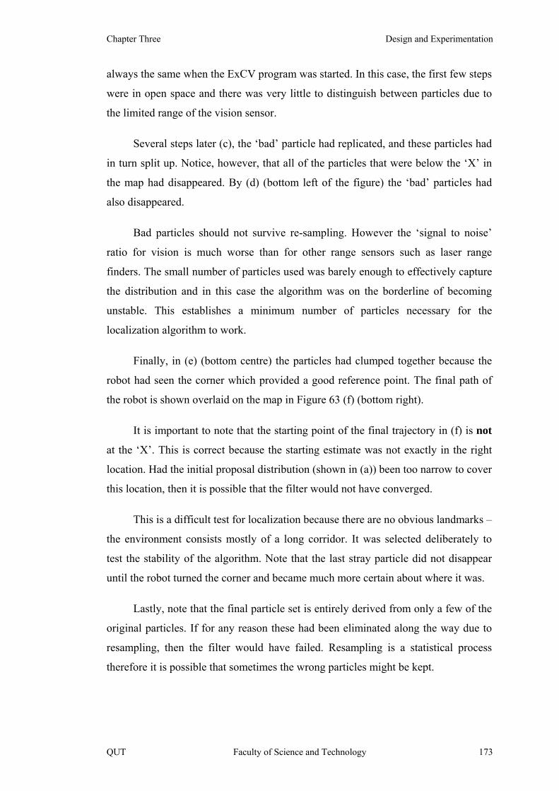
Chapter Three Design and Experimentation
always the same when the ExCV program was started. In this case, the first few steps
were in open space and there was very little to distinguish between particles due to
the limited range of the vision sensor.
Several steps later (c), the ‘bad’ particle had replicated, and these particles had
in turn split up. Notice, however, that all of the particles that were below the ‘X’ in
the map had disappeared. By (d) (bottom left of the figure) the ‘bad’ particles had
also disappeared.
Bad particles should not survive re-sampling. However the ‘signal to noise’
ratio for vision is much worse than for other range sensors such as laser range
finders. The small number of particles used was barely enough to effectively capture
the distribution and in this case the algorithm was on the borderline of becoming
unstable. This establishes a minimum number of particles necessary for the
localization algorithm to work.
Finally, in (e) (bottom centre) the particles had clumped together because the
robot had seen the corner which provided a good reference point. The final path of
the robot is shown overlaid on the map in Figure 63 (f) (bottom right).
It is important to note that the starting point of the final trajectory in (f) is not
at the ‘X’. This is correct because the starting estimate was not exactly in the right
location. Had the initial proposal distribution (shown in (a)) been too narrow to cover
this location, then it is possible that the filter would not have converged.
This is a difficult test for localization because there are no obvious landmarks –
the environment consists mostly of a long corridor. It was selected deliberately to
test the stability of the algorithm. Note that the last stray particle did not disappear
until the robot turned the corner and became much more certain about where it was.
Lastly, note that the final particle set is entirely derived from only a few of the
original particles. If for any reason these had been eliminated along the way due to
resampling, then the filter would have failed. Resampling is a statistical process
therefore it is possible that sometimes the wrong particles might be kept.
QUT Faculty of Science and Technology 173

Mapping of Indoor Environments by Robots using Low-cost Vision Sensors Trevor Taylor
3.9.8 Quality of Generated Maps
The nature of the experiments was such that the maps were grossly distorted if
SLAM failed. Quantitative comparison was not necessary in these cases because the
differences were clearly visible to the naked eye.
However, it could be difficult to visually compare the resulting maps from
SLAM test runs based on the same data set using different sets of parameters. A
formal evaluation method was useful in this case.
Two different methods were used:
• Map Correlation; and
• Normalized Sum of Squared Differences.
Note that these comparisons require a ‘ground truth’ map. This is usually
available in an experimental environment, but it is often not available in the real
world.
Map Correlation used the same formula from [Thrun et al. 2005] as for
calculating the particle weights (section 2.7.8). This was applied to the entire map
and the result was a value between -1.0 and +1.0 with +1.0 meaning a perfect match.
Negative values indicate a very poor match, and should not occur if the generated
map is reasonably similar to the ground truth.
A SLAM map for one of the test runs was compared to the ground truth by
offsetting it by up to 20 grid cells in each direction. The resulting correlation values
were plotted as shown in Figure 64. This showed the sensitivity to displacement of
the SLAM map and gave some idea of the type of surface produced by map
correlation.
174 Faculty of Science and Technology QUT

Chapter Three Design and Experimentation
-20-10
010
20-20
-10
0
10
20
00.2
0.4
0.6
0.8
1
Figure 64 – Map Correlations versus map displacement
The Sum of Squared Differences (SSD) was calculated as follows:
• Take the difference between the values of corresponding grid cells;
• Squares these differences; and
• Sum them across the entire map.
The best possible value was zero (for a perfect match), and the worst possible
value was 1,647,993,600 for a 176x144 map. The resulting large numbers made it
difficult to understand the quality of the map, so two extra steps were added:
• Normalize the sum by dividing by the maximum possible value; and
• Subtract from 1.0 to invert the direction of curvature.
This was also tested by displacing the same generated SLAM map against the
ground truth. The surface curvature was not as great as Map Correlation, which
made this method less practical.
QUT Faculty of Science and Technology 175
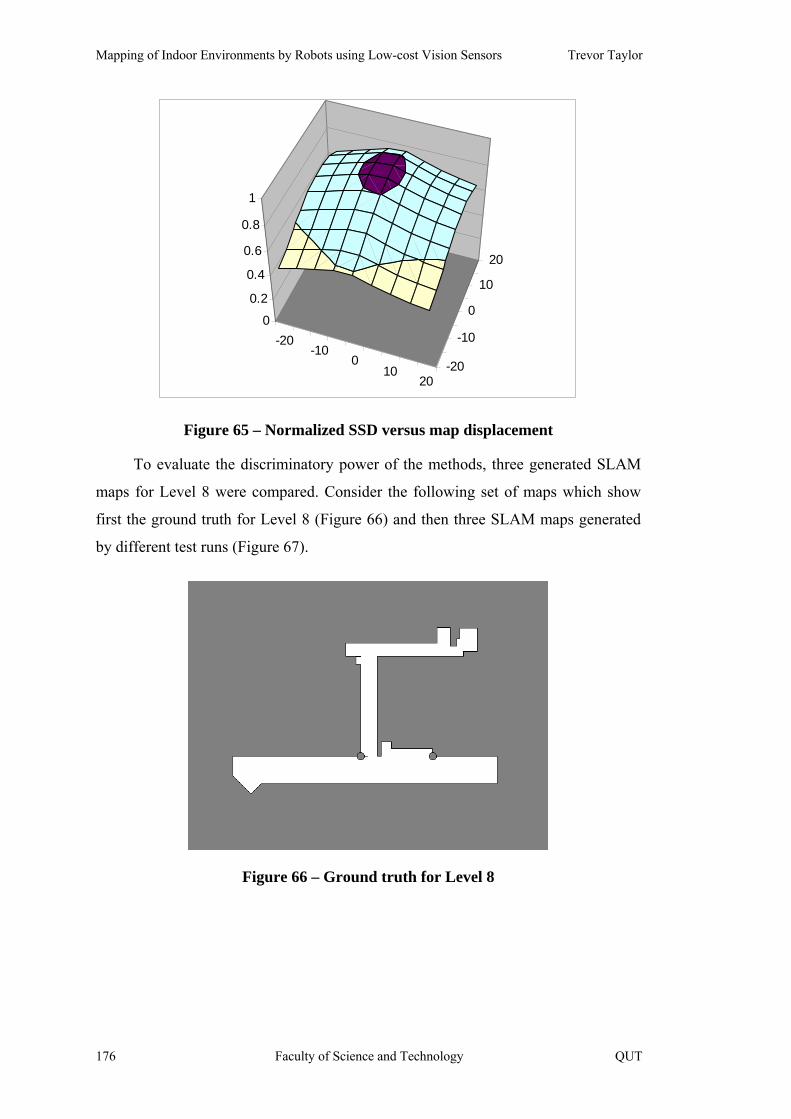
Mapping of Indoor Environments by Robots using Low-cost Vision Sensors Trevor Taylor
-20-10
010
20-20
-10
0
10
20
0
0.2
0.4
0.6
0.8
1
Figure 65 – Normalized SSD versus map displacement
To evaluate the discriminatory power of the methods, three generated SLAM
maps for Level 8 were compared. Consider the following set of maps which show
first the ground truth for Level 8 (Figure 66) and then three SLAM maps generated
by different test runs (Figure 67).
Figure 66 – Ground truth for Level 8
176 Faculty of Science and Technology QUT

Chapter Three Design and Experimentation
Figure 67 – Sample SLAM maps for Level 8
The resulting values for comparison against ground truth were as shown in the
table below.
QUT Faculty of Science and Technology 177

Mapping of Indoor Environments by Robots using Low-cost Vision Sensors Trevor Taylor
Table 4 – Comparison of Map Quality
Map
Number
Normalized
SSD
Map
Correlation
1 0.8709 0.7877
2 0.8136 0.6927
3 0.7198 0.5564
The results from the two methods agreed in their rankings. Visual inspection of
the maps also showed that the ranking was correct. Note that these numbers are
difficult to interpret as a ‘goodness of fit’, and can only be used for comparison
purposes.
3.10 Other SLAM Implementations
Other SLAM packages were tested with sample data generated by the
simulator to compare their stability against GridSLAM. The results of applying these
algorithms to test data generated by the simulator are shown in Chapter 4 – Results
and Discussion.
In early 2007, several researchers joined together to create the OpenSLAM
web site [OpenSLAM 2007] which offered open source versions of several SLAM
packages for download. This provided an opportunity to run some test data through
packages that had been written independently to see if they could produce reliable
maps using visual data from the experimental environment.
Two SLAM packages were selected for comparison:
• DP-SLAM [Eliazar & Parr 2003]
• GMapping [Grisetti et al. 2005, Grisetti et al. 2007]
Both of these packages were provided in source form for Unix. They were
based on Particle Filters and therefore similar in architecture to GridSLAM.
178 Faculty of Science and Technology QUT

Chapter Three Design and Experimentation
The packages were ported to Windows. To verify that each package ran
correctly, public domain data sets were run through of them and the results compared
to the corresponding maps available on the Internet. These are shown below simply
for validation.
3.10.1 DP-SLAM
For DP-SLAM, sample data and maps were obtained from the web site
http://www.cs.duke.edu/~parr/dpslam/ (accessed February, 2007).
The selected data set was Loop 5 from the Duke University Computer Science
Department on the Second Floor of the D-Wing of the LSRC building. This data set
was used courtesy of Austin Eliazar and Dr. Ronald Parr. The original map on the
web site was produced using 3,000 particles with a grid cell size of 3cm.
QUT Faculty of Science and Technology 179

Mapping of Indoor Environments by Robots using Low-cost Vision Sensors Trevor Taylor
Figure 68 – Validation of Windows version of DP-SLAM: (a) Map from the Internet; and (b) Map produced for this Thesis
Although an exact mathematical comparison was not performed, it was clear
from visual inspection of the maps that the Windows version of the program was
working correctly.
3.10.2 GMapping
For GMapping, a data set and map were obtained from Radish [Radish 2007]
for the Newell-Simon Hall, A Level at Carnegie Mellon University. This data is
courtesy of Nick Roy. These files were available from the web site
http://cres.usc.edu/radishrepository/view-one.php?name=cmu_nsh_level_a (accessed
February 2007).
180 Faculty of Science and Technology QUT

Chapter Three Design and Experimentation
Figure 69 – Validation of Windows version of GMapping: (a) Map from the Internet; and (b) Map produced for this Thesis
Visual comparison shows that the maps are substantially the same, although
the approaches used to draw the maps differ – GMapping only writes the end-points
of laser hits into the map and does not do ray casting to draw the free space. This
confirmed that the Windows version of GMapping worked correctly.
3.10.3 MonoSLAM
The MonoSLAM system is well known in the area of visual SLAM. Therefore
it seemed reasonable to try to use it.
Davison released the source code for his visual SLAM package, called
MonoSLAM, which built 3D maps in real time [Davison 1999]. A C# version of the
QUT Faculty of Science and Technology 181

Mapping of Indoor Environments by Robots using Low-cost Vision Sensors Trevor Taylor
code for Windows was available on the Internet from the following web site:
http://sluggish.uni.cc/monoSLAM/monoslam.htm.
MonoSLAM was tested using pre-recorded images from an X80 robot, but it
could not obtain a tracking lock. When Davison was contacted about the problems
with MonoSLAM, he replied that it requires a high frame rate. A wide-angle lens
also improves the chances of tracking an object because it appears in more frames
[Davison et al. 2004].
This was not a failing of the MonoSLAM package, but rather a limitation of
the experimental hardware used in this research. No qualifications were stated for
using MonoSLAM in the literature, although by implication the hardware should
have been similar in performance to the hardware listed in the relevant publications.
The issue was that the X80 robot was moving too far between images and the
tracking algorithm could not find matches. MonoSLAM had been shown to work
successfully with a hand-held video camera. However, the frame rate and resolution
were both much higher than for the X80.
In 2007, the author discussed MonoSLAM with one of Davison’s associates,
Dr. Neira, who explained that MonoSLAM has a tendency to lose tracking if the
camera is moved too fast. In Neira’s experience with making maps he found that he
had to move slowly and consistently with the camera.
Furthermore, MonoSLAM had no concept of scale because this could not be
determined from the available data. If the camera operator moved at varying speeds
some parts of the map would be stretched. In order to close large loops it was
therefore necessary to apply a map matching algorithm to a set of hierarchical maps
obtained using MonoSLAM [Clemente et al. 2007].
Lastly, note that MonoSLAM had typically been used in ‘feature rich’
environments with a lot of visible features that the algorithm could track. It had not
been used for exploration of indoor environments containing long featureless
corridors. The experiments using SIFT earlier in the chapter demonstrate why
MonoSLAM had a hard time working in the experiemental environment.
182 Faculty of Science and Technology QUT
Chapter Three Design and Experimentation
3.11 Exploration Process
The Distance Transform (DT) was selected as the exploration algorithm
because it is grid-based, and therefore a good match for an occupancy grid map, and
also because it provides an indication of when the exploration is complete.
The DT must be applied to a binary image. The occupancy grid map, therefore,
has a threshold applied to it to select the cells where the probability of being
occupied is high. (The probability of a cell being occupied might not always reach
1.0, so a lower threshold was used – typically around 0.75. This value must be
greater than 0.5 which corresponds to unknown space.)
The next step is to calculate the C-Space map. This might involve changing to
a different grid size as well, usually a coarser grid. In the case of the X80 robot, the
usual map grid size was 5cm and the ‘translate distance’ was 30cm, which is roughly
the diameter of the robot. This ‘translate distance’ becomes the grid size for the DT.
When calculating the C-Space map, the cells are resized from the map grid size
to the DT grid size. It is highly desirable for the DT grid size to be the same as, or a
multiple of, the map grid size. If the DT grid is larger than the map grid then it may
happen that an obstacle will only partially occupy a DT cell. In this case the resulting
path is even more conservative.
However, it is also possible that an unfortunate alignment of the map with the
real world will result in a gap that is too narrow for the robot to pass through, even
though in reality the robot will fit. Due to uncertainty in the position of the robot and
its motions, safety (avoiding collisions) was considered to be of primary importance
and therefore this issue was ignored.
Figure 70 shows an example of a DT path from the robot (which is the round
object near the middle of the diagram) to unknown space (grey area) in the top left.
Notice that the obstacles appear ‘fat’ because this is a C-Space map and they have
been expanded by the diameter of the robot.
QUT Faculty of Science and Technology 183
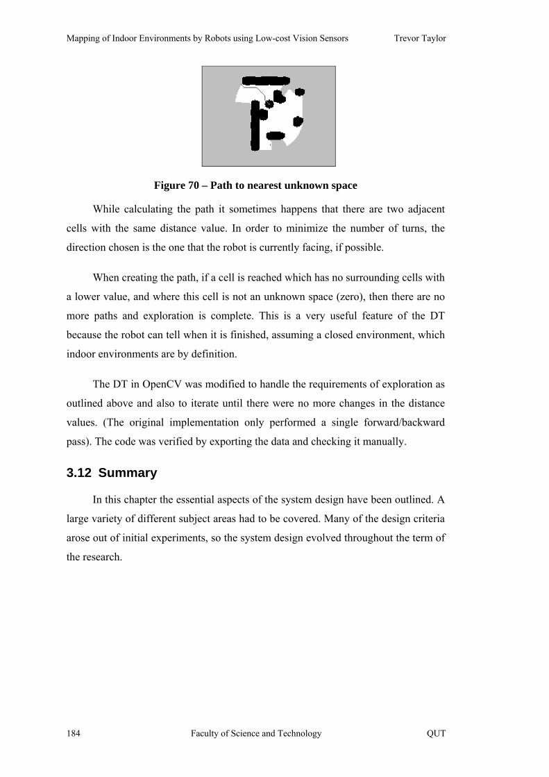
Mapping of Indoor Environments by Robots using Low-cost Vision Sensors Trevor Taylor
Figure 70 – Path to nearest unknown space
While calculating the path it sometimes happens that there are two adjacent
cells with the same distance value. In order to minimize the number of turns, the
direction chosen is the one that the robot is currently facing, if possible.
When creating the path, if a cell is reached which has no surrounding cells with
a lower value, and where this cell is not an unknown space (zero), then there are no
more paths and exploration is complete. This is a very useful feature of the DT
because the robot can tell when it is finished, assuming a closed environment, which
indoor environments are by definition.
The DT in OpenCV was modified to handle the requirements of exploration as
outlined above and also to iterate until there were no more changes in the distance
values. (The original implementation only performed a single forward/backward
pass). The code was verified by exporting the data and checking it manually.
3.12 Summary
In this chapter the essential aspects of the system design have been outlined. A
large variety of different subject areas had to be covered. Many of the design criteria
arose out of initial experiments, so the system design evolved throughout the term of
the research.
184 Faculty of Science and Technology QUT
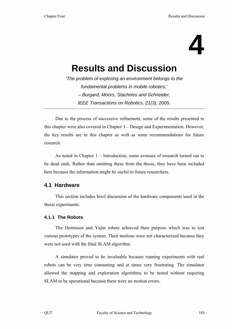
Chapter Four Results and Discussion
4 Results and Discussion
‘The problem of exploring an environment belongs to the
fundamental problems in mobile robotics.’
– Burgard, Moors, Stachniss and Schneider,
IEEE Transactions on Robotics, 21(3), 2005.
Due to the process of successive refinement, some of the results presented in
this chapter were also covered in Chapter 3 – Design and Experimentation. However,
the key results are in this chapter as well as some recommendations for future
research.
As noted in Chapter 1 – Introduction, some avenues of research turned out to
be dead ends. Rather than omitting these from the thesis, they have been included
here because the information might be useful to future researchers.
4.1 Hardware
This section includes brief discussion of the hardware components used in the
thesis experiments.
4.1.1 The Robots
The Hemisson and Yujin robots achieved their purpose which was to test
various prototypes of the system. Their motions were not characterized because they
were not used with the final SLAM algorithm.
A simulator proved to be invaluable because running experiments with real
robots can be very time consuming and at times very frustrating. The simulator
allowed the mapping and exploration algorithms to be tested without requiring
SLAM to be operational because there were no motion errors.
QUT Faculty of Science and Technology 185

Mapping of Indoor Environments by Robots using Low-cost Vision Sensors Trevor Taylor
The X80 robot was found to have several hardware limitations, such as the
camera resolution, reliability of the WiFi interface and accuracy of the wheel
encoders. However, these are real-world problems and affect all robots to some
extent.
4.1.2 Computational Requirements
The robots used in this thesis did not have onboard computers and were
remotely controlled by a PC. Two different PCs were used in the course of the
investigation:
• Desktop PC with 1.5 GHz Intel Pentium processor, 1GB of memory.
• Laptop PC with 2.0 GHz Intel Pentium M processor, 1GB of memory.
All of the SLAM test runs were performed using an X80 robot. Consider the
following details for a typical test run:
Duration: 2 hours
Images received: 8,045 (just over one frame per second)
Processed images: 2,054
Although this is an average of 3 to 4 seconds between images, much of this
time was while the robot was moving. From the log file, it was determined that
motions took between 1.7 and 5.4 seconds. The average time to process an image
was found to be only 0.69 seconds.
Because of the low frame rate, the bandwidth utilization (over WiFi) was only
a few percent. Therefore the network was not a limiting factor.
The computational and memory requirements increase in direct proportion to
the number of particles used for SLAM. A faster PC would result in faster
processing times.
It is clear from these details that the robot did not move in what might be
considered “real time”. However, the program was not optimized and contained a
large amount of debugging code, so some improvement would be possible.
186 Faculty of Science and Technology QUT
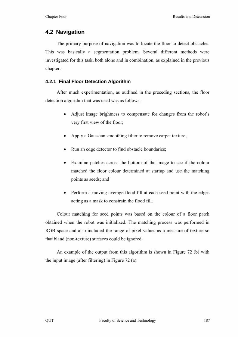
Chapter Four Results and Discussion
4.2 Navigation
The primary purpose of navigation was to locate the floor to detect obstacles.
This was basically a segmentation problem. Several different methods were
investigated for this task, both alone and in combination, as explained in the previous
chapter.
4.2.1 Final Floor Detection Algorithm
After much experimentation, as outlined in the preceding sections, the floor
detection algorithm that was used was as follows:
• Adjust image brightness to compensate for changes from the robot’s
very first view of the floor;
• Apply a Gaussian smoothing filter to remove carpet texture;
• Run an edge detector to find obstacle boundaries;
• Examine patches across the bottom of the image to see if the colour
matched the floor colour determined at startup and use the matching
points as seeds; and
• Perform a moving-average flood fill at each seed point with the edges
acting as a mask to constrain the flood fill.
Colour matching for seed points was based on the colour of a floor patch
obtained when the robot was initialized. The matching process was performed in
RGB space and also included the range of pixel values as a measure of texture so
that bland (non-texture) surfaces could be ignored.
An example of the output from this algorithm is shown in Figure 72 (b) with
the input image (after filtering) in Figure 72 (a).
QUT Faculty of Science and Technology 187

Mapping of Indoor Environments by Robots using Low-cost Vision Sensors Trevor Taylor
Figure 72 – Floor detected using Flood Fill and Edges
There were several ways in which the floor detection could fail. The most
common case was where the edge detector did not pick up a door, or conversely it
detected shadows.
Edge detection is a compromise. If the edge detector was too sensitive, then it
would pick up texture in the carpet. Gaussian smoothing helped to remove floor
texture, but it also disguised the real edges.
Figure 73 – Floor edges not detected
In Figure 73, the wall edge towards the top-left of the first image was not
detected because the edge was not distinct enough. In the second image, the wall at
the top-right is obscured due to shadow. These types of errors resulted in ‘break
outs’ that appeared in the map. In general, the resulting holes in the walls in the map
were filled in subsequent images as the robot got closer to the wall.
188 Faculty of Science and Technology QUT
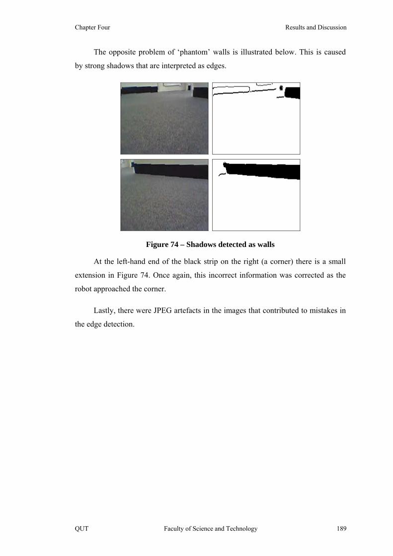
Chapter Four Results and Discussion
The opposite problem of ‘phantom’ walls is illustrated below. This is caused
by strong shadows that are interpreted as edges.
Figure 74 – Shadows detected as walls
At the left-hand end of the black strip on the right (a corner) there is a small
extension in Figure 74. Once again, this incorrect information was corrected as the
robot approached the corner.
Lastly, there were JPEG artefacts in the images that contributed to mistakes in
the edge detection.
QUT Faculty of Science and Technology 189
Mapping of Indoor Environments by Robots using Low-cost Vision Sensors Trevor Taylor
Figure 75 – Enlarged image showing JPEG artefacts
Figure 75 shows an original image (with the extracted floor) and one that has
been enlarged by a factor of 300% to show the detail. Note the blurring along the
wall edges and even false edges below the walls and in the doorway. Although it is
difficult to see, the colour of the carpet also bled into the walls in some places. These
are typical JPEG artefacts resulting from the compression of the image for
transmission over wireless Ethernet. The robot did not provide an uncompressed
mode in the firmware so these false features were unavoidable.
190 Faculty of Science and Technology QUT
Chapter Four Results and Discussion
4.3 Mapping
The mapping component of the system, based on occupancy grids, proved to
be very successful. It was tested extensively in simulation to verify the program code
before being used on real robots.
4.3.1 Inverse Perspective Mapping (IPM)
Equations were developed for Inverse Perspective Mapping based on the
camera geometry that were efficient to compute. These equations are highly non-
linear due to the nature of perspective. Consequently, errors in the estimated
distances increase rapidly as the distance from the robot increases. Eventually the
uncertainty becomes unacceptable.
Obtaining good results with this approach proved difficult. The problem lay in
measuring the values of b, h, d and w. Although these could be measured
approximately just with a ruler, the resulting values in the IPM lookup table for
longer distances were sensitive to small errors in the parameters.
Alternative methods of IPM are available, and in retrospect it might have been
more appropriate to use one of them rather than develop a new method.
As shown graphically in Chapter 3, the error between the calculated and
observed distances approached ±10cm for distances of 200cm or more. This
discrepancy was of some concern because it was equivalent to two grid cells on the
map (assuming a 5cm grid). However, given the low resolution and poor quality of
the camera, it was nonetheless a remarkable result because it was the equivalent of
only ±1 pixel in the image.
Edge detection is generally considered to be accurate to within ±1 pixel, but
larger errors can be encountered in practice. Even small amounts of jitter in the
camera’s position could affect the location of an edge in the image by more than a
pixel. Because edge detection was the primary means of locating obstacles, the
accuracy of the edges was important. If the resolution of the camera were increased,
then an error of one pixel in detecting an obstacle would correspond to a smaller
distance.
QUT Faculty of Science and Technology 191

Mapping of Indoor Environments by Robots using Low-cost Vision Sensors Trevor Taylor
The higher the camera resolution, the smaller the distance increments would be
in the IPM Lookup Table. Therefore a high resolution camera should produce more
accurate maps. Furthermore, a higher resolution would increase the distance before
the uncertainty became unacceptable effectively allowing the robot to ‘see further’.
This should improve localization. Further work is required to confirm this
hypothesis.
4.3.2 The Radial Obstacle Profile (ROP)
Two different approaches were used to calculate the ROP. The first algorithm
traced up pixel columns from the bottom of the image until a non-floor pixel was
encountered. The second method involved tracing rays in the image that emanated
from the camera.
This latter approach is more computationally intensive, but it produces more
accurate results. In particular, it allows the ROP to see ‘around corners’. The
explanation for this is clear from Figure 32 (b) (in Chapter 3) which was obtained
using the first method. Notice the shape of the floor (light grey area) just past the
right-hand side of the first obstacle. The floor is shown as rising vertically in the
floor image because it used the initial implementation. This was clearly not correct,
and it ignored a small amount of floor that was visible in the camera image of Figure
32 (a).
Note that this problem only arises if the camera is tilted. If the camera is
horizontal, it cannot see ‘around obstacles’. In fact, the camera is not seeing around
corners at all. Vertical edges appear tilted in the image due to the camera tilt, and so
a small region of the floor was ignored without ray casting.
There is another problem related to the tilted ‘vertical’ edges – a naïve
approach to mapping the floor inserted walls into the map corresponding to these
edges. However, this was incorrect. A method for eliminating this problem was
published by the author [Taylor et al. 2006, Taylor 2007] and is discussed in section
4.4.3.
192 Faculty of Science and Technology QUT
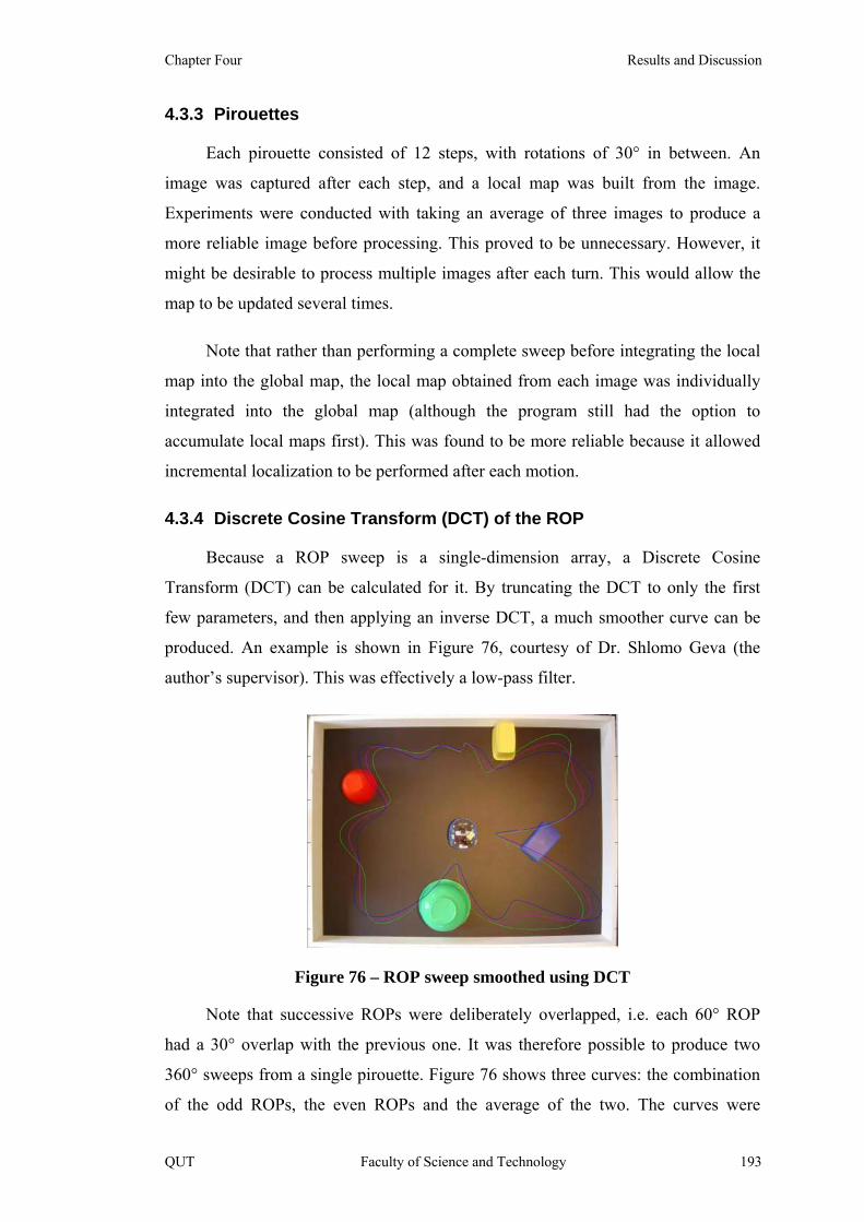
Chapter Four Results and Discussion
4.3.3 Pirouettes
Each pirouette consisted of 12 steps, with rotations of 30° in between. An
image was captured after each step, and a local map was built from the image.
Experiments were conducted with taking an average of three images to produce a
more reliable image before processing. This proved to be unnecessary. However, it
might be desirable to process multiple images after each turn. This would allow the
map to be updated several times.
Note that rather than performing a complete sweep before integrating the local
map into the global map, the local map obtained from each image was individually
integrated into the global map (although the program still had the option to
accumulate local maps first). This was found to be more reliable because it allowed
incremental localization to be performed after each motion.
4.3.4 Discrete Cosine Transform (DCT) of the ROP
Because a ROP sweep is a single-dimension array, a Discrete Cosine
Transform (DCT) can be calculated for it. By truncating the DCT to only the first
few parameters, and then applying an inverse DCT, a much smoother curve can be
produced. An example is shown in Figure 76, courtesy of Dr. Shlomo Geva (the
author’s supervisor). This was effectively a low-pass filter.
Figure 76 – ROP sweep smoothed using DCT
Note that successive ROPs were deliberately overlapped, i.e. each 60° ROP
had a 30° overlap with the previous one. It was therefore possible to produce two
360° sweeps from a single pirouette. Figure 76 shows three curves: the combination
of the odd ROPs, the even ROPs and the average of the two. The curves were
QUT Faculty of Science and Technology 193
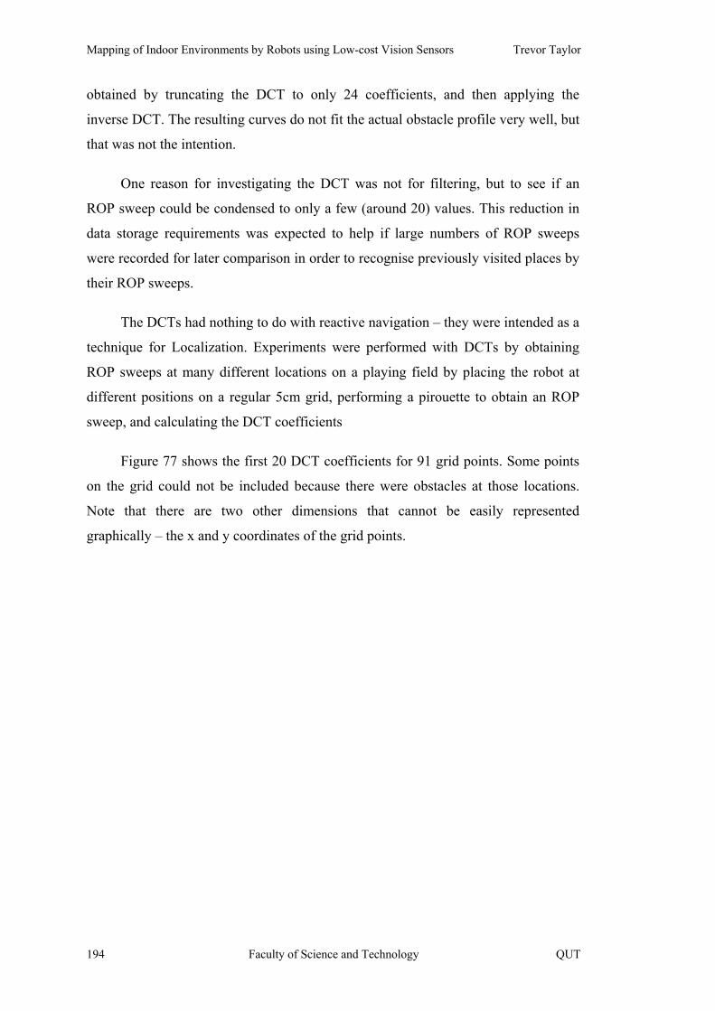
Mapping of Indoor Environments by Robots using Low-cost Vision Sensors Trevor Taylor
obtained by truncating the DCT to only 24 coefficients, and then applying the
inverse DCT. The resulting curves do not fit the actual obstacle profile very well, but
that was not the intention.
One reason for investigating the DCT was not for filtering, but to see if an
ROP sweep could be condensed to only a few (around 20) values. This reduction in
data storage requirements was expected to help if large numbers of ROP sweeps
were recorded for later comparison in order to recognise previously visited places by
their ROP sweeps.
The DCTs had nothing to do with reactive navigation – they were intended as a
technique for Localization. Experiments were performed with DCTs by obtaining
ROP sweeps at many different locations on a playing field by placing the robot at
different positions on a regular 5cm grid, performing a pirouette to obtain an ROP
sweep, and calculating the DCT coefficients
Figure 77 shows the first 20 DCT coefficients for 91 grid points. Some points
on the grid could not be included because there were obstacles at those locations.
Note that there are two other dimensions that cannot be easily represented
graphically – the x and y coordinates of the grid points.
194 Faculty of Science and Technology QUT
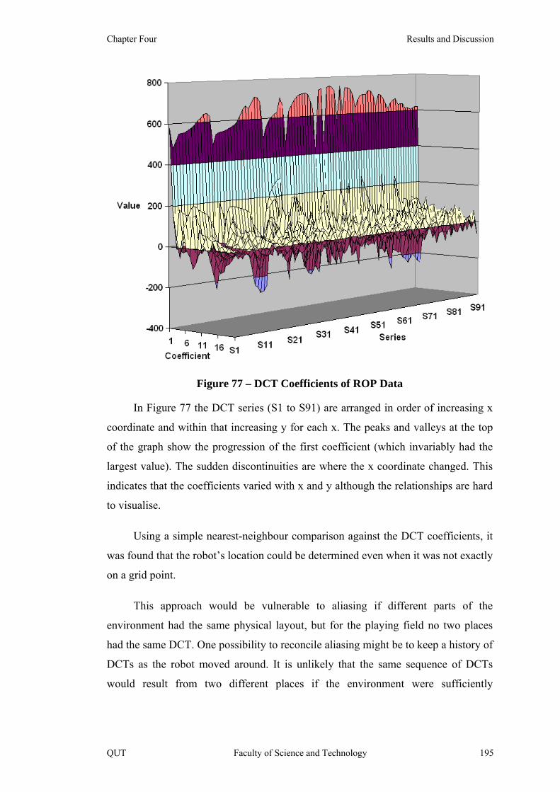
Chapter Four Results and Discussion
Figure 77 – DCT Coefficients of ROP Data
In Figure 77 the DCT series (S1 to S91) are arranged in order of increasing x
coordinate and within that increasing y for each x. The peaks and valleys at the top
of the graph show the progression of the first coefficient (which invariably had the
largest value). The sudden discontinuities are where the x coordinate changed. This
indicates that the coefficients varied with x and y although the relationships are hard
to visualise.
Using a simple nearest-neighbour comparison against the DCT coefficients, it
was found that the robot’s location could be determined even when it was not exactly
on a grid point.
This approach would be vulnerable to aliasing if different parts of the
environment had the same physical layout, but for the playing field no two places
had the same DCT. One possibility to reconcile aliasing might be to keep a history of
DCTs as the robot moved around. It is unlikely that the same sequence of DCTs
would result from two different places if the environment were sufficiently
QUT Faculty of Science and Technology 195

Mapping of Indoor Environments by Robots using Low-cost Vision Sensors Trevor Taylor
‘cluttered’. However, it was obvious that long featureless corridors would have many
similar DCTs.
The DCT was phase-sensitive, which meant that it was not rotation invariant.
If the robot’s orientation was changed before an ROP sweep, the DCT would also
change. This could potentially have been used to determine the robot’s orientation if
the location were known. However, the purpose was to determine the robot’s
location. Therefore the ROP sweep would first have to be ‘rotated’ (shift the array
left or right with wrap-around) before applying the DCT. This was an unrealistic
limitation because the robot’s orientation was not generally known.
Building a large collection of DCTs to use for localization would only be
feasible if the robot’s orientation were always known. Otherwise each new ROP
sweep would have to be rotated several times and compared against the table of
previously recorded DCTs to try to find the best match for both orientation and
location. Given the computational overhead that this approach would incur, it was
not pursued any further.
4.3.5 Floor Boundary Detection for Creating Local Maps
The first step in building a map was to make a local map based on the view
from the robot’s camera.
As explained in Chapter 3 – Design and Experimentation, turning a video
camera into a range sensor can be achieved by detecting the floor in the images. The
boundary where the floor meets the walls or obstacles can be used, via inverse
perspective mapping, to obtain range information in the form of an ROP. However,
floor detection requires good segmentation of the images. Various approaches to
segmentation were discussed in Chapter 3, with the final algorithm in section 4.2.1.
Regardless of the sensor used, there is the possibility that it will either miss an
obstacle or incorrectly register an obstacle where there is none. For instance, sonar
signals can bounce off walls so that they are not returned to the sender. This
generates a ‘maximum range’ reading, and the wall is not seen. A maximum range
reading will also occur for sonar if the wall is acoustically absorbent.
196 Faculty of Science and Technology QUT
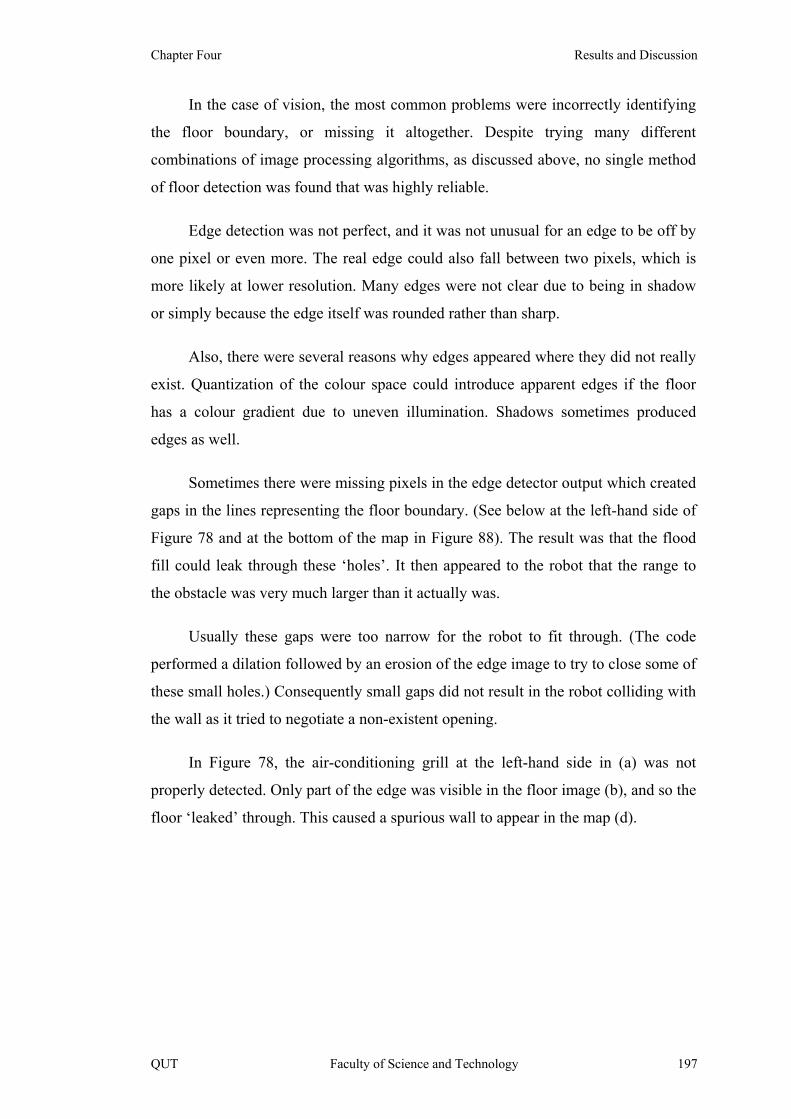
Chapter Four Results and Discussion
In the case of vision, the most common problems were incorrectly identifying
the floor boundary, or missing it altogether. Despite trying many different
combinations of image processing algorithms, as discussed above, no single method
of floor detection was found that was highly reliable.
Edge detection was not perfect, and it was not unusual for an edge to be off by
one pixel or even more. The real edge could also fall between two pixels, which is
more likely at lower resolution. Many edges were not clear due to being in shadow
or simply because the edge itself was rounded rather than sharp.
Also, there were several reasons why edges appeared where they did not really
exist. Quantization of the colour space could introduce apparent edges if the floor
has a colour gradient due to uneven illumination. Shadows sometimes produced
edges as well.
Sometimes there were missing pixels in the edge detector output which created
gaps in the lines representing the floor boundary. (See below at the left-hand side of
Figure 78 and at the bottom of the map in Figure 88). The result was that the flood
fill could leak through these ‘holes’. It then appeared to the robot that the range to
the obstacle was very much larger than it actually was.
Usually these gaps were too narrow for the robot to fit through. (The code
performed a dilation followed by an erosion of the edge image to try to close some of
these small holes.) Consequently small gaps did not result in the robot colliding with
the wall as it tried to negotiate a non-existent opening.
In Figure 78, the air-conditioning grill at the left-hand side in (a) was not
properly detected. Only part of the edge was visible in the floor image (b), and so the
floor ‘leaked’ through. This caused a spurious wall to appear in the map (d).
QUT Faculty of Science and Technology 197
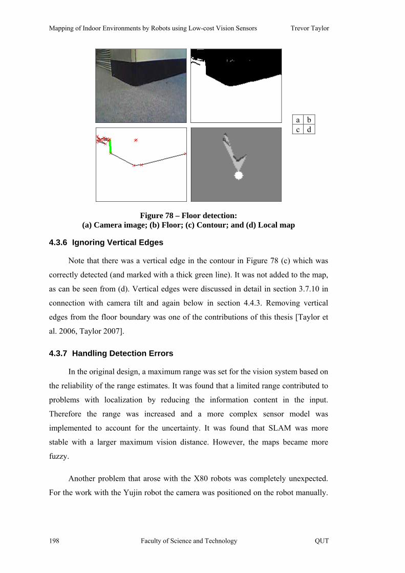
Mapping of Indoor Environments by Robots using Low-cost Vision Sensors Trevor Taylor
a b c d
Figure 78 – Floor detection: (a) Camera image; (b) Floor; (c) Contour; and (d) Local map
4.3.6 Ignoring Vertical Edges
Note that there was a vertical edge in the contour in Figure 78 (c) which was
correctly detected (and marked with a thick green line). It was not added to the map,
as can be seen from (d). Vertical edges were discussed in detail in section 3.7.10 in
connection with camera tilt and again below in section 4.4.3. Removing vertical
edges from the floor boundary was one of the contributions of this thesis [Taylor et
al. 2006, Taylor 2007].
4.3.7 Handling Detection Errors
In the original design, a maximum range was set for the vision system based on
the reliability of the range estimates. It was found that a limited range contributed to
problems with localization by reducing the information content in the input.
Therefore the range was increased and a more complex sensor model was
implemented to account for the uncertainty. It was found that SLAM was more
stable with a larger maximum vision distance. However, the maps became more
fuzzy.
Another problem that arose with the X80 robots was completely unexpected.
For the work with the Yujin robot the camera was positioned on the robot manually.
198 Faculty of Science and Technology QUT

Chapter Four Results and Discussion
This gave complete control over its orientation. With the X80 robots, however, the
CCD cameras were mounted inside sealed units.
It was found that the cameras in the X80s were slightly rotated in their
mountings, perhaps due to poor quality control. Even a rotation of the CCD as small
as two or three degrees resulted in walls appearing to be at significantly incorrect
angles, especially when they were in the top half of the image. This was a side-effect
of the inverse perspective mapping being applied to edges that were skewed by as
little as a couple of pixels.
The effect of this systemic error was to produce discontinuities in the walls
obtained from successive images, but more importantly it affected localization. To
overcome this problem, the images had to be counter-rotated by a small amount
before applying the image processing.
It should also be noted that a pan and tilt camera assembly can cause problems.
Although being able to move the cameras around might seem like an advantage, it
can be difficult to reproduce exactly the same positions on different test runs.
The last issue was one of image quality. For example, the images below in
Figure 79 show respectively: (a) data corruption on the wireless network; (b) poor
illumination; (c) too much illumination; and (d) colour changes due to illumination
as well as extraneous shadows by a power cord.
QUT Faculty of Science and Technology 199
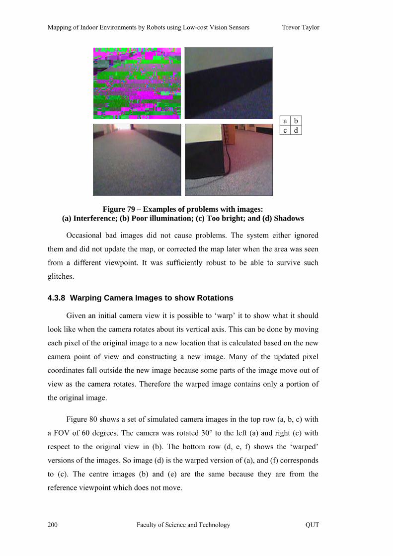
Mapping of Indoor Environments by Robots using Low-cost Vision Sensors Trevor Taylor
a b c d
Figure 79 – Examples of problems with images: (a) Interference; (b) Poor illumination; (c) Too bright; and (d) Shadows
Occasional bad images did not cause problems. The system either ignored
them and did not update the map, or corrected the map later when the area was seen
from a different viewpoint. It was sufficiently robust to be able to survive such
glitches.
4.3.8 Warping Camera Images to show Rotations
Given an initial camera view it is possible to ‘warp’ it to show what it should
look like when the camera rotates about its vertical axis. This can be done by moving
each pixel of the original image to a new location that is calculated based on the new
camera point of view and constructing a new image. Many of the updated pixel
coordinates fall outside the new image because some parts of the image move out of
view as the camera rotates. Therefore the warped image contains only a portion of
the original image.
Figure 80 shows a set of simulated camera images in the top row (a, b, c) with
a FOV of 60 degrees. The camera was rotated 30° to the left (a) and right (c) with
respect to the original view in (b). The bottom row (d, e, f) shows the ‘warped’
versions of the images. So image (d) is the warped version of (a), and (f) corresponds
to (c). The centre images (b) and (e) are the same because they are from the
reference viewpoint which does not move.
200 Faculty of Science and Technology QUT

Chapter Four Results and Discussion
a b cd e f
Figure 80 – Overlap between successive images: Top row – simulated camera images; and Bottom row – warped images
The overlapping areas between two images after a rotation are obvious from
(d) and (f). There is a very small area in the centre of the image that would still be
visible after another rotation. This is only true for a tilted camera. If the camera was
not tilted, a second rotation would have resulted in no overlap with the original
image because the FOV was twice the rotation angle. So a feature can remain in at
most two successive images during a pirouette.
These warped images were intended to be used as a means of confirming the
actual rotation by comparing the warped image against the new camera image.
However, the camera on the X80 robot was not located at the centre of the robot and
the actual transformation for the warped images was much more complex than the
one shown here. Furthermore, the X80 tended to move slightly sideways during
rotations and even small changes in position resulted in changes in the image that
could be incorrectly interpreted as rotations.
However, a useful conclusion can be drawn from this exercise: no feature, such
as the corner of an obstacle, was visible in the camera image for three successive
images (two rotations). This explains the difficulty of tracking features.
QUT Faculty of Science and Technology 201
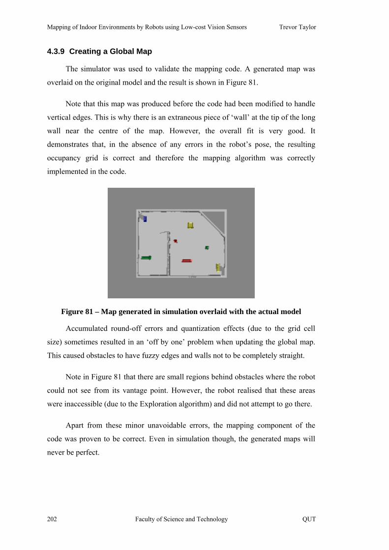
Mapping of Indoor Environments by Robots using Low-cost Vision Sensors Trevor Taylor
4.3.9 Creating a Global Map
The simulator was used to validate the mapping code. A generated map was
overlaid on the original model and the result is shown in Figure 81.
Note that this map was produced before the code had been modified to handle
vertical edges. This is why there is an extraneous piece of ‘wall’ at the tip of the long
wall near the centre of the map. However, the overall fit is very good. It
demonstrates that, in the absence of any errors in the robot’s pose, the resulting
occupancy grid is correct and therefore the mapping algorithm was correctly
implemented in the code.
Figure 81 – Map generated in simulation overlaid with the actual model
Accumulated round-off errors and quantization effects (due to the grid cell
size) sometimes resulted in an ‘off by one’ problem when updating the global map.
This caused obstacles to have fuzzy edges and walls not to be completely straight.
Note in Figure 81 that there are small regions behind obstacles where the robot
could not see from its vantage point. However, the robot realised that these areas
were inaccessible (due to the Exploration algorithm) and did not attempt to go there.
Apart from these minor unavoidable errors, the mapping component of the
code was proven to be correct. Even in simulation though, the generated maps will
never be perfect.
202 Faculty of Science and Technology QUT
Chapter Four Results and Discussion
4.4 Incremental Localization
As discussed in the next section on SLAM, performing incremental
localization proved to be essential for the stability of SLAM. The purpose of
incremental localization is to improve pose estimates prior to SLAM updates.
Odometry is notorious for being unreliable. Odometry errors were the major
cause of localization problems. Therefore this topic deserves further discussion.
In the course of this research several different approaches were investigated for
improving the pose estimates for the robot. These are discussed in the following sub-
sections.
4.4.1 Odometry Errors
Rotations of the robot were the chief cause of localization problems. One
common cause of errors was the motors not starting simultaneously. This tended to
jerk the robot as it pivoted around the stationary wheel (which was slower to start
up). When the motors eventually stopped, the opposite happened because the motor
that started first reached its target position first and therefore stopped slightly earlier.
This combination of effects caused the robot to move sideways, even though the
objective was a pure rotation.
Even small errors in the estimated rotations accumulated and would eventually
cause the robot to become lost. It is easy to understand why. Consider the following
exaggerated example where the robot is commanded to turn 30°, but actually only
turns 25°. If it now moves forward by a distance of just one metre, it will also move
sideways by 8.7cm. (This is a 5° difference extrapolated over 1m of travel). Clearly
this type of discrepancy, if left unchecked, will quickly result in large errors in the
robot’s position estimate.
Furthermore, if the robot makes a succession of rotations and loses 5° every
time, then it will soon think it is facing the wrong direction. Of course, a recurring
error of 5° would suggest that the robot control system needed adjustment and in
practice the errors can reasonably be expected to be much smaller than this.
QUT Faculty of Science and Technology 203
Mapping of Indoor Environments by Robots using Low-cost Vision Sensors Trevor Taylor
Wheel encoder information provides much better estimates of actual motion
than the commands to the robot’s motors. For instance, the robot might not receive a
command due to radio frequency interference and not move at all. In this case, the
wheel encoder values would correctly show zero motion.
Missing commands was a constant source of problems while running
experiments with the Yujin robot because it had one-way communication via a radio
modem and could not detect lost commands.
The X80 used UDP, which is not a reliable protocol, and connections were
sometimes lost when the robot was on the other side of the building from where the
wireless access point was located. The connection could be re-established, but in the
meantime the robot might have ‘lost’ a command resulting in a discrepancy between
the expected pose and the actual pose. This networking issue was outside the scope
of this research.
4.4.2 Using High-Level Features
Methods for using line features in the images to assist with localization have
been published in the author’s related papers [Taylor et al. 2006, Taylor 2007].
These methods rely on using features in the environment: Vertical edges appear in
images at the corners of walls or around doors; and Horizontal edges appear where
walls meet the floor. These are explained in more detail in the next two sub-sections.
4.4.3 Vertical Edges
When the camera is tilted, vertical edges in the real world do not appear
vertical in the images. Refer to Figure 82 which clearly shows vertical lines in a
simulated camera image. The slope of the lines varies across the image.
204 Faculty of Science and Technology QUT

Chapter Four Results and Discussion
Figure 82 – Verticals in an image with a tilted camera
For vertical edges, a very simple relationship exists between the slope, m, of
the line in the camera image and the location of where the edge meets the floor in
real world coordinates.
The following derivation can be found in [Taylor et al. 2006] and is one of the
contributions of this research.
Start with the robot coordinate system {x, y, z} which has its origin at the same
point as the camera coordinate system {X, Y, Z} as shown in Figure 5 in Chapter 2.
Note that the positive x axis is into the page. (It might make more sense to have the
origin of the robot coordinates on the floor, but only the x and z coordinates are of
interest because the robot moves in two dimensions). Therefore, the height off the
floor (in the y direction) is not important except to the extent that it affects the size of
the blind area in front of the robot.
Ignore the camera tilt for now. Start with the standard pin-hole camera
equations:
ZYfv
ZXfu == , (27)
where (u, v) are the coordinates of a pixel in the image (assuming the image
origin is at the centre) of a real-world point (X, Y, Z) expressed in the camera
coordinate system, and f is the camera focal length.
QUT Faculty of Science and Technology 205

Mapping of Indoor Environments by Robots using Low-cost Vision Sensors Trevor Taylor
By using an edge detector and a line detector, e.g. the Canny edge detector and
probabilistic Hough transform in the Intel OpenCV Library, it is possible to obtain a
set of lines from an image.
The slope of any given line in an image (which is a 2D space) can be obtained
from two points on the line, (u1, v1) and (u2, v2), as follows:
12
12
uuvvm
−−
= (28)
where m is the slope of the line.
If the actual angle is required, then this can be calculated as arctan(m). Note
that the nature of the tangent function is such that m approaches infinity as the line
approaches vertical, which can create computational problems. An alternative would
be to use the inverse slope, which would move the singularity to lines of zero slope –
well outside the range of interest.
Substitute into equation (2) after using equation (1) to determine the image
coordinates for two real-world points, p1 and p2. After a small amount of
simplification the result is:
2112
2112
ZXZXZYZYm
−−
= (29)
This equation describes the slope of a line between two points as it appears in
the image.
It is worth noting at this stage that the focal length has disappeared from the
equation. Also, it is irrelevant which point is chosen as p1.
In a robot-centric coordinate system the effect of the camera tilt is that the x
coordinates of all points in robot space remain the same in camera space, i.e. x = X.
However, the y and z coordinates must be transformed. The new coordinates can
easily be calculated as explained below.
For notational convenience, let c = cos(θ) and s = sin(θ). The rotation about the
X-axis can then be expressed as a rotation matrix:
206 Faculty of Science and Technology QUT
Chapter Four Results and Discussion
⎥⎥⎥
⎦
⎤
⎢⎢⎢
⎣
⎡−=csscR
00
001 (30)
In terms of robot coordinates, the rotated coordinates of two points can be
converted to camera space as follows:
( )( czsyszcyxp
czsyszcyxp
222222
111111
,,,,
+−= )+−=
(31)
If the two points were originally selected so that they were both on a vertical
edge in the real world, then in the robot coordinate system x1 = x2 and z1 = z2, i.e.
only the y coordinate varies. Therefore the subscripts have been dropped on x and z
in the following equations.
Using a similar approach to that used to obtain equation (3), substitute these
new coordinates from (5) into equations (1) and (2) and simplify:
)())()((
21
221
222
yysxscyscyzm
−+−+
= (32)
Applying the trigonometric identity c2 + s2 = 1, the final result is:
)sin(θxzm −
= (33)
The camera tilt angle, θ, can be determined from the extrinsic parameters once
the camera has been calibrated. The coordinates (x, z) are the location of the
intersection of the vertical edge with the floor in the real world relative to the robot’s
camera, i.e. measured across the floor.
Clearly, if the camera is horizontal so the tilt angle, θ, is zero, then m becomes
undefined. This corresponds to an infinite slope, or a vertical edge in the image. In
other words, with no tilt, all of the vertical edges actually appear vertical in the
images regardless of their position. This is only true in the special case of a camera
mounted horizontally.
QUT Faculty of Science and Technology 207
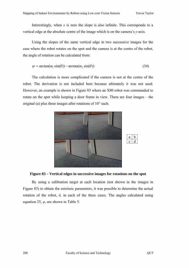
Mapping of Indoor Environments by Robots using Low-cost Vision Sensors Trevor Taylor
Interestingly, when x is zero the slope is also infinite. This corresponds to a
vertical edge at the absolute centre of the image which is on the camera’s y-axis.
Using the slopes of the same vertical edge in two successive images for the
case where the robot rotates on the spot and the camera is at the centre of the robot,
the angle of rotation can be calculated from:
))sin(arctan())sin(arctan( 21 θθψ mm −= (34)
The calculation is more complicated if the camera is not at the centre of the
robot. The derivation is not included here because ultimately it was not used.
However, an example is shown in Figure 83 where an X80 robot was commanded to
rotate on the spot while keeping a door frame in view. There are four images – the
original (a) plus three images after rotations of 10° each.
a b c d
Figure 83 – Vertical edges in successive images for rotations on the spot
By using a calibration target at each location (not shown in the images in
Figure 83) to obtain the extrinsic parameters, it was possible to determine the actual
rotation of the robot, δ, in each of the three cases. The angles calculated using
equation 25, ψ, are shown in Table 5.
208 Faculty of Science and Technology QUT
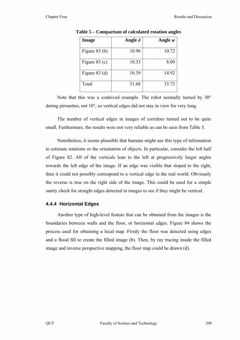
Chapter Four Results and Discussion
Table 5 – Comparison of calculated rotation angles
Image Angle δ Angle ψ
Figure 83 (b) 10.96 10.72
Figure 83 (c) 10.33 8.09
Figure 83 (d) 10.39 14.92
Total 31.68 33.73
Note that this was a contrived example. The robot normally turned by 30°
during pirouettes, not 10°, so vertical edges did not stay in view for very long.
The number of vertical edges in images of corridors turned out to be quite
small. Furthermore, the results were not very reliable as can be seen from Table 5.
Nonetheless, it seems plausible that humans might use this type of information
to estimate rotations or the orientation of objects. In particular, consider the left half
of Figure 82. All of the verticals lean to the left at progressively larger angles
towards the left edge of the image. If an edge was visible that sloped to the right,
then it could not possibly correspond to a vertical edge in the real world. Obviously
the reverse is true on the right side of the image. This could be used for a simple
sanity check for straight edges detected in images to see if they might be vertical.
4.4.4 Horizontal Edges
Another type of high-level feature that can be obtained from the images is the
boundaries between walls and the floor, or horizontal edges. Figure 84 shows the
process used for obtaining a local map. Firstly the floor was detected using edges
and a flood fill to create the filled image (b). Then, by ray tracing inside the filled
image and inverse perspective mapping, the floor map could be drawn (d).
QUT Faculty of Science and Technology 209
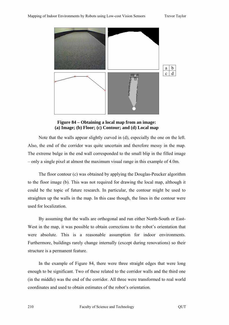
Mapping of Indoor Environments by Robots using Low-cost Vision Sensors Trevor Taylor
a b c d
Figure 84 – Obtaining a local map from an image: (a) Image; (b) Floor; (c) Contour; and (d) Local map
Note that the walls appear slightly curved in (d), especially the one on the left.
Also, the end of the corridor was quite uncertain and therefore messy in the map.
The extreme bulge in the end wall corresponded to the small blip in the filled image
– only a single pixel at almost the maximum visual range in this example of 4.0m.
The floor contour (c) was obtained by applying the Douglas-Peucker algorithm
to the floor image (b). This was not required for drawing the local map, although it
could be the topic of future research. In particular, the contour might be used to
straighten up the walls in the map. In this case though, the lines in the contour were
used for localization.
By assuming that the walls are orthogonal and run either North-South or East-
West in the map, it was possible to obtain corrections to the robot’s orientation that
were absolute. This is a reasonable assumption for indoor environments.
Furthermore, buildings rarely change internally (except during renovations) so their
structure is a permanent feature.
In the example of Figure 84, there were three straight edges that were long
enough to be significant. Two of these related to the corridor walls and the third one
(in the middle) was the end of the corridor. All three were transformed to real world
coordinates and used to obtain estimates of the robot’s orientation.
210 Faculty of Science and Technology QUT
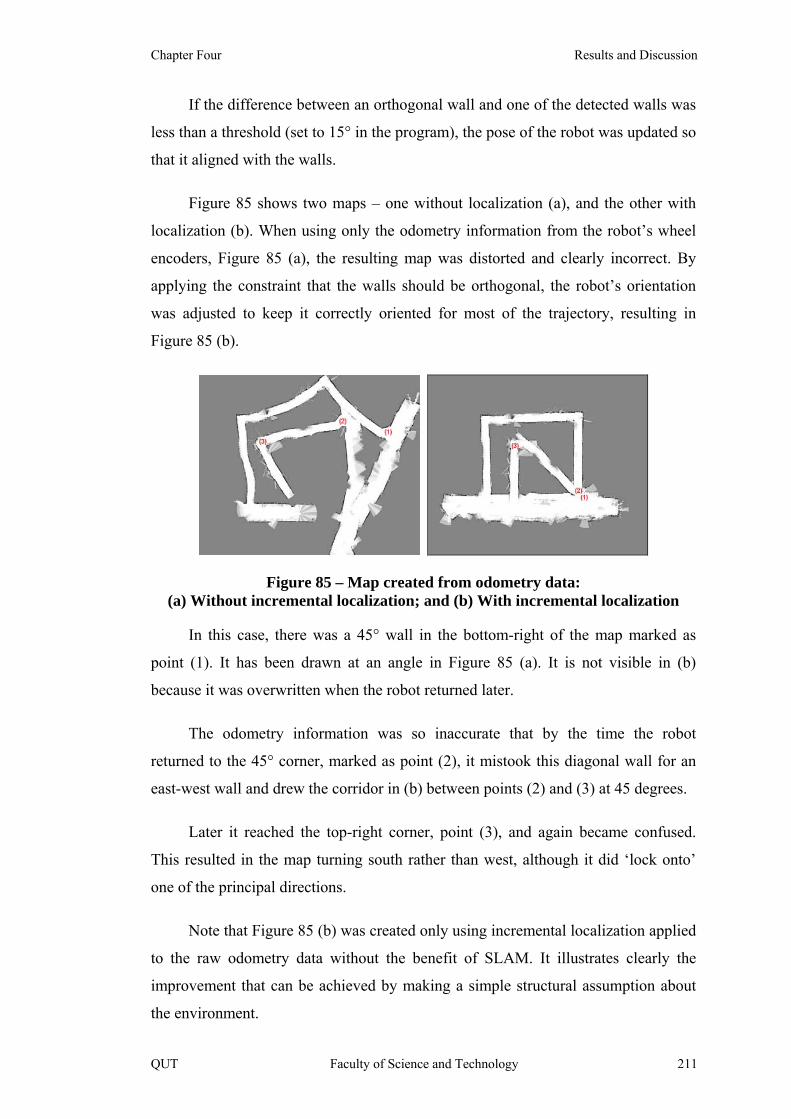
Chapter Four Results and Discussion
If the difference between an orthogonal wall and one of the detected walls was
less than a threshold (set to 15° in the program), the pose of the robot was updated so
that it aligned with the walls.
Figure 85 shows two maps – one without localization (a), and the other with
localization (b). When using only the odometry information from the robot’s wheel
encoders, Figure 85 (a), the resulting map was distorted and clearly incorrect. By
applying the constraint that the walls should be orthogonal, the robot’s orientation
was adjusted to keep it correctly oriented for most of the trajectory, resulting in
Figure 85 (b).
Figure 85 – Map created from odometry data: (a) Without incremental localization; and (b) With incremental localization
In this case, there was a 45° wall in the bottom-right of the map marked as
point (1). It has been drawn at an angle in Figure 85 (a). It is not visible in (b)
because it was overwritten when the robot returned later.
The odometry information was so inaccurate that by the time the robot
returned to the 45° corner, marked as point (2), it mistook this diagonal wall for an
east-west wall and drew the corridor in (b) between points (2) and (3) at 45 degrees.
Later it reached the top-right corner, point (3), and again became confused.
This resulted in the map turning south rather than west, although it did ‘lock onto’
one of the principal directions.
Note that Figure 85 (b) was created only using incremental localization applied
to the raw odometry data without the benefit of SLAM. It illustrates clearly the
improvement that can be achieved by making a simple structural assumption about
the environment.
QUT Faculty of Science and Technology 211

Mapping of Indoor Environments by Robots using Low-cost Vision Sensors Trevor Taylor
It should be feasible to add more discrete angles, such as 45°, 135°, 225° and
315°, to account for walls that are not at a multiple of 90 degrees. However, this was
not tested and has been left for future research. Note that this is an unusual feature of
a building.
As already noted, errors in orientation have a more significant effect on the
robot’s estimated pose than errors in its position. Therefore it is vitally important that
the orientation is correct. Hence the importance of this method of localization.
However, Figure 85 (b) indicates that the robot still incorrectly estimated the
distances travelled. The corridor at the bottom of the map is far too wide. The correct
width is shown in (a), but in (b) the robot retraced its path and in the process it
redrew the corridor much wider. This problem, and the incorrect orientations, were
corrected by using a particle filter to perform SLAM in conjunction with the
incremental localization. See Figure 89 below.
Side Note:
As this thesis was in its final stages a new SLAM algorithm was published,
called P-SLAM. It used the structure of indoor environments to improve localization
by recognising features such as corners in corridors [Chang et al. 2007].
P-SLAM used an environmental structure predictor to ‘look ahead’ and create
possible local maps based on the types of structures previously found during
exploration. For instance, if it encountered a corner in a corridor, it assumed that the
corridor then continued on for a certain distance at a right angle to the corridor it was
currently following based on having seen such corners before which produced
similar structures already in the map. The key point is that there is an underlying
assumption that the environment has regular features. This would most likely be
invalidated by a single 45° wall as in the example above.
It is interesting to note that the examples given by Chang et al. showed that a
conventional Rao-Blackwellized Particle Filter (RBPF) with 200 particles produced
a map which was severely distorted. To correct the problem a minimum of 1000
particles was required for the RBPF. This was with a laser range finder and also
applying scan matching.
212 Faculty of Science and Technology QUT
Chapter Four Results and Discussion
Conversely, P-SLAM was able to create a good map with only 200 particles. In
either case, the number of particles was substantially more than were used in the
experiments in this thesis (usually 50 or 100).
The P-SLAM paper appeared too late to be incorporated into this research. It is
a possible avenue for future work.
4.5 Difficulties with GridSLAM
The main focus of this work was not on developing new SLAM algorithms. To
the contrary, it was expected that existing algorithms could be used, but when it
came to finding appropriate software the results were disappointing. There was a
large discrepancy between what had been reported in the literature and the
availability of robust packaged software to make SLAM accessible to researchers
without the need to implement complex algorithms from scratch.
The approaches to Visual SLAM identified in the initial research were not
appropriate for the experimental hardware used in this research. The robot had only a
single camera; images were captured at a very low frame rate; and they exhibited
motion blur during moves. Using piecewise linear motion restricted the number of
images that were available for processing and the significant changes in the robot’s
pose between images meant that feature tracking was not feasible.
The major problem encountered in this research was getting SLAM to work
reliably. Despite SLAM having been an active research area for decades and claims
that the SLAM problem has been solved in a theoretical sense [Durrant-Whyte &
Bailey 2006, Bailey & Durrant-Whyte 2006], SLAM still has problems with the
practical aspects of implementation.
In particular, this research initially relied on algorithms published in
Probabilistic Robotics [Thrun et al. 2005]. While there was nothing fundamentally
wrong with these algorithms, they did not work reliably with the vision system and
there were some significant changes required to ensure convergence. Part of the
problem is related to the limited amount of information available from vision. As has
been pointed out previously, corridors do not provide a wealth of features. Both
these factors conspired to cause localization to fail.
QUT Faculty of Science and Technology 213
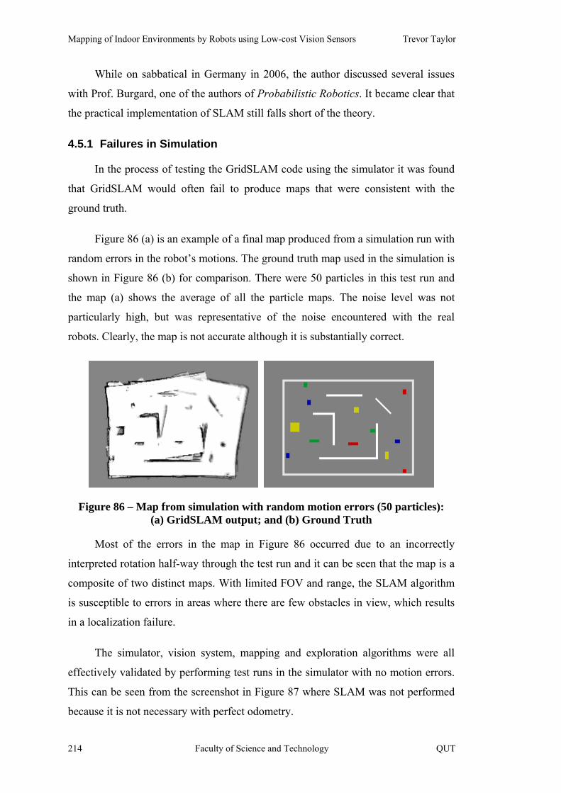
Mapping of Indoor Environments by Robots using Low-cost Vision Sensors Trevor Taylor
While on sabbatical in Germany in 2006, the author discussed several issues
with Prof. Burgard, one of the authors of Probabilistic Robotics. It became clear that
the practical implementation of SLAM still falls short of the theory.
4.5.1 Failures in Simulation
In the process of testing the GridSLAM code using the simulator it was found
that GridSLAM would often fail to produce maps that were consistent with the
ground truth.
Figure 86 (a) is an example of a final map produced from a simulation run with
random errors in the robot’s motions. The ground truth map used in the simulation is
shown in Figure 86 (b) for comparison. There were 50 particles in this test run and
the map (a) shows the average of all the particle maps. The noise level was not
particularly high, but was representative of the noise encountered with the real
robots. Clearly, the map is not accurate although it is substantially correct.
Figure 86 – Map from simulation with random motion errors (50 particles): (a) GridSLAM output; and (b) Ground Truth
Most of the errors in the map in Figure 86 occurred due to an incorrectly
interpreted rotation half-way through the test run and it can be seen that the map is a
composite of two distinct maps. With limited FOV and range, the SLAM algorithm
is susceptible to errors in areas where there are few obstacles in view, which results
in a localization failure.
The simulator, vision system, mapping and exploration algorithms were all
effectively validated by performing test runs in the simulator with no motion errors.
This can be seen from the screenshot in Figure 87 where SLAM was not performed
because it is not necessary with perfect odometry.
214 Faculty of Science and Technology QUT

Chapter Four Results and Discussion
Figure 87 – Map from simulation with no motion errors
Because of the problems encountered with the stability of the GridSLAM
algorithm, changes were made to the code during development to try to make the
filter more robust. These changes had no mathematical basis, and might invalidate
the original theory from which the filter was developed. They are explained in the
following sections.
4.5.2 Sensor Model
It has been explained previously how the accuracy of range estimates decreases
rapidly the further an obstacle is from the camera. Unless there is a long sequence of
very close obstacles, then the sensor measurements will generally contain a large
amount of error, which can be viewed as noise.
Experience on this project showed that the sensor model could have a
significant impact on the robustness of SLAM. In particular, if the model was too
simplistic then good information in the map was rapidly replaced by bad information
due to the clear-cut values for free space and obstacles.
In the case of the X80 robot, the images are converted to JPEG format by the
robot before transmission to the PC over the wireless LAN. This causes artefacts in
the images which sometimes induced artificial edges. As previously explained,
shadows can also induce artificial edges. Therefore the probability of an obstacle
should not be set to 1.0 at an edge. It should be somewhat lower to account for the
possibility that the detected edge was not an edge at all.
QUT Faculty of Science and Technology 215

Mapping of Indoor Environments by Robots using Low-cost Vision Sensors Trevor Taylor
Also, the frequency of updates from the sensor can be viewed as affecting the
sensor model in a subtle way. Laser range finders typically provide several updates
per second. This means that the same area is seen repeatedly, which naturally
increases the certainty of the cells in the map. Therefore the individual updates can
be more conservative.
However, in this work just one camera image was used after each step during
pirouettes. This meant that the values used in the sensor model had more extreme
values than would have been necessary if several updates had been performed from
each vantage point. The cumulative effect would be the same, except that occasional
bad images would have less impact on the map. Fortunately, errors tended to be
corrected because the robot usually saw the same area several times.
For these reasons, a more realistic model was developed, as explained in
section 3.7.6. The following diagram, Figure 88, is an example of the realistic sensor
model. It shows a local map generated as the robot approached the opening of a
corridor.
Figure 88 – Local map created with complex sensor model: (a) Camera image; and (b) Map showing uncertain range values
The wall in the map (b) on the near right-hand side does not have much ‘fuzz’
because the error was less than one grid cell. However, the far wall on the left-hand
side of the corridor was too far away to obtain a reliable range measurement.
Therefore it is quite fuzzy. Note too that there were quantization effects due to both
the pixel quantization in the image and round-off to grid cells in the map.
Figure 88 also illustrates one of the problems with the vision system. The stray
ray at the bottom edge of the local map extends to the maximum vision distance.
This occurred because of a failure in the detection of the floor boundary that allowed
216 Faculty of Science and Technology QUT

Chapter Four Results and Discussion
the floor to ‘leak’ through. In this case, it was an aluminium air-conditioning duct
that was a similar grey colour to the floor and very hard to detect. (Refer back to
Figure 78 for a better view of the duct).
Figure 89 – Maps created with: (a) Simple sensor model; and (b) Complex sensor model
Figure 89 shows two maps. The first map was created with the simple model.
The second map used the complex model. The walls are more clearly defined in the
second map, but they are qualitatively the same. The first model was less
computationally intensive.
4.5.3 Particle Filter Issues
There are several different parameters and approaches that can be used with
Particle Filters. Some issues with Particle Filters were identified during the literature
review. The issues included:
• Maintaining particle diversity (for a representative distribution);
• Determining the number of particles required for an accurate map;
• Improving the proposal distribution during an update;
• Avoiding particle depletion;
• Defining an appropriate motion model and determining its parameters;
• Obtaining importance weights with the widest possible spread of
values; and
• Implementing a suitable resampling algorithm.
QUT Faculty of Science and Technology 217

Mapping of Indoor Environments by Robots using Low-cost Vision Sensors Trevor Taylor
The following sections discuss these issues in the context of this research.
There are still many open research questions related to these issues.
4.5.4 Maintaining Particle Diversity
Particle diversity is important for successful operation of a particle filter. The
motion model parameters also have an impact on diversity, but this is discussed
below in the section 4.5.8 on the Motion Model.
Figure 90 – Particle trajectories: (a) Before; and (b) After closing a loop
Figure 90 shows how particle trajectories are affected by loop closure. The
robot started at the bottom-centre of the map and proceeded to the left travelling
around the loop in a clockwise direction. (It made a brief deviation to the right in the
bottom-right corner.) In (a), it was just about to join up with its ‘tail’ at the point
where it started. Notice that the particle trajectories had spread out significantly into
a ‘fan’.
In Figure 90 (b) the robot had started to retrace the early portion of its path. As
the robot became more certain about where it was, based on seeing part of the map
again, many of the particles were discarded and their trajectories disappeared. The
net effect was that after closing the loop there was only a single trajectory (the single
line at the left-hand side) that could be traced back to the very beginning of the test
run.
Notice in Figure 90 (a) that there were (at least) two distinctly different paths
(based on clumps of particles). On the scale of this map, which is roughly 20m
square, the trajectories at the left side of the map were about 60cm apart. However,
218 Faculty of Science and Technology QUT

Chapter Four Results and Discussion
after loop closure all but one of them was lost forever. This indicated that the number
of particles was very close to the minimum required to reliably close the loop.
Statistically speaking, it was quite likely that the robot’s pose was correct in
(b). However, the exact path that it took to reach where it ended up might actually
have been wrong. There could have been small errors in the map along the way, due
to an incorrect path, even though the final pose was close to being correct.
Sufficient particles are required to maintain diversity. However, this is always
a compromise because the computational requirements increase directly in
proportion to the number of particles.
4.5.5 Determining the Number of Particles Required
In the experiments, only 50 or 100 particles were typically used for
performance reasons. Even though piecewise linear motion allowed the robot to ‘sit
and think’, it was still using up battery power so elapsed time had to be minimized.
By re-running recorded video images and log files, various parameter settings
could be tested afterwards without having to be concerned about the battery life of
the robot. Using pre-recorded data was also essential to provide reproducible test
runs for comparison purposes when changes were made to the algorithms.
The maximum number of particles trialled was 500. Even this is a low number
compared with some examples reported in the literature. However, the program still
failed to produce a reliable map unless incremental localization was enabled (as
explained in section 4.4), which is one method of improving the proposal
distribution.
4.5.6 Improving the Proposal Distribution
In an attempt to improve the stability of the SLAM algorithm, code was added
to the filter to iteratively find the best local map for each particle during the selection
of new poses using the motion model. The number of iterations was limited because
it had a significant impact on the performance.
Another approach, which was suggested in Probabilistic Robotics, was to
iterate until the new pose was not inside an obstacle according to the particle’s own
QUT Faculty of Science and Technology 219
Mapping of Indoor Environments by Robots using Low-cost Vision Sensors Trevor Taylor
map. This makes a lot of sense from a physical point of view. However, it is possible
for the particle’s map to be wrong, but the selected pose to actually be correct.
After trialling both of these approaches, no noticeable improvement was found
in the performance of the SLAM algorithm. In other words, it still failed to produce
accurate maps.
Other researchers have used scan matching of laser range finder scans. As
noted previously, the non-linear nature of inverse perspective mapping makes
conventional approaches to scan matching inappropriate. New theoretical
development will be required to make scan matching viable for vision. However, as
long as there is only a small FOV, scan matching will still have problems unless the
frame rate is increased substantially to keep the incremental changes between images
very small. This line of research warrants further investigation.
Using incremental localization based on wall alignment eventually proved
successful. This was discussed at length in section 4.4.2 on Incremental Localization
using high-level features.
4.5.7 Avoiding Particle Depletion
One of the first problems that became apparent while testing the SLAM code
was that sometimes the particle set would be ‘flushed’ and a small number of
particles would effectively take over. This was in fact a previously recognized
problem known as particle depletion / deprivation [Thrun et al. 2005] or sample
impoverishment [Montemerlo & Thrun 2007].
The problem is basically a consequence of over-sampling. The objective of
resampling is to maintain diversity. However, if too many particles are replaced
during a single resampling step, then diversity will be reduced substantially because
deleted particles are replaced with clones of existing particles.
Montemerlo and Thrun claimed that this was due to a mismatch between the
proposal and posterior distributions over the robot’s pose. They suggested that this
happened when the robot’s sensor was ‘too accurate’ relative to the robot’s motion
error. However, the author did not find this to be the case for the experimental
220 Faculty of Science and Technology QUT

Chapter Four Results and Discussion
environment in this thesis. To the contrary, the sensor errors due to perspective were
significantly greater than the observed motion errors.
In this research it was found that ‘bad’ particles can be selected quite
unpredictably during resampling. Because the motion model uses probabilities, it can
happen that some of the particles might have poor pose estimates. However, there
might be insufficient information in the observations to eliminate these particles on
the next SLAM update because the particle weights are very similar.
If a bad particle is duplicated during the resampling process, then it has twice
the chance of affecting the filter stability. Each successive SLAM update that the bad
particles survive doubles the effect. Rapid growth in the number of bad particles
ensues, and the filter fails catastrophically.
This problem arises in the situation where the observations are not very
accurate, and therefore the calculation of the weights does not discriminate
sufficiently between ‘good’ and ‘bad’ particles. In a sense, this is the opposite of
what Montemerlo and Thrun suggest.
In [Bennewitz et al. 2006] the paper authors stated that: ‘Due to spurious
observations it is possible that good particles vanish because they have temporarily a
low likelihood.’
This argument supports the requirement for sufficient richness, or information
content, in the input data. A thought experiment helps to explain. If the input data is
‘bland’ so that all particles have equal weights, then wide variations in particle poses
are possible. For example, if the robot were in the middle of a large football stadium,
then it would have no way to discriminate between particles (because there would be
nothing to see within the range of the sensor) and any arbitrary pose could be
propagated because all weights would be equal.
4.5.8 Defining the Motion Model
The motion model consisted of simple translations and rotations (piecewise
linear motion). The noise distributions used in the motion model could be adjusted
via program parameters. Note that the initial pose of the robot was the same for all
particles because clearly it could only start from one location.
QUT Faculty of Science and Technology 221
Mapping of Indoor Environments by Robots using Low-cost Vision Sensors Trevor Taylor
Experience from this research showed that the parameters of the motion model
could be set too low. This is easy to understand from a thought experiment. If the
variances of the motion model were set to zero, then the particles would have no
variation and the filter would be almost certain to fail even if the motion model were
otherwise perfect because the robot itself always has noisy motions. In other words,
the particles would be unable to track the real motion of the robot. Therefore, some
minimum variance is required to encompass the actual motion variance of the robot
and to ensure that there will be sufficient particle diversity.
Conversely, if the motion model error variances were set too high, the particles
wandered around a lot. This increased the chance of a rogue particle being generated
that deviated significantly from the true path. If this particle survived for a
substantial amount of time, the resampling process cloned it. The overall effect was
to make the filter unstable.
As with the number of particles, there is no easy way to select the motion
model parameters. Texts such as [Thrun et al. 2005, Choset et al. 2005] offer
suggestions based on analysing the statistics of measured motions from logs of test
runs. The problem with this is that the real ground truth is rarely available. So the
estimated motion errors are based on the trajectory of the ‘best’ particle. This is
usually done off-line, but it could be done dynamically on-line. Further research is
required in this area.
4.5.9 Calculating Importance Weights using Map Correlation
During the resampling phase of the particle filter update it is necessary to
calculate weights for each of the particles to determine their ‘goodness of fit’ to the
existing map.
The Correlation-Based Measurement Model from [Thrun et al. 2005] was used
in this research. The textbook notes both the advantages and disadvantages of this
approach. In particular, there is no plausible physical explanation for this approach.
However, it has been widely used in the past.
It was found in this research that map correlation only produced a fairly narrow
range of weights. This arises to some extent due to the small area covered by the
222 Faculty of Science and Technology QUT
Chapter Four Results and Discussion
vision sensor. It is therefore possible for a ‘bad’ particle to survive resampling, and
even multiply. This was discussed above under Particle Depletion.
There are some other issues with map correlation as expressed in [Thrun et al.
2005]. Firstly, it suggests calculating the correlation over a local map that is square.
However, this includes many cells that are not in the robot’s sensor range because
the visible range is a segment of a circle. A mask was therefore added to the program
that included only the cells that were potentially visible. (See section 3.9.4).
Another issue is whether or not the summation should include cells where the
value is unknown space. In theory, there is no point including a cell from the global
map with a value of unknown because there is an equal chance of it being occupied
or unoccupied. (Such a cell has not been seen before). Similarly, the cells in the local
map with a value of unknown were not seen during the latest scan. It could therefore
be argued that they should not be included either.
In the author’s experience, excluding unknown cells from the correlation did
not have any significant impact on the stability of the SLAM algorithm. However,
the effect might have been minimal due to the fact that the number of cells involved
was small.
One other approach investigated was to accumulate information into temporary
local maps before updating the global map. For example, it seemed sensible to
combine all of the local maps from a pirouette before running a SLAM update and
integrating the information into the global map. This feature was added to the ExCV
program and it was found that there was a compromise – delaying SLAM updates
also delayed localization and the robot pose error could increase in the meantime.
Combining several scans into a single local map before performing the
correlation was also tested. This lead to more reliable matches, but it also meant that
there was potential for the robot to stray from the true path in the interim because it
made several moves before updating its pose estimate.
Instead of combining scans, an alternative approach was developed whereby a
moving average was kept for the weight of each particle. This had a smoothing effect
on the particle weights. The objective was to prevent a ‘bad’ particle from increasing
QUT Faculty of Science and Technology 223
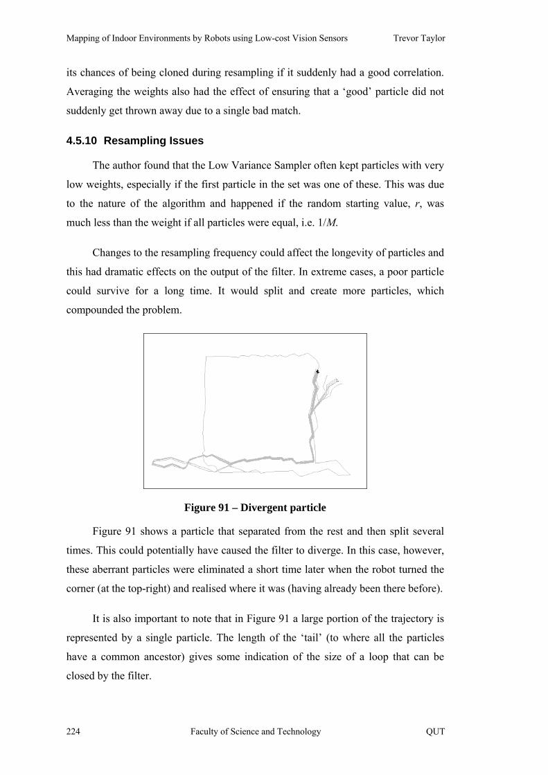
Mapping of Indoor Environments by Robots using Low-cost Vision Sensors Trevor Taylor
its chances of being cloned during resampling if it suddenly had a good correlation.
Averaging the weights also had the effect of ensuring that a ‘good’ particle did not
suddenly get thrown away due to a single bad match.
4.5.10 Resampling Issues
The author found that the Low Variance Sampler often kept particles with very
low weights, especially if the first particle in the set was one of these. This was due
to the nature of the algorithm and happened if the random starting value, r, was
much less than the weight if all particles were equal, i.e. 1/M.
Changes to the resampling frequency could affect the longevity of particles and
this had dramatic effects on the output of the filter. In extreme cases, a poor particle
could survive for a long time. It would split and create more particles, which
compounded the problem.
Figure 91 – Divergent particle
Figure 91 shows a particle that separated from the rest and then split several
times. This could potentially have caused the filter to diverge. In this case, however,
these aberrant particles were eliminated a short time later when the robot turned the
corner (at the top-right) and realised where it was (having already been there before).
It is also important to note that in Figure 91 a large portion of the trajectory is
represented by a single particle. The length of the ‘tail’ (to where all the particles
have a common ancestor) gives some indication of the size of a loop that can be
closed by the filter.
224 Faculty of Science and Technology QUT
Chapter Four Results and Discussion
4.5.11 Retaining Importance Weights to Improve Stability
According to the GridSLAM algorithm, a new importance weight is calculated
for each particle every time a new sensor update is received. When the importance
weights are very similar this can cause problems during resampling because ‘bad’
particles might be selected. A typical case where this might occur is in a large open
corridor where the robot sees only free space. In this case, all particles are likely to
have the same weights. This problem is compounded by a limited sensor range
(discussed below in section 4.7).
To try to reduce this effect, the weights were kept as a property of the particles
and accumulated across iterations. Two different ways to do this were investigated.
The weights were simply added together because they were subsequently normalized
anyway. Alternatively, the logarithm of the weights was taken to spread them out.
Adding them together was then equivalent to multiplying them together.
4.5.12 Adjusting Resampling Frequency
The GridSLAM algorithm says that the particle set should be resampled on
every update. Over-sampling is known to cause problems with particle filters.
Therefore, resampling of the particle set was not performed on every iteration of the
SLAM algorithm. However, it was necessary to decide how long to wait before
resampling.
One simple approach, which was implemented in GMapping, was to perform a
SLAM update only after the robot had moved by a certain distance or rotated by a
certain amount. These parameters had to be established by trial and error because
there were no published methods for doing so.
The concept of a ‘Number of Effective Particles’ had been introduced for
selective resampling [Grisetti et al. 2005]. The formula was based on the particle
weights:
∑=
= M
i
ieff
wN
1
2)(
1 (35)
QUT Faculty of Science and Technology 225

Mapping of Indoor Environments by Robots using Low-cost Vision Sensors Trevor Taylor
Neff is a measure of particle diversity. It works on the assumption that if all of
the particles are distributed according to the true posterior distribution then they
should have equal weights and the value of Neff would be equal to M. As the particles
start to diverge, the value of Neff will fall.
The literature suggested that resampling should only be done when Neff falls
below half the number of particles, or 50% of M. This did not occur very often
during the experiments. Therefore other criteria were used to decide when to
resample as explained previously.
The ExCV program accumulated the distance travelled by the robot, and the
total turn angle. When either of these exceeded a pre-set amount, then resampling
was performed. The value of Neff was used as a fallback, but this rarely triggered
resampling even when set to 65% of M.
4.6 Comparison with Other SLAM Algorithms
Two data sets containing random motion errors were generated using the
simulation environment, shown in Figure 92, to test the stability of two other SLAM
packages in comparison to the GridSLAM implementation in this research. The
GridSLAM algorithm was unable to produce a correct map with these data sets (see
Figure 95 and Figure 96 below in the section on GMapping). For these test runs the
maximum vision distance was set to 8m.
Figure 92 – Ground truth map for simulation
4.6.1 DP-SLAM
The map in Figure 93 (a) shows the initial result for DP-SLAM with 50
particles. (Ignore the rotation of the map which is not relevant and is an artefact of
226 Faculty of Science and Technology QUT

Chapter Four Results and Discussion
the program). Although DP-SLAM started out well, it became disoriented half way
through the test run. The map in Figure 93 (a) is collapsed on itself and should be
much larger as shown in (b).
Figure 93 – Test 1 with DP-SLAM: (a) Initial test run; and (b) After learning the motion model
The authors of DP-SLAM were contacted and the problem was discussed with
them. They suggested that the motion model might need to be updated to match the
robot, and another program was supplied that could learn the motion model. This
underscored the importance of a good motion model.
After performing some training runs to determine the motion model
parameters, the test data was again run through DP-SLAM. The number of particles
was also increased to 100. The resulting map is shown in Figure 93 (b). Although it
was significantly better, it still clearly had problems.
In Figure 93 (both a and b) there appear to be two distinct maps overlapping
each other with the second one slightly rotated with respect to the first. The most
likely cause was an area where the vision data is ambiguous due to the limited FOV
and range of the simulated camera. In this case the SLAM algorithm would be
unable to accurately determine the amount of rotation.
The second data set was also run with both 50 and 100 particles with the
results shown below in Figure 94. The second map was much better than the first
QUT Faculty of Science and Technology 227

Mapping of Indoor Environments by Robots using Low-cost Vision Sensors Trevor Taylor
one, which was not surprising because particle filters should work better with more
particles.
Figure 94 – Test 2 with DP-SLAM: (a) 50 Particles; and (b) 100 Particles
The examples on the DP-SLAM web site used thousands of particles.
However, in order to keep the comparison on a similar footing with the other SLAM
algorithms, the number was limited to 100. Also, DP-SLAM was found to be slower
than GridSLAM and using 1,000 particles (or more) would have been impractical.
4.6.2 GMapping
Comparisons of GridSLAM against GMapping are shown in Figure 95 and
Figure 96. These are easier to compare directly than GridSLAM and DP-SLAM
because of the format of the GMapping output which is from the CARMEN log2pic
program. The GridSLAM examples were for 50 particles and a grid cell size of 5cm
and the GMapping examples for 30 particles and a grid cell size of 10cm. The lower
parameter settings for GMapping were adopted after it was found that the algorithm
ran very slowly.
228 Faculty of Science and Technology QUT

Chapter Four Results and Discussion
Figure 95 – Test 1 – GridSLAM compared to GMapping: (a) GridSLAM; and (b) GMapping
Figure 96 – Test 2 – GridSLAM compared to GMapping: (a) GridSLAM; and (b) GMapping
GMapping produced better results in both tests. However, the maps still
showed obvious flaws.
GMapping was definitely not fast enough for use in real-time. This appears to
be due to the fact that it is a more complex algorithm. However, another test run was
performed with the second data set using 50 particles and a 5cm grid size. This is
shown in Figure 97.
QUT Faculty of Science and Technology 229

Mapping of Indoor Environments by Robots using Low-cost Vision Sensors Trevor Taylor
Figure 97 – GMapping with 50 Particles and 5cm grid size
This map from GMapping was substantially correct, although there is still a
double wall visible at the right-hand side.
4.7 Information Content Requirements for Stable SLAM
One aspect of SLAM that has been ignored in the literature is the Information
Content Requirements – the input (sensor measurement) data must provide enough
information for reliable SLAM to take place.
There are no stated requirements for ‘richness’ in the input data for any of the
major SLAM algorithms to the author’s knowledge. However, all algorithms should
include constraints on the input stream to satisfy stability and robustness criteria. The
literature implicitly assumes that the data will be sufficient for the task.
Problems arise from the nature of the vision sensor. There are three aspects to
information content that deserve mention:
• Field of View;
• Effective Range; and
• Frequency of updates.
The video camera on the X80 robot had a field of view only 50.8°, low
resolution (176 x 144), and a low frame rate (about 2 fps). As a consequence of
perspective, it has very limited range when the accuracy of the range data is taken
into account.
230 Faculty of Science and Technology QUT

Chapter Four Results and Discussion
In contrast, humans have a field of view that varies from 160° for a single eye
to as much as 200° for stereo vision [Wandell 1995]. There is no ‘frame rate’ for
human vision because separate parts of the visual pathways run asynchronously.
However, visual information is updated around 20 times per second.
Side Note:
To actually see how large your field of view is, stretch your arms out wide and
wriggle your fingers. Even while you are looking straight ahead, you will be able to
detect the motion of your fingers even though your direction of view is at 90° to your
arms. Humans are very sensitive to peripheral motions – a legacy from survival in
the wild.
Now consider the sensor of preference for SLAM research – the Laser Range
Finder. The best-known LRFs are manufactured by SICK GmbH. The product
specifications are available on their web site (http://www.sick.com). The following
information is for the SICK LMS 200.
Table 6 – Technical Specifications for SICK LMS 200
Feature Value
Field of View 180°
Range Maximum 80 m (262.5 ft)
Angular Resolution 0.25°/0.5°/1.0° (selectable)
Response Time 53 ms/26 ms/13 ms (Up to 75 Hz)
Measurement Resolution 10 mm (0.39 in)
System Error
(good visibility, 23°C
(73°F), reflectivity ≥10%)
Typ. ± 20 mm (mm-mode), range 1…8 m
(3.2…26.2 ft)
Typ. ± 4 cm (cm-mode), range 1…20 m
(3.2…65.6 ft)
Statistical Error, Standard
Deviation (1 sigma)
Typ. ± 5 mm (at range ≤ 8 m / ≥ 10%
reflectivity / ≤ 5 kLux)
QUT Faculty of Science and Technology 231
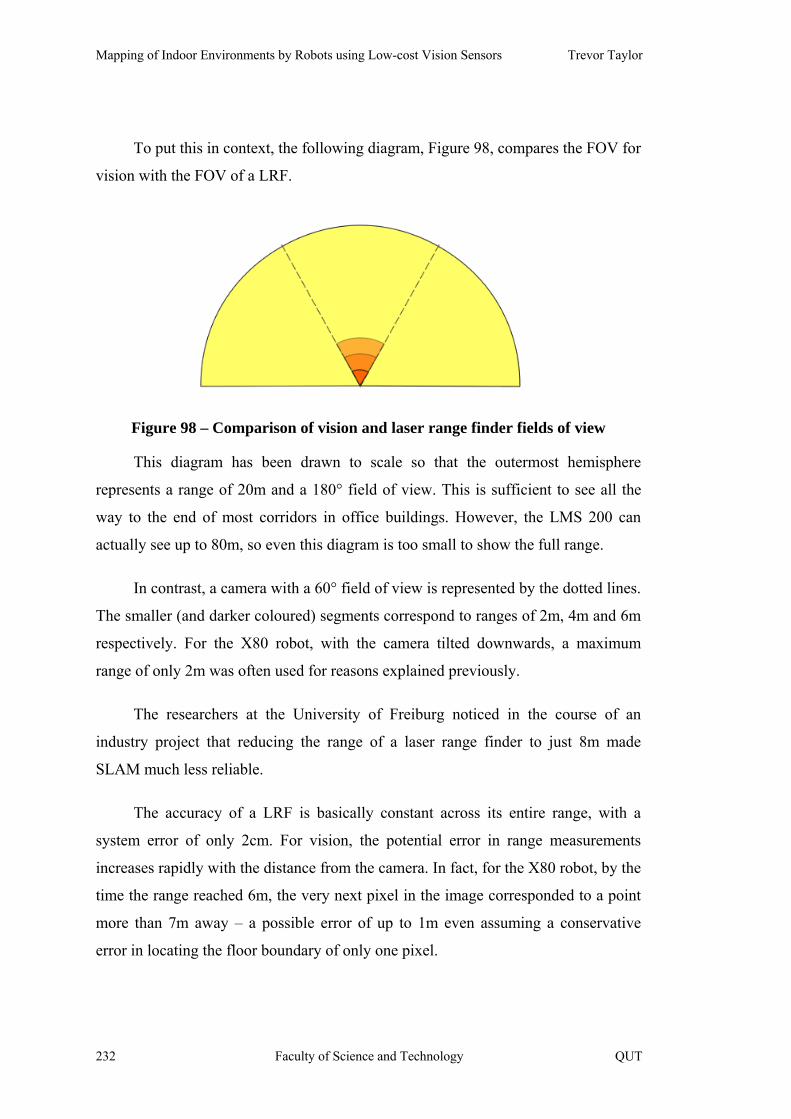
Mapping of Indoor Environments by Robots using Low-cost Vision Sensors Trevor Taylor
To put this in context, the following diagram, Figure 98, compares the FOV for
vision with the FOV of a LRF.
Figure 98 – Comparison of vision and laser range finder fields of view
This diagram has been drawn to scale so that the outermost hemisphere
represents a range of 20m and a 180° field of view. This is sufficient to see all the
way to the end of most corridors in office buildings. However, the LMS 200 can
actually see up to 80m, so even this diagram is too small to show the full range.
In contrast, a camera with a 60° field of view is represented by the dotted lines.
The smaller (and darker coloured) segments correspond to ranges of 2m, 4m and 6m
respectively. For the X80 robot, with the camera tilted downwards, a maximum
range of only 2m was often used for reasons explained previously.
The researchers at the University of Freiburg noticed in the course of an
industry project that reducing the range of a laser range finder to just 8m made
SLAM much less reliable.
The accuracy of a LRF is basically constant across its entire range, with a
system error of only 2cm. For vision, the potential error in range measurements
increases rapidly with the distance from the camera. In fact, for the X80 robot, by the
time the range reached 6m, the very next pixel in the image corresponded to a point
more than 7m away – a possible error of up to 1m even assuming a conservative
error in locating the floor boundary of only one pixel.
232 Faculty of Science and Technology QUT

Chapter Four Results and Discussion
To test the hypothesis that information content affects SLAM, the GMapping
algorithm was run using a modified log file where the data was truncated. Instead of
the full 180° of laser scan data, only 60° was used. In addition, the range of the data
was limited to 8m instead of 80m.
The resulting map is shown in Figure 99 and it has some obvious flaws.
Figure 99 – Map produced by GMapping with truncated data
In summary, the amount of information available from vision using a cheap
camera is much less than for a LRF. However, LRFs are very expensive compared to
web cameras.
Information content, or richness of the input signal, can also be considered in
the time domain, not just the spatial domain. As explained in Chapter 3, MonoSLAM
requires a high frame rate due to the way that it tracks features. In other words, then
it comes to tracking features in successive images the temporal separation between
images can be an important design parameter too.
4.8 Exploration
For a robot to build a map autonomously, it must have an exploration
algorithm. The Distance Transform (DT) was used in this research. The DT, as
implemented using the Borgefors algorithm [Borgefors 1986], is often referred to as
a two-pass process (forward and backward). Each pass is similar to a convolution.
However, for some maps, it is necessary to make multiple forward/backward passes
QUT Faculty of Science and Technology 233
Mapping of Indoor Environments by Robots using Low-cost Vision Sensors Trevor Taylor
[Jarvis 1993]. In the experiments this was rarely a problem, however, just to be
certain, the code iterated repeatedly until there were no changes. This always
resulted in executing a redundant iteration.
In the literature, has often been assumed that the map cell size matches the cell
size for robot motions. If the cell size is small compared to the robot, this leads to
paths that hug the walls and frequent direction changes.
These ‘too close’ paths, as they have been called [Zelinsky 1992], present two
problems. Firstly, the robot might side-swipe an object in passing, especially when
moving around corners. The second problem for the camera geometry in this
research was that the robot might move so close to an obstacle that the base of the
obstacle fell into the blind area in front of the robot. This made it impossible for the
robot to determine exactly where the obstacle was located.
To address the first problem, the robot always ‘looked’ before it moved. This
meant that the free space in front of the robot had to be re-assessed immediately
before each forward motion. A useful side-effect of this was that the robot could
detect objects that moved into its field of view, so in theory the environment did not
have to be completely static.
In the case of the X80 robot, an additional check could be made because the
robot had sonar sensors. For safety, the robot was programmed so that it would not
move forwards if the front centre sonar sensor value was less than the diameter of
the robot.
The second problem might be tackled by using active vision, for instance,
moving to a better vantage point in order to actually see the exact location of the
obstacle. A simple approach would be to move backwards, provided that the space
behind the robot was already known to be clear based on previous information. This
approach was not implemented. Instead, the ExCV program relied on the robot
seeing the blind space at some later stage of the exploration. In general this worked
fairly well because the robot did frequent pirouettes and therefore invariably looked
back at the area that it had come from.
234 Faculty of Science and Technology QUT
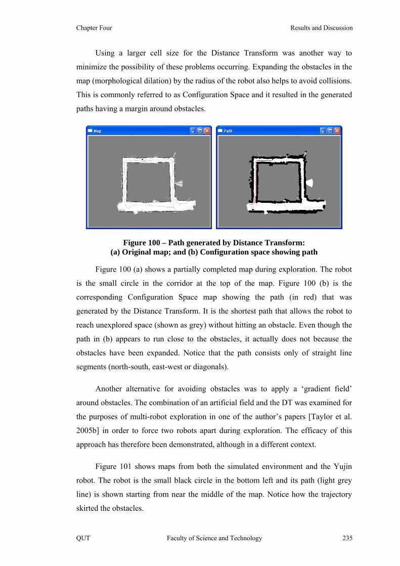
Chapter Four Results and Discussion
Using a larger cell size for the Distance Transform was another way to
minimize the possibility of these problems occurring. Expanding the obstacles in the
map (morphological dilation) by the radius of the robot also helps to avoid collisions.
This is commonly referred to as Configuration Space and it resulted in the generated
paths having a margin around obstacles.
Figure 100 – Path generated by Distance Transform: (a) Original map; and (b) Configuration space showing path
Figure 100 (a) shows a partially completed map during exploration. The robot
is the small circle in the corridor at the top of the map. Figure 100 (b) is the
corresponding Configuration Space map showing the path (in red) that was
generated by the Distance Transform. It is the shortest path that allows the robot to
reach unexplored space (shown as grey) without hitting an obstacle. Even though the
path in (b) appears to run close to the obstacles, it actually does not because the
obstacles have been expanded. Notice that the path consists only of straight line
segments (north-south, east-west or diagonals).
Another alternative for avoiding obstacles was to apply a ‘gradient field’
around obstacles. The combination of an artificial field and the DT was examined for
the purposes of multi-robot exploration in one of the author’s papers [Taylor et al.
2005b] in order to force two robots apart during exploration. The efficacy of this
approach has therefore been demonstrated, although in a different context.
Figure 101 shows maps from both the simulated environment and the Yujin
robot. The robot is the small black circle in the bottom left and its path (light grey
line) is shown starting from near the middle of the map. Notice how the trajectory
skirted the obstacles.
QUT Faculty of Science and Technology 235

Mapping of Indoor Environments by Robots using Low-cost Vision Sensors Trevor Taylor
Figure 101 – Maps generated by: (a) Simulation; and (b) Yujin Robot
Larger cell sizes reduce the number of moves. Fewer moves should help to
reduce the cumulative odometry errors. However, large cell sizes prevent the robot
from entering narrow corridors or passing through tight gaps.
Figure 101 (b) is distorted due to odometry errors. Also, there are spikes at the
edges that occurred because the robot’s shadow fell on the wall and it interpreted this
as the floor (which was black). However, the basic shape of the map and the path
followed are similar to the simulation, which confirms the algorithms and their
implementation in the program code.
Side Note:
The maps and the trajectories that the robots followed in the two diagrams of
Figure 101 are qualitatively very similar. This verified the accuracy of the
simulation. In addition, note that the second map was produced without the benefit
of a SLAM algorithm but it was still substantially correct. For this small
environment, the effects of odometry errors were not significant enough to seriously
distort the map. However, the ‘banana’ shape of the second map is testimony to the
inaccuracy of command execution by the robot.
Lastly, note that the robots automatically stopped exploring at the ends of the
paths shown in Figure 101. This is a useful feature of the Distance Transform.
4.9 Experimental Results
This section contains examples of maps that were produced by an X80 robot in
S Block of QUT. Initially the robot had no map. The robot was started in the middle
236 Faculty of Science and Technology QUT
Chapter Four Results and Discussion
of a corridor facing a wall so that it could orient itself initially. It was allowed to
explore on its own and build a map.
The process of building a map began with the robot performing a pirouette to
generate a ROP sweep. This gave it a 360° view of its surroundings, called a local
map. This local map was incorporated into the global map using SLAM, including
an incremental localization step. Based on the global map, the robot generated a path
to the nearest unexplored space using a Distance Transform. It then set out along this
path for a certain number of steps (usually set to 5 steps) incorporating new
information into the map as it went. After the specified number of steps, the robot
again performed a pirouette and the whole process was repeated until it determined
that there were no more areas left unexplored.
Typical test runs took about two hours to complete, due in part to the slow
movement of the robot (pirouettes take a lot of time) and also due to the
computations required. During test runs between 6,000 and 8,000 images were
captured and processed.
As an indication of the CPU requirements, re-processing of a saved log file
(with camera images) took about an hour on a laptop with a 2.0GHz Pentium M
(Centrino) processor.
The map in Figure 102 shows a map drawn using the raw data obtained from
the robot’s vision system on Level 7.
QUT Faculty of Science and Technology 237

Mapping of Indoor Environments by Robots using Low-cost Vision Sensors Trevor Taylor
Figure 102 – Map of Level 7 produced using raw data
There are several problems with the map, including some incorrect rotations
and two corridors that are doubled up. Obviously SLAM is necessary to correct the
map.
Applying the modified GridSLAM algorithm outlined in this thesis resulted in
the map shown in Figure 103. This map was produced using 50 particles with a
maximum vision range of 4 metres and the complex sensor model. The map grid cell
size was 5cm.
238 Faculty of Science and Technology QUT

Chapter Four Results and Discussion
Figure 103 – Map of Level 7 using SLAM with 4m vision range
There are several points to be made about the map in Figure 103.
• The robot had difficulty in distinguishing doors from the floor in
several places along the bottom of the map, resulting in the
characteristic ‘fans’ or ‘cones’. This was due to the similarity between
the colour of the doors and the carpet.
• There were two regions where the walls were at 45° – the bottom-left
corner and at the intersection of the right-hand corridor with the main
corridor (the horizontal corridor at the bottom of the map). The one at
the bottom-left is a little difficult to see because the robot interpreted a
door as the floor due to the similarity of the door colour with the carpet.
The one at the intersection of the right-hand corridor is clearly visible
and has the correct angle. This presented a challenge to the SLAM
algorithm.
• At the extreme right-hand side of the map, it appears that the robot saw
through the wall. However, there was no wall in the corridor – several
chairs had been placed there to prevent the robot from straying and it
could see between the legs of the chairs.
QUT Faculty of Science and Technology 239
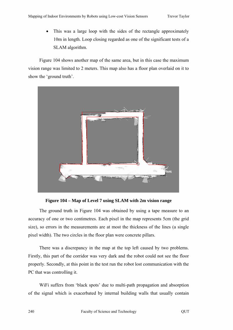
Mapping of Indoor Environments by Robots using Low-cost Vision Sensors Trevor Taylor
• This was a large loop with the sides of the rectangle approximately
10m in length. Loop closing regarded as one of the significant tests of a
SLAM algorithm.
Figure 104 shows another map of the same area, but in this case the maximum
vision range was limited to 2 meters. This map also has a floor plan overlaid on it to
show the ‘ground truth’.
Figure 104 – Map of Level 7 using SLAM with 2m vision range
The ground truth in Figure 104 was obtained by using a tape measure to an
accuracy of one or two centimetres. Each pixel in the map represents 5cm (the grid
size), so errors in the measurements are at most the thickness of the lines (a single
pixel width). The two circles in the floor plan were concrete pillars.
There was a discrepancy in the map at the top left caused by two problems.
Firstly, this part of the corridor was very dark and the robot could not see the floor
properly. Secondly, at this point in the test run the robot lost communication with the
PC that was controlling it.
WiFi suffers from ‘black spots’ due to multi-path propagation and absorption
of the signal which is exacerbated by internal building walls that usually contain
240 Faculty of Science and Technology QUT

Chapter Four Results and Discussion
metal studs. Because a motion command was lost, this caused the robot to become
disoriented. On re-establishing communication, the robot had to be driven manually
for a short distance until it could re-localize itself. This resulted in the ‘hole’ in the
corridor. However, wireless network connectivity was not one of the topics
addressed by this research.
Although this map is not perfect, it has all of the right features. The reason for
presenting a less than perfect map is to provide examples of the types of problems
encountered.
Additional lights were installed in the corridor and subsequent test runs
produced better results. An example is shown in Figure 105.
Figure 105 – Second map of Level 7 using SLAM
In this case the robot started at the centre of the top corridor. It completed a full
circuit before realising that it had not explored the bottom-left corner. In the process
of returning to the bottom-left it misjudged the top-left corner. The orientation of the
robot was wrong for a short period of time, and an extraneous corridor was started in
the map, but the localization procedure pulled it back on track.
QUT Faculty of Science and Technology 241
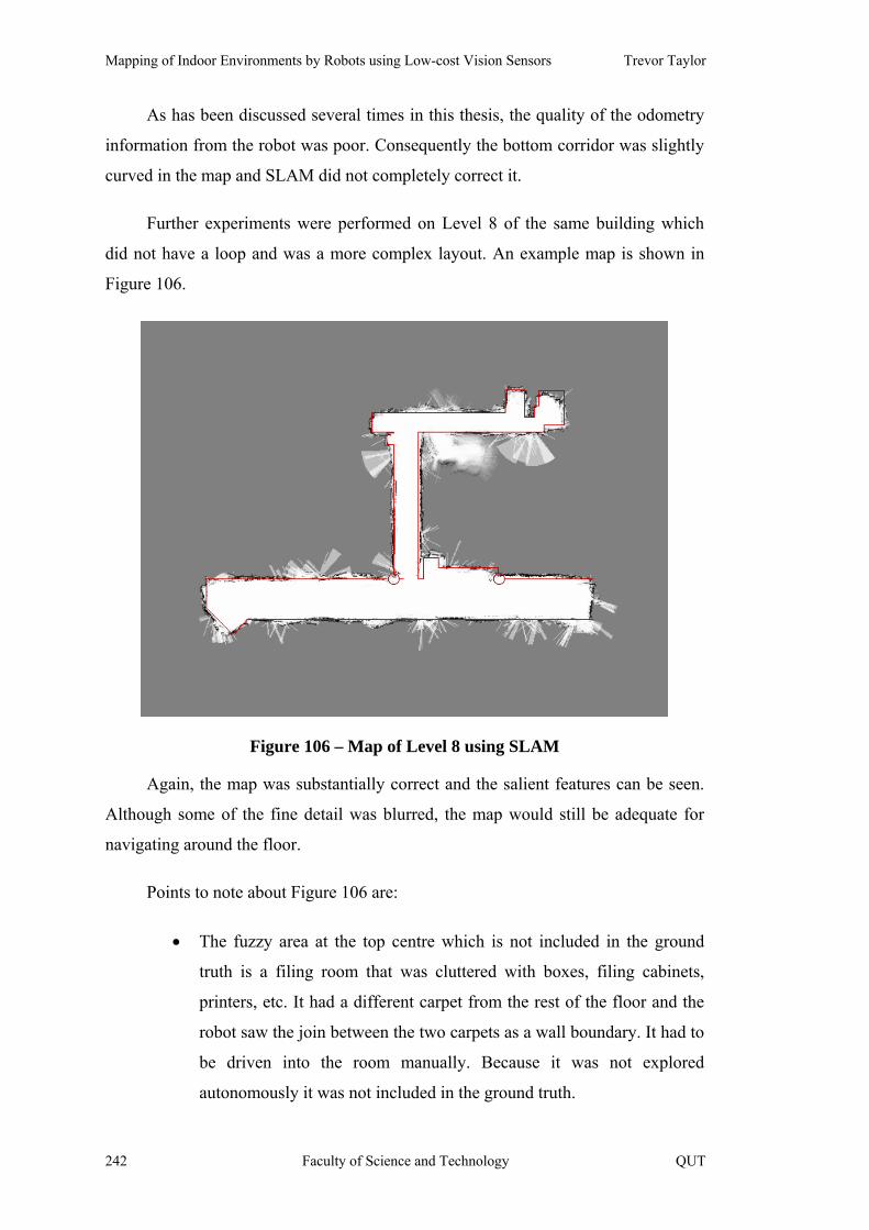
Mapping of Indoor Environments by Robots using Low-cost Vision Sensors Trevor Taylor
As has been discussed several times in this thesis, the quality of the odometry
information from the robot was poor. Consequently the bottom corridor was slightly
curved in the map and SLAM did not completely correct it.
Further experiments were performed on Level 8 of the same building which
did not have a loop and was a more complex layout. An example map is shown in
Figure 106.
Figure 106 – Map of Level 8 using SLAM
Again, the map was substantially correct and the salient features can be seen.
Although some of the fine detail was blurred, the map would still be adequate for
navigating around the floor.
Points to note about Figure 106 are:
• The fuzzy area at the top centre which is not included in the ground
truth is a filing room that was cluttered with boxes, filing cabinets,
printers, etc. It had a different carpet from the rest of the floor and the
robot saw the join between the two carpets as a wall boundary. It had to
be driven into the room manually. Because it was not explored
autonomously it was not included in the ground truth.
242 Faculty of Science and Technology QUT

Chapter Four Results and Discussion
• There were 45° walls in the bottom-left of the map similar to Level 7.
The walls in Figure 105 are more clearly defined.
4.10 Areas for Further Research
This section outlines several areas which were touched upon during the
research, but could not be explored fully due to time constraints. They merit further
investigation.
4.10.1 Using Colour in the ROP
Colour is a powerful tool for identifying and distinguishing amongst obstacles.
It should be possible to use the colour of obstacles to assist in the localization
process by incorporating it into the ROP.
However, there is a significant problem referred to in the field of computer
vision as Colour Constancy. Humans have the ability to perceive a wide range of
colours as actually resulting from the same base colour. Computers still have
difficulty with this.
Experiments were conducted with the Improved HLS system [Hanbury 2002]
and quantizing the Hue into 12 colours. Unfortunately, Hue has no representation for
black, white or shades of grey which are common colours in man-made
environments. Therefore, when the saturation was too low or too high the program
classified the ‘colour’ as black, white or grey depending on the lightness. This gave a
total of 15 ‘colours’.
In testing, it was found that it was not possible to reliably select the correct
colour. Furthermore, there is a problem with comparing colours when trying to
match two ROPs. For instance, is orange closer to red or yellow? Grey could
possibly match any colour in low light situations. Some sort of fuzzy logic needs to
be applied to colour comparisons.
4.10.2 Floor Segmentation
As has been explained in detail in this and previous chapters, colour is
primarily used to detect the floor. The author encountered a floor where the carpet
had a pattern consisting of two colours (instead of a single colour).
QUT Faculty of Science and Technology 243
Mapping of Indoor Environments by Robots using Low-cost Vision Sensors Trevor Taylor
One approach to multi-coloured carpets might be to replace all the different
(but known) colours with a single colour throughout the image, thereby converting
the floor to a single colour. While this sounds reasonable in theory, in practice there
is no such thing as a set of ‘fixed’ colours in an image – all colours cover a range of
pixel values. Therefore it was not feasible to replace all the carpet colours, including
the minor variations due to illumination.
A k-means clustering algorithm was implemented in the ExCV program that
determined the most commonly occurring pixel values in an image and grouped the
pixels together in clusters. In one test environment the colour of the carpet was very
similar to the colour of the walls. This was probably by design when the building
was first outfitted. As a result, the floor and walls contained areas with the same
cluster number in widely different parts of the images.
This highlights a significant drawback to the clustering approach – it loses
spatial information. The same is true when using histograms, colour equalization,
and so on.
An attempt was made to add the (u,v) coordinates of the pixels to the
information vector for clustering, but this was not successful because it produced too
many small clusters based on spatial proximity rather than colour.
Eventually the best approach that was found was to run a heavy smoothing
filter (Gaussian 11 x 11) on the images and then apply a flood fill algorithm. The
flood fill was constrained to lie within the major edges found in an image. Although
this resulted in the walls sometimes being blurred into the floor, there were generally
sharp edges between the wall and floor that limited the spread of the flood fill.
This is a perfect example of where a single image processing operation is not
sufficient to solve a problem. There is little doubt that humans apply a multitude of
algorithms simultaneously. Furthermore, humans can actually interpret what they see
and therefore apply logic to the segmentation problem to ‘see’ features that are not
really present at the level of individual pixels – a dotted line is a good example
which a human can interpret as a continuous line (although simultaneously
recognizing that it has gaps).
244 Faculty of Science and Technology QUT
Chapter Four Results and Discussion
There might be better ways to detect the floor, and this deserves further
investigation. Introducing additional methods in parallel, and then taking a majority
vote, might improve the reliability.
4.10.3 Map Correlation versus Scan Matching
As pointed out in the discussion on Localization, map correlation did not
produce a good spread of importance weights. Further research on alternative
correlation measures might produce a better result.
Scan matching (between successive ROPs) might be a better approach than
map correlation, but it will require some theoretical development to handle the
variation in range errors within an image because the Lu and Milios approach does
not work due to an implicit assumption that the errors are uniform regardless of the
range.
4.10.4 Information Content Required for Localization
Localization proved to be the most difficult issue in this project. One aspect of
localization that has not been extensively researched is the information content
requirements. It is generally assumed that there is sufficient information available
from the sensors, whatever they may be, to enable localization to be performed
reliably. Placing this on a solid theoretical footing is extremely difficult. However,
some observations are appropriate at this point.
The range of the sensor has a significant impact on map correlation because a
larger range provides more information for comparison between the local and global
maps.
A similar reduction in the effectiveness of map correlation results from a
narrow field of view, and cheap monocular cameras have quite a narrow FOV.
Most of the localization failures that were encountered in the experiments
could be attributed to one or both of these limitations. Quantifying these issues
would help future researchers to avoid falling into the same trap.
QUT Faculty of Science and Technology 245
Mapping of Indoor Environments by Robots using Low-cost Vision Sensors Trevor Taylor
4.10.5 Closing Loops and Revisiting Explored Areas
Seeing areas that are already on the map allows the robot to confirm its pose.
The experimental validation that was performed (see Chapter 3) showed that this
worked well.
Returning to previously visited areas is partially an exploration issue, but it is
very important for localization. This was noted in [Newman et al. 2002] which
discussed an ‘explore and return’ algorithm. Therefore, modifications should be
made to the exploration algorithm to periodically backtrack.
Closing large loops is known to be a problem with many SLAM algorithms.
The larger the loop that must be traversed, the more particles that are required to
maintain diversity. Actively closing loops has been proposed by [Stachniss et al.
2005].
4.10.6 Microsoft Robotics Developer Studio
Some preliminary work has been done with MRDS, but the vision program has
not been integrated into this environment because the vision code was written in
unmanaged C++, and MRDS is primarily a managed C# environment.
The simulator in MRDS is excellent, and it includes a simulated WebCam. It
could be used to replace the simulator in the ExCV program. Work on the simulator
would be useful for producing samples for use in teaching robotics and computer
vision.
4.11 Summary
This chapter has presented the details of the results obtained from the research.
Although the basic approach to using vision for mapping proved to be feasible, the
limited amount of information available from the vision system made it very difficult
for the SLAM algorithm to remain stable.
Incremental localization was added to the GridSLAM algorithm based on the
assumption that the walls were orthogonal. This was necessary to improve the
stability of GridSLAM and produce reliable maps.
246 Faculty of Science and Technology QUT

Glossary
5 Conclusions
‘The greatest single shortcoming in conventional mobile robotics is,
without doubt, perception …’
– R. Siegwart and I.R. Nourbakhsh,
Introduction to Autonomous Mobile Robots, 2004, page 11.
5.1 Motivation for the Research
As robots are introduced into homes and offices they will need maps in order
to perform many common tasks. It is essential that they be able to create the
necessary maps on their own rather than relying on the user to provide maps.
These robots will invariably have cameras. Digital cameras are now very cheap
and can provide information that is not available from any other type of sensor.
Therefore vision should be considered as a source of information for building maps.
A great deal of work had already been done on mapping using robots before
this research began in 2002. However most of this had been with sensors such as
laser range finders or sonar. This research pushed the edge of the envelope by
attempting to build maps based solely on monocular vision.
This chapter summarises the findings of this research in relation to the original
research questions and also offers some general recommendations and suggestions
for future areas of research.
QUT Faculty of Science and Technology 247

Mapping of Indoor Environments by Robots using Low-cost Vision Sensors Trevor Taylor
5.2 Mapping Indoor Environments Using Only Vision
The primary research question was:
How can an autonomous robot build maps of indoor environments using vision
as its only sense?
Implicit in this question was the assumption that it was possible to use only
vision. The research investigated many of the issues associated with visual mapping
and they are documented in this thesis. The main result of the research was a system
for robots to build maps that has been demonstrated to work in office corridors.
Three subsidiary questions were identified to break the research into smaller
pieces:
• How can vision be used as a range sensor?
• What mapping and exploration techniques are appropriate for indoor
environments?
• Are existing SLAM (Simultaneous Localization and Mapping)
approaches applicable to visual information?
The outcomes related to these subsidiary questions are addressed below.
5.3 Using Vision as a Range Sensor
Using a camera as a range sensor presents several challenges. Cheap cameras
typically have low resolution, a relatively narrow field of view, and are subject to
radial distortion. These characteristics of cheap cameras make them difficult to use
for mapping. Uneven illumination, including shadows, remains a significant problem
for vision. Even in indoor environments, artificial lighting does not necessarily
guarantee uniform illumination. Floor detection is not completely reliable when
based solely on the colour (and limited texture) of the floor.
Inverse Perspective Mapping (developed in section 3.7.2) provides a reliable
mechanism for determining the range to obstacles in an image once the camera has
been calibrated and assuming that the floor boundary can be correctly identified.
248 Faculty of Science and Technology QUT

Glossary
This research took a novel approach to building local maps called pirouettes –
the robot spun around on the spot taking a series of photos of its surroundings.
Pirouettes allowed Radial Obstacle Profile (ROP) sweeps to be made. (See section
3.7.6). The output of the vision system therefore appeared similar to a sonar sweep
or laser range scan. Once the data was in the form of a range scan, other open source
tools could be used such as CARMEN utilities and other SLAM algorithms. In other
words, the camera was effectively turned into a range sensor.
5.4 Mapping and Exploration for Indoor Environments
The mapping and exploration components of this research were successful
given the purpose as stated in Chapter 1 – building maps of indoor environments
using vision. This can be seen from the sample maps in Chapters 3 and 4.
Mapping and exploration algorithms were initially developed using a
simulator, prior to live testing. The simulation environment provided exact motions
and perfect pose information which eliminated the need for a SLAM algorithm
during testing of the mapping and exploration code. This allowed confirmation of the
suitability of the algorithms and that the program code was correctly implemented.
Piecewise linear motion – restricting movements to forward translations or on-
the-spot rotations – eliminated the requirement for real-time processing, and it
allowed exploration to be performed on a regular grid which fitted in well with the
Distance Transform for exploration.
Occupancy Grids were found to be a suitable map representation that could
easily be used with the Distance Transform for exploration.
The grid size for the occupancy grid should be selected based on the
environment and the size of the robot. The author suggests that the grid size should
be roughly one order of magnitude smaller than the robot.
The Distance Transform was selected as the exploration algorithm for this
research. Many exploration algorithms suffer from local minima problems, but the
Distance Transform does not. The Distance Transform also has the useful feature of
indicating when there is nothing left to be explored (that is reachable by the robot).
QUT Faculty of Science and Technology 249

Mapping of Indoor Environments by Robots using Low-cost Vision Sensors Trevor Taylor
On the other hand, the basic Distance Transform requires the robot to move on
a square grid rather than moving at random or by arbitrary amounts. Continuous
motion is also not feasible because the robot is constrained to move on a grid.
However, given the previously mentioned benefits of ‘piecewise linear’ motion and
the occasional adjustments that the robot made to its orientation in order to maintain
its alignment with the walls, this did not prove to be a problem in practice.
5.5 Simultaneous Localization And Mapping (SLAM) for use with Vision
This research found that it was possible to produce maps using a modified
SLAM algorithm. Examples are shown in section 4.8.16.
SLAM is a complex problem. Although many different solutions have been
published in the literature, there is no single algorithm that clearly stands out as the
‘best of breed’. It is still an active area of research and practice has not yet caught up
with the theory.
Localization is the single greatest challenge for a mobile robot. It requires the
robot to track its own movements and to recognize places that it has visited before.
Odometry is notoriously unreliable, so a variety of methods have been invented to
improve the accuracy of motion estimates and assist with localization.
Localization was found to be unreliable with a visual range sensor using map
correlation. The reasons for this were the limited field of view of the camera and a
practical limit on the useful visual range due to perspective. These factors limited the
amount of information in the input data stream from the visual range sensor, and
hence the number of map cells available for comparison.
Knowledge of the structure of the environment was used to perform
incremental localization to compensate for this deficit in the input information. This
approach was shown to be effective at improving the pose estimates for the robot.
A Particle Filter algorithm, called GridSLAM, was selected for use in this
research. This is a well-established algorithm published in a textbook by leading
researchers in the field. Problems were encountered in getting GridSLAM to work
250 Faculty of Science and Technology QUT

Glossary
successfully with the experimental setup in this research. Some of these problems
can be attributed to the equipment and the environment, but there is one fundamental
issue that is not addressed in the literature. There has been little work done on
specifying the requirements on the input data stream to guarantee the stability of
SLAM. The author refers to this as the ‘Information Content Requirement’.
The effect of a lack of ‘richness’ in the input data on the stability of SLAM
algorithms was confirmed using two other SLAM algorithms available as open
source implementations. However, incremental localization allowed GridSLAM to
produce acceptable maps.
5.6 General Recommendations
5.6.1 Adapting the Environment for Robots
There was an implicit assumption underlying this research that the
environment did not need to be modified to accommodate the robots. However,
humans constantly modify their environments and carefully regulate them to cater
for new technologies. The classic example is the automobile, which has resulted in
highly structured roads with clear markings and standardized dimensions.
If robots offer enough benefit, then people will be prepared to modify their
environments to better suit robots. It is recommended that in future the interior
design of buildings should be ‘robot friendly’.
This is not a difficult task. Mostly it just requires some fore-thought in the
design of buildings and the decoration of the internal spaces. These same changes
would also be beneficial to humans, especially those with poor eye-sight or in
situations like a fire when the building is filled with smoke. Therefore it is a very
sensible proposition.
The required changes are simple. They are based on experience with the robots
in this research:
• Arrange lighting so that it is uniform throughout the environment. Spot
lights should be avoided. Dark areas should also be eliminated. This
QUT Faculty of Science and Technology 251

Mapping of Indoor Environments by Robots using Low-cost Vision Sensors Trevor Taylor
makes sense from an occupational health and safety perspective
anyway.
• Use only uniformly coloured floor coverings. Alternatively, keep the
texture to a minimum so that it can easily be filtered out of camera
images.
• Ensure that all walls have a distinct strip along the bottom of the wall
where it meets the floor. Strips of different colours at waist level and/or
eye level might also be beneficial for both humans and robots by
helping to identify walls. One place where this is commonly done is on
glass doors to prevent people from walking into the doors.
• Paint all doors in a contrasting colour to the floor and walls. In
particular, consider changing one of the colour components (red, green
or blue) substantially so that doors are not visually similar to the floor.
The same applies to the door frame, which would assist in locating
doors even when they were open.
• Avoid unusual wall angles, curved walls and ‘niches’. Building only
straight walls with 90° corners will help robots to localize.
5.6.2 Additional Sensors
Humans perform multiple image processing operations simultaneously.
However, a vital aspect of human vision that makes it reliable is the ability to
interpret a scene even from a static image.
When analysing a scene, humans apply accumulated knowledge of the real
world including directional lighting effects, sophisticated pattern matching and
object recognition, high-level reasoning about distances and orientation, and
inferences regarding occlusions.
The current state of the art in computer vision still has a long way to go to
before it will approach the complexity of human vision. Therefore it is highly
advisable to incorporate additional sensors into any robot that must operate in a
252 Faculty of Science and Technology QUT

Glossary
human environment and interact with humans. It is not recommended that vision be
used as the only sensor on a commercial robot.
5.7 Contributions
5.7.1 Theoretical Contributions
Few researchers have attempted vision-only navigation, exploration and
mapping. Although the problem has not been completely solved, positive
contributions to the body of knowledge have been made both in terms of what does
work and what does not. This thesis documents the problems and identifies some
solutions.
The core contribution of this thesis is the confluence of range estimation from
visual floor segmentation with SLAM to produce maps from a single forward-facing
camera mounted on an autonomous robot. Contemporaneously with the writing of
this thesis, work was published [Stuckler and Benhke 2008] that reinforces and
validates the approach taken in this thesis.
The following is a summary of the topics covered in publications by the author
during the course of this research:
• A method for Inverse Perspective Mapping (IPM) using monocular
vision [Taylor et al. 2004a]. See sections 3.7.2 and 4.5.1.
• A novel approach to creating local maps by directing the robot to
perform a pirouette (spin on the spot) to obtain a Radial Obstacle
Profile (ROP) [Taylor et al. 2004b, Taylor et al. 2005a]. See sections
3.7.6 and 4.5.2.
• Extensions to the use of the Distance Transform for use in exploration
[Taylor et al. 2005a, Taylor et al. 2005b]. See sections 3.8 and 4.6.
• Development of a simple method for detecting vertical edges in an
image when the camera is tilted [Taylor et al. 2006, Taylor 2007] (see
sections 3.5.6 and 4.5.6); and
QUT Faculty of Science and Technology 253

Mapping of Indoor Environments by Robots using Low-cost Vision Sensors Trevor Taylor
• Development of methods for incremental localization based on
knowledge of the structure of the environment [Taylor et al. 2006,
Taylor 2007, Taylor et al. 2007]. By applying constraints, fewer
particles are required for stable operation of the GridSLAM algorithm.
See sections 3.10.2 and 4.7.
5.7.2 Practical Contributions
As noted in Chapter 1 – Introduction, a large amount of software was written
in the course of this project. The Experimental Computer Vision (ExCV) program
provides a robot-independent framework. It currently supports a Simulator (written
in OpenGL), Hemisson, Yujin and X80 robots.
From a purely practical perspective, this research produced over 80,000 lines
of source code, including the following (which is not an exhaustive list):
• An OpenGL simulator for computer vision experiments;
• An implementation of the GridSLAM algorithm;
• Facilities for recording and replaying test runs, including video;
• A program library for controlling X80 robots; and
• A complete working system based on X80 robots for map building in
indoor environments.
Versions of the code to control X80 robots were developed in both C++ and
C#. The code for the library is available under an open source licence from the
author’s company web site http://www.soft-tech.com.au/X80/.
The X80 software included a program that ran on a PDA for controlling an
X80 robot using a wireless LAN connection. This program, which allowed remote
teleoperation of an X80 from a hand-held device, was a world-first for this particular
robot.
Concurrent with this research, the author developed software examples for
Microsoft Robotics Developer Studio and co-authored a textbook on the subject
254 Faculty of Science and Technology QUT

Glossary
[Johns & Taylor 2008]. The software included a Maze Simulator and a simple
exploration program that performed mapping. These programs are available on the
Internet from the author’s book web site http://www.promrds.com/.
5.8 Future Research
Several topics for further investigation were listed at the end of Chapter 4 in
section 4.9. This section highlights the most important topics that the author
recommends for future research.
The floor segmentation algorithm that was ultimately used was not very
sophisticated. This deserves further investigation.
There are many aspects of particle filters and incremental localization
(discussed in section 4.8) that still warrant further research. Particle filters remain an
active research area.
The robot needs to see the same map features in many successive updates to
increase the correlations. The process adopted in this thesis of moving after every
image did not allow multiple images of the same location to be processed.
Furthermore, the large step size in the forward motions and rotations meant that there
was often not a lot of overlap between images.
A finer grain of step size, or capturing images on the fly may have helped.
However the hardware precluded this, due to both the low frame rate and the motion
blur in images taken while the robot was moving. Future work should use a camera
with a faster shutter speed (to reduce or eliminate motion blur); take photos more
frequently; and take multiple photos from the same vantage point.
In this research the robot did not deliberately return to previously explored
areas (unless it was just ‘passing through’ on its way to another unexplored area).
Actively backtracking might be a useful approach for improving localization.
Alternatively, the robot could simply turn to look again at nearby areas of the map
that were poorly defined.
Floor ‘contours’ were extracted from the ROPs using the Douglas-Peucker
algorithm in order to obtain straight wall segments. Although this information was
QUT Faculty of Science and Technology 255
Mapping of Indoor Environments by Robots using Low-cost Vision Sensors Trevor Taylor
used for incremental localization, it was not used to improve the quality of the map.
It should be feasible to straighten out the walls in the map based on the floor
contours. Also, the robot occasionally drove too close to a wall and could not see the
floor. Information from prior wall contours might be used to anticipate this problem
and correct it.
Localization was a significant issue in this research. The author has
hypothesised that the problems are related to the limited information content in the
input data stream that is available from vision. This should be investigated by
examining the effects of varying the field of view of the camera. Because this
requires changing the camera, initial work might be done in simulation.
The effect of increasing camera resolution on the reliability of IPM, and hence
SLAM, should also be investigated. The author conjectures that higher resolution
will improve the stability of SLAM by providing more accurate range information
and allowing the ‘maximum vision range’ to be increased. It should be possible to
perform initial testing by using a simulator and varying the resolution of the
simulated camera.
5.9 Summary
This research has demonstrated that mapping using only monocular vision
from a cheap camera is possible.
Some different approaches were used in this research from those that had been
used before and these contributed to the body of knowledge on visual mapping. In
particular, it introduced pirouettes and the Radial Obstacle Profile for local mapping
and piecewise linear motion for robot movements. The Distance Transform proved
to be a suitable exploration algorithm.
Vision provides a limited amount of information for mapping. Further research
is required into the input requirements for the stability of SLAM algorithms.
The characteristics of the environment can be used to perform incremental
localization. This allows the stability of SLAM to be improved so that maps can be
produced reliably.
256 Faculty of Science and Technology QUT

Glossary
Glossary
Words that are defined in the Glossary usually appear in italics the first time
that they are used in the text. In this Glossary, cross-references to other definitions
also appear in italics.
NOTE: The definitions provided here are the meanings as used in this thesis.
Autonomous Mobile Robot
An autonomous mobile robot is one that can move freely. It does not
necessarily have any on-board intelligence apart from that necessary to
control its wheels. ‘Autonomous’ therefore means unencumbered by a
cable connecting the robot to a computer. The word ‘mobile’ is important
because there are many robots that stay in a fixed location, such as the
ones that build cars.
Beacon
Beacons take many forms such as Infrared transmitters or barcodes
placed on walls or ceilings. The purpose is to assist robots with
localization. However, beacons require modifications to the environment
and are therefore expensive to install and maintain.
See also Feature, Landmark.
Bearing-only Sensor
A bearing-only sensor provides only a direction. For example, the
direction to a radio beacon can be determined by rotating the receiver’s
antenna to find the maximum signal strength, but not the distance to the
beacon.
See also Range Sensor.
Calibration
Camera calibration is the process whereby the intrinsic parameters of the
camera are determined. These parameters can then be used to undistort
camera images.
QUT Faculty of Science and Technology 257
Mapping of Indoor Environments by Robots using Low-cost Vision Sensors Trevor Taylor
CCD
A Charge Coupled Device is one of the common sensors used in a digital
camera. It relies on the impact of photons to charge up small cells within
the CCD. The voltage can then be measured thereby giving an estimate
of the light intensity at a particular pixel location.
CML
CML stands for Concurrent Mapping and Localization. This term is
mostly used in Europe. In American literature it is commonly referred to
as Simultaneous Localization and Mapping (SLAM).
Computer Vision
Computer Vision is a process that takes an image as input (usually after
Image Processing) and produces a decision or an action as the result.
Edges / Edge Detection
An edge in an image is an area of discontinuity in the colour. It usually
corresponds to a physical edge of an object in the real world. Edges can
be found in images using edge detection algorithms.
EKF
Extended Kalman Filter. An EKF linearizes the system around the
current state so that the Kalman Filter equations can be applied.
See also Kalman Filter.
Encoder
See Wheel Encoder.
Extrinsic Parameters
Extrinsic parameters can be calculated from the image of a calibration
target using the intrinsic parameters for a camera. They consist of a
rotation matrix and a translation vector that can be used to transform
from the camera coordinate frame to the coordinate frame of the
calibration grid.
Feature
In computer vision, an image feature is something that can be easily
distinguished in an image, such as corners. Ideally a feature should have
258 Faculty of Science and Technology QUT
Glossary
a unique signature (obtained from the feature selection algorithm) so that
it can be tracked through a sequence of images.
In localization, a feature is a point in the real world that can be identified
uniquely. For visual localization, image features can be used as
localization features.
Field Of View (FOV)
The Field Of View of a camera is the viewing angle, expressed in
degrees, visible in the image at the centre scanline. Note that this is a
horizontal FOV.
Focal Length
In the traditional mathematical model of a camera the focal length is the
distance from the centre of the camera lens to the image plane. In the
case of a digital camera, this is expressed in units of pixels which does
not necessarily have any physical significance.
Global Localization
Global localization involves the robot determining where it is on a map
given no a priori information.
Global Map
A global map is created from local maps using an appropriate algorithm
for combining the maps. In the case of grid maps, this is usually an
application of Bayes Rule.
Greyscale
Greyscale images are expressed using pixels that have a single value
which is the intensity of the light at that point. They are sometimes also
referred to as Black & White images, although they actually contain
shades of grey.
Ground Plane
The ground plane is the surface that the robot travels on. For indoor
environments, it is the floor.
QUT Faculty of Science and Technology 259

Mapping of Indoor Environments by Robots using Low-cost Vision Sensors Trevor Taylor
Holonomic (Motion)
If a robot can instantaneously change its direction of motion to move in
any direction, then it is referred to as holonomic. From a mathematical
viewpoint, it can follow any trajectory and is not constrained to follow
particular paths dictated by its method of locomotion. Cars, for example,
are not holonomic because they have a limited turning circle.
HSI, HSL, HSV
Hue, Saturation and Intensity / Lightness / Value are a set of related
colour spaces.
See also Hue, Intensity, Lightness, Saturation.
Hue
Hue is a measure of colour in the range of 0 to 360 degrees. Because it is
a circular metric, it has a discontinuity. The hue can be calculated from
the RGB values of a pixel but it is unreliable in low light situations
where it can swing wildly due to small variations in pixel values.
Image
An image is an array, usually rectangular, of pixels representing a scene
as viewed by a digital camera.
See also Greyscale, Pixel.
Image Processing
Image Processing is a process that takes an image as input and produces
another (modified) image as output. Contrast this with Computer Vision.
Importance Weights
Particles in a particle set are assigned importance weights as a measure
of how closely they represent the true value(s) being estimated. There are
many different criteria that can be used for determining the ‘goodness of
fit’. The resulting weights must be normalised so that they correspond to
the approximate probability of the particles being correct. These weights
are then used in resampling.
260 Faculty of Science and Technology QUT

Glossary
Incremental Localization
Incremental Localization is a process that is performed after each motion
to improve the pose estimate before applying a SLAM algorithm.
Infra-red Sensor
Infra-red (IR) sensors come in two varieties: passive and active. Passive
IR sensors detect the presence of infra-red radiation from the
environment and this gives an approximate measure of the proximity of
obstacles. Active IR sensors send out an IR pulse and wait for it to
bounce back. In this sense they are similar to Sonar sensors and Laser
Range Finders. However, IR sensors are extremely noisy and limited to
very short range because IR signals are easily absorbed or blocked.
Intensity
Intensity is a measure of how bright a pixel is. For the RGB colour
space, it can be calculated as the average of the three colour components.
Intrinsic Parameters
Intrinsic parameters describe the properties of a particular camera. They
include the focal length, principal point, skew, and distortion parameters
for radial and tangential distortion. The calibration process involves
taking photos of a calibration grid from a variety of viewpoints.
See also Extrinsic Parameters.
Inverse Perspective Mapping (IPM)
Given the coordinates of a pixel in an image that is known to lie on the
floor, inverse perspective mapping can be used to convert the pixel
coordinates to real-world coordinates, thereby inverting the perspective
effect.
Inverse Sensor Model
An inverse sensor model is used to convert sensor readings into the
probabilities of occupancy.
Kalman Filter (KF)
A Kalman Filter is a recursive state estimator. The Kalman Filter was
originally invented for target tracking where it provided the best
QUT Faculty of Science and Technology 261
Mapping of Indoor Environments by Robots using Low-cost Vision Sensors Trevor Taylor
estimate, in a least squares sense, of the position of a target. Because it is
recursive, it is quite efficient.
Landmark
A landmark is a point in the real world that can be uniquely identified for
the purposes of localization.
See also Feature.
Laser Range Finder (LRF)
A laser range finder (LRF) uses a laser to determine the distance to
nearby obstacles. The laser beam might be red or infra-red and the LRF
measures the time required for the beam to bounce off an obstacle and
return. For this reason they are classified as Time of Flight sensors. A
LRF typically uses a rotating mirror to fire a series of beams at different
angles. Therefore a LRF can provide both range and bearing.
Lightness
The lightness of a pixel is a measure of its intensity.
Local Localization
In this document, Local Localization means finding the robot’s pose
within a small region surrounding the last known pose. In other words, it
has a good estimate to begin with as opposed to Global Localization
where it has no idea of its pose.
Localization
Localization (also referred to as pose estimation in the literature)
involves the robot determining where it is relative to an existing map.
Markov Process
A discrete-time system that is described by a Markov process of the first
order is one where the current state of the system depends only on the
previous state and the input in the intervening period.
Monte Carlo Localization (MCL)
A Monte Carlo process is a random (stochastic) process. Monte Carlo
Localization uses particles to represent this randomness where each
262 Faculty of Science and Technology QUT

Glossary
particle has its own pose. The set of particles represents a probability
distribution for the true pose of the robot.
Monocular Vision
A single camera provides monocular vision. Two cameras give stereo
vision, and three produce trinocular vision.
Occupancy Grid
An occupancy grid is a type of metric map where the world is broken up
into a set of cells (usually a square grid). Each cell has an associated
value that indicates the probability that it is occupied.
Odometry
When a robot moves, the distance and direction of the motion can be
measured. This is referred to as odometry information.
Optic Flow
Optic flow is an estimate of localized motion, either of the camera or of
objects in the field of view, which is obtained from multiple successive
images. Optic flow algorithms generally track the movement of small
patches of pixels from one image to the next.
Orientation
The orientation of a robot is an angle measured with respect to a
designated ‘north’ direction. It determines which way the robot is facing.
Particle Filter (PF)
A particle filter is an approach to estimating a probability distribution
which might be multi-modal or non-gaussian. It consists of a set of
particles that each holds the necessary information, such as the pose of a
robot. The particles are updated at each time step based on an input, and
then evaluated against a measurement to derive an importance weight.
The best particles are kept and the poorest particles are discarded in a
resampling process. Then the whole procedure is repeated.
Piecewise Linear (Motion)
Piecewise linear motion involves only two types of motion: rotations and
translations. It does not allow moving along curved paths. By combining
these two motions, however, it is possible to approximate curves or in
QUT Faculty of Science and Technology 263
Mapping of Indoor Environments by Robots using Low-cost Vision Sensors Trevor Taylor
fact any arbitrarily complex trajectory. The accuracy of the
approximation depends on the length of the shortest translation.
Pinhole Camera Approximation
The pinhole camera model is an idealized approximation to a camera
based on all of the light entering the camera through a single point, or
pinhole. This simplifies the equations describing the camera optics.
Pirouette
A robot performs a pirouette by rotating on the spot in a series of steps
until it has completed a full circle. The purpose of this exercise is to
obtain a complete sweep of the surrounding environment for drawing a
map or for localization.
Pixel
The term pixel is a contraction of “picture element”. In a digital image,
the picture is divided into a rectangular array of pixels. A pixel is
therefore the smallest amount of information available in an image. Pixel
values are usually expressed as a triplet of Red, Green and Blue values.
Pose
The pose of a robot consists of its position and its orientation.
Position
For the purposes of this thesis, position refers to a pair of coordinates
that locate a robot in a 2D space, i.e. on the ground plane. The position
of the robot is always deemed to be the centre of the robot, regardless of
the shape of the robot.
Posterior Probability
The posterior probability of something is the probability after
incorporating some new information.
Prior Probability
The prior probability of something, also just called the prior, is the
probability before some new information is incorporated. For example, it
might be the probability of a map cell being occupied or the probability
that the robot has a particular pose.
264 Faculty of Science and Technology QUT

Glossary
Radial Obstacle Profile
A Radial Obstacle Profile (ROP) is a single-dimension array calculated
by processing an image. Each element in the array is the distance to the
nearest obstacle at a particular angle. The angular range and the
increment between angles are configuration parameters that are
constrained by the FOV of the camera and the camera resolution.
Range Sensor
A range sensor measures the distance to an object. All range sensors
have a maximum range, as well as a particular level of accuracy. Some
range sensors, such as laser range finders, also provide the bearing
(direction) associated with each range. This are sometimes referred to as
range and bearing sensors.
See also Laser Range Finder and Bearing-only Sensor.
Resampling
The particles in a particle set are periodically evaluated according to
some criterion and given an importance weight. These weights should be
proportional to the probability of the particle being correct. In other
words, they are estimates of ‘goodness of fit’. Based on the weights,
particles are selected to propagate to the next step.
Resolution
The resolution of a camera is the number of pixels in the horizontal and
vertical directions. A typical resolution for a cheap camera is 320 by 240.
See also Pixel.
RGB
RGB (Red, Green, Blue) is the most commonly used colour space.
However, many other colour spaces are also in use.
Saturation
The saturation of a pixel, expressed in the range 0 to 100%, is a measure
of how strong the colour is. Low saturation values correspond to washed-
out colours and high values are intense colours.
QUT Faculty of Science and Technology 265

Mapping of Indoor Environments by Robots using Low-cost Vision Sensors Trevor Taylor
Scan
The term scan is usually used in connection with laser range finders. The
LRF returns a range scan, which is an array of distances and the
corresponding bearings.
Scanline
Each horizontal row of pixels in an image is a scanline. By convention,
scanlines number downwards from the top of the image.
Segmentation
Segmentation is the process of splitting an image up into regions that are
related according to some criterion. The most obvious example is
separating areas of the image based on colour. However, segmentation
can also be performed by using a texture measure in place of colour, or
applying edge detection to generate the boundaries between regions.
Sensor
A sensor is a device that measures something in the surrounding
environment and provides the information to the robot as input data.
Common sensors for robots include sonar, infra-red, laser range finders,
bump sensors, compasses, cameras and wheel encoders.
See also Laser Range Finder, Sonar Sensor, Range Sensor, Bearing-only
Sensor and Wheel Encoder.
Sensor Model
See inverse sensor model.
SIFT
Scale-Invariant Feature Transform. This is a popular feature detector
invented by Lowe [Lowe 2004].
SLAM
SLAM stands for Simultaneous Localization and Mapping. This term is
mostly used in America. In European literature, it is often referred to as
Concurrent Mapping and Localization (CML).
266 Faculty of Science and Technology QUT

Glossary
Sonar Sensor
A sonar sensor uses ultrasonic sound to detect nearby obstacles. The
sound bounces off the obstacle and the time it takes to return to the
sensor gives an estimate of the distance based on the speed of sound.
Sonar sensors are very noise and not very accurate because the sound
waves spread out in a cone as they move away from the sensor. This
means that a returning signal could have come from a wide range of
directions. Sonar sensors also have problems with lost echoes due to
sound-absorbent materials, or multiple echoes from adjacent obstacles.
See also Laser Range Finder, Range Sensor and Bearing-only Sensor.
Sweep
A sweep usually refers to a full 360° range scan. Originally it was used
in connection with sonar rings which provided proximity measurements
from all around a robot. However, it is sometimes used loosely when
referring to scans over a smaller angle especially for laser range finders
which typically provide 180° scans.
Vignetting
Due to limitations on the fact that a digital camera sensor is rectangular,
but the lens is round, the amount of light reaching the senor tends to fall
off towards the edges. This results in the image getting progressively
darker further from the centre – a problem known as vignetting.
Weights
See Importance Weights.
Wheel Encoder
A wheel encoder is a sensor that determines the amount by which a
wheel has rotated. These sensors usually count ‘ticks’ and their
resolution is specified in ticks per revolution. A tick is therefore
equivalent to a certain number of degrees of rotation.
QUT Faculty of Science and Technology 267

References
Aguirre, E., & Gonzalez, A. (2002). Integrating fuzzy topological maps and fuzzy
geometric maps for behavior-based robots. International Journal of
Intelligent Systems, 17(3), 333-368.
Andrade-Cetto, J., & Sanfeliu, A. (2006). Environment Learning for Indoor Mobile
Robots - A Stochastic State Estimation Approach to Simultaneous
Localization and Map Building (Vol. 23). Berlin, Germany: Springer-Verlag.
Andreasson, H., Triebel, R., & Lilienthal, A. (2006, Dec). Vision-based Interpolation
of 3D Laser Scans. Paper presented at the 3rd International Conference on
Autonomous Robots and Agents, Palmerston North, New Zealand.
Araujo, R., & de Almeida, A. T. (1998). Map building using fuzzy ART, and learning
to navigate a mobile robot on an unknown world. Paper presented at the
IEEE International Conference on Robotics and Automation (ICRA).
Araujo, R., & de Almeida, A. T. (1999). Learning sensor-based navigation of a real
mobile robot in unknown worlds. IEEE Transactions on Systems, Man and
Cybernetics, Part B, 29(2), 164-178.
Arkin, R. C. (1998). Behavior-Based Robotics. Cambridge, MA: MIT Press.
Ayache, N. & Faugeras, O.D. (1988). Building, Registrating, and Fusing Noisy
Visual Maps. International Journal of Robotics Research, 12(7), 45-65
Badal, S., Ravela, S., Draper, B., & Hanson, A. (1994). A Practical Obstacle
Detection and Avoidance System. Paper presented at the Workshop on
Applications of Computer Vision, Sarasota, FL.
Bailey, T., Nieto, J., & Nebot, E. (2006). Consistency of the FastSLAM Algorithm.
Paper presented at the IEEE International Conference on Robotics and
Automation (ICRA).
Bailey, T., Nieto, J., & Nebot, E. (2006). Consistency of the EKF-SLAM Algorithm.
Paper presented at the IEEE/RSJ International Conference on Intelligent
Robots and Systems (IROS).
Bailey, T., & Durrant-Whyte, H. F. (2006, Sep). Simultaneous localization and
mapping (SLAM): part II. IEEE Robotics & Automation Magazine, 13, 108-
QUT Faculty of Science and Technology 269

Mapping of Indoor Environments by Robots using Low-cost Vision Sensors Trevor Taylor
117.
Baker, S., & Nayar, S. K. (1998, Jan). A Theory of Catadioptric Image Formation.
Paper presented at the International Conference on Computer Vision (ICCV),
Bombay, India.
Ballard, D., & Brown, C. (1982). Computer Vision: Prentice Hall.
Beauchemin, S. S., & Barron, J. L. (1995). The Computation of Optical Flow. ACM
Computing Surveys, 27(3), 433-467.
Bennewitz, M., Stachniss, C., Burgard, W., & Behnke, S. (2006). Metric
Localization with Scale-Invariant Visual Features using a Single Perspective
Camera. Paper presented at the European Robotics Symposium (EUROS),
Palermo, Italy.
Bertozzi, M., Broggi, A., & Fascioli, A. (1998). Stereo inverse projection mapping:
theory and applications. Image and Vision Computing, 16, 585-590.
Bertozzi, M., Broggi, A., & Fascioli, A. (2000). Vision-based intelligent vehicles:
State of the art and perspectives. Robotics and Autonomous Systems, 32, 1-
16.
Borenstein, J., & Koren, Y. (1989). Real-Time Obstacle Avoidance for Fast Mobile
Robots. IEEE Transactions on Systems, Man, and Cybernetics, 19(5), 1179-
1187.
Borenstein, J., & Feng, L. (1996). Measurement and correction of systematic
odometry errors in mobile robots. IEEE Transactions on Robotics and
Automation, 12, 869-880.
Borenstein, J., Everett, H. R., & Feng, L. (1996). Where am I? Sensors and Methods
for Mobile Robot Positioning. Retrieved 10-Sep, 2003, from http://www-
personal.umich.edu/~johannb/shared/pos96rep.pdf
Borenstein, J., Everett, H. R., Feng, L., & Wehe, D. (1997). Mobile robot
positioning: Sensors and techniques. Journal of Robotic Systems, 14(4), 231-
249.
Borgefors, G. (1986). Distance Transformations in Digital Images. Computer Vision,
Graphics and Image Processing, 34, 344-371.
Bouguet, J.-Y., & Perona, P. (1995). Visual Navigation Using a Single Camera.
Paper presented at the International Conference on Computer Vision (ICCV).
Bouguet, J.-Y. (2006). Camera calibration toolbox for Matlab. Retrieved 19-Mar,
2006, from http://www.vision.caltech.edu/bouguetj/calib_doc
270 Faculty of Science and Technology QUT

Brooks, R. A. (1986). A Robust Layered Control System for a Mobile Robot. IEEE
Journal of Robotics and Automation, RA-2(1), 14-23.
Brooks, R. A. (2002). Flesh and Machines: How Robots Will Change Us: Pantheon
Books.
Bruce, J., Balch, T., & Veloso, M. (2000). Fast and inexpensive color image
segmentation for interactive robots. Paper presented at the International
Conference on Intelligent Robots and Systems (IROS).
Burgard, W., Fox, D., Moors, M., Simmons, R., & Thrun, S. (2000). Collaborative
multi-robot exploration. Paper presented at the IEEE International
Conference on Robotics and Automation (ICRA), San Francisco, CA.
Burgard, W., Moors, M., Stachniss, C., & Schneider, F. (2005). Coordinated Multi-
Robot Exploration. IEEE Transactions on Robotics, 21(3), 376-388.
Burschka, D. & Hager, G.D. (2003, Oct). V-GPS - image-based control for 3D
guidance systems. Paper presented at the IEEE/RSJ International Conference
on Intelligent Robots and Systems (IROS).
Burschka, D. & Hager, G.D. (2004). V-GPS(SLAM): vision-based inertial system for
mobile robots. Paper presented at the IEEE International Conference on
Robotics and Automation (ICRA).
Campbell, J., Sukthankar, R., Nourbakhsh, I. R., & Pahwa, A. (2005, Apr). A Robust
Visual Odometry and Precipice Detection System Using Consumer-grade
Monocular Vision. Paper presented at the IEEE Conference on Robotics and
Automation (ICRA).
Camus, T., Coombs, D., Herman, M., & Hong, T. H. (1996). Real-time single-
workstation obstacle avoidance using only wide-field flow divergence. Paper
presented at the 13th International Conference on Pattern Recognition.
Canny, J. F. (1986). A computational approach to edge detection. IEEE Transactions
on Pattern Analysis and Machine Intelligence, 8(6), 679-697.
CARMEN. (2007). Carmen Robot Navigation Toolkit. Retrieved 2-Feb, 2007, from
http://carmen.sourceforge.net/home.html
Castellanos, J. A., & Tardós, J. D. (1999). Mobile Robot Localization and Map
Building - A Multisensor Fusion Approach. Norwell, MA: Kluwer Academic
Publishers.
Castellanos, J. A., Montiel, J. M. M., Neira, J., & Tardós, J. D. (1999). The SPmap: a
probabilistic framework for simultaneous localization and map building.
QUT Faculty of Science and Technology 271

Mapping of Indoor Environments by Robots using Low-cost Vision Sensors Trevor Taylor
IEEE Transactions on Robotics and Automation, 15(5), 948-952.
Castellanos, J. A., Neira, J., & Tardós, J. D. (2004, Jul). Limits to the consistency of
EKF-based SLAM. Paper presented at the 5th IFAC/EURON Symposium on
Intelligent Autonomous Vehicles, Lisbon, Portugal.
Chang, H. J., Lee, C. S. G., Lu, Y.-H., & Hu, Y. C. (2007). P-SLAM: Simultaneous
Localization and Mapping With Environmental-Structure Prediction. IEEE
Transactions on Robotics, 23(2), 281-293.
Cheng, G., & Zelinsky, A. (1996, Nov). Real-Time Visual Behaviours for Navigating
a Mobile Robot. Paper presented at the IEEE/RSJ International Conference
on Intelligent Robots and Systems (IROS).
Cheng, G., & Zelinsky, A. (1998). Goal-oriented behaviour-based visual navigation.
Paper presented at the IEEE International Conference on Robotics and
Automation (ICRA).
Choi, W., Ryu, C., & Kim, H. (1999). Navigation of a mobile robot using mono-
vision and mono-audition. Paper presented at the IEEE International
Conference on Systems, Man and Cybernetics.
Chong, K. S., & Kleeman, L. (1997, Sep). Indoor Exploration Using a Sonar Sensor
Array: A Dual Representation Strategy. Paper presented at the IEEE/RSJ
International Conference on Intelligent Robots and Systems (IROS).
Choset, H., Lynch, K. M., Hutchinson, S., Kantor, G., Burgard, W., Kavraki, L. E.,
et al. (2005). Principles of Robot Motion. Cambridge, MA: MIT Press.
Clemente, L. A., Davison, A. J., Reid, I. D., Neira, J., & Tardós, J. D. (2007, Jun).
Mapping Large Loops with a Single Hand-Held Camera. Paper presented at
the Robotics: Science and Systems (RSS), Atlanta, GA.
CMU. (2006). The CMUcam Vision Sensors. Retrieved 6-Dec, 2006, from
http://www.cs.cmu.edu/~cmucam/
Comaniciu, D., & Meer, P. (2002). Mean shift: A robust approach toward feature
space analysis. IEEE Trans. Pattern Analysis and Machine Intelligence, 24,
603-619.
Dahlkamp, H., Kaehler, A., Stavens, D., Thrun, S., & Bradski, G. (2006, Aug). Self-
supervised Monocular Road Detection in Desert Terrain. Paper presented at
the Robotics: Science and Systems, Philadelphia, PA.
Das, A. K., Fierro, R., Kumar, V., Southall, B., Spletzer, J., & Taylor, C. J. (2001).
Real-time vision-based control of a nonholonomic mobile robot. Paper
272 Faculty of Science and Technology QUT
presented at the IEEE International Conference on Robotics and Automation,
Seoul, Korea.
Davison, A. J., & Murray, D. W. (1998). Mobile Robot Localisation Using Active
Vision. Paper presented at the 5th European Conference on Computer Vision
(ECCV), Freiburg, Germany.
Davison, A. J. (1999). Mobile Robot Navigation using Active Vision. Unpublished
PhD, University of Oxford.
Davison, A. J., & Murray, D. W. (2002). Simultaneous localization and map-
building using active vision. IEEE Trans. Pattern Analysis and Machine
Intelligence, 24(7), 865-880.
Davison, A. J. (2003, Oct). Real-time simultaneous localisation and mapping with a
single camera. Paper presented at the 9th IEEE International Conference on
Computer Vision, Nice, France.
Davison, A. J., Cid, Y. G., & Kita, N. (2004, Jul). Real-time 3D SLAM with Wide-
Angle Vision. Paper presented at the 5th IFAC/EURON Symposium on
Intelligent Autonomous Vehicles (IAV), Lisbon, Portugal.
Dellaert, F., Burgard, W., Fox, D., & Thrun, S. (1999, Jun). Using the Condensation
Algorithm for Robust, Vision-based Mobile Robot Localization. Paper
presented at the IEEE Computer Society Conference on Computer Vision and
Pattern Recognition (CVPR).
DeSouza, G. N., & Kak, A. C. (2002). Vision for Mobile Robot Navigation: A
Survey. IEEE Transactions on Pattern Analysis and Machine Intelligence,
24(2), 237-267.
Dissanayake, M. W. M. G., Newman, P., Clark, S., Durrant-Whyte, H. F., & Csorba,
M. (2001). A solution to the simultaneous localization and map building
(SLAM) problem. IEEE Transactions on Robotics and Automation, 17(3),
229-241.
Doucet, A., de Freitas, N., & Gordon, N. (Eds.). (2001). Sequential Monte Carlo
Methods in Practice. New York, NY: Springer-Verlag.
Dr Robot Inc. (2008). Sentinel2 Robot with Constellation System. Retrieved 29-Jun,
2008, from
http://www.drrobot.com/products_item.asp?itemNumber=Sentinel2
Dr Robot Inc. (2008). X80 WiFi Robot. Retrieved 29-Jun, 2008, from
http://www.drrobot.com/products_item.asp?itemNumber=X80
QUT Faculty of Science and Technology 273
Mapping of Indoor Environments by Robots using Low-cost Vision Sensors Trevor Taylor
Duda, R. O., & Hart, P. E. (1972). Use of the Hough Transformation to Detect Lines
and Curves in Pictures. Communications of the ACM, 15, 11-15.
Duda, R. O., Hart, P. E., & Stork, D. G. (2001). Pattern Classification (2nd ed.):
Wiley-Interscience.
Dudek, G., & Jenkin, M. R. M. (2000). Computational Principles of Mobile
Robotics: Cambridge University Press.
Durrant-Whyte, H. F. (1988). Uncertain geometry in robotics. IEEE Transactions of
Robotics and Automation, 4(1), 23-31.
Durrant-Whyte, H. F., & Bailey, T. (2006, Jun). Simultaneous localization and
mapping: part I. IEEE Robotics & Automation Magazine, 13, 99-110.
Eade, E., & Drummond, T. (2006, Jun). Scalable Monocular SLAM. Paper presented
at the IEEE Computer Society Conference on Computer Vision and Pattern
Recognition (CVPR).
Egido, V., Barber, R., Boada, M. J. L., & Salichs, M. A. (2002, May). Self-
Generation by a Mobile Robot of Topological Maps of Corridors. Paper
presented at the IEEE International Conference on Robotics and Automation
(ICRA), Washington, DC.
Elfes, A. (1989). Using occupancy grids for mobile robot perception and navigation.
Computer, 22(6), 46-57.
Eliazar, A., & Parr, R. (2003). DP-SLAM: Fast, Robust Simultaneous Localization
and Mapping Without Predetermined Landmarks. Paper presented at the
International Joint Conference on Artificial Intelligence.
Everett, H. R. (1995). Sensors for Mobile Robots: Theory and Applications. Natick,
MA: A K Peters, Ltd.
Evolution Robotics. (2005). Robots, robot kits, OEM Solution: Evolution Robotics.
Retrieved 20-Jun, 2005, from http://www.evolution.com/er1/
Evolution Robotics. (2008). Northstar System. Retrieved 29-Jun, 2008, from
http://www.evolution.com/products/northstar/
Faugeras, O. D. (1993). Three-Dimensional Computer Vision. Cambridge, MA: MIT
Press.
Filliat, D., & Meyer, J.-A. (2000). Active Perception and Map Learning for Robot
Navigation. Paper presented at the 6th International Conference on
Simulation and Adaptive Behaviour.
Filliat, D., & Meyer, J.-A. (2001). Global localization and topological map-learning
274 Faculty of Science and Technology QUT
for robot navigation. Paper presented at the 7th International Conference on
Simulation and Adaptive Behaviour.
Finlayson, G. D., Schiele, B., & Crowley, J. L. (1998). Comprehensive Colour
Image Normalization. Lecture Notes in Computer Science, 1406, 475.
Firby, R. J., Kahn, R. E., Prokopopowitz, P. N., & Swain, M. J. (1995). An
Architecture for Vision and Action. Paper presented at the Fourteenth
International Joint Conference on Artificial Intelligence (IJCAI).
Forsyth, D. A., & Ponce, J. (2003). Computer Vision - A Modern Approach. Upper
Saddle River, NJ: Prentice-Hall Inc.
Fox, D., Ko, J., Konolige, K., Limketkai, B., Schulz, D., & Stewart, B. (2006).
Distributed Multirobot Exploration and Mapping. Proceedings of the IEEE,
94(7), 1325-1339.
Funt, B. V., & Finlayson, G. D. (1995). Color constant color indexing. IEEE
Transactions on Pattern Analysis and Machine Intelligence, 17(5), 522-529.
Funt, B., Barnard, K., & Martin, L. (1998). Is Machine Colour Constancy Good
Enough. Lecture Notes in Computer Science, 1406, 445-449.
Gaussier, P., Joulain, C., Banquet, J. P., Leprêtre, S., & Revel, A. (2000). The visual
homing problem: An example of robotics/biology cross fertilization. Robotics
and Autonomous Systems, 30, 155-180.
Geusebroek, J. M., van den Boomgaard, R., Smeulders, A. W. M., & Geerts, H.
(2001). Color invariance. IEEE Transactions on Pattern Analysis and
Machine Intelligence, 23(12), 1338-1350.
Goncalves, L., di Bernardo, E., Benson, D., Svedman, M., Ostrowski, J., Karlsson,
N., & Pirjanian, P. (2005, Apr). A Visual Front-end for Simultaneous
Localization and Mapping. Paper presented at the IEEE International
Conference on Robotics and Automation (ICRA).
Grisetti, G., Stachniss, C., & Burgard, W. (2005). Improving Grid-based SLAM with
Rao-Blackwellized Particle Filters by Adaptive Proposals and Selective
Resampling. Paper presented at the IEEE International Conference on
Robotics and Automation (ICRA).
Grisetti, G., Stachniss, C., & Burgard, W. (2007). Improved Techniques for Grid
Mapping with Rao-Blackwellized Particle Filters. IEEE Transactions on
Robotics, 23(1), 34-46.
Gutmann, J.-S., Burgard, W., Fox, D., & Konolige, K. (1998). An experimental
QUT Faculty of Science and Technology 275

Mapping of Indoor Environments by Robots using Low-cost Vision Sensors Trevor Taylor
comparison of localization methods. Paper presented at the IEEE/RSJ
International Conference on Intelligent Robots and Systems (IROS).
Gutmann, J.-S., & Konolige, K. (1999, Nov). Incremental mapping of large cyclic
environments. Paper presented at the International Symposium on
Computational Intelligence in Robotics and Automation, Monterey, CA.
Hähnel, D., Burgard, W., Fox, D., & Thrun, S. (2003, Oct). An efficient FastSLAM
algorithm for generating maps of large-scale cyclic environments from raw
laser range measurements. Paper presented at the IEEE/RSJ International
Conference on Intelligent Robots and Systems (IROS).
Hähnel, D. (2004). Mapping with Mobile Robots. Unpublished PhD, University of
Freiburg, Freiburg, Germany.
Hanbury, A. (2002). The Taming of the Hue, Saturation and Brightness Colour
Space. Paper presented at the 7th Computer Vision Winter Workshop, Bad
Aussee, Austria.
Harris, C., & Stephens, M. (1988). A Combined Corner and Edge Detector. Paper
presented at the Fourth Alvey Vision Conference, Manchester, UK.
Hart, P. E., Nilsson, N. J., & Raphael, B. (1968). A formal basis for the heuristic
determination of minimum cost paths. IEEE Transactions on Systems Science
and Cybernetics, 4(2), pp 100-107.
Hartley, R., & Zisserman, A. (2003). Multiple View Geometry in Computer Vision
(2nd ed.). Cambridge, UK: Cambridge University Press.
Hoffman, D. D. (1998). Visual Intelligence: W.W. Norton & Company.
Hong, S., Moradi, H., Lee, S., & Lee, S. (2006, Dec). A Comparative Study of Local
Minima Escape in Potential Field Method. Paper presented at the 3rd
International Conference on Autonomous Robots and Agents, Palmerston
North, New Zealand.
Horn, B. K. P. (1986). Robot Vision. Cambridge, MA: MIT Press.
Horswill, I. D., & Brooks, R. A. (1988). Situated Vision in a Dynamic World:
Chasing Objects. Paper presented at the American Association of Artificial
Intelligence, St. Paul, MN.
Horswill, I. D. (1993). Polly: A Vision-Based Artificial Agent. Paper presented at the
11th National Conference on Artificial Intelligence.
Horswill, I. D. (1994). Visual Collision Avoidance by Segmentation. Paper presented
at the Image Understanding Workshop.
276 Faculty of Science and Technology QUT

Horswill, I. D. (1994). Specialization of Perceptual Processes. Unpublished PhD,
MIT.
Horswill, I. D. (1997). Visual architecture and cognitive architecture. Journal of
Experimental and Theoretical Artificial Intelligence (JETAI), 9(2-3), 277-
292.
Howard, A., & Kitchen, L. (1997). Fast Visual Mapping for Mobile Robot
Navigation. Paper presented at the IEEE International Conference on
Intelligent Processing Systems, Beijing, China.
Howard, A. (2006). Multi-robot Simultaneous Localization and Mapping using
Particle Filters. International Journal of Robotics Research, 25(12), 1243-
1256.
Intel. (2005). Open Source Computer Vision Library. Retrieved 2-Aug, 2005, from
http://www.intel.com/technology/computing/opencv
iRobot. (2006). iRobot Corporation: iRobot Roomba. Retrieved 9-Nov, 2006, from
http://www.irobot.com/sp.cfm?pageid=122
Ishiguro, H. (1998). Development of low-cost compact omnidirectional vision
sensors and their applications. Paper presented at the International
Conference on Information Systems, Analysis and Synthesis.
Jarvis, R. A. (1984). Collision-free Trajectory Planning Using Distance Transforms.
Paper presented at the National Conference and Exhibition on Robotics,
Melbourne, Australia.
Jarvis, R. A. (1993). Distance Transform Based Path Planning For Robot Navigation.
In Y. F. Zheng (Ed.), Recent Trends in Mobile Robots (Vol. 11, pp. 3-31):
World Scientific.
Johns, K., & Taylor, T. (2008). Professional Microsoft Robotics Developer Studio:
Wrox (Wiley Publishing).
Johnson, C. R., Jr., & Taylor, T. (1980). Failure of a parallel adaptive identifier with
adaptive error filtering. IEEE Transactions on Automatic Control, 25(6),
1248-1250.
Julier, S. J., & Uhlmann, J. K. (1997, Apr). A new extension of the Kalman filer to
nonlinear systems. Paper presented at the 11th SPIE International
Symposium on Aerospace/Defense Sensing, Simulation and Controls,
Orlando, FL.
Julier, S. J., & Uhlmann, J. K. (2001, May). A counter example to the theory of
QUT Faculty of Science and Technology 277

Mapping of Indoor Environments by Robots using Low-cost Vision Sensors Trevor Taylor
simultaneous localization and map building. Paper presented at the IEEE
International Conference on Robotics and Automation (ICRA), Seoul, Korea.
Julier, S. J., & Uhlmann, J. K. (2004). Unscented filtering and nonlinear estimation.
Proceedings of the IEEE, 92(3), 401-422.
Kak, A. C., & DeSouza, G. N. (2002). Robotic vision: what happened to the visions
of yesterday? Paper presented at the 16th International Conference on Pattern
Recognition.
Kalman, R. E. (1960). A new approach to linear filtering and prediction problems.
Transactions of the ASME, Journal of Basic Engineering, 82, 35-45.
Karlsson, N., di Bernardo, E., Ostrowski, J., Goncalves, L., Pirjanian, P. and
Munich, M.E. (2005, Apr). The vSLAM Algorithm for Robust Localization
and Mapping. Paper presented at the IEEE International Conference on
Robotics and Automation (ICRA).
Khatib, O. (1985). Real-time obstacle avoidance for manipulators and mobile
robots. Paper presented at the IEEE International Conference on Robotics
and Automation (ICRA).
Koch, C. (2004). The Quest for Consciousness. Englewood, CO: Roberts and
Company Publishers.
Koenig, S., Tovey, C., & Halliburton, W. (2001). Greedy mapping of terrain. Paper
presented at the IEEE International Conference on Robotics and Automation
(ICRA).
K-Team. (2006). K-TEAM Corporation (Hemisson). Retrieved 10-Nov, 2006, from
http://www.k-
team.com/kteam/index.php?site=1&rub=22&page=16&version=EN
Kuffner, J. J. (2004, Sep). Efficient Optimal Search of Uniform-Cost Grids and
Lattices. Paper presented at the IEEE/RSJ International Conference on
Intelligent Robots and Systems (IROS), Sendai, Japan.
Kurzweil, R. (2005). The Singularity is Near - When Humans Transcend Biology:
Penguin Books.
Lee, D. (1996). The Map-Building and Exploration Strategies of a Simple Sonar-
Equipped Mobile Robot. Cambridge, UK: Cambridge University Press.
Lenser, S., & Veloso, M. (2003, Oct). Visual sonar: fast obstacle avoidance using
monocular vision. Paper presented at the IEEE/RSJ International Conference
on Intelligent Robots and Systems (IROS).
278 Faculty of Science and Technology QUT
Lorigo, L. M., Brooks, R. A., & Grimson, W. E. L. (1997). Visually-guided obstacle
avoidance in unstructured environments. Paper presented at the IEEE/RSJ
International Conference on Intelligent Robots and Systems (IROS).
Lourakis, M. I. A., & Orphanoudakis, S. C. (1998, Jan). Visual Detection of
Obstacles Assuming a Locally Planar Ground. Paper presented at the Asian
Conference on Computer Vision (ACCV).
Lowe, D. G. (2004). Distinctive Image Features from Scale-Invariant Keypoints.
International Journal of Computer Vision, 60(2), pp 91-110.
Lu, F., & Milios, E. (1994). Robot pose estimation in unknown environments by
matching 2D range scans. Paper presented at the IEEE Computer Society
Conference on Computer Vision and Pattern Recognition (CVPR), Seattle,
WA.
Lu, F., & Milios, E. (1997). Globally consistent range scan alignment for
environment mapping. Autonomous Robots, 4, 333-349.
Maja, J. M., Takahashi, T., Wang, Z. D., & Nakano, E. (2000). Real-time obstacle
avoidance algorithm for visual navigation. Paper presented at the IEEE/RSJ
International Conference on Intelligent Robots and Systems (IROS).
Mallot, H. A., Bülthoff, H. H., Little, J. J., & Bohrer, S. (1991). Inverse perspective
mapping simplifies optical flow computation and obstacle detection.
Biological Cybernetics, 64, 177-185.
Manko, E. (2003). CodeGuru: Creating a High-Precision, High Resolution and
Highly Reliable Timer. Retrieved 14-Mar, 2003, from
http://www.codeguru.com/Cpp/W-P/system/timers/article.php/c5759/
Marr, D. (1982). Vision: a Computational Investigation into the Human
Representation and Processing of Visual Information. New York, NY: W.H.
Freeman.
Martin, M. C. (2001). The Simulated Evolution of Robot Perception. Unpublished
PhD Dissertation, Carnegie Mellon University, Pittsburgh, PA, USA.
Martin, M. C. (2002, Aug). Genetic Programming for Robot Vision. Paper presented
at the From Animals to Animats 7: The Seventh International Conference on
the Simulation of Adaptive Behavior.
Martinez-Cantin, R., & Castellanos, J. A. (2006, May). Bounding uncertainty in
EKF-SLAM: the robocentric local approach. Paper presented at the IEEE
International Conference on Robotics and Automation (ICRA).
QUT Faculty of Science and Technology 279

Mapping of Indoor Environments by Robots using Low-cost Vision Sensors Trevor Taylor
Milford, M.J., Wyeth, G.F., & Prasser, D.P. (2004). Simultaneous Localization and
Mapping from Natural Landmarks using RatSLAM. Paper presented at the
Australasian Conference on Robotics and Automation, Canberra, Australia.
Miro, J.V., Dissanayake, G., Zhou, W. (2005, Dec). Vision-based SLAM using
natural features in indoor environments. Paper presented at the International
Conference on Intelligent Sensors, Sensor Networks and Information
Processing.
Montemerlo, M., Thrun, S., Koller, D., & Wegbreit, B. (2003). FastSLAM 2.0: An
Improved Particle Filtering Algorithm for Simultaneous Localization and
Mapping that Provably Converges. Paper presented at the International Joint
Conferences on Artificial Intelligence (IJCAI).
Montemerlo, M., & Thrun, S. (2007). FastSLAM - A Scalable Method for the
Simultaneous Localization and Mapping Problem in Robotics (Vol. 27).
Berlin, Germany: Springer-Verlag.
Moravec, H. P. (1977, Aug). Towards Automatic Visual Obstacle Avoidance. Paper
presented at the 5th International Joint Conferences on Artificial Intelligence
(IJCAI), Cambridge, MA.
Moravec, H. P. (1980). Obstacle Avoidance and Navigation in the Real World by a
Seeing Robot Rover. Unpublished PhD, Stanford.
Moravec, H. P. (1983). The Stanford Cart and the CMU Rover. Proceedings of the
IEEE, 71(7), 872-884.
Moravec, H. P., & Elfes, A. (1985, Mar). High-resolution maps from wide-angle
sonar. Paper presented at the IEEE International Conference on Robotics
Automation (ICRA), St. Louis, MI.
Murphy, R. R. (2000). Introduction to AI Robotics. Cambridge, MA: MIT Press.
Murray, D., & Jennings, C. (1997, Apr). Stereo vision based mapping and
navigation for mobile robots. Paper presented at the IEEE International
Conference on Robotics and Automation (ICRA), Albuquerque, New
Mexico.
Murray, D., & Little, J. J. (2000). Using Real-Time Stereo Vision for Mobile Robot
Navigation. Autonomous Robots, 8(2), 161-171.
Nayar, S. K. (1997, 17-19 June). Catadioptric omnidirectional camera. Paper
presented at the IEEE Computer Society Conference on Computer Vision and
Pattern Recognition (CVPR), San Juan, Puerto Rico.
280 Faculty of Science and Technology QUT
Newman, P. M. (1999). On the Structure and Solution of the Simultaneous
Localisation and Map Building Problem. Unpublished PhD, University of
Sydney, Sydney.
Newman, P. M., Leonard, J. J., Neira, J., & Tardós, J. D. (2002). Explore and return:
Experimental validation of real time concurrent mapping and localization.
Paper presented at the IEEE International Conference on Robotics and
Automation (ICRA).
Nieto, J., Bailey, T., & Nebot, E. (2005). Scan-SLAM: Combining EKF-SLAM and
Scan Correlation. Paper presented at the International Conference on Field
and Service Robotics (FSR).
Nilsson, N. J. (1984). Shakey the Robot (Technical Report No. 323). Menlo Park,
CA: SRI International.
Oh, J. S., Choi, Y. H., Park, J. B., & Zheng, Y. F. (2004). Complete coverage
navigation of cleaning robots using triangular-cell-based map. IEEE
Transactions on Industrial Electronics, 51(3), 718-726.
OpenSLAM. (2007). OpenSLAM. Retrieved 19 Feb, 2007, from
http://www.openslam.org/
Pei, S.-C., & Horng, J.-H. (1998). Finding the optimal driving path of a car using the
modified constrained distance transformation. IEEE Transactions on
Robotics and Automation, 14, 663-670.
Pérez, J. A., Castellanos, J. A., Montiel, J. M. M., Neira, J., & Tardós, J. D. (1999,
May). Continuous mobile robot localization: vision vs. laser. Paper presented
at the IEEE International Conference on Robotics and Automation (ICRA),
Detroit, Michigan.
Pérez Lorenzo, J. M., Vázquez-Martín, R., Núñez, P., Pérez, E., & Sandoval, F.
(2004, Dec). A Hough-based Method for Concurrent Mapping and
Localization in Indoor Environments. Paper presented at the IEEE
Conference on Robotics, Automation and Mechatronics (RAM), Singapore.
Prasser, D.P., Wyeth, G.F. & Milford, M.J. (2004, Oct). Biologically inspired visual
landmark processing for simultaneous localization and mapping. Paper
presented at the IEEE/RSJ International Conference on Intelligent Robots
and Systems (IROS).
Radish. (2006). Radish - The Robotics Data Set Repository. Retrieved 15-Nov, 2006,
from http://sourceforge.net/radish
QUT Faculty of Science and Technology 281

Mapping of Indoor Environments by Robots using Low-cost Vision Sensors Trevor Taylor
Rekleitis, I., Sim, R., Dudek, G., & Milios, E. (2001). Collaborative exploration for
the construction of visual maps. Paper presented at the IEEE/RSJ
International Conference on Intelligent Robots and Systems (IROS), Maui,
Hawaii.
Reyes, N. H., Barczak, A. L., & Messon, C. H. (2006, Dec). Fast Colour
Classification for Real-time Colour Object Identification: AdaBoost Training
of Classifiers. Paper presented at the 3rd International Conference on
Autonomous Robots and Agents, Palmerston North, New Zealand.
Rosenfeld, A., & Pfaltz, J. L. (1966). Sequential operations in digital picture
processing. Journal of the Association for Computing Machinery, 13(4), 471-
494.
Rutgers University. (2004). Edge Detection and Image SegmentatiON system
(EDISON). Retrieved 12-Oct, 2004, from
http://www.caip.rutgers.edu/riul/research/code/EDISON
RxPG News. (2006). Microsaccades are indeed responsible for most of our visual
experience. Retrieved 10-Nov, 2006, from
http://www.rxpgnews.com/research/ophthalmology/article_3188.shtml
Schiele, B., & Crowley, J. L. (1994, May). A Comparison of Position Estimation
Techniques Using Occupancy Grids. Paper presented at the IEEE
International Conference on Robotics and Automation (ICRA), San Diego,
CA.
Schultz, A. C., & Adams, W. (1996). Continuous Localization using Evidence Grids
(No. NCARAI Report AIC-96-007). Washington, DC: Naval Research
Laboratory.
Se, S., Lowe, D., & Little, J. J. (2001). Vision-based Mobile robot localization and
mapping using scale-invariant features. Paper presented at the IEEE
International Conference on Robotics and Automation (ICRA), Seoul, Korea.
Se, S., Lowe, D., & Little, J. J. (2002). Mobile Robot Localization and Mapping with
Uncertainty using Scale-Invariant Visual Landmarks. International Journal
of Robotics Research, 21(8), 735-758.
Shi, J., & Tomasi, C. (1994). Good Features to Track. Paper presented at the IEEE
Computer Society Conference on Computer Vision and Pattern Recognition
(CVPR), Seattle, Washington.
Shih, F. Y., & Wu, Y.-T. (2004). Fast Euclidean distance transformation in two
282 Faculty of Science and Technology QUT
scans using a 3 x 3 neighborhood. Computer Vision and Image
Understanding, 93, 195–205.
Siegwart, R., & Nourbakhsh, I. R. (2004). Introduction to Autonomous Mobile
Robots. Cambridge, MA: MIT Press.
Sim, R., & Dudek, G. (2003, Oct). Effective exploration strategies for the
construction of visual maps. Paper presented at the IEEE/RSJ International
Conference on Intelligent Robots and Systems (IROS).
Sim, R., Elinas, P., Griffin, M., Shyr, A., & Little, J.J. (2006, Jun). Design and
analysis of a framework for real-time vision-based SLAM using Rao-
Blackwellised particle filters. Paper presented at the 3rd Canadian
Conference on Computer and Robot Vision.
Simmons, R., Apfelbaum, D., Burgard, W., Fox, D., Moors, M., Thurn, S., et al.
(2000). Coordination for Multi-Robot Exploration and Mapping. Paper
presented at the 17th National Conference on Artificial Intelligence.
Sintorn, I.-M., & Borgefors, G. (2001). Weighted distance transforms in rectangular
grids. Paper presented at the 11th International Conference on Image
Analysis and Processing.
Smith, R. C., & Cheeseman, P. (1986). On the representation and estimation of
spatial uncertainty. International Journal of Robotics Research (IJRR), 5(4),
56-68.
Smith, R. C., Self, M., & Cheeseman, P. (1990). Estimating uncertain spatial
relationships in robotics. In I. J. Cox & G. T. Wilfong (Eds.), Autonomous
Robot Vehicles (pp. 167-193). New York: Springer-Verlag.
Smith, S. M., & Brady, J. M. (1995). SUSAN - A new approach to low level image
processing (No. TR95SMS1c): Oxford University.
Smith, P., Reid, I., & Davison, A. (2006). Real-Time Monocular SLAM with Straight
Lines. Paper presented at the British Machine Vision Conference (BMVC).
Stachniss, C., Hähnel, D., Burgard, W., & Grisetti, G. (2005). On Actively Closing
Loops in Grid-based FastSLAM. International Journal of the Robotics
Society of Japan, 19(10), 1059-1080.
Stentz, A. (1994, May). Optimal and Efficient Path Planning for Partially-Known
Environments. Paper presented at the IEEE International Conference on
Robotics and Automation (ICRA).
Tang, K. W., & Jarvis, R. A. (2003). A Simple and Efficient Algorithm for Robotic
QUT Faculty of Science and Technology 283
Mapping of Indoor Environments by Robots using Low-cost Vision Sensors Trevor Taylor
Swarm Exploratory Tasks (Technical Report No. MECSE-11-2003).
Melbourne, Australia: Department of Electrical and Computer Systems
Engineering, Monash University.
Taylor, T., Geva, S., & Boles, W. W. (2004, Dec). Vision-based Pirouettes using the
Radial Obstacle Profile. Paper presented at the IEEE Conference on
Robotics, Automation and Mechatronics (RAM), Singapore.
Taylor, T., Geva, S., & Boles, W. W. (2004, Jul). Monocular Vision as a Range
Sensor. Paper presented at the International Conference on Computational
Intelligence for Modelling, Control & Automation (CIMCA), Gold Coast,
Australia.
Taylor, T., Geva, S., & Boles, W. W. (2005, Dec). Directed Exploration using a
Modified Distance Transform. Paper presented at the Digital Image
Computing Techniques and Applications (DICTA), Cairns, Australia.
Taylor, T., Geva, S., & Boles, W. W. (2005, Sep). Early Results in Vision-based
Map Building. Paper presented at the 3rd International Symposium on
Autonomous Minirobots for Research and Edutainment (AMiRE), Awara-
Spa, Fukui, Japan.
Taylor, T. (2006). MSRS Code Page. Retrieved 10-Nov, 2006, from
http://sky.fit.qut.edu.au/~taylort2/MSRS/
Taylor, T. (2006). X80 WiRobot. Retrieved 10-Nov, 2006, from
http://sky.fit.qut.edu.au/~taylort2/X80/
Taylor, T., Geva, S., & Boles, W. W. (2006, Dec). Using Camera Tilt to Assist with
Localisation. Paper presented at the 3rd International Conference on
Autonomous Robots and Agents, Palmerston North, New Zealand.
Taylor, T. (2007). Applying High-Level Understanding to Visual Localisation for
Mapping. In S. C. Mukhopadhyay & G. Sen Gupta (Eds.), Autonomous
Robots and Agents (Vol. 76, pp. 35-42): Springer-Verlag.
Taylor, T., Boles, W. W., & Geva, S. (2007, Dec). Map Building using Cheap
Digital Cameras. Paper presented at the Digital Image Computing
Techniques and Applications (DICTA), Adelaide, Australia.
Thau, R. S. (1997). Reliably Mapping a Robot's Environment using Fast Vision and
Local, but not Global, Metric Data. Unpublished PhD, MIT.
Thrun, S., & Bucken, A. (1996). Integrating Grid-Based and Topological Maps for
Mobile Robot Navigation. Paper presented at the 13th National Conference
284 Faculty of Science and Technology QUT
on Artificial Intelligence.
Thrun, S. (1998). Learning metric-topological maps for indoor mobile robot
navigation. Artificial Intelligence, 99(1), 21-71.
Thrun, S., Burgard, W., & Fox, D. (1998). A probabilistic approach to concurrent
mapping and localization for mobile robots. Machine Learning, 31(1-3), 29-
53.
Thrun, S., Beetz, M., Bennewitz, M., Burgard, W., Cremers, A. B., Dellaert, F., et al.
(2000). Probabilistic algorithms and the interactive museum tour-guide robot
Minerva. International Journal of Robotics Research, 19(11), 972-999.
Thrun, S. (2001). A probabilistic on-line mapping algorithm for teams of mobile
robots. International Journal of Robotics Research, 20(5), 335-363.
Thrun, S. (2002). Robotic Mapping: A Survey. In G. Lakemeyer & B. Nebel (Eds.),
Exploring Artificial Intelligence in the New Millenium (pp. 1-36): Morgan
Kaufmann.
Thrun, S. (2003). Learning Occupancy Grid Maps with Forward Sensor Models.
Autonomous Robots, 15(2), 111-127.
Thrun, S., Burgard, W., & Fox, D. (2005). Probabilistic Robotics. Cambridge, MA:
MIT Press.
Thrun, S. (2006). Winning the DARPA Grand Challenge. Retrieved 25-Nov, 2006,
from
http://video.google.com/videoplay?docid=8594517128412883394&q=thrun
Thrun, S., Montemerlo, M., Dahlkamp, H., Stavens, D., Aron, A., Diebel, J., et al.
(2007). Stanley: The Robot That Won the DARPA Grand Challenge. In M.
Buehler, K. Iagnemma & S. Singh (Eds.), The 2005 DARPA Grand
Challenge (pp. 1-43). Heidelberg: Springer.
Tomatis, N., Nourbakhsh, I., & Siegwart, R. (2001). Simultaneous localization and
map-building: a global topological model with local metric maps. Paper
presented at the IEEE/RSJ International Conference on Intelligent Robots
and Systems (IROS), Mauii, Hawaii, USA.
Tomatis, N., Nourbakhsh, I., & Siegwart, R. (2002). Hybrid simultaneous
localization and map building: closing the loop with multi-hypothesis
tracking. Paper presented at the IEEE International Conference on Robotics
and Automation (ICRA).
Ullman, S. (1996). High-Level Vision. Cambridge, MA: MIT Press.
QUT Faculty of Science and Technology 285
Mapping of Indoor Environments by Robots using Low-cost Vision Sensors Trevor Taylor
Ulrich, I., & Nourbakhsh, I. (2000, Apr). Appearance-Based Place Recognition for
Topological Localization. Paper presented at the IEEE International
Conference on Robotics and Automation (ICRA), San Francisco, CA.
Ulrich, I., & Nourbakhsh, I. (2000, Jul). Appearance-Based Obstacle Detection with
Monocular Color Vision. Paper presented at the National Conference on
Artificial Intelligence, Austin, TX.
Wandell, B. A. (1995). Foundations of Vision. Sunderland, MA: Sinaur Associates.
Wang, L. C., Yong, L. S., & Ang, M. H., Jr. (2002). Hybrid of global path planning
and local navigation implemented on a mobile robot in indoor environment.
Paper presented at the IEEE International Symposium on Intelligent Control.
Wheeler, J. (2003). CodeGuru: CWaitableTimer. Retrieved 14-Mar, 2003, from
http://www.codeguru.com/cpp/w-p/system/timers/article.php/c2837/
Wolf, J., Burgard, W., & Burkhardt, H. (2005). Robust Vision-Based Localization by
Combining an Image Retrieval System with Monte Carlo Localization. IEEE
Transactions on Robotics, 21(2), 208-216.
WowWee. (2006). RS Media. Retrieved 15-Dec, 2006, from
http://www.rsmediaonline.com/
Wyszecki, G., & Stiles, W. S. (1967). Color Science: John Wiley & Sons, Inc.
Yamauchi, B. (1997, Jul). A Frontier Based Approach for Autonomous Exploration.
Paper presented at the IEEE International Symposium on Computational
Intelligence in Robotics and Automation, Monterey, CA.
Yamazawa, K., Yagi, Y., & Yachida, M. (1995). Obstacle detection with
omnidirectional image sensor HyperOmni vision. Paper presented at the
IEEE International Conference on Robotics and Automation (ICRA).
Yu, W., Chung, Y., & Soh, J. (2004, Aug). Vignetting distortion correction method
for high quality digital imaging. Paper presented at the 17th International
Conference on Pattern Recognition.
Zelinsky, A. (1992). A mobile robot exploration algorithm. IEEE Transactions on
Robotics and Automation, 8(6), 707-717.
Zelinsky, A., Jarvis, R. A., Byrne, J. C., & Yuta, S. (1993). Planning Paths of
Complete Coverage of an Unstructured Environment by a Mobile Robot.
Paper presented at the International Conference on Advanced Robotics,
Tokyo, Japan.
Zhang, Z., Weiss, R., & Hanson, A. R. (1997). Obstacle Detection Based on
286 Faculty of Science and Technology QUT
Qualitative and Quantitative 3D Reconstruction. IEEE Transactions on
Pattern Analysis and Machine Intelligence, 19(1), 15-26.
QUT Faculty of Science and Technology 287