maple experiments in discrete mathematicssamples.jbpub.com/9780763772062/maplelabbook09.pdf5 0...
TRANSCRIPT
Copyright © 2009 by James L. Hein. All rights reserved.
Maple Experiments in Discrete Mathematics
James L. Hein Portland State University March 2009
2
Contents Preface .........................................................................................................4 0 Introduction to Maple...............................................................................5
0.1 Getting Started ...........................................................................5 0.2 Some Programming Tools...........................................................6
1 Elementary Notions and Notations ..........................................................8 1.1 Logic Operations .........................................................................8 1.2 Set Operations.i.Set operations .................................................9 1.3 List Operations ...........................................................................11 1.4 String Operations........................................................................12 1.5 Graph Constructions...................................................................13 1.6 Spanning Trees ...........................................................................15
2 Facts About Functions.............................................................................17 2.1 Sequences ....................................................................................17 2.2 The Map Function.......................................................................18 2.3 Function Compositions ...............................................................20 2.4 If-Then-Else Definitions for Functions .......................................21 2.5 Evaluating Expressions ..............................................................23 2.6 Comparing Functions..................................................................24 2.7 Type Checking .............................................................................26 2.8 Properties of Functions ...............................................................27
3 Construction Techniques.........................................................................29 3.1 Examples of Recursively Defined Functions ..............................29 3.2 Strings and Palindromes ............................................................31 3.3 A Recursively Defined Sorting Function ....................................32 3.4 Binary Trees ................................................................................33 3.5 Type Checking for Inductively Defined Sets ...............................34 3.6 Inductively Defined Sets .............................................................35 3.7 Subsets and Power Sets .............................................................36
Contents 3
4 Binary Relations ......................................................................................39 4.1 Composing Two Binary Relations ..............................................39 4.2 Constructing Closures of Binary Relations ...............................40 4.3 Testing for Closures ....................................................................42 4.4 Warshall/Floyd Algorithms ........................................................43 4.5 Orderings .....................................................................................46
5 Analysis Techniques ...............................................................................48 5.1 Finite Sums.................................................................................48 5.2 Permutations ..............................................................................50 5.3 Combinations..............................................................................51 5.4 Error Detection and Correction...................................................52 5.5 The Birthday Paradox.................................................................57 5.6 It Pays to Switch .........................................................................58 5.7 Markov Chains............................................................................63 5.8 Efficiency and Accumulating Parameters ..................................63 5.9 Solving Recurrences ....................................................................65 5.10 Generating Functions..................................................................68 5.11 The Factorial and GAMMA Functions.......................................70 5.12 Orders of Growth .........................................................................72
Answers to Selected Experiments ................................................................75 Index.............................................................................................................82
4
Preface This book contains programming experiments that are designed to reinforce the learning of discrete mathematics. Most of the experiments are short and to the point, just like traditional homework problems, so that they reflect the daily classroom work. The experiments in the book are organized to accom-pany the first five chapters of Discrete Structures, Logic, and Computability, Third Edition, by James L. Hein. In traditional experimental laboratories, there are certain tools that are used to perform various experiments. The Maple programming environment is the tool used for the experiments in this book. Maple is easy to learn and use because its syntax and semantics are similar to that of mathematics. So the learning curve is steep and no prior knowledge of the language is assumed. In fact, the experiments are designed to introduce language features as tools to help explore the problems being studied. The instant feedback provided by the Maple interactive programming environment can help the process of learning. When students get immediate feedback to indicate success or failure, there is a powerful incentive to try and get the right solution. This encourages students to ask questions like, “What happens if I do this?” This supports the idea that exploration and experiment are keys to learning. The book builds on the traditional laboratory experiences that most stu-dents receive in high school science courses. i.e., experimentation, observation, and conclusion. Each section contains an informal description of a topic—with examples as necessary—and presents a list of experiments to perform. Some experiments are simple, like using a program to check answers to hand calcu-lations, and some experiments are more sophisticated, like checking whether a definition works, or constructing a small program to explore a concept.
5
0 Introduction to Maple
The Maple language allows us to explore a wide range of topics in discrete mathematics. After a brief introduction to Maple we’ll start right in doing ex-periments. To keep the emphasis on discrete mathematics we’ll introduce new Maple tools in the experiments where they are needed.
0.1 Getting Started This section contains a few key facts to get you started using Maple. The first thing you need to do is start a Maple session, and this depends on your com-puter environment. In a UNIX environment you can start Maple by typing the word
maple
followed by a return. Once maple has started up, it displays the prompt
>
which indicates that the interpreter is waiting for a command. All commands (except quitting and getting help) must end with a semi-colon. For example, the command
> 4+5;
will cause Maple to return 9. To quit Maple type the command
> quit
and hit return.
6 Maple Experiments
Maple has an outstanding interactive help system that gives explana-tions, definitions, and examples. Information and help about a particular function can be found by typing a question mark followed by the name of the function. For example, type the command
> ?help
and hit return to find out about the help system itself. For example, if we need to know about Maple’s arithmetic operations we can type
> ?arithmetic
For another example, to find out about the max function type the command
> ?max
0.2 Some Programming Tools We’ll list here a few programming tools that should come in handy from time to time. You can find out more about these tools and many others with the help system. • You can always access the previous expression with %. (In older versions of
maple the double quote is used.) For example, the command
> 4 + 5;
results in the value 9. So the command
> % + 6;
returns the value 15.
• The up/down arrow keys can be used to move the cursor up and down through the commands of a session. If they don’t work, try control p for the previous command and control n for the next command.
• To read in the contents of the file named filename type
> read filename;
Maple Experiments 7
If filename contains unusual characters (e.g., "/", ".", etc.) then the name must be enclosed in backquotes. For example,
> read `file.2`;
If the file contains Maple commands, then the commands will be loaded and executed.
• You can display the definition of a user-defined function ƒ by typing
> print(ƒ);
• To trace the execution of a function ƒ type
> trace(ƒ);
and then type the expression you wish evaluated—like ƒ(14). To stop the trace of ƒ type
> untrace(ƒ);
• To save the definitions for ƒ, g, and h to a file named foo type
> save ƒ, g, h, foo;
• Some letters and names in Maple are protected and can’t be used unless they are unprotected. Find out more about this with the help system by typing the command
> ?unprotect
• To edit a UNIX file named x with, say, the vi editor without leaving Maple, type
> system(`vi x`);
• The UNIX file named
.mapleinit
is used to hold maple commands and/or definitions that you want loaded automatically at the start of a Maple session. This file is quite handy as a place for the collection of tools and you want to use again and again.
8
1 Elementary Notions and Notations
In this chapter we’ll use Maple to explore some of the ideas presented in Chapter One of the textbook. In particular, we’ll do experiments with logic op-erations, set operations, list operations, string operations, graph construc-tions, and spanning trees.
1.1 Logic Operations This experiment tests whether the logical operations of not, or, and and are implemented correctly in Maple. We’ll also see how to define a new logical op-eration. Try out the following Maple tests to get started with the experiment.
> true and false; > true or false; > not true; > a or false; > a or true; > a or b; > a and false; > a and true; > a and b; > not a; > not a or false; > not a or true;
Elementary Notions and Notations 9
Now, suppose we define a new operation “if_then” as follows:
> if_then := (x, y) -> not x or y;
We can test this operation by applying it to various truth values. For example, try out the following test:
> if_then(true, true);
If we want to rename the if_then function to the name “ofCourse” we can do it by writing
> ofCourse := if_then;
Then we can use the new name. For example,
> ofCourse(true, true);
To convince ourselves that the two names define the same operation we can observe the two definitions:
> print(if_then); > print(ofCourse);
Experiments to Perform
1. Verify the rest of the entries in the truth tables for not, and, and or.
2. Find the rest of the truth table entries for the if_then operation.
3. Use the help system to find out about the precedence of the three opera-tions not, and, and or when used in combination without parentheses. Just type
> ?precedence
Try out various combinations of the three operators not, and, and or to verify the precedence of evaluation in the absence of parentheses.
1.2 Set Operations In this experiment we’ll explore some of the basic ideas about sets. Try out the following commands to get used to working with sets and set operations in Maple.
10 Maple Experiments
> A := {a, a, b, b, b};
> member(a, A);
> member(c, A);
> evalb({a} = {a, a});
> B := {b, c};
> evalb(A = B);
> A union B;
> A intersect B;
> A minus B;
> nops(A);
> nops(B);
> nops(A intersect B);
Now let’s try to define the symmetric difference of two sets:
> symDiff := (x, y) -> (x minus y) union (y minus x);
> symDiff(A, B);
Experiments to Perform
1. Why is the computed answer to the first command A := {a, b} rather than A := {a, a, b, b, b}?
2. Check each of the following statements by hand and then use Maple commands to confirm your answers:
a. x ∈ {a, b}. b. x ∈ {a, x}. c. a ∈ {a}.
d. ∅ ∈ {a, b}. e. ∅ ∈ ∅. f. ∅ ∈ {∅}.
g. {a, b} ∈ {a, b, c}. h. {a, b} ∈ {{a, b}, b, c}.
3. The following two properties of sets relate the subset operation to the operations of intersection or union.
A ⊆ B if and only if A ∩ B = A. A ⊆ B if and only if A ∪ B = B.
Test each property by defining a “subset” operation, where the command
> subset(A, B);
decides whether A is a subset of B.
Elementary Notions and Notations 11
4. Use the help system to find out about the precedence of the three opera-tions union, intersect, and minus when used in combination without pa-rentheses. Just type
> ?precedence
Try out various combinations of the three operators union, intersect, and minus to verify that the precedence of evaluation in the absence of paren-theses.
1.3 List Operations Lists are very useful structures for representing information and Maple has a nice collection of tools that allow us to work with them. Try out the following commands to get used to working with lists in Maple.
> A := [a, a, b, b, b];
> B := [b, c];
> [op(A), op(B)];
This is a cumbersome expression to type whenever we want to concatenate two lists. We can define a concatenation operation for two lists as follows.
> catLists := (x, y) -> [op(x), op(y)];
Now we can concatenate the two lists A and B with the following command.
> catLists(A, B);
Suppose that we want to use the primitive operations of cons, head, and tail to construct, access the head, and access the tail of a list, respectively. Maple doesn’t have definitions for these operations. So we’ll have to define them our-selves. We’ll refer to them as cons, hd, and tl.
> cons := (x, y) -> [x, op(y)];
> cons(a, B);
> hd := x -> x[1];
> hd(A);
Before we decide on a definition for tail, we’ll look at two possible definitions because different versions of Maple may give different results.
12 Maple Experiments
> tl1 := x -> [x[2..nops(x)]]; > tl1(A); > tl2 := x -> x[2..nops(x)]; > tl2(A);
Experiments to Perform
0. a. Depending on the results of the tl1 and tl2 tests, choose the proper definition for tl.
b. Then put the definitions for hd, tl, and cons in your .mapleinit file so they will always be loaded and available for each Maple session.
c. Test hd, tl, and cons on arguments for which they are not defined. For example, hd(a), hd([ ]), tl(a), tl([ ]), and cons(a, b).
1. Define each of the following functions and perform at least three tests for each definition.
a. The function “heads” maps two nonemtpy lists to a list consisting of the heads of the two lists. For example,
heads([a, b], [c, d, e]) = [a, c].
b. The function “tails” maps two nonemtpy lists to a list consisting of the tails of the two lists. For example,
tails([a, b], [c, d, e]) = [[b], [d, e]].
c. The function “examine” maps a list to a list consisting of the head and tail of the given list. For example,
examine([a, b, c]) = [a, [b, c]].
d. The function “add2” attaches two new elements to the left end of a list. For example,
add2(a, b, [c, d, e]) = [a, b, c, d, e].
1.4 String Operations Strings of characters can be processed in Maple. A string is a sequence of characters enclosed in double quotes. The string with no elements is called the empty string and in Maple it is denoted by "". Try out the following exam-ples to get used to working with strings in Maple.
> A := "ab#*9bd";
Elementary Notions and Notations 13
> length(A); > substring(A, 1); > substring(A, 2); > substring(A, length(A)); > substring(A, 1..3); > substring(A, 2..4); > substring(A, 2..length(B)); > substring(A, 2..1); > emptyString := ""; > cat(A, A); > cat(A, emptyString); > cat("", "ab","cd"); > cat(A, emptyString);
Experiments to Perform
1. Make a definition for the operation head, where head(x) returns the first character of the nonempty string x. Test your definition.
2. Make a definition for the operation tail, where tail(x) returns the string obtained from the nonempty string x by removing its head. Test your definition.
3. Make a definition for the operation last, where last(x) returns the last character of the nonempty string x. Test your definition.
4. A palindrome is a string that equals itself when reversed. Make a defini-tion for the operation pal to test whether a string of three characters is a palindrome. For example, pal("aba") is true and pal("xxy") is false. Hint: Use evalb to test the first and third characters for equality.
1.5 Graph Constructions Maple has some nice tools to construct finite graphs. The networks package contains tools for working with graphs. We can load the package with the fol-lowing command.
> with(networks);
There are several tools that we can use to generate some well-known graphs.
14 Maple Experiments
For example, try out the following commands.
> draw(complete(4));
> draw(void(6)); > draw(cycle(6)); > draw(octahedron());
Suppose that we want to construct a graph G with 8 vertices labeled with the numbers 1, 2, ..., 8. Try the following commands to accomplish the task.
> G := void(8);
> draw(G); > vertices(G);
We can add some edges to G in several ways. For example, try out the follow-ing commands.
> connect({1}, {3, 5, 7}, G); > draw(G); > edges(G); > ends(G); > ends(e1, G);
The vertices of a graph may have names other than numbers. For example, let’s define a graph with vertex set {a, b, c, d}.
> new(G);
> addvertex({a, b, c, d}, G); > connect({a, b}, {c, d}, G); > connect(a, b, G); > draw(G); > connect(c, d, G); > delete(e4, G); > draw(G);
Now that we have a better idea of how to deal with graphs, let’s see whether we can construct a directed graph with weighted edges.
> new(H);
> addvertex({a, b, c}, H); > addedge([[a, b], [b, a], [b, c], [a, c]], weights = [4, 2, 1, 3], H);
Elementary Notions and Notations 15
> draw(H); > eweight(H);
Experiments to Perform
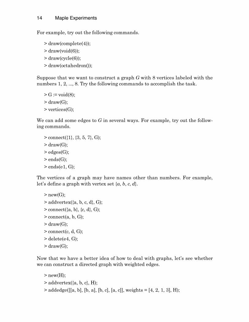
1. Use the help system to find out more about the “connect” and “addedge” functions. Suppose G is the following weighted graph.
c
b
a d
15 10
55
10
a. Construct G by using the connect function to create the edges. Don’t worry about the orientation of the graph that Maple draws.
b. Construct G by using the addedge function to create the edges. Again, don’t worry about the orientation of the graph that Maple draws.
2. Use the help system to find out about the “show” command. Use it on the graph G in the preceding experiment. Try to figure out the meanings of the various parts of the output.
3. Use the help system to find out about two commands in the networks package that you have not yet used. Try them out.
1.6 Spanning Trees We can use Maple to compute spanning trees for finite graphs. Recall that a spanning tree for a connected graph is a subgraph that is a tree and contains all the vertices of the graph. A minimal spanning tree for a connected weighted graph is a spanning tree such that the sum of the edge weights is minimum among all spanning trees. Try out the following Maple commands to discover the main ideas.
> with(networks);
> new(G); > addvertex({a, b, c}, G); > addedge([[a, b], [b, a], [b, c], [a, c]], weights = [4, 2, 1, 3], G); > draw(spantree(G)); > spantree(G, a, w);
16 Maple Experiments
> draw(%); > w; > spantree(G, a, w); > unassign(‘w’); > w; > spantree(G, a, w); > w;
Experiments to Perform
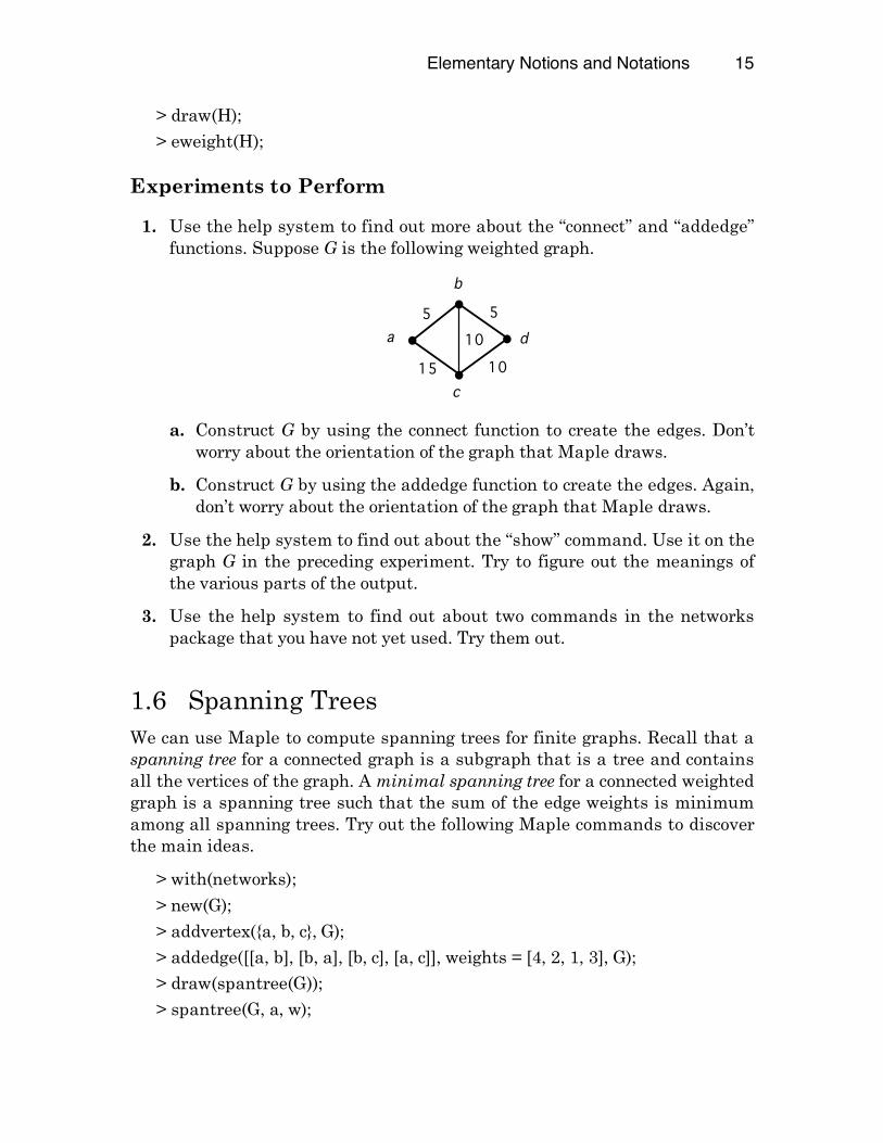
1. Suppose that H is the following weighted graph. Use Maple to find a minimal spanning tree for H.
c
b
a d
15 10
55
10
2. Use the Maple help system to find out about the Petersen graph. Use Maple to construct and draw the graph and to draw a spanning tree for the graph. Note: The Petersen graph is an example of a graph that is not planar.
17
2 Facts About Functions
In this chapter we’ll use Maple to explore some basic ideas about functions presented in Chapter Two of the textbook. We’ll do experiments with se-quences, the map function, composition, if-then definitons, evaluating expres-sions, comparing functions, type checking, and properties of functions.
2.1 Sequences Maple has some useful expressions for working with finite sequences of ob-jects. In Maple a sequence is a listing of objects separated by commas. So a sequence is like a list without the delimiters on the ends. However, we’ll see that, if we wish, we can put delimiters on the ends of a sequence of objects. Try out the following commands to get a feel for some of the techniques that can be used to construct and use sequences.
> seq(i, i=0..9); > seq(hello, i=1..4); > seq({i, i+1}, i=1..5); > seq(i**2 + i, i=1..6); > f := x -> x*x; > seq(f(i), i=3..12); > 3..15; > $3..15; > A := $1..12; > seq(x+x, x=A); > sequence := x -> [$0..x]; > sequence(17); > g := x -> {$-x..x}; > g(5);
18 Maple Experiments
> {$-4..4}; > [$-4..4]; > h := n -> [$-n..n]; > h(5);
Experiments to Perform
1. Suppose that we want to construct the function ƒ defined by
ƒ(n) = [[0, 0], [1, 1], ..., [n, n]].
We can use the seq function to define ƒ as follows:
> ƒ:= n -> [seq([k, k], k=0..n)];
Use Maple to perform three tests of the function.
2. Use the seq function to construct a Maple version of the function g de-fined by
g(n) = [[n, n], ..., [1, 1], [0, 0]].
Use Maple to perform three tests of the function.
3. Use the seq function to construct a Maple version of the function h de-fined by
h(n) = [[n, 0], [n – 1, 1], ..., [1, n – 1], [0, n]].
Use Maple to perform three tests of the function.
4. Use the seq function to construct a Maple version of the function s de-fined by
s(n) = [{0}, {0, 1}, {0, 1, 2}, {0, 1, 2, 3}, ..., {0, 1, 2, 3, ..., n}].
Use Maple to perform three tests of the function.
2.2 The Map Function The map function is a very useful tool for working with functions for which we need several values. Recall that the map function “maps” a function and a list of domain elements onto a list of values. For example, if {a, b, c} is a subset of the domain of ƒ, then
Facts About Functions 19
map(ƒ, [a, b, c]) = [ƒ(a), ƒ(b), ƒ(c)].
Try out the following commands to get used to using Maple’s map function.
> map(abs, [-1, 3, -32, 4]); > map(abs, {1, -1, 2, -2}); > f := x -> x**2; > map(f, [1, 2, 3, 4, 5]); > map(f, [$-5..5]); > map(f, {$-5..5}); > diff(sin(x), x); > diff(cos(x), x); > map(diff, [sin(x), cos(x), tan(x)], x); > map(diff, [1, x, x**2, x**3], x); > f := (x, y, z) -> x**2 + y + z; > map(f, {1, 2, 3}, 4, 5); > newf := x -> f(x[1], x[2], x[3]); > map(newf, {[1, 2, 3], [4, 5, 6]});
Notice the error that occurs when we try to map an infix operation like union.
> map(union, [{a}, {b}], {c});
It can be fixed by enclosing the name in back quotes. Try the following.
> map(`union`, [{a}, {b}], {c}); > map(`union`, {{a}, {b}}, {c}); From the examples it can be seen that for functions of arity n, where n ≥ 2, the map operation must specify the second through the nth arguments that will be used by the function. For example, suppose that g has arity 3. Observe the result of the following command.
> map(g, [a, b, c], x, y);
There is also a map2 operation for functions having arity n, where n ≥ 2. In this case the map2 operation must specify the first argument and the third through the nth arguments. For example, observe the following command and compare its result with the previous command.
> map2(g, x, [a, b, c], y);
20 Maple Experiments
Experiments to Perform
1. Describe how you would use Maple to find the image of a finite subset A of the domain of a function g.
2. Use the map function to define each of the following functions. Be sure to test each definition.
a. The function “heads” maps any list of nonempty lists to a list of the heads of the lists. For example,
heads([[a, b], [a, b, c], [b, d]]) = [a, a, b].
b. The function “tails” maps any list of nonempty lists to a list of the tails of the lists. For example,
tails([[a, b], [a, b, c], [b, d]]) = [[b], [b, c], [d]].
3. Use the map2 function to define the function “dist” that distributes an element x into a list L of elements by creating a list of pairs made up by pairing x with each element of L. For example,
dist(x, [a, b, c]) = [[x, a], [x, b], [x, c]].
Hint: Suppose that we define the function pair that makes a 2-tuple out of its two arguments. E.g., suppose that pair(x, y) = [x, y]. Now use pair in your construction of dist.
2.3 Function Compositions Maple allows us to define functions by composition either with variables or without variables. Note that Maple uses the symbol @ instead of ° to denote composition. Try out the following examples to see how composition of func-tions can be used with Maple.
> f := x -> x + 1; > g := x -> x**2; > f(g(x)); > (f@g)(x); > g(f(x)); > (g@f)(x); > h := g@ƒ; > k := ƒ@g;
Facts About Functions 21
> h(x); > k(x);
Of course, we could also define h and k using variables as follows.
> h := x -> g(f(x)); > k := x -> f(g(x)); > h(x); > k(x);
It’s easy to see that composition is not commutative in general. For example, we can plot the graphs of g@ƒ, ƒ@g, and the difference g@ƒ – ƒ@g. Try out the following tests.
> plot(h(x), x = 0..10); > plot(k(x), x = 0..10); > plot(h(x) - k(x), x = 0..10);
Experiments to Perform
1. Define two new different numeric functions ƒ and g of your own choosing and do the following things.
a. Construct and test both ƒ@g and g@ƒ to see whether they are equal.
b. Plot the graphs of ƒ@g and g@ƒ.
2. The operations cons, hd, and tl that we defined in (1.3 List Operations) are related by the following equation for all nonempty lists x.
cons(hd(x), tl(x)) = x.
a. Test this equation on several lists using the evalb operation.
b. If we let g(x) = (hd(x), tl(x)) and h = cons@g, then we can rewrite the given equation as h(x) = x for all nonempty lists x. Define g and h as Maple functions and then test the rewritten version of the equation on several lists using the evalb operation.
2.4 If-Then-Else Definitions for Functions When a function is defined by cases, we can use the if-then-else form to imple-ment the function in Maple. For example, suppose that we want to define an absolute value function. Although Maple already has the “abs” function to do
22 Maple Experiments
the job, we’ll define our own version. The absolute value function, which we’ll call “absolute” can be defined by cases as follows:
!
absolute(x) =x if x " 0
#x if x < 0
$ % &
We can implement this case definition in Maple as follows:
> absolute := x -> if x >= 0 then x else –x fi;
The if-then-else rule can be used more than once if there are several cases in a definition. For example, suppose we want to classify the roots of a quadratic equation having the following form:
ax2 + bx + c = 0.
We can define the function “classifyRoots” to give the appropriate statements as follows:
classifyRoots(a, b, c) = if b2 – 4ac > 0 then “The roots are real and distinct.” else if b2 – 4ac < 0 then “The roots are complex conjugates.” else “The roots are real and repeated.” We can implement the definition in Maple as follows. (Note that elif is used for “else if,” and backward quotes enclose strings.)
> classifyRoots := (a, b, c) -> if b*b - 4*a*c > 0 then `The roots are real and distinct.` elif b*b - 4*a*c < 0 then `The roots are complex conjugates.` else `The roots are real and repeated.` fi;
Experiments to Perform
1. Test the abs and classifyRoots functions. Your tests should include a va-riety of inputs to test all possible cases of each definition.
Facts About Functions 23
2. We can define a function “max2” to return the maximum of two numbers as follows.
max2 := (x, y) -> if x < y then y else x fi;
Test max2 on several pairs of numbers. Then for each of the following conditions, write and test a definition for the function “max3” to return the maximum of three numbers.
a. Use max2 to define max3.
b. Write an if-then-else definition for max3 that does not use any other functions.
2.5 Evaluating Expressions Although Maple is very good at symbolic manipulation, it is still just a com-puter program that is not quite as intelligent as a normal human being. When evaluating expressions Maple sometimes needs some guidance from us. For example, try out the following statements.
> 1/2; > eval(1/2); > eval((1+3)/2); > evalf(1/2); > evalf((1+3)/2); > simplify(1/2); > simplify((1+3)/2); > g := log[2]; > g(16); > simplify(g(16)); > evalf(g(16)); > plot(g(x), x=1..16); > map(g, {$1..16}); > map(g, [$1..16]);
In this experiment we’ll consider a property of binary trees. We know that among the binary trees with n nodes, the minimum depth that any tree can have is floor(log2 n). We’ll call this function minDepth and write it as the com-position
minDepth = floor ° log2.
24 Maple Experiments
This function can be implemented in Maple as follows:
> minDepth := floor @ log[2];
Experiments to Perform
1. Find out about minDepth by doing the following experiments.
a. Plot minDepth over the values 1..16.
b. Find the image of the set {1, 2, ..., 16} by minDepth.
c. Find the list of values of minDepth when applied to elements in the list [1, 2, ..., 16].
2. As (1) shows, Maple doesn’t give us the kind of answers that we want for minDepth. We want to redefine minDepth so that it gives us integer val-ues. Suppose we try the following definition.
> newMinDepth := floor @ evalf @ log[2].
a. Test newMinDepth by performing the three tests of (1).
b. What is wrong with the new definition of minDepth?
c. Try to redefine minDepth as a composition of functions, without vari-ables, so that it correctly returns all values as integers. Test your definition with at least the three tests used in (1).
2.6 Comparing Functions Functions can usually be defined in many different ways. So it is useful to be able to easily compare definitions to see whether they define the same func-tion over various sets. For example, the following two definitions both claim to test whether an integer is even.
> f := x -> if x mod 2 = 0 then true else false fi;
> g := x -> if 2 * floor(x/2) = x then true else false fi;
We can compare results of the two functions by constructing a function to do the comparing.
> compare := x -> if f(x) = g(x) then true else false fi;
Facts About Functions 25
For example, we can test the two functions to see whether they are equal on the set {0, 1, ..., 20} with commands such as
> map(compare, {$0..20}); or > map(compare, {seq(i, i=0..20)});
If the result is {true}, then things are OK over the set {0, 1, ..., 20}. If the result is {true, false}, then there are problems that can be examined by using a list to check where the two definitions differ.
> map(compare, [$0..20]);
Experiments to Perform
1. An alternative to the if-then-else comparison for two functions ƒ and g is to use evalb as follows.
> compare := x -> evalb(f(x) = g(x));
Try out this definition of compare by repeating the sample tests.
2. In addition to the floor function, Maple has a ceiling function, ceil, and a truncation function, trunc. Try out the following tests to observe the dif-ferences between these functions
> floor(-3.1); > floor(5.9); > ceil(-3.1); > ceil(5.9); > trunc(-3.1); > trunc(5.9);
a. The three functions are all equal on integer arguments. Verify this fact over the set {-50, -49, ..., 49, 50}.
b. Each of the three functions differs from the other two for certain sets of non-integer arguments. For example, we can compare ceil and trunc on a set of rational numbers that are not integers as follows.
> compare := x -> evalb(ceil(x) = trunc(x)); > map(compare, {seq(x + 0.5, x = -10..10)});
Test each of the pairs of functions {floor, ceil}, {floor, trunc}, and {ceil, trunc} to find and verify the sets of non-integer arguments for which they are equal and for which they are not equal.
26 Maple Experiments
3. The function ƒ below claims to define the mod function.
> ƒ := (x, n) -> x - n*floor(x/n);
Compare ƒ with Maple’s mod function. Do they agree? If not, describe the differences between the two functions.
4. Write two different definitions for a function to test whether a number is odd. Test your definitions to make sure that they agree on the numbers in the set {-1000, ... 1000}.
2.7 Type Checking There are many predefined types in Maple. To check whether an expression E has type T we write a query of the form
> type(E, T).
Try out the following Maple commands to get a feel for type checking.
> type(2, integer); > type(1.5, integer); > type(xy, string); > type(9, string); > type(“9”, string); > type(4, {string, integer}); > type(xy, {string, integer});
Experiments to Perform
1. Use Maple’s help system to learn about the types numeric, realcons, and rational. Do some tests to show how these types differ from each other.
2. Use Maple’s help system to discover five other types. For each of the five types, do two tests: one true and one false.
3. Define your own ceiling function “ceil2” as an if-then-else definition that uses at least one type expression. You may use Maple’s trunc function in your definition. But you may not use Maple’s floor and ceil functions. Test the definition by comparing it with the ceil function. Test it not only on integers, but on other numbers too. For example, you might try the fol-lowing comparison.
> compare := x -> evalb(ceil(x/2) = ceil2(x/2));
Facts About Functions 27
> map(compare, {$-20..20});
4. Define your own floor function “floor2” as an if-then-else definition that uses at least one type expression. You may use Maple’s trunc function in your definition. But you may not use Maple’s floor and ceil functions. Be sure to test the definition by comparing it with the floor function. Test it not only on integers, but on other numbers too.
5. Use Maple’s help system to learn about “error”. Then redefine your cons, hd, and tl functions to return error messages in the following cases.
a. cons returns an error if the second argument is not at list.
b. hd returns an error if the argument is the empty list or not alist .
c. tl returns an error if the argument is the empty list or not alist .
2.8 Properties of Functions Maple can sometimes help us tell whether a function is injective, surjective, or bijective. For example, suppose we want to study properties of the function ƒ defined by the expression
!
ƒ(x) =1
x +1.
Over the real numbers, ƒ is defined everywhere except x = –1. We can get an idea about ƒ by looking at its graph at various intervals using the plot func-tion. To see whether ƒ is injective we must see whether x ≠ y implies ƒ(x) ≠ ƒ(y) for all x and y in the domain of ƒ. In other words, using the contrapositive statement, we want to see whether ƒ(x) = ƒ(y) implies x = y. The following Maple command will do the job. That is, solve the equation ƒ(x) = ƒ(y) for x and see if the answer is y.
> solve(f(x) = f(y), x);
Since Maple returns y, we know that ƒ is injective. What about surjective? In this case we want to see if any element y in the codomain of ƒ is equal to ƒ(x) for some x in the domain of ƒ. So we would like to solve the equation ƒ(x) = y for x, which we can do in Maple with the follow-ing command.
> solve(f(x) = y, x);
28 Maple Experiments
Maple returns an expression for x. We can test whether ƒ maps the expression to y with the following Maple command.
> f(%);
Now simplify the result to see whether it is equal to y:
> simplify(%);
The result is y. So things look good so far. Any problems with x = – 1?
Experiments to Perform
1. Use Maple to see whether each of the following functions is injective, sur-jective, or bijective.
a. ƒ(x) = x/(x + 1).
b. ƒ(x) = x/(1 – x).
c. ƒ(x) = (1 – x)/x.
29
3 Construction Techniques
In this chapter we’ll use Maple to explore some of the basic ideas about the construction of recursively defined functions and inductively defined sets pre-sented in Chapter Three of the textbook. We’ll do experiments with lists, strings, trees, and sets.
3.1 Examples of Recursively Defined Functions It’s easy to translate definitions for recursively defined functions into Maple. For example, suppose we have the following recursive definition of the func-tion to concatenate two lists:
concat([ ], y) = y concat(h :: t, y) = h :: concat(t, y).
We can easily convert this definition into a Maple if-then-else program as fol-lows, where cons, hd, and tl are the user defined functions from (1.3 List Op-erations):
> concat := (x, y) -> if x = [ ] then y else cons(hd(x), concat(tl(x), y)) fi;
For example, try out the following command.
> concat([a, b, c], [d, e]);
To see how the recursion unfolds we need to do a trace.
> trace(concat);
30 Maple Experiments
> concat([a, b, c], [d, e]);
Experiments to Perform
1. Consider the following definition of a function ƒ to compute floor(x/2) for any natural number x. In other words, ƒ(x) = floor(x/2).
> ƒ := x -> if x = 0 or x = 1 then 0 else 1 + ƒ(x – 2) fi;
a. Test ƒ to see whether it computes floor(x/2) for x a natural number.
b. Trace ƒ to observe the unfolding of the recursion.
c. What happens when ƒ is applied to a non-natural number?
2. The following function returns the sum of a list of numbers, where we as-sume that an empty sum is zero.
total([ ]) = 0 total(h :: t) = h + total(t).
A Maple implementation of total can be defined as follows:
total := x -> if x = [] then 0 else hd(x) + total(tl(x)) fi;
Test total on several lists of numbers. For example,
> total([3, 2, 9 , 5.34]); > total([$1..10]);
Trace total on a list of numbers to observe the unfolding of the recursion.
3. The function “last” finds the last element of a non-empty list.
last([x]) = x last(h :: t) = last(t).
Construct a Maple definition for last. Notice that the basis case is for a list with one element, which can be described as a list whose tail is the empty list. Test it on several examples and use the trace command on one test to observe the recursion.
4. Construct a recursive Maple program—and test it—for the “small” func-tion, which returns the smallest element of a nonempty list of numbers. For example, small([9, 78, 5, 38]) returns 5.
5. Construct a recursive Maple program—and test it—for the “first” func-
Construction Techniques 31
tion, which removes the rightmost element of a nonempty list. For exam-ple, first([a, b, c]) returns [a, b].
6. Construct a recursive Maple program—and test it—for the “pairs” func-tion, which takes two lists of equal length and outputs a list consisting of the corresponding pairs from the two input lists. For example, pairs([a, b, c], [1, 2, 3]) returns [[a, 1], [b, 2], [c, 3]].
7. Construct a recursive Maple program—and test it—for the “dist” func-tion, which takes an element and a list and outputs a list of pairs made up by distributing the given element with each element of the list. For example, dist(x, [a, b, c]) returns [[x, a], [x, b], [x, c]].
8. Construct a recursive Maple program—and test it—for the “prod” func-tion, which takes two lists and outputs the product of the two lists. For example, prod([1, 2], [a, b, c]) returns the list
[[1, a], [1, b], [1, c], [2, a], [2, b], [2, c]].
Hint: The dist function might be helpful.
3.2 Strings and Palindromes Recall that a palindrome is a string that equals itself when reversed. For ex-ample, the string aba is a palindrome. In Maple the string of digits 101 is considered a number. To make it into a string we can give the command > convert(101, string); Then we can treat the result as a string and test whether it is a palindrome. The following function “pal” is a test to see whether it’s input—either a string or a number considered as a string of digits—is a palindrome. The functions F, L, and M return the first character of a string, the last character of a string, and the middle of a string, respectively.
pal := x -> if type(x, string) then if length(x) <= 1 then true elif F(x) = L(x) then pal(M(x)) else false fi else pal(convert(x, string)) fi;
32 Maple Experiments
Experiments to Perform
1. Write the definitions for F, L, and M. Then test pal on several strings and numbers.
2. The convert operation in Maple can be used to find the binary represen-tation of a natural number. For example,
> convert(45, binary);
returns the number 101101.
Notice that the binary string is a palindrome. Write a program “pals” to construct a list of the first n natural numbers whose binary representa-tions are palindromes. For example,
> pals(4);
returns the list [0, 1, 3, 5]. Test pals and see if you can find some rela-tionships between or properties of these numbers.
3.3 A Recursively Defined Sorting Function As another example of a recursively defined function, we’ll write a sorting function for a list of numbers. The idea we’ll use is sorting by insertion, where the head of the list is inserted into the sorted version of the tail of the list. For the moment, we’ll assume that “insert” does the job of inserting an element into a sorted list. We’ll use the name “isort” because Maple already has its own “sort” function.
> isort := x -> if x = [ ] then x else insert(hd(x), isort(tl(x))) fi;
Of course, we can’t test this definition until we write the definition for the in-sert function. This function inserts an element into a sorted list by comparing the element with each member of the list until it reaches a larger element or the end of the list, at which time the element is placed in the proper position. Here’s a definition for the insert function in if-then-else form:
> insert := (a, x) -> if x = [ ] then [a] elif a <= hd(x) then cons(a, x) else cons(hd(x), insert(a, tl(x))) fi;
Construction Techniques 33
Now we can test both the insert function and the isort function.
> insert(7, [1, 4, 9, 14]). > isort([4, 9, 3, 5, 0]);
Experiments to Perform
1. Perform several tests of insert and isort. Do at least one trace for each function to see what is going on.
2. What happens if we insert an element in a list that is not sorted?
3. Modify the definition of insert by replacing =< with <. Try out some tests to demonstrate what happens. Is one version more efficient than the other?
3.4 Binary Trees Binary trees are inherently recursive in nature. In this experiment we’ll see how binary trees can be created, searched, and traversed by simple recursive algorithms. We’ll represent binary trees as lists, where the empty binary tree is the empty list and a nonempty binary tree is a list of the form
[L, x, R],
where L is the left subtree, x is the root, and R is the right subtree. We can construct a binary search tree from a list of numbers as follows:
build([ ]) = [ ] build(H :: T) = insert(H, build(T))
where insert takes a number and a binary search tree and returns a new bi-nary search tree that contains the number.
insert(x, [ ]) = [[ ], x, [ ]]
insert(x, [L, y, R]) = if x ≤ y then [insert(x, L), y, R] else [L, y, insert(x, R]]
Experiments to Perform
1. Implement and test “build” and “insert” as Maple functions. To do this you will need to be able to pick out the root and the left and right sub-trees of a nonempty binary tree. Test them on several lists.
34 Maple Experiments
2. The form of the binary search trees is not inviting. To see the information in a binary search tree we can traverse it by one of the standard methods, preorder, inorder, and postorder. For each of these orderings, write a pro-cedure to print out the values of the nodes.
3. Build and test a Maple function “isIn” to see whether a number is in a binary search tree.
3.5 Type Checking for Inductively Defined Sets In this experiment we’ll see how to construct types that are inductively de-fined sets. A couple of examples should suffice to get the idea. For example, suppose that we have a set S that is inductively defined as follows.
Basis: 2 ∈ S. Induction: If x ∈ S then x + 3 ∈ S.
To build our own type checker for S we make the following definition, which will allow us to use Maple’s type function.
> `type/S` := x -> if not type(x, integer) then false elif x < 2 then false elif x = 2 then true else type(x - 3, S) fi;
Now we can check to see whether an expression has type S by using Maple’s type function. For example, try out the following commands. > type(2, S); > type(3, S); > type(2+3, S); For another example, suppose that T is a set of lists that has the following inductive definition.
Basis: [ ] ∈ T. Induction: if x ∈ T then cons(a, x) ∈ T.
As in the previous example, we can build our own type checker for T, which is given as follows.
Construction Techniques 35
> `type/T` := x -> if not type(x, list) then false elif x = [ ] then true elif hd(x) = a then type(tl(x), T) else false fi;
Experiments to Perform
1. Write down an informal description of the set S. Then perform some tests to see whether the type function tests for membership in the set S that you described. For example, you might try some tests like the follow-ing to see what happens.
> map(type, [$1..10], S);
2. Write down an informal description of the set T. Then perform some tests to see whether the type function tests for membership in the set T that you described.
3. Let A be the set defined inductively as follows:
Basis: 0 ∈ A. Induction: if x ∈ A then 2x + 1 ∈ A.
a. Write down an informal description of A.
b. Define A as a Maple type function and then test your definition to see whether it works properly to test membership in the set A that you described.
3.6 Inductively Defined Sets In this experiment we’ll look at some ways to pick out elements or subsets of elements from an inductively defined set. For example, if an inductively de-fined set has a single basis element and a single construction rule, then it’s easy to define a function to select the nth element of the set. For example, suppose that S is defined inductively as follows.
Basis: 2 ∈ S. Induction: If x ∈ S then x + 3 ∈ S.
Let getS(n) return the nth element of S. We can define getS as follows in Ma-ple:
getS := n -> if n = 1 then 2 else getS(n – 1) + 3 fi;
36 Maple Experiments
Now we can compute the individual elements of S. For example, try out the following commands.
> getS(1); > getS(35);
We can use the map function to find various subsets of S. For example, try out the following command to obtain the first 10 elements of S.
> map(getS, {$1..10});
Experiments to Perform
1. Let A be the set of elements defined inductively as follows.
Basis: 0 ∈ A. Induction: if x ∈ A then 2x + 1 ∈ A.
Define getA and then use it to generate some elements of A and some subsets of A.
2. Let T be the set of elements defined inductively as follows.
Basis: [ ] ∈ T. Induction: if x ∈ T then cons(a, x) ∈ T.
Define getT and then use it to generate some elements of T and some subsets of T.
3.7 Subsets and Power Sets Sets are represented in Maple in such a way that the elements can be ac-cessed. But the ordering of elements in a set is based on the internal ad-dresses of expressions, which may differ from machine to machine. For exam-ple, try out the following commands. > A := {a, c, c, b, b, d}; > B := {a, b, d, x}; > C := {c, c, b, d, a}; > {a, b}; > {b, a};
We can still work with sets and access elements of a set as long as we don’t
Construction Techniques 37
rely on a specific ordering of the elements. Try out the following commands.
> A := {a, b, c, d, e}; > nops(A); > op(A); > A[1]; > A[3]; > {A[1]}; > A[2..4]; > {A[2..4]}; The head and tail functions defined for lists should also work for sets because Maple stores the elements of a set by a fixed internal ordering of expressions. For example, try out the following commands. > hd := x -> x[1]; > tl := x -> x[2..nops(x)]; > hd(A); > tl(A); If we want to construct a set similar to a list, then we’ll need a different defi-nition for cons. > setCons := (x, S) -> {x, op(S)}; > setCons(a, {b, d, x}); With this definition the following equation should hold for all sets S.
S = setCons(hd(S), tl(S)).
For example, we can use evalb to test the equation for any particular set. Try out the following commands.
> S := {1, 5, b, a}; > evalb(A = setCons(hd(A), tl(A)));
38 Maple Experiments
Experiments to Perform
1. Construct a recursive definition for the “subset” function, which deter-mines whether one set is a subset of another. For example, the Maple command
> subset({a, b}, {b, c, a, d});
should return true. Be sure to give your definition a good test.
2. Construct a recursive definition for the “power” function, where power(S) returns the power set of the finite set S (the set of all subsets of S). For example,
> power({a, b});
should return the set consisting of all four subsets of {a, b}. Be sure to give your definition a good test. Hint: Notice that the map and map2 functions can be used to add an element to each set in a collection of sets. For example, either of the commands
> map2(`union`,{a} , {{ }, {b}, {c}, {b, c}}); or
> map(`union`, {{ }, {b}, {c}, {b, c}}, {a});
will return the set {{a}, {a, b}, {a, c}, {a, b, c}}.
3. (Efficiency considerations). Try out the following tests to verify that ac-tual parameters are passed by value (i. e., evaluated before being passed).
> g:= x -> [power(x), power(x)]; > h := x -> [x, x]; > j := x -> h(power(x)); > A := {$1..10}; > time(h(power(A))); > time(j(A)); > time(g(A));
Why do these tests indicate that parameters are passed by value?
39
4 Binary Relations
In this chapter we’ll use Maple to explore some of the basic ideas about binary relations presented in Chapter Four of the textbook. We’ll do experiments with composition, closure, and order.
4.1 Composing Two Binary Relations In this experiment we’ll see how to construct the composition of two binary re-lations. If we are given two binary relations R and S, the composition R ° S is defined as follows.
R° S = { [a, c] | there is a value b such that [a, b] ∈ R and [b, c] ∈ S}.
We’ll let “compose” be the function that returns the composition of two finite binary relations. So compose(R, S) returns the composition R° S. Here’s a way to construct compose(R, S). If R ≠ { }, then we can take the first pair of R, say [a, b], and look through S for those pairs whose first com-ponent is b. Whenever a pair [b, c] occurs in S, we put the pair [a, c] in our composition set. Once this has been done, we can apply the same procedure to the tail of R and union the two sets to get the desired composition. We’ll let the function getPairs do the job of composing a singleton pair from R with S. In other words, getPairs has the definition
getPairs([a, b], S) = {[a, c] | There is a pair [b, c] ∈ S}.
Assuming that we have written a Maple definition for getPairs, we can write the Maple definition for compose as follows.
40 Maple Experiments
> compose := (R, S) -> if R = { } then { } else getPairs(hd(R), S) union compose(tl(R), S) fi;
Experiments to Perform
1. Write a Maple definition for the function getPairs. For example, the Ma-ple command
> getPairs([a, b], {[b, c], [c, d], [b, d]});
should return the set {[a, c], [a, d]}. Be sure to test getPairs on several ex-amples.
2. Now test the compose function on several pairs of binary relations. For example, define the following relations.
> less := {[1, 2], [1, 3], [1, 4], [2, 3], [2, 4], [3, 4]};
> greater := {[4, 3], [4, 2], [4, 1], [3, 2], [3, 1], [2, 1]};
> equal := {[1, 1], [2, 2], [3, 3], [4, 4]};
Perform tests to compute the following nine compositions.
less ° less less ° equal less ° greater
equal ° less equal ° equal equal ° greater
greater ° less greater ° equal greater ° greater
4.2 Constructing Closures of Binary Relations In this experiment we’ll be concerned with techniques to construct the three famous closures of a binary relation: reflexive, symmetric, and transitive. We’ll start with the reflexive closure of a binary relation R over the set A, which is defined as the following set.
R ∪ {[a, a] | a ∈ A}.
To compute this set we need to construct the equality relation for a set A, which we’ll denote by eq(A). A definition for eq can be given as follows.
> eq := A -> if A = { } then { } else {[hd(A), hd(A)]} union eq(tl(A)) fi;
For example, try out the following test.
Binary Relations 41
> B := {a, b, c}; > eq(B);
With the means to find the equality relation for a set, it’s an easy matter to find the reflexive closure of a binary relation R over a set A, which we’ll denote by rc(R, A). A definition for rc can be written as follows.
> rc := (R, A) -> R union eq(A);
For example, we’ll compute the reflexive closure of a binary relation.
> R := {[a, b], [b, c], [c, a]}; > C := rc(R, {a, b, c});
Now let’s consider the symmetric closure of a binary relation R, which is de-fined as the following set.
R ∪ {[a, b] | [b, a] ∈ R}.
To compute this set we’ll need to compute the converse of a binary relation R, which we’ll denote by converse(R). A definition for converse can be written as follows.
> converse := R -> if R = { } then { } else {[hd(R)[2], hd(R)[1]]} union converse(tl(R)) fi;
With the means to find the converse of a relation, it’s an easy matter to find the symmetric closure of a binary relation R, which we’ll denote by sc(R, A). A definition for sc can be written as follows.
> sc := R -> R union converse(R);
Experiments to Perform
1. Test this definition of symmetric closure on the binary relation
R = {[a, b], [b, c], [c, a]}.
Test sc on two other binary relations of your choice.
2. Let comp(R, n) denote the composition of the binary relation R with itself n times. For example, comp(R, 2) = R° R and comp(R, 3) = R° R° R. The
42 Maple Experiments
transitive closure of R over an n-element set, which we denote as tc(R, n) is defined as the following union.
tc(R) = R ∪ R2 ∪ ... ∪ Rn
= comp(R, 1) ∪ comp(R, 2) ∪ ... ∪ comp(R, n).
So the tc function can be defined in terms of the comp function. This al-lows us to make the following definition for tc.
> tc := (R, n) -> if n = 0 then { } else comp(R, n) union tc(R, n – 1) fi;
a. Use “compose” from Section 4.1 to define the comp function. Use the following relation for one of the tests. L = {[0, 1], [1, 2], [2, 3], [3, 4]}.
b. Test tc on at least two binary relations.Use the following relation for one of the tests. L = {[0, 1], [1, 2], [2, 3], [3, 4]}.
3. We know that the smallest equivalence relation containing a binary rela-tion R is tsr(R). For each of the following relations R use Maple to find the smallest equivalence relation containing R. Also test the relation rst(R) to show that the order of application can not be changed.
a. R = { } over the set A = {a, b, c}.
b. R = {[a, b]} over the set A = {a, b, c}.
c. R = {[a, b], [a, c]} over the set A = {a, b, c}.
d. R = {[1, 2], [1, 3], [4, 5], [6, 3]} over the set A = {1, 2, 3, 4, 5, 6}.
4.3 Testing for Closures This experiment considers the problem of testing whether a binary relation is reflexive, symmetric, or transitive. We’ll start by considering ways to test for the reflexive property of a binary relation. Let isReflexive(R, A) test whether the binary relation R over A is reflexive. Here is a definition for the function.
> isReflexive := (R, A) -> if A = { } then true elif member([hd(A), hd(A)], R) then isReflexive(R, tl(A)) else false fi;
This definition just checks to see whether the equality relation for A is a sub-set of R. If we have access to the functions eq and subset from prior experi-
Binary Relations 43
ments, then we can define isReflexive as follows.
> isReflexive := (R, A) -> subset(eq(A), R);
Alternatively, we could use the the fact that a binary relation is reflexive if and only if it equals its reflexive closure. If we have access to the function rc to compute the reflexive closure from the previous experiment, then we can de-fine isReflexive as follows.
> isReflexive := (R, A) -> evalb(R = rc(R, A));
Experiments to Perform
1. Do the following test for each of the three definitions of isReflexive.
> A := {a, b, c}; > R := {[a, a], [a, b], [b, b], [b, c], [c, c]}; > isReflexive(R, A);
Test the three definitions of isReflexive on a binary relation that is not reflexive.
2. Construct a function isSymmetric to test whether a binary relation is symmetric. Test your function on two relations that are symmetric and two relations that are not symmetric.
3. Construct a function isTransitive to test whether a binary relation is transitive. Test your function on two relations that are transitive and two relations that are not transitive.
4.4 Warshall/Floyd Algorithms In this experiment we’ll look at some algorithms to answer questions about binary relations when we think of them in the form of directed graphs. In the process we’ll see another way to compute the transitive closure of a binary re-lation. We’ll construct algorithms that for any pair of vertices i and j in a di-rected graph will answer the following questions.
Is there a path from i to j? What is the length of the shortest path from i to j? What is the shortest path from i to j?
44 Maple Experiments
A directed graph with n vertices will be represented as an n by n adjacency matrix over the set of indices {1, 2, ..., n}. To get used to working with matrices in Maple try out the following commands.
> [[0, 0, 1], [1, 1, 0], [0, 0, 1]]; > a := matrix(%); > evalm(a); > a[3, 2]; > b := matrix(2, 2); > evalm(b); > b[1, 2] := 3; > evalm(b); > for i from 1 to 2 do b[i, i] := 0 od; > evalm(b);
It makes sense to place data like matrices in a file instead of typing them out during a session. For example, create a file named matrixInput with the fol-lowing data.
[[0, 0, 1], [1, 1, 0], [0, 0, 1]];
Then the first line of the preceding Maple commands can be replaced by the following command.
> read matrixInput;
Now the other commands can be performed as before. For example, try out the following commands again.
> a := matrix(%); > evalm(a); > a[3, 2];
We can answer the question, “Is there a path from i to j?” if we have access to the transitive closure of the binary relation representing the directed graph. Warshall’s algorithm computes the transitive closure of a binary relation rep-resented as an adjacency matrix. Here is a Maple version of the algorithm with some preceding comments.
# Warshall's algorithm # The algorithm computes the transitive closure of a binary # relation (digraph) represented as an n by n adjacency. # If M is an n by n adjacency matrix, then the command # > war(M, n); # will output the adjacency matrix of the transitive closure.
Binary Relations 45
war := proc(M, n) local A; A := matrix(n, n); for i from 1 to n do for j from 1 to n do A[i, j] := M[i, j] od od; for k from 1 to n do for i from 1 to n do for j from 1 to n do if A[i, k] = 1 and A[k, j] = 1 then A[i, j] := 1 fi od od od; print(evalm(A)) end;
Experiments to Perform
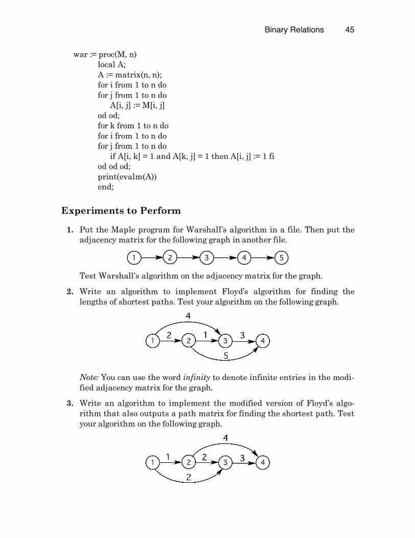
1. Put the Maple program for Warshall’s algorithm in a file. Then put the adjacency matrix for the following graph in another file.
1 2 3 4 5
Test Warshall’s algorithm on the adjacency matrix for the graph.
2. Write an algorithm to implement Floyd’s algorithm for finding the lengths of shortest paths. Test your algorithm on the following graph.
Note: You can use the word infinity to denote infinite entries in the modi-fied adjacency matrix for the graph.
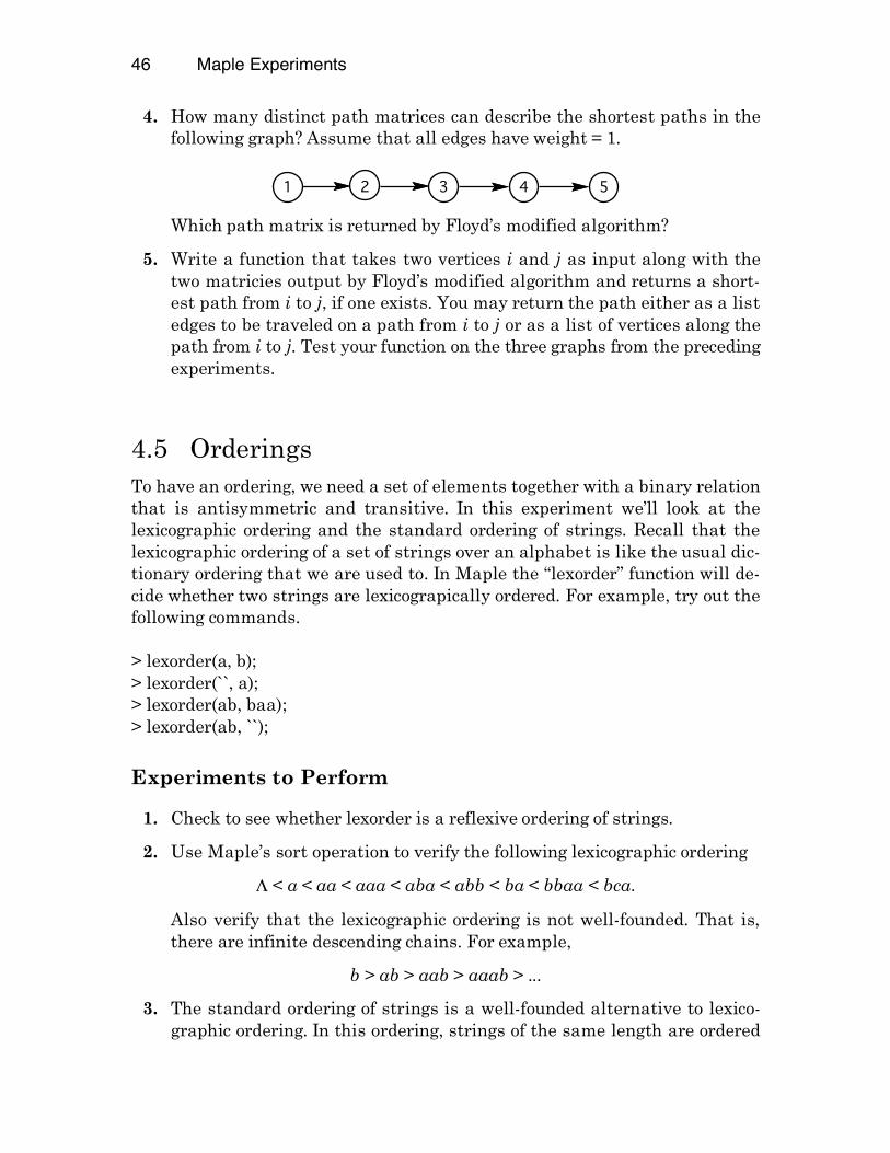
3. Write an algorithm to implement the modified version of Floyd’s algo-rithm that also outputs a path matrix for finding the shortest path. Test your algorithm on the following graph.
46 Maple Experiments
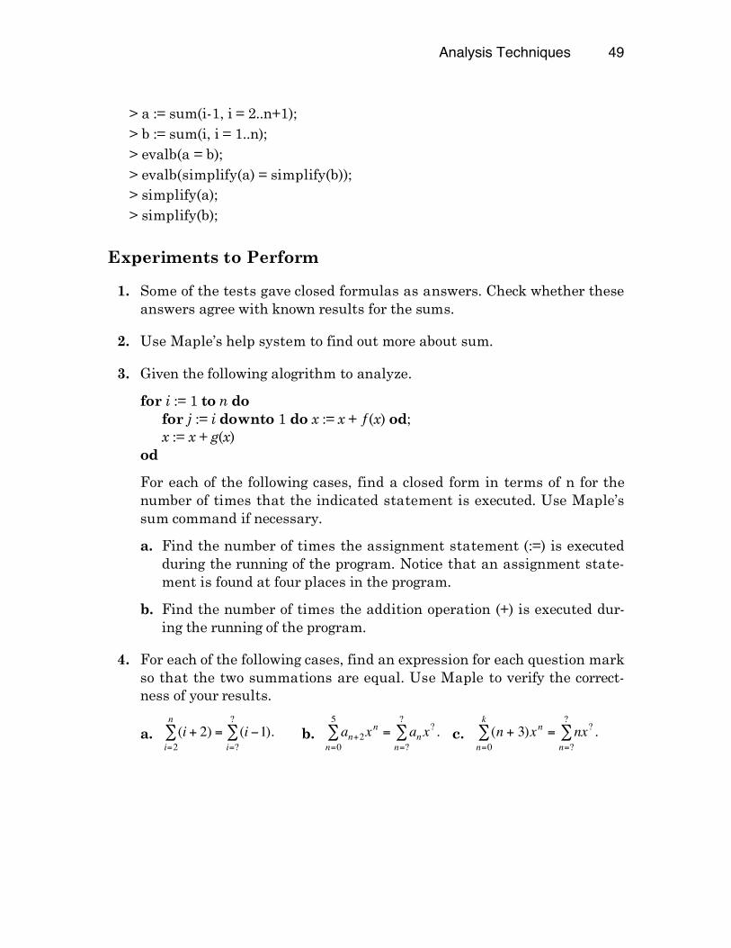
4. How many distinct path matrices can describe the shortest paths in the following graph? Assume that all edges have weight = 1.
1 2 3 4 5
Which path matrix is returned by Floyd’s modified algorithm?
5. Write a function that takes two vertices i and j as input along with the two matricies output by Floyd’s modified algorithm and returns a short-est path from i to j, if one exists. You may return the path either as a list edges to be traveled on a path from i to j or as a list of vertices along the path from i to j. Test your function on the three graphs from the preceding experiments.
4.5 Orderings To have an ordering, we need a set of elements together with a binary relation that is antisymmetric and transitive. In this experiment we’ll look at the lexicographic ordering and the standard ordering of strings. Recall that the lexicographic ordering of a set of strings over an alphabet is like the usual dic-tionary ordering that we are used to. In Maple the “lexorder” function will de-cide whether two strings are lexicograpically ordered. For example, try out the following commands. > lexorder(a, b); > lexorder(``, a); > lexorder(ab, baa); > lexorder(ab, ``);
Experiments to Perform
1. Check to see whether lexorder is a reflexive ordering of strings.
2. Use Maple’s sort operation to verify the following lexicographic ordering
Λ < a < aa < aaa < aba < abb < ba < bbaa < bca.
Also verify that the lexicographic ordering is not well-founded. That is, there are infinite descending chains. For example,
b > ab > aab > aaab > ...
3. The standard ordering of strings is a well-founded alternative to lexico-graphic ordering. In this ordering, strings of the same length are ordered

Binary Relations 47
lexicographically, while strings of different length are ordered by length.
a. Define the operation “std” to decide whether two strings are in stan-dard order.
b. Test std on strings over {a, b, c}. For example, use Maple’s sort with std to verify the standard ordering of the strings in the list
[ba, Λ, a, aba, aa, aaa, abb, bbaa, bca].
4. The lexicographic ordering of ℕ × ℕ is defined by (x1, x2) < (y1, y2) if either
x1 < y1 or x1 = y1 and x2 < y2.
a. Define the operation “lex” to decide whether pairs of natural numbers are lexicographically ordered. For example, lex([1, 2], [2, 0]) is true.
b. Test lex on several pairs of natural numbers. Then use it with the sort operation to sort the list
[[4,0], [0, 2], [1, 1], [0, 1], [1, 0]].
48
5 Analysis Techniques
In this chapter we’ll use Maple to explore some of the basic ideas from Chap-ter Five of the textbook. We’ll do experiments with finite sums, counting, probability, solving recurrences, and orders of growth.
5.1 Finite Sums This experiment looks at various ways that Maple can be used to evaluate finite sums and to find closed forms for finite sums in some cases. Try out the following tests to see how Maple calculates sums. > sum(i, i=1..20); > sum(i, i=1..n); > sum(i*i, i=1..n); > sum(i*i*i, i=1..n); > sum(i*i*i*i, i=1..n); > sum(i*(a**i), i=1..n); > sum('a[k]*x^k','k'=0..n); When dealing with expressions that involve summations it can often be quite useful to change the limits of summation. For example,
!
(i "1)i=2
n+1
# = i
i=1
n
# .
We can use Maple to verify that changes we make in limits of summation are correct. For example, try out the following Maple commands.
Analysis Techniques 49
> a := sum(i-1, i = 2..n+1); > b := sum(i, i = 1..n); > evalb(a = b); > evalb(simplify(a) = simplify(b)); > simplify(a); > simplify(b);
Experiments to Perform
1. Some of the tests gave closed formulas as answers. Check whether these answers agree with known results for the sums.
2. Use Maple’s help system to find out more about sum.
3. Given the following alogrithm to analyze.
for i := 1 to n do for j := i downto 1 do x := x + ƒ(x) od; x := x + g(x) od
For each of the following cases, find a closed form in terms of n for the number of times that the indicated statement is executed. Use Maple’s sum command if necessary.
a. Find the number of times the assignment statement (:=) is executed during the running of the program. Notice that an assignment state-ment is found at four places in the program.
b. Find the number of times the addition operation (+) is executed dur-ing the running of the program.
4. For each of the following cases, find an expression for each question mark so that the two summations are equal. Use Maple to verify the correct-ness of your results.
a.
!
(i + 2)i=2
n
" = (i #1)i=?
?
" . b.
!
an+2x
n
n=0
5
" = anx?
n=?
?
" .
c.
!
(n + 3)xn
n=0
k
" = nx?
n=?
?
" .

50 Maple Experiments
5.2 Permutations In this experiment we’ll use Maple to explore counting with permutations. Try out the following commands to see how maple deals with permutations. > with(combinat); > permute({a, b, c}); > permute({a, b, a}); > permute([r, a, d, a, r]); > permute(4, 2); > numbperm(4, 2);
Experiments to Perform
1. Maple has many combinatorial functions. Explore the package with the following help command.
> ?combinat
Use the help system to find out about three different functions that deal with permutations. Perform some tests.
2. Notice from the examples that when the permute operation is applied to a list of elements it returns bag permutations. For each of the following lists apply the permute operation. Then verify in each case that the number of permutations listed can be computed by the formula for bag permutations.
a. [b, l, o, b].
b. [t, o, o, t].
c. [r, a, d, a, r].
d. [b, a, n, a, n, a].
3. Suppose we want to build a code to represent each of 29 distinct objects with a binary string having the same minimal length n, where each string has the same number of 0’s and 1’s. Somehow we need to solve an inequality like
!
n!
k!k!" 29 ,
where k = n/2. We find by trial and error that n = 8. Try it.
Analysis Techniques 51
5.3 Combinations In this experiment we’ll examine some elementary principles of counting com-binations. For example, try out the following commands to see how Maple deals with combinations. > with(combinat); > binomial(10, 4); > choose({a, b, c}); > choose({a, b, a}); > choose(4, 2); > numbcomb(4, 2); > binomial(4, 2); > sum(binomial(5, i), i = 0..5);
Experiments to Perform
1. Maple has many combinatorial functions. Explore the package with the following help command.
> ?combinat
Use the help system to find out about three different functions that deal with combinations. Perform some tests.
2. How do we really know that the element in the nth row and kth column of Pascal’s triangle is
n
k( )? It depends on the following useful result about binomial coefficients.
!
n
k
"
# $ %
& ' =
n (1
k
"
# $
%
& ' +
n (1
k (1
"
# $
%
& ' .
Use Maple to test this equation for several values of n.
3. Can you find some other interesting patterns in Pascal’s triangle? There are lots of them. For example, look down the column labeled 2 and notice that, for each n ≥ 2, the element in position (n, 2) is the value of the arith-metic sum 1 + 2 + ... + (n – 1). In other words, we have the formula
!
n
2
"
# $ %
& ' =
n(n (1)
2.
Use Maple to test this equation for several values of n.
52 Maple Experiments
4. In how many ways can four coins be selected from a collection of pennies, nickels, and dimes? Let S = {penny, nickel, dime}. Then we need the num-ber of four-element bags chosen from S. The answer is
!
3+ 4 "1
4
#
$ %
&
' ( =
6
4
#
$ % &
' ( =15.
Can you figure out a way to have Maple compute and output a listing of the bags.
5. Design a Maple function that can be used to test the following equation for several values of n.
!
(1)(1)(3)L(2n " 3)
n!2n
=2
n
2n " 2
n "1
#
$ %
&
' ( .
6. Design a Maple function that can be used to test the following equation on several values of n.
!
n
0
"
# $ %
& ' +
n
1
"
# $ %
& ' + ...+
n
n (1
"
# $
%
& ' +
n
n
"
# $ %
& ' = 2
n.
5.4 Error Detection and Correction A binary block code is a set of binary strings that have the same length. Each string is called a code word. The distance between two code words is the num-ber of digits where the two code words differ. For example, the distance be-tween 1011 and 1010 is 1 and the distance between 00110 and 10111 is 2. We can write a Maple function to detect the distance between two code words of the same length as follows, where F and T are functions to return the first character (the head) and the tail of a string, respectively.
dis := (x, y) -> if type(x, string) and type(y, string) then if x = "" then 0 elif F(x) = F(y) then dis(T(x), T(y)) else 1 + dis(T(x), T(y)) fi else dis(convert(x, string), convert(y, string)) fi;
For example, the command
> dis(1001,1111);
Analysis Techniques 53
returns the value 2. If there are leading 0’s in a binary string we need to place double quotes around the string to capture each bit. For example, the com-mand
> dis("0000",1011);
returns the value 3 and the command
> dis("0111", 1000);
returns the value 4
Error Detection Whenever the distance between any two code words is at least 2, the code is a single error-detection code because any word with a single error will not be equal to any of the given code words. For example, suppose our code consists of the following four words.
000, 110, 101, 011.
The distance between any two of these words is 2. If one of the words is transmitted and a single error occurs, then the received word must be one of the following strings
100, 010, 001, 111.
This set of words is disjoint from the given set of code words. One way to construct an error detection scheme is to take any set of code words and add a single “parity” bit to each word, where the bit is 1 if the number of 1’s in the word is odd and 0 otherwise. So the number of 1’s in any code word (including the parity bit) is always even. Thus the distance between any two code words is an even number. For example, suppose we start with the following code of eight words.
000, 001, 010, 011, 100, 101, 110, 111.
Notice that some pairs are distance 1 apart. We’ll add a parity bit on the right of each word to obtain the following code.
0000, 0011, 0101, 0110, 1001, 1010, 1100, 1111.
Notice that each word in this set has an even number of 1’s. So if a single error occurs, then there will be an odd number of 1’s in the received word.
54 Maple Experiments
If we represent a code word as a list of binary digits, then it is easy to check for single errors. For example, the sum of the digits taken modulo 2 will give us the parity of the word. Try out the following Maple commands. > x := [0, 1, 1, 0, 1]; > sum(x[i], i = 1..5) mod 2;
Error Correction A single error can be detected and corrected if the distance between any two code words is at least 3. This follows because if a code word x is transmitted and the result y contains a single error, then the distance between x and y is 1 while the distance between y and any other code word is at least 2. This is an example of the following more general result about error correction.
Whenever a code has the property that the distance between any two code words is at least 2k + 1, then the code is a k-error-correcting code.
One method to create a single error-correction code is to use parity bits. For example, suppose we start with the following code of eight words.
000, 001, 010, 011, 100, 101, 110, 111.
Notice that some pairs are distance 1 apart. We’ll add three parity bits on the right of each word as follows: If C1C2C3 is a three bit string, then construct the six bit string C1C2C3P1P2P3, where
P1 = (C1 + C2) mod 2 P2 = (C1 + C3) mod 2 P3 = (C2 + C3) mod 2
The eight code words with three parity bits added are listed as follows.
000000, 001011, 010101, 011110, 100110, 101101, 110011, 111000.
Notice, with some work, that the distance between any two of these six bit words is at least 3. With this method (due to Hamming), we can detect and correct a single error by recomputing the three parity bits when the word is received. If an er-ror occurred in some parity bit Pi, then that is the only change. If an error oc-curred in one of the bits Ci, then exactly two of the parity bits are wrong. For example, let x = 000000 and suppose that x is transmitted and the code word received is y = 000100. Recomputing the parity bits for y give us the
Analysis Techniques 55
word 000000. The only difference is in the parity bit, which means that the error is in the parity bit. So the correct value of y is 000000. Now suppose that x is transmitted and the code word received is z = 100000. Recomputing the parity bits for z give us the word 100110, which dif-fers from z in exactly two parity bits P1 and P2. This tells us that the an error occurred in one of the bits Ci. But which Ci is in error? Let’s again observe the calculation P1 and P2.
P1 = (C1 + C2) mod 2 P2 = (C1 + C3) mod 2
Notice that there is a common bit in the calculation of P1 and P2, namely C1. That is the key to which bit is in error. So the correct value of z is 000000. If we represent a code word as a list of binary digits, then it is easy to de-tect and correct single errors. To get the idea, try out the following Maple commands. > x := [0, 0, 0, 0, 0, 0];
> y := [1, 0, 0, 0, 0, 0];
> p[1] := (y[1] + y[2]) mod 2;
> evalb(p[1] = y[4]);
Experiments to Perform
1. Write the definitions for the functions F and T. Then try out several tests of the distance function.
2. This experiment deals with adding parity bits to code words.
a. Write a Maple function to transform a binary block code by adding a parity bit to each code word so that the total number of 1's is even. Represent the input and the output as a list of code words, where each code word is represented as a list of binary digits. For example, if addParityBit is the name of the function, then the Maple command
> addParityBit([ [1, 0, 1, 1], [1, 0, 0, 0], [0, 0, 0, 0] ]);
returns the list [ [1, 0, 1, 1, 1], [1, 0, 0, 0, 1], [0, 0, 0, 0, 0] ].
Test your function on this example and on the example list of eight 3-bit code words.
56 Maple Experiments
b. Write a Maple function to take a block code of 3-bit code words and add three parity bits to each word. For example, if addThreeBits is the name of the function, then the Maple command
> addThreeBits([[1, 1, 1], [1, 0, 1]]);
returns the list [ [1, 1, 1, 0, 0, 0], [1, 0, 1, 1, 0, 1] ].
Test your function on this example and on the example set of eight 3-bit code words.
3. Write a function to detect single errors in a list of code words that origi-nally have even parity (i.e., each word has an even number of 1's). The output should be a sublist consisting of those code words with an odd number of 1's. For example, if parityErrors is the name of the function, then the maple command
> parityErrors ([ [1, 0, 1, 1], [1, 0, 1, 0], [0, 0, 1, 0] ]);
returns the list [ [1, 0, 1, 1], [0, 0, 1, 0] ].
a. Test parityErrors on the example input and on another list of your choosing the input of eight 4-bit words.
b. We can use a random number generator to simulate the transmission of a set of code words with the possibility that single errors may occur in some the of words. (See Maple's help ? rand.) Here is a program, called errorTest, to do the job, and to detect which words contain er-rors.
errorTest := proc(L) local X, p, i, s, n; print(L); X := L; p := rand(1..2); for i to nops(X) do if p() = 1 then # Call p(); if it is 1, introduce random error. s := rand(1..nops(X[i])); n := s(); X[i][n] := (X[i][n] + 1) mod 2 fi od; print(X); parityErrors(X) end;
Analysis Techniques 57
Perform the following tests of errorTest. First, call errorTest four times for the input list [ [1, 0, 1, 1, 1], [1, 0, 0, 0, 1], [0, 0, 0, 0, 0] ]. Sec-ond, call errorTest four times for the input list of eight 4-bit code words of even parity.
4 Write two Maple programs, one to detect single errors and one to correct single errors, to process lists of 6-bit code words, where the last three bits are parity bits. For example, if detectErrors is the program to detect single errors, then the Maple command
> detectErrors([ [0, 0, 0, 0, 0, 0], [1, 1, 1, 0, 1, 0], [1, 0, 0, 1, 0, 1] ]);
returns the list [ [1, 1, 1, 0, 1, 0], [1, 0, 0, 1, 0, 1] ].
If we let correctErrors be the program to correct single errors, then the Maple command
> correctErrors( [ [1, 1, 1, 0, 1, 0], [1, 0, 0, 1, 0, 1] ]);
returns the list [ [1, 1, 1, 0, 0, 0], [1, 0, 1, 1, 0, 1] ].
a. Test detectErrors on the example input and then use the output to test correctErrors. Do a second test of the two programs on another list of 6-bit code words,
b. What happens when 2 or more errors occur in some code word?
c. Modify the errorTest program used in (4b) to introduce random single errors in a list of 6-bit code words, where the last three bits are parity bits. The program then calls detectErrors and correctErrors. Perform the following tests of errorTest. First, call errorTest four times for the input list [ [0, 0, 0, 0, 0, 0], [1, 0, 0, 1, 1, 0], [1, 1, 1, 0, 0, 0] ]. Second, call errorTest four times for the input list of all eight 6-bit code words.
5.5 The Birthday Paradox This experiment is designed to test some results of discrete probability by us-ing a random number generator. The “birthday paradox” illustrates that some coincidences are actually probable events. For example, we know that if we choose 23 numbers (e.g., birthdays) at random out of 365 possible numbers (e.g., the days of the year), then the probability that two of the chosen num-bers will be the same is 0.507. For 30 numbers the probability is 0.706, and for 40 numbers the probability is 0.891. Consider the following Maple pro-gram to generate a list of random numbers in the interval 1 to 365.
58 Maple Experiments
number := rand(1..365); birth := N -> [seq(number( ), i=1..N)];
For example, try out the following commands to get used to things.
> number( ); > number( ); > birth(23);
Experiments to Perform
1. It is hard for our eyes to find duplicates in a list of random numbers. But it is not hard to write a program that picks out duplicates, if there are any, from a list of numbers. Let dup(L) return the set of duplicates that occur in the list L. For example,
dup([2, 4, 5, 9, 3, 4, 6, 3, 4, 2]) = {2, 3, 4}.
Let trial(N) return the set of duplicates that occur in a list of N random numbers in the interval 1 to 365. The definition for trial is easy:
trial := dup @ birth.
Your task is to construct and test the function “dup” so that trial works as desired.
2. Test the birthday paradox by doing 10 trials for each of the following val-ues of N. In each case, observe how close the results of the 10 trials come to the actual probabilities.
a. 23 numbers.
b. 30 numbers.
c. 40 numbers.
5.6 It Pays to Switch This experiment is designed to test some results of discrete probability by us-ing a random number generator. Suppose there is a set of three numbers. One of the three numbers will be chosen as the winner of a three-number lottery. We pick one of the three numbers. Later, we are told that one of the two re-maining numbers is not a winner, and we are given the chance to keep the
Analysis Techniques 59
number that we picked or to switch and choose the remaining number. What should we do? We should switch. To see this, notice that once we pick a number, the probability that we did not pick the winner is 2/3. In other words, it is more likely that one of the other two numbers is a winner. So when we are told that one of the other numbers is not the winner, it follows that the remaining other number has probability 2/3 of being the winner. So go ahead and switch. To test this theory consider the following Maple program to generate a list of pairs of random numbers from the set {1, 2, 3}, where we can consider a pair to contain the winning number and the number picked.
number := rand(1..3); pays := N -> [seq([number(),number()], i=1..N)];
For example, try out the following commands to see a few lists of pairs of ran-dom numbers from the set {1, 2, 3}.
> pays(5); > pays(10); > pays(20);
If we always choose to switch, then we count the number of distinct pairs re-turned and divide by the total number of pairs to obtain an idea of how we would fair in such an experiment.
Experiments to Perform
1. It is hard for our eyes to find pairs that are distinct in a large list of pairs of random numbers. Suppose that we have a program “distinct” to take such a list and return the number of pairs that are distinct. For example,
distinct([[1, 3], [1, 1], [3, 2], [1, 2], [2, 2]]) = 3.
Let trial(N) return the number of distinct pairs out of N pairs of random numbers from the set {1, 2, 3}. The definition for trial is easy:
trial := distinct @ pays.
Your task is to construct and test the function “distinct” so that trial works as desired.
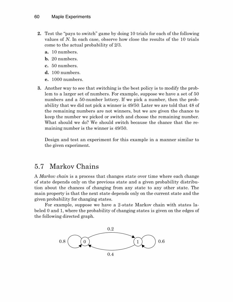
60 Maple Experiments
2. Test the “pays to switch” game by doing 10 trials for each of the following values of N. In each case, observe how close the results of the 10 trials come to the actual probability of 2/3.
a. 10 numbers. b. 20 numbers. c. 50 numbers. d. 100 numbers. e. 1000 numbers.
3. Another way to see that switching is the best policy is to modify the prob-lem to a larger set of numbers. For example, suppose we have a set of 50 numbers and a 50-number lottery. If we pick a number, then the prob-ability that we did not pick a winner is 49/50. Later we are told that 48 of the remaining numbers are not winners, but we are given the chance to keep the number we picked or switch and choose the remaining number. What should we do? We should switch because the chance that the re-maining number is the winner is 49/50.
Design and test an experiment for this example in a manner similar to
the given experiment.
5.7 Markov Chains A Markov chain is a process that changes state over time where each change of state depends only on the previous state and a given probability distribu-tion about the chances of changing from any state to any other state. The main property is that the next state depends only on the current state and the given probability for changing states. For example, suppose we have a 2-state Markov chain with states la-beled 0 and 1, where the probability of changing states is given on the edges of the following directed graph.
1 0.8
0.2
0
0.4
0.6
Analysis Techniques 61
We can represent this graph by a transition matrix P of probabilities. Try out the following Maple command to construct P.
> P := matrix([[.8, .2], [.6, .4]]);
To observe the value of P, just type the command
> evalm(P);
The matrix of probabilities for entering some state after two stages of the process is given by the product P2 = PP. Try out the following command to compute this product.
> evalm(P.P);
The matrix of probabilities for entering a state after three stages of the proc-ess is given by the command
> evalm(P.P.P);
Suppose there is an equal chance of starting the process in either of the two states 0 and 1. In other words, we’ll assume that the initial probability vector is X0 = (0.5, 0.5). We can represent this vector in Maple with the follow-ing command.
> X0 := vector([0.5, 0.5]);
The probability of entering some state after one stage is given by the vector X0P, which we can compute with the command
> evalm(X0.P);
To calculate the probabilities for entering some state after 2, 3, or 4 stages of the process, we can type the following commands.
> evalm(X0.P.P);
> evalm(X0.P.P.P);
> evalm(X0.P.P.P.P);
Notice that these vectors appear to be converging to a particular vector. Let X = (u, v) be the unique probability vector such that XP = X. Try the following command to construct X.
> X := vector([u, v]);
62 Maple Experiments
To calculate XP type the following command.
> evalm(X.P);
Now, we’re in position to solve the equation XP = X, where u + v = 1. Type the following command to solve the resulting set of simultaneous equations for u and v. Note: We are assuming that % refers to the value of the previous vector evalm(X.P).
> solve({%[1] = u, %[2] = v, u +v = 1}, [u, v]);
This is the vector X such that XP = X. The Markov chain theorem tells us that the previous sequence of vectors converges to X. We should note that the value of the initial probability vector X0 does not change the eventual outcome. For example, try out the following tests with X0 = (0.3, 0.7) and observe the sequence converges to X.
> X0 := vector([.3, .7]);
> evalm(X0.P);
> evalm(%.P);
> evalm(%.P);
> evalm(%.P);
Experiments to Perform
1. Use the sample matrix P to compute the sequence
X0P, X0P2, X0P
3, X0P4
for each case and observe the convergence of the sequence to the vector X.
a. X0 = (0.02, 0.98).
b. X0 = (0.98, 0.02).
2. A company has gathered statistics on three of its products A, B, and C. (You can think of A, B, and C as three breakfast cereals, or as three models of automobile, or as any three products that compete with each other for market share.) The statistics show that customers switch be-tween products according to the following transition matrix.
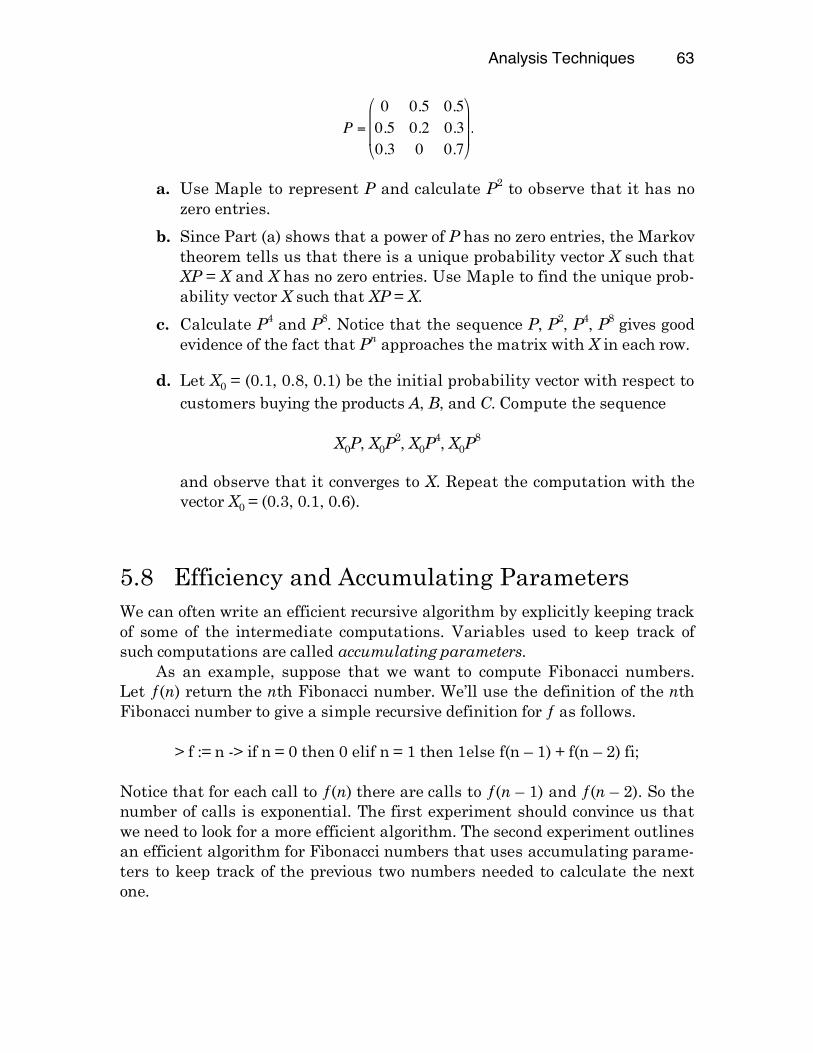
Analysis Techniques 63
!
P =
0 0.5 0.5
0.5 0.2 0.3
0.3 0 0.7
"
#
$ $
%
&
' ' .
a. Use Maple to represent P and calculate P2 to observe that it has no zero entries.
b. Since Part (a) shows that a power of P has no zero entries, the Markov theorem tells us that there is a unique probability vector X such that XP = X and X has no zero entries. Use Maple to find the unique prob-ability vector X such that XP = X.
c. Calculate P4 and P8. Notice that the sequence P, P2, P4, P8 gives good evidence of the fact that Pn approaches the matrix with X in each row.
d. Let X0 = (0.1, 0.8, 0.1) be the initial probability vector with respect to customers buying the products A, B, and C. Compute the sequence
X0P, X0P2, X0P
4, X0P8
and observe that it converges to X. Repeat the computation with the vector X0 = (0.3, 0.1, 0.6).
5.8 Efficiency and Accumulating Parameters We can often write an efficient recursive algorithm by explicitly keeping track of some of the intermediate computations. Variables used to keep track of such computations are called accumulating parameters. As an example, suppose that we want to compute Fibonacci numbers. Let ƒ(n) return the nth Fibonacci number. We’ll use the definition of the nth Fibonacci number to give a simple recursive definition for ƒ as follows.
> f := n -> if n = 0 then 0 elif n = 1 then 1else f(n – 1) + f(n – 2) fi;
Notice that for each call to ƒ(n) there are calls to ƒ(n – 1) and ƒ(n – 2). So the number of calls is exponential. The first experiment should convince us that we need to look for a more efficient algorithm. The second experiment outlines an efficient algorithm for Fibonacci numbers that uses accumulating parame-ters to keep track of the previous two numbers needed to calculate the next one.
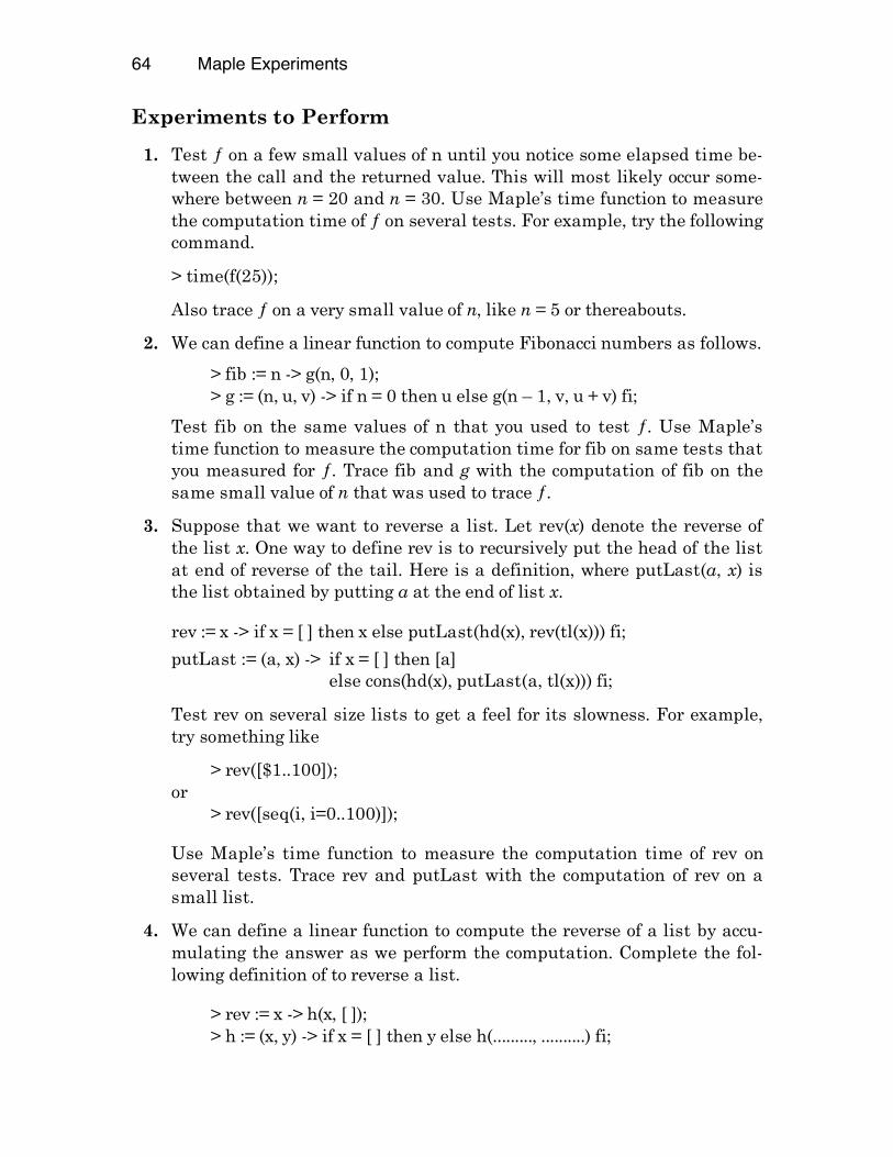
64 Maple Experiments
Experiments to Perform
1. Test ƒ on a few small values of n until you notice some elapsed time be-tween the call and the returned value. This will most likely occur some-where between n = 20 and n = 30. Use Maple’s time function to measure the computation time of ƒ on several tests. For example, try the following command.
> time(f(25));
Also trace ƒ on a very small value of n, like n = 5 or thereabouts.
2. We can define a linear function to compute Fibonacci numbers as follows.
> fib := n -> g(n, 0, 1); > g := (n, u, v) -> if n = 0 then u else g(n – 1, v, u + v) fi;
Test fib on the same values of n that you used to test ƒ. Use Maple’s time function to measure the computation time for fib on same tests that you measured for ƒ. Trace fib and g with the computation of fib on the same small value of n that was used to trace ƒ.
3. Suppose that we want to reverse a list. Let rev(x) denote the reverse of the list x. One way to define rev is to recursively put the head of the list at end of reverse of the tail. Here is a definition, where putLast(a, x) is the list obtained by putting a at the end of list x.
rev := x -> if x = [ ] then x else putLast(hd(x), rev(tl(x))) fi;
putLast := (a, x) -> if x = [ ] then [a] else cons(hd(x), putLast(a, tl(x))) fi;
Test rev on several size lists to get a feel for its slowness. For example, try something like
> rev([$1..100]); or > rev([seq(i, i=0..100)]);
Use Maple’s time function to measure the computation time of rev on several tests. Trace rev and putLast with the computation of rev on a small list.
4. We can define a linear function to compute the reverse of a list by accu-mulating the answer as we perform the computation. Complete the fol-lowing definition of to reverse a list.
> rev := x -> h(x, [ ]); > h := (x, y) -> if x = [ ] then y else h(........., ..........) fi;
Analysis Techniques 65
Test your new definition of rev on the same lists that you used to test the previous version. Use Maple’s time function to measure the computation time for rev on same tests that you used for the previous version. Trace rev and h with the computation of rev on the same small list that was used to trace the previous rev and putLast.
5.9 Solving Recurrences Maple can help us find closed form solutions for some recurrences. To intro-duce the ideas we’ll start out with a simple recurrence like the following.
x0 = 1 xn = 2xn–1 + 3n.
Try to solve this recurrence by hand to find a closed form solution. Then check your answer with Maple by typing the following expression:
> rsolve({x(0) = 1, x(n) = 2*x(n-1) + 3*n}, x);
To assign x(n) the value of the expression returned by Maple, we type the fol-lowing command:
> x := unapply(%, n);
Now we can compute some values of x. For example, try out the following commands.
> x(0); > x(1); > x(2);
Some recurrences have solutions that are complicated expressions. Maple of-ten needs help in evaluating such expressions. The following commands can be useful in such cases.
simplify, expand, numer, and denom.
For example, let’s consider the Fibonacci numbers. The nth Fibonacci number Fn is given by the following definition.
F0 = 0 F1 = 1 Fn = Fn – 1 + Fn – 2
66 Maple Experiments
We can solve this recurrence with the following Maple command.
> rsolve({F(0) = 0, F(1) = 1, F(n) = F(n – 1) + F(n – 2)}, F);
The resulting expression is quite complicated. We can try to simplify it with the command
> simplify(%);
Now let’s try to find some values of F. To assign F(n) the value of the expres-sion returned by Maple, we type the following command.
> F := unapply(%, n);
Now we can compute some values of F. For example, try out the following commands.
> F(0); > F(1);
The expression for F(1) is not satisfactory. We can try to simplify it with the command
> simplify(%);
Let’s try the following command to expand the denominator of this expression:
> numer(%)/expand(denom(%));
If we find that a particular combination of commands works well and we wish to use them over and over, then it makes sense to construct a function to do the job. For example, if we want to use the preceding command more than once, we could define a function like the following.
> mySimp := x -> numer(x)/expand(denom(x));
Then we could simply give the following command each time we wanted to ex-pand the denominator of an expression.
> mySimp(%);
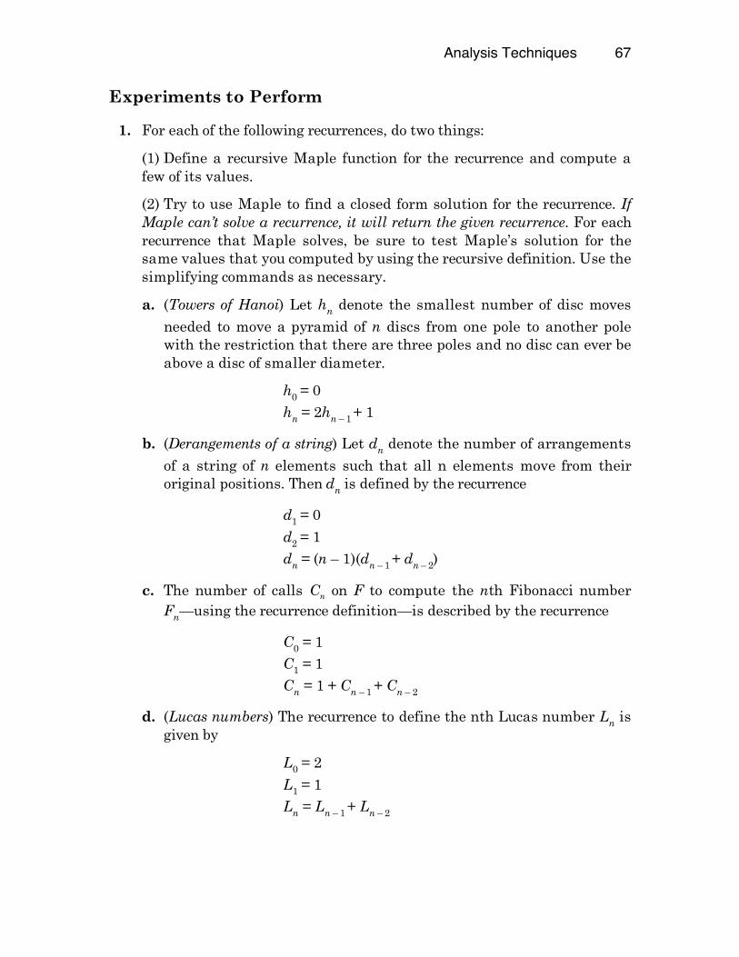
Analysis Techniques 67
Experiments to Perform
1. For each of the following recurrences, do two things:
(1) Define a recursive Maple function for the recurrence and compute a few of its values.
(2) Try to use Maple to find a closed form solution for the recurrence. If Maple can’t solve a recurrence, it will return the given recurrence. For each recurrence that Maple solves, be sure to test Maple’s solution for the same values that you computed by using the recursive definition. Use the simplifying commands as necessary.
a. (Towers of Hanoi) Let hn denote the smallest number of disc moves
needed to move a pyramid of n discs from one pole to another pole with the restriction that there are three poles and no disc can ever be above a disc of smaller diameter.
h0 = 0 hn = 2hn – 1 + 1
b. (Derangements of a string) Let dn denote the number of arrangements
of a string of n elements such that all n elements move from their original positions. Then dn is defined by the recurrence
d1 = 0
d2 = 1 dn = (n – 1)(dn – 1 + dn – 2)
c. The number of calls Cn on F to compute the nth Fibonacci number Fn—using the recurrence definition—is described by the recurrence
C0 = 1 C1 = 1 Cn = 1 + Cn – 1 + Cn – 2
d. (Lucas numbers) The recurrence to define the nth Lucas number Ln is given by
L0 = 2
L1 = 1 Ln = Ln – 1 + Ln – 2
68 Maple Experiments
5.10 Generating Functions Some recurrences can’t be solved by cancellation and some can’t even be solved by the Maple rsolve operation. A powerful technique that uses generat-ing functions can often be used to solve these recurrences. The technique is presented in Section 5.5.3 of the textbook. Recall that the generating function for the sequence
a0, a1, ... , an, ...
is given by the the following infinite polynomial.
A(x) = a0 + a1x + a2x2 + ... + anxn + ...
=
!
anxn
n=0
"
# .
For example, the generating function for the sequence 1, 1, ..., 1, ... is
!
xn
n=0
"
# .
The closed form for this generating function is given by the following formula.
!
1
1" x= x
n
n=0
#
$ .
Recall that we can use such a formula to solve recurrences. For example, sup-pose we have a recurrence that defines the sequence a0, a1, ... , an, ..., and we calculate, using the method of generating functions, that
!
A(x) =1
1" 3x.
Then we can rewrite it as follows:
!
A(x) =1
1" 2x=
1
1" (2x)= (2x)
n
n=0
#
$ = 2nxn
n=0
#
$ .
Since A(x) =
!
anxn
n=0
"# ,
we can equate coefficients to obtain the solution an = 3n. In other words, the
solution sequence is 1, 3, 9, ..., 3n, ... .
Analysis Techniques 69
The textbook introduces the method of solving recurrences by generating functions as a three step process. In Step 1 the given recurrence is used to con-struct an equation with A(x) as the unknown. Step 2 solves the equation for A(x) and, often with the help of partial fractions, writes A(x) as a sum of known generating functions. Step 3 equates coefficients to find the result. Maple can be used in Step 2 to solve for A(x) and to transform the result-ing expression into partial fractions. First replace A(x) by a new variable y. Then convert the equation to the form
expression = 0.
Then the equation can be solved with the Maple command
> solve(expression, y);
The result can be converted into partial fractions by the Maple command
> convert(%, parfrac, x);
For example, we’ll solve the equation
A(x) – x = 5 x A(x) – 6 x2A(x).
Replace A(x) by y and transform the equation into the form “expression = 0” to obtain the equation
x – y + 5xy – 6x2y = 0
Now we solve for y by giving Maple the following command.
> solve(x - y + 5*x*y-6*y*x^2, y);
The result is the expression
!
x
1" 5x + 6x2
We can use Maple to convert this expression to partial fractions with the fol-lowing command.
> convert(%, parfrac, x);
70 Maple Experiments
The result is the expression
!
1
2x "1"
1
3x "1.
Experiments to Perform
1. Use generating functions and Maple to solve each of the following recur-rences.
a. a0 = 0, a1 = 4, an = 2an – 1 + 3an – 2 (n ≥ 2).
b. a0 = 0, a1 = 1, an = 7an – 1 – 12an – 2 (n ≥ 2).
c. a0 = 0, a1 = 1, a2 = 1, an = 2an – 1 + an – 2 – 2an – 3 (n ≥ 3).
5.11 The Factorial and GAMMA Functions Maple has a factorial function to compute n!. But we can also define our own factorial function. For example, suppose we define the factorial function recur-sively as follows:
ƒ(0) = 1 ƒ(n) = n*ƒ(n – 1).
Of course we can translate this definition directly into Maple. But we can also solve the recurrence with Maple as follows.
> rsolve({ƒ(0) = 1, ƒ(n) = n*ƒ(n – 1)}, ƒ);
Notice that the answer is GAMMA(n + 1). Try out GAMMA on some samples as follows:
Analysis Techniques 71
> g := GAMMA; > g(1); > g(2); > g(3); > g(4); > g(20);
Notice what happens when you test GAMMA with the argument 0:
> g(0);
Experiments to Perform
1. What relationship do you see between Maple’s “factorial” and GAMMA functions?
2. Test the GAMMA function on several arguments that are not integers. For example, explore the results for several arguments between 4 and 5. Also, try out arguments in decimal form and in fractional form. For ex-ample, GAMMA(0.5) and GAMMA(1/2).
3. Test the GAMMA function on several arguments between 0 and 1. Be sure to explore the results as arguments get closer and closer to 0.
4. Use plot to help with your analysis. For example, try out the following examples.
> plot(n!, n=0..5); > plot(GAMMA(x), x=0..5); > plot(GAMMA(x + 1), x=0..5);
5. Make some observations about the GAMMA function, based on your tests.
6. The following recurrence can’t be solved with the rsolve command. Try it.
d1 = 0 d2 = 1 dn = (n – 1)(dn – 1 + dn – 2)
An alternative recurrence to define dn is given as follows.
dn = 1
dn = ndn – 1 + (–1)n
72 Maple Experiments
a. Write recursive functions for these two definitions and verify that the two define the same function by testing over several ranges of natural numbers.
b. Use rsolve on the second definition. Note that the result uses the GAMMA function. Test the solution on several numbers to see that it agrees with the the two functions of part (a). Note: You may need to use Maple’s simplify operation to obtain an integer value for each ex-pression.
5.12 Orders of Growth In this experiment we’ll use Maple to compare the growth rates of functions by examining their asymptotic behavior. Suppose that ƒ and g are two functions for which we have the following limit.
!
limn " #
ƒ(n)
g(n)= c .
We have the following results: If c = 0, then ƒ has lower order than g. We represent this fact with the fol-lowing little oh notation.
ƒ(n) = o(g(n)).
If c = ∞, then ƒ has higher order than g. We represent this fact with the following little oh notation.
g(n) = o(ƒ(n)).
If c ≠ 0 and c ≠ ∞, then ƒ has the same order as g. We represent this fact with the following big theta notation
ƒ(n) = Θ(g(n)).
We can use Maple to compute limits. So it follows that we can compare the rates of growth of functions with Maple. Try out the following examples to get used to the idea of taking limits.
> limit((n**2 + 3*n)/ 4578*n, n = infinity);
> limit(log[2](n)/n, n = infinity);
Analysis Techniques 73
Experiments to Perform
1. Let ƒ(n) g(n) mean that ƒ has lower order than g. Use Maple to verify the following ordering.
log2 n n n log2 n n2 2n.
2. Use Maple to verify the following statements, where k > 0 is any positive constant.
a. log2 (log2 (n)) = o(log2 n).
b. n(n+ 1)/2 = Θ(n2).
c. log2 (kn) = Θ(log2 n), where k > 0 is any positive constant.
d. log2 (k + n) = Θ(log2 n), where k > 0 is any positive constant.
3. Construct a Maple function “lower” that decides whether a function ƒ has lower order than a function g. In other words, lower(ƒ(n), g(n)) should re-turn true if ƒ(n) = o(g(n)). For example, the command
> lower(log[2](n), n);
should return true because log[2](n) = o(n). Test your definition of lower on the following pairs of functions by applying it first to the given pair and then to the reverse of the pair.
a. log2 (log2 (n)) and log2 n.
b. n(n+ 1)/2 and n2.
c. log2 (n) and log2 n45.
d. 2n and n39.
4. Use the help system to review Maple’s sort function. Then use Maple’s “sort” function together with the “lower” relation defined in (3) to sort the following lists of functions. Notice that some lists have more than one function of the same order.
a. [n2, 2n, log2 n, 25, 9n, 1, 8n2].
b. [2n, n, nlog2 n, n2, 1].
74 Maple Experiments
5. We want to use Maple to verify the following hierarchy of functions, where ƒ(n) g(n) means that ƒ has lower order than g.
!
1p log2 n p n p n log2 n p n2
p n3p n
50p 2n p 3n p 50n p n!p n
n .
We might start by using Maple’s sort function together with “lower” from (3). However, the result in general is not definitive because the sort func-tion does not tell us specifically that each member of the sorted list has lower order than its successor in the sorted list. We don’t want to spend the time writing down all the limit commands necessary to verify the or-dering. Instead, construct a function “limits” that takes as input a non-empty list of functions and outputs the list of limits of quotients of suc-cessive pairs of functions in the list. So if there are k functions in the in-put list, then the output will be a list of k – 1 limits of quotients. Test your definition on each of the following lists of functions.
a. [n2, 2n, log2 n, 25, 9n, 1, 8n2].
b. [2n, n, nlog2 n, n2, 1].
c. The list of functions in the given hierarchy.
75
Answers to Selected Experiments
Chapter 1 1.2 Set Operations 1. Maple's sets reflect the fact that sets don't have repeated elements. 3. For example, subset := (A, B) -> evalb(A intersect B = A);
1.3 List Operations heads := (x, y) -> [hd(x), hd(y)]; tails := (x, y) -> [tl(x), tl(y)]; examine := x -> [hd(x), tl(x)]; add2 := (a, b, x) -> cons(a, cons(b, x));
1.4 String Operations 1. head := x -> substring(x, 1..1); 2. tail := x -> substring(x, 2..length(x)); 3. last := x -> substring(x, length(x)); 4. pal := x -> evalb(head(x) = last(x));
1.6 Spanning Trees 1. The graph H has a minimal spanning tree of weight 20. 2. The petersen graph contains 10 vertices, each of degree three, and 15 edges. It forms a pentagon containing a five point star where each vertex of the star is connected to the “opposite” two vertices of the star and one vertex of the pentagon.
76 Answers to Selected Experiments
Chapter 2
2.1 Sequences 2. g := n -> [seq([n-k, n-k], k=0..n)]; 3. h := n -> [seq([n-k, k], k=0..n)]; 4. s := n -> [seq({$0..k}, k=0..n)];
2.2 The Map Function 1. The image f(A) is just map(f, A). 2a. h := x -> map(hd, x); 2b. t := x -> map(tl, x); 3. dist := (x, L) -> map2(f, x, L); f := (x, y) -> [x, y];
2.5 Evaluating Expressions 1b. map(minDepth, {$1..16}); 1c. map(minDepth, [$1..16]); 2b. The definition minDepth := floor@evalf@log[2] yields an incorrect result when applied to 16, due to rounding. 2c. minDepth := floor@simplify@log[2]
2.7 Type Checking 3. ceil2 := x -> if type(x, integer) then x elif x < 0 then trunc(x) else trunc(x + 1) fi; 4. floor2 := x -> if type(x, integer) then x elif x < 0 then trunc(x – 1) else trunc(x) fi; 5. a. cons := (x, y) -> if type(y, list) then [x, op(y)] else error “second argument is not a list” fi;
Chapter 3
3.1 Examples of Recursively Defined Functions 3. last := x -> if tl(x) = [] then hd(x) else last(tl(x)) fi; 5. first := x -> if tl(x) = [] then [] else cons(hd(x), first(tl(x))) fi; 6. pairs := (x, y) -> if x = [] or y = [] then [] else cons([hd(x), hd(y)], pairs(tl(x), tl(y))) fi; 7. dist := (a, x) -> if x = [] then [] else cons([a, hd(x)], dist(a, tl(x))) fi; 8. prod := (x, y) -> if x = [] then [] else concat(dist(hd(x), y), prod(tl(x), y)) fi;
3.2 Strings and Palindromes 1. F := x -> substring(x, 1); L := x -> substring(x, length(x)); M := x -> substring(x, 2..length(x)-1);
Answers to Selected Experiments 77
2. Pals finds a list of the first n natural numbers whose binary representa-tions are palindromes. pals := proc(n) L := []; a:= 0; for i from 1 to n do x := convert(a, binary); while not pal(x) do a := a + 1; x := convert(a, binary); od; L := cons(a, L); a := a+1; od; print(L); end;
3.3 A Recursively Defined Sorting Function 2. An element inserted in an unsorted list is inserted just to the left of the first element that is greater.
3. The original insert with ≤ is more efficient when there are repeated occur-rences of the element being inserted because the element is inserted before the first repeated occurrence.
3.5 Type Checking for Inductively Defined Sets 3. `type/A` := x -> if not type(x, integer) then false elif x < 0 then false elif x = 0 then true else type((x-1)/2), A) fi;
3.6 Inductively Defined Sets 1. getA := n -> if n = 1 then 0 else getA(n - 1)*2 + 1 fi; 2. getT := n -> if n = 1 then [ ] else cons(a, getT(n-1)) fi;
3.7 Subsets and Power Sets 1. subset := (x, y) -> if x = { } then true elif member(hd(x), y) then subset(tl(x),y) else false fi; 2. One version is the following, which is quite inefficient because each call of power(x) results is two calls on power(tl(x)).
power := x -> if x = { } then {{ }} else power(tl(x)) union map(`union`, power(tl(x)), {hd(x)}) fi;
78 Answers to Selected Experiments
A more efficient version is the following, which for each call of power(x) results in only one call to power(tl(x)).
pow := S -> if S = { } then {{ }} else g(pow(tl(S)), hd(S)) fi;
where g is defined by
g := (S, x) -> S union map(`union`, S, {x});
Chapter 4
4.1 Composing Two Binary Relations 1. Two possible solutions, one recursive and one iterative, are listed. getPairs := (x, S) -> if S = { } then { } elif x[2] = S[1][1] then {[x[1], S[1][2]]} union getPairs(x, tl(S)) else getPairs(x, tl(S)) fi; getPairs := (x, S) -> {seq(`if`(x[2] = S[i][1], cons(x[1], S[i][2]), []), i = 1..nops(S))} minus {[]};
4.2 Constructing Closures of Binary Relations 2. comp := (R, n) -> if n = 1 then R else compose(R, comp(R, n-1)) fi;
4.3 Testing for Closures 2. Two possibilities are isSymmetric := R -> evalb(R = converse(R)); and isSymmetric := R -> evalb(R = sc(R)); 3. isTransitive := (R, n) -> evalb(R = tc(R, n));
4.4 Warshall/Floyd Algorithms 2. Floyd’s algorithm to compute the minimum distances between points in a digraph represented by an n by n matrix m with the following properties:
m[i, j] = weight of edge (i, j) for all edges where i ≠ j. m[i, i] = 0 for i = 1...n. m[i, j] = infinity (a number larger than the sum of all edge weights) for all other edges (i, j) not in the graph. The call floyd(m, n) will output the matrix of minimum distances.

Answers to Selected Experiments 79
floyd := proc(m, n) local a; a := matrix(n, n); for i from 1 to n do for j from 1 to n do a[i, j] := m[i, j] od od; for k from 1 to n do for i from 1 to n do for j from 1 to n do a[i, j] := min(a[i, j] , a[i, k] + a[k, j]); od od od; print(evalm(a)) end;
3. The Paths algorithm modifies Floyds algorithm to compute the matrix from which the actual points on the shortest path can be found. The input is the same as for Floyd’s algorithm. Namely, a digraph represented by an n by n matrix m with the following properties:
m[i, j] = weight of edge (i, j), for all edges where i ≠ j. m[i, i] = 0, for i = 1...n. m[i, j] = infinity, for all other edges (i, j) not in the graph.
The call paths(m, n) will output the Floyd matrix and the paths matrix.
paths := proc(m, n) local a, p; a := matrix(n, n); p := matrix(n, n); for i from 1 to n do for j from 1 to n do a[i, j] := m[i, j]; p[i, j] := 0 od od; for k from 1 to n do for i from 1 to n do for j from 1 to n do if a[i, k] + a[k, j] < a[i, j] then a[i, j] := a[i, k] + a[k, j]; p[i, j] := k fi od od od; print(evalm(a)); print(evalm(p)) end;
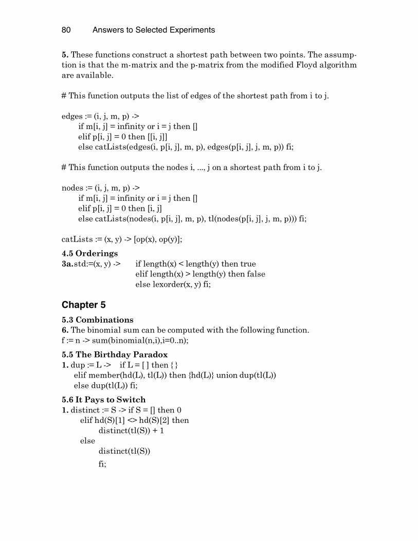
80 Answers to Selected Experiments
5. These functions construct a shortest path between two points. The assump-tion is that the m-matrix and the p-matrix from the modified Floyd algorithm are available. # This function outputs the list of edges of the shortest path from i to j. edges := (i, j, m, p) -> if m[i, j] = infinity or i = j then [] elif p[i, j] = 0 then [[i, j]] else catLists(edges(i, p[i, j], m, p), edges(p[i, j], j, m, p)) fi; # This function outputs the nodes i, ..., j on a shortest path from i to j. nodes := (i, j, m, p) -> if m[i, j] = infinity or i = j then [] elif p[i, j] = 0 then [i, j] else catLists(nodes(i, p[i, j], m, p), tl(nodes(p[i, j], j, m, p))) fi; catLists := (x, y) -> [op(x), op(y)];
4.5 Orderings 3a. std:=(x, y) -> if length(x) < length(y) then true elif length(x) > length(y) then false else lexorder(x, y) fi;
Chapter 5
5.3 Combinations 6. The binomial sum can be computed with the following function. f := n -> sum(binomial(n,i),i=0..n);
5.5 The Birthday Paradox 1. dup := L -> if L = [ ] then { } elif member(hd(L), tl(L)) then {hd(L)} union dup(tl(L)) else dup(tl(L)) fi;
5.6 It Pays to Switch 1. distinct := S -> if S = [] then 0 elif hd(S)[1] <> hd(S)[2] then distinct(tl(S)) + 1 else distinct(tl(S))
fi;
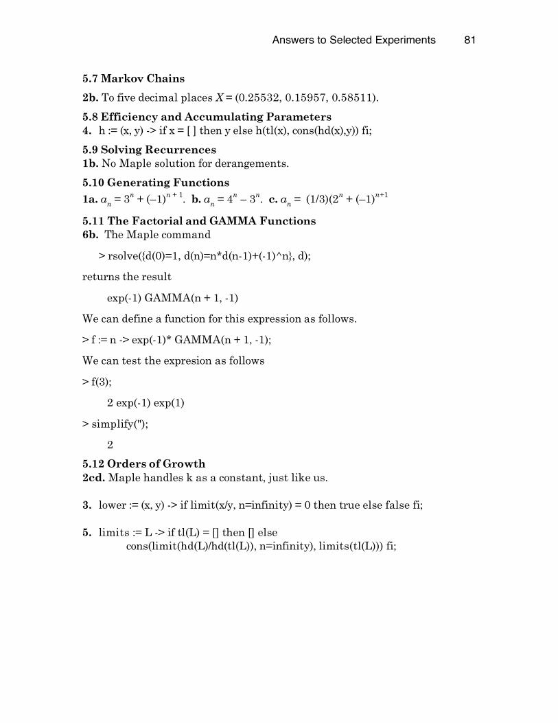
Answers to Selected Experiments 81
5.7 Markov Chains
2b. To five decimal places X = (0.25532, 0.15957, 0.58511).
5.8 Efficiency and Accumulating Parameters 4. h := (x, y) -> if x = [ ] then y else h(tl(x), cons(hd(x),y)) fi;
5.9 Solving Recurrences 1b. No Maple solution for derangements.
5.10 Generating Functions
1a. an = 3n + (–1)n + 1. b. an = 4n – 3n. c. an = (1/3)(2n + (–1)n+1
5.11 The Factorial and GAMMA Functions 6b. The Maple command
> rsolve({d(0)=1, d(n)=n*d(n-1)+(-1)^n}, d);
returns the result
exp(-1) GAMMA(n + 1, -1)
We can define a function for this expression as follows.
> f := n -> exp(-1)* GAMMA(n + 1, -1);
We can test the expresion as follows
> f(3);
2 exp(-1) exp(1)
> simplify(");
2
5.12 Orders of Growth 2cd. Maple handles k as a constant, just like us. 3. lower := (x, y) -> if limit(x/y, n=infinity) = 0 then true else false fi; 5. limits := L -> if tl(L) = [] then [] else cons(limit(hd(L)/hd(tl(L)), n=infinity), limits(tl(L))) fi;
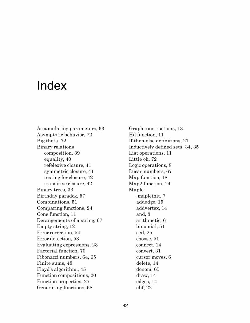
82
Index
Accumulating parameters, 63 Asymptotic behavior, 72 Big theta, 72 Binary relations
composition, 39 equality, 40 refelexive closure, 41 symmetric closure, 41 testing for closure, 42 transitive closure, 42
Binary trees, 33 Birthday paradox, 57 Combinations, 51 Comparing functions, 24 Cons function, 11 Derangements of a string, 67 Empty string, 12 Error correction, 54 Error detection, 53 Evaluating expressions, 23 Factorial function, 70 Fibonacci numbers, 64, 65 Finite sums, 48 Floyd’s algorithm;, 45 Function compositions, 20 Function properties, 27 Generating functions, 68
Graph constructions, 13 Hd function, 11 If-then-else definitions, 21 Inductively defined sets, 34, 35 List operations, 11 Little oh, 72 Logic operations, 8 Lucas numbers, 67 Map function, 18 Map2 function, 19 Maple
.mapleinit, 7 addedge, 15 addvertex, 14 and, 8 arithmetic, 6 binomial, 51 ceil, 25 choose, 51 connect, 14 convert, 31 cursor moves, 6 delete, 14 denom, 65 draw, 14 edges, 14 elif, 22
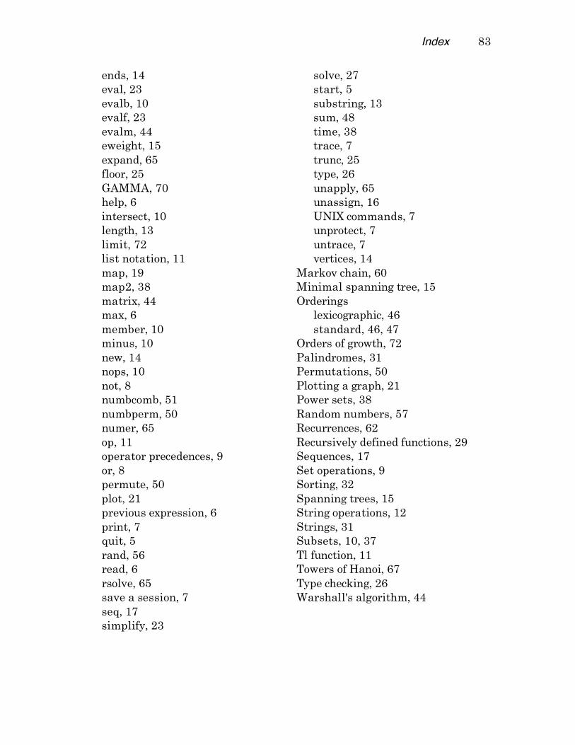
Index 83
ends, 14 eval, 23 evalb, 10 evalf, 23 evalm, 44 eweight, 15 expand, 65 floor, 25 GAMMA, 70 help, 6 intersect, 10 length, 13 limit, 72 list notation, 11 map, 19 map2, 38 matrix, 44 max, 6 member, 10 minus, 10 new, 14 nops, 10 not, 8 numbcomb, 51 numbperm, 50 numer, 65 op, 11 operator precedences, 9 or, 8 permute, 50 plot, 21 previous expression, 6 print, 7 quit, 5 rand, 56 read, 6 rsolve, 65 save a session, 7 seq, 17 simplify, 23
solve, 27 start, 5 substring, 13 sum, 48 time, 38 trace, 7 trunc, 25 type, 26 unapply, 65 unassign, 16 UNIX commands, 7 unprotect, 7 untrace, 7 vertices, 14
Markov chain, 60 Minimal spanning tree, 15 Orderings
lexicographic, 46 standard, 46, 47
Orders of growth, 72 Palindromes, 31 Permutations, 50 Plotting a graph, 21 Power sets, 38 Random numbers, 57 Recurrences, 62 Recursively defined functions, 29 Sequences, 17 Set operations, 9 Sorting, 32 Spanning trees, 15 String operations, 12 Strings, 31 Subsets, 10, 37 Tl function, 11 Towers of Hanoi, 67 Type checking, 26 Warshall's algorithm, 44