Map Analysis with Networks

Francisco Olivera, Ph.D., P.E.Department of Civil Engineering

Texas A&M University

Some of the figures included in this presentation have been taken from the ESRI Campus online course Introduction to ArcView Network Analyst. This presentation is to be used exclusively by students of Texas

A&M University.

Network Overview

A Network is a set of connected line features called links.

Networks represent roads, streets, pipelines, utilities, steams, etc.

The Network Analyst ArcView Extension allows one to model the movement of goods throughout the network.

Example: Networks

Network Overview

The Best Route is the path that connects a set of points producing the minimum cost.

Network Overview

The Closest Facility is the one point – out of a set of points – to which traveling from a given location produces the minimum cost.

Network Overview

Service Area is the polygon that includes all points which can be reached from a location at a cost less than a given reference cost.

Example: Area within a 12-minute drive from the hospital.

Travel Cost

Traveling on a link has a Travel Cost, which is usually related to travel distance or travel time.

The optimal path for moving goods between two points is the one that produces the minimum cost.

Delays at intersections caused by turns, traffic lights, stop signs, etc. can be factored into the travel cost.

Example: Shortest and fastest paths.

Pathfinding Algorithm

There are many algorithms which solve the least-cost path problem, but the simplest and most well-known was developed by Dijkstra (1959).

Dijkstra's algorithm strikes a balance by calculating a path that is very close to the optimal path yet is computationally manageable.

Network Data Model

All links begin and end at a FNODE_ (from-node) and TNODE_ (to-node). Despite these nodes are labeled from and to, links can represent flow in any direction.

Flow direction is defined in a ONE_WAY field in the network attribute table. In this field: (1) FT = from node -> to node, (2) TF = to node -> from node, (3) N = no flow, and (4) other value = both directions.

From-node

To-node

Network Data Model

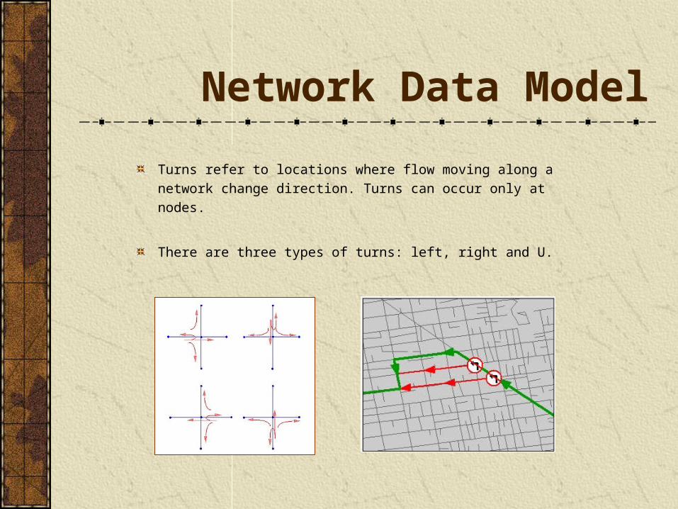
Turns refer to locations where flow moving along a network change direction. Turns can occur only at nodes.

There are three types of turns: left, right and U.

Network Data Model

Each record in the turntable represents one turn in the network.

The turntable has the following fields:

Node_ : intersection node

Arc1_ : link before turn

Arc2_ : link after turn

[Cost] : travel cost of making the turn. Negative values imply a prohibited turn. Cost field name should be the same as in the network.

Turntables have to be declared with the DeclaringATurntable.ave script.

Network Data Model

Lines that cross but do not intersect (i.e., complex lines), represent over/underpasses. Over/underpasses do not allow turns.

Over/under pass Intersection

Network Data Model

1 2

3

4

7

85

9

10

13

1211

6

14

1 2

3 4 5

6

7

8 9

12

14

10

1315

11

LineID FNODE_ TNODE_ <Cost> ONE_WAY

1 1 14 90 B

2 2 3 85 B

3 6 14 110 B

4 14 3 75 FT

Node_ Arc1_ Arc2_ <Cost>

14 1 4 -1

7 7 8 43

9 15 14 54

Network attribute table

Turn table

Problem Definition Dialog

The Problem Definition Dialog is the window in which the problem parameters are entered.

There is a different Problem Definition Dialog depending on the problem to be solved.

When a Problem Definition Dialog is opened a Result Theme is added to the View.

The Problem Definition Dialog can be used to redefine the problem and update the Result Theme.

Best RouteA Route is a line of travel through a network from one point to another.

A route can visit many locations, also called Stops, between its starting and ending point. A route can have a minimum number of two stops: Origin and Destination.

The user can specify the sequence in which stops are visited, as well as if the origin and destination coincide.

Best Route

To find the best route:

Make the network theme active,

Click on Network/Find Best Route,

Click on Load Stops to define the point theme of points that have to be visited,

Click on the “solve” button.

Best RouteStops can also be added by clicking on the network on the map with the Add Location tool, or by specifying the stop address (see Address Geocoding) with the Add Location by Address tool.

To load Stop names into the Label column of the Problem Definition Dialog, the point theme of Stops must have an attribute named or aliased "label".

In the Problem Definition Dialog, Stop points can be removed or changed in sequence.

The Properties button of the Problem Definition Dialog is used to define the attribute of the network theme that stores the travel cost.

Closest Facility

Finding the Closest Facility consists on identifying the point (facility) that is closest, in terms of travel cost, to a given point (event), as well as the best route to connect them.

The user can specify the number of facilities to be identified.

Closest Facility

To find the closest facility:

Make the network theme active,

Click on Network/Find Closest Facility,

Select the facilities theme in the Facilities slot,

Click on Load Events to define the event location,

Click on the “solve” button.

Closest Facility

Facilities should be within a certain distance of a Network link, which depends on the View display size, before they are recognized by Network Analyst.

The Properties button of the Problem Definition Dialog is used to define the attribute of the network theme that stores the travel cost.

Service Area

A Service Area is the polygon that embraces all locations that can be reached from a Site within a given travel cost.

Service Area

To find the service area of a site:

Make the network theme active,

Click on Network/Find Service Area,

Click on Load Sites to define the sites that provide the service,

Enter the travel cost allowed for each site,

Click on the “solve” button.

Address Geocoding

Address Geocoding is the process of creating an event point feature dataset from tabular information. Geocoded points are located along network links.

For most civil engineering applications, it is enough to locate points along roads, pipelines, utilities or streams regardless the side in which they lay.

Address Geocoding

For address geocoding, the network theme properties have to be defined to make it matchable.

7495

Texas

79 84 86US Single Range:

Address Geocoding

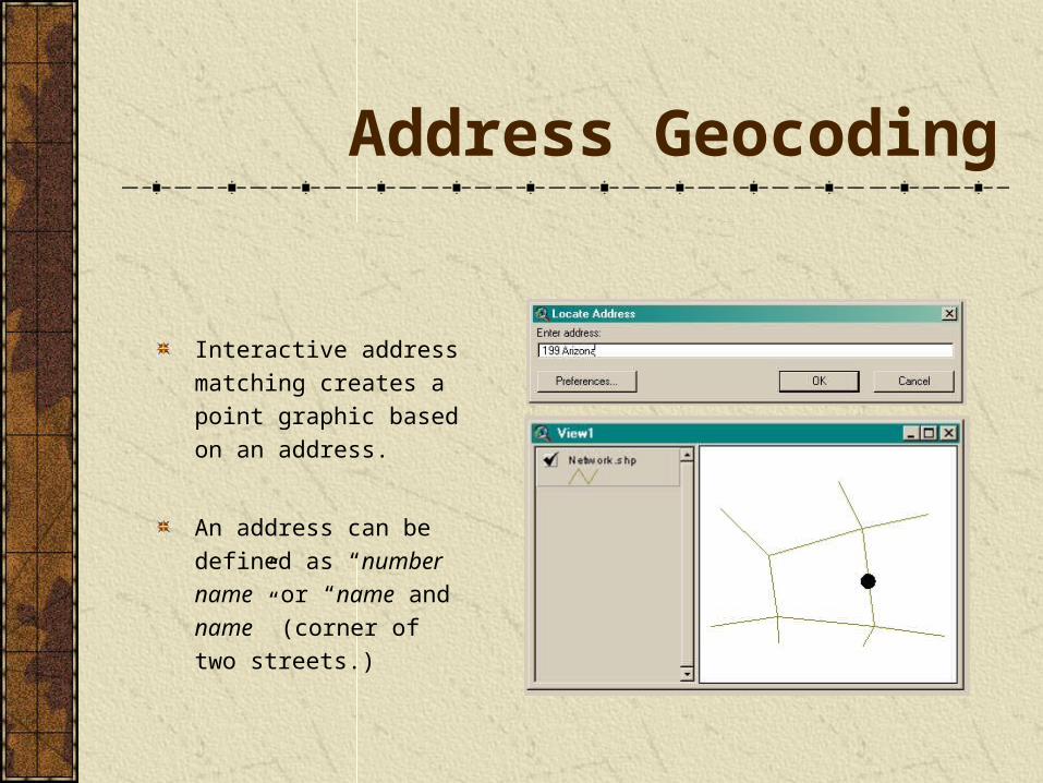
Interactive address matching creates a point graphic based on an address.

An address can be defined as “number name” or “name and name” (corner of two streets.)

Address Geocoding

Address matching using an address list creates a point feature dataset.