manual xlstatpro
TRANSCRIPT

User’s manual
XLSTAT-Pro
Copyright © 2004, Addinsoft
http://www.addinsoft.com

2
Table of Contents Version 7.5: More than just another release ............................................... 5 Minimum system configuration .................................................................. 6 Installing XLSTAT .................................................................................... 7 Regional settings.....................................................................................10 Data types ..............................................................................................11 Selecting data in Excel ............................................................................12 Time required for data entry .....................................................................14 Time required for calculation ....................................................................15 Time required for display .........................................................................16 Options ...................................................................................................17 Data Sampling ........................................................................................22 Distribution Sampling...............................................................................24 Discretization and histogram ....................................................................28 Coding....................................................................................................31 Presence/absence coding........................................................................33 Full Disjunctive Coding ............................................................................34 Coding by Ranks.....................................................................................35 Partition recoding ....................................................................................36 Transformation........................................................................................37 Anamorphosis.........................................................................................40 Descriptive Statistics ...............................................................................44 Histograms .............................................................................................49 Normality Tests.......................................................................................51 Contingency Table (Two-way Table) and Chi-square .................................54 Similarity/Dissimilarity Matrix (Correlation …) ............................................56 Factor Analysis .......................................................................................60 Principal Component Analysis (PCA)........................................................64 Gabriel Biplot ..........................................................................................69 Discriminant Analysis (DA).......................................................................73 Correspondence Analysis (CA) ................................................................77 Multiple Correspondence Analysis (MCA) .................................................82 Multidimensional Scaling (MDS)...............................................................87 Agglomerative Hierarchical Clustering (AHC) ............................................92 k-means Clustering .................................................................................98 Univariate Clustering .............................................................................102 AxesZoomer .........................................................................................104 DataFlagger ..........................................................................................105 Easy Labels ..........................................................................................106 MicroMover...........................................................................................107 MinMaxSearch......................................................................................108 Plot Transformer ...................................................................................109 Scatter plots..........................................................................................110 Parallel Coordinates Visualization ..........................................................113 Distribution Fitting .................................................................................116 Linear Regression .................................................................................121 ANOVA ................................................................................................128 ANCOVA ..............................................................................................135 Logistic Regression ...............................................................................142 Nonlinear Regression ............................................................................148 Nonparametric Regression ....................................................................154 Tests on Contingency Tables .................................................................163 Correlation Tests...................................................................................170
3
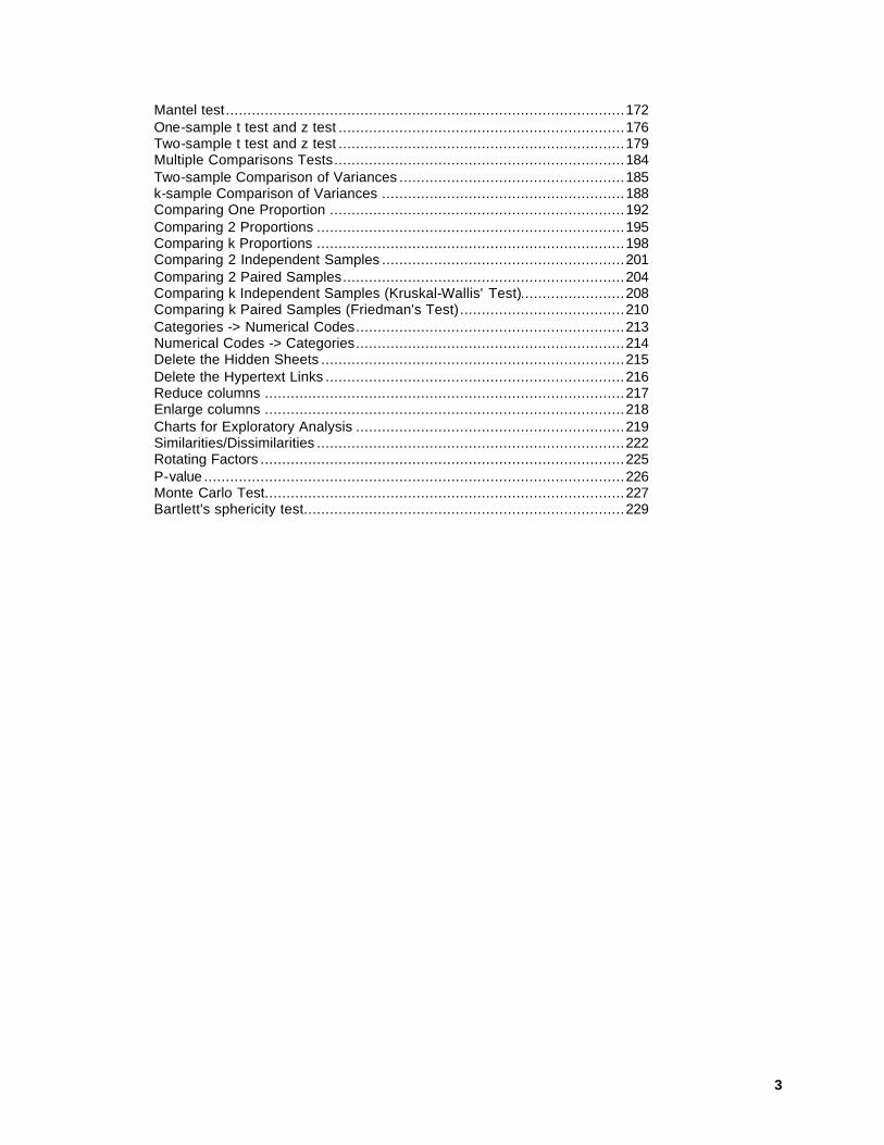
Mantel test............................................................................................172 One-sample t test and z test ..................................................................176 Two-sample t test and z test ..................................................................179 Multiple Comparisons Tests...................................................................184 Two-sample Comparison of Variances ....................................................185 k-sample Comparison of Variances ........................................................188 Comparing One Proportion ....................................................................192 Comparing 2 Proportions .......................................................................195 Comparing k Proportions .......................................................................198 Comparing 2 Independent Samples ........................................................201 Comparing 2 Paired Samples.................................................................204 Comparing k Independent Samples (Kruskal-Wallis' Test)........................208 Comparing k Paired Samples (Friedman's Test)......................................210 Categories -> Numerical Codes..............................................................213 Numerical Codes -> Categories..............................................................214 Delete the Hidden Sheets ......................................................................215 Delete the Hypertext Links .....................................................................216 Reduce columns ...................................................................................217 Enlarge columns ...................................................................................218 Charts for Exploratory Analysis ..............................................................219 Similarities/Dissimilarities .......................................................................222 Rotating Factors ....................................................................................225 P-value .................................................................................................226 Monte Carlo Test...................................................................................227 Bartlett's sphericity test..........................................................................229

4

5
Version 7.5: More than just another release XLSTAT version 7.5 includes several changes from the previous version. XLSTAT functions have been revised and expanded. XLSTAT has been modified in order to provide:
• easier data entry,
• management of missing data in all treatments,
• faster calculation,
• clearer and faster and more complete results,
• more features,
• more extensive help,
• more information in the error messages,
• more settings for XLSTAT.
6
Minimum system configuration PC with a 200 MHz Pentium or equivalent processor, 32 MB RAM, Microsoft® Windows 95, 98, Me, NT 4.0, 2000, or XP, Microsoft® Excel 97 (version 8.0) SR-2, Excel 2000 (version 9.0) SR-3, Excel 2002 (version 10.0) SR-2, or Excel 2003.
Note: We suggest you download the patch called xl8p10pkg.exe from the Microsoft® Web site http://office.microsoft.com/downloaddetails/xl8p10pkg.htm in order to upgrade to version SR-2 (l). This patch corrects several problems with Excel 97 SR-2.
7
Installing XLSTAT
XLSTAT 7.5 Software License Agreement
Starting XLSTAT
Macro alert
XLSTAT 7.5 Software License Agreement
ADDINSOFT SARL ("ADDINSOFT") IS WILLING TO LICENSE VERSION 7.5 OF ITS XLSTAT(r) SOFTWARE AND THE ACCOMPANYING DOCUMENTATION (THE "SOFTWARE") TO YOU ONLY ON THE CONDITION THAT YOU ACCEPT ALL OF THE TERMS IN THIS AGREEMENT. PLEASE READ THE TERMS CAREFULLY. BY CLICKING ON THE "YES" BUTTON BELOW YOU ACKNOWLEDGE THAT YOU HAVE READ THIS AGREEMENT, UNDERSTAND IT AND AGREE TO BE BOUND BY ITS TERMS AND CONDITIONS. IF YOU DO NOT AGREE TO THESE TERMS, ADDINSOFT IS UNWILLING TO LICENSE THE SOFTWARE TO YOU. YOU SHOULD CLICK ON THE "NO" BUTTON TO DISCONTINUE THE INSTALLATION PROCESS.
1. LICENSE. Addinsoft hereby grants you a nonexclusive license to install and use the Software in machine-readable form on a single computer for use by a single individual if you are using the demo version of if your have registered your demo version to use it with no time limits. If you have ordered a multi-users license then the number of users depends directly on the terms specified on the invoice sent to your company by Addinsoft.
2. RESTRICTIONS. Addinsoft retains all right, title, and interest in and to the Software, and any rights not granted to you herein are reserved by Addinsoft. You may not reverse engineer, disassemble, decompile, or translate the Software, or otherwise attempt to derive the source code of the Software, except to the extent allowed under any applicable law. If applicable law permits such activities, any information so discovered must be promptly disclosed to Addinsoft and shall be deemed to be the confidential proprietary information of Addinsoft. Any attempt to transfer any of the rights, duties or obligations hereunder is void. You may not rent, lease, loan, or resell for profit the Software, or any part thereof. You may not reproduce, distribute, publicly perform or publicly display the Software except as expressly permitted under Section 1, and you may not create derivative works of the Software.
3. SUPPORT. Registered users of the Software are entitled to Addinsoft's standard support services, as such services are modified from time to time in Addinsoft's discretion. Demo version users may contact Addinsoft for support but with no guarantee to benefit from Addinsoft's standard support services.

8
4. NO WARRANTY. THE SOFTWARE IS PROVIDED "AS IS" AND WITHOUT ANY WARRANTY OR CONDITION, WHETHER EXPRESS, IMPLIED OR STATUTORY. Some jurisdictions do not allow the disclaimer of implied warranties, so the foregoing disclaimer may not apply to you. This warranty gives you specific legal rights and you may also have other legal rights which vary from state to state.
5. LIMITATION OF LIABILITY. IN NO EVENT WILL ADDINSOFT OR ITS SUPPLIERS BE LIABLE FOR ANY LOST PROFITS OR OTHER CONSEQUENTIAL, INCIDENTAL OR SPECIAL DAMAGES (HOWEVER ARISING, INCLUDING NEGLIGENCE) IN CONNECTION WITH THE SOFTWARE OR THIS AGREEMENT, EVEN IF ADDINSOFT HAS BEEN ADVISED OF THE POSSIBILITY OF SUCH DAMAGES. In no event will Addinsoft's liability in connection with the Software, regardless of the form of action, exceed $100. Some jurisdictions do not allow the foregoing limitations of liability, so the foregoing limitations may not apply to you.
6. TERM AND TERMINATION. This Agreement shall continue until terminated. You may terminate the Agreement at any time by deleting all copies of the Software. This license terminates automatically if you violate any terms of the Agreement. Upon termination you must promptly delete all copies of the Software.
7. CONTRACTING PARTIES. If the Software is installed on computers owned by a corporation or other legal entity, then this Agreement is formed by and between Addinsoft and such entity. The individual executing this Agreement represents and warrants to Addinsoft that they have the authority to bind such entity to the terms and conditions of this Agreement.
8. INDEMNITY. You agree to defend and indemnify Addinsoft against all claims, losses, liabilities, damages, costs and expenses, including attorney's fees, which Addinsoft may incur in connection with your breach of this Agreement.
9. GENERAL. The Software is a "commercial item." This Agreement is governed and interpreted in accordance with the laws of the Court of Paris, France, without giving effect to its conflict of laws provisions. The United Nations Convention on Contracts for the International Sale of Goods is expressly disclaimed. Any claim arising out of or related to this Agreement must be brought exclusively in a court located in PARIS, FRANCE, and you consent to the jurisdiction of such courts. If any provision of this Agreement shall be invalid, the validity of the remaining provisions of this Agreement shall not be affected. This Agreement is the entire and exclusive agreement between Addinsoft and you with respect to the Software and supersedes all prior agreements (whether written or oral) and other communications between Addinsoft and you with respect to the Software.
COPYRIGHT (c) 2004 BY Addinsoft SARL, Paris, FRANCE. ALL RIGHTS RESERVED.
XLSTAT(r) IS A REGISTERED TRADEMARK OF ADDINSOFT SARL.

9
Paris, FRANCE, July 2004
Starting XLSTAT
To start XLSTAT, click Start, choose Programs, Addinsoft, and click XLSTAT-Pro, or click on the shortcut on the desktop, or click on the (x) icon in the Excel toolbar.
Note: XLSTAT does not work under Microsoft® Excel 95: it will not load if you try to run it with that version.
You can also start XLSTAT-Pro by clicking directly on XLSTAT-Pro.xla, or by opening XLSTAT-Pro.xla from Excel.
The first time XLSTAT is loaded during the installation, a button is added to the standard Excel toolbar. Afterward to load XLSTAT-Pro, simply click this button. To remove this button from your toolbar, go to Tools/Customize, drag the button off the toolbar and click <Close>.
Note: Under Microsoft® Excel 2002 (version 10.0), in the check of the background errors, XLSTAT deactivates automatically the rule for the numbers stored as texts. To restore the rule, please go to Tools/Options/Errors checking and tick the rule for "Number stored as text".
Macro alert
By default, a macro alert message is displayed while XLSTAT loads into Excel. With Excel 97, the following macro alert message is used:
click <Enable Macros> in order to use XLSTAT. To disable the alert message, choose Tools, Options, click the General tab, remove the check from "Macro virus protection" and then click <OK>.
With Excel 2000, the following macro alert message is displayed:
click <Enable Macros> in order to use XLSTAT. To disable the alert message, choose Tools, Macro, Security, and select "Low" instead of "Medium", then click <OK>. With Excel 2002 you must run another time XLSTAT.

10
Regional settings Two regional settings are vital for XLSTAT: the decimal symbol and the list separator. To view these settings, choose Start, Settings, Control Panel, Regional Settings, Number. With Excel 2002 and Excel 2003 You can also directly change these settings from the Tools/Options/International/Number handling panel.
XLSTAT can work with any one-character decimal symbol, even if you modify the decimal symbol during a session. The same holds true for the list separator, used when making multiple selections.
Note: If you use a comma as the decimal symbol, and if you also use a comma for the list separator as defined in the Number tab, then Windows uses the semicolon as the list separator.

11
Data types XLSTAT checks the data you enter according to the algebraic structure of the variable:
• quantitative,
• ordinal (ranks),
• categorical (or qualitative),
• binary.
Quantitative variables cannot contain text. Ordinal variables coded as ranks must be numerical values. Categorical variables may include numerical values or text because XLSTAT processes all these values as character strings. For binary variables (e.g. full disjunctive table), the data must be numerical data, with a value of 0 or 1.
The value of a cell that appears empty – i.e. that is indeed empty or that contains one or more "spaces"– as well as error values returned by Excel, for instance:
• #NUM!
• #N/A!
• #N/A
• #DIV/0!
• #VALUE!
• #REF!
• #NAME?
are interpreted by XLSTAT as missing data. Certain types of XLSTAT processing may create missing data, in particular when transforming values for which the function being used is undefined (e.g. the logarithm for a negative value). Normally missing data do not prevent XLSTAT modules from processing your data, unless the calculation engine detects that there is not enough information to proceed.
Note: the 0 is never considered as the value coding a missing value in the data, except in the case of the Numerical Codes -> Categories tool, and in the case of partitions where 0 corresponds to the missing data partition.
Note : A missing weight is considered as a null weight.
12
Selecting data in Excel You can use standard methods for selecting data:
• hold down the left mouse button while moving the mouse pointer
• hold down the SHIFT key while clicking on the first cell in the range, then click the last cell in the range.
In a large table, however – containing several hundred lines – it is much faster to use the keyboard. To select all the values starting in the current cell, press and hold down the SHIFT and CTRL keys simultaneously, then use the arrow keys to select and define the range.
Note: This selection mode does not work if you have selected a chart, nor with Excel 2000 versions prior to SR-3 and Excel 2002 version prior to SR-2.
XLSTAT allows you to select data directly by columns, select data from different sheets in the active workbook, and perform multiple selections. Furthermore, you can enable the assisted entry mode in order to avoid errors when selecting data.
Note: The names of the sheets in an Excel workbook cannot contain the following characters:"?", "/", "\", "*", "[", "]". Furthermore, since XLSTAT allows you to make multiple selections, make sure you do not include the current list separator in worksheet names.
To reset all the data selections in a dialog box use the "Refresh" button: .
See also: Selecting by column
Selecting data in different sheets
Multiple data entry
Assisted entry mode
Selecting by column
If the data in your sheet starts on the first row, you may want to select directly via the column headers. XLSTAT provides two modes for selecting by columns: simple entry mode and extended entry mode. The difference between these modes concerns the criterion used to stop reading data in the selected columns.
In simple entry mode, the number of lines in a table is determined by the longest continuous column in the selection (i.e. that has no empty cells).
In extended entry mode, the number of rows is determined by the first row of data that is followed by N empty rows, where N is fixed (see the Data entry tab to know how to modify N).
When using the extended entry mode, you must specify the maximum length for the sequence of empty rows that can exist in your data without stopping the reading of the columns (see the Data entry tab).

13
Selecting data in different sheets
To select data in different sheets in the active workbook, separate the ranges entered by the current list separator. You cannot use the mouse to select the various sheets within a given data entry field.
Multiple data entry
To select data in several ranges, hold down the CTRL key while you select data ranges. The selection mode must be homogenous: within a given multiple selection, you cannot select both using column headers and range selection mode. When your data appears naturally in adjacent columns (e.g. correlation matrix), XLSTAT requires that you use simple (not multiple) data entry. XLSTAT accepts intersections between ranges only if the result of the intersections makes sense. If it doesn't a message is displayed.
Assisted entry mode
When the assisted entry mode is enabled (see the Data entry tab), XLSTAT specifies the number of rows and columns for the data selection. If the displayed values are incorrect, you may have made a mistake or, for a selection by columns, XLSTAT may not be able to determine the data range due to an unusual distribution of missing data. In the latter case, select your data by range instead of by column headers.

14
Time required for data entry The amount of time required for data entry by XLSTAT in an Excel sheet depends on the selection mode used. To obtain the fastest entry, use selection by range, because XLSTAT immediately identifies all the values you want to process. On the other hand, selection by column headers requires an additional step in order to determine the exact data range, and this takes longer.
For very large sheets (with several hundred or thousand rows), it is much faster to use range selection mode.

15
Time required for calculation All the calculations performed in XLSTAT use the calculation engine, in an ActiveX DLL. You can optionally obtain the rights to use this DLL for programs you develop yourself.
The calculations are normally fairly fast, except for modules that use iterative optimization methods (e.g. Multidimensional Scaling) or dynamic programming (Fisher's algorithm). In these cases, the calculation can take quite some time according to the settings used and/or the size of the data sets.
In order to get an idea of the response times for iterative methods on your system, adjust the settings that control the number of repetitions, the maximum number of iterations, and the convergence threshold to low values. Then gradually increase the number of repetitions and the maximum number of iterations, and reduce the convergence threshold until the response times become unacceptable.
For the Fisher algorithm, XLSTAT manages the calculation time and displays a message as soon as the estimated calculation time exceeds 30 seconds on a 500 MHz processor. In this case, you can cancel the calculation in progress.

16
Time required for display Displaying output tables in an Excel sheet has been significantly improved. However, the display of graphics can be still slow. Pay attention to the options proposed during the display. Beside chart readability issues, avoid for example displaying 500 observations labels in a PCA because the display time will be extremely long. To avoid this type of situation, XLSTAT proposes a watchdog in the Charts tab that allows you to limit the number of observations that can be displayed in a chart generated after a multivariate technique has been used (PCA, MCA, AHC). This watchdog can inactivated either in the options panel or by checking the option in the message box.

17
Options The options box allows a user to manage the various parameters of XLSTAT. A definition of options is linked to a particular user profile, as well as the memorization of the options of the various dialog boxes, including the user's functions library in the nonlinear regression tool.
Default: click on this button to restore the default options of the user.
Redefine : click on this button to redefine the default options of a user, and set them to the current options.
Restore: click on this button to restore the default options and set them to their default XLSTAT value.
Apply: click on this button to apply the options as currently defined in the options box. XLSTAT memorizes the current options of the user.
General
Data entry
Calculations
Outputs
Display
Charts
Modules
General
Language : you can dynamically change the language used to display the menus, dialog boxes, and results.
Dialog box memory: XLSTAT provides two modes for using dialog boxes: in memory off mode, dialog boxes are always reset, while in memory on mode the ranges and options are saved. To clear the memory of all dialog boxes for the current language, click the <Clear> button.
Memory limited to the current session: check this option if you want to erase the memory from the previous session when the current session starts. Remove the check if you want to keep the memory from the previous session.
Immediate memorization: check this option if you want the information to be memorized immediately when you click the <OK> button in a dialog box. Remove the check if you prefer to wait for all the calculations to execute correctly before memorizing the state of the dialog box.

18
Warnings: click on this button, if you want to reactivate the warning messages of XLSTAT (XLSTAT upgrades, confirmation of selections, …).
Data entry
Assisted entry mode : Check this option to display a message indicating the number of rows and columns in the data selection as identified by XLSTAT. You can use this option to check that the data entered is correct without waiting for the processing report to be displayed.
Control of the column labels: Check this option so that XLSTAT tells you when it has detected numerical labels in the first cell of a column which could indicate that you have mistakenly activated the option Column labels in a dialog box, although the first cell is in fact the first value to take into account.
Select by column: With XLSTAT you can directly select data by selecting column headers. Two modes are available: simple entry mode and extended entry mode. The difference between these modes concerns the criterion used to stop reading data in the selected columns. In simple entry mode, the number of lines in a table is determined by the longest column (i.e. with no missing data).
In extended entry mode, the number of rows used for the analysis corresponds to the row number of the first row that is followed by N empty rows, where N is an input that the user can modify. Default value is 10.
Codes for the user defined missing values: XLSTAT allows the user to define the missing values he/she would like to be recognized by XLSTAT (for example Null, 9999, -99.999 etc.). To add a new missing value code, enter it in the Missing value filed, then click on the <Add>. To delete a code click on <Delete>. The detection of codes is case sensitive. Note: adding your own codes might slow down the process of analyzing the data.
Calculations
Missing value estimation: Check this option if you want that XLSTAT suggests you estimating the missing data all the times when it is possible. In current version, XLSTAT estimates the missing data of a quantitative variable by the mean, and the missing data of a categorical variable by the mode.
Pseudo-random numbers generator: The pseudo-random numbers generator in XLSTAT is used on several occasions in various calculation modules. Any sequence of pseudo-random numbers is determined by the generator seed, a value that initialize the generator the first time it is used. You can choose to always initialize the seed with a certain value, so that all calculations that use pseudo-random numbers can be reproduced, or you can choose not to reinitialize the seed for each calculation (e.g. when you want to simulate random data sets). With these options you can therefore control whether the results of procedures using pseudo-random numbers can be reproduced.
Statistical tests: The statistical tests performed by XLSTAT generally include p-values (or associated probabilities). These values are compared with a significance level or type I error. The type I error of a statistical test is the probability of rejecting the null hypothesis when it is true. There is also a type II error which is the probability of accepting a null hypothesis when it is false, but XLSTAT explicitly processes type I error only. You can enter the value of the default type I error that will be displayed in dialog boxes for statistical tests.

19
Sampling a distribution: When you generate pseudo-random values according to a probability distribution or an empirical reference distribution, you may want to systematically produce data sets of a certain size. To do this, enter the default number of values to be generated for the most common usage of the Distribution Sampling module.
Outputs
Output option for results: When using memory off mode, you can define four default output modes for results in Excel:
• last option used: The output option is the one used the last time the dialog box was displayed, i.e. a range, a sheet, or a workbook
• always in a range: The output option is always a range
• always in a sheet: The output option is always a sheet
• always in a workbook: The output option is always a workbook
The last three modes are mainly used to reset the default output mode for all the dialog boxes at the same time. The "last option used" method is often the most practical: if you choose it, XLSTAT learns your habits as you work.
Position of the results sheet: this option allows you to specify where in the data workbook the results sheet should be inserted (this option is relevant only if you choose to display the results in a sheet, the alternatives being a range or a workbook). The four possible options are:
• First sheet in the workbook: XLSTAT inserts the results sheet at the beginning of the workbook.
• Last sheet in the workbook: XLSTAT inserts the results sheet at the end of the workbook.
• Before the data sheet: XLSTAT inserts the results sheet just before the sheet where the data are stored.
• After the data sheet: XLSTAT inserts the results sheet just after the sheet where the data are stored.
• New sheets with grid: activate this option so that the background grid is displayed in the results sheets.
Clean before writing: activate this option to clear all the content of the right-bottom part of the sheet starting from the selected cell (concerns the output in a range).
New sheets with gridlines: activate this option to display the gridlines in the new sheets added by XLSTAT.

20
Back up workbooks automatically: If you check this option, output workbooks are saved systematically as soon as they are created. XLSTAT automatically assigns a name to the workbooks, so that the new workbook does not overwrite a similar workbook in the current folder.
Reach the report by a hyperlink: If you check this option, in the case of an output in a range, XLSTAT writes directly the result and place the report in another sheet reachable by a hyperlink. This option concerns exclusively the modules that appear in the following list (to view the list, click the <Modules> button):
• Data Sampling,
• Distribution Sampling,
• Discretization and histogram,
• Coding,
• Presence absence coding
• Full Disjunctive Coding,
• Coding by Ranks,
• Partition recoding,
• Transformation,
• Anamorphosis,
• Plot Transformer.
Default zoom (%): Enter the default value for the zoom on output sheets. The zoom value must be between 25 and 400.
Display
Number of decimal places: specify the number of decimal places for the non integer numerical results. The number of decimal places (between 0 et 30) can be fixed – XLSTAT offers the possibility to use another number of decimal places for the percentages – or variable, Excel displaying the numbers after the comma until they are zeros (example: 0.025 instead of 0.02500 when the number of decimal places was set to 5).
Styles: select the style of the titles and of the headers of the columns in the results tables.
Prefix: option not available in this version.
Comments: activate this option if you want the comments to be displayed in the Excel cells. This option can also be modified in the Excel options panel.

21
Charts
Charts on separate sheets: If you check this option, charts are always displayed in separate sheets instead of in sheets that contain output tables.
Display the charts to the right of the tables: check this box if you want that the charts are displayed on the right side of the tables instead of under the tables.
Show intermediate sheets: If you check this option, the intermediate sheets used to create certain charts remain visible. When the sheets are visible, you can easily identify them and manually delete them if you wish. Otherwise, an XLSTAT utility automatically deletes all hidden sheets in the active workbook (see Delete the Invisible Sheets).
Request unit for stem-and-leaf plots: If you check this option, XLSTAT displays a dialog box allowing you to change the default unit for each stem and leaf plot created by the Descriptive Statistics module.
Request the number of classes for scattergrams: If you check this option, XLSTAT displays a dialog box allowing you to change the default number of classes for each scattergram created by the Descriptive Statistics module.
Orthonormal charts: activate this option if you want that the multivariate methods charts are always orthonormal.
Control of number of labels: Given Excel's limited speed for displaying charts, XLSTAT allows you to set the maximum number of observations labels to display in multivariate methods including AHC. Activate this option if you wish to activate this watchdog.
Maximum number of labels: This value sets the threshold for the activation of the watchdog message during the creation of charts. You still have the possibility to change the settings when the watchdog message is displayed. Default value: 100.
Chart background color: Choose from the list a background color for Excel charts produced by XLSTAT.
Modules
Modules: list of the complementary modules installed and activated in XLSTAT. A module is installed when it is listed. A module is activated when the box is checked. An activated module has an entry in the XLSTAT menu and on the XLSTAT main toolbar. A specific toolbar is associated to a module. In the list, you will find the version of the module and its status (Registered or Evaluation) and, if relevant, the corresponding limits in terms of evaluation period. Contrary to XLSTAT-Pro, the activation of a dialog box of a module counts for one use of the module. You can inactivate a single module by un-checking it, or you can inactivate them all by clicking on Inactivate. To remove all the inactivated modules, click on the <Remove> button. It is not possible to remove a module that would not have been previously inactivated. To restore all the modules installed on the computer that are compatible with your XLSTAT-Pro version, click on the <Restore>.
22
Data Sampling Use this module to extract a sample of size n for a variable in a table, and produce an indicator variable that matches the resulting sample. The indicator variable contains as many rows as the table to be sampled. The indicator variable is coded as follows:
• 0 for rows not included in the sample.
• 1 for the rows included in the sample,
• n for the rows included n times in the sample (random with replacement)
See also: Description
Elements of the dialog box
To know more about it
Description
Several sampling methods are provided for a table with rows and columns:
• random without replacement: rows in the table are chosen at random and may occur only once in the sample,
• random with replacement: rows in the table are chosen at random and may occur several times in the sample,
• systematic from random start: rows in the table are chosen systematically starting from a row k that is chosen at random (e.g. cells k , k + 2, k + 4, k + 6 etc.),
• systematic centered: rows in the table are chosen systematically in the centers of n sequences of equal-length rows,
• random stratified with one item per stratum: rows in the table are chosen at random within n sequences of equal-length rows,
• first rows: the n first rows are extracted,
• last rows: the n last rows are extracted.
• user defined: an indicator variable identifies the rows to include in the sample. 0 corresponds to excluding the row from the sample, and 1 corresponds to include the row in the sample. A value greater than 1 allows to sample with replacement the corresponding row.
23
Elements of the dialog box
Data: choose the observations/variables table from which you want to extract the sample. When missing data are found in the column, XLSTAT suggests ignoring the corresponding rows. If the user refuses, the dialog box is closed and all computations are stopped.
Observation labels: enter the range for the column of the observations labels.
Sampling: choose a sampling method from the list.
Size: enter the number of rows to include in the sample.
Sampling indicator variable: in the case of a user defined sampling, select the indicator variable that describes the composition of the target sample.
Range: the sample is displayed based on a cell located in an existing sheet, and the other results are displayed in a sheet of the active workbook. This sheet is directly accessible via a hyperlink to the selected cell.
Sheet: Results are displayed in a sheet of the active workbook.
Workbook: Results are displayed in a new workbook.
Column labels: the first cell of the selected column contains a label.
To know more about it
Cochran W.G. (1977). Sampling techniques. Third edition. John Wiley & Sons, New York.
Hedayat A.S. & B.K. Sinha (1991). Design and inference in finite population sampling. John Wiley & Sons, New York.
Tomassone R., Dervin C. & Masson J.P. (1993). Biométrie. Modélisation de phénomènes biologiques. Masson, Paris, pp. 55-62.
24
Distribution Sampling Use this module to generate random data based on a theoretical or empirical distribution. For a theoretical distribution, you must choose the probability distribution and define its parameters. For an empirical distribution, you must select a column with quantitative reference data.
See also: Description
Elements of the dialog box
To know more about it
Description
Several probability distribution are available: uniform, standard Gaussian, Gaussian, lognormal, Student, Fisher, Chi-square, Beta, exponential, Poisson, binomial, negative binomial, Weibull.
Elements of the dialog box
Distribution theoretical / empirical: choose the type of distribution used to create random data.
Reference : for sampling an empirical distribution, enter the range for the reference variable column. When missing data are found in the column, XLSTAT suggests ignoring the corresponding rows. If the user refuses, the dialog box is closed and the computations are stopped.
Probability distribution:
• Beta
a1: enter a number for the first shape parameter of the Beta distribution
a2: enter a number for the second shape parameter of the Beta distribution
• Binomial
n: enter the number of trials that defines the binomial distribution
p: enter the probability of success that defines the binomial distribution
• Chi-square
df: enter the number of degrees of freedom for the Chi-square distribution
• Exponential
Lambda: enter the inverse of the average wait time between two events of a random phenomenon to define the exponential distribution

25
• Fisher
df 1: enter the number of degrees of freedom for the numerator of the Fisher's F
df 2: enter the number of degrees of freedom for the denominator of the Fisher's F
• Gaussian (or normal distribution)
µ: enter the value of the expectation
sigma²: enter the value of the variance
• Lognormal (the logarithm of the variable distributed using a lognormal distribution follows normal distribution with parameters µ and sigma² parameters)
µ: enter the value of the expectation of normal distribution according to which ln(x) is distributed
sigma²: enter the value of the variance of normal distribution according to which ln(x) is distributed
• Negative binomial (1)
There are several ways to write the negative binomial density function. Here we have chose the following:
( ) kxkk
x ppCxXP −−−− −== 1)( 111 , x>0
In that case the mean is k/p and the variance k(1-p)/p².
k : enter the number of successes that defines the negative binomial distribution
p : enter the probability of success that defines the negative binomial distribution
• Negative binomial (2)
There are several ways to write the negative binomial density function. Here we have chose the following:
xk
x
pkxpxk
xXP++Γ
+Γ==
)1)((!)(
)(, x>=0, k,p>0
In that case the mean is kp and the variance kp(p+1).
k : enter the number that corresponds to the first parameter
p : enter the number that corresponds to the second parameter
• Poisson
Lambda: enter a mean value greater than 0 to define Poisson's distribution
26
• Standard Gaussian (or standard normal distribution): Gauss' distribution with null mean and unit variance.
• Student
df: enter the number of degrees of freedom for the Student distribution
• Uniform
a: enter a number that defines the lower bound of the interval for the uniform distribution
b: enter a number that defines the upper bound of the interval for the uniform distribution
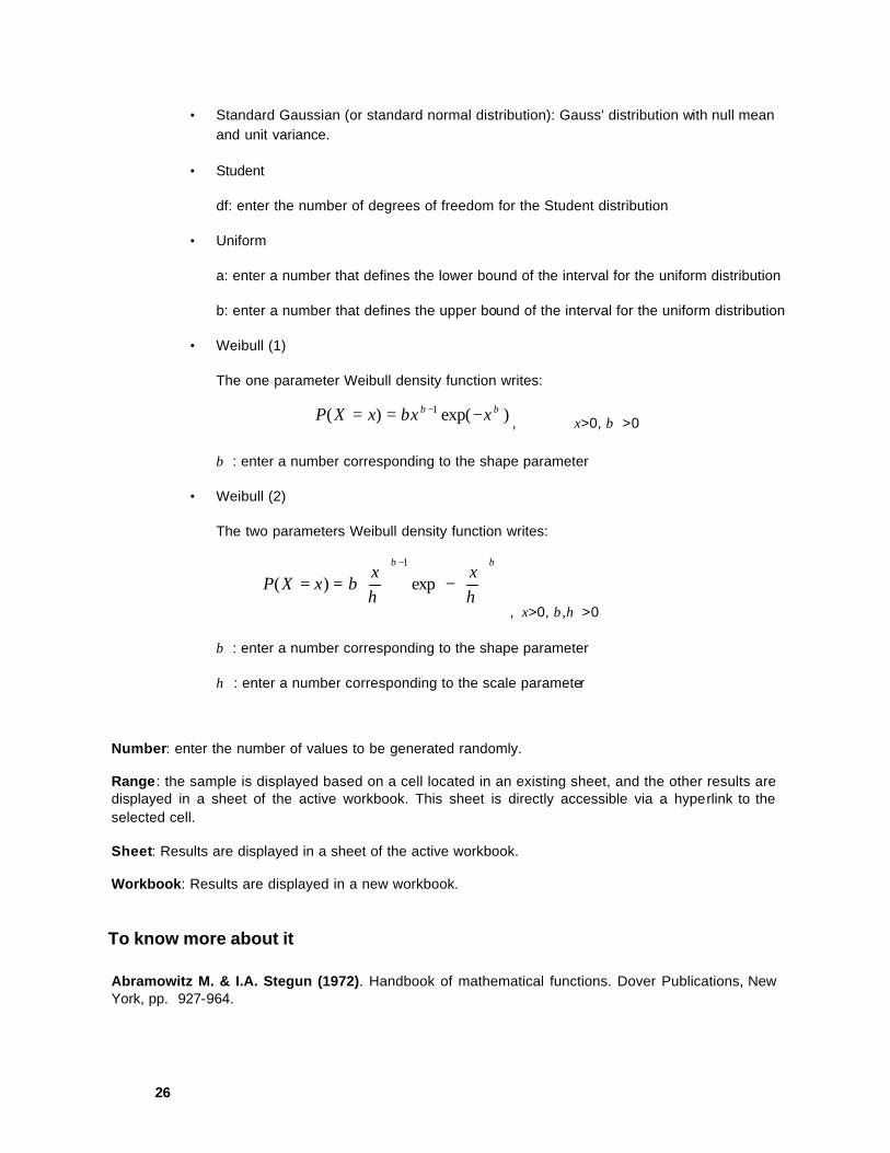
• Weibull (1)
The one parameter Weibull density function writes:
)exp()( 1 βββ xxxXP −== −, x>0, β >0
β : enter a number corresponding to the shape parameter
• Weibull (2)
The two parameters Weibull density function writes:
−
==
− ββ
ηηβ
xxxXP exp)(
1
, x>0, β,η >0
β : enter a number corresponding to the shape parameter
η : enter a number corresponding to the scale parameter
Number: enter the number of values to be generated randomly.
Range: the sample is displayed based on a cell located in an existing sheet, and the other results are displayed in a sheet of the active workbook. This sheet is directly accessible via a hyperlink to the selected cell.
Sheet: Results are displayed in a sheet of the active workbook.
Workbook: Results are displayed in a new workbook.
To know more about it
Abramowitz M. & I.A. Stegun (1972). Handbook of mathematical functions. Dover Publications, New York, pp. 927-964.
27
Aïvazian S., Enukov I. & Mechalkine L. (1986). Eléments de modélisation et traitement primaire des données. Mir, Moscou, pp. 126-183.
Manoukian E.B. (1986). Guide de statistique appliquée. Hermann, Paris, pp. 19-68.
Ripley B.D. (1983). Computer generation of random variables: a tutorial. International Statistical Review, 51: 301-319.
Ripley B.D. (1987). Stochastic simulation. John Wiley & Sons, New York.
Saporta G. (1990). Probabilités, analyse des données et statistique. Technip, Paris, pp. 30-56.
Tomassone R., Dervin C. & Masson J.P. (1993). Biométrie. Modélisation de phénomènes biologiques. Masson, Paris, pp. 62-65.

28
Discretization and histogram Use this module to discretize a quantitative variable in order to obtain classes of values, i.e. a categorical ordinal variable, and to obtain a histogram.
See also: Description
Elements of the dialog box
Editing bounds
Example
To know more about it
Description
This full-featured module allows you to define all possible classes. Several discretization modes are provided:
• division in constant steps between the minimum and maximum values in the selected column of values,
• with equal frequencies in non-weighted data, or with a constant weight, when the data are weighted,
• calculation of optimal classes in order to minimize within-class inertia (this makes the classes as compact as possible). The exact result is obtained using the Fisher's algorithm (dynamic programming algorithm) while an approximate result may be obtained using an algorithm that iteratively improves an initial solution. The calculation time for the Fisher's algorithm increases rapidly with a large number of different values and a large number of classes. XLSTAT displays a message as soon as the estimated calculation time exceeds 30 seconds for a 500 MHz processor. You can then (if so desired) change the calculation method and use an iterative improvement algorithm,
• by importing a list of class bounds, or by manually changing the class bounds using the edit module (select the data and then click "user defined").
Elements of the dialog box
Data: enter the range for the column of values to discretize. When missing data are found in the column, XLSTAT suggests ignoring the corresponding rows. If the user refuses, the dialog box is closed and the computations are stopped.
Type: choose the type of histogram to display, that means the type of values display on the ordinates axis (frequency, relative frequency, or density).
Number of classes: enter the number of intervals to calculate.

29
Constant amplitude / Equal frequencies / Optimal classes / User defined: choose the type of interval calculation:
• Constant amplitude : the amplitude depends on the number of classes.
• Equal frequencies: XLSTAT determines the bounds of the intervals that enable to have as much as possible equal frequencies or equal weights for the selected number of classes.
• Optimal classes: choose between the exact method and the approximation method, and choose the precision of the convergence threshold for successive values for within-class inertia (criterion to be minimized). For the approximation method, you must also choose the number of repetitions for the algorithm based on different random initial solutions so that XLSTAT proposes the best final solution.
• User defined: select the list of bounds and click on "Import". The bounds do not need to be sorted. Even if the "Column labels" option is activated, do not select a header for the selected column. Note that you can manually add lower and upper bounds: select the data and the click on the "user defined option" so that the edit section appears.
Compute: click on that button to compute the bounds of the intervals corresponding to each class.
Import: this button is activated only if the "User defined" option is activated. Click on this button to import the list of bounds.
Range: the sample is displayed based on a cell located in an existing sheet, and the other results are displayed in a sheet of the active workbook. This sheet is directly accessible via a hyperlink to the selected cell.
Sheet: Results are displayed in a sheet of the active workbook.
Workbook: Results are displayed in a new workbook.
Column labels: the first cell of each selected column contains a label.
Explicit classes: the categories of the resulting categorical ordinal variable are based on the class bounds, not on a class number.
Histogram: check this option to create the histogram. Check the "Bars" option if you want a histogram with vertical bars showing the interval bounds.
Weights: check this option if you want to weight the data, then enter the range for the weights column. Missing data in weights are combined with the missing data found in the data.
Editing bounds
If no computations have been previously done, and if not list of bounds has been imported, only the amplitude range is displayed. If not, the complete list of intervals is displayed .
To add an interval, click on the rows of the headers of the list of intervals, and add the value of the new bound in the new field that appears, and click on <Add>.

30
To edit the bounds of an interval, select the interval, by clicking on it. Then modify the upper and lower bounds by entering the values you wish, or by using an increment automatically determined depending on the range of the values.
When the list contains two or more intervals, you can delete one interval, or remove all the intervals.
Display: click on this button to visualize the histogram of frequencies.
Modify: click on this button to modify the bounds of an interval.
Add: click on this button to add a new bound.
Delete : click on this button to delete the selected interval.
Reset : click on this button delete all the intervals. Resetting makes that the only interval remaining corresponds to the amplitude range of the selected data.
Example
A tutorial on how to build a histogram with this tool is available on the XLSTAT website on the following page:
http://www.xlstat.com/demo-histo.htm
To know more about it
Anderberg M.R. (1973). Cluster analysis for applications. Academic Press, New York.
Diday E., Lemaire J., Pouget J. & Testu F. (1982). Eléments d'analyse de données. Dunod, Paris, pp. 32-40, 45-46.
Fisher W.D. (1958). On grouping for maximum homogeneity. Journal of the American Statistical Association, 53: 789-798.
Frontier S. (1981). Méthode statistique. Masson, Paris, pp. 42-59.
31
Coding Use this module to code or recode the categories of a categorical variable.
See also: Description
Elements of the dialog box
Continuation of the dialog box
Description
You have two possibilities: either you directly code the variable, or you import an existing coding table, apply it, and (optionally) change the coding displayed in the table. The grouping of categories is only a special form of coding in which a single code is assigned to several categories. The coding procedure generates a recoded variable as well as a correspondence table showing the old and new codes.
Elements of the dialog box
Data: enter the range for the column containing a categorical variable. Missing data are allowed and can be recoded if the user whishes so. Missing data are displayed in the list of old codes by an opening bracket followed by a closing bracket.
Column labels: the first cell of each selected column contains a label.
Coding table: enter the range for a table with two columns: the first contains the old codes and the second contains the new codes. When a code is found several times in the column of old codes, XLSTAT will use as the code the one which corresponds to the last occurrence where the old code is found. The notion of missing value does not exist for the coding table: any cell which is empty or which contains an Excel error is considered as the code for the XLSTAT missing data, and not as a missing code.
Import: click this button to start importing the entered coding table.
Range: the recoded variable is displayed based on a cell located in an existing sheet, and the other results are displayed in a sheet of the active workbook. This sheet is directly accessible via a hyperlink to the selected cell.
Sheet: Results are displayed in a sheet of the active workbook.
Workbook: Results are displayed in a new workbook.
Edit: click this button to edit the categories.
More: click this button to display the advanced options of the dialog box.

32
Continuation of the dialog box
In edit mode, two lists are added to the dialog box: the left-hand list displays the correspondence between the old and new categories, and the right -hand list allows you to select the categories to recode. To select several categories, hold down the CTRL key when you click the categories in the right-hand list.
Label for recoding: enter the label to be assigned to all the categories selected in the right-hand list.
Restore: click this button to cancel the recoding of a category selected in the right-hand list in order to return to the previous value. The number of coding steps and the number of undo's are unlimited, so you can always return to a previous state.
Refresh: click on this button to refresh the list of categories when you have changed the data selection.
Recode: click this button to actually perform the recoding. The left- and right-hand lists are updated and you can create new codes.
33
Presence/absence coding Use this module to code a set of lists of attributes into a presence/absence table.
See also: Description
Elements of the dialog box
Description
In many domains, the data are available as sets of lists of attributes (a list by statistical individual). It might be a list of pharmaceutical properties for a list of plant species, or a list of occurrences of plant species in relevés. These lists cannot be manipulated by most statistical tools, and therefore, they first need to be transformed into a presence/absence table, where each cell has a 0 if the attribute is absent and a 1 if the attribute is present.
Elements of the dialog box
Data: select a table that includes all data and the observations labels.
Observation labels, in rows and in columns: select the option that corresponds to the way your data are organized. If the lists are organized in rows, observations labels must be in left column of the selection. If the lists are organized in columns, observations labels must be in the first row of the selection. In the case of an organization in rows, the columns selection mode is not adapted. Therefore you need to use the range mode.
Range: the presence/absence table is displayed based on a cell located in an existing sheet, and the other results are displayed in a sheet of the active workbook. This sheet is directly accessible via a hyperlink to the selected cell.
Sheet: Results are displayed in a sheet of the active workbook.
Workbook: Results are displayed in a new workbook.

34
Full Disjunctive Coding Use this module to code a table with the observations in rows and the categorical variables in columns as a binary table (0/1) by using full disjunctive coding.
See also: Description
Elements of the dialog box
To know more about it
Description
With full disjunctive coding, XLSTAT assigns a 1 to the category of a categorical variable for the observation in question, and a 0 to all the other categories of that variable. If you apply this coding method to a set of categorical variables, this procedure is repeated for each variable. The resulting table contains as many columns as there are total categories for all the categorical variables, and as many 1s for an observation as there are variables.
Elements of the dialog box
Data: enter the range of a table with the observations in rows and the categorical variables in columns. If a missing value is found in an [i,j] cell (which means for the observation on row i and the categorical variable in column j) all the categories of variable j are set to 0 for the ith observation.
Observation labels: if you want to create a disjunctive table with special labels for the observations, enter the range for the labels column. By default, the label of an observation is its row number in the table.
Range: the results are displayed based on a cell located in an existing sheet.
Sheet: Results are displayed in a sheet of the active workbook.
Workbook: Results are displayed in a new workbook.
Column labels: the first cell of each selected column contains a label.
To know more about it
Diday E., Lemaire J., Pouget J. & Testu F. (1982). Eléments d'analyse de données. Dunod, Paris, pp. 42-44.
Tomassone R., Dervin C. & Masson J.P. (1993). Biométrie. Modélisation de phénomènes biologiques. Masson, Paris, p. 112.
35
Coding by Ranks Use this module to code an array by rank, with the observations in rows and the variables in columns.
See also: Description
Elements of the dialog box
Description
For each variable, observations are ranked in ascending order by value. Tied observations (with equal values) are ranked by the average of their initial ranks, or by the rank of their common value.
Note: the first method for processing ties is the only valid one for performing statistical tests (for example, to test the correlation between two variables).
Elements of the dialog box
Data: enter the range of an array with the observations in rows and quantitative variables in columns. Missing data are allowed and their rank is set to 0.
Observation labels: if you want to create a ranks table with special labels for the observations, enter the range for the labels column. By default, the label of an observation is its row number in the table.
Average ranking for ties: check this option if you want to use ranks to perform statistical tests.
Range: the results are displayed based on a cell located in an existing sheet.
Sheet: Results are displayed in a sheet of the active workbook.
Workbook: Results are displayed in a new workbook.
Column labels: the first cell of each selected column contains a label.

36
Partition recoding Use this module to recode a partition while removing a level of indirection corresponding an intermediary partition.
See also: Description
Elements of the dialog box
Description
It is a common strategy in agglomerative hierarchical clustering to run first a k-means clustering to obtain from the initial set of observations a reduced number of homogenous groups, and then a hierarchical ascending clustering on the groups. By truncating the dendrogram, you obtain the final partition. This mixture of methods gives a partition of the groups obtained from the first step, but not from the initial observations. Partition recoding allows to eliminate the intermediary partition, and to reassign each initial observation to its final group. Partition recoding can of course be used in any case that you can formulate in a similar way.
Elements of the dialog box
First partition: select the column that corresponds to the intermediary partition, (that indicates to which group belongs which initial observation).
Second partition: select the column that corresponds to the final partition.
Observation labels: activate this option if you want to use specific labels for the observations, and select the column that corresponds to the labels. By default, the label of an observation is its row number.
Range: the recoded partition is displayed based on a cell located in an existing sheet, and the other results are displayed in a sheet of the active workbook. This sheet is directly accessible via a hyperlink to the selected cell.
Sheet: results are displayed in a sheet of the active workbook.
Workbook: results are displayed in a new workbook.
Column labels: the first cell of each selected column contains a label.
37
Transformation Use this module to transform a quantitative variable using an analytical function.
See also: Description
Elements of the dialog box
Continuation of the dialog box
To know more about it
Description
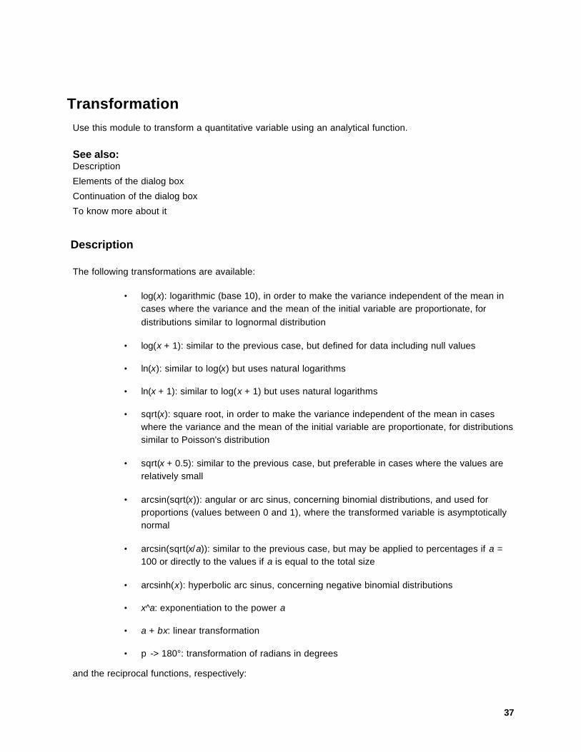
The following transformations are available:
• log(x): logarithmic (base 10), in order to make the variance independent of the mean in cases where the variance and the mean of the initial variable are proportionate, for distributions similar to lognormal distribution
• log(x + 1): similar to the previous case, but defined for data including null values
• ln(x): similar to log(x) but uses natural logarithms
• ln(x + 1): similar to log(x + 1) but uses natural logarithms
• sqrt(x): square root, in order to make the variance independent of the mean in cases where the variance and the mean of the initial variable are proportionate, for distributions similar to Poisson's distribution
• sqrt(x + 0.5): similar to the previous case, but preferable in cases where the values are relatively small
• arcsin(sqrt(x)): angular or arc sinus, concerning binomial distributions, and used for proportions (values between 0 and 1), where the transformed variable is asymptotically normal
• arcsin(sqrt(x/a)): similar to the previous case, but may be applied to percentages if a = 100 or directly to the values if a is equal to the total size
• arcsinh(x): hyperbolic arc sinus, concerning negative binomial distributions
• x^a: exponentiation to the power a
• a + bx: linear transformation
• p -> 180°: transformation of radians in degrees
and the reciprocal functions, respectively:

38
• 10^x
• 10^x – 1
• exp(x)
• exp(x) – 1
• x²
• x² – 0.5
• (sin(x))²
• a(sin(x))²
• sinh(x)
• x^(1/a)
• (x-a)/b
• 180° -> p
Elements of the dialog box
Data: enter the range for a column of quantitative values. Missing data in the data column are of course still missing in the results column. Missing data are generated if the transformation is not possible (for example, the logarithm of negative values).
Column labels: the first cell of the selected column contains a label.
Select the function to be used to transform your data.
Range: the transformed variable is displayed based on a cell located in an existing sheet, and the other results are displayed in a sheet of the active workbook. This sheet is directly accessible via a hyperlink to the selected cell.
Sheet: results are displayed in a sheet of the active workbook.
Workbook: results are displayed in a new workbook.
Scientific notation: check this option if you want values that are too small or too large to be displayed in scientific notation. A value is considered too small if the displayed value does not include any digits after the decimal place that are different than 0, and too large if the value is greater than 1E+9.
More: click this button to display the advanced options of the dialog box.

39
Continuation of the dialog box
Rest of the functions available. When the selected function requires a parameter, a data entry field is displayed for you to enter the value for this parameter.
"Degrees" / "Radians": select "Degrees" if the argument of sin(x) and the result of arcsin(x) are expressed in degrees, and select "Radians" if the argument of sin(x) and the result of arcsin(x) are expressed in radians.
Quick transformations: select this option if you want to use the following one step transformations:
Variance en 1/(n-1): activate this option to compute the variance with n-1 as the denominator. Uncheck this option to use n.
Center: check this option to center the values (subtract the mean).
Reduce: check this option to reduce the data (divide them by their standard deviation).
Greater or equal to 0: select this option to that all values are non negative.
Greater than 0: select this option to that all values are strictly positive.
To know more about it
Dagnelie P. (1986). Théorie et méthodes statistiques. Vol. 2. Les Presses Agronomiques de Gembloux, Gembloux, pp. 361-375.
Sokal R.R. & Rohlf F.J. (1995). Biometry. The principles and practice of statistics in biological research. Third edition. Freeman, New York, pp. 409-422.

40
Anamorphosis Use this module to transform a quantitative variable using an anamorphosis of its cumulative distribution function.
See also: Description
Elements of the dialog box
Example
To know more about it
Description
Each value of a quantitative variable Z is associated with a probability in its cumulative distribution function. The principle of anamorphosis consists in replacing the value of the initial variable Z with the value corresponding to the same probability in the cumulative distribution function of the resulting variable Y. Fig. 1 illustrates the principle of anamorphosis, in cases of anamorphosis towards the standard normal distribution (Gauss' standard distribution).
Fig.1: principle for defining the anamorphosis function )(zy φ= . (a) Empirical cumulative distribution function F(z) of the data to be transformed (cumulative distribution). (b) Cumulative distribution function G(y) of the standard normal distribution.
Three anamorphosis modes are provided: empirical, theoretical, and reciprocal theoretical.
Empirical anamorphosis is based on two empirical cumulative distribution functions: a function of the initial variable and a function of the reference variable, or resulting variable. This procedure allows XLSTAT to transform a variable so that it is distributed like another variable, no matter which.
Theoretical anamorphosis requires you to choose a probability distribution among those available: uniform, standard Gaussian, Gaussian, lognormal, Student, Fisher, Chi-square, Beta, exponential. This procedure uses a numerical approximation of the theoretical cumulative distribution function for the probability distribution used.
Reciprocal theoretical anamorphosis requires you to choose a probability distribution as a model for the initial variable, and a reference variable. This procedure uses a numerical approximation of the reciprocal cumulative distribution function for the probability distribution used.
Notes:
• Because the numerical approximation allowing theoretical anamorphosis of a variable does not generally offer the same degree of accuracy as the numerical approximation of theoretical reciprocal anamorphosis, you will not obtain exactly the same results as your initial values if you run a full cycle Z -> Y then Y -> Z. However, empirical anamorphosis
41
returns the exact initial values because it is perfectly symmetrical, based on the same cumulative distribution functions,
• the presence of several null values, or too small a number of values makes it very difficult (if not impossible) to obtain a satisfactory transformation using empirical anamorphosis.
Elements of the dialog box
Variable: select the column which contains the values to be transformed. When missing data are found in the column, XLSTAT suggests ignoring the corresponding rows. If the user refuses, the dialog box is closed and the computations are stopped.
Anamorphosis: choose the anamorphosis method for transforming your data. Empirical anamorphosis requires you to select the reference data. Theoretical anamorphosis requires you to select a probability distribution. Reciprocal theoretical anamorphosis requires you to select a probability distribution for the data to be transformed, and the reference data.
Reference : for empirical anamorphosis and reciprocal theoretical anamorphosis, enter the range for the reference variable column. When missing data are found in the column, XLSTAT suggests ignoring the corresponding rows. If the user refuses, the dialog box is closed and the computations are stopped.
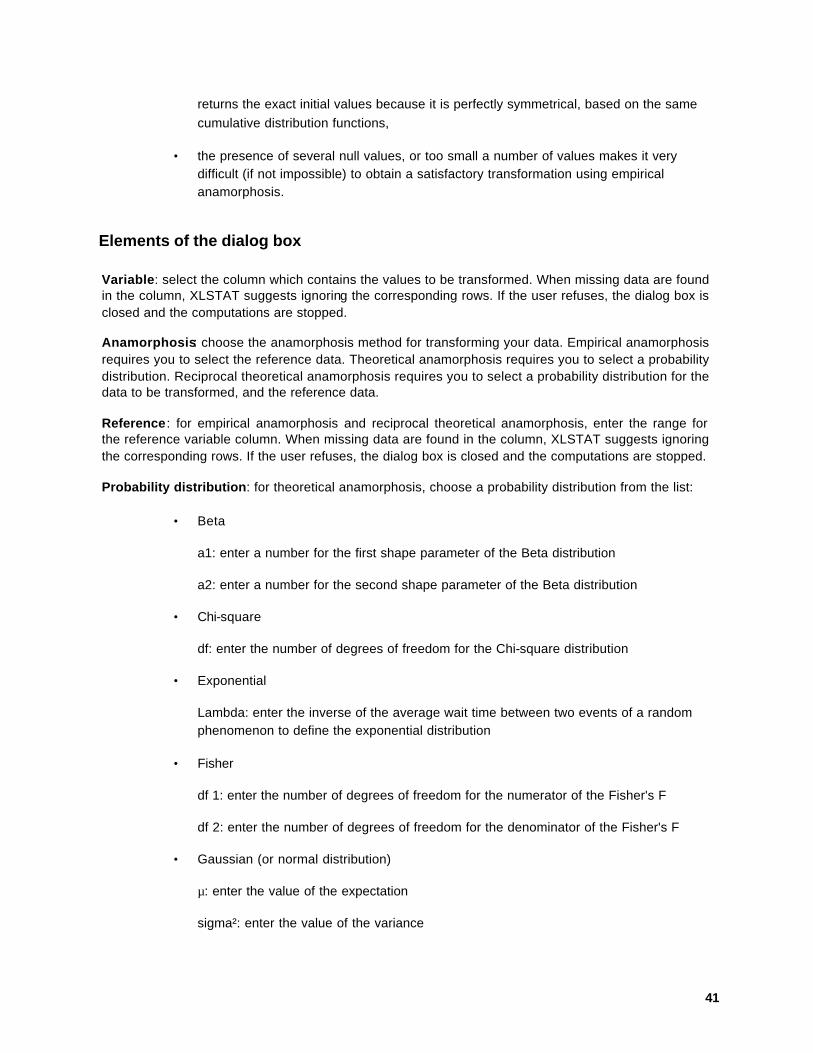
Probability distribution: for theoretical anamorphosis, choose a probability distribution from the list:
• Beta
a1: enter a number for the first shape parameter of the Beta distribution
a2: enter a number for the second shape parameter of the Beta distribution
• Chi-square
df: enter the number of degrees of freedom for the Chi-square distribution
• Exponential
Lambda: enter the inverse of the average wait time between two events of a random phenomenon to define the exponential distribution
• Fisher
df 1: enter the number of degrees of freedom for the numerator of the Fisher's F
df 2: enter the number of degrees of freedom for the denominator of the Fisher's F
• Gaussian (or normal distribution)
µ: enter the value of the expectation
sigma²: enter the value of the variance

42
• Lognormal (the logarithm of the variable distributed using a lognormal distribution follows normal distribution with parameters µ and sigma² parameters)
µ: enter the value of the expectation of normal distribution according to which ln(x) is distributed
sigma²: enter the value of the variance of normal distribution according to which ln(x) is distributed
• Standard Gaussian (or standard normal distribution): Gauss' distribution with null mean and unit variance.
• Student
df: enter the number of degrees of freedom for the Student distribution
• Uniform
a: enter a number that defines the lower bound of the interval for the uniform distribution
b: enter a number that defines the upper bound of the interval for the uniform distribution
• Weibull (1)
The one parameter Weibull density function writes:
)exp()( 1 βββ xxxXP −== −, x>0, β >0
β : enter a number corresponding to the shape parameter
• Weibull (2)
The two parameters Weibull density function writes:
−
==
− ββ
ηηβ
xxxXP exp)(
1
, x>0, β,η >0
β : enter a number corresponding to the shape parameter
η : enter a number corresponding to the scale parameter
Column labels: the first cell of the selected column contains a label.
Range: the transformed variable is displayed based on a cell located in an existing sheet, and the other results are displayed in a sheet of the active workbook. This sheet is directly accessible via a hyperlink to the selected cell.
Sheet: results are displayed in a sheet of the active workbook.

43
Workbook: results are displayed in a new workbook.
Example
To know more about it
Abramowitz M. & I.A. Stegun (1972). Handbook of mathematical functions. Dover Publications, New York, pp. 927-964.
Aïvazian S., Enukov I. & Mechalkine L. (1986). Eléments de modélisation et traitement primaire des données. Mir, Moscou, pp. 126-183.
Deutsch C.V. & A.G. Journel (1992). GSLIB. Geostatistical Software Library and user's guide. Oxford University Press, New York, p. 138.
Goovaerts P. (1997). Geostatistics for natural resources evaluation. Oxford University Press, New York, pp. 266-271.
Manoukian E.B. (1986). Guide de statistique appliquée. Hermann, Paris, pp. 19-68.
44
Descriptive Statistics Use this module to calculate a set of descriptive statistics for one or several categorical or quantitative variables, and to create graphical or semi-graphical displays used for exploratory data analysis.
See also: Description
Elements of the dialog box
Continuation of the dialog box
To know more about it
Description
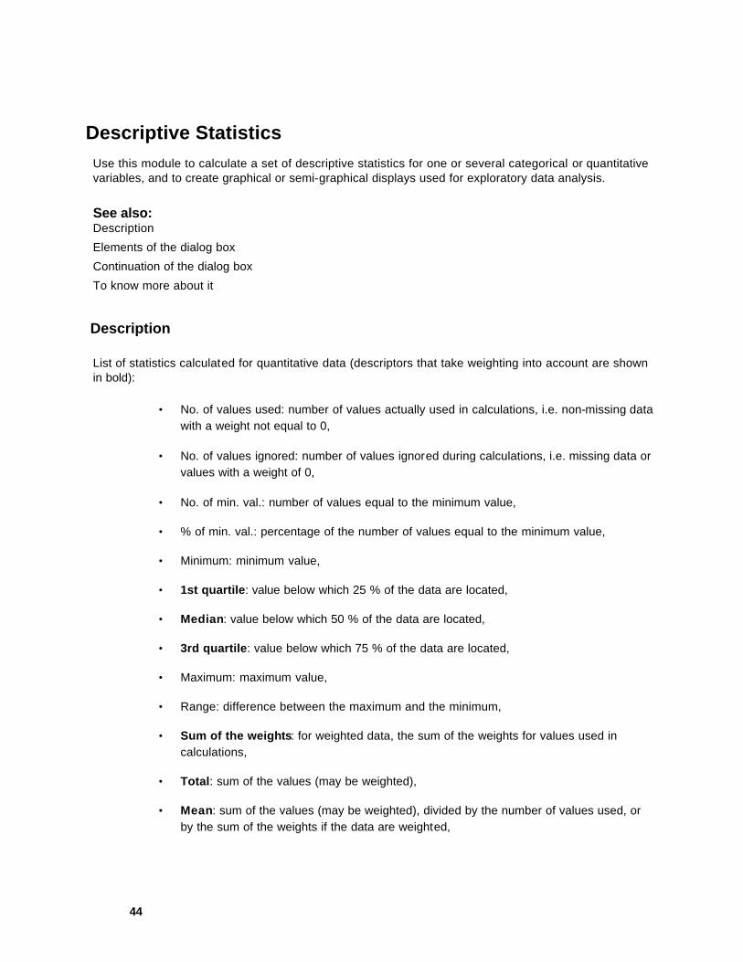
List of statistics calculated for quantitative data (descriptors that take weighting into account are shown in bold):
• No. of values used: number of values actually used in calculations, i.e. non-missing data with a weight not equal to 0,
• No. of values ignored: number of values ignored during calculations, i.e. missing data or values with a weight of 0,
• No. of min. val.: number of values equal to the minimum value,
• % of min. val.: percentage of the number of values equal to the minimum value,
• Minimum: minimum value,
• 1st quartile: value below which 25 % of the data are located,
• Median: value below which 50 % of the data are located,
• 3rd quartile: value below which 75 % of the data are located,
• Maximum: maximum value,
• Range: difference between the maximum and the minimum,
• Sum of the weights: for weighted data, the sum of the weights for values used in calculations,
• Total: sum of the values (may be weighted),
• Mean: sum of the values (may be weighted), divided by the number of values used, or by the sum of the weights if the data are weighted,

45
• Geometric mean: mean that is barely affected by high values. The geometric mean is not defined for data containing negative or null values,
• Harmonic mean: mean that is barely affected by a few values that are much higher than the others, but is sensitive to much smaller values. The harmonic mean is not defined for data containing null values,
• Kurtosis (Pearson): coefficient that represents the peaked or flattened shape of a distribution compared to a Gaussian distribution. For a Gaussian distribution (normal distribution), kurtosis is equal to 0. A negative value represents a flatter distribution than the normal distribution (platycurtic distribution) while a positive value represents a more peaked distribution than normal distribution (leptocurtic distribution),
• Skewness (Pearson): coefficient that represents the degree of skewness for a distribution compared to its mean. For a Gaussian distribution (normal distribution), skewness is equal to 0. A negative value indicates that the distribution is skewed to the left, while a positive value indicates that the distribution is skewed to the right,
• Kurtosis: kurtosis coefficient as calculated by Excel,
• Skewness: skewness coefficient as calculated by Excel,
• CV (standard deviation/mean): variation coefficient that measures the relative dispersion, obtained by dividing the standard deviation by the mean. This coefficient allows you to compare the dispersion of variables that have different units, or that have very different means,
• Sample variance : variance of the data, (in case of unweighted data, the denominator is n, i.e. the size of the sample),
• Estimated variance: estimation of the variance for a population whose data makes up a sample (unbiased estimator: in case of unweighted data, the denominator is n-1, with n the size of the sample),
• Standard deviation of a sample: square root of the variance of the data,
• Estimated standard deviation: square root of the estimation of the variance for the source data population,
• Mean absolute deviation: dispersion measure that indicates the average of the absolute values of the deviations for each value compared to the mean,
• Standard deviation of the mean: square root of the ratio of the estimated variance to the number of values used in the calculation. This estimation of the variance of the mean is valid only if the data consists of a sample taken at random (and without replacement) from an infinite population (simple random sample of an infinite population),
• Mean absolute deviation: dispersion measure that indicates the average of the absolute values of the deviations for each value compared to the mean,

46
• Absolute median deviation: median of the absolute deviations from the median.
Charts created for quantitative variables
• box plots,
• univariate scattergrams
• collection of bivariate scattergrams
• Q-Q plots,
• p-p plots,
• stem and leaf plots.
List of statistics calculated for categorical data
Summary for all variables:
• No. of categories: number of categories for the variable,
• Mode: the category that occurs most often, or that has the highest weight (if the data are weighted),
• Mode frequency: for non-weighted data, frequency of the mode,
• Mode weight: for weighted data, weight of the mode,
• % mode: percentage of the mode,
• Rel. freq. mode: relative frequency of the mode.
Statistics table for each variable:
• Frequency: for unweighted data, frequency of the category,
• Weight: for weighted data, weight of the category,
• %: percentage of the category,
• Rel. freq.: relative frequency of the category.
Charts created for categorical variables
• histograms,
• pie charts.

47
Elements of the dialog box
Data: enter the range for the variables to be described. When missing data are found in a column, XLSTAT suggests ignoring them. If the user refuses, the dialog box is closed and the computations are stopped.
Quantitative / Categorical: choose the type of variable.
Column labels: the first cell of each selected column contains a label.
Range: the results are displayed based on a cell located in an existing sheet.
Sheet: Results are displayed in a sheet of the active workbook.
Workbook: Results are displayed in a new workbook.
More: click this button to display the advanced options of the dialog box.
Continuation of the dialog box
Group descriptor: check this option if you want XLSTAT to consider a categorical variable that describes the groups of values, then enter the range for the group descriptor column. Missing data for group descriptor are combined with missing data for the data.
Compare : if you are applying a group descriptor, check this option to compare the results obtained for each group with those obtained for all the values.
Weight: check this option if you want to weight the data, then enter the range for the weight column. Missing data for the weights are set to zeros and imply the inactivation of the corresponding row.
For quantitative variables
• Display X/Y charts: check this option to display the collection of bivariate scattergrams obtained by comparing pairs of all the selected quantitative variables.
• "X/Y and X/X" / "X/Y and Q-Q"/ "X/Y and p-p": choose to display either the collection of bivariate scattergrams (including those that compare each variable with itself), or the collection of bivariate scattergrams and Q-Q plots or p-p plots for all variables. These charts cannot be displayed if there are more than 6 variables or 30,000 points.
• Box plots: check this option to obtain box plot. These charts cannot be displayed if there are more than 16 variables or 30,000 points.
• Scattergrams: check this option to obtain univariate scattergrams. These charts cannot be displayed if there are more than 24 variables or more than 30,000 points.
• Vertical boxes / Horizontal boxes: choose the orientation of box plots and scattergrams.

48
• Standardization: check this option to cancel the effect of the order of magnitude differences between the variables when creating box plots and scattergrams, by dividing the values of each variable by the corresponding standard deviation.
• Stem-and-leaf plots: check this option to obtain stem-and-leaf plots.
For categorical variables
• Histograms: check this option to display the corresponding histograms.
• Pie charts: check this option to display the pie charts.
• Group charts: check this option to display all the charts on a separate sheet.
To know more about it
Sokal R.R. & Rohlf F.J. (1995). Biometry. The principles and practice of statistics in biological research. Third edition. Freeman, New York, pp. 28-30, 39-60, 151-152.
Tomassone R., Dervin C. & Masson J.P. (1993). Biométrie. Modélisation de phénomènes biologiques. Masson, Paris, p. 115-121.

49
Histograms Use this module to display histograms of the frequencies that approximate the probability density function of a quantitative variable and the distribution of cumulative frequencies that approximate its cumulative distribution function.
Note: You can also create histograms with the Discretization and histogram module using other methods, and manually change the bounds.
See also: Elements of the dialog box
Continuation of the dialog box
To know more about it
Elements of the dialog box
Data: select the data corresponding to a quantitative variable. When missing data are found, XLSTAT suggests ignoring the corresponding rows. If the user refuses, the dialog box is closed and the computations are stopped.
Continuous/Discrete : choose the option that corresponds to the type of your data.
Type: choose the type of histogram to display, that means the type of values display on the ordinates axis (frequency, relative frequency, or density).
Cumulative distribution: check this option to create the cumulative distribution. Check the "Bars" option if you want a cumulative distribution with vertical bars showing the interval bounds. The maximum number of values allowed is 30,000 when the "Bars" option is not checked, and 15,000 if it is.
Histogram: check this option to create the histogram. Check the "Bars" option if you want a histogram with vertical bars showing the interval bounds.
Number of intervals: enter the number of intervals with a constant amplitude for creating the histogram.
Range: the results are displayed based on a cell located in an existing sheet.
Sheet: Results are displayed in a sheet of the active workbook.
Workbook: Results are displayed in a new workbook.
Column labels: the first cell of the selected column contains a label.
Charts: check this option to display charts of the histogram and the cumulative distribution.
Tables: check this option to display tables that describe the histogram and the cumulative distribution (interval bounds, frequencies).
50
More: click this button to display the advanced options of the dialog box.
Continuation of the dialog box
Histogram / Frequency polygon: choose the type of chart. If you select "Histogram" then the chart shows the intervals, and if you select "Frequency polygon" the chart joins the interval centers.
Weight: check this option if you want to weight the data, then enter the range for the weight column. Missing data for weights are combined with missing data for the data.
Example
A tutorial on how to build a histogram with this tool is available on the XLSTAT website on the following page:
http://www.xlstat.com/demo-histo.htm
To know more about it
Frontier S. (1981). Méthode statistique. Masson, Paris, pp. 42-59.
Sokal R.R. & Rohlf F.J. (1995). Biometry. The principles and practice of statistics in biological research. Third edition. Freeman, New York, pp. 19-32.
51
Normality Tests Use this tool to test if a sample is normally distributed. This tool complements the Distribution fitting tool, which allows you to determine the value of the parameters of the normal distribution and to test the goodness of fit using a Chi-square or a Kolmogorov Smirnov test.
See also: Description
Elements of the dialog box
Missing data
Results
Example
To know more about it
Description
Assuming that a sample is normally distributed is common in statistical analysis. For example, in linear regression, in ANOVA or in ANCOVA the errors of the model are assumed to follow a normal distribution. As for any assumption, it is necessary, to test it.
XLSTAT offers you four methods to test the normality: the Shapiro-Wilk test that can be used with up to 5000 observations, the Anderson-Darling test, the Jarque-Bera test which is an asymptotic test which performance increases with the number of observations, and the Lilliefors test.
Elements of the dialog box
Data: select the data corresponding to a quantitative variable.
Set of independent columns: activate this option if all columns in your selection are independent. This option is activated only if XLSTAT detects that several columns are selected.
Weights: select the weights of the observations.
Significance level (%): enter the value of the type I error for the test.
Shapiro-Wilk test: activate this option to compute the Shapiro-Wilk test.
Anderson-Darling test: activate this option to compute the Anderson-Darling test.

52
Jarque-Bera test: activate this option to compute the Jarque-Bera test.
Lilliefors test: activate this option to compute the Lilliefors test.
Range: the results are displayed based on a cell located in an existing sheet.
Sheet: Results are displayed in a sheet of the active workbook.
Workbook: Results are displayed in a new workbook.
Column labels: the first cell of the selected column contains a label.
Summary: activate this option to display summary statistics for each column.
Charts:
• Q-Q plot: activate this option to display a normal Quantile-Quantile plot.
• p-p plot: activate this option to display a normal Probability- Probability plot.
Missing data
If missing data are detected, XLSTAT gives you the possibility to remove them or to replace them.
When your data are set in a observations/variables table, XLSTAT gives you the possibility to delete the observations where at least one missing data has been found. If you refuse that option, missing data are only removed column by column (casewise deletion).
When your data are in one column, or in a set of independent columns, missing data are ignored.
Results
XLSTAT displays the results for the selected tests. An interpretation of the results is added, as well as the decision that should be taken, given the selected significance level.
Example
A tutorial on using the normality tests is available on the XLSTAT website on the following page:
http://www.xlstat.com/demo-norm.htm

53
To know more about it
D'Agostino R.B. & Stephens M.A. (1986). Goodness-of-fit techniques. Marcel Dekker, New York, USA : 560 p.
Dallal G.E. & Wilkinson L. (1986). An Analytic Approximation to the Distribution of Lilliefors's Test Statistic for Normality. Statistical Computing, 40, pp. 294-296.
Jarque C.M. & Bera A.K. (1980). Efficient Tests for Normality, Heteroscedasticity and Serial Independence of Regression Residuals. Economic Letters, 6, pp. 255-259.
Royston P. (1982). An Extension of Shapiro and Wilk's W Test for Normality to Large Samples. Applied Statistics, 31, pp. 115–124.
Royston P. (1982). Algorithm AS 181: The W Test for Normality. Applied Statistics, 31, pp. 176–180.
Royston P. (1995). A Remark on Algorithm AS 181: The W Test for Normality. Applied Statistics, 44, pp. 547–551.
Shapiro S. S. & Wilk M. B. (1965). An analysis of variance test for normality (complete samples). Biometrika, 52, 3 and 4, pp. 591-611.
Thode H.C. (2002). Testing for normality. Marcel Dekker, New York, USA, 479 p.

54
Contingency Table (Two-way Table) and Chi-square Use this module to calculate the contingency table (two-way table) for two sets of categorical variables, as well as the derivative tables, and test the association between the rows and the columns.
Note: tests concerning contingency tables are much more fully developed in the Tests on Contingency Tables module.
See also: Elements of the dialog box
Continuation of the dialog box
To know more about it
Elements of the dialog box
Qualitative variables in rows: enter the range for the categorical variables whose categories will make up the contingency table rows. When missing data are found, XLSTAT suggests ignoring them when building the contingency table. If the user refuses, the dialog box is closed and the computations are stopped.
Qualitative variables in columns: enter the range for the categorical variables whose categories will make up the contingency table columns. When missing data are found, XLSTAT suggests ignoring them when building the contingency table. If the user refuses, the dialog box is closed and the computations are stopped.
Chi-square independence test: test the independence between the rows and columns in the contingency table using a Chi-square test.
Significance level: enter the value of the type I error for the test.
Range: the results are displayed based on a cell located in an existing sheet.
Sheet: Results are displayed in a sheet of the active workbook.
Workbook: Results are displayed in a new workbook.
Column labels: the first cell of each selected column contains a label.
More: click this button to display the advanced options of the dialog box.
Continuation of the dialog box
Weight: select the range for the weights column. When missing data are found, XLSTAT suggests ignoring the corresponding rows. If the user refuses, the dialog box is closed and the computations are stopped.
55
Combinations: check this option to display a table with the combinations of categories in rows and in columns. This table contains the same information as the contingency table and the table of percentages in relation to the total size, but the information is presented in a different format.
Observed frequencies: check this option to display the contingency table to which the marginal totals and the total have been added.
Expected frequency: check this option to display the table of expected frequencies calculated assuming that the rows and columns in the contingency table are independent.
Contributions to Chi-square: check this option to display the table of the basic contributions of each cell in the contingency table for the Chi-square value calculated for the entire contingency table.
"Chi-square by cell": check this option to display a table that shows a) whether the observed frequency is greater than, less than, or equal to the expected frequency, and b) the result of the partial Chi-square test called the "Chi-square by cell" test. The "Chi-square by cell" test is a Chi-square test calculated on a table with four cells: one cell represents cell [i,j] in the original contingency table, the other cells represent frequencies for row i minus cell [i,j], for column j minus cell [i,j], and for the rest of the table.
Percentages/proportions in relation to rows: check this option to display the table of percentages or proportions compared to the sums of the rows.
Percentages/proportions in relation to columns: check this option to display the table of percentages or proportions compared to the sums of the columns.
Percentages/proportions in relation to total: check this option to display the table of percentages or proportions compared to the total.
Percentages / Proportions: choose the display mode for the three previous tables, either as percentages (values between 0 and 100), or as proportions (values between 0 and 1).
To know more about it
Sokal R.R. & Rohlf F.J. (1995). Biometry. The principles and practice of statistics in biological research. Third edition. Freeman, New York, pp. 724-743.
Tomassone R., Dervin C. & Masson J.P. (1993). Biométrie. Modélisation de phénomènes biologiques. Masson, Paris, pp. 92-95.

56
Similarity/Dissimilarity Matrix (Correlation …) Use this module to calculate a similarity or dissimilarity matrix for a rectangular array by comparing the rows or the columns, and test the hypothesis that there is no correlation structure in case of parametric correlation matrix (Pearson's correlation coefficient) using Bartlett's sphericity test.
See also: Elements of the dialog box
Continuation of the dialog box
To know more about it
Elements of the dialog box
Data: select the data table. When missing data are found,, XLSTAT suggests first ignoring the corresponding rows. If the user refuses, XLSTAT suggest to use all the available information by simply ignoring the missing data (pairwise deletion), otherwise the dialog box is closed and the computations are stopped.
quantitative / binary / all types: choose the type of data. This enables XLSTAT to perform validity checks on the data, and to avoid methodological errors concerning the choice of a similarity/dissimilarity coefficient. For quantitative or binary variables, only the coefficients defined specifically for these data types are proposed. For all types (quantitative data and/or categorical data), only one coefficient is proposed as XLSTAT considers the data to be at the lowest level of algebraic structure, i.e. at the level of a nominal categorical variable: the values are distinguished among them only on the basis of the strict equality/inequality.
Row labels: enter the range for the column of labels that represent the data array rows.
Similarity / Dissimilarity: choose whether the calculated values should be higher if the data are similar (similarity), or lower if the data are similar (dissimilarity). The type of measurement you choose determines the list of coefficients proposed.
For quantitative data:
Similarity Dissimilarity
Pearson's correlation coefficient Euclidean distance
Spearman's coefficient of rank correlation Chi-square distance
Kendall's coefficient of rank correlation Manhattan distance
Inertia Pearson's dissimilarity
Covariance (n) Spearman's dissimilarity
Covariance (n-1) Kendall's dissimilarity

57
Cosine Mahalanobis' distance
Bhattacharya's distance
Chebychev's distance
Canberra's distance
Chord distance
Squared chord distance
Geodesic distance
Note: the only difference between "Covariance (n)" and "Covariance (n-1)" is the denominator used, i.e. either n or n-1, where n is the size (number of rows if you compare by columns, or number of columns if compare by rows). In the second case, this is an estimation without bias of the variance-covariance matrix for a multivariate normal distribution.
For binary data (0/1):
Similarity/Dissimilarity
Jaccard coefficient
Dice coefficient
Sokal & Sneath coefficient (2)
Rogers & Tanimoto coefficient
Simple matching coefficient
Sokal & Sneath coefficient (1)
Phi coefficient
Ochiai's coefficient
Kulczinski's coefficient
For all types data:
Similarity Dissimilarity
Percent agreement Percent disagreement
Cooccurrences

58
In order to process different types of variables (quantitative and categorical), you can use a general similarity/dissimilarity (percent agreement/disagreement) or the cooccurrences that handles all the variables at the lowest algebraic level, i.e. the nominal variable level. This allows to identify the rows or the columns that are considered as similar.
Range: results are displayed based on a cell located in an existing sheet.
Sheet: Results are displayed in a sheet of the active workbook.
Workbook: the results are displayed in a new workbook.
Show labels: a label appears in the first cell of each selected column.
Column labels: the first cell of each selected column contains a label.
More: click this button to display the advanced options of the dialog box.
Continuation of the dia log box
Compare "rows" / "columns": choose if the similarity/dissimilarity matrix should compare the data array rows or columns.
Note: if the dialog box is in memory off mode, XLSTAT adapts this option according to the type of variable and the type of coefficient (similarity or dissimilarity). For a quantitative variable, by default the similarity calculation is performed by comparing the columns (for example, the correlation between the variables in an observations/variables table), and the dissimilarity calculation is performed by comparing the rows (for example, the Euclidean distance between the observations in an observations/variables table). In the other cases, by default calculations are performed by comparing the rows (for example, the Jaccard coefficient between the observations in an observations/variables table).
Bartlett's sphericity test: When the Pearson's correlation coefficient is used (similarity for quantitative data), check this option to perform Bartlett's sphericity test which checks for the existence of a significant correlation structure within the correlation matrix, using the significance level defined by "Significance level". For more information on this test, click here.
Significance level: enter the value of the type I error for Bartlett's sphericity test.
Detect similar data : when percent agreement is used (all types of data), check this option to highlight similar data (rows or columns based on the option you chose previously) using the threshold defined by "Threshold value (%)".
Threshold value (%): enter the value for the minimum similarity beyond which data are considered to be similar. Data are declared to be similar if the similarity is greater than the threshold value, or (to put it another way), if the dissimilarity is less than 100 % minus the threshold value.
List of similar data: check this option to display a table showing the data pairs (rows or columns) identified as being similar.

59
To know more about it
Dillon W.R. & Goldstein M. (1984). Multivariate analysis. Methods and applications. John Wiley & Sons, New York, pp. 157-167.
Gower J.C. & Legendre P. (1986). Metric and Euclidean properties of dissimilarity coefficients. Journal of Classification, 3: 5-48.
Jambu M. (1978). Classification automatique pour l'analyse des données. 1 - méthodes et algorithmes. Dunod, Paris, pp. 484-518.
Jobson J.D. (1992). Applied multivariate data analysis. Volume II: categorical and multivariate methods. Springer-Verlag, New York, pp. 345-388.
Legendre L. & Legendre P. (1984). Ecologie numérique. Tome 2. La structure des données écologiques. Masson, Paris, pp. 5-50.
Roux M. (1985). Algorithmes de classification. Masson, Paris, pp. 126-134.
Sokal R.R. & Rohlf F.J. (1995). Biometry. The principles and practice of statistics in biological research. Third edition. Freeman, New York, pp. 724-743.
Tomassone R., Dervin C. & Masson J.P. (1993). Biométrie. Modélisation de phénomènes biologiques. Masson, Paris, pp. 157-158 .

60
Factor Analysis Use factor analysis to summarize the data correlation structure described by several quantitative variables, by identifying the underlying factors shared by variables, that to a large extent can explain the variability of the data.
See also: Description
Elements of the dialog box
Continuation of the dialog box
Display options dialog box
Example
To know more about it
Description
The purpose of factor analysis is to describe a set of variables using a linear combination of common underlying factors, and a variable representing the specific part of the original variables. The variance of an original variable may be broken down into a part shared with other variables (explained by the factors) called the communality of the variable, and a specific part called the specific variance.
Among the various methods available, XLSTAT uses the principal factor method (or PFA). The communality of each variable is initialized so that a variable with a very low correlation to the others has a low communality and therefore a high specific variance. By default, XLSTAT initializes the communalities using the square of the multiple correlation with the other variables. If this method cannot be used, or if it is too time consuming, XLSTAT uses the square of the highest simple correlation with the other variables. After the communalities are initialized, the are estimated by iteratively using the principal factor method until the values stabilize or until the maximum number of iterations is reached.
Note: this module accepts up to 250 variables.
Elements of the dialog box
Data: enter the range for the data, corresponding to a rectangular observations/variables table or to a correlation matrix. In the case of rectangular observations/variables table, when missing data are found, XLSTAT suggests first ignoring the corresponding rows. In case the user refuses, XLSTAT suggests estimating the missing data by the mean of the corresponding variable (see the "Missing value estimation" option). Otherwise, XLSTAT indicates it is possible to use all the available information (pairwise deletion) by using the Similarity/Dissimilarity Matrix module, and then dialog box is closed and the computations are stopped. For a correlation matrix, missing data are not allowed. However, because the matrix is symmetrical, it is enough that the data of the selection allow to reconstitute correctly the totality of the matrix. For example, only enter the lower half-matrix, the upper half-matrix, part in the lower half-matrix and the other part in the upper half-matrix, etc.

61
Table / Matrix : choose the data format, observations/variables table or correlation matrix.
Number of factors: enter the maximum number of factors to be considered. After making all the calculations, XLSTAT may display fewer than the requested number of factors.
Column labels: for an observations/va riables table, the label of each variable appears in the first cell of each selected column. For a correlation matrix, the labels of the rows and columns appear in the selected range.
Range: results are displayed based on a cell located in an existing sheet.
Sheet: Results are displayed in a sheet of the active workbook.
Workbook: the results are displayed in a new workbook.
Matrix: check this option to display the correlation matrix.
Cronbach's Alpha: check this option to compute the Cronbach's alpha coefficient.
Observations: check this option display the results for the observations.
Charts: check this option to display the plot of convergence speed, the histogram of eigenvalues and the plots of the variables.
More: click this button to display the advanced options of the dialog box.
Continuation of the dialog box
Axes rotation: optionally choose the type of rotation for the axes: Varimax or Quartimax.
Supplementary qualitative variable: in the case of an observations/variables table, select the data corresponding to a supplementary qualitative variable. The m categories of that variable define m groups of observations, each group being represented on the factorial maps by its centroid. Missing values found here are taken into account when defining the active observations. When missing data are detected, XLSTAT gives you the possibility to either delete the corresponding rows or to estimate them by the mode of the variable (see the "Missing value estimation" option).
Conditions to stop:
• Iterations: enter the maximum number of iterations authorized for estimating the communalities of the variables. Even if the convergence of the communalities has not been reached, the iterative estimation will be stopped once the specified maximum number of iterations is reached. Default value: 25.
• Convergence: enter the convergence threshold between two successive estimations of the square root of the communalities. The convergence is reached when the absolute deviation between two successive estimations is less than or equal to the specified threshold. Default value: 0.001.

62
Display options dialog box
Display labels for:
• observations: if you check this option, XLSTAT displays the observations labels in the plot.
Subset of the observations: activate this option to display a subset of observations.
• None: no observation is displayed on the plot
• Random without replacement
• Systematic from random start
• Systematic centered
• Random stratified
• First rows
• Last rows
• Centroids only
Note: the centroids only option is available only if a supplementary qualitative variable has been selected.
Number of observations: if you selected a subset select other than "None", you should enter the number of observations you want to display.
Example
A tutorial on Factor analysis is available on the XLSTA T website on the following page:
http://www.xlstat.com/demo-fa.htm
To know more about it
Dillon W.R. & Goldstein M. (1984). Multivariate analysis. Methods and applications. John Wiley & Sons, New York, pp. 53-106.
Jobson J.D. (1992). Applied multivariate data analysis. Volume II: categorical and multivariate methods. Springer-Verlag, New York, pp. 388-426.

63
Johnson R.A. & Wichern D.W. (1992). Applied multivariate statistical analysis. Prentice-Hall, Englewood Cliffs, pp. 396-458.
Lebart L., Morineau A. & Piron M. (1997). Statistique exploratoire multidimensionnelle. 2ème édition. Dunod, Paris, pp. 246-250.
Sharma S. (1996). Applied multivariate techniques. John Wiley & Sons, New York, pp. 90-143.

64
Principal Component Analysis (PCA) Use principal component analysis to summarize the structure of data described by several quantitative variables, while obtaining the uncorrelated factors between them. These factors may be used as new variables which allows you to:
• avoid multicolinearity in multiple regression or in discriminant analysis,
• perform cluster analysis while considering only essential information, i.e. by keeping the primary factors only.
See also: Description
Elements of the dialog box
Continuation of the dialog box
Display plots dialog box
Example
To know more about it
Description
Principal component analysis (PCA) expresses a set of variables as a set of linear combinations of factors that are not correlated between them; these factors represent an increasingly small fraction of the variability of the data. This method allows you to represent the original data (observations and variables) with fewer dimensions than the original, while keeping data loss to a minimum. Representing the data in a limited number of dimensions (2 dimensions in this case) greatly facilitates analysis.
PCA differs from factor analysis in that it creates a set of factors that have no correlation to one another; this corresponds to the special case where all communalities are equal to 1 (null specific variance).
Note: this module accepts up to 250 variables.
Elements of the dialog box
Data: enter the range for the data, corresponding to a rectangular observations/variables table or to a correlation matrix. In the case of rectangular observations/variables table, when missing data are found, XLSTAT suggests first ignoring the corresponding rows. In case the user refuses, XLSTAT suggests estimating the missing data by the mean of the corresponding variable (see the "Missing value estimation" option). Otherwise, XLSTAT indicates it is possible to use all the available information (pairwise deletion) by using the Similarity/Dissimilarity Matrix module, and then closes the dialog box and stops the computations. For a correlation matrix, missing data are not allowed. However, because the matrix is symmetrical, it is enough that the data of the selection allow to reconstitute correctly the totality of the matrix. For example, only enter the lower half-matrix, the upper half-matrix, part in the lower half-matrix and the other part in the upper half-matrix, etc.

65
"Obs/Variables" / "Matrix": choose the data format: observations/variables table or correlation matrix.
Column labels: for an observations/variables table, the label of each variable appears in the first cell of each selected column. For a correlation matrix, the labels of the rows and columns appear in the selected range.
Observation labels: for an observations/variables table, enter the range for the labels column that correspond to the rows of the data array.
Range: results are displayed based on a cell located in an existing sheet.
Sheet: results are displayed in a sheet of the active workbook.
Workbook: results are displayed in a new workbook.
Observations: for an observations/variables table, check this option to display the res ults concerning the observations.
Matrix: check this option to display the correlation or covariance matrix.
Charts: check this option to display the histogram of eigenvalues and the plots.
More: click this button to display the advanced options of the dialog box.
Continuation of the dialog box
Supplementary observations: For an observations/variables table, enter the range for the supplementary or passive observations. Passive observations are not used in the calculations but are included in the plots with the active observations. Missing data are combined with missing data for the active data: XLSTAT suggests ignoring the corresponding rows or estimating the missing data by the mean of the variable (see the "Missing value estimation" option), computed using all the available information, which means taking into account the supplementary observations.
Supplementary variables: For an observations/variables table, enter the range for the supplementary or passive observations. Passive variables are not used in the calculations but are included in the plots with the active variables. Missing data are combined with missing data for the active data: XLSTAT suggests ignoring the corresponding rows or estimating the missing data by the mean of the variable (see the "Missing value estimation" option).
Variances calculation: select "Use 1/n" if you want to obtain results that correspond to an Euclidean framework, or select "Use 1/(n-1)" is you want to obtain results that correspond to the multivariate Gaussian framework. This option allows you to find the results you might find in any data analysis book or software.
Type of PCA: for an observations/variables table, if you want to perform a normalized PCA, choose the type of correlation, either parametric (Pearson) or nonparametric (Spearman, Kendall), or choose "Covariance " to perform a non-normalized PCA.
Supplementary categorical variable : for an observations/variables table, enter the range for a supplementary categorical variable. The m categories for this variable define m observation groups, and each group is represented in plots by its centroid. Missing data are combined with missing data for

66
the active data: XLSTAT suggests ignoring the corresponding rows or estimating the missing data by the mode of the variable (see the "Missing value estimation" option).
Weight: for an observations/variables table, enter the range for the observation weights column. Missing data for weights are combined with missing data for the active data: XLSTAT suggests ignoring the corresponding rows or estimating the missing data by the mean of the weights (see the "Missing value estimation" option), computed without taking into account the weights equal to zero.
Rotate axes: optionally choose the type of rotation for the axes, Varimax or Quartimax.
Display options dialog box
General options
Display observations labels for:
• Active observations
o on the plot: activate this option to display the labels of the active observations on the plot.
o on the biplot: activate this option to display the labels of the active observations on the biplot.
• Supplementary observations
o on the plot: activate this option to display the labels of the supplementary observations on the plot.
o on the biplot: activate this option to display the labels of the supplementary observations on the biplot.
Subset of the observations: activate this option to display a subset of observations. The methods for selecting a subset are:
• None: no observation is displayed on the plot
• Random without replacement
• Systematic from random start
• Systematic centered
• Random stratified
• First rows
• Last rows

67
• Maximum contributions: active observations are sorted by decreasing order of contributions (the mean contribution for the two axes selected for the map, weighted by the % of variance corresponding to each axis)
• Centroids only
Note: the "Maximum contributions" is available only if no rotation has been requested. The "Centroids only" option is available only if a supplementary qualitative variable has been selected.
Number of observations: if you selected a subset select other than "None", you should enter the number of observations you want to display.
Advanced options
Type: choose the type of Gabriel biplot you want to display (correlation biplot, distance biplot or intermediary biplot).
Exponent: enter the singular values exponent for the intermediary biplot (between 0 and 1). With r=0 you will obtain a correlation biplot; with r=1 you will obtain the distance biplot; with r=0.5 you will obtain a biplot with a symmetrical distribution of the singular values on the rows and the columns.
Coefficient: in the case of a correlation biplot, choose the contraction coefficient for the factor scores.
• None
• n
• n/p
When n is selected you obtain the same result as you would with the Gabriel biplot on standardized data. The n/p coefficient (see Lebart et al., 1997) was available by default in the earlier versions of XLSTAT.
Vectors / Same length: activate this option if you want all the vectors to have the same arbitrary length.
Vectors / True lengths: activate this option if you want each vector to be displayed with its true length.
Note: to obtain the biplot available in the versions prior to version 7.0 of XLSTAT you need to choose options "n/p" and "True lengths".
Example
A tutorial on PCA is available on the XLSTAT website on the following page:
http://www.xlstat.com/demo-pca.htm
68
To know more about it
Dillon W.R. & Goldstein M. (1984). Multivariate analysis. Methods and applications. John Wiley & Sons, New York, pp. 23-52.
Escofier B. & Pages J. (1990). Analyses factorielles simples et multiples. Objectifs, méthodes et interprétation. Dunod, Paris, pp. 7-24.
Jobson J.D. (1992). Applied multivariate data analysis. Volume II: categorical and multivariate methods. Springer-Verlag, New York, pp. 345-388.
Johnson R.A. & Wichern D.W. (1992). Applied multivariate statistical analysis. Prentice-Hall, Englewood Cliffs, pp. 356-395.
Lebart L., Morineau A. & Piron M. (1997). Statistique exploratoire multidimensionnelle. 2ème édition. Dunod, Paris, pp. 32-66.
Saporta G. (1990). Probabilités, analyse des données et statistique. Technip, Paris, pp. 159-186.
Sharma S. (1996). Applied multivariate techniques. John Wiley & Sons, New York, pp. 58-89.
Tomassone R., Dervin C. & Masson J.P. (1993). Biométrie. Modélisation de phénomènes biologiques. Masson, Paris, pp. 134-143.

69
Gabriel Biplot Use the Gabriel Biplot to simultaneously display on the same two-dimensional chart the rows and the columns of a quantitative data table: the rows are represented as points, and the columns as vectors. The term biplot refers to the conjoint representation of rows and columns and not to the fact that the chart is two-dimensional.
See also: Description
Elements of the dialog box
Display plots dialog box
Missing data
Results
Example
To know more about it
Description
The Gabriel biplot is obtained by factorizing the data table Y (n × m) by a product AB' such that:
jiijy ba′=
where A is an (n × q) matrix and B an (m × q) matrix. The n rows of A correspond to the rows of Y and the m rows of B correspond to the columns of Y. The rank of Y is q ≤ Min(n,m). If q=2, the scalar
product jiba′is exactly equal to ijy
. The biplot is a two-dimensional map that geometrically displays the algebraic relation AB'=Y. When q>2 and if only two dimensions are represented, the scalar product approximates the data table. The biplot is a multivariate visualization method that displays information in a lower dimensional space, as well as PCA does.
The optimal solutions for A and B in terms of minimal quadratic error of the approximation of Y are obtained by decomposing into singular values (or Eckart-Young decomposition) of table Y. This decomposition writes:
Y = AB' = UDV'
where U is an (n × q) matrix, D a diagonal (q × q) matrix, and V an (m × q) matrix. The solutions for A and B can be obtained in three different ways depending on the way the singular values are distributed on the diagonal of D:
A = U B = VD
A = UD B = V
70
rUDA = r)( −= 1VDB
where r is in the [0, 1] range. In the first case, the biplot is a correlation biplot in which the angles between the vectors approximate the correlations between the columns of Y in the original space, and the Euclidean distances between the points approximate their Mahalanobis distances in the original space. In the second case, the biplot is a distance biplot where the Euclidean distances between points approximate the Euclidean distances in the original space. Last, in the third case, it is an intermediary biplot where there is no specific interpretation for the proximities between points or vectors.
Note: this module accepts up to 250 variables.
Elements of the dialog box
Data: select the data. The selection must correspond to a rectangular observations/variables table.
Center/Reduce : activate this option if you want to center and/or reduce the variables. You can modify both options at the same time by clicking on the "center/reduce" label. Note: standardizing a variable allows to avoid scale effects which make some variables weight more or less during the computations.
Observation labels: for an observations/variables table, enter the range for the labels column that correspond to the rows of the data array.
Type: choose among the three available biplot types, which are, as described in the description section: correlation biplot, distance biplot, and intermediary biplot.
Exponent: in the case of the intermediary biplot, choose the r exponent, between 0 and 1. With r=0 you will obtain a correlation biplot; with r=1 you will obtain the distance biplot; with r=0.5 you will obtain a biplot with a symmetrical distribution of the singular values on the rows and the columns.
Range: results are displayed based on a cell located in an existing sheet.
Sheet: results are displayed in a sheet of the active workbook.
Workbook: results are displayed in a new workbook.
Column labels: for an observations/variables table, the label of each variable appears in the first cell of each selected column. For a correlation matrix, the labels of the rows and columns appear in the selected range.
Tables: activate this option to display the tables resulting from the factorization which are the matrices A and B described in the description section.
Biplot: activate this option to display the biplot.
Origin at the centroid: activate this option so that the origin of the plot corresponds to the centroid of the points displayed, and not necessary to the (0,0) point. The default value of this option is controlled
71
by an option in the options dialog box of XLSTAT. This option is useful if you did not choose to center the data.
Display options dialog box
Display of the labels:
• Observations: if you check this option, XLSTAT uses the observations labels in the plot.
Subset: activate this option to display a subset of the observations on the chart. Then select the method for sampling the subset. Choose "none" if you want to display only the vectors. The methods for selecting a subset are:
• None
• Random without replacement
• Systematic from random start
• Systematic centered
• Random stratified
• First rows
• Last rows
Number of observations: if you did not choose "none" but a another method, enter the number of observations you want to display on the biplot.
Missing data
When missing data are detected, XLSTAT suggests the user to ignore the rows with missing data. If the user refuses that option, XLSTAT suggests to replace missing values by the mean of the corresponding variable (see option "Missing value estimation"). If the user refuses that option, the dialog box is closed and the analysis is stopped.

72
Results
Mean and standard deviation of the columns: this table displays the mean and the standard deviation of the columns of Y.
Singular values: this table displays the singular values (diagonal of the D matrix), together with a chart showing the decreasing of the singular values (scree plot).
Table A: A matrix which rows correspond to the rows of the Y matrix.
Table B: B matrix which rows correspond to the columns of the Y matrix.
Gabriel biplot: Gabriel biplot chart corresponding to the selected type (correlation biplot, distance biplot, intermediary biplot). If you wish to compare this biplot to a biplot obtained using another method such as PCA, use the visualization tool Plot Transformer, which allows to rotate axes and to make the charts comparable.
Example
To know more about it
Gabriel K.R. (1971). The biplot graphic display of matrices with application to principal component analysis. Biometrika, 58 : 453-467.
Gower J.C. & Hand D.J. (1996). Biplots. Monographs on Statistics and Applied Probability, 54. Chapman and Hall, London, 277 p.
Gower J.C. (2003). Unified Biplot Geometry. In : A. Ferligoj & A. Mrvar (Eds.), Developments in Applied Statistic, Metodoloski zvezki, 19, pp. 1-22, Ljubljana.
Legendre P. & Legendre L. (1998). Numerical Ecology. Second English Edition. Elsevier, Amsterdam, The Netherlands, pp. 403-406.
Morineau A. & Aluja-Banet T. (1998). Analyse en Composantes Principales. CISIA-CERESTA, Saint-Mandé, France, pp. 133-135.
73
Discriminant Analysis (DA) Use discriminant analysis to classify new observations described by several quantitative variables, based on a sample of observations described by those variables, that have known groups, and to analyze how the descriptive variables contribute to the makeup of the groups.
Note: discriminant analysis is closely linked to multivariate analysis of variance (MANOVA).
See also: Description
Elements of the dialog box
Continuation of the dialog box
Example
To know more about it
Description
Discriminant analysis (DA) is a method used to model the extent to which an observation belongs to a group based on the values of several variables, then to determine the most likely group for a given observation knowing only the values of the variables for this observation. In XLSTAT, the variables that describe the observations must be quantitative variables and the groups are specified by a categorical variable. DA may be considered to be an extension of multiple regression in cases where the variable to be explained is a categorical variable that describes the groups.
Note: the calculations performed in DA will not work if the explanatory variables are linearly dependent (multicolinearity). Therefore, no variables should be inferred from another variable based on a linear relationship. For example, in a set of explanatory variables that represent the percentage of votes cast for a set of candidates, you should not include in the explanatory variables the percentage of votes not cast, because this variable is inferred linearly from the others (100 % minus the sum of the percentages of votes cast). XLSTAT proposes to automatically verify that the explanatory variables are indeed linearly independent by calculating the multiple correlation of each variable with all the others, after centering by group. Two statistics are commonly used to diagnose multicolinearity:
• The tolerance which is 1-R², where R² is the square of the multiple correlation
• The VIF (Variance Inflation Factor), which is the inverse of the tolerance.
You can also sometimes detect the problem of the multicolinearity with the Similarity/Dissimilarity Matrix module by calculating the correlation matrix between the variables and by checking that there are no closely correlated variable pairs.
Note: this module accepts up to 250 explanatory variables.
74
Elements of the dialog box
Variable to be explained: enter the range for the categorical variable that describes the groups of observations. When missing data are found, XLSTAT suggests first ignoring the corresponding rows. In case the user refuses, XLSTAT suggests estimating them using the mode of the variable (see the "Missing value estimation" option); otherwise, the dialog box is closed and the computations are stopped.
Explanatory variables: enter the range for the quantitative variables that determine how observations belong to various groups. Missing data are combined with the possible missing data of the variable to be explained. XLSTAT suggests ignoring the corresponding rows, or estimating the missing data for each variable by the mean of the variable (see the "Missing value estimation" option).
Column labels: activate this option if the label of each variable appears in the first cell of each selected column.
Observation labels: enter the range for the column of observations labels.
Significance level: enter the value for the type I error of the tests.
Verify linear independence : check this option so that XLSTAT verifies the linear independence between variables. When this verification is disabled, the multicolinearity problem is detected during the actual DA calculations. In that case, the analysis is stopped.
Tolerance limit: after the centering by groups, the predictors which tolerance value is lower or equal to the value specified here are identified as linearly dependent on the others. The value must be between 0 and 1. Default value is 0.0001.
Range: results are displayed based on a cell located in an existing sheet.
Sheet: Results are displayed in a sheet of the active workbook.
Workbook: the results are displayed in a new workbook.
Matrices: check this option to display the dispersion matrices.
• Variance: activate this option to display the covariance matrices
• Inertia: activate this option to display the inertia matrices
Charts: check this option to display the histogram of eigenvalues and the plots.
Observations: check this option to display the results concerning the observations.
Factors: activate this option to display the results of the eigenanalysis and the factor loadings
More: click this button to display the advanced options of the dialog box.

75
Continuation of the dialog box
Equality of the within-group variance/covariance matrices: check this option if you assume that the variance/covariance matrices for the various groups are not significantly different. XLSTAT performs a test so that you can verify that your assumption is reasonable. When this option is not checked, the table of the squares of the Mahalanobis distances is replaced by the generalized distances, the associated Fisher's F and the p-values are not available, the classification functions are different.
Supplementary observations: enter the range for the supplementary or passive observations. Passive observations are not used in the calculations but are included in the plots with the active observations. Missing data are combined with missing data for the active data: XLSTAT suggests ignoring the corresponding rows or estimating the missing data by the mean of the variable (see the "Missing value estimation" option), computed using all the available information, which means taking into account the supplementary observations).
Weight: enter the range for the observations weights column. Missing data for weights are combined with missing data for the active data: XLSTAT suggests ignoring the corresponding rows or estimating the missing data by the mean of the weights (see the "Missing value estimation" option), computed without taking into account the weights equal to zero.
Validation: check this option to calculate the classification error rate on a test-sample (where the DA is performed on a learning-sample), and enter the range for the binary variable (1/0) that indicates the observations of the learning-sample (value 1) and the observations of the sample-test (value 0). Missing data are not allowed for the binary variable.
Note: the classification error rate that is calculated only on the learning-sample (i.e. without validation) automatically increases with the number of explanatory variables and may be excellent if the number of variables is high, without ensuring that the model will correctly predict the supplementary observations groups. The resubstitution rate calculated on the learning-sample or the apparent error rate is fairly optimistic because it systematically underestimates the real error rate. It is preferable to use the validation in order to estimate the error rate using the resubstitution rate calculated on the test-sample, e.g. by taking 75% of the observations for the learning-sample and the 25% remaining for the error rate estimation.
Display options dialog box
Display labels for:
• Active observations: activate this option to display the labels of the active observations on the plot.
• Supplementary observations: activate this option to display the labels of the supplementary observations.
• Reclassified observations: activate this option to display the labels of the reclassified observations.
76
Example
A tutorial on Discriminant analysis is available on the XLSTAT website on the following page:
http://www.xlstat.com/demo-da.htm
To know more about it
Dillon W.R. & Goldstein M. (1984). Multivariate analysis. Methods and applications. John Wiley & Sons, New York, pp. 360-429.
Jobson J.D. (1992). Applied multivariate data analysis. Volume II: categorical and multivariate methods. Springer-Verlag, New York, pp. 209-278.
Johnson R.A. & Wichern D.W. (1992). Applied multivariate statistical analysis. Prentice-Hall, Englewood Cliffs, pp. 246-284.
Lebart L., Morineau A. & Piron M. (1997). Statistique exploratoire multidimensionnelle. 2ème édition. Dunod, Paris, pp. 251-277.
Saporta G. (1990). Probabilités, analyse des données et statistique. Technip, Paris, pp. 403-428.
Sharma S. (1996). Applied multivariate techniques. John Wiley & Sons, New York, pp. 287-316.
Tomassone R., M. Danzart, J.J. Daudin & J.P. Masson (1988). Discrimination et classement. Masson, Paris.
Tomassone R., Dervin C. & Masson J.P. (1993). Biométrie. Modélisation de phénomènes biologiques. Masson, Paris, pp. 348-352, 358-367.

77
Correspondence Analysis (CA) Use correspondence analysis to study the link between two sets of categories that make up the rows and columns of a contingency table.
See also: Description
Elements of the dialog box
Continuation of the dialog box
Display plots dialog box
Example
To know more about it
Description
Correspondence analysis (CA) seeks the best simultaneous representation of two sets that make up the rows and columns of a contingency table, where these two sets have symmetrical roles. Correspondence analysis can be transformed into principal component analysis (PCA) by making appropriate changes to variables; it is also a special case of discriminant analysis (DA).
Elements of the dialog box
Contingency table / Observations/variables: choose the data format, either as an observations/variables table or directly as a contingency table.
Categorical variables in rows: for an observations/variables table, enter the range for the categorical variables whose categories will make up the rows of the contingency table. When missing data are found, XLSTAT suggests ignoring them when building the contingency table. In case the user refuses, XLSTAT suggests estimating them using the mode of the variable (see the "Missing value estimation" option); otherwise, the dialog box is closed and the computations are stopped.
Categorical variables in columns: for an observations/variables table, enter the range for the categorical variables whose categories will make up the columns of the contingency table. When missing data are found, XLSTAT suggests ignoring them when building the contingency table. In case the user refuses, XLSTAT suggests estimating them using the mode of the variable (see the "Missing value estimation" option); otherwise, the dialog box is closed and the computations are stopped.
Data: for a contingency table, enter the range for the table. Missing data are not allowed.
Column labels / Labels included: the first cell of each selected column contains a label. For a contingency table, the labels of the rows and columns appear in the selected range.
Long labels: activate this option so that the labels of the rows and columns of the contingency table contain the variable name followed by the category label.
Range: results are displayed based on a cell located in an existing sheet.

78
Sheet: Results are displayed in a sheet of the active workbook.
Workbook: the results are displayed in a new workbook.
Table: check this option to display the contingency table.
Distances: activate this option to display the matrix of the Chi-square distances between rows and columns.
Advanced charts: check this option to display the chart options dialog box after the analysis. When this option is not activated, only the default plot (symmetric rows profiles and columns profiles biplot) is displayed.
More: click this button to display the advanced options of the dialog box.
Continuation of the dialog box
Variables in additional rows: for an observations/variables table, enter the range for the supplementary categorical variables whose categories will make up the additional rows of the contingency table. Missing data are combined with the missing data found in the active data: XLSTAT suggests ignoring them when building the contingency table. In case the user refuses, XLSTAT suggests estimating them using the mode of the variable (see the "Missing value estimation" option); otherwise, the dialog box is closed and the computations are stopped.
Variables in additional columns: for an observations/variables table, enter the range for the supplementary categorical variables whose categories will make up the additional columns of the contingency table. Missing data are combined with the missing data found in the active data: XLSTAT suggests ignoring them when building the contingency table. In case the user refuses, XLSTAT suggests estimating them using the mode of the variable (see the "Missing value estimation" option); otherwise, the dialog box is closed and the computations are stopped.
Weight: for an observations/variables table, enter the range for the observation weights column. When missing data are found for the weights, XLSTAT suggests ignoring the corresponding rows or estimating the missing data by the mean of the weights (see the "Missing value estimation" option), computed without taking into account the weights equal to zero.
Number of supplementary rows: for a contingency table, enter the number of consecutive rows at the end of the table that represent the supplementary rows (passive rows).
Number of supplementary columns: for a contingency table, enter the number of consecutive columns at the right of the table that represent the supplementary columns (passive columns).
Display plots dialog box
Symmetric chart: activate this option to display the row and columns profiles chart.
Contingency table chart: check this option to display the contingency table as a 3D chart.
Rows profiles:
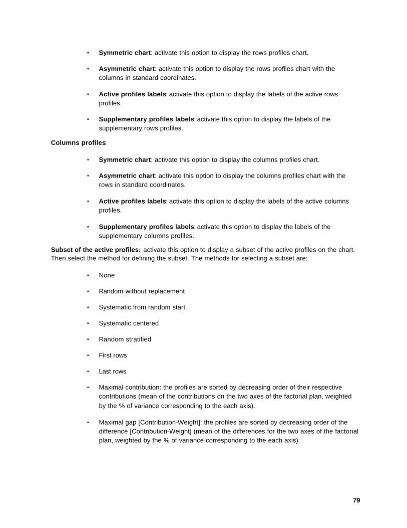
79
• Symmetric chart: activate this option to display the rows profiles chart.
• Asymmetric chart: activate this option to display the rows profiles chart with the columns in standard coordinates.
• Active profiles labels: activate this option to display the labels of the active rows profiles.
• Supplementary profiles labels: activate this option to display the labels of the supplementary rows profiles.
Columns profiles:
• Symmetric chart: activate this option to display the columns profiles chart.
• Asymmetric chart: activate this option to display the columns profiles chart with the rows in standard coordinates.
• Active profiles labels: activate this option to display the labels of the active columns profiles.
• Supplementary profiles labels: activate this option to display the labels of the supplementary columns profiles.
Subset of the active profiles: activate this option to display a subset of the active profiles on the chart. Then select the method for defining the subset. The methods for selecting a subset are:
• None
• Random without replacement
• Systematic from random start
• Systematic centered
• Random stratified
• First rows
• Last rows
• Maximal contribution: the profiles are sorted by decreasing order of their respective contributions (mean of the contributions on the two axes of the factorial plan, weighted by the % of variance corresponding to the each axis).
• Maximal gap [Contribution-Weight]: the profiles are sorted by decreasing order of the difference [Contribution-Weight] (mean of the differences for the two axes of the factorial plan, weighted by the % of variance corresponding to the each axis).
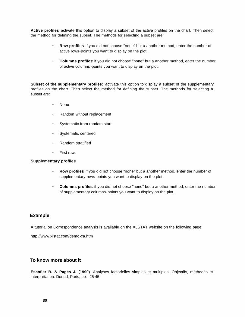
80
Active profiles: activate this option to display a subset of the active profiles on the chart. Then select the method for defining the subset. The methods for selecting a subset are:
• Row profiles: if you did not choose "none" but a another method, enter the number of active rows-points you want to display on the plot.
• Columns profiles: if you did not choose "none" but a another method, enter the number of active columns -points you want to display on the plot.
Subset of the supplementary profiles: activate this option to display a subset of the supplementary profiles on the chart. Then select the method for defining the subset. The methods for selecting a subset are:
• None
• Random without replacement
• Systematic from random start
• Systematic centered
• Random stratified
• First rows
Supplementary profiles:
• Row profiles: if you did not choose "none" but a another method, enter the number of supplementary rows-points you want to display on the plot.
• Columns profiles: if you did not choose "none" but a another method, enter the number of supplementary columns-points you want to display on the plot.
Example
A tutorial on Correspondence analysis is available on the XLSTAT website on the following page:
http://www.xlstat.com/demo-ca.htm
To know more about it
Escofier B. & Pages J. (1990). Analyses factorielles simples et multiples. Objectifs, méthodes et interprétation. Dunod, Paris, pp. 25-45.

81
Jobson J.D. (1992). Applied multivariate data analysis. Volume II: categorical and multivariate methods. Springer-Verlag, New York, pp. 433-462.
Lebart L., Morineau A. & Piron M. (1997). Statistique exploratoire multidimensionnelle. 2ème édition. Dunod, Paris, pp. 67-107.
Saporta G. (1990). Probabilités, analyse des données et statistique. Technip, Paris, pp. 199-216, pp. 199-216.
Tomassone R., Dervin C. & Masson J.P. (1993). Biométrie. Modélisation de phénomènes biologiques. Masson, Paris, pp. 143-150.

82
Multiple Correspondence Analysis (MCA) Use multiple correspondence analysis to study your data as a table of observations described by several categorical variables. This method is well-suited to analyzing surveys for which the array rows are usually the observations (there may be several thousand) and the columns are categories of categorical variables, usually categories of answers to questions.
See also: Description
Elements of the dialog box
Continuation of the dialog box
Display plots dialog box
Example
To know more about it
Description
Multiple Correspondence Analysis (MCA) is an extension of correspondence analysis (CA); but while CA is applied to a contingency table, MCA is applied to a full disjunctive table. This method may also be seen as the equivalent of principal component analysis (PCA) for categorical variables.
Elements of the dialog box
Data: enter the range for the data, corresponding to an observations/variables table or to a full disjunctive table.
Array / Disjunctive table: choose the data format, either as an array with the observations in rows and the categorical variables in columns, or directly as a full disjunctive table with the observations in rows and the categorical variables categories in columns. In the case of an observations/variables table, when missing data are found, XLSTAT suggests first ignoring them. If the user refuses, XLSTAT suggests estimating them using the mode of the corresponding variable (see the "Missing value estimation" option), otherwise, the dialog box is closed and the computations are stopped. In the case of a disjunctive table, when missing data are found, XLSTAT suggests ignoring them, otherwise, the dialog box is closed, and the computations are stopped.
Column labels: the first cell of each selected column contains a label.
Long labels: activate this option so that the labels of the rows and columns of the contingency table contain the variable name followed by the category label.
Observation labels: enter the range for the column of the observations labels.
Range: the results are displayed based on a cell located in an existing sheet.

83
Sheet: results are displayed in a sheet of the active workbook.
Workbook: results are displayed in a new workbook.
Observations: check this option to display the results concerning the observations.
Disjunctive table: check this option to display the full disjunctive table submitted to the MCA (if it is not already in the data), either because the data consists of an observations/variables table, or because weights are used to weight an original full disjunctive table.
Advanced charts: check this option to display the chart options dialog box after the analysis. When this option is not activated, only the default plot (symmetric observations and categories biplot) is displayed.
More: click this button to display the advanced options of the dialog box.
Continuation of the dialog box
Supplementary observations: enter the range for the supplementary or passive observations. Passive observations are not used in the calculations but are included in the plots with the active observations. Missing data are combined with the missing data found in the active data: XLSTAT suggests ignoring them, and in case of an observations/variables table, estimating them using the mode of the variable (see the "Missing value estimation" option), computed using all the available information, which means taking into account the supplementary observations.
Supplementary variables: enter the range for the supplementary or passive variables. Passive variables are not used in the calculation but are included in the plots with the active variables. Missing data are combined with the missing data found in the active data: XLSTAT suggests ignoring them, and in case of an observations/variables table, estimating them using the mode of the variable (see the "Missing value estimation" option).
Supp. quantitative variables: enter the range of an array with the active observations in rows and the supplementary quantitative variables in columns. When missing data are found for a variable, XLSTAT suggests estimating them using the mean of the variable (see the "Missing value estimation" option), otherwise the dialog box is closed, and all computations are stopped, because the missing data for the supplementary quantitative variables are not allowed.
Weight: enter the range for the observation weights column. Null weights are not allowed. When missing data are found for the weights, XLSTAT suggests estimating them using the mean of the weights (see the "Missing value estimation" option), computed without taking into account the null weights, otherwise the dialog box is closed and the computations are stopped, because missing weights are equivalent to null weights which are not allowed.
Display options dialog box
Symmetric chart: activate this option to display the row and columns profiles chart.
Burt's table chart: check this option to display the Burt's table as a 3D chart.
Observations:

84
• Symmetric chart: activate this option to display the observations chart.
• Asymmetric chart: activate this option to display the obs ervations chart with the categories in standard coordinates.
• Active observations labels: activate this option to display the labels of the active observations.
• Supplementary observations labels: activate this option to display the labels of the supplementary observations.
Categories:
• Symmetric chart: activate this option to display the categories chart.
• Asymmetric chart: activate this option to display the categories chart with the observations in standard coordinates.
• Active categories labels: activate this option to display the labels of the active categories.
• Supplementary categories labels: activate this option to display the labels of the supplementary categories.
Subset of the active observations: activate this option to display a subset of the active observations on the chart. Then select the method for defining the subset. The methods for selecting a subset are:
• None
• Random without replacement
• Systematic from random start
• Systematic centered
• Random stratified
• First rows
• Last rows
• Maximal contribution: the observations are sorted by decreasing order of their respective contributions (mean of the contributions on the two axes of the factorial plan, weighted by the % of variance corresponding to the each axis).
• Maximal gap [Contribution-Weight]: the observations are sorted by decreasing order of the difference [Contribution-Weight] (mean of the differences for the two axes of the factorial plan, weighted by the % of variance corresponding to the each axis).
Active data : activate this option to display a subset of the active data on the chart. Then select the method for defining the subset. The methods for selecting a subset are:

85
• Observations: if you did not choose "none" but a another method, enter the number of active observations you want to display on the plot.
• Categories: if you did not choose "none" but a another method, enter the number of active categories you want to display on the plot.
Subset of the supplementary data: activate this option to display a subset of the supplementary data on the chart. Then select the method for defining the subset. The methods for selecting a subset are:
• None
• Random without replacement
• Systematic from random start
• Systematic centered
• Random stratified
• First rows
Supplementary data:
• Observations: if you did not choose "none" but a another method, enter the number of supplementary observations you want to display on the plot.
• Categories: if you did not choose "none" but a another method, enter the number of supplementary categories you want to display on the plot.
Example
A tutorial on Multiple Correspondence Analysis is available on the XLSTAT website on the following page:
http://www.xlstat.com/demo-mca.htm
To know more about it
Escofier B. & Pages J. (1990). Analyses factorielles simples et multiples. Objectifs, méthodes et interprétation. Dunod, Paris, pp. 47-66.
Jobson J.D. (1992). Applied multivariate data analysis. Volume II: categorical and multivariate methods. Springer-Verlag, New York, pp. 462-465.

86
Lebart L., Morineau A. & Piron M. (1997). Statistique exploratoire multidimensionnelle. 2ème édition. Dunod, Paris, pp. 108-142.
Saporta G. (1990). Probabilités, analyse des données et statistique. Technip, Paris, pp. 217-239.
Tomassone R., Dervin C. & Masson J.P. (1993). Biométrie. Modélisation de phénomènes biologiques. Masson, Paris, pp. 150-155.

87
Multidimensional Scaling (MDS) Use multidimensional scaling to represent in a limited number of dimensions the observations for which only a similarity or dissimilarity matrix is available.
See also: Description
Elements of the dialog box
Continuation of the dialog box
Example
To know more about it
Description
Multidimensional scaling (MDS) is a method for analyzing a (similarity or dissimilarity) proximity matrix based on a set of observations. The purpose of MDS is to model the proximity of observations in order to represent them as accurately as possible in a limited number of dimensions (usually 2). There are different MDS algorithms: XLSTAT uses the SMACOF (Scaling by MAjorizing a COnvex Function) algorithm that minimizes the "normalized stress" function. Furthermore, there are several MDS models (or representation functions), i.e. several ways to transform the dissimilarities into disparities. The disparities are the distances that describe the optimal representation for the observations. The difference between the disparities and the distances measured on the representation resulting from the MDS is called the stress: the lower the stress, the better the representation of the observations.
When the representation function simply respects the relative order of the observations, one speaks about ordinal MDS or nonmetric MDS. When the dissimilarities are transformed into disparities using a specific parametric function, one speaks about metric MDS. The following models are available in the current version of XLSTAT:
Metric MDS
• absolute MDS: each dissimilarity dij must exactly match the distance between points i and j in the representation space.
• ratio MDS: the ratio of all distance pairs in the representation space must correspond to the ratio of the corresponding dissimilarities.
• interval MDS: the ratio of all differences between distances in the representation space must correspond to the ratio of the differences of the corresponding dissimilarities.
Note: the current version of XLSTAT does not support negative disparities that may occur if you use the "interval" model. If an error message is displayed on this subject, you must use another model to process your data.

88
Nonmetric MDS
• ordinal (1): the order of the distances in the representation space must correspond to the order of the corresponding dissimilarities. If there are two dissimilarities of the same rank, then there are no restrictions on the corresponding distances.
• ordinal (2): identical to the previous model, but if dissimilarities exist in the same rank, the corresponding distances must be equal.
The stress measures the quality of the representation for a given number of dimensions. The lower it is, the better the representation. Various formulas have been proposed by different authors. Although the minimization is always based on the normalized stress, XLSTAT allows to show the results using the four formulas defined below:
• Raw stress: it gives the quality of the representation based on the squared errors of the representation compared with the disparities. The formula gives:
( )∑<
−=ji
ijijijr dDw 2σ
where Dij is the disparity between individuals i and j, and dij is the Euclidean distance on the representation for the same individuals. wij is the weight of the ij proximity (value is 1 by default).
• Normalized Stress: it gives the quality of the representation based on the squared errors of the representation compared with the disparities, divided by the sum of the squared disparities. The formula gives:
( )
∑
∑
<
<
−=
jiijij
jiijijij
nDw
dDw
2
2
σ
• Kruskal's stress 1: it gives the quality of the representation based on the square root of the squared errors of the representation compared with the disparities, divided by the sum of the squared distances on the representation. The formula gives:
( )
∑
∑
<
<
−=
jiijij
jiijijij
dw
dDw
2
2
1σ
• Kruskal's stress 2: it gives the quality of the representation based on the square root of the squared errors of the representation compared with the disparities, divided by the sum of the squared centered distances on the representation. The formula gives:
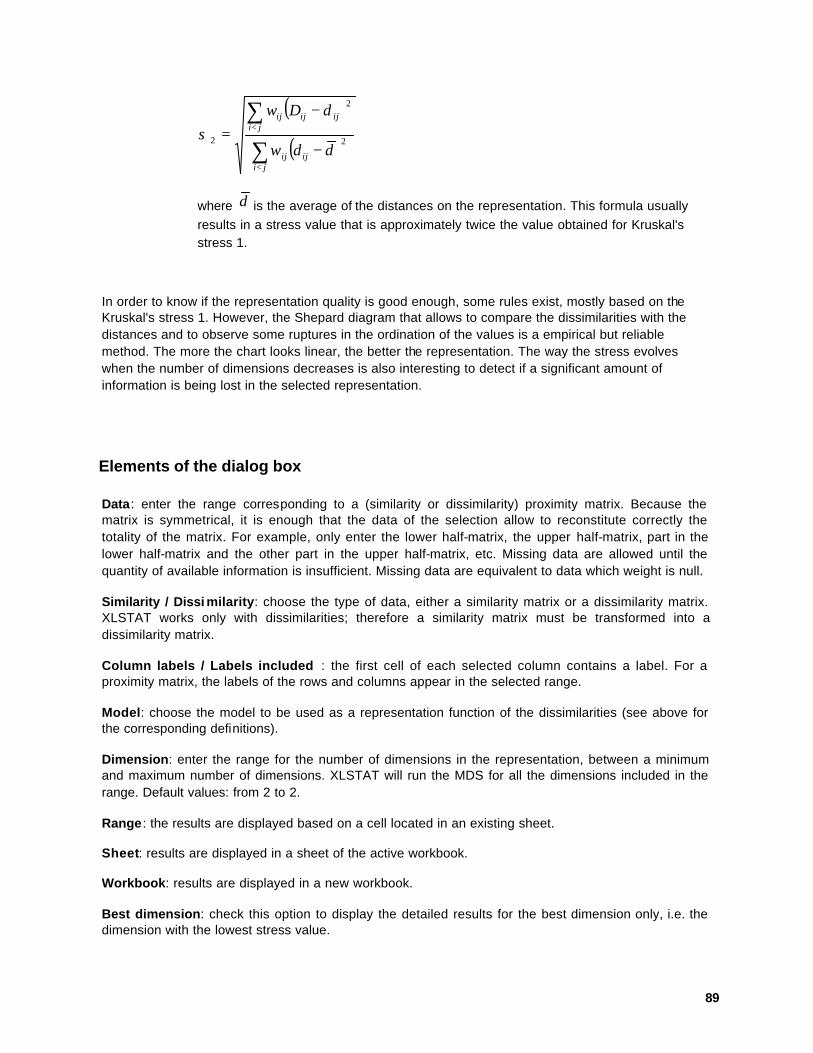
89
( )
( )∑
∑
<
<
−
−=
jiijij
jiijijij
ddw
dDw
2
2
2σ
where d is the average of the distances on the representation. This formula usually results in a stress value that is approximately twice the value obtained for Kruskal's stress 1.
In order to know if the representation quality is good enough, some rules exist, mostly based on the Kruskal's stress 1. However, the Shepard diagram that allows to compare the dissimilarities with the distances and to observe some ruptures in the ordination of the values is a empirical but reliable method. The more the chart looks linear, the better the representation. The way the stress evolves when the number of dimensions decreases is also interesting to detect if a significant amount of information is being lost in the selected representation.
Elements of the dialog box
Data: enter the range corresponding to a (similarity or dissimilarity) proximity matrix. Because the matrix is symmetrical, it is enough that the data of the selection allow to reconstitute correctly the totality of the matrix. For example, only enter the lower half-matrix, the upper half-matrix, part in the lower half-matrix and the other part in the upper half-matrix, etc. Missing data are allowed until the quantity of available information is insufficient. Missing data are equivalent to data which weight is null.
Similarity / Dissi milarity: choose the type of data, either a similarity matrix or a dissimilarity matrix. XLSTAT works only with dissimilarities; therefore a similarity matrix must be transformed into a dissimilarity matrix.
Column labels / Labels included : the first cell of each selected column contains a label. For a proximity matrix, the labels of the rows and columns appear in the selected range.
Model: choose the model to be used as a representation function of the dissimilarities (see above for the corresponding definitions).
Dimension: enter the range for the number of dimensions in the representation, between a minimum and maximum number of dimensions. XLSTAT will run the MDS for all the dimensions included in the range. Default values: from 2 to 2.
Range: the results are displayed based on a cell located in an existing sheet.
Sheet: results are displayed in a sheet of the active workbook.
Workbook: results are displayed in a new workbook.
Best dimension: check this option to display the detailed results for the best dimension only, i.e. the dimension with the lowest stress value.
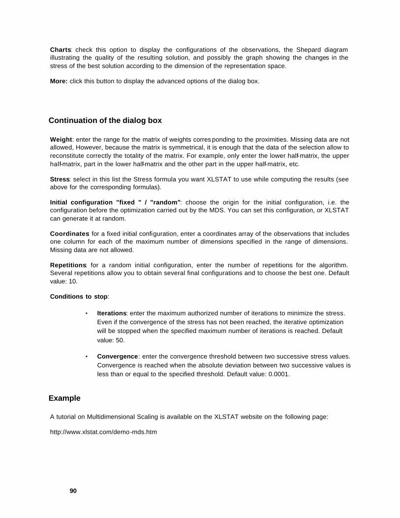
90
Charts: check this option to display the configurations of the observations, the Shepard diagram illustrating the quality of the resulting solution, and possibly the graph showing the changes in the stress of the best solution according to the dimension of the representation space.
More: click this button to display the advanced options of the dialog box.
Continuation of the dialog box
Weight: enter the range for the matrix of weights corres ponding to the proximities. Missing data are not allowed, However, because the matrix is symmetrical, it is enough that the data of the selection allow to reconstitute correctly the totality of the matrix. For example, only enter the lower half-matrix, the upper half-matrix, part in the lower half-matrix and the other part in the upper half-matrix, etc.
Stress: select in this list the Stress formula you want XLSTAT to use while computing the results (see above for the corresponding formulas).
Initial configuration "fixed " / "random": choose the origin for the initial configuration, i.e. the configuration before the optimization carried out by the MDS. You can set this configuration, or XLSTAT can generate it at random.
Coordinates: for a fixed initial configuration, enter a coordinates array of the observations that includes one column for each of the maximum number of dimensions specified in the range of dimensions. Missing data are not allowed.
Repetitions: for a random initial configuration, enter the number of repetitions for the algorithm. Several repetitions allow you to obtain several final configurations and to choose the best one. Default value: 10.
Conditions to stop:
• Iterations: enter the maximum authorized number of iterations to minimize the stress. Even if the convergence of the stress has not been reached, the iterative optimization will be stopped when the specified maximum number of iterations is reached. Default value: 50.
• Convergence: enter the convergence threshold between two successive stress values. Convergence is reached when the absolute deviation between two successive values is less than or equal to the specified threshold. Default value: 0.0001.
Example
A tutorial on Multidimensional Scaling is available on the XLSTAT website on the following page:
http://www.xlstat.com/demo-mds.htm
91
To know more about it
Borg I. & P. Groenen (1997). Modern multidimensional Scaling. Theory and applications. Springer Verlag, New York.
Dillon W.R. & Goldstein M. (1984). Multivariate analysis. Methods and applications. John Wiley & Sons, New York, pp. 107-156.
Jobson J.D. (1992). Applied multivariate data analysis. Volume II: categorical and multivariate methods. Springer-Verlag, New York, pp. 568-605.
Kruskal J.B. & Wish M. (1978). Multidimensional Scaling. Sage Publications, London.
Tomassone R., Dervin C. & Masson J.P. (1993). Biométrie. Modélisation de phénomènes biologiques. Masson, Paris, pp. 172-173.
92
Agglomerative Hierarchical Clustering (AHC) Use agglomerative hierarchical clustering to create similar observation groups (clusters) on the basis of their description by a set of quantitative variables, binary variables (0/1), or possibly all types of variables.
Note: for non-binary categorical variables, it is preferable to first perform a Multiple Correspondence Analysis (MCA) and to consider the coordinates of the observations on the factorial axes as new variables.
See also: Description
Elements of the dialog box
Continuation of the dialog box
Display dendrogram box
Example
To know more about it
Description
Agglomerative hierarchical classification (AHC) gradually builds an aggregate of observations based on their similarity, measured using a similarity or dissimilarity coefficient. The algorithm first gathers all the most similar observation pairs, then progressively aggregates the other observations or observation groups according to their similarity until all the observations are in a single group. The AHC produces a binary clustering tree (dendrogram), whose root is the class that contains all the observations. This dendrogram represents a hierarchy of partitions, where a partition is obtained by truncating the dendrogram at a certain level of similarity. The partition contains fewer and fewer clusters as the truncation is made in the top of the dendrogram (i.e. towards the root). If you truncate underneath the first node in the tree, then each cluster will contain one observation only (this partition is the base of the dendrogram) and if you truncate beyond the root level of the dendrogram, you will create a single cluster containing all the observations.
There are several ways to measure similarity (similarities or dissimilarities), and several ways to recalculate the similarity when the algorithm creates groups (aggregation criteria). XLSTAT proposes selected coefficients and criteria based on their mathematical properties and their practical or pedagogical interest.
List of similarities/dissimilarities
XLSTAT proposes several similarities/dissimilarities that are suitable for a particular type of data.
For quantitative data:
Similarity Dissimilarity
Pearson's correlation coefficient Euclidean distance
Spearman's coefficient of rank correlation Chi-square distance

93
Kendall's coefficient of rank correlation Manhattan distance
Inertia Pearson's dissimilarity
Covariance 1/n Spearman's dissimilarity
Covariance 1/(n-1) Kendall's dissimilarity
Cosine Mahalanobis' distance
Bhattacharya's distance
Chebychev's distance
Canberra's distance
Chord distance
Squared chord distance
Geodesic distance
For binary data (0/1):
Similarity/Dissimilarity
Jaccard coefficient
Dice coefficient
Sokal & Sneath coefficient (2)
Rogers & Tanimoto coefficient
Simple matching coefficient
Sokal & Sneath coefficient (1)
Phi coefficient
Ochiai's coefficient
Kulczinski's coefficient
For all types data:
Similarity Dissimilarity
Percent agreement Percent disagreement
Cooccurrences

94
Note: in order to process different types of variables (quantitative and categorical), you can use a general similarity/dissimilarity (percent agreement/disagreement) that handles all the variables at the lowest algebraic level, i.e. the nominal variable level. This inevitably results in the loss of information. It may be more interesting to discretize the quantitative va riables using the Discretization and histogram module, then jointly analyze the categorical variables using Multiple Correspondence Analysis (MCA), in order to use the observation factor coordinates as new variables.
List of aggregation criteria
The dissimilarity between two groups of objects A and B may be calculated using different methods, called aggregation criteria, where each criterion determines the structure of the binary hierarchy produced by the AHC algorithm. XLSTAT offers seven of the existing criteria: simple linkage, complete linkage, unweighted pair-group average linkage, weighted pair-group average linkage, flexible linkage, strong linkage, as well as Ward's method based on the increase of inertia.
Simple linkage: the dissimilarity between A and B is the dissimilarity between the object of A and the object of B that are the most similar. Aggregation using simple linkage tends to contract the data space and to flatten the levels of each step in the dendrogram. As the dissimilarity between two elements of A and of B is sufficient to link A and B, this criterion can lead to connect very lengthened clusters (chaining effect).
Complete linkage: the dissimilarity between A and B is the largest dissimilarity between an object of A and an object of B. Aggregation using complete linkage tends to dilate the data space and to produce compact clusters.
Unweighted pair-group average linkage: the dissimilarity between A and B is the average of the dissimilarities between the objects of A and the objects of B. Aggregation using Unweighted pair-group average linkage is a good compromise between the two preceding extremes, and provides a fair representation of the data space properties.
Weighted pair-group average linkage: the average dissimilarity between the objects of A and of B is calculated as the sum of the weighted dissimilarities, so that equal weights are assigned to both groups. As with unweighted pair-group average linkage, this criterion provides a fairly good representation of the data space properties.
Flexible linkage: this criterion uses a ß parameter that varies between [-1,+1]; this can generate a family of aggregation criteria. For ß = 0 the criterion is weighted pair-group average linkage. When ß is near to 1, chain-like clusters result, but as ß decreases and becomes negative, you obtain more and more dilatation.
Strong linkage: this criterion uses both the average of the distances within each group and the average of the distances between the groups. It tends to create very compact clusters.
Ward's method: this method aggregates two groups so that within-group inertia increases as little as possible to keep the clusters homogeneous. This criterion, proposed by Ward (1963), can only be used in cases with quadratic distances, i.e. cases of Euclidian distance and Chi-square distance.
Note: by default, XLSTAT proposes to use Ward's method for quadratic distances (Euclidian and Chi-square distances) and unweighted pair-group average linkage in all other cases. Other criteria should be applied by knowledgeable users only.

95
Elements of the dialog box
Data: select the range for the data corresponding to a rectangular observations/variables table or to a similarity/dissimilarity matrix.
Table / Matrix : choose the data format: observations/variables table or similarity/dissimilarity matrix. In the case of a table containing missing data, XLSTAT suggests ignoring the corresponding rows, otherwise XLSTAT indicates it is possible to use all the available information (pairwise deletion) by using the Similarity/Dissimilarity Matrix module and then closes the dialog box, and stops the computations. For a similarity/dissimilarity matrix, missing data are not allowed. However, because the matrix is symmetrical, it is enough that the data of the selection allow to reconstitute correctly the totality of the matrix. For example, only enter the lower half-matrix, the upper half-matrix, part in the lower half-matrix and the other part in the upper half-matrix, etc.
Center / Reduce : for an observations/variables table containing quantitative data, check these two options to standardize the variables.
Column labels: the first cell of each selected column contains a label. For a proximity matrix, the labels of the rows and columns appear in the selected range.
Row labels: for an observations/variables table, enter the range for the column of labels that correspond to the data array rows.
Similarity / Dissimilarity: choose whether the values calculated from the observations/variables table or the values contained in the matrix are similarities or dissimilarities. This choice determines the list of aggregation criteria that are proposed as well as how the data are processed.
Range: the results are displayed based on a cell located in an existing sheet.
Sheet: results are displayed in a sheet of the active workbook.
Workbook: results are displayed in a new workbook.
Proximity matrix: for an observations/variables table, check this option to display the proximity matrix calculated by XLSTAT before performing the AHC.
Description: activate this option to display the table that describes the dendrogram.
Charts: check this option to display the histogram of the node levels as well as the dendrogram.
Variance/Inertia : activate this option to display the results in terms of variance or inertia when relevant (for example with the Ward's method).
Results in original space : activate this option to compute the complementary results without taking into account the standardization and the weights of the variables.
More: click this button to display the advanced options of the dialog box.
96
Continuation of the dialog box
Clustering "of the rows" / "of the columns": for an observations/variables table, choose whether the similarity/dissimilarity matrix should cross the rows or the columns of the data array.
Weights of the columns/rows: for an observations/variables table, enter the range (one column) for the weights of the columns (when you are analyzing rows) or for the weights of the rows (when you are analyzing columns).
Truncate: check this option to truncate the dendrogram and obtain a partition.
• Automatic: the truncation level of the dendrogram – and as a result the number of clusters in the partition – is determined automatically by XLSTAT according to the structure of the levels histogram.
• Number of clusters: enter the desired number of clusters in the partition.
• Level: enter the truncation level. Normally you must execute the module once before being able to decide on a correct truncation level.
Display dendrogram box
Chart title: enter the chart title.
Axis title: enter the axis title.
Width: enter the chart width.
Height: enter the chart height.
Delta: enter a value below one, to obtain a pyramidal dendrogram.
Labels can be edited: when the dendrogram is not displayed on a separate sheet, the title of the chart, the axis, and the objects labels are dissociated so that you can edit them.
Objects labels: If you check this option, the labels of the clustered objects are displayed at the base of the dendrogram.
Nodes labels: check this option to display a label for each node in the dendrogram.
• • "Rank" / "Level": if you choose "Rank", the label of each node has a rank that matches the aggregation order; if you choose "Level" then the label of each node is the value of the coefficient, calculated during the aggregation.
"Vertical dendrogram " / "Horizontal dendrogram": if you choose "Vertical dendrogram ", the root of the dendrogram appears at the top of the chart, while if you choose "Horizontal dendrogram " the root appears at the right of the chart.
On a separate sheet: If you check this option, the dendrogram is displayed on a separate sheet.
97
Default: click on this button to reset the options to their default value.
Example
A tutorial on Agglomerative Hierarchical Clustering is available on the XLSTAT website on the following page:
http://www.xlstat.com/demo-cluster.htm
To know more about it
Benzécri J.P. (1984). L'analyse des données. 1. La taxinomie. Quatrième édition. Dunod, Paris.
Diday E., Lemaire J., Pouget J. & Testu F. (1982). Eléments d'analyse de données. Dunod, Paris, pp. 46-116.
Dillon W.R. & Goldstein M. (1984). Multivariate analysis. Methods and applications. John Wiley & Sons, New York, pp. 157-186.
Jambu M. (1978). Classification automatique pour l'analyse des données. 1 - méthodes et algorithmes. Dunod, Paris.
Jobson J.D. (1992). Applied multivariate data analysis. Volume II: categorical and multivariate methods. Springer-Verlag, New York, pp. 483-568.
Johnson R.A. & Wichern D.W. (1992). Applied multivariate statistical analysis. Prentice-Hall, Englewood Cliffs, pp. 584-602.
Lebart L., Morineau A. & Piron M. (1997). Statistique exploratoire multidimensionnelle. 2ème édition. Dunod, Paris, pp. 155-206.
Roux M. (1985). Algorithmes de classification. Masson, Paris.
Saporta G. (1990). Probabilités, analyse des données et statistique. Technip, Paris, pp. 251-260.
Tomassone R., Dervin C. & Masson J.P. (1993). Biométrie. Modélisation de phénomènes biologiques. Masson, Paris, pp. 166-174.
Ward J.H. (1963). Hierarchical grouping to optimize an objective function. Journal of the American Statistical Association, 58: 238-244.
98
k-means Clustering Use the k-means method to divide the observations into homogeneous clusters, based on their description by a set of quantitative variables.
Note: for categorical variables, you must first perform a Multiple Correspondence Analysis (MCA) and consider the resulting coordinates of the observations on the factorial axes as new variables.
See also: Description
Elements of the dialog box
Continuation of the dialog box
Example
To know more about it
Description
The k-means algorithm consists in iteratively improving an initial partition by minimizing with-group inertia. At each iteration, the algorithm calculates the centroids of the clusters in the current partition, then assigns each observation to the nearest centroid in order to form a new partition whose within-group inertia is lower than the previous one. The variation used by XLSTAT ensures that all clusters contain at least one observation.
This method does not ensure that the solution at convergence is the optimal solution, i.e. the best of all possible solutions. In this sense, this algorithm should be viewed as a heuristic, that simply provides a good solution; the exact resolution of the underlying combinatorial optimization problem is not generally possible except for very small data sets. The best strategy to obtain a very good solution with a reasonable calculation time is to execute the k-means algorithm based on several different initial partitions, then to select the best final partition from those that are created.
When several repetitions of the method are carried out based on different initial partitions, XLSTAT identifies the stable groups, i.e. the observation groups that have always been classified together. The stable groups are the intersection of all the partitions considered. Observations that are not part of any stable group are assigned to one cluster or another depending on the initial partition used. These observations are generally in intermediate regions located between stable groups. To identify stable groups, XLSTAT considers at most the 10 best partitions obtained via several executions of the algorithm.
Note: using within-group inertia as a criterion to be minimized leads to the creation of compact clusters. For example, in a two-dimensional space, the k-means algorithm tends to propose clusters that are as round as possible. As a result, you should not use this method if you know a priori that the shape of natural clusters underlying your data is not compact but is lengthened (for example): in this case the optimized criterion is not suitable.
99
Elements of the dialog box
Data: select the range corresponding to a rectangular observations/variables table. When missing data are found, XLSTAT suggests first ignoring the corresponding rows. If the user refuses, XLSTAT suggests estimating the missing data of the variable by the mean of the variable (see the "Missing value estimation" option), otherwise the dialog box is closed and the computations are stopped.
Standardize: check this option to standardize the variables, i.e. divide the values by the standard deviation of the corresponding variable in order to cancel the effect of the differences between units.
Number of clusters: enter the number of clusters of the desired partition.
Column labels: the first cell of each selected column contains a label.
Observation labels: enter the range for the column of labels that represent the data array rows.
Range: the results are displayed based on a cell located in an existing sheet.
Sheet: results are displayed in a sheet of the active workbook.
Workbook: results are displayed in a new workbook.
Charts: check this option to display the curve of the evolution of the within-group variance or inertia.
Distances: check this option to display the results corresponding to the distances.
Variance/Inertia : activate this option to display the results in terms of variance or inertia.
Results in original space : activate this option to compute the complementary results without taking into account the standardization and the weights of the variables.
More: click this button to display the advanced options of the dialog box.
Continuation of the dialog box
Weights of the observations: enter the range for the observations weights column. Missing data for weights are combined with missing data for the data: XLSTAT suggests ignoring the corresponding rows or estimating the missing data by the mean of the weights (see the "Missing value estimation" option), computed without taking into account the weights equal to zero.
Weights of the variables: enter the range for the variables weights column. Missing data for weights are combined with missing data for the data: XLSTAT suggests ignoring the corresponding columns or estimating the missing data by the mean of the weights (see the "Missing value estimation" option), computed without taking into account the weights equal to zero.
Initial partition: choose the initial partition, i.e. the partition of the observations prior to optimization carried out by the k-means algorithm. There are three possibilities:
• Random: the initial partition is randomly generated.
100
• User defined: the group of each observation is available in a separate column.
• Defined by centers: the coordinates of the initial centers are give by the user.
Partition: for a user defined initial partition, enter the range corresponding to a column that describes the partition (categorical variable). Missing data are not allowed.
Partition: for a user defined by centers initial partition, select the table that corresponds to the coordinates of the centers enter the range corresponding to a column that describes the partition (categorical variable). Missing data are not allowed.
Repetitions: for an automatic initial partition, enter the number of repetitions for the algorithm (between 1 and 1000). Several repetitions allow you to obtain several final partitions and to choose the best one. Default value: 10.
Conditions to stop:
• Iterations: enter the maximum authorized number of iterations for minimizing within-group inertia. Even if the convergence of the within-group inertia has not yet been reached, the iterative improvement will be stopped when the specified maximum number of iterations is reached. Default value: 50.
• Convergence: enter the convergence threshold of the algorithm. The convergence is reached when the absolute deviation between two successive values, compared to the current within-group inertia, is less than or equal to the specified threshold. Default value: 0.0001.
Example
A tutorial on k-means Clustering is available on the XLSTAT website on the following page:
http://www.xlstat.com/demo-cluster2.htm
To know more about it
Diday E. (1971). Une nouvelle méthode en classification automatique et reconnaissance des formes, la méthode des nuées dynamiques. Revue de Statistique Appliquée, 19 19-33.
Diday E., Lemaire J., Pouget J. & Testu F. (1982). Eléments d'analyse de données. Dunod, Paris, pp. 116-129.
Jobson J.D. (1992). Applied multivariate data analysis. Volume II: categorical and multivariate methods. Springer-Verlag, New York, pp. 560-562.
Johnson R.A. & Wichern D.W. (1992). Applied multivariate statistical analysis. Prentice-Hall, Englewood Cliffs, pp. 596-602.
Lebart L., Morineau A. & Piron M. (1997). Statistique exploratoire multidimensionnelle. 2ème édition. Dunod, Paris, pp. 148-154.

101
Roux M. (1985). Algorithmes de classification. Masson, Paris, pp. 61-75.
Tomassone R., Dervin C. & Masson J.P. (1993). Biométrie. Modélisation de phénomènes biologiques. Masson, Paris, pp. 159-165.

102
Univariate Clustering Use univariate clustering to optimally partition observations in homogeneous clusters, based on their description using a single quantitative variable.
See also: Description
Elements of the dialog box
Continuation of the dialog box
Example
To know more about it
Description
Univariate clustering provides a partition that minimizes within-group inertia. XLSTAT uses a dynamic programming algorithm: the Fisher's algorithm (1958). This algorithm ensures that the resulting solution is the optimal solution, i.e. the best possible solution.
Note: The calculation time increases quickly if you have a large number of different values in your data and if you request a large number of clusters. XLSTAT displays a message as soon as the estimated calculation time exceeds 30 seconds for a 500 MHz processor. In that case you can choose to cancel the current procedure and use the k-means method in order to quickly obtain a good solution (that is not necessarily the optimal solution).
Elements of the dialog box
Data: select the range corresponding to the column containing the variable. When missing data are found, XLSTAT suggests first ignoring the corresponding rows. If the user refuses, XLSTAT suggests estimating the missing data of the variable by the mean of the variable (see the "Missing value estimation" option), otherwise the dialog box is closed and the computations are stopped.
Number of clusters: enter the desired number of clusters for the partition.
Observation labels: enter the range for the column of labels that represent the data array rows.
Range: the results are displayed based on a cell located in an existing sheet.
Sheet: results are displayed in a sheet of the active workbook.
Workbook: results are displayed in a new workbook.
Column labels: the first cell of each selected column contains a label.
More: click this button to display the advanced options of the dialog box.

103
Continuation of the dialog box
Weights of the observations: enter the range for the observations weights column. Missing data for weights are combined with missing data for the data: XLSTAT suggests ignoring the corresponding rows or estimating the missing data by the mean of the weights (see the "Missing value estimation" option), computed without taking into account the weights equal to zero.
Example
A tutorial on Univariate Clustering is available on the XLSTAT website on the following page:
http://www.xlstat.com/demo-unicluster.htm
To know more about it
Aubry P. & C. Egretaud (1994). Classification non dirigée optimale d'une image monocanal. International Journal of Remote Sensing, 15: 3839-3843.
Diday E., Lemaire J., Pouget J. & Testu F. (1982). Eléments d'analyse de données. Dunod, Paris, pp. 129-132.
Fisher W.D. (1958). On grouping for maximum homogeneity. Journal of the American Statistical Association, 53: 789-798.
Sakarovitch M. (1984). Optimisation combinatoire. Méthodes mathématiques et algorithmiques. Programmation Discrète. Hermann, Paris, pp. 185-223.

104
AxesZoomer This tool allows you to modify the minimum and maximum values of the abscissa and ordinates axes of an Excel chart, until you are satisfied.

105
DataFlagger This tool allows you to identify some Excel cells - within a selected range - that correspond to some criterion you define. The criterion can be a text, a value or an interval.
For highlighting the cells you can change the color, the font size, or select the bold or italic format.

106
Easy Labels A very simple thing that Excel can't do: add labels which are not values to a data series. To use easy labels, double click on a plot, and select a data series. then click on the Easy Labels button, and select the range where the labels are stored (in column). The number of labels should be equal to the number of values.
The formats of the labels can optionally be replicated from the spreadsheet to the chart (colors, size, …). The background and border properties of the Excel cells where the labels are stored can also be replicated.
Column label included: the first cell of the selected column contains the label of the column itself.
Use text properties: allows to reproduce all the properties of the labels on the plot (size, color ...).
Use cell properties: allows to reproduce all the properties of the cells on the plot (border, pattern color ...).

107
MicroMover This tool allows you to move any object with a full control on the direction and on the number of pixels your object is moved.
Note: Before activating the MicroMover, make sure you have selected an object on an Excel sheet, or that a chart is activated (to activate a chart, double-click on it).

108
MinMaxSearch Use this tool to quickly locate the minimum or the maximum value in a dataset.

109
Plot Transformer With this tool, just by selecting a plot (a chartsheet or chart object on a sheet) and indicating what transformation you want to do, you will obtain a new plot taking into account the transformations you asked for. This tool is a useful complement to Multidimensional Scaling (MDS). It can also be used to compare charts generated from multivariate methods (PCA, Gabriel Biplot, etc.)

110
Scatter plots Use the Scatter plots to create 2 dimensional or 3 dimensional graphics (the third dimension is represented by the size of the point) while taking into account the following elements:
• the possible belonging of an observation to a group,
• the possible superimposition of some points on the graphic,
• the possible presence of observation labels,
• the need to cross several X variables (abscissa) and Y variables (ordinates).
The Scatter plots tool allows you to save a lot of time when avoiding your manipulating the Excel graphics to reach a satisfactory result.
See also: Description
Elements of the dialog box
Continuation of the dialog box
Example
To know more about it
Description
Many options are available in the Scatter plots tool, to allow you to take into account complex situations. For example, if you want to include a third dimension, and if your observations are grouped, and if you want to avoid that the large bubbles cover the small bubbles, Scatter plots will help you to create the best graphic as possible with Excel. If several points have the same coordinates, it is possible to let XLSTAT display the sum of the frequencies next to the point displayed.
Elements of the dialog box
X(s): select here the variable(s) that you want to be used as the coordinates on the abscissa axis
111
Y(s): select here the variable(s) that you want to be used as the coordinates on the ordinates axis
Switch Xs and Ys: click on this button to switch the selections of Xs and Ys.
Column labels: activate this option if the first cell of each selected column contains a label.
Observations Labels: activate this option if there are observations labels. Then select the data that you want to be used to determine the label for each observation.
• Use text properties: activate this option if you want that XLSTAT keeps the text properties when displaying the labels.
• Use cell properties: activate this option if you want that XLSTAT keeps the cell properties when displaying the labels (background properties and border properties).
Range: results are displayed based on a cell located in an existing sheet.
Sheet: results are displayed in a sheet of the active workbook.
Workbook: results are displayed in a new workbook.
Frequencies: activate this option if you want the frequencies to be displayed
Only if >1: activate this option if you want the frequencies to be displayed only if the frequency is greater than 1
Legend: activate this option if you want the legend to be displayed
Axes Titles: activate this option if you want the axes titles to be displayed
More: click here to display the next part of the dialog box
Continuation of the dialog box
Z: activate this option if there is a third dimension. Then select the variable that you want to be used to determine the size of the bubbles (the third dimension)
Weights: activate this option if the data are weighted. Then select the data that you want to be used to weight the data in the corresponding box.
Groups: activate this option if you want to group the data. Then select the data that correspond to the group to which each observation belongs.

112
Example
A tutorial for the tool Scatter plots is available on the XLSTAT website on the following page:
http://www.xlstat.com/demo-scatter.htm
To know more about it
Jacoby W. G. (1997). Statistical Graphics for Univariate and Bivariate Data, Sage Publications, London.
Wilkinson L. (1999). The Grammar of Graphics, Springer Verlag, New York.

113
Parallel Coordinates Visualization Use this tool to visualize multidimensional data (described by P numerical and Q nominal variables) on a single two dimensional chart.
See also: Description
Elements of the dialog box
Missing data
Results
Example
To know more about it
Description
This visualization method is useful for data analysis when you need to discover or validate a groups structure, for example after a clustering. Using this method you are able to visually determine which variables are discriminant.
If you consider N observations described by P numerical and Q nominal variables, the Parallel Coordinates chart consists of P+Q vertical axes corresponding to the P+Q variables, and N lines corresponding to each observation. Each line crosses each axis at the value corresponding to the value that the observation takes for the variable corresponding to the axis.
If the number of observations is too high, the visualization might be not very efficient or even impossible due to the Excel restrictions (maximum of 255 data series). In that case, it is recommended to use the random sampling option.
Elements of the dialog box
Data: select the data. Numerical and nominal data can be selected together. The variables appear on the chart as they have been selected.
Sample size(%): enter the size in % of the random sample to generate from the initial sample for the visualization (random sampling without replacement).
Groups: activate this option and select the column correspond to the groups descriptor. This information is used to display the groups with different colors.

114
Observations Labels: activate this option if there are observations labels. Then select the data that you want to be used to determine the label for each observation.
• Display: activate this option if you want the observations labels to be displayed
Range: results are displayed based on a cell located in an existing sheet.
Sheet: results are displayed in a sheet of the active workbook.
Workbook: results are displayed in a new workbook.
Column labels: activate this option if the first cell of each selected column contains a label.
Rescaling: activate this option if you want that all variables are rescaled to a 0%-100% scale (for a given numerical variable 0 corresponds to the minimum and 100 to the maximum). Categories of nominal variables are regularly spaced. The order corresponds to their order of in the input table.
Colors: activate this option if you want the lines to be displayed with different colors.
Mean lines: activate this option if you want to display the lines corresponding the means of the numerical variables and the modes of the nominal variables.
Categories: activate this option if you want to display the name of the categories of the nominal variables.
Missing data
If missing data are detected by XLSTAT, you are asked whether you want to remove the observations with missing data. If you do not want to remove the corresponding observations the analysis stops.
Results
XLSTAT displays the Parallel Coordinates chart. As the chart is a standard Excel chart you can modify options such as titles, colors or text fonts.
115
Example
A tutorial on using Parallel Coordinates Visualization is available on the XLSTAT website on the following page:
http://www.xlstat.com/demo-pcor.htm
To know more about it
Inselberg A. (1985). The plane with parallel coordinates. The Visual Computer, 1, pp. 69-91.
Eickemeyer J. S., Inselberg A. & Dimsdale B. (1992). Visualizing p-flats in n-space using parallel coordinates. Technical Report G320-3581, IBM Palo Alto Scientific Center.
Wegman E.J. (1990). Hyperdimensional Data Analysis Using Parallel Coordinates. J. Amer. Statist. Assoc, 85, 411, pp. 664-675.

116
Distribution Fitting Use this module to fit a probability distribution to your quantitative data (continuous or discrete data), and to check the quality of the resulting fit.
See also: Description
Elements of the dialog box
Example
To know more about it
Description
Fitting a probability distribution to a distribution of values involves seeking the best parametric model from those proposed by XLSTAT. This consists of choosing a probability distribution and the values of parameters for that distribution, so that the difference between the values of the data and the values of the model is as small as possible.
Several probability distributions are available: uniform, Gaussian, lognormal, Student, Fisher, Chi-square, Beta, exponential, Poisson, binomial, negative binomial and Weibull. XLSTAT allows you to directly enter the parameters values for the chosen probability distribution, or to automatically estimate them.
In order to evaluate the quality of the fit, XLSTAT displays the values of the expectation, the variance, the skewness, and the kurtosis, estimated using the data, and the calculated values for the selected probability distribution, given its parameters (entered or estimated). If both sets of values agree, this is an initial indication that the distribution of the values and the fitted model also agree.
XLSTAT also includes two nonparametric tests:
• the Kolmogorov-Smirnov test that evaluates the similarity between the cumulative distribution of the data and the cumulative distribution function of the fitted probability distribution,
• the Chi-square goodness of fit test between the histogram of observed frequencies and the histogram of theoretical frequencies.
The Chi-square test requires you to define the histogram by:
• entering the number of classes with a constant amplitude,
• importing the class bounds,
• using the discrete bounds in the case of a discrete distribution (Poisson distribution, binomial and negative binomial distributions).
Sometimes the Chi-square test reports a bad fit due to a class that makes a high contribution to the Chi-square value. This may be due to the way the histogram is broken down into classes, and a

117
different breakdown may change the test results. In order to evaluate the impact of the highest contribution to the Chi-square in the test results, XLSTAT also runs the Chi-square test without taking the highest contribution into account.
Elements of the dialog box
Data: select the range corresponding to the column of values. Missing data are not allowed.
Parameters "enter" / "estimate": choose whether the parameters for the probability distribution should be entered manually or estimated automatically.
Estimation method: for some distributions, two estimation methods are available: maximum likelihood and moments. For the binomial distribution, if you choose to automatically estimate the parameters, check this option to perform an estimation using an iterative method (maximum likelihood). When this option is not checked, XLSTAT asks if you want to enter the value of n (number of trials): if this value is known, you will obtain a better estimation of p (probability of success).
Probability distribution: choose the probability distribution to be fitted from the list. If you choose to enter the parameter values, additional fields are displayed in the dialog box, according to the chosen probability distribution:
• Beta
a1: enter a number for the first shape parameter of the Beta distribution
a2: enter a number for the second shape parameter of the Beta distribution
• Binomial
n: enter the number of trials that defines the binomial distribution
p: enter the probability of success that defines the binomial distribution
• Chi-square
df: enter the number of degrees of freedom for the Chi-square distribution
• Exponential
Lambda: enter the inverse of the average wait time between two events of a random phenomenon to define the exponential distribution
• Fisher
df 1: enter the number of degrees of freedom for the numerator of the Fisher's F
df 2: enter the number of degrees of freedom for the denominator of the Fisher's F
• Gaussian (or normal distribution)
µ: enter the value of the expectation
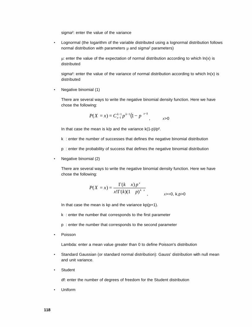
118
sigma²: enter the value of the variance
• Lognormal (the logarithm of the variable distributed using a lognormal distribution follows normal distribution with parameters µ and sigma² parameters)
µ: enter the value of the expectation of normal distribution according to which ln(x) is distributed
sigma²: enter the value of the variance of normal distribution according to which ln(x) is distributed
• Negative binomial (1)
There are several ways to write the negative binomial density function. Here we have chose the following:
( ) kxkk
x ppCxXP −−−− −== 1)( 111 , x>0
In that case the mean is k/p and the variance k(1-p)/p².
k : enter the number of successes that defines the negative binomial distribution
p : enter the probability of success that defines the negative binomial distribution
• Negative binomial (2)
There are several ways to write the negative binomial density function. Here we have chose the following:
xk
x
pkxpxk
xXP++Γ
+Γ==
)1)((!)(
)(, x>=0, k,p>0
In that case the mean is kp and the variance kp(p+1).
k : enter the number that corresponds to the first parameter
p : enter the number that corresponds to the second parameter
• Poisson
Lambda: enter a mean value greater than 0 to define Poisson's distribution
• Standard Gaussian (or standard normal distribution): Gauss' distribution with null mean and unit variance.
• Student
df: enter the number of degrees of freedom for the Student distribution
• Uniform

119
a: enter a number that defines the lower bound of the interval for the uniform distribution
b: enter a number that defines the upper bound of the interval for the uniform distribution
• Weibull (1)
The one parameter Weibull density function writes:
)exp()( 1 βββ xxxXP −== −, x>0, β >0
β : enter a number corresponding to the shape parameter
• Weibull (2)
The two parameters Weibull density function writes:
−
==
− ββ
ηηβ
xxxXP exp)(
1
, x>0, β,η >0
β : enter a number corresponding to the shape parameter
η : enter a number corresponding to the scale parameter
Parameters: check this option to display the values of the parameters for position (mean), dispersion (variance) and shape (skewness and kurtosis), estimated using the data, and the calculated theoretical values for the fitted probability distribution.
Kolmogorov-Smirnov test: check this option to test if the empirical and theoretical cumulative distributions are equal.
Chi-square conformity test: check this option to test if the histograms of observed and theoretical frequencies are equal.
"Constant amplitude" / "Import" / "Discrete bounds": choose the mode for creating the histogram of observations, either by specifying the number of classes with a constant amplitude, either by importing the list of class bounds, or (for a discrete distribution) by specifying the maximum number of classes. In case the list of class bounds is imported, missing data are not allowed.
Significance level: enter the value of the type I error of the tests.
No. of estimated parameters: when the parameters are entered, you must specify the number of estimated parameters in order to calculate properly the number of degrees of freedom for the Chi-square goodness of fit test.
Number of classes/ Maximum number of classes: enter the number of classes with a constant amplitude in the histogram. If you are using discrete bounds, XLSTAT optimizes the grouping of limits according to the maximum number of classes.

120
Range: the results are displayed based on a cell located in an existing sheet.
Sheet: the results are displayed in a sheet of the active workbook.
Workbook: the results are displayed in a new workbook.
Example
A tutorial for the Distribution fitting is available on the XLSTAT website on the following page:
http://www.xlstat.com/demo-dfit.htm
To know more about it
Abramowitz M. & Stegun I.A. (1972). Handbook of mathematical functions. Dover Publications, New York, pp. 927-964.
Aïvazian S., Enukov I. & Mechalkine L. (1986). Eléments de modélisation et traitement primaire des données. Mir, Moscou, pp. 126-183.
Dagnelie P. (1986). Théorie et méthodes statistiques. Vol. 2. Les Presses Agronomiques de Gembloux, Gembloux, pp. 61-72.
Manoukian E.B. (1986). Guide de statistique appliquée. Hermann, Paris, pp. 19-68.
Sokal R.R. & Rohlf F.J. (1995). Biometry. The principles and practice of statistics in biological research. Third edition. Freeman, New York, pp. 686-724.
Tomassone R., Dervin C. & Masson J.P. (1993). Biométrie. Modélisation de phénomènes biologiques. Masson, Paris, pp. 90-97.
121
Linear Regression This tool supplies all the classic results (including the charts) of simple and multiple linear regression analysis. Automatic model selection is possible using three different methods.
Note: with this tool you can select multiple dependent variables and model them one by one in the same report with just one click.
See also: Elements of the dialog box
Continuation of the dialog box
Missing data
Results
Example
To know more about it
Elements of the dialog box
Dependent variable(s): you can model one ore more quantitative variable(s) at the same time. Select the quantitative variable(s) that you want to model. If more than one variable is selected, the models will be computed for each variable one after the other.
Weights: activate this option and select the data corresponding to the weights of the observations. This is only necessary is some weights are not equal to 1.
Quantitative variables: select the quantitative explanatory variables to use in the model.
Qualitative variables: if you activate this option, you will switch to the ANCOVA model (analysis of covariance).
Observation labels: select the labels corresponding to the rows if they are available. If the option "Column labels" has been selected, make sure that the first cell of the selection is the header of the column.
Range: results are displayed from the cell of an existing sheet. Once you choose this option, select in the corresponding box the cell that will correspond to the top left corner of the results tables.
Sheet: results are displayed in a new sheet of the active workbook.
Workbook: results are displayed in a new workbook.
Intercept = 0 : select this option to constrain the model to have constant equal to 0.

122
Column labels: select this option if the first row of the selected variables (dependent variables, weights, explanatory variables and labels column) are labeled.
Charts: activate this option to display the charts.
Residuals: select this option to let XLSTAT display the tables corresponding to the analysis of the predictions and residuals.
Confidence intervals: activate this option if you want that the confidence intervals are displayed on the chart.
More: click this button to display the advanced options of the dialog box.
Continuation of the dialog box
Once you have clicked on the "More" button, the second part of the dialog box is displayed. To go back to the previous size of the dialog box, click on the "Less" button.
Confidence interval (%): this value (between 1 and 99) is used to compute the confidence intervals on the estimators.
Cook's D: activate this option is you want the Cook's distance to be computed and displayed for each observation. Note: activating this option might slow down the computations.
Type I SS, Type III SS: activate this option is you wish to compute the F statistics for the various Type I SS and Type III SS (SS stands for sum of squares).
Model selection: activate this option if you want that XLSTAT automatically selects the best model. Four model selection methods are available:
• Forward: the explanatory variables are added to the model step by step, starting from the constant model, until none of the variables that are not included in the model, has a p-value lower than the threshold value (see below) when being added to the model. At each step, the variable that influences best the model considering the chosen criterion is selected.
• Backward: starting from the full model (all the explanatory variables are selected), the variables are removed from the model one by one, until the all the variables left in the model have a p-value (corresponding to their Student's t statistic) lower than the threshold value. At each step, the variable that has the lowest impact on the criterion is removed.
• Stepwise: the process of adding and removing variables is progressive. The method starts by a forward regression process for the first two variables. Then it alternates forward and backward selection, to avoid that previously selected variables are redundant with a combine of later selected variables, and to make sure that all the selected variables have a significant impact on the model, given the criterion. The procedure stops when no more variables can be added to the model.

123
• Best: for a criterion and a range of number of variables [p, q] set by the user, XLSTAT looks for the best model among all possible combinations of variables. Note: this method can be very time consuming because the number of models to explore is the sum of the Cn,k, where k varies from p to q and Cn,k equals n!/[(n-k)!k !]. However, before it starts the computations, XLSTAT gives you an estimation of the time that might be necessary.
Criteria: three criteria are available:
• R² : coefficient of determination. This criterion does not take into account the number of variables that are included in the model, but only the quality of the fit.
)1()(
12
2
−−
−=ns
pnsR
y
é
where n is the number of observations, p the number of parameters in the model, s² is
the mean square root of the residuals for the model with p parameters, and where 2ys
is the sample variable of the dependent variable.
Note: if the intercept of the model is fixed to zero, XLSTAT uses the coefficient of determination between the observed and predicted values of the dependent variable. This formula gives the same results as the one above when the intercept is not fixed to zero.
• Adjusted R²: adjusted coefficient of determination. Ce critère prend en compte le nombre de variables utilisées.
pnpRn
R−
−−−=
1)1(ˆ2
2
where n is the number of observations and p the number of parameters in the model.
• Cp : Mallows' Cp. This criterion is available only with the Best method. XLSTAT displays detailed results for the model that gives the lowest Cp.
np
pnsC p −+
−= 2
ˆ)(
2
2
σ
where n is the number of observations, p the number of parameters in the model, 2σ̂ is
the mean square root of the residuals for the full model (all the available variables are selected), and s² is the mean square root of the residuals for the model with p parameters.
Threshold value (%): enter the value that is used by the Forward, Backward and Stepwise methods to determine when to stop. This value is compared with the p-value of each variable. For example, when this value is set to 5, the forward selection will stop when none of the variables that have not yet been selected have a p-value lower than 0.05, meaning that the impact of the remaining variables do not have a significant impact on the model.

124
Min nbr of var: when the Best method is selected, enter the minimum of number of variables that XLSTAT should use when looking for the best model.
Max nbr of var: when the Best method is selected, enter the maximum of number of variables that XLSTAT should use when looking for the best model.
Supplementary observations: activate this option if you want XLSTAT to compute predictions on observations that have not been used to build the model. XLSTAT offers you two ways to define the supplementary observations:
• Rows: use this option if you want XLSTAT to run the regression model on the last N rows. The value N must be entered in the "Number of rows" field.
• Select: use this option if you want XLSTAT to run the regression model on additional observations that you want to select. Select the explanatory variables as you did for the data used to build the model. Do not include column labels in the selection.
Missing data
If is some missing data are detected you can choose to either estimate them or to remove the corresponding observations. This is true for the observations used to build the model, and for the supplementary observations.
If you choose to replace the missing data, the mean is used for the quantitative explanatory variables, dependent variable(s) and the weights.
When the remove option is chosen, an observation is removed only for a given model and not for all the variables to model to avoid loosing some valuable information.
Results
XLSTAT displays several tables and charts after the model has been calculated to ease the interpretation of the results. The following results are computed for each of the models that have estimated, which means for each dependent variable to model.
Summary for the dependent variable: table displaying the mean and the standard error for the variable that is being modeled.
Summary Statistics for Quantitative variables: table displaying the mean and the standard error for the quantitative explanatory variables.
Goodness of fit coefficients: you will find here
• the coefficient of correlation (R), which is the square-root of the coefficient of determination;
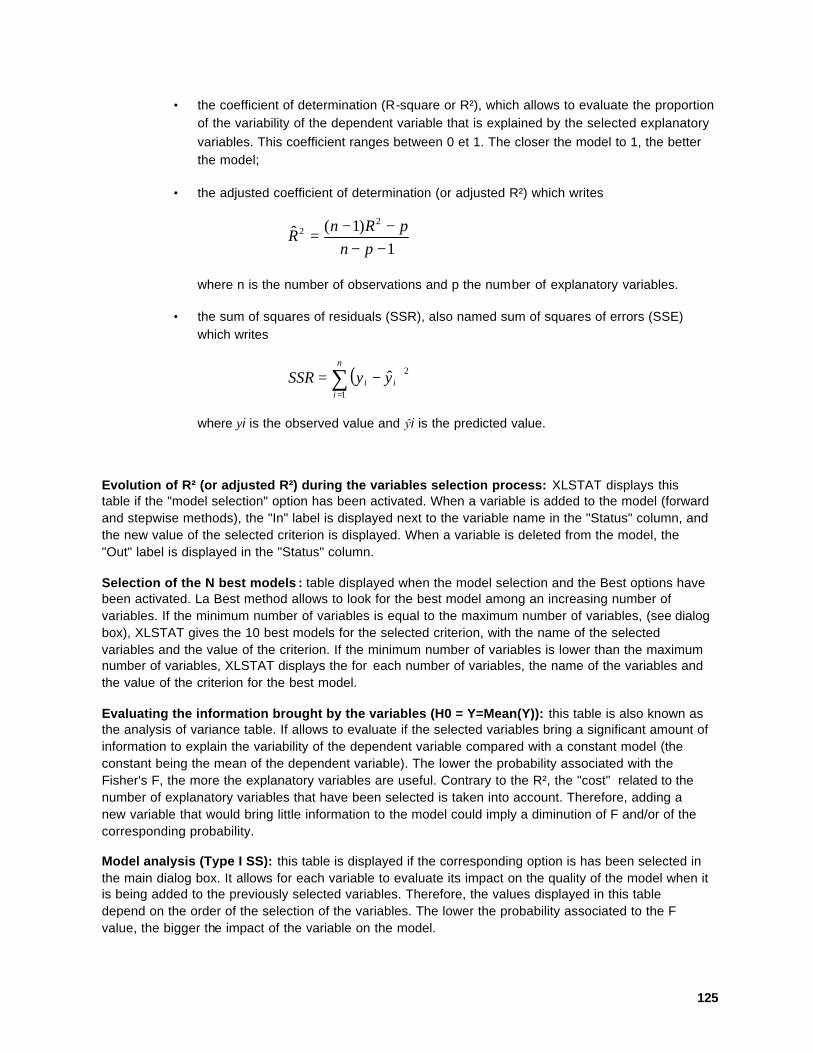
125
• the coefficient of determination (R-square or R²), which allows to evaluate the proportion of the variability of the dependent variable that is explained by the selected explanatory variables. This coefficient ranges between 0 et 1. The closer the model to 1, the better the model;
• the adjusted coefficient of determination (or adjusted R²) which writes
1)1(ˆ
22
−−−−
=pn
pRnR
where n is the number of observations and p the number of explanatory variables.
• the sum of squares of residuals (SSR), also named sum of squares of errors (SSE) which writes
( )∑
=
−=n
iii yySSR
1
2ˆ
where yi is the observed value and ŷi is the predicted value.
Evolution of R² (or adjusted R²) during the variables selection process: XLSTAT displays this table if the "model selection" option has been activated. When a variable is added to the model (forward and stepwise methods), the "In" label is displayed next to the variable name in the "Status" column, and the new value of the selected criterion is displayed. When a variable is deleted from the model, the "Out" label is displayed in the "Status" column.
Selection of the N best models : table displayed when the model selection and the Best options have been activated. La Best method allows to look for the best model among an increasing number of variables. If the minimum number of variables is equal to the maximum number of variables, (see dialog box), XLSTAT gives the 10 best models for the selected criterion, with the name of the selected variables and the value of the criterion. If the minimum number of variables is lower than the maximum number of variables, XLSTAT displays the for each number of variables, the name of the variables and the value of the criterion for the best model.
Evaluating the information brought by the variables (H0 = Y=Mean(Y)): this table is also known as the analysis of variance table. If allows to evaluate if the selected variables bring a significant amount of information to explain the variability of the dependent variable compared with a constant model (the constant being the mean of the dependent variable). The lower the probability associated with the Fisher's F, the more the explanatory variables are useful. Contrary to the R², the "cost" related to the number of explanatory variables that have been selected is taken into account. Therefore, adding a new variable that would bring little information to the model could imply a diminution of F and/or of the corresponding probability.
Model analysis (Type I SS): this table is displayed if the corresponding option is has been selected in the main dialog box. It allows for each variable to evaluate its impact on the quality of the model when it is being added to the previously selected variables. Therefore, the values displayed in this table depend on the order of the selection of the variables. The lower the probability associated to the F value, the bigger the impact of the variable on the model.

126
Model analysis (Type III SS): this table is displayed if the corresponding option is has been selected in the main dialog box. It allows for each variable to evaluate its impact on the quality of the model when it is removed from the full model. Therefore, contrary to the previous table, these results do not depend on the order of the selection of the variables. The lower the probability associated to the F value, the bigger the impact of the variable on the model.
Estimating the parameters of the model: this table displays the estimate for each parameter of the model. The standard error of the estimator, the corresponding Student's t value and probability, and the confidence interval are also included. If the probability is low, it means the parameter brings a significant amount of information to the model. If it is high, removing the corresponding variable would have little effect on the quality of the fit of the model.
Predictions, Residuals, and confidence ranges: this table gives for each observation input value, the value estimated by the model, the residuals, and the standardized, and two confidence intervals. The first interval is for the mean value and is using a Student's t (α/2, n-p-1), and the second is for a punctual value and is also using a Student's t (α/2, n-p-1). The Cook's distance is added if the corresponding option has been selected.
Durbin-Watson statistic: the Durbin-Watson statistic is automatically computed by XLSTAT. This value can be used to test if the residuals are correlated with a lap 1 (reminder: the linear model makes the assumption that the residuals are independent). This test is mostly used for time series analysis.
Predictions for the supplementary observations: if supplementary observations have been selected, XLSTAT computes the model for the various observations, as well as confidence intervals.
Charts:
If only one quantitative explanatory variable has been selected, the first chart shows the regression line, with the input data, and the confidence intervals if the corresponding option has been selected.
If only one quantitative explanatory variable has been selected, the second chart shows the standardized residuals (ordinates) given the explanatory variable (abscissa). This chart is useful to detect regions where the model is more or less well fitted, or correlations between residuals.
A chart with standardized residuals as ordinates, and the input data for the variable to model (abscissa) is displayed, followed by a histogram of the standardized residuals. The histogram is useful to detect outliers or a misfit of the model: given the normality assumptions, there shouldn't be more than 95% of the standardized residuals out of the [-1.96,1.96] interval.
Example
Tutorials for the tool Regression are available on the XLSTAT website on the following pages:
http://www.xlstat.com/demo-reg.htm
http://www.xlstat.com/demo-reg2.htm

127
To know more about it
Jobson J. D. (1996). Applied Multivariate Data Analysis: Regression and Experimental Design. Springer Verlag, New York.
Mallows C.L. (1973). Some comments on Cp, Technometrics, 15, pp. 661-675.
Montgomery D.C. (2001). Introduction to Linear Regression Analysis, 3rd Edition. Wiley, New York.
128
ANOVA This tool supplies all the classic results (including the charts) of simple and multiple way ANOVA. Up to order 4 interactions of can be computed.
Note: with this tool you can select multiple dependent variables and model them one by one in the same report with just one click. This feature is useful for those who do sensory data analysis.
See also: Elements of the dialog box
Continuation of the dialog box
Multiple Comparisons tests dialog box
Factors and interactions dialog box
Missing data
Results
Example
To know more about it
Elements of the dialog box
Dependent variable(s): you can model one ore more quantitative variable(s) at the same time. Select the quantitative variable(s) that you want to model. If more than one variable is selected, the models will be computed for each variable one after the other.
Weights: activate this option and select the data corresponding to the weights of the observations. This is only necessary is some weights are not equal to 1.
Quantitative variables: if you activate this option, you will switch to the ANCOVA model (analysis of covariance).
Qualitative variables: select the qualitative explanatory variables to use in the model.
Observation labels: select the labels corresponding to the rows if they are available. If the option "Column labels" has been selected, make sure that the first cell of the selection is the header of the column.
Range: results are displayed from the cell of an existing sheet. Once you choose this option, select in the corresponding box the cell that will correspond to the top left corner of the results tables.
Sheet: results are displayed in a new sheet of the active workbook.
Workbook: results are displayed in a new workbook.

129
Intercept = 0 : select this option to constrain the model to have constant equal to 0.
Column labels: select this option if the first row of the selected variables (dependent variables, weights, explanatory variables and labels column) are labeled.
Charts: activate this option to display the charts.
Residuals: select this option to let XLSTAT display the tables corresponding to the analysis of predictions and residuals.
Confidence intervals: activate this option if you want that the confidence intervals are displayed on the chart.
More: click this button to display the advanced options of the dialog box.
Continuation of the dialog box
Once you have clicked on the "More" button, the second part of the dialog box is displayed. To go back to the previous size of the dialog box, click on the "Less" button.
Confidence interval (%): this value (between 1 and 99) is used to compute the confidence intervals on the estimators.
Cook's D: activate this option is you want the Cook's distance to be computed and displayed for each observation. Note: activating this option might slow down the computations.
Type I SS, Type III SS: activate this option is you wish to compute the F statistics for the various Type I SS and Type III SS (SS stands for sum of squares).
Constraints: some constraints need to be applied to allow the ANOVA model to be fitted. These constraints have no influence on the fit of the model and on the predicted values. The user can choose the type of constraints that eases the most the interpretation of the results.
• a1 = 0 : for each qualitative variable, the parameter corresponding to the first category is fixed to zero. This constraint is useful when the first category corresponds to a standard or to a "null" effect.
• Sum (ai) = 0 : for each qualitative variable, the sum of the parameters corresponding to the various categories is fixed to zero.
• Sum (ni.ai) = 0 : for each qualitative variable, the weighted sum of the parameters corresponding to the various categories is fixed to zero. The weights are the frequency of the categories.
Interactions: activate this option if you want to take into account the interactions between the first two qualitative variables.
130
Comparisons: activate this option if you want XLSTAT to perform multiple comparisons tests between the categories for each qualitative variable. If this option is activated, a dialog box dedicated to these tests will be displayed during the computations.
Supplementary observations: activate this option if you want XLSTAT to compute predictions on observations that have not been used to build the model. XLSTAT offers you two ways to define the supplementary observations:
• Rows: use this option if you want XLSTAT to run the ANOVA model on the last N rows. The value N must be entered in the "Number of rows" field.
• Select: use this option if you want XLSTAT to run the regression model on additional observations that you want to select. Select the explanatory variables as you did for the data used to build the model. Do not include column labels in the selection.
Factors and interactions dialog box
This dialog is displayed if you activated the Interactions option in the main dialog box, and if at least two qualitative variables have been selected.
Interactions between qualitative variables are generated for all possible combines up to order four (for example, A * B * C * D).
You can choose to let the model compute the parameters for all possible interactions, or you can reduce the number of degrees of freedom used by the model by unselecting some interactions that are not relevant in your opinion.
Multiple comparisons tests dialog box
If the "comparisons" option has been activated in the main dialog box, the Multiple comparisons tests is displayed during the computations to allow the user to choose the tests to run, for each qualitative variable.
Tukey's HSD test: this is among the most commonly used tests (HSD: honestly significant difference).
Fisher's LSD test: this is Student's t test that tests the hypothesis that all the means for the various categories are equal (LSD: least significant difference).
Bonferroni's t* test: this test is derived from the Student's test. It is slightly better, although criticized, as it takes into account that several comparisons are done at the same time by modifying the significance level.
Dunn-Sidak's test: this test is derived from the Bonferroni's test. It is more reliable in some situations.

131
The following tests are more complex as they are based on iterative procedures where the results depends on the number of combines that are to be tested for each category.
Newman-Keuls's test (SNK) : this test is derived from the Student's t test (SNK: Student Newman-Keuls), and is very often used although not very reliable.
Duncan's test: this test is criticized by several authors.
REGWQ procedure: this test is among the most reliable multiple comparisons procedure and should be used (REGW: Ryan-Einot-Gabriel-Welsch).
Dunnett's test: this test allows to compare the categories of a qualitative variable with one of the categories, often called the control group. The control group can be selected from the list which is updated for each qualitative variable. The Dunnett's test can be two-tailed (you test the difference with the control), left-tailed (you test if the category is less than the control), or right-tailed (you test if the category is greater than the control).
Contrasts: this option allows you to choose which type of hypothesis you are going to test:
• µi-µj = 0: select option if you want to test if the means of the groups of the factor of interest are significantly different or not.
• µi-µj – bi-bj = 0: select option if you want to test if the means of the groups of the factor of interest are significantly different or not, once the effects of the previous factors have been removed.
• µi-µj – S(bi-bj) = 0: select option if you want to test if the means of the groups of the factor of interest are significantly different or not, once the effects of all the other factors have been removed.
Sort Ascending/Descending: select how the groups should be sorted when the results are displayed.
Confidence interval: enter the value of the confidence range you want to use for the multiple comparisons tests.
Identical for all variables: if the Dunnett's test is not selected, you may select this option if you want XLSTAT to apply the same options to all factors.
Missing data
If is some missing data are detected you can choose to either estimate them or to remove the corresponding observations. This is true for the observations used to build the model, and for the supplementary observations.

132
If you choose to replace the missing data, the mean is used for the quantitative explanatory variables, the dependent variable(s) and the weights. For the qualitative variables, the mode of the variable is used.
When the remove option is chosen, an observation is removed only for a given model and not for all the variables to model to avoid loosing some valuable information.
Results
XLSTAT displays several tables and charts after the model has been calculated to ease the interpretation of the results. The following results are computed for each of the models that have estimated, which means for each dependent variable.
Summary for the dependent variable: table displaying the mean and the standard error for the variable that is being modeled.
Summary for the qualitative variables: table displaying for each qualitative variable, the number of categories, the name of the categories and their respective frequency.
Goodness of fit coefficients: you will find here
• the coefficient of correlation (R), which is the square-root of the coefficient of determination;
• the coefficient of determination (R-square or R²), which allows to evaluate the proportion of the variability of the dependent variable that is explained by the selected explanatory variables. This coefficient ranges between 0 et 1. The closer the model to 1, the better the model;
• the adjusted coefficient of determination (or adjusted R²) which writes
1)1(ˆ
22
−−−−
=pn
pRnR
where n is the number of observations and p the number of explanatory variables.
• the sum of squares of residuals (SSR), also named sum of squares of errors (SSE) which writes
( )∑
=
−=n
iii yySSR
1
2ˆ
where yi is the observed value and ŷi is the predicted value.

133
Evaluating the information brought by the variables (H0 = Y=Mean(Y)): this table is also known as the analysis of variance table. If allows to evaluate if the selected variables bring a significant amount of information to explain the variability of the dependent variable compared with a constant model (the constant being the mean of the dependent variable). The lower the probability associated with the Fisher's F, the more the explanatory variables are useful. Contrary to the R², the "cost" related to the number of explanatory variables that have been selected is taken into account. Therefore, adding a new variable that would bring little information to the model could imply a diminution of F and/or of the corresponding probability.
Model analysis (Type I SS): this table is displayed if the corresponding option is has been selected in the main dialog box. It allows for each variable to evaluate its impact on the quality of the model when it is being added to the previously selected variables. Therefore, the values displayed in this table depend on the order of the selection of the variables. The lower the probability associated to the F value, the bigger the impact of the variable on the model.
Model analysis (Type III SS): this table is displayed if the corresponding option is has been selected in the main dialog box. It allows for each variable to evaluate its impact on the quality of the model when it is removed from the full model. Therefore, contrary to the previous table, these results do not depend on the order of the selection of the variables. The lower the probability associated to the F value, the bigger the impact of the variable on the model.
Estimating the parameters of the model: this table displays the estimator for each parameter of the model. The standard error of the estimator, the corresponding Student's t value and probability, and the confidence interval are also included. If the probability is low, it means the parameter brings a significant amount of information to the model. If it is high, removing the corresponding variable would have little effect on the quality of the fit of the model.
Predictions, Residuals, and confidence ranges: this table gives for each observation input value, the value estimated by the model, the residuals, and the standardized, and two confidence intervals. The first interval is for the mean value and is using a Student's t (α/2, n-p-1), and the second is for a punctual value and is also using a Student's t (α/2, n-p-1). The Cook's distance is added if the corresponding option has been selected.
Multiple comparisons tests: if the option "comparisons" has been selected in the main dialog box, and if some tests have been chosen in the tests dialog box, XLSTAT displays the results of the tests for each qualitative variable.
Except for the Dunnett's test, the first table displays the results for the one to one comparisons for all the categories for a given variable. For each comparison, the test is considered significant (the difference is significant) if the probability is out of the confidence interval. A second table shows the sorting and the groupings of the categories based on the significance results. If two categories are not significantly different, they share the same letter (A, B, …).
For the Dunnett's test, there is only one table where the various categories are compared with the control category.
Predictions for the supplementary observations: if supplementary observations have been selected, XLSTAT computes the model for the various observations, as well as confidence intervals.
Charts: a chart with standardized residuals as ordinates, and the input data for the variable to model (abscissa) is displayed, followed by a histogram of the standardized residuals. The histogram is useful to detect outliers or a misfit of the model: given the normality assumptions, there shouldn't be more than 95% of the standardized residuals out of the [-1.96,1.96] interval. Additional charts are displayed
134
to facilitate the visualization of the means for the various categories of one factor, or to visualize the interactions between two factors.
Example
Tutorials on ANOVA are available on the XLSTAT website on the following pages:
http://www.xlstat.com/demo-ano.htm
http://www.xlstat.com/demo-ano2.htm
To know more about it
Hsu J.C. (1996). Multiple Comparisons: Theory and Methods, CRC Press, Boca Raton.
Jobson J. D. (1996). Applied Multivariate Data Analysis: Regression and Experimental Design, Springer Verlag, New York.
Lea P., Naes T. & Robotten M. (1997). Analysis of Variance for Sensory Data, John Wiley & Sons, London.
Sahai H. & Ageel M. (2000). The Analysis of Variance: Fixed, Random and Mixed Models, Springer Verlag, New York.

135
ANCOVA ANCOVA is just a mixture of ANOVA and regression : to explain the variations of a Y variable, you can use numerical and categorical variables.
See also: Elements of the dialog box
Continuation of the dialog box
Factors and interactions dialog box
Multiple Comparisons tests dialog box
Missing data
Results
Example
To know more about it
Elements of the dialog box
Dependent variable(s): you can model one ore more quantitative variable(s) at the same time. Select the quantitative variable(s) that you want to model. If more than one variable is selected, the models will be computed for each variable one after the other.
Weights: activate this option and select the data corresponding to the weights of the observations. This is only necessary is some weights are not equal to 1.
Quantitative variables: if you unselect this option, you will switch to an ANOVA model (analysis of variance).
Qualitative variables: if you unselect this option, you will switch to an Regression model.
Observation labels: select the labels corresponding to the rows if they are available. If the option "Column labels" has been selected, make sure that the first cell of the selection is the header of the column.
Range: results are displayed from the cell of an existing sheet. Once you choose this option, select in the corresponding box the cell that will correspond to the top left corner of the results tables.
Sheet: results are displayed in a new sheet of the active workbook.
Workbook: results are displayed in a new workbook.
Intercept = 0 : select this option to constrain the model to have constant equal to 0.
136
Column labels: select this option if the first row of the selected variables (dependent variables, weights, explanatory variables and labels column) are labeled.
Charts: activate this option to display the charts.
Residuals: select this option to let XLSTAT display the tables corresponding to the analysis of predictions and residuals.
Confidence intervals: activate this option if you want that the confidence intervals are displayed on the chart.
More: click this button to display the advanced options of the dialog box.
Continuation of the dialog box
Once you have clicked on the "More" button, the second part of the dialog box is displayed. To go back to the previous size of the dialog box, click on the "Less" button.
Confidence interval (%): this value (between 1 and 99) is used to compute the confidence intervals on the estimators.
Cook's D: activate this option is you want the Cook's distance to be computed and displayed for each observation. Note: activating this option might slow down the computations.
Type I SS, Type III SS: activate this option is you wish to compute the F statistics for the various Type I SS and Type III SS (SS stands for sum of squares).
Constraints: some constraints need to be applied to allow the ANOVA model to be fitted. These constraints have no influence on the fit of the model and on the predicted values. The user can choose the type of constraints that eases the most the interpretation of the results.
• a1 = 0 : for each qualitative variable, the parameter corresponding to the first category is fixed to zero. This constraint is useful when the first category corresponds to a standard or to a "null" effect.
• Sum (ai) = 0 : for each qualitative variable, the sum of the parameters corresponding to the various categories is fixed to zero.
• Sum (ni.ai) = 0 : for each qualitative variable, the weighted sum of the parameters corresponding to the various categories is fixed to zero. The weights are the frequency of the categories.
Interactions: activate this option if you want to take into account the interactions between the first two qualitative variables.
Comparisons: activate this option if you want XLSTAT to perform multiple comparisons tests between the categories for each qualitative variable. If this option is activated, a dialog box dedicated to these tests will be displayed during the computations.

137
Supplementary observations: activate this option if you want XLSTAT to compute predictions on observations that have not been used to build the model. XLSTAT offers you two ways to define the supplementary observations:
• Rows: use this option if you want XLSTAT to run the ANCOVA model on the last N rows. The value N must be entered in the "Number of rows" field.
• Select: use this option if you want XLSTAT to run the regression model on additional observations that you want to select. Select the explanatory variables as you did for the data used to build the model. Do not include column labels in the selection.
Factors and interactions dialog box
This dialog is displayed if you activated the Interactions option in the main dialog box, and if at least two qualitative variables or one quantitative and one qualitative variables have been selected.
Interactions between qualitative variables are generated for all possible combines up to order four (for example, A * B * C * D). Interactions between one quantitative variable and one qualitative variable are also generated.
You can choose to let the model compute the parameters for all possible interactions, or you can reduce the number of degrees of freedom used by the model by unselecting some interactions that are not relevant in your opinion.
Multiple comparisons tests dialog box
If the "comparisons" option has been activated in the main dialog box, the Multiple comparisons tests is displayed during the computations to allow the user to choose the tests to run, for each qualitative variable.
Tukey's HSD test: this is among the most commonly used tests (HSD: honestly significant difference).
Fisher's LSD test: this is Student's t test that tests the hypothesis that all the means for the various categories are equal (LSD: least significant difference).
Bonferroni's t* test: this test is derived from the Student's test. It is slightly better, although criticized, as it takes into account that several comparisons are done at the same time by modifying the significance level.
Dunn-Sidak's test: this test is derived from the Bonferroni's test. It is more reliable in some situations.
The following tests are more complex as they are based on iterative procedures where the results depends on the number of combines that are to be tested for each category.
138
Newman-Keuls's test (SNK): this test is derived from the Student's t est (SNK: Student Newman-Keuls), and is very often used although not very reliable.
Duncan's test: this test is criticized by several authors.
REGWQ procedure: this test is among the most reliable multiple comparisons procedure and should be used (REGW: Ryan-Einot-Gabriel-Welsch).
Dunnett's test: this test allows to compare the categories of a qualitative variable with one of the categories, often called the control group. The control group can be selected from the list which is updated for each qualitative variable. The Dunnett's test can be two-tailed (you test the difference with the control), left-tailed (you test if the category is less than the control), or right-tailed (you test if the category is greater than the control).
Contrasts: this option allows you to choose which type of hypothesis you are going to test:
• µi-µj = 0: select option if you want to test if the means of the groups of the factor of interest are significantly different or not.
• µi-µj – bi-bj = 0: select option if you want to test if the means of the groups of the factor of interest are significantly different or not, once the effects of the previous factors have been removed.
• µi-µj – S(bi-bj) = 0: select option if you want to test if the means of the groups of the factor of interest are significantly different or not, once the effects of all the other factors have been removed.
• bi-bj = 0: this options is displayed only for the factors that correspond to interactions between quantitative and qualitative variables. Select this option if you want to test if the slopes are significantly different or not for the various groups.
Sort Ascending/Descending: select how the groups should be sorted when the results are displayed.
Confidence interval: enter the value of the confidence range you want to use for the multiple comparisons tests.
Identical for all variables: if the Dunnett's test is not selected, you may select this option if you want XLSTAT to apply the same options to all factors.

139
Missing data
If is some missing data are detected you can choose to either estimate them or to remove the corresponding observations. This is true for the observations used to build the model, and for the supplementary observations.
If you choose to replace the missing data, the mean is used for the quantitative explanatory variables, the dependent variable(s) and the weights. For the qualitative variables, the mode of the variable is used.
When the remove option is chosen, an observation is removed only for a given model and not for all the variables to model to avoid loosing some valuable information.
Results
XLSTAT displays several tables and charts after the model has been calculated to ease the interpretation of the results. The following results are computed for each of the models that have estimated, which means for each dependent variable.
Summary for the dependent variable: table displaying the mean and the standard error for the variable that is being modeled.
Summary for the quantitative variables: table displaying the mean and the standard error for the quantitative explanatory variables.
Summary for the qualitative variables: table displaying for each qualitative variable, the number of categories, the name of the categories and their respective frequency.
Goodness of fit coefficients: you will find here
• the coefficient of correlation (R), which is the square-root of the coefficient of determination;
• the coefficient of determination (R-square or R²), which allows to evaluate the proportion of the variability of the dependent variable that is explained by the selected explanatory variables. This coefficient ranges between 0 et 1. The closer the model to 1, the better the model;
• the adjusted coefficient of determination (or adjusted R²) which writes
1)1(ˆ
22
−−−−
=pn
pRnR
where n is the number of observations and p the number of explanatory variables.
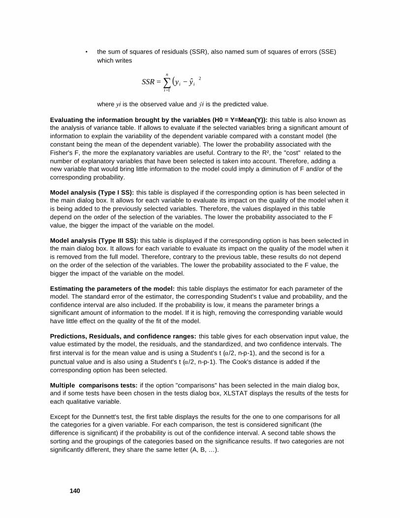
140
• the sum of squares of residuals (SSR), also named sum of squares of errors (SSE) which writes
( )∑
=
−=n
iii yySSR
1
2ˆ
where yi is the observed value and ŷi is the predicted value.
Evaluating the information brought by the variables (H0 = Y=Mean(Y)): this table is also known as the analysis of variance table. If allows to evaluate if the selected variables bring a significant amount of information to explain the variability of the dependent variable compared with a constant model (the constant being the mean of the dependent variable). The lower the probability associated with the Fisher's F, the more the explanatory variables are useful. Contrary to the R², the "cost" related to the number of explanatory variables that have been selected is taken into account. Therefore, adding a new variable that would bring little information to the model could imply a diminution of F and/or of the corresponding probability.
Model analysis (Type I SS): this table is displayed if the corresponding option is has been selected in the main dialog box. It allows for each variable to evaluate its impact on the quality of the model when it is being added to the previously selected variables. Therefore, the values displayed in this table depend on the order of the selection of the variables. The lower the probability associated to the F value, the bigger the impact of the variable on the model.
Model analysis (Type III SS): this table is displayed if the corresponding option is has been selected in the main dialog box. It allows for each variable to evaluate its impact on the quality of the model when it is removed from the full model. Therefore, contrary to the previous table, these results do not depend on the order of the selection of the variables. The lower the probability associated to the F value, the bigger the impact of the variable on the model.
Estimating the parameters of the model: this table displays the estimator for each parameter of the model. The standard error of the estimator, the corresponding Student's t value and probability, and the confidence interval are also included. If the probability is low, it means the parameter brings a significant amount of information to the model. If it is high, removing the corresponding variable would have little effect on the quality of the fit of the model.
Predictions, Residuals, and confidence ranges: this table gives for each observation input value, the value estimated by the model, the residuals, and the standardized, and two confidence intervals. The first interval is for the mean value and is using a Student's t (α/2, n-p-1), and the second is for a punctual value and is also using a Student's t (α/2, n-p-1). The Cook's distance is added if the corresponding option has been selected.
Multiple comparisons tests: if the option "comparisons" has been selected in the main dialog box, and if some tests have been chosen in the tests dialog box, XLSTAT displays the results of the tests for each qualitative variable.
Except for the Dunnett's test, the first table displays the results for the one to one comparisons for all the categories for a given variable. For each comparison, the test is considered significant (the difference is significant) if the probability is out of the confidence interval. A second table shows the sorting and the groupings of the categories based on the significance results. If two categories are not significantly different, they share the same letter (A, B, …).
141
For the Dunnett's test, there is only one table where the various categories are compared with the control category.
Predictions for the supplementary observations: if supplementary observations have been selected, XLSTAT computes the model for the various observations, as well as confidence intervals.
Charts: a chart with standardized residuals as ordinates, and the input data for the variable to model (abscissa) is displayed, followed by a histogram of the standardized residuals. The histogram is useful to detect outliers or a misfit of the model: given the normality assumptions, there shouldn't be more than 95% of the standardized residuals out of the [-1.96,1.96] interval. Additional charts are displayed to facilitate the visualization of the means for the various categories of one factor, or to visualize the interactions between two factors.
Example
A tutorial on ANCOVA is available on the XLSTAT website on the following page:
http://www.xlstat.com/demo-anco.htm
To know more about it
Hsu J.C. (1996). Multiple Comparisons: Theory and Methods. CRC Press, Boca Raton.
Jobson J. D. (1996). Applied Multivariate Data Analysis: Regression and Experimental Design. Springer Verlag, New York.
Lea P., Naes T. & Robotten M. (1997). Analysis of Variance for Sensory Data, John Wiley & Sons, London.
Sahai H. & Ageel M. (2000). The Analysis of Variance: Fixed, Random and Mixed Models. Springer Verlag, New York.
142
Logistic Regression Use this module to run logistic regression and other related binary response models. Results include goodness of fit tests, residuals analysis, probability analysis and a chart.
See also: Description
Elements of the dialog box
Continuation of the dialog box
Missing data
Results
Example
To know more about it
Description
Logistic regression and the other binary response data models available in this section are of high interest for people doing medical tests, epidemiological or social research, pharmaceutical and agricultural experiments, quantitative marketing, and risk modeling (scoring).
Imagine a doctor is doing a clinical experiment in a hospital. He wants to test doses of a new pharmaceutical product, to test it's effect on the remission of a particular disease. The response will not be as in agricultural sciences a yield (a quantitative value), but "yes" or "not" (categorical binary results) or counts of "yes" and "no". So usual linear models cannot be used.
The powerful tool to be used in such a case is a Model for Binary Response Data. What the doctor will try to determine is the probability that a patient will be cured if he takes the D dose. So the model must give its results between 0 and 1.
The most commonly used models are the Logit (based on the logistic function) and the Probit (based on the normal distribution function) models. These two functions are sigmoidal and symmetric. XLSTAT offers two other choices which are close the Logit function : the Log-log complementary model is also sigmoidal, but not symmetric : the function is closer to the upper asymptote. The Gompertz function is on the contrary closer the axis of abscissa.
The analytical expression of the models are as follow:
• Logit: P = exp(aX+b) / (1+ exp(aX+b))
• Probit: P = F(aX+b) where F is the standard normal cumulative distribution function,
• Gompertz: P = exp(-exp(-(aX+b)))
• Complementary Log-log: P = 1- exp(-exp(aX+b))
This is what the results could be:
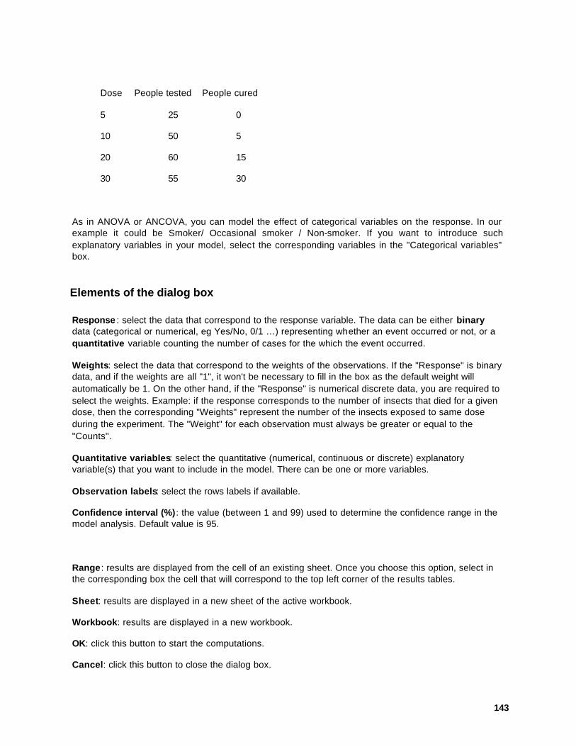
143
Dose People tested People cured
5 25 0
10 50 5
20 60 15
30 55 30
As in ANOVA or ANCOVA, you can model the effect of categorical variables on the response. In our example it could be Smoker/ Occasional smoker / Non-smoker. If you want to introduce such explanatory variables in your model, select the corresponding variables in the "Categorical variables" box.
Elements of the dialog box
Response : select the data that correspond to the response variable. The data can be either binary data (categorical or numerical, eg Yes/No, 0/1 …) representing whether an event occurred or not, or a quantitative variable counting the number of cases for the which the event occurred.
Weights: select the data that correspond to the weights of the observations. If the "Response" is binary data, and if the weights are all "1", it won't be necessary to fill in the box as the default weight will automatically be 1. On the other hand, if the "Response" is numerical discrete data, you are required to select the weights. Example: if the response corresponds to the number of insects that died for a given dose, then the corresponding "Weights" represent the number of the insects exposed to same dose during the experiment. The "Weight" for each observation must always be greater or equal to the "Counts".
Quantitative variables: select the quantitative (numerical, continuous or discrete) explanatory variable(s) that you want to include in the model. There can be one or more variables.
Observation labels: select the rows labels if available.
Confidence interval (%): the value (between 1 and 99) used to determine the confidence range in the model analysis. Default value is 95.
Range: results are displayed from the cell of an existing sheet. Once you choose this option, select in the corresponding box the cell that will correspond to the top left corner of the results tables.
Sheet: results are displayed in a new sheet of the active workbook.
Workbook: results are displayed in a new workbook.
OK: click this button to start the computations.
Cancel: click this button to close the dialog box.

144
Help: click this button to activate the XLSTAT online help.
Column labels: select this option if the first row of the selected variables (response variable and explanatory variables) are labeled.
Residuals: select this option to let XLSTAT display the tables corresponding to the analysis of predictions and residuals.
Chart: activate this option to display the chart. A chart is displayed only when there is one quantitative explanatory variable.
Confidence intervals: activate this option if you want that the confidence intervals are displayed on the chart.
Model: XLSTAT offers you the possibility to fit four different models to the data:
Probit: ∫∞−
−=
X
dxxβ
ππ
2exp
2
1 2
Logit: )exp(1)exp(X
Xβ
βπ
+=
Gompertz: ( )[ ]Xβπ −−= expexp
Complementary Log-log: ( )[ ]Xβπ expexp1 −−=
X represents the linear combine of the explanatory variables
NB: to fit the model, XLSTAT maximizes the likelihood function.
Intercept=0: Select this option to constrain the model to have a constant term equal to 0.
Continuation of the dialog box
Qualitative variables: Select the qualitative explanatory variable(s) that you want to include in the model. There can be one or more qualitative variables, and can include two or more categories each. The variables can be binary variables (exposed to light yes/no) or multinomial variables (age category or citizenship, for example).
Convergence: the value used to determine when the likelihood value have converged. Default value is 0.00001.
145
Constraints: select here the constraint to put on the qualitative variables
• a1 = 0: the parameter corresponding to the first category is set to 0, for each qualitative variable.
• Sum (ai) = 0: the sum of the parameters corresponding to the categories is set to 0 for each qualitative variable.
Supplementary observations: activate this option if you want XLSTAT to compute predictions on observations that have not been used to build the model. XLSTAT offers you two ways to define the supplementary observations:
• Rows: use this option if you want XLSTAT to run the logistic regression model on the last N rows. The value N must be entered in the "Number of rows" field.
• Select: use this option if you want XLSTAT to run the regression model on additional observations that you want to select. Select the explanatory variables as you did for the data used to build the model. Do not include column labels in the selection.
Missing data
If is some missing data are detected you can choose to either estimate them or to remove the corresponding observations. This is true for the observations used to build the model, and for the supplementary observations.
If you choose to replace the missing data, the mean is used for the quantitative explanatory variables, and the response variable if it is quantitative and the weights. For the qualitative variables, and the response variable if it is binary, the mode of the variable is used.
Results
XLSTAT displays several tables and charts after the model has been calculated to ease the interpretation of the results. The following results are computed for each of the models that have estimated, which means for each dependent variable.
Summary Statistics for the variable to model: table displaying several statistics for the variable to model including the mean and the standard deviation.
Summary Statistics for Quantitative variables: table displaying the mean and the standard deviation for the quantitative explanatory variables.
Summary Statistics for Qualitative variables: table displaying the number of different categories, the name of each category, and the respective frequency for all the qualitative explanatory variable.
Model parameters: table displaying the estimator for each parameter of the model. The standard error of the estimator, the corresponding Chi-square value and the corresponding probability are also included. If the probability is low, it means the parameter brings a significant amount of information to

146
the model. If it is high, removing the corresponding variable would have little effect on the quality of the fit of the model.
Evaluating the goodness of fit of the model:
• Observations: the total number of observations taken into account to estimate the model parameters (sum of the weights);
• Log likelihood: the logarithm of the likelihood function (the higher, the better the model). Note: the parameters estimators are computed by maximizing the likelihood function;
• Log likelihood (indep): the logarithm of the likelihood function corresponding to the independent model. Note: the independent model is the constant model where the probability is equal to the average probability for the event to occur computed for the selected data; the independent model can be interpreted as the case where no information is available; the greater the difference between the Log likelihood and the Log likelihood (indep), the more information the selected variables bring to the model
• Pearson's Chi-Sq: measures the Chi-square distance between the observed frequencies and the predicted frequencies. The lower the value, the better the fit;
• Pearson's DF: the degrees of freedom of the Chi-square distribution associated to the Pearson's Chi-Sq. (DF = sum of the weights – number of parameters used in the model);
• Prob>Pearson's Chi-Sq: the probability corresponding to the Pearson's Chi-Sq. This value gives the probability of being wrong when saying that the explanatory variables bring significant information to explain the observed values;
• L.R. Chi-Sq: the Log ratio between the likelihood and the likelihood (indep) - the exact formula is 2.Log[likelihood indep / likelihood];
• DF (L.R. Chi-Sq): the degrees of freedom of the Chi-Square distribution corresponding to the L.R. Chi-Sq value;
• Prob>L.R. Chi-Sq: the probability corresponding to the L.R. Chi-Sq. This value gives the probability of being wrong when saying that the explanatory variables bring significant information compared to the independent model.
• R²: the determination coefficient (R-Square) for the observed and predicted values. Not as well suited as for linear regression;
• R² (McFadden): a modified R² which is better suited for this kind of models. As the R², the McFadden's R² is contained between 0 and 1.
Predictions and residuals: Table giving for each observation the details the input data and the outputs of the selected model, including the estimated probability (model and independent model), the residuals, and the standardized residuals.
Probability analysis with the fitted model: this table is displayed only when there is one quantitative variable and no qualitative variable. It presents a range of probabilities and the corresponding values for the quantitative variable, given the model. This is a reverse analysis of the model. The corresponding confidence intervals are also displayed. The Heterogeneity factor is computed when the Probability (Prob>Pearson's Chi-Sq) is lower than 0.1, in which case a second set of confidence intervals is added. These values cannot always be computed because of numerical constraints.
147
Predictions for the supplementary observations: if supplementary observations have been selected, XLSTAT computes the model for the various observations, as well as a confidence interval.
Charts: if only one quantitative explanatory variable has been selected, the chart shows the model line, with the input data, and the confidence intervals if the corresponding option has been selected.
Example
A tutorial on Logistic regression is available on the XLSTAT website on the following page:
http://www.xlstat.com/demo-log.htm
To know more about it
Abbott W.S. (1925). A method for computing the effectiveness of an insecticide. Jour. Econ. Entomol. 18, pp. 265-267.
Agresti A. (1990). Categorical data analysis. John Wiley & Sons, New York.
Finney, D.J. (1971). Probit Analysis. 3rd ed., Cambridge, London and New-York.

148
Nonlinear Regression Use this tool allows to fit any function to any data by optimizing the parameters of the function. The function can either be a function included in the XLSTAT package, or a function coded and added to the functions library by the end user. This tool performs simple and multiple nonlinear regression (one or more explanatory variables can be used).
See also: Description
Elements of the dialog box
Continuation of the dialog box
Elements of the functions dialog box
Adding a function to the functions user's library
Missing data
Results
Example
To know more about it
Description
Nonlinear regression allows to model complex phenomena. XLSTAT provides you with a list of pregrogrammed functions within which the user can select one or more models he believes are relevant for the subject of interest. If the relevant model is not listed, you can add your own function, and if possible the derivatives of the function for each parameter to speed up the computations.
When it is possible (pregrogrammed functions or user defined functions when the derivatives are available) the Levenberg-Marquardt algorithm is used. When the derivatives are not available, a more complex and slower but efficient algorithm is used.
The model(s) are fitted to the observations by minimizing the SSR (sum of square of residuals).
Elements of the dialog box
Dependent variable: select the quantitative variable that you want to model. If more than one variable is selected, the models will be computed for each variable one after the other.
Quantitative variables: select the quantitative explanatory variables to use in the model.
Column labels: select this option if the first row of the selected variables (dependent variables, weights, explanatory variables and labels column) are labeled.
Observation labels: select the labels corresponding to the rows if they are available. If the option "Column labels" has been selected, make sure that the first cell of the selection is the header of the column.

149
Range: results are displayed from the cell of an existing sheet. Once you choose this option, select in the corresponding box the cell that will correspond to the top left corner of the results tables.
Sheet: results are displayed in a new sheet of the active workbook.
Workbook: results are displayed in a new workbook.
OK: click this button to start the computations.
Cancel: click this button to close the dialog box.
Help: click this button to activate the XLSTAT online help.
Residuals: select this option to let XLSTAT display the tables corresponding to the analysis of predictions and residuals.
Charts: activate this option to display the charts.
More: click this button to display the advanced options of the dialog box.
Continuation of the dialog box
Weights: activate this option and select the data corresponding to the weights of the observations. This is only necessary is some weights are not equal to 1.
Supplementary observations: activate this option if you want XLSTAT to compute predictions on observations that have not been used to build the model. XLSTAT offers you two ways to define the supplementary observations:
• Rows: use this option if you want XLSTAT to run the logistic regression model on the last N rows. The value N must be entered in the "Number of rows" field.
• Select: use this option if you want XLSTAT to run the regression model on additional observations that you want to select. Select the explanatory variables as you did for the data used to build the model. Do not include column labels in the selection.
Parameters bounds: if you activate this option, you have to select on an Excel sheet the lower (left column) and upper (right column) for the various parameters of the model.
Starting point: if you activate this option, select on an Excel sheet the values that will be used as a starting point for the computations. The values must be the one under the other, and there must be as many values as there are parameters in the model.
Parameters labels: if you want to give names to the parameters, select on an Excel sheet the names that will be used when displaying the results. The names must be the one under the other, and there must be as many names as there are parameters in the model.

150
Elements of the functions dialog box
Preprogrammed functions:
In that section you will find the list of preprogrammed functions. You may select one, several or all functions. Each selected function will be fitted to the observations. Detailed results are displayed only for the function that best fits the observations.
Notes:
• If you select the first function (polynomial function) XLSTAT needs that you enter the order of the polynomial function (default value: 2).
• If, in the previous dialog box, you have selected a starting point, bounds for the parameters or the parameters names, XLSTAT will only fit the models that have the same number of parameters.
Conditions to stop:
• Iterations: this value is used to determine the maximum number of iterations that should be run for the fitting of the model(s), and, if no starting point has been specified, this value is also used to determine the number of random repetitions to find the best starting point. The more complex the function, the higher this value should be. Default value is 500.
• Convergence: the value used to determine when the likelihood value have converged. Default value is 0.00001.
User defined functions: in that section you will find the list of preprogrammed functions. You may select one, several or all functions. Each selected function will be fitted to the observations. Detailed results are displayed only for the function that best fits the observations.
Note: If, in the previous dialog box, you have selected a starting point, bounds for the parameters or the parameters names, XLSTAT will only fit the models that have the same number of parameters.
Delete : if you select one or more functions, you can delete them from the user defined functions library by clicking on this button. The removal of a function is irreversible.
Add: click this button to add a new function to the user defined functions list.
Adding a function to the user defined functions library
To add a function to the user defined functions, you have to write the function in the «Function: Y = » box, while following the syntax rules:
• The N parameters of the function must be written pr1, pr2, …, prN.
• The P explanatory variables must be represented as X1, X2, …, XP.
• The Excel functions can be used (Exp(), Sin(), Pi(), Sqrt(), …).

151
If you want, you can select the function derivatives of each parameter. The derivatives must follow the same conventions as the function. They must be written (the one under the other) in an Excel sheet. To avoid Excel producing errors (especially when they begin with a minus) you can put a quote ‘ at the beginning of the derivatives.
Note: there must be as many derivatives as there are parameters in the function.
To add the function to the user defined functions library and to able to use it, click on the Save button. When you click that button, the function is automatically saved and selected in the list of user defined functions.
Note:
The library is saved as Models.txt file in the Application Data \ Addinsoft \ XLSTAT folder. The library is built as follows:
Row 1: number of functions defined by user
Row 2: N1= number of parameters in function 1
Row 3: function 1 definition
Rows 4 to (3 + N1): derivatives definition for function 1
Row 4+N1: N2= number of parameters in function 2
Row 5+N1: function 2 definition
…
When the derivatives have not been supplied by the user, "Unknown" replaces the derivatives of the function.
You can modify manually the items of this file but you should be cautious not to make an error.
Missing data
If is some missing data are detected you can choose to either estimate them or to remove the corresponding observations. This is true for the observations used to build the model, and for the supplementary observations.
If you choose to replace the missing data, the mean is used for the quantitative explanatory variables, the dependent variable and the weights.
Results
XLSTAT displays several tables and charts after the model has been optimized, to ease the interpretation of the results.

152
Summary Statistics for the dependent variable: Table displaying several statistics for the dependent variable including the mean and the standard deviation.
Summary Statistics for Quantitative variables: Table displaying the mean and the standard deviation for the quantitative explanatory variables.
Results for the selected models: Table displaying a quick summary for each of the computed models. The summary includes the model definition, the equation after the model has been fitted to the data, and the corresponding R² and SSR (sum of square residuals). The following results are only displayed for the best model – the model with the lowest SSR.
Goodness of fit coefficients: Table displaying
• the coefficient of correlation (R), which is the square-root of the coefficient of determination;
• the coefficient of determination (R-square or R²), which allows to evaluate the proportion of the variability of the dependent variable that is explained by the selected explanatory variables. This coefficient ranges between 0 et 1. The closer the model to 1, the better the model;
• the sum of square residuals (SSR), which is criterion used for the optimization.
Model parameters: Table displaying the estimator for each parameter of the model. The standard error of the estimator, is displayed when possible (preprogrammed functions and user defined functions when the derivatives are available.
Predictions and residuals: Table giving for each observation the details the input data and the outputs of the selected model, including the estimated value for the dependent variable, the residuals, and the standardized residuals.
Charts: If only one quantitative explanatory variable has been selected, the first chart shows the model line, with the input data. If only one quantitative explanatory variable has been selected, the second chart shows the standardized residuals (ordinates) given the explanatory variable (abscissa). This chart is useful to detect regions where the model is more or less well fitted, or correlations between residuals. A chart with standardized residuals as ordinates, and the input data for the variable to model (abscissa) is displayed, followed by a histogram of the standardized residuals.
Predictions for the supplementary observations: if supplementary observations have been selected, XLSTAT computes the model for the various observations, as well as a confidence interval.
Example
A tutorial on nonlinear regression is available on the XLSTAT website on the following page:
http://www.xlstat.com/demo-nonlin.htm

153
To know more about it
Ramsay J.O. et al. (1997). Functional Data Analysis . Springer-Verlag, New York.
Ramsay J.O. et al. (2002). Applied Functional Data Analysis . Springer-Verlag, New York.
Ratkowsky D.A. (1983). Nonlinear Regression Modeling. Marcel Dekker, New York.
154
Nonparametric Regression Use this tool to perform Kernel or LOWESS regression, two methods for nonparametric regression. Kernel Regression is one class of modeling methods that belongs to the smoothing methods family. Kernel Regression is used on longitudinal data, for example in finance. Other smoothing methods, related to time series analysis are available in the XLSTAT-Time module. Kernel regression does not take into account seasonalities, as the Holt-Winters method does, but it is able to take into account a set of explanatory variables. Kernel regression allows you to base the prediction of a value on passed observations, and to weight the impact of passed observations depending on how similar they are compared with the current values of the explanatory variables. The classical and robust LOWESS (Locally weighted scatter plot smoother) regressions are available in this section.
See also: Description
Elements of the dialog box
Missing data
Results
Example
To know more about it
Description
Kernel Regression is a powerful non parametric smoothing method. Unlike linear regression which is both used to explain phenomena and for prediction, Kernel regression is mostly used for prediction. The model is often complex and its structure varies with the data, making any "physical" interpretation difficult.
As with any modeling method, a learning sample of size nlearn is used to estimate the parameters of the model. A sample of size nvalid can then be used to cross-validate the quality of the model, and to adjust some characteristics of the model. Last, the model can be applied on a prediction sample of size npred, for which the values of the dependent variable Y are unknown.
The first characteristic of Kernel Regression is the use of a kernel function, to weigh the observations of the learning sample, depending on their "distance" to the predicted observation. The more the values of the explanatory variables for a given observation of the learning sample are close to the values observed for the observation being predicted, the higher the weigh. Many kernel functions have been suggested. XLSTAT includes the following kernel functions: Uniform, Triangle, Epanechnikov, Quartic, Triweight, Tricube, Gaussian, and Cosine.
The second characteristic is the bandwidth associated to each variable. It is involved in the computation of the weight, and it allows to differentiate or rescale the effect of the variables on the weights, while at the same time reduce or augment the impact of observations of the learning sample, depending on how far they are from the observation to predict.

155
Example: let Y be the dependent variable, and (X1, X2, …, Xk) being k explanatory variables. For the prediction of yi from observation i (1 ≤ i ≤ nvalid), given the observation j (1 ≤ j ≤ nlearn), the weight is determined using a Gaussian kernel, with a bandwidth fixed to hl for each of the Xl variables (l = 1…k), the weight is computed by using a Gaussian kernel:
( )
∑
−−=
=
=∏
k
l l
iljlk
ll
kij h
xx
hw
1
2
1
exp2
1
π
The third characteristic is the polynomial degree used when fitting the model to the observations of the learning sample. In the case where the polynomial degree is 0 (constant polynomial), the Nadaraya-Watson formula is used to compute the ith prediction:
∑
∑=
=
=
lean
lean
n
jij
n
jjij
i
w
ywy
1
1
In the case of the constant polynomial, the explanatory variables are taken into account only for the computing of the weight. For higher polynomial degrees (XLSTAT allows to work with polynomials of degrees 0 to 2), the variables are also involved in the fitting of the polynomial. Once the model has been fitted, it is applied on the validation or prediction sample in order to estimate the values of the dependent variable. The formula to compute the prediction yi write:
• Degree 1: ∑+==
k
l
lilli xaay
10
• Degree 2: ∑ ∑+∑+== ==
k
l
k
mimillm
k
l
llili xxbxaay
1 11,0
Notes:
• Before we estimate the parameters of the polynomial model, the observations of the learning sample are previously weighted using the Nadaraya-Watson formula.
• In the case of the degrees 1 and 2 polynomial, for each observation of the validation and prediction samples, the polynomial parameters are estimated. This makes Kernel Regression a numerically intensive method.
Two strategies are suggested in order to restrict the size of the learning sample taken into account for the estimation of the parameters of the polynomial:
• Moving window: to estimate yi, we take into account a fixed number of observations previously observed. Consequently, with this strategy, the learning sample evolves at each step.
• k nearest neighbours: this method, complementary of the previous, allows to restrict the size of the learning sample to a fixed number of the observations or to a fixed percentage of the total size of the learning sample.

156
Details on the kernel functions:
The weight wij computed for observation j, for the estimation of prediction yi, writes:
( )∏
=
=k
l l
ijlij h
uKw
1 m where l
jlilijl h
xxu
−=
where K is a kernel function. The kernel functions available in XLSTAT are:
• Uniform: the kernel function writes:
( ) 1.
21
≤Ι= uuK
• Triangle: the kernel function writes:
( ) ( ) 1.1 ≤Ι−= uuuK
• Epanechnikov: the kernel function writes:
( ) ( ) 1
2 .143
≤Ι−= uuuK
• Quartic: the kernel function writes:
( ) ( ) 1
22 .11615
≤Ι−= uuuK
• Triweight: the kernel function writes:
( ) ( ) 1
32 .13235
≤Ι−= uuuK
• Tricube: the kernel function writes:
( ) ( ) 1
33 .1 ≤Ι−= uuuK
• Gaussian: the kernel function writes:
( ) 2
2
21 u
euK−
=π
• Cosine: the kernel function writes:

157
( ) 1.
2cos
4 ≤Ι
= uuuK
ππ
Details on the LOWESS regression:
The LOWESS method (locally weighted regression and smoothing scatter plots) was first introduced by Cleveland in 1979. New versions have since then been proposed in order to increase the robustness of the models. LOWESS regression is close to Kernel regression as it is also based on polynomial regression and as it requires a kernel function to weight the observations.
The LOWESS algorithm can be described as follows: for each point i to predict:
1 - First, the euclidean distances (i,j) between the observations i and j are computed. The fraction f of the closest observations to observation i are selected among the N observations. For the selected observations, the weights are computed using the Tricube kernel on the following distance:
)),((
),(),(
jidMaxjid
jiDj
=
( )),()( jiDTricubejWeight =
2 - A regression model is then fitted, and a prediction is computed for observation i.
For the Robust LOWESS regression, additional computations are performed:
3 - The weights are computed again using the following distance:
))((.6
)(),('
jrMedian
jrjiD
j
=
where r(j) is the residual corresponding to observation j after the previous step,
the weights are computed using the Quartic kernel:
( )),(')( jiDQuarticjWeight =
4 - A regression is then fitted again using the new weights.
5 - Steps 3 and 4 are performed a second time. A final prediction is then computed for observation i.
Notes:
- With the LOWESS and Robust LOWESS regression methods, the only input parameters apart from the observations are the f fraction (in % in XLSTAT) and the polynomial degree.
- Robust LOWESS regression is about three times more time consuming than LOWESS regression.

158
Elements of the dialog box
Dependent variable: select the quantitative variable that you want to model. If more than one variable is selected, the models will be computed for each variable one after the other.
Quantitative variables: select the quantitative explanatory variables to use in the model.
Column labels: select this option if the first row of the selected variables (dependent variables, weights, explanatory variables and labels column) are labeled.
Observation labels: select the labels corresponding to the rows if they are available. If the option "Column labels" has been selected, make sure that the first cell of the selection is the header of the column.
Range: results are displayed from the cell of an existing sheet. Once you choose this option, select in the corresponding box the cell that will correspond to the top left corner of the results tables.
Sheet: results are displayed in a new sheet of the active workbook.
Workbook: results are displayed in a new workbook.
OK: click this button to start the computations.
Cancel: click this button to close the dialog box.
Help: click this button to activate the XLSTAT online help.
Residuals: select this option to let XLSTAT display the tables corresponding to the analysis of predictions and residuals.
Charts: activate this option to display the charts.
• Time as abscissa: select this option if you want that the charts that displays the model curve and the residuals, do not use the explanatory variable but a time variable.
Learning sample:
• Moving window: choose this option if you want the size of the learning sample to be constant. You need to enter the size S of the window. In that case, to estimate Y(i+1), the observations i-S-1 to i will be used, and the first observation XLSTAT will be able to compute a prediction for, is the S+1 observation.
• Expanding window: choose this option if you want the size of the learning sample to be expanding step by step. You need to enter the initial size S of the window. In that case, to estimate Y(i+1), the observations 1 to i will be used, and the first observation XLSTAT will be able to compute a prediction for, is the S+1 observation.

159
• Rows: if the total sample size is N, XLSTAT will subdivide it into n rows for the learning sample, and N-n rows for the validation and/or prediction samples, where n is the number of rows you need enter in the corresponding box.
• %: if the total sample size is N, XLSTAT will subdivide it into n rows for the learning sample, and N-n rows for the validation and/or prediction samples, where n is round(p.N), and where p is percentage to enter in the corresponding box.
• 1/1: the learning and validation/prediction samples are built taking iteratively one observation for the learning sample, and one observation for the validation/prediction sample.
• 2/1: the learning and validation/prediction samples are built taking iteratively two observations for the learning sample, and one observation for the validation/prediction sample.
• 1/2: the learning and validation/prediction samples are built taking iteratively one observation for the learning sample, and two observations for the validation/prediction sample.
• All: the learning and validation/prediction samples are identical. This method has no interest for prediction, but it is a way to evaluate the method in case of perfect information.
Method:
• LOWESS: choose this option so that the predictions are computed using the LOWESS method. If you choose this option, the other settings will automatically be changed. The only parameters you can change are the polynomial degree , and the K nearest neighbours % that corresponds to the fraction of points taken into account.
• Robust LOWESS: choose this option so that the predictions are computed using the Robust LOWESS method. If you choose this option, the other settings will automatically be changed. The only parameters you can change are the polynomial degree , and the K nearest neighbours % that corresponds to the fraction of points taken into account.
• Mean: choose this option so that the predictions are computed using the Nadaraya-Watson formula.
• Median: choose this option so that the predictions are computed using a weighted median.
• Polynomial: choose this option so that the predictions are computed using a polynomial.
Polynomial degree: enter here the degree of the polynomial. The accepted values are 0,1,2. Choosing a polynomial of degree 0 is equivalent to choosing the "Mean" method.
K nearest neighbours: activate this option to define the size of the learning sample. Two options are available:

160
• Rows: the k points retained for the analysis are k points which are the closest to the point to predict, for a given bandwidth and a given kernel function. k is the value to enter here.
• %: the points retained for the analysis are the closest to the point to predict, for a given bandwidth and a given kernel function, and they represent x% of the total learning sample available, where x is the value to enter.
Kernel: the kernel function that will be used. The possible options are: Uniform, Triangle, Epanechnikov, Quartic, Triweight, Tricube, Gaussian, Cosine. A description of these functions is available in the description section.
Bandwidth: XLSTAT allows you to choose a method for automatically computing the bandwidths (one per variable), or you can fix them. The different options are:
• Constant: the bandwidth is constant and equal to the value to enter.
• Fixed: the bandwidth is defined for each variable in a cell of an Excel sheet, which you need to select. The cells must be the one under the other, and in the same order as the variables.
• Range: the value hl of the bandwidth for each variable Xl is determined by the following formula:
( ) ( )
learnlearn niilniill xMinxMaxh ..1..1 == −=
• Standard deviation: the value hl of the bandwidth for each variable Xl is equal to the standard deviation of the variable computed on the learning sample.
Missing data
If is some missing data are detected in the explanatory variables, you can choose to either estimate them, ignore them (dependent variable only) or remove the corresponding observations.
If is some missing data are detected in the dependent variable, and if you choose to ignore the missing values, if the missing data belong to the learning sample, they will be replaced by an estimator given by the Nadaraya-Watson using the selected kernels and bandwidths. If the missing data do not belong to the learning sample, they will be estimated as any value to predict, using the selected method.
Results
XLSTAT displays several tables and charts after the model has been optimized, to ease the interpretation of the results.
161
Summary Statistics for the dependent variable: Table displaying several statistics for the dependent variable including the mean and the standard deviation.
Summary Statistics for Quantitative variables: Table displaying the mean and the standard deviation for the quantitative explanatory variables.
Goodness of fit coefficients: Table displaying
• the coefficient of correlation (R), which is the square-root of the coefficient of determination;
• the coefficient of determination (R-square or R²), which allows to evaluate the proportion of the variability of the dependent variable that is explained by the selected explanatory variables. This coefficient ranges between 0 et 1. The closer the model to 1, the better the model;
• the sum of square residuals (SSR), which is criterion used for the optimization.
Predictions and residuals: Table giving for each observation the details the input data and the outputs of the selected model, including the estimated value for the dependent variable and the residuals.
Charts: If only one quantitative explanatory variable has been selected, or if the "time as abscissa" option has been selected, the first chart shows the model line, with the input data. If only one quantitative explanatory variable has been selected, or if the "time as abscissa" option has been selected, the second chart shows the residuals (ordinates) given the explanatory variable (abscissa) or the time. This chart is useful to detect regions where the model is more or less well fitted, or correlations between residuals. A chart with residuals as ordinates, and the input data for the variable to model (abscissa) is displayed, followed by a histogram of the residuals. If the "time as abscissa" option has been selected, the abscissa correspond to the time variable. If not, the abscissa correspond to the observation labels.
Example
A tutorial on Kernel regression is available on the XLSTAT website on the following page:
http://www.xlstat.com/demo-kernel.htm
To know more about it

162
Cleveland W.S. (1979). Robust locally weighted regression and smoothing scatterplots. J. Amer. Statist. Assoc., 74 829-836.
Cleveland W.S. (1994). The Elements of Graphing Data. Hobart Press, Summit, New Jersey.
Härdle W. (1992). Applied Nonparametric Regression. Cambridge University Press, Cambridge.
Nadaraya E.A. (1964). On estimating regression. Theory Probab. Appl., 9 141-142.
Wand M.P. & Jones M.C. (1995). Kernel Smoothing. Chapman and Hall, New York.
Watson G.S. (1964). Smooth regression analysis. Sankhya Ser.A, 26 101-116.
163
Tests on Contingency Tables Use this module to calculate tables derived from a contingency table, to test the association between rows and columns, and to calculate various specific statistics.
Note: to calculate a contingency table (or two-way table) for two sets of categorical variables, use the Contingency Table (Two-way Table) and Chi square module.
See also: Description
Elements of the dialog box
Continuation of the dialog box
Example
To know more about it
Description
A wide variety of statistics is available to test the null hypothesis of independence between rows and columns, or simply to describe the association between the rows and columns in a contingency table. These statistics may be grouped according to the structure of the table (number of rows and columns); a few of them are specific to ordinal categories.
Contingency tables containing any number of rows and columns (R × C tables)
• Chi-square Pearson statistic: tests the independence between rows and columns. The higher the value of the Pearson's Chi-square ?², the stronger the evidence against the null hypothesis.
• Wilks' G²: statistic corresponding to the Chi-square likelihood ratio, obtained using the maximum likelihood method. The higher the value of G², the stronger the evidence against the null hypothesis. The Wilks' G² is sometimes preferable to Chi-square, but the conclusions of the associated tests are identical when the sizes are large enough, because the Wilks' G² is asymptotically equivalent to Chi-square.
• Monte Carlo I: the p-value corresponding to the test for independence between the rows and columns is approximated using the Monte Carlo test proposed by Raymond & Rousset (1995). This test uses Markov chains.
• Monte Carlo II: the p-value corresponding to the test for independence between the rows and columns is computed using a quadratic interpolation on the empirical cumulative distribution (cdf) function of the Chi-square distance. The empirical cdf is estimated using N tables generated using a Monte Carlo algorithm. N is a value to be specified by the user. The simulated tables are R x C tables with the same row and column margins as the original table.

164
• Phi coefficient: measure of association related to Chi-square based on the relation ?² = nf ², where n is the total frequency. The phi coefficient f has the advantage of not being dependent on the total frequency.
• Cramer V: association measurement related to the Chi-square but that does not depend on the total frequency. The Cramer V varies between [0,1]; a value near 0 indicates independence and a value near 1 indicates dependence. The Cramer V can reach its maximum even when the number of rows is different from the number of columns.
• Tschuprow T: measurement of association related to the Chi-square but that does not depend on the total frequency. The Tschuprow T varies between [0,1]; a value near 0 indicates independence and a value near 1 indicates dependence. The Tschuprow T can reach its maximum only in a square contingency table.
• Contingency coefficient: measurement of association related to the Chi-square but that does not depend on the total frequency. The contingency coefficient C varies between [0,1], and values near 0 indicate independence while values near 1 indicate dependence. Note that the contingency coefficient C never reaches the value 1. The maximum value Cmax is approached as a direct function of the degree of freedom so that C cannot be used to compare several contingency tables of different dimensions. For example, for a 2 × 2 table, Cmax = 0.71 while for a 4 × 4 table, Cmax = 0.87. The contingency coefficient C is recommended for tables that are 5 × 5 and larger.
Note: for a 2 × 2 contingency table, the Cramer V and the Tschuprow T coefficients are equal, the square of Cramer V is equal to the square of the phi coefficient, and is also equal to the averaged Goodman & Kruskal Tau.
• Theil U (R|C): uncertainty coefficient for the rows defined as an increase in the log-likelihood obtained for the most general model compared to the independence model, divided by the marginal log-likelihood for the rows.
• Theil U (C|R): coefficient defined like the previous one, but for columns, and conditionally for rows.
• Averaged Theil U: coefficient with the same numerator as the previous two, but whose denominator is the average of both.
• Goodman & Kruskal Tau (R|C): prediction measurement that tends to describe the explained proportion of variation for a row given a column. The Goodman & Kruskal Tau is calculated as the reduction of the total variation of the rows taken into account by the columns, divided by the total variation of the rows. A high value represents a strong association.
• Goodman & Kruskal Tau (C|R): measurement defined like the previous one, but for columns, and conditionally for rows.
• Averaged Goodman & Kruskal Tau: average of the two previous measures.
Note: the Goodman & Kruskal Tau and Theil U (or uncertainty coefficient) are two alternative statistics with identical objectives. Both are measures of association that indicate the reduction of error when

165
categories of rows (or of columns) are used to predict the categories of columns (or of rows). A value equal to 0 indicates independence, meaning that it is impossible to predict rows (columns) given the columns (rows). One difficulty with this type of measurement is to determine as of which value the statistic represents a strong association.
R × C contingency tables whose categories appearing in rows and columns are ordered
• Goodman & Kruskal Gamma: measurement of the association between ordinal variables, defined as the deviation between the probability of concordance and the probability of discordance. The Goodman & Kruskal gamma ? varies between [-1,+1]. The measurement ? has an absolute value of 1 when the relation between the two ordinal variables is monotone. Note that a perfect association is obtained even when the relation is not strictly monotone. The value ? = 1 is obtained for a null discordance probability, and the value ? = -1 is obtained when the concordance probability is null. The independence between rows and columns implies ? = 0 but the opposite is not true. The Goodman & Kruskal gamma processes variables symmetrically: if you invert the order of categories for one of the variables, only the sign of ? changes.
R × R square contingency table
• Cohen Kappa: measurement of agreement calculated only for a square contingency table. For the Kappa statistic, the rows and columns correspond to the replies of two judges (in the abstract sense of the term). The judges agree with one another along the diagonal and disagree away from the diagonal. The statistic measures how much higher the frequencies along the diagonal compared to the expected frequencies calculated assuming independence. Kappa is equal to 0 when the agreement between the judges matches the expected frequencies assuming independence, and is equal to 1 in a perfect agreement.
2 × 2 contingency table
There are several specific statistics that describe the association between rows and columns in a contingency table comparing two variables, where each variable has two categories. The corresponding contingency table may look like this:
• Chi-square with Yates'correction: it is traditionally accepted that in the special case of a 2 × 2 contingency table, the Chi-square should be corrected using the Yates' correction for continuity.
• Fisher's exact test: the p-value for the independence test between the rows and columns of the contingency table is calculated by considering all the contingency tables that have the same marginal totals, and by using hypergeometric probability distribution. The test may be either one-tailed or two-tailed.
166
• Odds ratio: the odds ratio ? is the ratio of the products ad / bc. The odds ratio ? can have any non-negative value. When a, b, c and d are all positive, the independence between the rows and columns implies ? = 1. When 1 < ? < 8, the observations corresponding to row 1 have a higher probability of giving a response 1 than the observations corresponding to row 2. When 0 < ? < 1, response 1 is less probable in row 1 than in row 2. When a cell in the table has zero probability, ? equals 0 or 8. The odds ratio does not change when the orientation of the table is reversed so that the rows become columns and the columns become rows. A value of ? farther from 1 in a given direction represents a high degree of association between the rows and the columns. Two values of ? represent the same level of association, but in opposite directions, when one value is the inverse of the other. When the order of the rows (or columns) is reversed, the new value of ? is the inverse of the original value. Finally, ? does not vary if you change the scale in the rows and the columns, in that, if r1>0, r2>0, c1>0 and c2>0, then (r1c1a)(r2c2d) / (r1c2b)(r2c1c) = ad / bc = ?.
• ln(odds ratio): it is often easier to use ln(?) instead of ?. The logarithm of ? can have any value between -8 and +8. Independence represents ln(?) = 0. The function ln(?) is symmetrical to 0, and the reversion of the rows or columns changes its sign. Thus, two values ?1 and ?2 where ln(?1) = -ln(?2) represent the same level of association, but in opposite directions.
• Yule Q: coefficient based on the products of the concordances ad and of the differences bc, linked to the odds ratio ? by the following formula: Q = (? - 1) / (? + 1). The Yule Q is a monotone transformation of ? from the interval [0, 8] to the interval [-1,+1]. The Yule Q is a special case of the Goodman & Kruskal gamma calculated for a 2 × 2 table. Values with an absolute value near 1 correspond to a close association between the rows and columns. A negative value indicates dissimilarity, a positive value indicates similarity, and a null value indicates independence. The Yule Q is often interpreted as the difference between the conditional probability of agreement and the conditional probability of disagreement, when two observations are chosen at random from the same population.
• Yule Y: coefficient based on the products of the concordances ad and of the differences bc, linked to the odds ratio ? by the following formula: Q = (v? - 1) / (v? + 1). The Yule Y is similar to the Yule Q but is more sensitive to differences in the margins of the 2 × 2 table.
• Phi coefficient: measure of association related to Chi-square based on the relation ?² = nf ², where n is the total frequency. For a 2 × 2 table, the phi coefficient f varies between [-1,+1] and may be interpreted as a correlation coefficient, where f = 0 represents independence.
Elements of the dialog box
Data: enter the range corresponding to the contingency table. Missing data are not allowed.
Ordinal categories: check this option if the categories in rows and columns are ordered.

167
Comments on tests: check this option to display the explicit conclusions of the tests or comments.
Significance level: enter the value of the type I error for the test.
Range: the results are displayed based on a cell located in an existing sheet.
Sheet: Results are displayed in a sheet of the active workbook.
Workbook: Results are displayed in a new workbook.
Labels included: the row and column labels appear in the selected range.
More: click this button to display the advanced options of the dialog box.
Continuation of the dialog box
Fisher's exact test: check this option to perform the Fisher's exact test for a 2 × 2 contingency table.
" one-tailed " / " two-tailed": choose the type of Fisher's exact test, either one-tailed or two-tailed.
Monte Carlo I: check this option to perform the approximate calculation of the p-value using the exact test for an R × C contingency table, using a Monte Carlo test.
• Iterations: enter the number of iterations for the Monte Carlo method that approximates the p-value of the exact test for a R × C contingency table. The fewer the iterations, the less accurate the approximation. Value within [1000, 1000000]. Default value: 50,000.
Monte Carlo II: check this option to perform the Monte Carlo simulations of R × C contingency tables having the same margin properties as the input table.
• Repetitions: enter the number of repetitions for the Monte Carlo procedure. The fewer the iterations, the less accurate the approximation. Value within [100, 1000000]. Default value: 10,000.
Combinations: check this option to display a table with the combinations of categories in rows and in columns. This table contains the same information as the contingency table and the table of percentages in relation to the total size, but the information is presented in a different format.
Observed frequencies: check this option to display the contingency table to which the marginal totals and the total have been added.
Expected frequency: check this option to display the table of expected frequencies calculated assuming that the rows and columns in the contingency table are independent.
Contributions to Chi-square: check this option to display the table of the basic contributions of each cell in the contingency table for the Chi-square value calculated for the entire contingency table.

168
Chi-square by cell: check this option to display a table that shows a) whether the observed frequency is greater than, less than, or equal to the expected frequency, and b) the result of the partial Chi-square test called the "Chi-square by cell" test. The "Chi-square by cell" test is a Chi-square test calculated on a table with four cells: one cell represents cell [i,j] in the original contingency table, the other cells represent frequencies for row i minus cell [i,j], for column j minus cell [i,j], and for the rest of the table.
Percentages/proportions in relation to rows: check this option to display the table of percentages or proportions compared to the sums of the rows.
Percentages/proportions in relation to columns: check this option to display the table of percentages or proportions compared to the sums of the columns.
Percentages/proportions in relation to total: check this option to display the table of percentages or proportions compared to the total.
"Percentages" / "Proportions": choose the display mode for the three previous tables, either as percentages (values between 0 and 100), or as proportions (values between 0 and 1).
Example
To know more about it
Agresti A. (1990). Categorical data analysis. John Wiley & Sons, New York.
Bloch D.A. & Kraemer H.C. (1989). 2 × 2 Kappa coefficients: measures of agreement or association. Biometrics, 45: 269-287.
Conlon M. & Thomas R.G. (1993). The power function for Fisher's exact test. Applied Statistics, 42: 258-260.
Dagnelie P. (1986). Théorie et méthodes statistiques. Vol. 2. Les Presses Agronomiques de Gembloux, Gembloux, pp. 81-90, 395-397.
Dillon W.R. & Goldstein M. (1984). Multivariate analysis. Methods and applications. John Wiley & Sons, New York, pp. 302-315.
Fleiss J.L. (1981). Statistical methods for rates and proportions. John Wiley & Sons, New York.
Herman J. (1986). Analyse de données qualitatives. 1. Traitement d'enquêtes, échantillons, répartitions, associations. Masson, Paris.
Hudson W.D. & Ramm C.W. (1987). Correct Formulation of the Kappa Coefficient of Agreement. Photogrammetric Engineering and Remote Sensing, 53: 421-422.
Lehmann E.L. & D'Abrera H.J.M. (1975). Nonparametrics. Statistical methods based on ranks. Holden-Day, San Francisco.
Raymond M. & Rousset F. (1995). An exact test for population differentiation. Evolution, 49: 1280-1283.

169
Siegel S. (1956). Nonparametric statistics for the behavioral sciences. McGraw-Hill Kogakusha, Tokyo, Japan.
Sokal R.R. & Rohlf F.J. (1995). Biometry. The principles and practice of statistics in biological research. Third edition. Freeman, New York, pp. 724-743, 760-778.

170
Correlation Tests Use this module to measure and test the linear correlation between two quantitative variables, ordinal variables, or even binary variables.
See also: Description
Elements of the dialog box
Example
To know more about it
Description
XLSTAT proposes three traditional correlation coefficients to measure and test the intensity of the linear relation between two variables. These coefficients range between [-1,+1], and both limits correspond to a perfectly linear relation. This is a reverse relation when the correlation is negative (the values of a variable increase when those of the other decrease), and a direct relation when the correlation is positive (both variables vary in the same direction, either by increasing or by decreasing). The null value represents the absence of a linear relation.
Note: the independence between the two variables implies a null correlation, but the opposite is not necessarily true. Th e absence of a linear relation does not mean that there is no relation between the variables: the relation may be different than that of a simple direct linear relation. You can try to change the variables in order to linearize a non-linear relation for the original variables.
Pearson's correlation coefficient: covariance of the compared variables, standardized by the standard deviations, or (which amounts to the same thing), covariance calculated on the normalized data.
Spearman's coefficient of rank correlation: nonparametric correlation coefficient, strictly equivalent to the Pearson's correlation coefficient calculated on the ranks of the values.
Kendall's coefficient of rank correlation: nonparametric correlation coefficient, i.e. calculated on the ranks of the values.
Note: for two binary variables, the Pearson's correlation coefficient (or its equivalent in this case, Spearman's coefficient of rank correlation) is equal to the phi coefficient calculated in the Tests on Contingency Tables module for the corresponding 2 × 2 contingency table.
Elements of the dialog box
Variable 1: enter the range for the column of the first variable.
Variable 2: enter the range for the column of the second variable.
Column labels: the first cell of each selected column contains a label.
Correlation: choose a correlation coefficient from the list.
171
Range: the results are displayed based on a cell located in an existing sheet.
Sheet: Results are displayed in a sheet of the active workbook.
Workbook: Results are displayed in a new workbook.
Significance level: enter the value of the type I error for the test.
Charts: check this option to display the chart of the dispersion of values (Pearson's correlation) or of the rank of values (Spearman's or Kendal's correlation).
Example
To know more about it
Dagnelie P. (1986). Théorie et méthodes statistiques. Vol. 2. Les Presses Agronomiques de Gembloux, Gembloux, pp. 309-320, 397-398.
Siegel S. (1956). Nonparametric statistics for the behavioral sciences. McGraw-Hill Kogakusha, Tokyo, Japan, pp. 202-223.
Sokal R.R. & Rohlf F.J. (1995). Biometry. The principles and practice of statistics in biological research. Third edition. Freeman, New York, pp. 569-583, 593-598.
Tomassone R., Dervin C. & Masson J.P. (1993). Biométrie. Modélisation de phénomènes biologiques. Masson, Paris, pp. 98-108.

172
Mantel test Use this module to measure and test the linear correlation between two proximity matrices (simple Mantel test) or between two matrices while taking into account the linear correlation with a third matrix (partial Mantel test).
See also: Description
Elements of the dialog box
Continuation of the dialog box
Missing values
Results
Example
To know more about it
Description
To test the correlation between two matrices, it is not possible to use the classical correlation tests, even by reformatting the matrices into a vector. As a matter of fact, the proximity values in each matrix are not independent from each other, which violates the application conditions of the classical correlation tests, whether they are parametric or non parametric tests. Therefore, there is a need for specific tests, the most known being the Mantel test.
The standardized Mantel statistic is a Pearson correlation coefficient computed between all the cells of an A and a B matrix. However, the way to determine the p-value is different from the classical correlation coefficient test. The p-value can be exactly computed by considering all the permutations of the rows and the columns of one of the two matrices, under the null hypothesis H0, that each permutation has the same probability. It is the position of the observed value (that means for the particular permutation corresponding to the data) in the distribution established under H0, that defines the p-value. When the dimension of the matrix is too high (n>10), it is almost impossible to compute the statistic for all the permutations. However, it is possible to sample randomly in the permutations to obtain a precise estimate of the p-value (the precision increases with the number of random permutations).
An extension of the Mantel test allows to treat the problem of the partial correlation between two proximity matrices while taking into account a third proximity matrix, C.
XLSTAT expects matrices with dimension n>2, not necessarily symmetric, with similarities or dissimilarities. When interpreting the sign of the correlation, it is recommended to be cautious and to take into account the nature of the matrix (similarities or dissimilarities), and it is advised to use the same type of matrices (either similarities, or dissimilarities) to avoid confusions.
173
Elements of the dialog box
Matrix A: select the data corresponding to the proximity matrix (similarities or dissimilarities).
Matrix B: select the data corresponding to the proximity matrix (similarities or dissimilarities), as for matrix A.
Matrix C: check this option if you want to run a partial Mantel test, and select the data corresponding to the third proximity matrix, as for matrices A and B.
Correlation: choose the type of correlation, whether parametric (Pearson) or non parametric (Spearman).
Significance level: enter the value of the type I error for the test.
Labels included: activate this option if the the labels of the rows and columns have been selected with the matrices.
Symmetric matrices: check this option if all the matrices are symmetric, which is the default option for proximity matrices, and which allows to restrict the computations to the half of the matrices instead of the full matrices.
Distribution: check this option to display the values of the statistic under H0.
Charts: check this option to display the charts (dispersion of the values and distribution histogram under H0).
More: click this button to display the advanced options of the dialog box.
Continuation of the dialog box
Set of permutations, exhaustive/sample: choose exhaustive if you want to compute the exact p-value by computing all the permutations, or choose sample if you want to estimate the p-value by randomly sampling with replacement in the set of permutations. The option exhaustive is not possible if n>10. The randomized permutations are obtained with the method of Edgington (1987) and not with the method used by Manly (1993) which does not approximate as well the exact distribution.
Sample size: enter the size of the permutations sample to use when estimating the p-value. A value lower than 1000 is not accepted. The maximum number of randomized permutations has been fixed to 10 000 000. Default value is 10 000. Use the default value for a prototype, and use higher values for publications (for example 100 000 or 1 000 000). The estimation of the p-value is unbiased, and the distribution of the p-value is asymptotically normal with mean p and variance p(1-p)/m, where m is the sample size.
Two-tailed test: check this option to run a two-tailed test.
174
Missing data
Because the matrix is symmetrical, it is enough that the data of the selection allow to reconstitute correctly the totality of the matrix. For example, only enter the lower half-matrix, the upper half-matrix, part in the lower half-matrix and the other part in the upper half-matrix. Otherwise, missing values are not accepted.
Results
Permutation test / Randomization test: in the case of an exhaustive permutation test, the value corresponds to the number of permutations, and in the case of a randomization test, the value corresponds to the number of randomized permutations to estimate the p-value, and to the seed of the pseudo-random numbers generator (so that you can reproduce exactly the same results if you wish).
Correlation (A, B): correlation between A and B. If the test is partial, the correlations between A and B, B and C, A and C, A and B conditionally to C are displayed.
A table displays the observed value, the p-value with comments, and the significance level of the test. The conclusion of the test is also displayed.
Distribution under H0: vector of the values of the statistic that build the distribution under H0.
Charts: dispersion chart of the values (Pearson correlation) or the ranks of the values (Spearman correlation) and histogram of the distribution under H0.
Example
A tutorial on the Mantel test is available on the XLSTAT website on the following page:
http://www.xlstat.com/demo-mantel.htm
To know more about it
Dietz E.J. (1983). Permutation tests for association between two distance matrices. Systematic Zoology, 32 : 21-26.
Edgington E.S. (1987). Randomization tests. Second edition. Marcel Dekker, New York, 341 p.
175
Faust K. & Romney A.K. (1995). The effect of skewed distributions on matrix permutation tests. British Journal of Mathematical and Statistical Psychology, 38 : 152-160.
Jackson D.A. & Somers K.M. (1989). Are probability estimates from the permutation model of Mantel's test stable? Canadian Journal of Zoology, 67 : 766-769.
Luo J. & Fox B.J. (1996). A review of the Mantel test in dietary studies: effect of sample size and inequality of samples sizes. Wildlife Research, 23 : 267-288.
Oden N.L. & Sokal R.R. (1992). An investigation of three-matrix permutation tests. Journal of Classification, 9 : 275-290.
Manly B.J.F. (1993). Randomization, bootstrap and Monte Carlo methods in biology. Chapman & Hall, London, 399 p.
Mantel N. (1967). A technique of disease clustering and a generalized regression approach. Cancer Research, 27 : 209-220.
Mantel N. & Valand R.S. (1970). A technique of nonparametric multivariate analysis. Biometrics, 26 : 547-558.
Mielke P.W. (1978). Clarification and appropriate inference for Mantel and Valand's nonparametric multivariate analysis technique. Biometrics, 34 : 277-282.
Smouse P.E., Long J.C. & Sokal R.R. (1986). Multiple regression and correlation extension of the Mantel test of matrix correspondence. Systematic Zoology, 35 : 627-632.

176
One-sample t test and z test Use these parametric tests to determine if the expectation (theoretical mean) of a given sample is significantly different from a reference value. Use the t test when the variance is estimated and the z test when it is known.
See also: Description
Elements of the dialog box
Dialog box for selecting hypotheses
Missing data
To know more about it
Description
The sample is assumed to belong a population with mean µ. The two-tailed (or two-sided) test corresponds to testing the equality between µ and a reference value µ0 , and the null (H0) and alternative (H1) assumptions are:
• H0 : µ = µ0
• H1 : µ ≠ µ0
For the one-tailed (or one-sided) test, two cases are possible, whether you are testing if µ is lower or bigger than µ0.
For the left one- tailed test, the assumptions write:
• H0 : µ = µ0
• H1 : µ < µ0
For the right one- tailed test, the assumptions write:
• H0 : µ = µ0
• H1 : µ > µ0
To these tests correspond the following underlying assumption: the data are independent and identically distributed, and follow a normal distribution.

177
Elements of the dialog box
Sample : select a column of data with quantitative data.
Significance level: enter the value of the type I error for the test.
Student' t test: activate this option pour to run a t test. A second dialog box will then be displayed to allow you to choose the hypothesis to test.
z test: activate this option pour to run a z test. A second dialog box will then be displayed to allow you to choose the hypothesis to test.
Range: the results are displayed based on a cell located in an existing sheet.
Sheet: Results are displayed in a sheet of the active workbook.
Workbook: Results are displayed in a new workbook.
Column label: the first cell of the selected column contains a label.
Dialog box for selecting hypotheses
Null hypothesis, "H0: Mean = 0 ": enter the reference value. Default value: 0, in order to test that the means are equal.
Alternative hypothesis to be tested: choose the type of test to perform: two-tailed, left one-tailed, or right one-tailed (see Description).
In the case of a z test:
Variances Estimated/Theoretical : enter the value of the variance of the population. Click on the arrow to copy the estimated variance into the theoretical variance.
Missing data
When XLSTAT finds missing data, it simply ignores them.

178
To know more about it
Dagnelie P. (1986). Théorie et méthodes statistiques. Vol. 2. Les Presses Agronomiques de Gembloux, Gembloux.
Frontier S. (1981). Méthode statistique. Masson, Paris.
Manoukian E.B. (1986). Guide de statistique appliquée. Hermann, Paris.
Sokal R.R. & Rohlf F.J. (1995). Biometry. The principles and practice of statistics in biological research. Third edition. Freeman.
179
Two-sample t test and z test Use these parametric tests when you have two samples, in order to determine if the samples expectations (theoretical means) differ by a given quantity D (Student's t test, test z).
See also: Description of the Student t test for independent samples
Dialog box for selecting hypotheses
Description of the Student t test for paired samples
Dialog box for selecting hypotheses
Description of the z test for independent samples
Dialog box for selecting hypotheses
Description of the z test for paired samples
Dialog box for selecting hypotheses
Elements of the dialog box
Example
To know more about it
Description of the Student t test for independent samples
Samples 1 and 2 are taken respectively from two populations with expectations µ1 and µ2. The two-tailed test evaluates the difference between µ1 - µ2 and D, using the null (H0) and alternative (H1) hypotheses shown below:
• H0: µ1 - µ2 = D
• H1: µ1 - µ2 ≠ D
In the one-tailed case, you should note the left (or lower) one-tailed test and the right (or higher) one-tailed test.
In the left one-tailed test, the following hypotheses are tested:
• H0: µ1 - µ2 = D
• H1: µ1 - µ2 < D
In the right one-tailed test the following hypotheses are tested:
• H0: µ1 - µ2 = D
• H1: µ1 - µ2 > D

180
This test is based on the following assumptions:
• both samples were taken at random from their respective populations, distributed using normal distributions with the same variance,
• besides the independence within each sample, both samples are mutually independent.
Note: the test supposes in principle that theoretical variances of both populations are equal. However, XLSTAT can perform this test even if the variances are not equal, by using a linear combination of critical values of t.
Dialog box for selecting hypotheses
Null hypothesis, "H0: Mean 1 – Mean 2 = D": enter the value of D. Default value: 0, in order to test that the means are equal.
Alternative hypothesis to be tested: choose the type of test to perform: two-tailed, left one-tailed, or right one-tailed (see Description of the Student t test for independent samples).
Hypothesis of equality of the theoretical variances: check this option to assume that the theoretical variances are equal.
Note: if the Fisher test is performed, XLSTAT uses the conclusion of the variance equality test to add or remove the check from the previous option.
Description of the Student t test for paired samples
Let d represent the expectation of the differences di = xi2 - xi1, where xi2 is the ith value for sample 2 and xi1 the ith value for sample 1. The two-tailed test corresponds to the test of the difference between d and D, and the null (H0) and alternative (H1) hypotheses are as follows:
• H0: d = D
• H1: d ≠ D
In the one-tailed case, you should note the left (or lower) one-tailed test and the right (or higher) one-tailed test.
In the left one-tailed test, the following hypotheses are tested:
• H0: d = D
• H1: d < D
In the right one-tailed test the following hypotheses are tested:
• H0: d = D
• H1: d > D

181
This test is based on the following assumptions:
• both samples are random samples taken from their respective populations,
• the samples are paired,
• the difference is distributed using a normal distribution (this is a less restrictive condition than the normality of the two original populations).
Dialog box for selecting hypotheses
Null hypothesis, "H0: Mean 1 – Mean 2 = D": enter the value of D. Default value: 0, in order to test that the averages are equal.
Alternative hypothesis to be tested: choose the type of test to perform: two-tailed, left one-tailed, or right one-tailed (see Description of the Student t test for paired samples).
Description of the z test for independent samples
The z test is performed against the standard normal distribution and does not require equality for the variances of populations from which the samples are taken. There are two situations where theoretical variances are known, or are simply estimated based on the samples. In a special dialog box, XLSTAT allows you to directly enter theoretical variance values, or to transfer the estimated variances to theoretical variances fields. When you replace theoretical variances with their estimates, the use of the z test means realizing two separate estimations of the variances and not a global estimation of the common variance as in the Student's t test. The z test may be used whenever the sizes of both samples are large enough (where n1 and n2 are at least around 20 or 30).
The tested hypotheses are identical to those of the Student's t test for independent samples (see Description of the Student t test for independent samples).
Dialog box for selecting hypotheses
Null hypothesis, "H0: Mean 1 – Mean 2 = D": enter the value of D. Default value: 0, in order to test that the averages are equal.
Alternative hypothesis to be tested: choose the type of test to perform: two-tailed, left one-tailed, or right one-tailed (see Description of the z test for independent samples).
Variances, Theoretical 1: enter the value of theoretical variance for the original population of sample 1. If you click the double-arrow, you can copy the value of the estimated variance to the theoretical variance field.
Variances, Theoretical 2: enter the value of theoretical variance for the original population of sample 2. If you click the double-arrow, you can copy the value of the estimated variance to the theoretical variance field.

182
Description of the z test for paired samples
For paired samples, the variance is that of the difference di = xi2 - xi1, with xi2 the ith value for sample 2 and xi1 the ith value for sample 1.
The tested hypotheses are identical to those of the Student t test for paired samples (see Description of the Student t test for paired samples).
Dialog box for selecting hypotheses
Null hypothesis, "H0: Mean 1 – Mean 2 = D": enter the value of D. Default value: 0, in order to test that the means are equal.
Alternative hypothesis to be tested: the test to be performed is two-tailed (see Description of the z test for paired samples).
Variances, Theoretical: enter the value of theoretical variance of the difference. If you click the double-arrow, you can copy the value of the estimated variance to the theoretical variance field.
Elements of the dialog box
Data in different columns: if the samples appear in different columns, select samples 1 and 2 (the columns may have different sizes).
Data in one column: If the data are grouped, the data range represents a column of values, and the membership in samples is expressed by a Groups column.
Sample 1: if the samples appear in different columns, select the range for the first sample.
Sample 2: if the samples appear in different columns, select the range for the second sample.
Data: for grouped data, select the range corresponding to the values of both samples.
Groups: for grouped data, select the range corresponding to a categorical variable that indicates the sample to which each value belongs.
Significance level: enter the value of the type I error for the test.
Samples: independent / paired: choose the type of relation between the two samples. Paired samples may correspond for example to two treatments that concern a single set of experimental subjects.
Range: the results are displayed based on a cell located in an existing sheet.
Sheet: Results are displayed in a sheet of the active workbook.
Workbook: Results are displayed in a new workbook.
Column labels: the first cell of each selected column contains a label.

183
Chart: check this option to display the dominance diagram comparing both samples (up to 50 × 50 values).
Student's t Test: check this option to perform a t test.
z Test: check this option to perform a z test.
Missing data
If XLSTAT finds missing data
• If the samples are independent, XLSTAT uses all the available information and simply ignores missing data.
• If the samples are paired, XLSTAT suggests to remove the rows with missing data for the analysis.
Example
To know more about it
Dagnelie P. (1986). Théorie et méthodes statistiques. Vol. 2. Les Presses Agronomiques de Gembloux, Gembloux, pp. 16-17, 21-29, 35-39, 50-53.
Frontier S. (1981). Méthode statistique. Masson, Paris, pp. 119-127, 189-190.
Manoukian E.B. (1986). Guide de statistique appliquée. Hermann, Paris, pp. 125-132, 135-136.
Sokal R.R. & Rohlf F.J. (1995). Biometry. The principles and practice of statistics in biological research. Third edition. Freeman, New York, pp. 184-190, 223-227.
Tomassone R., Dervin C. & Masson J.P. (1993). Biométrie. Modélisation de phénomènes biologiques. Masson, Paris, pp. 70-72.

184
Multiple Comparisons Tests Multiple comparisons parametric tests (k-sample comparisons of the means) are available in the ANOVA tool of XLSTAT.
185
Two-sample Comparison of Variances Use these parametric tests when you have two samples, in order to determine if the samples come from populations with identical variances.
Note: these tests required independent samples
See also: Description
Elements of the dialog box
Missing data
To know more about it
Description
The Fisher's F is the ratio of the variance estimations for populations 1 and 2. XSTAT always divides
the largest variance σmax² by the smallest σmin². The value of the statistic is tested against Fisher's
distribution for degrees of freedom 1max −n
and 1min −n , where maxn is the size of the sample having
the largest variance and minn is the size of the sample having the smallest variance. The following null (H0) and alternative (H1) hypotheses are used:
• H0: σmax² / σmin² = 1
• H1: σmax² / σmin² > 1
The Bartlett's and Levene's statistics are described in the general k samples case in the "k samples comparison of variances" section.
The null (H0) and alternative (H1) hypotheses write:
• H0 : σ1² = σ2²
• H1 : σ1² ≠ σ2²
As for the Fisher's F test, the Bartlett's test is very sensitive to the non-normality of the samples, whatever the samples sizes. The Bartlett's test is equivalent to the Fisher's F test if the size of the two samples is identical..
186
Elements of the dialog box
Data in different columns: if the samples appear in different columns, select samples 1 and 2 (the columns may have different sizes).
Data in one column: If the data are grouped, the data range represents a column of values, and the membership in samples is expressed by a Groups column.
Sample 1: if the samples appear in different columns, select the range for the first sample.
Sample 2: if the samples appear in different columns, select the range for the second sample.
Data: for grouped data, select the range corresponding to the values of both samples.
Groups: for grouped data, select the range corresponding to a categorical variable that indicates the sample to which each value belongs.
Significance level: enter the value of the type I error for the test.
Range: the results are displayed based on a cell located in an existing sheet.
Sheet: results are displayed in a sheet of the active workbook.
Workbook: results are displayed in a new workbook.
Column labels: the first cell of each selected column contains a label.
Bartlett's test: check this option to perform a Bartlett's test.
Levene's test: check this option to perform a Levene's test. Choose whether you want to use the definition based on the mean or the one based on the median. The definition based on the median is recommended for its robustness when the data are not normally distributed.
Missing data
When XLSTAT finds missing data, it simply ignores them.

187
To know more about it
Dagnelie P. (1986). Théorie et méthodes statistiques. Vol. 2. Les Presses Agronomiques de Gembloux, Gembloux.
Frontier S. (1981). Méthode statistique. Masson, Paris.
Manoukian E.B. (1986). Guide de statistique appliquée. Hermann, Paris.
Sokal R.R. & Rohlf F.J. (1995). Biometry. The principles and practice of statistics in biological research. Third edition. Freeman.

188
k-sample Comparison of Variances Use these parametric tests when you have k samples (k>1), in order to determine if the samples come from populations with identical variances.
Note: these tests required independent samples
See also: Description
Elements of the dialog box
Missing data
To know more about it
Description
The null (H0) and alternative (H1) hypotheses write:
• H0 : σ1² = σ2²
• H1 : for at least one (i,j) with i≠j, σi² ≠ σ j²
Bartlett test:
The Bartlett test statistic is defined as:
( )
−
−+
−
∑
∑
= •
=•
k
i i
k
iii
k 1
1
22
1113
11
ˆlnˆln
νν
σνσν
where 1−= ii nν
and ∑
=• =
k
ii
1
νν
This statistic is distributed as a Chi-distribution with k-1 degrees of freedom.
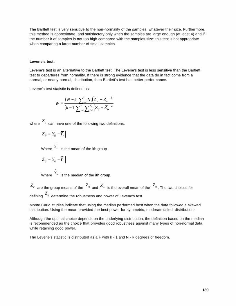
189
The Bartlett test is very sensitive to the non-normality of the samples, whatever their size. Furthermore, this method is approximate, and satisfactory only when the samples are large enough (at least 4) and if the number k of samples is not too high compared with the samples size: this test is not appropriate when comparing a large number of small samples.
Levene's test:
Levene's test is an alternative to the Bartlett test. The Levene's test is less sensitive than the Bartlett test to departures from normality. If there is strong evidence that the data do in fact come from a normal, or nearly normal, distribution, then Bartlett's test has better performance.
Levene's test statistic is defined as:
( ) ( )( ) ( )∑ ∑
∑= = •
= •••
−−
−−= k
i
N
j iij
k
i ii
i ZZk
ZZNkNW
1 1
21
2
1
where ijZ can have one of the following two definitions:
•−= iijij YYZ
Where •iY is the mean of the ith group.
•−= iijij YYZ~
Where •iY~
is the median of the ith group.
•iZ are the group means of the ijZ
and ••Z is the overall mean of the ijZ. The two choices for
defining ijZ determine the robustness and power of Levene's test.
Monte Carlo studies indicate that using the median performed best when the data followed a skewed distribution. Using the mean provided the best power for symmetric, moderate-tailed, distributions.
Although the optimal choice depends on the underlying distribution, the definition based on the median is recommended as the choice that provides good robustness against many types of non-normal data while retaining good power.
The Levene's statistic is distributed as a F with k - 1 and N - k degrees of freedom.

190
Elements of the dialog box
Data in different columns: if the samples appear in different columns, select the columns. The sizes of the columns can be different.
Data in one column: If the data are grouped, the data range represents a column of values, and the membership in samples is expressed by a Groups column.
Groups: for grouped data, select the range corresponding to a categorical variable that indicates the sample to which each value belongs.
Significance level: enter the value of the type I error for the test.
Range: the results are displayed based on a cell located in an existing sheet.
Sheet: results are displayed in a sheet of the active workbook.
Workbook: results are displayed in a new workbook.
Column labels: the first cell of each selected column contains a label.
Fisher's F test: check this option to perform a Fisher's F test.
Bartlett's test: check this option to perform a Bartlett's test.
Levene's test: check this option to perform a Levene's test. Choose whether you want to use the definition based on the mean or the one based on the median. The definition based on the median is recommended for its robustness when the data are not normally distributed.
Missing data
When XLSTAT finds missing data, it simply ignores them.
To know more about it
Dagnelie P. (1986). Théorie et méthodes statistiques. Vol. 2. Les Presses Agronomiques de Gembloux, Gembloux.
Frontier S. (1981). Méthode statistique. Masson, Paris.

191
Manoukian E.B. (1986). Guide de statistique appliquée. Hermann, Paris.
Sokal R.R. & Rohlf F.J. (1995). Biometry. The principles and practice of statistics in biological research. Third edition. Freeman.

192
Comparing One Proportion Use this module to compare a proportion describing a sample to a known proportion.
See also: Description
Elements of the dialog box
Dialog box for selecting hypotheses
Example
To know more about it
Description
The number n of the observations that check a given property, among the total N observations considered, follows a binomial distribution of parameters N (number of trials) and p (probability of success). When N is large enough and p is neither too close to 0 or too close to 1, the binomial distribution may be approximated by a normal distribution of expectation Np and of variance Np(1-p). Therefore the proportion n/N approximately follows a normal distribution of mean p and of variance p(1-p)/N. XLSTAT carries out a z test suited to cases with one proportion by approximating the binomial distribution using the normal distribution.
Let us define by p1 = n / N, the observed proportion on the sample, and by p2 a proportion to which we want to compare p1. p2 is usually a proportion that is known and that characterizes the population of interest. D is the assumed difference (exact, minimum or maximum) between the two proportions p1 and p2. D is usually 0.
The two-tailed test corresponds to testing the difference between p1 - p2 and D, using the null (H0) and alternative (H1) hypotheses shown below:
• H0: p1 - p2 = D
• H1: p1 - p2 ≠ D
In the one-tailed case, you should note the left (or lower) one-tailed test and the right (or higher) one-tailed test. In the left one-tailed test, the following hypotheses are used:
• H0: p1 - p2 = D
• H1: p1 - p2 < D
In the right one-tailed test the following hypotheses are used:

193
• H0: p1 - p2 = D
• H1: p1 - p2 > D
This test is based on the following assumptions:
• the observations are mutually independent,
• the probability p of having the property in question is identical for all observations,
• the number of observations is large enough, and the proportions are neither too close to 0 nor to 1.
Note: to determine whether N is sufficiently large one should make sure that:
( )( )
<−+
−−<
1/1
/10
111
111
Nppp
Nppp
Elements of the dialog box
proportions / frequencies: choose the type of data, either proportion (value between 0 and 1) or frequency (value less than or equal to the sample size).
Proportion / Frequency: enter the proportion or the frequency of observations with the property of interest in the sample.
Sample size: enter the total size of the sample.
Test proportion: enter the test proportion (enter a value that belongs to ]0, 1[).
Significance level: enter the value of the type I error for the test.
Range: the results are displayed based on a cell located in an existing sheet.
Sheet: Results are displayed in a sheet of the active workbook.
Workbook: Results are displayed in a new workbook.

194
Dialog box for selecting hypotheses
Null hypothesis, "H0: Proportion 1 – Test Proportion = D": enter the value of D. Default value: 0, in order to test that the proportions are equal.
Alternative hypothesis to be tested: choose the type of test to perform: two-tailed, left one-tailed, or right one-tailed (see Description).
Example
An example for the comparison of proportions is available on
http://www.xlstat.com/demo-prop.htm
To know more about it
Dagnelie P. (1986). Théorie et méthodes statistiques. Vol. 2. Les Presses Agronomiques de Gembloux, Gembloux, pp. 90-96.
Fleiss J.L. (1981). Statistical methods for rates and proportions. John Wiley & Sons, New York.
Sincich T. (1996). Business Statistics by Example, 5th edition. Prentice-Hall, Upper Saddle River.
195
Comparing 2 Proportions Use this module to compare two proportions.
See also: Description
Elements of the dialog box
Dialog box for selecting hypotheses
Example
To know more about it
Description
The number n of the observations that check a given property, among the total N observations considered, follows a binomial distribution of parameters N (number of trials) and p (probability of success). When N is large enough and p is neither too close to 0 or too close to 1, the binomial distribution may be approximated by a normal distribution of expectation Np and of variance Np(1-p). Therefore the proportion n/N approximately follows a normal distribution of mean p and of variance p(1-p)/N. XLSTAT carries out a z test suited to cases with two proportions by approximating the binomial distribution using the normal distribution.
Let us define by p1 = n1 / N1, the observed proportion on a first sample, and by p2 = n2 / N2, the observed proportion on a second sample. p is the estimated proportion for the population and is defined by p = (n1 + n2)/(N1 + N2). D is the assumed difference (exact, minimum or maximum) between the two proportions p1 and p2. D is usually 0.
The two-tailed test corresponds to testing the difference between p1 - p2 and D, using the null (H0) and alternative (H1) hypotheses shown below:
• H0: p1 - p2 = D
• H1: p1 - p2 ≠ D
In the one-tailed case, you should note the left (or lower) one-tailed test and the right (or higher) one-tailed test. In the left one-tailed test, the following hypotheses are used:
• H0: p1 - p2 = D
• H1: p1 - p2 < D
In the right one-tailed test the following hypotheses are used:
• H0: p1 - p2 = D
• H1: p1 - p2 > D
This test is based on the following assumptions:

196
• the observations are mutually independent,
• the probability p of having the property in question is identical for all observations,
• the number of observations is large enough, and the proportions are neither too close to 0 nor to 1.
Note: to determine whether N1 and N2 are sufficiently large one should make sure that:
( )( )
<−+
−−<
1/1
/10
1111
1111
Nppp
Nppp
and
( )( )
<−+
−−<
1/1
/10
2222
2222
Nppp
Nppp
Elements of the dialog box
proportions / frequencies: choose the type of data, either proportions (values between 0 and 1) or frequencies (values less than or equal to the respective size).
Proportion 1 / Frequency 1: enter the proportion or the frequency of observations with the property of interest the first group.
Sample size 1: enter the size of the sample for the first group.
Proportion 2 / Frequency 2: enter the proportion or the frequency of observations with the property of group 2.
Sample size 2: enter the size of the sample for the second group.
Significance level: enter the value of the type I error for the test.
Range: the results are displayed based on a cell located in an existing sheet.
Sheet: Results are displayed in a sheet of the active workbook.
Workbook: Results are displayed in a new workbook.
Dialog box for selecting hypotheses
Null hypothesis, "H0: Proportion 1 – Proportion 2 = D": enter the value of D. Default value: 0, in order to test that the proportions are equal.

197
Alternative hypothesis to be tested: choose the type of test to perform: two-tailed, left one-tailed, or right one-tailed (see Description).
Example
An example for the comparison of proportions is available on
http://www.xlstat.com/demo-prop.htm
To know more about it
Dagnelie P. (1986). Théorie et méthodes statistiques. Vol. 2. Les Presses Agronomiques de Gembloux, Gembloux, pp. 90-96.
Fleiss J.L. (1981). Statistical methods for rates and proportions. John Wiley & Sons, New York.
Frontier S. (1981). Méthode statistique. Masson, Paris, pp. 128-134.
Manoukian E.B. (1986). Guide de statistique appliquée. Hermann, Paris, pp. 133-134.
Sokal R.R. & Rohlf F.J. (1995). Biometry. The principles and practice of statistics in biological research. Third edition. Freeman, pp. 686-687.
Tomassone R., Dervin C. & Masson J.P. (1993). Biométrie. Modélisation de phénomènes biologiques. Masson, Paris, p. 70.

198
Comparing k Proportions Use this module to compare k proportions, and to determine if they can be considered as equal, or if at least one pair of proportions shows a significant difference.
See also: Description
Elements of the dialog box
Missing data
Results
Example
To know more about it
Description
XLSTAT offers three different approaches to compare proportions and to determine whether they can be considered as equal (null hypothesis H0) or if at least two proportions are significantly different (alternative hypothesis H1).
The Chi-square test is identical to the independence test performed on contingency tables.
The Monte Carlo method allows to compute the distribution of the Chi-square distance using resampling simulations that are constrained to respect the sample sizes of the k groups. The simulations allow to obtain an empirical distribution, that gives a reliable critical value and p-value. If the number of simulations is big enough these values should be more reliable than those obtained from the theoretical Chi-square distribution which corresponds to the asymptotical case.
It is advised to use the Marascuilo procedure if the Chi-square test or the equivalent test based on Monte Carlo simulations reject H0. The Marascuilo procedure compares all pairs of proportions. That allows to identify which proportion(s), might be responsible for the rejecting of the null hypothesis H0.
Elements of the dialog box
proportions / frequencies: choose the type of data, either proportions (values between 0 and 1) or frequencies (values less than or equal to the respective size).

199
Proportions / Frequencies: select the column of data that corresponds to the k proportions of to the k frequencies of the k groups. Proportions must belong to the [0, 1] interval. Frequencies should be such that each frequency is lower or equal to the corresponding sample size.
Sample sizes: select the column that contains the sample size of each of the k groups.
Group labels: select the data that correspond to the labels of the k groups.
Significance level: enter the value of the type I error for the test.
Range: the results are displayed based on a cell located in an existing sheet.
Sheet: Results are displayed in a sheet of the active workbook.
Workbook: Results are displayed in a new workbook.
Chi-square test: activate this option to use a Chi-square test to compare the proportions.
Monte Carlo: activate this option to use Monte Carlo simulations to compute the critical value and p-value Chi-square statistics.
Marascuilo procedure: activate this option to run the Marascuilo procedure to compare the proportions.
Missing data
If missing data are detected by XLSTAT, you are asked whether you want to ignore the corresponding groups or not. If you do not want to ignore the corresponding groups, the analysis stops.
Results
If the Chi-square option has been selected, the first results correspond to the Chi-square test.
The results of the test based on Monte Carlo simulations are all the more close to the Chi-square results that the number of simulations and the sample sizes are high. The differences relates only to the critical value and the p-value.
If the null hypothesis is rejected by the Chi-square of the Monte Carlo test, the Marascuilo procedure allows to identify which proportions are responsible for the rejecting of the null hypothesis. One can identify which pairs of proportions are significantly different by looking at the results in the "Significant" column of the Marascuilo procedure table.
200
Note: it might be that the Marascuilo procedure does not identify significant differences among the pairs of proportions, while the Chi-square and/or the Monte Carlo tests reject the null hypothesis. Looking closer at the results you will usually find that one or more pairs of proportions are almost significantly different. More in-depth analysis might be necessary before making a decision.
Example
An example for the comparison of proportions is available on
http://www.xlstat.com/demo-prop.htm
To know more about it
Agresti A. (1990). Categorical data analysis. John Wiley & Sons, New York.
Marascuilo L. A. & Serlin R. C. (1988). Statistical Methods for the Social and Behavioral Sciences. Freeman, New York.

201
Comparing 2 Independent Samples Use this non-parametric test module when you have2 independent samples, in order to determine if the samples come from the same population or from 2 different populations. XLSTAT propose two tests:
• the Kolmogorov-Smirnov test,
• the Mann-Whitney test.
Note: the Mann-Whitney test is a nonparametric alternative to the Student's t test (equivalent to the one-way analysis of variance for two samples). As for the Student's t test, the samples may be of different sizes.
See also: Description of the Kolmogorov-Smirnov test
Description of the Mann-Whitney test
Dialog box for selecting hypotheses
Elements of the dialog box
Missing data
Example
To know more about it
Description of the Kolmogorov-Smirnov test
The purpose of the Kolmogorov-Smirnov test is to determine if the populations from which the samples were taken have different cumulative distribution functions. XLSTAT performs a two-tailed test.
Assume that F(x) and G(x) are the cumulative distribution functions of two populations from which the samples were taken. The two-tailed test corresponds to the test of the difference between these two populations, and the null (H0) and alternative (H1) hypotheses are as follows:
• H0: F(x) = G(x) for all values of x
• H1: F(x) ≠ G(x) for at least one value of x
Description of the Mann-Whitney test
The purpose of the Mann-Whitney test is to determine if the samples come from a single population or from two different populations. XLSTAT can perform a two-tailed or a one-tailed test.
Assume two populations A and B from which samples are taken that include values a and b. The two-tailed test corresponds to the test of the difference between A and B, and the null (H0) and alternative (H1) hypotheses are as follows:
• H0: P(a < b) = 1/2
202
• H1: P(a < b) ≠ 1/2
In the one-tailed case, you should note the left (or lower) one-tailed test and the right (or higher) one-tailed test. In the left one-tailed test, the alternative hypothesis indicates that population A generally has lower values than those in population B:
• H0: P(a < b) ≤1/2
• H1: P(a < b) > 1/2
In the right one-tailed test, the alternative hypothesis indicates that population A generally has higher values than population B:
• H0: P(a < b) ≥1/2
• H1: P(a < b) < 1/2
This test is based on the following assumptions:
• both samples are random samples taken from their respective populations,
• besides the independence within each sample, both samples are mutually independent,
• the data is at least ordinal data.
Note: the Mann-Whitney statistic is related to the Wilcoxon statistic, in that the (unsigned) Wilcoxon test is equivalent to the Mann-Whitney test.
Dialog box for selecting hypotheses
Alternative hypothesis to be tested: choose the type of test to perform: two-tailed, left one-tailed, or right one-tailed (see Description of the Mann-Whitney test).
Elements of the dialog box
Data in different columns: if the samples appear in different columns, select samples 1 and 2 (the columns may have different sizes).
Data in one column: If the data are grouped, the data range represents a column of values, and the membership in samples is expressed by a Groups column.
Sample 1: if the samples appear in different columns, select the range for the first sample.
Sample 2: if the samples appear in different columns, select the range for the second sample.
Data: for grouped data, select the range corresponding to the values of both samples.
Groups: for grouped data, select the range corresponding to a categorical variable that indicates the sample to which each value belongs.
Significance level: enter the value of the type I error for the test.

203
Range: the results are displayed based on a cell located in an existing sheet.
Sheet: results are displayed in a sheet of the active workbook.
Workbook: results are displayed in a new workbook.
Column labels: the first cell of each selected column contains a label.
Chart: check this option to display the dominance diagram comparing both samples (up to 100 × 100 values).
Mann-Whitney test: check this option to perform a Mann-Whitney F test.
Kolmogorov-Smirnov test: check this option to perform a Kolmogorov-Smirnov test.
Missing data
When XLSTAT finds missing data, it simply ignores them.
Example
To know more about it
Dagnelie P. (1986). Théorie et méthodes statistiques. Vol. 2. Les Presses Agronomiques de Gembloux, Gembloux, pp. 381-385.
Lehmann E.L. & D'Abrera H.J.M. (1975). Nonparametrics. Statistical methods based on ranks. Holden-Day, San Francisco, pp. 5-31.
Manoukian E.B. (1986). Guide de statistique appliquée. Hermann, Paris, pp. 139-140, 146.
Siegel S. (1956). Nonparametric statistics for the behavioral sciences. McGraw-Hill Kogakusha, Tokyo, Japan, pp. 116-136.
Sokal R.R. & Rohlf F.J. (1995). Biometry. The principles and practice of statistics in biological research. Third edition. Freeman, New York, pp. 427-439.
Tomassone R., Dervin C. & Masson J.P. (1993). Biométrie. Modélisation de phénomènes biologiques. Masson, Paris, pp. 216-220.

204
Comparing 2 Paired Samples Use this module of nonparametric tests when you have 2 paired samples, in order to determine if the samples come from the same population or from two different populations. XLSTAT includes two tests:
• the Wilcoxon signed-ranks test,
• the sign test.
Notes: The use of these tests provide a nonparametric alternative to the Student's t test for paired data. Because the samples are paired, they must include the same number of observations.
See also: Description of the Wilcoxon signed-ranks test
Dialog box for selecting hypotheses
Description of the sign test
Dialog box for selecting hypotheses
Elements of the dialog box
Missing data
Example
To know more about it
Description of the Wilcoxon signed-ranks test
The purpose of the Wilcoxon signed-ranks test is to determine if the samples come from a single population or from two different populations. XLSTAT can perform a two-tailed test or a one-tailed test.
Assume two populations A and B from which samples are taken that contain the values a and b. Let d represent the median of the differences db-a = b-a for all the data pairs. The two-tailed test corresponds to the test of the difference between A and B, and the null (H0) and alternative (H1) hypotheses are as follows:
• H0: d = 0
• H1: d ≠ 0
In the one-tailed case, you should note the left (or lower) one-tailed test and the right (or higher) one-tailed test. In the left one-tailed test, the alternative hypothesis indicates that population A has generally lower values than population B:
• H0: d ≤ 0
• H1: d > 0
In the right one-tailed test, the alternative hypothesis indicates that population A has in general higher values than in population B:

205
• H0: d ≥ 0
• H1: d < 0
This test is based on the following assumptions:
• the distribution of db-a is symmetrical,
• db-a are independent,
• db-a are real values.
Dialog box for selecting hypotheses
Alternative hypothesis to be tested: choose the type of test to perform: two-tailed, left one-tailed, or right one-tailed (see Description of the Wilcoxon signed-ranks test).
Description of the sign test
The purpose of the sign test is to determine if the samples come from a single population or from two different populations. XLSTAT can perform a two-tailed or a one-tailed test.
Assume two populations A and B from which samples are taken that include values a and b. The sign test considers the number of differences b-a with a positive sign. The two-tailed test evaluates the difference between A and B, and the null (H0) and alternative (H1) hypotheses are as follows:
• H0: P(a < b) = P(a > b)
• H1: P(a < b) ≠ P(a > b)
In the one-tailed case, you should note the left (or lower) one-tailed test and the right (or higher) one-tailed test. In the left one-tailed test, the alternative hypothesis indicates that population A generally has lower values than those in population B:
• H0: P(a < b) ≤ P(a > b)
• H1: P(a < b) > P(a > b)
In the right one-tailed test, the alternative hypothesis indicates that population A generally has higher values than population B:
• H0: P(a < b) ≥ P(a > b)
• H1: P(a < b) < P(a > b)
This test is based on the following assumptions:
• the data pairs are independent,
• the data are at least ordinal data.

206
Note: to calculate the p-value associated with the number of positive differences, XLSTAT uses the binomial distribution in all cases; it does not approximate the binomial distribution by using the normal distribution.
Dialog box for selecting hypotheses
Alternative hypothesis to be tested: choose the type of test to perform: two-tailed, left one-tailed, or right one-tailed (see Description of the sign test).
Elements of the dialog box
Sample 1: select the range for the first sample.
Sample 2: select the range for the second sample.
Significance level: enter the value of the type I error of the tests.
Wilcoxon signed-ranks Test: check this option to perform the Wilcoxon signed-ranks test.
Sign test: check this option to perform the sign test.
Range: the results are displayed based on a cell located in an existing sheet.
Sheet: Results are displayed in a sheet of the active workbook.
Workbook: Results are displayed in a new workbook.
Column labels: the first cell of each selected column contains a label.
Chart: check this option to display the dominance diagram comparing both samples (up to 50 × 50 values).
Missing data
If XLSTAT finds missing data, it suggests to remove the rows with missing data for the analysis.
Example
207
To know more about it
Dagnelie P. (1986). Théorie et méthodes statistiques. Vol. 2. Les Presses Agronomiques de Gembloux, Gembloux, pp. 385-389.
Lehmann E.L. & D'Abrera H.J.M. (1975). Nonparametrics. Statistical methods based on ranks. Holden-Day, San Francisco, pp. 120-132.
Siegel S. (1956). Nonparametric statistics for the behavioral sciences. McGraw-Hill Kogakusha, Tokyo, Japan, pp. 68-83.
Sokal R.R. & Rohlf F.J. (1995). Biometry. The principles and practice of statistics in biological research. Third edition. Freeman, New York, pp. 440-444.
208
Comparing k Independent Samples (Kruskal-Wallis' Test) Use this nonparametric test when you have k independent samples, in order to determine if the samples come from a single population or if at least one sample comes from a different population than the others.
Note: you can use the Kruskal-Wallis' test as a nonparametric alternative to the one-way analysis of variance (ANOVA 1). As with ANOVA 1, the sample may have different sizes.
See also: Description
Elements of the dialog box
Missing data
Example
To know more about it
Description
The purpose of the Kruskal-Wallis' test is to determine if the samples come from a single population or if at least one sample comes from a different population than the others. The null (H0) and alternative (H1) hypotheses for the test are therefore as follows:
• H0: the k samples come from the same population
• H1: at least one of the samples comes from a different population than the others
This test is based on the following assumptions:
• all the samples are random samples taken from their respective populations,
• besides the independence within each sample, the samples are mutually independent,
• the data are at least ordinal data.
Elements of the dialog box
Data in different columns: if the samples appear in different columns, select the columns. The sizes of the columns can be different.
Data in one column: If the data are grouped, the data range represents a column of values, and the membership in samples is expressed by a Groups column.
Groups: for grouped data, select the range corresponding to a categorical variable that indicates the sample to which each value belongs.
Significance level: enter the value of the type I error of the tests.

209
Range: the results are displayed based on a cell located in an existing sheet.
Sheet: results are displayed in a sheet of the active workbook.
Workbook: results are displayed in a new workbook.
Column labels: the first cell of each selected column contains a label.
Missing data
When XLSTAT finds missing data, it simply ignores them.
Example
To know more about it
Dagnelie P. (1986). Théorie et méthodes statistiques. Vol. 2. Les Presses Agronomiques de Gembloux, Gembloux, pp. 390-392.
Lehmann E.L. & D'Abrera H.J.M. (1975). Nonparametrics. Statistical methods based on ranks. Holden-Day, San Francisco, pp. 204-210.
Manoukian E.B. (1986). Guide de statistique appliquée. Hermann, Paris, pp. 181-182.
Siegel S. (1956). Nonparametric statistics for the behavioral sciences. McGraw-Hill Kogakusha, Tokyo, Japan, pp. 184-194.
Sokal R.R. & Rohlf F.J. (1995). Biometry. The principles and practice of statistics in biological research. Third edition. Freeman, New York, pp. 423-427.
Tomassone R., Dervin C. & Masson J.P. (1993). Biométrie. Modélisation de phénomènes biologiques. Masson, Paris, pp. 240-241.
210
Comparing k Paired Samples (Friedman's Test) Use this nonparametric test when you have k paired samples corresponding to k treatments concerning the same blocks, in order to illustrate a difference between the treatments.
Note: you can use the Friedman's test as a nonparametric alternative to the two-way analysis of variance with fixed effects (ANOVA 2). The terms "treatment" and "block" should be interpreted very broadly. A few sample applications:
• k medical treatments, where the blocks are volunteer subjects,
• ratings given by a panel of consumers concerning k food products, where the blocks are the consumers and the treatments are the food products,
• a population density rating for biological species in k different geographical regions, where the blocks are the species and the treatments are the geographical regions and their ecological conditions.
Because the samples are paired, they must include the same number of blocks.
See also: Description
Elements of the dialog box
Missing data
Example
To know more about it
Description
The purpose of the Friedman's test is to determine if all the treatments give the same result, or if at least one treatment is different from the others. The null (H0) and alternative (H1) hypotheses for the test are therefore as follows:
• H0: the k samples were taken from the same population
• H1: at least one of the samples comes from a different population than the others
This test is based on the following assumptions:
• the blocks are randomized,
• the samples are paired,
• the data are at least ordinal data.
211
Elements of the dialog box
Data: select the range corresponding to an array with the blocks in rows and the treatments in columns (without rows labels). Missing data are not allowed.
Significance level: enter the value of the type I error of the tests.
Multiple comparison tests: activate this option to perform multiple comparison tests"
Bonferroni: activate this option to use the Bonferroni adjustment to the overall significance level"
Binary: activate this option to obtain the results of the multiple comparison tests as binary tables (0/1).
Range: the results are displayed based on a cell located in an existing sheet.
Sheet: Results are displayed in a sheet of the active workbook.
Workbook: Results are displayed in a new workbook.
Column labels: the first cell of each selected column contains a label.
Missing data
If XLSTAT finds missing data, it suggests to remove the rows with missing data for the analysis.
Example
To know more about it
Dagnelie P. (1986). Théorie et méthodes statistiques. Vol. 2. Les Presses Agronomiques de Gembloux, Gembloux, pp. 393-394.
Lehmann E.L. & D'Abrera H.J.M. (1975). Nonparametrics. Statistical methods based on ranks. Holden-Day, San Francisco, pp. 262-270.
Manoukian E.B. (1986). Guide de statistique appliquée. Hermann, Paris, pp. 183-184.
Siegel S. (1956). Nonparametric statistics for the behavioral sciences. McGraw-Hill Kogakusha, Tokyo, Japan, pp. 166-173.

212
Sokal R.R. & Rohlf F.J. (1995). Biometry. The principles and practice of statistics in biological research. Third edition. Freeman, New York, pp. 440-442.
Tomassone R., Dervin C. & Masson J.P. (1993). Biométrie. Modélisation de phénomènes biologiques. Masson, Paris, pp. 242-243.
213
Categories -> Numerical Codes Use this tool to recode the categories of a categorical variable and to indicate the numerical codes in the comments area of the cell containing the variable label.
The first line of comments contains the variable label as it appears in the first cell of the selected column (e.g. "Q9"). The second line of comments contains by default the label of the variable (this already exists in the first line). You can replace the contents of the second line with a detailed description (e.g. "Global satisfaction" instead of "Q9"). The other lines represent the variable categories, whose codes start at 1.
This procedure may be run on several columns at once, located anywhere in a sheet of the active workbook.

214
Numerical Codes -> Categories Use this tool to replace the numerical codes of a categorical variable with the categories that appear in the comments area of the cell containing the variable label. Following this procedure, the comments area is deleted.
Note: the code 0 represents a missing value.
Use detailed variable description: check this option if you want to replace the variable label with the detailed description that appears in the comments.
Typically the first line of the comments contains the variable label (e.g. "Q9"), the second line contains the detailed variable description (e.g. "Global Satisfaction"), and the following lines contain the variable categories, whose codes start at 1. There can also be only one line before the list of numerical codes: in this case, the content of the first line is used as the detailed variable description.
This procedure may be run on several columns at once, located anywhere in a sheet of the active workbook.

215
Delete the Hidden Sheets Use this utility to delete all the hidden sheets in the active workbook. XLSTAT disables Excel warnings asking you to confirm the deletion.

216
Delete the Hypertext Links Use this tool to delete all the hypertext links in the active sheet as well as all the sheets to which it refers. XLSTAT disables Excel warnings asking you to confirm the deletion.

217
Reduce columns Use this tool to automatically adjust the column widths according to column contents, only if this reduces the columns width.
Note: this adjustment never increases the column width.

218
Enlarge columns Use this tool to automatically adjust the column widths according to column contents, only if this increases the columns width.
Note: this adjustment never reduces the column width.
219
Charts for Exploratory Analysis Box plot
Stem and leaf plot
Q-Q plot and p-p plot
To know more about it
Box plot
A box plot is a chart that indicates the central tendency of the values, their variability, the symmetry of the distribution, and the presence of outliers (values very different from the others). Box plots are often used to compare several sets of data.
There are several ways to display a box plot. XLSTAT uses the following format:
• the lower edge of the box represents the first quartile Q1,
• a black line represents the median Q2 ,
• a red line represents the average,
• the upper edge of the box represents the third quartile Q3
Two intervals are defined on either side of the first and third quartiles:
• IQ1 = [Q1 - 1.5 × (Q3 – Q1) , Q1]
• IQ3 = [Q3 , Q3 + 1.5 × (Q3 – Q1)]
• the lower part of the box plot reaches from Q1 to the value nearest to the lower bound of IQ1, while remaining within IQ1,
• the upper part of the box plot reaches from Q3 to the value nearest to the upper bound of IQ3, while remaining within IQ3,
• the values underneath the lower part and above the upper part are represented individually by circles. These circles are filled in when the values are more than 3 times the distance between the quartiles (Q3 – Q1), and are empty if they are within that interval,
• the minimum and maximum values are shown in the box plot.
Stem and leaf plot
A stem and leaf plot is a semi-graphical representation of frequency distribution for a set of data, by using the values themselves. The stem represents classes of values, and the leaf shows the number of data items in the class, represented by the various values.

220
To build a stem and leaf plot, you must divide each value into a main part (the stem) and a secondary part (the leaf); this division does not have to be at the decimal point. The stems are displayed vertically in ascending order, and the leaves are displayed horizontally to the right of the stems, also in ascending order. XLSTAT automatically calculates the most appropriate unit to divide the values into stems and leaves, but you can modify that unit (see the Charts tab). To improve readability, before each diagram XLSTAT displays the unit used, and describes the meaning of a basic 1|1 stem and leaf.
Q-Q plot and p-p plot
The Q-Q plot (or normal probability plot, or "quantile-quantile" chart) and the p-p plot (or probability-probability plot) provides a graphical view to help you determine if the data appears to follow a normal distribution, by comparing the cumulative frequency distribution for the data with the cumulative distribution function of the normal distribution for identical mean and variance. The Q-Q plot compares values, while the p-p plot compares probabilities. In both cases, if the points are aligned along the chart's first bisector, then the normal distribution is compatible with the data.
p-p plot
In a p-p plot, the axis of the abscissa corresponds to the relative frequencies of the values and the ordinates correspond to the probabilities that the values would have if they were distributed using a normal distribution, with the same mean and variance as the data.
Thus each abscissa of the p-p plot represents the ordinate of each value on the cumulative frequency distribution of the data, and the corresponding ordinate in the p-p plot is the ordinate of the cumulative distribution function of the normal distribution, with the same mean and variance as the data, for the value in question.
Q-Q plot
In a Q-Q plot, the axis of the abscissas corresponds to the observed values and the ordinates correspond to the values of the normal distribution with the same mean and variance as the data, calculated for the relative frequencies of the observed values.
Thus each abscissa of the Q-Q plot represents the abscissa of each value on the cumulative frequency distribution of the data, and the corresponding ordinate in the Q-Q plot is the abscissa of the cumulative distribution function of the normal distribution, with the same mean and variance as the data, for the probability in question.
To know more about it
Jobson J.D. (1991). Applied multivariate data analysis. Volume I: regression and experimental design. Springer-Verlag, New York, pp. 35-36, 45-46, 62-65.
Johnson R.A. & Wichern D.W. (1992). Applied multivariate statistical analysis. Prentice-Hall, Englewood Cliffs, pp. 154-158.
Sokal R.R. & Rohlf F.J. (1995). Biometry. The principles and practice of statistics in biological research. Third edition. Freeman, New York, pp. 28-30, 116-123, 151-152.

221
Tomassone R., Dervin C. & Masson J.P. (1993). Biométrie. Modélisation de phénomènes biologiques. Masson, Paris, pp. 119-121.

222
Similarities/Dissimilarities There are several ways to measure similarity (or dissimilarity). XLSTAT proposes selected coefficients based on their mathematical properties and their practical or pedagogical interest.
See also: Quantitative Data
Binary Data
To know more about it
Quantitative Data
Pearson's correlation coefficient: covariance of two compared rows or columns, standardized by the standard deviations, or (which amounts to the same thing), covariance calculated on the normalized data. Result in the interval [-1,+1].
Spearman's coefficient of rank correlation: nonparametric correlation coefficient identical to the Pearson's correlation coefficient calculated on the ranks of the values. Result in the interval [-1,+1].
Kendall's coefficient of rank correlation: nonparametric correlation coefficient, i.e. calculated on the ranks of the values. Result in the interval [-1,+1].
Note: The correlation coefficients were created in order to measure the similarity between variables. To evaluate the similarity between observations, they should be used carefully.
Euclidean distance: metric of Euclidian space (classical geometrical space). The Euclidean distance equals 0 for two identical rows or columns, but it has no upper bound. The Euclidean distance increases as the number of variables increases, and its value also depends on the scale of each variable. Therefore by simply changing the scales, you can obtain very different results. To avoid this, you should standardize the variables.
Chi-square distance: To overcome the problems related to the Euclidean distance, you can use the Chi-square distance which is based on the sums of the rows and the columns in the data table. For example, when calculating the Chi-square distance between two rows, the terms in each row are compared to their sum and a column contributes to the distance in inverse proportion to its weight. Calculating the Chi-square distance is equivalent to calculating the Euclidean distance on data transformed using the following equation: xij -> xij / (xi.vx.j) where xi. is the sum on the columns for row i and x.j is the sum on the rows for column j. The Chi-square distance satisfied the principle of distributional equivalence i.e. the distance does not change between the rows or columns if you replace two columns or two rows with the same profile by their sum. The Chi-square distance is especially suited to homogeneous arrays of frequencies or additive sizes (e.g. tons, kilometers, percentages).
Manhattan distance: L1 metric, calculated using the absolute differences instead of quadratic differences in the case of the Euclidean distance.
Pearson's dissimilarity: transformation of Pearson's coefficient into a dissimilarity in the range of [0,1], or r -> (1 - r) / 2

223
Spearman's dissimilarity: transformation of Spearman's coefficient into a dissimilarity in the range [0,1], or rS -> (1 – rS) / 2.
Kendall's dissimilarity: transformation of Kendall's coefficient into a dissimilarity in the range [0,1], or t -> (1 – t ) / 2.
Binary Data
If i and j are two entries in a table (two rows or two columns), let a represent the number of 1s present in both i and j, let b represent the number of 1s of i that correspond to 0s for j, let c represent the number of 1s for j that correspond to 0s for i, and let d represent the number of 0s common to both i and j. The binary data coefficients are defined using a, b and c, and possibly d. Note that the data a, b, c and d are simply the observations in the following 2 × 2 contingency table:
i / j 1 0
1 a b a+b
0 c d c+d
a+c b+d n=a+b+c+d
The coefficients are presented as similarities S, but may be easily expressed as dissimilarities D by calculating D = 1 – S when S varies from [0,1], and by calculating D = (1 – S)/2 when S varies from [-1,+1].
Jaccard coefficient: a / (a + b + c). Result in the interval [0,1]. Assigns an equal weight for the various terms, and does not consider double 0s (term d).
Dice coefficient: 2a / (2a + b + c), where a is divided by the arithmetic mean number of 1s for i and j. Result in the interval [0,1]. Based on the model for the Jaccard coefficient, the Dice coefficient assigns weights that are twice as large as double 1s (term a).
Sokal & Sneath coefficient (2): a / (a + 2b +2c). Result in the interval [0,1]. Based on the model for the Jaccard coefficient, the Sokal & Sneath (2) coefficient assigns weights that are twice as large as the differences appearing in the denominator (terms b and c).
Note: the Jaccard, Dice, and Sokal & Sneath (2) coefficients return the same ordinal relationship between the observations. As a result, in an agglomerative hierarchical clustering you obtain dendrograms with the same structure (or topology).
Simple matching coefficient (1): (a + d) / (a + b + c + d). Result in the interval [0,1]. This coefficient is based on the principle that double 1s (term a) and double 0s (term d) play a symmetrical role, which implies that both categories of the variable may indifferently be coded with either 1 or 0.
Rogers & Tanimoto coefficient: (a + d) / (a + 2b + 2c + d). Result in the interval [0,1]. Based on the model for the simple matching coefficient, this coefficient assigns to the differences (terms b and c) a weight that is twice as high as the matches (terms a and d).

224
Sokal & Sneath coefficient (1): (2a + 2d) / (2a + b + c + 2d). Result in the interval [0,1]. Based on the model for the simple matching coefficient, this coefficient assigns to the matches (terms a and d) a weight that is twice as high as the differences ( terms b et c ).
Note: the simple matching, Rogers & Tanimoto, and Sokal & Sneath (1) coefficients return the same ordinal relationship between the observations. As a result, in an agglomerative hierarchical clustering you obtain dendrograms with the same topology.
Phi coefficient: (ad – bc) / √(a + b)(c + d)(a + c)(b + d). Result in the interval [-1,+1]. This coefficient subtracts the product of the differences (term bc) from the product of the matches (term ad). The phi coefficient f is related to the Chi-square as follows: ?² = nf ², where n is the total of the 2 × 2 table. To obtain a dissimilarity, XLSTAT performs a transformation to the interval [0,1]: f -> (1 – f )/2.
Ochiai coefficient: a / √(a + b) (a + c) where a is divided by the geometric mean of the number of 1s for i and j. Result in the interval [0,1].
Kulczinski coefficient: a(1/(a + b) + 1/(a + c))/2 where a is divided by the harmonic mean of the number of 1s for i and j. Result in the interval [0,1].
Note: the Ochiai and Kulczinski coefficients are variations of the Dice coefficient using the geometric mean and the harmonic mean, respectively, instead of the arithmetic average. Therefore the values of these coefficients are usually fairly close, with a wider variation when (a + b) and (a + c) are very different.
To know more about it
Dagnelie P. (1986). Théorie et méthodes statistiques. Vol. 2. Les Presses Agronomiques de Gembloux, Gembloux, pp. 88-90, 395-398.
Dillon W.R. & Goldstein M. (1984). Multivariate analysis. Methods and applications. John Wiley & Sons, New York, pp. 157-167.
Gower J.C. & Legendre P. (1986). Metric and Euclidean properties of dissimilarity coefficients. Journal of Classification, 3: 5-48.
Jambu M. (1978). Classification automatique pour l'analyse des données. 1 - méthodes et algorithmes. Dunod, Paris, pp. 484-518.
Jobson J.D. (1992). Applied multivariate data analysis. Volume II: categorical and multivariate methods. Springer-Verlag, New York, pp. 345-388.
Legendre L. & Legendre P. (1984). Ecologie numérique. Tome 2. La structure des données écologiques. Masson, Paris, pp. 5-50.
Roux M. (1985). Algorithmes de classification. Masson, Paris, pp. 126-134.

225
Rotating Factors There are two types of techniques for rotating factors in order to simplify analysis: orthogonal and oblique rotation. Unlike an oblique rotation, an orthogonal rotation retains the original orientation between the factors so that they are always orthogonal (not correlated) after the rotation. XLSTAT offers the two most commonly used orthogonal rotation techniques: varimax and quartimax rotations.
See also: Varimax Rotation
Quartimax Rotation
To know more about it
Varimax Rotation
Use the varimax rotation to simplify the interpretation of factors by minimizing the number of variables that contribute significantly to each factor.
The goal of the orthogonal varimax rotation is to identify a factorial structure where for each factor, a few variables have strong contributions and the other factors have very weak contributions. This goal is obtained by maximizing, for a given factor, the variance of the squares of the contributions among the variables, with the constraint that the variance of each variable must remain unchanged.
Quartimax Rotation
Use the quartimax rotation to simplify the analysis of variables by minimizing the number of factors required to explain each variable.
The goal of the quartimax rotation is to identify a factorial structure where the variables have strong contributions for a given factor. Furthermore, each variable must have a non-null contribution for another factor, and practically null contributions for all the remaining factors. This goal is obtained by maximizing the variance of the contributions among the factors with the constraint that the variance of each variable must remain unchanged.
To know more about it
Dillon W.R. & Goldstein M. (1984). Multivariate analysis. Methods and applications. John Wiley & Sons, New York, pp. 87-95.
Sharma S. (1996). Applied multivariate techniques. John Wiley & Sons, New York, pp. 137-141.
226
P-value In XLSTAT, each statistical test has an associated p-value. The p-value is defined as the probability, calculated under the null hypothesis, of obtaining a value of the statistic that is as extreme as the one observed for the data (in a given direction). This definition implies that a p-value is useful in a one-tailed test because the direction used for the calculation represents the alternative hypothesis of the test. For example, in a right one-tailed Student t test, the p-value represents the area under the right Student distribution of tobs, while in a left one-tailed test, the p-value represents the area under the left Student distribution of tobs.
Intuitively, you can think of the p-value as the strength the evidence against the null hypothesis. The weaker the p-value, the lower the probability of obtaining by chance a result that is as extreme as the observed result, and therefore the more significant the result. The traditional way to use a type I error a is to accept the alternative hypothesis if the p-value is less than or equal to a. The relation between the p-value and the type I error leads one to interpret the p-value as the lowest level of significance for which the observed value of the statistic is significant, in a given direction.
See also: To know more about it
To know more about it
Berger J.O. & T. Sellke (1987). Testing a point null hypothesis: the irreconcilability of P values and evidence (with discussion, pp. 123-139). Journal of the American Statistical Association, 82: 112-122.
Casella G. & R.L. Berger (1987). Reconciling bayesian and frequentist evidence in the one-sided testing problem (with discussion, pp. 123-139). Journal of the American Statistical Association, 82: 106-111.
Gibbons J.D. (1986). P values. In: Kotz S. & N.L. Johnson (Eds.), Encyclopedia of statistical sciences, John Wiley & Sons, New York, pp. 366-368.
Yoccoz N.G. (1991). Use, overuse, and misuse of significance tests in evolutionary biology and ecology. Bulletin of the Ecological Society of America, 72: 106-111.

227
Monte Carlo Test The principle of a Monte Carlo test is to estimate the p-value associated with the observed statistic using a method that implements random numbers. This type of method is called a computer intensive statistical method because it is based on the power of the computer.
For example, consider the test of the Pearson's correlation coefficient between two random variables X and Y, using a sample of X values and a sample of Y values. The Monte Carlo test would involve the following steps:
1. model one of the two variables. For example, the Distribution Fitting module can identify a parametric model for the Y variable based on the data of the corresponding sample, of size n,
2. simulate a large number of random samples of size n based on the previously fitted model,
3. calculate the distribution of the correlation coefficient under the null hypothesis H0 by calculating the correlation between each simulated sample for Y and the observed sample for X,
4. calculate the p-value of the observed value of the correlation based on the distribution defined under H0.
This type of method is especially useful for obtaining approximate solutions to statistical problems that are too complex to be solved mathematically.
See also: To know more about it
To know more about it
Besag J. & Clifford P. (1989). Generalized Monte Carlo significance tests. Biometrika, 76: 633-642.
Besag J. & Clifford P. (1991). Sequential Monte Carlo p-values. Biometrika, 78: 301-304.
Manly B.F.J. (1993). Randomization, bootstrap and Monte Carlo methods in biology. Second edition. Chapman & Hall, London, UK.
Marriot F.H.C. (1979). Barnard's Monte Carlo Tests: How many simulations ? Applied Statistics, 28: 75-77.
Noreen E.W. (1989). Computer-intensive methods for testing hypotheses: an introduction. John Wiley & Sons, New York.
Sokal R.R. & Rohlf F.J. (1995). Biometry. The principles and practice of statistics in biological research. Third edition. Freeman, New York, pp. 810-819.

228
229
Bartlett's sphericity test Within the framework of the multivariate Gaussian model, it is possible to test the hypothesis that p random variables are mutually independent with identical variance. If the hypothesis is confirmed, the multivariate distribution function is said to be spherical.
The sphericity test is a global independence test for the p random variables that allows to decide if the variables are significantly linearly related or not. This test can be applied on the empirical covariance or correlation matrices computed for the p variables. In both cases, the statistic used for the test follows a Chi-square distribution. However the statistics have different values and a different number of degrees of freedom.
Note: in some software, the formula corresponding to the statistic for the covariance matrix is used for the correlation matrix. Other software test the correlation matrix even when the covariance matrix is computed. XLSTAT computes the appropriate sphericity test for both cases with the correct formula. However, in the case of a covariance matrix, XLSTAT displays as well the the result for the corresponding covariance matrix. When the number of observations is small, or when the multivariate Gaussian model does not seem to be appropriate, the sphericity test must be considered with caution.
To know more about it
Dillon W.R. & Goldstein M. (1984). Multivariate analysis. Methods and applications. John Wiley & Sons, New York, pp. 44-47.
Jobson J.D. (1992). Applied multivariate data analysis. Volume II: categorical and multivariate methods. Springer-Verlag, New York, pp. 165-166.

230