manual do gamess.pdf
DESCRIPTION
GAMESS - cálculo de química quânticaTRANSCRIPT
Introduction 1-1
(11 August 2011)
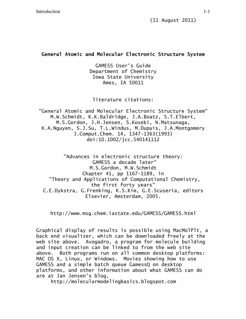
General Atomic and Molecular Electronic Structure System
GAMESS User's GuideDepartment of ChemistryIowa State University
Ames, IA 50011
literature citations:
"General Atomic and Molecular Electronic Structure System"M.W.Schmidt, K.K.Baldridge, J.A.Boatz, S.T.Elbert,M.S.Gordon, J.H.Jensen, S.Koseki, N.Matsunaga,
K.A.Nguyen, S.J.Su, T.L.Windus, M.Dupuis, J.A.MontgomeryJ.Comput.Chem. 14, 1347-1363(1993)
doi:10.1002/jcc.540141112
"Advances in electronic structure theory: GAMESS a decade later"M.S.Gordon, M.W.Schmidt
Chapter 41, pp 1167-1189, in "Theory and Applications of Computational Chemistry,
the first forty years"C.E.Dykstra, G.Frenking, K.S.Kim, G.E.Scuseria, editors
Elsevier, Amsterdam, 2005.
http://www.msg.chem.iastate.edu/GAMESS/GAMESS.html
Graphical display of results is possible using MacMolPlt, aback end visualizer, which can be downloaded freely at theweb site above. Avogadro, a program for molecule buildingand input creation can be linked to from the web siteabove. Both programs run on all common desktop platforms:MAC OS X, Linux, or Windows. Movies showing how to useGAMESS and a simple batch queue GamessQ on desktopplatforms, and other information about what GAMESS can doare at Jan Jensen's blog, http://molecularmodelingbasics.blogspot.com

Introduction 1-2
Contents of this manual:
Section 1 - INTRO.DOC - Overview Section 2 - INPUT.DOC - Input Description Section 3 - TESTS.DOC - Input Examples Section 4 - REFS.DOC - Further Information Section 5 - PROG.DOC - Programmer's Reference Section 6 - IRON.DOC - Hardware Specifics
Contents of Section 1:
Capabilities____________________________________________________________ 3History of GAMESS_____________________________________________________ 7Distribution Policy _____________________________________________________ 23Input Philosophy ______________________________________________________ 24Input Checking________________________________________________________ 28Program Limitations ___________________________________________________ 29Restart Capability______________________________________________________ 30
Introduction 1-3
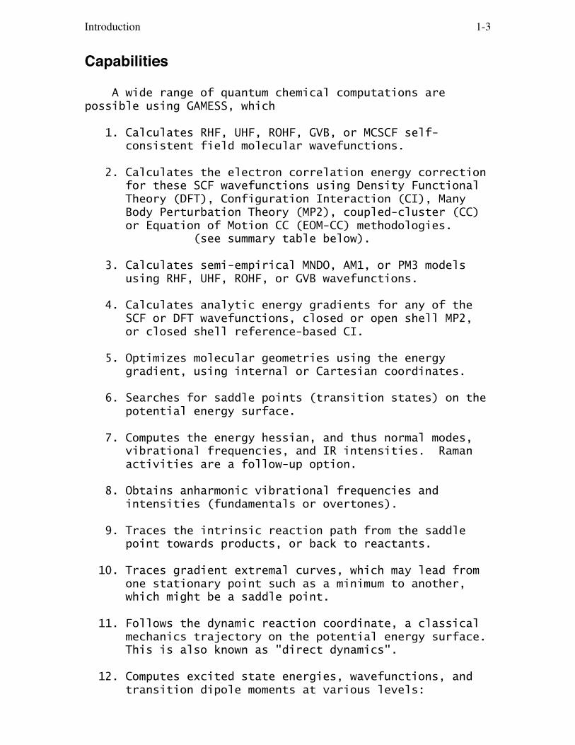
Capabilities
A wide range of quantum chemical computations arepossible using GAMESS, which
1. Calculates RHF, UHF, ROHF, GVB, or MCSCF self- consistent field molecular wavefunctions.
2. Calculates the electron correlation energy correction for these SCF wavefunctions using Density Functional Theory (DFT), Configuration Interaction (CI), Many Body Perturbation Theory (MP2), coupled-cluster (CC) or Equation of Motion CC (EOM-CC) methodologies. (see summary table below).
3. Calculates semi-empirical MNDO, AM1, or PM3 models using RHF, UHF, ROHF, or GVB wavefunctions.
4. Calculates analytic energy gradients for any of the SCF or DFT wavefunctions, closed or open shell MP2, or closed shell reference-based CI.
5. Optimizes molecular geometries using the energy gradient, using internal or Cartesian coordinates.
6. Searches for saddle points (transition states) on the potential energy surface.
7. Computes the energy hessian, and thus normal modes, vibrational frequencies, and IR intensities. Raman activities are a follow-up option.
8. Obtains anharmonic vibrational frequencies and intensities (fundamentals or overtones).
9. Traces the intrinsic reaction path from the saddle point towards products, or back to reactants.
10. Traces gradient extremal curves, which may lead from one stationary point such as a minimum to another, which might be a saddle point.
11. Follows the dynamic reaction coordinate, a classical mechanics trajectory on the potential energy surface. This is also known as "direct dynamics".
12. Computes excited state energies, wavefunctions, and transition dipole moments at various levels:
Introduction 1-4
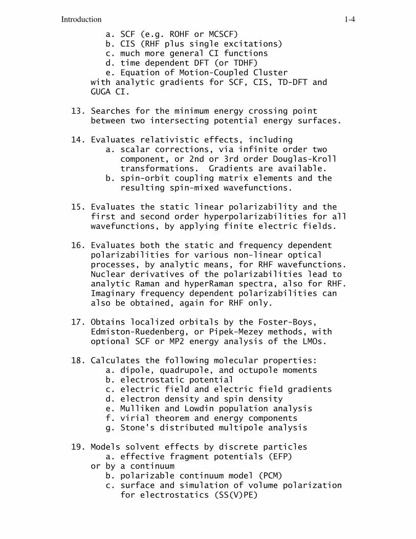
a. SCF (e.g. ROHF or MCSCF) b. CIS (RHF plus single excitations) c. much more general CI functions d. time dependent DFT (or TDHF) e. Equation of Motion-Coupled Cluster with analytic gradients for SCF, CIS, TD-DFT and GUGA CI.
13. Searches for the minimum energy crossing point between two intersecting potential energy surfaces.
14. Evaluates relativistic effects, including a. scalar corrections, via infinite order two component, or 2nd or 3rd order Douglas-Kroll transformations. Gradients are available. b. spin-orbit coupling matrix elements and the resulting spin-mixed wavefunctions.
15. Evaluates the static linear polarizability and the first and second order hyperpolarizabilities for all wavefunctions, by applying finite electric fields.
16. Evaluates both the static and frequency dependent polarizabilities for various non-linear optical processes, by analytic means, for RHF wavefunctions. Nuclear derivatives of the polarizabilities lead to analytic Raman and hyperRaman spectra, also for RHF. Imaginary frequency dependent polarizabilities can also be obtained, again for RHF only.
17. Obtains localized orbitals by the Foster-Boys, Edmiston-Ruedenberg, or Pipek-Mezey methods, with optional SCF or MP2 energy analysis of the LMOs.
18. Calculates the following molecular properties: a. dipole, quadrupole, and octupole moments b. electrostatic potential c. electric field and electric field gradients d. electron density and spin density e. Mulliken and Lowdin population analysis f. virial theorem and energy components g. Stone's distributed multipole analysis
19. Models solvent effects by discrete particles a. effective fragment potentials (EFP) or by a continuum b. polarizable continuum model (PCM) c. surface and simulation of volume polarization for electrostatics (SS(V)PE)

Introduction 1-5
d. conductor-like screening model (COSMO) e. self-consistent reaction field (SCRF) allowing for EFP and PCM to be combined.
20. Performs all-electron calculations based on the Fragment Molecular Orbital (FMO) method.
21. Models the formation of aperiodic polymers with the Elongation Method.
22. Perform QM/MM style HF, DFT, GVB, MCSCF, MP2 and TDDFT calculations, using the integrated QuanPol program.
23. When combined with the plug-in TINKER molecular mechanics program, performs Surface IMOMM (SIMOMM) or IMOMM QM/MM type simulations. Download from http://www.msg.chem.iastate.edu/GAMESS/GAMESS.html
24. When combined with the plug-in NEO program (Nuclear Electron Orbitals), performs quantum mechanics computations of nuclear structure. NEO's code is included with GAMESS source distributions, see the directory ~/gamess/qmnuc.
25. When combined with the plug-in VB2000 program, performs valence bond calculations. See http://www.scinetec.com/~vb for more information.
26. When combined with the plug-in XMVB program, performs valence bond calculations. Please contact Professor Wei Wu of Xiamen University for more information, [email protected], and see also http://ctc.xmu.edu.cn/xmvb/index.html.
27. When combined with the plug-in NBO program, performs Natural Bond Order analyses. This program is available at http://www.chem.wisc.edu/~nbo5, for a modest license fee.
Many of these calculations may be performed in parallel!
Introduction 1-6
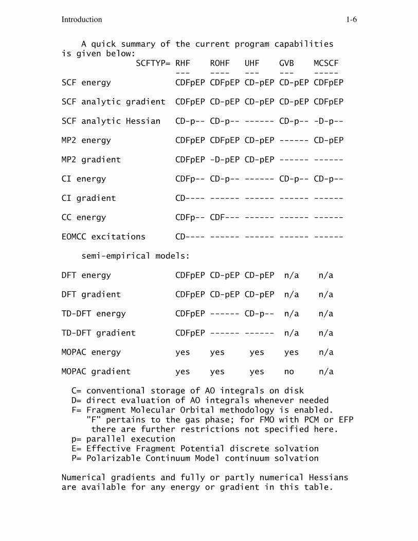
A quick summary of the current program capabilitiesis given below: SCFTYP= RHF ROHF UHF GVB MCSCF --- ---- --- --- -----SCF energy CDFpEP CDFpEP CD-pEP CD-pEP CDFpEP
SCF analytic gradient CDFpEP CD-pEP CD-pEP CD-pEP CDFpEP
SCF analytic Hessian CD-p-- CD-p-- ------ CD-p-- -D-p--
MP2 energy CDFpEP CDFpEP CD-pEP ------ CD-pEP
MP2 gradient CDFpEP -D-pEP CD-pEP ------ ------
CI energy CDFp-- CD-p-- ------ CD-p-- CD-p--
CI gradient CD---- ------ ------ ------ ------
CC energy CDFp-- CDF--- ------ ------ ------
EOMCC excitations CD---- ------ ------ ------ ------
semi-empirical models:
DFT energy CDFpEP CD-pEP CD-pEP n/a n/a
DFT gradient CDFpEP CD-pEP CD-pEP n/a n/a
TD-DFT energy CDFpEP ------ CD-p-- n/a n/a
TD-DFT gradient CDFpEP ------ ------ n/a n/a
MOPAC energy yes yes yes yes n/a
MOPAC gradient yes yes yes no n/a
C= conventional storage of AO integrals on disk D= direct evaluation of AO integrals whenever needed F= Fragment Molecular Orbital methodology is enabled. "F" pertains to the gas phase; for FMO with PCM or EFP there are further restrictions not specified here. p= parallel execution E= Effective Fragment Potential discrete solvation P= Polarizable Continuum Model continuum solvation
Numerical gradients and fully or partly numerical Hessiansare available for any energy or gradient in this table.
Introduction 1-7
History of GAMESS
GAMESS was put together from several existing quantumchemistry programs, particularly HONDO, by the staff of theNational Resources for Computations in Chemistry. The NRCCproject (1 Oct 77 to 30 Sep 81) was funded by NSF and DOE,and was limited to the field of chemistry. The NRCC staffadded new capabilities to GAMESS as well. Besidesproviding public access to the code on the CDC 7600 at thesite of the NRCC (the Lawrence Berkeley Laboratory), theNRCC made copies of the program source code (for a VAX)available to users at other sites. The original citationfor this program was M. Dupuis, D. Spangler, and J. J. Wendoloski National Resource for Computations in Chemistry Software Catalog, University of California: Berkeley, CA (1980), Program QG01
This manual is a completely rewritten version of theoriginal documentation for GAMESS. Any errors found inthis documentation, or the program itself, should not beattributed to the original NRCC authors.
The present version of the program has undergone manychanges since the NRCC days. This occurred at North DakotaState University from 1982 up to 1992, and now continues atIowa State University to the present.
It would be difficult to overestimate the contributionsMichel Dupuis has made to this program, in its originalform, and since. This includes the donation of code fromHONDO, and numerous suggestions for other improvements.
The continued development of this program from 1982 oncan be directly attributed to the nurturing environmentprovided by Professor Mark Gordon, at North Dakota Stateand then Iowa State University.
It is important to also single out Professor EmeritusKlaus Ruedenberg of Iowa State University, whose group isresponsible for the determinant technology lying underneaththe MCSCF programs in GAMESS.
Even when our students and postdocs leave Iowa State,many continue to make contributions to GAMESS. Inaddition, we have also included many codes developed in

Introduction 1-8
other groups over the years, so that the list of authors ofGAMESS is actually much longer than the author list of the1993 J. Comput. Chem. article. A complete list of authorsmay be found at the top of every log file from a GAMESSrun.
Funding of many of the developments in GAMESS from1982 to the present time was, and is provided by the AirForce Office of Scientific Research. This has always beenthe backbone of the support for GAMESS.
In late 1987, NDSU and IBM reached a Joint StudyAgreement. One goal of this JSA was the development of aversion of GAMESS that was vectorized for the IBM 3090'sVector Facility, which was accomplished by the fall of1988. This phase of the JSA led to a program which is alsoconsiderably faster in scalar mode as well. The secondphase of the JSA, which ended in 1990, was to enhanceGAMESS' scientific capabilities. These additions includeanalytic hessians, ECPs, MP2, spin-orbit coupling andradiative transitions, and so on. Everyone who uses thecurrent version of GAMESS owes thanks to IBM in general,and Michel Dupuis of IBM Kingston in particular, for theirsponsorship of GAMESS during this JSA.
During the first six months of 1990, Digital awarded aInnovator's Program grant to NDSU. The purpose of thisgrant was to ensure GAMESS would run on the DECstation, andto develop graphical display programs. As a result, thecompanion programs MOLPLT, PLTORB, DENDIF, and MEPMAP weremodernized for the X-windows environment, and interfaced toGAMESS. These programs now run under the X-windowsenvironments, and many other X-windows environments aswell. The ability to visualize the molecular structures,orbitals, and electrostatic potentials is a significantimprovement. These graphics programs eventually formed thenucleus of the program MacMolPlt.
Parallelization of GAMESS began in 1991, with most ofthe early work and design strategy done by Theresa Windus.This benefited greatly from the ARPA sponsorship of theTouchstone Delta experimental computer. Message passingused the TCGMSG library of Robert Harrison in the earlyyears, up to 1999. Parallelization of GAMESS has turnedinto a multi-year process as detailed below.
The DoD awarded a CHSSI grant to ISU in 1996 to extendthat scalability of existing parallel methods, and moreimportantly develop new techniques. This brought Graham
Introduction 1-9
Fletcher on board as a postdoc, and led to the introductionof the Distributed Data Interface (DDI) programming model.The first version of DDI, written at ISU, was used fromJune 1999 to May 2004. Ryan Olson, with help from AlistairRendell of Australian National University, rewrote DDIentirely in C, adding optimizations for the commonplace SMPnodes, especially System V memory use. Dmitri Fedorov ofthe National Institute for Advanced Industrial Science andTechnology added the concept of subgroups at the same time.This combined new version of DDI has been the messagepassing support layer for GAMESS since May 2004.
The DoE awarded a SciDAC grant to ISU in 2002 to enableadditional scientific capabilities in GAMESS, with emphasison scalable algorithms. To date, this has supportedparallelization of the EFP solvent molecule, and new codesfor analytic MCSCF Hessians, and open shell MP2 gradients.
Some summary of these various grants and initiatives isin order. The 1982 version of GAMESS contained roughly80,000 lines of FORTRAN code, implementing the present fivewavefunction types, and analytic nuclear gradients foreach, enabling geometry optimization and transition statesearch, and numerically differentiated frequencies. Theonly electron correlation method available was GUGA basedCI computation. All computations were in the gas phase.
By 2005, GAMESS had grown to roughly 650,000 lines ofFORTRAN. Analytic hessian computation is now routine atthe SCF levels. Electron correlation is now treated withdirect determinant CI codes, and in addition perturbationtheory, density functional, or coupled cluster methods(with analytic gradients for some of these) may be used.New AO integral codes, including effective core potentialsare used, and direct AO integral computation is possible.Discrete and continuum models for solvated molecules areprovided, and there is an associated program for surfacechemistry. Additional chemistry runs are provided, such asreaction paths and dynamical trajectories, IR and Ramanspectra, anharmonic vibrational corrections, static orfrequency dependent polarizabilities, transition moments,and spin-orbit couplings. Scalar relativistic correctionscan be applied to any computation. Improvements orcomplete rewrites have been made for geometry searches, SCFconvergers, internal coordinates, ease of use, availablebasis sets, and so on. The majority of these computationscan be run on parallel computers.
The rest of this section gives more specific credit
Introduction 1-10
to the sources of various parts of the program.
* * * *
GAMESS is a synthesis, with many major modifications,of several programs. A large part of the program originatefrom HONDO 5.
For sp basis functions, modified Gaussian76 s,p,L shellcode is used. Both the sp rotated axis integrals and thesp gradient packages were modified in 2001 by Jose MariaSierra of Synstar Computer Services in Madrid, Spain. Thesp integral routines were modified in 2003 and in 2004 byKazuya Ishimura of the Institute for Molecular Science touse McMurchie-Davidson quadratures for the basic axes-1integrals, after which they are rotated ala Hehre/Pople.For spd functions, the s,p,d,L shell rotated axis codewritten by Kazuya Ishimura of the Institute for MolecularScience is used. For integral quartets with higher angularmomentum, the s,p,d,f,g Electron Repulsion IntegralCalculator (ERIC) code written by Graham Fletcher atNASA/Eloret in 2004 is used, provided the total angularmomentum of the quartet is no more than 5. Both rotatedaxis codes, the sp gradient code, and ERIC share a common,fully accurate evaluation of Fm(t) integrals, and have beentested for very small (down to 0.005) and very large(1.0d+11) Gaussian exponents. The Rys polynomial programof Michel Dupuis is used to handle the general integralcase: s,p,d,f,g, or L shells. HONDO 1e- and 2e- Rysroutines were redimensioned to handle up to g shells byTheresa Windus at North Dakota State University in 1991.
Any sp gradient integrals are done with Jose Sierra'smodified version of the Gaussian80 code due to Schlegel.The spdfg gradient package consists of Michel Dupuis' RysPolynomial code, and was adapted into GAMESS by Brett Bodeat Iowa State University in 1994.
The use of quantum fast multipole methods for avoidinglong range integral evaluation in large molecules wasprogrammed by Cheol Choi at Iowa State and at KyungpookNational University, and included in GAMESS in 2001.
The ECP code goes back to Louis Kahn, with gradientmodifications originally made by K.Kitaura, S.Obara, andK.Morokuma at IMS in Japan. The code was adapted to HONDOby Stevens, Basch, and Krauss, from whence Kiet Nguyenadapted it to GAMESS at NDSU. Modifications for ffunctions were made by Drora Cohen and Brett Bode. This

Introduction 1-11
code was completely rewritten to use spdfg basis sets, toexploit shell structure during integral evaluation, and toadd the capability of analytic second derivatives by BrettBode at ISU in 1997-1998. Jose Sierra of Synstar removedthe last few bugs from this in 2003.
The Model Core Potential (MCP) codes originate from theUniversity of Alberta and the University of Kyushu. MCPenergy code was interfaced to GAMESS in 2003 by MariuszKlobukowski (UofA). Many model core potentials, and theirassociated valence basis sets, were added as a basislibrary by Mariusz in 2005. Hirotoshi Mori and EisakuMiyoshi (KyuDai) developed the nuclear gradient code forMCP with the assistance of a JSPS grant, and this code wasincluded in GAMESS in March 2007. The ZFK family of modelcore potentials for p-block elements was added to GAMESS byToby Zeng in April 2010.
Changes in the manner of entering the basis set, andthe atomic coordinates (including Z-matrix forms) are dueto Jan Jensen at North Dakota State University.
The direct SCF implementation was done at NDSU, guidedby a pilot code for the RHF case by Frank Jensen.
The UHF code was taught to do high spin ROHF by JohnMontgomery at United Technologies, who extended DIIS use toROHF and the one pair GVB case.
The GVB code is a heavily modified version of GVBONE.
The SCF for Molecular Interactions option was added toGAMESS in 1997 by Antonino Famulari, during a summer visitfrom the University of Milan. This two fragment code wasreplaced with a multi-fragment code from Maurizio Sironi ofthe University of Milan in 2004.
The Direct Inversion in the Iterative Subspace (DIIS)convergence procedure was implemented by Brenda Lam (thenat the University of Houston) in 1986, for RHF and UHFfunctions. Additional GVB-DIIS cases were programmed byGalina Chaban at ISU. The approximate second order SCFconverger was implemented by Galina Chaban at Iowa StateUniversity in 1995, and was provided for RHF, ROHF, GVB,and MCSCF cases. The FULLNR and FOCAS MCSCF convergerswere contributed by Michel Dupuis from his HONDO program.A parallel implementation of the FULLNR converger waswritten by Graham Fletcher at Eloret in 2002. The Jacobiorbital rotation scheme for MCSCF orbital optimization was

Introduction 1-12
written by Joe Ivanic and Klaus Ruedenberg at Iowa StateUniversity in 2001.
The Ames Laboratory determinant full CI code waswritten by Joe Ivanic and Klaus Ruedenberg. As befits codewritten by an Australian living in Iowa, it was interfacedto GAMESS during an extremely cordial visit to AustraliaNational University in January 1998. An update by Joe inOctober 2000 exploits Abelian point group symmetry. Ageneral CI program based on selected determinants was addedby Joe and Klaus in July 2001. After moving from AmesLaboratory at ISU to the Advanced Biomedical ComputingCenter of the National Cancer Institute-Frederick, FortDetrick, Joe wrote a determinant based program for secondorder CI, in 2002. In early 2003, Joe added the OccupationRestricted Multiple Active Space determinant CI program,again written at NCI.
The GUGA CI is based on Brooks and Schaefer's unitarygroup program which was modified to run within GAMESS,using a Davidson eigenvector method written by SteveElbert.
Programming of the GUGA analytic CI gradient was doneby Simon Webb in 1996 at Iowa State University.
The CIS gradient program was written in 2003 by SimonWebb of the Advanced Biomedical Computing Center of theNational Cancer Institute in Frederick. Transition momentswere added by Simon and Pooja Arora in June 2005.
The sequential MP2 and UMP2 energy code was adaptedfrom HONDO in 1994 by Nikita Matsunaga at ISU. Nikitaprogrammed the RMP open shell energy in 1992. The ZAPTopen shell energy was programmed by Rob Bell in 1999. Theserial closed shell MP2 gradient code is also from HONDO,and was adapted to GAMESS in 1995 by Simon Webb and NikitaMatsunaga. In 1996, Simon Webb added the frozen coregradient option at ISU. The parallel closed shell MP2 codeis a descendant of work for GAMESS-UK by Graham Fletcher,Alistair Rendell, and Paul Sherwood at Daresbury. This wasadapted to GAMESS at ISU by Graham Fletcher in 1999.Serial and parallel codes for the spin unrestricted UMP2gradient were programmed by Christine Aikens at ISU, in2002. Christine Aikens added a parallel spin-restrictedopen shell (ZAPT) gradient code in 2005. Programs forparallel closed shell MP2 energy (2006) and gradient (2007)using disk storage were written by Kazuya Ishimura at theInstitute for Molecular Science (IMS) in Okazaki. The
Introduction 1-13
parallel Resolution of the Identity MP2 program by MichioKatouda, also from IMS, was added in 2010.
Credits for multiconfigurational PT follow. HaruyukiNakano, then at the University of Tokyo, interfaced hismultireference MCQDPT code (based on CSFs) to GAMESS duringa 1996 visit to ISU. Parallelization of the Tokyomultireference PT code was done by Hiroaki Umeda at MieUniversity, and included into GAMESS in 2001. Adeterminant based equivalent to MRMP/MCQDPT was programmedin 2005 by Joe Ivanic of the National Cancer Institute,this is MRMP=MRPT. In 2008, Haruyuki Nakano of theUniversity of Kyushu contributed a general MCSCF referencequasi-degenerate perturbation theory code, MRMP=GMCPT,which is capable of treating non-CAS references, includingthose of the ORMAS type.
The grid-free DFT energy and gradient code was writtenby Kurt Glaesemann at Iowa State University, starting fromthe code of Almlof and Zheng, adding four center overlapintegrals, a gradient program, developing the auxiliarybasis option, and adding some functionals. This wasincluded in GAMESS in 1999.
The grid based DFT program was introduced in 2001 atthe University of Tokyo, by Takao Tsuneda, Muneaki Kamiya,Susumu Yanagisawa, and Dmitri Fedorov. The original programis from Nevin Oliphant, Hideo Sekino, and Rod Bartlett atQTP. Many improvements were made to this early program atU. Tokyo: using point group symmetry, switching from coarseto fine grids, functional development, and parallelization.Sarom Sok at ISU added many new functionals in 2007, 2008,and 2009, some with the help of Huub van Dam's densityfunctional repository. Sarom added the Truhlar group'smeta-GGA M06 and M08 functionals in 2008 and 2009, usingsource code from U.Minnesota. Roberto Peverati of theUniversity of Zurich added Grimme's dispersion correctionin 2008. Roberto added "wB97" range separated GGA, "B97"style GGA and metaGGA, and B2-PLYP in 2009. FedericoZahariev at ISU included the TPSS family of meta-GGAs in2008 and 2009. Kiet Nguyen at Wright-Patterson AFB addedCAM-B3LYP in 2009. The HPTi project (Jean-PhilippeBlaudeau, Shawn Brown, Mike Lasinksi, Nick Romero, AnthonyYau) enabled the use of Lebedev or Standard Grid-1 grids inApril 2008, and Janssen's grids in May 2009.
The time dependent DFT program originated in the groupof Takao Tsuneda at University of Tokyo, and was includedinto GAMESS in the fall of 2006 by Mahito Chiba at AIST in

Introduction 1-14
Tsukuba. He also included the "long range correction"option (aka "range separation") for both ground and excitedstates. The analytic TDDFT gradient for singlet excitedstates from a closed shell reference was added by MahitoChiba in August 2007. Mahito Chiba, in collaboration withDmitri Fedorov, also developed FMO functionality in TDDFTenergies. The TDDFT energy for UHF ground states was addedby Soohaeng Yoo at Iowa State, in February 2008.Tamm/Dancoff approximation coding was done by FedericoZahariev at ISU in 2010. The HPTi project parallelized theclosed shell TDDFT energy and gradient programs in April2008. Sarom Sok and Federico Zahariev have developedhigher derivatives for many functionals, allowing them tobe used in TDDFT energies and gradients.
TD-DFT solvation effects include EFP1 discretesolvation, added to the closed shell TD-DFT excitationenergies in 2008 by Soohaeng Yoo, and to its gradient in2010 by Noriyuki Minezawa at ISU. C-PCM solvent effects onTD-DFT closed shell excitation energies were added byMahito Chiba in December 2008, with PCM modifications tothis gradient by Yali Wang and Hui Li in November 2009.The combined TDDFT/EFP/PCM solvation model was finished inNovember 2010 by Nandun Thellamurege and Hui Li at U.Nebraska.
Incorporation of enough MOPAC version 6 routines to runPM3, AM1, and MNDO calculations from within GAMESS was doneby Jan Jensen at North Dakota State University.
The numerical force constant computation and normalmode analysis was adapted from Andy Komornicki's GRADSCFprogram, with decomposition of normal modes in internalcoordinates written at NDSU by Jerry Boatz.
The code for the analytic computation of RHF Hessianswas contributed by Michel Dupuis of IBM from HONDO 7. Highand low spin restricted open shell CPHF code was written atNDSU in 1989. The TCSCF CPHF code is the result of acollaboration between NDSU and John Montgomery, then atUnited Technologies, in 1990. Analytic IR intensities andpolarizabilities (during hessian runs) were programmed bySimon Webb at ISU in 1995. Analytic Hessians for MCSCFwavefunctions based on determinants were coded, and enabledfor parallel execution, by Tim Dudley at ISU, and includedinto GAMESS in April 2004, with a souped-up version addedin March 2006.

Introduction 1-15
Code for Raman intensity prediction was written atTokyo Metropolitan University in April 2000.
The vibrational SCF and MP2 anharmonic frequency codefor fundamental modes and overtones was written by GalinaChaban, Joon Jung, and Benny Gerber at U.California-Irvineand Hebrew University of Jerusalem, and included in GAMESSin 2000. The solver was modified to perform degenerateperturbation theory for more accurate results by NikitaMatsunaga at Long Island University in 2001.
Delocalized internal coordinates were implemented byJim Shoemaker at the Air Force Institute of Technology in1997, and put online in GAMESS by Cheol Choi at ISU afterfurther improvements in 1998.
Most of the geometry search procedures (OPTIMIZE andSADPOINT) were developed by Frank Jensen of the Universityof Aarhus. These methods are adapted to use GAMESSsymmetry, and Cartesian or internal coordinates. Numericaldifferentiation of the energy to obtain gradients andHessians which may be used in OPTIMIZE or SADPOINT searcheswas programmed by Ryan Olson at ISU in 2003. The MEXprocedure for searching for minimum energy crossing pointsbetween two surfaces was programmed by Jeremy Harvey andNikita Matsunaga, and finally included into GAMESS in 2006.The non-gradient optimization (so aptly named TRUDGE) wasadapted from HONDO 7 by Mariusz Klobukowski at U.Alberta,this may be more interesting for its exponent optimizationoption.
The intrinsic reaction coordinate pathfinder waswritten at North Dakota State University, and modifiedlater for new integration methods by Kim Baldridge. TheGonzales-Schelegel IRC stepper was incorporated by ShujunSu at Iowa State, based on pilot code from Frank Jensen.
The code for the Dynamic Reaction Coordinate wasdeveloped by Tetsuya Taketsugu at Ochanomizu U. and U. ofTokyo, and added to GAMESS by him at ISU in 1994.
The two algorithms for tracing gradient extremals wereprogrammed by Frank Jensen, now at the University ofAarhus.
The program for Monte Carlo generation of trialstructures along with a simulated annealing protocol waswritten by Paul Day at Wright-Patterson Air Force Base.

Introduction 1-16
Modifications to this were made by Pradipta Bandyopadhyayat ISU, and the code was included in 2001.
The surface scanning option was implemented by RichardMuller at the University of Southern California.
Static polarizabilities for any type of energy valueare bases on a code from Henry Kurtz of the University ofMemphis. This uses a numerical differentiation based onapplication of finite electric fields. The program wasadded in 1992, and was modified by Sanka Ghosh to produceall tensor components in 2005.
Henry Kurtz' program for the fully analytic calculationof static and frequency dependent polarizabilities for NLOproperties for closed shell systems was included in 1994,based on a MOPAC implementation by Prakashan Korambath atU. Memphis.
An extended TDHF package for the analytic computationof static and frequency dependent polarizabilities, andalso their nuclear derivatives, plus Raman and hyperRamanspectra prediction was written by Olivier Quinet and BenoitChampagne at the Facultes Universitaires Notre-Dame de laPaix, and coworker Bernard Kirtman at UC-Santa Barbara.Financial support for this was provided by Belgium. Thispackage was added to GAMESS in February 2005.
Ivana Adamovic programmed the imaginary frequencypolarizability computation for closed shell functions in2005, at ISU.
Edmiston-Ruedenberg energy localization is done with aversion of the ALIS program "LOCL", modified at NDSU to runinside GAMESS. Foster-Boys localization is based on ahighly modified version of QCPE program 354 by D.Boerth,J.A.Hasmall, and A.Streitweiser. John Montgomeryimplemented the Pipek/Mezey population localization. TheLCD SCF decomposition and the MP2 decomposition werewritten by Jan Jensen at Iowa State in 1994.
Point Determined Charges were implemented by MarkSpackman at the University of New England, Australia.
The Morokuma decomposition was implemented by Wei Chenat Iowa State University, in 1995. The Localized MolecularOrbital Energy Decomposition Analysis was implemented byPeifeng Su and Hui Li at the University of Nebraska in2009.

Introduction 1-17
The radiative transition moment and effective nuclearcharge spin-orbit coupling modules were written by ShiroKoseki at North Dakota State University in 1990.
The full Breit-Pauli spin-orbit coupling integralpackage was written by Thomas Furlani. This code wasincorporated into GAMESS by Dmitri Fedorov at Iowa StateUniversity in 1997, who generalized the spin-orbit couplingmatrix element code generously provided by Thomas Furlani(restricted to an active space of two electrons in twoorbitals), with assistance from visits to ISU by ThomasFurlani and Shiro Koseki. Dmitri Fedorov has sincegeneralized the full two electron approach to allow for anyspins, for more than two spin multiplicities at a time, anda partial treatment of the the two electron terms that runsin time similar to the one electron operator. Space andspin symmetries are exploited to speed up the runs. DmitriFedorov programmed the SO-MCQDPT options at the Universityof Tokyo in 2001. Density matrix calculation for spin-orbit coupled states was programmed by Toby Zeng andMariusz Klobukowski at the University of Alberta, and addedto GAMESS in April 2010.
Inclusion of relativistic effects by means of theDouglas-Kroll transformation was developed to the thirdorder by Takahito Nakajima and Kimihiko Hirao at theUniversity of Tokyo. It was implemented into GAMESS byTakahito Nakajima and Dmitri Fedorov, including energy,semi-analytic nuclear gradient, and spin-orbit coupling (atthe first order, DK1). The program was included withGAMESS in November 2003.
Inclusion of relativistic effects by the Relativisticscheme of Elimination of Small Components (RESC) method,was developed by Takahito Nakajima and Kimihiko Hirao atthe University of Tokyo. This code was written by TakahitoNakajima and consequently adapted into GAMESS by DmitriFedorov, who extended the methodology in March 2000 to thecomputation of gradients. RESC provides both scalar (spinfree) and vector (spin-dependent) relativistic corrections.
The Normalized Elimination of Small Components (NESC)was programmed by Dmitri Fedorov at ISU and the Universityof Tokyo. Special thanks are due to Kenneth Dyall for hisassistance in providing check values. Extension of NESC toinclude gradient computation was also done by Dmitri.
Introduction 1-18
Finally, inclusion of scalar relativstic corrections toan infinite order two-component (IOTC) transformation wasadded in September 2010, by Maria Barysz of NicholasCopernicus University.
Development of the EFP method began in the group ofWalt Stevens at NIST's Center for Advanced Research inBiotechnology (CARB) in 1988. Walt is the originator ofthis method, and has provided both guidance and some earlyfinancial support to ISU for its continued development.Mark Gordon's group's participation began in 1989-90 asdiscussions during a year Mark spent in the DC area, andbecame more serious in 1991 with a visit by Jan Jensen toCARB. At this time the method worked for the energy, andgradient with respect to the ab initio nuclei, for onefragment only. Jan has assisted with most aspects of themulti-fragment development since. Paul Day at NDSU and ISUderived and implemented the gradient with respect tofragments, and programmed EFP geometry optimization, from1992-1994. Wei Chen at ISU debugged many parts of the EFPenergy and gradient, developed the code for following IRCs,improved geometry searches, and fitted much more accuraterepulsive potentials, from 1995-1996. Simon Webb at ISUprogrammed the current self-consistency process for theinduced dipoles in 1994. The EFP method was sufficientlydeveloped, tested, and described, to be released inSeptember 1996, with an RHF level potential for water.Code for charge penetration was added by Mark Freitag in2001, and made numerically stabile by Lyuda Slipchenko in2006. Ivana Adamovic included a DFT level EFP for water in2002. Parallelization of the EFP codes was done by HeatherNetzloff in 2005.
The second EFP theory (called EFP2) was begun in 1996by Jan Jensen, who programmed an analytic formula for theexchange repulsion. Hui Li replaced this with a faster,more accurate code in 2005. Ivana Adamovic programmed adispersion term for EFP2 in 2005. Hui Li added the chargetransfer term for EFP2 in 2005.
Two other methods using the EFP model are available. Acombination of EFP + PCM energies (an onion-like solutionmodel) was programmed by Pradipta Bandyopadhyay in 2000.The use of EFPs to model biological systems, including aboundary across a covalent bond, was coded at theUniversity of Iowa in 2000, by Jan Jensen, VisvaldasKairys, and Hui Li.
Introduction 1-19
The SCRF solvent model was implemented by Dave Garmerat CARB, and was adapted to GAMESS by Jan Jensen and SimonWebb at Iowa State University.
The COSMO model was developed by Andreas Klamt and KimBaldridge, starting at the San Diego Supercomputer Center,and later at University of Zurich. It was included intoGAMESS by Laura Brovold in March 2000 during a visit toAmes. Subsequent additions were made by Yohann Potier andRoberto Peverati, at the University of Zurich, and includedin GAMESS in June 2010.
The PCM code originated in the group of Jacopo Tomasiat the University of Pisa. Benedetta Mennucci wasinstrumental in interfacing the original D-PCM code toGAMESS in 1997, and answering many technical questionsabout the code, the methodology, and the documentation. In2000, Benedetta Menucci provided code implementing animproved IEF solver for the PCM surface charges. Thechanges to implement iterative solution of the PCMequations for large molecules, and to provide an accuratenuclear gradient were carried out by Hui Li and Jan Jensenat the University of Iowa in 2001-2004, along with theparallelization. This included implementation of two newsurface tessellation schemes, GEPOL-AS and GEPOL-RT. Huiand Jan also implemented the Conductor-PCM method, andextended the PCM methodology to all types of SCF functions.Hui Li's research group at the University of Nebraskaimplemented the following improvements: FIXPVA tessellationwith smooth switching functions for reliable geometryoptimizations (Peifeng Su, 2008), extension of FIXPVA tocavitation, repulsion, and dispersion (2009), heterogenousCPCM (Dejun Si, 2009), closed shell PCM/TDDFT gradients(Yali Wang, 2009), closed shell PCM/MP2 gradients (DejunSi, 2010), open shell PCM/MP2 gradients (Dejun Si,September 2010), and combined EFP/PCM solvation for allsingle reference MP2 gradients (Nandun Thellamurege andDejun Si, November 2010). The SMD modifications to the PCMmodel are due to Alek Marenich, Junjun Liu, Chang-Guo Zhan,Christopher Cramer, and Don Truhlar at U. Minnesota(November 2010).
The Surface and Volume Polarization for Electrostaticscontinuum solvation model is written by Dan Chipman ofNotre Dame University, using several integral routineswritten by Michel Dupuis for the SVP model included inHONDO. The SVP model was added to GAMESS in June 2005.

Introduction 1-20
The SIMOMM model for surface chemistry is based on theTinker program of Jay Ponder's group, and is available as aplug-in option. The treatment is QM embedded in a MMbackground. The coding for this was done by Jim Shoemakerat the Air Force Institute of Technology, and finished byCheol Ho Choi at ISU. The interface to GAMESS wascompleted in 1998.
The Coupled-Cluster (CC) and Equation of MotionCoupled-Cluster (EOMCC) programs included in GAMESS are dueto Piotr Piecuch, Karol Kowalski, Marta Wloch, JeffreyGour, and Jesse Lutz of Michigan State University (MSU),and Stanislaw A. Kucharski and Monika Musial of theUniversity of Silesia. In addition to a number of standardCC and EOMCC methods, including the older CCSD, CCSD(T),and EOMCCSD approaches, the CC codes incorporated in GAMESSare capable of performing renormalized (R) and completelyrenormalized (CR) CCSD[T] and CCSD(T) calculations for theground state, the ground-state calculations employing therigorously size extensive completely renormalized non-iterative triples CR-CCSD(T)_L = CR-CC(2,3) approach. Thecombined corrections due to triply and quadruply excitedclusters are available in the factorized forms of theCCSD(TQ), renormalized CCSD(TQ), and completelyrenormalized CCSD(TQ) models. For excited states,completely renormalized EOMCCSD(T) (CR-EOMCCSD(T)) and EOM-CR-CC(23) calculations are possible. Electron attachmentand detachments (including excitations) are available asIP-EOM and EA-CC methods. The one-body reduced densitymatrices, dipole moments, transition dipole moments, andoscillator strengths are available at the CCSD and EOMCCSDlevels, for RHF. The ground-state CC, R-CC, and CR-CCprograms were initially incorporated into GAMESS in May2002. The excited-state EOMCC and CR-EOMCC programs wereincorporated in April 2004. Quadruples corrections andCCSD/EOM-CCSD density matrices were added in June 2005.The CR-CC(2,3) ground-state approach was added in January2006. Parallel computation of CCSD and CCSD(T) for closedshell references was enabled by Ryan Olson and JonathanBentz at Iowa State, in October 2006. Open shell CCSD andCR-CCL based on ROHF reference orbitals was added in May2007. CR-EOML and IP-EOMCC2/EA-EOMCC2 were included inOctober 2009, and active triples for IP/EA calculationswere finished in September 2010. All of these programswere developed with the support of the US Department ofEnergy, Office of Basic Energy Sciences, SciDACComputational Chemistry Program and the Chemical Sciences,Geosciences, and Biosciences Division. Additional support

Introduction 1-21
has been provided by the NSF's ITR program and the AlfredP. Sloan Foundation.
The GIAO computation of NMR properties for closed shellmolecules was programmed by Mark Freitag at Iowa StateUniversity, and included in GAMESS in November 2003.
The code for the Fragment Molecular Orbital (FMO)method incorporated and distributed as a part of thestandard GAMESS package since May 2004 is being developedat the National Institute of Advanced Industrial Scienceand Technology (AIST, Japan) by Dmitri Fedorov and KazuoKitaura. The FMO method is the successor of the EDA schemedeveloped by K. Kitaura and K. Morokuma (known in GAMESS asMorokuma-Kitaura decomposition), however, the FMO code waswritten independently. In GAMESS only the full FMO methodis incorporated whereas in the literature one can also finda simplified approach suited for molecular crystals. Since"FMO" is also used to mean "Frontier Molecular Orbitals"and the concept of fragments is also introduced in the EFPmethod (see above), it is stressed here that the FMO methodbears no relation to either of the two methods, that is tosay, it is independent of the two, but might be combinedwith either of them in the future just as EFPs are used ine.g. RHF.
The Nuclear Electron Orbital (NEO) plug-in code isdeveloped in the group of Sharon Hammes-Schiffer atPennsylvania State University, with programming by Simon P.Webb, Tzvetelin Iordanov, Mike Pak, and Chet Swalina. Theinitial release in 2006 permits HF and MP2 level treatmentof nuclear wavefunctions.
The elongation method, coded and linked to the standardGAMESS package since April 2006, is a method to mimic themechanism of the polymerization/copolymerization inexperiment. Attacking monomers approach a starting chain,one by one and the electron structure is determined in theinteractive region. Thus, one can perform very efficientcalculations for the electronic structure of huge random(aperiodic) polymers. The elongation method was firstproposed by A. Imamura and Y. Aoki in 1990s. The presentcode was written by Feng Long Gu, Jacek Korchowiec, MarcinMakowski, and Yuriko Aoki at the Department of Molecularand Material Sciences, Faculty of Engineering Sciences, atKyushu University.
The Divide and Conquer SCF, MP2, and CCSD programs weredeveloped at Waseda University, and were included in GAMESS

Introduction 1-22
in January 2009. The code was written by Masato Kobayashi,Tomoko Akama, and Hiromi Nakai.
The quantum chemistry polarizable force field program(QuanPol) was written by Hui Li, Nandun Thellamurege andDejun Si at the University of Nebraska-Lincoln. Theseauthors finished the initial implementation of QuanPol inAugust 2011, under an NSF support.
Many of the options just mentioned have been programmedto run in parallel, on systems ranging from Linux clustersto high-end parallel systems. The same software interfacesits between the quantum chemistry in GAMESS and any suchhardware, namely the Distributed Data Interface (DDI).This implements a mechanism for using the memory of theentire system to store the large arrays appearing inquantum chemistry codes. The first version of DDI was dueto Graham Fletcher and Mike Schmidt, introduced in 1999.The second version of DDI is due to Ryan Olson of ISU, andAlistair Rendell of the Australian National University, andincludes optimizations for SMP systems, along with otherimprovements for some high end systems. The second versionalso includes the 'group' scheme, presently used only inFMO jobs. This DDI was introduced into GAMESS in April2004, with public release in June 2004.

Introduction 1-23
Distribution Policy
To get a copy, please fill out the application formavailable at http://www.msg.chem.iastate.edu/GAMESS/GAMESS.html
Persons receiving copies of GAMESS are requested toacknowledge that they will not make copies of GAMESS foruse at other sites, or incorporate any portion of GAMESSinto any other program, without receiving permission to doso from ISU. If you know anyone who wants a copy ofGAMESS, please refer them to the web site above, for themost up to date version available.
No large program can ever be guaranteed to be free ofbugs, and GAMESS is no exception. If you would like toreceive an updated version (fewer bugs, and with newcapabilities), simply return to the web site mentioned.You should probably allow a half year or so to pass forenough significant changes to accumulate. The web pagealways contains a short synopsis of the most recentchanges.

Introduction 1-24
Input Philosophy
Input to GAMESS may be in upper or lower case. Allinput groups begin with a $ sign in column 2, meaningexactly column 2 or else it is not detected, followed bya name identifying that group. There are three types ofinput groups in GAMESS:
1. A pseudo-namelist, free format, keyword drivengroup. Almost all input groups fall into this firstcategory.
2. A free format group which does not use keywords.The first line of these will contain only the group name,followed by several lines of positional data usually withno keywords, and a last line containing " $END" only.The only members of this category are $DATA, $ECP, $MCP,$GCILST, $POINTS, $STONE, and the EFP related data $EFRAG,$FRAGNAME, $FRGRPL, and $DAMPGS.
3. Formatted data. This data is NEVER typed by theuser, but rather is generated in the correct format bysome earlier GAMESS run. Like category 2, the first linecontains only the group name, and the last line is aseparate $END line.
Type 1 groups may have keyword input on the same lineas the group name, and the $END may appear anywhere.
Because each group has a unique name, the groups maybe given in any order desired. In fact, multipleoccurrences of category 1 groups are permissible.
* * *
Most of the groups can be omitted if the programdefaults are adequate. An exception is $DATA, which isalways required. A typical free format $DATA group is
$DATASTO-3G test case for waterCNV 2
OXYGEN 8.0 STO 3
HYDROGEN 1.0 -0.758 0.0 0.545 STO 3

Introduction 1-25
$END
Here, position is important. For example, the atomname must be followed by the nuclear charge and then thex,y,z coordinates. Note that missing values will be readas zero, so that the oxygen is placed at the origin.The zero Y coordinate must be given for the hydrogen,so that the final number is taken as Z.
The free format scanner code used to read $DATA isadapted from the ALIS program, and is described in thedocumentation for the graphics programs which accompanyGAMESS. Note that the characters ;>! mean somethingspecial to the free format scanner, and so use of thesecharacters in $DATA and $ECP should probably be avoided.
Because the default type of calculation is a singlepoint (geometry) closed shell SCF, the $DATA group shownis the only input required to do a RHF/STO-3G watercalculation.
* * *
As mentioned, the most common type of input is anamelist-like, keyword driven, free format group. Thesegroups must begin with the $ sign in column 2, but have nofurther format restrictions. You are not allowed toabbreviate the keywords, or any string value they mightexpect. They are terminated by a $END string, appearinganywhere. The groups may extend over more than onephysical card. In fact, you can give a particular groupmore than once, as multiple occurrences will be found andprocessed. We can rewrite the STO-3G water calculationusing the keyword groups $CONTRL and $BASIS as
$CONTRL SCFTYP=RHF RUNTYP=ENERGY $END $BASIS GBASIS=STO NGAUSS=3 $END $DATASTO-3G TEST CASE FOR WATERCnv 2
Oxygen 8.0 0.0 0.0 0.0Hydrogen 1.0 -0.758 0.0 0.545 $END
Keywords may expect logical, integer, floating point,or string values. Group names and keywords never exceed 6characters. String values assigned to keywords never

Introduction 1-26
exceed 8 characters. Spaces or commas may be used toseparate items:
$CONTRL MULT=3 SCFTYP=UHF,TIMLIM=30.0 $END
Floating point numbers need not include the decimal,and may be given in exponential form, i.e. TIMLIM=30,TIMLIM=3.E1, and TIMLIM=3.0D+01 are all equivalent.
Numerical values follow the FORTRAN variable nameconvention. All keywords which expect an integer valuebegin with the letters I-N, and all keywords which expecta floating point value begin with A-H or O-Z. String orlogical keywords may begin with any letter.
Some keyword variables are actually arrays. Arrayelements are entered by specifying the desired subscript:
$SCF NO(1)=1 NO(2)=1 $END
When contiguous array elements are given this may begiven in a shorter form:
$SCF NO(1)=1,1 $END
When just one value is given to the first element ofan array, the subscript may be omitted:
$SCF NO=1 NO(2)=1 $END
Logical variables can be .TRUE. or .FALSE. or .T.or .F. The periods are required.
The program rewinds the input file before searchingfor the namelist group it needs. This means that theorder in which the namelist groups are given isimmaterial, and that comment cards may be placed betweennamelist groups.
Furthermore, the input file is read all the waythrough for each free-form namelist so multiple occurrenceswill be processed, although only the LAST occurrence of avariable will be accepted. Comment fields within afree-form namelist group are turned on and off by anexclamation point (!). Comments may also be placed afterthe $END's of free format namelist groups. Usually,comments are placed in between groups,
$CONTRL SCFTYP=RHF RUNTYP=GRADIENT $END

Introduction 1-27
--$CONTRL EXETYP=CHECK $END $DATAmolecule goes here...
The second $CONTRL is not read, because it does nothave a blank and a $ in the first two columns. Here acareful user has executed a CHECK job, and is now runningthe real calculation. The CHECK card is now just acomment line.
* * *
The final form of input is the fixed format group.These groups must be given IN CAPITAL LETTERS only! Thisincludes the beginning $NAME and closing $END cards, aswell as the group contents. The formatted groups are$VEC, $HESS, $GRAD, $DIPDR, and $VIB. Each of these isproduced by some earlier GAMESS run, in exactly thecorrect format for reuse. Thus, the format by which theyare read is not documented in section 2 of this manual.
* * *
Each group is described in the Input Descriptionsection. Fixed format groups are indicated as such, andthe conditions for which each group is required and/orrelevant are stated.
There are a number of examples of GAMESS input givenin the Input Examples section of this manual.

Introduction 1-28
Input Checking
Because some of the data in the input file may not beprocessed until well into a lengthy run, a facility tocheck the validity of the input has been provided. IfEXETYP=CHECK is specified in the $CONTRL group, GAMESSwill run without doing much real work so that all theinput sections can be executed and the data checked forcorrect syntax and validity to the extent possible. Theone-electron integrals are evaluated and the distinct rowtable is generated. Problems involving insufficientmemory can be identified at this stage. To help avoid theinadvertent absence of data, which may result in theinappropriate use of default values, GAMESS will reportthe absence of any control group it tries to read in CHECKmode. This is of some value in determining which controlgroups are applicable to a particular problem.
The use of EXETYP=CHECK is HIGHLY recommended for theinitial execution of a new problem.
Introduction 1-29
Program Limitations
GAMESS can use an arbitrary Gaussian basis of spdfgtype for computation of the energy or gradient. Somerestrictions apply, for example, analytic hessians arelimited to spd basis sets.
This program is limited to a total of 2,000 atoms. Thetotal number of symmetry unique basis set shells cannotexceed 5,000, containing no more than 20,000 Gaussianprimitives. Each contraction must contain no more than 30Gaussians. The total number of contracted basis functions,or AOs, cannot exceed 8192. You may use up to 1050effective fragments, of at most 5 types, containing no morethan 2000 multipole/polarizability/other expansion points.
In practice, you will probably run out of CPU time ordisk storage before you encounter any of these limitations.See Section 5 of this manual for information about changingany of these limits, or minimizing program memory use.
Except for these limits, the program is basicallydimension limitation free. Memory allocations other thanthese limits are dynamic, from the storage requested by theinput.
Introduction 1-30
Restart Capability
The program checks for CPU time, and will stop if timeis running short. Restart data are printed and punched outautomatically, so the run can be restarted where it leftoff.
At present all SCF modules will place the currentorbitals on the punch file if the maximum number ofiterations is reached. These orbitals may be used inconjunction with the GUESS=MOREAD option to restart theiterations where they quit. Also, if the TIMLIM option isused to specify a time limit just slightly less than thejob's batch time limit, GAMESS will halt if there isinsufficient time to complete another full iteration, andthe current orbitals will be punched.
When searching for equilibrium geometries or saddlepoints, if time runs short, or the maximum number of stepsis exceeded, the updated hessian matrix is punched forrestart. Optimization runs can also be restarted with thedirect access file DICTNRY. See $STATPT for details.
Force constant matrix runs can be restarted from cards.See the $VIB group for details.
The two electron integrals may be reused. The Newton-Raphson formula tape for MCSCF runs can be saved andreused.
* * * *
The binary file restart options are rarely used, and somay not work well (or at all). Restarts which change thecard input (adding a partially converged $VEC, or updatingthe coordinates in $DATA, etc.) are far more likely to besuccessful than restarts from the DAF file.
Input Description 2-1
(12 August 2011)
********************************* * * * Section 2 - Input Description * * * *********************************
This section of the manual describes the input toGAMESS. The section is written in a reference, rather thantutorial fashion. However, there are frequent remindersthat more information can be found on a particular inputgroup, or type of calculation, in the 'Further Information'section of this manual. Numerous complete input files areshown in the 'Input Examples' section.
Note that this chapter of the manual can be searchedonline by means of the "gmshelp" command, if your computerruns Unix. A command such as gmshelp scfwill display the $SCF input group. With no arguments, thegmshelp command will show you all of the input group names.Type "<return>" to see the next screen, "b" to back up tothe previous screen, and "q" to exit the pager. If gmshelpdoes not work, ask the person who installed GAMESS to fixthe 'gmshelp' script, as it is extremely useful.
The order of this section is chosen to approximate theorder in which most people prepare their input ($CONTRL,$BASIS/$DATA, $GUESS, and so on). The next few pagescontain a list of all possible input groups, grouped inthis way. The PDF version of this file contains an indexof all group names in alphabetical order.

Input Description 2-2
* name function module:routine ---- -------- --------------Molecule, basis set, wavefunction specification:
$CONTRL chemical control data INPUTA:START$SYSTEM computer related options INPUTA:START$BASIS basis set INPUTB:BASISS$DATA molecule, geometry, basis set INPUTB:MOLE$ZMAT internal coordinates ZMATRX:ZMATIN$LIBE linear bend coordinates ZMATRX:LIBE$SCF HF-SCF wavefunction control SCFLIB:SCFIN$SCFMI SCF-MI input control data SCFMI :MIINP$DFT density functional theory DFT :DFTINP$TDDFT time-dependent DFT TDDFT :TDDINP$CIS singly excited CI CISGRD:CISINP$CISVEC vectors for CIS CISGRD:CISVRD$MP2 2nd order Moller-Plesset MP2 :MP2INP$RIMP2 resolution of the identity MP2 RIMP2 :RIDRVR$AUXBAS RI-MP2's basis set specifiction RIMP2 :RIDRVR$CCINP coupled cluster input CCSDT :CCINP$EOMINP equation of motion CC EOMCC :EOMINP$MOPAC semi-empirical specification MPCMOL:MOLDAT$GUESS initial orbital selection GUESS :GUESMO$VEC orbitals (formatted) GUESS :READMO$MOFRZ freezes MOs during SCF runs EFPCOV:MFRZIN Note that MCSCF and CI input is listed below.
Potential energy surface options:
$STATPT geometry search control STATPT:SETSIG$TRUDGE nongradient optimization TRUDGE:TRUINP$TRURST restart data for TRUDGE TRUDGE:TRUDGX$FORCE hessian, normal coordinates HESS :HESSX$CPHF coupled-Hartree-Fock options CPHF :CPINP$MASS isotope selection VIBANL:RAMS$HESS force constant matrix (formatted) HESS :FCMIN$GRAD gradient vector (formatted) HESS :EGIN$DIPDR dipole deriv. matrix (formatted) HESS :DDMIN$VIB HESSIAN restart data (formatted) HESS :HSSNUM$VIB2 num GRAD/HESS restart (formatted) HESS :HSSFUL$VSCF vibrational anharmonicity VSCF :VSCFIN$VIBSCF VSCF restart data (formatted) VSCF :VGRID$GAMMA 3rd nuclear derivatives HESS :GAMMXX$EQGEOM equilibrium geometry data HESS :FFCARX$HLOWT hessian data from equilibrium HESS :FFCARX$GLOWT 3rd derivatives at equilibrium HESS :FFCARX$IRC intrinsic reaction coordinate RXNCRD:IRCX$DRC dynamic reaction path DRC :DRCDRV

Input Description 2-3
$MEX minimum energy crossing point MEXING:MEXINP$CONICL conical intersection search$MD molecular dynamics trajectory MDEFP :MDX$RDF radial dist. functions for MD MDEFP :RDFX$GLOBOP Monte Carlo global optimization GLOBOP:GLOPDR$GRADEX gradient extremal path GRADEX:GRXSET$SURF potential surface scan SURF :SRFINP
Interpretation, properties:
$LOCAL localized molecular orbitals LOCAL :LMOINP$TRUNCN localized orbital truncations EFPCOV:TRNCIN$ELMOM electrostatic moments PRPLIB:INPELM$ELPOT electrostatic potential PRPLIB:INPELP$ELDENS electron density PRPLIB:INPELD$ELFLDG electric field/gradient PRPLIB:INPELF$POINTS property calculation points PRPLIB:INPPGS$GRID property calculation mesh PRPLIB:INPPGS$PDC MEP fitting mesh PRPLIB:INPPDC$RADIAL atomic orbital radial data PRPPOP:RADWFN$MOLGRF orbital plots PARLEY:PLTMEM$STONE distributed multipole analysis PRPPOP:STNRD$RAMAN Raman intensity RAMAN :RAMANX$ALPDR alpha polar. der. (formatted) RAMAN :ADMIN$NMR NMR shielding tensors NMR :NMRX$MOROKM Morokuma energy decomposition MOROKM:MOROIN$LMOEDA LMO-based energy decomposition MOROKM:MMOEDIN$QMEFP QM/EFP energy decomposition EFINP :QMEFPAX$FFCALC finite field polarizabilities FFIELD:FFLDX$TDHF time dependent HF of NLO props TDHF :TDHFX$TDHFX TDHF for NLO, Raman, hyperRaman TDX:FINDTDHFX
Solvation models:
$EFRAG use effective fragment potential EFINP :EFINP$FRAGNAME specifically named fragment pot. EFINP :RDSTFR$FRGRPL inter-fragment repulsion EFINP :RDDFRL$EWALD Ewald sums for EFP electrostatics EWALD :EWALDX$MAKEFP generate effective fragment pot. EFINP :EFPX$PRTEFP simplified EFP generation EFINP :PREFIN$DAMP EFP multipole screening fit CHGPEN:CGPINP$DAMPGS initial guess screening params CHGPEN:CGPINP$PCM polarizable continuum model PCM :PCMINP$PCMGRD PCM gradient control PCMCV2:PCMGIN$PCMCAV PCM cavity generation PCM :MAKCAV$TESCAV PCM cavity tesselation PCMCV2:TESIN$NEWCAV PCM escaped charge cavity PCM :DISREP$IEFPCM PCM integral equation form. data PCM :IEFDAT$PCMITR PCM iterative IEF input PCMIEF:ITIEFIN

Input Description 2-4
$DISBS PCM dispersion basis set PCMDIS:ENLBS$DISREP PCM dispersion/repulsion PCMVCH:MORETS$SVP Surface Volume Polarization model SVPINP:SVPINP$SVPIRF reaction field points (formatted) SVPINP:SVPIRF$COSGMS conductor-like screening model COSMO :COSMIN$SCRF self consistent reaction field SCRF :ZRFINP
Integral, and integral modification options:
$ECP effective core potentials ECPLIB:ECPPAR$MCP model core potentials MCPINP:MMPRED$RELWFN scalar relativistic integrals INPUTB:RWFINP$EFIELD external electric field PRPLIB:INPEF$INTGRL 2e- integrals INT2A :INTIN$FMM fast multipole method QMFM :QFMMIN$TRANS integral transformation TRANS :TRFIN
Fragment Molecular Orbital method:
$FMO define FMO fragments FMOIO :FMOMIN$FMOPRP FMO properties and convergers FMOIO :FMOPIN$FMOXYZ atomic coordinates for FMO FMOIO :FMOXYZ$OPTFMO input for special FMO optimizer FMOGRD:OPTFMO$FMOHYB localized MO for FMO boundaries FMOIO :FMOLMO$FMOBND FMO bond cleavage definition FMOIO :FMOBON$FMOENM monomer energies for FMO restart FMOIO :EMINOU$FMOEND dimer energies for FMO restart FMOIO :EDIN$OPTRST OPTFMO restart data FMOGRD:RSTOPT$GDDI group DDI definition INPUTA:GDDINP
Polymer model:
$ELG polymer elongation method ELGLIB:ELGINP
Divide and conquer model:
$DANDC DC SCF input DCLIB :DCINP$DCCORR DC correlation method input DCLIB :DCCRIN$SUBSCF subsystem definition for SCF DCLIB :DFLCST$SUBCOR subsystem definition for MP2/CC DCLIB :DFLCST$MP2RES restart data for DC-MP2 DCMP2 :RDMPDC$CCRES restart data for DC-CC DCCC :RDCCDC
quantum mechanics/molecular mechanics model:
$FFDATA QuanPol calcualtion for molecules QUANPO:QUANPOL$FFPDB QuanPol calculation for proteins QUANPO:QUANPOL
MCSCF and CI wavefunctions, and their properties:

Input Description 2-5
$CIINP control over CI calculation GAMESS:WFNCI$DET determinant full CI for MCSCF ALDECI:DETINP$CIDET determinant full CI ALDECI:DETINP$GEN determinant general CI for MCSCF ALGNCI:GCIINP$CIGEN determinant general CI ALGNCI:GCIINP$ORMAS determinant multiple active space ORMAS :FCINPT$CEEIS CI energy extrapolation CEEIS :CEEISIN$CEDATA restart data for CEEIS CEEIS :RDCEEIS$GCILST general MCSCF/CI determinant list ALGNCI:GCIGEN$GMCPT general MCSCF/CI determinant list GMCPT :OSRDDAT$PDET parent determinant list GMCPT :OSMKREF$ADDDET add determinants to reference GMCPT :OSMKREF$REMDET remove determinants from ref. GMCPT :OSMKREF$SODET determinant second order CI FSODCI:SOCINP$DRT GUGA distinct row table for MCSCF GUGDRT:ORDORB$CIDRT GUGA CI (CSF) distinct row table GUGDRT:ORDORB$MCSCF control over MCSCF calculation MCSCF :MCSCF$MRMP MRPT selection MP2 :MRMPIN$DETPT det. multireference pert. theory DEMRPT:DMRINP$MCQDPT CSF multireference pert. theory MCQDPT:MQREAD$CASCI IVO-CASCI input IVOCAS:IVODRV$IVOORB fine tuning of IVO-CASCI IVOCAS:ORBREAD$CISORT GUGA CI integral sorting GUGSRT:GUGSRT$GUGEM GUGA CI Hamiltonian matrix GUGEM :GUGAEM$GUGDIA GUGA CI diagonalization GUGDGA:GUGADG$GUGDM GUGA CI 1e- density matrix GUGDM :GUGADM$GUGDM2 GUGA CI 2e- density matrix GUGDM2:GUG2DM$LAGRAN GUGA CI Lagrangian LAGRAN:CILGRN$TRFDM2 GUGA CI 2e- density backtransform TRFDM2:TRF2DM$TRANST transition moments, spin-orbit TRNSTN:TRNSTX
* this column is more useful to programmers than to users.
Input Description $CONTRL 2-6
==========================================================
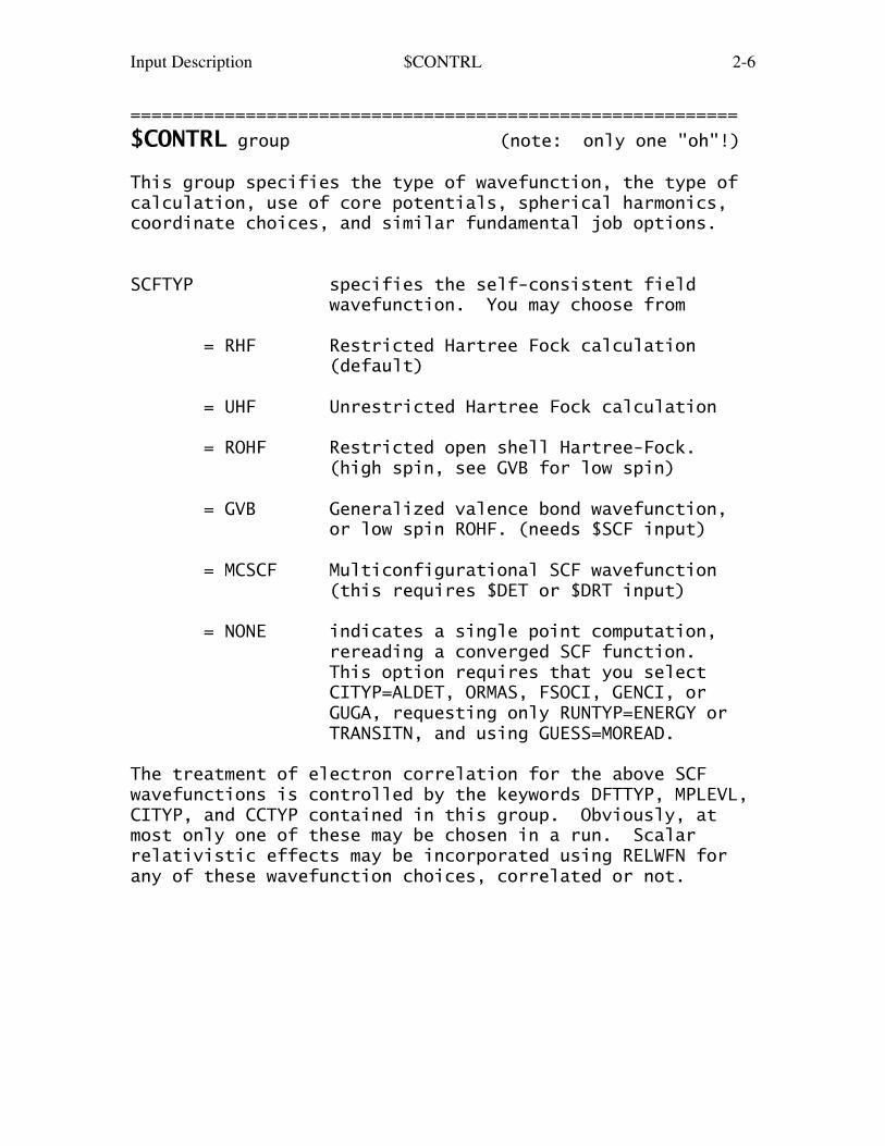
$CONTRL group (note: only one "oh"!)
This group specifies the type of wavefunction, the type ofcalculation, use of core potentials, spherical harmonics,coordinate choices, and similar fundamental job options.
SCFTYP specifies the self-consistent field wavefunction. You may choose from
= RHF Restricted Hartree Fock calculation (default)
= UHF Unrestricted Hartree Fock calculation
= ROHF Restricted open shell Hartree-Fock. (high spin, see GVB for low spin)
= GVB Generalized valence bond wavefunction, or low spin ROHF. (needs $SCF input)
= MCSCF Multiconfigurational SCF wavefunction (this requires $DET or $DRT input)
= NONE indicates a single point computation, rereading a converged SCF function. This option requires that you select CITYP=ALDET, ORMAS, FSOCI, GENCI, or GUGA, requesting only RUNTYP=ENERGY or TRANSITN, and using GUESS=MOREAD.
The treatment of electron correlation for the above SCFwavefunctions is controlled by the keywords DFTTYP, MPLEVL,CITYP, and CCTYP contained in this group. Obviously, atmost only one of these may be chosen in a run. Scalarrelativistic effects may be incorporated using RELWFN forany of these wavefunction choices, correlated or not.

Input Description $CONTRL 2-7
DFTTYP = NONE ab initio computation (default) = XXXXXX perform density functional theory run, using the functional specified. Many choices for XXXXXX are listed in the $DFT and $TDDFT input groups.
TDDFT = NONE no excited states (default) = EXCITE generate time-dependent DFT excitation energies, using the DFTTYP= functional, for RHF or UHF references. Analytic nuclear gradients are available for RHF. See $TDDFT. = SPNFLP spin-flip TD-DFT, for either UHF or ROHF references. Nuclear gradients are available for UHF. See $TDDFT.
* * * * *
MPLEVL = chooses Moller-Plesset perturbation theory level, after the SCF. See $MP2, or $MRMP for MCSCF. = 0 skip the MP computation (default) = 2 perform second order energy correction.
MP2 (a.k.a. MBPT(2)) is implemented for RHF, UHF, ROHF, andMCSCF wavefunctions, but not GVB. Gradients are availablefor RHF, UHF, or ROHF based MP2, but for MCSCF, you mustchoose numerical derivatives to use any RUNTYP other thanENERGY, TRUDGE, SURFACE, or FFIELD.
* * * * *
CITYP = chooses CI computation after the SCF, for any SCFTYP except UHF. = NONE skips the CI. (default) = CIS single excitations from a SCFTYP=RHF reference, only. This is for excited states, with analytic nuclear gradients available. See the $CIS input group. = SFCIS spin-flip style CIS, see $CIS input. = ALDET runs the Ames Laboratory determinant full CI package, requiring $CIDET. = ORMAS runs an Occupation Restricted Multiple Active Space determinant CI. The input
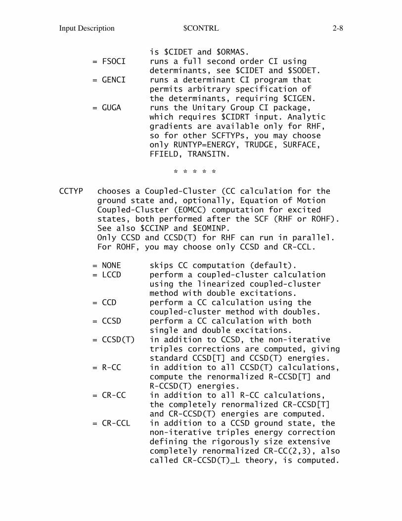
Input Description $CONTRL 2-8
is $CIDET and $ORMAS. = FSOCI runs a full second order CI using determinants, see $CIDET and $SODET. = GENCI runs a determinant CI program that permits arbitrary specification of the determinants, requiring $CIGEN. = GUGA runs the Unitary Group CI package, which requires $CIDRT input. Analytic gradients are available only for RHF, so for other SCFTYPs, you may choose only RUNTYP=ENERGY, TRUDGE, SURFACE, FFIELD, TRANSITN.
* * * * *
CCTYP chooses a Coupled-Cluster (CC calculation for the ground state and, optionally, Equation of Motion Coupled-Cluster (EOMCC) computation for excited states, both performed after the SCF (RHF or ROHF). See also $CCINP and $EOMINP. Only CCSD and CCSD(T) for RHF can run in parallel. For ROHF, you may choose only CCSD and CR-CCL.
= NONE skips CC computation (default). = LCCD perform a coupled-cluster calculation using the linearized coupled-cluster method with double excitations. = CCD perform a CC calculation using the coupled-cluster method with doubles. = CCSD perform a CC calculation with both single and double excitations. = CCSD(T) in addition to CCSD, the non-iterative triples corrections are computed, giving standard CCSD[T] and CCSD(T) energies. = R-CC in addition to all CCSD(T) calculations, compute the renormalized R-CCSD[T] and R-CCSD(T) energies. = CR-CC in addition to all R-CC calculations, the completely renormalized CR-CCSD[T] and CR-CCSD(T) energies are computed. = CR-CCL in addition to a CCSD ground state, the non-iterative triples energy correction defining the rigorously size extensive completely renormalized CR-CC(2,3), also called CR-CCSD(T)_L theory, is computed.
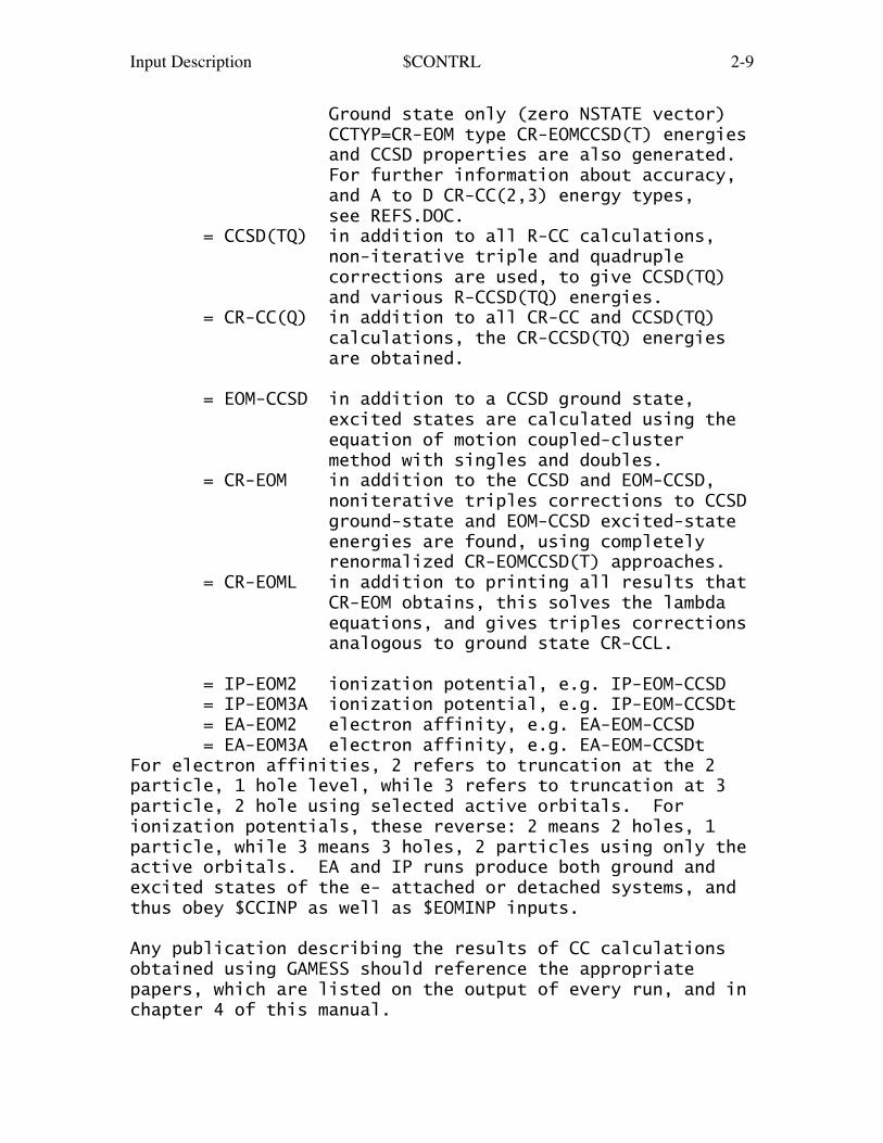
Input Description $CONTRL 2-9
Ground state only (zero NSTATE vector) CCTYP=CR-EOM type CR-EOMCCSD(T) energies and CCSD properties are also generated. For further information about accuracy, and A to D CR-CC(2,3) energy types, see REFS.DOC. = CCSD(TQ) in addition to all R-CC calculations, non-iterative triple and quadruple corrections are used, to give CCSD(TQ) and various R-CCSD(TQ) energies. = CR-CC(Q) in addition to all CR-CC and CCSD(TQ) calculations, the CR-CCSD(TQ) energies are obtained.
= EOM-CCSD in addition to a CCSD ground state, excited states are calculated using the equation of motion coupled-cluster method with singles and doubles. = CR-EOM in addition to the CCSD and EOM-CCSD, noniterative triples corrections to CCSD ground-state and EOM-CCSD excited-state energies are found, using completely renormalized CR-EOMCCSD(T) approaches. = CR-EOML in addition to printing all results that CR-EOM obtains, this solves the lambda equations, and gives triples corrections analogous to ground state CR-CCL.
= IP-EOM2 ionization potential, e.g. IP-EOM-CCSD = IP-EOM3A ionization potential, e.g. IP-EOM-CCSDt = EA-EOM2 electron affinity, e.g. EA-EOM-CCSD = EA-EOM3A electron affinity, e.g. EA-EOM-CCSDtFor electron affinities, 2 refers to truncation at the 2particle, 1 hole level, while 3 refers to truncation at 3particle, 2 hole using selected active orbitals. Forionization potentials, these reverse: 2 means 2 holes, 1particle, while 3 means 3 holes, 2 particles using only theactive orbitals. EA and IP runs produce both ground andexcited states of the e- attached or detached systems, andthus obey $CCINP as well as $EOMINP inputs.
Any publication describing the results of CC calculationsobtained using GAMESS should reference the appropriatepapers, which are listed on the output of every run, and inchapter 4 of this manual.
Input Description $CONTRL 2-10
Analytic gradients are not available, so use CCTYP only forRUNTYP=ENERGY, TRUDGE, SURFACE, or maybe FFIELD, or requestnumerical derivatives.
Generally speaking, the Renormalized energies are obtainedat similar cost to the standard values, while CompletelyRenormalized energies cost twice the time. For usage tipsand more information about resources on the various CoupledCluster methods, see Section 4, 'Further Information'.
* * * * *
RELWFN = NONE (default) See also the $RELWFN input group. = IOTC infinite-order two-component method of M. Barysz and A.J. Sadlej = DK Douglas-Kroll transformation, available at the 1st, 2nd, or 3rd order. = RESC relativistic elimination of small component, the method of T. Nakajima and K. Hirao, available at 2nd order only. = NESC normalised elimination of small component, the method of K. Dyall, 2nd order only.
* * * * *
RUNTYP specifies the type of computation, for example at a single geometry point:
= ENERGY Molecular energy. (default) = GRADIENT Molecular energy plus gradient. = HESSIAN Molecular energy plus gradient plus second derivatives, including harmonic harmonic vibrational analysis. See the $FORCE and $CPHF input groups. = GAMMA Evaluate up to 3rd nuclear derivatives, by finite differencing of Hessians. See $GAMMA, and also NFFLVL in $CONTRL.
multiple geometry options:
= OPTIMIZE Optimize the molecular geometry using analytic energy gradients. See $STATPT. = TRUDGE Non-gradient total energy minimization. See $TRUDGE and $TRURST.

Input Description $CONTRL 2-11
= SADPOINT Locate saddle point (transition state). See $STATPT. = MEX Locate minimum energy crossing point on the intersection seam of two potential energy surfaces. See $MEX. = CONICAL Locate conical intersection point on the intersection seam of two potential energy surfaces. See $CONICL. = IRC Follow intrinsic reaction coordinate. See $IRC. = VSCF anharmonic vibrational corrections. See $VSCF. = DRC Follow dynamic reaction coordinate. See $DRC. = MD molecular dynamics trajectory, see $MD. = GLOBOP Monte Carlo-type global optimization. See $GLOBOP. = OPTFMO genuine FMO geometry optimization using nearly analytic gradient. See $OPTFMO. = GRADEXTR Trace gradient extremal. See $GRADEX. = SURFACE Scan linear cross sections of the potential energy surface. See $SURF.
single geometry property options:
= G3MP2 evaluate heat of formation using the G3(MP2,CCSD(T)) methodology. See test example exam43.inp for more information. = PROP Properties will be calculated. A $DATA deck and converged $VEC deck should be input. Optionally, orbital localization can be done. See $ELPOT, etc. = RAMAN computes Raman intensities, see $RAMAN. = NACME non-adiabatic coupling matrix element between two or more state averaged MCSCF wavefunctions, of FORS/CAS type. The calculation has no special input group, but must use determinants (SCFTYP=MCSCF, using CISTEP=ALDET). = NMR NMR shielding tensors for closed shell molecules by the GIAO method. See $NMR. = EDA Perform energy decomposition analysis. Give one of $MOROKM or $LMOEDA inputs. = QMEFPEA QM/EFP solvent energy analysis, see $QMEFP.

Input Description $CONTRL 2-12
= TRANSITN Compute radiative transition moment or spin-orbit coupling. See $TRANST. = FFIELD applies finite electric fields, most commonly to extract polarizabilities. See $FFCALC. = TDHF analytic computation of time dependent polarizabilities. See $TDHF. = TDHFX extended TDHF package, including nuclear polarizability derivatives, and Raman and Hyper-Raman spectra. See $TDHFX. = MAKEFP creates an effective fragment potential, for SCFTYP=RHF or ROHF only. See $MAKEFP, $DAMP, $DAMPGS, $STONE, ... = FMO0 performs the free state FMO calculation. See $FMO.
* * * * * * * * * * * * * * * * * * * * * * * * * * * * * Note that RUNTYPs which require the nuclear gradient are GRADIENT, HESSIAN, OPTIMIZE, SADPOINT, GLOBOP, IRC, GRADEXTR, DRC, and RAMAN These are efficient with analytic gradients, which are available only for certain CI or MP2 calculations, but no CC calculations, as indicated above. See NUMGRD.* * * * * * * * * * * * * * * * * * * * * * * * * * * * *
NUMGRD Flag to allow numerical differentiation of the energy. Each gradient requires the energy be computed twice (forward and backward displacements) along each totally symmetric modes. It is thus recommended only for systems with just a few symmetry unique atoms in $DATA. The default is .FALSE.
EXETYP = RUN Actually do the run. (default) = CHECK Wavefunction and energy will not be evaluated. This lets you speedily check input and memory requirements. See the overview section for details. Note that you must set PARALL=.TRUE. in $SYSTEM to test distributed memory allocations. = DEBUG Massive amounts of output are printed, useful only if you hate trees. = routine Maximum output is generated by the

Input Description $CONTRL 2-13
routine named. Check the source for the routines this applies to.
* * * * * * *
ICHARG = Molecular charge. (default=0, neutral)
MULT = Multiplicity of the electronic state = 1 singlet (default) = 2,3,... doublet, triplet, and so on.
ICHARG and MULT are used directly for RHF, UHF, ROHF. For GVB, these are implicit in the $SCF input, while for MCSCF or CI, these are implicit in $DRT/$CIDRT or $DET/$CIDET input. You must still give them correctly.
* * * the next three control molecular geometry * * *
COORD = choice for molecular geometry in $DATA. = UNIQUE only the symmetry unique atoms will be given, in Cartesian coords (default). = HINT only the symmetry unique atoms will be given, in Hilderbrandt style internals. = PRINAXIS Cartesian coordinates will be input, and transformed to principal axes. Please read the warning just below!!! = ZMT GAUSSIAN style internals will be input. = ZMTMPC MOPAC style internals will be input. = FRAGONLY means no part of the system is treated by ab initio means, hence $DATA is not given. The system is defined by $EFRAG.
Note: the choices PRINAXIS, ZMT, ZMTMPC require input ofall atoms in the molecule. They also orient the molecule,and then determine which atoms are unique. Thereorientation is likely to change the order of the atomsfrom what you input. When the point group contains a 3-fold or higher rotation axis, the degenerate moments ofinertia often cause problems choosing correct symmetryunique axes, in which case you must use COORD=UNIQUE ratherthan Z-matrices.
Warning: The reorientation into principal axes is doneonly for atomic coordinates, and is not applied to the axisdependent data in the following groups: $VEC, $HESS, $GRAD,
Input Description $CONTRL 2-14
$DIPDR, $VIB, nor Cartesian coords of effective fragmentsin $EFRAG. COORD=UNIQUE avoids reorientation, and thus isthe safest way to read these.
Note: the choices PRINAXIS, ZMT, ZMTMPC require the useof a group named $BASIS to define the basis set. The firsttwo choices might or might not use $BASIS, as you wish.
UNITS = distance units, any angles must be in degrees. = ANGS Angstroms (default) = BOHR Bohr atomic units
NZVAR = 0 Use Cartesian coordinates (default). = M If COORD=ZMT or ZMTMPC, and $ZMAT is not given: the internal coordinates will be those defining the molecule in $DATA. In this case, $DATA may not contain any dummy atoms. M is usually 3N-6, or 3N-5 for linear. = M For other COORD choices, or if $ZMAT is given: the internal coordinates will be those defined in $ZMAT. This allows more sophisticated internal coordinate choices. M is ordinarily 3N-6 (3N-5), unless $ZMAT has linear bends.
NZVAR refers mainly to the coordinates used by OPTIMIZE or SADPOINT runs, but may also print the internal's values for other run types. You can use internals to define the molecule, but Cartesians during optimizations!
* * * * * * *
Pseudopotentials may be of two types: ECP (effective corepotentials) which generate nodeless valence orbitals, andMCP (model core potentials) producing valence orbitals withthe correct radial nodal structure. At present, ECPs haveanalytic nuclear gradients and Hessians, while MCPs haveanalytic nuclear gradients.
PP = pseudopotential selection. = NONE all electron calculation (default). = READ read ECP potentials in the $ECP group. = SBKJC use Stevens, Basch, Krauss, Jasien, Cundari ECP potentials for all heavy atoms (Li-Rn are available). = HW use Hay, Wadt ECP potentials for heavy

Input Description $CONTRL 2-15
atoms (Na-Xe are available). = MCP use Huzinaga's Model Core Potentials. The correct MCP potential will be chosen to match the requested MCP valence basis set (see $BASIS).
* * * * * * *
LOCAL = controls orbital localization. = NONE Skip localization (default). = BOYS Do Foster-Boys localization. = RUEDNBRG Do Edmiston-Ruedenberg localization. = POP Do Pipek-Mezey population localization. See the $LOCAL group. Localization does not work for SCFTYP=GVB or CITYP.
* * * * * * *
ISPHER = Spherical Harmonics option = -1 Use Cartesian basis functions to construct symmetry-adapted linear combination (SALC) of basis functions. The SALC space is the linear variation space used. (default) = 0 Use spherical harmonic functions to create SALC functions, which are then expressed in terms of Cartesian functions. The contaminants are not dropped, hence this option has EXACTLY the same variational space as ISPHER=-1. The only benefit to obtain from this is a population analysis in terms of pure s,p,d,f,g functions. = +1 Same as ISPHER=0, but the function space is truncated to eliminate all contaminant Cartesian functions [3S(D), 3P(F), 4S(G), and 3D(G)] before constructing the SALC functions. The computation corresponds to the use of a spherical harmonic basis.
QMTTOL = linear dependence threshhold Any functions in the SALC variational space whose eigenvalue of the overlap matrix is below this tolerence is considered to be linearly dependent. Such functions are dropped from the variational space. What is dropped is not individual basis functions, but rather some linear combination(s)

Input Description $CONTRL 2-16
of the entire basis set that represent the linear dependent part of the function space. The default is a reasonable value for most purposes, 1.0E-6.
When many diffuse functions are used, it is common to see the program drop some combinations. On occasion, in multi-ring molecules, we have raised QMTTOL to 3.0E-6 to obtain SCF convergence, at the cost of some energy.
MAXIT = Maximum number of SCF iteration cycles. This pertains only to RHF, UHF, ROHF, or GVB runs. See also MAXIT in $MCSCF. (default = 30)
* * * interfaces to other programs * * *
MOLPLT = flag that produces an input deck for a molecule drawing program distributed with GAMESS. (default is .FALSE.)
PLTORB = flag that produces an input deck for an orbital plotting program distributed with GAMESS. (default is .FALSE.)
AIMPAC = flag to create an input deck for Bader's Atoms In Molecules properties code. (default=.FALSE.) For information about this program, see the URL http://www.chemistry.mcmaster.ca/aimpac
FRIEND = string to prepare input to other quantum programs, choose from = HONDO for HONDO 8.2 = MELDF for MELDF = GAMESSUK for GAMESS (UK Daresbury version) = GAUSSIAN for Gaussian 9x = ALL for all of the above
PLTORB, MOLPLT, and AIMPAC decks are written to filePUNCH at the end of the job. Thus all of these correspondto the final geometry encountered during jobs such asOPTIMIZE, SAPDOINT, IRC...
In contrast, selecting FRIEND turns the job into aCHECK run only, no matter how you set EXETYP. Thus thegeometry is that encountered in $DATA. The input is

Input Description $CONTRL 2-17
added to the PUNCH file, and may require some (usuallyminimal) massaging.
PLTORB and MOLPLT are written even for EXETYP=CHECK.AIMPAC requires at least RUNTYP=PROP.
* * *
NFFLVL used to determine energies and gradients away from equilibrium structures, at the coordinates given in $DATA. The method will use a Taylor expansion of the potential surface around the stationary point. See $EQGEOM, $HLOWT, $GLOWT. This may be used with RUNTYP=ENERGY or GRADIENT. = 2 uses only Hessian information, which gives a reasonable energy, but not such a good gradient. = 3 uses Hessian and 3rd nuclear derivatives in the Taylor expansion, producing more accurate values for the energy and for the gradient.
* * * computation control switches * * *
For the most part, the default is the only sensiblevalue, and unless you are sure of what you are doing,these probably should not be touched.
NPRINT = Print/punch control flag See also EXETYP for debug info. (options -7 to 5 are primarily debug) = -7 Extra printing from Boys localization. = -6 debug for geometry searches = -5 minimal output = -4 print 2e-contribution to gradient. = -3 print 1e-contribution to gradient. = -2 normal printing, no punch file = 1 extra printing for basis,symmetry,ZMAT = 2 extra printing for MO guess routines = 3 print out property and 1e- integrals = 4 print out 2e- integrals = 5 print out SCF data for each cycle. (Fock and density matrices, current MOs = 6 same as 7, but wider 132 columns output. This option isn't perfect.

Input Description $CONTRL 2-18
= 7 normal printing and punching (default) = 8 more printout than 7. The extra output is (AO) Mulliken and overlap population analysis, eigenvalues, Lagrangians, ... = 9 everything in 8 plus Lowdin population analysis, final density matrix.
NOSYM = 0 the symmetry specified in $DATA is used as much as possible in integrals, SCF, gradients, etc. (this is the default) = 1 the symmetry specified in the $DATA group is used to build the molecule, then symmetry is not used again. Some GVB or MCSCF runs (those without a totally symmetric charge density) require you request no symmetry.
ETOLLZ = threshold to label molecular orbitals by Lz values. Small matrices of the Lz operator are diagonalized for the sets of MOs whose orbital energies are degenerate to within ETOLLZ. This option may be used in molecules with distorted linear symmetry for approximate labelling. Default: 1.0d-6 for linear, 0 (disable) if not.
INTTYP selects the integral package(s) used, all of which produce equally accurate results. This is therefore used only for debugging purposes. = BEST use the fastest integral code available for any particular shell quartet (default): s,p,L or s,p,d,L rotated axis code first. ERIC s,p,d,f,g precursor transfer equation code second, up to 5 units total ang. mom. Rys quadrature for general s,p,d,f,g,L, or for uncontracted quartets. = ROTAXIS means don't use ERIC at all, e.g. rotated axis codes, or else Rys quadrature. = ERIC means don't use rotated axis codes, e.g. ERIC code, or else Rys quadrature. = RYSQUAD means use Rys quadrature for everything.
GRDTYP = BEST use Schlegel routines for spL gradient blocks, and Rys quadrature for all other gradient integrals. (default) = RYSQUAD use Rys quadrature for all gradient
Input Description $CONTRL 2-19
integrals. This option is only slightly more accurate, but is rather slower.
NORMF = 0 normalize the basis functions (default) = 1 no normalization
NORMP = 0 input contraction coefficients refer to normalized Gaussian primitives. (default) = 1 the opposite.
ITOL = primitive cutoff factor (default=20) = n products of primitives whose exponential factor is less than 10**(-n) are skipped.
ICUT = n integrals less than 10.0**(-n) are not saved on disk. (default = 9). Direct SCF will calculate to a cutoff 1.0d-10 or 5.0d-11 depending on FDIFF=.F. or .T.
ISKPRP = 0 proceed as usual 1 skip computation of some properties which are not well parallelised. This includes bond orders and virial theorem, and can help parallel scalability if many CPUs are used. Note that NPRINT=-5 disables most property computations as well, so ISKPRP=1 has no effect in that case. (default: 0)
* * * restart options * * *
IREST = restart control options (for OPTIMIZE run restarts, see $STATPT) Note that this option is unreliable! = -1 reuse dictionary file from previous run, useful with GEOM=DAF and/or GUESS=MOSAVED. Otherwise, this option is the same as 0. = 0 normal run (default) = 1 2e restart (1-e integrals and MOs saved) = 2 SCF restart (1-,2-e integrls and MOs saved) = 3 1e gradient restart = 4 2e gradient restart
GEOM = select where to obtain molecular geometry = INPUT from $DATA input (default for IREST=0)

Input Description $CONTRL 2-20
= DAF read from DICTNRY file (default otherwise)
As noted in the first chapter, binary file restart isnot a well tested option!==========================================================

Input Description $SYSTEM 2-21
==========================================================
$SYSTEM group (optional)
This group provides global control information foryour computer's operation. This is system related input,and will not seem particularly chemical to you!
MWORDS = the maximum replicated memory which your job can use, on every node. This is given in units of 1,000,000 words (as opposed to 1024*1024 words), where a word is defined as 64 bits. (default=1) (In case finer control over the memory is needed, this value can be given in units of words with the old keyword MEMORY instead of MWORDS.)
MEMDDI = the grand total memory needed for the distributed data interface (DDI) storage, given in units of 1,000,000 words. See Chapter 5 of this manual for an extended explanation of running with MEMDDI.
note: the memory required on each processor for a run using p processors is therefore MEMDDI/p + MWORDS.
The parallel runs that currently require MEMDDI are: SCFTYP=RHF MPLEVL=2 energy or gradient SCFTYP=UHF MPLEVL=2 energy or gradient SCFTYP=ROHF MPLEVL=2 OSPT=ZAPT energy or gradient SCFTYP=MCSCF MPLEVL=2 energy SCFTYP=MCSCF using the FULLNR or JACOBI convergers SCFTYP=MCSCF analytic hessian SCFTYP=any CITYP=ALDET, ORMAS, GUGA SCFTYP=any energy localization SCFTYP=RHF CCTYP=CCSD or CCSD(T)All other parallel runs should enter MEMDDI=0, for they useonly replicated memory.Some serial runs execute the parallel code (on just 1 CPU),for there is only a parallel code. These serial runs mustgive MEMDDI as a result: SCFTYP=ROHF MPLEVL=2 OSPT=ZAPT gradient/property run SCFTYP=MCSCF analytic hessian
TIMLIM = time limit, in minutes. Set to about 95 percent of the time limit given to the batch job (if you use a queueing system) so that GAMESS can stop

Input Description $SYSTEM 2-22
itself gently. (default=525600.0 minutes)
PARALL = a flag to cause the distributed data parallel MP2 program to execute the parallel algorithm, even if you are running on only one node. The main purpose of this is to allow you to do EXETYP=CHECK runs to learn what the correct value of MEMDDI needs to be.
KDIAG = diagonalization control switch = 0 use a vectorized diagonalization routine if one is available on your machine, else use EVVRSP. (default) = 1 use EVVRSP diagonalization. This may be more accurate than KDIAG=0. = 2 use GIVEIS diagonalization (not as fast or reliable as EVVRSP) = 3 use JACOBI diagonalization (this is the slowest method)
COREFL = a flag to indicate whether or not GAMESS should produce a "core" file for debugging when subroutine ABRT is called to kill a job. This variable pertains only to UNIX operating systems. (default=.FALSE.)
BALTYP = Parallel load balance scheme: = SLB uses static load balancing. = DLB uses dynamic load balancing (default). Dynamic load balancing attempts to spread out possibly unequal work assignments based on the rate at which different nodes complete tasks. For historical reasons, it is permissible to spell SLB as LOOP, and DLB as NXTVAL.
MXSEQ2 = 300 (default)MXSEQ3 = 150 (default) Matrix/vector problem size in loops requiring either O(N**2) or O(N**3) work, respectively. Problems below these sizes are run purely serial, to avoid poor communication/computation ratios.
NODEXT = array specifying node extentions in GDDI for each file. Non-zero values force no extension. E.g., NODEXT(40)=1 forces file 40 (file numbers
Input Description $SYSTEM 2-23
are unit numbers used in GAMESS, see "rungms" or PROG.DOC) to have the name of $JOB.F40 on all nodes, rather than $JOB.F40, $JOB.F40.001, $JOB.F40.002 etc. This is convenient for FMO restart jobs, so that the file name need not be changed for each node, when copying the restart file. Note that on machines when several CPUs use the same directory (e.g., SMP) NODEXT should be zero. (default: all zeros)
IOSMP = Parallelise I/O on SMP machines with multiple hard disks. Two parameters are specified, whose meaning should be clear from the example. iosmp(1)=2,6 2 refers to the number of HDDs per SMP box. 6 is the location of the character in the file names that switches HDDs, i.e. if HDDs are mounted as /work1 and /work2, then 6 refers to the position of the number 1 in /work1. The file system should permit disks attached with directory names differing by one symbol. (default: 0,0, disable the feature)
==========================================================
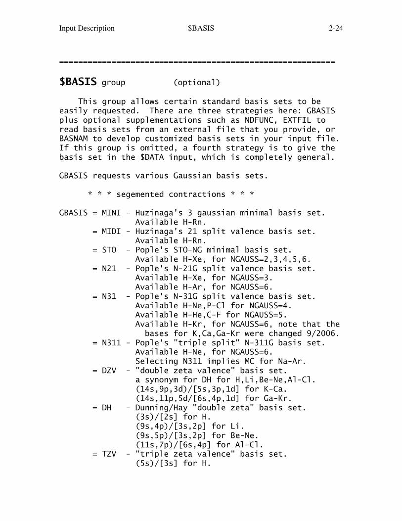
Input Description $BASIS 2-24
==========================================================
$BASIS group (optional)
This group allows certain standard basis sets to beeasily requested. There are three strategies here: GBASISplus optional supplementations such as NDFUNC, EXTFIL toread basis sets from an external file that you provide, orBASNAM to develop customized basis sets in your input file.If this group is omitted, a fourth strategy is to give thebasis set in the $DATA input, which is completely general.
GBASIS requests various Gaussian basis sets.
* * * segemented contractions * * *
GBASIS = MINI - Huzinaga's 3 gaussian minimal basis set. Available H-Rn. = MIDI - Huzinaga's 21 split valence basis set. Available H-Rn. = STO - Pople's STO-NG minimal basis set. Available H-Xe, for NGAUSS=2,3,4,5,6. = N21 - Pople's N-21G split valence basis set. Available H-Xe, for NGAUSS=3. Available H-Ar, for NGAUSS=6. = N31 - Pople's N-31G split valence basis set. Available H-Ne,P-Cl for NGAUSS=4. Available H-He,C-F for NGAUSS=5. Available H-Kr, for NGAUSS=6, note that the bases for K,Ca,Ga-Kr were changed 9/2006. = N311 - Pople's "triple split" N-311G basis set. Available H-Ne, for NGAUSS=6. Selecting N311 implies MC for Na-Ar. = DZV - "double zeta valence" basis set. a synonym for DH for H,Li,Be-Ne,Al-Cl. (14s,9p,3d)/[5s,3p,1d] for K-Ca. (14s,11p,5d/[6s,4p,1d] for Ga-Kr. = DH - Dunning/Hay "double zeta" basis set. (3s)/[2s] for H. (9s,4p)/[3s,2p] for Li. (9s,5p)/[3s,2p] for Be-Ne. (11s,7p)/[6s,4p] for Al-Cl. = TZV - "triple zeta valence" basis set. (5s)/[3s] for H.

Input Description $BASIS 2-25
(10s,3p)/[4s,3p] for Li. (10s,6p)/[5s,3p] for Be-Ne. a synonym for MC for Na-Ar. (14s,9p)/[8s,4p] for K-Ca. (14s,11p,6d)/[10s,8p,3d] for Sc-Zn. = MC - McLean/Chandler "triple split" basis. (12s,9p)/[6s,5p] for Na-Ar. Selecting MC implies 6-311G for H-Ne.
NGAUSS = the number of Gaussians (N). This parameter pertains only to GBASIS=STO, N21, N31, or N311.
Note: Polarization functions and/or diffuse functions areto be added separately to these GBASIS values, which defineonly the atom's occupied orbitals, with keywords such asNDFUNC and DIFFSP. Pople GBASIS keywords require NGAUSS.
* * * systematic basis set families * * *
GBASIS = CCn - Dunning-type Correlation Consistent basis sets, officially called cc-pVnZ. Use n = D,T,Q,5,6 to indicate the level of polarization. These provide a hierachy of basis sets suitable for recovering the correlation energy. Available for H-He, Li-Ne, Na-Ar, Ca, Ga-Kr and for Sc-Zn for n=T,Q. = ACCn - As CCn, but augmented with a set of diffuse functions, e.g. aug-cc-pVnZ. = CCnC - As CCn, but augmented with tight functions for recovering core and core-valence correlation, e.g. cc-pCVnZ. = ACCnC- As CCn, but augmented with both tight and diffuse functions, e.g. aug-cc-pCVnZ. = PCn - Jensen Polarization Consistent basis sets. n = 0,1,2,3,4 indicates the level of polarization. (n=0 is unpolarized, n=1 is DZP, n=2 is TZ2P, etc.). These provide a hierachy of basis sets suitable for DFT and HF calculations. Available H-Ar. = APCn - As PCn, but augmented with a set of diffuse functions. = SPK-nZP - Sapporo family of non-relativistic bases, n=D,T,Q, available H-Xe = SPK-AnZP - diffuse augmentation of the above.

Input Description $BASIS 2-26
= SPKrnZP - Sapporo family of relativistic bases n=D,T,Q, available H-Xe. These should be used only with a relativistic transformation of the integrals, such as RELWFN=IOTC or RELWFN=DK. These sets are identical to SPK-nZP up to Ar. = SPKrAnZP - diffuse augmentation of the above. = KTZV - Karlsruhe valence triple zeta basis, as developed by Prof.Ahlrichs, see REFS.DOC. = KTZVP- Karlsruhe valence triple zeta basis with a set of single polarization (P). = KTZVPP-Karlsruhe valence triple zeta basis with a set of double polarization (PP).
Important notes about CC and PC basis sets:
1. Normally these basis sets are used only as sphericalharmonics, see ISPHER=1 in $CONTRL. Failure to setISPHER=1 will result in a) discrepancies in energy results for this basis set, compared to the literature or other programs. b) probable difficulties in convergence of SCF/DFT or CCSD amplitude equations, due to linear dependency. c) longer run times in correlated methods due to the retention of unimportant MOs.2. The CC5, CC6, and PC4 basis sets (and correspondingaugmented versions) contain h-functions, and CC6 containsi-functions. As GAMESS' integral codes are currentlyrestricted to g-functions, these basis sets presently omitthese functions, and therefore are not the standard sets.3. The implementation of the cc-pVnZ basis sets for Al-Arinclude one additional tight d-function, producing the so-called cc-pV(n+d)Z sets, which is found (J.Chem.Phys. 114,9244(2001)) to improve the results. The same is true ofthe "aug-" counterpart. Note that the "core" versions ofthese elements (Al-Ar) don't have the extra d and should beregarded as inaccurate.4. Note that both the CC and PC basis sets are generallycontracted, which GAMESS can only handle by replicating theprimitive basis functions, leading to a less than optimumperformance in AO integral evaluation.5. In case you are interested in scalar relativisticeffects, the CCT-DK and CCQ-DK sets optimized for use withDouglas/Kroll are available for Sc-Kr. These will be usedif you type GBASIS=CCT or CCQ along with RELWFN=DK, using

Input Description $BASIS 2-27
NR sets for elements lighter than Sc. DK versions of ACCDor ACCT are available for Sc-Zn (but not Ga-Kr).
Notes about the Sapporo family:1. SPK is the international airport city code for Sapporo.2. These should be used only in spherical harmonic form.3. The relativistic bases were optimized at the 3rd orderof the Douglas-Kroll transformation, with a Gaussian nucleimodel, but can also be used with the infinite order two-component scheme IOTC (see RELWFN in $CONTRL). It would bevery illogical to use these all-electron relativistic baseswithout turning on scalar relativity!4. The basis sets were extracted from the data base ofSegmented Gaussian Basis Sets, maintained by Takeshi Noro,Quantum Chemistry Group, Sapporo, Japan: http://setani.sci.hokudai.ac.jp/sapporo/Welcome.doThe mapping between the data base names and the keywordsused in GAMESS is (for n=D,T,Q): data base name keyword Sapporo-nZP SPK-nZP Sapporo-nZP+diffuse SPK-AnZP Sapporo-DK-nZP SPKrnZP Sapporo-DK-nZP+diffuse SPKrAnZP
* * * Effective Core Potential (ECP) bases * * *
GBASIS = SBKJC- Stevens/Basch/Krauss/Jasien/Cundari valence basis set, for Li-Rn. This choice implies an unscaled -31G basis for H-He. = HW - Hay/Wadt valence basis. This is a -21 split, available Na-Xe, except for the transition metals. This implies a 3-21G basis for H-Ne.
* * * Model Core Potential (MCP) bases * * *
Notes: Select PP=MCP in $CONTRL to automatically use themodel core potential matching your basis choice below.References for these bases, and other information aboutMCPs can be found in the REFS.DOC chapter. Another familycovering almost all elements is available in $DATA only.
GBASIS = MCP-DZP, MCP-TZP, MCP-QZP - a family of double, triple, and quadruple zeta

Input Description $BASIS 2-28
quality valence basis sets, which are akin to the correlation consistent sets, in that these include increasing levels of polarization (and so do not require "supplements" like NDFUNC or DIFFSP) and must be used as spherical harmonics (see ISPHER). Availability: MCP-DZP: 56 elements Z=3-88, except V-Zn, Y-Cd, La, Hf-Hg MCP-TZP, MCP-QZP: 85 elements Z=3-88, except La The basis sets for hydrogen atoms will be the corresponding Dunning's cc-pVNZ (N=D,T,Q).
= MCP-ATZP, MCP-AQZP - MCP-TZP and MCP-QZP core potentials whose basis sets were augmented with diffuse functions Availability: same as for MCP-TZP, MCP-QZP
= MCPCDZP, MCPCTZP, MCPCQZP - based on MCP-DZP, MCP-TZP, MCP-QZP, with core-valence functions provided for the alkali and alkaline earth atoms Na through Ra.
= MCPACDZP, MCPACTZP, MCPACQZP - based on MCPCDZP, MCPCTZP, MCPCQZP, with core-valence functions provided for the alkali and alkaline earth atoms Na through Ra, and augmented with diffuse functions.
The basis sets were extracted from the data base SegmentedGaussian Basis Sets, maintained by Takeshi Noro, QuantumChemistry Group, Sapporo, Japan: http://setani.sci.hokudai.ac.jp/sapporo/Welcome.doThe mapping between the data base names and the names usedin GAMESS is data base name GAMESS keyword
MCP/NOSeC-V-DZP MCP-DZP MCP/NOSeC-V-TZP MCP-TZP MCP/NOSeC-V-QZP MCP-QZP
MCP/NOSeC-V-TZP+diffuse MCP-ATZP MCP/NOSeC-V-QZP+diffuse MCP-AQZP
MCP/NOSeC-CV-DZP MCPCDZP MCP/NOSeC-CV-TZP MCPCTZP

Input Description $BASIS 2-29
MCP/NOSeC-CV-QZP MCPCQZP
MCP/NOSeC-CV-DZP+diffuse MCPACDZP MCP/NOSeC-CV-TZP+diffuse MCPACTZP MCP/NOSeC-CV-QZP+diffuse MCPACQZP
GBASIS = IMCP-SR1 and IMCP-SR2 - valence basis sets to be used with the improved MCPs with scalar relativistic effects. These are available for transition metals except La, and the main group elements B-Ne, P-Ar, Ge, Kr, Sb, Xe, Rn. The 1 and 2 refer to addition of first and second polarization shells, so again don't use any of the "supplements" and do use spherical harmonics. = IMCP-NR1 and IMCP-NR2 - closely related valence basis sets, but with nonrelativistic model core potentials.
GBASIS = ZFK3-DK3, ZFK4-DK3, ZFK5-DK3, or ZFK3LDK3, ZFK4LDK3, ZFK5LDK3These are a family of model core potential basis setsdeveloped by Zeng/Fedorov/Klobukowski, for the p-blockelements from 2p to 6p. The potentials were paramaterizedtaking into account both DK3 scalar relativistic and DK-SOCeffects. The fundamental basis functions are from theWell-Tempered Basis Sets. The number after ZFK indicatesthe augmentation levels, e.g. ZFK3 means the diffusefunctions from aug-cc-pVTZ are added, ZFK4 means from aug-cc-pVQZ, etc. The difference between ZFKn-DK3 and ZFKnLDK3is that the common s and p exponents have been contractedas a single L-shell for the outermost s and p valenceshells to save time in the "L" case. The s-block elementsfrom 1s to 4s have also been put in the library. For H/He,all-electron aug-cc-pVnZ basis sets are used. For Li/Be,the relativistically contracted atomic natural orbital all-electron basis sets (ANO-RCC) are used. For Na/Mg, andK/Ca, unpublished MCP and basis sets based on ANO-RCC areavailable, although the potentials have not beenextensively tested yet. No d-block elements can be used.
* * * semiempirical basis sets * * *
GBASIS = MNDO - selects MNDO model hamiltonian
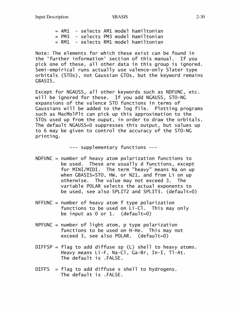
Input Description $BASIS 2-30
= AM1 - selects AM1 model hamiltonian = PM3 - selects PM3 model Hamiltonian = RM1 - selects RM1 model hamiltonian
Note: The elements for which these exist can be found inthe 'further information' section of this manual. If youpick one of these, all other data in this group is ignored.Semi-empirical runs actually use valence-only Slater typeorbitals (STOs), not Gaussian GTOs, but the keyword remainsGBASIS.
Except for NGAUSS, all other keywords such as NDFUNC, etc.will be ignored for these. If you add NGAUSS, STO-NGexpansions of the valence STO functions in terms ofGaussians will be added to the log file. Plotting programssuch as MacMolPlt can pick up this approximation to theSTOs used up from the ouput, in order to draw the orbitals.The default NGAUSS=0 suppresses this output, but values upto 6 may be given to control the accuracy of the STO-NGprinting.
--- supplementary functions ---
NDFUNC = number of heavy atom polarization functions to be used. These are usually d functions, except for MINI/MIDI. The term "heavy" means Na on up when GBASIS=STO, HW, or N21, and from Li on up otherwise. The value may not exceed 3. The variable POLAR selects the actual exponents to be used, see also SPLIT2 and SPLIT3. (default=0)
NFFUNC = number of heavy atom f type polarization functions to be used on Li-Cl. This may only be input as 0 or 1. (default=0)
NPFUNC = number of light atom, p type polarization functions to be used on H-He. This may not exceed 3, see also POLAR. (default=0)
DIFFSP = flag to add diffuse sp (L) shell to heavy atoms. Heavy means Li-F, Na-Cl, Ga-Br, In-I, Tl-At. The default is .FALSE.
DIFFS = flag to add diffuse s shell to hydrogens. The default is .FALSE.

Input Description $BASIS 2-31
Warning: if you use diffuse functions, please read QMTTOLin the $CONTRL group for numerical concerns.
POLAR = exponent of polarization functions = COMMON (default for GBASIS=STO,N21,HW,SBKJC) = POPN31 (default for GBASIS=N31) = POPN311 (default for GBASIS=N311, MC) = DUNNING (default for GBASIS=DH, DZV) = HUZINAGA (default for GBASIS=MINI, MIDI) = HONDO7 (default for GBASIS=TZV)
SPLIT2 = an array of splitting factors used when NDFUNC or NPFUNC is 2. Default=2.0,0.5
SPLIT3 = an array of splitting factors used when NDFUNC or NPFUNC is 3. Default=4.00,1.00,0.25
The splitting factors are from the Pople school, and areprobably too far apart. See for example the Binning andCurtiss paper. For example, the SPLIT2 value will usuallycause an INCREASE over the 1d energy at the HF level forhydrocarbons.
The actual exponents used for polarization functions, aswell as for diffuse sp or s shells, are described in the'Further References' section of this manual. This sectionalso describes the sp part of the basis set chosen byGBASIS fully, with all references cited.
Note that GAMESS always punches a full $DATA group. Thus,if $BASIS does not quite cover the basis you want, you canobtain this full $DATA group from EXETYP=CHECK, and thenchange polarization exponents, add Rydbergs, etc.
* * *
EXTFIL = a flag to read basis sets from an external file, defined by EXTBAS, rather than from a $DATA group. (default=.false.)
Except for MCP basis sets, no external file is providedwith GAMESS, thus you must create your own. The GBASISkeyword must give an 8 or less character string, obviously

Input Description $BASIS 2-32
not using any internally stored names. Every atom must bedefined in the external file by a line giving the chemicalsymbol, and this chosen string. Following this header line,give the basis in free format $DATA style, containing onlyS, P, D, F, G, and L shells, and terminating each atom bythe usual blank line. The external file may have severalfamilies of bases in the same file, identified by differentGBASIS strings.
* * *
This may only be used with COORD=UNIQUE or HINT!
BASNAM = an array of names of customized basis set input groups. Built in basis sets can be used as parts of the basis sets. Obey the rule of no more than six characters starting with letters in the names, and avoid using any standard group names.
This is best explained by an example where a core potentialis used only on a transition metal, not the ligands:
$contrl scftyp=rohf icharg=+3 mult=4 runtyp=gradient pp=read ispher=1 $end $system mwords=1 $end $guess guess=huckel $end $basis basnam(1)=metal, ligO,ligO,ligO,ligO,ligO,ligO, ligH,ligH,ligH,ligH,ligH,ligH, ligH,ligH,ligH,ligH,ligH,ligH $end $dataCr+3(H2O)6 complex...SBKJC & 6-31G(d) geometryTh
CHROMIUM 24.0 .0000000000 .0 .0000000000OXYGEN 8.0 .0000000000 .0 2.0398916104HYDROGEN 1.0 .7757887450 .0 2.6122732372 $end! core potential basis for Chromium $metalsbkjc
$end! normal 6-31G(d) for oxygen ligands $ligO

Input Description $BASIS 2-33
n31 6d 1 ; 1 0.8 1.0
$end! unpolarized basis for hydrogens $ligHn31 6
$end $ecpCr-ecp SBKJCO-ecp noneO-ecp noneO-ecp noneO-ecp noneO-ecp noneO-ecp noneH-ecp none ...snipped... there must be 12 H's given hereH-ecp none $end
=========================================================

Input Description $DATA 2-34
==========================================================
$DATA group (required)$DATAS group (if NESC chosen, for small component basis)$DATAL group (if NESC chosen, for large component basis)
This group describes the global molecular data such aspoint group symmetry, nuclear coordinates, and possiblythe basis set. It consists of a series of free formatcard images. See $RELWFN for more information on large andsmall component basis sets. The input structure of $DATASand $DATAL is identical to the COORD=UNIQUE $DATA input.
----------------------------------------------------------
-1- TITLE a single descriptive title card.
----------------------------------------------------------
-2- GROUP, NAXIS
GROUP is the Schoenflies symbol of the symmetry group,you may choose from C1, Cs, Ci, Cn, S2n, Cnh, Cnv, Dn, Dnh, Dnd, T, Th, Td, O, Oh.
NAXIS is the order of the highest rotation axis, andmust be given when the name of the group contains an N.For example, "Cnv 2" is C2v. "S2n 3" means S6. Use ofNAXIS up to 8 is supported in each axial groups.
For linear molecules, choose either Cnv or Dnh, and enterNAXIS as 4. Enter atoms as Dnh with NAXIS=2. If theelectronic state of either is degenerate, check the noteabout the effect of symmetry in the electronic statein the SCF section of REFS.DOC.
----------------------------------------------------------
In order to use GAMESS effectively, you must be ableto recognize the point group name for your molecule. Thispresupposes a knowledge of group theory at about the levelof Cotton's "Group Theory", Chapter 3.

Input Description $DATA 2-35
Armed with only the name of the group, GAMESS is ableto exploit the molecular symmetry throughout almost all ofthe program, and thus save a great deal of computer time.GAMESS does not require that you know very much else aboutgroup theory, although a deeper knowledge (charactertables, irreducible representations, term symbols, and soon) is useful when dealing with the more sophisticatedwavefunctions.
Cards -3- and -4- are quite complicated, and are rarelygiven. A *SINGLE* blank card may replace both cards -3-and -4-, to select the 'master frame', which is defined onthe next page. If you choose to enter a blank line, skipto one of the -5- input sequences.
Note!If the point group is C1 (no symmetry), skip over cards-3- and -4- (which means no blank card).
----------------------------------------------------------
-3- X1, Y1, Z1, X2, Y2, Z2
For C1 group, there is no card -3- or -4-.For CI group, give one point, the center of inversion.For CS group, any two points in the symmetry plane.For axial groups, any two points on the principal axis.For tetrahedral groups, any two points on a two-fold axis.For octahedral groups, any two points on a four-fold axis.
----------------------------------------------------------
-4- X3, Y3, Z3, DIRECT
third point, and a directional parameter.For CS group, one point of the symmetry plane, noncollinear with points 1 and 2.For CI group, there is no card -4-.
For other groups, a generator sigma-v plane (if any) isthe (x,z) plane of the local frame (CNV point groups).
A generator sigma-h plane (if any) is the (x,y) plane ofthe local frame (CNH and dihedral groups).
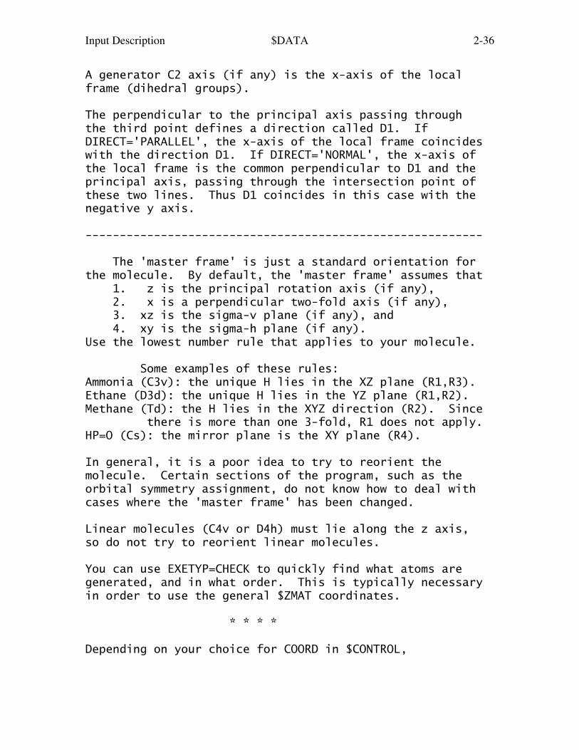
Input Description $DATA 2-36
A generator C2 axis (if any) is the x-axis of the localframe (dihedral groups).
The perpendicular to the principal axis passing throughthe third point defines a direction called D1. IfDIRECT='PARALLEL', the x-axis of the local frame coincideswith the direction D1. If DIRECT='NORMAL', the x-axis ofthe local frame is the common perpendicular to D1 and theprincipal axis, passing through the intersection point ofthese two lines. Thus D1 coincides in this case with thenegative y axis.
----------------------------------------------------------
The 'master frame' is just a standard orientation forthe molecule. By default, the 'master frame' assumes that 1. z is the principal rotation axis (if any), 2. x is a perpendicular two-fold axis (if any), 3. xz is the sigma-v plane (if any), and 4. xy is the sigma-h plane (if any).Use the lowest number rule that applies to your molecule.
Some examples of these rules:Ammonia (C3v): the unique H lies in the XZ plane (R1,R3).Ethane (D3d): the unique H lies in the YZ plane (R1,R2).Methane (Td): the H lies in the XYZ direction (R2). Since there is more than one 3-fold, R1 does not apply.HP=O (Cs): the mirror plane is the XY plane (R4).
In general, it is a poor idea to try to reorient themolecule. Certain sections of the program, such as theorbital symmetry assignment, do not know how to deal withcases where the 'master frame' has been changed.
Linear molecules (C4v or D4h) must lie along the z axis,so do not try to reorient linear molecules.
You can use EXETYP=CHECK to quickly find what atoms aregenerated, and in what order. This is typically necessaryin order to use the general $ZMAT coordinates.
* * * *
Depending on your choice for COORD in $CONTROL,

Input Description $DATA 2-37
if COORD=UNIQUE, follow card sequence U if COORD=HINT, follow card sequence U if COORD=CART, follow card sequence C if COORD=ZMT, follow card sequence G if COORD=ZMTMPC, follow card sequence M
Card sequence U is the only one which allows you to definea completely general basis here in $DATA.
Recall that UNIT in $CONTRL determines the distance units.
----------------------------------------------------------
-5U- Atom input. Only the symmetry unique atoms areinput, GAMESS will generate the symmetry equivalent atomsaccording to the point group selected above.
if COORD=UNIQUE NAME, ZNUC, X, Y, Z ***************
NAME = 10 character atomic name, used only for printout. Thus you can enter H or Hydrogen, or whatever.ZNUC = nuclear charge. It is the nuclear charge which actually defines the atom's identity.X,Y,Z = Cartesian coordinates.
if COORD=HINT *************
NAME,ZNUC,CONX,R,ALPHA,BETA,SIGN,POINT1,POINT2,POINT3
NAME = 10 character atomic name (used only for print out).ZNUC = nuclear charge.CONX = connection type, choose from 'LC' linear conn. 'CCPA' central conn. 'PCC' planar central conn. with polar atom 'NPCC' non-planar central conn. 'TCT' terminal conn. 'PTC' planar terminal conn. with torsionR = connection distance.ALPHA= first connection angleBETA = second connection angleSIGN = connection sign, '+' or '-'POINT1, POINT2, POINT3 = connection points, a serial number of a previously input atom, or one of 4 standard points: O,I,J,K
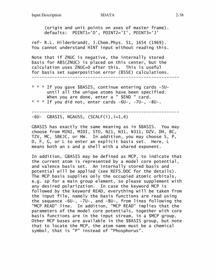
Input Description $DATA 2-38
(origin and unit points on axes of master frame). defaults: POINT1='O', POINT2='I', POINT3='J'
ref- R.L. Hilderbrandt, J.Chem.Phys. 51, 1654 (1969).You cannot understand HINT input without reading this.
Note that if ZNUC is negative, the internally storedbasis for ABS(ZNUC) is placed on this center, but thecalculation uses ZNUC=0 after this. This is usefulfor basis set superposition error (BSSE) calculations.----------------------------------------------------------
* * * If you gave $BASIS, continue entering cards -5U- until all the unique atoms have been specified. When you are done, enter a " $END " card.* * * If you did not, enter cards -6U-, -7U-, -8U-.
-----------------------------------------------------------6U- GBASIS, NGAUSS, (SCALF(i),i=1,4)
GBASIS has exactly the same meaning as in $BASIS. You maychoose from MINI, MIDI, STO, N21, N31, N311, DZV, DH, BC,TZV, MC, SBKJC, or HW. In addition, you may choose S, P,D, F, G, or L to enter an explicit basis set. Here, Lmeans both an s and p shell with a shared exponent.
In addition, GBASIS may be defined as MCP, to indicate thatthe current atom is represented by a model core potential,and valence basis set. An internally stored basis andpotential will be applied (see REFS.DOC for the details).The MCP basis supplies only the occupied atomic orbitals,e.g. sp for a main group element, so please supplement withany desired polarization. In case the keyword MCP isfollowed by the keyword READ, everything will be taken fromthe input file, namely the basis functions are read usingthe sequence -6U-, -7U-, and -8U-, from lines following the"MCP READ" line. In addition, "MCP READ" implies that theparameters of the model core potentials, together with corebasis functions are in the input stream, in a $MCP group.Other MCP bases are available in the $BASIS group, but notethat to locate the MCP, the atom name must be a chemicalsymbol, that is "P" instead of "Phosphorus".

Input Description $DATA 2-39
NGAUSS is the number of Gaussians (N) in the Pople stylebasis, or user input general basis. It has meaning onlyfor GBASIS=STO, N21, N31, or N311, and S,P,D,F,G, or L.
Up to 4 scale factors may be entered. If omitted, standardvalues are used. They are not documented as every GBASIStreats these differently. Read the source code if you needto know more. They are seldom given.----------------------------------------------------------
* * * If GBASIS is not S,P,D,F,G, or L, either add more shells by repeating card -6U-, or go on to -8U-.* * * If GBASIS=S,P,D,F,G, or L, enter NGAUSS cards -7U-.
-----------------------------------------------------------7U- IG, ZETA, C1, C2
IG = a counter, IG takes values 1, 2, ..., NGAUSS. ZETA = Gaussian exponent of the IG'th primitive. C1 = Contraction coefficient for S,P,D,F,G shells, and for the s function of L shells. C2 = Contraction coefficient for the p in L shells.----------------------------------------------------------
* * * For more shells on this atom, go back to card -6U-.* * * If there are no more shells, go on to card -8U-.
-----------------------------------------------------------8U- A blank card ends the basis set for this atom.----------------------------------------------------------
Continue entering atoms with -5U- through -8U- until allare given, then terminate the group with a " $END " card.
--- this is the end of card sequence U ---
COORD=CART input:
----------------------------------------------------------
-5C- Atom input.
Cartesian coordinates for all atoms must be entered. Theymay be arbitrarily rotated or translated, but must possessthe actual point group symmetry. GAMESS will reorient the

Input Description $DATA 2-40
molecule into the 'master frame', and determine whichatoms are the unique ones. Thus, the final order of theatoms may be different from what you enter here.
NAME, ZNUC, X, Y, Z
NAME = 10 character atomic name, used only for printout. Thus you can enter H or Hydrogen, or whatever.ZNUC = nuclear charge. It is the nuclear charge which actually defines the atom's identity.X,Y,Z = Cartesian coordinates.
----------------------------------------------------------
Continue entering atoms with card -5C- until all aregiven, and then terminate the group with a " $END " card.
--- this is the end of card sequence C ---
COORD=ZMT input: (GAUSSIAN style internals)
----------------------------------------------------------
-5G- ATOM
Only the name of the first atom is required.See -8G- for a description of this information.----------------------------------------------------------
-6G- ATOM i1 BLENGTH
Only a name and a bond distance is required for atom 2.See -8G- for a description of this information.----------------------------------------------------------
-7G- ATOM i1 BLENGTH i2 ALPHA
Only a name, distance, and angle are required for atom 3.See -8G- for a description of this information.----------------------------------------------------------
-8G- ATOM i1 BLENGTH i2 ALPHA i3 BETA i4
ATOM is the chemical symbol of this atom. It can be followed by numbers, if desired, for example Si3.

Input Description $DATA 2-41
The chemical symbol implies the nuclear charge.i1 defines the connectivity of the following bond.BLENGTH is the bond length "this atom-atom i1".i2 defines the connectivity of the following angle.ALPHA is the angle "this atom-atom i1-atom i2".i3 defines the connectivity of the following angle.BETA is either the dihedral angle "this atom-atom i1- atom i2-atom i3", or perhaps a second bond angle "this atom-atom i1-atom i3".i4 defines the nature of BETA, If BETA is a dihedral angle, i4=0 (default). If BETA is a second bond angle, i4=+/-1. (sign specifies one of two possible directions).----------------------------------------------------------
o Repeat -8G- for atoms 4, 5, ... o The use of ghost atoms is possible, by using X or BQ for the chemical symbol. Ghost atoms preclude the option of an automatic generation of $ZMAT. o The connectivity i1, i2, i3 may be given as integers, 1, 2, 3, 4, 5,... or as strings which match one of the ATOMs. In this case, numbers must be added to the ATOM strings to ensure uniqueness! o In -6G- to -8G-, symbolic strings may be given in place of numeric values for BLENGTH, ALPHA, and BETA. The same string may be repeated, which is handy in enforcing symmetry. If the string is preceeded by a minus sign, the numeric value which will be used is the opposite, of course. Any mixture of numeric data and symbols may be given. If any strings were given in -6G- to -8G-, you must provide cards -9G- and -10G-, otherwise you may terminate the group now with a " $END " card.
----------------------------------------------------------
-9G- A blank line terminates the Z-matrix section.
----------------------------------------------------------
-10G- STRING VALUE
STRING is a symbolic string used in the Z-matrix.VALUE is the numeric value to substitute for that string.

Input Description $DATA 2-42
----------------------------------------------------------
Continue entering -10G- until all STRINGs are defined.Note that any blank card encountered while reading -10G-will be ignored. GAMESS regards all STRINGs as variables(constraints are sometimes applied in $STATPT). It is notnecessary to place constraints to preserve point groupsymmetry, as GAMESS will never lower the symmetry fromthat given at -2-. When you have given all STRINGs aVALUE, terminate the group with a " $END " card.
--- this is the end of card sequence G ---
* * * *
The documentation for sequence G above and sequence Mbelow presumes you are reasonably familiar with the inputto GAUSSIAN or MOPAC. It is probably too terse to beunderstood very well if you are unfamiliar with these. Agood tutorial on both styles of Z-matrix input can befound in Tim Clark's book "A Handbook of ComputationalChemistry", published by John Wiley & Sons, 1985.
Both Z-matrix input styles must generate a moleculewhich possesses the symmetry you requested at -2-. Ifnot, your job will be terminated automatically.
COORD=ZMTMPC input: (MOPAC style internals)
----------------------------------------------------------
-5M- ATOM
Only the name of the first atom is required.See -8M- for a description of this information.----------------------------------------------------------
-6M- ATOM BLENGTH
Only a name and a bond distance is required for atom 2.See -8M- for a description of this information.----------------------------------------------------------
-7M- ATOM BLENGTH j1 ALPHA j2
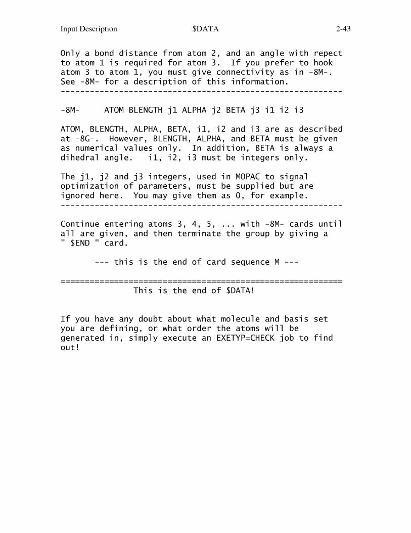
Input Description $DATA 2-43
Only a bond distance from atom 2, and an angle with repectto atom 1 is required for atom 3. If you prefer to hookatom 3 to atom 1, you must give connectivity as in -8M-.See -8M- for a description of this information.----------------------------------------------------------
-8M- ATOM BLENGTH j1 ALPHA j2 BETA j3 i1 i2 i3
ATOM, BLENGTH, ALPHA, BETA, i1, i2 and i3 are as describedat -8G-. However, BLENGTH, ALPHA, and BETA must be givenas numerical values only. In addition, BETA is always adihedral angle. i1, i2, i3 must be integers only.
The j1, j2 and j3 integers, used in MOPAC to signaloptimization of parameters, must be supplied but areignored here. You may give them as 0, for example.----------------------------------------------------------
Continue entering atoms 3, 4, 5, ... with -8M- cards untilall are given, and then terminate the group by giving a" $END " card.
--- this is the end of card sequence M ---
========================================================== This is the end of $DATA!
If you have any doubt about what molecule and basis setyou are defining, or what order the atoms will begenerated in, simply execute an EXETYP=CHECK job to findout!
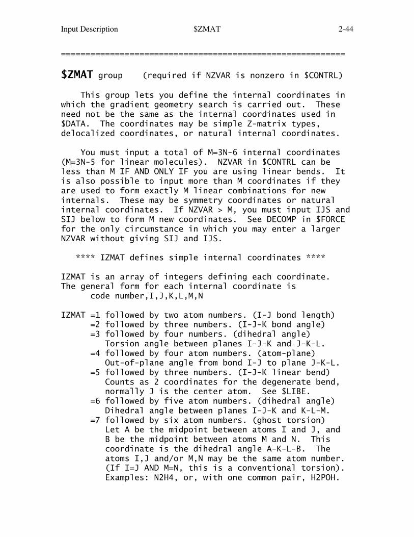
Input Description $ZMAT 2-44
==========================================================
$ZMAT group (required if NZVAR is nonzero in $CONTRL)
This group lets you define the internal coordinates inwhich the gradient geometry search is carried out. Theseneed not be the same as the internal coordinates used in$DATA. The coordinates may be simple Z-matrix types,delocalized coordinates, or natural internal coordinates.
You must input a total of M=3N-6 internal coordinates(M=3N-5 for linear molecules). NZVAR in $CONTRL can beless than M IF AND ONLY IF you are using linear bends. Itis also possible to input more than M coordinates if theyare used to form exactly M linear combinations for newinternals. These may be symmetry coordinates or naturalinternal coordinates. If NZVAR > M, you must input IJS andSIJ below to form M new coordinates. See DECOMP in $FORCEfor the only circumstance in which you may enter a largerNZVAR without giving SIJ and IJS.
**** IZMAT defines simple internal coordinates ****
IZMAT is an array of integers defining each coordinate.The general form for each internal coordinate is code number,I,J,K,L,M,N
IZMAT =1 followed by two atom numbers. (I-J bond length) =2 followed by three numbers. (I-J-K bond angle) =3 followed by four numbers. (dihedral angle) Torsion angle between planes I-J-K and J-K-L. =4 followed by four atom numbers. (atom-plane) Out-of-plane angle from bond I-J to plane J-K-L. =5 followed by three numbers. (I-J-K linear bend) Counts as 2 coordinates for the degenerate bend, normally J is the center atom. See $LIBE. =6 followed by five atom numbers. (dihedral angle) Dihedral angle between planes I-J-K and K-L-M. =7 followed by six atom numbers. (ghost torsion) Let A be the midpoint between atoms I and J, and B be the midpoint between atoms M and N. This coordinate is the dihedral angle A-K-L-B. The atoms I,J and/or M,N may be the same atom number. (If I=J AND M=N, this is a conventional torsion). Examples: N2H4, or, with one common pair, H2POH.

Input Description $ZMAT 2-45
Example - a nonlinear triatomic, atom 2 in the middle: $ZMAT IZMAT(1)=1,1,2, 2,1,2,3, 1,2,3 $ENDThis sets up two bonds and the angle between them.The blanks between each coordinate definition arenot necessary, but improve readability mightily.
**** the next define delocalized coordinates ****
DLC is a flag to request delocalized coordinates. (default is .FALSE.)
AUTO is a flag to generate all redundant coordinates, automatically. The DLC space will consist of all non-redundant combinations of these which can be found. The list of redundant coordinates will consist of bonds, angles, and torsions only. (default is .FALSE.)
NONVDW is an array of atom pairs which are to be joined by a bond, but might be skipped by the routine that automatically includes all distances shorter than the sum of van der Waals radii. Any angles and torsions associated with the new bond(s) are also automatically included.
The format for IXZMAT, IRZMAT, IFZMAT is that of IZMAT:
IXZMAT is an extra array of simple internal coordinates which you want to have added to the list generated by AUTO. Unlike NONVDW, IXZMAT will add only the coordinate(s) you specify.
IRZMAT is an array of simple internal coordinates which you would like to remove from the AUTO list of redundant coordinates. It is sometimes necessary to remove a torsion if other torsions around a bond are being frozen, to obtain a nonsingular G matrix.
IFZMAT is an array of simple internal coordinates which you would like to freeze. See also FVALUE below, which is required input when IFZMAT is given. IFZMAT/FVALUE work with ordinary coordinate input using IZMAT, as well as with DLC, but in the former

Input Description $ZMAT 2-46
case be careful that IFZMAT specifies coordinates that were already given in IZMAT. In addition, IFZMAT works only for IZMAT=1,2,3 type coordinates. See IFREEZ in $STATPT you wish to freeze regular or natural internal coordinates.
FVALUE is an array of values to which the internal coordinates should be constrained. It is not necessary to input $DATA such that the initial values match these desired final values, but it is helpful if the initial values are not too far away.
**** SIJ,IJS define natural internal coordinates ****
SIJ is a transformation matrix of dimension NZVAR x M, used to transform the NZVAR internal coordinates in IZMAT into M new internal coordinates. SIJ is a sparse matrix, so only the non-zero elements are given, by using the IJS array described below. The columns of SIJ will be normalized by GAMESS. (Default: SIJ = I, unit matrix)
IJS is an array of pairs of indices, giving the row and column index of the entries in SIJ.
example - if the above triatomic is water, using IJS(1) = 1,1, 3,1, 1,2, 3,2, 2,3 SIJ(1) = 1.0, 1.0, 1.0,-1.0, 1.0
gives the matrix S= 1.0 1.0 0.0 0.0 0.0 1.0 1.0 -1.0 0.0
which defines the symmetric stretch, asymmetric stretch,and bend of water.
references for natural internal coordinates: P.Pulay, G.Fogarasi, F.Pang, J.E.Boggs J.Am.Chem.Soc. 101, 2550-2560(1979) G.Fogarasi, X.Zhou, P.W.Taylor, P.Pulay J.Am.Chem.Soc. 114, 8191-8201(1992)reference for delocalized coordinates: J.Baker, A. Kessi, B.Delley J.Chem.Phys. 105, 192-212(1996)

Input Description $ZMAT 2-47
==========================================================

Input Description $LIBE 2-48
==========================================================
$LIBE group (required if linear bends are used in $ZMAT)
A degenerate linear bend occurs in two orthogonal planes,which are specified with the help of a point A. The firstbend occurs in a plane containing the atoms I,J,K and theuser input point A. The second bend is in the planeperpendicular to this, and containing I,J,K. One suchpoint must be given for each pair of bends used.
APTS(1)= x1,y1,z1,x2,y2,z2,... for linear bends 1,2,...
Note that each linear bend serves as two coordinates, sothat if you enter 2 linear bends (HCCH, for example), thecorrect value of NZVAR is M-2, where M=3N-6 or 3N-5, asappropriate.
==========================================================
Input Description $SCF 2-49
==========================================================
$SCF group relevant if SCFTYP = RHF, UHF, or ROHF, required if SCFTYP = GVB)
This group of parameters provides additional controlover the RHF, UHF, ROHF, or GVB SCF steps. It must begiven to define GVB open shell or perfect pairingwavefunctions. See $MCSCF for multireference inputs.
DIRSCF = a flag to activate a direct SCF calculation, which is implemented for all the Hartree-Fock type wavefunctions: RHF, ROHF, UHF, and GVB. This keyword also selects direct MP2 computation. The default of .FALSE. stores integrals on disk storage for a conventional SCF calculation.
FDIFF = a flag to compute only the change in the Fock matrices since the previous iteration, rather than recomputing all two electron contributions. This saves much CPU time in the later iterations. This pertains only to direct SCF, and has a default of .TRUE. This option is implemented only for the RHF, ROHF, UHF cases.
Cases with many diffuse functions in the basis set, or large molecules, may sometimes be "mushy" at the end, rather than converging. Increasing ICUT in $CONTRL by one may help this, or consider turning this parameter off.
---- The next flags affect convergence rates.
NOCONV = .TRUE. means neither SOSCF nor DIIS will be used. The default is .FALSE., making the choice of the primary converger as follows: for RHF, GVB, UHF, or ROHF (if Abelian): SOSCF for any DFT, or for non-Abelian groups: DIIS.DIIS = selects Pulay's DIIS interpolation.SOSCF = selects second order SCF orbital optimization.
Once either DIIS or SOSCF are initiated, the followingless important accelerators are placed in abeyance:
EXTRAP = selects Pople extrapolation of the Fock matrix.
Input Description $SCF 2-50
DAMP = selects Davidson damping of the Fock matrix.SHIFT = selects level shifting of the Fock matrix.RSTRCT = selects restriction of orbital interchanges.DEM = selects direct energy minimization, which is implemented only for RHF. (default=.FALSE.)
defaults for EXTRAP DAMP SHIFT RSTRCT DIIS SOSCFab initio: T F F F F/T T/Fsemiempirical: T F F F F F
The above parameters are implemented for all SCFwavefunction types, except that DIIS will work for GVB onlyfor those cases with NPAIR=0 or NPAIR=1.
---- These parameters fine tune the various convergers.
CONV = SCF density convergence criteria. Convergence is reached when the density change between two consecutive SCF cycles is less than this in absolute value. One more cycle will be executed after reaching convergence. Less accuracy in CONV gives questionable gradients. The default is 1.0d-05, except runs involving CI, MP2, CC, or TDDFT use 1.0d-06 to obtain more crisply converged virtual orbitals.
SOGTOL = second order gradient tolerance. SOSCF will be initiated when the orbital gradient falls below this threshold. (default=0.25 au)
ETHRSH = energy error threshold for initiating DIIS. The DIIS error is the largest element of e=FDS-SDF. Increasing ETHRSH forces DIIS on sooner. (default = 0.5 Hartree)
MAXDII = Maximum size of the DIIS linear equations, so that at most MAXDII-1 Fock matrices are used in the interpolation. (default=10)
SWDIIS = density matrix convergence at which to switch from DIIS to SOSCF. A value of zero means to keep using DIIS at all geometries, which is the default. However, it may be useful to have DIIS work only at the first geometry, in the

Input Description $SCF 2-51
initial iterations, for example transition metal ECP runs which has a less good Huckel guess, and then use SOSCF for the final SCF iterations at the first geometry, and ever afterwards. A suggested usage might be DIIS=.TRUE. ETHRSH=2.0 SWDIIS=0.005. This option is not programmed for GVB.
DEMCUT = Direct energy minimization will not be done once the density matrix change falls below this threshold. (Default=0.5)
DMPCUT = Damping factor lower bound cutoff. The damping damping factor will not be allowed to drop below this value. (default=0.0)note: The damping factor need not be zero to achieve validconvergence (see Hsu, Davidson, and Pitzer, J.Chem.Phys.,65, 609 (1976), see the section on convergence control),but it should not be astronomical either.
* * * * * * * * * * * * * * * * * * * * * For more info on the convergence methods, see the 'Further Information' section. * * * * * * * * * * * * * * * * * * * * *
---- orbital modification options ----
The four options UHFNOS, VVOS, MVOQ, and ACAVO aremutually exclusive. The latter 3 require RUNTYP=ENERGY,and should not be used with any correlation treatment.
UHFNOS = flag controlling generation of the natural orbitals of a UHF function. (default=.FALSE.)
VVOS = flag controlling generation of Valence Virtual Orbitals. See J.Chem.Phys. 120, 2629-2637(2004).VVOs are a quantitative realization of the concept of"lowest unoccupied orbital" and are also useful for MCSCFstarting orbitals. The implementation at present allowsonly RHF functions, elements up to Xe (excluding transitionmetals), and core potentials may not be used. The defaultis .FALSE. VVOS should be better MCSCF starting orbitalsthan either MVOQ or ACAVO type virtuals.
MVOQ = 0 Skip MVO generation (default)

Input Description $SCF 2-52
= n Form modified virtual orbitals, using a cation with n electrons removed. Implemented for RHF, ROHF, and GVB. If necessary to reach a closed shell cation, the program might remove n+1 electrons. Typically, n will be about 6. = -1 The cation used will have each valence orbital half filled, to produce MVOs with valence-like character in all regions of the molecule. Implemented for RHF and ROHF only.
ACAVO = Flag to request Approximate Correlation-Adapted Virtual Orbitals. Implemented for RHF, ROHF, and GVB (w/o direct SCF). Default is .FALSE.
PACAVO = Parameters used to define the ACAVO generating operator, which is defined as a*T + b*Vne + c*Jcore + d*Jval + e*Kcore + f*KvalThe default, PACAVO(1)=0,0,0,0,0,-1, maximizes the exchangeinteraction with valence MOs (see for example J.L.Whitten,J.Chem.Phys. 56, 5458-5466(1972).The K-orbitals of D.Feller, E.R.Davidson J.Chem.Phys. 74,3977-3979 are PACAVO(1)= 0.06,0.06,0.12,0.12,-0.06,-1.06,which is 0.06*F-K(valence).Of course, canonical virtuals are PACAVO(1)=1,1,2,2,-1,-1.
----- GVB wavefunction input -----
The next parameters define the GVB wavefunction. Seealso MULT in the $CONTRL group. The GVB wavefunctionassumes orbitals are in the order core, open, pairs.
NCO = The number of closed shell orbitals. The default almost certainly should be changed! (default=0).
NSETO = The number of sets of open shells in the function. Maximum of 10. (default=0)
NO = An array giving the degeneracy of each open shell set. Give NSETO values. (default=0,0,0,...).
NPAIR = The number of geminal pairs in the -GVB- function. Maximum of 12. The default corresponds to open shell SCF (default=0).

Input Description $SCF 2-53
CICOEF = An array of ordered pairs of CI coefficients for the -GVB- pairs. (default = 0.90,-0.20,0.90,-0.20,...)For example, a two pair case for water, say, might beCICOEF(1)=0.95,-0.05,0.95,-0.05. If not normalized, as inthe default, CICOEF will be. This parameter is useful inrestarting a GVB run, with the current CI coefficients.
COUPLE = A switch controlling the input of F, ALPHA, and BETA. (Default=.FALSE.)Input for F, ALPHA, BETA will be ignored unless you selectthis variable as .TRUE.
F = An vector of fractional shell occupations.
ALPHA = An array of A coupling coefficients, given in lower triangular order.
BETA = An array of B coupling coefficients, given in lower triangular order.
Note: The default for F, ALPHA, and BETA depends onthe state chosen. Defaults for the most commonly occuringcases are internally stored. See "Further Information" forother cases, including degenerate open shells. Note: ALPHA and BETA can be given for -ROHF- orbitalcanonicalization control, see "Further Information".
----- miscellaneous options -----
NPUNCH = option for output to the PUNCH file = 0 do not punch out the final orbitals = 1 punch out the occupied orbitals = 2 punch out occupied and virtual orbitals The default is NPUNCH = 2.
NPREO = energy and orbital printing options, applying after other output options, for example NPRINT=-5 for no orbital output overrules this keyword. Orbitals from NPREO(1) to NPREO(2) and orbital energies from NPREO(3) to NPREO(4) are printed. Positive values indicate plain ordinal numbers. Non-positive values are relative to HOMO. For NPREO(1) and (3), 0 is HOMO, -1 is HOMO+1 etc.

Input Description $SCF 2-54
For NPREO(2) and (4), 0 is HOMO, -1 is HOMO+1 etc. Numbers exceeding the total orbital count are automatically adjusted to the maximum value. Orbitals printed by NPREO(1) and NPREO(2) will always have the orbital energy labels attached, NPREO(3) to NPREO(4) define separate print-out of the orbital energies. HOMO here means the highest occupied orbital, assuming a singlet RHF orbital occupation, that is to say NE/2, no matter what SCFTYP is. To print only the HOMO and LUMO LCAO coefficients. and all orbital energies, enter: NPREO(1)=0,-1,1,9999 Default: 1,9999,2,1 (meaning print all orbitals, but no separate list of orbital energies).
----- options for virial scaling -----
VTSCAL = A flag to request that the virial theorem be satisfied. An analysis of the total energy as an exact sum of orbital kinetic energies is printed. The default is .FALSE.This option is implemented for RHF, UHF, and ROHF, forRUNTYP=ENERGY, OPTIMIZE, or SADPOINT. Related input is:
SCALF = initial exponent scale factor when VTSCAL is in use, useful when restarting. The default is 1.0.
MAXVT = maximum number of iterations (at a single geometry) to satisfy the energy virial theorem. The default is 20.
VTCONV = convergence criterion for the VT, which is satisfied when 2<T> + <V> + R x dE/dR is less than VTCONV. The default is 1.0D-6 Hartree.
For more information on this option, which is most usefulduring a geometry search, see M.Lehd and F.Jensen,J.Comput.Chem. 12, 1089-1096(1991).
* * * * * * * * * * * * * * * * * * * For more discussion of GVB/ROHF input see the 'further information' section

Input Description $SCF 2-55
* * * * * * * * * * * * * * * * * * *
==========================================================

Input Description $SCFMI 2-56
==========================================================
$SCFMI group (optional, relevant if SCFTYP=RHF)
The Self Consistent Field for Molecular Interactions(SCF-MI) method is a modification of the usual Roothaanequations that avoids basis set superposition error (BSSE)in intermolecular interaction calculations, by expandingeach monomer's orbitals using only its own basis set.Thus, the resulting orbitals are not orthogonal. Thepresence of a $SCFMI group in the input triggers the useof this option.
The implementation is limited to ten monomers, treatedat the RHF level. The energy, gradient, and thereforesemi-numerical hessian are available. The SCF step may berun in direct SCF mode, and parallel calculation is alsoenabled. The calculation must use Cartesian Gaussian AOsonly, not spherical harmonics. The SCF-MI driver differsfrom normal RHF calculations, so not all converger methodsare available. Finally, this option is not compatible withelectron correlation treatments (DFT, MP2, CI, or CC).
The first 3 parameters must be given. All atoms of afragment must appear consecutively in $DATA.
NFRAGS = number of distinct fragments present. Both the supermolecule and its constituent monomers must be well described as closed shells by RHF wavefunctions.
NF = an array containing the number of doublyoccupied MOs for each fragment.
MF = an array containing the number of atomic basis functions located on each fragment.
ITER = maximum number of SCF-MI cycles, overriding the usual MAXIT value. (default is 50).
DTOL = SCF-MI density convergence criteria. (default is 1.0d-10)

Input Description $SCFMI 2-57
ALPHA = possible level shift parameter. (default is 0.0, meaning shifting is not used)
DIISON = a flag to active the DIIS convergence. (default is .TRUE.)
MXDIIS = the maximum number of previous effective Fockand overlap matrices to be used in DIIS(default=10)
DIISTL = the density change value at which DIIS starts. (default=0.01)
A Huckel guess is localized by the Boys procedure onto eachfragment to provide starting orbitals for each:
ITLOC = maximum number of iteration in the localization step (Default is 50)
CNVLOC = convergence parameter for the localization. (default is .01).
IOPT = prints additional debug information. = 0 standard outout (default) = 1 print for each SCF-MI cycle MOs, overlap between the MOs, CPU times. = 2 print some extra informations in secular systems solution.
==========================================================
"Modification of Roothan Equations to exclude BSSE from Molecular Interaction calculations" E. Gianinetti, M. Raimondi, E. Tornaghi Int. J. Quantum Chem. 60, 157-166 (1996)
"Implementation of Gradient optimization algorithms and Force Constant computations in BSSE-free direct and conventional SCF approaches"
A. Famulari, E. Gianinetti, M. Raimondi, M. Sironi Int. J. Quantum Chem. 69, 151-158 (1997)

Input Description $DFT 2-58
==========================================================
$DFT group (relevant if DFTTYP is chosen) (relevant if SCFTYP=RHF,UHF,ROHF)
Note that if DFTTYP=NONE, an ab initio calculation willbe performed, rather than density functional theory.
This group permits the use of various one electron(usually empirical) operators instead of the true manyelectron Hamiltonian. Two programs are provided, METHOD=GRID or GRIDFREE. The programs have different functionalsavailable, and so the keyword DFTTYP (which is entered in$CONTRL) and other associated inputs are documentedseparately below. Every functional that has the same namein both lists is an identical functional, but each METHODhas a few functionals that are missing in the other.
The grid free implementation is based on the use of theresolution of the identity to simplify integrals so thatthey may be analytically evaluated, without using gridquadratures. The grid free DFT computations in theirpresent form have various numerical errors, primarily inthe gradient vectors. Please do not use the grid-free DFTprogram without reading the discussion in the 'FurtherReferences' section regarding the gradient accuracy.
The grid based DFT uses a typical grid quadrature tocompute integrals over the rather complicated functionals,using two possible angular grid types.
Achieving a self-consistent field with DFT is rathermore difficult than for normal HF, so DIIS is the defaultconverger.
Both DFT programs will run in parallel. See the twolists below for possible functionals in the two programs.
See also the $TDDFT input group for excited states.
METHOD = selects grid based DFT or grid free DFT. = GRID Grid based DFT (default) = GRIDFREE Grid free DFT

Input Description $DFT 2-59
DFTTYP is given in $CONTRL, not here in $DFT! Possiblevalues for the grid-based program are listed first,
----- options for METHOD=GRID -----
DFTTYP = NONE means ab initio computation (default)
Many choices are given below, perhaps the most sensible are local DFT: SVWN pure DFT GGA: BLYP, PW91, B97-D, PBE/PBEsol hybrid DFT GGA: B3LYP, X3LYP, PBE0 pure DFT meta-GGA: revTPSS hybrid DFT meta-GGA: TPSSh, M06but of course, everyone has their own favorite!
pure exchange functionals: = SLATER Slater exchange = BECKE Becke 1988 exchange = GILL Gill 1996 exchange = OPTX Handy-Cohen exchange = PW91X Perdew-Wang 1991 exchange = PBEX Perdew-Burke-Ernzerhof exchangeThese will be used with no correlation functional at all.
pure correlation functionals: = VWN Vosko-Wilk-Nusair correlation, using their electron gas formula 5 (VWN5) = VWN1 Vosko-Wilke-Nusair correlation, using their e- gas formula 1, with RPA params. = PZ81 Perdew-Zener 1981 correlation = P86 Perdew 1986 correlation = LYP Lee-Yang-Parr correlation = PW91C Perdew-Wang 1991 correlation = PBEC Perdew-Burke-Ernzerhof correlation = OP One-parameter Progressive correlationThese will be used with 100% HF exchange, if chosen.
combinations (partial list): = SVWN SLATER exchange + VWN5 correlation Called LDA/LSDA in physics for RHF/UHF. = BLYP BECKE exchange + LYP correlation
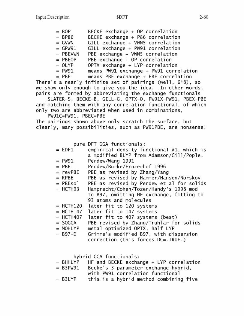
Input Description $DFT 2-60
= BOP BECKE exchange + OP correlation = BP86 BECKE exchange + P86 correlation = GVWN GILL exchange + VWN5 correlation = GPW91 GILL exchange + PW91 correlation = PBEVWN PBE exchange + VWN5 correlation = PBEOP PBE exchange + OP correlation = OLYP OPTX exchange + LYP correlation = PW91 means PW91 exchange + PW91 correlation = PBE means PBE exchange + PBE correlationThere's a nearly infinite set of pairings (well, 6*8), sowe show only enough to give you the idea. In other words,pairs are formed by abbreviating the exchange functionals SLATER=S, BECKE=B, GILL=G, OPTX=O, PW91X=PW91, PBEX=PBEand matching them with any correlation functional, of whichonly two are abbreviated when used in combinations, PW91C=PW91, PBEC=PBEThe pairings shown above only scratch the surface, butclearly, many possibilities, such as PW91PBE, are nonsense!
pure DFT GGA functionals: = EDF1 empirical density functional #1, which is a modified BLYP from Adamson/Gill/Pople. = PW91 Perdew/Wang 1991 = PBE Perdew/Burke/Ernzerhof 1996 = revPBE PBE as revised by Zhang/Yang = RPBE PBE as revised by Hammer/Hansen/Norskov = PBEsol PBE as revised by Perdew et al for solids = HCTH93 Hamprecht/Cohen/Tozer/Handy's 1998 mod to B97, omitting HF exchange, fitting to 93 atoms and molecules = HCTH120 later fit to 120 systems = HCTH147 later fit to 147 systems = HCTH407 later fit to 407 systems (best) = SOGGA PBE revised by Zhang/Truhlar for solids = MOHLYP metal optimized OPTX, half LYP = B97-D Grimme's modified B97, with dispersion correction (this forces DC=.TRUE.)
hybrid GGA functionals: = BHHLYP HF and BECKE exchange + LYP correlation = B3PW91 Becke's 3 parameter exchange hybrid, with PW91 correlation functional = B3LYP this is a hybrid method combining five

Input Description $DFT 2-61
functionals, namely Becke + Slater + HF exchange, and LYP + VWN5 correlation. = B3LYP1 use VWN1 in place of VWN5, matching the e- gas formula chosen by some programs. = B97 Becke's 1997 hybrid functional = B97-1 Hamprecht/Cohen/Tozer/Handy's 1998 reparameterization of B97 = B97-2 Wilson/Bradley/Tozer's 2001 mod to B97 = B97-3 Keal/Tozer's 2005 mod to B97 = B97-K Boese/Martin's 2004 mod for kinetics = B98 Schmider/Becke's 1998 mode to B97, using their best "2c" parameters. = PBE0 a hybrid made from PBE = X3LYP HF+Slater+Becke88+PW91 exchange, and LYP+VWN1 correlation.Each includes some Hartree-Fock exchange, and also may usea linear combination of many DFT parts.
range separated functionals:These are also known as "long-range corrected functionals".LC-BOP, LC-BLYP, or LC-BVWN are available by selecting BOP,BLYP, BVWN as well as setting the flag LC=.TRUE. (see LCbelow). Others are selected by a specific name: = CAMB3LYP coulomb attenuated B3LYP = wB97 omega separated form of B97 = wB97X wB97 with short-range HF exchange = wB97X-D dispersion corrected wB97X
"double hybrid" GGA: = B2PLYP mixes BLYP, HF exchange, and MP2! It lacks analytic nuclear derivatives. See related inputs CHF and CMP2 below. "double hybrid" and "range separated": = wB97X-2 intended for use with GBASIS=CCT,CCQ,CC5 = wB97X-2L intended for use with GBASIS=N311 NGAUSS=6 NDFUNC=3 NFFUNC=1 NPFUNC=3 DIFFSP=.T. DIFFS=.T.Note: the B2PLYP family uses the conventional MP2 energyand may be used for closed shell or spin-unrestricted openshell cases. The wB97X-2 family uses the SCS-MP2 energy,and thus is limited to closed shell cases at present.

Input Description $DFT 2-62
meta-GGA functionals:These are not hybridized with HF exchange, unless that isexplicitly stated below. = VS98 Voorhis/Scuseria, 1998 = PKZB Perdew/Kurth/Zupan/Blaha, 1999 = tHCTH Boese/Handy's 2002 metaGGA akin to HCTH = tHCTHhyb tHCTH's hybrid with 15% HF exchange = BMK Boese/Martin's 2004 parameterization of tHCTHhyb for kinetics = TPSS Tao/Perdew/Staroverov/Scuseria, 2003 = TPSSh TPSS hybrid with 10% HF exchange = TPSSm TPSS with modified parameter, 2007 = revTPSS revised TPSS, 2009 = M05 Minnesota exchange-correlation, 2005 a hybrid with 28% HF exchange. = M05-2X M05, with doubled HF exchange, to 56% = M06 Minnesota exchange-correlation, 2006 a hybrid with 27% HF exchange. = M06-L M06, with 0% HF exchange (L=local) = M06-2X M06, with doubled HF exchange, to 54% = M06-HF M06 correlation, using 100% HF exchange = M08-HX M08 with 'high HF exchange' = M08-SO M08 of similar form, different paramsWhen the M06 family was created, Truhlar recommended M06for the general situation, but see his "concluding remarks"in the M06 reference about which functional is best forwhat kind of test data set.
An extensive bibliography for these functionals can befound in the 'Further References' section of this manual.
Note that only a subset of these functionals can be usedfor TD-DFT energy or gradients. These subsets are listedin the $TDDFT input group.
• * * dispersion corrections * * *
DFT is notorious for failures to compute intra- and inter-molecular dispersion interactions accurately. Two possiblecorrection schemes are provided below. The first usesempirically chosen C6 and C8 coefficients, while the latterobtains these from the molecular DFT densities. At most,only one of the LRDFLG or DC options below may be chosen.

Input Description $DFT 2-63
DC = a flag to turn on Grimme's empirical dispersion correction, involving scaled R**(-6) terms. N.B. This empiricism may also be added to plain Hartree-Fock, by choosing DFTTYP=NONE with DC=.T. Three different versions exist, see IDCVER. (default=.FALSE., except if DFTTYP=B97-D, wB97X-D)
IDCVER = 1 means 1st 2004 implementation. = 2 means 2nd 2006 implementation DFT-D2, default for B97-D, wB97X-D. = 3 means 3rd 2010 implementation DFT-D3, default for all others. Setting IDCVER will force DC=.TRUE.
DCCHG = a flag to use Chai-Head-Gordon damping function instead of Grimme's 2006 function. Pertinent only for the DFT-D2 method. Forces DC=.TRUE. (default=.FALSE. except for wB97X-D)
DCABC = a flag to turn on the computation of the E(3) non- additive energy term. Pertinent only for DFT-D3, it forces DC=.TRUE. (default=.FALSE.)
The following parameters govern Grimme's semiempiricaldispersion term. They are basis set and functionaldependent, so they exist for only a few DFTTYP. Defaultvalues are automatically selected and printed out in theoutput file for many common density functionals. The following keywords are for entering non-standardvalues. For DFT-D2 values, see also: R.Peverati and K.K.Baldridge J.Chem.Theory Comput. 4, 2030-2048 (2008).For DFT-D3 values, and a detailed explanation of eachparameter, see: S. Grimme, J. Antony, S. Ehrlich and H. Krieg, J.Chem.Phys. 132, 154104/1-19(2010)
DCALP = alpha parameter in the DFT-D damping function (same as alpha6 in Grimme's DFT-D3 notation). Note also that alpha8 and alpha10 in DFT-D3 have constrained values of: alpha8 = alpha6 + 2, alpha10 = alpha8 + 2. Default=14.0 for DFT-D3 =20.0 for DFT-D2 =23.0 for DFT-D1

Input Description $DFT 2-64
=6.00 for DCCHG=.TRUE.
DCSR = sR exponential parameter to scale the van der Waals radii (same as sR,6 in Grimme's DFT-D3 notation). Note also that sR,8 in DFT-D3 have a fixed value of 1.0. Optimized values are automatically selected for some of the more common functionals, otherwise, the default is 1.00 for DFT-D3, 1.10 for DFT-D2, and 1.22 for DFT-D1.
DCS6 = s6 linear parameter for scaling the C6 term. Optimized values are automatically selected for some of the more common functionals, otherwise, the default is 1.00.
DCS8 = s8 linear parameter for scaling the C8 term of DFT-D3. Pertinent only for DFT-D3. Optimized values are automatically selected for some of the more common functionals, otherwise, the default is 1.00.
The old keywords DCPAR and DCEXP were replaced by DCS6 andDCSR in 2010. Similarly, DCOLD has morphed into IDCVER.
- - -
The Local Response Dispersion (LRD) correction includesatomic pair-wise -C6/R**6, -C8/R**8, and -C10/R**10 terms,whose coefficients are computed from the molecular system'selectron density and its nuclear gradient. The nucleargradient assumes the dispersion coefficients do not varywith geometry, which causes only a very small error in thegradient. Optionally, 3 and 4 center terms may be added,at the 1/R**6 level; in this case, nuclear gradients maynot be computed at all.
Since the three numerical parameters are presently knownonly for the long-range exchange corrected BOP functional,calculations may specify simply DFTTYP=LCBOPLRD. The"LCBOPLRD" functional will automatically select thefollowing: DFTTYP=BOP LC=.TRUE. MU=0.47 LRDFLG=.TRUE. LAMBDA=0.232 KAPPA=0.600 RZERO=3.22leaving only the choice for MLTINT up to you.
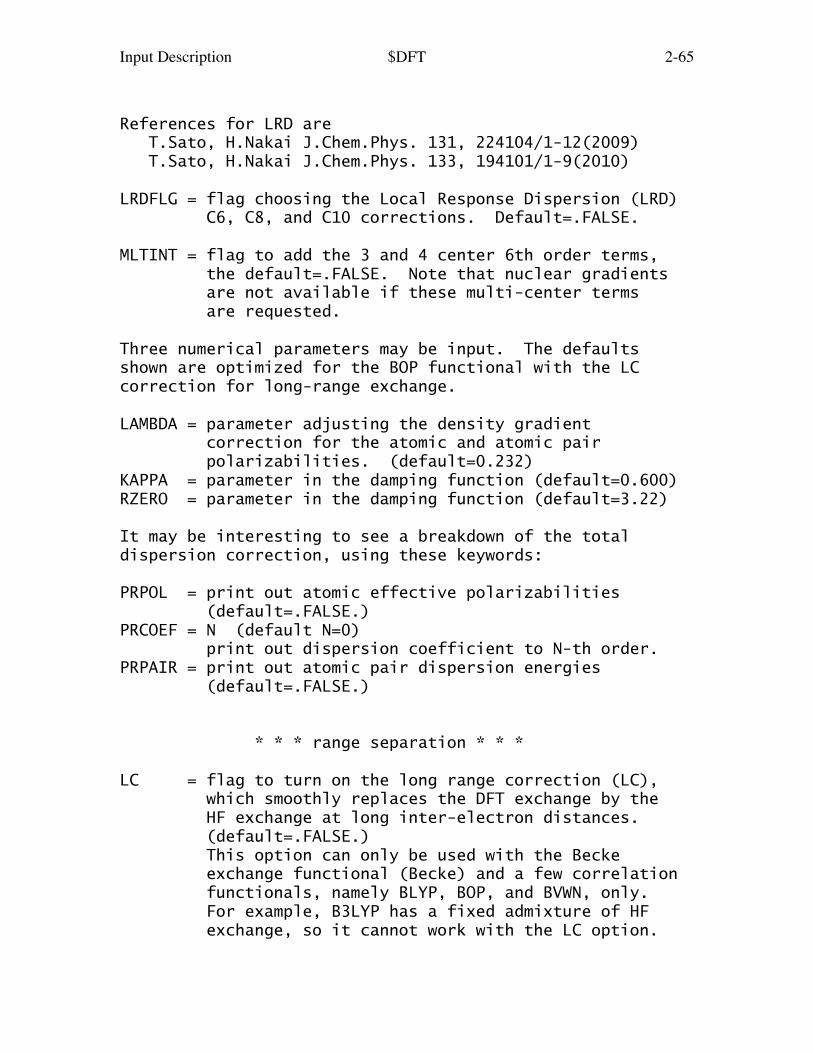
Input Description $DFT 2-65
References for LRD are T.Sato, H.Nakai J.Chem.Phys. 131, 224104/1-12(2009) T.Sato, H.Nakai J.Chem.Phys. 133, 194101/1-9(2010)
LRDFLG = flag choosing the Local Response Dispersion (LRD) C6, C8, and C10 corrections. Default=.FALSE.
MLTINT = flag to add the 3 and 4 center 6th order terms, the default=.FALSE. Note that nuclear gradients are not available if these multi-center terms are requested.
Three numerical parameters may be input. The defaultsshown are optimized for the BOP functional with the LCcorrection for long-range exchange.
LAMBDA = parameter adjusting the density gradient correction for the atomic and atomic pair polarizabilities. (default=0.232)KAPPA = parameter in the damping function (default=0.600)RZERO = parameter in the damping function (default=3.22)
It may be interesting to see a breakdown of the totaldispersion correction, using these keywords:
PRPOL = print out atomic effective polarizabilities (default=.FALSE.)PRCOEF = N (default N=0) print out dispersion coefficient to N-th order.PRPAIR = print out atomic pair dispersion energies (default=.FALSE.)
* * * range separation * * *
LC = flag to turn on the long range correction (LC), which smoothly replaces the DFT exchange by the HF exchange at long inter-electron distances. (default=.FALSE.) This option can only be used with the Becke exchange functional (Becke) and a few correlation functionals, namely BLYP, BOP, and BVWN, only. For example, B3LYP has a fixed admixture of HF exchange, so it cannot work with the LC option.

Input Description $DFT 2-66
See H.Iikura, T.Tsuneda, T.Yanai, and K.Hirao, J.Chem.Phys. 115, 3540 (2001).
MU = A parameter for the long range correction scheme. (default=0.33)
Other range-separated options exist, invoked by naming thefunctional, such as DFTTYP=CAMB3LYP (see the DFTTYP keywordfor a full list).
* * * B2x-PLYP double hybrid functionals * * *
B2xPLYP Double Hybrid functionals have the general formula: Exc = (1-cHF) * ExGGA + cHF * ExHF + (1-cMP2) * EcGGA + cMP2 * E(2)
The next keywords allow the choice of cHF and cMP2. Bothvalues must be between 0 and 1 (0-100%).
CHF = amount of HF exchange. (default=0.53)
CMP2 = amount of MP2. (default=0.27)
Some other common double hybrid functionals are availablesimply by chosing DFTTYP=B2PLYP, and changing the CHF andCMP2 parameters. Popular parametrizations are: CHF CMP2 ------------------------------------------ B2-PLYP (default) | 0.53 | 0.27 | ------------------------------------------ B2K-PLYP | 0.72 | 0.42 | ------------------------------------------ B2T-PLYP | 0.60 | 0.31 | ------------------------------------------ B2GP-PLYP | 0.65 | 0.36 | ------------------------------------------
* * * Grid Input * * *
Only one of the three grid types may be chosen for the run.The default (if no selection is made) is the Lebedev grid.In order to duplicate results obtained prior to April 2008,select the polar coordinate grid NRAD=96 NTHE=12 NPHI=24.
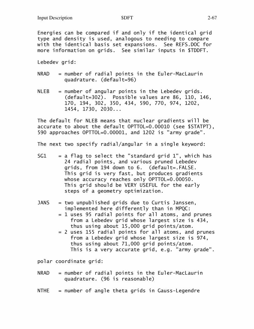
Input Description $DFT 2-67
Energies can be compared if and only if the identical gridtype and density is used, analogous to needing to comparewith the identical basis set expansions. See REFS.DOC formore information on grids. See similar inputs in $TDDFT.
Lebedev grid:
NRAD = number of radial points in the Euler-MacLaurin quadrature. (default=96)
NLEB = number of angular points in the Lebedev grids. (default=302). Possible values are 86, 110, 146, 170, 194, 302, 350, 434, 590, 770, 974, 1202, 1454, 1730, 2030...
The default for NLEB means that nuclear gradients will beaccurate to about the default OPTTOL=0.00010 (see $STATPT),590 approaches OPTTOL=0.00001, and 1202 is "army grade".
The next two specify radial/angular in a single keyword:
SG1 = a flag to select the "standard grid 1", which has 24 radial points, and various pruned Lebedev grids, from 194 down to 6. (default=.FALSE. This grid is very fast, but produces gradients whose accuracy reaches only OPTTOL=0.00050. This grid should be VERY USEFUL for the early steps of a geometry optimization.
JANS = two unpublished grids due to Curtis Janssen, implemented here differently than in MPQC: = 1 uses 95 radial points for all atoms, and prunes from a Lebedev grid whose largest size is 434, thus using about 15,000 grid points/atom. = 2 uses 155 radial points for all atoms, and prunes from a Lebedev grid whose largest size is 974, thus using about 71,000 grid points/atom. This is a very accurate grid, e.g. "army grade".
polar coordinate grid:
NRAD = number of radial points in the Euler-MacLaurin quadrature. (96 is reasonable)
NTHE = number of angle theta grids in Gauss-Legendre
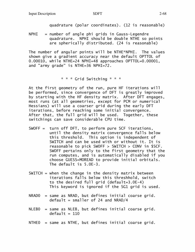
Input Description $DFT 2-68
quadrature (polar coordinates). (12 is reasonable)
NPHI = number of angle phi grids in Gauss-Legendre quadrature. NPHI should be double NTHE so points are spherically distributed. (24 is reasonable)
The number of angular points will be NTHE*NPHI. The valuesshown give a gradient accuracy near the default OPTTOL of0.00010, while NTHE=24 NPHI=48 approaches OPTTOL=0.00001,and "army grade" is NTHE=36 NPHI=72.
* * * Grid Switching * * *
At the first geometry of the run, pure HF iterations willbe performed, since convergence of DFT is greatly improvedby starting with the HF density matrix. After DFT engages,most runs (at all geometries, except for PCM or numericalHessians) will use a coarser grid during the early DFTiterations, before reaching some initial convergence.After that, the full grid will be used. Together, theseswitchings can save considerable CPU time.
SWOFF = turn off DFT, to perform pure SCF iterations, until the density matrix convergence falls below this threshold. This option is independent of SWITCH and can be used with or without it. It is reasonable to pick SWOFF > SWITCH > CONV in $SCF. SWOFF pertains only to the first geometry that the run computes, and is automatically disabled if you choose GUESS=MOREAD to provide initial orbitals. The default is 5.0E-3.
SWITCH = when the change in the density matrix between iterations falls below this threshhold, switch to the desired full grid (default=3.0E-4) This keyword is ignored if the SG1 grid is used.
NRAD0 = same as NRAD, but defines initial coarse grid. default = smaller of 24 and NRAD/4
NLEB0 = same as NLEB, but defines initial coarse grid. default = 110
NTHE0 = same as NTHE, but defines initial coarse grid.

Input Description $DFT 2-69
default = smaller of 8, NTHE/3
NPHI0 = same as NPHI, but defines initial coarse grid. default = smaller of 16, NPHI/3
technical parameters:
THRESH = threshold for ignoring small contributions to the Fock matrix. The default is designed to produce no significant energy loss, even when the grid is as good as "army grade". If for some reason you want to turn all threshhold tests off, of course requiring more CPU, enter 1.0e-15. default: 1.0e-4/Natoms/NRAD/NTHE/NPHI
GTHRE = threshold applied to gradients, similar to THRESH. < 1 assign this value to all thresholds = 1 use the default thresholds (default). > 1 divide default thresholds by this value. If you wish to increase accuracy, set GTHRE=10. The default introduces an error of roughly 1e-7 (a.u./bohr) in the gradient.
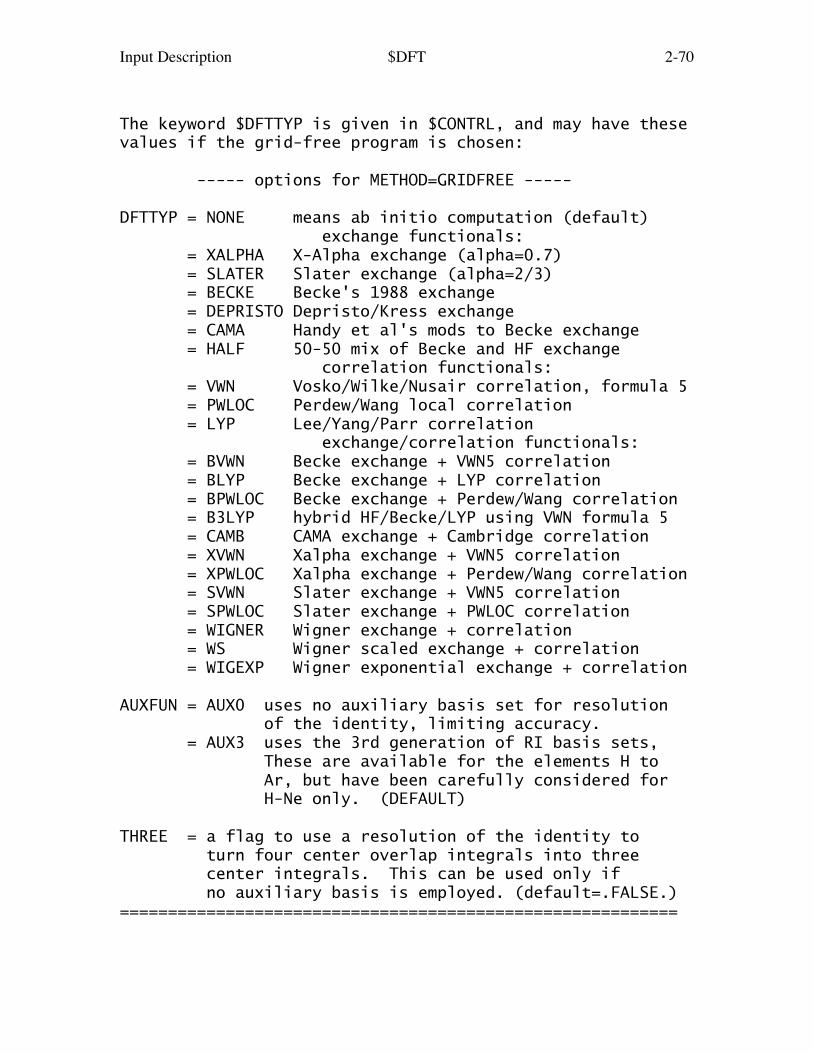
Input Description $DFT 2-70
The keyword $DFTTYP is given in $CONTRL, and may have thesevalues if the grid-free program is chosen:
----- options for METHOD=GRIDFREE -----
DFTTYP = NONE means ab initio computation (default) exchange functionals: = XALPHA X-Alpha exchange (alpha=0.7) = SLATER Slater exchange (alpha=2/3) = BECKE Becke's 1988 exchange = DEPRISTO Depristo/Kress exchange = CAMA Handy et al's mods to Becke exchange = HALF 50-50 mix of Becke and HF exchange correlation functionals: = VWN Vosko/Wilke/Nusair correlation, formula 5 = PWLOC Perdew/Wang local correlation = LYP Lee/Yang/Parr correlation exchange/correlation functionals: = BVWN Becke exchange + VWN5 correlation = BLYP Becke exchange + LYP correlation = BPWLOC Becke exchange + Perdew/Wang correlation = B3LYP hybrid HF/Becke/LYP using VWN formula 5 = CAMB CAMA exchange + Cambridge correlation = XVWN Xalpha exchange + VWN5 correlation = XPWLOC Xalpha exchange + Perdew/Wang correlation = SVWN Slater exchange + VWN5 correlation = SPWLOC Slater exchange + PWLOC correlation = WIGNER Wigner exchange + correlation = WS Wigner scaled exchange + correlation = WIGEXP Wigner exponential exchange + correlation
AUXFUN = AUX0 uses no auxiliary basis set for resolution of the identity, limiting accuracy. = AUX3 uses the 3rd generation of RI basis sets, These are available for the elements H to Ar, but have been carefully considered for H-Ne only. (DEFAULT)
THREE = a flag to use a resolution of the identity to turn four center overlap integrals into three center integrals. This can be used only if no auxiliary basis is employed. (default=.FALSE.)==========================================================

Input Description $TDDFT 2-71
==========================================================
$TDDFT group (relevant if TDDFT chosen in $CONTRL)
This group generates molecular excitation energies bytime-dependent density functional theory computations (ortime-dependent Hartree-Fock, also known as the Random PhaseApproximation). The functional used for the excited statesis necessarily the same one that is used for the referencestate, specified by DFTTYP in $CONTRL.
For conventional TD-DFT (TDDFT=EXCITE in $CONTRL), theorbitals are optimized for RHF or UHF type referencestates. Analytic nuclear gradients are available forsinglet excited states, while the energy of excited statesof other multiplicities can be computed.
For spin-flip TD-DFT (TDDFT=SPNFLP in $CONTRL), thecalculation obtains orbitals for a reference state ofeither UHF or ROHF type, with MULT in $CONTRL determiningthe Ms quantum number of the reference. The referencestate's Ms is set equal to the S value implied by $CONTRL'sMULT=2S+1. The SF-TD-DFT then uses only determinants withMs=S-1, due to the flip of one alpha spin into a beta spin.This means that target states (which are spin contaminated)will have multiplicities around the range S-1 to S, only.It is quite possible for some of the target states to havea lower energy than the reference!!! Nuclear gradients andproperties are available.
See just below for "limitations" below regarding the twodifferent TD-DFT types.
TDDFT is a single excitation theory. All of the caveatslisted in the $CIS input group about states with doubleexcitation character, need for Rydberg basis sets, greatlydifferent topology of excited state surfaces, and so onapply here as well. Please read the introduction to the$CIS input group! If you use very large or very smallGaussian exponents, you may need to increase the number ofradial grid points (the program prints advice in suchcases).
TDHF, TDDFT, and CIS are related in the following way:

Input Description $TDDFT 2-72
-- Tamm/Dancoff approximation --> | TDHF CIS DFT | V TDDFT TDDFT/TDA
Here TDHF means absorption of photons, to produce excitedstates (TDHF is called RPA in the physics community). Thismeaning of TDHF should not be confused with the photonscattering processes computed by RUNTYP=TDHF or TDHFX,which generate polarizabilities. Note, in particular, thatCITYP=CIS is equivalent to using TDDFT=EXCITE DFTTYP=NONETAMMD=.TRUE., provided the former is run with no frozencores. Solvent effects for CIS calculations are thereforeavailable via the TDDFT codes.
Excited state properties are calculated using the TDDFTexcited state electronic density only during gradient runs,or by setting TDPRP below.
The TD-DFT codes excite all electrons, that is, there isno frozen core concept. Please see the 4th chapter of thismanual for more information on both types of TD-DFT.
"limitations" for TDDFT=EXCITE:
Permissible values for DFTTYP are shown below. Theseinclude "NONE" which uses TDHF (i.e. the Random PhaseApproximation), noting that extra states may need to besolved for in order to be sure of getting the first fewstates correctly. If nuclear gradients are needed, you maychoose any of the following functionals: NONE SVWN, SOP, SLYP, OLYP, BVWN, BOP, BLYP (and their LC=.TRUE. versions) B3LYP, CAMB3LYP, B3LYP1, PBE, PBE0For evaluation of just the excitation energies, you may usemany more functionals, notably including the metaGGAs inthe last three lines: NONE SVWN, SVWN1, SPZ81, SP86, SOP, SLYP, BVWN, BVWN1, BPZ81, BP86, BOP, BLYP, OLYP, B3LYP, CAMB3LYP, B3LYP1, B3PW91, X3LYP, PW91, PBE, PBE0 VS98, PKZB, M05, M05-2X, M06, M06-HF, M06-L, M06-2X, M08-HX, M08-SO TPSS, TPSSm, TPSSh, and revTPSS

Input Description $TDDFT 2-73
The LC flag in $DFT automatically carries over to TDDFTruns. The LC option may be used with the "B" functionals,and (like the similar range-separated CAMB3LYP) is usefulin obtaining better descriptions for charge-transferexcitations or Rydberg excitation energies than are theconventional exchange correlation functionals (whether pureor hybrid). The LC flag is also available for excitedstate gradient computation.
Limits specific to the references for TDDFT=EXCITE are:
For SCFTYP=RHF, excitation energies can be found forsinglet or triplet coupled excited states. For singletexcited states only, analytic gradients and properties canbe found, for either full TD-DFT or in the Tamm/Dancoffapproximation. For RHF references, solvent effects can beincluded by EFP1 or PCM (or both together), for both TD-DFTexcitation energies and their nuclear gradients.
For SCFTYP=UHF, excited states with the same spinprojection as the ground state are found. MULT in $CONTRLgoverns the number of alpha and beta electrons, henceMs=(MULT-1)/2 is the only good quantum number for eitherthe ground or excited states. Since U-TDDFT is a singleexcitation theory, excited states with <S> values near Msand near Ms+1 will appear in the calculation. There are noproperties other than the excitation energy, nor gradients,nor solvent effects, at present.
"limitations" for TDDFT=SPNFLP:
Permissible values for DFTTYP are fewer than the listshown above for conventional TD-DFT. In particular, nohybrid functional may be used (collinear approximation).The LC option for range-separation hybrids cannot be used,which also removes CAMB3LYP. Finally, no meta-GGA may beused. Note that spin-flip TD-DFT in the Tamm/Dancoffapproximation using DFTTYP=NONE is equivalent to spin-flipCIS.
MULT below is ignored, as the Ms of target states isfixed solely by MULT in $CONTRL. The spin-flip codeoperates only in the Tamm/Dancoff approximation, so TAMMDbelow is automatically .TRUE. Nuclear gradients and/or

Input Description $TDDFT 2-74
excited state properties are available only in the gasphase. Solvation effects are available only for energycalculations, and only for EFP1 and C-PCM.
---------
NSTATE = Number of states to be found (excluding the reference state). The default is 1 more state.
IROOT = State used for geometry optimization and property evaluation. (default=1) TDDFT=EXCITE counts the reference as 0, and this should be the lowest state. Hence IROOT=1 means the 1st excited state, just as you might guess. TDDFT=SPNFLP labels the reference state as 0, but this might not be the lowest state overall. The meaning of IROOT=1 is the lowest state, omitting the reference state from consideration. Hence IROOT=1 might specify the ground state!
MULT = Multiplicity (1 or 3) of the singly excited states. This keyword applies only when the reference is a closed shell. (default is 1) This parameter is ignored when TDDFT=SPNFLP.
TDPRP = a flag to request property computation for the state IROOT. Properties can only be obtained when the nuclear gradient is computable, see gradient restrictions noted in the introduction to this group. Properties require significant extra computer time, compared to the excitation energy alone, so the default is .FALSE. Properties are always evaluated during nuclear gradient runs, when they are a free by-product.
TAMMD is a flag selecting the Tamm/Dancoff approximation be used. This may be used with closed shell excitation energies or gradients, or open shell excitation energies. Default = .FALSE. This parameter is ignored by TDDFT=SPNFLP, which is only coded in the Tamm/Dancoff approximation.

Input Description $TDDFT 2-75
NONEQ is a flag controlling PCM's solvent behavior: .TRUE. splits the dielectric constant into a bulk value (EPS in $PCM) and a fast component (EPSINF), see Cossi and Barone, 2001. The idea is that NONEQ=.t. is appropriate for vertical excitations, and .f. for adiabatic. (the default is .TRUE.) This keyword is ignored by TDDFT=SPNFLP.
* * * Grid Selection * * *
The grid type and point density used in $TDDFT may bechosen independently of the values in $DFT. Excitationenergies accurate to 0.01 eV may be obtained with gridsthat are much sparser than those needed for the groundstate, and this is reflected in the defaults. Prior toApril 2008, the default grid was NRAD=24 NTHE=8 NPHI=16.
NRAD = number of radial grid points in Euler-Maclaurin quadrature, used in calculations of the second or third derivatives of density functionals. (default=48)
NLEB = number of angular points in the Lebedev grid. (default=110)
NTHE = number of theta grid points if a polar coordinate grid is used.
NPHI = number of phi grid points if a polar coordinate grid is used. NPHI should be twice NTHE.
SG1 = flag selecting "standard grid one". (default=.FALSE.)
See both $DFT and REFS.DOC for more information on grids.The "army grade" standard for $TDDFT is NRAD=96 combinedwith either NLEB=302 or NTHE=12/NPHI=24.
the remaining parameters are technical in nature:
CNVTOL = convergence tolerance in the iterative TD-DFT step. (default=1.0E-7)

Input Description $TDDFT 2-76
MAXVEC = the maximum number of expansion vectors used by the solver's iterations, per state (default=50). The total size of the expansion space will be NSTATE*MAXVEC.
NTRIAL = the number of initial expansion vectors used. (default is the larger of 5 and NSTATE).
==========================================================

Input Description $CIS 2-77
==========================================================
$CIS group required when CITYP=CIS required when CITYP=SFCIS
The CIS method (singly excited CI) is the simplest wayto treat excited states. By Brillouin's Theorem, a singledeterminant reference such as RHF will have zero matrixelements with singly substituted determinants. The groundstate reference therefore has no mixing with the excitedstates treated with singles only. Reading the referencesgiven in Section 4 of this manual will show the CIS methodcan be thought of as a non-correlated method, rigorously sofor the ground state, and effectively so for the variousexcited states. Some issues making CIS rather less than ablack box method are: a) any states characterized by important doubles are simply missing from the calculation. b) excited states commonly possess Rydberg (diffuse) character, so the AO basis used must allow this. c) excited states often have different point group symmetry than the ground state, so the starting geometries for these states must reflect their actual symmetry. d) excited state surfaces frequently cross, and thus root flipping may very well occur.
The normal CIS implementation allows the use of only RHFreferences, but can pick up both singlet and tripletexcited states. Nuclear gradients are available, as areproperties. The CIS run automatically includes computationof the dipole moments of all states, and all pairwisetransition dipoles and oscillator strengths.
The spin-flip type of CIS is very similar to spin-flip TD-DFT (the $TDDFT group contains more information about howspin-flip runs select the target state's Ms by $CONTRL'sMULT value). The reference state must be UHF or ROHF, withMULT in $CONTRL at least 3. The target states of the CIShave one lower Ms, after one alpha spin in the reference isflipped to beta. Nuclear gradients are possible.
Solvent effects are not available for either CIS or SFCIS.
It is worthwhile to look at the $TDDFT group, which is avery similar calculation. The TD-DFT program offers the

Input Description $CIS 2-78
possibility of recovering some of the correlation energy,permits some solvent models, and can be used for MEX/CONICLsurface intersection searches.
The first six keywords are chemically important, while theremainder are mostly technical.
NACORE = n Omits the first n occupied orbitals from the calculation (frozen core approximation). For CITYP=CIS, the default for n is the number of chemical core orbitals. For CITYP=SFCIS, the default, which is also the only possibility, is 0.
NSTATE = Number of states to be found (excluding the reference state). No default is provided.
IROOT = State for which properties and/or gradient will be calculated. Only one state can be chosen. The reference state is referred to as 0, and in the case of CITYP=SFCIS, might have a higher energy than some of the NSTATE target states.
CISPRP = Flag to request the determination of CIS level properties, using the relaxed density. Relevant to RUNTYP=ENERGY jobs, although the default is .FALSE. because additional CPHF calculation will be required. Properties are an automatic by- product of runs involving the CIS or SFCIS nuclear gradient.
HAMTYP = Type of CI Hamiltonian to use, if CITYP=CIS. = SAPS spin-adapted antisymmetrized product of the desired MULT will be used (default) = DETS determinant based, so both singlets and triplets will be obtained.
MULT = Multiplicity (1 or 3) of the singly excited SAPS (the reference can only be singlet RHF). Only relevant for SAPS-based CITYP=CIS run, as SFCIS controls the Ms for target states by the value of MULT in $CONTRL.
- - - - - - - - - - - -
Input Description $CIS 2-79
DIAGZN = Hamiltonian diagonalization method. = DAVID use Davidson diagonalization. (default) = FULL construct the full matrix in memory and diagonalize, thus determining all states (not recommended except for small cases).
DGAPRX = Flag to control whether approximate diagonal elements of the CIS Hamiltonian (based only on the orbital energies) are used in the Davidson algorithm. Note, this only affects the rate of convergence, not the resulting final energies. If set .FALSE., the exact diagonal elements are determined and used. Default=.TRUE.
NGSVEC = Dimension of the Hamiltonian submatrix that is diagonalized to form the initial CI vectors. The default is the greater of NSTATE*2 and 10.
MXVEC = Maximum number of expansion basis vectors in the iterative subspace during Davidson iterations, before the expansion basis is truncated. The default is the larger of 8*NSTATE and NGSVEC.
NDAVIT = Maximum number of Davidson iterations. Default=50.
DAVCVG = Convergence criterion for Davidson eigenvectors. Eigenvector accuracy is proportional to DAVCVG, while the energy accuracy is proportional to its square. The default is 1.0E-05.
CHFSLV = Chooses type of CPHF solver to use. = CONJG selects an ordinary preconditioned conjugate gradient solver. (default) = DIIS selects a diis-like iterative solver.
RDCISV = Flag to read CIS vectors from a $CISVEC group in the input file. Default is .FALSE.
MNMEDG = Flag to force the use of the minimal amount of memory in construction of the CIS Hamiltonian diagonal elements. This is only relevant when DGAPRX=.FALSE., and is meant for debug purposes. The default is .FALSE.

Input Description $CIS 2-80
MNMEOP = Flag to force the use of the minimal amount of memory during the Davidson iterations. This is for debug purposes. The default is .FALSE.
==========================================================
$CISVEC group required if RDCISV in $CIS is chosen
This is formatted data generated by a previous CIS run, tobe read back in as starting vectors. Sometimes molecularorbital phase changes make these CI vectors problematic.==========================================================
Input Description $MP2 2-81
==========================================================
$MP2 group (relevant to SCFTYP=RHF,UHF,ROHF if MPLEVL=2)
Controls 2nd order Moller-Plesset perturbation runs,if requested by MPLEVL in $CONTRL. MP2 is implemented forRHF, high spin ROHF, or UHF wavefunctions, but see also$MRMP for MCSCF. Analytic gradients and the first ordercorrection to the wavefunction (i.e. properties) areavailable for RHF, ROHF (if OSPT=ZAPT), and UHF. The $MP2group is not usually given. See also the DIRSCF keyword in$SCF to select direct MP2.
The spin-component-scaled MP2 (SCS-MP2) energy ofGrimme is printed for SCFTYP=RHF references during energyruns. See also the keyword SCSPT below. Only the CODE=IMSprogram is able to do analytic gradients for SCS-MP2.
Special serial codes exist for RHF or UHF MP2 energyor gradient, or the ROHF MP2 energy. Parallel codes usingdistributed memory are available for RHF, ROHF, or UHF MP2gradients. In fact, the only way that ROHF MP2 gradientscan be computed on one node is with the parallel code,using MEMDDI!
MP2 energy values using solution models are computedby using the solvated SCF orbitals in the perturbationstep. All of the MP2 nuclear gradient programs containadditional terms required for EFP, PCM, EFP plus PCM, orCOSMO solvation models.
NACORE = n Omits the first n occupied orbitals from the calculation. The default for n is the number of chemical core orbitals.
NBCORE = Same as NACORE, for the beta orbitals of UHF. It is almost always the same value as NACORE.
MP2PRP= a flag to turn on property computation for jobs jobs with RUNTYP=ENERGY. This is appreciably more expensive than just evaluating the second order energy correction alone, so the default is to skip properties. Properties are always computed during gradient runs, when they are an almost free byproduct. (default=.FALSE.)
Input Description $MP2 2-82
OSPT= selects open shell spin-restricted perturbation. This parameter applies only when SCFTYP=ROHF. Please see the 'further information' section for more information about this choice. = ZAPT picks Z-averaged perturbation theory. (default) = RMP picks RMP (aka ROHF-MBPT) perturbation theory.
CODE = the program implementation to use, choose from SERIAL, DDI, or IMS according to the following chart, depending on SCFTYP and whether the run involves gradients,
RHF RHF UHF UHF ROHF ROHF ROHFenergy gradient energy gradient energy gradient energy OSPT=ZAPT ZAPT RMPSERIAL SERIAL SERIAL SERIAL SERIAL - SERIALDDI DDI DDI DDI DDI DDI -IMS IMS - - - - -RIMP2 - RIMP2 - - - -
The default for serial runs (p=1) is CODE=IMS for RHF, andCODE=SERIAL for UHF or ROHF (provided PARALL is .FALSE. in$SYSTEM). When p>1 (or PARALL=.TRUE.), the default becomesCODE=DDI. However, if FMO is in use, the default forclosed shell parallel runs is CODE=IMS. The "SERIAL" codefor OSPT=RMP will run with modest scalability when p>1.
The many different MP2 programs are written for differenthardware situations. Here N is the number of atomic basisfunctions, and O is the number of correlated orbitals inthe run:
The original SERIAL programs use N**3 memory, and havelarger disk files and generally takes longer than CODE=IMS.
The IMS program uses N*O**2 memory, and places most of itsdata on local disks (so you must have good disk access),and will run in parallel...ideal for small clusters. Usingthis program on a node where the disks are of poor quality(SATA-type) and with many cores accessing that single diskmay be very I/O bound. Adding more memory can make thisprogram run more efficiently. Network traffic is modestwhen running in parallel.

Input Description $MP2 2-83
The DDI program uses N**4 memory, but this is distributedacross all nodes, and there is essentially no I/O...idealfor large parallel machines where the manufacturer hasforgotten to include disk drives. MEMDDI must be given in$SYSTEM for these codes, so large problems may require manynodes to aggregate enough MEMDDI. The network traffic ishigh, so an Infiniband quality network or better preferred.Scalability is very good, for example, this program hasbeen used up to 4,000 cores on Altix/ICE equipment.
All of the programs just mentioned should generate the samenumerical results, so select which one best matches yourhardware.
The RIMP2 program is an approximation to the true MP2energy, using the "resolution of the identity" to reducethe amount of data stored (in memory and/or on disk), andalso the total amount of computation. See the paper onthis program for its reduced CPU and memory requirements.Network traffic is modest. The code has options within the$RIMP2 input to govern the use of replicated memory versusshared memory, as well as the use of disk storage versusdistributed memory, so you can tune this to your hardware.
References for the various programs are given in REFS.DOC.
NOSYM = disables the orbital symmetry test completely. This is not recommended, as loss of orbital symmetry is likely to mean a bad calculation. It has the same meaning as the keyword in $CONTRL, but just for the MP2 step. (Default=0)
CUTOFF = transformed integral retention threshold, the default is 1.0d-9 (1.0d-12 in FMO runs).
The following keyword applies only to RHF references:
SCSPT = spin component scaled MP2 energy selection. = NONE - the energy will be the normal MP2 value. This is the default. = SCS - the energy used for the potential surface will be the SCS energy value.Use of SCSPT=SCS causes gradients to be those for the SCS-MP2 potential surface. For CODE=IMS, the nuclear gradientcan be evaluated analytically. See NUMGRD in $CONTRL if
Input Description $MP2 2-84
for some reason you wish to use the other two closed shellcodes for SCS-MP2 gradients.
The following keywords apply to any CODE=SERIAL MP2 run, orto parallel ROHF+MP2 runs using OSPT=RMP:
LMOMP2= a flag to analyze the closed shell MP2 energy in terms of localized orbitals. Any type of localized orbital may be used. This option is implemented only for RHF, and its selection forces use of the METHOD=3 transformation, in serial runs only. The default is .FALSE.
CPHFBS = BASISMO solves the response equations during gradient computations in the MO basis. This is programmed only for RHF references without frozen core orbitals, when it is the default. = BASISAO solves the response equations using AO integrals, for frozen core MP2 with a RHF reference, or for ROHF or UHF based MP2.
NWORD = controls memory usage. The default uses all available memory. Applies to CODE=SERIAL. (default=0)
METHOD= n selects transformation method, 2 being the segmented transformation, and 3 being a more conventional two phase bin sort implementation. 3 requires more disk, but less memory. The default is to attempt method 2 first, and method 3 second. Applies only to CODE=SERIAL.
AOINTS= defines AO integral storage during conventional integral transformations, during parallel runs. DUP stores duplicated AO lists on each node, and is the default for parallel computers with slow interprocessor communication, e.g. ethernet. DIST distributes the AO integral file across all nodes, and is the default for parallel computers with high speed communications. Applies only to parallel OSPT=RMP runs.
==========================================================

Input Description $RIMP2 2-85
===========================================================
$RIMP2 group (optional, relevant if CODE=RIMP2 in $MP2)
This group controls the resolution of the identity MP2program, which approximately evaluates the MP2 energy. TheRI approximation greatly reduces the computer resourcesrequired, while suffering only a small error in theenergies. Thus, very large atomic basis sets may be used.The input below controls both utilization of the computerresources, and the accuracy of the calculation. See also$AUXBAS, regarding the auxiliary basis set, whose choicealso affects the accuracy of the calculation.
The program is enabled for parallel calculation, and istuned to today's SMP nodes. It is limited to energycalculations only, without any solvent effects, for RHF orUHF references.
IAUXBF = 0 uses Cartesian Gaussians = 1 uses spherical harmonics for the auxiliary basis set used to expand the MP2 energy expression into products of 3-index matrices. The default is inherited from ISPHER.
The next two control computer resources, trading memory fordisk storage.
GOSMP = flag requesting shared memory use. The default is .TRUE. in multi-core nodes, but .FALSE. in a uniprocessor. This option means only one copy of certain large matrices is stored per node.
USEDM = a flag to store two and three center repulsion integrals in distributed memory (.TRUE.), or in disk files (.FALSE., which is the default). Selection of this flag requires MEMDDI in $SYSTEM. The default is .TRUE.
The RI approximation reduces CPU time, memory requirements,and total disk storage requirements compared to exactcalculation. Experimentation with these two keywords willlet you tune the program to your hardware situation. Forexample, choosing GOSMP=.TRUE. and USEDM=.TRUE. will runwithout any extra disk files, while setting GOSMP=.TRUE.
Input Description $RIMP2 2-86
and USEDM .FALSE. will minimize memory usage (and networkusage) at the expense of doing disk I/O.
Total memory usage per node can be obtained by runningEXETYP=CHECK. Note the largest replicated memory printedduring the RIMP2's output, dividing by 1000000 to get thecorrect input for MWORDS (round up a bit). Note thelargest shared memory requirement printed, also dividing by100000, and rounding up a bit. Note the distributed memoryrequirement, which is already in megawords, and is thecorrect input for MEMDDI. Then, assuming you use p totalcompute process on multiple n-way nodes, the memory pernode is GBytes/node= 8(n*MWORDS + shared + n*MEMDDI/p)/1024Turning off GOSMP reduces the shared memory to 0 butincreases MWORDS, which is multiplied by the number ofcores per node! Turning off USEDM leads to MEMDDI=0 byusing disk storage instead.
If additional memory is available, increasing MWORDS canlead to a reduction in the level of the occupied orbitalbatch, or "LV". Larger MWORDS permits a smaller LV, whichwill in turn reduce the required computational time, andthe required network traffic or disk I/O. The value of LVused is the last line appearing after "CHECKING SIZE OFOCCUPIED ORBITAL BATCH".
The next four control numerical accuracy, but see $AUXBASwhich is even more influential in regards the accuracy!
OTHAUX = flag to orthogonalize the RI basis set by diagonalization of the overlap matrix. If there is reason to suspect linear dependence may exist in the RI basis, select this option to have a more numerically stable result. Larger RI basis sets such as CCT and ACCT, in particular, may benefit from selecting this. (default=.FALSE.)
STOL = threshold at which to remove small overlap matrix eigenvectors, ignored if OTHAUX=.FALSE. This keyword is analogous to QMTTOL in $CONTRL for the true AO basis. (default= 1.0d-6)
IVMTD = selects the procedure for removing redundancies when inverting the two-center, two-e- matrix.
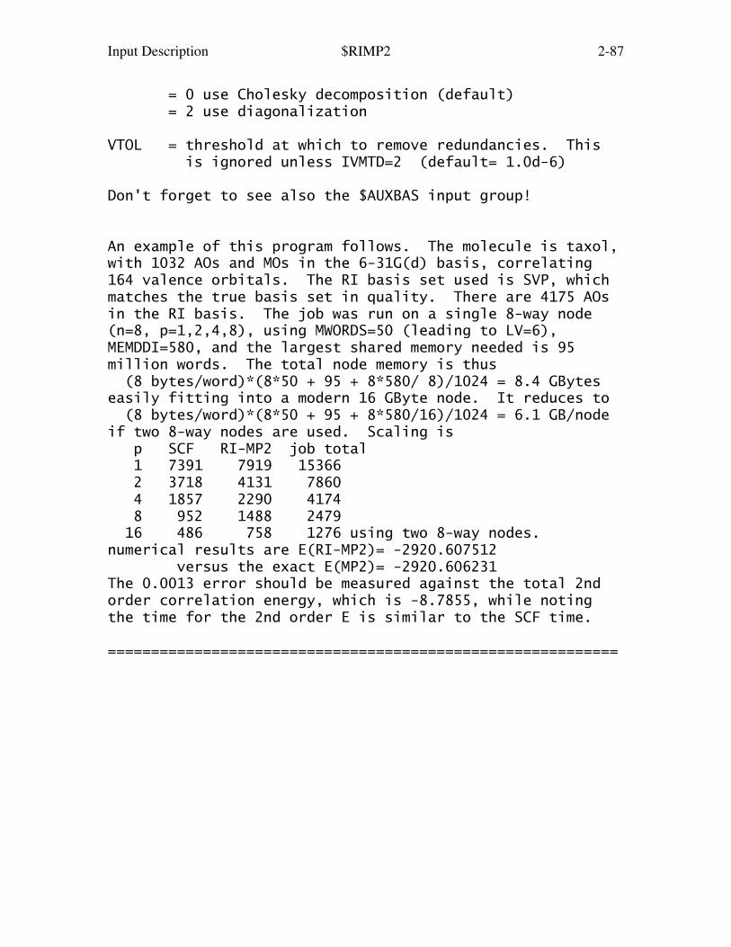
Input Description $RIMP2 2-87
= 0 use Cholesky decomposition (default) = 2 use diagonalization
VTOL = threshold at which to remove redundancies. This is ignored unless IVMTD=2 (default= 1.0d-6)
Don't forget to see also the $AUXBAS input group!
An example of this program follows. The molecule is taxol,with 1032 AOs and MOs in the 6-31G(d) basis, correlating164 valence orbitals. The RI basis set used is SVP, whichmatches the true basis set in quality. There are 4175 AOsin the RI basis. The job was run on a single 8-way node(n=8, p=1,2,4,8), using MWORDS=50 (leading to LV=6),MEMDDI=580, and the largest shared memory needed is 95million words. The total node memory is thus (8 bytes/word)*(8*50 + 95 + 8*580/ 8)/1024 = 8.4 GByteseasily fitting into a modern 16 GByte node. It reduces to (8 bytes/word)*(8*50 + 95 + 8*580/16)/1024 = 6.1 GB/nodeif two 8-way nodes are used. Scaling is p SCF RI-MP2 job total 1 7391 7919 15366 2 3718 4131 7860 4 1857 2290 4174 8 952 1488 2479 16 486 758 1276 using two 8-way nodes.numerical results are E(RI-MP2)= -2920.607512 versus the exact E(MP2)= -2920.606231The 0.0013 error should be measured against the total 2ndorder correlation energy, which is -8.7855, while notingthe time for the 2nd order E is similar to the SCF time.
===========================================================

Input Description $AUXBAS 2-88
===========================================================
$AUXBAS group (required if CODE=RIMP2 in $MP2)
This group specifies the auxiliary basis set used todefine the resolution of the identity in the RI-MP2 method.The RI methods are formally exact if the RI basis set iscomplete, so selecting larger bases improves the results.However, this also increases the computational cost of therun! It is reasonable to use smaller RI basis sets whenthe AO basis is modest, and increase the RI basis when youuse very large AO bases.
CABNAM specifies built-in basis sets for the RI: = SVP Ahlrich's SVP basis, available H-Kr = TZVP Ahlrich's TZVP basis, available H-Ar = TZVPP Ahlrich's TZVPP basis, available H-Ar = CCD cc-pVDZ basis, available H-Ar = ACCD aug-cc-pVDZ basis, available H-Ar = CCT cc-pVTZ basis, available H-Ar = ACCT aug-cc-pVTZ basis, available H-Ar = XXXXX externally defined: see EXTCAB.CABNAM has no default, this is a required input!
Note IAUXBF in $RIMP2 for selecting spherical harmonicsversus Cartesian Gaussians.
EXTCAB = flag to read the basis from an external file. (default is .FALSE.)
This is analogous to EXTBAS in $BASIS: no external filesare provided with GAMESS. The value for XXXX must be 8 orfewer letters, obviously avoiding the use of any built inauxiliary basis. Every atom present in your molecule mustbe defined in the external file by a line giving itschemical symbol, and this chosen string. Following thisheader line, give the basis in free format $DATA style,containing only S, P, D, F, and G shells, and terminatingeach atom by the usual blank line. The external file mayhave several families of bases in the same file, identifiedby different CABNAM strings.
===========================================================
Input Description $CCINP 2-89
==========================================================
$CCINP group (optional, relevant for any CCTYP)
This group controls a coupled-cluster calculation ofany type specified by CCTYP in $CONTRL. The referenceorbitals may be RHF or high spin ROHF. If this input groupis not given, as is usually the case, all valence electronswill be correlated.
Excited state runs CCTYP=EOM-CCSD or CR-EOM also readthis group to define the orbitals and to control the groundstate CCSD step that preceeds computation of excitations.Excitation energies are possible only for a RHF reference.
Parallel computation is possible for RHF referencesonly, and only for CCTYP=CCSD or CCSD(T). Memory use inparallel runs is exotic, be certain to use EXETYP=CHECK (onone processor, with PARALL in $SYSTEM set) before running.
See the "Further Information" section of this manualfor more details.
The first four inputs pertain to both RHF and ROHF cases:
NCORE = gives the number of frozen core orbitals to be omitted from the CC calculation. The default is the number of chemical core orbitals.
NFZV = the number of frozen virtual orbitals to be omitted from the calculation. (default is 0)
MAXCC = defines the maximum number of CCSD (or LCCD, CCD) iterations. This parameter also applies to ROHF's left CC vector solver, but not RHF's left vector. See MAXCCL for RHF. (default=30)
ICONV = defines the convergence criterion for the cluster amplitudes, as 10**(-ICONV). The ROHF reference also uses this for its left eigenstate solver, but see CVGEOM in $EOMINP for RHF references. (default is 7, but it tightens to 8 for FMO-CC.)

Input Description $CCINP 2-90
**** the next group pertains to RHF reference only ****
CCPRP = a flag to select computation of the CCSD level ground state density matrix (see also CCPRPE in $EOMINP for EOM-CCSD level excited states). The computation takes significant extra time, to obtain left eigenstates, so the default is .FALSE. except for CCTYP=CR-CCL or CR-EOML, where the work required for properties must be done anyway. This keyword is only available in serial runs.
Notes: CCSD is the only level at which properties can beobtained. Therefore this option can only be chosen forCCTYP=CCSD, CR-CCL, EOM-CCSD, or CR-EOM. The run willchange CCTYP to EOM-CCSD if you choose CCSD, and willtherefore read $EOMINP. However, if you don't selectNSTATE in $EOMINP, your original CCTYP=CCSD will notinclude anything except the ground state in the EOM-CCSD.Note that the convergence criterion for left eigenstateswill be CVGEOM in $EOMINP, which is set to obtainexcitation energies, and may need tightening. Use ofCCTYP=CR-EOM will do triples corrections, after doing theSD level properties.
There is little reason to select any of these:
MAXCCL = iteration limit on the left eigenstate needed by CCSD properties, or CR-CCL energies. This is just a synonym for MAXEOM in $EOMINP. If you want to alter the left state's convergence tolerance, use CVGEOM in $EOMINP. The right state convergence is set by MAXCC and ICONV above.
NWORD = a limit on memory to be used in the CC steps. The default is 0, meaning all memory available will be used.
IREST = defines the restart option. If the value of IREST is greater or equal 3, program will restart from the earlier CC run. This requires saving the disk file CCREST from the previous CC run. Values of IREST between 0 and 3 should not be used. In general, the value of IREST is used by the program

Input Description $CCINP 2-91
to set the iteration counter in the restarted run. The default is 0, meaning no restart is attempted.
MXDIIS = defines the number of cluster amplitude vectors from previous iterations to be included in the DIIS extrapolation during the CCSD (or LCCD, CCD) iterative process. The default value of MXDIIS is 5 for all but small problems. The DIIS solver can be disengaged by entering MXDIIS = 0. It is not necessary to change the default value of MXDIIS, unless the CC equations do not converge in spite of increasing the value of MAXCC.
AMPTSH = defines a threshold for eliminating small cluster amplitudes from the CC calculations. Amplitudes with absolute values smaller than AMPTSH are set to zero. The default is to retain all small amplitudes, meaning fully accurate CC iterations. Default = 0.0.
**** the next group pertains to ROHF reference only **** There is little reason to select any of these.
MULT = spin multiplicity to use in the CC computation. The value of MULT given in the $CONTRL group determines the spin state for the ROHF reference orbitals, and is the default for the CC step.
IOPMET = method for the CR-CC(2,3) triples correction. = 0 means try 1 and then try 2 (default) = 1, the high memory option This option uses the most memory, but the least disk storage and the least CPU time. = 2, the high disk option This option uses least memory, by storing a large disk file. Time is slightly more than IOPMET=1, but the disk file is (NO**3 * NU**3)/6 words, where NO = correlated orbitals, and NU= virtuals. = 3, the high I/O option This option requires slightly more memory than 2, and slightly more disk than 1, but does much I/O. It is also the slowest of the three choices.Check runs will print memory needed by all three options.

Input Description $CCINP 2-92
KREST = 0 fresh start of the CCSD equations (default) = 1 restart from AMPROCC file of a previous run
KMICRO = n performs DIIS extrapolation of the open shell CCSD, every n iterations (default is 6) Enter 0 to avoid using the DIIS converger.
LREST = 0 fresh start of the left CCSD equations (default) = 1 restart from AMPROCC file of a previous run
LMICRO = n performs DIIS extrapolation of the open shell left equations, every n iterations (default is 5) Enter 0 to avoid using the DIIS converger. KMICRO and LMICRO are ignored for trivial problem sizes.
==========================================================

Input Description $EOMINP 2-93
==========================================================
$EOMINP group (optional, for CCTYP=EOM-CCSD, CR-EOM, or CR-EOML) (optional, for CCTYP=EA-EOM2 or IP-EOM2) (optional for CCSD properties, or CCTYP=CR-CCL)
This group controls the calculation of excited statesby the equation of motion coupled cluster with single anddouble excitations, with optional triples corrections. Italso pertains to electron attachment and detachmentprocesses, which may result in the system being left in anexcited state.
The input group permits selection of how many statesare computed (machine time is linear in the number ofstates). Since the default is only one excited state in thetotally symmetric representation, it is usually necessaryto give this group. The input also allows selection ofvarious computational procedures.
An excited state coupled cluster run consists of an RHFcalculation, followed by a ground state CCSD (see the$CCINP group to control the ground state calculation, andthe orbital range correlated), followed by an EOM-CCSDcalculation. If CCTYP=CR-EOM, triples corrections based onthe method of moments approach may follow these steps.
The various types of triples corrections mentionedbelow, and other information, can be found in the "FurtherInformation" section of this manual.
--- state symmetry and state selection:
GROUP the name of the Abelian group to be used, which may be only one of the groups shown in the table below. The default is taken from $DATA, and is reset to C1 if the group is non-Abelian. The purpose is to let the Abelian symmetry be turned off by setting GROUP=C1, if desired. Symmetry is used to help with the initial excited state selection, for controlling the EOMCC calculations, and for labeling the calculated states in the output (not to speed

Input Description $EOMINP 2-94
up the calculations).
NSTATE an array of up to 8 integers telling how many singlet excited states of each symmetry type should be computed. The default is NSTATE(1)=1,0,0,0,0,0,0,0 which means 1 excited totally symmetric singlet state is to be found. The ground state, which must lie in the totally symmetric irrep due to use of an RHF reference is always computed, and therefore should NOT be included in the number of totally symmetric excited states requested. There is no particular reason to think the first excited state will be totally symmetric, so most runs should give NSTATE input. Up to 10 states can be found in any irrep. Machine time is linear in the number of states to be found, so be realistic about how many states you solve for (particularly, with multi-root solvers). The choice of NSTATE(1)=0,0,0,0,0,0,0,0 means calculating the ground state only, yielding the new types of ground-state CR-CCSD(T) corrections labeled as types I, II, and III (see MTRIP).
irreducible representation symmetry table: irrep 1 2 3 4 5 6 7 8 C1 A C2 A B Cs A' A'' Ci Ag Au C2v A1 A2 B1 B2 C2h Ag Au Bg Bu D2 A B1 B2 B3 D2h Ag Au B1g B1u B2g B2u B3g B3u Note that this differs from $DET, $MCQDPT, etc!
IROOT selects the state whose energy is to be saved for further calculations (default IROOT(1)=1,0). The first integer lists the irrep number, from the same table as NSTATE. The second lists the number of the excited state. The default corresponds to the ground state (labeled as state 0), as this state must lie in the totally symmetric representation. IROOT(1)=3,2 means the second excited state of symmetry B1, if the

Input Description $EOMINP 2-95
if the point group is C2v. The energy of the state selected is stored as the energy used for numerical derivative calculation, TRUDGE, etc. The energy saved will be the EOMCCSD value unless the triples correction are obtained, in which case the type III energy will be saved (if available) or else the type ID energy. If degenerate states are present, triples are evaluated for only one such state, namely the one with lower irrep number. The EOM-CCSD energies will be used to map an IROOT for a higher irrep number to this, but if the triples corrections alter the order of the states, the new IROOT may not pick up the state you are interested in. Fixes: pick the lower irrep number, or request states only in one symmetry type.
IP-EOM and EA-EOM runs use the next three:
MULT = target spin multiplicities of the states. = -1 means target both doublet and quartet states = 2 means consider only doublet states = 4 means consider only quartet states, which can be produced at the EOM-CCSD level by a double that unpairs two electrons, and attaches (or detaches) a third electron. The default for RHF is MULT=-1. If quartets are sought, be sure to use the guess procedure MINIT=1 so suitable starting guesses include these. This parameter is ignored if SCFTYP=ROHF, where the equations are not spin-adapted. Note that IP-EOM and EA-EOM always run through the ROHF codes, even if the reference is closed shell, but in the latter case the run is fully spin-adapted.
JREST = 0 this is not a restart = 1 restart data is read from AMPROCC file One use for this is to request additional states, with the restart taking any converged roots from disk, and doing an initial guess for additional states. You must not change MULT when restarting.
NACT = the number of unoccupied MOs in the active space for the EA-EOMCCSDt or IP-EOMCCSDt methods. For CCTYP=EA-EOM3A or IP-EOM3A based on a closed-shell reference, the active space consists of the NACT lowest unoccupied MOs of the RHF reference. In general, for

Input Description $EOMINP 2-96
both SCFTYP=RHF and ROHF, NACT is the number of lowest unoccupied beta spin-orbitals to be included in the active space. This keyword ignored for other EOM runs.
IP-EOM or EA-EOM runs will also require inputs for NSTATE,MINIT, NOACT and NUACT (or MOACT), and perhaps CVGEOM,MAXEOM, or other keywords in this group.
* * * * *
CCPRPE = a flag to select computation of the EOM-CCSD level excited state density matrices (see also CCPRP in $CCINP for ground states). The computation takes extra time, to obtain left eigenstates, so the default is .FALSE.
Note: CCPRPE will evaluate excited states' dipole moments,and the transition moments and oscillator strengths betweenall states. This option can be chosen for CCTYP=EOMCCSD orCR-EOM, with the latter doing triples corrections after theSD level properties are obtained. Selecting this option,or CCPRP in $CCINP, requires extra time due to solving forthe left eigenvectors (from the so-called "lambda"equation). CVGEOM will affect the accuracy of the computedproperties. The resulting density matrices are square, notsymmetric, and at present cannot be used for any propertyother than the dipole quantities. As a temporaryexpedient, they are output in the PUNCH file for possibleuse elsewhere.
--- methods of converging the EOMCCSD equations and selecting triples corrections to EOMCCSD energies:
MEOM selects the solver for the EOMCCSD calculations: 0 = one EOMCCSD root at a time, united iterative space for all calculated roots (default) 1 = one root at a time, separate iterative space for each calculated root 2 = the Hirao-Nakatsuji multi-root solver 3 = one root at a time, separate iterative space for all computed right/left roots. (compare to 1) 4 = one root at a time, united iterative spaces for each right/left root (compare to 0).
Input Description $EOMINP 2-97
MEOM=0,1,2 obtain all the right eigenvectors first, andthen if properties are being computed, proceed to computethe left eigenvectors. MEOM=3,4 obtain right and lefteigenvectors simultaneously, and therefore should only bechosen if you are computing properties (see CCPRP/CCPRPE).
the next two apply only to CCTYP=CR-EOM:
MTRIP selects the type of noniterative triples corrections to EOMCCSD energies: 1 = compute the CR-EOMCCSD(T) triples corrections termed type I and II in the output. This is the default, which skips the iterative CISD calculations needed to construct the CR-EOMCCSD(T) triples corrections of type III. 2 = after performing an additional CISD calculation, evaluate all types of the CR-EOMCCSD(T) triples corrections, including types I, II, and III. This choice of MTRIP uses approximately 50 % more memory, but less CPU time than MTRIP=4. 3 = evaluate the CR-EOMCCSD(T) corrections of type III only. As with MTRIP=2, this calculation includes the iterative CISD calculation, which is needed to construct the type III triples corrections, in addition to the EOMCCSD and CR-EOMCCSD(T) calculations. 4 = carry out MTRIP=1 calculations, followed by MTRIP=3 calculations, thus evaluating all types of the CR-EOMCCSD(T) corrections (types I, II, and III in the output). As with MTRIP=2, this calculation includes the CISD iterations, which are needed to construct the type III triples corrections, in addition to the EOMCCSD and CR-EOMCCSD(T) calculations. Compared to MTRIP=2, this choice of MTRIP uses less memory, but more CPU time.
MCI selects the solver for the CISD step, which is irrelevant unless MTRIP is bigger than 1. 1 = one root at a time, separate iterative space for each calculated root (default) 2 = the Hirao-Nakatsuji multi-root solver (slower)

Input Description $EOMINP 2-98
--- initial guess for the EOMCCSD and possible CISD steps:
MINIT selects the initial guess procedure for both the EOMCCSD and CISD iterations (when MTRIP>1). 1 = (not a default, but HIGHLY RECOMMENDED). Use EOMCCSd to start the EOMCCSD iterations and use CISd to start the CISD iterations during the CR-EOMCCSD(T), type III, calculations. This means that the initial guesses for the calculated states are defined using all single excitations (letter S in EOMCCSd and CISd) and a small subset of double excitations (the little d in EOMCCSd and CISd) defined by active orbitals or orbital range specified by the user. The inclusion of a small set of active doubles in addition to all singles in the initial guess facilitates finding excited states characterized by relatively large doubly excited amplitudes. This choice of MINIT is strongly recommended. (see NOACT, NUACT, and MOACT). 2 = Use CIS wave functions as initial guesses for the EOMCCSD and possible CISD calculations. This is the default, but may cause severe convergence difficulties or even miss some states entirely if the calculated states have significant doubly excited character. MINIT=1 is much better in these situations and strongly recommended, particularly when there is a chance of having low-lying states with nonnegligible bi-excited or multi-configurational character.
the next three apply only to MINIT=1:
NOACT the number of occupied MOs in the active space for the EOMCCSd and CISd initial guesses.NUACT the number of unoccupied MOs in the active space for the EOMCCSd and CISd initial guesses. The NOACT and NUACT variables are used only by MINIT=1, and are reset to 0 if MINIT=2. There are no default values of NOACT and NUACT and the user MUST provide NOACT and NUACT values when MINIT=1. The values of NOACT and NUACT should be small (5 or so), since they only describe the numbers of highest-energy occupied and lowest-energy unoccupied MOs that should

Input Description $EOMINP 2-99
help to capture the leading orbital excitations defining the excited states of interest (see an example below). The user should make sure that the active orbital range defined by NOACT and NUACT does not fall across degenerate orbitals (e.g., if NUACT is chosen such that only one of the two degenerate pi orbitals is included in the active orbital range for the EOMCCSd and CISd initial guesses, the user should increase NUACT at least by 1 to make sure that both pi orbitals are included in the active orbital set). See also the MOACT input for fine tuning.MOACT array allowing explicit selection of the active orbitals used to define the EOMCCSd and CISd initial guesses. If not provided, the MOACT array is filled such that the NOACT highest occupied and NUACT lowest unoccupied orbitals are selected. If MOACT array is given, the number of values in it must equal NOACT+NUACT. Sometimes, instead of defining larger NUACT values that increase memory requirements for the EOMCCSd and CISd initial guesses, it may be helpful to specify the unoccupied orbitals, since the lowest virtual orbitals of RHF, whenever there are diffuse functions in the basis set, may not be good at representing valence excited states. Here is an example in which the user is more selective about picking active unoccupied orbitals for the EOMCCSd and CISd initial guesses. In this example, the user picks the highest 3 occupied and selected 5 unoccupied orbitals of RHF as active for a 30-electron system (15 occupied orbitals total) and at least 30 orbitals total: MINIT=1 NOACT=3 NUACT=5 MOACT(1)=13,14,15, 19,20,24,25,30
--- iteration control:
CVGEOM convergence criterion on the EOMCCSD excitation amplitudes R1 and R2 (default=1.0d-4).MAXEOM maximum number of iterations in the EOMCCSD calculations (default=50). For MEOM=0 or 1, this is the maximum number of iterations per

Input Description $EOMINP 2-100
each calculated state. For MEOM=2, this is the maximum number of iterations for all states of the EOMCCSD multi-root procedure.MICEOM maximum number of microiterations in the EOMCCSD calculations (default=80). Rarely used. For MEOM=1 (separate iterative space for each root), this is the maximum number of microiterations for each calculated state. For MEOM=0 or 2 (united iterative space for all calculated roots), this is the maximum number of microiterations for all calculated states. It is much better to perform calculations with MICEOM > MAXEOM (i.e., in a single iteration cycle). If for some reason the EOMCCSD convergence is very slow and the iterative space becomes very large, it may be worth changing the default MICEOM value to MICEOM < MAXEOM to reduce the disk usage. This is not going to happen too often and normally there is no need to change the default MICEOM value.
the next three apply only to CCTYP=CR-EOM, and only if the triples method MTRIP is greater than 1:
CVGCI convergence criterion for the CISD expansion coefficients (default=1.0d-4).MAXCI maximum number of iterations in the CISD calculation (default=50). For MCI=1, this is the maximum number of iterations per each calculated CISD state. For MCI=2, this is the maximum number of iterations for all states of the CISD multi-root procedure.MICCI maximum number of microiterations in the CISD calculation (default=80). Rarely used. For MCI=1 (separate iterative space for each root), this is the maximum number of microiterations for each calculated state. For MCI=2 (united iterative space for all calculated roots), this is the maximum number of microiterations for all calculated states. In analogy to MICEOM, it is much better to perform the CISD calculations with MICCI > MAXCI (i.e., in a single iteration cycle).

Input Description $EOMINP 2-101
==========================================================

Input Description $MOPAC 2-102
==========================================================
$MOPAC group (relevant if GBASIS=PM3, AM1, or MNDO)
This group affects only semi-empirical jobs, which areselected in $BASIS by keyword GBASIS.
PEPTID = flag for peptide bond correction. By default a molecular mechanics-style torsion potential term is added for every peptide bond linkage found. The intent is to correct these torsions to be closer to planar than they would otherwise be in the semi-empirical model. Here, the peptide bond means any
O H \\ / C----N / \ X
One such torsion is added for O-C-N-H and one for O-C-N-X. This term is parameterized as in MOPAC6. Default=.TRUE.
==========================================================
Input Description $GUESS 2-103
==========================================================
$GUESS group (optional, relevant for all SCFTYP's)
This group controls the selection of initial molecularorbitals.
GUESS = Selects type of initial orbital guess. = HUCKEL Carry out an extended Huckel calculation using a Huzinaga MINI basis set, and project this onto the current basis. This is implemented for atoms up to Rn, and will work for any all electron or ECP basis set. (default for most runs) = HCORE Diagonalize the one electron Hamiltonian to obtain the initial guess orbitals. This method is applicable to any basis set, but does not work as well as the HUCKEL guess. = MOREAD Read in formatted vectors punched by an earlier run. This requires a $VEC deck, and you MUST pay attention to NORB below. = RDMINI Read in a $VEC deck from a converged calculation that used GBASIS=MINI and no polarization functions, and project these orbitals onto the current basis. Do not use this option if the current basis involve ECP basis sets. = MOSAVED (default for restarts) The initial orbitals are read from the DICTNRY file of the earlier run. = SKIP Bypass initial orbital selection. The initial orbitals and density matrix are assumed to be in the DICTNRY file. Mostly used for RUNTYP=HESSIAN when the hessian is being read in from the input.The next options are less general, being for FragmentMolecular Orbital runs, or Divide and Conquer runs: = FMO Read orbitals from the DICTNRY file, from previous FMO run with MODPRP=1. = HUCSUB Perform a Huckel guess in each subsystem of a Divide and Conquer run = DMREAD Read a density matrix from a formatted $DM

Input Description $GUESS 2-104
group, produced by a previous Divide and Conquer run, see NDCPRT in $DANDC.
All GUESS types except 'SKIP' permit reordering of theorbitals, carry out an orthonormalization of the orbitals,and generate the correct initial density matrix, for RHF,UHF, ROHF, and GVB, but note that correct computation ofthe GVB density requires also CICOEF in $SCF. The densitymatrix cannot be generated from the orbitals alone for MP2,CI, or MCSCF, so property evaluation for these should beRUNTYP=ENERGY rather than RUNTYP=PROP using GUESS=MOREAD.PRTMO = a flag to control printing of the initial guess. (default=.FALSE.)
PUNMO = a flag to control punching of the initial guess. (default=.FALSE.)
MIX = rotate the alpha and beta HOMO and LUMO orbitals so as to generate inequivalent alpha and beta orbital spaces. This pertains to UHF singlets only. This may require use of NOSYM=1 in $CONTRL depending on your situation. (default=.FALSE.)
NORB = The number of orbitals to be read in the $VEC group. This applies only to GUESS=MOREAD.
For -RHF-, -UHF-, -ROHF-, and -GVB-, NORB defaults to thenumber of occupied orbitals. NORB must be given for -CI-and -MCSCF-. For -UHF-, if NORB is not given, only theoccupied alpha and beta orbitals should be given, back toback. Otherwise, both alpha and beta orbitals mustconsist of NORB vectors.NORB may be larger than the number of occupied MOs, if youwish to read in the virtual orbitals. If NORB is lessthan the number of atomic orbitals, the remaining orbitalsare generated as the orthogonal complement to those read.
NORDER = Orbital reordering switch. = 0 No reordering (default) = 1 Reorder according to IORDER and JORDER.
IORDER = Reordering instructions, giving the new molecular orbital order. This parameter applies to the common orbitals (both alpha and beta) except for UHF, where IORDER only affects the alpha MOs.
Input Description $GUESS 2-105
Examples (let there be 10 occupied orbitals): transposition of HOMO and LUMO: IORDER(10)=11,10 a different transposition: IORDER(10)=15 IORDER(15)=10 a more general permutation: IORDER(8)=11,8,9,10 so the new orbital 10 is the original 9th. The default is IORDER(i)=i.
JORDER = Reordering instructions. Same as IORDER, but for the beta MOs of UHF.
INSORB = the first INSORB orbitals specified in the $VEC group will be inserted into the Huckel guess, making the guess a hybrid of HUCKEL/MOREAD. This keyword is meaningful only when GUESS=HUCKEL, and it is useful mainly for QM/MM runs where some orbitals (buffer) are frozen and need to be transferred to the initial guess vector set, see $MOFRZ. (default=0)
* * * the next are 3 ways to clean up orbitals * * *
PURIFY = flag to symmetrize starting orbitals. This is the most soundly based of the possible procedures. However it may fail in complicated groups when the orbitals are very unsymmetric. (default=.FALSE.)
TOLZ = level below which MO coefficients will be set to zero. (default=1.0E-7)
TOLE = level at which MO coefficients will be equated. This is a relative level, coefficients are set equal if one agrees in magnitude to TOLE times the other. (default=5.0E-5)
SYMDEN = project the initial density in order to generate symmetric orbitals. This may be useful if the HUCKEL or HCORE guess types give orbitals of impure symmetry (?'s present). The procedure will generate a fairly high starting energy, and thus its use may not be a good idea for orbitals of the quality of MOREAD. (default=.FALSE.)

Input Description $GUESS 2-106
==========================================================
Input Description $VEC $DM $MOFRZ 2-107
==========================================================
$VEC group (optional, relevant for all SCFTYP's) (required if GUESS=MOREAD)
This group consists of formatted vectors, as writtenonto file PUNCH in a previous run. It is considered goodform to retain the titling comment cards punched beforethe $VEC card, as a reminder to yourself of the origin ofthe orbitals.
For Morokuma decompositions, the names of this groupare $VEC1, $VEC2, ... for each monomer, computed in theidentical orientation as the supermolecule. For transitionmoment or spin-orbit coupling runs, orbitals for statesone and possibly two are $VEC1 and $VEC2.
==========================================================
$DM group (relevant in Divide and Conquer runs)
This group consists of a formatted density matrix,read in exactly the format it was written. See GUESS=DM,and NDCPR in $DANDC.==========================================================
$MOFRZ group (optional, relevant for RHF, ROHF, GVB)
This group controls freezing the molecular orbitalsof your choice during the SCF procedure. If you choosethis option, select DIIS in $SCF since SOSCF will notconverge as well. GUESS=MOREAD is required in $GUESS.
FRZ = flag which triggers MO freezing. (default=.FALSE.)
IFRZ = an array of MOs in the input $VEC set which are to be frozen. There is no default for this.
==========================================================

Input Description $STATPT 2-108
==========================================================
$STATPT group (for RUNTYP=OPTIMIZE or SADPOINT)
This group controls the search for stationary points.Note that NZVAR in $CONTRL determines if the geometrysearch is conducted in Cartesian or internal coordinates.
METHOD = optimization algorithm selection. Pick from
NR Straight Newton-Raphson iterate. This will attempt to locate the nearest stationary point, which may be of any order. There is no steplength control. RUNTYP can be either OPTIMIZE or SADPOINT
RFO Rational Function Optimization. This is one of the augmented Hessian techniques where the shift parameter(s) is(are) chosen by a rational function approximation to the PES. For SADPOINT searches it involves two shift parameters. If the calculated stepsize is larger than DXMAX the step is simply scaled down to size.
QA Quadratic Approximation. This is another version of an augmented Hessian technique where the shift parameter is chosen such that the steplength is equal to DXMAX. It is completely equivalent to the TRIM method. (default)
SCHLEGEL The quasi-NR optimizer by Schlegel.
CONOPT, CONstrained OPTimization. An algorithm which can be used for locating TSs. The starting geometry MUST be a minimum! The algorithm tries to push the geometry uphill along a chosen Hessian mode (IFOLOW) by a series of optimizations on hyperspheres of increasingly larger radii. Note that there currently are no restart capabilitites for this method, not even manually.

Input Description $STATPT 2-109
OPTTOL = gradient convergence tolerance, in Hartree/Bohr. Convergence of a geometry search requires the largest component of the gradient to be less than OPTTOL, and the root mean square gradient less than 1/3 of OPTTOL. (default=0.0001)
NSTEP = maximum number of steps to take. Restart data is punched if NSTEP is exceeded. The default is 50 steps for a minimum search, but only 20 for a transition state search, which benefit from relatively frequent Hessian re-evaluations.
--- the next four control the step size ---
DXMAX = initial trust radius of the step, in Bohr. For METHOD=RFO, QA, or SCHLEGEL, steps will be scaled down to this value, if necessary. (default=0.3 for OPTIMIZE and 0.2 for SADPOINT) For METHOD=NR, DXMAX is inoperative. For METHOD=CONOPT, DXMAX is the step along the previous two points to increment the hypersphere radius between constrained optimizations. (default=0.1)
the next three apply only to METHOD=RFO or QA:
TRUPD = a flag to allow the trust radius to change as the geometry search proceeds. (default=.TRUE.)
TRMAX = maximum permissible value of the trust radius. (default=0.5 for OPTIMIZE and 0.3 for SADPOINT)
TRMIN = minimum permissible value of the trust radius. (default=0.05)
--- the next three control mode following ---
IFOLOW = Mode selection switch, for RUNTYP=SADPOINT. For METHOD=RFO or QA, the mode along which the energy is maximized, other modes are minimized. Usually refered to as "eigenvector following". For METHOD=SCHLEGEL, the mode whose eigenvalue is (or will be made) negative. All other curvatures will be made positive.

Input Description $STATPT 2-110
For METHOD=CONOPT, the mode along which the geometry is initially perturbed from the minima. (default is 1) In Cartesian coordinates, this variable doesn't count the six translation and rotation degrees. Note that the "modes" aren't from mass-weighting.
STPT = flag to indicate whether the initial geometry is considered a stationary point. If .true. the initial geometry will be perturbed by a step along the IFOLOW normal mode with stepsize STSTEP. (default=.false.) The positive direction is taken as the one where the largest component of the Hessian mode is positive. If there are more than one largest component (symmetry), the first is taken as positive. Note that STPT=.TRUE. has little meaning with HESS=GUESS as there will be many degenerate eigenvalues.
STSTEP = Stepsize for jumping off a stationary point. Using values of 0.05 or more may work better. (default=0.01)
IFREEZ = array of coordinates to freeze. These may be internal or Cartesian coordinates. For example, IFREEZ(1)=1,3 freezes the two bond lengths in the $ZMAT example, which was for a triatomic $CONTRL NZVAR=3 $END $ZMAT IZMAT(1)=1,1,2, 2,1,2,3, 1,2,3 $END while optimizing the angle.
If NZVAR=0, so that this value applies to the Cartesian coordinates instead, the input of IFREEZ(1)=4,8 means to freeze the x coordinate of the 2nd and y coordinate of the 3rd atom.
See also IFZMAT and FVALUE in $ZMAT, and IFCART below, as IFREEZ does not apply to DLC internals.
In a numerical Hessian run, IFREEZ specifies Cartesian displacements to be skipped for a Partial Hessian Analysis. For more information: J.D.Head, Int.J.Quantum Chem. 65, 827, 1997
Input Description $STATPT 2-111
H.Li, J.H.Jensen Theoret. Chem. Acc. 107, 211-219(2002)
IFCART = array of Cartesian coordinates to freeze during a geometry optimization using delocalized internal coordinates. This probably works less well than IFREEZ when it freezes Cartesians. Only one of IFREEZ or IFCART may be chosen in a single run.
IACTAT = array of "active atoms", which is a complimentary input to IFREEZ. Any atom *not* included in the list has its Cartesian coordinates frozen. Thus IACTAT(1)=3,-5,107,144,202,-211 allows 15 atoms, namely 3-5, 107, 144, and 202-211 to be optimized, while all other atoms are frozen. NZVAR in $CONTRL must be 0 when this option is chosen.
IFREEZ and IACTAT are mutually exclusive. The latter actsby generating a IFREEZ for all atom coordinates not definedas "active", so users can input whichever list is shorter.
--- The next two control the hessian matrix quality ---
HESS = selects the initial hessian matrix. = GUESS chooses an initial guess for the hessian. (default for RUNTYP=OPTIMIZE) = READ causes the hessian to be read from a $HESS group. (default for RUNTYP=SADPOINT) = RDAB reads only the ab initio part of the hessian, and approximates the effective fragment blocks. = RDALL reads the full hessian, then converts any fragment blocks to 6x6 T+R shape. (this option is seldom used). = CALC causes the hessian to be computed, see the $FORCE group.
IHREP = the number of steps before the hessian is recomputed. If given as 0, the hessian will be computed only at the initial geometry if you choose HESS=CALC, and never again. If nonzero, the hessian is recalculated every IHREP steps, with the update formula used on other steps. (default=0)

Input Description $STATPT 2-112
HSSEND = a flag to control automatic hessian evaluation at the end of a successful geometry search. (default=.FALSE.)
--- the next two control the amount of output --- Let 0 mean the initial geometry, L mean the last geometry, and all mean every geometry. Let INTR mean the internuclear distance matrix. Let HESS mean the approximation to the hessian. Note that a directly calculated hessian matrix will always be punched, NPUN refers only to the updated hessians used by the quasi-Newton step.
NPRT = 1 Print INTR at all, orbitals at all 0 Print INTR at all, orbitals at 0+L (default) -1 Print INTR at all, orbitals never -2 Print INTR at 0+L, orbitals never
NPUN = 3 Punch all orbitals and HESS at all 2 Punch all orbitals at all 1 same as 0, plus punch HESS at all 0 Punch all orbitals at 0+L, otherwise only occupied orbitals (default) -1 Punch occ orbitals at 0+L only -2 Never punch orbitals
---- the following parameters are quite specialized ----
PURIFY = a flag to help eliminate the rotational and translational degrees of freedom from the initial hessian (and possibly initial gradient). This is much like the variable of the same name in $FORCE, and will be relevant only if internal coordinates are in use. (default=.FALSE.)
PROJCT = a flag to eliminate translation and rotational degrees of freedom from Cartesian optimizations. The default is .TRUE. since this normally will reduce the number of steps, except that this variable is set false when POSITION=FIXED is used during EFP runs.
ITBMAT = number of micro-iterations used to compute the step in Cartesians which corresponds to the

Input Description $STATPT 2-113
desired step in internals. The default is 5.
UPHESS = SKIP do not update Hessian (not recommended) BFGS default for OPTIMIZE using RFO or QA POWELL default for OPTIMIZE using NR or CONOPT POWELL default for SADPOINT MSP mixed Murtagh-Sargent/Powell update SCHLEGEL only choice for METHOD=SCHLEGEL
---- NNEG, RMIN, RMAX, RLIM apply only to SCHLEGEL ----
NNEG = The number of negative eigenvalues the force constant matrix should have. If necessary the smallest eigenvalues will be reversed. The default is 0 for RUNTYP=OPTIMIZE, and 1 for RUNTYP=SADPOINT.
RMIN = Minimum distance threshold. Points whose root mean square distance from the current point is less than RMIN are discarded. (default=0.0015)
RMAX = Maximum distance threshold. Points whose root mean square distance from the current point is greater than RMAX are discarded. (default=0.1)
RLIM = Linear dependence threshold. Vectors from the current point to the previous points must not be colinear. (default=0.07)==========================================================
* * * * * * * * * * * * * * * * * * * * * See the 'further information' section for some help with OPTIMIZE and SADPOINT runs * * * * * * * * * * * * * * * * * * * * *

Input Description $TRUDGE 2-114
==========================================================
$TRUDGE group (required for RUNTYP=TRUDGE)
This group defines the parameters for a non-gradientoptimization of exponents or the geometry. The TRUDGEpackage is a modified version of the same code from MichelDupuis' HONDO 7.0 system, origially written by H.F.King.Presently the program allows for the optimization of 10parameters.
Exponent optimization works only for uncontractedprimitives, without enforcing any constraints. Twonon-symmetry equivalent H atoms would have their pfunction exponents optimized separately, and so would twosymmetry equivalent atoms! A clear case of GIGO.
Geometry optimization works only in HINT internalcoordinates (see $CONTRL and $DATA groups). The totalenergy of all types of SCF wavefunctions can be optimized,although this would be extremely stupid as gradientmethods are far more efficient. The main utility is foropen shell MP2 or CI geometry optimizations, which maynot be done in any other way with GAMESS. If your runrequires NOSYM=1 in $CONTRL, you must be sure to use onlyC1 symmetry in the $DATA group.
OPTMIZ = a flag to select optimization of either geometry or exponents of primitive gaussian functions. = BASIS for basis set optimization. = GEOMETRY for geometry optimization (default). This means minima search only, there is no saddle point capability.
NPAR = number of parameters to be optimized.
IEX = defines the parameters to be optimized.
If OPTMIZ=BASIS, IEX declares the serial number of the Gaussian primitives for which the exponents will be optimized.
If OPTMIZ=GEOMETRY, IEX define the pointers to the HINT internal coordinates which will be optimized.
Input Description $TRUDGE 2-115
(Note that not all internal coordinates have to be optimized.) The pointers to the internal coordinates are defined as: (the number of atom on the input list)*10 + (the number of internal coordinate for that atom). For each atom, the HINT internal coordinates are numbered as 1, 2, and 3 for BOND, ALPHA, and BETA, respectively.
P = Defines the initial values of the parameters to be optimized. You can use this to reset values given in $DATA. If omitted, the $DATA values are used. If given here, geometric data must be in Angstroms and degrees.
A complete example is a TCSCF multireference 6-31Ggeometry optimization for methylene, $CONTRL SCFTYP=GVB CITYP=GUGA RUNTYP=TRUDGE COORD=HINT $END $BASIS GBASIS=N31 NGAUSS=6 $END $DATAMethylene TCSCF+CISD geometry optimizationCnv 2
C 6. LC 0.00 0.0 0.00 - O KH 1. PCC 1.00 53. 0.00 + O K I $END $SCF NCO=3 NPAIR=1 $END $TRUDGE OPTMIZ=GEOMETRY NPAR=2 IEX(1)=21,22 P(1)=1.08 $END $CIDRT GROUP=C2V SOCI=.TRUE. NFZC=1 NDOC=3 NVAL=1 NEXT=-1 $ENDusing GVB-PP(1), or TCSCF orbitals in the CI. The startingbond length is reset to 1.09, while the initial angle willbe 106 (twice 53). Result after 17 steps is R=1.1283056,half-angle=51.83377, with a CI energy of -38.9407538472
Note that you may optimize the geometry for an excitedCI state, just specify $GUGDIA NSTATE=5 $END $GUGDM IROOT=3 $ENDto find the equilibrium geometry of the third state (offive total states) of the symmetry implied by your $CIDRT.
==========================================================
Input Description $TRURST 2-116
==========================================================
$TRURST group (optional, relevant forRUNTYP=TRUDGE)
This group specifies restart parameters for TRUDGEruns and accuracy thresholds.
KSTART indicates the conjugate gradient direction in whichthe optimization will proceed. ( default = -1 ) -1 .... indicates that this is a non-restart run. 0 .... corresponds to a restart run.
FNOISE accuracy of function values.Variation smaller than FNOISE are not considered to besignificant (Def. 0.0005)
TOLF accuracy required of the function (Def. 0.001)
TOLR accuracy required of conjugate directions (Def. 0.05)
For geometry optimization, the values which givebetter results (closer to the ones obtained with gradientmethods) are: TOLF=0.0001, TOLR=0.001, FNOISE=0.00001
==========================================================

Input Description $FORCE 2-117
==========================================================
$FORCE group
(optional, relevant for RUNTYP=HESSIAN,OPTIMIZE,SADPOINT)
This group controls the computation of the hessianmatrix (the energy second derivative tensor, also knownas the force constant matrix), and an optional harmonicvibrational analysis. This can be a very time consumingcalculation. However, given the force constant matrix,the vibrational analysis for an isotopically substitutedmolecule is very cheap. Related input is HESS= in$STATPT, and the $MASS, $HESS, $GRAD, $DIPDR, $VIB groups.Calculation of the hessian automatically yields the dipolederivative tensor, giving IR frequencies. Ramanintensities are obtained by following with RUNTYP=RAMAN.
METHOD = chooses the computational method: = ANALYTIC is a fully analytic calculation. This is implemented for SCFTYP=RHF, ROHF, GVB (for NPAIR=0 or 1, only), and MCSCF (for CISTEP=ALDET or ORMAS, only). This is the default for these cases. = SEMINUM does numerical differentiation of analytically computed first derivatives. This is the default for UHF, MCSCF using other CISTEPs, DFT, all solvent, models, relativistic corrections, and most MP2 or CI runs. = FULLNUM numerically twice differentiates the energy, which can be used by all other cases. It requires many energies (a check run will tell how many) and so it is mainly useful for systems with only very few symmetry unique atoms.
The default for METHOD is to pick ANALYTIC over SEMINUM ifthat is programmed, and SEMINUM otherwise. FULLNUM willnever be chosen unless you specifically request it.
RDHESS = a flag to read the hessian from a $HESS group, rather than computing it. This variable pertains only to RUNTYP=HESSIAN. See also HESS= in the $STATPT group. (default is .FALSE.)

Input Description $FORCE 2-118
PURIFY = controls cleanup Given a $ZMAT, the hessian and dipole derivative tensor can be "purified" by transforming from Cartesians to internals and back to Cartesians. This effectively zeros the frequencies of the translation and rotation "modes", along with their IR intensities. The purified quantities are punched out. Purification does change the Hessian slightly, frequencies at a stationary point can change by a wave number or so. The change is bigger at non-stationary points. (default=.FALSE. if $ZMAT is given)
PRTIFC = prints the internal coordinate force constants. You MUST have defined a $ZMAT group to use this. (Default=.FALSE.)
--- the next four apply to numeric differentiation ----
NVIB = The number of displacements in each Cartesian direction for force field computation. This pertains only to METHOD=SEMINUM, as FULLNUM always uses double difference formulae. = 1 Move one VIBSIZ unit in each positive Cartesian direction. This requires 3N+1 evaluations of the wavefunction, energy, and gradient, where N is the number of SYMMETRY UNIQUE atoms given in $DATA. = 2 Move one VIBSIZ unit in the positive direction and one VIBSIZ unit in the negative direction. This requires 6N+1 evaluations of the wavefunction and gradient, and gives a small improvement in accuracy. In particular, the frequencies will change from NVIB=1 results by no more than 10-100 wavenumbers, and usually much less. However, the normal modes will be more nearly symmetry adapted, and the residual rotational and translational "frequencies" will be much closer to zero. (default)
VIBSIZ = Displacement size (in Bohrs). This pertains to Both SEMINUM and FULLNUM. Default=0.01

Input Description $FORCE 2-119
Let 0 mean the Vib0 geometry, and D mean all the displaced geometries
NPRT = 1 Print orbitals at 0 and D = 0 Print orbitals at 0 only (default)
NPUN = 2 Punch all orbitals at 0 and D = 1 Punch all orbitals at 0 and occupied orbs at D = 0 Punch all orbitals at 0 only (default)
----- the rest control normal coordinate analysis ----
VIBANL = flag to activate vibrational analysis. (the default is .TRUE. for RUNTYP=HESSIAN, and otherwise is .FALSE.)
SCLFAC = scale factor for vibrational frequencies, used in calculating the zero point vibrational energy. Some workers correct for the usual overestimate in SCF frequencies by a factor 0.89. ZPE or other methods might employ other factors, see J.P.Merrick, D.Moran, L.Radom J.Phys.Chem.A 111, 11683-11700 (2007). The output always prints unscaled frequencies, so this value is used only during the thermochemical analysis. (Default is 1.0)
TEMP = an array of up to ten temperatures at which the thermochemistry should be printed out. The default is a single temperature, 298.15 K. To use absolute zero, input 0.001 degrees.
FREQ = an array of vibrational frequencies. If the frequencies are given here, the hessian matrix is not computed or read. You enter any imaginary frequencies as negative numbers, omit the zero frequencies corresponding to translation and rotation, and enter all true vibrational frequencies. Thermodynamic properties will be printed, nothing else is done by the run.
PRTSCN = flag to print contribution of each vibrational mode to the entropy. (Default is .FALSE.)

Input Description $FORCE 2-120
DECOMP = activates internal coordinate analysis. Vibrational frequencies will be decomposed into "intrinsic frequencies", by the method of J.A.Boatz and M.S.Gordon, J.Phys.Chem., 93, 1819-1826(1989). If set .TRUE., the $ZMAT group may define more than 3N-6 (3N-5) coordinates. (default=.FALSE.)
PROJCT = controls the projection of the hessian matrix. The projection technique is described by W.H.Miller, N.C.Handy, J.E.Adams in J. Chem. Phys. 1980, 72, 99-112. At stationary points, the projection simply eliminates rotational and translational contaminants. At points with non-zero gradients, the projection also ensures that one of the vibrational modes will point along the gradient, so that there are a total of 7 zero frequencies. The other 3N-7 modes are constrained to be orthogonal to the gradient. Because the projection has such a large effect on the hessian, the hessian is punched both before and after projection. For the same reason, the default is .FALSE. to skip the projection, which is mainly of interest in dynamical calculations.
==========================================================
There is a program ISOEFF for the calculation of kineticand equilibrium isotope effects from the group of PiotrPaneth at the Technical University of Lodz. This programwill accepts data computed by GAMESS (and other programs),and can be requested from [email protected]

Input Description $CPHF $MASS 2-121
==========================================================
$CPHF group (relevant for analytic RUNTYP=HESSIAN)
This group controls the solution of the responseequations, also known as coupled Hartree-Fock.
POLAR = a flag to request computation of the static polarizability, alpha. Because this property needs 3 additional response vectors, beyond those needed for the hessian, the default is to skip the property. (default = .FALSE.)
CPHF = MO forms response equations from transformed MO integrals. (default for ROHF/GVB/MCSCF) = AO forms response equations from AO integrals, which takes less memory, and is programmed only for RHF wavefunctions. (default if RHF) = AODDI forms response equations from AO integrals, using distributed memory (see MEMDDI). This does AO integrals about 2x more than AO, but spreads the CPHF memory requirement out across multiple nodes. Coded only for RHF.
SOLVER = linear equation solver choice. This is primarily a debugging option. For RHF analytic Hessians, choose from CONJG (default), DIIS, ONDISK, not all of which will work for all CPHF= choices. For imaginary frequency dependent polarizability responses (MAKEFP jobs), choose GMRES (default), biconjugate gradient stabilized BCGST, DODIIS, or an explicit solver GAUSS. Most response equations have only one solver programmed, and thus ignore this keyword.
NWORD = controls memory usage for this step. The default uses all available memory. (default=0)
==========================================================
$MASS group (relevant for RUNTYP=HESSIAN, IRC, or DRC)
This group permits isotopic substitution during thecomputation of mass weighted Cartesian coordinates. Ofcourse, the masses affect the frequencies and normal modes

Input Description $CPHF $MASS 2-122
of vibration.
AMASS = An array giving the atomic masses, in amu. The default is to use the mass of the most abundant isotope. Masses through element 104 are stored.
example - $MASS AMASS(3)=2.0140 $ENDwill make the third atom in the molecule a deuterium.
==========================================================

Input Description $HESS $GRAD 2-123
==========================================================
$HESS group (relevant for RUNTYP=HESSIAN if RDHESS=.TRUE.) (relevant for RUNTYP=IRC if FREQ,CMODE not given) (relevant for RUNTYP=OPTIMIZE,SADPOINT if HESS=READ)
Formatted force constant matrix (FCM), i.e. hessianmatrix. This data is punched out by a RUNTYP=HESSIAN job,in the correct format for subsequent runs. The first cardin the group must be a title card.
A $HESS group is always punched in Cartesians. Itwill be transformed into internal coordinate space if ageometry search uses internals. It will be mass weighted(according to $MASS) for IRC and frequency runs.
The initial FCM is updated during the course of ageometry optimization or saddle point search, and will bepunched if a run exhausts its time limit. This allowsrestarts where the job leaves off. You may want to readthis FCM back into the program for your restart, or youmay prefer to regenerate a new initial hessian. In anycase, this updated hessian is absolutely not suitable forfrequency prediction!
==========================================================
$GRAD group (relevant for RUNTYP=OPTIMIZE or SADPOINT) (relevant for RUNTYP=HESSIAN when RDHESS=.TRUE.)
Formatted gradient vector at the $DATA geometry. Thisdata is read in the same format it was punched out.
For RUNTYP=HESSIAN, this information is used todetermine if you are at a stationary point, and possiblyfor projection. If omitted, the program pretends thegradient is zero, and otherwise proceeds normally.
For geometry searches, this information (if known) canbe read into the program so that the first step can betaken instantly.
==========================================================

Input Description $DIPDR $VIB $VIB2 2-124
==========================================================
$DIPDR group (relevant for RUNTYP=HESSIAN if RDHESS=.T.)
Formatted dipole derivative tensor, punched in a previousRUNTYP=HESSIAN job. If this group is omitted, then avibrational analysis will be unable to predict the IRintensities, but the run can otherwise proceed.
==========================================================
$VIB group (relevant for RUNTYP=HESSIAN, METHOD=SEMINUM)
Formatted restart data, consisting of energies,gradients, and dipole moments. This data is read in thesame format by which is was written to the RESTART file.Just add a " $END" card, and place this group into theinput file to effect a restart. If the final gradient waswritten as zero, delete the entire last data set (energy,gradient, and dipole).
This group can also be used to turn a less accurate singledifferencing run into a more accurate double differencingrun (NVIB in $HESS).
The mere presence of this group triggers the restart.==========================================================
$VIB2 group (relevant for hessians, METHOD=FULLNUM) (relevant for gradients, with NUMGRD=.TRUE.)
Formatted restart information, consisting of energy values,as written to the RESTART file. Just add a " $END" line atthe bottom, and place this group into the input file toeffect a restart. This group has the same name ($VIB2),but different contents, depending on whether you arerestarting a numerical gradient or a fully numericalhessian job.
The mere presence of this group triggers the restart.===========================================================

Input Description $VSCF 2-125
==========================================================
$VSCF group (optional, relevant to RUNTYP=VSCF)
This group governs the computation of vibrationalfrequencies including anharmonic effects. Besides thekeywords shown below, the input file must contain a $HESSgroup (and perhaps a $DIPDR group), to start withpreviously obtained harmonic vibrational information. TheVSCF method requires only energies, so any energy type inGAMESS may be used, perhaps with fully numerical harmonicvibrational information. Energies are sampled along thedirections of the harmonic normal modes, and usually alongpairs of harmonic normal modes, after which the nuclearvibrational wavefunctions are obtained. The dipole on thegrid points may be used to give improved IR intensities.
The most accurate calculation computes the potentialsurface directly, on all grid points, but this involvesmany energy evaluations. An attractive alternative is theQuartic Force Field approximation of Yagi et al., whichcomputes a fit to the derivatives up to fourth order bycomputing a specialized set of points, after which this fitis used to generate the full grid of points for the solver.
Since there are a great many independent energyevaluations, no matter which type of surface is computed,the VSCF method allows for computations in subgroups (muchlike the FMO method). Thus the $GDDI group will be readand acted upon, if found.
Vibrational wavefunctions are obtained at an SCF-likelevel, termed VSCF, using product nuclear wavefunctions,along with an MP2-like correction to the vibrationalenergy, which is termed correlation corrected (cc-VSCF).In addition, vibrational energy levels based on secondorder degenerate pertubation theory (see VDPT) or a CIanalog (see VCI) may be obtained.
Most VSCF applications have been carried out with anelectronic structure level of MP2 with triple zeta basissets. This is thought to give accuracy to 50 wavenumbersfor the larger fundamentals. Use of internal coordinatesis known to give improved accuracy for lower frequencies,particularly in weakly bound clusters.

Input Description $VSCF 2-126
Restarts involve the $VIBSCF group (which has differentformats for each PETYP), and the READV keyword. Restartsare safest on the same machine, where normal mode phasesare reproducible.
References for the VSCF method, the QFF approximation,and the solvers are given in Chapter 4 of this manual,along with a number of sample applications.
* * * * *
The first input variables control the generation of thepotential surface on which the nuclear vibrations occur:
PETYP = DIRECT computes the full potential energy surface, according to NCOUP/NGRID. The total number of energy/dipole calculations for NCOUP=2 will be M*NGRID + (M*(M-1)/2)*NGRID*NGRID, where M is the number of normal modes. This is the default. = QFF the Quartic Force Field approximation to the potential surface is obtained. This is usually only slightly less accurate, but has a greatly reduced computational burden, namely 6*M + 12*M*(M-1)/2 energy/dipoles.
INTCRD = flag setting the coordinate system used for the grids. Any internal coordinates to be used must be defined in $ZMAT, using only 3N-6 simple coordinates (no DLC or natural internals), and of course you must give NZVAR in $CONTRL as well. The default is to use Cartesians (default .FALSE.)
INTTYP = 0 default if INTCRD=.FALSE. (ignore this keyword) = 1 implies that the $ZMAT contains only stretches, bends, and torsions. It also selects an approximate transformation between Cartesian and internal coords. = 2 the other $ZMAT coordinates may be used, and the coordinate transformation will be iterated to convergence. (default if INTCRD=.TRUE.)
NCOUP = the order of mode couplings included.

Input Description $VSCF 2-127
= 1 computes 1-D grids along each harmonic mode = 2 adds additionally, 2-D grids along each pair of normal modes. (default=2) = 3 adds additionally, 3-D grids for mode triples, for PETYP=DIRECT only.
NGRID = number of grid points to be used in solving for the anharmonic vibrational levels. In the case of PETYP=DIRECT, each of these grid points must be explicitly computed. For PETYP=QFF these grid points are obtained from a fitted quartic force field. Reasonable values are 8 or 16 for DIRECT, with 16 considered significantly more accurate. For PETYP=QFF, the generation of the solver grid is very fast, so use 16 always. (default=16)
AMP = step size for PETYP=DIRECT displacements. The maximum distance along each mode is a function of its frequency, amplitude(i)=sqrt(2*(AMP+1/2)/freq(i)) so that AMP resembles a vibrational quantum number. The default goes far enough past the classical turning points of the fundamentals to capture the relevant part of the surface. (default = 7.0)
STPSZ = step size for PETYP=QFF displacements. The step along each mode depends on the harmonic frequency, as well as this parameter, whose default is usually satisfactory (default=0.5)
In case the user wants to control each normal mode with aseparate parameter, arrays of values may be given, usingthe keywords AMPX(1)=xx,yy,... or STPSZX(1)=xx,yy,zz...
IMODE = array of modes for which anharmonic effects will be computed. IMODE(1)=10,19 computes anharmonic energies and wavefunctions for modes 10 and 19, only. In the current implementation, pairs of modes cannot be coupled, so NCOUP is forced to 1 if this option is specified. This approximation is intended for larger molecules, where the whole VSCF calculation is prohibitive.
* * * * *

Input Description $VSCF 2-128
The next set of keywords relates to the solver step whichfinds the vibrational states. The results always includeVSCF and cc-VSCF (SCF and non-degenerate MP2-likesolutions). Use of the restart option makes comparing thesolvers very fast, compared to the time to generate theelectronic potential energy surface's points.
VDPT = option to use 2nd order degenerate perturbation theory, based on the ground and singly excited vibrational levels. Results for virtual CI within the same singly excited space will also be given. (default=.TRUE.)
VCI = option to use the virtual CI solver within a space of the ground and both singly and doubly excited vibrational levels. Selection of VCI turns VDPT off. (default=.FALSE.)
The solver always finds the ground vibrational state (v=0)by default, and defaults to finding the fundamentals (v=1in every mode). It can rapidly find excited levels (suchas all v=2) if restarted (see READV) from $VIBSCF, usingthe following to control the excitation levels:
IEXC = 1 obtain fundamental frequencies (default) = 2 instead, obtain first overtones = 3 instead, obtain second overtones
IEXC2 = 0 skip combination bands (default) = 1 add one additional quanta in other modes = 2 add two other quanta in one mode at a time.
IEXC IEXC2 for H2O, which has only three modes: 0 0 only 000 ground state, no transitions 1 0 000, and 100, 010, 001 (fundamentals) 2 0 000, and 200, 020, 002 (1st overtones) 3 0 000, and 300, 030, 003 (2nd overtones) 1 1 000, and 100, 010, 001, 110, 101, 110 (1st overtones and combinations) 1 2 000, and 100, 010, 001, 210, 201, 021 2 1 000, and 200, 020, 002, 120, 102, 012 between them, 1st and 2nd overtones, and all 2-1-0 combinations.

Input Description $VSCF 2-129
ICAS1, ICAS2 = starting and ending vibrations whose quanta are included. The default is all modes, ICAS1=1 and ICAS2=3N-6 (or 3N-5).
SFACT = a numerical cutoff for small contributions in the solver. The default is 1d-4: 5d-3 or 1d-3 may affect accuracy of results, 1d-4 is safer, and 1d-5 might not converge.
VCFCT = scaling factor for pair-coupling potential. Sometimes when pair-coupling potential values are larger than the corresponding single mode values, they must be scaled down. It is seldom necessary to select a scaling other than unity. (Default=1.0)
* * * * *
The next two relate to simplified intensity computation.These simplifications are aimed at speeding up MP2 runs, ifone does not care so much about intensities, and would liketo eliminate the considerable extra time to compute MP2-level dipoles. DMDR must not be used if overtones arebeing computed.
DMDR = if true, indicates that the harmonic dipole derivative tensor $DIPDR will be read and used, rather than computing dipoles. (default=.FALSE.)
MPDIP = for MP2 electronic structure, a value of .FALSE. uses SCF level dipoles in order to save the time needed to obtain the MP2 density at every grid point. It is more accurate to use the DMDR flag instead of this option, if an MP2 level $DIPDR is available. (default=.TRUE.)
* * * *
These relate to the initial harmonic mode generation. Normally, a $HESS is provided, from which harmonic modes are obtained. It is possible to give the harmonic data explictly with the first two:
RDFRQ = array of harmonic frequencies, starting from the smallest.

Input Description $VSCF 2-130
CMODE = array of normal mode displacements given in the same order as the frequencies read in RDFRQ. The data should be the x,y,z displacement of the first atom of the first mode, then x,y,z for the second atom, then going on to give each additional mode.
PROJCT = controls the projection of the hessian matrix (same meaning as in $FORCE). Default is .TRUE. which removes small mixings between rotations or translations and the harmonic modes.
* * * *
READV = flag to indicate restart data $VIBSCF should be read in to resume an interrupted calculation, or to obtain overtones in follow-on runs. (default is .FALSE.)
GEONLY = option to generate all points on the potential energy surface needed by the VSCF routine, without energy evaluations. The purpose of this is to prepare a set of geometries at which the energy is needed. A possible use for this is to obtain energies from a different program package, which might have an energy unavailable in GAMESS, but which lacks its own VSCF program. (default=.false.)
==========================================================
$VIBSCF group (optional, relevant to RUNTYP=VSCF)
This is restart data, as written to the disk file RESTARTin a complete or partially completed previous run. Appenda " $END", and also select READV=.TRUE. to read the data.
$VIBSCF's contents are different for PETYP=DIRECT or QFF.
The format of this group changed in December 2006, so thatold groups can no longer be used.==========================================================

Input Description $GAMMA $EQGEOM $HLOWT $GLOWT 2-131
==========================================================
$GAMMA group required if RUNTYP=GAMMA
This group governs evaluation of the 3rd derivative of theenergy with respect to nuclear coordinates, by finitedifferentiation of Hessians (see $FORCE options).
NFCM = n describes the amount of restart data provided. The default is n=-1, to evaluate everything. A value of n means that n+1 $FCM groups are to be read from the file (hessian #0 means the equilibrium geometry). Restart data is read from a .gamma file, created by an earlier run.
DELTA = step size, default=0.01 Bohr
PRTALL = flag to print full Hessian and Gamma matrix, the default is .FALSE.
PRTSYM = flag to print unsymmetrical Gamma elements, the default is .FALSE.
PRTBIG = flag to print large Gamma elements, default = .F.==========================================================
$EQGEOM group required if NFFLVL=2 or 3 in $CONTRL
The coordinates of the stationary point, where the hessianand possibly 3rd derivative information was evaluated, inexactly the format it was printed by RUNTYP=GAMMA.==========================================================
$HLOWT group required if NFFLVL=2 or 3 in $CONTRL$GLOWT group required if NFFLVL=3 in $CONTRL
These are the lower triangular parts of the hessian and 3rdderivative matrices, read in the same format as printed byan earlier RUNTYP=GAMMA.==========================================================
Input Description $IRC 2-132
==========================================================
$IRC group (relevant for RUNTYP=IRC)
This group governs the location of the intrinsicreaction coordinate (also called the minimum energy path,MEP), a steepest descent path in mass weighted coordinates,that connects the saddle point to reactants and products.The IRC serves a proof of the mechanism for a reaction, andis a starting point for reaction path dynamics.
The IRC may be found for systems with QM atoms, EFPparticles, or the combinations of QM and EFP particles, orQM plus the optional SIMOMM plug-in MM atoms.
Restart data for RUNTYP=IRC is written into the PUNCHfile. Information summarizing the reaction path is writtento the TRAJECT file, which should be saved, appending theseas various restarts are done. The graphics programMacMolPlt can display a movie of the entire mechanism, ifyou join the entire forward and entire backwards trajectoryfiles, while changing the path distance parameter in thereverse part to a negative value.
----- there are five integration methods chosen by PACE.
PACE = GS2 selects the Gonzalez-Schlegel second order method. This is the default method. Related input is:
GCUT cutoff for the norm of the mass-weighted gradient tangent (the default is chosen in the range from 0.00005 to 0.00020, depending on the value for STRIDE chosen below. RCUT cutoff for Cartesian RMS displacement vector. (the default is chosen in the range 0.0005 to 0.0020 Bohr, depending on the value for STRIDE) ACUT maximum angle from end points for linear interpolation (default=5 degrees) MXOPT maximum number of contrained optimization steps for each IRC point (default=20) IHUPD is the hessian update formula. 1 means Powell, 2 means BFGS (default=2)

Input Description $IRC 2-133
GA is a gradient from the previous IRC point, and is used when restarting. OPTTOL is a gradient cutoff used to determine if the IRC is approaching a minimum. It has the same meaning as the variable in $STATPT. (default=0.0001)
PACE = LINEAR selects linear gradient following (Euler's method). Related input is:
STABLZ switches on Ishida/Morokuma/Komornicki reaction path stabilization. The default is .TRUE. DELTA initial step size along the unit bisector, if STABLZ is on. Default=0.025 Bohr. ELBOW is the collinearity threshold above which the stabilization is skipped. If the mass weighted gradients at QB and QC are almost collinear, the reaction path is deemed to be curving very little, and stabilization isn't needed. The default is 175.0 degrees. To always perform stabilization, input 180.0. READQB,EB,GBNORM,GB are energy and gradient data already known at the current IRC point. If it happens that a run with STABLZ on decides to skip stabilization because of ELBOW, this data will be punched to speed the restart.
PACE = QUAD selects quadratic gradient following. Related input is:
SAB distance to previous point on the IRC. GA gradient vector at that historical point.
PACE = AMPC4 selects the fourth order Adams-Moulton variable step predictor-corrector. Related input is:
GA0,GA1,GA2 which are gradients at previous points.
PACE = RK4 selects the 4th order Runge-Kutta variable step method. There is no related input.
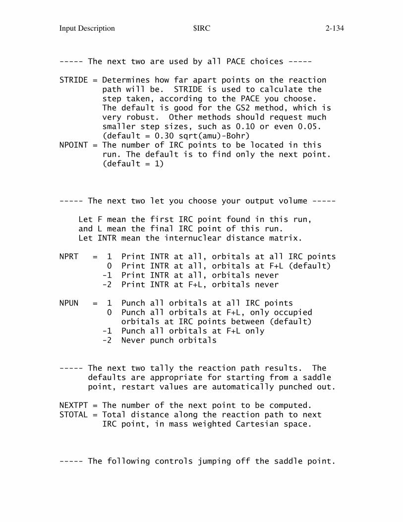
Input Description $IRC 2-134
----- The next two are used by all PACE choices -----
STRIDE = Determines how far apart points on the reaction path will be. STRIDE is used to calculate the step taken, according to the PACE you choose. The default is good for the GS2 method, which is very robust. Other methods should request much smaller step sizes, such as 0.10 or even 0.05. (default = 0.30 sqrt(amu)-Bohr)NPOINT = The number of IRC points to be located in this run. The default is to find only the next point. (default = 1)
----- The next two let you choose your output volume -----
Let F mean the first IRC point found in this run, and L mean the final IRC point of this run. Let INTR mean the internuclear distance matrix.
NPRT = 1 Print INTR at all, orbitals at all IRC points 0 Print INTR at all, orbitals at F+L (default) -1 Print INTR at all, orbitals never -2 Print INTR at F+L, orbitals never
NPUN = 1 Punch all orbitals at all IRC points 0 Punch all orbitals at F+L, only occupied orbitals at IRC points between (default) -1 Punch all orbitals at F+L only -2 Never punch orbitals
----- The next two tally the reaction path results. The defaults are appropriate for starting from a saddle point, restart values are automatically punched out.
NEXTPT = The number of the next point to be computed.STOTAL = Total distance along the reaction path to next IRC point, in mass weighted Cartesian space.
----- The following controls jumping off the saddle point.
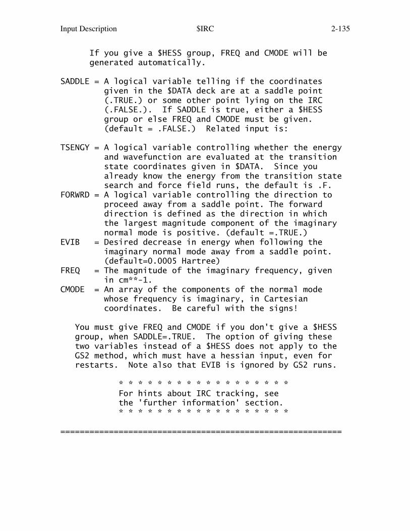
Input Description $IRC 2-135
If you give a $HESS group, FREQ and CMODE will be generated automatically.
SADDLE = A logical variable telling if the coordinates given in the $DATA deck are at a saddle point (.TRUE.) or some other point lying on the IRC (.FALSE.). If SADDLE is true, either a $HESS group or else FREQ and CMODE must be given. (default = .FALSE.) Related input is:
TSENGY = A logical variable controlling whether the energy and wavefunction are evaluated at the transition state coordinates given in $DATA. Since you already know the energy from the transition state search and force field runs, the default is .F.FORWRD = A logical variable controlling the direction to proceed away from a saddle point. The forward direction is defined as the direction in which the largest magnitude component of the imaginary normal mode is positive. (default =.TRUE.)EVIB = Desired decrease in energy when following the imaginary normal mode away from a saddle point. (default=0.0005 Hartree)FREQ = The magnitude of the imaginary frequency, given in cm**-1.CMODE = An array of the components of the normal mode whose frequency is imaginary, in Cartesian coordinates. Be careful with the signs!
You must give FREQ and CMODE if you don't give a $HESS group, when SADDLE=.TRUE. The option of giving these two variables instead of a $HESS does not apply to the GS2 method, which must have a hessian input, even for restarts. Note also that EVIB is ignored by GS2 runs.
* * * * * * * * * * * * * * * * * * For hints about IRC tracking, see the 'further information' section. * * * * * * * * * * * * * * * * * *
==========================================================

Input Description $DRC 2-136
==========================================================
$DRC group (relevant for RUNTYP=DRC)
This group governs "direct dynamics", following thedynamical reaction coordinate, which is a classicaltrajectory based on quantum chemistry potential energysurfaces. These may be either ab initio or semi-empirical,and are computed "on the fly" as the trajectory proceeds.
Because the vibrational period of a normal mode withfrequency 500 wavenumbers is 67 fs, a DRC needs to run formany steps in order to sample a representative portion ofphase space. Restart data can be found in the job's OUTPUTfile, with important results summarized to the TRAJECTfile. Almost all DRCs break molecular symmetry, so buildyour molecule with C1 symmetry in $DATA, or specify NOSYM=1in $CONTRL. RUNTYP=DRC may not be used with EFP particles.
NSTEP = The number of DRC points to be calculated, not including the initial point. (default = 1000)
DELTAT = is the time step. (default = 0.1 fs)
TOTIME = total duration of the DRC computed in a previous job, in fs. The default is the correct value when initiating a DRC. (default=0.0 fs)
* * *
In general, a DRC can be initiated anywhere, so $DATA might contain coordinates of the equilibrium geometry, or a nearby transition state, or something else. You must also supply an initial kinetic energy, and the direction of the initial velocity, for which there are a number of options:
EKIN = The initial kinetic energy (default = 0.0kcal/mol) See also ENM, NVEL, and VIBLVL regarding alternate ways to specify the initial value.
VEL = an array of velocity components, in Bohr/fs. When NVEL is false, this is simply the direction

Input Description $DRC 2-137
of the velocity vector. Its magnitude will be automatically adjusted to match the desiredinitial kinetic energy, and it will be projected so that the translation of the center of mass is removed. Give in the order vx1, vy1, vz1, vx2, vy2, ...
NVEL = a flag to compute the initial kinetic energy from the input VEL using the sum of mass*VEL*VEL/2. This flag is usually selected only for restarts. (default=.FALSE.)
The next three allow the kinetic energy to be partitioned over all normal modes. The coordinates in $DATA are likely to be from a stationary point! You must also supply a $HESS group, which is the nuclear force constant matrix at the starting geometry.
VIBLVL = a flag to turn this option on (default=.FALSE.)
VIBENG = an array of energies (in units of multiples of the hv of each mode) to be imparted along each normal mode. The default is to assign the zero point energy only, VIBENG(1)=0.5, 0.5, ..., 0.5 when HESS=MIN, and 0.0, 0.5, ..., 0.5 if HESS=TS. If given as a negative number, the initial direction of the velocity vector is along the reverse direction of the mode. "Reverse" means the phase of the normal mode is chosen such that the largest magnitude component is a negative value. An example might be VIBENG(4)=2.5 to add two quanta to mode 4, along with zero point energy in all modes.
RCENG = reaction coordinate energy, in kcal/mol. This is the initial kinetic energy given to the imaginary frequency normal mode when HESS=TS. If this is given as a negative value, the direction of the velocity vector will be the "reverse direction", meaning the phase of the normal mode will be chosen so its largest component is negative.
* * *
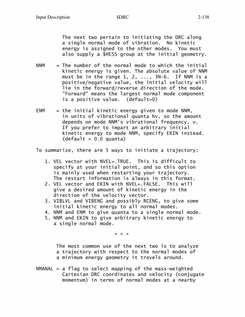
Input Description $DRC 2-138
The next two pertain to initiating the DRC along a single normal mode of vibration. No kinetic energy is assigned to the other modes. You must also supply a $HESS group at the initial geometry.
NNM = The number of the normal mode to which the initial kinetic energy is given. The absolute value of NNM must be in the range 1, 2, ..., 3N-6. If NNM is a positive/negative value, the initial velocity will lie in the forward/reverse direction of the mode. "Forward" means the largest normal mode component is a positive value. (default=0)
ENM = the initial kinetic energy given to mode NNM, in units of vibrational quanta hv, so the amount depends on mode NNM's vibrational frequency, v. If you prefer to impart an arbitrary initial kinetic energy to mode NNM, specify EKIN instead. (default = 0.0 quanta)
To summarize, there are 5 ways to initiate a trajectory:
1. VEL vector with NVEL=.TRUE. This is difficult to specify at your initial point, and so this option is mainly used when restarting your trajectory. The restart information is always in this format. 2. VEL vector and EKIN with NVEL=.FALSE. This will give a desired amount of kinetic energy in the direction of the velocity vector. 3. VIBLVL and VIBENG and possibly RCENG, to give some initial kinetic energy to all normal modes. 4. NNM and ENM to give quanta to a single normal mode. 5. NNM and EKIN to give arbitrary kinetic energy to a single normal mode.
* * *
The most common use of the next two is to analyze a trajectory with respect to the normal modes of a minimum energy geometry it travels around.
NMANAL = a flag to select mapping of the mass-weighted Cartesian DRC coordinates and velocity (conjugate momentum) in terms of normal modes at a nearby
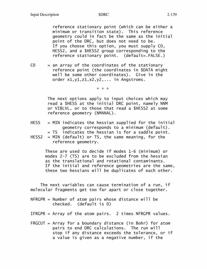
Input Description $DRC 2-139
reference stationary point (which can be either a minimum or transition state). This reference geometry could in fact be the same as the initial point of the DRC, but does not need to be. If you choose this option, you must supply C0, HESS2, and a $HESS2 group corresponding to the reference stationary point. (default=.FALSE.)
C0 = an array of the coordinates of the stationary reference point (the coordinates in $DATA might well be some other coordinates). Give in the order x1,y1,z1,x2,y2,... in Angstroms.
* * *
The next options apply to input choices which may read a $HESS at the initial DRC point, namely NNM or VIBLVL, or to those that read a $HESS2 at some reference geometry (NMANAL).
HESS = MIN indicates the hessian supplied for the initial geometry corresponds to a minimum (default). = TS indicates the hessian is for a saddle point.HESS2 = MIN (default) or TS, the same meaning, for the reference geometry.
These are used to decide if modes 1-6 (minimum) or modes 2-7 (TS) are to be excluded from the hessian as the translational and rotational contaminants. If the initial and reference geometries are the same, these two hessians will be duplicates of each other.
The next variables can cause termination of a run, ifmolecular fragments get too far apart or close together.
NFRGPR = Number of atom pairs whose distance will be checked. (default is 0)
IFRGPR = Array of the atom pairs. 2 times NFRGPR values.
FRGCUT = Array for a boundary distance (in Bohr) for atom pairs to end DRC calculations. The run will stop if any distance exceeds the tolerance, or if a value is given as a negative number, if the
Input Description $DRC 2-140
distance becomes shorter than the absolute value. In case the trajectory starts outside the bounds specified, they do not apply until after the trajectory reaches a point where the criteria are satisfied, and then goes outside again. Give NFRGPR values.
* * *
The final variables control the volume of output. Let F mean the first DRC point found in this run, and L mean the last DRC point of this run.
NPRTSM = summarize the DRC results every NPRTSM steps, to the TRAJECT file. (default = 1)
NPRT = 1 Print orbitals at all DRC points 0 Print orbitals at F+L (default) -1 Never print orbitals
NPUN = 2 Punch all orbitals at all DRC points 1 Punch all orbitals at F+L, and occupied orbitals at DRC points between 0 Punch all orbitals at F+L only (default) -1 Never punch orbitals
==========================================================

Input Description $MEX 2-141
===========================================================
$MEX group (relevant if RUNTYP=MEX)
This group governs a search for the lowest energy on the3N-7 dimensional "seam" of intersection of two differentelectronic potential energy surfaces. Such Minimum EnergyCrossing Points are important for processes such as spin-orbit coupling that involve transfer from one surface toanother, and thus are analogous to transition states on asingle surface. The present program requires that the twosurfaces differ in spin quantum number, or space symmetry,or both. Analytic gradients are used in the search.
In case the two potential surfaces have identical spinand space symmetry, this kind of intersection point isreferred to as a Conical Intersection. See $CONICL usingRUNTYP=CONICAL instead.
SCF1, SCF2 = define the molecular wavefunction types, possibly in conjunction with the usual MPLEVL and DFTTYP keywords.
MULT1, MULT2 = give the spin multiplicity of the states.
Permissible combinations of wavefunctions are RHF with ROHF/UHF ROHF with ROHF UHF with UHF as well as their MP2 and DFT counterparts, and GVB with ROHF/UHF MCSCF with MCSCF (CISTEP=ALDET or GUGA only)
NSTEP = maximum number of search steps (default=50)
STPSZ = Step size during the search (default = 0.1D+00)
NRDMOS = Initial orbitals can be read in = 0 No initial orbitals (default) = 1 Read in orbitals for first state (in $VEC1) = 2 Read in orbitals for second state (in $VEC2) = 3 Read in orbitals for both ($VEC1 and $VEC2)

Input Description $MEX 2-142
NMOS1 = Number of orbitals for first state's $VEC1.
NMOS2 = Number of orbitals for second state's $VEC2.
NPRT = Printing orbitals = 0 No orbital printed out except at the first geometry (default) = 1 Orbitals are printed each geometry. If MCSCF is used, CI expansions are also printed.
Finer control of the convergence criterion:
TDE = energy difference between two states (default = 1.0D-05)
TDXMAX = maximum displacement of coordinates (default = 2.0D-03)
TDXRMS = root mean square displacement (default = 1.5D-03)
TGMAX = maximum of effective gradient between the two states (default = 5.0D-04)
TGRMS = root mean square effective gradient tolerance (default = 3.0D-04)
===========================================================
Usage notes:
1. Normally $CONTRL will not give SCFTYP or MULT keywords.SCF1 and SCF2 can be given in any order. The combinationspermitted ensure roughly equal sophistication in thetreatment of electron correlation.2. After reading $MEX, SCFTYP and MULT will be set to themore complex of the two choices, which is considered to beRHF < ROHF < UHF < GVB < MCSCF. This permits the $SCFinput defining a GVB wavefunction to be read and tested forcorrectness, in a GVB+ROHF run. Since only one SCFTYP isstored while reading the input, you might need to providesome keywords that are normally set by default for theother (such as ensuring DIIS is selected in $SCF if eitherof the states is UHF).

Input Description $MEX 2-143
3. It is safest by far to prepare and read $VEC1 and $VEC2groups so that you know what electronic states you startwith. It is a good idea to regenerate both states at theend of the MEX search, to be sure that they remain as youbegan.4. It is your responsibility to make sure that the stateshave a different space symmetry, or a different spinsymmetry (or both). That is why note 3 is so important.5. $GRAD1 and/or $GRAD2 groups containing gradients may begiven to speed up the first geometry of the MEX search.6. The search is even trickier than a saddle point search,for it involves the peaks and valleys of BOTH surfacesbeing generated. Starting geometries may be guessed aslying between the minima of the two surfaces, but thelowest energy on the crossing seam may turn out to besomewhere else. Be prepared to restart!7. The procedure is a Newton-Raphson search, conducted inCartesian coordinates, with a Lagrange multiplier imposingthe constraint of equal energy upon the two states. Thehessian matrices in the search are guessed at, andsubjected to BFGS updates. Internal coordinates will beprinted (for monitoring purposes) if you define $ZMAT, butthe stepper operates in Cartesian coordinates only. Nogeometry constraints can be applied, apart from the pointgroup in $DATA.
A good paper to read about this kind of search isA.Farazdel, M.Dupuis J.Comput.Chem. 12, 276-282(1991)

Input Description $CONICL 2-144
===========================================================
$CONICL group (relevant if RUNTYP=CONICAL)
This group governs a search for the lowest energy on the3N-7 dimensional "seam" of intersection of two electronicpotential energy surfaces of the same spin and spacesymmetry. Such Conical Intersections (CI) are important inphotochemistry, where they serve as "funnels" for thetransfer from an excited state to a lower state. SeeRUNTYP=MEX and the $MEX input for the simpler case wherethe two surfaces differ by either space or spin symmetry.
Three search procedures are given, one of which requiresthe non-adiabatic coupling matrix element (NACME), and twoothers which do not require NACME information. The conicalintersection search is available only for MCSCF (for whichNACME are available) or for TD-DFT potential surfaces(where NACME are not available). The TD-DFT must be usedin the Tamm/Dancoff approximation (see TAMMD in $TDDFT),but can be either conventional or spin-flip.
The search utilizes some of the options of $STATPT, butnote that the Schlegel stepper and HESS=CALC are notpermitted. It may be reasonable to try the RFO steppersometimes. The search can only be run in Cartesiancoordinates. Restarts are possible only by updating thecoordinates in $DATA.
At present, the only solvation model that is supportedis conventional TD-DFT with EFP1.
OPTTYP = search procedure choice, see references below! = GPWNAC Gradient Projection with NACME, so this is only available for MCSCF. = BPUPD branching plane updating method (default) = PENALTY penalty-constrained optimization method
Note that for MCSCF surfaces, if state-averaging is used,the program executes the code needed to produce NACMEvectors, to producing the state-averaged gradients. Thereis essentially no extra time required to produce also theNACME, hence the GPWNAC stepper might as well be used.

Input Description $CONICL 2-145
IXROOT = array of two states whose CI point is sought. For example, this might be IXROOT(1)=2,3 The roots are counted exactly the same as IROOT in the $DET or $TDDFT input groups. For the latter case, set IXROOT to 0 if you want the ground state to be one of the two surfaces searched on. There is no default for IXROOT!
SYMOFF = flag to switch off point group symmetry, the default is .TRUE.
DEBUG = flag to print debugging info, default is .FALSE.
The following are meaningful only for OPTTYP=PENALTY:
TOLSTP = energy difference tolerance default=1d-6 Hartree
TOLGRD = gradient convergence tolerance default=5d-3 Hartree/Bohr
ALPHA = parameter ensuring a singularity free penalty, default=0.02 Hartree
SIGMA = Lagrange multiplier for the penalty term. In case the energy gap between the states is not acceptable at the CI point, increase the value. default = 3.5 (unitless)
An understanding of the search procedures can be gained byreading the following papers:
Gradient Projection with NACME: M.J.Bearpark, M.A.Robb, H.B.Schlegel Chem.Phys.Lett. 223, 269(1994) Branching Plane Updating method: S.Maeda, K.Ohno, K.Morokuma J.Chem.Theor Comput. 6, 1538(2010) Penalty constrained update method: B.G.Levine, C.Ko, J.Quenneville, T.J.Martinez Mol.Phys. 104, 1039(2006) B.G.Levine, J.D.Coe, T.J.Martinez J.Phys.Chem.B 112, 405(2008)
A comparative study of the first two procedures is

Input Description $CONICL 2-146
T.W.Keal, A.Koslowski, W.Thiel Theoret.Chem.Acc. 118, 837(2007)
===========================================================

Input Description $MD 2-147
===========================================================
$MD group (relevant if RUNTYP=MD)
This group controls the molecular dynamics trajectory for acollection of quantum mechanical atoms and/or EffectiveFragment Potential particles.
A typical MD simulation starts with an equilibration phase,running long enough to produce a randomized structure andvelocity distribution. Typically equilibration is donewith an NVT ensemble, allowing the system to equilibrate toa desired temperature. A production run restarts with thepositions and the velocity and quaternion data from theequilibration run, might use either a NVE or NVT ensemble,and collects radial distribution functions and otherproperties.
Only a few properties are computed from the MD trajectory,apart from correct radial distribution functions. Inparticular, the pressures, diffusion constants, and heatsof vaporization that appear on the printout (presently onlyfor pure EFP runs) are from a preliminary code, which hasnot yet been verified.
If the system contains only EFP particles, it may be placedin a periodic box, according to the minimum imageconvention. The optional periodic boundary conditions,along with cut-offs, are given in the $EFRAG input. Seealso the $EWALD input group for long-range electrostatictreatment if PBC is used.
The first keywords relate to the steps:
MDINT = MD integrator selection. = FROG (leapfrog). This is less accurate, and lacks the special ensemble stepper option NVTNH. = VVERLET (velocity Verlet) - default.
DT = MD time step size, in seconds, default=1.0d-15, which is a femtosecond.
NVTNH selects a integrator step appropriate to the desired ensemble. This is only implemented for

Input Description $MD 2-148
velocity Verlet. = 0 means use NVE Verlet stepping = 1 means use NVT Verlet stepping = 2 means use Nose/Hoover chain NVT Verlet stepping The default is 2 if either NVT option RSTEMP or RSRAND is chosen, but is 0 otherwise.
NSTEPS = number of MD time steps to be found in this run, default=10000.
TTOTAL = total time elapsed in the previous part of a MD trajectory which is being restarted (READ=.TRUE.). The default means this trajectory is a new one, or perhaps the start of a production phase of the MD. (default=0.0 seconds)
* * *
BATHT = bath temperature, in Kelvin (default=300.0) This value is used during NVT runs, or if the MD is initialized to a Maxwell-Boltzmann velocity distribution.
* * *
Two options exist to create NVT runs, to bring the system to a desired bath temperature. If neither is chosen, the ensemble is NVE:
RSTEMP = flag to rescale the temperature. default=.FALSE.
DTEMP = temperature range for the RSTEMP option. The velocities are rescaled to the bath temperature if T < (BATHT-DTEMP) or T > (BATHT+DTEMP). The default is DTEMP=100.0 degrees.
RSRAND = flag to reset to Maxwell-Boltzmann distribution, using random numbers (same algorithm as MBT and MBR) to choose individual velocity magnitudes and directions. default=.FALSE.
NRAND = number of steps for the RSRAND option. Reassign velocities (translational and rotational) every NRAND time steps. Default=1000.

Input Description $MD 2-149
NVTOFF = step number at which to turn off either NVT thermostat, and switch to NVE. At this point, the NVTNH parameter will be reset to 0, and the PROD flag will be turned on, so that the production run will start (gathering and printing the RDF information to .log file). This keyword is also useful in NVE runs to postpone the accumulation of production information. The default means no switch to NVE (default=0).
JEVERY = report simulation quantities (write info such as energies, temps, etc. to .log file) and collect RDF info each JEVERY time step. Default=10
KEVERY = write coordinates (to log and TRAJECT files), velocity/quaternion restart info (to the TRAJECT file and RDFs (to log file) at each KEVERY step. default=100
PROD = production run, at present this means only that information for radial distribution functions is collected, and printed. default=.FALSE.
DELR = spacing for radial bins in RDF calculations, default=0.02 Angstroms.
NPROP = step number at which to begin collecting data for the other properties, such as pressure and diffusion constants. This should be a value between 1 and NSTEPS, as it counts off the current run's steps. Default=0.
PBCOUT = print PBC coordinates in the end of simulation (i.e. all molecules will be contained in one box) Default=.FALSE.
* * *
The following keywords control starting MD conditions.Normally an MD trajectory is initiated with both MBT andMBR chosen, while restarts would select only READ. Therestart data is written to the TRAJECT file. To restartrequires merging particle coordinates into $DATA and/or$EFRAG, and placing the $MD group below your existing $MD

Input Description $MD 2-150
group, thus keeping your choices for the variables above(both $MD groups will be read).
MBT = get translational velocities from a random Maxwell-Boltzmann ensemble. Default=.FALSE.
MBR = get rotational velocities from a random Maxwell- Boltzmann ensemble. Default=.FALSE.
QRAND = if .TRUE., generate random quaternions, an option that is not normally chosen. if .FALSE., use EFP particle coordinates and the initial MBT/MBR assigned velocities to set correct quaternion data (default is .FALSE.)
READ = read velocities (translational and rotational) and quaternions and their first and second derivatives from input file. Default is .FALSE. Set the other three values MBT/MBR/QRAND off if you choose restarting with READ.
For READ=.TRUE., the following restart data is required.This data may be copied from the TRAJECT file, in exactlythe format it was written out. The required data dependson your choice for the integrator, see MDINT above. Inaddition, you will need to update the particle coordinatesin $DATA and/or $EFRAG, using data from the TRAJECT file.
TVELQM(1)= quantum atom's translational velocities (both).TVEL(1)= array of EFP translational velocities (both).RVEL(1)= array of EFP rotational velocities (VVERLET).RMOM(1)= array of EFP rotational momenta (FROG).QUAT(1)= array of EFP quaternions (both).QUAT1D(1)= EFP quaternion first derivatives (VVERLET).QUAT2D(1)= EFP quaternion second derivatives (VVERLET).
extra reading: "Computer Simulation of Liquids" M.P.Allen, D.J.Tildesley Oxford Science, 1987 "Understanding Molecular Simulation" D.Frenkel, B.Smit Academic Press, 2002
===========================================================

Input Description $RDF 2-151
==========================================================
$RDF group (relevant for RUNTYP=MD)
This group defines the pairs of atoms for which theradial distribution functions are to be computed, at theend of a molecular dynamics trajectory. The input issimilar in style to $EFRAG, consisting of separate lines,with the word STOP ending each particular pair.
Line 1. NRDF=<no.RDFs>gives the number of RDFs which should be computed.
Line 2. <pair title> <FRAG1> <FRAG2> <no.pairs>gives a string for the printout (a good choice involvesboth atoms, such as ClCl), the name of the $FRAGNAMEcontaining the first atom of the pair, the name of the$FRAGNAME group with the second atom of the pair, and howmany such pairs exist.
Line 3. <label> <num.atom1> <num.atom2>gives a label (arbitrary), the position of the atom withinthe $FRAG1 group, and the 2nd atom's within the $FRAG2.This line must be repeated <no.pairs> times.
Line 4. STOPthe word STOP ends this RDF's pair input.
Lines 2-4 must then be repeated a total of <no.RDFs> times.
An example will make this all clear. If there is only onetype of fragment used, such as water (so $EFRAG containsonly FRAGNAME=WATER), and assuming that this $WATER groupdefining the water EFP has atoms in the order O,H,H:
$RDFnrdf=3OO water water 1 dum 1 1STOPOH water water 4 dum 1 2 dum 1 3 dum 2 1 dum 3 1

Input Description $RDF 2-152
STOPHH water water 4 dum 2 2 dum 2 3 dum 3 2 dum 3 3STOP $end
==========================================================

Input Description $GLOBOP 2-153
==========================================================
$GLOBOP group (relevant to RUNTYP=GLOBOP)
This controls a search for the global minimum energy.It is primarily intended for locating the best position foreffective fragment "solvent" molecules, perhaps with an abinitio "solute" present. There are options for a singletemperature Monte Carlo search, or a multiple temperaturesimulated annealing. Local minimization of some or all ofthe structures selected by the Monte Carlo is optional.See REFS.DOC for an overview of this RUNTYP.
The coordinates of accepted structures are written tothe file TRAJECT. A perl script named "globop_extract" isprovided in the standard GAMESS distribution, which canextract the lowest energies (and matching coordinates) fromthe TRAJECT data set.
RNDINI = flag to randomize the particles given in $EFRAG, usually choosing the particle at random, placing it near the center of the coordinate origin but in such a way that it does not collide with any particles placed earlier. The default is to use coordinates as given in $EFRAG (default .FALSE.)
RIORD = relevant only if RNDINI is .TRUE. = RAND selects EFP particles in random order, as well as randomizing their coordinates. (default) = STANDARD chooses the particles in the same order that they were given in $EFRAG, so only their positions are randomized.
See REFS.DOC for some ideas on how to build clusters withthese two inputs.
TEMPI = initial temperature used in the simulation. (default = 20000 K)
TEMPF = final temperature. If TEMPF is not given and NTEMPS is greater than 1, TEMPF will be calculated based on a cooling factor of 0.95.
NTEMPS = number of temperatures used in the simulation.
Input Description $GLOBOP 2-154
If NTEMPS is not given but TEMPF is given, NTEMP will be calculated based on a cooling factor of 0.95. If neither NTEMP nor TEMPF is given, the job defaults to a single temperature Monte Carlo calculation.
NFRMOV = number of fragments to move on each step. (default=1)
NGEOPT = number of geometries to be evaluated at each temperature. (default = 100)
NTRAN = number of translational steps in each block. (default=5)
NROT = number of rotational steps in each block. (default=5)
NBLOCK = the number of blocks of steps can be set directly with this variable, instead of being calculated from NGEOPT, NTRAN, and NROT, according to NBLOCK=NGEOPT/(NTRAN+NROT) If NBLOCK is input, the number of geometries at each temperature will be taken as NGEOPT=NBLOCK*(NTRAN+NROT) Each block has NTRAN translational steps followed by NROT rotational steps.
MCMIN = flag to enable geometry optimization to minimize the energy is carried out every NSTMIN steps. (default=.true.)
NSTMIN = After this number of geometry steps are taken, a local (Newton-Raphson) optimization will be carried out. If this variable is set to 1, a local minimization is carried out on every step, reducing the MC space to the set of local minima. Irrelevant if MCMIN is false. (default=10)
OPTN = if set to .TRUE., at the end of the run local minimizations are carried out on the final geometry and on the minimum-energy geometry. (default=.FALSE.)
SCALE = an array of length two. The first element is the
Input Description $GLOBOP 2-155
initial maximum step size for the translational coordinates (Angstroms). The second element is the initial maximum stepsize for the rotational coordinates (pi-radians). (defaults = 1,1)
AIMOVE = step range for moving ab initio atoms in the MC simulation. If set to zero, the ab initio atoms do not move in MC. The motion of ab initio atoms is unsophisticated, as the move consists only of shifting each Cartesian coordinate in the range of plus AIMOVE to minus AIMOVE atomic units. Ab initio atoms are allowed to relax during possible geometry optimizations implied by MCMIN/NSTMIN. (default=0.0)
ALPHA = controls the rate at which information from successful steps is folded into the maximum step sizes for each of the 6*(number of fragments) coordinates. ALPHA varies between 0 and 1. ALPHA=0 means do not change the maximum step sizes, and ALPHA=1 throws out the old step sizes whenever there is a successful step and uses the successful step sizes as the new maxima. This update scheme was used with the Parks method where all fragments are moved on every step. It is normally not used with the Metropolis method. (default = 0)
DACRAT = the desired acceptance ratio, the program tries to achieve this by adjusting the maximum step size. (default = 0.5)
UPDFAC = the factor used to update the maximum step size in the attempt to achive the desired acceptance ratio (DACRAT). If the acceptance ratio at the previous temperature was below DACRAT, the step size is decreased by multiplying it by UPDFAC. If the acceptance ratio was above DACRAT, the step size is increased by dividing it by DACRAT It should be between 0 and 1. (default = 0.95)
SEPTOL = the separation tolerence between atoms in the ab initio piece and atoms in the fragments, as well as between atoms in different fragments. If a step moves atoms closer than this tolerence, the

Input Description $GLOBOP 2-156
step is rejected. (default = 1.5 Angstroms)
XMIN, XMAX, YMIN, YMAX, ZMIN, ZMAX = mimimum and maximum values for the Cartesian coordinates of the fragment. If the first point in a fragment steps outside these boundaries, periodic boundary conditions are used and the fragment re-enters on the opposite side of the box. The defaults of -10 for minima and +10 for maxima should usually be changed.
BOLTWT = method for calculating the Boltzmann factor, which is used as the probability of accepting a step that increases the energy. = STANDARD = use the standard Boltzmann factor, exp(-delta(E)/kT) (default) = AVESTEP = scale the temperature by the average step size, as recommended in the Parks reference when using values of ALPHA greater than 0.
NPRT = controls the amount of output, with = -2 reduces output below that of -1 = -1 reduces output further, needed for MCMIN=.true. = 0 gives minimal output (default) = 1 gives the normal GAMESS amount of output = 2 gives maximum output For large simulations, even IOUT=0 may produce a log file too large to work with easily. If geometry optimization is being done at each Monte Carlo generated structure, you can use the NPRT in $STATPT to further suppress output.
RANDOM = controls the choice of random number generator. = DEBUG uses a simple random number generator with a constant seed. Since the same sequence of random numbers is generated during each job, it is useful for debugging. = RAND1 uses the simple random number generator used in DEBUG, but with a variable seed. = RAND3 uses a more sophisticated random number generator described in Numerical Recipes, with a variable seed (default).
IFXFRG = array whose length is the number of fragments. It allows one or more fragments to be fixed

Input Description $GLOBOP 2-157
during the simulation. =0 allows the fragment to move during the run =1 fixes the fragment For example, IFXFRG(3)=1 would fix the third fragment, the default is IFXFRG(1)=0,0,0,...,0
==========================================================

Input Description $GRADEX 2-158
==========================================================
$GRADEX group (optional, for RUNTYP=GRADEXTR)
This group controls the gradient extremal followingalgorithm. The GEs leave stationary points parallel toeach of the normal modes of the hessian. Sometimes a GEleaving a minimum will find a transition state, and thusprovides us with a way of finding that saddle point. GEshave many unusual mathematical properties, and you shouldbe aware that they normally differ a great deal from IRCs.
The search will always be performed in cartesiancoordinates, but internal coordinates along the way maybe printed by the usual specification of NZVAR and $ZMAT.
METHOD = algorithm selection. SR A predictor-corrector method due to Sun and Ruedenberg (default). JJH A method due to Jorgensen, Jensen and Helgaker.
NSTEP = maximum number of predictor steps to take. (default=50)
DPRED = the stepsize for the predictor step. (default = 0.10)
STPT = a flag to indicate whether the initial geometry is considered a stationary point. If .TRUE., the geometry will be perturbed by STSTEP along the IFOLOW normal mode. (default = .TRUE.)
STSTEP = the stepsize for jumping away from a stationary point. (default = 0.01)
IFOLOW = Mode selection option. (default is 1) If STPT=.TRUE., the intial geometry will be perturbed by STSTEP along the IFOLOW normal mode. Note that IFOLOW can be positive or negative, depending on the direction the normal mode should be followed in. The positive direction is defined as the one where the largest component of the Hessian eigenvector is positive.

Input Description $GRADEX 2-159
If STPT=.FALSE. the sign of IFOLOW determines which direction the GE is followed in. A positive value will follow the GE in the uphill direction. The value of IFOLOW should be set to the Hessian mode which is parallel to the gradient to avoid miscellaneous warning messages.
GOFRST = a flag to indicate whether the algorithm should attempt to locate a stationary point. If .TRUE., a straight NR search is performed once the NR step length drops below SNRMAX. 10 NR step are othen allowed, a value which cannot be changed. (default = .TRUE.)
SNRMAX = upper limit for switching to straight NR search for stationary point location. (default = 0.10 or DPRED, whichever is smallest)
OPTTOL = gradient convergence tolerance, in Hartree/Bohr. Used for optimizing to a stationary point. Convergence of a geometry search requires the rms gradient to be less than OPTTOL. (default=0.0001)
HESS = selection of the initial hessian matrix, if STPT=.TRUE. = READ causes the hessian to be read from a $HESS group. = CALC causes the hessian to be computed. (default)
---- the next parameters apply only to METHOD=SR ----
DELCOR = the corrector step should be smaller than this value before the next predictor step is taken. (default = 0.001)
MYSTEP = maximum number of micro iteration allowed to bring the corrector step length below DELCOR. (default=20)
SNUMH = stepsize used in the numerical differentiation of the Hessian to produce third derivatives. (default = 0.0001)

Input Description $GRADEX 2-160
HSDFDB = flag to select determination of third derivatives. At the current geometry we need the gradient, the Hessian, and the partial third derivative matrix in the gradient direction.
If .TRUE., the gradient is calculated at the current geometry, and two Hessians are calculated at SNUMH distance to each side in the gradient direction. The Hessian at the geometry is formed as the average of the two displaced Hessians.
If .FALSE., both the gradient and Hessian are calculated at the current geometry, and one additional Hessian is calculated at SNUMH in the gradient direction.
The default double-sided differentiation produces a more accurate third derivative matrix, at the cost of an additional wave function and gradient. (default = .TRUE.)
==========================================================
* * * * * * * * * * * * * * * * * * * See the 'further information' section for some help with GRADEXTR runs. * * * * * * * * * * * * * * * * * * *
Input Description $SURF 2-161
==========================================================
$SURF group (relevant for RUNTYP=SURFACE)
This group allows you to probe a potential energysurface along a small grid of points. Note that there isno option to vary angles, only distances. The scan canbe made for any SCFTYP, or for the MP2 or CI surface. Youmay specify two rather different calculations to be doneat each point on the grid, through the RUNTYPn, SCFTYPn,and electron correlation keywords.
* * * below, 1 and 2 refer to different calculations * * *
RUNTP1,RUNTYP2 = some RUNTYP supported in $CONTRL First RUNTYP=RUNTP1 and then RUNTYP=RUNTP2 will be performed, for each point on the grid. The second run is omitted if RUNTP2 is set to NONE. default: RUNTP1=ENERGY RUNTP2=NONE
SCFTP1,SCFTP2 = some SCFTYP supported in $CONTRL default: SCFTYP in $CONTRL
CITYP1,CITYP2 = some CITYP supported in $CONTRL default: CITYP in $CONTRL
MPLEV1,MPLEV2 = some MPLEVL supported in $CONTRL default: MPLEVL in $CONTRL
CCTYP1,CCTYP2 = some CCTYP supported in $CONTRL default: CCTYP in $CONTRL
DFTYP1,DFTYP2 = some DFTTYP supported in $DFT default: DFTTYP in $DFT
You may need to help by giving values in $CONTRL that willpermit the program to estimate what is coming in the valueshere. For example, if you want to request hessians here,it may be good to give RUNTYP=HESSIAN in $CONTRL so thatin its earliest stages of a job, the program can initializefor 2nd derivatives. There is less checking here than on$CONTRL input, so don't request something impossible suchas two correlaton methods simultaneously, or analytichessians for MP2, or other things that are impossible.

Input Description $SURF 2-162
* * * below, 1 and 2 refer to different coordinates * * *
IVEC1 = an array of two atoms, defining a coordinate from the first atom given, to the second.
IGRP1 = an array specifying a group of atoms, which must include the second atom given in IVEC1. The entire group will be translated (rigidly) along the vector IVEC1, relative to the first atom given in IVEC1.
ORIG1 = starting value of the coordinate, which may be positive or negative. Zero corresponds to the distance given in $DATA.
DISP1 = step size for the coordinate. If DISP1 is set to zero, then the keyword GRID1 is read.
NDISP1 = number of steps to take for this coordinate.
GRID1 = an array of grid points at which to compute the energy. This option is an alternative to the ORIG1, DISP1 input which produces an equidistant grid. To use GRID1, one has to set DISP1=0.0. The number of grid points is given in NDISP1, and is limite to at most 100 grid points. The input of GRID1(1)=ORIG1,ORIG1+DISP1,ORIG1+DISP1*2,... would reproduce an equidistant grid given by ORIG1 and DISP1.
ORIG1, DISP1, and GRID1 should be given in Angstrom. There are no reasonable defaults for these keywords.
IVEC2, IGRP2, ORIG2, DISP2, NDISP2, GRID2 have the samemeaning as their "1" counterparts, and permit you to makea two dimensional map along two displacement coordinates.If the "2" data are not input, the surface map proceeds inonly one dimension.
==========================================================
Input Description $LOCAL 2-163
==========================================================
$LOCAL group (relevant if LOCAL=RUEDNBRG, BOYS, or POP)
This group allows input of additional data to controlthe localization methods. If no input is provided, thevalence orbitals will be localized as much as possible,while still leaving the wavefunction invariant. There aremany specialized options for Localized Charge Distributionanalysis, and for EFP generation.
N.B. Since Boys localization needs the dipole integrals, do not turn off dipole moment calculation in $ELMOM.
MAXLOC = maximum number of localization cycles. This applies to BOYS or POP methods only. If the localization fails to converge, a different order of 2x2 pairwise rotations will be tried. (default=250)
CVGLOC = convergence criterion. The default provides LMO coefficients accurate to 6 figures. (default=1.0E-6)
SYMLOC = a flag to restrict localization so that orbitals of different symmetry types are not mixed. This option is not supported in all possible point groups. The purpose of this option is to give a better choice for the starting orbitals for GVB-PP or MCSCF runs, without destroying the orbital's symmetry. This option is compatible with each of the 3 methods of selecting the orbitals to be included. If chosen in a run requesting VVOS (see $SCF), occupied and virtual orbitals will also not be permitted to mix in a localization of these two separate orbital spaces. (default=.FALSE.)
ORIENT = a flag to request orientation of the localized orbitals for bond-order analysis. After the localization, the orbitals on each atom are rotated only among themselves, in order to direct the orbitals towards neighboring atom's orbitals, to which they are bonded. The density matrix, or bond-order matrix, of these Oriented LMOs is readily interpreted as atomic populations and
Input Description $LOCAL 2-164
bond orders. This option can be used only for SCFTYP=MCSCF and LOCAL=RUEDNBRG. (default=.FALSE.)
PRTLOC = a flag to control supplemental printout. The extra output is the rotation matrix to the localized orbitals, and, for the Boys method, the orbital centroids, for the Ruedenberg method, the coulomb and exchange matrices, for the population method, atomic populations. (default=.FALSE.)
----- The following keywords select the orbitals which are to be included in the localization. You may select from FCORE, NOUTA/NOUTB, or NINA/NINB, but may choose only one of these three groups.
FCORE = flag to freeze all the chemical core orbitals present. All the valence orbitals will be localized. You must explicitly turn this option off to choose one of the other two orbital selection options. (default=.TRUE.)
* * *
NOUTA = number of alpha orbitals to hold fixed in the localization. (default=0)
MOOUTA = an array of NOUTA elements giving the numbers of the orbitals to hold fixed. For example, the input NOUTA=2 MOOUTA(1)=8,13 will freeze only orbitals 8 and 13. You must enter all the orbitals you want to freeze, including any cores. This variable has nothing to do with cows.
NOUTB = number of beta orbitals to hold fixed in -UHF- localizations. (default=0)
MOOUTB = same as MOOUTA, except that it applies to the beta orbitals, in -UHF- wavefunctions only.
* * *
NINA = number of alpha orbitals which are to be

Input Description $LOCAL 2-165
included in the localization. (default=0)
MOINA = an array of NINA elements giving the numbers of the orbitals to be included in the localization. Any orbitals not mentioned will be frozen.
NINB = number of -UHF- beta MOs in the localization. (default=0)
MOINB = same as MOINA, except that it applies to the beta orbitals, in -UHF- wavefunctions only.
ORMFUL = this flag is relevant only to CISTEP=ORMAS MCSCF localizations. By default, the localization is restricted such that the multiple active spaces are not mixed, leaving the total wavefunction invariant. It may be used to localize within the full range of active MOs. (Default is .FALSE.)
----- The following keywords are used for the localized charge distribution (LCD), a decomposition scheme for the energy, or multipole moments, or the first polarizability. See also LOCHYP in $FFCALC for the decomposition of hyperpolarizabilities.
EDCOMP = flag to turn on LCD energy decomposition. Note that this method is currently implemented for SCFTYP=RHF and ROHF and LOCAL=RUEDNBRG only. The SCF LCD forces all orbitals to be localized, overriding input on the previous page. See also LMOMP2 in the $MP2 group. (default = .FALSE.) $LOCAL
MOIDON = flag to turn on LMO identification and subsequent LMO reordering, and assign nuclear LCD automat- ically. (default = .FALSE.)
DIPDCM = flag for LCD molecular dipole decomposition. (default = .FALSE.)
QADDCM = flag for LCD molecular quadrupole decomposition. (default = .FALSE.)

Input Description $LOCAL 2-166
POLDCM = flag to compute the static alpha polarizability, and its decomposition in terms of LCDs. The computation is done analytically, unless either of POLNUM or POLAPP is chosen. This method is implemented for SCFTYP=RHF or ROHF and LOCAL=BOYS or RUEDNBRG. (default=.FALSE., except that RUNTYP=MAKEFP turns this computation on, automatically. LMO dipole polarizabilities are the polarizability term in the EFP model) See also POLDYN in this group.
POLNUM = flag to forces numerical rather than analytical calculation of the polarizabilities. This may be useful in larger molecules. The numerical polarizabilities of bonds in or around aromatic rings sometimes are unphysical. (default=.FALSE.) See D.R.Garmer, W.J.Stevens J.Phys.Chem. 93, 8263-8270(1989). POLDYN may not be used with this keyword.
POLAPP = flag to force calculation of the polarizabilities using a perturbation theory expression. This may be useful in larger molecules. (default=.FALSE.) See R.M. Minikis, V. Kairys, J.H. Jensen J.Phys.Chem.A 105, 3829-3837(2001) POLDYN may not be used with this keyword.
POLANG = flag to choose units of localized polarizability output. The default is Angstroms**3, while false will give Bohr**3. (default=.TRUE.)
ZDO = flag for LCD analysis of a composite wavefunction, given in a $VEC group of a van der Waals complex, using the zero differential overlap approximation. The MOs are not orthonormalized and the inter- molecular electron exchange energy is neglected. Also, the molecular overlap matrix is printed out. This is a very specialized option. (default = .FALSE.)
----- The following keywords can be used to define the nuclear part of an LCD. They are usually used to rectify mistakes in the automatic definition made when MOIDON=.TRUE. The index defining the

Input Description $LOCAL 2-167
LMO number then refers to the reordered list of LMOs.
NMOIJ = array giving the number of nuclei assigned to a particular LMO.
IJMO = is an array of pairs of indices (I,J), giving the row (nucleus I) and column (orbital J) index of the entries in ZIJ and MOIJ.
MOIJ = arrays of integers K, assigning nucleus K as the site of the Ith charge of LCD J.
ZIJ = array of floating point numbers assigning a charge to the Ith charge of LCD J.
IPROT = array of integers K, defining nucleus K as a proton.
DEPRNT = a flag for additional decomposition printing, such as pair contributions to various energy terms, and centroids of the Ruedenberg orbitals. (default = .FALSE.)
----- The following keywords are used to build large EFPs from several RUNTYP=MAKEFP runs on smaller molecular fragments, by excluding common regions of overlap. For example, an EFP for n-octanol can be build from two MAKEFP runs, on n-pentane and n-pentanol, CH3CH2CH2CH2-CH2CH2CH2CH2OH CH3CH2CH2CH2[-CH3] [CH3]-CH2CH2CH2CH2OH by excluding operlapping regions shown in brackets from the two EFPs. See J.Phys.Chem.A 105, 3829-3837, (2001) for more information.
NOPATM = array of atoms that define an area to be excluded from a DMA ($STONE) during a RUNTYP=MAKEFP run. All atomic centers specified, and the midpoints of any bonds to them, are excluded as expansion points. The density due to all LMOs primarily centered on these atoms are excluded from the DMA (see also KMIDPT). Furthermore, polarizability tensors for these LMOs are excluded.

Input Description $LOCAL 2-168
KPOINT = array of "boundary atoms", those atoms that are covalently bonded to the atoms given in NOATM.
KMIDPT = flag to indicate whether the density due to bond LMOs (and associated expansion points) between the NOPATM atoms and the KPOINT atoms are to be included in the DMA. (default = .TRUE.)
NODENS = an array that specifies the atoms for which the associated electronic density will be removed before the multipole expansion. This provides an EFP with net integer charge. (P.A.Molina, H.Li, J.H.Jensen J.Comput.Chem. 24, 1972-1979(2003).
The following keywords relate to the computation ofimaginary frequency dynamic polarizabilities. This isuseful in the development of the dispersion energy formulain the EFP2 model, but may also be computed separately, ifwished.
POLDYN = a flag to compute imaginary frequency dependent dynamic polarizabilities (alpha), by analytic means. (default=.FALSE., but .TRUE. if RUNTYP=MAKEFP)
NDPFRQ = number of imaginary frequencies to compute. Default=1 for most runs, but=12 if RUNTYP=MAKEFP.
DPFREQ = an array of imaginary frequencies to be used, entered as real numbers (absolute values). The default=0.0 for most runs, which is silly, because this just computes the normal static dipole polarizability! For RUNTYP=MAKEFP, the program uses 12 internally stored values, which serve as the roots for a Gauss-Legendre quadrature to extract the C6 dispersion coefficients. Given in atomic units.
For more information, see I.Adamovic, M.S.Gordon Mol.Phys. 103, 379-387(2005).
==========================================================
* * * * * * * * * * * * * * * * * *

Input Description $LOCAL 2-169
For hints about localizations, and the LCD energy decomposition, see the 'further information' section. * * * * * * * * * * * * * * * * * *
==========================================================
Input Description $TRUNCN 2-170
==========================================================
$TRUNCN group (optional, relevant for RHF)
This group controls the truncation of some of thelocalized orbitals to just the AOs on a subset of theatoms. This option is particularly useful to generatelocalized orbitals to be frozen when the effectivefragment potential is used to partition a system across achemical bond. In other words, this group prepares thefrozen buffer zone orbitals. This group should be used inconjunction with RUNTYP=ENERGY (or PROP if the orbitalsare available) and either LOCAL=RUEDNBRG or BOYS, withMOIDON set in $LOCAL.
DOPROJ = flag to activate MO projection/truncation, the default is to skip this (default=.FALSE.)
AUTOID = forces identification of MOs (analogous to MOIDON in $LOCAL). This keyword is provided in case the localized orbitals are already present in $VEC, in which case this is a faster RUNTYP=PROP with LOCAL=NONE job. Obviously, GUESS=MOREAD. (default=.FALSE.)
PLAIN = flag to control the MO tail truncation. A value of .FALSE. uses corresponding orbital projections, H.F.King, R.E.Stanton, H.Kim, R.E.Wyatt, R.G.Parr J. Chem. Phys. 47, 1936-1941(1967) and generates orthogonal orbitals. A value of .TRUE. just sets the unwanted AOs to zero, so the resulting MOs need to go through the automatic orthogonalization step when MOREAD in the next job. (default=.FALSE.)
IMOPR = an array specifying which MOs to be truncated. In most cases involving normal bonding, the options MOIDON or AUTOID will correctly identify all localized MOs belonging to the atoms in the zone being truncated. However, you can inspect the output, and give a list of all MOs which you want to be truncated in this array, in case you feel the automatic assignment is incorrect. Any orbital not in the truncation set, whether this is chosen automatically or by IMOPR, is left

Input Description $TRUNCN 2-171
completely unaltered.
- - -
There are now two ways to specify what orbitals are tobe truncated. The most common usage is for preparation ofa buffer zone for QM/MM computations, with an EffectiveFragment Potential representing the non-quantum part ofthe system. This input is NATAB, NATBF, ICAPFR, ICAPBF,in which case the $DATA input must be sorted into threezones. The first group of atoms are meant to be treatedin later runs by full quantum mechanics, the secondgroup by frozen localized orbitals as a 'buffer', and thethird group is to be substituted later by an effectivefragment potential (multipoles, polarizabilities, ...).Note that in the DOPROJ=.TRUE. run, all atoms are stillquantum atoms.
NATAB = number of atoms to be in the 'ab initio' zone.
NATBF = number of atoms to be in the 'buffer' zone. The program can obtain the number of atoms in the remaining zone by subtraction, so it need not be input.
In case the MOIDON or AUTOID options lead to confusedassignments (unlikely in ordinary bonding situationsaround the buffer zone), there are two fine tuning values.
ICAPFR = array indicating the identity of "capping atoms" which are on the border between the ab initio and buffer zones (in the ab initio zone).
ICAPBK = array indicating the identity of "capping atoms" which are on the border between the buffer and EFP zones (in the effective fragment zone).
See also IXCORL and IXLONE below.
- - -
In case truncation seems useful for some other purpose,you can specify the atoms in any order within the $DATAgroup, by the IZAT/ILAT approach. You are supposed togive only one of these two lists, probably whichever is

Input Description $TRUNCN 2-172
shorter:
IZAT = an array containing the atoms which are NOT in the buffer zone.
ILAT = an array containing the atoms which are in the buffer zone.
The AO coefficients of the localized orbitals present inthe buffer zone which lie on atoms outside the buffer willbe truncated.
See also IXCORL and IXLONE below.
- - -
The next two values let you remove additional orbitalswithin the buffer zone from the truncation process, if thatis desirable. These arrays can only include atoms that arealready in the buffer zone, whether this was defined byNATBF, or IZAT/ILAT. The default is to include all coreand lone pair orbitals, not just bonding orbitals, as thebuffer zone orbitals.
IXCORL = an array of atoms whose core and lone pair orbitals are to be considered as not belonging to the buffer zone orbitals.
IXLONE = an array of atoms for which only the lone pair orbitals are to be considered as not belonging to the buffer zone orbitals.
The final option controls output of the truncated orbitalsto file PUNCH for use in later runs:
NPUNOP = punch out option for the truncated orbitals = 1 the MOs are not reordered. = 2 punch the truncated MOs as the first vectors in the $VEC MO set, with untransformed vectors following immediately after. (default)
==========================================================

Input Description $ELMOM 2-173
==========================================================
$ELMOM group (not required)
This group controls electrostatic moments calculation.
The symmetry properties of multipoles are discussed in A.Gelessus, W.Thiel, W.Weber J.Chem.Ed. 72, 505-508(1995)
The quadrupole and octopole tensors on the printout areformed according to the definition of Buckingham. Caution:only the first nonvanishing term in the multipole chargeexpansion is independent of the coordinate origin chosen,which is normally the center of mass.
IEMOM = 0 - skip this property 1 - calculate monopole and dipole (default) 2 - also calculate quadrupole moments 3 - also calculate octopole moments
WHERE = COMASS - center of mass (default) NUCLEI - at each nucleus POINTS - at points given in $POINTS.
OUTPUT = PUNCH, PAPER, or BOTH (default)
* * the following are for atomic multipole moments * *
The Cartesian atomic multipole moments printed are ageneralization of Mulliken charges, generated bydistributing density factors according to the atomicorbitals used. Only the first point is used as an expansioncenter, so generally only WHERE=COMASS or providing asingle point make sense. For details refer to W.A.Sokalski, R.A.Poirier Chem.Phys.Lett. 98, 86-92(1983) K.M.Langner, P.Kedzierski, W.A.Sokalski, J.Leszczynski J.Phys.Chem.B 110, 9720-9727(2006)
IAMM = 0 - skip generation of Atomic Multipole Moments n - generate atomic moments up to rank n The default is n=0, note that n may not exceed 12.
CUM = Flag to accumulate the atomic moments to their

Input Description $ELMOM 2-174
local atom coordinates, if IAMM was selected. When .FALSE., the resulting moments are additive and sum up to corresponding molecular moments, printed by selecting IEMOM. Setting this flag to .TRUE. recombines the atomic moments to their local coordinates system, making them invariant of the reference frame. Default=.FALSE.
IEMINT = 0 - skip printing of integrals (default) 1 - print dipole integrals 2 - also print quadrupole integrals 3 - also print octopole integrals -2 - print quadrupole integrals only -3 - print octopole integrals only
==========================================================

Input Description $ELPOT 2-175
==========================================================
$ELPOT group (not required)
This group controls electrostatic potential calculation.
IEPOT = 0 skip this property (default) 1 calculate electric potential
WHERE = COMASS - center of mass NUCLEI - at each nucleus (default) POINTS - at points given in $POINTS GRID - at grid given in $GRID PDC - at points controlled by $PDC.
OUTPUT = PUNCH, PAPER, BOTH (default), or NONE This property is the electrostatic potential V(a) feltby a test positive charge, due to the molecular chargedensity, of both nuclei and electrons. If there is anucleus at the evaluation point, that nucleus is ignored,avoiding a singularity. If this property is evaluated atthe nuclei, it obeys the equation sum on nuclei(a) Z(a)*V(a) = 2*V(nn) + V(ne).The electronic portion of this property is called thediamagnetic shielding.==========================================================
Input Description $ELDENS 2-176
==========================================================
$ELDENS group (not required)
This group controls electron density calculation.
IEDEN = 0 skip this property (default) = 1 compute the electron density.
MORB = The molecular orbital whose electron density is to be computed. If zero, the total density is computed. (default=0)
WHERE = COMASS - center of mass NUCLEI - at each nucleus (default) POINTS - at points given in $POINTS GRID - at grid given in $GRID
OUTPUT = PUNCH, PAPER, or BOTH (default)
IEDINT = 0 - skip printing of integrals (default) 1 - print the electron density integrals
==========================================================

Input Description $ELFLDG 2-177
==========================================================
$ELFLDG group (not required)
This group controls electrostatic field and electricfield gradient calculation.
IEFLD = 0 - skip this property (default) 1 - calculate field 2 - calculate field and gradient
WHERE = COMASS - center of mass NUCLEI - at each nucleus (default) POINTS - at points given in $POINTS
OUTPUT = PUNCH, PAPER, or BOTH (default)
IEFINT = 0 - skip printing these integrals (default) 1 - print electric field integrals 2 - also print field gradient integrals -2 - print field gradient integrals only
The Hellman-Feynman force on a nucleus is the nuclearcharge multiplied by the electric field at that nucleus.The electric field is the gradient of the electricpotential, and the field gradient is the hessian of theelectric potential. The components of the electric fieldgradient tensor are formed in the conventional way, i.e.see D.Neumann and J.W.Moskowitz.
==========================================================
Input Description $POINTS $GRID 2-178
==========================================================
$POINTS group (not required)
This group is used to input points at which propertieswill be computed. This first card in the group mustcontain the string ANGS or BOHR, followed by an integerNPOINT, the number of points to be used. The next NPOINTcards are read in free format, containing the X, Y, and Zcoordinates of each desired point.
==========================================================
$GRID group (not required)
This group is used to input a grid (plane or cube) onwhich properties will be calculated. This group should begiven if WHERE=GRID in $ELPOT or $ELDENS. This output willbe in the PUNCH file whenever OUTPUT=PUNCH or BOTH.
MODGRD = 0 generates 2-D grid (default) = 1 generates 3-D grid, also called "cube file", which can be visualized by several programs.ORIGIN(i) = coords of the lower left corner of the plotXVEC(i) = coords of the lower right corner of the plotYVEC(i) = coords of the upper left corner of the plotZVEC(i) = coordinates of the diagonal corner of the 3-D grid, given if and only if MODGRD=1.SIZE = grid increment, default is 0.25.UNITS = units of the above four values, it can be either ANGS (the default) or BOHR.
Note that XVEC and YVEC are not necessarily parallel tothe X and Y axes, rather they are the axes which youdesire to see plotted by the MEPMAP contouring program.
==========================================================
* * * * * * * * * * * * * * * * * * * * For conversion factors, and references see the 'further information' section. * * * * * * * * * * * * * * * * * * * *

Input Description $PDC 2-179
==========================================================
$PDC group (relevant if WHERE=PDC in $ELPOT)
This group determines the points at which to computethe electrostatic potential, for the purpose of fittingatomic charges to this potential. Constraints on the fitwhich determines these "potential determined charges" caninclude the conservation of charge, the dipole, and thequadrupole.
PTSEL = determines the points to be used, choose GEODESIC to use a set of points on several fused sphere van der Waals surfaces, with points selected using an algorithm due to Mark Spackman. The results are similar to those from the Kollman/Singh method, but are less rotation dependent. (default) CONNOLLY to use a set of points on several fused sphere van der Waals surfaces, with points selected using an algorithm due to Michael Connolly. This is identical to the method used by Kollman & Singh (see below) CHELPG to use a modified version of the CHELPG algorithm, which produces a symmetric grid of points for a symmetric molecule.
CONSTR = NONE - no fit is performed. The potential at the points is instead output according to OUTPUT in $ELPOT. CHARGE - the sum of fitted atomic charges is constrained to reproduce the total molecular charge. (default) DIPOLE - fitted charges are constrained to exactly reproduce the total charge and dipole. QUPOLE - fitted charges are constrained to exactly reproduce the charge, dipole, and quadrupole.
Note: the number of constraints cannot exceed the number of parameters, which is the number of nuclei. Planar molecules afford fewer constraint equations, namedly two dipole constraints and three quadrupole constraints,
Input Description $PDC 2-180
instead of three and five, repectively.
* * the next 5 pertain to PTSEL=GEODESIC or CONNOLLY * *
VDWSCL = scale factor for the first shell of VDW spheres. The default of 1.4 seems to be an empirical best value. Values for VDW radii for most elements up to Z=36 are internally stored.
VDWINC = increment for successive shells (default = 0.2). The defaults for VDWSCL and VDWINC will result in points chosen on layers at 1.4, 1.6, 1.8 etc times the VDW radii of the atoms.
LAYER = number of layers of points chosen on successive fused sphere VDW surfaces (default = 4)
Note: RUNTYP=MAKEFP's screening calculation changes thedefaults to VDWSCL=0.5 or 0.8 depending on the type ofStone analysis, VDWINC=0.1, LAYER=25, and MAXPDC=100,000.
NFREQ = flag for particular geodesic tesselation of points. Only relevant if PTSEL=GEODESIC. Options are: (10*h + k) for {3,5+}h,k tesselations -(10*h + k) for {5+,3}h,k tesselations Of course both nh and nk must be less than 10, so NFREQ must lie within the range -99 to 99. The default value is NFREQ=30 (=03)
PTDENS = density of points on the surface of each scaled VDW sphere (in points per square au). Relevant if PTSEL=CONNOLLY. Default=0.28 per au squared, which corresponds to 1.0 per square Angstrom, the default recommended by Kollman & Singh.
* * * the next two pertain to PTSEL=CHELPG * * *
RMAX = maximum distance from any point to the closest atom. (default=3.0 Angstroms)
DELR = distance between points on the grid. (default=0.8 Angstroms)
Input Description $PDC 2-181
MAXPDC = an estimate of the total number of points whose electrostatic potential will be included in the fit. (default=10000)
CENTER = an array of coordinates at which the moments were computed.
DPOLE = the molecular dipole.
QPOLE = the molecular quadrupole.
PDUNIT = units for the above values. ANGS (default) will mean that the coordinates are in Angstroms, the dipole in Debye, and quadrupole in Buckinghams. BOHR implies atomic units for all 3.
Note: it is easier to compute the moments in the current run, by setting IEMOM to at least 2 in $ELMOM. However, you could fit experimental data, for example, by reading it in here.
==========================================================
There is no unique way to define fitted atomiccharges. Smaller numbers of points at which the electro-static potential is fit, changes in VDW radii, asymmetricpoint location, etc. all affect the results. A usefulbibliography is
U.C.Singh, P.A.Kollman, J.Comput.Chem. 5, 129-145(1984)L.E.Chirlain, M.M.Francl, J.Comput.Chem. 8, 894-905(1987)R.J.Woods, M.Khalil, W.Pell, S.H.Moffatt, V.H.Smith, J.Comput.Chem. 11, 297-310(1990)C.M.Breneman, K.B.Wiberg, J.Comput.Chem. 11, 361-373(1990)K.M.Merz, J.Comput.Chem. 13, 749(1992)M.A.Spackman, J.Comput.Chem. 17, 1-18(1996)
Start your reading with the last paper shown.

Input Description $RADIAL 2-182
==========================================================
$RADIAL group (relevant only to atoms)
This input data governs the computation of radialexpectation values <r> and <r**2> for atomic orbitals. Theatomic wavefunctions can be any SCFTYP except UHF. Theatomic calculation should preserve radial degeneracy in p,d, or f shells, so UHF is not allowed, and furthermore,many atoms will require GVB or MCSCF inputs (see the'Further References' section about doing atomic SCF). Itis OK to use core potentials (MCP or ECP) or to applyscalar relativistic effects, so long as the calculationpreserves degeneracy 2l+1 in every occupied shell.
One should keep in mind that there is some arbitrarinessin how different SCFTYPs canonicalize orbitals, so thatindividual orbitals may vary, for exactly the same totalwavefunction. For example, ROHF orbitals within the doublyoccupied set of orbitals change as a function of the A andB canonicalization inputs (see 'Further References').Similar comments apply to orbitals from GVB or MCSCF.
It is recommended that you do two runs, first to checkif radial degeneracy is maintained (equal eigenvalues forall three p, or all five d orbitals). This preliminary runwill help count which orbitals lie in degenerate shells,for MEMSH below. The quality of the numerical radialintegration can be assessed from its closeness to 1.0.Radial wavefunctions can be printed, as an option. Thereare no defaults provided for the first three keywords,which are required inputs, if this group is given.
NSHELL - number of atomic shells to be computed
IDEGSH - an array of NSHELL values, giving the degeneracy of each shell (1, 3, 5, or 7)
MEMSH - an array containing the sum of all IDEGSH values, listing the members of each shell.
RMAX - maximum radius to be considered, in Bohr. The default is most appropriate for valence orbitals, which for bottom row elements may extend to five Angstrons (default=10.0). Inner shell orbitals

Input Description $RADIAL 2-183
may require input of a smaller RMAX, to move some of the tick marks closer to the nucleus.
NTICKS - radial increment is RMAX/NTICKS, so the default step size is 0.01 Bohr (default NTICKS=1001)
PRTRAD - flag to print each shell's radial wavefunction at every radial tick mark (default is .FALSE.)
The following example uses a basis that is too small to beconverged, printing radial expectation values for manganeseas 1s=0.0615, 3p=0.9156, 4s=3.4027, and 3d=1.1095:
$contrl scftyp=rohf mult=6 ispher=1 $end $guess guess=huckel norder=1 iorder(10)=15,10,11,12,13,14 $end $basis gbasis=n31 ngauss=6 $end $scf rstrct=.true. $end $radial nshell=4 idegsh(1)=1,3,1,5 memsh(1)=1, 7,8,9, 10, 11,12,13,14,15 $end $dataMn atom...(4s)2(3d)5...6-S...spherical harmonicsDnh 2
Mn 25.0 $end
==========================================================
Input Description $MOLGRF 2-184
==========================================================
$MOLGRF group (relevant only if you have MOLGRAPH)
This option provides an interface for viewing orbitalsthrough a commercial package named MOLGRAPH, from DaikinIndustries. Note that this option uses three disk fileswhich are not defined in the GAMESS execution scripts weprovide, since we don't use MOLGRAPH ourselves. You willneed to define files 28, 29, 30, as generic names PRGRID,COGRID, MOGRID, of which the latter is passed to MOLGRAPH.
GRID3D = a flag to generate 3D grid data. (default is .false.).
TOTAL = a flag to generate a total density grid data. "Total" means the sum of the orbital densities given by NPLT array. (default is .false.).
MESH = numbers of grids. You can use different numbers for three axes. (default is MESH(1)=21,21,21).
BOUND = boundary coordinates of a 3D graphical cell. The default is that the cell is larger than the molecular skeleton by 3 bohr in all directions. E.g., BOUND(1)=xmin,xmax,ymin,ymax,zmin,zmax
NPLOTS = number of orbitals to be used to generate 3D grid data. (default is NPLOTS=1).
NPLT = orbital IDs. The default is 1 orbital only, the HOMO or SOMO. If the LOCAL option is given in $CONTRL, localized orbital IDs should be given. For example, NPLT(1)=n1,n2,n3,...
CHECK = debug option, printing some of the grid data.
If you are interested in graphics, look at the GAMESS webpage for information about other graphics packages withGAMESS, particularly MacMolPlt and Avogadro, both areavailable for all common desktop operating systems.
==========================================================
Input Description $STONE 2-185
==========================================================
$STONE group (optional)
This group defines the expansion points for Stone'sdistributed multipole analysis (DMA) of the electrostaticpotential.
The DMA takes the multipolar expansion of each overlapcharge density defined by two Gaussian primitives, andtranslates it from the center of charge of the overlapdensity to the nearest expansion point. Some referencesfor the method are
A.J.Stone Chem.Phys.Lett. 83, 233-239 (1981) A.J.Stone, M.Alderton Mol.Phys. 56, 1047-1064(1985) A.J.Stone J.Chem.Theory and Comput. 1, 1128-1132(2005)
The existence of a $STONE group in the input is whattriggers the analysis. The first set of lines must appearas the first line after $STONE (enter a blank line if youmake no choice), then enter as many choices as you wish, inany order, from the other sets.
----------------------------------------------------------
BIGEXP <value> exponents larger than this are treated by the original Stone expansion, and those smaller by a numerical integration. The default is 0.0, meaning no numerical grid. The other parameters are meaningless if BIGEXP remains zero.
NRAD <nrad> number of radial grid points (default 100)NANG <nang> number of angular grid points, choose one of the Lebedev grid values (default 590)SMOOTH <nbecke> degree of Becke smoothing (default=2)SMRAD <nbckrd> Radii choice, 0=constant, 1=Bragg-Slater, which is the default.
----------------------------------------------------------
ATOM i name, where
ATOM is a keyword indicating that a particular
Input Description $STONE 2-186
atom is selected as an expansion center. i is the number of the atom name is an optional name for the atom. If not entered the name will be set to the name used in the $DATA input.
----------------------------------------------------------
ATOMS is a keyword selecting all nuclei in the molecule as expansion points. No other input on the line is necessary.
----------------------------------------------------------
BONDS is a keyword selecting all bond midpoints in the molecule as expansion points. No other input on the line is necessary.
----------------------------------------------------------
BOND i j name, where
BOND is a keyword indicating that a bond mid- point is selected as an expansion center. i,j are the indices of the atoms defining the bond, corresponding to two atoms in $DATA. name an optional name for the bond midpoint. If omitted, it is set to 'BOND'.
----------------------------------------------------------
CMASS is a keyword selecting the center of mass as an expansion point. No other input on the line is necessary.
----------------------------------------------------------
POINT x y z name, where
POINT is a keyword indicating that an arbitrary point is selected as an expansion point. x,y,z are the coordinates of the point, in Bohr. name is an optional name for the expansion point. If omitted, it is set to 'POINT'.

Input Description $STONE 2-187
----------------------------------------------------------
While making the EFPs for QM/MM run, a single keywordQMMMBUF is necessary. Adding additional keywords may leadto meaningless results. The program will automaticallyselect atoms and bond midpoints which are outside thebuffer zone as the multipole expansion points.
QMMMBUF nmo, where
QMMMBUF is a keyword specifying the number of QM/MM buffer molecular orbitals, which must be the first NMO orbitals in the MO set. These orbitals must be frozen in the buffer zone, so this is useful only if $MOFRZ is given. NMO is the number of buffer MO-s (if NMO is omitted, it will be set to the number of frozen MOs in $MOFRZ)
==========================================================
The second and third moments on the printout can beconverted to Buckingham's tensors by formula 9 of A.D.Buckingham, Quart.Rev. 13, 183-214 (1959)These can in turn be converted to spherical tensorsby the formulae in the appendix of S.L.Price, et al. Mol.Phys. 52, 987-1001 (1984)

Input Description $RAMAN 2-188
==========================================================
$RAMAN group (relevant for all SCFTYPs)
This input controls the computation of Raman intensityby the numerical differentiation produre of Komornicki andothers. It is applicable to any wavefunction for whichthe analytic gradient is available, including some MP2 andCI cases. The calculation involves the computation of 19nuclear gradients, one without applied electric fields,plus 18 no symmetry runs with electric fields applied invarious directions. The numerical second differencingproduces intensity values with 2-3 digits of accuracy.
This run must follow an earlier RUNTYP=HESSIAN job,and the $GRAD and $HESS groups from that first job must begiven as input. If the $DIPDR is computed analyticallyby this Hessian job, it too may be read in, if not, thenumerical Raman job will evaluate $DIPDR. Once the datafrom the 19 applied fields is available, the $ALPDR tensoris evaluated. Then the nuclear derivatives of the dipolemoment and alpha polarizability will be combined with thenormal coordinate information to produce the IR and Ramanintensity of each mode.
To study isotopic substitution speedily, input the$GRAD, $HESS, $DIPDR, and $ALPDR groups along with thedesired atomic masses in $MASS.
The code does not permit semi-empirical or solvationmodels to be used.
EFIELD = applied electric field strenth. The literature suggests values in the range 0.001 to 0.005. (default = 0.002 a.u.)
==========================================================

Input Description $ALPDR 2-189
==========================================================
$ALPDR group (relevant for RUNTYP=RAMAN or HESSIAN)
Formatted alpha derivative tensor, punched by a previousRUNTYP=RAMAN job. If both $DIPDR and this group are foundin the input file, the applied field computation will beskipped, to immediately evaluate IR and Raman intensities.
If this group is found during RUNTYP=HESSIAN, the Ramanintensities will be added to the output. You might wantto run as RUNTYP=HESSIAN instead of RUNTYP=RAMAN in orderto have access to PROJCT or the other options available inthe $FORCE group.
==========================================================

Input Description $NMR 2-190
==========================================================
$NMR group (optional, relevant if RUNTYP=NMR)
This group governs the analytic computation of the NMRshielding tensor for each nucleus, using the GaugeInvariant Atomic Orbital (GIAO) method, also known asLondon orbitals. The most useful input values are thefirst three printing options. The wavefunction must beRHF, the atomic basis set may be spdfg, the EFP model maybe used to include solvent effects, and the McMurchie-Davidson integrals used are not fast.
ANGINT = a flag to control the evaluation of the perturbed two-electron integrals by increasing the angular momentum on the unperturbed 2e- integrals. With this selected, only two passes through the 2e- NMR integral code are needed. Otherwise, six slow passes are needed, and option meant only for debugging purposes. (default=.TRUE.)
INMEM A flag to carry all integrals in memory. If selected, the calculation will require several multiples of NAO**4. By default, the calculation will require space on the order of NATOMS*NAO**2, where NAO is the basis set dimension. This is useful for debugging. (default=.FALSE.)
The rest are print flags, in increasing order of the amountof output created, as well as decreasing order of interest.The default for all of these options is .FALSE.
PDIA Print diamagnetic term of the shielding tensor.
PPARA Print paramagnetic term of the shielding tensor.
PEVEC Print eigenvectors of asymmetric shielding tensor.
PITER Print iteration data for the formation of the three first-order density matrices.
PRMAT Print the three first-order perturbed density matrices, the three first-order H matrices for

Input Description $NMR 2-191
each nucleus, the unperturbed density matrix, and the nine second-order H matrices for each nucleus.
POEINT Print all one-electron integrals.
PTEINT Print the perturbed two-electron integrals.
TEDBG Print VAST amounts of debugging information for the McMurchie-Davidson two-electron intgrals. Should only be used for the smallest test jobs.
==========================================================

Input Description $MOROKM 2-192
==========================================================
$MOROKM group (relevant if RUNTYP=EDA)
This performs an analysis of the energy contributionsto dimerization (or formation of larger clusters of up toten monomers), according to the Morokuma-Kitaura and/orReduced Variational Space schemes. The analysis is limitedto closed shell RHF monomers. In other words, the monomersshould be distinct molecular species: avoid breakingchemical bonds! For more general energy decompositions,see the $LMOEDA input group. See also PIEDA in the FMOcodes.
Solvation models are not supported.
MOROKM = a flag to request Morokuma-Kitaura decomposition. (default is .TRUE.)
RVS = a flag to request "reduced variation space" decomposition. This differs from the Morokuma analysis. One or the other or both may be requested in the same run. (default is .FALSE.)
Generally speaking, RVS handles non-orthogonality ofmonomers better. When diffuse functions are used, theMOROKM analysis sometimes fails, but RVS will work.
BSSE = a flag to request basis set superposition error be computed. You must ensure that CTPSPL is selected. This option applies only to MOROKM decompositions, as a basis superposition error is automatically generated by the RVS scheme. This is not the full Boys counterpoise correction, as explained in the reference. (default is .FALSE.)
* * *
The inputs here control how the RHF supermolecule, whosecoordinates are given in the $DATA group, is divided intotwo or more monomers.
IATM = An array giving the number of atoms in each of the monomer. Up to ten monomers may be defined. Your input in $DATA must have all the atoms in
Input Description $MOROKM 2-193
the first monomer defined before the atoms in the second monomer, before the third monomer... The number of atoms belonging to the final monomer can be omitted. There is no sensible default for IATM, so don't omit it from your input.
ICHM = An array giving the charges of the each monomer. The charge of the final monomer may be omitted, as it is fixed by ICH in $CONTRL, which is the total charge of the supermolecule. The default is neutral monomers, ICHM(1)=0,0,0,...
EQUM = a flag to indicate all monomers are equivalent by symmetry (in addition to containing identical atoms). If so, which is not often true, then only the unique computations will be done. (default is .FALSE.)
* * *
CTPSPL = a flag to decompose the interaction energy into charge transfer plus polarization terms. This is most appropriate for weakly interacting monomers. (default is .TRUE.)
CTPLX = a flag to combine the CT and POL terms into a single term. If you select this, you might want to turn CTPSPL off to avoid the extra work that that decomposition entails, or you can analyze both ways in the same run. (default is .FALSE.)
RDENG = a flag to enable restarting, by reading the lines containing "FINAL ENERGY" from a previous run. The $EMORO group is single lines read under format A16,F20.10 containing the energies, and a card $END to complete. The 16 chars = anything. (default is .FALSE.)
==========================================================
The present implementation has some quirks:
1. The initial guess of the monomer orbitals is notcontrolled by $GUESS. The program first looks for a $VEC1,$VEC2, ... group for each monomer. The orbitals must be

Input Description $MOROKM 2-194
obtained for the identical coordinates which that monomerhas within the supermolecule. If any $VECn groups arefound, they will be MOREAD. If any are missing, the guessfor that monomer will be constructed by HCORE. Check yourmonomer energies carefully! The initial guess orbitals forthe supermolecule are formed from a block diagonal matrixcontaining the monomer orbitals.2. The use of symmetry is turned off internally.3. Spherical harmonics (ISPHER=1) may not be used.4. There is no direct SCF option. File ORDINT will be afull C1 list of integrals. File AOINTS will containwhatever subset of these is needed for each particulardecomposition step. So extra disk space is needed comparedto RUNTYP=ENERGY.5. This run type applies only to ab initio RHF treatment ofthe monomers. To be quite specific: this means that DFT(which involves a grid, not just integrals) will not work,nor will MOPAC's approximated 2e- integrals6. This kind of calculation will run in parallel.
Quirks 1, 3 and 4 can be eliminated by using PIEDA if onlytwo monomers are present. For more monomers PIEDA resultswill slightly differ. PIEDA is a special case of FMO, q.v.
References:
C.Coulson in "Hydrogen Bonding", D.Hadzi, H.W.Thompson, Eds., Pergamon Press, NY, 1957, pp 339-360.C.Coulson Research, 10, 149-159 (1957).K.Morokuma J.Chem.Phys. 55, 1236-44 (1971).K.Kitaura, K.Morokuma Int.J.Quantum Chem. 10, 325 (1976).K.Morokuma, K.Kitaura in "Chemical Applications of Electrostatic Potentials", P.Politzer,D.G.Truhlar, Eds. Plenum Press, NY, 1981, pp 215-242.The method coded is the newer version described in the 1976and 1981 papers. In particular, note that the CT term iscomputed separately for each monomer, as described in thewords below eqn. 16 of the 1981 paper, not simultaneously.
Reduced Variational Space:W.J.Stevens, W.H.Fink, Chem.Phys.Lett. 139, 15-22(1987).
A comparison of the RVS and Morokuma decompositions can befound in the review article: "Wavefunctions and ChemicalBonding" M.S.Gordon, J.H.Jensen in "Encyclopedia of

Input Description $MOROKM 2-195
Computational Chemistry", volume 5, P.V.R.Schleyer, editor,John Wiley and Sons, Chichester, 1998.
BSSE during Morokuma decomposition:R.Cammi, R.Bonaccorsi, J.TomasiTheoret.Chim.Acta 68, 271-283(1985).
The present implementation:"Energy decomposition analysis for many-body interactions, and application to water complexes"W.Chen, M.S.Gordon J.Phys.Chem. 100, 14316-14328(1996)
Input Description $LMOEDA 2-196
==========================================================
$LMOEDA group (relevant if RUNTYP=EDA)
This group governs the Localized Molecular OrbitalEnergy Decomposition Analysis, which is capable of moresophisticated treatment of "monomers" than the Morokuma orRVS schemes (see $MOROKM). For example, the wavefunctionsof the monomers may be RHF, ROHF, or UHF, the DFTcounterparts of each of these, the MP2 counterparts of eachof these, or CCSD and CCSD(T) for RHF and ROHF references.Furthermore, division of the system into "monomers" caninvolve splitting chemical bond pairs, as the MMULT examplebelow shows.
If one or more monomers are open shell, to be treatedby ROHF, use SCFTYP=ROHF in $CONTRL. Whenever a monomerhas an even number of electrons, so that its MMULT=1 below,SCFTYP=ROHF (or UHF) automatically reduces to RHF on thatmonomer. Note that open shell monomers sometimes have morethan one possible electron occupancy (for example, oxygenatom can fill 3 p orbitals by 4 electrons in various ways),in which case the energy decomposition isn't unique.
MATOM = an array giving the number of atoms in each monomer. Up to ten monomers may be defined. Your input in $DATA must have all the atoms in the first monomer defined before the atoms in the second monomer, before the third monomer etc. The sum of the MATOM array must be equal to the total number in the supermolecule.
MCHARG = an array giving the charge of each monomer. Up to ten monomers may be defined. The sum of the charges in the monomers must be equal to the total charge of the supermolecule.
MMULT = an array giving the multiplicity of each monomer. Up to ten monomers may be defined. A positive integer means alpha spin, a negative integer means beta spin. For example, if an ethane molecule is separated into two neutral CH3 groups, MMULT(1)=2,-2 or MMULT(1)=-2,2.

Input Description $LMOEDA 2-197
SUPBAS = a flag to request Boys and Bernardi style counterpoise method for correcting basis set superposition errors. (default is .TRUE.). Usually it works well with Hartree-Fock and MP2 and coupled cluster methods, but less well with DFT methods due to SCF divergent problems.
The paper describing this method is P.Su, H.Li J.Chem.Phys. 131, 014102/1-15(2009)
Notes:1. scalar relativistic effects can be handled by ECP orMCP, but at present, all electron treatment by RELWFN=IOTCor DK is not enabled.2. the initial guess should be HCORE, as there is no optionat present to read monomer orbitals.
==========================================================

Input Description $QMEFP 2-198
===========================================================
$QMEFP group (relevant for RUNTYP=QMEFPEA)
This run type prints a detailed breakdown of QM/EFP1and EFP1/EFP1 interaction energies, for combined quantummechanics/effective fragment potential (QM/EFP) systems.The run first performs a gas phase QM calculation, and thenincludes the explicit EFP1 solvent molecules. Any QMcalculation that supports EFP runs and also generates theQM density matrix may be used. Certain non-variationalruns must therefore select as .TRUE. the approriate QMdensity matrix evaluation: see MPPRP in $MP2, TDPRP in$TDDFT, CCPRP in $CCINP, or CCPRPE in $EOM. Note thatcalculations for which the QM density is not available maynot be performed, such as multi-reference MP2 or triplescorrected CC methods.
Very often, this entire input group is omitted, as theinputs are related to restarts. One very good reason fordoing two steps is in case the EFP solvation changes theorder of the excited states, so that two different IROOTvalues must be given to specify the target state.
STEP1 is a flag requesting the gas phase step be run, but note that the EFP particles must be present in the input file's $EFRAG.
STEP2 is a flag requesting the QM+EFP step be run. the default for both is .TRUE. so that the full results are obtained in a single run.
In case STEP1 is .FALSE., three restart data (which may befound in the PUNCH output file) must be given for thesecond step:
STOTAL total QM energy, without EFP molecules
EMULT expectation value of the QM/EFP electrostatics for the isolated solute.
EREM expectation value of the QM/EFP remainder term, which is largely exchange repulsion, for the

Input Description $QMEFP 2-199
isolated solute.
Those QM methods which are not based on fully self-consistent solutions of the QM/EFP interaction Hamiltonian(namely TDDFT, CIS, MP2, CCSD, EOM-CCSD) provide resultswhich include the EFP's perturbation by the correlateddensity, and/or a particular excited state's density. Thisapproach is termed "Method 2" in the following references:
1. P.Arora, L.V.Slipchenko, S.P.Webb, A.DeFusco, M.S.Gordon J.Phys.Chem.A 114, 6742-6750(2010)2. A.DeFusco, J.Ivanic, M.W.Schmidt, M.S.Gordon J.Phys.Chem.A 115, 4574-4582(2011)
===========================================================
Input Description $FFCALC 2-200
==========================================================
$FFCALC group (relevant for RUNTYP=FFIELD)
This group permits the study of the influence of anapplied electric field on the wavefunction. The mostcommon finite field calculation applies a sequence offields to extract the linear polarizability and the firstand second order hyperpolarizabilities (static alpha, beta,and gamma tensors). The method is general, because itrelies on finite differencing of the energy values, and soworks for all ab initio wavefunctions. If the dipolemoments are available (true for SCF or CI functions, andsee MPPROP in $MP2), the same tensors are formed bydifferencing the dipoles, which is more accurate. Someidea of the error in the numerical differentiations can begleaned by comparing energy based and dipole basedquantities.
For analytic computation of static polarizabilitiesalpha, beta, and gamma (as well as frequency dependent NLOproperties), for closed shell cases, see $TDHF and $TDHFX.For analytic computation of the static polarizabilityalpha, see POLAR in $CPHF.
The standard computation obtains the polarizabilities,by double numerical differentiation. See ONEFLD to apply asingle electric field, but for a more general approach toapplied static fields, see $EFIELD.
OFFDIA = .TRUE. computes the entire polarizability tensors, which requires a total of 49 wavefunction evaluations (some of gamma is not formed). = .FALSE. forms only diagonal components of the polarizabilities, using 19 wavefunctions. The default is .TRUE.
ESTEP = step size for the applied electric field strength, 0.01 to 0.001 is reasonable. (default=0.001 a.u.)
The next parameters pertain to applying a field in only onedirection:

Input Description $FFCALC 2-201
ONEFLD = flag to apply one field (default=.FALSE.)
SYM = a flag to specify when the field to be applied does not break the molecular symmetry. Since most fields do break the nuclear point group symmetry, the default is .FALSE.
EFIELD = an array of the three x,y,z components of the single applied field.
LOCHYP = a flag to perform a localized orbital analysis of the alpha, beta, and gamma polarizabilities. See $LOCAL for similar analyses of the energy, multipole moments, or alpha tensor. References for this keyword are given below.
Finite field calculations require large basis sets, andextraordinary accuracy in the wavefunction. To convergethe SCF to many digits is sometimes problematic, but wesuggest you use the input to increase integral accuracy andwavefunction convergence, for example
$CONTRL ICUT=20 ITOL=30 $END $SCF CONV=1d-7 FDIFF=.FALSE. $END
Examples of fields that do not break symmetry are a Z-axis field for an axial point group which is notcentrosymmetric (i.e. C2v). However, a field in the X or Ydirection does break the C2v symmetry. Application of a Z-axis field for benzene breaks D6h symmetry. However, youcould enter the group as C6v in $DATA while using D6hcoordinates, and regain the prospect of using SYM=.TRUE.If you wanted to go on to apply a second field for benzenein the X direction, you might want to enter Cs in $DATA,which will necessitate the input of two more carbon andhydrogen atom, but recovers use of SYM=.TRUE.
References: J.E.Gready, G.B.Bacskay, N.S.Hush Chem.Phys. 22, 141-150(1977) H.A.Kurtz, J.J.P.Stewart, K.M.Dieter J.Comput.Chem. 11, 82-87(1990).

Input Description $FFCALC 2-202
polarizability analysis: S.Suehara, P.Thomas, A.P.Mirgorodsky, T.Merle-Mejean, J.C.Champarnaud-Mesjard, T.Aizawa, S.Hishita, S.Todoroki, T.Konishi, S.Inoue Phys.Rev.B 70, 205121/1-7(2004) S.Suehara, T.Konishi, S.Inoue Phys.Rev.B 73, 092203/1-4(2006)
==========================================================
Input Description $TDHF 2-203
==========================================================
$TDHF group (relevant for SCFTYP=RHF if RUNTYP=TDHF)
This group permits the analytic calculation of variousstatic and/or frequency dependent polarizabilities, with anemphasis on important NLO properties such as second andthird harmonic generation. The method is programmed onlyfor closed shell wavefunctions, at the semi-empirical or abinitio level. Ab initio calculations may be direct SCF, orparallel, if desired, except INIG=2.
Because the Fock matrices computed during the time-dependent Hartree-Fock CPHF are not symmetric, you may notuse symmetry. You must enter NOSYM=1 in $CONTRL!
For a more general numerical approach to the staticproperties, see $FFCALC. For additional closed shelldynamic polarizabilities and spectra, see $TDHFX.
NFREQ = Number of frequencies to be used. (default=1)
FREQ = An array of energy values in atomic units. For example: if NFREQ=3 then FREQ(1)=0.0,0.1,0.25. By default, only the static polarizabilities are computed. (default is freq(1)=0.0)
The conversion factor from wavenumbers to Hartree is to divide by 219,474.6. To convert a wavelength to Hartree, compute FREQ=45.56/lamda, lambda in nm.
MAXITA = Maximum number of iterations for an alpha computation. (default=100)
MAXITU = Maximum number of iterations in the second order correction calculation. This applies to iterative beta values and all gammas. (default=100)
DIIS = use the DIIS extrapolation using residual induced Fock matrix (default=.TRUE.).
MAXDII = the maximum number of Fock matrices to be used in DIIS extrapolation (default=50).

Input Description $TDHF 2-204
ATOL = Tolerance for convergence of first-order results. (default=1.0d-05)
BTOL = Tolerance for convergence of second-order results. (default=1.0d-05)
RETDHF = a flag to choose starting points for iterative calculations from best previous results. (default=.true.)
* * * the following NLO properties are available * * *
alpha polarizabilities are always calculated.
INIB = 0 turns off all beta computation (default) = 1 calculates only noniterative beta = 2 calculate iterative and noniterative beta The next flags allow further BETA tuning
BSHG = Calculate beta for second harmonic generation.
BEOPE = Calculate beta for electrooptic Pockels effect.
BOR = Calculate beta for optical rectification.
INIG = 0 turns off all gamma computation (default) = 1 calculates only noniterative gamma = 2 calculate iterative and noniterative gamma The next flags allow further GAMMA tuning
GTHG = Calculate gamma for third harmonic generation.
GEFISH = Calculate gamma for electric-field induced second harmonic generation.
GIDRI = Calculate gamma for intensity dependent refractive index.
GOKE = Calculate gamma for optical Kerr effect.
These will be computed only if a nonzero energy (FREQ)is requested. The default for each flag is .TRUE., andthey may be turned off individually by setting some .FALSE.Note however that the program determines the best way to

Input Description $TDHF 2-205
calculate them. For example, if you wish to have the SHGresults but no gamma results are needed, the SHG beta willbe computed in a non-iterative way from alpha(w) andalpha(2w). However if you request the computation of theTHG gamma, the second order U(w,w) results are needed andan iterative SHG calculation will be performed whether yourequest it or not, as it is a required intermediate.
Only the following combinations make sense: INIB INIG giving FREQ(1)=0.0,0.1 e.g. w=0.1 0 0 static alpha, a(w) 1 0 static alpha,beta a(w),a(2w) noniterative b(OR), b(EOPE), b(SHG) 2 0 static alpha,beta a(w),a(2w) noniterative b(OR), b(EOPE), b(SHG) iterative b(OR), b(EOPE), b(SHG) 2 1 static alpha,beta,gamma a(w),a(2w) iterative b(OR), b(EOPE), b(SHG) noniterative g(THG), g(EFISH), g(IDRI), g(OKE) 2 2 static alpha,beta,gamma a(w),a(2w) iterative b(OR), b(EOPE), b(SHG) noniterative g(THG), g(EFISH), g(IDRI), g(OKE) iterative static gamma, g(OKE), g(THG), g(EFISH), g(IDRI), g(DC-OR)
This is a quirky program:
1. INIG=2 only runs in serial, and only runs with AOintegrals on disk.2. ISPHER=1 may not be chosen.3. INIB=1 and INIB=2 print the same components for OR, OPE,SHG, but different totals from the whole tensor. It is notclear which is correct.4. units are not well specified on the output!
References:for static polarizabilities,G.J.B.Hurst, M.Dupuis, E.Clementi J.Chem.Phys. 89, 385-395(1988)for dynamic polarizabilities,S.P.Karna, M.Dupuis J.Comput.Chem. 12, 487-504 (1991).P.Korambath, H.A.Kurtz, in "Nonlinear Optical Materials",

Input Description $TDHF 2-206
ACS Symposium Series 628, S.P.Karna and A.T.Yeates, Eds.pp 133-144, Washington DC, 1996.Review: D.P.Shelton, J.E.Rice, Chem.Rev. 94, 3-29(1994).
==========================================================
Input Description $TDHFX 2-207
==========================================================
$TDHFX group (relevent for SCF=RHF if RUNTYP=TDHFX)
This group permits the analytical determination ofstatic and/or frequency dependent polarizabilities andhyperpolarizabilities (alpha, beta, and gamma), as well astheir first- and second-order geometrical derivatives (ofalpha and beta). This permits the prediction of dynamic(nonresonant) Raman and hyper-Raman spectra, yielding bothintensities and depolarizations. The method is onlyavailable for closed shell systems (RHF).
For other polarizability options, see $FFCALC and $TDHF.For ordinary Raman spectra, see $RAMAN.
You must not use point group symmetry in this kind ofcalculation (except to enter the molecule's structure), soprovide NOSYM=1. Since the derivative level is quite high,it is a good idea to converge the SCF problem crisply,CONV=1.0D-6. These options are not forced by the RUNTYP,so please use explicit input.
The $TDHFX group acts as a script. Each keyword must beon a separate line, terminated by a $END. The availablekeywords are gathered into 3 sets. Those belonging to thefirst set must appear before the second set, which mustappear before the third set.
Set 1:
Here is a list of keywords that specifies the number ofparameters (electric fields and geometrical distortions)that will be taken into account in the computations.
ALLDIRS = compute the responses for all the electric field directions (x,y,z).
DIR idir = compute the responses for one electric field specific direction: x(idir=1), y(idir=2) and z(idir=3).
USE_C = do the computation in Cartesian coordinates.
USE_Q = do the computation in normal coordinates.

Input Description $TDHFX 2-208
The default is ALLDIRS and USE_C.
Set 2:
The following two keywords must be specified before anycomputation that requires vibrational frequencies or normalmodes of vibration:
FREQ = compute the normal modes and the harmonic vibrational frequencies. Do a HESSIAN job.
FREQ2 = same as FREQ but store the second derivative of the monoelectronic Hamiltonian. Required if you want to determine geometrical second-order derivatives of properties.
Set 3:
The following keywords are related to the generalizediterative method to solve TDHF mixed derivative equations.They can be inserted anywhere in the $TDHFX group andchange the behavior of the generalized iterative method forany of the following tasks that might be requested.
DIIS = Use the DIIS method. This is the default method.
NOACCEL = Do not use any accelerating method.
ITERMAX imax = Specify the maximum number of iterations to obtain the converged solution. Default=100.
CONV threshold = the threshold convergence criterion for the U response matrices. Default=1E-5.
Below are the keywords to select a particular computation.The xx_NI version will call a non-iterative procedure.
The laser energy (w) must be given in Hartree. Divide by219,474.6 to convert a frequency in wavenumbers (cm-1) to aphoton energy in Hartree. Wavelength (in nm) is 45.56/w,when w is in Hartree. Static polarizabilities may beobtained from w=0.0.
MU = compute the dipole moment.

Input Description $TDHFX 2-209
ALPHA w = compute the dynamic polarizability: alpha(-w;w).
BETA w1 w2 / BETA_NI w1 w2 = compute the dynamic first hyperpolarizability: beta(-w1-w2;w1,w2).
GAMMA w1 w2 w3 / GAMMA_NI w1 w2 w3 = compute the dynamic second hyperpolarizability: gamma(-w1-w2-w3;w1,w2,w3).
POCKELS w / POCKELS_NI w = compute electro-optic Pockels effect: beta(-w;w,0).
OR w / OR_NI w = optical rectification: beta(0;w,-w).
SHG w / SHG_NI w = second harmonic generation: beta(-2w;w,w).
KERR w / KERR_NI w = DC Kerr effect: gamma(-w;w,0,0).
ESHG w / ESHG_NI w = electric field induced 2nd harm gen: gamma(-2w;w,w,0).
THG w / THG_NI w = third harmonic generation: gamma(-3w;w,w,w).
DFWM w / DFWM_NI w = degenerate four wave mixing gamma(-w;w,-w,w).
See the review D.P.Shelton, J.E.Rice Chem.Rev. 94, 3-29(1994)for more information on the quantities just above. Thenext options are nuclear derivatives of some of the above.
DMDX_NI = compute the dipole derivative matrix, the geometrical first derivative of MU.
DADX w / DADX_NI w = compute the polarizability derivative matrix, the

Input Description $TDHFX 2-210
geometrical first-order derivative of alpha(-w;w).
DBDX w1 w2 / DBDX_NI w1 w2 = compute the geometrical first-order derivative of beta(-w1-w2;w1,w2).
D2MDX2_NI = compute geometrical second derivatives of MU
D2ADX2_NI w = compute geometrical second derivatives of alpha(-w;w).
D2BDX2_NI w1 w2 = geometrical second derivatives of beta(-w1-w2;w1,w2).
The next two keywords automatically select paths throughthe package generating the required intermediates (bothpolarizabilities and their nuclear derivatives) to formspectra. The most efficient path through the program willbe selected automatically.
RAMAN w = Summarize the Raman responses in a table, and if necessary, compute the geometrical first-order derivatives of alpha(-w;w).
HRAMAN w = Summarize the hyper-Raman responses in a table, and if necessary, compute the geometrical first- order derivatives of beta(-2w;w,w).
The following keywords permit the deletion of disk filesassociated with the set of frequencies w1,w2,...
FREE w1FREE w1 w2FREE w1 w2 w3
Below is an example of a TDHFX group:
$TDHFX ALLDIRS USE_Q FREQ DIIS ITERMAX 100 CONV 0.1E-7
Input Description $TDHFX 2-211
HRAMAN 0.02 FREE 0.02 FREE 0.02 0.02 HRAMAN 0.03$END
References:"Time Dependent Hartree-Fock schemes for analyticevaluation of the Raman intensities"O.Quinet, B.Champagne J.Chem.Phys. 115, 6293-6299(2001).
"Analytical TDHF second derivatives of dynamic electronicpolarizability with respect to nuclear coordinates.Application to the dynamic ZPVA correction."O.Quinet, B.Champagne, B.KirtmanJ.Comput.Chem. 22, 1920-1932(2001).
"Analytical time-dependent Hartree-Fock schemes for theevaluation of the hyper-Raman intensities"O.Quinet, B.Champagne J.Chem.Phys. 117, 2481-2488(2002).errata: JCP 118, 5692(2003)
"Analytical time-dependent Hartree-Fock evaluation of thedynamically zero-point averaged (ZPVA) firsthyperpolarizability"O.Quinet, B.Kirtman, B.ChampagneJ.Chem.Phys. 118, 505-513(2003).
Computer quirks:
1. This package uses file numbers 201, 202, ... but somecompilers (chiefly g77) may not support unit numbers above99. The remedy is to use a different computer or compiler.
2. If you experience trouble running this package underAIX, degrade the optimization of subroutine JDDFCK inhss2b.src, by placing this line @PROCESS OPT(2)immediately before JDDFCK, recompile hss2b, and relink.
==========================================================

Input Description $EFRAG 2-212
==========================================================
$EFRAG group (optional)
The Effective Fragment Potential (EFP) is a potentialextracted from rigorous quantum mechanics, permitting thetreatment of solvent molecules (or other types ofsubsystems) with a potential. There are two models, EFP1and EFP2, with more accurate physics in the latter. Formore information, see chapter 4 of this manual.
EFP1 calculations are typically limited to a QM systemwith water molecules, the latter modeled by RHF-based orDFT-based potentials which are built into the program. Ifa QM system is present, the calculations (energy andanalytic gradient) can treat it by RHF, UHF, ROHF, GVB, orMCSCF wavefunctions, with both DFT or MP2 correlationenergy corrections to RHF, UHF, and ROHF. Closed shell TD-DFT excited states can also use EFP1. The entire QM/EFP1system can be embedded in a PCM continuum (see $PCM),except when the QM system is treated by MP2 or TD-DFT.
EFP2 calculations should use COORD=FRAGONLY at thepresent time, as the QM/EFP2 interaction terms are underactive development. The programming for EFP2/EFP2interactions is completed. See RUNTYP=MAKEFP to createEFP2 potentials.
This group gives the name and position of one or moreeffective fragment potentials. It consists of a series offree format card images, which may not be combined onto asingle line! The position of a fragment is defined bygiving any three points within the fragment, relative tothe ab initio system defined in $DATA, since the effectivefragments have a frozen internal geometry. All other atomswithin the fragment are defined by information in the$FRAGNAME group.
----------------------------------------------------------
-1- a line containing one or more of these options:
If you choose more options than are able to be fit on asingle 80 character line, type an > character to continueonto the next line.

Input Description $EFRAG 2-213
If you do not choose any of these options, input a blankline to accept defaults.
COORD =CART selects use of Cartesians coords to define the fragment position at line -3-. (default) =INT selects use of Z-matrix internal coordinates at line -3-.
POLMETHD=SCF indicates the induced dipole for each fragment due to the ab initio electric field and other fragment fields is updated only once during each SCF iteration. =FRGSCF requests microiterations during each SCF iteration to make induced dipoles due to ab initio and other fragment fields self consistent amoung the fragments. (default) Both methods converge to the same dipolar interaction.
POSITION=OPTIMIZE Allows full optimization within the ab initio part, and optimization of the rotational and translational motions of each fragment. (default) =FIXED Allows full optimization of the ab initio system, but freezes the position of the fragments. This makes sense only with two or more fragments, as what is frozen is the fragments' relative orientation. =EFOPT the same as OPTIMIZE, but if the fragment gradient is large, up to 5 geometry steps in which only the fragments move may occur, before the geometry of the ab initio piece is relaxed. This may save time by reusing the two electron integrals for the ab initio system.
NBUFFMO = n First n orbitals in the MO matrix are deemed to belong to the QM/MM buffer and will be excluded from

Input Description $EFRAG 2-214
the interaction with the EFP region. This makes sense only if these first MOs are frozen via the $MOFRZ group.
The next few inputs apply periodic boundary conditions,which is only possible if the system contains only EFPparticles, with no ab initio atoms. The default is to usethe minimum image convention, for all terms in thepotentials, but see also the $EWALD input group in order toperform the long range electrostatic interactions in a moreaccurate manner. You may choose no more than one of thepossible sets of cutoffs, with the switching functionSWR1/SWR2 being the most physically reasonable.
XBOX, YBOX, ZBOX = dimensions of the periodic box, which must be given in Angstroms. If these sizes are omitted, the simulation is an isolated cluster.
SWR1, SWR2 = distance cutoffs for the switching function that gradually drops the interactions from full strength at SWR1 to zero at SWR2. Choose SWR2 <= min(XBOX/2,YBOX/2,ZBOX/2) and SWR1 <= SWR2 (typically 80%), to cut off interactions within a single box. In Angstrom
RCUT a radial cutoff, implemented as a step function, which should be chosen like SWR2. In Angstrom
XCUT, YCUT, ZCUT = cutoffs (as step functions) beyond which effective fragment potential interactions are not computed, XCUT <= XBOX/2, etc. Angstroms
For a simulation of 64 CCl4 molecules, PBC input might be xbox=21.77 ybox=21.77 zbox=21.77 swr1=8.0 swr2=10.0Box sizes are typically chosen to give a correct value forthe density of the system.
The following turn off selected terms in the potentials,even if data for the term is found in the various $FRAGNAMEinput groups. These keywords are standalone strings,

Input Description $EFRAG 2-215
without a value assigned to them. They allow data frompotentials generated by MAKEFP runs to be kept in the$FRAGNAME, for possible future use. The first two are ofinterest in production runs, while the others are primarilymeant for debugging purposes, as the latter terms arenormally quite large.
NOCHTR = switch off charge transfer in EFP2 NODISP = switch off dispersion in EFP2 NOEXREP = switch off exchange repulsion (EFP1/EFP2) NOPOL = switch off polarization (implies NOPSCR) NOPSCR = switch off polarization screening, only
The following parameters are related to screening of someterms in the potentials, when fragments are at closedistances. Note that they are relevant only to EFP2 runs.Prior to May 2009, the defaults were ISCRELEC=0 ISCRPOL=0 ISCRDISP=0at which time the defaults were changed to ISCRELEC=0 ISCRPOL=1 ISCRDISP=1If you need to reproduce results or continue an ongoing setof computations, simply input the old defaults.
ISCRELEC = fragment-fragment electrostatic screening, a correction for "charge penetration": E(elec) = E(multipoles) + E(chg.pen.) = 0 damping by various formulae is controlled by SCREEN1, SCREEN2, or SCREEN3 input sections in the $FRAGNAME group(s). If none are found, there will be no charge penetration screening of electrostatics. (default) = 1 use an overlap based damping correction E(chg.pen.)= -2(S**2/R)/sqrt(-2ln|S|) to the classical multipole energy. Since the overlap integrals used here, as well as in ISCRDISP must be evaluated as part of the exchange repulsion energy, there is essentially no overhead for selecting this.
ISCRPOL = fragment-fragment polarization screening. = 0 damping is controlled by POLSCR sections in the $FRAGNAME groups. If not found, there will be no screening. If POLSCR is found,

Input Description $EFRAG 2-216
you must also use ISCRELEC=0 and SCREEN3. = 1 damping will use a Tang-Toennis style Gaussian formula, (1-exp(aR**2)(1+aR**2) where the default value of a=0.6. In order to change the 'a' parameter, give POLAB <a's value> STOP in the $FRAGNAME group. A smaller value may be useful for ionic EFPs. (default)
ISCRDISP = fragment-fragment dispersion screening = 0 Use Tang-Toennies damping, with a fixed parameter a=1.5. = 1 use an overlap based damping factor, 1-S**2(1-2ln|S|+2ln**2|S|) instead. There is no parameterization, so there's no other input. (default)
It is possible to choose ISCRELEC, ISCRPOL, and ISCRDISPindependently, as they apply to distinct parts of thefragment-fragment effective potential, and apart fromPOLSCR/SCREEN3, are independently implemented.
FRCPNT this keyword activates decomposing and printing the forces at the desired points in the EFP fragments, in additional to the traditional summing of the forces at the fragments' center-of-masses. This is useful for coarse graining the EFP data. If this option is selected, FORCE POINT section(s) must be given in the $FRAGNAME group(s).
----------------------------------------------------------
-2- FRAGNAME=XXX
XXX is the name of the fragment whose coordinates are to begiven next. XXX may not exceed 6 characters. Examplesmight be C6H6, BENZEN, DMSO, ...
All information defining the EFP2-type fragment potentialis given in a supplemental $XXX group, which is referred tobelow as a $FRAGNAME group.

Input Description $EFRAG 2-217
Two different EFP1-type water potentials are internallystored. FRAGNAME=H2ORHF will select a water potentialdeveloped at the RHF/DZP level, while FRAGNAME=H2ODFT willselect a potential corresponding to B3LYP/DZP (see $BASISfor the precise meaning of DZP). If you choose one ofthese internally stored potentials, you do not need toinput either a $FRAGNAME or $FRGRPL groups.
Since the EFP model consists of distributed multipoles anddistributed polarizabilities, it is trivial to map some ofthe literature's simplified water potentials onto the EFP1programming. For example, the octupole expansions used inEFP can be truncated to point charges (monopole term). So,FRAGNAME may also be any of the following water models: SPC, SPCE, TIP5P, TIP5PE, or POL5PTheir EFP/EFP repulsion term is a typical 6-12 Lennard-Jones form. Repulsion between the QM and EFP particlesfollows the EFP1 style, when used with a QM system.
----------------------------------------------------------
-3- NAME, X, Y, Z (COORD=CART) NAME, I, DISTANCE, J, BEND, K, TORSION (COORD=INT)
NAME = the name of a fragment point. The name used here must match one of the points in $FRAGNAME. For the internally stored H2ORHF and H2ODFT potential, the atom names are O1, H2, and H3.
X, Y, Z = Cartesian coordinates defining the position of this fragment point RELATIVE TO THE COORDINATE ORIGIN used in $DATA. The choice of units is controlled by UNITS in $CONTRL.
I, DISTANCE, J, BEND, K, TORSION = the usual Z-matrix connectivity internal coordinate definition. The atoms I, J, K must be atoms in the ab initio system from in $DATA, or fragment points already defined in the current fragment or previously defined fragments.
If COORD=INT, line -3- must be given a total of three timesto define this fragment's position.If COORD=CART, line -3- must be given three times, which issufficient to orient the rigid EFP particle. However, it

Input Description $EFRAG 2-218
is good form to read in any remaining nuclei in the EFP,for example all 12 atoms in a benzene EFP, although onlythe first three lines determine the entire EFP's position,whenever you have the data for the extra nuclei.----------------------------------------------------------
Repeat lines -2- and -3- to enter as many fragments as youdesire, and then end the group with a $END line.
Note that it is quite typical to repeat the same fragmentname at line -2-, to use the same type of fragment systemat many different positions.
==========================================================
* * * * * * * * * * * * * * * * * * * * * For tips on effective fragment potentials see the 'further information' section * * * * * * * * * * * * * * * * * * * * *

Input Description $FRAGNAME 2-219
==========================================================
$FRAGNAME group (required for each FRAGNAME given in $EFRAG)
This group gives all pertinent information for a givenEffective Fragment Potential (EFP). This information fallsinto three categories, with the first two shared by theEFP1 and EFP2 models: electrostatics (distributed multipoles, screening) polarizability (distributed dipole polarizabilities)The EFP1 model contains one final term, fitted exchange repulsionwhereas the EFP2 model contains a collection of terms, exchange repulsion, dispersion, charge transfer...An Effective Fragment Potential is input using severaldifferent subgroups. Each subgroup is specified by aparticular name, and is terminated by the word STOP. Youmay omit any of the subgroups to omit that term from theEFP. All values are given in atomic units.
To input monopoles, follow input sequence -EM-To input dipoles, follow input sequence -ED-To input quadrupoles, follow input sequence -EQ-To input octopoles, follow input sequence -EO-To input electrostatic screening, follow input seq. -ES-To input polarizable points, follow input sequence -P-To input polarizability screening, follow input seq. -PS-To input fitted "repulsion", follow input sequence -R-To input Pauli exchange, follow input sequence -PE-To input dispersion, follow input sequence -D-To input charge transfer, follow input sequence -CT-
The data contained in a $FRAGNAME is normally generated byperforming a RUNTYP=MAKEFP using a standard $DATA group abinitio computation on the desired solvent molecule. AMAKEFP run will generate all terms for an EFP2 potential,including multipole screening parameters. The screeningoption is controlled by $DAMP and $DAMPGS input, and by youchecking the final fitting parameters for reasonableness.
Note that the ability to fit the "repulsion" term in anEFP1 potential is not included in GAMESS, meaning that EFP1computations normally use built-in EFP1 water potentials.
Input Description $FRAGNAME 2-220
----------------------------------------------------------
-1- a single descriptive title card----------------------------------------------------------
-2- COORDINATES
COORDINATES signals the start of the subgroup containingthe multipolar expansion terms (charges, dipoles, ...).Optionally, one can also give the coordinates of thepolarizable points, or centers of exchange repulsion.
-3- NAME, X, Y, Z, WEIGHT, ZNUC
NAME is a unique string identifying the point.X, Y, Z are the Cartesian coordinates of the point, and must be in Bohr units.WEIGHT, ZNUC are the atomic mass and nuclear charge, and should be given as zero only for points which are not nuclei.
In EFP1 potentials, the true nuclei will appear twice, oncefor defining the positive nuclear charge and its screening,and a second time for defining the electronic distributedmultipoles.
Repeat line -3- for each expansion point, and terminatethe list with a "STOP".----------------------------------------------------------
Note: the multipole expansion produced by RUNTYP=MAKEFPcomes from Stone's distributed multipole analysis (DMA).An alternative expansion, from a density based multipoleexpansion (DBME) performed on an adaptive grid is placed inthe job's PUNCH file. This alternative multipole expansionmay be preferable if large basis sets are in use (the DMAexpansion is basis set sensitive). The DBME values can beinserted in place of the DMA values, for -EM-, -ED, -EQ-,and -EO- sections, if you wish. Experience suggests thatDBME multipoles are about as accurate as those obtainedusing DMA.
-EM1- MONOPOLES
MONOPOLES signals the start of the subgroup containing

Input Description $FRAGNAME 2-221
the electronic and nuclear monopoles.
-EM2- NAME, CHARGE1, CHARGE2
NAME must match one given in the COORDINATES subgroup.CHARGE1 = electronic monopole at this point.CHARGE2 = nuclear monopole at this point. Omit or enter zero if this is a bond midpoint or some other expansion point that is not a nucleus.
Repeat -EM2- to define all desired charges.Terminate this subgroup with a "STOP".-----------------------------------------------------------ED1- DIPOLES
DIPOLES signals the start of the subgroup containing thedipolar part of the multipolar expansion.
-ED2- NAME, MUX, MUY, MUZ
NAME must match one given in the COORDINATES subgroup.MUX, MUY, MUZ are the components of the electronic dipole.
Repeat -ED2- to define all desired dipoles.Terminate this subgroup with a "STOP".-----------------------------------------------------------EQ1- QUADRUPOLES
QUADRUPOLES signals the start of the subgroup containingthe quadrupolar part of the multipolar expansion.
-EQ2- NAME, XX, YY, ZZ, XY, XZ, YZ
NAME must match one given in the COORDINATES subgroup.XX, YY, ZZ, XY, XZ, and YZ are the components of theelectronic quadrupole moment.
Repeat -EQ2- to define all desired quadrupoles.Terminate this subgroup with a "STOP".-----------------------------------------------------------EO1- OCTUPOLES (note: OCTOPOLES is misspelled)
OCTUPOLES signals the start of the subgroup containingthe octupolar part of the multipolar expansion.
Input Description $FRAGNAME 2-222
-EO2- NAME, XXX, YYY, ZZZ, XXY, XXZ, XYY, YYZ, XZZ, YZZ, XYZ
NAME must match one given in the COORDINATES subgroup.XXX, ... are the components of the electronic octopole.
Repeat -EO2- to define all desired octopoles.Terminate this subgroup with a "STOP".----------------------------------------------------------
-ES1a- SCREEN
SCREEN signals the start of the subgroup containingGaussian screening (A*exp[-B*r**2]) for the distributedmultipoles, which account for charge penetration effects.
SCREEN pertains to ab initio-EFP multipole interactions, incontrast to the SCREENx groups defined just below for EFP-EFP interactions.
-ES1b- NAME, A, B
NAME must match one given in the COORDINATES subgroup.A, B are the parameters of the Gaussian screening term.
Repeat -ES1b- to define all desired screening points.Terminate this subgroup with a "STOP".----------------------------------------------------------
note: SCREENx input (any x) is only obeyed if ISCRELEC=0. SCREENx input will be ignored if ISCRELEC=1.
One (and only one) of the following groups should appear todefine the EFP-EFP multipole screening:
-ES2a- SCREEN1 or SCREEN2 or SCREEN3
SCREEN1 signals the start of the subgroup containingGaussian screening (A*exp[-B*r**2]) for the distributedmultipoles, which account for charge-charge penetrationeffects.
SCREEN2 signals the start of the subgroup containingexponential screening (A*exp[-B*r]) for the distributed

Input Description $FRAGNAME 2-223
multipoles, which account for charge-charge penetrationeffects. This is often the EFP-EFP screening of choice.
SCREEN3 signals the start of the subgroup containing thescreening terms (A*exp[-B*r]) for the distributedmultipoles, which account for high-order penetrationeffects (higher terms means charge-charge, as for SCREEN1or SCREEN2, but also charge-dipole, charge-quadrupole, anddipole-dipole and dipole-quadrupole terms).
-ES2b- NAME, A, B
NAME must match one given in the COORDINATES subgroup.A, B are the parameters of the exponential screening term.
Repeat -ES2b- to define all desired screening points.Terminate this subgroup with a "STOP".----------------------------------------------------------
-P1- POLARIZABLE POINTS
POLARIZABLE POINTS signals the start of the subgroupcontaining the distributed dipole polarizability tensors,and their coordinates. This subgroup allows thecomputation of the polarization energy.
-P2- NAME, X, Y, Z
NAME gives a unique identifier to the location of thispolarizability tensor. It might match one of the pointsalready defined in the COORDINATES subgroup, but often doesnot. Typically the distributed polarizability tensors arelocated at the centroids of localized MOs.
X, Y, Z are the coordinates of the polarizability point.They should be omitted if NAME did appear in COORDINATES.The units are controlled by UNITS= in $CONTRL.
-P3- XX, YY, ZZ, XY, XZ, YZ, YX, ZX, ZY
XX, ... are components of the distributed polarizability,which is not a symmetric tensor. XY means dMUx/dFy, whereMUx is a dipole component, and Fy is a component of anapplied field.

Input Description $FRAGNAME 2-224
Repeat -P2- and -P3- to define all desired polarizabilitytensors, and terminate this subgroup with a "STOP".----------------------------------------------------------
-PS1- POLSCR
This section must not be given if ISCRPOL=1. If not given,when ISCRPOL=0, no polarization screening is performed.
POLSCR signals the start of the subgroup containing thescreening (by exp[-B*r]) for the induced dipoles. Itpertains only to EFP-EFP interactions. It requires thatyou be using SCREEN3 damping of the multipole-multipoleinteractions! It applies to charge/induced dipole,dipole/induced dipole, quadrupole/induced dipole, andinduced dipole/induced dipole terms.
-PS2- NAME, B
NAME must match one of the distributed dipole points givenin the POLARIZABLE subgroup.B is the exponent of the exponential screening term, and atypical value is about 1.5.
Repeat -PS2- to define all desired screening points.Terminate this subgroup with a "STOP".----------------------------------------------------------
FORCE POINT
This section controls coarse graining of the gradient, ifFRCPNT is selected in $EFRAG. The input consists of thecoordinates of the desired points: COM x y z FP1 x y z FP2 x y x ... STOPwhere x,y,z are the coordinates of center of mass (COM) andalso any desired "force points" FP1, FP2, ...
Terminate this subgroup with a "STOP".----------------------------------------------------------

Input Description $FRAGNAME 2-225
EFP1 versus EFP2
The EFP1 model consists of a fitted potential, which is aremainder term, after taking care of electrostatics andpolarization with the input described above. The fittedterm is called a "repulsive potential" because its largestcontribution stems from Pauli exchange repulsion. The fitactually contains several other interactions, since it isjust a fit to the total interaction potential's remainderafter subtracting the elecrostatic and polarizationinteractions.
The EFP2 model uses analytic representations for exchangerepulsion and other terms, and these are documented afterthe EFP1's "repulsive potential".
----------------------------------------------------------
-R1- REPULSIVE POTENTIAL
See also the $FRGRPL input group, which defines the fit forthe EFP1-EFP1 repulsion term.
REPULSIVE POTENTIAL signals the start of the subgroupcontaining the fitted exchange repulsion potential, for theinteraction between the fragment and the ab initio part ofthe system. This term also accounts, in part, for othereffects, since it is a fit to a remainder. The fittedpotential has the form
N sum C * exp[-D * r**2] i i i
-R2- NAME, X, Y, Z, N
NAME may match one given in the COORDINATES subgroup, butneed not. If NAME does not match one of the known points,you must give its coordinates X, Y, and Z, otherwise omitthese three values. N is the total number of terms in thefitted repulsive potential.

Input Description $FRAGNAME 2-226
-R3- C, D
These two values define the i-th term in the repulsivepotential. Repeat line -R3- for all N terms.
Repeat -R2- and -R3- to define all desired repulsivepotentials, and terminate this subgroup with a "STOP".----------------------------------------------------------
The following terms are part of the developing EFP2 model.This model replaces the "kitchen sink" fitted repulsion inthe EFP1 model by analytic formulae. These formulae are tobe specific for each kind of physical interaction, and topertain to any solvent, not just water. The terms whichare programmed so far are given below.
----------------------------------------------------------
-PE1- PROJECTION BASIS SET-PE2- PROJECTION WAVEFUNCTION n m-PE3- FOCK MATRIX ELEMENTS-PE4- LMO CENTROIDS
These four sections contain the data needed to compute thePauli exchange repulsion, namely 1. the original basis set used to extract the potential. 2. the localized orbitals, expanded in that basis. 3. the Fock matrix, in the localized orbital basis. 4. the coordinates of the center of each localized orb.The information generated by a MAKEFP that follows thesefour strings is largely self explanatory. Note, however,that the orbitals (PE2) must have two integers giving thenumber of occupied orbitals -n- and the size of the basisset -m-. The PE2 and PE3 subsections do not contain STOPlines.
----------------------------------------------------------
-D1- DYNAMIC POLARIZABLE POINTS
DYNAMIC POLARIZABLE POINTS signals the start of thesubgroup containing the distributed imaginary frequencydipole polarizability tensors, and their coordinates. Thisinformation permits the computation of dispersion energies.
Input Description $FRAGNAME 2-227
-D2- NAME, X, Y, Z
NAME gives a unique identifier to the location of thispolarizability tensor. It might match one of the pointsalready defined in the COORDINATES subgroup, but often doesnot. Typically the distributed polarizability tensors arelocated at the centroids of localized MOs.
X, Y, Z are the coordinates of the polarizability point.They should be omitted if NAME did appear in COORDINATES.The units are controlled by UNITS= in $CONTRL.
-D3- XX, YY, ZZ, XY, XZ, YZ, YX, ZX, ZY
XX, ... are components of the distributed polarizability,which is not a symmetric tensor. XY means dMUx/dFy, whereMUx is a dipole component, and Fy is a component of anapplied field.
Repeat -D2- and -D3- to define all desired polarizabilitytensors, and then repeat for all desired imaginaryfrequencies. MAKEFP jobs use 12 imaginary frequencies atcertain internally stored values, to enable quadrature ofthese tensors, to form the C6 dispersion coefficient. ThusD2 and D3 input is repeated 12 times. Terminate thissubgroup with a "STOP".----------------------------------------------------------
-CT1- CANONVEC n m-CT2- CANONFOK
These two sections contain the data needed to compute thecharge transfer energy, namely 1. the canonical orbitals, expanded in the -PE1- basis. 2. the Fock matrix, in the canonical orbital basis.The information generated by a MAKEFP that follows thesetwo strings is largely self explanatory. The MO and AOsizes given by -n- and -m- have the same meaning as for the-PE2- group. The CT1 group does not have a STOP line.
----------------------------------------------------------
The EFP2 model presently can generate the energy for asystem with an ab initio molecule and EFP2 solvents, ifonly Pauli exchange repulsion is used. The AI-EFP gradient
Input Description $FRAGNAME 2-228
for this term is not yet programmed, nor are there AI-EFPcodes for dispersion or charge transfer. Thus use of theEFP2 model, for all practical purposes, is limited to EFP-EFP interactions only, via COORD=FRAGONLY.
==========================================================
The entire $FRAGNAME group is terminated by a " $END".
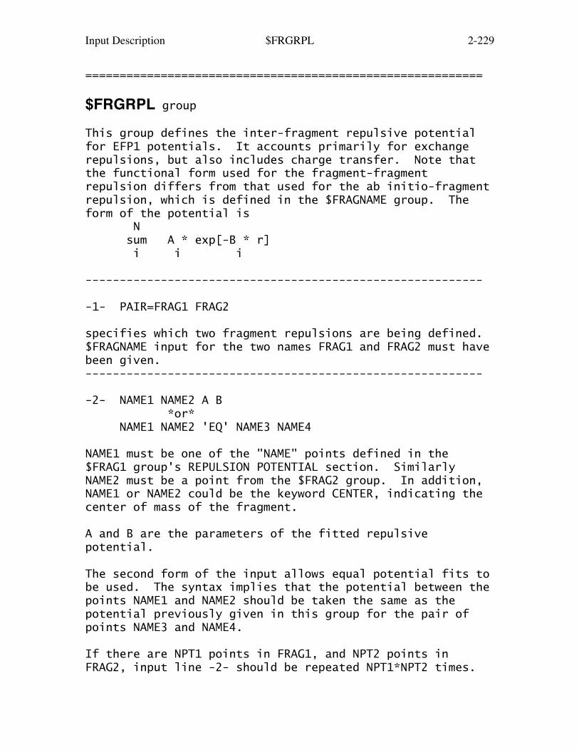
Input Description $FRGRPL 2-229
==========================================================
$FRGRPL group
This group defines the inter-fragment repulsive potentialfor EFP1 potentials. It accounts primarily for exchangerepulsions, but also includes charge transfer. Note thatthe functional form used for the fragment-fragmentrepulsion differs from that used for the ab initio-fragmentrepulsion, which is defined in the $FRAGNAME group. Theform of the potential is N sum A * exp[-B * r] i i i
----------------------------------------------------------
-1- PAIR=FRAG1 FRAG2
specifies which two fragment repulsions are being defined.$FRAGNAME input for the two names FRAG1 and FRAG2 must havebeen given.----------------------------------------------------------
-2- NAME1 NAME2 A B *or* NAME1 NAME2 'EQ' NAME3 NAME4
NAME1 must be one of the "NAME" points defined in the$FRAG1 group's REPULSION POTENTIAL section. SimilarlyNAME2 must be a point from the $FRAG2 group. In addition,NAME1 or NAME2 could be the keyword CENTER, indicating thecenter of mass of the fragment.
A and B are the parameters of the fitted repulsivepotential.
The second form of the input allows equal potential fits tobe used. The syntax implies that the potential between thepoints NAME1 and NAME2 should be taken the same as thepotential previously given in this group for the pair ofpoints NAME3 and NAME4.
If there are NPT1 points in FRAG1, and NPT2 points inFRAG2, input line -2- should be repeated NPT1*NPT2 times.

Input Description $FRGRPL 2-230
Terminate the pairs of potentials with a "STOP" card.Any pairs which you omit will be set to zero interaction.
Typically the number of points on which fitted potentialsmight be taken to be all the nuclei in a fragment, plusthe center of mass.----------------------------------------------------------
Repeat lines -1- and -2- for all pairs of fragments, thenterminate the group with a $END line.
==========================================================

Input Description $EWALD 2-231
==========================================================
$EWALD group (relevant for all-EFP runs with PBC)
This group controls evaluation of the electrostaticenergy of EFP calculations by means of the Ewald sumformulae. This gives a more accurate evaluation of theselong range interactions than the minimum image convention,which sums only up to a distance of one box, centered oneach particle. Ewald sum formulae are not used for theother, shorter range interactions in the EFP model, such asexchange repulsion and polarization, which are alwaysevaluated by the minimum image convention. This group isrelevant if and only if a periodic box is defined in the$EFRAG input group.
IFEWLD = a flag to activate Ewald sums for electrostatics The default is .FALSE.
LEVEL = 1 means Ewald sum charge-charge interactions only, which is the default if IFEWLD is turned on. = 2 charge-charge, charge-dipole, dipole-dipole = 3 charge-charge, charge-dipole, dipole-dipole, and charge-quadrupole terms should be Ewald summed.
TNFOIL = a flag to select tin foil boundary conditions, which uses a metallic continuum past the cutoffs, instead of a vacuum. The default is .TRUE.
BETA = parameter for the direct summation, in 1/Bohr. It should be 1.7/cutoff. Cutoffs are specified in $EFRAG, with the periodic box sizes, use a cutoff in units Angstrom in this formula, as the value 1.7 includes the conversion factor. The default=0.2
KMAX = number of reciprocal vectors in each direction. This should be kmax >= 3.2L/cutoff, where the radial cutoff, and box side L are both given in your $EFRAG. The default=10
==========================================================

Input Description $MAKEFP 2-232
==========================================================
$MAKEFP group (relevant if RUNTYP=MAKEFP)
This group controls generation of the effectivefragment potential (EFP2 style) from the wavefunction of asingle monomer. EFP generation is allowed for SCFTYP=RHFand ROHF. Multipole moments for electrostatics are alwaysgenerated, and the default for the keywords below is togenerate all additional terms.
FRAG = a string of up to 8 letters to identify this EFP. For example, WATER or BENZENE or CH3OH or ... (default=FRAGNAME, which you can hand edit later)
SCREEN = a flag to generate screening information for the multipole electrostatics, and maybe polarizability screening. See $DAMP and $DAMPGS. (default=.TRUE. for RHF, so far ROHF is not coded)
POL = a flag to generate dipole polarizabilities. (default=.TRUE.)See POLNUM in $LOCAL for an alternative way to generate thepolarizabilities, which may be faster for large molecules.
EXREP = a flag to generate exchange repulsion parameters. (default=.TRUE.)
CHTR = a flag to generate charge transfer parameters. (default=.TRUE. for RHF, so far ROHF is not coded)
DISP = a flag to generate information for dispersion. (default=.TRUE. for RHF, so far ROHF is not coded)
See also similar inputs NOPOL, NOEXREP, NOCHTR, NODISPin the $EFRAG input group, to ignore these terms if theyare generated.
==========================================================

Input Description $PRTEFP 2-233
==========================================================
$PRTEFP group (optional)
This group provides control for generating integercharge EFP fragments for constructing large EFPs. SeeP.A.Molina, H.Li, J.H.Jensen J.Comput.Chem. 24, 1971-1979(2003)
This group is mainly used in RUNTYP=MAKEFP runs. However,in MOPAC RUNTYP=ENERGY runs, the presence of a $PRTEFPgroup causes AM1 or PM3 charges to be printed andpunched out in a suitable format for EFP calculations.
NOPRT = an array specifying the atoms for which EFP multipole and polarizability points will not be printed/punched out. Example: For a molecule with the connectivity A1-A2-A3-A4-A5, NOPRT(1)=4,5 means that multipoles centered on atoms 4 and 5, and bond midpoints BO34 and BO45 are not part of the EFP.
MIDPRT = an array specifying atoms whose bond midpoints neglected by using NOPRT should be printed out. Example: MIDPRT(1)=3 forces the printout of bond midpoint BO34.
The neglect of monopoles leads to EFPs with overall non-integer charge. The next keyword defines "collection points" to which the removed monopoles are added. Thus, the net charge of the EFP=ICHARG. The presence of this "fictitious" charge is compensated for by adding an opposing dipole to the collection point.
NUMFFD = an array that defines (1) a collection point, (2) the number of atoms contributing to monopoles to this point, and (3) the numbers of the atoms. More than one collection point can be defined. An opposing dipole is calculated as -0.5Q*r (Q = sum of neglected monopoles, r = distance between collection point and nearest neglected monopole) and placed at the collection point.
Example: NUMFFD(1)=3,2,4,5. The sum of monopoles

Input Description $PRTEFP 2-234
at A4, A5, BO34 and BO45 (Q) is added to the A3 monopole. A dipole, -0.5Q*r, is placed on A3, where r is the distance between A3 and BO34. If MIDPRT(1)=3, Q does not include the BO34 monopole, r is the distance between BO34 and A4, and the resulting dipole is centered on BO34.
==========================================================

Input Description $DAMP 2-235
==========================================================
$DAMP group (optional, relevant if RUNTYP=MAKEFP)
This group provides control over the screening of thecharge term in the distributed multipole expansion used bythe EFP model for electrostatic interactions, to accountfor charge penetration. See M.A.Freitag, M.S.Gordon, J.H.Jensen, W.A.Stevens J.Chem.Phys. 112, 7300-7306(2000) L.V.Slipchenko, M.S.Gordon J.Comput.Chem. 28, 276-291(2007)
The screening exponents are optimized by fitting adamped multipolar electrostatic potential to the actualquantum mechanical potential of the wavefunction, computedon concentric layers of united spheres (namely, "GEODESIC"layers for WHERE=PDC in $ELPOT). See $STONE's generationof the unscreened classical multipoles, $PDC's generationof the true quantum potentia, and $DAMPGS.
Different multipole damping functions can be generated.The first contains a single exponential form, (1 - beta*exp(-alpha*r))and the second function is a single Gaussian form, (1 - beta*exp(-alpha*r**2))The exponent 'alpha' values are optimized (normally withbeta=one), with starting values defined in $DAMPGS. Theexponential fit is used for fragment-fragment chargepenetration screening, while the Gaussian fit is used in abinitio-fragment screening. See equations 28 and 4 in thereference. These two screen only the charge-chargeinteractions.
It is also possible to generate a "higher orderexponential" screening term, meaning that in addition tothe charge-charge energy, also affects charge-dipole,charge-quadrupole, and dipole-dipole energy terms.
Words of advice:1. Higher order screening is usually similar in accuracy tojust charge-charge screening, except in molecules withoutdipole moment, such as ethylene or benzene.

Input Description $DAMP 2-236
2. If the bond midpoints have smaller charges, it may bemore physically reasonable to screen only the atomicmonopoles, see ISCCHG.3. Use of the numerical Stone distributed multipoleanalysis may not be fully converged with respect to thelevel of highest used multipole moment (octapole) andcorresponding energy terms (quadrupole-quadrupole), whichmakes screening much more problematic.4. Accuracy of screening with the damping function of asingle exponential form depends on a region of fitting thequantum mechanical electrostatic potential, i.e., a radiusof first sphere with grid points (parameter VDWSCL in$PDC). A general trend is that for molecules with strongerelectrostatic interaction, and, consequently, shorterintermolecular separations, e.g., methanol and water,smaller values of VDWSCL are preferable, whereas for weakerinteracting molecules, e.g., dichloromethane and acetone,bigger VDWSCL values are more acceptable. Our recommendedVDWSCL values are 0.4-0.5 for methanol, 0.5-0.8 for water,and 0.7-0.9 for weaker bonded molecules. Note that VDWSCLvalues of 1.0 and higher often result in not converged orbadly converged damping parameters, and are notrecommended. The default VDWSCL value is 0.7.5. If the non-linear parameters alpha increase to 10, thatterm is effectively removed from the screening. Thishappens sometimes with buried atoms, and fairly often withbond mid-points.6. Double check the numerical results carefully.
ISCCHG = 0 use both atoms and bond midpoints as screening centers (the default) 1 use only atoms as screening centers
IFTTYP = selects the type of multipole screening fit: 0 means generate a Gaussian fit, for use as SCREEN input in $FRAGNAME. 2 means generate an exponential charge-charge fit, for use as SCREEN2 input in $FRAGNAME. 3 means generate an exponential higher order fit, for use as SCREEN3 input in $FRAGNAME.
If you wish to use Gaussian screening for EFP-EFP, simply copy the SCREEN output into a SCREEN1 section.
Input Description $DAMP 2-237
IFTFIX = 0 means the coefficients in the fit (beta) are free parameters 1 means the coefficients are held to unity. In case the linear coefficients become large, and particularly if they are negative, a fit with unit coefficients is more reasonable.
The default is to do both fits in one run, IFTTYP(1)=2,0,using unit coefficients, IFTFIX(1)=1,1.
The remaining parameters are seldom given:
NMAIN = the number of centers to receive a smaller alpha initial value, 2.0, which defaults to the number of atoms. The remaining centers, usually the bond midpoints, receive a larger starting value, 4.0. $DAMPGS gives more control of the values.MAXIT = maximum iterations in the fit, default=30.THRSH = printing threshold for large deviations. The default is 100.0 kcal/mol.
==========================================================

Input Description $DAMPGS 2-238
==========================================================
$DAMPGS group (relevant if $DAMP was given)
This is a free-format, line by line input group thatsets the initial values damping functions used to screenthe multipole expansion. A check run may be helpful inlisting the names of the expansion points that are chosenby MAKEFP jobs. Very often the input group contains onlytype -1- lines, and only in its second form.
-----------------------------------------------------------1- <exp.pt.> <nterms> or <exp.pt.>=<prev.exp.pt.>
This line gives the name of the expansion point, and howmany terms are in the damping function (always 1 atpresent). The second form of this line lets you equate thecurrent point to some previous point's values in $DAMPGS,skipping line -2-.-----------------------------------------------------------2- <coef> <exponent>
The linear coefficient (usually 1.0) and exponent of thisterm in the damping function. Repeat -2- <nterms> times.If not given, the starting exponent for atoms is 2.0, andfor bond midpoints, 4.0.
----------------------------------------------------------An example, for water, enforcing equivalent points, is: $dampgs or much more simply,O1 1 since the left is default exponents, 1.0 2.0 $dampgsH2 1 H3=H2 1.0 2.0 BO31=BO21H3=H2 $endBO21 1 1.0 4.0BO31=BO21 The "BO" is short for bond midpoint. $end==========================================================

Input Description $PCM 2-239
==========================================================
$PCM group (optional)
This group controls solvent effect computations usingthe Polarizable Continuum Model. If this group is found inthe input file, a PCM computation is performed. Thedefault calculation, chosen by selecting only the SOLVNTkeyword, is to compute the electrostatic free energy.Appropriate numerical constants are provided for a widerange of solvents. Typical input might be as simple as $PCM SOLVNT=H2O $ENDThere is in fact little need to give other PCM input data,except perhaps atomic radii in $PCMCAV if your moleculecontains an unusual atom.
Additional keywords (ICOMP, ICAV, IDISP, or IREP/IDP)allow for more sophisticated computations, namelycavitation, repulsion, and dispersion free energies. Themethodology for these is general, but numerical constantsare provided only for water.
Alternatively, the PCM codes for electrostatics can becombined with U. Minnesota codes to implement the SMDsolvation model. SMD combines the electrostatics with analternative cavitation, dispersion, and solute structurereorganization (CDS) correction. Since SMD also changesthe atomic radii, the electrostatics interaction ischanged. See keyword SMD below (and the 4th chapter ofthis manual).
Calculations are possible on either a solute embedded ina PCM continuum, or a system combining a solute & EFPexplicit solvent molecules, embedded in a PCM continuum.The energy and/or nuclear gradients are programmed for RHF,ROHF, UHF, GVB, and MCSCF wavefunctions, and for DFT or MP2level calculations using RHF, ROHF, and UHF. Closed shellTD-DFT excited states have analytic gradients, as well.Polarizabilities in solution may be found by RUNTYP=TDHF.Parallel computation is enabled, with scaling similar tothe scaling of the corresponding gas phase calculation.PCM is not programmed for CI, Coupled Cluster, orsemiempirical MOPAC runs.
Input Description $PCM 2-240
See the Fragment Molecular Orbital section of theReferences chapter for information on using PCM within theFMO model.
There is additional information on PCM in the Referenceschapter of this manual. This includes information on whichkeyword combinations were default values in the past.
IEF switch to choose the type of PCM model used. The default is -10, iterative C-PCM. = 0 isotropic dielectrics using the original formulation of PCM for dielectrics (D-PCM) = 1 anisotropic dielectric using the Integral Equation Formalism (IEF) of PCM, see $IEFPCM = 2 ionic solutions using IEF-PCM, see $IEFPCM = 3 isotropic dielectrics using IEF-PCM with matrix inversion solver, see $IEFPCM = -3 isotropic dielectric IEF-PCM with iterative solver, see $PCMITR. = 10 conductor-like PCM (C-PCM) with matrix inversion. Charge scaling is(Eps-1.0)/Eps =-10 C-PCM, with iterative solver. See $PCMITR.
C-PCM is normally a better choice than IEF-PCM. Theiterative solvers chosen by IEF=-3 or -10 usually reproducethe energy of the explicit solvers IEF=3 or 10 to within1.0d-8 Hartrees, and will be much faster and use lessmemory for large molecules. D-PCM should be consideredobsolete, and choices 1 and 2 are seldom made.
* * *
SOLVNT = keyword naming the solvent, whose choices depend on use of non-SMD or SMD models. For the former, the eight numerical constants defining the solvent are internally stored for: WATER (or H2O) CH3OH C2H5OH CLFORM (or CHCl3) CTCL (or CCl4) METHYCL (or CH2Cl2) 12DCLET (or C2H4Cl2) BENZENE (or C6H6) TOLUENE (or C6H5CH3) CLBENZ (or C6H5Cl) NITMET (or CH3NO2) NEPTANE (or C7H16) CYCHEX (or C6H12) ANILINE (or C6H5NH2) ACETONE (or CH3COCH3)

Input Description $PCM 2-241
THF DMSO (or DMETSOX) SMD has many additional solvents, see below.
The default solvent name is "INPUT" which means you mustgive the numerical values defining some other solvent, asdescribed below.
* * * non-SMD calculations * * *
The next set of parameters controls the computation:parameterization of the solvents, ICOMP which has an impacton the PCM electrostatics, and other keywords related tocavitation, dispersion, and repulsion corrections: ICAV,IDISP, IREP/IDP. -------
ICOMP = Compensation procedure for induced charges. Gradient runs require ICOMP be 0 or 2 only. = 0 None. (default) = 1 Yes, each charge is corrected in proportion to the area of the tessera to which it belongs. = 2 Yes, using the same factor for all tesserae. = 3 Yes, with explicit consideration of the portion of solute electronic charge outside the cavity, by the method of Mennucci and Tomasi. See the $NEWCAV group.
Technical issues are: IEF=0 should normally choose ICOMP=2.Options IEF=1 or 2 are incompatible with gradients and mustchoose ICOMP=0, and presently contain bugs (do not choosethese!). IEF=3 may not choose ICOMP=3, but if diffusebasis functions are in use, it may benefit from ICOMP=2.
------
ICAV = calculate the cavitation energy, by the method of Pierotti and Claverie. The cavitation energy is computed at the end of the run (e.g. at the final geometry) as an additive constant to the energy. = 0 skip the computation (default) = 1 perform the computation.
If ICAV=1, the following parameter is relevant:
TABS = the temperature, in Kelvin. (default=298.0)

Input Description $PCM 2-242
-------
There are two procedures for the calculation of therepulsion and dispersion contributions to the free energy.Parameterizations were obtained for RHF cases, so theimplementation permits their use only for RHF.
IDISP is older, and is incompatible with IREP and/or IDP.Nuclear gradients are available for IDISP (select eitherICLAV or ILJ in $DISREP). The older GEPOL-GB tessellationdoes some gradient terms numerically, which results in aless accurate gradient.
IDISP = Calculation of both dispersion and repulsion free energy through the empirical method of Floris and Tomasi. = 0 skip the computation (default) = 1 perform the computation. See $DISREP group.
The next two options add repulsive and dispersive terms tothe solute hamiltonian, in a more ab initio manner, by themethod of Amovilli and Mennucci. These may be used only insingle point energy calculations (see IDISP if you wish touse gradients).
IREP = Calculation of repulsion free energy = 0 skip the computation (default) = 1 perform the computation. See $NEWCAV group.
IDP = Calculation of dispersion free energy = 0 skip the computation (default) = 1 perform the computation. See $DISBS group.
If IDP=1, then three additional parameters must be defined. The two solvent values correspond to water, and therefore these must be input for other solvents.
WA = solute average transition energy. This is computed from the orbital energies for RHF, but must be input for MCSCF runs. (default=1.10)WB = ionization potential of solvent, in Hartrees. (default=0.451)ETA2 = square of the zero frequency refractive index

Input Description $PCM 2-243
of the solvent. (default=1.75)
--- the next 8 values define the solvent, if SOLVNT=INPUT:
RSOLV = the solvent radius, in units AngstromEPS = the dielectric constantEPSINF = the dielectric constant at infinite frequency. This value must be given only for RUNTYP=TDHF, if the external field frequency is in the optical range and the solvent is polar; in this case the solvent response is described by the electronic part of its polarization. Hence the value of the dielectric constant to be used is that evaluated at infinite frequency, not the static one (EPS). This value also must be given for TD-DFT/PCM, when NONEQ is selected in $TDDFT. For nonpolar solvents, the difference between the two is almost negligible.TCE = the thermal expansion coefficient, in units 1/KVMOL = the molar volume, in units ml/molSTEN = the surface tension, in units dyne/cmDSTEN = the thermal coefficient of log(STEN)CMF = the cavity microscopic coefficient
Values for TCE, VMOL, STEN, DSTEN, CMF need to be givenonly for the case ICAV=1. Input of any or all of thesevalues will override an internally stored value, if youhave chosen a solvent by its name.
* * * SMD calculations * * *
The Solvation Model Density (SMD) uses the solute's quantummechanical density (the D in the model's name) for IEF-PCMor C-PCM's electrostatics. It adds "CDS" corrections forcavitation, dispersion, and solvent structure, all of whichhave nuclear gradient contributions coded. The SMD model'sparameters were developed using IEF-PCM and GEPOL cavityconstruction, but SMD may also be used with the more robustC-PCM model and FIXPVA cavity tessellation.
SMD = a flag to select "Solvation Model Density". default=.FALSE. If chosen, naming the solvent by SOLVNT=xxx picks numerical values for the six SOLX keywords just below, which may then be omitted. The SMD model knows 178 solvents, see

Input Description $PCM 2-244
chapter 4 of this manual for a listing.
SOLA = Abraham's hydrogen bond aciditySOLB = Abraham's hydrogen bond basicitySOLC = aromaticity: fraction of non-H solvent atoms which are aromatic Carbon atomsSOLG = macroscopic surface tension at the air/solvent interface, in units of cal/mole/angstrom**2SOLH = halogenicity: fraction of non-H solvent atoms which are F, Cl, or BrSOLN = index of refraction at optical frequencies at 298K, n-sub-20-super-D.
In addition to the parameters just above, SMD provides itsown set of radii for each atom's sphere, so $PCMCAV inputmust not be given. Of course, if you choose SMD=.TRUE.,with its built in CDS correction, you must selectICOMP=ICAV=IDISP=IREP=IDP=0! See also SMVLE in $SVP.
* * *
--- interface to Fragment Molecular Orbital method:
IFMO specifies "n" for the n-body FMO expansion of the total electron density to be used in PCM. Non- zero IFMO can be used only within the regular FMO framework (q.v. for further FMO limitations). IFMO should be less or equal than NBODY in $FMO, Not all PCM options can be used with FMO! The following are explicitly permitted: IEF=-3,-10; ICOMP=0,1,2; MTHALL=2,4; IDISP=0,1; IDP=0; IREP=0,1. Gradient runs require ICOMP=0. IFMO may take the values of 0,1,2,3. (default=0)
--- the next set of keywords defines the molecular cavity,used for electrostatic (surface charge) calculations. Seealso $PCMCAV, $TESCAV, and $NEWCAV for other cavities.
NESFP = option for spheres forming the cavity: = 0 centers spheres on each nucleus in the quantum solute, and every atom in EFP. (default) = N use N initial sphere, whose centers XE, YE, ZE and radii RIN must be specified in $PCMCAV.
Input Description $PCM 2-245
The cavity generation algorithm may use additionalspheres to smooth out sharp grooves, etc. If you areinterested in smoother cavities, see the SVPE and SS(V)PEmethods, which use a cavity based on isodensity surfaces.The following parameters control how many extra spheres aregenerated:
OMEGA and FRO = GEPOL parameters for the creation of the 'added spheres' defining the solvent accessible surface. When an excessive number of spheres is created, which may cause problems of convergence, the value of OMEGA and/or FRO must be increased. For example, OMEGA from 40 to 50 ... up to 90, FRO from 0.2 ... up to 0.7. (defaults are OMEGA=40.0, FRO=0.7)
RET = minimum radius (in A) of the added spheres. Increasing RET decreases the number of added spheres. A value of 100.0 (default) inhibits the addition of any spheres, while 0.2 fills in many. The use of added spheres is strongly discouraged.
MODPAR = cavity generation's parallelization option: 0 parallelize tessellation, 1= do not parallelize. The present parallel code is inefficient, so MODPAR=0 is recommended. (default=0) Don't confuse this with running PCM in parallel!
MXSP = the maximum number of spheres. Default: MXATM parameter in GAMESS.
MXTS = the maximum number of tesserae. Default: Nsph*NTSALL*2/3, where Nsph is the number of spheres (usually equal to the number of atoms). If less than 20 spheres are present, default is Nsph*NTSALL. For GEPOL-RT, NTSALL=960 is used in setting the default value.
Note on MXSP and MXTS: PCM usually constructs more than one cavity (for example, a different one for the cavitation energy). MXSP and MXTS must be large enough to handle every possible cavity.
--- arcane parameters:

Input Description $PCM 2-246
IPRINT = 0 normal printing (default) = 1 turns on debugging printout
IFIELD = At the end of a run, calculate the electric potential and electric field generated by the apparent surface charges. = 0 skip the computation (default) = 1 on nuclei = 2 on a planar grid
If IFIELD=2, the following data must be input:
AXYZ,BXYZ,CXYZ = each defines three components of the vertices of the plane where the reaction field is to be computed (in Angstroms) A ===> higher left corner of the grid B ===> lower left corner of the grid C ===> higher right corner of the gridNAB = vertical subdivision (A--B edge) of the gridNAC = horizontal subdivision (A--C edge) of the grid.
==========================================================

Input Description $PCMCAV 2-247
==========================================================
$PCMCAV group (optional)
This group controls generation of the cavity holding thesolute during Polarizable Continuum Model runs. The cavityis a union of spheres, according to NESFP given in $PCM.The data in this group supplements cavity data given in$PCM. It is unlikely that users will input anything here,except perhaps a few RIN values. The data given here mustbe in Angstrom units.
XE,YE,ZE = arrays giving the coordinates of the spheres. if NESFP=0, the atomic positions will be used. if NESFP>0, you must supply NESFP values here.
RADII = three tables of values (Angstroms!) are available: VANDW selects van der Waals radii (default) This table has radii for atoms H,He, B,C,N,O,F,Ne, Na,Al,Si,P,S,Cl,Ar, K,As,Se,Br,Kr, Rb,Sb,Te,I, Cs,Bi internally tabulated, otherwise give RIN. = VDWEFP, similar to VANDW, except that radii not tabulated by VANDW are assigned as 1.60A. This option is most useful for protein-EFP calculations. = SUAHF, the simplified united atomic radii will be be used for the array RIN, namely H:0.01 C:1.77 N:1.68 O:1.59 P:2.10 S:2.10 For the other elements with Z<16, 1.50 is used. For the elements with Z>16, 2.30 will be applied.
RIN = an array giving the sphere radii. Radii given here will overwrite the values selected by RADII's tables. RIN values are multiplied by ALPHA, see just below. if NESFP=0, the program will look up the internally data according to the RADII keyword. if NESFP>0, give NESFP values.
Example: Suppose the 4th atom in your molecule is Fe, but all other atoms have van der Waals radii. You decide a good guess for Fe is twice the covalent radius: $PCMCAV RIN(4)=2.33 $END. Due to ALPHA, traditionally 1.2, the Fe radius will be 2.796.

Input Description $PCMCAV 2-248
The source for the van der Waals radii is "The Elements",2nd Ed., John Emsley, Clarendon Press, Oxford, 1991, exceptfor C,N,O where the Pisa group's experience with the bestradii for PCM treatment of singly bonded C,N,O atoms istaken. The radii for a few transition metals are given byA.Bondi, J.Phys.Chem. 68, 441-451(1964).
ALPHA = an array of scaling factors, for the definition of the solvent accessible surface. If only the first value is given, all radii are scaled by the same factor. (default is ALPHA(1)=1.2)
EPSHET = an array of dielectric constants, for each atom in the heterogeneous CPCM. The default is to use the same dielectric for every atom, namely the value of EPS in $PCM. (only if IEF=10 or -10). The default EPSHET(1)=X,X,X,X where EPS=X means homogeneous CPCM.
==========================================================

Input Description $TESCAV 2-249
==========================================================
$TESCAV group (optional)
This group controls the tessellation procedure for thecavity surfaces in PCM computations. The default valuesfor this group will normally be satisfactory. Use of theFIXPVA mechanism for dividing the surface of the atomicspheres into tesserae should allow for convergent PCMgeometry optimizations. To converge to small OPTTOL valuesmay require the use of internal coordinates, since thetessellation amounts to a finite grid (so the PCM energy isnot strictly rotationally invariant).
Cartesian geometry optimizations may require a highdensity of tesserae on the cavity surface: NTSALL=240 (or 960)This may require raising the maximum number of tesserae,see MXTS in $PCM. It is reasonable to just try internalcoordinates first, as this should be sufficient w/oincreasing the tesserae density. See also IFAST=1 in$PCMGRD.
--- The first two arrays control the density of tesseraeand the method to generate the tesserae.
INITS = array defines the initial number of tesserae for each sphere. Only 60, 240 and 960 are allowed, but the value can be different for each sphere. (Default is INITS(1)=60,60,60,...) See NTSALL.
METHOD = array defining the tessellation method for each sphere. The value can be different for each sphere. The default is 4 for all spheres, e.g. METHOD(1)=4,4,4,... See also MTHALL. = 1 GEPOL-GB, "Gauss-Bonet" tessellation. = 2 GEPOL-AS, "area scaling" tessellation. = 3 GEPOL-RT, "regular tessellation". = 4 FIXPVA, "Fixed points with variable area".FIXPVA gives smooth potential surfaces during geometryoptimizations, works with the $PCM options ICAV, IDISP,IDP, and IRP, and is the preferred tessellation method.
--- The next three parameters are presets for filling the arrays INITS and METHOD with identical values.
Input Description $TESCAV 2-250
NTSALL = 60, 240 or 960 (default = 60) All values in the array INITS are set to NTSALL
MTHALL = 1, 2, 3, or 4 (default = 4) All values in the array METHOD are set to MTHALL
MTHAUT = 0 or 1 (default = 0) If RUNTYP=OPTIMIZE and frozen atoms are defined by IFCART, MTHAUT=1 will select METHOD=1 for frozen atoms. See also AUTFRE and NTSFRZ.
note: Explicitly defining INITS and METHOD from the input deck will overrule the presets from NTSALL, MTHALL and/or MTHAUT.
--- The following two parameters control GEPOL-RT
AREATL = The area criterion (A*A) for GEPOL-RT. Tesserae with areas < AREATL at the boundary of intersecting spheres will be neglected. Default=0.010 A*A. Smaller AREATL cause larger number of tesserae. AREATL < 0.00010 is not recommended.
BONDRY = Controls (by scaling) the distance within which tesserae are considered "close" to the boundary. Such tesserae will be recursively divided into smaller ones until their areas are < AREATL. The default (= 1.0) means the distance is the square root of the tessera area. A large BONDRY value like 1000.0 will lead to fine tessellation for the entire surface with all tessera areas < AREATL.
--- The next two parameters are only relevant if MTHAUT=1
AUTFRE = Distance (A) for frozen atoms to be treated as moving atoms when MTHAUT=1. Default=2.0 A.
NTSFRZ = 60, 240 OR 960, initial tessera number for frozen atoms. Default=60
==========================================================
Input Description $NEWCAV 2-251
==========================================================
$NEWCAV group (optional)
This group controls generation of the "escaped charge"cavity, used when ICOMP=3 or IREP=1 in $PCM. This cavityis used only to calculate the fraction of the soluteelectronic charge escapes from the original cavity.
IPTYPE = choice for tessalation of the cavity's spheres. = 1 uses a tetrahedron = 2 uses a pentakisdodecahedron (default)
ITSNUM = m, the number of tessera to use on each sphere. if IPTYPE=1, input m=30*(n**2), with n=1,2,3 or 4 if IPTYPE=2, input m=60*(n**2), with n=1,2,3 or 4 (default is 60)
*** the next three parameters pertain to IREP=1 ***
RHOW = density, relative to liquid water (default = 1.0)
PM = molecular weight (default = 18.0)
NEVAL = number of valence electrons on solute (default=8)
The defaults for RHOW, PM, and NEVAL correspond to water,and therefore must be correctly input for other solvents.
==========================================================
Input Description $PCMGRD 2-252
==========================================================
$PCMGRD group (optional)
This group controls the PCM gradient computations. Itis of a technical nature, and is seldom given.
IPCDER = selects different methods for PCM gradients 1 use Ux(q) approximation (C-PCM and IEF-PCM), or use charge-derivative method (D-PCM). This is the default for D-PCM. 2 Variable-Tessera-Number Approximation. Implemented only for C-PCM and IEF-PCM, and the default for GEPOL-AS tesselation. 3 The same as 2, but for FIXPVE tessellation.The program will pick the correct default for IPCDER!
note: If ICAV = 1 or IDISP = 1 in $PCM, the derivatives of the cavitation energy or dispersion-repulsion, respectively, will automatically be calculated. You must be using the following input: $PCM ICAV=1 IDISP=1 $END $DISREP ICLAV=1 $END
IFAST = Controls the PCM calculations for RUNTYP=OPTIMIZE. 0 update PCM charges at each SCF cycle at every geometry (default) 1 update PCM charges at each SCF cycle for the initial geometry. For the subsequent geometries, calculate PCM charges at the first SCF cycle and use the PCM charges for the following SCF cycles; after the density change falls below DENTOL, update the PCM charges one time (to save CPU time).
==========================================================

Input Description $IECPCM 2-253
==========================================================
$IEFPCM group (optional)
This group defines data for the integral equationformalism version of PCM solvation. It includes specialoptions for ionic or anisotropic solutions.
The next two sets are relevant only for anisotropicsolvents, namely IEF=1:
EPS1, EPS2, EPS3 = diagonal values of the dielectric permittivity tensor with respect to the laboratory frame. The default is EPS in $PCM
EUPHI, EUTHE, EUPSI = Eulerian angles which give the rotation of the solvent orientation with respect to the lab frame. The term lab frame means $DATA orientation. The default for each is zero degrees.
The next two are relevant to ionic solvents, namely IEF=2:
EPSI = the ionic solutions's dielectric, the default is EPS from $PCM.
DISM = the ionic strength, in Molar units (mol/dm**3) The default is 0.0
==========================================================

Input Description $PCMITR 2-254
==========================================================
$PCMITR group (optional, for IEF=-3 or -10 in $PCM)
This group provides control over the iterativeisotropic IEF-PCM calculation. See C.S.Pomelli, J.Tomasi, V.Barone Theoret.Chem.Acc. 105, 446-451(2001) H.Li, C.S.Pomelli, J.H.Jensen Theoret.Chem.Acc. 109, 71-84(2003)
MXDIIS = Maximum size of the DIIS linear equations, the value impacts the amount of memory used by PCM. Memory=2*MXDIIS*NTS, where NTS is the number of tesserae. MXDIIS=0 means no DIIS, instead the point Jacobi iterative method will be used. (Default=50)
MXITR1 = Maximum number of iters in phase 1. (Default=50)
MXITR2 = Maximum number of iters in phase 2. (Default=50)
note: if MXDIIS is larger than both MXITR1 and MXITR2 MXDIIS will be reset to be the larger of these two.
THRES = Convergence threshold for the PCM Apparent Surface Charges (ASC). (Default=1.0D-08)
THRSLS = Loose threshold used in the early SCF cycles when the density change is above DENSLS. If THRSLS < THRESH, this option is turned off. Default is 5.0D-04.
DENSLS = If the density change is above DENSLS the loose threshold THRSLS applies. (Default = 0.01 au)
IDIRCT = 1, Directly compute the electronic potential at each tessera and the ASC potential at the electronic coordinates, with no disk storage. (Default) 0, Compute and save above data to hard disk.
Keywords for region wise multipole expansion of ASCsin approximating interaction among tesserae:

Input Description $PCMITR 2-255
(C.S.Pomelli, J.Tomasi THEOCHEM 537, 97-105(2001))
IMUL = Region wise multipole expansion order in the approximate interaction among tesserae. = 0, Neglected (Only for test purposes) = 1, Monopole = 2, Monopole+Dipole = 3, Monopole+Dipole+Quadrupole (Default)
RCUT1 = Cutoff radius (Angstrom) for mid-range interactions among tesserae. Default=15.0 A If RCUT1 is larger than your molecule, the option is effectively turned off.
RCUT2 = Cutoff radius (Angstrom) for long range interactions among tesserae. Default=30.0 A
The remaining keywords apply only to PCM calculations witha QM/EFP solute (see Li et al.)
Keywords for region wise multipole expansion of ASCsin approximating interaction between ASCs and QM region:
IMGASC = 1, Use region wise multipole expansion of ASCs to compute the ASC potential at QM region. 0, no use of the multipole expansion method. (default)
RASC = Cutoff radius (Angstrom) for used of the IMGASC multipole expansion (Default=20.0 A)
Keywords for multipole expansion of the QM region inapproximating the QM region potential:
IMGABI = 0, multipole expansion of the QM region is turned off (default). 1, turn multipole expansion of the QM region on.
RABI = Cutoff radius (Angstrom) for used of the IMGABI multipole expansion (Default=4.0 A)
Keywords for the coupling of PCM and EFP polarizabilitytensors:
IEFPOL = 1, PCM ASCs induce EFP dipoles.(default)

Input Description $PCMITR 2-256
0, PCM ASCs do not induce EFP dipoles.
REFPOL = When IEFPOL=1, if the distance (Angstrom) between a polarizability point and a tessera is less than REFPOL, they are considered too close and the field from the tessera will not induce dipole for the polarizability point. Default=0.0 A means always induce the dipole.
==========================================================

Input Description $DISBS 2-257
==========================================================
$DISBS group (optional)
This group defines auxiliary basis functions used toevaluate the dispersion free energy by the method ofAmovilli and Mennucci. These functions are used only forthe dispersion calculation, and thus have nothing to dowith the normal basis given in $BASIS or $DATA. If theinput group is omitted, only the normal basis is used forthe IDP=1 dispersion energy.
NADD = the number of added shells
XYZE = an array giving the x,y,z coordinates (in bohr) of the center, and exponent of the added shell, for each of the NADD shells.
NKTYPE = an array giving the angular momenta of the shells
An example placing 2s,2p,2d,1f on one particular atom,
$DISBS NADD=7 NKTYP(1)= 0 0 1 1 2 2 3 XYZE(1)=2.9281086 0.0 .0001726 0.2 2.9281086 0.0 .0001726 0.05 2.9281086 0.0 .0001726 0.2 2.9281086 0.0 .0001726 0.05 2.9281086 0.0 .0001726 0.75 2.9281086 0.0 .0001726 0.2 2.9281086 0.0 .0001726 0.2 $END
==========================================================

Input Description $DISREP 2-258
==========================================================
$DISREP group (optional)
This group controls evaluation of the dispersion andrepulsion energies by the empirical method of Floris andTomasi. The group must be given when IDISP=1 in $PCM,whenever the solvent is not water. Only one of the twooptions ICLAV or ILJ should be selected. Due to its lackof parameters, almost no one chooses ILJ.
ICLAV = selects Claverie's disp-rep formalism. = 0 skip computation. = 1 Compute the solute-solvent disp-rep interaction as a sum over atom-atom interactions through a Buckingham-type formula (R^-6 for dispersion, exp for repulsion). (default) Ref: Pertsin-Kitaigorodsky "The atom-atom potential method", page 146.
ILJ = selects a Lennard-Jones formalism. = 0 skip computation. (default) = 1 solute atom's-solvent molecule interaction is modeled by Lennard-Jones type potentials, R^-6 for dispersion, R^-12 for repulsion).
---- the following data must given for ICLAV=1:
RHO = solvent numeral densityN = number of atom types in the solvent moleculeNT = an array of the number of atoms of each type in a solvent moleculeRDIFF = distances between the first atoms of each type and the cavityDKT = array of parameters of the dis-rep potential for the solventRWT = array of atomic radii for the solvent
The defaults are appropriate for water, RHO=3.348D-02 N=2 NT(1)=2,1 RDIFF(1)=1.20,1.50 DKT(1)=1.0,1.36 RWT(1)=1.2,1.5
Input Description $DISREP 2-259
DKA = array of parameters of the dis-rep potential for the solute. Defaults are provided for some common elements: H: 1.00 Be: 1.00 B: 1.00 C: 1.00 N: 1.10 O: 1.36 P: 2.10 S: 1.40
RWA = array of atomic radii for the solute to compute dis-rep. Defaults are provided for some common elements: H: 1.20 Be: 1.72 B: 1.72 C: 1.72 N: 1.60 O: 1.50 P: 1.85 S: 1.80
Other elements have DKA and RWA values of 0.0 and so mustbe given in the input deck, or the dispersion/repulsionenergy will be 0. For EFP/PCM calculations, only QM atomsneed DKA and RWA values to calculate the DIS-REP energy.
---- the following data must given for ILJ=1:
RHO = solvent numeral densityEPSI = an array of energy constants referred to each atom of the solute molecule.SIGMA = an array of typical distances, relative to each solute atom==========================================================

Input Description $SVP 2-260
==========================================================
$SVP group (optional)
The presence of this group in the input turns on use ofthe Surface and Simulation of Volume Polarization forElectrostatics (SS(V)PE) solvation model, or the more exactSurface and Volume Polarization for electrostatics (SVPE)model. These model the solvent as a dielectric continuum,and are available with either an isodensity or sphericalcavity, around the solute. A semi-empirical correction forshort-range electrostatics may be chosen. The solute maybe described only by RHF, UHF, ROHF, GVB, or MCSCFwavefunctions. The energy is reported as a free energy,which includes the factor of 1/2 that accounts for the workof solvent polarization assuming linear response. Gradientsare not yet available.
Typical use of either the SS(V)PE or the SVPE methodwill involve a prior step to do an equivalent calculationon the given solute in the gas phase. This provides a setof orbitals that can be used as a good initial guess forthe subsequent run including solvent. It also provides thegas phase energy that can be subtracted from the energy insolvent to obtain the electrostatic contribution to thefree energy of solvation. The solvation free energy is thedifference in the "FINAL" energy found in the gas phase andsolvated runs (not to be confused with the "reaction fieldenergy" found on the solvated output).
Many runs will be fine with all parameters set attheir default values. The most important parameters a usermay want to consider changing are:
NVLPL = treatment of volume polarization 0 - SS(V)PE method, which simulates volume polarization by effectively folding in an additional surface polarization (default) N - SVPE method, which explicitly treats volume polarization with N extra layers
DIELST = static dielectric constant of solvent (default = 78.39, appropriate for water)
IVERT = 0 do an equilibrium calculation (default)

Input Description $SVP 2-261
1 do a nonequilibrium calculation to get the final state of a vertical excitation - this requires that IRDRF=1 to read the $SVPIRF input group that was punched with IPNRF=1 in a run on the initial state - note that a meaningful result is obtained only if the initial and final states both come from the same wavefunction/basis set/ geometry/solvation model.
DIELOP = optical dielectric constant of solvent - this only relevant if IVERT=1 (default 1.776, appropriate for water)
EGAS = gas phase energy (optional): if given, the program will output the free energy of solvation and the change in solute internal energy due to solvation. note that a meaningful result is obtained only if EGAS comes from the same wavefunction/basis set/ geometry as is used in the solvation calculation
SMVLE = flag to turn on a semi-empirical correction for local electrostatic effects based on the electric field's normals to the surface cavity. This also adds cavitation/dispersion/solvent structure (CDS) effects drawn from the SMD model, see SMD in $PCM. (Default=.FALSE.)
ISHAPE = sets the shape of the cavity surface 0 - electronic isodensity surface (default) 1 - spherical surface
RHOISO = value of the electronic isodensity contour used to specify the cavity surface, in electrons/bohr**3 (relevant if ISHAPE=0; default=0.001)
RADSPH = sphere radius used to specify the cavity surface. A positive value means it is given in Bohr, negative means Angstroms. (relevant if ISHAPE=1; default is half the distance between the outermost atoms plus 1.4 Angstroms)
INTCAV = selects the surface integration method 0 - single center Lebedev integration (default) 1 - single center spherical polar integration, not recommended; Lebedev is far more efficient

Input Description $SVP 2-262
NPTLEB = number of Lebedev-type points used for single center surface integration. The default value has been found adequate to obtain the energy to within 0.1 kcal/mol for solutes the size of monosubstituted benzenes. (relevant if INTCAV=0) Valid choices are 6, 14, 26, 38, 50, 86, 110, 146, 170, 194, 302, 350, 434, 590, 770, 974, 1202, 1454, 1730, 2030, 2354, 2702, 3074, 3470, 3890, 4334, 4802, 5294, or 5810. (default=1202)
NPTTHE, NPTPHI = number of (theta,phi) points used for single center surface integration. These should be multiples of 2 and 4, respectively, to provide symmetry sufficient for all Abelian point groups. (relevant if INTCAV=1; defaults = 8,16; these defaults are probably too small for all but the tiniest and simplest of solutes.)
TOLCHG = a convergence criterion on the program variable named CHGDIF, which is the maximum change in any surface charge from its value in the previous iteration (default=1.0D-7). This is checked in each SCF iteration, although the actual value is not printed until final convergence is reached.
The single-center surface integration approach may fail forcertain highly nonspherical molecular surfaces. The programwill automatically check for this and bomb out with awarning message if need be. The single-center approachsucceeds only for what is called a star surface, meaningthat an observer sitting at the center has an unobstructedview of the entire surface. Said another way, for a starsurface any ray emanating out from the center will passthrough the surface only once. Some cases of failure may befixed by simply moving to a new center with the ITRNGRparameter described below. But some surfaces are inherentlynonstar surfaces and cannot be treated with this programuntil more sophisticated surface integration approaches areimplemented.
ITRNGR = translation of cavity surface integration grid 0 - no translation (i.e., center the grid at the origin of the atomic coordinates) 1 - translate to center of nuclear mass

Input Description $SVP 2-263
2 - translate to center of nucl. charge (default) 3 - translate to midpoint of outermost atoms 4 - translate to midpoint of outermost non-Hydrogen atoms 5 - translate to user-specified coordinates, in Bohr 6 - translate to user-specified coordinates, in Angstroms
TRANX, TRANY, TRANZ = x,y,z coordinates of translated cavity center, relevant if ITRNGR=5 or 6. (default = 0,0,0)
IROTGR = rotation of cavity surface integration grid 0 - no rotation 1 - rotate initial xyz axes of integration grid to coincide with principal moments of nuclear inertia (relevant if ITRNGR=1) 2 - rotate initial xyz axes of integration grid to coincide with principal moments of nuclear charge (relevant if ITRNGR=2; default) 3 - rotate initial xyz axes of integration grid through user-specified Euler angles as defined by Wilson, Decius, Cross
ROTTHE, ROTPHI, ROTCHI = Euler angles (theta, phi, chi) in degrees for rotation of the cavity surface integration grid, relevant if IROTGR=3. (default=0,0,0)
IOPPRD = choice of the system operator form. The default symmetric form is usually the most efficient, but when the number of surface points N is big it can require very large memory (to hold two N by N matrices). The nonsymmetric form requires solution of two consecutive system equations, and so is usually slower, but as trade-off requires less memory (to hold just one N by N matrix). The two forms will lead to slightly different numerical results, although tests documented in the third reference given in Further Information show that the differences are generally less than the inherent discretization error itself and so are not meaningful. 0 - symmetric form (default)

Input Description $SVP 2-264
1 - nonsymmetric form
The remaining parameters below are rather specializedand rarely of concern. They should be changed from theirdefault values only for good reason by a knowledgeableuser.
TOLCAV = convergence criterion on maximum deviation of calculated vs. requested RHOISO (relevant if ISHAPE=0; default=1.0D-10)
ITRCAV = maximum number of iterations to allow before giving up in search for isodensity surface. (relevant if ISHAPE=0; default=99)
NDRCAV = highest analytic density derivative to use in the search for isodensity surface. 0 - none, use finite differences (default) 1 - use analytic first derivatives
LINEQ = selects the solvers of linear equatio solver equations that determine the effective point charges on the cavity surface. 0 - use LU decomposition in memory if space permits, else switch to LINEQ=2 1 - use conjugate gradient iterations in memory if space permits, else use LINEQ=2 (default) 2 - use conjugate gradient iterations with the system matrix stored externally on disk.
CVGLIN = convergence criterion for solving linear equations by the conjugate gradient iterative method (relevant if LINEQ=1 or 2; default = 1.0D-7)
CSDIAG = a factor to multiply diagonal elements to improve the surface potential matrix, S. (default = 1.104, optimal for Lebedev integration)
IRDRF = a flag to read in a set of point charges as an initial guess to the reaction field. 0 - no initial guess reaction field (default) 1 - read point charges from $SVPIRF input group. It is up to the user to be sure that the number of charges read is appropriate.

Input Description $SVP 2-265
IPNRF = a flag to punch the final reaction field. 0 - no punch (default) 1 - punch in format of $SVPIRF input group
==========================================================

Input Description $SVPIRF 2-266
==========================================================
$SVPIRF group (optional; relevant for SVP runs)
Formatted card images of reaction field point charges, aspunched by setting IPNRF=1 in a previous SVP run. These canbe used by setting IRDRF=1 in a subsequent SVP run toprovide an initial guess to the reaction field.
These charges from the initial state are required ifIVERT=1 in $SVP to do a vertical excitation calculation onthe final state.
==========================================================
Input Description $COSGMS 2-267
==========================================================
$COSGMS group (optional)
The presence of this group in the input turns on theuse of the conductor-like screening model (COSMO) withmolecular shaped cavity for closed and open shell HF, DFT,and MP2. Open shells may be high spin-restricted or anysort of spin-unrestricted case. The energy and/or thegradient can be computed for each of these.
The implementation of the COSMO cavity has a limit ofabout 150-200 atoms. Like other limits in GAMESS, this canbe raised according to directions in the Programmer'sReference.
EPSI = the dielectric constant, 80 is often used for H2O This parameter must be given, except for the perfect conductor approximation (see PRFCND).
PRFCND = perfect conductor approximation, sets EPSI equal to infinity. Relevant only if EPSI is not given. (default=.FALSE.)
COSRAD = the multiplicative factor for the van der Waals radii used for cavity construction. (default=1.2)
NSPA = the number of surface points on each atomic sphere that form the cavity. (default=92)
DISEX = parameter for the refinement of crevices (default=10.0D+00)
OUTCHG select the method for the correction of the outlying charge error (OCE). = DMULTI sets the multipole expansion method. = DBLCAV sets the double cavity method (default).
COSWRT = flag to generate the .cosmo output file, used as input to the COSMO-RS program, from the company COSMOlogic. A replacement output source file is needed (full version of cosprt.src). Users need to sign a special license agreement to enable this option, see http://ocikbws.uzh.ch/gamess COSWRT forces PRFCND=.T. and requires GBASIS=KTZVP

Input Description $COSGMS 2-268
and DFTTYP=BP86, because COSMO-RS is parametrized for use only with this specific setup. (default=.FALSE.)
DCOSMO = flag to use the DCOSMO-RS method. This requires reading in a supplementary .pot file, obtained by processing COSWRT's .cosmo output with the COSMO-RS software. (default is .FALSE.)
COSBUG = flag to turn on debugging printout.
Additional information on the COSMO model can be found in the References chapter of this manual.
==========================================================

Input Description $SCRF 2-269
==========================================================
$SCRF group (optional)
The presence of this group in the input turns on theuse of the Kirkwood-Onsager spherical cavity model for thestudy of solvent effects. The method is implemented forRHF, UHF, ROHF, GVB and MCSCF wavefunctions and gradients,and so can be used with any RUNTYP involving the gradient.The method is not implemented for MP2, CI, any of thesemiempirical models, or for analytic hessians.
DIELEC = the dielectric constant, 80 is often used for H2O
RADIUS = the spherical cavity radius, in Angstroms
G = the proportionality constant relating the solute molecule's dipole to the strength of the reaction field. Since G can be calculated from DIELEC and RADIUS, do not give G if they were given.
==========================================================
Additional information on the SCRF model can be found in the Further Information chapter.

Input Description $ECP 2-270
==========================================================
$ECP group (required if PP=READ in $CONTRL)
This group lets you read in effective core potentials,for some or all of the atoms in the molecule. You can usebuilt in potentials for some of the atoms if you like.This is a free format (positional) input group. Since theinput is a little tricky, it is good to look at the twoexamples at the end of this group.
*** Give a card set -1-, -2-, and -3- for each atom ***
-card 1- PNAME, PTYPE, IZCORE, LMAX+1
PNAME is a 8 character descriptive tag for this potential.
If PNAME is repeated later, for the same type of element, the previously defined potential is copied to this atom. No other information should be given on this card, and cards -2- and -3- must be skipped.
Do not use this "copy" option when there is no core potential, instead type "NONE" over and over again.
PTYPE = GEN a general potential should be read. = SBKJC look up the Stevens/Basch/Krauss/Jasien/ Cundari potential for this type of atom. = HW look up the Hay/Wadt built in potential for this type of atom. = NONE treat all electrons on this atom.IZCORE is the number of core electrons to be removed. Obviously IZCORE must be an even number, or in other words, all core orbitals being removed must be completely occupied.LMAX is the maximum angular momentum occupied in the core orbitals being removed (usually). Give IZCORE and LMAX only if PTYPE is GEN.
*** For the first occurence of PNAME, if PTYPE is GEN, ****** then give cards -2- and -3-. Otherwise go to -1-. ***
*** Card sets -2- and -3- are repeated LMAX+1 times ***
The potential U(LMAX+1) is given first, followed by U(L)-U(LMAX+1), for L=1,LMAX.

Input Description $ECP 2-271
-card 2- NGPOT
NGPOT is the number of Gaussians in this part of the local effective potential.
-card 3- CLP,NLP,ZLP (repeat this card NGPOT times)
CLP is the coefficient of this Gaussian in the potential.NLP is the power of r for this Gaussian, 0 <= NLP <= 2.ZLP is the exponent of this Gaussian.
Note that PTYPE lets you to type in one or more atomsexplicitly, while using built in data for other atoms.
By far the easiest way to use the SBKJC potential for allatoms in the formic acid molecule is to request PP=SBKJCin $CONTRL. But here we show two alternatives. Note thatboth examples copy one oxygen potential to the other, andboth explicitly declare there is no potential on everyhydrogen.
Assume that the atoms in $DATA are generated in the orderC, H, O, O, H.
The first way is to look up the program's internallystored SBKJC potentials one atom at a time:
$ECPC-ECP SBKJCH-ECP NONEO-ECP SBKJCO-ECPH-ECP NONE $END
The second oxygen duplicates the first, no core electronsare removed on hydrogen. The order of the atoms mustfollow that generated by $DATA. All atoms must be givenhere in $ECP, not just the symmetry unique atoms.
The second example reads all SBKJC potentials explicitly:
$ECPC-ECP GEN 2 1

Input Description $ECP 2-272
1 ----- CARBON U(P) ----- -0.89371 1 8.564682 ----- CARBON U(S)-U(P) ----- 1.92926 0 2.81497 14.88199 2 8.11296H-ECP NONEO-ECP GEN 2 11 ----- OXYGEN U(P) ----- -0.92550 1 16.117182 ----- OXYGEN U(S)-U(P) ----- 1.96069 0 5.05348 29.13442 2 15.95333O-ECPH-ECP NONE $END
Again, the 2nd oxygen copies from the first. It is handyto use the rest of card -2- as a descriptive comment.
As a final example, for antimony we have LMAX+1=3 (thereare core d's). One must first enter U(f), followed byU(s)-U(f), U(p)-U(f), U(d)-U(f).
==========================================================

Input Description $MCP 2-273
==========================================================
$MCP group (required if MCP READ was given on card -6U-)
This group lets you read in model core potentials, forsome or all of the atoms in the molecule. This is a fixedformat input group. For the review of the MCP method, seeM.Klobukowski, S.Huzinaga, and Y.Sakai, pp. 49-74 in J.Leszczynski, "Computational Chemistry", vol. 3 (1999) .
*** Give input -1-, -2-, ..., -9- for each MCP atom ***
-card 1- ANAT
ANAT is a 8 character name for the MCP atom. It must match the name given for that atom in the $DATA group.
-card 2- NOAN, (NO(IS),NG(IS), IS=1,4) FORMAT(9I3) IS = 1, 2, 3, 4 for s, p, d, and f symmetry, resp.
NOAN is the number of terms in the MCP NO(IS) is the number of core orbitals in symmetry IS NG(IS) is the number of basis functions used to expand the core orbitals in symmetry IS
-card 3- ZEFF, MCPFMT FORMAT(F10.2, A8)
ZEFF is the number of valence electrons, e.g. 7.0 for Fluorine MCPFMT is the format for reading floating-point numbers in the MCP data
-card 4- (ACOEF(L), L=1,NOAN) FORMAT(MCPFMT)
ACOEF(L) is the L-th coefficient in the expansion of the model core potential; more than one line may be provided ACOEF(L) is the defined as A(l) in Eq. (38) of the MCP review paper.
-card 5- (AEXPN(L), L=1,NOAN) FORMAT(MCPFMT)
AEXPN(L) is the L-th exponent in the expansion of the model core potential; more than one line may be provided
Input Description $MCP 2-274
AEXPN(L) is the defined as alpha(l) in Eq. (38) of the MCP review paper.
-card 6- (NINT(L), L=1,NOAN) FORMAT(10I3)
NINT(L) is the power of R in the expansion of the model core potential; NINT(L) is defined as n(l) in Eq. (38) of the MCP review paper.
*** For each symmetry IS present in the core orbitals *** *** read the card set -7-, -8-, and -9- ***
-card 7- (BPAR(K), K=1,NO(IS)) FORMAT(MCPFMT) BPAR(K) is the constant in the core projector operator, B(k) in Eq. (41) of the review.
-card 8- (EX(I), I=1,NG(IS)) FORMAT(MCPFMT) EX(I) is the exponent of the I-th Gaussian function used to expand the core orbitals
*** Repeat -9- for each core orbital in symmetry IS ***
-card 9- (C(I), I=1,NG(IS)) FORMAT(MCPFMT) C(I) expansion coefficients of the core orbital
The following example input file is for H2CO, and bythe way, provides another example of COORD=HINT.
! $CONTRL RUNTYP=ENERGY COORD=HINT PP=MCP $END $DATAFormaldehyde H2COCNV 2
C 6.0 LC 0.00 0.0 0.0 - O K MCP READ <<<< this is an MCP atom L 3 <<<< (311/311/1) basis 1 18.517235 -0.16370140 0.22673090E-01 2 2.5787547 -0.26304451 0.19109693 3 0.58994362 0.58040872 0.50918856 L 1 1 0.17330638 1.0000000 1.0000000 L 1 1 0.60957120E-01 1.0000000 1.0000000 D 1; 1 0.600 1.0

Input Description $MCP 2-275
O 8.0 LC 1.2031 0.0 0.0 - O K MCP READ <<<< this is an MCP atom L 3 <<<< (311/311/1) basis 1 44.242510 -0.13535836 0.17372951E-01 2 6.2272700 -0.30476423 0.16466813 3 1.4361751 0.43955753 0.46721611 L 1 1 0.40211473 1.0000000 1.0000000 L 1 1 0.12688798 1.0000000 1.0000000 D 1; 1 1.154 1.0
H 1.0 PCC 1.1012 121.875 0.0 + O K I TZV <<<< not an MCP atom, TZV+pol basis P 1; 1 1.100 1.0
$END
$MCP <<<< start of the MCP data <<<< empty lines allowedMCP for C NR (2S/2P) S(2)P(2) <<<< comment <<<< empty lines allowed C <<<< MCP for the atom C 2 1 14 <<<< NOAN, NO(1), NG(1) 4.00(4D15.8) <<<< ZEFF, MCPFMT .41856306 .99599513E-01 <<<< ACOEF 16.910482 7.4125554 <<<< AEXPN 0 0 <<<< NINT 22.676882 <<<< B(1s) 26848.283 8199.1206 2798.3668 1048.2982 423.36984 181.26843 81.068295 37.403931 17.629539 8.4254263 4.0611964 1.9672294 .95541420 .46459041 .10743274D-03 .21285491D-03 .99343100D-03 .28327774D-02 .83154481D-02 .21694082D-01 .52916004D-01 .11618593D+00 .21812785D+00 .32180986D+00 .29375407D+00 .10974353D+00 .70844050D-02 .17825971D-02
MCP for O NR (2S/2P) S(2)P(4)
O <<<< MCP for the atom O 2 1 16 6.00(4D15.8) .31002267 .27178756E-01
Input Description $MCP 2-276
25.973731 13.843290 0 0 41.361784 57480.749 17270.167 5766.9282 2107.0076 829.06758 346.04791 151.12147 68.233250 31.542773 14.815300 7.0298236 3.3561489 1.6077662 .77153240 .37052330 .17799002 .85822477D-04 .18173691D-03 .84803428D-03 .25439914D-02 .76877460D-02 .20823429D-01 .52424753D-01 .11864010D+00 .22782741D+00 .33492260D+00 .28833079D+00 .93046197D-01 .55937988D-02 .16121923D-02 .10915544D-04 .21431633D-03
$END
==========================================================
Input Description $RELWFN 2-277
==========================================================
$RELWFN group (optional)
This group is relevant if RELWFN in $CONTRL chose oneof the relativistic transformations (DK, RESC, or NESC) forelimination of the small components of relativisticwavefunctions, to produce a corrected single componentwavefunction. For DK or RESC, only one electron integralcorrections are added, whereas for NESC, corrections to twoelectron integrals are accounted for by means of arelativistically averaged basis set. All relativisticmethods in GAMESS neglect two-electron corrections comingfrom pVp integrals. The 3rd order DK transformation willnormally afford the most sound results, from a theoreticalpoint of view.
Analytic gradients are programmed for both RESC andNESC computations. For DK, all non-relativistic gradientterms are analytic, while the relativistic contributionsare evaluated numerically by a double difference formula.
During geometry optimizations, in rare cases, thenumber of nearly linearly independent functions in theResolution of the Identity (RI) used to evaluate the mostdifficult integrals may change at some new geometry. Ifso, the job will quit with an error message, and the usermust restart it again manually.
For IOTC, DK, or RESC, ordinary basis sets are used.This however is a misleading statement, for while any basisset will run, accurate answers may be hard to obtainwithout the use of basis sets constructed using therelativistic approximations. Certainly at least thecontraction coefficients must be modified to account foreffects such as the s orbital size contraction underrelativity, but the reoptimization of exponents may also beimportant. Experience suggests that large uncontractedbasis sets using non-relativistic exponents are probablyOK, but standard contractions from NR atomic calculationscan lead to spurious results. As a rule of thumb, elementsH-Xe might perhaps be OK, but for heavier elements, userelativistically derived basis sets.

Input Description $RELWFN 2-278
There are two possible basis set choices for IOTC, DK,or RESC calculations. The Sapporo relativistic segmentedcontractions are available for elements down to Xenon (seeGBASIS=SPKrnZP or SPKrAnZP). DK3 basis sets for H-Lrobtained at U. of Tokyo exist in the form of generalcontractions, http://www.riken.jp/qcl/ publications/dk3bs/periodic_table.htmlwhich gives the EPAPS data published by T.Tsuchiya, M.Abe, T.Nakajima, K.Hirao J.Chem.Phys. 115,4463-4472(2001)A program to extract this web page into GAMESS's formatis provided with GAMESS, see file ~/gamess/tools/dk3.f.Light to medium atom main group (H-Kr) DK2 bases exist,look for the names cc-pVnZ_DK on http://www.emsl.pnl.gov:2080/forms/basisform.html
For NESC, you must provide three basis sets, for thelarge and small components and an averaged one, which aregiven in $DATAL, $DATAS, $DATA, respectively. The onlypossible choice for these basis sets is due to Dyall, andthese are available from http://www.emsl.pnl.gov:2080/forms/basisform.html Theirnames are similar to cc-pVnZ(pt/sf/lc), pt=point orfi=finite nucleus, sf for spin-free and the final field islc=large component ($DATAL), sc=small component ($DATAS),and wf is a typo for Foldy-Wouthuysen 2e- basis ($DATA).In GAMESS you can only use point nucleus approximation. Theneed to input three basis sets means that you cannot use a$BASIS group, and you must use COORD=UNIQUE style input inthe various $DATA's. The three $DATA groups must containidentical information except for the primitive expansioncoefficients, as the three basis sets must have the sameexponents. In case the option to treat only some atomsrelativistically is chosen, all non-relativistic atoms musthave identical basis input in all three groups.
The finite size of nuclei is not taken into account, sodo not use any basis set obtained including this effect.
For NESC, the one electron part of the spin-orbitoperator can be corrected, while for RESC, one can computespin-orbit coupling with relativistic corrections to bothone and two electron SOC integrals, unless internaluncontraction is requested (in this case only 1 electron

Input Description $RELWFN 2-279
SOC integrals are modified). It should be noted thatinternally uncontracted basis sets containing very largeexponents have large SOC integrals, thus the averageasymmetry due to RESC appears larger (before contraction).
For any order DK, the 1e- SOC integrals are correctedonly to first order (DK1). It has been observed by manypeople that even the first order correction is small, andthus it should be sufficient. The IOTC treatment of scalarrelativity has not yet been adapted to perform DK1 spin-orbit corrections. Please use 3rd order DK if you useNESOC=1.
* * * the next parameter applies only to RELWFN=DK:
NORDER gives the order of the DK transformation to be applied to the one-electron potential: 1 corresponds to the free particle 2 is the most commonly implemented DK method. It has all relativistic corrections to second order. (default) 3 represents 3rd order DK transformation. It does not include all 3rd order relativity corrections, in the sense of collecting all terms in the same order of c (speed of light), due to using only a 2nd order form of the Coulomb potential (1/rij). However, DK3 gives the closest approximation to the Dirac-Coulomb equation of all methods here.
MODEQR is the mode of quasi-relativistic calculation. These options pertain to the DK or RESC methods. The default is 1 (or 3 if ISPHER=1 in $CONTRL).
These are additive (bitwise) options, meaning you must enter 5 to request options 1+4: = 0 use the input contracted atomic basis set for the Resolution of the Identity (RI) used to simplify the pVp relativistic integrals in order to evaluate them in closed form. Use of this option will reproduce RESC results prior to June 2001. As the accuracy of the RI is compromised, this option is not recommended. = 1 use the Gaussian primitives constituting the input contracted atomic basis set to define the

Input Description $RELWFN 2-280
RI. This produces a considerable increase in accuracy of the integrals. = 2 HONDO's implementation of the RI for RESC is mimicked, namely for ISPHER=+1, the space used for the RI will have no spherical contaminants, similar to the MO space. This option is not available for RESC gradients. = 4 avoid redundant exponents when splitting L shells into s and p, when generating the internally uncontracted basis set. This is necessary if you are using s or p primitives with the same exponents as in some L shell. This is unlikely to occur, but if so, the L shell must be entered before the s or p. Option 4 requires 1. = 8 use 128 bit precision in the RIs. Select this option if your exponent range is larger than 64 bits can handle (for example, if your basis set's s primitive's exponents run from 1e+14 to 1e-2, 16 orders, exhausting the 14-16 decimal places that 64 bits supports on most machines). Note that setting this option also reduces numerical noise in the gradient. This option can be used with or without the internal uncontraction. 1. 128 bit math can be very slow, depending on your CPU and/or compiler's support for it. Only relativistic 1e- integrals use 128 bits. 2. If your FORTRAN library does not support the REAL*16 data type (128 bits), the code compiles itself in 64 bit mode, and will halt if you ask for 128 bits.
NESOC = Douglas-Kroll style 1st order relativistic corrections for SOC integrals. Relevant only if OPERAT=HSO1, HSO2P, or HSO2, for RUNTYP=TRANSITN. = 0 no corrections (default for no relativity) = 1 apply correction to one-electron spin-orbit integrals (default if RESC, NESC, or DK scalar relativity options are chosen). This is not yet implemented for RELWFN=IOTC.
NRATOM the number of different elements to be treated nonrelativistically. For example, in Pb3O4, to

Input Description $RELWFN 2-281
treat only lead relativistically, enter NRATOM=1. The elements to be treated nonrelativistically are defined by CHARGE. (default=0) For NESC, this parameter affects the choice of the basis sets, you should use identical large, small, and averaged basis set for such atoms. For DK or RESC, MODEQR=1 won't uncontract to the primitives of such atoms.
CHARGE is an array containing nuclear charges of the atoms to be treated nonrelativistically. (e.g. CHARGE(1)=8.0, to drop all oxygen atoms)
CLIGHT gives the speed of light (atomic units), introduced as a parameter in order to reproduce exactly results published with a slightly different choice. Default: 137.0359895
* * * the next parameters are used only with DK or RESC:
QMTTOL same as in $CONTRL, but used for the preparation of the RI space. It is sensible to use a value smaller than $CONTRL, if desired. (default: from $CONTRL).
QRTOL parameter for relativistic gradients.
RESC: tolerance for equating nearly degenerate eigenvalues of the kinetic energy and overlaps, when evaluating the gradient. Values that are too large (>1e-6) can cause numerical errors in the gradient, approximately on the same order as QRTOL. Too small values can add very large values to the gradient due to division by numbers that are zero within machine precision that are not avoided with this tolerance filter. The recommended values for MODEQR=1 are 1e-6 for gold to 1e-7 for silver. For MODEQR=0, 1d-8 or smaller can be used. (default = smaller of 1d-8 or QMTTOL).
DK: Coordinate offset in bohr for the numerical differentiation of the relativistic contributions to the gradient (analagous to VIBSIZ in $HESS, but applied to gradients). Note that the offset is applied to linear combinations of Cartesian

Input Description $RELWFN 2-282
coordinates that conserve symmetry, and have the translations and rotations projected out; the change in Cartesian coordinates is equal to the offset times the expansion coefficient. Default: 1e-2.
NVIB The number of offsets per coordinate (similar to NVIB in $FORCE). NVIB can be 1 or 2 (or -1 or -2). This parameter applies only to DK gradients. Positive values correspond to the projected mode, in which translations, rotations, and any modes which are not totally symmetric are projected out. Negative values correspond to using Cartesian coordinates. In most cases projected modes are superior; however they can cause slight distortions away from the true symmetry -IF- you specify lower symmetry than the molecule actually possesses. (default=2)
==========================================================
Input Description $EFIELD 2-283
==========================================================
$EFIELD group (not required)
This group permits the study of the influence of anexternal electric field on the molecule. The method isgeneral, and so works for all wavefunctions, and for bothenergies and nuclear gradients.
EVEC = an array of the three x,y,z components of the applied electric field, in a.u., where 1 Hartree/e*bohr = 5.1422082(15)D+11 V/m A typical size for the EVEC components is therefore about 0.001 a.u.
SYM = a flag to specify when the field breaks the the molecular symmetry. Since most fields break symmetry, the default is .FALSE.
==========================================================Restrictions: analytic hessians are not available, butnumerical hessians are. Because an external field causes amolecule with a dipole to experience a torque, geometryoptimizations must be done in Cartesian coordinates only.Internal coordinates eliminate the rotational degrees offreedom, which are no longer free.
A nuclear hessian calculation will have two rotationalmodes with non-zero "frequency", caused by the torque. Agas phase molecule will rotate so that the dipole moment isanti-parallel to the applied field. To carry out thisrotation during geometry optimization will take many steps,and you can help save much time by inputting a fieldopposite the molecular dipole. There is also a stationarypoint at higher energy with the dipole parallel to thefield, which will have two imaginary frequencies in thehessian. These will appear as the first two modes in ahessian run, but will not have the i for imaginary includedon the printout since they are rotational modes.
sign conventions:Dipole vectors are considered to point from the negativeend of the molecule to the positive end. Thus HCl at theMP2/aug-cc-pVDZ level's geometry of R=1.2831714 has apositive dipole, if we place Cl at the origin and H along
Input Description $EFIELD 2-284
the positive z-axis. The sign convention on applied fieldsis such that a +1 charge particle feels a force in thepositive direction under a positive field, namely, as ifthere was a negative plate at large +Z and a positive plateat large -Z. Hence positive fields enhance HCl's dipole: EVEC(z) E(MP2) mu(MP2) -0.001 -460.2567905970 1.112875 -0.0001 -460.2571917846 1.153172 0.0 -460.2572372416 1.157646 +0.0001 -460.2572828745 1.162119 +0.001 -460.2577014871 1.202350and the higher energy for each negative EVEC means HClwould prefer to turn around in the field.
Thus, one use for this group is calculation of the electricdipole by finite differencomg, for wavefunctions thatcannot yield molecular properties due to not having arelaxed density matrix. Perform two RUNTYP=ENERGY jobs percomponent, with fields 0.001 and -0.001 a.u. The centraldifference formula for each component of the dipole is mu = 2.541766*(E(+0.001)-E(-0.001)/0.002, in Debye.The differentiation using data from HCl gives 1.157635.
For an application to molecular ionization in intensefields generated by lasers, see H.Kono, S.Koseki, M.Shiota, Y.Fujimura J.Phys.Chem.A 105, 5627-5636(2001)
==========================================================
Input Description $INTGRL 2-285
==========================================================
$INTGRL group (optional)
This group controls AO integral formats. Probably theonly values that should ever be selected are QFMM orNINTIC, as the program picks sensible values otherwise.
QFMM = a flag to use the quantum fast multipole method for linear scaling Fock matrix builds. This is available for RHF, UHF, and ROHF wavefunctions, and for DFT, but not with any other correlation treatment. You must select DIRSCF=.TRUE. in $SCF if you use this option. The RHF and closed shell DFT gradients also uses QFMM techniques. The Optimal Parameter FMM code will run at a comparable speed to a ordinary run doing all integrals for molecules about 15 Angstroms in size, and should run faster for 20 Angstroms or more. See also the $FMM group. (default=.FALSE.)
SCHWRZ = a flag to activate use of the Schwarz inequality to predetermine small integrals. There is no loss of accuracy when choosing this option, and there are appreciable time savings for bigger molecules. Default=.TRUE. for over 5 atoms, or for direct SCF, and is .FALSE. otherwise.
NINTMX = Maximum no. of integrals in a record block. (default=15000 for J or P file, =10000 for PK)
NINTIC = Controls storage of integrals in memory, with any remaining integrals will be stored on disk. Caution: memory set aside for this parameter is unavailable to the quantum chemistry methods. Positive NINTIC indicate the number of integrals, negative the amount of memory used for integrals and labels (in words). At present NINTIC works robustly for RHF, ROHF, or UHF, is thought to work for GVB or MCSCF and mostly works for sequential MP2 as well. Direct SCF does not use this option! (default=0).
Input Description $INTGRL 2-286
Various antiquated or antediluvian parameters follow:
NOPK = 0 PK integral option on, which is permissible for RHF, UHF, ROHF, GVB energy/gradient runs. = 1 PK option off (default for all jobs). Must be off for anything with a transformation.
NORDER = 0 (default) = 1 Sort integrals into canonical order. There is little point in selecting this option, as no part of GAMESS requires ordered integrals. See also NSQUAR through NOMEM.
NSQUAR = 0 Sorted integrals will be in triangular canonical order (default) = 1 instead sort to square canonical order. NDAR = Number of direct access logical records to be used for the integral sort (default=2000) LDAR = Length of direct access records (site dependent) NBOXMX = 200 Maximum number of bins. NWORD = 0 Memory to be used (default=all of it). NOMEM = 0 If non-zero, force external sort.
The following parameters control integral restarts. IST=JST=KST=LST=1 NREC=1 INTLOC=1Values shown are defaults, and mean not restarting.==========================================================
Input Description $FMM 2-287
==========================================================
$FMM group (relevant if QFMM selected in $INTGRL)
This group controls the quantum fast multipole methodevaluation of Fock matrices. The defaults are reasonable,so there is little need to give this input.
ITGERR = Target error in final energy, to 10**-(ITGERR) Hartree. The accuracy is usually better than the setting of ITGERR, in fact QFMM runs should suffer no loss of accuracy or be more accurate than a conventional integral run (default=7).
QOPS = a flag to use the Quantum Optimum Parameter Searching technique, which finds an optimum FMM parameter set. (Default=.TRUE.)
If QOPS=.FALSE., the ITGERR value is not used. In thiscase the user should specify the following parameters:
NP = the highest multipole order for FMM (Default=15).
NS = the highest subdivision level (Default=2).
IWS = the minimum well-separateness (Default=2).
IDPGD = point charge approximation error (10**(-IDPGD)) of the Gaussian products (Default=9).
IEPS = very fast multipole method (vFMM) error, (10**(-IEPS)) (Default=9)
==========================================================

Input Description $TRANS 2-288
==========================================================
$TRANS group (optional for -CI- or -MCSCF-) (relevant to analytic hessians) (relevant to energy localization)
This group controls the integral tranformation. MP2integral transformations are controlled instead by the $MP2input group. There is little reason to give any but thefirst variable.
DIRTRF = a flag to recompute AO integrals rather than storing them on disk. The default is .FALSE. for MCSCF and CI runs. If your job reads $SCF, and you select DIRSCF=.TRUE. in that group, a direct transformation will be done, no matter how DIRTRF is set.
Note that the transformation may do many passes over the AO integrals for large basis sets, and thus the direct recomputation of AO integrals can be very time consuming.
CUTTRF = Threshold for keeping transformed two electron integrals. (default= 1.0d-9, except FMO=1.0d-12)
IPURFY = orbital purification, like PURIFY in $GUESS. = 0 skip orbital purification before transform. = 1 perform purification once per geometry, for example, in the first iteration of MCSCF only. = 2 purify during every MCSCF iteration. The default is 0. Use of 2 causes example 9 to take one more iteration to converge, due to the small upsetting of the orbitals between each iteration by this purification. This option is useful if PURIFY in $GUESS at the initial geometry is insufficient purification.
NOSYM = disables the orbital symmetry test completely. This is not recommended, as loss of orbital symmetry is likely to mean a calculation is turning into garbage. It has the same meaning as the keyword in $CONTRL, but pertains to just the integral transform. (Default is 0)
Input Description $TRANS 2-289
The remaining keywords refer almost entirely to the serialintegral transformation codes, not the distributed memoryroutines:
MPTRAN = method to use for the integral transformation. the default is try 0, then 1, then 2. 0 means use the incore method 1 means use the segmented method. 2 means use the alternate method, which uses less memory than 2, but much more disk.
NWORD = Number of words of fast memory to allow. Zero uses all available memory. (default=0)
AOINTS = AO integral storage during parallel runs. It pertains only to CPHF=MO analytic Hessians. DUP stores duplicated AO lists on each node. DIST distributes the AO integral file across all nodes.
=========================================================
Input Description $FMO 2-290
==========================================================
$FMO group (optional, activates FMO option)
The presence of this group activates the FragmentMolecular Orbital option, which divides large molecules(think proteins or clusters) into smaller regions forfaster computation. The small pieces are termed 'monomers'no matter how many atoms they contain. Calculations withinmonomers, then 'dimer' pairs, and optionally 'trimer' setsact so as to approximate the wavefunction of the fullsystem. The quantum model may be SCF, DFT, MP2, CC, MCSCF,TDDFT, or CI.
Sample inputs, and auxiliary programs, and otherinformation may be found in the GAMESS source distributionin the directory ~/gamess/tools/fmo.
NBODY = n-body FMO expansion: 0 only run initial monomer guess (maybe remotely useful to create the restart file, or as an alternative to EXETYP=CHECK). 1 run up to monomer SCF 2 run up to dimers (FMO2, the default) 3 run up to trimers (FMO3)
IEFMO = switch to turn on EFMO 0 = use FMO 1 = use EFMO
MODFD = switch to freeze the electronic state of some fragments. FMO/FD and FMO/FDD require RUNTYP=OPTIMIZE and two layers in FMO. 0 = regular FMO 1 = FMO/FD (frozen domain) 3 = FMO/FDD (frozen domain and dimers)
I. The following parameters define layers.
NLAYER = the number of layers (default: 1)
MPLEVL = an array specifying n in MPn PT for each layer, n=0 or 2. (default: all 0s).

Input Description $FMO 2-291
Note that MCQDPT is not available and therefore one may not choose this for MCSCF.
DFTTYP = an array specifying the DFT functional type for each layer. (default: DFTTYP in $DFT). See $DFT for possible functionals. Only grid- based DFT is supported (all functionals).
SCFTYP = an array specifying SCF type for each layer. At present the only valid choices are RHF, ROHF, and MCSCF (default: SCFTYP in $CONTRL for all).
CCTYP = an array specifying CC type for each layer, which may be only the following choices from $CONTRL: LCCD, CCD, CCSD, CCSD(T), CCSD(T), CCSD(TQ), CR-CCL, or non-size extensive R-CC or CR-CC. Since FMO's CC methods involve adding corrections from pairs of monomers together, it is better to choose a size extensive method.
TDTYP = an array specifying TDDFT type for each layer, of the same kind as TDDFT in $CONTRL. Default: TDDFT in $CONTRL for all layers.
CITYP = an array specifying CI type for each layer, see CITYP in $CONTRL. At present, only CIS may be used (FMO1-CIS energy only, i.e., nbody=1). Default: CITYP from $CONTRL, for all layers.
II. Parameters defining FMO fragments:
NFRAG = the number of FMO fragments (default: 1)
LAYER = an array defining the layer for each fragment. Default: all fragments in layer 1, i.e., LAYER(1)=1,1,1,...,1
FRGNAM = an array of names for each fragment (each 1-8 character long) (default: FRG00001,FRG00002...).
INDAT = an array assigning atoms to fragments. Two styles are supported (the choice is made based on INDAT(1): if it is nonzero, choice (a) is taken, otherwise INDAT(1) is ignored and choice (b) is
Input Description $FMO 2-292
taken): a) INDAT(i)=m assigns atom i is to fragment m. INDAT(i) must be given for each atom. b) the style is a1 a2 ... ak 0 b1 b2 ... bm 0 ... Elements a1...ak are assigned to fragment 1, then b1...bm are assigned to fragment 2,etc. An element is one of the following: I or I -J where I means atom I, and a pair I,-J means the range of atoms I-J. There must be no space after the "-"! Example: indat(1)=1,1,1,2,2,1 is equivalent to indat(1)=0, 1,-3,6,0, 4,5,0 Both assign atoms 1,2,3 and 6 to fragment 1, and 4,5 to fragment 2.
ICHARG = an array of charges on the fragments (default: all 0 charges)
MULT = an array of multiplicities for each fragment. At most one fragment is allowed to differ from a singlet, and then only for the ROHF or MCSCF fragment. (default: all 1's)
SCFFRG = an array giving the SCF type for each fragment. At present, the only choice is one ROHF or one MCSCF fragment: all the rest must be RHF. The values in SCFTYP overwrite SCFFRG, that is, if you want to do a 2-layer calculation, the first layer being RHF and the other MCSCF, then you would use SCFTYP(1)=RHF,MCSCF and SCFFRG(N)=MCSCF, where you should replace N by your MCSCF fragment number. Then the first layer will be all RHF and the other will have one MCSCF fragment. In special cases, some SCFFRG values may be set to NONE, in which case SCF is not performed. This is useful in conjunction with ATCHRG. (default: SCFTYP in $CONTRL).
MOLFRG = an array listing fragments for selective FMO, where not all dimers (and/or trimers) are

Input Description $FMO 2-293
computed. Setting MOLFRG imposes various restrictions, such as RUNTYP=ENERGY only. See MODMOL. Default: all 0.
IACTFG = array specifying fragments in the active domain in FMO/FD(D). Ranges can be specified as in INDAT, so INDAT(1)=1,2,-5,8 means fragments 1,2,3,4,5,8. All IACTFG fragments should be in the 2nd layer, and the interfragment distance between fragments in IACTFG and the 1st layer's fragments should not be zero (i.e., no detached bonds between them). Default: all zeroes.
NOPFRG = printing and other additive options, specified for each fragment, 1 set the equivalent of $CONTRL NPRINT=7 (printing option). Useful if you want to print orbitals only for a few selected monomers. 2 set MVOQ to +6 to obtain better virtual orbitals (ENERGY runs only, useful mostly to prepare good initial orbitals for MCSCF). 4 generate cube file for the specified fragment, the grid being chosen automatically. (default: all 0s) 64 use frozen atomic charges (defined in ATCHRG) instead of the variational ones to compute converged fragment densities, to describe the electrostastic field from a fragment acting upon other fragments. 128 apply options 1 and 4 above only at the final SCF iteration (correlation or GRADIENT only).
NACUT = automatically divides a molecule into fragments by assigning NACUT atoms to each fragment (useful for something like water clusters). This sets FRGNAM and INDAT, so they need not be given. If 0, the automatic option is disabled. (default: 0)
IEXCIT = options for FMO based TDHF, TDDFT, or CI calculations:
IEXCIT(1): ordinal number for the excited state fragment. There is no default for IEXCIT(1), you should always set it.IEXCIT(2): chooses the many-body level excitation n, e.g.

Input Description $FMO 2-294
for FMOn-TDDFT. n=1 means only the fragment given in IEXCIT(1) will be excited. n=2 adds dimer corrections (from fragment pairs involving IEXCIT(1)). IEXCIT(2) must not exceed NBODY. Default: 1.IEXCIT(3): (relevant for FMO2-TDDFT only) = 0 economic mode: only TDDFT dimer calculations are performed (skipping all other dimers). = 1 all dimer calculations are performed to obtain not just the excitation but also the total excited state energy. Default: 0.IEXCIT(4): excited state matching method in FMO2-TDDFT used to determine which excitations in dimers correspond to those in the TDDFT fragment given in IEXCIT(1). Default=2. = 0 trivial or identity matching (assume the same order of the excited states in monomers and dimers. = 1 match the dominant orbital pair (aka DRF) coefficient. = 2 match the whole excitation vector. Methods 1 and 2 try to match monomer dimer orbitals first, and then use DRF coefficients. In difficult cases (i.e., if the orbitals in a dimer are very delocalised), methods 1 and 2 may not be able to find the right transition, so some visual checking is recommended.
ATCHRG = array of atomic charges, to be used with NOPFRG, set for some fragments to 64 (i.e., to freeze some of fragment electrostatic potentials during SCC).Nota bene: the order of atoms in ATCHRG is not the same asin FMOXYZ. In ATCHRG, you should specify atomic charges forall atoms in fragment 1, then for fragment 2 etc, as asingle array. For covalently connected fragments there areformally divided atoms (some redundant), and ATCHRG shouldthen list charges for them as well, all in the exact orderof atoms in which fragments are defined in FMO. The numberof entries in ATCHRG is NATFMO+NBDFG, where NATFMO is thenumber of atoms in $FMOXYZ and NBDFG is the number of bondsdefined in FMOBND.
NATCHA = option applicable to molecular clusters made

Input Description $FMO 2-295
exclusively of the same molecules. Only NATCHA atoms are then specified in ATCHRG, and the rest are copied from the first set.
RAFO = array of three thresholds defining model systems in FMO/AFO. All of them are multiplicative factors applied to distances. Two atoms are considered covalently bonded if they are separated by the predefined distance determined by their van der Waals radii. Larger RAFO values make further separated atoms to be considered as bonded.
All atoms within RAFO(1) distance from BDA or BAA areincluded into the model system in AFO ($FMOBND lists BDAsand BAAs in this order as –BDA BAA). Atoms within RAFO(2)from the set defined by RAFO(1) are replaced by hydrogens.AO coefficients expanding localized orbitals to be frozenare saved for use in FMO for atoms within RAFO(3) from BDAor BAA. A nonzero RAFO(1) turns on FMO/AFO, else FMO/HOP isused. Default: 0,0,0.
MODMOL = additive options for dimers and trimers in the selective FMO based on MOLFRG. 1 only do selected correlated calculations, 0 do selected correlated and all SCF dimers/trimers. This is the default. 2 modifies the choice of dimers/trimers to those within MOLFRG; else (0) to those involving exactly one fragment from MOLFRG. 4 do not store NFRAG**3 arrays in FMO3, to be used with MODMOL=2, to reduce memory in special cases. No property summary will be provided, just whatever is printed in SCF for each trimer.
III. Parameters defining FMO approximations
MODESP = options for ESP calculations. 0 the original distance definition (uniform), 1 an improved distance definition (many-body consistent, applied to unconnected n-mers), 2 an improved distance definition (many-body consistent, applied to all n-mers). (default: 0 (FMO2) or 1 (FMO3))
MODGRD = 0 subtract the external potential from the

Input Description $FMO 2-296
Lagrangian (default). 1 do not do that. 2 add ESP derivatives(MODESP should be 0) 8 add Mulliken charge derivatives to MODGRD=2 16 do not add HOP derivatives 32 add CPHF-related terms needed for the fully analytic gradient, which are implemented only for FMO2-RHF, with no EFP or PCM. This option also requires entering RESPPC=0. Note that other terms should be added, too, so MODGRD=42 (=2+8+32) gives a fully analytic gradient. Default: 10 (=2+8, for FMO2) or 0 (for FMO3).
RESPAP = cutoff for Mulliken atomic population approx, namely, usage of only diagonal terms in ESPs. It is applied if the distance between two monomers is less than RESPAP, the distance is relative to van der Waals radii; e.g. two atoms A and B separated by R are defined to have the distance equal to R/(RA+RB), where RA and RB are van der Waals radii of A and B). RESPAP has no units, as may be deduced from the formula. RESPAP=0.0 disables this approximation. (default: 0.0)
RESPPC = cutoff for Mulliken atomic point charge approximation, namely replacing 2e integral contributions in ESPs by effective 1e terms). See RESPAP. (default: 2.0 (FMO2) or 2.5 (FMO3))
RESDIM = cutoff for approximating the SCF energy by electrostatic interaction (1e terms), see RESPAP. This parameter must be nonzero for ab initio electron correlation methods. RESDIM=0 disables this approximation. (default: 2.0 (FMO2) or RITRIM(1)+RITRIM(3) for FMO3 energy, 0 for FMO3 gradient)
RCORSD = cutoff that is compared to the distance between two monomers and all dynamic electron correlation during the dimer run is turned off if the distance is larger than this cutoff. RCORSD must be less than or equal to RESDIM and it affects only MP2, CC, CI, and TDDFT.

Input Description $FMO 2-297
(default: 2.0 (FMO2), RITRIM(1)+RITRIM(4) for FMO3 energy, 0 for FMO3 gradient)
RITRIM = an array of 4 thresholds determining neglect of 3-body terms (FMO3 only). The first three are for uncorrelated trimers and the exact definition can be found in the source code. The fourth one neglects correlated trimers with the separation larger than the threshold value. RITRIM(4) should not exceed RITRIM(3). (default: 1.25,-1.0,2.0,2.0, which corresponds to the medium accuracy with medium basis sets, see REFS.DOC).
SCREEN = an array of two elements, alpha and beta, giving the exponent and the multiplicative factor defining the damping function 1-beta*exp(-alpha*R**2). This damping function is used to screen the potential due to point charges of bond detached atoms and it can only be applied for RESPPC=-1, i.e., when ESP is approximated by point charges. Default: 0,0 (no screening). Other sensible values are 1,1.
VDWRAD = array of van der Waals radii in Angstrom, one for each atom in the periodic table. Reasonable values are set only for a few light atoms and otherwise a value of 2.5 is used. VDWRAD values are used only to compute distance between fragments and thus somewhat affect all distance-based approximations.
ORSHFT = orbital shift, the universal constant that multiplies all projection operators. The value of 1e+8 was sometimes erroneously quoted instead of the actual value of 1e+6 in some FMO publications. (default: 1e+6).
MAXKND = the maximum number of hybrid orbital sets (one set is given for each basis set located at the atoms where bonds are detached). See also $FMOHYB. (default: 10)
MAXCAO = the maximum number of hybrid orbitals in an LMO set. (default: 5)

Input Description $FMO 2-298
MAXBND = the maximum number of detached bonds. (default: NFG*2+1)==========================================================

Input Description $FMOPRP 2-299
==========================================================
$FMOPRP group (optional for FMO runs)
Options setting up SCF convergers, parallelization andproperties are given here.
I. Parameters for SCF convergers and initial guess
MAXIT = the maximum number of monomer SCF iterations. (default 30)
CONV = monomer SCF energy convergence criterion. It is considered necessary to set CONV in $SCF to a value less or equal to the CONV in $FMO. Usually 1e-7 works well, but for poorly converging monomer SCF (frequently seen with DFT) one order, smaller value for CONV in $SCF is recommended, (1e-7 in $FMO and 1e-8 in $SCF) (default: 1e-7).
NGUESS = controls initial guess (cumulative options, add all options desired) (default=2): 1 run free monomer SCF 2 if set, dimer density/orbitals are constructed from the "sum" of monomer quantities, otherwise Huckel guess will be used. 4 insert HMO projection operator in Huckel guess 8 apply dimer HO projection to dimer initial guess 16 do RHF for each dimer and trimer, then run DFT. 128 do not use orbitals from the previous geometry during geometry optimization. This is mostly useful for multilayer optimizations, when this choice must always be set if basis sets differ . 512 reorder initial orbitals manually using $GUESS options (IORDER), applies to MCSCF layers only.
IJVEC = Index array enabling reading $VEC groups defining initial orbitals for individual runs (monomers and dimers). This consists of pairs: ifg1,jfg1, ifg2,jfg2, ... The first pair indexes $VEC1 with ifg1,jfg1, the second pair handles $VEC2 etc. ifg,jfg defines a dimer if both are non-zero or a monomer if jfg is zero. The first 0,0 pair ends
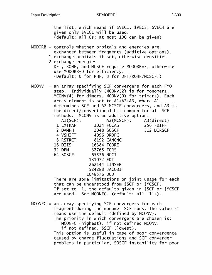
Input Description $FMOPRP 2-300
the list, which means if $VEC1, $VEC3, $VEC4 are given only $VEC1 will be used. (default: all 0s; at most 100 can be given)
MODORB = controls whether orbitals and energies are exchanged between fragments (additive options). 1 exchange orbitals if set, otherwise densities 2 exchange energies DFT, ROHF, and MCSCF require MODORB=3, otherwise use MODORB=0 for efficiency. (Default: 0 for RHF, 3 for DFT/ROHF/MCSCF.)
MCONV = an array specifying SCF convergers for each FMO step. Individually (MCONV(2) is for monomers, MCONV(4) for dimers, MCONV(9) for trimers). Each array element is set to A1+A2+A3, where A1 determines SCF and A2 MCSCF convergers, and A3 is the direct/conventional bit common for all SCF methods. MCONV is an additive option: A1(SCF): A2(MCSCF): A3(direct) 1 EXTRAP 1024 FOCAS 256 FDIFF 2 DAMPH 2048 SOSCF 512 DIRSCF 4 VSHIFT 4096 DROPC 8 RSTRCT 8192 CANONC 16 DIIS 16384 FCORE 32 DEM 32768 FORS 64 SOSCF 65536 NOCI 131072 EKT 262144 LINSER 524288 JACOBI 1048576 QUD There are some limitations on joint usage for each that can be understood from $SCF or $MCSCF. If set to -1, the defaults given in $SCF or $MCSCF are used. See MCONFG. (default: all -1's).
MCONFG = an array specifying SCF convergers for each fragment during the monomer SCF runs. The value -1 means use the default (defined by MCONV). The priority in which convergers are chosen is: MCONFG (highest), if not defined MCONV, if not defined, $SCF (lowest). This option is useful in case of poor convergence caused by charge fluctuations and SCF converger problems in particular, SOSCF instability for poor

Input Description $FMOPRP 2-301
initial guess. Default: all -1.
ESPSCA = scale factors for up to nine initial monomer SCF iterations. ESPs will be multiplied by these factors, to soften the effect of environment and help convergence. At most nine factors can be defined. (default: all 1.0's)
CNVDMP = damping of SCF convergence, that is, loosen convergence during the initial monomer SCF iterations to gain speed. CONV in $SCF and ITOL and ICUT in $CONTRL are modified. CONV is set roughly to min(DE/CNVDMP,1e-4), where DE is the convergence in energy at the given monomer SCF iteration. It is guaranteed that CONV,ITOL and ICUT at the end will be set to the values given in $SCF. Damping is disabled if CNVDMP is 0. Reasonable values are 10-100. Care should be taken for restart jobs: since restart jobs do not know how well FMO converged, restart jobs start out at the same rough values as nonrestart jobs, if CNVDMP is used. Therefore for restart jobs either set CNVDMP appropriately for the restart (i.e., normally 10-100 times larger than for the original run) or turn this option off, otherwise regressive convergence can incur additional iterations (default: 0).
COROFF = parameter turning off DFT in initial monomer SCF, similar to SWOFF. COROFF is used during monomer SCF, and it turns off DFT until monomer energies converge to this threshold. If COROFF is nonzero, SWOFF is ignored during monomer SCF, but is used for dimers and trimer iterations. Setting COROFF=1e-3 and SWOFF=0 usually produces good DFT convergence. COROFF may be thought as a macro- analogue of SWOFF. If monomer SCF converges poorly (>25 iterations), it is also recommended to raise CONV in $SCF to 1e-8 (if CONV in $FMO is 1e-7). Default:1.0E-3 (0.0 skips this option).
NPCMIT = the maximum number of FMO/PCM[m] iterations, applicable to m>1 only (for m=1, $FMOPRP MAXIT is used). NPCMIT=2 can be thought as having special meaning: it is used to define FMO/PCM[l(m)] runs

Input Description $FMOPRP 2-302
by forcing the FMO/PCM loop run only twice, which corresponds to determining PCM charges during the first iteration (and the m-body level) and then using them during the second iteration (l-body). For FMO/PCM[l(m)] only l=1 is implemented and "m" is given in $PCM IFMO. Default: 30.
CNVPCM = convergence threshold for FMO/PCM[m] iterations, applicable to m>1 only (for m=1, $FMOPRP CONV is used). CNVPCM is applied to the total FMO energy Default: 1.0D-07 Hartree.
PCMOFF = parameter turning PCM off in initial monomer SCF iterations, analogous to COROFF. PCM is turned off, until convergence reaches PCMOFF. PCMOFF=0 disables this feature. Default: 0.0
NCVSCF = an array of 2 elements to alter SCF convergers. After NCVSCF(1) monomer SCF iterations the SCF converger will switch between SOSCF <-> FULLNR. This option is useful in converging difficult cases in the following way: $SCF diis=.t. soscf=.f. $end $FMOPRP NCVSCF(1)=2 mconv(4)=65 $end This results in the initial 2 monomer SCF iterations being done with DIIS, then a switch to SOSCF occurs. mconv(4)=65 switches to SOSCF for dimers. Note that NCVSCF(1) will only overwrite MCONV, but not MCONFG. The SCF converger in MCONV(2) will be enforced after NCVSCF(2) monomer SCF iterations, overwriting MCONFG as well. This is useful for the most obnoxiously converging cases. See other FMO documentation. Default: 9999,9999 (which means do not use).
NAODIR = a parameter to decide whether to enforce DIRSCF. Useful for incore integral runs in parallel. NAODIR is the number of AO orbitals that is expected to produce 100,000,000 non-zero integrals. Using this and assuming NAO**3.5 dependence, the program will then guess how many integrals will each n-mer have and whether they will fit into the available memory. If they are determined not to fit, DIRSCF will be set true.

Input Description $FMOPRP 2-303
This option overwrites MCONV but not MCONFG. If set to 0, then the default in-core integral strategy is used. (default=0)
II. Parameters defining parallel execution
MODPAR = parallel options (additive options) 1 turns on/off heavy job first strategy (reduces waiting on remaining jobs at barrier points) (see also 8) 4 broadcast all fragments done by a group at once rather than fragment by fragment. 8 alters the behavior of fragment initialixation: if set, fragments are always done in the reverse order (nfg, nfg-1, ...1) because distance calculation costs decrease in the same order and they usually prevail over making Huckel orbitals or running free monomer SCF. Note that during SCC (monomer SCF) iterations the order in which monomers are done is determined by MODPAR=1. 16 if set, hybrid orbital projectors will not be parallelized (may be useful on slow networks) 32 reserved 64 Broadcast F40 for FMO restarts. F40 should only be precopied to the grand master scratch directory and it should NOT exist on all slaves. (default: 13, which is 1+4+8) 256 Replace I/O to fragment density file by parallel broadcasts from group masters
NGRFMO = an array that sets the number of GDDI groups during various stages of the calculation. The first ten elements are used for layer 1, the next 10 for layer 2, etc. ngrfmo(1) monomer SCF ngrfmo(2) dimers ngrfmo(3) trimers ngrfmo(4) correlated monomers ngrfmo(5) separated dimers ngrfmo(6) SCF monomers in FMO-MCSCF (MCSCF monomer will be done with ngrfmo(1) groups) ngrfmo(7) SCF dimers in FMO-MCSCF (MCSCF dimer be done with ngrfmo(2) groups) ngrfmo(8-10) reserved If any of them is zero, the corresponding stage
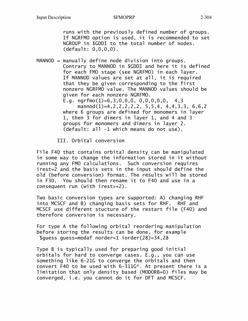
Input Description $FMOPRP 2-304
runs with the previously defined number of groups. If NGRFMO option is used, it is recommended to set NGROUP in $GDDI to the total number of nodes. (default: 0,0,0,0).
MANNOD = manually define node division into groups. Contrary to MANNOD in $GDDI and here it is defined for each FMO stage (see NGRFMO) in each layer. If MANNOD values are set at all, it is required that they be given corresponding to the first nonzero NGRFMO value. The MANNOD values should be given for each nonzero NGRFMO. E.g. ngrfmo(1)=6,3,0,0,0, 0,0,0,0,0, 4,3 mannod(1)=4,2,2,2,2,2, 5,5,4, 4,4,3,3, 6,6,2 where 6 groups are defined for monomers in layer 1, then 3 for dimers in layer 1, and 4 and 3 groups for monomers and dimers in layer 2. (default: all -1 which means do not use).
III. Orbital conversion
File F40 that contains orbital density can be manipulatedin some way to change the information stored in it withoutrunning any FMO calculations. Such conversion requiresirest=2 and the basis sets in the input should define theold (before conversion) format. The results will be storedin F30. You should then rename it to F40 and use in aconsequent run (with irest>=2).
Two basic conversion types are supported: A) changing RHFinto MCSCF and B) changing basis sets for RHF. RHF andMCSCF use different stucture of the restart file (F40) andtherefore conversion is necessary.
For type A the following orbital reordering manipulationbefore storing the results can be done, for example $guess guess=modaf norder=1 iorder(28)=34,28
Type B is typically used for preparing good initialorbitals for hard to converge cases. E.g., you can usesomething like 6-21G to converge the orbitals and thenconvert F40 to be used with 6-311G*. At present there is alimitation that only density based (MODORB=0) files may beconverged, i.e. you cannot do it for DFT and MCSCF.

Input Description $FMOPRP 2-305
MAXAOC = The new (i.e., after conversion) maximum number of AOs per fragment. If you don't know what it should be you can run a CHECK job with the new basis set and find the number in "Max AOs per frg:". If this number is equal to the old value, then type A is chosen.
IBFCON = the array giving pairs of the old and new numbers of AOs for each atom in $DATA (type B only).
MAPCON = maps determining how to copy old orbitals into new (type B only). See the example.
Example: $DATA contains only H and O (in this order), F40was computed with 6-31G and you want to convert to 6-31G**.One water per fragment. MAXAOC=25 25=5*2+15=new basis size for 6-31G** IBFCON(1)=2,5, 9,15 2 and 5 for H (6-31 and 6-31G**), 9 and 15 for O MAPCON(1)=1,2,0,0,0, 1,2,3,4,5,6,7,8,9,0,0,0,0,0,0Here we copy the two s functions of each H, and add ppolarization p to each H (3 0's), and similarly we copynine s,p functions for O, and add d polarization (6 0's)
In order to construct MAPCON, you should know in what orderGaussian primitives are stored. The easiest way to learnthis is to run a simple calculation and check the output(SHELL information).
IV. Printing, properties, restart, and dimensions.
NPRINT = controls print-out (bit additive) bits 1-2 0 normal output 1 reduced output (recommended for single points) 2 minimum output (recommended for optimizations) 4 print interfragment distances. Note: any of RESPAP, RESPPC, or RESDIM must be non-zero or otherwise nothing will be printed. If you only want the distances but no approximations, set the thresholds to huge values, e.g. resdim=1000. 8 print Mulliken charges Note: RESPPC must be set (non-zero), see above. 64 print atomic coordinates for each fragment

Input Description $FMOPRP 2-306
PRTDST = array of three print-out thresholds: 1. print all pairs of fragments separated by less than PRTDST(1). 2. print a warning if two fragments are closer than PRTDST(2), intended mostly to monitor suspicious geometries during optimization. 3. print a warning if two fragments are closer than PRTDST(3) and have no detached bond between them, intended to check input. PRTDST(3) values should slightly exceed the longest detached bond in the system. Using zero for PRTDST(1) and PRTDST(2) turns them off. Similarly, use PRTDST(3)=-1 to turn it off. PRTDST has no units, as it applies to unitless FMO distances (e.g., 0.5 means half the sum of van der Waals radii for the closest pair of atoms). (default: 0.0,0.5,0.6)
IREST = restart level (all non-zero values require file .F40 with restart data be precopied to each node). (unless MODPAR=64 is set) See CNVDMP 0 no restart 2 restart monomer SCF (SCC). 4 restart dimers. Requires monomer energies be given in $FMOENM. Some or no dimer energies may also be given in $FMOEND, in which case those dimers with energies will not be run. Usually the only property that can be obtained with IREST=4 is the energy. The only exception is: a) IREST=1024 was set when monomer SCF was run and b) the property restart files (*.F38*) from each node were saved and copied to the scratch directory for the IREST=1028 job. If these two conditions are met, gradient and ES moments can be restarted with IREST=1028. 1024 write property restart files during monomer SCF and/or use them to restart gradient and/or ES moments. No other property may be restarted. Default: 0.
MODPRP = some extra FMO properties (bit additive) 1 total electron density (AO-basis matrix, written to F10: useful to create initial orbitals for ab initio).
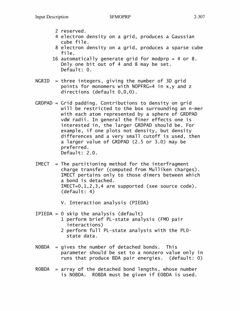
Input Description $FMOPRP 2-307
2 reserved. 4 electron density on a grid, produces a Gaussian cube file. 8 electron density on a grid, produces a sparse cube file. 16 automatically generate grid for modprp = 4 or 8. Only one bit out of 4 and 8 may be set. Default: 0.
NGRID = three integers, giving the number of 3D grid points for monomers with NOPFRG=4 in x,y and z directions (default 0,0,0).
GRDPAD = Grid padding. Contributions to density on grid will be restricted to the box surrounding an n-mer with each atom represented by a sphere of GRDPAD vdW radii. In general the finer effects one is interested in, the larger GRDPAD should be. For example, if one plots not density, but density differences and a very small cutoff is used, then a larger value of GRDPAD (2.5 or 3.0) may be preferred. Default: 2.0.
IMECT = The partitioning method for the interfragment charge transfer (computed from Mulliken charges). IMECT pertains only to those dimers between which a bond is detached. IMECT=0,1,2,3,4 are supported (see source code). (default: 4)
V. Interaction analysis (PIEDA)
IPIEDA = 0 skip the analysis (default) 1 perform brief PL-state analysis (FMO pair interactions) 2 perform full PL-state analysis with the PL0- state data.
N0BDA = gives the number of detached bonds. This parameter should be set to a nonzero value only in runs that produce BDA pair energies. (default: 0)
R0BDA = array of the detached bond lengths, whose number is N0BDA. R0BDA must be given if E0BDA is used.
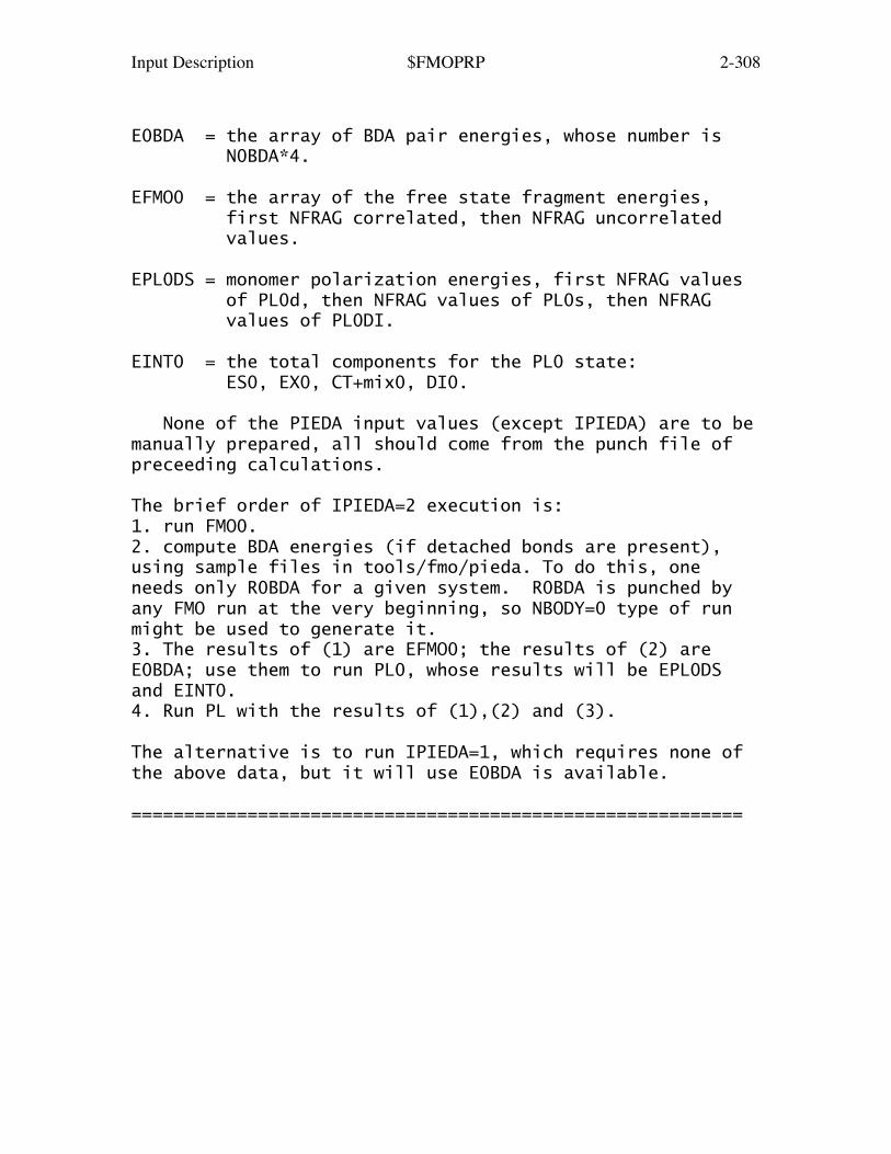
Input Description $FMOPRP 2-308
E0BDA = the array of BDA pair energies, whose number is N0BDA*4.
EFMO0 = the array of the free state fragment energies, first NFRAG correlated, then NFRAG uncorrelated values.
EPL0DS = monomer polarization energies, first NFRAG values of PL0d, then NFRAG values of PL0s, then NFRAG values of PL0DI.
EINT0 = the total components for the PL0 state: ES0, EX0, CT+mix0, DI0.
None of the PIEDA input values (except IPIEDA) are to bemanually prepared, all should come from the punch file ofpreceeding calculations.
The brief order of IPIEDA=2 execution is:1. run FMO0.2. compute BDA energies (if detached bonds are present),using sample files in tools/fmo/pieda. To do this, oneneeds only R0BDA for a given system. R0BDA is punched byany FMO run at the very beginning, so NBODY=0 type of runmight be used to generate it.3. The results of (1) are EFMO0; the results of (2) areE0BDA; use them to run PL0, whose results will be EPL0DSand EINT0.4. Run PL with the results of (1),(2) and (3).
The alternative is to run IPIEDA=1, which requires none ofthe above data, but it will use E0BDA is available.
==========================================================

Input Description $FMOXYZ 2-309
==========================================================
$FMOXYZ group (given for FMO runs)
This group provides an analog of $DATA for $FMO, exceptthat no explicit basis set is given here. It contains anynonzero number of lines of the following type:
A.N Q X Y Z
A is the dummy name of an atom.N is an optional basis set number (if omitted, it will beset to 1). N is intended for mixed basis set runs, forexample, if you want to put diffuse functions on carboxylgroups.Q is the atomic charge.Z is the integer atomic charge.X, Y and Z are Cartesian coordinates. These obey UNITSgiven in $CONTRL.
There is no default, this group must always be given forFMO runs. Alternatively, you may use the chemical symbolinstead of Q. Note that "A" is ignored in all cases, butmust be given.
Here is how $DATA is used in FMO:Each atom given in $DATA defines the basis set for thatatom type, entirely omitting Cartesian coordinates (whichare in $FMOXYZ). There are two ways to input basis sets inFMO.
I. easy!
This works only if you want to use the same built-in basisset for all atoms. It is possible to use EXTFIL as usualfor externally defined basis sets. 1. Define $BASIS as usual 2. Put each atom type in $DATA, e.g. for (H2O)2,
$DATAH2OC1 ! FMO does not support symmetry, so always use C1H 1O 8

Input Description $FMOXYZ 2-310
$end
II. advanced.
This allows you to mix basis sets, have multiple layers ora non-standard without involving EXTFIL.
1. Do not define $BASIS.2. Put each atom type in $DATA, followed by basis set,either explicit or built in.
The names of atoms in $DATA have the following format,where brackets indicate optional parameters:S[.N][-L]N and L may be omitted (taking the default value of 1),S is the atom name (discarded upon reading),N is the basis set ordinal number,L is the layer.S[.N][-L] may not exceed 8 characters.
Example: 2-layer water dimer. In the first layer, you wantto use STO-3G for the first molecule and your own basis setfor the second. In the second layer, you want to use 6-31Gand 6-31G* for the first and second molecules,respectively.
$DATAwater dimer (H2O)2C1H-1 1 ! explanation: layer 1, basis 1 (STO-3G) for Hydr.sto 3
O-1 8 ! explanation: layer 1, basis 1 (STO-3G) for Oxygensto 3
H.2-1 1 ! layer 1, basis 2 (manual) for hydrogens 1 ; 1 2.0 1
O.2-1 8 ! explanation: layer 1, basis 2 (manual) for Oxygens 21 100.0 0.82 10.0 0.6l 11 5.0 1 1

Input Description $FMOXYZ 2-311
H-2 1 ! explanation: layer 2, basis 1 (6-31G) for Hydr.n31 6
O-2 8 ! explanation: layer 2, basis 1 (6-31G) for Oxygenn31 6
H.2-2 1 ! layer 2, basis 2 (6-31G* = 6-31G) for Hydrogenn31 6
O.2-2 8 ! explanation: layer 2, basis 2 (6-31G*) for Oxygenn31 6d 1 ; 1 0.8 1
$endYour $FMOXYZ matching this $DATA will then look as follows: $FMOXYZO 8 x y zH 1 x y zH 1 x y zO.2 8 x y zH.2 1 x y zH.2 1 x y z $END
Note that if you define mixed basis sets for the atomswhere bond detachment occurs (do not do this for basis setswith diffuse functions), then you should provide allrequired sets in $FMOHYB as well, and define $FMOBNDproperly.
==========================================================

Input Description $OPTFMO 2-312
==========================================================
$OPTFMO group (relevant if RUNTYP=OPTFMO)
This group controls the search for stationary pointsusing optimizers developed for the Fragment MolecularOrbital (FMO) method. There is no restriction on the numberof atoms in the molecule, whereas optimising FMO withstandard optimizers (RUNTYP=OPTIMIZE) has a restriction to2000 atoms (unless you rebuild your GAMESS appropriately).OPTFMO runs may be restarted by providing the updatedcoordinates in $FMOXYZ and, optionally, optimizationrestart data (punched out for each step) in $OPTRST (thedata differs for each method).
METHOD = optimization method STEEP steepest descent CG conjugate gradient BFGSL approximate BFGS numeric updates of the inverse Hessian, that do not require explicitly storing that matrix. HSSUPD numeric updates of the inverse Hessian Default: HSSUPD.
HESS = initial inverse Hessian for METHOD=HSSUPD GUESS diagonal guess of 3 READ read from F38 (advanced option) Default: GUESS.
UPDATE = inverse Hessian update scheme for METHOD=HSSUPD BFGS Broyden-Fletcher-Goldfarb-Shanno DFP Davidon-Fletcher-Powell Default: BFGS.
OPTTOL = gradient convergence tolerance, in Hartree/Bohr. Convergence of a geometry search requires the largest component of the gradient to be less than OPTTOL, and the root mean square gradient less than 1/3 of OPTTOL. (default=0.0001)
NSTEP = maximum number of steps to take. Restart data are punched at each step. (default=200)
IFREEZ = array of coords to freeze during optimization.

Input Description $OPTFMO 2-313
The usage is the same as for the similar option in $STATPT.
IACTAT = array of active (not frozen) atoms in geometry optimizations, see $STATPT for its description.
STEP = initial step factor. This multiplies the gradient to prevent large steps. The values of 0.1-0.2 are considered useful in the vicinity of minimum, and 0.5-1.0 is probably OK at the start. (default: 1)
STPMIN = the minimum permitted value of dynamically chosen STEP size (see STPFAC). (default: 0)
STPMAX = the maximum permitted value of dynamically chosen STEP size (see STPFAC). (default: 1)
STPFAC = Dynamic adjustment of STEP. If the energy goes down considerably, the new STEP is set to the old STEP multiplied by 1/STPFAC, if the energy goes up significantly, STEP is set to STEP*STPFAC, both constrained by STPMIN and STPMAX. The default is 1, which means do not use dynamic adjustment. The value 0.9 may be useful if dynamically adjusted steps are desired.
==========================================================
Input Description $FMOLMO 2-314
==========================================================
$FMOHYB group (optional, for FMO runs) (this group was previously known as $FMOLMO)
Hybrid orbitals are used to describe bond detachment whendividing a molecule into fragments. These are the familiarsp3 orbitals for C, plus the 1s core orbital. One set isgiven for each basis set used. The number of basisfunctions L1 (see below) should match your basis set(s).This group is not required if no detached bonds arepresent, for example in water clusters, where the FMOboundaries do not detach bonds. FMO/AFO also does not use$FMOHYB and this group may be omitted.
Format:NAM1 L1 M1I1,1 J1,1 C1,1 C2,1 C3,1 ... CL1,1...I1,M1 J1,M1 C1,M1 C2,M1 C3,M1 ... CL1,M1NAM2 L2 M2I2,1 J2,1 C1,1 C2,1 C3,1 ... CL1,1...I2,M2 J2,M2 C1,M2 C2,M2 C3,M2 ... CL2,M2where NAM are set names (up to 8 characters long), L1 isthe basis set size, M1 is the number of hybrid orbitals inthis set.
Ci,j are LCAO coefficients (i is AO, j is MO) so it is thetransposed matrix of what is usually considered. Ii,j andJi,j are bond assignment numbers, defining to which sidethe corresponding projection operator is added. Usuallyone of each pair of I and J is 1, and the other 0.(default: nothing, that is, no detached bonds).
Orbitals to be put into $FMOHYB are provided for manycommon basis sets (see gamess/tools/fmo/HMO).
==========================================================

Input Description $FMOBND 2-315
==========================================================
$FMOBND group (optional, for FMOruns)
The atom indices involved in the bond detachment are given,in pairs for each bond. Bonds are always detached betweenfragments, layers in multilayer FMO are defined fragment-wise, i.e., whole fragments are assigned to layers.
-I1 J1 NAM1,1 NAM1,2 ... NAM1,n ICH1 IMUL1-I2 J2 NAM2,1 NAM2,2 ... NAM2,n ICH2 IMUL2...I and J are positive integers giving absolute atom indices.NAMs are hybrid orbital set names, defined in $FMOHYB.
Each line is allowed to have different set of NAMs, whichcan happen if different type of bonds are detached, forexample, one line describing C-C bond and another C-N.Every bond given is detached in such a way that the I-atomwill get nothing of it, effectively remove one electron(1/2 of a single covalent bond) from its fragment. The J-atom will get all of the bond and thus adds one electron toits fragment (e.g., formally heterolytic assignment,although in practice all electrons remain through theCoulomb field). The number 'n' above is the number oflayers.
ICH and IMUL are ignored in FMO/HOP. For FMO/AFO, theydefine the charge and multiplicity of the model systemconstructed for the given bond (both 0 by default). IMULfollows the same rules and in $CONTRL. In FMO/AFO any nameshould be used in place of NAM as NONE, if ICH or MULshould be specified, otherwise only -I and J may be given(i.e., omitting NAM, ICH and MUL). (default: nothing, that is, no detached bonds).
Example, for a two-layer run with STO-3G and 6-31G* in thefirst and second layers, respectively. $FMOBND-10 15 STO-3G 6-31G*-20 27 STO-3G 6-31G* $END==========================================================

Input Description $FMOENM $FMOEND $OPTRST 2-316
==========================================================
$FMOENM group (optional, for FMO runs)
This group defines monomer energies for restart jobs. Thegroup should be taken from a previous run.
The format is IFG and ILAY, followed by 4 monomer energies,of which only the first two are used (noncorrelated andcorrelated).
IFG is the fragment number and ILAY is the layer number.This group is required for FMO restarts IREST=4.
==========================================================
$FMOEND group (optional, for FMO runs)
Dimer energies for restart jobs. The group should be takenfrom a previous run.
The format is IFG, JFG and ILAY, followed by 2 dimerenergies, (E'IJ and Tr(deltaDIJ*VIJ)). IFG and JFG describethe dimer and ILAY is the layer number.
This group is optional for FMO restarts IREST=4 and isotherwise ignored. Note that for parallel restarts,$FMOEND groups from all nodes should be collected andmerged into one group.
==========================================================
$OPTRST group (optional, for RUNTYP=OPTFMO)
Restart data for FMO geometry optimizations. The datainside vary for each optimization method, and are supposedto be taken from a previous run (from the punch file).
==========================================================

Input Description $GDDI 2-317
==========================================================
$GDDI group (parallel runs only)
This group controls the partitioning of a large set ofprocessors into sub-groups of processors, each of whichmight compute separate quantum chemistry tasks. If thereis more than one processor in a group, the task assigned tothat group will run in parallel within that group. Notethat the implementation of groups in DDI requires that thegroup boundaries be on SMP nodes, not individualprocessors.
At present, only two procedures in GAMESS can utilizeprocessor groups, namely the FMO method which breaks largecalculations into many small ones, or VSCF, which has toevaluate the same energy at many geometries. For example,the FMO method can farm out different monomer or dimercomputations to different processor subgroups. This isadvantageous, as the monomers are fairly small, andtherefore do not scale to very many processors, althoughthe monomer, dimer, and maybe trimer calculations arenumerous, and can be farmed out on a large parallel system.
NGROUP = the number of groups in GDDI. Default is 0 which means standard DDI (all processes in one group).
PAROUT = flag to create punch and log files for all nodes. It is recommended to set this flag to .TRUE. if you switch the number of groups on the fly (such as in FMO).
BALTYP = load balancing at the group level, otherwise similar to the one in $SYSTEM. BALTYP in $SYSTEM is used for intragroup load balancing and the one in $GDDI for intergroup. It is very seldom when .FALSE. is useful (default: .FALSE.).
MANNOD = manual node division into groups. Subgroups must split up on node boundaries (a node contains one or more cores). Provide an array of node counts, whose sum must equal the number of nodes fired up when GAMESS is launched. Note the distinction between nodes and cores, also

Input Description $GDDI 2-318
called processers, If you are using six quad-core nodes, you might enter NGROUP=3 MANNOD(1)=2,2,2 so that eight CPUs go into each subgroup. If MANNOD is not given (the most common case), the NGROUP groups are chosen to have equal numbers of nodes in them. For example, a 8 node run that asks for NGROUP=3 will set up 3,3,2 nodes/group.
Note on memory usage in GDDI: Distributed memory MEMDDI isallocated globally, MEMDDI/p words per computing process,where p is the total number of processors. This means anindividual subgroup has access to MANNOD(i)*ncores*MEMDDI/pwords of distributed memory. Thus, if you use groups ofvarious sizes, each group will have different amounts ofdistributed memory (which can be desirable if you havefragments of various sizes in FMO).
===========================================================

Input Description $ELG 2-319
===========================================================
$ELG group (polymer elongation calculation)
This group of parameters provides control of elongationcalculations, which steadily increase the size of aperiodicpolymers, by adding attacking monomers to the end of anexisting chain. The existing chain consists of two parts:an A region, with a frozen electron density, farthest fromthe new monomer, and a B region at whose end the monomerattacks. The wavefunction of the B region and the newmonomer are optimized quantum mechanically. Disk filescontaining integrals and/or wavefunction information mustbe saved from one elongation run to the next.
A large number of examples are provided with the sourcecode distribution, see ~/gamess/tools/elg for this, perhapsstarting with the (gly)5, (gly)6, (gly)7 examples. See theliterature cited below for more help.
NELONG = a flag to activate an elongation calculation, 0 means normal GAMESS run (default) 1 same as 0 but without reorientation of geometry 2 means elongation starting cluster calculation, this initiates a chain's A and B regions. 3 implies the monomer elongation of the chain.
NATM = NUMBER OF ATOMS IN A-REGION Coordinates of the A-region atoms must be listed at the beginning of the input geometry in $DATA
NASPIN = multiplicity of the A-region
NTMLB = NUMBER OF TERMINAL ATOMS IN B-REGION
NCT = CONTROLLER FOR AO-CUT 0 means no AO-cut 1 means AO-cut activated
IPRI = PRINT LEVEL 0 minimum printing (default) 3 debugging printing
LDOS = LOCAL DENSITY OF STATES CALCULATION

Input Description $ELG 2-320
0 means no LDOS calculation 1 means LDOS calculation
I2EA = READ-IN 2E-INTEGRALS FOR A-REGION 0 means A-region 2e-integrals are recalculated 1 means A-region 2e-integrals are read from a previous calculation
ATOB = Flag to shift one unpaired electron to the A- or the B-region, for covalently bonded A and B. .TRUE. means shift one electron to B-region .FALSE. means shift one electron to A-region
For more information on this method, see
A.Imamura, Y.Aoki, K.Maekawa J.Chem.Phys. 95, 5419-5431(1991)Y.Aoki, A.Imamura J.Chem.Phys. 97, 8432-8440(1992)Y.Aoki, S.Suhai, A.Imamura Int.J.Quantum Chem. 52, 267-280(1994)Y.Aoki, S.Suhai, A.Imamura J.Chem.Phys. 101, 10808-10823(1994)
and particularly the new implementation described in
"Application of the elongation method to nonlinear opticalproperties: finite field approach for calculating staticelectric (hyper)polarizabilities" F.L.Gu, Y.Aoki, A.Imamura, D.M.Bishop, B.Kirtman Mol.Phys. 101, 1487-1494(2003)"A new localization scheme for the elongation method" F.L.Gu, Y.Aoiki, J.Korchowiec, A.Imamura, B.Kirtman J.Chem.Phys. 121, 10385-10391(2004)"Elongation method with cutoff technique for linear SCFscaling" J.Korchowiec, F.L.Gu, A.Imamura, B.Kirtman, Y.Aoki Int.J.Quantum Chem. 102, 785-794(2005)"Elongation method at Restricted Open-Shell Hartree-Focklevel of theory" J.Korchowiec, F.L.Gu, Y.Aoki Int.J.Quantum Chem. 105, 875-882(2005)
==========================================================
Input Description $DANDC 2-321
==========================================================
$DANDC group (optional, relevant if SCFTYP=RHF or UHF)
This group controls the divide-and-conquer (DC) SCFcalculations, in which the total 1-electron density matrixis obtained as sum of subsystem density matrices. In thiscalculation, the total system is partitioned into severaldisjoint subsystems (central regions). A subsystem densitymatrix is expanded by bases in the central region and itsneighboring enviromental region (buffer).
The present implementation allows energy and analyticnuclear gradients, for HF, DFT, and semi-empirical runs,for SCFTYP=RHF or UHF only. The discrete EFP and variouscontinuum solvation models are available. DC correlationenergies are also available for either MP2 and CC, see$DCCORR, without nuclear gradients. Dynamic and staticpolarizabilities (but no hyperpolarizabilities) based onDC-HF are available by specifying RUNTYP=TDHF (not TDHFX).
The initial guess is given by a density matrix, notorbitals. The only available options are GUESS=HUCKEL,HCORE, HUCSUB, DMREAD, and MOREAD (the latter meansorbitals for the entire system).
For a review paper on Divide-and-Conquer in GAMESS: M.Kobayashi, H.Nakai in Linear-Scaling Techniques in Computational Chemistry and Physics: Methods and Applications (Springer), Chap. 5 (2011) For more information on the DC-SCF method, see W.Yang, T.-S.Lee J.Chem.Phys. 103, 5674-5678(1995) T.Akama, M.Kobayashi, H.Nakai J.Comput.Chem. 28, 2003-2012(2007) T.Akama, A.Fujii, M.Kobayashi, H.Nakai Mol.Phys. 105, 2799-2804(2007) T.Akama, M.Kobayashi, H.Nakai Int.J.Quant.Chem. 109, 2706-2713(2009) M.Kobayashi, T.Yoshikawa, H.Nakai Chem.Phys.Lett. 500, 172-177(2010) [open-shell] M.Kobayashi, T.Kunisada, T.Akama, D.Sakura, H.Nakai J.Chem.Phys. 134, 034105/1-11(2011) [gradient]

Input Description $DANDC 2-322
For more information on DC-MP2 and DC-CC, see M.Kobayashi, Y.Imamura, H.Nakai J.Chem.Phys. 127, 074103/1-7(2007) M.Kobayashi, H.Nakai J.Chem.Phys. 129, 044103/1-9(2008) M.Kobayashi, H.Nakai J.Chem.Phys. 131, 114108/1-9(2009) M.Kobayashi, H.Nakai Int.J.Quant.Chem. 109, 2227-2237(2009) For more information on DC-TDHF polarizability, see T.Touma, M.Kobayashi, H.Nakai Chem.Phys.Lett. 485, 247-252(2010)
Of course, the trick to methods that divide up a largeproblem into small ones is to control the errors thatresult. A simple way to set up a DC-MP2 calculation iswith atomic partitions: $contrl scftyp=rhf mplevl=2 runtyp=energy $end $system mwords=25 $end $scf dirscf=.true. $end $dandc dcflg=.true. subtyp=atom bufrad=8.0 $end $dccorr dodccr=.true. rbufcr=5.0 $end $guess guess=hucsub $end (if DC-SCF is used)This leads to as many subsystems as there are atoms, withthe buffer region around the central atom being defined bya radius. This input recognizes that exchange effects inHartree-Fock are longer range than correlation, and thususes dual level radii. It may be reasonable to simply do aconventional and thus fully accurate SCF computation byDCFLG=.FALSE., obtaining only the MP2 correlation energy bythe divide and conquer method. Faster run times may resultfrom other partitionings, such as manually dividing aprotein into subsystems containing a single amino acid.
DCFLG = flag to activate DC-SCF calculation. (default=.FALSE.)
Note: If you want to treat only the correlated MP2/CC procedure in the DC manner, after a standard HF calculation, this option may be set to .FALSE.
SUBTYP = chooses a method to construct disjoint subsystems (central region). = ATOM individual atom is 1 subsystem.

Input Description $DANDC 2-323
(default if NSUBS=0 or not given) = MANUAL manually selects using NSUBS and LBSUBS keywords. (default if NSUBS>=1) = CARD reads from card. $SUBSCF is used for SCF and $SUBCOR for MP2/CC calculation. = AUTO constructs subsystems automatically by dividing total system by cubic grid. Grid size can be set by SUBLNG. = AUTBND considers bond strength after AUTO.
NSUBS = number of subsystems when SUBTYP=MANUAL.
LBSUBS = an array assigning atoms to subsystems. The style is the same as INDAT keyword in $FMO. Two styles are supported (the choice is made based on LBSUBS(1): if it is nonzero, choice (a) is taken, otherwise LBSUBS(1) is ignored and choice (b) is taken): a) LBSUBS(i)=m assigns atom i is to subsystem m. LBSUBS(i) must be given for each atom. b) the style is a1 a2 ... ak 0 b1 b2 ... bm 0 ... Elements a1...ak are assigned to subsystem 1, then b1...bm are assigned to subsystem 2,etc. An element is one of the following: I or I -J where I means atom I, and a pair I,-J means the range of atoms I-J. There must be no space after the "-"! Example: LBSUBS(1)=1,1,1,2,2,1 is equivalent to LBSUBS(1)=0, 1,-3,6,0, 4,5,0 Both assign atoms 1,2,3 and 6 to subsystem 1, and 4,5 to subsystem 2.
SUBLNG = grid length of cube used in SUBTYP=AUTO or AUTBND. This value should be in the unit given by UNITS keyword in $CONTRL. (default=2.0 Angstroms).
BUFTYP = chooses a method to construct buffer region. = RADIUS selects atoms included in spheres centered at atoms in the central region (default). The radius is given by BUFRAD keyword for

Input Description $DANDC 2-324
DC-SCF and by the RBUFCR keyword in $DCCORR for DC-MP2/CC. = RADSUB selects subsystems containing one or more atom(s) which is included in spheres centered at atoms in the central region. This selection can avoid cutting bonds within each subsystem. = CARD reads from $SUBSCF or $SUBCOR card. Only available when SUBTYP=CARD.
BUFRAD = buffer radius in DC-SCF calculation. This value should be in the units given by UNITS keyword in $CONTRL (default=5.0 Angstroms).
FRBETA = inverse temperature parameter of Fermi function used in DC-SCF procedure in a.u. (default=200.0) Reducing this value may improve SCF convergence but may obtain worse total energy.
MXITDC = maximum number of iteration cycles for determining Fermi level (default=100). Usually, you need not care about this keyword.
FTOL = Fermi function cutoff factor (default=15.0). = p The value of Fermi function less than 10**(-p) is considered as 0. The value greater than [1 - 10**(-p)] is considered as 1.
NDCPRT = DC print-out option which is the sum of followings (default=0). = +1 not used (reserved). = +2 prints density matrix ($DM section) on punch. = +4 prints energy corresponding to each subsystem. Gives correct energy only in HF calculation. = +8 prints orbitals in each subsystem.
IORBD = selects molecular orbital in total system whose electron density is to be computed. Print format is given in $ELDENS. = -1, -2, ... correspond to HOMO, HOMO-1, ... = 1, 2, ... correspond to LUMO, LUMO+1, ... = 0 no calculation (default).
In the DC-SCF procedure, the available SCF accelerationtechniques are DIIS, DAMP, EXTRAP as well as DC-DIIS and
Input Description $DANDC 2-325
VFON which are specific to the DC-SCF. In DC-SCFcalculation, only DIIS is used by default. DC-DIIS(DIIDCF=.TRUE.) is not normally needed for convergence.
The following keywords control (DC-)DIIS convergence:
DIITYP = selects the error vector used in the standard DIIS extrapolation = FDS Pulay's modified DIIS (e=FDS-SDF). Although this type of error vector behaves well in standard SCF, it may not for DC-SCF. = DELTAF Pulay's original DIIS (e[i]=F[i]-F[i-1]), or so-called Anderson mixing (default).
DIIQTR = .TRUE. uses orthogonal basis (in entire system) for DIIS extrapolation. Normally, this does not make sense in DC-SCF run. .FALSE. uses atomic basis function for DIIS extrapolation (default).
EXTDII = energy error threshold in absolute value for exiting DIIS (default=0.0).
PEXDII = percentage threshold of energy error change for exiting DIIS (default=1.0). PEXDII is preferential to EXTDII.
DIIDCF = a flag to activate DC-DIIS interpolation (default=.FALSE.).
ETHRDC = energy error threshold for initiating DC-DIIS. Increasing ETHRDC forces DC-DIIS on sooner (default = 1.D-4 if DIIDCF=.TRUE.).
The following keywords control the convergence accelerationbased on the varying fractional occupation number (VFON).The final electronic temperature is given by FRBETA.
FONTYP = selects the variation pattern of electronic temperature (beta) in SCF iteration = DIIER logarithmic variation with respect to DIIS error. = NONE no variation (default).
Input Description $DANDC 2-326
BETINI = initial beta value in a.u. (default = FRBETA/4 for FONTYP=DIIER).
FONSTA = threshold to start variation of beta (default=1.0 for FONTYP=DIIER).
FONEND = threshold to stop variation of beta (default=1.D-4 for FONTYP=DIIER).
When FONTYP=DIIER, the beta value used in the iteration(of which the DIIS error is DIISer) is the following: beta = BETINI [for DIISER>FONSTA] = FRBETA [for DIISER<=FONEND] = FRBETA + C_FON * Log(DIISer/FONEND) [otherwise]where (C_FON = (BETINI-FRBETA) / Log(FONSTA/FONEND)
Option for the type of nuclear gradient:
NDCGRD = selects the DC-SCF gradient implementation = 0 use a formula proposed by Yang and Lee in 1995 = 1 use a formula proposed by Kobayashi et al. in 2011 (default)
Next are options for printing density of states (DOS).
DOSITV = Interval between plot points in Hartree. The default is zero,meaning no DOS print-out. If you print out DOS, DOSITV=0.05 may be sufficient.
DOSRGL = Left end of the plot range in Hartree. (default=-2.0)
DOSRGR = Right end of the plot range in Hartree. (default=+2.0)
BDOS = Inverse temperature parameter (beta) for distributing states. This value should not be given because it is set to be equivalent to FRBETA in $DANDC by default.
==========================================================

Input Description $DCCORR 2-327
==========================================================
$DCCORR group (optional) relevant for MPLEVL=2 relevant for CCTYP=LCCD, CCD, CCSD, CCSD(T), R-CC
This group controls the linear-scaling DC-based MP2 orCC calculations. In this method, subsystem correlationenergy is evaluated in each subsystem by means of subsystemMOs. Total correlation energy is obtained by summing upsubsystem contributions.
The present implementation allows only RHF reference.DC-MP2 calculations can be run in parallel (using CODE=DDI,IMS, or SERIAL in $MP2), but DC-CC is limited to serialexecution. DC-MP2 with CODE=IMS is only compatible withDIRSCF=.TRUE. Coupled cluster code is only available forCCTYP=LCCD, CCD, CCSD, CCSD(T), or R-CC. No solvationmodels are available. This group must be given if the"double-hybrid" DFT is used (e.g., DFTTYP=B2PLYP).
Note: Although $DANDC input is usually used together toselect subsystem and buffer information, DC-SCF calculationis not indispensable to perform DC correlation calculation.You can perform DC correlation calculation without DC-SCFby setting DCFLG=.FALSE. in $DANDC and DODCCR=.TRUE.
For more information (and references), see $DANDC.
DODCCR = a flag to activate DC-MP2/CC calculation. This is forced to be .TRUE. if DCFLG=.TRUE. in $DANDC. This keyword enables to perform DC-MP2/CC calculation after standard (non-DC) RHF.
RBUFCR = buffer radius used in DC-MP2/CC calculation. This value should be in the unit given by UNITS option in $CONTRL. By default, RBUFCR is set to be equal to BUFRAD in $DANDC. This keyword is mainly used to perform so-called dual-buffer DC-MP2/CC calculations, see the paper on the DC-CC method for more details.
RMKORB = a flag to remake orbitals in each subsystems. This

Input Description $DCCORR 2-328
is forced to be .TRUE. if RBUFCR is different from BUFRAD in $DANDC or standard HF calculation was performed. Apart from these cases, RMKORB=.FALSE. by default. This keyword is meant for debug purposes.
HFFRM = a flag to use the Fermi level determined in the preceding HF calculations even when RMKORB=.TRUE. (default=.FALSE.) The Fermi level is used to classify the subsystem orbitals into occupied and virtual ones. Usually, this option does not change the results except for the use of diffuse basis functions.
WOCC = a parameter determining proportion of occupied contribution. This should be between 0 and 1. The proportion of virtual contribution becomes [1 - WOCC]. (default=1.0) This is forced to be 1.0 in DC-CC calculation, except when WOCC=0.0, which only calculates virtual contribution. We recommend 1.0 to obtain accurate results.
ONLYOC = a flag to disable MP2 calculation for virtual contributions. This is forced to be .FALSE. if WOCC is not 1.0, and to be .TRUE. in DC-CC calculation. = .TRUE. Performs DC-MP2 calculation only for occupied contributions. This option will accelerate the CPU time. (default) = .FALSE. Performs DC-MP2 calculation for occupied and virtual contributions.
ITPART = specifies the partitioning for (T) correction. This is only relevant to CCTYP=CCSD(T) or R-CC. = XY (two-digit integer) uses [X,Y] type partitioning defined in the following article: J.Chem.Phys.131,114108(2009) (default=00)
ISTCOR = restart option for DC-MP2/CC. = 0 does DC-MP2/CC calculation from the beginning (default). = n reads subsystem correlation energies corresponding to subsystem 1-(n-1) from input

Input Description $DCCORR 2-329
and perform DC-MP2/CC calculation from n-th subsystem. $MP2RES and $CCRES inputs are required for DC-MP2 and DC-CC calculations, respectively.
FZCORE = a flag to freeze core electrons in DC-MP2 or DC-CC calculation. Other frozen orbital options options such as NACORE in $MP2 and NCORE in $CCINP do not pertain to DC-MP2/CC calculations. The default is .TRUE. to freeze cores.
==========================================================

Input Description $SUBSCF $SUBCOR 2-330
==========================================================
$SUBSCF group (relevant during Divide and Conquer)$SUBCOR group
These groups specify the central and buffer regionswhen SUBTYP=CARD or BUFTYP=CARD in $DANDC. $SUBSCF is usedfor DC SCF and $SUBCOR is for DC-MP2/CC. If BUFTYP is notCARD, only central region is specified by these groups.They consist of free format integer numbers of which thestyle is like this:
$SUBSCF! SUBSYSTEM 1 1 3 -5 0 2 6 -8 0 0! SUBSYSTEM 2 2 6 -9 11 0 1 3 4 10 12 -14 0 0! SUBSYSTEM 3 ... $END
Lines starting with ! are comments neglected when reading.
First, atoms in the central region of subsystem 1 isspecified according to the (b) style of LBSUBS in $DANDC.A single 0 separates the central and buffer region of thesame subsystem. Then, specify atoms in the buffer region ofsubsystem 1. A double 0 separates subsystems. These areiterated until all subsystems are specified.
In the above case, the subsystems are the followings:
Subsystem 1 central: 1,3,4,5 buffer : 2,6,7,8Subsystem 2 central: 2,6,7,8,9,11 buffer : 1,3,4,10,12,13,14
==========================================================
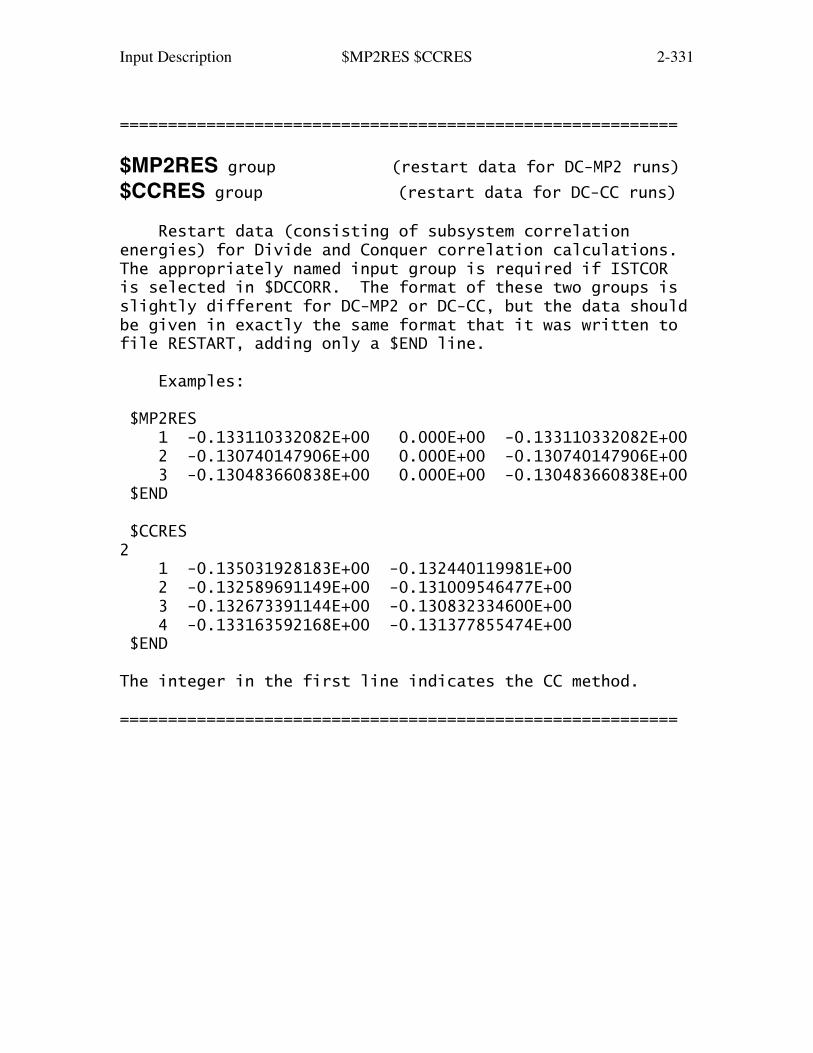
Input Description $MP2RES $CCRES 2-331
==========================================================
$MP2RES group (restart data for DC-MP2 runs)
$CCRES group (restart data for DC-CC runs)
Restart data (consisting of subsystem correlationenergies) for Divide and Conquer correlation calculations.The appropriately named input group is required if ISTCORis selected in $DCCORR. The format of these two groups isslightly different for DC-MP2 or DC-CC, but the data shouldbe given in exactly the same format that it was written tofile RESTART, adding only a $END line.
Examples:
$MP2RES 1 -0.133110332082E+00 0.000E+00 -0.133110332082E+00 2 -0.130740147906E+00 0.000E+00 -0.130740147906E+00 3 -0.130483660838E+00 0.000E+00 -0.130483660838E+00 $END
$CCRES2 1 -0.135031928183E+00 -0.132440119981E+00 2 -0.132589691149E+00 -0.131009546477E+00 3 -0.132673391144E+00 -0.130832334600E+00 4 -0.133163592168E+00 -0.131377855474E+00 $END
The integer in the first line indicates the CC method.
==========================================================

Input Description $FFDATA $FFPDB 2-332
==========================================================
$FFDATA group (optional, relevant if QuanPol is used)
$FFPDB group (optional, relevant if QuanPol is used)
QuanPol (quantum chemistry polarizable force fieldprogram) can perform MM, QM/MM or QM/MM/Continuum solventMD simulation or geometry optimization, using HF, DFT, GVB,MCSCF, MP2 or TDDFT wavefunctions. To use QuanPol, either$FFDATA or $FFPDB needs to be present, to define the MMatoms. Quantum atoms, if any, are given in $DATA as usual.
After the initial input giving QuanPol's options, onegives either explicit coordinates (in which case this groupmust be named $FFDATA) or Protein Data Bank coordinates (inwhich case this is $FFPDB).
Force field data sets are located by the environmentvariable QUANPOL.
----------------------------------------------------------
-1- one or more lines, containing one or more options:
DT = MD time step size. Default=1.0D-15 seconds.
NSTEPS = number of MD and OPTIMIZE steps. Default=1000.
OPTTOL = geometry optimization gradient criterion. Default=1.0D-04 hartree/bohr
NPROP = start to calculate properties after NPROP steps. Default=0
JOUT = report simulation information such as energies and temperature to log file every JOUT steps. Default=1.
KOUT = write coordinates to the log file every KOUT steps. Default=100
LOUT = special action control = 314159 to create the $FFDATA group for a molecule using the information in LOUT314159.PAR file.

Input Description $FFDATA $FFPDB 2-333
ITSTAT = flag to enable the thermostat (velocity scaling) = 0 no thermostat (default) = 1 velocity scaling = 2 Berenedsen thermostat = 3 Andersen thermostat
IPSTAT = flag to enable the barostat (volume scaling) = 0 no barostat (default) = 1 Berenedsen barostat after NPROP steps. A barostat is meaningful only for PBC system. For spherical systems with a soft-wall, volume and pressure are self-adjusted.
TEMP0 = bath temperature. Default=298.15 K.
PRES0 = bath pressure. Default=1.0 bar. A pre-equilibrium system may show huge positive or negative pressures like 100,000 bar. An equilibrium system may show pressures fluctuating by several hundreds bar.
INTALG = MD integrator algorithm. = 1 Beeman algorithm (default) = 2 velocity verlet algorithm
NRANDOM= selects the seed for QuanPol's random number generator: = 0 use fixed seeds for reproducibility (default) = 1 use time/date to generate seeds QuanPol uses a 16-bit pseudo-random integer generator with a cycle length 6953607871644. See Wichmann & Hill, Appl.Statist. 31, 188-190 (1982) Fixed and time/date seeds should give the same randomness. Using fixed seeds, serial MD jobs are reproducible; parallel MD jobs are reproducible for ~500 steps.
MXFFAT = maximum number of MM atoms.MXBOND = maximum number of bonds.MXANGL = maximum number of bond angles.MXDIHR = maximum number of dihedral rotation angles.MXDIHB = maximum number of dihedral bending angles. (i.e. improper torsion in CHARMM).MXWAGG = maximum number of wagging angles.

Input Description $FFDATA $FFPDB 2-334
MXCMAP = maximum number of CHARMM correction map cases. All of these are for memory allocation purposes. Default varies from 10,000 to 100,000, depending on the number of processors.
MXLIST = maximum number of non-bond MM atoms around a given MM atom. Default=1400 is good for SWR2=12.
BUFLIST= The width of the buffer region for the non-bond list. Default = 2.0 angstrom. A new non-bond list will be generated if any atom moves more than half BUFLIST since the last updating of the non-bond list.
IADDWAT= specifies how to add water molecules to the system = 0 No adding water (default) = 1 Add water in PBC master box = 2 Add water in a sphere
ITYPWAT= selects the water model. (the default is 301) = 301 Nonpolarizable flexible 3-point model = 302 Polarizable flexible 3-point model = 303 SPC/Fw model by Wu/Tepper/Voth, see J.Chem.Phys. 124, 024503(2006). = 304 flexible TIP3P as implemented in CHARMM22/27.
Water models 301 and 302 are optimized using SWR1=10,SWR2=12, SWMODE=3, 510 waters, PBC, at 298.15 K and 1 bar.Density, O-O rdf, self-diffusion coefficient are good andnot size-sensitive. Dielectric constants are ~70 for 301,~56 for 302 when 510 waters are used, and are ~110 for 301,~96 for 302 when 2187 waters are used.
JADDNA1= flag to add NA+ ions to DNA/RNA PO4- sites.JADDK1 = flag to add K+ ions to DNA/RNA PO4- sites. = 0 skip (default) = 1 Add NA+/K+ ions to all possible PO4- sites
IADDNA1= number of Na+ ions randomly added. Default=0.IADDK1 = number of K+ ions randomly added. Default=0.IADDCA2= number of Ca2+ ions randomly added. Default=0.IADDMG2= number of Mg2+ ions randomly added. Default=0.IADDCL1= number of Cl- ions randomly added. Default=0.
CENTER = X, Y, Z

Input Description $FFDATA $FFPDB 2-335
define the center of the PBC master box or the sphere center. If not found, it will be automatically calculated. Use the same CENTER for restart jobs.
XBOX,YBOX,ZBOX = size of the periodic box in Angstrom. Default 1.0D+30 means no PBC is imposed.
RCUT = radial cutoff of MM-MM interactions in angstrom.RCUTQ = radial cutoff of QM-MM interactions in angstrom.
SWMODE = selects the switching function mode, default=3 Note that shifting functions operate on the range zero to SWR2, while switching functions work in the tail region, from SWR1 to SWR2. = 1 atom-atom switching function. Tests show that atom-atom SWF gives incorrect water structure and properties. = 2 group-group switching function. Terminal atoms (H, F, Cl,... and carbonyl O) will be grouped to their node atoms. Tests show that group-group SWF can give a correct water structure. = 3 the atom-atom shifting function S(r)=(1-r/SWR2)**2 is used for charge-charge interaction. The same shifting function is used by the ENCAD and ilMM codes. In addition, this option means that group-group switching function is used for both charge-charge and Lennard-Jones interactions in the range between SWR1 and SWR2. Set SWR1=SWR2 to turn off the switching, but keep the shifting. = 4 similar to SWMODE=3, but with the atom-atom shifting function S(r)=[1-(r/SWR2)**2]**2. which is one of the CHARMM shifting functions. Switching function is used as in option 3. = 5 similar to SWMODE=3, but the atom-atom shifting function is choosen to mimic a dielectric reaction field for charge-charge interaction. RXNEPS & SWR2 are required. The shifting function is Eq (5) in Rick, J.Chem.Phys. 120, 6085 (2004)
Input Description $FFDATA $FFPDB 2-336
Switching function is used as in option 3.
The switching function implemented in QuanPol is W(r) = 1 - 10*D**3 + 15*D**4 - 6*D**5 with D = (r**2 - SWR1**2)/(SWR2**2-SWR1**2)
SWR1,SWR2 = distance cutoffs for the switching function that gradually drops the interactions from full strength at SWR1 to zero at SWR2. In angstrom. For MM atoms only.
SWR1Q,SWR2Q = same as SWR1 and SWR2, but for QM-MM interactions.
SPHRAD = radius of the sphere containing the QM/MM system. Default is a huge value, meaning no sphere. A Lennard-Jones type potential is applied to keep the heavy atoms in the sphere. For each such atom: V=4*SPHEPS*{[SPHSIG/(r-R)]**12 - [SPHSIG/(r-R)]**6} R = SPHRAD + [2**(1/6)-1]*SPHSIG V = -SPHEPS when r = SPHRAD - SPHSIG
SPHEPS = Lennard-Jones epsilon parameter for SPHRAD. Default = 0.15 kcal/mol is good for water. Proper values should be determined empirically.
SPHSIG = Lennard-Jones sigma parameter for SPHRAD. Default = 1.5 A is good for water. Proper values should be close to the radii of the solvent atoms, which are usually around 1.5.
IRXNFLD= flag to enable spherical reaction field model = 0 no reaction field (default) = 1 image charge method, currently only for pure MM system = 60, 240, 960, 3840 to choose surface charge method and define the number of surface elements. Available for MM and QM/MM.
RXNEPS = dielectric constant in RXNFLD (default = 1.0)
RXNRAD = radius of sphere in angstrom (default = 1.0D+30). SPHRAD is required. For water solvent,

Input Description $FFDATA $FFPDB 2-337
RXNRAD = SPHRAD + 0.60 A RXNEPS = 78.39 SPHEPS = 0.15 SPHSIG = 1.50 are strongly suggested.
RDF = NRDF, NAME1, NAME2, ... = specifies the number of pairs for the radial distribution function calculation, and the names of the atoms. Must give NRDF pairs of names. Default for NDRF is 0. The RDF will be calculated every JOUT steps.
DELRDF = specifies the radial increment in the radial distribution function calculation. Default= 0.02 angstrom.
DIFFUSE= NDFS, NAME1, NAME2, ... = specifies the number of atoms for diffusion coefficient calculation, and the names of the atoms. Must give NDFS names. Default is NDFS=0.
TIMDFS = time interval for diffusion coefficient calculation. Default = 3.0D-12 seconds is good for water. Can be larger, but should not be smaller. There must be sufficient displacement in order to apply the statistical formula.
NATPDB = number of atoms in the PDB file. If $FFPDB is used, NATPDB will be automatically determined. The main usage is for restart jobs in which only $FFDATA is provided.
NFIXPDB= fix the coordinates of PDB atoms for the initial NFIXPDB steps of an MD or OPTIMIZE procedure. This is useful for initial solvent equilibration. Reasonable values are 1000-10000. Default = 0.
NRIJ = NRIJ, I1, J1, I2, J2, ... = specifies up to 20 pairs of atoms to print out their distances at every JOUT steps. Useful when one wants to monitor H-bond distances. Default NRIJ = 0.

Input Description $FFDATA $FFPDB 2-338
NRMSD = flag root-mean-square-displacement calculation. = 0 skip = 1 calculate RMSD from the initial coordinates at every JOUT steps.
NGYRA = flag radius of gyration calculation (see TIMGYRA). = 0 skip = 1 calculate radius of gyration using formula: R=SQRT[sum(m*r*r)/sum(m)] r: distance from COM m: atom mass So R is mass-weighted RMS distance from COM.
TIMGYRA= time interval for radius of gyration calculation. Default=1.0D-12 seconds. Can be larger or smaller.
NRALL = flag to activate internuclear distance calculation (see TIMRALL). = 0 skip = 1 calculate internuclear distances and compare to those in the initial structure. Unsigned and RMS displacements will be printed out.
TIMRALL= time interval for internuclear distance calculation. Default = 1.0D-12 seconds. Can be larger or smaller, but frequent calculation slows down the MD.
NDIEL = flag MD simulation of dielectric constant. = 0 skip (default) = 1 calculate dielectric constant using formula: Eps = 1 + (<M**2> - <M>**2)/(3kT<V>) M = total dipole of the master box or sphere k = Boltzmann constant T = temperature V = volume When spherical systems are used, a sphere with radius = SPHRAD-SPHSIG is used to calculate M and V. Tests show this gives Eps very similar to those from PBC simulations. When induced point dipoles are used, each dipole is decomposed into two point charges at the opposite sites of the point dipole. These charges are considered for M calculation. One

Input Description $FFDATA $FFPDB 2-339
of them may be relocated when PBC is imposed, or may be excluded if it is outside of the sphere.
AANAM = a name for the LOUT=314159 purpose. This name should be in the LOUT314159.TOP file. Give any name, if no intention to use LOUT314159.TOP.
NFOLD = this is used only in $FFDATA to duplicate the input molecule in 3D space NFOLD times. Reasonable values are 0, 3, 6, 9, 12 and 15, which leads to 1, 8, 64, 512, 4096 and 32768 copies. 0-20 can be used. Default=0, no action.
RFOLD = specifies the spacing when NFOLD is active. The value should be calculated using density. Default= 0.0 angstrom.
IDOCHG = flag to include MM chargesIDOPOL = flag to include MM polarizationIDOLJ = flag to include MM Lennard-JonesIDOCMAP= flag to include CHARMM correction map for proteins For all of these, = 1 include (default) = 0 exclude
NFFTYP = select the force field type = 20022, which is CHARMM22/27 (default)
WT14 = scaling factor for 1-4 LJ, charge-charge and polarization interactions. Default 1.00
RETAIN = retaining factor (0.0 - 1.0, default 0.5) for MM force field covalent terms that involve only QM atoms, one of which is a boundary atom with repulsion potentials in place of a frontier MM atom. Using 0.5 is reasonable for weakened boundary bonds. Use 0.0 if the boundary bonds are not weakened. The retaining factor for MM covalent terms involving only QM atoms (none of which is a boundary atom in place of a frontier MM atom) is always 0.0 and cannot be changed from the input deck.
QMREP = NQMREP, IATOM1, NTERM1, C11, Z11, C12, Z12 ...,
Input Description $FFDATA $FFPDB 2-340
IATOM2, NTERM2, C21, Z21, C22, Z22 ... = specify effective Gaussian repulsion potentials at boundary QM/MM atoms (typically H atoms in place of alpha carbons of a peptide) to produce the desired longer bond lengths. NQMREP = number of QM atoms with Gaussian potentials. Up to 200 atoms. IATOMn = QM atom sequential number in $DATA NTERMn = number of Gaussians at IATOMn. Up to 4 C11,.. = strength part of the Gaussian, e/bohr Z11,.. = radial part of the Gaussian, 1/bohr**2 Must enter NTERMn pairs of C and Z for atom IATOMn. For example, to define 1 Gaussian for QM atom 1 and 3 Gaussians for QM atom 7, give QMREP=2,1,1,3.0,3.0,7,3,8.0,6.0,3.0,3.0,0.3,1.0 For H atom forming C-H bond, a single Gaussian with C=3.0 Z=3.0 is a good option.
The remainder of this group depends on whether it is a $FFDATA or a $FFPDB!
Input Description $FFDATA $FFPDB 2-341
---------------------------------------------------------
**** the following inputs pertain to $FFDATA ****
-2- the input is given in subsections with a keyword at the start of the subsection, and STOP at its end.
COORDINATESNAME, NUC, X, Y, Z NAME = The name of the atom. NUC = nuclear charge of the atom X,Y,Z = Cartesian coordinates in angstromSTOP
PARAMETERSNAME, MASS, Q, POL, SIGMA, EPSILON, SIGMA2, EPSILON2 NAME = The name of the atom. Q = Force field charge (e) on the atom. POL = Polarizability of the atom, in A**3 SIGMA = Lennard-Jones parameter in angstrom. CHARMM uses RMIN/2. QuanPol will automatically check whether it is SIGMA or RMIN/2. EPSILON = Lennard-Jones parameter in kcal/mol SIGMA2, EPSILON2 = the LJ parameters for select 1-4 cases in CHARMM. Give zeros if not these.
Give the same number of lines as specified in the COORDINATES sectionSTOP
QMMMREPN, C1, Z1, C2, Z2, C3, Z3, C4, Z4 N = number of Gaussian type potentials. currently only 4 is allowed. C1 - C4 = strength factor of the potential Z1 - Z4 = radial factor of the potential
give the same number of lines as specified in the COORDINATES sectionSTOP
BOND

Input Description $FFDATA $FFPDB 2-342
SERIAL#, ATOM1, ATOM2, BFC, R0 SERIAL# = serial number of the bond. this is only for notation purpose. ATOM1 = serial number in COORDINATES section for the first atom in the bond. ATOM2 = same as ATOM1, but for the second atom. BFC = bond force constant in kcal/mol/A**2 R0 = equilibrium bond length in angstrom.STOP
ANGLESERIAL#, ATOM1, ATOM2, ATOM3, AFC, ANGLE0 SERIAL# = serial number of the angle. this is only for notation purpose. ATOM1 = serial number in COORDINATES section for the first atom in the angle. ATOM2 = same as ATOM1, but for the second atom. ATOM3 = same as ATOM1, but for the third atom. AFC = angle bending force constant in kcal/mol/rad**2 ANGLE0 = equilibrium angle in degree.STOP
DIHROTSERIAL#, ATOM1, ATOM2, ATOM3, ATOM4, VROT, N, GAMMA SERIAL# = serial number of the dihedral rotation angle. This is only for notation purpose. ATOM1 = serial number in COORDINATES section for the first atom in the dihedral rotation angle. ATOM2 = same as ATOM1, but for the second atom. ATOM3 = same as ATOM1, but for the third atom. ATOM4 = same as ATOM1, but for the fourth atom. VROT = rotational barrier in kcal/mol N = multiplicity, an integer. GAMMA = the phase factor in degree.STOP
DIHBNDSERIAL#, ATOM1, ATOM2, ATOM3, ATOM4, DBFC, DIHB0 SERIAL# = serial number of the dihedral bending (improper torsion) angle. this is only for notation purpose. ATOM1 = serial number in COORDINATES section

Input Description $FFDATA $FFPDB 2-343
for the first atom in the dihedral bending angle. ATOM2 = same as ATOM1, but for the second atom. ATOM3 = same as ATOM1, but for the third atom. ATOM4 = same as ATOM1, but for the fourth atom. DBFC = dihedral bending force constant in kcal/mol/rad**2 DIHB0 = equilibrium dihedral bending angle in degree.STOP
CMAPSERIAL#, ATOM1, ATOM2, ATOM3, ATOM4, ATOM5, ITYPE SERIAL# = serial number of the CHARMM correction map phi,psi couples. this is only for notation purpose. ATOM1 = serial number in COORDINATES section for the first atom in the phi angle (the carbonyl carbon of an amino acid residue) of the peptide backbone in a phi,psi couple. ATOM2 = serial number in COORDINATES section for the second atom in the phi angle (peptide N atom) of a phi,psi couple. this is the first atom of the psi angle. ATOM3 = serial number in COORDINATES section for the third atom in the phi angle (the alpha C atom) of a phi,psi couple. this is the 2nd atom of the psi angle. ATOM4 = serial number in COORDINATES section for the fourth atom in the phi angle (a carbonyl carbon) of a phi,psi couple. this is the third atom of the psi angle. ATOM5 = serial number in COORDINATES section for the fourth atom in the psi angle (the next peptide N atom). ITYPE = specifies the two amino acid residues a phi,psi couple belongs to. =1 alanine-alanine (most cases) =2 alanine-proline =3 glycine-glycine/glycine-proline =4 proline-alanine =5 proline-proline (here alanine stands for any amino acid residue other than glycine and proline)

Input Description $FFDATA $FFPDB 2-344
STOP
When $FFPDB is given, CMAP is automatically generated forrestart jobs, via $FFDATA input.
WAGGINGSERIAL#, ATOM2, ATOM3, ATOM4, ATOM1, WFC SERIAL# = serial number of the wagging angle. this is only for notation purpose. ATOM2 = serial number in COORDINATES section for the second atom in the wagging angle. ATOM3 = same as ATOM2, but for the third atom. ATOM4 = same as ATOM2, but for the fourth atom. ATOM1 = same as ATOM2, but for the first atom. WFC = wagging force constant kcal/mol/rad**2STOP
Use a $END line to end $FFDATA.
----------------------------------------------------------
**** the following inputs pertain to $FFPDB ****
-2- Simply paste a PDB text file into $FFPDB will work.
(1). H atoms must be added beforehand and appear at the correct places. Currently QuanPol cannot add H atoms or any other missing atoms.(2). PDB format is enforced. Sequential numbers are not used by QuanPol. Chemical symbols are used.(3). Rename the atom at the very end of each chain as 'OXT' or 'HXT', and delete the 'TER' lines. Multiple chains are allowed.(4). SSBOND lines are required to define S-S bonds.
Use a $END line to end $FFPDB.
==========================================================

Input Description $CIINP 2-345
The remaining groups apply only to MCSCF and CI runs.
* * * * * * * * * * * * * * * * * * * For hints on how to do MCSCF and CI see the 'further information' section * * * * * * * * * * * * * * * * * * *
==========================================================
$CIINP group (optional, relevant for any CITYP)
This group is the control box for Graphical UnitaryGroup Approach (GUGA) CI calculations or determinant basedCI. Each step which is executed potentially requires afurther input group described later.
NRNFG = An array of 10 switches controlling which steps of a CI computation are performed. 1 means execute the module, 0 means don't.
NRNFG(1) = Generate the configurations. See either $CIDRT or $CIDET input. (default=1) NRNFG(2) = Transform the integrals. See $TRANS. (default=1) NRNFG(3) = determinants: skip the CI iterations. GUGA: Sort integrals and calculate the Hamiltonian matrix, see $CISORT and $GUGEM. (default=1) NRNFG(4) = determinants: meaningless GUGA: Diagonalize the Hamiltonian matrix, see $GUGDIA or $CIDET. (default=1) NRNFG(5) = Construct the one electron density matrix, and generate NO's. See $GUGDM or $CIDET. (default=1) NRNFG(6) = Construct the two electron density matrix. See $GUGDM2 or $CIDET. (default=0 normally, but 1 for CI gradients) NRNFG(7) = Construct the Lagrangian of the CI function. Requires DM2 matrix exists. See $LAGRAN. (default=0 normally, but 1 for CI gradients) This does not apply to determinants. NRNFG(8-10) are not used.
Users are not encouraged to change these values, as thedefaults are quite reasonable.

Input Description $CIINP 2-346
NPFLG = An array of 10 switches to produce debug printout. There is a one to one correspondance to NRNFG, set to 1 for output. (default = 0,0,0,0,0,0,0,0,0,0) The most interesting is NPFLG(2)=1 to see the transformed 1e- integrals, NPFLG(2)=2 adds the very numerous transformed 2e- integrals to this.
IREST = n Restart the -CI- at stage NRNFG(n).==========================================================
Input Description $DET $GEN $CIDET $CIGEN 2-347
==========================================================
$DET group (required by MCSCF if CISTEP=ALDET or ORMAS)$GEN group (required by MCSCF if CISTEP=GENCI)
$CIDET group (required if CITYP=ALDET, ORMAS, or FSOCI)$CIGEN group (required if CITYP=GENCI)
This group describes the determinants to be used in aMCSCF or CI wavefunction:
a) For full CI calculations (ALDET) the $DET/$CIDETwill generate a full list of determinants. If the CI ispart of an MCSCF, this means the MCSCF is of the FORS type(which is also known as CASSCF). b) For Occupation Restricted Multiple Active Space(ORMAS) CI, the input in $ORMAS will partition the activeorbitals defined here into separate spaces, that is,provide both $DET/$CIDET and $ORMAS. c) For Full Second Order CI, provide $CIDET and $SODETinputs. d) For a general CI (meaning user specified space orbitalproducts) provide $DET/$CIDET plus $GEN/$CIGEN and mostlikely $GCILST (according to the keyword GLIST).
In the above, group names for MCSCF/CI jobs are separatedby a slash.
Determinants contain several spin states, in contrastto configuration state functions. The Sz quantum numberof each determinant is the same, but the Hamiltonianeigenvectors will have various spins S=Sz, Sz+1, Sz+2, ...so NSTATE may need to account for states of higher spinsymmetry. In Abelian groups, you can specify the exactspatial symmetry you desire.
GLIST = general determinant list option The keyword GLIST must not be given in a $DET or $CIDET input group! These both generate full determinant lists, automatically. = INPUT means an input $GCILST group will be read. = EXTRNL means the list will be read from a disk file GCILIST generated in an earlier run. = SACAS requests generation of sevaral CAS spaces of different space symmetries, specified by

Input Description $DET $GEN $CIDET $CIGEN 2-348
the input IRREPS. This option is intended for state averaged calculations for cases of high symmetry, where degenerate irreps of the true group may fall into different irreps of the Abelian subgroup used.
* * * The next four define the orbital spaces * * * There is no default for NCORE, NACT, and NELS:
NCORE = total number of orbitals doubly occupied in all determinants.
NACT = total number of active orbitals.
NELS = total number of active electrons.
SZ = azimuthal spin quantum number for each of the determinants, two times SZ is therefore the number of excess alpha spins in each determinant. The default is SZ=S, extracted from the MULT=2S+1 given in $CONTRL.
* * * The following determine the state symmetry * * *
GROUP = name of the point group. The default is to copy this from $DATA, if that group is Abelian (C1, Ci, Cs, C2, C2v, C2h, D2, or D2h). If not, the point group used will be C1 (no symmetry).
STSYM = specifies the spatial symmetry of the state. Of course these names are the standard group theory symbols for irreducible representations: C1 A Ci Ag Au Cs AP APP (P stands for prime, i.e. ') C2 A B C2v A1 A2 B1 B2 C2h Ag Bu Bg Au D2 A B1 B2 B3 D2h Ag B1g B2g B3g Au B1u B2u B3u Default is STSYM being the totally symmetric state, listed as the first column above. The free format scanner is not able to read quotes

Input Description $DET $GEN $CIDET $CIGEN 2-349
so the letters "P" must be used in Cs.
IRREPS = specifies the symmetries of the GLIST=SACAS space determinant list. This variable should always be an array, as a single symmetry is more quickly obtained by the regular full CI code. The values given are more primitive than STSYM, being the following integers, not strings: IRREPS= 1 2 3 4 5 6 7 8 meaning C1 A Ci Ag Au Cs A' A'' C2 A B C2v A1 A2 B1 B2 C2h Ag Bu Bg Au D2 A B1 B2 B3 D2h Ag B1g B2g B3g Au B1u B2u B3u
* * * the following control the diagonalization * * *
NSTATE = Number of CI states to be found, including the ground state. The default is 1, meaning ground state only. The maximum number of states is 100. See also IROOT below (two places).
PRTTOL = Printout tolerance for CI coefficients, the default is to print any larger than 0.05.
ANALYS = a flag to request analysis of the CI energy in terms of single and double excitation pair correlation energies. This is normally used in CI computations, rather than MCSCF, and when the wavefunction is dominated by a single reference, as the analysis is done in terms of excitations from the determinant with largest CI coefficient. The defalt is .FALSE.
ITERMX = Maximum number of Davidson iterations per root. The default is 100. A CI calculation will fail if convergence is not obtained before reaching the limit. MCSCF computations will not bomb if the iteration limit is reached, instead the last CI vector is used to proceed into the next orbital update. In cases with very large active

Input Description $DET $GEN $CIDET $CIGEN 2-350
spaces, it may be faster to input ITERMX=2 or 3 to allow the program to avoid fully converging the CI eigenvalue problem during the early MCSCF iterations. For small active spaces, it is best to allow the CI step to be fully converged on every iteration.
CVGTOL = Convergence criterion for Davidson eigenvector routine. This value is proportional to the accuracy of the coeficients of the eigenvectors found. The energy accuracy is proportional to its square. The default is 1.0E-5, but 1E-6 if gradients, MPLEVL, CITYP, or FMO selected).
NHGSS = dimension of the Hamiltonian submatrix which is diagonalized to obtain the initial guess eigenvectors. The determinants forming the submatrix are chosen on the basis of a low diagonal energy, or if needed to complete a spin eigenfunction. The default is 300.
NSTGSS = Number of eigenvectors from the initial guess Hamiltonian to be included in the Davidson's iterative scheme. It is seldom necessary to include extra states to obtain convergence to the desired states. The default equals NSTATE.
MXXPAN = Maximum number of expansion basis vectors in the iterative subspace during the Davidson iterations before the expansion basis is truncated. The default is the larger of 10 or 2*NSTGSS. Larger values might help convergence, do not decrease this parameter below 2*NSTGSS.
CLOBBR = a flag to erase the disk file containing CI vectors from the previous MCSCF iteration. The default is to use these as starting values for the current iteration's CI. If you experience loss of spin symmetry in the CI step, reverse the default, to always take the CI from the top. Default = .FALSE.
* * * the following control the 1st order density * * *
Input Description $DET $GEN $CIDET $CIGEN 2-351
The following pertain to CI calculations by CITYP=xxx (notthe CI step within MCSCF jobs). Similar keywords apply toMCSCF runs, see just below.
PURES = flag to say that IROOT and NGFLGDM just below should count only those states whose S value is a match to that implied by MULT in $CONTRL. Thus, PURES=.TRUE. (the default) allows selection of S1 as IROOT=2 (the second singlet), even if there is a T1 state (and maybe others!) between S0 and S1. Of course, NSTATE must be large enough to reach S1 (at least 3, if there is a T1 between S0 and S1). Setting PURES to .FALSE. ignores the spin of each state when using IROOT and NFLGDM.
IROOT = the root whose density is saved on the disk file for subsequent property analysis. Only one root can be saved, and the default value of 1 means the ground state. Be sure to set NFLGDM to form the density of the state you are interested in! IROOT has a similar meaning for MCSCF, see below.
NFLGDM = Array controlling each state's density formation. 0 -> do not form density for this state. 1 -> form density and natural orbitals for this state, print and punch occ.nums. and NOs. 2 -> same as 1, plus print density over MOs. 3 -> same as 2, plus print properties for this state (see $ELMOM, $ELPOT, et cetera). The default is NFLGDM(1)=1,0,0,...,0 meaning only ground state NOs are generated.
* * * the following control the state averaged * * * * * * 1st and 2nd order density matrix computation * * *
The following keywords apply to the CI step within theMCSCF iterations. See just above for similar inputspertaining to CITYP=xxx calculations.
PURES = a flag controlling the spin purity of the state avaraging. If true, the WSTATE array pertains to the lowest states of the same S value as is given by the MULT keyword in $CONTRL. In this

Input Description $DET $GEN $CIDET $CIGEN 2-352
case the value of NSTATE will need to be bigger than the total number of weights given by WSTATE if there are other spin states present at low energies. If false, it is possible to state average over more than one S value, which might be of interest in spin-orbit coupling jobs. The default is .TRUE.
WSTATE = An array of up to 100 weights to be given to the densities of each state in forming the average. The default is to optimize a pure ground state, WSTATE(1)=1.0,0.0,...,0.0 A small amount of the ground state can help the convergence of excited states greatly. Gradient runs are possible only with pure states. Be sure to set NSTATE above appropriately!
IROOT = the MCSCF state whose energy will be used as the desired value. The default means to use the average (according to WSTATE) of all states as the FINAL energy, which of course is not a physically meaningful quantity. This is mostly useful for the numerical gradient of a specific state obtained with state averaged orbitals. (default=0). IROOT has a similar meaning for CI, see above.
==========================================================
Input Description $ORMAS 2-353
==========================================================
$ORMAS group (required by MCSCF if CISTEP=ORMAS) (required for CITYP=ORMAS)
This group partitions an active space, defined in $DETor $CIDET, into Occupation Restricted Multiple ActiveSpaces (ORMAS). All possible determinants satisfying theoccupation restrictions (and of course the space symmetryrestriction given in $DET/$CIDET) will be generated. Thisgroup's usefulness lies in reducing the large number ofdeterminants present in full CI calculations with largeactive spaces.
There are no sensible defaults for these inputs, but ifthe group is entirely omitted, a full CI calculation willbe performed. That is, the defaults are NSPACE=1, MSTART(1)=NCORE+1, MINE(1)=NELS, MAXE(1)=NELSmeaning all active orbitals are in one partition.
NSPACE = number of orbital groups you wish to partition the active space (NACT in $DET/$CIDET) into.
MSTART = an array of NSPACE integers. These specify where each orbital group starts in the full list. You must not overlook the NCORE core orbitals in computing MSTART values. Space I runs from orbital MSTART(I) up to orbital MSTART(I+1)-1, or NACT+NCORE if I is the last space, I=NSPACE.
IMPORTANT !!!! Remember to make sure your orbitals have been reordered to suit MSTART, using NORDER in $GUESS.
MINE = an array of NSPACE integers. These specify the minimum numbers of electrons that must always occupy the orbital groups. In other words, MINE(I) is the minimum number of electrons that can occupy space I in any of the determinants.
MAXE = an array of NSPACE integers. These specify the maximum numbers of electrons that must always occupy the orbital groups. In other words, MAXE(I) is the maximum number of electrons that can occupy space I in any of the determinants.

Input Description $ORMAS 2-354
The number of active electrons is NELS in $DET or $CIDET, and the program will check that MINE/MAXE values are consistent with this total number.
BLOCK = a flag to request that for CI calculations (but not CISTEP=ORMAS in MCSCF) that the generation of natural orbitals prevent any mixing between the NSPACE different orbital subspaces. This means that the NOs are not the true NOs, but they can be used in MOREAD to exactly reproduce the ORMAS CI energy, which is invariant to rotations within the orbital subspaces. (Default = .FALSE.)
QCORR = a flag to request Davidson-style +Q corrections. If this is not sensible for your CI choice, the program will not print this correction, anyway. The default is .TRUE.
FDIRCT = a flag to choose storage in memory of some intermediates. This is very large, and slower in the case of many occupied orbitals, but helpful with a smaller number of orbitals. Therefore the default for this is .TRUE. for MCSCF runs, but .FALSE. during CI computations.
*** See REFS.DOC for more information on using ORMAS ***
==========================================================

Input Description $CEEIS 2-355
==========================================================
$CEEIS group (optional, for extrapolation to FCI limit)
The method termed Correlation Energy Extrapolation byIntrinsic Scaling (CEEIS) allows one to extrapolatesequences of CI energies, computed with the ORMAS program,to what is effectively the full CI limit for a given basisset. Typically, the energy for SD and SDT excitationlevels using all orbitals (m=M, meaning occupied + allvirtuals) is combined, using certain scaling relations,with explicit computations using m orbitals for quadruple,quintuple... excitations (x), using a smaller m for eachhigher excitation, to obtain the extrapolated FCI limit,within an estimated error bar. When this is done forseveral basis sets, it is possible to extrapolate theindividual full CI energies to the limit of the completebasis set.
A series of papers combines complete basis set CEEISenergies with scalar relativistic, spin-orbit, and longrange electrostatic corrections to produce a very accuraterotational-vibrational spectrum of F2, seeL.Bytautas, T.Nagata, M.S.Gordon, K.Ruedenberg J.Chem.Phys. 127, 164317/1-20 (2007)L.Bytautas, N.Matsunaga, T.Nagata, M.S.Gordon, K.Ruedenberg J.Chem.Phys. 127, 204301/1-12 (2007)L.Bytautas, N.Matsunaga, T.Nagata, M.S.Gordon, K.Ruedenberg J.Chem.Phys. 127, 204313/1-19 (2007)L.Bytautas, K.Ruedenberg J.Chem.Phys. 130, 204101/1-14 (2009)
The input description below is quite terse. A fulldescription of how to use CEEIS with ORMAS is provided in aseparate file (a Word document) named ~/gamess/tools/ci-tools/ceeis/CEEIS.doccontaining a much more detailed description of how to dothis kind of calculation. This document explains how touse an Excel spreadsheet to allow visual checking of theenergy data that are being extrapolated. Several inputexamples are given in the same directory.
ENREF = reference energy, usually either a zero-excited ORMAS reference wavefunction, or some SCF level energy (if the reference is one determinant).

Input Description $CEEIS 2-356
ISTPEX = highest excitation level considered by the CEEIS, the default is 8 (octuple excitations).
M1M2EX = an array to specify the various ORMAS computations to be performed, at each excitation level x. 0's start the specification of m values for each level x=3,4,...ISTPEX. Some examples follow, M1M2EX(1)= 0,0,0, 0,7,10,-14,20 0,7,10,-14 ISTEPX=5The final two zero's on the first (SDT) line mean do theSDT computations with the entire virtual space, and alsofor all m values used at the higher excitations. The SDTQenergies are found for m=7,10,11,12,13,14,20, that is, theminus sign implies all values in the range 10-14. TheSDTQ5 computations do not include m=20. If there is notenough memory to do the entire SDT calculation, this can beextrapolated (losing accuracy in the entire CEEIS process),by input such as M1M2EX(1)= 0,7,10,-14,20,27, 0,7,10,-14,20 0,7,10,-14 ISTEPX=5Changing the 0,0 part of the triples line to what is shownextrapolates from m=27. Note that it is an error not toinclude the same m values that higher excitations will use.There is no input for doubles, as in all cases the programwill generate the SD energy for the entire virtual space,and additional SD energies for the m values chosen for useby the higher excitation levels. M1M2EX(1)= all 0's will carry out a fully automated CEEISusing MMIN to MMIN+4, testing convergence, possibly addingMMIN+5 to MMIN+9 and so forth.
IDELTM = range increment for the m1,m2 ranges given as {m1,-m2} in M1M2EX. Default=1.
ISCHME = extrapolation choice (the default is 1) for energy increments (DEMAT = differences of EMAT values): = 1 means extrapolate excitation level "x" by DEMAT(m,x) = a*DEMAT(m,x-2) + b = 2 means extrapolate quadruples as above, but x=5+6 or x=7+8,... are extrapolated together: DEMAT(m,x) = A*DEMAT(m,2) + B*DEMAT(m,3) + C In this case energies for odd excitation levels
Input Description $CEEIS 2-357
are not needed, and their computation can be avoided by making the odd levels in M1M2EX be the same input for 5+6, 7+8, ...
MMIN = "m" value of the lowest virtual orbital to be considered in the extrapolation. The default is NCORE + 1 + MAX(no. valence e-, no. valence orbs), which is in fact the lowest "m" that should ever be used.
XTRTOL = an array of thresholds for each extrapolated energy E(x), if the automated CEEIS is being used. default = 2D-4 Hartree for all levels x.
NSEXT = an array containing NSPACE entries. Each entry corresponds to an ORMAS orbital group defined by MSTART in $ORMAS, and can be either 0 or 1. An entry of 1 means include excitations from this space during the CEEIS. 0 means do not include any such excitations, meaning electrons in this subspace are NOT being correlated, apart from the correlation built into the original ORMAS. The final entry in the list is the virtual space, and must be given as 1. The default is all 1's.
RESTRT = a flag to say that the CEEIS calculation is being restarted, in which case energies provided in the $CEDATA group are read, and only the missing energies will be calculated. Default = .FALSE.
IEXPND = expands the excitation level in restarts, e.g. if the previous data was computed for ISTPEX=6, and you now wish to use ISTPEX=8, enter IEXPND=2 to add two more columns to the matrix EMAT(m,x) being read in $CEDATA.==========================================================
$CEDATA group (optional restart data for CEEIS runs)
This group contains previously computed ORMAS energies,forming the EMAT array, to be used to restart CEEIS runs.It is required if RESTRT in $CEEIS is true.==========================================================
Input Description $GCILST 2-358
==========================================================
$GCILST group (required by MCSCF if CISTEP=GENCI) (required if CITYP=GENCI)
This group defines space products to be used in thegeneral CI calculation, or in a MCSCF wavefunction. Theinput is free format.
Line 1: NSPACE ISYM
The first line gives the total number of space products tobe entered in the second lines. The option ISYM can beomitted, or given as 0, in which case the program willverify that all space products typed in the second linesindeed have the spatial symmetry defined by STSYM in the$GEN or $CIGEN input groups. If ISYM is 1, the user isindicating that more than one space symmetry is known to bein the list, that this is intentional, and the programshould proceed with the calculation. This might be of usein state averaging two representations in a group that hasmore than two total representations, and therefore fasterthan turning symmetry off completely by GROUP=C1. ISYM=2has the same meaning but turns on additional printing.
Line 2 is repeated NSPACE times. Each line 2 contains NACTintegers, which must be 0, 1, or 2, and therefore tells theoccupation of each of the active orbitals in each spaceproduct. An example input is: $GEN GLIST=INPUT NELS=6 NACT=4 SZ=0.0 $END $GCILST52 2 2 02 1 2 12 0 2 22 2 0 20 2 2 2 $ENDwhich generates 6 Ms=0 determinants, much less than the 16determinants in a C1 symmetry full list for 6 e- in 4 MOs.
The second space product above generates two determinants.All space products with singly occupied orbitals are usedto form all possible determinants, to ensure that the final
Input Description $GCILST 2-359
states are eigenfunctions of the S**2 operator (meaningthey will be pure spin states).
Note that there is no way at present to generate lists suchas singles and doubles from a single reference.
Convergence of MCSCF calculations with arbitrary lists ofspace products will depend on how well chosen your list is,and may very well require the use of FULLNR or JACOBIconvergers.
A utility program to pre-select the important part of CIexpansions with high excitation levels, based oninformation from CI-SDT calculations, is distributed withthe source code. See the file ~/gamess/tools/ci-tools/select/readme.1stfor more information.
==========================================================

Input Description $GMCPT 2-360
==========================================================
$GMCPT group (relevant if CISTEP=GMCCI in $MCSCF) (relevant if MRPT=GMCPT in $MRMP)
This group specifies the determinants to be used in ageneral MCSCF wavefunction. Additional inputs give thenecessary information to compute a 2nd order perturbationenergy correction to the MCSCF energy of such a MCSCFreference, by choosing MPLEVL=2 in $CONTRL and MRPT=GMCPT.
The PT is of quasidegenerate type, in which severalMCSCF states can be perturbed simultaneously. After 2ndorder correction to both its diagonal and off-diagonalmatrix elements, this model Hamiltonian is diagonalized togive the GMC-QDPT energies. The diagonalization alsoyields some information about the remixing of the referencestates at 2nd order. Of course, the program can also beused to obtain the 2nd order correction to the energy ofjust one state.
GMC-QDPT is therefore analogous to the two equivalentMCQDPT programs (MRPT=MCQDPT or DETMRPT) for CAS-typereferences, but allows more general types of MCSCFreference. Compared to those programs, there are alsochoices for the 0-th order states, for the orbitalenergies, and for the treatment of external excitations.
The letters GMCPT should be understood as standing forGMC-QDPT, and have been shortened only because of theconstraints on input group names to 6 or fewer letters.
At the present time, this program does not supportEXETYP=CHECK. It is enabled for parallel execution.
1. data to specify active space and electronic state:
NMOFZC: number of frozen core orbitals, during the PT the shape of these orbitals will be optimized in the MCSCF stage, so they are "frozen" in the sense of not being correlated in the PT. The default is the number of chemical core orbitals.
NMODOC: number of orbitals restricted to double occupancy

Input Description $GMCPT 2-361
during MCSCF, but which are correlated in the PT calculation. In other words, the filled valence orbitals. (no default). (It is possible to enter a different keyword NMOCOR which is the total number of doubly occupied orbitals, and NMOFZC. In this case the program will obtain NMODOC by subtraction, namely NMODOC = NMOCOR - NMOFZC).
NMOACT: number of active orbitals in the MCSCF (no default)
NMOFZV: number of virtual orbitals to be omitted from the PT step. The default is 0, retaining all virtuals.
NELACT: number of active electrons. Since the default is computed from the total number of electrons given in $DATA and $CONTRL's ICHARG, minus 2*NMOFZC minus 2*NMODOC, there is little reason to input this.
MULT: multiplicity of the state, with the default being taken from MULT in $CONTRL.
SZ: spin projection quantum number for determinants, default is (MULT-1)/2
STSYM: The symmetry of the electronic state. See $DET for possible values: use AP/APP in Cs, not primes. Default is the totally symmetric representation.
If you are treating a system with degenerate states in anappropriate Abelian subgroup of the true group, up to threeSTSYM values can be given, to specify all components ofthat originally degenerate state. For example, STSYM(1)=b1u,b2u,b3ugenerates all P states for an atom running in the Abeliansubgroup D2h.
2. data to specify the MCSCF CI (and PT's reference CI):
The type of general MCSCF reference is specified by REFTYP,which can be MRX, ORMAS, or RAS:
REFTYP= MRX means multi-reference determinant list, plus excitations (default). The determinants will be
Input Description $GMCPT 2-362
given in a $PDET group, and the keywords NPDET and NEXCIT defined below are required.
REFTYP= RAS means the active space is divided into three subspaces, known as RAS1, RAS2, and RAS3. Keywords MSTART and NEXCIT defined below are required. For example, MSTART(1)=4,6,9 defines a RAS with three orbitals in the NMOFZC/NMODOC spaces, while the RAS1, RAS2, and RAS3 subspaces contain 2, 3, and NMOACT-5 orbitals. It remains only to specify the excitation level NEXCIT between these spaces.
REFTYP= ORMAS defines even more general subspaces than RAS, and requires inputs NSPACE, MSTART, MINE, and MAXE. These have the same meaning as the $ORMAS keywords.
NPDET is the number of parent determinants, to be given as NPDET lines in the $PDET group. A value is required for REFTYP=MRX.
NEXCIT is an excitation level. A value is required for REFTYP=MRX or REFTYP=RAS.
NSPACE is the number of subspaces into which the active space is divided. Required for REFTYP=ORMAS.
MSTART is an array telling the starting MO of each orbital space. It is required for REFTYP=RAS and ORMAS.
MINE is an array giving the minimum number of electrons occupying each subspace. Required for REFTYP=ORMAS.
MAXE is an array giving the maximum number of electrons occupying each subspace. Required for REFTYP=ORMAS.
NSPACE, MSTART, MINE, and MAXE have the same meaning as inthe $ORMAS group. See $ORMAS, and also in the MCSCF/CIsection of REFS.DOC, for help in understanding the power ofthe ORMAS type of reference determinant list.
3. data to define the reference CI states:
KSTATE is an array of states to be used. As an example, KSTATE(1)=0,1,0,1 means use states 2 and 4. The

Input Description $GMCPT 2-363
default is the ground state, KSTATE(1)=1,0,0...
WSTATE is a set of weights for each state. The default is equal weight assigned to every state selected by KSTATE (WSTATE(1)=1.0, 1.0, 1.0, ...)
IROOT specificies which state's energy should be saved for use in numerical gradient evaluation. IROOT counts only for those states included by KSTATE, so KSTATE(1)=0,1,0,1 and IROOT=2 refers to the second root computed (4th overall). Default: IROOT=1.
ISPINA spin adaptation (default=0) 0 means off, 1 means on (strictly), -1 means on (loosely). Proper spin states are picked up automatically so this input is usually skipped. See NSOLUT in this context.
KNOSYM a flag to turn off space symmetry use, i.e. STSYM. .FALSE. will ignore symmetry (default=.TRUE.)
KNOSPN a flag to ignore spin symmetry, i.e. MULT. Give as .FALSE. to ignore the spin (default=.TRUE.)
The next few influence the Davidson CI diagonalization, andare quite similar to $MCQDPT keywords, so the descriptionhere is terse.
NSOLUT is the number of roots to be obtained. If there are not enough states of the correct spin found in the first NSOLUT states to satisfy KSTATE/WSTATE, increase this parameter to find enough.
MXITER is the maximum number of Davidson iterations to find the states (default=200)
THRCON is the convergence criterion on the CI coefficient convergence (default= 1.0d-6)
THRENE is a convergence criterion on the total energy of the states. This is ignored if given as a negative number. (default = -1.0d-12 Hartree)
MAXBAS maximum expansion space size in the Davidson diagonalization subspace (default=100)

Input Description $GMCPT 2-364
MDI dimension of the initial guess subspace used to initiate the Davidson iterative CI solver. See NHGSS in $DET for more information (default=300).
4. data to define perturbation theory computation:
KXGMC a flag to choose the 0-th order Hamiltonian used, when more than one state is included by KSTATE and WSTATE. KXGMC has no impact on single state runs. .TRUE. selects Granovsky's XMCQDPT equations for the zero-th order Hamiltonian, see A.A.Granovsky, J.Chem.Phys. 134, 214113(2011). .FALSE. selects the original definition of the unperturbed Hamiltonian. The default is .TRUE.
IWGT selects wavefunction analysis (default=1) 0 means off, 1 means on (external), -1 means on (internal orbitals). This will compute the approximate weight of the MCSCF reference CI in the first order wavefunction. It is therefore a very useful diagnostic for the quality of the calculation, as the MCSCF state should be a high percentage. The formula for the decomposition is changed from the original CAS-type MCQDPT (REFWGT in $MCQDPT), see Miyajima, Watanabe, and Nakano's reference cited below. Select IWGT=0 if the fastest speed is desired.
KFORB flag to request canonicalization (default=.TRUE.) Canonicalization within the core, virtual, and any rotationally invariant active subspaces yields a well defined theoretical model. You would not normally turn this option off.
KROT flag for treating (ij)->(ab) exitations .TRUE. means treating this type of term by the traditional MCQDPT formulae .FALSE. uses a MP2-type formula when this type of term arises between two identical determinants, while using zero otherwise. This is thought to be better in terms of size-consistency. (default) KROT has an impact on run times and on the numerical result. See the paper cited below by

Input Description $GMCPT 2-365
Ebisuzaki, Watanabe, and Nakano for details.
THRWGT threshold weight on the square of CI coefficients, for determinant selection. Any determinants that are excluded from the reference list due to THRWGT are treated in the outer space of the perturbation. Give as a negative number to retain all of the determinants, even those of very little importance, in the reference of the perturbation treatment. The default is 1.0d-8.
KSZDOE flag to use spin (Sz) dependent orbital energies. This variable is ignored for singlet state(s), or if SZ is chosen as 0. If .TRUE., alpha and beta orbital energies are not the same, Ealp(i) = h(i,i) + sum_kl { Dalp(k,l)[(ii|kl)-(il|ki)] +Dbet(k,l) (ii|kl)} Ebet(i) = h(i,i) + sum_kl { Dbet(k,l)[(ii|kl)-(il|ki)] +Dalp(k,l) (ii|kl)} If .FALSE. both sets use the energies E(i) = h(i,i) + sum_kl D(k,l)[(ii|kl)-1/2*(il|ki)] = [Ealp(i)+Ebet(i)]/2 from the total density D(k,l)=Dalp(k,l)+Dbet(k,l) Default=.TRUE.
THRGEN threshold on generator constants. Default=1.0d-9 Raising lowers accuracy but produces speedups. Lowering to 1.0d-12 should give full accuracy for benchmarking purposes.
THRHDE threshold to ignore |<I|V|nu>/dE|, which is not a very effective screening, and its use is thus not recommended. Default is 1.0 which should not screen anything. Possible values are 0.05-0.10, since many |<I|V|nu>/dE| are around 0.02-0.03.
The next two deal with the so-called "intruder stateavoidance". There are theoretical difficulties with eitherone. THRDE just drops terms, so the potential surface mayhave small discontinuities. EDSHFT always shifts results alittle bit, even if no small denominators (aka intruderstates) are actually present. Clearly both are "band-
Input Description $GMCPT 2-366
aids"! Note that the first ISA technique is turned on, bydefault.
THRDE is a threshold to simply drop out any term whose energy denominator is too small. The default for this is 0.005 Hartree. Change to zero to turn this option off.
EDSHFT is the same as the same keyword in $MCQDPT. The denominators D are changed to D + EDSHFT/D. Turn off THRDE if you select this option. A reasonable value to try is 0.02, the default is 0.0.
5. miscellaneous data
CEXCEN = string defining the units for the excitation energy. Choose from these 4 strings (any case): eV (default), cm-1, Kcal/mol, KJ/mol
DDTFPT = a flag requesting the distributed data integral transformation be used, if the run is parallel. This option requires MEMDDI in $SYSTEM. If there is not enough memory to allow this, turn this option off to use an alternate parallel transformation (DEFAULT=.TRUE.).
Note: There are additional technical parameters in the$GMCPT group, documented in the source code file gmcpt.src.
----
In case it is desirable for the GMC-QDPT program toreproduce results obtained by the DETMRPT/MCQDPT programs:
a) use a CAS-SCF reference in the MCSCF stepb) select REFTYP=ORMAS here, and enter NSPACE=1, givingonly one value for MSTART, MINE, MAXEc) retain the entire CAS reference in the internaldeterminant's perturbation space, THRWGT=-1.0d) select the original external determinant space'sperturbation treatment, KROT=.FALSE.e) use equal alpha/beta orbital energies, KSZDOE=.FALSE.f) in multi-state mode, select KXGMC off, to reproducethose program's 0-th order reference statesg) ensure ISA is turned off, THRDE= -1.0
Input Description $GMCPT 2-367
h) perhaps adjust numerical parameters to full accuracy, toincrease the no. of decimals: THRGEN=1D-12, THRHDE=1D+10.
References for GMC-QDPT:
a) H.Nakano, R.Uchiyama, K.Hirao J.Comput.Chem. 23, 1166-1175(2002)b) M.Miyajima, Y.Watanabe, H.Nakano J.Chem.Phys. 124, 044101/1-9(2006)c) R.Ebisuzaki, Y.Watanabe, H.Nakano Chem.Phys.Lett. 442, 164-169(2007)
The first paper introduced the theory, with furtherdevelopments including reference state weights given in thesecond. The present computer code is based on theefficient formulation involving ionized intermediatedeterminants, as described in the third paper.
==========================================================

Input Description $PDET/$ADDDET/$REMDET 2-368
==========================================================
$PDET group (required if NPDET>0 in $GMCPT)
This group defined the "parent" determinants, whichwill be excited to excitation level NEXCIT. There must bea total of NPDET determinants given in the group. Eachdeterminant may have spaces at the front or rear, but notembedded within the string. An example, presuming NPDET=3,is
$PDET 2200 2+-0 2-+0 $END
==========================================================
$ADDDET group (optional, if NPDET>0 in $GMCPT)$REMDET group (optional, if NPDET>0 in $GMCPT)
These two groups add (or remove) determinants from thereference list. The first line in the group tells how manydeterminants are contained in the group.
$ADDDET/$REMDET 2 2002 +-02 $END
These two determinants would be generated if the $PDET listwas used with NEXCIT=2 (or higher), but this $REMDET wouldremove them from the generated total reference CI.
==========================================================
Input Description $SODET 2-369
==========================================================
$SODET group (required if CITYP=FSOCI)
This group controls a full second order CI calculationusing determinants (see also the keyword SOCI in $CIDRT).Most of the characteristics of the active space (such asNCORE, NACT, NELS) must be given in a $CIDET group, asa preliminary full CI according to $CIDET will be made.The FCI states will then used as the initial guess forthe full second order CI. A few additional parameters maybe given in this group, but many runs will not need togive any of these.
NEXT = the number of external orbitals to be included. The default is the entire virtual MO space.
NSOST = the number of states to be found in the SOCI. The default is copied from NSTATE in $CIDET.
MAXPSO = maximum expansion space size used in the SOCI. The default is copied from MXXPAN in $CIDET.
ORBS = MOS means use the MCSCF orbitals, which should be allowed to undergo canonicalization (see the CANONC keyword in $MCSCF), or the input $VEC group in case SCFTYP=NONE. (default) NOS means to instead use the natural orbitals of the MCSCF.
==========================================================

Input Description $DRT $CIDRT 2-370
==========================================================
$DRT group (required by MCSCF if CISTEP=GUGA)$CIDRT group (required if CITYP=GUGA) This group describes the Configuration State Functions(CSFs) used by the MCSCF or CI calculation. The DistinctRow Table (DRT) is the means by which the Graphical UnitaryGroup Approach (GUGA) specifies configurations. The groupis spelled $DRT for MCSCF runs, and $CIDRT for CI runs.The main difference in these is NMCC versus NFZC.
There is no default for GROUP, and you must choose oneof FORS, FOCI, SOCI, or IEXCIT.
GROUP = the name of the point group to be used. This is usually the same as that in $DATA, except for RUNTYP=HESSIAN, when it must be C1. Choose from the following: C1, C2, CI, CS, C2V, C2H, D2, D2H, C4V, D4, D4H. If your $DATA group is not listed, choose only C1 here.
FORS = flag specifying the Full Optimized Reaction Space set of configuration should be generated. This is usually set true for MCSCF runs, but if it is not, see FORS in $MCSCF. (Default=.FALSE.)
FOCI = flag specifying first order CI. In addition to the FORS configurations, all singly excited CSFs from the FORS reference are included. Default=.FALSE.
SOCI = flag specifying second order CI. In addition to the FORS configurations, all singly and doubly excited configurations from the FORS reference are included. (Default=.FALSE.)
IEXCIT= electron excitation level, for example 2 will lead to a singles and doubles CI. This variable is computed by the program if FORS, FOCI, or SOCI is chosen, otherwise it must be entered.
INTACT= flag to select the interacting space option. See C.F.Bender, H.F.Schaefer J.Chem.Phys. 55, 4798-4803(1971). The CI will include only those

Input Description $DRT $CIDRT 2-371
CSFs which have non-vanishing spin couplings with the reference configuration. Note that when the Schaefer group uses this option for high spin ROHF references, they use Guest/Saunders orbital canonicalization.
* * the next variables define the single reference * *
The single configuration reference is defined byfilling in the orbitals by each type, in the order shown.The default for each type is 0.
Core orbitals, which are always doubly occupied:NMCC = number of MCSCF core MOs (in $DRT only).NFZC = number of CI frozen core MOs (in $CIDRT only).
Internal orbitals, which are partially occupied:NDOC = number of doubly occupied MOs in the reference.NAOS = number of alpha occupied MOs in the reference, which are singlet coupled with a corresponding number of NBOS orbitals.NBOS = number of beta spin singly occupied MOs.NALP = number of alpha spin singly occupied MOs in the reference, which are coupled high spin.NVAL = number of empty MOs in the reference.
External orbitals, occupied only in FOCI or SOCI:NEXT = number of external MOs. If given as -1, this will be set to all remaining orbitals (apart from any frozen virtual orbitals).NFZV = number of frozen virtual MOs, never occupied.
* * the next two help with state symmetry * *
STSYM= The symmetry of the electronic state. See $DET for possible values: use AP/APP in Cs, not primes. Default is the totally symmetric representation.
note: This option overwrites whatever symmetry is implied by NALP/NAOS/NBOS. It is easier to pick STSYM than to allow its inference from the singly occupied orbitals, which is a relic of ancient input files.
NOIRR= controls labelling of the CI state symmetries. = 1 no labelling (default)

Input Description $DRT $CIDRT 2-372
= 0 usual labelling. This can be very time consuming if the group is non-Abelian. =-1 fast labelling, in which all CSFs with small CI coefficients are ignored. This can produce weights quite different from one, due to ignoring small coefficients, but overall seems to work OK. Note that it is normal for the weights not to sum to 1 even for NOIRR=0 because for simplicity the weight determination is focused on the relative weights rather than absolute. However weight do not sum to one only for row-mixed MOs. = -2,-3... fast labelling and sets SYMTOL=10**NOIRR for runs other than TRANSITN. All irreps with weights greater than SYMTOL are considered.
* * * the final choices are seldom used * * *
MXNINT = Buffer size for sorted integrals. (default=20000) Adjust this upwards if the program tells you to, which may occur in cases with large numbers of external orbitals.
MXNEME = Buffer size for energy matrix. (default=10000)
NPRT = Configuration printout control switch. This can consume a HUMUNGUS amount of paper! 0 = no print (default) 1 = print electron occupancies, one per line. 2 = print determinants in each CSF. 3 = print determinants in each CSF (for Ms=S-1).
==========================================================

Input Description $MCSCF 2-373
==========================================================
$MCSCF group (for SCFTYP=MCSCF)
This group controls the MCSCF orbital optimizationstep. The difference between the five convergence methodsis outlined in the Further Information chapter, which youshould carefully study before trying MCSCF computations.
--- the next chooses the configuration basis ---
CISTEP = ALDET chooses the Ames Lab. determinant full CI, and requires $DET input. (default) = ORMAS chooses an Occupation Restricted Multiple Active Space determinant CI, requiring both $DET and $ORMAS inputs. = GUGA chooses the graphical unitary group CSFs, and requires $DRT input. This is the only value usable with the QUAD converger. = GENCI chooses the Ames Laboratory general CI, and requires $GEN input. = GMCCI chooses the Kyushu University general CI, and requires $GMCPT input.
--- the next five choose the orbital optimizer ---
FOCAS = a flag to select a method with a first order convergence rate. (default=.FALSE.) Parallel runs with FOCAS do not use MEMDDI.
SOSCF = a flag selecting an approximately second order convergence method, using an approximate orbital hessian. (default=.TRUE.) Parallel runs with SOSCF do not use MEMDDI.
FULLNR = a flag selecting a second order method, with an exact orbital hessian. (default=.FALSE.) Parallel runs with FULLNR require input of MEMDDI.
QUAD = a flag to pick a fully quadratic (orbital and CI coefficient) optimization method, which is applicable to FORS or non-FORS wavefunctions. QUAD may not be used with state-averaging. (default = .FALSE.) This converger can be used only in serial runs.

Input Description $MCSCF 2-374
JACOBI = a flag to pick a program that minimizes the MCSCF energy by a sequence of 2x2 Jacobi orbital rotations. This is very systematic in forcing convergence, although the number of iterations may be high and the time longer than the other procedures. This option does not compute the orbital Lagrangian, hence at present nuclear gradients may not be computed. (default = .FALSE.) This converger can be used only in serial runs.
Note that FOCAS must be used only with FORS=.TRUE. in $DRT.The other convergers are usable for either FORS or non-FORSwavefunctions, although convergence is always harder in thelatter case, when FORS below must be set .FALSE.
--- the next apply to all convergence methods ---
ACURCY = the major convergence criterion, the maximum permissible asymmetry in the Lagrangian matrix. (default=1E-5, but 1E-6 if MPLEVL, CI, or FMO is selected.)
ENGTOL = a secondary convergence criterion, the run is considered converged when the energy change is smaller than this value. (default=1.0E-10)
MAXIT = Maximum number of iterations (default=100 for FOCAS, 60 for SOSCF, 30 for FULLNR or QUAD)
MICIT = Maximum number of microiterations within a single MCSCF iteration. (default=5 for FOCAS or SOSCF, or 1 for FULLNR or QUAD)
NWORD = The maximum memory to be used, the default is to use all available memory. (default=0)
CANONC = a flag to cause formation of the closed shell Fock operator, and generation of canonical core orbitals. This will order the MCC core by their orbital energies. (default=.TRUE.)
FORS = a flag to specify that the MCSCF function is of

Input Description $MCSCF 2-375
the Full Optimized Reaction Space type, which is sometimes known as CAS-SCF. .TRUE. means omit active-active rotations from the optimization. Since convergence is usually better with these rotations included, the default is sensible: for FOCAS: .TRUE., for FULLNR or QUAD: .FALSE. for FULLNR or QUAD, and for SOSCF: .TRUE. for ALDET/GUGA but .FALSE. for ORMAS/GENCI) It is seldom a good idea to enter this keyword.
EKT = a flag to cause generation of extended Koopmans' theorem orbitals and energies. (Default=.FALSE.) For this option, see R.C.Morrison and G.Liu, J.Comput.Chem., 13, 1004-1010 (1992). Note that the process generates non-orthogonal orbitals, as well as physically unrealistic energies for the weakly occupied MCSCF orbitals. The method is meant to produce a good value for the first I.P.
NPUNCH = MCSCF punch option (analogous to $SCF NPUNCH) 0 do not punch out the final orbitals 1 punch out the occupied orbitals 2 punch out occupied and virtual orbitals The default is NPUNCH = 2.
NPFLG = an array of debug print control. This is analagous to the same variable in $CIINP. Elements 1,2,3,4,6,8 make sense, the latter controls debugging the orbital optimization.
--- the next refers to SOSCF optimizations ---
NOFO = number of FOCAS iterations before switching to the SOSCF converger. May be 0, 1, ... (default=1). One FOCAS iteration at the first geometry permits a canonicalization of the virtual space to occur, which is likely to be crucial for convergence.
MCFMO = set to 1 to remove redandant orbital Lagrangian elements in FMO-MCSCF. Note that corresponding orbital rotations will still be optimised but not considered when deciding whether a run converged. This option is only in effect if detached bonds
Input Description $MCSCF 2-376
are present (for which redundant orbitals exist). Default: 1. (This variable is irrelevant except to FMO runs)
--- the next three refer to FOCAS optimizations ---
CASDII = threshold to start DIIS (default=0.05)
CASHFT = level shift value (default=1.0)
NRMCAS = renormalization flag, 1 means do Fock matrix renormalization, 0 skips (default=1)
--- the next applies to the QUAD method --- (note that all FULLNR input is also relevant to QUAD)
QUDTHR = threshold on the orbital rotation parameter, SQCDF, to switch from the initial FULLNR iterations to the fully quadratic method. (default = 0.05)
--- The JACOBI converger accepts FULLNR options --- --- NORB, NOROT, MOFRZ, and FCORE as input ---
--- all remaining input applies only to FULLNR ---
DAMP = damping factor, this is adjusted by the program as necessary. (default=0.0)
METHOD = DM2 selects a density driven construction of the Newton-Raphson matrices. (default). = TEI selects 2e- integral driven NR construction. See the 'further information' section for more details concerning these methods. TEI is slow!
LINSER = a flag to activate a method similar to direct minimization of SCF. The method is used if the energy rises between iterations. It may in some circumstances increase the chance of converging excited states. (default=.FALSE.)
FCORE = a flag to freeze optimization of the MCC core orbitals, which is useful in preparation for RUNTYP=TRANSITN jobs. Setting this flag will automatically force CANONC false. This option
Input Description $MCSCF 2-377
is incompatible with gradients, so can only be used with RUNTYP=ENERGY. It is a good idea to decrease TOLZ and TOLE in $GUESS by two orders of magnitude to ensure the core orbitals are unchanged during input. (default=.FALSE.)
--- the last four FULLNR options are seldom used ---
DROPC = a flag to include MCC core orbitals during the CI computation. The default is to drop them during the CI, instead forming Fock operators which are used to build the correct terms in the orbital hessian. (default = .TRUE.)
NORB = the number of orbitals to be included in the optimization, the default is to optimize with respect to the entire basis. This option is incompatible with gradients, so can only be used with RUNTYP=ENERGY. (default=number of AOs given in $DATA).
MOFRZ = an array of orbitals to be frozen out of the orbital optimization step (default=none frozen).
NOROT = an array of up to 250 pairs of orbital rotations to be omitted from the NR optimization process. The program automatically deletes all core-core rotations, all act-act rotations if FORS=.T., and all core-act and core-virt rotations if FCORE=.T. Additional rotations are input as I1,J1,I2,J2... to exclude rotations between orbital I running from 1 to NORB, and J running up to the smaller of I or NVAL in $TRANS.
==========================================================

Input Description $MRMP 2-378
==========================================================
$MRMP group (relevant if SCFTYP=MCSCF, MPLEVL=2)
This group allows you to specify which multi-referenceperturbation program is executed.
The results from these programs should never be called"CASPT2". That method is similar in spirit, but is adifferent set of equations, which are not numericallyidentical to those used below. The first two programsshould be called MRMP when applied to a single state, andMCQDPT when applied to more than one state. See REFS.DOCfor details about different multireference PTs.
MRPT = DETMRPT requests a determinant program. The MCSCF computation must use CISTEP=ALDET, as this program inherits orbital spaces, and state selection options only from a $DET group. See $DETPT for related input. (default for most runs) = MCQDPT requests a CSF (GUGA based) program. Its advantages compared to DETMRPT are that it can do spin-orbit MRPT, apply energy denominator shifts in case of so-called "intruder states", or find the weight of the MCQDPT zeroth order state. CISTEP can be ALDET or GUGA, your choice. See $MCQDPT for related input. (default for RUNTYP=TRANSITN) = GMCPT requests a determinant based program that can use non-CAS type reference functions, including ORMAS or user defined lists. See $GMCPT for related input and more info.
Both the DETMRPT and MCQDPT programs produce numericallyidentical results, if you select a tight value ofTHRGEN=1D-12 for the latter program (in some cases you mayalso need to tighten their CI convergence criteria). Eightor more decimal place energy agreement between the twocodes has been observed, when being careful about thesecutoffs. This is true whether the codes are running insingle state mode, which the literature calls MRMP, or inmulti-state mode, which the literature calls MCQDPT.

Input Description $MRMP 2-379
Generally speaking, the determinant code uses direct CItechnology to avoid disk I/O, and is much faster when usedwith larger active spaces (particularly above 12 activeorbitals). The determinant code uses essentially no diskspace beyond that required by the MCSCF itself. Thedeterminant code uses native integral transformation codes,including the distributed memory parallel transformation.However, the determinant code is perhaps a bit slower whenthere is a small active space and very many filled valenceorbitals included in the PT. Both codes exploitdistributed memory parallelization.
The determinant program is relatively new, and still lackscomplete control of state weights and canonicalization. Becareful to read in only canonicalized core, active, andvirtual MOs if you pick RDVECS=.TRUE. with this program.
RDVECS = a flag controlling whether the orbitals should be MCSCF optimized in this run. A value of .TRUE. means that your converged MCSCF orbitals are being given in $VEC, and the program will branch to the perturbation treatement. (default=.FALSE.)
notes:If you select RDVECS, and are not doing spin-orbit couplingwith the CSF program, $GUESS method GUESS=MOREAD is used toprocess the orbitals. Its options such as NORB and PURIFYwill apply to reading the $VEC group, and as always, MOREADin $GUESS will orthogonalize.If you are the CSF program for spin-orbit coupling, $GUESSis ignored, and the $VEC or $VECn group must contain allvirtuals. The orbitals will not be reorthogonalized unlessyou select the MODVEC option.
In either case, if your orbitals are not orthogonal, youare better off repeating MCSCF with RDVECS=.FALSE.!
MODVEC = 0 skip orthogonalization (default) = 1 do orthogonalization in the SO-MCQDPT program.
==========================================================

Input Description $DETPT 2-380
==========================================================
$DETPT group (relevant if SCFTYP=MCSCF and MPLEVL=2)
This input group applies to the determinant-basedmulti-reference perturbation theory program, if chosen byMRPT=DETMRPT in $MRMP group.
When applied to only one state, the theory is known asmulti-reference Moller-Plesset (MRMP), but the term MCQDPTis used when this theory is used in its multi-state form.Please note that this perturbation theory is not the samething as the CASPT2 theory, and should -NEVER- be calledthat. A more complete discussion may be found in the'Further Information' chapter.
NVAL = number of filled valence orbitals in the MCSCF to be included in the dynamic correlation treatment. This is analogous to NMODOC in the $MCQDPT group. The number of frozen cores orbitals is found by subtracting NVAL from NCORE in $DET, so that you need not specify the chemical core's size. Also, there is no input for specifying the active space, which is inherited from $DET. The default for NVAL correlates valence orbitals, but freezes any chemical cores.
NEXT = number of external orbitals to use. The default means to use all of them (default=-1).
NOS = a flag to use MCSCF natural orbitals rather than canonicalized orbitals as the basis of the PT. This changes the numerical results!!!
Omitting NPTST, IPTST, and WPTST is the simplest option,meaning that any state with a non-zero WSTATE in $DET isincluded in the pertubation. Canonicalization of theorbitals is normally done by the MCSCF program, see CANONCin $MCSCF. However, if not, or if the state weights arechanged, the canonicalization is done in the perturbationcode, according to CANON in this group. The default is themost computationally efficient.
CANON = flag to request canonicalization. Default=.TRUE.
Input Description $DETPT 2-381
Turning off canonicalization is for experimental purposes, so most runs should not avoid it. The canonicalization will be done in the perturbation code under three circumstances, RDVECS=.TRUE. was used, at the first geometry, the MCSCF step skipped canonicalization, or you enter NPTST/IPTST/SPTST information. Canonicalization uses the state averaged density matrix to build the "standard Fock operator", and involves diagonalizing its diagonal sub-blocks.
NPTST = the number of states to include in generation of the unperturbed CAS states. If NPTST is chosen, spins of the states will be ignored, like using PURES=.F. in $DET, so you must be careful in your matching IPTST input.
IPTST = an array of CAS-CI states to be included in the perturbation theory, give NPTST values.
WPTST = an array of state weights. Like NPTST/IPTST, the default for WPTST is derived from WSTATE in $DET.
example: NPTST=3 IPTST(1)=1,3,5 might be used to includethree singlets, S0,S1,S2 in a MCQDPT-type treatment, butskip over T1 and T2. You will have done an earlier CI orMCSCF run, in order to know that you need NPTST five orhigher to capture the lowest three singlets, and that thesesinglets appear where they do. NSTATE in $DET must be atleast 5 in this example, to find enough roots.
EDSHFT is the same as the same keyword in $MCQDPT. The denominators D are changed to D + EDSHFT/D. Reasonable values are 0.02 to 1D-4, if you need any shift at all. The default is 0.0.
==========================================================

Input Description $MCQDPT 2-382
==========================================================
$MCQDPT group (relevant if SCFTYP=MCSCF and MPLEVL=2)
Controls 2nd order MCQDPT (multiconfiguration quasi-degenerate perturbation theory) runs, if requested byMPLEVL=2 in $CONTRL. MCQDPT2 is implemented only for FORS(aka CASSCF) wavefunctions. The MCQDPT method is amultistate, as well as multireference perturbation theory.The implementation is a separate program, interfaced toGAMESS, with its own procedures for determination of thecanonical MOs, CSF generation, integral transformation, CIin the reference CAS, etc. Therefore some of the input inthis group repeats data given elsewhere, particularly for$DET/$DRT.
Analytic gradients are not available. Spin-orbitcoupling may be treated as a perturbation, included at thesame time as the energy perturbation. If spin-orbitcalculations are performed, the input groups for eachmultiplicity are named $MCQD1, $MCQD2, ... rather than$MCQDPT. Parallel calculation is enabled.
When applied to only one state, the theory is known asmulti-reference Moller-Plesset (MRMP), but the term MCQDPTis used when this theory is used in its multi-state form.Please note that this perturbation theory is not the samething as the CASPT2 theory, and should -NEVER- be calledthat. A more complete discussion may be found in the'Further Information' chapter.
*** MCSCF reference wavefunction ***
NEL = total number of electrons, including core. (default from $DATA and ICHARG in $CONTRL)
MULT = spin multiplicity (default from $CONTRL)
NMOACT = Number of orbitals in FORS active space (default is the active space in $DET or $DRT)NMOFZC = number of frozen core orbitals, NOT correlated in the perturbation calculation. (default is number of chemical cores)NMODOC = number of orbitals which are doubly occupied in every MCSCF configuration, that is, not active

Input Description $MCQDPT 2-383
orbitals, which are to be included in the perturbation calculation. (The default is all valence orbitals between the chemical core and the active space)NMOFZV = number of frozen virtuals, NOT occupied during the perturbation calculation. The default is to use all virtuals in the MP2. (default=0)
If the input file does not provide a $DET or $DRT, the usermust give NMOFZC, NMODOC, and NMOACT correctly here.
STSYM = The symmetry of the target electronic state(s). See $DET for possible values: use AP/APP in Cs, not primes. This must be given, and need not match the state symmetry used in optimizing the orbitals by $DET or $DRT, although it often does. Default is the totally symmetric representation.
NOSYM = 0 use CSF symmetry (see the STSYM keyword). off diagonal perturbations vanish if states are of different symmetry, so the most efficient computation is a separate run for every space symmetry. (default) 1 turn off CSF state symmetry so that all states are treated at once. STSYM is ignored. Presently this option does not seem to work!! -1 Symmetry purify the orbitals. Since $GUESS is not read by MCQDPT runs, this option can be used as a substitute for its PURIFY. After cleaning the orbitals, they are reorthogonalised within each irrep and within each group (core, double, active, virtual) separately. Since this occurs without MCSCF optimization if you have chosen to use RDVECS in $MRMP, it is *your* responsibility to ensure that any purification of the orbitals is small enough that the CAS energies for the original CASSCF and the CAS-CI performed during the MCQDPT are the same!
*** perturbation specification ***
KSTATE= state is used (1) or not (0) in the MCQDPT2. Maximum of 20 elements, including zeros. For example, if you want the perturbation correction to the second and the fourth roots,

Input Description $MCQDPT 2-384
KSTATE(1)=0,1,0,1 See also WSTATE. (default=1,0,0,0,0,0,0,...)
XZERO a flag to choose the 0-th order Hamiltonian used, when more than one state is included by KSTATE and WSTATE. XZERO has no impact on single state runs. .TRUE. selects Granovsky's XMCQDPT equations for the zero-th order Hamiltonian, see A.A.Granovsky, J.Chem.Phys. 134, 214113(2011). .FALSE. selects the original definition of the unperturbed Hamiltonian. The default is .FALSE.
*** Intruder State Removal ***
EDSHFT = energy denominator shifts. (default=0.0,0.0) See also REFWGT.
Intruder State Avoidance (ISA) calculations can be made bychanging the energy denominators around poles (where thedenominator is zero). Each denominator x is replaced by x+ EDSHFT/x, so that far from the poles (when x is large)the effect of such change is small. EDSHFT is an array oftwo values, the first is used in spin-free MCQDPT, and thesecond is for spin-orbit MCQDPT. Both values are used ifRUNTYP=TRNSTN, only the first is used otherwise. Asuggested pair of values is 0.02,0.1, but experimentationwith your system is recommended. Setting these values tozero is ordinary MCQDPT, whereas infinite collapses to theMCSCF reference.
Note that the energy denominators (which are ket-dependentin MCQDPT) are changed in a different way for each ket-vector, that is, for each row in MCQDPT Hamiltonian matrix.In other words, the zeroth order energies are not"universal", but state specific. This is strictly speakingan inconsistency in defining zeroth order energies that areusually chosen "universally".
In order to maintain continuity when studying a PES, oneusually uses the same EDSHFT values for all points on PES.In order to study the potential surface for any extendedrange of geometries, it is recommended to use ISA, as it isquite likely that one or more regions of the PES will beunphysical due to intruder states.

Input Description $MCQDPT 2-385
For an example of how intruder states can appear at somepoints on the PES, see Figures 1,2,7 of K.R.Glaesemann, M.S.Gordon, H.Nakano Phys.Chem.Chem.Phys. 1, 967-975(1999)and also H.A.Witek, D.G.Fedorov, K.Hirao, A.Viel, P.-O.Widmark J.Chem.Phys. 116, 8396-406(2002)For a discussion of intruder state removal from MCQDPT, see H.A.Witek, Y.-K.Choe, J.P.Finley, K.Hirao J.Comput.Chem. 23, 957-965(2002)
REFWGT = a flag to request decomposition of the second order energy into internal, semi-internal, and external contributions, and to obtain the weight of the MCSCF reference in the 1st order wave function. This option significantly increases the run time! When you run in parallel, only the transformation steps will speed up, as the PT part of the reference weight calculation has not been adapted for speedups (default=.FALSE.)
The EDSHFT option does not apply if REFWGT is used. One purpose of using REFWGT is to try to understand the nature of the intruder states.
*** Canonical Fock orbitals ***
IFORB = 0 omit this step. = 1 determine the canonical Fock orbitals. (default) = 3 canonicalise the Fock orbitals averaged over all $MCQDx input groups.
This option pertains only to RUNTYP=TRANSITN. It isprimarily meant to include spin-orbit coupling perturbationinto the energy perturbation, but could also be used inconjunction with OPERAT=DM to calculate only the secondorder energy perturbation. IFORB=3 means that WSTATE isused as follows: In each $MCQDx group, the WSTATE weightsare divided by the total number of states (sum(i)IROOTS(i)), so the sum over all WSTATE values in all $MCQDxgroups is normalized to sum to 1. Thus there is nonormalization to 1 within each $MCQDx group.This option might be used to speed up an atomic MCQDPT,e.g. if computing the 3-P ground state of carbon, one wouldwant to average over all three spatial components of the P

Input Description $MCQDPT 2-386
term, to be sure of spatial degeneracy, but then run theperturbation using symmetry, separately on the B1g+B2g+B3gsubspecies (within D2h) of a P term. It is very importantto give weights appropriate for the symmetry, the inputrequires care.
WSTATE = weight of each CAS-CI state in computing the closed shell Fock matrix. You must enter 0.0 whenever the same element in KSTATE is 0. In most cases setting the WSTATEs for states to be included in the MCQDPT to equal weights is the best, and this is the default.
*** Miscellaneous options ***
ISELCT is an option to select only the important CSFs for inclusion into the CAS-CI reference states. Set to 1 to select, or 0 to avoid selection of CSFs (default = 0) All CSFs in a preliminary complete active space CI whose CI coefficients exceed the square root of THRWGT are kept in a smaller CI to determine the zero-th order states. Note that the CSFs with smaller coefficients, while excluded from the reference states, are still used during the perturbation calculation, so most of their energy contribution is still retained. This can save appreciable computer time in cases with large active spaces.
THRWGT = weight threshold for retaining CSFs in selected configuration runs. In quantum mechanics, the weight of a CSF is the square of its CI coefficient. (default=1d-6)
THRGEN = threshold for one-, two-, and three-body density matrix elements in the perturbation calculation. The default gives about 5 decimal place accuracy in energies. Increase to 1.0D-12 if you wish to obtain higher accuracy, for example, in numerical gradients (default=1D-8). Tightening THRGRN and perhaps CI diagonalization should allow 7-8 decimal place agreement with the determinant code.
Input Description $MCQDPT 2-387
THRENE = threshold for the energy convergence in the Davidson's method CAS-CI. (default=-1.0D+00)
THRCON = threshold for the vector convergence in the Davidson's method CAS-CI. (default=1.0D-06)
MDI = dimension of small Hamiltonian diagonalized to prepare initial guess CI states. (default=50)
MXBASE = maximum number of expansion vectors in the Davidson diagonalization subspace (e.g. MXXPAN). (default=50)
NSOLUT = number of states to be solved for in the Davidson's method, this might need to exceed the number of states in the perturbation treatment in order to "capture" the correct roots.
NSTOP = maximum number of iterations to permit in the Davidson's diagonalization.
LPOUT = print option, 0 gives normal printout, while <0 gives debug print (e.g. -1, -5, -10, -100) In particular, LPOUT=-1 gives more detailed timing information. (default=0)
The next three parameters refer to parallel execution:
DOORD0 = a flag to select reordering of AO integrals which speeds the integral transformations. This reduces disk writes, but increases disk reads, so you can try turning it off if your machine has slow writes. (default=.TRUE.)
PARAIO = access 2e- integral file on every node, at the same time. This affects only runs with DOORD0 true, and it may be useful to turn this off in the case of SMP nodes sharing a common disk drive. (default=.TRUE.)
DELSCR = a flag to delete file 56 containing half- transformed integrals after it has been used. This reduces total disk requirements

Input Description $MCQDPT 2-388
if this file is big. (default=.FALSE.)
Note that parallel execution will be more effective if youuse distributed memory, MEMDDI in $SYSTEM. UsingAOINTS=DIST in $TRANS is likely to be helpful in situationswith relatively poor I/O rates compared to communication,e.g. SMP enclosures forced to share a single scratch disksystem. See PROG.DOC for more information on parallelexecution.
Finally, there are additional very specialized options,described in the source code routine MQREAD: IROT, LENGTH,MAXCSF, MAXERI, MAXROW, MXTRFR, THRERI, MAINCS, NSTATE
==========================================================

Input Description $CASCI 2-389
==========================================================
$CASCI group (relevant to SCFTYP=RHF MPLEVL=2)
This group carries out the Improved Virtual Orbital -Complete Active Space CI method of Freed, Chaudhuri, andco-workers. IVO-CASCI starts with a RHF reference, andthen generates IVOs, which are used in a CI computationwithin an active space chosen by the user. The inputconsists of this group, the $MCQDPT group, and perhaps a$IVOORB group, along with SCFTYP=RHF and MPLEVL=2. MULT in$CONTRL applies to the SCF reference, while MULT in $MCQDPTselects the spin of the IVO-CASCI state(s). Doublets aretreated by using a cation RHF reference.
IVOCAS = a flag to turn on IVO-CASCI computation. This is usually the only input required (default=.FALSE.)
MOLIST = a flag to request complete control over the active space specification. The default uses the parameters in $MCQDPT to select from the IVOs with the lowest energy. (default=.FALSE.)
DEGENR = a flag to indicate the HOMO is degenerate. The program should set this for you.
PRINT = a flag to print debugging info (default=.FALSE.)
The user should request IFORB=0 in $MCQDPT to suppress itsgeneration of canonical orbitals, so that the IVOs areused. A Huckel guess is usually fine. The $MCQDPT shoulddefine the active orbitals taken from the IVO set by givingNMOFZC, NMODOC, and NMOACT, and the electronic state isspecified by that group's MULT, NSTATE, and NSTSYM.
References:
D.M.Potts, C.M.Taylor, R.K.Chaudhuri, K.F.Freed J.Chem.Phys. 114, 2592-2600(2001)R.K.Chaudhuri, K.F.Freed, S.A.Abrash, D.M.Potts J.Mol.Spectrosc. 547, 83-96(2001)R.K.Chaudhuri, K.F.Freed J.Chem.Phys. 126, 114103/1-6(2007)
A simple example follows,

Input Description $CASCI 2-390
$contrl scftyp=rhf mplevl=2 runtyp=energy ispher=1 $end $casci IVOCAS=.true. $end $mcqdpt mult=3 stsym=b1 nstate=1 iforb=0 nel=8 nmofzc=1 nmodoc=2 nmoact=2 $end $basis gbasis=ccd $end $guess guess=huckel $end $dataMethylene...3-B-1 state...RHF/cc-pVDZCnv 2
C 6.0 0.0 .0000000000 .0289123030H 1.0 0.0 .9813851814 .4758735367 $end
The result for the 1st order energy will be -38.9156231594,which is a full CI within a two orbital space, generated bythe IVO process, rather than a more expensive MCSCF run.
==========================================================
$IVOORB group (relevant if MOLIST=.T. in$CASCI)
In case the IVOs are not generated in the desired order,this group can fully specify the orbital counts in eachirreducible representation.
line 1: NIRREP - gives the total number of irreps
line 2: NDIM, NCORE, NDOC, NUNOCC, NSING - for this irrep,gives its total dimension, the number of core MOs in theCASCI, and 3 parameters which define the active orbitals:filled, empty, and singly occupied (0,1 only) in thereference. Repeat NIRREP times. A 6 active e- example is $IVOORB259 4 2 2 026 0 1 1 0 $END==========================================================

Input Description $CISORT $GUGEM 2-391
The input groups $CISORT, $GUGEM, $GUGDIA, $GUGDM, $GUGDM2,$LAGRAN, and $TRFDM2 pertain only to GUGA CI, chosen byeither CITYP=GUGA or CISTEP=GUGA. The most important ofthese values may be given for determinant runs (using thesame keyword spellings) in the $DET group.
==========================================================
$CISORT group (relevant for GUGA -CI- or -MCSCF-) This group provides further control over the sortingof the transformed molecular integrals into the order theGUGA program requires.
NDAR = Number of direct access records. (default = 2000)
LDAR = Length of direct access record (site dependent)
NBOXMX = Maximum number of boxes in the sort. (default = 200)
NWORD = Number of words of fast memory to use in this step. A value of 0 results in automatic use of all available memory. (default = 0)
NOMEM = 0 (set to one to force out of memory algorithm)
==========================================================
$GUGEM group (relevant for GUGA -CI- or -MCSCF-)
This group provides further control over thecalculation of the energy (Hamiltonian) matrix.
CUTOFF = Cutoff criterion for the energy matrix. (default=1.0E-8)
NWORD = not used.
==========================================================

Input Description $GUGDIA 2-392
==========================================================
$GUGDIA group (relevant for GUGA -CI- or -MCSCF-)
This group provides control over the Davidson methoddiagonalization step.
NSTATE = Number of CI states to be found, including the ground state. (default=1, ground state only.) You can solve for any number of states, but only 100 can be saved for subsequent sections, such as state averaging. See IROOT in $GUGDM/$GUGDM2.
PRTTOL = Printout tolerance for CI coefficients (default = 0.05)
MXXPAN = Maximum no. of expansion basis vectors used before the expansion basis is truncated. (default=30)
ITERMX = Maximum number of iterations (default=50)
CVGTOL = Convergence criterion for Davidson eigenvector routine. This value is proportional to the accuracy of the coeficients of the eigenvector(s) found. The energy accuracy is proportional to its square. (default=1.0d-5, but 1E-6 if gradients, MPLEVL, CITYP, or FMO selected).
NWORD = Number of words of fast memory to use in this step. A value of zero results in the use of all available memory. (default = 0)
MAXHAM = specifies dimension of Hamiltonian to try to store in memory. The default is to use all remaining memory to store this matrix in memory, if it fits, to reduce disk I/O to a minimum.
MAXDIA = maximum dimension of Hamiltonian to send to an incore diagonalization. If the number of CSFs is bigger than MAXDIA, an iterative Davidson procedure is invoked. Default=100
NIMPRV = Maximum no. of eigenvectors to be improved every iteration. (default = nstate)
Input Description $GUGDIA 2-393
NSELCT = Determines initial guess to eigenvectors. = 0 -> Unit vectors corresponding to the NSTATE lowest diagonal elements and any diagonal elements within SELTHR of them. (default) < 0 -> First abs(NSELCT) unit vectors. > 0 -> use NSELCT unit vectors corresponding to the NSELCT lowest diagonal elements.
SELTHR = Guess selection threshold when NSELCT=0. (default=0.01)
NEXTRA = Number of extra expansion basis vectors to be included on the first iteration. NEXTRA is decremented by one each iteration. This may be useful in "capturing" vectors for higher states. (default=5) On AXP processors, enter as 0 to avoid core dumps.
KPRINT = Print flag bit vector used when NPFLG(4)=1 in the $CIINP group (default=8) value 1 bit 0 print final eigenvalues value 2 bit 1 print final tolerances value 4 bit 2 print eigenvalues and tolerances at each truncation value 8 bit 3 print eigenvalues every iteration value 16 bit 4 print tolerances every iteration
Inputs for a multireference Davidson correction, in casethe orbitals are from a MCSCF.
NREF = number of CSFs in the MCSCF (full CI) job.
EREF = the energy of the MCSCF reference.
==========================================================
Input Description $GUGDM 2-394
==========================================================
$GUGDM group (relevant for GUGA -CI-)
This group provides further control over formation ofthe one electron density matrix. See NSTATE in $GUGDIA.
NFLGDM = Array controlling each state's density formation. 0 -> do not form density for this state. 1 -> form density and natural orbitals for this state, print and punch occ.nums. and NOs. 2 -> same as 1, plus print density over MOs. The default is NFLGDM(1)=1,0,0,...,0 meaning only ground state NOs are generated.Note that forming the 1-particle density for a state isnegligible compared to diagonalization time for that state.
IROOT = The root whose density matrix is saved on desk for later computation of properties. You may save only one state's density per run. By default, this is the ground state (default=1).
WSTATE = An array of up to 100 weights to be given to the 1 body density of each state. The averaged density will be used for property computations, as well as "state averaged natural orbitals". The default is to use NFLGDM/IROOT, unless WSTATE is given, when NFLGDM/IROOT are ignored. It is not physically reasonable to average over any CI states that are not degenerate, but it may be useful to use WSTATE to produce a totally symmetric density when the states are degenerate.
IBLOCK = Density blocking switch. If nonzero, the off diagonal block of the density above row IBLOCK will be set to zero before the (now approximate) natural orbitals are found. One use for this is to keep the internal and external orbitals in a FOCI or SOCI calculation from mixing, where IBLOCK is the highest internal orbital. (default=0)
NWORD = Number of words of memory to use. Zero means use all available memory (default=0).
==========================================================
Input Description $GUGDM2 2-395
==========================================================
$GUGDM2 group (relevant for GUGA -CI- or -MCSCF-)
This group provides control over formation of the2-particle density matrix.
WSTATE = An array of up to 100 weights to be given to the 2 body density of each state in forming the DM2. The default is to optimize a pure ground state. (Default=1.0,99*0.0) A small amount of the ground state can help the convergence of excited states greatly. Gradient runs are possible only with pure states.
IROOT = the MCSCF state whose energy will be used as the desired value. The default means to use the average (according to WSTATE) of all states as the FINAL energy, which of course is not a physically meaningful quantity. This is mostly useful for the numerical gradient of a specific state obtained with state averaged orbitals. (default=0).
Be sure to set NSTATE in $GUGDIA appropriately!
CUTOFF = Cutoff criterion for the 2nd-order density. (default = 1.0E-9)
NWORD = Number of words of fast memory to use in sorting the DM2. The default uses all available memory. (default=0).
NOMEM = 0 uses in memory sort, if possible. = 1 forces out of memory sort.
NDAR = Number of direct access records. (default=4000)
LDAR = Length of direct access record (site dependent)
NBOXMX = Maximum no. of boxes in the sort. (default=200)
==========================================================

Input Description $LAGRAN 2-396
==========================================================
$LAGRAN group (relevant for GUGA -CI- gradient)
This group provides further control over formation ofthe CI Lagrangian, a quantity which is necessary for thecomputation of CI gradients.
NOMEM = 0 form in core, if possible = 1 forces out of core formation
NWORD = 0 (0=use all available memory)
NDAR = 4000
LDAR = Length of each direct access record (default is NINTMX from $INTGRL)
==========================================================
Input Description $TRFDM2 2-397
==========================================================
$TRFDM2 group (relevant for GUGA -CI- gradient)
This group provides further control over the backtransformation of the 2 body density to the AO basis.
NOMEM = 0 transform and sort in core, if possible = 1 transform in core, sort out of core, if poss. = 2 transform out of core, sort out of core
NWORD = 0 (0=use all available memory)
CUTOFF= 1.0D-9, threshold for saving DM2 values
NDAR = 2000
LDAR = Length of each direct access record (default is system dependent)
NBOXMX= 200
==========================================================
Usually neither $LAGRAN or $TRFDM2 group are given. Sincethese groups are normally used only for CI gradient runs,we list here the restrictions on the GUGA CI gradients: a) SCFTYP=RHF, only b) no FZV orbitals in $CIDRT, all MOs must be used. c) the derivative integrals are computed in the 2nd derivative code, which is limited to spd basis sets. d) the code does not run in parallel. e) Use WSTATE in $GUGDM2 to specify the state whose gradient is to be found. Use IROOT in $GUGDM to specify the state whose other properties will be found. These must be the same state! f) excited states often have different symmetry than the ground state, so think about GROUP in $CIDRT. g) the gradient can probably be found for any CI for which you have sufficient disk to do the CI itself. Time is probably about 2/3 additional.
See also $CISGRD for CI singles gradients.
===========================================================

Input Description $TRANST 2-398
$TRANST group (relevant for RUNTYP=TRANSITN) (only for CITYP=GUGA or MPLEVL=2)
This group controls the evaluation of the radiativetransition moment, or spin orbit coupling (SOC). An SOCcalculation can be based on variational CI wavefunctions,using GUGA CSFs, or based on 2nd order perturbation theoryusing the MCQDPT multireference perturbation theory.These are termed SO-CI and SO-MCQDPT below. The orbitalsare typically obtained by MCSCF computations, and sincethe CI or MCQDPT wavefunctions are based on those MCSCFstates, the zero-th order states are referred to below asthe CAS-CI states. SOC jobs prepare a model Hamiltonianin the CAS-CI basis, and diagonalize it to produce spin-mixed states, which are linear combinations of the CAS-CIstates. If scalar relativistic corrections were includedin the underlying spin-free wavefunctions, it is possibleeither to include or to neglect similar corrections to thespin-orbit integrals, see keyword NESOC in $RELWFN.
An input file to perform SO-CI will contain SCFTYP=NONE CITYP=GUGA MPLEVL=0 RUNTYP=TRANSITNwhile a SO-MCQDPT calculation will have SCFTYP=NONE CITYP=NONE MPLEVL=2 RUNTYP=TRANSITNThe SOC job will compute a Hamiltonian matrix as the sumof spin-free terms and spin-orbit terms, H = H-sf + H-so.For SO-CI, the matrix H-sf is diagonal in the CAS-CI statebasis, with the LS-coupled CAS-CI energies as the diagonalelements, and H-so contains only off-diagonal couplingsbetween these LS states, H-sf = CAS-CI spin-free E H-so = CAS SOC Hamiltonian (e.g. HSO1, HSO2P, HSO2)For SO-MCQDPT, the additional input PARMP defines thesematrices differently. For PARMP=0, the spin-free termhas diagonal and off-diagonal MCQDPT perturbations: H-sf - CAS-CI spin-free E + 2nd order spin-free MCQDPT H-so - CAS SOC HamiltonianFor PARMP not equal to 0, the spin orbit operator is alsoincluded into the perturbing Hamiltonian of the MCQDPT: H-sf - CAS-CI spin-free E + 2nd order spin-free MCQDPT H-so - CAS SOC Hamiltonian + 2nd order SO-MCQDPT
Pure transition moment calculations (OPERAT=DM) arepresently limited to CI wavefunctions, so please use only
Input Description $TRANST 2-399
CITYP=GUGA MPLEVL=0. The transition moments computed bySO-MCQDPT runs (see TMOMNT flag) will form the transitiondensity for the CAS-CI zeroth order states rather than the1st order perturbed wavefunctions.
Please see REFS.DOC for additional information on whatis actually a fairly complex input file to prepare.
OPERAT selects the type of transition being computed. = DM calculates radiative transition moment between states of same spin, using the dipole moment operator. (default) = HSO1 one-electron Spin-Orbit Coupling (SOC) = HSO2P partial two electron and full 1e- SOC, namely core-active 2e- contributions are computed, but active-active 2e- terms are ignored. This generally captures >90% of the full HSO2 computation, but with spin-orbit matrix element time similar to the HSO1 calculation. = HSO2 one and two-electron SOC, this is the full Pauli-Breit operator. = HSO2FF one and two-electron SOC, the form factor method gives the same result as HSO2, but is more efficient in the case of small active spaces, small numbers of CAS-CI states, and large atomic basis sets. This final option applies only to SO-CI.
PARMP = controls inclusion of the SOC terms in SO-MCQDPT, for OPERAT=HSO1 (default=1) or for HSO2P/HSO2 (default=3) only. 0 - no SOC terms should be included in the MCQDPT corrections at 2nd order, but they will be included in the CAS states on which the MCQDPT (i.e. up to 1st order) 1 - include the 1e- SOC perturbation in MCQDPT -1 - defined under "3", read on... 3 - full 1-electron and partial 2-electron in the form of the mean field perturbation (this is very similar to HSO2P, but in the MCQDPT2 perturbation). Only doubly occupied orbitals (NMODOC) are used for the core 2e terms. If the option is set to -1, then all core orbitals (NMOFZC+NMODOC) are used. Neither

Input Description $TRANST 2-400
calculation includes extra diagrams including filled orbitals, so both are "partial".PARMP=3 (or -1) has almost no extra cost compared toPARMP=1, but can only be used with OPERAT=HSO2 or HSO2P.The options -1 and 3 are not rigorously justified, contraryto HOS2P for a SO-CI, as 2e integrals with 2 core indicesappear in the second order in two ways. There is a mean-field addition to 1e integrals, which is included when youchoose PARMP=3 or -1. But, there are separate terms fromadditional diagrams that are not implemented, so that thereis some imbalance in including the partial 2e correction.Nevetheless, it may be better to include such "partial"partial 2e contributions than not to. Note that at firstorder in the energy (the CAS-CI states) the N-electronterms are treated exactly as specified by OPERAT.
NFFBUF = sets buffer size for form factors in SO-MCQDPT. (applies only to OPERAT = HSO1, HSO2 or HSO2P). This is a very powerful option that speeds up SO-MCQDPT calculations by precomputing the total multiplicative factor in front of each diagram so that the latter is computed only once (this is in fact what happens in MCQDPT). It is not uncommon for this option to speed up calculations by a factor of 10. Since this option forces running the SO-CASCI part twice (due to the SO-MCQDPT Hamiltonian being non-Hermitian), it is possible that in rare cases NFFBUF=0 may perform similarly or better. The upper bound for NFFBUF is NACT**2, where NACT=NOCC-NFZC. Due to the sparseness of the coupling constants it is usually sufficient to set NFFBUF to 3*NACT. To use the older way of dynamically computing form factors and diagrams on the fly, set NFFBUF to 0. Default: 3*(NOCC-NFZC)
It is advisable to tighten up the convergence criteria inthe $MCQDx groups since SOC is a fairly small effect, andthe spin-free energies should be accurately computed, forexample THRCON=1e-8 THRGEN=1e-10.
PARMP has a rather different meaning for OPERAT=HSO2FF:It refers to the difference between ket and bra's Ms, -1 do matrix elements for ms=-1 only 0 do matrix elements for ms=0 only 1 do matrix elements for ms=1 only

Input Description $TRANST 2-401
-2 do matrix elements for all ms (0, 1, and -1), which is the default. -3 calculates form factors so they can be saved
* * * next defines the orbitals and wavefunctions * * *
NUMCI = For SO-CI, this parameter tells how many CI calculations to do, and therefore defines how many $DRTx groups will be read in. For SO-MCQDPT, this parameter tells how many MCQDPT calculations to do, and therefore defines how many $MCQDx groups will be read in. (default=1) IROOTS, IVEX, NSTATE, and ENGYST below will all have NUMCI values. NUMCI may not exceed 64.You may wish to define one $DRTx or $MCQDx group for eachspatial symmetry representation occuring within each spinmultiplicity, as the use of symmetry during these separatecalculations may make the entire job run much faster.
NUMVEC = the meaning is different depending on the run: a) spin-orbit CI (SO-CI), Gives the number of different MO sets. This can be either 1 or 2, but 2 can be chosen only for FORS/CASSCF or FCI wavefunctions. (default=1) If you set NUMVEC=2 and you use symmetry in any of the $DRTx groups, you may have to use STSYM in the $DRT groups since the order of orbitals from the corresponding orbital transformation is unpredictable. b) spin-orbit perturbation (SO-MCQDPT), The option to have different MOs for different states is not implemented, so your job will have only one $VEC1 group, and IVEX will not normally be input. The absolute value of NUMVEC should be be equal to the value of NUMCI above. If NUMVEC positive, the orbitals in the $VEC1 will be used exactly as given, whereas if NUMVEC is a negative number, the orbitals will be canonicalized according to IFORB in $MCQDx. Using NUMVEC=-NUMCI and IFORB=3 in all $MCQDx to canonicalize over all states is recommended.Note that $GUESS is not read by this RUNTYP! Orbitals mustbe in $VEC1 and possibly $VEC2 input groups.
Input Description $TRANST 2-402
NFZC = For SO-CI, this is equal to NFZC in each $DRTx group. When NUMVEC=2, this is also the number of identical core orbitals in the two vector sets. For SO-MCQDPT, this should be NMOFZC+NMODOC given in each of the $MCQDx groups. The default is the number of AOs given in $DATA, this is not very reasonable.
NOCC = the number of occupied orbitals. For SO-CI this should be NFZC+NDOC+NALP+NAOS+NBOS+NVAL, but add the external orbitals if the CAS-CI states are CI-SD or FOCI or SOCI type instead of CAS. For SO-MCQDPT enter NUMFZC+NUMDOC+NUMACT. The default is the number of AOs given in $DATA, which is not usually correct.
Note: IROOTS, NSTATE, ENGYST, IVEX contain NUMCI values.
IROOTS = array containing the number of CAS-CI states to be used from each CI or MCQDPT calculation. The default is 1 for every calculation, which is probably not a correct choice for OPERAT=DM runs, but is quite reasonable for the HSO operators. The total number of states included in the SOC Hamiltonian is the summation of the NUMCI values of IROOTS times the multiplicity of each CI or MCQDPT. See also ETOL/UPPREN.
NSTATE = array containing the number of CAS-CI states to be found by diagonalising the spin-free Hamiltonians. Of these, the first IROOTS(i) states will be used to find transition moments or SOC. Obviously, enter NSTATE(i) >= IROOTS(i). The default for NSTATE(i) is IROOTS(i), but might be bigger if you are curious about the additional energies, or to help the Davidson diagonalizer. NSTATE is ignored by SO-MCQDPT runs, and you must ensure that your IROOTS input corresponds to the KSTATE option in $MCQDx.
ETOL = energy tolerance for CI state elimination. This applies only to SO-CI and OPERAT=HSO1,2,2P. After each CI finds NSTATE(i) CI roots for each $DRTx, the number of states kept in the run is

Input Description $TRANST 2-403
normally IROOTS(i), but ETOL applies the further constraint that the states kept be within ETOL of the lowest energy found for any of the $DRTx. The default is 100.0 Hartree, so that IROOTS is the only limitation.
UPPREN = similar to ETOL, except it is an absolute energy, instead of an energy difference.
IVEX = Array of indices of $VECx groups to be used for each CI calculation. The default for NUMVEC=2 is IVEX(1)=1,2,1,1,1,1,1..., and of course for NUMVEC=1, it is IVEX(1)=1,1,1,1,1... This applies only to CITYP=GUGA jobs.
ENGYST = energy values to replace the spin-free energies. This parameter applies to SO-CI only. A possible use for this is to use first or second order CI energies (FOCI or SOCI in $DRT) on the diagonal of the Hamiltonian (obtained in some earlier runs) but to use only CAS wavefunctions to evaluate off diagonal HSO matrix elements. The CAS-CI is still conducted to get CI coefs, needed to evaluate the off diagonal elements. Enter MXRT*NUMCI values as a square array, by the usual FORTRAN convention (that is, MXRT roots of $DRT1, MXRT roots of $DRT2 etc), in hartrees, with zeros added to fill each column to MXRT values. MXRT is the maximum value in the IROOTS array. (the default is the computed CAS-CI energies) See B.Schimmelpfennig, L.Maron, U.Wahlgren, C.Teichteil, H.Fagerli, O.Gropen Chem.Phys.Lett. 286, 261-266(1998).
* * * the next pertain only to spin-orbit runs * * *
ISTNO if given as positive values: an array of one or two state indices which govern computation of the density matrix of one state, or the transition density of two states. if given as negative values: one state-averaged density with equal weights. ISTNO(1)=5 state-specific density of state 5 ISTNO(1)=1,2 transition density between 1 and 2
Input Description $TRANST 2-404
ISTNO(1)=-1,-6 state-average all states 1 to 6 The default is ISTNO(1)=0,0 meaning no density.
Computation of the density gives access to the full Gaussian property package, except Mulliken populations. At present, computation of the transition density does just that, without any oscillator strengths. If the computation is of SO-MCQDPT type, the density or transition density that is computed will be that for the unperturbed SO-CASCI states.
DEGTOL = array of two tolerances to help define what states are considered degenerate. This is ignored except for linear molecules or atoms. The purpose is to decide what states are grouped together during the determination of simultaneous eigenstates of the spin-orbit Hamiltonian and Jz. DEGTOL(1) is in wavenumbers, and defines which spin-orbit states have the same energy. DEGTOL(2) is in units of electrons, and defines which natural orbitals are considered to be degenerate. If the Jz values in your run seem incorrect, tighten or relax the two degeneracy tolerances to get the correct groupings of the states. Default= 0.02,0.002
RSTATE = sets the zero energy level format: ndrt*1000+iroot for adiabatic state (root) 0000 sets zero energy to the lowest diabatic root default: 1001 (1st root in $DRT1 or $MCQD1)
ZEFTYP specifies effective nuclear charges to use. = TRUE uses true nuclear charge of each atom, except protons are removed if an ECP basis is being used (default). = 3-21G selects values optimized for the 3-21G basis, but these are probably appropriate for any all electron basis set. Rare gases, transition metals, and Z>54 will use the true nuclear charges. = SBKJC selects a set obtained for the SBKJC ECP basis set, specifically. It may not be sensible to use these for other ECP sets. Rare gases, lanthanides, and Z>86 will use

Input Description $TRANST 2-405
the true nuclear charges.
ZEFF = an array of effective nuclear charges, overriding the charges chosen in ZEFTYP.
Note that effective nuclear charges can be used for any HSO type OPERAT, but traditionally these are used mainly for HSO1 as an empirical correction to the omission of the 2e- term, or to compensate for missing core orbitals in ECP runs.
ONECNT = uses a one-center approximation for SOC integrals: = 0 compute all SOC integrals without approximations = 1 compute only one-center 1e and 2e SOC integrals = 2 compute all 1e, but only one-center 2e integrals Numerical tests indicate the error of the one-center approximation (ONECNT=1) is usually on the order of a few wavenumbers for Li-Ne (a bit larger for F) and its errors appear to become negligible for anything heavier than Ne. ONECNT=1 appears to give a better balanced description than ONECNT=2. Very careful users can check how well the approximation works for their particular system by using ONECNT=0, then ONECNT=1, to compare the results. One important advantage of ONECNT=1/2 is that this removes the dependence of SOC 2e integrals upon the molecular geometry. This means the program needs to compute SOC 2e integrals only once for a given set of atoms and then they can be read by using SOC integral restart. RUNTYP=SURFACE automatically takes advantage of this fact.
JZ controls the calculation of Jz eigenvalues = 0 do not perform the calculation = 1 do the calculation By default, Jz is set to 1 for molecules that are recognised as linear (this includes atoms!). Jz cannot be computed for nonlinear molecules. The matrix of Jz=Lz+Sz operator is constructed between spin-mixed states (eigenvalues of Hso). Setting Jz to 1 can enforce otherwise avoided (by symmetry) calculations of SOC matrix elements. JZ applies only to HSO1,2,2P.
TMOMNT = flag to control computation of the transition

Input Description $TRANST 2-406
dipole moment between spin-mixed wavefunctions (that is, betweeen eigenvectors of the Pauli-Breit Hamiltonian). Applies only to HSO1,2,2P. (default is .FALSE.)
SKIPDM = flag to omit(.TRUE.) or include(.FALSE.) dipole moment matrix elements during spin-orbit coupling. Usually it takes almost no addition effort to calculate <R> excluding some cases when the calculation of forbidden by symmetry spin-orbit coupling matrix elements <Hso> may have to be performed since <R> and <Hso> are computed simultaneously. Applies only to HSO1,2,2P. Since the lack of a MCQDPT density matrix means there are no MCQDPT dipole moments at present, SO-MCQDPT jobs will compute the dipole matrix elements for the CAS-CI states only. However, the dipole moments in the spin-mixed states will be computed with the MCQDPT mixing coefficients. (default is .TRUE.)
IPRHSO = controls output style for matrix elements (HSO*) =-1 do not output individual matrix elements otherwise these are accumulative: = 0 term-symbol like kind of labelling: labels contain full symmetry info (default) = 1 all states are numbered consequently within each spin multiplicity (ye olde style) = 2 output only nonzero (>=1e-4) matrix elements
PRTPRM = flag to provide detailed information about the composition of the spin-mixed states in terms of adiabatic states. This flag also provides similar information about Jz (if JZ set). (default is .FALSE.)
LVAL = additional angular momentum symmetry values: For the case of running an atom: LVAL is an array of the L values (L**2 = L(L+1)) for each $MCQD/$DRT group (L=0 is S, 1 is P, etc.) For the case of running a linear molecule: LVAL is an array that gives the |Lz| values. Note that real-valued wavefunctions (e.g. Pi-x, Pi-y) have Lz and -Lz components mixed, so you should input |Lz| as 1 and 1 for both Pi-x and Pi-y.
Input Description $TRANST 2-407
This parameter should not be given for a nonlinear polyatomic system.
Default: all set to -1 (that is, do not use these additional symmetry labels. It is the user's responsibility to ensure the values' correctness.
Note that for SO-MCQDPT useful options in $MCQDPT are NDIAOP and KSTATE. They enable efficient separation of atomic/linear symmetry irreps).
It is acceptable to set only some values and leave others as -1, if only some groups have definite values. Note that normally Lz values are printed at the end of the log file, so its easy to double check the initial values for LVAL. For the case of atoms LVAL drastically reduces the CPU time, as it reduces a square matrix to tridiagonal form. For the case of linear molecules the savings at the spin-orbit level are somewhat less, but they are usually quite significant at the preceding spin-free MCQDPT step.
MCP2E = Model Core Potential SOC 2e contributions. Note that MCP 1e contributions are handled as in case of all-electron runs because MCP orbitals contain all proper nodes). = 0 do not add the MCP 2e core-active contribution, but add any other 2e- terms asked for by OPERAT. = 1 add this contribution, but no other 2e SOC term. This is recommended, and the default. = 2 add this contribution and the 2e- contributions requested by OPERAT, for any e- which are being treated by quantum mechanics (not MCP cores).
Note that for MCP2E=0 and 2, HSO2, HSO1, HSO2P values of OPERAT are supported for the explicit 2e- contributions. The recommended approach is to assume that MCP alone can capture all the 2e SOC, for this use MCP2E=1 OPERAT=HSO2P. The entire 2e- contribution is achieved with MCP2E=2 OPERAT=HSO2. If your MCP leaves out many core electrons as particles, MCP2E=2 OPERAT=HSO2P can be tested to see if it adds a sizable amount to SOC, compared to MCP2E=1 OPERAT=HSO2P).

Input Description $TRANST 2-408
MCP2E=2 OPERAT=HSO1 is an illegal combination. MCP2E=1 OPERAT=HSO1 is illogical since the MCP 2e integrals are computed but not used anywhere.
The following table explains MCP2E and gives all useful combinations:
MCP2E/OPERAT 2e SOC contributions SOC 2e ints 2 HSO2 MCPcore-CIact + CIcore-CIact MCP+basis + CIact-CIact 2 HSO2P MCPcore-CIact + CIcore-CIact MCP+basis 1 HSO2P MCPcore-CIact MCP using the following orbital space definitions: MCPcore orbitals whose e- are replaced by MCP CIcore always doubly occupied CIact MOs allowed to have variable occupation
* * * expert mode HSO control options * * *
MODPAR = parallel options, which are independent bit options, 0=off, 1=on. Bit 1 refers only to HSO2FF, bit 2 to HSO1,2,2P. Enter a decimal value 0, 1, 2, 3 meaning binary 00, 01, 10, 11. bit 1 = 0/1 (HSO2FF) uses static/dynamic load balancing in parallel if available, otherwise use static load balancing. Dynamic algorithm is usually faster but may utilize memory less efficiently, and I/O can slow it down. Also, dynamical algorithm forces SAVDSK=.F. since its unique distribution of FFs among nodes implies no savings from precalculating form factors. bit 2 = 0/1 (HSO1,2,2P) duplicate/distribute SOC integrals in parallel. If set, 2e AO integrals and the four-index transformation are divided over nodes (distributed), and SOC MO integrals are then summed over nodes. The default is 3, meaning both bits are set on (11)
PHYSRC = flag to force the size of the physical record to be equal to the size of the sorting buffers. This option can have a dramatic effect on the efficency. Usually, setting PHYSRC=.t. is helpful if the code complains that low memory enforces SLOWFF=.TRUE., or you set it yourself. For large active spaces and large memory (more precisely, if
Input Description $TRANST 2-409
reclen is larger than the physical record size) PHYSRC=.TRUE. can slow the code down. Setting PHYSRC to .true. forces SLOWFF to be .false. See MODPAR. (default .FALSE.) (only with HSO2FF)
RECLEN = specifies the size of the record on file 40, where form factors are stored. This parameter significantly affects performance. If not specified, RECLEN have to be guessed, and the guess will usually be either an overestimate or underestimate. If the former you waste disk space, if the latter the program aborts. Note that RECLEN will be different for each pair of multiplicities and you must specify the maximum for all pairs. The meaning of this number is how many non-zero form factors are present given four MO indices. You can decrease RECLEN if you are getting a message "predicted sorting buffer length is greater than needed..." Default depends on active space. (only HSO2FF)
SAVDSK = flag to repeat the form factor calculation twice. This avoids wasting disk space as the actually required record size is found during the 1st run. (default=.FALSE.) (only with HSO2FF)
SLOWFF = flag to choose a slower FF write-out method. By default .FALSE., but this is turned on if: 1) not enough memory for the fast way is available 2) the maximum usable memory is available, as when the buffer is as large as the maximum needed, then the "slow FF" algorythm is faster. Generally SLOWFF=.true. saves up to 50% or so of disk space. See PHYSRC. (only with HSO2FF)
ACTION controls disk file DAFL30 reuse. = NORMAL calculate the form factors in this run. = SAVE calculate, and store the form factors on disk for future runs with the same active space characteristics. = READ read the form factors from disk from an earlier run which used SAVE. (default=NORMAL) (only with HSO2FF) Note that currently in order to use ACTION = SAVE or READ you should specify MS= -1, 0, or 1

Input Description $TRANST 2-410
* * * some control tolerances * * *
NOSYM= -1 forces use of symmetry-contaminated orbitals symmetry analysis, otherwise the same as NOSYM=0 = 0 fully use symmetry = 1 do not use point group symmetry, but still use other symmetries (Hermiticity, spin). = 2 use no symmetry. Also, include all CSFs for HSO1, 2, 2P. = 3 force the code to assume the symmetry specified in $DATA is the same as in all $DRT groups, but is otherwise identical to NOSYM=-1. This option saves CPU time and money(memory). Since the $DRT works by mapping non-Abelian groups into their highest Abelian subgroup, do not use NOSYM=3 for non-Abelian groups.
SYMTOL = relative error for the matrix elements. This parameter has a great impact upon CPU time, and the default has been chosen to obtain nearly full accuracy while still getting good speedups. (default=1.0E-4)
* * * the remaining parameters are not so important * * *
PRTCMO = flag to control printout of the corresponding orbitals. (default is .FALSE.)
HSOTOL = HSO matrix elements are considered zero if they are smaller than HSOTOL. This parameter is used only for print-out and statistics. (default=1.0E-1 cm-1)
TOLZ = MO coefficient zero tolerance (as for $GUESS). (default=1.0E-8)
TOLE = MO coefficient equating tolerance (as for $GUESS). (default=1.0E-5)
==========================================================
* * * * * * * * * * * * * * * * * * * For information on RUNTYP=TRANSITN,

Input Description $TRANST 2-411
see the 'further information' section * * * * * * * * * * * * * * * * * * *
Input Description group name index 2-412
Here is an alphabetical listing of all input group names:
ADDDET, 368ALPDR, 189AUXBAS, 88
BASIS, 24
CASCI, 389CCINP, 89CCRES, 331CEDATA, 357CEEIS, 355CIDET, 347CIDRT, 370CIGEN, 347CIINP, 345CIS, 77CISORT, 391CISVEC, 80CONTRL, 6, 144COSGMS, 267CPHF, 121
DAMP, 235DAMPGS, 238DANDC, 321DATA, 34DATAL, 34DATAS, 34DCCORR, 327DET, 347DETPT, 380DFT, 58DIPDR, 124DISBS, 257DISREP, 258DM, 107DRC, 136DRT, 370
ECP, 270EFIELD, 283
EFRAG, 212ELDENS, 176ELFLDG, 177ELG, 319ELMOM, 173ELPOT, 175EOMINP, 93EQGEOM, 131EWALD, 231
FFCALC, 200FFDATA, 332FFPDB, 332FMM, 287FMO, 290FMOEND, 316FMOENM, 316FMOHYB, 314FMOPRP, 299FMOXYZ, 309FORCE, 117FRAGNAME, 219FRGRPL, 229
GAMMA, 131GCILST, 358GDDI, 317GEN, 347GLOBOP, 153GLOWT, 131GMCPT, 360GRAD, 123GRADEX, 158GRID, 178GUESS, 103GUGDIA, 392GUGDM, 394GUGDM2, 395GUGEM, 391
HESS, 123HLOWT, 131
IEFPCM, 253INTGRL, 285IRC, 132IVOORB, 390
LAGRAN, 396LIBE, 48LMOEDA, 196LOCAL, 163
MAKEFP, 232MASS, 121MCP, 273MCQDPT, 382MCSCF, 373MD, 147MEX, 141MOFRZ, 107MOLGRF, 184MOPAC, 102MOROKM, 192MP2, 81MP2RES, 331MRMP, 378
NEWCAV, 251NMR, 190
OPTFMO, 312OPTRST, 316ORMAS, 353
PCM, 239PCMCAV, 247PCMGRD, 252PCMITR, 254PDC, 179PDET, 368POINTS, 178PRTEFP, 233
QMEFP, 198
RADIAL, 182RAMAN, 188RDF, 151RELWFN, 277REMDET, 368RIMP2, 85
SCF, 49SCFMI, 56SCRF, 269SODET, 369STATPT, 108STONE, 185SUBCOR, 330SUBSCF, 330SURF, 161SVP, 260SVPIRF, 266SYSTEM, 21
TDDFT, 71TDHF, 203TDHFX, 207TESCAV, 249TRANS, 288TRANST, 398TRFDM2, 397TRUDGE, 114TRUNCN, 170TRURST, 116
VEC, 107VEC1, 107VEC2, 107VIB, 124VIB2, 124VIBSCF, 130VSCF, 125
ZMAT, 44

Input Examples 3-1
(24 March 2010)
****************************** * * * Section 3 - Input Examples * * * ******************************
The distribution of GAMESS contains a number of shortexamples, named EXAM*.INP. You should run all of thesetests to be sure you have installed GAMESS correctly. Theanswers are shown in the comments preceeding each of theshort input tests. The "correct" answers were obtained ona IBM computer using the xlf compiler, and other machinesmay differ in the last energy digit, or the last couple ofgradient digits. Please note the existence of a scriptnamed ~/gamess/tools/checktst/checktstto assist in verifying the numerical results.
The examples are listed in the rest of this section,and serve a secondary purpose as a useful tutorial aboutGAMESS input files.
Example Description ------- ----------- 1 CH2 RHF geometry optimization 2 CH2 UHF + gradient 3 CH2 ROHF + gradient 4 CH2 GVB + gradient 5 CH2 RHF + CI gradient 6 CH2 MCSCF geometry optimization 7 HPO RHF + gradient 8 H2O RHF + MP2 gradient 9 H2O MCSCF + MCQDPT energy correction 10 H2O RHF + hessian 11 HCN RHF IRC 12 HCCH closed shell DFT geometry opt. 13 H2O RHF properties 14 H2O CI transition moment 15 C2- GVB/ROHF on 2-pi-u state 16 Si GVB/ROHF on 3-P state 17 CH2 GVB/ROHF + hessian 18 P2 RHF + hessian, effective core pot. 19 NH spin-orbit coupling 20 I- exponent TRUDGE optimization 21 CH3 OS-TCSCF hessian 22 H3CN UHF + UMP2 gradient 23 SiH3- PM3 geometry optimization
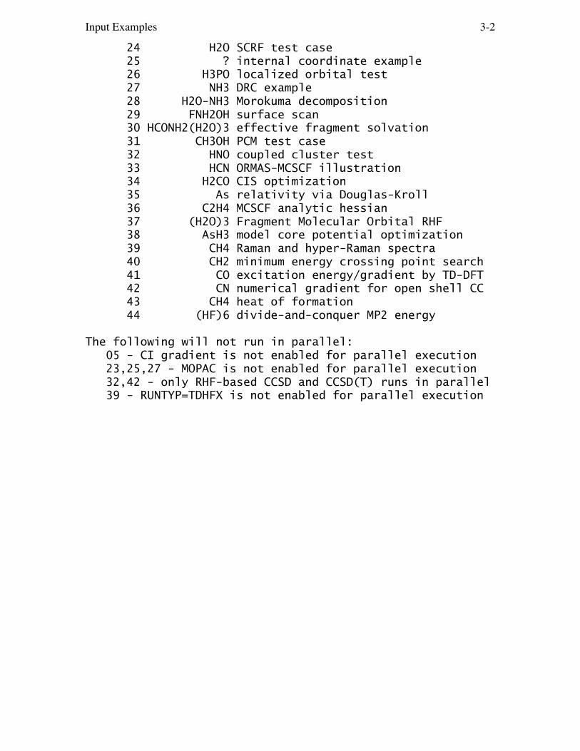
Input Examples 3-2
24 H2O SCRF test case 25 ? internal coordinate example 26 H3PO localized orbital test 27 NH3 DRC example 28 H2O-NH3 Morokuma decomposition 29 FNH2OH surface scan 30 HCONH2(H2O)3 effective fragment solvation 31 CH3OH PCM test case 32 HNO coupled cluster test 33 HCN ORMAS-MCSCF illustration 34 H2CO CIS optimization 35 As relativity via Douglas-Kroll 36 C2H4 MCSCF analytic hessian 37 (H2O)3 Fragment Molecular Orbital RHF 38 AsH3 model core potential optimization 39 CH4 Raman and hyper-Raman spectra 40 CH2 minimum energy crossing point search 41 CO excitation energy/gradient by TD-DFT 42 CN numerical gradient for open shell CC 43 CH4 heat of formation 44 (HF)6 divide-and-conquer MP2 energy
The following will not run in parallel: 05 - CI gradient is not enabled for parallel execution 23,25,27 - MOPAC is not enabled for parallel execution 32,42 - only RHF-based CCSD and CCSD(T) runs in parallel 39 - RUNTYP=TDHFX is not enabled for parallel execution

Input Examples 3-3
! EXAM01.! 1-A-1 CH2 RHF geometry optimization using GAMESS.!! Although internal coordinates are used (COORD=ZMAT),! the optimization is done in Cartesian space (NZVAR=0).! This run uses a criterion (OPTTOL) on the gradient! which is tighter than is normally used.!! This job tests the sp integral module, the RHF module,! and the geometry optimization module.!! Using the default search METHOD=STANDARD,! FINAL E= -37.2322678015, 8 iters, RMS grad= .0264308! FINAL E= -37.2308175316, 7 iters, RMS grad= .0320881! FINAL E= -37.2375723414, 7 iters, RMS grad= .0056557! FINAL E= -37.2379944431, 6 iters, RMS grad= .0017901! FINAL E= -37.2380387832, 8 iters, RMS grad= .0003391! FINAL E= -37.2380397692, 6 iters, RMS grad= .0000030! $CONTRL SCFTYP=RHF RUNTYP=OPTIMIZE COORD=ZMT NZVAR=0 $END $SYSTEM TIMLIM=2 MEMORY=100000 $END $STATPT OPTTOL=1.0E-5 $END $BASIS GBASIS=STO NGAUSS=2 $END $GUESS GUESS=HUCKEL $END $DATAMethylene...1-A-1 state...RHF/STO-2GCnv 2
CH 1 rCHH 1 rCH 2 aHCH
rCH=1.09aHCH=110.0 $END

Input Examples 3-4
! EXAM02.! 3-B-1 CH2 UHF calculation on methylene groundstate.!! This test uses the default choice, COORD=UNIQUE, to! enter the molecule. Only the symmetry unique atoms! are given, and they must be given in the orientation! which GAMESS expects.!! This job tests the UHF energy and the UHF gradient.! In addition, the orbitals are localized.!! The initial energy is -37.228465066.! The FINAL energy is -37.2810867258 after 11iterations.! The unrestricted wavefunction has <S**2> = 2.013.! Mulliken, Lowdin charges on C are -0.020584, 0.018720.! The spin density at Hydrogen is -0.0167104.! The dipole moment is 0.016188.! The RMS gradient is 0.027589766.! FINAL localization sums are 30.57 and 25.14 Debye**2.! $CONTRL SCFTYP=UHF MULT=3 RUNTYP=GRADIENT LOCAL=BOYS $END $SYSTEM TIMLIM=1 MEMORY=100000 $END $BASIS GBASIS=STO NGAUSS=2 $END $GUESS GUESS=HUCKEL $END $DATAMethylene...3-B-1 state...UHF/STO-2GCnv 2
Carbon 6.0Hydrogen 1.0 0.0 0.82884 0.7079 $END

Input Examples 3-5
! EXAM03.! 3-B-1 CH2 ROHF calculation on methylene ground state.! The wavefunction is a pure triplet state (<S**2> = 2),! and so has a higher energy than the second example.!! For COORD=CART, all atoms must be given, and as in the! present case, these may be in an unoriented geometry.! GAMESS deduces which atoms are unique, and orients! the molecule appropriately. The geometry here is thus! identical to the second example.!! This job tests the ROHF wavefunction and gradientcode.! It also tests the direct SCF procedure.!! The initial energy is -37.228465066.! The FINAL energy is -37.2778767089 after 7 iterations.! Mulliken, Lowdin charges on C are -0.020346, 0.019470.! The Hydrogen atom spin density is 0.0129735.! The dipole moment is 0.025099 Debye.! The RMS gradient is 0.027505548! $CONTRL SCFTYP=ROHF MULT=3 RUNTYP=GRADIENT COORD=CART $END $SYSTEM TIMLIM=1 MEMORY=100000 $END $SCF DIRSCF=.TRUE. $END $BASIS GBASIS=STO NGAUSS=2 $END $GUESS GUESS=HUCKEL $END $DATAMethylene...3-B-1 state...ROHF/STO-2GCnv 2
Hydrogen 1.0 0.82884 0.7079 0.0Carbon 6.0Hydrogen 1.0 -0.82884 0.7079 0.0 $END
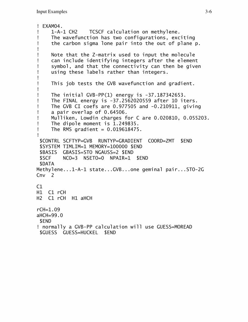
Input Examples 3-6
! EXAM04.! 1-A-1 CH2 TCSCF calculation on methylene.! The wavefunction has two configurations, exciting! the carbon sigma lone pair into the out of plane p.!! Note that the Z-matrix used to input the molecule! can include identifying integers after the element! symbol, and that the connectivity can then be given! using these labels rather than integers.!! This job tests the GVB wavefunction and gradient.!! The initial GVB-PP(1) energy is -37.187342653.! The FINAL energy is -37.2562020559 after 10 iters.! The GVB CI coefs are 0.977505 and -0.210911, giving! a pair overlap of 0.64506.! Mulliken, Lowdin charges for C are 0.020810, 0.055203.! The dipole moment is 1.249835.! The RMS gradient = 0.019618475.! $CONTRL SCFTYP=GVB RUNTYP=GRADIENT COORD=ZMT $END $SYSTEM TIMLIM=1 MEMORY=100000 $END $BASIS GBASIS=STO NGAUSS=2 $END $SCF NCO=3 NSETO=0 NPAIR=1 $END $DATAMethylene...1-A-1 state...GVB...one geminal pair...STO-2GCnv 2
C1H1 C1 rCHH2 C1 rCH H1 aHCH
rCH=1.09aHCH=99.0 $END! normally a GVB-PP calculation will use GUESS=MOREAD $GUESS GUESS=HUCKEL $END

Input Examples 3-7
! EXAM05! CH2 CI calculation.! The wavefunction is RHF + CI-SD, within the minimal! basis, containing 55 configurations. Two CI roots! are found, and the gradient of the higher state is! then computed.!! Note that CI gradients have several restrictions,! which are further described in the $LAGRAN group.!! FINAL energy of RHF = -38.3704885128 after 10 iters.! State 1 EIGENvalue = -38.4270674136, c(1) = 0.970224! State 2 EIGENvalue = -38.3130036824, c(29) = 0.990865! The upper state dipole moment is 0.708275 Debye.! The upper state has RMS gradient 0.032264079! $CONTRL SCFTYP=RHF CITYP=GUGA RUNTYP=GRADIENT $END $SYSTEM TIMLIM=3 MEMORY=300000 $END $BASIS GBASIS=STO NGAUSS=3 $END $GUESS GUESS=HUCKEL $END! look at all state symmetries, by using C1 symmetry $CIDRT GROUP=C1 IEXCIT=2 NFZC=1 NDOC=3 NVAL=3 $END! ground state is 1-A-1, 1st excited state is 1-B-1 $GUGDIA NSTATE=2 $END! compute properties of the 1-B-1 state $GUGDM NFLGDM(1)=1,1 IROOT=2 $END! compute gradient of the 1-B-1 state $GUGDM2 WSTATE(1)=0.0,1.0 $END $DATAMethylene...CI...STO-3G basisCnv 2
Carbon 6.0Hydrogen 1.0 0.0 0.82884 0.7079 $END

Input Examples 3-8
! EXAM06.! 1-A-1 CH2 MCSCF methylene geometry optimization.! The two configuration ansatz is the same as used in! the fourth example.!! The optimization is done in internal coordinates,! as NZVAR is non-zero. Since a explicit $ZMAT is! given, these are used for the internal coordinates,! rather than those used to enter the molecule in! the $DATA. (Careful examination of this trivial! triatomic's input shows that $ZMAT is equivalent! to $DATA in this case. You would normally give! $ZMAT only if it is somehow different.)! This job tests the MCSCF wavefunction and gradient.! At the initial geometry:! The initial energy is -37.187342653,! the FINAL E= -37.2562020559 after 14 iterations,! the RMS gradient is 0.0256396.! After 4 steps,! FINAL E= -37.2581791686, RMS gradient=0.0000013,! r(CH)=1.1243359, ang(HCH)=98.8171674$CONTRL SCFTYP=MCSCF RUNTYP=OPTIMIZE NZVAR=3 COORD=ZMT $END $SYSTEM TIMLIM=5 MEMORY=300000 $END $BASIS GBASIS=STO NGAUSS=2 $END $DATAMethylene...1-A-1 state...MCSCF/STO-2GCnv 2
CH 1 rCHH 1 rCH 2 aHOH
rCH=1.09aHOH=99.0 $END $ZMAT IZMAT(1)=1,1,2, 1,1,3, 2,2,1,3 $END! Normally one starts a MCSCF run with converged SCF! orbitals, as Huckel orbitals normally do not converge.! Even if they do converge, the extra iterations are! very expensive, so use MOREAD for your runs!! $GUESS GUESS=HUCKEL $END!! two active electrons in two active orbitals! The ground 3-B-1 state is of different symmetry so we! need only solve for the lowest A-1 symmetry root.! $DET STSYM=A1 NCORE=3 NACT=2 NELS=2 NSTATE=1 $END

Input Examples 3-9

Input Examples 3-10
! EXAM07.! 1-A' HPO RHF calculation using GAMESS.! This job tests the HONDO integral & gradient packages,! due to the d function on phosphorus. The input also! illustrates the use of a more flexible basis set than! the methylene examples.! Although HUCKEL would be better, HCORE is tested.!! The initial energy is -397.591192627,! the FINAL E= -414.0945320854 after 18 iterations,! The dipole moment is 2.535169.! The RMS gradient is 0.023723942.! $CONTRL SCFTYP=RHF RUNTYP=GRADIENT $END $SYSTEM TIMLIM=20 MEMORY=300000 $END $GUESS GUESS=HCORE $END $DATAHP=O ... 3-21G+* RHF calculation at STO-2G* geometryCs
Phosphorus 15.0 N21 3 L 1 1 0.039 1.0 1.0 D 1 1 0.55 1.0
Oxygen 8.0 1.439 N21 3
Hydrogen 1.0 -0.3527854 1.36412 N21 3
$END
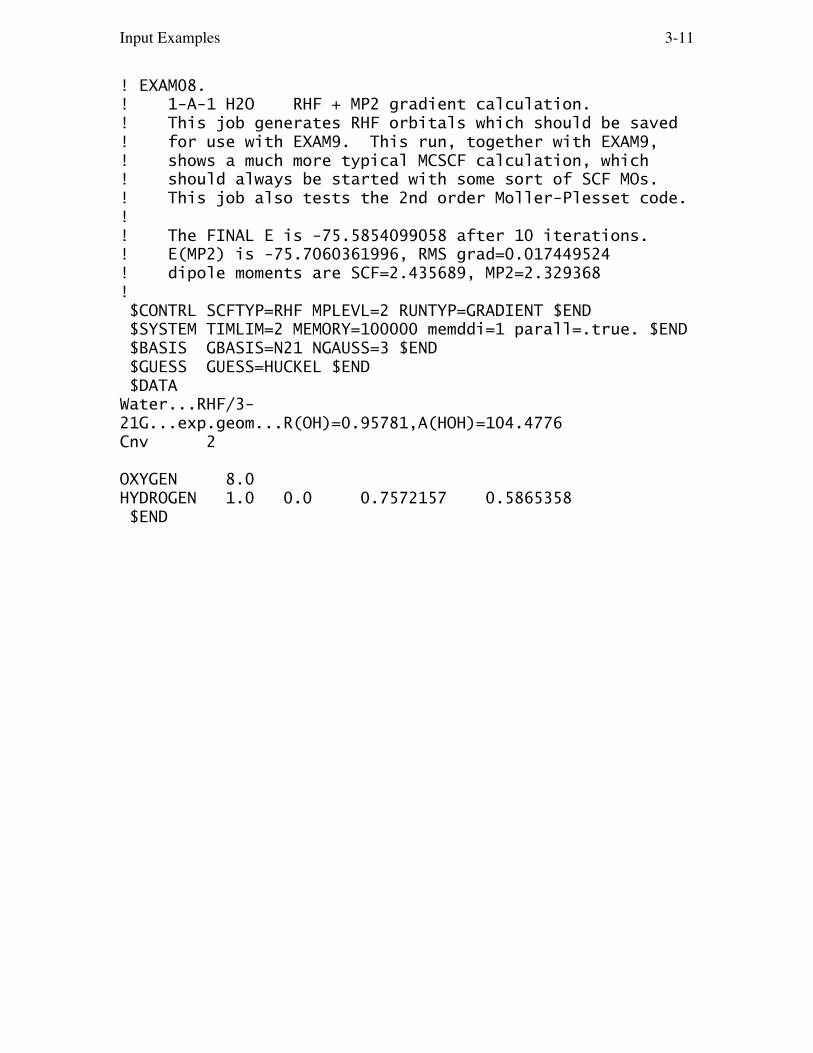
Input Examples 3-11
! EXAM08.! 1-A-1 H2O RHF + MP2 gradient calculation.! This job generates RHF orbitals which should be saved! for use with EXAM9. This run, together with EXAM9,! shows a much more typical MCSCF calculation, which! should always be started with some sort of SCF MOs.! This job also tests the 2nd order Moller-Plesset code.!! The FINAL E is -75.5854099058 after 10 iterations.! E(MP2) is -75.7060361996, RMS grad=0.017449524! dipole moments are SCF=2.435689, MP2=2.329368! $CONTRL SCFTYP=RHF MPLEVL=2 RUNTYP=GRADIENT $END $SYSTEM TIMLIM=2 MEMORY=100000 memddi=1 parall=.true. $END $BASIS GBASIS=N21 NGAUSS=3 $END $GUESS GUESS=HUCKEL $END $DATAWater...RHF/3-21G...exp.geom...R(OH)=0.95781,A(HOH)=104.4776Cnv 2
OXYGEN 8.0HYDROGEN 1.0 0.0 0.7572157 0.5865358 $END

Input Examples 3-12
! EXAM09.! 1-A-1 H2O 2nd order MC-QDPT calculation! This job finds the Full Optimized Reaction Space! MCSCF (or CAS-SCF) wavefunction for water. Its! initial RHF orbitals are taken from EXAM08.! The MCSCF wavefunction contains 65 determinants,! not all of which are singlets, of course.! The second order perturbation theory correction! to the MCSCF energy is then obtained, using a! determinant code as well.!! MCSCF:! On the 1st iteration, the energy is -75.601726236.! The FINAL MCSCF E= -75.6386218843 after 14 iters,! with c(1) = 0.9884456 and dipole moment = 2.301620! MRMP (single state MCQDPT) E(MP2) = -75.7109705643! $CONTRL SCFTYP=MCSCF MPLEVL=2 $END $SYSTEM TIMLIM=1 $END $BASIS GBASIS=N21 NGAUSS=3 $END---- EXPERIMENTAL GEOM, R(OH)=0.95781A, HOH=104.4776 DEG. $DATAWATER...3-21G BASIS...FORS-MCSCF...EXPERIMENTAL GEOMETRYCnv 2
Oxygen 8.0Hydrogen 1.0 0.0 0.7572157 0.5865358 $END $GUESS GUESS=MOREAD NORB=13 $END $DET NCORE=1 NACT=6 NELS=8 $END
---- CONVERGED 3-21G WATER VECTORS, E=-75.585409913 - - - $VEC 1 1 0.98323195E+00 0.95883436E-01 0.00000000E+00 ... ... vectors deleted to save paper ...13 3 0.35961579E+00 0.28728587E+00 0.35961579E+00 $END

Input Examples 3-13
! EXAM 10.! This run duplicates the first column of table 6 in! Y.Yamaguchi, M.Frisch, J.Gaw, H.F.Schaefer, and! J.S.Binkley J.Chem. Phys. 1986, 84, 2262-2278.!! FINAL energy at the VIB 0 geometry is -74.9659012159.!! If run with METHOD=ANALYTIC,! the FREQuencies are 2170.05, 4140.00, and 4391.07! the INTENSities are 0.17129, 1.04807, and 0.70930! the mean POLARIZABILITY is 0.40079!! If run with METHOD=NUMERIC, NVIB=2,! the FREQuencies are 2170.14, 4140.18, and 4391.12! the INTENSities are 0.17169, 1.04703, and 0.70909! $CONTRL SCFTYP=RHF RUNTYP=HESSIAN UNITS=BOHR NZVAR=3 $END $SYSTEM TIMLIM=4 MEMORY=100000 $END $FORCE METHOD=ANALYTIC $END $CPHF POLAR=.TRUE. $END $BASIS GBASIS=STO NGAUSS=3 $END $DATAWater at the RHF/STO-3G equilibrium geometryCNV 2
OXYGEN 8. 0.0 0.0 0.0702816679HYDROGEN 1. 0.0 1.4325665478 -1.1312080153 $END $ZMAT IZMAT(1)=1,1,2, 1,1,3, 2,2,1,3 $END $GUESS GUESS=HUCKEL $END

Input Examples 3-14
! EXAM 11.! 1A' HCN RHF Intrinsic Reaction Coordinate! This job tests the reaction path finder. The reaction! is followed back to the HNC isomer. Four points on the! IRC (counting the saddle point) are found,! Pt. R(N-C) R(N-H) A(HNC) Energy distance! T.S. 1.22136 1.43764 52.993 -91.5648510 0.0! 1 1.22533 1.33296 58.476 -91.5673097 0.29994! 2 1.22802 1.23827 64.747 -91.5735346 0.59986! 3 1.22974 1.16350 72.039 -91.5814775 0.89968! $CONTRL SCFTYP=RHF RUNTYP=IRC NZVAR=3 $END $SYSTEM TIMLIM=5 MEMORY=400000 $END $IRC PACE=GS2 SADDLE=.TRUE. TSENGY=.TRUE. FORWRD=.FALSE. NPOINT=3 $END $GUESS GUESS=HUCKEL $END $ZMAT IZMAT(1)=1,1,2 1,1,3 2,2,1,3 $END $BASIS GBASIS=STO NGAUSS=3 $END $DATAHYDROGEN CYANIDE...STO-3G...INTRINSIC REACTION COORDINATECS
NITROGEN 7.0 -.0004620071 .0002821165.0000000000CARBON 6.0 1.2208931990 -.0003427488.0000000000HYDROGEN 1.0 .8654562191 1.1478852258.0000000000 $END $HESSENERGY IS -91.5648510307 E(NUC) IS 23.4154954113 1 1 1.10665682E+00 1.58946320E-02 0.00000000E+00...... 2nd derivatives deleted to save paper ... 9 2-8.04548379E-09 0.00000000E+00 0.00000000E+00-1.42096449E-08 $END

Input Examples 3-15
! EXAM 12.! This job illustrates linear bends, for acetylene, and! tests the closed shell LDA density functional program.!! At the input geometry,! the FINAL E= -765352334525 after 12 iterations,! and the RMS gradient is 0.0944557.!! At the final geometry, 5 steps later,! the FINAL E= -76.5841347569, RMS gradient=0.0000007,! R(CC)=1.21193 and R(CH)=1.07797.! $CONTRL SCFTYP=RHF RUNTYP=OPTIMIZE NZVAR=5 $END $SYSTEM TIMLIM=2 $END $DFT DFTTYP=SVWN $END $BASIS GBASIS=N31 NGAUSS=6 NDFUNC=1 $END $GUESS GUESS=HUCKEL $END! Note, this OPTTOL is smaller than the accuracy of the! integration grid actually supports (see REFS.DOC) $STATPT OPTTOL=0.00001 $END $DATAAcetylene geometry optimization in internal coordinatesDnh 4
CARBON 6.0 0.0 0.0 0.70HYDROGEN 1.0 0.0 0.0 1.78 $END $ZMAT IZMAT(1)=1,1,2, 1,1,3, 1,2,4, 5,1,2,4, 5,2,1,3 $END------- XZ is 1st plane for both bends ------- $LIBE APTS(1)=1.0,0.0,0.0,1.0,0.0,0.0 $END
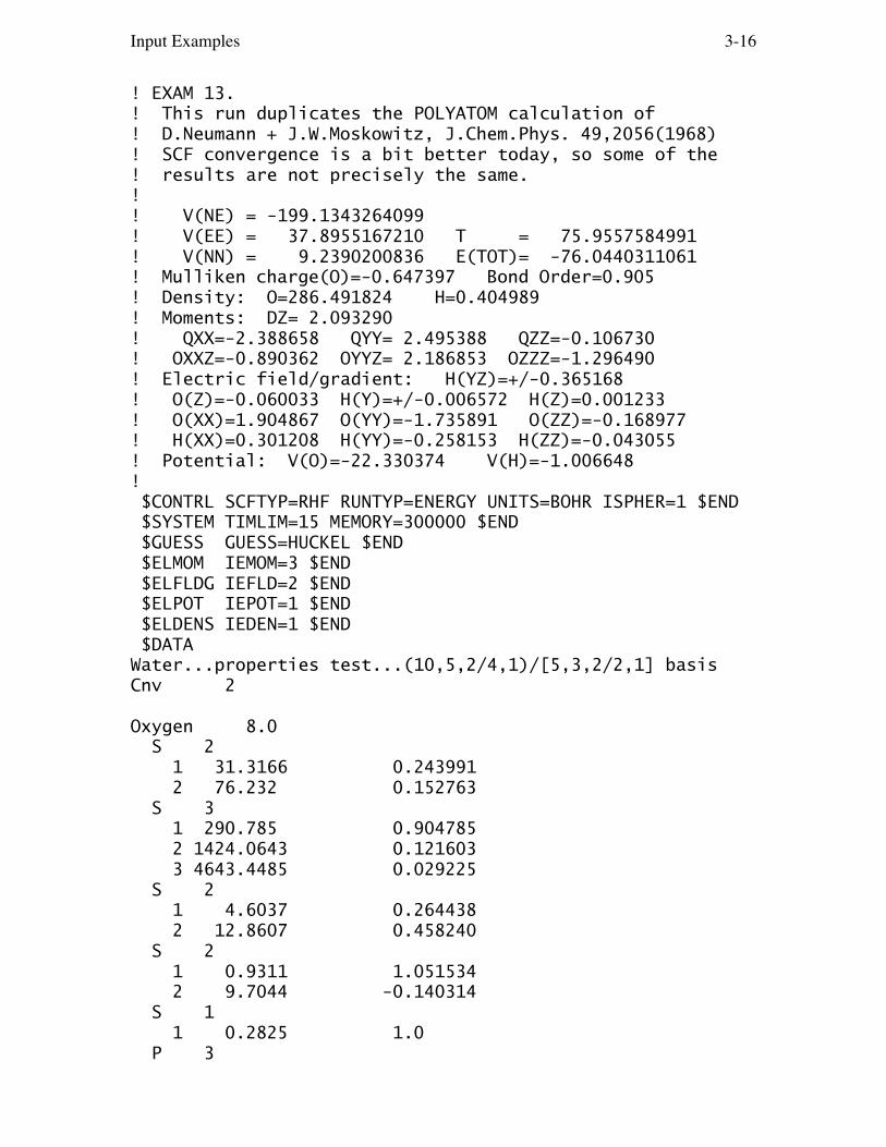
Input Examples 3-16
! EXAM 13.! This run duplicates the POLYATOM calculation of! D.Neumann + J.W.Moskowitz, J.Chem.Phys. 49,2056(1968)! SCF convergence is a bit better today, so some of the! results are not precisely the same.!! V(NE) = -199.1343264099! V(EE) = 37.8955167210 T = 75.9557584991! V(NN) = 9.2390200836 E(TOT)= -76.0440311061! Mulliken charge(O)=-0.647397 Bond Order=0.905! Density: O=286.491824 H=0.404989! Moments: DZ= 2.093290! QXX=-2.388658 QYY= 2.495388 QZZ=-0.106730! OXXZ=-0.890362 OYYZ= 2.186853 OZZZ=-1.296490! Electric field/gradient: H(YZ)=+/-0.365168! O(Z)=-0.060033 H(Y)=+/-0.006572 H(Z)=0.001233! O(XX)=1.904867 O(YY)=-1.735891 O(ZZ)=-0.168977! H(XX)=0.301208 H(YY)=-0.258153 H(ZZ)=-0.043055! Potential: V(O)=-22.330374 V(H)=-1.006648! $CONTRL SCFTYP=RHF RUNTYP=ENERGY UNITS=BOHR ISPHER=1 $END $SYSTEM TIMLIM=15 MEMORY=300000 $END $GUESS GUESS=HUCKEL $END $ELMOM IEMOM=3 $END $ELFLDG IEFLD=2 $END $ELPOT IEPOT=1 $END $ELDENS IEDEN=1 $END $DATAWater...properties test...(10,5,2/4,1)/[5,3,2/2,1] basisCnv 2
Oxygen 8.0 S 2 1 31.3166 0.243991 2 76.232 0.152763 S 3 1 290.785 0.904785 2 1424.0643 0.121603 3 4643.4485 0.029225 S 2 1 4.6037 0.264438 2 12.8607 0.458240 S 2 1 0.9311 1.051534 2 9.7044 -0.140314 S 1 1 0.2825 1.0 P 3
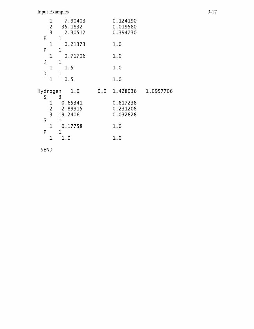
Input Examples 3-17
1 7.90403 0.124190 2 35.1832 0.019580 3 2.30512 0.394730 P 1 1 0.21373 1.0 P 1 1 0.71706 1.0 D 1 1 1.5 1.0 D 1 1 0.5 1.0
Hydrogen 1.0 0.0 1.428036 1.0957706 S 3 1 0.65341 0.817238 2 2.89915 0.231208 3 19.2406 0.032828 S 1 1 0.17758 1.0 P 1 1 1.0 1.0
$END

Input Examples 3-18
! EXAM 14.! CI transition moments. Water, using RHF/STO-3G MOs.! All orbitals are occupied, transition is 1-1A1 to 2-1A1.!! E(STATE 1)= -75.0101113548, E(STATE 2)= -74.3945819375! Dipole LENGTH is <Q>=0.392614! Dipole VELOCITY is <d/dQ>=0.368205! $CONTRL SCFTYP=NONE CITYP=GUGA RUNTYP=TRANSITN UNITS=BOHR$END $SYSTEM TIMLIM=1 MEMORY=100000 $END $BASIS GBASIS=STO NGAUSS=3 $END! standard SD-CI calculation $DRT1 GROUP=C2V IEXCIT=2 NFZC=1 NDOC=4 NVAL=2 $END $TRANST NFZC=1 IROOTS(1)=2 $END $DATAWATER MOLECULE...STO-3G...TRANSITION MOMENTCNV 2
OXYGEN 8.0 0.0 0.0 0.0HYDROGEN 1.0 0.0 1.428 -1.096 $END
--- RHF ORBITALS --- GENERATED AT 09:24:04 18-FEB-88WATER MOLECULE...STO-3G...TRANSITION MOMENTE(RHF)= -74.9620539825, E(NUC)= 9.2384802989, 8ITERS $VEC1 1 1 9.94117078E-01 2.66680164E-02 0.00000000E+00 ...... vectors deleted to save paper ... 7 2-8.42653177E-01 8.42653177E-01 $END

Input Examples 3-19
! EXAM 15.! C2- diatom, in the electronic state doublet-pi-u.! This illustrates a open shell SCF calculation, using! fed in coupling coefficients, and the GVB/ROHF code.!! The FINAL energy is -75.5579181071 after 8 iterations.! $CONTRL SCFTYP=GVB MULT=2 ICHARG=-1 UNITS=BOHR $END $SYSTEM TIMLIM=15 MEMORY=300000 $END $BASIS GBASIS=DH NDFUNC=1 POLAR=DUNNING $END $DATAC2-...DOUBLET-PI-UNGERADE...OPEN SHELL SCFDNH 4
CARBON 6.0 0.0 0.0 -1.233 $END $GUESS GUESS=MOREAD NORB=30 NORDER=1 IORDER(5)=7,5,6 $END $SCF NCO=5 NSETO=1 NO=2 COUPLE=.TRUE. F(1)=1.0, 0.75 ALPHA(1)=2.0, 1.5, 1.00 BETA(1)=-1., -.75, -0.5 $END
--- RHF ORBITALS --- GENERATED AT 14:05:16THU MAR 24/88 CC R(C-C) = 2 * 1.233 BOHR BAS=831+1DE(RHF)= -75.3856001855, E(NUC)= 14.5985401460, 18ITERS $VEC 1 1-7.06500288E-01-1.39103044E-03-3.57452331E-04 ...... vectors deleted to save paper ... $END

Input Examples 3-20
! EXAM 16.! ROHF/GVB on Si 3-P state, using Gordon's 6-31G basis.!! The purpose of this example is two-fold, namely to! show off the open shell capabilities of the GVB code,! and to emphasize that the 6-31G basis for Si in GAMESS! is Mark Gordon's version. The basis stored in GAMESS is! completely optimized, whereas Pople's uses the core from! from a 6-21G set, reoptimizing only the -31G part.! The energy from Pople's basis would be only -288.828405.!! Jacobi diagonalization is intrinsically slow, but! results in pure subspecies in degenerate p irreps.! In fact, these may be labeled in the highest Abelian! subgroup of the atomic point group Kh.!! The FINAL energy is -288.8285729745 after 7 iterations.! $CONTRL SCFTYP=GVB MULT=3 $END $SYSTEM TIMLIM=2 MEMORY=100000 KDIAG=3 $END $BASIS GBASIS=N31 NGAUSS=6 $END $DATASi...3-P term...ROHF in full Kh symmetryDnh 2
Silicon 14. $END $GUESS GUESS=HUCKEL $END $SCF NCO=6 NSETO=1 NO=3 COUPLE=.TRUE. F(1)=1.0, 0.333333333333333 ALPHA(1)=2.0, 0.66666666666667, 0.16666666666667 BETA(1)=-1.0, -0.33333333333333, -0.16666666666667 $END

Input Examples 3-21
! EXAM 17.! Analytic hessian for an open shell SCF function.! Methylene's 1-B-1 excited state.! FINAL energy= -38.3334724780 after 8 iterations.! The FREQuencies are 1224.19, 3563.44, 3896.23! The INTENSities are 0.13317, 0.21652, 0.14589! The mean POLARIZABILITY is 0.53018! $CONTRL SCFTYP=GVB MULT=1 RUNTYP=HESSIAN UNITS=BOHR$END $SYSTEM TIMLIM=4 MEMORY=100000 $END $CPHF POLAR=.TRUE. $END $BASIS GBASIS=STO NGAUSS=3 $END $SCF NCO=3 NSETO=2 NO(1)=1,1 NPAIR=0 $END $ZMAT IZMAT(1)=1,1,2, 1,1,3, 2,2,1,3 $END $GUESS GUESS=HUCKEL $END $DATAMETHYLENE...1-B-1 STATE...ROHF...STO-3G BASISCNV 2
CARBON 6.0 0.0 0.0 0.0041647278HYDROGEN 1.0 0.0 1.8913952563 0.7563907037 $END

Input Examples 3-22
! EXAM 18.! effective core potential...diatomic P2...RHF/CEP-31G*! See Stevens,Basch,Krauss, J.Chem.Phys. 81,6026-33(1984).! GAMESS FINAL E= -12.6956518702, FREQ=913.17! A separate run gives E(P)= -6.32635 so De=26.95 kcal/mol! $CONTRL SCFTYP=RHF RUNTYP=HESSIAN ECP=SBKJC NZVAR=1 $END $SYSTEM TIMLIM=15 MEMORY=900000 $END $GUESS GUESS=HUCKEL $END $ZMAT IZMAT(1)=1,1,2 $END $DATAdiatomic phosphorousDnh 4
PHOSPHORUS 15.0 0.0000000000 0.00000000000.9393077548 SBKJC D 1 1 0.45 1.0
$END
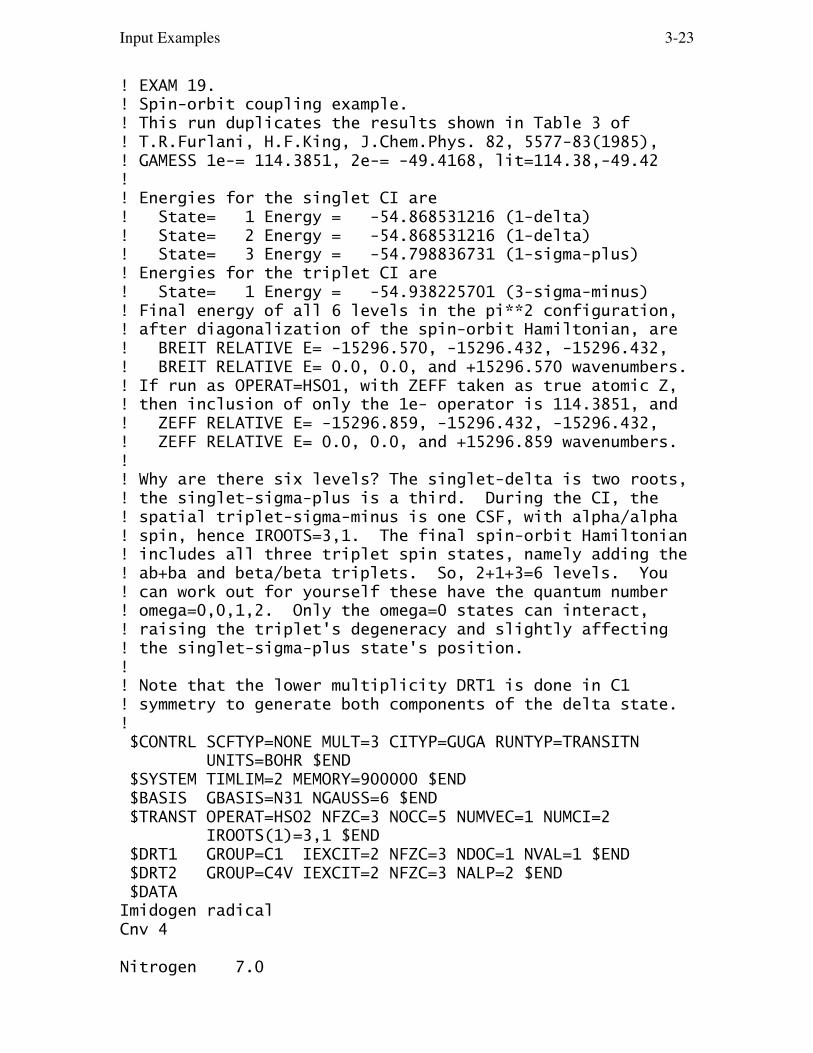
Input Examples 3-23
! EXAM 19.! Spin-orbit coupling example.! This run duplicates the results shown in Table 3 of! T.R.Furlani, H.F.King, J.Chem.Phys. 82, 5577-83(1985),! GAMESS 1e-= 114.3851, 2e-= -49.4168, lit=114.38,-49.42!! Energies for the singlet CI are! State= 1 Energy = -54.868531216 (1-delta)! State= 2 Energy = -54.868531216 (1-delta)! State= 3 Energy = -54.798836731 (1-sigma-plus)! Energies for the triplet CI are! State= 1 Energy = -54.938225701 (3-sigma-minus)! Final energy of all 6 levels in the pi**2 configuration,! after diagonalization of the spin-orbit Hamiltonian, are! BREIT RELATIVE E= -15296.570, -15296.432, -15296.432,! BREIT RELATIVE E= 0.0, 0.0, and +15296.570 wavenumbers.! If run as OPERAT=HSO1, with ZEFF taken as true atomic Z,! then inclusion of only the 1e- operator is 114.3851, and! ZEFF RELATIVE E= -15296.859, -15296.432, -15296.432,! ZEFF RELATIVE E= 0.0, 0.0, and +15296.859 wavenumbers.!! Why are there six levels? The singlet-delta is two roots,! the singlet-sigma-plus is a third. During the CI, the! spatial triplet-sigma-minus is one CSF, with alpha/alpha! spin, hence IROOTS=3,1. The final spin-orbit Hamiltonian! includes all three triplet spin states, namely adding the! ab+ba and beta/beta triplets. So, 2+1+3=6 levels. You! can work out for yourself these have the quantum number! omega=0,0,1,2. Only the omega=0 states can interact,! raising the triplet's degeneracy and slightly affecting! the singlet-sigma-plus state's position.!! Note that the lower multiplicity DRT1 is done in C1! symmetry to generate both components of the delta state.! $CONTRL SCFTYP=NONE MULT=3 CITYP=GUGA RUNTYP=TRANSITN UNITS=BOHR $END $SYSTEM TIMLIM=2 MEMORY=900000 $END $BASIS GBASIS=N31 NGAUSS=6 $END $TRANST OPERAT=HSO2 NFZC=3 NOCC=5 NUMVEC=1 NUMCI=2 IROOTS(1)=3,1 $END $DRT1 GROUP=C1 IEXCIT=2 NFZC=3 NDOC=1 NVAL=1 $END $DRT2 GROUP=C4V IEXCIT=2 NFZC=3 NALP=2 $END $DATAImidogen radicalCnv 4
Nitrogen 7.0
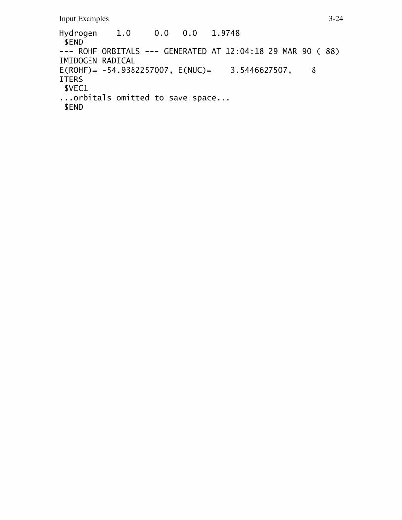
Input Examples 3-24
Hydrogen 1.0 0.0 0.0 1.9748 $END--- ROHF ORBITALS --- GENERATED AT 12:04:18 29 MAR 90 ( 88)IMIDOGEN RADICALE(ROHF)= -54.9382257007, E(NUC)= 3.5446627507, 8ITERS $VEC1...orbitals omitted to save space... $END
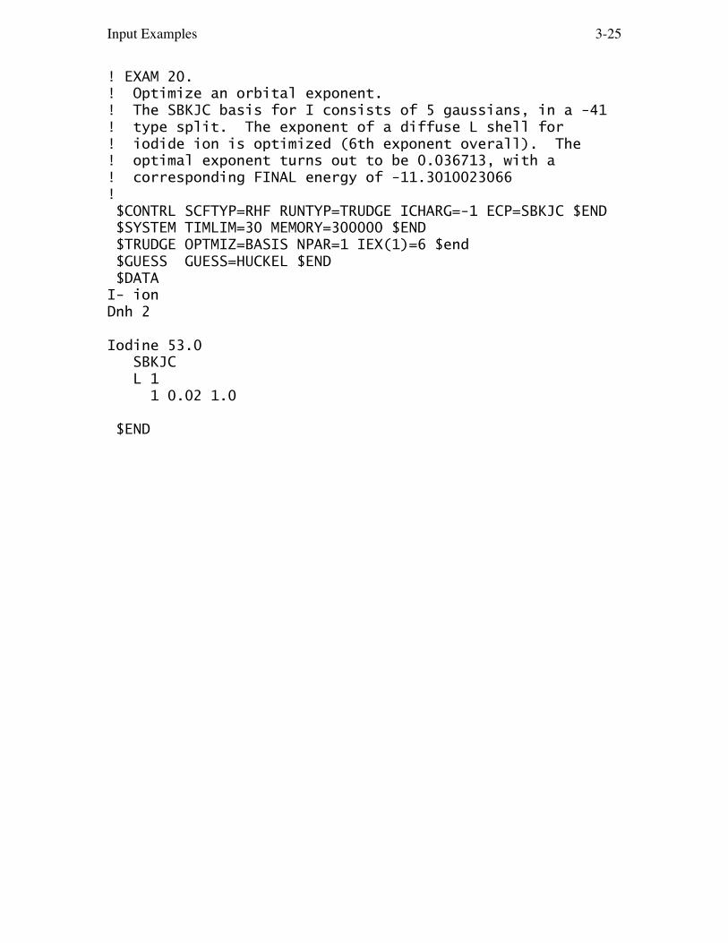
Input Examples 3-25
! EXAM 20.! Optimize an orbital exponent.! The SBKJC basis for I consists of 5 gaussians, in a -41! type split. The exponent of a diffuse L shell for! iodide ion is optimized (6th exponent overall). The! optimal exponent turns out to be 0.036713, with a! corresponding FINAL energy of -11.3010023066! $CONTRL SCFTYP=RHF RUNTYP=TRUDGE ICHARG=-1 ECP=SBKJC $END $SYSTEM TIMLIM=30 MEMORY=300000 $END $TRUDGE OPTMIZ=BASIS NPAR=1 IEX(1)=6 $end $GUESS GUESS=HUCKEL $END $DATAI- ionDnh 2
Iodine 53.0 SBKJC L 1 1 0.02 1.0
$END
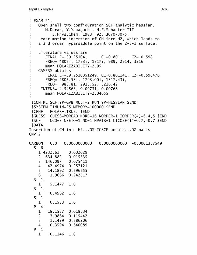
Input Examples 3-26
! EXAM 21.! Open shell two configuration SCF analytic hessian.! M.Duran, Y.Yamaguchi, H.F.Schaefer III! J.Phys.Chem. 1988, 92, 3070-3075.! Least motion insertion of CH into H2, which leads to! a 3rd order hypersaddle point on the 2-B-1 surface.!! Literature values are! FINAL E=-39.25104, C1=0.801, C2=-0.598! FREQ= 4805i, 1793i, 1317i, 989, 2914, 3216! mean POLARIZABILITY=2.05! GAMESS obtains! FINAL E=-39.2510351249, C1=0.801141, C2=-0.598476! FREQ= 4805.53i, 1793.00i, 1317.43i,! FREQ= 988.81, 2913.52, 3216.42! INTENS= 4.54563, 0.09731, 0.00768! mean POLARIZABILITY=2.04655! $CONTRL SCFTYP=GVB MULT=2 RUNTYP=HESSIAN $END $SYSTEM TIMLIM=25 MEMORY=100000 $END $CPHF POLAR=.TRUE. $END $GUESS GUESS=MOREAD NORB=16 NORDER=1 IORDER(4)=6,4,5 $END $SCF NCO=3 NSETO=1 NO=1 NPAIR=1 CICOEF(1)=0.7,-0.7 $END $DATAInsertion of CH into H2...OS-TCSCF ansatz...DZ basisCNV 2
CARBON 6.0 0.0000000000 0.0000000000 -0.0001357549 S 6 1 4232.61 0.002029 2 634.882 0.015535 3 146.097 0.075411 4 42.4974 0.257121 5 14.1892 0.596555 6 1.9666 0.242517 S 1 1 5.1477 1.0 S 1 1 0.4962 1.0 S 1 1 0.1533 1.0 P 4 1 18.1557 0.018534 2 3.9864 0.115442 3 1.1429 0.386206 4 0.3594 0.640089 P 1 1 0.1146 1.0

Input Examples 3-27
HYDROGEN 1.0 0.0000000000 0.0000000000 1.0922959062 DH 0 1.2 1.2
HYDROGEN 1.0 0.0000000000 0.4152229538 -1.4824967459 DH 0 1.2 1.2
$END--- these are 2-A1 ROHF vectors ------ ROHF ORBITALS --- GENERATED AT 08:23:42 27 JUN 90 (178)INSERTION OF CH INTO H2...OS-TCSCF ANSATZ...DZ BASISE(ROHF)= -39.2316245004, E(NUC)= 8.0760320442, 12 ITERS $VEC 1 1 6.01223299E-01 4.37813104E-01 ...... vectors deleted to save paper ...16 4-2.12429766E-02 $END

Input Examples 3-28
! EXAM22.!! 3-A-2 H3CN UMP2/6-31G*//UHF/6-31G*!! The FINAL UHF energy= -94.0039683697 after 14 iters.! E(MP2)= -94.2315757668, with RMS grad=0.003359454! Dipoles for HF and MP2 are 2.049391 and 2.098487 D.! $CONTRL SCFTYP=UHF MULT=3 RUNTYP=GRADIENT MPLEVL=2 COORD=ZMT $END $SYSTEM TIMLIM=5 MWORDS=1 MEMDDI=1 PARALL=.TRUE. $END $BASIS GBASIS=N31 NGAUSS=6 NDFUNC=1 NPFUNC=0 $END $GUESS GUESS=HUCKEL $END $DATAMethylnitrene...UHF/6-31G* structureCnv 3
NC 1 rCNH 2 rCH 1 aHCNH 2 rCH 1 aHCN 3 120.0H 2 rCH 1 aHCN 3 -120.0
rCN=1.4329216rCH=1.0876477aHCN=110.21928 $END
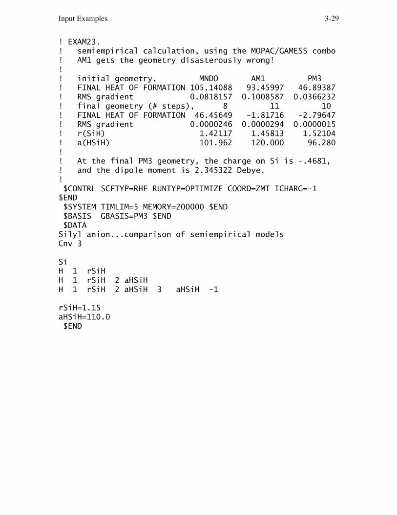
Input Examples 3-29
! EXAM23.! semiempirical calculation, using the MOPAC/GAMESS combo! AM1 gets the geometry disasterously wrong!!! initial geometry, MNDO AM1 PM3! FINAL HEAT OF FORMATION 105.14088 93.45997 46.89387! RMS gradient 0.0818157 0.1008587 0.0366232! final geometry (# steps), 8 11 10! FINAL HEAT OF FORMATION 46.45649 -1.81716 -2.79647! RMS gradient 0.0000246 0.0000294 0.0000015! r(SiH) 1.42117 1.45813 1.52104! a(HSiH) 101.962 120.000 96.280!! At the final PM3 geometry, the charge on Si is -.4681,! and the dipole moment is 2.345322 Debye.! $CONTRL SCFTYP=RHF RUNTYP=OPTIMIZE COORD=ZMT ICHARG=-1$END $SYSTEM TIMLIM=5 MEMORY=200000 $END $BASIS GBASIS=PM3 $END $DATASilyl anion...comparison of semiempirical modelsCnv 3
SiH 1 rSiHH 1 rSiH 2 aHSiHH 1 rSiH 2 aHSiH 3 aHSiH -1
rSiH=1.15aHSiH=110.0 $END

Input Examples 3-30
! EXAM24.! Self-consistent reaction field test, of water in water.! Cavity radius is calculated from the 1.00 g/cm**3density.! FINAL energy is -74.9666740755 after 12 iterations! Induced dipole= -0.03663, RMS gradient= 0.033467686! $contrl scftyp=rhf runtyp=gradient coord=zmt $end $system memory=300000 $end $basis gbasis=sto ngauss=3 $end $guess guess=huckel $end $scrf radius=1.93 dielec=80.0 $end $datawater in water, arbitrary geometryCnv 2
OH 1 rOHH 1 rOH 2 aHOH
rOH = 0.95aHOH = 104.5 $end

Input Examples 3-31
! EXAM25.! Illustration of coordinate systems for geometrysearches.! Arbitrary molecule, chosen to illustrate ring, methylon! ring, methine H10, imino in ring, methylene in ring.!! H8 H9! \|! H7-C6 O1---O5 H13! \ / \ /! C2 C4! / \ / \! H10 N3 H12! |! H11!! The initial AM1 energy is -48.6594935! initial RMS final E final RMS#steps! Cartesians 0.0200113 -48.7022520 0.0000304 50! dangling Z-mat 0.0600637 ... OO bond crashes on 1ststep! good Z-matrix 0.0232915 -48.7022510 0.0000285 21! deloc. coords. 0.0176452 -48.7022537 0.0000267 22! nat. internals 0.0209442 -48.7022570 0.0000183 15! $contrl scftyp=rhf runtyp=optimize coord=zmt $end $system memory=300000 $end $statpt hess=guess nstep=100 nprt=-1 npun=-2 $end $basis gbasis=am1 $end $guess guess=huckel $end $dataIllustration of coordinate systemsC1OC 1 rCOaN 2 rCNa 1 aNCOC 3 rCNb 2 aCNC 1 wCNCOO 4 rCOb 3 aOCN 2 wOCNCC 2 rCC 1 aCCO 5 wCCOOH 6 rCH1 2 aHCC1 1 wHCCO1H 6 rCH2 2 aHCC2 1 wHCCO2H 6 rCH3 2 aHCC3 1 wHCCO3H 2 rCHa 1 aHCOa 5 wHCOOaH 3 rNH 2 aHNC 1 wHNCOH 4 rCHb 5 aHCOb 1 wHCOObH 4 rCHc 5 aHCOc 1 wHCOOc
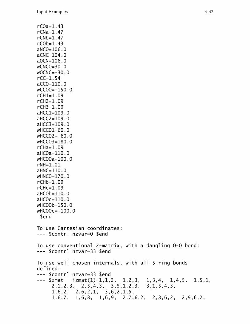
Input Examples 3-32
rCOa=1.43rCNa=1.47rCNb=1.47rCOb=1.43aNCO=106.0aCNC=104.0aOCN=106.0wCNCO=30.0wOCNC=-30.0rCC=1.54aCCO=110.0wCCOO=-150.0rCH1=1.09rCH2=1.09rCH3=1.09aHCC1=109.0aHCC2=109.0aHCC3=109.0wHCCO1=60.0wHCCO2=-60.0wHCCO3=180.0rCHa=1.09aHCOa=110.0wHCOOa=100.0rNH=1.01aHNC=110.0wHNCO=170.0rCHb=1.09rCHc=1.09aHCOb=110.0aHCOc=110.0wHCOOb=150.0wHCOOc=-100.0 $end
To use Cartesian coordinates:--- $contrl nzvar=0 $end
To use conventional Z-matrix, with a dangling O-O bond:--- $contrl nzvar=33 $end
To use well chosen internals, with all 5 ring bondsdefined:--- $contrl nzvar=33 $end--- $zmat izmat(1)=1,1,2, 1,2,3, 1,3,4, 1,4,5, 1,5,1, 2,1,2,3, 2,5,4,3, 3,5,1,2,3, 3,1,5,4,3, 1,6,2, 2,6,2,1, 3,6,2,1,5, 1,6,7, 1,6,8, 1,6,9, 2,7,6,2, 2,8,6,2, 2,9,6,2,

Input Examples 3-33
3,7,6,2,1, 3,8,6,2,1, 3,9,6,2,1, 1,10,2, 2,10,2,1, 3,10,2,1,5, 1,11,3, 2,11,3,2, 3,11,3,2,1, 1,12,4, 2,12,4,5, 3,12,4,5,1, 1,13,4, 2,13,4,5, 3,13,4,5,1 $end
To use delocalized coordinates:--- $contrl nzvar=33 $end--- $zmat dlc=.true. auto=.true. $end
To use natural internal coordinates: $contrl nzvar=44 $end $zmat izmat(1)=1,1,2, 1,2,3, 1,3,4, 1,4,5, 1,5,1, ! ring! 2,5,1,2, 2,1,2,3, 2,2,3,4, 2,3,4,5, 2,4,5,1, 3,5,1,2,3, 3,1,2,3,4, 3,2,3,4,5, 3,3,4,5,1, 3,4,5,1,2, 1,2,6, 2,6,2,1, 2,6,2,3, 4,6,2,1,3, ! methyl C! 1,6,7, 1,6,8, 1,6,9, ! methyl Hs! 2,7,6,8, 2,8,6,9, 2,9,6,7, 2,9,6,2, 2,7,6,2, 2,8,6,2, 3,7,6,2,1, 1,10,2, 2,10,2,1, 2,10,2,3, 2,10,2,6, ! methine ! 1,11,3, 2,11,3,2, 2,11,3,4, 4,11,3,2,4, ! imino ! 1,12,4, 1,13,4, ! methylene ! 2,12,4,13, 2,12,4,3, 2,13,4,3, 2,12,4,5, 2,13,4,5
ijS(1)=1,1, 2,2, 3,3, 4,4, 5,5, ! ring ! 6,6, 7,6, 8,6, 9,6,10,6, 7,7, 8,7, 9,7,10,7, 11,8,12,8,13,8,14,8,15,8, 11,9,12,9, 14,9,15,9, 16,10, 17,11,18,11, 19,12, ! methyl C! 20,13, 21,14, 22,15, ! methyl Hs! 23,16, 24,16, 25,16, 26,16, 27,16, 28,16, 23,17, 24,17, 25,17, 24,18, 25,18, 26,19, 27,19, 28,19, 27,20, 28,20, 29,21, 30,22, 31,23,32,23,33,23, 32,24,33,24, !methine ! 34,25, 35,26,36,26, 37,27, ! imino ! 38,28, 39,29, ! methylene ! 40,30, 41,30, 42,30, 43,30, 44,30, 41,31, 42,31, 43,31, 44,31, 41,32, 42,32, 43,32, 44,32,

Input Examples 3-34
41,33, 42,33, 43,33, 44,33
Sij(1)=1.0, 1.0, 1.0, 1.0, 1.0, ! ring ! 1.0, -0.8090, 0.3090, 0.3090, -0.8090, -1.1180, 1.8090, -1.8090, 1.1180, 0.3090, -0.8090, 1.0, -0.8090, 0.3090, -1.8090, 1.1180, -1.1180, 1.8090, 1.0, 1.0,-1.0, 1.0, ! methyl C ! 1.0, 1.0, 1.0, ! methyl Hs ! 1.0, 1.0, 1.0,-1.0,-1.0,-1.0, 2.0,-1.0,-1.0, 1.0,-1.0, 2.0,-1.0,-1.0, 1.0,-1.0, 1.0, 1.0, 2.0,-1.0,-1.0, 1.0,-1.0, ! methine ! 1.0, 1.0,-1.0, 1.0, ! imino ! 1.0, 1.0, ! methylene ! 4.0, 1.0, 1.0, 1.0, 1.0, 1.0,-1.0, 1.0,-1.0, 1.0, 1.0,-1.0,-1.0, 1.0,-1.0,-1.0, 1.0 $end

Input Examples 3-35
! EXAM26! Localized orbital test...Phys.Chem. 1984, 88, 382-389!! FINAL Energy= -415.2660357363 in 11 iters!! If you localize only the valence orbitals, by commenting! out the $LOCAL group below, the! Boys localization sum is 204.693589! Ruedenberg localization sum is 5.081667! population localization sum is 4.610528!! The SCF localized charge decomposition forces all MOs! to be localized, so the final diagonal sum is 28.389125.! The nuclear charge assigned to oxygen "lone pairs" is! redistributed so the total nuclear P and O charges are! correct. The energies for the PO bond, PH bonds,! and O lone pairs are -37.273022, -27.364212, -26.363865.! The corresponding dipoles are 2.041, 3.484, and 3.465.!! To analyze MP2 valence contributions, choose MPLEVL=2,! and turn EDCOMP and DIPDCM off. The results should be! E(MP2)=-415.4952200908, and contributions of PO bond,! PH bonds, and O lone pairs to the correlation energy are! -0.0442096, -0.0237793, and -0.0378790, respectively.! $contrl scftyp=rhf runtyp=energy local=ruednbrg mplevl=0$end $system memory=750000 $end $mp2 lmomp2=.true. $end $local edcomp=.true. moidon=.true. dipdcm=.true. ijmo(1)= 1,11, 2,11, 1,12, 2,12, 1,13, 2,13
zij(1)=1.666666667,0.333333333,1.6666666667,0.333333333, 1.666666667,0.333333333 moij(1)= 2,1, 2,1, 2,1 nnucmo(11)=2,2,2 $end $basis gbasis=n21 ngauss=3 ndfunc=1 $end $dataphosphine oxide...3-21G* basis...localized orbital testCnv 3
P 15.0O 8.0 0.0000000000 0.0 1.4701H 1.0 1.2335928631 0.0 -0.6421021244 $end

Input Examples 3-36
! EXAM27.! NH3 semi-empirical DRC calculation!! The dynamic reaction coordinate is initiated at the! planar inversion transition state, with a velocity! parallel to the mode with imaginary frequency. The! reactive trajectory is given one kcal/mole energy in! excess of the amount needed to traverse the barrier.! The trajectory is analyzed in terms of the equilibrium! geometry's coordinates and normal modes. Because! this is a test run, the trajectory is stopped after! a much too short time interval.!! The last point on the trajectory has! T=0.00163, V=-9.12874, E=-9.12710,! q(L6)=-0.153112, p(L6)=-0.014313,! velocity(H,z)=0.028857623667 $CONTRL SCFTYP=RHF RUNTYP=DRC $END $SYSTEM MEMORY=300000 $END $BASIS GBASIS=AM1 $END $DATAammonia...DRC starting from the planar transition stateC1NITROGEN 7.0 0.0000000000 0.00000000000.0000000000HYDROGEN 1.0 -0.4882960784 0.84575361680.0000000000HYDROGEN 1.0 -0.4882960784 -0.84575361680.0000000000HYDROGEN 1.0 0.9765921567 0.00000000000.0000000000 $END $DRC NPRTSM=1 NSTEP=10 DELTAT=0.1 NMANAL=.TRUE. EKIN=1.0 VEL(1)=0.0 0.0 -0.1128, 0.0 0.0 0.5213, 0.0 0.0 0.5213, 0.0 0.0 0.5213 C0(1)=0.0000000000 0.0000000000 0.0291576578 -0.4692651161 0.8127910232 -0.3097192193 -0.4692651161 -0.8127910232 -0.3097192193 0.9385302321 0.0000000000 -0.3097192193 $END $HESSENERGY IS -9.1354556210 E(NUC) IS 6.8369847904 1 1 6.16231432E-01 3.45452916E-11-1.03923982E-05 ...... 2nd derivatives deleted to save paper ...12 3 1.38181166E-10 5.72335505E-02 $END

Input Examples 3-37
! EXAM28. Morokuma energy decomposition.! This run duplicates a result from Table 16 of! H.Umeyama, K.Morokuma, J.Am.Chem.Soc. 99,1316(1977)!! GAMESS literature! ES= -14.02 -14.0! EX= 8.98 9.0! PL= -1.12 -1.1! CT= -2.37 -2.4! MIX= -0.43 -0.4! total -8.96 -9.0!! Enter $LMOEDA instead of $MOROKM for an alternative! energy analysis, supporting many more calculations.! $contrl scftyp=rhf runtyp=eda coord=zmt $end $system timlim=1 $end $basis gbasis=n31 ngauss=4 $end $guess guess=huckel $end $morokm iatm(1)=3 $end $datawater-ammonia dimer...4-31G basis setCs
HO 1 rOHH 2 rOH 1 aHOHN 2 R 1 aHOH 3 0.0H 4 rNH 3 aHNaxis 1 180.0H 4 rNH 3 aHNaxis 5 +120.0H 4 rNH 3 aHNaxis 5 -120.0
rOH=0.956aHOH=105.2rNH=1.0124aHNaxis=112.1451 ! makes HNH=106.67R=2.93 $end

Input Examples 3-38
! EXAM29. surface scan! The scan is done over a 3x3 grid centered on the SCF! transition state for the SN2 type reaction! F- + NH2OH -> F-NH2-OH anion -> FNH2 + OH-!! Groups 1 and 2 are F and OH, and their distance from! the N is varied antisymmetrically, which is more or! less what the IRC should be like. The results seem to! indicate that the MP2/3-21G saddle point would shift! further into the product channel, since the higher! MP2 energies occur at shorter r(NF) and longer r(NO):!! FINAL E= -229.0368324615, E(MP2)= -229.3873302375! FINAL E= -229.0356378402, E(MP2)= -229.3866642673! FINAL E= -229.0309266321, E(MP2)= -229.3822094777! FINAL E= -229.0372146702, E(MP2)= -229.3923234074! FINAL E= -229.0385440296, E(MP2)= -229.3936486644! FINAL E= -229.0367369562, E(MP2)= -229.3913683073! FINAL E= -229.0328601144, E(MP2)= -229.3918932009! FINAL E= -229.0364643934, E(MP2)= -229.3948325500! FINAL E= -229.0372478250, E(MP2)= -229.3943498144!! A more conclusive way to tell this would be to compute! single point MP2 energies along the SCF IRC, since the! true reaction path always curves, and thus does not lie! along rectangular grid points.! $contrl scftyp=rhf runtyp=surface icharg=-1 coord=zmt mplevl=2 $end $system memory=500000 timlim=30 memddi=2 $end $surf ivec1(1)=2,1 igrp1=1 ivec2(1)=2,5 igrp2(1)=5,6 disp1= 0.10 ndisp1=3 orig1=-0.10 disp2=-0.10 ndisp2=3 orig2= 0.10 $end $basis gbasis=n21 ngauss=3 $end $guess guess=huckel $end $dataF-NH2-OH exchange (inspired by J.Phys.Chem. 1994,98,7942-4)Cs
FN 1 rNFH 2 rNH 1 aFNHH 2 rNH 1 aFNH 3 aHNH +1O 2 rNO 3 aONH 4 aONH -1H 5 rOH 2 aHON 1 180.0
rNF=1.7125469

Input Examples 3-39
rNH=0.9966981rNO=1.9359887rOH=0.9828978aFNH=90.18493aONH=79.34339aHON=100.78851aHNH=108.57000 $end

Input Examples 3-40
! EXAM30! Test of water EFP ... formamide/three water complex! FINAL E= -169.0085352303 after 12 iterations! RMS gradient=0.008099469! The geometry below combines a computed gas phase! structure for formamide, with three waters located! in a cylic fashion whose positions approximate the! minimum structure of W.Chen and M.S.Gordon. This! approximate structure lies about 11 mHartee above! the actual minimum. $contrl scftyp=rhf runtyp=gradient coord=zmt $end $system memory=300000 $end $basis gbasis=dh npfunc=1 ndfunc=1 $end $dataformamide with three effective fragment watersC1CO 1 rCON 1 rCN 2 aNCOH 3 rNHa 1 aCNHa 2 0.0H 3 rNHb 1 aCNHb 2 180.0H 1 rCH 2 aHCO 4 180.0
rCO=1.1962565rCN=1.3534065rNHa=0.9948420rNHb=0.9921367rCH=1.0918368aNCO=124.93384aCNHa=119.16000aCNHb=121.22477aHCO=122.30822 $end $efragcoord=intfragname=H2ORHFO1 4 1.926 3 175.0 1 180.0H2 7 0.9438636 4 117.4 3 -175.0H3 7 0.9438636 8 106.70327 4 95.0fragname=H2ORHFO1 8 1.901 7 175.0 4 0.0H2 10 0.9438636 8 110.0 4 -5.0H3 10 0.9438636 11 106.70327 8 -95.0fragname=H2ORHFH2 2 1.951 1 150.0 3 0.0O1 13 0.9438636 2 177.0 3 0.0H3 14 0.9438636 13 106.70327 3 140.0 $end

Input Examples 3-41
! EXAM31.! methanol in PCM water...RHF geometry optimization! FINAL E= -115.0425099569, 10 iters, RMS Grad= 0.0019075! FINAL E= -115.0425563041, 7 iters, RMS Grad= 0.0006106! FINAL E= -115.0425615962, 6 iters, RMS Grad= 0.0001950! FINAL E= -115.0425621855, 5 iters, RMS Grad= 0.0000403! FINAL E= -115.0425622093, 4 iters, RMS Grad= 0.0000309! FINAL E= -115.0425622106, 3 iters, RMS Grad= 0.0000033!! ------- RESULTS OF PCM CALCULATION -------! FREE ENERGY IN SOLVENT = -115.0425622106 A.U.! INTERNAL ENERGY IN SOLVENT = -115.0346408480 A.U.! DELTA INTERNAL ENERGY = .0000000000 A.U.! ELECTROSTATIC INTERACTION = -.0079213626 A.U.! PIEROTTI CAVITATION ENERGY = .0000000000 A.U.! DISPERSION FREE ENERGY = .0000000000 A.U.! REPULSION FREE ENERGY = .0000000000 A.U.! TOTAL INTERACTION = -.0079213626 A.U.! TOTAL FREE ENERGY IN SOLVENT = -115.0425622106 A.U.! $contrl scftyp=rhf runtyp=optimize nzvar=12 $end $system mwords=2 $end $pcm solvnt=water $end $basis gbasis=n31 ngauss=6 ndfunc=1 $end $guess guess=huckel $end $zmat izmat(1)=1,1,2, 1,2,3, 1,3,4, 1,3,5, 1,3,6, 2,1,2,3, 2,2,3,4, 2,2,3,5, 2,2,3,6, 3,1,2,3,4, 3,1,2,3,5, 3,1,2,3,6 $end $statpt opttol=1d-5 $end $dataMethanol in PCM water...starting at gas phase geomCs
H 1.0 -1.0616171503 0.8036449245 0.0000000000O 8.0 -0.6870131482 -0.0653470836 0.0000000000C 6.0 0.7093551399 0.0291827007 0.0000000000H 1.0 1.0836641283 0.5408321444 0.8835398105H 1.0 1.0975386849 -0.9797829903 0.0000000000 $end

Input Examples 3-42
! EXAM32.! Test of Coupled-Cluster energy for HNO! The basis set used is 6-31G(d,p), with 35 AOs.! An advanced non-iterative triples energy is! computed, which should be better than CCSD(T).! The two chemical core orbitals are not correlated.!! RHF FINAL E= -129.7891059395 after 13 iters! Highest level result is E(CR-CC(2,3))= -130.1517479953!! Other results are! 19 CCSD iterations needed to converge T1 and T2.! E(MBPT(2)) = -130.1278985212, aka MP2 energy! E(CCSD) = -130.1398314377! The T1 diagnostic is 0.01448788, and the largest T2! amplitude is for the pi->pi* double, namely -0.146352.! It takes 15 iterations to converge the left eigen-! state (lambda equation). A number of other! "completely renormalized" energies are computed, with! CR-CCL aka CR-CC(2,3),D being considered the best.! The CCSD level dipole is 1.658371 Debye!! The "standard" E(CCSD(T)) is not computed by this run,! change to CCTYP=CCSD(T) to see that.! $contrl scftyp=rhf cctyp=cr-ccl runtyp=energy nzvar=3 $end $system timlim=2 $end $guess guess=huckel $end $basis gbasis=n31 ngauss=6 ndfunc=1 npfunc=1 $end $zmat izmat(1)=1,1,2, 1,2,3, 2,1,2,3 $end $dataHNO...CR-CC(2,3) computation in small DZP basisCs
H 1.0 -0.3153213523 0.9784305023 0.0N 7.0 0.0188021294 0.0012704060 0.0O 8.0 1.1940439356 0.0007180427 0.0 $end
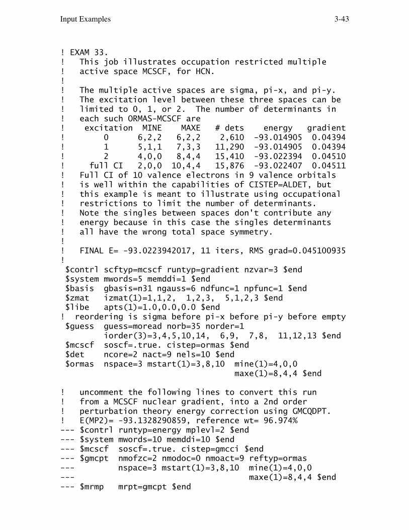
Input Examples 3-43
! EXAM 33.! This job illustrates occupation restricted multiple! active space MCSCF, for HCN.!! The multiple active spaces are sigma, pi-x, and pi-y.! The excitation level between these three spaces can be! limited to 0, 1, or 2. The number of determinants in! each such ORMAS-MCSCF are! excitation MINE MAXE # dets energy gradient! 0 6,2,2 6,2,2 2,610 -93.014905 0.04394! 1 5,1,1 7,3,3 11,290 -93.014905 0.04394! 2 4,0,0 8,4,4 15,410 -93.022394 0.04510! full CI 2,0,0 10,4,4 15,876 -93.022407 0.04511! Full CI of 10 valence electrons in 9 valence orbitals! is well within the capabilities of CISTEP=ALDET, but! this example is meant to illustrate using occupational! restrictions to limit the number of determinants.! Note the singles between spaces don't contribute any! energy because in this case the singles determinants! all have the wrong total space symmetry.!! FINAL E= -93.0223942017, 11 iters, RMS grad=0.045100935! $contrl scftyp=mcscf runtyp=gradient nzvar=3 $end $system mwords=5 memddi=1 $end $basis gbasis=n31 ngauss=6 ndfunc=1 npfunc=1 $end $zmat izmat(1)=1,1,2, 1,2,3, 5,1,2,3 $end $libe apts(1)=1.0,0.0,0.0 $end! reordering is sigma before pi-x before pi-y before empty $guess guess=moread norb=35 norder=1 iorder(3)=3,4,5,10,14, 6,9, 7,8, 11,12,13 $end $mcscf soscf=.true. cistep=ormas $end $det ncore=2 nact=9 nels=10 $end $ormas nspace=3 mstart(1)=3,8,10 mine(1)=4,0,0 maxe(1)=8,4,4 $end
! uncomment the following lines to convert this run! from a MCSCF nuclear gradient, into a 2nd order! perturbation theory energy correction using GMCQDPT.! E(MP2)= -93.1328290859, reference wt= 96.974%--- $contrl runtyp=energy mplevl=2 $end--- $system mwords=10 memddi=10 $end--- $mcscf soscf=.true. cistep=gmcci $end--- $gmcpt nmofzc=2 nmodoc=0 nmoact=9 reftyp=ormas--- nspace=3 mstart(1)=3,8,10 mine(1)=4,0,0--- maxe(1)=8,4,4 $end--- $mrmp mrpt=gmcpt $end

Input Examples 3-44
$dataHCN...6-31G(d,p) MCSCF using ORMAS...RHF geometryCnv 4
H 1.0 0.0 0.0 -1.0589956C 6.0 0.0 0.0 0.0N 7.0 0.0 0.0 1.1327718 $end
--- CLOSED SHELL MO's --- GENERATED Mon, Jan 13, 2003E(RHF)= -92.8771381048, with MVOQ=4 used to make virtuals. $VEC...orbitals deleted... $END

Input Examples 3-45
! EXAM34.! CIS treatment of excited states of formaldehyde.!! EXCITED STATE 1's E=-113.7017742428, RMS=0.0290048! The S0->S1 transition dipole is (0,0,0.006029),! and the S0 -> S1 transition energy is 4.56 eV.!! geometry optimization would lead in 18 steps to! -113.7053624528, at r(CO)=1.2553, r(CH)=1.0854,! a(HCO)= 117.74, with C's pyramidalization= 24.88.! This reproduces the fourth line of Table III in! Foresman et al. J.Phys.Chem. 96, 135-149(1992),! using no frozen core orbitals in order to do so.! Since it is well known that the geometry of this! state lies within Cs symmetry, the initial guess! geometry below is very slightly bent into Cs.! $contrl scftyp=rhf cityp=cis runtyp=gradient nzvar=6 $end $system timlim=1 $end $basis gbasis=n31 ngauss=6 ndfunc=1 diffsp=.t. $end $guess guess=huckel $end $cis hamtyp=saps mult=1 nacore=0 nstate=1 istate=1 $end $zmat izmat(1)=1,1,2, 1,2,3, 1,2,4, 2,1,2,3, 2,1,2,4, 4,1,2,4,3 $end $dataFormaldehyde CIS/6-31+G(d) 1(n->pi*) state optimizationCs
O 8.0 .01 -.8669736159 .0C 6.0 .0 .3455497481 .0H 1.0 -0.01 .9295804473 .9376713430 $end

Input Examples 3-46
! EXAM35.! As atom...Test of relativistic energy correction,! by the Douglas-Kroll transformation to 3rd order.!! the FINAL DK3 energy is -2259.0955118230! web page says -2259.095511826!! convergence of the DK transformation is typical,! 0th order -2234.2372862734 (non-relativistic)! 1st order -2264.6131852344! 2nd order -2258.9450216276! 3rd order -2259.0955118230! in that 1st order way undershoots, 2nd order comes! back close, and 3rd order is not insubstantial.! Compare with -2259.456841 which is the point! nucleus Dirac-Coulomb numerical Hartree-Fock from! L.Visscher, K.G.Dyall! At.Data Nucl.Data Tables 67, 207-224(1997)!! The uncontracted 20s15p9d basis set below is from! T.Tsuchiya, M.Abe, T.Nakajima, K.Hirao! J.Chem.Phys. 115, 4463-4472(2001)! using exponents downloaded from the web page of! this group at the University of Tokyo. A general! contraction of this basis can easily be obtained,! by manipulating the $VEC coefs produced by this run.! The semicolon divides two lines of input that happen! to be given on a single physical line of the file.! $contrl scftyp=rohf mult=4 relwfn=dk ispher=1 $end $system mwords=2 $end $relwfn norder=3 $end $guess guess=huckel $end $dataillustration of 3rd order Douglas-Kroll for AsDnh 2
Arsenic 33.0 S 1 ; 1 7.2421890D+07 1.0 S 1 ; 1 7.7040750D+06 1.0 S 1 ; 1 1.3365730D+06 1.0 S 1 ; 1 3.0394350D+05 1.0 S 1 ; 1 8.3289250D+04 1.0 S 1 ; 1 2.5994450D+04 1.0 S 1 ; 1 8.9795770D+03 1.0 S 1 ; 1 3.3667950D+03 1.0 S 1 ; 1 1.3464700D+03 1.0 S 1 ; 1 5.6774580D+02 1.0

Input Examples 3-47
S 1 ; 1 2.4923080D+02 1.0 S 1 ; 1 1.1199520D+02 1.0 S 1 ; 1 4.6328140D+01 1.0 S 1 ; 1 2.2611220D+01 1.0 S 1 ; 1 1.0910110D+01 1.0 S 1 ; 1 4.5498340D+00 1.0 S 1 ; 1 2.1494630D+00 1.0 S 1 ; 1 1.0337510D+00 1.0 S 1 ; 1 3.0892460D-01 1.0 S 1 ; 1 1.1206710D-01 1.0 P 1 ; 1 4.9515580D+04 1.0 P 1 ; 1 8.4637830D+03 1.0 P 1 ; 1 2.2908560D+03 1.0 P 1 ; 1 7.7965970D+02 1.0 P 1 ; 1 3.0545690D+02 1.0 P 1 ; 1 1.3097990D+02 1.0 P 1 ; 1 5.9698960D+01 1.0 P 1 ; 1 2.8408790D+01 1.0 P 1 ; 1 1.3883000D+01 1.0 P 1 ; 1 6.6102210D+00 1.0 P 1 ; 1 3.0821260D+00 1.0 P 1 ; 1 1.3919830D+00 1.0 P 1 ; 1 4.8254700D-01 1.0 P 1 ; 1 1.9228260D-01 1.0 P 1 ; 1 7.2849660D-02 1.0 D 1 ; 1 7.1896480D+02 1.0 D 1 ; 1 2.0798400D+02 1.0 D 1 ; 1 7.9590850D+01 1.0 D 1 ; 1 3.4514110D+01 1.0 D 1 ; 1 1.5730540D+01 1.0 D 1 ; 1 7.2805600D+00 1.0 D 1 ; 1 3.3000700D+00 1.0 D 1 ; 1 1.4173160D+00 1.0 D 1 ; 1 5.4472730D-01 1.0
$end

Input Examples 3-48
! EXAM36! analytic hessian for determinant MCSCF, at the! transition state for C=C rotation in ethylene!! There are 38 AOs and 36 MOs using spherical harmonics.! The 4e-, 4 orbital active space (CC sigma, pi, pi*, and! sigma* orbitals) generates a total of 36 determinants.!! FINAL E= -77.9753563834 after 14 iterations! imaginary FREQ= 1847.32i! true FREQ= 319.87(2), 1005.72(2), 1082.80, 1578.13! true FREQ= 1605.72, 3311.13, 3315.17, 3405.91(2)! the lowest true vibration is the most intense, 1.09748! $contrl scftyp=mcscf runtyp=hessian ispher=1 $end $system mwords=1 memddi=5 timlim=50 $end $basis gbasis=n31 ngauss=6 ndfunc=1 $end $guess guess=moread norb=36 norder=1 iorder(3)=4,5,6,7, 3,8,9,10 $end $det ncore=6 nact=4 nels=4 $end $dataC2H4 at rotational saddle point...sigma,pi,pi*,sigma*activeDnd 2
C 6.0 0.0000000000 0.0000000000 0.7486926908H 1.0 0.6500976762 0.6500976762 1.3062796706 $end
How to prepare the starting orbitals, also take noteof the orbital reordering to select the CC sigma:
--- $contrl scftyp=rohf mult=3 runtyp=energy $end--- $scf mvoq=2 $end--- $guess guess=huckel norder=0 $end
--- OPEN SHELL ORBITALS --- Tue Apr 6 10:00:30 2004E(ROHF)= -77.9570103652 $VEC 1 1 7.04639833E-01......36 8 3.55118554E-02-8.89989950E-03-3.55118554E-02 $END

Input Examples 3-49
! EXAM 37.! water trimer...illustration of FMO method on clusters!! A total of 21 energies are computed in this run,! of which the very first and last are -75.0201194583! and -149.9943977172, from various monomer and dimer! calculations. Combined together, the results for! 2-body FMO-RHF are:! Euncorr(2)= -224.910612407, RMS GRADIENT = 0.0267805!! Explicit RHF/STO-3G calculation on these coords has! E= -224.9112662623, grad=0.0269349!! See ../gamess/tools/fmo for larger examples based on! published data and examples involving bondfractioning.! $contrl scftyp=rhf runtyp=gradient $end $system timlim=2 $end $basis gbasis=sto ngauss=3 $end $fmo nfrag=3 icharg(1)=0,0,0 frgnam(1)=frag01,frag02,frag03 indat(1)=1,1,1, 2,2,2, 3,3,3 $end $fmoprp nprint=0 $end $fmoxyzO O .000000 .000000 .000000H H .000000 .000000 .957200H H .926627 .000000 -.239987O O 2.542027 .893763 -1.001593H H 1.991815 1.623962 -1.284979H H 2.958433 .581215 -1.804806O O .162059 2.462918 -1.477183H H -.189749 1.755643 -.936605H H -.375542 2.449889 -2.269046 $end $dataBasis set input, with no atomic coordinatesC1h-1 1c-1 6n-1 7o-1 8 $end

Input Examples 3-50
! EXAM 38.! Analytic gradients for Model Core Potentials,! with a DZP quality basis, for BiCl3. Model Core! Potentials account for scalar relativity effects,! and preserve all valence orbital radial nodes.!! The latter point stands in contrast to the! Effective Core Potential (ECP) pseudopotentials.!! FINAL RHF E= -116.3966190322, RMS grad= 0.0053955! FINAL RHF E= -116.3972798590, RMS grad= 0.0036800! FINAL RHF E= -116.3976422769, RMS grad= 0.0014246! FINAL RHF E= -116.3976891713, RMS grad= 0.0001135! FINAL RHF E= -116.3976900830, RMS grad= 0.0000485! FINAL RHF E= -116.3976902416, RMS grad= 0.0000001! $contrl scftyp=rhf runtyp=optimize pp=mcp ispher=1 coord=zmt nzvar=6 $end $system timlim=5 mwords=4 $end $basis gbasis=mcp-dzp $end $statpt opttol=1.0d-5 $end $dataBiCl3Cnv 3
BiCl 1 rBiClCl 1 rBiCl 2 aClBiClCl 1 rBiCl 2 aClBiCl 3 aClBiCl +1
rBiCl=2.48aClBiCl=99.0 $end

Input Examples 3-51
! EXAM 39.! The non-resonant Raman and hyper-Raman spectra of CH4!! Please see the actual file, supplied with GAMESS, for! its very long preamble about the inadequacy of the! basis set used below, and how to interpret the output.! $contrl scftyp=rhf runtyp=tdhfx nosym=1 ispher=0 $end $system mwords=1 $end $basis gbasis=n21 ngauss=3 $end $guess guess=huckel $end $scf dirscf=.true. conv=1d-6 $end $force method=analytic $end $cphf cphf=AO polar=.false. $end $tdhfx FREQ2 DADX 0.04 DADX_NI 0.04 DBDX 0.04 0.04 DBDX_NI 0.04 0.04 RAMAN 0.04 HRAMAN 0.04 D2ADX2_NI 0.04 D2BDX2_NI 0.04 0.04 $end $datamethane RHFTd
C 6.0 0.0 0.0 0.0H 1.0 0.6252197764 0.6252197764 0.6252197764 $END

Input Examples 3-52
! EXAM40.! CH2 singlet/triplet...minimum energy crossing.! Ansatz is full valence MCSCF in cc-pVDZ basis,! 25 AOs and 24 MOs, using spherical harmonics.!! It is well known that the ground state of CH2! (A.Kalemos, T.H.Dunning, A.Mavridis, J.F.Harrison! Can.J.Chem. 82, 684-693(2004)) is a triplet,! but that the singlet state becomes the! lowest surface at small angles. In this basis,! the states have their minima at! r(CH) a(HCH) Energy! 3-B-1 1.10155 130.9955 -38.9605726! 1-A-1 1.13868 99.9417 -38.9415486! and we know there is a crossing of these states! somewhere. Starting between the minima, near! R=1.11 and angle=115, where! triplet E= -38.9565003, dE/dZ(C)=+.0259717! singlet E= -38.9359506, dE/dZ(C)=-.0411344,! the seam minimization stops in 13 steps at! C 0.0 .0000000000 .0977833873! H 0.0 -.8659658151 -.6448916937! H 0.0 .8659658151 -.6448916937! which is R=1.1408, angle=98.77, actually just! inside the 1-A-1's bond angle. This MEX point! is the "transition state" for spin-orbit-coupling! induced inter-system-crossing (ISC) between! these two surfaces, see N.Matsunaga, S.Koseki,! M.S.Gordon J.Chem.Phys. 104, 7988-7996(1996).! Note that the MEX's energy and structure are! very similar to the singlet state's minimum:! Energy of First State = -38.941516! Energy of Second State = -38.941513! Energy Difference = .000003! Max Effective Gradient = .000009! RMS Effective Gradient = .000005! Max Change of X = .000023! RMS change of X = .000011! PARALLEL GRADIENT (in seam) has RMS=.026456! $contrl runtyp=mex ispher=1 nzvar=3 $end $basis gbasis=ccd $end $guess guess=moread norb=24 $end $zmat izmat(1)=1,1,2, 1,1,3, 2,2,1,3 $end $mex scf1=mcscf mult1=3 nmos1=24 scf2=mcscf mult2=1 nmos2=24 nrdmos=3 $end $det1 stsym=B1 ncore=1 nact=6 nels=6 $end $det2 stsym=A1 ncore=1 nact=6 nels=6 $end

Input Examples 3-53
$datamethylene...cc-pVDZ basis setCnv 2
Carbon 6.0Hydrogen 1.0 0.0 0.936 -0.596 $end
3-B-1 state: E(MCSCF)= -38.9565003122 $VEC1...snipped... $END
1-A-1 state: E(MCSCF)= -38.9359506088 $VEC2...snipped... $END
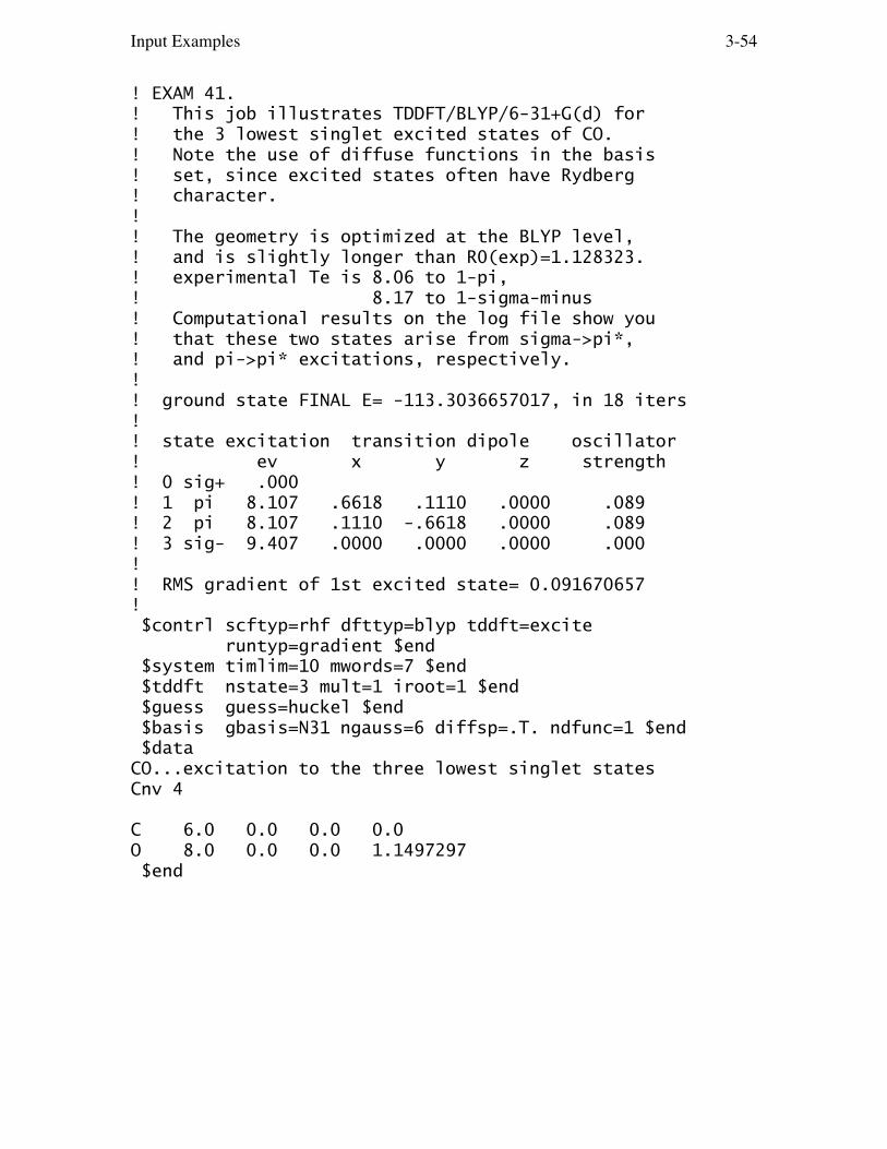
Input Examples 3-54
! EXAM 41.! This job illustrates TDDFT/BLYP/6-31+G(d) for! the 3 lowest singlet excited states of CO.! Note the use of diffuse functions in the basis! set, since excited states often have Rydberg! character.!! The geometry is optimized at the BLYP level,! and is slightly longer than R0(exp)=1.128323.! experimental Te is 8.06 to 1-pi,! 8.17 to 1-sigma-minus! Computational results on the log file show you! that these two states arise from sigma->pi*,! and pi->pi* excitations, respectively.!! ground state FINAL E= -113.3036657017, in 18 iters!! state excitation transition dipole oscillator! ev x y z strength! 0 sig+ .000! 1 pi 8.107 .6618 .1110 .0000 .089! 2 pi 8.107 .1110 -.6618 .0000 .089! 3 sig- 9.407 .0000 .0000 .0000 .000!! RMS gradient of 1st excited state= 0.091670657! $contrl scftyp=rhf dfttyp=blyp tddft=excite runtyp=gradient $end $system timlim=10 mwords=7 $end $tddft nstate=3 mult=1 iroot=1 $end $guess guess=huckel $end $basis gbasis=N31 ngauss=6 diffsp=.T. ndfunc=1 $end $dataCO...excitation to the three lowest singlet statesCnv 4
C 6.0 0.0 0.0 0.0O 8.0 0.0 0.0 1.1497297 $end

Input Examples 3-55
EXAM 42.! numerical gradient for PH3, using CCTYP=CR-CCL! there are 40 AOs, 38 MOs, 5 frozen cores, so! 4 valence orbitals correlated by 29 virtuals.!! This tests the numerical gradient driver, and also! emphasizes that the Dunning correlation consistent! basis sets should be used in spherical harmonic form.!! Since this molecule has two totally symmetric degrees! of freedom, 1 numerical gradient requires 5 energies:! at the input geometry, and at a pair of geometries! displaced along each totally symmetric direction.!! See METHOD=FULLNUM in $FORCE for numerical hessians,! and RUNTYP=FFIELD for numerical polarizabilities.!! E(RHF)= -342.4761838200, E(CCSD)= -342.6400065656,! T1 diag=0.01066308, mu(CCSD)= 0.717048 Debye! standard E(CCSD(T)) is not generated by this run.!! E(CR-CCL)= E(CR-CC(2,3)= -342.6433870011,! RMS gradient= 0.004511564! $contrl scftyp=rhf cctyp=cr-ccl runtyp=gradient numgrd=.true. ispher=1 coord=zmt nzvar=6 $end $system timlim=5 mwords=2 $end $basis gbasis=ccd $end $dataPH3...RHF/cc-pVDZ geometryCnv 3
PH 1 rPHH 1 rPH 2 aHPHH 1 rPH 2 aHPH 3 aHPH +1
rPH=1.412958aHPH=95.2045121 $end

Input Examples 3-56
EXAM 42.! numerical gradient for CN, using open shell CC(2,3).!! This tests the numerical gradient driver, and also! emphasizes that the Dunning correlation consistent! basis sets should be used in spherical harmonic form.!! A numerical gradient computation requires the energy! at the molecule's actual geometry, plus energies at! a pair of geometries displaced along each of its! totally symmetric directions.! A diatomic has 1 totally symmetric degree of freedom,! so this run requires 3 energies for 1 gradient.!! See METHOD=FULLNUM in $FORCE for numerical hessians,! and RUNTYP=FFIELD for numerical polarizabilities.!! There are 30 AOs, 28 MOs, 2 frozen cores, so 5 alpha! and 4 beta valence electrons are correlated.!! E(ROHF)= -92.1960778308, E(CCSD)= -92.4767618032,! the CR-CCL energy E(CC(2,3)) = -92.4930167395,! and RMS gradient= 0.029652621 at the CC(2,3) level.! (will optimize to -92.4941853332 at 1.1966876)! $contrl scftyp=rohf cctyp=cr-ccl mult=2 nzvar=1 runtyp=gradient numgrd=.true. ispher=1 $end $system timlim=5 $end $basis gbasis=ccd $end $zmat izmat(1)=1,1,2 $end $ccinp maxcc=50 $end $dataCN...experimental geometry...X-2-sigma-plus stateCnv 4
C 6.0 0.0 0.0 0.0N 7.0 0.0 0.0 1.1718 $end

Input Examples 3-57
! EXAM 43.! methane G3(MP2,CCSD(T)) heat of formation! 6-31G(d) has 23 AOs and 23 MOs,! G3Large has 79 AOs and 74 MOs.! --------------------------------------------------------! MP2/6-31G(D) = -40.332552 CCSD(T)/6-31G(D)= -40.355850! MP2/G3MP2LARGE = -40.404248 BASIS CONTRIBUT = -.071696! ZPE(HF/6-31G(D)= .042659 ZPE SCALE FACTOR= .892900! HLC = -.036680 FREE ENERGY = .030480! THERMAL ENERGY = .050629 THERMAL ENTHALPY= .051573! HEAT OF FORMATION (0K): -16.01 KCAL/MOL! HEAT OF FORMATION (298K): -17.83 KCAL/MOL! --------------------------------------------------------! The literature, namely JCP 110,4705(1999), says the! heat of formation by G3(MP2,QCISD(T)) = -17.8 @ 298! This run substitutes the standard CCSD(T) energy for! QCI, as considered by! L.A.Curtiss, K.Ragavachari, P.C.Redfern, A.G.Baboul,! J.A.Pople Chem.Phys.Lett. 314, 101-107(1999)! RUNTYP=G3MP2 performs a sequence of computations,! First, using the 6-31G(d) Cartesian GTO basis set:! HF geometry optimization (much like runtyp=optimize)! HF frequencies and ZPE evaluation (runtyp=hessian)! MP2 geometry, with no frozen cores (runtyp=optimize)! CCSD(T) energy calculation (runtyp=energy)! Then, using the G3Large basis, as spherical harmonics:! MP2 energy calculation, with frozen cores! All these intermediate energies are then gathered! together by the G3 recipe to produce the results.! Note that there is no particular input. The two basis! sets that are used, and the switch from Cartesian to! spherical harmonics is handled internally, so there is! no $BASIS group. The necessary asis sets are available! for H-Ca, Ga-Kr. Parallel computation is enabled. The! reference state must be RHF at present.! You can assist the run by giving a converged HF/6-31G(d)! geometry in $DATA, although this is not necessary. $contrl scftyp=rhf runtyp=g3mp2 $end $system timlim=5 mwords=2 memddi=5 $end $scf dirscf=.true. $end $dataMethane...G3(MP2,CCSD(T))Td
C 6.0 0.0000000 0.0000000 0.0000000H 1.0 0.6375302 0.6375302 0.6375302 $end

Input Examples 3-58
! EXAM 44.! Hydrogen fluoride hexamer...(HF)6! using the divide-and-conquer (DC) method!! Divide-and-conquer HF and MP2 energies are:! FINAL DC-RHF E= -599.9471636844, 14 iters! E(MP2)= -600.7388336079! An explicit MP2/6-31G calculation yields:! RHF E= -599.9475140963, 12 iters! MP2 E= -600.7399209860!! CCSD calculation requires changing one keyword in! $CONTRL. The divide-and-conquer CCSD energy is! E(CCSD)= -600.7487442686! compared to the explicit CCSD/6-31G calculation:! CCSD ENERGY= -600.7485966549! $CONTRL SCFTYP=RHF RUNTYP=ENERGY MPLEVL=2 COORD=ZMT $END $SYSTEM MWORDS=1 $END $BASIS GBASIS=N31 NGAUSS=6 $END $GUESS GUESS=HUCSUB $END $DCCORR DODCCR=.TRUE. RBUFCR=3.0 $END $DANDC DCFLG=.TRUE. BUFRAD=5.0 BUFTYP=RADSUBNSUBS=6 LBSUBS(1)=1,2,3,4,5,6,1,2,3,4,5,6 $END $DATAzigzag hexamer (HF)6C1FF 1 rFFF 2 rFF 1 aHFHF 3 rFF 2 aHFH 1 180.0F 4 rFF 3 aHFH 2 180.0F 5 rFF 4 aHFH 3 180.0H 1 rHFL 2 aHFH 3 180.0H 2 rHF 3 aHFH 4 180.0H 3 rHF 4 aHFH 5 180.0H 4 rHF 5 aHFH 6 180.0H 4 rFH 3 aHFH 2 180.0H 5 rFH 4 aHFH 3 180.0
rFF=2.5rHF=0.97rFH=1.43aHFH=116.0rHFL=0.97 $END
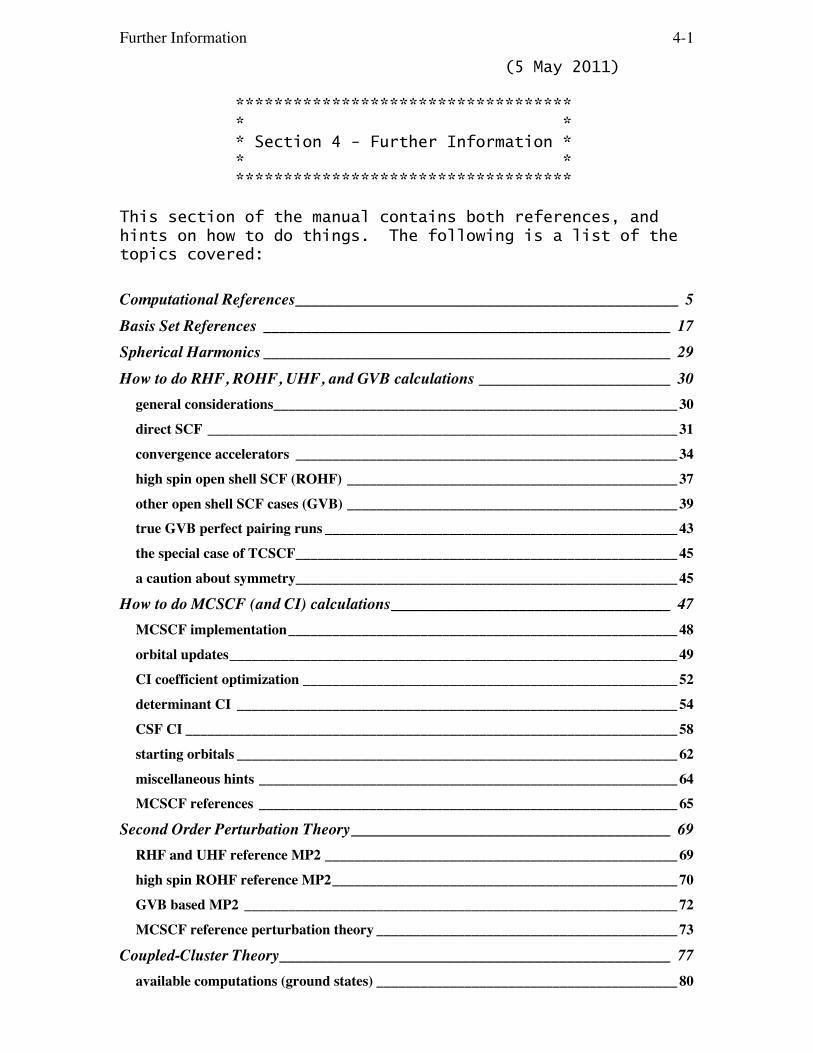
Further Information 4-1
(5 May 2011)
*********************************** * * * Section 4 - Further Information * * * ***********************************
This section of the manual contains both references, andhints on how to do things. The following is a list of thetopics covered:
Computational References________________________________________________ 5Basis Set References ___________________________________________________ 17Spherical Harmonics ___________________________________________________ 29How to do RHF, ROHF, UHF, and GVB calculations ________________________ 30
general considerations_______________________________________________________ 30
direct SCF ________________________________________________________________ 31
convergence accelerators ____________________________________________________ 34
high spin open shell SCF (ROHF) _____________________________________________ 37
other open shell SCF cases (GVB) _____________________________________________ 39
true GVB perfect pairing runs ________________________________________________ 43
the special case of TCSCF____________________________________________________ 45
a caution about symmetry____________________________________________________ 45
How to do MCSCF (and CI) calculations___________________________________ 47MCSCF implementation_____________________________________________________ 48
orbital updates_____________________________________________________________ 49
CI coefficient optimization ___________________________________________________ 52
determinant CI ____________________________________________________________ 54
CSF CI ___________________________________________________________________ 58
starting orbitals ____________________________________________________________ 62
miscellaneous hints _________________________________________________________ 64
MCSCF references _________________________________________________________ 65
Second Order Perturbation Theory________________________________________ 69RHF and UHF reference MP2 ________________________________________________ 69
high spin ROHF reference MP2_______________________________________________ 70
GVB based MP2 ___________________________________________________________ 72
MCSCF reference perturbation theory _________________________________________ 73
Coupled-Cluster Theory_________________________________________________ 77available computations (ground states) _________________________________________ 80

Further Information 4-2
available computations (excited states) _________________________________________ 88
density matrices and properties _______________________________________________ 94
excited state example________________________________________________________ 98
resource requirements ______________________________________________________ 99
restarts in ground-state calculations __________________________________________ 104
initial guesses in excited-state calculations _____________________________________ 106
eigensolvers for excited-state calculations ______________________________________ 107
references and citations required in publications ________________________________ 109
Density Functional Theory _____________________________________________ 116DFTTYP keywords ________________________________________________________ 116
grid-free DFT_____________________________________________________________ 117
DFT with grids ___________________________________________________________ 118
Time Dependent Density Functional Theory (TD-DFT) __________________________ 120
references for DFT ________________________________________________________ 122
Summary of excited state methods _______________________________________ 133Geometry Searches and Internal Coordinates ______________________________ 135
quasi-Newton Searches _____________________________________________________ 135
the nuclear Hessian ________________________________________________________ 138
coordinate choices _________________________________________________________ 139
the role of symmetry _______________________________________________________ 144
practical matters __________________________________________________________ 145
saddle points _____________________________________________________________ 147
mode following____________________________________________________________ 149
Intrinisic Reaction Coordinate Methods___________________________________ 151Gradient Extremals ___________________________________________________ 156Continuum Solvation Methods __________________________________________ 162
Self Consistent Reaction Field (SCRF) ________________________________________ 162
Polarizable Continuum Model (PCM)_________________________________________ 163
SVPE and SS(V)PE. _______________________________________________________ 172
Conductor-like screening model (COSMO) ____________________________________ 176
The Effective Fragment Potential Method _________________________________ 178terms in an EFP___________________________________________________________ 179
constructing an EFP1 ______________________________________________________ 180
constructing an EFP2 ______________________________________________________ 181
current limitations_________________________________________________________ 182
practical hints for using EFPs _______________________________________________ 183
global optimization ________________________________________________________ 185

Further Information 4-3
QM/MM across covalent bonds ______________________________________________ 187
Simpler potentials _________________________________________________________ 189
references________________________________________________________________ 190
The Fragment Molecular Orbital method__________________________________ 196Surfaces and solids ________________________________________________________ 198
FMO variants ____________________________________________________________ 199
Effective fragment molecular orbital method (EFMO) ___________________________ 200
Guidelines for approximations with FMO3_____________________________________ 200
How to perform FMO-MCSCF calculations ____________________________________ 201
How to perform multilayer runs _____________________________________________ 202
How to mix basis sets in FMO _______________________________________________ 202
How to perform FMO/PCM calculations ______________________________________ 203
How to perform FMO/EFP calculations _______________________________________ 204
Geometry optimizations for FMO ____________________________________________ 204
Pair interaction energy decomposition analysis (PIEDA) _________________________ 204
Excited states _____________________________________________________________ 206
Selective FMO ____________________________________________________________ 206
Frozen domains ______________________________________________________ 206Analyzing and visualizing the results__________________________________________ 207
Parallelization of FMO runs with GDDI _______________________________________ 207
Limitations of the FMO method in GAMESS___________________________________ 207
Restarts with the FMO method ______________________________________________ 208
Note on accuracy __________________________________________________________ 209
FMO References __________________________________________________________ 209
MOPAC Calculations within GAMESS ___________________________________ 214Molecular Properties and Conversion Factors______________________________ 217
Polarizabilities ____________________________________________________________ 218
Localized Molecular Orbitals ___________________________________________ 220Transition Moments and Spin-Orbit Coupling______________________________ 226
states____________________________________________________________________ 227
orbitals __________________________________________________________________ 228
symmetry ________________________________________________________________ 229
spin orbit details __________________________________________________________ 230
input nitty-gritty __________________________________________________________ 232
references________________________________________________________________ 233
examples_________________________________________________________________ 235

Further Information 4-4
For people who are newcomers to computational chemistry, itmay be helpful to study an introductory book.
First, some texts about quantum chemistry:
"Ab Initio Molecular Orbital Theory"W.J.Hehre, L.Radom, J.A.Pople, P.v.R.SchleyerWiley and Sons, New York, 1986
"Modern Quantum Chemistry" (now a Dover paperback)A.Szabo, N.S.Ostlund McGraw-Hill, 1989
"Quantum Chemistry, 6th Edition"I.N.Levine Prentice Hall, 2008
Then, a few books more focused on computation:
"Introduction to Quantum Mechanics in Chemistry"M.A.Ratner, G.C.Schatz Prentice Hall, 2000
"Introduction to Computational Chemistry, 2nd Edition"Frank Jensen Wiley and Sons, Chichester, 2006
"Molecular Modeling Basics"Jan H. Jensen CRC Press, Boca Raton, 2010
Frank's book is an outstanding survey of methods, basissets, properties, and other topics.
Jan's book is a good complement to Frank's, staying at asimpler level, using GAMESS input examples. It has anaccompanying online blog, http://molecularmodelingbasics.blogspot.com

Further Information 4-5
Computational References
GAMESS - M.W.Schmidt, K.K.Baldridge, J.A.Boatz, S.T.Elbert, M.S.Gordon, J.J.Jensen, S.Koseki, N.Matsunaga, K.A.Nguyen, S.Su, T.L.Windus, M.Dupuis, J.A.Montgomery J.Comput.Chem. 14, 1347-1363 (1993)
M.S.Gordon, M.W.Schmidt pp 1167-1189 in "Theory and Applications of Computational Chemistry, the first forty years" C.E.Dykstra, G.Frenking, K.S.Kim, G.E.Scuseria (editors), Elsevier, Amsterdam, 2005.
HONDO -These papers describes many of the algorithms in detail,and much of these applies also to GAMESS:"The General Atomic and Molecular Electronic Structure System: HONDO 7.0" M.Dupuis, J.D.Watts, H.O.Villar, G.J.B.Hurst Comput.Phys.Comm. 52, 415-425(1989)"HONDO: A General Atomic and Molecular Electronic Structure System" M.Dupuis, P.Mougenot, J.D.Watts, G.J.B.Hurst, H.O.Villar in "MOTECC: Modern Techniques in Computational Chemistry" E.Clementi, Ed. ESCOM, Leiden, the Netherlands, 1989, pp 307-361."HONDO: A General Atomic and Molecular Electronic Structure System" M.Dupuis, A.Farazdel, S.P.Karna, S.A.Maluendes in "MOTECC: Modern Techniques in Computational Chemistry" E.Clementi, Ed. ESCOM, Leiden, the Netherlands, 1990, pp 277-342.M.Dupuis, S.Chin, A.Marquez in "Relativistic and ElectronCorrelation Effects in Molecules", G.Malli, Ed. PlenumPress, NY 1994, pp 315-338.
sp integrals and gradient integrals -inner axis sp integration is done by McMurchie/DavidsonJ.A.Pople, W.J.Hehre J.Comput.Phys. 27, 161-168(1978)H.B.Schlegel, J.Chem.Phys. 77, 3676-3681(1982)
spd integrals by rotated axis/McMurchie-DavidsonK.Ishimura, S.Nagase Theoret.Chem.Acc. 120, 185-189(2008)
McMurchie/Davidson integrals -L.E.McMurchie, E.R.Davidson J.Comput.Phys. 26, 218-231(1978)
spdfg integrals -"Numerical Integration Using Rys Polynomials"

Further Information 4-6
H.F.King and M.Dupuis J.Comput.Phys. 21,144(1976)"Evaluation of Molecular Integrals over Gaussian Basis Functions" M.Dupuis,J.Rys,H.F.King J.Chem.Phys. 65,111-116(1976)"Molecular Symmetry and Closed Shell HF Calculations" M.Dupuis and H.F.King Int.J.Quantum Chem. 11,613(1977)"Computation of Electron Repulsion Integrals using the Rys Quadrature Method" J.Rys,M.Dupuis,H.F.King J.Comput.Chem. 4,154-157(1983)
ERIC spdfg integrals -"Recursion Formula for Electron Repulsion Integrals OverHermite Polynomials" G.D.Fletcher Int.J.Quantum Chem. 106, 355-360(2006)
spdfg gradient integrals -"Molecular Symmetry. II. Gradient of Electronic Energy with respect to Nuclear Coordinates" M.Dupuis and H.F.King J.Chem.Phys. 68,3998(1978)although the implementation is much newer than this paper.
spd hessian integrals -"Molecular Symmetry. III. Second derivatives of Electronic Energy with respect to Nuclear Coordinates" T.Takada, M.Dupuis, H.F.King J.Chem.Phys. 75, 332-336 (1981)
the Q matrix, and integral transformation symmetry -E.Hollauer, M.Dupuis J.Chem.Phys. 96, 5220 (1992)
spdfg effective core potential (ECP) integral/derivatives -C.F.Melius, W.A.Goddard Phys.Rev.A 10,1528-1540(1974)L.R.Kahn, P.Baybutt, D.G.Truhlar J.Chem.Phys. 65, 3826-3853 (1976)M.Krauss, W.J.Stevens Ann.Rev.Phys.Chem. 35, 357-385(1985)J.Breidung, W.Thiel, A.Komornicki Chem.Phys.Lett. 153, 76-81(1988)B.M.Bode, M.S.Gordon J.Chem.Phys. 111, 8778-8784(1999)See also the papers listed for SBKJC and HW basis sets.
model core potential (MCP) reviews -S.Huzinaga Can.J.Chem. 73, 619-628(1995)M.Klobukowski, S.Huzinaga, Y.Sakai, in ComputationalChemistry: Reviews of current trends, volume 3, pp 49-74,edited by J.Leszczynski, World Scientific, Singapore, 1999.
Quantum fast multipole method (QFMM) -E.O.Steinborn, K.Ruedenberg Adv.Quantum Chem. 7, 1-81(1973)
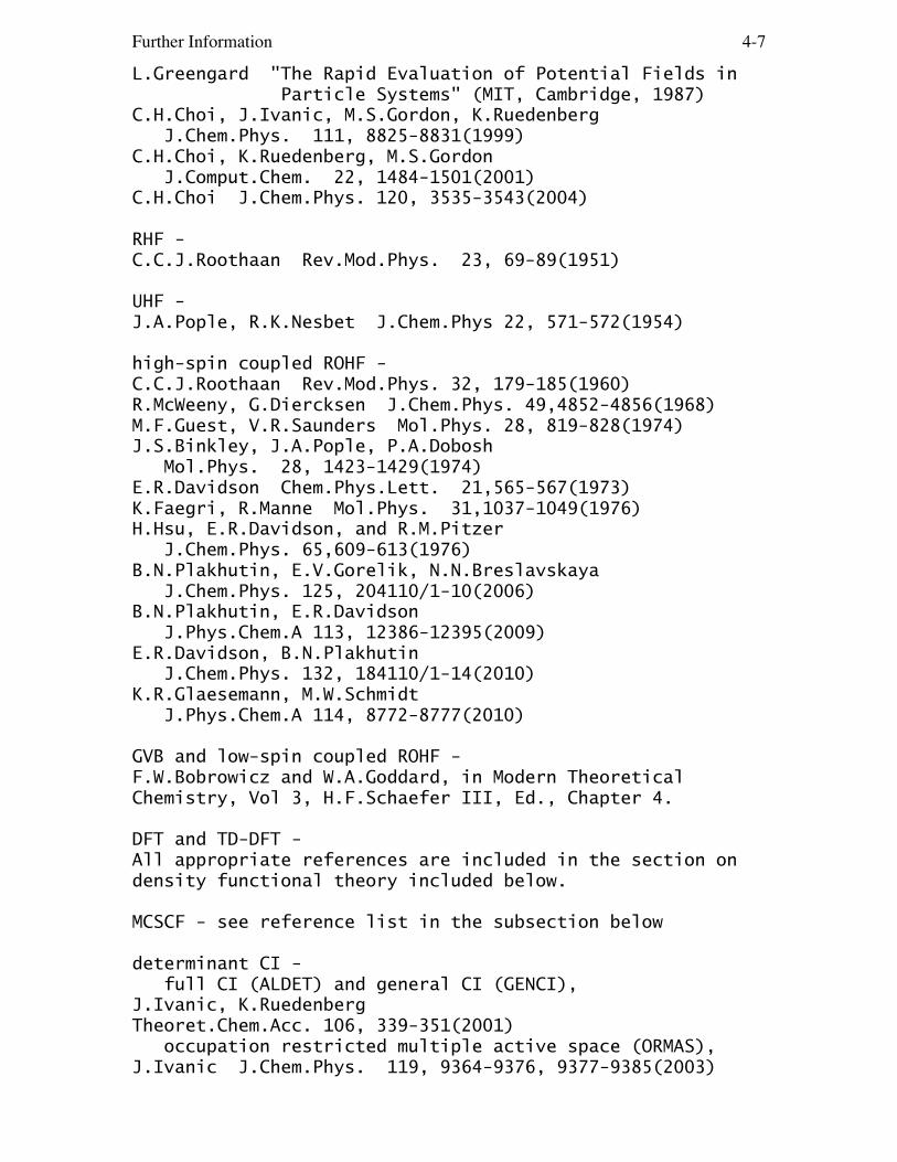
Further Information 4-7
L.Greengard "The Rapid Evaluation of Potential Fields in Particle Systems" (MIT, Cambridge, 1987)C.H.Choi, J.Ivanic, M.S.Gordon, K.Ruedenberg J.Chem.Phys. 111, 8825-8831(1999)C.H.Choi, K.Ruedenberg, M.S.Gordon J.Comput.Chem. 22, 1484-1501(2001)C.H.Choi J.Chem.Phys. 120, 3535-3543(2004)
RHF -C.C.J.Roothaan Rev.Mod.Phys. 23, 69-89(1951)
UHF -J.A.Pople, R.K.Nesbet J.Chem.Phys 22, 571-572(1954)
high-spin coupled ROHF -C.C.J.Roothaan Rev.Mod.Phys. 32, 179-185(1960)R.McWeeny, G.Diercksen J.Chem.Phys. 49,4852-4856(1968)M.F.Guest, V.R.Saunders Mol.Phys. 28, 819-828(1974)J.S.Binkley, J.A.Pople, P.A.Dobosh Mol.Phys. 28, 1423-1429(1974)E.R.Davidson Chem.Phys.Lett. 21,565-567(1973)K.Faegri, R.Manne Mol.Phys. 31,1037-1049(1976)H.Hsu, E.R.Davidson, and R.M.Pitzer J.Chem.Phys. 65,609-613(1976)B.N.Plakhutin, E.V.Gorelik, N.N.Breslavskaya J.Chem.Phys. 125, 204110/1-10(2006)B.N.Plakhutin, E.R.Davidson J.Phys.Chem.A 113, 12386-12395(2009)E.R.Davidson, B.N.Plakhutin J.Chem.Phys. 132, 184110/1-14(2010)K.R.Glaesemann, M.W.Schmidt J.Phys.Chem.A 114, 8772-8777(2010)
GVB and low-spin coupled ROHF -F.W.Bobrowicz and W.A.Goddard, in Modern TheoreticalChemistry, Vol 3, H.F.Schaefer III, Ed., Chapter 4.
DFT and TD-DFT -All appropriate references are included in the section ondensity functional theory included below.
MCSCF - see reference list in the subsection below
determinant CI - full CI (ALDET) and general CI (GENCI),J.Ivanic, K.RuedenbergTheoret.Chem.Acc. 106, 339-351(2001) occupation restricted multiple active space (ORMAS),J.Ivanic J.Chem.Phys. 119, 9364-9376, 9377-9385(2003)

Further Information 4-8
configuration state function CI (GUGA) -B.Brooks and H.F.Schaefer J.Chem. Phys. 70,5092(1979)B.Brooks, W.Laidig, P.Saxe, N.Handy, and H.F.Schaefer, Physica Scripta 21, 312(1980).
CIS energy and gradient -J.B.Foresman, M.Head-Gordon, J.A.Pople, M.J.Frisch J.Phys.Chem. 96, 135-149(1992)R.M.Shroll, W.D.Edwards Int.J.Quantum Chem. 63, 1037-1049(1997)the parallel CIS implementation in GAMESS is described in S.P.Webb Theoret.Chem.Acc. 116, 355-372(2006)which has a nice review of other excited state methods.
spin-flip CIS:A.I.Krylov Chem.Phys.Lett. 338, 375(2001)
closed, unrestricted open shell 2nd order Moller-Plesset -J.A.Pople, J.S.Binkley, R.Seeger Int. J. Quantum Chem. S10, 1-19(1976)M.J.Frisch, M.Head-Gordon, J.A.Pople, Chem.Phys.Lett. 166, 275-280(1990)C.M.Aikens, S.P.Webb, R.L.Bell, G.D.Fletcher, M.W.Schmidt, M.S.Gordon Theoret.Chem.Acc., 110, 233-253(2003)with the TCA "overview article" being a thorough review ofthe single determinant MP2 gradient equations.
CODE=SERIAL is generally based on the CPL paper above, asdescribed in the HONDO references given above.
The next two document CODE=DDI for RHF and UHF,G.D.Fletcher, M.W.Schmidt, M.S.Gordon Adv.Chem.Phys. 110, 267-294(1999)C.M.Aikens, M.S.Gordon J.Phys.Chem.A, 108, 3103-3110(2004)
The next two document CODE=IMS for RHF,K.Ishimura, P.Pulay, S.Nagase J.Comput.Chem. 27, 407-413(2006)K.Ishimura, P.Pulay, S.Nagase J.Comput.Chem. 28, 2034-2042(2007)
The next documents code=RIMP2 for RHF and UHF,M.Katouda, S.Nagase Int.J.Quantum Chem. 109, 2121-2130(2009)
Spin Component Scaled MP2 (SCS-MP2)S.Grimme

Further Information 4-9
J.Chem.Phys. 118, 9095-9102(2003)
spin restricted open shell MP2, ZAPT energy -T.J.Lee, D.Jayatilaka Chem.Phys.Lett. 201, 1-10(1993)T.J.Lee, A.P.Rendell, K.G.Dyall, D.Jayatilaka J.Chem.Phys. 100, 7400-7409(1994)
nuclear gradients for ZAPT -The next two document the CODE=DDI program,G.D.Fletcher, M.S.Gordon, R.L.Bell Theoret.Chem.Acc. 107, 57-70(2002)C.M.Aikens, G.D.Fletcher, M.W.Schmidt, M.S.Gordon J.Chem.Phys. 124, 014107/1-14(2006)
spin restricted open shell MP2, RMP method -P.J.Knowles, J.S.Andrews, R.D.Amos, N.C.Handy, J.A.Pople Chem.Phys.Lett. 186, 130-136 (1991)W.J.Lauderdale,J.F.Stanton,J.Gauss,J.D.Watts,R.J.Bartlett Chem.Phys.Lett. 187, 21-28(1991)
multiconfigurational quasidegenerate perturbation theory -H.Nakano J.Chem.Phys. 99, 7983-7992(1993)
Coupled-Cluster -Equation of Motion Coupled-Cluster (EOMCC) - this is a subset of the relevant papers:P.Piecuch, S.A.Kucharski, K.Kowalski, M.Musial, Comput.Phys.Commun. 149, 71-96(2002)K.Kowalski, P.Piecuch, J.Chem.Phys. 120, 1715-1738 (2004)P.Piecuch, S.A.Kucharski, K.Kowalski, M.Musial Comput.Phys.Commun. 149, 71-96(2002).
parallel CCSD(T) program -J.L.Bentz, R.M.Olson, M.S.Gordon, M.W.Schmidt, R.A.Kendall Comput.Phys.Commun. 176, 589-600(2007)R.M.Olson, J.L.Bentz, R.A.Kendall, M.W.Schmidt, M.S.Gordon J.Comput.Theoret.Chem. 3, 1312-1328(2007)
Any publication describing the results of ground-stateand/or excited-state calculations using the equation ofmotion coupled-cluster and/or completely renormalizedEOMCCSD(T) options (CCTYP=EOM-CCSD or CR-EOM) obtained withGAMESS should reference the specific papers appearing inthe printout. For more references to the primaryliterature for both types of coupled-cluster methods, seethe section "Coupled-Cluster theory" below.

Further Information 4-10
RHF/ROHF/TCSCF coupled perturbed Hartree Fock -"Single Configuration SCF Second Derivatives on a Cray" H.F.King, A.Komornicki in "Geometrical Derivatives of Energy Surfaces and Molecular Properties" P.Jorgensen J.Simons, Ed. D.Reidel, Dordrecht, 1986, pp 207-214."A parallel Distributed data CPHF algorithm for analyticHessians" Y.Alexeev, M.W.Schmidt, T.L.Windus, M.S.Gordon J.Comput.Chem. 28, 1685-1694(2007).Y.Osamura, Y.Yamaguchi, D.J.Fox, M.A.Vincent, H.F.Schaefer J.Mol.Struct. 103, 183-186(1983)M.Duran, Y.Yamaguchi, H.F.Schaefer J.Phys.Chem. 92, 3070-3075(1988)"A New Dimension to Quantum Chemistry" Y.Yamaguchi,Y.Osamura, J.D.Goddard, H.F.Schaefer Oxford Press, NY 1994
MCSCF coupled perturbed Hartree-Fock -M.R.Hoffman, D.J.Fox, J.F.Gaw, Y.Osamura, Y.Yamauchi,R.S.Grev, G.Fitzgerald, H.F.Schaefer, P.J.Knowles,N.C.Handy J.Chem.Phys. 80, 2660-2668(1984)the book by Osamura, Goddard, and Schaefer just mentioned.T.J.Dudley, R.M.Olson, M.W.Schmidt, M.S.Gordon J.Comput.Chem. 27, 353-362(2006)
non-adiabatic coupling matrix element (NACME) -J.C.Tully, chapter 5 (pp 217-267) in "Dynamics of MolecularCollisions - Part B", edited by W.H.Miller, Plenum Press,NY, 1976.B.H.Lengsfield, D.R.Yarkony, chapter 1 (pp. 1-71) in"State-selected and state-to-state in-molecule reactiondynamics- Part 2, theory", edited by M.Baer and C.-Y.Ng,John Wiley, NY, 1992.
harmonic vibrational analysis in Cartesian coordinates -W.D.Gwinn J.Chem.Phys. 55,477-481(1971)
Normal coordinate decomposition analysis -J.A.Boatz and M.S.Gordon, J.Phys.Chem. 93, 1819-1826(1989).
Partial Hessian vibrational analysis -H.Li, J.H.Jensen, Theoret.Chem.Acc. 107, 211-219(2002)
anharmonic vibrational spectra (VSCF) -
a review of VSCF:R.B.Gerber, J.O.Jung in "Computational Molecular Spectroscopy" P.Jensen, P.R.Bunker, eds. Wiley and Sons, Chichester, 2000, pp 365-390.

Further Information 4-11
the basic method for VSCF and cc-VSCF:G.M.Chaban, J.O.Jung, R.B.Gerber J.Chem.Phys. 111, 1823-1829(1999) the QFF approximation:K.Yagi, K.Hirao, T.Taketsugu, M.W.Schmidt, M.S.Gordon J.Chem.Phys. 121, 1383-1389(2004) the VDPT solver:N.Matsunaga, G.M.Chaban, R.B.Gerber J.Chem.Phys. 117, 3541-3547(2002) solver for larger systems:L.Pele, B.Brauer, R.B.Gerber Theoret.Chem.Acc. 117, 69-72(2007) use of internal coordinates, and thermochemistryB.Njegic, M.S.Gordon J.Chem.Phys. 125, 224102/1-12(2006)
applications of RUNTYP=VSCF:G.M.Chaban, J.O.Jung, R.B.Gerber J.Phys.Chem.A 104, 2772-2779(2000)J.Lundell, G.M.Chaban, R.B.Gerber Chem.Phys.Lett. 331, 308-316(2000)K.Yagi, T.Taketsugu, K.Hirao, M.S.Gordon J.Chem.Phys. 113, 1005-1017(2000)G.M.Chaban, R.B.Gerber, K.C.Janda J.Phys.Chem.A 105, 8323-8332(2001)A.T.Kowal Spectrochimica Acta A 58, 1055-1067(2002)G.M.Chaban, S.S.Xantheas, R.B.Gerber J.Phys.Chem.A 107, 4952-4956(2003)G.M.Chaban J.Phys.Chem.A 108, 4551-4556(2004)Y.Miller, G.M.Chaban, R.B.Gerber J.Phys.Chem.A 109, 6565-6574(2005)Y.Miller, G.M.Chaban, R.B.Gerber Chem.Phys. 313, 213-224(2005)C.A.Brindle, G.M.Chaban, R.B.Gerber, K.C.Janda Phys.Chem.Chem.Phys. 7, 945-954(2005)G.M.Chaban, R.M.Gerber Theoret.Chem.Acc. 120, 273-279(2008)
Raman spectrum -A.Komornicki, J.W.McIver J.Chem.Phys. 70, 2014-2016(1979)G.B.Bacskay, S.Saebo, P.R.Taylor Chem.Phys. 90, 215-224(1984)
static polarizabilities:H.A.Kurtz, J.J.P.Stewart, K.M.Dieter J.Comput.Chem. 11, 82-87 (1990)
dynamic polarizabilities:P.Korambath, H.A.Kurtz, in "Nonlinear Optical Materials",

Further Information 4-12
ACS Symposium Series 628, S.P.Karna and A.T.Yeates, Eds.pp 133-144, Washington DC, 1996.
nuclear derivatives of dynamic polarizabilities, and dynamic Raman and hyper-Raman:O.Quinet, B.Champagne J.Chem.Phys. 115, 6293-6299(2001)O.Quinet, B.Champagne B.Kirtman J.Comput.Chem. 22, 1920-1932(2001)O.Quinet, B.Champagne J.Chem.Phys. 117, 2481-2488(2002)O.Quinet, B.Kirtman, B.Champagne J.Chem.Phys. 118, 505-513(2003)
Geometry optimization and saddle point location -J.Baker J.Comput.Chem. 7, 385-395(1986).T.Helgaker Chem.Phys.Lett. 182, 503-510(1991).P.Culot, G.Dive, V.H.Nguyen, J.M.Ghuysen Theoret.Chim.Acta 82, 189-205(1992).
Dynamic Reaction Coordinate (DRC) -J.J.P.Stewart, L.P.Davis, L.W.Burggraf, J.Comput.Chem. 8, 1117-1123 (1987)S.A.Maluendes, M.Dupuis, J.Chem.Phys. 93, 5902-5911(1990)T.Taketsugu, M.S.Gordon, J.Phys.Chem. 99, 8462-8471(1995)T.Taketsugu, M.S.Gordon, J.Phys.Chem. 99, 14597-604(1995)T.Taketsugu, M.S.Gordon, J.Chem.Phys. 103, 10042-9(1995)M.S.Gordon, G.Chaban, T.Taketsugu J.Phys.Chem. 100, 11512-11525(1996)T.Takata, T.Taketsugu, K.Hirao, M.S.Gordon J.Chem.Phys. 109, 4281-4289(1998)T.Taketsugu, T.Yanai, K.Hirao, M.S.Gordon THEOCHEM 451, 163-177(1998)
Energy orbital localization -C.Edmiston, K.Ruedenberg Rev.Mod.Phys. 35, 457-465(1963).R.C.Raffenetti, K.Ruedenberg, C.L.Janssen, H.F.Schaefer, Theoret.Chim.Acta 86, 149-165(1993)
Boys orbital localization -S.F.Boys, "Quantum Science of Atoms, Molecules, and Solids"P.O.Lowdin, Ed, Academic Press, NY, 1966, pp 253-262.See the first paper on oriented localized orbitals if youwish to know the true origin of "Boys localization"
Population orbital localization -J.Pipek, P.Z.Mezey J.Chem.Phys. 90, 4916(1989).
Oriented localized orbitals -J.Ivanic, G.M.Atchity, K.Ruedenberg Theoret.Chem.Acc. 120, 281-294(2008)

Further Information 4-13
J.Ivanic, K.Ruedenberg Theoret.Chem.Acc. 120, 295-305(2008)
Valence Virtual Orbitals (VVOS) -W.C.Lu, C.Z.Wang, M.W.Schmidt, L.Bytautas, K.M.Ho,K.Ruedenberg J.Chem.Phys. 120, 2629-2637 and 2638-2651(2004)W.C.Lu, C.Z.Wang, T.L.Chan, K.Ruedenberg, K.M.Ho Phys.Rev.B 70, 041101-1/4(2004)
Mulliken Population Analysis -R.S.Mulliken J.Chem.Phys. 23, 1833-1840, 1841-1846, 2338-2342, 2343-2346(1955)
so called "Lowdin Population Analysis" -This should be described as "a Mulliken population analysis(ref M1-M4 above) based on symmetrically orthogonalizedorbitals (ref L)", where reference L is P.-O.Lowdin Adv.Chem.Phys. 5, 185-199(1970)Lowdin populations are not invariant to rotation if thebasis set used is Cartesian d,f,...: I.Mayer, Chem.Phys.Lett. 393, 209-212(2004).
Bond orders and valences -M.Giambiagi, M.Giambiagi, D.R.Grempel, C.D.Heymann J.Chim.Phys. 72, 15-22(1975)I.Mayer, Chem.Phys.Lett. 97,270-274(1983), 117,396(1985).M.S.Giambiagi, M.Giambiagi, F.E.Jorge Z.Naturforsch. 39a, 1259-73(1984)I.Mayer, Theoret.Chim.Acta 67, 315-322(1985).I.Mayer, Int.J.Quantum Chem. 29, 73-84(1986).I.Mayer, Int.J.Quantum Chem. 29, 477-483(1986).The same formula (apart from a factor of two) may also beseen in equation 31 of the second of these papers (the bondorder formula in the 1st of these is not the same formula):T.Okada, T.Fueno Bull.Chem.Soc.Japan 48, 2025-2032(1975)T.Okada, T.Fueno Bull.Chem.Soc.Japan 49, 1524-1530(1976)a review about bond orders: I. Mayer, J.Comput.Chem. 28, 204-221(2007).
Direct SCF -J.Almlof, K.Faegri, K.Korsell J.Comput.Chem. 3, 385-399 (1982)M.Haser, R.Ahlrichs J.Comput.Chem. 10, 104-111 (1989)
DIIS (Direct Inversion in the Iterative Subspace) -P.Pulay J.Comput.Chem. 3, 556-560(1982)

Further Information 4-14
SOSCF -G.Chaban, M.W.Schmidt, M.S.Gordon Theor.Chem.Acc. 97, 88-95(1997)T.H.Fischer, J.Almlof J.Phys.Chem. 96,9768-74(1992)
Modified Virtual Orbitals (MVOs) -C.W.Bauschlicher, Jr. J.Chem.Phys. 72,880-885(1980)
Thermochemistry (RUNTYP=G3MP2) - G3(MP2,CCSD(T)) is defined inL.A.Curtiss, K.Ragavachari, P.C.Redfern, A.G.Baboul,J.A.Pople Chem.Phys.Lett. 314, 101-107(1999) based on various other G3 basis set/method papers:L.A.Curtiss, P.C.Redfern, K.Raghavachari, V.Rassolov,J.A.Pople J.Chem.Phys. 110, 4703-4709(1999)L.A.Curtiss, P.C.Redfern, K.Raghavachari, V.Rassolov,J.A.Pople J.Chem.Phys. 114, 9287-9295(2001)L.A.Curtiss, P.C.Redfern, K.Raghavachari, V.Rassolov,J.A.Pople J.Chem.Phys. 109,7764-7776(1998)L.A.Curtiss, K.Ragavachari Theoret.Chem.Acc. 108, 61-70(2002)
EVVRSP, in memory diagonalization -S.T.Elbert Theoret.Chim.Acta 71,169-186(1987)
Davidson eigenvector method -E.R.Davidson J.Comput.Phys. 17,87(1975)"Matrix Eigenvector Methods" p. 95-113 in "Methods inComputational Molecular Physics", edited by G.H.F.Diercksenand S.Wilson, D.Reidel Publishing, Dordrecht, 1983.M.L.Leininger, C.D.Sherrill, W.D.Allen, H.F.Schaefer, J.Comput.Chem. 22, 1574-1589(2001)
DK (Douglas-Kroll relativistic transformation) -M.Douglas, N.M.Kroll Ann.Phys. 82, 89-155(1974)B.A.Hess Phys.Rev. A33, 3742-3748(1986)G.Jansen, B.A.Hess Phys.Rev. A39, 6016-6017(1989)T.Nakajima, K.Hirao J.Chem.Phys. 113, 7786-7789(2000)T.Nakajima, K.Hirao Chem.Phys.Lett. 329, 511-516(2000)W.A.DeJong, R.J.Harrison, D.A.Dixon J.Chem.Phys. 114, 48-53(2001)A.Wolf, M.Reiher, B.A.Hess J.Chem.Phys. 117, 9215-26(2002)T.Nakajima, K.Hirao J.Chem.Phys. 119, 4105-4111(2003) (and see just below for DK1 during SOC)
IOTC (Infinite-Order Two-Component) relativy correction -M.Barysz, A.J.Sadlej J.Chem.Phys. 116, 2696-2704(2002)M.Barysz, Progress in Theoretical Chemistry and Physics, Kluwer Academic Publishers, 349-397(2002)

Further Information 4-15
D.Kedziera, M.Barysz, A.J.Sadlej Struct.Chem. 15, 369-377(2004)D.Kedziera, M.Barysz, J.Chem.Phys. 121, 6719-6727(2004)M.Barysz, L.Mentel, J.Leszczynski J.Chem.Phys. 130, 164114/1-7(2009)
RESC (Relativistic Elimination of Small Components) -T.Nakajima, K.Hirao Chem.Phys.Lett. 302, 383-391(1999)T.Nakajima, T.Suzumura, K.Hirao Chem.Phys.Lett. 304, 271(1999)D.G.Fedorov, T.Nakajima, K.Hirao Chem.Phys.Lett. 335, 183-187(2001)
NESC (Normalized Elimination of Small Components) -K.G.Dyall J.Comput.Chem. 23, 786-793(2002)
Spin-orbit coupling and transition moments –Many references can be found in the section on this topicbelow. For the 1st order Douglas-Kroll transformation ofthe 1e- part of the spin orbit operator, see T.Zeng, D.G.Fedorov, M. Klobukowski J.Chem.Phys. 131, 124109/1-17 (2009) T.Zeng, D.G.Fedorov, M.Klobukowski J.Chem.Phys. 132, 074102/1-15 (2010)
GIAO NMR -R.Ditchfield Mol.Phys. 27, 789-807(1974)M.A.Freitag, B.Hillman, A.Agrawal, M.S.Gordon J.Chem.Phys. 120, 1197-1202(2004)
Solvation models: EFP, SCRF, PCM, or COSMO.All appropriate references are included in the sections onthese topics included below.
MOPAC 6 -J.J.P.Stewart J.Computer-Aided Molecular Design 4, 1-105 (1990)References for parameters for individual atoms may be foundon the printout from your runs.
MacMolPlt -B.M.Bode, M.S.Gordon J.Mol.Graphics Mod. 16, 133-138(1998)
quantum chemistry parallelization in GAMESS -for SCF, see the main GAMESS paper quoted above.T.L.Windus, M.W.Schmidt, M.S.Gordon, Chem.Phys.Lett. 216, 375-379(1993)T.L.Windus, M.W.Schmidt, M.S.Gordon, Theoret.Chim.Acta 89, 77-88 (1994)

Further Information 4-16
T.L.Windus, M.W.Schmidt, M.S.Gordon, in "Parallel Computing in Computational Chemistry", ACS Symposium Series 592, Ed. by T.G.Mattson, ACS Washington, 1995, pp 16-28.K.K.Baldridge, M.S.Gordon, J.H.Jensen, N.Matsunaga,M.W.Schmidt, T.L.Windus, J.A.Boatz, T.R.Cundari ibid, pp 29-46.G.D.Fletcher, M.W.Schmidt, M.S.Gordon Adv.Chem.Phys. 110, 267-294 (1999)H.Umeda, S.Koseki, U.Nagashima, M.W.Schmidt J.Comput.Chem. 22, 1243-1251 (2001)C.H.Choi, K.Ruedenberg J.Comput.Chem. 22, 1484-1501(2001)D.G.Fedorov, M.S.Gordon ACS Symp.Series 828, 1-22(2002)H.Li, C.S.Pomelli, J.H.Jensen Theoret.Chem.Acc. 109, 71-84(2003)C.M.Aikens, M.S.Gordon J.Phys.Chem.A 108, 3103-3110(2004)H.M.Netzloff, M.S.Gordon J.Comput.Chem. 25, 1926-1936(2004)T.J.Dudley, R.M.Olson, M.W.Schmidt, M.S.Gordon J.Comput.Chem. 27, 353-362(2006)C.M.Aikens, G.D.Fletcher, M.W.Schmidt, M.S.Gordon J.Chem.Phys. 124, 014107/1-14(2006)Y.Alexeev, M.W.Schmidt, T.L.Windus, M.S.Gordon J.Comput.Chem. 28, 1685-1694(2007).R.M.Olson, J.L.Bentz, R.A.Kendall, M.W.Schmidt, M.S.Gordon J.Comput.Theoret.Chem. 3, 1312-1328(2007)J.L.Bentz, R.M.Olson, M.S.Gordon, M.W.Schmidt, R.A.Kendell Comput.Phys.Commun., 176, 589-600 (2007).G.D.Fletcher Mol.Phys. 105, 2971-2976(2007)
The Distributed Data Interface (DDI), which is the computerscience layer underneath the parallel quantum chemistry -G.D.Fletcher, M.W.Schmidt, B.M.Bode, M.S.Gordon Comput.Phys.Commun. 128, 190-200 (2000)R.M.Olson, M.W.Schmidt, M.S.Gordon, A.P.Rendell Proc. of Supercomputing 2003, IEEE Computer Society. This does not exist on paper, but can be downloaded at http://www.sc-conference.org/sc2003/tech_papers.phpD.G.Fedorov, R.M.Olson, K.Kitaura, M.S.Gordon, S.Koseki J.Comput.Chem. 25, 872-880(2004).
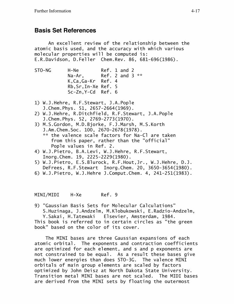
Further Information 4-17
Basis Set References
An excellent review of the relationship between theatomic basis used, and the accuracy with which variousmolecular properties will be computed is:E.R.Davidson, D.Feller Chem.Rev. 86, 681-696(1986).
STO-NG H-Ne Ref. 1 and 2 Na-Ar, Ref. 2 and 3 ** K,Ca,Ga-Kr Ref. 4 Rb,Sr,In-Xe Ref. 5 Sc-Zn,Y-Cd Ref. 6
1) W.J.Hehre, R.F.Stewart, J.A.Pople J.Chem.Phys. 51, 2657-2664(1969).2) W.J.Hehre, R.Ditchfield, R.F.Stewart, J.A.Pople J.Chem.Phys. 52, 2769-2773(1970).3) M.S.Gordon, M.D.Bjorke, F.J.Marsh, M.S.Korth J.Am.Chem.Soc. 100, 2670-2678(1978). ** the valence scale factors for Na-Cl are taken from this paper, rather than the "official" Pople values in Ref. 2.4) W.J.Pietro, B.A.Levi, W.J.Hehre, R.F.Stewart, Inorg.Chem. 19, 2225-2229(1980).5) W.J.Pietro, E.S.Blurock, R.F.Hout,Jr., W.J.Hehre, D.J. DeFrees, R.F.Stewart Inorg.Chem. 20, 3650-3654(1980).6) W.J.Pietro, W.J.Hehre J.Comput.Chem. 4, 241-251(1983).
MINI/MIDI H-Xe Ref. 9
9) "Gaussian Basis Sets for Molecular Calculations" S.Huzinaga, J.Andzelm, M.Klobukowski, E.Radzio-Andzelm, Y.Sakai, H.Tatewaki Elsevier, Amsterdam, 1984.This book is referred to in certain circles as "the greenbook" based on the color of its cover.
The MINI bases are three Gaussian expansions of eachatomic orbital. The exponents and contraction coefficientsare optimized for each element, and s and p exponents arenot constrained to be equal. As a result these bases givemuch lower energies than does STO-3G. The valence MINIorbitals of main group elements are scaled by factorsoptimized by John Deisz at North Dakota State University.Transition metal MINI bases are not scaled. The MIDI basesare derived from the MINI sets by floating the outermost
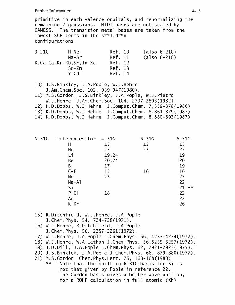
Further Information 4-18
primitive in each valence orbitals, and renormalizing theremaining 2 gaussians. MIDI bases are not scaled byGAMESS. The transition metal bases are taken from thelowest SCF terms in the s**1,d**nconfigurations.
3-21G H-Ne Ref. 10 (also 6-21G) Na-Ar Ref. 11 (also 6-21G)K,Ca,Ga-Kr,Rb,Sr,In-Xe Ref. 12 Sc-Zn Ref. 13 Y-Cd Ref. 14
10) J.S.Binkley, J.A.Pople, W.J.Hehre J.Am.Chem.Soc. 102, 939-947(1980).11) M.S.Gordon, J.S.Binkley, J.A.Pople, W.J.Pietro, W.J.Hehre J.Am.Chem.Soc. 104, 2797-2803(1982).12) K.D.Dobbs, W.J.Hehre J.Comput.Chem. 7,359-378(1986)13) K.D.Dobbs, W.J.Hehre J.Comput.Chem. 8,861-879(1987)14) K.D.Dobbs, W.J.Hehre J.Comput.Chem. 8,880-893(1987)
N-31G references for 4-31G 5-31G 6-31G H 15 15 15 He 23 23 23 Li 19,24 19 Be 20,24 20 B 17 19 C-F 15 16 16 Ne 23 23 Na-Al 22 Si 21 ** P-Cl 18 22 Ar 22 K-Kr 26
15) R.Ditchfield, W.J.Hehre, J.A.Pople J.Chem.Phys. 54, 724-728(1971).16) W.J.Hehre, R.Ditchfield, J.A.Pople J.Chem.Phys. 56, 2257-2261(1972).17) W.J.Hehre, J.A.Pople J.Chem.Phys. 56, 4233-4234(1972).18) W.J.Hehre, W.A.Lathan J.Chem.Phys. 56,5255-5257(1972).19) J.D.Dill, J.A.Pople J.Chem.Phys. 62, 2921-2923(1975).20) J.S.Binkley, J.A.Pople J.Chem.Phys. 66, 879-880(1977).21) M.S.Gordon Chem.Phys.Lett. 76, 163-168(1980) ** - Note that the built in 6-31G basis for Si is not that given by Pople in reference 22. The Gordon basis gives a better wavefunction, for a ROHF calculation in full atomic (Kh)

Further Information 4-19
symmetry, 6-31G Energy virial Gordon -288.828573 1.999978 Pople -288.828405 2.000280 See the input examples for how to run in Kh.22) M.M.Francl, W.J.Pietro, W.J.Hehre, J.S.Binkley, M.S.Gordon, D.J.DeFrees, J.A.Pople J.Chem.Phys. 77, 3654-3665(1982).23) Unpublished, copied out of GAUSSIAN82.24) For Li and Be, 4-31G is actually a 5-21G expansion.25) V.A.Rassolov, J.A.Pople, M.A.Ratner, T.L.Windus J.Chem.Phys. 109, 1223-1229(1998)26) A.V.Mitin, J.Baker, P.Pulay J.Chem.Phys. 118, 7775-7782(2003) - not in GAMESS.27) V.A.Rassolov, M.A.Ratner, J.A.Pople, P.C.Redfern, L.A.Curtiss J.Comput.Chem. 22, 976-984(2001).Note that reference 27 renames basis sets published earlieras "6-31G*" in references 25 and 32. GAMESS was changed touse the 6-31G* basis sets from reference 27 for K, Ca, andGa-Kr in September 2006. Sc-Zn remain those of ref. 25.
Extended basis sets
--> 6-311G
28) R.Krishnan, J.S.Binkley, R.Seeger, J.A.Pople J.Chem.Phys. 72, 650-654(1980).
--> valence double zeta "DZV" sets:
"DH" basis - DZV for H, Li-Ne, Al-Ar30) T.H.Dunning, Jr., P.J.Hay Chapter 1 in "Methods of Electronic Structure Theory", H.F.Schaefer III, Ed. Plenum Press, N.Y. 1977, pp 1-27. Note that GAMESS uses inner/outer scale factors of 1.2 and 1.15 for DH's hydrogen (since at least 1983). To get Thom's usual basis, scaled 1.2 throughout: HYDROGEN 1.0 x, y, z DH 0 1.2 1.2 DZV for K,Ca31) J.-P.Blaudeau, M.P.McGrath, L.A.Curtiss, L.Radom J.Chem.Phys. 107, 5016-5021(1997) "BC" basis - DZV for Ga-Kr32) R.C.Binning, Jr., L.A.Curtiss J.Comput.Chem. 11, 1206-1216(1990)Note, this basis set is available only by GBASIS=DZV, sinceit is no longer considered to be the 6-31G substitute.

Further Information 4-20
--> valence triple zeta "TZV" sets:
TZV for H,Li-Ne40) T.H. Dunning, J.Chem.Phys. 55 (1971) 716-723. TZV for Na-Ar - also known as the "MC" basis41) A.D.McLean, G.S.Chandler J.Chem.Phys. 72,5639-5648(1980). TZV for K,Ca42) A.J.H. Wachters, J.Chem.Phys. 52 (1970) 1033-1036. (see Table VI, Contraction 3). TZV for Sc-Zn (taken from HONDO 7)This is Wachters' (14s9p5d) basis (ref 42) contractedto (10s8p3d) with the following modifications 1. the most diffuse s removed; 2. additional s spanning 3s-4s region; 3. two additional p functions to describe the 4p; 4. (6d) contracted to (411) from ref 43, except for Zn where Wachter's (5d)/[41] and Hay's diffuse d are used.43) A.K. Rappe, T.A. Smedley, and W.A. Goddard III, J.Phys.Chem. 85 (1981) 2607-2611
Valence only basis sets (ECPs and MCPs)
SBKJC ECP, these are -31G splits for main group, bigger fortransition metals (available Li-Rn):50) W.J.Stevens, H.Basch, M.Krauss J.Chem.Phys. 81, 6026-6033 (1984)51) W.J.Stevens, M.Krauss, H.Basch, P.G.Jasien Can.J.Chem. 70, 612-630 (1992)52) T.R.Cundari, W.J.Stevens J.Chem.Phys. 98, 5555-5565(1993)
HW ECP, these are -21 splits (sp exponents not shared) transition metals (not built in at present, although they will work if you type them in):53) P.J.Hay, W.R.Wadt J.Chem.Phys. 82, 270-283 (1985) main group (available Na-Xe)54) W.R.Wadt, P.J.Hay J.Chem.Phys. 82, 284-298 (1985) see also55) P.J.Hay, W.R.Wadt J.Chem.Phys. 82, 299-310 (1985)
Model core potentials (MCP):
To understand the model core potential formalism itself,see the review articles S.Huzinaga Can.J.Chem. 73, 619-628(1995)
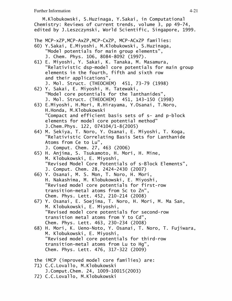
Further Information 4-21
M.Klobukowski, S.Huzinaga, Y.Sakai, in ComputationalChemistry: Reviews of current trends, volume 3, pp 49-74,edited by J.Leszczynski, World Scientific, Singapore, 1999.
The MCP-xZP,MCP-AxZP,MCP-CxZP, MCP-ACxZP families:60) Y.Sakai, E.Miyoshi, M.Klobukowski, S.Huzinaga, "Model potentials for main group elements", J. Chem. Phys. 106, 8084-8092 (1997).61) E. Miyoshi, Y. Sakai, K. Tanaka, M. Masamura, "Relativistic dsp-model core potentials for main group elements in the fourth, fifth and sixth row and their applications", J. Mol. Struct. (THEOCHEM) 451, 73-79 (1998)62) Y. Sakai, E. Miyoshi, H. Tatewaki, "Model core potentials for the lanthanides", J. Mol. Struct. (THEOCHEM) 451, 143-150 (1998)63) E.Miyoshi, H.Mori, R.Hirayama, Y.Osanai, T.Noro, H.Honda, M.Klobukowski "Compact and efficient basis sets of s- and p-block elements for model core potential method" J.Chem.Phys. 122, 074104/1-8(2005)64) M. Sekiya, T. Noro, Y. Osanai, E. Miyoshi, T. Koga, "Relativistic Correlating Basis Sets for Lanthanide Atoms from Ce to Lu", J. Comput. Chem. 27, 463 (2006)65) H. Anjima, S. Tsukamoto, H. Mori, H. Mine, M. Klobukowski, E. Miyoshi, "Revised Model Core Potentials of s-Block Elements", J. Comput. Chem. 28, 2424-2430 (2007)66) Y. Osanai, M. S. Mon, T. Noro, H. Mori, H. Nakashima, M. Klobukowski, E. Miyoshi, "Revised model core potentials for first-row transition-metal atoms from Sc to Zn", Chem. Phys. Lett. 452, 210-214 (2008)67) Y. Osanai, E. Soejima, T. Noro, H. Mori, M. Ma San, M. Klobukowski, E. Miyoshi, "Revised model core potentials for second-row transition metal atoms from Y to Cd", Chem. Phys. Lett. 463, 230-234 (2008)68) H. Mori, K. Ueno-Noto, Y. Osanai, T. Noro, T. Fujiwara, M. Klobukowski, E. Miyoshi, "Revised model core potentials for third-row transition-metal atoms from Lu to Hg", Chem. Phys. Lett. 476, 317-322 (2009)
the iMCP (improved model core families) are:71) C.C.Lovallo, M.Klobukowski J.Comput.Chem. 24, 1009-10015(2003)72) C.C.Lovallo, M.Klobukowski
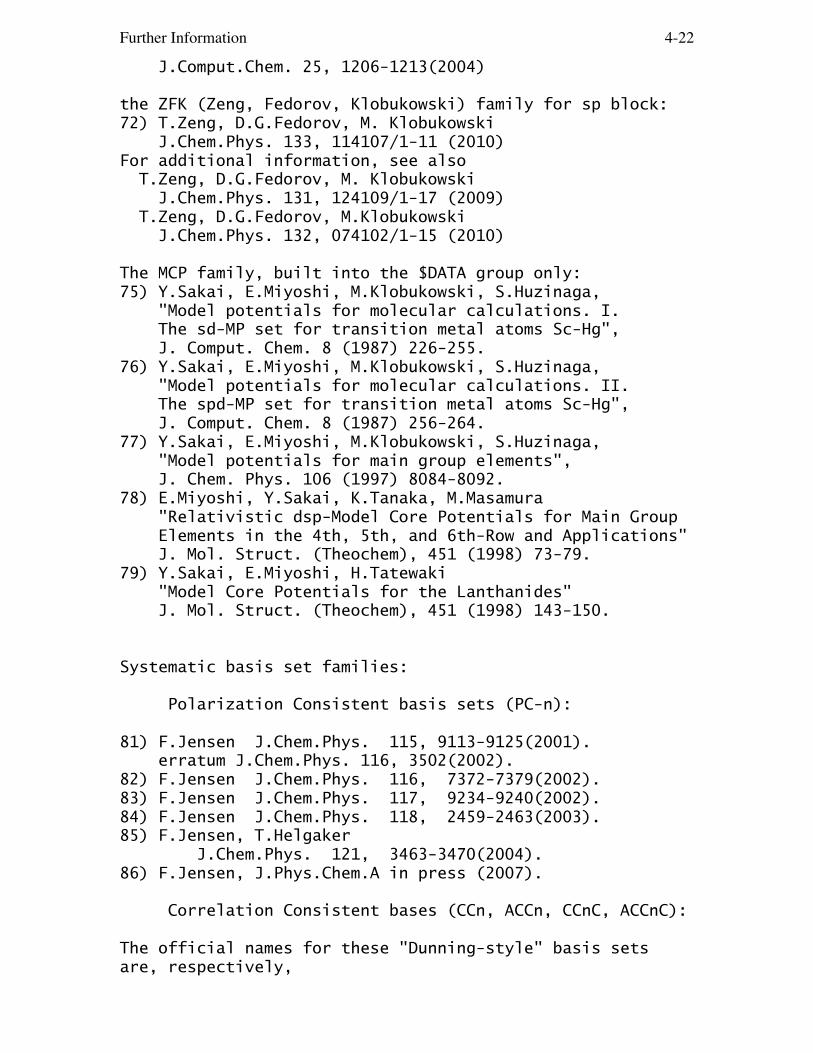
Further Information 4-22
J.Comput.Chem. 25, 1206-1213(2004)
the ZFK (Zeng, Fedorov, Klobukowski) family for sp block:72) T.Zeng, D.G.Fedorov, M. Klobukowski J.Chem.Phys. 133, 114107/1-11 (2010)For additional information, see also T.Zeng, D.G.Fedorov, M. Klobukowski J.Chem.Phys. 131, 124109/1-17 (2009) T.Zeng, D.G.Fedorov, M.Klobukowski J.Chem.Phys. 132, 074102/1-15 (2010)
The MCP family, built into the $DATA group only:75) Y.Sakai, E.Miyoshi, M.Klobukowski, S.Huzinaga, "Model potentials for molecular calculations. I. The sd-MP set for transition metal atoms Sc-Hg", J. Comput. Chem. 8 (1987) 226-255.76) Y.Sakai, E.Miyoshi, M.Klobukowski, S.Huzinaga, "Model potentials for molecular calculations. II. The spd-MP set for transition metal atoms Sc-Hg", J. Comput. Chem. 8 (1987) 256-264.77) Y.Sakai, E.Miyoshi, M.Klobukowski, S.Huzinaga, "Model potentials for main group elements", J. Chem. Phys. 106 (1997) 8084-8092.78) E.Miyoshi, Y.Sakai, K.Tanaka, M.Masamura "Relativistic dsp-Model Core Potentials for Main Group Elements in the 4th, 5th, and 6th-Row and Applications" J. Mol. Struct. (Theochem), 451 (1998) 73-79.79) Y.Sakai, E.Miyoshi, H.Tatewaki "Model Core Potentials for the Lanthanides" J. Mol. Struct. (Theochem), 451 (1998) 143-150.
Systematic basis set families:
Polarization Consistent basis sets (PC-n):
81) F.Jensen J.Chem.Phys. 115, 9113-9125(2001). erratum J.Chem.Phys. 116, 3502(2002).82) F.Jensen J.Chem.Phys. 116, 7372-7379(2002).83) F.Jensen J.Chem.Phys. 117, 9234-9240(2002).84) F.Jensen J.Chem.Phys. 118, 2459-2463(2003).85) F.Jensen, T.Helgaker J.Chem.Phys. 121, 3463-3470(2004).86) F.Jensen, J.Phys.Chem.A in press (2007).
Correlation Consistent bases (CCn, ACCn, CCnC, ACCnC):
The official names for these "Dunning-style" basis setsare, respectively,
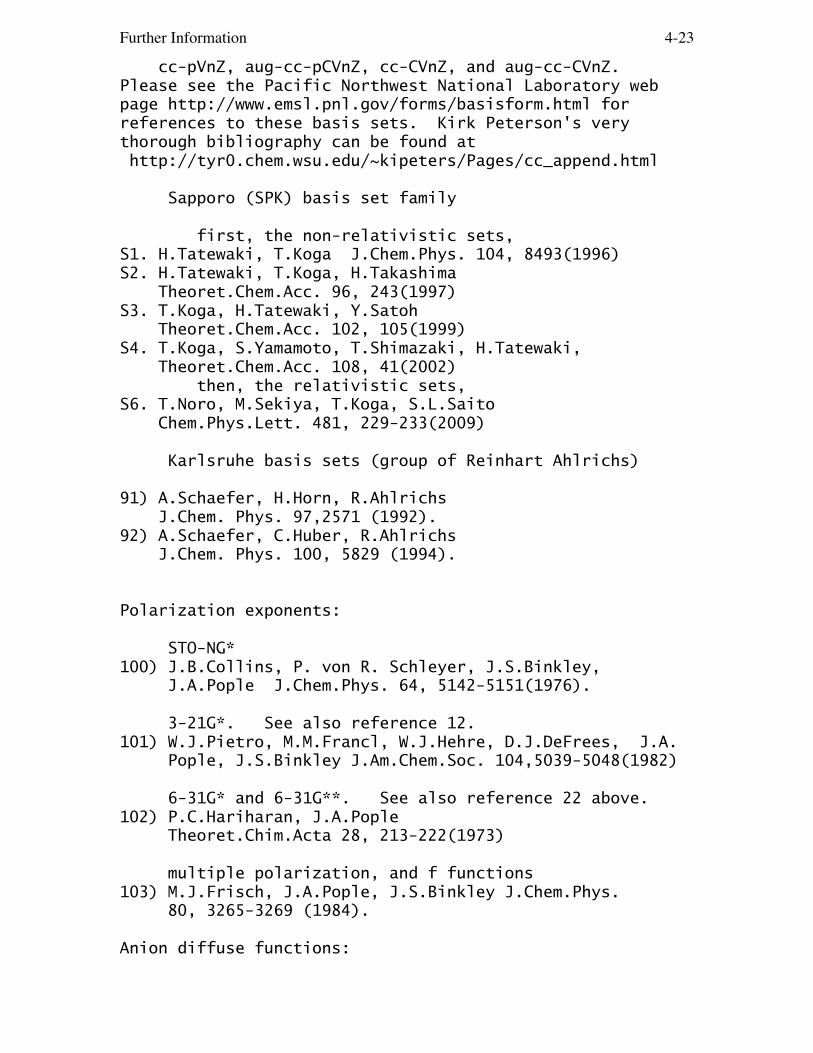
Further Information 4-23
cc-pVnZ, aug-cc-pCVnZ, cc-CVnZ, and aug-cc-CVnZ.Please see the Pacific Northwest National Laboratory webpage http://www.emsl.pnl.gov/forms/basisform.html forreferences to these basis sets. Kirk Peterson's verythorough bibliography can be found at http://tyr0.chem.wsu.edu/~kipeters/Pages/cc_append.html
Sapporo (SPK) basis set family
first, the non-relativistic sets,S1. H.Tatewaki, T.Koga J.Chem.Phys. 104, 8493(1996)S2. H.Tatewaki, T.Koga, H.Takashima Theoret.Chem.Acc. 96, 243(1997)S3. T.Koga, H.Tatewaki, Y.Satoh Theoret.Chem.Acc. 102, 105(1999)S4. T.Koga, S.Yamamoto, T.Shimazaki, H.Tatewaki, Theoret.Chem.Acc. 108, 41(2002) then, the relativistic sets,S6. T.Noro, M.Sekiya, T.Koga, S.L.Saito Chem.Phys.Lett. 481, 229-233(2009)
Karlsruhe basis sets (group of Reinhart Ahlrichs)
91) A.Schaefer, H.Horn, R.Ahlrichs J.Chem. Phys. 97,2571 (1992).92) A.Schaefer, C.Huber, R.Ahlrichs J.Chem. Phys. 100, 5829 (1994).
Polarization exponents:
STO-NG*100) J.B.Collins, P. von R. Schleyer, J.S.Binkley, J.A.Pople J.Chem.Phys. 64, 5142-5151(1976).
3-21G*. See also reference 12.101) W.J.Pietro, M.M.Francl, W.J.Hehre, D.J.DeFrees, J.A. Pople, J.S.Binkley J.Am.Chem.Soc. 104,5039-5048(1982)
6-31G* and 6-31G**. See also reference 22 above.102) P.C.Hariharan, J.A.Pople Theoret.Chim.Acta 28, 213-222(1973)
multiple polarization, and f functions103) M.J.Frisch, J.A.Pople, J.S.Binkley J.Chem.Phys. 80, 3265-3269 (1984).
Anion diffuse functions:

Further Information 4-24
3-21+G, 3-21++G, etc.105) T.Clark, J.Chandrasekhar, G.W.Spitznagel, P. von R. Schleyer J.Comput.Chem. 4, 294-301(1983)106) G.W.Spitznagel, Diplomarbeit, Erlangen, 1982.
------------
STO-NG* means d orbitals are used on third row atoms only. The original paper (ref 100) suggested z=0.09 for Na and Mg, and z=0.39 for Al-Cl. We prefer to use the same exponents as are used in 3-21G* and 6-31G*, so we know we're looking at changes in the sp basis, not the d exponent.
3-21G* means d orbitals on main group elements in the third and higher periods. Not defined for the transition metals, where there are p's already in the basis. Except for alkalis and alkali earths, the 4th and 5th row zetas are from Huzinaga, et al. (ref 9). The exponents are normally the same as for 6-31G*.
6-31G* means d orbitals on second and third row atoms. We use Mark Gordon's z=0.395 for Silicon, as well as his fully optimized sp basis (ref 21). This is often written 6-31G(d) today. For the first row transition metals, the * means an f function is added. The transition metal 3d 6-31G orbital is NOT of triple zeta quality, and thus is probably not very accurate.
6-31G** means the same as 6-31G*, except that p functions are added on hydrogens. This is often written 6-31G(d,p) today.
6-311G** means p orbitals on H, and d orbitals elsewhere. The exponents were derived from correlated atomic states, and so are considerably tighter than the polarizing functions used in 6-31G**, etc. This is often written 6-311G(d,p) today.
The exponents for 6-31G* for C-F are disturbing, inthat each atom has exactly the same value. Dunning and Hay(ref 30) have recommended a better set of exponents forsecond row atoms and a slightly different value for H.
2p, 3p, 2d, 3p polarization sets are usually thought ofas arising from applying splitting factors to the 1p and 1dvalues. For example, SPLIT2=2.0, 0.5 means to double and

Further Information 4-25
halve the single value. The default values for SPLIT2 andSPLIT3 are taken from reference 103, and were derived withcorrelation in mind. The SPLIT2 values often produce ahigher (!) HF energy than the singly polarized run, becausethe exponents are split too widely. SPLIT2=0.4,1.4 willalways lower the SCF energy (the values are the unpublishedpersonal preference of MWS), and for SPLIT3 we mightsuggest 3.0,1.0,1/3.
With all this as background, we are ready to presentthe tables of polarization exponents that are built intoGAMESS. Please note that the names associated with eachcolumn are only generally descriptive. The column marked"COMMON" is obtained from both Pople (mostly his 6-31G, butusing Gordon's value for Silicon) and Huzinaga (from the"green book"). The exponents for K-Kr under "Dunning" arefrom Curtiss, et al., not Thom Dunning, and so on. Theexponents are for d functions unless otherwise indicated.
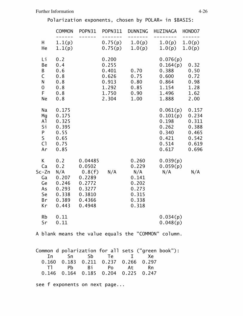
Further Information 4-26
Polarization exponents, chosen by POLAR= in $BASIS:
COMMON POPN31 POPN311 DUNNING HUZINAGA HONDO7 ------ ------ ------- ------- -------- ------ H 1.1(p) 0.75(p) 1.0(p) 1.0(p) 1.0(p) He 1.1(p) 0.75(p) 1.0(p) 1.0(p) 1.0(p)
Li 0.2 0.200 0.076(p) Be 0.4 0.255 0.164(p) 0.32 B 0.6 0.401 0.70 0.388 0.50 C 0.8 0.626 0.75 0.600 0.72 N 0.8 0.913 0.80 0.864 0.98 O 0.8 1.292 0.85 1.154 1.28 F 0.8 1.750 0.90 1.496 1.62 Ne 0.8 2.304 1.00 1.888 2.00
Na 0.175 0.061(p) 0.157 Mg 0.175 0.101(p) 0.234 Al 0.325 0.198 0.311 Si 0.395 0.262 0.388 P 0.55 0.340 0.465 S 0.65 0.421 0.542 Cl 0.75 0.514 0.619 Ar 0.85 0.617 0.696
K 0.2 0.04485 0.260 0.039(p) Ca 0.2 0.0502 0.229 0.059(p)Sc-Zn N/A 0.8(f) N/A N/A N/A N/A Ga 0.207 0.2289 0.141 Ge 0.246 0.2772 0.202 As 0.293 0.3277 0.273 Se 0.338 0.3810 0.315 Br 0.389 0.4366 0.338 Kr 0.443 0.4948 0.318
Rb 0.11 0.034(p) Sr 0.11 0.048(p)
A blank means the value equals the "COMMON" column.
Common d polarization for all sets ("green book"): In Sn Sb Te I Xe 0.160 0.183 0.211 0.237 0.266 0.297 Tl Pb Bi Po At Rn 0.146 0.164 0.185 0.204 0.225 0.247
see f exponents on next page...

Further Information 4-27
f polarization functions, from reference 103: Li Be B C N O F Ne 0.15 0.26 0.50 0.80 1.00 1.40 1.85 2.50 Na Mg Al Si P S Cl Ar 0.15 0.20 0.25 0.32 0.45 0.55 0.70 --
Anions usually require diffuse basis functions toproperly represent their spatial diffuseness. The use ofdiffuse sp shells on atoms in the second and third rows isdenoted by a + sign, also adding diffuse s functions onhydrogen is symbolized by ++. These designations can beapplied to any of the Pople bases, e.g. 3-21+G, 3-21+G*,6-31++G**. The following exponents are for L shells,except for H. For H-F, they are taken from ref 105. ForNa-Cl, they are taken directly from reference 106. Thesevalues may be found in footnote 13 of reference 103. ForGa-Br, In-I, and Tl-At these were optimized for the atomicground state anion, using ROHF with a flexible ECP basisset, by Ted Packwood at NDSU.
H 0.0360 Li Be B C N O F 0.0074 0.0207 0.0315 0.0438 0.0639 0.0845 0.1076 Na Mg Al Si P S Cl 0.0076 0.0146 0.0318 0.0331 0.0348 0.0405 0.0483 Ga Ge As Se Br 0.0205 0.0222 0.0287 0.0318 0.0376 In Sn Sb Te I 0.0223 0.0231 0.0259 0.0306 0.0368 Tl Pb Bi Po At 0.0170 0.0171 0.0215 0.0230 0.0294
Additional information about diffuse functions and alsoRydberg type exponents can be found in reference 30.

Further Information 4-28
The following atomic energies are UHF (RHF on 1-Sstates), p orbitals are not symmetry equivalent, using thedefault scale factors. They may be useful in picking abasis of the desired accuracy.
Atom state STO-2G STO-3G 3-21G 6-31GH 2-S -.454397 -.466582 -.496199 -.498233He 1-S -2.702157 -2.807784 -2.835680 -2.855160Li 2-S -7.070809 -7.315526 -7.381513 -7.431236Be 1-S -13.890237 -14.351880 -14.486820 -14.566764B 2-P -23.395284 -24.148989 -24.389762 -24.519492C 3-P -36.060274 -37.198393 -37.481070 -37.677837N 4-S -53.093007 -53.719010 -54.105390 -54.385008O 3-P -71.572305 -73.804150 -74.393657 -74.780310F 2-P -95.015084 -97.986505 -98.845009 -99.360860Ne 1-S -122.360485 -126.132546 -127.803825 -128.473877Na 2-S -155.170019 -159.797148 -160.854065 -161.841425Mg 1-S -191.507082 -197.185978 -198.468103 -199.595219Al 2-P -233.199965 -239.026471 -240.551046 -241.854186Si 3-P -277.506857 -285.563052 -287.344431 -288.828598P 4-S -327.564244 -336.944863 -339.000079 -340.689008S 3-P -382.375012 -393.178951 -395.551336 -397.471414Cl 2-P -442.206260 -454.546015 -457.276552 -459.442939Ar 1-S -507.249273 -521.222881 -524.342962 -526.772151
Atom state DH 6-311G MC SCF limit*H 2-S -.498189 -.499810 -- -0.5He 1-S -- -2.859895 -- -2.861680Li 2-S -7.431736 -7.432026 -- -7.432727Be 1-S -14.570907 -14.571874 -- -14.573023B 2-P -24.526601 -24.527020 -- -24.529061C 3-P -37.685571 -37.686024 -- -37.688619N 4-S -54.397260 -54.397980 -- -54.400935O 3-P -74.802707 -74.802496 -- -74.809400F 2-P -99.395013 -99.394158 -- -99.409353Ne 1-S -128.522354 -128.522553 -- -128.547104Na 2-S -- -- -161.845587 -161.858917Mg 1-S -- -- -199.606558 -199.614636Al 2-P -241.855079 -- -241.870014 -241.876699Si 3-P -288.829617 -- -288.847782 -288.854380P 4-S -340.689043 -- -340.711346 -340.718798S 3-P -397.468667 -- -397.498023 -397.504910Cl 2-P -459.435938 -- -459.473412 -459.482088Ar 1-S -- -- -526.806626 -526.817528
* M.W.Schmidt and K.Ruedenberg, J.Chem.Phys. 71, 3951-3962(1979). These are ROHF energies in Kh symmetry.H-Xe can be found in Phys.Rev.A 46, 3691-3696(1992).

Further Information 4-29
Spherical Harmonics
The implementation of ISPHER in $CONTRL does not relyon using a spherical harmonic basis set, in fact the atomicbasis remains the Cartesian Gaussians. Instead, certainMOs formed from particular combinations of the CartesianGaussians (for example, xx+yy+zz) are deleted from the MOspace. Thus a run with ISPHER=1 will have fewer MOs thanAOs. Since neither the occupied nor virtual MOs containany admixture of xx+yy+zz, the resulting energy and wave-function is exactly equivalent to the use of a sphericalharmonic basis.
The log file output will contain expansions of each MOin terms of 6 d's, 10 f's, and 15 g's, and the $VEC alsocontains the same expansion over Cartesian Gaussians. Boththe matrix in your log file and in $VEC will contain fewerMOs than AOs, the exact number of MOs used is printed inthe initial guess section of the log file. It should bepossible to read such $VEC groups into runs with differentsettings of ISPHER, should you choose to do so.
The advantage of this approach is that intelligence inthe generation of symmetry orbitals combined with thecapability to drop linearly dependent MO combinations meansthat the details of ISPHER are located only in the orbitaloptimization code, where the variational spaces are simplyreduced in size to eliminate the undesired contaminantfunctions. This means that none of the integral routinesneed be modified, as the atomic basis remains the CartesianGaussians. The disadvantage is that AO integral files runover the Cartesian Gaussians, and thus are not reduced insize. Of course transformed MO integrals and variouscomputations in correlated calculations are reduced insize, since the number of MOs may be greatly reduced.
Computationally, the advantages of ISPHER=1 are notlimited to the reduced CPU time associated with fewer totalMOs. Questions about d orbital participation as measuredby Mulliken populations are cleanly addressed when the d'susage in the MOs does not contain any contamination fromthe s shape xx+yy+zz. Less obviously, the use of sphericalharmonics frequently greatly reduces problems with lineardependency, that exhibit as poor SCF convergence.

Further Information 4-30
How to do RHF, ROHF, UHF, and GVB calculations
general considerations
These four SCF wavefunctions are all based on Fockoperator techniques, even though some GVB runs use morethan one determinant. Thus all of these have an intrinsicN**4 time dependence, because they are all driven byintegrals in the AO basis. This similarity makes itconvenient to discuss them all together. In this sectionwe will use the term HF to refer generically to any ofthese four wavefunctions, including the multi-determinateGVB-PP functions. $SCF is the main input group for allthese HF wavefunctions.
As will be discussed below, in GAMESS the term ROHFrefers to high spin open shell SCF only, but other openshell coupling cases are possible using the GVB code.
Analytic gradients are implemented for every possibleHF type calculation possible in GAMESS, and thereforenumerical hessians are available for each.
Analytic hessian calculation is implemented for RHF,ROHF, and any GVB case with NPAIR=0 or NPAIR=1. Analytichessians are more accurate, and much more quickly computedthan numerical hessians, but require additional diskstorage to perform an integral transformation, and alsomore physical memory.
The second order Moller-Plesset energy correction (MP2)is implemented for RHF, UHF, ROHF, and MCSCF wavefunctions.Analytic gradients may be obtained for MP2 with RHF, UHF,or ROHF reference wavefunctions, and MP2 level propertiesare therefore available for these, see MP2PRP in $MP2. Allother cases give properties for the SCF function.
Direct SCF is implemented for every possible HF typecalculation. The direct SCF method may not be used withDEM convergence. Direct SCF may be used during energy,gradient, numerical or analytic hessian, CI or MP2 energycorrection, or localized orbital computations.

Further Information 4-31
direct SCF
Normally, HF calculations proceed by evaluating a largenumber of two electron repulsion integrals, and storingthese on a disk. This integral file is read in once duringeach HF iteration to form the appropriate Fock operators.In a direct HF, the integrals are not stored on disk, butare instead reevaluated during each HF iteration. Sincethe direct approach *always* requires more CPU time, thedefault for DIRSCF in $SCF is .FALSE.
Even though direct SCF is slower, there are at leasttwo reasons why you may want to consider using it. Thefirst is that it may not be possible to store all of theintegrals on the disk drives attached to your computer.Second, what you are really interested in is reducing thewall clock time to obtain your answer, not the CPU time.Workstations, particularly nodes with multiple CPUs andonly one disk subsystem, may have modest hardware I/Ocapabilities. Other environments such as a mainframeshared by many users may also have very poor CPU/wall clockperformance for I/O bound jobs such as conventional HF.
You can estimate the disk storage requirements forconventional HF using a P or PK file by the followingformulae:
nint = 1/sigma * 1/8 * N**4 Mbytes = nint * x / 1024**2
Here N is the total number of basis functions in your run,which you can learn from an EXETYP=CHECK run. The 1/8accounts for permutational symmetry within the integrals.Sigma accounts for the point group symmetry, and isdifficult to estimate accurately. Sigma cannot be smallerthan 1, in no symmetry (C1) calculations. For benzene,sigma would be almost six, since you generate 6 C's and 6H's by entering only 1 of each in $DATA. For water sigmais not much larger than one, since most of the basis set ison the unique oxygen, and the C2v symmetry applies only tothe H atoms. The factor x is 12 bytes per integral forbasis sets smaller than 255, and 16 otherwise. Finally,since integrals that are very close to zero need not bestored on disk, the actual power dependence is not as badas N**4, and in fact in the limit of very large moleculescan be as low as N**2. Thus plugging in sigma=1 shouldgive you an upper bound to the actual disk space needed.If the estimate exceeds your available disk storage, youronly recourse is direct HF.

Further Information 4-32
What are the economics of direct HF? Naively, if weassume the run takes 10 iterations to converge, we mustspend 10 times more CPU time computing the integrals oneach iteration. However, we do not have to waste any CPUtime reading blocks of integrals from disk, or in unpackingtheir indices. We also do not have to waste any wall clocktime waiting for a relatively slow mechanical device suchas a disk to give us our data.
There are some less obvious savings too, as first notedby Almlof. First, since the density matrix is known whilewe are computing integrals, we can use the Schwarzinequality to avoid doing some of the integrals. In aconventional SCF this inequality is used to avoid doingsmall integrals. In a direct SCF it can be used to avoiddoing integrals whose contribution to the Fock matrix issmall (density times integral=small). Secondly, we canform the Fock matrix by calculating only its change sincethe previous iteration. The contributions to the change inthe Fock matrix are equal to the change in the densitytimes the integrals. Since the change in the density goesto zero as the run converges, we can use the Schwarzscreening to avoid more and more integrals as thecalculation progresses. The input option FDIFF in $SCFselects formation of the Fock operator by computing onlyits change from iteration to iteration. The FDIFF optionis not implemented for GVB since there are too many densitymatrices from the previous iteration to store, but is thedefault for direct RHF, ROHF, and UHF.
So, in our hypothetical 10 iteration case, we do notspend as much as 10 times more time in integral evaluation.Additionally, the run as a whole will not slow down bywhatever factor the integral time is increased. A directrun spends no additional time summing integrals into theFock operators, and no additional time in the Fockdiagonalizations. So, generally speaking, a RHF run with10-15 iterations will slow down by a factor of 2-4 timeswhen run in direct mode. The energy gradient time isunchanged by direct HF, and this is a large time comparedto HF energy, so geometry optimizations will be slowed downeven less. This is really the converse of Amdahl's law:if you slow down only one portion of a program by a largeamount, the entire program slows down by a much smallerfactor.
To make this concrete, here are some times for GAMESSfor a job which is a RHF energy for a SbC4O2NH4. These

Further Information 4-33
timings were obtained an extremely long time ago, on aDECstation 3100 under Ultrix 3.1, which was running onlythese tests, so that the wall clock times are meaningful.This system is typical of Unix workstations in that it usesSCSI disks, and the operating system is not terribly goodat disk I/O. By default GAMESS stores the integrals ondisk in the form of a P supermatrix, because this will savetime later in the SCF cycles. By choosing NOPK=1 in$INTGRL, an ordinary integral file can be used, whichtypically contains many fewer integrals, but takes more CPUtime in the SCF. Because the DECstation is not terriblygood at I/O, the wall clock time for the ordinary integralfile is actually less than when the supermatrix is used,even though the CPU time is longer. The run takes 13iterations to converge, the times are in seconds.
P supermatrix ordinary file # nonzero integrals 8,244,129 6,125,653 # blocks skipped 55,841 55,841 CPU time (ints) 709 636 CPU time (SCF) 1289 1472 CPU time (job total) 2123 2233 wall time (job total) 3468 3200
When the same calculation is run in direct mode (integralsare processed like an ordinary integral disk file whenrunning direct),
iteration 1: FDIFF=.TRUE. FDIFF=.FALSE. # nonzero integrals 6,117,416 6,117,416 # blocks skipped 60,208 60,208 iteration 13: # nonzero integrals 3,709,733 6,122,912 # blocks skipped 105,278 59,415 CPU time (job total) 6719 7851 wall time (job total) 6764 7886
Note that elimination of the disk I/O dramaticallyincreases the CPU/wall efficiency. Here's the bottom lineon direct HF:
best direct CPU / best disk CPU = 6719/2123 = 3.2 best direct wall/ best disk wall= 6764/3200 = 2.1
Direct SCF is slower than conventional disk SCF, but notoutrageously so! From the data in the tables, we can seethat the best direct method spends about 6719-1472 = 5247seconds doing integrals. This is an increase of about5247/636 = 8.2 in the time spent doing integrals, in a run

Further Information 4-34
that does 13 iterations (13 times evaluating integrals).8.2 is less than 13 because the run avoids all CPU chargesrelated to I/O, and makes efficient use of the Schwarzinequality to avoid doing many of the integrals in itsfinal iterations.
convergence accelerators
Generally speaking, the simpler the HF function, thebetter its convergence. In our experience, the majority ofRHF and ROHF runs converge readily from GUESS=HUCKEL. UHFoften takes considerably more iterations than either ofthese, due to the extremely common occurrence of heavy spincontamination. GVB runs typically require GUESS=MOREAD,although the Huckel guess usually works for NPAIR=0. GVBcases with NPAIR greater than one are particularlydifficult.
Unfortunately, not all HF runs converge readily. Thebest way to improve your convergence is to provide betterstarting orbitals! In many cases, this means to MOREADorbitals from some simpler HF case. For example, if youwant to do a doublet ROHF, and the HUCKEL guess does notseem to converge, do this: Do an RHF on the +1 cation. RHFis typically more stable than ROHF, UHF, or GVB, andcations are usually readily convergent. Then MOREAD thecation's orbitals into the neutral calculation which youwanted to do at first.
GUESS=HUCKEL does not always start with the correctelectronic configuration. It may be useful to use PRTMO in$GUESS during a CHECK run to examine the starting orbitals,and then reorder them with NORDER if that seemsappropriate.
Of course, by default GAMESS uses the convergenceprocedures which are usually most effective. Still, thereare cases which are difficult, so the $SCF group permitsyou to select several alternative methods for improvingconvergence. Briefly, these are
EXTRAP. This extrapolates the three previous Fockmatrices, in an attempt to jump ahead a bit faster. Thisis the most powerful of the old-fashioned accelerators, andnormally should be used at the beginning of any SCF run.When an extrapolation occurs, the counter at the left ofthe SCF printout is set to zero.

Further Information 4-35
DAMP. This damps the oscillations between severalsuccessive Fock matrices. It may help when the energy isseen to oscillate wildly. Thinking about which orbitalsshould be occupied initially may be an even better way toavoid oscillatory behaviour.
SHIFT. Level shifting moves the diagonal elements ofthe virtual part of the Fock matrix up, in an attempt touncouple the unoccupied orbitals from the occupied ones.At convergence, this has no effect on the orbitals, justtheir orbital energies, but will produce different (andhopefully better) orbitals during the iterations.
RSTRCT. This limits mixing of the occupied orbitalswith the empty ones, especially the flipping of the HOMOand LUMO to produce undesired electronic configurations orstates. This should be used with caution, as it makes itvery easy to converge on incorrectly occupied electronicconfigurations, especially if DIIS is also used. If youuse this, be sure to check your final orbital energies tosee if they are sensible. A lower energy for an unoccupiedorbital than for one of the occupied ones is a sure sign ofproblems.
DIIS. Direct Inversion in the Iterative Subspace is amodern method, due to Pulay, using stored error and Fockmatrices from a large number of previous iterations tointerpolate an improved Fock matrix. This method wasdeveloped to improve the convergence at the final stages ofthe SCF process, but turns out to be quite powerful atforcing convergence in the initial stages of SCF as well.By giving ETHRSH as 10.0 in $SCF, you can practicallyguarantee that DIIS will be in effect from the firstiteration. The default is set up to do a few iterationswith conventional methods (extrapolation) before engagingDIIS. This is because DIIS can sometimes converge tosolutions of the SCF equations that do not have the lowestpossible energy. For example, the 3-A-2 small angle stateof SiLi2 (see M.S.Gordon and M.W.Schmidt, Chem.Phys.Lett.,132, 294-8(1986)) will readily converge with DIIS to asolution with a reasonable S**2, and an energy about 25milliHartree above the correct answer. A SURE SIGN OFTROUBLE WITH DIIS IS WHEN THE ENERGY RISES TO ITS FINALVALUE. However, if you obtain orbitals at one point on aPES without DIIS, the subsequent use of DIIS with MOREADwill probably not introduce any problems. Because DIIS isquite powerful, EXTRAP, DAMP, and SHIFT are all turned offonce DIIS begins to work. DEM and RSTRCT will still be inuse, however.
Further Information 4-36
SOSCF. Approximate second-order (quasi-Newton) SCForbital optimization. SOSCF will converge about as well asDIIS at the initial geometry, and slightly better atsubsequent geometries. There's a bit less work solving theSCF equations, too. The method kicks in after the orbitalgradient falls below SOGTOL. Some systems, particularlytransition metals with ECP basis sets, may have Huckelorbitals for which the gradient is much larger than SOGTOL.In this case it is probably better to use DIIS instead,with a large ETHRSH, rather than increasing SOGTOL, sinceyou may well be outside the quadratic convergence region.SOSCF does not exhibit true second order convergence sinceit uses an approximation to the inverse hessian. SOSCFwill work for MOPAC runs, but is slower in this case. SOSCFwill work for UHF, but its convergence may be better thanDIIS. SOSCF will work for non-Abelian cases, but mayencounter problems if the open shell is degenerate.
It should be clear that SOSCF and DIIS are the twowork-horse convergers, with DAMP (and possibly SHIFT)useful in cases where the initial guess is such that thesetwo are not engaged immediately. If you compute manydifferent types of molecules, you will find cases whereSOSCF works but DIIS does not, but also cases where DIISworks but SOSCF does not (although often both will work).If you do not obtain convergence with one of these, try theother one! If you still have problems, attempt to getbetter starting orbitals.
DEM. Direct energy minimization should be your lastrecourse. It explores the "line" between the currentorbitals and those generated by a conventional change inthe orbitals, looking for the minimum energy on that line.DEM should always lower the energy on every iteration, butis very time consuming, since each of the points consideredon the line search requires evaluation of a Fock operator.DEM will be skipped once the density change falls belowDEMCUT, as the other methods should then be able to affectfinal convergence. While DEM is working, RSTRCT is heldto be true, regardless of the input choice for RSTRCT.Because of this, it behooves you to be sure that theinitial guess is occupying the desired orbitals. DEM isavailable only for RHF. The implementation in GAMESSresembles that of R.Seeger and J.A.Pople, J.Chem.Phys. 65,265-271(1976). Simultaneous use of DEM and DIIS resemblesthe ADEM-DIOS method of H.Sellers, Chem.Phys.Lett. 180,461-465(1991). DEM does not work with direct SCF.

Further Information 4-37
high spin open shell SCF (ROHF)
Open shell SCF calculations are performed in GAMESS byboth the ROHF code and the GVB code. Note that when theGVB code is executed with no pairs, the run is NOT a trueGVB run, and should be referred to in publications anddiscussion as a ROHF calculation. Low spin couplings arepossible with the GVB program.
The ROHF module in GAMESS can handle any number of openshell electrons, provided these have a high spin coupling.For example: one open shell, doublet: $CONTRL SCFTYP=ROHF MULT=2 $END two open shells, triplet: $CONTRL SCFTYP=ROHF MULT=3 $END m open shells, high spin: $CONTRL SCFTYP=ROHF MULT=m+1 $END
John Montgomery (who was then at United Technologies)is responsible for the ROHF implementation in GAMESS. Thefollowing discussion is due to him, dating from 1988 whenhis method of forming a combined Fock operator was includedin GAMESS. Other choices (Euler and two "canonical" sets)were added to the table in 2009/2010.
The Fock matrix in the MO basis has the form closed open virtual closed F2 | Fb | (Fa+Fb)/2 ----------------------------------- open Fb | F1 | Fa ----------------------------------- virtual (Fa+Fb)/2 | Fa | F0where Fa and Fb are the usual alpha and beta Fock matricesany UHF program produces. All ROHF methods agree on these,as they are the variational conditions that separate thedoubly occupied, alpha occupied, and empty orbital spaces.The diagonal blocks can be written F2 = Acc*Fa + Bcc*Fb F1 = Aoo*Fa + Boo*Fb F0 = Avv*Fa + Bvv*FbSome choices for the canonicalization coefficients todefine the diagonal blocks are Acc Bcc Aoo Boo Avv Bvv Guest and Saunders 1/2 1/2 1/2 1/2 1/2 1/2 Roothaan single matrix -1/2 3/2 1/2 1/2 3/2 -1/2 Davidson/1988 1/2 1/2 1 0 1 0 Binkley, Pople, Dobosh 1/2 1/2 1 0 0 1 McWeeny and Diercksen 1/3 2/3 1/3 1/3 2/3 1/3 Faegri and Manne 1/2 1/2 1 0 1/2 1/2
Further Information 4-38
GVB program/Euler 1/2 1/2 1/2 0 1/2 1/2 "canonical 1" 0 1 1 0 1 0 "canonical 2" (2S+1)/2S -1/2S 0 1 -1/2S (2S+1)/2SSee below for how these last two rows connect to ionizationevents.
The 1988 GAMESS ROHF program using a now deletedDavidson-type ROHF produced final orbitals matching theline above. This differs from the choices made inDavidson's own MELD program. The MELD program itself hasalways done a "cleanup" of the virtual space, afterconvergence, using Avv=Bvv=1/2, producing orbitals whichare the same as Faegri/Manne. If MELD's MP2 option ischosen, the occupied space is also altered afterconvergence, using Aoo=Boo=1/2, which is the Guest/Saundersline above. Thus the term "Davidson orbitals" is used hereto refer to the behavior of the now-deleted 1988 ROHF codein GAMESS, which didn't have either type of final orbitalcleanup.
The choice of the diagonal blocks is arbitrary, as ROHFis converged when the off diagonal blocks go to zero. Theexact choice for these blocks can however have an effect onthe convergence rate. This choice also affects the MOcoefficients, and orbital energies, as the differentchoices produce different canonical orbitals within thethree subspaces. All methods, however, will give identicaltotal wavefunctions, and hence identical properties such asgradients and hessians. Some of the perturbation theoriesfor open shell cases are defined in terms of a particularcanonicalization, if so, GAMESS automatically canonicalizesafter convergence so the desired orbitals and energies aregiven to the perturbation theory codes.
The default coupling case in GAMESS is the Roothaansingle matrix set. Note that pre-1988 versions of GAMESSproduced "Davidson" orbitals. If you would like to foolaround with any of these other canonicalizations, the Acc,Aoo, Avv and Bcc, Boo, Bvv parameters can be input as thefirst three elements of ALPHA and BETA in $SCF. Forexample, the McWeeny/Diercksen canonicalization, in doubleprecision, is obtained by $scf couple=.true. alpha(1)=0.333333333333333333, 0.333333333333333333, 0.666666666666666667 beta(1)=0.666666666666666667, 0.333333333333333333, 0.333333333333333333 $end

Further Information 4-39
Here is some idea of the range of eigenvalues thatresult from using the various canonicalization schemes inthe table above. The system is 6-31G nitrogen atom, allruns give E= -54.3820511123 (matching all 10 decimals): 1s 2s 2p "3p" "3s"Roothaan -15.5514 -0.5306 -0.1774 +0.7666 +0.8704McWeeny,Diercksen -15.6214 -0.8745 -0.1183 +0.8984 +0.9684Davidson -15.6355 -0.9432 -0.5657 +0.8457 +0.9292Guest,Saunders -15.6355 -0.9432 -0.1774 +0.9248 +0.9880Binkley,Pople,Dob. -15.6355 -0.9432 -0.5657 +1.0039 +1.0469Faegri,Manne -15.6355 -0.9432 -0.5657 +0.9248 +0.9880GVB (aka Euler) -15.6355 -0.9432 -0.2828 +0.9248 +0.9880"canonical 1" -15.5933 -0.7370 -0.5657 +0.8457 +0.9292"canonical 2" -15.7065 -1.2863 +0.2109 +1.0567 +1.0861
Since the ionization potential (IP) for a 2p electronin Nitrogen is 0.53 Hartree, it is clear that most of theorbital energies above do not approximately predict thisIP. Recent work by Boris Plakhutin and co-workers (see the3 papers in the ROHF references above) leads to two sets oforbitals and eigenvalues, for the prediction of both IP andelectron affinities (EA), for various ionization events,starting from a high spin ROHF state: canonical 1 (to produce high spin final states) A1 = remove beta e- from filled space, B1 = remove alpha e- from open shell, C1 = attach alpha e- to virtual space. canonical 2 (to produce low spin final states) A2 = remove alpha e- from filled space, B2 = attach beta e- to filled space, C2 = attach beta e- to virtual space.Correct handling of spin requires the value of the spin Sof the initial state in the 2nd canonicalization set. Twodifferent ROHF runs are necessary to get all six EA and IPprocesses.
Additional discussion about ROHF orbital energies maybe found in K.R.Glaesemann, M.W.Schmidt J.Phys.Chem.A 114, 8772-8777(2010) [available on-line]along with a demonstration of the non-uniqueness of ROHF-based perturbation theories.
other open shell SCF cases (GVB)
Genuine GVB-PP runs will be discussed later in thissection. First, we will consider how to do open shell SCFwith the GVB part of the program.

Further Information 4-40
It is possible to do other open shell cases with theGVB code, which can handle the following cases:
one open shell, doublet: $CONTRL SCFTYP=GVB MULT=2 $END $SCF NCO=xx NSETO=1 NO(1)=1 $ENDtwo open shells, triplet: $CONTRL SCFTYP=GVB MULT=3 $END $SCF NCO=xx NSETO=2 NO(1)=1,1 $ENDtwo open shells, singlet: $CONTRL SCFTYP=GVB MULT=1 $END $SCF NCO=xx NSETO=2 NO(1)=1,1 $END
Note that the first two cases duplicate runs which theROHF module can do better. Note that all of these casesare really ROHF, since the default for NPAIR in $SCF is 0.
Many open shell states with degenerate open shells (forexample, in diatomic molecules) can be treated as well.There is a sample of this in the 'Input Examples' sectionof this manual.
If you would like to do any cases other than thoseshown above, you must derive the coupling coefficientsALPHA and BETA, and input them with the occupancies F inthe $SCF group.
Mariusz Klobukowski of the University of Alberta hasshown how to obtain coupling coefficients for the GVB openshell program for many such open shell states. These canbe obtained from Appendix A of the book "A General SCFTheory" by Ramon Carbo and Josep M. Riera, Springer-Verlag(1978). The basic rule is
(1) F(i) = 1/2 * omega(i) (2) ALPHA(i) = alpha(i) (3) BETA(i) = - beta(i),
where omega, alpha, beta are symbols used in these Tables.Values for the excited terms in the p**N configurationswere extracted from C.F.Jackels and E.R.Davidson Int. J.Quantum Chem. 8, 707-714(1974), which also explains theidea of averaging over equivalent determinants to enforce asymmetric density matrix, and thus preserve radial symmetryin the atomic orbitals.
The variable NSETO should give the number of openshells, and NO should give the degeneracy of each open

Further Information 4-41
shell. Thus the 5-S state of carbon would have NSETO=2,and NO(1)=1,3.
Some specific examples for all terms in each of theatomic p**N configurations follow. Be sure to give all thedigits, as these values are part of a double precisionenergy formula!
! p**1 2-P state $CONTRL SCFTYP=GVB MULT=2 $END $SCF NCO=xx NSETO=1 NO=3 COUPLE=.TRUE. F(1)= 1.0 0.16666666666667 ALPHA(1)= 2.0 0.33333333333333 0.00000000000000 BETA(1)= -1.0 -0.16666666666667 -0.00000000000000 $END
! p**2 3-P state $CONTRL SCFTYP=GVB MULT=3 $END $SCF NCO=xx NSETO=1 NO=3 COUPLE=.TRUE. F(1)= 1.0 0.33333333333333 ALPHA(1)= 2.0 0.66666666666667 0.16666666666667 BETA(1)= -1.0 -0.33333333333333 -0.16666666666667 $END
For the 1-D excited state, change the open-shell parametersto ALPHA(3)=0.1 and BETA(3)= +0.03333333333333For the 1-S excited state, change the open-shell parametersto ALPHA(3)=0.0 and BETA(3)= +0.33333333333333
! p**3 4-S state $CONTRL SCFTYP=ROHF MULT=4 $ENDwhich is equivalent to $CONTRL SCFTYP=GVB MULT=4 $END $SCF NCO=xx NSETO=1 NO=3 COUPLE=.TRUE. F(1)= 1.0 0.50000000000000 ALPHA(1)= 2.0 1.00000000000000 0.50000000000000 BETA(1)= -1.0 -0.50000000000000 -0.50000000000000 $END
For 2-D, use ALPHA(3)= 0.4 and BETA(3)= -0.2for 2-P, use ALPHA(3)= 0.33333333333333 and BETA(3)= 0.0
! p**4 3-P state $CONTRL SCFTYP=GVB MULT=3 $END $SCF NCO=xx NSETO=1 NO=3 COUPLE=.TRUE. F(1)= 1.0 0.66666666666667 ALPHA(1)= 2.0 1.33333333333333 0.83333333333333 BETA(1)= -1.0 -0.66666666666667 -0.50000000000000 $END
For 1-D, use ALPHA(3)= 0.76666666666667 and BETA(3)= -0.3for 1-S, use ALPHA(3)= 0.66666666666667 and BETA(3)= 0.0

Further Information 4-42
! p**5 2-P state $CONTRL SCFTYP=GVB MULT=2 $END $SCF NCO=xx NSETO=1 NO=3 COUPLE=.TRUE. F(1)= 1.0 0.83333333333333 ALPHA(1)= 2.0 1.66666666666667 1.33333333333333 BETA(1)= -1.0 -0.83333333333333 -0.66666666666667 $END
Coupling constants for the highest spin states in the d**Nconfigurations are from the book "Handbook of GaussianBasis Sets", R.Poirier, R.Kari, I.G.Csizmadia, Elsevier,Amsterdam, 1985.
! d**1 2-D state $CONTRL SCFTYP=GVB MULT=2 $END $SCF NCO=xx NSETO=1 NO=5 COUPLE=.TRUE. F(1)=1.0,0.1 ALPHA(1)= 2.0, 0.20, 0.00 BETA(1)=-1.0,-0.10, 0.00 $END
! d**2 average of 3-F and 3-P states $CONTRL SCFTYP=GVB MULT=3 $END $SCF NCO=xx NSETO=1 NO=5 COUPLE=.TRUE. F(1)=1.0,0.2 ALPHA(1)= 2.0, 0.40, 0.05 BETA(1)=-1.0,-0.20,-0.05 $END
! d**3 average of 4-F and 4-P states $CONTRL SCFTYP=GVB MULT=4 $END $SCF NCO=xx NSETO=1 NO=5 COUPLE=.TRUE. F(1)=1.0,0.3 ALPHA(1)= 2.0, 0.60, 0.15 BETA(1)=-1.0,-0.30,-0.15 $END
! d**4 5-D state $CONTRL SCFTYP=GVB MULT=5 $END $SCF NCO=xx NSETO=1 NO=5 COUPLE=.TRUE. F(1)=1.0,0.4 ALPHA(1)= 2.0, 0.80, 0.30 BETA(1)=-1.0,-0.40,-0.30 $END
! d**5 6-S state $CONTRL SCFTYP=ROHF MULT=6 $END
! d**6 5-D state $CONTRL SCFTYP=GVB MULT=5 $END $SCF NCO=xx NSETO=1 NO=5 COUPLE=.TRUE. F(1)=1.0,0.6 ALPHA(1)= 2.0, 1.20, 0.70 BETA(1)=-1.0,-0.60,-0.50 $END
! d**7 average of 4-F and 4-P states $CONTRL SCFTYP=GVB MULT=4 $END $SCF NCO=xx NSETO=1 NO=5 COUPLE=.TRUE. F(1)=1.0,0.7

Further Information 4-43
ALPHA(1)= 2.0, 1.40, 0.95 BETA(1)=-1.0,-0.70,-0.55 $END
! d**8 average of 3-F and 3-P states $CONTRL SCFTYP=GVB MULT=3 $END $SCF NCO=xx NSETO=1 NO=5 COUPLE=.TRUE. F(1)=1.0,0.8 ALPHA(1)= 2.0, 1.60, 1.25 beta(1)=-1.0,-0.80,-0.65 $end
! d**9 2-D state $CONTRL SCFTYP=GVB MULT=2 $END $SCF NCO=xx NSETO=1 NO=5 COUPLE=.TRUE. F(1)=1.0,0.9 ALPHA(1)= 2.0, 1.80, 1.60 BETA(1)=-1.0,-0.90,-0.80 $END
Note that GAMESS can do a proper calculation on the groundterms for the d**2, d**3, d**7, and d**8 configurationsonly by means of state averaged MCSCF. For d**8, use
$contrl scftyp=mcscf mult=3 $end $det group=c1 ncore=xx nact=5 nels=8 nstate=10 wstate(1)=1,1,1,1,1,1,1,0,0,0 $end
to correctly average the 7 lowest roots (3-F) with noweight given to the highest three roots (3-P). Althoughthis is done with the SCFTYP=MCSCF program, this is a SCFtype calculation since only the orbitals, and not any CIcoefficients, are optimized in this run.
Open shell cases such as s**1,d**n are probably most easilytackled with the state-averaged MCSCF program. The ORMASCI code may be convenient in fixing the number of electronsfound in each open shell.
true GVB perfect pairing runs
True GVB runs are obtained by choosing NPAIR nonzero.If you wish to have some open shell electrons in additionto the geminal pairs, you may add the pairs to the end ofany of the GVB coupling cases shown above. The GVB moduleassumes that you have reordered your MOs into the order:NCO double occupied orbitals, NSETO sets of open shellorbitals, and NPAIR sets of geminals (with NORDER=1 in the$GUESS group).
Each geminal consists of two orbitals and contains twosinglet coupled electrons (perfect pairing). The first MOof a geminal is probably heavily occupied (such as a
Further Information 4-44
bonding MO u), and the second is probably weakly occupied(such as an antibonding, correlating orbital v). If youhave more than one pair, you must be careful that theinitial MOs are ordered u1, v1, u2, v2..., which is -NOT-the same order that RHF starting orbitals will be found in.Use NORDER=1 to get the correct order.
These pair wavefunctions are actually a limited form ofMCSCF. GVB runs are much faster than MCSCF runs, becausethe natural orbital u,v form of the wavefunction permits aFock operator based optimization. However, convergence ofthe GVB run is by no means assured. The same care inselecting the correlating orbitals that you would apply toan MCSCF run must also be used for GVB runs. Inparticular, look at the orbital expansions when choosingthe starting orbitals, and check them again after the runconverges.
GVB runs will be carried out entirely in orthonormalnatural u,v form, with strong orthogonality enforced on thegeminals. Orthogonal orbitals will pervade your thinkingin both initial orbital selection, and the entire orbitaloptimization phase (the CICOEF values give the weights ofthe u,v orbitals in each geminal). However, once thecalculation is converged, the program will generate andprint the nonorthogonal, generalized valence bond orbitals.These GVB orbitals are an entirely equivalent way ofpresenting the wavefunction, but are generated only afterthe fact.
Convergence of true GVB runs is by no means as certainas convergence of RHF, UHF, ROHF, or GVB with NPAIR=0. Youcan assist convergence by doing a preliminary RHF or ROHFcalculation, and use these orbitals for GUESS=MOREAD. Few,if any, GVB runs with NPAIR non-zero will converge withoutusing GUESS=MOREAD. Generation of MVOs during thepreliminary SCF can also be advantageous. In fact, all theadvice outlined for MCSCF computations below is germane,for GVB-PP is a type of MCSCF computation.
The total number of electrons in the GVB wavefunctionis given by the following formula:
NE = 2*NCO + sum 2*F(i)*NO(i) + 2*NPAIR i
The charge is obtained by subtracting the total number ofprotons given in $DATA. The multiplicity is implicit inthe choice of alpha and beta constants. Note that ICHARG

Further Information 4-45
and MULT must be given correctly in $CONTRL anyway, as thenumber of electrons from this formula is double checkedagainst the ICHARG value.
the special case of TCSCF
The wavefunction with NSETO=0 and NPAIR=1 is calledGVB-PP(1) by Goddard, two configuration SCF (TCSCF) bySchaefer or Davidson, and CAS-SCF with two electrons in twoorbitals by others. Note that this is just semantics, asthese are identical. This is a very important type ofwavefunction, as TCSCF is the minimum acceptable treatmentfor singlet biradicals. The TCSCF wavefunction can beobtained with SCFTYP=MCSCF, but it is usually much fasterto use the Fock based SCFTYP=GVB. Because of itsimportance, the TCSCF function (together with open shells,if desired) permits analytic hessian computation.
a caution about symmetry
Caution! Some exotic calculations with the GVB programdo not permit the use of symmetry. The symmetry algorithmin GAMESS was "derived assuming that the electronic chargedensity transforms according to the completely symmetricrepresentation of the point group", Dupuis/King, JCP, 68,3998(1978). This may not be true for certain open shellcases, and in fact during GVB runs, it may not be true forclosed shell singlet cases!
First, consider the following correct input for thesinglet-delta state of NH: $CONTRL SCFTYP=GVB NOSYM=1 $END $SCF NCO=3 NSETO=2 NO(1)=1,1 $ENDfor the x**1y**1 state, or for the x**2-y**2 state, $CONTRL SCFTYP=GVB NOSYM=1 $END $SCF NCO=3 NPAIR=1 CICOEF(1)=0.707,-0.707 $ENDNeither gives correct results, unless you enter NOSYM=1.The electronic term symbol is degenerate, a good tip offthat symmetry cannot be used. However, some degeneratestates can still use symmetry, because they use couplingconstants averaged over all degenerate states within asingle term, as is done in EXAM15 and EXAM16. Here the"state averaged SCF" leads to a charge density which issymmetric, and these runs can exploit symmetry.
Secondly, since GVB runs exploit symmetry for each ofthe "shells", or type of orbitals, some calculations on

Further Information 4-46
totally symmetric states may not be able to use symmetry.An example is CO or N2, using a three pair GVB to treat thesigma and pi bonds. Individual configurations such as(sigma)**2,(pi-x)**2,(pi-y*)**2 do not have symmetriccharge densities since neither the pi nor pi* level iscompletely filled. Correct answers for the sigma-plusground states result only if you input NOSYM=1.
Problems of the type mentioned should not arise if thepoint group is Abelian, but will be fairly common in linearmolecules. Since GAMESS cannot detect that the GVBelectronic state is not totally symmetric (or averaged toat least have a totally symmetric density), it is left upto you to decide when to input NOSYM=1. If you have anyquestion about the use of symmetry, try it both ways. Ifyou get the same energy, both ways, it remains valid to usesymmetry to speed up your run.
And beware! Brain dead computations, such as RHF onsinglet O2, which actually is a half filled degenerateshell, violate the symmetry assumptions, and also violatenature. Use of partially filled degenerate shells alwaysleads to very wild oscillations in the RHF energy, which ishow the program tries to tell you to think first, andcompute second. Configurations such as pi**2, e**1, orf2u**4 can be treated, but require GVB wavefunctions and F,ALPHA, BETA values from the sources mentioned.

Further Information 4-47
How to do MCSCF (and CI) calculations
Multi-configuration self consistent field (MCSCF)wavefunctions are the most general SCF possible. MCSCFallows for a natural description of chemical processesinvolving the separation of electrons (bond breaking,electronic excitation, etc), which are often not wellrepresented using the single configuration SCF methods.
MCSCF wavefunctions, as the name implies, contain morethan one configuration, each of which is multiplied by aconfiguration interaction (CI) coefficient, optimized todetermine its weight. In addition, the shapes of theorbitals used to form each of the configurations areoptimized, just as in a simpler SCF, to self consistency.
Typically every different chemical problem requiresthat an MCSCF wavefunction be designed to treat it, on acase by case basis, by choosing an "active space". Forexample, one may be interested in describing the reactivityof a particular functional group, instead of elsewhere inthe molecule. So, the active electrons and active orbitalswill be those that are "active" on that functional group.Orbitals elsewhere in the molecule just remain doublyoccupied, as for RHF. This means some attention must bepaid to orbitals in order to obtain the desired results.
Procedures for the selection of configurations (whichamounts to choosing the number of active electrons andactive orbitals), for the two mathematical optimizationsjust mentioned, ways to interpret the resulting MCSCFwavefunction, and treatments for dynamical electroncorrelation of MCSCF wavefunctions are the focus of areview article: "The Construction and Interpretation of MCSCF wavefunctions" M.W.Schmidt and M.S.Gordon, Annu.Rev.Phys.Chem. 49,233-266(1998)One section of this article is devoted to the problem ofdesigning the correct active space to treat your problem.Additional reading is listed at the end of this section.
These pages describe a powerful and mature MCSCFprogram, allowing computation of the MCSCF energy, nucleargradient, and nuclear hessian for pure states. State-averaged energies can be obtained. Efficient perturbativetreatments of the dynamical correlation energy for all
Further Information 4-48
electrons, whether in active and filled orbitals, areprovided. Effective procedures for generating startingorbitals are available. Localized orbital analysis of thefinal active orbitals is provided. If desired, spin-orbitcouplings or transition moments can be found (see elsewherein this chapter). Of course, parallel computation has beenenabled.
The most efficient technique implemented in GAMESS forfinding the dynamic correlation energy of MCSCF is secondorder perturbation theory, in the variant known as MCQDPT(known as MRMP for one state). MCQDPT is discussed in adifferent section of this chapter.
The use of CI, probably in the form of second order CI,will be described below, en passant, during discussion ofthe input defining the configurations for MCSCF. Selectionof a CI following any type of SCF (except UHF) is made withCITYP in the $CONTRL group, and masterminded by $CIINP.
MCSCF implementation
With the exception of the QUAD converger, the MCSCFprogram is of the type termed "unfolded two-step" by Roos.This means the orbital and CI coefficient optimizations areseparated. The latter are obtained in a conventional CIdiagonalization, while the former are optimized by aseparate orbital improvement step.
Each MCSCF iteration (except for the JACOBI and QUADconvergers) consists of the following steps:1) transformation of AO integrals to the current MO basis,2) generation of the Hamiltonian matrix and optimization of the CI coefficients by a Davidson diagonalization,3) generation of the first and second order density matrix,4) improvement of the molecular orbitals.During the first iteration at the first geometry, you willreceive verbose output from each of these steps, but eachsubsequent iteration produce only a single summary line.
The CI problem in steps two and three has four optionsfor the many electron basis, namely ALDET, ORMAS, or GENCIusing determinants, or GUGA using CSFs. This choice ismade with the keyword CISTEP in $MCSCF. Much more will besaid below about the differences between determinants andCSFs. The word "configuration" will be used throughoutthis section to refer to either determinants or CSFs, whena generic term is needed for the many-electron functions.

Further Information 4-49
Most people use CSF and configuration interchangeably, soplease note the distinction made here.
The orbital update in step four has five options,namely FOCAS, SOSCF, FULLNR, JACOBI, and QUAD, listed herein roughly the order of their increasing mathematicalsophistication, convergence characteristics, and of course,their computer resource requirements. Again, these arechosen by keywords in the $MCSCF group. More will be saidjust below about the relative merits of these.
Depending on the converger chosen, the program willselect the appropriate kind of integral transformation atstep one. There's seldom need to try to fine tune this, butnote that the $TRANS group allows you to choose an AOintegral direct transformation, with the DIRTRF flag.
The type of CI and the type of orbital converger are tosome extent "mix and match". This is particularly true forthe two full CI programs, GUGA or ALDET, where eitherproduces exactly the same CI density matrices. Here is achart of the ways to combine CI and orbital optimizers: parallel run's orbital transformation CI computation via CISTEP= converger memory GUGA ALDET GENCI ORMAS --------- -------------- ---- ----- ----- ----- FOCAS replicated ok ok silly silly SOSCF replicated ok ok ok ok FULLNR distributed ok ok ok ok QUAD serial ok xx xx xx JACOBI serial ok ok ok ok"xx" means QUAD converger is coded only for CISTEP=GUGA."silly" means that this converger ignores active-active rotations, so these runs are likely to be divergent, or perhaps converge to a false solution."serial" means this can only run sequentially at present.
The next two sections provide more information on thetwo mathematical optimizations, first how the orbital shapeis refined, and then the determinantion of CI coefficients.
orbital updates
There are presently five orbital improvement options,namely FOCAS, SOSCF, FULLNR, JACOBI, and QUAD. All but theJACOBI update run in parallel. Each converger is discussedbriefly below, in order of increasing robustness. The mostcommonly used convergers are SOSCF and FULLNR.
Further Information 4-50
The input to control the orbital update step is the$MCSCF group, where you can pick the convergence procedure.Most of the input in this group is rather specialized, butnote in particular MAXIT and ACURCY, which control theconvergence behavior.
FOCAS is a first order, complete active space MCSCFoptimization procedure. It is based on a novel approachdue to Meier and Staemmler, using very fast but numerousmicroiterations to improve the convergence of what isintrinsically a first order method. Since FOCAS requiresonly one virtual orbital in the integral transformation tocompute the Lagrangian (whose asymmetry is the orbitalgradient, and must fall below ACURCY at convergence), thetotal MCSCF job may take less time than a second ordermethod, even though it may require many more iterations toconverge. The use of microiterations is crucial to FOCAS'ability to converge. It is important to take a great dealof care choosing the starting orbitals.
SOSCF is a method built upon the FOCAS code, whichseeks to combine the speed of FOCAS with approximate secondorder convergence properties. Thus SOSCF is an approximateNewton-Raphson, based on a diagonal guess at the orbitalhessian, and in fact has much in common with the SOSCFoption in $SCF. Its time requirements per iteration arelike FOCAS, with a convergence rate better than FOCAS butnot as good as true second order. Storage of only thediagonal of the orbital hessian allows the SOSCF method tobe used with much larger basis sets than exact second ordermethods. Because SOSCF usually requires the least CPUtime, disk space, and memory needs, it is the default.Good convergence by the SOSCF method requires that youprepare starting orbitals carefully, and read in all MOs in$VEC, as providing canonicalized virtual orbitals increasesthe diagonal dominance of the orbital hessian. Parallelcomputations are possible with SOSCF, but only to a modestnumber of nodes.
FULLNR means a full Newton-Raphson orbital improvementstep is taken, using the exact orbital hessian. FULLNR isa robust convergence method, and normally takes the fewestiterations to converge. Computing the exact orbitalhessian requires two virtual orbital indices be included inthe integral transformation, making this step quite timeconsuming, and of course memory for storage of the orbitalhessian must be available. Because both the transformationand orbital improvement steps of FULLNR are time consuming,
Further Information 4-51
FULLNR is not the default. You may want to try FULLNR whenconvergence is difficult, assuming you have already triedpreparing good starting orbitals by the hints below.
The serial FULLNR code uses the augmented hessianmatrix approach to solve the Newton-Raphson equations.There are two suboptions for computation of the orbitalhessian: DM2 is faster, but takes more memory than TEI.The parallel implementation of FULLNR avoids explicitstorage of the orbital hessian, by recomputing the productof the hessian times orbital rotation vector during thesubiterations solving the Newton-Raphson problem. Thepartial integral transformation used to set up the FULLNRconverger has been changed to use distributed memory, andwill scale like the MP2 energy/gradient programs, to manynodes. Parallel FULLNR requires large MEMORY only for theCI step (if the active space is big), but always requires alarge MEMDDI. The parallel FULLNR program is essentiallydiskless, apart from storage of converged CI vectors.
The JACOBI method uses a series of 2 by 2 orbitalrotations by an angle predicted to lower the energy. Thisshould essentially ensure convergence after sweepingthrough all possible orbital pairs enough times. Theprocedure was created to converge selected (general)determinant MCSCF functions, but of course it can be usedwill full lists as well in difficult cases. The JACOBIcalculation will consist of a full four indextransformation over all MOs before the iterations begin.Each iteration consists of 1. a small 4 index transformation over active orbitals 2. optimization of the CI vector 3. generation of the 1e- and 2e- density matrices 4. sweeps over Jacobi rotations, using MO integrals in memory to generate each rotation, with a subsequent update after each pair is rotated. 5. when sufficient energy lowering has been achieved, begin a new iteration.This procedure never generates the orbital Lagrangian!Unfortunately this means that at present it is not possibleto compute nuclear gradients. Due to lack of a Lagrangian,ACURCY is of course irrelevant, so the convergence test ison ENGTOL.
QUAD uses a fully quadratic, or second order approachand is thus the most powerful MCSCF converger. The QUADcode is programmed only for CISTEP=GUGA. QUAD runs beginwith normal unfolded FULLNR iterations, until the orbitalsapproach convergence sufficiently. QUAD then begins the

Further Information 4-52
simultaneous optimization of CI coefficients and orbitals,and convergence should be obtained in 3-4 additional MCSCFiterations. The QUAD method requires building the fullelectronic hessian, including orbital/orbital, orbital/CI,and CI/CI blocks, which is a rather big matrix. Inprinciple, this is the most robust method available, but itis limited to perhaps 50-100 CSFs only, because it is amemory hog. QUAD may be helpful in converging excitedelectronic states, but note that you may not use stateaveraging with QUAD. In practice, QUAD has not receivedvery much use compared to the unfolded convergers.
CI coefficient optimization
Determinants or configuration state functions (CSFs)may be used to form the many electron basis set. It isnecessary to explain these in a bit of detail so that youcan understand the advantages of each.
A determinant is a simple object: a product of spinorbitals with a given Sz quantum number, that is, thenumber of alpha spins and number of beta spins are aconstant. Matrix elements involving determinants arecorrespondingly simple, but unfortunately determinants arenot necessarily eigenfunctions of the S**2 operator.
To expand on this point, consider the four familiar 2e-functions which satisfy the Pauli principle. Here u, v arespace orbitals, and a, b are the alpha and beta spinfunctions. As you know, the singlet and triplets are: S1 = (uv + vu)/sqrt(2) * (ab - ba)/sqrt(2) T1 = (uv - vu)/sqrt(2) * aa T2 = (uv - vu)/sqrt(2) * (ab + ba)/sqrt(2) T3 = (uv - vu)/sqrt(2) * bbIt is a simple matter to multiply out S1 and T2, and toexpand the two determinants which have Sz=0, D1 = |ua vb| D2 = |va ub|This reveals that S1 = (D1+D2)/sqrt(2) or D1 = (S1 + T2)/sqrt(2) T2 = (D1-D2)/sqrt(2) D2 = (S1 - T2)/sqrt(2)Thus, one must take a linear combination of determinants inorder to have a wavefunction with the desired total spin.There are two important points to note: a) A two by two Hamiltonian matrix over D1 and D2 has eigenfunctions with -different- spins, S=0 and S=1. b) use of all determinants with Sz=0 does allow for the construction of spin adapted states. D1+D2, or D1-D2, are -not- spin contaminated.

Further Information 4-53
By itself, a determinant such as D1 is said to be "spincontaminated", being a fifty-fifty admixture of singlet andtriplet. (It is curious that calculations with just onesuch determinant are often called "singlet UHF", when thisis half triplet!). Of course, some determinants are spinadapted all by themselves, for example the spin adaptedfunctions T1 and T3 above are single determinants, as arethe closed shells S2 = (uu) * (ab - ba)/sqrt(2). S3 = (vv) * (ab - ba)/sqrt(2).It is possible to perform a triplet calculation, with nosinglet states present, by choosing determinants with Sz=1such as T1, since then no state with Sz=0 exists in thedeterminant basis set (as is required when S=0). Tosummarize, the eigenfunctions of a Hamiltonian formed bydeterminants with any particular Sz will be spin stateswith S=Sz, S=Sz+1, S=Sz+2, ... but will not contain any Svalues smaller than Sz.
CSFs are an antisymmetrized combination of a spaceorbital product, and a spin adapted linear combination ofsimple alpha-beta products. Namely, the following CSF C1 = A (uv) * (ab-ba)/sqrt(2)which has a singlet spin function is identical to S1 aboveif you write out what the antisymmetrizer A does, and theCSFs C2 = A (uv) * aa C3 = A (uv - vu)/sqrt(2) * (ab + ba)/sqrt(2) C4 = A (uv) * bbequal T1-T3. Since the three triplet CSFs have the sameenergy, GAMESS works with the simpler form C2. Singlet andtriplet computations using CSFs are done in separate runs,because when spin-orbit coupling is not considered, theHamiltonian is block diagonal in a CSF basis. Technicalinformation about the CSFs is that they use Yamanouchi-Kotani spin couplings, and matrix elements are obtainedusing a GUGA, or graphical unitary group approach.
Determinant and CSF are both primarily used for MCSCFwavefunctions, but can be used in CI (see CITYP in$CONTRL). Other comparisons between the determinant andCSF implementations, as they exist in GAMESS today, are determinants CSFs parallel execution yes yes direct CI yes no use Abelian group symmetry yes yes state average mixed spins yes no first order density yes yes state averaged densities yes yes

Further Information 4-54
analytic nuclear hessian yes no can form CI Lagrangian no yesIn nearly every circumstance the determinant CI will runfaster than GUGA, so it is the default. Here are timingsfor N electrons in N orbitals, no symmetry used: N in N ALDET GENCI --- GUGA --- 8 1 1 1 0 10 8 38 19 33 12 228 3122 534 2209 14 7985 -- 15377 130855The reason there are two numbers under GUGA is that thefirst is for writing the loops (Hamiltonian data) to disk,and the second is for the actual diagonalization. Notethat the GUGA Hamiltonian time alone is greater than theentire ALDET computation! The ALDET program does not storeanything on disk, and so runs at CPU/wall ratios of 1. Thequality of the initial guess of the CI eigenvector in thevarious determinant codes is much better than in the GUGACSF code, so the chances of converging to an incorrectexcited state root is much less. Finally, determinantinput is generally easier. No wonder determinants are nowthe default configurations!
Two of the determinant CI programs, namely ALDET orORMAS (but not GENCI) have been changed to use replicatedmemory parallelism, with modest scaling. The GUGA programis parallel in its solving, but not its Hamiltoniangeneration, and as already noted, its H formation takesmore time than the entire determinant CI (translation: useCISTEP=ALDET, not CISTEP=GUGA). The GENCI program will runas a serial bottleneck (no speedup) in parallel runs.
The next two sections describe in detail the input forspecification of the configurations, either determinants orCSFs.
determinant CI
Three determinant CI codes are provided for MCSCF, onefor full CI spaces (ALDET), another named the OccupationRestricted Multiple Active Spaces (ORMAS), and finallythere is a program for arbitrary (selected) determinantlists (GENCI). For straight CI, but not MCSCF, there is afourth program, the full second order CI (CITYP=FSOCI),whose purpose is MR-CISD.
ALDET is a full CI within the chosen active space. Itis possible to go up to 16 electrons in 16 orbitals, if

Further Information 4-55
your computer has a lot of memory. ALDET is the onlyCISTEP for which analytic nuclear hessian is possible, andit is also the most scalable CI code (using replicatedmemory to store CI vectors). A sample input for ALDET is $DET STSYM=B1 NSTATE=3 NCORE=xx NELS=8 NACT=6 $ENDKeywords in this group actually relate to all determinantprograms, and are described below.
The $DET input group is basic to all determinant CIcodes. Keywords GROUP and STSYM specify the desiredspatial symmetry of the determinants. Most runs need giveonly the orbital and electron counts: NCORE, NACT, andNELS. The number of electrons is 2*NCORE+NELS, and will bechecked against the charge implied by ICHARG. The MULTgiven in $CONTRL is used to determine the desired Sz value,by extracting S from MULT=2S+1, then by default Sz=S. Ifyou wish to include lower spin multiplicities, which willincrease the CPU time of the run, but will let you knowwhat the energies of such states are, just input a smallervalue for SZ. The states whose orbitals will be MCSCFoptimized will be those having the requested MULT value,unless you choose otherwise with the PURES flag.
The remaining parameters in the $DET group give extracontrol over the diagonalization process. Most are notgiven in normal circumstances, except NSTATE, which you mayneed to adjust to produce enough roots of the desired MULTvalue. The only important keyword which has not beendiscussed is the WSTATE array, giving the weights for eachstate in forming the first and second order density matrixelements, which drive the orbital update methods. Notethat analytic gradients are available only when the WSTATEarray is a unit vector, corresponding to a pure state, suchas WSTATE(1)=0,1,0 which permits gradients of the firstexcited state to be computed. When used for state averagedMCSCF, WSTATE is normalized to a unit sum, thus input ofWSTATE(1)=1,1,1 really means a weight of 0.33333... forthe each of the states being averaged.
ORMAS (Occupation Restricted Multiple Active Space) isa program designed to limit the size of the full CIproblem, and may be useful when the number of activeorbitals is 10 or higher. By dividing your total activespace into multiple subspaces, and specifying a range ofelectrons to occupy each subspace, most of the full CI'seffect can be included. ORMAS generates a full CI withineach orbital subspace, taking the product of each smallfull CI to generate the determinant list.
Further Information 4-56
Here are some ideas on how to use ORMAS, which is avery flexible CI program:
a) single reference, arbitrary excition level CI-X, froma closed shell reference:
$det ncore=y nact=z nels=10 (y+z=entire basis) $ormas nspace=2 mstart(1)=y+1,y+6 mine(1)=10-x,0 maxe(1)=10,x This excites the 5 doubly occupied orbitals, to the desired excitation level of X.
An open shell example of CI-SD from ...22111 might be $contrl mult=4 $det ncore=y nact=z nels=7 (y+z=entire basis) $ormas nspace=3 mstart(1)=y+1,y+3,y+6 mine(1)=2,1,0 maxe(1)=4,5,2 No more than 2e- are allowed to be promoted from the doubly occupied or singly occupied spaces, and no more than 2 are allowed to enter the singly occupied or empty spaces.
b) simple product of active spaces For example, consider furan, with two active subspaces. Keeping the 5 true core and the 4 CH bonds in the core space, the sigma subspace might contains 5 ring sigma, one oxygen lone pair, and 5 ring sigma antibonds, with a total of 12 e-. The pi active space contains 5 pi orbitals and 6 e-: $det ncore=9 nact=16 nels=18 $ormas nspace=2 mstart(1)=10,21 mine(1)=12,6 maxe(1)=12,6 Having the minimum and maximum electron counts the same is what makes this the simple product of two separate active spaces. In other words, this is similar to the QCAS procedure of Nakano and Hirao, but ORMAS limits only the total electron counts, not separately the numbers of alpha and beta e-, in other words all spin couplings are used.
c) flexible occupancy between active subspaces Imagine that you are interested in excited states of formaldehyde, some of which will have Rydberg character, dominated by single excitations into diffuse orbitals. H2CO's valence states arise from 3 orbitals, the CO pi and pi* and one oxygen lone pair. Placing the O sp lone pair and three sigma bonds into the filled space, and centering diffuse s,p,d shells on the carbon:

Further Information 4-57
$det ncore=6 nact=12 nels=4 $ormas nspace=2 mstart(1)=7,10 mine(1)=3,0 maxe(1)=4,1 This is a 4e-, 3 orbital n,pi,pi* space to describe valence states, and excites one electron into the 9 diffuse orbitals to describe Rydberg states. It is many fewer determinants than a 4e- in 12 orbital FCI.
d) RAS-like CI The previous example is reminiscent of Roos' RAS-SCF. In fact ORMAS can do RAS-SCF, which is three spaces: the lowest space is allowed to excite only a few electrons, a middle space that is the rest, and a top space into which only a few electrons can be excited. Suppose there are 10 e-, 10 orbitals, that the bottom and top spaces involve 3 orbitals, and that a "few" means specifically 2 e-: $det ncore=20 nact=10 nels=10 $end $ormas nspace=3 mstart(1)=21,24,28 mine(1)=4,2,0 maxe(1)=6,6,2 However, ORMAS can use more than 3 orbital subspaces.
e) first or second order CI. Consider C2H4, with a 4 orbital active space of CC sigma, pi, pi*, and sigma*. In order to correlate the four valence CH orbitals by double excitations, an MCSCF based on $DET, followed by SOCI based on $CIDET and $ORMAS, is: $contrl scftyp=mcscf cityp=ormas $mcscf cistep=aldet $det ncore=6 nact=4 nels=4 $cidet ncore=2 nact=y nels=12 (y=rest of basis) $ormas nspace=3 mstart(1)=3,7,11 mine(1)=6,2,0 maxe(1)=8,6,2 which permits singles and doubles out of the CH and CC spaces, into the CC and external spaces.
ORMAS is a full CI (or several full CI's) within eachorbital subspace. However, ORMAS does not generate allexcitation levels between spaces (just those implied by theminimum and maximum electron counts you give). This meansORMAS MCSCF runs must optimize active-active rotationsbetween the subspaces, and therefore you should expectbetter convergence from FULLNR than SOSCF.
ORMAS is sure to require orbital reordering. For thefuran example just mentioned, there is no reason to expectthat the RHF occupied orbitals will not have the filledsigma and pi orbitals intermingled. You must use the

Further Information 4-58
NORDER and IORDER keywords in $GUESS to carefully partitionstarting orbitals into sigma and pi subspaces.
The selected (general) determinant list is used ifCISTEP=GENCI, and the list is controlled by two inputgroups. The first is $GEN, which is identical to $DETexcept for inclusion of an additional keyword GLIST=INPUT.This reads the determinants (as space products) from anadditional input group $GCILST. Completely arbitrarychoices for the space products may be made, but peculiarlists may lead to poor MCSCF convergence. The FOCASconverger should not be used, as it assumes full CI spaces.
If you are doing straight CI calculations, the requiredinput for each determinant CITYP is: ALDET needs $CIDET ORMAS needs $CIDET and $ORMAS GENCI needs $CIDET and $CIGEN and probably $GCILST FSOCI needs $CIDET and $SODETIn other words, $CIDET replaces $DET, and $CIGEN replaces$GEN, but the keywords in the groups mean the same thing.The reason for different names is to allow CI calculationsto follow MCSCF in the same run, without clashing inputgroup names.
CSF CI
The GUGA-based CSF package was originally a set ofdifferent programs, so its input is spread over severalinput groups. The CSFs are specified by a $CIDRT group inthe case of CITYP=GUGA, and by a $DRT group for MCSCFwavefunctions. Thus it is possible to perform an MCSCFdefined by a $DRT input (or perhaps using $DET during theMCSCF), and follow this with a second order CI defined by a$CIDRT group, in the same run.
The remaining input groups used by the GUGA CSFs are$CISORT, $GUGEM, $GUGDIA, and $GUGDM2 for MCSCF runs, withthe latter two being the most important, and in the case ofCI computations, $GUGDM and possibly $LAGRAN groups arerelevant. Perhaps the most interesting variables outsidethe $DRT/$CIDRT group are NSTATE in $GUGDIA to includeexcited states in the CI computation, IROOT in $GUGDM toselect the CI state for properties, and WSTATE in $GUGDM2to control which state's orbitals are optimized, andpossible state-averaging.
Further Information 4-59
The $DRT and $CIDRT groups are almost the same, withthe only difference being orbitals restricted to doubleoccupancy are called MCC in $DRT, and FZC in $CIDET.Therefore the rest of this section refers only to "$DRT".
The CSFs are specified by giving a reference CSF,together with a maximum degree of electron excitation fromthat single CSF. The MOs in the reference CSF are filledin the order MCC or FZC first, followed by DOC, AOS, BOS,ALP, VAL, and EXT (the Aufbau principle). AOS, BOS, andALP are singly occupied MOs. ALP means a high spin alphacoupling, while AOS/BOS are an alpha/beta coupling to anopen shell singlet. This requires the value NAOS=NBOS, andtheir MOs alternate. An example is NFZC=1 NDOC=2 NAOS=2 NBOS=2 NALP=1 NVAL=3which gives the reference CSF FZC,DOC,DOC,AOS,BOS,AOS,BOS,ALP,VAL,VAL,VALThis is a doublet state with five unpaired electrons. VALorbitals are unoccupied only in the reference CSF, theywill become occupied as the other CSFs are generated. Thisis done by giving an excitation level, either explicitly bythe IEXCIT variable, or implicitly by the FORS, FOCI, orSOCI flags. One of these four keywords must be chosen, andduring MCSCF runs, this is usually FORS.
Consider another simpler example, for an MCSCF run, NMCC=3 NDOC=3 NVAL=2which gives the reference CSF MCC,MCC,MCC,DOC,DOC,DOC,VAL,VALhaving six electrons in five active orbitals. MCSCFcalculations are usually of the Full Optimized ReactionSpace (FORS) type. Some workers refer to FORS as CASSCF,complete active space SCF. These are the same, but thekeyword is spelled FORS in GAMESS. In the presentinstance, choosing FORS=.TRUE. gives an excitation level of4, as the 6 valence electrons have only 4 holes availablefor excitation. MCSCF runs typically have only a smallnumber of VAL orbitals. It is common to summarize thisexample as "six electrons in five orbitals".
The next example is a first or second order multi-reference CI wavefunction, where NFZC=3 NDOC=3 NVAL=2 NEXT=-1leads to the reference CSF FZC,FZC,FZC,DOC,DOC,DOC,VAL,VAL,EXT,EXT,...FOCI or SOCI is chosen by selecting the appropriate flag,the correct excitation level is automatically generated.Note that the -1 for NEXT causes all remaining MOs to beincluded in the external orbital space. One way of viewing

Further Information 4-60
FOCI and SOCI wavefunctions is as all singles, or allsingles and doubles, from the entire MCSCF wavefunction asa reference. An equivalent way of saying this is that allCSFs with N electrons (in this case N=6) distributed in thevalence orbitals in all ways (that is the FORS MCSCFwavefunction) make up the reference wavefunction. To this,FOCI adds all CSFs with N-1 electrons in active and 1electron in external orbitals. SOCI adds all CSFs with N-2electrons in active orbitals and 2 in external orbitals.SOCI is often prohibitively large, but is also a veryaccurate wavefunction. SOCI can also be performed withdeterminants, as CITYP=FSOCI, or CITYP=ORMAS. The lattermay be the most efficient way to generate SOCI energies.For larger molecules, where SOCI is impractical, the mosteffective way to recover dynamic correlation energy is themultireference perturbation method.
Sometimes people use the CI package for ordinary singlereference CI calculations, such as NFZC=3 NDOC=5 NVAL=34which means the reference RHF wavefunction is FZC FZC FZC DOC DOC DOC VAL VAL ... VALand in this case NVAL is a large number conveying the totalnumber of -virtual- orbitals into which electrons areexcited. The excitation level would be given as IEXCIT=2,perhaps, to perform a SD-CI. All excitations smaller thanthe value of IEXCIT are automatically included in the CI.Note that NVAL's spelling was chosen to make the most sensefor MCSCF calculations, and so it is a bit of a misnomerhere.
Before going on, there is a quirk related to singlereference CI that should be mentioned. Whenever the singlereference contains unpaired electrons, such as NFZC=3 NDOC=4 NALP=2 NVAL=33some "extra" CSFs will be generated. The reference herecan be abbreviated 2222 11 000 000 000 000 000 000 000 000 000 000 000Supposing IEXCIT=2, the following CSF 2200 22 000 011 000 000 000 000 000 000 000 000 000will be generated and used in the CI. Most people wouldprefer to think of this as a quadruple excitation from thereference, but acting solely on the reasoning that no morethan two electrons went into previously vacant NVALorbitals, the GUGA CSF package decides it is a double. So,an open shell SD-CI calculation with GAMESS will not givethe same result as other programs, although the result forany such calculation with these "extras" is correctlycomputed. Note that if you also select the INTACT option,
Further Information 4-61
the extra space products are eliminated, but that some ofthe spin couplings for the truly IEXCIT'd space productsare also eliminated. Note that this kind of problem doesnot arise if you use ORMAS!
As was discussed above, the CSFs are automaticallyspin-symmetry adapted, with S implicit in the referenceCSF. The spin quantum number you appear to be requestingin $DRT (basically, S = NALP/2) will be checked against thevalue of MULT in $CONTRL. The total number of electrons,2*NMCC(or NFZC) + 2*NDOC + NAOS + NBOS + NALP will bechecked against the input given for ICHARG.
The CSF package is also able to exploit spatialsymmetry, which like the spin and charge, is implicitlydetermined by the choice of the reference CSF. The keywordGROUP in $DRT governs the use of spatial symmetry.
The CSF program works with Abelian point groups, whichare D2h and any of its subgroups. However, $DRT allows theinput of some (but not all) higher point groups. For non-Abelian groups, the program automatically assigns theorbitals to an irrep in the highest possible Abeliansubgroup. For the other non-Abelian groups, you must atpresent select GROUP=C1. Note that when you are computinga Hessian matrix, many of the displaced geometries areasymmetric, hence you must choose C1 in $DRT (however, besure to use the highest symmetry possible in $DATA!).
The symmetry of the reference CSF given in your $DRT isone way to determine the symmetry of the CSFs which aregenerated. As an example, consider a molecule with Cssymmetry, and these two reference CSFs ...MCC...DOC DOC VAL VAL ...MCC...DOC AOS BOS VALSuppose that the 2nd and 3rd active MOs have symmetries a'and a". Both of these generate singlet wavefunctions, with4 electrons in 4 active orbitals, but the former constructs1-A' CSFs, while the latter generates 1-A" CSFs. However,if the 2nd and 3rd orbitals have the same symmetry type, anidentical list of CSFs is generated. The alternative is toenter the spatial symmetry with the STSYM keyword.
In cases with high point group symmetry, it may bepossible to generate correct state degeneracies only byusing no symmetry (GROUP=C1) when generating CSFs. As anexample, consider the 2-pi ground state of NO. If you useGROUP=C4V, which will be mapped into its highest Abeliansubgroup C2v, the two components of the pi state will be

Further Information 4-62
seen as belonging to different irreps, B1 and B2. The onlyway to ensure that both sets of CSFs are generated is toenforce no symmetry at all, so that CSFs for bothcomponents of the pi level are generated. This permitsstate averaging (WSTATE(1)=0.5,0.5) to preserve cylindricalsymmetry. It is however perfectly feasible to use C4v orD4h symmetry in $DRT when treating sigma states.
The use of spatial symmetry decreases the number ofCSFs, and thus the size of the Hamiltonian that must becomputed. In molecules with high symmetry, this may leadto faster run times with the GUGA CSF code, compared to thedeterminant code.
starting orbitals
The first step is to partition the orbital space intocore, active, and external sets, in a manner which issensible for your chemical problem. This is a bit of anart, and the user is referred to the references quoted atthe end of this section. Having decided what MCSCF toperform, you now must consider the more pedantic problem ofwhat orbitals to begin the MCSCF calculation with.
You should always start an MCSCF run with orbitals fromsome other run, by means of GUESS=MOREAD. Do not expect tobe able to use HUCKEL! At the start of a MCSCF problem,use orbitals from some appropriate converged SCF run. Arealistic example of an MCSCF calculation is examples 8 and9. Once you get an MCSCF to converge, you can and shoulduse these MCSCF MOs at other nearby geometries (MOREAD willapply an appropriate Schmidt orthogonalization).
Starting from SCF orbitals can take a little bit ofcare. Most of the time (but not always) the orbitals youwant to correlate will be the highest occupied orbitals inthe SCF. Fairly often, however, the correlating orbitalsyou wish to use will not be the lowest unoccupied virtualsof the SCF. You will soon become familiar with NORDER=1 in$GUESS, as reordering is needed in 50% or more cases.
The occupied and especially the virtual canonical SCFMOs are often spread out over regions of the molecule otherthan "where the action is". Orbitals which remedy this cangenerated by two additional options at almost no CPU cost.
One way to improve upon the SCF orbitals as startingMOs is to generate valence virtual orbitals (VVOs). These

Further Information 4-63
are constructed by projection of internally stored atomiccore and valence orbitals onto the SCF orbitals, so byconstruction, the resulting virtual orbitals are valence incharacter. See VVOS in $SCF. An alternative choice, notusually as good, are the modified virtual orbitals. MVOsare obtained by diagonalizing the Fock operator of a verypositive ion, within the virtual orbital space only. Asimplemented in GAMESS, MVOs can be obtained at the end ofany RHF, ROHF, or GVB run by setting MVOQ in $SCF nonzero,at the cost of a single SCF cycle. Typically, we useMVOQ=+6. Generating MVOs does not change any of theoccupied SCF orbitals of the original neutral, but givesmore valence-like LUMOs.
Another way to improve SCF starting orbitals is by apartial localization of the occupied orbitals. TypicallyMCSCF active orbitals are concentrated in the part of themolecule where bonds are breaking, etc. Canonical SCF MOsare normally more spread out. By choosing LOCAL=BOYS alongwith SYMLOC=.TRUE. in $LOCAL, you can get orbitals whichare localized, but still retain orbital symmetry to helpspeed the MCSCF along. In groups with an inversion center,a SYMLOC Boys localization does not change the orbitals,but you can instead use LOCAL=POP. Localization tends toorder the orbitals fairly randomly, so be prepared toreorder them appropriately.
Pasting the virtuals from a MVOQ run onto the occupiedorbitals of a SYMLOC run (both can be done in the same SCFcomputation) gives the best possible set of startingorbitals. If you also take the time to design your activespace carefully, select the appropriate starting orbitalsfrom this combined $VEC, and inspect your convergedresults, you will be able to carry out MCSCF computationscorrectly.
Convergence of MCSCF is by no means guaranteed. Poorconvergence can invariably be traced back to either a poorinitial selection of orbitals, or poor design of the activespace. The best advice is, before you even start: "Look at the orbitals." "Then, look at the orbitals again".Later, if you have any trouble: "Look at the orbitals some more".Few people are able to see the orbital shapes in the LCAOmatrix in a log file, and so need a visualization program.In particular, you should download a copy of MacMolPlt from http://www.msg.chem.iastate.edu/GAMESS/GAMESS.html
Further Information 4-64
This runs on all popular desktop operating systems, MAC OSX, Linux, and Windows, making it easy to see your orbitalshapes.
Even if you don't have any trouble, look at theorbitals to see if they converged to what you expected, andhave reasonable occupation numbers. It is particularlyuseful to check the oriented localized MCSCF orbitals (seethe discussion of this in the section on localized orbitalsin this section for more information). MCSCF is by nomeans the sort of "black box" that RHF is these days, soplease look very carefully at your final results.
miscellaneous hints
It is very helpful to execute a EXETYP=CHECK run beforedoing any MCSCF or CI run. The CHECK run will tell you thetotal number of configurations and check the charge andmultiplicity and electronic state symmetry, based on yourinput. The CHECK run also lets the program feel out thememory that will be required to actually do the run. Thusthe CHECK run can potentially prevent costly mistakes, ortell you when a calculation is prohibitively large.
A very common MCSCF wavefunction has 2 electrons in 2active MOs. This is the simplest possible wavefunctiondescribing a singlet diradical. While this function can beobtained in an MCSCF run (using NACT=2 NELS=2 or NDOC=1NVAL=1), it can be obtained much faster by use of the GVBcode, with one GVB pair. This GVB-PP(1) wavefunction isalso known in the literature as two configuration SCF, orTCSCF. The two configurations of this GVB are equivalentto the three configurations used in this MCSCF, as orbitaloptimization in natural form (configurations 20 and 02)causes the coefficient of the 11 configuration to vanish.
If you are using a large active space (say, 12 or moreorbitals), the main bottleneck in the MCSCF calculation isthe formation and diagonalization of the Hamiltonian, notthe integral transformation and orbital updates. Ofcourse, since determinants are much faster than CSFs, anddo not use large disk files, you should use determinantsfor large active spaces. In this case, you would be wiseto switch to FULLNR, which will minimize the total numberof iterations, and thus the number of CI calculations.Note that by selecting ITERMX=5 in $DET or $GEN, you canavoid fully converging the CI during each MCSCF iteration,saving a bit of time. Since each iteration's CI

Further Information 4-65
calculation starts with the previous iteration's result,the CI vectors will become fully converged during the MCSCFcycles. The total run time may decrease, although a fewadditional MCSCF iterations may be required. For smallactive spaces, where the CI step takes trivial time, youshould use a bigger ITERMX to ensure fully converged CIstates are generated every iteration.
If you choose to use ORMAS, a general determinant CI,or if you select an CSF excitation level IEXCIT smallerthan that needed to generate the FORS space, you must usethe SOSCF, JACOBI, or FULLNR method as these can optimizeactive-active rotations. Be sure to set FORS=.FALSE. in$MCSCF when for non-full CI cases, or else very poorconvergence will result. Actually, the convergence forincomplete active spaces is likely to be poorer than forfull active spaces, anyway.
A good way to check the active space is to localize theorbitals, to see if they resemble the atomic orbitals whichyou imagined formed the bonds, antibonds, and lone pairs inthe active space. The ORIENT keyword in $LOCAL will printa density matrix analysis, showing active electron bondingand antibonding patterns (see reference 18/19 below).
- - - - -
The MCSCF technology in GAMESS is the result of someconsiderable programming effort: The FOCAS, serial FULLNR,and QUAD convergers were adapted from Michel Dupuis' HONDOprogram. The SOSCF converger was written by Galina Chaban,the parallel FULLNR converger is due to Graham Fletcher,and the JACOBI converger is due to Joe Ivanic. The GUGA CIprograms were written by Bernie Brooks and others, whileall determinant CI codes (ALDET, GENCI, ORMAS, and FSOCI)stem from Joe Ivanic. Analytic nuclear Hessians wereprogrammed by Tim Dudley. The CSF-based multireferencepertubation program was written by Haruyuki Nakano, with adeterminant implementation provided by Joe Ivanic. ShiroKoseki and Dmitri Fedorov are responsible for the spin-orbit coupling and transition moment codes. The expertiseof Klaus Ruedenberg in MCSCF wavefunctions has been theinspiration for many of these developments!
MCSCF references
There are several review articles about MCSCF listedbelow. Of these, the first two are a nice overview of thesubject, the final 3 are more technical.

Further Information 4-66
1. "The Construction and Interpretation of MCSCF wavefunctions" M.W.Schmidt and M.S.Gordon, Ann.Rev.Phys.Chem. 49,233-266(1998) 2a. "The Multiconfiguration SCF Method" B.O.Roos, in "Methods in Computational Molecular Physics", edited by G.H.F.Diercksen and S.Wilson D.Reidel Publishing, Dordrecht, Netherlands, 1983, pp 161-187. 2b. "The Multiconfiguration SCF Method" B.O.Roos, in "Lecture Notes in Quantum Chemistry", edited by B.O.Roos, Lecture Notes in Chemistry v58, Springer-Verlag, Berlin, 1994, pp 177-254. 3. "Optimization and Characterization of a MCSCF State" J.Olsen, D.L.Yeager, P.Jorgensen Adv.Chem.Phys. 54, 1-176(1983). 4. "Matrix Formulated Direct MCSCF and Multiconfiguration Reference CI Methods" H.-J.Werner, Adv.Chem.Phys. 69, 1-62(1987). 5. "The MCSCF Method" R.Shepard, Adv.Chem.Phys. 69, 63-200(1987).
There is an entire section on the choice of activespaces in Reference 1. As this is a matter of greatimportance, here are two alternate presentations of thedesign of active spaces:
6. "The CASSCF Method and its Application in Electronic Structure Calculations" B.O.Roos, in "Advances in Chemical Physics", vol.69, edited by K.P.Lawley, Wiley Interscience, New York, 1987, pp 339-445. 7. "Are Atoms Intrinsic to Molecular Electronic Wavefunctions?" K.Ruedenberg, M.W.Schmidt, M.M.Gilbert, S.T.Elbert Chem.Phys. 71, 41-49, 51-64, 65-78 (1982).
Two papers germane to the FOCAS implementation are
8. "An Efficient first-order CASSCF method based on the renormalized Fock-operator technique." U.Meier, V.Staemmler Theor.Chim.Acta 76, 95-111(1989) 9. "Modern tools for including electron correlation in electronic structure studies" M.Dupuis, S.Chen, A.Marquez, in "Relativistic and Electron Correlation Effects in Molecules and Solids", edited by G.L.Malli, Plenum, NY 1994

Further Information 4-67
The paper germane to the the SOSCF converger is
10. "Approximate second order method for orbital optimization of SCF and MCSCF wavefunctions" G.Chaban, M.W.Schmidt, M.S.Gordon Theor.Chem.Acc. 97: 88-95(1997)
Two papers germane to the FULLNR converger, and twodiscussing implementation details are
11. "General second order MCSCF theory: A Density Matrix Directed Algorithm" B.H.Lengsfield, III, J.Chem.Phys. 73,382-390(1980). 12. "The use of the Augmented Matrix in MCSCF Theory" D.R.Yarkony, Chem.Phys.Lett. 77,634-635(1981). 13. M.Dupuis, P.Mougenot, J.D.Watts, in "Modern Techniques in Theoretical Chemistry", E.Clementi, editor, ESCOM, Leiden, 1989, chapter 7. 14. "A parallel multi-configuration self-consistent field algorithm" G.D.Fletcher, Mol.Phys. 105, 2971-2976(2007)
The paper describing the JACOBI converger is
15. "A MCSCF method for ground and excited states based on full optimizatons of successive Jacobi rotations" J.Ivanic, K.Ruedenberg J.Comput.Chem. 24, 1250-1262(2003)
For determinant CI codes, see
16. "Identification of deadwood in configuration spaces through general direct configuration interaction" J.Ivanic, K.Ruedenberg Theoret.Chem.Acc. 106, 339-351(2001) 17. "Direct configuration interaction and multi- configurational self-consistent-field method for multiple active spaces with variable occupancies. Part I.Method Part II.Applications" J.Ivanic J.Chem.Phys. 119, 9364-9376 and 9377-9385(2003)
For CSFs, see
18. "GUGA approach to the electron correlation problem" B.R.Brooks, H.F.Schaefer J.Chem.Phys. 70, 5092-5106(1979)

Further Information 4-68
Orientation of localized MCSCF active orbitals forbonding analysis:
19. J.Ivanic, G.M.Atchity, K.Ruedenberg Theoret.Chem.Acc. 120, 281-294(2008) 20. J.Ivanic, K.Ruedenberg Theoret.Chem.Acc. 120, 295-305(2008)

Further Information 4-69
Second Order Perturbation Theory
The perturbation theory techniques available in GAMESSexpand to the second order energy correction only, butpermit use of nearly any zeroth order SCF wavefunction.Since MP2 theory for systems well described by the chosenzeroth order reference recovers about 80-85% of thedynamical correlation energy (assuming the use of largebasis sets), MP2 is often a computationally effectivetheory. For higher accuracy, you can instead choose themore time consuming coupled cluster theory. When usingMPLEVL=2, it is important to ensure that your system iswell described at zeroth order by your choice of SCFTYP.
The input for second order pertubation calculationsbased on SCFTYP=RHF, UHF, or ROHF is found in $MP2, whilefor SCFTYP=MCSCF, see $MRMP.
By default, frozen core MP2 calculations are performed.
RHF and UHF reference MP2
These methods are well defined, due to the uniqueness ofthe Fock matrix definitions. These methods are also wellunderstood, so there is little need to say more, except topoint out an overview article on RHF or UHF MP2 gradients: C.M.Aikens, S.P.Webb, R.L.Bell, G.D.Fletcher, M.W.Schmidt, M.S.Gordon Theoret.Chem.Acc. 110, 233-253(2003)The distributed memory parallel MP2 gradient program isdescribed in G.D.Fletcher, M.W.Schmidt, M.S.Gordon Adv.Chem.Phys. 110, 267-294(1999)and that for UMP2 in C.M.Aikens, M.S.Gordon J.Phys.Chem.A 108, 3103-3110(2004)
One point which may not be commonly appreciated is thatthe density matrix for the first order wavefunction for theRHF and UHF case, which is generated during gradient runsor if properties are requested in the $MP2 group, is of thetype known as "response density", which differs from themore usual "expectation value density". The eigenvalues ofthe response density matrix (which are the occupationnumbers of the MP2 natural orbitals) can therefore begreater than 2 for frozen core orbitals, or even negative

Further Information 4-70
values for the highest 'virtual' orbitals. The sum is ofcourse exactly the total number of electrons. We have seenvalues outside the range 0-2 in several cases when thesingle configuration HF wavefunction is not an appropriatedescription of the system, and thus these occupancies mayserve as a guide to the wisdom of using a HF reference: M.S.Gordon, M.W.Schmidt, G.M.Chaban, K.R.Glaesemann, W.J.Stevens, C.Gonzalez J.Chem.Phys. 110,4199-4207(1999)
high spin ROHF reference MP2
There are a number of open shell perturbation theoriesdescribed in the literature. It is important to note thatthese methods give different results for the second orderenergy correction, reflecting ambiguities in the selectionof the zeroth order Hamiltonian and in defining the ROHFFock matrices. See K.R.Glaesemann, M.W.Schmidt J.Phys.Chem.A 114, 8772-8777(2010)for a figure showing 4 different ROHF-based perturbationtheory potentials, which are highly parallel, but havedifferent total energy values.
Two of the perturbation theories mentioned below, RMPand ZAPT, are available in GAMESS using SCFTYP=ROHF (seeOSPT in $MP2). Nuclear gradients can be obtained for ZAPT.The OPT1 results can be generated using MPLEVL=2 withSCFTYP=MCSCF, using an active space where every orbital issingly occupied with the highest MULT possible (which issingle-determinant).
One theory is known as RMP, which it should be pointedout, is entirely equivalent to the ROHF-MBPT2 method. Thetheory is as UHF-like as possible, and can be chosen inGAMESS by selection of OSPT=RMP. The second order energyis defined by 1. P.J.Knowles, J.S.Andrews, R.D.Amos, N.C.Handy, J.A.Pople Chem.Phys.Lett. 186, 130-136(1991) 2. W.J.Lauderdale, J.F.Stanton, J.Gauss, J.D.Watts, R.J.Bartlett Chem.Phys.Lett. 187, 21-28(1991).The submission dates are in inverse order of publicationdates, and -both- papers should be cited when using thismethod. Here we will refer to the method as RMP in keepingwith much of the literature. The RMP method diagonalizesthe alpha and beta Fock matrices separately, so theiroccupied-occupied and virtual-virtual blocks arecanonicalized. This generates two distinct orbital sets,whose double excitation contributions are processed by the

Further Information 4-71
usual UHF MP2 program, but an additional energy term fromsingle excitations is required.
RMP's use of different orbitals for different spins addsto the CPU time required for integral transformations, ofcourse. just like UMP2. RMP is invariant under all of theorbital transformations for which the ROHF itself isinvariant. Unlike UMP2, the second order RMP energy doesnot suffer from spin contamination, since the referenceROHF wave-function has no spin contamination. The RMPwavefunction, however, is spin contaminated at 1st andhigher order, and therefore the 3rd and higher order RMPenergies are spin contaminated. Other workers haveextended the RMP theory to gradients and hessians at secondorder, and to fourth order in the energy, 3. W.J.Lauderdale, J.F.Stanton, J.Gauss, J.D.Watts, R.J.Bartlett J.Chem.Phys. 97, 6606-6620(1992) 4. J.Gauss, J.F.Stanton, R.J.Bartlett J.Chem.Phys. 97, 7825-7828(1992) 5. D.J.Tozer, J.S.Andrews, R.D.Amos, N.C.Handy Chem.Phys.Lett. 199, 229-236(1992) 6. D.J.Tozer, N.C.Handy, R.D.Amos, J.A.Pople, R.H.Nobes, Y.Xie, H.F.Schaefer Mol.Phys. 79, 777-793(1993)We deliberately omit references to the ROMP precursor ofthe RMP formalism. RMP gradients are not available.
The Z-averaged perturbation theory (ZAPT) formalism forROHF perturbation theory is the preferred implementation ofopen shell spin-restricted perturbation theory (OSPT=ZAPTin $MP2). The ZAPT theory has only a single set oforbitals in the MO transformation, and therefore runs in atime similar to the RHF perturbation code. The secondorder energy is free of spin-contamination, but some spin-contamination enters into the first order wavefunction (andhence properties). This should be much less contaminationthan for OSPT=RMP. For these reasons, OSPT=ZAPT is thedefault open shell method.
References for ZAPT are 7. T.J.Lee, D.Jayatilaka Chem.Phys.Lett. 201, 1-10(1993) 8. T.J.Lee, A.P.Rendell, K.G.Dyall, D.Jayatilaka J.Chem.Phys. 100, 7400-7409(1994)The formulae for the seven terms in the ZAPT energy areclearly summarized in the paper 9. I.M.B.Nielsen, E.T.Seidl J.Comput.Chem. 16, 1301-1313(1995)The ZAPT gradient equations are found in 10. G.D.Fletcher, M.S.Gordon, R.L.Bell Theoret.Chem.Acc. 107, 57-70(2002)

Further Information 4-72
11. C.M.Aikens, G.D.Fletcher, M.W.Schmidt, M.S.Gordon J.Chem.Phys. 124, 014107/1-14(2006)We would like to thank Tim Lee for his gracious assistancein the implementation of the ZAPT energy.
There are a number of other open shell theories, withnames such as HC, OPT1, OPT2, and IOPT. The literature forthese is 12. I.Hubac, P.Carsky Phys.Rev.A 22, 2392-2399(1980) 13. C.Murray, E.R.Davidson Chem.Phys.Lett. 187,451-454(1991) 14. C.Murray, E.R.Davidson Int.J.Quantum Chem. 43, 755-768(1992) 15. P.M.Kozlowski, E.R.Davidson Chem.Phys.Lett. 226, 440-446(1994) 16. C.W.Murray, N.C.Handy J.Chem.Phys. 97, 6509-6516(1992) 17. T.D.Crawford, H.F.Schaefer, T.J.Lee J.Chem.Phys. 105, 1060-1069(1996)The latter two of these give comparisons of the varioushigh spin methods, and the numerical results in ref. 17 arethe basis for the conventional wisdom that restricted openshell theory is better convergent with order of theperturbation level than unrestricted theory. Paper 8 hassome numerical comparisons of spin-restricted theories aswell. We are aware of one paper on low-spin coupled openshell SCF perturbation theory 18. J.S.Andrews, C.W.Murray, N.C.Handy Chem.Phys.Lett. 201, 458-464(1993)but this is not implemented in GAMESS. See the MCSCFreference perturbation code for this case.
GVB based MP2
This is not implemented in GAMESS. Note that the MCSCFperturbation program discussed below should be able todevelop the perturbation corrections to open shellsinglets, by using a $DRT input such as NMCC=N/2-1 NDOC=0 NAOS=1 NBOS=1 NVAL=0which generates a single CSF if the two open shells havedifferent symmetry, or for a one pair GVB function NMCC=N/2-1 NDOC=1 NVAL=1which generates a 3 CSF function entirely equivalent tothe two configuration TCSCF, a.k.a GVB-PP(1). For therecord, note that if we attempt a triplet state with theMCSCF program, NMCC=N/2-1 NDOC=0 NALP=2 NVAL=0

Further Information 4-73
we get a result equivalent to the OPT1 open shell methoddescribed above, not the RMP or ZAPT result. It ispossible to generate the orbitals with a simpler SCFcomputation than the MCSCF $DRT examples just given, andread them into the MCSCF based MP2 program described below,by RDVECS=.TRUE..
MCSCF reference perturbation theory
Just as for the open shell case, there are several waysto define a multireference perturbation theory. The mostnoteworthy are the CASPT2 method of Roos' group, the MRMP2method of Hirao, the closely related MCQDPT2 method ofNakano, and the MROPTn methods of Davidson. Although thetotal energies of each method are different, energydifferences should be rather similar. In particular, theMRMP/MCQDPT method implemented in GAMESS gives results forthe singlet-triplet splitting of methylene in closeagreement to CASPT2, MRMP2(Fav), and MROPT1, and differs by2 Kcal/mole from MRMP2(Fhs), and the MROPT2 to MROPT4methods.
The MCQDPT method implemented in GAMESS is a multistateperturbation theory due to Nakano. If applied to 1 state,it is the same as the MRMP model of Hirao. When applied tomore than one state, it is of the philosophy "perturbfirst, diagonalize second". This means that perturbationsare made to both the diagonal and off-diagonal elements togive an effective Hamiltonian, whose dimension equals thenumber of states being treated. The effective Hamiltonianis diagonalized to give the second order state energies.Diagonalization after inclusion of the off-diagonalperturbation ensures that avoided crossings of states ofthe same symmetry are treated correctly. Such an avoidedcrossing is found in the LiF molecule, as shown in thefirst of the two papers on the MCQDPT method: H.Nakano, J.Chem.Phys. 99, 7983-7992(1993) H.Nakano, Chem.Phys.Lett. 207, 372-378(1993)The closely related single state "diagonalize, thenperturb" MRMP model is discussed by K.Hirao, Chem.Phys.Lett. 190, 374-380(1992) K.Hirao, Chem.Phys.Lett. 196, 397-403(1992) K.Hirao, Int.J.Quant.Chem. S26, 517-526(1992) K.Hirao, Chem.Phys.Lett. 201, 59-66(1993)Computation of reference weights and energy contributionsis illustrated by H.Nakano, K.Nakayama, K.Hirao, M.Dupuis J.Chem.Phys. 106, 4912-4917(1997)

Further Information 4-74
T.Hashimoto, H.Nakano, K.Hirao J.Mol.Struct.(THEOCHEM) 451, 25-33(1998)Single state MCQDPT computations are very similar to MRMPcomputations. A beginning set of references to the othermultireference methods used includes: P.M.Kozlowski, E.R.Davidson J.Chem.Phys. 100, 3672-3682(1994) K.G.Dyall J.Chem.Phys. 102, 4909-4918(1995) B.O.Roos, K.Andersson, M.K.Fulscher, P.-A.Malmqvist, L.Serrano-Andres, K.Pierloot, M.Merchan Adv.Chem.Phys. 93, 219-331(1996).and a review article is available comparing these methods, E.R.Davidson, A.A.Jarzecki in "Recent Advances in Multi- reference Methods" K.Hirao, Ed. World Scientific, 1999, pp 31-63.
The CSF (GUGA-based) MRMP/MCQDPT code was written byHaruyuki Nakano, and was interfaced to GAMESS by him in thesummer of 1996. This program makes extensive use of diskfiles during its specialized transformations and theperturbation steps. Its efficiency is improved if you canadd extra physical memory to reduce the number of filereads. In practice we have used this program up to about12 active orbitals, and with very large disks, to about 500AOs. In 2005, Joe Ivanic programmed a determinant basedMRMP/MCQDPT program. This uses the normal integraltransformation routines already present in GAMESS, anddirect CI technology to avoid disk I/O. The determinantprogram is able to handle larger active spaces than the CSFprogram, and has already been used for cases with 16electrons in 16 orbitals, and basis sets up to 500 AOs.
When proper care is taken with numerical cutoffs, suchas CI vector convergence and the generator cutoff in theCSF code, both programs produce identical results. Bothare enabled for parallel execution. The more mature CSFprogram has several interesting options not found in thedeterminant program: perturbative treatment of spin-orbitcoupling, energy denominators which are a band-aid for thehorribly named "intruder states", and the ability to findthe weight of the MCSCF reference in the 1st orderwavefunction. Neither program produces a density matrixfor property evaluation, nor are analytic gradientsprogrammed.
We end with an input example to illustrate open shelland multireference pertubation computations on the groundstate of NH2 radical:

Further Information 4-75
! 2nd order perturbation test on NH2, following! T.J.Lee, A.P.Rendell, K.G.Dyall, D.Jayatilaka! J.Chem.Phys. 100, 7400-7409(1994), Table III.! State is 2-B-1, 69 AOs, either 1 or 49 CSFs.!! For 1 CSF reference,! E(ROHF) = -55.5836109825! E(ZAPT) = -55.7763947115! [E(ZAPT) = -55.7763947289 at lit's ZAPT geom]! E(RMP) = -55.7772299958! E(OPT1) = -55.7830422945! [E(OPT1) = -55.7830437413 at lit's OPT1 geom]!! For 49 CSF full valence MCSCF reference,! CSFs: E(MRMP2) = -55.7857440268! dets: E(MRMP2) = -55.7857440267! $contrl scftyp=mcscf mplevl=2 runtyp=energy mult=2 $end $system mwords=1 memddi=1 $end $guess guess=moread norb=69 $end $mcscf fullnr=.true. $end!! Next set of lines carry out a MRMP computation,! after a preliminary MCSCF orbital optimization.!! using determinants $det stsym=B1 ncore=1 nact=6 nels=7 $end
! using CSFs, for the very same calculation.--- $mcscf cistep=guga $end--- $drt group=c2v stsym=B1 fors=.t.--- nmcc=1 ndoc=3 nalp=1 nval=2 $end--- $mrmp mrpt=mcqdpt $end--- $mcqdpt stsym=B1 nmofzc=1 nmodoc=0 nmoact=6 $end
! Next lines carry out a single reference OPT1.--- $det stsym=B1 ncore=4 nact=1 nels=1 $end--- $mrmp mrpt=mcqdpt rdvecs=.true. $end--- $mcqdpt nmofzc=1 nmodoc=3 nmoact=1 stsym=B1 $end
! Next lines are single reference RMP and/or ZAPT--- $contrl scftyp=rohf $end--- $mp2 ospt=rmp $end
$data2-B-1 state...TZ2Pf basis, RMP geom. of Lee, et al.Cnv 2
Nitrogen 7.0

Further Information 4-76
S 6 1 13520.0 0.000760 2 1999.0 0.006076 3 440.0 0.032847 4 120.9 0.132396 5 38.47 0.393261 6 13.46 0.546339 S 2 1 13.46 0.252036 2 4.993 0.779385 S 1 ; 1 1.569 1.0 S 1 ; 1 0.5800 1.0 S 1 ; 1 0.1923 1.0 P 3 1 35.91 0.040319 2 8.480 0.243602 3 2.706 0.805968 P 1 ; 1 0.9921 1.0 P 1 ; 1 0.3727 1.0 P 1 ; 1 0.1346 1.0 D 1 ; 1 1.654 1.0 D 1 ; 1 0.469 1.0 F 1 ; 1 1.093 1.0
Hydrogen 1.0 0.0 0.7993787 0.6359684 S 3 ! note that this is unscaled 1 33.64 0.025374 2 5.058 0.189684 3 1.147 0.852933 S 1 ; 1 0.3211 1.0 S 1 ; 1 0.1013 1.0 P 1 ; 1 1.407 1.0 P 1 ; 1 0.388 1.0 D 1 ; 1 1.057 1.0
$end
OPT1 geom: H 1.0 0.0 0.7998834 0.6369401RMP geom: H 1.0 0.0 0.7993787 0.6359684ZAPT geom: H 1.0 0.0 0.7994114 0.6357666
E(ROHF)= -55.5836109825, E(NUC)= 7.5835449477, 9 ITERS $VEC...omitted... $END

Further Information 4-77
Coupled-Cluster Theory
The single-reference coupled-cluster (CC) theory, employingthe exponential wave function ansatz
|Psi0> = exp(T) |Phi> = exp(T1+T2+...) |Phi>,
where T1, T2, etc. are the singly excited (1-particle-1-hole), doubly excited (2-particle-2-hole), etc. componentsof the cluster operator T and |Phi> is the single-determinantal reference state (e.g., the Hartree-Fockdeterminant), is widely recognized as one of the mostaccurate methods for describing ground electronic states ofatoms and molecules. CC approaches provide the bestcompromise between relatively low computer costs and highaccuracy. They are particularly effective in accounting forthe dynamical correlation effects. For example, theCCSD(T) approach, which is a No**2 * Nu**4 (or N**6)procedure in the iterative CCSD steps and a No**3 * Nu**4(or N**7) procedure in the non-iterative steps related tothe calculation of triples (T3) energy corrections, iscapable of providing results of the CISDTQ or betterquality (CISDTQ is an iterative No**4 * Nu**6 or N**10procedure) when closed-shell molecules are examined. Hereand elsewhere in this section, No and Nu are the numbers ofcorrelated occupied and unoccupied orbitals. Symbol Ndesignates a measure of the system size in the followingsense: N=2 means a simultaneous increase of the number ofcorrelated electrons and basis functions by a factor oftwo. Unlike single- and multi-reference CI methods and somevariants of multi-reference perturbation theory, allstandard CC methods, such as CCSD or CCSD(T), provide asize extensive description of molecular systems, i.e. noloss of accuracy occurs due to the mere increase of thesystem size when CC calculations are performed.
Thanks to numerous advances in both the formal aspectsof CC theory and the development of efficient computercodes, the single-reference CC approaches, such as CCSD andCCSD(T), are nowadays routinely used in calculations fornon-degenerate closed- and open-shell electronic groundstates of atomic and molecular systems with up to 50 or socorrelated electrons and up to 200-300 or so basisfunctions. The application of the local correlationformalism within the context of CC theory enables one toextend the applicability of the CCSD(T) and similar CCapproaches to systems with approximately 100 light atoms

Further Information 4-78
(hundreds of correlated electrons and > 1000 basisfunctions). Generalizations of CC theory to open-shell,quasi-degenerate, and excited states are possible, via themulti-reference, renormalized, extended, equation-of-motion, and response CC formalisms, and some of theseextensions (for example, the equation-of-motion CC methodsfor excited states) have become as popular as the multi-reference CI, multi-reference perturbation theory, orCASSCF methods. We should also add that CC theory is afundamental many-body formalism, whose applicability rangesfrom electronic structure of atoms and molecules andnuclear physics to extended systems, phase transitions,condensed matter theory, theories of homogeneous electrongas, and relativistic quantum field theory, to mention afew examples. Examples of applications of quantum chemicalCC methods in ab initio calculations for atomic nucleiusing modern nucleon-nucleon interactions by Piecuch andco-workers are listed in the reference section below.
A number of review articles have been written over theyears and it is difficult to cite all of them here. Werecommend that users of GAMESS planning to use CC/EOMCCmethods read one or more reviews listed below:
"Coupled-cluster theory" J. Paldus, in S. Wilson and G.H.F. Diercksen (Eds.), Methods in Computational Molecular Physics, NATO Advanced Study Institute, Series B: Physics, Vol. 293, Plenum, New York, 1992, pp. 99-194."Applications of post-Hartree-Fock methods: a tutorial." R.J. Bartlett and J.F. Stanton, in K.B. Lipkowitz and D.B.Boyd (Eds.), Reviews in Computational Chemistry, Vol. 5, VCH Publishers, New York, 1994, pp. 65-169."Coupled-Cluster Theory: Overview of Recent Developments" R.J. Bartlett, in D.R. Yarkony (Ed.), Modern Electronic Structure Theory, Part I, World Scientific, Singapore, 1995, pp. 1047-1131."Achieving chemical accuracy with coupled-cluster theory" T.J. Lee and G.E. Scuseria, in S.R. Langhoff (Ed.), Quantum Mechanical Electronic Structure Calculations with Chemical Accuracy, Kluwer, Dordrecht, The Netherlands, 1995, pp. 47-108."Coupled-cluster Theory" J. Gauss, in Encyclopedia of Computational Chemistry, P.v.R. Schleyer, N.L. Allinger, T. Clark, J. Gasteiger, P.A. Kollman, H.F. Schaefer III, P.R. Schreiner (Eds.) Wiley, Chichester, U.K., 1998, Vol. 1, pp. 615-636."A Critical Assessment of Coupled Cluster Method in Quantum Chemistry"

Further Information 4-79
J. Paldus and X. Li, Adv. Chem. Phys. 110, 1-175 (1999),"EOMXCC: A New Coupled-Cluster Method for Electronically Excited States" P. Piecuch and R.J. Bartlett, Adv. Quantum Chem. 34, 295-380 (1999)."An Introduction to Coupled Cluster Theory for Computational Chemists" T.D.Crawford, H.F.Schaefer in K.B. Lipkowitz and D.B.Boyd (Eds.), Reviews in Computational Chemistry, Vol. 14, VCH Publishers, New York, 2000, pp. 33-136."In Search of the Relationship between Multiple Solutions Characterizing Coupled-Cluster Theories" P. Piecuch and K. Kowalski, in J. Leszczynski (Ed.), Computational Chemistry: Reviews of Current Trends, Vol. 5, World Scientific, Singapore, 2000), pp. 1-104."Recent Advances in Electronic Structure Theory: Method of Moments of Coupled-Cluster Equations and Renormalized Coupled-Cluster Approaches" P. Piecuch, K. Kowalski, I.S.O. Pimienta, M.J. McGuire, Int. Rev. Phys. Chem. 21, 527-655 (2002)."New Alternatives for Electronic Structure Calculations: Renormalized, Extended, and Generalized Coupled-Cluster Theories" P. Piecuch, I.S.O. Pimienta, P.-F. Fan, and K. Kowalski, in J. Maruani, R. Lefebvre, and E. Brandas (Eds.), Progress in Theoretical Chemistry and Physics, Vol. 12, Advanced Topics in Theoretical Chemical Physics, Kluwer, Dordrecht, 2003, pp. 119-206."Coupled Cluster Methods" J. Paldus, in Handbook of Molecular Physics and Quantum Chemistry, edited by S. Wilson (Wiley, Chichester, 2003), Vol. 2, pp. 272-313."Method of Moments of Coupled-Cluster Equations: A New Formalism for Designing Accurate Electronic Structure Methods for Ground and Excited States" P. Piecuch, K. Kowalski, I.S.O. Pimienta, P.-D. Fan, M. Lodriguito, M.J. McGuire, S.A. Kucharski, T. Kus, and M. Musial, Theor. Chem. Acc. 112, 349-393 (2004)."Noniterative Coupled-Cluster Methods for Excited Electronic States" P. Piecuch, M. Wloch, M. Lodriguito, and J.R. Gour, in Progress in Theoretical Chemistry and Physics, Vol. 15, Recent Advances in the Theory of Chemical and Physical Systems," edited by S. Wilson, J.-P. Julien, J. Maruani, E. Brandas, and G. Delgado-Barrio (Springer, Berlin, 2006), pp. XXX-XXXX, in press."Bridging Quantum Chemistry and Nuclear Structure Theory:

Further Information 4-80
Coupled-Cluster Calculations for Closed- and Open-ShellNuclei"P. Piecuch, M. Wloch, J.R. Gour, D.J. Dean, M. Hjorth-Jensen, and T. Papenbrock, in V. Zelevinsky (Ed.), Nucleiand Mesoscopic Physics: Workshop on Nuclei and MesoscopicPhysics WNMP 2004, AIP Conference Proceedings, Vol. 777,AIP Press, 2005, pp. 28-45.
These reviews point to the other review articles and manyoriginal papers. The list of original papers relevant toCC/EOMCC methods implemented in GAMESS is provided below.
available computations (ground states)
The CC programs incorporated in GAMESS enable user toperform conventional LCCD, CCD, CCSD, CCSD[T] (also knownas CCSD+T(CCSD)), CCSD(T), and CCSD(TQ) calculations,renormalized (R) and completely renormalized (CR) CCSD[T],CCSD(T), and CCSD(TQ) calculations, and calculations usingthe rigorously size extensive completely renormalized CR-CC(2,3) (or CR-CCSD(T)L) approach for closed-shell RHFreferences. Performance of the ground-state CC methods hasbeen discussed in a number of places (cf. the reviewarticles mentioned above and references listed at the endof the "Coupled-Cluster Theory" section). Methods such as,for example, CCSD(T), CR-CC(2,3), and CCSD(TQ) provideexcellent results for molecules in or near the equilibriumgeometries. Almost all CC methods are excellent indescribing dynamical correlation, while being relativelyinexpensive and easy to use. One must remember, however,that the conventional single-reference CC methods, such asCCSD(T), should not be applied to bond breaking,diradicals, and other quasi-degenerate states, particularly(but not only) when the RHF determinant is used as areference. In some of the most frequent cases of electronicquasi-degeneracies, including single-bond breaking anddiradicals, the CR-CCSD(T), CR-CCSD(TQ), and CR-CC(2,3)=CR-CCSD(T)L methods can be used instead. The recentlyproposed CR-CC(2,3) approach seems particularly promisingin this regard, although the CR-CCSD(T) and CR-CCSD(TQ)approaches are very useful as well. The CR-CC(2,3) methodhas costs similar to those characterizing the CCSD(T)approach, while providing the results of the very high,full CCSDT, quality for diradicals and single-bond breakingwhere CCSD(T) fails. At the same time, the accuracy of CR-CC(2,3) calculations is comparable to or, sometimes, evenbetter than that obtained with the conventional CCSD(T)approach for closed-shell molecules near the equilibrium
Further Information 4-81
geometries. Just like CCSD(T), the CR-CC(2,3) approximationis rigorously size extensive, while working much betterthan CCSD(T) when non-dynamical correlation effects becomelarge. CR-CC(2,3) (CCTYP=CR-CCL) is among the mostattractive ground-state CC options in GAMESS, providingGAMESS users with the highly accurate energies in theclosed-shell, single-bond breaking, and diradical regionsof molecular potential energy surfaces, and a number ofone-electron properties calculated at the CCSD level at aprice of single, relatively inexpensive calculation of theCCSD(T) type.
One of the interesting features of GAMESS that can beparticularly useful in high accuracy calculations forclosed-shell systems is the presence of the (TQ)corrections to CCSD energies among various ground-state CCoptions. This includes the factorized CCSD(TQ),b methodsuggested by Kowalski and Piecuch, which describes tripleseffects at the CCSD(T) level, using noniterative steps thatscale as N**7 with the system size, while providinginformation about the dominant effects due to quadruplyexcited clusters. The CCSD(TQ),b method is closely relatedto its CCSD(TQf) predecessor proposed by Kucharski andBartlett. In fact, if desired, one can extract theCCSD(TQf) energy from the information printed in the GAMESSoutput when CCTYP=CCSD(TQ) or CR-CC(Q) as follows:
CCSD + [R1-CCSD(TQ),A – CCSD] * [CCSD(TQ),A DENOMINATOR]
(the R1-CCSD(TQ),A method in the GAMESS output representsone of the renormalized CCSD(TQ) approaches, termed R-CCSD(TQ)-1,a, which are discussed below). The differencesbetween the CCSD(TQ),b and CCSD(TQf) methods are minimaland the accuracies and costs of both approaches arevirtually identical. In particular, both methods userelatively inexpensive noniterative steps that scale asN**6 or N**7 with the system size to determine thequadruples corrections.
The unique features of the ground-state CC code inGAMESS are the renormalized (R) and completely renormalized(CR) CCSD[T], CCSD(T), and CCSD(TQ) methods [see K.Kowalski and P. Piecuch, J. Chem. Phys. 113, 18-35 (2000),idem., ibid. 113, 5644-5652 (2000), and P. Piecuch and K.Kowalski, in J. Leszczynski (Ed.), Computational Chemistry:Reviews of Current Trends, Vol. 5, World Scientific,Singapore, 2000, pp. 1-104], and the most recent (Fall2005), rigorously size extensive formulation of CR-CCSD(T),termed CR-CC(2,3) or CR-CCSD(T)L [see P. Piecuch and M.
Further Information 4-82
Wloch, J. Chem. Phys. 123, 224105-1 - 224105-10 (2005) andP. Piecuch, M. Wloch, J.R. Gour, and A. Kinal, Chem. Phys.Lett. 418, 467-474 (2006)]. All of these approaches arebased on the more general formalism of the method ofmoments of coupled-cluster equations (MMCC; biorthogonalMMCC in the case of CR-CC(2,3)), developed by the Piecuchgroup at Michigan State University. They remove orconsiderably reduce the pervasive failing of theconventional CCSD[T], CCSD(T), and CCSD(TQ) approximationsat larger internuclear separations and for diradicalsystems, while preserving the ease of use and therelatively low cost of the single-reference methods of theCCSD(T) or CCSD(TQ) type. In analogy to the CCSD[T],CCSD(T), and CCSD(TQ) methods, the R-CCSD[T], R-CCSD(T), R-CCSD(TQ)-n,x (n=1,2;x=a,b), CR-CCSD[T], CR-CCSD(T), CR-CC(2,3), and CR-CCSD(TQ),x (x=a,b) approaches are based onan idea of improving the CCSD results by adding aposteriori noniterative corrections to CCSD energies. Thesecorrections employ the generalized moments of CCSDequations (projections of the Schroedinger equation for theCCSD wave function on the triply (T) or triply andquadruply (TQ) excited determinants) and are designed byextracting the leading terms that define the theoreticaldifference between the CCSD and full CI energies. The CR-CCSD[T], CR-CCSD(T), and CR-CC(2,3) approaches are capableof eliminating the unphysical humps on the potential energysurfaces involving single bond breaking produced by theconventional CCSD[T] and CCSD(T) methods. They alsosignificantly improve the poor description of diradicalspecies (for example, diradical transition states andintermediates) by the CCSD[T] and CCSD(T) methods. What isimportant in practical applications, the CR-CCSD(T) and CR-CC(2,3) approaches are capable of providing a good balancebetween the dynamical and nondynamical correlation effectswhen the diradical and closed-shell structures have to beexamined together. The rigorously size extensive CR-CC(2,3)method is particularly effective in this regard, althoughthe older and somewhat less expensive CR-CCSD(T) approachis very useful as well. The R-CCSD[T] and R-CCSD(T)approaches may improve the CCSD[T] and CCSD(T) results atintermediate internuclear separations, but they usuallyfail at larger distances. The CR-CCSD[T], CR-CCSD(T), andCR-CC(2,3) methods are better in this regard, since theyoften provide a very good description of single bondbreaking at all internuclear separations. This includesvarious cases of unimolecular dissociations and exchangeand bond insertion chemical reactions, in which singlebonds break and form. We DO NOT recommend applying the CR-CCSD[T], CR-CCSD(T), and CR-CC(2,3) approaches to multiple

Further Information 4-83
bond breaking, although some types of multiple bondstretching can be described by these methods very well ifthe relevant stretches of chemical bonds are not too large.In general, however, multiple bond dissociations requireusing the higher-order methods, such as the completelyrenormalized CCSD(TQ) and CCSDT(Q) approaches (the CR-CCSD(TQ) methods are available in GAMESS), the so-calledMMCC(2,6) method, and the more recent generalized andquadratic MMCC methods, if the single-reference approach ispreferred, or the multi-reference CC methods of the state-universal and state-specific type (some of the mostpromising approaches in these categories, including active-space and state-universal CC methods, will be included inGAMESS in the future). In particular, the CR-CCSD(TQ)approaches available in GAMESS are reasonably accurate insituations involving double bond dissociations and asimultaneous stretching or breaking of two single bonds.They may work reasonably well even when the triple bondstretching or breaking is examined, but the results formore complicated cases of bond breaking are not as good asthose that one can obtain with the best multi-referenceapproaches. A detailed description of the R-CCSD[T], R-CCSD(T), CR-CCSD[T], CR-CCSD(T), CR-CC(2,3), R-CCSD(TQ),and CR-CCSD(TQ) approaches and other MMCC methods can befound in several papers by Piecuch and coworkers listed atthe very end of the "Coupled-Cluster Theory" section.
Unlike the newest CR-CC(2,3) approximation, the somewhatolder R-CCSD[T], R-CCSD(T), CR-CCSD[T], CR-CCSD(T), R-CCSD(TQ), and CR-CCSD(TQ) methods are not strictly sizeextensive, i.e. there are unlinked terms in the MBPT (many-body perturbation theory) expansions of the renormalizedand completely renormalized [T], (T), and (TQ) correctionsto CCSD energies. This has little or no effect on bondbreaking (on the contrary, the CR-CCSD[T], CR-CCSD(T), andCR-CCSD(TQ) potential surfaces are MUCH better thanpotential energy surfaces obtained in the standard and sizeextensive CCSD[T], CCSD(T), and CCSD(TQ) calculations), butlack of strict size extensivity may have an effect on theresults of calculations for larger and extended systems. Alot depends on the values of T2 amplitudes and the chemicalproblem of interest. If the T2 amplitudes are small, thenthe overlap denominator expressions which define therenormalized [T], (T), and (TQ) corrections of the R-CCSD[T], R-CCSD(T), CR-CCSD[T], CR-CCSD(T), R-CCSD(TQ), andCR-CCSD(TQ) methods are close to 1, in which case there isno major problem. If the T2 amplitudes are large, thenthese denominators may become significantly greater than 1.This behavior of the R-CCSD[T], R-CCSD(T), CR-CCSD[T], CR-

Further Information 4-84
CCSD(T), R-CCSD(TQ), and CR-CCSD(TQ) denominatorexpressions is extremely useful for improving the resultsfor bond breaking, since the denominators defining therenormalized [T], (T), and (TQ) corrections damp theunphysical values of the standard [T], (T), and (TQ)corrections at larger internuclear separations or when thewave function gains a significant multi-referencecharacter. The same applies to diradical species, where thestandard [T], (T), and (TQ) corrections produce unphysicalresults and need damping that the renormalized methodsprovide. However, for larger many-electron systems (with50 correlated electrons or more), the denominators definingthe renormalized [T], (T), and (TQ) corrections may"overdamp" the [T], (T), and (TQ) energy corrections. Onthe other hand, the renormalized [T], (T), and (TQ) energycorrections are constructed using the cluster amplitudesresulting from the size extensive CCSD calculations.Moreover, it is often the case that the number ofcorrelated electrons used in CC calculations for largermolecules (and only these electrons are used inconstructing the renormalized [T], (T), and (TQ)corrections to CCSD energies) is much smaller than thetotal number of electrons. Thus, the consequences of thelack of strict size extensivity of the R-CCSD[T], R-CCSD(T), CR-CCSD[T], CR-CCSD(T), R-CCSD(TQ), and CR-CCSD(TQ) methods do not have to be serious for largersystems, particularly when one examines, for example, therelative energies of stationary points along the reactionpathways relative to the relevant reactants (see commentsbelow). A number of interesting chemical problemsinvolving smaller and medium size polyatomic diradicalsystems, including, for example, the Cope rearrangement of1,5-hexadiene, the cycloaddition of cyclopentyne toethylene, the isomerizations of bicyclopentene andtricyclopentane into cyclopentadiene, the thermalstereomutations of cyclopropane, and the relativeenergetics of dicopper systems relevant to molecular oxygenactivation by copper metalloenzymes, where the standardCCSD(T) approach and, in some cases, the low-order multi-reference perturbation theory methods encounter seriousdifficulties, have been successfully examined with the CR-CCSD(T) approach, demonstrating that problems of sizeextensivity in CR-CCSD(T) calculations are of no majorsignificance in molecules of these sizes. But one may haveto be more careful when chemical systems have more than 50correlated electrons. Extensive numerical tests indicatethat lack of strict size extensivity has little (fractionof a millihartree or so) effect on the results of the CR-CCSD[T], CR-CCSD(T), and CR-CCSD(TQ) calculations for

Further Information 4-85
smaller systems. For larger systems, such as the glycinedimer described by the 6-31G basis set, the departure fromrigorous size extensivity, as measured by forming thedifference of the sum of the energies of isolated glycinemolecules from the energy of the dimer consisting ofglycine molecules at very large (200 bohr) distance, is ca.3 millihartree (2 kcal/mol). The violation of strict sizeextensivity by the CR-CCSD(T) methods has been estimated atapproximately 0.5 % of the total correlation energy(changes in the correlation energy if the relative energiesalong reaction pathways are examined), which is often asmall price to pay considering the significant improvementsthat the renormalized CC methods offer for potential energysurfaces and diradicals and the ease with which the CR-CCcalculations can be performed. IMPORTANT PRACTICAL ADVICE:In studies of reaction pathways with the CR-CCSD(T)approach, where reactants and products are connected by oneor more transition states and intermediates and where thereare two or more reactants, we STRONGLY RECOMMEND that theuser of CR-CCSD(T) proceeds in a manner similar to multi-reference CI calculations. Thus, we advise to calculate theenergies of transition states, intermediates, and productsrelative to reactants, using the total CR-CCSD(T) energy ofa noninteracting complex formed by reactants (reactantsseparated by a large distance, say, 200 Angs.) as thereference energy of reactants rather than the sum of theCR-CCSD(T) energies of isolated reactants. This reduces thepossible size extensivity errors in the CR-CCSD(T)calculations for larger systems to a minimum, since allspecies along a reaction pathway (including reactants,transition states, intermediates, and products) are treatedthen in the same, well balanced, manner. Similar remarksapply to the CR-CCSD(TQ) (and all R-CC) calculations. Noneof the above has to be done when the CR-CC(2,3) approach isemployed, since CR-CC(2,3) is size extensive and the CR-CC(2,3) energy of A+B equals the sum of CR-CC(2,3) energiesof A and B.
The rigorously size extensive modifications of the CR-CC methods have recently (2005) been developed, using theidea of locally renormalized methods, such as LR-CCSD(T),which lead to size extensive results when localizedorbitals are employed, and, in an alternative formulation,the idea of exploiting the left CC states combined with theso-called biorthogonal MMCC theory. The latter developmentseems particularly attractive. The resulting CR-CC(2,3)method, also called CR-CCSD(T)L, which combines the bestfeatures of CCSD(T) and CR-CCSD(T) and which we alreadymentioned above, satisfies the following criteria: (i) is

Further Information 4-86
at least as accurate as (sometimes more accurate than)CCSD(T) for nondegenerate ground states, (ii) provideshighly accurate results for single-bond breaking anddiradicals with the noniterative No**3 * Nu**4 stepssimilar to those of CCSD(T) and CR-CCSD(T),(iii) is moreaccurate than the CR-CCSD(T), LR-CCSD(T), and other non-iterative triples CC approaches, such as CCSD(2)T, whichall aim at eliminating the failures of CCSD(T) in thediradical/bond breaking regions, and (iv) is rigorouslysize extensive without localizing orbitals. The criterion(ii) of a highly accurate description at the triples levelof CC theory is defined here by the accuracy provided bythe full CCSDT approach, which is almost exact in studiesof diradicals and single-bond breaking, but also limited tovery small systems with up to 2-3 light atoms due to veryexpensive iterative No**3 * Nu**5 steps that it uses. Asdemonstrated, for example, in recent studies of therelative energetics of the Cu2O2 systems with up to sixammonia ligands and thermal stereomutations of cyclopropaneinvolving the trimethylene diradical as a transition state,CR-CC(2,3) has a wide range of applicability that includeslarger polyatomic systems with up to 10-20 light and a fewtransition metal atoms. At the same time, CR-CC(2,3)provides a size extensive, highly accurate, and wellbalanced description of dynamical and nondynamicalcorrelation effects in studies of single bond breaking anddiradicals, particularly when the molecular systemsinvolving a varying degree of diradical character along therelevant reaction pathways are examined.
For all these reasons, the CR-CC(2,3) approach has beenrecently included in GAMESS. The CR-CC(2,3) method (invokedby typing CCTYP=CR-CCL in the input) seems to represent themost accurate non-iterative triples CC approximationformulated to date. Since the construction of the triplescorrections to CCSD energies in CR-CC(2,3) calculationsrequires the determination of the left CCSD eigenstates,the CCPRP variable from $CCINP is automatically set at.TRUE. when variable CCTYP in $CONTRL is set at CR-CCL. Asa result, by running the CR-CC(2,3) calculations, the userof GAMESS obtains a great deal of useful information inaddition to excellent energetics (excellent as long asmultiple bonds are not broken). This information includesthe first-order reduced density matrices (printed in thePUNCH file), natural occupation numbers, and a variety ofone-electron properties (e.g., electrostatic multipolemoments) calculated at the CCSD level of theory. Theground-state CR-EOMCCSD(T) energies (cf. the next

Further Information 4-87
subsection), corresponding to CCTYP=CR-EOM calculationswith NSTATE(1)=0,0,0,0,0,0,0,0, are printed as well.
The CR-CC(2,3) approach has several variants, labeledwith an additional letter, A-D (D means a full treatment ofthe perturbative denominators that are used to definetriple excitation components, based on the diagonal matrixelements of the triples-triples block of the CCSDsimilarity transformed Hamiltonian; A means the crudesttreatment of these denominators through bare orbitalenergies). Of all printed CR-CC(2,3) energies, the CR-CC(2,3),D value, which corresponds to the most completevariant of CR-CC(2,3), is the most accurate one and weSTRONGLY RECOMMEND to use it in high accuracy calculationsof molecular energetics. Because of the way the CR-CC(2,3),D approach is presently implemented in GAMESS, itis safer, for now, to use the simplified CR-CC(2,3),A orCR-CC(2,3),B models in numerical derivative calculations ifthere are orbital degeneracies (the aforementioned CCSD(2)Tapproach is equivalent to the CR-CC(2,3),A approximation).Because of some small simplifications in the presentcomputer implementation of the CR-CC(2,3),D method, the CR-CC(2,3),D energies may slightly depend on the choice ofmolecular coordinate system if there are orbitaldegeneracies. Although changes in the most accurate CR-CC(2,3),D energies for systems with orbital degeneraciesdue to changes of the coordinate system are minimal (0.1millihartree or less), it is safer to calculate numericalCR-CC(2,3) derivatives for systems with orbitaldegeneracies using the CR-CC(2,3),A or CR-CC(2,3),Bapproximations. For this reason, the CR-CC(2,3),A energy isautomatically passed to the numerical derivativecalculations with GAMESS if they are requested by the user,with the most complete CR-CC(2,3),D approach providing themost accurate energetics. We should emphasize, however,that the above technical issues are only limited to systemswith orbital degeneracies. When there are no orbitaldegeneracies (which is the case when the highest molecularsymmetry group is an Abelian group), the presentimplementation of the CR-CC(2,3),D approach in GAMESS leadsto perfectly invariant energies. The issue of a slight (0.1millihartree or less) dependence of the CR-CC(2,3),D (alsoCR-CC(2,3),C) energies on the choice of molecularcoordinate system when orbital degeneracies are present isonly temporary and will be eliminated in the futurereleases of GAMESS via a suitable modification of the CR-CC(2,3) code.

Further Information 4-88
Since CR-CC methods can find use in applicationsinvolving bond breaking and reaction pathways, one has tomake sure that the underlying solution of the CCSDequations, on which the completely renormalized [T], (T),(2,3), and (TQ) corrections are based, represents the samephysical solution as those defining other regions of agiven molecular potential energy surface. This remark isquite important, since, for example, diradical regions ofpotential energy surface are characterized by largercluster amplitudes and one has to make sure that theproperly converged values of these amplitudes are obtained.GAMESS is equipped with a good algorithm for convergingCCSD equations and a restart option discussed in a laterpart of this document that facilitate converging largercluster amplitudes in difficult cases.
The user is encouraged to examine various interestingelements of the CC input and output. In addition to CCenergies, GAMESS prints the largest T1 and T2 clusteramplitudes obtained in the CCSD calculations, the T1diagnostic, norms of T1 and T2 vectors, and the R-CCSD[T],R-CCSD(T), and R-CCSD(TQ) denominators that define therenormalized and completely renormalized triples andquadruples corrections. For example, bond breaking anddiradical cases are characterized by larger clusteramplitudes (particularly, T2) and a significant increase inthe values of the R-CCSD[T], R-CCSD(T), and CR-CCSD(TQ)denominators, which damp unphysical triples and quadruplescorrections of the standard CCSD[T], CCSD(T), and CCSD(TQ)approximations, compared to closed-shell regions ofpotential energy surface. As already mentioned, the CR-CC(2,3) calculations provide user with one-particle reduceddensity matrices, natural occupation numbers, and a numberof one-electron properties, calculated at the CCSD level,in addition to the highly accurate CR-CC(2,3) and someother CR-CC energies.
available computations (excited states)
The equation of motion coupled cluster (EOMCC) methodand the closely related response CC and symmetry-adaptedcluster configuration interaction (SAC-CI) approachesprovide very useful extensions of the ground-state CCtheory to excited states. In the EOMCC theory, the excitedstates |PsiK> are obtained by applying the excitationoperator
R = R0 + R1 + R2 + ...,
Further Information 4-89
where R0, R1, R2, etc. are the reference, singly excited(1-particle-1-hole), doubly excited (2-particle-2-hole),etc. components of R, to the CC ground state |Psi0>. Thus,the EOMCC expression for the excited state |PsiK> is
|PsiK> = R |Psi0> = R exp(T) |Phi> = (R0+R1+R2+...) exp(T1+T2+...) |Phi> .
In practice, the standard EOMCC calculations are performedby diagonalizing the CC similarity transformed HamiltonianH-bar = exp(-T) H exp(T) in the space of exciteddeterminants included in the cluster operator T and theexcitation operator R. For example, the basic EOMCCSDcalculations defined by the truncation schemes T=T1+T2 andR=R0+R1+R2 are performed by diagonalizing exp(-T1-T2) Hexp(T1+T2) in the space of singly and doubly exciteddeterminants defining the CCSD (T=T1+T2) approximation.The direct result of such diagonalization are the verticalexcitation energies omegaK = EK - E0 (EK and E0 and theexcited- and ground- state energies, respectively).
The EOMCC methods have several advantages. The mostexpensive steps of the basic EOMCCSD calculations scaleonly as No**2 * Nu**4 and yet the accuracy of the EOMCCSDresults for excited states dominated by one-electrontransitions (single excitations or singles or 1-particle-1-hole excitations) is very good. The errors in the EOMCCSDcalculations for such states are often on the order of 0.1-0.3 eV, which is acceptable in many applications. TheEOMCCSD approximation and other standard EOMCC methods havean ease of application that is not matched by the multi-reference techniques, since formally the EOMCC theory is asingle-reference formalism. Thus, the EOMCC methods areparticularly well suited for calculations where activeorbital spaces required in CASSCF-related calculationsbecome very large or difficult to identify. Givensufficient computational resources, the EOMCCSDcalculations for systems involving up to 10-20 light or afew heavy atoms are nowadays (meaning year 2004 and on)routine. The EOMCCSD method works reasonably well forexcited states dominated by singles, but it fails todescribe states dominated by two-electron transitions(doubles) and potential energy surfaces along bond breakingcoordinates. These failures can be remedied by the CR-EOMCCSD(T) approximations described below.
The EOMCC programs incorporated in GAMESS enable user toperform standard EOMCCSD calculations employing the RHF

Further Information 4-90
reference determinant. They also enable to improve theEOMCCSD results by adding the state-selective noniterativecorrections due to triples to the ground and excited-stateCCSD/EOMCCSD energies via the completely renormalizedEOMCCSD(T) (CR-EOMCCSD(T)) approaches developed by thePiecuch group. The CR-EOMCCSD(T) approaches representextensions of the ground-state CR-CCSD(T) method to excitedstates. In particular, in analogy to the CR-CCSD(T)approximation, the excited-state CR-EOMCCSD(T) approachesare based on the formalism of the method of moments ofcoupled-cluster equations (MMCC). Moreover, the CR-EOMCCSD(T) methods preserve the relatively low computercosts and ease of use of the ground-state CCSD(T)calculations. The most expensive noniterative steps of theCR-EOMCCSD(T) approach scale as No**3 * Nu**4. The CR-EOMCCSD(T) option (CCTYP=CR-EOM) is a unique feature ofGAMESS. At this time, the applicability of the EOMCCSD andCR-EOMCCSD(T) codes in GAMESS is limited to singlet states.
The main advantage of the MMCC-based CR-EOMCCSD(T)approximations, in addition to their "black-box" characterand relatively low computer costs, is their high (0.1 eV orso) accuracy in the calculations of excited statesdominated by double excitations and excited-state potentialenergy surfaces along bond breaking coordinates, for whichthe standard EOMCCSD method fails (producing errors on theorder of 1 eV or even bigger). In this regard, the CR-EOMCCSD(T) methods are quite similar to the CR-CCSD(T)approach, which is capable of describing ground-statepotential energy surfaces involving single bond breaking.As a matter of fact, when limited to the ground-stateproblem, the CR-EOMCCSD(T) approximations becomeessentially identical to the CR-CCSD(T) method. There are,however, small differences and the CR-EOMCCSD(T) energiesof the ground state are slightly different than the CR-CCSD(T) energies discussed in the earlier section. This isdue to the fact that the original CR-CCSD(T) approximationhas been designed for the ground states only, whereas theCR-EOMCCSD(T) approaches apply to ground and excited statesand this required small modifications in the ground-stateenergy equations.
A few different variants of the CR-EOMCCSD(T) method,termed the CR-EOMCCSD(T),IX, CR-EOMCCSD(T),IIX, and CR-EOMCCSD(T),III approaches (X=A,B,C,D) have been proposedand included in GAMESS. Types I, II, and III refer tothree different ways of defining the approximate wavefunctions |PsiK> that are used to construct the CR-EOMCCSD(T) triples corrections to EOMCCSD energies in the

Further Information 4-91
underlying MMCC formalism. Types I and II use perturbativeexpressions for |PsiK> in terms of cluster components T1and T2 and excitation components R0, R1, and R2. Type IIIuses additional CISD (CI singles and doubles) calculationsin designing the wave functions |PsiK> that enter the CR-EOMCCSD(T) triples corrections. Thus, user should be awareof the fact that CR-EOMCCSD(T),III calculations involve thesingle-reference CISD calculations, in addition to theCCSD, EOMCCSD, and (T) steps common to all CR-EOMCCSD(T)methods. This increases the CPU timings of the CR-EOMCCSD(T),III calculations, when compared to CR-EOMCCSD(T),IX and CR-EOMCCSD(T),IIX (X=A-D) approaches.Additional letters A-D that label the CR-EOMCCSD(T),I andCR-EOMCCSD(T),II approximations refer to different ways oftreating perturbative denominators in evaluating the (T)triples corrections (D means full treatment of thesedenominators, based on the diagonal matrix elements of thetriples-triples block of the CCSD similarity transformedHamiltonian, A means the crudest treatment through bareorbital energies). The user interested in further detailsis referred to a 2004 paper by Kowalski and Piecuch (J.Chem. Phys. 120, 1715-1738 (2004)).
Our experience to date indicates that the CR-EOMCCSD(T),ID and CR-EOMCCSD(T),III methods are the mostaccurate ones when it comes to the calculations of excitedstates dominated by double excitations and excited-statepotential energy surfaces along bond breaking coordinates,at least for moderate bond stretches. The CR-EOMCCSD(T),IDand CR-EOMCCSD(T),III methods are particularly good whenexamining the total energies of excited states (forexample, as functions of nuclear geometries). If the useris only interested in vertical excitation energies ratherthan total energies, the good balance between ground andexcited states, particularly when excited states aredominated by doubles, can be achieved by considering mixedapproximations, such as CR-EOMCCSD(T),ID/IB. The ID/IBacronym means that the excitation energy is obtained bysubtracting the CR-EOMCCSD(T),IB ground-state energy fromthe CR-EOMCCSD(T),ID energy of excited state. Other mixedapproaches (IID/IB, etc.) are obtained in a similar way.The ID/IB results are particularly good when the excitedstates have significant doubly excited character. The factthat the CR-EOMCCSD(T),ID results for excited states areusually better than the CR-EOMCCSD(T),IA,IB,IC results isrelated to a better treatment of perturbative denominatorsin evaluating the (T) triples corrections in the CR-EOMCCSD(T),ID approximation.
Further Information 4-92
In addition to the total CR-EOMCCSD(T),IX, CR-EOMCCSD(T),IIX (X=A-D), and CR-EOMCCSD(T),III energies andvertical excitation energies based on the idea of mixingdifferent approximations for excited and ground states (theID/IA, IID/IA, ID/IB, and IID/IB excitation energies),GAMESS prints the so-called DELTA-CR-EOMCCSD(T) values (thedel(IA), del(IB), del(IC), del(ID), del(IIA), del(IIB),del(IIC), del(IID), and del(III) energies). These are thevertical excitation energies obtained by directlycorrecting the EOMCCSD excitation energies rather than thetotal CCSD/EOMCCSD energies by triples corrections. Forexample, del(ID) refers to the vertical excitation energyobtained by subtracting the CCSD ground-state energy fromthe excited-state CR-EOMCCSD(T),ID energy. The DELTA-CR-EOMCCSD(T) values may be somewhat worse than the pure CR-EOMCCSD(T) (e.g., CR-EOMCCSD(T),ID) or CR-EOMCCSD(T),III)or mixed CR-EOMCCSD(T) (e.g., CR-EOMCCSD(T),ID/IB)) valuesof vertical excitation energies for states dominated bydoubles, but they may provide a reasonable balance betweenground and excited states and somewhat bigger improvementsfor vertical excitation energies corresponding to statesdominated by singles. The DELTA-CR-EOMCCSD(T) methodsprovide a reasonably good balance between improvements inthe results for excited states dominated by singles andimprovements in the results for excited states dominated bydoubles, but one should treat this remark with caution.
In addition to the above CR-EOMCCSD(T) results, GAMESSalso prints the so-called (T)/R excitation energies. Theseare the analogs of the EOMCCSD(T~) excitation energiesproposed by Watts and Bartlett, obtained by using the righteigenvectors of the CCSD similarity transformed and right-hand moments of EOMCCSD equations rather than the lefteigenstates of EOMCCSD and left-hand analogs of the EOMCCSDmoments (see K. Kowalski and P. Piecuch, J. Chem. Phys.120, 1715-1738 (2004) for details). Just like theEOMCCSD(T~) method of Watts and Bartlett, the (T)/Rapproach is based on the idea of directly correcting theEOMCCSD vertical excitation energies by triples. Inanalogy to the EOMCCSD(T~) method, the (T)/R correctionsimprove the EOMCCSD results for states dominated bysingles, but they may fail to produce reasonable resultsfor states dominated by doubles and for excited-statepotential energy surfaces along bond breaking coordinates.The CR-EOMCCSD(T) methods are considerably more robust inthis regard.
In performing the CR-EOMCCSD(T) calculations, usershould realize that the EOMCCSD method can provide a wrong

Further Information 4-93
state ordering if low-lying doubly excited states are mixedup with singly excited states in the electronic spectrum.This may require calculating a larger number of EOMCCSDstates before correcting them for triples. An example ofthis situation has been described in K. Kowalski and P.Piecuch, J. Chem. Phys. 120, 1715-1738 (2004). TheEOMCCSD method provides an incorrect ordering of thesinglet A1 states of ozone, so that one must use the thirdexcited EOMCCSD state of the singlet A1 (1A1) symmetry (thefourth 1A1 state total, using the CCSD/EOMCCSD energyordering of ground and excited states) to calculate thenoniterative CR-EOMCCSD(T) triples correction thatdescribes the first excited singlet A1 (the second 1A1)state. Without calculating several states of each symmetryat the EOMCCSD level prior to CR-EOMCCSD(T) calculations,one would risk losing information about some important low-lying doubly excited states. Because of the inherentlimitations of the EOMCCSD approximation, complicateddoubly excited states resulting from the EOMCCSDcalculations may be shifted to high energies, mixing withthe singly excited states that are accurately described bythe EOMCCSD method. After correcting the EOMCCSD energiesfor the effect of triples, these doubly excited states maybecome low-lying states. This is exactly what we observe inthe case of ozone and other cases of severe quasi-degeneracies.
The issues of size extensivity in the EOMCCSD and CR-EOMCCSD(T) calculations are highly complex and much beyondthe scope of this writing. Briefly, none of the EOMCCmethods are rigorously size extensive and yet all EOMCCmethods are very useful in great many applications. TheEOMCCSD approach is size intensive for excited statesdominated by singles and the EOMCCSD energies correctlyseparate when the one-electron charge-transfer excitationsare considered. Thus, the EOMCCSD approach correctlydescribes the dissociation of a singly excited system (AB)*into the A* + B, A + B*, (A+) + (B-), and (A-) + (B+)fragments (* designates a one-electron excitation). We mustremember, however, that the above separability propertiesof the EOMCCSD energies are no longer true if the referencedeterminant |Phi> does not separate correctly (for example,the RHF determinant does not correctly separate if the AB-> A+B fragmentation involves the dissociation of theclosed-shell system AB into open-shell fragments A and B).As in the case of the ground-state CR-CCSD(T) approach, theCR-EOMCCSD(T) methods slightly violate the rigorous sizeextensivity/intensivity (at the level of 1-2 millihartreefor systems with up to 30-50 correlated electrons), but at

Further Information 4-94
the same time the CR-EOMCCSD(T) approaches significantlyimprove a poor description of excited states withsignificant double excitation components by the EOMCCSDmethod. As a result, lack of strict size extensivity of theCR-EOMCCSD(T) theories is of relatively minor significancein applications for systems with up to at least 50correlated electrons [see M. Wloch, J.R. Gour, K. Kowalski,and P. Piecuch, J. Chem. Phys. 122, 214107-1 - 214107-15(2005) for a thorough discussion of the complicatedextensivity issues in EOMCCSD and CR-EOMCCSD(T)calculations].
The user is encouraged to examine various interestingelements of the EOMCC input and output. In addition toEOMCC energies, GAMESS prints the largest R1 and R2excitation amplitudes and the so-called reduced excitationlevel (REL) diagnostic, which provides information aboutthe character of a given excited state (REL close to 1means singly excited, REL close to 2 means doubly excited).GAMESS also prints the R0 value (the coefficient at thereference in the EOMCCSD wave function). If a molecule hassymmetry and R0 equals 0, user immediately learns theexcited state has a different symmetry than the groundstate. GAMESS provides full information about irreps ofthe calculated excited states.
density matrices and properties
One of the major advantages of EOMCC methods, includingEOMCCSD, is a relatively straightforward access to reduceddensity matrices and molecular properties that thesemethods offer. This is done by considering the lefteigenstates of the similarity transformed Hamiltonian H-bar= exp(-T) H exp(T) mentioned in the earlier sections. Thesimilarity transformed Hamiltonian H-bar is not hermitian,so that, in addition to the right eigenstates R|Phi>, whichdefine the "ket" CC or EOMCC wave functions discussed inthe previous section, we can also define the lefteigenstates of H-bar, <Phi|L, which determine the "bra" CCor EOMCC wave functions,
<PsiK| = <Phi| L exp(-T) = <Phi|(L0+L1+L2+...)exp(-T1-T2-...),
where L0=1 for the ground state and 0 for excited statesand where L1, L2, etc. are the one-body, two-body, etc.deexcitation operators, respectively. In the ground-statecase, we often write

Further Information 4-95
<Psi0| = <Phi|(1+Lambda) exp(-T) = <Phi|(1+Lambda1+Lambda2+...)exp(-T1-T2-...),
where Lambda1, Lambda2, etc. are the one-body, two-body,etc. components of the deexcitation Lambda operator of theanalytic gradient CC theory. The left eigenstates of H-bar,<Phi|L, and the right eigenstates R|Phi> form abiorthonormal set. We can use these eigenstates tocalculate expectation values and transition matrix elementsof quantum-mechanical operators (observables), involvingthe CC and EOMCC ground and excited states, as follows:
<PsiK| W |PsiM> = <Phi|L(K) W-bar R(M) |Phi>,
where W-bar = exp(-T) W exp(T) is a similarity transformedform of the observable W we are interested in and where weadded labels K and M to operators L and R to indicate theCC/EOMCC electronic states they are associated with. Theoperator W could be, for example, a dipole or quadrupolemoment. It could also be a product of creation andannihilation operators, which we could use to calculate thereduced density matrices. For example, if the operatorW = (ap-dagger) aq, where ap-dagger and aq are the creationand annihilation operators associated with the spin-orbitals p and q, respectively, we can calculate the CC orEOMCC one-body reduced density matrix in the electronicstate K, Gamma(qp,K), as
Gamma(qp,K) = <Phi|L(K) {exp(-T)[(ap-dagger)aq]exp(T)} R(K) |Phi>.
For the corresponding transition density matrix involvingtwo different states K and M, say ground and excited statesor some other combination, we can write
Gamma(qp,KM) = <Phi|L(K) {exp(-T)[(ap-dagger)aq]exp(T)} R(M) |Phi>.
By having access to reduced density matrices, we cancalculate various properties analytically. For example, bycalculating the one-body reduced density matrices of groundand excited states and the corresponding transition densitymatrices, we can determine all one-electron properties andthe corresponding transition matrix elements involving one-electron properties using a single mathematical expression:
<PsiK| W |PsiM> = Sum_pq <p|w|q> Gamma(qp,KM),

Further Information 4-96
where <p|w|q> are matrix elements of the one-body propertyoperator W in a basis set of molecular spin-orbitals usedin the calculations. The calculation of reduced densitymatrices provides the most convenient way of calculating CCand EOMCC properties of ground and excited states. Inaddition, by having reduced density matrices, one cancalculate CC and EOMCC electron densities,
rhoK(x) = Sum_pq Gamma(qp,K) (phi_q(x))* phi_p(x),
where phi_p(x) and phi_q(x) are molecular spin-orbitals andx represents the electronic (spatial and spin) coordinates.By diagonalizing Gamma(qp,K), one can determine the naturaloccupation numbers and natural orbitals for the CC or EOMCCstate |PsiK>.
The above strategy of handling molecular propertiesanalytically by determining one-body reduced densitymatrices was implemented in the CC/EOMCC programsincorporated in GAMESS. At this time, the calculations ofreduced density matrices and selected properties arepossible at the CCSD (ground states) and EOMCCSD (groundand excited states) levels of theory (T=T1+T2, R=R1+R2,L=L0+L1+L2). Currently, in the main output the programprints the CCSD and EOMCCSD electric multipole (dipole,quadrupole, etc.) moments and several other one-electronproperties that one can extract from the CCSD/EOMCCSDdensity matrices, the EOMCCSD transition dipole moments andthe corresponding dipole and oscillator strengths, and thenatural occupation numbers characterizing the CCSD/EOMCCSDwave functions. In addition, the complete CCSD/EOMCCSD one-body reduced density matrices and transition densitymatrices in the RHF molecular orbital basis and the CCSDand EOMCCSD natural orbital occupation numbers are printedin the PUNCH output file. The eigenvalues of the densitymatrix (natural occupation numbers) are ordered such thatthe corresponding eigenvectors (CCSD or EOMCCSD naturalorbitals) have the largest overlaps with the consecutiveground-state RHF MOs. Thus, the first eigenvalue of thedensity matrix corresponds to the CCSD or EOMCCSD naturalorbital that has the largest overlap with the RHF MO 1, thesecond with RHF MO 2, etc. This ordering is particularlyuseful for analyzing excited states, since in this way onecan easily recognize orbital excitations that define agiven excited state.
One has to keep in mind that the reduced densitymatrices originating from CC and EOMCC calculations are notsymmetric. Thus, if we, for example, want to calculate the
Further Information 4-97
dipole strength between states K and M for the x componentof the dipole mu_x, |<PsiK | mu_x | PsiM>|**2, we mustwrite
|<PsiK | mu_x | PsiM>|**2 = <PsiK | mu_x | PsiM><PsiM | mu_x | PsiK>,
where each matrix element in the above expression isevaluated using the expression for <PsiK| W |PsiM> shownabove. A similar remark applies to the correspondingcomponent of the oscillator strength, (2/3)*|EK-EM|*|<PsiK| mu_x|PsiM>|**2,which we have to write as (2/3)*|EK-EM|*<PsiK|mu_x|PsiM><PsiM|mu_x|PsiK>.In other words, both matrix elements <PsiK | mu_x | PsiM>and <PsiM | mu_x | PsiK> have to be evaluated, since theyare not identical. This is reflected in the GAMESS output,where the user can see quantities such as the left andright transition dipole moments.
From the above description, it follows that in order tocalculate reduced density matrices and properties using CCand EOMCC methods, one has to determine the left as well asthe right eigenstates of the similarity transformedHamiltonian H-bar. For the ground state, this is done bysolving the linear system of equations for the deexcitationoperator Lambda (in the CCSD case, the one- and two-bodycomponents Lambda1 and Lambda2). For excited states, we canproceed in several different ways. We can solve the linearsystem of equations for the amplitudes defining the EOMCCdeexcitation operator L, after determining thecorresponding EOMCC excitation operator R and excitationenergy omega (recommended option, default in GAMESS), or wecan solve for the L and R amplitudes simultaneously in theprocess of diagonalizing the similarity transformedHamiltonian. These different ways of solving the EOMCCproblem are discussed in section "Eigensolvers for excited-state calculations."
As already mentioned, the left eigenstates of thesimilarity transformed Hamiltonian of the CCSD approach arealso used to construct the triples corrections to CCSDenergies defining the rigorously size extensive completelyrenormalized CR-CC(2,3) approximation. This is why the usergets an immediate access to electrostatic multipole momentsand other one-electron properties calculated at the CCSDlevel, when running the CR-CC(2,3) calculations.
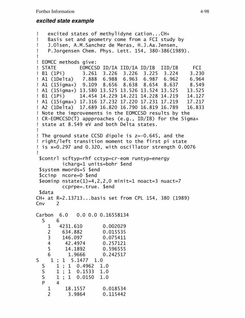
Further Information 4-98
excited state example
! excited states of methylidyne cation...CH+! Basis set and geometry come from a FCI study by! J.Olsen, A.M.Sanchez de Meras, H.J.Aa.Jensen,! P.Jorgensen Chem. Phys. Lett. 154, 380-386(1989).!! EOMCC methods give:! STATE EOMCCSD ID/IA IID/IA ID/IB IID/IB FCI! B1 (1Pi) 3.261 3.226 3.226 3.225 3.224 3.230! A1 (1Delta) 7.888 6.988 6.963 6.987 6.962 6.964! A1 (1Sigma+) 9.109 8.656 8.638 8.654 8.637 8.549! A1 (1Sigma+) 13.580 13.525 13.526 13.524 13.525 13.525! B1 (1Pi) 14.454 14.229 14.221 14.228 14.219 14.127! A1 (1Sigma+) 17.316 17.232 17.220 17.231 17.219 17.217! A2 (1Delta) 17.689 16.820 16.790 16.819 16.789 16.833! Note the improvements in the EOMCCSD results by the! CR-EOMCCSD(T) appproaches (e.g., ID/IB) for the Sigma+! state at 8.549 eV and both Delta states.!! The ground state CCSD dipole is z=-0.645, and the! right/left transition moment to the first pi state! is x=0.297 and 0.320, with oscillator strength 0.0076! $contrl scftyp=rhf cctyp=cr-eom runtyp=energy icharg=1 units=bohr $end $system mwords=5 $end $ccinp ncore=0 $end $eominp nstate(1)=4,2,2,0 minit=1 noact=3 nuact=7 ccprpe=.true. $end $dataCH+ at R=2.13713...basis set from CPL 154, 380 (1989)Cnv 2
Carbon 6.0 0.0 0.0 0.16558134 S 6 1 4231.610 0.002029 2 634.882 0.015535 3 146.097 0.075411 4 42.4974 0.257121 5 14.1892 0.596555 6 1.9666 0.242517S 1 ; 1 5.1477 1.0 S 1 ; 1 0.4962 1.0 S 1 ; 1 0.1533 1.0 S 1 ; 1 0.0150 1.0 P 4 1 18.1557 0.018534 2 3.9864 0.115442
Further Information 4-99
3 1.1429 0.386206 4 0.3594 0.640089 P 1 ; 1 0.1146 1.0 P 1 ; 1 0.011 1.0 D 1 ; 1 0.75 1.0
Hydrogen 1.0 0.0 0.0 -1.97154866 S 3 1 1.924060D+01 3.282800D-02 2 2.899200D+00 2.312080D-01 3 6.534000D-01 8.172380D-01 S 1 ; 1 1.776D-01 1.0 S 1 ; 1 2.5D-02 1.0 P 1 ; 1 1.0 1.0 $end
resource requirements
User can perform LCCD, CCD, and CCSD calculations, thatis without calculating the [T], (T), (2,3), and (TQ)corrections, or calculate the entire set of the standardand renormalized [T], (T), (2,3), and (TQ) ground-statecorrections, in addition to the CCSD energies. User canalso perform the EOMCCSD calculations of excited states andstop at EOMCCSD or continue to obtain some or all CR-EOMCCSD(T) triples corrections (cf. the values of inputvariable CCTYP in $CONTRL and $EOMINP group). Finally, usercan perform the calculations of ground-state properties atthe CCSD level or calculate ground- and excited-stateproperties. It is also possible to combine some of theabove calculations. For example, one can calculate the CCSDand EOMCCSD properties and obtain triples corrections tothe calculated CCSD and EOMCCSD energies from a singleinput (see the example above). The CR-CC(2,3) calculationproduces the MBPT(2) and CCSD energies, and CCSD one-electron properties and density matrices, in addition tothe CR-CC(2,3) and some other CR-CC triples corrections tothe CCSD energies, again all from a single input (CCTYP=CR-CCL). The most expensive steps in CC/EOMCC calculationsscale as follows:
LCCD, CCD, CCSD, EOMCCSD No**2 times Nu**4 (iterative)
CCSD[T], CCSD(T), R-CCSD[T], R-CCSD(T), CR-CCSD[T],CR-CCSD(T), CR-CC(2,3) (#1), CR-EOMCCSD(T) (#2) No**3 times Nu**4 (non-iterative) plus No**2 times Nu**4 (iterative)
Further Information 4-100
CCSD(TQ), R-CCSD(TQ), CR-CCSD(TQ) No**2 times Nu**5 or Nu**6 (#3) (non-iterative) plus No**3 times Nu**4 (non-iterative) plus No**2 times Nu**4 (iterative)
----
(#1) In addition to the usual No**2 times Nu**4 iterativeCCSD steps and No**3 times Nu**4 non-iterative steps neededto determine the (2,3) triples correction, the CR-CC(2,3)calculations require extra No**2 times Nu**4 iterativesteps needed to obtain the left CCSD state, which entersthe CR-CC(2,3) triples correction formula.(#2) In addition to the No**2 times Nu**4 iterativeCCSD and EOMCCSD steps and No**3 times Nu**4 non-iterative(T) steps that are common to all CR-EOMCCSD(T) models,the CR-EOMCCSD(T),III method requires the iterativeNo**2 times Nu**4 steps of CISD. The CR-EOMCCSD(T),IXand CR-EOMCCSD(T),IIX (X=A-D) methods do not requirethese additional CISD calculations.(#3) To reduce the cost, the program will automaticallychoose between the No**2 times Nu**5 and Nu**6 algorithmsin the (Q) part, depending on the ratio of Nu to No.----
The cost of calculating the standard CCSD[T] and CCSD(T)energies and the cost of calculating the R-CCSD[T] and R-CCSD(T) energies are essentially the same. The cost ofcalculating the triples corrections of the CR-CCSD[T] andCR-CCSD(T) approaches is essentially twice the cost ofcalculating the standard CCSD[T] and CCSD(T) corrections.Similar relationships hold between the costs of theCCSD(TQ), R-CCSD(TQ), and CR-CCSD(TQ) calculations. Thecost of calculating the triples corrections of the CR-CC(2,3),X (X=A-D) approaches is also twice the cost ofcalculating the CCSD[T] and CCSD(T) triples corrections,but additional No**2 times Nu**4 iterative steps arerequired to generate the left CCSD state after convergingthe CCSD equations in order to calculate the final CR-CC(2,3) energies. Although the noniterative triplescorrections may be seen to grow as the seventh power of thesystem size, they often require less time than the sixthpower iterations of the CCSD step, while providing a greatincrease in accuracy. Similar remarks apply to the CR-EOMCCSD(T) calculations: The cost of the CR-EOMCCSD(T)calculation for a single electronic state, in itsnoniterative triples part, is twice the cost of computing

Further Information 4-101
the standard (T) corrections of CCSD(T). The total CPU timeof the CR-EOMCCSD(T) calculations scales linearly with thenumber of calculated states. In spite of the formal N**6scaling, the calculations of the CCSD/EOMCCSD propertiesper single electronic state are considerably less expensivethan the CCSD calculations for two reasons. First of all,the process of obtaining the left eigenstates of thesimilarity transformed Hamiltonian H-bar can reuse theintermediates (matrix elements of H-bar) which are obtainedin the prior CCSD calculations. Second, converging lefteigenstates of H-bar is usually much quicker thanconverging the CCSD equations when one obtains the lefteigenstates of H-bar by solving the linear system ofequations for the L deexcitation amplitudes afterdetermining the R excitation amplitudes and excitationenergies. This means that computing properties at theCCSD/EOMCCSD level is not very expensive once the CCSD andEOMCCSD right eigenvectors are obtained. Similar remarksapply to the CR-CC(2,3) calculations, which require theleft CCSD eigenstates in addition to the CCSD T1 and T2amplitudes: The determination of the left CCSD states thatare needed to determine the non-iterative triplescorrections of the CR-CC(2,3) approach makes the entireCCSD part of the CR-CC(2,3) calculation only somewhat moreexpensive than the regular CCSD iterations needed to obtainT1 and T2 clusters. The CCSD(TQ), R-CCSD(TQ), and CR-CCSD(TQ) calculations are more expensive than the CCSD(T)calculations, in spite of the fact that all of thesemethods use non-iterative N**7 steps. This is related tothe fact that the No**2 times Nu**5 steps of the (TQ)methods are more expensive than the No**3 times Nu**4 stepsof the (T) approaches. On the other hand, the CCSD(TQ), R-CCSD(TQ), and CR-CCSD(TQ) methods are much less expensivethan the iterative ways of obtaining the information aboutquadruply excited clusters. This is a result of anefficient use of diagram factorization in coding theCCSD(TQ), R-CCSD(TQ), and CR-CCSD(TQ) methods, which leadsto a reduction of the N**9-type steps in the original (Q)expressions to N**7 steps.
Rough estimates of the memory required are:
CCSD 4 No**2 times Nu**2 + No times Nu**3
CCSD[T], CCSD(T), R-CCSD[T], R-CCSD(T) 4 No**2 times Nu**2 + No times Nu**3
CR-CCSD[T], CR-CCSD(T) No**2 times Nu**2 + 2 * No times Nu**3 (faster algorithm)

Further Information 4-102
4 No**2 times Nu**2 + No times Nu**3 (slower, less memory)
CR-CC(2,3) The most expensive routine requires 3 * No * Nu**3 + 3 * Nu**3 + 5 * No**2 *Nu**2 words
CCSD(TQ),b, R-CCSD(TQ)-n,x (n=1,2;x=a,b), CR-CCSD(TQ),x(x=a,b)2 * No times Nu**3 + No**2 times Nu**2 + Nu**3, precededand followed by steps that require memories, such as, forexample, 3 * Nu**3 + 5 * No**2 * Nu**2
EOMCCSD No times Nu**3 + 4 No**2 times Nu**2 (MEOM=0,1) if MEOM=2, add to this (4 times number of roots + 2) times No**2 times Nu**2
CR-EOMCCSD(T),IX, 2 * No times Nu**3 + 3 No**2 times Nu**2CR-EOMCCSD(T),IIX(X=A-D) [MTRIP=1 in $EOMINP]
CR-EOMCCSD(T) 3 * No times Nu**3 + 5 No**2 times Nu**2all variants (faster algorithm) [MTRIP=2 in $EOMINP]
CR-EOMCCSD(T),III 2 * No times Nu**3 + 5 No**2 times Nu**2[MTRIP=3 in $EOMINP]
CR-EOMCCSD(T) 2 * No times Nu**3 + 5 No**2 times Nu**2all variants (slower algorithm) [MTRIP=4 in $EOMINP]
The program automatically selects the algorithm for the CR-CCSD[T] and CR-CCSD(T) calculations, depending on theamount of available memory. A similar remark applies to theEOMCCSD calculations, where some additional reductions ofmemory requirements are possible if memory is low. Theabove estimates are rough.
The time required for calculating the CR-CCSD[T] and CR-CCSD(T) triples corrections is only twice the time used tocalculate the standard CCSD[T] and CCSD(T) corrections.Thus, by just doubling the CPU time for the noniterativetriples corrections and by selecting CCTYP=CR-CC, we gainaccess to all six noniterative triples corrections (theCCSD[T], CCSD(T), R-CCSD[T], R-CCSD(T), CR-CCSD[T], and CR-CCSD(T) energies) plus, of course, to the MBPT(2) and CCSDenergies. At the same time, the CR-CCSD[T] and CR-CCSD(T)results for stretched nuclear geometries and diradicals arebetter than the results of the conventional CCSD[T] andCCSD(T) calculations. In some cases, choosing CCTYP=R-CCmight be reasonable, too. The choice CCTYP=R-CC gives fivedifferent energies (CCSD, CCSD[T], CCSD(T), R-CCSD[T], and

Further Information 4-103
R-CCSD(T)) for the price of three (CCSD, CCSD[T], andCCSD(T)) as the there is no extra time needed for the R-theories compared to the standard ones. If we ignore theiterative CCSD steps and additional iterative steps neededto determine the left CCSD state, the time required forcalculating the size extensive CR-CC(2,3) triplescorrections is also only twice the time of calculating theCCSD[T] and CCSD(T) corrections. There is an additionalbonus though: The CR-CC(2,3) calculations automaticallyproduce a variety of CCSD one-electron properties at noextra cost. Similar remarks apply to quadruples and excitedstate calculations, although in the latter case a lotdepends on user's expectations. If user is only interestedin excited states dominated by singles and if accuracies onthe order of 0.1-0.3 eV (sometimes better, sometimes worse)are acceptable, EOMCCSD is a good choice. However, it maybe worth improving the EOMCCSD results by performing theCR-EOMCCSD(T) calculations, which often lower the errors incalculated excited states to 0.1 eV or less without makingthe calculations a lot more expensive (the CR-EOMCCSD(T)corrections are noniterative, so that the CPU time neededto calculate them may be comparable to the time spent inall EOMCCSD iterations). If there is a risk of encounteringlow-lying states having significant doubly excitedcontributions or multi-reference character, choosing CR-EOMCCSD(T) is a necessity, since errors obtained in EOMCCSDcalculations for states dominated by doubles can easily beon the order of 1 eV. The CCSD(T) approach is often finefor closed-shell molecules, but there are cases, such asthe vibrational frequencies of ozone and properties ofother multiply bonded systems, where inclusion ofquadruples is necessary. The CR-CCSD(T) approach is veryuseful in cases involving single bond breaking anddiradicals, but CR-CC(2,3) and CR-CCSD(TQ) should bebetter. In addition, the CR-CC(2,3) method providesrigorously size extensive results. In cases of multiplebond dissociations, CR-CCSD(TQ) is a better alternative.The program is organized such that choosing a CR-CCSD(TQ)option (CCTYP=CR-CC(Q)) produces all energies obtained withCCTYP=CR-CCSD(T) and all CCSD(TQ), R-CCSD(TQ), and CR-CCSD(TQ) energies. By selecting CCTYP=CCSD(TQ), the usercan obtain the CCSD(TQ) and R-CCSD(TQ) energies, inaddition to the CCSD, CCSD[T], CCSD(T), R-CCSD[T], and R-CCSD(T) energies.
We encourage the user to read papers, such as P.Piecuch, S.A.Kucharski, K.Kowalski, M.Musial Comput. Phys. Comm., 149, 71-96(2002); K. Kowalski and P. Piecuch,

Further Information 4-104
J. Chem. Phys., 120, 1715-1738 (2004); M. Wloch, J.R. Gour, K. Kowalski, and P. Piecuch, J. Chem. Phys. 122, 214107 (2005); K. Kowalski, P. Piecuch, M. Wloch, S.A. Kucharski, M. Musial, and M.W. Schmidt, in preparation,where time and memory requirements for various types of CCand EOMCC calculations are described in considerabledetail.
restarts in ground-state calculations
The CC code incorporated in GAMESS is quite good inconverging the CCSD equations with the default guess forcluster amplitudes. The code is designed to converge inrelatively few iterations for significantly stretchednuclear geometries, where it is not unusual to obtain largecluster amplitudes whose absolute values are close to 1.This is accomplished by combining the standard Jacobialgorithm with the DIIS extrapolation method of Pulay. Themaximum number of amplitude vectors used in the DIISextrapolation procedure is defined by the input variableMXDIIS. The default for MXDIIS is as follows: MXDIIS = 5, for 5 < No*Nu, MXDIIS = 3, for 2 < No*Nu < 6, MXDIIS = 0, for No*Nu < 3.Thus, in the vast majority of cases, the default value ofMXDIIS is 5. However, for very small problems, when theDIIS expansion subspace leads to singular systems of linearequations, it is necessary to reduce the value of MXDIIS to2-4 (we chose 3) or switch off DIIS altogether (which isthe case when MXDIIS = 0).
It may, of course, happen that the solver for the CCSDequations does not converge, in spite of increasing themaximum number of iterations (input variable MAXCC; thedefault value is 30) and in spite of changing the defaultvalue of MXDIIS. In order to facilitate the calculationsin all such cases, we included the restart option in the CCcodes incorporated in GAMESS. Thus, user can restart aCCSD (or (L)CCD) calculation from the restart file createdby an earlier CC calculation. In order to use the restartoption, user must save the disk file CCREST (unit 70) fromthe previous CC run (cf. the GAMESS script rungms) and makesure that this file is copied to scratch directory wherethe restarted calculation is carried out. A restart isinvoked by entering a nonzero value for IREST, which shouldbe the number of the last iteration completed, and must be

Further Information 4-105
some value greater than or equal 3. Examples of using therestart option include the following situations:
o The CCSD program did not converge in MAXCC iterations, but there is a chance to converge it if the value of MAXCC is increased. User restarts the calculation with the increased value of MAXCC.
o User ran a CCSD calculation, obtaining the converged CCSDenergy, but later decided to run CR-CCSD(T) or CR-CC(2,3)calculation. Instead of running the entire CCSD --> CR-CCSD(T) or CCSD --> CR-CC(2,3) task again, user restartsthe calculation after changing the value of inputvariable CCTYP to CR-CC (the CR-CCSD(T) case) or CR-CCL(the CR-CC(2,3) case) and entering IREST to reuse theprevious CCSD amplitudes, proceeding at once to the non-iterative triples corrections (left CCSD calculations andtriples corrections in the CR-CC(2,3) case).
o The CCSD program diverged for some geometry with a significantly stretched bond. User performs an extra calculation for a different nuclear geometry, for which it is easier to converge the CCSD equations, and restarts the calculation from the restart file generated by an extra calculation. This technique of restarting the CC calculations from the cluster amplitudes obtained for a neighboring nuclear geometry is particularly useful for scanning PESs and for calculating energy derivatives by numerical differentiation.
There also are situations where restart of the ground-state CCSD calculations is useful for excited-state andproperty calculations:
o User ran a CCSD, CCSD(T), or CR-CCSD(T) calculation, obtaining the converged CC energies for the ground state, but later decided to run an excited-state EOMCCSD or CR-EOMCCSD(T) calculations. Instead of running the entire CCSD --> EOMCCSD or CCSD --> CR-EOMCCSD(T) task, user restarts the calculation after changing the value of input variable CCTYP to EOM-CCSD or CR-EOM, selecting excited-state options in $EOMINP, and entering IREST greater or equal to 3 to reuse the previously converged CCSD amplitudes, proceeding at once to the excited-state (EOMCCSD or CR-EOMCCSD(T)) calculations.
o User ran an EOMCCSD excited-state calculation, obtaining the converged CCSD amplitudes, but later discovered (by analyzing R1 and R2 amplitudes and REL values)
Further Information 4-106
that some states are dominated by doubles, so that the EOMCCSD results need to be improved by the CR-EOMCCSD(T) triples corrections. Instead of running the entire CCSD --> CR-EOMCCSD(T) task, user restarts the calculation after changing the value of input variable CCTYP from EOM-CCSD to CR-EOM, and entering IREST greater or equal to 3 to reuse the previously converged CCSD amplitudes, proceeding at once to the EOMCCSD and CR-EOMCCSD(T) calculations.
o User ran a CR-CCSD(T) calculation, obtaining theconverged ground-state energies, but later decided to runCCSD and EOMCCSD properties. Instead of running the CCSD--> EOMCCSD task again, user restarts the calculation afterchanging the value of input variable CCTYP to EOM-CCSD,adding CCPRPE=.TRUE. and the desired values of NSTATE in$EOMINP, and entering IREST to reuse the previouslyconverged CCSD amplitudes, proceeding at once to CCSD andEOMCCSD properties.
initial guesses in excited-state calculations
The EOMCCSD calculation is an iterative procedure whichneeds initial guesses for the excited states of interest.The popular initial guess for the EOMCCSD calculations isobtained by performing the CIS calculations (diagonalizingthe Hamiltonian in a space of singles only). This isacceptable for states dominated by singles, but user mayencounter severe convergence difficulties or even miss somestates entirely if the calculated states have significantdoubly excited character. One possible philosophy is notto worry about it and use the CIS initial guess only, sinceEOMCCSD fails to describe states with large doubly excitedcomponents. This is not the philosophy of the EOMCCprograms in GAMESS. GAMESS is equipped with the CR-EOMCCSD(T) triples corrections to EOMCCSD energies, whichare capable of reducing the large errors in the EOMCCSDresults for states dominated by two-electron transitions,on the order of 1 eV, to 0.1 eV or even less. Thus, theability to capture states with significant doubly excitedcontributions is an important element of the EOMCC GAMESScodes.
Excited states with significant contributions fromdouble excitations can easily be found by using the EOMCCSd(little d) initial guesses provided by GAMESS. In theEOMCCSd calculations (and analogous CISd calculations usedto initiate the CISD calculations for the CR-EOMCCSD(T),III

Further Information 4-107
method), the initial guesses for the calculated excitedstates are defined using all single excitations (letter Sin EOMCCSd and CISd) and a small subset of doubleexcitations (the little d in EOMCCSd and CISd) defined byactive orbitals or orbital range specified by the user.The inclusion of a small set of active double excitationsin addition to all singles in the initial guess greatlyfacilitates finding excited states characterized byrelatively large doubly excited amplitudes. GAMESS inputoffers a choice between the CIS and EOMCCSd/CISd initialguesses. The use of EOMCCSd/CISd initial guesses is highlyrecommended. This is accomplished by setting the inputvariable MINIT at 1 and by selecting the orbital range(active orbitals to define "little doubles" d) through thenumbers of active occupied and active unoccupied orbitals(variables NOACT and NUACT, respectively) or an array ofactive orbitals called MOACT.
eigensolvers for excited-state calculations
The basic eigensolver for the EOMCCSD calculations isthe Hirao and Nakatsuji's generalization of the Davidsondiagonalization algorithm to non-Hermitian problems (thesimilarity transformed Hamiltonian H-bar is non-Hermitian).GAMESS offers the following three choices of EOMCCSDeigensolvers for the right eigenvalue problem (R amplitudesand energies only):o the true multi-root eigensolver based on the Hirao and Nakatsuji's algorithm, in which all states are calculated at once using a united iterative space (variable MEOM=2).o the single-root eigensolver, in which one calculates one state at a time, but the iterative subspace corresponding to all calculated roots remains united (variable MEOM=0).o the single-root eigensolver, in which one calculates one state at a time and each calculated root has a separate iterative subspace (variable MEOM=1).
The latter option (MEOM=1) leads to the fastestalgorithm, but there is a risk (often worth taking) thatsome states will be converged more than once. The truemulti-root eigensolver (MEOM=2) is probably the safest, butit is also the most expensive solver and there are somerisks associated with using it too. When MEOM=2, there isa risk that one root, which is difficult to converge, maycause the entire multi-root procedure fail in spite of thefact that all other roots participating in the calculation
Further Information 4-108
converged. The EOMCCSD program in GAMESS is prepared tohandle this problem by saving individual roots thatconverged during multi-root iterations in case the entireprocedure fails because of one or more roots which aredifficult to converge. In this way, at least some rootsare saved for the subsequent CR-EOMCCSD(T) calculations.The middle option (MEOM=0) seems to offer the bestcompromise. MEOM=0 is a single-root eigensolver, so thereare no risks associated with loosing some states duringmulti-root calculations. At the same time, the use of theunited iterative subspace for all calculated roots helps toeliminate the problem of MEOM=1 of obtaining the same rootmore than once. The single-root eigensolver with a unitediterative subspace (MEOM=0) is recommended (and used as adefault), although other ways of converging the rightEOMCCSD equations (MEOM=1,2) are very useful too.
As pointed out earlier, in order to calculate reduceddensity matrices and properties using CCSD and EOMCCSDmethods, one has to determine the left as well as the righteigenstates of the non-Hermitian similarity transformedHamiltonian H-bar. For the ground state, this is done bysolving the linear system of equations for the deexcitationoperator Lambda (in the CCSD case, the one- and two-bodycomponents Lambda1 and Lambda2). For the amplitudesdefining the L1 and L2 components of the excited-stateoperator L, one can proceed in several different ways andthese different ways are reflected in the EOMCCSD algorithmincorporated in GAMESS. One can, for example, solve thelinear system of equations for the amplitudes defining theEOMCCSD deexcitation operator L=L1+L2, after determiningthe corresponding excitation operator R=R1+R2 andexcitation energy omega. This is a highly recommendedoption, which is also a default in GAMESS. This option isexecuted with any choice of MEOM=0,1,2 and when the userselects CPRPE=.TRUE. In case of unlikely difficulties withobtaining the L1 and L2 components, one can solve for theEOMCCSD values of the L1,L2 and R1,R2 amplitudes andexcitation energies simultaneously in the process ofdiagonalizing the similarity transformed Hamiltonian H-barcompletely in a single sequence of iterations. Thisapproach is reflected by the following two additionalchoices of the input variable MEOM:o MEOM=3, one root at a time, separate iterative space for each computed root, left and right eigenvectors of the similarity transformed Hamiltonian and energies (like MEOM=1, but both left and right eigenvectors are iterated).o MEOM=4, one root at a time, united iterative spaces

Further Information 4-109
for all calculated roots, left and right eigenvectors of the similarity transformed Hamiltonian and energies (like MEOM=0, but both left and right eigenvectors are iterated).In both cases, the user has to select CCPRPE=.TRUE. inorder for these two choices of MEOM to work.
references and citations required in publications
Any publication describing the results of CC calculationsobtained using GAMESS should give reference to the relevantpapers. Depending on the specific CCTYP value, these are:
CCTYP = LCCD, CCD, CCSD, CCSD(T)P. Piecuch, S.A. Kucharski, K. Kowalski, and M. Musial Comput. Phys. Commun. 149, 71-96 (2002).
CCTYP = R-CC, CR-CC, CCSD(TQ), CR-CC(Q)P. Piecuch, S.A. Kucharski, K. Kowalski, and M. Musial Comput. Phys. Commun. 149, 71-96 (2002);K. Kowalski and P. Piecuch J. Chem. Phys. 113, 18-35 (2000);K. Kowalski and P. Piecuch J. Chem. Phys. 113, 5644-5652 (2000).
CCTYP = CR-CCLP. Piecuch, S.A. Kucharski, K. Kowalski, and M. Musial Comput. Phys. Commun. 149, 71-96 (2002);P. Piecuch and M. Wloch J. Chem. Phys. 123, 224105/1-10 (2005).
CCTYP = EOM-CCSD, CR-EOMP. Piecuch, S.A. Kucharski, K. Kowalski, and M. Musial Comput. Phys. Commun. 149, 71-96 (2002);K. Kowalski and P. Piecuch, J. Chem. Phys. 120, 1715-1738 (2004);M. Wloch, J.R. Gour, K. Kowalski, and P. Piecuch, J. Chem. Phys. 122, 214107-1 - 214107-15 (2005).
CCTYP = CR-EOMLP. Piecuch, J. R. Gour, and M. Wloch Int. J. Quantum Chem. 109, 3268-3304(2009)and the first two papers cited for CR-EOM just above
CCTYP = IP-EOM2, EA-EOM2J. R. Gour, P. Piecuch, M. Wloch J. Chem. Phys. 123, 134113/1-14(2005)J. R. Gour, P. Piecuch

Further Information 4-110
J. Chem. Phys. 125, 234107/1-17(2006)
In addition, the explicit use of CCPRP=.TRUE. in $CCINPand/or the use of CCPRPE=.TRUE. in $EOMINP should reference
M. Wloch, J.R. Gour, K. Kowalski, and P. Piecuch, J. Chem. Phys. 122, 214107/1-15 (2005).
---The rest of this section is a list of references to theoriginal formulation of various areas in Coupled-ClusterTheory relevant to methods available in GAMESS:
Electronic structure:J. Cizek, J. Chem. Phys. 45, 4256 (1966).J. Cizek, Adv. Chem. Phys. 14, 35 (1969).J. Cizek, J. Paldus, Int.J.Quantum Chem. 5, 359 (1971).
Nuclear theory (examples):F. Coester, Nucl. Phys. 7, 421 (1958).F. Coester, H. Kuemmel, Nucl. Phys. 17, 477 (1960).K. Kowalski, D.J. Dean, M. Hjorth-Jensen, T. Papenbrock, P. Piecuch, Phys. Rev. Lett. 92, 132501 (2004).D.J. Dean, J.R. Gour, G. Hagen, M. Hjorth-Jensen, K. Kowalski, T. Papenbrock, P. Piecuch, M. Wloch, Nucl. Phys. A. 752, 299 (2005).M. Wloch, D.J. Dean, J.R. Gour, P. Piecuch, M. Hjorth-
Jensen, T. Papenbrock, K. Kowalski, Eur. Phys. J. A 25(Suppl. 1), 485 (2005).
M. Wloch, J.R. Gour, P. Piecuch, D.J. Dean, M. Hjorth-Jensen, T. Papenbrock, J. Phys. G: Nucl. Phys. 31,S1291 (2005).
M. Wloch, D.J. Dean, J.R. Gour, M. Hjorth-Jensen, K. Kowalski, T. Papenbrock, P. Piecuch, Phys. Rev. Lett. 94, 212501 (2005).P. Piecuch, M. Wloch, J.R. Gour, D.J. Dean, M. Hjorth- Jensen, T. Papenbrock, in V. Zelevinsky (Ed.), Nuclei and Mesoscopic Physics, AIP Conference
Proceedings, Vol. 777 (AIP Press, 2005), p. 28.D.J. Dean, M. Hjorth-Jensen, K. Kowalski, T. Papenbrock, M.
Wloch, and P. Piecuch, in Key Topics in NuclearStructure, Proceedings of the 8th International SpringSeminar on Nuclear Physics, edited by A. Covello(World Scientific, Singapore, 2005), p. 147.
Coupled-Cluster Method with Doubles (CCD) -J. Cizek, J. Chem. Phys. 45, 4256 (1966).J. Cizek, Adv. Chem. Phys. 14, 35 (1969).J. Cizek, J. Paldus, Int.J.Quantum Chem. 5, 359 (1971).

Further Information 4-111
J.A. Pople, R. Krishnan, H.B. Schlegel, J.S. Binkley, Int. J. Quantum Chem. Symp. 14, 545 (1978).R.J. Bartlett and G.D. Purvis, Int. J. Quantum Chem. Symp. 14, 561 (1978).J. Paldus, J. Chem. Phys. 67, 303 (1977) [orthogonally spin-adapted formulation].
Linearized Coupled-Cluster Method with Doubles (LCCD; cf., also, D-MBPT(infinity), CEPA(0))J. Cizek, J. Chem. Phys. 45, 4256 (1966).J. Cizek, Adv. Chem. Phys. 14, 35 (1969).R.J. Bartlett, I. Shavitt, Chem.Phys.Lett.50, 190 (1977) 57, 157 (1978) [Erratum].R. Ahlrichs, Comp. Phys. Commun. 17, 31 (1979).
Coupled-Cluster Method with Singles and Doubles (CCSD) -G.D.Purvis III, R.J.Bartlett, J.Chem.Phys. 76, 1910 (1982) [spin-orbital formulation].P. Piecuch, J. Paldus, Int.J.Quantum Chem. 36, 429 (1989). [orthogonally spin-adapted formulation].G.E.Scuseria, A.C.Scheiner, T.J.Lee, J.E.Rice, H.F.Schaefer III, J. Chem. Phys. 86, 2881 (1987) [non-orthogonally spin-adapted formulation].G.E. Scuseria, C.L. Janssen, H.F.Schaefer III J. Chem. Phys. 89, 7382 (1988) [non-orthogonally spin-adapted formulation].T.J. Lee and J.E. Rice, Chem. Phys. Lett. 150, 406 (1988) [non-orthogonally spin-adapted formulation].
Coupled-Cluster Method with Singles and Doubles andNoniterative Triples, CCSD[T] = CCSD+T(CCSD) -M. Urban, J. Noga, S. J. Cole, and R. J. Bartlett, J. Chem. Phys. 83, 4041 (1985).P. Piecuch and J. Paldus, Theor. Chim. Acta 78, 65 (1990) [orthogonally spin-adapted formulation].P. Piecuch, S. Zarrabian, J. Paldus, and J. Cizek, Phys. Rev. B 42, 3351-3379 (1990) [orthogonally spin-adapted formulation].P. Piecuch, R. Tobola, and J. Paldus, Int. J. Quantum Chem. 55, 133-146 (1995) [orthogonally spin-adapted formulation].
Coupled-Cluster Method with Singles and Doubles andNoniterative Triples, CCSD(T) -K. Raghavachari, G. W. Trucks, J. A. Pople, M. Head-Gordon, Chem. Phys. Lett. 157, 479 (1989).
Equation of Motion Coupled-Cluster Method, ResponseCC/Time Dependent CC Approaches, SAC-CI (Original Ideas), -

Further Information 4-112
H. Monkhorst, Int. J. Quantum Chem. Symp. 11, 421 (1977).K. Emrich, Nucl. Phys. A 351, 379 (1981).H. Sekino and R.J. Bartlett, Int. J. Quantum Chem. Symp. 18, 255 (1984).E. Daalgard and H. Monkhorst, Phys. Rev. A 28, 1217 (1983).M. Takahashi and J. Paldus, J. Chem. Phys. 85, 1486 (1986).H. Koch and P. Jorgensen, J. Chem. Phys. 93, 3333 (1990).H. Nakatsuji, K. Hirao, Chem. Phys. Lett. 47, 569 (1977).H. Nakatsuji, K. Hirao, J.Chem.Phys. 68, 2053, 4279 (1978).
Equation of Motion Coupled-Cluster Method with Singles andDoubles, EOMCCSD -J. Geertsen, M. Rittby, and R.J. Bartlett, Chem. Phys. Lett. 164, 57 (1989).J.F. Stanton and R.J. Bartlett, J. Chem. Phys. 98, 7029 (1993).
Method of Moments of Coupled-Cluster Equations andRenormalized and Completely Renormalized Coupled-ClusterMethods (Overviews) -P. Piecuch, K. Kowalski, I.S.O. Pimienta, S.A. Kucharski, in M.R. Hoffmann, K.G. Dyall (Eds.), Low-Lying Potential Energy Surfaces, ACS Symposium Series, Vol. 828, Am. Chem. Society, Washington, D.C., 2002, p. 31 [ground and excited states].P. Piecuch, K. Kowalski, I.S.O. Pimienta, M.J. McGuire, Int. Rev. Phys. Chem. 21, 527 (2002) [ground and excited states].P. Piecuch, I.S.O. Pimienta, P.-F. Fan, K. Kowalski, in J. Maruani, R. Lefebvre, E. Brandas (Eds.), Progress in Theoretical Chemistry and Physics, Vol. 12, Advanced Topics in Theoretical Chemical Physics, Kluwer, Dordrecht, 2003, p. 119 [ground states].P. Piecuch, K. Kowalski, I.S.O. Pimienta, P.-D. Fan, M. Lodriguito, M.J. McGuire, S.A. Kucharski, T. Kus, M. Musial, Theor. Chem. Acc. 112, 349 (2004) [ground and excited states].P. Piecuch, M. Wloch, M. Lodriguito, and J.R. Gour, in S. Wilson, J.-P. Julien, J. Maruani, E. Brandas, and G. Delgado-Barrio (Eds.), Progress in Theoretical Chemistry and Physics, Vol. 15, Recent Advances in the Theory of Chemical and Physical Systems, Springer, Berlin, 2006, p. XX, in press [excited states].P. Piecuch, I.S.O. Pimienta, P.-D. Fan, and K. Kowalski, in A.K. Wilson (Ed.), Recent Progress in Electron Correlation Methodology, ACS Symposium Series, Vol. XXX, Am. Chem. Society, Washington, D.C., 2006, p. XX
Further Information 4-113
[in press; ground states].P.-D. Fan and P. Piecuch, Adv. Quantum Chem., in press
(2006).
Renormalized and Completely Renormalized Coupled-ClusterMethods, Method of Moments of Coupled-Cluster Equations(Initial Original Papers, Ground States) -P. Piecuch, K. Kowalski, in J. Leszczynski (Ed.), Computational Chemistry: Reviews of Current Trends, Vol. 5, World Scientific, Singapore, 2000, p. 1.K. Kowalski, P. Piecuch, J. Chem. Phys. 113, 18 (2000).K. Kowalski, P. Piecuch, J. Chem. Phys. 113, 5644 (2000).
Biorthogonal Method of Moments of Coupled-Cluster Equationsand Size Extensive Completely Renormalized Coupled-ClusterSingles, Doubles, and Non-iterative Triples Approach (CR-CC(2,3)=CR-CCSD(T)L; Initial Original Papers) –P. Piecuch and M. Wloch, J. Chem. Phys. 123, 224105(2005).P. Piecuch, M. Wloch, J.R. Gour, and A. Kinal, Chem. Phys.
Lett. 418, 467-474 (2006).
Renormalized and Completely Renormalized Coupled-ClusterMethods, Method of Moments of Coupled-Cluster Equations(Other Original Papers, Higher-Order Methods, Ground-StateBenchmarks) -K. Kowalski, P. Piecuch, Chem. Phys. Lett. 344, 165 (2001).P. Piecuch, S.A. Kucharski, K. Kowalski, Chem. Phys. Lett. 344, 176 (2001).P. Piecuch, S.A. Kucharski, V. Spirko, K. Kowalski, J.Chem.Phys. 115, 5796 (2001).P. Piecuch, K. Kowalski, and I.S.O. Pimienta, Int. J. Mol. Sci. 3, 475 (2002).M.J. McGuire, K. Kowalski, P. Piecuch, J. Chem. Phys. 117, 3617 (2002).P. Piecuch, S.A. Kucharski, K. Kowalski, M. Musial, Comput. Phys. Comm., 149, 71 (2002).I.S.O. Pimienta, K. Kowalski, and P. Piecuch, J. Chem. Phys. 119, 2951 (2003).S. Hirata, P.-D. Fan, A.A. Auer, M. Nooijen, P. Piecuch, J. Chem. Phys. 121, 12197 (2004).K. Kowalski and P. Piecuch, J. Chem. Phys. 122, 074107 (2005).P.-D. Fan, K. Kowalski, and P. Piecuch, Mol. Phys. 103,
2191 (2005).
Completely Renormalized Coupled-Cluster Methods, Examplesof Large-Scale Applications to Ground-State Properties -I. Ozkan, A. Kinal, M. Balci,

Further Information 4-114
J.Phys.Chem. A 108, 507 (2004).R.L. DeKock, M.J. McGuire, P. Piecuch, W.D. Allen,H.F. Schaefer III, K. Kowalski, S.A. Kucharski, M. Musial,A.R. Bonner, S.A. Spronk, D.B Lawson, S.L. Laursen, J. Phys. Chem. A 108, 2893 (2004).M.J. McGuire, P. Piecuch, K. Kowalski, S.A. Kucharski, M. Musial, J. Phys. Chem. A 108, 8878 (2004).M.J. McGuire, P. Piecuch J. Am. Chem. Soc. 127, 2608 (2005).A. Kinal, P. Piecuch, J. Phys. Chem. A 110, 367 (2006).C.J. Cramer, M. Wloch, P. Piecuch, C. Puzzarini, and L.
Gagliardi, J. Phys. Chem. A 110, 1991 (2006).
Completely Renormalized Equation of Motion Coupled-ClusterMethods, Method of Moments of Coupled-Cluster Equationsfor Ground and Excited States (Original Papers) -K. Kowalski P. Piecuch, J. Chem. Phys. 115, 2966 (2001).K. Kowalski P. Piecuch, J. Chem. Phys. 116, 7411 (2002).K. Kowalski P. Piecuch, J. Chem. Phys. 120, 1715 (2004).M. Wloch, J.R. Gour, K. Kowalski, and P. Piecuch, J. Chem. Phys. 122, 214107 (2005).Also, multi-reference and other externally corrected MMCCmethods including ground and excited states,K. Kowalski and P. Piecuch, J. Molec. Struct.: THEOCHEM 547, 191 (2001).K. Kowalski and P. Piecuch, Mol. Phys. 102}, 2425 (2004).M.D. Lodriguito, K. Kowalski, M. Wloch, and P. Piecuch J. Mol. Struct: THEOCHEM, in press (2006).
Completely Renormalized Equation of Motion Coupled-ClusterMethods, Method of Moments of Coupled-Cluster Equationsfor Ground and Excited States (Selected Benchmarks andApplications)C.D. Sherrill, P. Piecuch, J.Chem.Phys. 122, 124104 (2005)R.K. Chaudhuri, K.F. Freed, G. Hose, P. Piecuch, K. Kowalski, M. Wloch, S. Chattopadhyay, D. Mukherjee, Z. Rolik, A. Szabados, G. Toth, and P.R. Surjan, J. Chem. Phys. 122, 134105-1 (2005).K. Kowalski, S. Hirata, M. Wloch, P. Piecuch, and T.L. Windus, J. Chem. Phys. 123, 074319 (2005).S. Nangia, D.G. Truhlar, M.J. McGuire, and P. Piecuch J. Phys. Chem. A 109, 11643 (2005).P. Piecuch, S. Hirata, K. Kowalski, P.-D. Fan, and T.L. Windus, Int. J. Quantum Chem. 106, 79 (2006).M. Wloch, M.D. Lodriguito, P. Piecuch, and J.R. Gour Mol. Phys., in press (2006).S. Coussan, Y. Ferro, A. Trivella, P. Roubin, R. Wieczorek,

Further Information 4-115
C. Manca, P. Piecuch, K. Kowalski, M. Wloch, S.A.Kucharski, and M. Musial, J. Phys. Chem. A, in press(2006).
Completely Renormalized Coupled-Cluster and Equation ofMotion Coupled-Cluster Methods, GAMESS Implementations -P. Piecuch, S.A. Kucharski, K. Kowalski, M. Musial, Comput. Phys. Comm., 149, 71 (2002).K. Kowalski and P. Piecuch J. Chem. Phys. 120, 1715 (2004).M. Wloch, J.R. Gour, K. Kowalski, and P. Piecuch,
J. Chem. Phys. 122, 214107 (2005).P. Piecuch and M. Wloch, J. Chem. Phys. 123, 224105 (2005).K. Kowalski, P. Piecuch, M. Wloch,S.A. Kucharski,M. Musial, and M.W. Schmidt, in preparation.
T1 diagnostic:T.J.Lee, P.R.Taylor Int.J.Quantum Chem., S23, 199-207(1989).It is often assumed that T1>0.02 indicates that CCSD maynot be correct for a system which is not very singlereference in nature. (T) corrections tolerate greatersingles amplitudes. However, T1 diagnostic is in many casesmisleading, since one can easily have small (or evenvanishing) T1 cluster amplitudes due to symmetry and asignificant configurational quasi-degeneracy and multi-reference character. In general, in typical multi-referencesituations, such as bond stretching and diradicals, oneobserves a significant increase of T2 cluster amplitudes.The larger values of T2 amplitudes are a clear signature ofa multi-reference character of the wave function. The CR-CCSD(T), CR-CCSD(TQ), and CR-CC(2,3) methods toleratesignificant increases of T2 amplitudes in cases of single-bond breaking and diradicals. CCSD(T) and CCSD(TQ)approaches cannot do this, when the spin-adapted RHFreferences are employed.
Written by Piotr Piecuch, Michigan State University(updated March 18, 2006)
Further Information 4-116
Density Functional Theory
There are actually two DFT programs in GAMESS, one usingthe typical grid quadrature for integration of functionals,and one using resolution of the identity to avoid the needor grids. The default METHOD=GRID program is discussedbelow, following a short description of METHOD=GRIDFREE.The final section is references to various functionals, andother topics of interest.
DFTTYP keywords
Let's begin with a translation table to NWchem's input: GAMESS NWchem's XC keyword Slater slater Gill gill96 SVWN slater vwn_5 Becke becke88 BVWN becke88 vwn_5 BLYP becke88 lyp B97 becke97 B97-1,B97-2,B97-3 becke97-1, becke-2, becke-3 HCTH93,HCTH120,HCTH147,HCTH407 hcth,hcth120,hcth147,hcth407 B98 becke98 B3LYP HFexch 0.20 slater 0.80 \ becke88 nonlocal 0.72 \ lyp 0.81 vwn_5 0.19 B3LYP1 b3lyp or, if you like to type: HFexch 0.20 slater 0.80 \ becke88 nonlocal 0.72 \ lyp 0.81 vwn_1_rpa 0.19 X3LYP HFexch 0.218 slater 0.782 \ becke88 nonlocal 0.542 \ xperdew91 nonlocal 0.167 \ lyp 0.871 vwn_1_rpa 0.129 PW91 xperdew91 perdew91 B3PW91 HFexch 0.20 slater 0.80 \ becke88 nonlocal 0.72 \ perdew91 0.81 pw91lda 1.00 PBE xpbe96 cpbe96 PBE0 pbe0 revPBE revpbe cpbe96

Further Information 4-117
VS98 vs98 M06 m06 (and similarly for M05-2X, etc.) PKZB xpkzb99 cpkzb99 TPSS xtpss03 cptss03 TPSSh xctpssh
Note that B3LYP in GAMESS is based in part on the VWN5electron gas correlation functional. Since there are fiveformulae with two possible parameterizations mentioned inthe VWN paper about local correlation, other programs mayuse other choices, and therefore generate different B3LYPenergies. For example, NWChem's manual says it uses the"VWN 1 functional with RPA parameters as opposed to theprescribed Monte Carlo parameters" as its default. Shouldyou wish to use this VWN1 formula in a B3LYP hybrid, simplychoose "DFTTYP=B3LYP1".
grid-free DFT
The grid-free code is a research tool into the use ofthe resolution of the identity to simplify evaluation ofintegrals over functionals, rather than quadrature grids.This trades the use of finite grids and their associatederrors for the use of a finite basis set used to expand theidentity, with an associated truncation error. The presentchoice of auxiliary basis sets was obtained by tests onsmall 2nd row molecules like NH3 and N2, and hence thebuilt in bases for the 3rd row are not as well developed.Auxiliary bases for the remaining elements do not exist atthe present time.
The grid-free Becke/6-31G(d) energy at a C1 AM1 geometryfor ethanol is -154.084592, while the result from a runusing the "army grade grid" is -154.105052. So, the errorusing the AUX3 RI basis is about 5 milliHartree per 2nd rowatom (the H's must account for some of the error too). Theenergy values are probably OK, the differences noted shouldby and large cancel when comparing different geometries.
The grid-free gradient code contains some numericalinaccuracies, possibly due to the manner in which the RI isimplemented for the gradient. Computed gradientsconsequently may not be very reliable. For example, aBecke/6-31G(d) geometry optimization of water started fromthe EXAM08 geometry behaves as: FINAL E= -76.0439853638, RMS GRADIENT = .0200293 FINAL E= -76.0413274662, RMS GRADIENT = .0231574 FINAL E= -76.0455283912, RMS GRADIENT = .0045887

Further Information 4-118
FINAL E= -76.0457360477, RMS GRADIENT = .0009356 FINAL E= -76.0457239113, RMS GRADIENT = .0001222 FINAL E= -76.0457216186, RMS GRADIENT = .0000577 FINAL E= -76.0457202264, RMS GRADIENT = .0000018 FINAL E= -76.0457202253, RMS GRADIENT = .0000001Examination shows that the point on the PES where thegradient is zero is not where the energy is lowest, in factthe 4th geometry is the lowest encountered.
The behavior for Becke/6-31G(d) ethanol is as follows: FINAL E= -154.0845920132, RMS GRADIENT = .0135540 FINAL E= -154.0933138447, RMS GRADIENT = .0052778 FINAL E= -154.0885472996, RMS GRADIENT = .0009306 FINAL E= -154.0886268185, RMS GRADIENT = .0002043 FINAL E= -154.0886352947, RMS GRADIENT = .0000795 FINAL E= -154.0885599794, RMS GRADIENT = .0000342 FINAL E= -154.0885514829, RMS GRADIENT = .0000679 FINAL E= -154.0884955093, RMS GRADIENT = .0000205 FINAL E= -154.0886438244, RMS GRADIENT = .0000330 FINAL E= -154.0886596883, RMS GRADIENT = .0000325 FINAL E= -154.0886094081, RMS GRADIENT = .0000120 FINAL E= -154.0886054003, RMS GRADIENT = .0000109 FINAL E= -154.0885939751, RMS GRADIENT = .0000152 FINAL E= -154.0886711482, RMS GRADIENT = .0000439 FINAL E= -154.0886972557, RMS GRADIENT = .0000230with similar fluctuations through a total of 50 stepswithout locating a zero gradient. Note that the secondenergy above is substantially below all later points, sogeometry optimizations with the grid-free DFT gradient codeare at this time unsatisfactory.
DFT with grids
METHOD=GRID (the default for DFT) produces good energyand gradient quantities. Its energy errors should usuallybe less than 10 microHartree/atom, using the default grid.
The default grid was changed on April 11, 2008 to useLebedev angular grids. This changes all results obtainedprior to that date using the original polar coordinateangular grid. The old grids can still be used, $dft nrad=96 nthe=12 nphi=24 $end $tddft nrad=24 nthe=8 nphi=16 $endin case you need to reproduce numbers from older versions.Since April 2008, the default is $dft nrad=96 nleb=302 $end $tddft nrad=48 nleb=110 $end
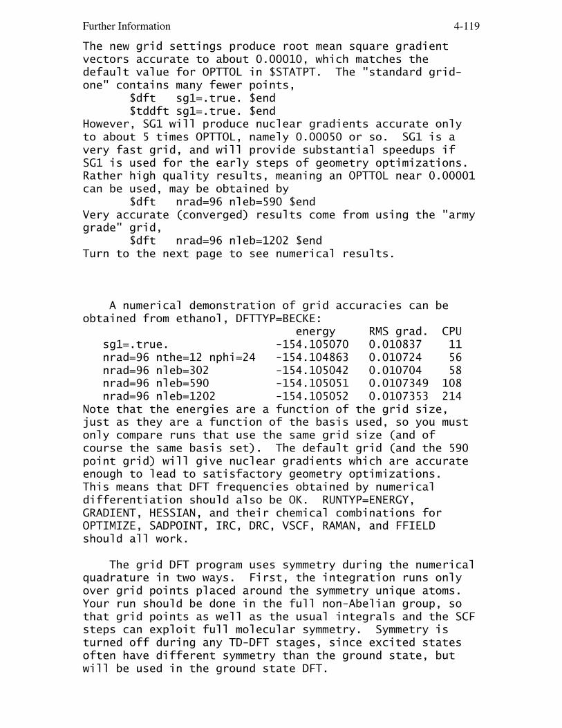
Further Information 4-119
The new grid settings produce root mean square gradientvectors accurate to about 0.00010, which matches thedefault value for OPTTOL in $STATPT. The "standard grid-one" contains many fewer points, $dft sg1=.true. $end $tddft sg1=.true. $endHowever, SG1 will produce nuclear gradients accurate onlyto about 5 times OPTTOL, namely 0.00050 or so. SG1 is avery fast grid, and will provide substantial speedups ifSG1 is used for the early steps of geometry optimizations.Rather high quality results, meaning an OPTTOL near 0.00001can be used, may be obtained by $dft nrad=96 nleb=590 $endVery accurate (converged) results come from using the "armygrade" grid, $dft nrad=96 nleb=1202 $endTurn to the next page to see numerical results.
A numerical demonstration of grid accuracies can beobtained from ethanol, DFTTYP=BECKE: energy RMS grad. CPU sg1=.true. -154.105070 0.010837 11 nrad=96 nthe=12 nphi=24 -154.104863 0.010724 56 nrad=96 nleb=302 -154.105042 0.010704 58 nrad=96 nleb=590 -154.105051 0.0107349 108 nrad=96 nleb=1202 -154.105052 0.0107353 214Note that the energies are a function of the grid size,just as they are a function of the basis used, so you mustonly compare runs that use the same grid size (and ofcourse the same basis set). The default grid (and the 590point grid) will give nuclear gradients which are accurateenough to lead to satisfactory geometry optimizations.This means that DFT frequencies obtained by numericaldifferentiation should also be OK. RUNTYP=ENERGY,GRADIENT, HESSIAN, and their chemical combinations forOPTIMIZE, SADPOINT, IRC, DRC, VSCF, RAMAN, and FFIELDshould all work.
The grid DFT program uses symmetry during the numericalquadrature in two ways. First, the integration runs onlyover grid points placed around the symmetry unique atoms.Your run should be done in the full non-Abelian group, sothat grid points as well as the usual integrals and the SCFsteps can exploit full molecular symmetry. Symmetry isturned off during any TD-DFT stages, since excited statesoften have different symmetry than the ground state, butwill be used in the ground state DFT.

Further Information 4-120
Secondly, for polar coordinate angular grids only,"octant symmetry" is implemented using an appropriateAbelian subgroup of the full group. The grid evaluationautomatically uses an appropriate subgroup to reduce thenumber of grid points for atoms that lie on symmetry axesor planes. For example, in Cs, atoms lying in the xy planewill be integrated only over the upper hemisphere of theirgrid points. Octant symmetry is not used for any of these: a) if a non-standard axis orientation is input in $DATA b) if the angular grid size (NTHE,NTHE0,NPHI,NPI0) is not a multiple of the octant symmetry factors, such as NTHE=15 in C2v. The permissible values depend on the group, but NTHE a multiple of 2 and NPHI a multiple of 4 is generally safe.
Time Dependent Density Functional Theory (TD-DFT)
Two review articles are available,
"Single-Reference ab Initio Methods for the Calculation ofExcited States of Large Molecules" A.Dreuw, M.Head-Gordon Chem.Rev. 105, 4009-4037(2005)
"Excited states from time-dependent density functionaltheory" P.Elliott, F.Furche, K.Burke Rev.Comp.Chem. 26, 91-166(2009)
The following article is very informative: S.Hirata, M.Head-Gordon Chem.Phys.Lett. 314, 291-299(1999)It also explains the Tamm/Dancoff approximation whichconnects TD-DFT to CIS.
TD-DFT requires higher functional derivatives of theexchange correlation energy with respect to the density:2nd derivatives to do TD-DFT excitation energies, and 3rdderivatives to do TD-DFT nuclear gradients. Consequently,some of the functionals permit only excitation energies.To use metaGGAs in TD-DFT, the above functional derivativesinvolve a non-trivial differentiation of the kinetic energytau's density dependence. The latter is the subject of aforthcoming paper, F.Zahariev, S.Sok, M.S.Gordon (to be submitted)

Further Information 4-121
The TD-DFT nuclear gradient implementation in GAMESS is M.Chiba, T.Tsuneda, K.Hirao J.Chem.Phys. 124, 144106/1-11 (2006)and the long-range correction (useful in Rydberg and/orcharge transfer states is Y.Tawada, T.Tsuneda, S.Yanagisawa, Y.Yanai, K.Hirao J.Chem.Phys. 120, 8425-8433(2004)See also K.A.Nguyen, P.N.Day, R.Pachter Int.J.Quantum Chem. 110, 2247-2255(2010)
The "lambda diagnostic" is described by M.J.G.Peach, P.Benfield, T.Helgaker, D.J.Tozer J.Chem.Phys. 128, 044118/1-8(2008)This is a procedure for separating valence states fromcharge transfer and Rydberg states.
Note that it is possible to do TD-HF excitation energies,by requesting TDDFT=EXCITE, but leaving DFTTYP=NONE.
Solvation effects can be added by PCM or EFP or both, withnuclear gradients.PCM + TD-DFT gradient: Y.Wang, H.Li J.Chem.Phys. 133, 034108/1-11(2010)EFP1 + TD-DFT energy: S.Yoo, F.Zahariev, S.Sok, M.S.Gordon J.Chem.Phys. 129, 144112/1-8(2008)EFP1 + TD-DFT gradient: N.Minezawa, N.De Silva, F.Zahariev, M.S.Gordon J.Chem.Phys. 134, 05411(2011)POL5P + TD-DFT gradient (similar polarizable solvent): D.Si, H.Li J.Chem.Phys. 133, 144112(2010)
* * * * *
In some cases, a more balanced description of the statesmight be obtained if the orbitals are optimized for areference with unpaired electrons. This is possible withspin-flip methods, see TDDFT=SPNFLP. For example, in C2H4,one might optimize the orbitals for the triplet state(pi)1(pi*)1, but be interested in the energies of the threesinglets and one triplet states N=(pi)2, T=(pi)1(pi*)1,V=(pi)1(pi*)1, and Z=(pi*)2. Using the T state as thereference optimizes the shape of both pi and pi*, sinceboth are occupied. Flipping one of the two unpaired alphaspins in the T reference will access all four valencestates (recall that a triplet state with Ms=0 is perfectlyOK, namely ab+ba). For more information, see Y.Shao, M.Head-Gordon, A.I.Krylov

Further Information 4-122
J.Chem.Phys. 118,4807(2003) F.Wang, T.Ziegler J.Chem.Phys. 121, 12191(2004) J.Chem.Phys. 122, 074109(2005) O.Vahtras, Z.Rinkevicius J.Chem.Phys. 126, 114101(2007) Z.Rinkevicius, H.Agren Chem.Phys.Lett. 491, 132(2010) Z.Rinkevicius, O.Vahtras, H.Agren J.Chem.Phys. 113, 114101(2010 M.Huix-Rotllant, B.Natarajan, A.Ipatov, C.M.Wawire, T.Deutsch, M.E.Casida Phys.Chem.Chem.Phys. 12, 12811(2010)The penalty constrained optimization procedure was used tofind ethylene's conical intersections by N.Minezawa, M.S.Gordon J.Phys.Chem.A 113, 12749(2009)
references for DFT
An excellent overview of DFT can be found in Chapter 6 ofFrank Jensen's book. Two other monographs are "Density Functional Theory of Atoms and Molecules" R.G.Parr, W.Yang Oxford Scientific, 1989 "A Chemist's Guide to Density Functional Theory" W.Koch, M.C.Holthausen Wiley-VCH, 2001If you would like to understand the "theory" of DensityFunctional Theory, see Kieron Burke's online book "The ABCof DFT", at http://dft.uci.edu/dftbook.html. You may alsoenjoy "Fourteen easy lessons in Density Functional Theory",by John Perdew and Adrienn Ruzsinszky, Int. J. QuantumChem., in press 2010.
A delightful and thought provoking paper on therelationship of DFT to conventional quantum mechanics usingwavefunctions: P.M.W.Gill Aust.J.Chem. 54, 661-662(2001)
A paper comparing DFT's approach to correlation totraditional quantum chemistry methods: E.J.Baerends, O.V.Gritsenko J.Phys.Chem.A 101, 5383-5403(1997)
Some philosophy about designing functionals at each rung ofDFT's "Jacob's ladder": J.P.Perdew, A.Ruzsinszky, J.Tao, V.N.Staroverov, G.E.Scuseria, G.I.Csonka J.Chem.Phys. 123, 062201/1-9(2005)

Further Information 4-123
On hybridization: J.P.Perdew, M.Ernzerhof, K.Burke J.Chem.Phys. 105, 9982-9985(1996) G.I.Csonka, J.P.Perdew, A.Ruzsinszky J.Chem.Theory Comput. 6, 3688-3703(2010)
Some reading on the grid-free approach to densityfunctional theory is: Y.C.Zheng, J.Almlof Chem.Phys.Lett. 214, 397-401(1996) Y.C.Zheng, J.Almlof J.Mol.Struct.(Theochem) 288, 277(1996) K.Glaesemann, M.S.Gordon J.Chem.Phys. 108, 9959-9969(1998) K.Glaesemann, M.S.Gordon J.Chem.Phys. 110, 6580-6582(1999) K.Glaesemann, M.S.Gordon J.Chem.Phys. 112, 10738-10745(2000)
References about gridding: A.D.Becke J.Chem.Phys. 88, 2547-2553(1988) C.W.Murray, N.C.Handy, G.L.Laming Mol.Phys. 78, 997-1014(1993) P.M.W.Gill, B.G.Johnson, J.A.Pople Chem.Phys.Lett. 209, 506-512(1993) A.A.Jarecki, E.R.Davidson Chem.Phys.Lett. 300, 44-52(1999) R.Lindh, P.-A.Malmqvist, L.Gagliardi Theoret.Chem.Acc. 106, 178-187(2001) S.-H.Chien, P.M.W.Gill J.Comput.Chem. 27, 730-739(2006) J.Grafenstein, D.Izotov, D.Cremer J.Chem.Phys. 127, 164113/1-7(2007)Gill's 1993 paper is the reference for SG1=.TRUE.Handy's 1993 paper is a reference for polar coordinates.Lebedev grids may be referenced as V.I.Lebedev, D.N.Laikov Doklady Math. 59, 477-481(1999)GAMESS uses Christoph van Wuellen's FORTRAN translation ofthese grids, originally coded in C by Laikov (www.ccl.net).
--- exchange functionals
Slater exchange: J.C.Slater Phys.Rev. 81, 385-390(1951)XALPHA is Slater with alpha=0.70
BECKE (often called B88) exchange:

Further Information 4-124
A.D.Becke Phys.Rev. A38, 3098-3100(1988)
GILL (often called G96) exchange: P.M.W.Gill Mol.Phys. 89, 433-445(1996)
OPTX exchange: N.C.Handy, A.J.Cohen Mol.Phys. 99, 403-412(2001)
Depristo/Kress exchange: A.E.DePristo, J.E.Kress J.Chem.Phys. 86, 1425-1428(1987)
--- correlation functionals
VWN local correlation: S.H.Vosko, L.Wilk, M.Nusair Can.J.Phys. 58, 1200-1211(1980)This paper has five formulae in it, and since the 5th isa good quality fit, it states "since formula 5 is easiestto implement in LSDA calculations, we recommend its use".
PZ81 correlation: J.P.Perdew, A.Zunger Phys.Rev.B 23, 5048-5079(1981)
P86 GGA correlation: J.P.Perdew Phys.Rev.B 33, 8822(1986)
PW local correlation (used in PW91): J.P.Perdew, Y.Wang Phys.Rev.B 45, 13244-13249(1992)
LYP correlation: C.Lee, W.Yang, R.G.Parr Phys.Rev. B37, 785-789(1988)For practical purposes this is always used in a transformedway, involving the square of the density gradient: B.Miehlich, A.Savin, H.Stoll, H.Preuss Chem.Phys.Lett. 157, 200-206(1989)
OP (One-parameter Progressive) correlation: T.Tsuneda, K.Hirao Chem.Phys.Lett. 268, 510-520(1997) T.Tsuneda, T.Suzumura, K.Hirao J.Chem.Phys. 110, 10664-10678(1999)
--- exchange/correlation functionals
PW91 exchange/correlation: J.P.Perdew, J.A.Chevray, S.H.Vosko, K.A.Jackson, M.R.Pederson, D.J.Singh, C.Fiolhais Phys.Rev. B46, 6671-6687(1992)
EDF1 - empirical density functional #1, a tweaked BLYP
Further Information 4-125
developed for use with 6-31+G(d) basis sets, R.D.Adamson, P.M.W.Gill, J.A.Pople Chem.Phys.Lett. 284, 6-11(1998)
MOHLYP - metal optimized OPTX exchange, half LYP correlation N.E.Schultz, Y.Zhao, D.G.Truhlar J.Phys.Chem.A 109, 11127-11143(2005)See also comp.chem.umn.edu/info/MOHLYP_reference.pdf forinformation about the related functional MOHLYP2.
PBE exchange/correlation functional: J.P.Perdew, K.Burke, M.Ernzerhof Phys.Rev.Lett. 77, 3865-8(1996); Err. 78,1396(1997)
revPBE (revised PBE exchange, but see RPBE below): Y.Zhang, W.Yang Phys.Rev.Lett. 80, 890(1998)
RPBE (a different revision of PBE exchange): B.Hammer, L.B.Hansen, J.K.Norskov Phys.Rev.B 59, 7413-7421(1999)This revision retains the same increase in accuracy foratomization energies that revPBE affords, while rigorouslypreserving the correct Lieb-Oxford limit, unlike revPBE.
PBEsol (modified PBE parameters, for solid properties): J.P.Perdew, A.Ruzsinszky, G.I.Csonka, O.A.Vydrov, G.E.Scuseria, L.A.Constantin, Z.Zhou, K.Burke Phys.Rev.Lett. 100, 136406/1-7(2008)
Dispersion corrections:
Local Response Dispersion (LRD) T.Sato, H.Nakai J.Chem.Phys. 131, 224104/1-12(2009) T.Sato, H.Nakai J.Chem.Phys. 132, 194101/1-9(2010)
empirical dispersion correction (DC): This is developed in three successive versions by Grimme1: S.Grimme J.Comput.Chem. 25, 1463-1473(2004)2: S.Grimme J.Comput.Chem. 27, 1787-1799(2006)3: S.Grimme, J.Antony, S.Ehrlich, H.Krieg J.Chem.Phys. 132, 154104/1-19(2010)which are applied to different functionals with differentparameterizations of the correction. Setting DC=.TRUE.thus converts functionals such as BLYP/B3LYP/PBE/BP86/TPSSto BLYP-D, B3LYP-D, and so forth. See the papers for moredetails.

Further Information 4-126
A functional where the input keyword contains alreadythe -D, namely B97-D, consists of a revamping of the B97functional to remove its hybridization with HF exchange andreparameterization, as well as adding the dispersioncorrection: S.Grimme J.Comput.Chem. 27, 1787-1799(2006)A somewhat different form for the dispersion correction isused in the wB97-D functional. Selection of DFTTYP=B97-Dor wB97-D does not require setting DC on.
The next two occur in the grid-free program only,
various WIGNER exchange/correlation functionals: Q.Zhao, R.G.Parr Phys.Rev. A46, 5320-5323(1992)
CAMA/CAMB exchange/correlation functionals: G.J.Laming, V.Termath, N.C.Handy J.Chem.Phys. 99. 8765-8773(1993)
--- hybrids with HF exchange
B3PW91 hybrid: A.D.Becke J.Chem.Phys. 98, 5648-5642(1993)
B3LYP hybrid: A.D.Becke J.Chem.Phys. 98, 5648-5642(1993) P.J.Stephens, F.J.Devlin, C.F.Chablowski, M.J.Frisch J.Phys.Chem. 98, 11623-11627(1994) R.H.Hertwig, W.Koch Chem.Phys.Lett. 268, 345-351(1997)
The first paper is actually on B3PW91 hybridization, andoptimizes the mixing of five functionals with PW91 as thecorrelation GGA. The second paper then proposed use of LYPin place of PW91, without reoptimizing the mixing ratios ofthe hybrid. The final paper discusses the controversysurrounding which VWN functional is used in the hybrid.GAMESS uses VWN5 in its B3LYP hybrid, but see also B3LYP1to use the RPA parameterized VWN1 formula.
B97 hybrid: A.D.Becke J.Chem.Phys. 107, 8554-8560(1997)
B97-1 hybrid, a reparameterization of B97: F.A.Hamprecht, A.J.Cohen, D.J.Tozer, N.C.Handy J.Chem.Phys. 109, 6264-6271(1998)
B97-2 hybrid, a reparameterization of B97: P.J.Wilson, T.J.Bradley, D.J.Tozer J.Chem.Phys. 115, 9233-9242(2001)

Further Information 4-127
B97-3 hybrid, a reparameterization of B97: T.W.Keal, D.J.Tozer J.Chem.Phys. 123, 121103-1/4(2005)
B97-K and BMK hybrids, K=kinetics: A.D.Boese, J.M.L.Martin J.Chem.Phys. 123, 3405-3416(2004)
HCTH93, HCTH120, HCTH147, and HCTH407 use training setswith the indicated number of atoms and molecules used toadjust the B97 functional:
HCTH93 is defined in the B97-1 paper.HCTH120 and HCTH147: A.D.Boese, N.L.Doltsinis, N.C.Handy, M.Sprik J.Chem.Phys. 112, 1670-1678(2000)HCTH407: A.D.Boese, N.C.Handy J.Chem.Phys. 114, 5497-5503(2001)
B98, Becke's reparameterization of B97: A.D. Becke J.Chem.Phys. 108, 9624-9631(1998)
...bringing to an end "the B97 family".
X3LYP hybrid: X.Xu, Q.Zhang, R.P.Muller, W.A.Goddard J.Chem.Phys. 122, 014105/1-14(2005)
PBE0 hybrid: C.Adamo, V.Barone J.Chem.Phys. 110, 6158-6170(1999)
in the grid free program only,
HALF exchange: This is programmed as 50% HF plus 50% B88 exchange.BHHLYP exchange/correlation: This is 50% HF plus 50% B88, with LYP correlation.Note: neither is the HALF-AND-HALF exchange/correlation: A.D.Becke J.Chem.Phys. 98, 1372-1377(1993)which he defined as 50% HF + 50% SVWN.
--- meta-GGA functionals
These are pure DFT meta-GGAs, unless the descriptionexplicitly says it is a hybrid!

Further Information 4-128
PKZB (a prototype of the TPSS family): J.P.Perdew, S.Kurth, A.Zupan, P.Blaha Phys.Rev.Lett. 82, 2544-2547(1999)
tHCTH and tHCTHhyb=15% HF exchange: A.D.Boese, N.C.Handy J.Chem.Phys. 116, 9559-9569(2002)
TPSS: J.P.Perdew, J.Tao, V.N.Staroverov, G.E.Scuseria Phys.Rev.Lett. 91, 146401/1-4(2003) J.P.Perdew, J.Tao, V.N.Staroverov, G.E.Scuseria J.Chem.Phys. 120, 6898-6911(2004)
TPSSm, a modified TPSS improving atomization energies: J.P.Perdew, A.Ruzsinszky, J.Tao, G.I.Csonka, G.E.Scuseria Phys.Rev.A 76, 042506/1-6(2007)
TPSSh, a 10% hybrid using TPSS: V.N.Staroverov, G.E.Scuseria, J.Tao, J.P.Perdew J.Chem.Phys. 119, 12129-12137(2003), erratum is J.Chem.Phys. 121, 11507(2004)
revTPSS, "workhorse functional for CMP and QC" J.P.Perdew, A.Ruzsinsky, G.I.Csonka, L.A.Constantin, J.Sun Phys.Rev.Lett. 103, 026403/1-4(2009)
VS98 (whose form is the prototype of the M06 family): T.V.Voorhis, G.E.Scuseria J.Chem.Phys. 109, 400-410(1998)
U.Minnesota hybrid meta-GGA family:M05: Y.Zhao, N.E.Schultz, D.G.Truhlar J.Chem.Phys. 123, 161103/1-4(2005)M05-2X: Y.Zhao, D.G.Truhlar J.Comput.Chem.Theory Comput. 2, 1009-1018(2006)M06: Y.Zhao, D.G.Truhlar Theoret.Chem.Acc. 120,215-241(2008)M06-2X: ibidM06-HF: Y.Zhao, D.G.Truhlar J.Phys.Chem.A 110, 13126-13130(2006)M06-L: Y.Zhao, D.G.Truhlar J.Chem.Phys. 125, 194101/1-18(2006)SOGGA: Y.Zhao, D.G.Truhlar J.Chem.Phys. 128, 184109/1-8(2008)M08-HX and M08-SO: Y.Zhao, D.G.Truhlar J.Chem.Theory Comput. 4, 1849-1868(2008)For reviews, please see the paper for M06, and also Y.Zhao, D.G.Truhlar Acc.Chem.Res. 41, 157-167(2008)

Further Information 4-129
These contain recommendations for choosing the one mostappropriate to your problem.
---- long-range corrected functionals:
LC-BLYP, LC-BOP, LC-BVWN: Y.Tawada, T.Tsuneda, S.Yanagisawa, Y.Yanai, K.Hirao J.Chem.Phys. 120, 8425-8433(2004)
CAM-B3LYP: T.Yanai, D.P.Tew, N.C.Handy Chem.Phys.Lett. 393, 51-57(2004)
wB97, wB97X, wB97X-D: J.-D. Chai, M.Head-Gordon J.Chem.Phys. 128, 084106/1-15(2004) J.-D. Chai, M.Head-Gordon Phys.Chem.Chem.Phys. 10, 6615-6620(2008)
A review on the topic of long range corrections, which arealso called 'range separated hybrids', is D.Jacquemin, E.A.Perpete, G.E.Scuseria, I.Ciofini, C.Adamo J.Chem.Theory Comput. 4, 123-135(2008)
---- "double-hybrid" ----
The B2PLYP family is a mixture of B88 and HF exchange, anda mixture of LYP and MP2 correlation: B2-PLYP: S.Grimme J.Chem.Phys. 124, 034108/1-15(2006) B2G-PLYP: A.Karton, A.Tarnopolsky, J.F.Lamere, G.C.Schatz, J.M.L.Martin J.Phys.Chem. A 112, 12868(2008) B2K-PLYP, B2T-PLYP: A.Tarnopolsky, A.Karton, R.Sertchook, D.Vuzman, J.M.L.Martin J.Phys.Chem. A 112, 3(2008)Double hybrids which are also "long range corrected" (andwhose parameters depend on the basis set): wB97X-2, wB97X-2L: J.-D. Chai, M.Head-Gordon J.Chem.Phys. 131, 174105/1-13(2009)
* * * * *
Some of the recent functional additions to GAMESS weremade using code from the "density functional repository", http://www.cse.clrc.ac.uk/qcg/dft

Further Information 4-130
We thank Huub van Dam for his assistance with this, andparticularly for providing the VWN1 functional. TheMinnesota functionals are based on subroutines provided bythe Truhlar group at the University of Minnesota. Somefunctionals, and particularly their high derivatives neededby TDDFT, were created by MAXIMA's algebraic manipulation,along the lines described by P.Salek, A.Hesselmann J.Comput.Chem. 28, 2569-2575(2007)
* * * * *
The paper of Johnson, Gill, and Pople listed below has auseful summary of formulae, and details about a gradientimplementation. A paper on 1st and 2nd derivatives of DFTwith respect to nuclear coordinates and applied fields is A.Komornicki, G.Fitzgerald J.Chem.Phys. 98, 1398-1421(1993)and see also P.Deglmann, F.Furche, R.Ahlrichs Chem.Phys.Lett. 362, 511-518(2002).
A few of the many papers assessing the accuracy of DFT:
B.Miehlich, A.Savin, H.Stoll, H.Preuss Chem.Phys.Lett. 157, 200-206(1989) B.G.Johnson, P.M.W.Gill, J.A.Pople J.Chem.Phys. 98, 5612-5626(1993) N.Oliphant, R.J.Bartlett J.Chem.Phys. 100, 6550-6561(1994) L.A.Curtiss, K.Raghavachari, P.C.Redfern, J.A.Pople J.Chem.Phys. 106, 1063-1079(1997) E.R.Davidson Int.J.Quantum Chem. 69, 241-245(1998) B.J.Lynch, D.G.Truhlar J.Phys.Chem.A 105, 2936-2941(2001) R.A.Pascal J.Phys.Chem.A 105, 9040-9048(2001) A.D.Boese, J.M.L.Martin, N.C.Handy J.Chem.Phys. 119, 3005-3014(2003) Y.Zhao, D.G.Truhlar, J.Phys.Chem.A 109, 5656-5667(2005) K.E.Riley, B.T.Op't Holt, K.M.Merz J.Chem.Theory Comput. 3, 407-433(2007) S.F.Sousa, P.A.Fernandes, M.J.Ramos J.Phys.Chem.A 111, 10439-10452(2007)Boese et al. include basis set comparisons, as well asfunctional comparisons. The final paper is a review ofreviews, and encourages you to think past B3LYP, whichafter all dates from 1993! Of course there are assessmentsin many of the functional papers as well.

Further Information 4-131
On the accuracy of DFT for large molecule thermochemistry:
L.A.Curtiss, K.Ragavachari, P.C.Redfern, J.A.Pople J.Chem.Phys. 112, 7374-7383(2000) P.C.Redfern, P.Zapol, L.A.Curtiss, K.Ragavachari J.Phys.Chem.A 104, 5850-5854(2000)
Spin contamination in DFT:
1. It is empirically observed that the <S**2> values forunrestricted DFT are smaller than for unrestricted HF.2. GAMESS computes the <S**2> quantity in an approximateway, namely it pretend that the Kohn-Shan orbitals can beused to form a determinant (WRONG, WRONG, WRONG, there isno wavefunction in DFT!!!) and then uses the same formulathat UHF uses to evaluate that determinant's spinexpectation value. See G.J.Laming, N.C.Handy, R.D.Amos Mol.Phys. 80, 1121-1134(1993) J.Baker, A.Scheiner, J.Andzelm Chem.Phys.Lett. 216, 380-388(1993) C.Adamo, V.Barone, A.Fortunelli J.Chem.Phys. 98, 8648-8652(1994) J.A.Pople, P.M.W.Gill, N.C.Handy Int.J.Quantum Chem. 56, 303-305(1995) J.Wang, A.D.Becke, V.H.Smith J.Chem.Phys. 102, 3477-3480(1995) J.M.Wittbrodt, H.B.Schlegel J.Chem.Phys. 105, 6574-6577(1996) J.Grafenstein, D.Cremer Mol.Phys. 99, 981-989(2001)and commentary in Koch & Holthausen, pp 52-54.
Orbital energies:
The discussion on page 49-50 of Koch and Holthausen showsthat although the highest occupied orbital's eigenvalueshould be the ionization potential for exact Kohn-Shamcalculations, the functionals we actually have greatlyunderestimate IP values. The 5th reference below shows howinclusion of HF exchange helps this, and provides a linearcorrection formula for IPs. The first two papers belowconnect the HOMO eigenvalue to the IP, and the third showsthat while the band gap is underestimated by existingfunctionals, the gap's center is correctly predicted.However, the 5th paper shows that DFT is actually prettyhopeless at predicting these gaps. The 4th paper uses SCF

Further Information 4-132
densities to generate exchange-correlation potentials thatactually give fairly good IP values:
J.F.Janak Phys.Rev.B 18, 7165-7168(1978) M.Levy, J.P.Perdew, V.Sahni Phys.Rev.A 30, 2745-2748(1984) J.P.Perdew, M.Levy Phys.Rev.Lett. 51, 1884-1887(1983) A.Nagy, M.Levy Chem.Phys.Lett. 296, 313-315(1998) G.Zhang, C.B.Musgrave J.Phys.Chem.A 111, 1554-1561(2007)

Further Information 4-133
Summary of excited state methods
This is not a "how to" section, as the actual calculationswill be carried out by means described elsewhere in thechapter. Instead, a summary of methods that can treatexcited states is given.
The simplest possibility is SCFTYP. For example, a closedshell molecule's first triplet state can always be treatedby SCFTYP=ROHF MULT=3. Assuming there is some symmetrypresent, the GVB program may be able to do excited singletsvariationally, provided they are of a different spacesymmetry than the ground state. The MCSCF program gives ageneral entree into excited states, since upper roots of aHamiltonian are always variational: see for example NSTATEand WSTATE and IROOT in $DET.
CI calculations also give a simple entry into excitatedstates. There are a variety of programs, selected by CITYPin $CONTRL. Note in particular CITYP=CIS, programmed forclosed shell ground states, with gradient capability forsinglet excited states, and the calculation of tripletstate energies. The other CI programs can generate veryflexible wavefunctions for the evaluation of the excitationenergy, and property values. Note that the GUGA programwill do nuclear gradients provided the reference is RHF.
The TD-DFT method treats singly excited states, includingcorrelation effects, and is a popular alternative to CIS.The program allows for excitation energies from a UHFreference, but is much more powerful for RHF references:nuclear gradients and/or properties may be computed. Useof a "long range corrected" or "range separated" functional(the two terms are synonymous) is often thought to beimportant when treating charge transfer or Rydberg states:see the LC=.TRUE. flag or CAMB3LYP.
Equation of Motion (EOM) coupled cluster can give accurateestimates of excitation energies. There are no gradients,and properties exist only for EOM-CCSD, but triplescorrections to the energy are available. See $EOMINP formore details.
Most of the runs will predict oscillator strengths, orEinstein coefficients, or similar data regarding theelectronic transition moments. Full prediction of UV-visspectra is not possible without Franck-Condon information.

Further Information 4-134
Excited states frequently come close together, andcrossings between them are of great interest. SeeRUNTYP=TRANSITION for spin-orbit coupling, responsible forInterSystem Crossing (ISC) between states of differentmultiplicity. See RUNTYP=NACME for the non-adiabaticcoupling matrix elements that cause Internal Conversion(IC) between states of the same spin multiplicity. It ispossible to search for the lowest energy on the crossingseam between two surfaces, provided those surfaces havedifferent spins, or different space symmetries (or both),see RUNTYP=MEX.
Solvent effects (EFP and/or PCM) can easily be incorporatedwhen using SCFTYP to generate the states, and nucleargradients are available. It is now possible to assesssolvent effects on TD-DFT excitation energies from closedshell references, using either EFP or PCM.
Excited states often possess Rydberg character, so diffusefunctions in the basis set are likely to be important.

Further Information 4-135
Geometry Searches and Internal Coordinates
Stationary points are places on the potential energysurface with a zero gradient vector (first derivative ofthe energy with respect to nuclear coordinates). Theseinclude minima (whether relative or global), better knownto chemists as reactants, products, and intermediates; aswell as transition states (also known as saddle points).
The two types of stationary points have a precisemathematical definition, depending on the curvature of thepotential energy surface at these points. If all of theeigenvalues of the hessian matrix (second derivativeof the energy with respect to nuclear coordinates) arepositive, the stationary point is a minimum. If there isone, and only one, negative curvature, the stationarypoint is a transition state. Points with more than onenegative curvature do exist, but are not important inchemistry. Because vibrational frequencies are basicallythe square roots of the curvatures, a minimum has allreal frequencies, and a saddle point has one imaginaryvibrational "frequency".
GAMESS locates minima by geometry optimization, asRUNTYP=OPTIMIZE, and transition states by saddle pointsearches, as RUNTYP=SADPOINT. In many ways these aresimilar, and in fact nearly identical FORTRAN code is usedfor both. The term "geometry search" is used here todescribe features which are common to both procedures.The input to control both RUNTYPs is found in the $STATPTgroup.
As will be noted in the symmetry section below, anOPTIMIZE run does not always find a minimum, and aSADPOINT run may not find a transtion state, even thoughthe gradient is brought to zero. You can prove you havelocated a minimum or saddle point only by examining thelocal curvatures of the potential energy surface. Thiscan be done by following the geometry search with aRUNTYP=HESSIAN job, which should be a matter of routine.
quasi-Newton Searches
Geometry searches are most effectively done by what iscalled a quasi-Newton-Raphson procedure. These methodsassume a quadratic potential surface, and require the

Further Information 4-136
exact gradient vector and an approximation to the hessian.It is the approximate nature of the hessian that makes themethod "quasi". The rate of convergence of the geometrysearch depends on how quadratic the real surface is, andthe quality of the hessian. The latter is something youhave control over, and is discussed in the next section.
GAMESS contains different implementations of quasi-Newton procedures for finding stationary points, namelyMETHOD=NR, RFO, QA, and the seldom used SCHLEGEL. Theydiffer primarily in how the step size and direction arecontrolled, and how the Hessian is updated. The CONOPTmethod is a way of forcing a geometry away from a minimumtowards a TS. It is not a quasi-Newton method, and isdescribed at the very end of this section.
The NR method employs a straight Newton-Raphson step.There is no step size control, the algorithm will simplytry to locate the nearest stationary point, which may be aminimum, a TS, or any higher order saddle point. NR isnot intended for general use, but is used by GAMESS inconnection with some of the other methods after they havehomed in on a stationary point, and by Gradient Extremalruns where location of higher order saddle points iscommon. NR requires a very good estimate of the geometryin order to converge on the desired stationary point.
The RFO and QA methods are two different versions ofthe so-called augmented Hessian techniques. They bothemploy Hessian shift parameter(s) in order to control thestep length and direction.
In the RFO method, the shift parameter is determined byapproximating the PES with a Rational Function, instead ofa second order Taylor expansion. For a RUNTYP=SADPOINT,the TS direction is treated separately, giving two shiftparameters. This is known as a Partitioned RationalFunction Optimization (P-RFO). The shift parameter(s)ensure that the augmented Hessian has the correct eigen-value structure, all positive for a minimum search, andone negative eigenvalue for a TS search. The (P)-RFO stepcan have any length, but if it exceeds DXMAX, the step issimply scaled down.
In the QA (Quadratic Approximation) method, the shiftparameter is determined by the requirement that the stepsize should equal DXMAX. There is only one shiftparameter for both minima and TS searches. Again theaugmented Hessian will have the correct structure. There

Further Information 4-137
is another way of describing the same algorithm, namely asa minimization on the "image" potential. The latter isknown as TRIM (Trust Radius Image Minimization). Theworking equation is identical in these two methods.
When the RFO steplength is close to DXMAX, there islittle difference between the RFO and QA methods. However,the RFO step may in some cases exceed DXMAX significantly,and a simple scaling of the step will usually not producethe best direction. The QA step is the best step on thehypersphere with radius DXMAX. For this reason QA is thedefault algorithm.
Near a stationary point the straight NR algorithm isthe most efficient. The RFO and QA may be viewed asmethods for guiding the search in the "correct" directionwhen starting far from the stationary point. Once thestationary point is approached, the RFO and QA methodsswitch to NR, automatically, when the NR steplength dropsbelow 0.10 or DXMAX, whichever is the smallest.
The QA method works so well that we use it exclusively,and so the SCHLEGEL method will probably be omitted fromsome future version of GAMESS.
You should read the papers mentioned below in order tounderstand how these methods are designed to work. Thefirst 3 papers describe the RFO and TRIM/QA algorithms. Agood but slightly dated summary of search procedures isgiven by Bell and Crighton, and see also the review bySchlegel. Most of the FORTRAN code for geometry searches,and some of the discussion in this section was written byFrank Jensen of the University of Aarhus, whose papercompares many of the algorithms implemented in GAMESS:
1. J.Baker J.Comput.Chem. 7, 385-395(1986) 2. T.Helgaker Chem.Phys.Lett. 182, 503-510(1991) 3. P.Culot, G.Dive, V.H.Nguyen, J.M.Ghuysen Theoret.Chim.Acta 82, 189-205(1992) 4. H.B.Schlegel J.Comput.Chem. 3, 214-218(1982) 5. S.Bell, J.S.Crighton J.Chem.Phys. 80, 2464-2475(1984). 6. H.B.Schlegel Advances in Chemical Physics (Ab Initio Methods in Quantum Chemistry, Part I), volume 67, K.P.Lawley, Ed. Wiley, New York, 1987, pp 249-286. 7. F.Jensen J.Chem.Phys. 102, 6706-6718(1995).

Further Information 4-138
the nuclear Hessian
Although quasi-Newton methods require only anapproximation to the true hessian, the quality of thismatrix has a great affect on convergence of the geometrysearch.
There is a procedure contained within GAMESS forguessing a positive definite hessian matrix, HESS=GUESS.If you are using Cartesian coordinates, the guess hessianis based on pairwise atom stretches. The guess is moresophisticated when internal coordinates are defined, asempirical rules will be used to estimate stretching andbending force constants. Other angular force constants areset to 1/4. The guess often works well for minima, butcannot possibly find transition states (because it ispositive definite). Therefore, GUESS may not be selectedfor SADPOINT runs.
Two options for providing a more accurate hessian areHESS=READ and CALC. For the latter, the true hessian isobtained by direct calculation at the initial geometry, andthen the geometry search begins, all in one run. The READoption allows you to feed in the hessian in a $HESS group,as obtained by a RUNTYP=HESSIAN job. The second procedureis actually preferable, as you get a chance to see thefrequencies. Then, if the local curvatures look good, youcan commit to the geometry search. Be sure to include a$GRAD group (if the exact gradient is available) in theHESS=READ job so that GAMESS can take its first stepimmediately.
Note also that you can compute the hessian at a lowerbasis set and/or wavefunction level, and read it into ahigher level geometry search. In fact, the $HESS groupcould be obtained at the semiempirical level. This trickworks because the hessian is 3Nx3N for N atoms, no matterwhat atomic basis is used. The gradient from the lowerlevel is of course worthless, as the geometry search mustwork with the exact gradient of the wavefunction and basisset in current use. Discard the $GRAD group from the lowerlevel calculation!
You often get what you pay for. HESS=GUESS is free, butmay lead to significantly more steps in the geometrysearch. The other two options are more expensive at thebeginning, but may pay back by rapid convergence to thestationary point.

Further Information 4-139
The hessian update frequently improves the hessian for afew steps (especially for HESS=GUESS), but then breaksdown. The symptoms are a nice lowering of the energy orthe RMS gradient for maybe 10 steps, followed by crazysteps. You can help by putting the best coordinates into$DATA, and resubmitting, to make a fresh determination ofthe hessian.
The default hessian update for OPTIMIZE runs is BFGS,which is likely to remain positive definite. The POWELLupdate is the default for SADPOINT runs, since the hessiancan develop a negative curvature as the search progresses.The POWELL update is also used by the METHOD=NR and CONOPTsince the Hessian may have any number of negativeeigenvalues in these cases. The MSP update is a mixture ofMurtagh-Sargent and Powell, suggested by Josep Bofill,(J.Comput.Chem., 15, 1-11, 1994). It sometimes worksslightly better than Powell, so you may want to try it.
coordinate choices
Optimization in cartesian coordinates has a reputationof converging slowly. This is largely due to the factthat translations and rotations are usually left in theproblem. Numerical problems caused by the small eigen-values associated with these degrees of freedom are thesource of this poor convergence. The methods in GAMESSproject the hessian matrix to eliminate these degrees offreedom, which should not cause a problem. Nonetheless,Cartesian coordinates are in general the most slowlyconvergent coordinate system.
The use of internal coordinates (see NZVAR in $CONTRLas well as $ZMAT) also eliminates the six rotational andtranslational degrees of freedom. Also, when internalcoordinates are used, the GUESS hessian is able to useempirical information about bond stretches and bends.On the other hand, there are many possible choices for theinternal coordinates, and some of these may lead to muchpoorer convergence of the geometry search than others.Particularly poorly chosen coordinates may not evencorrespond to a quadratic surface, thereby ending all hopethat a quasi-Newton method will converge.
Internal coordinates are frequently strongly coupled.Because of this, Jerry Boatz has called them "infernalcoordinates"! A very common example to illustrate thismight be a bond length in a ring, and the angle on the
Further Information 4-140
opposite side of the ring. Clearly, changing one changesthe other simultaneously. A more mathematical definitionof "coupled" is to say that there is a large off-diagonalelement in the hessian. In this case convergence may beunsatisfactory, especially with a diagonal GUESS hessian,where a "good" set of internals is one with a diagonallydominant hessian. Of course, if you provide an accuratelycomputed hessian, it will have large off-diagonal valueswhere those are truly present. Even so, convergence maybe poor if the coordinates are coupled through large 3rdor higher derivatives. The best coordinates are thereforethose which are the most "quadratic".
One very popular set of internal coordinates is theusual "model builder" Z-matrix input, where for N atoms,one uses N-1 bond lengths, N-2 bond angles, and N-3 bondtorsions. The popularity of this choice is based on itsease of use in specifying the initial molecular geometry.Typically, however, it is the worst possible choice ofinternal coordinates, and in the case of rings, is noteven as good as Cartesian coordinates.
However, GAMESS does not require this particular mixof the common types. GAMESS' only requirement is that youuse a total of 3N-6 coordinates, chosen from these 3 basictypes, or several more exotic possibilities. (Of course,we mean 3N-5 throughout for linear molecules). Theseadditional types of internal coordinates include linearbends for 3 collinear atoms, out of plane bends, and so on.There is no reason at all why you should place yourself ina straightjacket of N-1 bonds, N-2 angles, and N-3torsions.If the molecule has symmetry, be sure to use internalswhich are symmetrically related.
For example, the most effective choice of coordinatesfor the atoms in a four membered ring is to define allfour sides, any one of the internal angles, and a dihedraldefining the ring pucker. For a six membered ring, thebest coordinates seem to be 6 sides, 3 angles, and 3torsions. The angles should be every other internalangle, so that the molecule can "breathe" freely. Thetorsions should be arranged so that the central bond ofeach is placed on alternating bonds of the ring, as ifthey were pi bonds in Kekule benzene. For a five memberedring, we suggest all 5 sides, 2 internal angles, againalternating every other one, and 2 dihedrals to fill in.The internal angles of necessity skip two atoms where thering closes. Larger rings should generalize on the idea

Further Information 4-141
of using all sides but only alternating angles. If thereare fused rings, start with angles on the fused bond, andalternate angles as you go around from this position.
Rings and more especially fused rings can be tricky.For these systems, especially, we suggest the Cadillac ofinternal coordinates, the "natural internal coordinates"of Peter Pulay. For a description of these, see
P.Pulay, G.Fogarosi, F.Pang, J.E.Boggs, J.Am.Chem.Soc. 101, 2550-2560 (1979). G.Fogarasi, X.Zhou, P.W.Taylor, P.Pulay J.Am.Chem.Soc. 114, 8191-8201 (1992).
These are linear combinations of local coordinates, exceptin the case of rings. The examples given in these twopapers are very thorough.
An illustration of these types of coordinates is givenin the example job EXAM25.INP, distributed with GAMESS.This is a nonsense molecule, designed to show many kindsof functional groups. It is defined using standard bonddistances with a classical Z-matrix input, and the anglesin the ring are adjusted so that the starting value ofthe unclosed OO bond is also a standard value.
Using Cartesian coordinates is easiest, but takes a verylarge number of steps to converge. This however, is betterthan using the classical Z-matrix internals given in $DATA,which is accomplished by setting NZVAR to the correct 3N-6value. The geometry search changes the OO bond length toa very short value on the 1st step, and the SCF fails toconverge. (Note that if you have used dummy atoms in the$DATA input, you cannot simply enter NZVAR to optimize ininternal coordinates, instead you must give a $ZMAT whichinvolves only real atoms).
The third choice of internal coordinates is the best setwhich can be made from the simple coordinates. It followsthe advice given above for five membered rings, and becauseit includes the OO bond, has no trouble with crashing thisbond. It takes 20 steps to converge, so the trouble ofgenerating this $ZMAT is certainly worth it compared to theuse of Cartesians.
Natural internal coordinates are defined in the finalgroup of input. The coordinates are set up first for thering, including two linear combinations of all angles andall torsions withing the ring. After this the methyl is
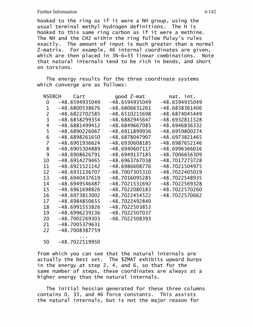
Further Information 4-142
hooked to the ring as if it were a NH group, using theusual terminal methyl hydrogen definitions. The H ishooked to this same ring carbon as if it were a methine.The NH and the CH2 within the ring follow Pulay's rulesexactly. The amount of input is much greater than a normalZ-matrix. For example, 46 internal coordinates are given,which are then placed in 3N-6=33 linear combinations. Notethat natural internals tend to be rich in bends, and shorton torsions.
The energy results for the three coordinate systemswhich converge are as follows:
NSERCH Cart good Z-mat nat. int. 0 -48.6594935049 -48.6594935049 -48.6594935049 1 -48.6800538676 -48.6806631261 -48.6838361406 2 -48.6822702585 -48.6510215698 -48.6874045449 3 -48.6858299354 -48.6882945647 -48.6932811528 4 -48.6881499412 -48.6849667085 -48.6946836332 5 -48.6890226067 -48.6911899936 -48.6959800274 6 -48.6898261650 -48.6878047907 -48.6973821465 7 -48.6901936624 -48.6930608185 -48.6987652146 8 -48.6905304889 -48.6940607117 -48.6996366016 9 -48.6908626791 -48.6949137185 -48.7006656309 10 -48.6914279465 -48.6963767038 -48.7017273728 11 -48.6921521142 -48.6986608776 -48.7021504975 12 -48.6931136707 -48.7007305310 -48.7022405019 13 -48.6940437619 -48.7016095285 -48.7022548935 14 -48.6949546487 -48.7021531692 -48.7022569328 15 -48.6961698826 -48.7022080183 -48.7022570260 16 -48.6973813002 -48.7022454522 -48.7022570662 17 -48.6984850655 -48.7022492840 18 -48.6991553826 -48.7022503853 19 -48.6996239136 -48.7022507037 20 -48.7002269303 -48.7022508393 21 -48.7005379631 22 -48.7008387759 ... 50 -48.7022519950
from which you can see that the natural internals areactually the best set. The $ZMAT exhibits upward burpsin the energy at step 2, 4, and 6, so that for thesame number of steps, these coordinates are always at ahigher energy than the natural internals.
The initial hessian generated for these three columnscontains 0, 33, and 46 force constants. This assiststhe natural internals, but is not the major reason for

Further Information 4-143
its superior performance. The computed hessian at thefinal geometry of this molecule, when transformed into thenatural internal coordinates is almost diagonal. Thisalmost complete uncoupling of coordinates is what makesthe natural internals perform so well. The conclusionis of course that not all coordinate systems are equal,and natural internals are the best. As another example,we have run the ATCHCP molecule, which is a populargeometry optimization test, due to its two fused rings:
H.B.Schlegel, Int.J.Quantum Chem., Symp. 26, 253-264(1992)T.H.Fischer and J.Almlof, J.Phys.Chem. 96, 9768-9774(1992)J.Baker, J.Comput.Chem. 14, 1085-1100(1993)
Here we have compared the same coordinate types, using aguess hessian, or a computed hessian. The latter set ofruns is a test of the coordinates only, as the initialhessian information is identical. The results show clearlythe superiority of the natural internals, which like theprevious example, give an energy decrease on every step:
HESS=GUESS HESS=READCartesians 65 41 stepsgood Z-matrix 32 23natural internals 24 13
A final example is phosphinoazasilatrane, with three ringsfused on a common SiN bond, in which 112 steps in Cartesianspace became 32 steps in natural internals. The moral is:
"A little brain time can save a lot of CPU time."
In late 1998, a new kind of internal coordinate method was included into GAMESS. This is the delocalizedinternal coordinate (DLC) of J.Baker, A. Kessi, B.Delley J.Chem.Phys. 105, 192-212(1996)although as is the usual case, the implementation is notexactly the same. Bonds are kept as independentcoordinates,while angles are placed in linear combination by the DLCprocess. There are some interesting options for applyingconstraints, and other options to assist the automatic DLCgeneration code by either adding or deleting coordinates.It is simple to use DLCs in their most basic form: $contrl nzvar=xx $end $zmat dlc=.true. auto=.true. $endOur initial experience is that the quality of DLCs is

Further Information 4-144
not as good as explicitly constructed natural internals,which benefit from human chemical knowledge, but are almostalways better than carefully crafted $ZMATs using only theprimitive internal coordinates (although we have seen a fewexceptions). Once we have more numerical experience withthe use of DLC's, we will come back and revise the abovediscussion of coordinate choices. In the meantime, theyare quite simple to choose, so give them a go.
the role of symmetry
At the end of a succesful geometry search, you willhave a set of coordinates where the gradient of the energyis zero. However your newly discovered stationary pointis not necessarily a minimum or saddle point!
This apparent mystery is due to the fact that thegradient vector transforms under the totally symmetricrepresentation of the molecular point group. As a directconsequence, a geometry search is point group conserving.(For a proof of these statements, see J.W.McIver andA.Komornicki, Chem.Phys.Lett., 10,303-306(1971)). Insimpler terms, the molecule will remain in whatever pointgroup you select in $DATA, even if the true minimum is insome lower point group. Since a geometry search onlyexplores totally symmetric degrees of freedom, the onlyway to learn about the curvatures for all degrees offreedom is RUNTYP=HESSIAN.
As an example, consider disilene, the silicon analogof ethene. It is natural to assume that this molecule isplanar like ethene, and an OPTIMIZE run in D2h symmetrywill readily locate a stationary point. However, as acalculation of the hessian will readily show, thisstructure is a transition state (one imaginary frequency),and the molecule is really trans-bent (C2h). A carefulworker will always characterize a stationary point aseither a minimum, a transition state, or some higher orderstationary point (which is not of great interest!) byperforming a RUNTYP=HESSIAN.
The point group conserving properties of a geometrysearch can be annoying, as in the preceeding example, oradvantageous. For example, assume you wish to locate thetransition state for rotation about the double bond inethene. A little thought will soon reveal that ethene isD2h, the 90 degrees twisted structure is D2d, andstructures in between are D2. Since the saddle point is

Further Information 4-145
actually higher symmetry than the rest of the rotationalsurface, you can locate it by RUNTYP=OPTIMIZE within D2dsymmetry. You can readily find this stationary point withthe diagonal guess hessian! In fact, if you attempt to doa RUNTYP=SADPOINT within D2d symmetry, there will be nototally symmetric modes with negative curvatures, and itis unlikely that the geometry search will be very wellbehaved.
Although a geometry search cannot lower the symmetry,the gain of symmetry is quite possible. For example, ifyou initiate a water molecule optimization with a trialstructure which has unequal bond lengths, the geometrysearch will come to a structure that is indeed C2v (towithin OPTTOL, anyway). However, GAMESS leaves it up toyou to realize that a gain of symmetry has occurred.
In general, Mother Nature usually chooses moresymmetrical structures over less symmetrical structures.Therefore you are probably better served to assume thehigher symmetry, perform the geometry search, and thencheck the stationary point's curvatures. The alternativeis to start with artificially lower symmetry and see ifyour system regains higher symmetry. The problem withthis approach is that you don't necessarily know whichsubgroup is appropriate, and you lose the great speedupsGAMESS can obtain from proper use of symmetry. It is goodto note here that "lower symmetry" does not mean simplychanging the name of the point group and entering moreatoms in $DATA, instead the nuclear coordinates themselvesmust actually be of lower symmetry.
practical matters
Geometry searches do not bring the gradient exactly tozero. Instead they stop when the largest component of thegradient is below the value of OPTTOL, which defaults toa reasonable 0.0001. Analytic hessians usually haveresidual frequencies below 10 cm**-1 with this degree ofoptimization. The sloppiest value you probably ever wantto try is 0.0005.
If a geometry search runs out of time, or exceedsNSTEP, it can be restarted. For RUNTYP=OPTIMIZE, restartwith the coordinates having the lowest total energy(do a string search on "FINAL"). For RUNTYP=SADPOINT,restart with the coordinates having the smallest gradient

Further Information 4-146
(do a string search on "RMS", which means root meansquare).These are not necessarily at the last geometry!
The "restart" should actually be a normal run, that isyou should not try to use the restart options in $CONTRL(which may not work anyway). A geometry search can berestarted by extracting the desired coordinates for $DATAfrom the printout, and by extracting the corresponding$GRAD group from the PUNCH file. If the $GRAD group issupplied, the program is able to save the time it wouldordinarily take to compute the wavefunction and gradientat the initial point, which can be a substantial savings.There is no input to trigger reading of a $GRAD group: iffound, it is read and used. Be careful that your $GRADgroup actually corresponds to the coordinates in $DATA, asGAMESS has no check for this.
Sometimes when you are fairly close to the minimum, anOPTIMIZE run will take a first step which raises theenergy, with subsequent steps improving the energy andperhaps finding the minimum. The erratic first step iscaused by the GUESS hessian. It may help to limit the sizeof this wrong first step, by reducing its radius, DXMAX.Conversely, if you are far from the minimum, sometimes youcan decrease the number of steps by increasing DXMAX.
When using internals, the program uses an iterativeprocess to convert the internal coordinate change intoCartesian space. In some cases, a small change in theinternals will produce a large change in Cartesians, andthus produce a warning message on the output. If thesewarnings appear only in the beginning, there is probablyno problem, but if they persist you can probably devisea better set of coordinates. You may in fact have one ofthe two problems described in the next paragraph. Insome cases (hopefully very few) the iterations to findthe Cartesian displacement may not converge, producing asecond kind of warning message. The fix for this mayvery well be a new set of internal coordinates as well,or adjustment of ITBMAT in $STATPT.
There are two examples of poorly behaved internalcoordinates which can give serious problems. The firstof these is three angles around a central atom, whenthis atom becomes planar (sum of the angles nears 360).The other is a dihedral where three of the atoms arenearly linear, causing the dihedral to flip between 0 and180. Avoid these two situations if you want your geometry

Further Information 4-147
search to be convergent.
Sometimes it is handy to constrain the geometry searchby freezing one or more coordinates, via the IFREEZ array.For example, constrained optimizations may be useful whiletrying to determine what area of a potential energy surfacecontains a saddle point. If you try to freeze coordinateswith an automatically generated $ZMAT, you need to knowthat the order of the coordinates defined in $DATA is
y y x r1 y x r2 x a3 y x r4 x a5 x w6 y x r7 x a8 x w9
and so on, where y and x are whatever atoms and molecularconnectivity you happen to be using.
saddle points
Finding minima is relatively easy. There are largetables of bond lengths and angles, so guessing startinggeometries is pretty straightforward. Very nasty casesmay require computation of an exact hessian, but thelocation of most minima is straightforward.
In contrast, finding saddle points is a black art.The diagonal guess hessian will never work, so you mustprovide a computed one. The hessian should be computed atyour best guess as to what the transition state (T.S.)should be. It is safer to do this in two steps as outlinedabove, rather than HESS=CALC. This lets you verify youhave guessed a structure with one and only one negativecurvature. Guessing a good trial structure is the hardestpart of a RUNTYP=SADPOINT!
This point is worth iterating. Even with sophisticatedstep size control such as is offered by the QA/TRIM or RFOmethods, it is in general very difficult to move correctlyfrom a region with incorrect curvatures towards a saddlepoint. Even procedures such as CONOPT or RUNTYP=GRADEXTRwill not replace your own chemical intuition about wheresaddle points may be located.
The RUNTYP=HESSIAN's normal coordinate analysis isrigorously valid only at stationary points on the surface.This means the frequencies from the hessian at your trial

Further Information 4-148
geometry are untrustworthy, in particular the six "zero"frequencies corresponding to translational and rotational(T&R) degrees of freedom will usually be 300-500 cm**-1,and possibly imaginary. The Sayvetz conditions on theprintout will help you distinguish the T&R "contaminants"from the real vibrational modes. If you have defined a$ZMAT, the PURIFY option within $STATPT will help zap outthese T&R contaminants).
If the hessian at your assumed geometry does not haveone and only one imaginary frequency (taking into accountthat the "zero" frequencies can sometimes be 300i!), thenit will probably be difficult to find the saddle point.Instead you need to compute a hessian at a better guessfor the initial geometry, or read about mode followingbelow.
If you need to restart your run, do so with thecoordinates which have the smallest RMS gradient. Notethat the energy does not necessarily have to decrease in aSADPOINT run, in contrast to an OPTIMIZE run. It is oftennecessary to do several restarts, involving recomputationof the hessian, before actually locating the saddle point.
Assuming you do find the T.S., it is always a goodidea to recompute the hessian at this structure. Asdescribed in the discussion of symmetry, only totallysymmetric vibrational modes are probed in a geometrysearch. Thus it is fairly common to find that at your"T.S." there is a second imaginary frequency, whichcorresponds to a non-totally symmetric vibration. Thismeans you haven't found the correct T.S., and are back tothe drawing board. The proper procedure is to lower thepoint group symmetry by distorting along the symmetrybreaking "extra" imaginary mode, by a reasonable amount.Don't be overly timid in the amount of distortion, or thenext run will come back to the invalid structure.
The real trick here is to find a good guess for thetransition structure. The closer you are, the better. Itis often difficult to guess these structures. One wayaround this is to compute a linear least motion (LLM)path. This connects the reactant structure to the productstructure by linearly varying each coordinate. If yougenerate about ten structures intermediate to reactantsand products, and compute the energy at each point, youwill in general find that the energy first goes up, andthen down. The maximum energy structure is a "good" guessfor the true T.S. structure. Actually, the success of

Further Information 4-149
this method depends on how curved the reaction path is.
A particularly good paper on the symmetry which asaddle point (and reaction path) can possess is by P.Pechukas, J.Chem.Phys. 64, 1516-1521(1976)
mode following
In certain circumstances, METHOD=RFO and QA can walkfrom a region of all positive curvatures (i.e. near aminimum) to a transition state. The criteria for whetherthis will work is that the mode being followed should beonly weakly coupled to other close-lying Hessian modes.Especially, the coupling to lower modes should be almostzero. In practise this means that the mode being followedshould be the lowest of a given symmetry, or spatially faraway from lower modes (for example, rotation of methylgroups at different ends of the molecule). It is certainlypossible to follow also modes which do not obey thesecriteria, but the resulting walk (and possibly TS location)will be extremely sensitive to small details such as thestepsize.
This sensitivity also explain why TS searches oftenfail, even when starting in a region where the Hessian hasthe required one negative eigenvalue. If the TS mode isstrongly coupled to other modes, the direction of the modeis incorrect, and the maximization of the energy alongthat direction is not really what you want (but what youget).
Mode following is really not a substitute for theability to intuit regions of the PES with a single localnegative curvature. When you start near a minimum, itmatters a great deal which side of the minima you startfrom, as the direction of the search depends on the signof the gradient. We strongly urge that you read beforetrying to use IFOLOW, namely the papers by Frank Jensenand Jon Baker mentioned above, and see also Figure 3 ofC.J.Tsai, K.D.Jordan, J.Phys.Chem. 97, 11227-11237 (1993)which is quite illuminating on the sensitivity of modefollowing to the initial geometry point.
Note that GAMESS retains all degrees of freedom in itshessian, and thus there is no reason to suppose the lowestmode is totally symmetric. Remember to lower the symmetryin the input deck if you want to follow non-symmetricmodes. You can get a printout of the modes in internal

Further Information 4-150
coordinate space by a EXETYP=CHECK run, which will helpyou decide on the value of IFOLOW.
* * *
CONOPT is a different sort of saddle point searchprocedure. Here a certain "CONstrained OPTimization" maybe considered as another mode following method. The ideais to start from a minimum, and then perform a series ofoptimizations on hyperspheres of increasingly largerradii. The initial step is taken along one of the Hessianmodes, chosen by IFOLOW, and the geometry is optimizedsubject to the constraint that the distance to the minimumis constant. The convergence criteria for the gradientnorm perpendicular to the constraint is taken as 10*OPTTOL,and the corresponding steplength as 100*OPTTOL.
After such a hypersphere optimization has converged, astep is taken along the line connecting the two previousoptimized points to get an estimate of the next hyper-sphere geometry. The stepsize is DXMAX, and the radius ofhyperspheres is thus increased by an amount close (but notequal) to DXMAX. Once the pure NR step size falls belowDXMAX/2 or 0.10 (whichever is the largest) the algorithmswitches to a straight NR iterate to (hopefully) convergeon the stationary point.
The current implementation always conducts the searchin cartesian coordinates, but internal coordinates may beprinted by the usual specification of NZVAR and ZMAT. Atpresent there is no restart option programmed.
CONOPT is based on the following papers, but the actualimplementation is the modified equations presented inFrank Jensen's paper mentioned above. Y. Abashkin, N. Russo, J.Chem.Phys. 100, 4477-4483(1994). Y. Abashkin, N. Russo, M. Toscano, Int.J.Quant.Chem. 52, 695-704(1994).
There is little experience on how this method works inpractice, experiment with it at your own risk!

Further Information 4-151
Intrinisic Reaction Coordinate Methods
The Intrinsic Reaction Coordinate (IRC) is defined asthe minimum energy path connecting the reactants toproducts via the transition state. In practice, the IRC isfound by first locating the transition state for thereaction. The IRC is then found in halves, going forwardand backwards from the saddle point, down the steepestdescent path in mass weighted Cartesian coordinates. Thisis accomplished by numerical integration of the IRCequations, by a variety of methods to be described below.
The IRC is becoming an important part of polyatomicdynamics research, as it is hoped that only knowledge ofthe PES in the vicinity of the IRC is needed for predictionof reaction rates, at least at threshhold energies. TheIRC has a number of uses for electronic structure purposesas well. These include the proof that a certain transitionstructure does indeed connect a particular set of reactantsand products, as the structure and imaginary frequencynormal mode at the saddle point do not always unambiguouslyidentify the reactants and products. The study of theelectronic and geometric structure along the IRC is also ofinterest. For example, one can obtain localized orbitalsalong the path to determine when bonds break or form.
The accuracy to which the IRC is determined is dictatedby the use one intends for it. Dynamical calculationsrequire a very accurate determination of the path, asderivative information (second derivatives of the PES atvarious IRC points, and path curvature) is required later.Thus, a sophisticated integration method (such as GS2), andsmall step sizes (STRIDE=0.05, 0.01, or even smaller) maybe needed. In addition to this, care should be taken tolocate the transition state carefully (perhaps decreasingOPTTOL by a factor of 10, to OPTTOL=1D-5), and in theinitiation of the IRC run. The latter might require ahessian matrix obtained by double differencing, certainlythe hessian should be PROJCT'd or PURIFY'd. Note also thatEVIB must be chosen carefully, as decribed below.
On the other hand, identification of reactants andproducts allows for much larger step sizes, and cruderintegration methods. In this type of IRC one might want tobe careful in leaving the saddle point (perhaps STRIDEshould be reduced to 0.10 or 0.05 for the first few stepsaway from the transition state), but once a few points have
Further Information 4-152
been taken, larger step sizes can be employed. In general,the defaults in the $IRC group are set up for this latter,cruder quality IRC. The STRIDE value for the GS2 methodcan usually be safely larger than for other methods, nomatter what your interest in accuracy is.
The next few paragraphs describe the variousintegrators, but note that GS2 is superior to the others.
The simplest method of determining an IRC is lineargradient following, PACE=LINEAR. This method is also knownas Euler's method. If you are employing PACE=LINEAR, youcan select "stabilization" of the reaction path by theIshida, Morokuma, Komornicki method. This type ofcorrector has no apparent mathematical basis, but worksrather well since the bisector usually intersects thereaction path at right angles (for small step sizes). TheELBOW variable allows for a method intermediate to LINEARand stabilized LINEAR, in that the stabilization will beskipped if the gradients at the original IRC point, and atthe result of a linear prediction step form an anglegreater than ELBOW. Set ELBOW=180 to always perform thestabilization.
A closely related method is PACE=QUAD, which fits aquadratic polynomial to the gradient at the current andimmediately previous IRC point to predict the next point.This pace has the same computational requirement as LINEAR,and is slightly more accurate due to the reuse of the oldgradient. However, stabilization is not possible for thispace, thus a stabilized LINEAR path is usually moreaccurate than QUAD.
Two rather more sophisticated methods for integratingthe IRC equations are the fourth order Adams-Moultonpredictor-corrector (PACE=AMPC4) and fourth order Runge-Kutta (PACE=RK4). AMPC4 takes a step towards the next IRCpoint (prediction), and based on the gradient found at thispoint (in the near vincinity of the next IRC point) obtainsa modified step to the desired IRC point (correction).AMPC4 uses variable step sizes, based on the input STRIDE.RK4 takes several steps part way toward the next IRC point,and uses the gradient at these points to predict the nextIRC point. RK4 is one of the most accurate integrationmethod implemented in GAMESS, and is also the most timeconsuming.
The Gonzalez-Schlegel 2nd order method (PACE=GS2) findsthe next IRC point by a constrained optimization on the
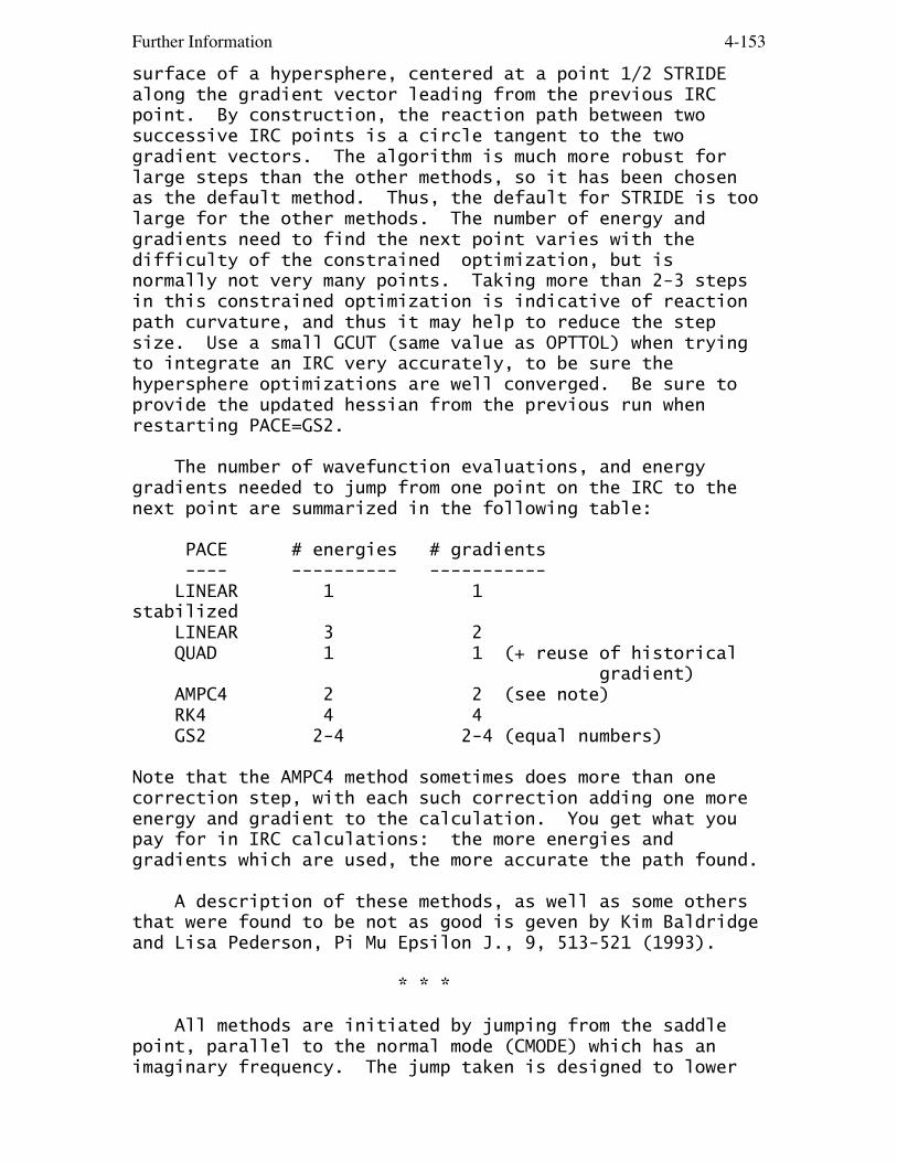
Further Information 4-153
surface of a hypersphere, centered at a point 1/2 STRIDEalong the gradient vector leading from the previous IRCpoint. By construction, the reaction path between twosuccessive IRC points is a circle tangent to the twogradient vectors. The algorithm is much more robust forlarge steps than the other methods, so it has been chosenas the default method. Thus, the default for STRIDE is toolarge for the other methods. The number of energy andgradients need to find the next point varies with thedifficulty of the constrained optimization, but isnormally not very many points. Taking more than 2-3 stepsin this constrained optimization is indicative of reactionpath curvature, and thus it may help to reduce the stepsize. Use a small GCUT (same value as OPTTOL) when tryingto integrate an IRC very accurately, to be sure thehypersphere optimizations are well converged. Be sure toprovide the updated hessian from the previous run whenrestarting PACE=GS2.
The number of wavefunction evaluations, and energygradients needed to jump from one point on the IRC to thenext point are summarized in the following table:
PACE # energies # gradients ---- ---------- ----------- LINEAR 1 1stabilized LINEAR 3 2 QUAD 1 1 (+ reuse of historical gradient) AMPC4 2 2 (see note) RK4 4 4 GS2 2-4 2-4 (equal numbers)
Note that the AMPC4 method sometimes does more than onecorrection step, with each such correction adding one moreenergy and gradient to the calculation. You get what youpay for in IRC calculations: the more energies andgradients which are used, the more accurate the path found.
A description of these methods, as well as some othersthat were found to be not as good is geven by Kim Baldridgeand Lisa Pederson, Pi Mu Epsilon J., 9, 513-521 (1993).
* * *
All methods are initiated by jumping from the saddlepoint, parallel to the normal mode (CMODE) which has animaginary frequency. The jump taken is designed to lower

Further Information 4-154
the energy by an amount EVIB. The actual distance taken isthus a function of the imaginary frequency, as a smallerFREQ will produce a larger initial jump. You can simplyprovide a $HESS group instead of CMODE and FREQ, whichinvolves less typing. To find out the actual step takenfor a given EVIB, use EXETYP=CHECK. The direction of thejump (towards reactants or products) is governed by FORWRD.Note that if you have decided to use small step sizes, youmust employ a smaller EVIB to ensure a small first step.The GS2 method begins by following the normal mode by onehalf of STRIDE, and then performing a hypersphereminimization about that point, so EVIB is irrelevant tothis PACE.
The only method which proves that a properly convergedIRC has been obtained is to regenerate the IRC with asmaller step size, and check that the IRC is unchanged.Again, note that the care with which an IRC must beobtained is highly dependent on what use it is intendedfor.
Some key IRC references are:K.Ishida, K.Morokuma, A.Komornicki J.Chem.Phys. 66, 2153-2156 (1977)K.Muller Angew.Chem., Int.Ed.Engl. 19, 1-13 (1980)M.W.Schmidt, M.S.Gordon, M.Dupuis J.Am.Chem.Soc. 107, 2585-2589 (1985)B.C.Garrett, M.J.Redmon, R.Steckler, D.G.Truhlar,K.K.Baldridge, D.Bartol, M.W.Schmidt, M.S.Gordon J.Phys.Chem. 92, 1476-1488(1988)K.K.Baldridge, M.S.Gordon, R.Steckler, D.G.Truhlar J.Phys.Chem. 93, 5107-5119(1989)C.Gonzales, H.B.Schlegel J.Chem.Phys. 90, 2154-2161(1989)
The IRC discussion closes with some practical tips:
The $IRC group has a confusing array of variables, butfortunately very little thought need be given to most ofthem. An IRC run is restarted by moving the coordinates ofthe next predicted IRC point into $DATA, and inserting thenew $IRC group into your input file. You must select thedesired value for NPOINT. Thus, only the first job whichinitiates the IRC requires much thought about $IRC.
The symmetry specified in the $DATA deck should be thesymmetry of the reaction path. If a saddle point happensto have higher symmetry, use only the lower symmetry in the

Further Information 4-155
$DATA deck when initiating the IRC. The reaction path willhave a lower symmetry than the saddle point whenever thenormal mode with imaginary frequency is not totallysymmetric. Be careful that the order and orientation ofthe atoms corresponds to that used in the run whichgenerated the hessian matrix.
If you wish to follow an IRC for a different isotope,use the $MASS group. If you wish to follow the IRC inregular Cartesian coordinates, just enter unit masses foreach atom. Note that CMODE and FREQ are a function of theatomic masses, so either regenerate FREQ and CMODE, or moresimply, provide the correct $HESS group.
Further Information 4-156
Gradient Extremals
This section of the manual, as well as the source codeto trace gradient extremals was written by Frank Jensen ofthe University of Aarhus.
A Gradient Extremal (GE) curve consists of points wherethe gradient norm on a constant energy surface isstationary. This is equivalent to the condition thatthe gradient is an eigenvector of the Hessian. Such GEcurves radiate along all normal modes from a stationarypoint, and the GE leaving along the lowest normal modefrom a minimum is the gentlest ascent curve. This is notthe same as the IRC curve connecting a minimum and a TS,but may in some cases be close.
GEs may be divided into three groups: those leadingto dissociation, those leading to atoms colliding, andthose which connect stationary points. The latter classallows a determination of many (all?) stationary points ona PES by tracing out all the GEs. Following GEs is thus asemi-systematic way of mapping out stationary points. Thedisadvantages are: i) There are many (but finitely many!) GEs for a large molecule. ii) Following GEs is computationally expensive. iii) There is no control over what type of stationary point (if any) a GE will lead to.
Normally one is only interested in minima and TSs, butmany higher order saddle points will also be found.Furthermore, it appears that it is necessary to follow GEsradiating also from TSs and second (and possibly alsohigher) order saddle point to find all the TSs.
A rather complete map of the extremals for the H2COpotential surface is available in a paper which explainsthe points just raised in greater detail: K.Bondensgaard, F.Jensen, J.Chem.Phys. 104, 8025-8031(1996).An earlier paper gives some of the properties of GEs: D.K.Hoffman, R.S.Nord, K.Ruedenberg, Theor. Chim. Acta 69, 265-279(1986).
There are two GE algorithms in GAMESS, one due to Sunand Ruedenberg (METHOD=SR), which has been extended toinclude the capability of locating bifurcation points and
Further Information 4-157
turning points, and another due to Jorgensen, Jensen, andHelgaker (METHOD=JJH): J. Sun, K. Ruedenberg, J.Chem.Phys. 98, 9707-9714(1993) P. Jorgensen, H. J. Aa. Jensen, T. Helgaker Theor. Chim. Acta 73, 55 (1988).
The Sun and Ruedenberg method consist of a predictorstep taken along the tangent to the GE curve, followed byone or more corrector steps to bring the geometry back tothe GE. Construction of the GE tangent and the correctorstep requires elements of the third derivative of theenergy, which is obtained by a numerical differentiationof two Hessians. This puts some limitations on whichsystems the GE algorithm can be used for. First, thenumerical differentiation of the Hessian to produce thirdderivatives means that the Hessian should be calculated byanalytical methods, thus only those types of wavefunctionswhere this is possible can be used. Second, eachpredictor/corrector step requires at least two Hessians,but often more. Maybe 20-50 such steps are necessary fortracing a GE from one stationary point to the next. Asystematic study of all the GE radiating from a stationarypoint increases the work by a factor of ~2*(3N-6). Oneshould thus be prepared to invest at least hundreds, andmore likely thousands, of Hessian calculations. In otherwords, small systems, small basis sets, and simple wave-functions.
The Jorgensen, Jensen, and Helgaker method consists oftaking a step in the direction of the chosen Hessianeigenvector, and then a pure NR step in the perpendicularmodes. This requires (only) one Hessian calculation foreach step. It is not suitable for following GEs where theGE tangent forms a large angle with the gradient, and itis incapable of locating GE bifurcations.
Although experience is limited at present, the JJHmethod does not appear to be suitable for following GEs ingeneral (at least not in the current implementation).Experiment with it at your own risk!
The flow of the SR algorithm is as follows: Apredictor geometry is produced, either by jumping awayfrom a stationary point, or from a step in the tangentdirection from the previous point on the GE. At thepredictor geometry, we need the gradient, the Hessian, andthe third derivative in the gradient direction. Dependingon HSDFDB, this can be done in two ways. If .TRUE. thegradient is calculated, and two Hessians are calculated at
Further Information 4-158
SNUMH distance to each side in the gradient direction.The Hessian at the geometry is formed as the average ofthe two displaced Hessians. This corresponds to a double-sided differentiation, and is the numerical most stablemethod for getting the partial third derivative matrix.If HSDFDB = .FALSE., the gradient and Hessian arecalculated at the current geometry, and one additionalHessian is calculated at SNUMH distance in the gradientdirection. This corresponds to a single-sided differen-tiation. In both cases, two full Hessian calculations arenecessary, but HSDFDB = .TRUE. require one additionalwavefunction and gradient calculation. This is usuallya fairly small price compared to two Hessians, and thenumerically better double-sided differentiation hastherefore been made the default.
Once the gradient, Hessian, and third derivative isavailable, the corrector step and the new GE tangent areconstructed. If the corrector step is below a threshold,a new predictor step is taken along the tangent vector.If the corrector step is larger than the threshold, thecorrection step is taken, and a new micro iteration isperformed. DELCOR thus determines how closely the GE willbe followed, and DPRED determine how closely the GE pathwill be sampled.
The construction of the GE tangent and corrector stepinvolve solution of a set of linear equations, which inmatrix notation can be written as Ax=B. The A-matrix isalso the second derivative of the gradient norm on theconstant energy surface.
After each corrector step, various things are printedto monitor the behavior: The projection of the gradientalong the Hessian eigenvalues (the gradient is parallelto an eigenvector on the GE), the projection of the GEtangent along the Hessian eigenvectors, and the overlapof the Hessian eigenvectors with the mode being followedfrom the previous (optimzed) geometry. The sign of theseoverlaps are not significant, they just refer to anarbitrary phase of the Hessian eigenvectors.
After the micro iterations has converged, the Hessianeigenvector curvatures are also displayed, this is anindication of the coupling between the normal modes. Thenumber of negative eigenvalues in the A-matrix is denotedthe GE index. If it changes, one of the eigenvalues musthave passed through zero. Such points may either be GEbifurcations (where two GEs cross) or may just be "turning

Further Information 4-159
points", normally when the GE switches from going uphillin energy to downhill, or vice versa. The distinction ismade based on the B-element corresponding to the A-matrixeigenvalue = 0. If the B-element = 0, it is a bifurcation,otherwise it is a turning point.
If the GE index changes, a linear interpolation isperformed between the last two points to locate the pointwhere the A-matrix is singular, and the correspondingB-element is determined. The linear interpolation pointswill in general be off the GE, and thus the evaluation ofwhether the B-element is 0 is not always easy. Theprogram additionally evaluates the two limiting vectorswhich are solutions to the linear sets of equations, theseare also used for testing whether the singular point is abifurcation point or turning point.
Very close to a GE bifurcation, the corrector stepbecome numerically unstable, but this is rarely a problemin practice. It is a priori expected that GE bifurcationwill occur only in symmetric systems, and the crossing GEwill break the symmetry. Equivalently, a crossing GE maybe encountered when a symmetry element is formed, howeversuch crossings are much harder to detect since the GEindex does not change, as one of the A-matrix eigenvaluesmerely touches zero. The program prints an message ifthe absolute value of an A-matrix eigenvalue reaches aminimum near zero, as such points may indicate thepassage of a bifurcation where a higher symmetry GEcrosses. Run a movie of the geometries to see if a moresymmetric structure is passed during the run.
An estimate of the possible crossing GE direction ismade at all points where the A-matrix is singular, and twoperturbed geometries in the + and - direction are writtenout. These may be used as predictor geometries forfollowing a crossing GE. If the singular geometry is aturning point, the + and - geometries are just predictorgeometries on the GE being followed.
In any case, a new predictor step can be taken to tracea different GE from the newly discovered singular point,using the direction determined by interpolation from thetwo end point tangents (the GE tangent cannot be uniquelydetermined at a bifurcation point). It is not possible todetermine what the sign of IFOLOW should be when startingoff along a crossing GE at a bifurcation, one will have totry a step to see if it returns to the bifurcation pointor not.

Further Information 4-160
In order to determine whether the GE index change itis necessary to keep track of the order of the A-matrixeigenvalues. The overlap between successive eigenvectorsare shown as "Alpha mode overlaps".
Things to watch out for:1) The numerical differentiation to get third derivativesrequires more accuracy than usual. The SCF convergenceshould be at least 100 times smaller than SNUMH, andpreferably better. With the default SNUMH of 10**(-4)the SCF convergence should be at least 10**(-6). Sincethe last few SCF cycles are inexpensive, it is a good ideato tighten the SCF convergence as much as possible, tomaybe 10**(-8) or better. You may also want to increasethe integral accuracy by reducing the cutoffs (ITOL andICUT) and possibly also try more accurate integrals(INTTYP=HONDO). The CUTOFF in $TRNSFM may also be reducedto produce more accurate Hessians. Don't attempt to use avalue for SNUMH below 10**(-6), as you simply can't getenough accuracy. Since experience is limited at present,it is recommended that some tests runs are made to learnthe sensitivity of these factors for your system.
2) GEs can be followed in both directions, uphill ordownhill. When stating from a stationary point, thedirection is implicitly given as away from the stationarypoint. When starting from a non-stationary point, the "+"and "-" directions (as chosen by the sign of IFOLOW)refers to the gradient direction. The "+" direction isalong the gradient (energy increases) and "-" is oppositeto the gradient (energy decreases).
3) A switch from one GE to another may be seen when twoGE come close together. This is especially troublesomenear bifurcation points where two GEs actually cross. Insuch cases a switch to a GE with -higher- symmetry mayoccur without any indication that this has happened,except possibly that a very large GE curvature suddenlyshows up. Avoid running the calculation with lesssymmetry than the system actually has, as this increasesthe likelihood that such switches occuring. Fix: alterDPRED to avoid having the predictor step close to thecrossing GE.
4) "Off track" error message: The Hessian eigenvectorwhich is parallel to the gradient is not the same asthe one with the largest overlap to the previousHessian mode. This usually indicate that a GE switch

Further Information 4-161
has occured (note that a switch may occur without thiserror message), or a wrong value for IFOLOW when startingfrom a non-stationary point. Fix: check IFOLOW, if it iscorrect then reduce DPRED, and possibly also DELCOR.
5) Low overlaps of A-matrix eigenvectors. Small overlapsmay give wrong assignment, and wrong conclusions about GEindex change. Fix: reduce DPRED.
6) The interpolation for locating a point where one of theA-matrix eigenvalues is zero fail to converge. Fix:reduce DPRED (and possibly also DELCOR) to get a shorther(and better) interpolation line.
7) The GE index changes by more than 1. A GE switch mayhave occured, or more than one GE index change is locatedbetween the last and current point. Fix: reduce DPRED tosample the GE path more closely.
8) If SNRMAX is too large the algorithm may try to locatestationary points which are not actually on the GE beingfollowed. Since GEs often pass quite near a stationarypoint, SNRMAX should only be increased above the default0.10 after some consideration.

Further Information 4-162
Continuum Solvation Methods
In a very thorough 1994 review of continuum solvationmodels, Tomasi and Persico divide the possible approachesto the treatment of solvent effects into four categories: a) virial equations of state, correlation functions b) Monte Carlo or molecular dynamics simulations c) continuum treatments d) molecular treatmentsThe Effective Fragment Potential method, documented in thefollowing section of this chapter, falls into the lattercategory, as each EFP solvent molecule is modeled as adistinct object (discrete solvation). This sectiondescribes the four continuum models which are implementedin the standard version of GAMESS, and a fifth model whichcan be interfaced.
Continuum models typically form a cavity of some sortcontaining the solute molecule, while the solvent outsidethe cavity is thought of as a continuous medium and iscategorized by a limited amount of physical data, such asthe dielectric constant. The electric field of the chargedparticles comprising the solute interact with thisbackground medium, producing a polarization in it, which inturn feeds back upon the solute's wavefunction.
Self Consistent Reaction Field (SCRF)
A simple continuum model is the Onsager cavity model,often called the Self-Consistent Reaction Field, or SCRFmodel. This represents the charge distribution of thesolute in terms of a multipole expansion. SCRF usuallyuses an idealized cavity (spherical or ellipsoidal) toallow an analytic solution to the interaction energybetween the solute multipole and the multipole which thisinduces in the continuum. This method is implemented inGAMESS in the simplest possible fashion: i) a spherical cavity is used ii) the molecular electrostatic potential of the solute is represented as a dipole only, except a monopole is also included for an ionic solute.The input for this implementation of the Kirkwood-Onsagermodel is provided in $SCRF.
Some references on the SCRF method are 1. J.G.Kirkwood J.Chem.Phys. 2, 351 (1934)

Further Information 4-163
2. L.Onsager J.Am.Chem.Soc. 58, 1486 (1936) 3. O.Tapia, O.Goscinski Mol.Phys. 29, 1653 (1975) 4. M.M.Karelson, A.R.Katritzky, M.C.Zerner Int.J.Quantum Chem., Symp. 20, 521-527 (1986) 5. K.V.Mikkelsen, H.Agren, H.J.Aa.Jensen, T.Helgaker J.Chem.Phys. 89, 3086-3095 (1988) 6. M.W.Wong, M.J.Frisch, K.B.Wiberg J.Am.Chem.Soc. 113, 4776-4782 (1991) 7. M.Szafran, M.M.Karelson, A.R.Katritzky, J.Koput, M.C.Zerner J.Comput.Chem. 14, 371-377 (1993) 8. M.Karelson, T.Tamm, M.C.Zerner J.Phys.Chem. 97, 11901-11907 (1993)
The method is very sensitive to the choice of the soluteRADIUS, but not very sensitive to the particular DIELEC ofpolar solvents. The plots in reference 7 illustrate thesepoints very nicely. The SCRF implementation in GAMESS isZerner's Method A, described in the same reference. Thetotal solute energy includes the Born term, if the soluteis an ion. Another limitation is that a solute's electro-static potential is not likely to be fit well as a dipolemoment only, for example see Table VI of reference 5 whichillustrates the importance of higher multipoles. Finally,the restriction to a spherical cavity may not be veryrepresentative of the solute's true shape. However, in thespecial case of a roundish molecule, and a large dipolewhich is geometry sensitive, the SCRF model may includesufficient physics to be meaningful: M.W.Schmidt, T.L.Windus, M.S.Gordon J.Am.Chem.Soc. 117, 7480-7486(1995).Most cases should choose PCM (next section) over SCRF!!!
Polarizable Continuum Model (PCM)
A much more sophisticated continuum method, named thePolarizable Continuum Model, is also available. The PCMmethod places a solute in a cavity formed by a union ofspheres centered on each atom. PCM includes a more exacttreatment of the electrostatic interaction of the solutewith the surrounding medium, on the cavity's surface. Thecomputational procedure divides this surface into manysmall tesserae, each having a different "apparent surfacecharge", reflecting the solute's and other tesserae'selectric field at each. These surface charges are the PCMmodel's "solvation effect" and make contributions to theenergy and to the gradient of the solute.

Further Information 4-164
Typically the cavity is defined as a union of atomicspheres, which should be roughly 1.2 times the atomic vander Waals radii. A technical difficulty caused by thepenetration of the solute's charge density outside thiscavity is dealt with by a renormalization. The solvent ischaracterized by its dielectric constant, surface tension,size, density, and so on. Procedures are provided not onlyfor the computation of the electrostatic interaction of thesolute with the apparent surface charges, but also for thecavitation energy, and for the dispersion and repulsioncontributions to the solvation free energy.
Methodology for solving the Poisson equation to obtainthe "apparent surface charges" has progressed from D-PCM toIEF-PCM to C-PCM over time, with the latter preferred.Iterative solvers require far less computer resources thandirect solvers. Advancements have also been made inschemes to divide the surface cavity into tiny tesserae.As of fall 2008, the FIXPVA tessellation, which has smoothswitching functions for tesserae near sphere boundaries,together with iterative C-PCM, gives very satisfactorygeometry optimizations for molecules of 100 atoms. TheFIXPVA tessellation was extended to work for cavitation(ICAV), dispersion (IDP), and repulsion (IREP) options infall 2009, and dispersion/repulsion (IDISP) in spring 2010.Other procedures remain, and make the input seem complex,but their use is discouraged. Thus $PCM SOLVNT=WATER $ENDchooses iterative C-PCM (IEF=-10) and FIXPVA tessellation(METHOD=4 in $TESCAV) to do basic electrostatics in anaccurate fashion.
The main input group is $PCM, with $PCMCAV providingauxiliary cavity information. If any of the optionalenergy computations are requested in $PCM, the additionalinput groups $IEFPCM, $NEWCAV, $DISBS, or $DISREP may berequired.
It is useful to summarize the various cavities used byPCM, since as many as three cavities may be used: the basic cavity for electrostatics, cavity for cavitation energy, if ICAV=1, cavity for dispersion/repulsion, if IDISP=1.The first and second share the same radii (see RADII in$PCMCAV), which are scaled by ALPHA=1.2 for electrostatics,but are used unscaled for cavitation. The dispersioncavity is defined in $DISREP with a separate set of atomicradii, and even solvent molecule radii! Only theelectrostatics cavity can use any of the GEPOL-GB, GEPOL-AS
Further Information 4-165
or recommended FIXPVA tessellation, while the other two useonly the original GEPOL-GB.
Radii are an important part of the PCM parameterization.Their values can have a significant impact on the qualityof the results. This is particularly true if the solute ischarged, and thus has a large electrostatic interactionwith the continuum. John Emsley's book "The Elements" is auseful source of van der Waals and other radii.
PCM is at heart a means of treating the electrostaticinteractions between the solute's wavefunction and adielectric model for the bulk solvent. The former isrepresented as an electron density from whatever quantummechanical treatment is used for the solute, and the latteris a set of surface charges on the finite elements of thecavity (tessellation). This leaves out other importantcontributions to the solvation energy! These include theenergy needed to make a hole in the solvent (cavitationenergy), dispersion or repulsive interactions between thesolute and solvent, and in the SMD model (see below)solvent structure changes such as would occur in the firstsolvation shell. Some empirical formulae for such "CDS"corrections are provided as keywords ICAV, IDISP, IREP/IDP,which may not work with all wavefunctions, and may not becompatible with gradients.
The SMD model gives an alternative set of such "CDS"corrections, which are compatible with nuclear gradients:see SMD=.TRUE. in $PCM. A more detailed description of SMDis given in the paper cited below. The SMD solventparameters is described (as of 2010) in http://comp.chem.umn.edu/solvation/mnsddb.pdfThis gives numerical parameters, all built into GAMESS, asthe various SOLX values, for SOLVNT= ACETACID CLPROPAN PHOPH EGME E2PENTEN ACETONE OCLTOLUE DPROAMIN MEACETAT PENTACET ACETNTRL M-CRESOL DODECAN MEBNZATE PENTAMIN ACETPHEN O-CRESOL MEG MEBUTATE PFB ANILINE CYCHEXAN ETSH MEFORMAT BENZALCL ANISOLE CYCHEXON ETHANOL MIBK PROPANAL BENZALDH CYCPENTN ETOAC MEPROPYL PROPACID BENZENE CYCPNTOL ETOME ISOBUTOL PROPANOL BENZNTRL CYCPNTON EB TERBUTOL PROPNOL2 BENZYLCL DECLNCIS PHENETOL NMEANILN PROPNTRL BRISOBUT DECLNTRA C6H5F MECYCHEX PROPENOL BRBENZEN DECLNMIX FOCTANE NMFMIXTR PROPACET BRETHANE DECANE FORMAMID ISOHEXAN PROPAMIN BROMFORM DECANOL FORMACID MEPYRID2 PYRIDINE
Further Information 4-166
BROCTANE EDB12 HEPTANE MEPYRID3 C2CL4 BRPENTAN DIBRMETN HEPTANOL MEPYRID4 THF BRPROPA2 BUTYLETH HEPTNON2 C6H5NO2 SULFOLAN BRPROPAN ODICLBNZ HEPTNON4 C2H5NO2 TETRALIN BUTANAL EDC12 HEXADECN CH3NO2 THIOPHEN BUTACID C12DCE HEXANE NTRPROP1 PHSH BUTANOL T12DCE HEXNACID NTRPROP2 TOLUENE BUTANOL2 DCM HEXANOL ONTRTOLU TBP BUTANONE ETHER HEXANON2 NONANE TCA111 BUTANTRL ET2S HEXENE NONANOL TCA112 BUTILE DIETAMIN HEXYNE NONANONE TCE NBA MI C6H5I OCTANE ET3N NBUTBENZ DIPE IOBUTANE OCTANOL TFE222 SBUTBENZ DMDS C2H5I OCTANON2 TMBEN124 TBUTBENZ DMSO IOHEXDEC PENTDECN ISOCTANE CS2 DMA CH3I PENTANAL UNDECANE CARBNTET CISDMCHX IOPENTAN NPENTANE M-XYLENE CLBENZEN DMF IOPROPAN PENTACID O-XYLENE SECBUTCL DMEPEN24 CUMENE PENTANOL P-XYLENE CHCL3 DMEPYR24 P-CYMENE PENTNON2 XYLENEMX CLHEXANE DMEPYR26 MESITYLN PENTNON3 CLPENTAN DIOXANE METHANOL PENTENEand provides a translation table to full chemical names, ifyou can't guess from the input choices given above. Thetranslations can also be found in the source code. Twoimportant things to note about SMD are: a) the atomic radii are changed, so although thealgorithms for electrostatics are those of standard PCM,the numerical results for the electrostatics do change. b) SMD's parameterization was developed for IEF-PCMusing GEPOL tessellation with a fine grid: IEF=-3 andMTHALL=2, NTSALL=240. However it is considered acceptableto use SMD's parameters, unchanged, with C-PCM and with theFIXPVA tessellation, at default coarseness. Hence, inputsuch as $pcm solvnt=dmso smd=.true. $endis enough to carry out a SMD-style C-PCM treatment in DMSO. c) The CDS correction involves cavitation, dispersion,and as a collective "solvent structure contribution"estimates for partial hydrogen bonding, repulsion, anddeviation of the dielectric constant from its bulk value. d) See also SMVLE in the more sophisticated SS(V)PEcontinuum model's description.
Solvation of course affects the non-linear opticalproperties of molecules. The PCM implementation extendsRUNTYP=TDHF to include solvent effects. Both static andfrequency dependent hyperpolarizabilities can be found.Besides the standard PCM electrostatic contribution, the
Further Information 4-167
IREP and IDP keywords can be used to determine the effectsof repulsion and dispersion on the polarizabilities.
The implementation of the PCM model in GAMESS hasreceived considerable attention from Hui Li and Jan Jensenat the University of Iowa, Iowa State University, andUniversity of Nebraska. This includes new iterativetechniques to solving the surface charge problem, newtessellations that provide for numerically stable nucleargradients, the implementation of C-PCM equations, theextension of PCM to all SCFTYPs and TDDFT, development ofan interface with the EFP model (quo vadis), andheterogenous dielectric. Dmitri Fedorov at AIST hasinterfaced PCM to the FMO method (quo vadis), and reducedstorage requirements.
Due to its sophistication, users of the PCM model arestrongly encouraged to read the primary literature:
Of particular relevance to PCM in GAMESS:
1) "Continuum solvation of large molecules described byQM/MM: a semi-iterative implementation of the PCM/EFPinterface" H.Li, C.S.Pomelli, J.H.Jensen Theoret.Chim.Acta 109, 71-84(2003)2) "Improving the efficiency and convergence of geometryoptimization with the polarizable continuum model: newenergy gradients and molecular surface tessellation" H.Li, J.H.Jensen J.Comput.Chem. 25, 1449-1462(2004)3) "The polarizable continuum model interfaced with theFragment Molecular Orbital method" D.G.Fedorov, K.Kitaura, H.Li, J.H.Jensen, M.S.Gordon J.Comput.Chem. 27, 976-985(2006)4) "Energy gradients in combined Fragment Molecular Orbitaland Polarizable Continuum Model (FMO/PCM)" H.Li, D.G.Fedorov, T.Nagata, K.Kitaura, J.H.Jensen, M.S.Gordon J.Comput.Chem. 31, 778-790(2010)5) "Continuous and smooth potential energy surface forconductor-like screening solvation model using fixed pointswith variable area" P.Su, H.Li J.Chem.Phys. 130, 074109/1-13(2009)6) "Heterogenous conductorlike solvation model" D.Si, H.Li J.Chem.Phys. 131, 044123/1-8(1009)7) "Quantum mechanical/molecular mechanical/continuum stylesolvation model: linear response theory, variationaltreatment, and nuclear gradients" H.Li J.Chem.Phys. 131, 184103/1-8(2009)
Further Information 4-168
8) "Smooth potential energy surface for cavitation,dispersion, and repulsion free energies in polarizablecontinuum model" Y.Wang, H.Li J.Chem.Phys. 131, 206101/1-2(2009)9) "Excited state geometry of photoactive yellow proteinchromophore: a combined conductorlike polarizable continuummodel and time-dependent density functional study" Y.Wang, H.Li J.Chem.Phys. 133, 034108/1-11(2010)
Paper number 7 is about the treatment of QM systems withthe solvation models EFP and/or C-PCM.
SMD and its CDS cavitation/dispersion/solvent structurecorrections are described in"Universal solution model based on solute electron densityand on a continuum model of the solvent defined by the bulkdielectric constant and atomic surface tensions" A.V.Marenich, C.J.Cramer, D.G.Truhlar J.Phys.Chem.B 113, 6378-6396(2009)
General papers on PCM:10) S.Miertus, E.Scrocco, J.Tomasi Chem.Phys. 55, 117-129(1981)11) J.Tomasi, M.Persico Chem.Rev. 94, 2027-2094(1994)12) R.Cammi, J.Tomasi J.Comput.Chem. 16, 1449-1458(1995)13) J.Tomasi, B.Mennucci, R.Cammi Chem.Rev. 105, 2999-3093(2005)
The GEPOL-GB method for cavity construction:14) J.L.Pascual-Ahuir, E.Silla, J.Tomasi, R.Bonaccorsi J.Comput.Chem. 8, 778-787(1987)
Charge renormalization (see also ref. 12):15) B.Mennucci, J.Tomasi J.Chem.Phys. 106, 5151-5158(1997)
Derivatives with respect to nuclear coordinates: (energy gradient and hessian) See also paper 2 and 3.16) R.Cammi, J.Tomasi J.Chem.Phys. 100, 7495-7502(1994)17) R.Cammi, J.Tomasi J.Chem.Phys. 101, 3888-3897(1995)18) M.Cossi, B.Mennucci, R.Cammi J.Comput.Chem. 17, 57-73(1996)
Derivatives with respect to applied electric fields: (polarizabilities and hyperpolarizabilities)19) R.Cammi, J.Tomasi Int.J.Quantum Chem. Symp. 29, 465-474(1995)20) R.Cammi, M.Cossi, J.Tomasi J.Chem.Phys. 104, 4611-4620(1996)21) R.Cammi, M.Cossi, B.Mennucci, J.Tomasi
Further Information 4-169
J.Chem.Phys. 105, 10556-10564(1996)22) B. Mennucci, C. Amovilli, J. Tomasi Chem.Phys.Lett. 286, 221-225(1998)
Cavitation energy:23) R.A.Pierotti Chem.Rev. 76, 717-726(1976)24) J.Langlet, P.Claverie, J.Caillet, A.Pullman J.Phys.Chem. 92, 1617-1631(1988)
Dispersion and repulsion energies:25) F.Floris, J.Tomasi J.Comput.Chem. 10, 616-627(1989)26) C.Amovilli, B.Mennucci J.Phys.Chem.B 101, 1051-1057(1997)
Integral Equation Formalism PCM. The first of thesedeals with anisotropies, the last 2 with nuclear gradients.27) E.Cances, B.Mennucci, J.Tomasi J.Chem.Phys. 107, 3032-3041(1997)28) B.Mennucci, E.Cances, J.Tomasi J.Phys.Chem.B 101, 10506-17(1997)29) B.Mennucci, R.Cammi, J.Tomasi J.Chem.Phys. 109, 2798-2807(1998)30) J.Tomasi, B.Mennucci, E.Cances J.Mol.Struct.(THEOCHEM) 464, 211-226(1999)31) E.Cances, B.Mennucci J.Chem.Phys. 109, 249-259(1998)32) E.Cances, B.Mennucci, J.Tomasi J.Chem.Phys. 109, 260-266(1998)
Conductor PCM (C-PCM):33) V.Barone, M.Cossi J.Phys.Chem.A 102, 1995-2001(1998)34) M.Cossi, N.Rega, G.Scalmani, V.Barone J.Comput.Chem. 24, 669-681(2003)
C-PCM with TD-DFT:35) M.Cossi, V.Barone J.Chem.Phys. 115, 4708-4717(2001)See also paper #8 above for the coding in GAMESS.
At the present time, the PCM model in GAMESS has thefollowing limitations:
a) Any SCFTYP may be used (RHF to MCSCF). MP2 or DFT may be used with any of the RHF, UHF, and ROHF gradient programs. Closed shell TD-DFT excited state gradients may also be used. CI and Coupled Cluster programs are not available. b) semi-empirical methods may not be used. c) the only other solvent method that may be used at used with PCM is the EFP model. d) point group symmetry is switched off internally

Further Information 4-170
during PCM. e) The PCM model runs in parallel for IEF=3, -3, 10, or -10 and for all 5 wavefunctions (energy or gradient), but not for RUNTYP=TDHF jobs. f) D-PCM stores electric field integrals at normals to the surface elements on disk. IEF-PCM and C-PCM using the explicit solver (+3 and +10) store electric potential integrals at normals to the surface on disk. This is true even for direct AO integral runs, and the file sizes may be considerable (basis set size squared times the number of tesserae). IEF-PCM and C-PCM with the iterative solvers do not store the potential integrals, when IDIRCT=1 in the $PCMITR group (this is the default) g) nuclear derivatives are limited to gradients, although theory for hessians is given in paper 17.
* * *
The only PCM method prior to Oct. 2000 was D-PCM, whichcan be recovered by selecting IEF=0 and ICOMP=2 in $PCM.The default PCM method between Oct. 2000 and May 2004 wasIEF-PCM, recoverable by IEF=-3 (but 3 for non-gradientruns) and ICOMP=0. As of May 2004, the default PCM methodwas changed to C-PCM (IEF=-10, ICOMP=0). The extension ofPCM to all SCFTYPs as of May 2004 involved a correction tothe MCSCF PCM operator, so that it would reproduce RHFresults when run on one determinant, meaning that it isimpossible to reproduce prior MCSCF PCM calculations.
The cavity definition was GEPOL-GB (MTHALL=1 in $TESCAV)prior to May 2004, GEPOL-AS (MTHALL=2) from then untilSeptember 2008, and FIXPVA (MTHALL=4) to the present time.The option for generation of 'extra spheres' (RET in $PCM)was changed from 0.2 to 100.0, to suppress these, in June2003.
* * *
In general, use of PCM electrostatics is very simple, asmay be seen from exam31.inp supplied with the program.
The calculation shown next illustrates the use of someof the older PCM options. Since methane is non-polar, itsinternal energy change and the direct PCM electrostaticinteraction is smaller than the cavitation, repulsion, anddispersion corrections. Note that the use of ICAV, IREP,and IDP are currently incompatible with gradients, so a

Further Information 4-171
reasonable calculation sequence might be to perform thegeometry optimization with PCM electrostatics turned on,then perform an additional calculation to include the othersolvent effects, adding extra functions to improve thedispersion correction.
! calculation of CH4 (metano), in PCM water.!! This input reproduces the data in Table 2, line 6, of! C.Amovilli, B.Mennucci J.Phys.Chem.B 101, 1051-7(1997)! To do this, we must use many original PCM options.!! The gas phase FINAL energy is -40.2075980292! The FINAL energy in PCM water is -40.2048210283! (lit.)! FREE ENERGY IN SOLVENT = -25234.89 KCAL/MOL! INTERNAL ENERGY IN SOLVENT = -25230.64 KCAL/MOL! DELTA INTERNAL ENERGY = .01 KCAL/MOL ( 0.0)! ELECTROSTATIC INTERACTION = -.22 KCAL/MOL (-0.2)! PIEROTTI CAVITATION ENERGY = 5.98 KCAL/MOL ( 6.0)! DISPERSION FREE ENERGY = -6.00 KCAL/MOL (-6.0)! REPULSION FREE ENERGY = 1.98 KCAL/MOL ( 2.0)! TOTAL INTERACTION = 1.73 KCAL/MOL ( 1.8)! TOTAL FREE ENERGY IN SOLVENT= -25228.91 KCAL/MOL! $contrl scftyp=rhf runtyp=energy $end $guess guess=huckel $end $system mwords=2 $end! the "W1 basis" input here exactly matches HONDO's DZP $DATACH4...gas phase geometry...in PCM waterTd
Carbon 6. DZV D 1 ; 1 0.75 1.0
Hydrogen 1. 0.6258579976 0.6258579976 0.6258579976 DZV 0 1.20 1.15 ! inner and outer scale factors P 1 ; 1 1.00 1.0
$END! The reference cited used a value for H2O's solvent! radius that differs from the built in value (RSOLV).! The IEF, ICOMP, MTHALL, and RET keywords are set to! duplicate the original code's published results,! namely D-PCM and GEPOL-GB. This run doesn't put in! any "extra spheres" but we try that option (RET)! like it originally would have.

Further Information 4-172
$PCM SOLVNT=WATER RSOLV=1.35 RET=0.2 IEF=0 ICOMP=2 IDISP=0 IREP=1 IDP=1 ICAV=1 $end $TESCAV MTHALL=1 $END $NEWCAV IPTYPE=2 ITSNUM=540 $END! dispersion "W2 basis" uses exponents which are! 1/3 of smallest exponent in "W1 basis" of $DATA. $DISBS NADD=11 NKTYP(1)=0,1,2, 0,1, 0,1, 0,1, 0,1 XYZE(1)=0.0,0.0,0.0, 0.0511 0.0,0.0,0.0, 0.0382 0.0,0.0,0.0, 0.25 1.1817023, 1.1817023, 1.1817023, 0.05435467 1.1817023, 1.1817023, 1.1817023, 0.33333333 -1.1817023, 1.1817023,-1.1817023, 0.05435467 -1.1817023, 1.1817023,-1.1817023, 0.33333333 1.1817023,-1.1817023,-1.1817023, 0.05435467 1.1817023,-1.1817023,-1.1817023, 0.33333333 -1.1817023,-1.1817023, 1.1817023, 0.05435467 -1.1817023,-1.1817023, 1.1817023, 0.33333333 $end
SVPE and SS(V)PE.
The Surface Volume Polarization for Electrostatics(SVPE), and an approximation to SVPE called the Surface andSimulation of Volume Polarization for Electrostatics(SS(V)PE) are continuum solvation models. Compared toother continuum models, SVPE and SS(V)PE pay carefulattention to the problems of escaped charge, the shape ofthe surface cavity, and to integration of the Poissonequation for surface charges.
The original references for what is now called theSVPE (surface and volume polarization for electrostatics)method are the theory paper: "Charge penetration in Dielectric Models of Solvation" D.M.Chipman, J.Chem.Phys. 106, 10194-10206 (1997)and the two implementation papers: "Volume Polarization in Reaction Field Theory" C.-G.Zhan, J.Bentley, D.M.Chipman J.Chem.Phys. 108, 177-192 (1998)and "New Formulation and Implementation for Volume Polarization in Dielectric Continuum Theory" D.M.Chipman, J.Chem.Phys. 124, 224111-1/10 (2006)which should be cited in any publications that utilize theSVPE code.

Further Information 4-173
The original reference for the SS(V)PE (surface andsimulation of volume polarization for electrostatics)method is: "Reaction Field Treatment of Charge Penetration" D.M.Chipman, J.Chem.Phys. 112, 5558-5565 (2000)which should be cited in any publications that utilize theSS(V)PE code.
Further information on the performance of SVPE and ofSS(V)PE can be found in: "Comparison of Solvent Reaction Field Representations" D.M.Chipman, Theor.Chem.Acc. 107, 80-89 (2002).Details of the SS(V)PE convergence behavior and programmingstrategy are in: "Implementation of Solvent Reaction Fields for Electronic Structure" D.M.Chipman, M.Dupuis, Theor.Chem.Acc. 107, 90-102 (2002).
The SMVLE option (solvation model with volume andlocal electrostatics) is described in "Free energies of solvation with surface, volume, andlocal electrostatic effects and atomic surface tensions torepresent the first solvation shell" J.Liu, C.P.Kelly,A.C.Goren, A.V.Marenich, C.J.Cramer, D.G.Truhlar, C.-G.Zhan J.Chem.Theory Comput. 6, 1109-1117(2010).
The SVPE and SS(V)PE models are like PCM and COSMO inthat they treat solvent as a continuum dielectric residingoutside a molecular-shaped cavity, determining the apparentcharges that represent the polarized dielectric by solvingPoisson's equation. The main difference between SVPE andSS(V)PE is in treatment of volume polarization effects thatarise because of the tail of the electronic wave functionthat penetrates outside the cavity, sometimes referred toas the "escaped charge." SVPE treats volume polarizationeffects explicitly by including apparent charges in thevolume outside the cavity as well as on the cavity surface.With a sufficient number of grid points, SVPE can thenprovide an exact treatment of charge penetration effects.SS(V)PE, like PCM and COSMO, is an approximate treatmentthat only uses apparent charges located on the cavitysurface. The SS(V)PE equation is particularly designed tosimulate as well as possible the influence of the missingvolume charges. For more information on the similaritiesand differences of the SVPE and SS(V)PE models with othercontinuum methods, see the paper "Comparison of SolventReaction Field Representations" cited just above.
Further Information 4-174
In addition, the cavity construction and Poissonsolver used in this implementation of SVPE and SS(V)PE alsoreceive careful numerical treatment. For example, thecavity may be chosen to be an isodensity contour surface,and the Lebedev grids for the Poisson solver can be chosenvery densely. The Lebedev grids used for surfaceintegration are taken from the Fortran translation by C.van Wuellen of the original C programs developed by D.Laikov. They were obtained from the CCL web sitewww.ccl.net/cca/software/SOURCES/FORTRAN/Lebedev-Laikov-Grids. A recent leading reference is V. I. Lebedev and D.N. Laikov, Dokl. Math. 59, 477-481 (1999). All these gridshave octahedral symmetry and so are naturally adapted forany solute having an Abelian point group. The larger and/orthe less spherical the solute may be, the more surfacepoints are needed to get satisfactory precision in theresults. Further experience will be required to developdetailed recommendations for this parameter. Values assmall as 110 are usually sufficient for simple diatomicsand triatomics. The default value of 1202 has been foundadequate to obtain the energy to within 0.1 kcal/mol forsolutes the size of monosubstituted benzenes. The SVPEmethod uses additional layers of points outside the cavity.Typically just two layers are sufficient to converge thedirect volume polarization contribution to better than 0.1kcal/mol.
The SVPE and SS(V)PE codes both report the amount ofsolute charge penetrating outside the cavity as calculatedby Gauss' Law. The SVPE code additionally reports the samequantity as alternatively calculated from the explicitvolume charges, and any substantial discrepancy betweenthese two determinations indicates that more volumepolarization layers should have been included for betterprecision. The energy contribution from the outermostvolume polarization layer is also reported. If it issignificant then again more layers should have beenincluded. However, these tests are only diagnostic.Passing them does not guarantee that enough layers areincluded.
The SVPE and SS(V)PE models treat the electrostaticinteraction between a quantum solute and a classicaldielectric continuum solvent. No treatment is yetimplemented for cavitation, dispersion, or any of a varietyof other specific solvation effects. Note that correctionsfor these latter effects that might be reported by otherprograms are generally not transferable. The reason isthat they are usually parameterized to improve the ultimate

Further Information 4-175
agreement with experiment. In addition to providingcorrections for the physical effects advertised, theytherefore also inherently include contributions that helpto make up for any deficiencies in the electrostaticdescription. Consequently, they are appropriate only foruse with the particular electrostatic model in which theywere originally developed.
Analytic nuclear gradients are not yet available forthe SVPE or SS(V)PE energy, but numerical differentiationwill permit optimization of small solute molecules.Wavefunctions may be any of the SCF type: RHF, UHF, ROHF,GVB, and MCSCF, or the DFT analogs of some of these. In theMCSCF implementation, no initial wavefunction is availableso the solvation code does not kick in until the seconditeration.
We close with a SVPE example. The gas phase energy,obtained with no $SVP group, is -207.988975, and the runjust below gives the SVPE energy -208.006282. The freeenergy of solvation, -10.860 kcal/mole, is the differenceof these, and is quoted at the right side of the 3rd linefrom the bottom of Table 2 in the paper cited. The"REACTION FIELD FREE ENERGY" for SVPE is -12.905 kcal/mole,which is only part of the solvation free energy. There isalso a contribution due to the SCRF procedure polarizingthe wave function from its gas phase value, causing thesolute internal energy in dielectric to differ from that ingas. Evaluating this latter contribution is what requiresthe separate gas phase calculation. Changing the number oflayers (NVLPL) to zero produces the SS(V)PE approximationto SVPE, E= -208.006208.
! SVPE solvation test...acetamide! reproduce data in Table 2 of the paper on SVPE,! D.M.Chipman J.Chem.Phys. 124, 224111/1-10(2006)! $contrl scftyp=rhf runtyp=energy $end $system mwords=4 $end $basis gbasis=n31 ngauss=6 ndfunc=1 npfunc=1 $end $guess guess=moread norb=16 $end $scf nconv=8 $end $svp nvlpl=3 rhoiso=0.001 dielst=78.304 nptleb=1202 $end $dataCH3CONH2 cgz geometry RHF/6-31G(d,p)C1C 6.0 1.361261 -0.309588 -0.000262C 6.0 -0.079357 0.152773 -0.005665H 1.0 1.602076 -0.751515 0.962042

Further Information 4-176
H 1.0 1.537200 -1.056768 -0.767127H 1.0 2.002415 0.542830 -0.168045O 8.0 -0.387955 1.310027 0.002284N 7.0 -1.002151 -0.840834 -0.011928H 1.0 -1.961646 -0.589397 0.038911H 1.0 -0.752774 -1.798630 0.035006 $endgas phase vectors, E(RHF)= -207.9889751769 $VEC 1 1 1.18951670E-06 1.74015997E-05...snipped... $END
Conductor-like screening model (COSMO)
The COSMO (conductor-like screening model) represents adifferent approach for carrying out polarized continuumcalculations. COSMO was originally developed by AndreasKlamt, with extensions to ab initio computation in GAMESSby Kim Baldridge.
In the COSMO method, the surrounding medium is modeledas a conductor rather than as a dielectric in order toestablish the initial boundary conditions. The assumptionthat the surrounding medium is well modeled as a conductorsimplifies the electrostatic computations and correctionsmay be made a posteriori for dielectric behavior.
The original model of Klamt was introduced using amolecular shaped cavity, which had open parts along thecrevices of intersecting atomic spheres. While havingconsiderable technical advantages, this approximationcauses artifacts in the context of the more generalizedtheory, so the current method for cavity constructionincludes a closure of the cavity to eliminate crevices orpockets.
Two methodologies are implemented for treatment of theoutlying charge errors (OCE). The default is the well-established double cavity procedure using a second, largercavity around the first one, and calculates OCE through thedifference between the potential on the inner and the outercavity. The second involves the calculation of distributedmultipoles up to hexadecapoles to represent the entirecharge distribution of the molecule within the cavity.
The COSMO model accounts only for the electrostaticinteractions between solvent and solute. Klamt has

Further Information 4-177
proposed a novel statistical scheme to compute the fullsolvation free energy for neutral solutes, COSMO-RS, whichis formulated for GAMESS by Peverati, Potier and Baldridge,and is available as external plugin to the COSMOthermprogram by COSMOlogic GmbH&Co.
The iterative inclusion of non-electrostatic effects isalso possible right after a COSMO-RS calculation. TheDCOSMO-RS approach was implemented in GAMESS by Peverati,Potier, and Baldridge, and more information is available onBaldridge website at:
http://ocikbws.uzh.ch/gamess/
The simplicity of the COSMO model allows computation ofgradients, allowing optimization within the context of thesolvent. The method is programmed for RHF and UHF, allcorresponding kinds of DFT (including DFT-D), and thecorresponding MP2, energy and gradient.
Some references on the COSMO model are: A.Klamt, G.Schuurman J.Chem.Soc.Perkin Trans 2, 799-805(1993) A.Klamt J.Phys.Chem. 99, 2224-2235(1995) K.Baldridge, A.Klamt J.Chem.Phys. 106, 6622-6633 (1997) V.Jonas, K.Baldridge J.Chem.Phys. 113, 7511-7518 (2000) L.Gregerson, K.Baldridge Helv.Chim.Acta 86, 4112-4132 (2003) R.Peverati, Y.Potier, K.Baldridge TO BE PUBLISHED SOON
Additional references on the COSMO-RS model, withexplanation of the methodology and program can be found: A.Klamt, F.Eckert, W.Arlt Annu.Rev.Chem.Biomol.Eng. 1, (2010)

Further Information 4-178
The Effective Fragment Potential Method
The basic idea behind the effective fragment potential(EFP) method is to replace the chemically inert part of asystem by EFPs, while performing a regular ab initiocalculation on the chemically active part. Here "inert"means that no covalent bond breaking process occurs. This"spectator region" consists of one or more "fragments",which interact with the ab initio "active region" throughnon-bonded interactions, and so of course these EFPinteractions affect the ab initio wavefunction. The EFPparticles can be closed shell or open shell (high spinROHF) based potentials. The "active region" can use nearlyevery kind of wavefunction available in GAMESS.
A simple example of an active region might be a solutemolecule, with a surrounding spectator region of solventmolecules represented by fragments. Each discrete solventmolecule is represented by a single fragment potential, inmarked contrast to continuum models for solvation.
The quantum mechanical part of the system is entered inthe $DATA group, along with an appropriate basis. The EFPsdefining the fragments are input by means of a $EFRAGgroup, and one or more $FRAGNAME groups describing eachfragment's EFP. These groups define non-bondedinteractions between the ab initio system and thefragments, and also between the fragments. The formerinteractions enter via one-electron operators in the abinitio Hamiltonian, while the latter interactions aretreated by analytic functions. The only electronsexplicitly treated (with basis functions used to expandoccupied orbitals) are those in the active region, so thereare no new two electron terms. Thus the use of EFPs leadsto significant time savings, compared to full ab initiocalculations on the same system.
There are two types of EFP available in GAMESS, EFP1 andEFP2. EFP1, the original method, employs a fittedrepulsive potential. EFP1 is primarily used to model watermolecules to study aqueous solvation effects, at theRHF/DZP or DFT/DZP (specifically, B3LYP) levels, seereferences 1-3 and 26, respectively. EFP2 is a moregeneral method that is applicable to any species, includingwater, and its repulsive potential is obtained from firstprinciples. EFP2 has been extended to include othereffects as well, such as charge transfer and dispersion.
Further Information 4-179
EFP2 forms the basis of the covalent EFP method describedbelow for modeling enzymes, see reference 14.
Parallelization of the EFP1 and EFP2 models is describedin reference 32.
MD simulations with EFP are described in reference 31.
The ab initio/EFP1, or pure EFP system can be wrapped ina Polarizable Continuum Model, see references 23, 43, and50.
terms in an EFP
The non-bonded interactions currently implemented are:
1) Coulomb interaction. The charge distribution of thefragments is represented by an arbitrary number of charges,dipoles, quadrupoles, and octopoles, which interact withthe ab initio hamiltonian as well as with multipoles onother fragments (see reference 2 and 18). It is possibleto use a screening term that accounts for the chargepenetration (reference 17 and 42). This screening term isautomatically included for EFP1. Typically the multipoleexpansion points are located on atomic nuclei and at bondmidpoints.
2) Dipole polarizability. An arbitrary number of dipolepolarizability tensors can be used to calculate the induceddipole on a fragment due to the electric field of the abinitio system as well as all the other fragments. Theseinduced dipoles interact with the ab initio system as wellas the other EFPs, in turn changing their electric fields.All induced dipoles are therefore iterated to self-consistency. Typically the polarizability tensors arelocated at the centroid of charge of each localized orbitalof a fragment. See reference 41.
3) Repulsive potential. Two different forms are used inEFP1: one for ab initio-EFP repulsion and one for EFP-EFPrepulsion. The form of the potentials is empirical, andconsists of distributed Gaussian or exponential functions,respectively. The primary contribution to the repulsion isthe quantum mechanical exchange repulsion, but the fittingtechnique used to develop this term also includes theeffects of charge transfer. Typically these fittedpotentials are located on each atomic nucleus within thefragment (see reference 3). In EFP2, polarization energies

Further Information 4-180
can also be augmented by screening terms, analogous to theelectrostatic screening, to prevent "polarization collapse"(MS in preparation)
For EFP2, the third term is divided into separate analyticformulae for different physical interactions: a) exchange repulsion b) dispersion c) charge transferA summary of EFP2, and its contrast to EFP1 can be found inreference 18 and 44. The repulsive potential for EFP2 isbased on an overlap expansion using localized molecularorbitals, as described in references 5, 6, and 9.Dispersion energy is described in reference 34, and chargetransfer in reference 39 (which supercedes reference 22'sformulae).
EFP2 potentials have no fitted parameters, and can beautomatically generated during a RUNTYP=MAKEFP job, asdescribed below.
constructing an EFP1
RUNTYP=MOROKUMA assists in the decomposition of inter-molecular interaction energies into electrostatic,polarization, charge transfer, and exchange repulsioncontributions. This is very useful in developing EFPssince potential problems can be attributed to a particularterm by comparison to these energy components for aparticular system.
A molecular multipole expansion can be obtained using$ELMOM. A distributed multipole expansion can be obtainedby either a Mulliken-like partitioning of the density(using $STONE) or by using localized molecular orbitals($LOCAL: DIPDCM and QADDCM). The dipole polarizabilitytensor can be obtained during a Hessian run ($CPHF), and adistributed LMO polarizability expression is also available($LOCAL: POLDCM).
In EFP1, the repulsive potential is derived by fittingthe difference between ab initio computed intermolecularinteraction energies, and the form used for Coulomb andpolarizability interactions. This difference is obtainedat a large number of different interaction geometries, andis then fitted. Thus, the repulsive term is implicitly afunction of the choices made in representing the Coulomb
Further Information 4-181
and polarizability terms. Note that GAMESS currently doesnot provide a way to obtain these EFP1 repulsive potential.
Since a user cannot generate all of the EFP1 termsnecessary to define a new $FRAGNAME group using GAMESS, inpractice the usage of EFP1 is limited to the internallystored H2ORHF or H2ODFT potentials mentioned below.
constructing an EFP2
As noted above, the repulsive potential for EFP2 isderived from a localized orbital overlap expansion. It isgenerally recommended that one use at least a double zetaplus diffuse plus polarization basis set, e.g. 6-31++G(d,p)to generate the EFP2 repulsive potential. However, it hasbeen observed that 6-31G(d) works reasonably well due to afortuitous cancellation of errors. The EFP2 potential forany molecule can be generated as follows:
(a) Choose a basis set and geometry for the molecule ofinterest. The geometry is ordinarily optimized at yourchoice of Hartree-Fock/MP2/CCSD(T), with your chosen basisset, but this is not a requirement. It is good to recall,however, that EFP internal geometries are fixed, so it isimportant to give some thought to the chosen geometry.
(b) Perform a RUNTYP=MAKEFP run for the chosen moleculeusing the chosen geometry in $DATA and the chosen basis setin $BASIS. This will generate the entire EFP2 potential inthe run's .efp file. The only user-defined variable thatmust be filled in is changing the FRAGNAME's group name, to$C2H5OH or $DMSO, etc. This step can use RHF or ROHF todescribe the electronic structure of the system.
(c) Transfer the entire fragment potential for the moleculeto any input file in which this fragment is to be used.Since the internal geometry of an EFP is fixed, one needonly specify the first three atoms of any fragment in orderto position them in $EFRAG. Coordinates of any other atomsin the rigid fragment will be automatically determined bythe program.
If the EFP contains less than three atoms, you can stillgenerate a fragment potential. After a normal MAKEFP run,add dummy atoms (e.g. in the X and/or Y directions) withzero nuclear charges, and add corresponding dummy bondmidpoints too. Carefully insert zero entries in themultipole sections, and in the electrostatic screening
Further Information 4-182
sections, for each such dummy point, but don't add data toany other kind of EFP term such as polarizability. Thistrick gives the necessary 3 points for use in $EFRAG groupsto specify "rotational" positions of fragments.
current limitations
1. For EFP1, the energy and energy gradient are programmed,which permits RUNTYP=ENERGY, GRADIENT, and numericalHESSIAN. The necessary programing to use the EFP gradientsto move on the potential surface are programmed forRUNTYP=OPTIMIZE, SADPOINT, IRC, and VSCF, but the othergradient based potential surface explorations such as DRCare not yet available. Finally, RUNTYP=PROP is alsopermissible.
For EFP2, the gradient terms for ab initio-EFP interactionshave not yet been coded, so geometry optimizations are onlysensible for a COORD=FRAGONLY run; that is, a run in whichonly EFP2 fragments are present.
2. The ab initio part of the system must be treated withRHF, ROHF, UHF, the open shell SCF wavefunctions permittedby the GVB code, or MCSCF. DFT analogs of RHF, ROHF, andUHF may also be used. Correlated methods such as MP2 andCI should not be used.
3. EFPs can move relative to the ab initio system andrelative to each other, but the internal structure of anEFP is frozen.
4. The boundary between the ab initio system and EFP1'smust not be placed across a chemical bond. However, seethe discussion below regarding covalent bonds.
5. Calculations must be done in C1 symmetry at present.
6. Reorientation of the fragments and ab initio system isnot well coordinated. If you are giving Cartesiancoordinates for the fragments (COORD=CART in $EFRAG), besure to use $CONTRL's COORD=UNIQUE option so that the abinitio molecule is not reoriented.
7. If you need IR intensities, you have to use NVIB=2. Thepotential surface is usually very soft for EFP motions, anddouble differenced Hessians should usually be obtained.

Further Information 4-183
practical hints for using EFPs
At the present time, we have only two internally storedEFP potentials suitable for general use. These modelwater, using the fragment name H2ORHF or H2ODFT. TheH2ORHF numerical parameters are improved values over thevalues which were presented and used in reference 2, andthey also include the improved EFP-EFP repulsive termdefined in reference 3. The H2ORHF water EFP was derivedfrom RHF/DH(d,p) computations on the water dimer system.When you use it, therefore, the ab initio part of yoursystem should be treated at the SCF level, using a basisset of the same quality (ideally DH(d,p), but probablyother DZP sets such as 6-31G(d,p) will give good results aswell). Use of better basis sets than DZP with this waterEFP has not been tested. Similarly, H2ODFT was developedusing B3LYP/DZP water wavefunctions, so this should be used(rather than H2ORHF) if you are using DFT to treat thesolute. Since H2ODFT water parameters are obtained from acorrelated calculation, they can also be used when thesolute is treated by MP2.
As noted, effective fragments have frozen internalgeometries, and therefore only translate and rotate withrespect to the ab initio region. An EFP's frozencoordinates are positioned to the desired location(s) in$EFRAG as follows: a) the corresponding points are found in $FRAGNAME. b) Point -1- in $EFRAG and its FRAGNAME equivalent are made to coincide. c) The vector connecting -1- and -2- is aligned with the corresponding vector connecting FRAGNAME points. d) The plane defined by -1-, -2-, and -3- is made to coincide with the corresponding FRAGNAME plane.Therefore the 3 points in $EFRAG define only the relativeposition of the EFP, and not its internal structure. So, ifthe "internal structure" given by points in $EFRAG differsfrom the true values in $FRAGNAME, then the order in whichthe points are given in $EFRAG can affect the positioningof the fragment. It may be easier to input water EFPs ifyou use the Z-matrix style to define them, because then youcan ensure you use the actual frozen geometry in your$EFRAG. Note that the H2ORHF EFP uses the frozen geometryr(OH)=0.9438636, a(HOH)=106.70327, and the names of its 3fragment points are ZO1, ZH2, ZH3.
* * *
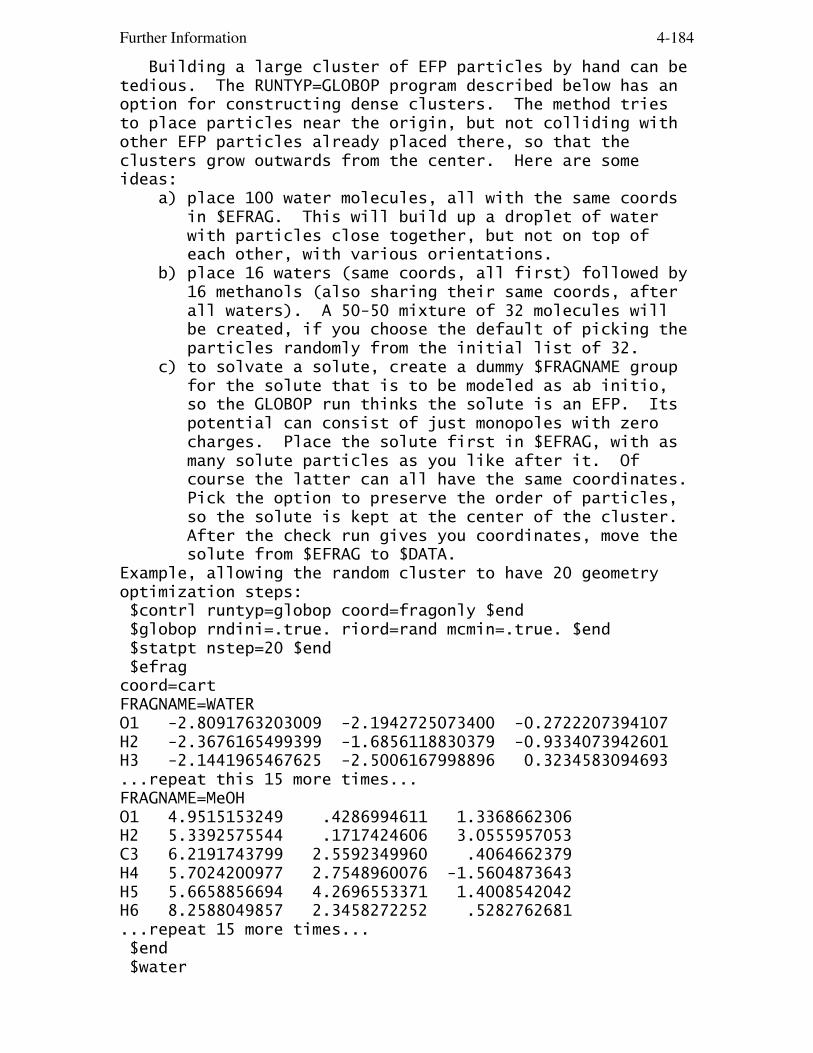
Further Information 4-184
Building a large cluster of EFP particles by hand can betedious. The RUNTYP=GLOBOP program described below has anoption for constructing dense clusters. The method triesto place particles near the origin, but not colliding withother EFP particles already placed there, so that theclusters grow outwards from the center. Here are someideas: a) place 100 water molecules, all with the same coords in $EFRAG. This will build up a droplet of water with particles close together, but not on top of each other, with various orientations. b) place 16 waters (same coords, all first) followed by 16 methanols (also sharing their same coords, after all waters). A 50-50 mixture of 32 molecules will be created, if you choose the default of picking the particles randomly from the initial list of 32. c) to solvate a solute, create a dummy $FRAGNAME group for the solute that is to be modeled as ab initio, so the GLOBOP run thinks the solute is an EFP. Its potential can consist of just monopoles with zero charges. Place the solute first in $EFRAG, with as many solute particles as you like after it. Of course the latter can all have the same coordinates. Pick the option to preserve the order of particles, so the solute is kept at the center of the cluster. After the check run gives you coordinates, move the solute from $EFRAG to $DATA.Example, allowing the random cluster to have 20 geometryoptimization steps: $contrl runtyp=globop coord=fragonly $end $globop rndini=.true. riord=rand mcmin=.true. $end $statpt nstep=20 $end $efragcoord=cartFRAGNAME=WATERO1 -2.8091763203009 -2.1942725073400 -0.2722207394107H2 -2.3676165499399 -1.6856118830379 -0.9334073942601H3 -2.1441965467625 -2.5006167998896 0.3234583094693...repeat this 15 more times...FRAGNAME=MeOHO1 4.9515153249 .4286994611 1.3368662306H2 5.3392575544 .1717424606 3.0555957053C3 6.2191743799 2.5592349960 .4064662379H4 5.7024200977 2.7548960076 -1.5604873643H5 5.6658856694 4.2696553371 1.4008542042H6 8.2588049857 2.3458272252 .5282762681...repeat 15 more times... $end $water

Further Information 4-185
...give a full EFP2 potential for water... $end $meoh...give a full EFP2 potential for methanol... $endNote that this run does not proceed into a full Monte Carlosimulation. You can start Monte Carlo (or simulatedannealing) by placing the randomized structure into $EFRAG,and of course provide relevant $GLOBOP inputs rather thanRNDINI=.TRUE.
* * *
The translations and rotations of EFPs with respect tothe ab initio system and one another are automaticallyquite soft degrees of freedom. After all, the EFP model ismeant to handle weak interactions! Therefore thesatisfactory location of structures on these flat surfaceswill require use of a tight convergence on the gradient:OPTTOL=0.00001 in the $STATPT group.
The effect of a bulk continuum surrounding the soluteplus EFP waters can be obtained by using the PCM model, seereference 23 and 43. To do this, simply add a $PCM groupto your input, in addition to the $EFRAG. The simultaneoususe of EFP and PCM allows for gradients, so geometryoptimization can be performed.
global optimization
If there are a large number of effective fragments, itis difficult to locate the lowest energy structures byhand. Typically these are numerous, and one would like tohave a number of them, not just the very lowest energy.The RUNTYP of GLOBOP contains a Monte Carlo procedure togenerate a random set of starting structures to look forthose with the lowest energy at a single temperature. Ifdesired, a simulated annealing protocol to cool thetemperature may be used. These two procedures may becombined with a local minimum search, at some or all of therandomly generated structures. The local minimum search iscontrolled by the usual geometry optimizer, namely $STATPTinput, and thus permits the optimization of any ab initioatoms.
The Monte Carlo procedure by default uses a Metropolisalgorithm to move just one of the effective fragments. Ifdesired, the method of Parks to move all fragments at once
Further Information 4-186
may be tried, by changing ALPHA from zero and settingBOLTWT=AVESTEP instead of STANDARD.
The present program was used to optimize the structureof water clusters. Let us consider the case of the twelvewater cluster, for which the following ten structures werepublished by Day, Pachter, Gordon, and Merrill: 1. (D2d)2 -0.170209 6. (D2d)(C2) -0.167796 2. (D2d)(S4) -0.169933 7. S6 -0.167761 3. (S4)2 -0.169724 8. cage b -0.167307 4. D3 -0.168289 9. cage a -0.167284 5. (C1c)(Cs) -0.167930 10. (C1c)(C1c) -0.167261A test input using Metropolis style Monte Carlo to examine300 geometries at each temperature value, using simulatedannealing cooling from 200 to 50 degrees, and with localminimization every 10 structures was run ten times. Eachrun sampled about 7000 geometries. One simulation foundstructure 2, while two of the runs found structure 3. Theother seven runs located structures with energy values inthe range -0.163 to -0.164. In all cases the runs beganwith the same initial geometry, but produced differentresults due to the random number generation used in theMonte Carlo. Clearly one must try a lot of simulations tobe confident about having found most of the low energystructures. In particular, it is good to try more than oneinitial structure, unlike what was done in this test.
If there is an ab initio molecule in your system, it isprobably impractical to carry out a simulated annealingprotocol. However, a single temperature Monte Carlocalculation may be feasible. In particular, you may wishto avoid the local minimization steps, and instead manuallyexamine the structures from the Monte Carlo steps in orderto choose a few for full geometry optimization. Note thatSMODIF input can allow the ab initio part of the system toparticipate in the Monte Carlo jumps. However, this shouldbe done with caution.
Monte Carlo references: N.Metropolis, A.Rosenbluth, A.Teller J.Chem.Phys. 21, 1087(1953). G.T.Parks Nucl.Technol. 89, 233(1990).Monte Carlo with local minimization: Z.Li, H.A.Scheraga Proc.Nat.Acad.Sci. USA 84, 6611(1987).Simulated annealing reference: S.Kirkpatrick, C.D.Gelatt, M.P.Vecci Science 220, 671(1983).
Further Information 4-187
The present program is described in reference 15. It ispattened on the work of D.J.Wales, M.P.Hodges Chem.Phys.Lett. 286, 65-72 (1998).
QM/MM across covalent bonds
Recent work by Visvaldas Kairys and Jan Jensen has madeit possible to extend the EFP methodology beyond the simplesolute/solvent case described above. When there is acovalent bond between the portion of the system to bemodeled by quantum mechanics, and the portion which is tobe treated by EFP multipole and polarizability terms, anadditional layer is needed in the model. The covalentlinkage is not so simple as the interactions between closedshell solute and solvent molecules. The "buffer zone"between the quantum mechanics and the EFP consists offrozen nuclei, and frozen localized orbitals, so that thequantum mechanical region sees a orbital representation ofthe closest particles, and multipoles etc. beyond that.Since the orbitals in the buffer zone are frozen, it needextend only over a few atoms in order to keep the orbitalsin the fully optimized quantum region within that region.
The general outline of this kind of computation is asfollows: a) a full quantum mechanics computation on a system containing the quantum region, the buffer region, and a few atoms into the EFP region, to obtain the frozen localized orbitals in the buffer zone. This is called the "truncation run". b) a full quantum mechanics computation on a system with all quantum region atoms removed, and with the frozen localized orbitals in the buffer zone. The necessary multipole and polarizability data to construct the EFP that will describes the EFP region will be extracted from the wavefunction. This is called the "MAKEFP run". It is possible to use several such runs if the total EFP region is quite large. c) The intended QM/MM run(s), after combining the information from these first two types of runs.
As an example, consider a protonated lysine residuewhich one might want to consider quantum mechanically in aprotein whose larger parts are to be treated with an EFP.The protonated lysine is
NH2
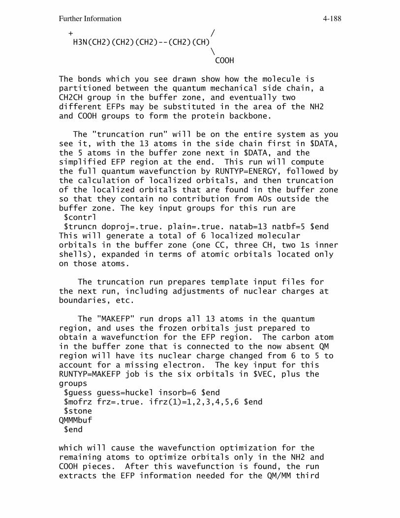
Further Information 4-188
+ / H3N(CH2)(CH2)(CH2)--(CH2)(CH) \ COOH
The bonds which you see drawn show how the molecule ispartitioned between the quantum mechanical side chain, aCH2CH group in the buffer zone, and eventually twodifferent EFPs may be substituted in the area of the NH2and COOH groups to form the protein backbone.
The "truncation run" will be on the entire system as yousee it, with the 13 atoms in the side chain first in $DATA,the 5 atoms in the buffer zone next in $DATA, and thesimplified EFP region at the end. This run will computethe full quantum wavefunction by RUNTYP=ENERGY, followed bythe calculation of localized orbitals, and then truncationof the localized orbitals that are found in the buffer zoneso that they contain no contribution from AOs outside thebuffer zone. The key input groups for this run are $contrl $truncn doproj=.true. plain=.true. natab=13 natbf=5 $endThis will generate a total of 6 localized molecularorbitals in the buffer zone (one CC, three CH, two 1s innershells), expanded in terms of atomic orbitals located onlyon those atoms.
The truncation run prepares template input files forthe next run, including adjustments of nuclear charges atboundaries, etc.
The "MAKEFP" run drops all 13 atoms in the quantumregion, and uses the frozen orbitals just prepared toobtain a wavefunction for the EFP region. The carbon atomin the buffer zone that is connected to the now absent QMregion will have its nuclear charge changed from 6 to 5 toaccount for a missing electron. The key input for thisRUNTYP=MAKEFP job is the six orbitals in $VEC, plus thegroups $guess guess=huckel insorb=6 $end $mofrz frz=.true. ifrz(1)=1,2,3,4,5,6 $end $stoneQMMMbuf $end
which will cause the wavefunction optimization for theremaining atoms to optimize orbitals only in the NH2 andCOOH pieces. After this wavefunction is found, the runextracts the EFP information needed for the QM/MM third
Further Information 4-189
run(s). This means running the Stone analysis fordistributed multipoles, and obtaining a polarizabilitytensor for each localized orbital in the EFP region.
The QM/MM run might be RUNTYP=OPTIMIZE, etc. dependingon what you want to do with the quantum atoms, and its$DATA group will contain both the 13 fully optimized atoms,and the 5 buffer atoms, and a basis set will exist on bothsets of atoms. The carbon atom in the buffer zone thatborders the EFP region will have its nuclear charge set to4 since now two bonding electrons to the EFP region arelost. $VEC input will provide the six frozen orbitals inthe buffer zone. The EFP atoms are defined in a fragmentpotential group.
The QM/MM run could use RHF or ROHF wavefunctions, togeometry optimize the locations of the quantum atoms (butnot of course the frozen buffer zone or the EFP piece). Itcould remove the proton to compute the proton affinity atthat terminal nitrogen, hunt for transition states, and soon. Presently the gradient for GVB and MCSCF is not quiteright, so their use is discouraged.
Input to control the QM/MM preparation is $TRUNCN and$MOFRZ groups. There are a number of other parameters invarious groups, namely QMMMBUF in $STONE, MOIDON and POLNUMin $LOCAL, NBUFFMO in $EFRAG, and INSORB in $GUESS that arerelevant to this kind of computation. For RUNTYP=MAKEFP,the biggest choices are LOCAL=RUEDENBRG vs. BOYS, andPOLNUM in $LOCAL, otherwise this is pretty much a standardRUNTYP=ENERGY input file.
Source code distributions of GAMESS contain a directorynamed ~/gamess/tools/efp, which has various tools for EFPmanipulation in it, described in file readme.1st. A fullinput file for the protonated lysine molecule is included,with instructions about how to proceed to the next steps.Tips on more specialized input possibilities are appendedto the file readme.1st.
Simpler potentials
Since the EFP model's electrostatics is a set ofdistributed multipoles (monopole to octopole) anddistributed polarizabilities (dipole), it is possible togenerate some water potentials found in the literature bysetting many EFP terms to zero. It is also necessary toprovide a Lennard-Jones 6-12 repulsive potential, and then

Further Information 4-190
make a choice to follow the EFP1 type formula for QM/EFPrepulsion. Accordingly, EFP1 type calculations can be madewith the following water potentials, FRAGNAME=SPC, SPCE, TIP5P, TIP5PE, or POL5PThe Wikipedia page http://en.wikipedia.org/wiki/Water_modeldefines the first four of these, which are not polarizablepotentials. The same web site references the primaryliterature, so that is not repeated here. POL5P is apolarizable potential, with parameters given by D.Si and H.Li J.Chem.Phys. 133, 144112/1-8(2010)
references
The first paper is more descriptive, while the secondpresents a very detailed derivation of the EFP1 method.Reference 18 is an overview article on EFP2. Reference 44is the most recent review.
The model development papers are: 1, 2, 3, 5, 6, 9, 14,17, 18, 22, 23, 26, 31, 32, 34, 39, 41, 42, 43, 44, 46, 50,51, 55, 57.
1. "Effective fragment method for modeling intermolecular hydrogen bonding effects on quantum mechanical calculations" J.H.Jensen, P.N.Day, M.S.Gordon, H.Basch, D.Cohen, D.R.Garmer, M.Krauss, W.J.Stevens in "Modeling the Hydrogen Bond" (D.A. Smith, ed.) ACS Symposium Series 569, 1994, pp 139-151.2. "An effective fragment method for modeling solvent effects in quantum mechanical calculations". P.N.Day, J.H.Jensen, M.S.Gordon, S.P.Webb, W.J.Stevens, M.Krauss, D.Garmer, H.Basch, D.Cohen J.Chem.Phys. 105, 1968-1986(1996).3. "The effective fragment model for solvation: internal rotation in formamide" W.Chen, M.S.Gordon, J.Chem.Phys., 105, 11081-90(1996)4. "Transphosphorylation catalyzed by ribonuclease A: Computational study using ab initio EFPs" B.D.Wladkowski, M. Krauss, W.J.Stevens J.Am.Chem.Soc. 117, 10537-10545(1995)5. "Modeling intermolecular exchange integrals between nonorthogonal orbitals" J.H.Jensen J.Chem.Phys. 104, 7795-7796(1996)6. "An approximate formula for the intermolecular Pauli repulsion between closed shell molecules" J.H.Jensen, M.S.Gordon Mol.Phys. 89, 1313-1325(1996)7. "A study of aqueous glutamic acid using the effective

Further Information 4-191
fragment potential model" P.N.Day, R.Pachter J.Chem.Phys. 107, 2990-9(1997)8. "Solvation and the excited states of formamide" M.Krauss, S.P.Webb J.Chem.Phys. 107, 5771-5(1997)9. "An approximate formula for the intermolecular Pauli repulsion between closed shell molecules. Application to the effective fragment potential method" J.H.Jensen, M.S.Gordon J.Chem.Phys. 108, 4772-4782(1998)10. "Study of small water clusters using the effective fragment potential method" G.N.Merrill, M.S.Gordon J.Phys.Chem.A 102, 2650-7(1998)11. "Solvation of the Menshutkin Reaction: A Rigourous test of the Effective Fragement Model" S.P.Webb, M.S.Gordon J.Phys.Chem.A 103, 1265-73(1999)12. "Evaluation of the charge penetration energy between nonorthogonal molecular orbitals using the Spherical Gaussian Overlap approximation" V.Kairys, J.H.Jensen Chem.Phys.Lett. 315, 140-144(1999)13. "Solvation of Sodium Chloride: EFP study of NaCl(H2O)n" C.P.Petersen, M.S.Gordon J.Phys.Chem.A 103, 4162-6(1999)14. "QM/MM boundaries across covalent bonds: frozen LMO based approach for the Effective Fragment Potential method" V.Kairys, J.H.Jensen J.Phys.Chem.A 104, 6656-65(2000)15. "A study of water clusters using the effective fragment potential and Monte Carlo simulated annealing" P.N.Day, R.Pachter, M.S.Gordon, G.N.Merrill J.Chem.Phys. 112, 2063-73(2000)16. "A combined discrete/continuum solvation model: Application to glycine" P.Bandyopadhyay, M.S.Gordon J.Chem.Phys. 113, 1104-9(2000)17. "Evaluation of charge penetration between distributed multipolar expansions" M.A.Freitag, M.S.Gordon, J.H.Jensen, W.J.Stevens J.Chem.Phys. 112, 7300-7306(2000)18. "The Effective Fragment Potential Method: a QM-based MM approach to modeling environmental effects in chemistry" M.S.Gordon, M.A.Freitag, P.Bandyopadhyay, J.H.Jensen, V.Kairys, W.J.Stevens J.Phys.Chem.A 105, 293-307(2001)19. "Accurate Intraprotein Electrostatics derived from first principles: EFP study of proton affinities of lysine 55 and tyrosine 20 in Turkey Ovomucoid" R.M.Minikis, V.Kairys, J.H.Jensen J.Phys.Chem.A 105, 3829-3837(2001)20. "Active site structure & mechanism of Human Glyoxalase"

Further Information 4-192
U.Richter, M.Krauss J.Am.Chem.Soc. 123, 6973-6982(2001)21. "Solvent effect on the global and atomic DFT-based reactivity descriptors using the EFP model. Solvation of ammonia." R.Balawender, B.Safi, P.Geerlings J.Phys.Chem.A 105, 6703-6710(2001)22. "Intermolecular exchange-induction and charge transfer: Derivation of approximate formulas using nonorthogonal localized molecular orbitals." J.H.Jensen J.Chem.Phys. 114, 8775-8783(2001)23. "An integrated effective fragment-polarizable continuum approach to solvation: Theory & application to glycine" P.Bandyopadhyay, M.S.Gordon, B.Mennucci, J.Tomasi J.Chem.Phys. 116, 5023-5032(2002)24. "The prediction of protein pKa's using QM/MM: the pKa of Lysine 55 in turkey ovomucoid third domain" H.Li, A.W.Hains, J.E.Everts, A.D.Robertson, J.H.Jensen J.Phys.Chem.B 106, 3486-3494(2002)25. "Computational studies of aliphatic amine basicity" D.C.Caskey, R.Damrauer, D.McGoff J.Org.Chem. 67, 5098-5105(2002)26. "Density Functional Theory based Effective Fragment Potential" I.Adamovic, M.A.Freitag, M.S.Gordon J.Chem.Phys. 118, 6725-6732(2003)27. "Intraprotein electrostatics derived from first principles: Divid-and-conquer approaches for QM/MM calculations" P.A.Molina, H.Li, J.H.Jensen J.Comput.Chem. 24, 1971-1979(2003)28. "Formation of alkali metal/alkaline earth cation water clusters, M(H2O)1-6, M=Li+, K+, Mg+2, Ca+2: an effective fragment potential caase study" G.N.Merrill, S.P.Webb, D.B.Bivin J.Phys.Chem.A 107, 386-396(2003)29. "Anion-water clusters A-(H2O)1-6, A=OH, F, SH, Cl, and Br. An effective fragment potential test case" G.N.Merrill, S.P.Webb J.Phys.Chem.A 107,7852-7860(2003)30. "The application of the Effective Fragment Potential to molecular anion solvation: a study of ten oxyanion- water clusters, A-(H2O)1-4" G.N.Merrill, S.P.Webb J.Phys.Chem.A 108, 833-839(2004)31. "The effective fragment potential: small clusters and radial distribution functions" H.M.Netzloff, M.S.Gordon J.Chem.Phys. 121, 2711-4(2004)32. "Fast fragments: the development of a parallel effective fragment potential method" H.M.Netzloff, M.S.Gordon J.Comput.Chem. 25, 1926-36(2004)33. "Theoretical investigations of acetylcholine (Ach) and acetylthiocholine (ATCh) using ab initio and effective

Further Information 4-193
fragment potential methods" J.Song, M.S.Gordon, C.A.Deakyne, W.Zheng J.Phys.Chem.A 108, 11419-11432(2004)34. "Dynamic polarizability, dispersion coefficient C6, and dispersion energy in the effective fragment potential method" I.Adamovic, M.S.Gordon Mol.Phys. 103, 379-387(2005)35. "Solvent effects on the SN2 reaction: Application of the density functional theory-based effective fragment potential method" I.Adamovic, M.S.Gordon J.Phys.Chem.A 109, 1629-36(2005)36. "Theoretical study of the solvation of fluorine and chlorine anions by water" D.D.Kemp, M.S.Gordon J.Phys.Chem.A 109, 7688-99(2005)37. "Modeling styrene-styrene interactions" I.Adamovic, H.Li, M.H.Lamm, M.S.Gordon J.Phys.Chem.A 110, 519-525(2006)38. "Methanol-water mixtures: a microsolvation study using the Effective Fragment Potential method" I.Adamovic, M.S.Gordon J.Phys.Chem.A 110, 10267-10273(2006)39. "Charge transfer interaction in the effective fragment potential method" H.Li, M.S.Gordon, J.H.Jensen J.Chem.Phys. 124, 214108/1-16(2006)40. "Incremental solvation of nonionized and zwitterionic glycine" C.M.Aikens, M.S.Gordon J.Am.Chem.Soc. 128, 12835-12850(2006)41. "Gradients of the polarization energy in the Effective Fragment Potential method" H.Li, H.M.Netzloff, M.S.Gordon J.Chem.Phys. 125, 194103/1-9(2006)42. "Electrostatic energy in the Effective Fragment Potential method: Theory and application to benzene dimer" L.V.Slipchenko, M.S.Gordon J.Comput.Chem. 28, 276-291(2007)43. "Polarization energy gradients in combined Quantum Mechanics, Effective Fragment Potential, and Polarizable Continuum Model Calculations" H.Li, M.S.Gordon J.Chem.Phys. 126, 124112/1-10(2007)44. "The Effective Fragment Potential: a general method for predicting intermolecular interactions" M.S.Gordon, L.V.Slipchenko, H.Li, J.H.Jensen Annual Reports in Computational Chemistry, Volume 3, pp 177-193 (2007).45. "An Interpretation of the Enhancement of the Water Dipole Moment Due to the Presence of Other Water Molecules"
Further Information 4-194
D.D.Kemp, M.S.Gordon J.Phys.Chem.A 112, 4885-4894(2008)46. "Solvent effects on optical properties of molecules: a combined time-dependent density functional/effective fragment potential approach" S.Yoo, F.Zahariev, S.Sok, M.S.Gordon J.Chem.Phys. 129, 144112/1-8(2008)47. "Modeling pi-pi interactions with the effective fragment potential method: The benzene dimer and substituents" T.Smith, L.V.Slipchenko, M.S.Gordon J.Phys.Chem.A 112, 5286-5294(2008)48. "Water-benzene interactions: An effective fragment potential and correlated quantum chemistry study" L.V.Slipchenko, M.S.Gordon J.Phys.Chem.A 113, 2092-2102(2009)49. "Ab initio QM/MM excited-state molecular dynamics study of Coumarin 151 in water solution" D.Kina, P.Arora, A.Nakayama, T.Noro, M.S.Gordon, T.Taketsugu Int.J.Quantum Chem. 109, 2308-2318(2009)50. "Damping functions in the effective fragment potential method L.V.Slipchenko, M.S.Gordon Mol.Phys. 197, 999-1016 (2009)51. "A combined effective fragment potential-fragment molecular orbital method. 1. the energy expression" T.Nagata, D.G.Fedorov, K.Kitaura, M.S.Gordon J.Chem.Phys. 131, 024101/1-12(2009)52. "Alanine: then there was water" J.M.Mullin, M.S.Gordon J.Phys.Chem.B 113, 8657-8669(2009)53. "Water and Alanine: from puddles(32) to ponds(49)" J.M.Mullin, M.S.Gordon J.Phys.Chem.B 113, 14413-14420(2009)54. "Structure of large nitrate-water clusters at ambient temperatures: simulations with effective fragment potentials and force fields with implications for atmospheric chemistry" Y.Miller, J.L.Thoman, D.D.Kemp, B.J.Finlayson-Pitts, M.S.Gordon, D.J.Tobias, R.B.Gerber J.Phys.Chem.A 113, 12805-12814(2009)55. "Quantum mechanical/molecular mechanical/continuum style solvation model: linear response theory, variational treatment, and nuclear gradients" H.Li J.Chem.Phys. 131, 184103/1-8(2009)56. "Aqueous solvation of bihalide anions" D.D.Kemp, M.S.Gordon J.Phys.Chem.A 114, 1298-1303(2010)57. "Exchange repulsion between effective fragment

Further Information 4-195
potentials and ab initio molecules" D.D.Kemp, J.M.Rintelman, M.S.Gordon, J.H.Jensen Theoret.Chem.Acc. 125, 481-491(2010).

Further Information 4-196
The Fragment Molecular Orbital method
coded by D.G. Fedorov, M.Chiba, T. Nagata and K. Kitaura at Research Institute for Computational Sciences (RICS) National Institute of Advanced Industrial Science and Technology (AIST) AIST Tsukuba Central 2, Umezono 1-1-1, Tsukuba, 305-8568, Japan.with code contributions by: C. Steinmann (U. Copenhagen).
The method was proposed by Professor Kitaura and coworkersin 1999, based on the Energy Decomposition Analysis (EDA,sometimes called the Morokuma-Kitaura energydecomposition). The FMO method is completely independent ofand bears no relation to: 1. Frontier molecular orbitals (FMO), 2. Fragment molecular orbitals (FMO).The latter name is often used for the process ofconstruction of full molecular orbitals by combining MOdiagrams for parts of a molecule, ala Roald Hoffmann.The effective fragment molecular orbital method (EFMO) isclosely related to but also bears significant difference toFMO, and discussed below.
The FMO program was interfaced with GAMESS and followsgeneral GAMESS guidelines for code distribution and usage.The users of the FMO program are requested to cite theFMO3-RHF paper as the basic FMO reference, D.G. Fedorov, K. Kitaura, J. Chem. Phys. 120, 6832-6840(2004)and other papers as appropriate (see below).
The basic idea of the method is to acknowledge the fact theexchange and self-consistency are local in most molecules(and clusters and molecular crystals), which permitstreating remote parts with Coulomb operators only, ignoringthe exchange. This idea further evolves into doingmolecular calculations, piecewise, with Coulomb fields dueto the remaining parts. In practice one divides themolecule into fragments and performs n-mer calculations ofthese in the Coulomb field of other fragments (n=1,2,3).There are no empirical parameters, and the only departurefrom ab initio rigor is the subjective fragmentation. Ithas been observed that if performed physically reasonably,the fragmentation scheme alters the results very little.What changes the accuracy the most is the fragment size,
Further Information 4-197
which also determines the computational efficiency of themethod.
The first question is how to get started. The easiest wayto prepare an FMO input file for GAMESS is to use free GUIsoftware Facio, developed by M. Suenaga at KyushuUniversity. It can do molecular modeling, automaticfragmentation of peptides, nucleotides and saccharides andcreate GAMESS/FMO input files.http://www1.bbiq.jp/zzzfelis/Facio.htmlAlternatively, if you prefer command line interface, andyour molecule is a protein found in the PDB(http://www.rcsb.org/pdb), you can simply use thefragmentation program "fmoutil" that is provided withGAMESS in tools/fmo, or at the FMO home page http://staff.aist.go.jp/d.g.fedorov/fmo/main.htmlfor the latest version. If you have a cluster of identicalmolecules, you can perform fragmentation with just onekeyword ($FMO nacut=).
Computationally, it is always better to partition in ageometrical way (close parts together), so that thedistance-based approximations are more efficient. Theaccuracy depends mainly upon the locality of the densitydistribution, and the appropriateness of partitioning itinto fragments. There is no simple connexion between thegeometrical proximity of fragmentation and accuracy.
Supposing you know how to fragment, you should choose abasis set and fragment size. We recommend 2 amino acidresidues or 2-4 water molecules per fragment for finalenergetics (or, even better, three-body with 1 molecule orresidue per fragment). For geometry optimizations one maybe able to use 1 res/mol per fragment, especially ifgradient convergence to about 0.001 is desired. Note thatalthough it was claimed that FMO gradient is analytic(Chem. Phys. Lett., 336 (2001), 163.) it is not so. Neithertheory nor program for fully analytic gradient has beendeveloped, to the best of our knowledge up to this day(December 21, 2006). The gradient implementation is nearlyanalytic, meaning three small terms are missing, one whichcan now be included using MODGRD=8+2. The magnitude ofthese small terms depends upon the fragment size (largerfragments have smaller errors). It has been our experiencethat in proteins with 1 residue per fragment one gets 1e-3...1e-4 error in the gradient, and with 2 residues perfragment it is about 1e-4...1e-5. If you experience energyrising during geometry optimizations, you can consider twocountermeasures:

Further Information 4-198
1. increase approximation thresholds, e.g. RESPPC from 2.0->2.5, RESDIM from 2.0 -> 2.5.2. increase fragment size (e.g. by merging very small fragments with their neighbors).Finally a word of caution: optimizing systems with chargedfragments in the absence of solvent is frequently not agood idea: oppositely charged fragments will most likelyseek each other, unless there is some conformationalbarrier.
One thing you should clearly understand about gradients isthat if you compare FMO gradients with full molecule abinitio gradients, there are two sources of errors: a) error of the analytic FMO gradient compared to ab initio. b) error of a "nearly analytic" FMO gradient compared to the analytic FMO gradient.Since the analytic FMO gradient is not available, these twoare not separable at the moment. If FMO gradients werefully analytic, geometry optimization and dynamics wouldhave run perfectly, irrespective of error a).
For basis sets you should use general guidelines and yourexperience developed for ab initio methods. There is a fileprovided (HMOs.txt) that contains hybrid molecular orbitals(HMO) used to divide the MO space along fragmentationpoints at covalent bonds. If your basis set is not thereyou need to construct your own set of HMOs. See the examplefile makeLMO.inp for this purpose.
Next you choose a wave function type. At present one canuse RHF, DFT, MP2, CC, and MCSCF (all except MCSCF supportthe 3-body expansion). Geometry optimization can beperformed with all of these methods, except CC.
Note that presence of $FMO turns FMO on.
Surfaces and solids
Until 2008, for treating covalently connected fragments,FMO had fully relaxed electron density of the detachedbonds. This method is now known as FMO/HOP (HOP=hybridorbital projection operator). It allows for a fullpolarization of the system and is thus well suited to verypolar systems, such as proteins with charged residues. In2008, an alternative fragmentation was suggested, based onadaptive frozen orbitals (AFO), FMO/AFO. In it, theelectron density for each detached bond is first computed

Further Information 4-199
in the automatically generated small model system (with thebond intact), and in the FMO fragment calculations thiselectron density is frozen. It was found that FMO/AFO worksquite well for surfaces and solids, where there is a densenetwork of bonds to be detached in order to definefragments (and the detached bonds interact quite strongly).In addition, by restricting the polarization, FMO/AFO wasfound to give a more balanced properties for large basissets (triple-zeta with polarization or larger), or incomparing different isomers. However, for proteins withcharged residues the original FMO/HOP scheme has a betteraccuracy (except large basis sets). At this point, FMO/AFOwas applied to zeolites only, and some more experience isneeded to give more practical advice to applications.FMO/AFO is turned on by a nonzero rafo(1) parameter (rafoarray provides the thresholds to build model systems).
FMO variants
In 2007, Dahlke et al. introduced the ElectrostaticallyEmbedded Many-Body Expansion method (see E. E. Dahlke andD. G. Truhlar, J. Chem. Theory Comput. 4, 1-6 (2008) formore recent work). This method is essentially FMO with theRESPPC approximation (point charges for the electrostaticfield) applied to all fragments, with the further provisionthat these charges may be defined at will (whereas RESPPCuses Mulliken charges), and they are kept frozen (notoptimized, as in FMO). Next, Kamiya et al. suggested a fastelectron correlation method (M. Kamiya, S. Hirata, M.Valiev, J. Chem. Phys. 128, 074103 (2008)), where again FMOwith the RESPPC approximation to all fragments is appliedwith the further provision that the charges are derivedfrom the electrostatic potential (so called ESP charges),and BSSE correction is added. The Dahlke's method wasgeneralized in GAMESS with the introduction of an arbitraryhybrid approach, in which some fragments may have fixed andsome variationally optimized charges. This implementationwas employed in FMO-TDDFT calculations of solid statequinacridone (see Ref. 16 below) by using DFT/PBC frozencharges. The present energy only implementation is mostlyintended for such cases as that (i.e., TDDFT), and somemore work is needed to finish it for general calculations.To turn this on, set RESPPC=-1 and define NOPFRG for frozencharge fragments to 64, set frozen charges in ATCHRG.Another FMO-like method is EFMO, see its own subsectionbelow. EFMO itself is related to several methods (PMISP: P.Soederhjelm, U. Ryde, J. Phys. Chem. A 2009, 113, 617–627;
Further Information 4-200
another is G. J. O. Beran, J. Chem. Phys. 2009, 130,164115).
Effective fragment molecular orbital method (EFMO)
EFMO has been formulated by combining the physical modelsin EFP and FMO, namely, in EFMO, fragments are computedwithout the ESP (of FMO), and the polarization is estimatedusing EFP models of fragment polarizabilities, which arecomputed on the fly, so this can be thought of asautomatically generated potentials in EFP. Consequently,close dimers are computed quantum-mechanically (withoutESP) and far dimers are computed using the electrostaticmultipole models of EFP. At present, only vacuum closed-shell RHF and DFT are supported, for energy and gradient;and only molecular clusters can be computed (no systemswith detached bonds). From the user point of view, EFMOfunctionality is very intensively borrowed from FMO, andthe calculation setup is almost identical. Most additionalphysical models such as PCM are not supported in EFMO. EFMOshould not be confused with FMO/EFP. The latter uses FMOfor some fragments and EFP for others. EFMO uses the samemodel (EFMO), which is neither FMO nor EFP. Forapproximations, EFMO at present has only RESDIM.
EFMO references are:1. Effective Fragment Molecular Orbital Method: A Merger ofthe Effective Fragment Potential and Fragment MolecularOrbital Methods.
C. Steinmann, D. G. Fedorov, J. H. Jensen,J. Phys. Chem. A 114, 8705-8712 (2010).
Guidelines for approximations with FMO3
Three sets are suggested, for various accuracies: low: resppc=2.5 resdim=2.5 ritrim(1)=0.001,-1,1.25 medium: resppc=2.5 resdim=3.25 ritrim(1)=1.25,-1,2.0 high: resppc=2.5 resdim=4.0 ritrim(1)=2,2,2For correlated runs, add one more value to ritrim, equal tothe third element (i.e., 1.25 or 2.0). Note that gradientruns do not support nonzero RESDIM and thus use RESDIM=0 ifgradient is to be computed. The "low" level of accuracyfor FMO3 has an error versus full ab initio similar toFMO2, except for extended basis sets (6-311G** etc) whereit is substantially better than FMO2. Thus the low level isonly recommended for those large basis sets, and if abetter level cannot be afforded. The medium level isrecommended for production FMO3 runs; the high level is
Further Information 4-201
mostly for accuracy evaluation in FMO development. Thecost is roughly: 3(low), 6(medium), 12(high). This meansthat FMO3 with the medium level takes roughly six timeslonger than FMO2.
Some of the default tolerances were changed as of January2009, when FMO 3.2 was included in GAMESS. In general,stricter parameters are now enforced when using FMO3, whichof course is intended to produce more accurate results. Ifyou wish to reproduce earlier results with the new code,use the input to revert to the earlier values: former -> FMO2 or FMO3 (as of 1/2009) RESPPC: 2.0 2.0 2.50 RESDIM: 2.0 2.0 3.25 RCORSD: 2.0 2.0 3.25 RITRIM: 2.0,2.0,2.0,2.0 -> 1.25,-1.0,2.0,2.0 (FMO3 only) MODESP: 1 0 1 MODGRD: 0 10 0and two other settings which are not strictly speaking FMOkeywords may change FMO results: MTHALL: 2 -> 4 (FMO/PCM only, see $TESCAV) DFT grid: spherical -> Lebedev (FMO-DFT only, see $DFT)Note that FMO2 energies printed during a FMO3 run willdiffer from those in a FMO2 run, due to the differenttolerances used.
How to perform FMO-MCSCF calculations
Assuming that you are reasonably acquainted with ab initioMCSCF, only FMO-specific points are highlighted. The activespace (the number of orbitals/electrons) is specified forthe MCSCF fragment. The number of core/virtual orbitals forMCSCF dimers will be automatically computed. The mostimportant issue is the initial orbitals for the MCSCFmonomer. Just as for ab initio MCSCF, you should exercisechemical knowledge and provide appropriate orbitals. Thereare two basic ways to input MCSCF initial orbitals: A) through the FMO monomer density binary file B) by providing a text $VEC group.The former way is briefly described in INPUT.DOC (seeorbital conversion). The latter way is really identical toab initio MCSCF, except the orbitals should be prepared forthe fragment (so in many cases you would have to get themfrom an FMO calculation). Once you have the orbitals, putthem into $VEC1, and use the IJVEC option in $FMOPRP (e.g.,if your MCSCF fragment is number 5, you would use $VEC1 andijvec(1)=5,0). For two-layer MCSCF the followingconditions apply. Usually one cannot simply use F40

Further Information 4-202
restart, because its contents will be overwritten with RHForbitals and this will mess up your carefully chosen MCSCForbitals. Therefore, two ways exist. One is to modify A)above by reordering the orbitals with something like $guess guess=skip norder=1 iorder(28)=29,30,31,32,28 $endThen the lower RHF layer will converge RHF orbitals thatyou reorder with iorder in the same run (add 512 to nguessin $FMO). This requires you know how to reorder beforerunning the job so it is not always convenient. Probablythe best way to run two-layer MCSCF is verbatim B) above,so just provide MCSCF monomer orbitals in $VEC1. Finally,it may happen that some MCSCF dimer will not converge.Beside the usual MCSCF tricks to gain convergence as thelast resort you may be able to prepare good initial dimerorbitals, put them into $VEC2 ($VEC3 etc) and read themwith ijvec. SOSCF is the preferred converger in FMO, andthe other one (FULLNR) has not been modified to eradicatethe artefacts of convergence (due to detached bonds). Inthe bad cases you can try running one or two monomer SCFiterations with FULLNR, stop the job and use its orbitalsin F40 to do a restart with SOSCF. We also found useful toset CASDII=0.005 and nofo=10 in some cases running FOCASlonger to get better orbitals for SOSCF.
How to perform multilayer runs
For some fragments you may like to specify a differentlevel of electron correlation and/or basis set. In atypical case, you would use high level for the reactioncenter and a lower level for the remaining part of thesystem. The set up for multilayer runs is very similar tothe unilayer case. You only have to specify to what layereach fragment belongs and for each layer define DFTTYP,MPLEVL, SCFTYP as well as a basis set. If detached bondsare present, appropriate HMOs should be defined. See theparagraph above for multilayer MCSCF. Currently geometryoptimizations of multilayer runs require adding 128 toNGUESS, if basis sets in layers differ from each other.
How to mix basis sets in FMO
You can mix basis sets in both uni and multilayer cases.The difference between a 2-layer run with one basis set perlayer and a 1-layer run with 2-basis sets is significant:in the former case the lower level densities are convergedwith all fragments computed at the lower level. In thelatter case, the fragments are converged simultaneously,

Further Information 4-203
each with its own basis set. In addition, dimer correctionsbetween layers will be computed differently: with the lowerbasis set in the former case and with mixed basis set inthe latter. The latter approach may result in unphysicalpolarization, so mixing basis sets is mainly intended toadd diffuse functions to anionic (e.g., carboxyl) groups,not as a substitute for two-layer runs.
How to perform FMO/PCM calculations
Solvent effects can be taken into account with PCM. PCM inFMO is very similar to regular PCM. There is one basicdifference: in FMO/PCM the total electron density thatdetermines the electrostatic interaction is computed usingthe FMO density expansion up to n-body terms. The cavityis constructed surrounding the whole molecule, and thewhole cavity is used in each individual m-mer calculation.There are several levels of accuracy (determined by the "n"above), and the recommended level is FMO/PCM[1(2)],specified by:
$pcm ief=-10 icomp=2 icav=1 idisp=1 ifmo=2 $end $fmoprp npcmit=2 $end $tescav ntsall=240 $end $pcmcav radii=suahf $end
Many PCM options can be used as in the regular PCM. Thefollowing restrictions apply: IEF may be only -3 or -10, IDP must be 0.No FMO/PCM gradients are available. Multilayer FMO runsare supported. Restarts are only limited to IREST=2, andin this case PCM charges (the ASCs) are not recycled.However, the initial guess for the charges is fairlyreasonable, so IREST=2 may be useful although reading theASCs may be implemented in future.
Note for advanced users. IFMO < NBODY runs are permitted.They are denoted by FMOm/PCM[n], where m=NBODY and n=IFMO.In FMOm/PCM[n], the ASCs are computed with n-body level.The difference between FMO2/PCM[1] and FMO2/PCM[1(2)] isthat in the former the ASCs are computed at the 1-bodylevel, whereas for the former at the 2-body level, butwithout self-consistency (which would be FMO2/PCM[2]).Probably, FMO3/PCM[2] should be regarded as the mostaccurate and still affordable (with a few thousand nodes)method. However, FMO3/PCM[1(2)] (specified with NBODY=3,IFMO=2 and NPCMIT=2) is much cheaper and slightly less

Further Information 4-204
accurate than FMO3/PCM[2]. FMO3/PCM[3] is the mostaccurate and expensive level of all.
How to perform FMO/EFP calculations
Solvent effects can also be taken into account with theEffective Fragment Potential model. The presence of both$FMO and $EFRAG groups selects FMO/EFP calculations. Seethe $EFRAG group and the $FMO group for details.
In the FMO/EFP method, the Quantum Mechanical part of thecalculation in the usual EFP method is replaced by the FMOmethod, which may save time for large molecules such asproteins.
In the present version, only FMOn/EFP1 (water solvent only)is available for RHF, DFT and MP2. One can use the MCglobal optimization technique for FMO/EFP by RUNTYP=GLOBOP.Of course, the group DDI (GDDI) parallelization techniquefor the FMO method can be used.
Geometry optimizations for FMO
The standard optimizers in GAMESS are now wellparallelized, and thus recommended to be used with FMO upto the limit hardwired in GAMESS (2000 atoms). In practice,if more than about 1000 atoms are present, numeric Hessianupdates often result in the improper curvature andoptimization stops. One can either do a restart, or useRUNTYP=OPTFMO (which does not diagonalize the Hessian).RUNTYP=OPTIMIZE applies to Cartesian coordinates only.Other types have not been tested and should be assumed tobe not usable with FMO. If your system has more than 2000atoms you can consider RUNTYP=OPTFMO, which can now useHessian updates and provides reasonable way to optimizealthough it is not as good as the standard means inRUNTYP=OPTIMIZE. Recently, there was gradient improvement,enabled with MODGRD (=2+8).
Pair interaction energy decomposition analysis (PIEDA)
PIEDA can be performed for the PL0 and PL states. The PL0state is the electronic state in which fragments arepolarised by the environment in its free (noninteracting)state. The simplest example is that in a water cluster,each molecule is computed in the electrostatic field

Further Information 4-205
exerted by the electron densities of free water molecules.The PL state is the FMO converged monomer state, that is,the state in which fragments are polarised by the self-consistently converged environment. Namely, following theFMO prescription, fragments are recomputed in the externalfield, until the latter converges. Using the PL0 staterequires a series of separate runs; and it also relies on a"free state" which can be defined in many ways formolecules with detached covalent bonds.
What should be done to do the PL0 state analysis?1. run FMO0.This computes the free state for each fragment, and thoseelectron densities are stored on file 30 (to be renamedfile 40 and reused in step 3).2. compute BDA energies (if detached bonds are present),using sample files in tools/fmo/pieda. This corrects forartifacts of bond detaching, and involves running a modelsystem like H3C-CH3, to amend for C-C bond detaching.3. Using results of (1) and (2), one can do the PL0analysis. In addition to pasting the data from the twopunch files in steps 1,2 and the density file in step 1should be provided.
What should be done to do the PL state analysis? The PLstate itself does not need either the free state or PL0results. However, if the PL0 results are available,coupling terms can be computed, and in this case IPIEDA isset to 2; otherwise to 1.
So the easiest and frequently sufficient way to run PIEDAis to set IPIEDA=1 and do not provide any data frompreceding calculations. The result of a PIEDA calculationis a set of pair interaction energies (interfragmentinteraction energies), decomposed into electrostatic,exchange-repulsion, charge transfer and dispersioncontributions.
Finally, PIEDA (especially for the PL state) can be thoughtof as FMO-EDA, EDA being the Kitaura-Morokuma decomposition(RUNTYP=MOROKUMA). In fact, PIEDA (for the PL state) inthe case of just two fragments of standalone molecules isentirely equivalent to EDA, which can be easily verified,by running the full PIEDA analysis (ipieda=2). Note thatPIEDA can be run as direct SCF, whereas EDA cannot be, andfor large fragments PIEDA code can be used to perform EDA.Also, EDA in GAMESS has no explicit dispersion.
Further Information 4-206
Excited states
At present, one can use CI, MCSCF, or TDDFT to computeexcited states in FMO. MCSCF is discussed separatelyabove, so here only TDDFT and CI are explained. They areenabled by setting the IEXCIT option (EXCIT(1) defines theexcited state's fragment ID).
Two levels are implemented for TDDFT (FMO1-TDDFT and FMO2-TDDFT). In the former, only monomer TDDFT calculations areperformed, whereas the latter adds pair corrections fromTDDFT dimers. PCM may be used for solvent effects withTDDFT (PCM[1] is usually sufficient).
CI can only be done for CIS at the monomer level (nbody=1),FMO1-CIS. The set-up for CI is similar to that for TDDFT.
Selective FMO
Sometimes, one is interested only in some pairinteractions, for example, between ligand and protein, orthe opposite, only pair interactions within ligand. Thissaves a lot of CPU time by omitting all other paircalculations, but does not give the total properties. Touse this feature, define MOLFRG and MODMOL. RUNTYP=ENERGYonly is implemented.
Frozen domains
To accelerate geometry optimisations, one can specify thatthe electronic state of the first layer in a 2-layer FMOcan be computed at the initial geometry and consequently befrozen. One can define the polarizable buffer (equal tolayer 2) and frozen domain (layer 1). Fragments in thepolarizable buffer which contain the atoms active ingeometry optimisation form the active domain. Thefragments in the active domain should have a nonzeroseparation from the frozen domain. In FMO/FD all dimers inthe polarizable buffer are computed; in FMO/FDD only thosedimers which have at least one monomer in the active domainare computed. FMO/FD and FNI/FDD are only implemented forRUNTYP=OPTIMIZE. MODFD and IACTAT in $FMO specifyFMO/FD(D) atop of the usual multilayer FMO setup with someatoms frozen in geometry optimization by the standard means(i.e., IACTAT in $STATPT). Note that in FMO/FD(D) theHessian as used in RUNTYP=OPTIMIZE is formed only for the

Further Information 4-207
atoms in the second layer, so this upper layer should nothave more than the GAMESS limit (currently, 2000 atoms).
Analyzing and visualizing the results
Annotated outputs provided in tools/fmo have matchingmathematical formulae added onto the outputs, for easierreading.Facio (http://www1.bbiq.jp/zzzfelis/Facio.html) can plotvarious FMO properties such as interaction energies, usinginteractive GUI viewers.To plot orbitals for an n-mer, set NPUNCH=2 in $SCF andPLTORB=.T.. There are several ways to produce cube fileswith electron densities. They are described in detail intools/fmo/fmocube/README. To plot pair interaction maps,use tools/fmo/fmograbres to generate CSV files from GAMESSoutput, which can be easily read into Gnuplot or Excel.
Parallelization of FMO runs with GDDI
The FMO method has been developed within a 2-levelhierarchical parallelization scheme, group DDI (GDDI),allowing massively parallel calculations. Different groupsof processors handle the various monomer, dimer, and maybetrimer computations. The processor groups should be sizedso that GAMESS' innate scaling is fairly good, and thefragments should be mapped onto the processor groups in anintelligent fashion.
This is a very important and seemingly difficult issue. Itis very common to be able to speed up parallel runs atleast several times just by using GDDI better. First ofall, do not use plain DDI and always employ GDDI whenrunning FMO calculations. Next, learn that you can andshould divide nodes into groups to achieve betterperformance. The very basic rule of thumb is to try to haveseveral times fewer groups than jobs. Since the number ofmonomers and dimers is different, group division shouldreflect that fact. Ergo, find a small parallel computerwith 8-32 nodes and experiment changing just two numbers:ngrfmo(1)=N1,N2 and see how performance changes for yourparticular system.
Limitations of the FMO method in GAMESS

Further Information 4-208
1. dimensions: in general none, except that geometryoptimizations use the standard GAMESS engine which meansyou are limited to 2000 atoms. This can be changed bychanging the source and recompiling GAMESS (see elsewhere).2. Almost none of the "SCF extensions" in GAMESS can beused with FMO. This means, in particular, no ECPs, noCHARMM, no SIMOMM, etc. Anything that is not a plain basisset, with atoms given only by those legally entered in$FMOXYZ, will not work. The only "SCF extensions"supported are the PCM and EFP solvent models, and MCP typepseudopotentials. Not every illegal combination istrapped, caveat emptor!3. RUNTYP is limited to ENERGY, GRADIENT, OPTIMIZE, OPTFMO,FMO0, and GLOBOP only! Do not even try other ones.4. For the three-body FMO expansion ($FMO NBODY=3). RESDIMmay be used with RUNTYP=ENERGY. Three-body FMO-MCSCF isnot implemented.5. No semiempirical methods may be used.
What will work the same way as ab initio:The various SCF convergers, all DFT functionals, in-coreintegrals, direct SCF.
Restarts with the FMO method
RUNTYP=ENERGY can be restarted from anywhere beforetrimers. To restart monomer SCF, copy file F40 with monomerdensities to the grandmaster node. To restart dimers,provide file F40 and monomer energies ($FMOENM).Optionally, some dimer energies can be supplied ($FMOEND)to skip computation of corresponding dimers.
RUNTYP=GRADIENT can be easily restarted from monomer SCF(which really means it is a restart of RUNTYP=ENERGY, sincegradient is computed at the end of this step). Providefile F40. There is another restart option (1024 in $FMOPRPirest=), supporting full gradient restart, requiring,however, that you set this option in the original run(whose results you use to restart). To use this option, youwould also need to keep (or save and restore) F38 files oneach node (they are different).
RUNTYP=OPTIMIZE can be restarted from anywhere within thefirst RUNTYP=GRADIENT run (q.v.). In addition, byreplacing FMOXYZ group, one can restart at a differentgeometry.

Further Information 4-209
RUNTYP=OPTFMO can be restarted by providing a new set ofcoordinates in $FMOXYZ and, optionally, by transferring$OPTRST from the punch into the input file.
Note on accuracy
The FMO method is aimed at computation of large molecules.This means that the total energy is large, for example, a6646 atom molecule has a total energy of -165,676 Hartrees.If one uses the standard accuracy of roughly 1e-9 (thatshould be taken relatively), one gets an error as much as0.001 hartree, in a single calculation. FMO involves manyab initio single point calculations of fragments and theirn-mers, thus it can be expected that numeric accuracy is 1-2 orders lower than that given by 1e-9. Therefore, it iscompulsory that accuracy should be raised, which is done bydefault.
The following default parameters are reset by FMO: ICUT/$CONTRL (9->12), ITOL/$CONTRL(20->24), CONV/$SCF(1e-5 -> 1e-7), CUTOFF/$MP2 (1e-9->1e-12), CUTTRF/$TRANS(1e-9->1e-10). CVGTOL/$DET,$GUGDIA (1e-5 -> 1e-6)This to some extent slows down the calculation (perhaps onthe order of 10-15%). It is suggested that you maintainthis accuracy for all final energetics. However, you maybe able to drop the accuracy a bit for the initial part ofgeometry optimization if you are willing to do manual workof adjusting accuracy in the input. It is recommended tokeep high accuracy at the flat surfaces (the final part ofoptimizations) though. For DFT the numeric grid's accuracymay be increased in accordance with the molecule size, e.g.extending the default grid of 96*12*24 to 96*20*40.However, some tests indicate that energy differences arequite insensitive to this increase.
FMO References
I. Basic FMO papers
A book chapter contains an introduction to FMO basics: Theoretical development of the fragment molecular orbital (FMO) method, D. G. Fedorov, K. Kitaura, in "Modern methods for theoretical physical chemistry of biopolymers", E. B. Starikov, J. P. Lewis, S. Tanaka,

Further Information 4-210
Eds., pp 3-38, Elsevier, Amsterdam, 2006.
There is now a full FMO book (11 chapters), which containsan introduction to FMO aimed at general applicationchemists, and a wealth of practical advice on doing FMOcalculations: The Fragment Molecular Orbital Method: Practical Applications to Large Molecular System, D. G. Fedorov, K. Kitaura, Eds., CRC Press, Boca Raton, FL, 2009.
An FMO review is published as a Feature Article: D. G. Fedorov, K. Kitaura J. Phys. Chem. A 111, 6904-6914(2007).
A very concise and detailed mathematical formulation of FMOincluding various extensions and property calculations ispublished as Mathematical formulation of the fragment molecular orbital method. T. Nagata, D. G. Fedorov, K. Kitaura. In "Linear-Scaling Techniques in Computational Chemistry and Physics". R. Zalesny, M. G. Papadopoulos, P. G. Mezey, J. Leszczynski, Eds., pp. 17-64, Springer, New York, 2011.
1. Fragment molecular orbital method: an approximatecomputational method for large molecules" K. Kitaura, E. Ikeo, T. Asada, T. Nakano, M. Uebayasi Chem. Phys. Lett., 313, 701(1999).2. Fragment molecular orbital method: application topolypeptides T. Nakano, T. Kaminuma, T. Sato, Y. Akiyama, M. Uebayasi, K. Kitaura Chem.Phys.Lett. 318, 614(2000).3. Fragment molecular orbital method: analytical energygradients K. Kitaura, S.-I. Sugiki, T. Nakano, Y. Komeiji, M. Uebayasi, Chem. Phys. Lett., 336, 163(2001).4. Fragment molecular orbital method: use of approximateelectrostatic potential T. Nakano, T. Kaminuma, T. Sato, K. Fukuzawa, Y. Akiyama, M. Uebayasi, K. Kitaura Chem. Phys. Lett., 351, 475(2002).5. The extension of the fragment molecular orbital methodwith the many-particle Green's function, K. Yasuda, D. Yamaki, J. Chem. Phys. 125, 154101(2006).6. The role of the exchange in the embedding electrostaticpotential for the fragment molecular orbital method.

Further Information 4-211
D. G. Fedorov, K. Kitaura J. Chem. Phys. 131, 171106(2009).
II. FMO in GAMESS
1. A new hierarchical parallelization scheme: generalizeddistributed data interface (GDDI), and an application tothe fragment molecular orbital method (FMO). D. G. Fedorov, R. M. Olson, K. Kitaura, M. S. Gordon, S. Koseki J. Comput. Chem. 25, 872-880(2004).2. The importance of three-body terms in the fragmentmolecular orbital method. D. G. Fedorov and K. Kitaura J. Chem. Phys. 120, 6832-6840(2004).3. On the accuracy of the 3-body fragment molecular orbitalmethod (FMO) applied to density functional theory D. G. Fedorov and K. Kitaura Chem. Phys. Lett. 389, 129-134(2004).4. Second order Moeller-Plesset perturbation theory basedupon the fragment molecular orbital method. D. G. Fedorov and K. Kitaura J. Chem. Phys. 121, 2483-2490(2004).5. Multiconfiguration self-consistent-field theory basedupon the fragment molecular orbital method. D. G. Fedorov and K. Kitaura J. Chem. Phys. 122, 054108/1-10(2005).6. Multilayer Formulation of the Fragment Molecular OrbitalMethod (FMO). D. G. Fedorov, T. Ishida, K. Kitaura J. Phys. Chem. A. 109, 2638-2646(2005).7. Coupled-cluster theory based upon the Fragment MolecularOrbital method. D. G. Fedorov, K. Kitaura J. Chem. Phys. 123, 134103/1-11 (2005)8. The polarizable continuum model (PCM) interfaced withthe fragment molecular orbital method (FMO). D. G. Fedorov, K. Kitaura, H. Li, J. H. Jensen, M. S. Gordon, J. Comput. Chem., 27, 976-985(2006)9. The three-body fragment molecular orbital method foraccurate calculations of large systems, D. G. Fedorov, K. Kitaura Chem. Phys. Lett. 433, 182-187(2006).10. Pair interaction energy decomposition analysis, D. G. Fedorov, K. Kitaura J. Comp. Chem. 28, 222-237(2007).11. On the accuracy of the three-body fragment molecularorbital method (FMO) applied to Moeller-Plessetperturbation theory, D. G. Fedorov, K. Ishimura, T. Ishida, K. Kitaura,

Further Information 4-212
P. Pulay, S. Nagase J. Comput. Chem., 28, 1476-1484 (2007).12. The Fragment Molecular Orbital method for geometryoptimizations of polypeptides and proteins, D.G.Fedorov, T. Ishida, M. Uebayasi, K. Kitaura J.Phys.Chem.A, 111, 2722-2732(2007).13. Time-dependent density functional theory with themultilayer fragment molecular orbital method M. Chiba, D. G. Fedorov, K. Kitaura Chem. Phys. Lett. 444, 346-350 (2007).14. Time-dependent density functional theory based upon thefragment molecular orbital method M. Chiba, D. G. Fedorov, K. Kitaura J. Chem. Phys. 127, 104108(2007).15. Polarizable continuum model with the fragment molecularorbital-based time-dependent density functional theory. M. Chiba, D. G. Fedorov, K. Kitaura J. Comput. Chem. 29, 2667-2676 (2008).16. Theoretical Analysis of the Intermolecular InteractionEffects on the Excitation Energy of Organic Pigments: SolidState Quinacridone. H. Fukunaga, D.G.Fedorov, M. Chiba, K. Nii, K. Kitaura J. Phys. Chem. A 112, 10887-10894 (2008).17. Covalent Bond Fragmentation Suitable To Describe Solidsin the Fragment Molecular Orbital Method. D. G. Fedorov, J. H. Jensen, R. C. Deka, K. Kitaura J. Phys. Chem. A 112, 11808-11816 (2008).18. Excited state geometry optimizations by time-dependentdensity functional theory based on the fragment molecularorbital method. M. Chiba, D. G. Fedorov, T. Nagata, K. Kitaura Chem. Phys. Lett. 474, 227-232 (2009).19. Derivatives of the approximated electrostaticpotentials in the fragment molecular orbital method. T. Nagata, D. G. Fedorov, K. Kitaura, Chem. Phys. Lett. 475, 124-131 (2009).20. A combined effective fragment potential - fragmentmolecular orbital method. I. The energy expression andinitial applications. T. Nagata, D. G. Fedorov, K. Kitaura, M. S. Gordon, J. Chem. Phys. 131, 024101 (2009).21. Analytic gradient for the adaptive frozen orbital bonddetachment in the fragment molecular orbital method. D. G. Fedorov, P. V. Avramov, J.H. Jensen, K. Kitaura, Chem. Phys. Lett. 477, 169-175 (2009).22. Fragment molecular orbital study of the electronicexcitations in the photosynthetic reaction center ofBlastochloris viridis.

Further Information 4-213
T. Ikegami, T. Ishida, D. G. Fedorov, K. Kitaura, Y.Inadomi, H. Umeda, M. Yokokawa, S. Sekiguchi,J. Comp. Chem. 31, 447-454 (2010).
23. Open-Shell Formulation of the Fragment MolecularOrbital Method. S. R. Pruitt, D. G. Fedorov, K. Kitaura, M. S. Gordon J. Chem. Theor. Comp. 6, 1-5 (2010)24. Energy gradients in combined fragment molecular orbitaland polarizable continuum model (FMO/PCM) calculation. H. Li, D. G. Fedorov, T. Nagata, K. Kitaura, J. H. Jensen, M. S. Gordon J. Comput. Chem. 31, 778-790 (2010).25. Nuclear-Electronic Orbital Method within the FragmentMolecular Orbital Approach. B. Auer, M. V. Pak, S. Hammes-Schiffer, J. Phys. Chem. C 114, 5582-5588 (2010).26. Importance of the hybrid orbital operator derivativeterm for the energy gradient in the fragment molecularorbital method. T. Nagata, D. G. Fedorov, K. Kitaura, Chem. Phys. Lett. 492, 302-308 (2010).27. Systematic Study of the Embedding Potential Descriptionin the Fragment Molecular Orbital Method. D. G. Fedorov, L. V. Slipchenko, K. Kitaura, J. Phys. Chem. A 114, 8742-8753 (2010).28. A combined effective fragment potential - fragmentmolecular orbital method. II. Analytic gradient andapplication to the geometry optimization of solvatedtetraglycine and chignolin. T. Nagata, D. G. Fedorov, T. Sawada, K. Kitaura, M. S. Gordon, J. Chem. Phys. 134, 034110 (2011).29. Geometry optimization of the active site of a largesystem with the fragment molecular orbital method. D. G. Fedorov, Y. Alexeev, K. Kitaura, J. Phys. Chem. Lett. 2, 282-288 (2011).30. Fully analytic energy gradient in the fragmentmolecular orbital method. T. Nagata, K. Brorsen, D. G. Fedorov, K. Kitaura, M. S. Gordon, J. Chem. Phys. 134, 124115(2011).
Other FMO references including applications can be foundat: http://staff.aist.go.jp/d.g.fedorov/fmo/main.html
EFMO references are given in its own subsection.

Further Information 4-214
MOPAC Calculations within GAMESS
Parts of MOPAC 6.0 have been included in GAMESS givingaccess to four semiempirical wavefunctions: MNDO, AM1,PM3, and RM1. RM1 is the most recent parameterization,replacing AM1 data for H, C-F, P-Cl, Br, and I. See G.Bruno Rocha, R. Oliveira Freire, A. Mayall Simas, andJ. J. P. Stewart, J. Comput. Chem. 27, 1101-1111(2006).
These wavefunctions are quantum mechanical in nature butneglect most two electron integrals, a deficiency that is(hopefully) compensated for by introduction of empiricalparameters. The quantum mechanical nature of semiempiricaltheory makes it quite compatible with the ab initiomethodology in GAMESS. As a result, very little of MOPAC6.0 actually is incorporated into GAMESS. The part thatdid make it in is the code that evaluates
1) the one- and two-electron integrals, 2) the two-electron part of the Fock matrix, 3) the cartesian energy derivatives, and 4) the ZDO atomic charges and molecular dipole.
Everything else is actually GAMESS: coordinate input(including point group symmetry), the SCF convergenceprocedures, the matrix diagonalizer, the geometrysearcher, the numerical hessian driver, and so on. Mostof the output will look like an ab initio output.
It is extremely simple to perform one of thesecalculations. All you need to do is specify GBASIS=MNDO,AM1, or PM3 in the $BASIS group. Note that this not onlypicks a particular Slater orbital basis, it also selects aparticular "hamiltonian", namely a particular parameterset.
MNDO, AM1, and PM3 will not work with every option inGAMESS. Currently the semiempirical wavefunctions supportSCFTYP=RHF, UHF, and ROHF in any combination withRUNTYP=ENERGY, GRADIENT, OPTIMIZE, SADPOINT, HESSIAN, andIRC. Note that all hessian runs are numerical finitedifferencing. The MOPAC CI and half electron methods arenot supported.
Because the majority of the implementation is GAMESSrather than MOPAC you will notice a few improvments.Dynamic memory allocation is used, so that GAMESS uses far

Further Information 4-215
less memory for a given size of molecule. The startingorbitals for SCF calculations are generated by a Huckelinitial guess routine. Spin restricted (high spin) ROHFcan be performed. Converged SCF orbitals will be labeledby their symmetry type. Numerical hessians will make useof point group symmetry, so that only the symmetry uniqueatoms need to be displaced. Infrared intensities will becalculated at the end of hessian runs. We have not atpresent used the block diagonalizer during intermediateSCF iterations, so that the run time for a single geometrypoint in GAMESS is usually longer than in MOPAC. However,the geometry optimizer in GAMESS can frequently optimizethe structure in fewer steps than the procedure in MOPAC.Orbitals and hessians are punched out for convenient reusein subsequent calculations. Your molecular orbitals canbe drawn with the PLTORB graphics program, which has beentaught about s and p STO basis sets.
However, because of the STO basis set used in semi-empirical runs, the various property calculations coded forGaussian basis sets are unavailable. This means $ELMOM,$ELPOT, etc. properties are unavailable. Likewise thesolvation models do not work with semi-empirical runs.Note that MOPAC6 did not include d STO functions, and itis therefore quite impossible to run transition metals.
To reduce CPU time, only the EXTRAP convergenceaccelerator is used by the SCF procdures. For difficultcases, the DIIS, RSTRCT, and/or SHIFT options will work,but may add significantly to the run time. With theHuckel guess, most calculations will converge acceptablywithout these special options.
MOPAC parameters exist for the following elements. Theprintout when you run will give you specific references foreach kind of atom. The quote on alkali's below means thatthese elements are treated as "sparkles", rather than asatoms with genuine basis functions.
For MNDO: HLi * B C N O FNa' * Al Si P S Cl K' * ... Zn * Ge * * BrRb' * ... * * Sn * * I* * ... Hg * Pb *
For AM1: For PM3: H H

Further Information 4-216
* * B C N O F Li Be * C N OFNa Mg Al Si P S Cl Na Mg Al Si P SCl K Ca ... Zn * Ge * * Br K Ca ... Zn Ga Ge As SeBrRb' * ... * * Sn * * I Rb' * ... Cd In Sn Sb TeI* * ... Hg * * * * * ... Hg Tl Pb Bi
For RM1: (AM1 will be used for any other atoms RM1.) H C N O F P S Cl Br I
Semiempirical calculations are very fast. One of themotives for the MOPAC implementation within GAMESS is totake advantage of this speed. Semiempirical models canrapidly provide reasonable starting geometries for abinitio optimizations. Semiempirical hessian matrices areobtained at virtually no computational cost, and may helpdramatically with an ab initio geometry optimization.Simply use HESS=READ in $STATPT to use a MOPAC $HESS groupin an ab initio run.
It is important to exercise caution as semiempiricalmethods can be dead wrong! The reasons for this are badparameters (in certain chemical situations), and theunderlying minimal basis set. A good question to askbefore using MNDO, AM1 or PM3 is "how well is my systemmodeled with an ab initio minimal basis sets, such asSTO-3G?" If the answer is "not very well" there is a goodchance that a semiempirical description is equally poor.
Further Information 4-217
Molecular Properties and Conversion Factors
These two papers are of general interest: A.D.Buckingham, J.Chem.Phys. 30, 1580-1585(1959). D.Neumann, J.W.Moskowitz J.Chem.Phys. 49, 2056-2070(1968).The first deals with multipoles, and the second with otherproperties such as electrostatic potentials.
All units are derived from the atomic units for distanceand the monopole electric charge, as given below.
distance - 1 au = 5.291771E-09 cm
monopole - 1 au = 4.803242E-10 esu 1 esu = sqrt(g-cm**3)/sec
dipole - 1 au = 2.541766E-18 esu-cm 1 Debye = 1.0E-18 esu-cm
quadrupole - 1 au = 1.345044E-26 esu-cm**2 1 Buckingham = 1.0E-26 esu-cm**2
octopole - 1 au = 7.117668E-35 esu-cm**3
electric potential - 1 au = 9.076814E-02 esu/cm
electric field - 1 au = 1.715270E+07 esu/cm**2 1 esu/cm**2 = 1 dyne/esu
electric field gradient- 1 au = 3.241390E+15 esu/cm**3
The atomic unit for electron density is electron/bohr**3for the total density, and 1/bohr**3 for an orbitaldensity.
The atomic unit for spin density is excess alpha spins perunit volume, h/4*pi*bohr**3. Only the expectation value iscomputed, with no constants premultiplying it.
IR intensities are printed in Debye**2/amu-Angstrom**2.These can be converted into intensities as defined byWilson, Decius, and Cross's equation 7.9.25, in km/mole, bymultiplying by 42.255. If you prefer 1/atm-cm**2, use aconversion factor of 171.65 instead. A good reference fordeciphering these units is A.Komornicki, R.L.JaffeJ.Chem.Phys. 1979, 71, 2150-2155. A reference showing howIR intensities change with basis improvements at the HF

Further Information 4-218
level is Y.Yamaguchi, M.Frisch, J.Gaw, H.F.Schaefer,J.S.Binkley, J.Chem.Phys. 1986, 84, 2262-2278.
Raman activities in A**4/amu multiply by 6.0220E-09 forunits of cm**4/g. One of the many sources explaining howactivity relates to intensity is D.Michalska, R.WysokinskiChem.Phys.Lett. 403, 211-217(2005)
Polarizabilities
Static polarizabilities are named alpha, beta, and gamma;and are called the polarizability, hyperpolarizability, andsecond hyperpolarizability. They are the 2nd, 3rd, and 4thderivatives of the energy with respect to applied uniformelectric fields, with the 1st derivative being the dipolemoment! It might be worth mentioning that a uniform fieldcan be applied using $EFIELD, if you wish to develop customusages, but $EFIELD is not to be given for any kind of rundiscussed below.
The general approach to computing static polarizabilitiesis numerical differentiation, namely RUNTYP=FFIELD, whichshould work for any energy method provided by GAMESS. Asequence of computations with fields applied in the x, y,and/or z directions will generate the tensors. See $FFCALCfor details. Analytic computation of all three tensors isavailable for SCFTYP=RHF only, see RUNTYP=TDHF and $TDHF.If you need to know just the alpha polarizability, seePOLAR in $CPHF during any analytic hessian job.
A break down of the static alpha polarizability in terms ofcontributions from individual localized orbitals can beobtained by setting POLDCM=.TRUE. in $LOCAL. Calculationwill be by analytic means, unless POLNUM in that group isselected. This option is available only for SCFTYP=RHF.The keyword LOCHYP in $FFCALC gives a similar analysis forall three static polarizabilities, determined by numericaldifferentiation.
Polarizabilities in a static electric field differ fromthose in an oscillating field such as a laser produces.For RHF cases only, a variety of frequency dependentpolarizabilities alpha, beta, and gamma can be generated,depending on the experiment. A particularly easy one todescribe is 'second harmonic generation', governed by abeta tensor describing the absorption of two photons andthe emission of one at doubled frequency. See RUNTYP=TDHF,

Further Information 4-219
and papers listed under $TDHF, for many other non-linearoptical experiments.
Nuclear derivatives of the dipole moment and the variouspolarizabilities are also of interest. For example,knowledge of the derivative of the dipole with respect tonuclear coordinates yields the IR intensity. Similarly,the nuclear derivative of the static alpha polarizabilitygives Raman intensities: see RUNTYP=RAMAN. Analytic of 1stor 2nd nuclear derivatives of static or frequency dependentpolarizabilities are available for SCFTYP=RHF only, seeRUNTYP=TDHFX and $TDHFX, giving rise to experimentalobservations such as resonance Raman and hyper-Raman.
Finally, instead of considering polarizabilities as afunction of real frequencies, they can be considered to bedependent on the imaginary frequency. The imaginaryfrequency dependent alpha polarizability can be computedanalytically for SCFTYP=RHF only, using POLDYN=.TRUE. in$LOCAL. Integration of this quantity over the imaginaryfrequency domain can be used to extract C6 dispersionconstants.
Polarizabilities are tensor quantities. There are a numberof different ways to define them, and various formulae toextract "scalar" and "vector" quantites from the tensors.A good reference for learning how to compare the output ofa theoretical program to experiment is A.Willetts, J.E.Rice, D.M.Burland, D.P.Shelton J.Chem.Phys. 97, 7590-7599(1992)

Further Information 4-220
Localized Molecular Orbitals
Three different orbital localization methods areimplemented in GAMESS. The energy and dipole basedmethods normally produce similar results, but seeM.W.Schmidt, S.Yabushita, M.S.Gordon in J.Chem.Phys.,1984, 88, 382-389 for an interesting exception. You canfind references to the three methods at the beginning ofthis chapter.
The method due to Edmiston and Ruedenberg works bymaximizing the sum of the orbitals' two electron selfrepulsion integrals. Most people who think about thedifferent localization criteria end up concluding thatthis one seems superior. The method requires the twoelectron integrals, transformed into the molecular orbitalbasis. Because only the integrals involving the orbitalsto be localized are needed, the integral transformation isactually not very time consuming.
The Boys method maximizes the sum of the distancesbetween the orbital centroids, that is the difference inthe orbital dipole moments.
The population method due to Pipek and Mezey maximizesa certain sum of gross atomic Mulliken populations. Thisprocedure will not mix sigma and pi bonds, so you will notget localized banana bonds. Hence it is rather easy tofind cases where this method give different results thanthe Ruedenberg or Boys approach.
GAMESS will localize orbitals for any kind of RHF, UHF,ROHF, or MCSCF wavefunctions. The localizations willautomatically restrict any rotation that would cause theenergy of the wavefunction to be changed (the totalwavefunction is left invariant). As discussed below,localizations for GVB or CI functions are not permitted.
The default is to freeze core orbitals. The localizedvalence orbitals are scarcely changed if the core orbitalsare included, and it is usually convenient to leave themout. Therefore, the default localizations are: RHFfunctions localize all doubly occupied valence orbitals.UHF functions localize all valence alpha, and then allvalence beta orbitals. ROHF functions localize all valencedoubly occupied orbitals, and all singly occupied orbitals,but do not mix these two orbital spaces. MCSCF functions

Further Information 4-221
localize all valence MCC type orbitals, and localize allactive orbitals, but do not mix these two orbital spaces.To recover the invariant MCSCF function, you must be usinga FORS=.TRUE. wavefunction, and you must set GROUP=C1 in$DRT, since the localized orbitals possess no symmetry.
In general, GVB functions are invariant only tolocalizations of the NCO doubly occupied orbitals. Anypairs must be written in natural form, so pair orbitalscannot be localized. The open shells may be degenerate, soin general these should not be mixed. If for some reasonyou feel you must localize the doubly occupied space, do aRUNTYP=PROP job. Feed in the GVB orbitals, but tell theprogram it is SCFTYP=RHF, and enter a negative ICHARG sothat GAMESS thinks all orbitals occupied in the GVB areoccupied in this fictitous RHF. Use NINA or NOUTA tolocalize the desired doubly occupied orbitals. Orbitallocalization is not permitted for CI, because we cannotimagine why you would want to do that anyway.
Boys localization of the core orbitals in moleculeshaving elements from the third or higher row almost neversucceeds. Boys localization including the core for secondrow atoms will often work, since there is only one innershell on these. The Ruedenberg method should work for anyelement, although including core orbitals in the integraltransformation is more expensive.
The easiest way to do localization is in the run whichgenerates the wavefunction, by selecting LOCAL=xxx in the$CONTRL group. However, localization may be convenientlydone at any time after determination of the wavefunction,by executing a RUNTYP=PROP job. This will require only$CONTRL, $BASIS/$DATA, $GUESS (pick MOREAD), the converged$VEC, possibly $SCF or $DRT to define your wavefunction,and optionally some $LOCAL input.
There is an option to restrict all rotations that wouldmix orbitals of different symmetries. SYMLOC=.TRUE. yieldsonly partially localized orbitals, but these still possesssymmetry. They are therefore very useful as startingorbitals for MCSCF or GVB-PP calculations. Because theystill have symmetry, these partially localized orbitals runas efficiently as the canonical orbitals. Because it ismuch easier for a user to pick out the bonds which are tobe correlated, a significant number of iterations can besaved, and convergence to false solutions is less likely.
* * *

Further Information 4-222
The most important reason for localizing orbitals is toanalyze the wavefunction. A simple example is to look atshapes of the orbitals with the MacMolPlt program. Or, youmight read the localized orbitals in during a RUNTYP=PROPjob to examine their Mulliken populations.
Localized orbitals are a particularly interesting wayto analyze MCSCF computations. The localized orbitals maybe oriented on each atom (see option ORIENT in $LOCAL) todirect the orbitals on each atom towards their neighborsfor maximal bonding, and then print a bond order analysis.The orientation procedure is newly programmed by J.Ivanicand K.Ruedenberg, to deal with the situation of more thanone localized orbital occuring on any given atom. Someexamples of this type of analysis are D.F.Feller, M.W.Schmidt, K.Ruedenberg J.Am.Chem.Soc. 104, 960-967 (1982) T.R.Cundari, M.S.Gordon J.Am.Chem.Soc. 113, 5231-5243 (1991) N.Matsunaga, T.R.Cundari, M.W.Schmidt, M.S.Gordon Theoret.Chim.Acta 83, 57-68 (1992).
In addition, the energy of your molecule can bepartitioned over the localized orbitals so that you maybe able to understand the origin of barriers, etc. Thisanalysis can be made for the SCF energy, and also the MP2correction to the SCF energy, which requires two separateruns. An explanation of the method, and application tohydrogen bonding may be found in J.H.Jensen, M.S.Gordon,J.Phys.Chem. 99, 8091-8107(1995).
Analysis of the SCF energy is based on the localizedcharge distribution (LCD) model: W.England and M.S.Gordon,J.Am.Chem.Soc. 93, 4649-4657 (1971). This is implementedfor RHF and ROHF wavefunctions, and it requires use ofthe Ruedenberg localization method, since it needs thetwo electron integrals to correctly compute energy sums.All orbitals must be included in the localization, eventhe cores, so that the total energy is reproduced.
The LCD requires both electronic and nuclear chargesto be partitioned. The orbital localization automaticallyaccomplishes the former, but division of the nuclearcharge may require some assistance from you. The programattempts to correctly partition the nuclear charge, if youselect the MOIDON option, according to the following: aMulliken type analysis of the localized orbitals is made.This determines if an orbital is a core, lone pair, or

Further Information 4-223
bonding MO. Two protons are assigned to the nucleus towhich any core or lone pair belongs. One proton isassigned to each of the two nuclei in a bond. When alllocalized orbitals have been assigned in this manner, thetotal number of protons which have been assigned to eachnucleus should equal the true nuclear charge.
Many interesting systems (three center bonds, back-bonding, aromatic delocalization, and all charged species)may require you to assist the automatic assignment ofnuclear charge. First, note that MOIDON reorders thelocalized orbitals into a consistent order: first comesany core and lone pair orbitals on the 1st atom, thenany bonds from atom 1 to atoms 2, 3, ..., then any coreand lone pairs on atom 2, then any bonds from atom 2 to3, 4, ..., and so on. Let us consider a simple casewhere MOIDON fails, the ion NH4+. Assuming the nitrogenis the 1st atom, MOIDON generates NNUCMO=1,2,2,2,2 MOIJ=1,1,1,1,1 2,3,4,5 ZIJ=2.0,1.0,1.0,1.0,1.0, 1.0,1.0,1.0,1.0The columns (which are LMOs) are allowed to span up to 5rows (the nuclei), in situations with multicenter bonds.MOIJ shows the Mulliken analysis thinks there are fourNH bonds following the nitrogen core. ZIJ shows thatsince each such bond assigns one proton to nitrogen, thetotal charge of N is +6. This is incorrect of course,as indeed will always happen to some nucleus in a chargedmolecule. In order for the energy analysis to correctlyreproduce the total energy, we must ensure that thecharge of nitrogen is +7. The least arbitrary way todo this is to increase the nitrogen charge assigned toeach NH bond by 1/4. Since in our case NNUCMO and MOIJand much of ZIJ are correct, we need only override asmall part of them with $LOCAL input: IJMO(1)=1,2, 1,3, 1,4, 1,5 ZIJ(1)=1.25, 1.25, 1.25, 1.25which changes the charge of the first atom of orbitals2 through 5 to 5/4, changing ZIJ to ZIJ=2.0,1.25,1.25,1.25,1.25, 1.0, 1.0, 1.0, 1.0The purpose of the IJMO sparse matrix pointer is to letyou give only the changed parts of ZIJ and/or MOIJ.
Another way to resolve the problem with NH4+ is tochange one of the 4 equivalent bond pairs into a "proton".A "proton" orbital AH treats the LMO as if it were a

Further Information 4-224
lone pair on A, and so assigns +2 to nucleus A. Use ofa "proton" also generates an imaginary orbital, withzero electron occupancy. For example, if we make atom2 in NH4+ a "proton", by IPROT(1)=2 NNUCMO(2)=1 IJMO(1)=1,2,2,2 MOIJ(1)=1,0 ZIJ(1)=2.0,0.0the automatic decomposition of the nuclear charges will be NNUCMO=1,1,2,2,2,1 MOIJ=1,1,1,1,1,2 3,4,5 ZIJ=2.0,2.0,1.0,1.0,1.0,1.0 1.0,1.0,1.0The 6th column is just a proton, and the decompositionwill not give any electronic energy associated withthis "orbital", since it is vacant. Note that the two wayswe have disected the nuclear charges for NH4+ will bothyield the correct total energy, but will give verydifferent individual orbital components. Most peoplewill feel that the first assignment is the least arbitrary,since it treats all four NH bonds equivalently.
However you assign the nuclear charges, you mustensure that the sum of all nuclear charges is correct.This is most easily verified by checking that the energysum equals the total SCF energy of your system.
As another example, H3PO is studied in EXAM26.INP.Here the MOIDON analysis decides the three equivalentorbitals on oxygen are O lone pairs, assigning +2 tothe oxygen nucleus for each orbital. This gives Z(O)=9,and Z(P)=14. The least arbitrary way to reduce Z(O)and increase Z(P) is to recognize that there is somebackbonding in these "lone pairs" to P, and insteadassign the nuclear charge of these three orbitals by1/3 to P, 5/3 to O.
Because you may have to make several runs, lookingcarefully at the localized orbital output before thecorrect nuclear assignments are made, there is anoption to skip directly to the decomposition when theorbital localization has already been done. Use $CONTRL RUNTYP=PROP $GUESS GUESS=MOREAD NORB= $VEC containing the localized orbitals! $TWOEIThe latter group contains the necessary Coulomb andexchange integrals, which are punched by the firstlocalization, and permits the decomposition to begin

Further Information 4-225
immediately.
SCF level dipoles can also be analyzed using theDIPDCM flag in $LOCAL. The theory of the dipoleanalysis is given in the third paper of the LCDsequence. The following list includes application ofthe LCD analysis to many problems of chemical interest:
W.England, M.S.Gordon J.Am.Chem.Soc. 93, 4649-4657 (1971)W.England, M.S.Gordon J.Am.Chem.Soc. 94, 4818-4823 (1972)M.S.Gordon, W.England J.Am.Chem.Soc. 94, 5168-5178 (1972)M.S.Gordon, W.England Chem.Phys.Lett. 15, 59-64 (1972)M.S.Gordon, W.England J.Am.Chem.Soc. 95, 1753-1760 (1973)M.S.Gordon J.Mol.Struct. 23, 399 (1974)W.England, M.S.Gordon, K.Ruedenberg, Theoret.Chim.Acta 37, 177-216 (1975)J.H.Jensen, M.S.Gordon, J.Phys.Chem. 99, 8091-8107(1995)J.H.Jensen, M.S.Gordon, J.Am.Chem.Soc. 117, 8159-8170(1995)M.S.Gordon, J.H.Jensen, Acc.Chem.Res. 29, 536-543(1996)
* * *
It is also possible to analyze the MP2 correlationcorrection in terms of localized orbitals, for the RHFcase. The method is that of G.Peterssen and M.L.Al-Laham,J.Chem.Phys., 94, 6081-6090 (1991). Any type of localizedorbital may be used, and because the MP2 calculationtypically omits cores, the $LOCAL group will normallyinclude only valence orbitals in the localization. Asmentioned already, the analysis of the MP2 correction mustbe done in a separate run from the SCF analysis, which mustinclude cores in order to sum up to the total SCF energy.
* * *
Typically, the results are most easily interpretedby looking at "the bigger picture" than at "the details".Plots of kinetic and potential energy, normally as afunction of some coordinate such as distance along anIRC, are the most revealing. Once you determine, forexample, that the most significant contribution to thetotal energy is the kinetic energy, you may wish to lookfurther into the minutia, such as the kinetic energiesof individual localized orbitals, or groups of LMOscorresponding to an entire functional group.

Further Information 4-226
Transition Moments and Spin-Orbit Coupling
A review of various ways of computing spin-orbit coupling: D.G.Fedorov, S.Koseki, M.W.Schmidt, M.S.Gordon, Int.Rev.Phys.Chem. 22, 551-592(2003)
GAMESS can compute transition moments and oscillatorstrengths for the radiative transitions between stateswritten in terms of CI wavefunctions (GUGA only). Themoments are computed using both the "length form" and the"velocity form". In a.u., where h-bar=m=1, we start from [A,q] = -i dA/dpFor A=H, dH/dp=p, and p= -i d/dq, [H,q] = -i p = -d/dq.For non-degenerate states, <a|[H,q]|b> = <a|-d/dq|b> (Ea-Eb)<a|q|b> = - <a|d/dq|b>This relates the dipole to the velocity form, <a|q|b> = -1/(Ea-Eb) <a|d/dq|b>but the CI states will give different numbers for eachside, since the states aren't exact eigenfunctions.Transition moment computation is OPERAT=DM in $TRANST. Fortransition moments, the CI is necessarily performed onstates of the same multiplicity.
All other operators are various spin-orbit couplingoptions. There are two kinds of calculations possible,which we will call SO-CI and SO-MCQDPT. Note that thereis a hyphen in "spin-orbit CI" to avoid confusion with"second order CI" in the sense of the SOCI keyword in $DRTinput. For SO-CI, the initial states may be any CI wave-function that the GUGA package can generate. For SO-MCQDPTthe initial states for spin-orbit coupling are of CAS type,and the operator mixing them corresponds to MCQDPTgeneralised for spin-dependent operators (with certainapproximations).
GAMESS can compute the "microscopic Breit-Paulispin-orbit operator", which includes both a one and twoelectron operator. The full Breit-Pauli operator can becomputed exactly (OPERAT=HSO2), or approximated in twoways: complete elimination of the 2e- term, whose absencecan be approximately accounted for by means of effectivenuclear charges (HSO1), or by inclusion of only the core-active 2e- terms which typically account for 90% or moreof the two electron term, while saving most of the 2e-terms' CPU cost (HSO2P).
Further Information 4-227
Spin-orbit runs can be done for general spins, formore than two different spin multiplicities at once, forgeneral active spaces. At times, when the spatial wave-function is degenerate, a spin-orbit run may involve onlyone spin multiplicity, e.g. a triplet-pi state in a linearmolecule. The most common case is two different spins.It is also possible to obtain the dipole transition momentsbetween the final spin-mixed wavefunctions, which of coursedo not any longer have a rigourous S quantum no. When therun is SO-MCQDPT, the transition moment are first computedonly between CAS states, and then combined with the spin-mixed SO-MCQDPT coefficients. Compared to older versions,the basis set has been fully generalized to allow any s, p,d, f, g, or L functions.
states
For transition moments, the states are generated byCI calculations using the GUGA package. These states arethe final states, and the results are just the transitionmoments between these states. The states are defined by$DRTx input groups.
For SO-CI, the energy of the CI states forms thediagonal of a spin-orbit Hamiltonian, as in the state basisthe spin-free Hamiltonian is of course diagonal. Additionof the Pauli-Breit operator does not change the diagonal,but does add H-so elements off diagonal. For SO-MCQDPT,the spin-free MCQDPT matrix elements are expanded intomatrices corresponding to all Ms values for a pair ofmultiplicities. These matrices are block-diagonal beforethe addition of spin-orbit coupling terms, coupling Msvalues. The diagonalization of this spin-orbit Hamiltoniangives new energy levels, and spin-mixed final states.Optionally, the transition dipoles between the final statescan be computed. The input requirements are $DRTx or$MCQDx groups which define the original pure spin states.
We will call the initial states CAS-CI, since most ofthe time they will be MCSCF states. There may be casessuch as the Na example below where SCF orbitals are used,or other cases where a FOCI or SOCI wavefunction might beused for the initial states. Please keep in mind that theterm does not imply the states must be MCSCF states, justthat they commonly are.
In the above, x may vary from 1 to 64. The reason forallowing such a large range is to permit the use of Abelian
Further Information 4-228
point group symmetry during the generation of the initialstates. The best explanation will be an example, but thenumber of these input groups depends on both the number oforbital sets input, and how much symmetry is present. Thenext two subsections discuss these points.
orbitals
The orbitals for transition moments or for SO-CI can beone common set of orbitals used by all CI states. If oneset of orbitals is used, the transition moment or spin-orbit coupling can be found for any type of GUGA CI wave-function. Alternatively, two sets of orbitals (obtained byseparate MCSCF orbital optimizations) can be used. Two ormore separate CIs will be carried out. The two MO setsmust share a common set of frozen core orbitals, and theCI must be of the complete active space type. Theserestrictions are needed to leave the CI wavefunctionsinvariant under the necessary rotation to correspondingorbitals. The non-orthogonal procedure implemented is aGUGA driven equivalent to the method of Lengsfield, et al.Note that the FOCI and SOCI methods described by theseworkers are not available in GAMESS.
If you would like to use separate orbitals during theCI, they may be generated with the FCORE option in $MCSCF.Typically you would optimize the ground state completely,then use these MCSCF orbitals in an optimization of theexcited state, under the constraint of FCORE=.TRUE.
For SO-MCQDPT calculations, only one set of orbitalsmay be input to describe all CAS-CI states. Typically thatorbital set will be obtained by state-averaged MCSCF, seeWSTATE in $DET/$DRT, and also in the $MCQDx input. Notethat although the RUNTYP=TRANSITN driver is tied to theGUGA CI package, there is no reason the orbitals cannot beobtained using the determinant CI package. In fact, forthe case of spin-orbit coupling, you might want to utilizethe ability to state average over several spins, see PURESin $DET.
If there is no molecular symmetry present, transitionmoment calculations will provide $DRT1 if there is one setof orbitals, otherwise $DRT1 defines the CI based on $VEC1and $DRT2 the CI based on $VEC2. Also for the case of nosymmetry, a spin-orbit job should enter one $DRTx or $MCQDxfor every spin multiplicity, and all states of the samemultiplicity have to be generated from $VEC1 or $VEC2,
Further Information 4-229
according to IVEX input.
symmetry
The CAS-CI states are most efficiently generated usingsymmetry, since states of different symmetry have zeroHamiltonian matrix elements. It is probably more efficientto do four CI calculations in the group C2v on A1, A2, B1,and B2 symmetry, than one CI with a combined Hamiltonianin C1 symmetry (unless the active space is very small), andsimilar remarks apply to the SO-MCQDPT case. In order toavoid repeatedly saying $DRTx or $MCQDx, the following fewparagraphs say $DRTx only.
Again supposing the group is C2v, and you areinterested in singlet-triplet coupling. After somepreliminary CI calculations, you might know that the lowest8 states are two 1-a1, 1-b1, two 1-b2, one 3-a1, and two 3-b2 states. In this case your input would consist of five$DRTx, of which you can give the three singlets in anyorder but these must preceed the two triplet input groupsto follow the rule of increasing multiplicity. Clearly itis not possible to write a formula for how many $DRTx therewill be, this depends not only on the point group, but alsothe chemistry of the situation.
If you are using two sets of orbitals, the generationof the corresponding orbitals for the two sets will permutethe active orbitals in an unpredictable way. Use STSYM todefine the desired state symmetry, rather than relying onthe orbital order. It is easy and safer to be explicitabout the spatial orbital symmetry.
The users are encouraged to specify full symmetry intheir $DATA input even though they may choose to set thesymmetry in $DRTx to C1. The CI states will be labelled inthe group given in $DATA. The use of non-Abelian symmetryis limited by the absence of non-Abelian CI or MCQDPT. Inthis case the users can choose between setting full non-Abelian symmetry in $DATA and C1 in $DRT or else an Abeliansubgroup in both $DATA and $DRT. The latter choice appearsto be most efficient at present.
An example of SO-MCQDPT illustrating how the carbonatom of Kh symmetry (full rotation-reflection group) can beentered in D2h, Kh's highest Abelian group. The run time isconsiderably longer in C1 symmetry.

Further Information 4-230
As another example, consider an organic molecule with asingly excited state, where that state might be coupled tolow or high spin, and where these two states might be closeenough to have a strong spin-orbit coupling. If it happensthat the S1 and S0 states possess different symmetry, avery reaasonable calculation would be to treat the S1 andT1 state with the same $VEC2 orbitals, leaving the groundstate described by $VEC1. After doing an MCSCF on the S0ground state for $VEC1, you could do a state-averaged MCSCFfor $VEC2 optimized for T1 and S1 simultaneously, usingPURES. The spin orbit job would obtain its initial statesfrom three GUGA CI computations, S0 from $VEC1 and $DRT1,S1 from $VEC2 and $DRT2, and T1 from $VEC2 and $DRT3. Your$TRANST would be NUMCI=3, IROOTS(1)=1,1,1, IVEX(1)=1,2,2.Note that the second IROOTS value is 1 because S1 waspresumed to have a different symmetry than S0, so STSYM in$DRT1 and $DRT2 will differ. The calculation just outlinedcannot be done if S0 and S1 have the same spatial symmetry,as IROOTS(1)=1,2,1 to obtain S1 during the second CI willbring in an additional S0 state (one expressed in terms ofthe $VEC2, at slightly higher energy). This problem is theorigin of the statement several paragraphs above that asystem with no symmetry will have one $DRTx for every spinmultiplicity included.
For transition moments, which do not diagonalize amatrix containing these duplicated states, it is OK toproceed, provided you ignore all transition moments betweenthe same states obtained in the two different CIs.
spin orbit details
Spin-orbit coupling is always performed in a quasi-degenerate perturbative manner. Typically the states closein energy are included into the spin-orbit coupling matrix."Close" has a easily understandable meaning, since in thelimit of small coupling the quasi-degenerate treatment isreduced to a second order perturbative treatment, that is,the affect of a state upon the state of primary interest isgiven by the square of the spin-orbit coupling matrixelement divided by the difference of the adibatic energies.This is useful to keep in mind when deciding how many CIstates to include in the matrix. The states that areincluded are treated in a fashion that is equivalent toinfinite order perturbation theory (exact) whereas thestates that are not included make no contribution.
The choice between HSO2 and HSO2FF is very often in
Further Information 4-231
favour of the former. HSO2 computes the matrix elements inCSF basis and then contracts them with CI coefficients,whereas HSO2FF uses a generalized density in AO basiscomputed for each pair of states, thus HSO2 is much moreefficient in case of multiple states given in IROOTS.HSO2FF takes less memory for integral storage, thus it canbe superior in case of small active spaces and large basissets, in part because it does not store 2e SOC integrals ondisk and secondly, it does not redundantly treat the samepair of determinants if they appear in different CSFs. Thenumerical results with HSO2 and HSO2FF should be identicalwithin machine and algorithmic accuracy.
The spin-orbit operator contains a one electron termarising from Pauli's reduction of the hydrogenic Diracequation to one-component form, and a two electron termadded by Breit. The only practical limitation on thecomputation of the Breit term is that HSO2FF is limited to10 active orbitals on 32 bit machines, and to about 26active orbitals on 64 bit machines. The spin-orbit matrixelements vanish for |delta-S| > 1, but it is possible toinclude three or more spins in the computation. Sincesinglets interact with triplets, and triplets interactwith pentuplets, inclusion of S=0,1,2 simultaneously letsyou pick up the indirect interaction between singlets andpentuplets that the intermediate triplets afford.
As an approximation, the nuclear charge appearing inthe one electron term can be regarded as an empirical scalefactor, compensating for the omission of the two electronoperator. In addition, these effective charges are oftenused to compensate for missing nodes in valence orbitalsof ECP runs, in which case the ZEFF are typically very farfrom the two nuclear charges. ZEFTYP selects some builtin values obtained by S.Koseki et al, but if you have somefavorite parameters, they can be read in as the ZEFF inputarray. Effective charges may be used for any OPERAT, butare most often used with HSO1.
Various symmetries are used to avoid computing zerospin-orbit matrix elements. NOSYM in $TRANST allows somecontrol over this: NOSYM=1 gives up point group symmetrycompletely, while 2 turns off additional symmetries suchas spin selection rules. HSO1,2,2P compute all matrixelements in a group (i.e. between two $DRTx groups withfixed Ms(ket)-Ms(bra)) if at least one of them does notvanish by symmetry, and HSO2PP actually avoids computationfor each pair of states if forbidden by symmetry. SettingNOSYM=2 will cause HSO2FF to consider the elements between
Further Information 4-232
two singlets, which are always calculated for HSO1,2,2Pwhen transition dipoles are requested as well.
SYMTOL has a dramatic effect on the run speed. Thiscutoff is applied to CSF coefficcients, their products,and these products times CSF orbital overlaps. The valuepermits a tradeoff of accuracy for run time, and since theerror in the spin-orbit properties approaches SYMTOL mainlyfor SOCI functions, it may be useful to increase SYMTOL tosave time for CAS or FOCI functions. Some experimentingwill tell you what you can get away with. SYMTOL is alsoused during CI state symmetry assignment, for NOIRR=-1in $DRT.
In case if you do not provide enough storage for theform factors sorting then some extra disk space will beused; the extra disk space can be eliminated if you setSAVDSK=.TRUE. (the amount of savings depends on the activespace and memory provided, it some cases it can decreasethe disk space up to one order of magnitude). The formfactors are in binary format, and so can be transferedbetween computers only if they have compatible binaryfiles. There is a built-in check for consistency of arestart file DAFL30 with the current run parameters.
input nitty-gritty
The transition moment and spin-orbit coupling driveris a rather restricted path through the GUGA CI part ofGAMESS. Note that $GUESS is not read, instead the MOs willbe MOREAD in a $VEC1 and perhaps a $VEC2 group. It is notpossible to reorder MOs. For SO-CI,
1) Give SCFTYP=NONE CITYP=GUGA MPLEVL=0.
2) $CIINP is not read. The CI is hardwired to consist of CI DRT generation, integral transformation/sorting, Hamiltonian generation, and diagonalization. This means $DRT1 (and maybe $DRT2,...), $TRANS, $CISORT, $GUGEM, and $GUGDIA input is read, and acted upon.
3) The density matrices are not generated, and so no properties (other than the transition moment or the spin-orbit coupling) are computed.
4) There is no restart capability provided, except for saving some form-factor information.

Further Information 4-233
5) $DRT1, $DRT2, $DRT3, ... must go from lowest to highest multiplicity.
6) IROOTS will determine the number of CI states in each CI for which the properties are calculated. Use NSTATE to specify the number of CI states for the CI Hamiltonian diagonalization. Sometimes the CI convergence is assisted by requesting more roots to be found in the diagonalization than you want to include in the property calculation.
For SO-MCQDPT, the steps are
1) Give SCFTYP=NONE CITYP=NONE MPLEVL=2.
2) the number of roots in each MCQDPT is controlled by $TRANST's IROOTS, and each such calculation is defined by $MCQD1, $MCQD2, ... input. These must go from lowest multiplicity to highest.
references
The review already mentioned:"Spin-orbit coupling in molecules: chemistry beyond the adiabatic approximation".D.G.Fedorov, S.Koseki, M.W.Schmidt, M.S.Gordon,Int.Rev.Phys.Chem. 22, 551-592(2003)
Reference for separate active orbital optimization: 1. B.H.Lengsfield, III, J.A.Jafri, D.H.Phillips, C.W.Bauschlicher, Jr. J.Chem.Phys. 74,6849-6856(1981)
References for transition moments:2a. H.C.Longuet-Higgins Proc.Roy.Soc.(London) A235, 537-543(1956)2b. F.Weinhold, J.Chem.Phys. 54,1874-1881(1970) 3. C.W.Bauschlicher, S.R.Langhoff Theoret.Chim.Acta 79:93-103(1991) 4. "Intermediate Quantum Mechanics, 3rd Ed." Hans A. Bethe, Roman Jackiw Benjamin/Cummings Publishing, Menlo Park, CA (1986), chapters 10 and 11. 5. S.Koseki, M.S.Gordon J.Mol.Spectrosc. 123, 392-404(1987)
References for Zeff spin-orbit coupling, and ZEFTYP values: 6. S.Koseki, M.W.Schmidt, M.S.Gordon J.Phys.Chem. 96, 10768-10772 (1992) 7. S.Koseki, M.S.Gordon, M.W.Schmidt, N.Matsunaga
Further Information 4-234
J.Phys.Chem. 99, 12764-12772 (1995) 8. N.Matsunaga, S.Koseki, M.S.Gordon J.Chem.Phys. 104, 7988-7996 (1996) 9. S.Koseki, M.W.Schmidt, M.S.Gordon J.Phys.Chem.A 102, 10430-10435 (1998)10. S.Koseki, D.G.Fedorov, M.W.Schmidt, M.S.Gordon J.Phys.Chem.A 105, 8262-8268 (2001)
References for full Breit-Pauli spin-orbit coupling:11. T.R.Furlani, H.F.King J.Chem.Phys. 82, 5577-5583 (1985)12. H.F.King, T.R.Furlani J.Comput.Chem. 9, 771-778 (1988)13. D.G.Fedorov, M.S.Gordon J.Chem.Phys. 112, 5611-5623 (2000)with the latter including information on the partialtwo electron operator method.
Reference for SO-MCQDPT:14. D.G.Fedorov, J.P.Finley Phys.Rev.A 64, 042502 (2001)
Reference for Spin-Orbit with Model Core Potentials:15. D.G.Fedorov, M.Klobukowski Chem.Phys.Lett. 360, 223-228(2002)
Recent applications:16. D.G.Fedorov, M.Evans, Y.Song, M.S.Gordon, C.Y.Ng J.Chem.Phys. 111, 6413-6421 (1999)17. D.G.Fedorov, M.S.Gordon, Y.Song, C.Y.Ng J.Chem.Phys. 115, 7393-7400 (2001)18. B.J.Duke J.Comput.Chem. 22, 1552-1556 (2001)19. D.G.Fedorov, S.Koseki, M.W.Schmidt, M.S.Gordon K.Hirao and Y.Ishikawa (eds.) Recent Advances in Relativistic Molecular Theory, Vol. 5, (World Scientific, Singapore), 2004, pp 107-136.
Reference for Spin-Orbit Natural Spinors:20. T. Zeng, D. G. Fedorov, M. W. Schmidt, M. Klobukowski J. Chem. Phys. 134, 214107/1-9(2011)
* * *
Special thanks to Bob Cave and Dave Feller for theirassistance in performing check spin-orbit coupling runswith the MELDF programs. Special thanks to Tom Furlanifor contributing his 2e- spin-orbit code and answeringmany questions about its interface. Special thanks toHaruyuki Nakano for explaining the spin functions usedin the MCQDPT package.
Further Information 4-235
examples
We end with 2 examples. Note that you must know whatyou are doing with term symbols, J quantum numbers, pointgroup symmetry, and so on in order to make skillful use ofthis part of the program. Seeing your final degeneraciesturn out like a text book says it should is beautiful!
! Compute the splitting of the famous sodium D line.! Joseph von Fraunhofer (Denkschriften der Koeniglichen! Akademie der Wissenschf. zu Muenchen, 5, 193(1814-1815))! observed the sun through good prisms, finding 700 lines,! and named the brightest ones A, B, C... just in order.! He was able to resolve the D line into two lines, which! occur at 5895.940 and 5889.973 Angstroms. It would take! a century to understand the D line is Na's 3s <-> 3p! transition, and that spin-orbit coupling is what splits! the D line into two. Charlotte Moore's Atomic Energy! Levels, volume 1, gives the experimental 2-P interval! as 17.1963, since the three relevent levels are at! 2-S-1/2= 0.0, 2-P-1/2= 16,956.183, 2-P-3/2= 16,973.379.
1. generate ground state 2-S orbitals by conventional ROHF. the energy of the ground state is -161.8413919816--- $contrl scftyp=rohf mult=2 $end--- $system kdiag=3 memory=300000 $end--- $guess guess=huckel $end
2. generate excited state 2-P orbitals, using a state-averaged SCF wavefunction to ensure radial degeneracy ofthe 3p shell is preserved. The open shell SCF energy is-161.7682895801. The computation is both spin and spacerestricted open shell SCF on the 2-P Russell-Saunders term.Starting orbitals are reordered orbitals from step 1.--- $contrl scftyp=gvb mult=2 $end--- $system kdiag=3 memory=300000 $end--- $guess guess=moread norb=13--- norder=1 iorder(6)=7,8,9,6 $end--- $scf nco=5 nseto=1 no(1)=3 rstrct=.t. couple=.true.--- f(1)= 1.0 0.16666666666667--- alpha(1)= 2.0 0.33333333333333 0.0--- beta(1)= -1.0 -0.16666666666667 0.0 $end
3. compute spin-orbit coupling in the 2-P term. The use ofC1 symmetry in $DRT1 ensures that all three spatial CSFsare kept in the CI function. In the preliminary CI, thespin function is just the alpha spin doublet, and all three

Further Information 4-236
roots should be degenerate, and furthermore equal to theGVB energy at step 2. The spin-orbit coupling code usesboth doublet spin functions with each of the three spatialwavefunctions, so the spin-orbit Hamiltonian is a 6x6matrix. The two lowest roots of the full 6x6 spin-orbitHamiltonian are the doubly degenerate 2-P-1/2 level, whilethe other four roots are the degenerate 2-P-3/2 level. $contrl scftyp=none cityp=guga runtyp=transitn mult=2 $end $system memory=2000000 $end $basis gbasis=n31 ngauss=6 $end $gugdia nstate=3 $end $transt operat=hso1 numvec=1 numci=1 nfzc=5 nocc=8 iroots=3 zeff=10.04 $end $drt1 group=c1 fors=.true. nfzc=5 nalp=1 nval=2 $end
$dataNa atom...2-P excited state...6-31G basisDnh 2
Na 11.0 $end
--- GVB ORBITALS --- GENERATED AT 7:46:08 CST 30-MAY-1996Na atom...2-P excited stateE(GVB)= -161.7682895801, E(NUC)= .0000000000, 5ITERS $VEC1 1 1 9.97912679E-01 8.83038094E-03 0.00000000E+00... ... orbitals from step 2 go here ...13 3-1.10674398E+00 0.00000000E+00 0.00000000E+00 $END
As an example of both SO-MCQDPT, and the use of as muchsymmetry as possible, consider carbon. The CAS-CI usesan active space of 2s,2p,3s,3p orbitals, and the spin-orbitjob includes all terms from the lowest configuration,2s2,2p2. These terms are 3-P, 1-D, and 1-S. If you lookat table 58 in Herzberg's book on electronic spectra, youwill be able to see how the Kh spatial irreps P, D, S arepartitioned into the D2h irreps input below.
! C SO-MRMP on all levels in the s**2,p**2 configuration.!! levels CAS and MCQDPT! 1 .0000 .0000 cm-1 3-P-0! 2-4 12.6879-12.8469 13.2721-13.2722 3-P-1! 5-9 37.8469-37.8470 39.5638-39.5639 3-P-2! 10-14 12169.1275 10251.7910 1-D-2

Further Information 4-237
! 15 19264.4221 21111.5130 1-S-0!! The active space consists of (2s,2p,3s,3p) with 4 e-.! D2h symmetry speeds up the calculation considerably,! on the same computer D2h = 78 and C1 = 424 seconds. $contrl scftyp=none cityp=none mplevl=2 runtyp=transitn $end $system memory=5000000 $end!! below is input to run in C1 subgroup!--- $transt operat=hso2 numvec=-2 numci=2 nfzc=1 nocc=9--- iroots(1)=6,3 parmp=3--- ivex(1)=1,1 $end--- $mrmp mrpt=mcqdpt rdvecs=.t. $end--- $MCQD1 nosym=1 nstate=6 mult=1 iforb=3--- nmofzc=1 nmodoc=0 nmoact=8--- wstate(1)=1,1,1,1,1,1 thrcon=1e-8 thrgen=1e-10 $END--- $MCQD2 nosym=1 nstate=3 mult=3 iforb=3--- nmofzc=1 nmodoc=0 nmoact=8--- wstate(1)=1,1,1 thrcon=1e-8 thrgen=1e-10 $END!! below is input to run in D2h subgroup! $transt operat=hso2 numvec=-7 numci=7 nfzc=1 nocc=9 iroots(1)=3,1,1,1, 1,1,1 parmp=3 ivex(1)=1,1,1,1,1,1,1 $end $mrmp mrpt=mcqdpt rdvecs=.t. $end $MCQD1 nosym=-1 mult=1 iforb=3 nmofzc=1 nmodoc=0 nmoact=8 stsym=Ag wstate(1)=1,1,1 thrcon=1e-8 thrgen=1e-10 $END $MCQD2 nosym=-1 mult=1 iforb=3 nmofzc=1 nmodoc=0 nmoact=8 stsym=B1g wstate(1)=1 thrcon=1e-8 thrgen=1e-10 $END $MCQD3 nosym=-1 mult=1 iforb=3 nmofzc=1 nmodoc=0 nmoact=8 stsym=B2g wstate(1)=1 thrcon=1e-8 thrgen=1e-10 $END $MCQD4 nosym=-1 mult=1 iforb=3 nmofzc=1 nmodoc=0 nmoact=8 stsym=B3g wstate(1)=1 thrcon=1e-8 thrgen=1e-10 $END $MCQD5 nosym=-1 mult=3 iforb=3 nmofzc=1 nmodoc=0 nmoact=8 stsym=B1g wstate(1)=1 thrcon=1e-8 thrgen=1e-10 $END $MCQD6 nosym=-1 mult=3 iforb=3 nmofzc=1 nmodoc=0 nmoact=8 stsym=B2g wstate(1)=1 thrcon=1e-8 thrgen=1e-10 $END $MCQD7 nosym=-1 mult=3 iforb=3 nmofzc=1 nmodoc=0 nmoact=8 stsym=B3g wstate(1)=1 thrcon=1e-8 thrgen=1e-10 $END

Further Information 4-238
!! input to prepare the 3-P ground state orbitals! great care is taken to create symmetry equivalent p's!--- $contrl scftyp=mcscf cityp=none mplevl=0--- runtyp=energy mult=3 $end--- $guess guess=moread norb=55 purify=.t. $end--- $mcscf cistep=guga fullnr=.t. $end--- $drt group=c1 fors=.true.--- nmcc=1 ndoc=1 nalp=2 nval=5 $end--- $gugdia nstate=9 maxdia=1000 $end--- $gugdm2 wstate(1)=1,1,1 $end! $dataC...aug-cc-pvtz (10s,5p,2d,1f) -> [4s,3p,2d,1f](1s,1p,1d,1f)Dnh 2
C 6.0 S 8 1 8236.000000 0.5310000000E-03 2 1235.000000 0.4108000000E-02 3 280.8000000 0.2108700000E-01 4 79.27000000 0.8185300000E-01 5 25.59000000 0.2348170000 6 8.997000000 0.4344010000 7 3.319000000 0.3461290000 8 0.3643000000 -0.8983000000E-02 S 8 1 8236.000000 -0.1130000000E-03 2 1235.000000 -0.8780000000E-03 3 280.8000000 -0.4540000000E-02 4 79.27000000 -0.1813300000E-01 5 25.59000000 -0.5576000000E-01 6 8.997000000 -0.1268950000 7 3.319000000 -0.1703520000 8 0.3643000000 0.5986840000 S 1 1 0.9059000000 1.000000000 S 1 1 0.1285000000 1.000000000 P 3 1 18.71000000 0.1403100000E-01 2 4.133000000 0.8686600000E-01 3 1.200000000 0.2902160000 P 1 1 0.3827000000 1.000000000 P 1 1 0.1209000000 1.000000000

Further Information 4-239
D 1 1 1.097000000 1.000000000 D 1 1 0.3180000000 1.000000000 F 1 1 0.7610000000 1.000000000 S 1 1 0.440200000E-01 1.00000000 P 1 1 0.356900000E-01 1.00000000 D 1 1 0.100000000 1.00000000 F 1 1 0.268000000 1.00000000
$end--- OPTIMIZED MCSCF MO-S --- GENERATED 22-AUG-2000E(MCSCF)= -37.7282408589, 11 ITERS $VEC1 1 1 9.75511467E-01 ...snipped... $END

Programmer's Reference 5-1
(29 April 2011)
************************************** * * * Section 5 - Programmer's Reference * * * **************************************
This section describes features of GAMESS programmingwhich are true for all machines. See the section 'hardwarespecifics' for information about specific machines. Thecontents of this section are:
Installation overview ____________________________________________________ 2Running Distributed Data Parallel GAMESS ________________________________ 5
parallelization history ________________________________________________________5
DDI compute and data server processes _________________________________________6
memory allocations and check jobs ____________________________________________ 11
representative performance examples __________________________________________ 13
Altering program limits _________________________________________________ 22Names of source code modules ___________________________________________ 24Programming Conventions ______________________________________________ 30Parallel broadcast identifiers_____________________________________________ 33Disk files used by GAMESS______________________________________________ 35
disk files in parallel runs_____________________________________________________ 41
Contents of the direct access file 'DICTNRY'________________________________ 43

Programmer's Reference 5-2
Installation overview
Very specific compiling directions are given in a fileprovided with the GAMESS distribution, namely ~/gamess/misc/readme.unixand this should be followed closely. The directions hereare of a more general nature.
Before starting the installation, you should also seethe pages about your computer in the 'Hardware Specifics'section of this manual, and at the compiler version notesthat are kept in the script 'comp'. There might be somespecial instructions for your machine.
The first step in installing GAMESS should be to printthe manual. If you are reading this, you've got that done!The second step would be to get the source code activatorcompiled and linked (note that the activator must beactivated manually before it is compiled). Third, youshould now compile all the quantum chemistry sources.Fourth, compile the DDI message passing library, and itsprocess kickoff program. Fifth, link the GAMESS program.Finally, run all the short examples provided with GAMESS,and very carefully compare the key results shown in the'sample input' section against your outputs. These"correct" results are from a IBM RS/6000, so there may bevery tiny (last digit) precision differences for othermachines. That's it! The rest of this section gives alittle more detail about some of these steps.
* * * * *
GAMESS will run on essentially any machine with aFORTRAN 77 compiler. However, even given the F77 standardthere are still a number of differences between variousmachines. For example, some chips still use 32 bitintegers, as primitive as that may seem, while many chipsallow for 64 bit processing (and hence very large run-timememory usage). It is also necessary to have a C compiler,as the message passing library is implemented entirely inthat language.
Although there are many types of computers, there isonly one (1) version of GAMESS.
This portability is made possible mainly by keepingmachine dependencies to a minimum (that is, writing in
Programmer's Reference 5-3
FORTRAN77, not vendor specific language extensions). Theunavoidable few statements which do depend on the hardwareare commented out, for example, with "*I64" in columns 1-4.Before compiling GAMESS on a 64 bit machine, these fourcolumns must be replaced by 4 blanks. The process ofturning on a particular machine's specialized code isdubbed "activation".
A semi-portable FORTRAN 77 program to activate thedesired machine dependent lines is supplied with the GAMESSpackage as program ACTVTE. Before compiling ACTVTE on yourmachine, use your text editor to activate the very fewmachine dependent lines in ACTVTE before compiling it. Becareful not to change the DATA initialization!
* * * * *
The quantum chemistry source code of GAMESS is in thedirectory ~/gamess/sourceand consists almost entirely of unactivated FORTRAN sourcecode, stored as *.src. There is a bit of C code in thisdirectory to implement runtime memory allocation.
The task of building an executable for GAMESS is: activate compile link *.SRC ---> *.FOR ---> *.OBJ ---> *.EXE source FORTRAN object executable code code code imagewhere the intermediate files *.FOR and *.OBJ are discardedonce the executable has been linked. It may seem odd atfirst to delete FORTRAN code, but this can always bereconstructed from the master source code using ACTVTE.
The advantage of maintaining only one master version isobvious. Whenever any improvements are made, they areautomatically in place for all the currently supportedmachines. There is no need to make the same changes in aplethora of other versions.
* * * * *
The Distributed Data Interface (DDI) is the messagepassing layer, supporting the parallel execution of GAMESS.It is stored in the directory tree ~/gamess/ddiIt is necessary to compile this software, even if you don'tintend to run on more than one processor. This directorycontains a file readme.ddi with directions about compiling,

Programmer's Reference 5-4
and customizing your computer to enable the use of System Vmemory allocation routines. It also has information aboutsome high end parallel computer systems.
* * * * *
The control language needed to activate, compile, andlink GAMESS on your brand of computer involves severalscripts, namely: COMP compiles a single quantum chemistry module. COMPALL compiles all quantum chemistry source modules. COMPDDI compiles the distributed data interface, and generates a process kickoff program, ddikick.x. LKED link-edit (links) together quantum chemistry object code, and the DDI library, to produce a binary executable gamess.x. RUNGMS runs a GAMESS job, in serial or parallel. RUNALL uses RUNGMS to run all the example jobs.There are files related to some utility programs: MBLDR.* model builder (internal to Cartesian) CARTIC.* Cartesian to internal coordinates CLENMO.* cleans up $VEC groups DK3.F prepare relativistic AO contractions.There are files related to two-D X-windows graphics, in: ~/gamess/graphicsBetter back-end graphics (3D as well as 2D) is available inthe MacMolPlt program, now available for all populardesktop operating systems.

Programmer's Reference 5-5
Running Distributed Data Parallel GAMESS
GAMESS consists of many FORTRAN files implementing itsquantum chemistry, and some C language files implementingthe Distributed Data Interface (DDI). The directions forcompiling DDI, configuring the system parameters to permitexecution of DDI programs, and how to use the 'ddikick.x'program which "kicks off" GAMESS processes may be found inthe file readme.ddi. If you are not the person installingthe GAMESS software, you can skip reading that.
Efficient use of GAMESS requires an understanding ofthree critical issues: The first is the difference betweentwo types of memory (replicated MWORDS and distributedMEMDDI) and how these relate to the physical memory of thecomputer which you are using. Second, you must understandto some extent the degree to which each type of computationscales so that the proper number of CPUs is selected.Finally, many systems run -two- GAMESS processes on everyprocessor, and if you read on you will find out why this isso.
Since all code needed to implement the Distributed DataInterface (DDI) is provided with the GAMESS source codedistribution, the program compiles and links ready forparallel execution on all machine types. Of course, youmay choose to run on only one processor, in which caseGAMESS will behave as if it is a sequential code, and thefull functionality of the program is available.
parallelization history
We began to parallelize GAMESS in 1991 as part of thejoint ARPA/Air Force piece of the Touchstone Delta project.Today, nearly all ab initio methods run in parallel,although some of these still have a step or two runningsequentially only. Only the RHF+CI gradients have noparallel method coded. We have not parallelized the semi-empirical MOPAC runs, and probably never will. Additionalparallel work occurred as a result of a DoD CHSSI softwareinitiative in 1996. This led to the DDI-based parallelRHF+MP2 gradient program, after development of the DDIprogramming toolkit itself. Since 2002, the DoE programSciDAC has sponsored additional parallelization. The DDItoolkit has been used since its 1999 introduction to addcodes for UHF+MP2 gradient, ROHF+ZAPT2 energy, and MCSCF

Programmer's Reference 5-6
wavefunctions as well as their analytic Hessians or MCQDPT2energy correction.
In 1991, the parallel machine of choice was the IntelHypercube although small clusters of workstations couldalso be used as a parallel computer. In order to havethe best blend of portability and functionality, we chosein 1991 to use the TCGMSG message passing library ratherthan one of the early vendor's specialized libraries. Asthe major companies began to market parallel machines, andas MPI version 1 emerged as a standard, we began to useMPI on some equipment in 1996, while still using the veryresilient TCGMSG library on everything else. However, inJune 1999, we retired our old friend TCGMSG when themessage passing library used by GAMESS changed to theDistributed Data Interface, or DDI. An SMP-optimizedversion of DDI was included with GAMESS in April 2004.
Three people have been extremely influential upon thecurrent parallel methodology. Theresa Windus, a graduatestudent in the early 1990s, created the first parallelversions. Graham Fletcher, a postdoc in the late 1990s,is responsible for the addition of distributed dataprogramming concepts. Ryan Olson rewrote the DDI softwarein 2003-4 to support the modern SMP architectures well, andthis was released in April 2004 as our standard messagepassing implementation.
DDI compute and data server processes
DDI contains the usual parallel programming calls, suchas initialization/closure, point to point messages, andthe collective operations global sum and broadcast. Thesesimple parts of DDI support all parallel methods developedin GAMESS from 1991-1999, which were based on replicatedstorage rather than distributed data. However, DDI alsocontains additional routines to support distributed memoryusage.
DDI attempts to exploit the entire system in a scalableway. While our early work concentrated on exploiting theuse of p processors and p disks, it required that all datain memory be replicated on every one of the p CPUs. Theuse of memory also becomes scalable only if the data isdistributed across the aggregate memory of the parallelmachine. The concept of distributed memory is contained inthe Remote Memory Access portion of MPI version 2, but sofar MPI-2 is not available from American computer vendors.

Programmer's Reference 5-7
The original concept of distributed memory was implementedin the Global Array toolkit of Pacific Northwest NationalLaboratory (see http://www.emsl.pnl.gov/pub/docs/global).
Basically, the idea is to provide three subroutinecalls to access memory on other processors (in the local oreven remote nodes): PUT, GET, and ACCUMULATE. These giveaccess to a class of memory which is assumed to be slowerthan local memory, but faster than disk:
<--- fastest slowest ---> registers cache(s) local_memory remote_memory disks tapes <--- smallest biggest --->
Because DDI accesses memory on other CPUs by means of anexplicit subroutine call, the programmer is aware that amessage must be transmitted. This awareness of the accessoverhead should encourage algorithms that transfer manydata items in a single message. Use of a subroutine callto reach remote memory is a recognition of the non-uniformmemory access (NUMA) nature of parallel computers. Inother words, the Distributed Data Interface (DDI) is anexplicitly message passing implementation of global sharedmemory.
In order to have one CPU pass data items to a secondCPU when the second CPU needs them, without significantdelay, the computing job on the first CPU must interruptits computation briefly to furnish the data. This type ofcommunication is referred to as "one sided messages" or"active messages" since the first CPU is an unwittingparticipant in the process, which is driven entirely by therequirements of the second CPU.

Programmer's Reference 5-8
The Cray T3E has a library named SHMEM to support thistype of one sided messages (and good hardware support forthis too) so, on the T3E, GAMESS runs as a single processper CPU. Its memory image looks like this:
node 0 node 1 p=0 p=1 --------------- --------------- | GAMESS | | GAMESS | | quantum | | quantum | | chem code | | chem code | --------------- --------------- | DDI code | | DDI code | --------------- --------------- input keywords: | replicated | | replicated | <-- MWORDS | data | | data | ----------------------------------------- | | | | | | <-- MEMDDI | | distributed| | distributed | | | | data | | data | | | | | | | | | | | | | | | | | | | | | --------------- --------------- | -----------------------------------------
where the box drawn around the distributed data is meant toimply that a large data array is residing in the memory ofall processes (in this example, half on one and half on theother).
Note that the input keyword MWORDS gives the amount ofstorage used to duplicate small matrices on every CPU,while MEMDDI gives the -total- distributed memory requiredby the job. Thus, if you are running on p CPUs, the memorythat is used on any given CPU is
total on any 1 CPU = MWORDS + MEMDDI/p
Since MEMDDI is very large, its units are in millions ofwords. Since good execution speed requires that you notexceed the physical memory belonging to your CPUs, it isimportant to understand that when MEMDDI is large, you willneed to choose a sufficiently large number of CPUs to keepthe memory on each reasonable.
To repeat, the DDI philosophy is to add more processorsnot just for their compute performance or extra disk space,

Programmer's Reference 5-9
but also to aggregate a very large total memory. Biggerproblems will require more CPUs to obtain sufficientlylarge total memories! We will give an example of how youcan estimate the number of CPUs a little ways below.
If the GAMESS task running as process p=1 in the aboveexample needs some values previously computed, it issues acall to DDI_GET. The DDI routines in process p=1 thenfigure out where this "patch" of data actually resides inthe big rectangular distributed storage. Suppose this ison process p=0. The DDI routines in p=1 send a message top=0 to interupt its computations, after which p=0 sends abulk data message to process p=1's buffer. This bufferresides in part of the replicated storage of p=1, wherecomputations can occur. Note that the quantum chemistrylayer of process p=1 was sheltered from most of the detailsregarding which CPU owned the patch of data that processp=1 wanted to obtain. These details are managed by the DDIlayer.
Note that with the exception of DDI_ACC's addition ofnew terms into a distributed array, no arithmetic is donedirectly upon the distributed data. Instead, distributeddata is accessed only by DDI_GET, DDI_PUT (its counterpartfor storage of data items), and DDI_ACC (which accumulatesnew terms into the distributed data). DDI_GET and DDI_PUTcan be thought of as analogous to FORTRAN READ and WRITEstatements that transfer data between disk storage andlocal memory where computations may occur.
It is the programmer's challenge to minimize thenumber of GET/PUT/ACC calls, and to design algorithms thatmaximize the chance that the patches of data are actuallywithin the local CPU's portion of the distributed data.
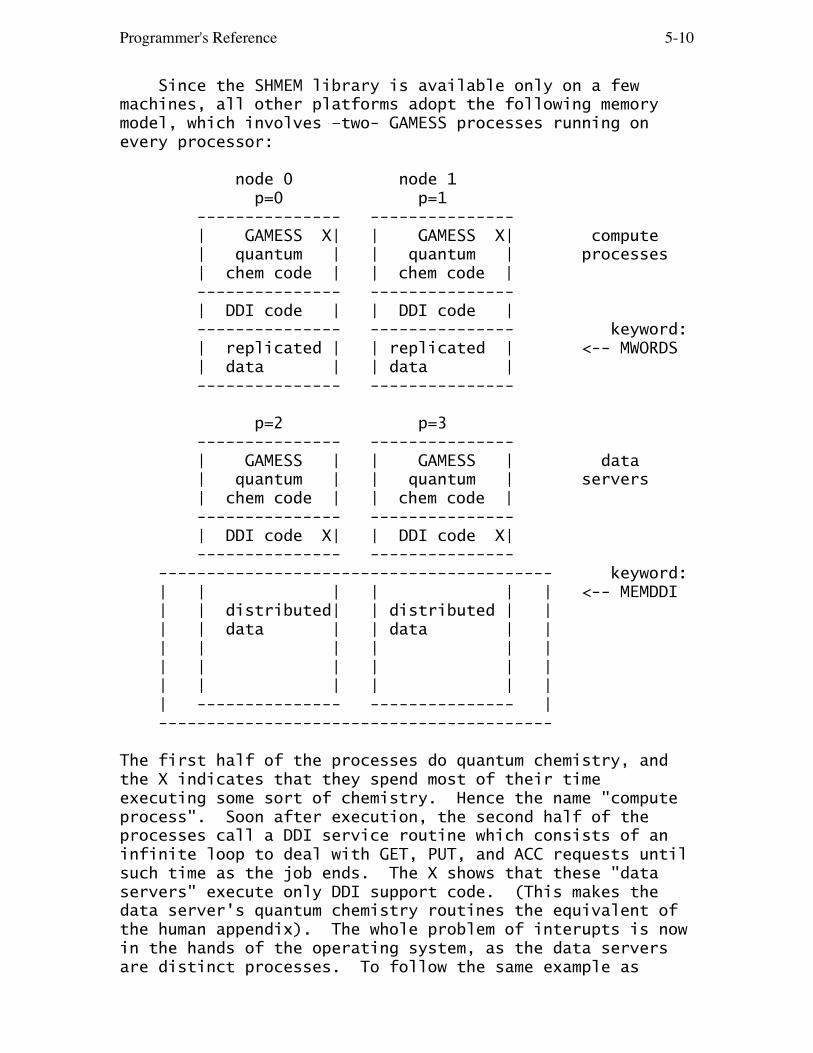
Programmer's Reference 5-10
Since the SHMEM library is available only on a fewmachines, all other platforms adopt the following memorymodel, which involves –two- GAMESS processes running onevery processor:
node 0 node 1 p=0 p=1 --------------- --------------- | GAMESS X| | GAMESS X| compute | quantum | | quantum | processes | chem code | | chem code | --------------- --------------- | DDI code | | DDI code | --------------- --------------- keyword: | replicated | | replicated | <-- MWORDS | data | | data | --------------- ---------------
p=2 p=3 --------------- --------------- | GAMESS | | GAMESS | data | quantum | | quantum | servers | chem code | | chem code | --------------- --------------- | DDI code X| | DDI code X| --------------- --------------- ----------------------------------------- keyword: | | | | | | <-- MEMDDI | | distributed| | distributed | | | | data | | data | | | | | | | | | | | | | | | | | | | | | --------------- --------------- | -----------------------------------------
The first half of the processes do quantum chemistry, andthe X indicates that they spend most of their timeexecuting some sort of chemistry. Hence the name "computeprocess". Soon after execution, the second half of theprocesses call a DDI service routine which consists of aninfinite loop to deal with GET, PUT, and ACC requests untilsuch time as the job ends. The X shows that these "dataservers" execute only DDI support code. (This makes thedata server's quantum chemistry routines the equivalent ofthe human appendix). The whole problem of interupts is nowin the hands of the operating system, as the data serversare distinct processes. To follow the same example as

Programmer's Reference 5-11
before, when the compute process p=1 needs data that turnsout to reside on process 0, a request is sent to the dataserver p=2 to transfer information back to the computeprocess p=1. The compute process p=0 is completely unawarethat such a transaction has occurred.
The formula for the memory required by any single CPUis unchanged, if p is the total number of CPUs used, total on any 1 CPU = MWORDS + MEMDDI/p.
As a technical matter, if you are running on a systemwhere all processors are in the same node (the SGI Altix isan example), or if you are running on an IBM SP where LAPIassists in implementing one-sided messaging, then the dataserver processes are not started. The memory model in theillustration above is correct, if you just mentally omitthe data server processes from it. In all cases, where theSHMEM library is not used, the distributed arrays arecreated by System V memory calls, shmget/shmat, and theirassociated semaphore routines. Your system may need to bereconfigured to allow allocation of large shared memorysegments, see 'readme.ddi' for more details.
The parallel CCSD and CCSD(T) programs add a third kindof memory to the mix: node-replicated. This is data (e.g.the doubles amplitudes) that is stored only once per node.Thus, this is more copies of the data than once perparallel job (fully distributed MEMDDI) but fewer than onceper CPU (replicated MWORDS). A picture of the memory modelfor the CCSD(T) program can be found in the "readme.ddi"file, so is not duplicated here. There is presently nokeyword for this type of memory, but the system limit onthe total SystemV memory does apply. It is important toperform a check run when using CCSD(T) and carefully followthe printout of its memory requirements.
memory allocations and check jobs
At present, not all runs require distributed memory.For example, in an SCF computation (no hessian or MP2 tofollow) the memory needed is on the order of the square ofthe basis set size, for such quantities as the orbitalcoefficients, density, Fock, overlap matrices, and so on.These are simply duplicated on every CPU in the MWORDS (orthe older keyword MEMORY in $SYSTEM) region. In this casethe data server processes still run, but are dormantbecause no distributed memory access is attempted.

Programmer's Reference 5-12
However, closed and open shell MP2 calculations, MCSCFwavefunctions, and their analytic hessian or MCQPDT energycorrection do use distributed memory when run in parallel.Thus it is important to know how to obtain the correctvalue for MEMDDI in a check run, and how to compute howmany CPUs are needed to do the run.
Check runs (EXETYP=CHECK) need to run quickly, and thefastest turn around always comes on one CPU only. Runswhich do not currently exploit MEMDDI distributed storagewill formally allocate their MWORDS needs, and feel outtheir storage needs while skipping almost all of the realwork. Since MWORDS is replicated, the amount that isneeded on 1 CPU remains unchanged if you later do the truecomputation on more than 1 CPU.
Check jobs which involve MEMDDI storage are a littlebit trickier. As noted, we want to run on only 1 CPU toget fast turn around. However, MEMDDI is typically a largeamount of memory, and this is unlikely to be available ona single CPU. The solution is that the check job will notactually allocate the MEMDDI storage, instead it justremembers what you gave as input and checks to see if thiswill be adequate. As someone once said, MEMDDI is a "fairytale number" during a check job. So, you can input a bigvalue like MEMDDI=25000 (25,000 million words is equal to25,000 * 1,000,000 * 8 = 200 GBytes) and run this check jobon a computer with only 1024 MB = 1 GB of memory perprocessor. Let us say that a closed shell MP2 check runfor this case gives the output of SCALED *PER-NODE* MEMORY REQUIREMENT NODES DISTRIBUTED/MWORDS REPLICATED/WORDS TOTAL/MBYTES 1 952 7284508 7624The real run requires MWORDS=8 MEMDDI=960. Note that wehave just rounded up a bit from the 7.3 and 952 in thisoutput, for safety.
Of course, the actual computation will have to run on alarge number of such processors, because you don't have 200GB on your CPU, we are assuming 1024 MB (1 GB). Let uscontinue to compute how many processors are needed. Weneed to reserve some memory for the operating system (25MB, say) and for the GAMESS program and local storage (letus say 50 MB, for GAMESS is a big program, and the computeprocesses should be swapped into memory). Thus ourhypothetical 1024 MB processor has 950 MB available,assuming no one else is running. In units of words, thismachine has 950/8 = 118 million words available for yourrun. We must choose the number of processors p to satisfy

Programmer's Reference 5-13
needed <= available MWORDS + MEMDDI/p <= free physical memory 8 + 960/p <= 118so solving for p, we learn this example requires p >= 9compute processes. The answer for roughly 8 GB ofdistributed memory on 1 GB processors was not 8, becausethe O/S, GAMESS itself, and the MWORDS requirementstogether mean less than 1 GB could be contributed to thedistributed total. More CPUs than 9 do not requirechanging MWORDS or MEMDDI, but will run faster than 9.Fewer CPUs than 9 do not have enough memory to run!
One more subtle point about CHECK runs with MEMDDI isthat since you are running on 1 CPU only, the code does notknow that you wish to run the parallel algorithm instead ofthe sequential algorithm. You must force the CHECK jobinto the parallel section of the program by $system parall=.true. $endThere's no harm leaving this line in for the true runs, asany job with more than one compute process is parallelregardless of the input keyword PARALL.
The check run for MCQDPT jobs will print three timesa line like this MAXIMUM MEMDDI THAT CAN BE USED IN ... IS x MWORDSTypically the 2nd such step, transforming over alloccupied and virtual canonical orbitals, will be thelargest of the three requirements. Its size can beguesstimated before running, as (Nao*Nao+Nao)/2 * ((Nocc*Nocc+Nocc)/2 + Nocc*Nvirt)where Nocc = NMOFZC+NMODOC+NMOACT, Nvirt=NMOEXT, andNao is the size of the atomic basis. Unlike the closedshell MP2 program, this section still does extensiveI/O operations even when MEMDDI is used, so it may beuseful to consider the three input keywords DOORD0,PARAIO, and DELSCR when running this code.
representative performance examples
This section describes the way in which the variousquantum chemistry computations run in parallel, and showssome typical performance data. This should give you as theuser some idea how many CPUs can be efficiently used forvarious SCFTYP and RUNTYP jobs
The performance data you will see below were obtainedon a 16 CPU Intel Pentium II Linux (Beowulf-type) cluster
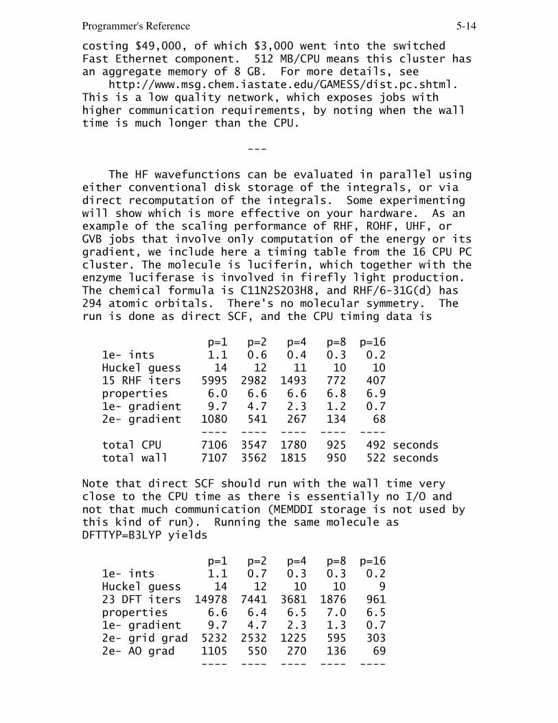
Programmer's Reference 5-14
costing $49,000, of which $3,000 went into the switchedFast Ethernet component. 512 MB/CPU means this cluster hasan aggregate memory of 8 GB. For more details, see http://www.msg.chem.iastate.edu/GAMESS/dist.pc.shtml.This is a low quality network, which exposes jobs withhigher communication requirements, by noting when the walltime is much longer than the CPU.
---
The HF wavefunctions can be evaluated in parallel usingeither conventional disk storage of the integrals, or viadirect recomputation of the integrals. Some experimentingwill show which is more effective on your hardware. As anexample of the scaling performance of RHF, ROHF, UHF, orGVB jobs that involve only computation of the energy or itsgradient, we include here a timing table from the 16 CPU PCcluster. The molecule is luciferin, which together with theenzyme luciferase is involved in firefly light production.The chemical formula is C11N2S2O3H8, and RHF/6-31G(d) has294 atomic orbitals. There's no molecular symmetry. Therun is done as direct SCF, and the CPU timing data is
p=1 p=2 p=4 p=8 p=16 1e- ints 1.1 0.6 0.4 0.3 0.2 Huckel guess 14 12 11 10 10 15 RHF iters 5995 2982 1493 772 407 properties 6.0 6.6 6.6 6.8 6.9 1e- gradient 9.7 4.7 2.3 1.2 0.7 2e- gradient 1080 541 267 134 68 ---- ---- ---- ---- ---- total CPU 7106 3547 1780 925 492 seconds total wall 7107 3562 1815 950 522 seconds
Note that direct SCF should run with the wall time veryclose to the CPU time as there is essentially no I/O andnot that much communication (MEMDDI storage is not used bythis kind of run). Running the same molecule asDFTTYP=B3LYP yields
p=1 p=2 p=4 p=8 p=16 1e- ints 1.1 0.7 0.3 0.3 0.2 Huckel guess 14 12 10 10 9 23 DFT iters 14978 7441 3681 1876 961 properties 6.6 6.4 6.5 7.0 6.5 1e- gradient 9.7 4.7 2.3 1.3 0.7 2e- grid grad 5232 2532 1225 595 303 2e- AO grad 1105 550 270 136 69 ---- ---- ---- ---- ----
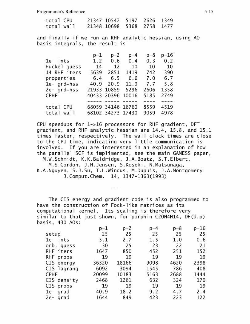
Programmer's Reference 5-15
total CPU 21347 10547 5197 2626 1349 total wall 21348 10698 5368 2758 1477
and finally if we run an RHF analytic hessian, using AObasis integrals, the result is
p=1 p=2 p=4 p=8 p=16 1e- ints 1.2 0.6 0.4 0.3 0.2 Huckel guess 14 12 10 10 10 14 RHF iters 5639 2851 1419 742 390 properties 6.4 6.5 6.6 7.0 6.7 1e- grd+hss 40.9 20.9 11.9 7.7 5.8 2e- grd+hss 21933 10859 5296 2606 1358 CPHF 40433 20396 10016 5185 2749 ----- ----- ----- ---- ---- total CPU 68059 34146 16760 8559 4519 total wall 68102 34273 17430 9059 4978
CPU speedups for 1->16 processors for RHF gradient, DFTgradient, and RHF analytic hessian are 14.4, 15.8, and 15.1times faster, respectively. The wall clock times are closeto the CPU time, indicating very little communication isinvolved. If you are interested in an explanation of howthe parallel SCF is implimented, see the main GAMESS paper, M.W.Schmidt, K.K.Baldridge, J.A.Boatz, S.T.Elbert, M.S.Gordon, J.H.Jensen, S.Koseki, N.Matsunaga,K.A.Nguyen, S.J.Su, T.L.Windus, M.Dupuis, J.A.Montgomery J.Comput.Chem. 14, 1347-1363(1993)
---
The CIS energy and gradient code is also programmed tohave the construction of Fock-like matrices as itscomputational kernel. Its scaling is therefore verysimilar to that just shown, for porphin C20N4H14, DH(d,p)basis, 430 AOs: p=1 p=2 p=4 p=8 p=16 setup 25 25 25 25 25 1e- ints 5.1 2.7 1.5 1.0 0.6 orb. guess 30 25 23 22 21 RHF iters 1647 850 452 251 152 RHF props 19 19 19 19 19 CIS energy 36320 18166 9098 4620 2398 CIS lagrang 6092 3094 1545 786 408 CPHF 20099 10183 5163 2688 1444 CIS density 2468 1261 632 324 170 CIS props 19 19 19 19 19 1e- grad 40.9 18.2 9.2 4.7 2.4 2e- grad 1644 849 423 223 122

Programmer's Reference 5-16
----- ----- ---- ---- ---- total CPU 68424 34526 17420 8994 4791 total wall 68443 34606 17853 9258 4985which is a speedup of 14.3 for 1->16.
---
For the next type of computation, we discuss the MP2correction. For closed shell RHF + MP2 and unrestrictedUHF + MP2, the gradient program runs in parallel usingdistributed memory, MEMDDI. In addition, the ROHF + MP2energy correction for OSPT=ZAPT runs in parallel usingdistributed memory, but OSPT=RMP does not use MEMDDI inparallel jobs. All distributed memory parallel MP2 runsresemble RHF+MP2, which is therefore the only example givenhere.
The example is a benzoquinone precursor to hongconin, acardioprotective natural product. The formula is C11O4H10,and 6-31G(d) has 245 AOs. There are 39 valence orbitalsincluded in the MP2 treatment, and 15 core orbitals.MEMDDI must be 156 million words, so the memory computationthat was used above tells us that our 512 MB/CPU PC clustermust have at least three processors to aggregate therequired MEMDDI. MOREAD was used to provide converged RHForbitals, so only 3 RHF iterations are performed. Thetiming data are CPU and wall times (seconds) in the 1st/2ndlines:
p=3 p=4 p=12 p=16 RHF iters 241 181 65 51 243 184 69 55 MP2 step 5,953 4,399 1,438 1,098 7,366 5,669 2,239 1,700 2e- grad 1,429 1,135 375 280 1,492 1,183 413 305 ----- ----- --- --- total CPU 7,637 5,727 1,890 1,440 total wall 9,116 7,053 2,658 2,077
3-->12 4-->16 CPU speedup 4.04 3.98 wall speedup 3.43 3.40
The wall clock time will be closer to the CPU time if thequality of the network between the computer is improved(remember, this run used just switched Fast Ethernet). Asnoted, the number of CPUs is more influenced by a need toaggregate the necessary total MEMDDI, more than by concerns
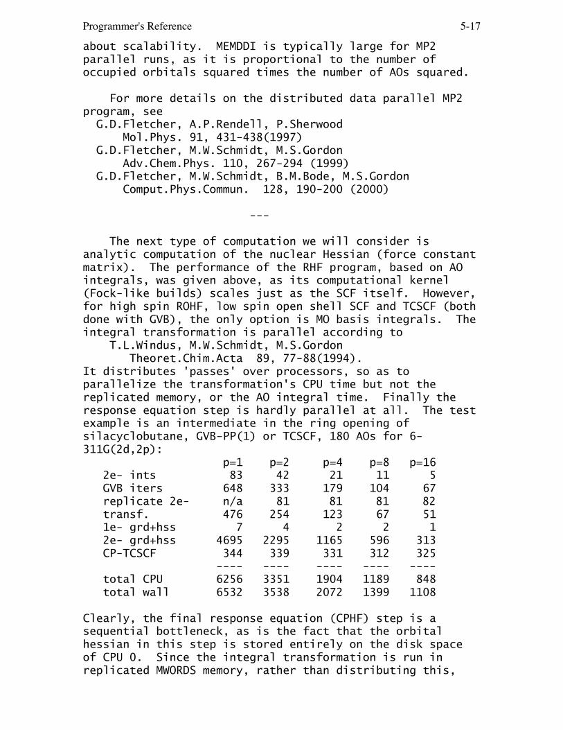
Programmer's Reference 5-17
about scalability. MEMDDI is typically large for MP2parallel runs, as it is proportional to the number ofoccupied orbitals squared times the number of AOs squared.
For more details on the distributed data parallel MP2program, see G.D.Fletcher, A.P.Rendell, P.Sherwood Mol.Phys. 91, 431-438(1997) G.D.Fletcher, M.W.Schmidt, M.S.Gordon Adv.Chem.Phys. 110, 267-294 (1999) G.D.Fletcher, M.W.Schmidt, B.M.Bode, M.S.Gordon Comput.Phys.Commun. 128, 190-200 (2000)
---
The next type of computation we will consider isanalytic computation of the nuclear Hessian (force constantmatrix). The performance of the RHF program, based on AOintegrals, was given above, as its computational kernel(Fock-like builds) scales just as the SCF itself. However,for high spin ROHF, low spin open shell SCF and TCSCF (bothdone with GVB), the only option is MO basis integrals. Theintegral transformation is parallel according to T.L.Windus, M.W.Schmidt, M.S.Gordon Theoret.Chim.Acta 89, 77-88(1994).It distributes 'passes' over processors, so as toparallelize the transformation's CPU time but not thereplicated memory, or the AO integral time. Finally theresponse equation step is hardly parallel at all. The testexample is an intermediate in the ring opening ofsilacyclobutane, GVB-PP(1) or TCSCF, 180 AOs for 6-311G(2d,2p): p=1 p=2 p=4 p=8 p=16 2e- ints 83 42 21 11 5 GVB iters 648 333 179 104 67 replicate 2e- n/a 81 81 81 82 transf. 476 254 123 67 51 1e- grd+hss 7 4 2 2 1 2e- grd+hss 4695 2295 1165 596 313 CP-TCSCF 344 339 331 312 325 ---- ---- ---- ---- ---- total CPU 6256 3351 1904 1189 848 total wall 6532 3538 2072 1399 1108
Clearly, the final response equation (CPHF) step is asequential bottleneck, as is the fact that the orbitalhessian in this step is stored entirely on the disk spaceof CPU 0. Since the integral transformation is run inreplicated MWORDS memory, rather than distributing this,
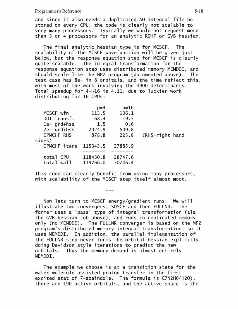
Programmer's Reference 5-18
and since it also needs a duplicated AO integral file bestored on every CPU, the code is clearly not scalable tovery many processors. Typically we would not request morethan 3 or 4 processors for an analytic ROHF or GVB hessian.
The final analytic hessian type is for MCSCF. Thescalability of the MCSCF wavefunction will be given justbelow, but the response equation step for MCSCF is clearlyquite scalable. The integral transformation for theresponse equation step uses distributed memory MEMDDI, andshould scale like the MP2 program (documented above). Thetest case has 8e- in 8 orbitals, and the time reflect this,with most of the work involving the 4900 determinants.Total speedup for 4->16 is 4.11, due to luckier workdistributing for 16 CPUs:
p=4 p=16 MCSCF wfn 113.5 106.1 DDI transf. 68.4 19.3 1e- grd+hss 1.5 0.6 2e- grd+hss 2024.9 509.8 CPMCHF RHS 878.8 225.8 (RHS=right handsides) CPMCHF iters 115343.5 27885.9 -------- -------- total CPU 118430.8 28747.6 total wall 119766.0 30746.4
This code can clearly benefit from using many processors,with scalability of the MCSCF step itself almost moot.
---
Now lets turn to MCSCF energy/gradient runs. We willillustrate two convergers, SOSCF and then FULLNR. Theformer uses a 'pass' type of integral transformation (alathe GVB hessian job above), and runs in replicated memoryonly (no MEMDDI). The FULLNR converger is based on the MP2program's distributed memory integral transformation, so ituses MEMDDI. In addition, the parallel implementation ofthe FULLNR step never forms the orbital hessian explicitly,doing Davidson style iterations to predict the neworbitals. Thus the memory demand is almost entirelyMEMDDI.
The example we choose is at a transition state for thewater molecule assisted proton transfer in the firstexcited stat of 7-azaindole. The formula is C7N2H6(H2O),there are 190 active orbitals, and the active space is the
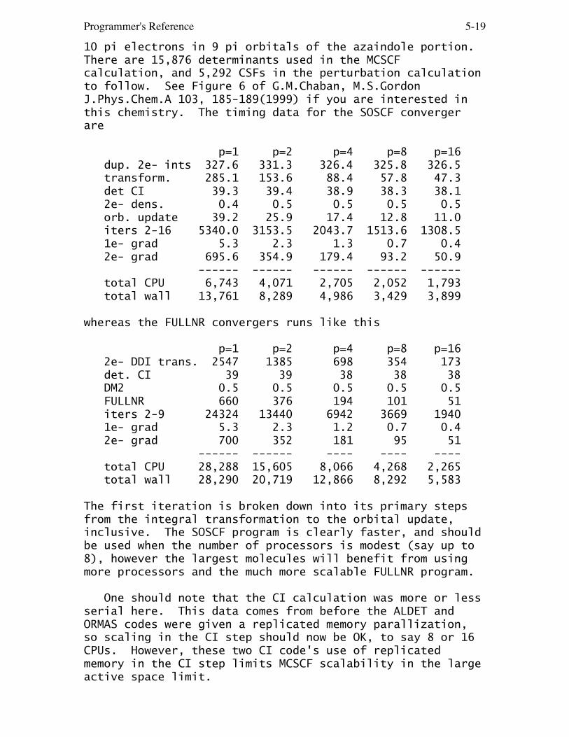
Programmer's Reference 5-19
10 pi electrons in 9 pi orbitals of the azaindole portion.There are 15,876 determinants used in the MCSCFcalculation, and 5,292 CSFs in the perturbation calculationto follow. See Figure 6 of G.M.Chaban, M.S.GordonJ.Phys.Chem.A 103, 185-189(1999) if you are interested inthis chemistry. The timing data for the SOSCF convergerare
p=1 p=2 p=4 p=8 p=16 dup. 2e- ints 327.6 331.3 326.4 325.8 326.5 transform. 285.1 153.6 88.4 57.8 47.3 det CI 39.3 39.4 38.9 38.3 38.1 2e- dens. 0.4 0.5 0.5 0.5 0.5 orb. update 39.2 25.9 17.4 12.8 11.0 iters 2-16 5340.0 3153.5 2043.7 1513.6 1308.5 1e- grad 5.3 2.3 1.3 0.7 0.4 2e- grad 695.6 354.9 179.4 93.2 50.9 ------ ------ ------ ------ ------ total CPU 6,743 4,071 2,705 2,052 1,793 total wall 13,761 8,289 4,986 3,429 3,899
whereas the FULLNR convergers runs like this
p=1 p=2 p=4 p=8 p=16 2e- DDI trans. 2547 1385 698 354 173 det. CI 39 39 38 38 38 DM2 0.5 0.5 0.5 0.5 0.5 FULLNR 660 376 194 101 51 iters 2-9 24324 13440 6942 3669 1940 1e- grad 5.3 2.3 1.2 0.7 0.4 2e- grad 700 352 181 95 51 ------ ------ ---- ---- ---- total CPU 28,288 15,605 8,066 4,268 2,265 total wall 28,290 20,719 12,866 8,292 5,583
The first iteration is broken down into its primary stepsfrom the integral transformation to the orbital update,inclusive. The SOSCF program is clearly faster, and shouldbe used when the number of processors is modest (say up to8), however the largest molecules will benefit from usingmore processors and the much more scalable FULLNR program.
One should note that the CI calculation was more or lessserial here. This data comes from before the ALDET andORMAS codes were given a replicated memory parallization,so scaling in the CI step should now be OK, to say 8 or 16CPUs. However, these two CI code's use of replicatedmemory in the CI step limits MCSCF scalability in the largeactive space limit.

Programmer's Reference 5-20
Now let's consider the second order pertubationcorrection for this example. As noted, it is an excitedstate, so the test corrects two states simultaneously (S0and S1). The parallel multireference perturbation programis described in H.Umeda, S.Koseki, U.Nagashima, M.W.Schmidt J.Comput.Chem. 22, 1243-1251 (2001)The run is given the converged S1 orbitals, so that it canskip directly to the perturbation calculation: p=1 p=2 p=4 p=8 p=16 2e- ints 332 332 329 328 331 MCQDPT 87921 43864 22008 11082 5697 ----- ----- ----- ----- ----- total CPU 88261 44205 22345 11418 6028 total wall 91508 45818 23556 12350 6852This corresponds to a speedup for 1->16 of 14.6.
---
In summary, most ab initio computations will run inless time on more than one processor. However, some thingscan be run only on 1 CPU, namely semi-empirical runs RHF+CI gradient Coupled-Cluster calculationsSome steps run with little or no speedup, formingsequential bottlenecks that limit scalability. They do notprevent jobs from running in parallel, but restrict thetotal number of processors that can be effectively used: ROHF/GVB hessians: solution of response equations MCSCF: Hamiltonian and 2e- density matrix (CI) energy localizations: the orbital localization step transition moments/spin-orbit: the final property step MCQDPT reference weight optionFuture versions of GAMESS will address these bottlenecks.
A short summary of the useful number of CPUs (based ondata like the above) would be RHF, ROHF, UHF, GVB energy/gradient, their DFT analogs, and CIS excited states 16-32+ MCSCF energy/gradient SOSCF 4-8 FULLNR 8-32+ analytic hessians RHF 16-32+ ROHF/GVB 4-8 MCSCF 64-128+ MPLEVL=2

Programmer's Reference 5-21
RHF, UHF, ROHF OSPT=ZAPT 8-256+ ROHF OSPT=RMP energy 8 MCSCF 16+

Programmer's Reference 5-22
Altering program limits
Almost all arrays in GAMESS are allocated dynamically,but some variables must be held in common as their use isubiquitous. An example would be the common block /NSHEL/which holds the ab initio atom's basis set. The followingUnix script, which we call 'mung' (see Wikipedia entry forrecursive acronyms), changes the PARAMETER statements thatset various limitations:
#!/bin/csh## automatically change GAMESS' built-in dimensions#chdir /u1/mike/gamess/source#foreach FILE (*.src) set FILE=$FILE:r echo ===== redimensioning in $FILE ===== echo "C dd-mmm-yy - SELECT NEW DIMENSIONS" \ > $FILE.munged sed -e "/MXATM=2000/s//MXATM=500/" \ -e "/MXAO=8192/s//MXAO=2047/" \ -e "/MXGSH=30/s//MXGSH=30/" \ -e "/MXSH=5000/s//MXSH=1000/" \ -e "/MXGTOT=20000/s//MXGTOT=5000/" \ -e "/MXRT=100/s//MXRT=100/" \ -e "/MXFRG=1050/s//MXFRG=65/" \ -e "/MXDFG=5/s//MXDFG=1/" \ -e "/MXPT=2000/s//MXPT=100/" \ -e "/MXFGPT=12000/s//MXFGPT=2000/" \ -e "/MXSP=500/s//MXSP=100/" \ -e "/MXTS=20000/s//MXTS=2500/" \ -e "/MXABC=6000/s//MXABC=1/" \ $FILE.src >> $FILE.munged mv $FILE.munged $FILE.srcendexit
The script shows how to reduce memory, by decreasingthe number of atoms and basis functions, and reducing thestorage for the effective fragment and PCM solvent models.
Of course, the 'mung' script can also be used toincrease the dimensions!

Programmer's Reference 5-23
To fully turn off effective fragment storage, useMXFRG=4, MXDFG=1, MXPT=8, MXFGPT=4. To fully turn off PCMstorage, use MXSP=1, MXTS=1. The parameters currently usedfor GAMESS imply about 75 MBytes of storage tied up incommon blocks, which is not unreasonable, even in a laptop.Reducing the storage size makes sense mainly on microkerneltype systems, without virtual memory managers.
In this script, MXATM = max number of ab initio atoms MXAO = max number of basis functions MXGSH = max number of Gaussians per shell MXSH = max number of symmetry unique shells MXGTOT= max number of symmetry unique Gaussians
MXRT = max number of MCSCF/CI states
MXFRG = max number of effective fragment potentials MXDFG = max number of different effective fragments MXPT = max number of points in any one term of any EFP MXFGPT= maximum storage for all EFPs, and is sized for a large number of EFPs with a small number of points (solvent applications), or a smaller number of EFPs with many points (biochemistry).
MXSP = max number of spheres (sfera) in PCM MXTS = max number of tesserae in PCM
MXABC = max number of A,B,C matrices in the COSMO algorithm. The default value of 6000 allows the construction of cavities for roughly 150 to 200 atoms.

Programmer's Reference 5-24
Names of source code modules
The source code for GAMESS is divided into a number ofsections, called modules, each of which does relatedthings, and is a handy size to edit. The following is alist of the different modules, what they do, and notes ontheir machine dependencies.
machinemodule description dependency------- ------------------------- ----------ALDECI Ames Lab determinant full CI code 1ALGNCI Ames Lab determinant general CI codeBASCCN Dunning cc-pVxZ basis setsBASECP SBKJC and HW valence basis setsBASEXT DH, MC, 6-311G extended basis setsBASG3L G3Large basis setsBASHUZ Huzinaga MINI/MIDI basis sets to XeBASHZ2 Huzinaga MINI/MIDI basis sets Cs-RnBASKAR Karlsruhe (Ahlrichs) TZV basis setsBASN21 N-21G basis setsBASN31 N-31G basis setsBASPCN Jensen polarization consistent basis setsBASSTO STO-NG basis setsBLAS level 1 basic linear algebra subprogramsCCAUX auxiliary routines for CC calculationsCCDDI parallel CCSD(T) programCCQAUX auxiliaries for CCSD(TQ) programCCQUAD renormalized CCSD(TQ) correctionsCCSDT renormalized CCSD(T) program 1CEEIS corr. energy extrap. by intrinsic scalingCHGPEN screening for charge penetration of EFPsCISGRD CI singles and its gradient 1COSMO conductor-like screening modelCOSPRT printing routine for COSMOCPHF coupled perturbed Hartree-Fock 1CPMCHF multiconfigurational CPHF 1CPROHF open shell/TCSCF CPHF 1DCCC divide and conquer coupled clusterDCGRD divide and conquer gradientsDCGUES divide and conquer orbital guessDCINT2 divide and conquer AO integrals 1DCLIB divide and conquer library routinesDCMP2 divide and conquer MP2 1DCSCF divide and conquer SCFDCTRAN divide and conquer integral transf. 1DDILIB message passing library interface code
Programmer's Reference 5-25
DELOCL delocalized coordinatesDEMRPT determinant-based MCQDPTDFT grid-free DFT drivers 1DFTAUX grid-free DFT auxiliary basis integralsDFTDIS empirical dispersion correction to DFTDFTFUN grid-free DFT functionalsDFTGRD grid DFT implementationDFTINT grid-free DFT integrals 1DFTXCA grid DFT functionals, hand codedDFTXCB grid DFT functionals, from repositoryDFTXCC grid DFT functionals for meta-GGADFTXCD grid DFT functionals B97, etcDFTXCE grid DFT functionals for PKZB/TPSS familyDFTXCF grid DFT functionals for CAMB3LYPdirDFTXCG grid DFT functional for revTPSSDGEEV general matrix eigenvalue problemDGESVD single value decompositionDMULTI Amos' distributed multipole analysisDRC dynamic reaction coordinateEAIPCC EA-EOM and IP-EOM methodECP pseudopotential integralsECPDER pseudopotential derivative integralsECPLIB initialization code for ECPECPPOT HW and SBKJC internally stored potentialsEFCHTR fragment charge transferEFDRVR fragment only calculation driversEFELEC fragment-fragment interactionsEFGRD2 2e- integrals for EFP numerical hessianEFGRDA ab initio/fragment gradient integralsEFGRDB " " " " "EFGRDC " " " " "EFINP effective fragment potential inputEFINTA ab initio/fragment integralsEFINTB " " " "EFMO EFP + FMO interfacingEFPAUL effective fragment Pauli repulsionEFPCM EFP/PCM interfacingEFPCOV EFP style QM/MM boundary codeEFPFMO FMO and EFP interfaceEFTEI QM/EFP 2e- integrals 1EIGEN Givens-Householder, Jacobi diagonalizationELGLIB elongation method utility routinesELGLOC elongation method orbital localizationELGSCF elongation method Hartree-Fock 1EOMCC equation of motion excited state CCSDEWALD Ewald summations for EFP modelFFIELD finite field polarizabilitieFMO n-mer drivers for Fragment Molecular OrbitalFMOESD elestrostatic potential derivatives for FMO
Programmer's Reference 5-26
FMOGRD gradient routines for FMOFMOINT integrals for FMOFMOIO input/output and printing for FMOFMOLIB utilities for FMOFMOPBC periodic boundary conditions for FMOFMOPRP properties for FMOFRFMT free format input scannerFSODCI determinant based second order CIG3 G3(MP2,CCSD(T)) thermochemistryGAMESS main program, important driver routinesGLOBOP Monte Carlo fragment global optimizerGMCPT general MCQDPT multireference PT code 1GRADEX traces gradient extremalsGRD1 one electron gradient integralsGRD2A two electron gradient integrals 1GRD2B specialized sp gradient integralsGRD2C general spdfg gradient integralsGUESS initial orbital guessGUGDGA Davidson CI diagonalization 1GUGDGB " " " 1GUGDM 1 particle density matrixGUGDM2 2 particle density matrix 1GUGDRT distinct row table generationGUGEM GUGA method energy matrix formation 1GUGSRT sort transformed integrals 1GVB generalized valence bond HF-SCF 1HESS hessian computation driversHSS1A one electron hessian integralsHSS1B " " " "HSS2A two electron hessian integrals 1HSS2B " " " "INPUTA read geometry, basis, symmetry, etc.INPUTB " " " "INPUTC " " " "INT1 one electron integralsINT2A two electron integrals (Rys) 1INT2B two electron integrals (s,p,L rot.axis)INT2C ERIC TEI code, and its s,p routines 11INT2D ERIC special code for d TEIINT2F ERIC special code for f TEIINT2G ERIC special code for g TEIINT2R s,p,d,L rotated axis integral packageINT2S s,p,d,L quadrature codeINT2T s,p,d,L quadrature codeINT2U s,p,d,L quadrature codeINT2V s,p,d,L quadrature codeINT2W s,p,d,L quadrature codeINT2X s,p,d,L quadrature codeIOLIB input/output routines,etc. 2

Programmer's Reference 5-27
IVOCAS improved virtual orbital CAS energy 1LAGRAN CI Lagrangian matrix 1LOCAL various localization methods 1LOCCD LCD SCF localization analysisLOCPOL LCD SCF polarizability analysis 1LRD local response dispersion correctionMCCAS FOCAS/SOSCF MCSCF calculation 1MCJAC JACOBI MCSCF calculationMCPGRD model core potential nuclear gradientMCPINP model core potential inputMCPINT model core potential integralsMCPL10 model core potential libraryMCPL20 " " " "MCPL30 " " " "MCPL40 " " " "MCPL50 " " " "MCPL60 " " " "MCPL70 " " " "MCPL80 " " " "MCQDPT multireference perturbation theory 1MCQDWT weights for MR-perturbation theoryMCQUD QUAD MCSCF calculation 1MCSCF FULLNR MCSCF calculation 1MCTWO two electron terms for FULLNR MCSCF 1MDEFP molecular dynamics using EFP particlesMEXING minimum energy crossing point searchMLTFMO multiscale solvation in FMOMM23 MMCC(2,3) corrections to EOMCCSDMOROKM Morokuma energy decomposition 1MNSOL U.Minnesota solution modelsMP2 2nd order Moller-Plesset 1MP2DDI distributed data parallel MP2MP2GRD CPHF and density for MP2 gradients 1MP2GR2 disk based MP2 gradient programMP2IMS disk based MP2 energy programMPCDAT MOPAC parameterizationMPCGRD MOPAC gradientMPCINT MOPAC integralsMPCMOL MOPAC molecule setupMPCMSC miscellaneous MOPAC routinesMTHLIB printout, matrix math utilitiesNAMEIO namelist I/O simulatorNEOSTB dummy routines for NEO programNMR nuclear magnetic resonance shifts 1ORDINT sort atomic integrals 1ORMAS1 occ. restricted multiple act. space CIPARLEY communicate to other programsPCM Polarizable Continuum Model setupPCMCAV PCM cavity creation
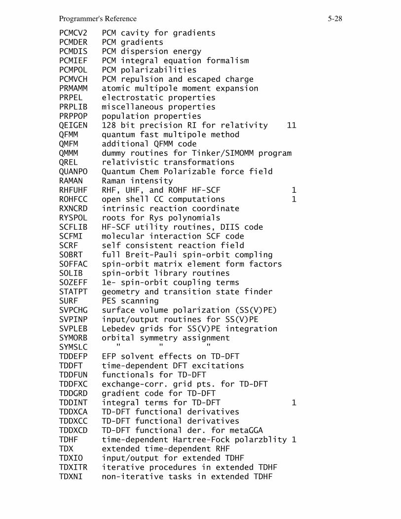
Programmer's Reference 5-28
PCMCV2 PCM cavity for gradientsPCMDER PCM gradientsPCMDIS PCM dispersion energyPCMIEF PCM integral equation formalismPCMPOL PCM polarizabilitiesPCMVCH PCM repulsion and escaped chargePRMAMM atomic multipole moment expansionPRPEL electrostatic propertiesPRPLIB miscellaneous propertiesPRPPOP population propertiesQEIGEN 128 bit precision RI for relativity 11QFMM quantum fast multipole methodQMFM additional QFMM codeQMMM dummy routines for Tinker/SIMOMM programQREL relativistic transformationsQUANPO Quantum Chem Polarizable force fieldRAMAN Raman intensityRHFUHF RHF, UHF, and ROHF HF-SCF 1ROHFCC open shell CC computations 1RXNCRD intrinsic reaction coordinateRYSPOL roots for Rys polynomialsSCFLIB HF-SCF utility routines, DIIS codeSCFMI molecular interaction SCF codeSCRF self consistent reaction fieldSOBRT full Breit-Pauli spin-orbit complingSOFFAC spin-orbit matrix element form factorsSOLIB spin-orbit library routinesSOZEFF 1e- spin-orbit coupling termsSTATPT geometry and transition state finderSURF PES scanningSVPCHG surface volume polarization (SS(V)PE)SVPINP input/output routines for SS(V)PESVPLEB Lebedev grids for SS(V)PE integrationSYMORB orbital symmetry assignmentSYMSLC " " "TDDEFP EFP solvent effects on TD-DFTTDDFT time-dependent DFT excitationsTDDFUN functionals for TD-DFTTDDFXC exchange-corr. grid pts. for TD-DFTTDDGRD gradient code for TD-DFTTDDINT integral terms for TD-DFT 1TDDXCA TD-DFT functional derivativesTDDXCC TD-DFT functional derivativesTDDXCD TD-DFT functional der. for metaGGATDHF time-dependent Hartree-Fock polarzblity 1TDX extended time-dependent RHFTDXIO input/output for extended TDHFTDXITR iterative procedures in extended TDHFTDXNI non-iterative tasks in extended TDHF

Programmer's Reference 5-29
TDXPRP properties from extended TDHFTRANS partial integral transformation 1TRFDM2 two particle density backtransform 1TRNSTN CI transition momentsTRUDGE nongradient optimizationUMPDDI distributed data parallel MP2UNPORT unportable, nasty code 3,4,5,6,7,8UTDDFT unrestricted TD-DFT 1VBDUM dummy routines for VB programsVECTOR vectorized version routines 10VIBANL normal coordinate analysisVSCF anharmonic frequenciesVVOS valence virtual orbitalsZAPDDI distrib. data ZAPT2 open shell PT gradientZHEEV complex matrix diagonalizationZMATRX internal coordinates
UNIX versions use the C code ZUNIX.C for dynamic memory.
The machine dependencies noted above are:1) packing/unpacking 2) OPEN/CLOSE statments3) machine specification 4) fix total dynamic memory5) subroutine walkback 6) error handling calls7) timing calls 8) LOGAND function10) vector library calls 11) REAL*16 data type
Note that the message passing support (DDI) for GAMESS isimplemented in C (for most machines), and is stored in aseparate subdirectory. Please see the ~/games/ddi tree formore information about the Distributed Data Interface'scode and usage.
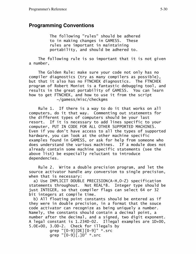
Programmer's Reference 5-30
Programming Conventions
The following "rules" should be adhered to in making changes in GAMESS. These rules are important in maintaining portability, and should be adhered to.
The following rule is so important that it is not givena number,
The Golden Rule: make sure your code not only has nocompiler diagnostics (try as many compilers as possible),but that it also has no FTNCHEK diagnostics. The FTNCHEKprogram of Robert Moniot is a fantastic debugging tool, andresults in the great portability of GAMESS. You can learnhow to get FTNCHEK, and how to use it from the script ~/gamess/misc/checkgms
Rule 1. If there is a way to do it that works on allcomputers, do it that way. Commenting out statements forthe different types of computers should be your lastresort. If it is necessary to add lines specific to yourcomputer, PUT IN CODE FOR ALL OTHER SUPPORTED MACHINES.Even if you don't have access to all the types of supportedhardware, you can look at the other machine specificexamples found in GAMESS, or ask for help from someone whodoes understand the various machines. If a module does notalready contain some machine specific statements (see theabove list) be especially reluctant to introducedependencies.
Rule 2. Write a double precision program, and let thesource activator handle any conversion to single precision,when that is necessary: a) Use IMPLICIT DOUBLE PRECISION(A-H,O-Z) specificationstatements throughout. Not REAL*8. Integer type should bejust INTEGER, so that compiler flags can select 64 or 32bit integers at compile time. b) All floating point constants should be entered as ifthey were in double precision, in a format that the soucecode activator can recognize as being uniquely a number.Namely, the constants should contain a decimal point, anumber after the decimal, and a signed, two digit exponent.A legal constant is 1.234D-02. Illegal examples are 1D+00,5.0E+00, 3.0D-2. Check for illegals by grep "[0-9][DE][0-9]" *.src grep "[0-9][.]D" *.src

Programmer's Reference 5-31
grep "[0-9][.][0-9][DE][0-9]" *.src grep "[0-9][DE][+-][1-9][^0-9]" *.src c) Double precision BLAS names are used throughout, forexample DDOT instead of SDOT, and DGEMM instead of SGEMM.
The source code activator ACTVTE will automatically convert these double precision constructs into the correct single precision expressions for machines that have 64 rather than 32 bit words.
Rule 3. FORTRAN 77 allows for generic functions. Thusthe routine SQRT should be used in place of DSQRT, as thiswill automatically be given the correct precision by thecompilers. Use ABS, COS, INT, etc. Your compiler manualwill tell you all the generic names.
Rule 4. Every routine in GAMESS begins with a cardcontaining the name of the module and the routine. Anexample is "C*MODULE xxxxxx *DECK yyyyyy". The secondstar is in column 18. Here, xxxxxx is the name of themodule, and yyyyyy is the name of the routine. This ruleis designed to make it easier for a person completelyunfamiliar with GAMESS to find routines.
Rule 5. Whenever a change is made to a module, thisshould be recorded at the top of the module. Theinformation required is the date, initials of the personmaking the change, and a terse summary of the change.
Rule 6. No imbedded tabs, statements must lie betweencolumns 7 and 72, etc. In other words, old style syntax.
* * *
The next few "rules" are not adhered to in all sections of GAMESS. Nonetheless they should be followed as much as possible, whether you are writing new code, or modifying an old section.
Rule 7. Stick to the FORTRAN naming convention forinteger (I-N) and floating point variables (A-H,O-Z). Ifyou've ever worked with a program that didn't obey this,you'll understand why.
Rule 8. Always use a dynamic memory allocation routinethat calls the real routine. A good name for the memory

Programmer's Reference 5-32
routine is to replace the last letter of the real routinewith the letter M for memory.
Rule 9. All the usual good programming techniques,such as indented DO loops ending on CONTINUEs, IF-THEN-ELSEwhere this is clearer, 3 digit statement labels inascending order, no three branch GO TO's, descriptivevariable names, 4 digit FORMATs, etc, etc.
The next set of rules relates to coding practices which are necessary for the parallel version of GAMESS to function sensibly. They must be followed without exception!
Rule 10. All open, rewind, and close operations onsequential files must be performed with the subroutinesSEQOPN, SEQREW, and SEQCLO respectively. You can findthese routines in IOLIB, they are easy to use. SQREAD,SQWRIT, and various integral I/O routines like PREAD areused to process the contents of such files. The variableDSKWRK tells if you are processing a distributed file (onesplit between all compute processes, DSKWRK=.TRUE.) or asingle file on the master process (DSKWRK=.FALSE.,resulting in broadcasts of the data from the master to allother CPUs).
Rule 11. All READ and WRITE statements for theformatted files 5, 6, 7 (variables IR, IW, IP, or namedfiles INPUT, OUTPUT, PUNCH) must be performed only by themaster task. Therefore, these statements must be enclosedin "IF (MASWRK) THEN" clauses. The MASWRK variable isfound in the /PAR/ common block, and is true on the masterprocess only. This avoids duplicate output from the otherprocesses.
Rule 12. All error termination is done by "CALL ABRT"rather than a STOP statement. Since this subroutine neverreturns, it is OK to follow it with a STOP statement, ascompilers may not be happy without a STOP as the finalexecutable statment in a routine. The purpose of callingABRT is to make sure that all parallel tasks get shut downproperly.
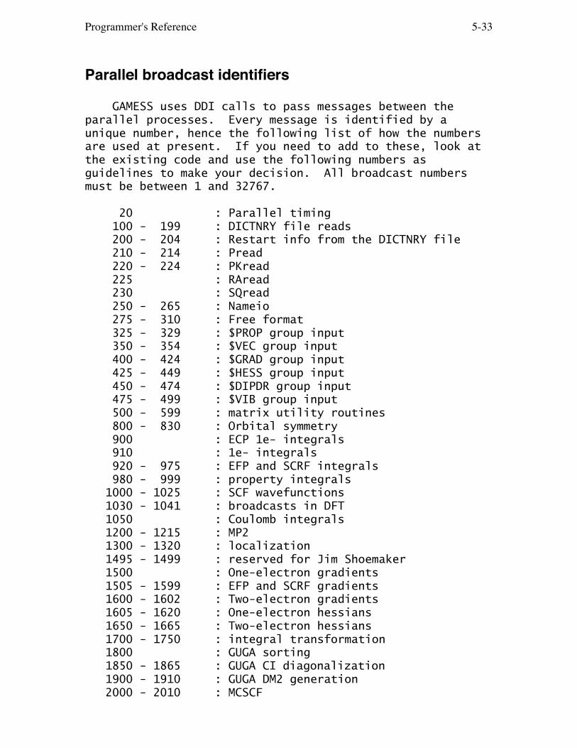
Programmer's Reference 5-33
Parallel broadcast identifiers
GAMESS uses DDI calls to pass messages between theparallel processes. Every message is identified by aunique number, hence the following list of how the numbersare used at present. If you need to add to these, look atthe existing code and use the following numbers asguidelines to make your decision. All broadcast numbersmust be between 1 and 32767.
20 : Parallel timing 100 - 199 : DICTNRY file reads 200 - 204 : Restart info from the DICTNRY file 210 - 214 : Pread 220 - 224 : PKread 225 : RAread 230 : SQread 250 - 265 : Nameio 275 - 310 : Free format 325 - 329 : $PROP group input 350 - 354 : $VEC group input 400 - 424 : $GRAD group input 425 - 449 : $HESS group input 450 - 474 : $DIPDR group input 475 - 499 : $VIB group input 500 - 599 : matrix utility routines 800 - 830 : Orbital symmetry 900 : ECP 1e- integrals 910 : 1e- integrals 920 - 975 : EFP and SCRF integrals 980 - 999 : property integrals 1000 - 1025 : SCF wavefunctions 1030 - 1041 : broadcasts in DFT 1050 : Coulomb integrals 1200 - 1215 : MP2 1300 - 1320 : localization 1495 - 1499 : reserved for Jim Shoemaker 1500 : One-electron gradients 1505 - 1599 : EFP and SCRF gradients 1600 - 1602 : Two-electron gradients 1605 - 1620 : One-electron hessians 1650 - 1665 : Two-electron hessians 1700 - 1750 : integral transformation 1800 : GUGA sorting 1850 - 1865 : GUGA CI diagonalization 1900 - 1910 : GUGA DM2 generation 2000 - 2010 : MCSCF

Programmer's Reference 5-34
2100 - 2120 : coupled perturbed HF 2150 - 2200 : MCSCF hessian 2300 - 2309 : spin-orbit jobs 2350 - 2353 : local response dispersion

Programmer's Reference 5-35
Disk files used by GAMESS
These files must be defined by your control language inorder to execute GAMESS. For example, on UNIX the "name"field shown below should be set in the environment to theactual file name to be used. Most runs will open only asubset of the files shown below, with only files 5, 6, 7,and 10 used by every run. Files 1, 2, 3 (both), 4, 5, 6,7, and 35 contain formatted data, while all others arebinary (unformatted) files. Files ERICFMT, EXTBAS, andMCPPATH are used to read data into GAMESS. Files MAKEFP,TRAJECT, RESTART, and PUNCH are supplemental output files,containing more concise summaries than the log file forcertain kinds of data.
unit name contents---- ---- -------- 1 MAKEFP effective fragment potential from MAKEFP run
2 ERICFMT Fm(t) interpolation table data, a data file named ericfmt.dat, supplied with GAMESS.
3 MCPPATH a directory of model core potentials and associated basis sets, supplied with GAMESS
3 EXTBAS external basis set library (user supplied)
3 GAMMA 3rd nuclear derivatives
4 TRAJECT trajectory results for IRC, DRC, or MD runs. summary of results for RUNTYP=GLOBOP.
35 RESTART restart data for numerical HESSIAN runs, numerical gradients, or for RUNTYP=VSCF. Used as a scratch unit during MAKEFP.
5 INPUT Namelist input file. This MUST be a disk file, as GAMESS rewinds this file often.
6 OUTPUT Print output (main log file). If not defined, UNIX systems will use the file "standard output" for this.
7 PUNCH Punch output. A copy of the $DATA deck, orbitals for every geometry calculated, hessian matrix, normal modes from FORCE, properties output, etc. etc. etc.
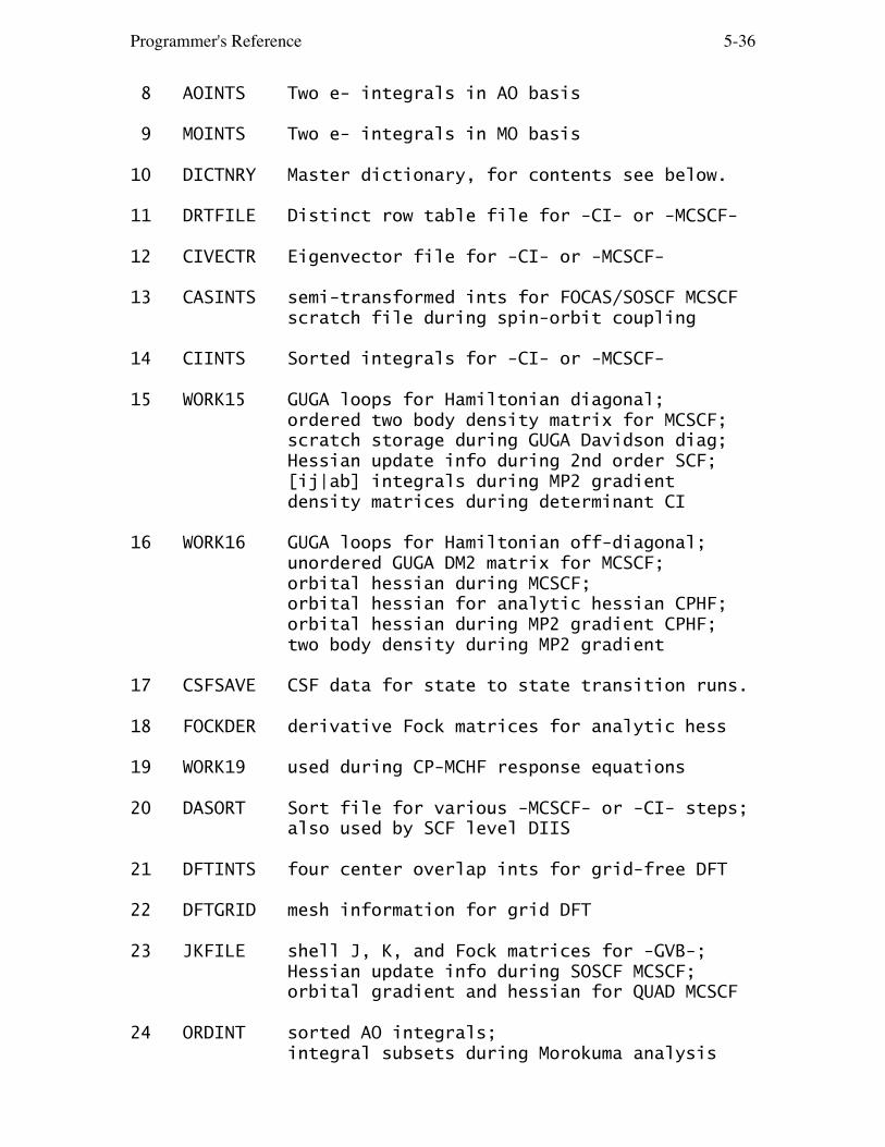
Programmer's Reference 5-36
8 AOINTS Two e- integrals in AO basis
9 MOINTS Two e- integrals in MO basis
10 DICTNRY Master dictionary, for contents see below.
11 DRTFILE Distinct row table file for -CI- or -MCSCF-
12 CIVECTR Eigenvector file for -CI- or -MCSCF-
13 CASINTS semi-transformed ints for FOCAS/SOSCF MCSCF scratch file during spin-orbit coupling
14 CIINTS Sorted integrals for -CI- or -MCSCF-
15 WORK15 GUGA loops for Hamiltonian diagonal; ordered two body density matrix for MCSCF; scratch storage during GUGA Davidson diag; Hessian update info during 2nd order SCF; [ij|ab] integrals during MP2 gradient density matrices during determinant CI
16 WORK16 GUGA loops for Hamiltonian off-diagonal; unordered GUGA DM2 matrix for MCSCF; orbital hessian during MCSCF; orbital hessian for analytic hessian CPHF; orbital hessian during MP2 gradient CPHF; two body density during MP2 gradient
17 CSFSAVE CSF data for state to state transition runs.
18 FOCKDER derivative Fock matrices for analytic hess
19 WORK19 used during CP-MCHF response equations
20 DASORT Sort file for various -MCSCF- or -CI- steps; also used by SCF level DIIS
21 DFTINTS four center overlap ints for grid-free DFT
22 DFTGRID mesh information for grid DFT
23 JKFILE shell J, K, and Fock matrices for -GVB-; Hessian update info during SOSCF MCSCF; orbital gradient and hessian for QUAD MCSCF
24 ORDINT sorted AO integrals; integral subsets during Morokuma analysis

Programmer's Reference 5-37
25 EFPIND electric field integrals for EFP
26 PCMDATA gradient and D-inverse data for PCM runs
27 PCMINTS normal projections of PCM field gradients
26 SVPWRK1 conjugate gradient solver for SV(P)SE
27 SVPWRK2 conjugate gradient solver for SV(P)SE
26 COSCAV scratch file for COSMO's solvent cavity
27 COSDATA output file to process by COSMO-RS program
27 COSPOT DCOSMO input file, from COSMO-RS program
28 MLTPL QMFM file, no longer used
29 MLTPLT QMFM file, no longer used
30 DAFL30 direct access file for FOCAS MCSCF's DIIS, direct access file for NEO's nuclear DIIS, direct access file for DC's DIIS. form factor sorting for Breit spin-orbit
31 SOINTX Lx 2e- integrals during spin-orbit
32 SOINTY Ly 2e- integrals during spin-orbit
33 SOINTZ Lz 2e- integrals during spin-orbit
34 SORESC RESC symmetrization of SO ints
35 RESTART documented at the beginning of this list
37 GCILIST determinant list for general CI program
38 HESSIAN hessian for FMO optimisations; gradient for FMO with restarts
39 QMMTEI reserved for future use
40 SOCCDAT CSF list for SOC; fragment densities/orbitals for FMO
41 AABB41 aabb spinor [ia|jb] integrals during UMP2
42 BBAA42 bbaa spinor [ia|jb] integrals during UMP2

Programmer's Reference 5-38
43 BBBB43 bbbb spinor [ia|jb] integrals during UMP2
files 50-63 are used for MCQDPT runs. files 50-54 are also used by CODE=IMS MP2 runs.
unit name contents---- ---- --------50 MCQD50 Direct access file for MCQDPT, its contents are documented in source code.51 MCQD51 One-body coupling constants <I/Eij/J> for CAS-CI and other routines52 MCQD52 One-body coupling constants for perturb.53 MCQD53 One-body coupling constants extracted from MCQD5254 MCQD54 One-body coupling constants extracted further from MCQD5255 MCQD55 Sorted 2e- AO integrals56 MCQD56 Half transformed 2e- integrals57 MCQD57 transformed 2e- integrals of (ii|ii) type58 MCQD58 transformed 2e- integrals of (ei|ii) type59 MCQD59 transformed 2e- integrals of (ei|ei) type60 MCQD60 2e- integral in MO basis arranged for perturbation calculations61 MCQD61 One-body coupling constants between state and CSF <Alpha/Eij/J>62 MCQD62 Two-body coupling constants between state and CSF <Alpha/Eij,kl/J>63 MCQD63 canonical Fock orbitals (FORMATTED)64 MCQD64 Spin functions and orbital configuration functions (FORMATTED)
unit name contents---- ---- -------- for RI-MP2 calculations only51 RIVMAT 2c-2e inverse matrix52 RIT2A 2nd index transformation data53 RIT3A 3rd index transformation data54 RIT2B 2nd index data for beta orbitals of UMP255 RIT3B 3rd index data for beta orbitals of UMP2
unit name contents---- ---- -------- for RUNTYP=NMR only61 NMRINT1 derivative integrals for NMR62 NMRINT2 " " " "63 NMRINT3 " " " "

Programmer's Reference 5-39
64 NMRINT4 " " " "65 NMRINT5 " " " "66 NMRINT6 " " " " for RUNTYP=MAKEFP (or dynamic polarizability run)67 DCPHFH2 magnetic hessian in dynamic polarizability68 DCPHF21 magnetic hessian times electronic hessian for NEO runs, only (DAFL30 has nuclear DIIS)67 ELNUINT electron-nucleus AO integrals68 NUNUINT nucleus-nucleus AO integrals69 NUMOIN nucleus-nucleus MO integrals70 NUMOCAS nucleus-nucleus half transformed integrals71 NUELMO nucleus-electron MO integrals72 NUELCAS nucleus-electron half transformed integrals for elongation method, only70 ELGDOS elongation density of states71 ELGDAT elongation frozen/active region data72 ELGPAR elongation geometry optimization info74 ELGCUT elongation cutoff information75 ELGVEC elongation localized orbitals77 ELINTA elongation 2e- for cut-off part78 EGINTB elongation 2e- for next elongation79 EGTDHF elongation TDHF (future use)80 EGTEST elongation test file
files 70-98 are used for closed shell Coupled-Cluster, all of these are direct access files.
unit name contents---- ---- --------70 CCREST T1 and T2 amplitudes for restarting71 CCDIIS amplitude converger's scratch data72 CCINTS MO integrals sorted by classes73 CCT1AMP T1 amplitudes and some No*Nu intermediates for MMCC(2,3)74 CCT2AMP T2 amplitudes and some No**2 times Nu**2 intermediates for MMCC(2,3)75 CCT3AMP M3 moments76 CCVM No**3 times Nu - type main intermediate77 CCVE No times Nu**3 - type main intermediate78 CCAUADS Nu**3 times No intermediates for (TQ)79 QUADSVO No*Nu**2 times No intermediates for (TQ)80 EOMSTAR initial vectors for EOMCCSD calculations81 EOMVEC1 iterative space for R1 components82 EOMVEC2 iterative space for R2 components83 EOMHC1 singly excited components of H-bar*R84 EOMHC2 doubly excited components of H-bar*R85 EOMHHHH intermediate used by EOMCCSD86 EOMPPPP intermediate used by EOMCCSD

Programmer's Reference 5-40
87 EOMRAMP converged EOMCCSD right (R) amplitudes88 EOMRTMP converged EOMCCSD amplitudes for MEOM=2 (if the max. no. of iterations exceeded)89 EOMDG12 diagonal part of H-bar90 MMPP diagonal parts for triples-triples H-bar91 MMHPP diagonal parts for triples-triples H-bar92 MMCIVEC Converged CISD vectors93 MMCIVC1 Converged CISD vectors for mci=2 (if the max. no. of iterations exceeded)94 MMCIITR Iterative space in CISD calculations95 EOMVL1 iterative space for L1 components96 EOMVL2 iterative space for L2 components97 EOMLVEC converged EOMCCSD left eigenvectors98 EOMHL1 singly excited components of L*H-bar99 EOMHL2 doubly excited components of L*H-bar
the next group of files (70-95) is for open shell CC:
unit name contents---- ---- --------70 AMPROCC restart info CCSD/Lambda eq./EA-EOM/IP-EOM71 ITOPNCC working copy of the same information72 FOCKMTX subsets of F-alpha and F-beta matrices73 LAMB23 data during CC(2,3) step74 VHHAA [i,k|j,l]-[i,l|j,k] alpha/alpha75 VHHBB [i,k|j,l]-[i,l|j,k] beta/beta76 VHHAB [i,k|j,l] alpha/beta77 VMAA [j,l|k,a]-[j,a|k,l] alpha/alpha78 VMBB [j,l|k,a]-[j,a|k,l] beta/beta79 VMAB [j,l|k,a] alpha/beta80 VMBA [j,l|k,a] beta/alpha81 VHPRAA [a,j|c,l]-[a,l|c,j] alpha/alpha82 VHPRBB [a,j|c,l]-[a,l|c,j] beta/beta83 VHPRAB [a,j|b,l] alpha/beta84 VHPLAA [a,b|k,l]-[a,l|b,k] alpha/alpha85 VHPLBB [a,b|k,l]-[a,l|b,k] beta/beta86 VHPLAB [a,b|k,l] alpha/beta87 VHPLBA [a,b|k,l] beta/alpha88 VEAA [a,b|c,l]-[a,l|b,c] alpha/alpha89 VEBB [a,b|c,l]-[a,l|b,c] beta/beta90 VEAB [a,j|c,d] alpha/beta91 VEBA [a,j|c,d] beta/alpha92 VPPPP all four virtual integrals93 INTERM1 one H-bar, some two H-bar, etc.94 INTERM2 some two H-bar, etc.95 INTERM3 remaining two H-bar intermediates96 ITSPACE iterative subspace data for EA-EOM/IP-EOM97 INSTART initial guesses for EA-EOM or IP-EOM runs98 ITSPC3 triples iterative data for EA-EOM

Programmer's Reference 5-41
unit name contents---- ---- -------- files 201-239 may be used by RUNTYP=TDHFX201 OLI201...running consecutively up to239 OLI239 files 250-257 are used by divide-and-conquer runs file 30 is used for the DC-DIIS data250 DCSUB subsystem atoms (central and buffer)251 DCVEC subsystem orbitals252 DCEIG subsystem eigenvalues253 DCDM subsystem density matrices254 DCDMO old subsystem density matrices255 DCQ subsystem Q matrices256 DCW subsystem orbital weights257 DCEDM subsystem energy-weighted density matrices files 297-299 are used by hyperpolarizability analysis297 LHYPWRK preordered LMOs298 LHYPKW2 reassigned LMOs299 BONDDPF bond dipoles with electric fields
Unit 301 is used for direct access using an internallyassigned filename during divide and conquer MP2 runs.
disk files in parallel runs
When a file is opened by the master compute process (whichis rank 0), its name is that defined by the 'setenv'. Onother processes (ranks 1 up to p-1, where p is the numberof running processes), the rank 'nnn' is appended to thefile name, turning the name xxx.Fyy into xxx.Fyy.nnn. Thenumber of digits in nnn is adjusted according to the totalnumber of processes started. Thus the common situation ofa SMP node sharing a single disk for several processes, onup to the case of a machine like the Cray XT having onlyone disk partition for all nodes does not lead to file nameconflicts.
By the way, only the master process needs to read theenvironment to learn file names: these names are sent asnetwork messages to the other processes.
When DDI subgroups are not in use, the variable DSKWRK (incommon /par/) defines the strategy. A large file like 2e-AO integrals (AOINTS) is computed as several smaller files,which taken together have all the integrals. When allprocesses are supposed to process files private to each

Programmer's Reference 5-42
process, DSKWRK is .TRUE., and every process has a file,usually containing different values. For smaller data,such as CI vectors, where all processes want to storeexactly the same data, only the master process needs tomaintain the file. This situation is DSKWRK=.FALSE. Whenthe data is to be recovered from disk, only the masterprocess reads the disk, after which, the data is sent as abroadcast message to all other processes. The special fileDICTNRY is always processed in this second way, so datarecovered from it is the same (to the least significantbits) on every process. Another example of a file read byonly one process is the run's INPUT file.
If DDI subgroups are used, DSKWRK is ignored, and everyprocess opens every file. These are often left empty,except on the master process in each subgroup. The inputfile (INPUT) is exempt from having the rank added to itsname, so that a machine with a common file system can haveall processes read from the same input file. If the groupshave different disks, the INPUT must be copied to themaster process of every group: a simple way to ensure thatis to copy INPUT to every node's work disk. Similarly, theOUTPUT file (and a few other files like PUNCH) are writtenby every group master. If the run goes badly, these extraoutput files may be interesting, but most of the time theOUTPUT from the master of the first subgroup has enoughinformation. The OUTPUT of non-group-masters is not veryinteresting.
The DICTNRY file is also treated in a special way whenrunning in groups, and that should be described here.
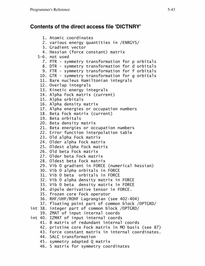
Programmer's Reference 5-43
Contents of the direct access file 'DICTNRY'
1. Atomic coordinates 2. various energy quantities in /ENRGYS/ 3. Gradient vector 4. Hessian (force constant) matrix 5-6. not used 7. PTR - symmetry transformation for p orbitals 8. DTR - symmetry transformation for d orbitals 9. FTR - symmetry transformation for f orbitals 10. GTR - symmetry transformation for g orbitals 11. Bare nucleus Hamiltonian integrals 12. Overlap integrals 13. Kinetic energy integrals 14. Alpha Fock matrix (current) 15. Alpha orbitals 16. Alpha density matrix 17. Alpha energies or occupation numbers 18. Beta Fock matrix (current) 19. Beta orbitals 20. Beta density matrix 21. Beta energies or occupation numbers 22. Error function interpolation table 23. Old alpha Fock matrix 24. Older alpha Fock matrix 25. Oldest alpha Fock matrix 26. Old beta Fock matrix 27. Older beta Fock matrix 28. Oldest beta Fock matrix 29. Vib 0 gradient in FORCE (numerical hessian) 30. Vib 0 alpha orbitals in FORCE 31. Vib 0 beta orbitals in FORCE 32. Vib 0 alpha density matrix in FORCE 33. Vib 0 beta density matrix in FORCE 34. dipole derivative tensor in FORCE. 35. frozen core Fock operator 36. RHF/UHF/ROHF Lagrangian (see 402-404) 37. floating point part of common block /OPTGRD/int 38. integer part of common block /OPTGRD/ 39. ZMAT of input internal coordsint 40. IZMAT of input internal coords 41. B matrix of redundant internal coords 42. pristine core Fock matrix in MO basis (see 87) 43. Force constant matrix in internal coordinates. 44. SALC transformation 45. symmetry adapted Q matrix 46. S matrix for symmetry coordinates
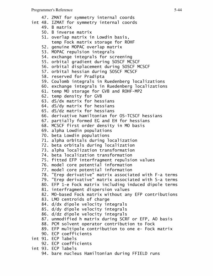
Programmer's Reference 5-44
47. ZMAT for symmetry internal coordsint 48. IZMAT for symmetry internal coords 49. B matrix 50. B inverse matrix 51. overlap matrix in Lowdin basis, temp Fock matrix storage for ROHF 52. genuine MOPAC overlap matrix 53. MOPAC repulsion integrals 54. exchange integrals for screening 55. orbital gradient during SOSCF MCSCF 56. orbital displacement during SOSCF MCSCF 57. orbital hessian during SOSCF MCSCF 58. reserved for Pradipta 59. Coulomb integrals in Ruedenberg localizations 60. exchange integrals in Ruedenberg localizations 61. temp MO storage for GVB and ROHF-MP2 62. temp density for GVB 63. dS/dx matrix for hessians 64. dS/dy matrix for hessians 65. dS/dz matrix for hessians 66. derivative hamiltonian for OS-TCSCF hessians 67. partially formed EG and EH for hessians 68. MCSCF first order density in MO basis 69. alpha Lowdin populations 70. beta Lowdin populations 71. alpha orbitals during localization 72. beta orbitals during localization 73. alpha localization transformation 74. beta localization transformation 75. fitted EFP interfragment repulsion values 76. model core potential information 77. model core potential information 78. "Erep derivative" matrix associated with F-a terms 79. "Erep derivative" matrix associated with S-a terms 80. EFP 1-e Fock matrix including induced dipole terms 81. interfragment dispersion values 82. MO-based Fock matrix without any EFP contributions 83. LMO centroids of charge 84. d/dx dipole velocity integrals 85. d/dy dipole velocity integrals 86. d/dz dipole velocity integrals 87. unmodified h matrix during SCRF or EFP, AO basis 88. PCM solvent operator contribution to Fock 89. EFP multipole contribution to one e- Fock matrix 90. ECP coefficientsint 91. ECP labels 92. ECP coefficientsint 93. ECP labels 94. bare nucleus Hamiltonian during FFIELD runs

Programmer's Reference 5-45
95. x dipole integrals, in AO basis 96. y dipole integrals, in AO basis 97. z dipole integrals, in AO basis 98. former coords for Schlegel geometry search 99. former gradients for Schlegel geometry search 100. dispersion contribution to EFP gradient
records 101-248 are used for NLO properties
101. U'x(0) 149. U''xx(-2w;w,w) 200. UM''xx(-w;w,0)102. y 150. xy 201. xy103. z 151. xz 202. xz104. G'x(0) 152. yy 203. yz105. y 153. yz 204. yy106. z 154. zz 205. yz107. U'x(w) 155. G''xx(-2w;w,w) 206. zx108. y 156. xy 207. zy109. z 157. xz 208. zz110. G'x(w) 158. yy 209. U''xx(0;w,-w)111. y 159. yz 210. xy112. z 160. zz 211. xz113. U'x(2w) 161. e''xx(-2w;w,w) 212. yz114. y 162. xy 213. yy115. z 163. xz 214. yz116. G'x(2w) 164. yy 215. zx117. y 165. yz 216. zy118. z 166. zz 217. zz119. U'x(3w) 167. UM''xx(-2w;w,w) 218. G''xx(0;w,-w)120. y 168. xy 219. xy121. z 169. xz 220. xz122. G'x(3w) 170. yy 221. yz123. y 171. yz 222. yy124. z 172. zz 223. yz125. U''xx(0) 173. U''xx(-w;w,0) 224. zx126. xy 174. xy 225. zy127. xz 175. xz 226. zz128. yy 176. yz 227. e''xx(0;w,-w)129. yz 177. yy 228. xy130. zz 178. yz 229. xz131. G''xx(0) 179. zx 230. yz132. xy 180. zy 231. yy133. xz 181. zz 232. yz134. yy 182. G''xx(-w;w,0) 233. zx135. yz 183. xy 234. zy136. zz 184. xz 235. zz137. e''xx(0) 185. yz 236. UM''xx(0;w,-w)138. xy 186. yy 237. xy139. xz 187. yz 238. xz140. yy 188. zx 239. yz

Programmer's Reference 5-46
141. yz 189. zy 240. yy142. zz 190. zz 241. yz143. UM''xx(0) 191. e''xx(-w;w,0) 242. zx144. xy 192. xy 243. zy145. xz 193. xz 244. zz146. yy 194. yz147. yz 195. yy148. zz 196. yz 197. zx 198. zy 199. zz
245. old NLO Fock matrix 246. older NLO Fock matrix 247. oldest NLO Fock matrix 249. polarizability derivative tensor for Raman 250. transition density matrix in AO basis 251. static polarizability tensor alpha 252. X dipole integrals in MO basis 253. Y dipole integrals in MO basis 254. Z dipole integrals in MO basis 255. alpha MO symmetry labels 256. beta MO symmetry labels 257. not used 258. Vnn gradient during MCSCF hessian 259. core Hamiltonian from der.ints in MCSCF hessian260-261. reserved for Dan 262. MO symmetry integers during determinant CI 263. PCM nuclei/induced nuclear Charge operator 264. PCM electron/induced nuclear Charge operator 265. pristine alpha guess (MOREAD or Huckel+INSORB) 266. EFP/PCM IFR sphere information 267. fragment LMO expansions, for EFP Pauli 268. fragment Fock operators, for EFP Pauli 269. fragment CMO expansions, for EFP charge transfer 270. not used 271. orbital density matrix in divide and conquerint 272. subsystem data during divide and conquer 273. old alpha Fock matrix for D&C Anderson-like DIIS 274. old beta Fock matrix for D&C Anderson-like DIIS 275. not used 276. Vib 0 Q matrix in FORCE 277. Vib 0 h integrals in FORCE 278. Vib 0 S integrals in FORCE 279. Vib 0 T integrals in FORCE 280. Zero field LMOs during numerical polarizability 281. Alpha zero field dens. during num. polarizability 282. Beta zero field dens. during num. polarizability 283. zero field Fock matrix. during num. polarizability

Programmer's Reference 5-47
284. Fock eigenvalues for multireference PT 285. density matrix or Fock matrix over LMOs 286. oriented localized molecular orbitals 287. density matrix of oriented LMOs290-299. not used 301. Pocc during MP2 (RHF or ZAPT) or CIS grad 302. Pvir during MP2 gradient (UMP2= 411-429) 303. Wai during MP2 gradient 304. Lagrangian Lai during MP2 gradient 305. Wocc during MP2 gradient 306. Wvir during MP2 gradient 307. P(MP2/CIS)-P(RHF) during MP2 or CIS gradient 308. SCF density during MP2 or CIS gradient 309. energy weighted density in MP2 or CIS gradient 311. Supermolecule h during Morokuma 312. Supermolecule S during Morokuma 313. Monomer 1 orbitals during Morokuma 314. Monomer 2 orbitals during Morokuma 315. combined monomer orbitals during Morokuma 316. RHF density in CI grad; nonorthog. MOs in SCF-MI 317. unzeroed Fock matrix when MOs are frozen 318. MOREAD orbitals when MOs are frozen 319. bare Hamiltonian without EFP contribution 320. MCSCF active orbital density 321. MCSCF DIIS error matrix 322. MCSCF orbital rotation indices 323. Hamiltonian matrix during QUAD MCSCF 324. MO symmetry labels during MCSCF 325. final uncanonicalized MCSCF orbitals 330. CEL matrix during PCM 331. VEF matrix during PCM 332. QEFF matrix during PCM 333. ELD matrix during PCM 334. PVE tesselation info during PCM335-339. not used 340. DFT alpha Fock matrix 341. DFT beta Fock matrix 342. DFT screening integrals 343. DFT: V aux basis only 344. DFT density gradient d/dx integrals 345. DFT density gradient d/dy integrals 346. DFT density gradient d/dz integrals 347. DFT M[D] alpha density resolution in aux basis 348. DFT M[D] beta density resolution in aux basis 349. DFT orbital description 350. overlap of true and auxiliary DFT basis 351. previous iteration DFT alpha density 352. previous iteration DFT beta density 353. DFT screening matrix (true and aux basis)

Programmer's Reference 5-48
354. DFT screening integrals (aux basis only) 355. h in MO basis during DDI integral transformation 356. alpha symmetry MO irrep numbers if UHF/ROHF 357. beta symmetry MO irrep numbers if UHF/ROHF358-369. not used 370. left transformation for pVp 371. right transformation for pVp 370. basis A (large component) during NESC 371. basis B (small component) during NESC 372. difference basis set A-B1 during NESC 373. basis N (rel. normalized large component) 374. basis B1 (small component) during NESC 375. charges of non-relativistic atoms in NESC 376. common nuclear charges for all NESC basis 377. common coordinates for all NESC basis 378. common exponent values for all NESC basis 372. left transformation for V during RESC 373. right transformation for V during RESC 374. 2T, T is kinetic energy integrals during RESC 375. pVp integrals during RESC 376. V integrals during RESC 377. Sd, overlap eigenvalues during RESC 378. V, overlap eigenvectors during RESC 379. Lz integrals 380. reserved for Ly integrals. 381. reserved for Lx integrals. 382. X, AO orthogonalisation matrix during RESC 383. Td, eigenvalues of 2T during RESC 384. U, eigenvectors of kinetic energy during RESC 385. exponents and contraction for the original basisint 386. shell integer arrays for the original basis 387. exponents and contraction for uncontracted basisint 388. shell integer arrays for the uncontracted basis 389. Transformation to contracted basis 390. S integrals in the internally uncontracted basis 391. charges of non-relativistic atoms in RESC 392. copy of one e- integrals in MO basis in SO-MCQDPT 393. Density average over all $MCQD groups in SO-MCQDPT 394. overlap integrals in 128 bit precision 395. kinetic ints in 128 bit precision, for relativity396-400. not used 401. dynamic polarizability tensors 402. GVB Lagrangian 403. MCSCF Lagrangian 404. GUGA CI Lagrangian (see 308 for CIS) 405. not used 406. MEX search state 1 alpha orbitals 407. MEX search state 1 beta orbitals 408. MEX search state 2 alpha orbitals

Programmer's Reference 5-49
409. MEX search state 2 beta orbitals 410. not used 411. alpha Pocc during UMP2 gradient (see 301-309) 412. alpha Pvir during UMP2 gradient 413. alpha Wai during UMP2 gradient 414. alpha Lagrangian Lai during UMP2 gradient 415. alpha Wocc during UMP2 gradient 416. alpha Wvir during UMP2 gradient 417. alpha P(MP2/CIS)-P(RHF) during UMP2/USFTDDFT grad 418. alpha SCF density during UMP2/USFTDDFT gradient 419. alpha energy wghted density in UMP2/USFTDDFT grad 420. not used421-429. same as 411-419, for beta orbitals 430. not used440-469. reserved for NEO 470. QUAMBO expansion matrix 471. excitation vectors for FMO-TDDFT 472. X+Y in MO basis during TD-DFT gradient 473. X-Y in MO basis during TD-DFT gradient 474. X+Y in AO basis during TD-DFT gradient 475. X-Y in AO basis during TD-DFT gradient 476. excited state density during TD-DFT gradient 477. energy-weighted density in AO basis for TD-DFT478-489. not used 490. transition Lagrangian right hand side during NACME 491. gradients vectors during NACME 492. NACME vectors during NACME 493. difference gradient in conical intersection search 494. derivative coupling vector in CI search 495. mean energy gradient in CI search 496. unused 497. temp storage of gradient of 1st state in CI search498-500. not used 501. A2 cavity data in COSMO 502. A3 cavity data in COSMO 503. AMTSAV cavity data in COSMO504-510. not used 511. effective polarizability in LRD 512. C6 coefficients in LRD 513. C8 coefficients in LRD 514. C10 coefficients in LRD 515. atomic pair LRD energy516-950. not used
In order to correctly pass data between differentmachine types when running in parallel, it is required thata DAF record must contain only floating point values, oronly integer values. No logical or Hollerith data may bestored. The final calling argument to DAWRIT and DAREAD

Programmer's Reference 5-50
must be 0 or 1 to indicate floating point or integer valuesare involved. The records containing integers are somarked in the list below.
Physical record 1 (containing the DAF directory) iswritten whenever a new record is added to the file. Thisis invisible to the programmer. The numbers shown aboveare "logical record numbers", and are the only thing thatthe programmer need be concerned with.

Hardware Specifics 6-1
(6 May 2010)
********************************** * * * Section 6 - Hardware Specifics * * * **********************************
This section of the manual contains pages dealing in ageneral way with dynamic memory allocation in GAMESS, theBLAS routines, and vectorization.
The remaining portions of this section consist ofspecific suggestions for each type of machine. You shouldcertainly read the section pertaining to your computer. Itis a good idea to look at the rest of the machines as well,as you may get some ideas! The directions for executingGAMESS are given, along with hints and other tidbits. Anyknown problems with certain compiler versions are describedin the control language files themselves, not here.
The currently supported machines are all running Unix.The embedded versions for IBM mainframes and VAX/VMS havenot been used in many years, and are no longer describedhere. There are binary versions for Windows available onour web site, but we do not supply a source code versionfor Windows (except that the Unix code will compile underthe Cygwin Unix environment for Windows). Please note thatwith the OS X system, the Macintosh is considered to be asystem running Unix, and is therefore well supported.
Dynamic memory in GAMESS ____________________________________________ 2BLAS routines _________________________________________________________ 4Vectorization of GAMESS________________________________________________ 5Notes for specific machines _______________________________________________ 7

Hardware Specifics 6-2
Dynamic memory in GAMESS
GAMESS allocates its working memory from one large poolof memory. This pool consists of a single large array,which is partitioned into smaller arrays as GAMESS needsstorage. When GAMESS is done with a piece of memory, thatmemory is freed for other uses.
The units for memory are words, a term which GAMESSdefines as the length used for floating point numbers, 64bits, that is 8 bytes per word.
GAMESS contains two memory allocation schemes. Forsome systems, a primitive implementation allocates a largearray of a *FIXED SIZE* in a common named /FMCOM/. This istermed the "static" implementation, and the parameterMWORDS in $SYSTEM cannot request an amount larger thanchosen at compile time. Wherever possible, a "dynamic"allocation of the memory is done, so that MWORDS can (inprinciple) request any amount. The memory managementroutines take care of the necessary details to fool therest of the program into thinking the large memory poolexists in common /FMCOM/.
Computer systems which have "static" memory allocationare IBM mainframes running VM or MVS to which we have nodirect access for testing purposes. If your job requires alarger amount of memory than is available, your onlyrecourse is to recompile UNPORT.SRC after choosing a largervalue for MEMSIZ in SETFM.
Computer which have "dynamic" memory allocation are allUnix systems and VMS. In principle, MWORDS can request anyamount you want to use, without recompiling. In practice,your operating system will impose some limitation. Asoutlined below, common sense imposes a lower limit thanyour operating system will.
By default, most systems allocate a small amount ofmemory: one million words. This amount is quite small bymodern standards, and therefore exists on all machines. Itis left up to you to increase this with your MWORDS inputto what your machine has. EXETYP=CHECK runs will alwaystell you the amount of memory you need.
Many computations in GAMESS implement out of memoryalgorithms, whenever the in memory algorithm can require an
Hardware Specifics 6-3
excessive amount. The in memory algorithms will performvery poorly when the work arrays reside in virtual memoryrather than physical memory. This excessive page faultingactivity can be avoided by letting GAMESS choose its out ofcore algorithms. These are programmed such that largeamounts of numbers are transferred to and from disk at thesame time, as opposed to page faulting for just a fewvalues in that page. So, pick an amount for MWORDS thatwill reside in the physical memory of your system! MWORDS,multiplied by 8, is roughly the number of Mbytes and shouldnot exceed more than about 90% of your installed memory(less if you are sharing the computer with other jobs!).
The routines involved in memory allocation are VALFM,to determine the amount currently in use, GETFM to grab ablock of memory, and RETFM to return it. Note that callsto RETFM must be in exactly inverse order of the calls toGETFM. SETFM is called once at the beginning of GAMESS toinitialize, and BIGFM at the end prints a "high water mark"showing the maximum memory demand. GOTFM tells how muchmemory is not yet allocated.
Hardware Specifics 6-4
BLAS routines
The BLAS routines (Basic Linear Algebra Subprograms)are designed to perform primitive vector operations, suchas dot products, or vector scaling. They are often foundimplemented in a system library, even on scalar machines.If this is the case, you should use the vendor's version!
The BLAS are a simple way to achieve BOTH moderatevectorization AND portability. The BLAS are easy toimplement in FORTRAN, and are provided in the file BLAS.SRCin case your computer does not have these routines in alibrary.
The BLAS are defined in single and double precision,e.g. SDOT and DDOT. The very wonderful implementation ofgeneric functions in FORTRAN 77 has not yet been extendedto the BLAS. Accordingly, all BLAS calls in GAMESS use thedouble precision form, e.g. DDOT. The source codeactivator translates these double precision names to singleprecision, for machines such as Cray which run in singleprecision.
If you have a specialized BLAS library on your machine,for example IBM's ESSL, Compaq's CXML, or Sun's PerformanceLibrary, using them can produce significant speedups incorrelated calculations. The compiling scripts attempt todetect your library, but if they fail to do so, it is easyto use one: a) remove the compilation of 'blas' from 'compall', b) if the library includes level 3 BLAS, set the value of 'BLAS3' to true in 'comp', c) in 'lked', set the value of BLAS to a blank, and set libraries appropriately, e.g. to '-lessl'.Check the compilation log for mthlib.src, in particular, tobe sure that your library is being found. It has aprofound effect on the speed of MP2 and CC computations!
The reference for the level 1 BLAS is C.L.Lawson, R.J.Hanson, D.R.Kincaid, F.T.Krogh ACM Trans. on Math. Software 5, 308-323(1979)

Hardware Specifics 6-5
Vectorization of GAMESS
As a result of a Joint Study Agreement between IBM andNDSU, GAMESS has been tuned for the IBM 3090 vectorfacility (VF), together with its high performance vectorlibrary known as the ESSL. This vectorization work tookplace from March to September of 1988, and resulted ina program which is significantly faster in scalar mode, aswell as one which can take advantage (at least to someextent) of a vector processor's capabilities. Since ourmove to ISU we no longer have access to IBM mainframes,but support for the VF, as well as MVS and VM remainsembedded within GAMESS. Several other types of vectorcomputers are supported as well.
Anyone who is using a current version of the program,even on scalar machines, owes IBM their thanks both forNDSU's having had access to a VF, and the programming timeto do code improvements in the second phase of the JSA,from late 1988 to the end of 1990.
Some of the vectorization consisted of rewriting loopsin the most time consuming routines, so that a vectorizingcompiler could perform automatic vectorization on theseloops. This was done without directives, and so anyvectorizing compiler should be able to recognize the sameloops.
In cases where your compiler allows you to separatescalar optimization from vectorization, you should choosenot to vectorize the following sections: INT2A, GRD2A,GRD2B, and GUGEM. These sections have many very smallloops, that will run faster in scalar mode. The remainingfiles will benefit, or at least not suffer from automaticcompiler vectorization.
The highest level of performance, obtained byvectorization at the matrix level (as opposed to thevector level operations represented by the BLAS) iscontained in the file VECTOR.SRC. This file containsreplacements for the scalar versions of routines by thesame names that are contained in the other source codemodules. VECTOR should be loaded after the object codefrom GAMESS.SRC, but before the object code in all theother files, so that the vector versions from VECTOR arethe ones used.

Hardware Specifics 6-6
Most of the routines in VECTOR consist of calls tovendor specific libraries for very fast matrix operations,such as IBM's Engineering and Scientific SubroutineLibrary (ESSL). Look at the top of VECTOR.SRC to seewhat vector computers are supported currently.
If you are trying to bring GAMESS up on some othervector machine, do not start with VECTOR. The remainingfiles (excepting BLAS, which are probably in a systemlibrary) represent a complete, working version of GAMESS.Once you have verified that all the regular code isrunning correctly, then you can adapt VECTOR to yourmachine for the maximum possible performance.
Vector mode SCF runs in GAMESS on the IBM 3090 willproceed at about 90 percent of the scalar speed on thesemachines. Runs which compute an energy gradient mayproceed slightly faster than this. MCSCF and CI runswhich are dominated by the integral transformation stepwill run much better in vector mode, as the transformationstep itself will run in about 1/4 time the scalar time onthe IBM 3090 (this is near the theoretical capability ofthe 3090's VF). However, this is not the only timeconsuming step in an MCSCF run, so a more realisticexpectation is for MCSCF runs to proceed at 0.3-0.6 timesthe scalar run. If very large CSF expansions are used(say 20,000 on up), however, the main bottleneck is the CIdiagonalization and there will be negligible speedup invector mode. Several stages in an analytic hessiancalculation benefit significantly from vector processing.
A more quantitative assessment of this can be reachedfrom the following CPU times obtained on a IBM 3090-200E,with and without use of its vector facility:
ROHF grad RHF E RHF hess MCSCF E ------- ------ ------- ------scalar 168 ( 1 ) 164 ( 1 ) 917 ( 1 ) 903 ( 1 )vector 146 (0.87) 143 (0.87) 513 (0.56) 517 (0.57)

Hardware Specifics 6-7
Notes for specific machines
GAMESS will run on many kinds of UNIX computers. Thesesystems runs the gamut from very BSD-like systems to veryATT-like systems, and even AIX. Our experience has beenthat all of these UNIX systems differ from each other. So,putting aside all the hype about "open systems", we dividethe Unix world into four classes:
Supported: Apple MAC under OS X, HP/Compaq/DEC AXP, HPPA-RISC, IBM RS/6000, 64 bit Intel/AMD chips such as theXeon/Opteron/Itanium, and Sun ultraSPARC. These are theonly types of computer we currently have at ISU, so theseare the only systems we can be reasonably sure will work(at least on the hardware model and O/S release we areusing). Both the source code and control language iscorrect for these.
Acquainted: Cray XT, IBM SP, SGI Altix/ICE, and SGIMIPS. We don't have any of these systems at ISU, so wecan't guarantee that these work. GAMESS has been run oneach of these offsite, perhaps recently, but perhaps not.The source code for these systems is probably correct, butthe control language may not be. Be sure to run all thetest cases to verify that the current GAMESS still works onthese brands.
Jettisoned: Alliant, Apollo, Ardent, Celerity, Convex,Cray T3E, Cray vectors, DECstations, FPS model 500, FujitsuAP and VPP, HP Exemplar, Hitachi SR, IBM AIX mainframes,Intel Paragon, Kendall Square, MIPS, NCube, and ThinkingMachines. In most cases the company is out of business, orthe number of machines in use has dropped to near zero. Ofthese, only the Celerity version's death should be mourned,as this was the original UNIX port of GAMESS, back in July1986.
Terra Incognita: everything else! You will have todecide on the contents of UNPORT, write the scripts, andgenerally use your head.
* * * * *
You should have a file called "readme.unix" at handbefore you start to compile GAMESS. These directionsshould be followed carefully. Before you start, read thenotes on your system below, and read the compiler clause

Hardware Specifics 6-8
for your system in 'comp', as notes about problems withcertain compiler versions are kept there.
Execution is by means of the 'rungms' script, and youcan read a great deal more about its DDIKICK command in theinstallation guide 'readme.ddi'. Note in particular thatexecution of GAMESS now uses System V shared memory on manysystems, and this will often require reconfiguring thesystem's limits on shared memory and semaphores, along witha reboot. Full details of this are in 'readme.ddi.
Users may find examples of the scalability of parallelruns in the Programmer's Reference chapter of this manual.
* * * * * *
AMD Opteron and other chips: see "linux64" below.
AXP: These are scalar systems. This category meansany AXP machines, whether labeled Digital or Compaq or HPon the front, with an O/S called OSF1, Digital Unix, orTru64. It also includes systems running Linux, see below.The unique identifier is therefore the AXP chip, so thecompiling target is 'axp64', rather than a company name.
The compiling script invokes the f77 compiler, so read'comp' if you have the f90 compiler instead. This versionwas changed to use native 64 bit integers in fall 1998.
You can also run GAMESS on AXP Linux, by using theTru64 Compaq compilers, which permit the Tru64 version torun. Do not use g77 which allocates 32 bit integers, asthe system's malloc routine for dynamic memory allocationreturns 64 bit addresses, which simply cannot be stored in32 bit integers. The Compaq compilers can easily generate64 bit integers, so obtain FORTRAN and C from http://h18000.www1.hp.com/products/software/alpha-toolsThen compile and link using target 'compaq-axp'.
Cray XT: a massively parallel platform, based on dualOpteron processor blades connected by Cray's 3D mesh,running a node O/S called "Compute Node Linux". Themessage passing involves a DDI running over MPI with a userselectable number of data servers. Unfortunately, the DDIis not fully integrated into our main code yet, and thescripting is a bit rough. Good support for these (XT3through XT6) is expected by summer 2010.

Hardware Specifics 6-9
Digital: See AXP above.
HP: Any Intel or PA-RISC series workstation or server.Help with this version has come from due to Fred Senese,Don Phillips, Tsuneo Hirano, and Zygmunt Krawczyk. DaveMullally at HP has been involved in siting HP systems atISU, presently Itanium2 based. So, we used 'hpux32' formany years, but are now running only the 'hpux64' version.The latter version can be considered to be carefullychecked since it is in use at ISU, but please be a littlemore careful checking tests if you use 'hpux32'.
IBM: "superscalar" RS/6000. There are two targets forIBM workstations, namely "ibm32" and "ibm64", neither ofthese should be used on a SP system. Parallelization isachieved using the TCP/IP socket calls found in AIX.
IBM-SP: The SP parallel systems. This is a 64 bitimplementation. The new DDI library will operate with LAPIsupport for one-sided messaging, and a special executionscript for LoadLeveler is included.
IBM Blue Gene: This target is "ibm-bg". The older BG/Lhas been outmoded by the BG/P, but we still have an "L" atISU. These are massively parallel machine, using a 32 bitPowerPC, and a limited amount of node memory. The "L" usesDDI running over the ARMCI library, running in turn overMPI, so the "L" does not use data servers. The "P" uses astraightforward DDI to MPI interface, with data servers.The "L" port was done by Brian Smith of IBM and Brett Bodeat ISU, included in GAMESS in June 2005, and changed to useARMCI in 2007 by Andrey Asadchev of ISU. Nick Nystrom'sinitial port to the "P" system was polished up by GrahamFletcher at Argonne National Labs in 2010. Special notes,and various files to be used on this system are stored inthe directory ~/gamess/machines/ibm-bg.
Linux32: this means any kind of 32 bit chips, buttypically is used only when "uname -p" replies "x86".Nearly every other chip is 64 bits, so see also Linux64just below. This version is originally due to PedroVazquez in Brazil in 1993, and modified by Klaus-PeterGulden in Germany. The usefulness of this version hasmatched the steady growth of interest in PC Unix, due tothe improvement in CPU, memory, and disks, to workstationlevels. We acquired a 266 MHz Pentium-II PC running RedHatLinux in August 1997, and found it performed flawlessly.In 1998 we obtained six 400 MHz Pentium-IIs for sequentialuse, and in 1999 a 16 PC cluster, running in parallel day

Hardware Specifics 6-10
in and day out. We have used RedHat 4.2, 5.1, 6.1, 7.1,and Fedora Core 1, prior to switching over exclusively to64-bit Linux. This version is based on gfortran or g77,gcc, and the gcclib, so it should work for any kind of 32bit Linux. This version uses 'sockets' for its messagepassing. The configuration script will suggest possiblemath library choices to you.
By 2010, probably most Linux systems in existence are64-bit capable, so the next version is more better!
Linux64: this means any sort of 64 bit chip running anappropriate 64 bit Linux operating system. The most common"linux64" build is on AMD or Intel chips, where "uname -p"returns x86_64 or ia64. However, if you choose the'gfortran' compiler, no processor-specific compiler flagsare chosen, so this version should run on any 64-bit Linuxsystem, e.g. AXP or SPARC.
If you are running on Intel/AMD processors, theconfiguration script lets you choose various FORTRANcompilers: GNU's gfortran, Intel's ifort, Portland Group'spgf77, and Pathscale's pathf90. You can choose a varietyof math libraries, such as Intel's MKL, AMD's ACML, orATLAS. You can choose to use MPI if your machine has agood network for parallel computing, with the options forthe MPI type specified in detail in the file, but socketsare an easy to use alternative to MPI.
The choices for FORTRAN, math library, and MPI librarycan all be "mixed and matched". Except for 'gfortran',almost all this software has to be added to a standardLinux distribution. It is your responsibility to installwhat you want to use, to set up execution paths, to set uprun time library paths (LD_LIBRARY_PATH), and so forth.The 'config' script will need to ask where these softwarepackages are installed, since your system manager may haveplaced them almost anywhere.
Macintosh OS X: This is for Apple running OS X, whichis a genuine Unix system "under the hood". This versionclosely resembles the Linux version. Installation ofApple's XCODE (from the OS X distribution DVD) gives you aC compiler and a math library. You can obtain a FORTRANcompiler (gfortran for 64 bit or g77 for 32 bits) from thewonderful web site of Gourav Khanna: http://hpc.sourceforge.netRequest target "mac32" if your OS X is 10.4, or "mac64" ifyour OS X is 10.5 or newer.

Hardware Specifics 6-11
NEC SX: vector system. This port was done by JanetFredin at the NEC Systems Laboratory in Texas in 1993, andshe periodically updates this version, including parallelusage, most recently in Oct. 2003. You should select both*UNX and *SNG when manually activating ACTVTE.CODE, andcompile actvte by "f90 -ew -o actvte.x actvte.f".
Silicon Graphics: The modern product line of thiscompany is called Altix or Altix ICE. The operating systemis Linux, the chips are 64 bit Intel processors, and thenatural compiler and math library choices are Intel's ifortand MKL. The SGI software ProPack turns these commoditycomponents into a supercomputer, and DDI should use the MPIlibrary 'mpt' found in ProPack. Accordingly, the compilingtarget should be 'linux64', selecting ifort, MKL, and thenmpt.
Silicon Graphics: The ancient product line of thiscompany use various MIPS chips such as R4x00, R5000,R12000, etc. There are very few of these machines left, sotarget's 'sgi32' and 'sgi64' should be regarded as "rusty".The 32 bit target uses sockets communications, while the 64bit one will use an old SHMEM interface, that onlypartially implements DDI. Hence FMO and parallel CCSD(T)will not run on 'sgi64'.
Sun: scalar system. This version is set up for theultraSPARC or Opteron chips, running Solaris. The targetfor either chip is "sun64" as the scripts can automaticallydetect which one you are using, and adjust for that. SinceSun provided a ultraSPARC E450 system in 1998, twoultraSPARC3 Sunfire 280R systems in 2002, and a OpteronV40Z system in 2006, to the group at Iowa State, the Sunversion is very reliable. Install the SunPerf math libraryfrom the compiler suite for maximum BLAS performance.Parallelization is accomplished using TCP/IP sockets andSystemV shared memory.