Manila to Malaysia, Quezon to Qatar: International Migration

and the Effects on Origin-Country Human Capital

Caroline Theoharides∗

University of Michigan

May 29, 2014

Abstract

International migration is a key labor market option for many individuals from devel-oping countries. One way that migration can affect the country of origin is by changinginvestment in human capital. U sing an original dataset of all new migrant departuresfrom the Philippines between 1992 and 2009 matched to the migrants’ province of origin,I examine the effect of migration demand on province-level secondary school enrollmentrates. To isolate exogenous changes in demand, I create a Bartik-style instrument thatexploits destination-specific migrant networks across local labor markets. Analysis at thelocal labor market level accounts for effects of migration on both migrant and non-migranthouseholds. I find that secondary enrollment increases by 2.1% in response to an averageyear-to-year percent increase in province-level migration demand. For each additional newmigrant, 2.8 more children are enrolled. Private school enrollment increases by 10.1%,while the effect on public school enrollment is near zero. These effects can occur throughtwo channels: the income channel or the wage premium channel. Exploiting variation ingender-specific migration demand, I test their relative importance and conclude that theincome channel is dominant.

JEL: O12, F22, I25

∗735 S. State St., Ann Arbor, MI, 48109. Email: cbtheo@umich.edu. I thank the Overseas Worker Wel-fare Administration (OWWA), Philippine Overseas Employment Administration (POEA), and Departmentof Education (DepEd) for access to the data; Dunhill Alcantara, Helen Barayuga, Nimfa de Guzman andNerissa Jimena of POEA, Carmelita S. Dimzon, Lex Pineda, and Rosanna Siray of OWWA, and Merci Castro-Trio of DepEd for their assistance with compiling these databases; and Marla Asis, Helen Barayuga, RhonaCaoli-Rodriguez, Liberty Casco, and Dalisay Maligalig for important background information on migrationand education in the Philippines. Chris Zbrozek provided invaluable assistance with constructing the BEISdataset. I thank my committee, Manuela Angelucci, Susan Dynarski, Jeffrey Smith, and Dean Yang, as wellas Kate Ambler, Raj Arunachalam, Emily Beam, John Bound, Jacqueline Doremus, Susan Godlonton, Jes-sica Goldberg, Joshua Hyman, Isaac Sorkin, Rebecca Thornton, and various seminar participants for valuablecomments. I gratefully acknowledge support from the Rackham Merit Fellowship and the National ScienceFoundation Graduate Research Fellowship.

1 Introduction

International migration is a key labor market option for many individuals from developing

countries. These labor market opportunities are typically characterized by large gains in wages

for both skilled and unskilled workers (Clemens, 2011; Clemens, Montenegro and Pritchett,

2008; Gibson and McKenzie, 2012). Such wage gains often result in increased income in

the migrant-sending country through the receipt of remittances, which lead to substantial

increases in both investment and consumption (Clemens and Tiongson, 2013; Yang, 2008).

One type of investment that may respond to increased income is human capital. Unlike

other investments, however, increases in migration opportunities may also affect human capital

investment by changing the expected wage premium for education. Depending on the education

level necessary to acquire jobs abroad, the education wage premium may either increase or

decrease, and individuals will change their optimal level of educational investment accordingly.

Thus, migration can affect investment in human capital in the origin country through two main

channels: the income channel and the wage premium channel.1

Due to data and research design limitations, most previous studies are unable to examine

the net effect of migration on human capital, but rather estimate the partial effect operating ei-

ther through the income channel (Ambler, Aycinena and Yang, 2013; Cox-Edwards and Ureta,

2003; Yang, 2008) or the wage premium channel (Beine, Docquier and Rapoport, 2007; Chand

and Clemens, 2008; Shrestha, 2012). The handful of studies that do estimate the net effect

typically focus exclusively on migrant households (Clemens and Tiongson, 2013; Hanson and

Woodruff, 2003; Kandel and Kao, 2001; McKenzie and Rapoport, 2011). As a result, they are

not able to capture the potential spillovers that occur within a local economy due to migration.

For example, non-migrant households may also benefit from the receipt of remittances or their

multiplier effects in the local economy as well as from changes in the expected wage premium.

Therefore, estimates focusing exclusively on migrant households underestimate the effects on

human capital in the economy as a whole. An exception is Dinkelman and Mariotti (2014),

who estimate the net effect of migration on educational attainment of primary school-aged

children across high and low cost migration areas in rural Malawi.

1Ambler (2013) finds that information asymmetries in migrant households matter for resource allocation.Thus, migration may also affect human capital investments by geographically splitting households and changingbargaining power. However, Clemens and Tiongson (2013) find that remittances overwhelmingly dominateeffects from splitting households.

1

In this paper, I estimate the net causal effect of international migration on province-level

secondary school enrollment rates in the Philippines. Estimation at the province level not

only captures the effects of both the income and expected wage premium channels, but also

spillovers and multiplier effects to non-migrant households in the local economy. The net effect

of migration on human capital at the local labor market level is a key parameter of interest

for policymakers in migrant-sending countries in order to predict the level of human capital in

the future labor force. My results provide some of the first estimates of this effect. Further,

following predictions set out in a basic theoretical framework, I examine the relative importance

of the income channel and the wage premium channel on secondary school enrollment decisions.

This is the first paper to attempt to disentangle the effects of these two mechanisms. Identifying

the dominant mechanism has the potential to guide the design of policies with the goal of

increasing the human capital stock.

I estimate the effect of the province-level migration rate on secondary school enrollment

decisions in the province. However, the observed province-specific migration rate will confound

changes in the demand and supply of migrants. To isolate exogenous changes in demand for

migrants, I collected a unique, individual-level, administrative dataset on all new migrant de-

partures from the Philippines matched to the migrant’s province of origin to create a plausibly

exogenous instrument for local migration demand following Bartik (1991). This Bartik-style

instrument exploits variation generated by shocks to destination country-specific migration

networks across local labor markets in the Philippines. Migrant networks are an important

determinant of where migrants move and the occupations in which they are employed (Mun-

shi, 2003). As a result of these networks, provinces will vary in the degree to which they are

affected by changes in demand from a given destination country. The instrument predicts the

number of migrants in each province-year, and is defined as the interaction of the destination-

country composition of migrants in each province at baseline and destination-specific total

national migration. Due to the unique nature of my micro data, this is the first instance

where a Bartik-style instrument is used to predict outmigration rates from a migrant-sending

country. In previous studies, the historic migration rate is often used to instrument for the

contemporaneous migration rate (see McKenzie and Rapoport (2010); Woodruff and Zenteno

(2007), among others), and the use the Bartik-style instrument with panel data is a substantial

improvement in terms of causal identification.

2

To identify the relative importance of the income channel versus the expected wage pre-

mium channel, I exploit differences in gender-specific migration demand. For instance, a change

in demand for female migrants should only affect the wage premium for females. Thus, female

enrollment may respond to this change in demand through the expected wage channel while

male enrollment should not. The income channel, on the other hand, may or may not affect

male and female students equivalently in response to a change in female migration demand. If

I find that a change in female migration demand impacts male and female enrollment equally,

then this suggests that the income channel is the dominant channel. If, on the other hand,

I find the effects are different, then both channels may matter. A positive effect of female

demand on male enrollment suggests the presence of the income channel. To test the effects of

demand by gender, I create separate Bartik-style instruments for male and female migration.2

I find a strong and statistically significant positive relationship between secondary school

enrollment and total migration demand. Total secondary school enrollment increases by 2.1%

in response to an average year-to-year percent increase in province-level migration demand.

This means that for each additional migrant, there are 2.8 more students enrolled in secondary

school. Private school enrollment increases by 10.1% for an average change in migration

demand. While there is a near-zero effect on public school enrollment, when combined with

the large effect on private school, one interpretation is that students switch from public to

private school while others are induced from no school into public school. Demand for female

migrants leads to similar increases in both male and female school enrollment, which leads me

to conclude that the income channel is the dominant channel through which migration affects

education, though there is suggestive evidence that the expected wage premium may matter

as well. I also examine heterogeneity of enrollment responses by grade level to identify the

location of marginal students in the education distribution. While enrollment increases for all

grade levels, the largest effect is on first year enrollment, suggesting that increased migration

demand induces students to enter secondary school who otherwise would not have enrolled.

The Philippines provides an excellent setting to address the effect of migration on educa-

tion. As the first country to adopt temporary overseas contract migration on a large scale,

approximately 2% of the Philippine working-age population migrates for employment each

2Migrant occupations from the Philippines are highly gender-specific, as shown in Section 2.1. However, as Idiscuss in Section 5.3, exogeneity of the gender instruments does not require that gender composition is stableover time or that occupations must be exclusively male or female.

3

year in a wide variety of occupations and destinations. Further, substantial heterogeneity in

the gender and skill composition of overseas migrants allows me to test the relative importance

of changes in income versus the wage premium. From a policy perspective, the Philippines has

served and continues to serve as a model for many other Asian countries such as Indonesia,

Bangladesh, and Sri Lanka in the establishment of temporary contract labor programs (Asis

and Agunias, 2012; Rajan and Misha, 2007; Ray, Sinha and Chaudhuri, 2007; World Bank,

2011). Understanding the implications of such a program on school enrollment decisions in

the migrant-sending country is thus increasingly important for policymakers in these countries

as they seek to understand the future level of human capital in their domestic workforce.

The remainder of the paper is organized as follows. Section 2 discusses background on

migration and education in the Philippines. Section 3 presents a basic theoretical framework

relating migration to education. The data are presented in Section 4, followed by a discussion

of the empirical strategy in Section 5. Section 6 discusses the main results, mechanisms, and

magnitudes of the estimates, and Section 7 concludes.

2 Background

2.1 Migration from the Philippines

As the first country to adopt temporary overseas contract migration on a large scale, the

Philippine government created an overseas employment program in 1974 in response to poor

economic conditions in the Philippines. The program has grown dramatically; in 2011, 1.3

million Filipinos departed overseas on labor contracts (representing 2% of the working age

population).3 Approximately 517,000 of these migrants were new hires with first time labor

contracts. Based on the perceived success of the migration program in the Philippines, several

other countries, such as Indonesia, India, Bangladesh, Sri Lanka, and Tajikistan, have adopted

or are in the process of adopting similar migration programs (Asis and Agunias, 2012; Rajan

and Misha, 2007; Ray, Sinha and Chaudhuri, 2007; World Bank, 2011).

Filipinos migrate to a wide range of destination countries, as shown in Table 1. Saudi

Arabia is the largest destination country, and the majority of migration is to the Middle

East or within Asia. Almost 50% of male migrants work in Saudi Arabia, whereas female

3This figure is for land-based workers only and excludes seafarers.

4

migrants are split more evenly across Japan, Saudi Arabia, Taiwan, Hong Kong, and the

United Arab Emirates. Filipinos also migrate in a variety of occupations. Table 2 shows the

top 20 occupations for migrants from the Philippines. Occupations tend to be highly gendered,

and occupations that are over 50% female are shaded in grey. Of the top 10 occupations,

domestic helpers, performing artists, caregivers, and medical workers are all over 80% female.

Plumbers, engineers, and laborers are almost exclusively male occupations while production

workers, cooks and waiters, and building caretakers are much more evenly split across genders.

Contract migration is largely temporary and legal by way of licensed recruitment agen-

cies. There are numerous fees associated with the migration process. Legally, recruitment

agencies may only charge a placement fee equivalent to one month’s wages (Orbeta, Abrigo

and Cabalfin, 2009). The worker satisfies this debt upon receipt of the first month’s wages.

However, in addition to the placement fee, a number of additional costs are incurred by po-

tential migrants such as travel to Manila and room and board prior to overseas deployment.

Migrants commonly resort to predatory lenders to cover these expenses (Barayuga, 2013). The

Philippine Overseas Employment Administration (POEA) regulates recruitment and verifies

work contracts prior to employment. One of the main regulatory functions of POEA is to

set occupation-destination specific minimum wages for overseas contracts. McKenzie, Theo-

harides and Yang (2014) find that these minimum wages are binding. In the absence of a

minimum wage policy, an increase in demand for migrants should lead to both an increase

in the quantity and wages of these workers. However, given that these minimum wages are

binding, McKenzie, Theoharides and Yang (2014) find that destination countries respond to

economic shocks by changing the quantity of overseas workers rather than altering the wage.

The rate of new hire migration varies substantially across the Philippines.4 In 2009, the

average new hire migration rate across provinces for new labor contracts was 0.54% of the

province population. However, this varied from a maximum of 1.3% of the population in

Bataan province to just 0.07% of the population in Tawi-Tawi province. This suggests that

migration is a more important labor market option in certain parts of the country than others.

4I examine how much of the movement in province-level migration rates is common across provinces versushow much is province specific. Following Blanchard and Katz (1992), I regress the log migration rate in provincep on the log total migration rate separately for each province. The adjusted R2 for each regression provides anempirical estimate for how much province-level migration rates move together from one year to the next. Theaverage adjusted R2 across all 83 province-level regressions is 0.22. Therefore, the majority of the movementin province-level migration rates is not explained by movement in the overall aggregate migration rate.

5

Figure 1 shows the new hire migration rate in 1993 in each province. While higher rates

of migration are largely concentrated on the northern island of Luzon, there is substantial

variation throughout the country as a whole. Even among high migration provinces, provinces

specialize in certain occupations and destinations, resulting in substantial heterogeneity in the

composition of migrants across the Philippines. Figure 2 shows province-level migration rates

in 1993 for migrants to Hong Kong compared to migrants to Saudi Arabia. Migration to Hong

Kong is concentrated in the northern part of Luzon, whereas migration to Saudi Arabia is more

heavily concentrated around Manila and in Mindanao, the southern part of the Philippines.

I exploit this variation in the destination composition of migrants across provinces in order

to identify the causal effect of migration demand on secondary school enrollment. While no

legal barriers prevent workers from other provinces from acquiring these jobs, the reliance on

social networks in choosing recruitment agencies and obtaining jobs abroad creates rigidities

across local labor markets. In personal interviews with POEA staff, Barayuga (2013) states

that migrants rely on family members and friends who have previously migrated to choose

recruiting agencies and find jobs abroad.

2.2 Migration and Education

The effect of migration on human capital through the expected wage premium channel depends

on whether jobs abroad require more or less education than jobs at home. To determine the

sign of the wage premium effect in the Philippines, it is important to note the location of

Filipino contract workers in the education distribution among all Filipino workers. Borjas

(1987) argues that workers migrating from countries with high income inequality to countries

with lower income inequality are negatively selected, and so one might expect an increase in

migration demand to reduce human capital investment due to low skill, high wage opportunities

abroad. While earnings inequality in the Philippines is high, Docquier, Lohest and Marfouk

(2007) suggest that emigration from the Philippines is positively selected. However, their study

is limited to OECD destinations. As shown in the previous section, the majority of contract

migrants work in non-OECD countries in the Middle East and Asia. To establish if this finding

holds for non-OECD countries, in Figure 3 I follow Chiquiar and Hanson (2005) and plot the

6

education distribution of all migrants and non-migrants in the 2000 Philippine Census.5 Panel

A shows the distributions for all migrants and non-migrants between the ages of 18 and 65.

The share of migrants with less than a high school education is smaller than the share of

non-migrants with less than a high school education. The opposite is true for high education

levels, especially for training programs. Training programs are vocational degrees that require

a high school diploma for enrollment, and in many occupations, a training program is required

to be eligible for overseas contract migration. Based on Panel A, it appears that migrants

from the Philippines are positively selected.

Panel B shows the same figure for individuals located in the ten provinces with the highest

rates of migration.6 Provinces that send a large number of migrants may be more educated

overall, and thus the apparent positive selection in Panel A might be driven by the fact

that migrants are from more educated provinces. While the degree of positive selection in

Panel B is somewhat less pronounced, migrants are still more educated than non-migrants

in high migration provinces. Panels C and D examine the distribution separately by gender

and indicate that both male and female migrants are positively selected, though the degree

of selection appears to be slightly higher for male migrants than for female migrants. One

additional concern is that differences in cohort may confound the distributions. Since migrants

are younger than the overall population, if younger cohorts get more education than older

cohorts, the apparent positive selection may simply be a result of comparing different cohorts.

Panels E and F show the education distribution for workers less than 35 years of age and

workers greater than 35 years of age. Both younger and older workers appear positively

selected, though the degree of positive selection is somewhat less for younger workers.

While there is no overall required level of education for contract laborers mandated by

either the Philippine government or employers, Figure 3 suggests that employers screen on

education. McKenzie, Theoharides and Yang (2014) argue that there is an excess supply of

Filipino workers who seek overseas employment. Given this, it is not surprising that employers

can be quite selective in terms of the workers that they hire for overseas contracts. Beam (2013)

collects data on job vacancies from a popular job-posting website in the Philippines and finds

that potential migrants without at least a high school education are qualified for very few jobs.

5Unlike Chiquiar and Hanson (2005), because the Philippine Census includes temporary contract migrants,I can create the education distributions based on a single data source.

6There are 80 provinces in the Philippines and 4 districts of Manila, which I count as provinces.

7

While certain occupations may not require the skills of a college-educated worker, when hiring

workers internationally, employers may rely on education to signal that the worker is a high

ability type.

2.3 Education in the Philippines

To understand the margin along which individuals may alter their investment in schooling, it

is important to note some key features of the Philippine education system. Primary education

in the Philippines consists of six years of schooling, and secondary education is four years, thus

totaling ten years.7,8 Public primary education is free and compulsory, whereas secondary ed-

ucation is free but not compulsory (Philippine Republic Act 6655, 1988). Despite the fact that

secondary education is officially free, in addition to the opportunity cost of schooling, house-

holds must also cover the cost of miscellaneous fees, uniforms, school supplies, transportation,

food allowances, and textbooks (World Bank, 2001).9,10 Approximately fifteen percent of stu-

dents drop out of secondary school,11 and evidence from household survey data indicates that

they do so mostly to work or because the cost of schooling is too high (Maligalig et al., 2010).

Because on-time graduation occurs at age fifteen or sixteen and the minimum age to work

abroad is eighteen, only domestic wages are relevant for an opportunity cost calculation.12

Private school education is a common alternative to public school, and eighteen percent of

students enrolled in secondary school attend private school.13 The fees for private school are

substantially higher than the costs of attending public school. While Filipinos perceive the

quality of private school to be higher than public school and cite sending children to private

7According to the Department of Education, children must enter school by age six. However, using householdsurvey data, Maligalig et al. (2010) find that fewer than half of six year olds are in school.

8In 2011, the Philippines passed a bill to switch to a K-12 education system. The addition of grades elevenand twelve will not occur until the 2016-2017 and 2017-2018 school year and thus is not relevant for this analysis(Philippine Republic Act 10533, 2013).

9Officially, miscellaneous fees may not bar a student from public school (Philippine Republic Act 6655, 1988).However, households cite these as major barriers to public school enrollment, suggesting that this policy is notenforced (World Bank, 2001).

10In 2008, the Department of Education implemented a no uniform policy (Philippine Department of Edu-cation Order 45, 2008) as an attempt to reduce the barriers to poor children attending public school.

11This number is an underestimate of the true dropout rate as it only counts students who ever enrolled insecondary school. 8.5% of students drop out of primary school (Maligalig et al., 2010), and there are certainlysome children who never enter school at all.

12Using household survey data from the 2006 Family Income and Expenditure Survey (FIES) and the 2007Labor Force Survey (LFS), I calculate that direct education costs are approximately 15,000 Philippine pesosper year (USD350), and indirect costs are 35,000 pesos per year (USD810). I calculate indirect costs as theaverage annual wages earned by children between ages twelve and seventeen, conditional on working.

13These are predominantly Catholic schools.

8

school as a major motivation for international migration (Bangko Sentral Ng Pilipinas, 2012),

there is little evidence to support the perception that the quality is higher in private schools

(Yamauchi, 2005).

3 Theoretical Underpinnings

In this section, I develop a theoretical framework that describes the secondary school enroll-

ment decision when international contract migration is a labor market alternative. The model

provides predictions to help distinguish between the income channel and the expected wage

premium channel. The basic framework is similar to McKenzie and Rapoport (2011), but I

extend their model so that schooling decisions are sequential due to uncertainty surrounding

potential labor market outcomes and the household budget.14,15

3.1 Optimal Education Choice Without Migration

First, consider the education decision when migration is not a labor market option. At the

completion of primary school, a risk neutral benevolent household dictator (the parent) chooses

whether to enroll a child in high school by maximizing the discounted present value of expected

lifetime earnings net of education costs. Education costs include both direct costs of schooling

such as school fees or uniforms, and indirect costs such as foregone income or alternative

investments. I assume there are imperfect credit markets,16 and the parent cannot borrow

against a child’s future earnings. Therefore, all direct costs for a year of schooling must be

paid from the household’s current budget at the time of enrollment. As a result, there are two

types of households: unconstrained and constrained. Unconstrained households will invest in

the optimal level of schooling for children, whereas constrained households invest in education

until the liquidity constraint binds.

A child’s expected wage is conditional on educational attainment. I assume that the parent

expects the child to receive this wage for his or her entire working life. For simplicity, I consider

14See e.g. Keane and Wolpin (1997) or Heckman, Lochner and Todd (2006) for surveys on uncertainty andthe returns to education.

15While ideally I would use individual-level panel data to test a dynamic model of the annual enrollmentdecision, such education data are not available in the Philippines. However, individual-level decisions haveimplications for the stock of students enrolled in secondary school, so instead I use a panel of aggregate province-level data to test the response of the stock to these aggregate changes.

16I later relax this assumption.

9

two levels of schooling, high school graduate, hs, and less than a high school education, lhs.17

I assume the expected wage is increasing with schooling, such that E[whs] > E[wlhs], where

E[whs] is the expected wage earned by a high school graduate, and E[wlhs] is the expected

wage earned with less than a high school education. The wage premium for a high school

education is defined as:

Wage Premium =E[whs]

E[wlhs](1)

The parent’s optimal choice of schooling is based on a forecast of household income and

expected returns to education when the child enters the labor market. At the start of each

school year, the parent receives updated information on household liquidity and the expected

returns to schooling. In response, they may revise their enrollment decision for the child. In the

event that expected household income was higher than realized income, the household may not

be able to enroll the child in school. Alternatively, if realized income is greater than expected

household income, the parent may enroll a child who would otherwise not be enrolled. For

constrained households, the constraint will either no longer bind or bind less strongly, and the

child is enrolled in school. Unconstrained households may also increase enrollment in response

to higher income by purchasing normal goods that complement education (e.g., electricity,

books, better healthcare), such that now the investment in education is worthwhile. Changes

in the wage premium may cause parents to revise their optimal level of schooling choice. If

the expected returns to education have fallen, children may receive less education, whereas if

the returns have increased, children may now receive more education.

3.2 Optimal Education Choice With Migration

Now suppose individuals have two potential labor market options: work at home or work

overseas.18 Introducing migration as a labor market alternative changes the expectation of

wages for a given level of schooling and thus the wage premium for a high school education.

17I discuss heterogeneity by grade-level enrollment in Appendix A.18Recall that one must be at least eighteen years of age to migrate. Since on-time graduation from high school

in the Philippines is at age 15 or 16, international migration will not induce individuals to drop out in order toimmediately migrate. Approximately twelve percent of eighteen year olds are currently enrolled in secondaryschool (2007 LFS and author’s calculations).

10

Specifically, conditional on searching for an overseas job, an individual’s expected wage is:

E[ws] = E[wa,s] ∗ pa,s + E[wd,s] ∗ (1− pa,s) for s = {hs, lhs} (2)

where pa,s is the probability that an individual with schooling level s will acquire a job

abroad, a. E[wa,s] is the expected wage overseas (net of migration fees) for schooling level s,

and E[wd,s] is the expected wage for schooling level s domestically, d. I assume individuals are

employed with probability 1.19 I also assume that individuals can renew their overseas work

contracts for as many periods as they choose, and thus may be a contract migrant for their

entire working life.20 Thus, the present discounted value of earnings is calculated assuming

that a parent expects a child to earn E[ws] for his or her entire working life. I assume that

1) Migration is positively skill-biased so pa,hs > pa,lhs; 2) Expected wages, both at home and

abroad, are increasing in education; and 3) For a given level of education, domestic wages are

assumed to be lower than wages earned abroad, E[wa,s] > E[wd,s].

Now consider an economic shock in a destination country that results in a change in

demand for migrants. This change affects the parent’s optimal choice of schooling for children

in the household through two channels—a change in income or a change in the expected high

school wage premium—and may cause households to revise the optimal level of schooling as

outlined above.21 I will discuss each of these channels below and predict what each implies for

the empirical results. Because households are unlikely to alter expectations in response to a

transitory shock, I assume that the change in migration demand is perceived to be persistent.

19Loosening this assumption and allowing for unemployment as a third alternative with probability pu,schanges the value of the wage premium quantitatively but not qualitatively. I assume that pu,hs < pu,lhs andE[wu,s] = 0. Thus, E[whs] > E[wlhs] still holds, and all predictions will remain valid.

20Yang (2006) states that most contracts are open to renewal. Contracts are typically two years, and onaverage each contract is renewed for 6 years (POEA and author’s calculations).

21Migration may also affect households by changing household structure. Cortes (2013) provides evidencethat children with migrant mothers are more likely to lag behind in school than children with migrant fathers.However, Clemens and Tiongson (2013) find that the effects of migration are largely through remittances ratherthan changes in household structure amongst migrant households. In addition, changes in household structureare a less important channel when examining the effect of migration at the local labor market level since onlya small fraction of households have an international migrant. As a result, I abstract away from householdstructure, but the predictions of the model for a change in household structure are qualitatively the same as achange in income.

11

3.3 Two Channels: Income and the Wage Premium

Three types of households may respond to the change in demand for migrants: 1) Households

that have at least one child of secondary schooling age, but experience no change in income in

response to migration demand; 2) Households that do not have children of secondary schooling

age, but receive remittances or benefit from multiplier effects due to the increase in migration

demand; and 3) Households that receive remittances or benefit from multiplier effects and

have secondary school-aged children.22 Parents in the first and third types of households may

change their enrollment decision based on the change in the expected wage premium. The

second and third types of households will experience a change in income due to the receipt

of remittances or their multiplier effect. For the second type of households, this increase in

income has no effect on school enrollment decisions. For the third type of household, a change

in income can lead to a revision of the school enrollment decision. Thus, Type 1 households

may change enrollment decisions due to the wage premium, and Type 3 households may change

enrollment decisions due to both the income and wage premium channels.

Changes in income may affect the enrollment decisions of both unconstrained and con-

strained Type 3 households. For unconstrained households, enrollment may rise in response

to the higher household income level through the direct purchase of more education or the

purchase of normal goods that complement education.23 Previously constrained non-migrant

households can get closer to or attain the optimal level of schooling, resulting in increased

school enrollment. For constrained migrant households, the effects on enrollment decisions de-

pend on their ability to borrow to pay for migration and education. Consider the case where

credit markets are imperfect for both migration and education.24 While households may want

to send a migrant overseas, they are liquidity constrained and do not have the ability to bor-

row. In response, parents may reallocate household resources to invest in sending a household

member abroad. While the household budget could be reallocated in a number of ways, one

potential option is that parents might invest in a lower level of education for children in the

22Type 3 households include both migrant households and non-migrant households that benefit from remit-tances.

23For every migrant, there are four households in the Philippines that receive remittances, suggesting thatmany non-migrant households benefit from changes in income as well (2006 FIES, 2007 LFS survey, and author’scalculations).

24Alternatively, if credit markets exist, otherwise constrained households are able to borrow to finance mi-gration and education costs. Thus, children will receive the optimal level of education.

12

household. Once the migrant is earning income abroad and the household begins to receive

remittances, the liquidity constraint loosens. Children may be reenrolled in school, and the

negative effect on enrollment is only temporary. Thus, unconstrained and remittance-receiving

non-migrant households should experience an increase in enrollment in response to higher in-

come levels, whereas the effect on constrained migrant households is ambiguous and depends

on the reallocation of household investments.

In a standard labor market setting, an increase in migration demand may affect the ex-

pected wage (and thus the expected wage premium) in two ways: 1) By changing the expected

probability of migrating, pa,s, or 2) By changing the expectation of the overseas wage, E[wa,s].25

However, due to binding minimum wages (see Section 2.1), pa,s will respond to a change in

migration demand, while wa,s (and thus E[wa,s]) cannot.26 pa,s affects enrollment in Type 1

and 3 households in the following way: given that a household perceives the change in demand

as persistent, they will update the expected probability, pa,s, that a child will work overseas in

the future for a given level of education, s. Depending on the household’s initial expectation

of pa,s and whether the change in demand for overseas labor is for high or low skilled workers,

the expected wage premium could either increase or decrease.

Interpretation 1: A persistent increase in migration demand affects enrollment through both

the income and wage premium channels. A positive effect could be due to increased remit-

tances or an increase in the wage premium. A negative effect could be due to the reallocation

of household resources to pay for migration costs or a decrease in the expected wage premium.

3.4 Gender-Specific Migration Demand

As discussed above, a change in migration demand may affect enrollment decisions through

the income channel, the wage premium channel, or some combination of the two. To determine

the relative importance of these two channels, I exploit the fact that occupation and desti-

25Because migration is positively skill biased, an increase in migration demand may result in a decrease inthe supply of educated labor in the local labor market. As a result, there are fewer educated workers, and thelabor supply curve for educated workers shifts back. Wages should rise domestically for educated workers, andthe wage premium for a high school education increases.

26An increase in migration demand may also change the wage premium through E[wa,s] due to changesin information about wages. Several studies show that individuals underestimate wages overseas (McKenzie,Gibson and Stillman, 2013), though the expectation in the Philippines is on average fairly accurate (Beam,2013).

13

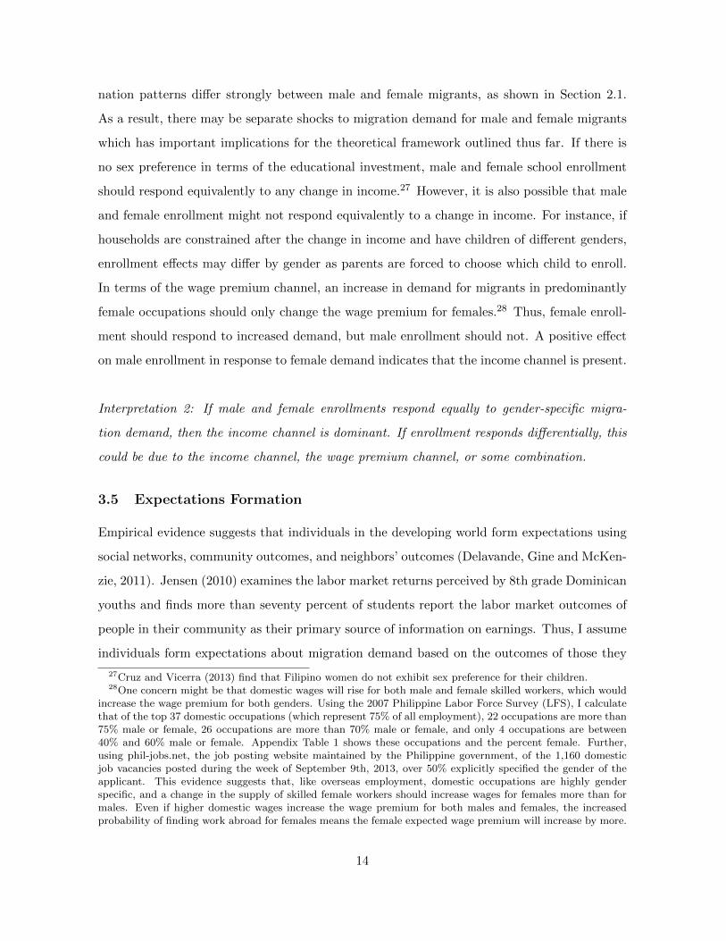
nation patterns differ strongly between male and female migrants, as shown in Section 2.1.

As a result, there may be separate shocks to migration demand for male and female migrants

which has important implications for the theoretical framework outlined thus far. If there is

no sex preference in terms of the educational investment, male and female school enrollment

should respond equivalently to any change in income.27 However, it is also possible that male

and female enrollment might not respond equivalently to a change in income. For instance, if

households are constrained after the change in income and have children of different genders,

enrollment effects may differ by gender as parents are forced to choose which child to enroll.

In terms of the wage premium channel, an increase in demand for migrants in predominantly

female occupations should only change the wage premium for females.28 Thus, female enroll-

ment should respond to increased demand, but male enrollment should not. A positive effect

on male enrollment in response to female demand indicates that the income channel is present.

Interpretation 2: If male and female enrollments respond equally to gender-specific migra-

tion demand, then the income channel is dominant. If enrollment responds differentially, this

could be due to the income channel, the wage premium channel, or some combination.

3.5 Expectations Formation

Empirical evidence suggests that individuals in the developing world form expectations using

social networks, community outcomes, and neighbors’ outcomes (Delavande, Gine and McKen-

zie, 2011). Jensen (2010) examines the labor market returns perceived by 8th grade Dominican

youths and finds more than seventy percent of students report the labor market outcomes of

people in their community as their primary source of information on earnings. Thus, I assume

individuals form expectations about migration demand based on the outcomes of those they

27Cruz and Vicerra (2013) find that Filipino women do not exhibit sex preference for their children.28One concern might be that domestic wages will rise for both male and female skilled workers, which would

increase the wage premium for both genders. Using the 2007 Philippine Labor Force Survey (LFS), I calculatethat of the top 37 domestic occupations (which represent 75% of all employment), 22 occupations are more than75% male or female, 26 occupations are more than 70% male or female, and only 4 occupations are between40% and 60% male or female. Appendix Table 1 shows these occupations and the percent female. Further,using phil-jobs.net, the job posting website maintained by the Philippine government, of the 1,160 domesticjob vacancies posted during the week of September 9th, 2013, over 50% explicitly specified the gender of theapplicant. This evidence suggests that, like overseas employment, domestic occupations are highly genderspecific, and a change in the supply of skilled female workers should increase wages for females more than formales. Even if higher domestic wages increase the wage premium for both males and females, the increasedprobability of finding work abroad for females means the female expected wage premium will increase by more.

14

observe in their local labor market, where I define the local labor market as the province.29

A number of papers in the U.S. examine how labor market expectations affect the decision

to enroll in post-secondary education. Much of the existing literature focuses on either the

effect of contemporaneous labor market conditions on college enrollment (Card and Lemieux,

2001; Dillon, 2012; Freeman, 1976)30 or the effect of ex post earnings on enrollment (Cunha

and Heckman, 2007; Willis and Rosen, 1979). A new literature examines the effects of ex ante

expected returns to schooling on the school enrollment decision. Attanasio and Kaufmann

(2010) find that ex ante subjective expectations matter for secondary schooling decisions for

youth in Mexico. Since I do not have data on the perceived ex ante migration rate, I assume

that parents form expectations of migration demand based on the observed migration rate,

which I define empirically as the migration rate in the previous calendar year.31 As mentioned

above, households will only alter investment in education in response to changes in the expected

wage premium if the change in migration demand is perceived as reasonably permanent. In

Section 6.1, I use a Fourier frequency decomposition to show that changes in migration demand

are overwhelmingly low frequency, implying they are both predictable and persistent. As a

result, it is reasonable for parents to alter their expectations of the wage premium based on

the observed migration rate in the previous year since these labor market conditions likely

persist.

4 Data

4.1 Migration Data

I construct an original dataset of all new migrant departures from the Philippines between 1992

and 2009. The data are from the Philippine Overseas Employment Administration (POEA)

and the Overseas Worker Welfare Administration (OWWA). Both under the Department of

Labor and Employment (DOLE) of the Philippine government, these agencies are responsible

for overseeing various aspects of the migration process. Specifically, POEA monitors recruit-

29One key reason to use the province as the local labor market is because recruitment agencies are grantedthe authority to recruit at the province level (Philippine Overseas Employment Administration, 2013).

30Survey evidence indicates that students form subjective expectations of future earnings based on contem-poraneous earnings in the labor market (Dominitz and Manski, 1997; Freeman, 1976; Manski and Wise, 1983).

31Because the school year commences in June, the observed annual migration rate used to make enrollmentdecisions at time t is the migration rate at time t− 1.

15

ment and regulates the employment program. Prior to deployment, all contract migrants must

visit POEA in order to have their contracts approved and receive exit clearance. As a result,

POEA maintains a rich database on all new contract hires from the Philippines, encompassing

4.8 million individual-level observations of migrant departures. The database includes the in-

dividual’s name, date of birth, sex, marital status, occupation, destination country, employer,

recruitment agency, salary, contract duration, and date deployed.

OWWA is the agency responsible for the protection and welfare of overseas workers and

their families. Upon processing overseas labor contracts at POEA, migrants are required to

become members of OWWA.32 OWWA maintains a membership database of new hires and

rehires including information similar to that housed at POEA with approximately 1 million

observations per year. However, while the POEA database includes information on the salary,

recruitment agency, and occupation to uphold their responsibility to monitor contracts and

recruitment, because OWWA is concerned with the welfare of both the migrant and his or her

family, home address of the migrant is one of the key variables in the OWWA database.

OWWA membership requirements have changed substantially over the sample period.

Since 2001, all contract hires are required to have active OWWA membership, but prior to

2001 membership was only required for new contract hires, domestic helpers, and seafarers.

In order to obtain a sample of only new hires, I match the OWWA data to the data from

POEA.33 This adds home address to the POEA data, creating a unique dataset including

both the origin and destination of all new contract migrants from one of the world’s largest

labor exporters. This paper is the first to make use of this unique data from OWWA.

To calculate province-level migration rates, I total the number of migrant workers in each

province-year and divide by the working aged population in the province.34,35 Because OWWA

32Membership entitles workers to a number of services such as repatriation or evacuation. OWWA alsoconducts mandatory Pre-Departure Orientation Seminars as well as Reintegration Seminars.

33I match the data using first name, middle name, last name, date of birth, destination country, gender, andyear of departure using fuzzy matching techniques as discussed in Winkler (2004). For the years of data usedin this analysis, the match rates are approximately 90% for 1992 and 1993 and between 95% and 98% for 2004to 2009.

34I define the working aged population as 18 to 60 since 18 is the minimum age at which one can migrate. Theage range 18 to 60 covers 99% of all migration episodes in my sample period. All population data are from the1990, 1995, 2000, and 2007 Philippine Censuses from the National Statistics Office, and I linearly interpolatevalues for years between censuses. Overseas contract workers are included in census population counts in thePhilippines.

35The home address variable from OWWA includes only the municipality of origin, not the province orregion. Out of 1630 municipalities, 332 have ambiguous names that are used in more than one province orregion. Thus, to calculate the number of migrants in the province, I assign municipalities with repeated names

16

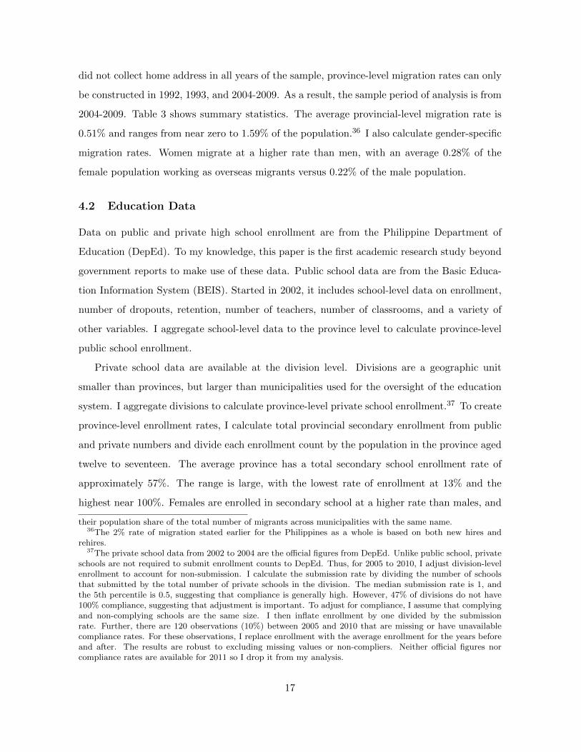
did not collect home address in all years of the sample, province-level migration rates can only

be constructed in 1992, 1993, and 2004-2009. As a result, the sample period of analysis is from

2004-2009. Table 3 shows summary statistics. The average provincial-level migration rate is

0.51% and ranges from near zero to 1.59% of the population.36 I also calculate gender-specific

migration rates. Women migrate at a higher rate than men, with an average 0.28% of the

female population working as overseas migrants versus 0.22% of the male population.

4.2 Education Data

Data on public and private high school enrollment are from the Philippine Department of

Education (DepEd). To my knowledge, this paper is the first academic research study beyond

government reports to make use of these data. Public school data are from the Basic Educa-

tion Information System (BEIS). Started in 2002, it includes school-level data on enrollment,

number of dropouts, retention, number of teachers, number of classrooms, and a variety of

other variables. I aggregate school-level data to the province level to calculate province-level

public school enrollment.

Private school data are available at the division level. Divisions are a geographic unit

smaller than provinces, but larger than municipalities used for the oversight of the education

system. I aggregate divisions to calculate province-level private school enrollment.37 To create

province-level enrollment rates, I calculate total provincial secondary enrollment from public

and private numbers and divide each enrollment count by the population in the province aged

twelve to seventeen. The average province has a total secondary school enrollment rate of

approximately 57%. The range is large, with the lowest rate of enrollment at 13% and the

highest near 100%. Females are enrolled in secondary school at a higher rate than males, and

their population share of the total number of migrants across municipalities with the same name.36The 2% rate of migration stated earlier for the Philippines as a whole is based on both new hires and

rehires.37The private school data from 2002 to 2004 are the official figures from DepEd. Unlike public school, private

schools are not required to submit enrollment counts to DepEd. Thus, for 2005 to 2010, I adjust division-levelenrollment to account for non-submission. I calculate the submission rate by dividing the number of schoolsthat submitted by the total number of private schools in the division. The median submission rate is 1, andthe 5th percentile is 0.5, suggesting that compliance is generally high. However, 47% of divisions do not have100% compliance, suggesting that adjustment is important. To adjust for compliance, I assume that complyingand non-complying schools are the same size. I then inflate enrollment by one divided by the submissionrate. Further, there are 120 observations (10%) between 2005 and 2010 that are missing or have unavailablecompliance rates. For these observations, I replace enrollment with the average enrollment for the years beforeand after. The results are robust to excluding missing values or non-compliers. Neither official figures norcompliance rates are available for 2011 so I drop it from my analysis.

17

this is true both for public and private schools. About 46% of the school-aged population is

enrolled in public schools, while approximately 11% are enrolled in private schools.

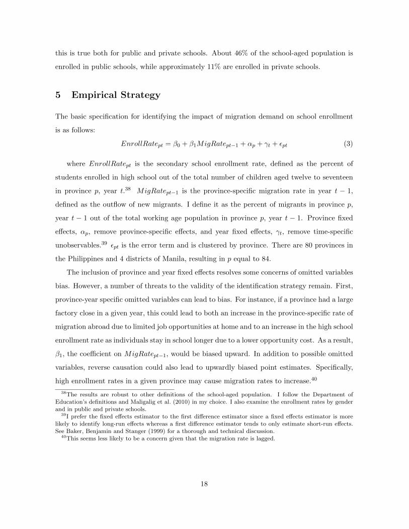
5 Empirical Strategy

The basic specification for identifying the impact of migration demand on school enrollment

is as follows:

EnrollRatept = β0 + β1MigRatept−1 + αp + γt + εpt (3)

where EnrollRatept is the secondary school enrollment rate, defined as the percent of

students enrolled in high school out of the total number of children aged twelve to seventeen

in province p, year t.38 MigRatept−1 is the province-specific migration rate in year t − 1,

defined as the outflow of new migrants. I define it as the percent of migrants in province p,

year t − 1 out of the total working age population in province p, year t − 1. Province fixed

effects, αp, remove province-specific effects, and year fixed effects, γt, remove time-specific

unobservables.39 εpt is the error term and is clustered by province. There are 80 provinces in

the Philippines and 4 districts of Manila, resulting in p equal to 84.

The inclusion of province and year fixed effects resolves some concerns of omitted variables

bias. However, a number of threats to the validity of the identification strategy remain. First,

province-year specific omitted variables can lead to bias. For instance, if a province had a large

factory close in a given year, this could lead to both an increase in the province-specific rate of

migration abroad due to limited job opportunities at home and to an increase in the high school

enrollment rate as individuals stay in school longer due to a lower opportunity cost. As a result,

β1, the coefficient on MigRatept−1, would be biased upward. In addition to possible omitted

variables, reverse causation could also lead to upwardly biased point estimates. Specifically,

high enrollment rates in a given province may cause migration rates to increase.40

38The results are robust to other definitions of the school-aged population. I follow the Department ofEducation’s definitions and Maligalig et al. (2010) in my choice. I also examine the enrollment rates by genderand in public and private schools.

39I prefer the fixed effects estimator to the first difference estimator since a fixed effects estimator is morelikely to identify long-run effects whereas a first difference estimator tends to only estimate short-run effects.See Baker, Benjamin and Stanger (1999) for a thorough and technical discussion.

40This seems less likely to be a concern given that the migration rate is lagged.

18

5.1 Migration Demand Index

To address these threats to causal identification and isolate changes in migration demand from

changes in migration supply, I instrument for the migration rate using a migration demand

index. Specifically, I create a Bartik-style instrument (Bartik, 1991; Blanchard and Katz, 1992;

Bound and Holzer, 2000; Katz and Murphy, 1992) by exploiting destination country-specific

historic migrant networks across provinces. However, rather than predicting employment

growth as is standard in this literature, I create an index of the predicted number of migrants

in each province-year. To predict the number of migrants, I weight the total number of

migrants nationally to 32 distinct destinations by the province share of the national total to

that destination in a base period. I then sum over all 32 destinations to predict the total

number of migrants in each province-year.41 Specifically, I define the migration demand index

as follows:

Dpt =∑i

MitMpi0

Mi0(4)

where Dpt is the predicted number of migrants in province p, year t, Mit is the number

of migrants to destination i, year t in the Philippines as a whole, andMpi0

Mi0is the share of

migrants at baseline in province p, destination i, out of the total number of migrants nationally

at baseline in destination i. I define baseline as 1993, but the results are robust to the choice

of other base years.42 By using these baseline shares, I am implicitly assuming that the

distribution of migrants to a given destination is stable across the Philippines over time, or

at least a reasonable predictor of future distributions of migrants (Munshi, 2003; Woodruff

and Zenteno, 2007). If this is not the case, the instrument will be a poor predictor of the

province-specific migration rate. I then divide the index by the working population in the

base year in order to obtain a predicted migration rate.

Panel B of Table 3 shows summary statistics for the Bartik-style instrument. The con-

41As a robustness check, I also create two analogous indices that exploit occupation-specific historic migrationnetworks and occupation x destination country-specific historic migration networks rather than destination-specific shares. For the occupation-based index, I use 38 occupations categories, and for the destination xoccupation-based index, I use 32 destination cells times 38 occupation cells. The results are robust to thechoice of index, and the main results are shown in Appendix Table 2.

42The results are robust to using 1992 or an average of 1992, 1993, and 1994 as the base year instead. Iuse 1993 as the base year for the majority of my analyses for two reasons: 1) 1993 has the fewest missingvalues for municipality and thus provides the most accurate counts of migrants at the province level and 2) Onelarge occupation, caregivers, only commenced as a migration opportunity in 1993. Thus, to accurately assignnetworks, I use the base year once it was established as a common occupation.

19

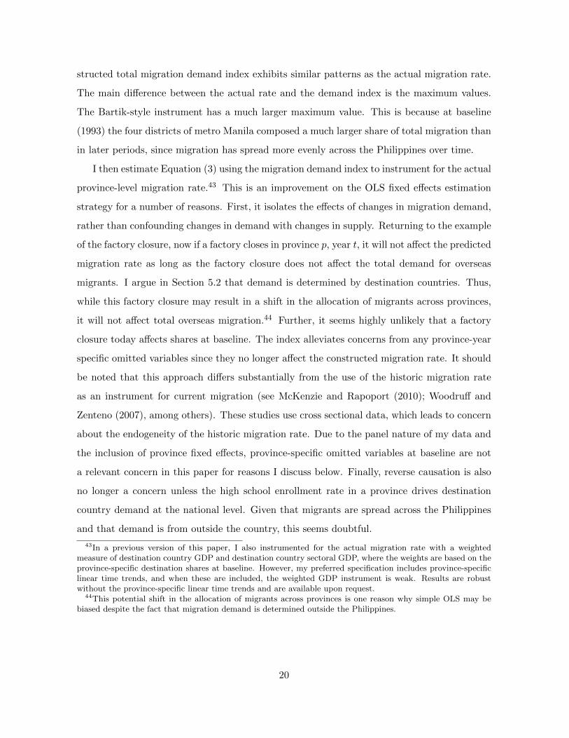
structed total migration demand index exhibits similar patterns as the actual migration rate.

The main difference between the actual rate and the demand index is the maximum values.

The Bartik-style instrument has a much larger maximum value. This is because at baseline

(1993) the four districts of metro Manila composed a much larger share of total migration than

in later periods, since migration has spread more evenly across the Philippines over time.

I then estimate Equation (3) using the migration demand index to instrument for the actual

province-level migration rate.43 This is an improvement on the OLS fixed effects estimation

strategy for a number of reasons. First, it isolates the effects of changes in migration demand,

rather than confounding changes in demand with changes in supply. Returning to the example

of the factory closure, now if a factory closes in province p, year t, it will not affect the predicted

migration rate as long as the factory closure does not affect the total demand for overseas

migrants. I argue in Section 5.2 that demand is determined by destination countries. Thus,

while this factory closure may result in a shift in the allocation of migrants across provinces,

it will not affect total overseas migration.44 Further, it seems highly unlikely that a factory

closure today affects shares at baseline. The index alleviates concerns from any province-year

specific omitted variables since they no longer affect the constructed migration rate. It should

be noted that this approach differs substantially from the use of the historic migration rate

as an instrument for current migration (see McKenzie and Rapoport (2010); Woodruff and

Zenteno (2007), among others). These studies use cross sectional data, which leads to concern

about the endogeneity of the historic migration rate. Due to the panel nature of my data and

the inclusion of province fixed effects, province-specific omitted variables at baseline are not

a relevant concern in this paper for reasons I discuss below. Finally, reverse causation is also

no longer a concern unless the high school enrollment rate in a province drives destination

country demand at the national level. Given that migrants are spread across the Philippines

and that demand is from outside the country, this seems doubtful.

43In a previous version of this paper, I also instrumented for the actual migration rate with a weightedmeasure of destination country GDP and destination country sectoral GDP, where the weights are based on theprovince-specific destination shares at baseline. However, my preferred specification includes province-specificlinear time trends, and when these are included, the weighted GDP instrument is weak. Results are robustwithout the province-specific linear time trends and are available upon request.

44This potential shift in the allocation of migrants across provinces is one reason why simple OLS may bebiased despite the fact that migration demand is determined outside the Philippines.

20

5.2 Identifying Assumptions

For this analysis to provide a causal estimate of the effect of migration demand on secondary

school enrollment, a number of identifying assumptions must hold.45 First, to satisfy the

relevance condition, there must be variation in the province-specific destination shares at

baseline. If, for instance, each province sends an equal share of migrants to Saudi Arabia in

the base period, then the instrument would explain little of the variation in province-level

migration rates. In Appendix Table 3, I show the quartiles, standard deviation, minimum and

maximum of the base shares for each of the 32 destination countries. There is substantial

variation in the size of the shares that each province comprises of total migration to a given

destination country, thus satisfying this condition.

The second assumption, which is necessary for the exogeneity of the instrument, states that

the number of migrants departing from the Philippines annually is determined by host country

demand. I argue that there is a large potential supply of Filipinos who want to migrate, and

the number hired is determined by demand from overseas employers. McKenzie, Theoharides

and Yang (2014) suggest, based on evidence from 2010 Gallup World Poll, that there may be

as many as 26 million Filipinos who would like to migrate if given the opportunity, compared

to only 2 million who currently work abroad each year. Further, they report from qualitative

interviews with recruiting agencies that there is an excess supply of Filipinos who want to

work abroad and that the overseas contract labor market is a buyer’s market.

If demand is determined outside the Philippines, then the actual number of migrants in

each year should not be influenced by economic conditions in the Philippines, but rather

by the economic conditions in the destination countries. McKenzie, Theoharides and Yang

(2014) show that there is a causal link between migrant numbers and GDP shocks in the

destination country. To further show that economic conditions in the Philippines do not

influence the number of migrants, I regress the log number of migrants in each of the 32

destination countries on log Philippine GDP, controlling for log GDP in the top ten destinations

for Filipinos. If economic conditions in the Philippines do not affect the number of overseas

workers, then Philippine GDP should not have an effect on migrant outflows. Appendix Table

45Blanchard and Katz (1992) discuss two identifying assumptions for the standard Bartik-style instrument.Goldsmith-Pinkham, Sorkin and Swift (2013) formalize their assumptions and assert that two additional as-sumptions must hold in the standard case for the instrument to be valid. Since the construction of my instrumentis slightly different, the identifying assumptions are modified accordingly.

21

4 shows the results of this analysis. Out of the 32 destinations, Philippine GDP only has a

statistically significant effect in 2 cases, roughly what would be expected due to chance. While

the coefficients are not precisely estimated zeros, they are smaller and less precisely estimated

than the point estimates on log GDP in the top ten destinations.

The final identifying assumption is that baseline shares are not correlated with trends in

variables related to the outcome variable.46 One way to test the validity of this exogeneity

assumption is to compare provinces with low destination-specific baseline migration rates to

those with high rates and compare their trends in variables related to education. If, for

example, provinces with high baseline rates have higher growth in enrollment than provinces

with low baseline rates, I would incorrectly estimate that an increase in demand has a positive

effect on enrollment, when in actuality the increase in enrollment was at least partly due to

differing trends due, presumably, to other factors.47

Ideally I would compare trends in education outcomes prior to the start of the overseas

migration program in areas that have high or low destination-specific migration rates at base-

line. However, the overseas migration program for the Philippines commenced in 1974, long

before data on education outcomes in the Philippines were available. In Figure 4, I plot the

migration outflows for the 9 destinations with the highest variation over the sample period.

It seems demand for at least some of the occupations remained relatively flat between 1993

and 2000. This suggests that the importance of shocks to migration demand was much larger

during the later years of the sample. Thus, in provinces with high and low destination-specific

migration rates, I examine trends in the high school enrollment rate in the period from 1993

to 2000.48

In Figure 5, I plot the average province-level high school enrollment rates for high and

low migration provinces for each of the 9 destinations with the highest variation in migrant

counts.49 This allows for a visual evaluation of the parallel trends assumption: in the absence of

the change in migration demand, enrollment should have remained parallel. In the pre-period,

46Because I am using panel data, province fixed effects absorb differences in the levels of any such omittedvariables.

47This is conceptually similar to testing for pre-trends in a difference-in-differences methodology.48I use destination-specific rates of migration at baseline to measure the level of treatment. The baseline

shares used in the construction of the index do not take into account the population of the province, thus theyare not measuring the density of migration experienced by the province.

49Since DepEd did not release enrollment data prior to 2002, I use the NSO’s quarterly Labor Force Surveyto calculate province-level high school enrollment rates.

22

the trends in enrollment appear quite parallel. This suggests, for example, that recruiters did

not choose to locate in areas where education was increasing at a higher rate. In the post

period, enrollment in the low migration provinces appears to be catching up, perhaps due to

poverty reduction policies or policies geared at increasing educational attainment specifically.50

While this is concerning for the parallel trends assumption, it will lead to downward bias of the

estimates of the effect of migration demand on enrollment. Since I hypothesize that migration

demand increases enrollment, increases in education for low migration areas compared to high

migration areas will bias the estimates against finding an effect from increased migration

demand.

To more rigorously examine if there are differential trends in enrollment, I estimate the

following equation separately for each destination country in the pre period, post period, and

full sample:

∆EnrollRatept = β0 + β1MigRatep0 + γt + εpt (5)

where ∆EnrollRatept is the percent change in the province-level high school enrollment

rate from time t−1 to time t, MigRatep0 is the province migration rate at baseline, γt are year

fixed effects, and εpt is the error term. t is equal to 1993 to 2000 for the pre period and 2006

to 2011 for the post period. A non-zero value for β1 would lead to concern that the enrollment

rate is trending differentially for different levels of the migration rate. Appendix Table 5

shows the results. While the point estimates are not precise, there is substantial variation

in the magnitudes of the coefficients. However, many of the destinations with large point

estimates are small and account for little of the variation in migrant demand over the sample

period. I highlight the 9 highest variation destination countries in grey. Other than Lebanon

and Singapore, the coefficients in the pre-period for these highest variance destinations are

close to zero. Given that most of the identifying variation will come from changes in demand

in these destinations, this reduces concerns about differential trending driving the results. The

inclusion of province-specific linear time trends in all preferred specifications further alleviates

this concern.

50Total high school enrollment data are not available from the LFS in 2001 to 2005.

23

5.3 Gender-Specific Demand Indices

In order to identify the mechanism through which migration affects human capital, I examine

the enrollment response to gender-specific demand for migrants as discussed in Section 3.4.

Estimating equation (3) with the province-level gender-specific migration rate as the key ex-

planatory variable will suffer from the same threats to identification as outlined for the overall

migration rate. Thus, I create gender-specific Bartik-style instruments:

Dgpt =∑i

MgitMgpi0

Mgi0(6)

where Dgpt is the predicted number of migrants of gender g in province p, year t, Mgit is

the number of migrants of gender g to destination i, year t in the Philippines as a whole, andMgpi0

Mgi0is the share of migrants at baseline of gender g in province p, destination i, out of the

total number of migrants nationally at baseline of gender g to destination i. While occupations

are highly gendered in the Philippines as shown in Section 2.1, the creation of this index does

not assume that the gender composition is stable over time. Rather, it simply assumes that,

given a certain number of female migrants hired for a certain destination, the share coming

from each province is relatively stable over time. The identifying assumptions are the same as

discussed in Section 5.2.

6 Results

6.1 Identifying Variation

One critique of Bartik-style instruments is that the source of underlying variation is often

unclear (Goldsmith-Pinkham, Sorkin and Swift, 2013). To address this, in Figure 4 I start by

plotting total migration over time in each of the 9 destinations with the highest variances over

the sample period in order to explicitly explore the identifying variation.51 Migrant outflows

change substantially over the sample period. Despite fluctuations in certain destination-years,

in general these plots of destination-specific migration demand suggest that migration demand

increased over time and that the variation in most destinations is fairly low frequency.

51Incidentally, these are also 7 of the top 10 largest destinations. Figures for all 32 destinations are availableupon request.

24

To formally test whether the variation in migrant demand is high or low frequency, I filter

the migration demand index into high and low frequency components following Baker, Ben-

jamin and Stanger (1999) and Bound and Turner (2006). Low frequency variation suggests

that changes in migration demand are persistent over time, whereas high frequency variation

would imply that changes in migration demand are quite transitory. If demand is high fre-

quency, it seems unlikely that individuals will change their expectations of the wage premium

in response to changes in migration demand. If demand is instead low frequency, such labor

market conditions are likely to persist and thus may cause individuals to revise expectations

of the wage premium. First, I employ a basic decomposition following Baker, Benjamin and

Stanger (1999), which filters the migration demand index into a high frequency component

and a low frequency component:

Dpt =1

2(Dpt −Dpt−1) +

1

2(Dpt +Dpt−1) (7)

The first component,1

2(Dpt−Dpt−1), is the first difference and encompasses high frequency

changes in the migration demand index. The second component,1

2(Dpt+Dpt−1) or the moving

average, represents low frequency changes in the index. Because I have data on the national

number of migrants by destination in all years of the sample period, the migration demand

index can be constructed from 1993 to 2009. Thus, I conduct the decomposition over the

entire sample period.52 Eighty-two percent of the variance in the migration demand index is

explained by the low frequency component, and when province-specific linear time trends are

included, 88% of the variance is explained by the low frequency component. This suggests

that long-run, persistent changes in migration demand will drive the results.

I next use a Fourier decomposition following Baker, Benjamin and Stanger (1999) and

Bound and Turner (2006) to divide the migration rate into orthogonal components at varying

frequencies, which more precisely determines the nature of the variation. Using seventeen

years of data from 1993 to 2009, I split the migration demand index into nine orthogonal

components of different frequencies using:

52While the IV results cannot be estimated over this sample period, the reduced form and IV results arequalitatively similar. Further, it seems reasonable that households will make educational investment decisionsbased on long-run variation from before my main sample period.

25

Dpt =

8∑k=0

(ξkcos

(2πk(t− 1)

17

))+

(γksin

(2πk(t− 1)

17

))(8)

To estimate ξk and γk, I follow Bound and Turner (2006) and run separate regressions for

each province (84 regressions in total). I then use these parameter estimates of ξk and γk to

calculate the nine Fourier components for each province-year. Each component is simply the

term under the summation for k equals 0 to 8. Over 87% of the variance in the migration

demand index is explained by the two lowest frequency components regardless of the inclusion

of province-specific linear time trends. The results of both the basic and Fourier decompositions

indicate that changes in province-specific migration demand are overwhelmingly low frequency

and thus are stable and predictable. As a result, when individuals in the Philippines observe

an increase in demand for migrants, it is reasonable for them to infer that such a change

is permanent and to change their expectations about future labor market opportunities in

response.

To further explore the determinants of demand, I uncover a number of institutional factors

that drive the identifying variation for the 9 highest variance destinations shown in Figure 4.

Panel A shows total migration to Saudi Arabia from 1992 to 2009. During the early part of

the sample period, migration fell due to the Gulf War (United Nations, 2006). From 2003

onward, migration to Saudi Arabia grew substantially as oil prices increased, and the hire

of engineers, building caretakers, domestic helpers, laborers, and medical workers increased

substantially. The dip at the end of the sample is due to a change in the minimum wage

for domestic helpers imposed by the Philippines in 2007 (McKenzie, Theoharides and Yang,

2014). With a minimum wage that was double the previous rate ($400 per month from $200

per month), the number of domestic helpers fell from 12,550 in 2006 to 3,870 in 2007, though

the hire of domestic helpers recovered by 2009.

Migrants to Japan are almost exclusively employed as Overseas Performing Artists (OPAs).

In Panel B, the large drop in the number of migrants to Japan in 2005 is due to barriers imposed

on migration of OPAs in response to pressure from the United States (Theoharides, 2014). The

dip in deployment of migrants to Japan between 1994 and 1995 was due to more stringent

requirements for OPAs imposed by the Philippine Labor Secretary in response to exploitation

of Filipinas (Philippine General Rule 120095, 1996).

26

Panels C, D, and F show steady increases in the number of Filipino migrants to the Middle

East from 2003 onward. This coincides with the rise in oil prices, and the number of migrants

employed as building caretakers, cooks, domestic helpers, engineers, plumbers, salesmen, and

other service workers increases substantially in these destinations during this period. Similar

to Saudi Arabia, the dip in the number of migrants in 2007 is due to the increase in minimum

wage for domestic helpers.

In Taiwan (Panel E), about 50% of migrants work in the production sector, which is largely

composed of factory workers. Growth in the hire of these workers over the sample period was

substantial due to growth in cell phones, computers, and other electronics during the 1990s,

and this growth remained steady through the 2000s. The other major occupations migrating

to Taiwan are caregivers and domestic helpers, though this declined substantially in 2006 for

caregivers and in 1997 for domestic helpers, likely due to the increased hire of these migrants

from Indonesia. The large drop in the number of workers to Taiwan in 2000 was due to a

hiring ban on Filipino workers imposed by Taiwan in June, 2000 due to deteriorating relations

between Taiwan and the Philippines (Migration News, 2000).

Almost all migrants to Hong Kong (Panel G) are employed as domestic helpers. While there

are fluctuations in demand for these workers over the sample period, the general trajectory

is upward. Indeed, the number of domestic helpers increased from about 13,500 in 1992 to

25,000 in 2009. Migrants to Lebanon (Panel I) are also almost exclusively domestic helpers.

The hire of domestic helpers grew substantially starting in 1998 and by 2005, over 11,000

domestic helpers were employed. However, in 2007, the Philippines imposed a two year ban

on the deployment of Filipinos due to fighting between Israel and Hezbollah (GMA News,

2011). Finally, migration to Singapore (Panel H) is mainly for domestic helpers, engineers,

and medical workers. The growth at the end of the sample period was due to a doubling of

the hire of medical workers between 2007 and 2008.

To summarize, the majority of the variation in the migration demand index is relatively

low frequency, indicating that changes in migration demand are persistent. Policy changes by

destination countries and the Philippines, the price of oil, and growth in the electronics field

seem to be the drivers behind changes in the number of Filipinos migrating abroad each year

overall as well as to specific destinations.

27

6.2 The Effect of Migration Demand on Enrollment

In Table 4, Panel A, Column 1, I report the first stage results of the effect of the total migration

demand index on the total migration rate. The index has a positive and statistically significant

relationship with the endogenous variable, but the F-statistic is less than 10, indicating that

weak instruments are an issue (Stock and Yogo, 2002).53 In column 2, I add province-specific

linear time trends to alleviate concerns about differential trending in omitted variables across

provinces at baseline as outlined in Section 5.2. The F-statistic increases to greater than

10, and the relationship between the endogenous variable and the instrument is larger in

magnitude. In Column 3, my preferred specification, I weight by the population in order to

obtain nationally representative results. The first stage results are much stronger with an

F-statistic of 46. Finally, in Column 4, I test if the highest migration province, the second

district of Manila, is driving the results. The first stage results appear robust. Therefore, I

proceed with Column 3 as my preferred specification, though I show the robustness of the

results to other specifications throughout.

Table 5, Panel A shows that total migration demand is positively related to secondary

school enrollment decisions. To interpret the point estimate in Panel A, Column 3, my pre-

ferred specification, for a 1-percentage point increase in total migration demand, school en-

rollment increases by 10.3 percentage points. However, it is important to note that, given

average migration rates of 0.51% of the total province working population, a 1-percentage

point increase in the province-level migration rate is unrealistic. Instead, I calculate the aver-

age year-to-year percentage point change in migration demand over my sample period to be

0.12 percentage points. For an average change in migration demand of 0.12 percentage points,

enrollment increases by 10.3*0.12=1.2 percentage points. This results in a 2.1% increase in

enrollment, off a sample mean of 56.8% enrolled. The results without the population weights

(Column 2) are qualitatively similar, but larger in magnitude. This indicates that the enroll-

ment response to education is different across small and large provinces in the Philippines.

Namely provinces with smaller populations have a larger education response to migration.

In Column 4, I drop the second district of Manila. The results are robust to this change in

sample. The effects on female and male enrollment Panels B and C are qualitatively similar to

53When using robust standard errors, the Cragg-Donald Wald statistic is not valid. Instead, I report theKleibergen-Paap statistic (Kleibergen and Paap, 2006).

28

the overall results. Male and female enrollment increase by 2.0% and 2.2% respectively, and I

cannot reject that the coefficients are the same.

In addition to the effect of migration demand on total secondary school enrollment, another

key consideration is whether households choose to send their children to public or private

school. One of the major motivations for international migration from the Philippines is the

desire to enroll children in private school (Asis, 2013). As income increases, parents may now

choose to switch to a type of schooling that they perceive as higher quality. The effect of the

expected wage premium on public and private enrollments remains an empirical question, and I

will test the channels affecting school choice below using gender-specific migration demand. In

Table 6, I examine the response of public and private secondary school enrollment to changes

in total migration demand. The effects on public school enrollment are small and imprecisely

estimated. However, they suggest that increases in migration demand lead to slightly greater

public school enrollment. Private school enrollment, on the other hand, increases statistically

significantly in response to migration demand. Looking at Panel B, Column 3, an average

year-to-year increase of 0.12 percentage points yields a 10.1% increase in private secondary

school enrollment off a sample mean of 11.4%. If I assume that most individuals who enroll

in private school in response to an increase in migration demand were previously enrolled in

public school, these results suggest that for every student switching to private school, there is

another previously unenrolled child who enrolls in public school.

6.3 Mechanisms

The results thus far provide evidence that total and private secondary school enrollment in-

crease in response to increases in total migration demand, while there is suggestive evidence

of slight increases in public school enrollment. In order to determine the mechanisms through

which these effects may occur, I examine the effect of gender-specific migration demand on

school enrollment. As discussed in Section 3.4, if the effects on male and female enrollment are

equal in response to an increase in, for instance, female migration demand, the income channel

is dominant. If the effects are not equal, either income, the wage premium, or some combina-

tion of the two could be the dominant channel. A positive effect of female migration demand

on male enrollment suggests that the income channel is present since the wage premium should

never have a positive effect. Panels B and C in Table 4 show the first stage results for the male-

29

and female-specific migration demand indices. Both indices have a positive and statistically

significant relationship with the gender-specific migration rates. However, the male migration

demand index has an F-statistic below the critical value of 10, and thus weak instruments are

a problem. The higher standard errors in the male regressions compared to the female regres-

sions suggest that there is less variation in the male migration rate over the sample period.

As a result of the weak first stage for male migration, I focus the gender-specific analysis on

the effect of female migration demand.

While the same identifying assumptions must hold for the gender-specific demand indices

as for the total migration demand index, by splitting demand by gender, I introduce the

potential for an additional omitted variable. Consider the effect of female migration demand.

If the provinces that are more affected by changes in the national number of female migrants

(ie., higher base share provinces) also experience an increase in the male migration rate, and

male migration also has an effect on school enrollment, then the results will be biased. To

test for this, I first examine the relationship between the male migration rate and the female

demand index as well as the relationship between the female migration rate and the male

demand index by regressing the gender-specific migration demand index on the migration rate

for the opposite gender. A positive relationship would suggest that the effect of gender-specific

migration demand on enrollment may be biased upward. The results are shown in Columns 1

and 2 of Appendix Table 6. For the female demand index, the male migration rate appears to

have little effect. As such, omitted variables bias due to the male migration rate is likely not

a concern.54 I also control for the male migration rate in the regressions that follow.

Table 7 reports the effect of female migration demand on total, female, and male enrollment.

Looking at my preferred specification in Panel A, Column 3, a change in female migration

demand has a positive but statistically imprecise effect on total secondary school enrollment.

In Column 5, I add a control for the male migration rate, and the results are robust to the

addition of this control. Turning to Panel B, Column 3, female migration demand has a

positive and significant effect on female secondary school enrollment. Specifically, an average

year-to-year percentage point increase in female migration demand of 0.05 percentage points

54On the other hand, the female migration rate and the male demand index have an inverse and statisticallysignificant relationship. Thus, if female migration has a positive effect on school enrollment, estimates of theeffect of the male migration demand index on enrollment will be biased downward. Thus, in addition to concernsabout the weak first stage for men, I proceed in my analysis using the female migration demand index due toconcerns about omitted variables bias with the male index.

30

leads to a 7.3*0.05=0.36 percentage point increase in female secondary school enrollment.

This is a 0.6% increase in enrollment off a sample mean of 60.0%. In Panel C, Column 3, the

effects of female migration demand on male enrollment are smaller than the effects on female

enrollment. However, I cannot reject that they are the same, suggesting that the income

channel is likely dominant. If I examine the estimates without population weights shown in

Column 2, the coefficients on male and female enrollment are quite similar. This leads me to

conclude that changes in income, rather than changes in the expected wage premium, are the

dominant channel through which migration affects school enrollment. The slight differences in

point estimates suggest that the expected wage premium may matter as well. The differential

effects could be due to either changes in the female-specific wage premium or households

preferring to invest in girls’ education when income increases. Because the coefficient on male

enrollment is positive, this indicates that the entire effect could not be from the wage premium,

and enrollment changes at least partially in response to the income channel.

In Table 8, I examine the response of public and private enrollment to a change in female

migration demand. Comparing Column 1 to Column 2 in Panel A, the public school enrollment

results are not particularly robust to the population weights. This suggests that while lower

population provinces in the Philippines respond positively to increases in female migration

demand in terms of public school enrollment, this is not true in Manila or other high population

areas. This may be indicative of lower income levels of migrant households outside Manila,

such that the marginal student is induced into public school, whereas in Manila a higher initial

portion of children in migrant households are enrolled. In Panel B, Column 2, private school

enrollment increases by 2.5% in response to an average year-to-year change. The results are of

a similar magnitude when both unweighted and weighted. The estimates without weights on

both public and private school enrollment are nearly identical for men and women and slightly

larger for women than for men when weights are included, though I cannot reject that they

are the same. This again suggests that the dominant channel through which migration affects

secondary school enrollment is through an income channel, rather than through changes in the

expected wage premium.

31

6.4 Effect of Migration Demand on Enrollment by Grade

Secondary school enrollment increases in response to increased migration demand, primarily

due to changes in income rather than changes in the wage premium. However, given that

the enrollment choice is sequential, aggregate enrollment results may miss potentially inter-

esting dynamics regarding the marginal student affected by changes in migration demand. To

examine these dynamics, I look at the effect of both total and female migration demand on

grade-level enrollment rates for each grade of high school. The results are shown in Table 9.

Panel A shows the effects of total migration demand by grade level. An increase in migra-

tion demand causes an increase in enrollment across all grades, indicating marginal students

are induced into enrollment at all grade levels. However, first year enrollment increases by

more than fourth year enrollment (3.2% compared to 2.4%), likely due to the bunching of

dropouts prior to the first year of high school. This could be a result of limited benefits to

partial completion of high school or because this is when compulsory schooling concludes,

among other reasons. Thus, while there are marginal students in all grades, this suggests a

large number of students never enroll in high school either because of liquidity constraints or

the returns on the education investment are too low.

Panel B shows the enrollment response to female migration demand. The effects are

positive and quite similar across grade levels, though imprecisely estimated. Turning to Panels

C and D, while there are equivalent effects on male and female aggregate enrollment in response

to a change in female migration demand, I find substantial heterogeneity when comparing the

male and female enrollment responses. Specifically, for year one, I can reject that female

migration demand has equal effects on male and female enrollment, while in later years I

cannot reject that the effects are the same, though the male point estimates are consistently

smaller than the female estimates. This differential response to gender-specific demand in the

first year suggests that while the aggregate results imply that income is the dominant channel,

first year enrollment may respond to some combination of both channels.

6.5 Interpreting Effect Sizes

The results suggest that an average year-to-year increase in total migration demand leads to

a 2.1% increase in total secondary school enrollment. Given that the average province sends

32

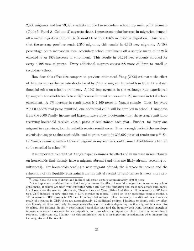
2,550 migrants and has 79,081 students enrolled in secondary school, my main point estimate

(Table 5, Panel A, Column 3) suggests that a 1 percentage point increase in migration demand

off a mean migration rate of 0.51% would lead to a 196% increase in migration. Thus, given

that the average province sends 2,550 migrants, this results in 4,998 new migrants. A 10.3

percentage point increase in total secondary school enrollment off a sample mean of 57.21%

enrolled is an 18% increase in enrollment. This results in 14,234 new students enrolled for

every 4,498 new migrants. Every additional migrant causes 2.8 more children to enroll in

secondary school.

How does this effect size compare to previous estimates? Yang (2008) estimates the effect

of differences in exchange rate shocks faced by Filipino migrant households in light of the Asian

financial crisis on school enrollment. A 10% improvement in the exchange rate experienced

by migrant households leads to a 6% increase in remittances and a 1% increase in total school

enrollment. A 6% increase in remittances is 2,160 pesos in Yang’s sample. Thus, for every

216,000 additional pesos remitted, one additional child will be enrolled in school. Using data

from the 2006 Family Income and Expenditure Survey, I determine that the average remittance

receiving household receives 76,273 pesos of remittances each year. Further, for every one

migrant in a province, four households receive remittances. Thus, a rough back-of-the-envelope

calculation suggests that each additional migrant results in 305,092 pesos of remittances.55 So,

by Yang’s estimate, each additional migrant in my sample should cause 1.4 additional children

to be enrolled in school.56

It is important to note that Yang’s paper examines the effects of an increase in remittances

on households that already have a migrant abroad (and thus are likely already receiving re-

mittances). For households sending a new migrant abroad, the increase in income and the

relaxation of the liquidity constraint from the initial receipt of remittances is likely more pro-

55Recall that the sum of direct and indirect education costs is approximately 50,000 pesos.56One important consideration is that I only estimate the effect of new hire migration on secondary school

enrollment. If rehires are positively correlated with both new hire migration and secondary school enrollment,I will overstate the results. McKenzie, Theoharides and Yang (2014) find that a 1% increase in GDP leadsto a 2.6% increase in new hires and a 1.9% increase in rehires. Based on their respective sample means, a1% increase in GDP results in 121 new hires and 148 rehires. Thus, for every 1 additional new hire as aresult of a change in GDP, there are approximately 1.2 additional rehires. I hesitate to simply split my effectsize linearly as there are likely heterogeneous effects on education depending on if a migrant is a new hireor rehire. For instance, liquidity constrained households may find the liquidity constraint loosened enough toincrease education in response to new migration, and thus when the migrant is rehired, there is no enrollmentresponse. Unfortunately, I cannot test this empirically, but it is an important consideration when interpretingthe magnitude of the results.

33

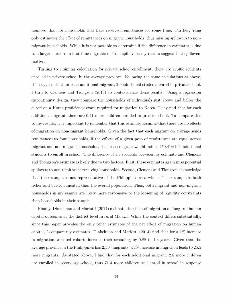
nounced than for households that have received remittances for some time. Further, Yang

only estimates the effect of remittances on migrant households, thus missing spillovers to non-

migrant households. While it is not possible to determine if the difference in estimates is due

to a larger effect from first time migrants or from spillovers, my results suggest that spillovers

matter.

Turning to a similar calculation for private school enrollment, there are 17,465 students

enrolled in private school in the average province. Following the same calculations as above,

this suggests that for each additional migrant, 2.9 additional students enroll in private school.

I turn to Clemens and Tiongson (2013) to contextualize these results. Using a regression

discontinuity design, they compare the households of individuals just above and below the

cutoff on a Korea proficiency exam required for migration to Korea. They find that for each

additional migrant, there are 0.41 more children enrolled in private school. To compare this

to my results, it is important to remember that this estimate assumes that there are no effects

of migration on non-migrant households. Given the fact that each migrant on average sends

remittances to four households, if the effects of a given peso of remittances are equal across

migrant and non-migrant households, then each migrant would induce 4*0.41=1.64 additional

students to enroll in school. The difference of 1.3 students between my estimate and Clemens

and Tiongson’s estimate is likely due to two factors. First, these estimates again miss potential

spillovers to non-remittance receiving households. Second, Clemens and Tiongson acknowledge

that their sample is not representative of the Philippines as a whole. Their sample is both

richer and better educated than the overall population. Thus, both migrant and non-migrant

households in my sample are likely more responsive to the loosening of liquidity constraints

than households in their sample.

Finally, Dinkelman and Mariotti (2014) estimate the effect of migration on long run human

capital outcomes at the district level in rural Malawi. While the context differs substantially,

since this paper provides the only other estimates of the net effect of migration on human

capital, I compare my estimates. Dinkelman and Mariotti (2014) find that for a 1% increase

in migration, affected cohorts increase their schooling by 0.88 to 1.3 years. Given that the

average province in the Philippines has 2,550 migrants, a 1% increase in migration leads to 25.5

more migrants. As stated above, I find that for each additional migrant, 2.8 more children

are enrolled in secondary school, thus 71.4 more children will enroll in school in response

34

to a 1% increase in migration. With a province-level average of 79,081 students enrolled

in secondary school, this results in a 0.1 percentage point increase in secondary enrollment

(0.17%). With 139,675 students of secondary schooling age, those 71.4 enrolled students will

create a very minimal increase in the cohort’s years of schooling, certainly much less than a 0.88

increase.57 While my effects are substantially smaller, Dinkelman and Mariotti (2014) examine

the marginal student in primary school in a context where education levels are substantially

lower than in the Philippines.

While my results are large, they are comparable with results found in these previous studies

in the Philippines, especially given the differences in sample and research design, and smaller

than studies that estimate the net effect of migration on human capital. These comparisons

emphasize the importance of spillovers to non-migrant households from migration.

7 Conclusion

As international migration continues to gain prominence as a labor market outcome, under-

standing the impacts of migration on migrant-sending economies can have important implica-

tions for development. One way in which migration can affect the home economy is by altering

the human capital stock. In this paper, I estimate the effect of migration on secondary school

enrollment in the Philippines. I conduct my analysis at the province level in order to account

for spillover effects from migration on non-migrant households. To do this, I use two large

administrative datasets to create an original dataset of all new migrant departures from the

Philippines linked to the migrant’s province of origin and calculate province-level migration

rates. Simply estimating the effect of the province-level migration rate on secondary school

enrollment is likely to suffer from a number of biases and confound changes in migrant de-

mand with changes in migrant supply. To isolate exogenous changes in demand for migrants,

I create an instrument following Bartik (1991) that exploits variation generated by shocks to

destination-specific migrant networks across local labor markets in the Philippines. As a result

of these networks, provinces will vary in the degree to which they are affected by changes in

demand for migrants from certain destination countries.

57For instance, if we assume an extreme case where all unenrolled students have 0 years of education and allenrolled students attain 10 years, the average education level would rise from 5.662 years to 5.667 years whenthe additional 71.4 students are enrolled.

35

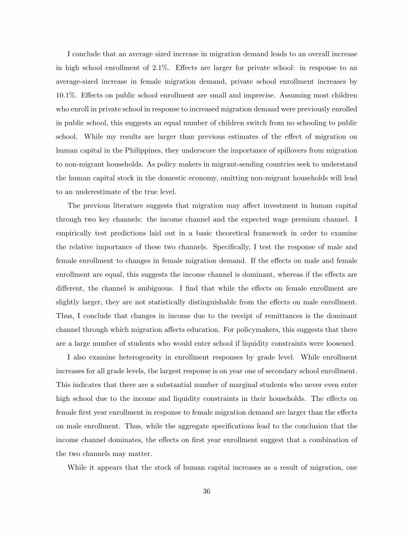
I conclude that an average sized increase in migration demand leads to an overall increase

in high school enrollment of 2.1%. Effects are larger for private school: in response to an

average-sized increase in female migration demand, private school enrollment increases by

10.1%. Effects on public school enrollment are small and imprecise. Assuming most children

who enroll in private school in response to increased migration demand were previously enrolled

in public school, this suggests an equal number of children switch from no schooling to public

school. While my results are larger than previous estimates of the effect of migration on

human capital in the Philippines, they underscore the importance of spillovers from migration

to non-migrant households. As policy makers in migrant-sending countries seek to understand

the human capital stock in the domestic economy, omitting non-migrant households will lead

to an underestimate of the true level.

The previous literature suggests that migration may affect investment in human capital

through two key channels: the income channel and the expected wage premium channel. I

empirically test predictions laid out in a basic theoretical framework in order to examine

the relative importance of these two channels. Specifically, I test the response of male and

female enrollment to changes in female migration demand. If the effects on male and female

enrollment are equal, this suggests the income channel is dominant, whereas if the effects are

different, the channel is ambiguous. I find that while the effects on female enrollment are

slightly larger, they are not statistically distinguishable from the effects on male enrollment.

Thus, I conclude that changes in income due to the receipt of remittances is the dominant

channel through which migration affects education. For policymakers, this suggests that there

are a large number of students who would enter school if liquidity constraints were loosened.

I also examine heterogeneity in enrollment responses by grade level. While enrollment

increases for all grade levels, the largest response is on year one of secondary school enrollment.

This indicates that there are a substantial number of marginal students who never even enter

high school due to the income and liquidity constraints in their households. The effects on

female first year enrollment in response to female migration demand are larger than the effects

on male enrollment. Thus, while the aggregate specifications lead to the conclusion that the

income channel dominates, the effects on first year enrollment suggest that a combination of

the two channels may matter.

While it appears that the stock of human capital increases as a result of migration, one

36

concern is that these students may eventually migrate away from the Philippines, leading

to brain drain. Recall that for each new migrant, there are 2.8 additional children enrolled

in school. For all of these additional students to acquire work abroad, demand for Filipino

migrants would need to increase by unprecedented proportions. This implies that migration

causes a substantial increase in the stock of high school educated labor in the Philippines.

Such increases, however, have important policy implications and highlight the vulnerability of

education levels in the Philippines to changes in migration demand. As a result, policymakers

in the Philippines and other migrant-sending countries may want to devote some portion of

their limited resources to provide a social safety net that helps smooth educational investment

in times of reduced migration demand.

References

Ambler, Kate. 2013. “Don’t Tell on Me: Experimental Evidence of Asymmetric Information

in Transnational Households.” Working Paper.

Ambler, Kate, Diego Aycinena, and Dean Yang. 2013. “Subsidizing Remittances for

Education: A Field Experiment Among Migrants from El Salvador.” Working Paper.

Asis, Marla. 2013. Personal Correspondence. Manila, Philippines:Scalabrini Migration Cen-

ter.

Asis, Marla, and Dovelyn Rannveig Agunias. 2012. “Strengthening Pre-Departure Ori-

entation Programmes in Indonesia, Nepal, and the Philippines.” Migration Policy Institute

Issue in Brief No. 5.

Attanasio, Orazio P., and Katja M. Kaufmann. 2010. “Educational Choices and Sub-

jective Expectations of Returns: Evidence on Intra-Household Decision Making and Gender

Differences.” NBER Working Paper 15087.

Baker, Michael, Dwayne Benjamin, and Shuchita Stanger. 1999. “The Highs and Lows

of the Minimum Wage Effect: A Time-Series Cross-Section Study of the Canadian Law.”

Journal of Labor Economics, 17(2): 318–350.

Bangko Sentral Ng Pilipinas. 2012. “Consumer Expectations Report.”

37

Barayuga, Helen. 2013. Personal Correspondence. Manila, Philippines:Former Director,

Philippine Overseas Employment Administration.

Bartik, Timothy J. 1991. Who Benefits from State and Local Economic Development Poli-

cies? Kalamazoo, MI: W.E. Upjohn Institute.

Beam, Emily. 2013. “Perceived Returns and Job-Search Selection.” Working Paper.

Beine, Michel, Frederic Docquier, and Hillel Rapoport. 2007. “Brain Drain and Hu-

man Capital Formation in Developing Countries: Winners and Losers.” Economic Journal,

118: 631–654.

Blanchard, Olivier, and Lawrence Katz. 1992. “Regional Evolutions.” Brookings Papers

on Economic Activity.

Borjas, George. 1987. “Self-Selection and the Earnings of Immigrants.” American Economic

Review, 77(4): 531–553.

Bound, John, and Harry Holzer. 2000. “Demand Shifts, Population Adjustments, and

Labor Market Outcomes during the 1980s.” Journal of Labor Economics, 18(1): 20–54.

Bound, John, and Sarah Turner. 2006. “Cohort crowding: How resources affect collegiate

attainment.” Journal of Public Economics, 91: 877–899.

Card, David, and Thomas Lemieux. 2001. “Dropout and Enrollment Trends in the Post-

war Period: What Went Wrong in the 1970s.” In Risky Behavior among Youths: An Eco-

nomic Analysis. , ed. Jonathan Gruber, 439–482.

Chand, Satish, and Michael Clemens. 2008. “Skilled Emigration and Skill Creation: A

quasi-experiment.” Center for Global Development Working Paper 152.

Chiquiar, Daniel, and Gordon Hanson. 2005. “International Migration, Self-Selection,

and the Distribution of Wages: Evidence from Mexico and the United States.” Journal of

Political Economy, 113(2): 239–281.

Clemens, Michael. 2011. “Economics and Emigration: Trillion-Dollar Bills on the Sidewalk.”

Journal of Economic Perspectives, 25: 83–106.

38

Clemens, Michael, and Erwin Tiongson. 2013. “Split Decisions: Family Finance When

a Policy Discontinuity Allocates Overseas Work.” Center for Global Development Working

Paper 324.

Clemens, Michael, Claudio E. Montenegro, and Lant Pritchett. 2008. “The Place

Premium: Wage Differences for Identical Workers Across the US Border.” World Bank

Policy Research Working Paper No. 4671.

Cortes, Patricia. 2013. “The Feminization of International Migration and its Effects on

Families Left Behind: Evidence from the Philippines.” World Development, forthcoming.

Cox-Edwards, Alejandra, and Manuelita Ureta. 2003. “International Migration, Re-

mittances, and Schooling: Evidence from El Salvador.” Journal of Development Economics,

72(2): 429–461.

Cruz, Christian Joy P, and Paolo Miguel Vicerra. 2013. “Fertility Behavior, Desired

Number and Gender Composition of Children: the Philippine Case.” Working Paper.

Cunha, Flavio, and James Heckman. 2007. “The Evolution of Inequality, Heterogeneity,

and Uncertainty in Labor Earnings in the U.S. Economy.” NBER Working Paper 13526.

Delavande, Adeline, Xavier Gine, and David McKenzie. 2011. “Measuring Subjective

Expectations in Developing Countries: A Critical Review and New Evidence.” Journal of

Development Economics, 94: 151–163.

Dillon, Eleanor Wiske. 2012. “The College Earnings Premium and Changes in College

Enrollment.” Working Paper.

Dinkelman, Taryn, and Martine Mariotti. 2014. “What are the Long Run Effects of

Labor Migration on Human Capital? Evidence from Malawi.” Working Paper.

Docquier, Frederic, Oliver Lohest, and Abdeslam Marfouk. 2007. “Brain Drain in

Developing Countries.” World Bank Economic Review, 21(2): 193–218.

Dominitz, Jeff, and Charles Manski. 1997. “Using Expectations Data to Study Subjective

Income Expectations.” Journal of the American Statistical Association, 92(439): 855–867.

39

Freeman, Richard. 1976. The Over-Educated American. New York: Academic Press.

Gibson, John, and David McKenzie. 2012. “The Economic Consequences of Brain Drain

of the Best and Brightest: Microeconomic Evidence from Five Countries.” Economic Jour-

nal, 122: 339–75.

GMA News. 2011. “Labor Attach: Hong Kong employers still prefer Pinoy work-

ers.” November 25. http://www.gmanetwork.com/news/ story/239642/pinoyabroad/labor-

attach-eacute-hong-kong-employers-still-prefer-pinoy-workers [accessed 3 February 2013].

Goldsmith-Pinkham, Paul, Isaac Sorkin, and Henry Swift. 2013. “Challenges in Esti-

mating Local Labor Supply Elasticities.” Working Paper.

Hanson, Gordon H., and Christopher Woodruff. 2003. “Emigration and Educational

Attainment in Mexico.” University of California at San Diego Working Paper.

Heckman, James J., Lance J. Lochner, and Petra E. Todd. 2006. “Earnings Functions,

Rates of Return and Treatment Effects.” Journal of Econometrics, 136(2): 341–396.

Jensen, Robert. 2010. “The (Perceived) Returns to Education and the Demand for School-

ing.” Quarterly Journal of Economics, 125(2): 515–548.

Kandel, William, and Grace Kao. 2001. “The Impact of Temporary Labor Migration

on Mexican Childrens Educational Aspirations and Performance.” International Migration

Review, 35(4): 1205–1231.

Katz, Lawrence F., and Kevin M. Murphy. 1992. “Changes in Relative Wages, 1963-

1987: Supply and Demand Factors.” The Quarterly Journal of Economics, 107(1): 35–78.

Keane, Michael P., and Kenneth I. Wolpin. 1997. “The Career Decisions of Young Men.”

Journal of Political Economy, 105(3): 473–522.

Kleibergen, Frank, and Richard Paap. 2006. “Generalized Reduced Rank Tests Using

the Singular Value Decomposition.” Journal of Econometrics, 133(1): 97–126.

Maligalig, Dalisay S., Rhona B. Caoli-Rodriguez, Arturo Martinez Jr., and Sining

Cuevas. 2010. “Education Outcomes in the Philippines.” ADB Economics Working Paper

Series 199.

40

Manski, Charles, and David Wise. 1983. College Choice in America. Boston: Harvard.

McKenzie, David, and Hillel Rapoport. 2010. “Self-Selection Patterns in Mexico-U.S. Mi-

gration: The Role of Migration Networks.” Review of Economics and Statistics, 92(4): 811–

821.

McKenzie, David, and Hillel Rapoport. 2011. “Can Migration Reduce Education At-

tainment? Evidence from Mexico.” Journal of Population Economics, 24: 1331–1358.

McKenzie, David, Caroline Theoharides, and Dean Yang. 2014. “Distortions in the

International Migrant Labor Market: Evidence from Filipino Migration and Wage Re-

sponses to Destination Country Economic Shocks.” American Economic Journal: Applied

Economics, 6: 49–75.

McKenzie, David, John Gibson, and Steven Stillman. 2013. “A Land of Milk and

Honey with Streets Paved with Gold: Do Emigrants have Over-optimistic Expectations

about Incomes Abroad?” Journal of Development Economics, 102: 116–127.

Migration News. 2000. “Taiwan-Philippines.” 7(10).

Munshi, Kaivan. 2003. “Networks in the Modern Economy: Mexican Migrants in the U.S.

Labor Market.” Quarterly Journal of Economics, 118(2): 549–599.

Orbeta, Aniceto, Michael Abrigo, and Michael Cabalfin. 2009. “Institutions Serv-

ing Philippine International Labor Migrants.” Philippine Institute for Development Studies

Discussion Paper Series 2009-31.

Philippine Department of Education Order 45. 2008.

Philippine General Rule 120095. 1996.

Philippine Overseas Employment Administration. 2013. “All About Illegal Recruit-

ment.” http://www.poea.gov.ph/air/howtoavoid.htm.

Philippine Republic Act 10533. 2013.

Philippine Republic Act 6655. 1988.

41

Rajan, S. Irudaya, and U.S. Misha. 2007. “Managing Migration in the Philippines:

Lessons for India.” Centre for Development Studies Working Paper 393.

Ray, Sougata, Anup Kumar Sinha, and Shekar Chaudhuri. 2007. “Making Bangladesh

a Leading Manpower Exporter: Chasing a Dream of US $30 Billion Annual Migrant Remit-

tances by 2015.” Indian Institute of Management Working Paper.

Shrestha, Slesh A. 2012. “Human Capital Investment Responses to Skilled Migration

Prospects: Evidence from a Natural Experiment in Nepal.” Working Paper.

Stock, James H., and Motohiro Yogo. 2002. “Testing for Weak Instruments in Linear IV

Regression.” NBER Working Paper No. 284.

Theoharides, Caroline. 2014. “Banned from the Band: The Effect of Migration Barriers

for Overseas Performing Artists on the Welfare of the Country of Origin.” Working Paper.

United Nations. 2006. “International Migration in the Arab Region.” Population Division

Report.

Willis, Robert J., and Sherwin Rosen. 1979. “Education and Self-Selection.” Journal of

Human Resources, 87(5): S7–S36.

Winkler, William E. 2004. “Methods for Evaluating and Creating Data Quality.” Informa-

tion Systems, 29(7): 531–550.

Woodruff, Christopher, and Rene Zenteno. 2007. “Migration Networks and Microenter-

prises in Mexico.” Journal of Development Economics, 82(2): 509–528.

World Bank. 2001. “Filipino Report Card on Pro-Poor Services.” Report No. 22181-PH.

World Bank. 2011. “Improving Capacity for Migration Management in Europe and Central

Asia.” [Available at: http://wbi.worldbank.org/sske/case/improving-capacity-migration-

management-europe-and-central-asia].

Yamauchi, Futoshi. 2005. “Why Do Schooling Returns Differ? Screening, Private Schools,

and Labor Markets in the Philippines and Thailand.” Economic Development and Cultural

Change, 53(4): 959–981.

42

Yang, Dean. 2006. “Why Do Migrants Return to Poor Countries? Evidence from Philip-

pine Migrants’ Responses to Exchange Rate Shocks.” Review of Economics and Statistics,

88(4): 715–735.

Yang, Dean. 2008. “International Migration, Remittances, and Household Investment: Evi-

dence from Philippine Migrants’ Exchange Rate Shocks.” Economic Journal, 118(2): 591–

630.

43

Figure 1: 1993 Migration Rates by Province

44

Figure 2: 1993 Destination-Specific Migration Rates by Province

45

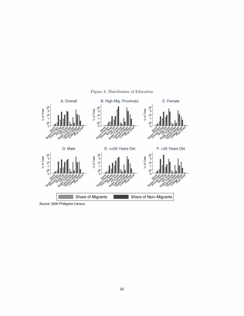
Figure 3: Distribution of Education

0.0

5.1

.15.2

.25

% o

f T

ota

l

Non

e

Some

Primar

y

Primar

y Gra

d

Some

HS

HS G

rad

Some

Training

Training

Gra

d

Some

College

College

Gra

d

Post G

rad

A. Overall

0.0

5.1

.15.2

.25

% o

f T

ota

l

Non

e

Some

Primar

y

Primar

y Gra

d

Some

HS

HS G

rad

Some

Training

Training

Gra

d

Some

College

College

Gra

d

Post G

rad

B. High Mig. Provinces

0.0

5.1

.15.2

.25

% o

f T

ota

l

Non

e

Some

Primar

y

Primar

y Gra

d

Some

HS

HS G

rad

Some

Training

Training

Gra

d

Some

College

College

Gra

d

Post G

rad

C. Female

0.0

5.1

.15.2

.25

% o

f T

ota

l

Non

e

Some

Primar

y

Primar

y Gra

d

Some

HS

HS G

rad

Some

Training

Training

Gra

d

Some

College

College

Gra

d

Post G

rad

D. Male

0.0

5.1

.15.2

.25

% o

f T

ota

l

Non

e

Some

Primar

y

Primar

y Gra

d

Some

HS

HS G

rad

Some

Training

Training

Gra

d

Some

College

College

Gra

d

Post G

rad

E. <=35 Years Old

0.0

5.1

.15.2

.25

% o

f T

ota

l

Non

e

Some

Primar

y

Primar

y Gra

d

Some

HS

HS G

rad

Some

Training

Training

Gra

d

Some

College

College

Gra

d

Post G

rad

F. >35 Years Old

Source: 2000 Philippine Census

Share of Migrants Share of Non−Migrants

46

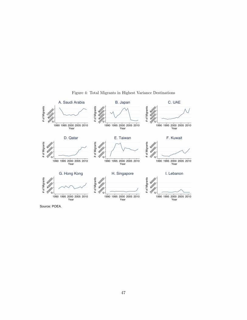
Figure 4: Total Migrants in Highest Variance Destinations

04000

08000

01200

00

# of

Mig

rant

s

1990 1995 2000 2005 2010Year

A. Saudi Arabia

02000

04000

06000

08000

0

# of

Mig

rant

s

1990 1995 2000 2005 2010Year

B. Japan

02000

04000

06000

08000

0

# of

Mig

rant

s

1990 1995 2000 2005 2010Year

C. UAE

02000

04000

06000

0

# of

Mig

rant

s

1990 1995 2000 2005 2010Year

D. Qatar

02000

04000

06000

0

# of

Mig

rant

s

1990 1995 2000 2005 2010Year

E. Taiwan

02000

04000

06000

0#

of M

igra

nts

1990 1995 2000 2005 2010Year

F. Kuwait

02000

04000

06000

0

# of

Mig

rant

s

1990 1995 2000 2005 2010Year

G. Hong Kong

02000

04000

06000

0

# of

Mig

rant

s

1990 1995 2000 2005 2010Year

H. Singapore

02000

04000

06000

0

# of

Mig

rant

s

1990 1995 2000 2005 2010Year

I. Lebanon

Source: POEA.

47

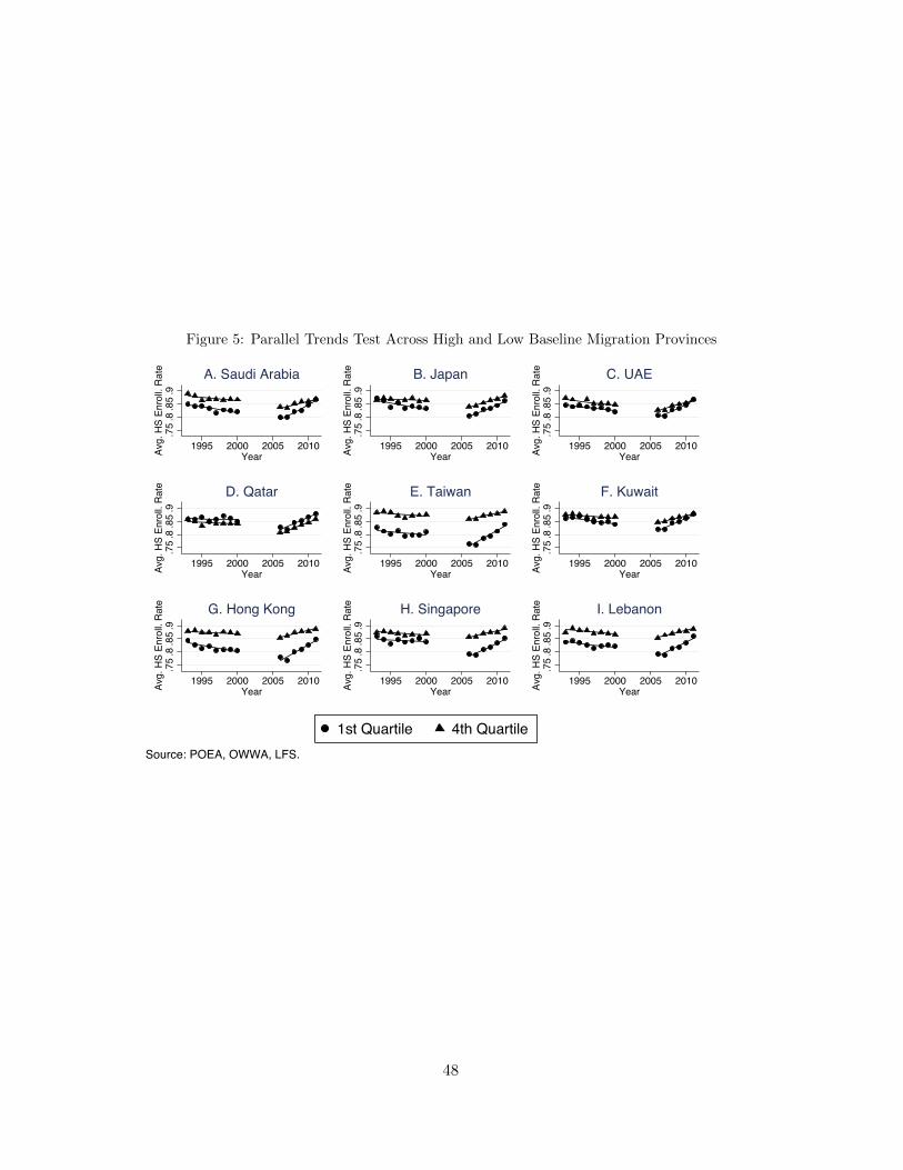
Figure 5: Parallel Trends Test Across High and Low Baseline Migration Provinces

.75

.8.8

5.9

Avg.

HS

Enro

ll. Ra

te

1995 2000 2005 2010Year

A. Saudi Arabia.7

5.8

.85

.9Av

g. H

S En

roll.

Rate

1995 2000 2005 2010Year

B. Japan

.75

.8.8

5.9

Avg.

HS

Enro

ll. Ra

te

1995 2000 2005 2010Year

C. UAE

.75

.8.8

5.9

Avg.

HS

Enro

ll. Ra

te

1995 2000 2005 2010Year

D. Qatar

.75

.8.8

5.9

Avg.

HS

Enro

ll. Ra

te

1995 2000 2005 2010Year

E. Taiwan

.75

.8.8

5.9

Avg.

HS

Enro

ll. Ra

te

1995 2000 2005 2010Year

F. Kuwait

.75

.8.8

5.9

Avg.

HS

Enro

ll. Ra

te

1995 2000 2005 2010Year

G. Hong Kong

.75

.8.8

5.9

Avg.

HS

Enro

ll. Ra

te

1995 2000 2005 2010Year

H. Singapore

.75

.8.8

5.9

Avg.

HS

Enro

ll. Ra

te

1995 2000 2005 2010Year

I. Lebanon

Source: POEA, OWWA, LFS.

1st Quartile 4th Quartile

48

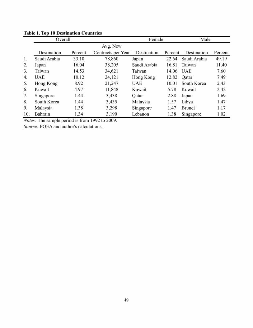
Table 1. Top 10 Destination Countries

Destination PercentAvg. New

Contracts per Year Destination Percent Destination Percent1. Saudi Arabia 33.10 78,860 Japan 22.64 Saudi Arabia 49.192. Japan 16.04 38,205 Saudi Arabia 16.81 Taiwan 11.403. Taiwan 14.53 34,621 Taiwan 14.06 UAE 7.604. UAE 10.12 24,121 Hong Kong 12.82 Qatar 7.495. Hong Kong 8.92 21,247 UAE 10.01 South Korea 2.436. Kuwait 4.97 11,848 Kuwait 5.78 Kuwait 2.427. Singapore 1.44 3,438 Qatar 2.88 Japan 1.698. South Korea 1.44 3,435 Malaysia 1.57 Libya 1.479. Malaysia 1.38 3,298 Singapore 1.47 Brunei 1.1710. Bahrain 1.34 3,190 Lebanon 1.38 Singapore 1.02

Overall Female Male

Source: POEA and author's calculations.Notes: The sample period is from 1992 to 2009.

49

Total % of Total % Female1. Domestic Helpers 1,139,053 23.97 97.462. Performing Artists 696,504 14.66 95.143. Production 328,486 6.91 43.994. Caregivers 238,408 5.02 96.075. Laborers 237,064 4.99 11.886. Medical Workers 214,832 4.52 81.257. Plumbers 197,508 4.16 0.358. Engineers 191,816 4.04 3.489. Cooks and Waiters 163,382 3.44 53.2410. Building Caretakers 140,199 2.95 72.1511. Electrical Workers 137,306 2.89 19.9712. Carpenters 131,314 2.76 0.4113. Machine Fitters 92,946 1.96 2.6914. Tailors and Sewers 87,185 1.83 83.1615. Other Service Workers 80,832 1.70 54.6116. Freight Handlers 74,995 1.58 3.6217. Clerical Workers 63,516 1.34 51.3218. Transport Equipment Operators 52,664 1.11 5.3919. Production Supervisors 43,434 0.91 5.1420. Machine-Tool Operators 39,609 0.83 5.87

4,751,936 60.66

Table 2. Top 20 Occupations for Overseas Contract Workers Occupation

TotalNotes: The sample period is from 1992 to 2009. Occupations that are shaded light grey are over 50% female.Source: POEA and author's calcuations.

50

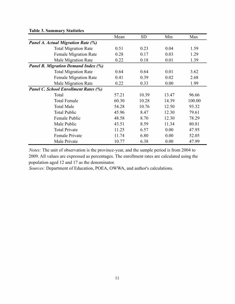
Mean SD Min Max Panel A. Actual Migration Rate (%)

Total Migration Rate 0.51 0.23 0.04 1.59Female Migration Rate 0.28 0.17 0.03 1.29Male Migration Rate 0.22 0.18 0.01 1.39

Panel B. Migration Demand Index (%)Total Migration Rate 0.64 0.64 0.01 3.62Female Migration Rate 0.41 0.39 0.02 2.68Male Migration Rate 0.22 0.33 0.00 1.99

Panel C. School Enrollment Rates (%)Total 57.21 10.39 13.47 96.66Total Female 60.30 10.28 14.39 100.00Total Male 54.28 10.76 12.50 93.32Total Public 45.96 8.47 12.30 79.61Female Public 48.58 8.70 12.30 78.29Male Public 43.51 8.59 11.34 80.81Total Private 11.25 6.57 0.00 47.95Female Private 11.74 6.80 0.00 52.05Male Private 10.77 6.38 0.00 47.99

Table 3. Summary Statistics

Notes: The unit of observation is the province-year, and the sample period is from 2004 to 2009. All values are expressed as percentages. The enrollment rates are calculated using the population aged 12 and 17 as the denominator.Sources: Department of Education, POEA, OWWA, and author's calculations.

51

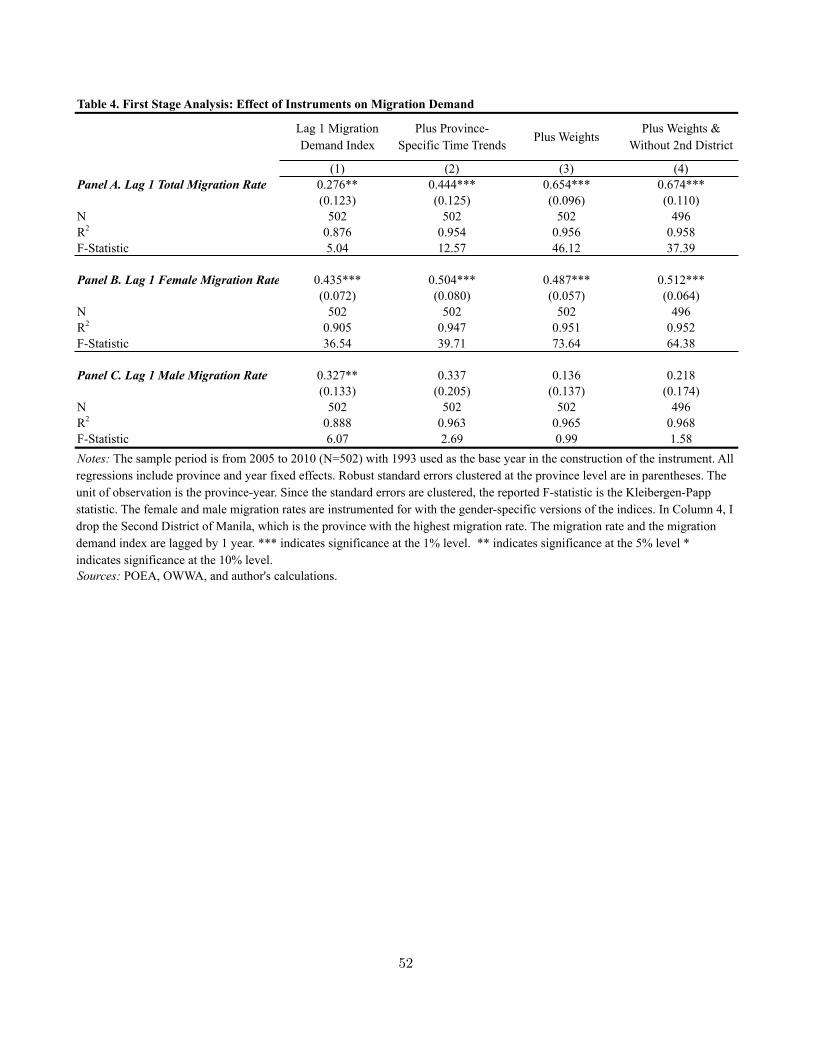
Lag 1 Migration Demand Index

Plus Province-Specific Time Trends

Plus WeightsPlus Weights &

Without 2nd District

(1) (2) (3) (4)Panel A. Lag 1 Total Migration Rate 0.276** 0.444*** 0.654*** 0.674***

(0.123) (0.125) (0.096) (0.110)N 502 502 502 496R2 0.876 0.954 0.956 0.958F-Statistic 5.04 12.57 46.12 37.39

Panel B. Lag 1 Female Migration Rate 0.435*** 0.504*** 0.487*** 0.512***(0.072) (0.080) (0.057) (0.064)

N 502 502 502 496R2 0.905 0.947 0.951 0.952F-Statistic 36.54 39.71 73.64 64.38

Panel C. Lag 1 Male Migration Rate 0.327** 0.337 0.136 0.218(0.133) (0.205) (0.137) (0.174)

N 502 502 502 496R2 0.888 0.963 0.965 0.968F-Statistic 6.07 2.69 0.99 1.58

Table 4. First Stage Analysis: Effect of Instruments on Migration Demand

Notes: The sample period is from 2005 to 2010 (N=502) with 1993 used as the base year in the construction of the instrument. All regressions include province and year fixed effects. Robust standard errors clustered at the province level are in parentheses. The unit of observation is the province-year. Since the standard errors are clustered, the reported F-statistic is the Kleibergen-Papp statistic. The female and male migration rates are instrumented for with the gender-specific versions of the indices. In Column 4, I drop the Second District of Manila, which is the province with the highest migration rate. The migration rate and the migration demand index are lagged by 1 year. *** indicates significance at the 1% level. ** indicates significance at the 5% level * indicates significance at the 10% level. Sources: POEA, OWWA, and author's calculations.

52

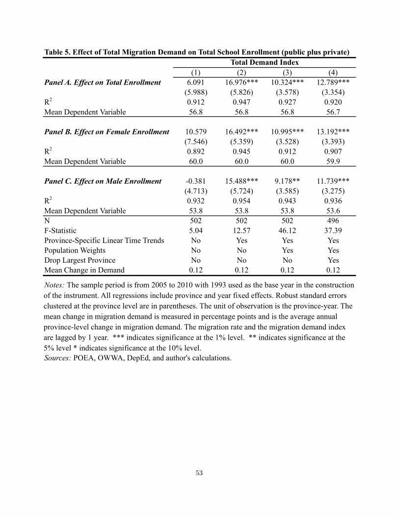
(1) (2) (3) (4)Panel A. Effect on Total Enrollment 6.091 16.976*** 10.324*** 12.789***

(5.988) (5.826) (3.578) (3.354)R2 0.912 0.947 0.927 0.920Mean Dependent Variable 56.8 56.8 56.8 56.7

Panel B. Effect on Female Enrollment 10.579 16.492*** 10.995*** 13.192***(7.546) (5.359) (3.528) (3.393)

R2 0.892 0.945 0.912 0.907Mean Dependent Variable 60.0 60.0 60.0 59.9

Panel C. Effect on Male Enrollment -0.381 15.488*** 9.178** 11.739***(4.713) (5.724) (3.585) (3.275)

R2 0.932 0.954 0.943 0.936Mean Dependent Variable 53.8 53.8 53.8 53.6N 502 502 502 496F-Statistic 5.04 12.57 46.12 37.39Province-Specific Linear Time Trends No Yes Yes YesPopulation Weights No No Yes YesDrop Largest Province No No No YesMean Change in Demand 0.12 0.12 0.12 0.12

Table 5. Effect of Total Migration Demand on Total School Enrollment (public plus private)Total Demand Index

Notes: The sample period is from 2005 to 2010 with 1993 used as the base year in the construction of the instrument. All regressions include province and year fixed effects. Robust standard errors clustered at the province level are in parentheses. The unit of observation is the province-year. The mean change in migration demand is measured in percentage points and is the average annual province-level change in migration demand. The migration rate and the migration demand index are lagged by 1 year. *** indicates significance at the 1% level. ** indicates significance at the 5% level * indicates significance at the 10% level. Sources: POEA, OWWA, DepEd, and author's calculations.

53

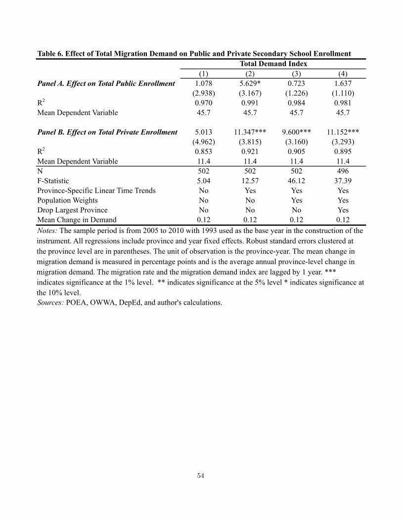
(1) (2) (3) (4)Panel A. Effect on Total Public Enrollment 1.078 5.629* 0.723 1.637

(2.938) (3.167) (1.226) (1.110)R2 0.970 0.991 0.984 0.981Mean Dependent Variable 45.7 45.7 45.7 45.7

Panel B. Effect on Total Private Enrollment 5.013 11.347*** 9.600*** 11.152***(4.962) (3.815) (3.160) (3.293)

R2 0.853 0.921 0.905 0.895Mean Dependent Variable 11.4 11.4 11.4 11.4N 502 502 502 496F-Statistic 5.04 12.57 46.12 37.39Province-Specific Linear Time Trends No Yes Yes YesPopulation Weights No No Yes YesDrop Largest Province No No No YesMean Change in Demand 0.12 0.12 0.12 0.12

Sources: POEA, OWWA, DepEd, and author's calculations.

Total Demand IndexTable 6. Effect of Total Migration Demand on Public and Private Secondary School Enrollment

Notes: The sample period is from 2005 to 2010 with 1993 used as the base year in the construction of the instrument. All regressions include province and year fixed effects. Robust standard errors clustered at the province level are in parentheses. The unit of observation is the province-year. The mean change in migration demand is measured in percentage points and is the average annual province-level change in migration demand. The migration rate and the migration demand index are lagged by 1 year. *** indicates significance at the 1% level. ** indicates significance at the 5% level * indicates significance at the 10% level.

54

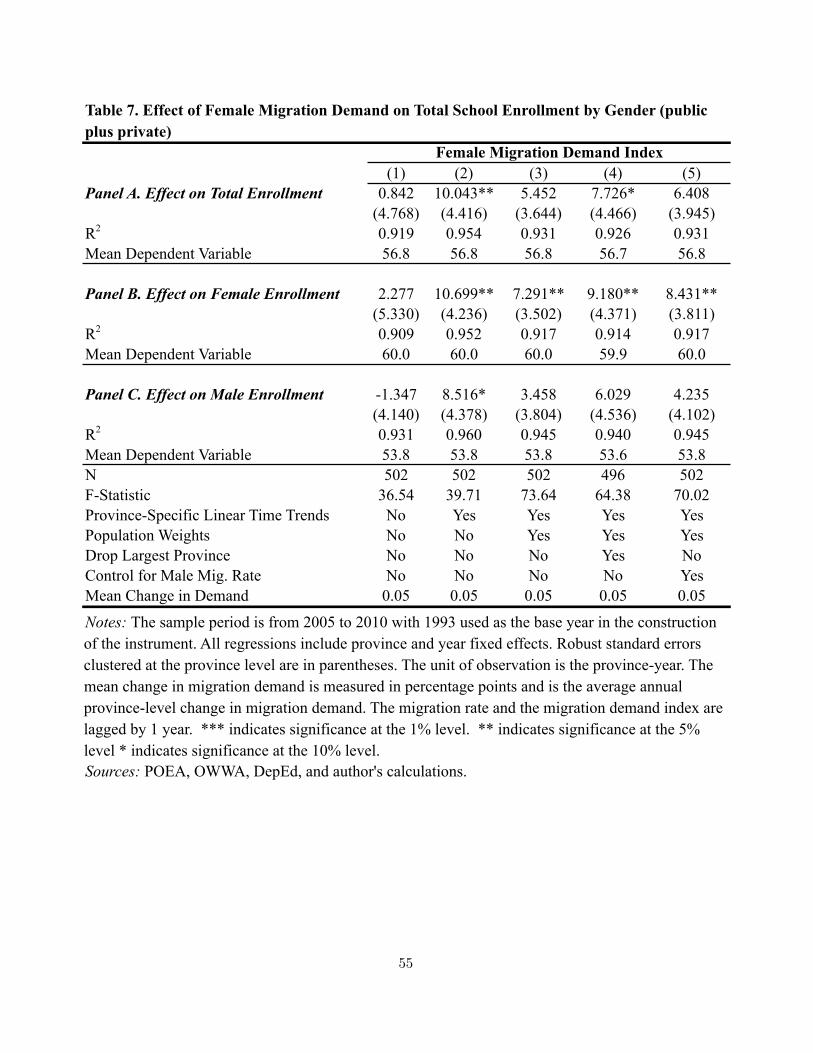
(1) (2) (3) (4) (5)Panel A. Effect on Total Enrollment 0.842 10.043** 5.452 7.726* 6.408

(4.768) (4.416) (3.644) (4.466) (3.945)R2 0.919 0.954 0.931 0.926 0.931Mean Dependent Variable 56.8 56.8 56.8 56.7 56.8

Panel B. Effect on Female Enrollment 2.277 10.699** 7.291** 9.180** 8.431**(5.330) (4.236) (3.502) (4.371) (3.811)

R2 0.909 0.952 0.917 0.914 0.917Mean Dependent Variable 60.0 60.0 60.0 59.9 60.0

Panel C. Effect on Male Enrollment -1.347 8.516* 3.458 6.029 4.235(4.140) (4.378) (3.804) (4.536) (4.102)

R2 0.931 0.960 0.945 0.940 0.945Mean Dependent Variable 53.8 53.8 53.8 53.6 53.8N 502 502 502 496 502F-Statistic 36.54 39.71 73.64 64.38 70.02Province-Specific Linear Time Trends No Yes Yes Yes YesPopulation Weights No No Yes Yes YesDrop Largest Province No No No Yes NoControl for Male Mig. Rate No No No No YesMean Change in Demand 0.05 0.05 0.05 0.05 0.05

Sources: POEA, OWWA, DepEd, and author's calculations.

Female Migration Demand Index

Table 7. Effect of Female Migration Demand on Total School Enrollment by Gender (public plus private)

Notes: The sample period is from 2005 to 2010 with 1993 used as the base year in the construction of the instrument. All regressions include province and year fixed effects. Robust standard errors clustered at the province level are in parentheses. The unit of observation is the province-year. The mean change in migration demand is measured in percentage points and is the average annual province-level change in migration demand. The migration rate and the migration demand index are lagged by 1 year. *** indicates significance at the 1% level. ** indicates significance at the 5% level * indicates significance at the 10% level.

55

(1) (2)Panel A. Total Public Enrollment 2.937* -0.378

(1.549) (1.240)R2 0.989 0.981Mean Dependent Variable 45.7 45.7Panel B. Total Private Enrollment 7.106** 5.830*

(3.590) (3.194)R2 0.928 0.911Mean Dependent Variable 11.4 11.4Panel C. Female Public Enrollment 2.907* 0.012

(1.501) (1.197)R2 0.989 0.982Mean Dependent Variable 48.5 48.5Panel D. Male Public Enrollment 2.959* -0.762

(1.653) (1.370)R2 0.989 0.982Mean Dependent Variable 43.2 43.2Panel E. Female Private Enrollment 7.792** 7.279**

(3.518) (3.147)R2 0.929 0.906Mean Dependent Variable 11.6 11.6Panel F. Male Private Enrollment 5.557 4.219

(3.479) (3.244)R2 0.929 0.916Mean Dependent Variable 10.7 10.7N 502 502F-Statistic 44.56 71.28Population Weights No YesMean Change in Demand 0.05 0.05

Female Migration Demand Index

Notes: The sample period is from 2005 to 2010 with 1993 used as the base year in the construction of the instrument. All regressions include province and year fixed effects and province-specific linear time trends. Robust standard errors clustered at the province level are in parentheses. The unit of observation is the province-year. The mean change in migration demand is measured in percentage points and is the average annual province-level change in migration demand. The migration rate and the migration demand index are lagged by 1 year. *** indicates significance at the 1% level. ** indicates significance at the 5% level * indicates significance at the 10% level. Sources: POEA, OWWA, DepEd, and author's calculations.

Table 8. Effect of Female Migration Demand on Public and Private School Enrollment

56

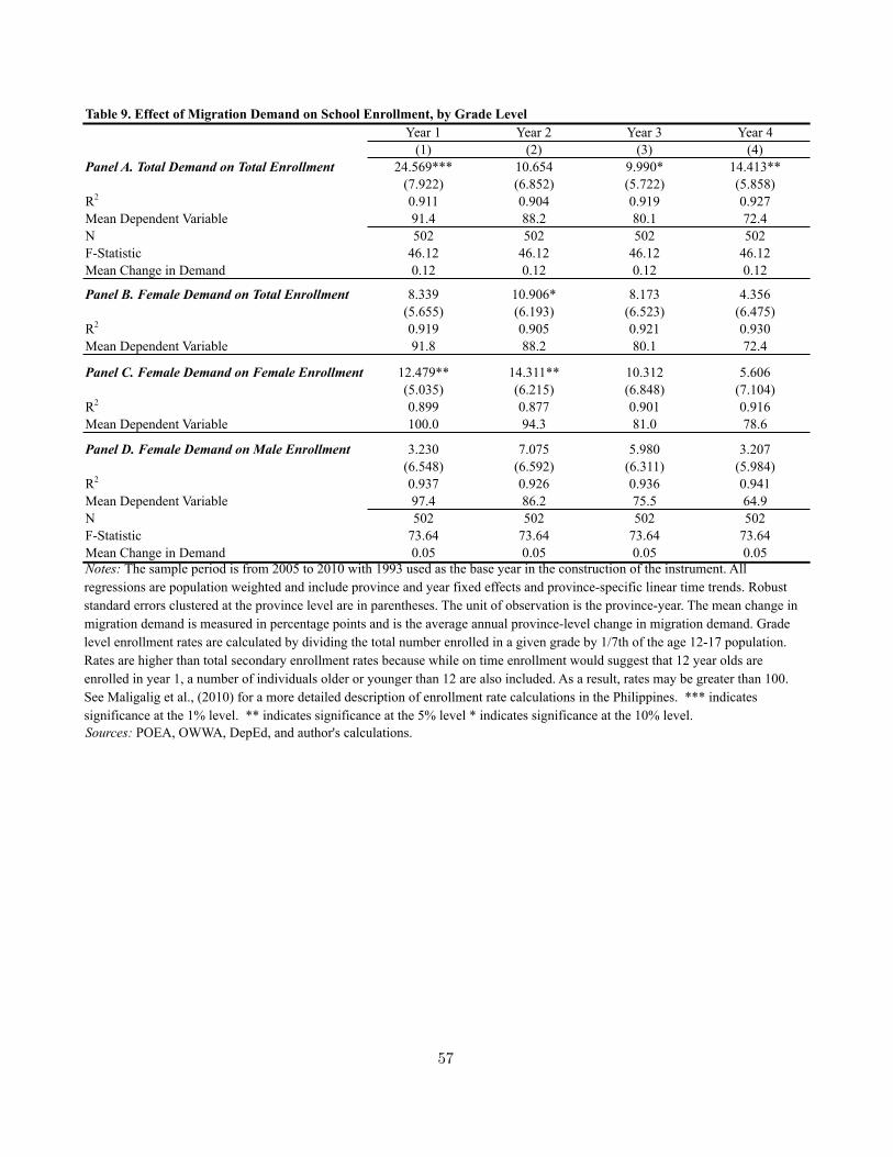
Year 1 Year 2 Year 3 Year 4(1) (2) (3) (4)

Panel A. Total Demand on Total Enrollment 24.569*** 10.654 9.990* 14.413**(7.922) (6.852) (5.722) (5.858)

R2 0.911 0.904 0.919 0.927Mean Dependent Variable 91.4 88.2 80.1 72.4N 502 502 502 502F-Statistic 46.12 46.12 46.12 46.12Mean Change in Demand 0.12 0.12 0.12 0.12

Panel B. Female Demand on Total Enrollment 8.339 10.906* 8.173 4.356(5.655) (6.193) (6.523) (6.475)

R2 0.919 0.905 0.921 0.930Mean Dependent Variable 91.8 88.2 80.1 72.4

Panel C. Female Demand on Female Enrollment 12.479** 14.311** 10.312 5.606(5.035) (6.215) (6.848) (7.104)

R2 0.899 0.877 0.901 0.916Mean Dependent Variable 100.0 94.3 81.0 78.6

Panel D. Female Demand on Male Enrollment 3.230 7.075 5.980 3.207(6.548) (6.592) (6.311) (5.984)

R2 0.937 0.926 0.936 0.941Mean Dependent Variable 97.4 86.2 75.5 64.9N 502 502 502 502F-Statistic 73.64 73.64 73.64 73.64Mean Change in Demand 0.05 0.05 0.05 0.05

Sources: POEA, OWWA, DepEd, and author's calculations.

Table 9. Effect of Migration Demand on School Enrollment, by Grade Level

Notes: The sample period is from 2005 to 2010 with 1993 used as the base year in the construction of the instrument. All regressions are population weighted and include province and year fixed effects and province-specific linear time trends. Robust standard errors clustered at the province level are in parentheses. The unit of observation is the province-year. The mean change in migration demand is measured in percentage points and is the average annual province-level change in migration demand. Grade level enrollment rates are calculated by dividing the total number enrolled in a given grade by 1/7th of the age 12-17 population. Rates are higher than total secondary enrollment rates because while on time enrollment would suggest that 12 year olds are enrolled in year 1, a number of individuals older or younger than 12 are also included. As a result, rates may be greater than 100. See Maligalig et al., (2010) for a more detailed description of enrollment rate calculations in the Philippines. *** indicates significance at the 1% level. ** indicates significance at the 5% level * indicates significance at the 10% level.

57

Appendix A Heterogeneity By Grade Level

In Section 3, I assume that parents make the decision whether or not to enroll their child in high

school and consider two levels of schooling, high school graduate and less than a high school

graduate. I test this empirically by examining the effects of migration demand on aggregate

secondary school enrollment. However, examining the effects on aggregate enrollment across

all grades may miss potentially interesting dynamics. By testing for differential responses

of grade level enrollments to migration demand, it is possible to further shed light on the

mechanisms through which migration affects overall secondary school enrollment, namely by

identifying the marginal students induced into schooling by changes in migration demand.

Understanding both the location of the marginal student in the education distribution and

the mechanisms through which they are induced in can help policymakers design policies to

increase human capital that are targeted at these students. The responses to migration demand

depend on the distribution across grades of unenrolled students from both unconstrained and

constrained households as well as the benefits to partial completion of high school. Thus

far, by comparing the wage premium for high school graduates compared to non-high school

graduates, I have essentially assumed there is no benefit to partial completion of high school.

I relax this assumption below.

First, however, consider the case where there is no benefit to partial completion of high

school. There will be a reduced probability of drop out in each subsequent year of high school,

with the bulk of unenrolled students dropping out prior to year one. Unconstrained households

may revise their education decision in response to a change in income or the expected wage

premium. Constrained households may revise their decision in response to a change in the

expected wage premium or a negative income shock, but they will only be able to respond

positively through the income channel if they experience a loosening of liquidity constraints.

Since most unenrolled students will drop out prior to year one of high school, I anticipate

that there will be a bunching on year one enrollment from either the income channel or the

expected wage premium channel.58

Now assume there are benefits to partial completion of high school, and students may

58Such bunching at year one could also occur due to fixed costs of high school that force a number of studentsto drop out at this point in their education.

58

drop out in any grade. Dropout rates in the Philippines decline by grade level.59 Thus, I

anticipate that the enrollment response for both constrained and unconstrained households to

the income channel will simply follow where marginal students are located in the education

distribution and will have the largest effect on year one with smaller effects on each subsequent

year.60 Again, the wage premium can only increase education for constrained households if

they also experience a loosening of the liquidity constraint. One might expect changes in the

wage premium to have the largest effect on those entering the fourth year of high school, since

labor market conditions are more likely to persist until these students graduate and enter the

labor force than for first year students. However, since dropout rates decline by grade level,

depending on the probability that parents assign to the chance that labor market conditions

will persist, any pattern of enrollment responses is possible. Based on these potential scenarios,

the location in the education distribution of marginal students induced into schooling by

increased migration demand is ambiguous. I test these predictions empirically in Section 6.4.

59Author’s calculations from Philippine Department of Education data.60This could, however, be more nuanced for parents with more than one child. In the event that the household

receives just enough extra income to send one child to school for one more year, sheepskin effects may meanthat the parent may enroll the older student rather than the younger student.

59

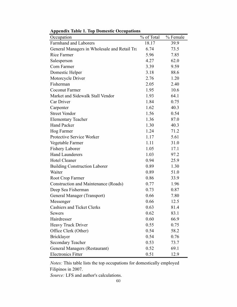
Occupation % of Total % FemaleFarmhand and Laborers 18.17 39.9General Managers in Wholesale and Retail Trade 6.74 73.5Rice Farmer 5.96 7.85Salesperson 4.27 62.0Corn Farmer 3.39 9.59Domestic Helper 3.18 88.6Motorcycle Driver 2.76 1.20Fisherman 2.05 2.40Coconut Farmer 1.95 10.6Market and Sidewalk Stall Vendor 1.93 64.1Car Driver 1.84 0.75Carpenter 1.62 40.3Street Vendor 1.56 0.54Elementary Teacher 1.36 87.0Hand Packer 1.30 40.3Hog Farmer 1.24 71.2Protective Service Worker 1.17 5.61Vegetable Farmer 1.11 31.0Fishery Laborer 1.05 17.1Hand Launderers 1.03 97.2Hotel Cleaner 0.94 25.9Building Construction Laborer 0.89 1.30Waiter 0.89 51.0Root Crop Farmer 0.86 33.9Construction and Maintenance (Roads) 0.77 1.96Deep Sea Fisherman 0.73 0.87General Manager (Transport) 0.66 7.80Messenger 0.66 12.5Cashiers and Ticket Clerks 0.63 81.4Sewers 0.62 83.1Hairdresser 0.60 66.9Heavy Truck Driver 0.55 0.75Office Clerk (Other) 0.54 58.2Bricklayer 0.54 0.76Secondary Teacher 0.53 73.7General Managers (Restaurant) 0.52 69.1Electronics Fitter 0.51 12.9

Source: LFS and author's calculations.

Appendix Table 1. Top Domestic Occupations

Notes: This table lists the top occupations for domestically employed Filipinos in 2007.

60

Destination Occupation Occupation x Destination(1) (2) (3)

Panel A. Total Migration Demand Index 10.324*** 6.038 4.858(3.578) (5.815) (3.354)

N 502 502 502R2 0.927 0.930 0.930F-Statistic 46.12 24.06 38.06

Panel B. Female Migration Demand Index 5.452 8.430*** 7.875***(3.644) (2.770) (2.611)

N 502 502 502R2 0.931 0.931 0.931F-Statistic 73.64 71.38 145.74

Index TypeAppendix Table 2. Effect of Total and Female Migration Demand on Total Secondary Enrollment, by Index Type

Notes: The sample period is from 2004 to 2009 with 1993 used as the base year in the construction of the instrument. Column 1 uses the destination-based index which is used for the main analysis. Column 2 creates the index in the same manner, but instead of destinations, it uses 38 occupation categories. Column 3 uses 38 x 32 occupation-destination groups to create the instrument. All regressions include province and year fixed effects as well as province-specific linear time trends. Robust standard errors clustered at the province level are in parentheses. The unit of observation is the province-year. The mean change in migration demand is measured in percentage points and is the average annual province-level change in migration demand. *** indicates significance at the 1% level. ** indicates significance at the 5% level * indicates significance at the 10% level. Sources: POEA, OWWA, DepEd, and author's calculations.

61

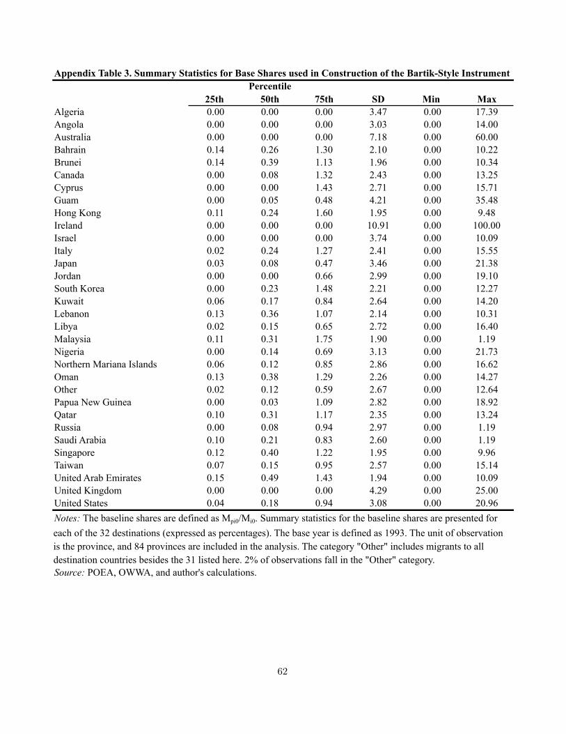
25th 50th 75th SD Min MaxAlgeria 0.00 0.00 0.00 3.47 0.00 17.39Angola 0.00 0.00 0.00 3.03 0.00 14.00Australia 0.00 0.00 0.00 7.18 0.00 60.00Bahrain 0.14 0.26 1.30 2.10 0.00 10.22Brunei 0.14 0.39 1.13 1.96 0.00 10.34Canada 0.00 0.08 1.32 2.43 0.00 13.25Cyprus 0.00 0.00 1.43 2.71 0.00 15.71Guam 0.00 0.05 0.48 4.21 0.00 35.48Hong Kong 0.11 0.24 1.60 1.95 0.00 9.48Ireland 0.00 0.00 0.00 10.91 0.00 100.00Israel 0.00 0.00 0.00 3.74 0.00 10.09Italy 0.02 0.24 1.27 2.41 0.00 15.55Japan 0.03 0.08 0.47 3.46 0.00 21.38Jordan 0.00 0.00 0.66 2.99 0.00 19.10South Korea 0.00 0.23 1.48 2.21 0.00 12.27Kuwait 0.06 0.17 0.84 2.64 0.00 14.20Lebanon 0.13 0.36 1.07 2.14 0.00 10.31Libya 0.02 0.15 0.65 2.72 0.00 16.40Malaysia 0.11 0.31 1.75 1.90 0.00 1.19Nigeria 0.00 0.14 0.69 3.13 0.00 21.73Northern Mariana Islands 0.06 0.12 0.85 2.86 0.00 16.62Oman 0.13 0.38 1.29 2.26 0.00 14.27Other 0.02 0.12 0.59 2.67 0.00 12.64Papua New Guinea 0.00 0.03 1.09 2.82 0.00 18.92Qatar 0.10 0.31 1.17 2.35 0.00 13.24Russia 0.00 0.08 0.94 2.97 0.00 1.19Saudi Arabia 0.10 0.21 0.83 2.60 0.00 1.19Singapore 0.12 0.40 1.22 1.95 0.00 9.96Taiwan 0.07 0.15 0.95 2.57 0.00 15.14United Arab Emirates 0.15 0.49 1.43 1.94 0.00 10.09United Kingdom 0.00 0.00 0.00 4.29 0.00 25.00United States 0.04 0.18 0.94 3.08 0.00 20.96

PercentileAppendix Table 3. Summary Statistics for Base Shares used in Construction of the Bartik-Style Instrument

Notes: The baseline shares are defined as Mpi0/Mi0. Summary statistics for the baseline shares are presented for each of the 32 destinations (expressed as percentages). The base year is defined as 1993. The unit of observation is the province, and 84 provinces are included in the analysis. The category "Other" includes migrants to all destination countries besides the 31 listed here. 2% of observations fall in the "Other" category.Source: POEA, OWWA, and author's calculations.

62

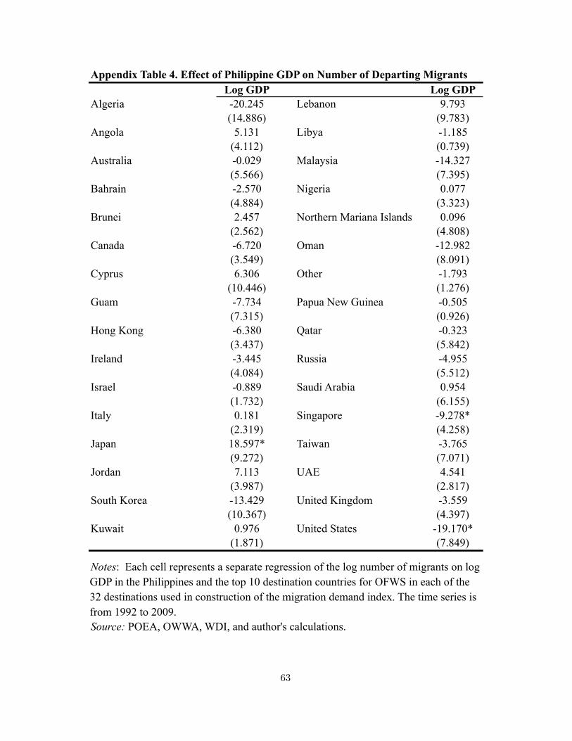
Log GDP Log GDPAlgeria -20.245 Lebanon 9.793

(14.886) (9.783)Angola 5.131 Libya -1.185

(4.112) (0.739)Australia -0.029 Malaysia -14.327

(5.566) (7.395)Bahrain -2.570 Nigeria 0.077

(4.884) (3.323)Brunei 2.457 Northern Mariana Islands 0.096

(2.562) (4.808)Canada -6.720 Oman -12.982

(3.549) (8.091)Cyprus 6.306 Other -1.793

(10.446) (1.276)Guam -7.734 Papua New Guinea -0.505

(7.315) (0.926)Hong Kong -6.380 Qatar -0.323

(3.437) (5.842)Ireland -3.445 Russia -4.955

(4.084) (5.512)Israel -0.889 Saudi Arabia 0.954

(1.732) (6.155)Italy 0.181 Singapore -9.278*

(2.319) (4.258)Japan 18.597* Taiwan -3.765

(9.272) (7.071)Jordan 7.113 UAE 4.541

(3.987) (2.817)South Korea -13.429 United Kingdom -3.559

(10.367) (4.397)Kuwait 0.976 United States -19.170*

(1.871) (7.849)

Source: POEA, OWWA, WDI, and author's calculations.

Appendix Table 4. Effect of Philippine GDP on Number of Departing Migrants

Notes: Each cell represents a separate regression of the log number of migrants on log GDP in the Philippines and the top 10 destination countries for OFWS in each of the 32 destinations used in construction of the migration demand index. The time series is from 1992 to 2009.

63

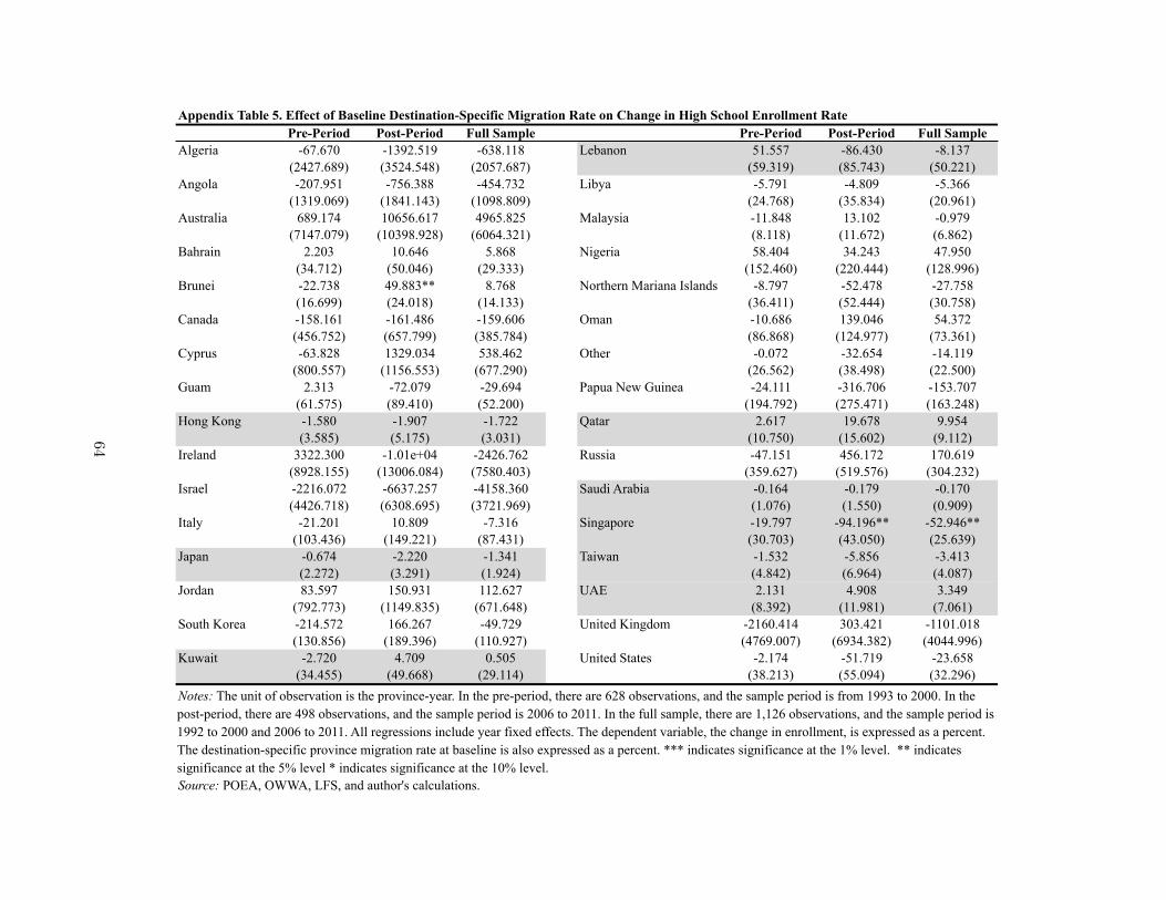
Pre-Period Post-Period Full Sample Pre-Period Post-Period Full SampleAlgeria -67.670 -1392.519 -638.118 Lebanon 51.557 -86.430 -8.137

(2427.689) (3524.548) (2057.687) (59.319) (85.743) (50.221)Angola -207.951 -756.388 -454.732 Libya -5.791 -4.809 -5.366

(1319.069) (1841.143) (1098.809) (24.768) (35.834) (20.961)Australia 689.174 10656.617 4965.825 Malaysia -11.848 13.102 -0.979

(7147.079) (10398.928) (6064.321) (8.118) (11.672) (6.862)Bahrain 2.203 10.646 5.868 Nigeria 58.404 34.243 47.950

(34.712) (50.046) (29.333) (152.460) (220.444) (128.996)Brunei -22.738 49.883** 8.768 Northern Mariana Islands -8.797 -52.478 -27.758

(16.699) (24.018) (14.133) (36.411) (52.444) (30.758)Canada -158.161 -161.486 -159.606 Oman -10.686 139.046 54.372

(456.752) (657.799) (385.784) (86.868) (124.977) (73.361)Cyprus -63.828 1329.034 538.462 Other -0.072 -32.654 -14.119

(800.557) (1156.553) (677.290) (26.562) (38.498) (22.500)Guam 2.313 -72.079 -29.694 Papua New Guinea -24.111 -316.706 -153.707

(61.575) (89.410) (52.200) (194.792) (275.471) (163.248)Hong Kong -1.580 -1.907 -1.722 Qatar 2.617 19.678 9.954

(3.585) (5.175) (3.031) (10.750) (15.602) (9.112)Ireland 3322.300 -1.01e+04 -2426.762 Russia -47.151 456.172 170.619

(8928.155) (13006.084) (7580.403) (359.627) (519.576) (304.232)Israel -2216.072 -6637.257 -4158.360 Saudi Arabia -0.164 -0.179 -0.170

(4426.718) (6308.695) (3721.969) (1.076) (1.550) (0.909)Italy -21.201 10.809 -7.316 Singapore -19.797 -94.196** -52.946**

(103.436) (149.221) (87.431) (30.703) (43.050) (25.639)Japan -0.674 -2.220 -1.341 Taiwan -1.532 -5.856 -3.413

(2.272) (3.291) (1.924) (4.842) (6.964) (4.087)Jordan 83.597 150.931 112.627 UAE 2.131 4.908 3.349

(792.773) (1149.835) (671.648) (8.392) (11.981) (7.061)South Korea -214.572 166.267 -49.729 United Kingdom -2160.414 303.421 -1101.018

(130.856) (189.396) (110.927) (4769.007) (6934.382) (4044.996)Kuwait -2.720 4.709 0.505 United States -2.174 -51.719 -23.658

(34.455) (49.668) (29.114) (38.213) (55.094) (32.296)

Source: POEA, OWWA, LFS, and author's calculations.

Appendix Table 5. Effect of Baseline Destination-Specific Migration Rate on Change in High School Enrollment Rate

Notes: The unit of observation is the province-year. In the pre-period, there are 628 observations, and the sample period is from 1993 to 2000. In the post-period, there are 498 observations, and the sample period is 2006 to 2011. In the full sample, there are 1,126 observations, and the sample period is 1992 to 2000 and 2006 to 2011. All regressions include year fixed effects. The dependent variable, the change in enrollment, is expressed as a percent. The destination-specific province migration rate at baseline is also expressed as a percent. *** indicates significance at the 1% level. ** indicates significance at the 5% level * indicates significance at the 10% level.

64

(1) (2)0.066 -0.196*

(0.109) (0.104)N 501 501R2 0.982 0.985

Appendix Table 6. Identification Check for Gender-Specific Demand Indices

Notes: The sample period is from 2005 to 2010 with 1993 used as the base year in the construction of the instrument. All regressions include province and year fixed effects as well as province-specific linear time trends. Robust standard errors clustered at the province level are in parentheses. The unit of observation is the province-year. *** indicates significance at the 1% level. ** indicates significance at the 5% level * indicates significance at the 10% level. Sources: POEA, OWWA, DepEd, and author's calculations.

Effect of Male Migration Rate on Female Index

Effect of Female Migration Rate on Male Index

65

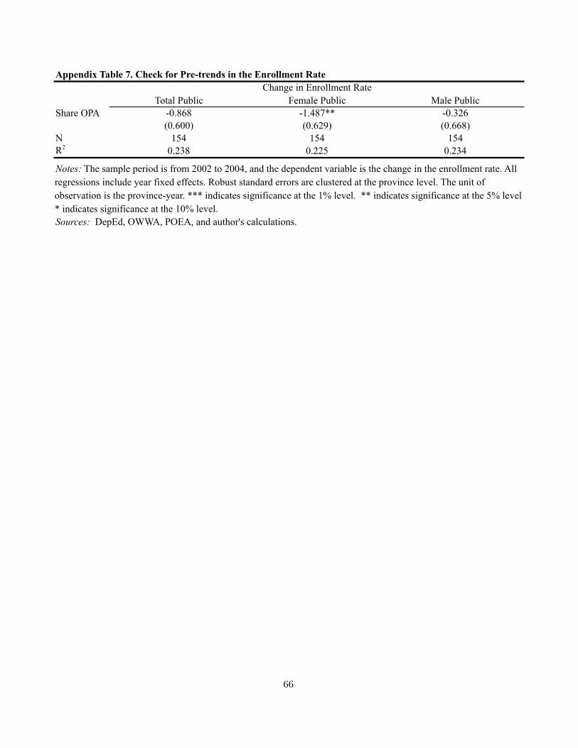
Total Public Female Public Male PublicShare OPA -0.868 -1.487** -0.326

(0.600) (0.629) (0.668)N 154 154 154R2 0.238 0.225 0.234

Sources: DepEd, OWWA, POEA, and author's calculations.

Appendix Table 7. Check for Pre-trends in the Enrollment RateChange in Enrollment Rate

Notes: The sample period is from 2002 to 2004, and the dependent variable is the change in the enrollment rate. All regressions include year fixed effects. Robust standard errors are clustered at the province level. The unit of observation is the province-year. *** indicates significance at the 1% level. ** indicates significance at the 5% level * indicates significance at the 10% level.

66