manifolds of classical probability distributions and ... · from a different point of view, the...

Information Geometry (2019) 2:231–271https://doi.org/10.1007/s41884-019-00022-1

RESEARCH PAPER

Manifolds of classical probability distributions andquantum density operators in infinite dimensions

F. M. Ciaglia1 · A. Ibort2 · J. Jost1 · G. Marmo3

Received: 12 June 2019 / Revised: 10 September 2019 / Published online: 24 October 2019© The Author(s) 2019

AbstractThe manifold structure of subsets of classical probability distributions and quantumdensity operators in infinite dimensions is investigated in the context of C∗-algebrasand actions of Banach-Lie groups. Specificaly, classical probability distributions andquantum density operators may be both described as states (in the functional analyticsense) on a givenC∗-algebraA which is Abelian for Classical states, and non-Abelianfor Quantum states. In this contribution, the space of states S of a possibly infinite-dimensional, unital C∗-algebra A is partitioned into the disjoint union of the orbitsof an action of the group G of invertible elements of A . Then, we prove that theorbits through density operators on an infinite-dimensional, separable Hilbert spaceH are smooth, homogeneous Banach manifolds of G = GL(H), and, whenA admitsa faithful tracial state τ like it happens in the Classical case when we consider prob-ability distributions with full support, we prove that the orbit through τ is a smooth,homogeneous Banach manifold for G .

Keywords Probability distributions · Quantum states · C∗-algebras · Banachmanifolds · Homogeneous spaces

B F. M. [email protected]

A. [email protected]

J. [email protected]

G. [email protected]

1 Max Planck Institute for Mathematics in the Sciences, Leipzig, Germany

2 ICMAT, Instituto de Ciencias Matemáticas (CSIC-UAM-UC3M-UCM), Departamento deMatemáticas, University Carlos III de Madrid, Leganés, Madrid, Spain

3 INFN-Sezione di Napoli, Naples, Italy

123

http://crossmark.crossref.org/dialog/?doi=10.1007/s41884-019-00022-1&domain=pdf

http://orcid.org/0000-0002-8987-1181

232 Information Geometry (2019) 2:231–271

1 Introduction

The use of differential geometric methods in the context of classical and quantuminformation theory is a well-established and flourishing trend. This has led to the birthof new perspectives in the understanding of theoretical issues, as well as to numerousachievements in the realm of applications. At the heart of this methodological attitudetowards classical and quantum information geometry there is the notion of a smoothmanifold. This clearly follows from the fact that differential geometry deals withsmooth manifolds and with all the additional structures with which smooth manifoldsmay be dressed. However, the smooth manifolds employed in the vast majority ofthe literature pertaining to classical and quantum information geometry are finite-dimensional. This is essentially due to the fact that working with infinite-dimensionalmanifolds requires to carefully handle a nontrivial number of technical issues, and thesetechnicalities may obscure the conceptual ideas one wants to convey. Consequently,it has been, and it still is useful to focus on finite-dimensional systems in order toexplicitly develop new ideas, and to postpone the analysis of the infinite-dimensionalsystems to later times. On the other hand, the number of conceptual results on finite-dimensional systems is growing so rapidly that we may dare to say to have a well-estabilished theoretical backbone for the information geometry of finite-dimensionalsystems so that it is reasonable to start looking inmore detail at the infinite-dimensionalsystems.

Of course, there already have been contributions in the information geometry ofinfinite-dimensional systems. For instance, in [50], a Banach manifold structure isgiven to the set Mμ of all probability measures on some measure space (X ,Σ) thatare mutually absolutely continuous with respect to a given probability measure μ on(X ,Σ) by means of Orlicz spaces, and, in [29], the infinite-dimensional analogue ofthe α-connections of Amari and Cencov on this class of manifolds is studied. Orliczspaces were also employed in the quantum framework in [33,53] to build a Banachmanifold structure on Gibbs-like density operators on an infinite-dimensional, com-plex, separable Hilbert space H, and in [39,40] to build a Banach manifold structureon the space of faithful, normal states on an abstract von Neumann algebra.

In [27], a Hilbert manifold was obtained by equipping the space of L2-probabilitymeasures with the Fisher metric. In [47], a Hilbert manifold structure is given to asubset of Mμ characterized by some constraint relations, and the α-connections on itare studied. In [12], the uniqueness (up to rescaling) of the Fisher–Rao metric tensoron the Frechet manifold Prob(M) of smooth positive densities normalized to 1 on asmooth, compact manifold M under the requirement of invariance with respect to thegroup of diffeomorphisms of M is solved.

In [8–10], a new approach to infinite-dimensional parametric models of probabilitymeasures on some measure space is taken, and tensorial structures are obtained byexploiting the natural immersion of the space of probability measures into the Banachspace of signed finite measures (where the norm is given by the total variation). Thismakes the theory independent of the choice of a reference measure, as everythingtransforms appropriately and integrability conditions are preservedwhen the referencemeasure is changed.

123

Information Geometry (2019) 2:231–271 233

From a different point of view, the structure of infinite dimensional groupshas been treated exhaustively in relation with mathematical physics problems, likehydrodynamical-like equations for instance, involving probability densities. It wasrealized that the proper way to deal with such problems was to consider a weaker formof differentiability called IHL-Lie groups introduced by Omori [48] (see for instance[2] and references therein).

In the context of quantum information theory, the geometrization of someof the rele-vant structures, for instance the Kähler–Hilbert manifold structure on the space of purequantum states given by the complex projective space of an infinite-dimensional, com-plex, separableHilbert spaceH, togetherwith aHamiltonian formulation of the unitaryevolutions of quantummechanics, as given for instance in [7,23–25,43], allows a sim-pler treatment of the differentiable structures of the corresponding infinite-dimensionalgroups present in the theory as it is shown in [4–6,13,16,32,44], where the action ofBanach-Lie groups of unitary operators on an infinite-dimensional, complex, separa-ble Hilbert spaceH is used to give a Banach manifold structure to appropriate subsetsof quantum density operators, positive semidefinite linear operators and elements ofBanach Lie-Poisson spaces or, as it will be shown in this paper, to certain orbits of thegroup of invertible elements on a C∗-algebra.

The purpose of this contribution is to look at infinite-dimensional systems in bothclassical and quantum information geometry from the unifying perspective comingfrom the interplay between the theory of C∗-algebras and the infinite-dimensionaldifferential geometry of Banach manifolds and Banach-Lie groups. The choice ofC∗-algebras as a main ingredient is due to the fact that classical spaces of probabil-ity distributions as well as spaces of quantum states are both concrete realizationsof the same mathematical object, i.e., the space S of (mathematical) states on aC∗-algebra A , with the classical case characterized by the requirement that A isAbelian.

Let us explain the motivations behind our idea by looking at a finite-dimensionalexample. Consider a quantum system described by a finite-dimensional Hilbert spaceHwith dim(H) = N < ∞. According to the formalism of standard quantummechan-ics, a (bounded) observable a of the system is an element of the algebra B(H) ofbounded, linear operators on H, while a state ρ of the system is a positive linearfunctional on H such that ρ(I) = 1, where I ∈ B(H) is the identity operator. Sincedim(H) = N < ∞, we may identify the dual space of B(H) with B(H) itself bymeans of the trace operation Tr on H, that is, an element ξ ∈ B(H) determines alinear functional on B(H) by means of

ξ(a) := Tr(ξ a), (1)

and every linear functional on B(H) is of this form. Consequently, a quantum statemay be identifiedwith a so-called density operator onH, that is, a self-adjoint, positivesemidefinite, linear operator ρ such that Tr(ρ) = 1. The set of all density operatorsonH is denoted byS (H), and it is a convex body in the affine hyperplane T1(H) ofself-adjoint, linear operators with unit trace. The interior ofS (H) inT1(H) is an openconvex set made of invertible (full-rank) density operators and denoted by SN (H).Being an open set in the affine hyperplane T1(H), the set SN (H) admits a natural

123


structure of smooth manifold modelled on T1(H), and this manifold structure makesSN (H) the subject of application of the methods of classical information geometryin the context of quantum information (see [11,28,36,37,46,49]). Note that, if weconsider the subset Sρ(H) of density operators commuting with a fixed ρ ∈ S andmutually-commuting with each other, the spectral theorem assures us that Sρ(H)

may be identified with the N -dimensional simplex representing classical probabilitydistributions on a finite sample space.

The manifold structure on SN (H) is compatible with an action of the Lie groupG (H) of invertible linear operators on S (H). Specifically, if g ∈ G (H) and ρ ∈SN (H), we may define the map1

(g, ρ) �→ g ρ g†

Tr(g ρ g†), (2)

an this map defines a smooth, transitive action of G (H) on SN (H). In particular, ifwe consider the subgroup U(H) of unitary operators, we obtain the co-adjoint actionU ρ U† ofU(H) the orbits of which are density operators with fixed eigenvalues. Fromthis, it is clear that the manifold SN (H) carries also the structure of homogeneousspace of the Lie group G (H), and it is precisely this feature that we aim to extend tothe infinite-dimensional setting.

The paper is structured as follows. In Sect. 2, given a possibly infinite-dimensional,unital C∗-algebraA , we will first define a linear action α of the Banach-Lie group Gof invertible elements of A on the space A ∗

sa of self-adjoint linear functionals on Athat preserves the cone of positive linear functionals. In Sect. 2.1, we will analyse thecasewhereA is the algebraB(H) of bounded linear operators on a complex, separableHilbert spaceH. Specifically,wewill prove that, if� is any positive trace-class operatoron H to which it is associated a unique normal, positive linear functional on B(H),the orbit of G = GL(H) (bounded, invertible linear operators on H) through � bymeans of the linear action α is a homogeneous Banach manifold of G . Furthermore,we provide sufficient conditions for two normal, positive linear functionals to belongto the same orbit of G . In Sect. 2.2 we will prove that, if A admits a faithful, finitetrace τ , the orbit through τ is a smooth, homogeneous Banach manifold of G .

The action α does not preserve the space of states S , and this leads us to present,in Sect. 3, a “deformation” of α, denoted by Φ, which is an infinite-dimensionalcounterpart of the map given in equation (2) and which is a left action of G on thespaceS of states ofA . We prove that an orbit of G through ρ ∈ S by means of Φ isa homogeneous Banach manifold of G if and only if the orbit of G through ρ bymeansof α is so. We exploit this fact in Sect. 3.1 where we apply the theory to the caseA =B(H)withH a complex, separableHilbert space. In particular, we obtain that the spaceof normal states on B(H), which can be identified with the space of density operatorson H, is partitioned into the disjoint union of homogeneous Banach manifolds of G ,and, as we do for the case of normal, positive linear functionals, we provide sufficientconditions for two normal states to belong to the same orbit of G . In this context,when H is infinite-dimensional, the space of faithful, normal states on B(H) may

1 More generally, this action iswell-defined on thewholeS (H) and its orbits are given by density operatorswith fixed rank (see [20] for a recent review).

123


not be identified with a convex, open submanifold of the space of self-adjoint, linearoperators onH with unit trace as it happens in the finite-dimensional case. The resultswe present point out that, if we consider the manifold structure to be associated witha not-necessarily-convex group action, any faithful, normal state on B(H) lies ona smooth homogeneous Banach manifold which is an orbit of G by means of .However, it is still an open question if there is only one such orbit for faithful, normalstates. In Sect. 3.2 we consider the case whereA admits a faithful, tracial state τ , andwe obtain that the orbit through τ is a smooth, homogeneous Banach manifold for G .

Some concluding remarks are presented in Sect. 4, while “Appendix A” is devotedto a brief introduction of themain notions, results and definitions concerning the theoryofC∗-algebras for which a more detailed account can be found in [15,19,41,52,54]. In“Appendix B” we recall some notions, results and definitions concerning Banach-Liegroups and their homogeneous spaces. In this case, we refer to [1,17,21,45,55] for adetailed account of the infinite-dimensional formulation of differential geometry thatis used in this paper.

2 Positivity-preserving action of G

LetA be a possibly infinite-dimensional, unitalC∗-algebra, that is, aC∗-algebra witha multiplicative identity element denoted by I. The existence of an identity element Iin A allows us to define the set G of invertible elements in A , that is, the set of allg ∈ A admitting an inverse g−1 ∈ A such that g g−1 = I. This is an open subsetof A , and, when endowed with the multiplication operation of A , it becomes a realBanach-Lie group in the relative topology induced by the norm topology of A . TheLie algebra g of G can be identified with A which is itself a real Banach-Lie algebra(see [55, p. 96]). We may define also the subgroup of unitary elements u ∈ G as thoseinvertible elements such that u∗ = u−1. Then, denoting such subgroup by U , we getthat U ⊂ G is a closed Banach-Lie subgroup.

The purpose of this paper is to show that some of the homogeneous spaces of thegroup G are actually subsets of the space of states S on A . Accordingly, even if Slacks of a differential structure as a whole, wemay partition it into the disjoint union ofBanach manifolds that are homogeneous spaces of the Banach-Lie group G . In orderto do this, we will first consider an action α of G on the spaceA ∗

sa of self-adjoint linearfunctionals onA . This action is linear, and preserves the positivity of self-adjoint linearfunctionals, and we show that the orbits inside the coneA ∗+ of positive linear function-als are homogeneous Banach manifolds of G . However, the action α does not preservethe space of statesS , and we need to suitably deform it in order to overcome this dif-ficulty. The resulting action, denoted by Φ, is well-defined only on the space of statesS , and we will prove that the orbits of Φ are homogeneous Banach manifolds of G .

We introduce a map α : A × A ∗sa −→ A ∗

sa given by

(a, ξ) �→ α(a, ξ) := ξa, ξa(b) := ξ(a† ba), ∀b ∈ Asa . (3)

Clearly, thismap is linear in ξ and it is possible to prove that α is smoothwith respect tothe real Banach manifold structures ofA × A ∗

sa (endowed with the smooth structurewhich is the product of the smooth structures of A and A ∗

sa) and A ∗sa .

123


Proposition 1 The map α : A × A ∗sa −→ A ∗

sa is smooth.

Proof Given a,b ∈ A and ξ ∈ A ∗sa we define ξab ∈ A ∗

sa to be

ξab(c) := 1

2

(

ξ(a† c b) + ξ(b† c a))

∀ c ∈ Asa . (4)

Then, we consider the map F : (A ×A ∗sa)× (A ×A ∗

sa)× (A ×A ∗sa) → A ∗

sa givenby

F(a, ξ ;b, ζ ; c, ϑ) := 1

3(ξbc + ζca + ϑab) . (5)

A direct computation shows that F is a bounded multilinear map and that

α(a, ξ) = F(a, ξ ; a, ξ ; a, ξ), (6)

which means that α is a continuous polynomial map between A × A ∗sa and A ∗

sa ,hence, it is smooth with respect to the real Banach manifold structures of A × A ∗

saand A ∗

sa (see [21, p. 63]). Since G is an open submanifold of A , the canonical immersion iG : G −→ A

given by iG (g) = g is smooth. Consequently, we may define the map

α : G × A ∗sa −→ A ∗

sa

α := α ◦ (iG × idA ∗), (7)

where idA ∗sa

is the identity map, and this map is clearly smooth because it is thecomposition of smooth maps.

A direct computation shows that α is a (smooth) left action of G on A ∗sa . We are

interested in the orbits ofα, in particular, we are interested in the orbits passing throughpositive linear functionals. It is possible to prove the following proposition.

Proposition 2 Let α be the action of G on A ∗, then we have

1. if A is a W ∗-algebra, then α preserves the space (A∗)sa of self-adjoint, normallinear functionals;

2. α preserves the set of positive linear functionals;3. if ω is a faithful, positive linear functional, then so is α(g, ω) for every g ∈ G .

Proof First of all, we note that the second and third points follow by direct inspection.Then, concerning the first point, we recall that a normal linear functional ξ is

a continuous linear functional which is also continuous with respect to the weak*topology onA generated by its topological predualA∗. Equivalently, for every normallinear functional ξ ∈ A ∗ there is an element˜ξ ∈ A∗ such that ξ = i∗∗(˜ξ)where i∗∗ isthe canonical inclusion ofA∗ in its double dualA ∗. Then, for every b ∈ A , the maps

lb : A → A , lb(a) := ba

rb : A → A , rb(a) := ab (8)

123


are continuous with respect to the weak* topology onA generated by its topologicalpredualA∗, and it it is immediate to check that the linear functional α(g, ξ) : A → C

may be written as

α(g, ξ) = ξ ◦ lg† ◦ rg, (9)

which means that α(g, ξ) is weak* continuous. LetOsa ⊂ A ∗

sa be an orbit of G by means of α. Considering ξ ∈ Osa and the cosetspace G /Gξ , where Gξ is the isotropy subgroup

Gξ = {g ∈ G : α(g, ξ) = ξ} , (10)

of ξ with respect to α, the map iαξ : G /Gξ → Osa given by

[g] �→ iαξ ([g]) = α(g, ξ) (11)

provides a set-theoretical bijection between the coset space G /Gξ and the orbitOsa forevery ξ ∈ Osa ⊂ A ∗

sa . According to the results recalled in “Appendix B”, this meansthat wemay dress the orbitOsa with the structure of homogeneous Banachmanifold ofG whenever the isotropy subgroup Gξ is a Banach-Lie subgroup of G . Specifically, itis the quotient space G /Gξ that is endowed with the structure of homogeneous Banachmanifold, and this structure may be “transported” to Osa in view of the bijection iαξbetween G /Gξ and Osa .

In general, the fact thatGξ is a Banach-Lie subgroup ofG depends on both ξ andA .However, we will now see that Gξ is an algebraic subgroup of G for every ξ and everyunital C∗-algebraA . According to [55, p. 117], a subgroupK of G is called algebraicof order n if there is a family Q of Banach-space-valued continuous polynomials onA × A with degree at most n such that

K ={

g ∈ G : p(g, g−1) = 0 ∀p ∈ Q}

. (12)

Proposition 3 The isotropy subgroup Gξ of ξ ∈ A ∗sa is an algebraic subgroup of G of

order 2 for every ξ ∈ A ∗sa.

Proof Define the family Qξ = {pξ,c}c∈A of complex-valued polynomials of order 2as follows2:

pξ,c(a,b) := ξ (c) − ξ(

a† ca)

. (13)

The continuity of every pξ,c follows easily from the fact that ξ is a norm-continuouslinear functional on A . A moment of reflection shows that

Gξ ={

g ∈ G : pξ,c(g, g−1) = 0 ∀pξ,c ∈ Qξ

}

, (14)

and thus Gξ is an algebraic subgroup of G of order 2 for all ξ ∈ A ∗sa .

2 Note that the dependence of pξ,c on the second variable is trivial, and this explains why b does not appearon the rhs.

123


Being an algebraic subgroup of G , the isotropy subgroup Gξ is a closed subgroup ofG which is also a real Banach-Lie group in the relativised norm topology, and its Liealgebra gξ ⊂ g is given by the closed subalgebra (see [35, p. 667], and [55, p. 118])

gξ = {a ∈ g ≡ A : exp(ta) ∈ Gξ ∀t ∈ R}

. (15)

According to Proposition 15, the isotropy subgroup Gξ is a Banach-Lie subgroup ofG if and only if the Lie algebra gξ of Gξ is a split subspace of g = A and exp(V ) isa neighbourhood of the identity element in Gξ for every neighbourhood V of 0 ∈ gξ

(see [55, p. 129] for an explicit proof). The fact that exp(V ) is a neighbourhood of theidentity element in Gξ for every neighbourhood V of 0 ∈ gξ follows from the fact thatGξ is an algebraic subgroup of G (see [35, p. 667]).

Next, if a ∈ g = A , we have that

gt = exp(ta) (16)

is a smooth curve in G for all t ∈ R. Consequently, we have the smooth curve ξt inA ∗ given by

ξt (b) = (α(gt , ξ))(b) = ξ(

g†t b gt)

(17)

for all t ∈ R and for all b ∈ A . Therefore, we may compute

d

d t

(

ξ(

g†t b gt))

t=0= lim

t→0

1

t

(

ξ(

g†t b gt)

− ξ(b))

= limt→0

1

t

+∞∑

j,k=0

(

ξ

((

ta†)k

k! b(ta) j

j !

)

− ξ(b)

)

= ξ(

a† b + b a)

(18)

for every b ∈ A , from which it follows that a is in the Lie algebra gξ of the isotropygroup Gξ if and only if

ξ(

a† b + b a)

= 0 (19)

for every b ∈ A . In particular, note that the identity operator I never belongs to gξ .When dim(A ) = N < ∞, the Lie algbera gξ is a split subspace for every ξ ∈ A ∗

sa ,and thus every orbit of G in A ∗

sa by means of α is a homogeneous Banach manifoldof G . Clearly, when A is infinite-dimensional, this is no-longer true, and a case bycase analysis is required. For instance, in Sect. 2.1, we will show that gξ is a splitsubspace of g = A when A is the algebra B(H) of bounded linear operators on acomplex, separable Hilbert space H, and ξ is any normal, positive linear functionalon B(H) (positive, trace-class linear operator on H). This means that all the orbitsof G = GL(H) passing through normal, positive linear functionals are homogeneous

123


Banach manifolds of G , and we will classify these orbits into four different types.Furthermore, in Sect. 2.2, we will prove that gξ is a split subspace of g = A wheneverξ is a faithful, finite trace on A .

Now, suppose ξ is such that gξ is a split subspace ofA , that is, the isotropy subgroupGξ is a Banach-Lie subgroup of G . In this case, the orbitOsa containing ξ is endowedwith a Banach manifold structure such that the map τα

ξ : G → Osa given by

g �→ ταξ (g) := α(g, ξ) (20)

is a smooth surjective submersion for every ξ ∈ Osa . Moreover,G acts transitively andsmoothly on Osa , and the tangent space TξOsa at ξ ∈ Osa is diffeomorphic to g/gξ

(see [17, p. 105] and [55, p. 136]). Note that this smooth differential structure onOsa

is unique up to smooth diffeomorphism. The canonical immersion isa : Osa −→ A ∗sa

given by isa(ξ) = ξ for every ξ ∈ Osa is easily seen to be a smooth map, and itstangent map is injective for every point in the orbit.

Proposition 4 Let ξ be such that the isotropy subgroup Gξ is a Banach-Lie subgroupof G , let Osa be the orbit containing ξ endowed with the smooth structure comingfrom G , and consider the map la : Osa −→ R, with a a self-adjoint element in A ,given by

la(ξ) := ξ(a). (21)

Then:

1. the canonical immersion map isa : Osa −→ A ∗sa is smooth;

2. the map la : Osa −→ R is smooth;3. the tangent map Tξ isa at ξ ∈ Osa is injective for all ξ in the orbit.

Proof 1. Wewill exploit Proposition 16 in “AppendixB” in order to prove the smooth-ness of the immersion isa . Specifically, we consider the map

αξ : G −→ A ∗sa, αξ (g) := α(g, ω) (22)

where α is the action of G onA ∗sa defined by Eq. (7), and note that, quite trivially,

it holds

αξ = isa ◦ ταξ . (23)

Consequently, being ταξ a smooth submersion for every ξ ∈ O, Proposition 16 in

“Appendix B implies that the immersion isa is smooth if ααξ is smooth. Clearly,

αξ is smooth because α is a smooth action according to Proposition 1 and thediscussion below.

2. Regarding the second point, it suffices to note that la is the composition of thelinear (and thus smooth) map La : A ∗

sa −→ R given by

La(ξ) = ξ(a) (24)

123


with the canonical immersion isa : Osa −→ A ∗sa which is smooth because of what

has been proved above.3. Now, consider the family {la}a∈A of smooth functions on the orbit Osa , and sup-

pose that Vξ and Wξ are tangent vectors at ξ ∈ Osa such that

〈(dla)ξ ; Vξ 〉 = 〈(dla)ξ ; Wξ 〉 (25)

for every a ∈ Asa . Since la = La ◦ isa , we have

〈(dla)ξ ; Vξ 〉 = 〈(dLa)isa(ξ); Tξ isa(Vξ )〉 (26)

and

〈(dla)ξ ; Wξ 〉 = 〈(dLa)isa(ξ); Tξ i(Wξ )〉 (27)

Note that the family of linear functions of the type La with a ∈ Asa (see Eq. (24))are enough to separate the tangent vectors at ξ for every ξ ∈ A ∗

sa because thetangent space at ξ ∈ A ∗

sa is diffeomorphic with A ∗sa in such a way that

〈(dLa)ξ ;Vξ 〉 = Vξ (a) = La(Vξ ) (28)

for everyVξ ∈ TξA ∗sa

∼= A ∗sa , andAsa (the predual ofA ∗

sa) separates the points ofA ∗

sa (see [42]). Consequently, since Tξ isa(Vξ ) and Tξ isa(Wξ ) are tangent vectorsat isa(ξ) ∈ A ∗

sa and the functions La with a ∈ Asa are enough to separate themand we conclude that the validity of Eq. (25) for all a ∈ Asa is equivalent to

Tξ isa(Vξ ) = Tξ isa(Wξ ). (29)

Then, if gt = exp(ta) is a one-parameter subgroup in G so that

ξt = α(gt , ξ) (30)

is a smooth curve in O starting at ξ with associated tangent vector Vξ , we have

〈(dLb)isa(ξ); Tξ isa(Vξ )〉 = d

dt(Lb ◦ isa(ξt ))t=0 (31)

which we may compute in analogy with Eq. (18) obtaining

d

dt(Lb ◦ isa(ξt ))t=0 = ξ

(

a† b + b a)

. (32)

Comparing Eq. (32) with Eq. (19) we conclude that Vξ andWξ satisfy Eq. (29) ifand only if they coincide, and thus Tξ isa is injective for all ξ ∈ Osa .

123


It is important to note that the topology underlying the differential structure on theorbit Osa containing ξ comes from the topology of G in the sense that a subset U ofthe orbit is open iff (τα

ξ )−1(U ) is open in G . In principle, this topology on Osa hasnothing to do with the topology of Osa when thought of as a subset of A ∗

sa endowedwith the relativised norm topology, or with the relativised weak* topology. However,from Proposition 4, it follows that the map la : Osa −→ R is continuous for everya ∈ Asa , and wemay conclude that the topology underlying the homogeneous Banachmanifold structure onOsa is stronger than the relativisedweak* topology coming fromA ∗

sa .In general, the action α does not preserve the space of states S on A . At this

purpose, in Sect. 3, we provide a modification of α that allows us to overcome thissituation.

2.1 Positive, trace-class operators

LetH be a complex, separable Hilbert space and denote by A the W ∗-algebra B(H)

of bounded, linear operators onH. The predual ofA may be identified with the spaceT (H) of trace-class linear operators on H (see [54, p. 61]). In particular, a normal,self-adjoint linear functional˜ξ onA may be identified with a self-adjoint, trace-classoperator ξ on H, and the duality relation may be expressed by means of the traceoperation

˜ξ(a) = Tr (ξ a) (33)

for all a ∈ A = B(H). Furthermore, it is known that A = B(H) may be identifiedwith the double dual of the C∗-algebra K(H) of compact, linear operators on H insuch a way that the linear functionals on K(H) are identified with the normal linearfunctionals on A (see [54, p. 64]).

Now, we will study the orbits of the action α of the group G of invertible elementsin A on the normal, positive linear functionals on A . The group G is the Banach-Lie group GL(H) of invertible, bounded linear operators on the complex, separableHilbert space H, and its action α on a self-adjoint, normal linear functional˜ξ reads

(

α(g, ˜ξ))

(a) = ˜ξ(

g† a g)

= Tr(

ξ g† a g)

∀ a ∈ A = B(H). (34)

Equivalently, we may say that α transform the element ξ in the predual (A∗)sa =(T (H))sa of Asa in the element ξg given by

ξg = g ξ g†. (35)

This last expression allows us to work directly with trace-class operators.

123


According to the spectral theory for compact operators (see[51, ch. VII]), given a positive, trace-class linear operator � �= 0 on H, there is a

decomposition

H = H� ⊕ H⊥� (36)

and a countable orthonormal basis {|e j 〉, | f j 〉} adapted to this decomposition suchthat � can be written as

� =dim(H�)∑

j=1

p j |e j 〉〈e j |, (37)

with dim(H�) > 0 and p j > 0 for all j ∈ [1, ..., dim(H�)]. In general, we have fourdifferent situations:

1. 0 < dim(H�) = N < ∞;2. dim(H�) = ∞ and 0 < dim(H⊥

� ) = M < ∞;

3. dim(H�) = ∞ and dim(H⊥� ) = 0

4. dim(H�) = dim(H⊥� ) = ∞,

and we set

(P∗)N := {

0 �= � ∈ P∗ | 0 < dim(H�) = N < ∞}

(P∗)⊥M :={

0 �= � ∈ P∗ | dim(H�) = ∞ and 0 < dim(

H⊥�

)

= M < ∞}

(P∗)⊥0 :={

0 �= � ∈ P∗ | dim(H�) = ∞ and dim(

H⊥�

)

= 0}

(P∗)∞ :={

0 �= � ∈ P∗ | dim(H�) = dim(

H⊥�

)

= ∞}

. (38)

The subscripts here denote either the dimension of the space on which � operates, orits codimension when the symbol ⊥ is used. Clearly, when dim(H) < ∞, we have(P∗)N = ∅ for all N > dim(H), and (P∗)⊥M = (P∗)⊥0 = (P∗)∞ = ∅.

The advantage of working with a separable Hilbert space is that every boundedlinear operator a ∈ B(H) = A may be looked at as an infinite matrix whose matrixelements a jk are given by

a jk = 〈e j |a|ek〉 (39)

where {|e j 〉} is an orthonormal basis in H. Clearly, the matrix describing a dependson the choice of the orthonormal basis. However, once this choice is made, we maytranslate the algebraic operations in B(H) = A , like the sum, the multiplication, andthe involution, in the language of matrix algebras (see [3, p. 48]).

In particular, if � �= 0 is a positive, trace-class linear operator, we may choose acountable orthonormal basis {|e j 〉, | f j 〉} adapted to the spectral decomposition of � sothat the matrix associated with � is diagonal. On the other hand, the matrix expression

123


A of a ∈ A = B(H) with respect to the countable orthonormal basis {|e j 〉, | f j 〉}adapted to the spectral decomposition of � reads

A =(

A1 A2A3 A4

)

, (40)

where A1 may be thought of as a bounded linear operator sending H� in itself, A2may be thought of as a bounded linear operator sendingH⊥

� inH�, A3 may be thought

of as a bounded linear operator sending H� in H⊥� , and A4 may be thought of as a

bounded linear operator sending H⊥� in itself.

Proposition 5 LetH be a complex, separable Hilbert space, let � be a positive, trace-class linear operator on H, and denote by {|ek〉, | fl〉} the orthonormal basis of Hadapted to the spectral decomposition of � (see Eqs. (36) and (37)). Then, the Liealgebra g� of the isotropy subgroup G� of � with respect to the action α in Eqs. (34)and (35) is given by

g� =

⎧

⎪

⎪

⎪

⎪

⎪

⎪

⎨

⎪

⎪

⎪

⎪

⎪

⎪

⎩

a ∈ A :

〈 fk |a| fl〉 arbitrary ∀ k, l ∈ [1, ..., dim(H⊥� )];

〈ek |a| fl〉 arbitrary ∀ l ∈ [1, ..., dim(H⊥� )], ∀ k ∈ [1, ..., dim(H�)]

〈 fl |a|ek〉 = 0 ∀ l ∈ [1, ..., dim(H⊥� )], ∀ k ∈ [1, ..., dim(H�)]

〈ek |a|el〉 = − pkpl

〈el |a|ek〉 ∀ k, l ∈ [1, ..., dim(H�)]

⎫

⎪

⎪

⎪

⎪

⎪

⎪

⎬

⎪

⎪

⎪

⎪

⎪

⎪

⎭

.

(41)

Proof Recall that an element a ∈ g = A = B(H) is in the Lie algebra g� of theisotropy subgroup G� of � if and only if (see Eq. (19))

�(a† b + b a) = Tr(

� (a† b + b a))

= 0 ∀ b ∈ A = B(H). (42)

Using the matrix expressions of �, a, and b, a direct computation shows that Eq. (42)poses no constraints on the factor A2 in the matrix expression of a, or, equivalenty,we have that

〈ek |a| fl〉 is arbitrary ∀ l ∈[

1, ..., dim(

H⊥�

)]

, ∀ k ∈ [1, ..., dim(H�)]

. (43)

Then, since b in Eq. (42) is arbitrary, if we fix k ∈ [1, ..., dim(H�)] and l ∈[1, ..., dim(H⊥

� )] and take b = |ek〉〈 fl |, Eq. (42) becomes

pk 〈 fl |a|ek〉 = 0 ⇐⇒ 〈 fl |a|ek〉 = 0. (44)

Clearly, we may do this for every k ∈ [1, ..., dim(H�)] and for every l ∈[1, ..., dim(H⊥

� )], whichmeans that if a is in the isotropy algebra g�, then A3 = 0. Sim-

ilarly, if we fix k ∈ [1, ..., dim(H�)] and l ∈ [1, ..., dim(H⊥� ) and take b = | fl〉〈ek |,

Eq. (42) becomes

123


pk 〈 fl |a|ek〉 = 0 (45)

which is equivalent to the previous equation. Then, if we fix k ∈ [1, ..., dim(H⊥� ) and

take b = | fk〉〈 fl |, we immediately see that Eq. (42) poses no constraints on a. Putteddifferently, if a is in g�, then the factor A4 in the matrix expression of a is arbitrary.Next, we take b = |el〉〈ek | with l, k ∈ [1, ..., dim(H�)], and a direct computationshows that we must have

〈ek |a|el〉 = − pkpl

〈el |a|ek〉. (46)

Consequently, noting that every a ∈ A may be written as the sum of two self-adjointelements in A , say x and y, as follows

a = x + ı y, (47)

we immediately obtain that Eq. (46) is equivalent to

xekl = ıpk − plpk + pl

yekl , (48)

where

xekl = 〈ek |x|el〉, yekl = 〈ek |y|el〉. (49)

This means that the self-adjoint part of a on Hρ is uniquely determined by the (arbi-trary) skew-adjoint part of a onHρ unless we are considering a subspace where ρ actsas a multiple of the identity, in which case, the self-adjoint part identically vanishes.

The characterization of g� given in Proposition 5 may be aesthetically unpleasant,

but it allows to find immediately an algebraic complement for g� in g = A = B(H).Indeed, if we set

k� =

⎧

⎪

⎪

⎨

⎪

⎪

⎩

b ∈ A :〈 fk |b| fl〉 = 0 ∀ k, l ∈ [1, ..., dim(H⊥

� )];〈ek |b| fl〉 = 0 ∀ l ∈ [1, ..., dim(H⊥

� )], ∀ k ∈ [1, ..., dim(H�)]〈 fl |b|ek〉 = arbitrary ∀ l ∈ [1, ..., dim(H⊥

� )], ∀ k ∈ [1, ..., dim(H�)]〈ek |b|el〉 = 〈el |b|ek〉 ∀ k, l ∈ [1, ..., dim(H�)]

⎫

⎪

⎪

⎬

⎪

⎪

⎭

,

(50)

it is clear that g� ∩ k� = {0}. Furthermore, since an arbitrary c ∈ g = A = B(H)

is uniquely determined by its matrix elements with respect to the orthonormal basis{|ek〉, | fl〉} of H adapted to the spectral decomposition of � (see Eqs. (36) and (37)),a direct computation shows that

g = g� ⊕ k�, (51)

123


algebraically. Then, according to Proposition 15, we have that the orbit of G passingthrough � inherits a Banach manifold structure from G /G� whenever k� is closed ing = A = B(H). The closedness of k� in g = A = B(H) is the content of the nextproposition.

Proposition 6 The linear subspace k� ⊂ g = A = B(H) is closed.

Proof Let {bn}n∈N be a sequence in k� norm-converging to b ∈ g = A = B(H). Theproof of this proposition reduces to a routine check of the matrix elements of b withrespect to the orthonormal basis {|ek〉, | fl〉} ofH adapted to the spectral decompositionof � in order to show that they satisfy all the conditions in Eq. (50).

The norm convergence of {bn}n∈N to b ∈ g = A = B(H) implies the convergenceof the sequence {(Fψφ)n}n∈N with

(Fψφ)n = 〈ψ |bn|φ〉 (52)

to

Fψφ = 〈ψ |b|φ〉 (53)

for all |ψ〉, |φ〉 ∈ H. In particular, if we take |ψ〉 = | fk〉 and |φ〉 = | fl〉, with arbitraryk, l ∈ [1, ..., dim(H⊥

� )], we have

0 = (Ffk fl )nn→∞−→ Ffk fl = 〈 fk |b| fl〉 (54)

which means

Ffk fl = 〈 fk |b| fl〉 = 0 (55)

for all k, l ∈ [1, ..., dim(H⊥� )]. Similarly, if we take |ψ〉 = |ek〉 and |φ〉 = | fl〉, with

arbitrary k ∈ [1, ..., dim(H�)] and l ∈ [1, ..., dim(H⊥� )], we obtain

Fek fl = 〈ek |b| fl〉 = 0 (56)

for all k ∈ [1, ..., dim(H�)] and l ∈ [1, ..., dim(H⊥� )].

Next, if we take |ψ〉 = | fl〉 and |φ〉 = |ek〉, with arbitrary k ∈ [1, ..., dim(H�)]and l ∈ [1, ..., dim(H⊥

� )], we have that (Fflek )n converges to the complex number

Fflek = 〈 fl |b|ek〉 (57)

and there are no constraints on Fflek for all k ∈ [1, ..., dim(H�)] and l ∈[1, ..., dim(H⊥

� )].Eventually, if we take |ψ〉 = |ek〉 and |φ〉 = |el〉, with k, l ∈ [1, ..., dim(H�)], we

have that (Fekel )n converges to the complex number

Fekel = 〈ek |b|el〉. (58)

123


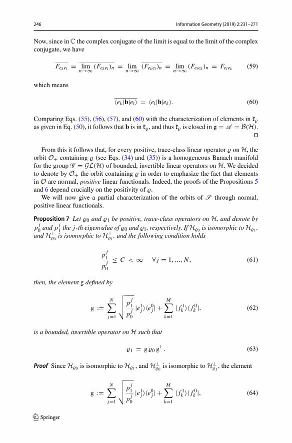
Now, since inC the complex conjugate of the limit is equal to the limit of the complexconjugate, we have

Fekel = limn→∞ (Fekel )n = lim

n→∞ (Fekel )n = limn→∞ (Felek )n = Felek (59)

which means

〈ek |b|el〉 = 〈el |b|ek〉. (60)

Comparing Eqs. (55), (56), (57), and (60) with the characterization of elements in k�as given in Eq. (50), it follows that b is in k�, and thus k� is closed in g = A = B(H).

From this it follows that, for every positive, trace-class linear operator � onH, the

orbit O+ containing � (see Eqs. (34) and (35)) is a homogeneous Banach manifoldfor the group G = GL(H) of bounded, invertible linear operators on H. We decidedto denote by O+ the orbit containing � in order to emphasize the fact that elementsin O are normal, positive linear functionals. Indeed, the proofs of the Propositions 5and 6 depend crucially on the positivity of �.

We will now give a partial characterization of the orbits of S through normal,positive linear functionals.

Proposition 7 Let �0 and �1 be positive, trace-class operators on H, and denote byp j0 and p j

1 the j-th eigenvalue of �0 and �1, respectively. IfH�0 is isomorphic toH�1 ,and H⊥

�0is isomorphic toH⊥

�1, and the following condition holds

p j1

p j0

≤ C < ∞ ∀ j = 1, ..., N , (61)

then, the element g defined by

g :=N∑

j=1

√

√

√

√

p j1

p j0

|e1j 〉〈e0j | +M∑

k=1

| f 1k 〉〈 f 0k |. (62)

is a bounded, invertible operator on H such that

�1 = g �0 g† . (63)

Proof Since H�0 is isomorphic toH�1 , and H⊥�0

is isomorphic toH⊥�1, the element

g :=N∑

j=1

√

√

√

√

p j1

p j0

|e1j 〉〈e0j | +M∑

k=1

| f 1k 〉〈 f 0k |, (64)

123


where N = dim(H�0) = dim(H�1) and M = H⊥�0

= H⊥�1, is well-defined, and a

direct (formal) computation shows that equation (63) actually holds. All that is leftto do is to check that g is bounded and invertible. At this purpose, we consider anarbitrary element ψ ∈ H which can be written as

|ψ〉 =N∑

j=1

ψj0 |e0j 〉 +

M∑

k=1

ψk0,⊥ | f 0k 〉 =

=N∑

j=1

ψj1 |e1j 〉 +

M∑

k=1

ψk1,⊥ | f 1k 〉 ,

(65)

with respect to the orthonormal bases inH adapted to the spectral decompositions of�0 and �1. From this, we have

||g(ψ)||2 = 〈ψ |g† g|ψ〉 =N∑

j=1

|ψ j0 |2 p j

1

p j0

+M∑

k=1

|ψk0,⊥|2 ≤

≤ CN∑

j=1

|ψ j0 |2 +

M∑

k=1

|ψk0,⊥|2 ≤ (C + 1) ||ψ ||2 < ∞ ,

(66)

where we used equation (61) in the second passage. Clearly, equation (66) impliesthat g is bounded. Then, setting

g−1 :=N∑

j=1

√

√

√

√

p j0

p j1

|e0j 〉〈e1j | +M∑

k=1

| f 0k 〉〈 f 1k |, (67)

we may proceed as we did for g to show that g−1 is bounded, and a direct computationshows that g−1 is the inverse of g.

Clearly, the assumptions in Proposition 7 are always satisfied if �0 and �1 arefinite-rank operators with the same rank.

The last step we want to take is to write down a tangent vectorV� at � ∈ O+, whereO+ is any of the orbits of G inside the positive, trace-class operators. At this purpose,we consider the canonical immersion i+ : O+ −→ A ∗

sa , and we recall Eq. (32), fromwhich it follows that

T�i+(Vρ)(b) = Tr(

�(

a† b + b a))

∀b ∈ A , (68)

where a is an arbitrary element in A = B(H). Clearly, different choices of a maylead to the same T�i+(V�). Then, writing a = x + ıy with x, y ∈ Asa , we have

T�i+(V�)(b) = Tr(({�, x} − ı

[

�, y])

b) ∀b ∈ A , (69)

with {·, ·} and [·, ·] the anticommutator and the commutator in B(H), respectively.

123


2.2 Faithful, finite trace

Let A be a unital C∗-algebra with a faithful, finite trace τ , that is, τ is a faithful,positive linear functional on A such that

τ(a b) = τ(b a) ∀ a,b ∈ A . (70)

In particular, ifA is Abelian, then every faithful, positive linear functional is a faithful,finite trace.

We will prove that the orbitOτ+ of G through τ by means of the linear action α (seeEq. (7)) is a homogeneous Banachmanifold ofG . At this purpose, the characterizationof an element a in the Lie algebra of the isotropy group Gτ given in Eq. (19) reads

τ((

a + a†)

b)

= 0 ∀ b ∈ A (71)

because τ is a trace, and we see that the skew-adjoint part of a is completely arbitrary.Then, we recall that τ induces an inner product 〈, 〉τ on A given by3

〈b, c〉τ = τ(

b† c)

. (72)

Consequently, the completion of A with respect to 〈, 〉τ is a Hilbert space in whichA is a dense subspace and thus the validity of equation (71) implies

a + a† = 0. (73)

This means that the Lie algebra gτ of Gτ coincides with the space of skew-adjointelements in g ∼= A , and this subspace is a closed and complemented subspace ofg ∼= A whose complement is the space of self-adjoint elements in g ∼= A . From thiswe conclude that the orbit Oτ+ of G through τ by means of the linear action α is ahomogeneous Banach manifold of G .

It is immediate to check that there is a bijection betweenOτ+ and the set of positive,invertible elements in A , that is, elements of the form g g† with g ∈ G . If A isfinite-dimensional, thenOτ coincides with the whole space of faithful, positive linearfunctionals.

3 State-preserving action of G

In this section, we will see how to “deform” the action of G in such a way that itpreserves the space of states S . Indeed, we recall that S is a subset of the space ofpositive linear functionals A ∗

sa characterized by the condition

ρ(I) = 1 (74)

3 Note that the faithfulness of τ is necessary for 〈, 〉τ to be an inner product on the whole A .

123


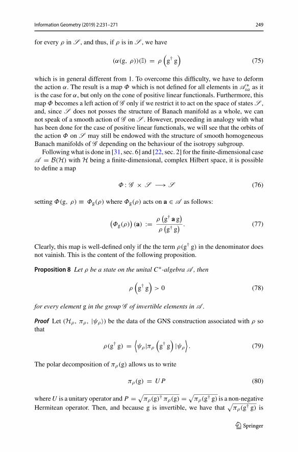
for every ρ inS , and thus, if ρ is inS , we have

(α(g, ρ))(I) = ρ(

g† g)

(75)

which is in general different from 1. To overcome this difficulty, we have to deformthe action α. The result is a map Φ which is not defined for all elements in A ∗

sa as itis the case for α, but only on the cone of positive linear functionals. Furthermore, thismap Φ becomes a left action of G only if we restrict it to act on the space of statesS ,and, since S does not posses the structure of Banach manifold as a whole, we cannot speak of a smooth action of G on S . However, proceeding in analogy with whathas been done for the case of positive linear functionals, we will see that the orbits ofthe action Φ on S may still be endowed with the structure of smooth homogeneousBanach manifolds of G depending on the behaviour of the isotropy subgroup.

Followingwhat is done in [31, sec. 6] and [22, sec. 2] for the finite-dimensional caseA = B(H) with H being a finite-dimensional, complex Hilbert space, it is possibleto define a map

Φ : G × S −→ S (76)

setting Φ(g, ρ) ≡ Φg(ρ) where Φg(ρ) acts on a ∈ A as follows:

(

Φg(ρ))

(a) := ρ(

g† a g)

ρ(

g† g) . (77)

Clearly, this map is well-defined only if the the term ρ(g† g) in the denominator doesnot vainish. This is the content of the following proposition.

Proposition 8 Let ρ be a state on the unital C∗-algebra A , then

ρ(

g† g)

> 0 (78)

for every element g in the group G of invertible elements in A .

Proof Let (Hρ, πρ, |ψρ〉) be the data of the GNS construction associated with ρ sothat

ρ(g† g) =⟨

ψρ |πρ

(

g† g)

|ψρ

⟩

. (79)

The polar decomposition of πρ(g) allows us to write

πρ(g) = U P (80)

whereU is a unitary operator and P = √πρ(g)† πρ(g) = √πρ(g† g) is a non-negativeHermitean operator. Then, and because g is invertible, we have that

√

πρ(g† g) is

123


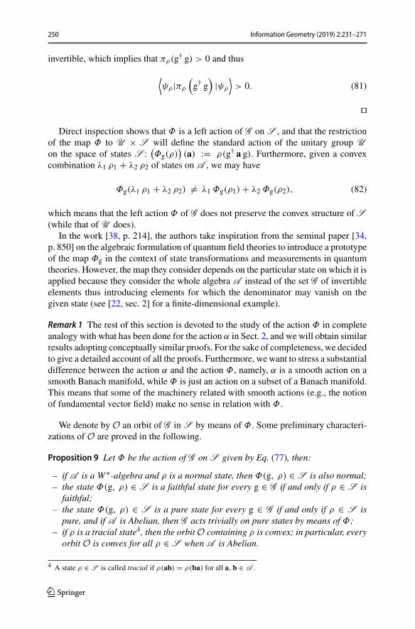
invertible, which implies that πρ(g† g) > 0 and thus

⟨

ψρ |πρ

(

g† g)

|ψρ

⟩

> 0. (81)

Direct inspection shows that Φ is a left action of G on S , and that the restriction

of the map Φ to U × S will define the standard action of the unitary group Uon the space of states S :

(

Φg(ρ))

(a) := ρ(g† a g). Furthermore, given a convexcombination λ1 ρ1 + λ2 ρ2 of states on A , we may have

Φg(λ1 ρ1 + λ2 ρ2) �= λ1 Φg(ρ1) + λ2 Φg(ρ2), (82)

which means that the left action Φ of G does not preserve the convex structure of S(while that of U does).

In the work [38, p. 214], the authors take inspiration from the seminal paper [34,p. 850] on the algebraic formulation of quantum field theories to introduce a prototypeof the map Φg in the context of state transformations and measurements in quantumtheories. However, the map they consider depends on the particular state on which it isapplied because they consider the whole algebra A instead of the set G of invertibleelements thus introducing elements for which the denominator may vanish on thegiven state (see [22, sec. 2] for a finite-dimensional example).

Remark 1 The rest of this section is devoted to the study of the action Φ in completeanalogy with what has been done for the action α in Sect. 2, and we will obtain similarresults adopting conceptually similar proofs. For the sake of completeness, we decidedto give a detailed account of all the proofs. Furthermore, we want to stress a substantialdifference between the action α and the action Φ, namely, α is a smooth action on asmooth Banach manifold, while Φ is just an action on a subset of a Banach manifold.This means that some of the machinery related with smooth actions (e.g., the notionof fundamental vector field) make no sense in relation with Φ.

We denote by O an orbit of G inS by means of Φ. Some preliminary characteri-zations of O are proved in the following.

Proposition 9 Let Φ be the action of G on S given by Eq. (77), then:

– ifA is a W ∗-algebra and ρ is a normal state, then Φ(g, ρ) ∈ S is also normal;– the state Φ(g, ρ) ∈ S is a faithful state for every g ∈ G if and only if ρ ∈ S isfaithful;

– the state Φ(g, ρ) ∈ S is a pure state for every g ∈ G if and only if ρ ∈ S ispure, and if A is Abelian, then G acts trivially on pure states by means of Φ;

– if ρ is a tracial state4, then the orbitO containing ρ is convex; in particular, everyorbit O is convex for all ρ ∈ S when A is Abelian.

4 A state ρ ∈ S is called tracial if ρ(ab) = ρ(ba) for all a,b ∈ A .

123


Proof Concerning the first point, a normal state ρ is an element of S which is alsocontinuous with respect to the weak* topology on A generated by its topologicalpredual A∗. Recall that, for every b ∈ A , the maps

lb : A → A , lb(a) := ba

rb : A → A , rb(a) := ab(83)

are continuous with respect to the weak* topology onA generated by its topologicalpredualA∗. Furthermore, given any normal state ρ and any invertible element g ∈ G ,we may define the positive real number

cρg := ρ(g† g). (84)

Now, let α : R+ × C → C be the continuous5 left action of the multiplicative groupR

+ of positive real numbers on C given by

α(c, z) := cz. (85)

It is immediate to check that the normalized positive linear functionalΦ(g, ρ) : A →C may be written as

Φ(g, ρ) = αc−1ρg

◦ ρ ◦ lg† ◦ rg, (86)

where αc(z) = α(c, z), and thus Φ(g, ρ) is weak* continuous.The second point follows by direct inspection.Concerning the third point, let (Hρ, πρ, |ψρ〉) be the GNS data associated with a

pure state ρ. Then, it is a matter of direct computation to show that (Hγ , πγ , |ψγ 〉),where Hγ = Hρ , πγ = πρ and

|ψγ 〉 = πρ(g)|ψρ〉√〈ψρ |πρ(g†g)|ψρ〉 , (87)

is the data of the GNS construction associated with γ = Φ(g, ρ). Since ρ is pure, wehave that πρ = πγ is irreducible which means that γ is pure, and we conclude that theorbitO containing the pure state ρ is made up only of pure states. A direct consequenceis that the the action of G on the space of pure states of a commutative, unital C∗-algebra is trivial in the sense that every pure state is a fixed point of the action. Indeed,recalling that the GNS representation associated with a pure state ρ is irreducible,then [15, p. 102] implies that the GNS Hilbert space Hρ is one-dimensional sinceA is commutative. Consequently, the GNS representation πρ sends every elementin the identity operator on Hρ and we conclude that the orbit O containing ρ is just

5 The topology on R+ is the Lie group topology, the topology on C is the norm topology associated with

the norm |z| := √zz, and the topology on R

+ × C is the product topology associated with the previoustwo topologies.

123


the singleton {ρ}. As we will see, this is in sharp contrast with what happens in thenon-commutative case.

Regarding the last point, we start taking λ ∈ [0, 1], a tracial state ρ, two elementsg1, g2 ∈ G , and writing

ρλ12 := λ Φ(g1, ρ) + (1 − λ)Φ(g2, ρ). (88)

Then, for every a ∈ A , we have

ρλ12(a) = λ

ρ(

g†1 a g1)

ρ(

g†1 g1) + (1 − λ)

ρ(

g†2 a g2)

ρ(

g†2 g2)

= ρ

⎛

⎝λg1 g

†1

ρ(

g1 g†1

) a

⎞

⎠+ ρ

⎛

⎝(1 − λ)g2 g

†2

ρ(

g2 g†2

) a

⎞

⎠

= ρ

⎛

⎝

⎛

⎝λg1 g

†1

ρ(

g1 g†1

) + ((1 − λ)g2 g

†2

ρ(

g2 g†2

)

⎞

⎠ a

⎞

⎠

= ρ(

Pλρ12 a)

, (89)

where we have set

Pλρ12 := λPρ

1 + (1 − λ)Pρ1 (90)

with

Pρ1 := g1 g

†1

ρ(

g1 g†1

) and Pρ2 := g2 g

†2

ρ(

g2 g†2

) . (91)

The elements Pρ1 := g1 g

†1

ρ(g1 g†1)

and Pρ2 are both positive, invertible elements in A , and

we have that the set

G+ = G ∩ A+ (92)

of positive, invertible elements (strictly positive elements) in A is an open cone (see[54, p. 11]), so that Pλρ

12 is still a positive, invertible element. Being a positive element,

Pλρ12 admits a (self-adjoint) square root, say pλρ

12 , and this square-root element is also

invertible, i.e., pλρ12 ∈ G . Consequently, noting that

ρ(

Pρ12

) = 1, (93)

123


we obtain

ρλ12(a) =

ρ

(

(

pλρ12

)†a pλρ

12

)

ρ

(

(

pλρ12

)†pλρ12

)

)

(94)

for all a ∈ A . This is equivalent to

ρλ12 = Φ

(

pλρ12 , ρ

)

, (95)

which means that the orbit O containing ρ is convex as claimed. In particular, everyorbit O is convex when A is Abelian because all states are tracial.

Let O ⊂ S be an orbit of G by means of Φ. Considering ρ ∈ O and the cosetspace G /Gρ , where Gρ is the isotropy subgroup

Gρ = {g ∈ G : Φ(g, ρ) = ρ} , (96)

of ρ with respect to Φ, the map iΦρ : G /Gρ → O given by

[g] �→ iΦρ ([g]) = Φ(g, ρ) (97)

provides a set-theoretical bijection between the coset space G /Gρ and the orbit Ofor every ρ ∈ S . According to the results recalled in “Appendix B”, this means thatwe may dress the orbit O with the structure of homogeneous Banach manifold of Gwhenever the isotropy subgroup Gρ is a Banach-Lie subgroup of G . Specifically, it isthe quotient space G /Gρ that is endowed with the structure of homogeneous Banachmanifold, and this structure may be “transported” to O in view of the bijection iΦρbetween G /Gρ and O.

As it happens for the action α defined in Sect. 2, in general, the fact that Gρ isa Banach-Lie subgroup of G depends on both ρ and A . However, Gρ is alwaysan algebraic subgroup of G for every ρ ∈ S and every unital C∗-algebra A (seethe discussion above Proposition 3 for the definition and the properties of algebraicsubgroups of a Banach-Lie group).

Proposition 10 The isotropy subgroup Gρ of ρ ∈ S is an algebraic subgroup of G oforder 2 for every ρ ∈ S .

Proof The proof is essentially the same of Proposition 3with only a slightmodificationof the family of polynomials considered. Define the family Qρ = {pρ,c}c∈A ofcomplex-valued polynomials of order 2 as follows6:

pρ,c(a,b) := ρ(a† a) ρ (c) − ρ(

a† ca)

. (98)

6 Note that the dependence of pρ,c on the second variable is trivial, and this explains why b does not appearon the rhs.

123


The continuity of every pρ,c follows easily from the fact that ρ is a norm-continuouslinear functional on A . A moment of reflection shows that

Gρ ={

g ∈ G : pρ,c(g, g−1) = 0 ∀pρ,c ∈ Qρ

}

, (99)

and thus Gρ is an algebraic subgroup of G of order 2 for all ρ ∈ S . Being an algebraic subgroup of G , the isotropy subgroup Gρ is a closed subgroup

of G which is also a real Banach-Lie group in the relativised norm topology, and itsLie algebra gρ ⊂ g = A is given by the closed subalgebra (see [35, p. 667], and [55,p. 118])

gρ = {a ∈ g ≡ A : exp(ta) ∈ Gρ ∀t ∈ R}

. (100)

According to Proposition 15, the isotropy subgroup Gρ of G is a Banach-Lie subgroupof G if and only if the Lie algebra gρ of Gρ is a split subspace of g = A and exp(V ) isa neighbourhood of the identity element in Gρ for every neighbourhood V of 0 ∈ gρ

(see [55, p. 129] for an explicit proof). The fact that exp(V ) is a neighbourhood of theidentity element in Gρ for every neighbourhood V of 0 ∈ gρ follows from the fact thatGρ is an algebraic subgroup of G (see [35, p. 667]).

Next, we may characterize gρ as we did in Sect. 2 by considering a ∈ g = A , thesmooth curve in G given by

gt = exp(ta) (101)

for all t ∈ R, the curve ρt inS given by

ρt (b) = (Φ(gt , ρ))(b) = ρ(

g†t b gt)

(102)

for all t ∈ R and for all b ∈ A , and computing

d

dt(ρt (b))t=0 = lim

t→0

ρt (b) − ρ(b)

t

= limt→0

1

t

⎛

⎝

ρ(

g†t b gt)

ρ(

g†t gt) − ρ(b)

⎞

⎠

= limt→0

1

t ρ(

g†t gt)

(

ρ(

g†t (b − ρ(b) I) gt))

= limt→0

1

t

(

ρ(

g†t (b − ρ(b) I) gt))

(

limt→0

1

ρ(g†t gt )

)

= limt→0

1

t

(

ρ(

g†t (b − ρ(b) I) gt))

123


= limt→0

1

t

+∞∑

j,k=0

(

ρ

((

ta†)k

k! (b − ρ(b) I)(ta) j

j !

))

= ρ(

a† (b − ρ(b) I))

+ ρ ((b − ρ(b) I) a)

= ρ(

a† b + b a)

− ρ(b) ρ(

a† + a)

(103)

for every b ∈ A , from which it follows that a is in the Lie algebra gρ of the isotropygroup Gρ if and only if

ρ(

a† b + b a)

− ρ(b) ρ(

a† + a)

= 0 (104)

for every b ∈ A . Incidentally, note that the last term in Eq. (103) gives the covariancebetween b and a evaluated at the state ρ whenever a is self-adjoint. Something relatedhas also been pointed out in [20, Eq. 34], and we postpone to a future work a morethorough analysis of the connection between the action of G on S and the existenceof contravariant tensor fields associated with the covariance between observables (inthe C∗-algebraic sense).

When dim(A ) = N < ∞, the Lie algbera gρ is a split subspace for ever ρ ∈ S ,and thus every orbit of G inS by means of Φ is a homogeneous Banach manifold ofG . Clearly, when A is infinite-dimensional, this is no-longer true, and a case by caseanalysis is required. For instance, in Sect. 3.1, we will show that gρ is a split subspaceof g = A when A is the algebra B(H) of bounded linear operators on a complex,separable Hilbert space H, and ρ is any normal state on B(H) (positive, trace-classlinear operator on H with unit trace). This means that all the orbits of G = GL(H)

passing through normal states are homogeneous Banach manifolds of G , and we willclassify these orbits into four different types.

Actually, the results of Sect. 3.1 naturally follows from the results of Sect. 2.1because, as we will now show, there is an intimate connection between the action α

of G on ρ when the latter is thought of as an element of A ∗sa , and the action Φ of G

on ρ when the latter is thought of as an element ofS . Indeed, from Eqs. (7) and (77),we easily obtain that if g is in the isotropy group G α

ρ of ρ with respect to the action α,then g is also in the isotropy group Gρ of ρ with respect to Φ, while the converse isnot necessarily true. Furthermore, if g is in G α

ρ , then eγ g is in Gρ for every γ ∈ R, and

it turns out that this is the most general expression for an element in Gρ . This is madeprecise in the following proposition where we show that the Lie algebra gρ ofGρ is justthe direct sum of the Lie algebra gα

ρ with the one-dimensional subspace determinedby the linear combinations of multiples of the identity with real coefficients.

Proposition 11 The Lie algebra gρ of the isotropy group Gρ of ρ with respect to Φ

may be written as

gρ = gαρ ⊕ spanR{I} (105)

123


where gαρ is the Lie algebra of the isotropy group G α

ρ of ρ with respect to the action α

introduced in Sect. 2, and spanR{I} is the real, linear subspace spanned by the identityoperator in G = A with real coefficients.

Proof It is a matter of direct inspection to see that if a is in gαρ (see Eq. (19)), then

a + γ I is in gρ for every γ ∈ R.On the other hand, since spanR{I} is one-dimensional, it is complemented in gρ ,

and we may characterize its complement as follows. First, we take the continuous,real linear functional F on spanR{I} given by

F(γ I) := γ, (106)

and extend it to the whole gρ . The extension of F is highly non-unique, and we maytake it to be the functional Fρ given by

Fρ(a) := 1

2(ρ + ρ†)(a) = 1

2ρ(a† + a) ∀ a ∈ gρ. (107)

Indeed, Fρ is a real, continuous linear functional on gρ because (ρ+ρ†) is a continuouslinear functional on the real Banach-Lie algebra g = A of which gρ is a closed, realsubalgebra, and clearly Fρ(γ I) = F(γ I) because ρ is a state. Then, we have abounded projection P from gρ to spanR{I} given by

P(a) = Fρ(a) I ∀ a ∈ gρ, (108)

and we may write

a = P(a) − (Idgρ − P)

(a) ∀ a ∈ gρ. (109)

This allows us to define the complement of spanR{I} in gρ as the closed linear subspacecρ given by the image of

(

Idgρ − P)

. Equivalently, an element b ∈ cρ may be writtenas

b = (

Idgρ − P)

(a) (110)

with a ∈ gρ . All that is left to do is to show that b ∈ cρ is actually in gαρ . At this

purpose, recalling Eq. (19), we have

ρ(

b† c + c b)

= ρ

(

(

a − 1

2ρ(

a† + a)

I

)†

c + c(

a − 1

2ρ(

a† + a)

I

)

)

= ρ(

a† c + c a)

− ρ(c) ρ(

a† + a)

= 0 (111)

because a is in gρ (see Eq. (104)).

123


From Proposition 11 it follows that Gρ is a Banach-Lie subgroup of G if and only ifG α

ρ is a Banach-Lie subgroup of G . Consequently, the orbit of G through ρ by meansof α is a homogeneous Banach manifold of G if and only if the orbit of G through ρ

by means of Φ is a homogeneous Banach manifold of G .

Proposition 12 The Lie algebra gρ is a split subspace of g = A if and only if the Liealgebra gα

ρ is so.

Proof According to Proposition 11 we may write

gρ = gαρ ⊕ spanR{I}. (112)

Consequently, if gρ is complemented in g = A , we have

g = gρ ⊕ kρ (113)

and thus the closed linear subspace kρ ⊕ spanR{I} provides a closed complement forgαρ . On the other hand, if gα

ρ is complemented in g = A , and we may write

g = gαρ ⊕ kαρ. (114)

Then, recall that γ I with γ ∈ R is in gαρ if and only if γ = 0 (see Eq. (19)), therefore,

the closed one-dimensional subspace spanR{I} is a closed linear subspace of kαρ , and itis complemented in kαρ because it is finite-dimensional. Denoting by cρ the complementof spanR{I} in kαρ , we have that

g = gαρ ⊕ spanR{I} ⊕ cαρ = gρ ⊕ cαρ, (115)

from which it follows that gρ is complemented in g = A . Now, supposeρ is such that gρ is a split subspace ofA , that is, the isotropy subgroup

Gρ is a Banach-Lie subgroup of G . In this case, the orbit O containing ρ is endowedwith a Banach manifold structure such that the map τΦ

ρ : G → O given by

g �→ τΦρ (g) := Φ(g, ρ) (116)

is a smooth surjective submersion for every ρ ∈ O. Moreover, G acts transitively andsmoothly on O, and the tangent space TρO at ρ ∈ O is diffeomorphic to g/gρ (see[17, p. 105] and [55, p. 136]). Note that this smooth differential structure on O isunique up to smooth diffeomorphism. Now, we will prove a proposition very similarto Proposition 4 in Sect. 2.

Proposition 13 Let ρ be such that the isotropy subgroup Gρ is a Banach-Lie subgroupof G , letO be the orbit containing ρ endowed with the smooth structure coming fromG , and consider the map la : O −→ R, with a a self-adjoint element in A , given by

la(ρ) := ρ(a). (117)

123


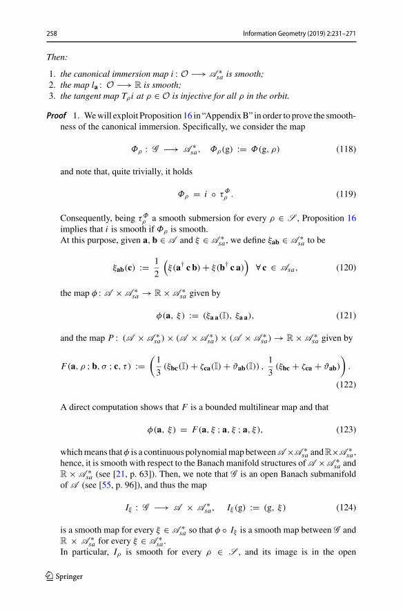
Then:

1. the canonical immersion map i : O −→ A ∗sa is smooth;

2. the map la : O −→ R is smooth;3. the tangent map Tρ i at ρ ∈ O is injective for all ρ in the orbit.

Proof 1. Wewill exploit Proposition 16 in “AppendixB” in order to prove the smooth-ness of the canonical immersion. Specifically, we consider the map

Φρ : G −→ A ∗sa, Φρ(g) := Φ(g, ρ) (118)

and note that, quite trivially, it holds

Φρ = i ◦ τΦρ . (119)

Consequently, being τΦρ a smooth submersion for every ρ ∈ S , Proposition 16

implies that i is smooth if Φρ is smooth.At this purpose, given a,b ∈ A and ξ ∈ A ∗

sa , we define ξab ∈ A ∗sa to be

ξab(c) := 1

2

(

ξ(a† c b) + ξ(b† c a))

∀ c ∈ Asa, (120)

the map φ : A × A ∗sa → R × A ∗

sa given by

φ(a, ξ) := (ξa a(I), ξa a), (121)

and the map P : (A × A ∗sa) × (A × A ∗

sa) × (A × A ∗sa) → R × A ∗

sa given by

F(a, ρ ;b, σ ; c, τ ) :=(

1

3(ξbc(I) + ζca(I) + ϑab(I)) ,

1

3(ξbc + ζca + ϑab)

)

.

(122)

A direct computation shows that F is a bounded multilinear map and that

φ(a, ξ) = F(a, ξ ; a, ξ ; a, ξ), (123)

whichmeans thatφ is a continuous polynomialmapbetweenA ×A ∗sa andR×A ∗

sa ,hence, it is smooth with respect to the Banach manifold structures ofA ×A ∗

sa andR × A ∗

sa (see [21, p. 63]). Then, we note that G is an open Banach submanifoldof A (see [55, p. 96]), and thus the map

Iξ : G −→ A × A ∗sa, Iξ (g) := (g, ξ) (124)

is a smooth map for every ξ ∈ A ∗sa so that φ ◦ Iξ is a smooth map between G and

R × A ∗sa for every ξ ∈ A ∗

sa .In particular, Iρ is smooth for every ρ ∈ S , and its image is in the open

123


submanifold R0 × A ∗sa of R × A ∗

sa . Therefore, considering the smooth mapβ : R0 × A ∗

sa → A ∗sa given by

β(b, ξ) := 1

bξ, (125)

it follows that β ◦ φ ◦ Iρ is a smooth map between G and A ∗sa for every ρ ∈ S ,

and a direct computation shows that

Φρ = β ◦ φ ◦ Iρ. (126)

From this it follows that Φρ is smooth which means that the canonical immersioni : O ⊂ S −→ A ∗

sa is smooth because of Proposition 16.2. It suffices to note that la is the composition of the linear (and thus smooth) map

La : A ∗sa −→ R given by

La(ξ) = ξ(a) (127)

with the canonical immersion i which is smooth because of what has been provedabove.

3. Now, consider the family {la}a∈A of smooth functions on the orbitO, and supposethat Vρ and Wρ are tangent vectors at ρ ∈ O such that

〈(dla)ρ; Vρ〉 = 〈(dla)ρ; Wρ〉 (128)

for every a ∈ Asa . Then, since la = La ◦ i , we have

〈(dla)ρ; Vρ〉 = 〈(dLa)i(ρ); Tρ i(Vρ)〉 (129)

and

〈(dla)ρ; Wρ〉 = 〈(dLa)i(ρ); Tρ i(Wρ)〉. (130)

Note that the family of linear functions of the type La with a ∈ Asa (see Eq. (24))are enough to separate the tangent vectors at ξ for every ξ ∈ A ∗

sa because thetangent space at ξ ∈ A ∗

sa is diffeomorphic with A ∗sa in such a way that

〈(dLa)ξ ;Vξ 〉 = Vξ (a) = La(Vξ ) (131)

for every Vξ ∈ TξA ∗sa

∼= A ∗sa , and Asa (the predual of A ∗

sa) separates the pointsof A ∗

sa (see [42]). Consequently, since Tρ i(Vρ) and Tρ i(Wρ) are tangent vectorsat i(ρ) ∈ A ∗

sa and the functions La with a ∈ Asa are enough to separate them andwe conclude that the validity of Eq. (128) for all a ∈ Asa is equivalent to

Tρ i(Vρ) = Tρ i(Wρ). (132)

123


Then, if gt = exp(ta) is a one-parameter subgroup in G so that

ρt = Φ(gt , ρ) (133)

is a smooth curve in O starting at ρ with associated tangent vector Vρ , we have

〈(dLb)i(ρ); Tρ i(Vρ)〉 = d

dt(Lb ◦ i(ρt ))t=0 (134)

which we may compute analogously to Eq. (103) to obtain

d

dt(Lb ◦ i(ρt ))t=0 = ρ

(

a† b + b a)

− ρ(b) ρ(

a† + a)

(135)

Comparing Eq. (135) with Eq. (103) we conclude thatVρ andWρ satisfy Eq. (29)if and only if they coincide, and thus Tρ i is injective for all ρ ∈ O.

It is important to note that the topology underlying the differential structure on O

comes from the topology of G in the sense that a subset U of the orbit is open iff(τΦ

ρ )−1(U ) is open in G . In principle, this topology on O has nothing to do with thetopology of O when thought of as a subset of S endowed with the relativised normtopology, or with the relativised weak* topology. However, from Proposition 13, itfollows that themap la : O −→ R is continuous for every a ∈ Asa . Therefore, wemayconclude that the topology underlying the homogeneous Banach manifold structureon O is stronger than the relativised weak* topology coming from A ∗

sa .

3.1 Density operators

Similarly to what is done in Sect. 2.1, we consider a complex, separable Hilbert spaceH and denote by A the W ∗-algebra B(H) of bounded, linear operators on H. Anormal state ρ of A may be identified with a density operator on H, that is, a trace-class, positive semidefinite operator ρ with unit trace, and the duality relation may beexpressed by means of the trace operation

ρ(a) = Tr (ρ a) (136)

for all a ∈ A = B(H).We will study the orbits of the group G of invertible, bounded linear operators in

A on the space N of normal states on A . The analysis will be very similar to theone presented in Sect. 2.1.

According to the spectral theory for compact operators (see [51, ch. VII]), given adensity operator ρ on H, there is a decomposition H = Hρ ⊕ H⊥

ρ and a countableorthonormal basis {|e j 〉, | f j 〉} adapted to this decomposition such that ρ can bewrittenas

123


ρ =dim(Hρ)∑

j=1

p j |e j 〉〈e j |, (137)

with p j > 0 and∑dim(Hρ)

j=1 p j = 1. In general, we have four different situations:

1. 0 < dim(Hρ) = N < ∞;2. dim(Hρ) = ∞ and 0 < dim(H⊥

ρ ) = M < ∞;3. dim(Hρ) = ∞ and dim(H⊥

ρ ) = 04. dim(Hρ) = dim(H⊥

ρ ) = ∞,

and we set

NN := {

ρ ∈ N | 0 < dim(Hρ) = N < ∞}

N ⊥M :=

{

ρ ∈ N | dim(Hρ) = ∞ and 0 < dim(H⊥ρ ) = M < ∞

}

N ⊥0 :=

{

ρ ∈ N | dim(Hρ) = ∞ and dim(H⊥ρ ) = 0

}

N∞ :={

ρ ∈ N | dim(Hρ) = dim(H⊥ρ ) = ∞

}

. (138)

The subscript here denotes either the dimension of the space on which ρ operates, orits codimension when the symbol ⊥ is used. Clearly, when dim(H) < ∞, we haveNN = ∅ for all N > dim(H), and N ⊥

M = N ⊥0 = N∞ = ∅.

Proceeding in exactly the same way as we did in Sect. 2.1, we may prove that theaction Φ of G is transitive on NN , on N ⊥

M , on N ⊥0 and on N∞. Consequently, the

space N of normal states on A = B(H) is partitioned into the disjoint union

N = N∞ N ⊥0

(

⊔

N∈NNN

)

(

⊔

M∈NN ⊥

M

)

. (139)

Propositions 11, 12, and 6 imply that the isotropy subgroup Gρ of ρ with respect to Φ

is a Banach-Lie subgroup of G = GL(H). By adapting the proof of Proposition 7 inthe obvious way, we may prove the following proposition:

Proposition 14 Let �0 and �1 be density operators onH, that is, positive, trace-classoperators with unit trace. Denote by p j

0 and p j1 the j-th eigenvalue of �0 and �1,

respectively. If H�0 is isomorphic to H�1 , and H⊥�0

is isomorphic to H⊥�1, and if the

following condition holds

p j1

p j0

≤ C < ∞ ∀ j = 1, ..., N , (140)

then, the element g given by

123


g :=N∑

j=1

√

√

√

√

p j1

p j0

|e1j 〉〈e0j | +M∑

k=1

| f 1k 〉〈 f 0k | (141)

is a bounded, invertible operator on H such that

�1 = g �0 g†

Tr(g �0 g†). (142)

Clearly, the assumptions in Proposition 14 are always satisfied if �0 and �1 arefinite-rank operators with the same rank.

Now, we want to write down a tangent vector Vρ at ρ ∈ O, where O is any ofthe orbits of G inside the space of density operators. At this purpose, we consider thecanonical immersion i : O −→ A ∗

sa , and we recall Eq. (135), from which it followsthat

Tρ i(Vρ)(b) = ρ(

a† b + b a)

− ρ(b) ρ(

a† + a)

∀b ∈ A , (143)

where a is an arbitrary element in A = B(H). Clearly, different choices of a maylead to the same Tρ i(Vρ). Then, writing a = x + ıy with x, y ∈ Asa , we have

Tρ i(Vρ)(b) = Tr(({ρ, x} − ı

[

ρ, y])

b)− Tr(ρ b)Tr ({ρ, x}) ∀b ∈ A , (144)

with {·, ·} and [·, ·] the anticommutator and the commutator in B(H), respectively.

3.2 Faithful, tracial state

Similarly to what is done in 2.2, we consider A to be a unital C∗-algebra with afaithful, tracial state τ , that is, τ is a faithful, state on A such that

τ(a b) = τ(b a) ∀ a,b ∈ A . (145)

In particular, if A is Abelian, then every faithful, state is a faithful, tracial state.The result of Sect. 2.2 and Proposition 12 allow us to conclude that the orbit Oτ

of G through τ by means of Φ (see Eq. (77)) is a homogeneous Banach manifold ofG . Furthermore, it is immediate to check that there is a bijection between Oτ and theset of positive, invertible elements in A with unit trace, that is, elements of the formgg†

τ(g g†)with g ∈ G . IfA is finite-dimensional, thenOτ coincides with the whole space

of faithful, tracial states, and, ifA is finite-dimensional and Abelian (i.e.,A ∼= Cn for

some n ∈ N), then Oτ may be identified with the open interior of the n-dimensionalsimplex. Note that points in the orbit through τ need not be tracial state when A isnon-Abelian (e.g., when A = B(H) with dim(H) < ∞ and τ the maximally mixedstate).

Now, we want to explore the example given by the Abelian W ∗-algebra A =L∞(X , ν), where (X ,Σ, ν) is a probability space (see [54, p. 109]), and the support

123


of ν is the whole X . The sum, multiplication and involution in A = L∞(X , ν) aredefined as for the C∗-algebra of complex-valued, bounded, continuous functions on aHausdorff topological space, but the norm is given by

|| f || = inf {C ≥ 0 | | f (x)| ≤ C for ν − almost every x} . (146)

In this case, the pre-dual space A∗ may be identified with L1(X , ν) by means of theduality

〈 f , ξ 〉 =∫

Xf (x) ξ(x) dν(x), (147)

while the dual space A ∗ may be identified with the space BV (Σ, ν) of complex-valued, finitely-additive, bounded functions onΣ which vanish on every locally ν-nullset (see [54, p. 116] for the explicit construction of the Banach space structure onBV (X , ν)) by means of the duality

μ( f ) =∫

Xf (x) dμ(x). (148)

The space S of states is then the space of normalized, positive, finitely-additive,bounded functions on Σ . When μ is a normal state, there exists μ ∈ A∗ ∼= L1(X , ν)

such that∫

Xf (x) dμ(x) = μ( f ) = 〈 f , μ〉 =

∫

Xf (x) μ(x) dν(x) (149)

for all f ∈ A . Clearly, the function μ is μ-integrable, non-negative, and such that

∫

Xμ(x) dν(x) = 1. (150)

Consequently, every normal stateμdetermines a probabilitymeasure on (X ,Σ)whichis absolutely continuous with respect to ν, and has μ as its Radon–Nikodym derivative.

The action of G on the normal state μ is easily written as

(Φ(g, μ)) ( f ) =∫

X |g(x)|2 f (x) dμ(x)∫

X |g(y)|2 dμ(y)≡∫

Xανg (x) f (x) dμ(x), (151)

where f is inA = L∞(X , ν), and ανg (x) is the strictly positive,μ-integrable function

αμg (x) = |g(x)|2

∫

X |g(y)|2 dμ(y)(152)

such thatμ(αμg ) = 1. Ifμ is faithful, the orbitOμ throughμ is a smooth, homogeneous

Banach manifold for G , and a point in Oμ is a probability measure μg which is

123


mutually absolutely continuous with respect to μ with αμg ∈ A = L∞(X , ν) as its

Radon–Nikodym derivative.In particular, ifwe take ν as the reference faithful, normal state,we have that the orbit

O containing ν is given by all the probability measures on (X ,Σ) that are mutuallyabsolutely continuous with respect to ν, and with a Radon–Nikodym derivative whichis a strictly positive function in A = L∞(X , ν) integrating to 1 with respect to ν.Therefore, the set

Mν :={

f ∈ L∞(X , ν) | f (x) > 0 ν − a.s.,∫

Xf (x) dν(x) = 1

}

(153)

is a homogeneous Banach manifold of the Banach-Lie group G of invertible elementsin L∞(X , ν).

4 Concluding remarks

In thiswork,wepresented apreliminary analysis concerning twopossible actions of theBanach-Lie groupG of invertible elements in a unitalC∗-algebraA on the continuous,self-adjoint linear functionals inA ∗

sa . Specifically, we analysed a linear action α of Gon A ∗

sa which is smooth and preserves the positivity and the normality of the linearfunctionals on which it acts. In the case where A is the algebra B(H) of boundedlinear operators on a complex, separable Hilbert space H, we were able to prove thatall the orbits passing through normal, positive linear functionals (positive trace-classoperators on H) are smooth, homogeneous Banach manifolds of G = GL(H) withrespect to the action α. Furthermore, we gave sufficient conditions for two normal,positive linear functionals to belong to the same orbit. If A admits a faithful, finitetrace τ , then we proved that the orbit through τ is a smooth, homogeneous Banachmanifold of G .

The action α does not preserve the space of states S on A . Consequently, weprovided a sort of deformation of α, denoted by Φ, which allows us to overcome thisproblem. However, Φ turns out to be an action of G which is well-defined only onthe space of states S , and, in general, it does not preserve the convex structure ofS . The subgroup of unitary elements in G is the maximal subgroup such that therestriction ofΦ preserves convexity. SinceS lacks a differential structure as a whole,it is meaningless to speak of the smoothness of Φ, nevertheless, an orbitO of Φ maystill inherit the structure of smooth homogeneous Banach manifold if the isotropysubgroup of an element (and thus of every element) in O is a Banach-Lie subgroupof G . At this purpose, we analysed the case whereA = B(H) mentioned before, andwe proved that the orbits through normal states (density operators on H) are indeedsmooth homogeneous Banach manifolds for G = GL(H) with respect to the actionΦ. Similarly to what we obtained for the action α in the case of normal positivefunctionals on A = B(H), we gave sufficient conditions for two normal states tobelong to the same orbit. Furthermore, if A admits a faithful, tracial state τ , then weproved that the orbit of G through τ by means ofΦ is a smooth, homogeneous Banachmanifold of G . In particular, ifA is finite-dimensional, the orbit through τ coincides

123


with the space of faithful states on A , while, if A is finite-dimensional and Abelian,the orbit through τ may be identified with the open interior of the finite-dimensionalsimplex. Note that points in the orbit through τ need not be tracial state when A isnon-Abelian, e.g., when A = B(H) with dim(H) < ∞ and τ the maximally mixedstate.

In the finite-dimensional case when A = B(H) with dim(H) < ∞, the spaceof faithful states (invertible density operators) may be identified with a smooth, opensubmanifold of the affine hyperplane of the self-adjoint operators with unit trace,and numerous constructions related with classical information geometry have beenadapted to this quantum case. However, a straightforward extension of this formalismto the infinite dimensional case is not possible because no density operator can beinvertible in this case, and this prevents the possibility of endowing the set of faithful(normal) states with a smooth manifold structure as it is done in the finite-dimensionalcase. As noted in the introduction, in the finite-dimensional case it is also known thatthe manifold structure on faithful normal states admits a compatible transitive actionof the group of invertible elements making it a smooth homogeneous space. Clearly,these twomanifold structures are completely equivalent in the finite-dimensional case.A relevant conclusion that can be drawn from the results of this manuscript is that, inthe infinite-dimensional case, it is possible to define a smooth homogeneous structureon the orbit of G = GL(H) through any given faithful normal state. However, it isstill an open question if there is only one such orbit as in the finite-dimensional case,and we plan to address this delicate issue in a future work.

The content of thiswork should be thought of as a preliminary step toward the gener-alization of the methods of quantum information geometry to the infinite-dimensionalcase, and, as such, it is far from being complete. For instance, the problem of character-izing the isotropy subgroups for other types ofC∗-algebras other than those consideredhere in order to understand if the associated orbit (with respect to α or Φ) is a smoothhomogeneous Banach manifold for G is still open. Then, it would be relevant to anal-yse the smoothness of well-known informational quantities (e.g., quantum relativeentropies) with respect to the smooth structures introduced in this work, so that, ifsmoothness is assured, we may proceed to analyse the statistical structures they giverise to in the infinite-dimensional case. Relevant examples would be given by the vonNeumann-Umegaki relative entropy, and by the Bures distance function (quantumfidelity).

Other geometrical structures that will emerge naturally for certain states, like acomplex structure or a symplectic structure [13,14], induced from the Banach-Liegroup of invertible elements, will be studied in a future contribution in relation withthe well-known informational metrics.

For this purpose, it may turn out to be helpful to analyse the smooth structure on thehomogeneous Banach manifolds in terms of the smooth subalgebra ofA determinedby the isotropy subgroup of the state ρ “labelling” the homogeneous Banach manifold[18]. Clearly, the smooth structure of the algebra will be related to the smooth structureof the orbit and it will provide a new insigh in the structure of the C∗-algebra obtainedfrom an action of a Lie group as indicated for instance in [26]. We plan to addressthese and related issues in future publications.

123


Acknowledgements Open access funding provided by Max Planck Society. A.I. and G.M. acknowledgefinancial support from the Spanish Ministry of Economy and Competitiveness, through the Severo OchoaProgramme for Centres of Excellence in RD (SEV-2015/0554). A.I. would like to thank partial supportprovided by the MINECO research project MTM2017-84098-P and QUITEMAD++, S2018/TCS-4342.G.M. would like to thank the support provided by the Santander/UC3M Excellence Chair Programme2019/2020.

Compliance with ethical standards

Conflict of interest On behalf of all authors, the corresponding author states that there is no conflict ofinterest.

Open Access This article is distributed under the terms of the Creative Commons Attribution 4.0 Interna-tional License (http://creativecommons.org/licenses/by/4.0/), which permits unrestricted use, distribution,and reproduction in any medium, provided you give appropriate credit to the original author(s) and thesource, provide a link to the Creative Commons license, and indicate if changes were made.

Appendix A: C*-algebras and states

Let (A , +, || · ||, ·) be a Banach algebra, that is, a Banach space endowed with a (notnecessarily commutative) multiplication operation which is continuous with respectto the norm topology and is such that

||a1 a2|| ≤ ||a1|| ||a2|| (154)

for every a1 and a2 in A . Suppose that there is a linear anti-isomorphism † on A ,called involution, such that (a†)† = a and:

(a1 a2)† = a†2 a†1 (155)

for every a1 and a2 inA . If the pentuple (A , +, || · ||, ·, †) satisfies the compatibilitycondition between the norm, the multiplication and the involution given by

||a||2 = ||a† a|| (156)

for every a inA , then (A , +, || · ||, ·, †) is called C∗-algebra. In the following, wewill avoid the notation (A , +, || · ||, ·, †) to denote a C∗-algebra, and will simplywrite A because, hopefully, all the operations will be clear from the context.

An element a ∈ A is called self-adjoint if a = a†, and we denote byAsa the spaceof self-adjoint elements inA . An element a ∈ A is called positive if it can be writtenas

a = bb† (157)

for some b ∈ A . Without loss of generality, we may take b to be self-adjoint (see [19,p. 33]). The space of positive elements in A is denoted by A+ and it is easy to seethat it is a cone in A .

123

http://creativecommons.org/licenses/by/4.0/


Let A be a possibly infinite-dimensional, unital C∗-algebra, that is, a C∗-algebrawith a multiplicative identity element denoted by I. LetA ∗ be the topological dual ofA , that is, the space of complex-valued, continuous linear functions onA . We denoteby T the Banach space topology (norm topology) on A ∗ induced by the canonicalnorm

||ω|| := sup||a||=1

|ω(a)|. (158)

A linear functional ω ∈ A ∗ is called self-adjoint if

ω(a†) = ω(a) (159)

so that ω takes real values when evaluated on self-adjoint elements in A . We denoteby A ∗+ be the cone of positive linear functionals on A , that is, the set of all ω ∈ A ∗such that ω(a† a) ≥ 0 for every a ∈ A . According to [19, p. 49], positive linearfunctionals are self-adjoint, and, given ω ∈ A ∗+ , it holds ||ω|| = ω(I) where I is theidentity ofA . We denote byS the space of states ofA , that is, the set of all ω ∈ A ∗+such that ||ω|| = 1. A state ω ∈ S is called faithful if ω(a) > 0 for all a ∈ A+. Astate ω ∈ S is called pure if, given ξ ∈ A ∗+ , then (ω − ξ) is in A ∗+ only if ξ = λω

with 0 ≤ λ ≤ 1. The set of pure states is denoted byP , and, according to [19, p. 53],the space of statesS is a convex, weak* compact convex subset ofA ∗, andP is theset of extremal points ofS , that is,S is the weak* closure of the convex envelope ofP . Note that the weak* compactness ofS depends on the fact thatA has an identityelement.

Given a positive linear functional ω ∈ A ∗+ , it is always possible to build a triple(Hω, πω, |ψω〉) whereHω is a possibly infinite-dimensional complex Hilbert space,πω is a *-representation ofA in B(Hω), and |ψω〉 is a nonzero vector inHω such that

ω(a) = 〈ψω|πω(a)|ψω〉 (160)

for all a ∈ A , and such that

Hω := {|ψ〉 ∈ Hψ : ∃ a ∈ A such that |ψ〉 = πω(a)|ψω〉} (161)

is a dense subset in Hω. This construction is referred to as the GNS constructionassociated with ω (see [15, sec. II.6.4], [19, ch. 2.3] and [41, ch. 4.5] for more details).Note that theGNSconstruction associatedwithω is uniqueup tounitary isomorphisms,and there is a one-to-one correspondence between positive linear functionals in A ∗+and the ∗-representations of A with a specified cyclic vector. Furthermore, the GNSrepresentation πω is irreducible if and only if ω is a pure state (see [19, p. 57]) and twoirreducible GNS representations πω and πρ are unitarily equivalent if ||ω − ρ|| < 2(see [30, p. 551]).

A W ∗-algebra A is a C∗-algebra which is the Banach dual of a Banach spaceA∗ called the predual of A . According to [52, p. 30], the predual A∗ is unique up toisometric isomorphisms.We denote by 〈·, ·〉 the canonical pairing betweenA∗ andA ,

123


that is, the action of a ∈ A on ξ ∈ A∗ when the former is thought of as a continuouslinear functional on A∗, reads

〈ξ, a〉 = a(ξ). (162)

There is a natural immersion i of A∗ into its double (topological) dual A ∗ given byξ �→ i(ξ)with (i(ξ)) (a) = 〈a, ξ 〉, and, by the very definition of the weak* topologyonA , it is clear that a linear functional˜ξ inA ∗ is continuouswith respect to theweak*topology on A if and only if there is an element ξ ∈ A∗ such that i(ξ) = ˜ξ . Linearfunctionals of this type are called normal, and the set of normal states onA is denotedbyN . In the finite dimensional case, every C∗-algebra is a W ∗-algebra, every linearfunctional ξ ∈ A ∗ is normal, and the immersion i is actually an isomorphism. This isno longer true in the infinite dimensional case.

Appendix B: Banach-Lie groups and homogeneous spaces

In this section we will assume familiarity with the notions of real, smooth Banachmanifolds, smoothmapsbetween (smooth)Banachmanifolds, andBanach-Lie groups.As stated at the end of the introduction, the main references concerning the infinite-dimensional differential geometry of Banach manifolds and Banach-Lie groups are[1,17,21,45,55], however, we think it is useful to recall here some notions regardingBanach-Lie subgroups of Banach-Lie groups.

According to [55, p. 96 and p. 114], every closed subgroup K of a given Banach-Liegroup G is a Banach-Lie group with respect to a unique Hausdorff topology in K suchthat the closed real subalgebra

k = {a ∈ g : exp(ta) ∈ K ∀t ∈ R} (163)

of the Lie algebra g of G is the Lie algebra of K . In general, the Hausdorff topologyon K does not coincide with the relative topology inherited from the norm topologyof G. A subgroup K of a Banach-Lie group G which is also a Banach submanifoldof G is called a Banach-Lie subgroup of G. In particular, a Banach-Lie subgroup Kof G is closed, it is a Banach-Lie group with respect to the relative topology inheritedfrom the topology of G, and its Lie algebra k is given by Eq. (163) (see [55, p. 128]).

Note that, in the finite-dimensional case dim(G) < ∞, it is always true that everyclosed subgroup of G is a Banach-Lie subgroup G.

An explicit characterization of Banach-Lie subgroups is given by the followingproposition (see [55, p. 129]).

Proposition 15 A closed subgroup K of a Banach-Lie group G is a Banach-Lie sub-group if and only if the closed subalgebra k given by Eq. (163) is a split subspace ofthe Lie algebra g of G, and for every neighbourhood U of 0 ∈ k, we have that exp(V )

is a neighbourhood of the identity element in K .

The importance of Banach-Lie subgroups comes from the following theorem (see[17, p. 105] and [55, p. 136]).

123


Theorem 1 Let K be a Banach-Lie subgroup of the Banach-Lie group G with Liealgebra g. Then, the quotient space M ≡ G/K carries the structure of an analyticBanach manifold such that the canonical projectio π : G −→ M is an analytic sub-mersion. Writing [h] = hK ≡ m ∈ M with h ∈ G, we have that the Lie group G actsanalytically on M by the left translation given L(g,m) := [gh] = ghK . The kernelof the tangent map Tπe : g −→ Tπ(e)M at the identity element e ∈ G coincides withthe closed, split subalgebra k of Eq. (163) so that Tπ(e)M ∼= g/k.

A smooth BanachmanifoldM which is diffeomorphic withG/K for someBanach-Lie group G with Banach-Lie subgroup K is called a homogeneous Banach manifoldof G. In particular, let G be a Banach-Lie group acting on a set S by means of the leftaction α : G× S −→ S, letO be an orbit of G in S by means of α, and let s ∈ O ⊆ S.The isotropy subgroup of G at s is the set

Gs := {g ∈ G | α(g, s) = s} . (164)

Then, the map is : G/Gs → O given by

[g] �→ is([g]) = α(g, s) (165)

defines a bijection from G/Gs toO for every s ∈ O. Consequently, if Gs is a Banach-Lie subgroup of G, we may endow the orbit O containing s with the structure ofBanach manifold according to Theorem 1 so that O becomes an homogeneous spaceof G for which the projection map τs : G −→ O, obtained composing the projectionof G onto G/Gs with the map is introduced above, is a surjective submersion. Notethat S is just a set and no structural properties on the action α are required. In particular,if G acts transitively on S, then S itself is an homogeneous Banach manifold of G.

Given a Banach manifold N , a useful tool for determining if a map ψ : O → Nis smooth is given by the following proposition provided we make the identificationsM = O, K = G and φ = τs for some s ∈ O (see [55, p. 125]).

Proposition 16 Let M, N , K be Banach manifolds, and consider the following com-mutative diagram:

M N

K

φ ϕ

ψ

Then, if φ is a surjective submersion and ϕ is smooth, then ψ is smooth. If ϕ is also asubmersion, then ψ is also a submersion.

123


References

1. Abraham,R.,Marsden, J.E., Ratiu, T.:Manifolds, TensorAnalysis, andApplications, 3rd edn. Springer,New York (2012)

2. Adams, M., Ratiu, T., Schmid, R.: The Lie Group Structure of Diffeomorphism Groups and InvertibleFourier Integral Operators with Applications. In: Kac, V. (ed.) Infinite Dimensional Groups withApplications. Mathematical Sciences Research Institute Publications, vol. 4. Springer, New York, NY(1985)

3. Akhiezer, N.I., Glazman, I.M.: Theory of Linear Operators in Hilbert Space. Dover, New York (1981)4. Andruchow, E., Stojanoff, D.: Differentiable structure of similarity orbits. J. Oper. Theory 21(2), 349–

366 (1989)5. Andruchow, E., Stojanoff, D.: Geometry of unitary orbits. J. Oper. Theory 26(1), 25–41 (1991)6. Andruchow, E., Varela, A.: Riemannian geometry of finite rank positive operators. Differ. Geom. Appl.

23, 305–326 (2005)7. Ashtekar, A., Schilling, T.A.: Geometrical formulation of quantum mechanics. In: Harvey, A. (ed.) On

Einstein’s Path: Essays in Honor of Engelbert Schucking, pp. 23–65. Springer, New York (1999)8. Ay, N., Jost, J., Van Le, H., Schwachhöfer, L.: Information geometry and sufficient statistics. Probab.

Theory Relat. Fields 162(1), 327–364 (2015)9. Ay,N., Jost, J., VanLe,H., Schwachhöfer, L.: InformationGeometry. Springer International Publishing,

New York (2017)10. Ay, N., Jost, J., Van Le, H., Schwachhöfer, L.: Parametrized measure models. Bernoulli 24(3), 1692–

1725 (2018)11. Ay, N., Tuschmann, W.: Duality versus dual flatness in quantum information geometry. J. Math. Phys.

44(4), 1512–1518 (2003)12. Bauer, M., Bruveris, M., Michor, P.W.: Uniqueness of the FisherâRao metric on the space of smooth

densities. Bull. Lond. Math. Soc. 48(3), 499–506 (2016)13. Beltita, D., Ratiu, T.S.: Symplectic leaves in real Banach Lie-Poisson spaces. Geom. Funct. Anal. 15,

753–779 (2005)14. Beltita, D., Ratiu, T.: Geometric representation theory for unitary groups of operator algebras. Adv.

Math. 208(1), 299–317 (2007)15. Blackadar,B.:OperatorAlgebras:TheoryofC∗-algebras andvonNeumannAlgebras. Springer-Verlag,

Berlin (2006)16. Bona, P.: Some considerations on topologies of infinite dimensional unitary coadjoint orbits. J. Geom.

Phys. 51(2), 256–268 (2004)17. Bourbaki, N.: Groupes et algébres de Lie, Chapitres 2 and 3 . Springer, Berlin (2006)18. Bratteli, O.: Derivations, Dissipations and Group Actions on C∗-algebras. Lect. Notes Maths., vol.

1229. Springer, New York (1986)19. Bratteli, O., Robinson, D.W.: Operator Algebras and Quantum Statistical Mechanics I, second edn.

Springer, Berlin (1997)20. Chruscinski, D., Ciaglia, F.M., Ibort, A., Marmo, G., Ventriglia, F.: Stratified manifold of quantum

states. Ann. Phys. 400, 221–245 (2019)21. Chu, C.: Jordan Structures in Geometry and Analysis. Cambridge University Press, Cambridge (2012)22. Ciaglia, F.M.,DiCosmo, F., Ibort,A., Laudato,M.,Marmo,G.:Dynamical vector fields on themanifold

of quantum states. Open Syst. Inf. Dyn. 24(3), 1740003–38 (2017)23. Cirelli, R., Lanzavecchia, P., Mania, A.: Normal pure states of the von Neumann algebra of bounded

operators as Kähler manifold. J. Phys. A Math. Gen. 16(16), 3829–3835 (1983)24. Cirelli, R., Mania, A., Pizzocchero, L.: Quantum mechanics as an infinite dimensional Hamiltonian

system with uncertainty structure. J. Math. Phys. 31(12), 2891–2903 (1990)25. Cirelli, R., Pizzocchero, L.: On the integrability of quantum mechanics as an infinite dimensional

Hamiltonian system. Nonlinearity 3(4), 1057–1080 (1990)26. Connes, A.: C∗-algebras and differential geometry (2001). arXiv:hep-th/0101093 (preprint)27. Friedrich, T.: Die Fisher-Information und symplektische Strukturen.Math.Nachr. 152, 273–296 (1991)28. Gibilisco, P., Isola, T.: Wigner–Yanase information on quantum state space: the geometric approach.

J. Math. Phys. 44(9), 3752–3762 (2003)29. Gibilisco, P., Pistone, G.: Connections on non-parametric statistical manifolds by Orlicz space geom-

etry. Infin. Dimens. Anal. Quantum Probab. Relat. Topics 01(02), 325–347 (1998)30. Glimm, J.G., Kadison, R.V.: Unitary operators in C∗-algebras. Pac. J. Math. 10(2), 547–556 (1960)

123

http://arxiv.org/abs/hep-th/0101093


31. Grabowski, J., Kus, M., Marmo, G.: Symmetries, group actions, and entanglement. Open Syst. Inf.Dyn. 13(04), 343–362 (2006)

32. Grabowski, J., Kus, M., Marmo, G., Shulman, T.: Geometry of quantum dynamics in infinite-dimensional Hilbert space. J. Phys. A Math. Theor. 51(16), 165301 (2018)

33. Grasselli, M.R., Streater, R.F.: The quantum information manifold for ε-bounded forms. Rep. Math.Phys. 46(3), 325–335 (2000)

34. Haag, R., Kastler, D.: An algebraic approach to quantum field theory. J. Math. Phys. 5(7), 848–861(1964)

35. Harris, L.A., Kaup, W.: Linear algebraic groups in infinite dimensions. Ill. J. Math. 21(3), 666–674(1977)

36. Hasegawa, H.: Quantum Communications and Measurement, Chapter Non-Commutative Extensionof the Information Geometry, pp. 327 –337. Springer, New York (1995)

37. Hasegawa, H., Petz, D.: Quantum Communication, Computing, and Measurement, Chapter Non-Commutative Extension of Information Geometry II, pp. 109 – 118. Springer, New York (1997)

38. Hellwig, K.-E., Kraus, K.: Pure operations and measurements. Commun. Math. Phys. 11, 214–220(1969)

39. Jencova, A.: Affine connections, duality and divergences for a von Neumann algebra (2003).arXiv:math-ph/0311004v1

40. Jencova, A.: A construction of a nonparametric quantum information manifold (2005).arXiv:math-ph/0511065v1

41. Kadison, R.V., Ringrose, J.R.: Fundamentals of the Theory of Operator Algebras Volume I: ElementaryTheory. Academic Press, New York (1983)

42. Kaijser, S.: A note on dual Banach spaces. Math. Scand. 41(2), 325–330 (1977)43. Kibble, T.W.B.: Geometrization of quantummechanics. Commun. Math. Phys. 65(2), 189–201 (1979)44. G. Larotonda. The metric geometry of infinite dimensional Lie groups and their homogeneous spaces

(2019). arXiv:1805.02631v3 [math.DG]45. Lang, S.: Fundamentals of Differential Geometry. Springer, Berlin (1999)46. Naudts, J.: Quantum statistical manifolds. Entropy 20(6), 472 (2018)47. Newton, N.J.: An infinite-dimensional statistical manifold modelled on Hilbert space. J. Funct. Anal.

263(6), 1661–1681 (2012)48. Omori, H.: Infinite Dimensional Lie Transformation Groups. Springer Lecture Notes Mathematics,

New York (1974)49. Petz, D., Sudar, C.: Geometries of Quantum States. J. Math. Phys. 37, 2662–2673 (1996)50. Pistone, G., Sempi, C.: An infinite-dimensional geometric structure on the space of all the probability

measures equivalent to a given one. Ann. Stat. 23(5), 1543–1561 (1995)51. Reed, M., Simon, B.: Methods of Modern Mathematical Physics I: Functional Analysis. Academic

Press, London (1980)52. Sakai, S.: C∗-algebras and W∗-algebras. Springer, Berlin (1971)53. Streater, R.F.: Quantum Orlicz spaces in information geometry. Open Syst. Inf. Dyn. 11, 359–375

(2004)54. Takesaki, M.: Theory of Operator Algebra I. Springer, Berlin (2002)55. Upmeier, H.: Symmetric Banach manifolds and Jordan C∗-algebras. Elsevier, Amsterdam (1985)

Publisher’s Note Springer Nature remains neutral with regard to jurisdictional claims in published mapsand institutional affiliations.

123

http://arxiv.org/abs/math-ph/0311004v1

http://arxiv.org/abs/math-ph/0511065v1

http://arxiv.org/abs/1805.02631v3

manifolds of classical probability distributions and ... · from a different point of view, the...

Documents