Managing Export Complexity:

the Role of Service Outsourcing

Giuseppe Berlingieri∗

Centre for Economic Performance, London School of Economics

September 29, 2015

Abstract

This study investigates the determinants of service outsourcing, and professional and

business services in particular, an industry that accounts for half of the growth of the total

service sector. Drawing on the insights of a model of the boundary of the firm based on adap-

tation costs and diminishing return to management, I argue that an increase in coordination

complexity (i.e. more inputs in the production process) leads firms to outsource a higher

share of their total costs and to focus on their core competences. Since country-specific

service inputs are needed to export to a particular country (e.g. a specific advertisement

campaign), I proxy coordination complexity with the number of export destination markets

and I find support for the theory using an extensive dataset of French firms. Over time,

firms that export to more countries increase the amount of purchased business services. The

finding is quantitatively very significant and robust to firm size, export intensity, internal

production, and many other determinants of outsourcing proposed in the literature. The

firm-level evidence also contributes to opening the black box of fixed export costs and to es-

tablishing a new causal link between globalization and structural transformation exploiting

exogenous demand shifters.

Keywords: Adaptation, Coordination Complexity, Core competencies, Firm Boundaries, Firm

Capabilities, Fixed Export Costs, Professional and Business Services, Structural Transformation.

JEL codes: D23, F10, L22, L23, L24, L84

∗ The CEP, LSE, Houghton Street, London, WC2A 2AE, United Kingdom, g.berlingieri@lse.ac.uk. A previousversion of this paper circulated under the title: “Exporting, Coordination Complexity, and Service Outsourcing.”I would like to thank Luis Garicano and Gianmarco Ottaviano for invaluable guidance and advice. I have benefitedfrom feedback and comments from Lorenzo Caliendo, Esteban Rossi-Hansberg, Rachel Ngai, Lindsay Oldenski,Emanuel Ornelas, Catherine Thomas, Richard Upward as well as colleagues and seminar participants at the LSE,the 2013 GEP Postgraduate Conference (University of Nottingham), the MOOD 2013 doctoral workshop (EIEF),the 2014 CEP Annual Conference, the 2014 EITI Conference (FREIT, Keio University, and ERIA), the EBRDLunch Seminar, the OECD Applied Economics WiP Seminar, the 2014 IDB-TIGN Conference, and the 2014ETSG Conference.

1 Introduction

Firms have become more specialized over time. As a consequence, more and more processes

and components have been handed over to external specialists, contributing to the growth of

outsourcing. Although this is a sensible statement there is no systematic analysis on the trend of

domestic outsourcing, as pointed out by Antras and Helpman (2004). However, a clearer picture

emerges when outsourcing is narrowed to the contracting out of services, and business services

in particular. Over the past few decades, firms have purchased more and more services from

external providers; namely accounting, engineering, legal services but also security, maintenance,

janitorial services just to cite few. These services are classified within Professional and Business

Services (PBS), and this sector has experienced a dramatic increase. In France, the share of PBS

in total GDP was 5.4% in 1970, while the same share was 14.7% in 2007; this almost threefold

increase accounts for 47% of the growth of the entire service sector.1 The pattern is by no means

specific to the French economy, a very similar picture holds true for the U.S., the U.K., and

many other developed countries.2 Moreover final demand plays a very marginal role in this rise.

The PBS sector is in fact unusual in this regard: in 2005 roughly 94% of its output was used by

firms, either as intermediate inputs or in the form of investment, highlighting the primary role

played by firms.3 Understanding what determines the firm’s decision to contract out its service

inputs is therefore key to explain the causes of the rise of this sector and of services in general.

Despite many studies having focused on service off-shoring, the vast majority of services is

actually contracted out domestically.4 In 2005, business services purchased internationally by

French firms accounted for just 7% of the total output of this sector. The small role still played

by international trade in services justifies the focus on the firm boundary dimension. Mainly for

data limitations, I do not intend to distinguish between domestic and international outsourcing;

but since the vast majority of the service inputs is outsourced domestically, what I observe in the

data almost coincides with domestic outsourcing. Moreover most of the literature has focused on

the consequences of service outsourcing.5 With few exceptions (e.g. Abraham and Taylor, 1996),

very little attention has been devoted to the determinants of service outsourcing. The goal of

this paper is to analyze the key forces that affect the firm’s decision to contract out its service

inputs, and in doing so I unveil new systematic evidence about domestic service outsourcing

using an extensive dataset of French firms. In particular, I find that an increase in the number

of export destination countries has a strong positive effect on the share of purchased business

services in total costs, even after controlling for firm size, export intensity, internal production,

and for many other determinants of outsourcing proposed in the literature. The finding sheds

1Data from the EU KLEMS database.2In a recent paper for the U.S., Berlingieri (2013), I show that this increase in vertical specialization has a

sizeable impact on the reallocation of labour across sectors, with business services outsourcing alone accountingfor 14% of the total increase of the service sector and 16% of the fall in manufacturing.

3Data from the OECD Input-Output database.4On service off-shoring see, among others, Gorg et al. (2008), Amiti and Wei (2009), and Jensen and Kletzer

(2010).5For instance, Siegel and Griliches (1992), Fixler and Siegel (1999), ten Raa and Wolff (2001), using indus-

try level data for the U.S., find that TFP growth in the manufacturing sector is positively related to serviceoutsourcing.

2

new light on the micro mechanisms that underpin the large share of services embedded in gross

exports (see Figure 3).

In order to rationalize these facts, a model of the boundaries of the firm is needed. The

Grossman-Hart-Moore property-rights model, well-established in the trade literature thanks to

Antras (2003), draws the boundary of the firm on the basis of which party owns the asset. But

asset ownership is less important in the case of services. Therefore this paper embraces a vision

of the firm where the residual rights are mainly in terms of control over the decisions to be taken,

and not over the assets. I do so by adopting a Transaction Cost Economics (TCE) and moral

hazard view of the firm that stresses the importance of ex-post inefficiencies and of monitoring

the actions of the agents. Ex-post adaptation will be at centre stage and the residual rights

of control are interpreted as the decision rights to choose the best action in the interest of the

organization as a whole.6

The contribution of the paper is to incorporate the cost of integration as originally stressed

by Ronald Coase. In his celebrated article of 1937, Coase argues that a firm is a method

of coordinating production that is alternative to the market; and the reason why firms exist

is because there are costs associated with using the price coordination mechanism. I adopt

coordination complexity as the main ingredient of the trade-off between market and internal

transactions, in the spirit of Becker and Murphy (1992). Ideally all tasks would be coordinated

in the market, as the price provides everything “participants need to know to be able to take the

right action” (Hayek, 1945, p. 527), and a transaction can be carried out independently from

all the others. Unfortunately the way each single input is produced (which can be the most

efficient when the input is produced independently) might not fit the overall firm’s production

process and some adaptation is needed ex-post. It is in this setting that the internal hierarchy

overcomes the market: the manager has the ability to steer and coordinate the actions of the

employees to implement the best action when adaptation is needed. As in the work of Bajari and

Tadelis (2001), the integration decision is driven by the trade-off between the ex-ante price and

the ex-post adaptation costs. If the input is purchased from the market, the ex-ante cost will be

low thanks to the high-powered incentives, but the ex-post cost that has to be sustained when

adaptation is needed will be very high. On the other hand, producing in-house by employing

the supplier reaches precisely the opposite result: the cost will be high because the employee has

to be compensated for taking an action that is not ideal for his own task, but the extra ex-post

cost when intervention is needed will be low, thanks to better coordination and authority. This

implies that more volatile inputs that need higher adaptation are more likely to be produced

in-house, a prediction for which I find strong support in the data.

Then why is not all production carried on by one big firm? TCE rules out the possibility of a

firm growing indefinitely assuming that selective intervention is severely limited: a firm cannot

simply outsource the production of tasks ex-ante to capture the benefits of higher incentives

and then internalize the modifications in case adaptation is needed. I propose an extra reason

based on the limits that bounded rationality imposes on the managerial ability to coordinate

production. As noticed by Winter (1988), bounded rationality is at the heart of TCE. But the

6See Costinot et al. (2011) for an example of a TCE setting applied to production outsourcing.

3

TCE literature has mainly appealed to bounded rationality to justify the existence of contract

incompleteness.7 In this paper I adopt bounded rationality to highlight the limits of coordination

following Cremer et al. (2007). Even allowing for the possibility of selective intervention, the

action of the manager still suffers from diminishing returns. Intuitively, if the manager has

to coordinate more tasks, she will inevitably become less effective in carrying out the needed

adaptation, and the cost of internal production will rise.

The literature has so far analyzed transactions independently, “a series of separable make-

or-buy decisions”, as pointed out by Williamson in his Nobel Prize Lecture.8 In the present

setting tasks will be interdependent: the inclusion of a new task hinders the performance of

others. Inside the firm, coordination takes place through communication and the manager will

choose the optimal communication code to deal with the problems she faces. Adding a new

task implies that the words used to communicate (which are limited in number given bounded

rationality) will have to be more generic, making it harder to diagnose all other tasks identified

by the same word.9 Therefore integration costs depend on the number and type of activities

already produced by the firm. This brings about the definition of coordination complexity put

forward in this paper: the higher the number of tasks that the manager has to supervise, the

lower the frequency of each of them and hence the higher the complexity of the environment.

In this respect, integration costs decrease when the firm reduces the number of tasks internally

produced.

I propose one possible driver of coordination complexity: the internationalization decision

of the firm. And I will mainly, but not exclusively, focus on the the service inputs that a

manufacturing firm needs to produce its products. The main reason for this choice is that

fixed export costs are often characterized as the service inputs needed to export to a particular

country; hence exporting to more destination countries implies that more inputs are needed

(e.g.: a different advertising campaign for each destination market).10 Each of these country-

specific service inputs is a low probability event from the point of view of the manager of the

manufacturing firm; and if a firm exports to more countries the probability of each event will

decrease, which translates into a more complex business environment. The model will then

predict that the share of outsourced inputs in total costs increases because coordinating these

infrequent tasks in-house would require a very costly communication code. I therefore proxy the

firm’s coordination complexity with the number of export destination countries.11

7Yet, in an insightful early paper, Williamson (1967) resorts to the bounded rationality to build a hierarchicalmodel of the firm where the size is limited due to the managerial loss of control.

8“Transaction Cost Economics: The Natural Progression”, 2009.9Note that the design of a common communication code does not only capture the mere cost of passing a

message but also the larger cognitive cost of interpreting and understanding that message; hence there is a tightrelationship with the cognitive skills a manager is endowed with.

10In motivating the presence of some fixed costs to exporting, Melitz (2003) asserts that a firm must informforeign buyers about its product, learn about the foreign market, research the foreign regulatory environment etc...These tasks correspond to advertising, market and legal research, and they are all supplied by the professionaland business industry. Das et al. (2007) and Morales et al. (2014) put forward very similar arguments. Amongothers, Eaton et al. (2011) and Helpman et al. (2008) adopt settings that feature country-specific fixed exportcosts.

11This choice is very much in line with the most common definition of complexity in systems theory, wherecomplexity arises through connectivity and the inter-relationships of a system’s constituent elements.

4

The model endogenizes the fixed export costs of a standard trade model with heterogeneous

firms like Melitz (2003), pinning down what drives the decision of producing these tasks in-house

or outsourcing them. When the importance of adaptation goes to zero, the model simplifies to

a standard case, as in Melitz (2003), with the only twist that the tasks related to the fixed

costs are entirely outsourced to external suppliers. In the general setting, on the other hand,

the ability of the manager also affects the fixed part of export costs, which are lower for a firm

with a better manager. This mechanism offers further insights on the role of managerial skills

in international trade and its impact on the results.

I empirically test the model using a panel of French firms over the period 1996-2007 and a

more detailed survey on service outsourcing available in 2005. Over the entire period I observe

purchases of selected business service inputs from other firms, like purchases of studies, IT

services, advertisement etc...; while in 2005 I can observe 35 specific types of service inputs. I

find that coordination complexity, measured as the number of export destination countries, has

a strongly positive and significant effect on the share of purchased business services. The result

holds on both the cross-sectional and the within-firm variation, and it is extremely robust to

internal production and to the inclusion of alternative determinants of outsourcing proposed

in the literature, including firm size, and capital, skill and contract intensities. I also find that

outsourcing of services is not driven by the trade intensive margin, so I provide direct evidence for

the widespread assumption that service inputs are a fixed export cost component. I contribute

to opening the black box of fixed export costs by showing the precise service inputs a firm needs

when exporting, and show that firms tend to acquire these key inputs by outsourcing them to

external providers, rather then producing them in-house. I also shed some light on the nature of

these costs, showing that a sizable part are sunk, rather than fixed costs incurred each period.

Moreover, drawing on the insights of the multi-product literature and assuming product

specific fixed export cost, I find that an increase in the number of exported products as well

as its interaction with the number of destination countries lead to a higher share of outsourced

services.12 I also find the same overall results when I analyze the outsourcing of non-core

activities. The model does not differentiate the inputs; therefore there is no ‘a priori’ clear

distinction between a service or a non-service task, apart from the intuitive assumption that, for

manufacturing firms, the importance of adaptation will be higher for the primary good inputs.

Coordination complexity has again a positive and even stronger impact on outsourcing, showing

that the results generalize to other types of inputs as well.

Finally, I investigate the causal effect of globalization on structural transformation through

the outsourcing of business services. I propose a set of firm-level instruments that exploit the

information on the product space of the firm and rely on exogenous demand shocks as shifters,

ruling out reverse causality or other endogeneity problems. The new channel I put forward is

not only present but it is also quantitatively very significant. The causal effect of globalization

explains more than two-thirds of the increase in business service outsourcing observed in the

sample. The model offers a precise explanation for why the OLS estimates are downward biased,

12Bernard et al. (2011) argue that product-specific fixed costs capture the market research, advertising, andregulation costs that need to be incurred when exporting a product.

5

mainly due to the fact that the unobserved level of managerial skills implies more in-sourcing

and a higher number of destination countries at the same time.

This paper is related to the recent literature on firm organization and vertical hierarchies

(e.g.: Garicano, 2000; Garicano and Rossi-Hansberg, 2006; Caliendo and Rossi-Hansberg, 2012).

I assume a very simple type of hierarchy: only two layers with a manager who directs and

coordinates her employees. Instead of analyzing the vertical dimension of the firm, I look at

the horizontal one and take the boundary of the firm explicitly into account to investigate

whether a task is produced internally or outsourced. Since those papers do not explicitly draw

the boundary of the firm, there is nothing that imposes that problem solvers, who have the

knowledge to solve exceptional problems, should be employed directly by the firm.13 By taking

the horizontal dimension explicitly into account, I can explain why Caliendo et al. (2012) do

not find empirical support for all theoretical predictions of their model (e.g. rate of expansion

of higher layers), and show how outsourcing allows firms to be more flexible, smoothing the

transition between different number of layers.

The paper is organized as follows. In the next section, I provide evidence for the aggregate

trend in service outsourcing observed in recent years. Section 3 reviews some of the key contri-

butions in the literature of service outsourcing, while the following section presents the model.

In Section 5, I test the main predictions of the model using firm-level data from France and in

the following section I provide detailed evidence on fixed export costs. Section 7 discusses alter-

native mechanisms by comparing outsourcing with internal production and Section 8 concludes.

Some extensions to the baseline model, the description of the data and some extra results are

contained in the Appendix.

2 Evidence on Service Outsourcing

Firms have become more specialized over time. As a consequence, more and more processes

and components have been handed over to external specialists, contributing to the growth of

outsourcing.14 Although this is a sensible statement, the evidence is quite scattered. Using the

Compustat Industry Segment database, Fan and Lang (2000) report some indirect evidence on

the increase of specialization; in fact, between 1979 and 1997 the number of publicly traded

non-finance firms that operate in a single segment have steadily increased over time. Unfortu-

nately, as pointed out by Antras and Helpman (2004), there is no systematic analysis on the

trend of domestic outsourcing. However, it is possible to get stronger evidence if outsourcing

13In fact Garicano and Rossi-Hansberg (2012), using a very similar setting, talk more generally about “referralmarkets”.

14The definition of outsourcing is standard; in Helpman’s (2006) words: “outsourcing means the acquisition ofan intermediate input or service from an unaffiliated supplier”. This paper will not deal with the choice of thelocation in which outsourcing is carried out; that is, I will not distinguish between domestic and internationaloutsourcing. The main reason is data limitation but at the same time this paper focuses on service outsourcingfor which international outsourcing still plays a relatively little role. For instance Yuskavage et al. (2006) pointout that, although the importance of imported services has risen in recent years, their magnitude is still very low,accounting for just 2.7% of total PBS in the U.S. in 2004. Similarly, Amiti and Wei (2009) find that the sameshare is 2.2% in 2000 and is even lower for other types of services. What this paper will try to shed light on iswhy firms that are more engaged in trade will have higher shares of domestic service outsourcing.

6

is narrowed to the contracting out of services, and business services in particular. Over the

past few decades, firms have purchased more and more services from external providers; namely

accounting, engineering, legal services but also security, maintenance, janitorial services just to

cite few. This section provides evidence for the aggregate rise of service outsourcing over time.

2.1 Industry Level Data

The main reason why the rise of service outsourcing is widely acknowledged is that many of

the services that have been intensively contracted out are classified within Professional and

Business Services (PBS), and this sector has experienced a dramatic increase over the past few

decades. In France, the share of PBS in total employment was 5.4% in 1970, while the same

share was 14.7% in 2007, almost a threefold increase. To give a sense to the magnitude of

these numbers, consider that the employment share of the total service sector (including the

government) has experienced an increase of 20 percentage point, rising from 65.3% in 1970 to

85.2% in 2007, as displayed in Figure 4 (left-hand side axis). This is a well-known fact in the

structural transformation literature but what has not been sufficiently appreciated is that PBS

account for a very large share of this increase. Figure 4 also shows the total growth of the

service sector and its components (right-hand side axis). PBS have increased their share in total

employment by 9.4 percentage points, accounting for 47.2% of the total growth of the entire

service sector, the biggest contribution among all industries. Adding Finance, Real Estate and

Health Care, these four industries account for almost the entire increase of the service sector in

total employment.15

The striking rise of PBS would not be sufficient per se to justify an increase in outsourcing.

In fact this rise could be driven by final demand. But the PBS sector is quite unusual in this

regard: in 2005 roughly 94% of its output was used by firms, either as intermediate inputs or

in the form of investment, highlighting the primary role played by firms in this rise. One of

the implications of these characteristics is that the remarkable growth in the share of PBS is

reflected in a parallel change of the input-output structure of the economy; a fact that has been

overlooked in the literature despite the widespread use of input-output data. One way to show

this change is looking at the horizontal sum of the coefficients in the total requirements table,

usually referred to as forward linkage. This is a measure of the interconnection of a sector to

all other sectors through the supply of intermediate inputs. Figure 5 shows, for some selected

industries, the evolution of the forward linkage divided by the total number of sectors. The

figure confirms that PBS have experienced a sharp increase in their forward linkage, overcoming

sectors with a traditionally high forward linkage like transportation. PBS have in fact become

the sector with the highest influence on the rest of the economy, considerably higher than the

influence of the average or median sector. In light of the insights provided by Acemoglu et al.

15The pattern is by no means specific to the French economy, a very similar picture holds true for the U.S., theU.K., and many other developed countries. In a related paper for the U.S., Berlingieri (2013), I show that thisincrease in vertical specialization has a sizable impact on the reallocation of labor across sectors, with businessservices outsourcing alone accounting for 14% of the total increase of the service sector and 16% of the fall inmanufacturing. In ongoing research, Berlingieri and Ngai (2014) show that the same pattern holds true for mostOECD countries and we investigate the impact of these changes on aggregate productivity.

7

(2012), the sharp rise of the PBS forward linkage implies that this sector has greatly increased

its influence on the rest of the economy. This fact highlights once more the importance of PBS

and why it is key to investigate the reasons that led firms to outsource a higher share of these

inputs.

The identification of outsourcing with PBS is quite common in the literature.16 Yet this

assumption could be a source of concern given that industry level data do not clearly distinguish

the boundary of the firm, and some of the increase could come from transactions between

establishments of the same firm. In a related paper for the U.S., Berlingieri (2013), I show

that the amount of purchased business services that are reported in the input-output tables are

a reliable measure of outsourcing. In fact I control for headquarter establishments and note

that the share of internal production remains remarkably constant over time. In any case, in

this paper, I overcome these issues looking directly at micro-data, where I can observe business

services directly purchased by firms. The downside is that I observe a more limited range of

services over the period, with more detailed information available in 2005 only.

2.2 Anecdotal Evidence and the Determinants of Service Outsourcing

The evidence on the rise of service outsourcing outlined in the previous section brings about

an immediate question: why have firms increasingly contracted out services? And in particular

what are the determinants of PBS outsourcing? In order to answer these questions it is insightful

to look at some anecdotal evidence first.

An interest case is the experience of Ducati. This firm has been growing very rapidly in recent

years, more than tripling the number of bikes produced and expanding to many new markets.

Ducati today exports to more than 61 countries. Yet, this success has come with growing

pains; among them, inefficiencies in coordinating the production of user manuals and technical

documentation, which had to be translated in all the languages of the destination markets.

Ducati has therefore decided to contract out its document management to Xerox, which claims

to have reduced printing and publishing costs by roughly 20%, together with paper consumption

and energy costs. Lowering the costs was certainly a key objective but what managers at Ducati

had in mind when they took this decision is probably better represented by the advertisement

campaign built on this case. A motorcyclist on a Ducati bike is awkwardly trying to deliver

documents inside an office, and the ad goes: “We focus on translating and delivering Ducati’s

global publications...Which leaves Ducati free to focus on building amazing bike”. Another

possibly more important objective was therefore to avoid the costs of coordinating all of these

peripherical tasks that were stealing the very precious time of managers. Also because the

managers could not even monitor the quality of the produced services because they could not

certainly learn more than 60 different languages.

It is also interesting to note that most service providers like Accenture, KPMG, IBM, McK-

insey, Xerox etc... are large multinationals with offices in many countries in the world. This

offers a simple explanation for why most of these services are outsourced domestically rather

16Among others, see Abraham and Taylor (1996), Fixler and Siegel (1999), ten Raa and Wolff (2001) andAbramovsky and Griffith (2006).

8

than internationally. It is likely that these services are “traded” within the borders of these

large multinationals. If, for instance, a French firm decides to enter the U.S. market, it is prob-

ably going to acquire the service inputs needed like marketing or accounting from the French

subsidiary of firms like Accenture or KPMG.

3 A Sketch of the Existing Literature

3.1 Service Outsourcing Literature

Abraham and Taylor (1996) is one of the the very few papers that investigate the determinants

of service outsourcing. The authors posit that three main factors may affect the firm’s decision

to contract out; namely: wage cost savings, the volatility of output demand, and the external

provider’s specialized skills. The latter consideration refers to the need to access the knowledge

and technology provided by the external provider; this comes from the fact that it might not be

optimal for a firm to invest in these competencies while an external provider can enjoy economies

of scale and amortize the sunk costs of these investments across several clients. Although focused

on parts and component production rather than service outsourcing, Bartel et al. (2009) expand

this explanation and provide a model in which the probability of outsourcing production is

positively related to the firm’s expectation of technological change. Investing in a new technology

implies some fixed costs; the faster technological change, the shorter the life-span of a new

technology, and the less time firms have to amortize their sunk costs. Therefore firms outsource

in order to avoid the fixed costs and, at the same time, to access the latest technology possessed

by the external providers, which can enjoy economies of scale and spread the fixed costs over a

larger demand.

Despite being certainly important, none of these mechanisms can clearly explain why firms

that export to more countries, which are usually large firms, outsource a higher share of their

costs. Moreover some of the determinants outlined in the previous section have been overlooked,

or at least not stressed as the business literature on the other hand does. In particular, the case

of Ducati highlights the importance of core competencies and of the managerial challenges that

are intrinsically connected with a firm’s growth, which often leads to inefficiencies due to complex

coordination. Some of these ideas can be found in the Resource-based view of the firm (Penrose,

1959; Wernerfelt, 1984; Prahalad and Hamel, 1990). For instance Quinn and Hilmer (1994) stress

that core competencies are skill and knowledge sets and that are usually limited in number: “As

work becomes more complex...managers find they cannot be best in every activity in the value

chain...they are unable to match the performance of their more focused competitors or suppliers.

Each skill set requires intensity and management dedication that cannot tolerate dilution.” In

linking core competencies to the firm’s strategic decision of outsourcing, they also emphasize the

role of internal transaction costs and the managerial challenges of producing in-house. These

internal transaction costs can be very high and they conclude that: “One of the great gains

of outsourcing is the decrease in executive time for managing peripheral activities - freeing top

management to focus more on the core of its business.”

9

3.2 The Boundaries of the Firm

Most of the literature on the theory of the firm draws the boundary of the firm on the basis

of which party owns the asset. But asset ownership is less important in the case of services.

For instance, service outsourcing is not very much related to capital intensity, in fact the strong

correlation unveiled by Antras (2003) for good inputs does not hold for services, as shown

in Figure 6. This is quite intuitive given that services are not capital intensive and there is no

reason why the final-good producer should contribute with capital. If anything the production of

services is human and knowledge intensive, and the contribution should be in terms of knowledge.

But in reality it is quite often the opposite, it is the service provider who has the knowledge on

that particular service and a company outsources the service precisely to access that knowledge.

This view is shared by, among others, Rajan and Zingales (2001) who claim that: “as physical

assets become less important and give way to human capital, the boundaries of the corporation

defined in terms of the ownership of physical assets are becoming less meaningful”.17 The service

sector is precisely where “the distinction between ownership and control is important.” And

services impose a much tighter relationship in the case of integration, which is essentially an

employment relationship. This paper therefore embraces a vision of the firm where the residual

rights are mainly in terms of control over the decisions to be taken by the firm, and not over

the assets; that is, the authority that gives one of the two parties the right to decide the course

of action.

4 The Model

The model adopts a moral hazard and TCE view of the firm, which stresses the importance of ex-

post inefficiencies and specificity even without specific investments. Ex-post adaptation will be

at centre stage and the residual rights of control are interpreted as the decision rights to choose

the best action in the interest of the organization as a whole. At the same time, the contribution

of this paper is to bring back to centre stage the cost of integration as originally stressed by

Coase: inside the firm it is the manager who directs and co-ordinates production but there are

diminishing returns to management, a given set of activities can hinder the performance of others.

Gibbons (2005) stresses the need to explore the complexity of coordination, and the limits that

bounded rationality consequently places on firm size and scope. This paper contributes in that

direction by modeling integration costs in terms of coordination, following Cremer et al. (2007).

Inside the firm coordination takes place through communication, highlighting the importance of

knowledge and bounded rationality. In fact, the design of a common code captures not only the

mere communication costs of passing a message but also the larger cognitive costs of interpreting

and understanding that message.

17In searching a definition for what a firm is, Holmstrom (1999) adds: “and yet the boundary question is in myview about the distribution of activities: what do firms do rather than what do they own?”

10

4.1 Buyer and Suppliers

I start with describing the fixed part of the production costs, whilst I postpone the analysis of

the variable costs and revenues to Section 4.6. As common in the trade literature (e.g.: Eaton

et al., 2011; Helpman et al., 2008), I assume that a country-specific input is needed to export

to a given destination. It is essentially an Armington assumption on the nature of fixed export

costs, for which I will find strong empirical support in the data. In particular, a firm that

exports to N countries must source N inputs, one for each destination country.18 The firm

has a simple two-layer hierarchical structure that is fixed: a manager and a certain number of

employees. The manager cares about the firm’s overall profits and has to decide how to source

the inputs. Each input is produced by an agent, and the manager has to make the choice between

producing the input in-house by employing the agent directly, or sourcing it from the agent as

an external supplier. Moreover there is a trade-off in the way each input is produced. If an

agent is focused on producing a certain input i, he will take a very specific action to minimize

the cost of producing that particular input, but in this way the input might not fit the overall

firm’s production process and a coordination cost has to be paid to adapt it. An example could

be the production of an accounting software; it can be designed either in a very specific way,

with the only objective of recording the transactions of a single product, or in a more flexible

way such that it can accommodate the bookkeeping for other products and be linked to the

enterprise resource planning system of the firm. In the spirit of Dessein and Santos (2006), I

assume a quadratic coordination cost that the manager has to incur if the input is very far from

the firm’s overall production process.19

The production fixed costs that the firm has to incur in order to export to a measure N of

countries are given by:

F =

∫ N

0P (i)di+ δ

∫ N

0(a(i)− θc)2di+M(t,N,K) (1)

where P (i) is the price paid by the firm for input i, and a(i) is the action taken by agent i

(employee or external supplier) in order to produce input i. The coordination cost (a(i)− θc)2

depends on the distance between the action a(i) and θc, the coordinating action that would

best fit the overall firm’s production process. The parameter δ captures the importance of

adapting each input to the overall firm’s need, hence δ(a(i)− θc)2 is the total coordination and

adaptation cost for input i. In the baseline version of the model, I take θc as a constant, a

parameter that characterizes the firm. In Appendix A.1, I propose an extension to the model

where the firm is characterized by the actual average action across all inputs (a). This approach

better captures the need of coordinating around the average action that characterizes the firm,

introduces extra interesting interdependences across the inputs, and is closer to the TCE idea

18To use calculus and keep the notation simple, I actually write the model in continuum and assume a measureN of inputs. All the qualitative results hold in the possibly more realistic discrete version of the model.

19Note, however, that I use a different terminology compared to Dessein and Santos (2006). They use adaptationto mean adapting to the specific local conditions of each task, instead I use adaptation in the classical TCE sense:ex-post coordinated adaptation under hierarchy (e.g. Tadelis and Williamsonn, 2012).

11

of ex-post adaptation, given that the mean will depend on the actual realizations of the input

conditions (defined below). The picture that emerges from the extended model is very rich,

the firm is characterized by the actual inputs that it needs, and the decision of adding another

input (exporting to another country) potentially affects the way in which all other inputs are

produced.

Finally M(t,N,K) is the total communication and monitoring costs that the manager has to

pay when she decides to employ the agents directly to produce the inputs in-house. These costs

are a function of the total number of inputs needed N , the number of employees t, and K, the

cognitive ability of the manager.20 Since each employee produces a single input, t captures both

the number of employees and the number of inputs internally produced. The manager has to

pay these costs in order to communicate with her employees and to monitor their actions, which

is going to be key in order to be able to steer production inside the firm. Unfortunately the

manager is boundedly rational, in the sense that her ability to communicate is going to limited

by the maximum number of words she can learn, as in Cremer et al. (2007). Since the firm is

identified with the manager who runs it, K is also a source of heterogeneity across firms and in

a general equilibrium setting it could be interpreted as the productivity draw of the firm, as in

Melitz (2003).

For each input i, there is a market with price taker suppliers and a large pool of entrants.

The agents in the market i maximize:

πs(i) = P (i)− (a(i)− θ(i))2 − f (2)

where a(i) is the action that they take to produce input i, and θ(i) is the input condition, the

best way to produce input i. This is essentially the simplest and cheapest way to produce input

i separately, without taking in consideration the externalities on coordination costs. θ(i) is a

random variable with mean θi and variance σ2. Each input i is therefore characterized by a

known distribution with different mean but same variance for all inputs, and the realizations of

the input conditions are independent across inputs. Moreover θ(i) is private information to agent

i, and we shall see how this information will be communicated or not, depending on whether

the agent is an employee or an independent supplier. The action a(i) is also in general non-

contractible (e.g. effort) in the market, while the monitoring activity of the manager will allow

her to control the actual action implemented.21 There is a fixed cost f to produce each input,

which can be interpreted as the knowledge cost that the supplier has to pay to learn how to

produce input i in its ideal conditions. As in Caliendo and Rossi-Hansberg (2012) and Caliendo

et al. (2012), the cost of knowledge is proportional to the wage, which I normalize to one.22

Implementing an action different from θ(i), then imposes an extra learning cost proportional

to the euclidean distance of the action. Finally each market i is ex-ante competitive, so that

20More precisely it is a measure N and t of inputs and employees, respectively. Abusing of terminology I usenumber and measure interchangeably.

21In an extension of the model, I also allow for contractible actions in the market (a court can enforce theaction) and show that all the qualitative results of the model still apply. See Appendix A.2.

22They assume that learning requires teachers in the schooling sector that earn a certain wage. Alternativelyall costs can be interpreted in terms of unit of labor, and hence each supplier employees a team of workers.

12

E[πs(i)] = 0 in equilibrium.

4.2 Firm Boundaries, Contracts and Timing

The manager can invest in a communication technology that allows her to understand the input

conditions and monitor the actions. In this context, the definition of the boundaries of the

firm are based on the decision to modify the communication technology in order to monitor the

actions for input i or not. The definition of integration is not based on the ownership of the

asset as in PRT, but it is closer to an employment decision. If the manager decides to produce

input i in-house, she will employ the agent in charge of it and will design the communication

technology in order to understand the information regarding the input condition θ(i), and to

monitor the action of the employee ex-post. This approach fits well the present study given that

the inputs are mainly business services, for which physical assets play a relatively small role and

the decision of the firm is really whether to employ specialists in-house or not (e.g. having an

internal accountant or purchase the accounting services from KPMG).

At time zero, the manager offers a contract, which, in general, is characterized by the tuple

{P (i), a(i)}. To avoid confusion I index the set of inputs produced internally (T ) by i, and

the outsourced ones by j. In the case of outsourcing, the manager cannot contract on a(j)

because she has not invested in the monitoring technology and the action is also not enforceable

in court (this assumption will be relaxed in Appendix A.2). In maximizing his profits according

to equation (2), the supplier therefore sets ao(j) = θ(j) once the input condition is realized.

The manager has no way to avoid this action because she has not invested in the monitoring

technology, and even if she could (e.g. in case a court could enforce a particular action), she

would not be able to improve much in terms of coordination because she would not know the

actual realization of the input condition (no communication). The best that the manager can do

in this situation is to simply offer P o(j) = f . Therefore, in the case of outsourcing, the contract

is characterized by a fixed price: the market gives high-powered incentives to the independent

supplier.

On the other hand, in the case of integration (employment), the manager can contract on

a(i) thanks to monitoring. She will tell the employee to implement a certain action av(i) and

will pay him: P v(i) = f+(av(i)−θ(i))2. Therefore employment is characterized by what Bajari

and Tadelis (2001) refer to as C+ contract, a contract that pays a fixed fee plus any cost the

agent might incur in producing the input. This is the closest situation to an actual employment

contract: the manager has the power and authority to tell the employee what to do but she

compensates him of any cost, providing soft-power incentives.

As it will be clearer in the next sub-section, the make or buy decision is driven by the trade-

off between the benefits of a better ex post coordination in-house and the costs of investing

in the communication technology. In fact by employing the agent directly the manager can

learn the actual realization of the input condition and hence achieve a better coordination ex

post by internalizing the (negative) externality that the agent’s action has on the rest of the

organization. At the same time the manager has to compensate the employee so that he will

13

Figure 1: The timing

be willing to perform an action that is not strictly optimal for the specific input on its own.

Outsourcing, on the other hand, reaches precisely the opposite result: the market offers high

power incentives through a fixed price, which will give the incentive to the external supplier to

take the cost-minimizing action for that particular input. Outsourcing allows the organization

to source that particular input at the ex-ante minimum price. This is of course the best thing to

do when the importance of adaptation (δ) is low or when setting up a common communication

code is very costly. The drawback is of course very high coordination costs in case adaptation

is needed.

Figure 1 clarifies the timing and the details of the game. At the beginning of the period the

manager decides for each input whether to source it from an external supplier or to produce

it internally by employing the agent. The contracts are set and the external suppliers are

immediately paid given that the price is fixed and does not depend on the action taken by the

agent (P o(j) = f). The employee on the other hand will be paid after the input condition is

realized and he has implemented the agreed action. Once the set of inputs produced internally is

decided, the manager designs the communication code that serves two purposes: understanding

the messages of the employees when they communicate their input conditions, and monitoring

their actions ex-post to check they have performed what they were told to do.

After the code is designed, all agents (both external suppliers and employees) observe their

input conditions. At that point the external suppliers take their optimal action, which, given

their payoff in (2) and the fact that they have received a fixed price, is clearly going to be:

ao∗(j) = θ(j). On the other hand, the employees communicate their input conditions to the

manager, who can understand them since the communication code has been designed precisely

to interpret the messages for that specific set of inputs (I will describe the communication

technology in more detail in Subsection 4.4).

The manager has not designed the communication code to understand the messages related

to the input conditions of the outsourced inputs. Communication is therefore not possible

under outsourcing, and any message from the external suppliers is pure noise for the manager.23

23Even if the manager could infer something, we would not be able to influence the action taken by the externalsupplier.

14

This is clearly an extreme case but it reflects the fact that internal communication within the

firm is usually more effective compared to communication with external suppliers, because the

incentives are more aligned. For instance in a full strategic communication setting, Alonso

et al. (2008) show that even allowing for some degree of horizontal communication, vertical

communication is always more effective. Moreover the present setting resembles the hard but

costly communication proposed by Dewatripont and Tirole (2005).

Once the manager has learned the input conditions, she is in the position to compute the

optimal actions for all inputs. In doing so, she minimizes the costs of producing each input

as well as the coordination costs in case of adaptation. Essentially the manager is capable of

achieving coordination at a lower cost because she can internalize the negative externality that

each input imposes on the rest of the organization. The manager then tells each employee

what to do, monitors them and ensures that they implement precisely what requested. Finally

coordination and adaptation costs are paid. The optimal internal actions are obtained in the

next subsection.

4.3 Optimal actions

The problem is solved by backward induction. Once input conditions are revealed, the manager

chooses the action av(i) for each input internally produced (∀i ∈ T ) in order to minimize total

costs. Assuming that a measure t of inputs is internally produced by an equal measure of

employees, the problem of the manager is the following one:

min{av(i)}

Nf +

∫ t

0(av(i)− θ(i))2di+ δ

∫ t

0(av(i)− θc)2di+ E

[δ

∫ N

t(ao(j)− θc)2dj

](3)

It is easy to show that the optimal action is a weighted average of input condition and the

coordinating action:

av∗(i) =1

1 + δθ(i) +

δ

1 + δθc (4)

The manager internalizes the externality that each input imposes on coordination costs when

adaptation is needed. Therefore the optimal action will lie somewhere in between the action

that minimizes the production costs of the specific input and the coordinating action that best

fits the overall firm’s production process and minimizes coordination costs in case of adaptation.

In this simple baseline model, the optimal action for input i does not depend on the actions for

other inputs. The interaction across inputs will only come from the communication costs; on

the other hand, in the extension of Appendix A.1, the optimal action for each input will depend

on all other internal actions, providing full interaction across inputs.

Since the external suppliers take an action ao∗(j) = θ(j) (minimizing costs for that par-

ticular input), and exploiting the fact that all input conditions are independently drawn from

distributions with the same variance, it is fairly easy to show that the expected fixed costs at

15

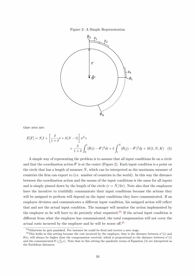
Figure 2: A Simple Representation

time zero are:

E[F ] = Nf +

[δ

1 + δt+ δ(N − t)

]σ2+

+δ

1 + δ

∫ t

0(θ(i)− θc)2di+ δ

∫ N

t(θ(j)− θc)2dj +M(t,N,K) (5)

A simple way of representing the problem is to assume that all input conditions lie on a circle

and that the coordination action θc is at the center (Figure 2). Each input condition is a point on

the circle that has a length of measure N , which can be interpreted as the maximum measure of

countries the firm can export to (i.e. number of countries in the world). In this way the distance

between the coordination action and the means of the input conditions is the same for all inputs

and is simply pinned down by the length of the circle (r = N/2π). Note also that the employees

have the incentive to truthfully communicate their input conditions because the actions they

will be assigned to perform will depend on the input conditions they have communicated. If an

employee deviates and communicates a different input condition, his assigned action will reflect

that and not the actual input condition. The manager will monitor the action implemented by

the employee so he will have to do precisely what requested.24 If the actual input condition is

different from what the employee has communicated, the total compensation will not cover the

actual costs incurred by the employee and he will be worse off.25

24Otherwise he gets punished. For instance he could be fired and receive a zero wage.25This holds in this setting because the cost incurred by the employee, that is the distance between av(i) and

θ(i), will always be higher than the compensation received, which is proportional to the distance between av(i)and the communicated θ ( δ

1+δr). Note that in this setting the quadratic terms of Equation (3) are interpreted as

the Euclidean distances.

16

Under this simple representation, the expected costs at time zero can be further simplified

as follows:

E[F ] = Nf +

[δ

1 + δt+ δ(N − t)

](σ2 + r2) +M(t,N,K) (6)

This expression shows very clearly the trade-off between outsourcing and integration. The

second term is decreasing in t and captures the benefits of integration: by coordinating the ac-

tions in-house the manager is able to steer production, internalize the externalities, and achieve

a lower coordination costs. On the other hand, by producing more inputs in-house, the com-

munication costs (third term) intuitively rise. In this simple baseline model, the returns to

in-sourcing do not depend on t, and the communication/monitoring costs do not depend on the

importance of adaptation δ and the variance of the input conditions σ2. Therefore even without

specifying much of the nature of the communication costs, I can state the first Proposition of

the paper.

Proposition 1: If the communication costs increase in t (∂M(t,N,K)∂t > 0), the expected

profits E[π] = −E[F ] are supermodular in t, σ2, δ. Hence, the optimal number (measure) of

inputs produced in-house t∗ increases with the importance of adaptation (δ) and the variance

of the input conditions (σ2): ∂t∗

∂δ > 0 and ∂t∗

∂σ2 > 0

Corollary 1: the complementarity with the variance of input conditions disappears when

the importance of adaptation goes to zero.

limδ→0

∂2E[π]

∂t∂σ2= lim

δ→0

δ2

1 + δ= 0 (7)

The proof is immediate and follows standard results on supermodularity.26 The intuition

is also quite straightforward. If adaptation is not very important, there is clearly no reason to

produce the inputs in-house because it is true that the manager can achieve better coordination

but this is needed only in case of adaptation and is costly due to communication costs.27 If

the conditions are very volatile, a situation in which the firm does not really know what it gets

or inputs are not very homogeneous, the firm will find it optimal to in-source more in order to

reduce the risk of having an input that will be very costly to coordinate because very far from

θc. Intuitively Corollary 1 further specifies that this effect disappears when adaptation is not

very important. These results are quite general because rely on a very simple and easily satisfied

assumption, namely that the communication costs increase in the number of inputs internally

produced.

26See for instance Milgrom and Roberts (1995).27An interesting extension to the model would be to have an heterogeneous adaptation need across inputs,

say δ(i), which could be interpreted as the probability of adaptation for that particular input. In this case it isintuitive that the first inputs to be outsourced would be the ones with very low adaptation probabilities, that isthe inputs that are fairly homogeneous or that are very far from the core competency of the firm, so that the firmhas no need to adapt them to its own production process.

17

4.4 Communication and Monitoring Costs

The manager has to communicate with all employees to learn their input conditions and then

monitoring their actions. Therefore the total monitoring costs are given by: M(t,N,K) =∫ t0 D(x,N,K)dx, where D(x,N,K) is the total diagnosis cost that the manager has to pay

to understand the message and monitor each employee. Following Cremer et al. (2007), the

manager is boundedly rational and can learn K words at most. Each word allows the manager

to identify and recognize a certain set of input conditions, which is referred to as the breath of

the word. The more general the word is (wider breadth), the higher is the diagnosis cost that the

manager has to incur in order to understand the content of the message. I simply assume that

the diagnosis cost for each word is linear in its breadth. Therefore the total expected diagnosis

cost is given by: D(x,N,K) =∑K

k=1 p(z∗k)z∗k, where z∗k is the optimal breadth of word k and

p(z∗k) is its probability. The words are of course not overlapping, that is, each of them refers to

different sets of events to minimize the costs.

In the simple setting of the present model, all the inputs are needed in equal proportions

(the production technology is Leontief), hence the manager will face the same probability of

communicating with each employee. Essentially the manager has to communicate with all

employees and therefore she will encounter all the input conditions with equal probability. In

the simple representation of Figure 2, each input condition lies on a point of the circle, and the

manager will therefore face an overall uniform distribution of events. Each input condition is in

fact equally likely and the overall distribution of input conditions that the manager encounters

is an uniform on the interval [0, N ], where N is again the measure of total input needed or, in

the empirical interpretation, the total number of countries the firm is exporting to.28

The manager will design an optimal code to minimize the total expected diagnosis cost given

the inputs that are produced internally. She will solve the following problem:

min{zk}Kk=1

K∑k=1

p(zk)zk s.t.K∑k=1

zk = x (8)

where p(zk) = zkN due to the fact that the underlying events are uniformly distributed. In this

setting the solution to the problem is very simple and all the words have the exact same breath:

z∗k = z∗h = xK , ∀l, h. Therefore the total expected diagnosis cost for each employee is given by:

D(x,N,K) = x2

KN . And the total communication costs are defined as follows:

M(t,N,K) =t3

3KN(9)

The costs are intuitively decreasing in the cognitive ability of the manager K and depend on

the set of inputs that are internally produced. Adding more inputs raises the costs for all other

inputs already internally produced because the manager has to change the code, and make

all words more imprecise in order to accommodate the new set of input conditions. Clearly

28Appendix A.3 shows that the main results of the paper holds in a more general setting, providing a constrainton a generic monitoring function.

18

Proposition 1 continues to hold in this setting. Finally, since the optimal actions refer to the

same underlying set of input conditions, the communication technology also allows the manager

to monitor the actions of the employees (for simplicity I assume that the cost is paid only once

for both activities).

4.5 The Optimal Outsourcing Share and the Effect of Globalization

Assuming the previous form of communication/monitoring costs, it is easy to solve the problem

that the manager faces at time zero and find the optimal measure of inputs internally produced.

A simple minimization of the expected costs in (6) with the communication costs as in (9), gives

the optimal share of inputs internally produced:

t∗

N= δ

√Kψ2

(1 + δ)Nwhere: ψ2 = σ2 + r2 (10)

When the firm outsources a positive share of its inputs the fixed cost function becomes:29

E[F ] =

FO︷ ︸︸ ︷(f + δψ2

)(N − t∗) +

FI︷ ︸︸ ︷[f +

3 + δ

3(1 + δ)δψ2

]t∗ = fN + δψ2N − 2

3

δ3ψ3

(1 + δ)

√KN

(1 + δ)(11)

where FO is the part of the fixed costs that is outsourced, and the share of outsourcing in total

fixed costs (Osh) can be defined as: Osh = E[FO/F ]. It is interesting to note that the total

expected fixed costs of the firm are decreasing in the manager’s skill (K) and increasing in the

importance of adaptation (δ).

I can then state the two main propositions of the paper, which will be tested in the empirical

section.

Proposition 2: If the number (measure) of destination countries increases, N ↑, the op-

timal share of outsourced inputs increases. This also implies that the elasticity of the share of

outsourcing in total fixed cost with respect to N is positive:

∂

∂N

(1− t∗

N

)=

1

2

t∗

N

1

N> 0 =⇒ εOsh,N > 0 (12)

Corollary 2: the share of outsourced inputs is concave in N :

∂2

∂N2

(1− t∗

N

)= −3

4

t∗

N

1

N2< 0 =⇒ ∂2Osh

∂N2< 0 (13)

Proposition 3: If the variance of the input conditions or the importance of adaptation

increase, σ2 ↑ or δ ↑, the optimal share of outsourced inputs decreases. This also implies that

29If t∗ = N the expected fixed costs are: E[F ] = fN + δ1+δ

ψ2N + N2

3K

19

the elasticity of the share of outsourcing in total fixed cost with respect to σ2 or δ is negative:

∂

∂σ2

(1− t∗

N

)= −1

2

t∗

N

1

σ2 + r2< 0 =⇒ εOsh,σ2 < 0 (14a)

∂

∂δ

(1− t∗

N

)= − 1

2δ

t∗

N

2 + δ

1 + δ< 0 =⇒ εOsh,δ < 0 (14b)

Corollary 3: Everything else constant, a manager with higher cognitive ability (K -

measure of skill) outsources a smaller share of inputs and the elasticity of the share of outsourcing

in total fixed cost with respect to K is negative:

∂

∂K

(1− t∗

N

)= −1

2

t∗

N

1

K< 0 =⇒ εOsh,K < 0 (15)

The proofs of both propositions follow immediately from the expressions for the optimal

share of inputs internally produced and the expected costs. The first part of the propositions is

straightforward, the second part requires simple but tedious algebra.

Proposition 2 gives the main effect of interest that will be extensively investigated in the

empirical part of the paper. When the number of destination countries increases, so does the

number of inputs needed to reach those destinations, making the coordination of these inputs

more and more complex. The reason is that the manager has to design a code that needs

to accommodate a larger set of different events, all arising with a very small probability. This

makes communication inside the firm very costly. The coordination benefits are still present and

the absolute number of inputs internally produced still increases, but their share in the total

number of inputs decreases. The reason is that the manager, facing too high communication

costs, finds it optimal to outsource to get the benefits of a low ex-ante price. Moreover Corollary

2 shows that the relationship between the optimal share of outsourced inputs and the number

of destination countries is non-linear, and concave in particular.

4.6 Profit Maximization and the Impact of Managerial Skills

I have so far focused on the cost of producing the fixed components of the exporting activity

and whether they are produced in-house or outsourced depending on the number of destination

markets reached by the firm. It is interesting to see what happens when also the variable part

of the cost function is specified together with the revenues generated by the firm. Especially

because this will allow me to investigate the impact of managerial skills on the total number of

export destinations chosen by the firm and on the share of outsourced costs.

I do this in a standard trade model with heterogeneous firms, as in Melitz (2003). There is

a continuum of firms, each characterized by the ability of its manager, K. After entering the

market of a particular differentiated good, the manger realizes her level of skills for that market,

which is drawn from an exogenous common distribution. The ability of the manager represents

the productivity level of the firm and affects the variable costs of producing a quantity q of the

good, q/K, expressed in labor units (wage is normalized to one). Consumers in each country

maximize a standard CES utility function, characterized by an elasticity of substitution ε =

20

1/(1−ρ) > 1. These preferences generate a total expenditure on each good equal to R(p/P )1−ε,

where R denotes aggregate expenditure and P the aggregate price index. In maximizing the

variable profits, each manager chooses the standard constant-markup pricing rule: p = 1/ρK.

This yields total variable profit in the domestic market equal to (1− ρ)R(ρKP )ρ/(1−ρ).

There is a continuum of export destinations, and the variable trade cost to export to a

certain country i takes the standard form of an “iceberg” transportation cost. If one unit of

any differentiated good is shipped to country i, only a fraction 1/τ(i) arrives. All countries

are symmetric and face an equal distribution of variable trade costs.30 This implies that all

countries will feature the same aggregate expenditure and price index. The total expected profit

of a firm that exports to N destination markets is then defined as follows:

E[π] = (1− ρ)R (ρKP )ρ

1−ρ

∫ N

0

(1

τ(i)

) ρ1−ρ

di− fN − δψ2N +2

3

δ3ψ3

(1 + δ)32

K12N

12 (16)

where countries are ranked with respect to the their variable trade cost τ(i).

Note that when the importance of adaptation goes to zero (δ → 0) the expression for the

total fixed cost simplifies to a standard case, as in Melitz (2003), with the only twist that

the fixed part is entirely outsourced by the firm to domestic suppliers. In the present settings

instead, the ability of the manager also affects the fixed part of export costs, which are lower

for a firm with a better manager. At the margin, exporting to an extra country is more costly

because this implies a higher coordination complexity for the manager. Therefore the manager,

depending on her ability, chooses the optimal number of destination markets by maximizing the

total profits in Equation (16). The optimal number of destination countries N∗ is pinned down

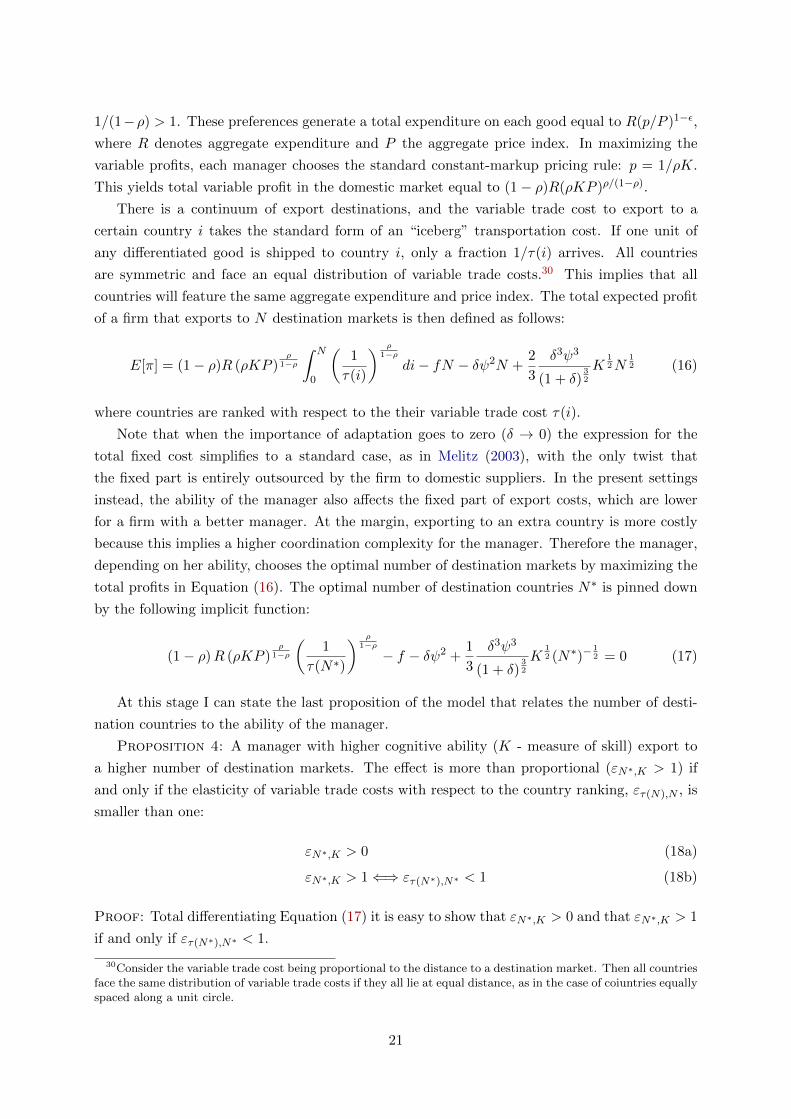
by the following implicit function:

(1− ρ)R (ρKP )ρ

1−ρ

(1

τ(N∗)

) ρ1−ρ− f − δψ2 +

1

3

δ3ψ3

(1 + δ)32

K12 (N∗)−

12 = 0 (17)

At this stage I can state the last proposition of the model that relates the number of desti-

nation countries to the ability of the manager.

Proposition 4: A manager with higher cognitive ability (K - measure of skill) export to

a higher number of destination markets. The effect is more than proportional (εN∗,K > 1) if

and only if the elasticity of variable trade costs with respect to the country ranking, ετ(N),N , is

smaller than one:

εN∗,K > 0 (18a)

εN∗,K > 1⇐⇒ ετ(N∗),N∗ < 1 (18b)

Proof: Total differentiating Equation (17) it is easy to show that εN∗,K > 0 and that εN∗,K > 1

if and only if ετ(N∗),N∗ < 1.

30Consider the variable trade cost being proportional to the distance to a destination market. Then all countriesface the same distribution of variable trade costs if they all lie at equal distance, as in the case of coiuntries equallyspaced along a unit circle.

21

The intuition for the proof is also quite straightforward. Not only is a better manager able to

produce at a lower marginal cost and hence sell more, but she is also more capable of managing

the extra complexity associated with exporting to more destination countries. The increase in

the number of destination countries will be higher the lower the increase in variable trade costs.

In the present setting, the solution intuitively depends on how fast the variable trade cost rise

with exporting to an extra country. If the elasticity is smaller than one, the marginal increase in

variable profit is dis-proportionally higher than the marginal increase in fixed cost due to higher

coordination complexity. It is interesting to note that this is generally the case if variable trade

costs are proportional to distance, in fact the elasticity of variable trade cost with respect to

distance is generally smaller than one, as found by Chen and Novy (2011).

5 Econometric Evidence from France

5.1 Data

The model is tested using firm level data from France for the period 1996-2007. I rely on

four main data sources. First, the Enquete annuelle d’Entreprise (EAE) that collects balance

sheet data on all French firms with more than 20 employees and a sample of smaller firms.

Second, the Declaration annuelle de donnees sociales (DADS) that collects employment data on

all firms with paid employees; the data used are aggregated at the establishment level. Third,

transaction level import-export data come from the French Customs; these data have been used

among others by Eaton et al. (2004). Finally, the service outsourcing data contained in the

EAE are integrated with the Enquete Recours aux Services par l’Industrie (ERSI), a survey of

firms with more than 20 employees and the census of firms with more than 250 employees that

collects detailed information about service outsourcing policies for the year 2005. The analysis

will mainly focus on manufacturing firms (NACE Rev1.1 D category).

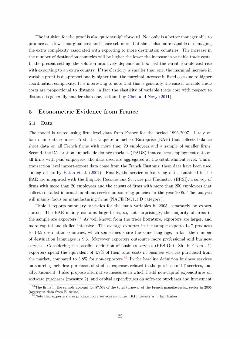
Table 1 reports summary statistics for the main variables in 2005, separately by export

status. The EAE mainly contains large firms, so, not surprisingly, the majority of firms in

the sample are exporters.31 As well known from the trade literature, exporters are larger, and

more capital and skilled intensive. The average exporter in the sample exports 14.7 products

to 13.5 destination countries, which sometimes share the same language, in fact the number

of destination languages is 9.5. Moreover exporters outsource more professional and business

services. Considering the baseline definition of business services (PBS Out. Sh. in Costs - 1)

exporters spend the equivalent of 4.7% of their total costs in business services purchased from

the market, compared to 3.8% for non-exporters.32 In the baseline definition business services

outsourcing includes: purchases of studies, expenses related to the purchase of IT services, and

advertisement. I also propose alternative measures in which I add non-capital expenditures on

software purchases (measure 2), and capital expenditures on software purchases and investment

31The firms in the sample account for 87.5% of the total turnover of the French manufacturing sector in 2005(aggregate data from Eurostat).

32Note that exporters also produce more services in-house: HQ Intensity is in fact higher.

22

Table 1: Summary Statistics by Export Status - 2005

Nonexporters Exporters

Mean Median N Mean Median N

Employment 44.6 30 5,220 158.4 48 16,453Turnover 7,107 3,331 5,076 47,257 8,577 16,360Total Exports 0 0 5,307 13,575 793 16,497Num. Countries 0 0 5,307 13.5 7 16,497Num. Products 0 0 5,307 14.7 7 16,497Num. Languages 0 0 5,307 9.44 7 16,497K/L Ratio 52.8 23.5 5,057 99.1 43.4 16,336S/U Ratio 0.65 0.26 4,984 1.12 0.42 15,961Professionals Sh. 0.074 0.045 5,049 0.13 0.086 16,171HQ Intensity 0.035 0 5,031 0.069 0 16,306PBS Out. Sh. in Costs - 1 0.034 0.0045 4,800 0.047 0.013 15,951PBS Out. Sh. in Costs - 1b 0.023 0.0037 4,800 0.034 0.01 15,951PBS Out. Sh. in Costs - 2 0.034 0.0046 4,800 0.047 0.014 15,951PBS Out. Sh. in Costs - 3 0.034 0.0049 4,934 0.048 0.015 16,241

Note: Turnover, total exports, and K/L ratio are measured in thousands of e. Full sample.

in R&D (measure 3).33 More precise variable definitions and the procedure employed to clean

the data are described in Appendix B.

Table 2 shows the change over time for the main variables of interest. On average firms have

increased their share of outsourced services in total costs by 10%, from a share of 3.86% in 1996

up to 4.25% in 2007. The average firm has increased the number of export destination countries

from 7.9 in 1996 to 10 in 2007, equivalent to a 27.5% increase.

Table 2: Change in Outsourcing Shares and Destination Countries

1996 2007 Change

PBS Out. Sh. in Costs - 1 0.0386 0.0425 10.10%PBS Out. Sh. in Costs - 2 0.0386 0.0426 10.36%PBS Out. Sh. in Costs - 3 0.0397 0.0432 8.82%Num. Countries 7.8787 10.0427 27.47%

5.2 The Impact of Coordination Complexity on PBS Outsourcing

By averaging across all firms exporting to a certain number of markets in all years, Figure 7 shows

that the share of purchased business service on sales is positively and significantly related to the

number of export destination countries, the main measure of coordination complexity used in

the analysis. The simple intuition is that the higher the number of countries a firm is exporting

to, the more complex its business environment is going to be. This is very much in line with

33The latter measure is probably the less reliable because it is not possible to completely rule out the possibilitythat part of the R&D investment is actually performed in-house.

23

the most common definition of complexity in systems theory, where complexity arises through

connectivity and the inter-relationships of a system’s constituent elements. In the present case,

the higher the number of connections (destination countries), the higher coordination complexity

is going to be, because exporting requires more inputs. Designing a communication code for

all these infrequent events is very costly and therefore, according to Proposition 2, the share of

outsourced inputs in total costs increases.

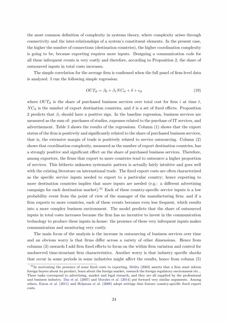
The simple correlation for the average firm is confirmed when the full panel of firm-level data

is analyzed. I run the following simple regression:

OUTit = β0 + β1NCit + δ + εit (19)

where OUTit is the share of purchased business services over total cost for firm i at time t,

NCit is the number of export destination countries, and δ is a set of fixed effects. Proposition

2 predicts that β1 should have a positive sign. In the baseline regression, business services are

measured as the sum of: purchases of studies, expenses related to the purchase of IT services, and

advertisement. Table 3 shows the results of the regressions. Column (1) shows that the export

status of the firm is positively and significantly related to the share of purchased business services,

that is, the extensive margin of trade is positively related to service outsourcing. Column (2)

shows that coordination complexity, measured as the number of export destination countries, has

a strongly positive and significant effect on the share of purchased business services. Therefore,

among exporters, the firms that export to more countries tend to outsource a higher proportion

of services. This hitherto unknown systematic pattern is actually fairly intuitive and goes well

with the existing literature on international trade. The fixed export costs are often characterized

as the specific service inputs needed to export to a particular country; hence exporting to

more destination countries implies that more inputs are needed (e.g.: a different advertising

campaign for each destination market).34 Each of these country-specific service inputs is a low

probability event from the point of view of the manager of the manufacturing firm; and if a

firm exports to more countries, each of these events becomes even less frequent, which results

into a more complex business environment. The model predicts that the share of outsourced

inputs in total costs increases because the firm has no incentive to invest in the communication

technology to produce these inputs in-house: the presence of these very infrequent inputs makes

communication and monitoring very costly.

The main focus of the analysis is the increase in outsourcing of business services over time

and an obvious worry is that firms differ across a variety of other dimensions. Hence from

columns (3) onwards I add firm fixed effects to focus on the within firm variation and control for

unobserved time-invariant firm characteristics. Another worry is that industry specific shocks

that occur in some periods in some industries might affect the results, hence from column (5)

34In motivating the presence of some fixed costs to exporting, Melitz (2003) asserts that a firm must informforeign buyers about its product, learn about the foreign market, research the foreign regulatory environment etc...These tasks correspond to advertising, market and legal research, and they are all supplied by the professionaland business industry. Das et al. (2007) and Morales et al. (2014) put forward very similar arguments. Amongothers, Eaton et al. (2011) and Helpman et al. (2008) adopt settings that feature country-specific fixed exportcosts.

24

Table 3: Purchased Business Services and Coordination Complexity

(1) (2) (3) (4) (5) (6) (7) (8)

Dependent Var. Out. 1 Out. 1 Out. 1 Out. 1 Out. 1 Out. 2 Out. 3 Out. 1

Exporter 0.554*** 0.098***(0.020) (0.017)

NC 0.185*** 0.083*** 0.086*** 0.087*** 0.078*** 0.086***(0.008) (0.010) (0.010) (0.010) (0.010) (0.022)

Observations 235,182 184,556 235,182 184,556 184,556 184,864 186,725 184,556Num. of firms 39,500 31,212 39,500 31,212 31,212 31,246 31,380 31,212Year FE Yes Yes Yes YesIndustry FE Yes YesIndustry-Year FE Yes Yes Yes YesFirm FE Yes Yes Yes Yes Yes YesCluster Firm Firm Firm Firm Firm Firm Firm Industry

Note: The dependent variable is the share of purchased services over total costs measured in logs. In columns(1)-(5) and (8) business services are measured as the sum of purchases of studies, expenses related to thepurchase of IT services, and advertisement. Column (6) adds non-capital expenditures on software purchases.Columns (7) adds capital expenditures on software purchases and investment in R&D. Data are for period1996-2007. Clustered standard errors in parentheses; (*, **. ***) indicate 10, 5, and 1 percent significancelevels.

onwards I control for a full set of interacted industry-by-year fixed effects. By focusing on the

within variation the magnitude of the results is smaller but becoming an exporter or increasing

the number of export destination is still highly related to more business services outsourcing.35

The effect is also quantitatively important. Considering the coefficient in column 5 and the

variation shown in Table 2, for the average firm in the sample, the increase in the number

of destination countries explains almost a quarter of the increase in the share of outsourced

services over the period. The following columns show that very little changes when I modify

the measure of outsourcing by adding non-capital expenditures on software purchases (column

6), and capital expenditures on software purchases and investment in R&D (column 7). Finally

column (8) shows that the result is still highly significant even after clustering standard errors

at the industry level and performing the full degrees of freedom adjustment due to non-nested

panels within clusters (firms that change industry).

The literature on firm boundaries has proposed many other potentially time-varying determi-

nants that could affect outsourcing, other than the proposed proxy for coordination complexity.

I therefore modify the basic regression to include other controls, I run the following regression:

OUTit = αi + β1NCit +W′

itβ2 + δjt + εit (20)

where OUTit and NCit are defined as before, Wit is a vector of controls, αi are firm fixed effects,

and δjt are the full interaction of industry and year fixed effects. The first interesting question

to ask is whether outsourcing of services is a fixed cost component as assumed so far, or it also

entails tasks related to variable costs. In the latter case outsourcing of business services would be

also affected by the export intensive margin. I therefore include total exports in the regression.

35A simple reason for the smaller magnitude could be the classic attenuation bias from measurement error, seeAngrist and Pischke (2008).

25

As column (2) of Table 4 shows, the intensive margin does not in fact drive the purchase of

business services. Hence the common assumption that business services are a fixed export cost

component seems to hold in the data. I will further investigate this issue in Section 6.

Table 4 also shows the baseline results after the inclusion of several controls common in

the vertical integration literature: capital intensity, human-capital intensity, and a measure of

scale economies (total number of employees) as in Antras (2003); a measure firm-level contract

intensity in the spirit of Nunn (2007); and a measure of headquarter intensity as proposed

by Antras and Helpman (2004, 2008). The effect of coordination complexity remains robust

and stable to the inclusion of all controls. Most importantly column (6) includes a measure of

internal production of services. The model predicts that when the number of infrequent tasks

increases, these will be outsourced. It is therefore important to verify that this increase in the

need of service inputs is not driven by an overall re-focus of the firm towards service activity,

which would imply a parallel increase in the internal production of services. Controlling for

internal production is not easy, even with micro-level data, because it is hard to observe the

tasks internally produced by firms. In a related paper for the U.S., Berlingieri (2013), I show that

this alternative story does not hold in the data at the aggregate manufacturing industry level,

after controlling for business services produced in-house. I adopt a similar strategy here and

control for the share of revenues generated by establishments of the firm that are classified within

services, which is essentially equivalent to controlling for the revenue share of headquarters. In

this specification I include establishments producing any type of services, not only business

services. As column (6) shows the results are very robust to this measure of internal production.

Table 4: Purchased Business Services and Coordination Complexity - Covariates

(1) (2) (3) (4) (5) (6) (7) (8) (9)

Exporter 0.098***(0.017)

NC 0.086*** 0.082*** 0.083*** 0.086*** 0.086*** 0.080*** 0.085*** 0.089***(0.010) (0.011) (0.011) (0.011) (0.011) (0.011) (0.013) (0.013)

Exports 0.003 0.003 0.001 0.002 -0.001 -0.000 0.000(0.005) (0.005) (0.005) (0.005) (0.005) (0.005) (0.006)

Capital Intensity 0.030*** 0.028** 0.028** 0.035*** 0.024* 0.022(0.011) (0.012) (0.012) (0.013) (0.014) (0.014)

Skill Intensity 0.047*** 0.046*** 0.051*** 0.051*** 0.051***(0.010) (0.010) (0.010) (0.011) (0.012)

HQ Intensity -0.052 -0.054 -0.047 -0.054(0.037) (0.037) (0.039) (0.039)

Scale 0.081*** 0.066*** 0.065***(0.022) (0.023) (0.024)

Num imp. products 0.014* 0.019**(0.008) (0.009)

Contract Intensity 0.015**(0.006)

Observations 235,182 184,556 184,556 183,487 174,908 174,682 174,682 150,874 144,927Number of firms 39,500 31,212 31,212 31,073 30,172 30,159 30,159 26,091 25,339R-sq W 0.01 0.01 0.01 0.01 0.01 0.01 0.01 0.01 0.01Fixed effects Firm Firm Firm Firm Firm Firm Firm Firm Firm

ind#yr ind#yr ind#yr ind#yr ind#yr ind#yr ind#yr ind#yr ind#yr

Note: The dependent variable is the share of purchased services over total costs. All variables are in logsapart from HQ Intensity. Data are for period 1996-2007. Firm-clustered standard errors in parentheses; (*,**. ***) indicate 10, 5, and 1 percent significance levels.

Some of the other controls are also worth discussing. It is interesting to note that the firm

26

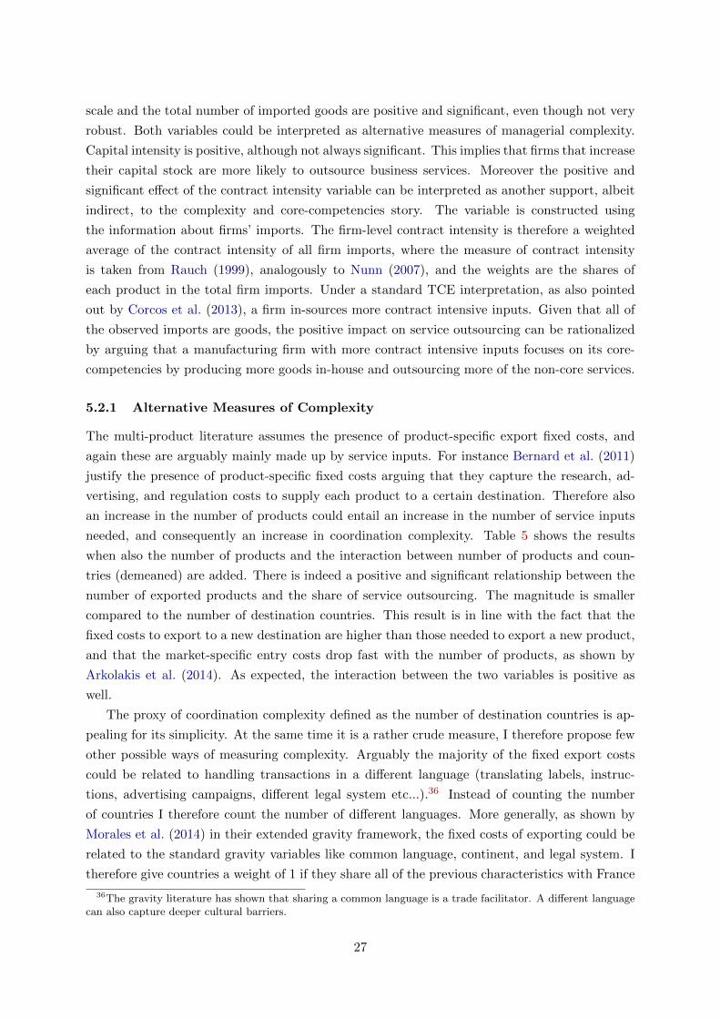
scale and the total number of imported goods are positive and significant, even though not very

robust. Both variables could be interpreted as alternative measures of managerial complexity.

Capital intensity is positive, although not always significant. This implies that firms that increase

their capital stock are more likely to outsource business services. Moreover the positive and

significant effect of the contract intensity variable can be interpreted as another support, albeit

indirect, to the complexity and core-competencies story. The variable is constructed using

the information about firms’ imports. The firm-level contract intensity is therefore a weighted

average of the contract intensity of all firm imports, where the measure of contract intensity

is taken from Rauch (1999), analogously to Nunn (2007), and the weights are the shares of

each product in the total firm imports. Under a standard TCE interpretation, as also pointed

out by Corcos et al. (2013), a firm in-sources more contract intensive inputs. Given that all of

the observed imports are goods, the positive impact on service outsourcing can be rationalized

by arguing that a manufacturing firm with more contract intensive inputs focuses on its core-

competencies by producing more goods in-house and outsourcing more of the non-core services.

5.2.1 Alternative Measures of Complexity

The multi-product literature assumes the presence of product-specific export fixed costs, and

again these are arguably mainly made up by service inputs. For instance Bernard et al. (2011)

justify the presence of product-specific fixed costs arguing that they capture the research, ad-

vertising, and regulation costs to supply each product to a certain destination. Therefore also

an increase in the number of products could entail an increase in the number of service inputs

needed, and consequently an increase in coordination complexity. Table 5 shows the results

when also the number of products and the interaction between number of products and coun-

tries (demeaned) are added. There is indeed a positive and significant relationship between the

number of exported products and the share of service outsourcing. The magnitude is smaller

compared to the number of destination countries. This result is in line with the fact that the

fixed costs to export to a new destination are higher than those needed to export a new product,

and that the market-specific entry costs drop fast with the number of products, as shown by

Arkolakis et al. (2014). As expected, the interaction between the two variables is positive as

well.

The proxy of coordination complexity defined as the number of destination countries is ap-

pealing for its simplicity. At the same time it is a rather crude measure, I therefore propose few

other possible ways of measuring complexity. Arguably the majority of the fixed export costs

could be related to handling transactions in a different language (translating labels, instruc-

tions, advertising campaigns, different legal system etc...).36 Instead of counting the number

of countries I therefore count the number of different languages. More generally, as shown by

Morales et al. (2014) in their extended gravity framework, the fixed costs of exporting could be

related to the standard gravity variables like common language, continent, and legal system. I

therefore give countries a weight of 1 if they share all of the previous characteristics with France

36The gravity literature has shown that sharing a common language is a trade facilitator. A different languagecan also capture deeper cultural barriers.

27

Table 5: PBS Outsourcing and Number of Products

(1) (2) (3) (4) (5) (6) (7) (8) (9) (10)

NC 0.086*** 0.068*** 0.082*** 0.080*** 0.081*** 0.084*** 0.083*** 0.078*** 0.081*** 0.084***(0.010) (0.011) (0.012) (0.012) (0.012) (0.012) (0.012) (0.013) (0.014) (0.014)

NP 0.028*** 0.038*** 0.036*** 0.036*** 0.036*** 0.037*** 0.034*** 0.032*** 0.031***(0.008) (0.009) (0.009) (0.009) (0.009) (0.009) (0.009) (0.010) (0.010)

NC#NP 0.029*** 0.030*** 0.030*** 0.030*** 0.030*** 0.027*** 0.027*** 0.028***(0.005) (0.006) (0.006) (0.006) (0.006) (0.006) (0.006) (0.006)

Exports 0.003 0.002 0.001 0.001 -0.001 0.000 0.001(0.005) (0.005) (0.005) (0.005) (0.005) (0.006) (0.006)

Capital Intensity 0.031*** 0.029** 0.029** 0.035*** 0.024* 0.022(0.011) (0.012) (0.012) (0.012) (0.014) (0.014)

Skill Intensity 0.047*** 0.046*** 0.050*** 0.050*** 0.050***(0.010) (0.010) (0.010) (0.011) (0.012)

HQ Intensity -0.058 -0.059 -0.051 -0.059(0.037) (0.037) (0.038) (0.039)

Scale 0.064*** 0.051** 0.049**(0.022) (0.023) (0.024)

Num imp. products 0.008 0.013(0.008) (0.009)

Contract Intensity 0.015**(0.006)

Observations 184,556 184,556 184,556 184,556 183,487 174,908 174,682 174,682 150,874 144,927Number of firms 31,212 31,212 31,212 31,212 31,073 30,172 30,159 30,159 26,091 25,339R-sq W 0.01 0.01 0.01 0.01 0.01 0.01 0.01 0.01 0.01 0.01Fixed effects Firm Firm Firm Firm Firm Firm Firm Firm Firm Firm

ind#yr ind#yr ind#yr ind#yr ind#yr ind#yr ind#yr ind#yr ind#yr ind#yr

Note: The dependent variable is the share of purchased services over total costs. All variables are in logs andinteraction variables are demeaned. See notes in Table 4.

Table 6: Alternative Measures of Coordination Complexity

(1) (2) (3) (4) (5) (6)

Exports 0.003 0.010 0.004 0.007 0.006 0.004(0.014) (0.014) (0.014) (0.014) (0.014) (0.014)

NC 0.135***(0.016)

Num Languages 0.113***(0.014)

NC (Gravity) 0.123***(0.016)

NC (WB Doing Business) 0.100***(0.014)

NC (WB Doing Business - Trade) 0.100***(0.014)

NC (Complexity) 0.143***(0.016)

Observations 176,492 176,492 176,492 176,492 176,492 176,492Number of firms 30,438 30,438 30,438 30,438 30,438 30,438R-sq W 0.01 0.01 0.01 0.01 0.01 0.01Fixed effects Firm Firm Firm Firm Firm Firm

ind#yr ind#yr ind#yr ind#yr ind#yr ind#yr

Note: The dependent variable is the share of purchased services over total costs. All columns also includethe following regressors: K/L, S/L, HQ Intensity, and Scale. Regressors are standardized. Only exportersare included in the sample. See also notes in Table 4.

28

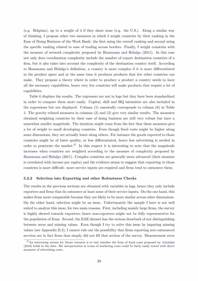
(e.g. Belgium), up to a weight of 4 if they share none (e.g. the U.S.). Along a similar way

of thinking, I propose other two measures in which I weight countries by their ranking in the

Ease of Doing Business of the Work Bank: the first using the overall ranking and second using

the specific ranking related to ease of trading across borders. Finally, I weight countries with

the measure of network complexity proposed by Hausmann and Hidalgo (2011). In this case

not only does coordination complexity include the number of export destination countries of a

firm, but it also takes into account the complexity of the destination country itself. According

to Hausmann and Hidalgo’s definition, a country is more complex if it is more differentiated

in the product space and at the same time it produces products that few other countries can

make. They propose a theory where in order to produce a product a country needs to have

all the necessary capabilities, hence very few countries will make products that require a lot of

capabilities.

Table 6 displays the results. The regressors are not in logs but they have been standardized

in order to compare them more easily. Capital, skill and HQ intensities are also included in

the regressions but not displayed. Column (1) essentially corresponds to column (6) in Table

4. The gravity related measures in columns (2) and (3) give very similar results. The measures

obtained weighting countries by their ease of doing business are still very robust but have a

somewhat smaller magnitude. The intuition might come from the fact that these measures give

a lot of weight to small developing countries. Even though fixed costs might be higher along

some dimensions, they are actually lower along others. For instance the goods exported to those

countries might be of lower quality, or less differentiated, hence less advertising is needed in

order to penetrate the market.37 In this respect it is interesting to note that the magnitude

increases when countries are weighted according to the measure of complexity proposed by

Hausmann and Hidalgo (2011). Complex countries are generally more advanced (their measure

is correlated with income per capita) and the evidence seems to suggest that exporting to those

countries is more difficult: more service inputs are required and firms tend to outsource them.

5.2.2 Selection into Exporting and other Robustness Checks

The results in the previous sections are obtained with variables in logs, hence they only include

exporters and firms that do outsource at least some of their service inputs. On the one hand, this

makes firms more comparable because they are likely to be more similar across other dimensions.

On the other hand, selection might be an issue. Unfortunately the sample I have is not well

suited to analyze this issue, for two main reasons. First, including mainly large firms, the survey

is highly skewed towards exporters; hence non-exporters might not be fully representative for

the population of firms. Second, the EAE dataset has the serious drawback of not distinguishing

between zeros and missing values. Even though I try to solve this issue by imputing missing

values (see Appendix B.3), I cannot rule out the possibility that firms reporting zero outsourced

services are in fact firms that simply did not fill that section of the survey. Measurement error

37An interesting avenue for future research is to test whether the form of fixed costs proposed by Arkolakis(2010) holds in the data. His interpretation in terms of marketing costs could be fairly easily tested with directmeasures of advertising costs.

29

is therefore likely to be present and might affect the results. Despite these warnings, I re-obtain

all the results without taking logs, and the exact same picture emerges. For instance Table

7 replicates the results of Table 4 without taking logs of the regressors but standardizing the

variables to compare them more easily. Coordination complexity measured as the number of

destination countries is still positive and highly significant in all specifications. Moreover the

overall trade extensive margin (being an exporter) is also positive and highly significant in all

specifications, while the trade intensive marking remains insignificant. A very similar picture

holds true when I also include firms that do not outsource services (or that do not report it).

Table 7: PBS Outsourcing and Coordination Complexity with Non-Exporters

(1) (2) (3) (4) (5) (6) (7) (8) (9) (10)

Exporter 0.042*** 0.035*** 0.035*** 0.035*** 0.035*** 0.034*** 0.035*** 0.035*** 0.035*** 0.040***(0.007) (0.007) (0.007) (0.008) (0.008) (0.008) (0.008) (0.008) (0.008) (0.011)

NC 0.141*** 0.141*** 0.137*** 0.137*** 0.130*** 0.130*** 0.128*** 0.121*** 0.120***(0.016) (0.016) (0.016) (0.016) (0.016) (0.016) (0.016) (0.016) (0.017)

Exports 0.003 0.004 0.004 -0.001 -0.001 0.003 -0.002 0.001(0.011) (0.011) (0.011) (0.012) (0.012) (0.015) (0.015) (0.014)

TFP -0.001 -0.001 0.002 0.002 0.001 0.001 0.002(0.005) (0.006) (0.006) (0.006) (0.006) (0.006) (0.006)

Capital Intensity -0.001 -0.004*** -0.004*** -0.004*** -0.004*** -0.004***(0.002) (0.001) (0.001) (0.001) (0.001) (0.001)

Skill Intensity 0.004 0.004 0.004 0.005 0.008(0.006) (0.006) (0.006) (0.006) (0.006)

HQ Intensity -0.004 -0.004 -0.004 -0.003(0.005) (0.005) (0.005) (0.005)

Scale 0.025* 0.019 0.018(0.014) (0.014) (0.013)

Num imp. products 0.027** 0.032***(0.011) (0.011)

Contract Intensity 0.002(0.008)

Observations 235,182 235,182 235,182 224,565 224,565 215,425 215,141 215,141 215,141 161,311Number of firms 39,500 39,500 39,500 37,614 37,614 36,606 36,582 36,582 36,582 27,947R-sq W 0.01 0.01 0.01 0.01 0.01 0.01 0.01 0.01 0.01 0.01Fixed effects Firm Firm Firm Firm Firm Firm Firm Firm Firm Firm

ind#yr ind#yr ind#yr ind#yr ind#yr ind#yr ind#yr ind#yr ind#yr ind#yr

Note: The dependent variable is the share of purchased services over total costs in logs. All other variablesare standardized. See also notes in Table 4.

Finally the baseline result is very robust across many specifications and controls. For instance

the same picture holds true when purchased services are weighted by total sales instead of total

costs. Moreover the EAE survey also contains a measure of outsourcing of non-core activities.

The model does not differentiate inputs; therefore there is no ’a priori’ clear distinction between a

service or a non-service input, apart from the intuitive assumption that for manufacturing firms

the importance of adaptation will be higher for the primary good inputs (hence, by Proposition

1, they will be more likely to be produced in-house compared to services). There are although

manufacturing firms whose activity has almost completely shifted towards services, which have

essentially become their core competencies (Nike and P&G are two leading examples). In this

respect a measure of outsourcing of non-core activities is possibly even more in line with the

model. Managerial complexity, measured as the number of export destination countries, has

again a positive and even stronger impact on outsourcing, when this alternative definition is

considered.38

38Table C.1 in the Appendix shows the results. An interpretation of this result is that most of these non-coreactivities are actually services given that only manufacturing firms are analyzed, the two measures of outsourcingcould be therefore quite similar (see the definitions in Appendix B.2).

30

5.3 Input Volatility and Managerial Skills: Evidence on Proposition 3

It is harder to provide empirical evidence on the other predictions of the model, since parameters

such as the variance of the input conditions and the importance of adaptation are not easy

to capture empirically. Still, the richness of the data allows me to provide good empirical

counterparts of these parameters and present results that support the theory.

The predictions of Proposition 3 simply further qualify what already stated in Proposition 1,

hence the intuition is precisely the same. An increase in the volatility of the inputs will result in

a higher share of in-sourcing because the manager does not know what she gets from the external

supplier, and this might result in a very costly ex-post coordination. And if the importance of

adaptation is higher it is clearly optimal to in-source more, because that gives more weight to

the ex-post coordination for which the internal production is better than the market.

The volatility of input conditions is intuitively related to the degree of homogeneity of the

input. Ideally I would use some direct measure of differentiation, as for instance provided by

Rauch (1999), but unfortunately this is not available for services. A first way to capture this

concept is to look at a measure of dispersion across inputs, rather than specific for each single

input. This might capture the overall volatility of inputs, which is not far from the prediction

of the model since I have assumed the same variance for all inputs.39 Given that a country-

specific task needs to be solved to export to a given destination, the overall input volatility can

be measured with the dispersion of export shares across destinations. I therefore proxy input

volatility with one minus the Herfindahl-Hirschman index of export shares, also known as the

Gini-Simpson diversity index. This is admittedly an imperfect measure of the homogeneity of

each single service input. Still, when I add this measure of export dispersion to the previous

regressions the results are in line with what predicted by the model, as Table 8 shows. The

elasticity of the share of outsourcing with respect to export dispersion is negative, although

marginally significant and not robust to all controls, especially when the sample is restricted to

firms that both import and export (last two columns of the table).

Table 8: Purchased Business Services and Input Volatility

(1) (2) (3) (4) (5) (6) (7) (8) (9)

NC 0.086*** 0.082*** 0.096*** 0.098*** 0.101*** 0.101*** 0.094*** 0.096*** 0.101***(0.010) (0.011) (0.014) (0.014) (0.014) (0.014) (0.014) (0.016) (0.016)

Exports 0.003 0.002 0.002 0.000 0.000 -0.002 -0.001 -0.001(0.005) (0.005) (0.005) (0.005) (0.005) (0.005) (0.005) (0.006)

Export Dispersion -0.048 -0.053* -0.054* -0.054* -0.051* -0.042 -0.045(0.029) (0.030) (0.030) (0.030) (0.030) (0.032) (0.033)

Observations 184,556 184,556 184,556 183,487 174,908 174,682 174,682 150,874 144,927Number of firms 31,212 31,212 31,212 31,073 30,172 30,159 30,159 26,091 25,339R-sq W 0.01 0.01 0.01 0.01 0.01 0.01 0.01 0.01 0.01Fixed effects Firm Firm Firm Firm Firm Firm Firm Firm Firm

ind#yr ind#yr ind#yr ind#yr ind#yr ind#yr ind#yr ind#yr ind#yr

Note: The dependent variable is the share of purchased services over total costs. All variables are in logsapart from HQ Intensity. Columns from 4 to 9 contain the exact same controls of Table 4. Data are forperiod 1996-2007. Firm-clustered standard errors in parentheses; (*, **. ***) indicate 10, 5, and 1 percentsignificance levels.

A better way to capture the volatility of the input conditions is to look directly at the

39The model can be extended to a input-specific variance σ(i).

31

characteristics of the service inputs. I can answer this question drawing on the extra information

contained in the ERSI survey, which provides data on service outsourcing policies at the firm-

service level. In particular the survey asks firms whether they outsource any of 34 detailed types

of services. Most of them are classified in the Professional and Business Services industry, but

there are also some transportation, financial and real estate services. Unfortunately the survey

is available in 2005 only and for a smaller sample of firms. In fact it includes all firms with more

than 250 employees but just a sample of smaller firms for a total of 4,745 manufacturing firms

(after the data cleaning procedure described in Appendix B.3), compared to 24,117 firms in the

EAE in 2005.40

I capture the characteristics of each service by analyzing the market in which it is produced.

In particular I compute the Gini-Simpson diversity index for the 4-digit industries that pro-

duce each type of service. As argued by Sutton (1991), if a product is more homogeneous,

the toughness of price competition should be expected to be high and the market to be more

concentrated, other things equal (in particular controlling for sunk costs). In other words, in a

less concentrated market the service type is going to be less homogeneous and firms are more

likely to need to re-adapt the service ex-post. I proxy the service firms’ market shares using

the share of total labor costs in each industry from the DADS data. Alternatively I use actual

market shares using the EAE survey for the service sector; in this case I do not have the entire

population of firms and I can calculate the dispersion index only for a sub-sample of service

types (27 out of 34). In any case the two measures are highly correlated, and results are very

robust to both definitions. The advantage of using the second measure is that I can control for

average sunk costs in the industry, which I proxy with the average capital stock.41 Using the

EAE survey I can also capture dispersion of the market with the shape parameter of the Pareto

distribution, as in Helpman et al. (2004).

The dependent variable is now a binary variable that takes value equal to one if the service

input s is outsourced by firm i. The regression specification is as follows:

OUT ∗is = β0 + β1NCi +W′

itβ2 + β3Disps + δj + δc + εis (21)

where Disps is a measure of dispersion for service s, δj and δc are industry and aggregate service

category fixed effects, and OUT ∗is is a latent variable such that:

OUTis =

{1 if OUT ∗is > 0

0 otherwise(22)

Table 9 reports the results of the exercise using OLS (columns 1-3), a Probit model (columns

4-6), or a Logit model (columns 7-9). Beyond those displayed, the set of control variables

Wit also includes capital, skill and HQ intensities. As expected, the dispersion of the service

sector is negative, strongly significant and extremely robust to the inclusion of other controls.

40The firms in the ERSI sample account for 50% of the total turnover of the French manufacturing sector in2005 (aggregate data from Eurostat).

41Ideally I would control for measures of endogenous sunk costs as well, such as advertising and R&D expen-ditures. Unfortunately for service industries almost no firm reports these measures.

32

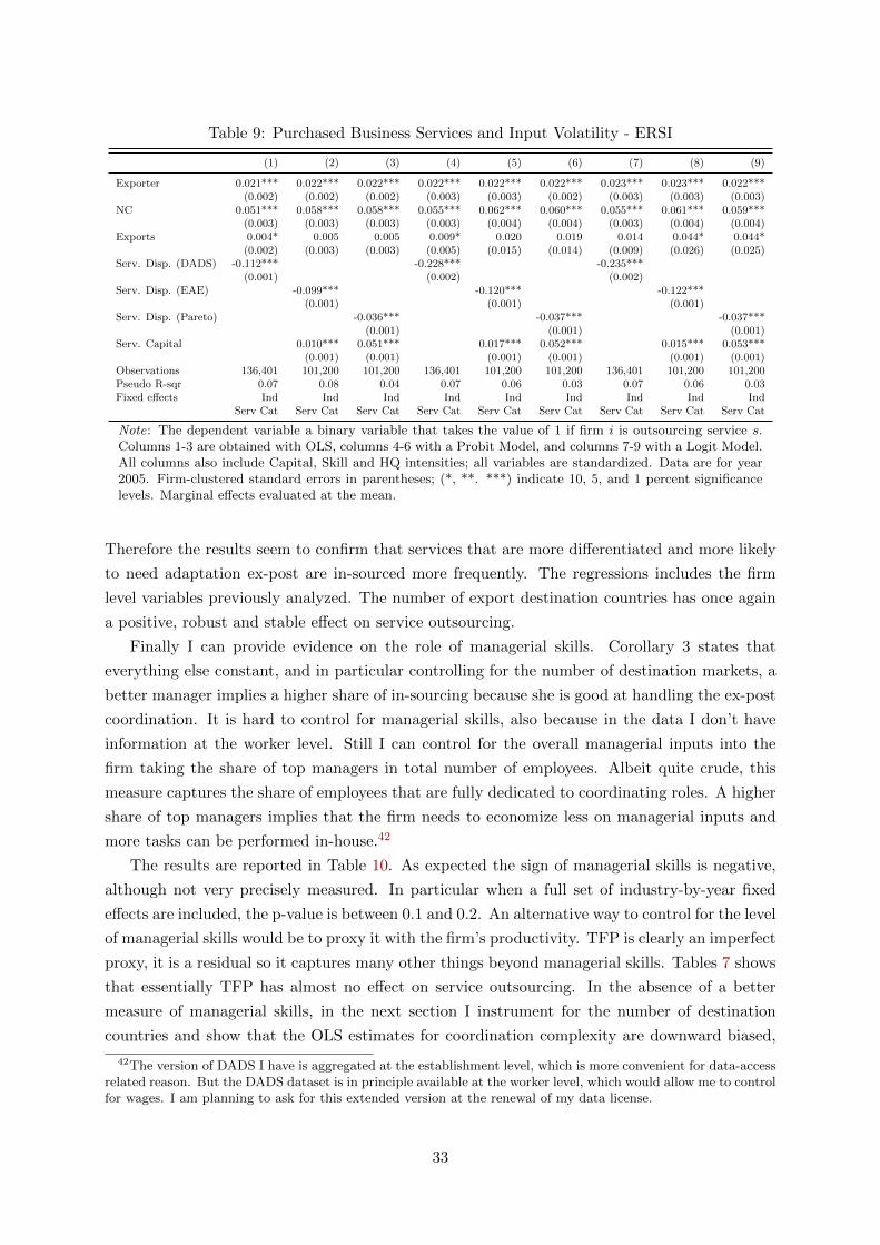
Table 9: Purchased Business Services and Input Volatility - ERSI

(1) (2) (3) (4) (5) (6) (7) (8) (9)

Exporter 0.021*** 0.022*** 0.022*** 0.022*** 0.022*** 0.022*** 0.023*** 0.023*** 0.022***(0.002) (0.002) (0.002) (0.003) (0.003) (0.002) (0.003) (0.003) (0.003)

NC 0.051*** 0.058*** 0.058*** 0.055*** 0.062*** 0.060*** 0.055*** 0.061*** 0.059***(0.003) (0.003) (0.003) (0.003) (0.004) (0.004) (0.003) (0.004) (0.004)

Exports 0.004* 0.005 0.005 0.009* 0.020 0.019 0.014 0.044* 0.044*(0.002) (0.003) (0.003) (0.005) (0.015) (0.014) (0.009) (0.026) (0.025)

Serv. Disp. (DADS) -0.112*** -0.228*** -0.235***(0.001) (0.002) (0.002)

Serv. Disp. (EAE) -0.099*** -0.120*** -0.122***(0.001) (0.001) (0.001)

Serv. Disp. (Pareto) -0.036*** -0.037*** -0.037***(0.001) (0.001) (0.001)

Serv. Capital 0.010*** 0.051*** 0.017*** 0.052*** 0.015*** 0.053***(0.001) (0.001) (0.001) (0.001) (0.001) (0.001)

Observations 136,401 101,200 101,200 136,401 101,200 101,200 136,401 101,200 101,200Pseudo R-sqr 0.07 0.08 0.04 0.07 0.06 0.03 0.07 0.06 0.03Fixed effects Ind Ind Ind Ind Ind Ind Ind Ind Ind

Serv Cat Serv Cat Serv Cat Serv Cat Serv Cat Serv Cat Serv Cat Serv Cat Serv Cat

Note: The dependent variable a binary variable that takes the value of 1 if firm i is outsourcing service s.Columns 1-3 are obtained with OLS, columns 4-6 with a Probit Model, and columns 7-9 with a Logit Model.All columns also include Capital, Skill and HQ intensities; all variables are standardized. Data are for year2005. Firm-clustered standard errors in parentheses; (*, **. ***) indicate 10, 5, and 1 percent significancelevels. Marginal effects evaluated at the mean.

Therefore the results seem to confirm that services that are more differentiated and more likely

to need adaptation ex-post are in-sourced more frequently. The regressions includes the firm

level variables previously analyzed. The number of export destination countries has once again

a positive, robust and stable effect on service outsourcing.

Finally I can provide evidence on the role of managerial skills. Corollary 3 states that

everything else constant, and in particular controlling for the number of destination markets, a

better manager implies a higher share of in-sourcing because she is good at handling the ex-post

coordination. It is hard to control for managerial skills, also because in the data I don’t have

information at the worker level. Still I can control for the overall managerial inputs into the

firm taking the share of top managers in total number of employees. Albeit quite crude, this

measure captures the share of employees that are fully dedicated to coordinating roles. A higher

share of top managers implies that the firm needs to economize less on managerial inputs and

more tasks can be performed in-house.42

The results are reported in Table 10. As expected the sign of managerial skills is negative,

although not very precisely measured. In particular when a full set of industry-by-year fixed

effects are included, the p-value is between 0.1 and 0.2. An alternative way to control for the level

of managerial skills would be to proxy it with the firm’s productivity. TFP is clearly an imperfect

proxy, it is a residual so it captures many other things beyond managerial skills. Tables 7 shows

that essentially TFP has almost no effect on service outsourcing. In the absence of a better

measure of managerial skills, in the next section I instrument for the number of destination

countries and show that the OLS estimates for coordination complexity are downward biased,

42The version of DADS I have is aggregated at the establishment level, which is more convenient for data-accessrelated reason. But the DADS dataset is in principle available at the worker level, which would allow me to controlfor wages. I am planning to ask for this extended version at the renewal of my data license.

33

Table 10: Purchased Business Services and Managerial Skills

(1) (2) (3) (4) (5) (6) (7) (8)

NC 0.085*** 0.085*** 0.084*** 0.079*** 0.086*** 0.086*** 0.086*** 0.080***(0.011) (0.011) (0.011) (0.011) (0.011) (0.011) (0.011) (0.011)

Exports 0.000 0.000 0.001 -0.002 0.001 0.001 0.001 -0.001(0.005) (0.005) (0.005) (0.005) (0.005) (0.005) (0.005) (0.005)

Top Managers -0.393 -0.431* -0.439* -0.347 -0.373 -0.412 -0.420* -0.328(0.251) (0.252) (0.252) (0.254) (0.252) (0.252) (0.252) (0.254)

Observations 174,760 174,104 173,878 173,878 174,760 174,104 173,878 173,878Number of firms 30,110 30,008 29,995 29,995 30,110 30,008 29,995 29,995R-sq W 0.01 0.01 0.01 0.01 0.01 0.01 0.01 0.01Fixed effects Firm Firm Firm Firm Firm Firm Firm Firm

ind, yr ind, yr ind, yr ind, yr ind#yr ind#yr ind#yr ind#yr

Note: The dependent variable is the share of purchased services over total costs. All variables are in logsapart from HQ Intensity. Columns 1-4 and 5-8 contain the exact sequence of controls of columns 4-7 in Table4, with the only difference that top mangers are excluded from the measure of Skill Intensity. Data are forperiod 1996-2007. Firm-clustered standard errors in parentheses; (*, **. ***) indicate 10, 5, and 1 percentsignificance levels.

as predicted by the theory.

5.4 Endogeneity: Is Reverse Causality a Problem?

Despite controlling for unobserved time-invariant firm characteristics and industry specific time

shocks, a full causal interpretation of the previous results might remain problematic. A potential

concern is reverse causality: firms might decide to outsource for reasons unrelated with exporting,

as a result of that they become more productive and this allows them to become exporters. Given

the positive relationship between outsourcing and productivity often found in the literature, this

possibility is certainly a concern. Moreover I do not have a good measure of managerial skills,

and this can introduce a standard omitted variable bias in the results.

A first way of investigating the issue of reverse causality is looking at this channel directly.

I perform the analysis at the end of Section 6, where using the ERSI survey I can test whether

the same inputs outsourced to start exporting are also the ones that generate the highest pro-

ductivity gains (Table 15). A second way is finding a plausible instrument. In the ideal setting

I would want an exogenous shock that makes exporting suddenly easier and more attractive; as

a consequence firms start exporting (or will export to more destination countries), and I would

like to observe whether they change their sourcing behavior at home, for services in particular.

Not having such a shock for France over the past fifteen years, I propose two alternatives. First,

I look at the export destination growth for the US. The growth in destination countries for US

firms can be related to the export opportunities of French firms, but at the same time unre-

lated to their productivity gains due to outsourcing. Second, I look at shocks to demand that

are plausibly exogenous to French firms. If the demand for French products increases globally,

French firms will find exporting more attractive. The ‘China shock’ and the EU enlargement

seem the obvious choice.

I instrument the increase in the number of destination countries with the plausibly exogenous

increase in the number of country-product varieties exported by the US or imported by China

34

and the new EU members. This approach is close in spirit to one of the instrumental variables

proposed by Bloom et al. (2011), and resembles the “shift-share” IV strategy used in the labor

literature (e.g. Bartik, 1991; Card, 2001). Since I have firm and industry-year fixed effects in

all regressions I need an instrument that varies at the firm level. To achieve that I exploit the

information on the products exported by each firm. I define the number of destination markets

of a firm in the initial year as the number of markets reached by the firm’s most successful

product. Then I keep the firm’s product space fixed and calculate the increase in the number of

destination markets for each product with the increase in the number of countries where the US

exports that particular product, or the number of countries that supply that particular product

to China or the new EU members. In all cases, in the country count I exclude France, the EU15

or the Eurozone countries (as of 2001). In any year, the number of destination countries is given

by the number of destination markets of the most successful product in that year.

The instrument is constructed as follows:

IV NCi,t,x = maxp∈Pi,t0

{NCp,t0 + ∆NCxp,t

}(23)

where p is a product exported by firm i, and Pi,t0 is the full set of products exported by that

firm in 1996 or the first year in which it exports. NCp,t0 is the number of countries where firm

i exports product p in the initial year, and ∆NCXp,t is the increase between year t0 and year

t in the number of export destinations of the US or in import sources of China or of new EU

members for product p (hence x ∈ {US-Exports, China-Imports, newEUmembers-Imports}). For

each x, I construct three instruments depending on the countries that I exclude in computing

∆NC: France (exFRA), the Eurozone countries as of 2001 (exEZ12), and the EU15 countries

(exEU15).43 I impose IV NCi,t,x >= 0, hence more precisely my instrument is defined as:

ˆIV NCi,t,x = max {IV NCi,t,x, 0}. Since I only include exporters in the regressions by taking

logs of all variables, whenever the constructed instrument is zero in a given year, the firm will

be dropped in that particular year (even if it is in fact an exporter). But results virtually do

not change if I do not drop those firms by imposing IV NCi,t > 0.

Table 11 shows the results of the exercise. Coordination complexity measured as the number

of destination countries is again positive and very significant across all specifications. It also

reassuring to see that the magnitude of the effect does not change much depending on the

instrument used, and all of them are very strong as the F statistics from the first stage show.

In Table 12, I perform a more demanding exercise where I only consider the change (hence

the growth since all variable are in logs) between three years before and three years after the

EU enlargement that took place in 2004. The model is therefore estimated in first differences

between 2001 and 2007. The effect is still present and the magnitude is again very similar and

robust to all the controls used in the regression.

Interestingly the previous OLS regressions were strongly underestimating the effect of inter-

43The Eurozone countries in 2001 were: Austria, Belgium, Finland, France, Germany, Greece, Ireland, Italy,Luxembourg, the Netherlands, Portugal, and Spain. The EU15 group include the previous countries and Denmark,Sweden, and the United Kingdom.

35

Table 11: Instrumental Variable Estimation

(1) (2) (3) (4) (5) (6) (7) (8) (9)

IV US-Exp US-Exp US-Exp China-Imp China-Imp China-Imp newEU-Imp newEU-Imp newEU-ImpexEU15 exEZ12 exFRA exEU15 exEZ12 exFRA exEU15 exEZ12 exFRA

NC 0.549*** 0.557*** 0.565*** 0.475*** 0.452*** 0.505*** 0.390*** 0.376*** 0.398***(0.162) (0.158) (0.160) (0.153) (0.152) (0.144) (0.131) (0.131) (0.129)

Exports -0.100*** -0.103*** -0.103*** -0.085** -0.080** -0.092*** -0.065** -0.062** -0.066**(0.035) (0.034) (0.034) (0.033) (0.033) (0.031) (0.028) (0.028) (0.028)

Capital Intensity 0.035*** 0.034*** 0.034*** 0.031** 0.032** 0.032** 0.032*** 0.033*** 0.033***(0.013) (0.013) (0.013) (0.013) (0.013) (0.013) (0.013) (0.013) (0.012)

Skill Intensity 0.039*** 0.039*** 0.037*** 0.043*** 0.043*** 0.041*** 0.043*** 0.043*** 0.043***(0.011) (0.011) (0.011) (0.011) (0.011) (0.011) (0.011) (0.011) (0.011)

HQ Intensity -0.074* -0.076** -0.077** -0.076** -0.070* -0.081** -0.074** -0.073* -0.075**(0.039) (0.039) (0.039) (0.038) (0.038) (0.038) (0.038) (0.038) (0.038)

Scale -0.002 -0.002 -0.005 0.003 0.009 -0.001 0.023 0.026 0.021(0.038) (0.038) (0.038) (0.037) (0.037) (0.035) (0.034) (0.034) (0.034)

Observations 160,887 160,799 160,917 164,546 164,638 164,960 166,092 165,659 165,764Number of firms 24,061 24,058 24,055 24,386 24,383 24,412 24,539 24,514 24,523F-stat 320.8 336.2 330.7 348.7 357.1 402.3 488.9 483.2 502.5Fixed effects Firm Firm Firm Firm Firm Firm Firm Firm Firm

ind#yr ind#yr ind#yr ind#yr ind#yr ind#yr ind#yr ind#yr ind#yr

Note: See notes in Table 6. The F-stat is the Kleibergen and Paap (2006) Wald rk F statistic provided bythe Baum et al.’s (2010) xtivreg2 Stata command.

Table 12: IV Estimation - New EU member countries: 2001-2007 change (growth)

(1) (2) (3) (4) (5) (6) (7) (8)

∆ IV newEU newEU newEU newEU newEU newEU newEU newEUexEU15 exEU15 exEU15 exEU15 exEU15 exEU15 exEZ12 exFRA

∆ NC 0.296** 0.413** 0.410** 0.489*** 0.449** 0.432** 0.450** 0.475***(0.121) (0.191) (0.200) (0.185) (0.191) (0.199) (0.192) (0.183)

∆ Exports -0.074 -0.076 -0.094* -0.084 -0.084 -0.088* -0.095*(0.052) (0.054) (0.051) (0.052) (0.052) (0.051) (0.049)

∆ Capital Intensity 0.056 0.073* 0.071* 0.076** 0.076** 0.077**(0.037) (0.037) (0.037) (0.037) (0.037) (0.037)

∆ Skill Intensity 0.080** 0.075* 0.080** 0.080** 0.079*(0.039) (0.039) (0.040) (0.041) (0.041)

∆ HQ Intensity 0.018 0.015 0.013 0.010(0.063) (0.062) (0.060) (0.060)

∆ Scale 0.060 0.057 0.053(0.057) (0.057) (0.058)

Observations 9,234 9,234 9,180 8,494 8,381 8,381 8,380 8,383F-stat 165.3 164.8 172.3 126.7 133.2 108.8 110.1 107.4

Note: The dependent variable is the growth of the share of outsourcing in total costs (log-change) between 2001 and2007. All controls are also in log-changes. Standard errors are clustered at the 2 digit industry level. The F-stat is theKleibergen and Paap (2006) Wald rk F statistic.

36

est. There could be several explanations for this result. But one in particular comes straight

from the model. Firms with managers with higher ability will tend to produce more in-house,

everything else constant (Corollary 3). Moreover from Proposition 4 we know that firms that

export to more destinations are more likely to employ better managers. Combining the two

reasons, firms that export to multiple destinations are more likely to produce inputs in-house,

everything else constant. If they had to export to many destinations, less productive firms would

tend to outsource a much higher proportion of their inputs, because they would not be able to

compete with external specialized suppliers. In reality these firms export to much fewer markets,

if any at all. Hence if the number of destination countries could be randomly assigned to firms,

the effect on outsourcing would be much stronger.

Considering the coefficients of the previous two tables, the average increase in the number of

destination countries explains between 66% and 100% of the increase in the share of outsourced

services over the period. The new channel between globalization and structural transformation

that I propose is not only present but it is also quantitatively very significant. The causal effect

of globalization explains over two-thirds of the increase in domestic service outsourcing observed

in the sample.

One reason why the overall effect might be partially overstated is that the average effect might

not be representative for the entire distribution of firms, due to the presence of non-linearities,

as the next section shows.

5.5 Non-linear Effects: Evidence on Corollary 2

A further interesting question to answer is whether the effect of coordination complexity on the

share of outsourcing exhibits a non-linear behavior. Proposition 4 predicts that the relation-

ship should be concave, that is, the increase in outsourcing should flatten when the number of

destination countries is large. This is precisely what happens, as Figure 8 shows.44

Multiple interpretations can be put forward to explain this fact. In the model, when the

number of overall inputs goes up, the probability that the manager needs to understand the

input condition for each one of them becomes smaller and smaller. Setting up a communication

code for such a high number of very rare events (all equally likely) is going to be very costly.

So the manager increases the number of inputs internally produced at a much lower speed

compared to the increase in the number of overall inputs needed. At some point the number of

in-house produced inputs hardly increases and if the denominator keeps rising the overall share

will become smaller and smaller till converging to zero. In the model the slope essentially goes

to zero only when also the share of internally produced inputs goes to zero (even though with a

lower order). In the data the slope is zero (even though not significant) when the share of internal

production is still positive. The reason is of course due to the fact that inputs are homogeneous

in the model while they are not in the data. It might be that the firm is outsourcing all of the

service inputs needed to export but it is still of course producing in-house all the other core

activities. One way to capture this effect in the model would be to have some heterogeneity in

44This effect is also confirmed by the negative sign on the square of the number of countries. The results of theregression are not reported but available on request.

37

the importance of adaptation (e.g.: different probabilities of adaptation). In such case, the core

activities would intuitively have a higher probability of adaptation and hence would be more

likely to be produced in-house.

A different explanation is that the distribution of events might change. If the service inputs

are not truly country-specific, but some of them are common across countries in a differential

way (e.g.: translation is shared across the countries with the same language, while transportation

services are shared across all countries), then it is possible that some inputs are recurring with a

higher and higher probability. In this situation the firm needs the input in different proportions

and the uniform distribution of events would not apply anymore. Since some inputs become

more and more frequent, the firm will find it optimal to produce them in-house because a code

designed to communicate those events is quite cheap. The firm essentially specializes in the

production of export-related services as it exports to more and more countries, and the share of

service outsourcing might even decrease.

As Figures 8 shows, the data are very noisy for firms that export to a very high number of

countries. In fact it is not possible to sign the slope, because the confidence interval allows for

both positive and negative slopes. So it is hard to disentangle the two stories in the data.

6 An Anatomy of Fixed Export Costs

This section is devoted to opening the black box of fixed export costs, by providing evidence

on their timing and nature. Related to the timing, an interesting question is whether service

export costs are more of a fixed or sunk nature. In the former case the costs have to be paid

every period, while in the latter they are paid once for all when a firm enters a new market.

In their quantitative exercise Morales et al. (2014) find that fixed costs are somewhat larger.

This contrasts with the results of Das et al. (2007), who find the opposite. Both papers obtain

estimates of these costs from structural models, while here I can provide direct evidence on the

nature of export costs (or at least part of them) from the data. To the best of my knowledge

this is the first paper that addresses this issue directly, and I do so through a simple analysis on

the timing of the incurrence of these costs. First I analyze the effect of the lead and lag of the

number of export destination countries. Then for each firm I define three dummy variables that

identify: a) the year after entering a new market; b) the year of entrance; and c) the year before

entering a new market. The first variable is the lag of the second, while the third is the lead of

the second. One would expect the costs that are sunk in nature to be paid before entering and

being related to the number of countries that will be entered, regardless the number of countries

that the firm exits.

This is precisely what happens, as Table 13 shows. Not only do firms appear to increase

their purchases of services also in the year before entrance but the number of export destination

countries at year t + 1 is the variable with the largest magnitude, significantly larger than the

effect of the number of export destination countries at year t − 1 (column 1).45 Moreover I

45It is harder to disentangle whether the cost paid in the year of entrance are fixed or sunk. Although notdisplayed, the regressions also includes exports, scale, capital, skill and HQ intensities as regressors.

38

build two sets of the aforementioned dummy variables, depending whether a firm is also exiting

countries or not: in the ‘gross’ case I simply set the variable to one if a firm enters a country

regardless of exit; in the ‘net’ case, on the other hand, I define entry only if the number of

entered countries is higher than the number of exited countries (hence the variable is zero if

a firm enters a country and exits another country at the same time). It turns out that the

magnitude of the coefficient is higher in the ‘gross’ case, hence the evidence points to costs that

are sunk in nature since exit does not seem to matter much. This statement is confirmed when I

analyze re-entry. I define three dummy variables as before but for cases in which firms re-entry

countries in which they had already exported in the past. When they re-entry these countries

without simultaneously entering other countries, the costs does not seem to move at all, if

anything the share of outsourcing is decreasing. In columns (5)-(8), I run the same regressions

but the regressors are standardized and not in logs, hence non-exporters are included and I can

add a dummy variable for exporters. This shows how the results are not driven by selection into

exporting, and they are actually even stronger.

Table 13: The Timing of Service Outsourcing

(1) (2) (3) (4) (5) (6) (7) (8)

Exporter 0.031*** 0.026*** 0.033*** 0.027***(0.010) (0.010) (0.009) (0.010)

NC (t-1) 0.020** 0.019(0.010) (0.015)

NC (t) 0.047*** 0.061***(0.012) (0.016)

NC (t+1) 0.049*** 0.075***(0.011) (0.015)

Country Entry (t-1, gross) 0.020** 0.017***(0.010) (0.005)

Country Entry (t, gross) 0.022** 0.015***(0.011) (0.005)

Country Entry (t+1, gross) 0.020** 0.013***(0.010) (0.005)

Country Entry (t-1, net) 0.002 0.006*(0.007) (0.003)

Country Entry (t, net) 0.005 0.005(0.008) (0.003)

Country Entry (t+1, net) 0.001 0.002(0.007) (0.003)

Country Re-entry (t-1, only) -0.001 -0.002(0.011) (0.003)

Country Re-entry (t, only) -0.018* -0.007**(0.011) (0.003)

Country Re-entry (t+1, only) -0.013 -0.004(0.010) (0.003)

Observations 135,401 127,831 127,831 108,944 170,701 156,962 156,962 132,726Number of firms 23,141 23,676 23,676 21,416 30,269 28,562 28,562 25,727R-sq W 0.01 0.01 0.01 0.01 0.01 0.01 0.01 0.01Fixed effects Firm Firm Firm Firm Firm Firm Firm Firm

ind#yr ind#yr ind#yr ind#yr ind#yr ind#yr ind#yr ind#yr

Note: The dependent variable is the share of purchased services over total costs. All columns also includethe following regressors: exports, K/L, S/L, HQ Intensity, and scale. See also notes in Table 4.

It is informative to analyze cases in which costs are more likely to be variable in nature rather

than fixed or sunk. For instance I look at employment outsourcing, that is, the use of temporary

work from employment agencies. It is likely that firms use these services when they have some

39

capacity constraints and decide to expand in a more flexible way, for instance to meet peaks of

demand. Table 14 provide strong evidence in this direction. In the baseline regression (column

1) it is now the intensive margin of trade to be positive and significant, and not the number of

destination countries. This result supports the idea that temporary employment is not used to

produce country-specific inputs. Looking at the timing, it is now the net entry that matters and

the costs are mostly incurred in the year of entrance and not before, in full contrast with the

previous results. Hence this type of labor input is likely to be related to variable costs, rather

than country specific entry costs. Very similar evidence applies for industrial outsourcing, the

outsourcing of goods and components rather than services. It is the trade intensive margin that

is positive and strongly significant, the number of countries is also positive but not significant.

Table 14: Employment and Industrial Outsourcing

(1) (2) (3) (4) (5) (6)

Dependent Var. Empl Empl Empl Ind Ind Ind

NC -0.009 0.016(0.010) (0.010)

Exports 0.010** 0.011*** 0.010** 0.028*** 0.032*** 0.032***(0.004) (0.004) (0.004) (0.004) (0.005) (0.005)

Capital Intensity 0.056*** 0.065*** 0.065*** 0.014 0.008 0.008(0.011) (0.014) (0.014) (0.012) (0.017) (0.017)

Skill Intensity -0.051*** -0.037*** -0.037*** 0.032*** 0.019 0.019(0.011) (0.013) (0.013) (0.010) (0.012) (0.012)

HQ Intensity -0.257*** -0.247*** -0.248*** -0.311*** -0.367*** -0.367***(0.038) (0.045) (0.045) (0.046) (0.058) (0.058)

Scale 0.101*** 0.111*** 0.110*** -0.133*** -0.166*** -0.166***(0.022) (0.028) (0.028) (0.025) (0.032) (0.032)

Country Entry (t-1, gross) -0.008 -0.008(0.009) (0.009)

Country Entry (t, gross) 0.000 -0.010(0.010) (0.010)

Country Entry (t+1, gross) 0.000 -0.008(0.009) (0.010)

Country Entry (t-1, net) 0.009 -0.004(0.006) (0.007)

Country Entry (t, net) 0.014* -0.006(0.007) (0.008)

Country Entry (t+1, net) 0.009 0.003(0.007) (0.007)

Observations 142,809 107,449 107,449 135,767 99,526 99,526Number of firms 26,510 21,468 21,468 26,080 20,468 20,468R-sq W 0.04 0.03 0.03 0.01 0.01 0.01Fixed effects Firm Firm Firm Firm Firm Firm

ind#yr ind#yr ind#yr ind#yr ind#yr ind#yr

Note: See notes in Table 6.

In order to open the black box of fixed/sunk export costs it is interesting to investigate

which are the specific service inputs that a firm needs in order to export to new countries. I can

answer this question again drawing on the extra information contained in the ERSI survey. I

run a set of separate Probit regressions for each service type to see which one is mostly related

to the number of destination countries. Table 15 reports the marginal effects at the mean for

40

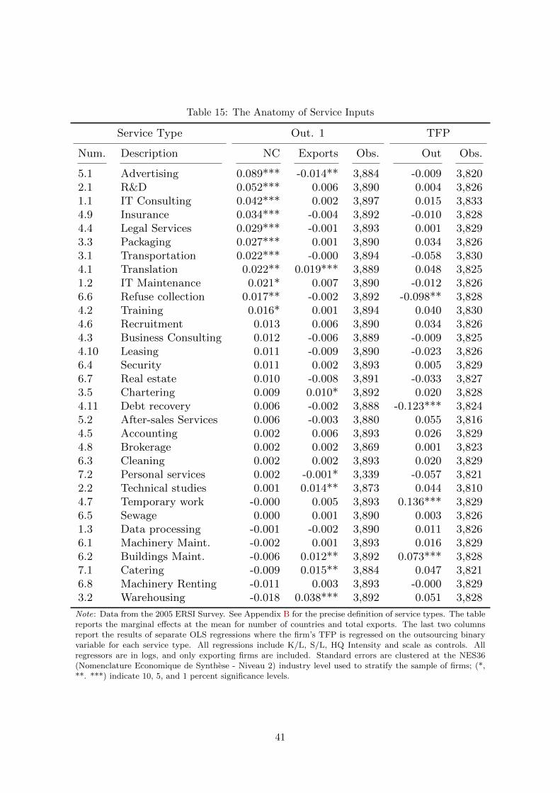
Table 15: The Anatomy of Service Inputs

Service Type Out. 1 TFP

Num. Description NC Exports Obs. Out Obs.

5.1 Advertising 0.089*** -0.014** 3,884 -0.009 3,8202.1 R&D 0.052*** 0.006 3,890 0.004 3,8261.1 IT Consulting 0.042*** 0.002 3,897 0.015 3,8334.9 Insurance 0.034*** -0.004 3,892 -0.010 3,8284.4 Legal Services 0.029*** -0.001 3,893 0.001 3,8293.3 Packaging 0.027*** 0.001 3,890 0.034 3,8263.1 Transportation 0.022*** -0.000 3,894 -0.058 3,8304.1 Translation 0.022** 0.019*** 3,889 0.048 3,8251.2 IT Maintenance 0.021* 0.007 3,890 -0.012 3,8266.6 Refuse collection 0.017** -0.002 3,892 -0.098** 3,8284.2 Training 0.016* 0.001 3,894 0.040 3,8304.6 Recruitment 0.013 0.006 3,890 0.034 3,8264.3 Business Consulting 0.012 -0.006 3,889 -0.009 3,8254.10 Leasing 0.011 -0.009 3,890 -0.023 3,8266.4 Security 0.011 0.002 3,893 0.005 3,8296.7 Real estate 0.010 -0.008 3,891 -0.033 3,8273.5 Chartering 0.009 0.010* 3,892 0.020 3,8284.11 Debt recovery 0.006 -0.002 3,888 -0.123*** 3,8245.2 After-sales Services 0.006 -0.003 3,880 0.055 3,8164.5 Accounting 0.002 0.006 3,893 0.026 3,8294.8 Brokerage 0.002 0.002 3,869 0.001 3,8236.3 Cleaning 0.002 0.002 3,893 0.020 3,8297.2 Personal services 0.002 -0.001* 3,339 -0.057 3,8212.2 Technical studies 0.001 0.014** 3,873 0.044 3,8104.7 Temporary work -0.000 0.005 3,893 0.136*** 3,8296.5 Sewage 0.000 0.001 3,890 0.003 3,8261.3 Data processing -0.001 -0.002 3,890 0.011 3,8266.1 Machinery Maint. -0.002 0.001 3,893 0.016 3,8296.2 Buildings Maint. -0.006 0.012** 3,892 0.073*** 3,8287.1 Catering -0.009 0.015** 3,884 0.047 3,8216.8 Machinery Renting -0.011 0.003 3,893 -0.000 3,8293.2 Warehousing -0.018 0.038*** 3,892 0.051 3,828

Note: Data from the 2005 ERSI Survey. See Appendix B for the precise definition of service types. The tablereports the marginal effects at the mean for number of countries and total exports. The last two columnsreport the results of separate OLS regressions where the firm’s TFP is regressed on the outsourcing binaryvariable for each service type. All regressions include K/L, S/L, HQ Intensity and scale as controls. Allregressors are in logs, and only exporting firms are included. Standard errors are clustered at the NES36(Nomenclature Economique de Synthese - Niveau 2) industry level used to stratify the sample of firms; (*,**. ***) indicate 10, 5, and 1 percent significance levels.

41

the number of destination countries and total exports (all regressions also include capital, skill,

HQ intensities, and scale as controls.). It turns out that advertising, R&D and IT consulting

are the service inputs most highly related to an increase of export destination countries, while

the intensive margin of trade again plays no role. These inputs were already contained in the

outsourcing variable used in the previous section, so it is reassuring to see that the results are

confirmed with this more detailed survey for a cross-section of firms. Other service inputs that

are key in order to export to new countries are: insurance, legal services, translation and quite

intuitively transportation and packaging. Results change very marginally if I use a logit or a

linear probability model.

Finally, the detailed data allow me to investigate the issue of reverse causality directly. In

particular I can test whether the same inputs outsourced to start exporting are also the ones

that generate the highest productivity gains. The last two columns of Table 15 report the

results, where I run separate OLS regressions for each service type to see whether outsourcing

of that particular service has an impact on the firm’s TFP. The table shows that there is no

correspondence between the outsourcing of service inputs needed to export to new countries and

an increase in the firm’s TFP, the reverse causality channel does not seem to be there.

7 Alternative Mechanisms

An alternative explanation for the rise in service outsourcing is that manufacturing firms are

simply becoming more service oriented. An overall increase in the production of services might

increase the need for service inputs, that in turn leads to more outsourcing. This could lead

to a parallel increase of services produced internally and services purchased from the market.

Controlling for internal production is therefore key in the analysis to rule out the possibility that

service outsourcing is driven by manufacturing firms simply becoming “service firms”. I propose

six other measures of internal production and the base result is robust to all of them, as shown

in Table 16. Column (1) displays the same regression of column (6) in Table 4, where I capture

internal service production with the share of revenues generated by establishments classified

in services (often the headquarters). In column (2), the definition of internal production of

services is very similar but the headquarter share is computed in terms of employment and

not revenues. The following two regressions employ similar definitions but instead of using the

shares of all service establishments they only include the establishments classified in business

service industries (for instance they exclude transportation, retail, wholesale etc...).46 Columns

(5) and (6) use respectively the share of total salaries and of total employment accounted in

establishments classified as headquarters by the firm itself.

All these measures have the common problem that they do not account for services produced

inside production establishments. This is a measurement issue is also present for the economy

as a whole: when a manager sits in the back of a production site performing accounting, billing,

marketing and other services, all this service activity goes completely undetected in industry

46Whenever the shares in terms of employment are used (columns 2 and 4), year 2007 is dropped due to missingdata.

42

Table 16: Alternative Measures of Internal Production of Services

(1) (2) (3) (4) (5) (6) (7)

NC 0.086*** 0.080*** 0.086*** 0.080*** 0.086*** 0.086*** 0.086***(0.011) (0.011) (0.011) (0.011) (0.011) (0.011) (0.011)

HQ Share (Rev) -0.052(0.037)

HQ Share (Empl) -0.005(0.049)

PBS Share (Rev) -0.047(0.369)

PBS Share (Empl) -0.210(0.420)

HQ Est. (Salaries) 0.053(0.071)

HQ Est. (Empl) 0.007(0.075)

Professionals Share (CS3) 0.043(0.084)

Observations 174,682 161,755 174,682 161,755 174,745 174,812 174,892Number of firms 30,159 29,464 30,159 29,464 30,126 30,161 30,172R-sq W 0.01 0.01 0.01 0.01 0.01 0.01 0.01Fixed effects Firm Firm Firm Firm Firm Firm Firm

ind#yr ind#yr ind#yr ind#yr ind#yr ind#yr ind#yr

Note: The dependent variable is the share of purchased services over total costs. All columns also includethe following regressors: exports, capital and skill intensities. Year 2007 dropped in columns 2 and 4. Seealso notes in Table 4.

data. This issue is probably not too worrisome in the present context since I mainly focus

on exporters. In fact it is well known that exporters are larger, and large firms tend to have

establishments dedicated to services, as reported by Young and Triplett (1996). In any case,

I propose another measure of internal production that is not subject to this problem since it

comes from occupation data. I use the share of workers classified as managers and professional

occupations in total employment (column 7). The measure comes from the DADS dataset and

it is a relatively good proxy for internal production of PBS services since these activities are

mainly performed by professionals.47

Another possibility is that manufacturing firms are not becoming more service oriented but

they “consume” relatively more services in order to export. This is of course at the heart of

the mechanism under study. Firms need more services inputs to export to more destination

countries and the overall increase in the need of services might exceed their expansion in terms

of total revenues or total costs, hence the share of services would mechanically increase. Firms

might decide to source them both from inside and outside the firm, and if the shift takes place at

the exact the same pace, the boundary of the firm might not be an issue after all. At first sight,

it looks like the overall need of services has in fact increased. Columns (1)-(4) of Table 17 show

the sum of both purchased services and internal production of services, measured as the share

of professionals in total employment. It is indeed strongly related to the number of destination

countries. This fact implies that the impact of globalization on structural transformation might

47This is category 3 (CS3) in the DADS data: “cadres et professions intellectuelles superieures”. Ideally I wouldcontrol for their share in the total employment bill but I do not have wages disaggregated at that level of detail.

43

Table 17: Total Service Production and Outsourcing versus Internal Production

(1) (2) (3) (4) (5) (6) (7) (8)

Dependent Var. Tot Serv Tot Serv Tot Serv Tot Serv OUT/IN OUT/IN OUT/IN OUT/IN

NC 0.105*** 0.107*** 0.111*** 0.124*** 0.084*** 0.079*** 0.064*** 0.067***(0.012) (0.013) (0.013) (0.015) (0.012) (0.013) (0.013) (0.015)

Exports -0.001 -0.000 0.001 0.004 -0.003 -0.001(0.005) (0.005) (0.006) (0.005) (0.005) (0.006)

Capital Intensity 0.028** 0.010 0.036*** 0.030*(0.014) (0.015) (0.014) (0.016)

Scale -0.039 -0.063** 0.213*** 0.194***(0.025) (0.027) (0.023) (0.025)

Num imp. products 0.030*** 0.012(0.010) (0.010)

Contract Intensity 0.021*** 0.012*(0.007) (0.007)

Observations 159,698 159,698 159,078 134,888 159,698 159,698 159,078 134,888Number of firms 28,178 28,178 28,086 23,976 28,178 28,178 28,086 23,976R-sq W 0.03 0.03 0.03 0.03 0.02 0.02 0.02 0.02Fixed effects Firm Firm Firm Firm Firm Firm Firm Firm

ind#yr ind#yr ind#yr ind#yr ind#yr ind#yr ind#yr ind#yr

Note: The dependent variable in columns 1-4 is the share of purchased services in total costs plus the shareof professionals in total employment, while in columns 5-8 is ratio of the two shares. All variables are in logs.Data are for period 1996-2007. Firm-clustered standard errors in parentheses; (*, **. ***) indicate 10, 5,and 1 percent significance levels.

be even stronger than what the data shows. Many of these professionals are not employed in

service establishments, hence they will be accounted within manufacturing when in fact they

are producing services. The larger magnitude of the coefficient of interest with respect to the

case of outsourcing only (Table 4) seems to point in that direction.

However the boundaries of the firms do matter. First of all, the magnitude for the overall

production of services is larger than in the case of outsourcing only, but marginally. Thus internal

production contributes much less then outsourcing, and exporting to more countries increases

the outsourced share of services dis-proportionally more than internal production. This fact can

be shown in two ways. First, in columns 5-8 of Table 17 I run a set or regressions where the

dependent variable is the ratio of outsourcing over internal production (hence the log difference

between the outsourcing share and the professionals share). The coefficients are positive and

strongly significant, so an increase in the number of destination countries leads firms to increase

outsourcing over internal production.

Second, it is evident from Table 18 that the magnitude of the effect for internal production

alone (share of professionals, column 2) is significantly smaller than the one for outsourcing. The

table also shows how other categories of occupations are related to the main variable of interest,

these categories correspond to the hierarchical layers described by Caliendo et al. (2012). As

expected the share of professionals (CS3, or Layer 2 in Caliendo et al. 2012) expands the most

compared to all other internal layers, confirming that this is the occupational category most

likely producing the specific services associated with exporting. Since the share of professionals

is the one increasing the most with the number of destination countries, the exercise in columns

(5)-(8) of Table 17 was the most demanding setting in which to test the ratio of the two. Table

18 also shows the ratio of outsourcing over internal production for all layers (columns 6-10,

44

column 7 coincides with column 7 of Table 17). Outsourcing increases with the number of

export destination countries disproportionally more than any measure of internal production.

All in all, the results appear to be very robust to internal production of services. This evidence

shows not only that business services are a fixed export cost component but also that firms tend

to acquire these key inputs by outsourcing them to external providers, rather then producing

them in-house.

Table 18: Internal Hierarchies and Outsourcing

(1) (2) (3) (4) (5) (6) (7) (8) (9) (10)

Dependent Var. CS2 CS3 CS4 CS5 CS6 OUT/CS2 OUT/CS3 OUT/CS4 OUT/CS5 OUT/CS6

NC -0.015*** 0.026*** 0.023*** 0.020*** -0.015*** 0.078*** 0.064*** 0.062*** 0.068*** 0.097***(0.004) (0.004) (0.004) (0.004) (0.003) (0.015) (0.013) (0.012) (0.012) (0.012)

Exports -0.010*** 0.001 0.000 -0.003* 0.002** 0.019*** -0.003 -0.002 0.003 -0.004(0.002) (0.002) (0.002) (0.002) (0.001) (0.006) (0.005) (0.005) (0.005) (0.005)

Capital Intensity -0.022*** -0.003 -0.003 0.001 0.019*** 0.061*** 0.036*** 0.037*** 0.033** 0.013(0.005) (0.004) (0.004) (0.004) (0.003) (0.016) (0.014) (0.012) (0.014) (0.014)

Scale -0.695*** -0.134*** -0.089*** -0.098*** 0.093*** 0.756*** 0.213*** 0.153*** 0.158*** -0.027(0.014) (0.009) (0.008) (0.010) (0.008) (0.033) (0.023) (0.022) (0.024) (0.024)

Observations 104,420 171,963 186,270 178,793 188,624 96,898 159,078 171,851 165,286 173,584Number of firms 22,640 29,141 30,899 30,256 31,318 21,722 28,086 29,719 29,126 30,098R-sq W 0.18 0.13 0.04 0.09 0.05 0.04 0.02 0.01 0.02 0.01Fixed effects Firm Firm Firm Firm Firm Firm Firm Firm Firm Firm

ind#yr ind#yr ind#yr ind#yr ind#yr ind#yr ind#yr ind#yr ind#yr ind#yr

Note: The dependent variable is the share of different occupational categories in total employment (column1-5) and the ratio of the share of purchased services in total costs over the share of the categories in totalemployment (column 6-10). All variables are in logs. See notes in Table 4.

An interesting point to note is that one of the empirical results that do not match with the

theory in Caliendo et al. (2012) is related to the proportional expansion of higher layers with

respect to lower layers. For firms that start exporting, the theory would predict that higher

layers should expand more than lower layers, but the authors do not seem to find evidence for

this theoretical prediction in the data. An explanation for this apparent puzzle is that the theory

developed by Garicano (2000) and Caliendo and Rossi-Hansberg (2012) does not explicitly draw

the boundary of the firm. So there is nothing that imposes that problem solvers, who have the

knowledge to solve exceptional problems, should be employed directly by the firm.48 My results

strongly suggest that the expansion of higher layers come from across the boundary of the firm:

firms outsource these high skill and infrequent services to external specialists. This strategy also

allows firms to be more flexible, in fact they do not need to pay the fixed cost correspondent

to the wage of the problem solver, but they can access his knowledge only when needed. In

the Caliendo and Rossi-Hansberg’s (2012) framework this could be seen a way to smooth the

transition between different number of layers.

8 Conclusions

By advancing the complexity of coordination, intrinsic to the managerial activity, as one of

the main determinants of integration costs, this paper offers a better understanding of how the

boundary of the firm are determined in presence of multiple inputs for which asset ownership is

48In fact Garicano and Rossi-Hansberg (2012), using a very similar setting, talk more generally about “referralmarkets”.

45

not very important, like many services. I have looked at one possible driver of coordination com-

plexity: the internationalization decision of the firm. Exporting to more destination countries

implies that more inputs are needed, and the higher number of inputs increases coordination

costs making market transactions more appealing. I find new systematic evidence about domes-

tic service outsourcing: an increase in the number of export destination countries has a strong

positive effect on the share of purchased business services in total costs. This result establishes

a new causal effect of globalization on structural transformation, which is quantitatively very

significant. In fact the IV estimates, based on plausibly exogenous demand shifts, show that

the average increase in the number of destination countries explains more than two-thirds of the

increase in domestic service outsourcing observed in the sample.

Finally the paper makes a significant step forward in understanding the nature of export

costs. Firms need to access a variety of specialized services to be able to export; often they

do not have the capabilities to produce these inputs in-house so they have to rely on external

suppliers. And the effect is stronger, the higher the number of markets that need to be reached.

A flourishing and productive business services industry is therefore a key ingredient for a country

export success, and its competitiveness on the world markets.

46

References

Abraham, K. G. and Taylor, S. K. (1996). Firms’ use of outside contractors: Theory and

evidence. Journal of Labor Economics, 14(3):394–424.

Abramovsky, L. and Griffith, R. (2006). Outsourcing and offshoring of business services: How

important is ICT? Journal of the European Economic Association, 4(2-3):594–601.

Acemoglu, D., Carvalho, V. M., Ozdaglar, A., and Tahbaz-Salehi, A. (2012). The network

origins of aggregate fluctuations. Econometrica, 80(5):1977–2016.

Alonso, R., Dessein, W., and Matouschek, N. (2008). When does coordination require central-

ization? American Economic Review, 98(1):145–79.

Amiti, M. and Wei, S.-J. (2009). Service offshoring and productivity: Evidence from the US.

The World Economy, 32(2):203–220.

Angrist, J. D. and Pischke, J.-S. (2008). Mostly Harmless Econometrics: An Empiricist’s Com-

panion. Princeton University Press.

Antras, P. (2003). Firms, contracts, and trade structure. The Quarterly Journal of Economics,

118(4):1375–1418.

Antras, P. and Helpman, E. (2004). Global sourcing. Journal of Political Economy, 112(3):552–

580.

Antras, P. and Helpman, E. (2008). Contractual frictions and global sourcing. In Helpman, E.,

Marin, D., and Verdier, T., editors, The Organization of Firms in a Global Economy, pages

311–339. Harvard University Press, Chicago, IL.

Arkolakis, C. (2010). Market penetration costs and the new consumers margin in international

trade. Journal of Political Economy, 118(6):1151–1199.

Arkolakis, C., Ganapati, S., and Muendler, M.-A. (2014). The extensive margin of exporting

products: A firm-level analysis. Mimeo, Yale University.

Bajari, P. and Tadelis, S. (2001). Incentives versus transaction costs: A theory of procurement

contracts. The RAND Journal of Economics, 32(3):387–407.

Bartel, A. P., Lach, S., and Sicherman, N. (2009). Outsourcing and technological change.

Discussion Paper 4678, IZA.

Bartik, T. J. (1991). Who Benefits from State and Local Economic Development Policies?

Number wbsle in Books from Upjohn Press. W.E. Upjohn Institute for Employment Research.

Baum, C. F., Schaffer, M. E., and Stillman, S. (2010). Ivreg2: Stata module for extended

instrumental variables/2sls and gmm estimation. Statistical Software Components, Boston

College Department of Economics.

47

Becker, G. S. and Murphy, K. M. (1992). The division of labor, coordination costs, and knowl-

edge. The Quarterly Journal of Economics, 107(4):1137–1160.

Berlingieri, G. (2013). Outsourcing and the rise in services. CEP Discussion Paper 1199, London

School of Economics.

Berlingieri, G. and Ngai, R. L. (2014). Intermediate goods, misallocation, and aggregate pro-

ductivity. Mimeo, London School of Economics.

Bernard, A. B., Redding, S., and Schott, P. K. (2011). Multiproduct firms and trade liberaliza-

tion. The Quarterly Journal of Economics, 126(3):1271–1318.

Bloom, N., Draca, M., and Van Reenen, J. (2011). Trade induced technical change? the impact

of chinese imports on innovation, it and productivity. CEP Discussion Papers dp1000, Centre

for Economic Performance, LSE.

Caliendo, L., Monte, F., and Rossi-Hansberg, E. (2012). The anatomy of french production

hierarchies. NBER Working Papers 18259, National Bureau of Economic Research, Inc.

Caliendo, L. and Rossi-Hansberg, E. (2012). The impact of trade on organization and produc-

tivity. The Quarterly Journal of Economics, 127(3):1393–1467.

Card, D. (2001). Immigrant inflows, native outflows, and the local labor market impacts of

higher immigration. Journal of Labor Economics, 19(1):22–64.

Chen, N. and Novy, D. (2011). Gravity, trade integration, and heterogeneity across industries.

Journal of International Economics, 85(2):206–221.

Coase, R. H. (1937). The nature of the firm. Economica, 4(16):386–405.

Corcos, G., Irac, D., Mion, G., and Verdier, T. (2013). The determinants of intrafirm trade:

Evidence from french firms. The Review of Economics and Statistics, 95(3).

Costinot, A., Oldenski, L., and Rauch, J. (2011). Adaptation and the boundary of multinational

firms. The Review of Economics and Statistics, 93(1):298–308.

Cremer, J., Garicano, L., and Prat, A. (2007). Language and the theory of the firm. The

Quarterly Journal of Economics, 122(1):373–407.

Das, S., Roberts, M. J., and Tybout, J. R. (2007). Market entry costs, producer heterogeneity,

and export dynamics. Econometrica, 75(3):837–873.

Dessein, W. and Santos, T. (2006). Adaptive organizations. Journal of Political Economy,

114(5):956–985.

Dewatripont, M. and Tirole, J. (2005). Modes of communication. Journal of Political Economy,

113(6):1217–1238.

48

Eaton, J., Kortum, S., and Kramarz, F. (2004). Dissecting trade: Firms, industries, and export

destinations. American Economic Review, 94(2):150–154.

Eaton, J., Kortum, S., and Kramarz, F. (2011). An anatomy of international trade: Evidence

from french firms. Econometrica, 79(5):1453–1498.

Fan, J. P. H. and Lang, L. H. P. (2000). The measurement of relatedness: An application to

corporate diversification. Journal of Business, 73(4):629–660.

Fixler, D. J. and Siegel, D. (1999). Outsourcing and productivity growth in services. Structural

Change and Economic Dynamics, 10(2):177–194.

Garicano, L. (2000). Hierarchies and the organization of knowledge in production. Journal of

Political Economy, 108(5):874–904.

Garicano, L. and Rossi-Hansberg, E. (2006). Organization and inequality in a knowledge econ-

omy. The Quarterly Journal of Economics, 121(4):1383–1435.

Garicano, L. and Rossi-Hansberg, E. (2012). Organizing growth. Journal of Economic Theory,

147(2):623–656.

Gibbons, R. (2005). Four formal(izable) theories of the firm? Journal of Economic Behavior &

Organization, 58:200–245.

Gorg, H., Hanley, A., and Strobl, E. (2008). Productivity effects of international outsourcing:

evidence from plant-level data. Canadian Journal of Economics, 41(2):670–688.

Hausmann, R. and Hidalgo, C. A. (2011). The network structure of economic output. Journal

of Economic Growth, 16(4):309–342.

Hayek, F. A. (1945). The use of knowledge in society. The American Economic Review,

35(4):519–530.

Helpman, E. (2006). Trade, FDI, and the organization of firms. Journal of Economic Literature,

44(3):589–630.

Helpman, E., Melitz, M., and Rubinstein, Y. (2008). Estimating trade flows: Trading partners

and trading volumes. The Quarterly Journal of Economics, 123(2):441–487.

Helpman, E., Melitz, M. J., and Yeaple, S. R. (2004). Export Versus FDI with Heterogeneous

Firms. American Economic Review, 94(1):300–316.

Holmstrom, B. R. (1999). The firm as a subeconomy. Journal of Law, Economics, and Organi-

zation, 15(1):74–102.

INSEE (2013). DADS: guide methodologique. Technical report, Direction des Statistiques

Demographiques et Sociales, Institut national de la statistique et des etudes economiques

(INSEE).

49

Jensen, J. B. and Kletzer, L. G. (2010). Measuring tradable services and the task content of

offshorable services jobs. In Labor in the New Economy, NBER Chapters, pages 309–335.

National Bureau of Economic Research.

Kleibergen, F. and Paap, R. (2006). Generalized reduced rank tests using the singular value

decomposition. Journal of Econometrics, 133(1):97–126.

Levinsohn, J. and Petrin, A. (2003). Estimating production functions using inputs to control

for unobservables. Review of Economic Studies, 70(2):317–341.

Mayer, T. and Zignago, S. (2011). Notes on cepiis distances measures: The geodist database.

Working Papers 2011-25, CEPII research center.

Melitz, M. J. (2003). The impact of trade on intra-industry reallocations and aggregate industry

productivity. Econometrica, 71(6):1695–1725.

Milgrom, P. and Roberts, J. (1995). Complementarities and fit strategy, structure, and organi-

zational change in manufacturing. Journal of Accounting and Economics, 19(2-3):179–208.

Morales, E., Sheu, G., and Zahler, A. (2014). Gravity and Extended Gravity: Using Moment

Inequalities to Estimate a Model of Export Entry. NBER Working Papers 19916, National

Bureau of Economic Research, Inc.

Nunn, N. (2007). Relationship-specificity, incomplete contracts, and the pattern of trade. The

Quarterly Journal of Economics, 122(2):569–600.

OECD (2013). OECD Science, Technology and Industry Scoreboard 2013. OECD Publishing.

Penrose, E. T. (1959). The Theory of the Growth of the Firm. John Wiley and Sons, New York.

Prahalad, C. K. and Hamel, G. (1990). The core competence of the corporation. Harvard

Business Review, 68(3):79–91.

Quinn, J. B. and Hilmer, F. G. (1994). Strategic outsourcing. Sloan Management Review,

35(4):43–55.

Rajan, R. G. and Zingales, L. (2001). The firm as a dedicated hierarchy: A theory of the origins

and growth of firms. The Quarterly Journal of Economics, 116(3):805–851.

Rauch, J. E. (1999). Networks versus markets in international trade. Journal of International

Economics, 48(1):7–35.

Siegel, D. and Griliches, Z. (1992). Purchased services, outsourcing, computers, and productivity

in manufacturing. In Griliches, Z., editor, Output Measurement in the Service Sectors, pages

429–460. University of Chicago Press, Chicago, IL.

Sutton, J. (1991). Sunk Costs and Market Structure. MIT Press.

50

Tadelis, S. and Williamsonn, O. (2012). Transaction cost economics. In Gibbons, R. and Roberts,

J., editors, The Handbook of Organizational Economics, pages 159–193. Princeton University

Press.

ten Raa, T. and Wolff, E. N. (2001). Outsourcing of services and the productivity recovery in

U.S. manufacturing in the 1980s and 1990s. Journal of Productivity Analysis, 16:149–165.

Wernerfelt, B. (1984). A resource-based view of the firm. Strategic Management Journal, 5:171–

180.

Williamson, O. E. (1967). Hierarchical control and optimum firm size. Journal of Political

Economy, 75:123–138.

Winter, S. G. (1988). On coase, competence, and the corporation. Journal of Law, Economics

and Organization, 4(1):163–80.

Wooldridge, J. M. (2009). On estimating firm-level production functions using proxy variables

to control for unobservables. Economics Letters, 104(3):112–114.

Young, P. and Triplett, J. E. (1996). The treatment of auxiliary establishments in industry

classification systems. Presented at the International Establishment Frame conference, Quebec

City, October, 1996.

Yuskavage, R. E., Strassner, E. H., and Medeiros, G. W. (2006). Outsourcing and imported

services in BEA’s industry accounts. Papers, Bureau of Economic Analysis.

51

Appendix

A Extensions to the Model

A.1 Adapting to the Average Action

This appendix solves a more general case, where the firm coordination costs are computed with

respect to the average action taken by the firm for the inputs internally produced. To show the

full set of implications, I start from the problem in a discrete setting and then see what happens

when I move to the continuous case. The problem of the manager, once the input conditions

have been realized, becomes:

min{av(i)}

Nf +∑i∈T

(av(i)− θ(i))2 + δE

∑i∈T

(av(i)− a)2 +∑j /∈T

(ao(j)− a)2

(A.1)

where a = 1N

∑N0 a(i), and T is the set of inputs produced in-house. Solving for the optimal

internal action is much more tedious and requires inverting a t-by-t matrix, but it can be shown

that:

av∗(i)({θ(i)}, {θ(i)}, {θ(j)}) = av+1

1 + δ(θ(i)−θ(i))+ δ

1 + δ

1

N + δ(N − t)∑i∈T

(θ(i)−θ(i)) (A.2)

where av = 11+δ θ(i) + δ

1+δ1

N+δ(N−t)∑

i∈T θ(i) + δ 1N+δ(N−t)

∑j /∈T θ(j). Hence the actions are

fully interdependent: the optimal action for input i depends on all the average actions, plus the

realizations of all the internal input conditions. The realization of the local input condition i

still gets a higher weight compared to all others input conditions, but in order to internalize all

externalities the manager moves away from that particular input condition to get closer to all

other inputs. The optimal action is therefore a weighted average of all input conditions.

It is then possible to show that the expected costs become:

E[F ] = Nf +

[δ

1 + δ

N + δ(N − t)− 1

N + δ(N − t)t+ δ

N − 1

N(N − t)

]σ2+

+δ

1 + δ

∑i∈T

(θ(i)− ˜θ)2 + δ

∑j /∈T

(θ(j)− ˜θ)2 +M(t,N,K) (A.3)

where˜θ is a weighted average of the means of the input conditions and is defined as follows:

˜θ = 1

N+δ(N−t)∑

i∈T θ(i) + 1+δN+δ(N−t)

∑j /∈T θ(j). Further assuming that all input conditions have

the same mean, the expression becomes:

E[F ] = Nf +

[δ

1 + δ

N + δ(N − t)− 1

N + δ(N − t)t+ δ

N − 1

N(N − t)

]σ2 +M(t,N,K) (A.4)

This expression generalizes the expected costs of the baseline model. It is clear that the returns

of integration are not constant anymore but depend on both t and N . It is possible to show

52

that t and N are complementary but become substitutes if t is large. This implies that the

advantage of in-sourcing diminishes when N grows large. The reason is that when the number

of inputs is very large the manager cannot really achieve much by coordinating all the inputs

in-house because the dispersion is too high.

Interestingly, when the model is written in the continuous case, the expected costs take the

same form as in the baseline model:

E[F ] = Nf +

[δ

1 + δt+ δ(N − t)

](σ2 + r2) +M(t,N,K) (A.5)

It is possible to formally show this result by re-solving the entire problem in continuum, or, more

simply, by extending equation (A.4) in the limit. It is clear that the terms containing discrete

elements tend to 1 (e.g. (N−1)/N). The intuition is that when the number of inputs grows very

large, it is essentially not possible to internalize all the small externalities on the mean action, or

more precisely, they do not matter in expectation. Mathematically all the interactions become

quantities of a lower order when N grows large. Since the expected costs are the same, all the

results in the main body of the paper apply.

A.2 Enforceable Contracts

This appendix investigates what happens when contracts are enforceable by an external court.

The reason why the firm decides to outsource is precisely not to pay the monitoring costs.

Assuming that there exists an external court that can do that for free implies assuming the

problem the away, and hence this setting is not fully in-line with the rest of the paper. Still, it is

reassuring that all the main effects of interest are also present in this setting, and this extension

offers interesting and intuitive results on the effect of institutional quality.

If an external court can fully enforce the contract (at no cost), the firm can specify a full

contract with price and action even in the case of outsourcing. The problem is that the firm is

not investing in the technology to communicate with the external supplier, so the manager will

only know the expected value and not the actual realization for the input conditions that are

outsourced. The manager will then solve the following problem:

min{av(i)},{ao(j)}

Nf+

∫ t

0(av(i)−θ(i))2di+δ

∫ t

0(av(i)−θc)2di+E

[∫ N

t(ao(j)− θ(j))2dj + δ

∫ N

t(ao(j)− θc)2dj

](A.6)

The optimal internal action does not change and it is easy to show that the optimal action for

the generic outsourced input j is:

E[ao∗(j)(θ(j), θc)] = ˆa(j)o∗

(θ(j), θc) =1

1 + δθ(j) +

δ

1 + δθc (A.7)

At time zero, the manager will then sign a contract with the external supplier that specifies

the tuple {P (j), ˆa(j)o∗}, where P (j) = f + (a(j)o∗ − θ(j))2. The payment is again a fixed price

but the court will check that the external supplier will not deviate ex-post and will enforce the

53

action ˆa(j)o∗

. What the firm is achieving is what Dessein and Santos (2006) define ex-ante and

rigid coordination. In fact the manager does not give any flexibility to the external supplier but

asks him to implement a specific action that is at least good on average, and hence can save

part of the coordination costs ex-post.

It is easy to show that the total expected costs will be lower and equal to:

E[F ]enf = Nf +

[δ

1 + δt+ δ(N − t)

]σ2 +N

δ

1 + δr2 +M(t,N,K) (A.8)

This is intuitive since the firm can achieve some degree of coordination despite avoiding the

monitoring costs thanks to contract enforceability by court. Moreover the optimal share of

inputs internally produced becomes:

t∗enf

N=

√Kσ2

(1 + δ)N(A.9)

This share is lower than the optimal share of the baseline case as long as δ > δ∗ = σ/√σ + r.

Hence, if adaptation is important enough, the share of outsourced inputs will be higher. This

implies that firms in countries with better contracting institutions will be in general better off

and will outsource a higher share of their inputs.

A.3 A General Condition on the Communication/Monitoring Cost Function

Another interesting extension of the paper is to study the general set of communication and

monitoring cost functions that are consistent with the empirical results. The optimal number

of inputs produced in-house is pinned down by:

δ2

1 + δ(σ2 + r2)−Mt(t,N,K) = 0 (A.10)

where Mt(t,N,K) is the marginal communication cost with respect to an increase in the number

of inputs internally produced. The main finding in the empirical results corresponds to the

following condition:∂t∗(N)/N

∂N< 0⇐⇒ εt∗,N < 1 (A.11)

where εt∗,N is the elasticity of t∗ with respect to N . The problem is separable and the previous

condition boils down to a constraint on form of the monitoring function:

εt∗,N < 1⇐⇒ −εMt,N

εMt,t< 1 (A.12)

where εMt,N and εMt,t are the elasticities of the marginal communication cost with respect to

the number of countries and the number of inputs internally produced, respectively.49

It is interesting to note that the result is certainly more general than the setting of the

49The problem is not separable and this condition does not hold only in the discrete version of the extensionpresented in Appendix A.1.

54

baseline model, which gives a simple expression for the effect of interest but is based on the

specific case of an uniform distribution for the overall events that the manager faces. Drawing

on the intuition provided by Cremer et al. (2007), we know that an uniform distribution of

events is actually the worst case, with the highest level of communication costs. The reason is

that all events are equally likely and the manager cannot design a code targeted to a certain set

of more frequent events. In a more general setting, the optimal code features words of different

breadths: in order to save on the diagnosis costs, very precise words are used to refer to very

frequent events, while very broad and costly words are used for rare events. Still, if fixed export

costs are country specific, adding another country implies adding different events or events that

were before very unlikely. Hence the overall distribution will tend to get closer to a uniform

distribution when the firm will start exporting to more and more countries.

B Data

B.1 Data Description

The industry level data come from the EU KLEMS database, while input-output data come from

the OECD STAN database. Professional and Business Services include (Nace Rev 1 industry in

parenthesis):

• Renting of machinery and equipment (71);

• Computer and related activities (72);

• Research and development (73);

• Other business activities (74), which include: legal, accounting, book-keeping and audit-

ing activities; tax consultancy; market research and public opinion polling; business and

management consultancy; architectural, engineering and other technical activities; adver-

tising; labor recruitment and provision of personnel; investigation and security activities;

industrial cleaning; miscellaneous business activities n.e.c.

The French micro-data come from the following four main data sources:

1. The Enquete annuelle d’Entreprise (EAE) that collects balance sheet data on all French

firms with more than 20 employees and a sample of smaller firms;

2. The Declaration annuelle de donnees sociales (DADS) that collects employment data on

all firms with paid employees; the data used are aggregated at the establishment level;

3. Transaction level import-export data come from the French Customs. These data have

been used among others by Eaton et al. (2004);

4. Finally the service outsourcing data contained in the EAE are integrated with the Enquete

Recours aux Services par l’Industrie (ERSI), a survey of firms with more than 20 employees

and the census of firms with more than 250 employees that collects detailed information

about service outsourcing policies for the year 2005. The total response rate of the survey

is 85% and is well-balanced across industries and firm sizes.

Data for the gravity variables are provided by Mayer and Zignago (2011).

55

B.2 Variable Definitions

B.2.1 The Enquete annuelle d’Entreprise and DADS

Exporter : the variable takes the value of 1 if the firm reports positive exports in the Custom

data, 0 otherwise (including the firms that do not appear in the Custom data).

Capital Intensity (K/L): ratio of the total capital stock to total employment, where the

capital stock is measured as the total of tangible capital assets at end of year (I150) and total

employment is the total number of full time equivalent employees (E101).

Headquarters intensity : ratio of workers employed in branches that produce services (Nace

codes from 50 to 93) to total employment. It is a measure of internal production of services.

Contract intensity : the variable is constructed using the information about firms’ imports.

The firm-level contract intensity is therefore a weighted average of the contract intensity of

all firm imports, where the measure of contract intensity is taken from Rauch (1999), and the

weights are the shares of each product in the total firm imports. An imported good is considered

as contract intense if it is neither sold on an organized exchange nor reference priced, I use the

Rauch’s (1999) ‘Liberal’ classification as in Nunn (2007) and Corcos et al. (2013).

PBS Outsourcing Share: in the baseline case it is defined as the sum of purchases of studies

(D321), purchases of IT services (D329), and advertising (D360) over either Total Costs or

Turnover (R310).

Professionals Share: it is the share of workers classified as managers and professional occu-

pations (cadres et professions intellectuelles superieures) in total employment. It comes from

DADS and it is another proxy for internal production of PBS services, given that they are mainly

produced by professionals.

Scale: total number of full time equivalent employees (yearly average, E101).

Skill Intensity (S/L): ratio of skilled workers to unskilled workers (from DADS). The number

of skilled workers is the sum over all establishments of non-secondary jobs at the end of the year

for the following categories: chief executives (chefs d’entreprises salaries), managers and pro-

fessional occupations (cadres et professions intellectuelles superieures), intermediate professions

and technicians (professions intermediaires). Unskilled workers include the following categories:

sales and administrative occupations (employes), qualified and unqualified operators and labor-

ers (ouvriers). All of the previous categories include ordinary employment only and exclude for

instance interns and apprentices.

Value Added over Sales (VA/Sales): ratio of value added to turnover (R310). Value added

is defined as turnover minus purchases of goods (R210) and purchases of raw materials (R212).

In the baseline definition I do not use other purchases and charges (R214), and other charges

(R222) because they also include some labor costs. The former contains charges for external

personnel (D350), while the latter board of directors’ fees.

TFP : It is computed using the revised Levinsohn and Petrin’s (2003) methodology proposed

by Wooldridge (2009). The coefficient of a Cobb-Douglas value-added production function are

estimated at the 3 digit NACE industry level using intermediate inputs (R210 and R212) as

the proxy for the productivity shock. Real value added is obtained by double-deflation using

56

deflators for output, intermediates, and capital from the OECD STAN database. TFP at the

firm level is then calculated as a residual between the actual and predicted value added using

the estimated coefficient.

Total costs: it is used to calculate the outsourcing shares. It is the sum of purchases of

goods (R210), purchases of raw materials (R212), other purchases and charges (R214), total

labor costs (R216), social contributions (R217), and other charges (R222).

B.2.2 ERSI

The ERSI survey contains information about 34 types of services; in particular for each service

type it provides a binary variable equal to one if the service is outsourced by the firm. Hence

the OUTis variable corresponds to the B* variables contained in the survey. I use the revised

version of the variables, adjusted to remove internal inconsistencies. The service types are:

1. ICT Services

1.1: IT consulting

1.2: Software and IT third party maintenance

1.3: Data processing and IT management

1.4: Telecommunications

2. R&D and Professional Services

2.1: Research and development

2.2: Architecture, engineering and technical studies

3. Transportation Services and Logistics

3.1: Railways, air, water and land transport

3.2: Handling and warehousing

3.3: Packaging

3.4: Courier and post

3.5: Chartering and international transport

4. Administrative Services

4.1: Secretariat, translation and interpreting

4.2: Vocational training

4.3: Business and management consultancy

4.4: Legal services

4.5: Accounting, book-keeping and auditing

4.6: Labour recruitment and provision of permanent personnel

4.7: Temporary work

4.8: Securities broking and fund management

4.9: Insurance and other financial services

4.10: Leasing

4.11: Invoicing/billing and debt recovery

5. Commercial Services

5.1: Advertising, marketing and communication

5.2: After-sales services

57

6. Maintenance and General Services

6.1: Car, equipment and machinery maintenance

6.2: Buildings maintenance

6.3: Cleaning

6.4: Investigation and security activities

6.5: Sewage and sanitation

6.6: Refuse collection, treatment and recycling

6.7: Real estate

6.8: Renting of machinery, car and transport equipment

7. Personnel Services

7.1: Restaurants, canteens and catering

7.2: Day care, nurseries and personal services

B.2.3 Robustness Checks

Scale 2 : sum of non-secondary jobs at the end of the year over all establishments from DADS

(EFF 3112 ET).

K/L 2 : capital intensity where capital is measured as before but total employment is taken

from DADS (EFF 3112 ET).

Out 2 : compared to the baseline case it adds non-capital expenditures on software purchases

(D511). It is again computed as a share of either Total Costs or Turnover (R310).

Out 3 : compared to Out 2 it adds capital expenditures on software purchases (I461) and

investment in R&D (I122). It is again computed as a share of either Total Costs or Turnover

(R310). The investment in R&D corresponds to expenses of the firm due to the acquisition, the

creation, the provision, or the transfer of R&D in the current year. It is not possible to rule out

the possibility that some of these expenses are actually incurred within the firm, hence this is

probably the least reliable measure of outsourcing.

Out 1b, Out 2b, Out 3b: compared to their respective cases they include outsourcing of non-

core activities (D323) instead of purchases of studies (D321). Outsourcing of non-core activities

corresponds to item 611 of the French national accounting code (Plan Comptable General -

PCG), which is defined as the outsourcing of tasks not specifically related to the core business

of the firm and not already counted in item 604 of the PCG (D321).

S/L 2 : skill intensity calculated as the ratio of skilled workers to total workers.

VA 2 : value added defined as the sum of turnover (R310) and other goods sold (R315) minus

purchases of goods (R210), purchases of raw materials (R212), and other purchases and charges

(R214). Note that other purchases and charges contain the cost of external personnel (payments

to employment agencies).

B.3 Data Cleaning

All variables from EAE before 2001 and salary from DADS before 2000 are transformed into

euro. Unfortunately there are no missing values in the database and all variables are zeros even

when they are clearly missing. So I set the relevant variables to missing in the following cases:

58

• If all balance sheet variables are zeros (E* R* D* I* S*);

• If all income statement variables are zeros (R1* R2* R3* R40* D* S001);

• If all cost variables are zeros (R2*);

• If all employment variables are zeros (E* S003 D350 D351 D352 - after having performed

the adjustments described below);

• If employment is zero (E101) but total labor costs are positive (R216);

• If all intangible investment variables are zeros;

• If capital stock is zero (I150);

• If purchases of studies (D321) and purchases of materials (D322) are zeros but the variable

containing their sum (D314) is positive;

• If all outsourcing and external charges are zeros (D3* D5*);

The following adjustments are also performed: Capital (I150): whenever possible, I obtain

the end of the year capital stock from the stock at the beginning of the year by adding acquisition

and revaluations and subtracting decumulation and disposals.

Exporter and other trade variables: I set them to missing (from zero) if a firm is reporting

positive exports in EAE but exports are missing in the Custom data. This is mainly true for

small exporters within the EU, who are not required to fill Customs data if the total value of

annual exports is below 100ke50. At the same time there are also some cases of large exporters,

this could be due for instance to confidential trade.

Other purchases and charges (R214): whenever it is zero or too small I take the sum of

its components, which, according to the French accounting rules (Plan Comptable General),

are: outsourcing of non-core activities (D323), payments for leasing (D330), salaries to external

employees (D350), advertising (D360).

Employment (E101): employment is measured as the total number of full time equivalent

employees (annual average). Whenever possible, I replace the zeros with the sum of the annual

average employment over all branches (S003), or with employment at the end of the year (E200),

or with with the sum of the annual average employment over all establishments (V001), or,

finally, with the sum of non-secondary jobs at the end of the year over all establishments from

DADS (EFF 3112 ET). I use employment at the end of the year from DADS instead of the

annual average employment (EFF MOY ET) because the latter is not available before 2002;

non-secondary jobs (postes non annexes) exclude secondary jobs that last or are paid too little

(see INSEE, 2013). When I use EFF 3112 ET as a robustness for capital intensity, I replace the

missing and zeros with E101 to keep the same sample size.

Headquarters intensity : when calculated in terms of labor shares, it is set to missing in 2007

because very few firms report employment by branch in that year.

Outsourcing shares: firms are dropped whenever any of the outsourcing shares (in terms of

turnover or total costs) exceed one.

Purchases of goods (R210), Purchases of raw materials (R212): they are set to missing if

negative (only few cases in 1996).

50The reporting threshold is 100kein the 2001-2005 period, 150kein 2006 and 2007, and 38ke(250k Francs)before 2001

59

Purchases of Studies (D321): the sum of purchases of studies and purchases of materials

(D322) is contained in the outsourcing of activities related to the core business (D314). I

calculate the average share of purchases of studies in the total at the two digit Nace industry

level. Whenever the total is positive but the components are missing, I impute their values by

using the industry average shares. I cannot impute missing values for the food and beverage

industry (Nace 15) because no firm is reporting the subcategories.

Value Added : I drop the observation if it is negative.

Total labor cost (R216): when I take total employment from DADS I also replace total labor

cost with the sum of gross salaries over all establishments from DADS (S BRUT). I do so only

when Total costs are non-missing, otherwise total costs would be heavily underestimated (would

contain labor cost only).

Total costs: instead of purchases of goods (R210), purchases of raw materials (R212), and

other purchases and charges (R214), I use their reported sum (total purchases and external

charges, R771) whenever it is bigger.

Turnover (R310): if it is zero, it is set equal to the sum of turnover over all branches (S001)

when this is positive. I also use turnover from branches if reported exports are larger than

turnover but smaller than turnover from branches (only two cases in 2005).

Finally I drop the observations in the following cases:

• Value added is negative;

• Turnover comes entirely from branches classified in services;

• Turnover is lower than total exports. More precisely I allow for a 10% reporting error,

hence I drop the observation if total exports are 10% bigger than turnover.

C Extra Results

60

Table C.1: Outsourcing of Non-core Activities and Coordination Complexity

(1) (2) (3) (4) (5) (6) (7) (8) (9)

Exporter 0.090***(0.017)

NC 0.069*** 0.084*** 0.083*** 0.080*** 0.079*** 0.079*** 0.087*** 0.090***(0.010) (0.011) (0.011) (0.011) (0.011) (0.011) (0.012) (0.013)

Exports -0.012*** -0.012** -0.010** -0.010** -0.011** -0.011** -0.010*(0.004) (0.004) (0.005) (0.005) (0.005) (0.005) (0.005)

Capital Intensity 0.007 0.011 0.011 0.012 0.013 0.006(0.011) (0.011) (0.011) (0.012) (0.013) (0.013)

Skill Intensity 0.042*** 0.041*** 0.042*** 0.050*** 0.052***(0.010) (0.010) (0.010) (0.012) (0.012)

HQ Intensity 0.081** 0.081** 0.085** 0.087**(0.036) (0.036) (0.037) (0.038)

Scale 0.009 0.000 -0.003(0.022) (0.024) (0.025)

Num imp. products 0.005 0.010(0.008) (0.009)

Contract Intensity 0.011*(0.006)

Observations 237,085 185,964 185,964 184,879 176,260 176,038 176,038 152,245 146,251Number of firms 39,595 31,287 31,287 31,147 30,246 30,234 30,234 26,168 25,417R-sq O 0.02 0.01 0.01 0.01 0.01 0.01 0.01 0.01 0.01Fixed effects Firm Firm Firm Firm Firm Firm Firm Firm Firm

ind#yr ind#yr ind#yr ind#yr ind#yr ind#yr ind#yr ind#yr ind#yr

Note: The dependent variable is the share of outsourcing (Out 1b) over total costs. All variables are in logsapart from HQ Intensity. Data are for period 1996-2007. Firm-clustered standard errors in parentheses; (*,**. ***) indicate 10, 5, and 1 percent significance levels.

Table C.2: Service Outsourcing and Country Re-entry

(1) (2) (3) (4) (5) (6) (7) (8) (9)

Exporter 0.042*** 0.034*** 0.034*** 0.034*** 0.033*** 0.034*** 0.034*** 0.034*** 0.039***(0.007) (0.007) (0.007) (0.007) (0.007) (0.007) (0.007) (0.007) (0.010)

NC 0.156*** 0.156*** 0.155*** 0.148*** 0.148*** 0.145*** 0.139*** 0.135***(0.017) (0.017) (0.017) (0.017) (0.017) (0.017) (0.017) (0.018)

NC-Reentry -0.007 -0.007 -0.007 -0.006 -0.006 -0.006 -0.006 -0.001(0.005) (0.005) (0.005) (0.005) (0.005) (0.005) (0.005) (0.005)

NC#NC-Reentry -0.004** -0.004** -0.004** -0.004** -0.004** -0.003** -0.003** -0.004**(0.002) (0.002) (0.002) (0.002) (0.002) (0.002) (0.002) (0.002)

Exports 0.006 0.005 0.001 0.001 0.004 -0.000 0.003(0.011) (0.011) (0.012) (0.012) (0.015) (0.014) (0.014)

Capital Intensity -0.000 -0.002 -0.002 -0.002 -0.002 -0.001(0.002) (0.002) (0.002) (0.002) (0.002) (0.002)

Skill Intensity 0.001 0.001 0.001 0.001 0.002(0.001) (0.001) (0.001) (0.001) (0.002)

HQ Intensity -0.004 -0.004 -0.005 -0.003(0.005) (0.005) (0.005) (0.005)

Scale 0.023 0.017 0.017(0.014) (0.013) (0.013)

Num imp. products 0.024** 0.029***(0.011) (0.011)

Contract Intensity 0.003(0.008)

Observations 235,182 235,182 235,182 234,756 224,561 224,260 224,260 224,260 167,621Number of firms 39,500 39,500 39,500 39,457 38,326 38,300 38,300 38,300 29,027R-sq W 0.01 0.01 0.01 0.01 0.01 0.01 0.01 0.01 0.01Fixed effects Firm Firm Firm Firm Firm Firm Firm Firm Firm

ind#yr ind#yr ind#yr ind#yr ind#yr ind#yr ind#yr ind#yr ind#yr

Note: The dependent variable is the share of outsourcing over total costs. All variables are in logs apart fromHQ Intensity. Data are for period 1996-2007. Firm-clustered standard errors in parentheses; (*, **. ***)indicate 10, 5, and 1 percent significance levels.

61

Figure 3: Services content of manufactured exports by type of service, 2009

Source: OECD-WTO, Trade in Value-Added (TiVA) Database (OECD, 2013).Note: The figure shows the services content of manufactured exports as percentage of total manufactured exports.

Figure 4: Service Sector Growth in France

Source: EU KLEMS Dataset.Note: The left-hand side axis displays the absolute share of the entire service sector (thick black line) in terms oftotal employment. The right-hand side axis applies to all series and displays the change in percentage points oftotal employment. The triangle marked line represents the percentage point change of Professional and BusinessServices (PBS); the cross marked line for the combined sector PBS, Finance and Real Estate; analogously thesquare marked line for the combined sector PBS, Finance, Real Estate and Health Care.

62

Figure 5: The Influence of PBS on the French Economy

Source: EU KLEMS Dataset.

Figure 6: Share of Service Outsourcing and Relative Factor Intensities

Source: BEA Bechmark Industry Accounts, NBER-CES Manufacturing Industry Database.Note: All data are for 1992. The set of industries is defined as in Antras (2003) apart from “other chemicalproducts” that is combined with “Industrial chemicals and synthetics”; concordance tables are available on request.

63

Figure 7: Share of Service Outsourcing over Number of Destination Countries

Source: The Enquete annuelle d’Entreprise (EAE) and French Customs data, 1997-2007.

Figure 8: Share of Service Outsourcing over Number of Destination Countries

Source: The Enquete annuelle d’Entreprise (EAE) and French Customs data, 1997-2007.Note: The fitted relationship corresponds to the best fitting quadratic functional form. The shaded area indicates95% confidence intervals. The y-axis and the x-axis depict the residuals of two regressions of the log share ofoutsourcing or the log of the number of countries on firm and year-by-industry fixed effects. A very similar pictureis obtained when also all other controls are added to the regressions.

64