Managing expectations and fiscal policy

Anastasios G. Karantounias

with Lars Peter Hansen and Thomas J. Sargent∗

October 6, 2009

Abstract

This paper studies an optimal fiscal policy problem of Lucas and Stokey (1983) but

in a situation in which the representative agent’s distrust of the probability model for

government expenditures puts model uncertainty premia into history-contingent prices.

This gives rise to a motive for expectation management that is absent within rational

expectations and a novel incentive for the planner to smooth the shadow value of the

agent’s subjective beliefs in order to manipulate the equilibrium price of government

debt. Unlike the Lucas and Stokey (1983) model, the optimal allocation, tax rate, and

debt all become history dependent despite complete markets and Markov government

expenditures.

JEL classification: D80; E62; H21; H63.

Key words: Ramsey plan, misspecification, robustness, taxes, debt, martingale, expansion.

∗First draft: November 2007. Karantounias (corresponding author): Federal Reserve Bank of Atlanta (e-mail: anastasios.karantounias@atl.frb.org); Hansen: University of Chicago (e-mail: l-hansen@uchicago.edu);Sargent: New York University and Hoover Institution (e-mail: thomas.sargent@nyu.edu). This paper circu-lated previously under the title “Ramsey taxation and fear of misspecification.” We are thankful to DavidBackus, Marco Bassetto, Pierpaolo Benigno, Marco Cagetti, Steve Coate, Kris Gerardi, Ricardo Lagos, An-dreas Lehnert, Guido Lorenzoni, Monika Piazzesi, Will Roberds, John Rust, Martin Schneider, John Shea,Karl Shell, Ennio Stacchetti, Tom Tallarini, Viktor Tsyrennikov, Tao Zha and to seminar participants atBirkbeck College, Cornell, EIEF, FRB, FRB Atlanta, FRB Chicago, Iowa, Maryland, NYU, Oxford, PennState, Warwick and Wharton. Karantounias would like to thank, without implicating, the Research andStatistics Division of the FRB and the Monetary Policy Strategy Division of the ECB for their hospitalityand support. Sargent’s research was supported by a grant to the National Bureau of Economic Research fromthe National Science Foundation. The views expressed herein are those of the authors and not necessarilythose of the Federal Reserve Bank of Atlanta or the Federal Reserve System.

1

1 Introduction

Optimal policy design problems heavily exploit the rational expectations assumption that

attributes a unique and fully trusted probability model to all agents. That useful assumption

precludes carrying out a coherent analysis that attributes fears of model misspecification to

some or all agents.

It seems natural to ask the question: How should we approach policy design problems in

macroeconomics when at least some agents distrust the model? This question is not just of

academic interest but of particular practical relevance. Lack of confidence in models seems

to have become pronounced in the recent financial crisis and has entered policy discussions.

Caballero and Krishnamurthy (2008), for example, impute sets of probability models and a

max-min criterion to private agents as a way to model Knightian uncertainty when a lender of

last resort copes with flights to quality, whereas Uhlig (2009) appeals to uncertainty aversion

to justify pessimism during bank runs. Our approach can be viewed as putting a particular

structure on a decision maker’s set of models and thereby on his pessimism. This additional

structure opens up channels of influence for policy makers not present in the analyses of

Caballero and Krishnamurthy (2008) and Uhlig (2009).1

This paper features a notion of expectation management that is absent from the standard

rational expectations paradigm. We formulate an optimal policy problem in which private

agents’ fears of model misspecification cause them to adjust their expectations in ways that

a Ramsey planner recognizes and exploits, bringing the household’s endogenous beliefs into

the forefront of an optimal policy design problem because they affect equilibrium prices.

We study a Ramsey fiscal policy problem in which a planner knows that a representative

household distrusts a probability model for exogenous sequences of government expenditures,

while the planner still trusts it. We start with the complete-markets economy without capital

analyzed by Lucas and Stokey (1983), but modify the representative household’s preferences

to express his concerns about misspecification of the stochastic process for government expen-

ditures. The planner can use a distortionary tax on labor income and issue state-contingent

debt in order to finance the exogenous government expenditures. Our household expresses

distrust of his model by ranking consumption plans according to the multiplier preferences

of Hansen and Sargent (2001); when a multiplier parameter assumes a special value, the

expected utility preferences of Lucas and Stokey (1983) emerge as a special case in which

the decision maker completely trusts his probability model.2

1For further policy recommendations based on the insights of Caballero and Krishnamurthy (2008) seeCaballero and Kurlat (2009).

2Multiplier preferences lead to tractable functional forms. See Maccheroni et al. (2006a,b) and Strzalecki

2

The Lucas and Stokey (1983) environment isolates essential dimensions of an optimal

macroeconomic policy design problem in which a representative household’s ambiguity about

its statistical model creates an avenue that motivates the planner to manipulate the house-

hold’s beliefs, because they affect equilibrium Arrow-Debreu prices.

More specifically, the Ramsey planner and the household share a common sequence of

transition densities πt+1(gt+1|gt) for government spending gt+1 conditional on histories gt

of gs for s from 0 to t. The household’s concern about misspecification leads it to twist

πt+1(gt+1|gt) pessimistically by multiplying it by a conditional likelihood ratio

m∗t+1(g

t+1) =exp

(−Vt+1(gt+1)

θ

)

∑gt+1

πt+1(gt+1|gt) exp(−Vt+1(gt+1)

θ

) , (1)

where Vt+1(gt+1) is a continuation value and θ ∈ [θ, +∞] is a positive multiplier parameter

expressing the household’s distrust of πt+1(gt+1|gt). Multiplication by (1) raises probabilities

of events that give rise to lower continuation values and lowers those giving rise to higher

continuation values. The continuation values are themselves constructed recursively in a

way that makes them depend on future distortions m∗t+j. In a competitive equilibrium,

the household’s distorted probabilities πt+1(gt+1|gt) = m∗t+1πt+1(gt+1|gt) help determine the

prices of date- and history-contingent securities. The Ramsey planner cares about these

prices because he wants to manipulate the value of government debt passed from one period

to the next. The fact that the distortions m∗t+1 depend on continuation values, which in

turn depend on continuation allocations, means that the planner influences the household’s

beliefs and equilibrium prices by its choices of state contingent tax and borrowing strategies.

The endogeneity of the household’s pessimistic beliefs contributes additional restrictions

on allocations that supplement implementability conditions already present in Lucas and

Stokey’s model. The planner’s response to these additional implementability conditions

injects a source of history dependence into taxes, government debt, and allocations that is

not present in Lucas and Stokey (1983).

A salient feature of the Ramsey plan of Lucas and Stokey (1983) is the absence of history

dependence in allocations, tax rates, and government debt. For example, with Markov

government expenditures, the value of government debt at date t depends only on the date t

value of the Markov state that drives government expenditures. Lucas and Stokey failed to

rationalize the permanent-income like predictions of Barro (1979) that put extensive history

(2008) for axioms that rationalize multiplier preferences as expressions of model ambiguity.

3

dependence into tax rates and government debt. The impression that observed time series of

government debt and taxes have apparently exhibited history dependence – observed series

on government debt are much smoother series than the ones predicted by the Lucas-Stokey

model and more like those in Barro’s model – prompted Aiyagari et al. (2002) and Battaglini

and Coate (2008) to put history dependence into a Ramsey plan, in the model of Aiyagari

et al. (2002), or a political-economic bargaining equilibrium, in the model of Battaglini and

Coate (2008), by dropping Lucas and Stokey’s assumption of complete markets. In our setup,

we retain the assumption of complete markets, but find that history dependence emerges

as a consequence of optimal policy, reflecting the planner’s management of the household’s

endogenous beliefs. For example, with quasi-linear preferences, dependence on the past can

be quite striking: for small doubts about the model, we show that the tax rate becomes a

random walk, whereas it would stay constant with full confidence in the model.

We use tools from the recursive contracts literature and utilize the Marcet and Marimon

(1998) method to find state variables with which to cast a recursive representation of the

Ramsey problem. Two martingales capture the history dependence of the optimal allocation.

What are the economic insights that emerge in our environment? Our state variables let

us identify a novel intertemporal smoothing motive for the planner in the form of a desire to

smooth the shadow value of the household’s continuation value by making it a martingale.

There is a simple intuition behind this finding that underscores the price manipulation that

partly motivates the planner: the planner strives to make consumption claims cheaper when

he buys them and more expensive when he sells them, by manipulating the household’s

endogenous beliefs.

To see that clearly, assume that the government expenditures take two values and that

there is a sequence of high shocks. Complete markets allow the planner to hedge shocks by

buying ex ante assets for the case of high shocks and selling ex ante assets (issuing government

debt) for the case of low shocks. In the Lucas and Stokey (1983) model, the planner’s

optimal policy depends only on the realization of the shock every period, and therefore

entails a constant tax rate, and a constant government deficit every period, corresponding

to the sequence of high shocks. With doubts about the model though, the planner has an

incentive to decrease the tax rate over time and increase the assets that he is buying ex ante.

The reason is that by decreasing the tax rate the planner raises the household’s utility and

leads the household to assign a lower probability on these contingencies, as seen from (1),

thereby decreasing the equilibrium price of consumption claims that the government buys.

The opposite would happen in the case of a sequence of low shocks, leading to an increasing

sequence of tax rates in order to increase the equilibrium price (decrease the interest rate)

4

of debt that the government issues. Therefore the planner front-loads taxes in the case of

a sequence of high government expenditure shocks and back-loads taxes in the case of a

sequence of low government expenditure shocks in order to affect equilibrium prices through

beliefs.

This illustrates the expectation management aspect of optimal policy. An important

feature of our optimal policy problem that needs to be stressed is the fact that expectation

management is not activated by a difference of beliefs between the planner and household.

Clearly though, the heterogeneity in beliefs consists an additional force that shapes our

results. A planner that does not doubt the model has an incentive to tax more when there

are high fiscal shocks because he considers them less probable than the pessimistic household

and less when there are low fiscal shocks since he considers more probable than the household,

leading to a behavior that acts in the opposite direction than his price manipulation efforts.

1.1 Related literature

Other contributions that share our aim of attributing misspecification fears to at least some

agents include Kocherlakota and Phelan (2008), who study a mechanism design problem

using a max-min expected utility criterion and Hansen and Sargent (2007, ch. 16), who

formulate a model in which a Stackelberg leader distrusts an approximating model while

a competitive fringe of followers completely trusts it.3 Hansen and Sargent’s assumptions

about the leader’s and followers’ specification concerns in effect reverse the ones made here.

In several ways, Woodford (2008) is the most interesting previous paper for us because he

also uses a general equilibrium model and because of how the timing is set up to conceal

the private sector’s beliefs from the government. In Woodford’s model, while both the

government and the private sectors fully trust their own models, the government distrusts

its knowledge of the private sector’s beliefs about prices. Arranging things so that this is

possible is subtle because with enough markets, equilibrium prices and allocations reveal

private sector beliefs. In contrast to Woodford, we set things up with complete markets

whose prices fully reveal private sector beliefs to the Ramsey planner.

Any analysis with multiple subjective probability models requires a convenient way to

express those models. Along with Woodford (2008), this paper uses the martingale repre-

sentation of Hansen and Sargent (2005, 2006) and Hansen et al. (2006). From the point

of view of the approximating model, these martingale perturbations look like multiplicative

3Our work is also linked in a general sense to that of Brunnermeier et al. (2007), who study a setting inwhich households choose their beliefs.

5

preference shocks. In the present context, the Ramsey planner manipulates those ‘shocks’.

This paper resides at the intersection of three strands of literature. Optimal policy

analysis by Bassetto (1999), Chari et al. (1994), Zhu (1992), Angeletos (2002) and Buera

and Nicolini (2004) in complete markets, or in incomplete markets by Aiyagari et al. (2002),

Shin (2006) and Marcet and Scott (2009), and recursive representations as in Chang (1998)

and Sleet and Yeltekin (2006) are all relevant antecedents of work. The multiplier preferences

we are using are closely related to risk-sensitive preferences and to Epstein and Zin (1989)

and Weil (1990) preferences and therefore our work is also related to Anderson (2005) and

Tallarini (2000), who study the impact of risk-sensitivity on risk-sharing and on business

cycles respectively, as well as to Hansen et al. (1999), who study the effect of doubts about

the model on permanent income theory and asset prices. Another related line of work is

Farhi and Werning (2008), who analyze the implications of recursive preferences in private

information setups.

2 The economy

To create an avenue for the planner to manipulate beliefs, we modify the preferences of

the representative consumer but not the planner in the model of Lucas and Stokey (1983).

Time t ≥ 0 is discrete and the horizon infinite. Labor is the only input into a linear

technology that produces one perishable good that can be allocated to private consumption

ct or government consumption gt. Markets are complete and competitive. The only source of

uncertainty is an exogenous sequence of government expenditures gt that potentially takes on

a finite or countable number of values. Let gt = (g0, ..., gt) denote the history of government

expenditures. Equilibrium plans for work and consumption have date t components that are

measurable functions of gt. A representative agent is endowed with one unit of time, works

ht(gt), enjoys leisure lt(g

t) = 1−ht(gt) and consumes ct(g

t) at history gt for each t ≥ 0. One

unit of labor can be transformed into one unit of the good. Feasible allocations satisfy

ct(gt) + gt = ht(g

t). (2)

Competition makes the real wage wt(gt) = 1 for all t ≥ 0 and any history gt. The government

finances its time t expenditures either by using a linear tax τt(gt) on labor income or by issuing

a vector of state-contingent debt bt+1(gt+1, gt) that is sold at price pt(gt+1, g

t) at history gt

and promises to pay one unit of the consumption good if government expenditures are gt+1

6

next period and zero otherwise. The one-period government budget constraint at t is

bt(gt) + gt = τt(g

t)ht(gt) +

∑gt+1

pt(gt+1|gt)bt+1(gt+1, gt). (3)

Equivalently, we can work with an Arrow-Debreu formulation in which all trades occur

at date 0 at Arrow-Debreu history- and date-contingent prices qt(gt). In this setting, the

government faces the single intertemporal budget constraint

b0 +∞∑

t=0

∑

gt

qt(gt)gt ≤

∞∑t=0

∑

gt

qt(gt)τt(g

t)ht(gt).

2.1 Fear of model misspecification

The representative agent and the government share an approximating model in the form of

a sequence of joint densities πt(gt) over histories gt ∀t ≤ ∞. Following Hansen and Sargent

(2005), we characterize model misspecifications with multiplicative perturbations that are

martingales with respect to the approximating model. The representative agent, but not the

government, fears that the approximating model is misspecified in the sense that the history

of government expenditures will actually be drawn from a joint density that differs from the

approximating model but is absolutely continuous with respect to the approximating model

over finite time intervals. Thus, by the Radon-Nikodym theorem there exists a non-negative

random variable Mt with E(Mt) = 1 that is a measurable function of the history gt and that

has the interpretation of a change of measure. The random variable Mt, which we take to

be a likelihood ratio Mt(gt) = πt(gt)

πt(gt)of a distorted density πt to the approximating density

πt is a martingale, i.e., EtMt+1 = Mt where E denotes expectation with respect to the

approximating model. Here the tilde refers to a distorted model. Evidently, we can compute

the mathematical expectation of a random variable Xt(gt) under a distorted measure as

E(Xt) = E(MtXt).

To attain a convenient decomposition of Mt, define

mt+1 ≡ Mt+1

Mt

for Mt > 0

and let mt+1 ≡ 1 when Mt = 0, (i.e., when the distorted model assigns zero probability to a

7

particular history). Then

Mt+1 = mt+1Mt (4)

= M0

t+1∏j=1

mj.

The non-negative random variable mt+1 distorts the conditional probability of gt+1 given

history gt, so that it is a conditional likelihood ratio mt+1 = πt+1(gt+1|gt)πt+1(gt+1|gt)

. It has to satisfy the

restriction that Etmt+1 = 1 in order qualify as a distortion to the conditional measure. We

measure discrepancies between conditional distributions by relative entropy, which is defined

as

εt(mt+1) = E(mt+1 log mt+1|gt).

Note that relative entropy is zero if the approximating and perturbed models coincide and

positive otherwise. Relative entropy is the expected log-likelihood ratio under the perturbed

model.

2.2 Preferences

To represent fear of model misspecification, we use the multiplier preferences of Hansen and

Sargent (2001) and Hansen et al. (2006) to describe how the representative consumer ranks

consumption, leisure plans whose time t components are measurable functions of gt: 4

minmt+1,Mt∞t=0≥0

∞∑t=0

βt∑

gt

πt(gt)Mt(g

t)U(ct(gt), 1− ht(g

t)) + βθ

∞∑t=0

∑

gt

βtπt(gt)Mt(g

t)εt(mt+1)

(5)

4In effect, we constrain the set of perturbations by the following constraint on a measure of discountedentropy

βE[ ∞∑

t=0

βtMtE(mt+1 log mt+1|gt)∣∣∣g0

]≤ η

where η measures the size of an entropy ball of models surrounding the approximating model. This constraintcould be used to formulate the constraint preferences of Hansen and Sargent (2001). They discuss therelation between constraint preferences and the multiplier preferences featured in this paper and show howto construct η ex post as a function of the multiplier θ in (5) and other parameters.

8

where U(ct, 1− ht) is the same period utility function assumed by Lucas and Stokey (1983)

and the multiplier θ > 0 is a penalty parameter that measures fear of model misspecification.5

Higher values of the multiplier parameter θ represent more confidence in the approximating

model πt. Full confidence is captured by θ = ∞, which reduces the above preferences

to the expected utility preferences of the Lucas and Stokey household. Along with Lucas

and Stokey, we assume that U(c, 1 − h) is strictly increasing, strictly concave, and thrice

continuously differentiable.6

2.3 The representative household’s problem

For any sequence of random variables at, let a ≡ at(gt)t,gt . The problem of the consumer

is7

maxc,h

minM≥0,m≥0

∞∑t=0

βt∑

gt

πt(gt)Mt(g

t)[U(ct(g

t), 1− ht(gt))

+θβ∑gt+1

πt+1(gt+1|gt)mt+1(gt+1) ln mt+1(g

t+1)]

subject to

∞∑t=0

∑

gt

qt(gt)ct(g

t) ≤∞∑

t=0

∑

gt

qt(gt)(1− τt(g

t))ht(gt) + b0 (6)

ct(gt) ≥ 0, ht(g

t) ∈ [0, 1]∀t, gt (7)

Mt+1(gt+1) = mt+1(g

t+1)Mt(gt),M0 = 1∀t, gt (8)∑

gt+1

πt+1(gt+1|gt)mt+1(gt) = 1,∀t, gt (9)

Inequality (6) is the intertemporal budget constraint of the household. The right side is

the discounted present value of after tax labor income plus an initial asset position b0 that

can assume positive (denoting government debt) or negative (denoting government assets)

values.

5The multiplier preferences can be written recursively as

Vt = U(ct, 1− ht) + β minmt+1

Etmt+1Vt+1 + θεt(mt+1).

6Strict concavity is not satisfied for the quasi-linear example to be studied in subsection 6.1.7We assume that uncertainty at t = 0 has been realized, so π0(g0) = 1. Thus, the distortion of the

probability of the initial period is normalized to be unity, so that M0 ≡ 1.

9

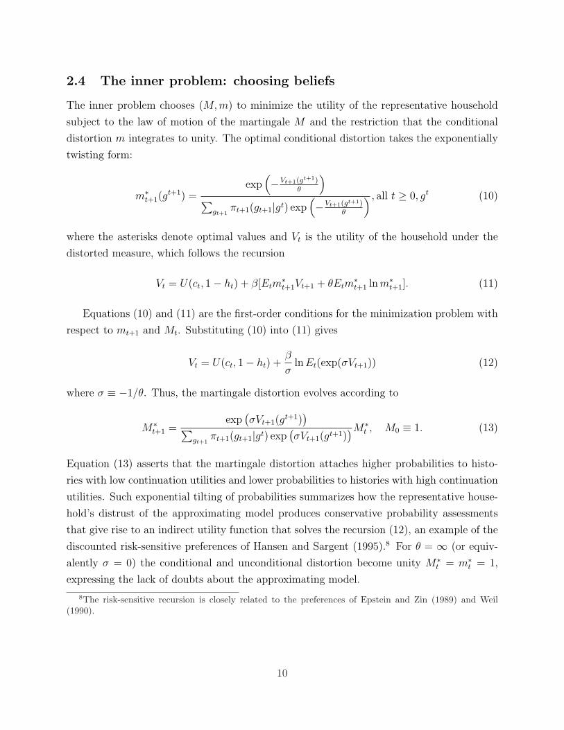
2.4 The inner problem: choosing beliefs

The inner problem chooses (M,m) to minimize the utility of the representative household

subject to the law of motion of the martingale M and the restriction that the conditional

distortion m integrates to unity. The optimal conditional distortion takes the exponentially

twisting form:

m∗t+1(g

t+1) =exp

(−Vt+1(gt+1)

θ

)

∑gt+1

πt+1(gt+1|gt) exp(−Vt+1(gt+1)

θ

) , all t ≥ 0, gt (10)

where the asterisks denote optimal values and Vt is the utility of the household under the

distorted measure, which follows the recursion

Vt = U(ct, 1− ht) + β[Etm∗t+1Vt+1 + θEtm

∗t+1 ln m∗

t+1]. (11)

Equations (10) and (11) are the first-order conditions for the minimization problem with

respect to mt+1 and Mt. Substituting (10) into (11) gives

Vt = U(ct, 1− ht) +β

σln Et(exp(σVt+1)) (12)

where σ ≡ −1/θ. Thus, the martingale distortion evolves according to

M∗t+1 =

exp(σVt+1(g

t+1))

∑gt+1

πt+1(gt+1|gt) exp(σVt+1(gt+1)

)M∗t , M0 ≡ 1. (13)

Equation (13) asserts that the martingale distortion attaches higher probabilities to histo-

ries with low continuation utilities and lower probabilities to histories with high continuation

utilities. Such exponential tilting of probabilities summarizes how the representative house-

hold’s distrust of the approximating model produces conservative probability assessments

that give rise to an indirect utility function that solves the recursion (12), an example of the

discounted risk-sensitive preferences of Hansen and Sargent (1995).8 For θ = ∞ (or equiv-

alently σ = 0) the conditional and unconditional distortion become unity M∗t = m∗

t = 1,

expressing the lack of doubts about the approximating model.

8The risk-sensitive recursion is closely related to the preferences of Epstein and Zin (1989) and Weil(1990).

10

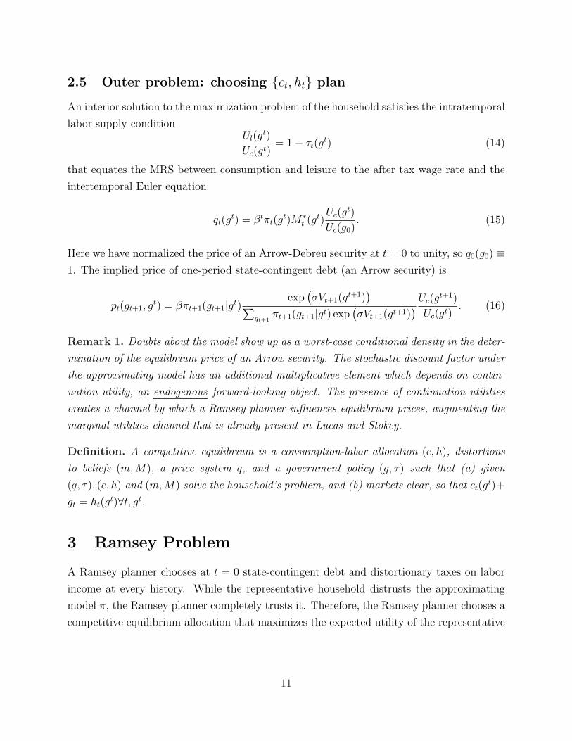
2.5 Outer problem: choosing ct, ht plan

An interior solution to the maximization problem of the household satisfies the intratemporal

labor supply conditionUl(g

t)

Uc(gt)= 1− τt(g

t) (14)

that equates the MRS between consumption and leisure to the after tax wage rate and the

intertemporal Euler equation

qt(gt) = βtπt(g

t)M∗t (gt)

Uc(gt)

Uc(g0). (15)

Here we have normalized the price of an Arrow-Debreu security at t = 0 to unity, so q0(g0) ≡1. The implied price of one-period state-contingent debt (an Arrow security) is

pt(gt+1, gt) = βπt+1(gt+1|gt)

exp(σVt+1(g

t+1))

∑gt+1

πt+1(gt+1|gt) exp(σVt+1(gt+1)

) Uc(gt+1)

Uc(gt). (16)

Remark 1. Doubts about the model show up as a worst-case conditional density in the deter-

mination of the equilibrium price of an Arrow security. The stochastic discount factor under

the approximating model has an additional multiplicative element which depends on contin-

uation utility, an endogenous forward-looking object. The presence of continuation utilities

creates a channel by which a Ramsey planner influences equilibrium prices, augmenting the

marginal utilities channel that is already present in Lucas and Stokey.

Definition. A competitive equilibrium is a consumption-labor allocation (c, h), distortions

to beliefs (m,M), a price system q, and a government policy (g, τ) such that (a) given

(q, τ), (c, h) and (m,M) solve the household’s problem, and (b) markets clear, so that ct(gt)+

gt = ht(gt)∀t, gt.

3 Ramsey Problem

A Ramsey planner chooses at t = 0 state-contingent debt and distortionary taxes on labor

income at every history. While the representative household distrusts the approximating

model π, the Ramsey planner completely trusts it. Therefore, the Ramsey planner chooses a

competitive equilibrium allocation that maximizes the expected utility of the representative

11

household under the approximating model .9

We use the primal approach employed by Lucas and Stokey (1983). The Ramsey planner

chooses allocations subject to the resource constraint (2) and implementability constraints

imposed by competitive equilibrium.

Proposition 1. The Ramsey planner faces the following implementability constraints

∞∑t=0

βt∑

gt

πt(gt)M∗

t (gt)Uc(gt)ct(g

t) =∞∑

t=0

βt∑

gt

πt(gt)M∗

t (gt)Ul(gt)ht(g

t) + Uc(g0)b0, (17)

the law of motion for the martingale that represents distortions to beliefs (13), and the

recursion for the representative household’s value function (12).

Proof. Besides the resource constraint, a competitive equilibrium is characterized fully by

the household’s two Euler equations, the intertemporal budget constraint (6) that holds with

equality at an optimum, and equations (13) and (12), which describe the evolution of the

endogenous beliefs of the agent. Use (14) and (15) to substitute for prices and after tax

wages in the intertemporal budget constraint to obtain (17).

Definition. The Ramsey problem is

max(c,h,M∗,V )

∞∑t=0

βt∑

gt

πt(gt)U

(ct(g

t), 1− ht(gt)

)

subject to

∞∑t=0

βt∑

gt

πt(gt)M∗

t (gt)[Uc(gt)ct(g

t)− Ul(gt)ht(g

t)] = Uc(g0)b0 (18)

ct(gt) + gt = ht(g

t),∀t, gt (19)

M∗t+1(g

t+1) =exp (σVt+1(g

t+1))∑gt+1

πt+1(gt+1|gt) exp (σVt+1(gt+1))M∗

t (gt),M0(g0) = 1, ∀t, gt (20)

Vt(gt) = U(ct(g

t), 1− ht(gt)) +

β

σln

∑gt+1

πt+1(gt+1|gt) exp(σVt+1(g

t+1)),

∀t, gt, t ≥ 1 (21)

9In Karantounias et al. (2007), we study alternative sets of assumptions that allow the Ramsey planner todoubt the approximating model and also possibly instruct the planner to evaluate expected utilities using therepresentative household’s beliefs. The current setup isolates key forces that also operate in that alternativesetting.

12

Remark 2. The presence of the distorted beliefs in (17) contributes two additional imple-

mentability constraints to those already in Lucas and Stokey (1983). The Ramsey planner

takes into account how the allocation (c, h) affects the utility of the agent Vt(gt), which deter-

mines in turn the endogenous likelihood ratio M∗t (gt) and the consequent worst-case beliefs.

Note that we could interpret the minimization problem of the household in the description

of the preferences in (5) as the problem of a malevolent alter ego who, by choosing a worst-

case probability distortion, motivates the household to value robust decision rules. Along the

lines of this interpretation, the Ramsey problem becomes a Stackelberg game with one leader

and two followers, namely, the representative household and the representative household’s

malevolent alter ego.

3.1 First-best benchmark (i.e., lump-sum taxes available)

By first-best, we mean the allocation that maximizes the expected utility of the household

under π subject to the resource constraint (2). Note that for any beliefs of the planner, the

first-best is characterized by the condition Ul(gt)

Uc(gt)= 1 and the resource constraint (2), so the

first-best allocation (c, h) is independent of probabilities π. Private sector beliefs affect asset

prices through (15), but not the allocation. Because lump-sum taxes are not available in our

model, the planner’s and the household’s beliefs both affect allocations.

3.2 Optimality conditions of the Ramsey problem

Define for convenience Ω(ct(gt), ht(g

t)) ≡ Uc(gt)ct(g

t)−Ul(gt)ht(g

t) 10 and attach multipliers

Φ, βtπt(gt)λt(g

t), βt+1πt+1(gt+1)µt+1(g

t+1), and βtπt(gt)ξt(g

t) to constraints (17), (2), (13),

and (12), respectively.

First-order necessary conditions11 for an interior solution are

10Note that Ωt represents the equilibrium government surplus or deficit in marginal utility terms, Ωt =Uct[τtht − gt].

11We set up the Lagrangian and derive the first-order condition with respect to Vt(gt) in a separateappendix available upon request.

13

ct : (1 + ξt(gt))Uc(g

t) + ΦM∗t (gt)Ωc(g

t) = λt(gt), t ≥ 1 (22)

ht : −(1 + ξt(gt))Ul(g

t) + ΦM∗t (gt)Ωh(g

t) = −λt(gt), t ≥ 1 (23)

M∗t : µt(g

t) = ΦΩ(gt) + β∑gt+1

πt+1(gt+1|gt)m∗t+1(g

t+1)µt+1(gt+1), t ≥ 1 (24)

Vt : ξt(gt) = σm∗

t (gt)M∗

t−1(gt−1)

[µt(g

t)−∑gt

πt(gt|gt−1)m∗t (g

t)µt(gt)

]

+m∗t (g

t)ξt−1(gt−1), t ≥ 1 (25)

c0 : (1 + ξ0)Uc(g0) + ΦM0Ωc(g0) = λ0(g0) + ΦUcc(g0)b0 (26)

h0 : −(1 + ξ0)Ul(g0) + ΦM0Ωh(g0) = −λ0(g0)− ΦUcl(g0)b0. (27)

In (24) and (25), we used expression (10) for the optimal conditional likelihood ratio

m∗t+1 to save notation.

Remark 3. In formulating the Ramsey problem, the last constraint (12) applies only from

period one on since the value of the agent at t = 0 V0 is not relevant to the problem due to

the normalization M0 ≡ 1. We can set the initial value of the multiplier equal to zero ξ0 = 0

to accommodate this. Equivalently, we could maximize with respect to V0 to get an additional

first-order condition ξ0 = 0.

Remark 4. Since ξ0 = 0,M0 = 1, the first-order conditions (26, 27) for the initial consumption-

labor allocation (c0, h0) are the same as the respective first-order conditions for the special

Lucas and Stokey (1983) case where the representative consumer fears no misspecification.

The first-order conditions (22-27) together with the constraints (18-21) determine the

Ramsey plan.

14

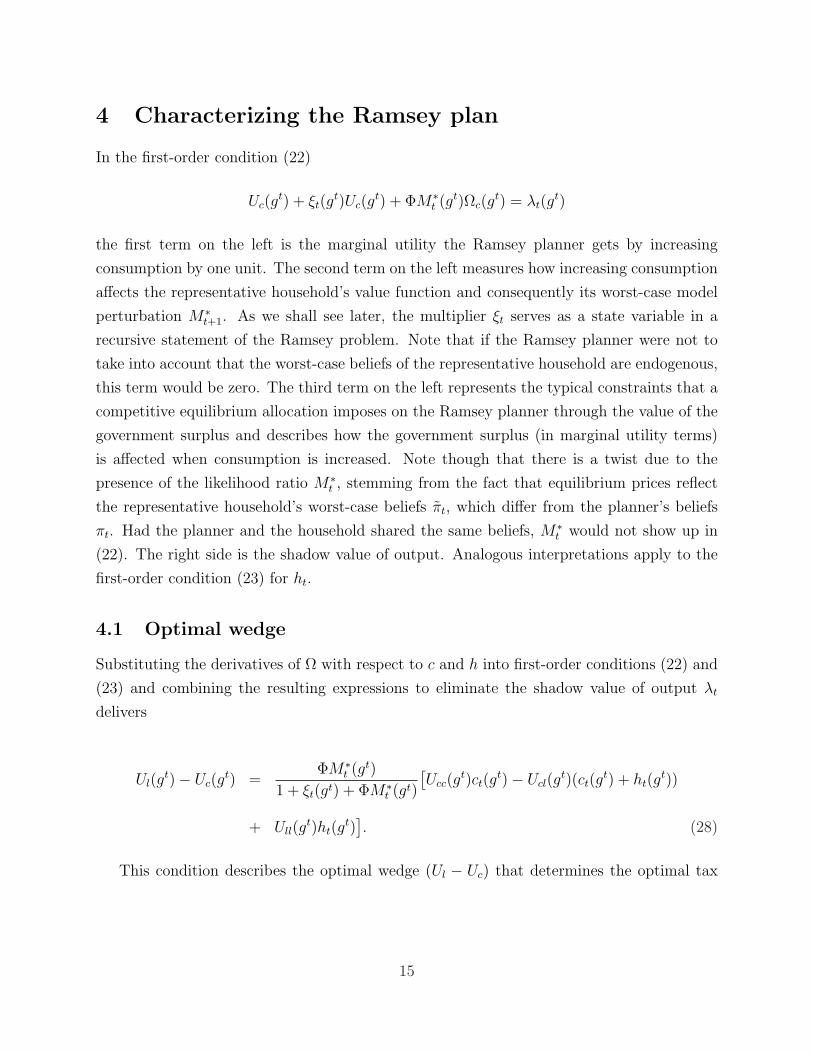
4 Characterizing the Ramsey plan

In the first-order condition (22)

Uc(gt) + ξt(g

t)Uc(gt) + ΦM∗

t (gt)Ωc(gt) = λt(g

t)

the first term on the left is the marginal utility the Ramsey planner gets by increasing

consumption by one unit. The second term on the left measures how increasing consumption

affects the representative household’s value function and consequently its worst-case model

perturbation M∗t+1. As we shall see later, the multiplier ξt serves as a state variable in a

recursive statement of the Ramsey problem. Note that if the Ramsey planner were not to

take into account that the worst-case beliefs of the representative household are endogenous,

this term would be zero. The third term on the left represents the typical constraints that a

competitive equilibrium allocation imposes on the Ramsey planner through the value of the

government surplus and describes how the government surplus (in marginal utility terms)

is affected when consumption is increased. Note though that there is a twist due to the

presence of the likelihood ratio M∗t , stemming from the fact that equilibrium prices reflect

the representative household’s worst-case beliefs πt, which differ from the planner’s beliefs

πt. Had the planner and the household shared the same beliefs, M∗t would not show up in

(22). The right side is the shadow value of output. Analogous interpretations apply to the

first-order condition (23) for ht.

4.1 Optimal wedge

Substituting the derivatives of Ω with respect to c and h into first-order conditions (22) and

(23) and combining the resulting expressions to eliminate the shadow value of output λt

delivers

Ul(gt)− Uc(g

t) =ΦM∗

t (gt)

1 + ξt(gt) + ΦM∗t (gt)

[Ucc(g

t)ct(gt)− Ucl(g

t)(ct(gt) + ht(g

t))

+ Ull(gt)ht(g

t)]. (28)

This condition describes the optimal wedge (Ul − Uc) that determines the optimal tax

15

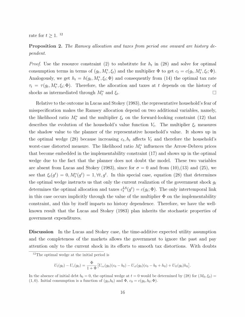
rate for t ≥ 1. 12

Proposition 2. The Ramsey allocation and taxes from period one onward are history de-

pendent.

Proof. Use the resource constraint (2) to substitute for ht in (28) and solve for optimal

consumption terms in terms of (gt,M∗t , ξt) and the multiplier Φ to get ct = c(gt,M

∗t , ξt; Φ).

Analogously, we get ht = h(gt,M∗t , ξt; Φ) and consequently from (14) the optimal tax rate

τt = τ(gt,M∗t , ξt; Φ). Therefore, the allocation and taxes at t depends on the history of

shocks as intermediated through M∗t and ξt.

Relative to the outcome in Lucas and Stokey (1983), the representative household’s fear of

misspecification makes the Ramsey allocation depend on two additional variables, namely,

the likelihood ratio M∗t and the multiplier ξt on the forward-looking constraint (12) that

describes the evolution of the household’s value function Vt. The multiplier ξt measures

the shadow value to the planner of the representative household’s value. It shows up in

the optimal wedge (28) because increasing ct, ht affects Vt and therefore the household’s

worst-case distorted measure. The likelihood ratio M∗t influences the Arrow-Debreu prices

that become embedded in the implementability constraint (17) and shows up in the optimal

wedge due to the fact that the planner does not doubt the model. These two variables

are absent from Lucas and Stokey (1983), since for σ = 0 and from (10),(13) and (25), we

see that ξt(gt) = 0,M∗

t (gt) = 1,∀t, gt. In this special case, equation (28) that determines

the optimal wedge instructs us that only the current realization of the government shock gt

determines the optimal allocation and taxes cLSt (gt) = c(gt; Φ). The only intertemporal link

in this case occurs implicitly through the value of the multiplier Φ on the implementability

constraint, and this by itself imparts no history dependence. Therefore, we have the well-

known result that the Lucas and Stokey (1983) plan inherits the stochastic properties of

government expenditures.

Discussion In the Lucas and Stokey case, the time-additive expected utility assumption

and the completeness of the markets allows the government to ignore the past and pay

attention only to the current shock in its efforts to smooth tax distortions. With doubts

12The optimal wedge at the initial period is

Ul(g0)− Uc(g0) =Φ

1 + Φ[Ucc(g0)(c0 − b0)− Ucl(g0)(c0 − b0 + h0) + Ull(g0)h0

].

In the absence of initial debt b0 = 0, the optimal wedge at t = 0 would be determined by (28) for (M0, ξ0) =(1, 0). Initial consumption is a function of (g0,b0) and Φ, c0 = c(g0, b0; Φ).

16

about the model, even though there is a unique intertemporal budget constraint due to the

complete markets assumption, history dependence emerges because intertemporal marginal

rates of substitution (and therefore equilibrium prices) are interconnected across histories

through continuation utilities.

4.2 Tax rate

We can express the optimal tax in terms of the allocation and (M∗, ξ) as follows. Dividing

(28) by −Uc(gt) and using τt = 1− Ul

Uc, we get for t ≥ 1

τt(gt) =

ΦM∗t (gt)

1 + ξt(gt) + ΦM∗t (gt)

[γRA(gt) +

Ucl(gt)

Uc(gt)(ct(g

t) + ht(gt))− Ull(g

t)

Uc(gt)ht(g

t)

], (29)

where γRA(gt) ≡ −Uccc/Uc, the coefficient of relative risk aversion.13

Remark 5. Formula (29) shows that the planner chooses smaller tax wedges at histories

that the representative household thinks are less probable than does the Ramsey planner, i.e.,

when M∗t (gt) is small. The planner chooses low tax rates for high values of the multiplier ξt.

4.3 State variables

The problem under commitment has history dependence that adds state variables to the

exogenous state variable gt. Proposition 2 suggests that the endogenous variables M∗t and ξt

are natural candidates for state variables in a recursive formulation of the Ramsey problem,

which we pursue along the lines of Marcet and Marimon (1998). 14

Proposition 3. Let the approximating model of government expenditures be Markov. Then

the Ramsey problem from period one onward can be represented recursively by keeping as a

state variable the vector (gt,M∗t , ξt). The likelihood ratio M∗

t and the multiplier ξt follow

13It is easy to show that the tax rate is positive when Ucl ≥ 0. According to (29), this amounts to showingthat expression 1+ξt+ΦM∗

t is positive, despite the fact that ξt can take negative values. Calculating Ωc in thefirst-order condition (22) and rearranging delivers expression Uct(1+ξt+ΦM∗

t ) = λt−ΦM∗t (Ucc,tct−Ucl,tht) >

0, since the shadow value of output λt is positive and Ucl ≥ 0.14The Bellman equation that describes the planner’s problem is constructed in a separate appendix avail-

able upon request.

17

laws of motion 15

M∗t = M∗(gt, gt−1,M

∗t−1, ξt−1; Φ)

ξt = ξ(gt, gt−1,M∗t−1, ξt−1; Φ),

with initial values (M0, ξ0) = (1, 0). The policy functions for consumption, household utility

and debt for t ≥ 1 are 16

ct = c(gt,M∗t , ξt; Φ)

Vt = V (gt,M∗t , ξt; Φ)

bt = b(gt,M∗t , ξt; Φ).

Discussion The logic of the Marcet and Marimon (1998) method (and in fact of any

method that tries to represent commitment problems recursively) is to augment the state

space appropriately in order to capture the restrictions that the planner has to respect every

period. The multiplier ξt (the co-state variable) on the forward-looking implementability

constraint (21) becomes a state variable, with initial value zero, which reflects the fact that

the planner at period one is not constrained to commit to the shadow value of his utility

promises to the household. The nature of our problem also requires the inclusion in the

state of the likelihood ratio M∗t with law of motion (13). This augmented state allows us to

express the policy problem as a functional saddle point problem.

4.4 Interpretation of µt

Fear of misspecification alters the essentially static nature of the Lucas and Stokey problem

by injecting the probability distortion and the multiplier (M∗t , ξt). In order to understand

how the planner tries to affect equilibrium prices though the channel of beliefs, it helps to

interpret the first-order conditions with respect to (M∗t , Vt).

Consider µt, the multiplier on the evolution equation for the likelihood ratio (13), which

represents the shadow value to the planner of distorting the probability of history gt. Using

15In the case of an i.i.d. approximating model we would have M∗t = M∗(gt,M

∗t−1, ξt−1; Φ) and ξt =

ξ(gt,M∗t−1, ξt−1; Φ).

16Note that, as our notation suggests, the policy functions are contingent on a value of the multiplier Φ.After finding the policy functions for ct = c(gt,M

∗t , ξt; Φ), t ≥ 1 and c0(g0, b0; Φ), the multiplier Φ is adjusted

so that the intertemporal budget constraint is satisfied.

18

the definition of Ω(gt) in equation (24) gives

µt(gt) = Φ[Uc(g

t)ct(gt)− Ul(g

t)ht(gt)] + β

∑gt+1

πt+1(gt+1|gt)m∗t+1(g

t+1)µt+1(gt+1).

Increasing M∗t (gt) to make history gt more probable has two effects: first, it affects prices at

history gt which is measured by the first term on the right, which is the marginal utility of a

government surplus Ωt multiplied by the shadow value of distortionary taxation Φ. Second,

it alters the unconditional probability of next period’s history, which is reflected by the

second term on the right.

Let qtt+i denote the equilibrium price of an Arrow-Debreu security in terms of consumption

at history gt,

qtt+i(g

t+i) ≡ qt+i(gt+i)

qt(gt)= βiπt+i(g

t+i|gt)i∏

j=1

m∗t+j(g

t+j)Uc(g

t+i)

Uc(gt).

Solving forward (24) allows us to express µt in terms of future government surpluses,

µt(gt) = ΦUc(g

t)∞∑i=0

∑

gt+i|gt

qtt+i(g

t+i)[τt+i(gt+i)ht+i(g

t+i)− gt+i]. (30)

Using the intertemporal budget constraint at time t, µt can be rewritten as

µt(gt) = ΦUc(g

t)bt(gt). (31)

The government’s budget constraint implies that the asset position of the government

bt(gt) equals the present discounted value of all future government surpluses, which renders

bt(gt) the relevant variable for capturing all intertemporal effects of changing the equilibrium

price of an Arrow-Debreu security qt(gt) by means of the likelihood ratio M∗

t .

4.5 Dynamics of ξt

Consider now the first-order condition with respect to Vt(gt), which delivers the law of motion

of the state variable ξt

ξt = σm∗t M

∗t−1[µt − Et−1m

∗t µt] + m∗

t ξt−1, t ≥ 1, ξ0 = 0 (32)

19

where E denotes mathematical expectation under the approximating model. The planner

faces intricate dynamic tradeoffs. By increasing Vt(gt), he affects the household’s expectation

at t − 1 for the current period t. However, the planner is constrained to confirm the value

Vt(gt) that he had earlier promised the household according to the promise-keeping constraint

(21). The shadow value to the planner of the promised utility to the household is captured

by the multiplier ξt−1, the second term on the right side of (32). The planner is able to steer

the household’s worst-case beliefs via equation (20) by committing to respect the recursion

of the household’s utility (21).

Furthermore, increasing Vt(gt) affects household beliefs for the current period by decreas-

ing the probability of the history gt and all subsequent future histories emanating from gt,

an effect measured by the multiplier µt in the first term of the right side. But decreasing

by means of Vt the probability of this particular node of the event tree implies increasing

probabilities attached to the other nodes, so that probabilities add to unity, as can be seen

clearly from equation (10). The total effect is measured by ηt ≡ µt − Et−1m∗t µt, i.e., the in-

novation in µt under the distorted measure π, or in other words, the one-step ahead forecast

error of µt with conditional mean under the distorted measure Et−1m∗t ηt equal to zero by

construction. This is the first term of the right-hand side. Optimality requires that the sum

of the two effects must equal the shadow value of the promised utility of next period ξt, the

left side of equation (32). Besides that, ξt has the following property:

Lemma 1. The multiplier ξt is a martingale under the approximating model.

Proof. Taking conditional expectation with respect to the approximating model π given

history gt−1 in the law of motion (32) for ξ and remembering that variables dated at t are

measurable functions of the history gt, we get

Et−1ξt = σM∗t−1Et−1m

∗t [µt − Et−1m

∗t µt] + ξt−1Et−1m

∗t

= σM∗t−1[Et−1m

∗t µt − Et−1m

∗t · Et−1m

∗t µt] + ξt−1Et−1m

∗t

= ξt−1,

since Et−1m∗t = 1.

Remark 6. Since the two state variables (M∗t , ξt) are martingales with respect to the ap-

proximating model, any transitory shock in government expenditures will have a permanent

effect on the state variables that are driving the Ramsey plan.

An immediate corollary of lemma 1 is that the mean value of the ξt is zero since E(ξt) =

20

E(E0ξt) = E(ξ0) = 0. Note also that ξt can take both positive and negative values because

constraint (12) can bind in both directions.

5 Manipulation of expectations and prices

In this section we show that the state variables depict two distinct forces that are shaping

the Ramsey plan: price manipulation of government debt through the management of the

household’s expectations (ξt) and the belief heterogeneity between planner and household

(M∗t ).

5.1 Incentives to manipulate continuation utilities and beliefs

The household’s doubts about the model make continuation utilities among the determinants

of equilibrium prices. This contributes a multiplier ξt that influences the Ramsey plan.17 We

will use as a guide the evolution of ξt (32) in order to interpret how the planner manipulates

equilibrium prices via continuation utilities and to describe implications for the tax rate.

There are two dimensions along which the household’s doubts about the model alter the

Ramsey plan, an intratemporal one (among realizations of government expenditures shocks

for a given t) and an intertemporal one. We explore the intratemporal dimension first by

focusing on µt.

The multiplier µt is the shadow value for the planner of the likelihood ratio M∗t and

captures the marginal benefit or cost of increasing the equilibrium price via the worst-case

beliefs of the household. It is easy to see how the likelihood ratio M∗t is associated with the

government bond holdings from the equilibrium intertemporal budget constraint

Uc0b0 = Ω0 + βE0m∗1Ω1 + ... + βt−1E0M

∗t−1Ωt−1 + βtE0M

∗t Uctbt︸ ︷︷ ︸

Uc0P

gt qt(gt)bt(gt)

,

which makes transparent the fact that µt is associated with the debt obligations of the

government µt = ΦUctbt, as we have shown before. Note that the multiplier µt would be zero

if the marginal cost of distortionary taxation Φ were zero. This reflects the fact that in a first-

best world where lump-sum taxes are available, the equilibrium price of state-contingent debt

is not relevant for the planner’s problem. 18 The multiplier µt takes positive or negative

17Remember that with full confidence in the model we have ξt = 0, which reflects the absence of a role forcontinuation utilities in equilibrium prices.

18Φ could also be zero if there were sufficiently large initial assets b0 ¿ 0, a case that would render the

21

values depending on the asset position of the government. More specifically, the planner

wants to increase the likelihood ratio and therefore the equilibrium price of consumption

claims at contingencies where the government has outstanding debt obligations (bt > 0) and

wants to decrease it when the public is a net debtor to the government (bt < 0).

The way to interpret the planner’s incentives is as follows. Positive government debt at

a particular contingency means that the government is ex-ante selling consumption claims.

Thus, the planner strives to make claims to consumption more expensive through the chan-

nel of worst-case beliefs when he is engaged in selling them. In the opposite situation of

government assets, the planner is ex-ante buying consumption claims, with the resulting

incentive of decreasing the price of claims by decreasing M∗t .

Of course, the planner is affecting the likelihood ratio M∗t by means of continuation

utility, which by (10) will affect also the rest of the conditional likelihood ratios at time t, so

that they integrate to unity. Therefore, the relevant object which properly takes into account

the total effect of changing continuation utility is actually the innovation in µt under the

household’s worst-case beliefs, which we defined in the previous section as ηt ≡ µt−Et−1m∗t µt.

So the innovation ηt captures the intratemporal dimension of the price manipulation effect

by determining the increment to the martingale ξt according to the law of motion (32) and

is associated by (31) with the government asset position as ηt = Φ[Uctbt − Et−1m∗t Uctbt]. A

convenient way to think about ηt and the total effect is by defining ωt−1 ≡ Et−1m∗t Uctbt, an

object that can be thought of as the market value at t − 1 of the government portfolio of

state-contingent debt at time t, and by noting that ηt = Φ(Uctbt − ωt−1).19 So the planner

increases the price by lowering continuation utilities at those contingencies upon which he

sells consumption claims above the market value of the government portfolio and decreases

the price in the opposite case. 20

Tax rate implications Furthermore, price manipulation through continuation utilities as

encoded in ξt has a direct impact on the Ramsey plan’s consumption and leisure allocation

and therefore on the tax rate through (29). A positive innovation ηt > 0 leads to lower ξt

and therefore - keeping everything else equal - higher tax rates. Thus, when the planner

wants to sell claims, he tries to increase equilibrium prices by lowering continuation utilities

optimal taxation problem trivial.19More precisely, we have ωt−1 = Uct

β

∑gt

pt−1(gt, gt−1)bt(gt).

20The market value of the government portfolio ωt−1 and the innovation ηt are not just convenient devicesbut very closely related to each other: ηt has a direct interpretation as the marginal change in the value of thegovernment portfolio induced by a change in continuation utility since ∂ωt−1

∂Vt= σπt|t−1m

∗t (Uctbt − ωt−1) =

σπt|t−1m∗t Φ

−1ηt.

22

and increasing the tax rate, whereas when he wants to buy claims (ηt < 0), he increases

continuation utilities and lowers tax rates.

Our discussion above is in terms of marginal incentives, since we focus on first-order

conditions and multipliers. Along with the marginal benefits of price manipulation through

continuation utilities, the planner has obviously to take into account the effects of changing

the marginal utility of consumption and leisure Uc and Ul, together with his financing needs

as captured by the multiplier Φ.

The preceding description of the incentives confronting the planner is evidently static. On

the intertemporal dimension, note that continuation utilities are forwarding-looking objects

and that any change in Vt(gt) will affect all past continuation utilities V1(g

1), ..., Vt−1(gt−1)

along the history gt through recursion (12), and as a result all the past worst-case beliefs of

the household and associated equilibrium prices. Therefore a change in Vt besides altering

the market value of the government portfolio at the end of period t − 1, ωt−1, affects also

all past market values of the government portfolios ωi, i < t − 1. Consequently, the past

innovations in government debt (in marginal utility terms) ηi, i ≤ t will matter since they

measure the shadow value for the planner of altering the respective equilibrium prices along

history gt through the channel of utility Vt. This can be easily seen by iterating backward

the law of motion of the multiplier ξt (32)

ξt = σM∗t (ηt + · · ·+ η1)

= σM∗t Ht, (33)

where Ht is the cumulative forecast error Ht ≡∑t

i=1 ηi, H0 ≡ 0. The cumulative forecast

error captures the essence of commitment: the planner must take into account how a gt-

contingent action chosen at t = 0 affects the choices of the household along the history gt.

Thus the history of the shocks as summarized by the state variable ξt matters because it

tracks dates in the past that the government was lending or borrowing on average, indicating

a corresponding incentive to reduce or increase the equilibrium price of consumption claims

and a respective utility promise.

Smoothing That the planner makes the shadow value of continuation utilities ξt a mar-

tingale with respect to his beliefs reflects a deeper smoothing motive that makes the planner

want to keep the shadow value of continuation utilities constant over time. There is a useful

analogy: With full confidence in the probability model, the standard prescription in the

23

optimal taxation literature is to “smooth” marginal utilities of consumption and leisure. On

the other hand, when the household has doubts about the model, there is an intertemporal

dimension coming from continuation utilities and their effects on equilibrium prices and the

optimal prescription is to smooth the shadow value of the additional channel of continuation

utilities. Note that the additional channel of continuation utilities is bringing back into the

picture the debt dynamics through the martingale ξt, a feature absent in the full-confidence

complete-markets economy of Lucas and Stokey (1983).

5.2 Heterogeneity in ambiguity attitudes and impact on tax rate

The likelihood ratio M∗t of the worst-case beliefs of the household over the beliefs of the

planner also influences the optimal wedge (28) and therefore the optimal tax rate in (29)

and functions as a state variable which reflects the heterogeneity in ambiguity attitudes

between the household and the planner. From (29), the planner has an incentive to tax

more heavily histories with a high likelihood ratio M∗t , i.e., histories that the household

considers more probable than the planner, keeping everything else equal. The source of this

incentive is that the representative household and the planner disagree about the evaluation

of welfare losses stemming from a tax τt(gt) at history gt because they evaluate the likelihood

of this contingency in a different way. 21 The welfare loss of a given tax at a contingency that

the household considers more probable than the planner is higher for the household than

for the planner. In this case, the planner has an incentive to increase the tax rate, since

the resulting loss coming from this action is not regarded as being so high by the planner.

In opposite cases, i.e. in contingencies that the planner considers more probable than the

household (low M∗t ), the planner tries to tax less, since high taxes carry high loss in the

planner’s evaluation of utility. For example, in the extreme case where M∗t approaches zero,

the tax rate approaches zero according to (29).

6 The effects of small doubts about the model

We can illustrate sharply the impacts of ambiguity aversion on the Ramsey plan by ex-

ploiting the fact that Lucas and Stokey ’s plan can be easily calculated due to the history

independence property. This feature allows us to use a perturbation method that expands in

σ ≡ −θ−1 around σ = 0, i.e. around the entire stochastic path associated with the Ramsey

21This is exactly the reason why the likelihood ratio shows up in the first-order conditions (22),(23) andtherefore in the optimal wedge (28).

24

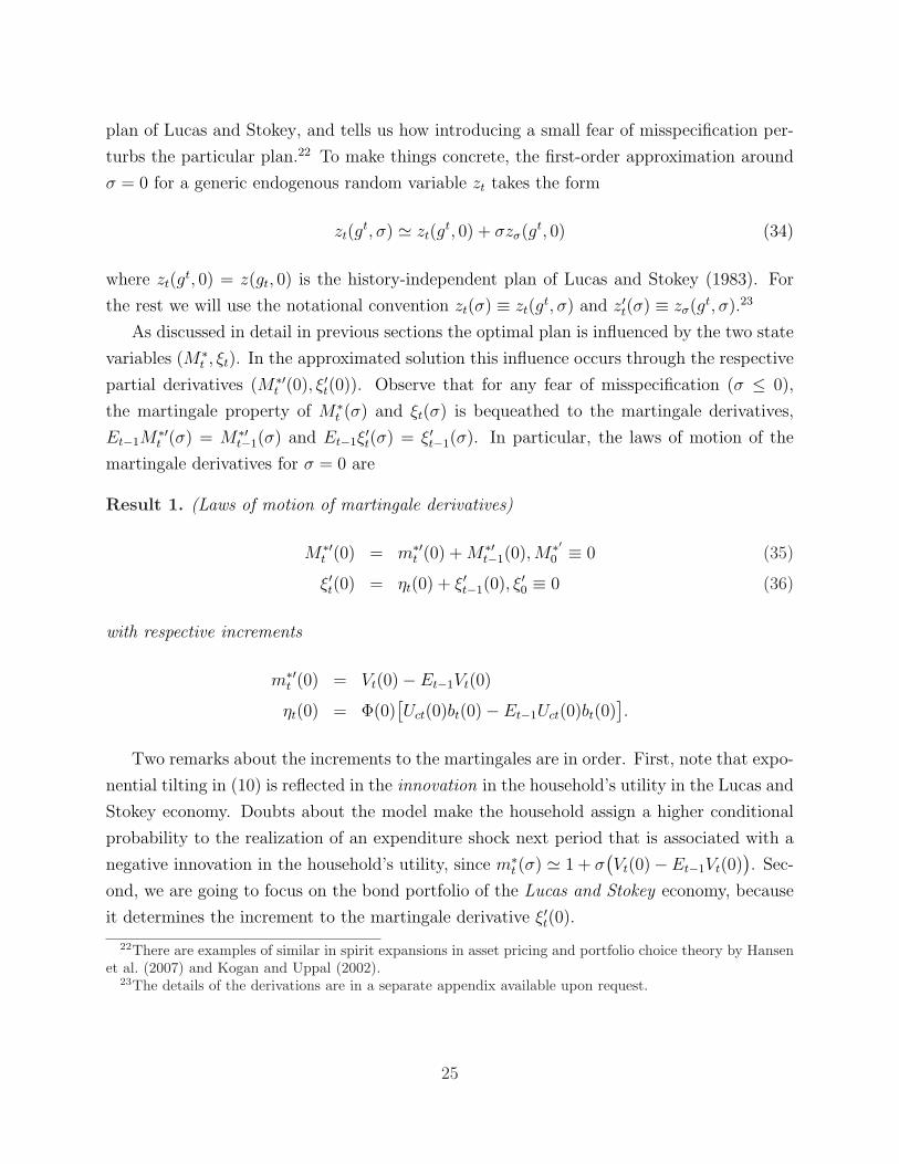
plan of Lucas and Stokey, and tells us how introducing a small fear of misspecification per-

turbs the particular plan.22 To make things concrete, the first-order approximation around

σ = 0 for a generic endogenous random variable zt takes the form

zt(gt, σ) ' zt(g

t, 0) + σzσ(gt, 0) (34)

where zt(gt, 0) = z(gt, 0) is the history-independent plan of Lucas and Stokey (1983). For

the rest we will use the notational convention zt(σ) ≡ zt(gt, σ) and z′t(σ) ≡ zσ(gt, σ).23

As discussed in detail in previous sections the optimal plan is influenced by the two state

variables (M∗t , ξt). In the approximated solution this influence occurs through the respective

partial derivatives (M∗′t (0), ξ′t(0)). Observe that for any fear of misspecification (σ ≤ 0),

the martingale property of M∗t (σ) and ξt(σ) is bequeathed to the martingale derivatives,

Et−1M∗′t (σ) = M∗′

t−1(σ) and Et−1ξ′t(σ) = ξ′t−1(σ). In particular, the laws of motion of the

martingale derivatives for σ = 0 are

Result 1. (Laws of motion of martingale derivatives)

M∗′t (0) = m∗′

t (0) + M∗′t−1(0),M∗′

0 ≡ 0 (35)

ξ′t(0) = ηt(0) + ξ′t−1(0), ξ′0 ≡ 0 (36)

with respective increments

m∗′t (0) = Vt(0)− Et−1Vt(0)

ηt(0) = Φ(0)[Uct(0)bt(0)− Et−1Uct(0)bt(0)

].

Two remarks about the increments to the martingales are in order. First, note that expo-

nential tilting in (10) is reflected in the innovation in the household’s utility in the Lucas and

Stokey economy. Doubts about the model make the household assign a higher conditional

probability to the realization of an expenditure shock next period that is associated with a

negative innovation in the household’s utility, since m∗t (σ) ' 1 + σ

(Vt(0)−Et−1Vt(0)

). Sec-

ond, we are going to focus on the bond portfolio of the Lucas and Stokey economy, because

it determines the increment to the martingale derivative ξ′t(0).

22There are examples of similar in spirit expansions in asset pricing and portfolio choice theory by Hansenet al. (2007) and Kogan and Uppal (2002).

23The details of the derivations are in a separate appendix available upon request.

25

6.1 Quasi-linear utility

We proceed with a quasi-linear example. Linearity in consumption eliminates the effects

of marginal utility on labor supply and on equilibrium prices. Let the period utility of the

agent take the form

U(c, l) = c + v(1− l)

Quasi-linear utility leads to Arrow-Debreu prices qt = βtπtM∗t . Thus, with this preference

specification, the planner cannot manipulate the marginal utility to allocate distortions over

histories. But he can still manipulate the endogenous beliefs of the agent through the channel

of continuation utilities. For the rest of this section, we assume that v(1− l) = v(h) = −12h2,

a specification which together with (28) delivers the following labor allocation and tax rate:

ht =1 + ξt + ΦM∗

t

1 + ξt + 2ΦM∗t

and τt = 1− ht =ΦM∗

t

1 + ξt + 2ΦM∗t

.

Equations (18-21), together with (24) and (25) determine the dynamics of (ξt,M∗t ) and the

size of Φ.

6.1.1 No fear of misspecification case (σ = 0)

The optimal plan prescribes constant taxes and labor over time and across states. The lack

of dependence of taxes and labor on the realization of gt is a special feature of quasi-linear

utility that will make more transparent the effects of the representative household’s fear of

misspecification. In particular,

ht(0) ≡ h =1 + Φ(0)

1 + 2Φ(0)

τ = 1− h

ct(0) = h− gt

bt(0) =τh

1− β− Et

∞∑i=0

βigt+i

where Φ(0) represents the value of the multiplier for the Lucas and Stokey economy, where

agents fully trust their model. 24 Having obtained the Ramsey plan for σ = 0, we can

24Since Φ(0) > 0, we have hLS ∈ (1/2, 1]. Labor (and therefore Φ(0)) can be pinned down from theintertemporal budget constraint, which leads to finding the root of equation Q(h) ≡ h2 − h + G, whereG ≡ (1 − β)[b0 + E0

∑∞t=0 βtgt]. Assume that G is smaller than 1/4, so that a solution exists, and larger

than 0 in order to rule out an initial surplus that can finance the present value of government expenditures,

26

proceed to the expansion.

6.1.2 Ramsey allocation for small robustness

The quasi-linearity allows us to derive simple formulas for our expansion. In particular, the

increments to the martingale derivatives are

m∗′t (0) = Vt(0)− Et−1Vt(0) = −(Et − Et−1)[

∞∑i=0

βigt+i] (37)

ηt(0) = Φ(0)[bt(0)− Et−1bt(0)] = −Φ(0)(Et − Et−1)[∞∑i=0

βigt+i] (38)

Equations (37) and (38) show that the dynamics are determined by the innovation in the

present value of government expenditures. 25

To attain more concrete results, assume a Wold moving average representation for the

approximating model of government expenditures

gt = µg + γ(L)εt (39)

where εt ∼ iid(0, σ2ε) and γ(β) > 0. 26

Then the innovation in the present value of government expenditures is

(Et − Et−1)[∞∑i=0

βigt+i] = γ(β)εt (40)

where γ(β) is the present value of the coefficients in the infinite order moving average rep-

resentation, which allows us to get convenient approximate formulas for the pessimistic

conditional distribution of εt.

Result 2. The distortion to the conditional distribution of εt is approximately equal to

m∗t = 1 +

1

θγ(β)εt

and discard the root that is less than 1/2 to get h = 1+√

1−4G2 .

25The innovation to the present value of the income of a representative consumer who fears misspecificationplays an important role in determining market prices of risk. For example, see Barillas et al. (2007).

26Note that here we drop the restriction that g lives on a countable space. We also assume that ε has abounded support, so that government expenditures remain positive.

27

The worst-case mean and variance of εt are approximately equal to

Etεt+1 ≡ Etm∗t+1εt+1 =

1

θγ(β)σ2

ε

V art(εt+1) ≡ Etm∗t+1(εt+1 − Etεt+1)

2 = σ2ε +

γ(β)

θEtε

3t+1

Result (2) implies that the household assigns higher probability on the event of a pos-

itive innovation in the present value of government expenditures and lower probability on

the event of a negative innovation. Note in this example that the perturbations around the

approximating model take the form of an increased conditional mean for government expen-

ditures innovations εt and an unaltered conditional variance, assuming a zero third moment

according to the approximating model (Etε3t+1 = 0).

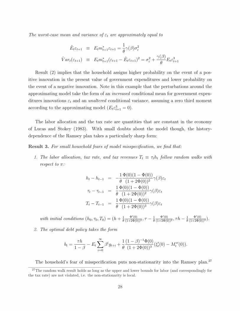
The labor allocation and the tax rate are quantities that are constant in the economy

of Lucas and Stokey (1983). With small doubts about the model though, the history-

dependence of the Ramsey plan takes a particularly sharp form:

Result 3. For small household fears of model misspecification, we find that:

1. The labor allocation, tax rate, and tax revenues Tt ≡ τtht follow random walks with

respect to π:

ht − ht−1 = −1

θ

Φ(0)(1− Φ(0))

(1 + 2Φ(0))2γ(β)εt

τt − τt−1 =1

θ

Φ(0)(1− Φ(0))

(1 + 2Φ(0))2γ(β)εt

Tt − Tt−1 =1

θ

Φ(0)(1− Φ(0))

(1 + 2Φ(0))3γ(β)εt

with initial conditions (h0, τ0, T0) = (h + 1θ

Φ′(0)(1+2Φ(0))2

, τ − 1θ

Φ′(0)(1+2Φ(0))2

, τh− 1θ

Φ′(0)(1+2Φ(0))3

).

2. The optimal debt policy takes the form

bt =τh

1− β− Et

∞∑i=0

βigt+i +1

θ

(1− β)−1Φ(0)

(1 + 2Φ(0))3(ξ′t(0)−M∗′

t (0)).

The household’s fear of misspecification puts non-stationarity into the Ramsey plan.27

27The random walk result holds as long as the upper and lower bounds for labor (and correspondingly forthe tax rate) are not violated, i.e. the non-stationarity is local.

28

Note the amount of history dependence in this example: even in the case of i.i.d. government

expenditures (γ0 = 1,γi = 0, i ≥ 1 ), the tax rate remains a random walk, a result reminiscent

of the Barro (1979) and Aiyagari et al. (2002) results in incomplete markets setups. Here

though, the source of the random walk property is the effort of the planner to smooth

continuation utilities and his disagreement with the agent and not the lack of insurance

markets.

More specifically, the price manipulation and the heterogeneity forces are entering into

the determination of the Ramsey plan though the difference in the two martingale derivatives

ξ′ −M∗′, which is a random walk with respect to π:

ξ′t(0)−M∗′t (0) = ξ′t−1(0)−M∗′

t−1(0) + (1− Φ(0))γ(β)εt. (41)

The increment to the random walk is directly associated with the price manipulation effect

Φ(0)γ(β)εt and the heterogeneity effect γ(β)εt. The size of Φ(0) depicts the relative strength

of the price manipulation effect. Consider for example the tax rate in result 3. A positive

innovation in the present value of government expenditures leads on the one hand to a higher

ξt and on the other hand to a positive innovation in the likelihood ratio M∗t . The increase in

ξt expresses the planner’s incentive to increase continuation utility in order to decrease the

equilibrium price which leads to a reduction in the tax rate, whereas the fact that the planner

doesn’t consider this event so probable leads to an increase in the tax rate.28 Notice that

the two forces operate in opposite directions. This is not a coincidence – high government

expenditures reduce continuation utilities (which increases M∗t ) and reduce government debt

issued ex ante for these contingencies (which increases ξt), due to the planner’s desire to use

the possibilities that complete markets offer and insure against high government expenditure

shocks. If Φ(0) > 1, i.e. if there is a high marginal cost of distortionary taxation in the Lucas

and Stokey (1983) economy, – a fact which makes equilibrium prices relatively important–

the price manipulation effect dominates the heterogeneity effect, whereas when Φ(0) < 1,

the opposite happens. The size of Φ(0) depends on the present value of government expen-

ditures and on initial debt b0. The two effects exactly cancel for the borderline case Φ(0) = 1

, which would correspond to a labor allocation in the Lucas and Stokey (1983) economy of

h = 2/3.

28The optimal tax rate formula (29) for small fear of misspecification and quasi-linear preferences takesthe form τt(σ) = τ + Φ(0)

(1+2Φ(0))2 [(M∗t (σ)− 1)− ξt(σ)] + σ Φ′(0)

(1+2Φ(0))2 , which makes clearer how (M∗t , ξt) enter

the solution. Taking first differences delivers the random walk result in Result 3.

29

Similar comments are due for the optimal debt policy implied by the above allocation.

Assume for convenience that the approximating model is i.i.d. Then with full confidence in

the model the optimal debt is

bt(0) =τh− µg

1− β− εt,

an expression that indicates that the government uses state-contingent debt to smooth the

distortions across histories by hedging fiscal shocks–insuring against high shocks with low

indebtedness towards the private sector and against low shocks with high indebtedness. Note

also how the optimal state-contingent debt inherits the i.i.d. nature of fiscal shocks. With

doubts about the model, the expression in Result 3 simplifies to

bt(σ) =τh− µg

1− β− εt +

1

θ

(1− β)−1Φ(0)

(1 + 2Φ(0))3(1− Φ(0))

t∑i=1

εi,

which shows that fear of misspecification adds a unit-root component to the initially i.i.d.

optimal debt. When the heterogeneity effect is larger than the price manipulation effect

(Φ(0) < 1), positive past innovations in government expenditures (εi, i ≤ t − 1) lead to

an increase in debt.29 This is because past positive innovations lead to a high current tax

rate, which by the logic of the budget constraint leads to higher amount of government debt

that can be sustained at the optimum. The opposite conclusions hold for Φ(0) > 1. As

expected, in the case of Φ(0) = 1 the two opposite effects cancel, implying - for small fear

of misspecification - the same optimal debt as in the Lucas and Stokey economy.

It is useful to calculate the derivative Φ′(0) in the quasi-linear case

Φ′(0) = (1− β)(1 + 2Φ(0))3E0

∞∑t=0

βtM∗′t (0)gt

= −(1− β)(1 + 2Φ(0))3γ(β)σ2ε

∞∑t=0

βt

t−1∑i=0

γi, (42)

where the second line follows from our particular moving average representation (39). Ex-

pression (42) measures the change in the multiplier if we impute fear of misspecification to

the representative household. If we assume that∑t−1

i=0 γi > 0 (γi > 0 would be sufficient for

29The contemporaneous effect of an innovation εt on bt is more likely to have a negative effect on debt forsmall σ due to the insurance motive of the government.

30

0 2 4 6 80

0.5

1

1.5

2

2.5

3x 10

−3

t

Mt*,θ = 100

0 2 4 6 80

0.5

1

1.5

2

2.5x 10

−5

t

ξt, θ = 100

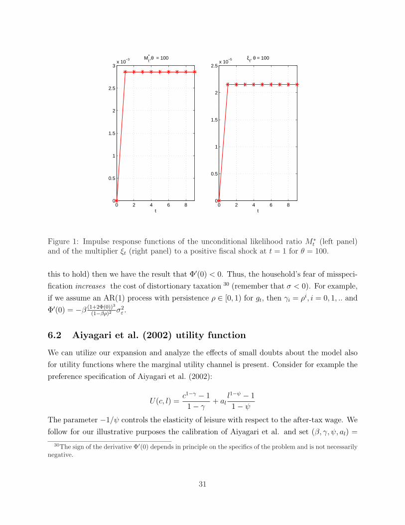
Figure 1: Impulse response functions of the unconditional likelihood ratio M∗t (left panel)

and of the multiplier ξt (right panel) to a positive fiscal shock at t = 1 for θ = 100.

this to hold) then we have the result that Φ′(0) < 0. Thus, the household’s fear of misspeci-

fication increases the cost of distortionary taxation 30 (remember that σ < 0). For example,

if we assume an AR(1) process with persistence ρ ∈ [0, 1) for gt, then γi = ρi, i = 0, 1, .. and

Φ′(0) = −β (1+2Φ(0))3

(1−βρ)2σ2

ε .

6.2 Aiyagari et al. (2002) utility function

We can utilize our expansion and analyze the effects of small doubts about the model also

for utility functions where the marginal utility channel is present. Consider for example the

preference specification of Aiyagari et al. (2002):

U(c, l) =c1−γ − 1

1− γ+ al

l1−ψ − 1

1− ψ

The parameter −1/ψ controls the elasticity of leisure with respect to the after-tax wage. We

follow for our illustrative purposes the calibration of Aiyagari et al. and set (β, γ, ψ, al) =

30The sign of the derivative Φ′(0) depends in principle on the specifics of the problem and is not necessarilynegative.

31

(0.95, 0.5, 2, 1). Furthermore, we scale up the amount of leisure available to the household

to l = 100 and set the initial debt equal to zero b0 = 0.

Shock process of Aiyagari et al. We use as an approximating model for government

expenditures the same process as Aiyagari et al. (2002), namely, an i.i.d. N(30, 2.52) and we

analyze the impulse responses of various variables of interest to a fiscal shock at t = 1 of a

size of roughly one standard deviation above mean. 31

A positive fiscal shock at t = 1 leads in figure 1 to an increase in the two state variables

(M∗t , ξt), due to a negative innovation in utility and bonds. The increase is permanent,

since the two variables are martingales. As a result, the fiscal shock will have in part also

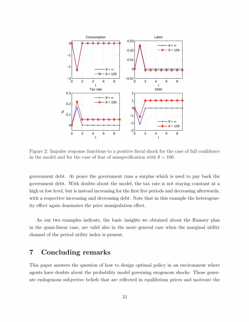
a permanent effect on the rest of the variables of interest. Consider figure 2, which shows

the impulse response functions for the Lucas and Stokey economy and for the case when the

household doubts the model with θ = 100, a penalty parameter that leads to a worst-case

distribution that does not essentially differ from the approximating distribution, as figure 3

attests. Note that in the Lucas and Stokey case all variables return to zero after the shock

at t = 1 due to the history-independence of the solution, whereas with doubts about the

model, they do not. This is not discernible for consumption and barely discernible for labor.

However, the effects of fear of misspecification are clearer for the tax rate and government

debt, which stay permanently above zero after t = 1. Remember that the (M∗t , ξt) affect the

various variables in opposite directions. It turns out that the heterogeneity effect dominates

the price manipulation effect in our example, which leads to a higher tax rate and higher

debt (or less assets) at t = 1 in comparison to the Lucas and Stokey (1983) case.

War-peace example. Assume now that the approximating model for government ex-

penditures is i.i.d. and that g can take two values (gL = 20, gH = 40) with probabilities

(πL, πH) = (0.9, 0.1). Let the household doubt the model with θ = 100, which leads to

a worst-case scenario in figure 4 that is practically the same as the approximating model.

However, the optimal tax rate and debt differ considerably with fear of misspecification.

Figure 5 depicts the time path of the tax rate and state-contingent debt for a sequence of

five high shocks (war) followed by five low shocks (peace) with and without full confidence

in the model. The Lucas and Stokey plan prescribes a high tax rate for times of war and a

low for peace. At times of war the government runs a deficit which is financed by issuing

31The distribution is approximated with gaussian quadrature with 11 nodes and the initial realization isset to be equal to the mean of government expenditures g0 = g = 30. We consider the level of each variableat history gt = (g, g, ..., g) and at history gt = (g, g′, g, ..., g), and plot the change among the two paths. Weuse a fiscal shock of size g′ = 32.32, which corresponds to the 7th node in our approximation scheme.

32

0 2 4 6 8−3

−2

−1

0

t

Consumption

0 2 4 6 8−0.01

0

0.01

0.02

0.03

t

Labor

0 2 4 6 8

0

0.1

0.2

0.3

t

%

Tax rate

0 2 4 6 8−3

−2

−1

0

1

2

t

Debt

θ = ∞θ = 100

θ = ∞θ = 100

θ = ∞θ = 100

θ = ∞θ = 100

Figure 2: Impulse response functions to a positive fiscal shock for the case of full confidencein the model and for the case of fear of misspecification with θ = 100.

government debt. At peace the government runs a surplus which is used to pay back the

government debt. With doubts about the model, the tax rate is not staying constant at a

high or low level, but is instead increasing for the first five periods and decreasing afterwards,

with a respective increasing and decreasing debt. Note that in this example the heterogene-

ity effect again dominates the price manipulation effect.

As our two examples indicate, the basic insights we obtained about the Ramsey plan

in the quasi-linear case, are valid also in the more general case when the marginal utility

channel of the period utility index is present.

7 Concluding remarks

This paper answers the question of how to design optimal policy in an environment where

agents have doubts about the probability model governing exogenous shocks. Those gener-

ate endogenous subjective beliefs that are reflected in equilibrium prices and motivate the

33

15 20 25 30 35 40 450

5

10

15

20

25

30

35

40

government expenditures

%

Worst−case beliefs of household

θ = ∞θ = 100

Figure 3: Shock distribution of Aiyagari et al. (2002) (θ = ∞) and household’s worst-casedistribution for θ = 100.

20 400

10

20

30

40

50

60

70

80

90

government expenditures

%

Worst−case beliefs of household

θ = ∞θ = 100

Figure 4: Approximating and worst-case model (θ = 100) of government expenditures:(πL, πH) = (0.9, 0.1) and (πL, πH) = (0.8978, 0.1022).

34

0 2 4 6 80.235

0.24

0.245

0.25

0.255

0.26

0.265

0.27

t

Tax rate

θ = ∞θ = 100

0 2 4 6 8−10

0

10

20

30

40

50

t

Debt

θ = ∞θ = 100

Figure 5: Time path of tax rate and debt with and without confidence in the model for asequence of five high shocks (gH = 40) followed by five low shocks (gL = 20).

planner to manipulate them in a way that puts history dependence into the Ramsey plan.

The history independence of the Lucas and Stokey (1983) Ramsey plan is a statement

that optimal policy treats the nodes of the event tree as atemporal objects. This is allowed

because there is a full set of securities at each node and because of the absence of any other

link between the nodes due to the time-additive expected utility assumption. However, with

doubts about the model, the nodes are interconnected through continuation values, which

show up in intertemporal marginal rates of substitution and therefore in equilibrium prices,

an object that the planner cares about.

The intertemporal links introduced by continuation values would play a non-trivial role

also in settings with capital accumulation as in the complete-markets economy of Chari et al.

(1994) and Zhu (1992). For example, Chari et al. show that for a special class of utility

functions (power utility of consumption and separability between consumption and labor)

the Ramsey plan without fear of misspecification prescribes a zero tax on capital income

after period zero. That will not be true with concerns about misspecification. We leave the

analysis of this topic for future research.

35

References

Aiyagari, S. Rao, Albert Marcet, Thomas J. Sargent, and Juha Seppala. 2002. Optimal

Taxation without State-Contingent Debt. Journal of Political Economy 110 (6):1220–

1254.

Anderson, Evan W. 2005. The dynamics of risk-sensitive allocations. Journal of Economic

Theory 125:93–150.

Angeletos, George-Marios. 2002. Fiscal Policy with Non-Contingent Debt and the Optimal

Maturity Structure. Quarterly Journal of Economics 117:1105–1131.

Barillas, Francisco, Lars Peter Hansen, and Thomas J. Sargent. 2007. Volatility or Doubts?

Unpublished paper, University of Chicago and New York University.

Barro, Robert J. 1979. On the Determination of the Public Debt. Journal of Political

Economy 87 (5):940–71.

Bassetto, Marco. 1999. Optimal Fiscal Policy with Heterogeneous Agents. Mimeo, Federal

Reserve Bank of Chicago.

Battaglini, Marco and Stephen Coate. 2008. A Dynamic Theory of Public Spending, Taxa-

tion and Debt. American Economic Review 98 (1):201–236.

Brunnermeier, Markus K, Christian Gollier, and Jonathan A Parker. 2007. Optimal Beliefs,

Asset Prices and the Preference for Skewed Returns. American Economic Review: Papers

and Proceedings 97 (2):159–165.

Buera, Francisco and Juan-Pablo Nicolini. 2004. Optimal maturity of government debt

without state contingent bonds. Journal of Monetary Economics 51:531–554.

Caballero, Ricardo J. and Arvind Krishnamurthy. 2008. Collective Risk Management in a

Flight to Quality Episode. Journal of Finance LXIII (5):2195–2230.

Caballero, Ricardo J. and Pablo Kurlat. 2009. The “Surprising” Origin and Natur of Finan-

cial Crises: A Macroeconomic Policy Proposal. Prepared for the Jackson Hole Symposium

on Financial Stability and Macroeconomic Policy, August 2009.

Chang, Roberto. 1998. Credible Monetary Policy in an Infinite Horizon Model: Recursive

Approaches. Journal of Economic Theory 81 (2):431–461.

36

Chari, V.V., Lawrence J. Christiano, and Patrick J. Kehoe. 1994. Optimal Fiscal Policy in

a Business Cycle Model. Journal of Political Economy 102 (4):617–652.

Epstein, L. and S. Zin. 1989. Substitution, Risk Aversion and the Temporal Behavior of

Consumption and Asset Returns: A Theoretical Framework. Econometrica 57:937–969.

Farhi, Emmanuel and Ivan Werning. 2008. Optimal savings distortions with recursive pref-

erences. Journal of Monetary Economics 55 (1):21–42.

Hansen, L. P. and T. J. Sargent. 2001. Robust Control and Model Uncertainty. American

Economic Review 91:60–66.

Hansen, L. P., T. J. Sargent, G. A. Turmuhambetova, and N. Williams. 2006. Robust

Control, Min-Max Expected Utility, and Model Misspecification. Journal of Economic

Theory 128:45–90.

Hansen, Lars Peter and Thomas Sargent. 1995. Discounted Linear Exponential Quadratic

Gaussian Control. IEEE Transactions on Automatic Control 40 (5):968–971.

Hansen, Lars Peter and Thomas J. Sargent. 2005. Robust Estimation and Control under

Commitment. Journal of Economic Theory 124 (2):258–301.

———. 2006. Recursive Robust Estimation and Control without Commitment. Unpublished.

———. 2007. Robustness. Princeton University Press, forthcoming.

Hansen, Lars Peter, Thomas Sargent, and Thomas Tallarini. 1999. Robust Permanent In-

come and Pricing. Review of Economic Studies 66:873–907.

Hansen, Lars Peter, John Heaton, Junghoon Lee, and Nikolai Roussanov. 2007. Intertem-

poral Substitution and Risk Aversion. Handbook of Econometrics 6A.

Karantounias, Anastasios G., Lars Peter Hansen, and Thomas J. Sargent. 2007. Ramsey

taxation and fear of misspecification: doubts of the planner. Unpublished paper, New

York University and University of Chicago.

Kocherlakota, Narayana and Christopher Phelan. 2008. On the robustness of laissez-faire.

Journal of Economic Theory Forthcoming.

37

Kogan, Leonid and Raman Uppal. 2002. Risk Aversion and Optimal Portfolio Policies in

Partial and General Equilibrium Economies. Mimeo, Sloan School of Management and

London Business School.

Lucas, Robert Jr. and Nancy L. Stokey. 1983. Optimal fiscal and monetary policy in an

economy without capital. Journal of Monetary Economics 12 (1):55–93.

Maccheroni, Fabio, Massimo Marinacci, and Aldo Rustichini. 2006a. Ambiguity Aversion,

Robustness, and the Variational Representation of Preferences. Econometrica 74 (6):1447–

1498.

———. 2006b. Dynamic Variational Preferences. Journal of Economic Theory 128:4–44.

Marcet, Albert and Ramon Marimon. 1998. Recursive Contracts. Mimeo, Universitat Pom-

peu Fabra and European University Institute.

Marcet, Albert and Andrew Scott. 2009. Debt and deficit fluctuations and the structure of

bond markets. Journal of Economic Theory 144.

Shin, Yongseok. 2006. Ramsey meets Bewley: Optimal Government Financing with Incom-

plete Markets. Mimeo, University of Wisconsin.

Sleet, Christopher and Sevin Yeltekin. 2006. Optimal taxation with endogenously incomplete

debt markets. Journal of Economic Theory 127.

Strzalecki, Tomasz. 2008. Axiomatic Foundations of Multiplier Preferences. Mimeo, Harvard

University.

Tallarini, Thomas D. 2000. Risk-sensitive real business cycles. Journal of Monetary Eco-

nomics 45 (3):507–532.

Uhlig, Harald. 2009. A model of a systemic bank run. NBER working paper 15072.

Weil, Philippe. 1990. Non-Expected Utility in Macroeconomics. Quarterly Journal of Eco-

nomics CV (1):29–42.

Woodford, Michael. 2008. Robustly Optimal Monetary Policy Under Near-Rational Expec-

tations. American Economic Review Forthcoming.

Zhu, Xiaodong. 1992. Optimal fiscal policy in a stochastic growth model. Journal of Eco-

nomic Theory 58 (2):250–289.

38