managerial economics & business strategy -...
TRANSCRIPT

Michael R. Baye, Managerial Economics and Business Strategy, 5e. ©The McGraw-Hill Companies, Inc., 2006
Managerial Economics & Business Strategy
Chapter 3Quantitative Demand Analysis

Michael R. Baye, Managerial Economics and Business Strategy, 5e. ©The McGraw-Hill Companies, Inc., 2006
Overview
I. The Elasticity ConceptOwn Price ElasticityElasticity and Total RevenueCross-Price ElasticityIncome Elasticity
II. Demand FunctionsLinear Log-Linear
III. Regression Analysis

Michael R. Baye, Managerial Economics and Business Strategy, 5e. ©The McGraw-Hill Companies, Inc., 2006
The Elasticity Concept
• How responsive is variable “G” to a change in variable “S”
If EG,S > 0, then S and G are directly related.If EG,S < 0, then S and G are inversely related.
SGE SG ∆
∆=
%%
,
If EG,S = 0, then S and G are unrelated.

Michael R. Baye, Managerial Economics and Business Strategy, 5e. ©The McGraw-Hill Companies, Inc., 2006
The Elasticity Concept Using Calculus
• An alternative way to measure the elasticity of a function G = f(S) is
GS
dSdGE SG =,
If EG,S > 0, then S and G are directly related.If EG,S < 0, then S and G are inversely related.If EG,S = 0, then S and G are unrelated.

Michael R. Baye, Managerial Economics and Business Strategy, 5e. ©The McGraw-Hill Companies, Inc., 2006
Own Price Elasticity of Demand
• Negative according to the “law of demand.”
Elastic:
Inelastic:
Unitary:
X
dX
PQ PQE
XX ∆∆
=%
%,
1, >XX PQE
1, <XX PQE
1, =XX PQE

Michael R. Baye, Managerial Economics and Business Strategy, 5e. ©The McGraw-Hill Companies, Inc., 2006
Perfectly Elastic & Inelastic Demand
)( ElasticPerfectly , −∞=XX PQE
D
Price
Quantity
D
Price
Quantity
)0, =XX PQE( Inelastic Perfectly
Michael R. Baye, Managerial Economics and Business Strategy, 5e. ©The McGraw-Hill Companies, Inc., 2006
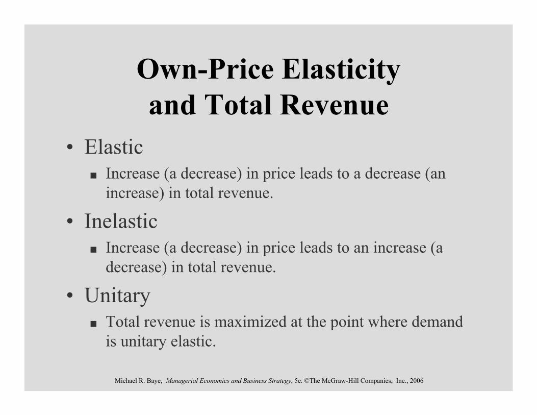
Own-Price Elasticity and Total Revenue
• Elastic Increase (a decrease) in price leads to a decrease (an increase) in total revenue.
• InelasticIncrease (a decrease) in price leads to an increase (a decrease) in total revenue.
• UnitaryTotal revenue is maximized at the point where demand is unitary elastic.
Michael R. Baye, Managerial Economics and Business Strategy, 5e. ©The McGraw-Hill Companies, Inc., 2006
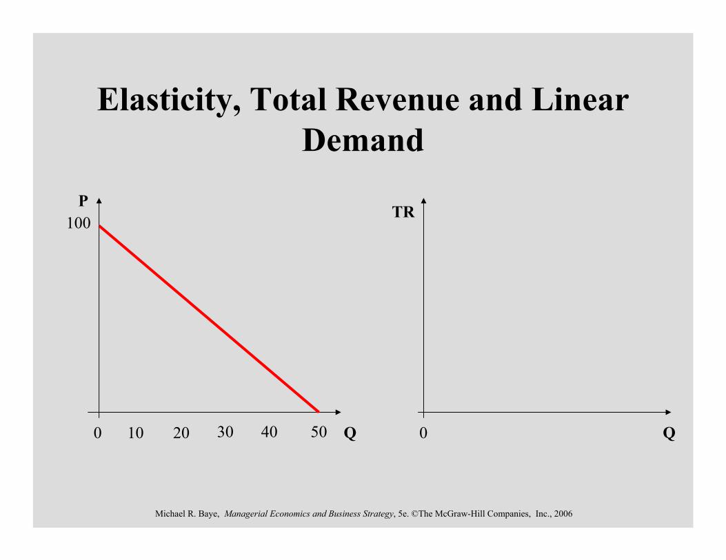
Elasticity, Total Revenue and Linear Demand
PTR
100
0 010 20 30 40 50
Michael R. Baye, Managerial Economics and Business Strategy, 5e. ©The McGraw-Hill Companies, Inc., 2006
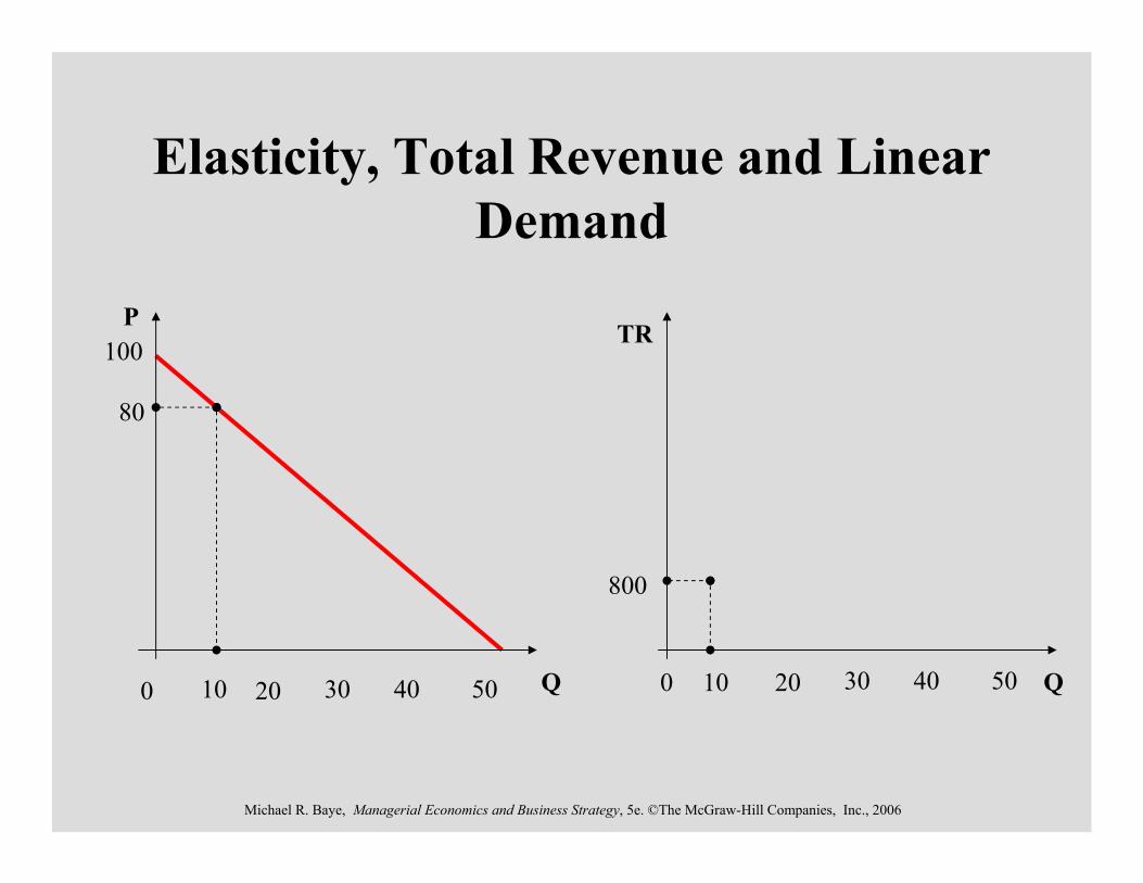
Elasticity, Total Revenue and Linear Demand
PTR
100
0 10 20 30 40 50
80
800
0 10 20 30 40 50

Michael R. Baye, Managerial Economics and Business Strategy, 5e. ©The McGraw-Hill Companies, Inc., 2006
Elasticity, Total Revenue and Linear Demand
PTR
100
80
800
60 1200
0 10 20 30 40 500 10 20 30 40 50

Michael R. Baye, Managerial Economics and Business Strategy, 5e. ©The McGraw-Hill Companies, Inc., 2006
Elasticity, Total Revenue and Linear Demand
PTR
100
80
800
60 1200
40
0 10 20 30 40 500 10 20 30 40 50

Michael R. Baye, Managerial Economics and Business Strategy, 5e. ©The McGraw-Hill Companies, Inc., 2006
Elasticity, Total Revenue and Linear Demand
PTR
100
80
800
60 1200
40
20
0 10 20 30 40 500 10 20 30 40 50

Michael R. Baye, Managerial Economics and Business Strategy, 5e. ©The McGraw-Hill Companies, Inc., 2006
Elasticity, Total Revenue and Linear Demand
PTR
100
80
800
60 1200
40
20
Elastic
Elastic
0 10 20 30 40 500 10 20 30 40 50
Michael R. Baye, Managerial Economics and Business Strategy, 5e. ©The McGraw-Hill Companies, Inc., 2006
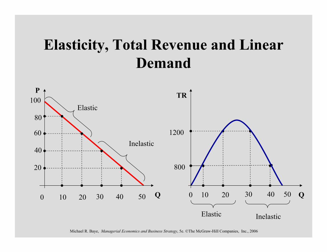
Elasticity, Total Revenue and Linear Demand
PTR
100
80
800
60 1200
40
20
Inelastic
Elastic
Elastic Inelastic
0 10 20 30 40 500 10 20 30 40 50

Michael R. Baye, Managerial Economics and Business Strategy, 5e. ©The McGraw-Hill Companies, Inc., 2006
Elasticity, Total Revenue and Linear Demand
P TR100
80
800
60 1200
40
20
Inelastic
Elastic
Elastic Inelastic
0 10 20 30 40 500 10 20 30 40 50
Unit elasticUnit elastic

Michael R. Baye, Managerial Economics and Business Strategy, 5e. ©The McGraw-Hill Companies, Inc., 2006
Factors Affecting Own Price Elasticity
Available Substitutes• The more substitutes available for the good, the more elastic
the demand.Time
• Demand tends to be more inelastic in the short term than in the long term.
• Time allows consumers to seek out available substitutes.Expenditure Share
• Goods that comprise a small share of consumer’s budgets tend to be more inelastic than goods for which consumers spend a large portion of their incomes.

Michael R. Baye, Managerial Economics and Business Strategy, 5e. ©The McGraw-Hill Companies, Inc., 2006
Cross Price Elasticity of Demand
If EQX,PY> 0, then X and Y are substitutes.
If EQX,PY< 0, then X and Y are complements.
Y
dX
PQ PQE
YX ∆∆
=%
%,

Michael R. Baye, Managerial Economics and Business Strategy, 5e. ©The McGraw-Hill Companies, Inc., 2006
Predicting Revenue Changes from Two Products
Suppose that a firm sells to related goods. If the price of X changes, then total revenue will change by:
( )( ) XPQYPQX PERERRXYXX
∆×++=∆ %1 ,,
Michael R. Baye, Managerial Economics and Business Strategy, 5e. ©The McGraw-Hill Companies, Inc., 2006
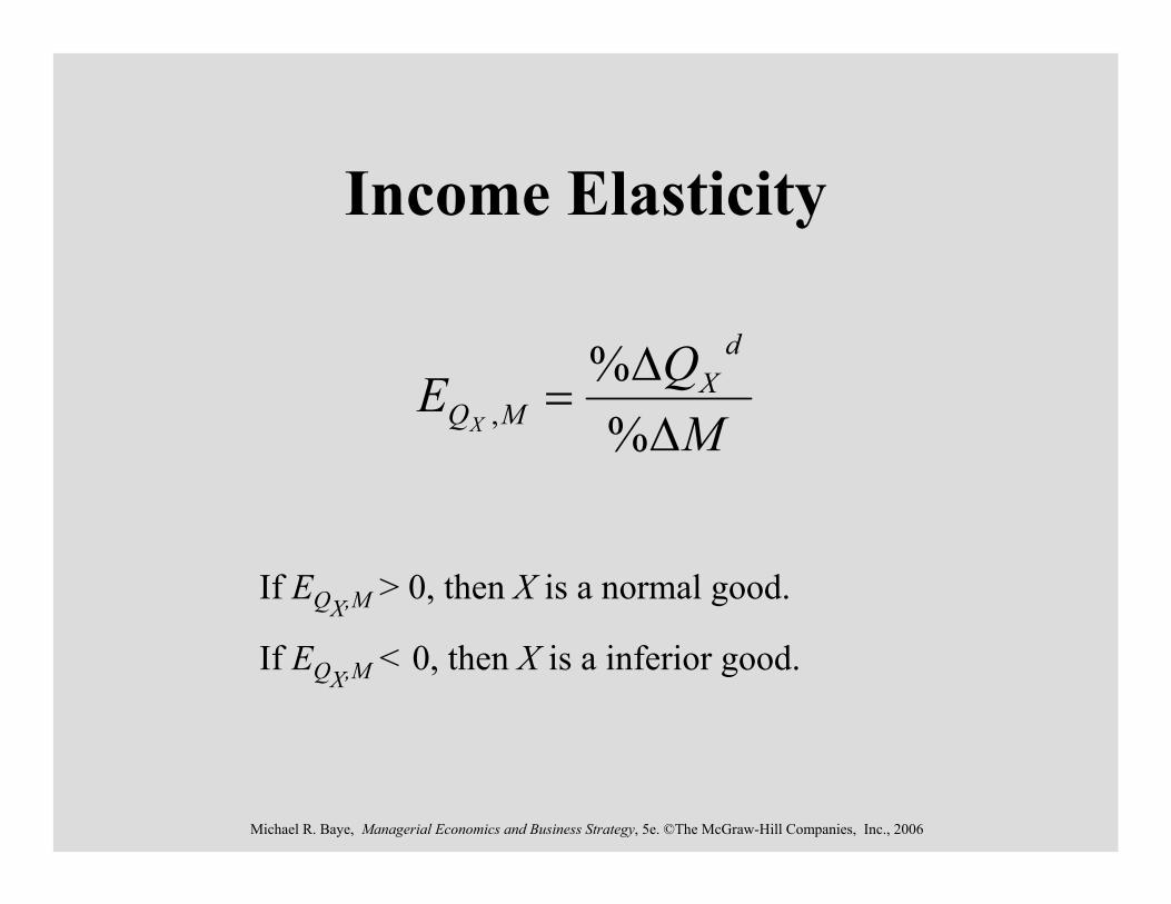
Income Elasticity
If EQX,M > 0, then X is a normal good.
If EQX,M < 0, then X is a inferior good.
MQE
dX
MQX ∆∆
=%
%,
Michael R. Baye, Managerial Economics and Business Strategy, 5e. ©The McGraw-Hill Companies, Inc., 2006
Uses of Elasticities
• Pricing.• Managing cash flows.• Impact of changes in competitors’ prices.• Impact of economic booms and recessions.• Impact of advertising campaigns.• And lots more!
Michael R. Baye, Managerial Economics and Business Strategy, 5e. ©The McGraw-Hill Companies, Inc., 2006
Example 1: Pricing and Cash Flows
• According to an FTC Report by Michael Ward, AT&T’s own price elasticity of demand for long distance services is -8.64.
• AT&T needs to boost revenues in order to meet it’s marketing goals.
• To accomplish this goal, should AT&T raise or lower it’s price?
Michael R. Baye, Managerial Economics and Business Strategy, 5e. ©The McGraw-Hill Companies, Inc., 2006
Answer: Lower price!
• Since demand is elastic, a reduction in price will increase quantity demanded by a greater percentage than the price decline, resulting in more revenues for AT&T.

Michael R. Baye, Managerial Economics and Business Strategy, 5e. ©The McGraw-Hill Companies, Inc., 2006
Example 2: Quantifying the Change
• If AT&T lowered price by 3 percent, what would happen to the volume of long distance telephone calls routed through AT&T?

Michael R. Baye, Managerial Economics and Business Strategy, 5e. ©The McGraw-Hill Companies, Inc., 2006
Answer• Calls would increase by 25.92 percent!
( )%92.25%
%64.8%3%3
%64.8
%%64.8,
=∆
∆=−×−−∆
=−
∆∆
=−=
dX
dX
dX
X
dX
PQ
Q
Q
Q
PQE
XX

Michael R. Baye, Managerial Economics and Business Strategy, 5e. ©The McGraw-Hill Companies, Inc., 2006
Example 3: Impact of a change in a competitor’s price
• According to an FTC Report by Michael Ward, AT&T’s cross price elasticity of demand for long distance services is 9.06.
• If competitors reduced their prices by 4 percent, what would happen to the demand for AT&T services?

Michael R. Baye, Managerial Economics and Business Strategy, 5e. ©The McGraw-Hill Companies, Inc., 2006
Answer• AT&T’s demand would fall by 36.24 percent!
%24.36%
%06.9%4%4
%06.9
%%06.9,
−=∆
∆=×−−∆
=
∆∆
==
dX
dX
dX
Y
dX
PQ
Q
Q
Q
PQE
YX
Michael R. Baye, Managerial Economics and Business Strategy, 5e. ©The McGraw-Hill Companies, Inc., 2006
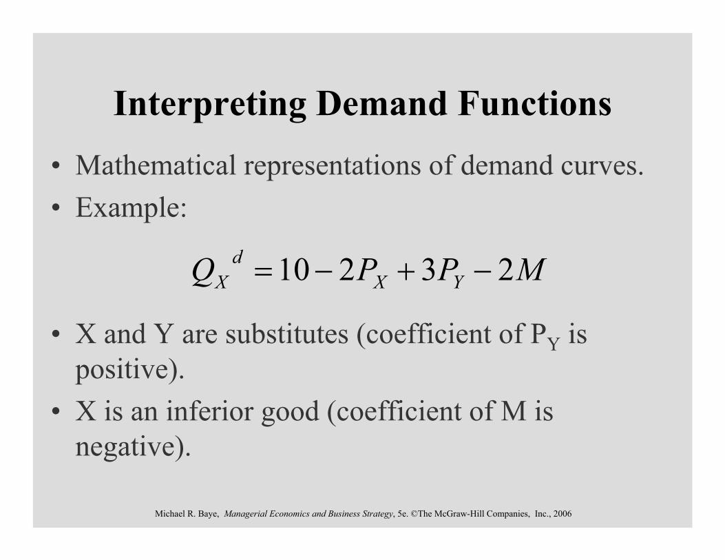
Interpreting Demand Functions• Mathematical representations of demand curves.• Example:
• X and Y are substitutes (coefficient of PY is positive).
• X is an inferior good (coefficient of M is negative).
MPPQ YXd
X 23210 −+−=
Michael R. Baye, Managerial Economics and Business Strategy, 5e. ©The McGraw-Hill Companies, Inc., 2006
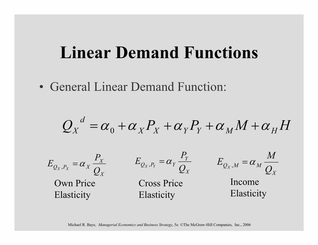
Linear Demand Functions
• General Linear Demand Function:
HMPPQ HMYYXXd
X ααααα ++++= 0
Own PriceElasticity
Cross PriceElasticity
IncomeElasticity
X
XXPQ Q
PEXX
α=,X
MMQ QME
Xα=,
X
YYPQ Q
PEYX
α=,
Michael R. Baye, Managerial Economics and Business Strategy, 5e. ©The McGraw-Hill Companies, Inc., 2006
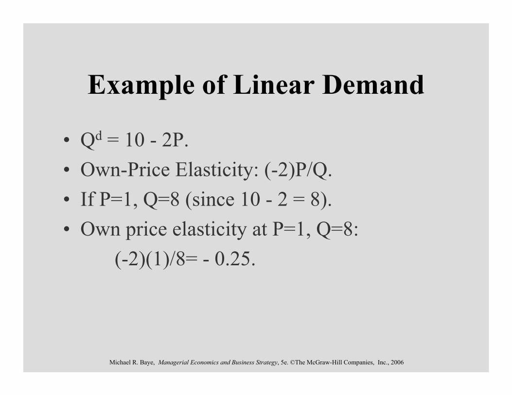
Example of Linear Demand
• Qd = 10 - 2P.• Own-Price Elasticity: (-2)P/Q.• If P=1, Q=8 (since 10 - 2 = 8).• Own price elasticity at P=1, Q=8:
(-2)(1)/8= - 0.25.

Michael R. Baye, Managerial Economics and Business Strategy, 5e. ©The McGraw-Hill Companies, Inc., 2006
0ln ln ln ln lndX X X Y Y M HQ P P M Hβ β β β β= + + + +
M
Y
X
:Elasticity Income:Elasticity Price Cross :Elasticity PriceOwn
βββ
Log-Linear Demand
• General Log-Linear Demand Function:
Michael R. Baye, Managerial Economics and Business Strategy, 5e. ©The McGraw-Hill Companies, Inc., 2006
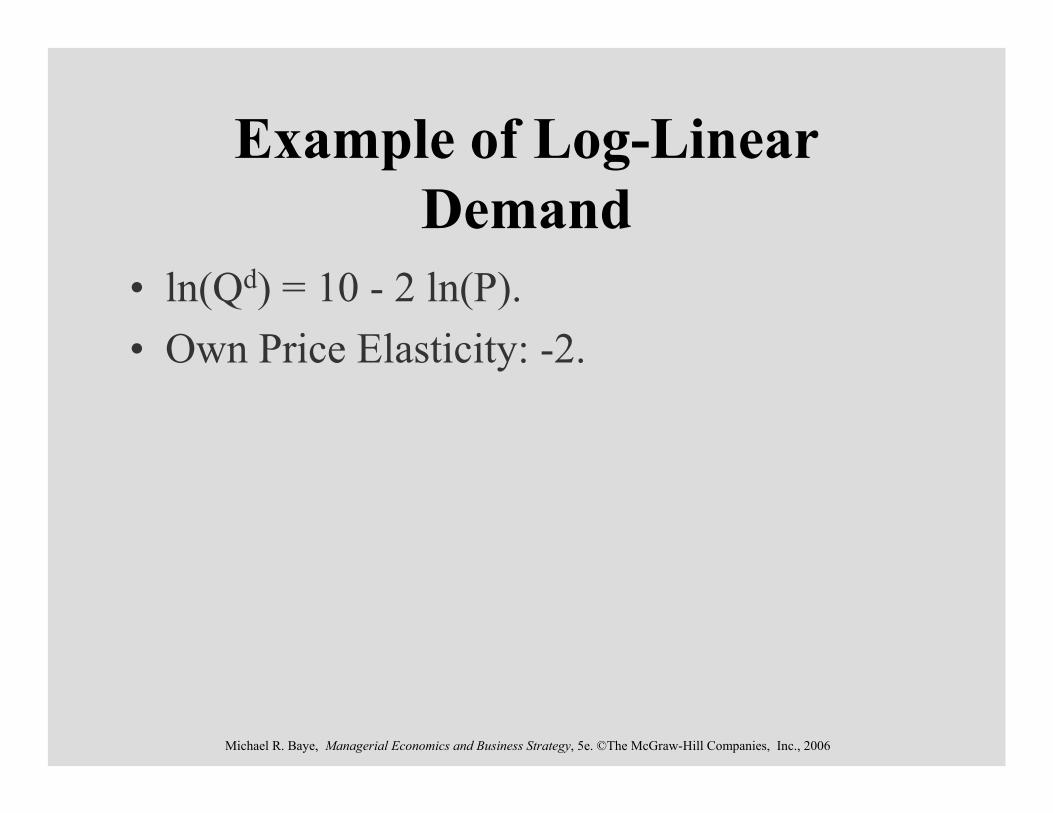
Example of Log-Linear Demand
• ln(Qd) = 10 - 2 ln(P).• Own Price Elasticity: -2.
Michael R. Baye, Managerial Economics and Business Strategy, 5e. ©The McGraw-Hill Companies, Inc., 2006
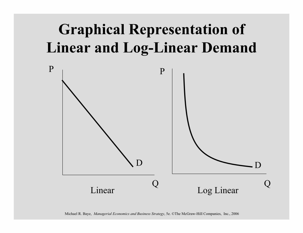
P
Q Q
D D
Linear Log Linear
Graphical Representation of Linear and Log-Linear Demand
P
Michael R. Baye, Managerial Economics and Business Strategy, 5e. ©The McGraw-Hill Companies, Inc., 2006
Regression Analysis
• One use is for estimating demand functions.• Important terminology and concepts:
Least Squares Regression: Y = a + bX + e.Confidence Intervals.t-statistic.R-square or Coefficient of Determination.F-statistic.

Michael R. Baye, Managerial Economics and Business Strategy, 5e. ©The McGraw-Hill Companies, Inc., 2006
An Example
• Use a spreadsheet to estimate the following log-linear demand function.
0ln lnx x xQ P eβ β= + +
Michael R. Baye, Managerial Economics and Business Strategy, 5e. ©The McGraw-Hill Companies, Inc., 2006
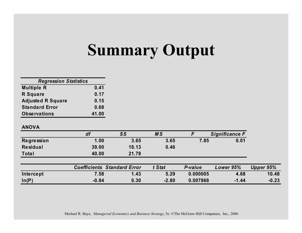
Summary OutputRegression Statistics
Multiple R 0.41R Square 0.17Adjusted R Square 0.15Standard Error 0.68Observations 41.00
ANOVAdf SS M S F Significance F
Regression 1.00 3.65 3.65 7.85 0.01Residual 39.00 18.13 0.46Total 40.00 21.78
Coefficients Standard Error t Stat P-value Lower 95% Upper 95%Intercept 7.58 1.43 5.29 0.000005 4.68 10.48ln(P) -0.84 0.30 -2.80 0.007868 -1.44 -0.23
Michael R. Baye, Managerial Economics and Business Strategy, 5e. ©The McGraw-Hill Companies, Inc., 2006
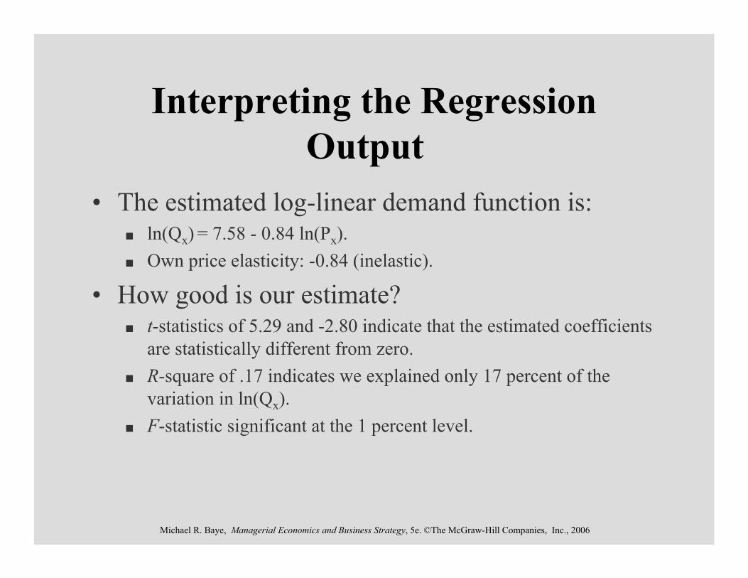
Interpreting the Regression Output
• The estimated log-linear demand function is:ln(Qx) = 7.58 - 0.84 ln(Px).Own price elasticity: -0.84 (inelastic).
• How good is our estimate?t-statistics of 5.29 and -2.80 indicate that the estimated coefficients are statistically different from zero.R-square of .17 indicates we explained only 17 percent of the variation in ln(Qx).F-statistic significant at the 1 percent level.

Michael R. Baye, Managerial Economics and Business Strategy, 5e. ©The McGraw-Hill Companies, Inc., 2006
Conclusion
• Elasticities are tools you can use to quantifythe impact of changes in prices, income, and advertising on sales and revenues.
• Given market or survey data, regression analysis can be used to estimate:
Demand functions.Elasticities.A host of other things, including cost functions.
• Managers can quantify the impact of changes in prices, income, advertising, etc.