managerial economicstestbankscafe.eu/sample/solution manual for managerial economics... · chapter...

—-1

—0

—+1

INSTRUCTOR’S MANUAL

Managerial Economics

SEVENTH EDITION

577-41323_ch00_3P.indd i577-41323_ch00_3P.indd i 6/17/09 4:23:04 PM6/17/09 4:23:04 PMFull file at http://TestbanksCafe.eu/Solution-Manual-for-Managerial-Economics-7th-Edition-Allen

-1—

0—

+1—

577-41323_ch00_3P.indd ii

577-41323_ch00_3P.indd ii 6/17/09 4:23:05 PM

6/17/09 4:23:05 PM

Full file at http://TestbanksCafe.eu/Solution-Manual-for-Managerial-Economics-7th-Edition-Allen

http://TestbanksCafe.eu/Solution-Manual-for-Managerial-Economics-7th-Edition-Allen

—-1

—0

—+1

INSTRUCTOR’S MANUAL

Managerial EconomicsSEVENTH EDITION

Robert BrookerGANNON UNIVERSITY

B W • W • NORTON & COMPANY • NEW YORK • LONDON

577-41323_ch00_3P.indd iii577-41323_ch00_3P.indd iii 6/17/09 4:23:05 PM6/17/09 4:23:05 PMFull file at http://TestbanksCafe.eu/Solution-Manual-for-Managerial-Economics-7th-Edition-Allen


-1—

0—

+1—

[Copyright TK]

577-41323_ch00_3P.indd iv

577-41323_ch00_3P.indd iv 6/17/09 4:23:05 PM

6/17/09 4:23:05 PM



—-1

—0

—+1

v

Contents

Chapter 1 Introduction 1

Chapter 2 Demand Theory 12

Chapter 3 Consumer Behavior and Rational Choice 28

Chapter 4 Production Theory 45

Chapter 5 The Analysis of Costs 59

Chapter 6 Perfect Competition 73

Chapter 7 Monopoly and Monopolistic Competition 83

Chapter 8 Managerial Use of Price Discrimination 99

Chapter 9 Bundling and Intrafi rm Pricing 117

Chapter 10 Oligopoly 132

Chapter 11 Game Theory 148

Chapter 12 Auctions 163

Chapter 13 Risk Analysis 173

Chapter 14 Principal– Agent Issues and Managerial Compensation 189

Chapter 15 Adverse Selection 204

Chapter 16 Government and Business 214

577-41323_ch00_3P.indd v577-41323_ch00_3P.indd v 6/17/09 4:23:05 PM6/17/09 4:23:05 PMFull file at http://TestbanksCafe.eu/Solution-Manual-for-Managerial-Economics-7th-Edition-Allen


-1—

0—

+1—

577-41323_ch00_3P.indd vi

577-41323_ch00_3P.indd vi 6/17/09 4:23:05 PM

6/17/09 4:23:05 PM



—-1

—0

—+1

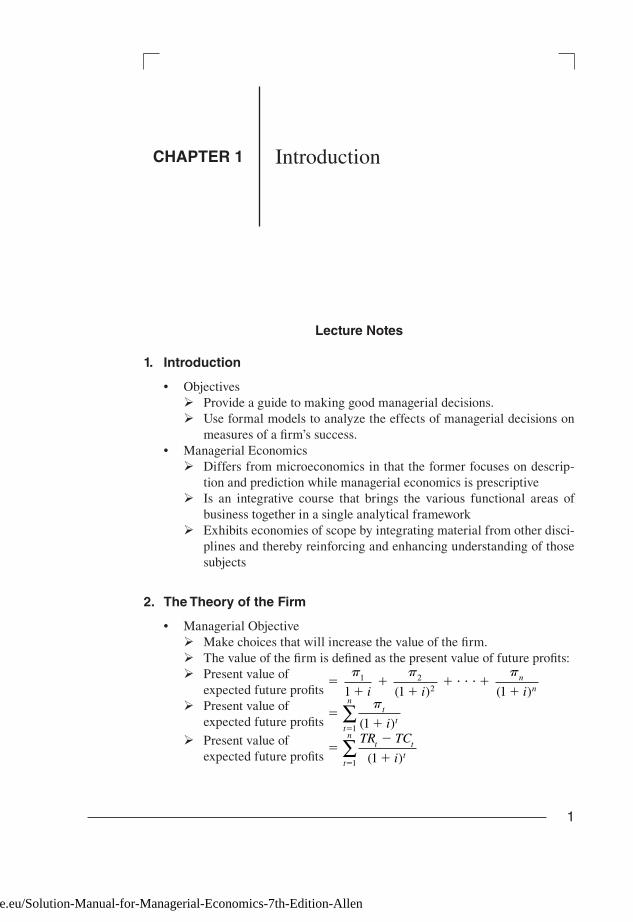
1

Lecture Notes

1. Introduction

• Objectives

ÿ Provide a guide to making good managerial decisions.

ÿ Use formal models to analyze the effects of managerial decisions on

mea sures of a fi rm’s success.

• Managerial Economics

ÿ Differs from microeconomics in that the former focuses on descrip-

tion and prediction while managerial economics is prescriptive

ÿ Is an integrative course that brings the various functional areas of

business together in a single analytical framework

ÿ Exhibits economies of scope by integrating material from other disci-

plines and thereby reinforcing and enhancing understanding of those

subjects

2. The Theory of the Firm

• Managerial Objective

ÿ Make choices that will increase the value of the fi rm.

ÿ The value of the fi rm is defi ned as the present value of future profi ts:

ÿ Present value of

expected future profi ts

ÿ Present value of


ÿ Present value of


��

��

� � � � ��

p p p1 221 1 1i i i

nn( ) ( )

��

1

p tt

t

n

i( )1∑�

�

��

1

TR TC

it t

tt

n

( )1∑

IntroductionCHAPTER 1

577-41323_ch01_3P.indd 1577-41323_ch01_3P.indd 1 6/17/09 4:25:29 PM6/17/09 4:25:29 PMFull file at http://TestbanksCafe.eu/Solution-Manual-for-Managerial-Economics-7th-Edition-Allen


-1—

0—

+1—

2 | Chapter 1

ÿ Notation

pt Profi t in time t � total revenue in time t � total cost in time ti Interest rate

n Number of time periods

TRt Total revenue in time tTCt Total cost in time t

• Managerial Choices

ÿ Infl uence total revenue by managing demand

ÿ Infl uence total cost by managing production

ÿ Infl uence the relevant interest rate by managing fi nances and risk

• Managerial Constraints

ÿ Available technologies

ÿ Resource scarcity

ÿ Legal or contractual limitations

STRATEGY SESSION:Bono Sees Red and Corporate Participants See Black

Discussion Questions

1. How can a fi rm assess the benefi ts and costs of cause marketing?

2. What other examples of cause marketing can you identify?

3. What Is Profi t?

• Two Mea sures of Profi t

ÿ Accounting profi t

* Historical costs

* Legal compliance

* Reporting requirements

ÿ Economic profi t

* Market value

* Opportunity, or implicit cost

* More useful mea sure for managerial decision making

4. Reasons for the Existence of Profi t

• Profi t

ÿ Mea sures the quality of managers’ decision making skills

ÿ Encourages good management decisions by linkage with incentives

• Sources of Profi t

ÿ Innovation: Producing products that are better than existing products

in terms of functionality, technology, and style.



—-1

—0

—+1

Introduction | 3

ÿ Risk taking: Knowing that future outcomes and their likelihoods are

unknown, as are the reactions of rivals.

ÿ Exploiting market ineffi ciencies: Building barriers to entry, employ-

ing sophisticated pricing strategies, diversifying, and making good

strategic production decisions

5. Managerial Interests and the Principal– Agent Problem

• Principal–Agent Problem

ÿ The interests of a fi rm’s own ers and those of its managers may differ,

unless the manager is the own er.

ÿ Separation of own ership and control

* The principals are the own ers. They want managers to maximize

the value of the fi rm.

* The agents are the managers. They want more compensation and

less accountability.

* The divergence in goals is the principal– agent problem.

ÿ Example of moral hazard (Moral hazard is explained in Chapter 14.)

* Moral hazard exists when people behave differently when they are

not subject to the risks associated with their behavior.

* Managers who do not maximize the value of the fi rm may do so

because they do not suffer as a result of their behavior.

ÿ Solutions

* Devise methods that lead to convergence of the interests of the

fi rm’s own ers and its managers.

* Examples: Stock option plans and bonuses linked to profi ts.

6. Demand and Supply: A First Look

• Market

ÿ A group of fi rms and individuals that interact with each other to buy

or sell a good

ÿ Part of an economy’s infrastructure

ÿ A social institution that exists to facilitate economic exchange

ÿ Relies on binding, enforceable contracts

STRATEGY SESSION:Baseball Discovers the Law of Supply and Demand


1. Do you see a relationship between variable pricing of baseball game tick-

ets and odds making on horse races?



-1—

0—

+1—

4 | Chapter 1

2. How do you think real- time variable pricing would infl uence the practice

of ticket scalping?

7. The Demand Side of a Market

• Demand Function

ÿ Quantity demanded relative to price, holding other possible infl uences

constant

ÿ Negative slope

ÿ Period of time

ÿ Shifts in demand

ÿ Other infl uences (held constant)

* Income

* Prices of substitutes and complements

* Advertising expenditures

* Product quality

* Government fi at

• Total Revenue Function

ÿ A fi rm’s total revenue (TR) for a given time period is equal to the price

charged (P) times the quantity sold (Q) during that time period.

ÿ TR � P � Qÿ The demand function refl ects the effect of changes in P on quantity

demanded (Q) per time period and, hence, the effect of changes in P

on TR.

8. The Supply Side of a Market

• Supply Function

ÿ Quantity supplied relative to price, holding other possible infl uences

constant

ÿ Positive slope

ÿ Period of time

ÿ Shifts in supply

ÿ Other infl uences (held constant)

* Technology

* Cost of production inputs (land, labor, capital)

STRATEGY SESSION:Demand and Supply— How High Oil Prices CoaxHigh- Cost Suppliers into the Market


1. During 2008, the price of a barrel of crude oil rose to above $130. In the

last quarter of 2008, fi nancial crisis lead to a global economic slowdown.



—-1

—0

—+1

Introduction | 5

The price of oil promptly dropped by half. Were these price fl uctuations

the result of changes in supply or demand?

2. Given the volatility of crude oil prices, do you think that private investors

will be likely to develop projects to extract oil from oil shale? How do you

think investment in alternative technologies like solar, geothermal, wind,

and biomass are likely to respond to oil price volatility?

3. Government can encourage the development of alternative sources of

energy such as extraction of oil from oil shale by offering incentives such as

tax credits or subsidies or by direct investment. Should it? What are the

pros and cons of government intervention in the development of energy

technologies?

9. Equilibrium Price

• Disequilibrium Price

ÿ Price is too high.

* Excess supply

* Surplus

* Causes price to fall

ÿ Price is too low.

* Excess demand

* Shortage

* Causes price to rise

• Equilibrium Price

ÿ Quantity demanded is equal to quantity supplied.

ÿ Price is stable.

ÿ The market is in balance because everyone who wants to purchase the

good can, and every seller who wants to sell the good can.

• Actual Price

ÿ Invisible hand is the situation when no governmental agency is needed

to induce producers to drop or increase their prices.

ÿ If the actual price is above the equilibrium price, there will be a sur-

plus that will put downward pressure on the actual price.

ÿ If the actual price is below the equilibrium price, there will be a short-

age that will put downward pressure on the actual price.

ÿ If the actual price is equal to the equilibrium price, there will be nei-

ther a shortage nor a surplus and price will be stable.

10. What If the Demand Curve Shifts?

• Increase in Demand

ÿ Represented by a rightward or upward shift in the demand curve



-1—

0—

+1—

6 | Chapter 1

ÿ Result of a change that makes buyers willing to purchase a larger quan-

tity of a good at the current price and/or pay a higher price for the cur-

rent quantity

ÿ Will create a shortage and cause the equilibrium price to increase

• Decrease in Demand

ÿ Represented by a leftward or downward shift in the demand curve

ÿ Result of a change that makes buyers purchase a smaller quantity of a

good at the current price and/or continue to buy the current quantity

only if the price is reduced

ÿ Will create a surplus and cause the equilibrium price to decrease

11. What If the Supply Curve Shifts?

• Increase in Supply

ÿ Represented by a rightward or downward shift in the supply curve

ÿ Result of a change that makes sellers willing to offer a larger quantity

of a good at the current price and/or offer the current quantity at a

lower price

ÿ Will create a surplus and cause the equilibrium price to decrease

• Decrease in Supply

ÿ Represented by a leftward or upward shift in the supply curve

ÿ Result of a change that makes sellers willing to offer a smaller quan-

tity of a good at the current price and/or offer the current quantity at a

higher price

ÿ Will create a shortage and cause the equilibrium price to increase

STRATEGY SESSION:Life During a Market Movement


1. Several factors are mentioned as contributing to disequilibrium in global

food markets. Among them are emotions (panic), government restrictions

on trade, the Malthusian specter of population growth outpacing food pro-

duction, slowing productivity growth in the agricultural sector, rising

incomes, and the production of ethanol. Which of these are supply factors,

and which are demand factors? How does each infl uence market price?

2. The market price for crude oil fl uctuated widely during 2008. What sup-

ply and demand factors contributed to these fl uctuations? Is the petroleum

market subject to any of the same factors cited as infl uencing agricultural

markets?



—-1

—0

—+1

Introduction | 7

Chapter 1: Problem Solutions

1. A book is to be written by Britney Spears. Batman Books agrees to pay Brit-

ney $6 million for the rights to this not- yet- written memoir. According to one

leading publisher, Batman Books could earn a profi t of roughly $1.2 million

if it sold 625,000 copies in hardcover. On the other hand, if it sold 375,000

copies, managers would lose about $1.3 million. Publishing executives stated

that it was hard to sell more than 500,000 copies of a nonfi ction hardcover

book, and very exceptional to sell 1 million copies. Were Batman managers

taking a substantial risk in publishing this book?

Solution:

There was a substantial risk of loss. On the other hand, there was substantial

opportunity for gain. Risk is unavoidable. The appropriate balance between

risk and return is what should determine managers’ decisions. Successful

decisions in circumstances of risk are a source of profi t.

2. Some say that any self- respecting top manager joining a company does so

with a front- end signing bonus. In many cases this bonus is in the seven fi g-

ures. At the same time the entering manager may be given a bonus guaran-

tee. No matter what happens to fi rm profi t, he or she gets at least a percentage

of that bonus. Do long- term bonus guarantees help to solve the principal–

agent problem, or do they exacerbate it? Why?

Solution:

An executive who spends a lifetime working for a single company or in a sin-

gle industry has a poorly diversifi ed human capital portfolio. Such an execu-

tive also often has a signifi cant, undiversifi ed fi nancial investment in the

form of stock options and pension plans that are used in partial substitution

for current salary to align the long- term wealth of the executive with that of

the shareholders. As an executive climbs the corporate ladder, the value

of his or her human capital becomes more closely tied to the fortunes of the

fi rm and industry. This lack of diversifi cation requires a compensating risk

premium. A large signing bonus may allow a risk- averse executive to make

an investment that increases the value of the fi rm but that the executive

would otherwise avoid because of concern for his or her own personal wealth;

thus the bonus may reduce the principal– agent confl ict. Of course, the ben-

efi ts of reduced risk to the executive come at the potential cost of indifference

to the wealth of the shareholders. Although a large signing bonus may help

solve the incentive alignment problem, compensation that is too great and too

insensitive to the fortunes of the shareholders makes the principal– agent prob-

lem worse.



-1—

0—

+1—

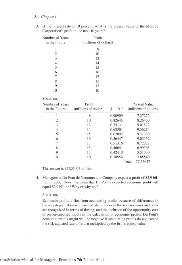
8 | Chapter 1

3. If the interest rate is 10 percent, what is the present value of the Monroe

Corporation’s profi t in the next 10 years?

Number of Years

in the Future

Profi t

(millions of dollars)

1 8

2 10

3 12

4 14

5 15

6 16

7 17

8 15

9 13

10 10

Solution:

Number of Years

in the Future

Profi t

(millions of dollars) (1 � i)�tPresent Value

(millions of dollars)

1 8 0.90909 7.27272

2 10 0.82645 8.26450

3 12 0.75131 9.01572

4 14 0.68301 9.56214

5 15 0.62092 9.31380

6 16 0.56447 9.03152

7 17 0.51316 8.72372

8 15 0.46651 6.99765

9 13 0.42410 5.51330

10 10 0.38554 3.85540

Total 77.55047

The answer is $77.55047 million.

4. Managers at Du Pont de Nemours and Company expect a profi t of $2.9 bil-

lion in 2008. Does this mean that Du Pont’s expected economic profi t will

equal $2.9 billion? Why or why not?

Solution:

Economic profi ts differ from accounting profi ts because of differences in

the way depreciation is mea sured, differences in the way revenues and costs

are recognized in terms of timing, and the inclusion of the opportunity cost

of owner- supplied inputs in the calculation of economic profi ts. Du Pont’s

economic profi ts might well be negative if accounting profi ts do not exceed

the risk- adjusted rate of return multiplied by the fi rm’s equity value.



—-1

—0

—+1

Introduction | 9

5. William Howe must decide whether to start a business renting beach umbrel-

las at an ocean resort during June, July, and August of next summer. He

believes he can rent each umbrella to vacationers at $5 a day, and he intends to

lease 50 umbrellas for the three- month period for $3,000. To operate this busi-

ness, he does not have to hire anyone (but himself), and he has no expenses

other than the leasing costs and a fee of $3,000 per month to rent the business

location. Howe is a college student, and if he did not operate this business, he

could earn $4,000 for the three- month period doing construction work.

a. If there are 80 days during the summer when beach umbrellas are

demanded, and Howe rents all 50 of his umbrellas on each of these days,

what will be his accounting profi t for the summer?

b. What will be his economic profi t for the summer?

Solution:

a. TR � (80 days) � (50 umbrellas) � ($5 per day) � $20,000

TC � (3 months) � ($3,000 per month rent) � ($3,000 umbrella lease)

� $12,000

Accounting Profi t � TR � TC � $8,000

b. Economic profi t � accounting profi t � opportunity cost

Economic profi t � $8,000 � $4,000 � $4,000

6. On March 3, 2008, a revival of Gypsy, the Stephen Sondheim musical,

opened at the St. James Theater in New York. Ticket prices ranged from

$117 to $42 per seat. The show’s weekly gross revenues, operating costs, and

profi t were estimated as follows, depending on whether the average ticket

price was $75 or $65:

Average Price

of $75

Average Price

of $65

Gross revenues $765,000 $680,000

Operating costs 600,000 600,000

Profi t 165,000 80,000

a. With a cast of 71 people, a 30- piece orchestra, and more than 500 cos-

tumes, Gypsy cost more than $10 million to stage. This investment was in

addition to the operating costs (such as salaries and theater rent). How

many weeks would it take before the investors got their money back,

according to these estimates, if the average price was $65? If it was $75?

b. George Wachtel, director of research for the League of American The-

aters and Producers, has said that about one in three shows opening on

Broadway in recent years has at least broken even. Were the investors in

Gypsy taking a substantial risk?

c. According to one Broadway producer, “Broadway isn’t where you make

the money any more. It’s where you establish the project so you can make



-1—

0—

+1—

10 | Chapter 1

the money. When you mount a show now, you really have to think about

where it’s going to play later.” If so, should the profi t fi gures here be inter-

preted with caution?

d. If the investors in this revival of Gypsy make a profi t, will this profi t be,

at least in part, a reward for bearing risk?

Solution:

a. Given a price of $75, the weekly operating profi t of $165,000 would pay

off the $10 million investment in 10,000/165 � 60.6 or 61 weeks. If the

price is $65, it would take 10,000/80 � 125 weeks to pay off the invest-

ment. This does not provide for any return on investment, however.

b. The investors in Gypsy were indeed taking a substantial risk. If only one

in three shows breaks even, two out of three make losses.

c. The profi t fi gures should be interpreted with caution because they do not

take into account the likelihood of profi ts when, and if, the show goes on

the road.

d. Yes.

7. If the demand curve for wheat in the United States is

P � 12.4 � 4QD

where P is the farm price of wheat (in dollars per bushel) and QD is the quan-

tity of wheat demanded (in billions of bushels), and the supply curve for wheat

in the United States is

P � �2.6 � 2QS

where QS is the quantity of wheat supplied (in billions of bushels), what is

the equilibrium price of wheat? What is the equilibrium quantity of wheat

sold? Must the actual price equal the equilibrium price? Why or why not?

Solution:

Setting demand equal to supply yields

12.4 � 4Q � �2.6 � 2Q Q � 15/6 � 2.5

P � 12.4 � (4)(2.5) � �2.6 � (2)(2.5) � $2.40

The actual price need not be equal to equilibrium price, although it will gen-

erally tend to move toward it because of the equilibrating effects of shortage

and surplus. Factors that might prevent the actual price from equaling the equi-

librium price include the cost and availability of information, transportation

costs, and a lack of opportunities for price equalizing arbitrage.

8. The lumber industry was hit hard by the subprime mortgage turmoil in

2008. Prices plunged from $290 per thousand board feet to less than $200



—-1

—0

—+1

Introduction | 11

per thousand board feet. Many observers believed this price decrease was

caused by the slowing of new home construction because of the glut of

unsold homes on the market. Was this price decrease caused by a shift in the

supply or demand curve?

Solution:

Because the demand for lumber is derived in large part from the demand for

new housing construction, a decline in construction would be likely to cause

the demand for lumber to fall, leading to lower lumber prices. Supply would

not be affected by changes in housing construction.

9. From November 2007 to March 2008, the price of gold increased from $865

per pound to over $1,000 per pound. Newspaper articles during this period

said there was little increased demand from the jewelry industry but signifi -

cantly more demand from investors who were purchasing gold because of

the falling dollar.

a. Was this price increase due to a shift in the demand curve for gold, a shift

in the supply curve for gold, or both?

b. Did this price increase affect the supply curve for gold jewelry? If so,

how?

Solution:

a. A change in the value of the dollar causes the dollar price of globally

traded commodities to change. If the value of the dollar falls, the dollar

price of commodities will rise. In this case, a decline in the value of the

dollar can be expected to cause the market for gold (with price mea sured

in dollars) to experience an increase in demand and a decrease in supply,

and thus an increase in price. There may also have been an additional

increase in demand due to expectations by investors that the dollar price

of gold would continue to rise. Finally, there may have been a further

supply decrease if producers, speculating that prices would rise further,

withheld gold from the market.

b. Gold is an input to the production of jewelry. An increase in the price of

gold would therefore be expected to reduce the supply of jewelry, result-

ing in higher jewelry prices.



-1—

0—

+1—

12

Lecture Notes

1. Introduction

• Objectives

ÿ Explain the importance of market demand in the determination of

profi t.

ÿ Understand the many factors that infl uence demand.

* Elasticity: Mea sures the percentage change in one factor given a

small (marginal) percentage change in another factor.

* Demand elasticity: Mea sures the percentage change in quantity

demanded given a small (marginal) percentage change in another

factor that is related to demand.

ÿ Explain the role of managers in controlling and predicting market

demand.

* Managers can infl uence demand by controlling, among other things,

price, advertising, product quality, and distribution strategies.

* Managers cannot control, but need to understand, elements of the

competitive environment that infl uence demand, including the avail-

ability of substitute goods, their pricing, and the advertising strate-

gies employed by their sellers.

* Managers cannot control, but need to understand how the macro-

economic environment infl uences demand, including interest rates,

taxes, and both local and global levels of economic activity.

2. The Market Demand Curve

• Market Demand Schedule

ÿ Table showing the total quantity of the good purchased at each price

Demand TheoryCHAPTER 2



—-1

—0

—+1

Demand Theory | 13

• Market Demand Curve

ÿ Plot of the market demand schedule on a graph.

ÿ Price (the x variable) is on the vertical, and quantity demanded (the y

variable) is on the horizontal axis.

ÿ Example (Figure 2.1): Demand curve for laptops.

• Characteristics of the Market Demand Curve

ÿ Quantity demanded is for output of the entire market, not of a single

fi rm.

ÿ For most products and ser vices, the market demand curve slopes down-

ward and to the right.

ÿ Quantity demanded is defi ned with regard to a par tic u lar time period.

* Determinants of the position and shape of the market demand

curve.

ÿ Consumer tastes

* Example (Figure 2.2): Increase in preference for laptop computers

causes an increase in demand for laptop computers.

ÿ Consumer income

* Normal and inferior goods.

* Example (Figure 2.3): Increase in income causes an increase in

demand for laptop computers.

ÿ Population size in the market

STRATEGY SESSION:The Customer Is Always Right— Wrong!


1. Like retail technology stores, clothing stores have their angels and dev ils.

How do you think the dev ils prey on clothing stores, and how could their

behavior be discouraged? How do you think angels could be encouraged

to shop at a par tic u lar clothing store?

Answer: Dev ils buy clothes, wear them, and then return them for a refund.

Stores can refuse to provide refunds on returns and, instead, provide a credit

for future purchases or only allow exchanges. Angels buy lots of clothes on

impulse. Stores could offer quantity discounts or a “shoppers club” with

special notifi cation of sales.

2. Some electronics stores refuse to allow customers to return or exchange

products, instead requiring them to deal directly with the manufacturer.

What are the pros and cons of this approach with regard to the stores’

objective of encouraging angels and discouraging dev ils?



-1—

0—

+1—

14 | Chapter 2

3. Industry and Firm Demand Functions

• Market demand function: The relationship between the quantity demanded

and the various factors that infl uence this quantity

ÿ Quantity of X(Q) � f (factors)

ÿ Factors include

* Price of X

* Incomes of consumers

* Tastes of consumers

* Prices of other goods

* Population

* Advertising expenditures

ÿ Example (equation 2.1): Q � b1P � b

2I � b

3S � b

4A

* Assumes that population is constant and that the demand function

is linear

* P � price of laptops

* I � per capita disposable income

* S � average price of software

* A � amount spent on advertising

* b1, b

2, b

3, and b

4 are pa ram e ters that are estimated using statistical

methods

ÿ Pa ram e ters: Constant or variable terms used in the function that helps

managers determine the specifi c form of the function but not its gen-

eral nature.

* Example (equation 2.2): Q � �700P � 200I � 500S � 0.01Aÿ Relationship between the market demand function and the market

de mand curve

* Market demand curve shows the relationship between Q and P

when all other variables are held constant at specifi c values.

* Market demand function does not explicitly hold any values

constant.

ÿ Example (equation 2.3): Q � �700P � 200(13,000) � 500(400) �

0.01(50,000,000)

* Example (equation 2.4): Q � 2,900,000 � 700P

* Example: P � 4,143 � 0.001429Q (graphed in Figure 2.4)

ÿ Example: Q � �700P � 200(13,000) � 500(200) � 0.01(50,000,000)

* Shift in demand due to a change in the average price of software

from 400 to 200

* Example (equation 2.5): Q � 3,000,000 � 700P

* Example (equation 2.6): P � 4,286 � 0.001429P (graphed in Fig-

ure 2.4)

• The Firm’s Demand Curve

ÿ Negative slope with regard to price

* Slope may not be the same as that of the market demand curve.



—-1

—0

—+1

Demand Theory | 15

ÿ Represents a portion of market demand

* Market share

* Responds to same market and macroeconomic factors as the mar-

ket demand curve

ÿ Directly related to the prices of substitute goods provided by com-

petitors

* Increase in competitor’s price will cause a decrease in a fi rm’s

de mand.

* Decrease in competitor’s price will cause an increase in a fi rm’s

de mand.

• Inversely related to the prices of substitute goods provided by com-

petitors

* Increase in competitor’s price will cause a decrease in a fi rm’s

de mand.

* Decrease in competitor’s price will cause an increase in a fi rm’s

de mand.

4. The Own- Price Elasticity of Demand

• Own- price elasticity of demand: More simply referred to as the price elas-

ticity of demand, this is the concept that managers use to mea sure their

own percentage change in quantity demanded resulting from a 1 percent

change in their own price.

ÿ The elasticity of a function is the percentage change in the dependent

( y) variable in response to a 1 percent increase in the in de pen dent (x)

variable.

ÿ The price elasticity of a demand function is the percentage change in

quantity demanded in response to a 1 percent increase in price.

ÿ h �P

Q

Q

P

⎛⎝⎜

⎞⎠⎟

�

�ÿ Price elasticity generally is different at different prices and on differ-

ent markets.

• Terminology

ÿ Price elasticity demand is symbolized by the Greek letter eta (h).

ÿ 0 � h � �ÿ When h � 1, demand is elastic.

ÿ When h � 1, demand is inelastic.

ÿ When h � 1, demand is unitary.

ÿ When h � 0, demand is perfectly inelastic, and the demand curve is

vertical.

* Quantity demanded is the same at all prices.

ÿ When h � �, demand is perfectly elastic, and the demand curve is

horizontal.



-1—

0—

+1—

16 | Chapter 2

* Price is the same for all quantities demanded.

* If price rises, quantity demanded falls to zero.

* If price falls, quantity demanded increases without limit.

• Linear Demand Curves

ÿ The slope of a linear demand curve is constant.

ÿ If the demand curve is neither vertical nor horizontal, the price elas-

ticity will differ depending on price.

* At the midpoint of a linear demand curve, h � �1, with h approach-

ing zero as price approaches the vertical intercept.

* At prices above the midpoint, demand is elastic, with h approach-

ing negative infi nity as price approaches zero.

* At prices below the midpoint, demand is inelastic.

ÿ Given a demand curve defi ned as P � a � bQ, the price elasticity of

demand is h = −⎛⎝

⎞⎠

−1

b

a bQ

Q

5. Point and Arc Elasticities

• The point price elasticity formula should be used working with an esti-

mated demand curve or when the change in price is very small.

ÿ h ��

�

Q

P

P

Q⎛⎝⎜

⎞⎠⎟⎛⎝⎜

⎞⎠⎟

ÿ Calculated value for small changes will differ depending on whether

P and Q are the starting values or the ending values after the price

change. The change will be small if the change is small.

* Example: P1 � 99.95, P

2 � 100.00, Q

1 � 20,002, and Q

2 �

20,000

* h � [(20002 � 20000)/(99.95 � 100)][99.95/20002] � �0.1999

* h � [(20000 � 20002)/(100 � 99.95][100/200000] � �0.22

ÿ If the price change is large, then the direction of change will infl uence

the calculated elasticity.

* Example: P1 � 5, P

2 � 4, Q

1 � 3, and Q

2 � 40

* h � [(40 � 3)/(4 � 5)][5/3] � �61.67

* h � [(3 � 40)/(5 � 4)][4/40] � �3.70

ÿ This problem is corrected by using the arc midpoints formula.

• The midpoints arc elasticity formula should be used to estimate the price

elasticity of demand from a demand schedule where price differences are

not very small.

ÿ h

�

�

�

�

�

Q

P

P P

Q Q⎛⎝⎜

⎞⎠⎟⎛

⎝⎜⎞

⎠⎟1 2

1 2ÿ Example: P

1 � 5, P

2 � 4, Q

1 � 3, and Q

2 � 40

ÿ h � [(40 � 3)/(4 � 5)][(5 � 4)/(3 � 40)] � �7.74



—-1

—0

—+1

Demand Theory | 17

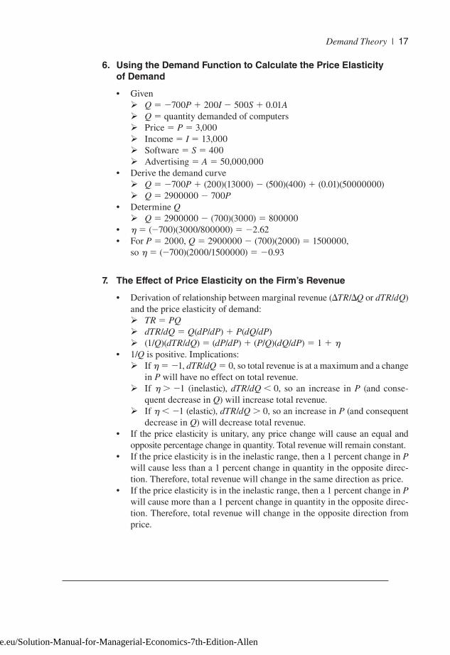
6. Using the Demand Function to Calculate the Price Elasticity of Demand

• Given

ÿ Q � �700P � 200I � 500S � 0.01Aÿ Q � quantity demanded of computers

ÿ Price � P � 3,000

ÿ Income � I � 13,000

ÿ Software � S � 400

ÿ Advertising � A � 50,000,000

• Derive the demand curve

ÿ Q � �700P � (200)(13000) � (500)(400) � (0.01)(50000000)

ÿ Q � 2900000 � 700P• Determine Q

ÿ Q � 2900000 � (700)(3000) � 800000

• h � (�700)(3000/800000) � �2.62

• For P � 2000, Q � 2900000 � (700)(2000) � 1500000,

so h � (�700)(2000/1500000) � �0.93

7. The Effect of Price Elasticity on the Firm’s Revenue

• Derivation of relationship between marginal revenue (�TR/�Q or dTR/dQ)

and the price elasticity of demand:

ÿ TR � PQÿ dTR/dQ � Q(dP/dP) � P(dQ/dP)

ÿ (1/Q)(dTR/dQ) � (dP/dP) � (P/Q)(dQ/dP) � 1 � h

• 1/Q is positive. Implications:

ÿ If h � �1, dTR/dQ � 0, so total revenue is at a maximum and a change

in P will have no effect on total revenue.

ÿ If h � �1 (inelastic), dTR/dQ � 0, so an increase in P (and conse-

quent decrease in Q) will increase total revenue.

ÿ If h � �1 (elastic), dTR/dQ � 0, so an increase in P (and consequent

decrease in Q) will decrease total revenue.

• If the price elasticity is unitary, any price change will cause an equal and

opposite percentage change in quantity. Total revenue will remain constant.

• If the price elasticity is in the inelastic range, then a 1 percent change in P

will cause less than a 1 percent change in quantity in the opposite direc-

tion. Therefore, total revenue will change in the same direction as price.

• If the price elasticity is in the inelastic range, then a 1 percent change in P

will cause more than a 1 percent change in quantity in the opposite direc-

tion. Therefore, total revenue will change in the opposite direction from

price.



-1—

0—

+1—

18 | Chapter 2

PROBLEM SOLVED:Price Elasticity of Demand: Philip Morris


1. The decline in total revenue from cigarette sales in 1993 is attributed to

Philip Morris’s cut in the price of cigarettes. Are there other factors that

might have contributed to this decline in revenue?

Answer: The price elasticity of demand assumes that “all other things”

are held constant. Changes in taxes, consumer income, or attitudes toward

tobacco during this period might have reduced demand, while the price

cut increased quantity demanded. If this were the case, then the true price

elasticity would likely be closer to �1.

8. Funding Public Transit

• Given

ÿ Price (fare) elasticity of demand for public transit in the United States

is about �0.3.

ÿ All public transit systems in the United States lose money.

ÿ Public transit systems are funded by federal, state, and local govern-

ments, all of which have bud get issues.

• Which transit systems have the most diffi cult time getting public funding?

ÿ Revenue from sales will increase if fares are increased, because demand

is inelastic.

ÿ Costs will likely decrease if fares are increased, because quantity

demanded (ridership) will fall.

ÿ Managers of public transit will therefore increase fares if they do not

receive enough public funds to balance their bud gets.

9. Determinants of the Own- Price Elasticity of Demand

• Number and similarity of available substitutes

• Product price relative to a consumer’s total bud get

• Time period available for adjustment to a price change

10. The Strategic Use of the Price Elasticity of Demand

• Example: Strategic pricing of fi rst- class (h � �0.45), regular economy

(h � �1.30), and excursion (h � �1.83) airline tickets between the United

States and Eu rope

ÿ First- class prices should be relatively high because demand is inelastic.



—-1

—0

—+1

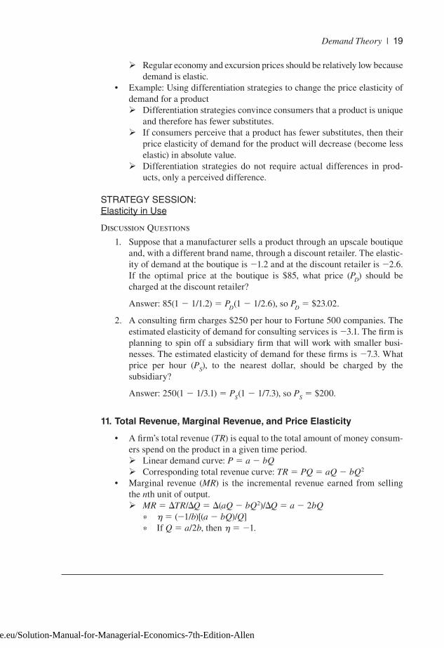
Demand Theory | 19

ÿ Regular economy and excursion prices should be relatively low because

demand is elastic.

• Example: Using differentiation strategies to change the price elasticity of

demand for a product

ÿ Differentiation strategies convince consumers that a product is unique

and therefore has fewer substitutes.

ÿ If consumers perceive that a product has fewer substitutes, then their

price elasticity of demand for the product will decrease (become less

elastic) in absolute value.

ÿ Differentiation strategies do not require actual differences in prod-

ucts, only a perceived difference.

STRATEGY SESSION:Elasticity in Use


1. Suppose that a manufacturer sells a product through an upscale boutique

and, with a different brand name, through a discount retailer. The elastic-

ity of demand at the boutique is �1.2 and at the discount retailer is �2.6.

If the optimal price at the boutique is $85, what price (PD) should be

charged at the discount retailer?

Answer: 85(1 � 1/1.2) � PD(1 � 1/2.6), so PD � $23.02.

2. A consulting fi rm charges $250 per hour to Fortune 500 companies. The

estimated elasticity of demand for consulting ser vices is �3.1. The fi rm is

planning to spin off a subsidiary fi rm that will work with smaller busi-

nesses. The estimated elasticity of demand for these fi rms is �7.3. What

price per hour (PS), to the nearest dollar, should be charged by the

subsidiary?

Answer: 250(1 � 1/3.1) � PS(1 � 1/7.3), so PS � $200.

11. Total Revenue, Marginal Revenue, and Price Elasticity

• A fi rm’s total revenue (TR) is equal to the total amount of money consum-

ers spend on the product in a given time period.

ÿ Linear demand curve: P � a � bQÿ Corresponding total revenue curve: TR � PQ � aQ � bQ2

• Marginal revenue (MR) is the incremental revenue earned from selling

the nth unit of output.

ÿ MR � �TR/�Q � �(aQ � bQ2)/�Q � a � 2bQ

* h � (�1/b)[(a � bQ)/Q]

* If Q � a/2b, then h � �1.



-1—

0—

+1—

20 | Chapter 2

* If Q � a/2b, then h is inelastic.

* If Q � a/2b, then h is elastic.

ÿ MR � �TR /�Q � �(PQ) /�Q � P(�Q /�Q) � Q (�P/�Q) �

P[1 � (Q/P)(�P/�Q), so MR � P(1 � 1/h).

* h � 1 (elastic) implies MR � 0.

* h � 1 (inelastic) implies MR � 0.

* h � 1 (unitary) implies MR � 0.

STRATEGY SESSION:Verizon and the Elasticity of Demand


1. What assumption was Verizon making about the elasticity of demand for

Internet ser vices?

Answer: That it was inelastic

2. What assumption was Verizon making about its marginal revenue from

Internet ser vices?

Answer: That it was negative

12. The Income Elasticity of Demand

• Income elasticity of demand (hI): The percentage change in quantity

demanded (Q) resulting from a 1 percent increase in consumers’ income (I)ÿ Income can be defi ned as aggregate consumer income or as per capita

income, depending on circumstances.

ÿ h I

Q

I

I

Q �

�

�

⎛⎝⎜

⎞⎠⎟⎛⎝⎜

⎞⎠⎟

ÿ hI � 0 for normal goods

* On average, goods are normal, since increases in aggregate income

are associated with increases in aggregate consumer spending.

ÿ hI � 0 for inferior goods

* Examples: Hamburgers and public transportation

• Strategic management and the income elasticity of demand

ÿ The demand for a product that has an income elasticity of demand

that is large in absolute value will vary widely with changes in income

caused by economic growth and recessions.

ÿ Managers can lessen the impact of economic changes on such prod-

ucts by limiting fi xed costs so that changes in production capacity can

be made quickly.

ÿ Managers can forecast demand for products using the income elastic-

ity of demand combined with forecasts of aggregate income.



—-1

—0

—+1

Demand Theory | 21

PROBLEM SOLVED:Income Elasticity of Demand


1. Suppose that a market demand function is defi ned as Q � 20,000 � 8P �

0.1I, where P � 2,000 and I � 20,000. What is the income elasticity of

demand?

Answer: Q � 6,000, so hI � 0.1(20000/6000) � �1 3

2. If the income elasticity of demand for a product is unitary, then a 1 per-

cent change in income will change demand in the same direction by 1

percent. If price remains constant, then spending on the product will

change by 1 percent, and consequently, spending on the product will be

the same percentage of income after the income change as it was before.

If the income elasticity of demand is greater than 1, then spending will

increase as a percentage of income as income increases. If it is less than 1,

spending will decrease as a percentage of income as income increases.

How do you think the percentage of income spent on jewelry, food, cloth-

ing, housing, and automobiles responds to a 1 percent increase in income?

13. Cross- Price Elasticities of Demand

• Cross- price elasticity of demand (hXY): The percentage change in quantity

demanded of one good (QX) resulting from a 1 percent increase in the price

of a related good (PY)

ÿ Income can be defi ned as aggregate consumer income or as per capita

income, depending on circumstances.

ÿ hXYX

Y

Y

X

Q

P

P

Q �

�

�

⎛

⎝⎜⎞

⎠⎟⎛

⎝⎜⎞

⎠⎟

ÿ hXY � 0 if the two products are substitutes.

* Example: Wheat and corn

ÿ hXY � 0 if the two products are complements.

* Example: Computers and computer software

ÿ hXY � 0 if the two products are in de pen dent

* Example: Butter and airline tickets

ÿ Example Calculation

* Given: QX � 1,000 � 0.2PX � 0.5PY � 0.04I, QX � 2,000, and

PY � 500

* hXY � 0.5(500/2000) � 0.125, so the two products are sub stitutes.

• Strategic management and the cross- price elasticity of demand

ÿ Managers can use information about the cross- price elasticity of demand

to predict the effect of competitors’ pricing strategies on the demand for

their product.



-1—

0—

+1—

22 | Chapter 2

ÿ Antitrust authorities use the cross- price elasticity of demand to deter-

mine the likely effect of mergers on the degree of competition in an

industry.

* A high cross- price elasticity, indicating that two goods are strong

substitutes, suggests that a merger would signifi cantly reduce com-

petition in the industry.

* A low cross- price elasticity, indicating that two goods are strong

complements, suggests that a merger might give the merged fi rm

excessive control over the supply chain.

14. The Advertising Elasticity of Demand

• Advertising elasticity of demand (hA): The percentage change in quantity

demanded (Q) resulting from a 1 percent increase in advertising expendi-

ture (A).

ÿ hA

Q

A

A

Q �

�

�

⎛⎝⎜

⎞⎠⎟⎛⎝⎜

⎞⎠⎟

ÿ Example Calculation

* Given: Q � 500 � 0.5P � 0.01I � 0.82A and A/Q � 2

* hA � 0.82(2) � 1.64

15. The Constant- Elasticity and Unitary Demand Function

• Constant- elasticity demand function: Mathematical form that always

yields that same elasticity, regardless of the product’s price and consum-

ers’ income

ÿ Example: Q � 200P�0.3I 2

ÿ Price elasticity of demand � �0.3

ÿ Income elasticity of demand � 2.0

• Unitary elastic demand function and total revenue (TR)

ÿ TR � PQ, so if TR is constant, Q � (TR)(P�1)

ÿ Price elasticity of demand � �1

ÿ Rectangular hyperbola

Chapter 2: Problem Solutions

1. The Dolan Corporation, a maker of small engines, determines that in 2008

the demand curve for its product is

P � 2,000 � 50Q

where P is the price (in dollars) of an engine and Q is the number of engines

sold per month.



—-1

—0

—+1

Demand Theory | 23

a. To sell 20 engines per month, what price would Dolan have to charge?

b. If managers set a price of $500, how many engines will Dolan sell per

month?

c. What is the price elasticity of demand if price equals $500?

d. At what price, if any, will the demand for Dolan’s engines be of unitary

elasticity?

Solution:

a. For Q � 20, P � 2,000 � 50(20) � $1,000

b. For P � 500, Q � 40 � 500/50 � 30

c. h � (�Q/�P)(P/Q) � (�1/50)(500/30) � �1⁄3

d. For P � $1,000, h � (�Q/�P)(P/Q) � (�1/50)(1,000/20) � �1

2. The Johnson Robot Company’s marketing managers estimate that the demand

curve for the company’s robots in 2008 is

P � 3,000 � 40Q

where P is the price of a robot and Q is the number sold per month.

a. Derive the marginal revenue curve for the fi rm.

b. At what prices is the demand for the fi rm’s product price elastic?

c. If the fi rm wants to maximize its dollar sales volume, what price should

it charge?

Solution:

a. MR � �TR/�Q � 3,000 � 80Qb. P � $1,500

c. P � $1,500

3. After a careful statistical analysis, the Chidester Company concludes the

demand function for its product is

Q � 500 � 3P � 2Pr � 0.1I

where Q is the quantity demanded of its product, P is the price of its prod-

uct, Pr is the price of its rival’s product, and I is per capita disposable income

(in dollars). At present, P � $10, Pr � $20, and I � $6,000.

a. What is the price elasticity of demand for the fi rm’s product?

b. What is the income elasticity of demand for the fi rm’s product?

c. What is the cross- price elasticity of demand between its product and its

rival’s product?

d. What is the implicit assumption regarding the population in the market?

Solution:

a. h � (�Q/�P)(P/Q) � (�3)(10/1,110) � �3/111

b. hI � (�Q/�I)(I/Q) � (0.1)(6,000/1,110) � 60/111



-1—

0—

+1—

24 | Chapter 2

c. hcross

� (�Q/�Pr)(Pr /Q) � (2)(20/1,110) � 4/111

d. The calculations assume that the population is constant.

4. The Haas Corporation’s executive vice president circulates a memo to the

fi rm’s top management in which he argues for a reduction in the price of the

fi rm’s product. He says such a price cut will increase the fi rm’s sales and

profi ts.

a. The fi rm’s marketing manager responds with a memo pointing out that

the price elasticity of demand for the fi rm’s product is about 20.5. Why is

this fact relevant?

b. The fi rm’s president concurs with the opinion of the executive vice presi-

dent. Is she correct?

Solution:

a. Whether total revenue will go up or down when the product price is low-

ered and more units are sold depends on whether the quantity of units

sold increases by a greater percentage than the price is reduced by. That

is, it depends on whether the demand is elastic or inelastic.

b. Assuming that the marketing manager is correct that the demand elastic-

ity is �0.5, than a price reduction will cause the number of units sold to

increase by a smaller percentage than the price has fallen, and both the

president and executive vice president will have egg on their faces when

total revenues decline after the price is reduced.

5. Managers of the Hanover Manufacturing Company believe the demand curve

for its product is

P � 5 � Q

where P is the price of its product (in dollars), and Q is the number of mil-

lions of units of its product sold per day. It is currently charging $1 per unit

for its product.

a. Evaluate the wisdom of the fi rm’s pricing policy.

b. A marketing specialist says that the price elasticity of demand for the

fi rm’s product is �1.0. Is this correct?

Solution:

a. At P � 1, MR � �3. The price is too low; increasing the price and sell-

ing fewer units would increase revenues.

b. No. While �Q/�P � �1, (�Q/�P)(P/Q) � �1/4 at P � 1.

6. On the basis of historical data, Richard Tennant has concluded, “The con-

sumption of cigarettes is . . . [relatively] insensitive to changes in price. . . .

In contrast, the demand for individual brands is highly elastic in its response

to price. . . . In 1918, for example, Lucky Strike was sold for a short time at



—-1

—0

—+1

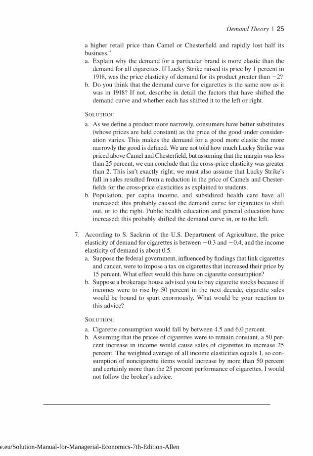
Demand Theory | 25

a higher retail price than Camel or Chesterfi eld and rapidly lost half its

business.”

a. Explain why the demand for a par tic u lar brand is more elastic than the

demand for all cigarettes. If Lucky Strike raised its price by 1 percent in

1918, was the price elasticity of demand for its product greater than �2?

b. Do you think that the demand curve for cigarettes is the same now as it

was in 1918? If not, describe in detail the factors that have shifted the

demand curve and whether each has shifted it to the left or right.

Solution:

a. As we defi ne a product more narrowly, consumers have better substitutes

(whose prices are held constant) as the price of the good under consider-

ation varies. This makes the demand for a good more elastic the more

narrowly the good is defi ned. We are not told how much Lucky Strike was

priced above Camel and Chesterfi eld, but assuming that the margin was less

than 25 percent, we can conclude that the cross- price elasticity was greater

than 2. This isn’t exactly right; we must also assume that Lucky Strike’s

fall in sales resulted from a reduction in the price of Camels and Chester-

fi elds for the cross- price elasticities as explained to students.

b. Population, per capita income, and subsidized health care have all

increased; this probably caused the demand curve for cigarettes to shift

out, or to the right. Public health education and general education have

increased; this probably shifted the demand curve in, or to the left.

7. According to S. Sackrin of the U.S. Department of Agriculture, the price

elasticity of demand for cigarettes is between �0.3 and �0.4, and the income

elasticity of demand is about 0.5.

a. Suppose the federal government, infl uenced by fi ndings that link cigarettes

and cancer, were to impose a tax on cigarettes that increased their price by

15 percent. What effect would this have on cigarette consumption?

b. Suppose a brokerage house advised you to buy cigarette stocks because if

incomes were to rise by 50 percent in the next de cade, cigarette sales

would be bound to spurt enormously. What would be your reaction to

this advice?

Solution:

a. Cigarette consumption would fall by between 4.5 and 6.0 percent.

b. Assuming that the prices of cigarettes were to remain constant, a 50 per-

cent increase in income would cause sales of cigarettes to increase 25

percent. The weighted average of all income elasticities equals 1, so con-

sumption of noncigarette items would increase by more than 50 percent

and certainly more than the 25 percent per for mance of cigarettes. I would

not follow the broker’s advice.



-1—

0—

+1—

26 | Chapter 2

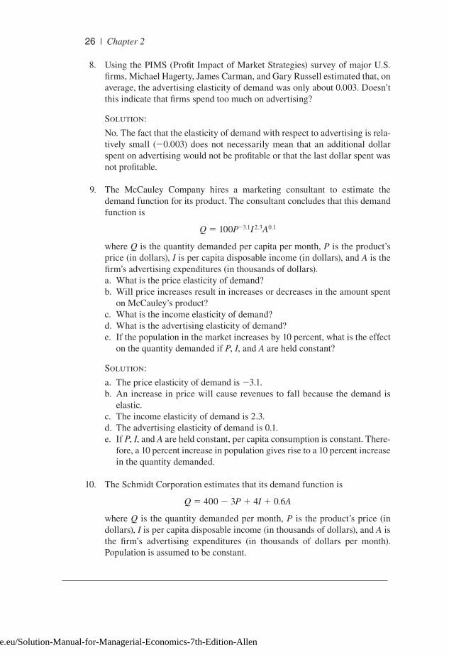
8. Using the PIMS (Profi t Impact of Market Strategies) survey of major U.S.

fi rms, Michael Hagerty, James Carman, and Gary Russell estimated that, on

average, the advertising elasticity of demand was only about 0.003. Doesn’t

this indicate that fi rms spend too much on advertising?

Solution:

No. The fact that the elasticity of demand with respect to advertising is rela-

tively small (�0.003) does not necessarily mean that an additional dollar

spent on advertising would not be profi table or that the last dollar spent was

not profi table.

9. The McCauley Company hires a marketing con sul tant to estimate the

demand function for its product. The con sul tant concludes that this demand

function is

Q � 100P�3.1I2.3A0.1

where Q is the quantity demanded per capita per month, P is the product’s

price (in dollars), I is per capita disposable income (in dollars), and A is the

fi rm’s advertising expenditures (in thousands of dollars).

a. What is the price elasticity of demand?

b. Will price increases result in increases or decreases in the amount spent

on McCauley’s product?

c. What is the income elasticity of demand?

d. What is the advertising elasticity of demand?

e. If the population in the market increases by 10 percent, what is the effect

on the quantity demanded if P, I, and A are held constant?

Solution:

a. The price elasticity of demand is �3.1.

b. An increase in price will cause revenues to fall because the demand is

elastic.

c. The income elasticity of demand is 2.3.

d. The advertising elasticity of demand is 0.1.

e. If P, I, and A are held constant, per capita consumption is constant. There-

fore, a 10 percent increase in population gives rise to a 10 percent increase

in the quantity demanded.

10. The Schmidt Corporation estimates that its demand function is

Q � 400 � 3P � 4I � 0.6A

where Q is the quantity demanded per month, P is the product’s price (in

dollars), I is per capita disposable income (in thousands of dollars), and A is

the fi rm’s advertising expenditures (in thousands of dollars per month).

Population is assumed to be constant.



—-1

—0

—+1

Demand Theory | 27

a. During the next de cade, per capita disposable income is expected to

increase by $5,000. What effect will this have on the fi rm’s sales?

b. If Schmidt wants to raise its price enough to offset the effect of the

increase in per capita disposable income, by how much must it raise its

price?

c. If Schmidt raises its price by this amount, will it increase or decrease the

price elasticity of demand? Explain. Make sure your answers refl ect the

fact that elasticity is a negative number.

Solution:

a. Sales will increase by 20 units per month.

b. Price must be increased by $6.67 per unit.

c. Two possible interpretations, both lead to more elastic demand. You

could assume that the question is asking if demand is more elastic after

both the income and price have increased. Since �Q/�P is unchanged

and P/Q has increased, the demand will be more elastic. Alternatively,

you might assume that the question is asking, as we increase the price to

choke off the anticipated increase in the quantity demanded after income

has gone up, does the demand become more or less elastic? This is, of

course, just moving up a linear demand curve, which implies an increas-

ingly elastic demand.



managerial economicstestbankscafe.eu/sample/solution manual for managerial economics... · chapter...

Documents