Male Incarceration, the Marriage Market and Female

Outcomes ∗

Kerwin Kofi CharlesUniversity of Michigan and NEBR

Ming Ching LuohNational Taiwan University

Abstract

This paper studies how rising male incarceration has affected women, throughits effect on the marriage market. Variation in the marriage market shocks causedby incarceration is isolated using two facts: the tendency of people to marrywithin marriage markets defined by the interaction of race, location and age;and the fact that increases in incarceration have been very different across thesethree characteristics. We find strong evidence that women have been affectedby rising incarceration precisely as the standard marriage market model wouldimply. Higher male imprisonment has lowered the likelihood that women marry,reduced the quality of their spouses when they do, and caused a shift in the gainsfrom marriage away from women and towards men. We find that women increaseschooling and labor supply in response to these changes, but this investment hasbeen insufficient to prevent an increase in female poverty.

Preliminary and Incomplete.

∗The paper has benefited from comments and conversations with Robert Axelrod, Rebecca Blank,John Bound, Charles Brown, John Dinardo, Patrick Kline, Gary Solon, Matthew Shapiro and MelvinStephens Jr. They, of course, bear no responsibility for its errors, omissions and other shortcomings.

1 Introduction

Whether measured in totals, or as a percentage of the population, more adults are

incarcerated in the United States than in all but a few countries in the world.1 The

desire to punish criminals and lower crime has led to a more than threefold increase in

the incarcerated population over the past forty years, and there is little evidence of any

slowdown in this trend.2 But rising levels on incarceration may have important social

ramifications quite separate from any effect on crime. This paper is interested in a

particular incarceration “externality”: how rising incarceration levels, by changing the

number of men in the marriage market, affects women’s marital outcomes, behavior

and wellbeing.

The theoretical basis for the effects we study is the marriage market model, first

outlined by Becker in a series of seminal papers ( see Becker (1973), (1974), (1981) and

(1982)). Since most prisoners are male, rising incarceration lowers the number of men

relative to women in society. The most obvious marriage-related effect of increased

imprisonment should be to lower the likelihood that women marry, simply because

there are fewer men as potential husbands to go around. Less obviously, a reduction in

the number of men should shift the distribution of the gains from marriage away from

wives and towards husbands, and should make women more likely to marry men whose

marital advances they would have previously rejected. These effects tend to lower

female incomes and economic well being. Women confronting high male incarceration

rates might thus be expected to make investments which augment their earnings power

and economic independence.3

1The Bureau of Justice Statistics reports that there were more than 2.1 million Americans held injails or prisons in 2003. This reflects a total rate of incarceration of about 715 Americans per 100,000:a rate of more than 1,300 per 100,000 for men, and one of about 113 per 100,000 women. Theserates are higher than all comparable rates in all OECD countries. See Society at a Glance: OECDIndicators, 2001.

2Several factors account for this increase, but most commentators think that the “War on Drugs”of the late 1980s, and changes since 1970 in sentencing guidelines are the two main reasons for thegrowth.

3This paper is interested in the effect of male incarceration on women’s outcomes. The standardmodel does make some predictions about how un-incarcerated men should be affected, but these are

1

Has the trend of increased incarceration produced the effects outlined above? There

is some evidence that it may have; for example, rising incarceration levels have coin-

cided with a nationwide reduction in marriage. However, there are several reasons

to be dubious that these, or other, correlations in aggregate trends represent causal

relationships. We might think, for example, that incarceration could not have caused

nationwide marriage reductions because imprisoned men are the kinds of men women

would be loath to marry had they not been in prison or jail. Moreover, secular in-

creases in male incarceration occurred at the same time as important changes in social

norms about sex roles, family forms and other social arrangements which likely had

independent effects on women’s choices. Without some way of controlling for the effect

of these confounding factors, correlations in aggregate national trends tell us little, if

anything, about incarceration’s causal effects.

This paper exploits the fact that the overwhelming majority of marriages occur

between women and men in sharply distinct markets, defined by the interaction of

race, age, and geographic region. Because the trend increase in incarceration has varied

tremendously over these three categories, rising incarceration has lowered the relative

presence of men by very different amounts in different marriage markets. Our research

strategy uses this variation to identify the effects of interest. Importantly, since most

of the variation used in the paper is within marriage markets over time, the estimates

should not be contaminated by the effect of unmeasured, fixed factors correlated with

race, state, or age. On the whole, we find that, indeed, rising male incarceration seems

to have produced effects on women’s outcomes and behaviors strongly consistent with

the predictions of the marriage market model. In addition, we show that rising levels of

male incarceration have redounded to the material detriment of young women, despite

investments women appear to have made to deal with the negative marriage market

changes.

not nearly as sharp as the predictions for women. At the end of our main analysis, we present anddiscuss some results for men.

2

Our work directly extends two different literatures. The first is the literature on

the effects of incarceration policy. Not surprisingly, most research on incarceration has

focused on the connection between prison populations and crime (Levitt and Kuziemko

(2001), Levitt (1996), and Marvell and Moody (1994)).4 But much of the controversy

about rising prison levels has actually not centered on whether the policy has been

effective at lowering crime. Rather, critics have raised questions about the severity of

sentencing, especially for non-violent drug offenses, the alleged inequities of sentencing

along racial and class lines, and the notion that incarceration may negatively affect

the communities from which prisoners come.5 There has, however, been little in the

way of formal analysis on these claims. Determining the magnitude and nature of

incarceration’s effect on the marriage market, presumably one of the mechanisms by

which the communities in question are affected, is this paper’s main task.

The paper also extends the literature that studies the connection between the

number of men relative to women in a market, and marriage outcomes. Identifying

exogenous variation in composition of the marriage market is a challenge faced by all of

these studies. Many empirical researchers, including Guttentag and Secord (1983), Cox

(1940), Freiden (1974) have used cross sectional variation to estimate the relationship

between the presence of men relative to women in a given area, and the incidence

of female marriage. Other work, using essentially the same identification strategy,

examines the link between sex ratios and female labor supply (see Chiappori, Fortin and

Lacroix (2001), South and Trent (1988) and South and Lloyd (1992). Unfortunately,4Incarceration is thought to lower crime by two mechanisms: an “incapacitation effect”, whereby

crime is lowered because criminals are removed from society; and a “deterrence effect”, whereby thethreat of imprisonment dissuades would-be criminals from engaging in criminal activity in the firstplace.

5For example, the organization The Drug Policy Alliance, argues in its literature that in-carceration policy has had a disproportionately devastating impact on minority families. (Seehttp://www.drugpolicy.org/communities/race). No rule determining imprisonment has generatedmore controversy than the mandatory sentencing drugs laws of New York State, known as the Rock-erfeller Laws. In recent years, criminal justice experts, judges and prisoners’ rights groups, a former“Drug Czar” (Gen. Barry McCaffrey), and former supporters like former State Senator John Dunnehave called for the repeal or reform of these laws on the grounds that the prison sentences they mandateare unjust and disproportionate to the crimes. (See New York Times Editorial, May 12, 2002.)

3

the results from all of these papers may be compromised by the fact that, in the cross

section, there may be reverse causality between marriage market outcomes and the

makeup of the marriage market in a particular place.

Angrist (2002) studies the effect of changes in sex ratios following the massive im-

migration into the United States in the early decades of the 20th century. Since new

arrivals were disproportionately male, this immigration wave generally increased sex

ratios, and did so differentially for different ethnic groups. Instead of the typical iden-

tification strategy in the literature of using point in time differences across location

in the relative presence of men, Angrist’s analysis exploits differences across ethnic

groups in the change over time in the sex ratio. This approach almost certainly im-

proves upon the approaches employed in earlier work. However, immigration into a

marriage market, even if that immigration followed the passage of laws whose timing

was essentially random, necessarily means that there was systematic sorting into the

market. Immigrants voluntarily migrated into the U.S., and to particular markets

within it. Although it seems reasonable that this migration hinged mainly on a desire

to earn higher incomes, considerations about marital preferences and possibilities may

have also played some role in the decision. For example, ethnic men who placed a

relatively high value of marriage and family were presumably less eager to migrate to

a foreign country with relatively few available brides.

Our analysis focuses on an ongoing and controversial policy, about whose social

effects there is independent interest. Although imprisonment is a marriage market

shock that may be subject to some of the same endogeneity concerns as voluntary

migration, the fact that we are able to characterize marriage markets finely by race, age,

and state of birth, and control for the confounding effects of these three factors, makes

it likely that the effects we estimate are indeed the causal effects of incarceration. In

extensions, we assess how sensitive the results are to the addition of various controls for

the levels crime in the particular market. If they are indeed robust, it is more likely that

the estimated effects are indeed the result of the men being removed from the market

4

because of incarceration, and not merely the “criminality” of those men. Finally, we

study a full set of marriage market outcomes, including the effect of incarceration on

marital sorting, and the connection between marriage market outcomes and schooling

investment and employment. Estimated effects for these other outcomes which are

also consistent with the predictions of the standard model serve to raise confidence in

notion that incarceration indeed causally affects women through the marriage market

channel.

The remainder of the paper is organized as follows. The next section offers a brief

overview of the connection between the number of men in a marriage market and

women’s marriage market outcomes. Section 3 describes the data. It discusses how

we characterize markets, summarizes changes in incarceration across those different

markets, and graphically illustrates the basic identification strategy. Section 4 presents

the main results. Section 5 presents extensions and robustness tests and Section 6

concludes.

2 Theoretical Overview

The standard marriage market model assumes that marriages are monogamous; that

there is full information about the returns to marriage; and that utility is determined by

consumption of a perfectly divisible, household-produced good.6 Output is produced

by a technology that uses the talents - or “quality” - of the adults in the household as

inputs. Although output is jointly produced in a household, it is divided between the

spouses. This insight highlights the fact that, within a marriage, husbands and wives

compete over marriage rents. Debates over who will wash dishes, whose entertainment

choices will be honored and the like are all subsumed in this idea of the within-marriage

competition between spouses. Utility is assumed to be strictly increasing in the fraction

of the gains from marriage the person can command. One can think of a person’s share

of these gains as the “price” their partner pays to induce them to marry at all, or to6The main papers from which this analysis borrows are Becker ((1973) , (1974), (1981) and (1992)).

5

not marry a different person.

People of a given sex compete in the marriage market by offering different prices

to potential spouses. There are, of course, a huge number of possible pairwise com-

binations in a marriage market. Fortunately, we know that any sorting that is an

equilibrium must satisfy two conditions. First, identical people must receive the same

income in equilibrium. Second, any equilibrium sorting arrangement must maximize

total societal output. If either of these conditions is violated for a particular sorting

arrangement, then there is an alternative arrangement under which at least one person

in the marriage market could be strictly better, with no else any worse off, meaning

that the original sorting could not have been an equilibrium.

Using these two conditions, it is easy to describe the effect of a change in the

number of men in the market. Consider first the case where there are no differences in

quality among either men or women. Suppose that unmarried men and women receive

income of 0, and that married output is strictly positive so that there are always gains

from marriage. When the total number of men equals the total number of men, each

person marries and receives more income than they would if single. Now, suppose

that some men are removed from the marriage market, so that women outnumber

men in total. The optimal sorting is now for all men to marry, and for some women

to remain single. Each single woman receives income of 0. And, because receiving

anything more would cause her to underbid in a competitive market, each married

woman also receives income of exactly 0. Men therefore receive all of the gains from

marriage.7 When there is no difference in quality among men and women, a reduction

in the number of men relative to women lowers women’s marital probabilities, lowers

female incomes, and ensures that the gains from marriage are redistributed away from

women and towards men.

The results are much the same if there are quality differences among men and7The situation is reversed if there are more women than men in the market. In that case, some

men remain married, receive income of 0, with the rest of marital output going to women.

6

women. Suppose that men in the marriage market are of either “high” or “low”

quality - j = H,L for men, and k = H,L for women.8 Let Yjk be the output from a

marriage between a type j man and a type k woman, and let the incomes of unmarried

men and women be gjm and gk

f , respectively. That there are always gains from marriage

implies that Yjk > gjm + gk

f for all j and k. It is standard to assume that male and

female quality are complements in the production of output, meaning that whatever

the quality of one spouse, output is higher the larger the quality of the other spouse.

Complementary implies that increasing both male and female quality raises household

output by a larger amount than the sum of separate increases in male and female

quality, or

YHH − YHL > YLH − YLL (1)

Given (1), the requirement that any equilibrium sorting maximize total societal

output implies that optimal sorting in the marriage market will demonstrate positive

assortative mating.9 That is, in equilibrium:10 as many HH marriages form as possi-

ble; redundant high quality persons after these matches are formed marry low quality

persons of the other sex; as many LL marriages form as possible from among remaining

low quality persons; and, finally, some low quality persons from whichever sex has the

larger total number of people remain unmarried.

A reduction in the number of men raises the likelihood that women outnumber

men in total, and thus lowers the probability of marriage for women overall, just as in

the case where there are no quality differences. This reduced marriage probability is

not felt evenly by all women; because high quality women are the most desired women,

they are the least likely to end up unmarried. Since male scarcity raises the odds that

each man ends up with a woman he most prefers, low quality women are displaced8The expression “quality” stands for anything that constitutes attractiveness, and may represent

different things for men and women.9There will be negative assortative mating in the unlikely event that male and female quality are

substitutes.10Although this is written as though there were a temporal ordering to the matches, this set of

outcomes will be simultaneously determined.

7

from any marriage they otherwise would have formed with high quality men and, if

the total reduction in men is large enough, are even forced out of their marriages to

low quality men. A reduction in the number of men therefore lowers the probability

that a woman marries a “superior” man and/or raises the probability that she marries

an “inferior one”, conditional on her being married at all.

Fewer men in the marriage market should also affect the output that men and

women receive in equilibrium. Since some low quality women are likely to be rendered

unmarried by an increase in male scarcity, the income of all low quality women -

whether they marry or not - should be forced down to gLf . Incomes, or the gains from

marriage, should also fall for high quality women. If the reduction in the number of men

is so large that even some high quality women remain unmarried, then competition

forces the incomes of all high quality women down to gHf . If the reduction in the

number of men is smaller, so that no high quality women remains unmarried, but

some are forced to marry low quality men, incomes received by all high quality women

will be lower because total output in LH marriages is lower than in the HH ones they

would have previously formed. Finally, even if the reduction in the number of men is

so small that all high quality women continue to marry high quality men, they must

transfer more of the gains from marriage to those men in order to induce them away

from marriages to low quality women who would now demand virtually none of the

marriage gains to be married to them.

This discussion forms the foundation of the empirical work to follow. The standard

marriage market model suggests that a reduction in the number of men resulting from

increased incarceration should produce a diverse set of effects. Specifically, it should:

(a) reduce the likelihood of marriage for women overall; (b) do so especially for the

“lowest quality” women; (c) transfer marriage rents from women to men; and (d) raise

the likelihood that, conditional on marrying at all, women form marriages with men of

lower “quality” and/or lower the probability that they marry men of higher quality. All

of these effects tend to lower women’s incomes. Women faced with declining relative

8

number of potential husbands should thus (e) exhibit a greater propensity to make

investments that raise their economic independence and cushion the negative effects

of the marriage market changes. The analysis tests for all of these effects.

3 Marriage Markets and Incarceration Trends

The empirical work hinges on the notion that changes in incarceration over time have

differentially affected different marriage markets. Our first task in this section is to

summarize changes in incarceration by race, age and state over the past 30 years.

Next, we show that men identified by race, age, and state of birth constitute distinct

marriage markets, which is the key assumption underlying the empirical strategy.

3.1 Imprisonment over the Past 30 Years

The paper uses data from four Census IPUMS from 1970 to 2000. The 1970 and

1980 Censuses identify inmates in jails or prisons.11 However, in 1990 and 2000,

the Census indicates only whether a respondent is “institutionalized”. We treat the

young men characterized as ”institutionalized” as being incarcerated. Several things

justify this decision. For one thing, given the set of institutions used by the Census

to define the “institutionalized” population, mental institutions are the only other

kind of institutions in which young men could logically be located.12 Work by Grob

(2000) shows that the number of persons in mental institutions has plummeted in the

past few decades, meaning that in later years, “institutionalized” effectively means

“incarcerated”.

Using the 1970 and 1980 data, we compute the fraction of people who would have

been classified as institutionalized in those Census years according to the 1990 and11“Jails” in the United States are institutions which house individuals with incarceration terms a

year or less. “Prisons” house persons with longer terms of imprisonment. We will not distinguishbetween these terms in the paper.

12In 1990 and 2000, institutionalized persons are in: jails and prisons, mental institutions, in-stitutions for the elderly handicapped and poor, nursing and convalescent homes, homes for ne-glected/depend children, other institutions for children, deaf/blind schools, schools for “feeble minded”,sanataria, poor houses and almshouses, poor farm/workhouses, homes for unmarried mothers, widowsand single women, and detention homes.

9

2000 definitions, but who were actually in jails or prisons in 1970 and 1980. We

find that for the men in the sample, in these early years when mental institution

populations were much higher, more than three-quarters who would have been classified

as “institutionalized” were in fact inmates, as expected.13 Finally, the patterns of

incarceration from the definitions we use line up in the aggregate nearly perfectly with

data on the incarcerated population from the Bureau of Justice Statistics.

We study men aged 20-35, splitting them throughout the analysis into younger (20-

27) and older (28-35) groups. Census respondents report not only their age, but also

their race and state of birth. We focus on three race categories: Whites, Blacks, and

non-Black, non-White Hispanics. For each state of birth, we compute the proportion

of men of a given race and age group who are incarcerated in a given Census year.

Later, we discuss the choice of state of birth rather than state of residence. Figure 1

graphically summarizes these numbers, which are depicted in Appendix Table 1.

The middle line in each graph shows the mean, across all states of birth, of the

incarceration rate of men on the type indicated in the graph heading. The top line in

each figure shows the 90th percentile of the distribution of incarceration rates across

states. The bottom line shows the 10th percentile of the same distribution. These

figures, which are all drawn with the same scale, reveal several interesting facts. First,

for all races and age groups, incarceration rates have risen dramatically over the last

30 years, and especially over the past twenty years.14 Nor have these increase been due

only to trends in high-incarceration states; the graphs show the essentially the same

pattern for the 90th and 10th percentile as well as the mean.

Second, the figures show that there has been tremendous variation across race in

both the level and rate of growth in incarceration. This difference is most pronounced

between Whites and the two racial minority groups. For example, while around 213For younger men aged 20-27, the proportion was 78% in 1970 and 1980; for men aged 28-35, the

proportions was 68% in the two years.14These trends are consistent with all other evidence about changes in the inmate population. See,

for example, U.S. Department of Justice, 2003.

10

percent of young White men aged 20-27 were incarcerated in 2000, the corresponding

numbers for young Hispanics and Black men were 10 and 18 percent, respectively.

Differences across races in the growth rate in the incarceration rate between 1970 and

2000 are equally striking. Most notably, the incarceration rates of blacks aged 20-27

from the highest incarceration states reached nearly thirty percent by 2000. For no

other group was the rate nearly as high.

Third, the figures show that the time series pattern of incarceration has not been

uniform across all states, and has differed across age groups for persons of the same race.

The gap between high and low incarceration states changed sharply, and differentially,

by race and age group between the 1970-2000 interval. For example, incarceration rates

for black men aged 20-27 from states with high and low incarceration rates converged

sharply between 1970 and 1980, and widened from 1990 to 2000. Among Hispanics by

contrast, while there was a widening in the incarceration experience over the last decade

studied, rates in the two types of states increased by essentially the same percentage

amounts between 1970 and 1980. The figures also show that the time series increase

in incarceration was generally higher for men aged 28-35, with the trend for Blacks in

this age group being especially explosive.

3.2 Marriage Markets: Who Marries Whom?

Do the men shown in Figure 1 belong to different marriage markets - distinct groups

of men and women who tend to marry within the group? If so, the patterns depicted

in the Figure 1 indicate that incarceration produced different shocks to these different

markets - a fact which could be exploited to identify the effects of interest.

Table 1 summarizes sorting by race and age among married couples in the United

States from 1970 to 2000.15 The first panel shows the fraction of all women of a

given race and age group who marry men of particular races. The results are striking:

virtually all marriages occur between people of the same race. This is especially true for15We have examined sorting in other Census years and find patterns by age, race and state that are,

if anything, stronger than those in these more recent years.

11

Black and White Americans. For these groups, well over ninety percent of marriages are

within-race. The numbers are lower for Hispanics, probably because being “Hispanic”

is partly an ethnic classification. However, even for this group within-race marriage is

by far the most common outcome.

The second panel looks at marital sorting by age category. The table shows that,

irrespective of race, women tend to marry men who are slightly older. For example,

among wives aged 18-25 of all races, more than seventy percent are married to men

aged 20-27. For wives aged 27-33, similarly high fractions are married to men aged

28-35.

These numbers indicate that men of a given race and narrow age range compete

among themselves for slightly younger wives of the same race. Marriage markets also

surely involve a spatial dimension. We know Census respondents’ state of birth and

state of residence, as of the survey. One problem with using state of residence to

characterize a marriage market is that where a person chooses to live may be partly

determined by local marriage market conditions. More importantly, because being

a prisoner in a given state does not indicate that the person lived in and socially

interacted in that state, using state of residence would systematically assign people

to the wrong marriage market.16 In particular, states with a large number of federal

prisoners, who are drawn from all over the country, would tend disproportionately to

be coded as having a large fraction of their men behind bars. For these reasons, we

distinguish persons in the sample by their states of birth.17 In fact, the assumption

that sorting occurs by state of birth is borne out in the data, as sixty percent of all

the wives we study, irrespective of race or age, marry men born in the same state.

In summary, in the analysis that follows a marriage market will consist of men

and women of a specific race, born in a given state, and who are aged either 18-25 for16Prisoners in the state prison system will generally have committed their crimes in the state, but

need not have lived there. In the federal system, which houses many persons serving drug relatedsentences, convicted persons may serve their sentences in any of the country’s federal facilities.

17In robustness tests later in the paper, we present results using state of residence instead of stateof birth.

12

women and 20-27 for men, or 26-33 for women and 28-35 for men.

3.3 Graphical Analysis

Before moving on to the formal regression analysis, we graphically illustrate the paper’s

identification strategy, and explore whether there is any first order evidence to support

the notion that higher incarceration rates for the men within a particular marriage

market affect the marriage market outcomes for women in that market.

In the data there are 3 races, 51 states of birth, and 2 age groups. For each of these

306 marriage markets (for example, the market for younger whites from Connecticut),

we have observations from four census years. The paper argues that in markets with

high rates of male incarceration, marriage outcomes should be worse for women. The

concern is that high inmate populations and negative female marriage market outcomes

may be related because of unmeasured factors. For example, it may be that states that

incarcerate many young men at a point in time, or which, because of their sentencing

guidelines, exhibit relatively high growth in incarceration over time, happen to be

places with high welfare payments, strong women’s rights movements, or other things

that directly lower female marriage probabilities. Our empirical methodology examines

variation within narrowly defined marriage markets defined above, so our estimates

should not be contaminated by these unmeasured factors that vary at the level of the

state. Much the same logic applies to concerns about factors that covary with race.

Figure 2 shows the logic of our preferred approach. In this expositional analysis, we

use only observations from the beginning and end of the sample period - the 1970 and

2000 Censuses. We also focus only on the incidence of marriage within the particular

marriage market, as this should be the first order marriage market effect on women

of higher male incarceration. For each marriage market, panel A of the figure plots

the incarceration rate of men (the number of men from that race/state/age cell who

are incarcerated, divided by the total number of such men) against the proportion of

the women in the market who report ever having been married, in the particular year.

13

The figure also has a fitted regression line showing the connection between these two

measures. The estimated relationship is strongly negative: each one percentage point

increase in the incarceration rate is associated with a 2.4 percentage point reduction in

the fraction of women in the marriage market who are ever married, with a t-statistic

well in excess of 15. This estimated relationship is as the theoretical discussion suggests

should be true.

The relationship in Panel A is estimated using variation marriage markets which

differ in terms of race, states, age group and time. In all likelihood, systematic dif-

ferences across various marriage markets may account for the correlation between the

two variables depicted in the graph. In the second panel of the figure, we relate the

change in the level of incarceration between 1970 and 2000 for a given marriage mar-

ket to the change in ever married experience of the women in that market over the

same time period. To the extent that there are unobserved differences across different

race/state/age group marriage markets, these estimates should be purged of the effect

of these factors.

As shown in the figure, the relationship remains strongly negative in the differenced

estimates. The figure also shows a smaller estimated relationship: the estimated re-

gression line now suggests that a 1 percentage point reduction in the incarceration rate

for men within a marriage market lowers ever married probabilities for women in that

market by 0.6 of a percentage point, with a standard error of 0.1. The relatively large

change in the point estimates in going from the cross-sectional to the difference analysis

indicates that there are indeed unobserved factors within particular markets for which

it is crucial to control. In the analysis that follows, we study the full set of outcomes

described above, and use regression analysis to control for systematic differences across

markets by race, state and age group.

14

4 Regression Analysis

4.1 Marriage Realizations

The first set of results assess the effect of higher male incarceration rates on the prob-

ability that women marry, and whom they marry when they do. We assume that

whether a woman i of race R , in state s , and in age group a, has ever been married

as of year t is given by

yiRsat = β0 + β1 IRsat + σRsa + εi

Rsat (2)

where y is a binary variable denoting the woman’s ever married status; σRsa, is a

dummy variable representing which of the 306 race/age/state marriage markets the

woman belongs to; β0 and β1 are coefficients, and εiRsat is a random error term. The

term IRsat is the incarceration rate of the men in woman i’s marriage market at time

t. In (2), the effect of incarceration on whether a woman has ever been married

is estimated off of changes over time within a woman’s marriage market. In some

specifications, we add year controls. When these are added to the model, the effect

of incarceration is estimated of the differential variation in the incarceration rate in a

market over time, relative to overall trends. This latter specification accounts for the

effect of other variables which vary over time and have an effect on both incarceration

and the outcome variable.

The second marriage realization studied is the sorting patterns of women and men

who do marry. We use men’s and women’s levels of completed schooling as an indi-

cator of their “quality”. People are sorted into three education attainment categories:

less than high school graduate; high school graduate; and a person with any college

training. To assess sorting, we run two different models. One, which measures how

high incarceration rates affect wives’ propensity to “marry down”, estimates a linear

probability model in which the outcome is equal to one if a wife has greater schooling

than her husband. The other model, which measures wives’ propensity to “marry up”

is also another linear probability model, in which the outcome is a dummy variable

15

which equals 1 if a wife has less schooling than her husband. In both sets of models,

the regression specifications are precisely as in (1). If incarceration has the effect on

sorting suggested by theory, the estimated effect of a higher incarceration rate should

be negative in the “marry up” regressions, and/or be positive in the “marry down”

regressions.

Table 2 presents the results for the regressions assessing the connection between

the incarceration rate in a young woman’s marriage market, and whether she reports

ever having been married. The standard errors reported in this and other tables allow

for arbitrary clustering across observations within a marriage market. In all models,

the incarceration rate is also measured in integer form - 1 for one percent, 3.4 for three

point four percent, etc. Column (I) shows the pairwise association between the two

variables. The estimated relationship is negative and strongly statistical significant.

However, as argued earlier, there is reason to be concerned that this estimate may

be biased. The second column adds the 306 marriage market fixed effects, ensuring

that all of the variation in within a marriage market over time. The point estimate is

smaller than the simple estimate in the first column which uses not only time variation,

but also variation across states, races and ages. The within-market estimate remains

negative and strongly significant. The point estimate indicates that a one percentage

point increase in incarceration in a market leads to a reduction of -0.025 percentage

points in the likelihood that a young woman has ever married by the time she is

observed. The standard deviation of the incarceration rate across the marriage markets

is 2.8 percentage points, meaning that a one standard deviation increase in the rate of

incarceration reduces the probability of a woman ever being married by 0.07, or about

twelve percent of the mean.

Column (III) adds year controls to the model. The estimated effect remains neg-

ative and strongly significant and is slightly higher in absolute value. Because this

specification accounts for the effects of effect of national level trends, estimating the

effect of incarceration off how the changes in the incarceration rate in the market

16

depart from that trend, this is arguably the preferred specification.

If high incarceration rates do indeed lower women’s marriage probabilities, this

effect should be most pronounced for the lowest quality women in the marriage mar-

ket. As noted earlier, we index a woman’s quality by her level of completed schooling.

Column (VI) adds two terms to the specification with the marriage market effects

and period controls: an indicator variable denoting that the woman has completed

only a high school education or less, and the interaction between this variable and the

incarceration rate. A larger negative effect of incarceration on low quality women im-

plies that the interaction term should be strongly negative and significant. The results

in column (VI) show that this prediction is strongly confirmed: higher incarceration

rates lower marriage probabilities more for less educated women. The final column is

an alternative specification to get at the same issue; this regression measures quality

at the highest end of the schooling distribution, denoting “high quality” by whether a

woman was at least a college graduate. The results from this specification show that

incarceration has smaller effects on high quality women, as expected. On the whole,

the results in Table 2 and the earlier graphical analysis both strongly suggest that

higher incarceration rates indeed lowered women’s probabilities of ever marrying.

Table 3 presents the linear probability estimates for marital sorting. The first four

columns shows various models for the likelihood that woman marries “down”- that she

has more schooling than her husband. The second four columns show the estimated

effect of the incarceration rate on the likelihood that a woman marries a man with less

schooling than she has.

On the whole, these results strongly support the notion that increases in male in-

carceration produce the effects on sorting discussed in Section 2. The raw correlation

between the incarceration rate and the likelihood of marrying down is positive and

strongly significant. When marriage market fixed effects are added, so that the vari-

ation is within a marriage market over time, the effect remains positive and strongly

significant. The point estimate of 0.007 implies that a one standard deviation increase

17

in the incarceration rate of 2.8 percentage points raises the probability that a woman

marries a man with less schooling by 0.0196 - an increase of about 10% relative to

the mean “marry down” rate in the sample. The first three sets of results for the

“marry up” show that higher male incarceration rates lower the likelihood that women

marry men with more schooling. The preferred point estimate, from the specification

in which marriage market fixed effects and time period are both controlled for, are

negative and strongly significant. Indeed, these estimates suggest the marginal effect

of higher incarceration is higher (in absolute value) for the “marrying up” probability

than it is for the probability that the woman marries down.

More than any other set of results discussed, the theoretical discussion suggests

that marital sorting may be especially sensitive not only to the overall incarceration

rate of the men in the marriage market, but also to where in the distribution those men

are drawn from. In the last set of results for both sets of linear probability models, we

separately include the incarceration rate for each of three types of men in the marriage

market, rather than the overall incarceration rate. These regressions include marriage

market fixed effects and period controls. The results for both sets of regressions show

that the rate for men with exactly a high school education is by far the most important

in determining sorting patterns for women in a market. These men - who constitute

the middle group of men in the tripartite classification - are the ones who women with

the highest level of schooling are most likely to marry when they marry down, and are

also the men who the lowest quality women are most likely to marry when they marry

up. It is thus not surprising that it is how incarceration affects this group that most

sensitively affects sorting patterns among married couples in the marriage market.

4.2 Behavioral Responses

The foregoing analysis shows that higher incarceration rates worsen women’s marriage

realizations, both in terms of whether they marry at all, and what types of men they

marry when they do. How do women respond to these changes? As marriage becomes

18

a less viable option, theory suggests that women should be more likely to engage in

activities that raise their level of economic independence. We focus on two behaviors:

a woman’s decision to work in the labor market, and her schooling attainment.

Table 4 shows the results for these two behavioral responses. Labor supply is

measured by an indicator denoting that the woman is working for pay. The table

presents linear probability estimates for this measure for the entire sample of women,

and for married and unmarried women separately. In the education attainment regres-

sions, schooling is measured both as a continuous variable reflecting years of completed

schooling, and as a binary measure indicating whether the woman has obtained any

positive amount of college training. All of the regressions control for marriage market

fixed effects and for time period controls.

The schooling regressions show that women in marriage markets with rising incar-

ceration rates respond to these changes by increasing their educational attainment.

The very strongly significant point estimate in the years of schooling suggests that a

one standard deviation increase in the incarceration rate of 2.8 percentage points raises

female educational attainment by slightly more than 0.33 years. A significant portion

of this increased schooling comes in the form of some college training: a one standard

deviation increase in the incarceration rate of young men raises the probability that

the young women in the market attend college for at least one year by 0.14 percentage

points.

This movement towards increased economic independence is also evident in women’s

labor supply response to higher incarceration rates. Increases in the number of men

behind bars are associated with strongly statistically significant increases in the prob-

ability that a woman works for pay. Not surprisingly, the effect is strongly significant

for single women. High incarceration rates mean that these women are less likely to

marry, so working in the labor market is an economic necessity. Interestingly, the

increased labor supply effect is especially large for married women. At first blush this

effect might seem strange. Recall, however, that the marriage market model suggests

19

that a reduction in the number of men available to marry should shift within-marriage

rents away from women and towards men. Assuming married women remain princi-

pally responsible for home production, an increase in their labor market work means

that they are shouldering more of a couple’s “work” and are receiving less of the rents

from marriage. These results are, on the whole quite supportive of the predictions of

the theory.

4.3 Wellbeing

What is the overall effect of higher male incarceration rates on female welfare? On

the one hand, we find evidence of a reduced probability of marrying at all, and an

increased probability of marrying low quality men when marriage does occur. These

effects should both lower female well being. On the other hand, we also find that

women appear to invest in higher schooling and increase their labor supply in the

face of higher incarceration, both of which should increase female material well being.

Table 5 assesses the overall effect of these changes by focusing directly on a measure

of female wellbeing - whether a woman lives in a poor household.

Column (I) presents linear probability estimates of the effect of the incarceration

rate of the young men in a marriage market on whether a woman lives in a house-

hold below the official Census poverty line. This first regression is an estimate of the

simple pairwise relationship between the variables and contains no other regression

controls. The results show that the estimated relationship is positive and strongly sta-

tistically significant. The point estimate implies that a one standard deviation increase

in the incarceration rate raises the likelihood of a woman living a poor household by 6

percentage points, a change of thirty percent relative to the mean.

This estimated effect is suspiciously large, and in all likelihood reflects the fact that

marriage markets with high marriage rates tend to be markets in which women have

higher poverty rates for other reasons. The next column shows the preferred estimates,

in which we control for marriage market fixed effects and time period. As expected,

20

this estimated effect of incarceration is reduced substantially, but remains strongly

statistically significant. Thus, a one standard deviation increase in the incarceration

rate raises the probability that a woman lives in a poor household by about 0.015

(2.8 ∗ 0.0053), or about seven percent relative to the mean poverty rate.

The third column adds a control for whether the woman has ever been married.

The result shows that much of the positive effect of incarceration on higher poverty is in

fact due to reduced marriage probability for the women in question. When the marital

status is controlled for, the effect of incarceration is substantially reduced (although it

remains positive) and is no longer statistically significant. In columns (IV) and (V),

the regressions control in turn for women’s educational attainment and labor supply.

The estimated effect of incarceration in these regressions is larger than the summary

estimate in (II), and is strongly significant in each case. If women had not reacted to

declining numbers of men by raising their schooling attainment and by working more,

these estimates suggest that their poverty rates would have been about twenty-five

percent larger than the preferred summary estimate in column (II).

The final column controls simultaneously for marital status, schooling attainment,

and labor supply. This regression asks how incarceration affected women’s poverty, net

of any effect of changes in marriage outcomes, and net of the two offsetting investments

made by women. The point estimate of 0.0043 is smaller than the summary estimate in

column (II), but is strongly statistically significant. Consistent with the prediction of

the standard model, incarceration lowers the well being of women in the communities

from which imprisoned men are drawn, principally by changing how they fare in the

marriage market. Even the adjustments that women make to offset these effects are

not large enough to override incarceration’s negative effects.

5 Extensions

In this section, we conduct a series of extensions to the results shown in the previous

section. Several possible tests come to mind. Perhaps the most obvious one has to do

21

with our argument that a reduction in the number of men causes the various effects

for women documented above. One possible objection to this interpretation is that

marriage markets experiencing high “social irresponsibility” would be characterized

by both sharply rising imprisonment for men and falling marriage for women, with the

two changes both caused by the fact that the community is socially dysfunctional. Any

relationship between incarceration and marriage outcomes is, by this argument, purely

spurious. It is not obvious how “social dysfunction” should be measured; any choice

is open to debate and always measures, at most, one dimension of the nebulous entity

we are after. We use the level of crime - both personal and property - in a given state

as a measure of overall social dysfunction.18 Adding these variables to the regressions

should, to a substantial degree, purge the estimates of the confounding effect of any

general effect of lawlessness, which would lead both to higher imprisonment for men

and diminished interest in marriage for women.

The second extension has to do with the size of marriage markets. The earlier

results do not control for the number women in the marriage market. One problem

with this is that the estimated effect of incarceration rate may in fact be due to changes

in cohort size. Men tend to marry younger women, so population growth or decline

can have independent effects on women’s marriage outcomes. For example, if there is

population growth, women confront a situation where men of the sort they are likely

to marry (i.e., older men) are scarce. If this growth coincides with rising incarceration,

our analysis would incorrectly attribute all of the falling marriage to the increase in

imprisonment, if population size were not controlled for. Controlling for marriage

market size also accounts for any differential trends in large and small markets.

As discussed earlier, the main results define marriage markets by respondents’

state of birth rather than state of residence because of concerns that the latter may be

endogenously determined, and because incarcerated men in a given state may have lived18We get property and personal crime numbers for each state in each of the four Census years from

the Bureau of Justice Statistics, http://www.ojp.usdo.gov/bjs.

22

in other states. Of course, it is simply impossible to know with perfect certainty what

(spatial) marriage market men would have belonged to had they not been incarcerated.

The final two extensions therefore do two things. First, we estimate the various models

using the state of residence to define the marriage market. In these regressions, a

marriage market is taken to be the men and women of a given age and race, living in

a given state. The incarceration rate is the number of incarcerated men in the state

divided by the male population of a given race and age in the state.

In addition, we estimate an alternative specification in which people and marriage

markets are characterized by the Census “divisions” in which they are born.19 Each

of the nine division spans multiple states, and the overwhelming majority of persons

live in a state in the Census division of their birth. One problem associated with

using any measure of “state” as the spatial dimension of a marriage market is that

some of race/age/state cells are small, especially for racial minorities. For example,

there are very few blacks either born or living in Montana in the years in question.

Using the Census division to characterize the marriage market ensures that estimated

incarceration rates are very precisely estimated, even for the racial minorities, because

of the large number of persons in every cell.

Table 6 presents the results for the various extensions outlined above. To conserve

space, we report only the estimated coefficient and (robust) standard error on the

incarceration rate term from each of the twenty regressions. The R-squared and other

regression diagnostics are very similar in these specifications to the results shown earlier

for each of the measures, so we do not report them in this table.20 All of the regression

control for marriage market fixed effects and period controls. For ease of comparison,

the top row of the table reproduces the results from particular main specification shown19he nine Census Divisions are: (a) ”New England” - CT, MA, ME, NH, RI, VT, (b) ”Mid Atlantic”

- NJ, NY, PA, (c) ”East North Central” - IL, IN, MI, OH, (d) ”West North Central” - IA, KS, MN,MO, ND, NE, SD, (e) ”South Atlantic” - DC, DE, FL, GA, MD, NC, SC, VA, WV, (f) ”East SouthCentral” - AL, KY, MS, TN, (g) ”West South Central” - AR, LA, OK, TX, (h) ”Mountain” - AZ,CO, ID, MT, NM, NV, UT, WY, (i) ”Pacific” - AK, CA, HI, OR, WA.

20The full regressions are available upon request.

23

in earlier sections.

The regressions in the second row of the table - the first extension - add controls

for the level of crime in a state in a given year to the regressions in the previous

section. Strikingly, the estimate effect of higher male incarceration rates is not only

qualitative identical to the main results, but in most cases, except employment and

povery, controlling for local crime has no meaningful quantitative effect on the point

estimate or implied marginal effect. For example, the results in Table 2 find a estimated

effect of -0.0279 of higher incarceration on whether young woman has ever married.

The comparable estimate from the main specification is a very strongly statistically

significant -0.0245. A comparison of the other point estimates and significance levels

show similarly tiny differences in the estimated effect between the main effect and

the extension results. On the whole, the results suggest strongly that the negative

relationship we find between incarceration and female marriage market outcomes is

not at all attributable to some aspect of social dysfunction that might be responsible

for the trend in both variables.

The third row investigates the importance of controlling for marriage market size.

As with the crime controls, the results show that adding controls for the total number of

men and women in the marriage market does not qualitatively change any of the paper’s

main conclusions: higher male incarceration rates lead to worse marriage outcomes for

women, an increase in schooling and labor supply investment, and an overall increase in

the incidence of poverty. If anything, controlling for the size of the population actually

strengthens the results. Most of the point estimates are slightly larger than the main

results once these controls are added. This makes intuitive sense. For the cohorts

studied, population is growing over time, which tends to improve women’s marriage

prospects. Netting out this effect as the results in the third row do isolates a larger

estimated effect of the incarceration rate.

The fourth row in the Table presents the results when the marriage market is

defined relative to state of residence. Again, these point estimates are of the same sign

24

as the main results presented earlier. However, the estimated effects are, many cases,

very different quantitatively from the main results, and are sometimes not statistically

significant. The imprecision of some of the estimates is precisely what one would

expect if, as we argue, being a prisoner in a state is often no indication of the state

where the imprisoned man lived and socially interacted. It is reassuring that, despite

its limitations, the “state of residence” results never contradict the main results in a

statistically significant way.

The last row shows the results when marriage markets are defined in terms of a

person’s Census division of birth. Recall, a Census division spans many states, so

under this definition each marriage market is much larger than with any of the other

regressions. The estimates of the incarceration rate in the market is very precise

for every cell. Also, this specification removes concerns about accurately identifying

the spatial dimension of the marriage market in which a man interacts because most

people live in the Census division in which they are born. The results show that the

variation over time in the incarceration rate of men of a given race and age, and born

in a given Census division, yields estimates effects on women’s outcomes perfectly

consistent with the main results and with the standard marriage market model. All

of the estimated effects are strongly statistically significant. Note also that most of

the point estimates are larger in absolute value than the main results. This is exactly

what one would expect if, as we argue, the larger area over which marriage markets

are being measured in this specification lowers measurement error on the incarceration

rate and removes the associated attenuation bias in the regressions.

Although this paper is about women’s outcomes and behaviors, what does the

marriage market model say about the effect of higher male incarceration rates on un-

incarcerated men? The naive view is that all the predicted effects for the outcomes

studied should be opposite in sign to those for women. In fact, there are only two cases

where this is unambiguously so. Firstly, if men do marry, they should marry women of

higher quality the higher the incarceration rate. And, married men who marry should

25

unambiguously receive more of the gains from marriage when male incarceration rates

are high. All of the other predictions for men are theoretically ambiguous.

One reason this is so has to with the very different way that men and women

appear to regard marriage. For example, casual empiricism suggests that if men find

themselves scarce they are unlikely to form marriages, even though the numerical

advantage in their favor implies that they could. Rather, they are likely to do things

like have multiple sexual partners, or engage in serial monogamy, and eschew formal

marriage. As a result, whether unincarcerated men marry more of less when male

incarceration rates are high is theoretically ambiguous. Also ambiguous is the effect

incarceration on schooling and poverty. If men invest in schooling partly to make

themselves attractive to potential spouses, diminished competition might lower the

need for such actions and thus lower male schooling attainment. On the other hand,

if men take advantage of the numerical advantage in their favor by not marrying, they

forego some of the material gains from marriage, and have greater need to invest in

schooling. By the same logic, the effect on male poverty is theoretically ambiguous as

well.

Further contributing to the ambiguity is that, whereas one could plausibly argue

that male incarceration affects women mainly through its effects on the marriage mar-

ket, men in markets with growing incarceration may increase their schooling simply

to prevent being imprisoned, with no consideration about marriage or the marriage

market at all. Even more importantly, because incarceration does not draw evenly

from the distribution of all men, higher male incarceration rates can mechanically af-

fect many of the outcomes we study. For example, in markets with relatively higher

rates of growth in incarceration, levels of schooling of the men left out of jail will tend

to increase simply because less educated men are more likely to be in jail.

Before concluding, we nonetheless present some results for un-incarcerated men in

Table 7. As before, the variation in these regressions comes from changes over time

in the incarceration rate within specific race/state/age cells. The only outcome not

26

shown is that for sorting: whether wives have more education than their husbands.

Since these regressions are run on precisely the same sample, and are simply the obverse

of the results for women, we know that men who marry, are more likely to “marry up”

when incarceration rates are high, confirming one of the two unambiguous predictions

of the marriage market account.

The first column in the table shows the results for whether men report ever having

been married. We find that higher rates of incarceration rates are associated with

lower marriage probabilities for un-incarcerated men. Men appear to take advantage

of being relatively scarce by putting off marriage. The second column presents results

for schooling. Interestingly, we find evidence of increased schooling when incarceration

is high. As argued earlier, this may have less to do marriage market considerations

than with the tendency for higher incarceration to make this mechanically true. Unlike

women, we find that higher incarceration rates are associated with lower labor supply

for men. When the incarceration rate is interacted with a man’s marital status, we

find that virtually all of the effect of reduced labor supply is because of reductions for

single men. Married men are no more or less likely to work when the incarceration rate

is high. Note, this result, when this is combined with the earlier result that married

women work more when incarceration rates are higher, lends credence to the earlier

claim that the rents from marriage are shifted away from men and towards women

when incarceration is high.

The final two columns in the table examine the effect of higher incarceration on

male poverty. As with women, we view poverty as a summary indicator of wellbeing.

The first result shows that, overall, men are more likely to be poor when the incarcer-

ation rate is high. However, when we control for the outcomes studied in the paper -

marriage, schooling, and employment - the negative effect of incarceration on poverty

vanishes. That is, although higher incarceration rates are associated with lower mar-

riage for men, and with a tendency to lower labor supply, the fact that men invest in

more schooling and marry “up” when incarceration rates are high completely offsets

27

these negative effects. Although we do not present these results, we conduct all of

the extensions for men that we do for women, and find that the results do not change

substantially from those shown in Table 7. We caution that we do not view these

results as testing the marriage market model, even when they are consistent with its

predictions, because of the points discussed above. We present them because they may

be of independent interest.

6 Conclusion

In this paper we study how women have been affected by rising male incarceration levels

over the past 30 years. Our empirical strategy for breaking the possible endogenous

relationship between marriage market outcomes and incarceration makes use of two

facts. First, we show that the increase in incarceration has not been uniform across all

types of men. Instead, there has been tremendous variation in rates of incarceration

across men of different races, locations and ages, and also great variation within each of

these categories. Second, we show that most marriages occur within relatively narrow

marriage markets, defined by the interaction of race, age and location. Taken together,

these two facts imply that different types of women have been exposed to dramatically

different shocks to the relative presence of men in their respective marriage markets.

We use these different shocks to identify the effects of interest.

Our results suggest that higher levels of male incarceration lower female marriage

and increase the tendency for women to marry men of inferior quality when they do

marry, precisely as implied by the standard marriage market model. We also show that

women increase both their schooling and labor supply in the face of higher male in-

carceration, presumably as a rational reaction to the negative marriage market effects.

The increase in labor supply occurs for both single and married women, indicating one

mechanism by which rents from marriage are transferred from women to men. Finally,

we find that the negative marriage market effects that women experience when men are

made scarce by incarceration are not fully overcome by their investments in schooling

28

and market work: female poverty rises when marriage rates are high. A series of ex-

tensions to our basic specification show that the results are not driven by rising levels

of “lawlessness” in the affected populations, nor to problems with correctly identifying

the spatial dimension of marriage markets.

Our results identify an important externality of the policy of increased incarcera-

tion. Whether this policy is socially beneficial also depends, of course, on the degree to

which imprisonment achieves it direct aim of lowering crime and punishing criminals,

and the relative societal valuations of these ends. Our work has nothing to say about

either of these things, but we argue that the results presented here should be a part of

the debate about the societal wisdom of increased incarceration.

29

Bibliography

Angrist, Joshua, 2002. “How Do Sex Ratios Affect Marriage and Labor Markets: Evi-dence from America’s Second Generation,” Quarterly Journal of Economics, 997-1038.

Black, Dan McKinninsh, and Seth Sanders, mimeo, “Does the Availability of HighWage Jobs for Low-Skill Men Affect Welfare Expenditures and Family Structure? Ev-idence for the Coal and Steel Industries”

Brien, Michael. 1997. ”Racial Differences in Marriage and the Role of Marriage Mar-kets,” Journal of Human Resources 32, Fall,: 741-778.

Chiappori, Pierre-Andre, Bernard Fortin, and Guy Lacroix. 2001. ”Marriage Market,Divorce Legislation, and Household Labor Supply,” Journal of Political Economy, 110,37-72.

Cox, Oliver C. 1940. ”Sex Ratio and Marital Status among Negroes,” American Soci-ological Review, 6, 937-947.

Easterlin, Richard A. 1961. ”The American Baby Boom in Historical Perspective,”American Economic Review, 51, 1-60.

Ellwood David and Mary Jo Bane ****. ”the Impact of AFDC on Family Structureand Living Arrangements, Research in Labor Economics 7: 137-207.

Fosset, M.A. and K.j. Kiecolt 1993. ”Mate Availability and Family Structure AmongAfrican Americans in U.S. Metropolitan Areas,” Journal of Marriage and Family, 55:288-302.

Fosset, M.A. and K.J. Kiecolt. 1991. ”A Methodological Review o fthe Sex Ratio:Alternatives for Comparative Research,” Journal of Marriage and Family, 53:941:947.

Freiden, Alan. 1974. ”The United States Marriage Market,” Journal of Political Econ-omy, 82(2):S34-S53.

Grob, Gerald N. 2000. ”Mental Health Policy in 20-th Century America,” in RonaldM. Manderscheid and Marilyn J. Henderson (eds.), Mental Health, United States, 2000,Rockville MD: U.S. Department of Health and Human Services, Substance Abuse andMental Health Services Administration.

Grossbard-Schechtman, Shoshana. 1984. ”A Theory of Time in Markets for Labourand Marriage,” Economic Journal, 94(4): 863-882.

Grossbard-Schechman, Shoshana, and M. Neideffer. 1997. ”Women’s Hours of Workand Marriage Market Imbalances,” in I. Persson and C. Jonung, eds., Economics ofthe Family and Policies. (London: Routledge)

Guttentag, Marcia, and Paul F Secord. 1983. Too Many Women? The Sex RatioQuestion. Beverly Hills, CA.: Sage Publications.

Hoffman, Saul and I. Michael Foster. 2000. ”AFDC Benefits and Non-Marital Birthsto Young Women,” Journal of Human Resources. Spring: 386-91.

Kiecolt, K Jill and Mark A Fossett. 1995. ”Mate Availability and Marriage AmongAfrican Americans: Aggregate and Individual-Level Analyses,” in The Decline in Mar-riage Among African Americans, edited by M Belinda Tucker and Claudia Mitchell-Kernan. New York: Russell Sage.

Levitt, Steven, 1996. ”The Effect of Prison Population Size on Crime Rates: Evidencefrom Prison Overcrowding Litigation,” Quarterly Journal of Economics 111:319-352.

Levitt, Steven and Ilyana Kuziemko. 2001. ”An Empirical Analysis of ImprisoningDrug Offenders,” NEBR Working Paper, # 8489.

Marvell, Thomas, and Carlisle Moody, 1994, ”Prison Population Growth and CrimeReduction,” Journal of Quantitative Criminology 10:109-140.

Sampson, Robert J. ”Unemployment and Imbalanced Sex Ratios: Race-Specific Conse-quences for Family Structure and Crime,” in The Decline in Marriage Among AfricanAmericans, edited by M. Belinda Tucker and Claudia Mitchell-Kernan, New York:Russell Sage.

South, Scott J. and Kim M. Lloyd. 1992. ”Marriage Opportunities and Family For-mation: Further Implications of Imbalanced Sex Ratios,” Journal of Marriage and theFamily, 54: 440-451.

South, Scott and Katherine Trent. 1988. ”Sex Ratios and Women’s Roles: A Cross-Sectional Analysis,” American Journal of Sociology, 93:1096-1115.

U.S. Department of Justice Bureau of Justice Statistics, 2003. Key Facts at a Glance:Correctional Populations. See http://www.ojp.usdoj.gov/bjs/glance/tables/corr2tab.htm.

Western, Bruce and Becky Pettit. 2000. ”Incarceration and Racial Inequality in Men’sEmployment,” Industrial and Labor Relations Review, 54:3-16.

White, Lynn K. 1979. ”The Correlates of Urban Illegitimacy in the United States,1960-1970,” The Journal of Marriage and Family, December:715:726.

Wilson, William J. 1987. The Truly Disadanvantaged: The Inner City, the Underclass,and Public Policy. Chicago IL: University of Chicago Press.

Wood, Robert. 1990. ”Marriage Rates and Marriageable Men: A test of the WilsonHypothesis.” The Journal of Human Resources. 30:163:193.

Table 1. Marriage Markets: Fraction of Wives Marrying Husbands of Particular Races and Ages, from 1970 to 2000Racial Sorting

Husband's RaceWife's Age Wife's Race White Black Hispanic Other Total

18-25 White 95.9% 0.5% 2.5% 1.0% 100% Black 1.9% 96.2% 1.4% 0.5% 100% Hispanic 23.4% 2.5% 72.4% 1.6% 100%

26-33 White 96.6% 0.5% 2.0% 0.9% 100% Black 1.7% 96.7% 1.0% 0.5% 100% Hispanic 28.9% 2.3% 66.9% 1.9% 100%

Age SortingHusband's Age

Wife's Race Wife's Age 20-27 28-35 Other TotalWhites 18-25 72.5% 22.6% 4.9% 100%

26-33 11.4% 68.7% 20.0% 100%

Blacks 18-25 70.2% 23.9% 5.9% 100% 26-33 12.0% 65.7% 22.3% 100%

Hispanics 18-25 72.5% 21.8% 5.7% 100% 26-33 14.6% 66.6% 18.9% 100%

Data in this Table are from the four Decennial Censuses between 1970 and 2000. See text for additional details.

Table 2. Estimated Effect of Changes in Incarceration Rate of Men in Marriage Market on Whether Young Womas Has Ever Married

Mean of Dependent Variable =0.58Standard Deviation of Dependent Var.=0.49

(I) (II) (III) (IV) (V) Regressors Incarceration Rate -0.0304 -0.0252 -0.0279 -0.0172 -0.0284

(0.0018)** (0.0018)** (0.0020)** (0.0016)** (0.0020)** High School Ed or Less? 0.1293

(0.0028)** Incarceration * High School Ed or Less -0.0153

(0.0007)** College and Above -0.108

(0.0030)** Incarceration * College and Above 0.0096

(0.0006)**Marriage Market Fixed Effect: State of Birth * Age Group * Race No Yes Yes Yes Yes

Census Year Controls No No Yes Yes Yes

Constant 0.6452 0.6341 0.6543 0.5793 0.6704(0.0133)** (0.0039)** (0.0047)** (0.0041)** (0.0048)**

Observations 4248319 4248319 4248319 4248319 4248319R-squared 0.03 0.22 0.24 0.25 0.25Robust standard errors in brackets are clustered by marriage market. * significant at 5%; ** significant at 1%The data in this Table are drawn from the 4 decennial Censuses from 1970 to 2000.

Table 3. Linear Probability Estimate of Effect of Marriage Market Male Incarceration Rate on Likelihood that Women Have More orLess Schooling Than Their Husbands. - "Marrying Up" and "Marrying Down" Respectively.(Schooling Measured as High School Dropout; Exactly High School; and At Least 1 Year College)

Proportion of Wives Marrying Men with Less, Same or More Schooling: 18.9%, 52.4%, and 28.6% respectively

Pr(Wife's Education > Husband's Education) Pr(Wife's Education < Husband's Education)

Overall Male Incarceration Rate 0.0085 0.0057 0.0069 -0.0084 -0.0202 -0.022(0.0004)** (0.0007)** (0.0008)** (0.0007)** (0.0014)** (0.0017)**

Incarceration Rate of H.S. Dropouts -0.0005 -0.0011(0.0005) (0.0012)

incarceration rate of H. S. Grad 0.0097 -0.0219(0.0014)** (0.0029)**

Incarceration Rate of College Trained -0.0039 0.003(0.0022) (0.004)

Marriage Market Fixed Effect: State of Birth * Age Group * Race No Yes Yes Yes No Yes Yes Yes

Census Year Controls No No Yes Yes No No Yes Yes

Constant 0.1644 0.1689 0.1608 0.1614 0.2814 0.2999 0.3112 0.3146(0.0022)** (0.0012)** (0.0014)** (0.0012)** (0.0043)** (0.0023)** (0.0029)** (0.0032)**

Observations 1930944 1930944 1930944 1930815 1930944 1930944 1930944 1930815R-squared 0.0018 0.0041 0.0046 0.0049 0.0013 0.0046 0.0054 0.0070Robust standard errors in brackets allow for arbitrary clustering across marriage markets. Data are from 1970-2000 Census IPUMS. See text for details. ** indicates statistical significance at the 1% level. * indicates significance at the 1% level.

Table 4. Effect of Incarceration Rate in Marriage Market on Women's Educational Attainment and Labor Supply

Educational Attainment Labor Supply: Currently Work for Pay Completed

Yrs. SchoolingAt Least 1 Yr.

College All Women Unmarried Women

Married Women

Mean of Dep. Var. 12.91 0.47 0.64 0.67 0.61 Std. Dev. Of Dep. Var. 2.16 0.5 0.48 0.47 0.49

(I) (II) (III) (IV) (V)

Incarceration Rate 0.1294 0.0305 0.0144 0.0081 0.0272(0.0099)** (0.0021)** (0.0012)** (0.0010)** (0.0021)**

Marriage Market Fixed Effect: State of Birth * Age Group * Race Yes Yes Yes Yes Yes

Census Year Controls Yes Yes Yes Yes Yes

Constant 12.5699 0.3912 0.5945 0.6487 0.5333(0.0248)** (0.0048)** (0.0031)** (0.0035)** (0.0041)**

Observations 4248319 4248319 4248616 2267917 1980402R-squared 0.06 0.04 0.02 0.05 0.02Robust standard errors in brackets allow for arbitrary clustering across marriage markets.Data are from 1970-2000 Census IPUMS. See text for details. ** indicates statistical significance at the 1% level.

Table 5. Linear Probability Estimates of Effect of Incarceration Rate on Women's Likelihood of Living in Poverty.

Mean of Dependent Variable: 0.1839Standard Deviation: 0.3874

Incarceration Rate 0.0204 0.0053 0.0007 0.0076 0.0078 0.0043(0.0011)** (0.0008)** (0.0005) (0.0009)** (0.0008)** (0.0006)**

Married? -0.1912 -0.2091(0.0040)** (0.0032)**

Employed? -0.1739 -0.1835(0.0032)** (0.0019)**

Exactly 12 Yrs. Schooling -0.1244 -0.0747(0.0040)** (0.0040)**

More than 12 Yrs Schooling -0.1313 -0.0752(0.0064)** (0.0061)**

Marriage Market Fixed Effect: State of Birth * Age Group * Race No Yes Yes Yes Yes Yes

Census Year Controls No Yes Yes Yes Yes Yes

Constant 0.14 0.1687 0.2701 0.2723 0.2721 0.4495(0.0020)** (0.0025)** (0.0021)** (0.0046)** (0.0036)** (0.0054)**

Observations 4248319 4248319 4248319 4248319 4248319 4248319R-squared 0.02 0.05 0.1 0.07 0.1 0.17Robust standard errors in brackets account for arbitrary clustering within marriage markets.

The excluded education category is less than a high school graduate.

* significant at 5%; ** significant at 1%

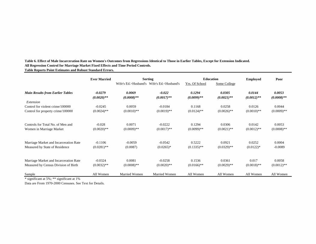
Table 6. Effect of Male Incarceration Rate on Women's Outcomes from Regressions Identical to Those in Earlier Tables, Except for Extension Indicated.All Regression Control for Marriage Market Fixed Effects and Time Period Controls.Table Reports Point Estimates and Robust Standard Errors.

Ever Married Sorting Education Employed PoorWife's Ed.>Husband's Wife's Ed.<Husband's Yrs. Of School Some College

Main Results from Earlier Tables -0.0279 0.0069 -0.022 0.1294 0.0305 0.0144 0.0053(0.0020)** (0.0008)** (0.0017)** (0.0099)** (0.0021)** (0.0012)** (0.0008)**

ExtensionControl for violent crime/100000 -0.0245 0.0059 -0.0184 0.1168 0.0258 0.0126 0.0044Control for property crime/100000 (0.0024)** (0.0010)** (0.0019)** (0.0124)** (0.0026)** (0.0010)** (0.0009)**

Controls for Total No. of Men and -0.028 0.0071 -0.0222 0.1294 0.0306 0.0142 0.0053Women in Marriage Market (0.0020)** (0.0009)** (0.0017)** (0.0099)** (0.0021)** (0.0012)** (0.0008)**

Marriage Market and Incarceration Rate -0.1106 -0.0059 -0.0542 0.5222 0.0921 0.0252 0.0004Measured by State of Residence (0.0281)** (0.0087) (0.0265)* (0.1335)** (0.0329)** (0.0122)* -0.0089

Marriage Market and Incarceration Rate -0.0324 0.0081 -0.0258 0.1536 0.0361 0.017 0.0058Measured by Census Division of Birth (0.0032)** (0.0008)** (0.0020)** (0.0166)** (0.0029)** (0.0018)** (0.0012)**

Sample All Women Married Women Married Women All Women All Women All Women All Women* significant at 5%; ** significant at 1%Data are From 1970-2000 Censuses. See Text for Details.

Table 7. Effect of Male Incarceration Rate on Un-Incarcerated MenOutcome

Ever Married? Yrs. Of School Any College Employed? Poor Household?Incarceration Rate -0.0277 0.0956 0.0162 -0.0085 -0.007 0.0026 0.0002

(0.0020)** (0.0104)** (0.0013)** (0.0014)** (0.0012)** (0.0006)** -0.0006Married? 0.1187 -0.0673

(0.0024)** (0.0013)**Incarceration Rate * Married? 0.0077

(0.0005)**Employed? -0.1934

(0.0030)**H.S. Graduate -0.0711

(0.0034)**Any College -0.0611

(0.0046)**Marriage Market Fixed Effect: State of Birth * Age Group * Race Yes Yes Yes Yes Yes Yes Yes

Census Year Controls Yes Yes Yes Yes Yes Yes Yes

Constant 0.6444 12.7955 0.4611 0.8582 0.7899 0.1157 0.3731(0.0045)** (0.0253)** (0.0030)** (0.0035)** (0.0028)** (0.0020)** (0.0052)**

Observations 4017423 4017423 4017423 4017423 4017423 4017423 4017423R-squared 0.18 0.05 0.04 0.04 0.07 0.03 0.1Robust standard errors in brackets* significant at 5%; ** significant at 1%

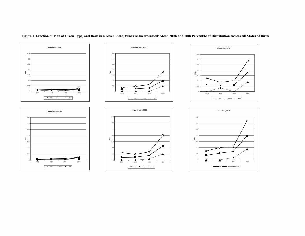
Figure 1. Fraction of Men of Given Type, and Born in a Given State, Who are Incarcerated: Mean, 90th and 10th Percentile of Distribution Across All States of Birth

White Men, 20-27

0

0.05

0.1

0.15

0.2

0.25

0.3

0.35

1970 1980 1990 2000

Rat

e

90th mean 10th

Hispanic Men, 20-27

0

0.05

0.1

0.15

0.2

0.25

0.3

0.35

1970 1980 1990 2000

Rat

e

90th mean 10th

Black Men, 20-27

0

0.05

0.1

0.15

0.2

0.25

0.3

0.35

1970 1980 1990 2000

Rat

e

90th mean 10th

White Men, 28-35

0

0.05

0.1

0.15

0.2

0.25

0.3

0.35

1970 1980 1990 2000

Rat

e

90th mean 10th

Hispanic Men, 28-35

0

0.05

0.1

0.15

0.2

0.25

0.3

0.35

1970 1980 1990 2000

Rat

e

90th mean 10th

Black Men, 28-35

0

0.05

0.1

0.15

0.2

0.25

0.3

0.35

1970 1980 1990 2000

Rat

e

90th mean 10th

Figure 2: Marriage Rate and Incarceration Rate in 1970 and 2000

A. marriage rate and incarceration rateincarceration rate

marriage rate Linear prediction

0.000 0.197

0.117

1.000

B. changes between 1970 and 2000change of incarceration rate

change of marriage rate Linear prediction

-0.087 0.194

-0.598

0.097

Appendix Table 1. Iincarceration rate by state of birth, year and race, Men aged 20-35All Men

1970 1980 1990 2000Alabama 1.3% 1.9% 2.0% 4.3%Alaska 0.0% 1.6% 1.3% 4.0%Arizona 1.1% 1.8% 1.9% 4.8%Arkansas 1.1% 1.6% 1.6% 3.3%California 1.6% 1.7% 1.7% 3.6%Colorado 1.3% 1.2% 1.3% 3.0%Connecticut 0.6% 1.0% 1.2% 3.0%Delaware 1.1% 1.9% 1.6% 3.3%District of Columbia 2.8% 2.7% 3.8% 4.6%Florida 1.7% 2.5% 4.1% 5.3%Georgia 1.7% 2.1% 2.9% 5.0%Hawaii 0.7% 1.4% 1.7% 4.4%Idaho 0.1% 1.0% 0.9% 1.9%Illinois 0.9% 1.3% 1.2% 3.8%Indiana 0.8% 1.3% 1.4% 2.6%Iowa 0.4% 0.8% 0.8% 1.5%Kansas 1.0% 1.0% 1.2% 2.1%Kentucky 0.8% 1.2% 1.4% 2.8%Louisiana 2.2% 2.2% 2.4% 5.4%Maine 0.8% 1.1% 0.8% 1.9%Maryland 2.1% 2.0% 2.1% 2.9%Massachusetts 1.0% 0.9% 1.1% 1.9%Michigan 1.0% 1.4% 1.2% 3.0%Minnesota 0.8% 1.0% 0.4% 1.2%Mississippi 1.7% 2.0% 2.2% 5.5%Missouri 1.1% 1.4% 1.8% 2.3%Montana 0.7% 0.8% 0.8% 2.8%Nebraska 0.5% 0.8% 0.8% 1.7%Nevada 1.2% 1.5% 2.2% 4.5%New Hampshire 0.9% 1.1% 0.8% 2.5%New Jersey 0.9% 1.1% 1.6% 3.8%New Mexico 0.9% 1.5% 1.7% 3.5%New York 1.0% 1.3% 1.6% 3.6%North Carolina 1.4% 2.0% 1.9% 3.6%North Dakota 0.2% 0.8% 0.6% 1.0%Ohio 0.9% 1.2% 1.4% 2.6%Oklahoma 1.3% 1.6% 2.0% 4.0%Oregon 1.2% 1.2% 1.4% 2.5%Pennsylvania 0.5% 1.1% 1.1% 2.7%Rhode Island 1.0% 0.9% 1.0% 1.2%South Carolina 2.0% 2.3% 3.0% 4.3%South Dakota 0.6% 1.0% 0.7% 1.7%Tennessee 1.2% 1.6% 1.8% 4.4%Texas 1.5% 1.9% 2.1% 4.8%Utah 0.6% 0.8% 0.8% 1.9%Vermont 0.6% 0.9% 0.8% 1.4%Virginia 2.0% 1.8% 1.9% 2.9%Washington 1.0% 1.5% 1.2% 2.6%West Virginia 1.2% 1.1% 0.9% 2.0%Wisconsin 0.8% 0.8% 0.7% 2.3%Wyoming 0.8% 0.9% 1.0% 4.1%Data are from Multiple Census Years. See text for details.

Appendix Table 1. Iincarceration rate by state of birth, year and race, Men aged 20-35Blacks

1970 1980 1990 2000Alabama 2.6% 3.6% 4.5% 10.0%Alaska 0.0% 8.3% 5.3% 26.6%Arizona 4.5% 8.6% 11.4% 22.0%Arkansas 1.8% 3.8% 4.7% 8.5%California 7.5% 5.9% 6.5% 13.0%Colorado 13.6% 3.8% 7.6% 17.1%Connecticut 2.0% 4.7% 8.0% 16.4%Delaware 0.0% 6.0% 6.8% 12.3%District of Columbia 6.1% 5.1% 7.7% 7.5%Florida 4.5% 5.9% 12.0% 13.5%Georgia 3.2% 4.2% 6.5% 10.2%Hawaii 0.0% 5.9% 9.1% 16.3%Idaho 0.0% 12.5% 0.0% 25.0%Illinois 5.2% 5.2% 5.5% 15.8%Indiana 5.4% 6.4% 7.3% 13.1%Iowa 0.0% 6.4% 11.0% 16.5%Kansas 6.3% 5.5% 8.0% 11.6%Kentucky 4.2% 4.6% 5.3% 13.7%Louisiana 2.9% 4.3% 5.0% 11.5%Maine . 5.1% 3.1% 40.0%Maryland 6.9% 6.1% 6.5% 9.2%Massachusetts 1.5% 5.9% 7.1% 12.3%Michigan 5.5% 6.0% 6.3% 12.2%Minnesota 0.0% 6.5% 4.6% 23.4%Mississippi 2.4% 3.4% 3.9% 9.4%Missouri 4.5% 6.4% 8.2% 9.0%Montana 0.0% 0.0% 8.3% 42.9%Nebraska 0.0% 8.0% 6.3% 12.2%Nevada 0.0% 11.9% 11.0% 17.0%New Hampshire 0.0% 0.0% 0.0% 47.6%New Jersey 6.0% 5.5% 8.9% 15.1%New Mexico 0.0% 11.3% 4.0% 29.9%New York 5.6% 6.7% 8.9% 14.9%North Carolina 3.1% 4.4% 4.4% 9.1%North Dakota . 3.8% 0.0% 25.0%Ohio 6.2% 5.3% 7.1% 11.9%Oklahoma 4.2% 5.6% 10.0% 17.5%Oregon 15.4% 4.6% 7.1% 17.6%Pennsylvania 3.3% 5.2% 6.8% 18.0%Rhode Island 10.0% 3.6% 8.4% 12.6%South Carolina 3.1% 3.6% 5.6% 8.1%South Dakota . 7.7% 8.3% 22.2%Tennessee 3.4% 4.1% 4.8% 13.0%Texas 4.5% 5.5% 7.2% 14.0%Utah 20.0% 5.0% 7.0% 25.9%Vermont 0.0% 0.0% 0.0% 42.9%Virginia 4.9% 4.5% 5.2% 8.5%Washington 14.3% 13.1% 6.0% 17.9%West Virginia 7.0% 4.7% 3.7% 15.1%Wisconsin 18.8% 6.8% 9.2% 23.0%Wyoming 33.3% 10.5% 4.5% 56.1%Data are from Multiple Census Years. See text for details.

Appendix Table 1. Incarceration rate by state of birth, year and race, Men aged 20-35Hispanics

1970 1980 1990 2000Alabama 1.9% 4.5% 6.1% 9.4%Alaska 0.0% 0.0% 0.0% 10.2%Arizona 2.1% 2.0% 2.7% 6.3%Arkansas 2.1% 0.8% 2.7% 26.2%California 2.7% 2.5% 2.3% 4.5%Colorado 1.8% 1.9% 3.0% 5.3%Connecticut 2.5% 3.0% 7.2% 8.4%Delaware 2.8% 5.9% 2.5% 4.9%District of Columbia 4.1% 0.7% 6.5% 6.8%Florida 3.9% 1.9% 2.8% 5.4%Georgia 3.2% 4.0% 2.7% 18.3%Hawaii 1.6% 2.3% 2.9% 9.0%Idaho 0.0% 0.9% 4.5% 7.7%Illinois 2.0% 2.1% 2.4% 5.5%Indiana 2.1% 1.5% 2.9% 6.1%Iowa 2.2% 0.8% 1.4% 7.1%Kansas 1.0% 1.9% 2.2% 5.6%Kentucky 1.0% 0.0% 4.2% 10.9%Louisiana 7.4% 1.7% 4.0% 12.8%Maine 1.1% 0.0% 5.0% 27.8%Maryland 5.3% 1.7% 3.8% 3.4%Massachusetts 4.0% 2.7% 6.8% 9.9%Michigan 2.8% 3.0% 2.0% 6.4%Minnesota 2.1% 2.1% 2.0% 8.2%Mississippi 1.6% 1.9% 3.0% 14.4%Missouri 2.6% 2.9% 3.5% 6.0%Montana 3.8% 6.0% 0.0% 26.2%Nebraska 1.4% 2.6% 1.6% 13.1%Nevada 0.0% 3.1% 1.9% 9.4%New Hampshire 0.0% 0.0% 15.8% 15.6%New Jersey 1.7% 3.1% 4.6% 7.2%New Mexico 1.0% 2.1% 2.3% 4.2%New York 2.7% 2.9% 4.9% 7.3%North Carolina 1.2% 3.0% 3.1% 11.4%North Dakota 2.3% 8.1% 2.9% 4.7%Ohio 1.5% 3.6% 2.9% 7.5%Oklahoma 3.5% 2.4% 3.1% 11.1%Oregon 4.7% 4.1% 1.4% 9.4%Pennsylvania 1.6% 1.8% 4.6% 13.3%Rhode Island 5.1% 6.8% 4.0% 3.1%South Carolina 2.8% 4.3% 3.2% 10.2%South Dakota 0.0% 0.0% 3.0% 10.6%Tennessee 1.4% 1.7% 2.5% 28.7%Texas 2.0% 1.9% 2.3% 5.4%Utah 1.1% 1.9% 4.6% 10.5%Vermont 0.0% 0.0% 0.0% 11.1%Virginia 2.6% 3.7% 3.3% 5.7%Washington 2.4% 2.2% 1.4% 6.3%West Virginia 2.0% 1.1% 3.4% 22.4%Wisconsin 0.7% 2.5% 3.6% 11.1%Wyoming 2.1% 2.7% 4.9% 17.1%Data are from Multiple Census Years. See text for details.

Appendix Table 1. Iincarceration rate by state of birth, year and race, Men aged 20-35Whites

1970 1980 1990 2000Alabama 0.6% 1.0% 0.9% 1.8%Alaska 0.0% 1.4% 1.1% 2.7%Arizona 0.4% 1.3% 1.1% 3.2%Arkansas 0.8% 1.0% 0.8% 1.8%California 1.2% 1.2% 1.1% 2.0%Colorado 0.9% 1.0% 0.8% 1.9%Connecticut 0.5% 0.8% 0.7% 1.3%Delaware 1.0% 1.2% 0.7% 1.4%District of Columbia 1.4% 1.3% 1.0% 1.6%Florida 0.6% 1.5% 1.9% 2.7%Georgia 0.8% 1.1% 1.4% 2.4%Hawaii 0.5% 1.0% 1.2% 2.5%Idaho 0.1% 0.9% 0.8% 1.5%Illinois 0.5% 0.8% 0.6% 1.3%Indiana 0.5% 1.0% 1.0% 1.8%Iowa 0.3% 0.8% 0.7% 1.3%Kansas 0.8% 0.8% 0.9% 1.4%Kentucky 0.6% 1.0% 1.1% 1.9%Louisiana 0.5% 1.1% 1.1% 2.0%Maine 0.8% 1.1% 0.7% 1.4%Maryland 0.8% 1.0% 1.1% 1.3%Massachusetts 0.8% 0.8% 0.9% 1.2%Michigan 0.6% 0.9% 0.7% 1.7%Minnesota 0.7% 0.9% 0.4% 0.8%Mississippi 1.2% 0.9% 0.9% 2.0%Missouri 0.7% 0.9% 1.1% 1.5%Montana 0.4% 0.7% 0.8% 2.0%Nebraska 0.4% 0.7% 0.6% 1.1%Nevada 1.4% 0.7% 1.5% 2.7%New Hampshire 1.0% 1.1% 0.8% 2.0%New Jersey 0.5% 0.7% 0.7% 1.2%New Mexico 0.9% 0.8% 1.1% 1.5%New York 0.5% 0.8% 0.7% 1.1%North Carolina 0.9% 1.1% 1.1% 1.5%North Dakota 0.1% 0.7% 0.6% 0.8%Ohio 0.6% 0.8% 0.9% 1.6%Oklahoma 0.9% 1.2% 1.3% 2.5%Oregon 0.8% 1.1% 1.4% 1.9%Pennsylvania 0.3% 0.7% 0.7% 1.2%Rhode Island 0.6% 0.8% 0.8% 0.8%South Carolina 1.1% 1.4% 1.5% 2.0%South Dakota 0.6% 0.9% 0.6% 1.5%Tennessee 0.9% 1.1% 1.2% 2.3%Texas 0.9% 1.1% 1.1% 2.6%Utah 0.5% 0.7% 0.6% 1.4%Vermont 0.7% 0.9% 0.8% 1.2%Virginia 1.1% 1.0% 1.0% 1.4%Washington 0.8% 1.1% 1.1% 1.9%West Virginia 0.9% 0.9% 0.8% 1.4%Wisconsin 0.7% 0.6% 0.5% 1.4%Wyoming 0.3% 0.7% 0.6% 2.0%Data are from Multiple Census Years. See text for details.