maintenance optimization of infrastructure networks using genetic algorithms

www.elsevier.com/locate/autcon

Automation in Constructio

Maintenance optimization of infrastructure networks using

genetic algorithms

G. Morcousa,*, Z. Lounisb

aSchool of Engineering, Acadia University, Wolfville, Nova Scotia, Canada B4P2R6bInstitute for Research in Construction, National Research Council of Canada, Ottawa, Ontario, Canada K1A0R6

Accepted 27 August 2004

Abstract

This paper presents an approach to determining the optimal set of maintenance alternatives for a network of infrastructure

facilities using genetic algorithms. Optimal maintenance alternatives are those solutions that minimize the life-cycle cost of an

infrastructure network while fulfilling reliability and functionality requirements over a given planning horizon. Genetic

algorithms are applied to maintenance optimization because of their robust search capabilities that resolve the computational

complexity of large-size optimization problems. In the proposed approach, Markov-chain models are used for predicting the

performance of infrastructure facilities because of their ability to capture the time-dependence and uncertainty of the

deterioration process, maintenance operations, and initial condition, as well as their practicality for network level analysis. Data

obtained from the Ministere des Transports du Quebec database are used to demonstrate the feasibility and capability of the

proposed approach in programming the maintenance of concrete bridge decks.

D 2004 Elsevier B.V. All rights reserved.

Keywords: Maintenance optimization; Concrete deck; Markov chain; Genetic algorithm; Infrastructure management

1. Introduction

The life-cycle cost analysis is a decision-making

approach that evaluates the total cost accrued over the

entire life of an infrastructure facility from its

construction to its replacement or final demolition

[13]. For an existing facility, the life-cycle cost analysis

0926-5805/$ - see front matter D 2004 Elsevier B.V. All rights reserved.

doi:10.1016/j.autcon.2004.08.014

* Corresponding author.

E-mail addresses: [email protected] (G. Morcous)8

[email protected] (Z. Lounis).

is considered an efficient approach for comparing the

long-term impacts of different maintenance strategies

and identifying the optimal ones. Fig. 1 shows an

example of the performance profile of an infrastructure

facility when two different maintenance strategies that

are technically acceptable (i.e. satisfy performance

requirements) are implemented. Using the life-cycle

cost approach allows the decision maker to compare

the two strategies from the economic perspective and

determine the most cost-effective one over a certain

planning horizon. This is extremely important for most

n 14 (2005) 129–142

Fig. 1. Performance profiles of two different maintenance strategies.

G. Morcous, Z. Lounis / Automation in Construction 14 (2005) 129–142130

facility managers because of the limitations on the

availability of resources required to fulfill even urgent

maintenance needs.

Infrastructure management systems have been

developed to apply the life-cycle costing approach

to optimize maintenance decisions at both network

and project levels and achieving network/project

performance requirements under financial constraints.

Since the early 1980s, many optimization techniques

have been adopted for this purpose, such as optimal

control theory, linear and nonlinear programming,

dynamic programming, and integer programming

[10,14,19]. Although these optimization techniques

have provided satisfactory results, many agencies still

prefer using traditional methods of maintenance

optimization in spite of their arbitrary nature and

relatively low degree of accuracy. These methods are

mostly heuristic and based on subjective ranking and

priority rules developed by domain experts. The

reason of this preference is due in-part to the

mathematical complication of formulating a main-

tenance optimization problem using these techniques

in addition to the computational complexity associ-

ated with large size networks.

Genetic Algorithms (GAs) are robust, practical,

and general-purpose stochastic search-based optimi-

zation techniques that can provide a comparable level

of accuracy while being more efficient than conven-

tional optimization techniques. GAs were developed

by Holland in the early 1970s based on the principles

of natural selection and genetics [12]. Since the early

1990s, GAs have been extensively used by many

researchers in civil engineering for solving global

optimization problems, such as the design of struc-

tures and transportation networks [25,28]. Although

the area of global optimization comprises several

techniques, such as simulated annealing, and Tabu

Search, GAs are highly recognized for their computa-

tional efficiency. This is mainly because other

techniques select a single solution and randomly

change it until it reaches the best solution, which

requires several iterations. GAs, on the other hand,

store multiple solutions to the problem (i.e. popula-

tion) and use probabilistic rules to generate new and

better populations, which is more efficient and

increases the likelihood of finding optimal solutions

in a timely fashion [11]. In addition, GAs use

information on the objective function only and do

not require any information on its gradients, which

greatly simplifies the mathematics of the problem.

The use of GAs in maintenance optimization has

been introduced by Fwa et al. [7] in an investigation

that led to the development of a computer model,

known as PAVENET, for maintenance planning of

pavement networks. Updated versions of this model

were developed to demonstrate the use of GAs in

solving the trade-off between maintenance and reha-

bilitation activities and resolving the complexity of

multiobjective problems [5,6]. Liu et al. [15] and

Miyamoto et al. [22] also developed GA-based

models for the determination of optimal long-term

maintenance strategies of bridge deck networks. In all

these investigations, linear and nonlinear deterministic

models were used for predicting the future condition

of a pavement section or a bridge deck as a function of

its initial condition, governing deterioration parame-

ters, and impact of maintenance alternatives. This is

because of the simplicity and computational efficiency

of deterministic deterioration models. However, these

models neglect the uncertainty due to the stochastic

nature of infrastructure deterioration and presence of

unobserved variables and measurement errors.

State-of-the art infrastructure management systems,

such as Pontis, BRIDGIT, and MicroPAVER, use

stochastic Markov chains for predicting the future

condition of infrastructure components, systems, and

networks [9,27]. A Markov chain is a special case of

the Markov process whose development can be

treated as a series of transitions between certain states.

A stochastic process is considered as a Markov

process if the probability of a future state in the

process depends only on the present state and not on

how it was attained [24]. Markov-chains are used as

G. Morcous, Z. Lounis / Automation in Construction 14 (2005) 129–142 131

performance prediction models for infrastructure by

defining discrete condition states and accumulating the

probability of transition from one condition state to

another over multiple discrete time intervals [1]. These

stochastic models have two main advantages over

deterministic models. First, they are able to capture the

considerable randomness that affects the performance

of structures due to uncertainties in initial condition,

applied stresses, condition assessment, and inherent

uncertainty of the deterioration process [16]. Second,

they are incremental models that account for the

current condition in predicting the future condition

[18]. Moreover, Markov-chain models are practical in

dealing with large-sized networks due to their compu-

tational efficiency and simplicity of use.

The objective of this paper is to present an

approach that uses genetic algorithms in conjunction

with Markov-chain models for programming main-

tenance alternatives. The proposed approach is

expected to enhance the capability and efficiency

of the optimization module in the existing infra-

structure management systems. The first section

presents the proposed formulation of the mainte-

nance optimization problem. The second section

presents the solution of this problem using a genetic

algorithm. The last section demonstrates the feasi-

bility of the proposed approach using an application

example on concrete bridge decks.

2. Problem formulation

From a review of the literature, the only main-

tenance optimization model that combines the use of

Markov-chain models and genetic algorithms is the

pavement management optimization model proposed

by Ferreira et al. [4]. This model is a segment-linked

model that identifies the segments of the road network

where maintenance actions should be applied every

year in the planning horizon. The decision variables in

this model represent the instruments that can be

applied to change the state of each segment. This is

practical when there is a small number of segments,

however, it is computationally inefficient for a net-

work with a large number of segments, which is the

case of most infrastructure networks. To address this

problem, the proposed formulation of the maintenance

optimization problem classifies infrastructure facilities

into groups according to some explanatory variables,

such as type, material properties, operating loads, and

environmental conditions, which govern the facility

performance. In this formulation, all facilities of the

same group are assumed to have the same perform-

ance characteristics and should be analyzed in a

similar manner. The objectives of such a classification

are threefold: (i) achieve reliable performance model-

ing; (ii) reduce the computational complexity of the

optimization problem; and (iii) provide the decision

maker with the flexibility to select the specific facility

that will be treated in every year according to some

other intangible factors (e.g. social, environmental,

political, etc.) that cannot be easily considered in the

formulation. The parameters of the proposed formu-

lation are defined as follows:

G=number of facility groups;

T=number of years in the planning horizon;

S=number of condition states in the adopted rating

system;

Qg=total quantity of facilities in group g (number

of units, length, or area);

Mg=number of possible maintenance alternatives

for facilities in group g;

Dgt=condition vector (1�S) of group g at the

beginning of year t;

Dgt ¼ j d1gt d2gt N d sgt j ð1Þ

where, dgts =percentage of facilities from group g in

condition state s at year t. Pgm=transition probability

matrix (S�S) of group g when the maintenance

alternative m is implemented;

Pgm ¼ j p1;1gm p1;2gm N p1;Sgm

p2;1gm p2;2gm N p2;Sgm

NN

pS;1gm pS;2gm N pS;Sgm

j ð2Þ

where, pgmi,j =transition probability of group g from

condition state i to condition state j during 1 year

when the maintenance alternative m is implemented.

Transition probabilities are obtained either from

accumulated condition data or by using an expert

judgment elicitation procedure, which requires the

participation of domain experts [26].


Xgmt=maintenance vector (1�S) of group g for

maintenance alternative m during year t;

Xgmt ¼ j x1gmt x2gmt N xSgmt j ð3Þ

where, xgmts=percentage of facilities in group g and

condition state s that had the maintenance alternative

m during year t.

Cgm=cost vector (S�1) of group g and main-

tenance alternative m.

Cgm ¼ j c1gmc2gmd

d

cSgm

j ð4Þ

where, cgms=unit cost of implementing maintenance

alternative m on the facilities in group g and condition

state s (these unit costs have to be adjusted for

inflation when long planning horizons are used).

The condition of facilities from group g at year t

can be predicted using the initial condition vector at

year (t�1) and the transition probability matrices

corresponding to the maintenance alternatives taken

during this year multiplied by the maintenance vectors

of this year as follows:

Dgt ¼Xm¼Mg

m¼1

Dg t�1ð Þ IX gm t�1ð Þ� �

Pgm ð5Þ

where, I is a unit vector (S�1)

This equation corresponds to the Chapman–Kol-

mogorov equations that define the multi-step transi-

tions for any values of the time t that is greater than or

equal to 1 and less than or equal to T. The present

value of the total cost of maintenance alternatives

implemented on facilities from group g over the entire

planning horizon T, denoted PVgT, assuming a

discount rate r, can be calculated as follows:

PVTg ¼ Qg

Xt¼T

t¼1

Xm¼Mg

m¼1

Dgt IXgmt

� �Cgm

1þ rð Þtð6Þ

The users’ costs and failure costs can be discounted

and added to the above maintenance cost to obtain the

total cost when adequate data become available.

Considering the maintenance costs only, the objective

is to minimize the sum of the present value of the

maintenance costs of all facility groups while keeping

the condition of every group at any time above a pre-

defined threshold value. The optimization problem

can be formulated as follows:

MinimizeXg¼G

g¼1

PVTg ð7aÞ

Subject to: DCumgt [ DThr

g ð7bÞ

where DgtCum is the cumulative condition vector of

group g at the beginning of year t, which contains the

percentages of facilities whose condition is equal to or

higher than a given condition state. DgThr is the

threshold condition vector (1�S) of group g, which

represents the minimum acceptable conditions that

will be compared with the cumulative condition

vector in every year. The threshold conditions are

determined by the facility managers or domain experts

based on their condition requirements and budget

availability (i.e. user defined). The threshold condition

vectors represent the constraints of the cost minimi-

zation problem that differ also from one group to

another. This is because the definition of facility

groups considers governing deterioration parameters

that implicitly represent the importance and vulner-

ability of the infrastructure and, consequently, control

the determination of the minimum acceptable con-

dition. For instance, bridge decks on express high-

ways with high traffic volume are more important

than those on collector highways with low traffic

volume. Therefore, the minimum acceptable condition

of bridge decks on an express highway is higher than

that of bridge decks on a collector highway. Other

constraints, such as non-negativity constraints, are

applied to this optimization model in order to

guarantee the feasibility of the solutions obtained.

The previous optimization problem is based on

cost minimization. However, in some cases where

there are constraints on the maintenance budget

available for every year in the planning horizon, the

optimization problem can be formulated differently as

a quality maximization problem. In this case, the

objective function tends to maximize the average

network condition given the annual budget con-


straints. The maintenance optimization problem can

be formulated as follows:

Maximize

Xs¼S

s¼1

SXt¼T

t¼1

Xg¼G

g¼1

d sgt

TGð8aÞ

Subject to :Xg¼G

g¼1

Qg

Xm¼Mg

m¼1

DgtIXgmtCgm\Bt ð8bÞ

where, Bt is the maintenance budget available for year

t. The following section demonstrates the use of GA

optimization techniques to solve the cost minimiza-

tion problem presented in Eqs. (7a) and (7b).

However, the same procedures can be applied to

solve the quality maximization problems presented in

Eqs. (8a) and (8b).

3. Maintenance optimization using Genetic

Algorithms

Fig. 2 shows a simplified flow chart of the process

of problem-solving using GAs. This process starts

with identifying the parameters that describe the

solutions of the given problem and determining its

objective function and constraints (which were pre-

sented in the problem formulation). The following

step is encoding the problem solutions into genetic

representation (i.e. chromosomes). In this representa-

tion, each solution contains several genes that can be

manipulated by the genetic operators described later.

These genes are represented by a string of symbols

that can be obtained using different encoding methods

[8]. A binary encoding method is used for the current

problem because it allows fast computation and easy

manipulation of genes [22]. Three issues have to be

considered when encoding and decoding between

chromosomes and solutions: feasibility, legality, and

uniqueness of mapping. Feasibility means that the

decoded solutions lie in the feasible region of the

given problem, which is determined by the problem

constraints. Legality refers to whether decoding

chromosomes results in meaningful solutions.

Uniqueness of mapping means that each chromosome

can be decoded into a single solution. The one-to-one

mapping is considered the best mapping method since

it allows easy and fast decoding. However, this

method may yield a number of illegal chromosomes

having lethal genes, which decreases the efficiency of

calculation. Therefore, a trade-off between the sim-

plicity of mapping and legality of solutions is required

for a good genetic representation.

Fig. 3 shows the genetic representation of an

individual solution for the current problem. This

solution identifies the percentages of facilities in each

group ( g) and condition state (s) that are subjected to

each maintenance alternative (m) in every year (t). For

each maintenance alternative, a 5-bit binary code is

used to express 32 different values. The values

corresponding to different maintenance alternatives

are divided by their total sum to calculate the

percentages of facilities that are subjected to each

maintenance alternative. Fig. 4 shows an example for

the binary code of three maintenance alternatives. The

percentages of facilities subjected to each alternative

are 50%, 21%, and 29% based on the ratio of the

decoded value relative to the sum of all decoded

values. Although this is considered to be an indirect

and complicated mapping method, it eliminates the

presence of lethal genes that negatively affects the

computational efficiency of the GA.

Then, the GA randomly selects an initial pool of

solutions, referred to as the parent pool or population,

with a predefined size. The individuals of this

population are evaluated using the so-called bfitnessfunctionQ, which is determined based on the objective

function and the constraints presented earlier. For cost

minimization problems, the fitter individual is the one

with lower present value of the total maintenance

costs. Since the maintenance programming is a

constraint optimization problem, the penalty method

is used to account for the constraints and ensure the

feasibility of the obtained solutions. If an individual

does not satisfy the condition constraint (i.e. facility

condition is less than the threshold values), a penalty

is applied in the form of extra maintenance cost. This

reduces the fitness value of the individual and

decreases its probability of being selected in the next

generation. Performance prediction models and cost

models are necessary inputs to the evaluation of

candidate solutions.

Two processes are implemented on the parent pool

to generate a new pool of solutions, referred to as the

offspring pool. Selection is the first process and is

considered the driving force of the GA since its selects

Fig. 2. Flow chart of problem solving using genetic algorithm.


the most promising chromosomes from the parent

pool and generates a mating pool that has the same

number of chromosomes. Several selection schemes,

such as roulette-wheel, tournament selection, and

linear and exponential ranking selection, can be

adopted [3]. For the current problem, the roulette-

wheel scheme was used, which is a common

stochastic procedure that correlates the probability of

selection for each chromosome to its fitness value

calculated earlier. Evolution is the second process in

which the chromosomes of the mating pool are

manipulated by two genetic operations, crossover

and mutation, in order to produce a new offspring

pool. In the crossover operation, pairs of parent

chromosomes are randomly selected with probability

( pc) and each pair exchanges the genes of the two

chromosomes at a crossing site randomly selected to

accelerate the search. This operation produces off-

spring solutions that have combined features from the

parent solutions, which is known as bexploitationQ. A

Fig. 3. Genetic encoding of problem solutions.


high crossover probability allows the generation of

promising solution quite fast. In the mutation oper-

ation, parent chromosomes are selected and their

genes are changed randomly from 0 to 1, or vice

versa, and with probability ( pm) to conduct a random

search. This operation introduces random changes

into a small fraction of solutions to try potential

solutions that have never been selected while it avoids

being trapped in a local optima, which is known as

bexplorationQ. A very low mutation probability

reduces the possibility of exploring new solutions,

while a very high mutation probability may seriously

affect the convergence of solutions.

The resulting population is then evaluated using

the fitness function and used as a new parent

population. The selection and evolution processes

are repeated iteratively until a predefined stopping

criterion is satisfied. This criterion may specify the

maximum number of iterations, minimum improve-

ment in the average fitness, or both. The optimum

solution is determined as the solution that has the

highest fitness in these iterations.

Fig. 4. Example for decoding a solution.

4. Application

Highway bridges are considered the most critical

and vital links in any transportation network because

the full or partial failure of these links affects sig-

nificantly the overall performance of the network and

may lead to catastrophes and serious economic

impacts. Concrete bridge decks are the weakest links

and the most expensive elements of most bridge

systems in North America and Europe, from durability

point of view [2]. This is mainly due to the effects of

the corrosion of reinforcing steel because of using de-

icing chemicals in winter, freezing and thawing cycles,

and direct exposure to traffic loads [17]. Concrete

bridge decks are selected as a bproof of conceptQapplication of the proposed approach, however, the

same procedures can be applied to other infrastructure

facilities.

The data required for developing Markov-chain

models of concrete bridge decks are obtained from the

Ministere des Transports du Quebec (MTQ) database,

which is part of a comprehensive system for managing

highway structures in Quebec. This database includes

inventory data, which consists of bridge identification,

description, environment, and geometry; condition

data, which contains the results of the detailed visual

inspections carried out on all bridges approximately

every 3 years; and maintenance data, which includes

the estimated costs and expected times for recom-

mended maintenance and rehabilitation activities. The

condition data comprises two condition ratings [20]:

(i) material condition rating (MCR), which represents

the condition of an element based on the severity and

extent of observed defects, and (ii) performance

condition rating (PCR), which describes the condition

of an element based on its ability to perform the

intended function in the structure. Both the MCR and

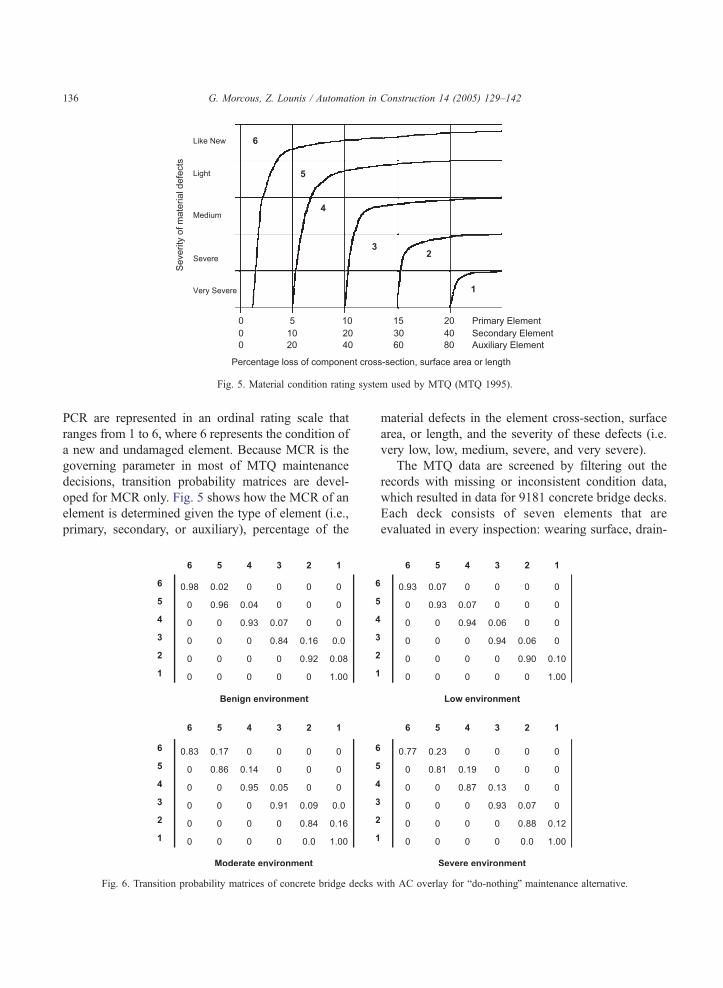
Fig. 5. Material condition rating system used by MTQ (MTQ 1995).


PCR are represented in an ordinal rating scale that

ranges from 1 to 6, where 6 represents the condition of

a new and undamaged element. Because MCR is the

governing parameter in most of MTQ maintenance

decisions, transition probability matrices are devel-

oped for MCR only. Fig. 5 shows how the MCR of an

element is determined given the type of element (i.e.,

primary, secondary, or auxiliary), percentage of the

Fig. 6. Transition probability matrices of concrete bridge decks

material defects in the element cross-section, surface

area, or length, and the severity of these defects (i.e.

very low, low, medium, severe, and very severe).

The MTQ data are screened by filtering out the

records with missing or inconsistent condition data,

which resulted in data for 9181 concrete bridge decks.

Each deck consists of seven elements that are

evaluated in every inspection: wearing surface, drain-

with AC overlay for bdo-nothingQ maintenance alternative.

Table 1

Maintenance alternatives and unit costs for bridge decks with AC overlay

Condition

state

Alternative 1: bDo-nothingQ Alternative 2: bRepairQ Alternative 3: bReplaceQ

Description Unit cost

($/m2)


($/m2)


($/m2)

6 Do Nothing 0 N/A N/A N/A N/A

5 Do Nothing 0 Minor repair 40 N/A N/A

4 Do Nothing 0 Major repair 60 Replace overlay and

repair substrate

160

3 Do Nothing 0 Rehabilitate 80 Replace overlay and

repair substrate

160

2 Do Nothing 0 Replace overlay and

repair substrate

160 Replace deck 300

1 Do Nothing 0 Replace overlay and

repair substrate

180 Replace deck 300


age system, two exterior faces, two end portions, and

the middle portion. The overall condition of the bridge

deck (MCR) is calculated as the aggregation of the

MCRs of the seven elements using the balancing

factors defined by bridge experts in the MTQ bridge

management system [21]. Fig. 6 shows the transition

probability matrices developed for concrete bridge

decks protected with asphaltic concrete (AC) overlay

in four environmental categories (benign, low, mod-

erate, and severe). These environmental categories

were determined for bridge decks in an earlier study

based on the values of four deterioration parameters:

highway class, region, average daily traffic and

percentage of truck traffic [23]. Since the proposed

approach of maintenance optimization is applied to

groups of facilities and not to individual facilities,

concrete bridge decks are classified into four groups

that correspond to the four environmental categories

determined earlier.

Transition probability matrices are developed for

1-year transition period when the bdo-nothingQ

Fig. 7. Transition probability matrices of concrete bridge deck

maintenance alternative is implemented and assuming

an undamaged initial state. For simplicity purposes,

the cells of the matrices shown in Fig. 6 are

considered zeros except for the diagonal line and

the line above it assuming that a bridge deck can

change by, at most, one condition state in a year.

Additionally, only three possible maintenance alter-

natives are considered for each bridge deck: (i) bdo-nothingQ; (ii) brepairQ; or (iii) breplaceQ. The descrip-

tion of each alternative, its applicability to concrete

bridge decks in different condition states, and its

estimated unit cost are listed in Table 1. Actual unit

costs may differ from the listed ones, however, the unit

costs of each alternative relative to other alternatives

are almost similar. Fig. 7 shows the transition

probability matrices when the brepairQ and breplaceQalternatives are implemented on bridge decks in any of

the four environmental categories. These matrices

represent the impact of each maintenance alternative

on the condition of concrete bridge decks and are

determined based on expert judgment.

s with AC overlay for maintenance alternatives 2 and 3.

Table 2

Size and threshold condition vector for the investigated bridge deck

groups

Bridge

deck

group

Size

(m2)

Threshold condition vector

(cumulative conditions)

6 5 4 3 2 1

Group 1 48,744 0.50 0.90 0.98 1.00 1.00 1.00

Group 2 50,090 0.40 0.90 0.95 0.98 1.00 1.00

Group 3 179,821 0.15 0.50 0.80 0.90 0.95 1.00

Group 4 9570 0.10 0.40 0.70 0.80 0.90 1.00


Table 2 shows the size of the bridge deck network

in each group (represented by the total deck surface

area) along with the threshold condition vector that is

defined as annual constraints on the network con-

dition for that group. These constraints are considered

in the optimization model using a penalty method

that adds a unit cost of $500 to the present value of

the solution that violates the condition constraints.

For simplification purposes, the bridge decks of each

group are assumed to have an undamaged initial

condition (Dg0=[1 0 0 0 0 0]). This condition

changes annually over the 15-year planning horizon

using the transition probability matrices shown in

Fig. 8. Average and best solu

Figs. 6 and 7 based on the chosen maintenance

alternative every year. A discount rate of 5% is used

to calculate the total present value of maintenance

costs.

In the proposed GA model, a population size of 50

individuals and a crossover probability of 50% were

estimated based on the values recommended by the

adopted GA simulator and those used earlier in the

literature for similar applications [15]. The crossover

method used was the single point method that has a

randomly chosen cut point to divide the selected

chromosomes. A mutation probability of 1% was

initially estimated and then adjusted automatically by

the GA simulator based on the model performance

(i.e. convergence) during iterations. In addition, the

simulator was used to test different types of crossover

(e.g. standard, arithmetic, and heuristic) and mutation

(e.g. standard, boundary, and non-uniform) operators

to find the optimal combination for the given problem.

Fig. 8 shows the progress graph of GA iterations that

plots the number of iterations versus the average and

best fitness values of each population while searching

for optimal solutions. A maximum number of 10,000

iterations is chosen as the stopping criterion because

tions in GA iterations.

Table

3

Optimal

maintenance

vectors

forbridgedecksin

group3


the progress graph indicated no increase in the

average fitness beyond this number.

Table 3 lists portions of the optimal solution that

represent the maintenance vectors of the concrete

bridge decks in group 3. This solution describes the

percentage of the deck area in each condition state

that requires each maintenance alternative for each

year in the planning horizon. Additionally, the overall

condition vectors that represent the results of applying

these alternatives are listed. For example, at year 3

(the shaded row), the optimal solution indicates that:

(i) 100% of the bridge decks in condition 6 will have

the bdo-nothingQ alternative; (ii) 75% of bridge decks

in condition 5 will have the bdo nothingQ alternative,while the remaining 25% will have the brepairQalternative; (iii) 58% of the bridge decks in condition

4 will have the bdo nothingQ alternative, 21% will

have the brepairQ alternative, and the remaining 21%

will have the breplaceQ alternative. These are percen-

tages from the overall condition vector of the

previous year (i.e. the year 2 in this example), which

has the following condition distribution: 75% of the

bridge decks are in condition 6, 23% are in condition

5, and only 2% are in condition 4. Applying these

maintenance vectors will result in the overall con-

dition distribution shown in the shaded row (i.e. 68%

of the bridge decks are in condition 6, 28% are in

condition 5, and 4% are in condition 4), which in turn

will be used in calculating the optimal maintenance

vectors of the following year (i.e. the year 4 in this

example).

In order to demonstrate the impact of applying the

optimal solution on concrete bridge decks, the

deterioration curves of the four bridge deck groups

over the entire planning horizon are plotted in Fig. 9.

This figure shows a significant improvement in the

overall condition at year 6 for all bridge deck groups

and a less significant improvement at year 11 for

groups 3 and 4 in particular. The timing of the first

maintenance indicates that in order to minimize the

long-term maintenance costs, early treatments of deck

defects are required. The amount of these treatments

and their frequency differ considerably from one

group to another. For example, bridge decks in group

4 (severe environment) required extensive treatments

every 5 years, while those in group 1 (benign

environment) required slight treatment only once

during the 15-year period. The total cost of these

Fig. 9. Impact of optimal maintenance alternatives on average condition rating of bridge decks.


treatments in every year is shown in Fig. 10 for each

group. This figure shows different spending policies

on the maintenance, rehabilitation, and replacement of

bridge decks. For instance, bridge decks in group 1 do

Fig. 10. Annual cost of optimal maintena

not require spending on maintenance in the first years

as much as in the last years because of their low

deterioration rate, while bridge decks in groups 2 and

3 require almost the same amount of spending on

nce alternatives for all four groups.


maintenance over the entire planning horizon. Due to

the high deterioration rate of bridge decks in group 4,

replacement may be required for some bridge decks,

which is evident from the clear peak shown in year 11.

5. Conclusions

This paper presents a new approach to program-

ming maintenance alternatives for a network of

infrastructure facilities. This approach uses genetic

algorithm optimization techniques to resolve the

computational complexity of the optimization prob-

lem and Markov-chain performance prediction models

to account for the uncertainty in infrastructure

deterioration, condition assessment, and measurement

errors. The formulation of the optimization problem

minimizes the life-cycle cost of an infrastructure

network over a given time period while keeping the

network condition above a predefined threshold value.

In this formulation, infrastructure facilities are classi-

fied into groups according to some explanatory

variables, such as type, material properties, operating

loads, and environmental conditions, which govern

the facility performance. This classification achieves

reliable performance prediction modeling and reduces

the computational complexity of the optimization

problem.

The proposed approach was applied to program-

ming the maintenance activities of concrete bridge

decks protected with asphaltic concrete overlay. Field

data obtained from the Ministere des Transports du

Quebec were used to develop four transition prob-

ability matrices that represent the deterioration of

concrete bridge decks in four environmental catego-

ries (benign, low, moderate, and severe). These

categories were used to set up the bridge deck

groups required for the proposed optimization for-

mulation. The output of this approach comprises the

percentages of the bridge deck areas in each group

that requires specific maintenance action in every

year of the planning horizon. These percentages

minimize the total maintenance costs and ensure that

the overall average condition of each group is

within acceptable limits. This application illustrated

the feasibility, efficiency, and capability of using

genetic algorithms in conjunction with Markov-chain

models.

Future research is recommended to compare the

proposed approach for maintenance optimization with

conventional stochastic optimization techniques, such

as stochastic dynamic programming, that can accom-

modate the use of Markov chains for performance

prediction. This comparison might consider the latest

developments in Neuro-dynamic programming, which

uses artificial neural networks and other approxima-

tion architectures to overcome the limitations of the

standard dynamic programming.

Notations

G number of facility groups

T number of years in the planning horizon

S number of condition states in the adopted rating

system

Qg quantity of facilities in group g

Mg number of possible maintenance alternatives

for facilities in group g

Dgt condition vector (1�S) of group g at the

beginning of year t

dgts percentage of deck area from group g in

condition state s at year t

Pgm transition probability matrix (S�S) of group

g when the maintenance alternative m is

implemented

pgmi,j transition probability of group g from condition

state i to condition state j during 1 year when

the maintenance alternative m is implemented

Xgmt maintenance vector (1�S) of group g for

maintenance alternative m during year t

xgmts percentage of facilities in group g and con-

dition state s that had the maintenance alter-

native m during year t

Cgm cost vector (S�1) of group g and maintenance

alternative m

cgms unit cost of implementing maintenance alter-

native m on the facilities in group g and

conditon state s

I unit vector (S�1)

r discount rate

PVgT present value of the total cost of maintenance

alternatives implemented on facilities from

group g over the entire planning horizon T

DgtCum cumulative condition vector of group g at the

beginning of year t

DgThr threshold condition vector (1�S) of group g

Bt maintenance budget available for year t


Acknowledgements

The authors are grateful to M. Guy Richard, Eng.,

Director, and M. Rene Gagnon, Bridge Engineer, of

the Structures Department—Ministere des Transports

du Quebec—for their invaluable help in providing the

authors with all available data, manuals and other

needed information.

References

[1] J.L. Bogdanoff, A new cumulative damage model: Part I,

Journal of Applied Mechanics 45 (2) (1978) 246–250.

[2] P.D. Cady, R.E. Weyers, Deterioration rates of concrete bridge

decks, Journal of Transportation Engineering, ASCE 110 (1)

(1984) 34–44.

[3] P. Chong, S. Zak, An Introduction to Optimization, John

Wiley & Sons, New York, 2001.

[4] A. Ferreira, A. Antunes, L. Picado-Santos, Probabilistic

segment-linked pavement management optimization model,

Journal of Transportation Engineering, ASCE 128 (6) (2002)

568–577.

[5] T.F. Fwa, W.T. Chan, K.Z. Hoque, Multiobjective optimization

for pavement maintenance programming, Journal of Trans-

portation Engineering, ASCE 126 (5) (2000) 367–374.

[6] T.F. Fwa, W.T. Chan, C.Y. Tan, Genetic algorithm program-

ming of road maintenance and rehabilitation, Journal of

Transportation Engineering, ASCE 122 (3) (1996) 246–253.

[7] T.F. Fwa, C.Y. Tan, W.T. Chan, Road-maintenance planning

using genetic algorithms II: analysis, Journal of Transportation

Engineering, ASCE 120 (5) (1994) 710–722.

[8] M. Gen, R. Cheng, Genetic Algorithms and Engineering

Optimization, John Wiley & Sons, NY, 2000.

[9] K. Golabi, R. Shepard, Pontis: a system for maintenance

optimization and improvement of US Bridge Networks,

Interfaces 27 (1997) 71–88.

[10] K. Golabi, R. Kulkarni, G. Way, A statewide pavement

management system, Interfaces 12 (6) (1982) 5–21.

[11] D.E. Goldberg, Genetic Algorithms in Search, Optimization,

and Machine Learning, Addison-Wesley Publishing, New

York, 1989.

[12] J. Holland, Genetic Algorithms, Scientific American, July,

1972.

[13] Y. Itoh, H. Nagata, C. Liu, K. Nishikawa, Comparative study

of optimized and conventional bridges: life cycle cost and

environmental impact, First Workshop on Life-Cycle Cost

Analysis and Design of Civil Infrastructure Systems, ASCE,

Honolulu, Hawaii, August, 2000.

[14] Y. Jiang, K.C. Sinha, A dynamic optimization model for

bridge management systems, Transportation Research Record,

TRB 1211 (1988) 92–100.

[15] C. Liu, A. Hammad, Y. Itoh, Maintenance strategy optimiza-

tion of bridge decks using genetic algorithm, Journal of

Transportation Engineering, ASCE 123 (2) (1997) 91–100.

[16] Z. Lounis, Reliability-based life prediction of aging con-

crete bridge decks, Life Prediction and Aging Manage-

ment of Concrete Structures, RILEM Publications, 2000,

pp. 229–238.

[17] Z. Lounis, M.S. Mirza, Reliability-based service life prediction

of deteriorating concrete structures, Proc. of the 3rd Interna-

tional Conference on Concrete Under Severe Conditions,

Vancouver, Canada, 2001, pp. 965–972.

[18] S. Madanat, R. Mishalani, W.H.W. Ibrahim, Estimation of

infrastructure transition probabilities from condition rating

data, Journal of Infrastructure Systems, ASCE 1 (2) (1995)

120–125.

[19] M.J. Markow, W.S. Balta, Optimal Rehabilitation Frequencies

for Highway Pavements, TRB, Transportation Research

Record 1035 (1985) 31–42.

[20] Ministere des Transports du Quebec (MTQ), Manuel d’Ins-

pection des Structures: Evaluation des Dommages, Bibliothe-

que Nationale du Quebec, Gouvernement du Quebec, Canada,

1995.

[21] Ministere des Transports du Quebec (MTQ), Manuel de

l’Usage du Systeme de Gestion des Structures SGS-5016,

Bibliotheque Nationale du Quebec, Gouvernement du Quebec,

Canada, 1997.

[22] A. Miyamoto, K. Kawamura, H. Makamura, Bridge manage-

ment system and maintenance optimization for existing

bridges, Computer-Aided Civil and Infrastructure Engineering

15 (2000) 45–55.

[23] G. Morcous, Z. Lounis, S.M. Mirza, Identification of environ-

mental categories for Markovian deterioration models of

bridge decks, Journal of Bridge Engineering, ASCE 8 (6)

(2003) 353–361.

[24] E. Parzen, Stochastic Processes, Holden Day, San Francisco,

CA, 1962.

[25] S. Rajeev, C.S. Krishnamoorthy, Discrete optimization of

structures using genetic algorithms, Journal of Structural

Engineering, ASCE 118 (5) (1992) 1233–1250.

[26] P.D. Thompson, R.W. Shepard, Pontis, Transportation

Research Circular, TRB 324 (1994) 35–42.

[27] R. Wirahadikusumah, D. Abraham, T. Iseley, Challenging

issues in modeling deterioration of combined sewers, Journal

of Infrastructure Systems, ASCE 7 (2) (2001) 77–84.

[28] Y. Xiong, J. Schneider, Transportation network design using a

cumulative genetic algorithm and neural networks, Trans-

portation Research Record, TRB 1364 (1992) 37–44.

maintenance optimization of infrastructure networks using genetic algorithms

Documents