Magnetic field measurement system based on rotating PCB coils

Gianluca Nicosia1, Joe DiMarco21Politecnico di Milano,2Fermilab Technical Division

September 26, 2014

Contents

1 Introduction 21.1 Rotating coil in magnetic field . . . . . . . . . . . . . . . . . . . . . . . . . . . . . . . . . . 21.2 Two dimensional multipole field . . . . . . . . . . . . . . . . . . . . . . . . . . . . . . . . . 21.3 Bucking . . . . . . . . . . . . . . . . . . . . . . . . . . . . . . . . . . . . . . . . . . . . . . 3

2 Set-up and noise analysis 42.1 DAQ . . . . . . . . . . . . . . . . . . . . . . . . . . . . . . . . . . . . . . . . . . . . . . . . 4

2.1.1 NI-4462 . . . . . . . . . . . . . . . . . . . . . . . . . . . . . . . . . . . . . . . . . . 42.2 Probes . . . . . . . . . . . . . . . . . . . . . . . . . . . . . . . . . . . . . . . . . . . . . . 5

2.2.1 PCB probe . . . . . . . . . . . . . . . . . . . . . . . . . . . . . . . . . . . . . . . . 52.2.2 Morgan probe . . . . . . . . . . . . . . . . . . . . . . . . . . . . . . . . . . . . . . . 6

2.3 Stepper motor . . . . . . . . . . . . . . . . . . . . . . . . . . . . . . . . . . . . . . . . . . 62.4 Power supply . . . . . . . . . . . . . . . . . . . . . . . . . . . . . . . . . . . . . . . . . . . 72.5 Conclusion . . . . . . . . . . . . . . . . . . . . . . . . . . . . . . . . . . . . . . . . . . . . 7

3 LABView VI 8

4 Measures 94.1 Dipole magnet . . . . . . . . . . . . . . . . . . . . . . . . . . . . . . . . . . . . . . . . . . 94.2 Quadrupole magnet . . . . . . . . . . . . . . . . . . . . . . . . . . . . . . . . . . . . . . . 11

5 Conclusions 11

A Additional tables 13

Abstract

This report presents the work carried out under the supervision of Joe DiMarco by GianlucaNicosia as Summer Intern at Fermilab Technical Division, Magnet Systems section. The intern-ship was focused on developing a magnetic field measurement system in LabVIEW and MATLABimplementing preexisting scripts and using it to analyze the performances of rotating PCB coils com-paring them to more traditional machine-wound harmonic coils. After a brief introduction about thephysics of multipole magnetic fields and their measurements, a description of the acquisition systemis presented, discussing its limitations. Then the PCB probe and the Morgan probe are characterizedin terms of noise. Finally, a set of measures performed using both PCB and Morgan probes on aquadrupole and on a dipole magnet is discussed in order to show the peculiarities of each sensor.

1

1 Introduction

1.1 Rotating coil in magnetic field

Induction coils, also known as search coils, are a kind of sensors employed in magnetic field measurements.They are based on the well known Faraday’s Induction Law:

E = −dΦ

dt= − d

dt

∫∫A

B · ndA = −∫∫

A

dB

dt· ndA−

∫∫∂A

v ×Bdl (1)

a net variation of magnetic flux Φ through a single winding of area A generates an electromotive forceE . It can be induced in two ways: by a time-varying magnetic field or by a displacement or deformationof the coil with local velocity v. Fixed-coils are employed if the magnetic field is not constant, whilerotating coils (also known as harmonic coils) are used to characterize a constant magnetic field [1]. Theflux is obtained integrating the output voltage.

Φ− Φ0 = −t∫

0

Edt

This expression is interesting from the signal analysis standpoint. As a matter of fact, integrationimplies that the coil output is intrinsically low-pass filtered to obtain the quantity of interest, thusstrongly limiting white noise bandwidth. However, any voltage offset due to the acquisition system willcause a drift that could negatively affect the measure. This problem can be limited by introducing adigital DC component suppression subtracting from the acquired voltage the average value of all theacquired samples.

Another important aspect to keep in mind when dealing with search coils is their circuit model. Asthese sensors are usually used at low frequency (under 10 kHz), they can be represented just as a voltagesource and a resistance, disregarding parasitic capacitances and inductors [1]. In figure 1, Rcoil representsthe coil output resistance, while Rin is the input impedance of the acquisition system. If Rcoil is notnegligible with respect to Rin, there will be an important signal loss due to voltage partition.

Rcoil

RinVfield Vin

Figure 1: Low-frequency lumped parameter model

1.2 Two dimensional multipole field

Let’s consider a region of space free of charges and current. Let’s also exclude the presence of propagatingelectromagnetic waves. From Maxwell’s fields equations, any magnetic field in this region must satisfy

∇ ·B = 0 (2)

∇×B = 0 (3)

It can be shown [5] that a magnetic field B = (Bx, By, Bz) with Bz constant, like in the case of amagnetic field inside a particle accelerator, and the other two components given by

By + iBx = Cn(x+ iy)n−1 = Cnzn−1 Cn ∈ C, n ∈ N (4)

2

satisfies equations 2 and 3. Equation 4 represents a multipole field : n is the order of the multipole, whileCn is a complex constant. For example, n = 1 is a dipole field, n = 2 is a quadrupole field. Thus, ageneric magnetic field can be written as the superposition of an infinite number of pure multipole fields.

By + iBx =

∞∑n=1

Cnzn−1 (5)

This is simply a 2D power series expansion with complex coefficients Cn = Bn + iAn: the harmonics.They represent the strength of the n− th multipole. Bn and An represent, respectively, the normal andskew components of the n − th multipole. As the units of Cn depends on the order of the multipole([C1] = T, [C2] = T m−1), it is convenient to normalize with respect to a reference radius Rr.

By + iBx =

∞∑n=1

Cn

(z

Rr

)n−1(6)

The results presented in section 4 present an additional normalization: the n − th harmonic has beendivided by the main field component BM and multiplied by a factor of 104. This is a standard represen-tational of the error field components.

cn = bn + ian = 104CnBM

(7)

Harmonics can be easily measured starting from the flux. As a matter of fact, it can be shown [3] [4]that the angular magnetic flux through a rotating coil can be expressed in a Fourier Series-like way:

Φ(θ) = Re

(∑n=1

CnKneinθ

)(8)

Kn is the winding sensitivity and is defined as [3]

Kn =

Nwires∑j=1

LjRrn

(xj + iyjRr

)n(−1)j (9)

where

• Lj is the length of the j − th wire

• (−1)j accounts for the current direction in each wire

• xj , yj are the locations of the j − th wire with respect to the rotation axis

Thus, to determine the harmonics it is sufficient to compute the FFT of the flux, compute the complexFourier coefficients Fn and divide them by the complex sensitivity.

Cn =FnKn

(10)

1.3 Bucking

To accurately measure higher order harmonics it is necessary to connect the coils in such a fashion as tosuppress the signal of the main field component [1]. This will consequently suppress spurious harmonicsdue to coil vibrations. This technique is called bucking.

Figure 2 shows, as an example, a dipole bucking scheme. It is made up of two identical coils: thefirst on top provides the so-called absolute field, the one on the bottom is connected in series oppositionto the former and rotates at smaller radius and different chirality [2]. In this way, the output ideallycontains only the error field. The results shown in section 4 employ dipole, quadrupole and sextupolebucked signals. This approach is used in the rotating PCB probe under analysis, while Morgan probesuse an opposite approach: instead of suppressing one multipole, the geometry of each coil provides justone pure multipole (and its allowed harmonics), and suppresses all others. Details on how this kind oftechnique works are beyond the scope of this report.

3

i

Rcoil

Rcoil

i

DB

UB

Figure 2: Dipole bucking scheme

2 Set-up and noise analysis

Measures were carried out inserting the probe in the magnet and connecting it to a stepper motor. Theangular position is acquired using an angular encoder that generates TTL pulses on two channels: oneprovides a pulse after each full turn of the probe; the other, instead, 1024 pulses evenly distributedduring each single turn. The output of each coil is connected through a coaxial cable to the DAQ.

2.1 DAQ

2.1.1 NI-4462

Voltages coming from the coils and the angular encoder are sampled by two National Instruments PXI-4462 Dynamic Signal Analyzers. These cards employ a Σ∆ ADC with the following characteristics:

• Maximum sampling frequency: 204.8kHz

• Fully-differential inputs

• Resolution: 24bit

• Minimum input range: ±0.316 V

• Differential input resistance: 1 MΩ

• Coupling set on DC

The highest coil output resistance is about 10 kΩ. Given the quite high DAQ input resistance, the signalwill be reduced only by 1%. Using data about resolution and input range, it is possible to compute thetheoretically minimum acquirable voltage (LSB) and the quantization noise (σ).

LSB = ∆ =0.316 V× 2

224≈ 37.67 nV σ =

∆√12≈ 10.87 nV (11)

In fact, noise picked up by the DAQ itself is higher then the quantization noise. Figure 3 shows thepower spectrum of the sampled data coming from one channel terminated using a 50 Ω resistor. As thebandwidth of interest for the harmonic analysis extends from 1 Hz up to about 100 Hz, taking a marginof 1 decade and applying Nyquist theorem, a sampling frequency of 2 kHz has been chosen. From thepower spectrum, it is possible to infer that the white component of the noise has a power spectral density√Sf ≈ 1 nV√

Hz. Neglecting the 1/f component, this means a total in-band noise power of approximately

1 nV√Hz×√

1 kHz ≈ 32 nV: much higher than the quantization noise.

A better insight on the limits of the DAQ is presented in Table 1. 1/f noise component brings thetotal noise power to a value approximately 10 times higher than the one computed considering onlywhite noise. This means that a significant improvement of the SNR can be achieved implementing amodulation scheme. Furthermore, the non negligible offset (few µV as reported in the table) can be a

4

Po

we

r [V

^2]

1E-13

1E-23

1E-22

1E-21

1E-20

1E-19

1E-18

1E-17

1E-16

1E-15

1E-14

Frequency [Hz]10000.1 1 10 100

PowerCoil 2

Figure 3: Noise Power Spectrum

Channel Mean [µV] Standard deviation [µV]AI0 -12.04 0.46AI1 5.34 0.36AI2 0.53 0.44AI3 4.64 7.08

Table 1: NI-4462 channels offset and noise

problem when computing the flux. A DC component suppression scheme has to be implemented in orderto prevent drifts of the measured flux. Channel AI3 is affected by a particularly high noise. It followsthat it should be used not to acquire signal coming from one of the coils, but to sample the ancillarysignals like index pulses or encoder pulses.

2.2 Probes

Random magnetic field from the environment can significantly compromise harmonic measurements.Furthermore, as Morgan probes have an output resistance much lower than PCB probes, there could bedifferences in terms of noise and sensitivity between them. In the following paragraphs will be discussedif these differences are meaningful or not.

2.2.1 PCB probe

The PCB probe used provides five signals:

• Unbucked (UB)

• Dipole bucked (DB)

• Dipole quadrupole bucked (DQB)

• Dipole quadrupole sextupole bucked (DQSB)

• Unbucked low gain (UBL): same configuration as UB, but with less windings

How each signal impacts on the final result will be explained in section 4.Figure 4 shows the power spectrum of the voltage induced in the unbucked coil when the probe is

not spinning. The main harmonic added at 60 Hz is due to the fact that the probe acts like an antennapicking up signal coming from the AC power plug. It is interesting pointing out that the white noise levelappears to be almost the same as the DAQ noise shown in figure 3. This can be explained as following.The main contribution to white noise comes from random motion of carriers in coil wires. The outputresistance of the unbucked coil is about 1 kΩ. Thus the white noise power density associated to it is√Sf =

√4kTRcoil ≈

√4kT × 1 kΩ ≈ 4 nV√

Hz: a value comparable to the DAQ white noise contribution.

As noise contributions adds up quadratically, overall white noise is increased by a factor ≈√

17 that isdifficult to see in a logarithmic graph like the previous one.

5

Po

we

r [V

^2]

1E-11

1E-23

1E-22

1E-21

1E-20

1E-19

1E-18

1E-17

1E-16

1E-15

1E-14

1E-13

1E-12

Frequency [Hz]10000.1 1 10 100

PowerCoil 1

Figure 4: UB coil. Probe still

Po

we

r [V

^2]

1E-11

1E-22

1E-21

1E-20

1E-19

1E-18

1E-17

1E-16

1E-15

1E-14

1E-13

1E-12

Frequency [Hz]10000.1 1 10 100

PowerCoil 3

Figure 5: DQB coil. Probe still

Let’s consider now the output of the dipole quadrupole bucked coil shown in figure 5. This windinghas an higher output resistance than the unbucked one: approximately 4.5 kΩ. Thus, its white noisepower will be

√Sf =

√4kT × 4.5 kΩ ≈ 8.5 nV√

Hz. As this value dominates over DAQ noise, the overall

white noise level is increased, as shown in figure 5. However, these variations are pretty small and it isnot expected that they will affect the SNR when performing harmonic measures.

2.2.2 Morgan probe

As previously stated, Morgan probes use a different wiring layout. While bucking schemes try to suppressone or more harmonics, wires in this kind of probes are wound in such a fashion that each coil is sensitive(ideally) only to one harmonic. The probe used has 6 outputs: 2P1, 4P1, 6P1, 8P1, 10P1, 12P1; each onesensitive, respectively, to dipole, quadrupole, sextupole, octapole, decapole and dodecapole. As wiresare machine-wound, they are thicker and the number of windings is fewer than in the PCB probe. Thus,the output resistance is much lower: just few Ω for all the windings. Basing on the considerations madein the previous section, it is possible to predict that the white noise measured is not due to the probe,but due to the DAQ.

This is confirmed by figures 6a and 6b: the white noise component has almost the same power inboth cases and it is equal to the one measured when the DAQ inputs where terminated.

2.3 Stepper motor

As previously stated, when measuring harmonics the probe will be spun using a stepper motor. Thiskind of motors can introduce an important amount of white noise.

Figures 7a 7b show respectively the power spectrum of the PCB unbucked and Morgan dipole sensitivecoils when the probe spins at 1 Hz. The peak at 2 Hz in 7a is due to residual magnetization of thequadrupole magnet and it is not present in 7b as the selected winding is not sensitive to quadrupole. Asexpected, white noise is much higher: from the previous

√Sf ≈ 1 nV√

Hz, it raised to

√Sf ≈ 1 µV√

Hz. The

fact that it is the same in both probes proves that the noise source is not the probe, but the motor.

6

10−2

10−1

100

101

102

103

10−21

10−20

10−19

10−18

10−17

10−16

10−15

10−14

10−13

10−12

Frequency (Hz)

Po

we

r/F

req

ue

ncy (

V2/H

z)

(a) 2P1 coil

10−2

10−1

100

101

102

103

10−21

10−20

10−19

10−18

10−17

10−16

10−15

10−14

10−13

10−12

Frequency (Hz)

Po

we

r/F

req

ue

ncy (

V2/H

z)

(b) 12P1 coil

Figure 6: Morgan probe. Not spinning

10−2

10−1

100

101

102

103

10−18

10−16

10−14

10−12

10−10

10−8

10−6

Coil 1 filtered

Frequency (Hz)

Po

we

r/F

req

ue

ncy (

V2/H

z)

(a) UB coil

100

101

102

103

10−18

10−17

10−16

10−15

10−14

10−13

10−12

10−11

10−10

Frequency (Hz)

Po

we

r/F

req

ue

ncy (

V2/H

z)

(b) 2P1 coil

Figure 7: Probe spinning at 1 Hz

2.4 Power supply

Magnets were powered using a Kepco BOP 36-12M DC bipolar power supply. Random fluctuations ofthe current provided by it cause fluctuations of the flux through the coil and thus contribute to theoverall noise power.

Figure 8 shows the power spectrum of the signal coming from the unbucked coil when the probe isinserted in the quadrupole magnet. Comparing it to figure 4, it is clear that the current generator hasintroduced a substantial amount of white noise. However, this amount is negligible with respect to theone introduced by the stepper motor.

2.5 Conclusion

The higher ouput resistance of PCB coils with respect to Morgan coils brings an increase of the whitenoise. However, this difference is negligible with respect to other noise sources. In particular, the steppermotor is what limits the sensitivity of the measurement system.

7

Po

we

r [V

^2]

1E-9

1E-22

1E-21

1E-20

1E-19

1E-18

1E-17

1E-16

1E-15

1E-14

1E-13

1E-12

1E-11

1E-10

Frequency [Hz]10000.1 1 10 100

PowerCoil 1

Figure 8: UB coil. Power supply on

3 LABView VI

Figure 9: VI flowchart

Figure 9 shows the flowchart of the Virtual Instrument (VI) developed to measure the harmonics gen-erated by the two magnets. The program let the user specify the number of turns to acquire, spinningfrequency, sampling frequency and whether or not to save the results on a file. While voltages comingfrom coils and encoder are sampled, magnetic fluxes and their FFTs are computed and displayed. Whenall turns are acquired, the harmonic analysis is performed, showing a plot of the field and displaying boththe normalized and not normalized harmonic components. Fluxes and harmonic coefficients computa-tions are performed using a MATLAB script developed by Joe DiMarco, while the VI and field plottinghave been developed by the supervisee. Samples coming from the ADC are continuously acquired, storedin the DAQ buffer and saved in a temporary .tdms file. An inner loop reads n samples from the DAQbuffer and keeps on storing them in a separate buffer until a full turn has been acquired. Then, the volt-ages are integrated in order to obtain the magnetic fluxes through each coil and their FFT is computedand plotted. This allows to show almost real-time the result of the measures. The process is repeateduntil all turns are acquired. Finally, all the buffers are flushed and the .tdms file containing the raw datais read and the harmonic analysis is performed. It has been chosen not to perform the harmonic analysisat each single step but just at the end of the whole acquisition to prevent buffer-overflow problems andartifacts in the Fourier analysis due to accidentally skipped samples.

8

4 Measures

Harmonics generated by a quadrupole and a dipole magnet were measured using both probes. The dipolewas powered with 10 A, thus generating a magnetic field of C1 ≈ 71 mT at reference radius Rref = 10 mm.On the other hand, the quadrupole was biased at 5 A. With this current, it generates C2 ≈ 2 mT atreference radius Rref = 10 mm. To suppress stray fields, measures where taken with both positive andnegative currents and results combined. Automatic coil coefficients calibration was performed in the caseof PCB probe when measuring the quadrupole field with the PCB probe in order to take into accountmisalignments of the board. The results of this calibration were used when measuring the dipole, asautomatic calibration is not possible when the second order harmonic is not dominant. Each set ofmeasures is obtained computing mean and standard deviation of 10 consecutive measures.

4.1 Dipole magnet

Signal f 2 3 4 5 6

Morgan1 Hz 942.79 313.68 147.84 60.925 47.622 Hz 302.1769 127.94 48.68 24.47 16.564 Hz 118.72 56.38 20.29 10.01 5.80

UB1 Hz 1639.4 722.62 343.60 169.56 97.812 Hz 2192.6 941.77 461.47 242.49 130.274 Hz 4347.6 1918.8 972.95 541.37 320.75

DB1 Hz 91.46 36.64 12.31 7.06 4.322 Hz 27.64 9.71 3.49 1.75 1.484 Hz 24.50 8.20 4.72 2.57 1.52

DQB1 Hz 91.46 70.71 17.06 9.62 5.362 Hz 27.64 24.31 8.52 3.33 2.294 Hz 24.50 40.10 16.49 7.97 4.77

DQSB1 Hz 91.46 70.71 56.22 20.55 10.012 Hz 27.64 24.31 35.22 11.70 6.054 Hz 24.50 40.10 77.58 30.37 14.66

UBL1 Hz 1840.0 775.48 354.72 165.92 90.272 Hz 2234.9 922.66 446.30 237.70 123.914 Hz 4312.0e 1885.3 944.94 518.58 302.56

Table 2: Standard deviation value σCnin milliunits. Dipole magnet

Table 6 summarizes all the measures taken on the dipole magnet. Tables showing relative errordefined as ε =

σCn

|Cn|and absolute mean value|Cn| can be found in appendix A.

As stated at the beginning of this report, bucking is important to minimize the impact of probevibrations on the harmonic measurement. This is clearly proven by table 6. As a matter of fact, signalscoming from unbucked coils are much nosier than all the other cases. Furthermore, ε increases as thespinning frequency increase, supporting this hypothesis. It is also interesting pointing out UB and UBLcoils generate a signal affected by almost the same level of uncertainty. This happens because, as shownin section 2.2, thermal noise have little effect on the overall noise. Thus, reducing the output resistanceof the coil does not affect the overall noise that, in this case, is due to probe vibrations.

The PCB probe performs better than the Morgan one. The higher number of windings of the formerprobe, but the same noise level, increases the SNR.

The relative error is a function of the spinning frequency. In the case of Morgan coils, ε decreasesas the probe spins faster. The PCB probe, instead, performs better at 2 Hz. This happens because thelatter probe has a not cylindrical symmetric geometry like the Morgan probe: vibrations increase a lotat 4 Hz and bucking is not enough to suppress spurious harmonics.

Figure 10a gives a better insight on the performances of the sensors employed. The unbucked signalhas been omitted as it is too much affected by vibrations. Normal components measured by Morganand PCB probes are in agreement, while skew components are slightly different. This can be due to amisalignment of the windings of the two probes and due to the fact that no centering correction wasperformed. The importance of bucking is furthermore stressed in figure 10b: both the unbucked and

9

unbucked low gain signals are not only affected by an higher uncertainty, but also they differ more fromthe mean value measured using the Morgan probe.

2 3 4 5 610

−4

10−3

10−2

10−1

100

101

102

103

104

Harmonic Order

Units

Bn

Morgan

DBUCK

DQBUCK

DQSBUCK

2 3 4 5 610

−3

10−2

10−1

100

101

Harmonic Order

Units

An

Morgan

DBUCK

DQBUCK

DQSBUCK

(a) Bucked

2 3 4 5 610

−4

10−3

10−2

10−1

100

101

102

103

104

Harmonic Order

Units

Bn

Morgan

UBUCK

UBUCKL

2 3 4 5 610

−3

10−2

10−1

100

101

Harmonic Order

Units

An

Morgan

UBUCK

UBLUCK

(b) Unbucked

Figure 10: Dipole harmonics comparison: normal component Bn and skew component An. Error as ±σ

10

4.2 Quadrupole magnet

Performing the harmonic analysis, few problems linked to the signs of the calibration coefficients of theMorgan probe arose. As correcting them would require quite a lot of effort in terms of time, it has beenchoosen to perform the comparison not on normal and skew components of the magnetic filed separately,but just on the magnitude.

2.5 3 3.5 4 4.5 5 5.5 6 6.510

−1

100

101

102

Harmonic Order

Un

its

|Cn|

Morgan

DQBUCK

DQSBUCK

Figure 11: Bucked

Figure 11 shows the results obtained. Unbucked signals have been omitted as they are too muchsensitive to vibrations as explained in the previous section. As happened for the dipole magnet, the twoprobes strongly agree on the value of the allowed harmonic (n = 6 for a quadrupole). Other values arestill quite in agreement.

Signal f 2 3 4 5 6

Morgan1 Hz 26957 11313 6023.7 2831.9 996.262 Hz 11694 3736.1 1479.0 810.32 412.034 Hz 6151.8 1610.5 652.78 303.33 145.48

DQB1 Hz 6382.5 1891.4 772.80 334.49 181.742 Hz 3059.3 703.09 268.72 108.98 64.554 Hz 7778.9 536.55 182.69 114.49 57.79

DQSB1 Hz 6382.5 1891.4 1929.5 676.43 325.132 Hz 3059.3 703.09 747.70 262.55 131.544 Hz 7778.9 536.55 554.74 254.58 118.683

Table 3: Standard deviation value σCnin milliunits. Quadrupole magnet

Table 3 further shows the better performaces of the PCB probe.

5 Conclusions

Measures performed with PCB coils are in agreement with one performed using a more traditionaltechnology like Morgan coils. The higher output resistance is not a problem in terms of thermal noise asit is comparable to the DAQ noise and the resolution of the acquisition system is limited by the steppermotor. Signal reduction due to not infinite input resistance of the acquisition system is tollerable whenperforming harmonic analysis. It is not negligible when measuring field strenght. However, it can easily

11

compensated. Thanks to their higher gain and same noise, the simplier geometry and the more precisewire placement, PCB coils have a better resolution than Morgan coils. Their accuracy can be furtherimproved replacing the stepper motor with a less noisy one and improving the geometry of the probe inorder to reduce vibrations.

12

A Additional tables

Signal f 2 3 4 5 6

Morgan1 Hz 1.00 4.70 68.67×10−3 162.14×10−3 3.11×10−3

2 Hz 1.06 4.84 87.66×10−3 158.21×10−3 3.11×10−3

4 Hz 1.08 4.82 86.45×10−3 157.86×10−3 10.10×10−3

UB1 Hz 5.76 5.17 101.59×10−3 179.20×10−3 13.66×10−3

2 Hz 5.57 5.08 156.80×10−3 159.67×10−3 16.26×10−3

4 Hz 5.76 5.12 170.95×10−3 168.69×10−3 36.22×10−3

DB1 Hz 786.07×10−3 4.48 59.10×10−3 156.21×10−3 4.71×10−3

2 Hz 788.83×10−3 4.48 55.94×10−3 157.13×10−3 5.44×10−3

4 Hz 782.52×10−3 4.49 55.67×10−3 159.07×10−3 5.43×10−3

DQB1 Hz 786.07×10−3 4.45 80.52×10−3 154.27×10−3 4.55×10−3

2 Hz 788.83×10−3 4.44 76.90×10−3 155.23×10−3 5.25×10−3

4 Hz 782.52×10−3 4.44 78.30×10−3 157.17×10−3 5.29×10−3

DQSB1 Hz 786.07×10−3 4.45 87.67×10−3 145.53×10−3 3.43×10−3

2 Hz 788.83×10−3 4.44 79.32×10−3 151.88×10−3 4.74×10−3

4 Hz 782.52×10−3 4.44 83.97×10−3 155.01×10−3 4.50×10−3

UBL1 Hz 5.86 5.32 105.84×10−3 157.84×10−3 17.33×10−3

2 Hz 5.60 5.24 140.25×10−3 158.42×10−3 16.38×10−3

4 Hz 5.76 5.26 150.69×10−3 164.47×10−3 34.65×10−3

Table 4: Mean value |Cn| in units. Dipole magnet

Signal f 2 3 4 5 6

Morgan1 Hz 0.96 66.40×10−3 2.1529 0.38 15.302 Hz 0.28 26.44×10−3 0.55 0.15 5.324 Hz 0.11 11.71×10−3 0.23 63.43×10−3 0.57

UB1 Hz 0.28 0.14 3.38 0.95 7.162 Hz 0.39 0.18 2.94 1.52 8.014 Hz 0.75 0.37 5.69 3.21 8.85

DB1 Hz 0.12 8.1724×10−3 0.21 45.17×10−3 0.922 Hz 35.04×10−3 2.17×10−3 62.37×10−3 11.16×10−3 0.274 Hz 31.315×10−3 1.83×10−3 84.86×10−3 16.15×10−3 0.28

DQB1 Hz 0.12 15.89×10−3 0.21 62.40×10−3 1.182 Hz 35.04×10−3 5.47×10−3 0.11 21.441×10−3 0.434 Hz 31.315×10−3 9.04×10−3 0.21 50.70×10−3 0.90

DQSB1 Hz 0.12 15.89×10−3 0.64 0.14 2.922 Hz 35.04×10−3 5.47×10−3 0.44 77.05×10−3 1.284 Hz 31.315×10−3 9.04×10−3 0.92 0.19 3.26

UBL1 Hz 0.31 0.15 3.35 1.05 5.212 Hz 0.40 0.17 3.18 1.50 7.564 Hz 0.75 0.36 6.27 3.15 8.73

Table 5: Relative error ε. Dipole magnet

13

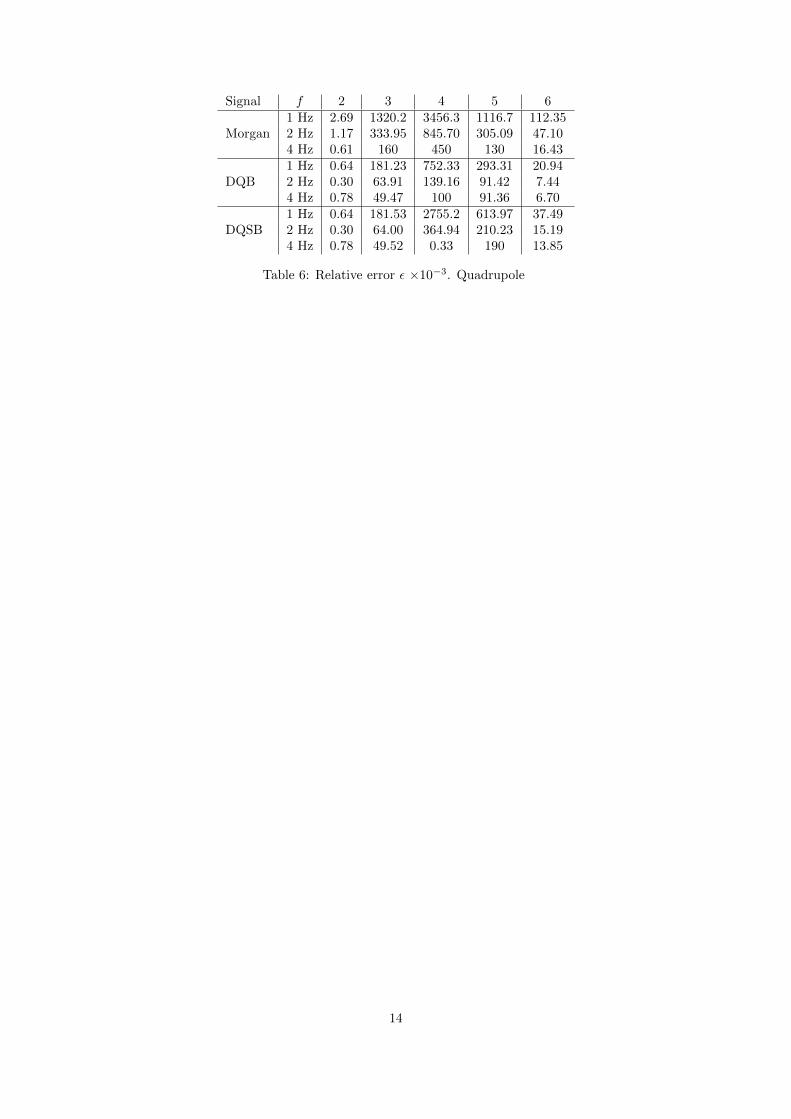
Signal f 2 3 4 5 6

Morgan1 Hz 2.69 1320.2 3456.3 1116.7 112.352 Hz 1.17 333.95 845.70 305.09 47.104 Hz 0.61 160 450 130 16.43

DQB1 Hz 0.64 181.23 752.33 293.31 20.942 Hz 0.30 63.91 139.16 91.42 7.444 Hz 0.78 49.47 100 91.36 6.70

DQSB1 Hz 0.64 181.53 2755.2 613.97 37.492 Hz 0.30 64.00 364.94 210.23 15.194 Hz 0.78 49.52 0.33 190 13.85

Table 6: Relative error ε ×10−3. Quadrupole

14

References

[1] M. Buzio. Fabrication and calibration of search coils. CERN-2010-004, pp. 387-421, 2011.

[2] J. DiMarco et al. Application of PCB and FDM Technologies to Magnetic Measurement ProbeSystem Development. 2012.

[3] J. DiMarco, D.J. Harding, V. Kashikhin, S. Kotelnikov, M. Lamm, A Makulski, R. Nehring, D. Orris,P. Schlabach, W. Schappert, C. Sylvester, M. Tartaglia, J. Tompkins, and G. V. Velev. A fast-sampling, fixed coil array for measuring the ac field of fermilab booster corrector magnets. AppliedSuperconductivity, IEEE Transactions on, 18(2):1633–1636, June 2008.

[4] L. Walckiers. Magnetic measurement with coils and wires. CERN-2010-004, pp. 357-385, 2011.

[5] Andrzej Wolski. Maxwell’s equations for magnets, 2011.

15