macroeconomic impacts of export barriers in a dynamic cge
TRANSCRIPT

Munich Personal RePEc Archive
Macroeconomic Impacts of Export
Barriers in a Dynamic CGE Model
Haqiqi, Iman and Bahalou, Marziyeh
University of Economic Sciences, University of Isfahan
June 2013
Online at https://mpra.ub.uni-muenchen.de/96404/
MPRA Paper No. 96404, posted 08 Oct 2019 09:04 UTC

Journal of Money and Economy Vol. 8, No.3 Summer 2013
Macroeconomic Impacts of Export Barriers
in a Dynamic CGE Model
Haqiqi, Iman
Bahalou Horeh, Marziyeh
Received: 5/21/2014 Approved: 12/14/2014
Abstract
A large economic literature discusses the implications of export sanctions
for a variety of states around the world. This paper investigates the macro-
level consequences of imposing oil export barriers on an oil exporting
country. We employ a large real financial computable general equilibrium
for Iran. The model is calibrated based on 1999 Social Accounting Matrix
for the economy of Iran including 112 commodities and 47 activities. We
find that the impact of a 50% negative shock in oil export would amount to a
4.6% reduction in GDP, a 6.8% fall in private consumption, a 20.2% cut in
government spending, a 20.4% decrease in import, a 9.9% contraction in
capital formation, and a +29.2% increase in non-oil export. We also find
that there is a conflict between government benefits and national benefit.
Our sensitivity analysis proves the robustness of the results.
Keywords: export barriers, government spending, capital formation,
Computable General Equilibrium, Social Accounting Matrix
JEL Classification: F51, F47, C68, E16
Assistant Professor, University of Economic Sciences, Tehran, [email protected]
Researcher, University of Isfahan

118 Money and Economy, Vol. 8, No. 3, Summer 2013
1. Introduction
The lower export levels expected by economic sanctions portend a cutback
in macroeconomic variables such as GDP, capital formation, government
spending, and private consumption. Since policy makers’ concern is the
shock’s incidence and impacts, the questions may arise that how much will
an economy suffer from a discriminatory export cut? What are the impacts
of a trade sanction on limited number of goods? What would happen in the
economy with lower export of one commodity?
The macroeconomic impacts of discriminatory export barriers are yet not
well understood, despite the contributions of many fine scholars. To measure
the detailed impacts and to answer the above arisen questions, it is required
to make a general equilibrium analysis of the shock. To this end,
policymakers need numerical information on incidence and impacts of the
shock. They concern mainly about GDP and other macro-level variables
which are well addressed in this study.
Theoretically, there are at least two opposite scale effects due to one
commodity export restriction. From one hand, cut in one commodity exports
may reduce the national income and decreases aggregate demand and
production. On the other hand, it makes the domestic currency cheaper.
Therefore, it stimulates the exports of other commodities and motivates
production. Depending on the size of these opposite effects in each sector,
production may rise or fall (we will discuss the transmission channels in
section 3). However, a multi sector comprehensive framework is required to
provide a complete analysis of the shock. To measure the macro-level
consequences of one commodity export shock, this paper performs a General
Equilibrium analysis. General Equilibrium structure provides an appropriate
framework to consider most of the direct and indirect effects of the shock
(Shoven and Whalley, 1992). To consider sectoral reallocation, we will
make the simulation by specific modeling of capital-labor substitution,
imperfect mobility of factors across sectors, sector specific capital, imperfect

Macroeconomic Impact of Export … 119
substitution of import and domestic products, and imperfect transformation
of export and domestic supply.
This paper investigates the impacts of imposing oil export barriers on
Iran as an oil exporting economy. Iran has experienced numerous export
sanctions. As Iranian government highly relies on oil revenue, the 2012
sanctions on Iran reduced public spending. Furthermore, it increased the
costs of imported commodities and the foreign exchange rate. This study
seeks to numerically measure the macro-level impacts of counterfactual
scenarios of a fall in oil export and a rise in exchange rate.
We calibrate our multi-sector general equilibrium model based on 1999
Social Accounting Matrix for the economy of Iran including 112
commodities and 47 activities. This rich database enables us to consider
most of the inter-sectoral linkages and reallocations in the economy.
The structure of the paper is as follows. The next section briefly
describes the literature. Then the theoretical backgrounds of the model and
the CGE framework are introduced in section 3. Section 4 introduces the
database. Section five then provides empirical results. Finally, discussion
and conclusions are provided in section six.
2. Economic Literature
2.1. Sanction and export barriers
There is a large qualitative literature on the impacts of economic sanctions
on the target states. Sanctions can negatively affect the access to food, clean
water, medicine and health care services (Cortright and Lopez, 2000; Weiss
et al., 1997; Garfield, 2002; Gibbons and Garfield, 1999). They may also
have a negative impact on life expectancy and infant mortality (Ali
Mohamed and Shah, 2000; Daponte and Garfield, 2000). Economic
sanctions may worsen the targeted government’s respect for human rights
(Peksen, 2009) and the level of democracy (Peksen and Drury, 2010).

120 Money and Economy, Vol. 8, No. 3, Summer 2013
However, research on the macroeconomic consequences of economic
sanctions is scarce. In a recent study, Neuenkirch & Neumeier (2014), find
that the imposition of UN sanctions decreases the target state’s real per
capita GDP growth rate by 2.3%–3.5%. While, comprehensive UN
economic sanctions, embargoes affecting nearly all economic activity,
trigger a reduction in GDP growth by more than 5%. Few empirical
researches exist on the impact of oil export sanction or other types of export
barriers. In most recent study, Yahia and Saleh (2008) have examined the
link between oil prices, economic sanctions and employment in Libyan
economy. In other studies, Jafarey and Lahiri (2002) have examined the
interaction between credit markets, trade sanctions, and the incidence of
child labor. Tarr (1989) developed a general equilibrium model to analyze
the welfare and employment effects of US quotas in textiles and steel. Black
and Cooper (1987) have illustrated how economic sanctions affect level and
distribution of welfare and employment in South Africa. Feenstra (1984)
have studied employment and welfare effects of voluntary export restraint on
U.S. autos as a form of trade barriers.
There is also some general equilibrium modeling efforts to analyze the
effects of NTBs1. Fugazza and Maura (2008) present previous general
equilibrium applications of the effects of NTBs. According to this survey,
the most comprehensive study made so far of the impact of NTBs in a CGE
model is Andriamanajara et al. (2004). Other important works are Gasiorek,
Smith and Venables (1992) and Harrison, Tarr and Rutherford (1994) and
Chemingui and Dessus (2007).
2.2. History of financial CGE modeling
The financial computable general equilibrium (FCGE) modeling started two
decades ago. In first version of Robinson model, one static model was
repeated at several periods and growth of stock variables has been defined in
1. Non-tariff Barriers

Macroeconomic Impact of Export … 121
every period. They usually were repeated in 5-10 periods (Robinson, 1991).
More complicated models have employed rational expectation models in
which households maximize their utility during the given period (Devarjan
and Go, 1998). In the recent years financial CGE models have received
increasing attention from researchers. Xiao and Wittwer (2009) use a
dynamic CGE model of China with a financial module and sectoral detail to
examine the real and nominal impacts of a nominal exchange rate
appreciation alone, fiscal policy alone and a combined fiscal and monetary
package to redress China's external imbalance. Li and Yang (2012) use a
financial CGE model to analyze real and financial sectors interaction in
China’s economy. They have considered the wage rigidity as a failure of the
labor market. The results show that wage rigidity has meaningful effects on
the results of their study. In another study, Lemelin, et al. (2013) have
presented an applied computable general equilibrium world model with
financial assets and endogenous current account, and capital and financial
account balances. In their simulations, the interaction of portfolio choices
with trade supply and demand behavior leads to endogenous sign reversals in
some current account balances, and it results in a different allocation of
investment among regions.
Two applied studies have been conducted in Iran using financial
computable general equilibrium model. In the first study, Haqiqi (2011) has
developed Shahmoradi et al. (2010) model. He described how to model
financial variables in computable general equilibrium models with different
approaches. In his study various approaches of modeling a financial CGE
have been introduced. Then, based on three different approaches, three
financial models have been compared. Overall, comparing the results of
different scenarios suggest that static financial CGE and stock adjustment
models give more realistic results than flow equilibrium models. The other
study was carried out by Salami and Javanbakht, (2011); they have presented

122 Money and Economy, Vol. 8, No. 3, Summer 2013
a real-financial CGE model for the economy of Iran and used it to examine
the effects of reducing interest rate of credits on investment and growth.
Their results showed that following a reduction in interest rate of credits, the
prices of commodities and services declined which resulted in reduction of
inflation rate by 0.53%. In addition, households’ income and savings
increased by 0.54 and 7.83%, respectively.
To our knowledge, our paper is the first study in Iran in which a large
dynamic financial CGE model with multi-assets and various financial
markets is employed. Although Haqiqi (2011) develops some dynamic
models, the models are too aggregated and include only two or three
production sectors. CGE model in Salami and Javanbakht (2011) is a static
model without any financial market. Although a considerable body of
research has been carried out in Iran employing CGE models, a small
number of studies test the sensitivity of their results. In this research, we
conduct a sensitivity analysis to prove the robustness of our findings.
Furthermore, the present paper provides important insights in regard to
the effects of oil export barriers on non-oil export and other macroeconomic
variables.
3. Theory and the Model
Reduction in oil exports has two opposite “scale effects” in the economy.
One effect tends to reduce the production and employment level while the
other tends to motivate export, production, and employment. The country
may also face a “substitution effect”, “reallocation effect”, and a change in
production mix. We describe these effects in the following paragraphs.
The first impact of a fall in oil exports is “shrinking effect” or “negative
scale effect”. A fall in the oil exports would lead to a substantial demand
deficit. It is plausible that the government expenditure decreases. According
to macroeconomic theory, decline in public expenditure brings a fall in
aggregate demand in the country, which may shrink economic activity and

Macroeconomic Impact of Export … 123
employment in short run (Mankiw, 2012). The effect will be intensified
when the cost of imported input rises and activity levels fall.
The second impact is an “expansion effect” or “positive scale effect”,
and happens due to increase in foreign exchange rate and import
substitution. Since, fall in oil exports would diminish supply of export
dollars (or any other foreign currency) a shortage in foreign currency would
increase the foreign exchange rate. According to economic theory, the rise in
the foreign exchange rate would foster non-oil export expansion. The more
the change in export of a commodity is, the more the change in activity level
and employment will be expected in that sector. On the other hand, the rise
in import prices would increase the demand for domestically produced goods
and services. Hence, it would have also a positive impact on the activity and
employment levels (James, Marsh, Sarno, 2012).
There would also be a third “reallocation effect” or a substitution
towards tradable sectors, especially those sectors with more exports share.
When this occurs, the changes in exchange rate will motivate more non-oil
exports by bringing more profit than before. Therefore, the production
resources re-allocate towards more non-oil export. As a result, labor and
capital would move to tradable sectors and to more exporting sectors.
We also expect a “substitution effect” due to import price increase. It
occurs when exchange rate increases and the imported commodities seem to
be more expensive. Hence, people prefer to buy domestic goods instead of
foreign goods (Hertel, 1998), which may encourage domestic production and
employment.
The economy might also face changes in the labor market. According to
Neoclassical Theory of labor supply, the choice between consumption and
leisure depends on wages and prices (Cahuc and Zylberberg, 2004). Hence,
the supply of skilled labor would change due to change in the price of
consumption goods after the shock in import prices.

124 Money and Economy, Vol. 8, No. 3, Summer 2013
On the other hand, changes in wages and prices would influence the
production technology. Depending on the changes in relative prices for each
sector, it would adjust toward more labor-intensive or more capital-intensive
technology.
However, the overall effect of oil export barriers on macroeconomic
variables is unknown and requires numerical calculations.
3.1. Optimizations in a typical CGE Model
We consider an economy comprising multiple activities indexed by
47,...,1Ss , multiple commodities indexed by 112,...,1Gg , and
multiple institutions indexed by oilfcocorgovconHh ,,,, . Each
activity employs two factors of production, labor and capital, which can be
used to produce different commodities. Factors are heterogeneous and
imperfectly mobile across sectors. Nf,h denotes the total endowment of each
factor f owned by institution h. The model has a nested structure in which
there is an optimization behavior in each nest.
Inter-temporal preferences: In this model, we have assumed that
agent’s action is based on inter-temporal optimization behavior. There is a
representative household whose objective is to find his lifetime optimal
consumption path. This agent derives utility from consuming “composite
commodity” at each period of time, Ct. (note that the combination of this
composite commodity is determined through another optimization in
“expenditures”). The lifetime maximization problem to determine composite
consumption in each period is known as Ramsey problem:
1
11
, ,max h h t h tU C (1)
, , ,
. .
(1 )
t h t t h t h t
h tt
s t
PL L PK K TRY
(2)

Macroeconomic Impact of Export … 125
where t is time periods, Uh is utility function of households, Ch,t denotes
household composite consumption in period t, α shows the CES1 parameter,
θ shows relative risk aversion parameter, Y is the lifelong income, PL is
wage of labor, PK displays capital return, TR stands for transfer payments,
and ρ displays discount factor. Note that θ is the inverse of inter-temporal
elasticity of substitution. In other words, we assume a substitution between
today consumption and future consumption. Expenditure: Aggregate consumption, Ch,t, depends on the consumption
of each commodity, QCg,h,t. Representative agent minimizes the cost of
consumption bundle in each period. Household’s consumption is a CES
aggregator of different goods and services. This agent minimizes the cost of
preparing the aggregate bundle at each period of time:
, , ,
11 1
, , , ,
min .
. .
h
h h
h h
g t g h t
g
h t g h g h t
g
PC QC
s t C QC
(3)
where PCg,t denotes price index of each commodity at each period, C is
aggregate consumption, QC is consumption demand for each good or
service, φ is share parameter, σ is the elasticity of substitution, g refers to
goods and services, and h refers to households. Cost minimization by
households at each period of time requires that:
,
, , , ,
,
1
11
, , , ,
h
h
h
h t
g h t g h h t
g t
h t g h g h t
g
CPIQC C
PC
CPI PC
(4)
1. Constant Elasticity of Substitution
126 Money and Economy, Vol. 8, No. 3, Summer 2013
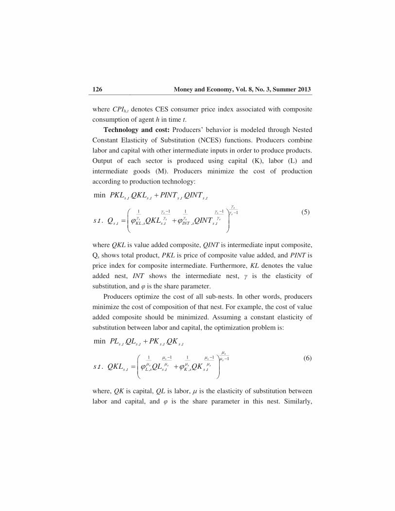
where CPIh,t denotes CES consumer price index associated with composite
consumption of agent h in time t.
Technology and cost: Producers’ behavior is modeled through Nested
Constant Elasticity of Substitution (NCES) functions. Producers combine
labor and capital with other intermediate inputs in order to produce products.
Output of each sector is produced using capital (K), labor (L) and
intermediate goods (M). Producers minimize the cost of production
according to production technology:
, , , ,
1 11 1 1
, , , , ,
min . .
. .
s
s s s
s s s s
s t s t s t s t
s t KL s s t INT s s t
PKL QKL PINT QINT
s t Q QKL QINT (5)
where QKL is value added composite, QINT is intermediate input composite,
Qs shows total product, PKL is price of composite value added, and PINT is
price index for composite intermediate. Furthermore, KL denotes the value
added nest, INT shows the intermediate nest, γ is the elasticity of
substitution, and φ is the share parameter.
Producers optimize the cost of all sub-nests. In other words, producers
minimize the cost of composition of that nest. For example, the cost of value
added composite should be minimized. Assuming a constant elasticity of
substitution between labor and capital, the optimization problem is:
, , , ,
1 11 1 1
, , , , ,
min . .
. .
s
s s s
s s s s
s t s t s t s t
s t L s s t K s s t
PL QL PK QK
s t QKL QL QK
(6)
where, QK is capital, QL is labor, is the elasticity of substitution between
labor and capital, and φ is the share parameter in this nest. Similarly,
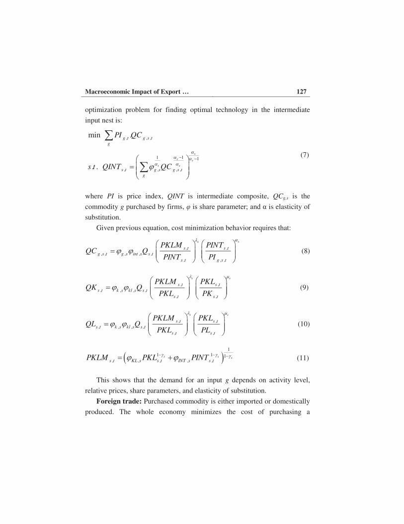
Macroeconomic Impact of Export … 127
optimization problem for finding optimal technology in the intermediate
input nest is:
, , ,
11 1
, , , ,
min .
. .
s
s s
s s
g t g s t
g
s t g s g s t
g
PI QC
s t QINT QC
(7)
where PI is price index, QINT is intermediate composite, QCg,s is the
commodity g purchased by firms, φ is share parameter; and α is elasticity of
substitution.
Given previous equation, cost minimization behavior requires that:
, ,
, , , , ,
, , ,
ss
s t s t
g s t g s int s s t
s t g s t
PKLM PINTQC Q
PINT PI
(8)
, ,
, , , ,
, ,
s s
s t s t
s t k s kl s s t
s t s t
PKLM PKLQK Q
PKL PK (9)
, ,
, , , ,
, ,
s s
s t s t
s t k s kl s s t
s t s t
PKLM PKLQL Q
PKL PL (10)
11 1 1
, , , , ,s s s
s t KL s s t INT s s tPKLM PKL PINT (11)
This shows that the demand for an input g depends on activity level,
relative prices, share parameters, and elasticity of substitution.
Foreign trade: Purchased commodity is either imported or domestically
produced. The whole economy minimizes the cost of purchasing a

128 Money and Economy, Vol. 8, No. 3, Summer 2013
commodity. Assuming imperfect substitution between domestic commodity
and imports (Armington, 1969), the optimization is:
1 1
, , , ,
1 1 1
, , , , ,
min . .
i
i i ii i
i i
i t i t i t i t
i t d i i t m i i t
PD QD PM QM
QTD QD QM (12)
where PD is price index for domestic commodity, PM is import price index,
QTD shows the Armington aggregator (total demand for commodity i), φ is
share parameter, and β is Armington elasticity of substitution. Given this
assumption, optimization requires that:
11 1 1
, , , ,
, , ,
,
, ,.
i
i i id i i t m i i t
i t m i i t
i t
i t t i t
PD PMQM QTD
PM
PM PFX PMF
(13)
where PFX is the index of foreign exchange rate and PMF is the foreign
price of imported commodity. According to this equation, the demand for
importing commodity i depends on total domestic demand, relative price of
imported commodity, Armington elasticity, and share of import in total
supply of commodity i. Similarly, the demand for domestically produced
commodity is:
11 1 1
, , , ,
, , ,
,
i
i i id i i t m i i t
i t m i i t
i t
PD PMQD QTD
PD (14)

Macroeconomic Impact of Export … 129
Likewise, domestic demand for domestically produced good depends on
total domestic demand, relative price of domestic products to imports,
Armington elasticity, and share of import in total supply of commodity i.
Armington aggregator determines the weighted price of domestically
purchased commodity. The price index possesses a CES form as follows:
11 1 1
, , , , ,g g g
g t d g d t m g m tP PD PM (15)
Domestically produced commodities are either exported to other
countries or supplied domestically. Producers choose to supply overseas or
at home according to the possibility of transformation and relative prices.
Assuming a Constant Elasticity of Transformation (CET) function for each
commodity:
1 1
, , , ,
1 1 1
, , , , ,
max . .
i
i i ii i
i i
i t i t i t i t
i t d i i t x i i t
PD QD PX QX
QTO QD QX
(16)
where PD, QD, PX, and QX denote domestic supply price index, quantity of
domestic supply, export price index, and quantity of export, respectively.
QTO shows the total output, θ is share parameter, and λ<0 is the elasticity of
transformation. Let PXF denote the foreign price index of exported
commodity. Solving this optimization problem, we obtain the following
expression for supply of a commodity to foreign countries:
11 1 1
, , , ,
, , ,
,
, ,.
i
i i ix i i t d i i t
i t x i i t
i t
i t t i t
PX PDQX QTO
PX
PX PFX PXF
(17)

130 Money and Economy, Vol. 8, No. 3, Summer 2013
Given our assumption about export, the optimization behavior yields
the supply of commodity i to domestic market:
11 1 1
, , , ,
, , ,
,
i
i i ix i i t d i i t
i t d i i t
i t
PX PDQD QTO
PD (18)
Note that λ measures the extent of technical possibility of transforming
export to domestic supply. Given our assumptions about trade and
technology, the nested form of production sector is shown in Figure 1.
Factor mobility: Factors are neither perfectly mobile nor specific at
each sector. We assume that factors of production are not homogenous. In
other words, it is not easy to move freely across sectors. A CET type
function is able to demonstrate imperfect factor mobility. Let τ<0 denote the
ease of movement across sectors. A factor owner chooses to supply factor f

Macroeconomic Impact of Export … 131
to sector s (QFf,s) according to factor endowment level (QN), sectoral factor
wages (PF), and the possibility of move across sectors. Given these
assumptions, the optimization behavior is:
1
, , , ,
1 147
, , , , ,
1
max
f
f ff
f
f s t f s t
s
f h t f s f s t
h s
PF QF
QN QF
(19)
Solving this equation, we obtain the optimum supply of each factor to
each sector as:
,
, , , , ,
, ,
147 1
1
, , , ,
1
f
ff
f t
f s t f s h f t
h f s t
f t f s f s t
s
PNQF QN
PF
PN PF
(20)
where PN is the CET weighted average of factor wages across sectors.
Saving and investment: The saving behavior of agents depends on
consumption at each time period. Agents are maximizing their consumption
and equating the marginal benefit of today consumption with that of
consumption in the future. Thus, the saving at each time period is
determined by:
, , ,h t h t h tS Y C
where S shows the amount of saving and Y denotes the total income of agent
h at each time t.
At each period of time, agents may also borrow funds from financial
markets. These funds plus savings are used either to make physical capital

132 Money and Economy, Vol. 8, No. 3, Summer 2013
formation which is called investment, or to purchase domestic and foreign
financial assets (supply of loanable funds). This condition requires that:
, , , , ,h t h t h t h t h tI VTA VNCO S VBOR
where VTA is the total value of domestic financial portfolio, VNCO
demonstrates the total value of foreign financial portfolio (net capital
outflow), and VBOR is total amount of borrowing. These are explained in
the following paragraphs.
Financial portfolio: We consider a financial market comprising multiple
assets indexed by “a” (deposit, loan, bond, equity, etc.). Each agent seeks to
maximize the return to financial portfolio and decides how to supply
loanable funds. We assume imperfect substitution between financial assets
as in reality they are not similar in risk and return . It allows to consider how
purchasing of different assets may change due to change in relative return of
assets. The optimization behavior in financial portfolio is:
,
, ,1 ,
,
, , ,
1 1
, , , ,
max
a h
a h a ha h
a h
a t a h t
a
h t a h a h t
a
r VFA
VTA VFA
where VTA is the total value of financial portfolio, VFA denotes the value of
purchasing each asset, r shows the assets’ return, σ<0 is substitution
elasticity among assets, and θ is share parameter. Solving this problem, we
obtain optimum value of each asset in the portfolio (supply of loanable
funds) as:
1. Tobin, James (1969). “A General Equilibrium Approach to Monetary Theory.” Journal of
Money, Credit, and Banking, 1:1, 15—29

Macroeconomic Impact of Export … 133
,
,,
17 1
1
, , , , , , ,
1
a h
a ha h
a h t a h h t a h a t a t
a
VFA VTA r r
Borrowing channels: Agents can borrow through various assets
(demand of loanable funds). We assume that borrowers are minimizing their
cost of finance. Given this assumption, the optimization equation is:
,
, ,1
,,
, . , .
1 1
. , , .
min
a h
a h a ha h
a h
a h t a h t
a
i t a h a h t
a
rr VBA
VBOR VBA
in which, rr is the interest rate of each asset (channel of borrowing), VB
shows the amount of borrowing through each asset, VBOR demonstrates
total borrowing, β is share parameter, γ denotes elasticity of substitution
among channels of finance. This optimization leads to optimum borrowing
for agent h as: ,
,,
1
11
, . , . , , . , .
a h
a ha h
a h t a h i t a h a h t a h tVB VBOR rr rr
Sectoral investment decision: Physical capital formation is made in
different sectors. Agents minimize the cost of purchasing capital composite
commodity in production sectors. Therefore, the optimization behavior is:
,
, ,1 ,
,
, , ,
1 1
, , , ,
min
k h
k h k hk h
k h
k t k h t
k
h t k h k h t
i
PK QK
I QK
where I is the total amount of capital formation by each agent h, PK is the
cost of capital composite commodity in sector k, QK amount of capital

134 Money and Economy, Vol. 8, No. 3, Summer 2013
formation by each agent h at each sector k, θ shows share parameter, and σ is
the substitution possibility. Solving this problem, we obtain the optimum
investment by each agent at each sector:
,
,,
1
11
, , ,
k h
k hk h
k h k h h k h k kQK VTK PK PK
3.2. Equilibrium conditions in a typical CGE Model
In equilibrium, all consumers maximize their utility; all firms minimize their
costs, and all markets clear. Market clearing for each factor f requires that
total supply of that factor by households equals total demand of that factor
by firms:
, , , ,f h t f s t
h s
QN QF
(21)
Similarly, Market clearance for each commodity requires that total
supply equals total demand. Given the structure of our model, total supply is
determined by import and domestic production (other models may have
inventory reduction). Total demand is determined by firms’ purchases,
institutions’ purchases, and export (capital formation and increase in
inventory is done by institutions). Therefore, market clearing condition for
commodity g requires that:
, , , , , , , ,g t g s t g s t g h t g t
s s h
QM QO QC QC QX
(22)
Finally, for each asset a, and in each period of time t, the equilibrium
condition requires that:
, , , ,a h t a h t
h h
VBA VFA

Macroeconomic Impact of Export … 135
3.3. Model dynamics and calibration
In the CGE literature the calibration of the single-period equilibrium is
straightforward. But, calibration procedure of dynamic models needs more
attention. Calibration in a dynamic context generally means the model is
parameterized in such a way that the balanced growth path is simulated
when the base policy is maintained (Pereira and Shoven 1988). For
specifying CGE models all the markets are assumed to be in equilibrium.
Then, the parameters of the model are chosen through a calibration
procedure. Calibration of the model involves specifying values for certain
parameters based on outside estimates, and deriving the remaining ones from
the restrictions posed by the equilibrium conditions. Thus, it is assumed that
the benchmark data base reflect period equilibrium. The calibrated parameter
values can then be used to solve the model for alternative equilibrium
associated with exogenous changes in policy variables. The so-called
“counterfactual” scenarios are imposed on the model to explore and evaluate
the impacts of different policy measures and shocks by comparing the results
of the benchmark equilibrium with the counterfactual (Springer, 1999).
Our dynamic CGE model can also be interpreted as a sequence of
counterfactuals to the base year run by altering the factor endowments
holding everything else constant. The first step in calibration of the dynamic
model is the same as in the static case. After having calibrated the
benchmark period of the model, the dynamics come in by updating the factor
endowments after every time step. We assume a constant growth rate for
labor endowment. In other words, labor supply evolves exogenously over
time. The labor endowment in first period is given by L0. Let n denotes the
labor growth rate. Therefore, labor supply at each period will be:
, , 1 1h t h tL L n (21)
Current period’s investment augments the capital stock in the next
period. Capital stock in each time period is updated by an accumulation

136 Money and Economy, Vol. 8, No. 3, Summer 2013
function equating the next period capital stock to the sum of depreciated
capital stock of the current period and the current period real investment.
, 1 , ,(1 )h t h t h tK K I
(22)
where δ denotes the rate of capital depreciation; K is capital stock and I
shows the investment.
The equilibrium in any sequence is connected to each other through
capital accumulation and labor growth. Each single period equilibrium
calculation begins with an initial labor and capital services endowment
resulting from the end of the period t-1. A new equilibrium of supply,
demand and relative prices is calculated for the next time period t based on
the exogenous and endogenous changes in endowments. Savings of the
current period t will augment the capital-services endowment at the end of
period t available in the next period t+1. Finally, lifetime decision comes in.
Households choose the consumption level at each period according to inter-
temporal relative prices and lifetime income. Our model is programmed in
the GAMS (Generalized Algebraic Modeling System) / MPSGE
(Mathematical Programming System for General Equilibrium analysis)
language (Rutherford, 1999).
Starting from the initial steady state, we shock the economy through a
parametric decline of oil export. We observe that all endogenous variables
converge to their steady state level in the period immediately following
the shock.
4. Data
CGE models generally use two kinds of data as their database: the first are
share and sectoral interaction parameters and the second are exogenous
parameters such as elasticity of substitution. Share parameters are calibrated
based on 1999 Iranian Social Accounting Matrix (SAM), while other

Macroeconomic Impact of Export … 137
parameters are obtained using other sources rather than SAMs. Table 1
shows the amount of exogenous parameters and the sources which we have
used to obtain these parameters.
Table 1: Exogenous parameters in the model
Parameter Level Source
Population growth rate 1.29% Statistical Center of Iran, 2011
Relative risk aversion parameter 1.5 Tavakolian, 2012
Time preference rate 0.96 Tavakolian, 2012
Depreciation rate 4.2% Amini and Haji Mohammad, 2005
In addition to exogenous parameters, we need additional data describing
both interaction between economic sectors and agents, and interaction
between real and financial sectors. Since 1999 SAM for Iran has all this
features, we use this database in our model calibration.
A Social Accounting Matrix is a descriptive tool which represents details
of the economy according to System of National Accounts. The SAM is a
square matrix which contains all the interactions and monetary flows
between economic agents and sectors. Table 2 shows the aggregated form of
1999 SAM for Iran. In this matrix, each cell shows the payment from the
account of its column to the account of its row. Therefore, the incomes of an
account appear along its row; and its expenditures appear along its column
(Pyatt, 1999).

138 Money and Economy, Vol. 8, No. 3, Summer 2013

Macroeconomic Impact of Export … 139
This SAM is appropriate for dynamic modeling as it involves detailed
information about saving, capital, and financial accounts. This matrix
includes the interaction between saving, capital formation, and net capital
flow. The intersection of the saving account and capital formation account
shows how each economic agent holds new investment. Generally, portfolio
of each agent includes fixed capital formation and financial assets. As Table
3 indicates, the value of households’ investment is 4599 billion Rls
(domestic currency) in agricultural sector, while it is 205066 billion Rls in
construction sector; likewise, households investment is 22744 billion Rls in
the form of cash and deposits and is 3310 billion Rls in the form of securities
such as bonds.
Table 3: The portfolio formation matrix
Household Government Oil and
gas
Non-
financial
firms
Financial
firms
Fixed
capital
formation
Agriculture 4599 1596
Oil and gas 10533
Other mining 31 658
Industry 6841 15228
Electricity, water and gas 194 7376
Construction 86 344
Transportation 9745 10367
Communications 3623
Estates 20506 2879
Other services 11541 6360 13878 1903
Financial
assets’
Monetary gold and SDR 1192
Cash and deposits 22744 3970 2312 20731 7381
Securities except for
shares 3310 -464
Facilities and loans 8448 1007 54100
Shares and similar assets 2035 5682 1603 7276 538
Other receivable/payable
accounts -389 1036 16415 53336 10544
Source: CBI (2004)
140 Money and Economy, Vol. 8, No. 3, Summer 2013
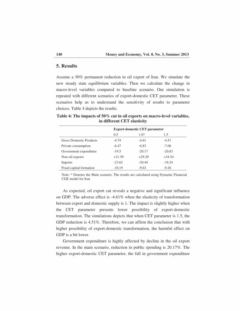
5. Results
Assume a 50% permanent reduction in oil export of Iran. We simulate the
new steady state equilibrium variables. Then we calculate the change in
macro-level variables compared to baseline scenario. Our simulation is
repeated with different scenarios of export-domestic CET parameter. These
scenarios help us to understand the sensitivity of results to parameter
choices. Table 4 depicts the results.
Table 4: The impacts of 50% cut in oil exports on macro-level variables,
in different CET elasticity
Export-domestic CET parameter
0.5 1.0* 1.5
Gross Domestic Products -4.74 -4.61 -4.51
Private consumption -6.47 -6.83 -7.06
Government expenditure -19.5 -20.17 -20.83
Non-oil exports +21.59 +29.20 +34.54
Imports -23.62 -20.44 -18.24
Fixed capital formation -10.19 -9.63 -9.26
Note: * Denotes the Main scenario. The results are calculated using Dynamic Financial
CGE model for Iran
As expected, oil export cut reveals a negative and significant influence
on GDP. The adverse effect is -4.61% when the elasticity of transformation
between export and domestic supply is 1. The impact is slightly higher when
the CET parameter presents lower possibility of export-domestic
transformation. The simulations depicts that when CET parameter is 1.5, the
GDP reduction is 4.51%. Therefore, we can affirm the conclusion that with
higher possibility of export-domestic transformation, the harmful effect on
GDP is a bit lower.
Government expenditure is highly affected by decline in the oil export
revenue. In the main scenario, reduction in public spending is 20.17%. The
higher export-domestic CET parameter, the fall in government expenditure

Macroeconomic Impact of Export … 141
is higher. Given the fact that exchange rate is higher when the CET
parameter is low (due to more foreign exchange supply from more non-oil
export); our results show a very important finding. Although government of
Iran is highly dependent on oil export revenue, the government can avoid the
revenue loss if the exchange rate is higher. That means the government may
seek to keep the foreign exchange rate high.
In contrast, we find that non-oil export increases due to 50% fall in oil
export. In the main scenario, the positive jump in non-oil export is equal to
29.20%. Furthermore, when the export-domestic CET parameter is higher,
the rise in non-oil export is also higher. When the CET parameter is 1.5, the
rise in non-oil export is 34.54%. In short, fall in oil export will increase the
foreign exchange rate and motivates non-oil exports.
To test the sensitivity of our results to other parameters, we repeat the
simulation with different levels of various parameters. The analysis proves
the robustness of the results. The only exception is Armington elasticity. The
results are a bit sensitive to Armington parameter (substitution elasticity
between import and domestic products). Table shows the simulation results
with different Armington parameter.
Table 5: The impacts of 50% cut in oil exports on macro-level variables
in different Armington elasticity
Import-domestic Armington parameter
0.5 1.0* 1.5
Gross Domestic Products -4.73 -4.61 -4.52
Private consumption -6.67 -6.83 -6.95
Government expenditure -19.60 -20.17 -20.58
Non-oil exports +33.52 +29.20 +26.14
Imports -16.37 -20.44 -23.38
Fixed capital formation -9.94 -9.63 -9.42
Note: * Denotes the Main scenario. The results are calculated using Dynamic Financial CGE
model for Iran.

142 Money and Economy, Vol. 8, No. 3, Summer 2013
We find that reductions in GDP, consumption, public spending, and
capital formation are not much affected by Armington elasticity. However,
when the possibility of import-domestic substitution is low, GDP loss is
higher. When Armington elasticity is low, the export jump is also higher.
There is a good explanation for our results. As import is the demand side in
foreign exchange market, lower Armington parameter leads to higher foreign
exchange rate. This is because the possibility of import adjustment (foreign
exchange reduction) is lower.
Table 6: The impacts of different scenarios of reduction in oil exports on
macro-level variables
10% 25% 50% 75% 90%
Gross Domestic Products -1.1 -2.7 -4.61 -5.6 -6.0
Private consumption -1.3 -3.4 -6.83 -9.6 -11.2
Government expenditure -3.8 -9.9 -20.17 -28.4 -31.1
Non-oil exports +6.8 +16.2 +29.20 +35.7 +33.9
Imports -5.2 -12.0 -20.44 -25.8 -28.5
Fixed capital formation -2.3 -5.4 -9.63 -12.8 -14.5
Note: The results are calculated using Dynamic Financial CGE model for Iran.
We also simulate other scenarios of permanent oil export cut (10%, 25%,
75%, and 90%). As shown in Table 6, we find that a 10% permanent
reduction in oil export leads to 1.1% steady state GDP loss. While GDP loss
is 2.7% in 25% oil export fall, it is calculated 6.0% in 90% oil export
reduction. With a 90% reduction in oil export, the reduction in private
consumption is 11.2%; the fall in government expenditure is 31.1%; imports
decrease by 28.5%; and capital formation reduces by 14.5%. In this scenario,
the increase in non-oil export is 33.9%.
6. Conclusion
In order to gain a complete understanding of impacts of reduction in oil
exports, it is useful to conduct a Computable General Equilibrium

Macroeconomic Impact of Export … 143
framework that examines all aspects of the shock including direct and
indirect effects. Theoretically, export barriers would have two opposite
effects: “Shrinking Effect” due to fall in oil export and rise in import costs,
and “Expansionary Effect” due to increase in the foreign exchange rate and
export growth.
The current CGE analysis demonstrates that a 50% decline in oil export
would amount to a 4.6% reduction in GDP, a 6.8% fall in private
consumption, a 20.2% cut in government spending, a 20.4% decrease in
import, a 9.9% contraction in capital formation, and a 29.2% increase in
non-oil export. Our results are robust to modification of exogenous
parameters and possibility of substitution and transformation in different
markets.
This study finds that lower possibility of substitution between domestic
and imported commodities, would lead to slightly higher GDP loss but
definitely higher non-oil exports. We find that exchange rate is significantly
important in this analysis. As import of goods and services would form the
demand side in foreign exchange market, lower Armington parameter would
lead to lower possibility of adjustment and import reduction. Therefore,
higher foreign exchange rate is expected.
Our results suggest that when transformation elasticity between export
and domestic supply is low, GDP loss is higher and Jump in non-oil export is
lower. It seems that this happens due to a lower expansionary effect. In other
words, the expansionary effect depends on the possibility of transformation
between export and domestic supply.
We found that there is a conflict between government benefits and
national benefits. Although higher possibility of substitution would reduce
the GDP loss, the government loss would be less in lower CET and
Armington elasticity. This may prevent the government to motivate export or

144 Money and Economy, Vol. 8, No. 3, Summer 2013
import substitution. An interesting finding is that government may prefer to
keep the foreign exchange rate higher to compensate its lost revenue.
A useful extension of this work would be to discover the sectoral
consequences of export sanctions. Another interesting research is the
influence of export reduction on poverty and income distribution. The
impact of sanctions on labor market and migration are other subjects of
interest.
References
Ali Mohamed, M. and I. Shah, (2000).” Sanctions and childhood mortality in
Iraq”, Lancet 355, 1851–1856.
Amini, A., & N. Haji Mohammad, (2005). “Time series estimation of capital
stock in the Iranian economy”. Journal of Management and budget.
Andriamananjara, S, J. Dean, R. Feinberg, M. Ferrantino, R. Ludema, & M.
Tsigas, (2004). “The Effects of Non-tariff Measures on Prices, Trade and
Welfare: CGE Implementation of Policy-based Price Comparisons. U.S
International Trade Commission”, Office of Economics, Working Paper No.
2004-04.A.
Armington, P., (1969). “A theory of demand for products distinguished by
place of production”, IMF Staff Papers, 16: 159-178.
Black, P., & H. Cooper, (1987). “On the Welfare and Employment Effects of
Economic Sanctions”. South African Journal of Economics(55), 1-15.
Cahuc, P., A. Zylberberg, (2004). Labor Economics, The MIT Press,
Cambridge.
CBI (Central Bank of Iran). (2004). The 1999 Social Accounting Matrix.
Chemingui, M., & S. Dessus, (2008). “Assessing Non-Tariff Barriers to
Trade in Syria”. Journal of Policy Modeling, 917-928.

Macroeconomic Impact of Export … 145
Cortright, D. and G. Lopez, eds. (2000). The sanctions decade: Assessing
UN strategies in the 1990s, Boulder, CO: Lynne Rienner.
Daponte, B. and R. Garfield, (2000). “The effect of economic sanctions on
the mortality of Iraqi children prior to the 1991 Persian Gulf War”, American
Journal of Public Health 90(4), 546–552.
Feenstra, R. C. (1984). “Voluntary Export Restraint in U.S. Autos, 1980-81:
Quality, Employment, and Welfare Effects. In R. E. Baldwin, & A. O.
Krueger, The Structure and Evolution of Recent U.S”. Trade Policy (pp. 35-
66). University of Chicago Press.
Fugazza, M., & J. C. Maur, (2008). Non-Tariff Barriers in Computable
General Equilibrium Modelling. Policy Issues in International Trade and
Commodities (pp. 1-14). New York and Geneva: United Nations Publication.
Garfield, R. (2002). “Economic sanctions, humanitarianism and conflict
after the Cold War”, Social Justice 29(3), 94–107.
Gasiorek, M, A. Smith, & A. Venables, (1992). “1992” Trade and Welfare-
A General Equilibrium Model. In Winters LA, Trade Flows and Trade Policy
After "1992". Cambridge, UK: Cambridge University Press.
Gibbons, E. and R. Garfield, (1999). “The impact of economic sanctions on
health and human rights in Haiti 1991–1994”, American Journal of Public
Health 89(10), 1499–1504.
Haqiqi, I. (2011). Modelling financial variables in a computable general
equilibrium model. Monetary and Banking Research Institute, Iran.
Harrison, G, D. Tarr, & T. Rutherford, (1994). “Product Standards,
Imperfect Competition, and the Completion of the Market in the European
Union”. World Bank Policy Research Working Paper No. 1293.
Hertel, T.W., (1998). Global Trade Analysis: Modeling and Applications.
Cambridge University Press, Cambridge and New York.

146 Money and Economy, Vol. 8, No. 3, Summer 2013
Jafarey, S, & S. Lahiri, (2002). “Will trade sanctions reduce child labor? The
role of credit markets”. Journal of Development Economics, 137-156.
James, J., Marsh, I., Sarno, L., 2012. Handbook of Exchange Rates. Wiley
and Sons, New York and London.
Lemelin, A., V. Robichaud, & B. Decaluwé, (2013). “Endogenous current
account balances in a world CGE model with international financial assets.”
Economic Modeling, 146-160.
Li, Meng and Yang Liang, (2012). “Rigid wage-setting and the effect of a
supply shock, fiscal and monetary policies on Chinese economy by a CGE
analysis”. Economic Modelling, Vol. 29, Issue 5, September 2012, Pages
1858-1869.
Mankiw, N. G., (2012). Principles of Macroeconomics. 6th ed, Cengage
Learning. Harvard University Press.
Neuenkirch, Matthias & Neumeier, Florian, (2014). “The Impact of UN and
US Economic Sanctions on GDP Growth”. Research Papers in Economics
2014-08, University of Trier, Department of Economics.
Neumeyer, P. A., & F. Perri, (2005). “Business Cycles in Emerging
Economies: The Role of Interest Rates”. Journal of Monetary Economics,
345-380.
Peksen, D. (2009). “Better or worse? The effect of economic sanctions on
human rights”, Journal of Peace Research 46(1), 59–77.
Peksen, D. and A. C. Drury, (2010). “Coercive or corrosive: The negative
impact of economic sanctions on democracy”, International Interactions
36(3), 240–264.
Pereira, A.M., J. B. Shoven, (1988). “Survey of dynamic computable general
equilibrium models for tax policy evaluation”, Journal of Policy Modeling,
10(3):401-436.

Macroeconomic Impact of Export … 147
Pyatt, Graham, (1999). “Some Relationships between T-Accounts, Input-
Output Tables and Social Accounting Matrices”, Economic Systems
Research, Taylor and Francis Journals, vol. 11(4), pages 365-387.
Robinson, S., (1991). “Macroeconomics, Financial Variables, and
Computable General Equilibrium Models.” World Development 19 (11),
1509-1525.
Rutherford, T. F., (1994). “General Equilibrium modeling with MPSGE as a
GAMS Subsystem’”, mimeo, Department of Economics, University of
Colorado.
Rutherford, T. F., (1999). “Applied General Equilibrium Modeling with
MPSGE as a GAMS Subsystem: An Overview of the Modeling Framework
and Syntax”. Computational Economics, 1-46
w
Salami, H., & O. Javanbakht, (2011). “Comparing Effects of Two Policies
Reducing Interest Rate and Increasing Supply of Credits on Growth of
Production in Iran: A FCGE Analysis”. Journal of Economics and
Agricultural Development.
Shahmoradi, A., I. Haqiqi, & R. Zahedi, (2010). “Modelling a computable
general equilibrium model for Iran”. Ministry of Economic Affairs
and Finance.
Shoven, J. B., J. Whalley, (1992). Applying general equilibrium. New York:
Cambridge University Press.
Springer, Katrin (1999). “Climate Policy and Trade: Dynamics and the
Steady-State Assumption in a multi-regional Framework”. Kiel Working
Papers 952, Kiel Institute for the World Economy.
Statistical Center of Iran, (2011). “Selection of General Population and
Housing Census”.

148 Money and Economy, Vol. 8, No. 3, Summer 2013
Tarr, D. (1989). “A General Equilibrium Analysis of the welfare and
Employment Effects of US Quotas in Textiles, Autos and Steel”. Bureau of
Economics Staff Report to the Federal Trade Commission.
Tavakolian, H., (2012). “A New Keynesian Phillips Curve in a DSGE Model
for Iran”. Tahghighate Eghtesadi, 2012 (Issue 100).
Tobin, J. (1969). “A general equilibrium approach to monetary theory.”
Journal of Money . Credit and Banking.
Weiss, T., D. Cortright, G. Lopez, and L. Minear, (1997). Political gain and
civilian pain, Boulder, CO: Rowman and Littlefield.
Xiao, J., & G. Wittwer, (2009). “Will an Appreciation of the Renminbi
Rebalance the Global Economy? A Dynamic Financial CGE Analysis”.
Centre of Policy Studies/IMPACT Centre Working Papers g-192, Monash
University, Centre of Policy Studies/IMPACT Centre.
Yahia, A. F, & S. A. Saleh, (2008). “Economic Sanctions, Oil Price
Fluctuations and Employment: New Empirical Evidence From Libya”.
American Journal of Applied Sciences, 1713-1719.

Macroeconomic Impact of Export … 149

150 Money and Economy, Vol. 8, No. 3, Summer 2013