macroeconomic experiments charles noussair tilburg university barcelona, june 14, 2015

Macroeconomic Experiments

Charles NoussairTilburg University

Barcelona, June 14, 2015

Outline of this lecture

• This talk is divided into three segments: – (1) Institutions and Growth– (2) Asset Market Bubbles – (3) DSGE Economies

• I will describe three lines of research. The idea is that they may stimulate research ideas on your part.

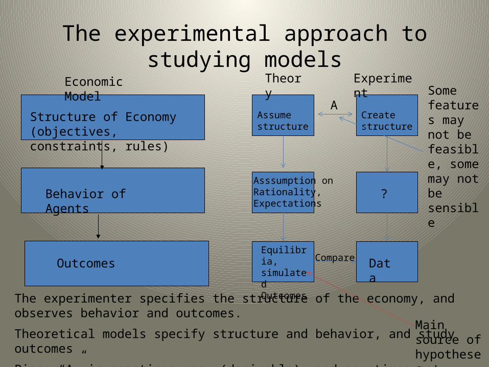
The experimental approach to studying models

Outcomes

Behavior of Agents

Structure of Economy (objectives, constraints, rules)

The experimenter specifies the structure of the economy, and observes behavior and outcomes.

Theoretical models specify structure and behavior, and study outcomes

Piece “A” is sometimes easy (desirable), and sometimes not

Theory Experiment

Asssumption on Rationality, Expectations

?

Assume structure

Create structure

Equilibria, simulated Outcomes

DataCompare

A

Main source of hypotheses

Some features may not be feasible, some may not be sensible

Economic Model

Part I: Growth and Institutions

• THE STRUCTURE OF THE MODEL• A representative consumer in the economy has a lifetime utility given by:

• ρ is the discount rate, Ct is the quantity of consumption at time t, and U(Ct) is the utility of consumption. The economy faces the resource constraint:

• δ is the depreciation rate, Kt is the economy’s aggregate capital stock at the beginning of period t, and A is an efficiency parameter on the production technology. The production function is concave.

• THE ASSUMPTION ON BEHAVIOR: The agent maximizes lifetime utility• • OUTCOME OF MODEL: the principal result of the model is that Ct and Kt converge

asymptotically to optimal steady state levels.

• The optimal steady state given by the solution to: C* = F(K*) – δK* and K* = ρ + δ

)()1(0

t

tt CU

tttt KKFAKC )1()(1

If individuals are given incentives to solve the dynamic optimization problem on their own, it is very difficult.

Social Planners

Figure 6: Time Series of Consumption: Social Planners High Endowment

0

5

10

15

20

25

1 2 3 4 5 6 7 8 9 10 11 12 13 14 15 16 17 18 19 20 21 22 23 24 25 26 27 28 29 30 31 32 33 34

Time

Co

nsu

mp

tio

n

A1

A2

C1

C2

E1

E2

C*

Suppose a team of five people is making the decision instead. They do better but still have a lot of trouble

Implement model as a Decentralized Economy.

• There are five agents in the economy• The economy’s production capability and utility function is divided up

among the five agents.• Agents are made asymmetric.• A market is available to exchange capital (using double auction rules,

because a competitive model is being tested).• There is money, an experimental currency, in the economy, which agents

use for purchases and sales of capital.

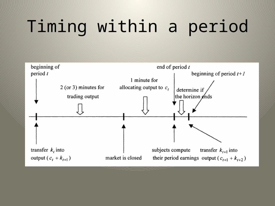
Timing within a period t

• At the beginning of period t, production occurs mapping kt into output (ct + kt+1)

• A double auction market for output is open for two minutes in which they can exchange output.

• Agents have one minute to allocate any portion of their output to consumption ct

• At the beginning of period t+1, production occurs mapping kt+1 into output (ct+1 + kt+2).

Timing within a period

Timing of sessions (ending a session)

• A horizon refers to the entire life of an economy.• Implementation of infinite horizon with discounting: In each

period, there was a /(1+ ) probability that the horizon would end. • If a horizon ended with more than one hour to go in the

experimental session, a new horizon was started.• If a horizon still had not ended at the scheduled end of the session,

the horizon would be continued on another evening.• Subjects would have the option of continuing in their roles in the

continued session. • If they chose not to continue, a substitute would be recruited to

take her place. The original subject would also receive the money earned by the substitute.

Results: Consumption patterns in the decentralized economy

0

2

4

6

8

10

12

14

16

18

1 2 3 4 5 6 7 8 9 10 11 12 13 14 15 16 17 18 19 20

Time

Cons

umpti

on C2E2F3G4C*

C*=12

K*=10

Ko =20

An environment with multiple equilibria

• Now suppose that there exist two stable equilibria, which are Pareto-ranked so that the inferior equilibrium represents a poverty trap.

• The value of the productivity parameter A depends on the economy’s capital stock. There exists a threshold level of capital stock, above which A has a higher value.

KKA

KKAA

ˆ if ,

ˆ if ,

Production function includes threshold externality

Aggregate Production Function

0

20

40

60

80

100

120

140

160

180

200

220

0 25 50 75 100 125 150

Units of Input

Out

put

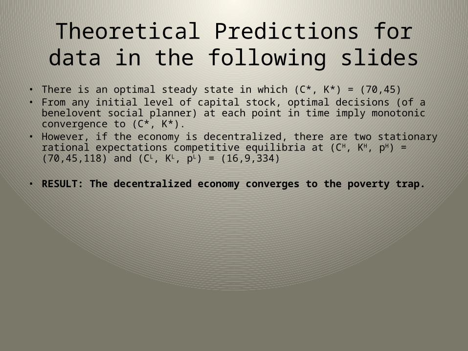
Theoretical Predictions for data in the following slides

• There is an optimal steady state in which (C*, K*) = (70,45) • From any initial level of capital stock, optimal decisions (of a benelovent social

planner) at each point in time imply monotonic convergence to (C*, K*).• However, if the economy is decentralized, there are two stationary rational

expectations competitive equilibria at (CH, KH, pH) = (70,45,118) and (CL, KL, pL) = (16,9,334)

• RESULT: The decentralized economy converges to the poverty trap.

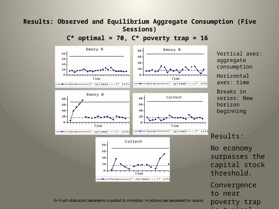
Results: Observed and Equilibrium Aggregate Consumption (Five Sessions)C* optimal = 70, C* poverty trap = 16

Em ory B1

0

20

40

60

80

Ti m e

Cons

umpt

ion

Da t a C* o p t i m a l C* i n f e r i o r

Em ory B2

0

20

40

60

80

Ti m e

Cons

umpt

ion


Em ory B3

0

20

40

60

80

Ti m e

Cons

umpt

ion


Cal t ech B1

0

20

40

60

80

Ti m e

Cons

umpt

ion


Cal t ech B2

0

20

40

60

80

Ti m e

Cons

umpt

ion


§ = E a c h d a t a p o i n t r e p r e s e n t s a p e r i o d i n a h o r i z o n . H o r i z o n s a r e s e p a r a t e d b y s p a c e s

Results:

No economy surpasses the capital stock threshold.

Convergence to near poverty trap is typical outcome

Vertical axes: aggregate consumption

Horizontal axes: time

Breaks in series: New horizon beginning

The Communication treatment

– Identical to the baseline treatment, except that before the market opened, subjects were allowed to communicate with each other.

– Each agent’s screen displayed a chat-room, which they could use to send and receive messages in real time.

– Communication was unrestricted and all agents could observe all messages.

Observed and Equilibrium Aggregate Consumption, Communication Treatment; C* optimal = 70, C* inferior = 16

Em or y C1

0

2 0

4 0

6 0

8 0

Ti m e

Cons

umpt

ion

Data C* o p timal C* in ferio r

Em or y C2

0

2 0

4 0

6 0

8 0

Ti m e

Cons

umpt

ion


Em or y C3

0

2 0

4 0

6 0

8 0

Ti m e

Cons

umpt

ion


Ca l t ec h C1

0

2 0

4 0

6 0

8 0

Ti m e

Cons

umpt

ion


Ca l t e c h C2

0

2 0

4 0

6 0

8 0

Ti m e

Cons

umpt

ion


Ca l t e c h C3

0

2 0

4 0

6 0

8 0

Ti m e

Cons

umpt

ion


Results: Individual sessions converge to near one of the equilibria.

However, which equilibrium it converges to varies between sessions.

Example of how institutional structure affects mean and variance of income.

Vertical axes: aggregate consumption

Horizontal axes: time


The Voting treatment– Identical to the baseline treatment except that consumption and

investment decisions were determined in the following manner:– Two agents were randomly chosen in each period to make

proposals on how much each agent in the economy should consume.

– Before submitting proposals, proposers received information indicating the current stock of capital held by each agent.

– Proposals were followed by majority voting. All agents were required to vote in favor of exactly one of the two proposals.

– The proposal that gained at least 3 (of the 5 total) votes became binding. Each agent consumed the quantity of output specified under the winning proposal, and began next period with the amount of capital allotted to her under the winning proposal.

Observed and Equilibrium Aggregate Consumption, Voting Treatment

C* optimal = 70, C* inferior = 16

Em or y V1

0

2 0

4 0

6 0

8 0

Ti m e

Cons

umpt

ion


Em or y V2

0

2 0

4 0

6 0

8 0

Ti m e

Cons

umpt

ion


Em or y V3

0

2 0

4 0

6 0

8 0

Ti m e

Cons

umpt

ion


Ca l t ec h V1

0

2 0

4 0

6 0

8 0

Ti m e

Cons

umpt

ion


Ca l t e c h V2

0

2 0

4 0

6 0

8 0

Ti m e

Cons

umpt

ion


Results:

-In most sessions, economy escapes poverty trap

- High variance from one period to the next within sessions.

- Convergence toward equilibrium typically does not occur

Vertical axis: aggregate consumption

Horizontal axis: time


The hybrid treatment: Both communication and voting are present

Timing in the hybrid treatment

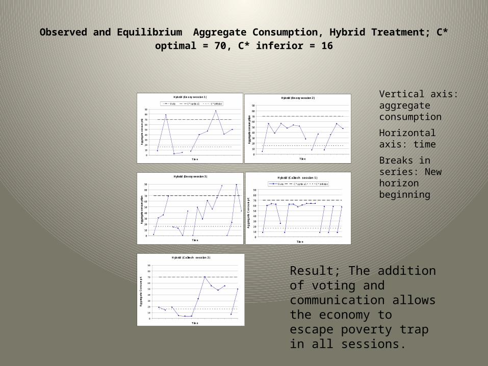
Observed and Equilibrium Aggregate Consumption, Hybrid Treatment; C* optimal = 70, C* inferior = 16

H yb r i d ( E m o r y s e s s io n 1 )

0

1 0

2 0

3 0

4 0

5 0

6 0

7 0

8 0

9 0

T im e

Ag

gre

ga

te c

on

sum

pti

on

D a ta C * o p t im a l C * in fe rio r

H yb r i d ( Em o ry s e s s io n 2 )

0

10

20

30

40

50

60

70

80

90

T im e

Agg

rega

te c

onsu

mpt

ion

H y b r id (Em o r y s e s s io n 3 )

0

10

20

30

40

50

60

70

80

90

T im e

Agg

reg

ate

con

sum

ptio

n

H yb r id (C a lt e c h s e s s i o n 1 )

0

1 0

2 0

3 0

4 0

5 0

6 0

7 0

8 0

9 0

T im e

Ag

gre

gat

e C

on

su

mp

tio

n

D a ta C * o p tim a l C * in fe r io r

H yb r id ( C a l t e c h s e s s io n 2 )

0

1 0

2 0

3 0

4 0

5 0

6 0

7 0

8 0

9 0

T im e

Ag

gre

gat

e C

on

su

mp

tio

n

Result; The addition of voting and communication allows the economy to escape poverty trap in all sessions.

Vertical axis: aggregate consumption

Horizontal axis: time


Results• Baseline: The economies of the baseline treatment converge

to near the poverty trap. Does not escape poverty trap in any session.

• Communciation: The economies of the communication treatment converges to close to one of the stationary equilibria. However, the one it converges toward varies between sessions. Probability of avoiding the poverty trap greater than under baseline.

• Voting: The voting treatment exhibits variable behavior from one period to the next. Probability of avoiding the poverty trap greater than under baseline.

• Hybrid: Also shows variable behavior from one period to the next. Escapes the poverty trap in all sessions.

Part 2: Bubbles and Crashes• I will discuss work on experimental markets

for long-lived assets. • In such markets, the bubble and crash pattern

in pervasive.• I will first describe the effect of different

market institutions and parameters on bubble formation

• Then I will concentrate on differences between sessions but within treatments.

The type of asset considered: the type first studied by (Smith, Suchanek Williams, 1988)

• The asset has a life of 15 periods. At the end of each period, the asset

pays a dividend which is equally likely to be 0, 8, 28 and 60 cents,

determined independently for each draw.

• After the last dividend is paid, the asset has no value.

• Assuming traders are risk neutral, the fundamental value of this asset

can be calculated at any point in time. It is equal to the expected total

future flow of dividends.

• Since the expected dividend in any dividend draw is equal to 24, the

fundamental value is equal to the number of dividend draws remaining

times 24.

• Therefore, the fundamental value is 360 at the beginning of the life of

the asset, and declines by 24 cents every period.

The fundamental value of this asset over time

What happens in such a market?

b) Benchmark

Rather than tracking the fundamental value, a bubble and crash pattern is typically observed.

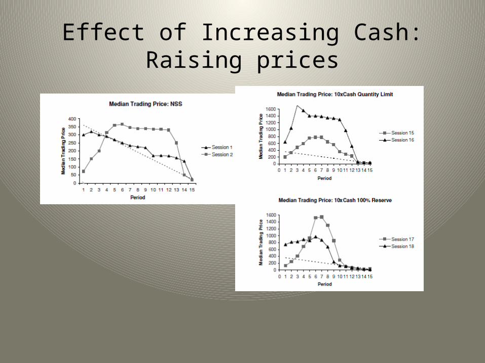
Effect of Increasing Cash: Raising prices

Effect of allowing short selling: lowering prices

Effect of adding a futures market, improving price discovery

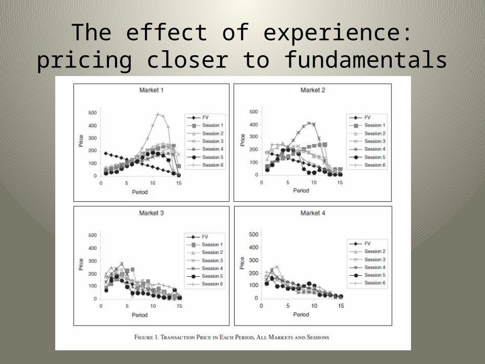
The effect of experience: pricing closer to fundamentals

The role of the fundamental value time path: Increasing FV trajectory

Decreasing fundamental value trajectory

Decreasing treatment tracks fundamentals more closely than increasing

Modeling trader types• Can we explain what is observed in the data with a model in

which there are multiple trader types?• Consider the following model (based on DeLong, Shleifer,

Summers, and Waldmann ,1990)• Assume three types of trader: (1) Fundamental value traders,

(2) Rational Speculators, and (3) Momentum traders.– Fundamental value traders purchase if prices are below fundamentals

and sell if they are above. – Rational speculators anticipate future price movements. They buy if

the price is going to increase in the next period, and sell if it is going to decrease.

– Momentum traders follow the current trend. They buy if the price has been going up and sell if it has been going down.

Demand functions of the three types

• The three types have net demand functions of the following form:– Fundamental value trader: -α(pt – ft), where pt is the price

in period t, and ft is the fundamental value in period t. – Rational speculator: γ(E(pt+1) - pt), – Momentum trader: -δ + β(pt-1 – pt-2)

• Six parameters: α, β, γ, δ, and the proportion of traders that is of each type.

• This structure generates bubbles and crashes, is consistent with treatment differences, and the types correlate with other behaviors.

• Now I will explore the relationship between trader characteristics and market behavior.

Loss aversion measurement

Cognitive reflection test (Frederick, 2005)• This consists of three questions, in which the first answer that comes to mind is incorrect,

but the correct answer is simple after some reflection.

• Example: If it takes 5 people 5 minutes to make 5 units, how much time does it take 100 people to make 100 units?– First answer that comes to mind is 100 minutes– With reflection realize the answer is 5 minutes

• Other two questions:• A bat and a ball cost 1.10 Euro in total. The bat costs 1 Euro more than the ball. How much

does the ball cost?• In a lake, there is a patch of lily pads. Every day, the patch doubles in size. If it takes 48

days for the patch to cover the entire lake, how long would it take for the patch to cover half of the lake?

Risk aversion measurement (Holt and Laury, 2002)

Correlation between price level and average risk aversion in the market: Bullmarket treatment

Correlation between number of trades in the market and average loss aversion: Bearmarket treatment

Average CRT score and departure from fundamental value

Final Individual Holdings and Risk Aversion Level

Number of trades at individual level and loss aversion

Individual CRT score and earnings

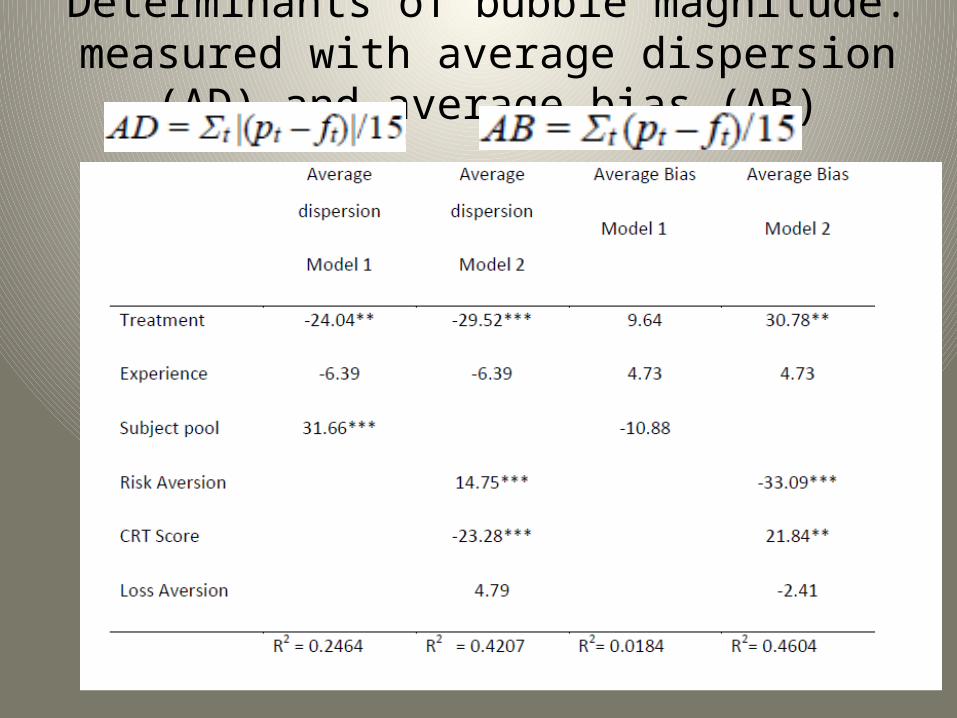
Determinants of bubble magnitude: measured with average dispersion (AD) and average bias (AB)

Correlation between trader characteristics and strategies

Emotional correlates of asset price movements

• Positive emotions have typically been associated with higher prices– Irrational exuberance (Greenspan, 1996)– Speculative euphoria (Galbraith, 1984)

• Empirical support– Weather affects returns (Hirshleifer and Shumway, 2003; Kamstra et al, 2003)– Outcomes of sporting events also affect prices (Edmans et al., 2007)– Twitter mood (Bollen et al., 2010) and anxiety level in blog postings (Gilbert

and Karahalios, 2009) predict stock price movements.

• Fear has been associated with low prices and volatility

Emotions and markets in the laboratory

• We consider whether these and other connections between emotions and market behavior appear in the laboratory

• We construct an experimental asset market with a monotonically decreasing fundamental value.

• All traders are videotaped throughout the session• The videotapes are analysed with Noldus Facereader at a later date.• The Facereader reads a facial expression and classifies it along seven

dimensions.– These correspond to the basic universal emotions identified by Ekman

(1978, 1999)

Facereading software• We use facereading software to track traders’ emotional state while the

market is operating.• These are

– Happiness– Anger– Sadness– Disgust– Fear– Surprise– Neutrality

• Facereader also reports the overall valence of emotion.• Unlike other neuroeconomic methodologies, Facereader translates

physiological responses directly into of psychological models

“Smiling” for a picture

Absence of negative emotions

…not so happy

Neutrality, anger and disgust

Neutrality with some anger

Very happy

Market Prices

Initial valence and average prices

Valence is typically negative: Experiments are not fun for subjects

We hypothesize that:(1) More

positive valence is associated with higher prices.

r = .708, p < .01

Initial fear and average pricesWe hypothesize that:

(2) Fear is associated with lower prices

= -.549p < .06

People who are more neutral during crash period earn more money Crash period: The period with the largest price decrease

Hypothesis 4:

Neutrality during market turbulence is associated with greater earnings

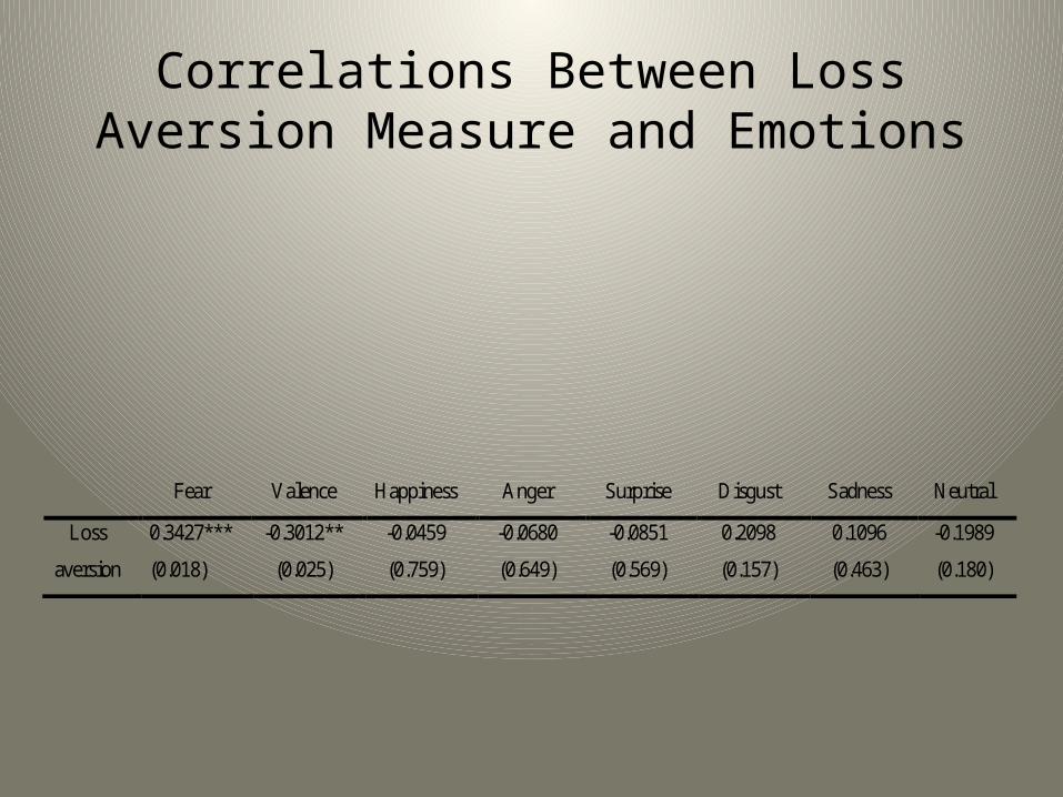
Correlations Between Loss Aversion Measure and Emotions

Fear Valence Happiness Anger Surprise Disgust Sadness Neutral

Loss

aversion

0.3427***

(0.018)

-0.3012**

(0.025)

-0.0459

(0.759)

-0.0680

(0.649)

-0.0851

(0.569)

0.2098

(0.157)

0.1096

(0.463)

-0.1989

(0.180)

Correlations between initial emotional state and likelihood of being a FV trader

Initial Emotional State Fundamental Value Trader

Neutral .202**

Happy .012

Sad -.050

Angry -.195**

Surprised -.091

Scared -.207**

Disgusted -.182*

Valence .097

More positive valence predicts more purchases

Buy t Buy t Sell t Sell t

Model 1 Model 2 Model 3 Model 4

valence t-1 .237* .238* fear t-1 2.151 2.690

money t-1 7.29e-06 4.95e-06 money t-1 5.79e-06 6.25e-06

units t-1 -.021** -.015 units t-1 .050*** .046***

P level t-1 -.00007 -.00008 P level t-1 -.00012 -.00012

Buy t-1 .355*** Sell t-1 .362***

Prob>chi2

=0.000Prob>chi2 =0.0586

Prob>chi2 =0.000Prob> chi2

=0.0000

9770 obs

49 groups

9770 obs

49 groups

9971 obs

50 groups

9971 obs

50 groups

Momentum traders buy more when they are in a more positive emotional state

Buy t Fundamental Value Trader Momentum Trader Rational Speculator Trader

Valence t-1 .280 .521** -.025

Money t-1 .00003 -.00004 -.00007**

Units t-1 .015 -.119*** -.068***

Price level t-1 -.0004* .0007*** 3.15e-06

Buy t-1 .435*** .141* .370***

Obs: 3762

Groups: 19

Prob>F =.0000

Obs: 3396

Groups: 17

Prob>F =.0000

Obs: 2612

Groups: 13

Prob>F =.0000

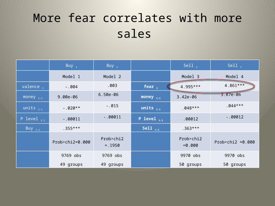
More fear correlates with more sales

Buy t Buy t Sell t Sell t

Model 1 Model 2 Model 3 Model 4

valence t -.004 .003 fear t 4.995*** 4.861***

money t-1 9.00e-06 6.50e-06

money t-1 3.42e-06 3.87e-06

units t-1 -.020**-.015

units t-1 .048***.044***

P level t-1 -.00011-.00011

P level t-1 .00012-.00012

Buy t-1 .355*** Sell t-1 .363***

Prob>chi2=0.000 Prob>chi2 =.1950 Prob>chi2 =0.000 Prob>chi2 =0.000

9769 obs

49 groups

9769 obs

49 groups

9970 obs

50 groups

9970 obs

50 groups

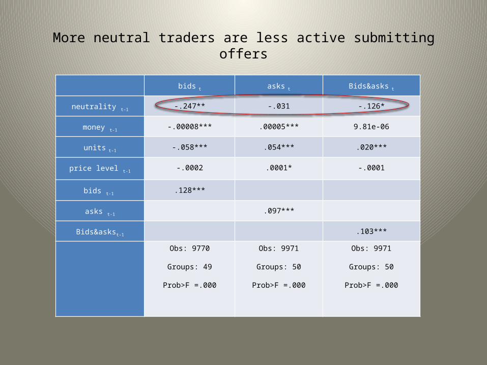
More neutral traders are less active submitting offers

bids t asks t Bids&asks t

neutrality t-1 -.247** -.031 -.126*

money t-1 -.00008*** .00005*** 9.81e-06

units t-1 -.058*** .054*** .020***

price level t-1 -.0002 .0001* -.0001

bids t-1 .128***

asks t-1 .097***

Bids&askst-1 .103***

Obs: 9770

Groups: 49

Prob>F =.000

Obs: 9971

Groups: 50

Prob>F =.000

Obs: 9971

Groups: 50

Prob>F =.000

Better overall financial position improves traders’ emotional state

Valence t Valence t

money t-12.51e-06* 4.01e-06**

units t-1.0013* .0022***

P level t-1-.000044*** -.000087***

valence t-1.480***

const.-.028** -.046***

Obs: 9927

Groups: 50

Prob>F =.000

Obs: 9970

Groups: 50

Prob>F =.000

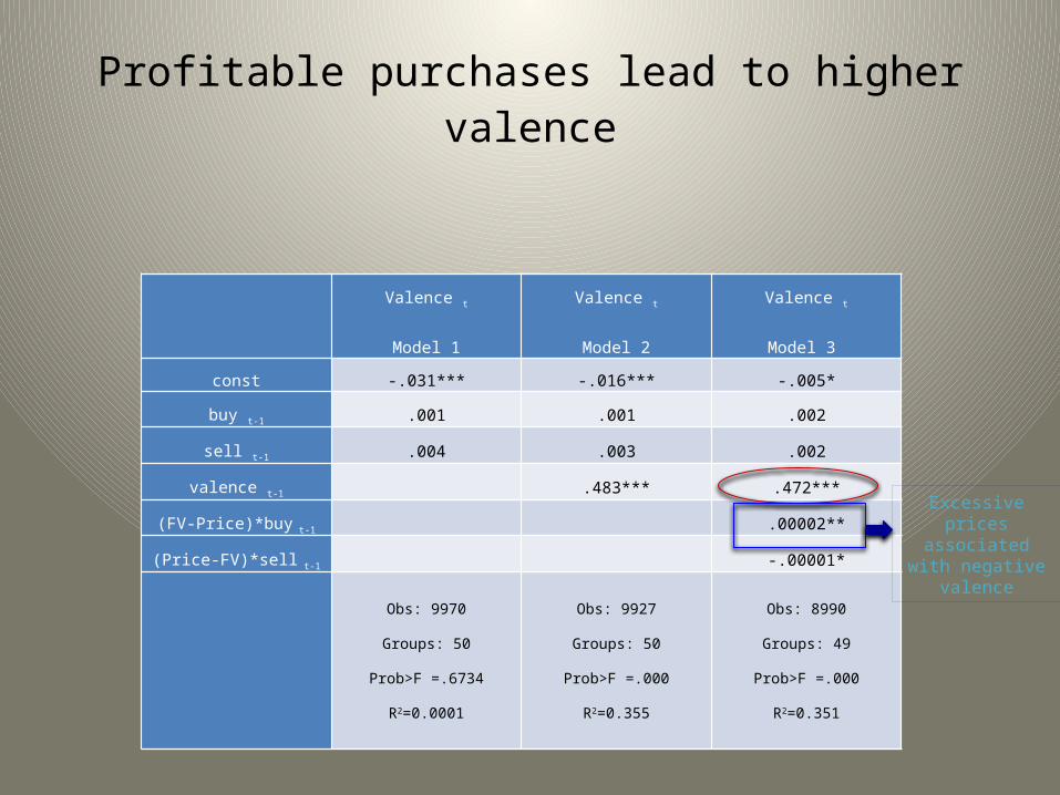
Profitable purchases lead to higher valence

Valence t

Model 1

Valence t

Model 2

Valence t

Model 3

const -.031*** -.016*** -.005*

buy t-1 .001 .001 .002

sell t-1 .004 .003 .002

valence t-1 .483*** .472***

(FV-Price)*buy t-1 .00002**

(Price-FV)*sell t-1 -.00001*

Obs: 9970

Groups: 50

Prob>F =.6734

R2=0.0001

Obs: 9927

Groups: 50

Prob>F =.000

R2=0.355

Obs: 8990

Groups: 49

Prob>F =.000

R2=0.351

Excessive prices associated with

negative valence

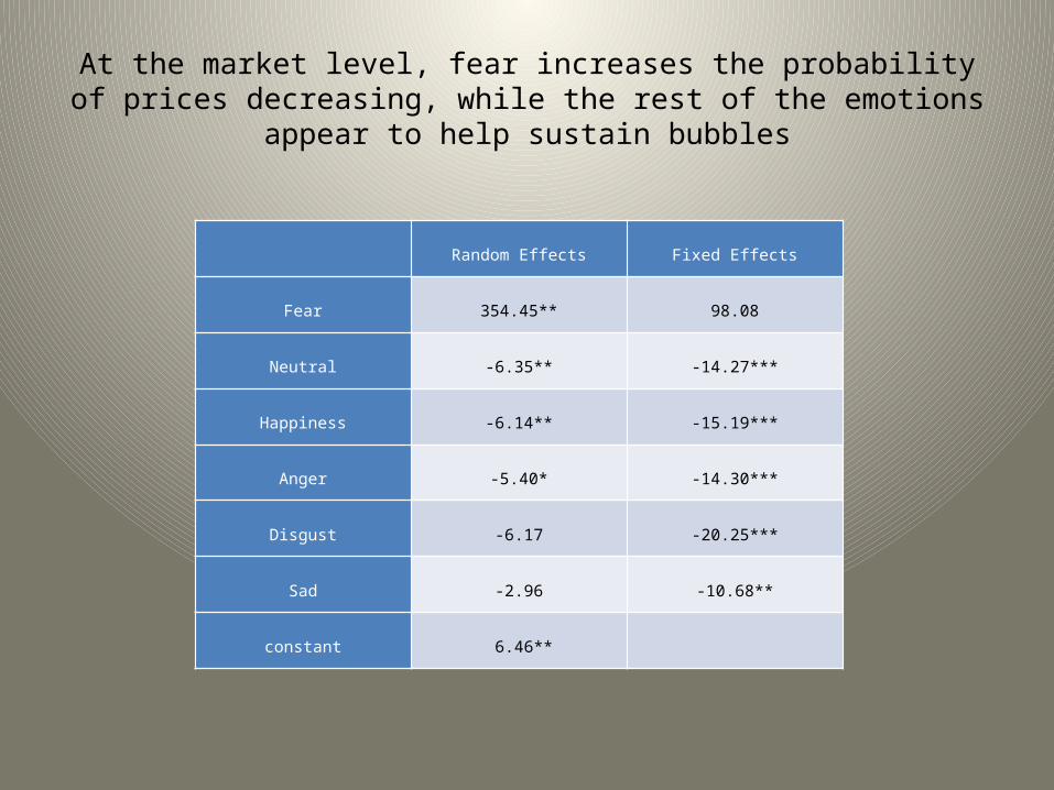
At the market level, fear increases the probability of prices decreasing, while the rest of the emotions appear to help sustain bubbles

Random Effects Fixed Effects

Fear 354.45** 98.08

Neutral -6.35** -14.27***

Happiness -6.14** -15.19***

Anger -5.40* -14.30***

Disgust -6.17 -20.25***

Sad -2.96 -10.68**

constant 6.46**

Conclusions • Bubbles and crashes in experimental markets are a complex phenomenon,

with many determinants of their magnitude.• Cash balances and quantity of shares available for sale influence price

levels.• Some time paths of fundamentals are more conducive to mispricing than

others.• The preference parameters of risk and loss aversion predict prices and

quantity traded. • Cognitive ability/motivation predicts mispricing. • There are consistent emotional substrates to market bubbles and crashes.• Emotional state of traders responds to and can predict subsequent market

activity.

Part 3: An experimental DSGE economy

• Construct an experimental macroeconomy, similar in structure to a New Keynesian DSGE macroeconomy. Close enough so that hypothesis from NK DSGE model can be evaluated.

• Three types of (infinitely lived) agents– Consumers: supply labor, purchase (3) products, and save for

the future– Producers: purchase labor, produce one of the (3) products, sell

output– Central bank: sets interest rates

• Preferences and productivity subject to shocks

What we want to model

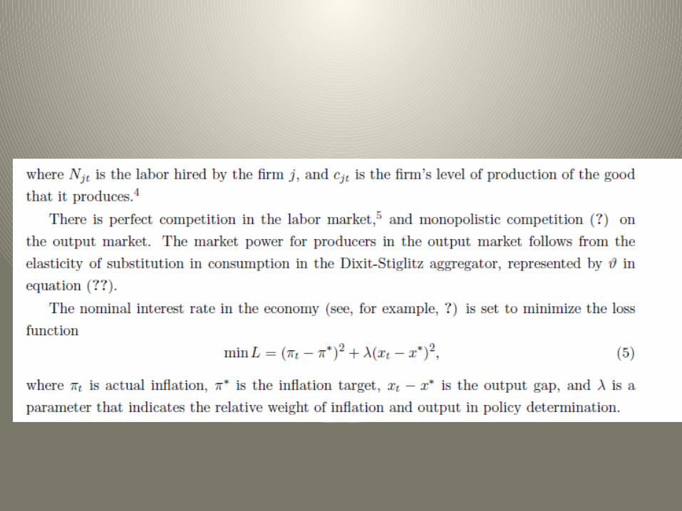
Producer incentives

• Maximize profit:Пit = pityit – wtLit

yit = AtLit

At = A0 + γAt-1 + δεt Where Пit = profit of firm i in period t

pit = price of good i in period t

yit = production of good i in t

wt = wage in t

Lit = labor bought by i in t

At = productivity parameter in t

εt = productivity shock in t

γ = 0.8, δ = 0.2, A0 = 0.7

Consumer incentives• Payoff in period t of consumer j = βt[Ujt(Cjt) – Dj(Ljt)] • Ujt(Cjt)=∑ihijt[cijt

(1-σ)/(1- σ)]• hijt = μij + τhijt-1 + δεjt

• D(Ljt) = d*Ljt1+η/ (1+η)

• Where Cjt= consumption at time t of consumer jLjt = labor supplied at t Dj(Ljt) = disutility to j of labor he supplies at tcijt = consumption of good i by consumer j at t ε jt = preference shock for consumer j in period t

β = .99, μij = 120, τ = 0.8, d = 15, η = 2, n = 3.

Consumer incentives

• Faces a budget constraint: wtLjt + 1/n∑iΠi,t-1 + (1 + rt)sj,t-1 = ∑ipitcijt + sjt

• sjt can be thought of as savings or bonds• Create monopolistic competition with

different preference shocks for each good.

Experimental Design

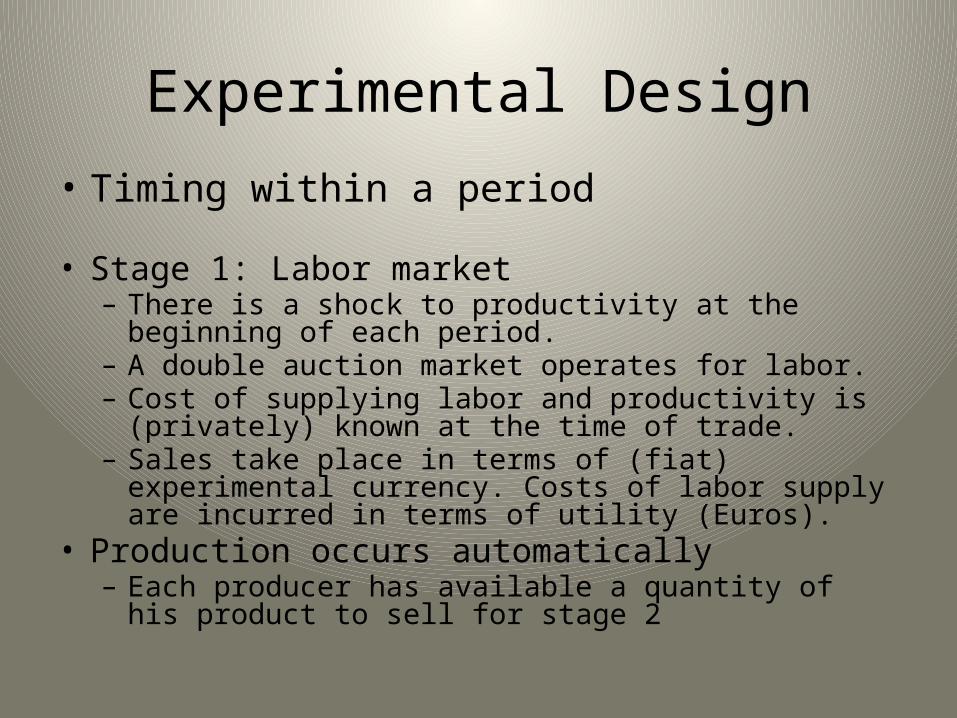
• Timing within a period

• Stage 1: Labor market– There is a shock to productivity at the beginning of each

period.– A double auction market operates for labor.– Cost of supplying labor and productivity is (privately) known

at the time of trade.– Sales take place in terms of (fiat) experimental currency.

Costs of labor supply are incurred in terms of utility (Euros). • Production occurs automatically

– Each producer has available a quantity of his product to sell for stage 2

Labor market: Consumer

Labor Market: Producer

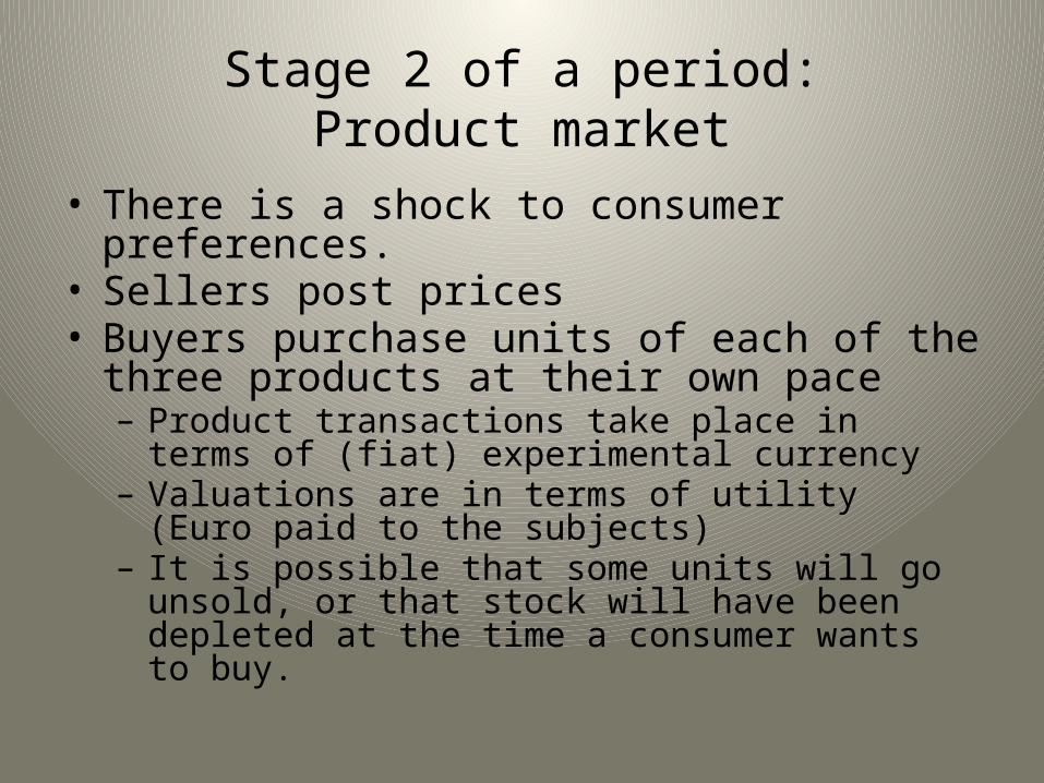
Stage 2 of a period:Product market

• There is a shock to consumer preferences.• Sellers post prices • Buyers purchase units of each of the three products

at their own pace– Product transactions take place in terms of (fiat)

experimental currency– Valuations are in terms of utility (Euro paid to the subjects)– It is possible that some units will go unsold, or that stock

will have been depleted at the time a consumer wants to buy.

Product market: Producer

Product Market: Consumer

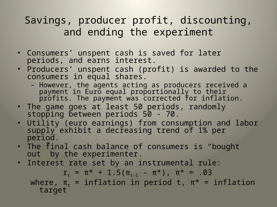
Savings, producer profit, discounting, and ending the experiment

• Consumers’ unspent cash is saved for later periods, and earns interest.• Producers’ unspent cash (profit) is awarded to the consumers in equal

shares. – However, the agents acting as producers received a payment in Euro equal

proportionally to their profits. The payment was corrected for inflation. • The game goes at least 50 periods, randomly stopping between periods 50

- 70. • Utility (euro earnings) from consumption and labor supply exhibit a

decreasing trend of 1% per period.• The final cash balance of consumers is “bought out” by the experimenter.• Interest rate set by an instrumental rule:

rt = π* + 1.5(πt-1 - π*), π* = .03where, πt = inflation in period t, π* = inflation target

Timing of a session

• A session took 3 ¾ – 4 ¾ hours.• Instructions read (~30 minutes)• 5 period practice economy (~30 minutes)• > 50 period economy that counted toward

earnings.• Placed bounds on wages and prices for the

first two periods.

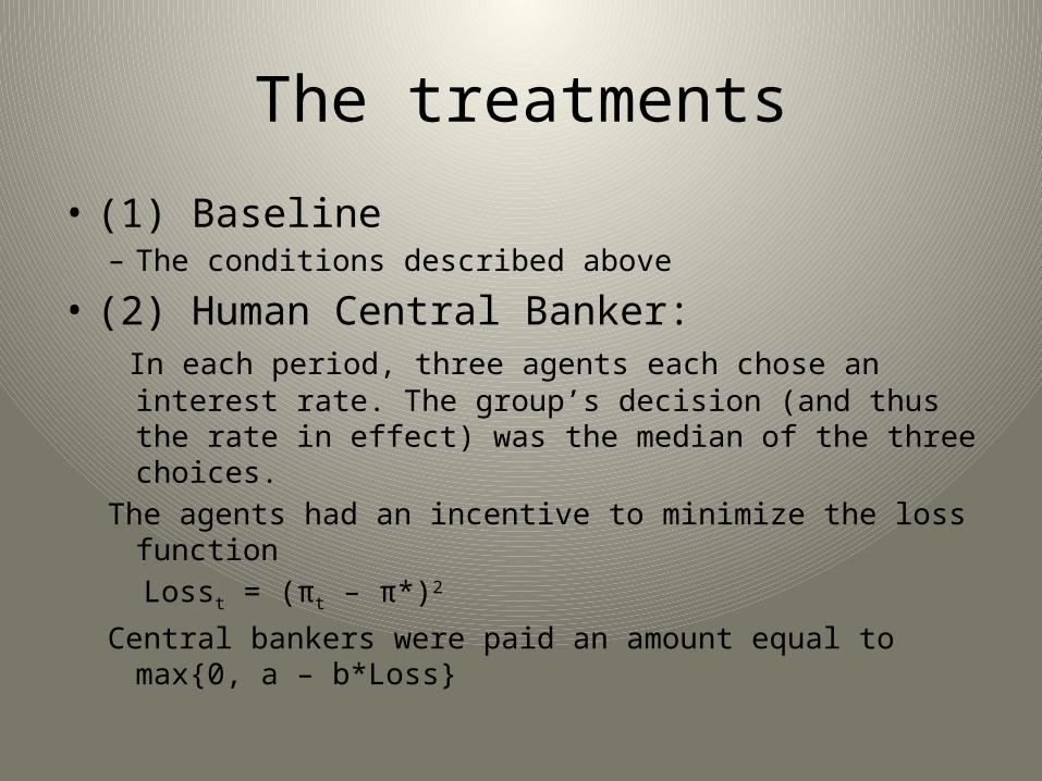
The treatments

• (1) Baseline– The conditions described above

• (2) Human Central Banker: In each period, three agents each chose an interest rate. The

group’s decision (and thus the rate in effect) was the median of the three choices.

The agents had an incentive to minimize the loss function Losst = (πt – π*)2

Central bankers were paid an amount equal to max{0, a – b*Loss}

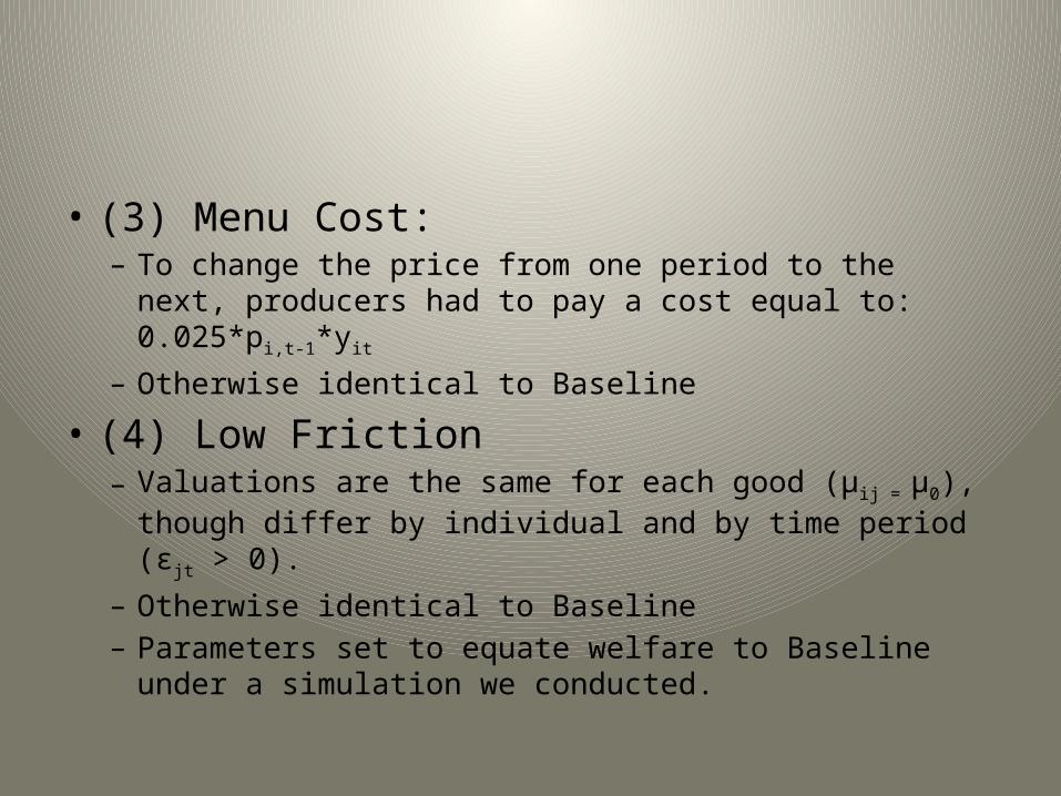
• (3) Menu Cost:– To change the price from one period to the next,

producers had to pay a cost equal to: 0.025*pi,t-1*yit

– Otherwise identical to Baseline

• (4) Low Friction– Valuations are the same for each good (μij = μ0), though

differ by individual and by time period (εjt > 0). – Otherwise identical to Baseline– Parameters set to equate welfare to Baseline under a

simulation we conducted.

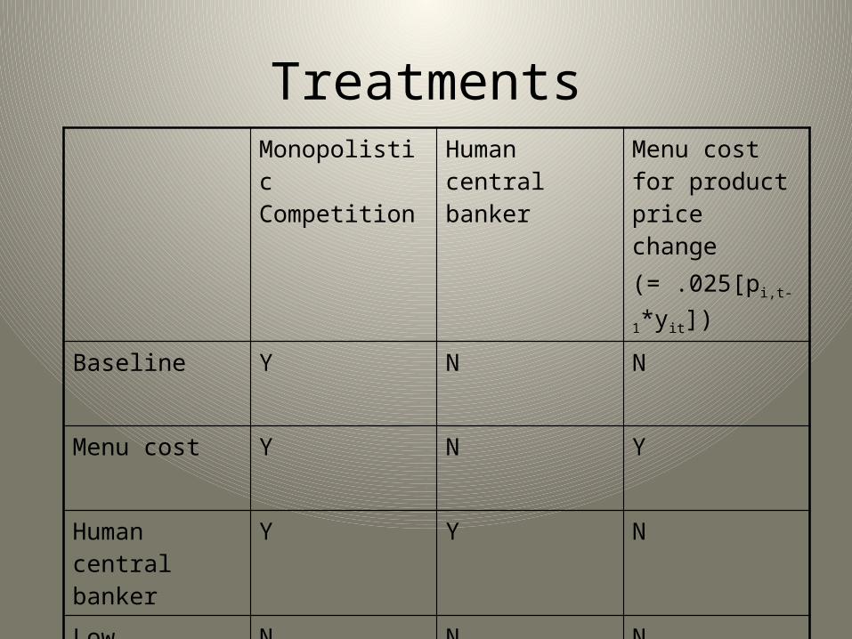
TreatmentsMonopolistic Competition

Human central banker

Menu cost for product price change (= .025[pi,t-1*yit])

Baseline Y N N

Menu cost Y N Y

Human central banker

Y Y N

Low friction N N N

Hypothesis

• Persistence of shocks (effect beyond the current period): – Treatment differences– In treatments Baseline, Human Central Banker, and Low Friction no

persistence, in treatment Menu Cost, shocks are persistent (both Menu Cost and market power are needed for persistence in New Keynesian DSGE model).

• Empirical stylized fact is that a shock to interest rates, output, or inflation, has persistent effects on itself and on some of the other two variables.

• Also can compare between treatments– GDP, inflation, welfare, employment, etc…

Results: GDP

GDP is highest under Low Friction

GDP is lowest in the late periods under Human Central Banker

Menu Costs do not affect GDP

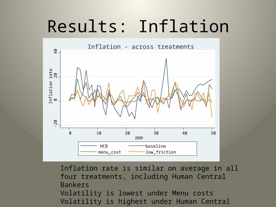
Results: Inflation

Inflation rate is similar on average in all four treatments, including Human Central Bankers Volatility is lowest under Menu costsVolatility is highest under Human Central Banker

-20

020

40In

flatio

n ra

te

0 10 20 30 40 50ppp

HCB baselinemenu_cost low_friction

Inflation - across treatments

A degree of heterogeneity exists within each treatment

02

004

006

008

001

000

Rea

l GD

P

0 10 20 30 40 50ppp

session2 session3session11 session12

Real GDP - baseline treatment

Impulse Responses: Baseline treatment

Productivity shock persistent

Shock to GDP/Productivity

Shock to demand Inflation

Shock to Interest Rate

Row 1-3: Effect on output, inflation, interest rates

Inflation Shock Persistent

Interest Rate Shock persistent

Price Puzzle

Inflation shock has persistent effect on policy

Impulse Responses: Menu Cost treatment




Row 1 - 3: Effect on output, inflation, interest rates



Price Puzzle

Impulse Responses: Low frictionShock to GDP/Productivity



Row 1: Effect on output

Row 2: Effect on inflation

Row 3: Effect on interest rates

Productivity shock persistentProductivity shock lowers prices

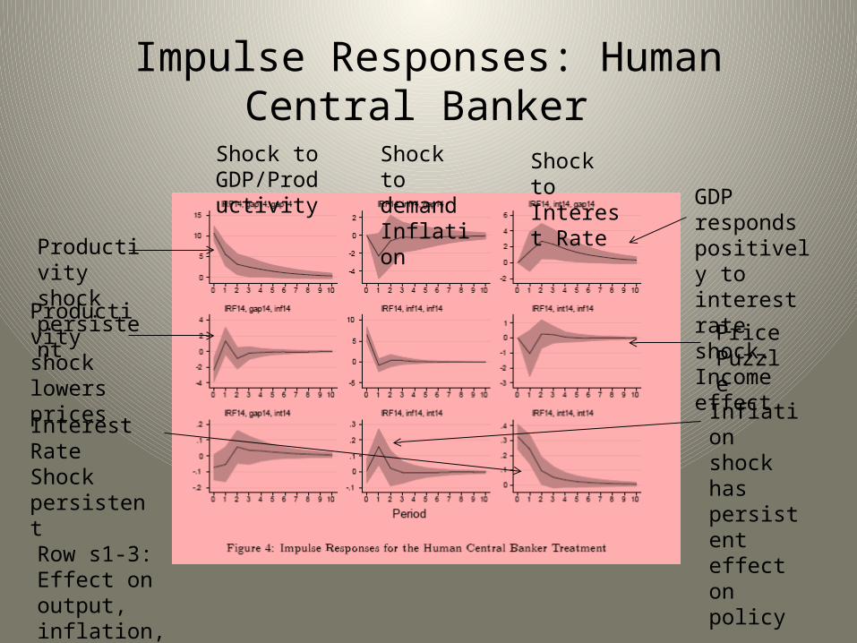
Impulse Responses: Human Central Banker




Row s1-3: Effect on output, inflation, interest rates


GDP responds positively to interest rate shock. Income effect Productivity

shock lowers prices


Inflation shock has persistent effect on policy

Price Puzzle

Evaluating the hypothesis• Very little persistence in the Low Friction treatment.

• Somewhat more persistence in Menu Cost than in Baseline.

• More persistence of policy (interest rate) shocks in Human Central Banker treatment

• Mixed evidence with regard to hypothesis. Monopolistic competition alone generates shock persistence, and menu costs add to it.

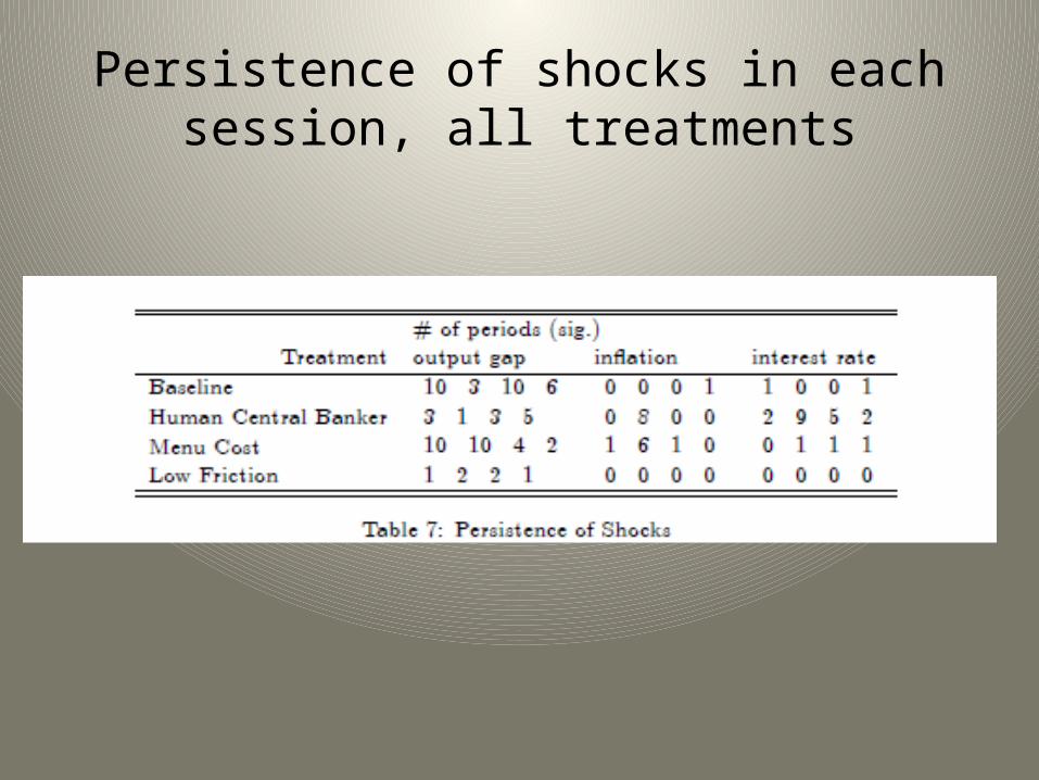
Persistence of shocks in each session, all treatments

How do the human central bankers set interest rates?

• Consider the following regression• rt = β0 + β1rt-1 + β2πt-1 + β3(GDP – GDP*)

• System GMM Dynamic Panel Estimator (Blundell and Bond, 1998)

• Taylor rule coefficient (relationship between interest rate and inflation) = β2/(1- β1) [Bullard and Mitra, 2007]

• Implied coefficient is close to 2, consistent with the Taylor principle since it is greater than 1.

Interest rate at t rt

Constant Interest rate at t-1, rt-1

Inflation at t-1, πt-1

Output gap GDP-GDP*

Estimate (std err)

.4212 (.2609)

.9395 (.0146)

.1538 (.0114)

.0184 (.0074)

Hazard Rate of Price Changes

Average duration of price spells similar except for Menu Cost, in which it is longer.

In Menu Cost, the hazard function is upward sloping. Price is more likely to change the longer it has been unchanged

Conclusions• Methodology

– It is feasible to construct a DSGE model in the laboratory. It is possible to verify stylized facts and consider the effect of some assumptions from a behavioral standpoint.

• Persistence– Monopolistic competition, in conjunction with multiple agents and

bounded rationality, is sufficient to generate some persistence– Menu costs add somewhat to this persistence.– Discretionary central banking affects shock persistence.– Negligible persistence in Low Friction. Biases in decision making of

producers and consumers alone do not generate persistence.

macroeconomic experiments charles noussair tilburg university barcelona, june 14, 2015

Documents