macroeconomicstktopenightcollege.in/.../02/macroeconomics...2019.pdf · 1) dornbusch. r, fisher.s.,...

1

MACROECONOMICS, M COM, SEM2 BY KRISHNAN NANDELA, ASSOCIATE PROFESSOR AND HEAD, DEPARTMENT OF

ECONOMICS, DR. TK TOPE ARTS & COMMERCE NIGHT SENIOR COLLEGE, PAREL – 12.

1

By

Krishnan Nandela

Associate Professor &

Head, Department of Economics

MACROECONOMICS MCOM(SEMESTER-II)

2



2

M.Com. Core Course in Economics Semester – II

Paper II: Macroeconomic concepts and applications

Preamble

The heavily application-oriented nature of macroeconomics subject is introduced to enable the

post graduate students to grasp fully the theoretical rationale behind policies at the country as

well as corporate level. This paper helps the students to receive a firm grounding on the basic

macroeconomic concepts that strengthen analysis of crucial economic policies. Students are

expected to regularly read suggested current readings and related articles in the dailies and

journals are analyzed class rooms.

Unit–I (5 lectures)

Aggregate Income and its dimensions: National income aggregates - and measurement; - GNP,

GDP, NDP, Real and nominal income concepts, measures of inflation and price indices - GDP

deflator, - Nominal and real interest rates- PPP income and HDI

Unit- II (5 lectures)

Keynesian concepts of Aggregate Demand (ADF), Aggregate Supply (ASF), Interaction of ADF

and ASF and determination of real income; Inflationary gap

Policy trade- off between Inflation and unemployment – Phillips’ curve – short run and long run-

Unit - III (10 lectures)

The IS-LM model: Equilibrium in goods and money market; Monetary and real influences on IS-

LM curves, Economic fluctuations and Stabilization policies in IS-LM framework -

Transmission mechanism and the crowding out effect; composition of output and policy mix, IS-

LM in India

Unit - IV (10 lectures)

International aspects of Macroeconomic policy: Balance of payments disequilibrium of an open

economy - corrective policy measures -Expenditure changing policies and expenditure switching

policies BOP adjustments through monetary and fiscal policies -The Mundell-Fleming model -

Devaluation, revaluation as expenditure switching policies - effectiveness of devaluation and J -

curve effect

Suggested readings 1) Dornbusch. R, Fisher.S., Macroeconomics, Tata McGraw-Hill 9th edition

2) D’Souza Errol., Macroeconomics, Pearson Education 2008

3) Gupta G.S., Macroeconomics Theory and Applications, Tata McGraw-Hill, New Delhi 2001

4) Dwivedi D.N., Macroeconomics theory and policy, Tata McGraw-Hill, New Delhi 2001

Current Readings Economic and Political Weekly

Indian Economic Review

Financial Dailies

3



3

MASTER OF COMMERCE, SEMESTER TWO

MACRO ECONOMICS CONCEPTS AND APPLICATIONS

UNIT

NAME

PAGE NO.

I.

NATIONAL INCOME AND ITS DIMENSIONS

1. National income aggregates and measurement - GNP, GDP, NDP, Real and

nominal income.

2. Price Level – measures of inflation, price indices, GDP deflator, Nominal and

Real Interest Rates, Purchasing Power Parity Income.

3. The Human Development Index

II. DETERMINATION OF NATIONAL INCOME

1. Theory of Aggregate Demand - Aggregate Demand (ADF), Aggregate Supply

(ASF), Interaction of ADF and ASF and determination of real income; Inflationary

gap.

2. Phillips Curve Analysis - Policy trade- off between Inflation and unemployment –

Phillips’ curve – short run and long run.

III.

THE IS & LM MODEL

1. Equilibrium in Goods and Money Market, Monetary and Real influences on IS-LM curves, Economic fluctuations and stabilization policies in IS-LM framework, Transmission mechanism and the crowding out effect, Composition of Output and Policy Mix, IS-LM in India.

IV.

INTERNATIONAL ASPECTS OF MACRO-ECONOMIC POLICY

1. Balance of payments disequilibrium of an open economy - corrective policy

measures -Expenditure changing policies and expenditure switching policies BOP

adjustments through monetary and fiscal policies -The Mundell-Fleming model -

Devaluation, revaluation as expenditure switching policy - effectiveness of

devaluation and J - curve effect

4



4

MODULE ONE


CHAPTER ONE

NATIONAL INCOME AGGREGATES AND MEASUREMENT

PREVIEW.

GNP, GDP & NDP.

Real and nominal income.

Measurement of National Income.

NATIONAL INCOME.

National income is the money value of all economic activities of a nation conducted in each year.

An economic activity refers to production of goods and services which can be valued at market

prices. It includes agricultural production, industrial production and production of services.

Goods and services which do not have an exchange value or market value are non-economic in

nature. For instance, services of a house wife or a house husband, services of members of family

to other members or their own selves, hobbies etc. The national income of a country can be

defined as the total market value of all final goods and services produced in the economy in each

year.

National income measures market value of annual output. It is therefore a monetary measure of

the value of goods and services. To measure the real national income or the measure the changes

in physical output of goods and services, the figure for national income is adjusted for price

changes. Further, for the accurate calculation of national income, all goods and services

produced in a year must be counted only once. Generally, goods are produced in different stages

before they reach the markets in their final form. Hence, components of goods are exchanged

many times. Thus, to avoid multiple counting, national income includes only the market value of

all final goods. This is how national income is defined in terms of product flow.

National income can also be defined in terms of money flow. Economic activities generate

money flow in the form of payments i.e., wage, interest, rents and profits. National income can

thus be obtained by adding the factor incomes land adjusting it for indirect taxes and subsidies.

National income obtained in this manner is known as National Income at Factor Cost.

National income can be viewed from different angles. It represents total receipts land it also

represents total expenditure. When goods and services are valued at their market prices, three

5



5

identities are created, namely: the value of receipts equal to the value of payments equal to the

value of goods and services produced and sold. These three identities can be put as:

National Income = National Expenditure = National Product.

To understand the concept, let us assume a two-sector model of an economy consisting of

households and firms. Firms produce goods and services. To produce, firms require factor

services namely: land, labor, capital and enterprise. Factors of production are paid their prices in

the form of rents, wages, interests and profits for their contribution to the production of goods

and services. The money value of net production must equal the total money value of factor

prices i.e. rents, wages, interests and profits. These incomes become the source of expenditure.

Thus, income flows from the firms to the households in exchange for productive services. The

income goes back to the firms in the form of expenditure made by households on goods and

services. This process is also referred to as the Circular Flow of Economic Activities. There are

thus three measures of national income of a country, namely:

1. The total value of all final goods and services produced.

2. The total of all incomes received by the factor owners in a year, and

3. The total of consumption expenditure, net investment expenditure and government

expenditure on goods and services.

These three measures denote the three fundamental functions of an economic system or a

national economy, namely: production, distribution and expenditure. The fourth fundamental

function is that of consumption and is subsumed in expenditure.

NATIONAL INCOME CONCEPTS.

1. Gross National Product (GNP).

The GNP is the most widely used measure of national income. It is the basic accounting

measure of the total output of goods and services. GNP is defined as the total market value of all

final goods and services produced in a year. It measures the market value of a yearly output and

therefore it is a monetary measure of national income. In the definition above, the term ‘final’ is

used to avoid the possibility of double counting and to ensure that only the value of final goods

and services is considered in measuring GNP. This is because the value of intermediate goods is

included within the value of final goods and services. The term ‘gross’ refer to the fact that

depreciation or capital consumption of goods has not been subtracted from the value of output.

While measuring the GNP, only the final value of goods and services is considered, i.e., the

value is added in each stage of the production process. For instance, there are many stages in the

production of bread. The farmer produces wheat. The miller converts wheat into flour. The

baker bakes the bread and finally the bread is sold by the retailer to the consumer. The value

addition process in the production of bread is shown in Fig. 1.5.

6



6

Stage 1 Stage 2 Stage 3 Stage 4 Stage 5

Value Added Value Added Value Added Value Added Final Value

By the Farmer by the Miller by the Baker by the Retailer of the Bread

Rs.5 Rs.2 Rs.5 Rs.3 Rs.15

Fig. 1.1 Value added in different stages of the Production of Bread.

As shown in Fig.1.1, value is added to the product at every stage of production as cost is incurred

at every stage of value addition. The final value of the bread is the total of the value added at

each stage. Suppose in the second stage, if we add up Rs.7 instead of Rs.2 and in the third sage

Rs.12 instead of Rs.5 and so on then it will be a case of multiple counting. This will give a

wrong and inflated picture of the actual value of the product produced in each period.

The rate of growth of GNP is the most important indicator of the nation’s economy. It shows the

rate at which the national income of a country is increasing or decreasing. It is the broadest

statistical aggregate of an economy’s output and growth. The estimate of national income in

terms of GNP provides the policy makers and business community a useful tool to analyze the

economic performance of the country.

In an open economy, the value of GNP at market prices may be symbolically stated as follows:

GNP(MP) = C + I + G + Xn + Rn, where:

GNP(MP) = Gross National Product at market prices.

C = Consumption goods.

Value of Wheat

Value of Milling Wheat into Flour Value of Wheat

Value of Baking Value of Milling Wheat into Flour Value of Wheat Value of Wheat

Value Added by the Retailer Value of Baking Value of Milling Wheat into Flour Value of Wheat

The Final Value of the Bread

7



7

I = Investment goods.

G = Government services.

Xn = Net exports i.e. exports minus imports.

Rn = Net receipts i.e. receipts minus payments.

GNP is the basic accounting measure of national output and represents final products valued at

current market prices.

2. Net National Product (NNP) or National Income at Market Prices (NIMP).

NNP is defined as GNP less depreciation. Symbolically,

NNP = GNP – Depreciation (D).

Depreciation is that part of total productive assets which is used to replace the capital worn out in

the process of creating national output. The value of depreciation is estimated land deducted

from the GNP to find our NJP. The NNP gives the measure of net output available for

consumption of the society. Since the NNP is the measure of the market value of all goods and

services minus depreciation, 9it is also called National Income at Market Prices.

3. National Income at Factor Cost (NIFC) or National Income (NI).

National income at factor cost refers to the sum of all incomes earned by factor owners for their

contribution of factor services namely: land, labor, capital and enterprise in the form of rent,

wages, interest and profits. It shows the quantum of economic resources required to produce the

net output. National Income at Factor cost can be stated as follows:

NIFC or NI = NNP or NIMP – Indirect Taxes (IT) + Subsidies (S).

The differences between national income at factor cost and national income at market prices is

because indirect taxes and subsidies cause market prices of output to be different from the factor

incomes. For example, if one litre of oil paint is sold for Rs.100 and it includes Rs.10 as excise

duty and sales tax, the factors would receive only Rs.90 per litre. The value of oil paint at factor

cost would be equal to its value at market prices less indirect taxes (excise duty and sales tax).

The effect of subsidies is such that the market price is less than the factor cost. For instance, let

us assume that one kilogram of groundnut oil is sold at Rs.50 through the Public Distribution

System and the government gives a subsidy of Rs.10 per kilogram. In this case, the consumer

pays Rs.40 for one kilogram of ground nut oil which would be the market price and the factor of

production would receive Rs.50 per kilogram (Rs.40 + Rs.10 = Rs.50). Thus, the value of one

kilogram of ground nut oil at factor cost would be equal to its market price plus the subsidies

paid on it. Thus, NIFC = NNP - IT + S.

8



8

4. Personal Income (PI).

Personal income is the sum of all incomes received by all individuals or households during a

given year. It is the income received by individuals and households. Personal Income can be

derived as follows:

PI = NI – (Social Security Contributions + Corporate Income Taxes

+ Undistributed Profits) + Transfer Payments.

Social security contribution, Corporate Income Taxes and Undistributed profits are not received

by individuals and households and therefore the sum of these three receipts is subtracted from

the national income. Similarly, transfer payments such as old-age pension, unemployment

compensations, relief payments, interest payments on public debts are not currently earned by

received by individuals and households. Therefore, transfer payments are added to national

income to obtain personal income.

5. Disposable Income (DI).

After accounting for direct personal taxes such as income tax, wealth tax etc., the remainder of

personal income is known as disposable income. It can be stated as follows:

DI = Personal Income – Personal Taxes.

Disposable income can either be saved or consumed in different proportions according to the

spending and saving habits of the people. Hence, it can also be written as follows:

DI = Consumption (C) + Savings (S)

6. Personal Savings (PS).

Personal Savings refers to the difference between disposable personal income and personal

consumption expenditure. It can be stated as follows:

PS = DI – C.

7. Gross Domestic Product at Market Prices (GDPMP).

The Gross Domestic Product refers to the value at market prices of goods and services produced

inside the country in each year. It can be stated as follows:

GDPMP = C + I + G + (X – M)

Where, C = Consumption goods.

I = Capital goods or Gross investments.

G = Government Services.

9



9

X = Exports, and

M = Imports.

Here, (X – M) refers to net exports or Xn which can be positive or negative. If exports are

greater than imports, net exports will be positive and vice versa. Net positive exports will lead to

rise in GDP and net negative exports will lead to fall in GDP.

8. Gross Domestic Product at Factor Cost (GDPFC).

GDP at factor cost refers to the sum of net value added by the factors of production plus capital

depreciation minus indirect taxes plus subsidies given by the government. GDP at market prices

includes indirect taxes and does not consider the subsidies given by the government. Hence to

arrive at GDP at factor cost, indirect taxes must be subtracted and subsidies should be added to

GDP at market prices. Symbolically, GDP at factor cost can be stated as follows:

GDPFC= GDPMP – IT + S

Indirect taxes are subtracted from GDP at market prices because the market value of goods and

services is higher than their total cost of production by an amount equal to indirect taxes. Since,

indirect taxes include transfer payments from the producers to the government, it must be

subtracted from the total value of the output. Further, consumers receive transfer payments from

the government in the form of subsidies. Hence, the sale price charged by producers is lower

than what it would have been in the absence of subsidies. Thus, to compute the correct factor

cost value of goods and services, subsidies must be added to the market value of the output.

9. Net Domestic Product (NDP).

While calculating the GDP, no provision is made for depreciation or capital expenditure. Net

Domestic Product is arrived at by subtracting depreciation from the GDP. Depreciation is

accounted for because factories, buildings etc., get depreciated over their life time during their

use in the production process. These goods need replacement once their life is over. Hence, a

part of the replacement cost of the capital is set aside in the form of depreciation allowance.

Symbolically, Net Domestic Product can be stated as follows:

NDP = GDP – D

Where, D = Depreciation.

NATIONAL INCOME AT CURRENT (Nominal Income) AND CONSTANT PRICES

(Real Income).

When goods and services produced in each year are multiplied with their current market prices,

we get national income at current prices. However, prices do not remain constant. The value of

national income at current prices changes according to the changes in prices. When we measure,

national income at current prices, what we get is the nominal national income. Thus, during a

period of price rise, the nominal national income would rise even when the physical quantity of

10



10

output produced remains constant. To find out the real rise in national income, the physical

quantity of output should be multiplied with constant prices or base year prices. This process is

called deflating the national income figures for the change in prices that have taken place during

a period. Thus, through adjustment or deflation, the national income is calculated at constant

prices. The national income at current prices is deflated by price index numbers to obtain

national income at constant prices. To find out the real national income, the following formula is

used:

National Income at = National Income at Current Prices× 100

Constant Prices Price Index Number

For instance, the estimates of India’s national income (NNP) for various years at current and

constant prices are given in Table 1.3. The table shows that the increase in Net National Income

at current prices is much greater than the increase in Net National Income at constant prices. The

nominal values of NNP are much greater than that of the real values because the prices have

increased during the period 2003-04 to 2007-08.

Table 1.1 Estimating National Income at Constant Prices from

National Income at Current Prices.

Year NI at Current

Prices

Rupees Trillion

Wholesale Price

Index No.

(Base 1999-2000)

NI at Constant

Prices

(1999-2000)

Rupees Trillion

1 2 3 4 = (2/3 x 100)

2003-04

2004-05

2005-06

2006-07

2007-08

25.20

28.55

32.50

37.60Q

42.63A

114.3

120.6

125.3

132.2

137.4

22.05

23.67

25.93

28.45Q

31.02A

QQuick Estimates, AAdvance Estimates. Source: Collated from IES 2007-08, Table 1.1.

MEASUREMENT OF NATIONAL INCOME.

In national income estimates, all goods and services produced and exchanged for money during a

year are considered. National output can be estimated at three different levels, namely:

production, distribution and expenditure. Thus, there are three methods of measuring national

income. These are as follows:

11



11

1. The Census of Products Method or Output Method.

2. The Census of Income Method, and

3. The Expenditure Method.

The estimates of national income indicate the performance of the economy and therefore it is an

important accessory in the economist’s toolkit. For economic analysis and forecasting, accurate

and reliable estimates of Gross National Product assume importance.

The Census of Products Method, Output Method or the Inventory Method.

According to this method, the economy is classified into three sectors, namely: the industrial

sector, the service sector and the external sector. Industrial sector includes all productive

activities. It constitutes the flow of goods in different sub-sectors like agriculture, mining,

transport and public utilities. In the service sector, the value of services which directly serve the

consumers is taken into consideration. All salary payments are included. Since, pension is a

transfer payment, it is excluded. In the external sector, the value of exports and imports (net

exports) and receipts from abroad and payments to other countries (net receipts) are taken into

consideration.

This method of estimating national income helps to find out the origin of the national income.

Hence, it is called national income by industrial origin. This method can be used in a country

where the census of production in each year is undertaken. Since, census data of production of

all industries are not available; this method is used along with other methods to arrive at national

income. For instance, the national Income Committee of India adopted Census of Production

method along with Income method to estimate national income. This method shows the relative

importance of the different sectors of the economy by revealing their respective contributions to

the national income.

In order to avoid multiple counting, there are two alternative approaches used in the

measurement of national income, namely: (1) the final goods method and, (2) the value-added

method.

1. The Final Goods Method of Estimating National Income.

According to this method, the final values of goods and services are considered without taking

into consideration the value of intermediate goods because the value of intermediate goods is

already included in the value of final goods. For instance, the price of motor car includes the

prices of its various components. To avoid multiple counting, only the final value of the goods

and services are considered to arrive at a correct estimate of national income.

2. The Value-Added Method of Estimating National Income.

According to the Value-Added Method, the national income estimate is obtained by a summation

of the value added at each stage of production until the final product is produced. The value-

added method is shown in Table 1.5. You will notice from Table 1.5 that the value of the final

12



12

product is added in the production process. To avoid multiple counting, on should consider

either the value of the final output or the sum of values added. National income estimates by

Value Added Method is a tedious exercise and hence the more convenient Final Goods Method

is adopted.

Table 1.5 - Value Added Method of Estimating National Income.

Precautions to be taken while estimating National Income by Census of Product or Output

Method.

The following precautions are required to be taken to arrive at a correct result of the national

income estimate being made with the Census of Product Method:

1. To avoid multiple counting, only the value of final product must be added. The value of

raw materials and intermediate goods must be excluded.

2. Farm output set aside for subsistence should be estimated and measured at the prevailing

market prices.

3. Indirect taxes should be deducted and subsides should be added to find out the correct

market value of the products.

4. Export income should be added and import expenditure must be deducted.

5. Valuation of quantities must be done with reference to base year prices.

After computing the value of GNP, the value of net exports (Xn = X – M) and the value of net

factor incomes from abroad (Rn = R – P) or net receipts are added to the GNP. Indirect taxes and

depreciation allowance is deducted from the GNP. Symbolically, the National Income estimate

made with the Census of Product Method can be stated as follows:

Y = (P – D) + (S – T) + [(X – M) + (R – P)]

Where, Y = National Income.

P = Domestic Output of all productive sectors.

D = Depreciation Allowance.

S = Subsidies.

T = Indirect Taxes.

X = Exports.

Production

Stage

Firm

Sales

Proceeds

Rs.

Cost of

Intermediate

Goods (Rs.)

Value Added

(Net Income)

Rs. (3 – 4)

1 2 3 4 5

1. Wheat Farmer 1,000 0 1000

2. Flour Flour Mill 1,400 1,000 400

3. Bread Baker 1,800 1,400 400

4. Trading Merchant 2,000 1,800 200

Total Sum of Value Added 2,000

13



13

M = Imports.

R = Receipts from abroad, and

P = Payments made abroad.

The Census of Product Method is used in USA where it is also known by ‘Total Product

Method’ or ‘Goods Flow Method’. However, in underdeveloped countries like India, there are

practical difficulties encountered in using this method because of the presence of a substantially

large non-monetized sector.

2. Census of Income Method or Factor Income Method.

The income method approaches national income from the distribution point of view.

Accordingly, the national income is measured after it has been distributed and appears as income

earned by individuals or factor owners. The national income is obtained by adding up the

incomes of all individuals of the country in the form of rent, wages, interests, profits,

undistributed profits of joint stock companies and incomes of self-employed people. This

method is therefore called National Income by Distributive Shares. Transfer payments like

subsidies, gifts, etc are deducted from the total factor incomes. National income is therefore

equal to factor incomes less transfer payments. This method is also known as Factor Income or

Factor Cost Method. To this, net exports and net receipts are added to obtain the National

Income. Symbolically, this method can be expressed as follows:

Y = Σ (r + w + i + π) + [(X – M) + (R –P)]

Where, w = Wages.

r = Rent.

i = Interest, and

π = Profits.

Precautions to be taken in the estimation of National Income by Income Method.

To obtain the correct estimates of national income by income method, the following precautions

should be taken:

1. Income from the sales receipts of second hand goods must be excluded but the brokerage

on such transactions must be accounted for in the national income.

2. Transfer payments such as unemployment allowance, pensions, charity, gifts, earning

from gambling, windfall gains from lotteries etc are to be excluded.

3. Financial investments are to be excluded as they do not add to the real national income.

All capital gains/losses related to wealth should be ignored.

4. Direct tax revenue to the government should be deducted from the total income as it is a

transfer income from the people to the government. In the same manner, government

subsidies should be deducted from the profits of the subsidized industries.

14



14

5. All unpaid services should be ignored. For instance, services of the housewife, service to

self etc for which payments are not made should be excluded.

6. Undistributed profits of companies, income from government property and profits of

public enterprises should be added.

7. Rent because self-occupied accommodation should be imputed and included in the

national income.

8. Value of production for self-consumption should be accounted for in the national income.

In India, the National Income Committee used the Income Method for summing up the net

income from the services sector. Due to the lack of personal accounting practices, it is difficult to

know the personal income of individuals and hence the income method is not used entirely for

the national income estimates. The Central Statistical Organization (CSO) uses a combination of

the Census of Product Method and the Census of Income Method for estimating the national

income.

3. The Expenditure Method of Estimating National Income.

This method is also known as the Consumption and Investment Method of measuring national

income. National income from the expenditure point of view is the sum of consumption

expenditure and investment expenditure. According to this method, national income is computed

in the following manner:

a) Estimate private and public consumption expenditure.

b) Add the value of investment in fixed capital and stocks.

c) Add the value of net exports i.e. (X – M) and the value of net receipts (R – P) or net

foreign income from abroad.

Symbolically, the national income so estimated can be expressed as follows:

Y = Σ (C + I + G) + [(X – M) + (R – P)]

Where, C = Consumption Expenditure.

I = Investment Expenditure, and

G = Government Expenditure.

Precautions to be taken in the estimation of National Income by Expenditure Method.

The following precautions are required to be taken in the estimation of national income by

expenditure method:

15



15

1. Expenditure on second hand goods should be excluded because they are a part of the

stock of goods produced in the past.

2. Expenditure on financial assets such as equity shares, bonds etc should be excluded

because they do not add to the real national income.

3. Expenditure on intermediate goods should be excluded.

4. Government expenditure on pensions, scholarships, unemployment allowance etc should

be ignored as these constitute transfer payments.

5. Expenditure on final goods and services should be included.

Reconciliation of the three methods of estimating National Income.

The output method, the income method and the expenditure method are the three different

methods of estimating national income. They give us three different measures of national

income, namely: Gross National Product by output method, Gross National Income by the

Income Method and Gross National Expenditure by the expenditure method. Since national

income is equal to national product which is equal to national expenditure, any of these three

methods will obtain an identical value of national income. Since change in output is equal to

change in income which is equal to change in expenditure i.e. ∆O = ∆Y = ∆E. Symbolically, the

three measures can be expressed as GNP = GNI = GNE.

Choice of Methods.

The three methods of estimating national income give the same measure of national income

provided he required data or information for each method is sufficiently available. However, all

the methods are not suitable for all the countries and for all purposes. This gives rise to the

problem of choice of methods. A given method is chosen based on two main considerations,

namely: (1) the purpose of national income analysis and (2) availability of the required data. If

the aim is to estimate the net output, the value-added method could be right choice. If the

objective is to estimate the factor income distributed, then the income method would be

appropriate. Similarly, if the aim is to find out the expenditure pattern of the national income,

the expenditure method should be used. The availability of adequate and appropriate data is an

important consideration in selecting a method of national income. The most common method,

however, is the value-added method because it is easy to classify economic activities and output

and the required data is also easily available. Nevertheless, no single method can accurately

measure national income because want of exhaustive data. Hence, the general practice is to use

two or more methods to measure national income.

16



16

MEASUREMENT OF NATIONAL INCOME IN INDIA.

The national income committee was constituted for the first time in India in 1949 under the

chairmanship of Dr. PC Mahalnobis. Dr. DR Gadgil and Dr. VKRV Rao were the members of

the committee. On the recommendation of the committee, the Directorate of National Sample

Survey was set up to collect data required for estimating national income. The committee

brought out estimates of national income for the period from 1949 to 1952. The committee also

provided the methodology for estimating national income which was followed till 1967. Later,

the Central Statistical Organization was set up which took over the function of estimating

national income. The CSO publishes its estimates in its publication “Estimates of National

Income”.

The CSO used product and income methods to estimate the national income. The value-added

method is used for agriculture and manufacturing sectors. For the service sector, the income

method is used. They had categorized the income in 13 sectors of the national economy to

estimate the national income. These sectors are as follows:

1) Agriculture.

2) Forestry and Logging.

3) Fishing.

4) Mining and Quarrying.

5) Large scale manufacturing.

6) Small scale manufacturing.

7) Construction.

8) Electricity, Gas and Water Supply.

9) Transport, Storage and Communication.

10) Trade, Hotels and Restaurants.

11) Finance land Real Estate.

12) Community and Personal Services, and

13) The Foreign Sector.

The combined gross output of all the sectors of the economy except the foreign sector is known

as GDP at factor cost. The GNP at factor cost is arrived at by adding the net factor income from

abroad to GDP at factor cost. In India, national income is estimated with the help of more than

one method. The contribution to domestic product from agriculture, livestock, forestry and

logging, fishing, mining and quarrying is estimated by using output method and the income

method is used for computing the income from irrigation services. About 27 percent of the

national income is estimated by the output method. The estimate of GDP from the secondary

sector is done by the output method for manufacturing sector. Income from the rest of the

sectors is computed by the income method. The main source of data for agricultural production

is estimates of areas and principal crops which are based on the crop results of the crop

estimation surveys conducted by the State government agencies. For estimating the value of

agricultural output, peak period primary market average wholesale prices are used. The

quinquennial Indian livestock census gives information on the number of livestock. The

Directorate of Economics and Statistics, Ministry of Agriculture provides data on forest products

through its annual publication ‘Forestry in India’. The Indian Bureau of Mines gives data on

17



17

mineral output. Reliable data is therefore available for estimating the national income from the

primary sector. Data from annual survey of industries are used for estimating production of the

registered manufacturing sector. The National Sample Survey data is used for unregistered

manufacturing consisting of the small-scale units and self-employed households in non-

agricultural categories. The NSS results provide adequate and comprehensive data on capital

investment, input, output and value added by the small-scale units.

DIFFICULTIES IN ESTIMATING NATIONAL INCOME OF INDIA.

The difficulties encountered in estimating national income are broadly classified into two

categories namely: conceptual and statistical. These are briefly discussed below.

Conceptual Difficulties.

Conceptual difficulties are encountered in the context of which is to be included and what is to

be excluded from the estimate of national income. Thus, there is an element of internal

inconsistency in including and excluding income streams. These inconsistencies are as follows:

1. Farm output set aside by farmers for self-consumption and farm output of subsistence

farmers is estimated and included in the national income. However, output of food from

domestic poultry, kitchen gardening etc is not included in the national income for want of

information.

2. The value of services of a housewife and other members of the household is excluded

because these services cannot be exchanged for a price. However, the services of a

domestic servant are accounted for in the national income. All unpaid services are

excluded from the national income because of enormous practical difficulties involved in

accounting for these activities.

3. The value of defense services is considered equal to the amount of defense expenditure

incurred by the government and it is included in the national income. However, failure in

managing the external relations particularly with the neighbors may result in higher

defense expenditure leading to higher national income. However, the undesirable

consequences of higher defense expenditure in terms of reduced economic welfare are

not factored in the national income.

4. Illegal transactions or black money generated in the parallel economy is not accounted

for in the national income. Every unaccounted economic transaction is considered illegal

and thus generating black income. It ranges from the groceries that a household

purchases from the grocery shop for which no receipt is given nor records are maintained

to smuggling of goods. The black economy in India is estimated to amount from about

15 per cent to 125 per cent of the official national income of the country. The national

income is thus under estimated to the extent of the black or parallel economy.

18



18

5. The line of separation between final and intermediate products is sometimes blurred. For

example, maida used in a biscuit or bread manufacturing firm is an intermediate product

but flour used to make chapattis at home by housewife is a final product.

Statistical Difficulties.

Statistical data on estimates of sectoral incomes is compiled from numerous sources. Hence,

there is a problem of reliability. Further, a large part of the agricultural output does not go

through the market mechanism and the estimates of subsistence agriculture at best are a

guesstimate. Hence, a substantial part of India’s national income cannot claim accuracy. Quick

estimates of national income are based on preliminary estimates. Government budget estimates

and sometimes outdated surveys are used for national income compilation. The national income

figures are revised according to the flow of information. Budget estimates revised estimates and

actual estimates of national income are examples in revision of national income figures. In the

presence of statistical and conceptual difficulties in estimating national income, the figures so

arrived cannot be completely accurate. There is a substantial margin of error in the estimates of

national income and given the problems, it is difficult to say that the margin of error is positive

or negative. Some of the statistical difficulties in addition to those mentioned above in the

Indian context are as follows:

1. Inadequate and inaccurate statistical data is a great limitation on presenting reliable

national income figures. A huge class of self-employed people, subsistence farmers and

self-employed professionals either under report or not even bother to report their

incomes.

2. The average Indian is habitually dependent on the government’s largesse. Under-

reporting is therefore in their self-interest. Data collected from such people cannot be

fully relied upon.

3. Massive illiteracy, want of information and lack of openness makes people in India

indifferent and non-cooperative to official inquiries.

4. Finally, the accuracy of statistical data also depends upon the training, efficiency and

integrity of the statistical staff.

19



19

Questions.

1. Define national income and explain the equation ‘National Income = National

Expenditure = National Product’.

2. Explain the following concepts:

a) GNP.

b) The National Income Deflator.

c) GDP and NDP.

3. Explain the difference between real and nominal income.

4. Write short notes on the following methods of measuring national income:

a. Census of Income Method.

b. Expenditure Method.

c. Census of Product Method.

5. Explain the ‘Census of Product Method’ of measuring national income and state the

precautions to be taken in estimating national income by this method.

6. Explain the difficulties encountered in the measurement of national income in India.

20



20

MODULE ONE


CHAPTER TWO

PRICE LEVEL

PREVIEW.

Measures of inflation

Price indices.

GDP deflator.

Nominal and real interest rates.

PPP income.

MEANING AND MEASURE OF INFLATION.

A sustained rise in the general price level over time is known as inflation. Conversely, a

sustained fall in the general price level would be known as deflation. Inflation is measured in

terms of a price index. For instance, in India, we have the wholesale price index (WPI) and the

consumer price index (CPI). The Price Index is based on a basket of goods and services. Within

a given basket, the prices of some goods and services may rise or fall. However, when there is a

net increase the price of the basket, it is called inflation.

Table 2.1

Inflation Rate based on Wholesale Price Index (WPI)

in India for the period 2004-05 to 2007-08.

Inflation is a rate of change in the price level. The rate of change is measured with reference to

the base year so that a long-term perspective is obtained with regard to price rise. For all

Year Wholesale

Price Index

Inflation Rate (%)

P = (P1 P0) P0 100

2003-04 180.3 -

2004-05 189.5 189.5 – 180.3/180.3 100 = 5.1%

2005-06 197.2 197.2 – 189.5/189.5 100 = 4.1%

2006-07 210.4 210.4 – 197.2/197.2 100 = 5.9%

2007-08 217.4 217.4 – 210.4/210.4 100 = 4.1%

21



21

practical purposes, inflation rate is measured on yearly basis. However, in recent years, the

inflation rate is also measured on monthly and weekly basis. The rate of inflation can be

measured as: P = (P1 P0) P0 100. For example, the price index based on the

Wholesale Prices in India for the year 2003-04 was 180.3 and in 2004-05, it was 189.5. The rate

of inflation for the year 2004-05 was 5.1 per cent. Inflation rate measured based on wholesale

price index (WPI) for the period 2004-05 to 2007-08 in India is given in Table 2.1.

PRICE INDICES.

There are two aspects to the changes in prices. They are: (1) Changes in relative prices which

influence the resource allocation of micro-economic units, and (2) Changes in the general price

level which influences the purchasing power of money. There are several price indices which are

used to explain the second aspect of changes in prices. We will try and understand the

construction of two types of price indices, namely; the Consumer Price Index (CPI) and the

Wholesale Price Index (WPI).

The Consumer Price Index.

The Consumer Price Index compares the total money that is required to purchase a given basket

of consumption goods and services overtime in percentage terms. The basket represents the

actual consumption pattern of a typical family from a specific group for which the CPI is being

constructed. As tastes and preferences vary across families and relative prices vary

geographically, a separate CPI is constructed for each of a few well-defined population groups.

Some such groupings are urban industrial workers, agricultural laborers, urban non-manual

employees etc. To construct the index for a given year with reference to a base year, the

following information is required:

1. Consumption basket in the base year,

2. Prices of the items in the basket in the base year, and

3. Relative prices for each item in the given year.

We can obtain the weights of each item in the consumption basket from (1) and (2) above. The

items in the consumption basket are grouped together into a small number of groups such as,

food, fuel and light, housing, clothing etc. There are further sub-groupings amongst the major

groups. For instance, in food item, we can have cereals, pulses, oils, fats etc. It is not necessary

to include all items in the calculation. If prices of a group of items show similar movements, only

one of them needs to be included in the index calculation. For example, in the vegetables and

fruits group, we can select two items each of vegetables and fruits for monitoring price

movements. Prices of other items in the category are presumed to move in the same direction as

the selected items move. The weights of the non-selected items are then appropriately distributed

over the selected items.

The data on consumption basket is obtained from family budget surveys which are carried out

from time to time. These surveys give estimates of commodity composition of consumption

expenditures of a typical family in a specified population group. Data on prices are obtained

from retail outlets by a large staff of field investigators. The base year is changed every few

22



22

years so that changes in taste, changes in the composition of the consumption basket etc. are

considered.

The Consumer Price Indices for various population groups are calculated and published by the

Bureau of Labor. In Table 2.1 below, a hypothetical example of CPI construction is given. Let us

assume that a typical urban working class family has only five items in its consumption basket.

The items, quantities purchased in 1998-99 per month, 1998-99 prices and 2008-09 prices are

given in the table.

Table 2.2: Construction of CPI

Item Quantity

1998-99

Prices

1998-99

Prices

2008-09

Price Relative

2008-09 =

Price2008-09100

Price 1998-99

Rice 20 kg Rs. 10/kg Rs. 15/kg 150

Wheat 10 kg Rs. 8/kg Rs. 12/kg 150

Milk 60 litres Rs. 10/ltr Rs. 15/ltr 150

Cotton

Cloth

05 mtrs Rs.

100/mtr

Rs.

200/mtr

200

House

Rent

Two

BHK

Rs.1500

p.m.

Rs.3,000

p.m.

200

1. Total expenditure in 1998-99.

= pi0qi0 = Rs. 2,880

2. Weights.

Let us consider the weight of House Rent in the total expenditure in 1998-99. It was Rs.

1,500 p.m. The share of House Rent in total expenditure was:

WHouse Rent = p0

Hr q0

Hr

pi0qi0 =

1,500

2,880 = 0.53

The weights of other items are as follows:

Rice = 0.07

Wheat = 0.02

Milk = 0.21

Cotton Cloth = 0.17

The sum of the weights will be equal to one or unity.

23



23

3. Price Relatives

Price Relative of Rice

pricet

price0 100 = 15

10 100 = 150

The price relative of other items can be similarly obtained and is also given in the table.

4. Laspeyre’s CPI

It = w1

pit

pi0 100 = 5,320

2,880 100 = 184.72

The Wholesale Price Index

The construction method of the Whole Price Index is like that of the Consumer Price Index. The

difference between the two indices is given below:

1) The items included in WPI are different from that of the CPI. The WPI includes items

like industrial raw materials, semi-finished goods, minerals, fertilizers, machinery,

equipment etc. in addition to items from the food, fuel, light and power groups. The WPI

can be considered as an index of prices paid by producers for their inputs.

2) Wholesale prices are used. For instance, in the case of minerals ex-mine prices are used,

for manufactured products, ex-factory prices, for agricultural commodities the first

wholesaler’s prices are used.

3) Weights are based on value of transaction in the various items in the base year. For

manufactured products, it is the value of production, for agricultural products, the value

of marketable surplus is considered.

The main groups of items are:

1) Primary Articles.

a) Food – Rice, wheat etc.

b) Non-food – raw cotton, jute etc.

c) Minerals – Iron ore, manganese ore etc.

A total of 80 primary articles are covered.

2) Manufactured Articles – 270 items.

3) Fuel, Power, Light and Lubricants – 10 items

24



24

THE NATIONAL INCOME DEFLATOR.

When we divide nominal national income by real national income, we obtain the national income

deflator. The real national income can be calculated by dividing nominal national income by the

national income deflator. The national income deflator for various years given is given in Table

2.3.

Table 2.3 - Calculating the National Income Deflator.

Year NI at Current

Prices

Rupees Trillion

NI at Constant

Prices

(1999-2000)

Rupees Trillion

The NI Deflator

1 2 3 4 = (2/3)

2003-04

2004-05

2005-06

2006-07

2007-08

25.20

28.55

32.50

37.60Q

42.63A

22.05

23.67

25.93

28.45Q

31.02A

1.143

1.206

1.253

1.322

1.374

You may notice from Table 2.3 that when we divide the nominal national income by the real

income, we can obtain national income deflator. However, to find out the real national income

one needs the price index of the relevant years. Once, we have the current year price index

number, we can find out the national income of the current year by dividing the nominal national

income of the current year by the current year price index and multiply the quotient by hundred.

Alternatively, the national income deflator can be found by dividing the current year price index

by the base year price index. Since the base year price index is always hundred, the national

income deflator can be simply found by moving the decimal points by two digits to the left. For

instance, the wholesale price index in the year 2003-04 divided by 100 would give the national

income deflator as 1.143. You may notice that we have simply shifted the decimal point by two

digits to the left. Now when we divide the nominal national income or the national income at

current prices by the national income deflator, we can obtain the real national income. For

example, Rs.25.20 Trillion divided by 1.143 will give us Rs.22.05 Trillion which is the real

national income for the year 2003-04.

25



25

NOMINAL AND REAL INTEREST RATES.

The nominal interest rate is the prevailing market rate of interest. Market interest rates are

determined in the money market by the forces of market demand for money and the supply of

money. The commercial banking system is the largest component of the money market. The

interest rate offered by the commercial banks on deposits for various term periods is the market

or nominal rate of interest. For instance, commercial banks in India offer interest rates in the

range of 7 to 7.5 percent per annum on deposits of one year maturity period. The real interest

rate is the difference between the nominal interest rate and the rate of inflation. If the rate of

inflation is six percent per annum, then the real interest would be calculated as follows:

Nominal interest rate – Rate of Inflation = Real interest rate.

The consumer price inflation rate in India in the year 2016 is about four percent. The

commercial banks offer an interest rate of 7.5 per cent for a fixed deposit of one year maturity.

Assuming, Rs.1000/- deposited for a period of one year, the real interest rate on a fixed deposit

made in a commercial bank would be 7.5 – 4 = 3.5. The depositor would earn only Rs.35/- at the

end of the year. However, if the inflation rate is greater than the nominal interest rate, depositors

would earn negative interest income i.e. they would be losing on their deposits.

The relationship between the real interest value (r), the nominal interest rate value (R), and the

inflation rate value (i) is given by (1 + r) = (1 + R)/(1 + i). In our example, the real interest rate

would be 1.075/1.04 = 1.037

When the inflation rate (i) is low, the real interest rate is approximately given by the nominal

interest rate minus the inflation rate, i.e.,r = R – i.

PURCHASING POWER PARITY THEORY.

The purchasing power parity theory of exchange rate determination was put forward by

Professor Gustav Cassel of Sweden in the year 1920. There are two versions of the PPP theory

known as the absolute and the relative versions. According to the absolute version, the exchange

rate between two currencies should be equal to the ratio of the price indexes in the two countries.

The formula for the absolute versions of the theory is as follows:

RAB = PA/PB

Here, RAB is the exchange rate between two countries A and B and ‘P’ refers to the price index.

The absolute version is not used because it ignores transportation costs and other factors which

hinder trade, non-traded goods, capital flows and real purchasing power.

The relative version which is widely used by Economists can be illustrated as follows. Let us

assume that India and the United States are on inconvertible paper standard and the domestic

26



26

purchasing power of $1 in the US is equal to Rs.45 in India. The exchange rate would therefore

be $1 = Rs.45. Assuming the price levels in both the countries to be constant, if the exchange

rate moves to $1 = Rs.40, it would mean that less rupees are required to buy the same bundle of

goods in India as compared to $1 in the US. It means that the US dollar is overvalued and the

Indian Rupee is undervalued. Appreciation of the rupee will discourage exports and encourage

imports in India. As a result, the demand for USD will increase and that of INR will fall till the

PPP exchange rate is restored at $1 = Rs.45. Conversely, if the exchange rate moves to $1 =

Rs.50, the INR is overvalued and the USD is undervalued. This will encourage exports and

discourage imports till once again the PPP exchange rate is restored.

According to the PPP theory, the exchange rate between two countries is determined at a point of

equality between the respective purchasing powers of the two currencies. The PPP exchange

rate is a moving par which changes with the changes in the price level. To calculate the

equilibrium exchange rate under the relative version of the theory, the following formula is used:

PA1 ∕ PA0

R = R0 × —————

PB1 ∕ PB0

Where 0 = base period,

1 = period one,

A&B = Countries A and B.

P = Price Index.

R0 = Exchange rate in the base period.

Assuming the price index of Country ‘A’ (India) to be 100 in the base period and 300 in period

one and that of United States to be 100 and 200 in the two periods respectively and the Original

exchange rate to be Rs.40, the new PPP exchange rate would be as follows:

300∕ 100 300 100 3

R = 40 × ————— = —— × —— = — = 1.5 = Rs.60

200 ∕ 100 100 200 2

Thus Rs.60/- or $1 = INR 60 will be the new PPP exchange rate. However, the PPP exchange

rate will be modified by the cost of transporting goods including duties, insurance, banking and

other charges. These costs are the limits within which the exchange rate can fluctuate given the

demand supply situation. These limits are the ‘upper limit’ or the commodity export point and

the ‘lower limit’ or the commodity import point.

Critical Assessment of the PPP Exchange Rate Theory. The PPP theory is criticized on the

following grounds:

1. Price Indices of Two Countries are not comparable. The base year of indices in two

countries may be different. The consumption basket may also be different. The PPP rate

may not therefore give an accurate exchange rate based on the relative purchasing powers

of any two currencies.

27



27

2. Base Year is Indeterminate. The theory assumes that the balance of payments is in

equilibrium in the base year. It is difficult to find the base year in which the balance of

payment was in equilibrium.

3. Capital Mobility Influences the Price Level. The theory assumes that there is no

capital mobility. The general price level does not affect items such as insurance,

shipping, banking transactions etc. However, these items influence the exchange rate.

4. Changes in the Exchange Rate affects the General Price Level. When the exchange

rate depreciates, the domestic price level is influenced by the rise in import prices.

Demand for exports increases, thereby raising the price of export goods. Conversely,

when the exchange rate appreciates, exports are affected and imports become cheaper,

thus bringing about a fall in the price level.

5. Laissez Faire does not exist. The theory is based on the policy of laissez-faire.

However, laissez faire does not exist. International trade is greatly influenced by

restrictive and protective trade policies. Non-market forces therefore influence the

exchange rate.

6. Elasticity of Reciprocal Demand influences Exchange Rates. According to Keynes,

the theory neglects the influence of elasticity of reciprocal demand. The exchange rate is

not only determined by relative prices but also by the elasticity of reciprocal demand

between trading countries.

7. Changes in the Demand for Imports and Exports influence Exchange Rate. The

exchange rate is not determined by purchasing power parity alone. The demand for

imports and exports also influence exchange rate. If the demand for imports rise,

purchasing power parity remaining constant, the exchange rate will rise and vice versa.

Conclusion.

In spite of the limitations, the PPP exchange rate theory is widely used in development

economics to ascertain the real level of development of an economy. The theory is therefore

useful and PPP exchange rate is therefore a useful macroeconomic tool. Haberler in support of

the theory says that, “While the price levels of different countries diverge, their price systems are

nevertheless interrelated and interdependent, although the relation need not be that of equality.

Moreover, supporters of the theory are quite right in contending that the exchanges can always

be established at any desired level of appropriate changes in the volume of money.

Questions.

1. What is inflation and how inflation is measured?

2. Explain the construction of Laspeyre’s Price Index giving an example.

3. Explain the construction of whole price index.

4. Explain the concept of GDP deflator.

5. Explain the difference between nominal and real interest rates.

6. Explain the concept of purchasing power parity income.

28



28

MODULE ONE


CHAPTER THREE

HUMAN DEVELOPMENT INDEX

PREVIEW.

Concept of HDI.

Components of HDI.

Measurement of HDI.

CONCEPT OF HUMAN DEVELOPMENT.

The UNDP Human Development Report 1997 describes human development as “the process of

widening people’s choices and the level of well-being they achieve are at the core of the

notion of human development. Such theories are neither finite nor static. But regardless of

the level of development, the three essential choices for people are to lead a long and

healthy life, to acquire knowledge and to have access to the resources needed for a decent

standard of living. Human development does not end there, however. Other choices highly

valued by many people, range from political, economic and social freedom to opportunities

for being creative and productive and enjoying self-respect and guaranteed human rights”.

The HDR 1997 further stated that, “Income clearly is only one option that people would

like to have though an important one. But it is not the sum-total of their lives. Income is

only a means with human development the end”.

What we understand from the description of human development found in HDR 1997 is that

human development is a continuous process. The process becomes developmental only if it

increases choices and improves human well-being. Amongst other choices, the three most

important choices are that of long and healthy life which is determined by life expectancy at

birth, to acquire knowledge which is determined by education and a decent standard of living

which is determined by GDP per capita. These three choices are also the components of human

development index. While these three choices are basic to human development, the choices go

beyond these three to include the ever expanding social, political and economic freedoms that

make human life worth living. Thus, guaranteed human rights become an important aspect of

human development.

29



29

According to Paul Streeton, human development is necessary due to the following reasons:

1. Economic growth is only a means to the end of achieving human development.

2. Investments in education, health and training will increase longevity and

productivity of the labor force and thereby improve human development.

3. Female education and development widens choices for women’s development.

Reduced infant mortality rate reduces fertility rate and reduces the size of the

family. It further improves female health and helps to reduce the rate of growth

of population.

4. Encroachment upon the natural environment is the result of growing size of

impoverished populations. Problems of desertification, deforestation, and soil

erosion, erosion of natural beauty, unpleasant habitats and surroundings will

reduce with human development.

5. Poverty reduction will encourage people to satisfy higher order needs like esteem

needs and the need for self-actualization. Thus, human development can

contribute to a better civil society, a credible democracy and social stability and

political stability.

THE HUMAN DEVELOPMENT INDEX (New method for 2011 data onwards).

1. Life Expectancy Index (LEI)

=𝐿𝐸 − 20

85 − 20

2. Education Index (EI)

=√𝑀𝑌𝑆𝐼 + 𝐸𝑌𝑆𝐼

2

2.1 Mean Years of Schooling Index (MYSI) = 𝑀𝑌𝑆

15

2.2 Expected Years of Schooling Index (EYSI) =𝐸𝑌𝑆

18

3. Income Index (II)

=ln(𝐺𝑁𝐼𝑝𝑐) − ln(100)

ln(75,000) − ln(100)

30



30

Finally, the HDI is the geometric mean of the previous three normalized indices:

𝐻𝐷𝐼 = (𝐿𝐸𝐼. 𝐸𝐼. 𝐼𝐼)1/3

LE : Life expectancy at birth

MYS : Mean years of schooling (Years that a 25-year-old person or older has spent in

Schools)

EYS : Expected years of schooling (Years that a 5-year-old child will spend with his

education in his whole life)

GNIpc : Gross national income at purchasing power parity per capita.

Calculating the Human Development Index

The Human Development Index (HDI) is a summary measure of human development. It

measures the average achievements in a country in three basic dimensions of human

development: a long and healthy life, access to knowledge and a decent standard of living. The

HDI is the geometric mean of normalized indices measuring achievements in each dimension.

There are two steps to calculating the HDI.

Step 1. Creating the dimension indices

Minimum and maximum values (goalposts) are set to transform the indicators expressed in

different units into indices between 0 and 1. These goalposts act as the ‘natural zeroes’ and

‘aspirational goals’, respectively, from which component indicators are standardized. They are

set at the following values:

imu

The justification for placing the natural zero for life expectancy at 20 years is based on historical

evidence that no country in the 20th century had a life expectancy of less than 20 years (Oeppen

and Vaupel 2002; Maddison 2010; Riley 2005).

Societies can subsist without formal education, justifying the education minimum of 0 years. The

maximum for mean years of schooling, 15, is the projected maximum of this indicator for 2025.

Dimension Indicator Minimum Maximum

Health Life Expectancy 20

85

Education

Expected Years of Schooling 0

18

Mean Years of Schooling 0

15

Standard of Living GNIPC (PPP 2011 $) 100 75000

Goalposts for the Human Development Index in this

Report

Life expectancy 83.4 20.0

(Japan, 2011) Mean years of schooling 13.1 0

(Czech Republic, 2005) Expected years of schooling 18.0 0

(capped at) Combined education index 0.978 0

(New Zealand, 2010) Per capita income (PPP $) 107,721 100

(Qatar, 2011)

31



31

The maximum for expected years of schooling, 18, is equivalent to achieving a master’s degree

in most countries.

The low minimum value for gross national income (GNI) per capita, $100, is justified by the

considerable amount of unmeasured subsistence and nonmarket production in economies close to

the minimum, which is not captured in the official data. The maximum is set at $75,000 per

capita. Kahneman and Deaton (2010) have shown that there is a virtually no gain in human

development and well-being from annual income beyond $75,000. Assuming annual growth rate

of 5 percent, only three countries are projected to exceed the $75,000 ceiling in the next five

years.

Having defined the minimum and maximum values, the dimension indices are calculated as:

𝑫𝒊𝒎𝒆𝒏𝒔𝒊𝒐𝒏𝑰𝒏𝒅𝒆𝒙 = 𝒂𝒄𝒕𝒖𝒂𝒍𝒗𝒂𝒍𝒖𝒆 − 𝒎𝒊𝒏𝒊𝒎𝒖𝒎𝒗𝒂𝒍𝒖𝒆

𝒎𝒂𝒙𝒊𝒎𝒖𝒎𝒗𝒂𝒍𝒖𝒆 − 𝒎𝒊𝒏𝒊𝒎𝒖𝒎𝒗𝒂𝒍𝒖𝒆

(1)

For the education dimension, equation 1 is first applied to each of the two indicators, and then

the arithmetic mean of the two resulting indices is taken. Because each dimension index is a

proxy for capabilities in the corresponding dimension, the transformation function from income

to capabilities is likely to be concave (Anand and Sen 2000)—that is, each additional dollar of

income has a smaller effect on expanding capabilities. Thus, for income, the natural logarithm of

the actual, minimum and maximum values is used.

Step 2. Aggregating the dimensional indices to produce the Human Development Index The HDI is the geometric mean of the three dimension indices:

HDI = (IHEALTH .IEDUCATION.IINCOME)1/3 (2)

Example: Costa Rica

Life expectancy at birth (years) 79.93

Mean years of schooling (years) 8.37

Expected years of schooling (years) 13.5

GNI per capita (PPP $) 13,011.7

Note: Values are rounded.

Health index = 79.93−20

85−20= 0.922

Mean years of schooling index = 8.37−0

15−0= 0.588

Expected years of schooling index = 13.5−0

18−0= 0.750

32



32

Education index = 0.558+0.750

2= 0.654

Income index = ln( 13,011.7)−ln(100)

ln(75,000)−ln (100)

= 9.47 − 4.60

11.22 −4.60= 0.735

Human Development Index = 𝐻𝐷𝐼 =(0.922+0.654+0.735)

3= 0.763

The HDR 2015 has grouped countries in four categories:

1. Very high human development - 0.800 - 1.00

2. High human development. - 0.700 - 0.799

3. Medium human development. - 0.550 - 0.699

4. Low human development. - < 0.550

The HDI trends for some selected countries are given in Table 3.1 below.

Table 3.1 – Human Development Index Trends.

VERY HIGH HUMAN DEVELOPMENT 1990 2000 2010 2014

1 Norway 0.849 0.917 0.940 0.944

2 Australia 0.865 0.898 0.927 0.933

3 Switzerland 0.831 0.888 0.924 0.930

4 Denmark 0.799 0.862 0.908 0.923

5 Netherlands 0.829 0.877 0.909 0.922

6 Germany 0.801 0.855 0.906 0.916

6 Ireland 0.770 0.861 0.908 0.916

8 United States 0.859 0.883 0.909 0.915

9 Canada 0.849 0.867 0.903 0.913

9 New Zealand 0.820 0.874 0.905 0.913

11 Singapore 0.718 0.819 0.897 0.912

12 Hong Kong China (SAR) 0.781 0.825 0.898 0.910

HIGH HUMAN DEVELOPMENT

50 Belarus - 0.683 0.786 0.798

50 Russian Federation 0.729 0.717 0.783 0.798

63 Mauritius 0.619 0.674 0.756 0.777

67 Cuba 0.675 0.685 0.778 0.769

69 Iran 0.567 0.665 0.743 0.766

73 Sri Lanka 0.620 0.679 0.738 0.757

MEDIUM HUMAN DEVELOPMENT

106 Botswana 0.584 0.561 0.681 0.698

33



33

110 Indonesia 0.531 0.606 0.665 0.684

116 South Africa 0.621 0.632 0.643 0.666

121 Iraq 0.572 0.606 0.645 0.654

130 India 0.428 0.496 0.586 0.609

132 Bhutan - - 0.573 0.605

142 Bangladesh 0.386 0.468 0.546 0.570

LOW HUMAN DEVELOPMENT

145 Kenya 0.473 0.447 0.529 0.548

147 Pakistan 0.399 0.444 0.522 0.538

188 Niger 0.214 0.257 0.326 0.348

The HDI for some selected countries along with their components is given in Table 2.2 below:

Table 2.2: HDI (2014) for Selected Countries.

Source: Compiled from UNDP HDR 2015.

HDI

Rank

Country HDI

Value

LEB

(Years)

MYS

(Years)

EYS

(Years)

GNIpc

(Constant

2011 PPP$)

Very High Human Development

1 Norway 0.944 81.6 12.6 17.5 64,992

6 Germany 0.916 80.9 13.1 16.5 43,919

8 United States 0.915 79.1 12.9 16.5 52,947

14 United Kingdom 0.907 80.7 13.1 16.2 39,267

20 Japan 0.891 83.5 11.5 15.3 36,927

22 France 0.888 82.2 11.1 16.0 38,056

39 Saudi Arabia 0.837 74.3 8.7 16.3 52,821

High Human Development

50 Russian Federation 0.798 70.1 12.0 14.7 22,352

63 Mauritius 0.777 74.4 8.5 15.6 17,470

69 Iran 0.766 75.4 8.2 15.1 15,440

73 Sri Lanka 0.757 74.9 10.8 13.7 9,779

90 China 0.727 75.8 7.5 13.1 12,547

Medium Human Development

106 Botswana 0.698 64.5 8.9 12.5 16,646

130 India 0.609 68.0 5.4 11.7 5,497

142 Bangladesh 0.570 71.6 5.1 10.0 3,191

Low Human Development

145 Kenya 0.548 61.6 6.3 11.0 2,762

147 Pakistan 0.538 66.2 4.7 7.8 4,866

188 Niger 0.348 61.4 1.5 5.4 908

34



34

CRITICISMS OF THE HDI.

The Human Development Index has been criticized for failing to include any ecological

considerations, focusing exclusively on national performance and ranking (although many

national Human Development Reports, looking at sub-national performance, have been

published by UNDP and others—so this last claim is untrue), not paying much attention to

development from a global perspective and based on grounds of measurement error of the

underlying statistics and formula changes by the UNDP which can lead to severe

misclassifications of countries in the categories of being a 'low', 'medium', 'high' or 'very high'

human development country.

Economists Hendrik Wolff, Howard Chong and Maximilian Auffhammer discuss the HDI from

the perspective of data error in the underlying health, education and income statistics used to

construct the HDI. They identify three sources of data error which are due to (i) data updating,

(ii) formula revisions and (iii) thresholds to classify a country’s development status and find that

11%, 21% and 34% of all countries can be interpreted as currently misclassified in the

development bins due to the three sources of data error, respectively. The authors suggest that

the United Nations should discontinue the practice of classifying countries into development bins

because the cut-off values seem arbitrary, can provide incentives for strategic behavior in

reporting official statistics, and have the potential to misguide politicians, investors, charity

donators and the public at large which use the HDI.

In 2010 the UNDP reacted to the criticism and updated the thresholds to classify nations as low,

medium and high human development countries. In a comment to The Economist in early

January 2011, the Human Development Report Office responded to a January 6, 2011 article in

The Economist which discusses the Wolff et al. paper. The Human Development Report Office

states that they undertook a systematic revision of the methods used for the calculation of the

HDI and that the new methodology directly addresses the critique by Wolff et al. in that it

generates a system for continuous updating of the human development categories whenever

formula or data revisions take place. Some common criticisms of the HDI are as follows:

1. It is a redundant measure that adds little to the value of the individual measures

composing it.

2. It is a means to provide legitimacy to arbitrary weightings of a few aspects of social

development.

3. It is a number producing a relative ranking which is useless for inter-temporal

comparisons, and difficult to compare a country's progress or regression since the HDI

for a country in each year depends on the levels of, say, life expectancy or GDP per

capita of other countries in that year. However, each year, UN member states are listed

and ranked according to the computed HDI. If high, the rank in the list can be easily used

as a means of national aggrandizement; alternatively, if low, it can be used to highlight

national insufficiencies.

35



35

Ratan Lal Basu criticizes the HDI concept from a completely different angle. According to him

the Amartya Sen-Mahbub ul Haq concept of HDI considers that provision of material amenities

alone would bring about Human Development, but Basu opines that Human Development in the

true sense should embrace both material and moral development. According to him human

development based on HDI alone, is similar to dairy farm economics to improve dairy farm

output. To quote: ‘so human development effort should not end up in amelioration of material

deprivations alone: it must undertake to bring about spiritual and moral development to assist the

biped to become truly human.’ For example, a high suicide rate would bring the index down.

A few authors have proposed alternative indices to address some of the index's shortcomings.

However, of those proposed alternatives to the HDI, few have produced alternatives covering so

many countries, and that no development index (other than, perhaps, Gross Domestic Product per

capita) has been used so extensively—or effectively, in discussions and developmental planning

as the HDI.

Questions.

1. Explain the concept of Human Development?

2. Explain the construction of the HDI with a suitable example.

3. Explain the criticisms of HDI.

36



36

MODULE TWO

DETERMINATION OF NATIONAL INCOME

CHAPTER FOUR

THEORY OF AGGREGATE DEMAND

PREVIEW.

Aggregate Demand (ADF).

Aggregate Supply (ASF).

Interaction of ADF and ASF and determination of real income.

Inflationary gap.

The Principle of Effective Demand.

According to John Maynard Keynes, the level of employment and output in an economy is

determined by the level of income and the level of income is determined by the level of effective

demand. Effective demand refers to the total expenditure made by the people in a country on

goods and services produced in each period. The expenditure stream determines the income

stream i.e. Aggregate Expenditure = Aggregate Income. The level of expenditure or Aggregate

Demand and the level of income are directly related to each other. Higher the level of

expenditure, higher will be the level of national income and vice-versa.

Aggregate expenditure in an economy is the sum of aggregate consumption and investment

expenditure. Effective demand, therefore, represents the aggregate demand for aggregate output

produced at any equilibrium level of income. Aggregate demand shows the monetary value of

national output or real national income. The national output consists of consumption and

investment goods. Effective demand is, therefore, determined by aggregate consumption and

investment demand. In modern welfare-oriented economies, government demand is also a major

component of aggregate demand and hence it becomes the third component of effective demand.

The component of effective demand can therefore be stated as follows:

Effective Demand = C + I + G

Where; C = Consumption expenditure of the households.

I = Investment expenditure by private firms.

G = Government expenditure on consumption and investment

goods.

37



37

Factors Determining Effective Demand.

According to Keynes, effective demand is determined by the interaction of aggregate demand

and supply functions.

Aggregate Demand Function (ADF).

The ADF is a schedule of maximum sales revenue expected to be received by the class of

entrepreneurs from the sale of output produced at various levels of employment. It is also known

as the demand price. There is a direct relationship between the aggregate demand price and the

level of income or employment. Higher the level of real income or employment, higher will be

the aggregate demand price and vice-versa. The aggregate demand function is shown in the form

of a schedule in Table 4.1 below with the help of a hypothetical data.

Table 4.1

The Aggregate Demand Schedule

Level of Real Income (Y)

(in Million Workers)

Aggregate Demand Price

(in billion rupees)

1 350

2 500

3 650

4 800

5 950

The aggregate demand schedule relates real income measured in terms of employment with the

flow of expenditure in the economy. The data in Table 4.1 can be graphically plotted to obtain

the aggregate demand curve as shown in Fig. 4.1 below. Fig. 4.1 below shows the aggregate

demand curve. It is a positive sloping curve showing direct relationship between the level of

employment or real income and the aggregate demand price.

Symbolically,

ADP = f (N)

Where; ADP = Aggregate Demand Price

N = Level of employment, and

f = Functional relationship

38



38

Y

ADP = f (N)

950 _

800 _

650 _

500 _

350 _

O 1 2 3 4 5 X

Employment (in Million workers)

Fig. 4.1: The Aggregate Demand Curve.

Aggregate Supply Function (ASF).

The aggregate supply function schedule shows the minimum expected sales revenue of the class

of entrepreneurs from output produced at various levels of employment. The aggregate supply

price is the minimum supply price or reserve price which the entrepreneurs must receive from

the output produced. It is the cost of production that the entrepreneurs must obtain from the sale

of output to continue to remain in business. According to Keynes, the supply price of national

output can be measured in terms of labor cost. Accordingly, a hypothetical aggregate supply

function schedule is tabulated in Table 4.2 below.

Table: 4.2

The Aggregate Supply Schedule

Level of Employment

(N)

(in Million workers)

Aggregate Supply Price

(ASP)

(in Billion rupees)

1 200

2 400

3 600

4 800

5 1000

Aggre

gate

Dem

an

d P

rice

(In

Bill

ion

ru

pee

s)

39



39

The data tabulated in Table 4.2 above assumes that money wages paid to a worker is Rs.200, 000

per annum. The schedule therefore shows the minimum expected revenue from the sale of

output produced at different levels of employment. Thus, to employ one million workers, the

entrepreneurs must receive Rs.200 Billion i.e., Rs.200, 000 X 1000,000 workers. The aggregate

supply price is directly related to the level of employment. Higher the level of employment,

higher will be the aggregate supply price and vice-versa.

The data given in Table 4.2 is graphically plotted in Fig. 4.2 to obtain the aggregate supply

curve.

Y

ASP

F

1000 _

800 _

600 _

400 _

200 _

O 1 2 3 4 5 X

Employment (in million workers)

Fig.4.2: The Aggregate Supply Curve.

In Fig. 4.2 above, the X-axis shows the level of employment and Y-axis shows the aggregate

supply price. The aggregate supply price curve (ASP) is positively sloping towards the right

indicating a direct relationship between the level of employment and the supply price. The ASP

curve becomes perfectly inelastic or vertical at the full employment level. In our example, the

full employment level is achieved when five million workers are employed. The ASP curve

becomes vertical at point ‘F’ as shown in Fig.4.2

Equilibrium Level of Employment.

The equilibrium level of employment and real national income is determined at the point of

equality between the aggregate demand price and the supply price. Employment and real output

continues to rise if demand price is greater than the supply price and stops at the point of

equality. You will notice from Table 4.3 below that when four million workers are employed the

AD price and the AS price are equal i.e., Rs.800 Billion. This point of equality is the point of

Effective demand. If employment is increased beyond the point of effective demand, the

Aggre

gate

Su

pp

ly P

rice

(In

Bill

ion

ru

pe

es)

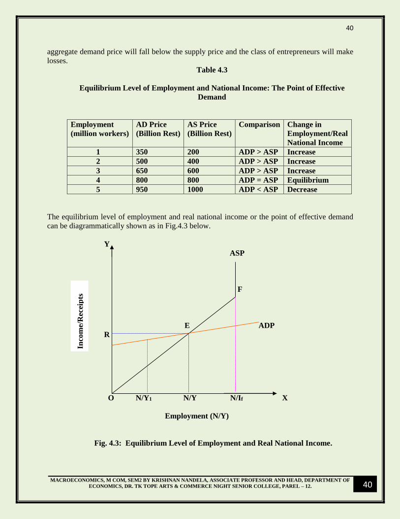
40



40

aggregate demand price will fall below the supply price and the class of entrepreneurs will make

losses.

Table 4.3

Equilibrium Level of Employment and National Income: The Point of Effective

Demand

Employment

(million workers)

AD Price

(Billion Rest)

AS Price

(Billion Rest)

Comparison Change in

Employment/Real

National Income

1 350 200 ADP > ASP Increase



4 800 800 ADP = ASP Equilibrium

5 950 1000 ADP < ASP Decrease

The equilibrium level of employment and real national income or the point of effective demand

can be diagrammatically shown as in Fig.4.3 below.

Y

ASP

F

E ADP

R

O N/Y1 N/Y N/If X

Employment (N/Y)

Fig. 4.3: Equilibrium Level of Employment and Real National Income.

Inco

me/

Rec

eip

ts

41



41

In Fig. 4.3 above, the two curves ADP and ASP intersect each other at point ‘E’. Point ‘E’ is the

point of effective demand. Corresponding to point ‘E’, point ‘R’ on the Y-axis indicates

equilibrium receipts and point ‘N’ on the X-axis indicates equilibrium level of employment and

real national income. However, point ‘E’ is only an under employment or less than full

employment equilibrium as full employment level is indicated by point ‘F’ on the aggregate

supply curve.

Per Keynes, the economy achieves equilibrium at less than full employment level because the

gap between income and consumption is not fully filled up by investment. Both investment and

savings are made by two different classes. While savings are made by the household sector,

investments are made by the class of entrepreneurs. Hence, investment cannot be equal to

saving. If aggregate investment is less than aggregate savings, economy will operate at less than

full employment level.

Increase in the Level of Effective Demand and Employment.

Per Keynes, the aggregate supply function is constant in the short run because the productive

capacity of the economy cannot be increased in the short period. However, the level of effective

demand and employment can be increased by increasing the aggregate demand function. This is

shown in Fig.4.4 below.

Y

ASP

F

E2ADP2

R2

E1ADP1

R1

O N/Y1 N/Y2 N/If X

Employment (N/Y)

Fig. 4.4: Increase in the level of Employment & Real National Income.

Inco

me/

Rec

eip

ts

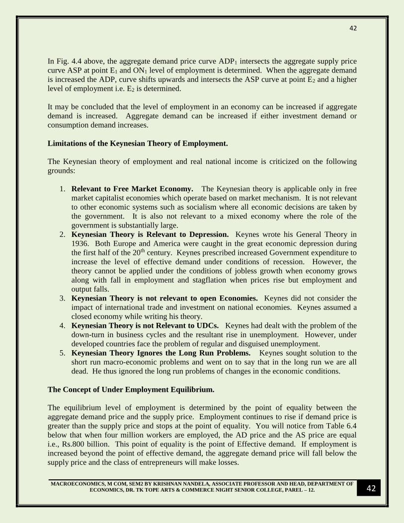
42



42

In Fig. 4.4 above, the aggregate demand price curve ADP1 intersects the aggregate supply price

curve ASP at point E1 and ON1 level of employment is determined. When the aggregate demand

is increased the ADP, curve shifts upwards and intersects the ASP curve at point E2 and a higher

level of employment i.e. E2 is determined.

It may be concluded that the level of employment in an economy can be increased if aggregate

demand is increased. Aggregate demand can be increased if either investment demand or

consumption demand increases.

Limitations of the Keynesian Theory of Employment.

The Keynesian theory of employment and real national income is criticized on the following

grounds:

1. Relevant to Free Market Economy. The Keynesian theory is applicable only in free

market capitalist economies which operate based on market mechanism. It is not relevant

to other economic systems such as socialism where all economic decisions are taken by

the government. It is also not relevant to a mixed economy where the role of the

government is substantially large.

2. Keynesian Theory is Relevant to Depression. Keynes wrote his General Theory in

1936. Both Europe and America were caught in the great economic depression during

the first half of the 20th century. Keynes prescribed increased Government expenditure to

increase the level of effective demand under conditions of recession. However, the

theory cannot be applied under the conditions of jobless growth when economy grows

along with fall in employment and stagflation when prices rise but employment and

output falls.

3. Keynesian Theory is not relevant to open Economies. Keynes did not consider the

impact of international trade and investment on national economies. Keynes assumed a

closed economy while writing his theory.

4. Keynesian Theory is not Relevant to UDCs. Keynes had dealt with the problem of the

down-turn in business cycles and the resultant rise in unemployment. However, under

developed countries face the problem of regular and disguised unemployment.

5. Keynesian Theory Ignores the Long Run Problems. Keynes sought solution to the

short run macro-economic problems and went on to say that in the long run we are all

dead. He thus ignored the long run problems of changes in the economic conditions.

The Concept of Under Employment Equilibrium.

The equilibrium level of employment is determined by the point of equality between the

aggregate demand price and the supply price. Employment continues to rise if demand price is

greater than the supply price and stops at the point of equality. You will notice from Table 6.4

below that when four million workers are employed, the AD price and the AS price are equal

i.e., Rs.800 billion. This point of equality is the point of Effective demand. If employment is

increased beyond the point of effective demand, the aggregate demand price will fall below the

supply price and the class of entrepreneurs will make losses.

43



43

Table 4.4

Equilibrium Level of Employment/Real National Income

The Point of Effective Demand

Employment

(million workers)

AD Price

(Billion Rest)

AS Price

(Billion Rest)

Comparison Change in

Employment/Real

National Income




4 800 800 ADP = ASP Equilibrium

5 950 1000 ADP < ASP Decrease

The equilibrium level of employment or the point of effective demand can be diagrammatically

shown as in Fig.4.5 below.

Y

ASP

F

EADP

R

O N/Y1 N/Y N/If X

Employment (N)

Fig. 4.5: Equilibrium Level of Employment.

Inco

me/

Rec

eip

ts

44



44

In Fig. 4.5 above, the two curves ADP and ASP intersect each other at point ‘E’. Point ‘E’ is the

point of effective demand. Corresponding to point ‘E’, point ‘R’ on the Y-axis indicates

equilibrium receipts and point ‘N’ on the X-axis indicates equilibrium level of employment.

However, point ‘E’ is only an under employment or less than full employment equilibrium as full

employment level is indicated by point ‘F’ on the aggregate supply curve. Per Keynes, the

economy achieves equilibrium at less than full employment level because the gap between

income and consumption is not fully filled up by investment. The reasons for the gap in

savings and investment are as follows:

1. The people who save and the people who invest are not same. The households save and

the entrepreneurs invest.

2. The factors which determine saving are different from the factors which determine

investment. For instance, people save to provide for education, marriage and

contingencies such as disease, unemployment and death. People may also save to acquire

durable goods such as houses, gold and to provide for old age. The level of investment

depends upon marginal efficiency of capital and the rate of interest in the short run and in

the long run, it depends upon population and technological progress.

In view of the reasons mentioned above, we may conclude that investment cannot be equal to

savings at full employment level. If the profit expectations of the entrepreneurs fall, the level of

investment will fall and hence the equilibrium level of national income and employment will also

fall.

CONCEPT OF INFLATIONARY GAP.

Inflation or price rise is the result of a persistent excess aggregate demand over aggregate supply

in the economy. The rise in aggregate demand beyond the capability of the economy during a

given time to offer a matching aggregate supply would result in price rise. The capability of the

economy is the productive capacity with the availability of the given productive resources. If the

rise in aggregate demand is because a large budget deficit financed by borrowing from the

Central Bank, there will be an increase in money supply and prices would rise. Thus, along with

rise in aggregate demand, a rise in money supply would also cause the generation of inflationary

forces. Because excess aggregate demand, inflationary gap will be created which if not vacated

or neutralized, prices will begin to rise. The fiscal policy instruments to control inflation are: (a)

reduction in government expenditure and (b) increase in taxes. Reduction in government

expenditure by way of reduction in the budget deficit and or by increasing the taxes, the level of

aggregate demand can be brought down. The process of decrease in government expenditure

and its impact on the level of aggregate demand is shown in Fig.4.6. The figure shows that the

aggregate demand curve C + I + G1 intersect the 45o line or the line of unity (C = Y) at point ‘E1’

and determines equilibrium national income and output at point Y1 which is the potential

productive capacity of the economy during the given time. Beyond this point if the aggregate

demand rises because increase in government expenditure, financed by a budget deficit, the

aggregate demand curve will intersect the line of unity at point E2. The new aggregate demand

curve C + I + G2 will determine Y2 level of income which is greater than the productive capacity

of the economy determined at point Y1.. Thus, excess aggregate demand over aggregate supply

45



45

by the amount E1A shown in the figure generates an inflationary pressure causing the prices to

rise. Such a price rise or inflation is also known as Demand-pull Inflation.

The inflationary gap can be vacated or neutralized by a decrease in the level of aggregate

demand. The level of aggregate demand can be reduced by a contractionary fiscal policy using

the fiscal policy instruments of reduced government expenditure and increase in taxes. With

equilibrium at point E2 and money income being OY2, if the government reduces expenditure by

E2 which is equal to the inflationary gap E1A, the aggregate demand curve C + I + G2 will shift

downward and once again the original equilibrium level of aggregate demand C + I + G1 and Y1

level of national income corresponding to the productive capacity of the economy will be

established. You will notice that the fall in the nominal national income Y2Y1 is much greater

than the fall in government expenditure E2B. This is because the operation of reverse income or

the investment multiplier.

Y

45o (C = Y)

C + I2 + G2

Inflationary Gap E2

A } ∆G C + I1 + G1

{ B

E1

1

∆Y = ∆G × _____

MPS

∆Y (GNP)

O

Y1 Y2 X

National Income

Fig. 4.6 –Inflationary Gap

Alternatively, the government can also bring about an increase in the direct taxes and reduce the

disposable income of the community to bring down the level of aggregate demand and prices to

their desired level. If the government has a balanced budget and the economy experiences

inflationary tendencies, it would mean that there are supply bottlenecks creating a shortfall in

supply relative to demand. In such a situation, an anti-inflationary or tight fiscal policy by way

of reduction in government expenditure will create a budget surplus. The government can vacate

Exp

end

itu

re

46



46

the budget surplus either by reducing or by impounding public debt. However, if the bduge5t

surplus is vacated by reducing public debt, the money supply will increase and thus dampen the

anti-inflationary impact of a tight fiscal policy. The best way to realize the full impact of a tight

fiscal policy in the event of la budget surplus is to keep the surplus idle so that money supply

does not increase and dampen the deflationary impact of an anti-inflationary fiscal policy.

Questions.

1. Explain the concept of effective demand.

2. Explain how real national income is determined under the Keynesian theory.

3. Explain the aggregate demand function.

4. Explain the aggregate supply function.

5. Explain how the actual level of real national income is less than full employment

level of income.

6. Explain the concept of inflationary gap.

7. Explain how the level of real national income can be increased according to the

Keynesian theory of income.

47



47

MODULE TWO

DETERMINATION OF NATIONAL INCOME

CHAPTER FIVE

PHILLIPS CURVE ANALYSIS

PREVIEW.

Introduction to Philips Curve.

Keynesian Explanation of the Phillips Curve.

Collapse of the Phillips Curve Hypothesis.

Natural Unemployment Rate Hypothesis and the theory of Adaptive Expectations.

Long Run Phillips Curve and the theory of Adaptive Expectations.

Rational Expectations and the Long Run Phillips Curve.

Relationship between the Short Run and the Long Run Philips Curve.

INTRODUCTION.

Economic growth without inflation and unemployment is the objective behind macro-economic

policies of modern times. However, in the short term, there seems to be a trade-off between

inflation and unemployment and hence macro-economic policy makers need to balance between

inflation, economic growth and unemployment. A low inflation rate is seen to accompany lower

economic growth rate and higher unemployment whereas a high inflation rate is seen to

accompany higher economic growth rate and lower unemployment. Here, in this chapter, we

look at the Phillips curve which was the first explanation of its kind to show the negative

relationship between unemployment and inflation rate. We also look at the long run picture and

see whether the negative relationship sustains in the long run.

In 1958, AW Phillips, a professor at the London School of Economics published a study of wage

behavior in the United Kingdom for the years 1861 and 1957. Phillips found an inverse

relationship between the rate of unemployment and the rate of inflation or the rate of increase in

money wages. The higher the rate of unemployment, the lower the rate of wage inflation i.e.

there is a trade-off between wage inflation and unemployment. The Phillips curve shows that the

rate of wage inflation decreases with the increase in unemployment rate. Such a Phillips curve is

depicted in Fig. 5.1.

You may notice that when the rate of inflation is ten per cent, the unemployment rate is three per

cent and when the rate of inflation is five per cent, the rate of unemployment increases to eight

per cent. Empirical or objective data collected from other developed countries also proved the

existence of Phillips Curve. Economists believed that there existed a stable Philips Curve

48



48

depicting a trade-off between unemployment and inflation. This trade-off presented a dilemma

to policy makers. The dilemma was a choice between two evils, namely: unemployment and

inflation. In a dilemma, you chose a lesser evil and inflation is a lesser evil for policy makers. A

little more inflation can always be traded off for a little more employment. However, further

empirical data obtained in the 70s and early 80s proved the non-existence of Phillips Curve.

During this period, both Britain and the USA experienced simultaneous existence of high

inflation and high unemployment. While prices rose rapidly, the economy contracted along with

more and more unemployment.

KEYNESIAN EXPLANATION OF PHILLIPS CURVE.

The explanation of Phillips curve by the Keynesian economists is shown in Fig. 4.2. Keynesian

economists assume the upward sloping aggregate supply curve. The AS curve slopes upwardly

due to two reasons. Firstly, as output is increased in the economy, the law of diminishing

marginal returns begins to operate and the marginal physical product of labor (MPPL) begins to

decline. Since the money wages are fixed, a fall in the MPPL leads to a rise in the marginal cost

of production because MC = W/ MPPL. Secondly, the marginal cost goes up due a rise in the

wage rate as employment and output are increased. Following rise in aggregate demand, demand

for labor increases and hence the wage rate also increases. As more and more labor is employed,

the wage rate continues to rise and the marginal cost of firms increases. You may notice that in

Panel (a) of Fig.4.2 that with the initial aggregate demand curve AD0 and the given aggregate

49



49

supply curve AS0, the price level P0 and output level Y0 are determined. When the aggregate

demand increases, the AD0 curve shifts to the right and the new aggregate demand curve AD1

intersects the aggregate supply curve at point ‘b’. Accordingly, a higher price level P1 is

determined along with a rise in GNP to Y1 level. With the increase in the real GNP, the rate of

unemployment falls to U2. Thus, the rise in the price level or the inflation rate from P0 to P1, the

unemployment rate falls thereby depicting an inverse relationship between the price level and the

unemployment rate. Now when the aggregate demand further increases, the AD curve shifts to

the right to become AD2. The new aggregate demand curve AD2 intersects the aggregate supply

curve at point ‘c’. Accordingly, the price level P2 and output level Y2 is determined. The level

of unemployment now falls to U3. In Panel (b) of Figure 4.2, points a, b and c are plotted and

these points corresponds to the three-equilibrium points a, b and c in Panel (a) of the figure.

Thus, a higher rate of increase in aggregate demand and a higher rate of rise in price level are

related with the lower rate of unemployment and vice versa. The Keynesian economists were

thus able to explain the downward sloping Philips curve showing inverse relation between rates

of inflation and unemployment.

COLLAPSE OF THE PHILLIPS CURVE HYPOTHESIS (1971-91).

The Phillips Curve hypothesis was accepted as a cure to increase the level of employment and

income in the sixties. It became a macroeconomic tool to explain the trade-off between inflation

rate and unemployment rate. It suggested that policy makers could choose different

combinations of unemployment inflation rates. Policy makers may choose low unemployment

and high inflation if it is politically and economically expedient. However, the stable relationship

between higher inflation and lower unemployment as seen in the sixties could not be replicated

in the seventies and thereafter, particularly in the United States and Great Britain. It was seen

50



50

that both inflation rate and unemployment rate had increased on numerous occasions and the

tradeoff had thus disappeared. Further, there cannot be a long run trade-off between inflation

and unemployment because in the long run the aggregate supply curve becomes vertical and any

further expansion after the point of full employment is reached will only add to the price level

without adding anything to income, employment and output. Thus, there is no permanent

unemployment-inflation trade-off. Data obtained in the seventies and thereafter indicated a

shift in the Phillips curve i.e. in various years, at a given rate of inflation, the Phillips curve either

shifted to the left or to the right, indicating thereby that at times, given the inflation rate,

unemployment rate has increased or decreased. The stable relationship between inflation rate

and unemployment rate thus was proved to be non-existent.

Causes of Shift in Phillips Curve.

The shifts in the Phillips curve according to Keynesians is due to adverse supply shocks

experienced in the seventies in the form of unprecedented oil price hikes. Adverse supply shocks

gave rise to the phenomenon of Stagflation and the breakdown of the Phillips curve hypothesis.

The impact of adverse supply shocks on national product and the price level is depicted in Fig.

5.3. The original aggregate demand and supply curves AD0 and AS0 are in equilibrium at point

E0. Accordingly, the price level P0 and national output Y0 is determined. The oil price hike

initiated by the Oil and Petroleum Exporting Countries (OPEC) an oil cartel of oil producing

Middle East countries contributed to the rise in cost of production of many goods and services in

which oil is used as an input. Increase in the cost of production caused the aggregate supply

curve to shift to the left in the upward direction, thereby causing the price level to rise along with

a decrease in national output. Notice that the new aggregate supply curve AS1 now intersects the

aggregate demand curve AD0 at point E1 and accordingly the new price level P1 is determined.

However, at a higher price level P1, the national output has fallen to Y1 leading to rise in

unemployment. Such a situation is explained in terms of stagflation where in both

unemployment and price level increases. This new phenomenon experienced, particularly by the

United States in the seventies and thereafter has caused the shift in the Phillips curve.

Stagflation, thus, consigned the Phillips curve hypothesis to the pages of economic history.

51



51

NATURAL UNEMPLOYMENT RATE HYPOTHESIS AND THE THEORY OF

ADAPTIVE EXPECTATIONS.

Milton Friedman put forward the concept of ‘natural rate of unemployment’ to prove that the

Phillips curve phenomenon does not operate in the long run and that the long run Phillips curve

is vertically sloping, thereby having no relationship between inflation rate and unemployment

rate. However, he accepted the fact that there is a short run negative relationship between

inflation rate and unemployment rate. Milton Friedman says that the economy is stable in the

long run at the natural rate of unemployment and any intervention in the form of expansionary

fiscal and monetary policies would only result in higher prices without higher output.

When current GDP is at its potential level, unemployment is not zero or there is no full

employment. The unemployment rate that exists because frictional and structural reasons when

the economy is operating at full employment level is called the natural rate of unemployment or

more appropriately NAIRU (Non-accelerating Inflation Rate of Unemployment). The natural

rate of unemployment is the rate at which in the labor market, the current number of unemployed

is equal to the number of jobs available. Natural unemployment exists due to frictional and

structural reasons. For example, fresh additions to the labor force may spend time to search

suitable jobs. Individuals pursuing higher education may be in the labor force but may not

participate in the workforce due to educational commitments. While the sunset industries may

52



52

be on the decline and thereby reducing the workforce from its rolls, the sunrise industries would

be expanding and adding to its workforce. However, unemployed labor force needs to be trained

for suitable jobs before they are recruited. Unemployment arising out of frictional and structural

causes is termed as natural unemployment and the number of such unemployed persons

constitutes the natural rate of unemployment. In other words, Milton Friedman argues that if

information were not to fail, there will be no divergence between full employment and actual

employment. The natural rate of unemployment is estimated in the range of four to six per cent

in the developed countries.

The term ‘NAIRU’ is a more appropriate term to describe the natural rate of unemployment

because the term ‘natural rate of unemployment’ connotes that unemployment cannot fall below

the natural rate. The Phillips curve hypothesis shows that unemployment rate can fall below the

NAIRU in the short term. Thus, when actual GDP is greater than potential GDP (Y > Y*),

unemployment will be less than NAIRU (U < U*) and vice versa. When the unemployment rate

is below the NAIRU, demand forces put pressure on wages to rise faster than productivity.

When the unemployment rate is above the NAIRU, demand forces put pressure on wages to rise

more slowly than productivity or even to fall. When unemployment is at the NAIRU, demand

forces exert no pressure on wages relative to productivity.

To prove the non-existence of Phillips curve in the long run, Milton Friedman put forward the

theory of adaptive expectations. People form their expectations based on previous and present

rate of inflation and adapt their expectations only when the actual inflation rate is different from

their expected rate. The trade-off between inflation and unemployment is therefore only in the

short run. Milton Friedman’s theory of adaptive expectations and the derivation of the vertically

sloping long run Phillips curve is depicted in Fig.5.5.

It is assumed that the economy is operating at point A0 on the short run Phillips curve (SPC1) and

the natural rate of unemployment is six per cent. The actual inflation rate is four per cent. The

nominal wages are set based on four per cent inflation rate and it is expected that the inflation

rate will continue to be the same in future. When the government adopts expansionary monetary

and fiscal policies, the inflation rate goes up to six per cent. Since the nominal wages are set

based on four per cent inflation rate, the firms make additional profits equal to two per cent and

hence they make fresh investments, thereby increasing the level of employment and output.

Because of fresh investments, the unemployment rate falls below the natural rate of

unemployment and the economy moves to point A1 where the corresponding inflation rate is six

per cent and the unemployment rate is three per cent. Thus, Milton Friedman and other

monetarists argue that there exists a short run trade-off between inflation rate and unemployment

rate.

53



53

LONG RUN PHILLIPS CURVE AND THE THEORY OF ADAPTIVE EXPECTATIONS.

The economy after having reached point A1 does not stay put at that point because after a time

lag, the workers are informed that the current inflation rate is six per cent and that their real

wages have fallen by two per cent. Organized workers will therefore demand compensation for

the inflation which is over and above the expected rate to restore their real incomes. When wage

compensation takes place, the profits levels are also restored to the original levels and the

economy returns to its original equilibrium position at point B0. However, point B0 is on the new

short run Phillips curve SPC2. Corresponding to point B0, the actual inflation rate is six per cent

and the unemployment rate is back at its natural level i.e. six per cent. Now the expected

inflation rate would be six per cent and workers will continue to expect the same rate of inflation

in future. The shift in the Phillips curve will continue if expansionary monetary and fiscal

policies are adopted by the Government and the economy will move along the points B1, C0 etc.

When points such as A0, B0, C0 are joined, the long run Phillips curve is obtained. Note that the

LPC is vertically sloping and the vertical slope indicates that it is neutral between inflation rate

and the unemployment rate. Milton Friedman thus proves that there is no long run trade-off

between inflation rate and unemployment rate. The theory of adaptive expectations indicate that

workers adapt to the new rates of inflation and their expected inflation rate gets adapted in due

course i.e. after a time lag and the economy returns to its original status with a higher rate of

inflation.

54



54

RATIONAL EXPECTATIONS AND THE LONG RUN PHILLIPS CURVE.

According to Milton Friedman’s theory of adaptive expectations, nominal wages lag changes in

the price level or the inflation rate. The adjustment lag in nominal wages to the price level

causes business profits to go up. When profits go up, business units expand their scale output

and thus the level of unemployment in the economy falls below the natural rate.

The advocates of rational expectation theory believe that there is no adjustment lag involved

between nominal wages and changing price level. They argue that there is a quick adjustment

between nominal wages and expected changes in the price level and hence there is no trade-off

between inflation and unemployment. The rate of inflation resulting from increase in aggregate

demand is well anticipated by workers and firms and gets factored in wage agreements. Such

adjustments made in quick succession sometimes and sometimes in advance lead to further price

increases. Thus, there is a rise in the price level without any rise in the real output or fall in

unemployment below the natural rate. According to the Rational Expectations theorists, given

the availability of resources and technology, the aggregate supply curve is vertically sloping at

the potential GDP level or at the natural unemployment rate level. The long run Phillips curve

therefore corresponds to the long run aggregate supply curve at the natural rate of

unemployment. The long run Phillips curve is therefore a vertical straight line or vertically

sloping at the natural rate of unemployment. The derivation of the long run aggregate supply

curve is shown in Fig. 4.6 and the long run Phillips curve is depicted in Fig. 5.7.

According to the Rational Expectations theorists, the workers and firms are rational beings and

have a good understanding of the operation of the economy. Both workers and firms can

therefore fairly and correctly anticipate the consequences of the economic policies of the

Government. Secondly, all product and factor markets are very competitive and hence factor and

product prices are highly flexible to bring about quick and rapid adjustments. Figure 4.6 shows

the argument made by Rational Expectations theorists about the relation between inflation and

unemployment. The original equilibrium is at point ‘a’ where the initial short run aggregate

demand curve AD0 and the short run aggregate supply curve AS0 intersect each other and the

equilibrium, full employment, national output OY0 and price level P0 is determined, given the

natural rate of unemployment.

Now when the government adopts expansionary monetary and fiscal policies, the economic units

or the factor owners will correctly anticipate the inflationary impact of these policies and make

upward adjustment in factor and product prices thereby holding real national output and real

wages at their original level. The shift in the short run aggregate demand and supply curves will

therefore be vertically upward as shown in the figure. The economy now operates at the new

equilibrium point ‘b’ which is corresponding to the original equilibrium point ‘a’. However, the

equilibrium is achieved at a higher price level P1. At every occasion when the Government

adopts expansionary policies when the economy is operating at the full employment level of

income and output, the aggregate demand and supply curves behave in the same manner and the

equilibrium point changes from point ‘b’ to point ‘c’ and so on and so forth. By joining these

55



55

points, the Long Run Aggregate Supply curve is obtained. Note that the long run AS curve is

vertically sloping indicating thereby that once the full employment equilibrium income and

output is determined at the natural rate of unemployment, any expansionary policy will only

result in price rise, real national output remaining constant.

As the long-run aggregate supply curve is vertically sloping at the natural unemployment rate,

the long run Phillips curve is also vertically sloping.

56



56

RELATIONSHIP BETWEEN SHORT AND LONG RUN PHILLIPS CURVE.

The position of the short run Phillips curve passing through a long run Phillips curve is

determined by the anticipated or expected inflation rate. The short run Phillips curve can be

compared to the short run aggregate supply curve because both the curves are drawn with a given

expected price level. The short run Phillips curve drawn with an expected inflation rate shifts its

position as the inflation rate changes (See figure 5.7). If the expected inflation rate is six per

cent, the short run Phillips curve (SPC1) also passes through the corresponding point ‘A0’ on the

long run Phillips curve with natural unemployment rate of six per cent. The movement along a

short run Phillips curve is determined by changes in aggregate demand. When there is an

unexpected increase in aggregate demand, the actual inflation rate is found to be more than the

expected inflation rate and the real national output increases causing the unemployment rate to

fall below the natural rate. The new short run equilibrium is determined at point ‘A1’ which is to

the left of the original equilibrium point. Conversely, if there is an unexpected decrease in

aggregate demand, the actual inflation rate will fall below the expected rate and the

unemployment rate will increase and real national output will fall. In this case, the movement

will be downwards and to the right. The shift in the short run Phillips curve is caused due to the

divergence between actual and expected inflation rates and this divergence is caused by

unexpected changes in monetary and fiscal policies of the government. If the actual inflation

rate is greater than the expected inflation rate, the short run Phillips curve will shift upward and

vice-versa. The distance by which the short run Phillips curve shifts to a new position is equal to

the change in the expected rate of inflation.

57



57

Questions.

1. Explain the trade-off between inflation and unemployment with the help of Phillips curve

analysis.

2. Explain the derivation of the Phillips curve with the Keynesian AD-AS model.

3. Write a note on the collapse of the Phillips Curve Hypothesis.

4. Explain the natural rate of unemployment hypothesis and the theory of adaptive

expectations.

5. Explain the long run Phillips curve and the theory of adaptive expectations.

6. Explain the theory of Rational Expectations and the long run Phillips curve.

7. Explain the relationship between the short and the long run Phillips curve.

58



58

MODULE THREE

THE IS-LM ANALYSIS

CHAPTER SIX

THE IS & LM MODEL

PREVIEW.

Equilibrium in Goods and Money Market. Monetary and Real influences on IS-LM curves. Economic fluctuations and stabilization policies in IS-LM framework. Transmission mechanism and the crowding out effect. Composition of Output and Policy Mix. IS-LM in India

Integrated Approach (The IS and the LM Model).

The IS-LM model shows how the equilibrium levels of income and interest rates are

simultaneously determined by the simultaneous equilibrium in the two interdependent goods and

money markets. Hicks, Hansen and Johnson put forward the IS-LM model based on Keynesian

framework of national income determination in which investment, national income, rate of

interest, demand for and supply of money are interrelated and inter–dependent. These variables

are represented by two curves, namely; the IS and the LM curves.

The IS curve (I stand for Investment and S stands for Savings) explains the market for real goods

and services, and the LM curve (L stands for Liquidity and M stands for Money) explains the

supply of and demand for money in an economy. A movement in either of the curves influences

both interest rates and the production of goods and services. A country’s fiscal policy is

responsible for movements in the IS curve, whereas its monetary policy is responsible for

movements in the LM curve. The ISLM is useful in explaining the effects that fiscal and

monetary policies have on interest rates, inflation, and short-term output.

Goods Market Equilibrium (The Derivation of the IS Curve).

The goods market is in equilibrium when aggregate demand is equal to national income. In a

closed two sector economy, the aggregate demand is determined by consumption demand and

Investment demand (AD = C + I). Changes in the interest rate affect aggregate demand through

changes in investment demand. With the fall in interest rates, the profitability of investment rises

because the cost of investment falls. Increase in investment demand leads to increase in

aggregate demand and rise in the equilibrium level of national income. The IS curve shows the

different combinations of national income and interest rates at which the goods market is

in equilibrium. The derivation of the IS curve is depicted in Figure 6.1 below. In panel (A) of

Fig. 6.1 you will notice that the relationship between planned investment and rate of interest is

59



59

depicted. It will be obvious from the figure that planned investment is inversely related to the

rate of interest. When the interest rate falls, planned investment rises, leading to an upward shift

in the aggregate demand function. The shift in the aggregate demand function is depicted in

panel (B) of the figure, where in, you will see that an upward shift caused in the aggregate

demand function leads to a higher level of national income in the goods market. Thus, in the

goods market, the level of national income is inter-connected with the interest rate through

planned investment. The IS curve is the locus of various combinations of interest rates and the

levels of national income at which the goods market is in equilibrium. In panel (C) of Fig. 6.1,

the IS curve is depicted. It shows that the changes in the level of national income are a function

of changes in the level of aggregate demand, planned investment and rate of interest. At the

given rate of interest r0, the level of national income Y0 is plotted. When the interest rate falls to

r1, planned investment increases to I1 and the aggregate demand function shifts from AD0 to AD1

with the goods market assuming equilibrium at Y1 level of national income. We therefore plot Y1

level of national income corresponding to r1 level of interest rate. Similarly, when the interest

rate further falls to r2, planned investment increases to I2 and the aggregate demand curve shifts

upward to AD2 with the goods market assuming equilibrium at Y2 level of national income. In

panel (C), the equilibrium national income Y2 is shown against the rate of interest r2. By

repeating this process for all possible interest rates, we can trace a series of combinations of

interest rates and income levels corresponding to goods market equilibrium. By joining points

such as E0, E1, E2 etc. in panel (C) of the diagram, we obtain the IS curve. You will notice that

the IS curve so obtained is downward sloping indicating that when the rate of interest falls, the

equilibrium national income rises.

National Income

National Income

Rat

e of

Inte

rest

Aggr

egat

e De

man

d

(B)

(C)

O

O

Y

Y

X

X

45 0

Y 0 Y 1 Y2

Y 0 Y 1 Y2

AD 0

AD 1

AD 2

E 0

E 0

E 1

E 1

E 2

E 2

I

I

Planned Investment

Rat

e of

Inte

rest

(A)

O

Y

X

I

I

r 0

r 0

r 1

r 1

r2

r2

I 0 I 1 I2

r

r

II

Fig. 6.1- Derivation of the IS Curve

60



60

The Slope of the IS Curve.

The IS curve has a negative slope indicating an inverse relationship between the rate of interest

and the level of aggregate demand. A higher interest rate will lower the level of planned

investment and hence lower the level of aggregate demand and the equilibrium level of national

income. Similarly, a lower interest rate will raise the level of planned investment and hence

higher will be the level of aggregate demand and the equilibrium level of national income.

The steepness of the IS curve is determined by the elasticity of investment demand curve and the

size of the investment multiplier. The elasticity of investment demand shows the degree of

responsiveness of investment expenditure to the changes in the rate of interest. If the investment

demand is relatively elastic, a given fall in the rate of interest will result in a more than

proportionate change in investment demand bringing about a larger shift in the aggregate

demand curve and larger level of national income, thus making the IS curve flatter. Conversely,

if the investment demand is relatively inelastic, the IS curve will be relatively steep.

The steepness of the IS curve is also determined by the size of the investment multiplier. The

value of the multiplier is determined by the size of the marginal propensity to consume. Greater

the mpc, greater will be the size of the investment multiplier and greater will be the level of

national income because of increase in investment. Thus, making the IS curve flatter.

Conversely, if the mpc is lower, the IS curve will have a steeper slope.

Real Influences on the IS Curve.

Changes in autonomous expenditure causes a shift in the IS curve. Autonomous expenditure is

independent of the level of income and the rate of interest. Autonomous expenditure may

increase because increase in government expenditure, increase in autonomous consumption

expenditure or increase in autonomous investment demand. Autonomous investment demand

may rise due to increase in firm’s optimism about future profits. Autonomous consumption

demand may rise due to households’ estimate of future incomes. Government expenditure has an

autonomous component given the wide-scale use of deficit financing. An increase in autonomous

expenditure at a given interest rate would shift the aggregate demand curve upwards leading to

an increase in the equilibrium level of national income. With interest rate remaining constant, an

upward shift in the aggregate demand curve will cause the IS curve to shift towards the right

indicating increase in national income at the given interest rate.

In figure 6.2 below, the shift in the IS curve is depicted by introducing the third component of

the aggregate demand namely government expenditure and it is denoted by ‘G’.

61



61

National Income

National Income

Rate

of

Inte

rest

Ag

gre

gate

Dem

an

d(A)

(B)

O

O

Y

Y

X

X

45 0

Y 0 Y 1

Y 0 Y 1

C + I (r ) = AD 0 0 0

C + I (r ) + G = AD 0 0 1

E 0

r 0

E 1

E 1

E 2

Fig. 6.2- Shift in the IS Curve due to Increase in Autonomous Expenditure

You will notice from the figure 6.2 that when the rate of interest is r0, the planned investment is

I0 and the Aggregate Demand Curve is AD. The AD curve intersects the 45 line at point E0 and

Y0 level of national income is determined. It is also depicted in panel (B) of the diagram by point

E0. Let us now introduce the government component in the composition of the aggregate demand

and assume that the entire component is autonomous in nature. Government expenditure ‘G’ will

shift the aggregate demand curve to AD1 which intersects the 45 line at point E1 and a higher

level of national income Y1 is determined. Correspondingly, we obtain point E1 on panel (B) of

the diagram as the new equilibrium point and accordingly Y1 level of national income is plotted.

The change in the level of national income from Y0 to Y1 is not because any change in the

interest rate and hence the IS curve shifts to the right. The new equilibrium point E1 is

horizontally contiguous and to the right of point E0 indicating a shift in the IS curve.

The movement along the IS curve indicates shifts in equilibrium income caused by shifts in the

aggregate demand curve due to changes in interest rates. A shift in the aggregate demand curve

caused by any other factor other than interest rate must be represented by a shift in the IS curve.

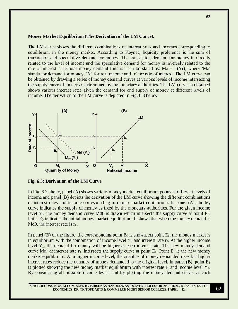
62



62

Money Market Equilibrium (The Derivation of the LM Curve).

The LM curve shows the different combinations of interest rates and incomes corresponding to

equilibrium in the money market. According to Keynes, liquidity preference is the sum of

transaction and speculative demand for money. The transaction demand for money is directly

related to the level of income and the speculative demand for money is inversely related to the

rate of interest. The total money demand function can be stated as: Md = L(Yr), where ‘Md’

stands for demand for money, ‘Y’ for real income and ‘r’ for rate of interest. The LM curve can

be obtained by drawing a series of money demand curves at various levels of income intersecting

the supply curve of money as determined by the monetary authorities. The LM curve so obtained

shows various interest rates given the demand for and supply of money at different levels of

income. The derivation of the LM curve is depicted in Fig. 6.3 below.

National Income

(B)

O

Y

XY 0 Y 1

E 0E 0

E 1

E 1

LM

Quantity of Money

Rate

of

Inte

rest

(A)

O

Y

X

M (Y )d0 0

Md (Y )1

1

r 1

r 0 r 0

M s

Fig. 6.3: Derivation of the LM Curve

In Fig. 6.3 above, panel (A) shows various money market equilibrium points at different levels of

income and panel (B) depicts the derivation of the LM curve showing the different combinations

of interest rates and income corresponding to money market equilibrium. In panel (A), the Ms

curve indicates the supply of money as fixed by the monetary authorities. For the given income

level Y0, the money demand curve Md0 is drawn which intersects the supply curve at point E0.

Point E0 indicates the initial money market equilibrium. It shows that when the money demand is

Md0, the interest rate is r0.

In panel (B) of the figure, the corresponding point E0 is shown. At point E0, the money market is

in equilibrium with the combination of income level Y0 and interest rate r0. At the higher income

level Y1, the demand for money will be higher at each interest rate. The new money demand

curve Md1 at interest rate r1, intersects the supply curve at point E1. Point E1 is the new money

market equilibrium. At a higher income level, the quantity of money demanded rises but higher

interest rates reduce the quantity of money demanded to the original level. In panel (B), point E1

is plotted showing the new money market equilibrium with interest rate r1 and income level Y1.

By considering all possible income levels and by plotting the money demand curves at each

63



63

income level and by plotting the corresponding equilibrium points in panel (B), the LM curve is

derived.

The Slope of the LM Curve:

The LM curve is upward sloping. At higher income levels, it requires higher interest rates to

maintain the money market equilibrium with constant money supply. If the quantity demanded of

money is proportionately greater than the change in the income level, the interest rate will be

higher and steeper will be the slope of the LM curve. Further, if the quantity demanded of money

is less responsive to the rise in interest rates, greater will be the rise in interest rate to maintain

the money market equilibrium and steeper will be the LM curve. Conversely, the more the

quantity of money demanded responds to interest rates and the less it responds to income, the

flatter will be the LM curve.

Monetary Influences on the LM Curve:

Given the money demand function, when the money supply increases, the rate of interest falls at

the given level of income. With fixed income level the rate of interest must fall with a rise in

money supply to maintain the money market equilibrium. The fall in interest rate will shift the

LM curve to the right indicating a rise in the money demand function. This is depicted in Fig. 6.4

below.

National IncomeQuantity of Money

Rate

of

Inte

rest

Y Y

X XO O

r0 r0

r1 r1

LM1

LM0

E0E0

E2

E2

E1

E1

Y0Ms

0 Ms

1 Y1

M (Y )d1

1

M (Y )d

0

(A) (B)

Fig. 6.4: Shift in the LM Curve because Increase in Money Supply

You will notice in panel (A) of fig. 6.4 that with the initial money supply Ms0 at Y0 level of

income, the money market is in equilibrium at the interest rate r0. When the money supply

increases to Ms1 at r0 interest rate, there is excess money supply at the given income level Y0. To

maintain the money market equilibrium, the interest rate must fall to r1 if the people are induced

to demand more money at the income level Y0 and the new money supply Ms1. The new interest

income combination (r1, Y0) will be on LM1 as shown in panel (B). Similarly, with the increase

64



64

in money supply from Ms0 to Ms

1 and with the given interest rate r0, the income must increase to

Y1 so that more money is demanded corresponding to the new money supply Ms1. You will

notice in panel (A) that with the increase in money supply at the given interest rate r0, the income

increases and raises the money demand curve to Md1(Y1) and the money market is in equilibrium

at point ‘E2’ with r0 as the interest rate and Y1 as the income level. The new interest-income

combination (r0, Y1) is plotted on the LM1 curve in panel (B). Thus, increase in money supply

will shift the LM curve to the right and if the money supply is reduced, it will raise the interest

rate at the given level of income and cause the LM curve to shift to the left.

The Simultaneous Equilibrium in the Goods and Money Markets.

The equilibrium rate of interest and the level of income is determined at the intersection point of

the IS and LM curve. The goods market is in equilibrium at all points on the IS curve and the

money market is in equilibrium at all points on the LM curve. Hence, only at the point of

intersection between these two curves, both the money market and the goods market will be

simultaneously assuming equilibrium. Such an equilibrium condition is depicted in Fig. 6.5

below.

National Income

Rate

of

Inte

rest

Y

B

C

IS

D

A

E

LM

XO

r0

r1

r2

Y1 Y2Y0

Fig. 6.5: Simultaneous Equilibrium in the Goods and Money Market

The simultaneous equilibrium in both the markets is determined at point E, whereby r0 is the

interest rate determined and Y0 is the level of national income. At interest rate r1 and income

level Y1, the goods market will be in equilibrium at point ‘A’ on the IS curve. But at the interest

rate r1, the money market will be in equilibrium only at income level Y2 at point ‘B’ on the LM

curve. At interest rate r1, the income level Y1 is too low for money market equilibrium and hence

the money demand is not enough to match the given quantity of money supply. With excess

supply of money, interest rate will fall until it reaches r0 level. At r0 interest rate, aggregate

demand and national income would have risen sufficiently to increase money demand so that

equilibrium in the two markets is obtained. Alternatively, at r2 interest level, the income level Y2

65



65

required for goods market equilibrium at point ‘C’ is greater than the income level Y1 required

for equilibrium in the money market at point ‘D’. With income, too high for money market

equilibrium, there is excess demand for money pushing the interest rates up until they reach r0

with Y0 income level where both markets are in equilibrium.

ECONOMIC FLUCTUATIONS AND STABILIZATION POLICIES IN IS-LM

FRAMEWORK.

The IS-LM model helps us to explain as to how changes in monetary policy initiated by the

Central Bank of a country and changes in fiscal policy initiated by the Government of a country

influences the rate of interest and the level of national income in a country.

The Transmission Mechanism and the Crowding-out Effect.

Changes in fiscal policy can be explained in terms of changes in government expenditure and

changes in taxes imposed by the Government. We will first look at the impact of increase in

government expenditure on the rate of interest and the level of national income. This is shown in

Fig. 6.6 below. Autonomous increase in government expenditure raises aggregate demand for

goods and services produced in an economy and pushes the IS curve to the right in the upward

direction. You will notice that autonomous increase in government expenditure shifts the IS

curve from IS1 to IS2. Here, the horizontal distance between the two IS curves is equal to G

1

MPS which shows the increase in income that takes place according to the Keynesian

multiplier. You may notice that with the LM curve remaining constant, the IS2 curve intersects

the LM curve at point F. The IS-LM model therefore explains us that with the increase in

autonomous government expenditure (G), the equilibrium shifts from point E to point F and the

rate of interest rises from R1 to R2 and the level of national income increases from Y1 to Y2. The

IS-LM model therefore explains us that increase in autonomous government expenditure or

expansionary fiscal policy helps to increase both the level of national income and the rate of

interest.

An interesting point that IS-LM model brings to light is the difference in the increase in national

income as given by the Keynesian multiplier and the one given by this model. The increase in

national income by Y1Y2 is less than what would happen given the Keynesian multiplier. Keynes

assumed that investment is fixed and autonomous and brought out his concept of investment

multiplier to explain changes in national income because of changes in investment expenditure.

However, the IS-LM model takes into consideration the fall in private investment due to the rise

in interest rate that takes place with the increase in government expenditure. The extent of fall

in private investment expenditure because of rise in interest rates is termed as Crowding-

Out effect. Similarly, a fall in government expenditure will bring about the leftward shift in the

IS curve and with the LM curve remaining constant, the rate of interest will fall along with a fall

in the level of national income. Reduction in government expenditure to control inflation is an

example of Anti-inflationary or Contractionary fiscal policy.

66



66

Now, we will see what is the impact of reduction in taxes on the rate of interest and the level of

national income in the economy. Reduction in taxes is an alternative to increase in government

expenditure. Tax reduction increases the disposable income of the people leading to increase in

consumption expenditure and thereby increase in aggregate demand. When the government

reduces taxes, the IS curve shifts to the right as shown in Fig. 6.7 below from IS1 to IS2. Once

again, you will notice that the change in national income as result of reduction in taxes is only

Y1Y2 which is less than what the Keynesian tax multiplier T MPC

MPS would make us available.

You may notice that the effective increase in national income because of the tax multiplier is

equal to EH. Whereas, the IS-LM model shows that the increase in national income is much less

than what the Keynesian tax multiplier would generate as the LM curve remains constant and the

new IS curve IS2 intersects the LM curve at point D. According to the new equilibrium point D,

the new rate of interest is R2 and the rise in national income is Y1Y2. Similarly, if the government

wants to control inflationary pressures in the economy, it may initiate a raise in taxes. When the

taxes are increased, the disposable incomes of the people would fall leading to a fall in

consumption expenditure. Fall in consumption expenditure will help in controlling price rise.

R1

X

Y

Rate

of In

tere

st

0

R2

Level of National Income

Y1 Y2

F

Y

H

IS1

IS2

E

G1

MPS

LM

Fig.6.6: Impact of increase in Government Expenditure on Interest Rate and National

Income

67



67

R1

X

YR

ate

of In

tere

st

0

R2


Y1 Y2

IS1

IS2

LM

Y

TMPS

MPC

Fig. 6.7: Impact of Reduction in Taxes on Interest Rate and National Income

Impact of Changes in Monetary Policy on the Rate of Interest and the Level of National

Income:

The monetary policy of the government is determined and executed by the Central Bank of the

country. Changes in the monetary policy can bring about changes in the rate of interest and the

level of national income. Like fiscal policy, the monetary policy can be expansionary or

contractionary. To increase the availability of credit and push economic growth rate to a higher

level, the Central Bank may follow an expansionary monetary policy. However, in times of

rising prices, the Central Bank may follow a contractionary or tight monetary policy to control

the rising prices. The IS-LM model can be used to show the impact of both expansionary and

contractionary monetary policies on the rate of interest and the level of national income. Changes

in money supply will cause a shift in the LM curve. While increase in money supply will shift

the LM curve to the right, the opposite will happen when money supply is reduced. If the

economy is in a state of recession i.e., when the growth rate in the national income is regularly

falling, the Central Bank would follow an expansionary monetary policy to draw the economy

out of recession. The Central Bank would follow steps that would increase money supply in the

economy. Increase in money supply, with demand for money remaining constant would create a

downward pressure on the rate of interest and the rate of interest would fall. When the interest

rate falls, investment demand will rise leading to an increase in national income in the economy.

Thus, with the increase in money supply, the LM curve will shift towards the right and intersect

the constant IS curve at point D as shown in Fig. 6.8 below. You will notice that the economy

moves from the initial equilibrium point E to D, the rate of interest falls from R1 to R2 and the

level of national income increases from and the level of national income increases from Y1 to Y2.

The IS-LM model therefore shows that expansion in money supply lowers the rate of interest and

increases national income. Similarly, if the economy is caught in an inflationary spiral, the

Central Bank may follow a tight monetary policy that is it would reduce money supply and bring

about a rise in the rate of interest and fall in the level of national income. Less income will

68



68

reduce the aggregate demand in the economy and reduce the pressure on rising prices thereby

controlling the inflation rate.


Y1 Y2

E

IS

R1

R2

Rate

of In

tere

st

X

D

LM2

LM1

Y

0

Fig. 6.8: Impact of Expansionary Monetary Policy on Interest Rate and National Income

COMPOSITION OF OUTPUT AND POLICY MIX.

The monetary and fiscal policy of the country influences real output or real income. An

expansionary monetary policy would bring down the rate of interest, expand investment,

employment and output whereas an expansionary fiscal policy will raise the rate of interest,

crowd-out private investment, raise the price level and bring out increase in employment, output

and real income. An expansionary fiscal policy is inherently inflationary whereas expansionary

monetary policy is not. A policy mix can achieve a higher level of income and output without

generating inflationary pressures. When expansionary fiscal policy is complemented by

accommodating expansionary monetary policy, the real national income or output goes up

without increasing the rate of interest. Such a situation is shown in Figure 6.9.

In Figure 6.9, the initial income level is Y0 and R0 is the equilibrium rate of interest. When the

government adopts an expansionary fiscal policy, the IS curve shifts from IS0 to IS1 and

intersects the original LM curve at point E1. The real national output increases to Y1. However,

the rate of interest also goes up to R1. The potential effect of an expansionary fiscal policy is

curtailed by crowding out of private investment. The horizontal distance between E0 and E2

measures the potential rise in real national output. However, the actual rise in real national

output is only Y1. When the monetary authorities complement the expansionary fiscal policy of

the government by an accommodating expansionary monetary policy, money supply increases

and the LM curve shifts to the right. The rate of interest falls to the original level and the full

69



69

potential of the expansionary fiscal policy is realized when the real output further increases to Y2

level.

A combination and monetary and fiscal policies can therefore achieve economic growth with

price stability i.e. increase in real national income without a price rise.

LM0

E1 LM1

R1

R0 E0 E2

IS1

IS0

0 Y0 Y1 Y2

Fig.6.9 – Policy Mix and Real Income.

IS – LM IN INDIA.

Fiscal policy was ordinarily used as a macroeconomic pool tool in India until 1990 when the new

economic policy was adopted. Monetary policy played a secondary role. Increases in

Government expenditure were financed by government borrowing. Government borrowing was

facilitated by increases in the Statutory Liquidity Ratio (SLR). In the year 1990, the SLR was

38.5 per cent. The money in the SLR account was used by commercial banks to purchase

government securities. However, banks earned low interest rates on their SLR investments. The

other source of financing increased government expenditure was borrowing from the Reserve

Bank of India by selling ad-hoc treasury bills. Financing government expenditure through ad-

hoc treasury bill led to monetization of the government deficit and increase in money supply

through the increase in reserve money. As per C Rangarajan, the changes in net RBI credit to the

central government accounted for 93 per cent of the variation in reserve money in the 1980s.

Automatic monetization of government deficit limited the scope of discretionary monetary

policy in India. After the adoption of the new economic policy of 1991, under the structural

adjustment program, controlling fiscal deficit assumed prime importance. The Fiscal

Responsibility and Budget Management Act (FRBM) was passed in 2003. By 1997, government

borrowing through the RBI by selling ad-hoc treasury bills was replaced by Ways and Means

Inte

rest

Rat

e

Real Income

70



70

Advances (WMA). Introduction of WMA raised the ability of the RBI to influence liquidity and

formulate independent monetary policy.

From 1995-96 to 2000-01, both fiscal and monetary policy were expansionary. During this

period, the fiscal deficit increased along with the increase in money supply. However, the

influence of fiscal policy was greater than that of monetary policy. During this period, the fiscal

deficit grew at the trend rate of 18.1 per cent and the real money supply trend growth rate was

10.3 per cent.

During the period 2001-02 to 2005-06, the fiscal deficit growth rate came down to -0.4 per cent

and real money supply came down marginally to 9.1 per cent. Large government borrowing

during the period 1995-96 to 2000-01 shifted the IS curve to the right much more than the shift

in the LM curve and raised the rate of interest in the Indian economy from 4.7 per cent in 1995-

96 to 7.4 per cent by 2000-01. High interest rate reduced investment demand and reduced the

growth in output.

During the period 2001-02 to 2005-06, there was a fall in the growth of government borrowing

and monetary policy continued to remain expansionary. Hence, the LM curve shifted more to

the right than the IS curve. The interest rate therefore began to decline and national output went

up. This was also the period when new technology was introduced in the Indian banking system.

The use of credit and debit cards reduced the transaction demand for money. The demand for

money slowed down despite of the higher growth rates in output and expansion in money supply.

The period 2001 to 2006 witnessed economic boom due to expansionary monetary policy and

reduction in fiscal deficit.

During the period 2006-07 to 2009-10, real money supply grew at the rate of 1.3 per cent as

compared to 9.1 per cent in the earlier period. However, the fiscal deficit began to increase

rapidly at the trend rate of 39.5 per cent from 2006-7 to 2009-10. Hence, the real interest rate

began to rise and the growth rate of GDP lowered.

Dua and Pandit (2002) have found that the money supply and government expenditure have an

impact on the interest rate in the Indian economy. However, the interest rate is also affected by

external factors. When domestic interest rates are greater than interest rates abroad, capital

inflows increase. Such capital inflows lead to increase in money supply. The Indian Economic

Survey 2002-03 have remarked that the share of net foreign exchange assets in reserve money

was only 9.1 per cent in end March 1991 and by 24th January, 2003, this share was 100.7 which

means that the entire increase in the supply of reserve money was due to capital inflows.

(Reference: Macroeconomics by Errol D’Souza, Chapter 8 IS-LM Model, Second Edition 2012,

p223 to 225).

71



71

Questions.

1. What is an IS curve? Explain the derivation of the IS curve.

2. What is a LM curve? Explain the derivation of the LM curve.

3. Explain how simultaneous equilibrium in the goods market and the money market is

determined.

4. What determines the slope of the IS curve?

5. Explain how increase in the level of autonomous expenditure leads to a shift in the IS

curve?

6. What determines the slope of the LM curve?

7. Explain how increase in money supply leads to a shift in the LM curve?

8. Explain the impact of fiscal policy on the rate of interest and level of income.

9. Compare the impact of increase in government expenditure and reduction in taxes on the

rate of interest and national income.

10. Examine the impact of monetary policy on the rate of interest and national income.

11. Define the following or explain briefly:

a) The IS Curve.

b) The LM Curve.

c) Goods Market Equilibrium.

d) Money Market Equilibrium.

e) Simultaneous Equilibrium in the Goods and Money Market.

f) Impact of government expenditure on national income and rate of interest.

g) Impact of reduction in government expenditure on national income and rate of

interest.

h) Impact of monetary policy on rate of interest and national income.

12. Explain how policy mix influences real national income.

13. Write a note on IS LM in India.

72



72

MODULE FOUR

INTERNATIONAL ASPECTS OF MACROECONOMIC POLICY

CHAPTER SEVEN

INTERNATIONAL ASPECTS OF MACROECONOMIC POLICY

PREVIEW.

Balance of payments disequilibrium of an open economy.

Corrective policy measures -Expenditure changing policies and expenditure switching

policies.

BOP adjustments through monetary and fiscal policies.

The Mundell-Fleming model.

Devaluation. Revaluation as expenditure switching policy. Effectiveness of devaluation and J – curve.

BALANCE OF PAYMENTS DISEQUILIBRIUM IN AN OPEN ECONOMY.

Equilibrium or disequilibrium in the balance of payments refer to the balance on those heads of

the account which do not include the drawings from the IMF, use of special drawing rights,

drawings from the reserves of foreign currencies held by the Central government etc. Excluding

these items, if there is neither deficit nor surplus in the balance of payments, it is known to be in

equilibrium. Otherwise, it will be in disequilibrium. The deficit in the balance of payment can

be financed by drawings from the IMF, use of Special Drawing Rights and drawings from the

reserves of foreign currencies. In 1999-2000, the deficit on the current account was financed by

the surplus on the capital account of India’s balance of payment. Nonetheless, India’s balance of

payment remains unfavorable and in disequilibrium because of a deficit on the current account.

It thus means that when there is neither surplus nor deficit on the current account, the balance of

payment is said to be in equilibrium. A more important concept of balance of payment is the

concept of basic balance. It is based on autonomous items in the balance of payment.

Autonomous items are those items which cannot be easily changed or influenced by the

government because they are determined by long term factors. Autonomous transactions take

place on their own because of peoples’ desire to consume more or to make higher profits. For

instance, both export and import of goods and services which are items on the current account

are undertaken to make profit or consume more goods and services. Exports and imports take

place irrespective of other transactions included in the balance of payment accounts. It is for this

reason they are called autonomous transactions. Autonomous transaction also includes long term

capital movements both on private and government account contained in the capital account. If

exports are equal to imports, there will be no other transaction but if they are not equal, it will

lead to short term capital movements in the form of international borrowing and lending. These

73



73

capital movements are undertaken for bridging the deficit in the balance of trade. Since the

short-term capital flows are accommodating or compensatory in nature, they are called induced

transactions. Induced transactions include borrowing from the International Monetary Fund or

Central Banks of other countries, drawings from Special Drawing Rights account. Induced

transactions are excluded from the concept of basic balance. Thus, when autonomous

transactions are equal and there is no need for induced transactions, the balance of payment is in

equilibrium. This equilibrium in the balance of payment is a state of balance which can be

sustained without government intervention. The concept of basic balance therefore can be stated

as:

(X – M) + LTC = 0

Where, X stands for exports.

M stands for imports, and

LTC stands for long term capital movements.

If exports are greater than imports (X > M), long term capital movement will be negative and

equal to net exports (Xn) which means there will be net capital outflow. Similarly, if exports are

less than imports (X < M), long term capital movement will be positive and equal to net imports

(Mn) which means there will be an inflow of capital to bridge the deficit in the current account.

CORRECTIVE POLICY MEASURES.

BALANCE OF PAYMENT ADJUSTMENTS.

Disequilibria in the balance of payment are corrected with the help of automatic adjustment

through price and income changes. Price changes are studied under flexible exchange rates and

under gold standard. Income changes are explained through the foreign trade multiplier. To

correct disequilibria in the balance of payments, adjustment policies are implemented by the

government of a country. These policies include expenditure changing and expenditure

switching policies, maintaining external and internal stability and direct controls. Adjustment

mechanisms are studied through the elasticity, absorption and monetary approaches.

Expenditure changing policies are aimed at changing aggregate expenditure in the economy

though monetary and fiscal policies to correct disequilibrium in the balance of payments.

Expenditure switching policies aim at devaluation or revaluation of a country’s currency so that

expenditure is switched from foreign goods to domestic goods and vice versa. Both devaluation

and direct controls are used to exercise switch in the expenditure from imported goods to

domestic goods.

74



74

BALANCE OF PAYMENTS AND POLICY MIX (ROLE OF MONETARY AND FISCAL

POLICY IN BALANCE OF PAYMENT ADJUSTMENT).

Internal stability or internal balance refers to full employment with price stability and external

stability refers to balance of payment equilibrium. JE Meade in his ‘The theory of International

Economic Policy’ pointed out that to maintain both internal and external balance, a country must

control both its aggregate expenditure and the exchange rate. It was HG Johnson in his ‘Money,

Trade and Economic Growth’ who pointed out the range of policy instruments to bring about

internal and external balance. He called them expenditure changing and expenditure

switching policies.

EXPENDITURE CHANGING MONETARY AND FISCAL POLICIES.

Expenditure changing policies are aimed at changing aggregate expenditure in the economy

through appropriate monetary and fiscal policies to achieve balance of payment equilibrium.

These policies can be explained with the help of IS-LM Balance of Payment technique where in

the IS curve represents the fiscal policy and LM curve represents the monetary policy and the

balance of payments (BP) curve representing external balance. The BP curve traces out those

combinations of interest rate and national income that produce balance of payment equilibrium.

An increase in income will increase imports and increase the balance of payment deficit by

increasing the current account deficit while an increase in interest rate will attract foreign

investments and there will be capital inflow thereby increasing the capital account surplus. Any

point above and to the left of the BP curve represents surplus in Balance of Payments and a point

below and right of the BP curve shows a balance of payment deficit. The impact of monetary

and fiscal policies and on balance of payment position is explained below.

MONETARY POLICY.

An expenditure changing monetary policy influences the economy through changes in money

supply and interest rates. A contractionary monetary policy leads to balance of payment surplus

and an expansionary monetary policy leads to a balance of payment deficit. The following

assumptions are made:

There is a fixed exchange rate.

There is relative capital mobility, and

There is no change in government expenditures i.e., the IS curve remains constant.

Expenditure Reducing Monetary Policy. A balance of payment deficit implies excess of

expenditure over income. In the case of a deficit, a contractionary monetary policy would reduce

money supply which increases interest rate thereby reducing investment and output which in turn

reduces income and aggregate demand for imported goods. There is also a reduction in the

domestic price level which may lead to switching of expenditure from foreign to domestic goods.

Hence, imports are reduced and exports increase thereby reducing current account deficit.

Further there is a reduced outflow of short term capital with reduction in imports which reduces

the deficit. Further, increase in domestic interest rates increase the inflow of capital thereby

75



75

eliminating the balance of payment deficit. The adjustment process would be opposite if an

expansionary monetary policy is adopted to correct a surplus in the balance of payments.

Expenditure reducing monetary policy and its effects is shown in Fig. 7.1 below.

BP

LM1

E1

R1 LM

E

R

IS

O

Y1 Y Income

Fig.7.1: Impact of Expenditure Reducing Monetary Policy on Balance of Payment.

The equilibrium in the economy is established at the intersection of IS-LM-BP curves at point E

and the equilibrium interest rate OR and income level OY is determined. When the domestic

money supply is reduced, the LM curve shifts to the left to LM1. The new equilibrium is at E1.

Since E1 is to the left of the BP curve, there is BoP surplus. The interest rate goes up from OR to

OR1 which generates a capital account surplus with capital inflow. The fall in income from OY

to OY1 generates a current account surplus because of the reduction in imports. Thus, a

contractionary monetary policy leads to a BoP surplus. But E1 does not represent permanent

equilibrium. The BoP surplus will increase the domestic money supply and gradually shift the

LM1 curve to the right towards the LM curve so that E1 begins to move down along the IS curve

to point E when the economy is again in BoP equilibrium.

Expenditure Increasing Monetary Policy.

An expansionary monetary policy leads to a BoP deficit as shown in Fig.7.2 below. When

money supply is increased, the LM curve shifts to the right to LM2 and the new equilibrium is

determined at point E2. Since point E2 is below and to the right of the BP curve, there is BoP

deficit. The interest rate falls from OR to OR2 which generates a capital account deficit with

capital outflow. The increase in income from OY to OY2 generates a current account deficit

with increase in imports. Thus an expansionary monetary policy leads to a BoP deficit. But E2

does not represent a permanent equilibrium. The BoP deficit will reduce the domestic money

Inte

rest

Rat

e

76



76

supply and gradually shift the LM2 curve to the left towards the LM curve so that E2 begins to

move up along the IS curve to point E and the economy is again in BoP equilibrium.

BP

LM1

E1

R1 LM2

E2

R2

IS

O

Y1 Y2 Income

Fig.7.2: Impact of Expenditure Increasing Monetary Policy on Balance of Payments.

FISCAL POLICY.

Fiscal policy refers to the income and expenditure policy of the government. An expansionary

fiscal policy will lead to increase in government expenditure. Reduction in taxes may be

considered as an alternative to increase in government expenditure. In reality, a combination of

higher expenditure and reduction in taxes may be pursued by the government. A contractionary

fiscal policy will be opposite to expansionary fiscal policy.

Expenditure Reducing Fiscal Policy. Under the following assumptions, the effects of

expenditure reducing fiscal policy in correcting Balance of Payment deficit is shown in Fig.7.3:

a) The exchange rate is fixed.

b) There is relative capital mobility.

c) There is no change in monetary policy so that the LM curve remains unchanged.

The original equilibrium is established at point E with OR interest rate and OY income level.

When the government adopts a contractionary fiscal policy, the IS curve shifts downwards to the

left to IS1 which intersects the LM curve at point E. Thus, the interest rate falls to OR2 leading to

an outflow of capital and to capital account deficit. The income level also falls from OY to OY1

Inte

rest

Rat

e

77



77

which reduces imports. But the effect of a contractionary fiscal policy is to have a BoP deficit

because point E2 is below and to the right of the BP curve. However, the effects of a

contractionary fiscal policy on BoP will depend upon the elasticity of the BP curve. In the above

case, the BP curve is elastic. If the BP curve is less elastic such as the BP1 curve, a

contractionary fiscal policy will lead to a BoP surplus. This is because point E2 is above and to

the left of the BP1 curve.

BP1

LM

E1 BP

R1

R2 E2

IS

IS2

O

Y2 Y1 Income

Fig.7.3: Impact of Expenditure Reducing Fiscal Policy on Balance of Payments.

Expenditure Increasing Fiscal Policy.

When the government increases its expenditure and or reduces taxes, the IS curve shifts upwards

to the right and intersects the LM curve at point E1 as shown in Fig.7.4 below. This new

equilibrium shows increase in interest rate from OR to OR1 and rise in income from OY to OY1.

The increase in interest rate leads to capital inflow thereby creating short run BoP surplus on

capital account. The rise in income increases imports thereby leading to a BoP deficit on current

account. The net overall effect on the BoP will depend upon the elasticity of the BP curve. If

the BP curve is elastic, the equilibrium point E1 will be above and to the left of the BP curve and

there will be BoP surplus. If the BP curve is inelastic, the equilibrium point being below and to

the right of the BP1 curve, there will be overall deficit.

Inte

rest

Rat

e

78



78

BP1

LM

E1 BP

R1

R E

IS1

IS

O

Y Y1 Income

Fig.7.4: Impact of Expenditure Reducing Fiscal Policy on Balance of Payments.

Conclusion.

The above analysis shows that a contractionary monetary policy is effective in correcting a BoP

deficit. But an expansionary fiscal policy can either improve or worsen a BoP deficit. Its effect

on the overall BoP is uncertain. The increase in interest rate creates short run BoP capital

account surplus and the increase in income to a current account deficit. If the former effect

predominates an expansionary fiscal policy will bring both the internal and external balance.

The same will not be achieved if the latter effect predominates. To solve the BoP deficit

problem and to bring about internal and external balance, policy makers suggest the mixing of

both monetary and fiscal policies.

Inte

rest

Rat

e

79



79

EXPENDITURE SWITCHING POLICIES.

Expenditure switching policies switch expenditure from foreign goods to domestic goods to

correct the disequilibrium in the balance of payments. Devaluation helps to switch expenditure

from imported goods to domestic goods whereas revaluation helps to switch expenditure from

domestic goods to imported goods. The second expenditure switching policy tool is that of

direct controls. Direct controls are used to correct deficits in the balance of payments by

controlling imports. The purpose of expenditure switching policy is to maintain external

balance.

Devaluation.

Devaluation refers to reduction in the external value of domestic currency in relation to a foreign

currency without changing the internal purchasing power of the domestic currency. When a

country having deficit in the balance of payments, devalues her currency, the domestic prices of

imports increases and the foreign price of her exports fall. Exports become more competitive

and imports become less attractive. Devaluation encourages exports and discourages imports,

thereby switching expenditure from imported goods to domestic goods. The demand for exports

increases and the demand for domestic goods also increase. The deficit in the balance of

payments is thus corrected.

The success of devaluation as a policy tool depends upon the following assumptions:

1. The demand for exports and imports is elastic.

2. The country has the productive capacity to meet higher demand for exports resulting

from devaluation.

3. There is no competitive devaluation or imposition of tariffs by the trading partner

country.

4. There is internal price stability after devaluation.

Under these assumptions, the effect of devaluation on deficit in the balance of payment through

imports and exports is shown in Figure 7.12 (A) and (B). In part ‘A’ of the figure, after

devaluation of the home currency, the demand for exports increases and the demand curve shifts

to the right. The demand for export has increased due to a fall in the export price of goods in

terms of US dollars. The US importer gets more INR for a given dollar than what he could

before devaluation. When the export price fall from PX1 to PX2 in terms of USD, the demand for

exports increase from X1 to X2. Here, the change in demand for exports is greater than the fall in

price. It indicates that the demand for exports is relatively elastic. Thus, India will earn more

export revenue than before.

In the opposite case, after devaluation, the import price in terms of INR will increase and the

demand for imports will decrease. In part ‘B’ of the figure before devaluation, the demand for

imports was OM1, after devaluation, the US dollar becomes more expensive in terms of INR and

at the new price PM2, the supply of US dollars falls thereby shifting the supply curve to the left.

The demand for imports falls to OM2. The fall in the demand for imports from OM1 to OM2 is

greater than the rise in price from PM1 to PM2. Since the demand for imports and exports is

80



80

elastic, India will save on imports and gain on exports. Increase in exports and decrease in

imports by India will therefore reduce the deficit on the balance of payments.

SX

E2

PX2

E1

PX1

DX2

DX1

O

X1 X2 Exports

Fig. 7.12 (A) Increase in Exports after Devaluation.

SM2

SM1

PM2 E2

E1

PM1

DX1

O

M2 M1 Imports

Fig. 7.12 (B) Decrease in Imports after Devaluation.

INR

/US

D E

xch

ange

Rat

e IN

R/U

SD

Exch

ange

Rat

e

81



81

Devaluation of the home currency is an alternative to depreciation. It is a generally adopted

method by countries facing a deficit in the balance of payments. Devaluation is an official

recognition of the fall in the external value of the home currency. While depreciation is de-facto,

devaluation is de-jure. The International Monetary Fund allows devaluation only when the

country is trapped in a fundamental disequilibrium. The impact of devaluation will be the same

as that of depreciation i.e. the exports will become cheaper and the imports dearer, thus bringing

about a correction in the balance of payment. However, devaluation as a measure to correct

persistent deficit in the balance of payment will be successful only under certain conditions.

Firstly, the elasticity of demand for exports and imports should be greater than unity. Otherwise,

devaluation will further worsen the deficit in the balance of payments.

Secondly, if the country exercising devaluation exports non-traditional items with a large

international demand, it will gain because improved terms of trade. However, if the export

consists of primary goods and the imports that of manufactured goods, then the terms of trade

will become unfavorable, thereby worsening the balance of payment situation.

Thirdly, after devaluation, the country should be able to maintain domestic price stability. If

devaluation leads to domestic price rise, the purpose of devaluation will be defeated. However,

the domestic cost price structure of a country may change if the domestic output of import

substitutes is not increased resulting into the price rise. Further, if the reduction of exportable

goods is not increased and if the rise in demand for exports is met by reducing the supply in the

domestic market, prices will rise in the domestic market and make exports less profitable.

Fourthly, if the import content of the exportable goods is high and if the country is capital deficit

and certain to import capital goods at a higher price, cost of production will go up making

imports less attractive to foreign countries. Further, if the price rise in certain category of goods

has chain effect leading to a rise in the general price level, organized labor will demand

compensation in the form of dearness allowance and there will be cost push inflation in the

country. However, if devaluation is combined with deflationary measures in the domestic

economy, domestic price stability can be maintained with a certain degree of success.

Fifthly, devaluation by a country, facing deficit in the balance of payments should not be

countered by competitive devaluation by foreign countries or foreign countries should not off-set

the impact of devaluation by imposing tariff and non-tariff barriers.

Finally, devaluation will be effective only if export promotion and import discouraging measures

are simultaneously implemented. However, devaluation has its negative side. It is a sign of the

economic weakness of a country and has the potential to induce price rise in the domestic

economy. Further, it leads to a rise in cot of debt servicing and if the macro-economic

management of the country is not sound and the country may have to take recourse to

devaluation from time to time as in the case of India.

82



82

Direct Controls.

The second type of expenditure switching policy is the use of direct controls to correct balance of

payment disequilibrium. Exchange control and use of non-monetary measures to restrict imports

and promote exports are used to adjust in the balance of payments.

Exchange control refers to restrictions imposed by the Central bank of a country on the use of

foreign exchange to correct the disequilibrium in the balance of payments. When an exchange

control is adopted, the Central bank collects all the foreign exchange earnings and releases

foreign exchange only for unavoidable and essential imports. Exchange control as a monetary

measure is superior to deflation, depreciation and devaluation because it directly controls the

demand and supply for foreign exchange. The exporters are required to surrender all their

foreign exchange earnings to the Central bank and the imports must obtain permission for import

of goods. The foreign exchange resources with the Central bank are distributed amongst imports

according to the quotas fixed. Exchange control is therefore a very effective method of

correcting deficit in the balance of payment of a country. However, exchange control is not a

permanent solution to long run disequilibrium because it only suppresses demand for imports

and does not cure the causes of deficit.

A judicious mix of monetary and non-monetary measures needs to be simultaneously

implemented to correct disequilibrium in the balance of payments. Both surplus and deficit in

the balance of payments call for correction. In the case of a persistent surplus, the measures

adopted to correct a deficit must be turned on their heads or reversed. For instance, a country

with a favorable balance of payments will face an appreciation in the external value of its

currency. In that case, the Central bank must encourage imports and discourage exports by

pursuing cheap money policy and revaluation of the currency.

Non-monetary measures help in correcting disequilibrium in the balance of payments without

changing the exchange rates. In case of a deficit in the balance of payments, the non-monetary

measures aim at promoting exports and discouraging imports. The following non-monetary

measures can be used to correct deficit in the balance of payment.

1. Export Promotion Measures.

Export promotion helps to improve the foreign exchange reserves of a country and thus corrects the

deficit. The government may implement export promotion measure such as export subsidies, tax

concessions to exporters, marketing facilities, export incentives, loans to exporters on a priority basis,

setting up of export zones land 100% export oriented units, organization of trade fairs in foreign countries

etc. Exportable surplus should be created of those goods which have a high demand in the foreign

countries by expanding production capacities and by discouraging domestic consumption of such goods.

2. Import Control Measures.

Import duties, import quotas and import substitution are the three important measures of import control.

These measures are complementary to export promotion measures to correct the deficit in the balance of

payments. Import duty is a fiscal instrument used to control imports. They result in increase in the price

of imported goods leading to a fall in import demand and reduction in the deficit. Import quota is a direct

83



83

method of correcting disequilibrium in the balance of payments. Import quotas have the immediate

impact in limiting imports as the marginal propensity to import becomes zero as the quota limit is

reached. Import quota is a quantitative measure of import restriction and hence they are highly effective

than import duties. The third measure to control imports is through import substitution. Import

substitution requires setting up of industries which can produce import substitutes inside the country.

However, import substitution industries needs to be set up with indigenous capital and technology and the

goods so produced must be comparable in quality.

Conclusion.

Both monetary and non-monetary measures used to correct disequilibrium in the balance of payments are

known to be an adjustment mechanism. Adjustment through changes in exchange rates relates to

exchange rate depreciation and devaluation. Adjustment through changes in income and price relates to

deflation and adjustment through controls relates to exchange controls and trade controls.

Exchange controls refer to rationing of foreign exchange and trade controls involve export promotion

and import control measures.

The non-monetary measures are considered more effective in correcting a deficit in the balance of

payments. Import duties, quantitative restrictions in the form of import quotas and import promotion

measures are found to be more effective in correcting a deficit.

THE MUNDELL-FLEMING MODEL.

The Mundell-Fleming model was developed by Mundell and Fleming in the 1960s for analyzing

the role of monetary and fiscal policies in the context of an open economy. This model is also

called the Keynesian Open Economy Model. This model analyses the relationship between two

instruments and two targets. The two instruments are monetary policy represented by the

interest rate and fiscal policy represented by government expenditure. The two targets are full

employment (internal balance) and balance of payments equilibrium (external balance). The

assignment rule is that monetary policy is assigned to achieve external balance and fiscal policy

is assigned to achieve internal balance. The model is based on the following assumptions:

1. Monetary policy is related to changes in interest rate.

2. Fiscal policy is related to deficit or surplus budget.

3. Exports are exogenously given.

4. Imports are a positive function of income.

5. International capital movements respond to domestic interest rate changes.

The Model.

According to Mundell, “in countries where employment and balance of payments policies are

restricted to monetary and fiscal instruments, monetary policy should be reserved for attaining

the desired level of the balance of payments and fiscal policy for preserving internal stability

under the conditions assumed here.” If monetary and fiscal policies are adjusted smoothly and

continuously without long time-lags, the assignment rule can work very well. In some cases, it

leads straight to the target while in others it may worsen the other problems temporarily.

However, finally it will achieve the objective. The internal and external balance of Mundell-

84



84

Fleming model in terms of monetary-fiscal policy mix under fixed and floating exchange rates

with perfect and relative capital mobility and their effects on balance of payments of a country is

explained below.

Fixed Exchange Rate with Perfect Capital Mobility.

When capital is perfectly mobile, a small change in the domestic interest rate brings large

inflows of capital. The balance of payments is said to be in equilibrium when the domestic

interest rate equals the world rate. Inflows and outflows of foreign capital respond to differences

in interest rate and bring about equilibrium in the world interest rate. The policy implication of

perfect mobility is shown in Fig. 4.5 where the BP curve is drawn horizontally. E is the initial

equilibrium point through which the IS-LM-BP curves pass. At point E, the Balance of Payment

is zero but the economy is not in full employment equilibrium. The BP curve is drawn

horizontally because a small change in the interest rate will bring about substantial flows of

capital. If the domestic interest rate is above OR, capital will flow into the country and if it is

below OR, capital will flow out of the country. Suppose OYF is the full employment income

level which the economy wants to achieve. To achieve full employment, an expansionary

monetary policy is adopted leading to increase in money supply. This shifts the LM curve to

LM1 which intersects the IS curve at point E1 so that interest rate falls to OR1. This leads to an

outflow of capital. Since fixed exchange rate is adopted, the monetary authority will finance the

outflow of capital by selling foreign exchange and the money supply will be reduced. Thus, the

LM1 curve shifts to the left to its original position. Thus, monetary policy is ineffective under

fixed exchange rates and perfect international capital mobility in maintaining internal balance.

This is because the economy cannot attain the full employment equilibrium point E2.

However, an expansionary fiscal policy has the effect of raising the income level by the extent of

capital inflows. This is shown in Fig. 7.5. Suppose the government expenditure is increased to

achieve full employment level of income OYF. The IS curve shifts to the right to IS1 which

intersects the LM curve at point E1. This causes the interest rate to rise to OR1 and the income

level to fall to OY1. The rise in interest rate leads to large inflows of capital from abroad. This

increases money supply and shifts the LM curve to LM1. The LM1 curve intersects the IS1 curve

at point E2 where at the fixed exchange rate full employment income level OYF is reached.

Thus, fiscal policy by increasing money supply raises aggregate demand, income and

employment.

Therefore, under perfect capital mobility and fixed exchange rates, fiscal policy is effective in

maintaining internal balance and monetary policy is impotent. As far as external balance is

concerned, it is maintained by itself because perfect capital mobility.

85



85

LM

LM1

E E2 BP

R

E1

R1

IS

O

Y Y1 YF Income

Fig.7.5: Impact of Expansionary Monetary Policy on Internal & External Balance.

LM

E1 LM1

R1

E E2 BP

R

IS1

IS

O

Y Y1 YFIncome

Fig.7.6: Impact of Expansionary Fiscal Policy on Internal & External Balance.

Inte

rest

Rat

e

Inte

rest

Rat

e

86



86

Floating Exchange Rates with Perfect Capital Mobility.

The removal of deficit under floating exchange rates is illustrated in Fig.7.7. Under an expansionary

monetary policy, the interest rate will come down and increase capital outflow, thus creating a deficit in

the balance of payments. The LM curve will shift to the right to LM1 and intersect the IS curve at point

E1, thereby reducing the interest rate to R1 and increasing the income level to Y1. These leads to capital

outflows and the consequent deficit in the balance of payments and depreciation of the exchange rate.

Depreciation will increase the foreign demand for domestic goods and help in increasing domestic output

and income. This will move the economy along the LM1 curve to point E2 when income rises to OY2 and

the interest rate rises to the old level OR. Equilibrium in the balance of payments is restored at E2 where

the increase in imports through rise in income is offset by surplus in trade balance due to depreciation.

Under an expansionary fiscal policy, the IS curve will shift to the right to IS1 and intersect the

LM curve at point E1 and OR1 interest rate will be determined at OY1 level of income. Since

point E1 is above the BP line, there is a surplus in the balance of payments. This surplus leads to

an appreciation of the exchange rate which in turn reduces the demand for domestic output. This

process of appreciation will continue so long as the domestics interest ate are above the world

rate and capital inflows continue. Appreciation will continue to reduce the demand for domestic

goods and offset the expansionary effect of fiscal policy till the IS1 curve shifts back to the IS

curve and the equilibrium is re-established at E where the interest rate and the income are back to

their original levels of OR and OY. At E, the balance of payments is in equilibrium but there is

trade deficit due to exchange appreciation which increases the prices of domestic goods for

foreigners and reduces the price of imports. Consequently, exports will decline and imports will

increase thereby creating a trade deficit. The equilibrium in the balance of payments is being

maintained at E1 by financing the trade deficit through capital inflows with expansionary fiscal

policy. Hence fiscal policy has no effect on income and employment under perfect capital

mobility. Thus, under floating exchange rate with perfect capital mobility monetary policy is

effective in maintaining internal and external balance land fiscal policy is ineffective.

LM

LM1

E E2 BP

R

E1

R1

IS

O

Inte

rest

Rat

e

87



87

Y Y1 Y2 Income

Fig.7.7: Impact of Expansionary Monetary Policy on Internal & External Balance

Under Floating Exchange Rates with Perfect Capital Mobility.

LM

E1

R1

E

R BP

IS1

IS

O

Y Y1 Income

Fig.7.8: Impact of Expansionary Fiscal Policy on Internal & External Balance

Under Floating Exchange Rates with Perfect Capital Mobility.

Fixed Exchange Rates with Relative Capital Mobility.

Under fixed exchange rates with relative capital mobility, the effect of monetary and fiscal

policies is illustrated in Fig.7.9 where the BP curve is steeper than the LM curve. The initial

equilibrium point is E with OR interest rate and OY income level. Under an expansionary fiscal

policy, the IS curve shifts to the right to IS1 which intersects the LM curve at point E2. The

interest rate rises to OR2 and the level of income increases from OY to OY2. There will be a

deficit in the balance of payments because E2 is below and to the right of the BP curve. This

deficit will bring a decline in the money supply as the monetary authority starts selling foreign

exchange. Thus, the LM curve shifts upward to the left to LM1 where it intersects the IS1 curve

and BP curve at E1. Consequently, the economy is at internal and external balance with OR1

interest rate and OY1 income level.

However, under fixed exchange rates with relative capital mobility, an expansionary monetary

policy will always lead to a deficit in the balance of payments. With this policy, the LM curve

shifts to the right to LM2, the interest rate will fall from OR to OR3 and the level of income from

OY to OY3. The fall in interest rate will lead to a capital account deficit with capital outflow and

increase in income to current account deficit with rise in imports. These deficits will force the

Inte

rest

Rat

e

88



88

monetary authority to sell foreign exchange which will reduce the money supply and thus shift

the LM2 curve to its original position of LM curve. Consequently, the equilibrium position

remains at point E with OR interest rate and OY income level. Thus, monetary policy is

ineffective.

However, fiscal-monetary policy mix can lead the economy to both internal and external

balance. This can be achieved by combining an expansionary fiscal policy with a restrictive

monetary policy. When an expansionary fiscal policy shifts the IS curve to the right to IS1 and a

restrictive monetary policy shifts the LM curve to the left to LM1 both intersect the BP curve at

point E1 in Fig.7.8 above. Thus, the economy attains full employment as well as Balance of

Payment equilibrium with OR1 interest rate and OY1 income level which is higher than the

original level at point E.

BP

LM1

R1 E1

LM

E2 LM2

R E

R E3

R3

IS1

IS

O

Y Y3 Y1 Y2 Income

Fig.7.9: Impact of Monetary & Fiscal Policy on Internal & External Balance under

Fixed Exchange Rates with Relative Capital Mobility.

Floating Exchange Rates with Relative Capital Mobility.

The effects of monetary and fiscal policies under floating exchange rates with relative capital

mobility are shown in Fig.7.10. Let us look at the effects of monetary policy with the initial

equilibrium point E where the BP-IS-LM curves intersect each other and OR interest rate and

OY income level is determined. Under an expansionary monetary policy, the LM curve will

shift to the right to LM1 and intersects the IS curve at E2. This leads to short run BoP deficit

Inte

rest

Rat

e

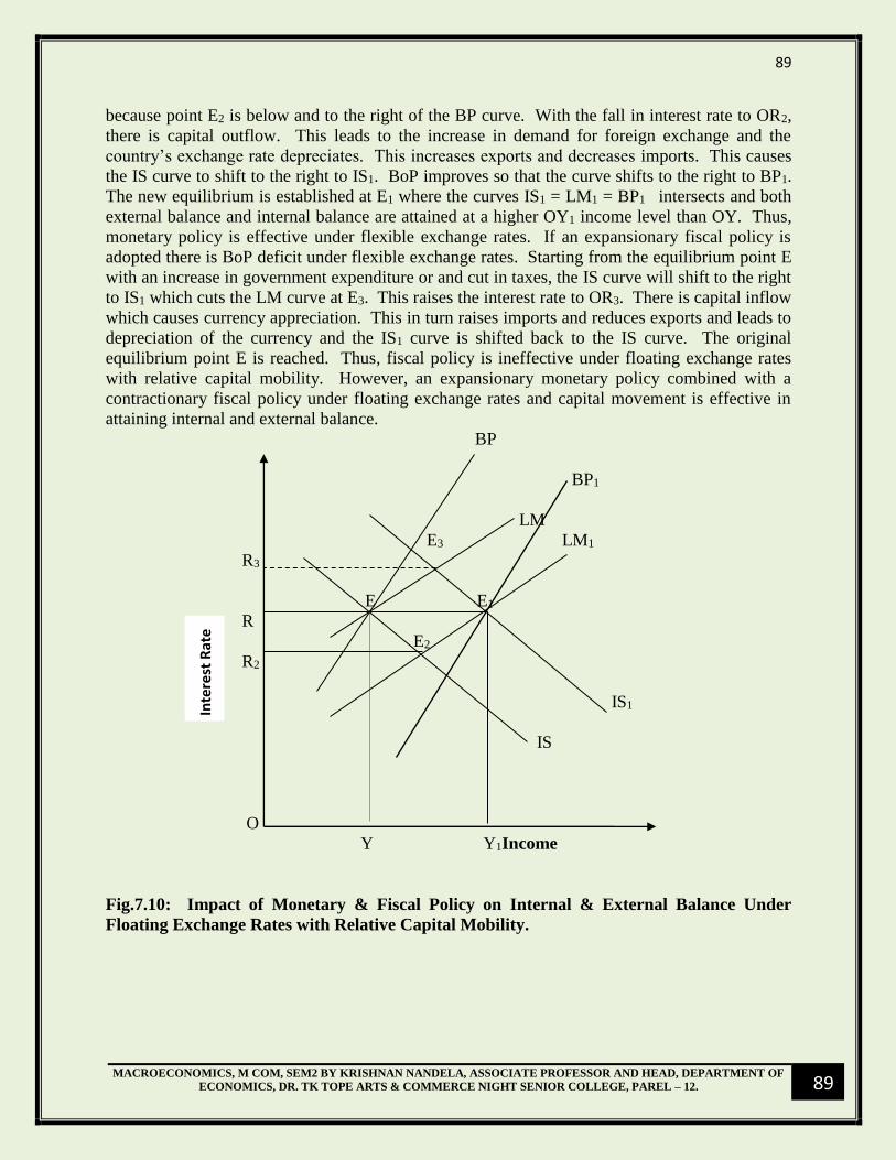
89



89

because point E2 is below and to the right of the BP curve. With the fall in interest rate to OR2,

there is capital outflow. This leads to the increase in demand for foreign exchange and the

country’s exchange rate depreciates. This increases exports and decreases imports. This causes

the IS curve to shift to the right to IS1. BoP improves so that the curve shifts to the right to BP1.

The new equilibrium is established at E1 where the curves IS1 = LM1 = BP1 intersects and both

external balance and internal balance are attained at a higher OY1 income level than OY. Thus,

monetary policy is effective under flexible exchange rates. If an expansionary fiscal policy is

adopted there is BoP deficit under flexible exchange rates. Starting from the equilibrium point E

with an increase in government expenditure or and cut in taxes, the IS curve will shift to the right

to IS1 which cuts the LM curve at E3. This raises the interest rate to OR3. There is capital inflow

which causes currency appreciation. This in turn raises imports and reduces exports and leads to

depreciation of the currency and the IS1 curve is shifted back to the IS curve. The original

equilibrium point E is reached. Thus, fiscal policy is ineffective under floating exchange rates

with relative capital mobility. However, an expansionary monetary policy combined with a

contractionary fiscal policy under floating exchange rates and capital movement is effective in

attaining internal and external balance.

BP

BP1

LM

E3 LM1

R3

E E1

R

E2

R2

IS1

IS

O

Y Y1Income

Fig.7.10: Impact of Monetary & Fiscal Policy on Internal & External Balance Under

Floating Exchange Rates with Relative Capital Mobility.

Inte

rest

Rat

e

90



90

DEVALUATION AND THE ‘J’ CURVE EFFECT.

Marshall-Lerner Condition.

The elasticity approach to Balance of Payment adjustment was put forward by Marshall and

Lerner and hence it is known as the Marshall-Lerner Condition. This approach studies the

conditions under which changes in exchange rate would re-establish equilibrium in balance of

payments by devaluing a country’s currency. Here we are going examine the price effect of

devaluation.

Theory.

Under these assumptions, when a country devalues its currency, the domestic prices of its

imports are raised and the foreign prices of its exports are reduced. Thus, devaluation helps to

improve balance of payment deficit of a country by increasing its exports and reducing its

imports. But the extent to which it will succeed depends on the country’s price elasticity of

domestic demand for imports and foreign demand for exports. According to Marshall and

Lerner, when the sum of price elasticity of demand for exports and imports in absolute terms is

greater than one, devaluation will improve the country’s balance of payment position.

Symbolically ex + em> 1 where ex is the price elasticity of exports and em is the price elasticity of

imports. Conversely, if the sum of price elasticity of demand for exports and imports in absolute

terms is less than unity, devaluation will worsen the balance of payment position i.e. the deficit

will increase. If the sum of elasticity in absolute terms is equal to unity, devaluation will have no

effect on the balance of payment position.

Operation of the Marshall-Lerner Condition.

The following is the process through which the Marshall-Lerner condition operates in removing

balance of payment deficit of a devaluing country.

Devaluation reduces the domestic prices of exports in terms of the foreign currency. With low

prices, exports increase. The extent to which they increase depends on the demand elasticity for

exports. It also depends on the nature of goods exported and the market conditions. If the

country is the sole supplier and exports raw materials or perishable good, the demand elasticity

for its exports will be low. If it exports machinery, tools and industrial products in competition

with other countries, the elasticity of demand for its products will be high and devaluation will

be successful in correcting the deficit.

Devaluation will increase the domestic price of imports which will reduce the import of goods

depending upon the demand elasticity of imports. The demand elasticity of imports depends on

the nature of goods imported by the devaluing country. If it imports consumer goods, raw

materials and inputs for industries, its elasticity of demand for imports will be low. It is only

when the import elasticity of demand for products is high that devaluation will help in correcting

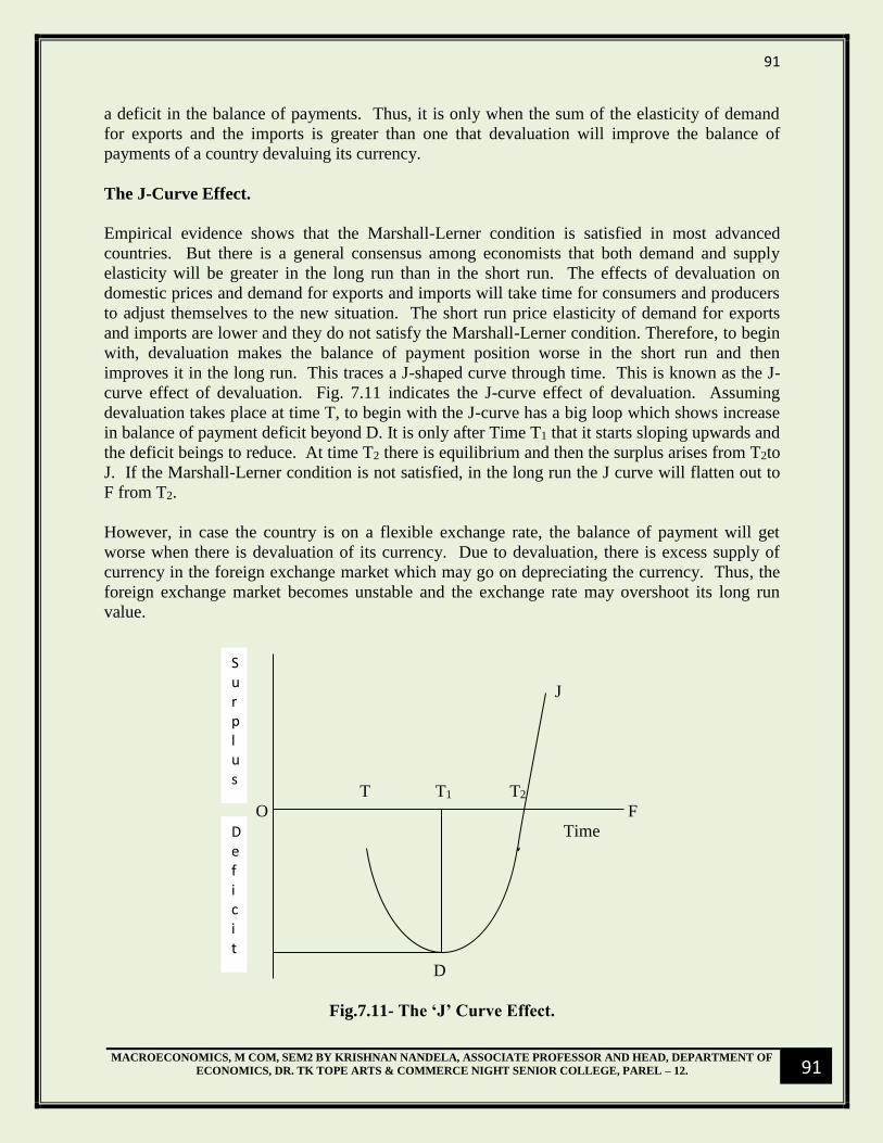
91



91

a deficit in the balance of payments. Thus, it is only when the sum of the elasticity of demand

for exports and the imports is greater than one that devaluation will improve the balance of

payments of a country devaluing its currency.

The J-Curve Effect.

Empirical evidence shows that the Marshall-Lerner condition is satisfied in most advanced

countries. But there is a general consensus among economists that both demand and supply

elasticity will be greater in the long run than in the short run. The effects of devaluation on

domestic prices and demand for exports and imports will take time for consumers and producers

to adjust themselves to the new situation. The short run price elasticity of demand for exports

and imports are lower and they do not satisfy the Marshall-Lerner condition. Therefore, to begin

with, devaluation makes the balance of payment position worse in the short run and then

improves it in the long run. This traces a J-shaped curve through time. This is known as the J-

curve effect of devaluation. Fig. 7.11 indicates the J-curve effect of devaluation. Assuming

devaluation takes place at time T, to begin with the J-curve has a big loop which shows increase

in balance of payment deficit beyond D. It is only after Time T1 that it starts sloping upwards and

the deficit beings to reduce. At time T2 there is equilibrium and then the surplus arises from T2to

J. If the Marshall-Lerner condition is not satisfied, in the long run the J curve will flatten out to

F from T2.

However, in case the country is on a flexible exchange rate, the balance of payment will get

worse when there is devaluation of its currency. Due to devaluation, there is excess supply of

currency in the foreign exchange market which may go on depreciating the currency. Thus, the

foreign exchange market becomes unstable and the exchange rate may overshoot its long run

value.

J

T T1 T2

O F

Time

D

Fig.7.11- The ‘J’ Curve Effect.

Surplus

Deficit

92



92

Questions.

1. Explain the concept of Balance of payments disequilibrium of an open economy.

2. Explain the impact of expenditure changing policies on Balance of Payment

disequilibrium.

3. Explain the impact of expenditure switching policies on balance of payments

disequilibrium.

4. Explain the Mundell-Fleming model.

5. Explain the impact of de-valuation on balance of payment disequilibrium. 6. Explain the impact of revaluation as expenditure switching policy on balance of payment

disequilibrium. 7. Explain the effectiveness of de-valuation with J – curve.

macroeconomicstktopenightcollege.in/.../02/macroeconomics...2019.pdf · 1) dornbusch. r, fisher.s.,...

Documents