Macroalgal distribution patterns and ecological performances in a tidal coastal lagoon,with emphasis on the non-indigenous Codium fragile ssp. tomentosoides

Mads Solgaard ThomsenCopenhagen, Denmark

M.S. Roskilde University, Denmark, 1998

A Dissertation presented to the Graduate Facultyof the University of Virginia in Candidacy for the Degree of

Doctor of Philosophy

Department of Environmental Sciences

University of VirginiaAugust 2004

i

i

Abstract

Codium fragile ssp. tomentosoides is a North-West Pacific macroalgae that has invaded

numerous lagoons. The success of C. fragile has been explained by its dispersal capacity,

growth rate, nutrient uptake, salinity and temperature tolerances, and grazer resistance. I

compared distribution, recruitment and growth of Codium to native algae in Hog Island

Bay, a shallow water lagoon in Virginia. To determine the extent of invaded habitats

algae were mapped from 1998-02. Codium was fourth most abundant, and hence

considered successful compared to most species in terms of its biomass. Codium was

found both unattached or attached to bivalve shells, while the majority of the dominant

Gracilaria verrucosa and Ulva curvata were incorporated into tube caps of the

polychaete Diopatra cuprea. Preference experiments showed that Diopatra incorporated

Ulva and Gracilaria most, Agardhiella subulata intermediate, and Codium and Fucus

vesiculosus least, and that the first 3 species were fragmented in the process. Thus,

Diopatra facilitated Ulva and Gracilaria, by providing an abundant substrate, reducing

flushing and maintaining a supply of fragments for regrowth. Tidal lagoons are

characterized by sedimentation, desiccation, high turbidity, and high abundance of

molluscan grazers. Short-term experiments showed that Codium was inferior under such

conditions compared to Gracilaria, Ulva, Hypnea musciformis, and Agardhiella,

decomposing faster when buried, being susceptible to desiccation, growing slower at high

and low levels of nutrient and light, and being the only species grazed by Ilyanasa

obsolata. To test if the success of Codium fragile could be related to its ability to

colonize hard substrate, recruitment bricks were incubated in the shallow subtidal with

ii

ii

and without a cover of unattached algae or sediments. Codium recruited well onto control

bricks, but not onto bricks covered by algae or sediments. After one year Codium,

Gracilaria, Crassostrea virginica (oyster) and Agardhiella were space-dominants, having

tolerated temperature regimes of 2-28ºC and desiccation at low spring tides. Thus

Codium is only successful compared to native species by having moderate growth over a

long season, and by being an effective colonizer of hard substrate in the shallow subtidal

zone in the absence of high sedimentation or drift algae accumulations.

iii

iii

Table of content

Abstract ................................................................................................................................ iTable of content..................................................................................................................iiiList of figures ....................................................................................................................viiList of tables ......................................................................................................................xiiAcknowledgement............................................................................................................xviChapter 1. Introduction: Marine invasions and Codium fragile ssp. tomentosoides in HogIsland Bay............................................................................................................................ 1

Marine invasions .......................................................................................................... 2Codium fragile invasions.............................................................................................. 3Approaches to invasions: invader vs. invaded system ................................................. 4Traits of Codium fragile, the invader ........................................................................... 5Lagoons, the invaded system........................................................................................ 6Study site: Hog Island Bay ........................................................................................... 7Guidelines..................................................................................................................... 9Hypothesis .................................................................................................................. 11Chapter 1. Tables........................................................................................................ 14Chapter 1. Figures ...................................................................................................... 15

Chapter 2. Interaction of spatio-temporal gradients determines macroalgal distributionpatterns in a shallow, soft-bottom lagoon ......................................................................... 17

Abstract....................................................................................................................... 18Introduction ................................................................................................................ 19Methods ...................................................................................................................... 22

Study site and gradients .......................................................................................... 22VCR/LTER Aquatic Plant Monitoring Program..................................................... 23Data analysis ........................................................................................................... 23Attachment survey .................................................................................................. 25

Results ........................................................................................................................ 25VCR-LTER Aquatic Plant Monitoring Program .................................................... 25Species richness ...................................................................................................... 26Total biomass .......................................................................................................... 26Biomass of Codium fragile ..................................................................................... 27Species-specific correlation .................................................................................... 28Secondary species dominance................................................................................. 29Attachment survey .................................................................................................. 30

Discussion................................................................................................................... 30Effects of macroalgal mats in lagoons .................................................................... 30Species patterns ....................................................................................................... 31Spatio-temporal gradients ....................................................................................... 32Potential for seagrass recolonization....................................................................... 35Distribution of Codium fragile ................................................................................ 36Conclusions ............................................................................................................. 37

Chapter 2. Tables........................................................................................................ 39

iv

iv

Chapter 2. Figures ...................................................................................................... 44Chapter 3. Facilitation of Macroalgae by the Sedimentary Tube Forming PolychaeteDiopatra cuprea ................................................................................................................ 49

Abstract....................................................................................................................... 50Introduction ................................................................................................................ 51Methods ...................................................................................................................... 52

Site description........................................................................................................ 53Ubiquity of tube caps .............................................................................................. 53Ubiquity of algae incorporated to tube caps............................................................ 54Stability of algae incorporated to tube caps ............................................................ 55Recovery of algae incorporated to tube caps .......................................................... 56Preference of algae incorporated to tube caps......................................................... 57

Results ........................................................................................................................ 58Ubiquity of tube caps .............................................................................................. 59Ubiquity of algae incorporated to tube caps............................................................ 59Stability of algae incorporated to tube caps ............................................................ 60Recovery of algae incorporated to tube caps .......................................................... 61Preference of algae incorporated to tube caps......................................................... 62

Discussion................................................................................................................... 63Chapter 3. Tables........................................................................................................ 70Chapter 3. Figures ...................................................................................................... 75

Chapter 4. Species type, thallus size and substrate condition determine macroalgal breakforces, break velocities and break places in a western mid-Atlantic low energy softbottom lagoon.................................................................................................................... 79

Abstract....................................................................................................................... 80Introduction ................................................................................................................ 80

Survival of sessile marine organism against hydrodynamic forces ........................ 80Biomechanical models ............................................................................................ 81

Methods ...................................................................................................................... 83Species and substrate types ..................................................................................... 83Measurements of break force, size and break place................................................ 84Calculation of break velocities................................................................................ 85Data analysis ........................................................................................................... 86Ambient hydrodynamic forces ................................................................................ 86Flume dislodgment.................................................................................................. 87Drift algae collections ............................................................................................. 88

Results ........................................................................................................................ 89Thallus size and break force, velocity and place..................................................... 89Ambient hydrodynamic regime............................................................................... 90Flume dislodgment.................................................................................................. 91Drift of algal clumps ............................................................................................... 92

Discussion................................................................................................................... 93Unattached survival................................................................................................. 93Allometric models of break force and break velocity ............................................. 95Effects of species, substrate and size on break force and velocity.......................... 96Effect of species, substrate and size on break place................................................ 96

v

v

Comparing break velocities to hydrodynamic regime ............................................ 97Entrainment and entanglement................................................................................ 99Other factors of importance................................................................................... 100

Chapter 4. Tables...................................................................................................... 102Chapter 4. Figures .................................................................................................... 107

Chapter 5. The alien Codium fragile have low performance characteristics compared tonative macroalgae in a soft bottom turbid lagoon, Virginia............................................ 112

Abstract..................................................................................................................... 113Introduction .............................................................................................................. 114Methods .................................................................................................................... 117

Study site ............................................................................................................... 117In situ experiments ................................................................................................ 118Elevation effects.................................................................................................... 119Sedimentation effects ............................................................................................ 119Cage experiments .................................................................................................. 120Light, Nutrient, and Grazer effects........................................................................ 121Methodological artifacts........................................................................................ 122Data analysis ......................................................................................................... 122Correlation of performances between species....................................................... 124Results ................................................................................................................... 125Effect of elevation ................................................................................................. 125Effect of days of sediment burial .......................................................................... 126Effect of shading ................................................................................................... 127Effect of nutrient addition ..................................................................................... 127Effect of snail addition .......................................................................................... 128Effect of twist-tie wrapping and caging ................................................................ 129Effect of species and distance on pooled experiments.......................................... 130Performance similarities between species............................................................. 131

Discussion................................................................................................................. 132Burial effects ......................................................................................................... 132Light effects .......................................................................................................... 133Nutrients effects .................................................................................................... 134Grazing effects ...................................................................................................... 135Elevation effects.................................................................................................... 136Distance effects ..................................................................................................... 137Methodological artifact and competition .............................................................. 138Performance of Codium fragile............................................................................. 140Conclusion............................................................................................................. 141

Chapter 5. Tables...................................................................................................... 143Chapter 5. Figures .................................................................................................... 151

Chapter 6. Performance of oyster reef associated sessile organisms: effects ofhydrodynamics and accumulations of sediments and drift algae.................................... 158

Abstract..................................................................................................................... 159Introduction .............................................................................................................. 160Methods .................................................................................................................... 163

Study site ............................................................................................................... 163

vi

vi

Experimental design.............................................................................................. 164Data analysis ......................................................................................................... 168

Results ...................................................................................................................... 170Drift algae accumulations, sedimentation and hydrodynamics............................. 170Recruitment ........................................................................................................... 172

Discussion................................................................................................................. 177Effects on sediments, drift algae and hydrodynamics........................................... 177Recruitment in open plots ..................................................................................... 180Recruitment under drift algae................................................................................ 184Recruitment under sediments ................................................................................ 185Temporal recruitment effects ................................................................................ 186Recruitment of C. fragile ...................................................................................... 187

Conclusion................................................................................................................ 188Chapter 6. Tables...................................................................................................... 190Chapter 6. Figures .................................................................................................... 197

Discussion ....................................................................................................................... 205Is Codium fragile superior in low energy soft bottom lagoons?............................ 206Wider distribution and higher abundance?............................................................... 206Strongest facilitation by Diopatra cuprea? .............................................................. 208Highest resistance to water forces? .......................................................................... 209Highest short-term tissue survival and growth? ....................................................... 211Highest long-term recruitment onto hard substrate? ................................................ 212Conclusions .............................................................................................................. 213Some implications and general future research directions ....................................... 214

Appendix. Additional graphs, photos and tables ............................................................ 217Appendix 1. Introduction.......................................................................................... 218

Distribution of Codium fragile .............................................................................. 218Appendix 2. Mapping............................................................................................... 218Appendix 3. Diopatra cuprea................................................................................... 219Appendix 4. Biomechanics....................................................................................... 219Appendix 5. Tissue performance.............................................................................. 219

Performance experiments conducted along distance gradient (Chapter 5). .......... 220Additional performance experiments conducted along elevation gradient........... 223

Appendix 6. Recruitment.......................................................................................... 225Recruitment experiment conducted around oyster reefs (Chapter 6).................... 225Additional recruitment experiment conducted along elevation and distancegradients ................................................................................................................ 226

Appendix 7. VCR/LTER water quality monitoring data.......................................... 230Appendix Tables....................................................................................................... 233Appendix Figures ..................................................................................................... 249

References ....................................................................................................................... 281

vii

vii

List of figures

Fig. 1.1. Hog Island Bay within the Virginia Coast Reserve on the Delmarva Peninsula

and 12 locations sampled in Aquatic Plant Monitoring Program................................15

Fig. 1.2. Extreme water level differences in Eastern Shore barrier island lagoons...........16

Fig. 2.1. Temporal variability in taxonomic richness of attached (A) and unattached (B)

algae along the distance from mainland gradient........................................................44

Fig. 2.2. Single factor effects of attachment, elevation, distance from

mainland, season and annual changes on taxonomic richness...........................................45

Fig. 2.3. Temporal variability in total assemblage biomass of attached and unattached

algae along the distance from mainland gradient........................................................46

Fig. 2.4. Single factor effects of attachment, elevation, distance from mainland, season

and annual changes on biomass of the total algal assemblage, G. verrucosa and C.

fragile...........................................................................................................................47

Fig. 2.5. Single factor effects of attachment, elevation, distance from mainland, season

and annual changes on biomass of the 12 most common species following the

dominant G. verrucosa.................................................................................................48

Fig. 3.1. Distribution of tube caps in Hog Island Bay.......................................................75

Fig. 3.2. Stability of G. verrucosa and U. curvata incorporated into tube caps................76

Fig. 3.3. Effects of disturbances on the abundance of D. cuprea tube caps, and tube cap

incorporated Gracilaria verrucosa, Ulva curvata, and total algal biomass................77

Fig. 3.4. Percent fragments incorporated into tube caps, and percent fragmentation, based

on preference experiments...........................................................................................78

viii

viii

Fig. 4.1. Thallus planform area, break force, break velocity and break place for 6 species,

2 substrate types and 2 size classes............................................................................107

Fig. 4.2. Current velocities in front, between and behind oyster bars in a mid-lagoon site

with high algal biomass.............................................................................................108

Fig. 4.3. Current velocity profiles at 3 distances from the bottom measured with an

Acoustic Doppler Profiler..........................................................................................109

Fig. 4.4. Map of peak currents in Hog Island Bay calculated from a 2d Bellamy

Kinematic hydrodynamic model................................................................................110

Fig. 4.5. Allometric models of planform area versus break velocities for 6 species

attached to D. cuprea tube caps and bivalve shells...................................................111

Fig. 5.1. Effect of elevation and burial on C. fragile performance (% change in biomass)

compared to five native macroalgae. ........................................................................151

Fig. 5.2. Effect of distance from mainland and shading on C. fragile performance (%

change in biomass) compared to five native macroalgae..........................................152

Fig. 5.4. Effect of distance from mainland and snail addition on C. fragile performance

(% change in biomass, % tissue nitrogen and total nitrogen) compared to five native

macroalgae.................................................................................................................153

Fig. 5.5. Effect of distance from mainland and twist-tie wrapping on C. fragile

performance (% change in biomass) compared to five native macroalgae...............154

Fig. 5.6. Effect of distance from mainland and caging on C. fragile performance (%

change in biomass) compared to five native macroalgae..........................................155

Fig. 5.7. Effect of distance from mainland and experimental design on C. fragile

performance (% change in biomass) compared to five native macroalgae...............156

ix

ix

Fig. 6.1. Species-abundances for 3 hydrodynamics regimes and 3 cover types..............197

Fig. 6.2. Interaction plots of accumulated sediments on bricks, sedimentation in PVC-

tubes, accumulated drift algae, current velocities and hydrodynamic drag on practice

golf balls.....................................................................................................................198

Fig. 6.3. Interaction plots of animal and plant richness per recruitment brick for separate

sampling times...........................................................................................................199

Fig. 6.4. Interaction plots of percent cover of animals pooled and plants pooled for

separate sampling times.............................................................................................200

Fig. 6.5. Interaction plots of percent cover of C. virginica and C. fragile for separate

sampling times...........................................................................................................201

Fig. 6.6. Percent cover of C. fragile versus C. virginia on all recruitment bricks...........202

Fig. 6.7. Interaction plots of percent cover of G. verrucosa and A. subulata for separate

sampling times...........................................................................................................203

Fig. 6.8. Interaction plots of percent cover of Enteromorpha sp. and U. curvata for

separate sampling times.............................................................................................204

Fig. A1. Map of geographic range of C. fragile..............................................................253

Fig. A2. Graph of attachment survey...............................................................................254

Fig. A3. Photos of G. verrucosa dominance and D. cuprea tube caps............................255

Fig. A4. Algae incorporated into D. cuprea tube caps....................................................256

Fig. A5. D. cuprea preference experiment......................................................................257

Fig. A6. Photos of C. fragile morphology and fragmentation.........................................258

Fig. A7. Photos of methodologies of performance experiments.....................................259

x

x

Fig. A8. Interaction plots of species, caging, distance from mainland, twist-tie wrapping

and experimental design versus algal performance (Chapter 5 experiments)...........260

Fig. A9. Interaction plots of tissue fragmentation along the distance gradient (Chapter 5

experiments)...............................................................................................................261

Fig. A10. Interaction plots of fluorescence yield along the distance from mainland

gradient (Chapter 5 experiments)...............................................................................262

Fig. A11. Interaction plots of fluorescence yield along the distance gradient (continued

from Fig. 14)..............................................................................................................263

Fig. A12. Reattachment of C. fragile and H. musciformis..............................................264

Fig. A13. Interaction plots of reattachment of H. musciformis along the distance from

mainland gradient (Chapter 5 experiments)...............................................................265

Fig. A14. Interaction plots of biomass performance patterns for additional experiments

along an elevation gradient (I)...................................................................................266

Fig. A15. Interaction plots of biomass performance patterns for additional experiments

along an elevation gradient (II)..................................................................................267

Fig. A16. Interaction plots of biomass performance patterns for additional experiments

along an elevation gradient (III)................................................................................268

Fig. A17. Interaction plots of biomass performance patterns for additional experiments

along an elevation gradient (IV)................................................................................269

Fig. A18. Photos of oyster reefs at mid-lagoon sites.......................................................270

Fig. A19. Elevation map a mid-lagoon site (Shoal 1) around oyster reefs......................271

Fig. A20. Photos of control recruitment bricks around oyster reefs................................272

xi

xi

Fig A21. Interaction plots of plant richness, animal richness, plant cover, animal cover,

and cover of the six most abundant taxa recruited onto bricks around oyster reefs

(Chapter 6 experiment)..............................................................................................273

Fig. A22. Abundance of sessile oyster reef associated organisms at different sampling

times at the mid-lagoon site (Chapter 6 experiment)................................................274

Fig. A23. Abundance of sessile reef associated organisms recruited onto bricks at

different elevations at the mid-lagoon site (S1, additional recruitment data)............275

Fig. A24. Abundance of sessile oyster-reef associated organisms at recruited onto bricks

at different positions along the distance from mainland gradient (C1, S1, H1,

additional recruitment data).......................................................................................276

Fig. A25. Abundance of sessile oyster-reef associated organisms (transplanted from S1 to

C1, S1, and H1, additional recruitment data).............................................................277

Fig. A26. Location of sample stations from the VCR/LTER WQ (Water Quality)

Monitoring Program...................................................................................................278

Fig. A27. Temporal development in total suspended solids (WQ-stations)....................279

Fig. A28. Temporal development in temperature (WQ-stations)....................................280

Fig. A29. Temporal development in secchi depth (WQ-stations)...................................281

Fig. A30. Temporal development in salinity (WQ-stations)...........................................282

Fig. A31. Temporal development in dissolved oxygen (WQ-stations)...........................283

Fig. A32. Temporal development in total suspended solids, temperature, salinity,

dissolved oxygen and secchi depth pooled from 10 VCR/LTER WQ-sampling

stations.......................................................................................................................284

xii

xii

List of tables

Table 1.1. Species of main interest in the thesis................................................................14

Table 2.1. Characteristics of 12 study sites........................................................................39

Table 2.2. Macroalgal taxa with mean and maximum biomass recorded in survey..........40

Table 2.3. Five-factorial ANOVAs of Log(x+1) transformed taxonomic richness and total

and C. fragile biomass.........................................................................................41

Table 2.4. Single factor ANOVAs of biomass, taxonomic richness and C. fragile

biomass........................................................................................................................42

Table 2.5. Correlation matrix for taxonomic richness, total biomass, and biomass of the

12 most abundant species.............................................................................................43

Table 3.1. ANOVA of tube cap densities..........................................................................70

Table 3.2. Abundance (in counts) of different attachment types and species incorporated

onto tube caps..............................................................................................................71

Table 3.3. Biomass per tube cap, relative abundance, frequency of occurrence and

attachment types of algae incorporated into tube caps................................................72

Table 3.4. ANOVA on tube cap densities and biomass of G. verrucosa and U. curvata for

two recovery experiments............................................................................................73

Table 3.5. ANOVA on percent attachment and percent fragmentation from preference

experiment....................................................................................................................74

Table 4.1. Allometric models of planform area vs. break force and break velocity........102

Table 4.2. ANOVA on thallus area, break force and break velocity for 6 species, 2

substrate types and 2 size-classes..............................................................................103

xiii

xiii

Table 4.3. 2-tests results on break place........................................................................104

Table 4.4. Flume dislodgment of small vs. large G. verrucosa and U. curvata

incorporated into D. cuprea tube caps at three velocities..........................................105

Table 4.5. Species and sizes of drift algal clumps...........................................................106

Table 5.1. Biotic and abiotic characteristics in Hog Island Bay at near-mainland (Creek),

mid-lagoon (Shoal) and near-ocean (Hog) sites........................................................143

Table 5.2. Summary of performance experiments...........................................................144

Table 5.3A. ANOVA results on assemblage performance (Experiment 1-6).................145

Table 5.3B. ANOVA results on assemblage performance (continued from Table 5.3A,

Experiment 7-9).........................................................................................................146

Table 5.4. ANOVA results on C. fragile performance....................................................147

Table 5.5. Correlation coefficients for pair-wise comparisons between species

performance...............................................................................................................148

Table 5.6. Number of replicates and mean and maximum biomass per fragment at the

start and end of experiments......................................................................................149

Table 5.7: Regressions of remaining biomass versus days of burial for 5 species..........150

Table 6.1. Light reduction in cages..................................................................................190

Table 6.2. ANOVA on Log(x+1) transformed cover of sediments, sedimentation rates,

cover of drift algae, current velocities, and drag on practice golf balls.....................191

Table 6.3. NPMANOVA on Log(x+1) transformed percent cover of attached organisms

(total assemblage data)...............................................................................................192

Table 6.4. Pair-wise comparisons for assemblage data following significant single factor

effects from NPMANOVA........................................................................................193

xiv

xiv

Table 6.5. Taxa contributing to 90% of within and between group variability (similarity

percentages), using Bray-Curtis similarity coefficient on Log(x+1) transformed

percent cover..............................................................................................................194

Table 6.6. Repeated ANOVA on Log(x+1) transformed animal richness, plant richness,

total cover of animals and total cover of algae..........................................................195

Table 6.7. Repeated ANOVA on the Log(x+1) transformed abundance of C. virginica, C.

fragile, G. verrucosa, A. subulata, Enteromorpha spp. and U. curvata....................196

Table A1. SNK-tests of all species along distance gradient (Chapter 5).........................233

Table A2. SNK-tests of C. fragile performance along distance gradient (Chapter 5).....234

Table A3. Percent fragmentation (based on E27, E29, E30, E34, Chapter 5).................235

Table A4. H. musciformis reattachment (based on E24, E27, E29, E30, and E34, Chapter

5)................................................................................................................................236

Table A5. Summery of additional performance experiments conducted along an elevation

gradient......................................................................................................................237

Table A6A. ANOVA on additional performance experiments along an elevation

gradient......................................................................................................................238

Table A6B. ANOVA on additional performance experiments along an elevation gradient

(continued from Table A6A).....................................................................................239

Table A7. SNK-tests on species performance along an elevation gradient (grouping

species, elevation levels and experiments)................................................................240

Table A8: ANOVA on C. fragile performance on additional performance experiments

along an elevation gradient........................................................................................241

xv

xv

Table A9: SNK-test on C. fragile performance on additional performance experiments

along an elevation gradient........................................................................................242

Table A10: r2Pearson correlation matrix comparing performances between species from

seven additional performance experiments along an elevation gradients..................243

Table A11. Fragmentation, fluorescence yield, and reattachment for additional

performance experiments conducted along an elevation gradient.............................244

Table A12. Light reduction in cages................................................................................245

Table A13. Rankings of current velocity, drift algae accumulations, sedimentation, drag

on practice golf balls, accumulated sediments based on SNK-tests (Chapter 6).......246

Table A14. Rankings of Animal and Plant richness and abundance, and abundance of C.

fragile, C. virginia, G. verrucosa, A. subulata, U. curvata, Enteromorpha sp. based

on SNK-tests following univariate ANOVA (Chapter 6)..........................................247

Table A15. Secchi depth, temperature, salinity, suspended solids and dissolved oxygen in

Hog Island Bay, 1999-2002, VCR/LTER Water Quality Monitoring Program .......248

xvi

xvi

Acknowledgement

This thesis would not have been possible without support from many people and

institutions. First I want to thank my supervisor, Karen McGlathery, who provided

alternative explanations to my ecological speculations and who always made me feel at

home in Team-McG. Thanks for believing that I could pull it off and for accepting my

tendencies to look at seaweeds outside my mudhole and occasionally follow a tangential

research methodology. Thanks to my committee: Pat Wiberg for clearing out some

hydrodynamic mysteries (although I am still not sure I get it), Jay Zieman for his

ecological perspective (and good stories), and Laura Galloway for showing interest in

those weird marine plants that (almost) lack differentiation, translocation, and embryo

protection. I am grateful for the logistic support provided by the VCR/LTER program and

associated people, including Randy Carlson, Jimmy Spitler, Kathleen Overman, Jason

Restein and Phillip Smith who got me to my sites, despite the good low tides often

coincided with inhumanly early hours. Funding came from The Danish Research

Academy, The Fulbright Commission, the NSF through the VCR/LTER, and the

Department of Environmental Sciences, through Exploratory and Odum Research

Awards. I am grateful for the Danish Research Academy for acknowledging, and

supporting financially, that important research perspectives can be acquired by visiting

contrasting systems. Also thanks to Jens Borum, University of Copenhagen for always

supporting my research plans. Also thanks to those who, in addition to Karen, helped

improve on my writing, repeatedly telling me to cut down on tangents and stick with a

single simple story, including Thomas Wernberg, Peter Staerh, Mat Vanderklift, and

xvii

xvii

Christy Tyler. I couldn t have asked for a better group of field comrades than Team-

McG: Christy Tyler, Jenn Rosinski, Ishi Buffam, Jessie Burton, Tracie Mastronicola,

Sarah Lawson, Diane Barnes and Kim Holzer. In particular, thanks to Christy for

introducing me to Hog Island Bay with its finest attributes (2ºC waters and silty anoxic

mudflats) on the day following my arrival, and for ensuring that I did not literally and

abstractly got lost in the US. Thanks to the group of LTER-field students who shared

limited and messy space in the old farm house, especially Rachel Michaels and Devin

Herod. Between us, we considered ourselves the residents of the field station for several

years (occasionally accommodating large numbers of guests), looking at more critters,

seaweeds and marsh plants than most people can brag about. Also thanks to Claudia

Jiron-Murphy and Meg Miller for help with running samples on the Carlo-Erba, P.

Wiberg and S. Lawson for providing hydrodynamic data and Jamie Robbinson for field

assistance. Cheers to Art Schwarzschild for providing good discussions, for letting me

borrow his beloved Ford Escort to bring me to the Eastern Shore, and for agreeing that

soccer is superior to football. A Bahamas team added an annually repeated pleasure of

being a student at the Department of Environmental Sciences. Thanks to Fred Diehl,

Christy Tyler, Brian Silliman, Dave Smith, Bob McNulty, Bev Marcum and of course

Robbie for many fun hours on a limestone platform, and for providing an opportunity to

get a clear perspective on marine ecology (visibility of 20-50 m) compared to the murky

picture that emerged from Hog Island Bay (visibility of 5-50 cm). I hope I convinced all

team-members that coral reefs should be named algal reefs, and that without marine

plants, snails would be lost. Also, from my relocated kiwi writing environment, I want to

thanks my neighbor Nigel Murphy for being willing to kick the soccer ball around when I

xviii

xviii

needed distractions as well as patiently explaining (and re-explaining) the national

cricket rules. A special thanks to Thomas Wernberg who (being on a similar but still

different boat) always provided great support and alternative views on the world. Thanks

for providing the opportunity to get a wavy perspective on marine ecology in Perth,

Australia, as opposed to the current dominated one in Hog Island Bay, and of course for

being an excellent devils advocate for my messy writing. During many years we have

agreed on disagreeing with everyone who did not agree with us. Also, thanks to Peter

Staerh for being a great email-supporter, providing useful suggestions and corrections,

not to mention the occasional fun we had in Hawaii or in cold Danish and Canadian

waters. A very special thanks goes of course to my parents, Anne Grethe and Finn, and

brothers Morten and Mikkel. Thanks for accepting that I wanted to pursue a degree

outside Denmark (although I did not tell you how long it would take), for accommodating

my visits, for providing updates on Danish politics and soccer results, and for the

frequent what is it good for/what can it be used for? questions. Finally, I want to thank

my wife Christina for coming along at just the right time and particularly at the right

place. Thanks for supporting my weird and long working hours and non-prestigious study

object. I do realize that a more cute, intelligent or tasty study object would have been

preferable in certain situations.

1

1

Chapter 1. Introduction: Marine invasions and

Codium fragile ssp. tomentosoides in Hog Island

Bay

2

2

Marine invasions

Invasions of alien species are considered a major threat to local, regional, and global

biodiversity because invaders often compete with, eat or infect native species (Carlton

1999, Meinesz 1999, Walker & Kendrick 1998). In addition invasions cause serious

economic damage due to competition with and infections of financially important crops

and livestocks (Carlton 1996b, Carlton 1999, McNeely 1999, Meinesz 1999, Ruiz et al.

1997). Alien species are also referred to as exotics, non-indigenous or non-native; all

terms imply that the appearance of the species is related to human-mediated

transportation (Minchin & Gollasch 2002, Wallentinus 2002). Today, it is difficult to

estimate the original and natural species assemblage given the long-term human

perturbations of nature. Introductions of alien species have occurred at a steadily

increasing pace in the last six centuries, due to growing human populations, increased

international trade and transport, and decreased transportation time (Carlton 1996c, b,

McNeely 1999). If alien species become spatially dominant in their new location and/or

have major impacts on the ecosystem, they are referred to as invasive. In the marine

environment, introductions are associated with transport of ballast water (e.g.

Mnemiopsis leidyi, Eriocheir sinensis), of economically important species for

aquacultural purposes (e.g. Sargassum muticum, Styela clava associated with transplanted

oysters), by accidental releases/escapes (e.g. Caulerpa taxifolia, Homarus americanus),

or on ship hulls and other floating manmade structures (e.g. Codium fragile, Undaria

pinnatifida) (Meinesz 1999, Minchin & Gollasch 2002, Rueness 1989, Wallentinus

2002). Marine macroalgae are commonly introduced to new regions and have caused

dramatic trans- and inter-oceanic invasions. Invasive species such as C. taxifolia (Vahl)

3

3

C. Agardh, U. pinnatifida (Harvey) Suringar, S. muticum (Yendo) Fensholt, and C.

fragile (Sur.) Hariot ssp. tomentosoides (Van Goor) Silva are well known for clogging

waterways, competing with native algae, altering the nursery habitat for fishes and

invertebrates, reducing light penetration, changing biogeochemical cycling, and

suffocating and/or drifting away with economically important shellfish (Chapman 1999,

Den Hartog 1998, Meinesz 1999, Minchin & Gollasch 2002, Norton 1976, Rueness 1989,

Stæhr et al. 2000, Trowbridge 1999, Walker & Kendrick 1998).

Codium fragile invasions

The invasive C. fragile is particular interesting, partly because the invasive organism is a

sub-species that in many regions resembles native and/or less invasive populations and

sub-species (Trowbridge 1998) and partly because it has invaded highly diverse habitats.

Invasive C. fragile can be found in rocky and soft bottom habitats, low to medium levels

of wave-energy, in both eurohaline and oligohaline systems, from intertidal rock-pools to

15 m depth, and in geographical regions ranging from high to low temperate latitudes

(e.g. Garbary & Jess 2000, Malinowski & Ramus 1973, Mathieson et al. 2003, Scheibling

& Anthony 2001, Searles et al. 1984). C. fragile invasions also highlight two important

aspects of invasions. First, many introductions are cryptic because no baseline

distribution data exist or because a similar looking organism is present (Carlton 1996a,

b). For example, in New Zealand, Australia and the west coast of Northern America other

C. fragile populations existed prior to invasions of ssp. tomentosoides and the invasions

were difficult to detect (Trowbridge 1996b, 1998, 1999). In contrast, on the east coast of

North America no Codium species were present and the dispersal and invasions were

4

4

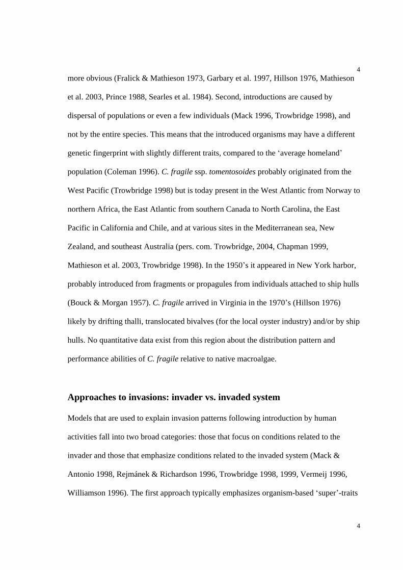
more obvious (Fralick & Mathieson 1973, Garbary et al. 1997, Hillson 1976, Mathieson

et al. 2003, Prince 1988, Searles et al. 1984). Second, introductions are caused by

dispersal of populations or even a few individuals (Mack 1996, Trowbridge 1998), and

not by the entire species. This means that the introduced organisms may have a different

genetic fingerprint with slightly different traits, compared to the average homeland

population (Coleman 1996). C. fragile ssp. tomentosoides probably originated from the

West Pacific (Trowbridge 1998) but is today present in the West Atlantic from Norway to

northern Africa, the East Atlantic from southern Canada to North Carolina, the East

Pacific in California and Chile, and at various sites in the Mediterranean sea, New

Zealand, and southeast Australia (pers. com. Trowbridge, 2004, Chapman 1999,

Mathieson et al. 2003, Trowbridge 1998). In the 1950 s it appeared in New York harbor,

probably introduced from fragments or propagules from individuals attached to ship hulls

(Bouck & Morgan 1957). C. fragile arrived in Virginia in the 1970 s (Hillson 1976)

likely by drifting thalli, translocated bivalves (for the local oyster industry) and/or by ship

hulls. No quantitative data exist from this region about the distribution pattern and

performance abilities of C. fragile relative to native macroalgae.

Approaches to invasions: invader vs. invaded system

Models that are used to explain invasion patterns following introduction by human

activities fall into two broad categories: those that focus on conditions related to the

invader and those that emphasize conditions related to the invaded system (Mack &

Antonio 1998, Rejmánek & Richardson 1996, Trowbridge 1998, 1999, Vermeij 1996,

Williamson 1996). The first approach typically emphasizes organism-based super -traits

5

5

such as fast growth (Campbell 1999, Vroom & Smith 2001, Wernberg et al. 2001), high

dispersal (Ceccherelli & Piazzi 2001, Mathieson et al. 2003, Rueness 1989, Stæhr et al.

2000), strong recovery potential (Fletcher 1975, Meinesz 1999, Vroom & Smith 2001),

high reproductive output (Arenas et al. 1995) and/or grazing and predation resistance

(Begin & Scheibling 2003, Chapman 1999). The second approach emphasizes that a

system is susceptible to invasions because (1) conditions are stressful (e.g

eutrophication), (2) it is small and isolated and likely has impoverished functional

diversity, (3) disturbances are frequent (e.g. following hurricanes or landslides), or (4) the

system is young (e.g. following glacial retreats or volcanic island creations) (Carlton

1996c, Hengeveld 1985, MacArthur & Wilson 1967, Ruiz et al. 1997, Williamson 1996).

A system that is susceptible to invasion would be characterized as open and unsaturated

with available space and niches (Myers & Bazely 2003). These two approaches merge

when the species-specific traits are matched with the characteristics of the ecosystem, for

example if an invader (e.g. C. fragile) has high nutrient uptake rates, is stress-tolerant and

invades a eutrophied and stressed system (e.g. lagoons on the Delmarva Peninsula).

Traits of Codium fragile, the invader

C. fragile is classified in the order Caulerpales, a genus containing more than 100 species

(Trowbridge 1998). C. fragile has a siphonious structure with intertwined multinucleated

filaments and swollen utricles, no cell cross-walls, and has a large component of intra

(vacuoles)- and inter (between filaments) cellular fluids which give the algae a soft

spongy texture (Chapman 1999, Trowbridge 1998). From a form-functional perspective

C. fragile is classified as a coarsely branched species with a low surface to volume ratios,

6

6

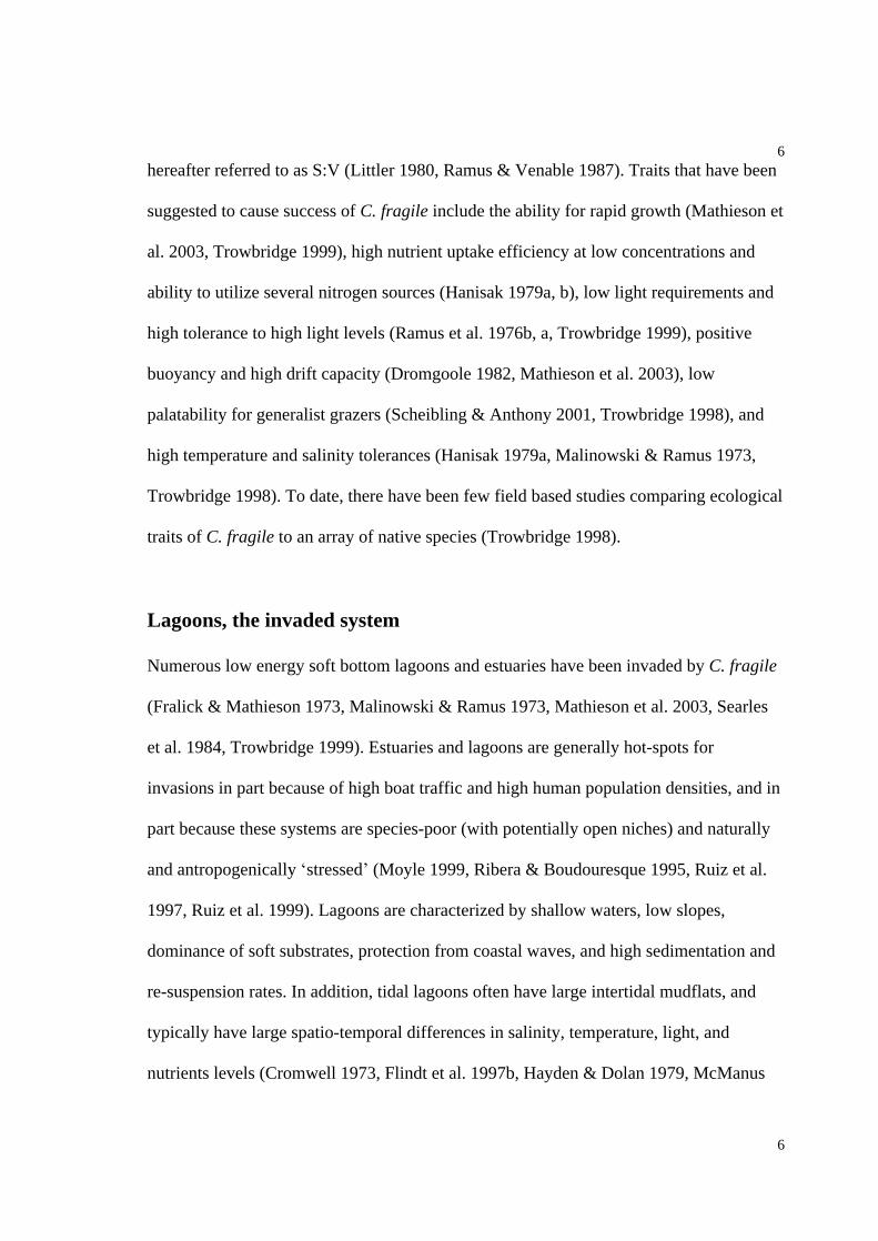
hereafter referred to as S:V (Littler 1980, Ramus & Venable 1987). Traits that have been

suggested to cause success of C. fragile include the ability for rapid growth (Mathieson et

al. 2003, Trowbridge 1999), high nutrient uptake efficiency at low concentrations and

ability to utilize several nitrogen sources (Hanisak 1979a, b), low light requirements and

high tolerance to high light levels (Ramus et al. 1976b, a, Trowbridge 1999), positive

buoyancy and high drift capacity (Dromgoole 1982, Mathieson et al. 2003), low

palatability for generalist grazers (Scheibling & Anthony 2001, Trowbridge 1998), and

high temperature and salinity tolerances (Hanisak 1979a, Malinowski & Ramus 1973,

Trowbridge 1998). To date, there have been few field based studies comparing ecological

traits of C. fragile to an array of native species (Trowbridge 1998).

Lagoons, the invaded system

Numerous low energy soft bottom lagoons and estuaries have been invaded by C. fragile

(Fralick & Mathieson 1973, Malinowski & Ramus 1973, Mathieson et al. 2003, Searles

et al. 1984, Trowbridge 1999). Estuaries and lagoons are generally hot-spots for

invasions in part because of high boat traffic and high human population densities, and in

part because these systems are species-poor (with potentially open niches) and naturally

and antropogenically stressed (Moyle 1999, Ribera & Boudouresque 1995, Ruiz et al.

1997, Ruiz et al. 1999). Lagoons are characterized by shallow waters, low slopes,

dominance of soft substrates, protection from coastal waves, and high sedimentation and

re-suspension rates. In addition, tidal lagoons often have large intertidal mudflats, and

typically have large spatio-temporal differences in salinity, temperature, light, and

nutrients levels (Cromwell 1973, Flindt et al. 1997b, Hayden & Dolan 1979, McManus

7

7

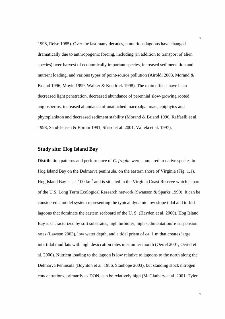
1998, Reise 1985). Over the last many decades, numerious lagoons have changed

dramatically due to anthropogenic forcing, including (in addition to transport of alien

species) over-harvest of economically important species, increased sedimentation and

nutrient loading, and various types of point-source pollution (Airoldi 2003, Morand &

Briand 1996, Moyle 1999, Walker & Kendrick 1998). The main effects have been

decreased light penetration, decreased abundance of perennial slow-growing rooted

angiosperms, increased abundance of unattached macroalgal mats, epiphytes and

phytoplankton and decreased sediment stability (Morand & Briand 1996, Raffaelli et al.

1998, Sand-Jensen & Borum 1991, Sfriso et al. 2001, Valiela et al. 1997).

Study site: Hog Island Bay

Distribution patterns and performance of C. fragile were compared to native species in

Hog Island Bay on the Delmarva peninsula, on the eastern shore of Virginia (Fig. 1.1).

Hog Island Bay is ca. 100 km2 and is situated in the Virginia Coast Reserve which is part

of the U.S. Long Term Ecological Research network (Swanson & Sparks 1990). It can be

considered a model system representing the typical dynamic low slope tidal and turbid

lagoons that dominate the eastern seaboard of the U. S. (Hayden et al. 2000). Hog Island

Bay is characterized by soft substrates, high turbidity, high sedimentation/re-suspension

rates (Lawson 2003), low water depth, and a tidal prism of ca. 1 m that creates large

intertidal mudflats with high desiccation rates in summer month (Oertel 2001, Oertel et

al. 2000). Nutrient loading to the lagoon is low relative to lagoons to the north along the

Delmarva Peninsula (Boynton et al. 1986, Stanhope 2003), but standing stock nitrogen

concentrations, primarily as DON, can be relatively high (McGlathery et al. 2001, Tyler

8

8

et al. 2001). Molluscan and amphipod grazers are prevalent and can control macroalgal

biomass accumulation at low to moderate macroalgal densities (Chapter 2, Giannotti &

McGlathery 2001, Rosinski 2004). There are numerous scattered unconsolidated bivalve

shells and consolidated reef-structures that provide islands of hard substrate. Seagrasses

have been extinct since the 1930 s (Hayden et al. 2000), and unattached drift algae can

occur in high abundances (Chapter 2, Giannotti & McGlathery 2001, McGlathery et al.

2001). A gradient in water residence time exist from near-mainland to near-ocean sites

because of restricted tidal inputs via the Machipongo Inlet and relatively little freshwater

input from the mainland (Lawson 2003). This gradient co-varies with sediment

characteristics such as porosity, organic content and CN-ratios, and water quality

parameters, such as nutrient levels and suspended solids (McGlathery et al. 2001).

The macroalgal species that are common and conspicuous in Hog Island Bay, and are

found both attached to bivalve shells and in unattached mats, were compared to C.

fragile, and include (Table 1.1): Fucus vesiculosus, Ulva curvata, Agardhiella subulata,

and Gracilaria verrucosa. Also, in certain chapters G. foliifera (Chapter 3, 4, Appendix

1) and Hypnea musciformis (Wulfen) Lamouroux (Chapter 5, Appendix 1) were added. It

is possible that G. foliifera and G. verrucosa are conspecific and should be referred to G.

tikvahiae (Bird & Rice 1990, McLachlan 1979). In this thesis the two morphologies were

treated as independent species and their old taxonomic nomenclature used (Humm 1979)

because of significant differences in abundance patterns within Hog Island Bay. Each of

the six native species have wide distribution patterns along the US east coast and co-exist

with C. fragile in numerous regions (Goshorn et al. 2001, Harlin & Rines 1993, Humm

9

9

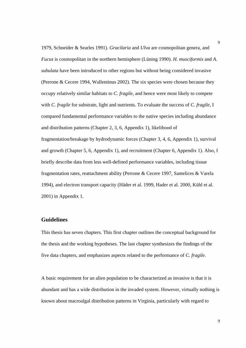
1979, Schneider & Searles 1991). Gracilaria and Ulva are cosmopolitan genera, and

Fucus is cosmopolitan in the northern hemisphere (Lüning 1990). H. musciformis and A.

subulata have been introduced to other regions but without being considered invasive

(Perrone & Cecere 1994, Wallentinus 2002). The six species were chosen because they

occupy relatively similar habitats to C. fragile, and hence were most likely to compete

with C. fragile for substrate, light and nutrients. To evaluate the success of C. fragile, I

compared fundamental performance variables to the native species including abundance

and distribution patterns (Chapter 2, 3, 6, Appendix 1), likelihood of

fragmentation/breakage by hydrodynamic forces (Chapter 3, 4, 6, Appendix 1), survival

and growth (Chapter 5, 6, Appendix 1), and recruitment (Chapter 6, Appendix 1). Also, I

briefly describe data from less well-defined performance variables, including tissue

fragmentation rates, reattachment ability (Perrone & Cecere 1997, Santelices & Varela

1994), and electron transport capacity (Häder et al. 1999, Hader et al. 2000, Kühl et al.

2001) in Appendix 1.

Guidelines

This thesis has seven chapters. This first chapter outlines the conceptual background for

the thesis and the working hypotheses. The last chapter synthesizes the findings of the

five data chapters, and emphasizes aspects related to the performance of C. fragile.

A basic requirement for an alien population to be characterized as invasive is that it is

abundant and has a wide distribution in the invaded system. However, virtually nothing is

known about macroalgal distribution patterns in Virginia, particularly with regard to

10

10

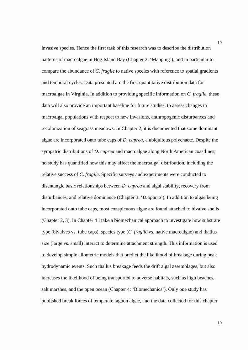
invasive species. Hence the first task of this research was to describe the distribution

patterns of macroalgae in Hog Island Bay (Chapter 2: Mapping ), and in particular to

compare the abundance of C. fragile to native species with reference to spatial gradients

and temporal cycles. Data presented are the first quantitative distribution data for

macroalgae in Virginia. In addition to providing specific information on C. fragile, these

data will also provide an important baseline for future studies, to assess changes in

macroalgal populations with respect to new invasions, anthropogenic disturbances and

recolonization of seagrass meadows. In Chapter 2, it is documented that some dominant

algae are incorporated onto tube caps of D. cuprea, a ubiquitous polychaete. Despite the

sympatric distributions of D. cuprea and macroalgae along North American coastlines,

no study has quantified how this may affect the macroalgal distribution, including the

relative success of C. fragile. Specific surveys and experiments were conducted to

disentangle basic relationships between D. cuprea and algal stability, recovery from

disturbances, and relative dominance (Chapter 3: Diopatra ). In addition to algae being

incorporated onto tube caps, most conspicuous algae are found attached to bivalve shells

(Chapter 2, 3). In Chapter 4 I take a biomechanical approach to investigate how substrate

type (bivalves vs. tube caps), species type (C. fragile vs. native macroalgae) and thallus

size (large vs. small) interact to determine attachment strength. This information is used

to develop simple allometric models that predict the likelihood of breakage during peak

hydrodynamic events. Such thallus breakage feeds the drift algal assemblages, but also

increases the likelihood of being transported to adverse habitats, such as high beaches,

salt marshes, and the open ocean (Chapter 4: Biomechanics ). Only one study has

published break forces of temperate lagoon algae, and the data collected for this chapter

11

11

fills a gap in the biomechanical literature. In Chapter 5 I take a direct and manipulative

approach to test the C. fragile -superiority hypothesis, by conducting several multi-

species and multi-factorial in situ tissue performance experiments (Chapter 5:

Performance ). In particular, I manipulate lagoon characteristics (the invaded system)

that have been suggested to influence performance of C. fragile (the invader), including

light and nutrient levels, grazer densities, sedimentation levels, and positions at different

elevations and distances from the mainland. These data indicated that long-term

experiments with entire individuals, not fragments, could provide clues to the invasive

success of C. fragile. I then conducted an experiment testing invasiveness, i.e. the

recruitment of C. fragile compared to native species onto barren substrate around oyster

reefs and under different levels of drift algae accumulations and sediments (Chapter 6:

Recruitment). This experiment ran for one year and is one of very few studies to

manipulate ecological processes on oyster-reef assemblages, in particular emphasizing

the success of invasive macroalgae.

Hypothesis

Based on the background information the following working hypothesis was created: C.

fragile has high abundance and superior performance compared to native macroalgal

species, particularly under conditions typical for shallow soft bottom turbid lagoons.

This hypothesis was tested by comparing C. fragile to native species under similar

conditions and exposing them to identical treatments. Each chapter treats a different

ecological aspect of importance in determining the success of macroalgae in Hog Island

12

12

Bay. Note that this C. fragile-oriented approach is not necessarily as dominant in the

chapters where the emphasis is on assemblage patterns or numerically dominant taxa.

The following is a brief description of the questions and hypothesis addressed in each

chapter.

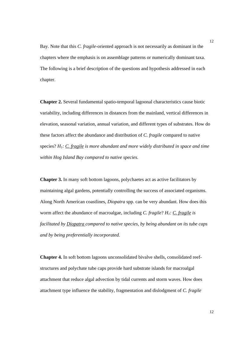
Chapter 2. Several fundamental spatio-temporal lagoonal characteristics cause biotic

variability, including differences in distances from the mainland, vertical differences in

elevation, seasonal variation, annual variation, and different types of substrates. How do

these factors affect the abundance and distribution of C. fragile compared to native

species? H1: C. fragile is more abundant and more widely distributed in space and time

within Hog Island Bay compared to native species.

Chapter 3. In many soft bottom lagoons, polychaetes act as active facilitators by

maintaining algal gardens, potentially controlling the success of associated organisms.

Along North American coastlines, Diopatra spp. can be very abundant. How does this

worm affect the abundance of macroalgae, including C. fragile? H1: C. fragile is

facilitated by Diopatra compared to native species, by being abundant on its tube caps

and by being preferentially incorporated.

Chapter 4. In soft bottom lagoons unconsolidated bivalve shells, consolidated reef-

structures and polychate tube caps provide hard substrate islands for macroalgal

attachment that reduce algal advection by tidal currents and storm waves. How does

attachment type influence the stability, fragmentation and dislodgment of C. fragile

13

13

compared to native species? H1: C. fragile resists water forces better than native species,

both when attached to tube caps and to bivalve shells.

Chapter 5. Tidal soft bottom lagoons are characterized by high levels of sedimentation,

intertidal desiccation, turbidity, molluscan abundance, and nutrient gradients. How do

these factors affect short-term performance of C. fragile compared to native species, and

do they interact with spatial location, which is characterized by predicable differences in

nutrient and light levels? H1: Compared to native species C. fragile has higher growth

rates, under low and high levels of mud snail densities, nutrient concentrations, light

levels, desiccation levels, sedimentation, and at all sites along the distance-from-

mainland gradient.

Chapter 6. Oysters reefs facilitate high diversity and productivity in soft bottom lagoons

by providing hard substrates for recruiting sessile organisms. However, increased burial

by sediments or drift algal mats may threaten recruiting oysters and associated sessile

organisms. Is C. fragile an efficient recruiter on oyster reefs, and do a cover of drift algae

or sediments affect recruitment of C. fragile compared to native species? H1: C. fragile

have higher recruitment than native species, including under algal mats and shallow

sediments.

14

14

Chapter 1. Tables

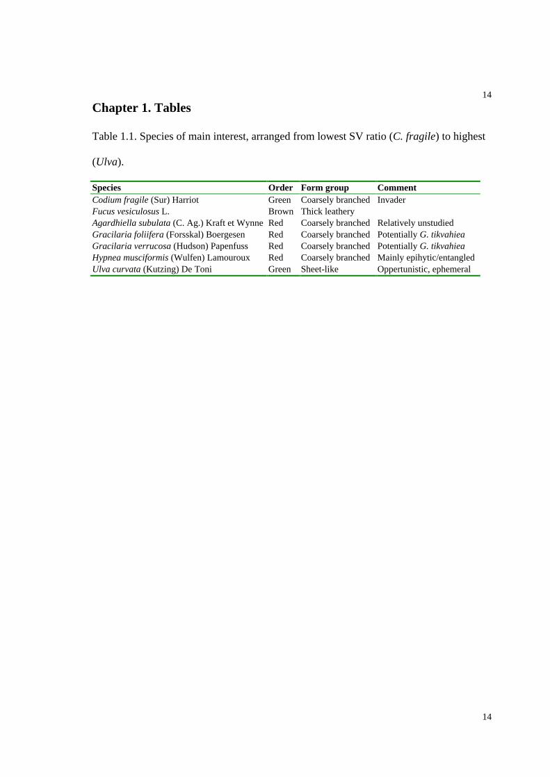
Table 1.1. Species of main interest, arranged from lowest SV ratio (C. fragile) to highest

(Ulva).

Species Order Form group CommentCodium fragile (Sur) Harriot Green Coarsely branched InvaderFucus vesiculosus L. Brown Thick leatheryAgardhiella subulata (C. Ag.) Kraft et Wynne Red Coarsely branched Relatively unstudiedGracilaria foliifera (Forsskal) Boergesen Red Coarsely branched Potentially G. tikvahieaGracilaria verrucosa (Hudson) Papenfuss Red Coarsely branched Potentially G. tikvahieaHypnea musciformis (Wulfen) Lamouroux Red Coarsely branched Mainly epihytic/entangledUlva curvata (Kutzing) De Toni Green Sheet-like Oppertunistic, ephemeral

15

15

Chapter 1. Figures

Fig. 1.1. Hog Island Bay (encircled) within the Virginia Coast Reserve on the Delmarva

Peninsula. The 12 locations sampled in Aquatic Plant Monitoring Program is inserted

(Chapter 2). Of these C1, S1 and H1 sites were revisited in Chapter 3, 5, and 6.

Mid-lagoon: Shoal 2 (S2)

Mid-lagoon: Shoal 1 (S1)

Near-Ocean: Hog 1 (H1)

Near-Ocean: Cobb1 (Cb1)

Near-Mainland:Oyster harbor (OH)

Near-Mainland:Creek 1 (C1)

Near-Mainland:Creek 2 (C2)

Near-Mainland:Whillis Wharf (WW)

16

16

Fig. 1.2. Extreme water level differences in Eastern Shore barrier island lagoons. Maps

from Hayden et al. (2000).

17

17

Chapter 2. Interaction of spatio-temporal

gradients determines macroalgal distribution

patterns in a shallow, soft-bottom lagoon

18

18

Abstract

Benthic algae and seagrasses typically dominate primary production in shallow coastal

ecosystems. Despite their importance, we know relatively little about the temporal and

spatial variability of macroalgae from soft-bottom habitats. The study area, Hog Island

Bay, Virginia, was once a clear water seagrass and oyster-dominated lagoon, but as a

result of storms and diseases it is currently dominated by benthic algae. From 1998 to

2002 we conducted 27 surveys of macroalgal biomass and species composition at 12

permanent sites. The red coarsely branched algae Gracilaria verrucosa was dominant,

constituting 78% of the total biomass, and an additional 15% was accounted for by Ulva

curvata, Bryopsis plumosa, and Codium fragile ssp. tomentosoides. C. fragile is an alien

species that has been in Virginia for ca. 30 years. Taxonomic richness and total biomass

were determined according to five test factors: attachment type, elevation relative to sea

level (intertidal vs. subtidal), distance from the mainland, season, and annual variation.

The biomass of attached and unattached algae was similar (17-19 gDW m-2). However,

taxonomic richness was higher for the attached algae, probably because attached algae

are more stable, less often exported to stressful habitats, and can accumulate an epiphytic

flora. Subtidal sites had higher richness and biomass than intertidal sites, presumably due

to lower desiccation stress. Near-mainland and back-barrier island sites had low richness

and biomass whereas mid-lagoon sites had high richness and biomass. Both richness and

biomass peaked in the summer months when temperature and light availability were

highest. In a separate, smaller survey we found that 70% of attached macroalgal thalli,

particularly G. verrucosa and U. curvata, were incorporated into the tube caps of the

polychaete Diopatra cuprea, suggesting that D. cuprea facilitates algal establishment. In

19

19

spite of low biomass and a patchy distribution, C. fragile was the fourth most abundant

species in Hog Island Bay. C. fragile was not found attached to the D. cuprea tube caps,

and the lack of this association may limit expansion of C. fragile within Hog Island Bay.

In summary, the Hog Island Bay algal assemblage is taxonomically simple and

dominated by a few stress tolerant and ephemeral algae. In addition, distribution patterns

were to a large extent determined by a few, readily quantified, important spatio-temporal

factors: distance from mainland, elevation, season and attachment type.

Introduction

Shallow lagoons are important land-margin ecosystems worldwide, constituting at least

14% of the world's coastline (Cromwell 1973). These shallow soft-bottom systems offer

extensive euphotic areas for aquatic macrophytes such as seagrasses and macroalgae

(Boynton et al. 1996, Hauxwell et al. 2001, Norton & Mathieson 1983, Sand-Jensen &

Borum 1991), and differ from deep estuaries that typically have a restricted littoral zone.

Many types of shallow littoral systems, such as seagrass beds and rocky macroalgal

communities, have been well-described in relation to multiple spatial and temporal

gradients and often show predictable zonational and successional patterns (Lewis 1964,

Stephenson & Stephenson 1949). Multi-factorial approaches used to investigate rocky

algal beds (Menge 1978, Underwood 1981a, Underwood & Jernakoff 1984) have less

commonly been applied to distribution patterns of soft-bottom algal communities. These

communities have typically been described with respect to one or two factors, e.g.

seasonal variation (Cecere et al. 1992, Virnstein & Carbonara 1985), grazing (Rowcliffe

et al. 2001), currents (Salomonsen et al. 1999, Salomonsen et al. 1997), waves and

20

20

nutrients (Pihl et al. 1996, Pihl et al. 1999), and nutrient levels or distance from a nutrient

source (Castel et al. 1996, McComb & Humphries 1992, McGlathery 1992, Raffaelli et

al. 1989, Taylor et al. 1995a, Taylor et al. 1995b). In the present study, our main

objective was to describe the distribution of macroalgae in a soft-bottom system within a

framework of multiple spatio-temporal factors (Keddy 1991). The factors we addressed

included a horizontal distance-from-mainland gradient, a vertical elevation gradient,

seasonal cycles, annual variation and different attachment types. This approach allowed

us to generate hypotheses about what underlying biotic and abiotic factors are important

in determining macroalgal distribution and abundance in soft-bottom lagoons.

Seagrasses and low density algal mats are important habitats for benthic fauna, providing

nursery grounds for fish, substrate for attachment for invertebrates, shelter from

predation, an abundant food supply, and amelioration of adverse stresses such as high

current velocities and intertidal desiccation (Norkko 1998, Norkko et al. 2000). Along the

Atlantic coast of North America, from Rhode Island to Texas, extensive barrier-island-

lagoon complexes dominate the coastal environment. Drift algal mats have become

increasingly abundant in these systems over the last 50 years, primarily in response to

nutrient enrichment, and have had a negative impact on the productivity and distribution

of seagrass meadows (Hauxwell et al. 2001, Lee & Olsen 1985, Taylor et al. 1995a,

Taylor et al. 1995b). Because these two groups of aquatic plants have different

environmental requirements, structural characteristics and ecosystem properties (Duarte

1992, 1995), it is important to know their relative distributions and dynamics. There have

been several studies reporting changes in submerged aquatic plants in lagoons along the

northern and southern U.S. Atlantic coast (e.g. Cowper 1978, Hauxwell et al. 2001,

21

21

Thorne-Miller et al. 1983, Virnstein & Carbonara 1985), yet little is known about mid-

Atlantic systems. The only published data about algal distributions in Virginia lagoons

are presence-absence or qualitative dominance studies (Connor 1980, Humm 1979,

Rhodes 1970, Wulff & Webb 1969) or are reported in the non-refereed literature

(Goshorn et al. 2001, Monti 1993). Thus, our secondary objectives were (1) to fill this

gap by providing a quantitative description of macroalgal distribution patterns from Hog

Island Bay, a part of the Virginia Coast Reserve and U.S. Long Term Ecological

Research Network (VCR/LTER) (Franklin et al. 1990), and (2) to establish a baseline

data set with which to track and evaluate future plant community changes. The VCR

lagoons may be in transition from an algal-dominated system following the local

extinction of seagrasses in the 1930 s to a seagrass-dominated system. The return of

seagrasses is the result of both natural recolonization and restoration efforts (R. Orth,

personal communication), and is likely to result in dramatic changes in biogeochemical

cycling and faunal communities.

In addition to eutrophication, overfishing, destruction of wetlands, and increased

sediment load, many lagoons and estuaries have been invaded by alien species. These

invasions have potentially large impacts on biodiversity and ecosystem functioning on

local, regional and global scales (Ruiz et al. 1997, Ruiz et al. 1999). Our final objective

was to screen the monitoring data for alien algal species and to provide a baseline for

evaluation of future invasions. The alien macroalga Codium fragile ssp. tomentosoides

(Chapman 1999, Trowbridge 1996b) has been present in Virginia for ca. 30 years

(Hillson 1976), and special attention was paid to the distribution patterns of this species.

Such analyses of species-specific distribution patterns can potentially provide insight into

22

22

invader traits, invasion effects and management and control (Rejmánek & Richardson

1996).

Methods

Study site and gradients

Hog Island Bay is located within the Machipongo drainage basin on the Delmarva

Peninsula, and is ca. 100 km2 in area. Intertidal Spartina alterniflora marshes border the

bay on the mainland side and on the leeward side of the barrier islands. Most of the bay is

soft-bottom sands and muds; unconsolidated bivalve shells, scattered relict oyster reefs,

and S. alterniflora stems provide hard substrate for sessile organisms. There is little

bathymetric complexity, except for a single deep channel. The average water depth is 1.5

m, 37% of the lagoonal surface area is intertidal and 81% is less than 3 m deep (Oertel

2001). The semidiurnal tidal range is ca. 1.5 m (Oertel 2001), although storm surges can

add at least an extra meter of water (pers. obs.). Tidal currents reach 2 m s-1 in the inlets

between the barrier islands (Oertel et al. 2000), but peak currents within the bay are

generally 0.05-0.70 m s-1 (Lawson 2003). Light extinction in the water column is high (k

2 m-1) but varies across the lagoon, largely as a result of wind-driven sediment

resuspension (Lawson 2003, McGlathery et al. 2001). There is a gradient of decreasing

dissolved nutrients and total suspended solids with increasing distance from the mainland

(Lawson 2003, McGlathery et al. 2001, Tyler et al. 2001). Air temperature varies

seasonally from ca. 5 to 35 C and water temperature from ca. 2 to 27 C (VCR/LTER

unpublished data). Salinity ranges from ca. 28 to 34 ppt. within the bay, but is relatively

constant throughout the year (VCR/LTER unpublished data).

23

23

VCR/LTER Aquatic Plant Monitoring Program

Twelve permanent sites were established in Hog Island Bay in summer 1998. There were

6 near-mainland sites, 2 mid-lagoon sites, and 4 near-ocean back-barrier island sites. This

distribution of sites represents the distance from mainland gradient (DIS). The sites were

further separated as 8 subtidal and 4 intertidal sites, which are used to represent the

elevation gradient (ELE). All sampling was conducted on low-slope muddy substrate.

Twenty seven surveys were conducted from June 1998 to November 2002, with the

lowest sampling frequency in winter and highest in summer. The 12 sites were reduced to

three representative subtidal sites (C1, S1 and H1, Table 2.1) during the last 14 surveys.

For each survey, macroalgae were collected in 6 random replicates per site using 0.15 m2

cores and separated in situ into attached and unattached groups (= attachment type, ATT).

Attached algae were classified as thalli that presented a resistance to a pull and/or were

attached to a bivalve shell, although specific attachment types were not recorded. The

samples were separated into different taxa in the lab, rinsed in deionized water, and the

dry weight was determined after lyophilization. A few inconspicuous and rare taxa were

only determined to genus or form-group. These groups were treated as separate

taxonomic units in our analysis.

Data analysis

In addition to the spatial patterns (DIS, ELE) and attachment type (ATT), the data were

analyzed based on two scales of temporal variability, annual (ANN) and seasonal (SEA).

Attached and unattached algae from the same core were treated as statistically

independent samples because attached algae were separated vertically (closest to the

24

24

sediment surface) and decoupled temporally (not drifting with the tides) from unattached

algae. ANOVA analyses were conducted on total algal dry weight, taxonomic richness

and C. fragile dry weight using fixed-factor type III Sum of Squares (SPSS 8.0). The

ANOVAs were performed both as full 5-factorial and as 5 single factor-ANOVAs, the

former representing the most complex and the latter the simplest approach to evaluate

factors of potential importance. All analyses were performed on Log(x+1) transformed

data to reduce variance heterogeneity, and in particular to reduce the statistical influence

of large outliers. Inspection of box-plots of raw data and with various transformation

types showed that logarithm transformation most efficiently reduced variances, even

though they remained heterogeneous (p < 0.05, Levines test) for all ANOVAs except for

annual variability vs. Log(biomass). To arrange significant factors according to relative

importance within an ANOVA, 2 was calculated (Levine & Hullet 2002, Welden &

Slauson 1986). Significant results should be interpreted conservatively because p-values

could be biased due to uneven sampling design (except for the attachment factor),

heterogeneous variances, and spatio-temporal autocorrelation effects (Underwood

1981b). Graphical analysis was used to suggest specific treatment effects following

significant single-factor results. This approach was preferred over unplanned multiple

statistical comparisons because the large sample size was likely to detect statistical

differences, even if treatments would not be different in an ecological context. Also, to

investigate if the dominant species had similar general distributions, a Pearson correlation

matrix was calculated including total biomass, taxonomic richness and the biomass of

each of the 12 most abundant species. Again, p-values should be interpreted with caution

because of non-normal distributions.

25

25

Attachment survey

As a supplement to the monitoring program, we described the algal attachment types in

more detail during April November 2002, using the following categories: 1) loose, 2)

partly buried, 3) incorporated into tube caps of the polychaete Diopatra cuprea, 4)

attached to unconsolidated bivalve shells, 5) epiphytic on or 6) entangled around a

basiphyte. We sampled 441 individuals from 17 soft-bottom sites, including the 12 sites

from the main survey. Individual thalli were selected randomly at each site and the

species and attachment type determined in situ. A X2-contingency test was used to

investigate if different algal species were attached to different categories in the same

proportions. Species-substrate combinations observed less than five times were omitted

to fulfill X2-test assumptions.

Results

VCR-LTER Aquatic Plant Monitoring Program

The macroalgal assemblage in Hog Island Bay was species-poor and dominated by a few

key taxa with relatively high biomass. The dominant species, Gracilaria verrucosa, was

found in approximately one third of all samples and accounted for 78% of the total

macroalgal biomass (Table 2.2). Together with G. verrucosa, Ulva curvata, Bryopsis

plumosa, C. fragile and Ectocarpus spp. accounted for 95% of the total biomass.

Eighteen other taxa were sampled in the 27 surveys, but most with few number of

observations (Table 2.2).

26

26

Species richness

The 5-factorial ANOVA that tested effects on taxonomic richness produced 21

significant factor-combinations (Table 2.3). Because the 5-factorial and 2 of the 4-

factorial combinations were significant, lower order interactions and single factor effects

should be evaluated with caution. However, the significant factors and combinations that

explained of the greatest proportion of the data-variability (>2% of the sum of squares)

were of a lower order: DIS, ATT, DIS*ANN, SEA*ANN, and DIS*SEA*ANN. The

temporal variations (SEA, ANN) were mainly important in interaction terms, but distance

(DIS) was important both as a single factor and in interaction with the temporal factors.

Thus, although numerous other factor combinations were significant, they were of

relatively low importance. Elevation in particular explained a small proportion of the sum

of squares. Species richness peaked at 4-6 taxa per sample in the summer months,

particularly at mid-lagoon sites for both attached and unattached samples (Fig. 2.1).

Temporal patterns were less clear for the low diversity back-barrier and near-mainland

sites, which generally had 0-3 taxa per sample. All single factor ANOVAs were highly

significant (Table 2.4) indicating that each test factor influenced species richness. The

highest taxonomic richness was found in attached forms (ATT), in the subtidal zone

(ELE), at mid-lagoon sites (DIS), during spring-summer (SEA) and during the last two

sampling years (ANN) (Fig. 2.2).

Total biomass

Sixteen factor-combinations were significant for biomass, with the most important being

DIS, SEA*ANN, and DIS*SEA*ANN which each explained 2-5% of the sum of squares

(Table 2.3). Biomass, like species richness, was determined primarily by the distance

27

27

from the mainland and the temporal variations. Again, elevation and combinations

including elevation were the least important factors. The greatest biomass was observed

for unattached drift algae at mid-lagoon sites during summer months (2-300 gDW m-2),

although attached biomass also had a single pronounced peak at this site in summer 1999

(400 gDW m-2; Fig. 2.3). Biomass was low at other sites and during the fall to spring

months (0-30 gDW m-2), except for two separate, but relatively small, summer blooms of

unattached algae at the near-mainland sites (ca. 100 gDW m-2). All single factor

ANOVAs were highly significant (Table 2.4), indicating that each test factor influenced

the accumulation of macroalgal biomass. Biomass was the highest in the subtidal zone

(ELE), at mid-lagoon sites (DIS) and in summer months (SEA; Fig. 2.4). Although there

were significantly more algae attached (19 gDW m-2) than unattached (17 gDW m-2) and

more at year 2 (21 gDW m-2) than year 1 (15 gDW m-2) these small differences are

probably of minor ecological importance (Fig. 2.4).

Biomass of Codium fragile

Although C. fragile was the fourth most abundant species (Fig. 2.5A, Table 2.2), it

occurred as a few large and patchily distributed individuals. C. fragile accounted for ca.

4% of the total biomass and was only found in 27 samples. The 5-factorial ANOVA

showed a single significant effect of season, which explained less than 1% of the data

variability (Table 2.3). On the other hand, each of the single factor ANOVAs was highly

significant, although they only explained a very small proportion of the data variability

(Table 2.4). C. fragile was predominantly unattached (ATT), in the subtidal zone (ELE)

and at mid-lagoon and back-barrier sites (DIS) (Fig. 2.4B-Q). In particular, C. fragile was

28

28

relatively important at back-barrier sites, being the most dominant species following G.

verrucosa (Fig. 2.5O). C. fragile was not found in surveys near the mainland or on

intertidal mudflats, but was occasionally observed in these habitats as ephemeral drift

material (pers. obs.). C. fragile was most common in the summer months (SEA) and in

years 3 and 4 (ANN). Even though C. fragile was not found during the winter surveys, it

was, on rare occasions observed as reduced individuals (pers. obs.).

Species-specific correlation

Biomass and richness were significantly correlated with each other and with the 12 most

important species in Hog Island Bay, although these only explained 1% of the sum of

squares (r2) for Enteromorpha spp. and Hypnea musciformis (Table 2.5). All of the 68

significant correlations (out of 90 combinations) were positive, suggesting similar

responses to the ambient environmental conditions and that the likelihood of finding a

species in a sample typically increased with the likelihood of finding any other species.

G. verrucosa biomass was significantly correlated to most of the other species and

explained 92% of the biomass data variability and 42% of the richness variability,

emphasizing the key status of this species. C. fragile had significant correlations

(arranged by highest r2) with Agardhiella subulata, U. curvata, G. verrucosa, B. plumosa,

Ceramium spp., G. foliifera, and Polysiphonia spp. These correlations, however, only

explained from <1 6 % of the data variability. The species B. plumosa, Ectocarpus spp.,

Polysiphonia spp., Ceramium spp., Champia parvula and H. musciformis were only

found unattached or epiphytic (primary attached, reattached or entangled) on G.

verrucosa, U. curvata, C. fragile or Fucus vesiculosus.

29

29

Secondary species dominance

Even though G. verrucosa was dominant along all test-factors, there are interesting

secondary dominance patterns across the test gradients (without G. verrucosa, Fig. 2.5).

Among the different years of the study, we observed dominance by U. curvata and B.

plumosa in year 1, even dominance among several species in year 2, C. fragile in year 3,

U. curvata in year 4 and B. plumosa in year 5 (Fig. 2.5B-F). Seasonally, the secondary

dominance patterns were as follows: (1) Ectocarpus spp. and U. curvata were particularly

common in winter and spring months (Fig. 2.5J and G), (2) summer samples were

dominated by U. curvata, B. plumosa and C. fragile (Fig. 2.5H), and (3) fall samples

were dominated by U. curvata and A. subulata (Fig. 2.5I). Spatially, the secondary

dominance patterns showed that the three most common taxa in the subtidal zone were U.

curvata, B. plumosa and C. fragile whereas in the intertidal zone it was U. curvata, B.

plumosa and Ectocarpus spp. (Fig. 2.5K, L). Near-mainland sites consisted mainly of U.

curvata and Ectocarpus spp. (Fig. 2.5M), mid-lagoon sites had high abundance of U.

curvata and B. plumosa (Fig. 2.5N), and back-barrier sites had high abundance of C.

fragile and B. plumosa (Fig. 2.5O). Finally, attached assemblages were dominated by U.

curvata, B. plumosa, Ectocarpus spp. and A. subulata (Fig. 2.5P), whereas unattached

assemblages were dominated by U. curvata, B. plumosa and C. fragile (Fig. 2.5Q). It

should be noted that the attached B. plumosa, Ectocarpus spp., Polysiphonia spp.,

Ceramium spp., C. parvula and H. musciformis were found only as epiphytes on attached

basiphytes.

30

30

Attachment survey

Algae were present on mudflats with different attachment types (i.e. algae and attachment

types were not distributed in equal proportions, p = 0.000, n = 433, X2 = 1014, Df = 45).

G. verrucosa and U. curvata constituted ca. 85% of the species observations. C. fragile

was overall the sixth most abundant species, following G. verrucosa, U. curvata,

Enteromorpha spp., F. vesiculosus, and A. subulata. Seventy percent of all algae were

attached to worm tubes, 10% were unattached, and 10% were attached to unconsolidated

bivalve shells. Buried, epiphytic and entangled algae were rarely encountered in this

survey. Of the 309 algae found attached to D. cuprea tube caps, G. verrucosa and U.

curvata constituted 98%. C. fragile was observed unattached 4 times and attached to

unconsolidated bivalve shells 5 times.

Discussion

Effects of macroalgal mats in lagoons

The quantification of the macroalgal assemblage in Hog Island Bay is ecologically and

economically important. Dense macroalgal accumulations can have negative

consequences by (1) creating anoxia when algal mats collapse and decompose, (2)

altering the diversity and community composition of benthic infauna and epifauna, (3)

out-competing seagrasses, (4) fouling trawl nets, (5) reducing performance of

maricultured bivalve spat, (6) reducing waterway access and clogging boat motors (7)

and creating foul smells and beach debris (Fletcher 1996, Hauxwell et al. 2001,

Holmquist 1997, Nelson & Lee 2001, Norkko & Bonsdorff 1996b, Raffaelli et al. 1998).

On the other hand, where algae are present in lower densities, they typically have a

31

31

positive influence, including: (1) acting as a temporary filter for land derived nutrients,

(2) creating habitats for invertebrates and fish, (3) providing protection from predators,

(4) providing an abundant food supply for grazers, and (5) providing a mechanism for

dispersal (Duffy & Hay 1991b, Holmquist 1994, McGlathery et al. 2001, Norkko et al.

2000, Raffaelli et al. 1998, Tyler 2002). Overall algal biomass in Hog Island Bay was

patchy and primarily at low densities. However, the summer biomass peak, which is

typical in temperate systems (Humm 1979, Lüning 1990), at the mid-lagoon sites,

occasionally crashed and were followed by areas of anoxia and the associated negative

impacts listed previously (McGlathery et al. 2001, Tyler et al. 2001, 2003).

Species patterns

The patterns of macroalgal distribution that we describe are restricted to the shallow, soft-

bottom portion of the lagoon; marsh areas, deep channels and oyster reefs may have

different patterns of biomass and species richness, although the species pool is the same

(pers. obs.). The species richness values of 20-30 species found in Hog Island Bay are

typical of soft bottom lagoonal systems (Cecere et al. 1992, Cowper 1978, Fletcher 1996,

Thorne-Miller et al. 1983). Likewise, the species assemblage, a mixture of filamentous

and sheet-like opportunistic and coarsely branched and thick leathery perennial taxa, was

similar to observations from other western mid-Atlantic systems (Connor 1980, Goshorn

et al. 2001, Rhodes 1970, Wulff & Webb 1969, Wulff et al. 1968, Zaneweld & Barnes

1965). G. verrucosa was a key species explaining a large proportion of the richness data,

typically carrying 1-3 epiphytic algal taxa. Thus, because of its wide distribution pattern,

high biomass, high productivity (McLachlan & Bird 1986, Tyler 2002) and its consistent

32

32

epiphytic flora, G. verrucosa can be considered a foundation species within Hog Island

Bay (sensu Dayton 1972). Species that were found year-round (G. verrucosa, A.

subulata, F. vesiculosus, C. fragile, and U. curvata) have perennial life history strategies

(Schneider & Searles 1991), with the exception of U. curvata which typically has an

ephemeral and highly fluctuating appearance (Littler 1980, Sears 1975, Wallentinus

1984). U. curvata can, however, survive periods of low light, low temperature and

sediment burial and this may facilitate its survival during adverse winter conditions in

unattached forms (Vermaat & Sand-Jensen 1987). When attached to bivalve shells, G.

verrucosa, A. subulata, and C. fragile were mainly found at reduced size during the

winter months (pers. obs.), suggesting winter fragmentation and/or a pseudo-perennial

life style (Fralick & Mathieson 1972, Sears 1975). B. plumosa and Ectocarpus spp. were

clearly the most important filamentous taxa, with the latter being the dominant in spring

and winter months, in the intertidal and at near-mainland sites. Although Ectocarpus spp.

is a well-known bloom-forming algae, it is less common to observe Bryopsis blooms in

temperate systems (Fletcher 1996, Morand & Briand 1996, Raffaelli et al. 1998).

Spatio-temporal gradients

In Hog Island Bay, the hydrodynamic regime provides a unifying framework for

generating hypotheses about large-scale patterns of species distribution and abundance.

First, the lunar cycle sets the stage for a vertical tidal wave with differences in inundation

time and amount of overlying water. This will have an effect on light availability,

sedimentation and grazing. Second, a horizontal tidal wave of nutrient-poor oceanic

water from the inlet coupled with inputs of nutrient-enriched groundwater from the

33

33

mainland, results in a gradient in water residence times and nutrient availability. This will

also be reflected in other water quality parameters (e.g., turbidity, light penetration,

temperature, and sedimentation levels). Third, storm waves entrain unattached, buried

and tube cap incorporated algae, and currents transport them in the lagoon, where they

potentially can re-attach (Brenchley 1976, Santelices & Varela 1994). The interaction

between tidal currents and attachment types can result in daily changes in the algal

assemblages. Because nearly 50% of the algal community consisted of unattached forms,

distribution patterns in Hog Island Bay can change dramatically within a tidal cycle and

after storm events, as observed in other drift algae communities (Flindt et al. 1997a,

Holmquist 1994, Salomonsen et al. 1999). Finally, storm-induced disturbances

potentially create seasonal and annual differences in algal export rates (export areas

include deep channels, high beaches, high marshes and the open ocean). Thus, if low-

energy low-export years coincide with favorable growth conditions (e.g. high light and

temperature), algal biomass is likely to accumulate in dense mats with increased risk of

localized anoxia. This emphasizes that Hog Island Bay should be viewed as a dynamic

algal system where currents and storms constantly relocate, import and export algal

biomass.

Within the lagoon, we documented that 2 spatial gradients (DIS, ELE), 2 types of

temporal variability (SEA, ANN) and attachment types (ATT) significantly affected the

distribution and abundance of macroalgae, and that these factors interacted, particularly

due to seasonal and annual variations. Elevation was considered relatively unimportant

based on the 5-factorial ANOVAs but this could partly be caused by the lack of intertidal

34

34

mid-lagoon sites. Typical interpretations of the single factor effects would suggest that

significant effects mainly were caused by differences in nutrients (along DIS, Castel et al.

1996, Flindt & Kamp-Nielsen 1997, McGlathery 1992, Tyler et al. 2001), desiccation

(along ELE, Doty 1946, Dring & Brown 1982, Dromgoole 1980), hydrodynamic forces

(along ATT, SEA and ANN, Lenihan 1999, Phillips et al. 1997, Pihl et al. 1999,

Salomonsen et al. 1997) and light and temperature (along SEA and ANN, Connor 1980,

Goshorn et al. 2001, Wolfe & Harlin 1988). However, because of covariation of these

factors along the gradients, controlled manipulative experiments are clearly needed to

demonstrate causation. For example, sedimentation and light co-vary with nutrient

concentrations along the distance gradient (Airoldi 2003), sedimentation, grazing, light,

and temperature co-vary with desiccation along the elevation-gradient (Lewis 1964), and

abrasion and nutrient encounter rates co-vary with hydrodynamic forces along the

attachment gradient (Hurd 2000).

The shallow portions of the lagoon can be divided into low diversity-low biomass

regions near the mainland and back-barrier islands and high diversity-high biomass

mid-lagoon regions. The three main environmental conditions that vary along this

gradient include light availability (highest water visibility near back barrier island sites),

nutrient availability (highest concentrations near mainland sites) and abrasion and burial

by suspended solids (highest concentrations near mainland sites) (Lawson 2003,

McGlathery et al. 2001). Most macroalgae could thus be limited by light and sediment

abrasion/burial at near-mainland sites (Lawson 2003, McGlathery et al. 2001) and

nutrients at near-ocean sites (McGlathery et al. 2001, Tyler et al. 2001), particularly in

35

35

summer months when the growth potential is highest (Tyler 2002). In comparison, mid-

lagoon sites with intermediate levels of these limiting factors should have relatively

benign growth conditions. G. verrucosa and U. curvata are frequently the dominant

species in US east coast lagoons (Goshorn et al. 2001, Thorne-Miller et al. 1983).

Because these two species were found most commonly incorporated into D. cuprea tube

caps (this study, Mangum et al. 1968, Myers 1972), we suggest that this association is a

neglected factor that potentially can structure benthic primary production and assemblage

structure/stability in D. cuprea-algal dominated west-Atlantic lagoons (Bell & Coen

1982b, Luckenbach 1986, Woodin 1978).

Potential for seagrass recolonization

Species-poor soft-bottom drift algal associations are well known worldwide, and often

are relatively similar to the Hog Island Bay assemblage in that they are dominated by a

few red and green algae (e.g. Cecere et al. 1992, Cowper 1978, Fletcher 1996, Lowthion

et al. 1985, Peckol & Rivers 1995, 1996, Pihl et al. 1996, Sfriso et al. 1992, Thorne-

Miller et al. 1983, Virnstein & Carbonara 1985). In several of these studies, seagrasses

were present in high quantities indicating that coexistence is possible as long as major

anoxia and shading are avoided (Hauxwell et al. 2001). This is an important condition if

Zostera marina should reestablish in Hog Island Bay (Goshorn et al. 2001, VCR/LTER

unpublished data). We speculate that the large and consistent summer biomass

accumulations at mid-lagoon sites could influence seagrass reestablishment in this region.

If unattached and attached samples were pooled, as done in aforementioned lagoon

studies, ca 10% of the samples would contain more than 100 gDW m-2, with a maximum

36

36

of 1807 gDW m-2. This indicates that Hog Island Bay does at certain times and sites have

high macroalgal densities, primarily at mid-lagoon sites, but also occasionally as patchy

and ephemeral drift accumulations at near-mainland and back-barrier sites. However,

given that these blooms occur in localized patches in Hog Island Bay (McGlathery et al.

2001), we believe that the potential for seagrass recolonization is high provided that

eutrophication does not accelerate appreciably in the region (Goshorn et al. 2001).

Nutrient inputs to the lagoon via groundwater and atmospheric deposition are impacted

by human activities such as agriculture and development (Stanhope 2003), however

overall loading rates are low relative to northern lagoons on the Delmarva Peninsula

(Boynton et al. 1996, Goshorn et al. 2001, Stanhope 2003). The rapid turnover of

nutrients in the sediments and the low, but steady supply of water column nutrients

provided by tidal currents are probably the mechanisms that currently support the

localized macroalgal blooms (McGlathery et al. 2001).

Distribution of Codium fragile

C. fragile ssp. tomentosoides originates from the North West Pacific Ocean, but has in

the last century dispersed to the East Pacific-, Southern-, East Atlantic-, and West

Atlantic-Oceans, probably using ship-hulls and imported oysters as vectors (Trowbridge

1998). C. fragile appeared in the East Atlantic in the late 1950s (Bouck & Morgan 1957)

and probably arrived in Virginia in the 1970s (Hillson 1976). Thirty years after it arrival,

C. fragile could be considered a successful invader in Hog Island Bay based on its

relative dominance, although absolute biomass remains low. It is interesting that C.

fragile was less common in a large-scale macroalgal survey in adjacent lagoons north of

37

37

Hog Island Bay (Goshorn et al. 2001), although details in the sampling procedures and

results of this study are unclear. All introduced species have some community and

ecosystem impacts (Carlton 1996b, Carlton 1999). However, the low biomass of C.

fragile in Hog Island Bay and the northern lagoons suggest relatively small effects on

larger spatio-temporal scales, particularly compared to other invaded systems where C.

fragile has formed dense monocultures and large canopies (Begin & Scheibling 2003,

Fralick & Mathieson 1973, Mathieson et al. 2003). We suggest that C. fragile was most

abundant in subtidal mid-lagoon and back-barrier sites because shell-substrates, a

necessity for recruitment (Borden & Stein 1969, Fralick & Mathieson 1973, Malinowski

& Ramus 1973), are relative abundant and that recruits probably experience less frequent

sediment burial compared to near-mainland sites. The lack of C. fragile in the high

intertidal zones and in winter months may be caused by low desiccation resistance and

winter fragmentation (Fralick & Mathieson 1972). This should be tested by future work

coupling the distribution patterns with manipulative growth experiments.

Conclusions

We have provided the first quantitative description of macroalgal distribution patterns

from Virginia by using a framework of multiple spatio-temporal test factors. Each of

these test factors was important in structuring the algal assemblages. Thus, if algal

distribution patterns are to be compared within and between soft-bottom lagoonal

systems, our data indicate that attachment types, horizontal and vertical position and

seasonal and yearly sampling time at the least should be considered. Despite the large

pool of 20-30 species and multiple interacting spatio-temporal gradients, Hog Island Bay

38

38

is a simple algal system because G. verrucosa constitute most of the biomass, followed

by a few common, but sub-dominant taxa (U. curvata, B. plumosa, C. fragile, Ectocarpus

spp). These patterns were relatively similar to other protected turbid soft-bottom shallow

systems. Finally, the only non-indigenous species we found in the system, C. fragile,

although the fourth most abundant species, was only present with relatively low biomass.

Hence, it is unlikely that C. fragile has had major effects at the ecosystem level.

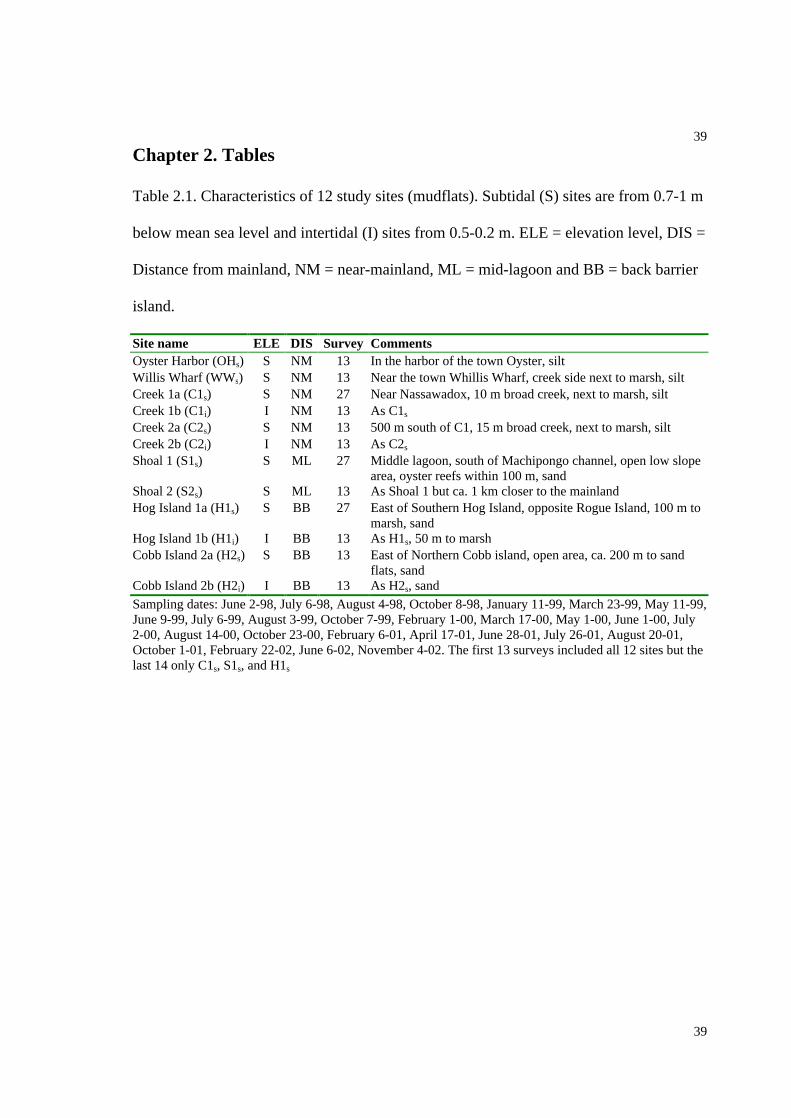
39

39

Chapter 2. Tables

Table 2.1. Characteristics of 12 study sites (mudflats). Subtidal (S) sites are from 0.7-1 m

below mean sea level and intertidal (I) sites from 0.5-0.2 m. ELE = elevation level, DIS =

Distance from mainland, NM = near-mainland, ML = mid-lagoon and BB = back barrier

island.

Site name ELE DIS Survey CommentsOyster Harbor (OHs) S NM 13 In the harbor of the town Oyster, siltWillis Wharf (WWs) S NM 13 Near the town Whillis Wharf, creek side next to marsh, siltCreek 1a (C1s) S NM 27 Near Nassawadox, 10 m broad creek, next to marsh, siltCreek 1b (C1i) I NM 13 As C1s

Creek 2a (C2s) S NM 13 500 m south of C1, 15 m broad creek, next to marsh, siltCreek 2b (C2i) I NM 13 As C2s

Shoal 1 (S1s) S ML 27 Middle lagoon, south of Machipongo channel, open low slopearea, oyster reefs within 100 m, sand

Shoal 2 (S2s) S ML 13 As Shoal 1 but ca. 1 km closer to the mainlandHog Island 1a (H1s) S BB 27 East of Southern Hog Island, opposite Rogue Island, 100 m to

marsh, sandHog Island 1b (H1i) I BB 13 As H1s, 50 m to marshCobb Island 2a (H2s) S BB 13 East of Northern Cobb island, open area, ca. 200 m to sand

flats, sandCobb Island 2b (H2i) I BB 13 As H2s, sand

Sampling dates: June 2-98, July 6-98, August 4-98, October 8-98, January 11-99, March 23-99, May 11-99,June 9-99, July 6-99, August 3-99, October 7-99, February 1-00, March 17-00, May 1-00, June 1-00, July2-00, August 14-00, October 23-00, February 6-01, April 17-01, June 28-01, July 26-01, August 20-01,October 1-01, February 22-02, June 6-02, November 4-02. The first 13 surveys included all 12 sites but thelast 14 only C1s, S1s, and H1s

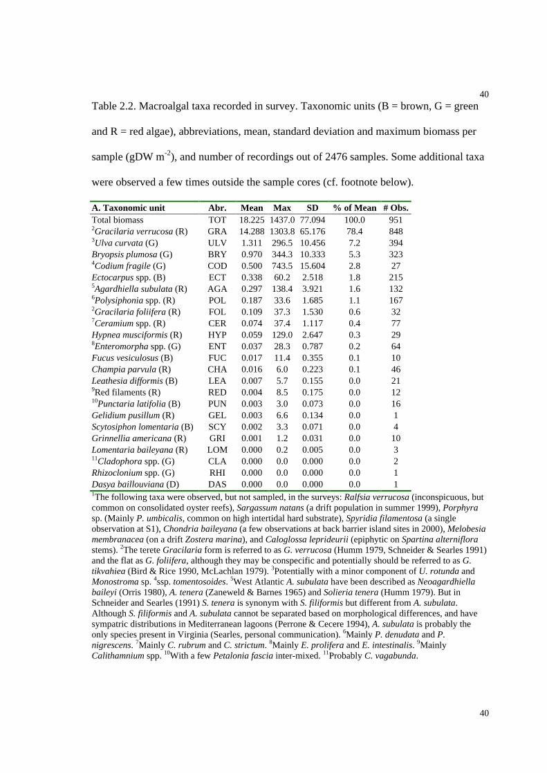
40

40

Table 2.2. Macroalgal taxa recorded in survey. Taxonomic units (B = brown, G = green

and R = red algae), abbreviations, mean, standard deviation and maximum biomass per

sample (gDW m-2), and number of recordings out of 2476 samples. Some additional taxa

were observed a few times outside the sample cores (cf. footnote below).

A. Taxonomic unit Abr. Mean Max SD % of Mean # Obs.Total biomass TOT 18.225 1437.0 77.094 100.0 9512Gracilaria verrucosa (R) GRA 14.288 1303.8 65.176 78.4 8483Ulva curvata (G) ULV 1.311 296.5 10.456 7.2 394Bryopsis plumosa (G) BRY 0.970 344.3 10.333 5.3 3234Codium fragile (G) COD 0.500 743.5 15.604 2.8 27Ectocarpus spp. (B) ECT 0.338 60.2 2.518 1.8 2155Agardhiella subulata (R) AGA 0.297 138.4 3.921 1.6 1326Polysiphonia spp. (R) POL 0.187 33.6 1.685 1.1 1672Gracilaria foliifera (R) FOL 0.109 37.3 1.530 0.6 327Ceramium spp. (R) CER 0.074 37.4 1.117 0.4 77Hypnea musciformis (R) HYP 0.059 129.0 2.647 0.3 298Enteromorpha spp. (G) ENT 0.037 28.3 0.787 0.2 64Fucus vesiculosus (B) FUC 0.017 11.4 0.355 0.1 10Champia parvula (R) CHA 0.016 6.0 0.223 0.1 46Leathesia difformis (B) LEA 0.007 5.7 0.155 0.0 219Red filaments (R) RED 0.004 8.5 0.175 0.0 1210Punctaria latifolia (B) PUN 0.003 3.0 0.073 0.0 16Gelidium pusillum (R) GEL 0.003 6.6 0.134 0.0 1Scytosiphon lomentaria (B) SCY 0.002 3.3 0.071 0.0 4Grinnellia americana (R) GRI 0.001 1.2 0.031 0.0 10Lomentaria baileyana (R) LOM 0.000 0.2 0.005 0.0 311Cladophora spp. (G) CLA 0.000 0.0 0.000 0.0 2Rhizoclonium spp. (G) RHI 0.000 0.0 0.000 0.0 1Dasya baillouviana (D) DAS 0.000 0.0 0.000 0.0 11The following taxa were observed, but not sampled, in the surveys: Ralfsia verrucosa (inconspicuous, butcommon on consolidated oyster reefs), Sargassum natans (a drift population in summer 1999), Porphyrasp. (Mainly P. umbicalis, common on high intertidal hard substrate), Spyridia filamentosa (a singleobservation at S1), Chondria baileyana (a few observations at back barrier island sites in 2000), Melobesiamembranacea (on a drift Zostera marina), and Caloglossa leprideurii (epiphytic on Spartina alterniflorastems). 2The terete Gracilaria form is referred to as G. verrucosa (Humm 1979, Schneider & Searles 1991)and the flat as G. foliifera, although they may be conspecific and potentially should be referred to as G.tikvahiea (Bird & Rice 1990, McLachlan 1979). 3Potentially with a minor component of U. rotunda andMonostroma sp. 4ssp. tomentosoides. 5West Atlantic A. subulata have been described as Neoagardhiellabaileyi (Orris 1980), A. tenera (Zaneweld & Barnes 1965) and Solieria tenera (Humm 1979). But inSchneider and Searles (1991) S. tenera is synonym with S. filiformis but different from A. subulata.Although S. filiformis and A. subulata cannot be separated based on morphological differences, and havesympatric distributions in Mediterranean lagoons (Perrone & Cecere 1994), A. subulata is probably theonly species present in Virginia (Searles, personal communication). 6Mainly P. denudata and P.nigrescens. 7Mainly C. rubrum and C. strictum. 8Mainly E. prolifera and E. intestinalis. 9MainlyCalithamnium spp. 10With a few Petalonia fascia inter-mixed. 11Probably C. vagabunda.

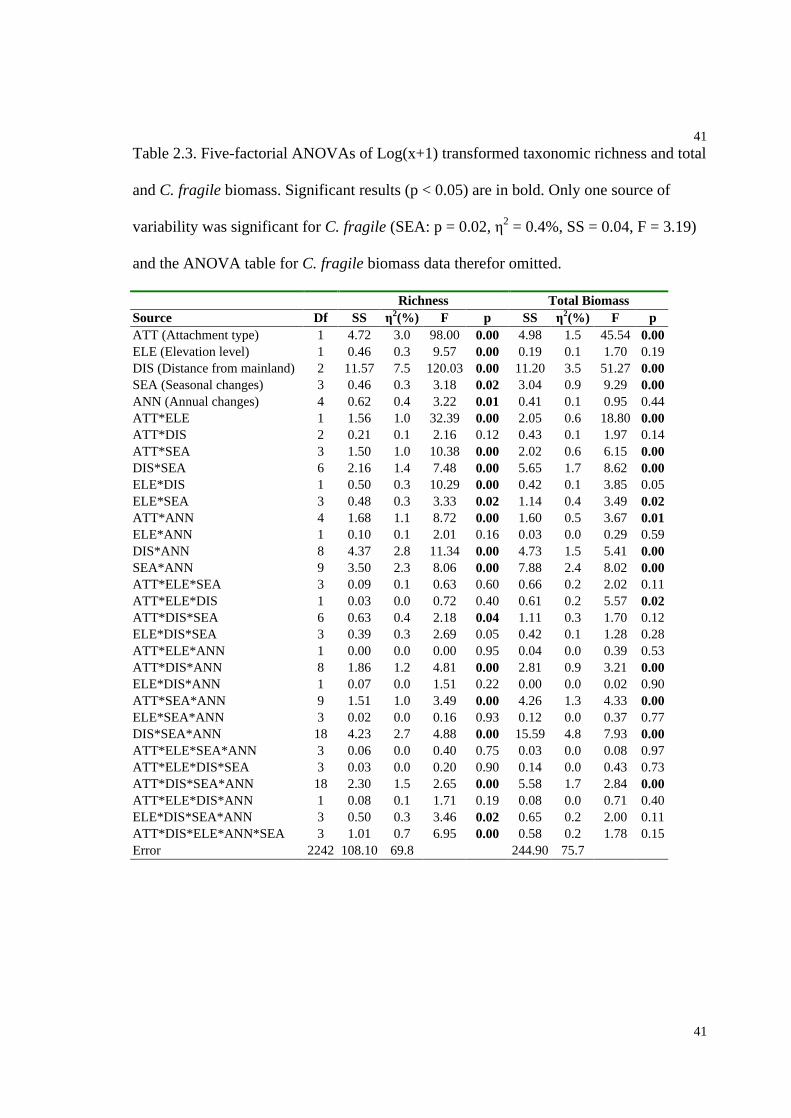
41

41

Table 2.3. Five-factorial ANOVAs of Log(x+1) transformed taxonomic richness and total

and C. fragile biomass. Significant results (p < 0.05) are in bold. Only one source of

variability was significant for C. fragile (SEA: p = 0.02, 2 = 0.4%, SS = 0.04, F = 3.19)

and the ANOVA table for C. fragile biomass data therefor omitted.

Richness Total BiomassSource Df SS 2(%) F p SS 2(%) F pATT (Attachment type) 1 4.72 3.0 98.00 0.00 4.98 1.5 45.54 0.00ELE (Elevation level) 1 0.46 0.3 9.57 0.00 0.19 0.1 1.70 0.19DIS (Distance from mainland) 2 11.57 7.5 120.03 0.00 11.20 3.5 51.27 0.00SEA (Seasonal changes) 3 0.46 0.3 3.18 0.02 3.04 0.9 9.29 0.00ANN (Annual changes) 4 0.62 0.4 3.22 0.01 0.41 0.1 0.95 0.44ATT*ELE 1 1.56 1.0 32.39 0.00 2.05 0.6 18.80 0.00ATT*DIS 2 0.21 0.1 2.16 0.12 0.43 0.1 1.97 0.14ATT*SEA 3 1.50 1.0 10.38 0.00 2.02 0.6 6.15 0.00DIS*SEA 6 2.16 1.4 7.48 0.00 5.65 1.7 8.62 0.00ELE*DIS 1 0.50 0.3 10.29 0.00 0.42 0.1 3.85 0.05ELE*SEA 3 0.48 0.3 3.33 0.02 1.14 0.4 3.49 0.02ATT*ANN 4 1.68 1.1 8.72 0.00 1.60 0.5 3.67 0.01ELE*ANN 1 0.10 0.1 2.01 0.16 0.03 0.0 0.29 0.59DIS*ANN 8 4.37 2.8 11.34 0.00 4.73 1.5 5.41 0.00SEA*ANN 9 3.50 2.3 8.06 0.00 7.88 2.4 8.02 0.00ATT*ELE*SEA 3 0.09 0.1 0.63 0.60 0.66 0.2 2.02 0.11ATT*ELE*DIS 1 0.03 0.0 0.72 0.40 0.61 0.2 5.57 0.02ATT*DIS*SEA 6 0.63 0.4 2.18 0.04 1.11 0.3 1.70 0.12ELE*DIS*SEA 3 0.39 0.3 2.69 0.05 0.42 0.1 1.28 0.28ATT*ELE*ANN 1 0.00 0.0 0.00 0.95 0.04 0.0 0.39 0.53ATT*DIS*ANN 8 1.86 1.2 4.81 0.00 2.81 0.9 3.21 0.00ELE*DIS*ANN 1 0.07 0.0 1.51 0.22 0.00 0.0 0.02 0.90ATT*SEA*ANN 9 1.51 1.0 3.49 0.00 4.26 1.3 4.33 0.00ELE*SEA*ANN 3 0.02 0.0 0.16 0.93 0.12 0.0 0.37 0.77DIS*SEA*ANN 18 4.23 2.7 4.88 0.00 15.59 4.8 7.93 0.00ATT*ELE*SEA*ANN 3 0.06 0.0 0.40 0.75 0.03 0.0 0.08 0.97ATT*ELE*DIS*SEA 3 0.03 0.0 0.20 0.90 0.14 0.0 0.43 0.73ATT*DIS*SEA*ANN 18 2.30 1.5 2.65 0.00 5.58 1.7 2.84 0.00ATT*ELE*DIS*ANN 1 0.08 0.1 1.71 0.19 0.08 0.0 0.71 0.40ELE*DIS*SEA*ANN 3 0.50 0.3 3.46 0.02 0.65 0.2 2.00 0.11ATT*DIS*ELE*ANN*SEA 3 1.01 0.7 6.95 0.00 0.58 0.2 1.78 0.15Error 2242 108.10 69.8 244.90 75.7

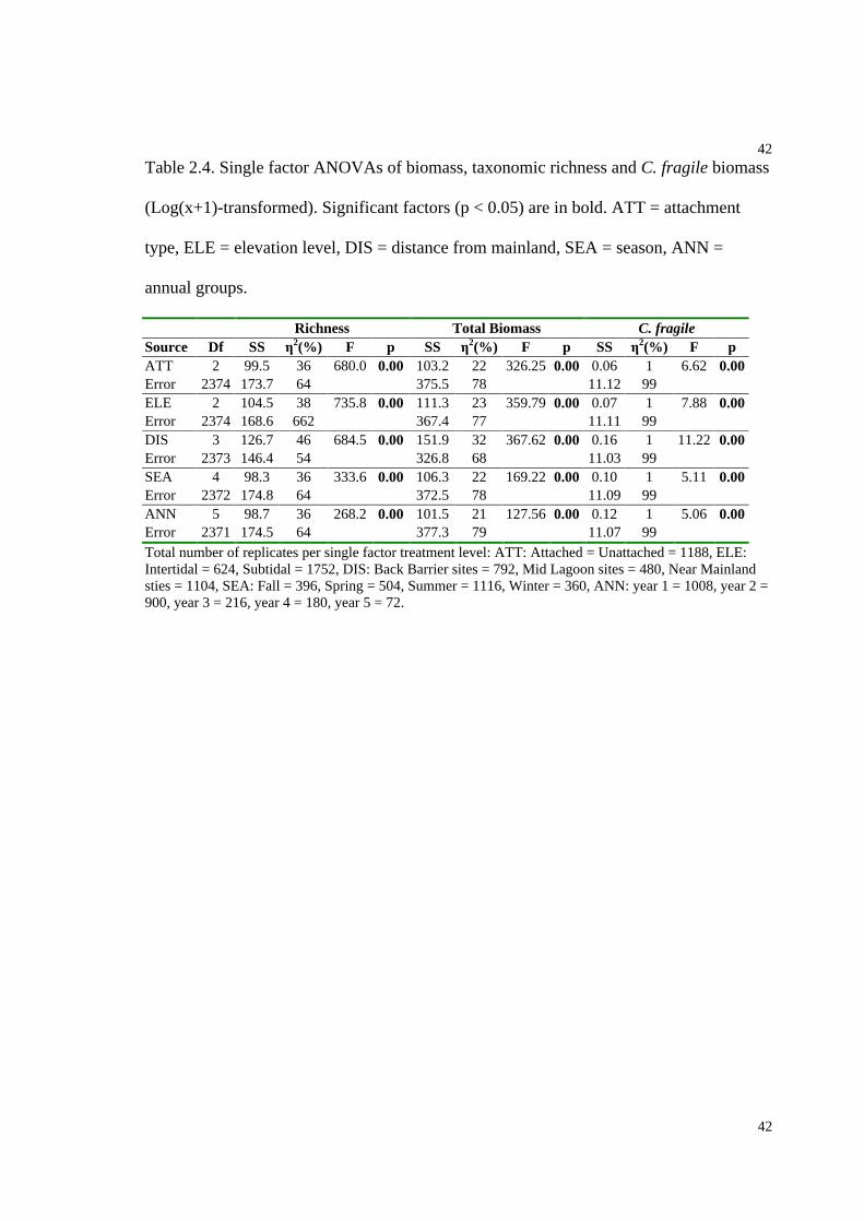
42

42

Table 2.4. Single factor ANOVAs of biomass, taxonomic richness and C. fragile biomass

(Log(x+1)-transformed). Significant factors (p < 0.05) are in bold. ATT = attachment

type, ELE = elevation level, DIS = distance from mainland, SEA = season, ANN =

annual groups.

Richness Total Biomass C. fragileSource Df SS 2(%) F p SS 2(%) F p SS 2(%) F pATT 2 99.5 36 680.0 0.00 103.2 22 326.25 0.00 0.06 1 6.62 0.00Error 2374 173.7 64 375.5 78 11.12 99ELE 2 104.5 38 735.8 0.00 111.3 23 359.79 0.00 0.07 1 7.88 0.00Error 2374 168.6 662 367.4 77 11.11 99DIS 3 126.7 46 684.5 0.00 151.9 32 367.62 0.00 0.16 1 11.22 0.00Error 2373 146.4 54 326.8 68 11.03 99SEA 4 98.3 36 333.6 0.00 106.3 22 169.22 0.00 0.10 1 5.11 0.00Error 2372 174.8 64 372.5 78 11.09 99ANN 5 98.7 36 268.2 0.00 101.5 21 127.56 0.00 0.12 1 5.06 0.00Error 2371 174.5 64 377.3 79 11.07 99Total number of replicates per single factor treatment level: ATT: Attached = Unattached = 1188, ELE:Intertidal = 624, Subtidal = 1752, DIS: Back Barrier sites = 792, Mid Lagoon sites = 480, Near Mainlandsties = 1104, SEA: Fall = 396, Spring = 504, Summer = 1116, Winter = 360, ANN: year 1 = 1008, year 2 =900, year 3 = 216, year 4 = 180, year 5 = 72.

43

43

Table 2.5. Correlation matrix for taxonomic richness, total biomass, and biomass of the

12 most abundant species. Significant factors (p < 0.05, bottom values) are in bold. The

corresponding r2Pearson (top value) was multiplied by 100. None of the significant

correlations had negative rPearson. n = 2476. Cf. Table 2.2 for species-abbreviations.

Bio AGA BRY CER CHA COD ECT ENT FOL GRA HYP POL ULVRich 53 6 13 4 3 2 7 1 5 42 1 6 14

p 0.00 0.00 0.00 0.00 0.00 0.00 0.00 0.00 0.00 0.00 0.00 0.00 0.00Bio 12 18 6 3 6 4 1 7 92 1 7 26p 0.00 0.00 0.00 0.00 0.00 0.00 0.00 0.00 0.00 0.00 0.00 0.00

AGA 4 2 1 4 0 0 4 10 0 1 4p 0.00 0.00 0.00 0.00 0.78 0.73 0.00 0.00 0.12 0.00 0.00

BRY 24 16 3 0 0 13 10 0 19 6p 0.00 0.00 0.00 0.96 0.84 0.00 0.00 0.00 0.00 0.00

CER 8 1 0 0 8 3 3 8 1p 0.00 0.00 0.13 0.81 0.00 0.00 0.00 0.00 0.00

CHA 0 0 0 3 2 0 9 0p 0.60 0.94 0.84 0.00 0.00 0.77 0.00 0.00

COD 0 0 1 3 0 0 4p 0.91 0.84 0.00 0.00 0.92 0.01 0.00

ECT 1 0 1 0 0 0p 0.00 0.71 0.00 0.81 0.48 0.94

ENT 0 1 0 0 1p 0.82 0.00 0.93 0.71 0.00

FOL 7 1 1 4p 0.00 0.00 0.00 0.00

GRA 0 4 17p 0.01 0.00 0.00

HYP 0 3p 0.65 0.00

POL 1p 0.00

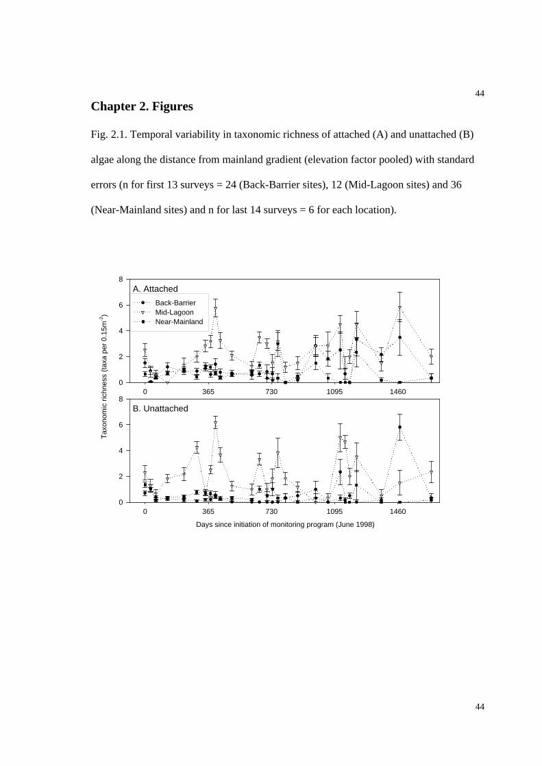
44

44

Chapter 2. Figures

Fig. 2.1. Temporal variability in taxonomic richness of attached (A) and unattached (B)

algae along the distance from mainland gradient (elevation factor pooled) with standard

errors (n for first 13 surveys = 24 (Back-Barrier sites), 12 (Mid-Lagoon sites) and 36

(Near-Mainland sites) and n for last 14 surveys = 6 for each location).

A. Attached

0 365 730 1095 1460

Tax

onom

ic r

ichn

ess

(tax

a pe

r 0.

15m

-2)

0

2

4

6

8

Back-BarrierMid-LagoonNear-Mainland

B. Unattached

0 365 730 1095 14600

2

4

6

8

Days since initiation of monitoring program (June 1998)

45

45

Fig. 2.2. Single factor effects of attachment (ATT), elevation (ELE), distance from

mainland (DIS), season (SEA) and annual changes (ANN) on taxonomic richness. With

standard errors, cf. Table 2.4 for number of replicates and corresponding single factor

ANOVA results (each factor was significant).

Attach

ed

Unattach

ed

Intertidal

Subtidal

Near-Mainland

Mid-Lagoon

Back-Barrie

r

Spring

SummerFall

WinterYear1

Year2Year3

Year4Year5

Tax

anom

ic r

ichn

ess

(0.1

5m-2

)

0.0

0.5

1.0

1.5

2.0

2.5

3.0ATT DIS ANNELE SEA

.

46

46

Fig. 2.3. Temporal variability in total assemblage biomass of attached (A) and unattached

(B) algae along the distance from mainland gradient (elevation factor pooled) with

standard errors (Cf. Fig. 2.1 for number of replicates)

A. Attached

0 365 730 1095 1460

Bio

mas

s (g

DW

m-2

)

0

100

200

300

400

B. Unattached

Days since monitoring program was initiated (June 1998)

0 365 730 1095 14600

100

200

300

400

Back-BarrierMid-LagoonNear-Mainland

47

47

Fig. 2.4. Single factor effects of attachment (ATT), elevation (ELE), distance from

mainland (DIS), season (SEA) and annual changes (ANN) on biomass of the total algal

assemblage, G. verrucosa and C. fragile. With standard errors, cf. Table 2.4 for number

of replicates and corresponding single factor ANOVA results for biomass and C. fragile

(each factor was significant for both variables).

Attach

ed

Unattach

ed

Intertidal

Subtidal

Near-Mainland

Mid-Lagoon

Back-Barrie

r

Spring

SummerFall

WinterYear1

Year2Year3

Year4Year5

Bio

mas

s (g

DW

m-2

)

0

10

20

30

40

50

60

70

Total BiomassGracilaria verrucosaCodium fragile

ATT DIS ANNELE SEA

.

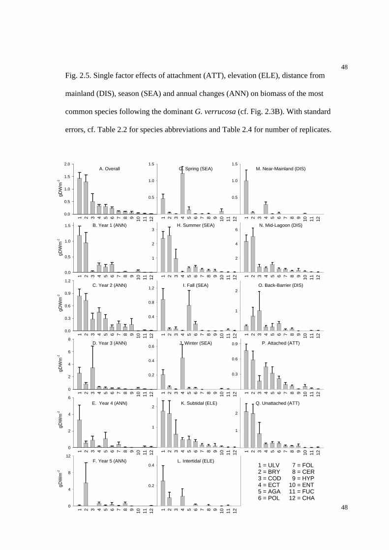
48

48

Fig. 2.5. Single factor effects of attachment (ATT), elevation (ELE), distance from

mainland (DIS), season (SEA) and annual changes (ANN) on biomass of the most

common species following the dominant G. verrucosa (cf. Fig. 2.3B). With standard

errors, cf. Table 2.2 for species abbreviations and Table 2.4 for number of replicates.

E. Year 4 (ANN)

1 2 3 4 5 6 7 8 9 10 11 12

0

2

4

6

1 2 3 4 5 6 7 8 9 10 11 12

1

2

B. Year 1 (ANN)

1 2 3 4 5 6 7 8 9 10 11 12

gDW

m-2

0.0

0.5

1.0

1.5

F. Year 5 (ANN)

1 2 3 4 5 6 7 8 9 10 11 12

0

4

8

12

D. Year 3 (ANN)

1 2 3 4 5 6 7 8 9 10 11 12

0

2

4

6

8

C. Year 2 (ANN)

1 2 3 4 5 6 7 8 9 10 11 12

0.0

0.3

0.6

0.9

1.2

A. Overall

1 2 3 4 5 6 7 8 9 10 11 12

0.0

0.5

1.0

1.5

2.0

J. Winter (SEA)

1 2 3 4 5 6 7 8 9 10 11 12

0.2

0.4

0.6

G. Spring (SEA)1 2 3 4 5 6 7 8 9 10 11 12

0.5

1.0

1.51 2 3 4 5 6 7 8 9 10 11 12

0.4

0.8

1.2

1 2 3 4 5 6 7 8 9 10 11 12

1

2

3

P. Attached (ATT)

1 2 3 4 5 6 7 8 9 10 11 12

0.3

0.6

0.9

M. Near-Mainland (DIS)

1 2 3 4 5 6 7 8 9 10 11 12

0.5

1.0

1.5

O. Back-Barrier (DIS)

1 2 3 4 5 6 7 8 9 10 11 12

1

2

N. Mid-Lagoon (DIS)

1 2 3 4 5 6 7 8 9 10 11 12

2

4

6H. Summer (SEA)

I. Fall (SEA)

gDW

m-2

gDW

m-2

gDW

m-2

gDW

m-2

gDW

m-2

K. Subtidal (ELE)

1 2 3 4 5 6 7 8 9 10 11 12

0.2

0.4L. Intertidal (ELE)

Q. Unattached (ATT)

1 2 3 4 5 6 7 8 9 10 11 12

1

2

1 = ULV2 = BRY3 = COD4 = ECT5 = AGA6 = POL

7 = FOL 8 = CER 9 = HYP10 = ENT11 = FUC12 = CHA

49

49

Chapter 3. Facilitation of Macroalgae by the

Sedimentary Tube Forming Polychaete Diopatra

cuprea

50

50

Abstract

Marine foundation organisms such as seagrasses, corals, and kelps facilitate the

distribution of numerous organisms by creating refuges from environmental stressors and

by providing food and substrate for settlement and growth. Barren soft-sediment systems

often have faunal organisms that facilitate other species by habitat modification. We

investigated how an abundant (21 m-2) tube cap forming polychaete, Diopatra cuprea,

facilitates macroalgal distribution in Hog Island Bay, a turbid shallow tidal lagoon,

Virginia, USA. 70% of the number of mudflat macroalgae were found incorporated into

protruding D. cupreas tube caps and field experiments showed that D. cuprea facilitates

algal persistence by providing a stable substrate that retains algae against hydrodynamic

forces such as tidal flushing and storm surge. If tube caps were removed, simulating

storm-induced erosion, they were rebuilt within days and new drift algae incorporated.

Also, D. cuprea facilitated the algal assemblage by fragmenting thalli in the attachment

process, thereby ensuring a constant fragment supply for vegetative re-growth if storm-

induced pruning occurs. On a species-specific level, Gracilaria verrucosa and Ulva

curvata benefited more from tube cap construction compared to Fucus vesiculosus,

Agardhiella subulata and the alien Codium fragile ssp. tomentosoides. This was partly

because G. verrucosa and U. curvata were incorporated and fragmented more readily,

and partly because they probably have physiological, morphological and biomechanical

traits that enable them to better co-exist with D. cuprea. These results suggest that

macroalgal distribution throughout Hog Island Bay to a large extent is linked to the

distribution of D. cuprea. The processes of algal attachment, retainment, recovery, re-

51

51

growth and fragmentation, can have important ecosystem implications because of the

sheer abundance of the Diopatra-Gracilaria/Ulva association.

Introduction

Coastal marine ecosystems are often defined according to a few key organisms, the most

well-known examples being kelp forests, coral reefs, and seagrass meadows (Connell et

al. 1997, Dayton 1971, Dayton et al. 1984, Heck & Wetstone 1977). These foundation

taxa provide substrate for settlement and growth, shelter from predators, an abundant

food supply, enhance propagule settlement rate, and alter the abiotic environment into

more benign conditions (Bruno & Bertness 2001). Positive interactions between

foundation and co-existing species are key processes that can drive productivity, food

web structure and nutrient flow within these habitats.

In soft-sediment communities, negative interactions such as predation and competition

have been studied in more detail than positive interactions (Lenihan & Micheli 2001).

Nevertheless, soft-bottom systems often have organisms that facilitate other species by

habitat-modifications, for example mussels beds (Albrecht 1998), oyster reefs (Barh &

Lanier 1981), and unattached drift algal mats (Norkko & Bonsdorff 1996c, Norkko et al.

2000). Also, burrowing, tube building or surface sediment casting polychaetes may

facilitate other organisms, by oxygenating sediments, providing predator refuges,

increasing larval settlement and retaining aquatic plant fragments (Eckman et al. 1981,

Fager 1964, Reise 1983). It is well documented that onuphid polychate tube builders

create such habitat modifications through their tube-forming activities (Bailey-Brock

52

52

1984, Bell & Coen 1982a, Luckenbach 1986, Pillsbury 1950). The onuphid Diopatra

cuprea (Bosc) is abundant in North American east coast lagoons from north of Cape Cod

to south of Florida (Mangum et al. 1968) where it modifies its habitat by incorporating

macroalgal fragments and bivalve shells into tube caps to provide tube structure and

strength (Brenchley 1976, Myers 1972), shelter from predators (Brenchley 1976,

Luckenbach 1984), a direct food supply (eating the algae) (Mangum et al. 1968), and/or

an indirect food supply (eating algae-associated invertebrates) (Bell & Coen 1982a). The

incorporation of algal fragments clearly benefit the polychaete and to a large extent the

associated invertebrates, but no studies have investigated if and how D. cuprea affect the

incorporated macroalgae.

We hypothesize that D. cuprea acts as a soft-bottom macroalgal facilitator by means of

tube cap incorporation, thereby physically controlling and enhancing the distribution and

abundance of macroalgae. This was investigated by testing how common D. cuprea is

within a shallow US east coast lagoon, how abundant and stable the algal-tube cap

assemblage is, how fast the association recovers after different levels of disturbance, and

if certain algal species are incorporated into tube caps more often than others. In addition

to the investigated physically based links between D. cuprea and macroalgal abundance,

nitrogen excretion by D. cuprea may also facilitate the incorporated algae, by stimulating

growth (Fong et al. 1997, Giannotti & McGlathery 2001), although this physiologically

based aspect was not considered in the present study.

Methods

53

53

Site description

We investigated if Diopatra cuprea facilitates algal communities in Hog Island Bay, a

protected shallow-water temperate soft-bottom lagoon in the Virginia Coast Reserve, and

an ecosystem under scrutiny being part of the U.S. Long Term Ecological Research

Network (Hayden et al. 2000, Swanson & Sparks 1990). Hog Island bay is located in the

Machipongo drainage basin on the Delmarva peninsula, and is approximately 100 km2

(McGlathery et al. 2001), where 30% is intertidal marshes, 7% is intertidal mudflats, and

52% is shallow mudflats to 2 m depth (Oertel 2001). There is little topographic

complexity; most of the bay is covered with sand, silt or clay, but scattered oyster reefs,

unconsolidated bivalve shells and Spartina alterniflora stems provide hard substrate for

sessile organisms. The sediment nitrogen and organic contents are higher and the bulk

density lower near the mainland compared to near-ocean sites (McGlathery et al. 2001).

Rooted angiosperms have been absent from the lagoon since the wasting disease of the

1930ties, and today unattached macroalgae are ubiquitous, with peak biomass up to 650 g

DW m-2, and being dominated by unattached mats of Gracilaria verrucosa (Hudson)

Papenfuss and Ulva curvata (Kutzing) De Toni (Humm 1979, McGlathery et al. 2001).

Because no rooted macrophytes exist to bind sediments and dampen hydrodynamic

forces, tidal currents and storms frequently re-suspend, erode and deposits sediments,

increase turbidity, and entrain and redistribute unattached algal mats (Dolan 1996, Flindt

et al. 1997a, Lawson 2003).

Ubiquity of tube caps

To test if Diopatra cuprea has the potential to facilitate algae over a lagoon-wide scale

we counted tube cap densities at 15 sites throughout the lagoon. Each site was allocated

54

54

to one of two elevation levels (lower intertidal vs. shallow subtidal) and one of three

adjacencies to the mainland (near-mainland, mid-lagoon, back-barrier island, cf. Tyler et

al (2001) for map of main sample locations). Each tube cap represents a live worm

(Mangum et al. 1968), and there is generally little seasonal fluctuation in D. cuprea

densities (Bell & Coen 1982a, Peckol & Baxter 1986). All sites were sampled

haphazardly in fall 2002, with a 0.15 m2 sampling frame (n = 6-9 per site). Densities

could not be transformed to variance homogeneity (Cochran s C: p < 0.05) and the p-

values from the 2-way ANOVA, testing effects of elevation and distance from the

mainland, should be interpreted with caution.

Ubiquity of algae incorporated to tube caps

To test if the algae-tube cap associations were ubiquitous in Hog Island Bay, we

conducted both qualitative and quantitative surveys. Qualitative observations were based

on approximately 200 field days from 1999-2002 covering all seasons, where random

tube caps were collected haphazardly and examined for attached macroalgae (n > 3000).

Quantitative observations were based on 441 macroalgal individuals sampled in the main

growing season in 2002 (April to November) at 17 mudflat sites distributed along the

previously described spatial gradients. Individuals were selected by randomly throwing

an object and collecting the nearest algae. The species were identified, and attachment

type recorded as loose-lying (= unattached), epiphytic, entangled, partly buried in

sediment, attached to a tube cap, or attached to an unconsolidated bivalve shell. X2-tests

were used to test if algae incorporated into tube caps were more common than algae with

other types of attachments, and to test for associations between attachment type and

55

55

elevation level, adjacency to mainland, and species type. Finally, to quantify incorporated

species-specific algal abundance s 92 tube caps where randomly collected in summer

2002 from an intertidal mid-lagoon mudflat where algal richness and biomass generally

are high (Shoal site, Tyler et al. 2001). The tube caps were transported to the laboratory

where the algae were removed, rinsed in fresh water, and wet weight (0.001 g)

determined after blotting with a towel. Attachment type (associated with the tube cap or

incorporated algae) and the presence of macroscopically visible reproductive tissue were

also recorded.

Stability of algae incorporated to tube caps

To test if drift algae in Hog Island Bay move with the tides on low slope intertidal and

shallow subtidal mudflats, strips of flagging tape were allocated to 18 random plots on a

mid-lagoon intertidal mudflat on 24 June 2002 (n = 6 strips per plot, at 0.65 m below

MSL, Shoal-site) (McGlathery et al. 2001). Flagging tape was used partly because the

slightly negatively buoyant and flat structure mimic small Ulva curvata fragment, partly

because the strips were easily detected on the extensive mudflat often covered with

patches of drift algae. None of the 108 strips were found the following day, despite an

intense search-effort. To test if the algae-tube cap association was more stable than

unattached algae (as exemplified by the stability of the flagging strips) and whatever

stability differed between the two most common algae eight Gracilaria verrucosa and U.

curvata, and their host tube caps were double-tagged on 24 June 2002 and tag-survival

recorded nine times during a 46 day period. Double tags were used to ensure that tag loss

was caused by algal or tube cap removal and not loss of tags. To test for the generality of

56

56

the results, the experiment was repeated on 4 October where survival was recorded 6

times over a 44 day period. It is unlikely that the tags (5 cm flagging tape) influence algal

survival because the tag provides minimal drag compared to the algal thallus. The

percentage remaining tags were calculated on each sampling date for each species and

experiment, and linear regression was used to calculate and compare decay-slopes

(percent algae remaining per day).

Recovery of algae incorporated to tube caps

To estimate the recovery ability of the algae-tube cap association, removal experiments

where conducted simulating different degrees of disturbance. Randomly allocated 0.1 m2

squared plots were manipulated using different combinations of disturbance intensities

and frequencies, and the recovery of tube caps and algal biomass were compared to

control plots. A low-intensity treatment was achieved by removing incorporated algae

(simulating hydrodynamic induced dislodgment) and a high-intensity treatment by

removing tube caps (simulating severe sediment erosion or deposition). In the summer

experiment the two intensities were applied on the 24 and/or 28 of June 2002 (Exp. 1:

0.65 m below MSL, mid-lagoon site, n = 4). The following five treatment-combinations

were applied (arranged from high to low severity): 1) tube caps removed on 24 and 28, 2)

algae removed on 24 and tube caps on 28, 3) tube caps removed on 28, 4) tube caps

removed on 24, and 5) algae removed on 28. On 4 July, i.e. after 10 and/or 6 days of

recovery, re-generated tube caps and incorporated algae were collected, brought to the

laboratory, the number of tube caps counted, the algae identified, and wet weight (0.001

g) determined after blotting with a towel. To investigate if the findings were robust a

57

57

second removal experiment was conducted in November 2002 (Exp. 2, near the

mainland, same elevation level). To increase the ability to detect disturbance effects (see

result section) the number of replicates were doubled (n = 8), but the applied treatments

reduced to only include: 1) Tube caps removed on 7, 2) tube caps removed on 4, and 3)

algae removed on 4. The treatments were compared to control plots on November 12, i.e.

after 8 and 5 days of recovery. Because the two experiments differed in number of

replicates and treatments and were conducted at different sites and seasons, they were

analyzed independently. To test for disturbance effects ANOVAs were conduced on

densities of re-generated tube caps and biomass of Gracilaria verrucosa, Ulva curvata

and the total algal assemblage, followed by SNK-post hoc test to separate different

treatments (Underwood 1981b). To reduce the problem of low test power (few replicates)

in the summer experiment, an additional set of ANOVAs were conducted with the three

high disturbance treatments pooled and tested against the two low treatments pooled

together with the control plots, corresponding to a test of High vs. Low disturbancve

levels (= Exp. 1b, Fig. 3.3). Some response variables were Log-transformed to ensure

variance homogeneity (Cochran s C > 0.05, Table 3.4). It should finally be noted that at

the termination of the two experiments all plots were also searched for unattached algae,

but none were found.

Preference of algae incorporated to tube caps

Finally, to test if some algae are preferred over others an in situ preference experiment

was conducted. The six most conspicuous macroalgae to be found year round in Hog

Island Bay were included (arranged after increasing S:V ratio, Chapter 4): Codium fragile

58

58

ssp. tomentosoides (Suringar) Hariot, Fucus vesiculosus Linnaeus, Agardhiella subulata

(C. Agardh) Kraft et Wynne (Solieria tenera in Humm, 1979), Gracilaria foliifera

(Forsskal) Børgensen, G. verrucosa, and Ulva curvata. A 30 cm round PVC cage was

inserted vertically 20 cm into the sediment around a haphazardly selected tube cap at a

near-mainland site. The tube cap-algae association was removed to force Diopatra

cuprea to build a new cap. Fresh algal fragments were added to cages in November 2002

either as single-species (3 fragments per cage) or multiple-species treatment (1 fragment

per cage, cf. Fig. 3.4a for specific biomass ), and cages were capped with 2 mm screening

mesh. After two days of incubation tube caps with incorporated algae and unattached

algae were collected, and the total and attached number of fragments were counted to

calculate percent attachment and percent fragmentation . Autogenic fragmentation (i.e.

without D. cuprea influence) was not measured because pilot experiments had revealed

that healthy tissue of the six species rarely fragmented in caged experiments with only

two days of incubation. Because some cages were lost due to storms, vandalism and

heavy sedimentation, the final sampling design was uneven (n = 4-11, cf. Fig. 3.4). These

response variables were tested with a 2-factorial ANOVA (species and addition type),

followed by SNK-tests to indicate different groupings. It should be noted that because

fragmentation could not be transformed to variance homogeneity, because species

responses potentially are non-independent in the multi-species cages, and because F.

vesiculosus and G. foliifera had fewer replicates that the other species, the p-values may

be biased and should be interpreted with caution.

Results

59

59

Ubiquity of tube caps

The overall tube cap density was 21 m-2, and there was a significant interaction between

densities found along the mainland-ocean and elevation gradients (Table 3.1). Highest

densities were found at intertidal mainland sites and at subtidal mid-lagoon sites with

typical mean densities of 35-40 caps m-2 and with maximum densities up to 180 caps m-2

(Fig. 3.1).

Ubiquity of algae incorporated to tube caps

Of the >3000 tube caps that were examined qualitatively in the field more than 90% had

algal fragments attached. The size range of fragments varied from pieces smaller than 1

cm, to 60 cm long Ulva curvata and 50 cm Gracilaria verrucosa. Algae were more often

encountered on tube caps than any other attachment type. The species observed on the

tube caps were G. verrucosa, and U. curvata (ubiquitous), Agardhiella subulata, Fucus

vesiculosus, G. foliifera, and Enteromorpha linza (up to 10 observations), and Codium

fragile, Punctaria latifolia Greville and Grinnellia americana (C. Agardh) Harvey (1

observation each). Approximately 10 attached carposporophytic G. verrucosa were also

observed. The quantitative observations showed that significantly more algae were found

attached to tube caps (70%, X26 = 927.2, Df = 5, p < 0.001, Table 3.2) than any other

attachment type. Also, the proportions of tube cap-attached algae varied with distance

from the mainland (smallest proportion attached at mid-lagoon sites, X26,3 = 46.4, Df =

10, p < 0.001) but not with elevation (X26,2 = 12.5, Df = 5, p = 0.028), and G. verrucosa

were found in significantly higher proportions than U. curvata (64 vs. 34%, X26,2 = 27.2,

Df = 1, p < 0.001). Other species found on tube caps (A. subulata, G. foliifera and F.

vesiculosus) were found in less than 1% of the cases, and were omitted from tests. All of

60

60

the 92 collected tube caps had incorporated algal fragments, with an average of 8.9 gWW

and a taxonomic richness of 2.7 per tube cap (Table 3.3). G. verrucosa was found

attached to 90 tube caps, three of them with cystocarps, accounting for 94% of the total

biomass, and 33 had U. curvata incorporated, corresponding to 2.4% of the total biomass.

Three tube caps had more than 50 gWW and 11 more than 20 gWW. Very few species

were found incorporated, and some taxa (e.g. Ceramium sp, Polysiphonia sp., Hypnea

musciformis (Wulfen) Lamouroux, Champia parvula (C. Agardh) Harvey), were only

recorded as epiphytic or entangled/secondarily attached on G. verrucosa (Norton &

Mathieson 1983, Perrone & Cecere 1997), thereby adding 1-2 taxa to the total tube cap

richness.

Stability of algae incorporated to tube caps

All loose-lying flagging tape strings were lost from the mudflat in less than 24 hours, i.e.

in less than two complete tidal cycles. This correspond well to our general observations,

with unattached algae on open tidal flats typically being mobile and probably only

accumulating under specific hydrodynamic, topographic, biological and meteorological

conditions. In the tagging experiments some tube caps were apparently lost, but

subsequently digging into the sediment revealed that the tags were buried under a few cm

of sediments. Thus, no tube caps were lost in any of the experiments, markedly different

for the incorporated algal fragments that was physically removed from tube caps within

days to month (Fig. 3.2). In both tagging experiments, incorporated Ulva curvata were

removed faster than Gracilaria verrucosa (7.0% and 21.1% d-1 vs. 2.2% and 2.0% d-1, r2

> 0.93, p < 0.05, for all slope coefficients). Using the mean slope coefficients from the

61

61

two experiments for each species, 50% survival periods were calculated to respectively 4

and 24 days. It was also observed that after tagged algae were lost from the tube caps,

small fragments (1-2 cm) remained incorporated, suggesting that re-growth is possible.

Recovery of algae incorporated to tube caps

All response variables (tube cap densities and biomass of Gracilaria verrucosa and Ulva

curvata) showed significant effects to different levels of disturbances (except one near-

significant effect, Table 3.4). However, the unplanned multiple SNK-comparisons could

only distinguish significant different subgroups for the weakest disturbance treatment

for U. curva in Exp. 1 (Fig. 3.3C), and for the controls of G. verrucosa (Fig. 3.3B) and U.

curvata in Exp. 2 (Fig. 3.3C). Thus, the relatively few replicates in the summer

experiment made it difficult to statistically separate groups, although graphical inspection

indicated a tendency for highest abundance s at the low disturbance plots, a pattern

especially clear for total algal biomass (Fig. 3.3D). Domination reversal was observed in

the algae removed on 24 treatment, that had less G. verrucosa incorporated compared to

the other plots with low levels of disturbances (the control and caps removed on 24

treatment, Fig. 3.3B). However, this deficiency was compensated for by incorporation of

U. curvata (Fig. 3.3C), resulting in near-identical total biomass (Fig. 3.3D). The

tendencies noted in Exp. 1 were verified statistically when the three lowest disturbance

levels plots were pooled and compared to the three highest levels (Exp. 1b, Fig. 3.3,

Table 3.4E-H). Here the abundance s of tube caps, G. verrucosa, U. curvata and total

incorporated algal biomass were significantly less in high-disturbance plots, suggesting

62

62

general algal facilitation on the 0.1 m2 plot-scale (most algal biomass in plots with

highest tube cap densities).

In the second experiment, the SNK-tests did not detect significant subgroups for either

tube cap densities (Fig. 3.3A) or total algal biomass (Fig. 3.3D), despite significant

ANOVAs (Table 3.4I, L), indicating a full recovery in less than 5 days. However,

splicing the total algal assemblage data into species-specific abundance s demonstrated

significant SNK-group effects on both U. curvata and G. verrucosa (Table 3.4, Fig. 3.3B,

C), and a marked shift was observed from G. verrucosa to U. curvata domination after all

of the three disturbance treatments. The control plots were characterized by high G.

verrucosa (ca. 130 gWW m-2) and low U. curvata (ca. 20 gWW m-2) biomass relatively

similar to the controls from Exp.1. However, in the fall experiment, the disturbed plots

changed into high U. curvata (ca. 150 gWW m-2) and low G. verrucosa associations (ca.

20 gWW m-2) similar to the aforementioned algae removed on 24 treatment.

Preference of algae incorporated to tube caps

In the test of effects on algal incorporation rates (= attachment), there was a significant

interaction between species and addition type, and a highly significant species effect

(Table 3.5, Fig. 3.4B). However, because the interaction effect only explained 7% of the

sum of squares compared to 49% for the species factor, the latter clearly was most

important. The SNK-test grouped the three species with lowest S:V ratios into a distinct

low-incorporation group (Codium fragile = 17%, Fucus vesiculosus = 18%, Agardhiella

subulata = 28%) compared to the species with highest S:V ratio (Gracilaria foliifera =

63

63

68%, G. verrucosa = 54%, Ulva curvata = 75%). There were no significant interaction

term for fragmentation, but two significant single factor effects (Table 3.5, Fig. 3.4C).

Again the species factor explained far more of the data variability compared to the

addition type factor and the latter could be ignored for practical purposes. The SNK-test

again grouped the three species with S:V ratios into a distinct low-fragmentation group

(C. fragile = 0%, F. vesiculosus = 0%, A. subulata = 14%), but the species with highest

S:V ratio were here spliced into two high-effect groups (U. curvata = 50% and G.

foliifera = 56% vs. G. verrucosa = 109%). Note that fragmentation could exceed 100% if

a tissue was fragmented more than once.

Discussion

Habitat modifiers typically facilitate other species by providing shelter from predation, by

reducing physical and physiological stress, by enhancing propagule supply and retention,

and by increasing food supply (Bruno & Bertness 2001). We argue that Diopatra cuprea

specifically facilitates macroalgal assemblages in North American soft-bottom shallow

lagoons by a) creating and maintaining attachment sites, b) increasing algal residence

time on mudflats compared to unattached algae and c) enhancing and retaining a supply

of small vegetative fragments. These mechanisms are important in soft-substrate

environment, where substrate for algal attachment is scarce, where hydrodynamic forces

often transport unattached algae up high on the beach or deep into the aphotic zone, and

where sexual reproduction in the drift algae population may be non-existing (Cecere et al.

1992, Norton & Mathieson 1983). These specific facilitation mechanisms were not

described for polychaete worms in the review by Bruno & Bertness (Bruno & Bertness

64

64

2001). It is likely that summer growth and productivity also is enhanced by D. cuprea, by

excretion of nitrogenous rich waste products (Fong et al. 1997, Giannotti & McGlathery

2001), although this hypothesis were not tested in our study.

The more abundant and ubiquitous a habitat modifier is the more likely it is that

facilitation is important on a large scale. Our first survey demonstrated that D. cuprea

exists in both subtidal and intertidal environments and from mainland to near-ocean sites

in Hog Island Bay, and occasionally with very high densities, suggesting that D. cuprea

has the potential to facilitate macroalgae throughout the lagoon. The mean of 21 D.

cuprea m-2, is similar to high density plots in Massachusetts lagoons, and our high

density areas (up to 180 D. cuprea m-2) were similar to previously recorded maximum

values from Delmarva peninsula back-barrier island lagoons (50-300 tube caps m-2)

(Mangum et al. 1968, Peckol & Baxter 1986). The distance from the mainland and the

elevation gradients represent predictable co-varying differences in water clarity, salinity,

suspended solids, nutrient concentrations, sediment organic content, and sediment texture

(McGlathery et al. 2001) and desiccation, light, temperature fluctuations, sedimentation,

and predation pressure. The widespread distribution suggests that D. cuprea is stress-

tolerant species with broad habitat requirements, clearly important if facilitation is to

have a large-scale impact. Kim (1992) found a significant spatial interaction for subtidal

D. ornata populations in California between exposure levels and small-scale spatial

patterns, and Mangum et al. (Mangum et al. 1968) suggested that D. cuprea densities

were positively correlated to current velocities and latitude, but not with substrate particle

size. It is today unknown what factors control site-specific distribution patterns of D.

65

65

cuprea, probably because co-variation between ecological factors and spatial gradients

makes it difficult to relate single causes to distribution patterns.

It is well documented that macroalgae have created new habitats in numerous otherwise

barren soft sediment systems, with specific associated species, food web structure,

diversity and altered biogeochemical cycling (Everett 1994, Holmquist 1994, Norkko &

Bonsdorff 1996a, Norkko et al. 2000, Raffaelli et al. 1998). In this context, the

incorporated algae are proximate habitat modifiers whereas D. cuprea is the ultimate

modifier, and the algae have an important ecosystem influence in the presence of D.

cuprea. However, different species may have different effects on local environmental

conditions, and hence it is of interest to know if certain species are more commonly

incorporated than others. Our results clearly show that out of a taxonomic pool of ca. 20-

40 species (Connor 1980, Rhodes 1970) only two were found incorporated in abundance,

and only a few other taxa were found very rarely. It was generally difficult to find tube

caps in Hog Island Bay that did not contain fragments of either G. verrucosa or U.

lactuca, an observation that was supported by each of the three surveys and the recovery

experiment. Although the potential importance of algae attached to D. cuprea has been

acknowledged several times (Bell & Coen 1982a, Brenchley 1976, Pillsbury 1950) only

Mangum et al. (1968) provided a species list, describing 16 taxa pooled from several sites

in Virginia. Most of these taxa were also found in the present study (Ulva, Gracilaria,

Agardhiella, Enteromorpha, Ceramium, Polysiphonia, Bryopsis). However, based on our

data we suspect that the filamentous genera mainly were found as epiphytes on

Gracilaria. It is interesting that older D. cuprea-studies from mid-Atlantic barrier island

66

66

localities (Brenchley 1976, Mangum et al. 1968, Woodin 1978, 1981) either did not

describe incorporated algae, or only described attached species qualitatively, indicating

much lower algal abundance in the 1960-70s. Due to the absence of published rigorous

quantitative macroalgal surveys from this region we can only speculate on such temporal

differences, but it is likely that the region has experienced intense coastal eutrophication

in the last 30 years, similar to lagoonal systems worldwide (Fletcher 1996, Goshorn et al.

2001, Raffaelli et al. 1998), resulting in high algal biomass increases and today

supporting the abundant algal assemblages in conjunction with D. cuprea.

The tagging experiment demonstrated that algal residence time on the mudflats, was

enhanced by association with D. cuprea, and that Gracilaria verrucosa is slightly favored

over Ulva curvata because of lower decay slope coefficients. We suggest that G.

verrucosa and U. curvata biomass loss was caused by peak tidal currents or storm-

induced waves forces (Bell 1999). Grazing is an alternative loss process, but is unlikely

to be important because Hog Island Bay have few grazers capable of consuming entire

thalli (pers. obs.). However, it is likely that the interaction between mesograzer wounding

and hydrodynamic forces increase the likelihood of biomass removal, especially for U.

curvata, that rarely were observed with intact thalli (Denny et al. 1989, Duggins et al.

2001, Padilla 1993). The calculated 50% survival time periods are constrained by site-

and time-specific effects of the lunar cycle, wind patterns, bathymetry, and fetch

(Thomas 1986), and we suspect that the incorporated algae have higher meta-population

stability on large scales especially if dislodged biomass is re-captured and re-attached

downstream of the disturbed site. It should be noted that the reported removal rates only

67

67

reflected main thallus loss, and that small fragments remained on tube caps, making re-

growth possible independently on the supply of drift algae.

The third aspect of algal facilitation is the rapid regeneration of the algae-tube cap

association, within a few days to weeks of disturbance. This is consistent with the

observation by Meyers (1972) that tube caps can be rebuilt within 48 hours. We observed

that repeated removal of tube caps did affect the abundance of macroalgae within the

time scale of 5-10 days, and that disturbances can trigger species-specific dominance

reversal (from G. verrucosa to U. curvata). Thus, because a high local supply of drift U.

curvata was observed at the time of the manipulations at the fall recovery experiment,

this species became the all-dominant taxa after disturbances. This suggests that D. cuprea

uses the available drift algae, and emphasize that the timing of disturbance (Petraitis &

Latham 1999, Sousa 1984) combined with the drift algal supply can change the

composition of the macroalgal assemblages overnight. It is likely that these effects would

be less prominent if the disturbances occur in late winter partly because less algae are

present and partly because the ability of D. cuprea to maintain its tube cap ceases below

2 C (Myers 1972). Also, the observation from the summer experiment that significantly

less algae were found in the highly disturbed plots (with fewer tube-caps), lend strong

support to our general hypothesis that D. cuprea facilitate algal distribution and

abundance, at least on the small spatial scale manipulated in the present study. However,

future studies should repeat these experiments on larger spatio-temporal scales to enable

stronger inferences about lagoon wide facilitation effects.

68

68

The preference experiment specifically tested for control mechanisms on the algal

assemblage structure. Even when added in less biomass, G. verrucosa, G. foliifera and U.

curvata were still preferred as building material over Agardhiella subulata, Codium

fragile and Fucus vesiculosus. This is different to findings by Brenchley (1976) who

reported that D. cuprea did not select, but used Ulva and bivalve shells according to

abundance. The pattern suggests that the S:V ratio is an important property for successful

incorporation, although it is likely that other species-specific properties (e.g. morphology,

chemistry, structure, biomechanics) also influence the attachment process. Fragmentation

was also positively related to the S:V ratio. Fragmentation is probably an important

process in maintaining algae on tube caps, because larger thalli were only stable on the

day-month time-scale. The low drag on the fragmented small thalli have a low risk of

dislodgment compared to larger incorporated thalli (Gaylord et al. 1994) and the small

fragments provides a biomass supply for regrowth if hydrodynamic forces removes larger

thalli. D. cuprea is therefore not fully dependent on locating new drift algae to replace

what currents and waves remove, although re-growth of small fragments primarily should

be important at sites and seasons with low and unpredictable drift algae supply.

In conclusion, our data suggest that D. cuprea affect the distribution, abundance and

stability of macroalgae in shallow soft-bottom systems along the North American east

coast, although studies from more localities are needed to verify this. Because of high

attachment, fragmentation, stability, and recovery rates the incorporated algae are

abundant in areas where they would otherwise be flushed. We also suggest that G.

verrucosa and U. curvata dominate tube caps in Hog Island Bay because 1) they are

69

69

selectively incorporated, 2) they are already present as building material in large

quantities, 3) they have structure, size, morphology and buoyancy properties that allows

D. cuprea to encounter, capture, fragment and incorporate them into a relatively strong

attachment, 4) they have high intrinsic growth rates, and 5) they are stress-tolerant

species that can survive sediment burial, fragmentation and desiccation. On the other

hand, the few other conspicuous perennial algae in Hog Island Bay are not dominants

probably because they lack above properties. For example, the alien invasive C. fragile

spread to in Virginia in the 1970s (Chapman 1999, Hillson 1976, Trowbridge 1998), is

today the fourth most common species in Hog Island Bay (Chapter 2) and is potentially

still expanding its distribution. Because C. fragile does not fulfill the listed properties

(unpublished data) we predict that it will not become a lagoon-wide dominant species

under the current ambient conditions. However, if eelgrass re-colonize Hog Island Bay, a

process observed in several nearby bays, a state change may occur with reduced water

turbidity and increased sediment stability (Hayden et al. 2000, Lawson 2003), potentially

altering D. cuprea recruitment, feeding success and survival, and thereby ultimately also

affecting the relative competitiveness of G. verrucosa, U. curvata, C. fragile and other

macroalgae.

70

70

Chapter 3. Tables

Table 3.1. ANOVA of tube cap densities. Significant results (p < 0.05) are shown in bold.

15 sites were sampled (n = 6-9 sample frames/site). Each site classified into 1 of 3

distances (near-mainland, mid-lagoon, near-ocean) and 1 of 2 elevation levels (shallow

subtidal, intertidal). Densities could not be transformed to variance homogeneity (Levines

test, p > 0.05).

Source Df SS 2(%) F pDistance 2 3232 4 2.44 0.097Elevation 1 69 0 0.10 0.748Distance * Elevation 2 8608 11 6.49 0.002Error 100 66280 85

71

71

Table 3.2. Abundance (in counts) of different A: attachment types and B: species

incorporated onto tube caps.

A: Attachment typeGradient Tub Loo Bur Epi Ent SheNear-mainland 116 12 1 1 1 1Mid-lagoon 127 29 14 8 3 39Near-ocean 66 4 4 4 1 10Intertidal 149 24 11 1 1 28Subtidal 160 21 8 12 4 22Total 309 45 19 13 5 50

B: SpeciesGradient Gra Ulv Aga Fol FucNear-mainland 73 43 0 0 0Mid-lagoon 89 36 1 0 1Near-ocean 36 28 0 1 1Intertidal 99 49 0 0 1Subtidal 99 58 1 1 1Total 198 107 1 1 2Tub = tube cap, Loo = looselying, Bur = Buried, Epi = Epiphytic, Ent = Entangled, She = Shell, Gra =Gracilaria verrucosa, Ulv = Ulva curvata, Aga = Agardhiella subulata, Fol = Gracilaria foliifera, Fuc =Fucus vesiculosus

72

72

Table 3.3. Mean biomass and variance per tube cap (gWW), relative abundance (%),

frequency of occurrence (counts) and attachment types of algae incorporated into tube

caps (n = 92).

Taxa Mean Variance % Counts AttachmentaRichness 2.674 1.849 92Biomass 8.911 137.720 92Gracilaria verrucosa 8.384 125.275 94.08 90 TubUlva lactura 0.215 0.909 2.42 33 TubCeramium rubrum 0.109 0.217 1.23 23 EpiHypnea musciformis 0.089 0.113 1.00 15 EpibBulgula turrita 0.050 0.115 0.56 18 EpiChampia parvula 0.019 0.016 0.21 10 EpiAgardhiella subulata 0.016 0.012 0.18 2 TubPolysiphonia sp. 0.011 0.011 0.13 3 EpicG. verrucosa carp. 0.008 0.003 0.09 3 TubCeramium strictum 0.002 0.000 0.02 2 EpiFucus vesiculosus 0.001 0.000 0.01 1 TubEnteromorpha linza 0.001 0.000 0.01 3 EpiaIn number of taxa per tube cap. bA bryozoa. cCaroposporophytic life stage, potentially with viablepropagules. Tub = tube cap; Epi = Epiphytic (entangled; hooked, primary attached, re-attached).

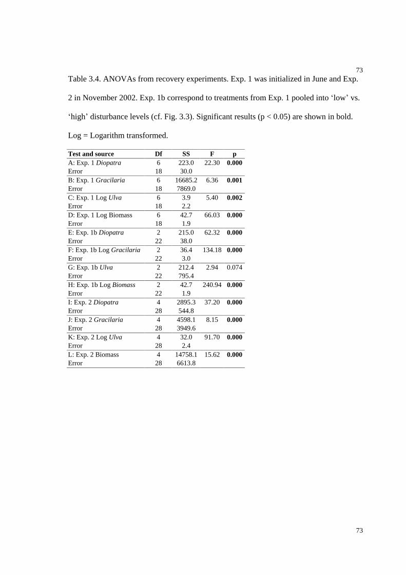
73

73

Table 3.4. ANOVAs from recovery experiments. Exp. 1 was initialized in June and Exp.

2 in November 2002. Exp. 1b correspond to treatments from Exp. 1 pooled into low vs.

high disturbance levels (cf. Fig. 3.3). Significant results (p < 0.05) are shown in bold.

Log = Logarithm transformed.

Test and source Df SS F pA: Exp. 1 Diopatra 6 223.0 22.30 0.000Error 18 30.0B: Exp. 1 Gracilaria 6 16685.2 6.36 0.001Error 18 7869.0C: Exp. 1 Log Ulva 6 3.9 5.40 0.002Error 18 2.2D: Exp. 1 Log Biomass 6 42.7 66.03 0.000Error 18 1.9E: Exp. 1b Diopatra 2 215.0 62.32 0.000Error 22 38.0F: Exp. 1b Log Gracilaria 2 36.4 134.18 0.000Error 22 3.0G: Exp. 1b Ulva 2 212.4 2.94 0.074Error 22 795.4H: Exp. 1b Log Biomass 2 42.7 240.94 0.000Error 22 1.9I: Exp. 2 Diopatra 4 2895.3 37.20 0.000Error 28 544.8J: Exp. 2 Gracilaria 4 4598.1 8.15 0.000Error 28 3949.6K: Exp. 2 Log Ulva 4 32.0 91.70 0.000Error 28 2.4L: Exp. 2 Biomass 4 14758.1 15.62 0.000Error 28 6613.8

74

74

Table 3.5. ANOVAs from preference experiment: Percent attachment and percent

fragmentation. Addition correspond to the addition type, with fragments being added as

single or multiple species to caged Diopatra cuprea. Significant results (p < 0.05) are

shown in bold. The fragmentation data could not be transformed to variance homogeneity

(Levines test, p > 0.05).

Attachment FragmentationSource Df SS 2(%) F p SS 2(%) F pSpecies 5 176299 49 20.26 0.000 161091 42 15.16 0.000Addition 1 4592 1 2.64 0.108 11372 3 5.35 0.023Species * Addition 5 23346 7 2.68 0.026 20004 5 1.88 0.105Error 89 154901 43 189156 50

75

75

Chapter 3. Figures

Fig. 3.1. Ubiquity of tube caps in Hog Island Bay: Diopatra cuprea densities along the

mainland-ocean and elevations gradients. With SE, n from left = 18, 18, 21, 16, 10, 23.

Mainland Lagoon Ocean

Den

sitie

s (m

-2)

0

10

20

30

40

50

60

SubtidalIntertidal

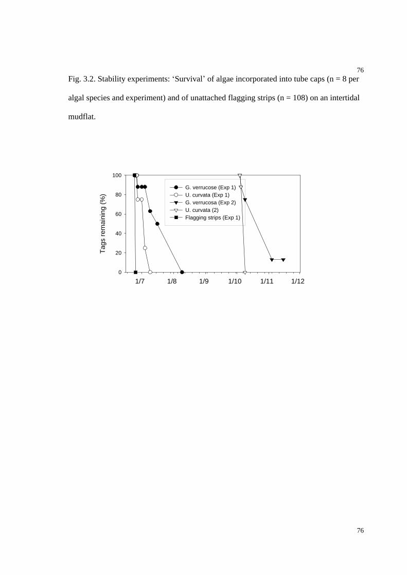
76

76

Fig. 3.2. Stability experiments: Survival of algae incorporated into tube caps (n = 8 per

algal species and experiment) and of unattached flagging strips (n = 108) on an intertidal

mudflat.

1/7 1/8 1/9 1/10 1/11 1/12

Tag

s re

mai

ning

(%

)

0

20

40

60

80

100

G. verrucose (Exp 1)U. curvata (Exp 1)G. verrucosa (Exp 2)U. curvata (2)Flagging strips (Exp 1)

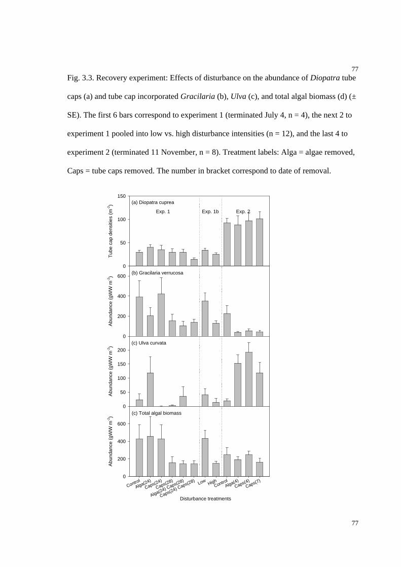
77

77

Fig. 3.3. Recovery experiment: Effects of disturbance on the abundance of Diopatra tube

caps (a) and tube cap incorporated Gracilaria (b), Ulva (c), and total algal biomass (d) (±

SE). The first 6 bars correspond to experiment 1 (terminated July 4, n = 4), the next 2 to

experiment 1 pooled into low vs. high disturbance intensities (n = 12), and the last 4 to

experiment 2 (terminated 11 November, n = 8). Treatment labels: Alga = algae removed,

Caps = tube caps removed. The number in bracket correspond to date of removal.

(a) Diopatra cuprea

1 2 3 4 5 6 7 8 9 10 11 12

Tub

e ca

p de

nsiti

es (

m-2

)

0

50

100

150

(b) Gracilaria verrucosa

1 2 3 4 5 6 7 8 9 10 11 12

Abu

ndan

ce (

gWW

m-2

)

0

200

400

600

(c) Ulva curvata

1 2 3 4 5 6 7 8 9 10 11 12

Abu

ndan

ce (

gWW

m-2

)

0

50

100

150

200

(c) Total algal biomass

Control

Alga(24)

Caps(24)

Caps(28)

Alga(24) Caps(28)

Caps(24) Caps(28)Low High

ControlAlga(4)

Caps(4)Caps(7)

Abu

ndan

ce (

gWW

m-2

)

0

200

400

600

Exp. 1 Exp. 2Exp. 1b

Disturbance treatments

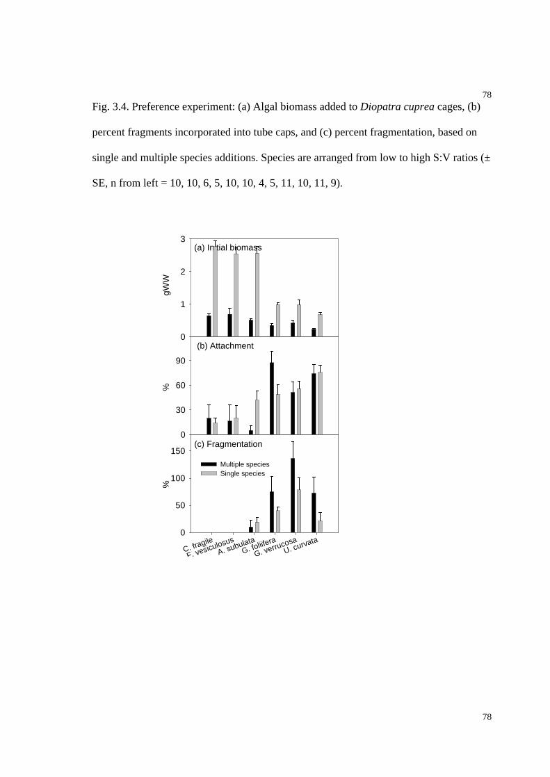
78

78

Fig. 3.4. Preference experiment: (a) Algal biomass added to Diopatra cuprea cages, (b)

percent fragments incorporated into tube caps, and (c) percent fragmentation, based on

single and multiple species additions. Species are arranged from low to high S:V ratios (±

SE, n from left = 10, 10, 6, 5, 10, 10, 4, 5, 11, 10, 11, 9).

(a) Initial biomass

gWW

0

1

2

3

(b) Attachment

%

0

30

60

90

(c) Fragmentation

C. fragile

F. vesiculosus

A. subulataG. foliifera

G. verrucosaU. curvata

%

0

50

100

150

Multiple speciesSingle species

79

79

Chapter 4. Species type, thallus size and substrate

condition determine macroalgal break forces,

break velocities and break places in a western

mid-Atlantic low energy soft bottom lagoon

80

80

Abstract

Wave-induced dislodgment of attached sessile marine macroalgae is an important

structuring force influencing population and community dynamics in high energy

habitats. However, little is known about whether hydrodynamic forces limit algal size and

distribution patterns in low energy soft bottom systems. Biomechanical pull-tests were

used to determine relationships between break force, break velocity and break place for 6

algal species collected from a shallow temperate lagoon (Hog Island Bay, Virginia),

attached to 2 types of substrates, and divided into 2 size classes. Ulva curvata,

Agardhiella subulata, Gracilaria verrucosa, small thalli and algae attached to polychatae

tube caps (Diopatra cuprea) had break forces between 0.3 and 6 N, whereas large Fucus

vesiculosus, Codium fragile ssp. tomentosoides, and G. foliifera attached to bivalve shells

had break forces between 6 and 12 N. From break forces and thallus sizes, break

velocities were calculated to range from 1-2 ms-1 for relatively large thalli on tube caps

and 6-10 ms-1 for small thalli on shells. Because velocities often reach 1 ms-1 during

hydrodynamic peak events in tidal soft bottom systems, thallus breakage is probably

common, limiting algal size, particularly for U. curvata and for algae incorporated into

tube-caps. It is suggested that entanglement by drift algal clumps, and entrainment of

algae attached to unconsolidated shells should be incorporated into future biomechanical

studies, to better understand algal breakage and mobility in shallow low energy soft

bottom habitats.

Introduction

Survival of sessile marine organism against hydrodynamic forces

81

81

Survival is a fundamental process which marine macroalgae must accomplish before

resources can be directed to growth, reproduction and dispersal. It is thus an important

task for ecologists to understand survival mechanisms, especially under extreme

environmental conditions where fatalities can be high. In marine open rocky coastal

habitats 5-10 meter high storm waves can create external forces on sessile macroalgae

that are higher than for any other habitats, with water velocities exceeding 15 ms-1 and

accelerations of more than 400 ms-2 (Gaines & Denny 1993, Koehl 1984, 1986, Norton

1991). Exposure to such forces is a major cause of mortality (Colman 1933, Denny 1995,

Denny 1987, Jones & Demetropoulus 1968, Lewis 1964, Norton 1991). In contrast, soft

bottom shallow lagoons are only exposed to small waves because terrestrial structures

and shallow depths reduce wave development. In these systems, tidal currents are often

the dominant hydrodynamic force, imposing skin and form drag on sessile organisms.

Hence acceleration forces can be neglected, and velocities rarely exceeds 1 ms-1

(Albrecht 1998, Hawes & Smith 1995, Lawson 2003, Oertel 2001).

Biomechanical models

Biomechanical models have been proposed as tools to understand and predict survival

from a hydrodynamic perspective (1995, Denny 1999, Denny et al. 1989, Gaylord et al.

1994, Gaylord & Denny 1997). Here, the break force of sessile organisms is measured

using pull tests (Dudgeon & Johnson 1992, Hawes & Smith 1995), and compared to the

ambient hydrodynamic forces and the forces experienced by the organism. This break

force is an important component of the drag equation and is used to calculate a

corresponding break velocity (Bell 1999, Denny 1995, Shaughnessy et al. 1996). Break

82

82

velocities are then interpreted as measures of gap-creation and susceptibility to mortality

(Bell 1999, Blanchette 1997, Denny 1995, Gaylord et al. 1994). Break forces are mainly

known for macroalgal species within the Fucales (Blanchette 1997, Haring et al. 2002,

Norton 1986), Gigartinales (Bell 1999, Carrington 1990, Shaughnessy et al. 1996) and

Laminarales (Blanchette et al. 2002, Milligan & DeWreede 2000, Utter & Denny 1996),

and are practically unknown for species from other taxonomic orders (Thomsen &

Wernberg submitted). Two of the most important factors that determine macroalgal break

forces are substrate type (Barnes & Topinka 1969, Milligan & DeWreede 2000, van

Tamelen & Stekoll 1996) and algal size (Gaylord et al. 1994, Shaughnessy et al. 1996),

where large individuals attached to hard substrates usually have higher break forces than

small individuals on soft substrates (Thomsen & Wernberg submitted). These

biomechanical finding are based on studies from high energy rocky coastlines; little is

known about if algal species, thallus size or substrate condition influence break forces

and break velocities in low energy soft bottom habitats, typically dominated by

macroalgae, being unattached or attached to bivalve shells (Anderson & Underwood

1997, Connor 1980, Cowper 1978, Havens et al. 2001, Hawes & Smith 1995, Norton &

Mathieson 1983). However, Hawes and Smith (1995), in the only macroalgal

biomechanical study from a temperate soft bottom lagoon, calculated that tidal forces can

set an upper limit to the size of the opportunistic green algae Ulva lactuca. Because of the

paucity of biomechanical studies from soft bottom tidal lagoons, the primary objective

was to test if species, substrate type or algal thallus size affects break forces.

Furthermore, to explore if breakage is a likely process, a second objective was to estimate

break velocities and compare these to typical lagoon velocities. Finally, because algae do

83

83

not always break at the holdfast-substrate junction under peak hydrodynamic events

(complete biomass removal = dislodgment), but sometimes break above the holdfast-

substrate junction (partial biomass removal = pruning) and thereby increase the chance of

recovery (Blanchette 1997, Dudgeon et al. 1999, Scrosati 1998, Shaughnessy et al. 1996),

the last objective was to investigate if the break place was on the substrate, holdfast, stipe

or frond.

Methods

Species and substrate types

Descriptions of the study site (Hog Island Bay), macroalgal species assemblages,

distribution patterns, taxonomic considerations and typical growth conditions are reported

in previous papers (Chapter 2, 5, McGlathery et al. 2001, Tyler et al. 2001). The six

conspicuous macroalgal species that are common year-round attached to bivalve shells

were included in the study for comparison: Codium fragile ssp. tomentosoides (van Goor)

Silva, Agardhiella subulata (C. Ag.) Kraft et Wynne, Fucus vesiculosus L., Ulva curvata

(Kutzing) De Toni, Gracilaria verrucosa (Hudson) Papenfuss, and G. foliifera (Forsskal)

Boergesen (Humm 1979). In addition to algae attached to bivalve shells, U. curvata and

G. verrucosa are commonly found incorporated into tube caps of the ubiquitous

polychaete Diopatra cuprea (Bosc) (Chapter 3). These algae likely provide tube-cap

strength (Brenchley 1976, Harwell & Orth 2001, Myers 1972), shelter from predators

(Brenchley 1976, Harwell & Orth 2001, Luckenbach 1984), and/or a direct or indirect

food supply (Bell & Coen 1982b, Mangum et al. 1968).

84

84

Measurements of break force, size and break place

Algal individuals attached to bivalve shells and D. cuprea tube caps were sampled

haphazardly from several shallow subtidal mid-lagoon sites in summer 2001 and 2002.

To determine break force, a piece of nylon webbing was tied around the mid-thallus and

pulled steadily and horizontal to the substrate with a 5 kg Imrad spring scale (0.001 kg)

for 2 - 5 seconds until breakage. The algae were then brought to the laboratory for wet

weight determination after blotting with a towel. Break place was classified into one of

nine categories, ordered from the substrate to the webbing: 1) substrate (shell or tube

cap), 2) subtrate-holdfast junction, 3) holdfast with minute fractions remaining attached,

4) holdfast with major parts remaining, 5) holdfast-stipe junction, 6) stipe, 7) stipe-thallus

junction, 8) the lower thallus below the webbing, and 9) the lower thallus near the

webbing. The measurement was discarded if the break location was near the webbing

(class 9) because the webbing itself can induce breakage and result in an underestimate of

Fbreak. Categories 1-3 correspond to dislodgment, whereas categories 4 - 8 correspond to

progressively decreasing levels of pruning intensity with increasing survival and recovery

probabilities. At least 30 individuals were sampled for each of the six species attached to

shells and of U. curvata and G. verrucosa attached to tube caps. Agardhiella, C. fragile,

F. vesiculosus and G. foliifera were extremely rare on tube caps (Chapter 2, 3). To obtain

estimates of break forces for these four species, algal fragments were added in fall 2002

to cages inserted into the sediment around live polychaetes at a mid-lagoon and a near-

mainland site (McGlathery et al. 2001). Tube caps within cages were removed in order to

force the polychaetes to build new caps and incorporate the added algae in the process

(Brenchley 1976). The cages were closed with 1 mm mesh to ensure no other algal

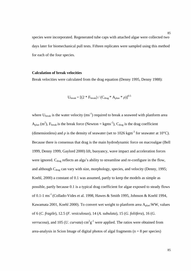
85

85

species were incorporated. Regenerated tube caps with attached algae were collected two

days later for biomechanical pull tests. Fifteen replicates were sampled using this method

for each of the four species.

Calculation of break velocities

Break velocities were calculated from the drag equation (Denny 1995, Denny 1988):

Ubreak = [(2 * Fbreak) / (Cdrag * Aplan

* )]0.5

where Ubreak is the water velocity (ms-1) required to break a seaweed with planform area

Aplan (m2), Fbreak is the break force (Newton = kgms-2), Cdrag is the drag coefficient

(dimensionless) and is the density of seawater (set to 1026 kgm-3 for seawater at 10 C).

Because there is consensus that drag is the main hydrodynamic force on macroalgae (Bell

1999, Denny 1999, Gaylord 2000) lift, buoyancy, wave impact and acceleration forces

were ignored. Cdrag reflects an alga s ability to streamline and re-configure in the flow,

and although Cdrag can vary with size, morphology, species, and velocity (Denny, 1995;

Koehl, 2000) a constant of 0.1 was assumed, partly to keep the models as simple as

possible, partly because 0.1 is a typical drag coefficient for algae exposed to steady flows

of 0.1-1 ms-1 (Collado-Vides et al. 1998, Hawes & Smith 1995, Johnson & Koehl 1994,

Kawamata 2001, Koehl 2000). To convert wet weight to planform area Aplan:WW, values

of 6 (C. fragile), 12.5 (F. vesiculosus), 14 (A. subulata), 15 (G. foliifera), 16 (G.

verrucosa), and 105 (U. curvata) cm2g-1 were applied. The ratios were obtained from

area-analysis in Scion Image of digital photos of algal fragments (n = 8 per species)

86

86

spread out on a white background, and by measuring the corresponding weight wet of the

fragments.

Data analysis

To test for allometric relationships between thallus area and break force, Model II linear

regressions were performed on Log-transformed data on the six species and two substrate

types. The relationship between thallus area and break velocity was also modeled by

linear regression on Log-transformed data. Because Ubreak is calculated from thallus area,

i.e. the two variables are not independent, no inferential statistical tests were performed

on the models, but Pearson correlation coefficients were listed as simple estimates of the

model s explanatory power. The effects of species, substrate type and size were further

tested with fixed factorial ANOVA on Log-transformed data. This transformation

ensured variance homogeneity for most variables (cf. Table 4.2). The effect on break

place was tested with logistic regressions for each species and substrate group vs. thallus

size, and with 2-tests on different combinations of species, substrate and size classes.

However, to fulfill 2-tests assumptions (maximum 20% of groups can have expected

frequencies < 5, Quinn & Keough 2002), the original categories were reduced to two

groups: Class 1-3 = complete biomass removal (dislodgment), and Class 4-8 = partial

biomass removal (pruning). Alpha < 0.05 and < 0.1 were used to indicate significant and

near-significant effects, and all statistical tests were conducted in SPSS 8.0.

Ambient hydrodynamic forces

To compare algal break forces with the ambient hydrodynamic forces, current velocities

were measured where algal biomass is highest in Hog Island Bay (Chapter 2, McGlathery

87

87

et al. 2001). Currents were measured with a Marsh-McBirney electromagnetic current

meter 13 times in summer 2001 in front, between and behind oyster reefs at a mid-lagoon

site (Chapter 6) at 0.6 to 0.8 m below mean sea level, when the water depth was 15-40

cm. These three sub-sites were sampled because oyster reefs potentially differentiated

hydro-dynamic regimes (Chapter 6, Lenihan 1999). The effects of sample day and reef

location on velocities were tested with ANOVA. Temporal velocity changes over several

tidal cycles were described using an Acoustic Doppler Profiler (ADP) during a two

month sample period (Lawson 2003). The ADP was located behind Rouge Island at ca. 2

m depth during a winter period (November 17 2002 to 23 January 23 2003) when winter-

storms potentially enhance tidal currents (Lawson 2003). The ADP measured currents at

20 cm vertical intervals starting at Z0 = 74 cm above the seabed, and with a 30 min

sampling interval. Finally, to compare large-scale horizontal differences within Hog

Island Bay, a map of maximum surface currents was presented based on a 2d Bellamy

Kinematic hydrodynamic model (Fugate & Friedrichs, Submitted) forced with a SWASS

wind-model using wind data from November 2002 (the current map was produced by S.

Lawson, UVa, Lawson 2003).

Flume dislodgment

To test if the calculated break velocity and measured break place results in dislodgment,

50 oyster shells (10 with each of 5 species attached; U. curvata was not found attached to

shells at the time of collection) and 16 tub caps with G. verrucosa and U. curvata.

incorporated were collected in November 2002 for flume tests (Hawes & Smith 1995). At

the time of collection, the five algal species on shells were mainly found attached as

88

88

relatively small individuals (approximately corresponding to size class 1, cf. Fig. 4.1A).

The flume dimensions were 0.3 m x 0.5 m x 3 m and could produce a maximum velocity

of 0.45 ms-1. Each oyster and tube cap were fixed in the mid-section of the flume, and

attached algae encountered water velocities of 0.10, 0.30 and 0.45 ms-1. No dislodgment

occurred at any flow velocity for algae attached to the oyster shells. However, some algae

broke on tube caps and the algae were collected downstream. The wet weight per species

and per tube cap was measured after blotting with a towel (removed and non-removed

algae pooled). After each flume run, the tube cap algae were divided into two size-classes

and the proportion of dislodged algae (pooled for the three flume velocities) was

calculated and tested with an ANOVA for effects of species type and size-class on Log-

transformed data.

Drift algae collections

Entanglement of drifting algal clumps (Holmquist 1994) can potentially increase the

total drag of attached algae without any increase in attachment strength. To quantify the

likelihood of clump encounter and to measure typical clump sizes, drifting algae were

collected 4 times in July 2002 on incoming tides at a mid-lagoon site between two small

oyster reefs. Two PVC poles were inserted into the oyster reef approximately 2 m apart.

All drifting clumps passing through the poles were collected at 2-3 min time intervals.

The water height and velocity was measured and the collected clumps were brought to

the laboratory, where wet weight was determined for each species after blotting with a

towel. Reproductive features were recorded if present and attachment types were

recorded as either unattached, attached to tube caps or attached to unconsolidated shells.

89

89

Results

Thallus size and break force, velocity and place

C. fragile, F. vesiculosus, G. verrucosa, and G. foliifera had significant positive

relationships between thallus area and break force (Table 4.1). In contrast, no species

attached to D. cuprea tube caps had significant relationships. All species had negative

relationships between thallus size and break velocity, with highest r2 when attached to

shells (except U. curvata). No logistic regressions were significant (Table 4.3),

suggesting that break place is independent of algal size.

All single factors and interactions were significant in the ANOVA on thallus area vs.

species, substrate and size-class (Table 4.2). A. subulata was largest, C. fragile and F.

vesiculosus intermediate, and G. foliifera, G. verrucosa and U. curvata smallest for size-

class 2 individuals attached to shells (Fig. 4.1A). All species attached to tube caps, except

U. curvata, had comparatively small planform areas for both size class 1 and 2. However,

U. curvata had large thallus areas for size class two individuals incorporated into tube

caps. The size-factor explained most data variability (28%) followed by the species *

substrate interaction (15%) and the species factor (6%).

Break force was significant for all single factors and the substrate * size and species *

size interactions (Table 4.2). For all species, except U. curvata, break forces were (1)

clearly larger for size-class 2 compared to size-class 1 when attached to shells, (2) were

clearly larger on shells compared to on tube caps, and (3) there was a tendency for algae

90

90

on shells with low Aplan:WW ratio to have high break forces (Fig. 4.2B). For algae

attached to tube caps, the break force was low and constant for all species and both size

groups (0.3-0.5 N). Substrate explained most of the data-variability (57%) followed by

species * substrate (10%) and the species factor (5%).

All single factors and interactions were significant or near-significant on break velocity

vs. species, substrate and size-class (Table 4.2). Size-class 2 individuals had smaller

break velocities than size-class 1, and algae on tube caps had smaller break velocities

than on shells (Fig. 4.1C). In addition the break velocities of size-class 2 were as follows:

F. vesiculosus and G. verrucosa > G. foliifera and C. fragile > A. subulata > U. curvata.

Substrate explained 39% of the data variability, followed by species (13%) and size (8%),

and with higher order interactions explaining less than 1%.

For break place there were significant main effects of species and substrate, but not size

(Table 4.3, Fig. 4.1D). This means that dislodgment to pruning ratios differed between

species and substrates, but not between size-classes. Out of the 6 species-specific tests of

size effects, only U. curvata had a significant effect with larger individuals experiencing

a higher degree of pruning compared to small individuals. On the other hand, all the 6

species-specific tests of substrate effects were significant or near-significant. Thus, C.

fragile, F. vesiculosus, G. verrucosa, G. foliifera and A. subulata had higher dislodgment

on tube caps, whereas U. curvata had highest dislodgment on shells.

Ambient hydrodynamic regime

91

91

Benthic velocities at the mid-lagoon shoal site (Fig. 4.2) were generally between 0.02 and

0.15 ms-1, and only rarely exceeded 0.3 ms-1 between oyster reefs. There were no

significant single factor effects, however, there was a significant interaction between reef

location and sample day (SS = 2.67, F = 3.25, Df = 26, p = 0.003, Fig. 4.2). This

interaction was significant because tidal currents between the oyster reefs vary more than

current velocities in front and behind reefs, which were always low. Thus, algae at mid-

lagoon sites are exposed to relatively low currents, and with algae between reefs

experiencing highest drag forces. The ADP profiles (Fig. 4.3) showed a maximum

surface current of 0.82 ms-1 during the two-month sample period. However, the ADP data

also showed that tidal peak surface currents of 0.75-0.80 ms-1 were encountered regularly

during each month. Near-bottom peak currents, i.e. corresponding to the flow conditions

sessile algae are exposed to, had a tendency to be slightly lower than surface currents,

typically between 0.55-0.65 ms-1. Currents at this near-ocean site were somewhat higher

than at the mid-lagoon site (although not measured at the same time). The map of surface

currents (Fig. 4.4) showed that velocities were low on the shallow mudflats but higher

near the inlet and in the main channel (> 0.3 ms-1). This map predicts that algal drag

would be highest at near-ocean sites.

Flume dislodgment

Algae attached to shells had no breakage at any velocities in the flume trials. This is in

agreement with the calculated break velocities (Fig. 4.1) which predict breakage at

velocities a factor ten higher than could be obtained in the flume (0.45 ms-1). However,

U. curvata and G. verrucosa attached to tube caps experienced breakage at the velocities

92

92

obtained in the flume, which is also in agreement with the calculated break velocities. U.

curvata tended to break at lower velocities than G. verrucosa. The ANOVA showed no

effect of species or species * size but a significant effect of size (F = 4.59, p = 0.04), with

most breakage occurring for large individuals. The break place in the flume trials was in

agreement with the in situ pull tests, with a relatively high degree of breakage at the frond

for U. curvata (7 out of 10) and high breakage at the substrate for G. verrucosa (5 out of

7). However, because the actual number of breakage observations was low, a 2 test did

not lend statistical support to any association between species and break place ( 2 = 0.93,

Df = 3, p = 0.81). Only a small proportion of the total algal biomass was removed during

the flume runs (2-6%). Nevertheless, as predicted from the drag equation, breakage

occurred within the velocity ranges encountered in Hog Island Bay: U. curvata dislodged

at lower velocities than G. verrucosa, and large thalli were significantly more severely

affected than small thalli.

Drift of algal clumps

Sixty-nine drifting algal clumps were captured during 1080 sec of sampling at the mid-

lagoon site (pooled from four consecutive summer sample days, Table 4.5). The mean

clump size was 80 gWW, corresponding to ca. 0.23 m2 of algal area, and had a

recurrence interval of 10 sec along 1 m of coastline (with a mean current velocity of 0.17

ms-1). An algal clump typically contained 3-4 entangled species with highest biomass of

G. verrucosa and C. fragile, and highest frequency of Bryopsis plumosa. Larger multi-

species clumps were generally observed tumbling (Holmquist 1994), whereas smaller

single species clumps, particularly of the positively buoyant C. fragile and F. vesiculosus,

93

93

typically were in the middle or upper regions of the water column. One G. verrucosa and

one G. foliifera were observed with tetrasporangia. All algae caught in the drifting

clumps were observed unattached, i.e. without any shells attached.

Discussion

This study is the first to present macroalgal break forces, break velocities and break

places for algae incorporated into tube caps of the polychaete D. cuprea, and only one

study have conducted pull tests of algae attached to bivalve shells (Hawes & Smith

1995). Considering that algae typically are abundant on these substrates (Bell & Coen

1982a, Brenchley 1976, Chapter 2, 3, Connor 1980, Mangum et al. 1968, Mathieson et al.

2003), and that the type of substrate have been documented to influence algal survival

(Barnes & Topinka 1969, Malm et al. 2003, Milligan & DeWreede 2000, van Tamelen &

Stekoll 1996) these data fill a gap in the biomechanical literature. Here it is documented

that substrate type and thallus size determine break forces, break velocities and break

places for 6 algal species in a low energy soft bottom lagoon.

Unattached survival

In soft bottom semi-enclosed systems breakage is not necessarily adverse but can under

some conditions and for certain species have beneficial effects on growth, dispersal and

re-colonization. Hence, whereas it is assumed that breakage equals mortality in

biomechanical studies from high energy rocky open habitats (Bell 1999, Blanchette 1997,

Denny 1995, Friedland & Denny 1995, Gaylord et al. 1994), in shallow semi-enclosed

systems survival will also depends on topography, residence time, and bordering habitats

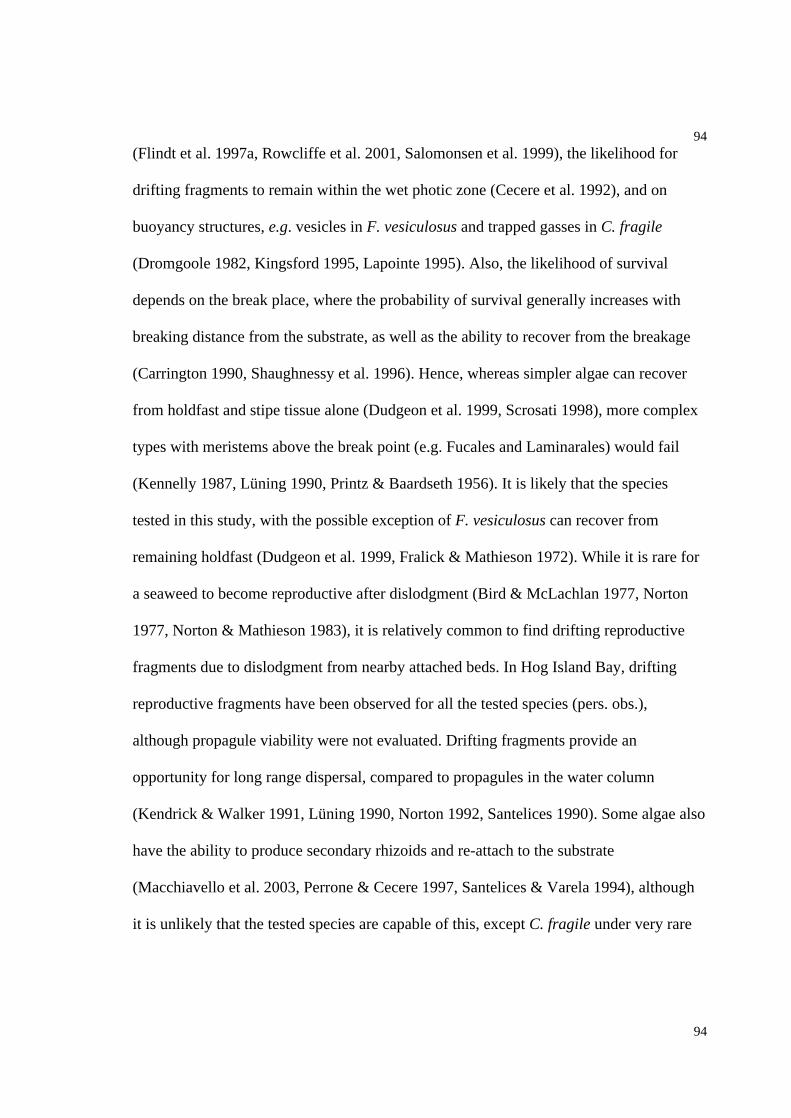
94

94

(Flindt et al. 1997a, Rowcliffe et al. 2001, Salomonsen et al. 1999), the likelihood for

drifting fragments to remain within the wet photic zone (Cecere et al. 1992), and on

buoyancy structures, e.g. vesicles in F. vesiculosus and trapped gasses in C. fragile

(Dromgoole 1982, Kingsford 1995, Lapointe 1995). Also, the likelihood of survival

depends on the break place, where the probability of survival generally increases with

breaking distance from the substrate, as well as the ability to recover from the breakage

(Carrington 1990, Shaughnessy et al. 1996). Hence, whereas simpler algae can recover

from holdfast and stipe tissue alone (Dudgeon et al. 1999, Scrosati 1998), more complex

types with meristems above the break point (e.g. Fucales and Laminarales) would fail

(Kennelly 1987, Lüning 1990, Printz & Baardseth 1956). It is likely that the species

tested in this study, with the possible exception of F. vesiculosus can recover from

remaining holdfast (Dudgeon et al. 1999, Fralick & Mathieson 1972). While it is rare for

a seaweed to become reproductive after dislodgment (Bird & McLachlan 1977, Norton

1977, Norton & Mathieson 1983), it is relatively common to find drifting reproductive

fragments due to dislodgment from nearby attached beds. In Hog Island Bay, drifting

reproductive fragments have been observed for all the tested species (pers. obs.),

although propagule viability were not evaluated. Drifting fragments provide an

opportunity for long range dispersal, compared to propagules in the water column

(Kendrick & Walker 1991, Lüning 1990, Norton 1992, Santelices 1990). Some algae also

have the ability to produce secondary rhizoids and re-attach to the substrate

(Macchiavello et al. 2003, Perrone & Cecere 1997, Santelices & Varela 1994), although

it is unlikely that the tested species are capable of this, except C. fragile under very rare

95

95

circumstances (Appendix 1, Fralick & Mathieson 1972, Mathieson et al. 2003, Yotsui &

Migita 1989).

Allometric models of break force and break velocity

In Hog Island Bay the four least opportunistic species (C. fragile, G. foliifera, F.

vesiculosus, G. verrucosa (Chapter 5, Appendix 1, Littler 1980, Nielsen & Sand-Jensen

1990) had significant increases of break forces versus thallus area when attached to

bivalve shells probably because large individuals have large holdfasts and thick stipes

(Friedland & Denny 1995, Gaylord et al. 1994, Kawamata 2001, Malm et al. 2003).

However, the two most opportunistic species (U. curvata, A. subulata) did not (Hawes &

Smith 1995). Also, the study documented that the Fbreak-Aplan relationship breaks down

when organisms are attached to weak substrates like D. cuprea tube caps. Even though

some species increased attachment force with size, it did not match the drag increase, and

hence all species on both substrate types showed an increasing likelihood of breakage

with size. This supports the hypothesis that the upper size of marine organisms can be

limited by hydrodynamic forces (Denny et al. 1985, Gaylord et al. 1994). The allometric

models support a mechanistic based model of the absence of C. fragile, A. subulata and

F. vesiculosus from tube caps (Chapter 3). These species typically grow into large

individuals, but because of low break velocities would dislodge at tidal peak currents.

Other possible explanations of the absence of these species on tube caps include low

encounter rates (Chapter 2, this Chapter), low desiccation and/or low burial tolerance

(Chapter 5, 6, Appendix 1), and low worm-preference (Chapter 3).

96

96

Effects of species, substrate and size on break force and velocity

Algal individuals in Hog Island Bay were small compared to dominant algae from open

temperate coasts, where kelps and large fucoids often have fronds 5-100 times larger than

observed in Hog Island Bay (Thomsen & Wernberg submitted)). It should be noted that

because size was presented as thallus area light species, e.g. U. curvata, were

comparable in size to heavy seaweeds like C. fragile and F. vesiculosus. Substrate was

the most important of the three test-factor both for break forces and break velocities

similar to other studies which have documented strong relationship between substrate

hardness and likelihood of biomass loss (Barnes & Topinka 1969, Malm et al. 2003,

Milligan & DeWreede 2000). U. curvata differed from the 5 other species by having a

low difference in break forces and velocities between the two substrate types. Thus, soft

substrates (tube caps) may potentially be beneficial for small and opportunistic algae with

weak attachment strengths, by providing space free of large competitors. The

morphological similar G. verrucosa, A. subulata and G. foliifera had relatively similar

break forces, being smaller than the larger C. fragile and F. vesiculosus, and larger than

the opportunistic U. curvata (based on WW). This is consistent with other studies that

found similar break forces between species of relatively similar morphologies and sizes

(Pratt & Johnson 2002, Shaughnessy et al. 1996).

Effect of species, substrate and size on break place

Algal break place can determine the likelihood of survival and hence the stability of

communities (Blanchette 1997, Dudgeon et al. 1999, Shaughnessy & DeWreede 2001).

In Hog Island Bay, all six algal species had between 30-60% pruning on bivalve shells,

suggesting that re-growth from holdfast and stipes likely are important recovery

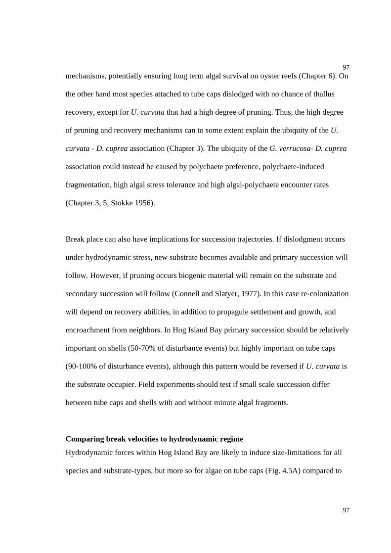
97

97

mechanisms, potentially ensuring long term algal survival on oyster reefs (Chapter 6). On

the other hand most species attached to tube caps dislodged with no chance of thallus

recovery, except for U. curvata that had a high degree of pruning. Thus, the high degree

of pruning and recovery mechanisms can to some extent explain the ubiquity of the U.

curvata - D. cuprea association (Chapter 3). The ubiquity of the G. verrucosa- D. cuprea

association could instead be caused by polychaete preference, polychaete-induced

fragmentation, high algal stress tolerance and high algal-polychaete encounter rates

(Chapter 3, 5, Stokke 1956).

Break place can also have implications for succession trajectories. If dislodgment occurs

under hydrodynamic stress, new substrate becomes available and primary succession will

follow. However, if pruning occurs biogenic material will remain on the substrate and

secondary succession will follow (Connell and Slatyer, 1977). In this case re-colonization

will depend on recovery abilities, in addition to propagule settlement and growth, and

encroachment from neighbors. In Hog Island Bay primary succession should be relatively

important on shells (50-70% of disturbance events) but highly important on tube caps

(90-100% of disturbance events), although this pattern would be reversed if U. curvata is

the substrate occupier. Field experiments should test if small scale succession differ

between tube caps and shells with and without minute algal fragments.

Comparing break velocities to hydrodynamic regime

Hydrodynamic forces within Hog Island Bay are likely to induce size-limitations for all

species and substrate-types, but more so for algae on tube caps (Fig. 4.5A) compared to

98

98

bivalve shells (Fig. 4.5B), and in the following order of severity: U. curvata > A.

subulata > G. foliifera = G. verrucosa > F. vesiculosus = C. fragile (on shells, Fig 4.5B).

Based on the allometric break velocity models it is further predicted that velocities

typical of Hog island Bay and other soft bottom tidal systems (0.1-1 ms-1)(Albrecht 1998,

Hawes & Smith 1995) would dislodge individuals in the size range of 0.01-0.1 m2 for

algae attached to tube caps, and for individuals in the size range of 0.1-1 m2 for algae

attached to shells. Such size limitations and thallus breakage would be most likely at

near-ocean sites and/or between physical structures were flow is elevated. It should be

noted that these estimates are based on a constant Cdrag, species-specific, not individual

based, Aplan:WW ratios and ignoring lift or acceleration forces. Whereas the two first

assumptions can under- or overestimate the true break velocity depending on whatever

the drag coefficient and thallus area are higher or lower than estimated here, the addition

of more hydrodynamic forces will always result in an lowering of Ubreak (Friedland &

Denny 1995, Shaughnessy et al. 1996, Utter & Denny 1996). Ignoring acceleration and

impact forces seems appropriate in low energy lagoons where waves are small. Lift could

be of importance for the positively buoyant F. vesiculosus and C. fragile, but Dromgoole

(1982a) showed that for C. fragile lift was small compared to drag and Friedland &

Denny (1995) also documented low lift for the vesiculated kelp Egregia menzeii. In spite

of the simplicity of the models, flume runs supported the predicted break velocities and

Hawes and Smith (1995) also found a similar correspondence for Ulva lactuca. Water

velocities have been interpreted as being generated from tidal currents. However, Lawson

(2003) calculated that during storms shallow water high frequency benthic wave stresses

may be similar in magnitude to tidal current stresses within Hog Island Bay, especially on

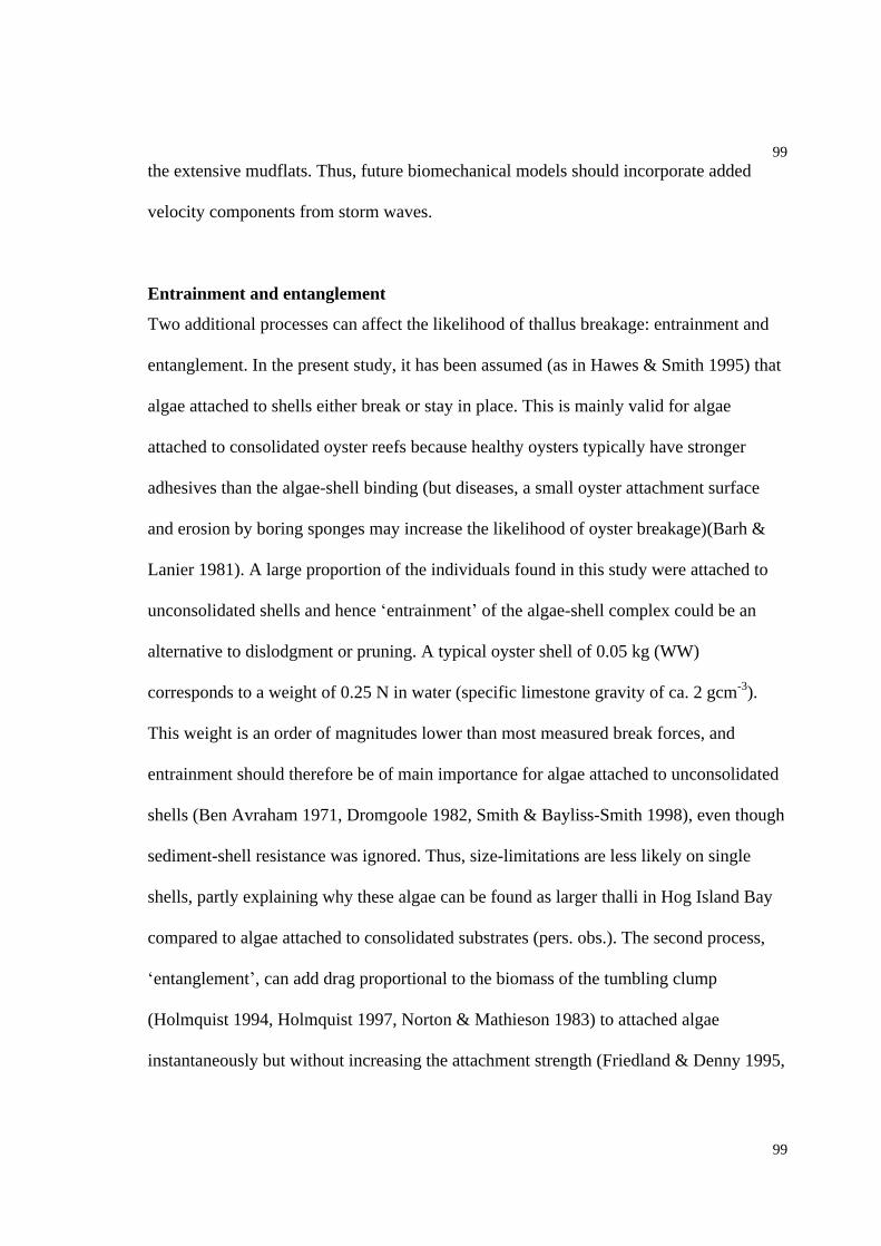
99

99

the extensive mudflats. Thus, future biomechanical models should incorporate added

velocity components from storm waves.

Entrainment and entanglement

Two additional processes can affect the likelihood of thallus breakage: entrainment and

entanglement. In the present study, it has been assumed (as in Hawes & Smith 1995) that

algae attached to shells either break or stay in place. This is mainly valid for algae

attached to consolidated oyster reefs because healthy oysters typically have stronger

adhesives than the algae-shell binding (but diseases, a small oyster attachment surface

and erosion by boring sponges may increase the likelihood of oyster breakage)(Barh &

Lanier 1981). A large proportion of the individuals found in this study were attached to

unconsolidated shells and hence entrainment of the algae-shell complex could be an

alternative to dislodgment or pruning. A typical oyster shell of 0.05 kg (WW)

corresponds to a weight of 0.25 N in water (specific limestone gravity of ca. 2 gcm-3).

This weight is an order of magnitudes lower than most measured break forces, and

entrainment should therefore be of main importance for algae attached to unconsolidated

shells (Ben Avraham 1971, Dromgoole 1982, Smith & Bayliss-Smith 1998), even though

sediment-shell resistance was ignored. Thus, size-limitations are less likely on single

shells, partly explaining why these algae can be found as larger thalli in Hog Island Bay

compared to algae attached to consolidated substrates (pers. obs.). The second process,

entanglement , can add drag proportional to the biomass of the tumbling clump

(Holmquist 1994, Holmquist 1997, Norton & Mathieson 1983) to attached algae

instantaneously but without increasing the attachment strength (Friedland & Denny 1995,

100

100

Koehl & Wainwright 1977, Utter & Denny 1996). Here, encounter rates were

documented to be high, indicating that entanglement can be an important drag-increasing

process in Hog Island Bay. However, in addition to the encounter rate, the actual

entanglement also depends on properties of both attached and drift algae and flow rates.

For example, C. fragile was often entangled by filamentous genera like Ectocarpus spp.

and Bryopsis spp., which would break before their host. Also whereas G. and U. curvata

tumble along the bottom, F. vesiculosus and C. fragile drift in the water column making it

unlikely for the latter taxa to entangle benthic algae.

Other factors of importance

Many factors other than species, size and substrate types influence algal break forces and

break velocities, e.g. season, exposure level, and wounding (Duggins et al. 2001, Pratt &

Johnson 2002, Thomsen & Wernberg submitted). It is likely that storm and spring-tide

currents remove weakly attached large individuals on predictable temporal scales (fall

and winter in Hog Island Bay, Dolan 1996, Lucy et al. 1986). Such temporal cycles can

create substantial variability in break forces depending on whatever sampling was

conducted before or after the storm (Bell 1999, Blanchette 1997, Milligan & DeWreede

2000, Pratt & Johnson 2002). Similarly, grazer scars may reduce break forces (DeWreede

et al. 1992, Duggins et al. 2001, Padilla 1993), and it was observed that U. curvata

generally had a Swiss-cheese morphology, probably due to amphipod grazing. Because

Hawes and Smith (1995) observed U. curvata breaking at the stipe, the high degree of U.

curvata breaking at the thallus in the present study could be caused by grazer scars.

Finally, sediment burial and anoxia can also lower break forces, and algae attached to

101

101

buried shells typically had black and necrotic holdfasts with lower break forces than

individuals sampled in the present survey (preliminary trials). Future biomechanical

studies from low energy soft bottom habitats should include entrainment and

entanglement process as well as more test factors into a multi-factorial biomechanical

framework, to improve on the proposed dislodgment models, and ultimately be able to

predict break events.

In conclusion, species and substrate type determine where an algae break, and species,

substrate type and thallus size further determine algal break forces and break velocities in

a low energy soft bottom lagoon. Dislodgment and pruning are probably common

processes at peak hydrodynamic stresses, particularly for opportunistic species, and for

large individuals attached to soft substrates like polychaete tube caps, although field

testing are needed to verify these prediction.

102

102

Chapter 4. Tables

Table 4.1. Linear models of Log Aplan (m2) vs. Log Fbreak (Newton) and Log Ubreak (ms-1).

Significant results are in bold (p < 0.05). Note that p-values were not provided for Ubreak

because interdependency between Aplan and Ubreak invalidates statistical testing.

Fbreak Ubreak

Species Substrate n Slope Intercept r2 p Slope Intercept r2

C. fragile Tube cap 15 -0.27 -1.21 0.01 0.73 -0.63 -1.90 0.18F. vesiculosus Tube cap 15 -0.26 -0.77 0.02 0.60 -0.63 -1.62 0.34A. subulata Tube cap 15 -0.74 -0.87 0.06 0.39 -0.87 -2.35 0.25G. foliifera Tube cap 15 0.12 -0.79 0.01 0.80 -0.44 -1.08 0.20G. verrucosa Tube cap 32 0.18 -0.58 0.03 0.85 -0.41 -0.89 0.36U. curvata Tube cap 30 0.13 -0.77 0.03 0.86 -0.44 -1.11 0.58C. fragile Shell 64 0.37 0.35 0.17 0.00 -0.31 -0.12 0.39F. vesiculosus Shell 83 0.39 0.39 0.43 0.00 -0.30 -0.02 0.64A. subulata Shell 29 0.11 0.41 0.07 0.17 -0.45 -0.50 0.84G. foliifera Shell 31 0.35 0.52 0.38 0.00 -0.32 -0.10 0.67G. verrucosa Shell 50 0.35 0.41 0.29 0.00 -0.32 -0.16 0.58U. curvata Shell 55 0.16 0.21 0.03 0.19 -0.42 -0.81 0.49

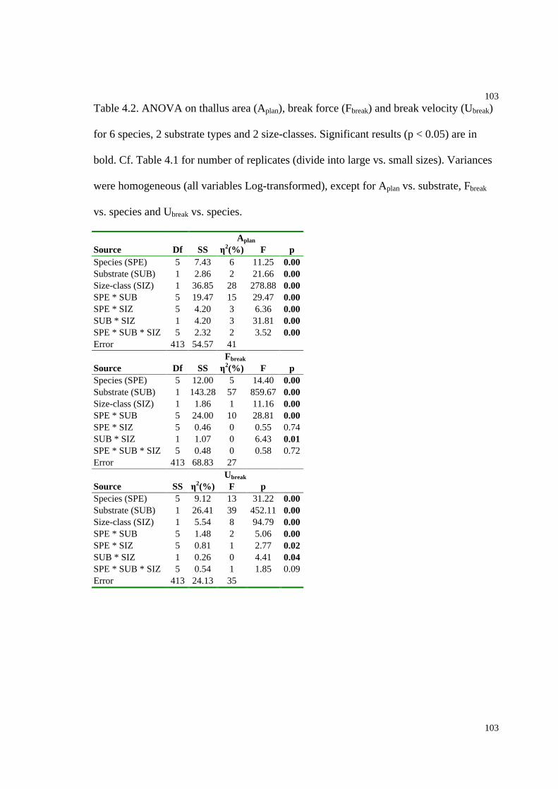
103

103

Table 4.2. ANOVA on thallus area (Aplan), break force (Fbreak) and break velocity (Ubreak)

for 6 species, 2 substrate types and 2 size-classes. Significant results (p < 0.05) are in

bold. Cf. Table 4.1 for number of replicates (divide into large vs. small sizes). Variances

were homogeneous (all variables Log-transformed), except for Aplan vs. substrate, Fbreak

vs. species and Ubreak vs. species.

Aplan

Source Df SS 2(%) F pSpecies (SPE) 5 7.43 6 11.25 0.00Substrate (SUB) 1 2.86 2 21.66 0.00Size-class (SIZ) 1 36.85 28 278.88 0.00SPE * SUB 5 19.47 15 29.47 0.00SPE * SIZ 5 4.20 3 6.36 0.00SUB * SIZ 1 4.20 3 31.81 0.00SPE * SUB * SIZ 5 2.32 2 3.52 0.00Error 413 54.57 41

Fbreak

Source Df SS 2(%) F pSpecies (SPE) 5 12.00 5 14.40 0.00Substrate (SUB) 1 143.28 57 859.67 0.00Size-class (SIZ) 1 1.86 1 11.16 0.00SPE * SUB 5 24.00 10 28.81 0.00SPE * SIZ 5 0.46 0 0.55 0.74SUB * SIZ 1 1.07 0 6.43 0.01SPE * SUB * SIZ 5 0.48 0 0.58 0.72Error 413 68.83 27

Ubreak

Source SS 2(%) F pSpecies (SPE) 5 9.12 13 31.22 0.00Substrate (SUB) 1 26.41 39 452.11 0.00Size-class (SIZ) 1 5.54 8 94.79 0.00SPE * SUB 5 1.48 2 5.06 0.00SPE * SIZ 5 0.81 1 2.77 0.02SUB * SIZ 1 0.26 0 4.41 0.04SPE * SUB * SIZ 5 0.54 1 1.85 0.09Error 413 24.13 35

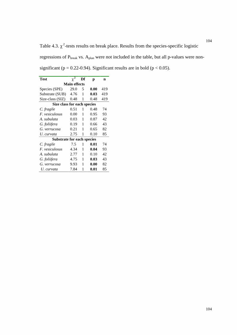
104

104

Table 4.3. 2-tests results on break place. Results from the species-specific logistic

regressions of Pbreak vs. Aplan were not included in the table, but all p-values were non-

significant (p = 0.22-0.94). Significant results are in bold (p < 0.05).

Test 2 Df p nMain effects

Species (SPE) 29.0 5 0.00 419Substrate (SUB) 4.76 1 0.03 419Size-class (SIZ) 0.48 1 0.48 419

Size class for each speciesC. fragile 0.51 1 0.48 74F. vesiculosus 0.00 1 0.95 93A. subulata 0.03 1 0.87 42G. foliifera 0.19 1 0.66 43G. verrucosa 0.21 1 0.65 82U. curvata 2.75 1 0.10 85

Substrate for each speciesC. fragile 7.5 1 0.01 74F. vesiculosus 4.34 1 0.04 93A. subulata 2.77 1 0.10 42G. foliifera 4.75 1 0.03 43G. verrucosa 9.93 1 0.00 82 U. curvata 7.84 1 0.01 85

105

105

Table 4.4. Flume dislodgment of small vs. large G. verrucosa and U. curvata

incorporated into D. cuprea tube caps at 3 velocities (n = 8 per species and size class,

with standard errors). The first rows correspond to the initial biomass of per tube cap

before flume induced breakage.

Velocity Species Size 1 SD Size 2 SDG. verrucosa 0.86 0.78 9.19 3.46Initial biomass per

tube cap (gWW) U. curvata 0.40 0.26 1.85 0.88G. verrucosa 0.00 0.00 0.03 0.08% dislodgment of

initial biomass at10 cm s-1

U. curvata 0.00 0.00 0.37 1.06

G. verrucosa 0.28 0.80 0.14 0.40% dislodgment ofinitial biomass at30 cm s-1

U. curvata 0.33 0.92 8.72 24.67

G. verrucosa 2.02 4.84 9.64 26.55% dislodgment ofinitial biomass at45 cm s-1

U. curvata 0.00 0.00 3.66 3.95

G. verrucosa 2.30 5.62 9.81 26.48% dislodgment ofinitial biomass -Total

U. curvata 0.33 0.92 12.75 25.90

106

106

Table 4.5. Species and sizes of drift algal clumps. Results from four summer surveys

were pooled (mean sample condition per survey were: 2.18 m between poles, 0.28 m

water height, 0.17 ms-1 current velocity, 270 sec sampling time). The average

reoccurrence interval (number of clumps encountered for a sessile benthic algae) was 8.9

secm-1 coastline. The median clump wet weight was 10 g and the maximum 1060 g. SE =

Standard errors.

Taxa gWW SE m2 #Richness 3.19 0.25 69Total 80.34 21.14 0.2306 69G. verrucosa 36.41 10.76 0.0583 41C. fragile 15.80 8.49 0.0079 8B. plumosa 11.52 4.17 0.1152 50G. foliifera 8.74 3.15 0.0131 17A. subulata 3.22 1.61 0.0045 11C. parvula 1.44 0.45 0.0036 31Polysiphonia spp. 1.30 0.62 0.0130 23U. curvata 1.03 0.61 0.0103 11Ceramium spp. 0.44 0.25 0.0044 11F. vesiculosus 0.19 0.18 0.0002 2L. bayileyana 0.04 0.04 0.0001 2

107

107

Chapter 4. Figures

Fig. 4.1. Thallus planform area (A), break force (B), break velocity (C) and break place

(D) for 6 species, 2 substrate types and 2 size classes. Species are arranged from low

(left) to high Splan:WW ratios (± SE, cf. Table 4.1 for number of replicates).

B. Break force

New

ton

0

2

4

6

8

10

12

14

A. Thallus size

m-2

0.00

0.01

0.02

0.03

0.04

0.05

0.06

Small on tube capsSmall on shellsLarge on tube capsLarge on shells

C. Break velocity

ms-1

0

2

4

6

8

10

D. Break place

C. fragile

F. vesiculosus

A. subulataG. foliifera

G. verrucosaU. curvata

% D

islo

dgm

ent

0

20

40

60

80

100

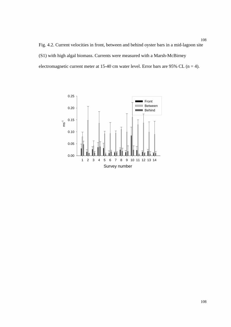
108

108

Fig. 4.2. Current velocities in front, between and behind oyster bars in a mid-lagoon site

(S1) with high algal biomass. Currents were measured with a Marsh-McBirney

electromagnetic current meter at 15-40 cm water level. Error bars are 95% CL (n = 4).

Survey number

1 2 3 4 5 6 7 8 9 10 11 12 13 14

ms-1

0.00

0.05

0.10

0.15

0.20

0.25

Front Between Behind

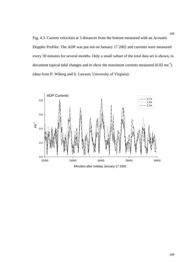
109

109

Fig. 4.3. Current velocities at 3 distances from the bottom measured with an Acoustic

Doppler Profiler. The ADP was put out on January 17 2002 and currents were measured

every 30 minutes for several months. Only a small subset of the total data set is shown, to

document typical tidal changes and to show the maximum currents measured (0.82 ms-1)

(data from P. Wiberg and S. Lawson, University of Virginia).

ADP Currents

Minuttes after midday January 17 2002

22000 24000 26000 28000 30000

ms-1

0.0

0.2

0.4

0.6

0.8 0.741.542.34

110

110

Fig. 4.4. Peak currents in Hog Island Bay at incoming mid-tide, calculated from a 2d

Bellamy Kinematic hydrodynamic model. The Map was produced by Lawson (2003) and

the model developed by Fugarte and Fridrich (Submitted).

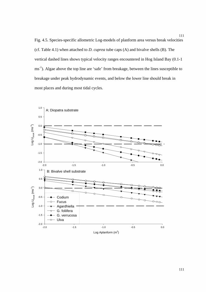
111

111

Fig. 4.5. Species-specific allometric Log-models of planform area versus break velocities

(cf. Table 4.1) when attached to D. cuprea tube caps (A) and bivalve shells (B). The

vertical dashed lines shows typical velocity ranges encountered in Hog Island Bay (0.1-1

ms-1). Algae above the top line are safe from breakage, between the lines susceptible to

breakage under peak hydrodynamic events, and below the lower line should break in

most places and during most tidal cycles.

A: Diopatra substrate

-2.0 -1.5 -1.0 -0.5 0.0

Log

Ubr

eak

(ms-1

)

-2.0

-1.5

-1.0

-0.5

0.0

0.5

1.0

B: Bivalve shell substrate

Log Aplanform (m2)

-2.0 -1.5 -1.0 -0.5 0.0

Log

Ubr

eak

(ms-1

)

-2.0

-1.5

-1.0

-0.5

0.0

0.5

1.0

CodiumFucusAgardhiellaG. foliiferaG. verrucosaUlva

112

112

Chapter 5. The alien Codium fragile have low

performance characteristics compared to native

macroalgae in a soft bottom turbid lagoon,

Virginia

113

113

Abstract

The chapter investigates whether the successful introduction of the Asian macroalgae

Codium fragile ssp. tomentosoides into Hog Island Bay, a shallow lagoon in Virginia

with extensive intertidal areas, can be explained by an ability to perform better than

native macroalgae. Hog Island Bay is characterized by high turbidity and high

sedimentation rates, high densities of herbivorous mud snails, relatively low nutrient

concentrations, and predictable gradients in water quality from mainland to ocean sites.

Given a well-documented ability of C. fragile to invade soft bottom lagoons we

hypothesized that C. fragile would perform better compared to native macroalgae. To test

this hypothesis, nine growth experiments were conducted between March and August

2002 using drift algal assemblages containing fragments of C. fragile, Fucus vesiculosus,

Gracilaria verrucosa, Agardhiella subulata, Hypnea musciformis and Ulva curvata.

Contrary to the hypothesis, C. fragile performed no better than the native species in all

experiments. C. fragile were less resistant to sedimentation, were more desiccation prone,

showed lower growth rates at either high or low light levels or nutrient concentrations,

and were more severely grazed by mud snails than the native species. Although C. fragile

was able to grow along the entire mainland-ocean gradient, growth was consistently

lowest at near-mainland sites, intermediate at near-ocean sites, and highest at mid-lagoon

sites. This pattern was most likely due to light limitation at the near-mainland site and

nutrient-limitation at the near-ocean site. In comparison, F. vesiculosus was resistant to

stressful conditions, particularly desiccation, G. verrucosa had some stress-tolerant traits,

and could sustain higher growth than C. fragile, and H. musciformis and U. curvata, and,

to a certain extent, A. subulata had opportunistic traits with high growth under high

114

114

nutrient and light conditions. These results provide a process oriented basis for why G.

verrucosa and U. curvata are more abundant and have a wider distribution pattern than C.

fragile within Hog Island Bay. The results also fit into a surface to volume ratio

framework (S:V), where growth and growth variability increased with increasing S:V

ratio. In conclusion, the commonly reported invasive success of C. fragile could not be

related to superior growth or stress resistance compared to native species in Hog Island

Bay.

Introduction

Invasions of alien species are considered a major threat to global biodiversity because the

invaders often outcompete, eat or infect native species (Carlton 1999, Meinesz 1999,

Ruiz et al. 1997). Several marine macroalgae have caused dramatic transoceanic

invasions. In particular, Caulerpa taxifolia, Undaria pinnatifada, Sargassum muticum,

and Codium fragile ssp. tomentosoides invasions have created adverse effects worldwide

by clogging waterways, competing with native algae, altering the nursery habitat for

fishes and invertebrates, reducing light penetration in the water column, changing

biogeochemical cycles, and suffocating or drifting away with economically important

shellfish (Chapman 1999, Den Hartog 1998, Meinesz 1999, Norton 1976, Stæhr et al.

2000, Wallentinus 2002). Often the invasive success of a species has been related to

super -traits (e.g. high intrinsic rate of growth, high dispersal capacity and high

regenerative abilities, Meinesz 1999, Norton 1976, Rejmánek & Richardson 1996, Stæhr

et al. 2000, Trowbridge 1998, Wernberg et al. 2001). It is therefore important to

115

115

understand how species traits influence performance if the effects of macroalgal

invasions are to be evaluated and future invasions predicted, managed and prevented.

The macroalgal invader C. fragile ssp. tomentosoides (van Goor) Silva originates from

Asia (Trowbridge 1998), but spread to the North American east coast in the 1950s and

arrived in Virginia in the 1970s (Hillson 1976). Today, C. fragile is the fourth most

common species in Hog Island Bay (Chapter 2), a shallow turbid lagoon, which is part of

the U.S. Long Term Ecological Research program (Virginia Coast Reserve, Hayden et al.

2000). Due to its high relative abundance, C. fragile can be considered successful in

Virginian turbid shallow waters. Conclusions about traits that make a species successful

have often been interpreted from single-species independent laboratory experiments (e.g.

Littler 1980, Lotze & Schamm 2000, Pedersen & Borum 1997, Wallentinus 1984), where

extrapolations to multi-species interdependent performance responses are limited. There

is a need for multi-species multi-factorial field experiments comparing performance of

invasive species to native species to understand invader success.

The lagoonal habitats successfully invaded are typically characterized by low light

penetration (Lawson 2003, McGlathery et al. 2001), high meso-grazer densities,

especially of mudsnails (this study, Giannotti & McGlathery 2001, Rosinski 2004,

Scheltema 1964), high sedimentation and re-suspension rates (Lawson 2003) and often

relatively high nutrient concentrations (Goshorn et al. 2001). In addition to these

characteristics, two spatial gradients may further influence macroalgal performance in

coastal soft bottom systems. On a small vertical scale, tidal changes create the potential

116

116

for different desiccation rates, grazing rates, sedimentation levels and light conditions at

different elevation levels (Colman 1933, Doty 1946, Lewis 1964). On a large horizontal

scale different distances from the mainland results in a gradient in nutrient loading and in

water residence time which influence turbidity, nutrient, light, temperature and

sedimentation levels (Castel et al. 1996, Lawson 2003, McGlathery et al. 2001). The

success of C. fragile in low energy lagoons and estuaries (Malinowski & Ramus 1973,

Trowbridge 1998) suggests a high tolerance to the variations in physical and chemical

characteristics within these lagoons.

The main objectives of this study were to investigate if C. fragile performs better in terms

of biomass gain relative to native macroalgae under a range of conditions within the

lagoon. Specifically, it was hypothesized that C. fragile would be superior under low and

high levels of mud snail grazing, nutrients, light, desiccation, sedimentation, and at all

sites along the distance-gradient. Because the elevation gradient is strong and well-

described (high levels = desiccation, Doty 1946, Dromgoole 1980, Lüning 1990)

compared to the distance gradient, the latter was of particular interest in this study. To

test these hypotheses, nine independent in situ experiments were conducted in spring and

summer 2002 directly comparing performance of C. fragile to native macroalgae in drift

algal mini-assemblages. In addition to C. fragile, assemblages contained tissue fragments

of Fucus vesiculosus L., Agardhiella subulata (C. Ag.) Kraft et Wynne, Gracilaria

verrucosa (Hudson) Papenfuss, Hypnea musciformis (Wulfen) Lamouroux, and Ulva

curvata (Kutzing) De Toni, arranged after surface area:volume (S:V) ratio with C. fragile

having lowest and U. curvata highest ratios (Nielsen & Sand-Jensen 1990). These species

117

117

were chosen because they are typical components of lagoonal drift algal assemblages

along West Atlantic coastlines (Cowper 1978, Goshorn et al. 2001, Thorne-Miller et al.

1983).

Methods

Study site

Hog Island Bay is a ca. 100 km2 low-energy lagoon on the Delmarva Peninsula on the

eastern shore of Virginia, US (McGlathery et al. 2001). Scattered unconsolidated bivalve

shells of the oyster Crassostrea virginica and clam Mercenaria mercenaria, and patchy

intertidal oyster reefs provide hard substrate for macroalgal attachment. The average

depth is 1.5 m and ca. 80 % of the lagoon is less than 3 m deep (Oertel 2001).

Semidiurnal tides move mats of drift algae around within the lagoon (McGlathery et al.

2001, Tyler et al. 2001) at typical flow rates of 0.1-0.3 ms-1 (Chapter 4). Mud snails are

present year-round in high densities in marshes and on mudflats (Table 5.1, Giannotti &

McGlathery 2001, Rosinski 2004). Dissolved nitrogen is typically 15-20 M and light

extinction between 1.7 to 2.2 m-1, with highest values near the mainland and lowest near

the ocean (Table 5.1, McGlathery et al. 2001). Sedimentation, re-suspension and

suspended solid concentrations are high throughout the lagoon, and storms can add or

remove several centimeters of sediment within a few hours (Lawson 2003). Codium, F.

vesiculosus, A. subulata, G. verrucosa and U. curvata are relatively common year-round

and they potentially compete for substrate, light and nutrients. H. musciformis is mainly

found in summer months as an entangled epiphyte (Norton & Mathieson 1983), and

probably does not compete for substrate. The six algal species constitute more than 90%

118

118

of the total algal biomass in Hog Island Bay (Chapter 2), and as such represent the typical

drift algal assemblages.

In situ experiments

Seven factorial experiments were conducted to test for effects on tissue performance of

species (SPE), distance from mainland (DIS), elevation level (ELE desiccation),

sedimentation/burial (SED), light reduction (LIG), nutrient addition (NUT), and

grazer/snail addition (GRA). Two additional experiments were conducted to test for

experimental artifact, such as effects of twist-tie wrapping (TWI) and cage enclosure

(CAG). Although assemblage experiments can produce statistically biased p-values

because of potential interdependence of species they have high predictive value

compared to single-species laboratory experiments because of a close resemblance to

natural in situ conditions (Peters 1991). Details on the experimental design are given in

Table 5.2. Apical fragments cut from healthy and fresh algal specimens (0.2 to 2 g WW;

species with high S:V ratio had lowest biomass) were collected from drift mats in the

mid-lagoon, and allowed 24 hours of wound recovery before field incubation (Ramus &

Venable 1987). Wet weight (0.001 g) was measured before and after incubation after

blotting with a towel. Performance was defined as percent change in biomass per

fragment per incubation period. This measure was preferred over the exponential growth

model (Pedersen 1995, Pedersen & Borum 1996) because the latter cannot account for a

total biomass loss. Because the main objective was to compare performance of C. fragile

to native species under a range of environmental conditions, mortality was frequently

encountered (=100% biomass loss). Another advantage of the time-integrated

119

119

performance measure is that it makes no assumption about temporal development in

biomass change. Daily biomass changes can be calculated from incubation time and

biomass data (Table 5.2, 5.6). A few fragments and assemblages were lost due to storms

resulting in a few slightly unbalanced designs.

Elevation effects

To estimate the relative importance of elevation and distance, two open plot experiments

were carried out in spring 2002 (16 and 14 days of incubation). An open plot design

eliminate cage artifacts associated with flow reductions. Because H. musciformis was not

found in spring and U. curvata only in minute quantities, these two species were not

included. A fragment of C. fragile, F. vesiculosus, A. subulata and G. verrucosa was

attached with a twist-tie which was gently wrapped around the fragment (a maximum of

5% of the fragments were physically covered by the twist tie) and attached to a cable tie

to mimic a typical assemblage. The cable ties were then attached at two elevations on

PVC poles: Low elevation = 0.8 m and High elevation = 0.0 m below mean sea level.

Poles were inserted into the sediment at five near-mainland, five mid-lagoon and five

near-ocean sites, each site being separated by a minimum of 500 m (n = 1 pole per site).

Because numerous fragments died at the high-treatment in the first experiment a lower

high-treatment was used in the second experiment (High = 0.5 m below mean sea level).

Sedimentation effects

To test for resistance to sediment burial, a litterbag decomposition experiment was

conducted. Pre-weighed fragments (minus H. musciformis which was not present in May

2002) were incubated in 4 mm mesh bags buried under 3 cm sandy sediment in the lower

120

120

intertidal zone (0.5 m below mean sea level) at a mid-lagoon mudflat. Litter bags were

recovered after 0, 1, 2, 3, 7, 12, 21, 27, 34 and 37 days of burial and wet weight was

measured on remaining fragments (n = 3-6 per sampling day). The sediment

characteristics at the site were: organic matter = 2.1% DW, sediment molar C:N = 11.8,

sediment bulk density 1.51 gcm-3 (McGlathery et al. 2001), and mean sediment grain

diameter = 63 m (Lawson 2003).

Cage experiments

Cage experiments were conducted to test for effects of nutrient addition, shading of light,

addition of grazing snails and for effects of methodological artifacts of twist tie wrapping

and cage enclosure. Each of these experiments were replicated at a near-mainland (Creek

1), a mid-lagoon (Shoal 1) and a near-ocean (Hog 1) site (McGlathery et al. 2001). This

design allowed us to test the interactions between the uncontrolled spatial gradient and

the controlled treatments listed below. All allocations were random (fragments,

treatments, order and position of cages, etc). Fragments were enclosed in 22 cm

transparent acrylic cages with 30 two-millimeter perforations to keep grazers out and

fragments inside of cages and to ensure a steady water flow. The cages reduced the

photosynthetic active radiation (PAR) by 11%, calculated from 10 PAR-measurements

taken during a sunny summer day from 10 AM to 6 PM. One fragment of each of the six

species was added to a cage and the ends were closed with plastic caps. The mean algal

density at the start of these experiments was 130 gWWm-2 (n = 230, SD = 33 gWWm-2,

Max. = 240 gWWm-2; Cage densities were calculated by estimating that 40% of the total

cylindrical cage surface (= 0.022 m2) provided substrate for looselying algal fragments).

121

121

Cages were kept submerged and aerated until incubation and were incubated horizontally

attached to floating PVC frames 15 cm below the water surface.

Light, Nutrient, and Grazer effects

The effect of light reduction was tested by comparing cages covered with white screening

nets to cages covered with black but identical screening nets (8 days of incubation).

These manipulations corresponded to 32 and 51% reduction in PAR compared to non-

caged open plots (PAR-sampling procedure as above, n = 4). The effect of nutrients on

growth rates was tested by adding two fertilizer stakes to half of a set of cages in two

consecutive experiments (7 and 6 days of incubation). A stake weighed 62 g and

contained 4% available phosphate and 2% NO3-, 2% urea, 2% other soluble N and 7%

water insoluble N (13% total N, Jobe s Fertilizer Spikes ). Similar fertilizer stakes have

been applied with success in other enrichment studies (cf. references in Worm et al.

2000). At the end of the experiments their were still minute quantities of the stakes left

within the cages. To test for effects of grazers, adult mud snails (Ilyanassa obsoleta (Say)

were added as 0, 2, 7 and 20 snails per cage following 24 hours of starvation (n = 2). The

mudsnails utilized all cage surfaces (top/bottom), and densities were calculated using the

total cage surface (0.055 m2) to 0, 36, 126 and 362 snails m-2 corresponding to typical

density ranges encountered in Hog Island Bay (Table 5.1, Giannotti & McGlathery 2001,

Rosinski 2004). Tissue nitrogen was measured on fragments from the nutrient experiment

to verify that the added stakes provided elevated levels of nutrients (algae are typical

nitrogen limited in summer month, Lapointe et al. 1992, Pedersen 1995, Pedersen &

Borum 1996). In addition, tissue nitrogen was measured in the snail addition experiment

122

122

because invertebrates have been shown to enhance growth by excretion of nitrogen-rich

waste products (Fong et al. 1997, Williams & Carpenter 1988). Tissue for N-analysis was

rinsed in de-ionized water, oven dried at 70 C, ground to homogeneity, and N-content (%

of DW) was measured in a Carlo-Erba NA 2500 Elemental Analyzer.

Methodological artifacts

Two experiments were conducted to facilitate comparisons between the cage experiments

with looselying unwrapped fragments, and the open plot experiments where fragments

were fixed with wrapped twist-tie. In the first experiment, the separate effect of twist-tie

was tested by wrapping half of the fragments ( TWI, n = 4). These fragments were

incubated looselying within the 22 cm cages. In the second experiment the combined

effect of twist-tying, spatial fixation, and cage-enclosure were tested by wrapping and

fixing algal fragments onto rebars and then incubating half of the rebars inside and half

outside closed cages ( CAG, n = 3).

Data analysis

Fixed factorial ANOVAs were conducted on individual experiments, except for the tests

of elevation and nutrient effects, where the second experiment was added as an

orthogonal treatment to increase the test-power. To provide a stronger test of distance

effects and to compare the integrated performance of C. fragile to the native species the

six summer experiments were pooled and tested for effect of species, distance and

experiment number. This design was balanced and the different experiments had

relatively similar designs, procedures, species, sites, replicates, and ambient temperature

123

123

and light conditions (experiment number was considered fixed, because it was not of

interest to extrapolate time- and design-specific effects). Factor specific contributions of

total data variability were calculated within each ANOVA as percent sum of squares out

of the total sum of squares (= 2) (Levine & Hullet 2002). Despite a tendency for 2 to be

slightly biased upwards (Quinn & Keough 2002, Underwood 1993), this measure was

preferred over 2 because of its simplicity, its analogy to the well-known r2 in correlation

analyses, and its ability to preserve rankings between different sources of variability

(Levine & Hullet 2002). To investigate in a formalized way if C. fragile had performed

better than the native macroalgae, each ANOVA was followed by Student-Neuman-Keul

(SNK) pair-wise comparisons on the species-factor (Underwood 1981a). Also, because

the emphasis was on C. fragile performance, a similar set of ANOVA s was conducted

only on C. fragile biomass changes, again followed by SNK-tests (here on the distance

factor). Because most treatment and species responses could not be transformed to

variance homogeneity (Cochran C < 0.05 for Log, X0.5, and arcsine transformation for at

least one factor in each experiment), analyses were conducted on non-transformed data.

ANOVA is relatively robust to violation of variance heterogeneity for balanced designs

with large sample sizes (Quinn & Keough 2002, Underwood 1997). For experiments

where tissue nitrogen was quantified, treatment effects on percent tissue nitrogen (%N of

gDW per fragment) and total nitrogen content per fragment (%N of gDW per fragment *

gDW per fragment, applying a DW:WW ratio of 10) were interpreted from graphs.

Finally, because decomposition experiments typically are modeled with first order kinetic

of time vs. remaining biomass (Bourgues et al. 1996, Enriquez et al. 1993) regression

analysis was used. Only samples where biomass remained were included since these

124

124

models cannot account for total biomass loss. A co-variance test was conducted

following regression, to test if decay slopes differed between species.

Correlation of performances between species

If asymmetric competition between species is strong, negative relationships between

species performances should be detectable in correlation analyses. Negative among-

sample correlation (sensu Underwood 1997) causes statistical inter-dependency and

increases the likelihood of detecting spurious differences, and is therefore important to

document. Alternatively, a negative correlation between species-performance could

indicate opposite traits to the ambient conditions, in which case samples are independent

and p-values unbiased. For example, if U. curvata responded positively to nutrient

addition whereas C. fragile responded negatively, it could either be because U. curvata

produced allelic substances, shaded out C. fragile or depleted nutrient sources

(competition), and/or because U. curvata was facilitated but C. fragile inhibited by high

nutrient concentrations (opposite traits). It should be noted that it is problematic to detect

symmetric competition with a correlation analysis. Analogous to a negative correlation, a

positive correlation could either indicate mutualism, or if no species-interactions occur,

indicate similar ecological traits. In this case real differences are less likely to be detected

(Underwood 1997). To test if species-specific performances were related, Pearsons

correlation coefficients were calculated for all species pairs following each ANOVA, in

particular searching for significant negative values. The correlation analyses do not

correspond to a rigorous test of competition, mutualism and traits similarities, but can

point to the potential merits of these processes.

125

125

Significance was determined as p < 0.05, and near-significant results as p < 0.10. No

statistical corrections were applied following multiple testing procedures on the same

data set. Instead, exact p-values are reported, with the knowledge that 1 out of 20 will be

significant by chance (Anderson 2000). All statistical analysis were conducted in SPSS

8.0.

Results

ANOVA results comparing species performances for each experiment are given in Table

5.3, and the single-species ANOVA testing C. fragile performance in Table 5.4. The

corresponding SNK-test results of rankings between species and C. fragile rankings

between sites are described in the text, but summary tables can be found in Appendix 1.5.

To facilitate a structured analysis of interaction effects and comparisons between species

performances within and between experiments, results were graphed with identical

interactions plots (Quinn & Keough 2002) showing performance (% change in biomass)

on the ordinate axis and species arranged after S:V ratios on the abscissa (Fig. 5.1-5.7).

These interaction plots portray all significant interaction- and single factor effects, except

for four interactions of low relevance for the study objectives. Graphs portraying these

results are shown in Appendix 1 for completeness.

Effect of elevation

In the elevation experiment there was a significant species * elevation * experiment

interaction and several significant lower order-interactions (Table 5.3). The third order

interaction effect was caused by the second experiment (Exp. 2, Table 5.2) applying a

126

126

lower and less adverse high -treatment. Single factor effects of species, elevation and

experiment explained most of the data variability (18%, 14%, and 11%, cf. 2-column in

Table 5.3). The distance factor was unimportant, only being nearly significant in the

interaction with elevation ( 2 = 1%). The SNK-test classified C. fragile into a low and F.

vesiculosus, G. verrucosa and A. subulata into a high performance group, although

graphical analysis rather indicated that F. vesiculosus was resistant, G. verrucosa

relatively resistant, and A. subulata and C. fragile sensitive to high elevations (Fig. 5.1A).

C. fragile had a significant elevation * experiment interaction (9%, Table 5.4), but it was

the elevation factor that dominated the data variability (52%). C. fragile had near-zero

growth at low elevations but high biomass loss at high elevations (Fig. 5.1A). Although

statistically insignificant (SNK-test), there was a tendency for lowest growth at near-

mainland sites and highest growth at mid-lagoon sites.

Effect of days of sediment burial

In the burial experiments there was a significant interaction between species and number

of days of burial (12%, Table 5.3), but it was the days of burial that explained the

majority of the data variability (69%), reflecting different decomposition rates. Fig. 5.1B

shows that C. fragile and A. subulata decomposed faster (within a week) than F.

vesiculosus, G. verrucosa and U. curvata that retained biomass for up to three weeks

(Fig. 5.1B). This pattern was supported by the SNK-test that grouped C. fragile and A.

subulata into the low performance group. The decay slopes were significant for each

species (Table 5.7, Aga > Cod > Gra = Ulv > Fuc) and a co-variance analysis detected

heterogeneous slopes, although a post-hoc Tukey-HSD interval test pooled all decay

127

127

slopes into one group. The time factor was highly significant for C. fragile growth,

explaining all of the data variability (100%, Table 5.4).

Effect of shading

The shading experiment had significant species * distance (8%, Table 5.3) and species *

light (9%, Table 5.3) interactions, but it was the species factor that was most important

(38%). All species grew in the various treatment combinations. However, whereas C.

fragile, F. vesiculosus and G. verrucosa showed little response to shading or distance

treatments, A. subulata, H. musciformis and U. curvata had particularly high growth at

the mid-lagoon site (Fig. 5.2A) and in the high-light treatment (Fig. 5.2B), indicating

opportunistic traits. In the SNK-test, C. fragile, G. verrucosa, F. vesiculosus and A.

subulata were classified in the lowest, U. curvata in the intermediate, and H. musciformis

in the high performance group. C. fragile had a near-significant distance * light

interaction (27%, Table 5.4), although the growth effect was small compared to other

species. The distance factor was statistically insignificant, although C. fragile again had

slightly lower growth at the near-mainland site (SNK-Table, Appendix 1).

Effect of nutrient addition

In the nutrient experiments the species * distance interaction was significant (4%, Table

5.3) and the species * experiment and species * nutrient interactions near-significant (1%

each). The species factor explained the majority of data variability (62%) compared to

other factors. U. curvata and H. musciformis showed strong treatment effects with

highest growth at Shoal 1 (Fig. 5.3A) and in cages with nutrient spikes (Fig. 5.3B),

indicating opportunistic traits, compared to the other species that had minimal treatment

128

128

effects. C. fragile, F. vesiculosus, A. subulata and G. verrucosa were classified into the

low, H. musciformis into the intermediate and U. curvata into the high performance

group. C. fragile generally had positive biomass changes with significant distance *

experiment (9%, Table 5.4) and nutrient * experiment (6%) interaction effects. This

suggests that distance and nutrient effects differed on the small temporal scale between

the two experiments. Although these interactions were significant, they were minor

compared to the similar treatment effects for H. musciformis and U. curvata performance.

C. fragile also had a highly significant distance effect (25%), and the SNK-test grouped

the near-mainland treatment into a low performance site. The tissue-nutrient graphical

analysis showed that percent tissue nitrogen was low at the barrier island site (Fig. 5.3C)

and high in nutrient-addition cages for all species, typically raising the tissue level

nitrogen content by 0.2-0.4% (Fig. 5.3D). These patterns were similar for the total tissue

nitrogen data (Fig. 5.3E and 5.3F).

Effect of snail addition

In the grazer experiment there were significant species * grazer (15%, Table 5.4) and

species * distance (5%) effects, although the species factor explained most of the data

variability (40%). All species, except for F. vesiculosus, had highest performance at the

mid-lagoon shoal site and lowest at the near-mainland site (Fig. 5.4A). Additional SNK-

tests conducted on the grazer-treatment for each species (pooling the distance factor,

Table 5.4) grouped the original four grazer densities into a distinct low (0 and 2 snails per

cage) and high (7 and 20 snails per cage) density treatment for all species. Hence, only

results based on these two grazer treatments are shown (Fig. 5.4B, n = 4). Graphical and

129

129

statistical analysis (Fig. 5.4B, Table 5.4) revealed that C. fragile suffered pronounced

negative effects of snail additions, F. vesiculosus was indifferent, and that A. subulata, G.

verrucosa, H. musciformis and U. curvata had marked performance enhancement

(opportunistic traits). The SNK-test grouped C. fragile and F. vesiculosus into the low, A.

subulata, G. verrucosa and H. musciformis into the intermediate, and U. curvata into the

high performance group. C. fragile had again lowest growth at the near-mainland,

although statistically insignificant (SNK-test). Whereas the nitrogen effect was weak on

percent tissue content (Fig. 5.4D) the total tissue nitrogen content was clearly highest in

high snail density treatments for the fast-growing species (Fig. 5.4F), suggesting that

snail-excreted N-compounds facilitated growth.

Effect of twist-tie wrapping and caging

Wrapping algae with a twist-tie had a significant effect (2%, Table 5.3), generally

reducing performance with 5-10% (most clearly for A. subulata, H. musciformis and U.

curvata, Fig 5.5B, although the species * twist tie interaction was non-significant). Fig.

5.5A shows a tendency for poor performance at the near-mainland site. Despite

significant and near-significant interactions of the distance factor, the majority of data

variability was explained by the species factor (50%). The SNK-test grouped C. fragile

and F. vesiculosus in the low, A. subulata, G. verrucosa, and H. musciformis in the

intermediate, and U. curvata in the high performance group. C. fragile did not

demonstrate any response to twist-tie wrapping, but a significant response to distance

(41%, Table 5.4), The latter effect was supported by the SNK-test that classified near-

mainland as a low performance site compared to mid-lagoon shoal and barrier island.

130

130

Thus, twist tie wrapping did not affect performances in any detrimental way and the

results from the elevation experiments should reflect real performance differences.

Enclosing fragments in transparent cages revealed a significant species * distance * cage

interaction (10%, Table 5.3), but slightly more important significant factors included

species (20%), species * distance (13%) and species * caging (11%). Caging had a

complex effect on tissue performance, depending on location and species. Performance of

A. subulata, G. verrucosa, H. musciformis and U. curvata were highest at Shoal 1 and

lowest at the near-mainland site (Fig. 5.6A, corresponding to the species * distance

interaction) and also highest in open plots for the latter three species (Fig. 5.6B,

corresponding to the species * twist tie interaction). The SNK-test grouped C. fragile, F.

vesiculosus and A. subulata in the low, H. musciformis and G. verrucosa in the

intermediate and U. curvata in the high performance group. For the ANOVA on C.

fragile performance there was a significant effect of distance (34%, Table 5.4) although

the effect were negligible compared the faster growing species. Finally, the SNK-test

classified the near-mainland sites as a poor growth site compared to mid-lagoon and near-

ocean sites.

Effect of species and distance on pooled experiments

The ANOVA test on species and distance effects conducted on the pooled summer

experiments revealed significant interactions between species * experiment number

(12%, Table 5.3), species * distance (4%) and distance * experiment (1%). However, the

single species factor clearly explained most of the data variability (33%). Thus, C. fragile

131

131

and F. vesiculosus had low, G. verrucosa and A. subulata intermediate, and H.

musciformis and U. curvata large performance variability between different locations

(Fig. 5.7A) and particularly between experiments (Fig. 5.7B). There was generally

highest performance at the mid-lagoon and lowest at the near-mainland site, although this

pattern was most clear for A. subulata, H. musciformis and U. curvata. The SNK-test

again classified C. fragile and F. vesiculosus in the lowest, A. subulata and G. verrucosa

in the intermediate, H. musciformis in the high and U. curvata in a very high performance

group. The ANOVA test on C. fragile performance showed significant effects of

experiment (30%, Table 5.4) and distance (4%), and the SNK-test grouped the near-

mainland sites into the low and the mid-lagoon and near-ocean sites into the high

performance sites.

Performance similarities between species

Out of the 106 test-combinations of species performance pattern 55 were significant and

10 near-significant (Table 5.5). Only 8 of these had negative correlation coefficients (6

significant and 2 near-significant), and each explained a relatively small proportion of the

data variability (r2 < 0.30). In the grazing experiment, C. fragile performance was

negatively related to H. musciformis and G. verrucosa biomass, probably because C.

fragile was grazed by mud snails while H. musciformis and G. verrucosa were facilitated

by enhanced nutrients. Based on the few negative correlations with low explanatory

powers, asymmetrical interspecific competition within cages is considered unlikely. The

overwhelming number of positive correlations instead suggested similar responses

between species to environmental conditions.

132

132

Discussion

Here we document that, contrary to our hypothesis, C. fragile did not have higher growth

than native species under environmental conditions characteristic for North-West Atlantic

lagoons. Contrary, C. fragile was inferior with low growth under benign conditions (high

light, lack of grazers, added nutrients, at low elevations and at the mid-lagoon site), and

higher biomass loss compared to other species under stressful conditions (low light, high

grazer abundance, sediment burial, at high elevations and at the near-mainland site). In

particular C. fragile was susceptible to burial, mud-snail grazing and desiccation, and it is

likely that these trait-limitations will hinder further dominance of C. fragile in Hog Island

Bay. Instead, U. curvata and H. musciformis (high S:V ratios) had high growth and high

growth variability, G. verrucosa, A. subulata medium (and medium S:V), and F.

vesiculosus and C. fragile low growth and growth variability (and low S:V ratios).

Burial effects

Sediment deposition and subsequent burial are fundamental characteristics of coastal

lagoons and estuaries (Keddy 2000, Lawson 2003, McManus 1998, Schoellhamer 1996).

In Hog Island Bay, sediment cores typically contain a top layer of recognizable seaweed

fragments (pers. obs.) and a deeper black organic-rich layers indicating both recent and

past burial events (Lawson 2003, Neira & Rackemann 1996), and hence it is important

for seaweeds to be resistant to temporary burial (Kamermans et al. 1998, Keddy 2000).

We found that C. fragile and A. subulata decomposed within days compared to G.

verrucosa, F. vesiculosus and U. curvata which decomposed within weeks. The

133

133

decomposition rates of C. fragile and A. subulata was also high compared to numerous

other red and green algae (Bourgues et al. 1996, Kamermans et al. 1998, Santelices et al.

1984, Trowbridge 1996a). It is noteworthy that C. fragile decomposed faster than U.

curvata, even though its high S:V ratio, simple and thin structure, high protein content,

and low C:N ratios should make U. curvata susceptible to physical and bacterial break-

down (Duarte 1992, Enriquez et al. 1993). Although the ability to resume growth was not

measured, pulse-amplified modulated fluorescence yield (Häder et al. 1999, Hader et al.

2000) measured on recovered tissue before biomass determination, indicated a correlation

between retrieved biomass and electron transport viability (Appendix 1). Thus, our

results suggest that C. fragile is inferior to many native species in burial resistance.

Light effects

Lagoons and estuaries are naturally turbid environments and hence it should be

advantageous to be optically dense to allow for efficient light absorption. C. fragile is

considered such an efficient light utilizer (Ramus 1978, Ramus et al. 1976b, a), and

should then perform well under low light levels in the shading experiment. Specifically,

Ramus (1990) suggested that C. fragile could outgrow U. curvata at low light levels

based on photosynthetic P-I curves measured in single-species laboratory experiments.

However, in our study C. fragile did not have higher growth compared to native

macroalgae under low light, suggesting that native species are equally efficient primary

producers. It is interesting that U. curvata and H. musciformis, actually had higher

growth at low light, although these taxa with high saturation and compensation points are

typically considered high light adapted (Littler 1980, Littler & Arnold 1982, Pedersen

134

134

1995). However, because C. fragile and F. vesiculosus are positively buoyant and have

upright and dense canopies when submerged (Begin & Scheibling 2003, Chapman 1995),

these species can have a light advantage that is not reflected in tissue-based comparisons

and can potentially shade species of similar size with prostrate morphologies and/or

negative buoyancy, e.g. G. verrucosa, A. subulata, U. curvata, and H. musciformis

(Schneider & Searles 1991).

Nutrients effects

Lagoons and estuaries are naturally nutrient-rich systems, and successful lagoon species

should be able to canalize high nutrient concentrations into high growth and/or

reproductive outputs. Nutrient rich areas have been particularly susceptible to invasion by

C. fragile (Hanisak 1979a, b, Trowbridge 1999), and enrichment has been suggested to

be of major importance for its invasive success. However, we found C. fragile to be

indifferent to nutrient additions, but that growth of H. musciformis and U. curvata with

higher S:V ratios were clearly stimulated. This supports the hypothesis that nutrient

effects and growth scale with S:V ratios (Nielsen & Sand-Jensen 1990, Pedersen &

Borum 1997, Rees 2003, Wallentinus 1984). It is interesting that species with low S:V

ratios and without growth response to nutrient additions, nevertheless increased tissue

nitrogen content, providing nitrogen storage to sustain growth if nutrients later are

depleted (Pedersen & Borum 1996, Pedersen & Borum 1997). In these cases the low

intrinsic growth rates, low metabolic demands, and a nitrogen storage pool can ensure a

competitive advantage of C. fragile and F. vesiculosus compared to high S:V-species

(Pedersen & Borum 1996, Pedersen & Borum 1997).

135

135

Grazing effects

Lagoons and estuaries are occasionally top-down controlled by migrating waterfowl

(Rowcliffe et al. 2001) and small herbivorous crustaceans and gastropods (Duffy & Hay

1991b, Duffy & Hay 1991a, Giannotti & McGlathery 2001, Hauxwell et al. 1998,

Rosinski 2004). Our results suggested inhibition of C. fragile and facilitation of species

with high S:V ratios by the omnivorous mudsnail Ilyanassa obsoleta, one of the most

ubiquitous gastropods in West Atlantic lagoons (Kelaher et al. 2003). This facilitation of

species with high S:V ratios was probably caused by uptake of nitrogenous excretory

product from the mudsnails, a hypothesis supported by the tissue nitrogen data (Fong et

al. 1997, Giannotti & McGlathery 2001, Williams & Carpenter 1988). The inhibition of

C. fragile was somewhat surprising considering that alien species often are successful in

invaded habitats due to grazer escape (Boudouresque & Verlaque 2002, Myers & Bazely

2003), because C. fragile in particular has been considered unpalatable and of poor food

quality for generalist herbivores (Scheibling & Anthony 2001, Trowbridge 1998), and

because high quality food items with high tissue nitrogen content, few chemical

deterrents, and low structural complexity were offered as food simultaneously (Cebrián &

Duarte 1994, Geertz-Hansen et al. 1993, Karban et al. 1997). Our findings also contrast

with results from Giannotti and McGlathery (2001) who reported significant mudsnail

grazing on U. curvata, but differences probably arise because the former experiment only

included U. curvata as food source, were laboratory based, and used a different algae-

grazer ratio (we used ca. 13gDWm2 vs. 48 g and both studies used typical field densities

of 150-300 snails m-2). However, several processes may reduce the ecological importance

136

136

of the reported top-down control of C. fragile: (1) in natural systems an indefinite

sediment supply with microbes, larvae, and detritus are available (2) flow rates are

reduced in cages, and hence replacement of nutrients and dilution of excretions should be

more important under natural conditions (Hurd 2000), (3) large and upright C. fragile

canopies may be difficult to grab and graze in tidal currents (Kawamata 1998), and (4)

predation by fish and decapods may limit mudsnail grazing efficiency during high tides

and in subtidal regions.

Elevation effects

There are several reasons why marine organisms have variable performance at different

tidal elevation levels: (1) species have different physiological tolerances (Colman 1933,

Stephenson & Stephenson 1949, Williams 1948), (2) interactions are constrained by time

of inundation (Connell 1961b, a, Paine 1966), and (3) physical disturbances are linked to

the water level and depth (Dayton 1971, Denny & Gaines 1990, Paine & Levin 1981). C.

fragile occurs in dense intertidal stands in geographical regions where winter freezing is

rare (Trowbridge 1999), and was expected to perform well at low and mid-intertidal

levels. However, C. fragile lost biomass at both 0.0 and 0.5 m below mean sea level, a

pattern confirmed in additional experiments (Appendix 1), and reflecting distribution data

within Hog Island Bay (Chapter 2). Thus, successful invasion in Virginia and nearby

states, should be limited to the lower intertidal zone. Native species that showed similar

sensitivity to high elevations were A. subulata and H. musciformis (cf. Appendix 1). High

intertidal elevation levels are particular stressful due to desiccation, the combined effect

of temperature and water stress (Doty 1946). The elevation gradient is of particular

137

137

importance in flat tidal habitats such as Hog Island Bay because minor differences in tidal

level still affect large horizontal areas with notably different emergence levels (Hayden et

al. 2000). In Hog Island Bay, the elevation level that corresponds to optimal performance

will change with season, the lunar cycle, and storm dynamics. For example, if a low

pressure system coincides with offshore winds and spring low tide, up to 80% of the

lagoon bottom on the Delmarva peninsula can become emerged (Hayden et al. 2000). If

such extreme low waters co-occurred with high temperatures and light levels, effects

could be detrimental for desiccation-prone species such as C. fragile and A. subulata in

large geographical areas, and could contribute to annual fluctuations in biomass patterns

(Chapter 2). Elevation level is clearly important in understanding algal distribution

patterns in shallow coastal systems such as Hog Island Bay.

Distance effects

Horizontal gradients also provide different growth conditions for marine organisms. In

particular, terrestrial influences are strongest at near-mainland sites and oceanic

influences increase with distance from the mainland, potentially causing performance

differences (Castel et al. 1996, Taylor et al. 1995a). One of the main objectives was to

cross the manipulative treatments with a distance gradient to test for interaction effects

and allows broad predictions about the likelihood of successful invasion by C. fragile.

Despite a high tolerance to environmental fluctuations (Malinowski & Ramus 1973,

Trowbridge 1998, 1999) C. fragile had poor performance at near-mainland sites,

probably reducing the likelihood of invasions in such habitats. Most native species also

had lowest growth at these sites, indicating general poor growth conditions. However,

138

138

because environmental factors co-vary along the distance gradient it is difficult to

identify a single cause (Table 5.1, Appendix 1, Flindt & Kamp-Nielsen 1997, Morand &

Briand 1996, Taylor et al. 1995a). In particular, because nutrient concentrations are

highest at these sites, adverse effects on growth are most likely related to a high

concentrations of suspended solids, potentially reducing light penetrations and abrading

and smothering thallus. Similarly, most species had highest growth a the mid-lagoon site,

probably because light, nutrients and flow conditions are favorable compared to near-by

locations. It is possible that these results would differ if experiments are repeated as non-

caged benthic growth experiments because grazing (Duffy & Hay 1991b, Hauxwell et al.

1998), waves and currents (Hawes & Smith 1995), sedimentation, and smothering by

drifting algal mats (Raffaelli et al. 1998) likely are most intense at the mid-lagoon site.

Also, because interactions between distance and the manipulated treatments were lacking

or weak, extrapolations of treatment effects to large areas are valid.

Methodological artifact and competition

Three aspects may limit inferences: (1) using twist tie wrapping or cage enclosures may

have influenced the results, (2) within-assemblage species-interactions may have affected

the ecological outcomes, and (3) if such within-assemblage interactions are important,

statistical tests involving the species factor could bias p-values. Wrapping algae with

twist-tie slightly reduced growth for species with high growth rates, probably due to

direct thallus shading or because the thallus was forced into a denser self-shading

configuration. Because the high growth could be sustained with twist tie wrapping this

method was considered suitable for fixation and not limiting interferences. Cage-structure

139

139

artifacts have been debated numerous times (e.g. Navarrete 1996, Parker et al. 1993,

Underwood 1997) and cage-control structures are often added to evaluate artifacts

(altered flow, sedimentation, grazing, drift algae accumulations, nutrient encounter rates).

We ignored cage-controls because co-variation between factors makes it problematic to

design a single cage-control (Chapter 6)(Parker et al. 1993, Woodin 1978), because it was

imperative to use unattached fragments to simulate the drift algal assemblage (semi-open

structures would not retain fragments), and because emphasis was on comparative

performance patterns. In the caging experiment, the structural complex and slow growing

species with low S:V-ratios (C. fragile, F. vesiculosus) were indifferent to enclosure,

whereas native species with high S:V-ratios had highest growth in open plots, probably

because light and nutrient encounter rates were highest outside cages. The lack of

negative significant correlation s between species performances indicated that

asymmetrical competition was not of major importance within the assemblages

(Underwood 1997). The significant positive interactions could instead indicate positive

interactions or common responses to the ambient test conditions. Positive relationships

are well-known from intertidal studies where desiccation is a main limiting factor (Bruno

et al. in press, Dring & Brown 1982, Jenkins et al. 1999, Leonard et al. 1999) and it is

possible that test conditions in our elevation experiment would have been harsher if

conducted as independent experiments for each species. However, in the other

experiments it is more likely that the species reacted to the ambient conditions in similar,

but relatively independent ways, i.e. the results were statistically robust (in addition,

because results were straightforward to interpret, they are even robust to many errors,

Roa 1992). The densities within the experimental cages (130 380 gWW m-2)

140

140

correspond to typical Hog Island Bay densities (Chapter 2, McGlathery et al. 2001), but

are low compared to many other systems (Morand & Briand 1996, Raffaelli et al. 1998).

This suggest that competition is of low importance in Hog Island Bay, except during

times and in localized areas where macroalgae bloom (Chapter 2, 6, Appendix 1).

Performance of Codium fragile

C. fragile had slow growth compared to native species with high S:V ratios, and based on

these results C. fragile is unlikely to be a successful invader. Nevertheless, C. fragile

gained biomass (1) in all treatments in the light and nutrient experiments, (2) at low

elevation in the elevation experiment and (3) in the control treatments of the grazing

experiment, and growth can add up to extensive biomass if accumulated during the entire

growing season from early spring to late fall (Borum 1996, Trowbridge 1998). However

it is clear that such biomass gain will not be possible sites and time periods where

sedimentation, mud-snail grazing and desiccation rates are high, limiting areas of

potential invasions. In comparison the reported high growth rates and strong competitive

abilities of H. musciformis and U. curvata are less likely to be sustained over long time

periods because U. curvata regularly produce spores followed by tissue necroses and can

be heavily grazed (Casteldelli et al. 2003, Geertz-Hansen et al. 1993, Ramus & Venable

1987) and H. musciformis is mainly found in summer months indicating that a low

tolerance to cold waters and low light levels (Berchez et al. 1993, Humm 1979). Several

other short-term performance studies have documented that ephemeral species with high

S:V ratios outperform perennial and larger species (Duarte 1992, Littler 1980, Littler &

Arnold 1982, Pedersen & Borum 1996, Pedersen & Borum 1997, Ramus & Venable

141

141

1987, Rees 2003) although larger species often dominate lagoonal habitats (Chapter 2,

Goshorn et al. 2001). Thus, distribution are clearly also influenced by traits other than

rates of nutrient uptake, photosynthesis and intrinsic growth, and for a slow growing

species like C. fragile, persistence is likely instead accomplished by minimizing biomass

loss during adverse conditions alternating with steady, but slow, growth when conditions

are benign (Sand-Jensen & Borum 1991). Alternative, but not investigated, explanations

to the success of C. fragile include (1) morphology (its large size and dense structure can

shade competitors, Trowbridge 1998), (2) reproduction (pathenogenesis, one individual

can create a population, Churchill & Moeller 1972), (3) recruitment (high recruitment

with large holdfast formation, Chapter 6), (4) recovery (all thallus parts have strong

recovery potentials, Trowbridge 1998, Yotsui & Migita 1989), and (5) biomechanical

(positive buoyancy, high dispersal, strong attachment, Chapter 4, Ben Avraham 1971,

Dromgoole 1982) characteristics. Ultimately, these alternatives should be tested in

controlled and manipulative field experiments to strengthen our abilities to predict

success of C. fragile introduced into new locations.

Conclusion

In conclusion, C. fragile did not outperform native and common North American

macroalgae under conditions reflecting coastal low-energy soft bottom habitats (high

sedimentation, high mud-snail densities, high desiccation rates, low-high light

availability, low-high nutrient concentrations). Instead it performed worse than most

other algae under most test conditions. Thus, other traits and ecosystem properties should

be explored to understand how this species can become dominant in certain shallow

142

142

lagoons and estuaries. In particular we suggest that successful introduction with sustained

high biomass will be limited to areas where mud-snail grazing, sedimentation and

desiccation are unimportant, and in addition we consider it unlikely for C. fragile to

become super-abundant over large-scale areas in Virginian soft bottom lagoons.

143

143

Chapter 5. Tables

Table 5.1. Biotic and abiotic characteristics ( SE) in Hog Island Bay at near-mainland

(Creek), mid-lagoon (Shoal) and near-ocean (Hog) sites. Water temperature can vary

seasonally from 2 to 28 C and air temperature from 5 to 35 C.

Creek Shoal Hog1Ilyanassa obsoleta densities (m-2) 16 4 0 0 78 132DIN ( M) 4.4 0.9 2.3

2.5 1.2 0.42DON ( M) 15.5 1.9 12.1

3.8 11.8 1.62DIP ( M) 1.4 0.2 0.8

0.8 0.5 0.12Light extinction k (m-1) 2.2

0.6 1.9 0.8 1.7

1.72Sediment bulk density (g cm-3) 0.89

0.09 1.51

0.15 1.78

0.042Sediment organic content (% DW) 3.8 0.2 2.1 0.3 0.48 0.33Temperature ( C) High variability Medium variability Low variability3Salinity ( ) 28-34 32-34 343Fetch (re-suspension, disturbance) Low High Low4Algal biomass (gDW m-2) 12.3 1.4 54.2 6.6 4.7 1.24Algal richness (number 0.15 m-2) 0.61 0.03 2.34 0.10 0.73 0.054G. verrucosa biomass (gDW m-2) 11. 07 1.34 42.18 5.65 1.86 0.274U. curvata biomass (gDW m-2) 0.82 0.27 4.21 0.85 0.24 0.054C. fragile biomass (gDW m-2) 0.00 0.00 0.81 0.31 1.01 0.941Random samples (5-6 sites and 5-8 samples per site) in fall 2002 (unpub. data). 2Annual averages ofsamples taken in all four seasons, from McGlathery et al.(2001), 3Unpub. data. 4n = 1104, 480, and 792 perlocation, 27 surveys, 1998-2002, Chapter 2).

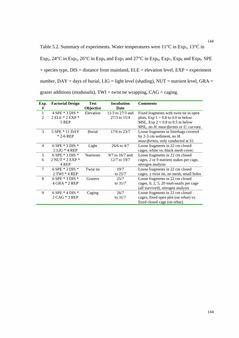
144

144

Table 5.2. Summary of experiments. Water temperatures were 11 C in Exp1, 13 C in

Exp2, 24 C in Exp3, 26 C in Exp4 and Exp5 and 27 C in Exp6, Exp7, Exp8 and Exp9. SPE

= species type, DIS = distance from mainland, ELE = elevation level, EXP = experiment

number, DAY = days of burial, LIG = light level (shading), NUT = nutrient level, GRA =

grazer additions (mudsnails), TWI = twist tie wrapping, CAG = caging.

Exp.#

Factorial Design TestObjective

IncubationDate

Comments

12

4 SPE * 3 DIS *2 ELE * 2 EXP *

5 REP

Elevation 11/3 to 27/3 and27/3 to 15/4

Fixed fragments with twist tie in openplots, Exp 1 = 0.8 to 0.0 m belowMSL, Exp 2 = 0.8 to 0.5 m belowMSL, no H. musciformis or U. curvata

3 5 SPE * 11 DAY* 2-6 REP

Burial 17/6 to 23/7 Loose fragments in litterbags coveredby 2-3 cm sediment, no H.musciformis, only conducted at S1

4 6 SPE * 3 DIS *2 LIG * 4 REP

Light 26/6 to 4/7 Loose fragments in 22 cm closedcages, white vs. black mesh cover.

56

6 SPE * 3 DIS *2 NUT * 2 EXP *

4 REP

Nutrients 9/7 to 16/7 and12/7 to 19/7

Loose fragments in 22 cm closedcages, 2 or 0 nutrient stakes per cage,nitrogen analysis

7 6 SPE * 3 DIS *2 TWI * 4 REP

Twist tie 19/7to 25/7

Loose fragments in 22 cm closedcages, ± twist tie, no mesh, small holes

8 6 SPE * 3 DIS *4 GRA * 2 REP

Grazers 25/7to 31/7

Loose fragments in 22 cm closedcages, 0, 2, 5, 20 mud-snails per cage(all survived), nitrogen analysis

9 6 SPE * 4 DIS *2 CAG * 3 REP

Caging 26/7to 31/7

Loose fragments in 22 cm closedcages, fixed open plot (on rebar) vs.fixed closed cage (on rebar)

145

145

Table 5.3A. ANOVA results on assemblage performance (Exp. 1-6). Significant results

are in bold (p < 0.05). Levenes test of equality of variances were significant for all tests.

Exp Source Df SS 2(%) F p1 & 2 Species (SPE) 3 206960 18 30.29 0.0001 & 2 Elevation (ELE) 1 162754 14 71.47 0.0001 & 2 Experiment (EXP) 1 122714 11 53.88 0.0001 & 2 Distance (DIS) 2 8011 1 1.76 0.1751 & 2 SPE * ELE 3 82851 7 12.13 0.0001 & 2 ELE * EXP 1 22633 2 9.94 0.0021 & 2 SPE * EXP 3 20784 2 3.04 0.0301 & 2 DIS * ELE 2 12483 1 2.74 0.0671 & 2 DIS * EXP 2 7373 1 1.62 0.2011 & 2 SPE * DIS 6 14729 1 1.08 0.3771 & 2 SPE * ELE * EXP 3 19292 2 2.82 0.0401 & 2 SPE * DIS * ELE 6 24493 2 1.79 0.1031 & 2 DIS * ELE * EXP 2 4822 0 1.06 0.3491 & 2 SPE * DIS * EXP 6 11460 1 0.84 0.5421 & 2 SPE * DIS * ELE * EXP 6 5479 0 0.40 0.8781 & 2 Error 181 412198 36

3 Days of burial (DAY) 9 151880 69 112.65 0.0003 SPE 4 22436 10 37.44 0.0003 SPE * DAY 36 25925 12 4.81 0.0003 Error 135 20224 94 SPE 5 611495 38 25.54 0.0004 Light level (LIG) 1 92409 6 19.30 0.0004 DIS 2 103218 6 10.78 0.0004 SPE * LIG 5 137360 9 5.74 0.0004 SPE * DIS 10 124461 8 2.60 0.0074 DIS * LIG 2 7036 0 0.73 0.4824 SPE * DIS * LIG 10 22752 1 0.48 0.9034 Error 105 502830 31

5 & 6 SPE 5 1781988 62 105.97 0.0005 & 6 DIS 2 59707 2 8.88 0.0005 & 6 Nutrients (NUT) 1 18056 1 5.37 0.0215 & 6 EXP 1 15926 1 4.74 0.0315 & 6 SPE * DIS 10 110087 4 3.27 0.0015 & 6 SPE * EXP 5 35546 1 2.11 0.0655 & 6 SPE * NUT 5 31972 1 1.90 0.0955 & 6 DIS * NUT 2 8411 0 1.25 0.2885 & 6 NUT * EXP 1 2220 0 0.66 0.4175 & 6 DIS * EXP 2 666 0 0.10 0.9065 & 6 SPE * NUT * EXP 5 19707 1 1.17 0.3245 & 6 SPE * DIS * NUT 10 25847 1 0.77 0.6595 & 6 DIS * NUT * EXP 2 269 0 0.04 0.9615 & 6 SPE * DIS * EXP 10 10123 0 0.30 0.9805 & 6 SPE * DIS * NUT * EXP 10 11775 0 0.35 0.9665 & 6 Error 216 726468 25

146

146

Table 5.3B. ANOVA results on assemblage performance (continued from Table 5.3A,

Exp. 7-9). Significant (p < 0.05) results are in bold. Levenes test of equality of variances

were significant for all tests.

Exp Source Df SS 2(%) F p7 SPE 5 134416 50 32.69 0.0007 Twist tie (TWI) 1 5263 2 6.40 0.0137 DIS 2 4652 2 2.83 0.0647 DIS * TWI 2 8697 3 5.29 0.0077 SPE * DIS 10 15561 6 1.89 0.0557 SPE * TWI 5 5177 2 1.26 0.2887 SPE * DIS * TWI 10 11834 4 1.44 0.1747 Error 100 82243 318 SPE 5 552785 40 37.19 0.0008 Grazing (GRA) 3 166662 12 18.69 0.0008 DIS 2 107919 8 18.15 0.0008 SPE * GRA 15 212153 15 4.76 0.0008 SPE * DIS 10 69098 5 2.32 0.0208 DIS * GRA 6 15483 1 0.87 0.5238 SPE * DIS * GRA 30 46596 3 0.52 0.9758 Error 72 214054 159 SPE 5 211489 20 7.92 0.0009 Caging (CAG) 1 72105 7 13.50 0.0009 DIS 2 20340 2 1.90 0.1579 SPE * CAG 5 114067 11 4.27 0.0029 SPE * DIS 10 130549 13 2.44 0.0159 DIS * CAG 2 22663 2 2.12 0.1289 SPE * DIS * CAG 10 106703 10 2.00 0.0479 Error 68 363282 35

Sum SPE 5 2328621 33 108.19 0.000Sum DIS 2 195322 3 22.69 0.000Sum EXP 5 163886 2 7.61 0.000Sum SPE * DIS 10 177596 2 4.13 0.000Sum SPE * EXP 25 850383 12 7.90 0.000Sum DIS * EXP 10 84669 1 1.97 0.034Sum SPE * DIS * EXP 50 268918 4 1.25 0.121Sum Error 705 3034706 43

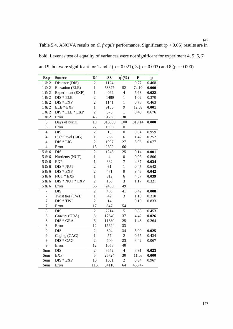
147

147

Table 5.4. ANOVA results on C. fragile performance. Significant (p < 0.05) results are in

bold. Levenes test of equality of variances were not significant for experiment 4, 5, 6, 7

and 9, but were significant for 1 and 2 (p = 0.021), 3 (p = 0.003) and 8 (p = 0.000).

Exp Source Df SS 2(%) F p1 & 2 Distance (DIS) 2 1124 1 0.77 0.4681 & 2 Elevation (ELE) 1 53877 52 74.10 0.0001 & 2 Experiment (EXP) 1 4092 4 5.63 0.0221 & 2 DIS * ELE 2 1480 1 1.02 0.3701 & 2 DIS * EXP 2 1141 1 0.78 0.4631 & 2 ELE * EXP 1 9155 9 12.59 0.0011 & 2 DIS * ELE * EXP 2 575 1 0.40 0.6761 & 2 Error 43 31265 30

3 Days of burial 10 315000 100 819.14 0.0003 Error 27 1038 04 DIS 2 15 0 0.04 0.9594 Light level (LIG) 1 255 6 1.42 0.2524 DIS * LIG 2 1097 27 3.06 0.0774 Error 15 2692 66

5 & 6 DIS 2 1246 25 9.14 0.0015 & 6 Nutrients (NUT) 1 4 0 0.06 0.8065 & 6 EXP 1 332 7 4.87 0.0345 & 6 DIS * NUT 2 61 1 0.45 0.6425 & 6 DIS * EXP 2 471 9 3.45 0.0425 & 6 NUT * EXP 1 312 6 4.57 0.0395 & 6 DIS * NUT * EXP 2 160 3 1.17 0.3215 & 6 Error 36 2453 49

7 DIS 2 488 41 6.42 0.0087 Twist ties (TWI) 1 42 3 1.10 0.3107 DIS * TWI 2 14 1 0.19 0.8337 Error 17 647 548 DIS 2 2214 5 0.85 0.4538 Grazers (GRA) 3 17340 37 4.42 0.0268 DIS * GRA 6 11630 25 1.48 0.2648 Error 12 15694 339 DIS 2 894 34 5.09 0.0259 Caging (CAG) 1 57 2 0.65 0.4349 DIS * CAG 2 600 23 3.42 0.0679 Error 12 1053 40

Sum DIS 2 3652 4 3.91 0.023Sum EXP 5 25724 30 11.03 0.000Sum DIS * EXP 10 1601 2 0.34 0.967Sum Error 116 54110 64 466.47

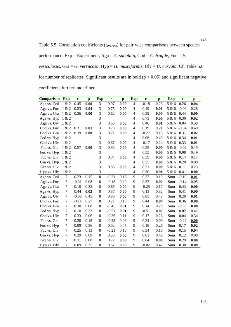
148

148

Table 5.5. Correlation coefficients (rPearson) for pair-wise comparisons between species

performance. Exp = Experiment, Aga = A. subulata, Cod = C. fragile, Fuc = F.

vesiculosus, Gra = G. verrucosa, Hyp = H. musciformis, Ulv = U. curvata. Cf. Table 5.6

for number of replicates. Significant results are in bold (p < 0.05) and significant negative

coefficients further underlined.

Comparison Exp r p Exp r p Exp r p Exp r pAga vs. Cod 1 & 2 0.45 0.00 3 0.97 0.00 4 -0.18 0.23 5 & 6 0.26 0.04Aga vs. Fuc 1 & 2 0.23 0.04 3 0.75 0.00 4 0.49 0.01 5 & 6 -0.09 0.28Aga vs. Gra 1 & 2 0.36 0.00 3 0.62 0.00 4 0.59 0.00 5 & 6 0.44 0.00Aga vs. Hyp 1 & 2 3 4 0.73 0.00 5 & 6 0.30 0.02Aga vs. Ulv 1 & 2 3 0.65 0.00 4 0.46 0.01 5 & 6 0.04 0.39Cod vs. Fuc 1 & 2 0.31 0.01 3 0.78 0.00 4 0.19 0.21 5 & 6 -0.04 0.40Cod vs. Gra 1 & 2 0.39 0.00 3 0.71 0.00 4 -0.27 0.13 5 & 6 0.31 0.02Cod vs. Hyp 1 & 2 3 4 0.06 0.40 5 & 6 0.34 0.01Cod vs. Ulv 1 & 2 3 0.67 0.00 4 -0.17 0.24 5 & 6 0.33 0.01Fuc vs. Gra 1 & 2 0.57 0.00 3 0.83 0.00 4 0.58 0.00 5 & 6 -0.02 0.45Fuc vs. Hyp 1 & 2 3 4 0.55 0.00 5 & 6 0.08 0.49Fuc vs. Ulv 1 & 2 3 0.84 0.00 4 0.59 0.00 5 & 6 0.14 0.17Gra vs. Hyp 1 & 2 3 4 0.55 0.00 5 & 6 0.20 0.08Gra vs. Ulv 1 & 2 3 0.85 0.00 4 0.71 0.00 5 & 6 0.11 0.23Hyp vs. Ulv 1 & 2 3 4 0.50 0.01 5 & 6 0.41 0.00Aga vs. Cod 7 0.23 0.15 8 -0.21 0.16 9 0.32 0.10 Sum -0.19 0.01Aga vs. Fuc 7 -0.31 0.08 8 -0.18 0.20 9 0.53 0.02 Sum -0.14 0.05Aga vs. Gra 7 0.10 0.33 8 0.65 0.00 9 -0.25 0.17 Sum 0.43 0.00Aga vs. Hyp 7 0.44 0.02 8 0.57 0.00 9 0.13 0.32 Sum 0.41 0.00Aga vs. Ulv 7 -0.03 0.45 8 0.86 0.00 9 0.05 0.43 Sum 0.20 0.01Cod vs. Fuc 7 -0.14 0.27 8 0.27 0.10 9 0.44 0.04 Sum 0.36 0.00Cod vs. Gra 7 0.30 0.08 8 -0.45 0.01 9 0.14 0.29 Sum -0.33 0.00Cod vs. Hyp 7 0.10 0.32 8 -0.51 0.01 9 -0.51 0.02 Sum 0.02 0.41Cod vs. Ulv 7 0.33 0.06 8 -0.26 0.11 9 0.17 0.26 Sum 0.04 0.34Fuc vs. Gra 7 0.20 0.18 8 -0.28 0.09 9 0.34 0.09 Sum -0.22 0.00Fuc vs. Hyp 7 0.09 0.36 8 0.02 0.45 9 0.18 0.26 Sum 0.17 0.02Fuc vs. Ulv 7 0.25 0.13 8 -0.21 0.16 9 0.34 0.10 Sum 0.15 0.04Gra vs. Hyp 7 0.29 0.09 8 0.56 0.00 9 0.01 0.49 Sum 0.12 0.08Gra vs. Ulv 7 0.31 0.08 8 0.72 0.00 9 0.64 0.00 Sum 0.29 0.00Hyp vs. Ulv 7 0.09 0.35 8 0.67 0.00 9 -0.02 0.47 Sum 0.30 0.00

149

149

Table 5.6. Number of replicates (n) and mean (X) and maximum (Max) biomass per

fragment at the start (WW-t0) and the end (WW-t1) of the experiments.

T0 T1

Exp Cod Fuc Aga Gra Hyp Ulv Cod Fuc Aga Gra Hyp Ulvn E1 28 28 28 28 28 28 28 28n E2 27 27 27 27 27 27 27 27n E3 37 37 37 37 37 37 37 37 37 37n E4 24 24 24 24 24 24 22 24 24 24 24 24n E5 24 24 24 24 24 24 24 24 24 24 24 24n E6 24 24 24 24 24 24 24 24 24 24 24 24n E7 24 24 24 24 24 24 23 22 23 23 22 23n E8 24 24 24 24 24 24 24 24 24 24 24 24n E9 18 18 18 18 18 18 18 18 17 18 17 17X E1 1.26 0.69 1.04 0.87 0.71 0.76 0.50 0.74X E2 1.15 0.70 1.05 0.81 0.86 1.15 0.94 1.33X E3 0.40 0.64 0.45 0.45 0.40 0.05 0.20 0.04 0.15 0.12X E4 0.68 0.48 0.75 0.43 0.22 0.32 0.81 0.52 1.14 0.51 0.66 0.63X E5 0.68 0.48 0.58 0.43 0.22 0.32 0.82 0.52 0.81 0.60 0.48 1.02X E6 1.00 0.70 0.85 0.63 0.17 0.25 1.16 0.76 0.73 0.63 0.35 0.78X E7 0.68 0.48 0.58 0.43 0.18 0.32 0.63 0.50 0.78 0.54 0.25 0.62X E8 0.68 0.48 0.58 0.43 0.18 0.18 0.60 0.46 1.07 0.82 0.38 0.46X E9 0.68 0.48 0.58 0.43 0.18 0.18 0.76 0.51 0.82 0.80 0.30 0.39

Max E1 1.61 1.02 1.37 1.23 1.75 1.24 1.58 1.86Max E2 1.44 1.06 1.32 1.16 1.54 2.46 5.09 3.72Max E3 0.40 0.64 0.45 0.45 0.40 0.41 0.77 0.46 0.46 0.44Max E4 0.68 0.48 0.75 0.43 0.22 0.32 1.02 0.56 2.71 0.72 1.48 1.81Max E5 0.68 0.48 0.58 0.43 0.22 0.32 0.96 0.60 1.27 0.86 1.53 1.93Max E6 1.33 0.93 1.13 0.83 0.22 0.32 1.76 1.06 1.48 1.05 0.70 1.76Max E7 0.68 0.48 0.58 0.43 0.18 0.32 0.73 0.57 1.18 0.64 0.39 0.92Max E8 0.68 0.48 0.58 0.43 0.18 0.18 0.93 0.56 2.43 1.45 0.82 0.91Max E9 0.68 0.48 0.58 0.43 0.18 0.18 0.90 0.58 1.38 1.33 1.29 1.22

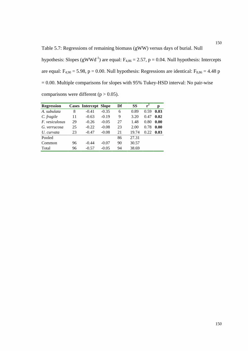
150

150

Table 5.7: Regressions of remaining biomass (gWW) versus days of burial. Null

hypothesis: Slopes (gWWd-1) are equal: F4,86 = 2.57, p = 0.04. Null hypothesis: Intercepts

are equal: F4,90 = 5.98, p = 0.00. Null hypothesis: Regressions are identical: F8,86 = 4.48 p

= 0.00. Multiple comparisons for slopes with 95% Tukey-HSD interval: No pair-wise

comparisons were different (p > 0.05).

Regression Cases Intercept Slope Df SS r2 pA. subulata 8 -0.41 -0.35 6 0.89 0.59 0.03C. fragile 11 -0.63 -0.19 9 3.20 0.47 0.02F. vesiculosus 29 -0.26 -0.05 27 1.48 0.80 0.00G. verrucosa 25 -0.22 -0.08 23 2.00 0.78 0.00U. curvata 23 -0.47 -0.08 21 19.74 0.22 0.03Pooled 86 27.31Common 96 -0.44 -0.07 90 30.57Total 96 -0.57 -0.05 94 38.69

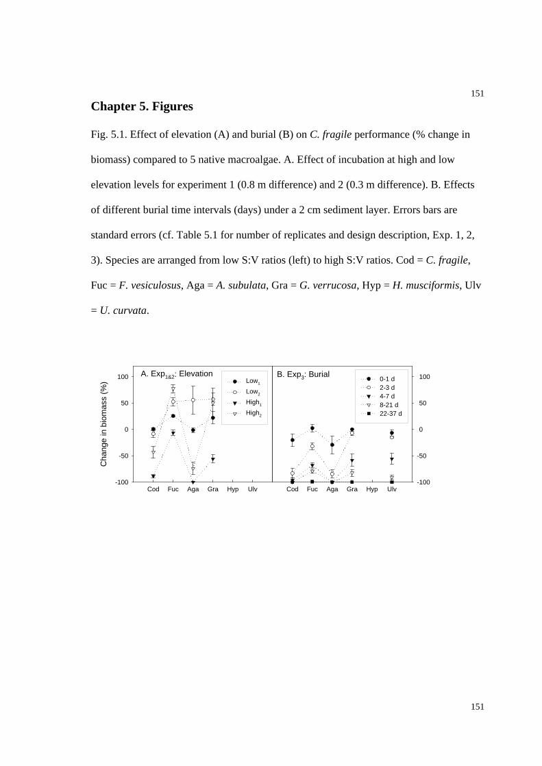
151

151

Chapter 5. Figures

Fig. 5.1. Effect of elevation (A) and burial (B) on C. fragile performance (% change in

biomass) compared to 5 native macroalgae. A. Effect of incubation at high and low

elevation levels for experiment 1 (0.8 m difference) and 2 (0.3 m difference). B. Effects

of different burial time intervals (days) under a 2 cm sediment layer. Errors bars are

standard errors (cf. Table 5.1 for number of replicates and design description, Exp. 1, 2,

3). Species are arranged from low S:V ratios (left) to high S:V ratios. Cod = C. fragile,

Fuc = F. vesiculosus, Aga = A. subulata, Gra = G. verrucosa, Hyp = H. musciformis, Ulv

= U. curvata.

A. Exp1&2: Elevation

Cod Fuc Aga Gra Hyp Ulv

Cha

nge

in b

iom

ass

(%)

-100

-50

0

50

100Low1

Low2

High1

High2

B. Exp3: Burial

Cod Fuc Aga Gra Hyp Ulv-100

-50

0

50

1000-1 d2-3 d4-7 d8-21 d22-37 d

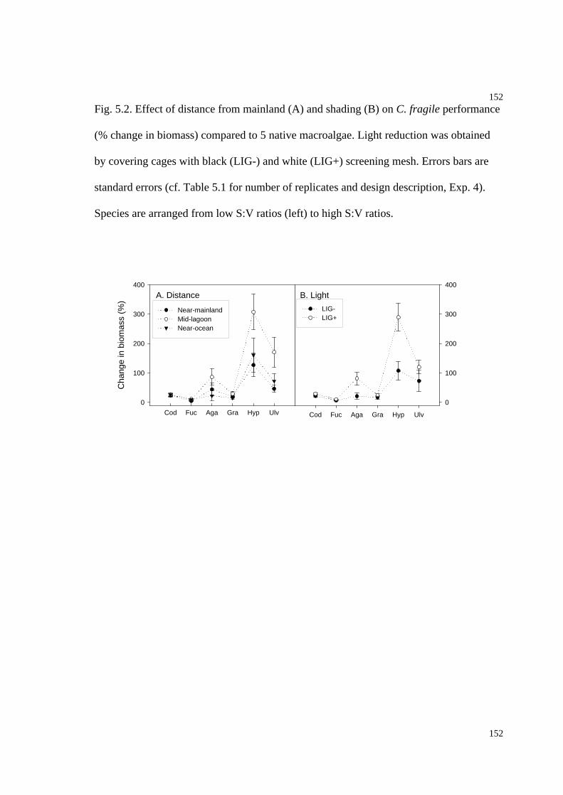
152

152

Fig. 5.2. Effect of distance from mainland (A) and shading (B) on C. fragile performance

(% change in biomass) compared to 5 native macroalgae. Light reduction was obtained

by covering cages with black (LIG-) and white (LIG+) screening mesh. Errors bars are

standard errors (cf. Table 5.1 for number of replicates and design description, Exp. 4).

Species are arranged from low S:V ratios (left) to high S:V ratios.

A. Distance

Cod Fuc Aga Gra Hyp Ulv

Cha

nge

in b

iom

ass

(%)

0

100

200

300

400

Near-mainlandMid-lagoonNear-ocean

B. Light

Cod Fuc Aga Gra Hyp Ulv

0

100

200

300

400

LIG-LIG+

153

153

Fig. 5.3. Effect of distance from mainland (left) and nutrient addition (right) on C. fragile

performance compared to 5 native macroalgae. Left graphs: effect of 3 distances for the

nutrient addition experiments data on biomass performance (A), nitrogen concentration

(C) and total nitrogen content per species (E). Right graphs: effects of nutrient addition

(NUT+) versus controls (NUT-) on biomass performance (B), nitrogen concentration (D)

and total nitrogen content per species (F). Errors bars are standard errors (cf. Table 5.1

for number of replicates and design description, Exp. 5, 6). Species are arranged from

low S:V ratios (left) to high S:V ratios.

A. Distance (biomass)

Cod Fuc Aga Gra Hyp Ulv

Cha

nge

in b

iom

ass

(%)

0

100

200

300Near-mainlandMid-lagoonNear-ocean

B. Nutrients (biomass)

Cod Fuc Aga Gra Hyp Ulv

0

100

200

300NUT-NUT+

C. Distance (tissue N)

Cod Fuc Aga Gra Hyp Ulv

%N

(D

W)

per

frag

men

t

0.8

1.2

1.6

2.0

D. Nutrients (tissue N)

Cod Fuc Aga Gra Hyp Ulv

0.8

1.2

1.6

2.0

E. Distance (total N)

Cod Fuc Aga Gra Hyp Ulv

gN (

DW

) pe

r fr

agm

ent

0.04

0.08

0.12

0.16F. Nutrients (total N)

Cod Fuc Aga Gra Hyp Ulv

0.04

0.08

0.12

0.16

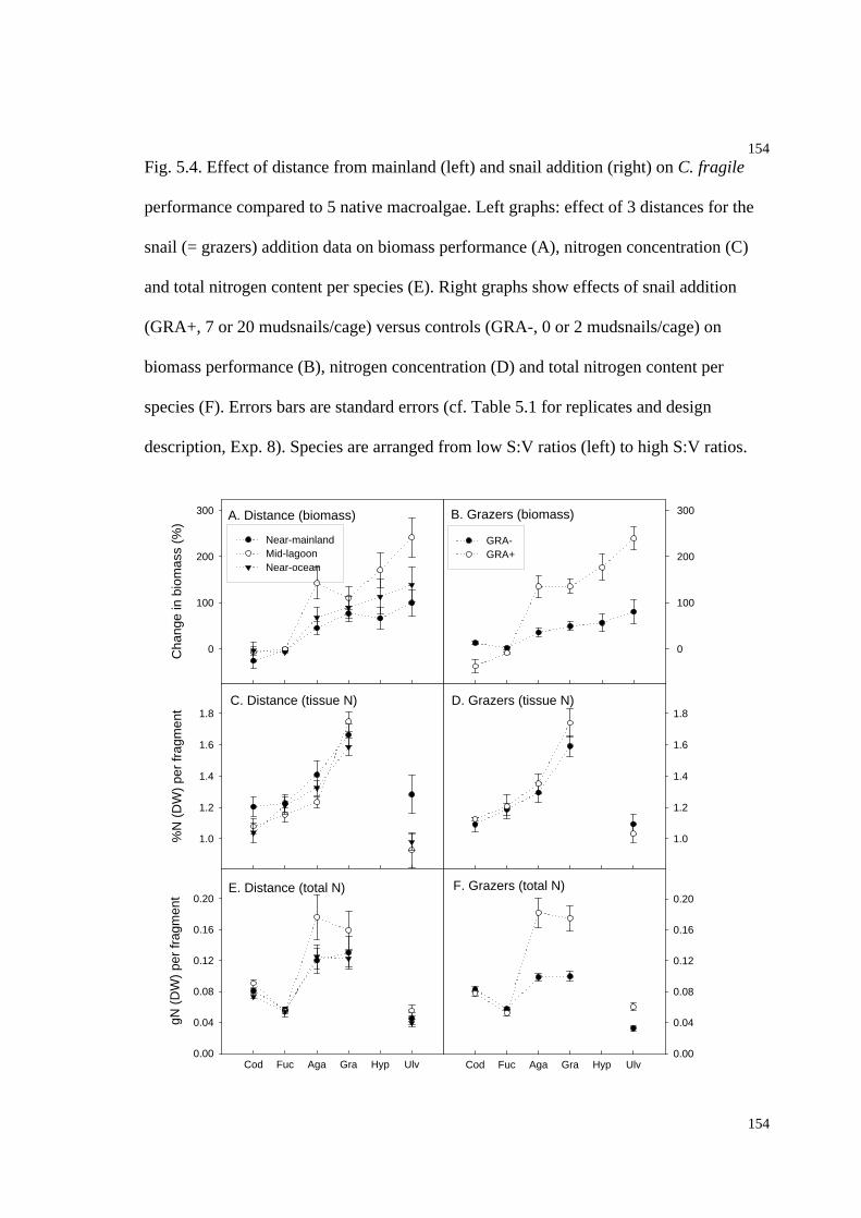
154

154

Fig. 5.4. Effect of distance from mainland (left) and snail addition (right) on C. fragile

performance compared to 5 native macroalgae. Left graphs: effect of 3 distances for the

snail (= grazers) addition data on biomass performance (A), nitrogen concentration (C)

and total nitrogen content per species (E). Right graphs show effects of snail addition

(GRA+, 7 or 20 mudsnails/cage) versus controls (GRA-, 0 or 2 mudsnails/cage) on

biomass performance (B), nitrogen concentration (D) and total nitrogen content per

species (F). Errors bars are standard errors (cf. Table 5.1 for replicates and design

description, Exp. 8). Species are arranged from low S:V ratios (left) to high S:V ratios.

A. Distance (biomass)

Cod Fuc Aga Gra Hyp Ulv

Cha

nge

in b

iom

ass

(%)

0

100

200

300

Near-mainlandMid-lagoonNear-ocean

B. Grazers (biomass)

Cod Fuc Aga Gra Hyp Ulv

0

100

200

300

GRA-GRA+

C. Distance (tissue N)

Cod Fuc Aga Gra Hyp Ulv

%N

(D

W)

per

frag

men

t

1.0

1.2

1.4

1.6

1.8D. Grazers (tissue N)

Cod Fuc Aga Gra Hyp Ulv

1.0

1.2

1.4

1.6

1.8

E. Distance (total N)

Cod Fuc Aga Gra Hyp Ulv

gN (

DW

) pe

r fr

agm

ent

0.00

0.04

0.08

0.12

0.16

0.20F. Grazers (total N)

Cod Fuc Aga Gra Hyp Ulv0.00

0.04

0.08

0.12

0.16

0.20

155

155

Fig. 5.5. Effect of distance from mainland (A) and twist-tie wrapping (B) on C. fragile

performance (% change in biomass) compared to 5 native macroalgae. Half of the tissue

were wrapped with twist-tie (TWI+) versus non-wrapped controls (TWI-) looselying in

cages. Errors bars are standard errors (cf. Table 5.1 for number of replicates and design

description, Exp. 7). Species are arranged from low S:V ratios (left) to high S:V ratios.

B. Twist tie

Cod Fuc Aga Gra Hyp Ulv

0

50

100

150

TWI-TWI+

A. Distance

Cod Fuc Aga Gra Hyp Ulv

Cha

nge

in b

iom

ass

(%)

0

50

100

150

Near-mainlandMid-lagoonNear-ocean

156

156

Fig. 5.6. Effect of distance from mainland (A) and caging (B) on C. fragile performance

(% change in biomass) compared to 5 native macroalgae. Fragments were fixed in space

with wrapped twist tie. Errors bars are standard errors (cf. Table 5.1 for number of

replicates and design description, Exp. 9). Species are arranged from low S:V ratios (left)

to high S:V ratios.

B. Caging

Cod Fuc Aga Gra Hyp Ulv

0

100

200

300CAG-CAG+

A. Distance

Cod Fuc Aga Gra Hyp Ulv

Cha

nge

in b

iom

ass

(%)

0

100

200

300

Near-mainlandMid-lagoonNear-ocean

157

157

Fig. 5.7. Effect of distance from mainland (A) and experimental design (B) on C. fragile

performance (% change in biomass) compared to 5 native macroalgae. Errors bars are

standard errors (cf. Table 5.1 for number of replicates and design description). Species

are arranged from low S:V ratios (left) to high S:V ratios.

A. Distance

Cod Fuc Aga Gra Hyp Ulv

Cha

nge

in b

iom

ass

(%)

0

100

200

300

Near-mainlandMid-lagoonNear-ocean

B. Experiment

Cod Fuc Aga Gra Hyp Ulv

0

100

200

300

E4E5E6E7E8E9

158

158

Chapter 6. Performance of oyster reef associated

sessile organisms: effects of hydrodynamics and

accumulations of sediments and drift algae

159

159

Abstract

Proliferation of drift algae and enhanced sedimentation are major disturbances in shallow

lagoons. It is well known that these disturbances affect seagrass beds and soft bottom

fauna, but less is known about how these disturbances affect lagoonal hard bottom

assemblages. In soft bottom lagoons the oyster is a foundation species that affects the

local biota by altering hydrodynamic conditions and biogeochemical cycles, and by

providing substrate for reef-associated organisms. To test if accumulations of drift algae

or sediments affected recruitment of oyster reef associated sessile organisms, cages were

constructed to trap either algae or sediments on recruitment bricks. The experiment was

conducted simultaneously in front, between, and behind a series of oyster reefs at a mid-

lagoon shoal site in Hog Island Bay, Virginia. These locations represent different

hydrodynamic habitats: wave-exposed, current-exposed and wave- and current-protected.

The abundances of attached taxa were mapped on the recruitment bricks four times

during a one-year period. There were significant multivariate effects of both cover type

and hydrodynamics on the species assemblage, but no interaction effects. The coverage

of either algae or sediments explained 2-6 times more of the assemblage variability than

hydrodynamics. Bricks with no cover (controls) had high taxonomic richness and

abundance of attached organisms. In comparison, bricks with drift algal cover had

medium richness and low abundance, and sediment-covered bricks low richness and very

low abundance. Overall, the red algae Gracilaria verrucosa and Agardhiella subulata,

the green algae Codium fragile ssp. tomentosoides, Ulva curvata and Enteromorpha sp.

and the oyster Crassostrea virginica were the most abundant taxa, particularly on the

control bricks. These taxa followed the pattern described for total abundance, except that

160

160

Enteromorpha and U. curvata were common under a cover of drift algae. C. fragile is an

alien macroalgae that some claim has smothered oyster beds. Here, C. virginica and C.

fragile showed similar distribution patterns, but were not observed co-occurring in high

abundance, suggesting that they may compete for space. Overall, cover of sediments or

drift algae profoundly affected the distribution and abundance of sessile reef-associated

organisms, favoring a few small ephemeral taxa. This suggests that drift algae growth and

sedimentation that are usually associated with eutrophication will cause an

impoverishment of oyster reef assemblages. Because oysters themselves recruited poorly

under a cover of drift algae or sediments, longer-term effects may result in diminishing

reef structures with potentially negative effects beyond the structure of a patch reef (e.g.

less hard substrate for sessile organisms, reduced topographic complexity, less shelter for

small invertebrates).

Introduction

In soft bottom lagoons, oysters reefs provide three-dimensional habitats that contain rich

and abundant floral and faunal assemblages (Barh & Lanier 1981, Galtsoff 1964).

Healthy oyster reefs alter local biogeochemical cycles by their water filtering and

sediment-binding capacities (Dame 1993, Haven & Whitcomb 1983, Lenihan 1999,

Mann 2000, Möbius 1877). In general, oyster reefs are similar to coral reefs, kelp forests,

mangroves, salt marshes, seagrass beds, and mussel beds, in that they are composed of a

few foundation species (sensu Dayton 1972) that facilitate the distribution and abundance

of a range of associated species (Bruno & Bertness 2001, Bruno et al. in press). Because

of ecological and economic benefits associated with healthy and abundant oyster reefs

161

161

(Barh & Lanier 1981, Galtsoff 1964, Mann 2000), oysters have been well-studied from

an autecological perspective, but synecological field experiments on oyster reef

assemblages are surprisingly few (Anderson & Underwood 1997, Underwood &

Anderson 1994). Oyster reefs in soft bottom lagoons provide physical relief in an

otherwise flat and smooth habitat, and as a result cause local flow accelerations and

decelerations (Barh & Lanier 1981, Lenihan 1999). Oyster reefs can thereby influence

processes that depend on hydrodynamic conditions and that affect biological

performance, such as sedimentation and resuspension rates (Airoldi 2003, Lawson 2003,

Lenihan 1999), drift algae accumulations (Chapter 4, Raffaelli et al. 1998), grazing rates

(Duggins et al. 2001, Kawamata 1998) and nutrient/particle encounter rates (Hurd 2000,

Lenihan et al. 1996, Wheeler 1988).

Lagoonal oyster reefs are threatened by diseases, over-harvesting, and natural predators

(Barh & Lanier 1981, Haven & Whitcomb 1983, Luckenbach et al. 1999, Mann 2000,

McCormick-Ray 1998). Urbanization, agricultural runoff, coastal development and

increased boat traffic are additional stressors that may also impact oyster reefs. The

impact on the oyster reefs include: (1) enhanced sedimentation/sediment instability

(Airoldi 2003, Koch & Gust 1999, McManus 1998), (2) nutrient enrichment followed by

enhanced drift algae accumulations (Fletcher 1996, Morand & Briand 1996, Raffaelli et

al. 1998), and (3) introduction of alien species (Moyle 1999, Ruiz et al. 1997, Ruiz et al.

1999).

162

162

Sedimentation, nutrient-enrichment and drift algae accumulations severely reduce the

productivity, depth penetration and spatial extent of rooted habitat-forming angiosperms

(Hauxwell et al. 2001, Holmquist 1997, Morand & Briand 1996, Nelson & Lee 2001,

Raffaelli et al. 1989, Sand-Jensen & Borum 1991, Valiela et al. 1997). These stresses also

limit infaunal and epifaunal species richness and abundance by suffocation, development

of anoxia, limiting larvae from reaching the substratum, reducing flow rate, and interfer

with feeding behaviors (Hull 1987, Norkko 1998, Norkko & Bonsdorff 1996c, a,

Raffaelli et al. 1998). However, it is not known if and how sediment and drift algae

stresses interfere with hard bottom assemblages, within soft bottom systems. The severity

of these disturbances is most likely linked to local hydrodynamic conditions. For

example, strong currents can reduce sedimentation rates and flush out algal mats, thereby

reducing adverse effects of increased stresses (Flindt et al. 1997a, Hiscock 1983,

Raffaelli et al. 1998, Salomonsen et al. 1997). On the other hand accumulations of drift

algae and sediments may be elevated in low energy habitats, i.e. with potential enhanced

stresses on associated reef organisms. Thus, it is possible that the influence of oyster reefs

on hydrodynamics can moderate or accelerate the effects of these stresses (Lenihan

1999).

In addition to enhanced sedimentation and drift algae accumulations, alien pests have

repeatedly invaded North American lagoons and estuaries, and some of these invasions

have previously been linked to nutrient enrichment (Moyle 1999, Ruiz et al. 1999). The

macroalgae Codium fragile ssp. tomentosoides has been a particular successful invader in

many low energy eutrophic lagoons and estuaries where oyster reefs are abundant

163

163

(Fralick & Mathieson 1973, Malinowski & Ramus 1973, Ramus & Venable 1987,

Trowbridge 1998). The dispersal and success of C. fragile has typically been associated

with oysters (Campbell 1999, Churchill & Moeller 1972, Garbary et al. 1997, Trowbridge

1998) and it has been suggested that C. fragile can smother and suffocate oysters, as well

as drift away with oysters attached to its holdfast (Fralick & Mathieson 1973, Hillson

1976, Mathieson et al. 2003, Trowbridge 1998, 1999). To have a significant negative

effect on oyster reefs, C. fragile must recruit onto reefs in high densities and grow fast

compared to native reef associated organisms. To our knowledge, there have been no

studies that have compared recruitment of C. fragile to that of native sessile oyster reef

taxa. The main study objectives were therefore threefold: (1) to test for effects of

sediments and drift algae on the recruitment, survival, and growth of oyster reef-

associated sessile organisms, (2) to test if oyster reef structures create different

hydrodynamic regimes and thereby influence sedimentation, drift algae accumulations

and recruitment of reef organisms, and (3) to test if the invasive C. fragile is a stronger

recruiter, compared to native reef organisms, under different conditions of drift algae and

sediment accumulation and hydrodynamic regimes.

Methods

Study site

Hog Island Bay is located in the Virginia Coast Reserve on the Delmarva Peninsula and

is part of the US Long Term Ecological Research Program (Hayden et al. 2000). Hog

Island Bay is a dynamic system that has changed considerably during the last 70 years

with extinction of extensive sediment-binding seagrass meadows in the 1930 s due to

164

164

storms and diseases (Hayden et al. 2000, Ralph & Short 2002), decimation of filter

feeding oyster populations in the 1940-1960 s by disease and overharvesting (Gottlieb &

Schweighofer 1996, Mann 2000), accumulations of drift algal mats in the 1960-1970 s

(Goshorn et al. 2001, Truitt 2002) and invasions of alien species in the 1970-1990 s

(Hayden et al. 2000, Hillson 1976, Monti 1993). The macroalgal pest C. fragile ssp.

tomentosoides originates from the northwest Pacific (Chapman 1999, Trowbridge 1999)

and arrived in Virginia and Hog Island Bay in the 1970 s (Hillson 1976, Monti 1993).

Although not dominant in absolute biomass terms on the lagoonal scale, C. fragile is

today the fourth most abundant macroalgae in the bay, and is particularly common below

0.6 m above mean sea level at mid-lagoon sites (Chapter 3, Appendix 1).

Experimental design

Preliminary experiments showed that sessile species typically found attached to oyster

shells could recruit onto clay bricks (20 * 8 * 6 cm, Appendix 1). Because we were

interested in taxonomic richness and detection of rare species, the percent cover method

was chosen over the more time-consuming method of determining species occurrence at

30 random pin points (Dethier et al. 1993). Before recording percent cover, each brick

was gently cleaned of sediments to ensure that small and buried sessile taxa were

observed. Cover could exceed 100% if organisms occupied different vertical layers

and/or covered more than 184 cm2 (the area of a single recruitment brick). To minimize

observer variability a training session, estimating cover of computer generated screen

patterns was conducted prior to a sampling event, and a sample-frame divided into 20

165

165

rectangles was used to aid in cover estimations (10 rectangles covered the brick, and 10

covered the brick peripherals).

An orthogonal experiment was designed to test if a cover of sediments or drift algae, and

hydrodynamic conditions affected recruitment of attached organisms. First, plots were

allocated to areas in front, between, and behind a series of scattered oyster reefs in the

mid-lagoon (Shoal site, McGlathery et al. 2001). Spatial location was hypothesized to

reflect hydrodynamic regime (Lenihan 1999) and was used as a natural experimental

treatment. Areas in front of oyster reefs were subject to the largest fetch and had the

steepest slope, and were hypothesized to be susceptible to waves generated under windy

conditions (hereafter wave-exposed sites). Areas between reefs were hypothesized to

have elevated tidal currents (hereafter current-exposed sites). Finally, areas behind reefs

were hypothesized to be protected from both waves and currents (hereafter protected

sites). All plots were positioned within the 0.6-0.8 m below mean sea level depth contour

where C. fragile had been observed to recruit with success (Appendix 1.6). Two random

sites were allocated in front, between and behind oyster reefs, situated to the east of and

parallel to the Machinpongo channel (Hayden et al. 2000, Oertel et al. 2000). These six

sites were separated by a minimum of 30 m. Within each site 2 open control plots, 2

sediment cages and 2 drift algae traps, were systematically allocated, each plot/cage

separated by approximately one meter. Sediment-cages were constructed of 65*50*50 cm

plastic boxes to reduce tidal currents and thereby trigger sediment deposition on small

spatial scales. The cages were transparent to minimize shading at low solar angles, but

resulted in a 5% light reduction accumulated over an entire day (Table 6.1). Cages were

166

166

fixed with rebar which was inserted through holes drilled in the corners and center of the

cages. Five cm depth of mixed sediments and unconsolidated oyster shells was added to

the cages to mirror the ambient benthic habitat, and small holes were drilled in the side

walls to ensure normal tidal fluctuations in water level. Cage-roofs were not added

because these structures get fouled within days by drift algae, sediments and epiphytes,

and as a result reduce light penetration and sedimentation. This design allowed access for

mobile grazers. Drift algae cages were constructed of four corner rebars connected by a

top-string (65*50*50 cm) in order to trap drift algae. This open-structure design, did not

affect light conditions (Table 6.1) or water flow (Table 6.5N, 6.5O, Table 6.6). It is

unlikely that the corner rebars by themselves should have affected sedimentation or

accessibility for mobile herbivores and predators (pers. obs.). Finally, non-caged open

control plots were established to quantify recruitment of attached organisms with low

background levels of sediments and drift algae covers. The experiment was initialized in

July 2002 by placing three bricks in each of the 36 plots (3 plots with different

hydrodynamic regimes * 3 plots with different cover types * 4 replicated plots). Attached

taxa were identified and percent cover was recorded on each brick on March 7, April 14,

June 11, and July 30 2002. The three within-plot bricks were separated by a few

centimeters and were treated as sub-replicates, i.e. species abundance per plot was

calculated as the mean abundance for the three bricks.

The cover of sediments, the cover of drift algae, hydrodynamic forces and potential co-

varying factors, were quantified. First, accumulated sediment depth was recorded with a

ruler to the nearest mm at 3 random sub-sites on each brick on March 7, June 11, and July

167

167

30, 2002. The average sediment depth per plot (3 bricks/plot * 3 sub-brick areas) was

used for the data analysis. In addition, sedimentation rates were measured in 20 cm PVC

tube traps, with an inner diameter of 50 mm2. A tube was placed in the center of each plot

and inserted ca. 10 cm into the sediment on the 17 of June 2002. On the 28 of June, the

tubes were brought to the laboratory and dried at 70 C to a constant weight. Because of

the closeness of the tube opening to the sediment surface, these sedimentation rates

include re-suspended sediments. Second, accumulated drift algae were collected in 60 *

50 cm sample frames (0.3 m2, similar to plot area) from each plot on five sampling dates

(July 17, December 15 2001, January 4, July 16, August 5 2002). Algae were brought to

the lab, blotted with a towel and the wet weight was measured. To test for hydrodynamic

effects three response variables were measured. First, tidal currents were measured in the

center of each plot after removal of drift algae with a Marsh-McBinney electromagnetic

current meter on July 17 (12:56, water level rising, 20 cm water depth) and June 25, 2002

(13:30, falling water level, 35 cm). Second, maximum water forces (Jones &

Demetropoulus 1968) were measured with drag meters (Bell & Denny 1994) centered in

each plot on July 20 and December 13, 2001 after 1 day of incubation. A 5 cm stainless

steel spring, 15 cm long when experiencing 125 g force, was inserted into a 20 cm PVC

tube. The spring was connected to a practice golf ball via a fishing line that extended five

centimeters outside the tube, and a piece of rubber was used as a marker to record

maximum spring extension during each incubation period. See Bell and Denny (1994) for

specific design details. Each drag meter tube was placed into the sediment. Drift algae

can entangle the line and the practice golf ball and thereby increase drag, a high value

could be indicative of either high water forces or entanglement by the algae. Third, wave

168

168

heights were estimated on several occasions under different weather conditions by

recording the wave height using a 2 m ruler as a reference marker (i.e. subtracting wave

trough heights from wave peaks) in front, between and behind reefs.

Water temperatures, oxygen levels and salinity were measured in the 36 plots on July 24,

2001 with an Orion DO meter and a refractometer, but none of these variables differed

between treatments (28-29ºC, 5-6 mg O2L-1, 34 ppt) i.e. even if these variables changed

in time, treatments are unlikely to differ. In addition, light reducing effect of cage

structures versus open plots was measured with an Apogee Quantum Meter 5 times from

early morning to mid-afternoon on August 4, 2002 in plot centers and corners (n = 2 per

time). Light differences between cage structures and open plots were minor, and mean

values are simply listed in Table 6.1 (time pooled).

Data analysis

Treatment effects were tested with repeated two-factorial ANOVAs on sediment

accumulation, sedimentation rate (no repeated component), drift algae accumulation,

current velocity, and maximum hydrodynamic force (Table 6.2), followed by SNK-tests

to group specific single-factor treatments (Underwood 1997). Since the data resolution of

the visually determined wave height data is poor, these are only discussed qualitatively.

To test if cover type and hydrodynamic regime had affected the recruited assemblages,

two-factorial non-parametric multivariate ANOVAs were conducted on each of the four

sampling times (Table 6.3, NPMANOVA do not allow a repeated design, Anderson

2001, Anderson & Ter Braak 2003), followed by pair-wise permutation t-tests to suggest

169

169

treatment differences (Table 6.4). To explore which species contributed most to the

assemblage variability within and between treatments, similarity percentages were

calculated on the hydrodynamics and cover factors separately with time pooled (SIMPER

does not allow for multi-factorial testing, Clarke & Warwick 1994). Treatment effects

were also tested with repeated measure ANOVAs on key assemblage summary variables

(taxonomic richness and total percent cover) for animals and plants respectively,

followed by SNK-tests on each factor to group specific treatments. Animals and plants

were kept separated because of potentially different treatment responses. Finally,

treatment effects were tested on individual taxa of special interest including (1) the reef

building oyster, Crassostrea virginica, (2) the alien algae C. fragile, (3) the two dominant

red coarsely branched algae Gracilaria verrucosa and Agardhiella subulata (Chapter 2,

Goshorn et al. 2001), and (4) the two opportunistic sheet-like green algae Enteromorpha

spp. and Ulva curvata that typically proliferate under stressed conditions (Fletcher 1996,

Morand & Briand 1996). Also, to explore if the abundance of C. fragile was related to the

abundance of C. virginica (Carlton & Scanlon 1985, Fralick & Mathieson 1973),

Pearsons correlation coefficient was calculated, using each brick as a replicate. All data

for ANOVA tests were Log(x+1) transformed prior to analysis to reduce variance

heterogeneity and the influence of outliers, and back-transformed for graphical display.

Inspection of box-plots and comparisons of Cochran s C-values showed that

transformations successfully reduced variance heterogeneity, although some variables

remained with heterogeneous variances despite the transformation (i.e. p < 0.05).

Because ANOVA is robust to minor variance heterogeneity, particularly for large

samples sizes and balanced designs (as in this study) these tests were included (Quinn &

170

170

Keough 2002, Underwood 1997), but marked with an asterisk after reported significant p-

values (cf. ANOVA tables, non-significant p-values remain statistically valid also with

variance heterogeneity). Eta square ( 2) was calculated to compare the relative

contribution of each test-factor to the total data variability (Levine & Hullet 2002,

Welden & Slauson 1986). Because the emphasis was on the between-subject effects, i.e.

effects of cover type and hydrodynamics, and less on within-subject time effects (Trial

factor), reporting of the results focuses primarily on the significant between-subject

effects. However, because temporal effects were important in most univariate ANOVAs

on recruitment, time differentiated abundance patterns were nevertheless visualized on

graphs.

Results

Drift algae accumulations, sedimentation and hydrodynamics

There were significant effects of accumulated sediment depth on the recruitment bricks

for Cover and Cover * Hydrodynamics, with Cover being by far most important (Table

6.2A). The SNK-test showed that sediment depth accumulated over a 3-4 month period

and was largest in PVC-cages (6.8 mm), intermediate in open plots (2.2 mm) and

smallest in drift algae cages (1.2 mm) (Fig. 6.2A). Also, the magnitude of these effects

depended on the ambient hydrodynamic regime and were most pronounced in wave-

exposed plots and least in current-exposed plots. For sedimentation rate, there were

significant effects of both Cover and Hydrodynamics, with the majority of data

variability explained by the Cover factor (Table 6.2B). The SNK-test indicated that

sedimentation was higher in control and sediment plots (0.029 gDWmm-2d-1) compared

171

171

to drift algae plots (0.021), and that current-exposed plots had higher sedimentation rates

(0.030) compared to wave-exposed plots (0.026) and protected plots (0.024)(Fig. 6.2B).

Drift algae accumulations were affected significantly by Cover, Hydrodynamics and

Cover * Hydrodynamics, again with the majority of data-variability explained by Cover

(Table 6.2C). The SNK-test showed that drift algae accumulations were highest in the

rebar-cages (1770 gWWm-2), medium in the PVC cages (767 gWWm-2) and lowest in the

open control plots (192 gWWm-2). Also, there was significantly more drift algae in the

protected and wave-exposed plots compared to the current-exposed plots (Fig. 6.2C).

There were significant effects on current velocities of Cover, Hydrodynamics, and Cover

* Hydrodynamics, with the two single factors explaining most of the data variability

(Table 6.2D). The SNK-test showed that velocities were largest in current-exposed plots

(5.5 ms-1), intermediate in wave-exposed plots (1.0 ms-1), and lowest in protected plots

(0.6 ms-1). Also, control plots and rebar cages had significant higher velocities (3.5 ms-1)

compared to the PVC cages (0.1 ms-1) (Fig. 6.2D). Since the trapped drift algae was

removed from the rebar cages before the measurements were made, these results

indicated that the rebar structure did not by itself influence free-stream velocity. There

was a near-significant effect of Cover on drag forces, but with low 2, probably due to

the relatively low hydrodynamic forces within Hog Island Bay (Table 6.2E, Fig. 6.2E).

Finally, wave heights were highest in the wave-exposed plots, intermediate at current-

exposed plots, and smallest in the protected plots. These results are relevant for

northeastern, northern and northwestern windy conditions or when boat wake activity

was high; southern winds only generated ripples at all locations.

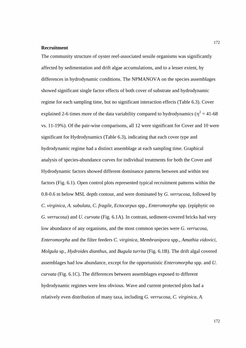
172

172

Recruitment

The community structure of oyster reef-associated sessile organisms was significantly

affected by sedimentation and drift algae accumulations, and to a lesser extent, by

differences in hydrodynamic conditions. The NPMANOVA on the species assemblages

showed significant single factor effects of both cover of substrate and hydrodynamic

regime for each sampling time, but no significant interaction effects (Table 6.3). Cover

explained 2-6 times more of the data variability compared to hydrodynamics ( 2 = 41-68

vs. 11-19%). Of the pair-wise comparisons, all 12 were significant for Cover and 10 were

significant for Hydrodynamics (Table 6.3), indicating that each cover type and

hydrodynamic regime had a distinct assemblage at each sampling time. Graphical

analysis of species-abundance curves for individual treatments for both the Cover and

Hydrodynamic factors showed different dominance patterns between and within test

factors (Fig. 6.1). Open control plots represented typical recruitment patterns within the

0.8-0.6 m below MSL depth contour, and were dominated by G. verrucosa, followed by

C. virginica, A. subulata, C. fragile, Ectocarpus spp., Enteromorpha spp. (epiphytic on

G. verrucosa) and U. curvata (Fig. 6.1A). In contrast, sediment-covered bricks had very

low abundance of any organisms, and the most common species were G. verrucosa,

Enteromorpha and the filter feeders C. virginica, Membranipora spp., Amathia vidovici,

Molgula sp., Hydroides dianthus, and Bugula turrita (Fig. 6.1B). The drift algal covered

assemblages had low abundance, except for the opportunistic Enteromorpha spp. and U.

curvata (Fig. 6.1C). The differences between assemblages exposed to different

hydrodynamic regimes were less obvious. Wave and current protected plots had a

relatively even distribution of many taxa, including G. verrucosa, C. virginica, A.

173

173

subulata, C. fragile, Ectocarpus spp. (epiphytic), Enteromorpha spp., U. curvata and

Punctaria latifolia, all with 2-4% cover (Fig. 6.1D, Time and Cover pooled). Wave-

exposed plots were primarily dominated by G. verrucosa, Enteromorpha sp., C. virginica

and C. fragile (Fig. 6.1E), whereas current exposed plots mainly were dominated by G.

verrucosa and Enteromorpha spp. (Fig. 6.1F). The SIMPER analysis (Table 6.5)

indicated that few species contributed to the majority of assemblage data variability, with

G. verrucosa, C. virginica and Enteromorpha spp. being the dominant taxa. Most

invertebrate taxa were relatively unimportant within the different assemblages, but when

added together contributed to a relatively large proportion of the between group

variability (B. turrita, A. vidovici, Membranipora spp., Molgula sp., H. dianthus, and

various hydroids).

Species richness and abundance were also affected by sedimentation, drift algae

accumulations, and hydrodynamic conditions. There was a significant interaction effect

between cover and hydrodynamics for animal richness, but with a low 2-value (Table

6.6A). Due to the lack of significant single factor effects, the SNK-test did not

differentiate between treatments (overall mean of 2 animals/brick). In particular, it was

noteworthy that sediment-covered plots supported as many animal taxa as algal-covered

and control plots (Fig. 6.3A-D). Plant species richness was significantly affected by

Cover and near-significantly affected by Hydrodynamics (Table 6.6B). The SNK-test

showed highest plant richness in control plots (4.8 plants/brick), intermediate in drift-

algae treatments (3.3) and lowest in sediment treatments (2.1). Also, plant richness was

significantly higher in protected and current-exposed plots (3.6) compared to wave-

174

174

exposed plots (3.2, Fig. 6.3E-H). Animal abundance was significantly affected by Cover

and by the interaction between cover and hydrodynamics, with most of the variability

explained by Cover (Table 6.6C). The SNK-test showed that control plots had higher

abundance of animals (6.2% cover/brick) compared to plots covered by drift algae or

sediments (2.2%) (Fig. 6.4A-D). For plant abundance, there were significant effects of

both Cover and Hydrodynamics, with Cover explaining the majority of the data

variability (Table 6.6D). Thus, plant abundance was highest in control plots (28%),

intermediate under a cover of drift algae (10%), and lowest under sediment cover (1.6%),

Current exposed plots (16%) had higher plant abundance compared to protected and

wave-exposed plots (12%). The interaction plots (Fig. 6.4E-H) showed a peak in

abundance in early summer, largely because of high abundance of G. verrucosa and

Enteromorpha sp.. Sessile algae were in general more abundant than sessile animals (Fig.

6.4). It should be noted that recruitment bricks were never fully occupied, indicating that

space was not a limiting resource during the 1 yr study period. Typically, 20-40% of the

space was occupied on bricks in open plots, 5-20% in drift algal covered plots and 2-5%

in sediment covered plots.

As with the assemblage response, all 6 taxa of interest were affected by sedimentation

and drift algae accumulations, and to a lesser extent by hydrodynamic conditions. The

reef-building oyster, C. virginica, was significantly affected by Cover (Table 6.7A), with

higher abundance in control plots (4.5%) compared to algal or sediment covered plots

(0.7%). Within the open plots recruitment were highest in wave-exposed plots at time 1

and 2 (Fig. 6.5A-B), but shifting to highest abundance in protected plots at time 3 and 4

175

175

(Fig. 6.5C-D). Similarly, the alien C. fragile, was significantly affected by Cover (Table

6.7B), and control plots had higher abundance (3.4%) compared to sediment and drift-

algae covered plots (0.0%). The interaction plots showed slightly lower abundance in

current-exposed plots compared to wave-exposed and protected plots (Fig. 6.5E-H). Of

all the mapped bricks, C. fragile occupied a maximum of 40% of a single brick. Also, of

the 144 observations on sediment-covered bricks (1/3 of 432 brick observations), C.

fragile recruits were found on 8, and all later died. Similarly out of drift-algal covered

bricks C. fragile was observed 14 times, again with 100% mortality. In contrast C. fragile

was observed 96 times, i.e. on 67% of the open block bricks. Of these 96, 38 were on

bricks behind reefs, 27 between reefs, and 31 in front of reefs. Despite similar abundance

patterns between C. fragile and C. virginica, they were not significantly correlated (r =

0.01, p = 0.90, n = 324). No bricks were found with high abundances of both species

(Fig. 6.6).

The ubiquitous coarsely-branched red alga G. verrucosa was significantly affected by

Cover and Hydrodynamics, with Cover being particularly important (Table 6.7C). G.

verrucosa was significantly more abundant in the control plots (14.1%) compared to drift

algae or sediment covered plots (ca. 1.0%), and also had higher abundance in current-

exposed plots (7.2%) compared to wave-exposed and protected plots (ca. 4.2%). Also, G.

verrucosa had a pronounced peak at sampling time 2 compared to times 1, 3 and 4 (Fig.

6.7A-D). For the other coarsely-branched red alga, A. subulata, there were significant

effects of both Cover and Hydrodynamics and a near significant interaction effect

between Cover and Hydrodynamics, although variance heterogeneity was relatively

176

176

pronounced for this data. The three factor-combinations explained roughly equal amounts

of the data variability (i.e. 18, 11, 15%, Table 6.7D). The SNK-test showed that A.

subulata was significantly more abundant in control plots (7.8%) compared to alga or

sediment covered plots (0.0%). Also, A. subulata had highest abundance in protected

plots (2.7%), intermediate in current exposed plots (1.2%) and lowest in wave-exposed

plots (0.0%, Fig. 6.7E-H). The opportunistic green algae Enteromorpha spp. was

significantly affected by Cover and Hydrodynamics, with the highest 2 for Cover (Table

6.7E), and the highest abundance at sampling time 2 (Fig. 6.8A-D). Enteromorpha spp.

was significantly more abundant under a drift algae cover (6.2%), intermediate in control

plots (1.4%) and lowest under a sediment cover (0.4%). Enteromorpha spp. also was

more abundant at current- and wave-exposed plots (3.2%) compared to protected plots

(1.7%). Finally, the opportunistic green alga U. curvata was significantly affected by

Cover (Table 6.7F), and the SNK-test showed that abundance was highest in control plots

and under a cover of drift algae (1.6%) compared to the sediment cover (0.3%). In

addition, a SNK-test on the Hydrodynamic factor suggested that U. curvata was more

abundant in current-exposed and protected plots (1.4%) compared to wave-exposed plots

(0.8%). However, the interaction plots indicated a complex pattern with treatment effects

changing between all sample times (Fig. 6.8E-H). Thus, U. curvata was mainly present at

times 1 and 2 in current-exposed control plots, at time 3 in most plots, and at time 4 in

current-exposed drift algal-covered plots and protected control plots. This confirmed that

U. curvata was an opportunistic species able to recruit onto hard substrate for short time

periods in most seasons and habitats.

177

177

Discussion

Quantifying succession and recruitment of sessile organisms has been a goal for benthic

ecologists for decades, and these processes have been well documented in rocky intertidal

and subtidal systems (e.g. Buschmann 1990, Connell 1961b, a, Dean & Connell 1987c, b,

Hirata 1986, 1987, Leonard et al. 1999, Parker et al. 1993, Petraitis & Latham 1999).

Relatively few studies have considered succession and recruitment of sessile organisms

in soft bottom lagoons and estuaries, where oyster reefs, mussel beds and man-made

constructions provide patches of hard substrate, which typically support a rich associated

flora and fauna (Albrecht 1998, Anderson 1999a, Connor 1980, Dean & Hurd 1980,

Lenihan 1999, Rhodes 1970, Underwood & Anderson 1994, Wells 1961). We document

that accumulations of sediments and drift algae negatively affect recruitment, survival

and growth of sessile oyster reef assemblages. Since eutrophication typically enhances

drift algae and sediment instability/sedimentation, increasing human pressures on coastal

systems are likely to cause impoverished oyster reef assemblages on large spatial scales.

Effects on sediments, drift algae and hydrodynamics

It is well-established that sedimentation structures sessile benthic assemblages (Airoldi

2003, Airoldi & Virgilio 1998, Rogers 1990). However, Airoldi (2003) reviewed the

literature and concluded that most impact studies only measured net accumulation or

sedimentation rates (or nothing at all). In the present study, both sediment accumulation

and sedimentation rates were quantified, and because patterns differed slightly both

should be reported as a general rule (Airoldi 2003). We believe that accumulated

sediments is the more ecologically relevant estimate of sediment stress that can reduce

178

178

adhesion strength (Charters et al. 1973, Devinny & Volse 1978) or bury and suffocate

sessile recruits (Airoldi 2003, Berger et al. 2003). The relative high sedimentation rate in

the control plots, compared to the amount of accumulated sediments, was likely caused

by the sediment tube structure itself which would induce small-scale turbulence, reduce

flow, and trigger sediment out-fall. This effect was most pronounced in the wave and

current-exposed plots where sediments frequently become resuspended or where

encounter rates are high (McManus 1998, Schoellhamer 1996). Drift algal densities in

eutrophied shallow systems commonly exceed 1 kgWWm2 (Menedez & Comin 2000,

Norkko & Bonsdorff 1996a, Peckol & Rivers 1996, Raffaelli et al. 1998, Tagliapietra et

al. 1998) and experiments testing for drift algal effects on soft bottom in and epi-fauna

have typically applied densities above this value, using green or brown sheet-like or

filamentous algae (Hull 1987, Norkko & Bonsdorff 1996a, Norkko et al. 2000, Osterling

& Pihl 2001, Raffaelli et al. 1989). We found minor effects of hydrodynamic differences

on the amount of accumulated drift algae, although there was a tendency for lowest

accumulations where currents were strongest (Flindt et al. 1997a, Martins et al. 2001,

Raffaelli et al. 1998). The accumulated drift algal mats were composed primarily of the

coarsely branched red algae G. verrucosa (Humm 1979), i.e. taxonomically and

structurally different from the aforementioned drift-algae impact studies. It should also be

noted that our trap approach in the low intertidal did not seem to cause algal

decomposition or development of anoxia. Velocities were low but not unusual for

lagoons (Hawes & Smith 1995, Lawson 2003, Schanz et al. 2000), and the accelerated

currents between the oyster reefs reflected that the reef structures altered local

hydrodynamics on small spatial scales (Barh & Lanier 1981, Lenihan 1999). It is

179

179

interesting that the mean velocities in the current-exposed plots were below 0.1 ms-1,

which was suggested by Hurd (2000) to demarcate low water motion regimes where

metabolic processes may be transfer limited. This suggests that in our experiment,

nutrient limitation may differ between treatments. The velocities were not measured

when the reefs were inundated, but it is likely that currents would be smaller (Lawson

2003). The wave climate was also affected by the reef structures, with 20-30 cm wind

and wake generated waves breaking in front of the reefs, and being non-existent behind.

Waves were also only observed before the reefs became inundated. Because benthic

wave stress decrease with water depths (Denny 1985), the measured wave heights

probably constitute near-maximal wave influences, although benthic stress may be higher

under extra-tropical storms (Dolan 1996, Hayden et al. 2000, Lucy et al. 1986). The

waves were observed to resuspend sediments, thereby increasing turbidity on small

spatial and temporal scales and also influencing light conditions (Lawson 2003,

Schoellhamer 1996, Ward et al. 1984).

We did not apply cage-controls because in systems where hydrodynamic regimes affect

nutrient and suspended solid encounters rates, sedimentation, resuspension, light

conditions, drift algae transport, dislodgment, propagule dispersal, and grazing (Chapter

2, 4, 5, Christensen 2000., Kastler & Wiberg 1996, Lawson 2003), such structures will

inevitable alter many factors simultaneously. Our open and simple drift algal trap

structure minimized the possibility of confounding for this treatment (similar to typical

cage-controls, Parker et al. 1993, Rosinski 2004, Woodin 1978), whereas the sediment

cages could be confounded by drift algae accumulations (quantified) or altered

180

180

accessibility of herbivores and predators (not quantified). However, because sediment

accumulations were lower under a cover of drift algae compared to controls (this study),

opposite to the effect of the sediment cages, it is likely that the imposed algae effect

within the sediment cages was minimal.

Recruitment in open plots

The orthogonal design between cover and hydrodynamics allowed for tests of interaction

effects, but because few interaction effects were significant, single factor effects could be

interpreted independently. Also, because the cover factor treatment was more severe than

the hydrodynamic factor, data could be interpreted as recruitment in open control plots

vs. drift algae covered plots vs. sediment covered plots. The taxa in the control plots are

common along the North American east coast, and have been observed attached to oyster

shells or recruitment panels (Connor 1980, Dean & Hurd 1980, Gosner 1978, Humm

1979, Lippson & Lippson 1997). However, in comparison to recruitment studies from

similar systems (Albrecht 1998, Anderson 1999a, Dean & Hurd 1980, Underwood &

Anderson 1994), macroalgae and growth of primary producers were more dominant in

Hog Island Bay (Barh & Lanier 1981, Dame et al. 1989, Dame 1992, Dame 1993). Many

algae commonly found in the drift assemblage, e.g. the filamentous Bryopsis plumosa,

Ectocarpus spp., Polysiphonia spp., Ceramium spp., Champia parvula and the coarsely

branched Hypnea musciformis (Chapter 2, 3, 4) did not recruit onto the bricks, but were

mainly observed entangled or epiphytic on larger primary attached algae. Thus, these

species mainly thrive unattached and epiphytic. Overall, G. verrucosa was the most

abundant species, adding a high recruitment ability to an array of previously described

181

181

successful lagoon adaptations, including high stress tolerance (Chapter 5, Stokke 1956),

high growth and recovery potential (Chapter 5, Hanisak et al. 1979, McLachlan & Bird

1986) and strong association with the polychaete facilitator Diopatra cuprea (Chapter 3),

together explaining the ubiquity of this species in North American east coast lagoons

(Cowper 1978, Goshorn et al. 2001, Chapter 2, Humm 1944, Peckol & Rivers 1996). The

larger algal species (A. subulata, C. fragile, G. verrucosa) generally recruited in high

densities, with large and small individuals being intermixed. Individuals of these species

can grow into large thalli within a few months under benign conditions (Chapter 5,

McLachlan & Bird 1986, Pedersen & Borum 1996, Poole & Raven 1997). However,

large individuals are susceptible to dislodgment and pruning by hydrodynamic forces

(Chapter 4, Blanchette 1997, Gaylord et al. 1994, Thomsen & Wernberg submitted), and

hydrodynamic forcing may frequently generate fragments to the drift algal assemblages

(Chapter 2, 3, 4). Also, because unattached algae in general do not become reproductive

(Norton & Mathieson 1983), the algae attached to the oyster reefs ensures that a

propagule bank is constantly produced (Santelices et al. 1995). Thus, reef attached algae

probably reduce the likelihood of local extinctions on the mudflats (where waves and

currents constantly remove algae) by providing a continuous supply of fragments.

The only animal that was space dominant on the bricks was the oyster C. virginica. This

is similarly to other soft bottom studies that also observed local oyster species to be

efficient recruiters (Anderson 1999a, Lenihan 1999, Underwood & Anderson 1994).

Other recruited animals were filter feeding subdominants (e.g. H. dianthus,

Membranipora spp., Molgula sp.) and seasonally fluctuating taxa (e.g. B. turrita, A.

182

182

vidovici) that generally perform relatively well in high depositional environments (Barh

& Lanier 1981, Dean & Hurd 1980, Lippson & Lippson 1997). We noted that a large

proportion of the oysters died within a few months of recruitment, probably due to

predation or diseases (Anderson 1999a, Barh & Lanier 1981, Lenihan 1999, O´Beirn et

al. 1996). Despite a high mortality, the shells of the recruited oysters still caused

increased topographic complexity, and may thereby have increased available space (Barh

& Lanier 1981, Connor 1980, Rhodes 1970).

The experiment was conducted on a small spatial scale within a hydrodynamic well-

mixed area, and propagules were probably distributed uniformly in the water masses

(Norton 1992, Santelices 1990). However, small-scale differences in hydrodynamic

process could cause different encounter rates between propagules and the experimental

substrates. Abundance patterns may thereby have reflected different propagule encounter

rates, different likelihood of attachment, and/or differential survival and growth rates.

Current-exposed plots should have encountered most propagules (Lenihan 1999, Leonard

et al. 1999), whereas wave-exposed plots may have had highest attachment success

because orbital water motion increases contact rates between suspended propagules and

the recruitment bricks (Denny 1988). Oyster reefs have previously been suggested to

influence local hydrodynamic conditions (Barh & Lanier 1981, Brooks 1996, Galtsoff

1964, Mann 2000). In particular Lenihan (1999) documented that reef sizes, reef shapes

and reef elevation influenced the local hydrodynamic regime, and thereby partly

explained survival and growth of oyster recruits. However, effects on recruitment of

oysters positioned at different elevations likely differed due to both effects associated

183

183

with the reef-structure (alteration of flow and flow-associated variables) and to effects

uncoupled from the reef-structure (e.g. light levels, orbital wave velocities, sedimentation

rates and re-suspension levels (Chapter 5, Appendix 1). In the present study, all plots had

similar elevations, and changes in physical conditions and assemblage patterns could

thereby only be attributed to the structure of the oyster reefs. We documented that the

reef position in itself caused significantly different sessile assemblages, although the

effects were less obvious compared to the effects of drift algae or sediment

accumulations (cf. 2 values in ANOVA models). Thus, even within apparently uniform

low-energy lagoons (< 0.1 m/s, Hurd 2000), different hydrodynamic regimes induce

differential performance patterns on small spatial scales. Species-specific performance

patterns are typically inter-related in assemblage based field experiments. Thus,

successful recruitment may be related to the abundance of other taxa already present

(Connell & Slatyer 1977, Petraitis & Latham 1999, Sutherland 1974, Underwood &

Anderson 1994), although inhibitory or facilitative effects probably were relatively

unimportant due to the low covers of sessile organisms. The limited success of C. fragile

and C. virginica in these plots could be caused either by spatial inhibition by G.

verrucosa or by a low tolerance to current induced drag and/or entanglement of drift

algae clumps. The main taxa-specific hydrodynamic effects were the absence of A.

subulata in front of reefs, a high abundance of G. verrucosa between reefs and relative

low abundance of C. fragile, C. virginica and A. subulata between reefs. The absence of

A. subulata was likely caused by frequent wave-induced thallus breakage because it has a

low adhesion strength (Chapter 4), but large drag when growing into a large organism

(Chapter 4, Denny 1995, 1999, Gaylord et al. 1994). G. verrucosa could be most

184

184

dominant between reefs because this species likely is the least susceptible to

entanglement by drift algae clumps (Chapter 4, Holmquist 1997), a potential detrimental

process where currents and drift algae transport are high (Flindt et al. 1997a, Martins et

al. 2001, Salomonsen et al. 1997). Transplantation experiments and improved

biomechanical measurements are needed to support these explanations.

Recruitment under drift algae

Eutrophication and subsequent increased drift algae abundance (Fletcher 1996, Morand

& Briand 1996, Raffaelli et al. 1998) may limit oyster recruitment (this study), and

thereby threaten reef maintenance process in coastal systems worldwide. Because the

oyster is a foundation species facilitating numerous associated organisms, and alter

biogeochemical cycles and abiotic conditions (Barh & Lanier 1981, Bruno & Bertness

2001, Bruno et al. in press), detrimental effects of drift algae proliferation may have

system wide consequences. A cover of drift algae significantly affected the sessile

assemblages. These effects were manifested through poor plant richness, and low cover

of plants and animals. In particular, the algal assemblage lacked large perennial taxa.

Recruits of these species were occasionally observed, but did not survive, potentially due

to light limitation or smothering/abrasion by the algal mat (Krause-Jensen et al. 1996,

Norkko & Bonsdorff 1996b, Raffaelli et al. 1998). Few oysters recruited onto these

bricks and those few that did recruit had 100% mortality. The effects of the drift algae

cover were not related to anoxia development as observed in other studies (Norkko &

Bonsdorff 1996a, Raffaelli et al. 1998), rather the drift cover effects were likely due to

reduced light penetration (Krause-Jensen et al. 1996, Peckol & Rivers 1996), filtering of

185

185

propagules (Olafsson 1988), reduced currents (Escartin & Aubrey 1995), and interference

with feeding apparatus (Norkko & Bonsdorff 1996a), as well as positive effects

associated with reduced desiccation. The green algae Enteromorpha spp. and U. curvata

were the most common space-occupying taxa, although only as mm-cm small

individuals. These taxa are ephemeral subdominants on primary substrates, but have high

growth and reproductive outputs (Littler 1980, Nielsen & Sand-Jensen 1990, Poole &

Raven 1997). U. curvata and Enteromorpha spp. were thus probably dominant because

of reduced grazing (Geertz-Hansen et al. 1993, Giannotti & McGlathery 2001, Poole &

Raven 1997), dislodgment (Chapter 4, Hawes & Smith 1995, Martins et al. 2001,

Thomsen & Wernberg submitted) and competition from canopy-forming algae.

Recruitment under sediments

Enhanced sedimentation is increasingly threatening coral reefs, rockweed beds and kelp

forests (Airoldi 2003, Devinny & Volse 1978, Johansson et al. 1998, Rogers 1990). Here

it is documented that sessile organisms in soft bottom lagoons also are detrimentally

affected by enhanced sedimentation. Enhanced sedimentation can be caused by decreased

abundance of sediment stabilizers, climatic changes, coastal construction projects,

changed agricultural practices, and reduction of sediment traps such as salt marshes

(Airoldi 2003). On the eastern shore of Virginia, these mechanisms already have caused,

or are likely to cause, enhanced sedimentation (Haven & Whitcomb 1983, Hayden et al.

2000, Ralph & Short 2002). The accumulation of 4-10 mm of sediment per 1-4 month

periods was sufficient to decrease the abundance of plant and animals, although animal

richness was unaffected, demonstrating that species did recruit onto the bricks but did not

186

186

survive, or had reduced growth. Sediment effects were particularly detrimental to the

algal assemblage, with the opportunistic U. curvata being the only species to occupy

small amounts of space for short times periods. The effects were also adverse for filter

feeders, although less so in current exposed plots where sediment accumulations were

smallest. Many filter feeding animals are relatively resistant to small amounts of

sediments (Dean & Hurd 1980), although eventually feeding structures will clog or

become buried. Oysters occasionally recruited onto these bricks, but did not survive.

Thus, the long term effects would again, similar to the drift algae treatments, be

diminished reef structures with potentially wide-ranging ecological effects.

Temporal recruitment effects

Temporal effects are the cornerstone of succession studies (Clements 1936, Connell &

Slatyer 1977, Cowles 1899), and temporal effects in recruitment patterns of sessile

marine organisms are well-studied (e.g. Dean & Connell 1987b, a, Hirata 1986, 1987,

Parker et al. 1993, Petraitis & Latham 1999). Although temporal effects could be deduced

from the present study, they were of secondary interest compared to effects of cover

stress and hydrodynamics. Because the experiment was unreplicated within and between

seasons, temporal interpretations also suffer from problems of auto-correlation and carry-

over effects (Anderson 1999a, b, Anderson & Underwood 1997, Underwood & Anderson

1994). Thus, studies by Anderson and Underwood (cf. above) specifically replicated

incubation panels in different seasons and found different assemblages. However, most of

these studies had incubation time of less than six months, making it possible that

assemblages could converge given several cycles of recruitment and life-history turnover

187

187

(Petraitis & Latham 1999, Sutherland 1974). Because the bricks in the present study had

low cover, independent recruitment was possible, although the available area would

shrink and expand depending on the performance of neighboring attached organisms. The

importance of temporal effects was apparent from the interaction plots and ANOVA

tests. Temporal changes were likely caused by lunar cycles (different emergence times,

different peak tidal currents), seasons, (temperature, light, storms) and life-history

strategies (length, intensity and timing of propagule supply)(Appendix 1, Santelices

1990, Schneider & Searles 1991). Our study lasted for one year, but it is possible that

inclusion of several life-history turnovers could alter the conclusions.

Recruitment of C. fragile

Our finding that the invasive C. fragile was the fourth most dominant recruiter in control

plots supports the claim that C. fragile is a successful recruiter onto barren space and a

strong space occupier on hard substrates in lagoons and estuaries (Fralick & Mathieson

1972, 1973, Malinowski & Ramus 1973), partly explaining its success as an invader

(Begin & Scheibling 2003, Chapman 1999, Hillson 1976, Mathieson et al. 2003). The

ability to recruit and survive on bricks positioned at various oyster reef locations

indicates tolerance to a range of hydrodynamic conditions (Mathieson et al. 2003,

Trowbridge 1998). C. fragile and C. virginica had similar distribution patterns, but they

were not found in high densities together, suggesting possible competition for space.

However, longer-term data, and specific experimental designs manipulating densities are

necessary to document negative effects of C. fragile. Our study also demonstrated that C.

fragile performed poorly under high sediment and drift algae accumulations, which are

188

188

important ecological stresses in eutrophied soft bottom systems, and factors that likely

will limit future success of the invader. Because sedimentation and drift algae

accumulations were also detrimental to the substrate provider C. virginica, (Carlton &

Scanlon 1985, Churchill & Moeller 1972, Dromgoole 1982, Garbary et al. 1997),

eutrophication and coastal development could have an even greater negative effect on C.

fragile distribution and abundance.

Conclusion

In conclusion, a sediment cover strongly reduced recruitment, survival and growth of

most organisms, particularly the space-dominant perennial macroalgae G. verrucosa, A.

subulata and C. fragile, and the filter feeding oyster C. virginica, but less so for a few

rare stress-tolerant and ephemeral animals. A cover of drift algae also decreased the

abundance of the space-dominant organisms, but the opportunistic green algae

Enteromorpha sp. and U. curvata proliferated in these habitats. The effects of the

hydrodynamic regime were less dramatic, but nevertheless demonstrated that G.

verrucosa was abundant in current-exposed plots, that A. subulata was absent from wave-

exposed plots and that several co-dominants were relatively evenly distributed in

protected plots. The invasive macroalgae C. fragile was the fourth most abundant

organism in the open control plots, being common under all hydrodynamic regimes, but

non-existent under sediment and drift algae covers. The former observations suggest that

C. fragile potentially can be a competitor to C. virginica whereas the latter observation

implies reduced invasion success as eutrophication progress. Because the reef-building C.

virginica also performed poorly under cover of sediments and drift algae, increased

189

189

eutrophication, sediment destabilization, and sediment enhancement may have wide-

ranging effects on oyster reefs in general, and thereby also negative effects on associated

flora and faunas, including the invasive C. fragile.

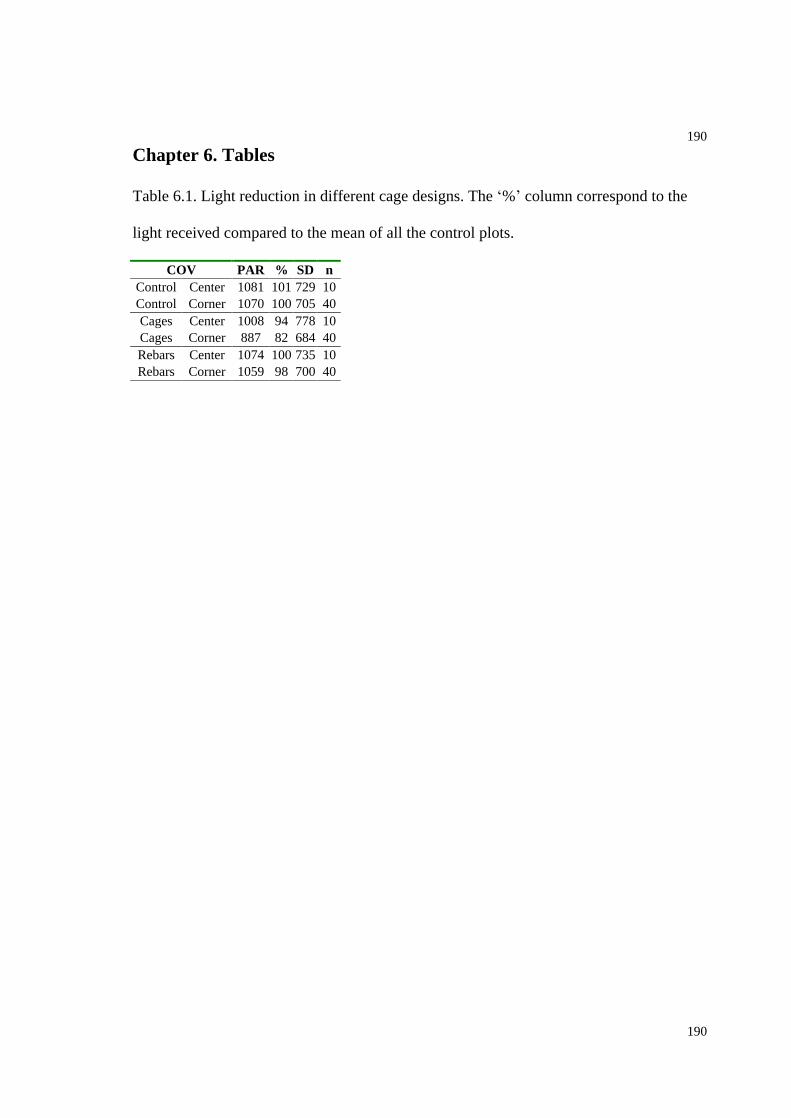
190

190

Chapter 6. Tables

Table 6.1. Light reduction in different cage designs. The % column correspond to the

light received compared to the mean of all the control plots.

COV PAR % SD nControl Center 1081 101 729 10Control Corner 1070 100 705 40Cages Center 1008 94 778 10Cages Corner 887 82 684 40Rebars Center 1074 100 735 10Rebars Corner 1059 98 700 40

191

191

Table 6.2. ANOVA on Log(x+1) cover of sediments (A), sedimentation rates (B), cover

of drift algae (C), current velocities (D), and drag on practice golf balls (E). Significant

values are in bold. Asterisk indicate that Cochran s C was significant for that factor.

Test Factor DF SS 2(%) F pA. Hydrodynamics (HYD) 2 0.01 0 0.20 0.817

Sediment Cover (COV) 2 4.94 44 84.49 0.000*accumulations HYD*COV 4 0.49 4 4.20 0.009

Error Between 27 0.79 7Time (TIM) 2 1.97 18 23.71 0.000HYD*TIM 4 0.04 0 0.22 0.928COV*TIM 4 0.29 3 1.74 0.154HYD*COV*TIM 8 0.35 3 1.06 0.404Error Within 54 2.25 20

B. HYD 2 0.06 13.9 5.30 0.011Sedimentation COV 2 0.17 41.3 15.83 0.000

rates HYD*COV 4 0.04 9.6 1.83 0.152(in tubes) Error 27 0.15 35.3

Total 35 0.42 100.0C. HYD 2 1.57 2 3.99 0.030*

Drift algae COV 2 42.84 46 108.73 0.000*accumulations HYD*COV 4 2.26 2 2.87 0.042

Error Between 27 5.32 6TIM 4 2.74 3 3.22 0.016HYD*TIM 8 4.30 5 2.53 0.015COV*TIM 8 8.44 9 4.96 0.000HYD*COV*TIM 16 2.20 2 0.65 0.839Error Within 108 22.98 25

D. HYD 2 2.61 30 52.42 0.000*Current COV 2 3.45 39 69.27 0.000*

velocities HYD*COV 4 1.37 16 13.75 0.000Error Between 27 0.67 8TIM 1 0.03 0 2.47 0.128HYD*TIM 2 0.06 1 2.39 0.111COV*TIM 2 0.23 3 8.46 0.001HYD*COV*TIM 4 0.04 0 0.74 0.576Error Within 27 0.36 4

E. HYD 2 0.00 0 0.22 0.804*Drag COV 2 0.04 6 2.69 0.086*

(on practice HYD*COV 4 0.04 5 1.19 0.339golf balls) Error Between 27 0.21 29

TIM 1 0.11 15 9.38 0.005HYD*TIM 2 0.01 2 0.58 0.568COV*TIM 2 0.00 0 0.14 0.875HYD*COV*TIM 4 0.03 4 0.66 0.629Error Within 24 0.27 38

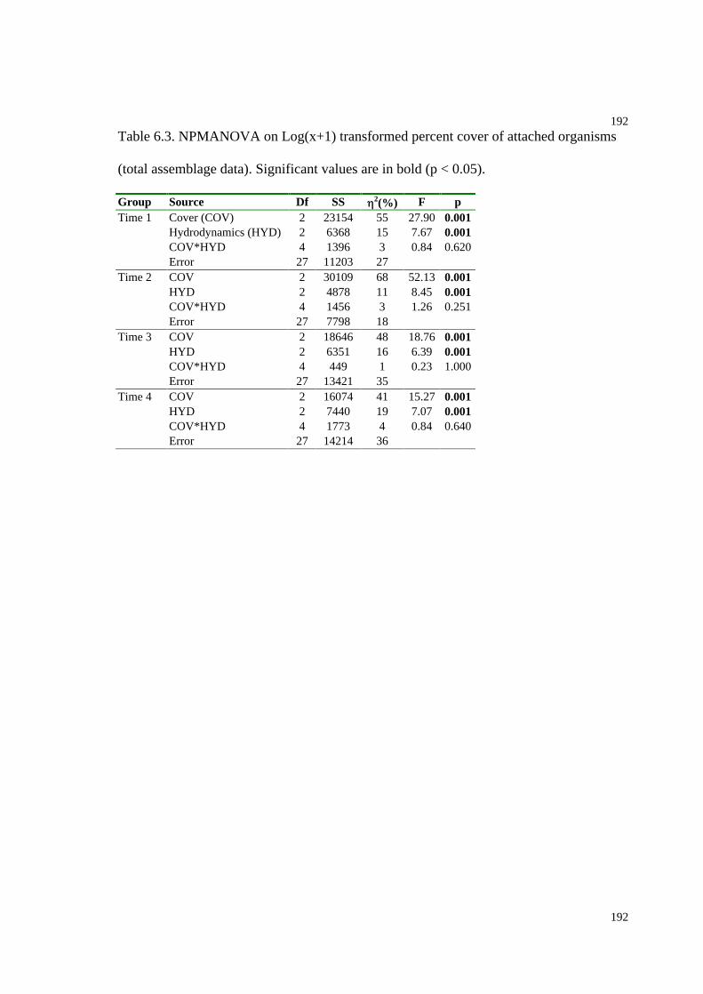
192

192

Table 6.3. NPMANOVA on Log(x+1) transformed percent cover of attached organisms

(total assemblage data). Significant values are in bold (p < 0.05).

Group Source Df SS 2(%) F pTime 1 Cover (COV) 2 23154 55 27.90 0.001

Hydrodynamics (HYD) 2 6368 15 7.67 0.001COV*HYD 4 1396 3 0.84 0.620Error 27 11203 27

Time 2 COV 2 30109 68 52.13 0.001HYD 2 4878 11 8.45 0.001COV*HYD 4 1456 3 1.26 0.251Error 27 7798 18

Time 3 COV 2 18646 48 18.76 0.001HYD 2 6351 16 6.39 0.001COV*HYD 4 449 1 0.23 1.000Error 27 13421 35

Time 4 COV 2 16074 41 15.27 0.001HYD 2 7440 19 7.07 0.001COV*HYD 4 1773 4 0.84 0.640Error 27 14214 36

193

193

Table 6.4. Pair-wise comparisons (permutation t-tests) for assemblage data following

significant single factor effects from NPMANOVA. Significant values are in bold (p <

0.05).

Time 1 Time 2 Time 3 Time 4Comparison t p t p t p t pSediment vs. Control 5.09 0.001 6.23 0.001 3.64 0.001 3.78 0.001Sediment vs. Drift 4.11 0.001 4.98 0.001 3.68 0.001 3 0.001Drift vs. Control 4.08 0.001 6.54 0.001 4.55 0.001 3.27 0.001Protected vs. Current 1.64 0.026 1.41 0.122 1.68 0.026 1.7 0.04Protected vs. Wavy 1.76 0.016 1.66 0.048 2.1 0.008 2.21 0.005Current vs. Wavy 1.74 0.032 1.14 0.249 1.51 0.048 1.91 0.008

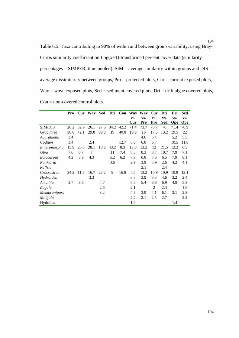
194

194

Table 6.5. Taxa contributing to 90% of within and between group variability, using Bray-

Curtis similarity coefficient on Log(x+1)-transformed percent cover data (similarity

percentages = SIMPER, time pooled). SIM = average similarity within groups and DIS =

average dissimilarity between groups, Pro = protected plots, Cur = current exposed plots,

Wav = wave exposed plots, Sed = sediment covered plots, Dri = drift algae covered plots,

Con = non-covered control plots.

Pro Cur Wav Sed Dri Con Wavvs.

Cur

Wavvs.Pro

Curvs.Pro

Drivs.Sed

Drivs.

Ope

Sedvs.

OpeSIM/DIS 28.2 32.9 26.1 27.6 34.2 42.2 71.4 73.7 70.7 76 71.4 76.9Gracilaria 30.6 42.1 29.8 39.3 19 40.8 19.9 16 17.5 13.2 19.5 22Agardhiella 3.4 4.6 5.4 5.2 5.5Codium 3.4 2.4 12.7 6.6 6.8 6.7 10.5 11.8Enteromorpha 15.9 20.8 28.1 18.2 43.2 8.3 13.8 13.2 12 21.5 12.2 6.5Ulva 7.6 6.7 7 11 7.4 8.3 8.3 8.7 10.7 7.9 7.1Ectocarpus 4.2 5.9 4.3 5.2 6.2 7.9 6.8 7.6 6.5 7.9 8.1Punktaria 3.6 2.9 3.9 3.9 2.6 4.2 4.1Ralfsia 2.1 2.4Crassostrea 24.2 11.8 16.7 22.2 9 16.8 11 13.2 10.9 10.9 10.8 12.1Hydroides 3.3 3.3 3.9 3.3 4.6 3.2 2.4Amathia 2.7 3.6 4.7 6.5 5.4 6.6 6.9 4.8 5.3Bugula 2.6 2.1 2 2.3 1.8Membranipora 3.2 4.5 3.9 4.1 6.1 3.1 2.3Molgula 2.2 2.1 2.5 2.7 2.2Hydroids 1.9 1.4

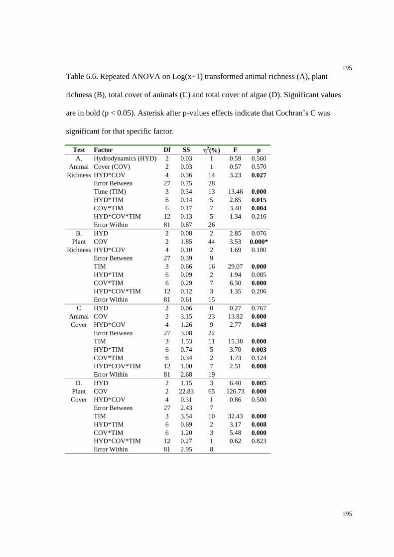
195

195

Table 6.6. Repeated ANOVA on Log(x+1) transformed animal richness (A), plant

richness (B), total cover of animals (C) and total cover of algae (D). Significant values

are in bold (p < 0.05). Asterisk after p-values effects indicate that Cochran s C was

significant for that specific factor.

Test Factor Df SS 2(%) F pA. Hydrodynamics (HYD) 2 0.03 1 0.59 0.560

Animal Cover (COV) 2 0.03 1 0.57 0.570Richness HYD*COV 4 0.36 14 3.23 0.027

Error Between 27 0.75 28Time (TIM) 3 0.34 13 13.46 0.000HYD*TIM 6 0.14 5 2.85 0.015COV*TIM 6 0.17 7 3.48 0.004HYD*COV*TIM 12 0.13 5 1.34 0.216Error Within 81 0.67 26

B. HYD 2 0.08 2 2.85 0.076Plant COV 2 1.85 44 3.53 0.000*

Richness HYD*COV 4 0.10 2 1.69 0.180Error Between 27 0.39 9TIM 3 0.66 16 29.07 0.000HYD*TIM 6 0.09 2 1.94 0.085COV*TIM 6 0.29 7 6.30 0.000HYD*COV*TIM 12 0.12 3 1.35 0.206Error Within 81 0.61 15

C HYD 2 0.06 0 0.27 0.767Animal COV 2 3.15 23 13.82 0.000Cover HYD*COV 4 1.26 9 2.77 0.048

Error Between 27 3.08 22TIM 3 1.53 11 15.38 0.000HYD*TIM 6 0.74 5 3.70 0.003COV*TIM 6 0.34 2 1.73 0.124HYD*COV*TIM 12 1.00 7 2.51 0.008Error Within 81 2.68 19

D. HYD 2 1.15 3 6.40 0.005Plant COV 2 22.83 65 126.73 0.000Cover HYD*COV 4 0.31 1 0.86 0.500

Error Between 27 2.43 7TIM 3 3.54 10 32.43 0.000HYD*TIM 6 0.69 2 3.17 0.008COV*TIM 6 1.20 3 5.48 0.000HYD*COV*TIM 12 0.27 1 0.62 0.823Error Within 81 2.95 8

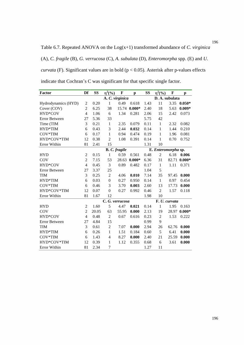
196

196

Table 6.7. Repeated ANOVA on the Log(x+1) transformed abundance of C. virginica

(A), C. fragile (B), G. verrucosa (C), A. subulata (D), Enteromorpha spp. (E) and U.

curvata (F). Significant values are in bold (p < 0.05). Asterisk after p-values effects

indicate that Cochran s C was significant for that specific single factor.

Factor Df SS 2(%) F p SS 2(%) F pA. C. virginica D. A. subulata

Hydrodynamics (HYD) 2 0.20 1 0.49 0.618 1.43 11 3.35 0.050*Cover (COV) 2 6.25 38 15.74 0.000* 2.40 18 5.63 0.009*HYD*COV 4 1.06 6 1.34 0.281 2.06 15 2.42 0.073Error Between 27 5.36 33 5.75 42Time (TIM 3 0.21 1 2.35 0.079 0.11 1 2.32 0.082HYD*TIM 6 0.43 3 2.44 0.032 0.14 1 1.44 0.210COV*TIM 6 0.17 1 0.94 0.474 0.19 1 1.96 0.081HYD*COV*TIM 12 0.38 2 1.08 0.391 0.14 1 0.70 0.752Error Within 81 2.41 15 1.31 10

B. C. fragile E. Enteromorpha sp.HYD 2 0.15 1 0.59 0.561 0.48 2 6.18 0.006COV 2 7.15 53 28.63 0.000* 6.36 31 82.71 0.000*HYD*COV 4 0.45 3 0.89 0.482 0.17 1 1.11 0.371Error Between 27 3.37 25 1.04 5TIM 3 0.25 2 4.06 0.010 7.14 35 97.45 0.000HYD*TIM 6 0.03 0 0.27 0.950 0.14 1 0.97 0.454COV*TIM 6 0.46 3 3.70 0.003 2.60 13 17.73 0.000HYD*COV*TIM 12 0.07 0 0.27 0.992 0.46 2 1.57 0.118Error Within 81 1.67 12 1.98 10

C. G. verrucosa F. U. curvataHYD 2 1.60 5 4.47 0.021 0.14 1 1.95 0.163COV 2 20.05 63 55.95 0.000 2.13 19 28.97 0.000*HYD*COV 4 0.48 2 0.67 0.616 0.23 2 1.53 0.222Error Between 27 4.84 15 0.99 9TIM 3 0.61 2 7.07 0.000 2.94 26 62.76 0.000HYD*TIM 6 0.26 1 1.51 0.184 0.60 5 6.41 0.000COV*TIM 6 1.43 4 8.27 0.000 2.40 21 25.59 0.000HYD*COV*TIM 12 0.39 1 1.12 0.355 0.68 6 3.61 0.000Error Within 81 2.34 7 1.27 11

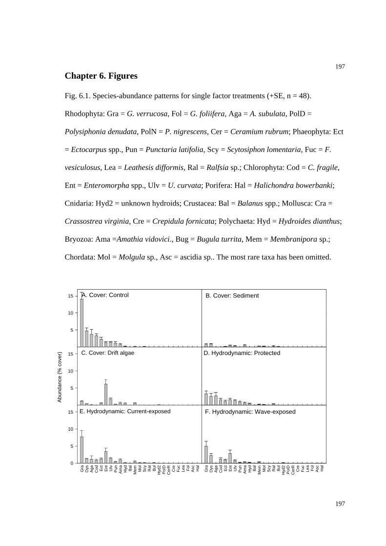
197

197

Chapter 6. Figures

Fig. 6.1. Species-abundance patterns for single factor treatments (+SE, n = 48).

Rhodophyta: Gra = G. verrucosa, Fol = G. foliifera, Aga = A. subulata, PolD =

Polysiphonia denudata, PolN = P. nigrescens, Cer = Ceramium rubrum; Phaeophyta: Ect

= Ectocarpus spp., Pun = Punctaria latifolia, Scy = Scytosiphon lomentaria, Fuc = F.

vesiculosus, Lea = Leathesis difformis, Ral = Ralfsia sp.; Chlorophyta: Cod = C. fragile,

Ent = Enteromorpha spp., Ulv = U. curvata; Porifera: Hal = Halichondra bowerbanki;

Cnidaria: Hyd2 = unknown hydroids; Crustacea: Bal = Balanus spp.; Mollusca: Cra =

Crassostrea virginia, Cre = Crepidula fornicata; Polychaeta: Hyd = Hydroides dianthus;

Bryozoa: Ama =Amathia vidovici., Bug = Bugula turrita, Mem = Membranipora sp.;

Chordata: Mol = Molgula sp., Asc = ascidia sp.. The most rare taxa has been omitted.

A. Cover: Control

Gra

Oys

Aga

Cod Ect

Ent

Ulv

Pun

Am

aH

yd Bal

Mem M

olS

cy Ral

Bul

Hyd

2P

olD

Cer

RC

reF

ucLe

aF

olA

sc Hal

Abu

ndan

ce (

% c

over

)

5

10

15 B. Cover: Sediment

Gra

Oys

Aga

Cod Ect

Ent

Ulv

Pun

Am

aH

yd Bal

Mem M

olS

cy Ral

Bul

Hyd

2P

olD

Cer

RC

reF

ucLe

aF

olA

sc HalC. Cover: Drift algae

Gra

Oys

Aga

Cod Ect

Ent

Ulv

Pun

Am

aH

yd Bal

Mem M

olS

cy Ral

Bul

Hyd

2P

olD

Cer

RC

reF

ucLe

aF

olA

sc Hal

5

10

15 D. Hydrodynamic: Protected

Gra

Oys

Aga

Cod Ect

Ent

Ulv

Pun

Am

aH

yd Bal

Mem M

olS

cy Ral

Bul

Hyd

2P

olD

Cer

RC

reF

ucLe

aF

olA

sc HalF. Hydrodynamic: Wave-exposed

Gra

Oys

Aga

Cod Ect

Ent

Ulv

Pun

Am

aH

yd Bal

Mem M

olS

cy Ral

Bul

Hyd

2P

olD

Cer

RC

reF

ucLe

aF

olA

sc Hal

E. Hydrodynamic: Current-exposed

Gra

Oys

Aga

Cod Ect

Ent

Ulv

Pun

Am

aH

yd Bal

Mem M

olS

cy Ral

Bul

Hyd

2P

olD

Cer

RC

reF

ucLe

aF

olA

sc Hal

0

5

10

15

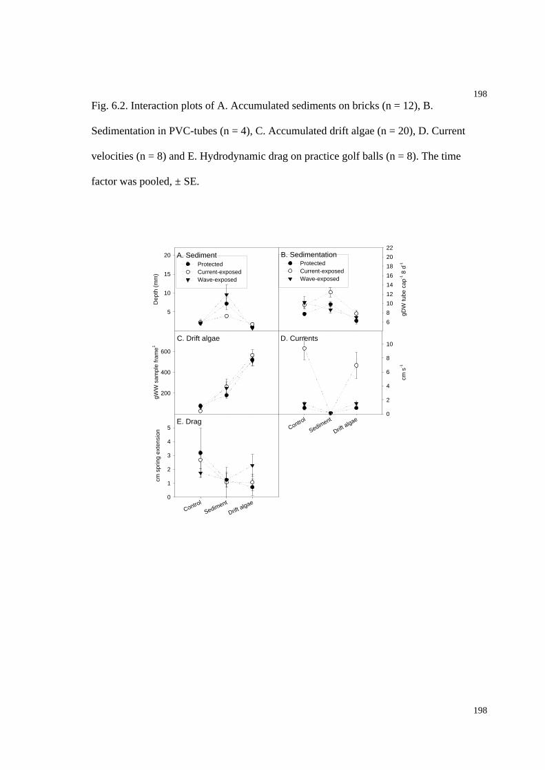
198

198

Fig. 6.2. Interaction plots of A. Accumulated sediments on bricks (n = 12), B.

Sedimentation in PVC-tubes (n = 4), C. Accumulated drift algae (n = 20), D. Current

velocities (n = 8) and E. Hydrodynamic drag on practice golf balls (n = 8). The time

factor was pooled, ± SE.

A. Sediment

Control SedimentDrift algae

Dep

th (

mm

)

5

10

15

20

ProtectedCurrent-exposedWave-exposed

B. Sedimentation

Control SedimentDrift algae

gDW

tube

cap

-1 8

d-1

6

8

10

12

14

16

18

20

22

C. Drift algae

Control SedimentDrift algae

gWW

sam

ple

fram

e1

200

400

600

D. Currents

Control

Sediment

Drift algae

cm s

-1

0

2

4

6

8

10

E. Drag

Control

Sediment

Drift algae

cm s

prin

g ex

tens

ion

0

1

2

3

4

5

ProtectedCurrent-exposedWave-exposed

199

199

Fig. 6.3. Interaction plots of animal (A-D) and plant richness (E-H) per recruitment brick

for separate sampling times (± SE, n = 4).

A. Time 1

Control SedimentDrift algae

Tax

a pe

r br

ick

1

2

3

4

5

ProtectedCurrent-exposedWave-exposed

B. Time 2

Control SedimentDrift algae

Tax

a pe

r br

ick

1

2

3

4

C. Time 3

Control SedimentDrift algae

Tax

a pe

r br

ick

1

2

3

4

D. Time 4

Control

Sediment

Drift algae

Tax

a pe

r br

ick

0

1

2

3

4

Animal Richness

E. Time 1

Control SedimentDrift algae

2

4

6

8

10

ProtectedCurrent-exposedWave-exposed

F. Time 2

Control SedimentDrift algae

2

4

6

8

G. Time 3

Control SedimentDrift algae

2

4

6

8

H. Time 4

Control

Sediment

Drift algae

0

2

4

6

8

Plant Richness

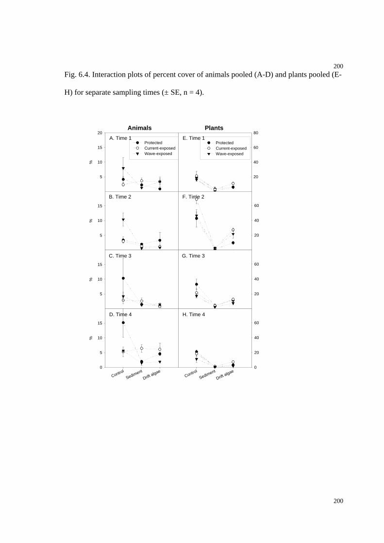
200

200

Fig. 6.4. Interaction plots of percent cover of animals pooled (A-D) and plants pooled (E-

H) for separate sampling times (± SE, n = 4).

A. Time 1

Control SedimentDrift algae

%

5

10

15

20

ProtectedCurrent-exposedWave-exposed

B. Time 2

Control SedimentDrift algae

%

5

10

15

C. Time 3

Control SedimentDrift algae

%

5

10

15

D. Time 4

Control

Sediment

Drift algae

%

0

5

10

15

Animals

E. Time 1

Control SedimentDrift algae

20

40

60

80

ProtectedCurrent-exposedWave-exposed

F. Time 2

Open Cage Rebar

20

40

60

G. Time 3

Control SedimentDrift algae

20

40

60

H. Time 4

Control

Sediment

Drift algae

0

20

40

60

Plants

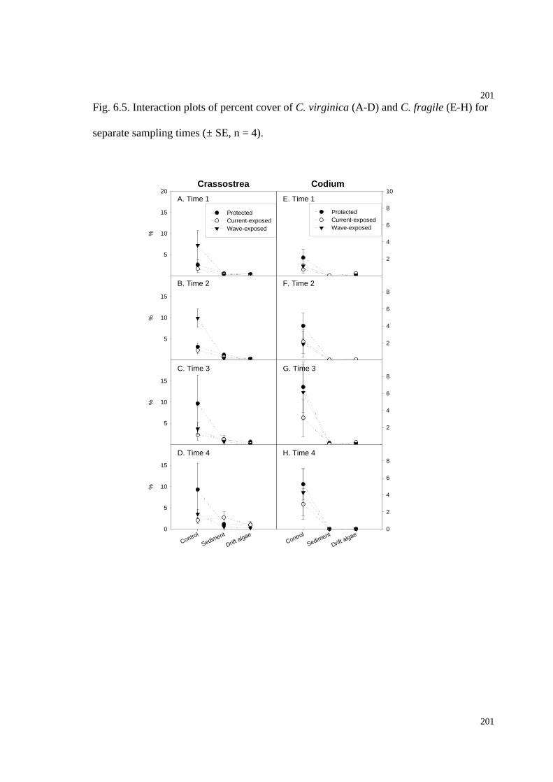
201

201

Fig. 6.5. Interaction plots of percent cover of C. virginica (A-D) and C. fragile (E-H) for

separate sampling times (± SE, n = 4).

A. Time 1

Control SedimentDrift algae

%

5

10

15

20

ProtectedCurrent-exposedWave-exposed

B. Time 2

Control SedimentDrift algae

%

5

10

15

C. Time 3

Control SedimentDrift algae

%

5

10

15

D. Time 4

Control

Sediment

Drift algae

%

0

5

10

15

Crassostrea

E. Time 1

Control SedimentDrift algae

2

4

6

8

10

ProtectedCurrent-exposedWave-exposed

F. Time 2

Control SedimentDrift algae

2

4

6

8

G. Time 3

Control SedimentDrift algae

2

4

6

8

H. Time 4

Control

Sediment

Drift algae

0

2

4

6

8

Codium

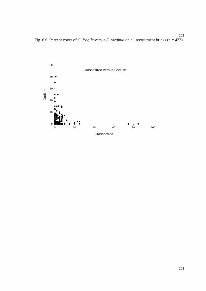
202

202

Fig. 6.6. Percent cover of C. fragile versus C. virginia on all recruitment bricks (n = 432).

Crassostrea versus Codium

Crassostrea

0 20 40 60 80 100

Cod

ium

0

10

20

30

40

50

203

203

Fig. 6.7. Interaction plots of percent cover of G. verrucosa (A-D) and A. subulata (E-H)

for separate sampling times (± SE, n = 4).

A. Time 1

Control SedimentDrift algae

%

10

20

30

40

50

ProtectedCurrent-exposedWave-exposed

B. Time 2

Control SedimentDrift algae

%

10

20

30

40

C. Time 3

Control SedimentDrift algae

%

10

20

30

40

D. Time 4

Control

Sediment

Drift algae

%

0

10

20

30

40

Gracilaria

E. Time 1

Control SedimentDrift algae

5

10

15

20

25

ProtectedCurrent-exposedWave-exposed

F. Time 2

Control SedimentDrift algae

5

10

15

20

G. Time 3

Control SedimentDrift algae

5

10

15

20

H. Time 4

Control

Sediment

Drift algae

0

5

10

15

20

Agardhiella

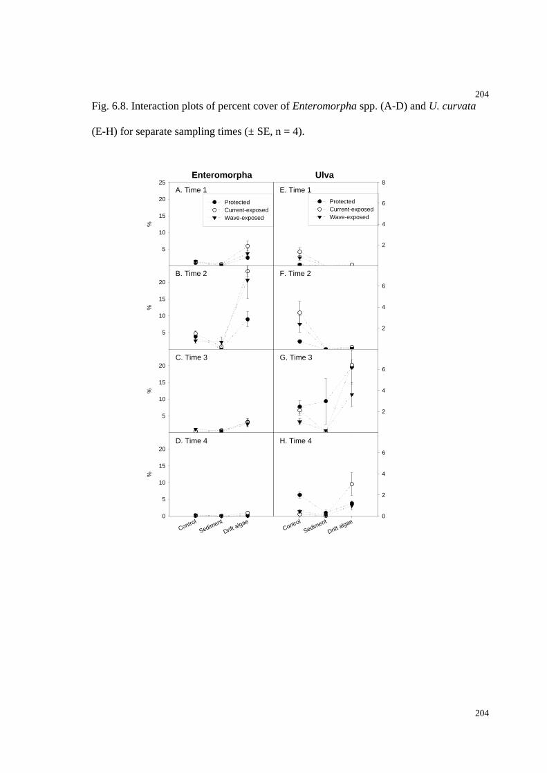
204

204

Fig. 6.8. Interaction plots of percent cover of Enteromorpha spp. (A-D) and U. curvata

(E-H) for separate sampling times (± SE, n = 4).

A. Time 1

Control SedimentDrift algae

%

5

10

15

20

25

ProtectedCurrent-exposedWave-exposed

B. Time 2

Control SedimentDrift algae

%

5

10

15

20

C. Time 3

Control SedimentDrift algae

%

5

10

15

20

D. Time 4

Control

Sediment

Drift algae

%

0

5

10

15

20

Enteromorpha

E. Time 1

Control SedimentDrift algae

2

4

6

8

ProtectedCurrent-exposedWave-exposed

F. Time 2

Control SedimentDrift algae

2

4

6

G. Time 3

Control SedimentDrift algae

2

4

6

H. Time 4

Control

Sediment

Drift algae

0

2

4

6

Ulva

205

205

Discussion

206

206

Is Codium fragile superior in low energy soft bottom lagoons?

Invasions by alien marine organisms have accelerated in the last century often, with

unknown ecological and economic consequences (Carlton 1996b, Carlton 1999). The

macroalga Codium fragile ssp. tomentosoides has been reported to be a dominant species

in numerous invaded low energy estuaries and lagoons (Campbell 1999, Fralick &

Mathieson 1973, Malinowski & Ramus 1973, Wassman & Ramus 1973). However, few

direct quantitative comparisons exist of the distribution and performance of C. fragile and

native macroalgae, but without inter-specific comparisons, it is difficult to evaluate the

success of C. fragile. I investigated aspects suggested to be of importance for the invasive

success of C. fragile, with an emphasis on environmental factors, gradients and

conditions typical of west Atlantic estuaries and lagoons. Based on the previously

reported success of C. fragile my main prediction was that C. fragile would perform

better than the native species under a range of low energy soft bottom lagoonal conditions

(cf. hypothesis, Chapter 1). Performance was interpreted broadly to include distribution

range and abundance, interactions (or lack of) with key invertebrates, biomechanical

properties, tissue resistance to adverse conditions, tissue growth rates under benign

conditions, and survival and growth of recruits under various in situ conditions.

Wider distribution and higher abundance?

My first hypothesis was that C. fragile would be more abundant and more widely

distributed in space and time within a recently invaded Virginian lagoon (Hog Island

Bay), compared to native species. This hypothesis was only partially supported. Based on

data from a large monitoring program (Chapter 2), C. fragile was the fourth most

207

207

abundant alga in terms of biomass. This is in itself a success criterion considering that C.

fragile was absent from the system 30 years ago (Hillson 1976). However, this

dominance was based on a few samples with large and heavy individuals, and C. fragile

would be considered less successful if data had been evaluated as presence-absence

appearances (Chapter 2). Additional surveys showed that Codium was the second most

abundant alga in terms of biomass in drifting summer algal assemblages (Chapter 4), and

the third most abundant algae (% cover), recruiting onto settling bricks in the vicinity of

oyster reefs (Chapter 6). C. fragile was mainly dominant at sites in the open mid-lagoon

shoal areas and near the barrier islands (Chapter 2, 6, Appendix 1), and on hard substrate

at wave-protected sites in the shallow subtidal zone (Chapter 6, Appendix 1). C. fragile

was not found attached to tube caps of the ubiquitous polychaete Diopatra cuprea, an

important alternative substrate occupied directly or indirectly by many native algae

(Chapter 2, 3), and was only rarely observed at near-mainland sites or in the mid to upper

intertidal zone (Chapter 2, Appendix 1). In comparison, many other algae within Hog

Island Bay (e.g. Gracilaria verrucosa, Agardhiella subulata, Ulva curvata,

Enteromorpha spp., Bryopsis plumosa, Ceramium spp., Polysiphonia spp., Ectocarpus

spp., Fucus vesiculosus, Ralfsia verrucosa, Punctaria latifolia and Scytosiphon

lomentaria) typically had wider distributions, were found in more samples (as smaller

individuals), and/or were more common in the intertidal zone and/or at near-mainland

sites (Chapter 2, 3, 6, Appendix 1). Thus, the belief that C. fragile is a successful invader

due to its ability to occupy a wide range of environmental conditions and habitats (e.g.

Campbell 1999, Carlton & Scanlon 1985, Hanisak 1979a, Malinowski & Ramus 1973) is

only partially true. Although C. fragile is relatively successful in Hog Island Bay in terms

208

208

of biomass it was restricted in distribution, and its environmental tolerance cannot be

considered high compared to filamentous or sheet-like cosmopolitans (Lüning

1990).With the exception of a narrow spatio-temporal window, the data from Hog Island

Bay does not concur with the common observation that C. fragile has taken over space in

many invaded systems (Fralick & Mathieson 1972, 1973, Hanisak 1979b, Prince 1988).

Specifically, spatial domination of C. fragile in Hog Island Bay is associated with (1)

locations where wave and current regimes are reduced and where oyster shells provide

abundant substrates; (2) in the depth interval of ca. 0.6 to 1.5 m above MSL where

desiccation and sediment burial is limited but light adequate; and (3) in later summer-

early fall before winter fragmentation reduces individual thallus sizes (Chapter 2, 6,

Appendix 1).

Strongest facilitation by Diopatra cuprea?

In many ecosystems, some species have disproportionately large effects on associated

organisms and enhance their distribution and abundance. It has even been suggested that

invasions may be facilitated by such species (Bruno & Bertness 2001, Bruno et al. in

press, Ruiz et al. 1997). My second hypothesis was that C. fragile would be facilitated

more by the polychaeta D. cuprea, one of the most conspicuous and ubiquitous

invertebrates in north American soft bottom coastal habitats (Chapter 2, Lippson &

Lippson 1997, Mangum et al. 1968, Myers 1972). D. cuprea is particularly well-known

for its gardening behavior, where it incorporates algae and shell material to its sediment-

extruding tube caps (Chapter 3, Bell & Coen 1982a, Bell & Coen 1982b, Brenchley 1976,

Myers 1972). This hypothesis would be supported if C. fragile was more abundant on its

209

209

tube caps (based on mapping data) and if C. fragile was fragmented and incorporated

more (based on preference experiment) compared to native species. However, the

hypothesis was rejected because C. fragile was extremely rare on tube caps and because

C. fragile rarely was incorporated and never fragmented by D. cuprea (Chapter 2, 3). In

addition, C. fragile had a patchy distribution pattern (Chapter 2), are positively buoyant

(Dromgoole 1982), and typical have a large thallus size (Chapter 4, Malinowski &

Ramus 1973), suggesting low encounter rates and a high likelihood of dislodgment if

fragments/individuals are incorporated (Chapter 3, 4). Species that benefited from D.

cuprea incorporation included G. verrucosa, U. curvata, and to a lesser extent G. foliifera

and A. subulata (Chapter 3). G. verrucosa and U. curvata were highly abundant within

Hog Island Bay, were fragmented, and were incorporated (Chapter 2, 3, 4). In addition

these species get entangled around tube caps when their negatively buoyant fragments

tumble along the bottom with the tides (Harwell & Orth 2001, Holmquist 1994). Finally,

both G. verrucosa and U. curvata are relatively resistant to desiccation and

sedimentation, important traits in habitats where D. cuprea is abundant (Bell & Coen

1982a, Bell & Coen 1982b, Brenchley 1976, Chapter 5, Appendix 1, Mangum et al.

1968, Vermaat & Sand-Jensen 1987).

Highest resistance to water forces?

The hypothesis that C. fragile would be superior in resisting water forces compared to

native species when attached onto typical substrates within Hog Island Bay (bivalve

shells and tube caps), was approached with correlative biomechanical measurements

implementing simple hydrodynamic modeling (Blanchette 1997, Denny 1995,

210

210

Shaughnessy et al. 1996). Again, C. fragile could not be considered superior to other

perennial macroalgae within Hog Island Bay, on either substrate (but superior to U.

curvata on shells, Chapter 4). Large individuals of C. fragile attached to bivalve shells

had the highest measured break forces, compared to G. verrucosa, G. foliifera, F.

vesiculosus, A. subulata and U. curvata (Chapter 4). However, because C. fragile also

had the largest hydrodynamic drag, it had the smallest break velocities (more susceptible

to dislodgment, Chapter 4). These calculations supported the observation that C. fragile

mainly form dense stands with large individuals on either unconsolidated oyster shells or

on low energy oyster reefs (Chapter 6, Appendix 1). Entrainment of the entire algae-

oyster complex is probably a common process (Ben Avraham 1971, Dromgoole 1982,

Hillson 1976), partly because C. fragile is often attached to unconsolidated oyster shells,

and partly because the oyster reefs may be friable because of weak cementation, small

attachment surfaces and weakening by boring sponges or diseases (Barh & Lanier 1981).

Indeed entrainment has been suggested to be of key importance in secondary dispersal,

following long-range introductions by ship hull transport or transplanted oysters (Carlton

& Scanlon 1985, Trowbridge 1998). Another important consequence is that C. fragile can

bring its own hard substrate and thus can occupy space in habitats where suitable

substrate is otherwise lacking, such as mudflats. Because C. fragile, as well as other algal

species, had low and size-independent attachment forces when incorporated into D.

cuprea tube caps (because break forces were controlled by the strength of tube cap and

not the algae), the likelihood of dislodgment on this substrate increases dramatically with

thallus size. Thus, only algae with small sizes, high fragmentation rates (Chapter 3),

and/or high recovery rates can survive on tube caps on longer time scales (Chapter 3, 4).

211

211

This implies that C. fragile and F. vesiculosus were most prone to dislodgment and would

be least favored by D. cuprea, compared to more fragile and fast-growing sheet-like and

coarsely-branched algae. These predictions should eventually be tested with flume and in

situ tagging experiments (Bell 1999, Hawes & Smith 1995).

Highest short-term tissue survival and growth?

The fourth hypothesis predicted that C. fragile would have higher growth rates under

benign conditions and less biomass loss under stressful conditions compared to native

species, and that C. fragile would perform equally well from near-mainland sites to near-

ocean sites. Benign conditions were defined as high light and nutrient levels, low grazer

density, and constant submergence, and stressful conditions were defined as desiccation,

sediment burial, low light and nutrient levels, and high grazer densities. Again, the results

were opposite to the predictions. C. fragile had the lowest growth rates and generally the

least resistance to environmental stress of all the algae tested (Chapter 5). When

compared to F. vesiculosus, A. subulata, G. verrucosa, Hypnea musciformis and U.

curvata, C. fragile decomposed faster when buried, grew slower at both high and low

levels of nutrients and lights, was more desiccation prone, and was the only species

negatively influenced by the mud snail Ilyanassa obsoleta (Chapter 5). This latter result

was particularly interesting because C. fragile has been considered an unattractive food

for generalist herbivores (Chapman 1999, Scheibling & Anthony 2001), and because

more palatable species (e.g. U. curvata) were present as alternative food choices (Cebrián

& Duarte 1994, Geertz-Hansen et al. 1993). C. fragile performed particularly poorly at

near-mainland sites and at intertidal elevations, reducing the likelihood of becoming

212

212

dominant in these habitats. These results reflect the distribution (Chapter 2) and

recruitment (Appendix 1) patterns of C. fragile, and illustrate that these habitats are

dominated by opportunistic and/or stress tolerant taxa like G. verrucosa, U. curvata,

Enteromorpa spp., Ceramium spp., Polysiphonia spp. and Ectocarpus spp. It should be

noted that C. fragile had net biomass gain at low elevations (below 0.6 m above MSL), in

shading and nutrient addition experiments, and along most experimental sites. If low

growth rates of perennial species are sustained over a long season, substantial biomass

can be produced (Borum 1996, Pedersen 1995) whereas populations of species with high

growth rates and S:V ratios (Nielsen & Sand-Jensen 1990) are more likely to collapse due

to storms (Denny 1995), grazing (Geertz-Hansen et al. 1993, Rosinski 2004), lowered

temperature and light levels or by propagule production (Ramus & Venable 1987,

Santelices 1990). Thus, these tissue experiments can only demonstrate the short term

response and do not necessarily reflect the outcome of exposure to long-term

environmental fluctuations.

Highest long-term recruitment onto hard substrate?

The last hypothesis predicted that C. fragile would occupy more space on hard substrate

(Dromgoole 1982, Scheibling & Anthony 2001) compared to native species under

environmental conditions typical of the lagoon, including high sedimentation and drift

algae accumulations and under different hydrodynamic regimes. This hypothesis was

supported in that C. fragile was one of the most dominant species recruiting successfully

onto hard substrates protected from tidal currents, although C. fragile was nearly

completely absent on substrates covered by a layer of drift algae or sediments, like most

213

213

other sessile organisms (Chapter 6). Under control conditions, C. fragile, G. verrucosa,

A. subulata, and Crassostrea virginica (American oyster) were the main space-dominant

recruiters. These species tolerated annual temperatures fluctuations of 2-28ºC and short-

term desiccation at low spring tides. Observations one and five month after the last

sampling supported the recruitment dominance of C. fragile, as several recruitment bricks

had even changed into pronounced C. fragile monocultures (Appendix 1).

Conclusions

In conclusion my data suggest that C. fragile is successful compared to native species in

eastern North American turbid lagoons by having high tolerance to annual temperature

and light fluctuations, by having moderate growth over a long growing season, and by

being an effective colonizer of hard substrates in the shallow subtidal zone. On the other

hand, C. fragile is unsuccessful at near-mainland sites and/or in the intertidal zone where

it is less stress tolerant than G. verrucosa, F. vesiculosus¸ A. subulata, H. musciformis, U.

curvata and Enteromorpha spp. (Chapter 2, 5, 6, Appendix 1). Overall, C. fragile was

inferior to many native taxa when considering the effects of polychaete facilitation,

mudsnail grazing, intertidal desiccation, enhanced nutrient levels, and cover of drift algal

or sediments. The two latter stresses are associated with anthropogenic impacts, and were

also detrimental to the oyster C. virginica (Chapter 6). Since C. virginica is an important

facilitator of C. fragile (Carlton & Scanlon 1985, Churchill & Moeller 1972, Dromgoole

1982, Garbary et al. 1997) increased eutrophication and coastal development could have

an even more pronounced negative effect on C. fragile distribution and abundance. In

addition to my findings, I suggest that the effects of traits like salinity tolerance,

214

214

buoyancy, regenerative abilities, modes of reproduction, alternations of life stages, and

life-span of holdfast, on performance patterns should be investigated using a similar

multi-species multi-factorial framework, to provide further clues to what habitats can be

invaded, what native species, if any, can be out-performed, and in particular under what

set of environmental conditions C. fragile can be considered superior.

Some implications and general future research directions

The introduction of C. fragile to Hog Island Bay, and the findings presented in the thesis

emphasize four key aspects of marine plant introductions and invasions. First, most

estuarine systems are open and susceptible to invasions. This depart from the old vision

of ecosystems being niche-packed habitats with highly competitive and well-adapted

species (Moyle 1999, Ruiz et al. 1997, Williamson 1996). Local dispersal mechanisms,

hydrodynamic conditions, physical stress, recovery/regeneration processes and biological

facilitation are likely major factors determining the success of post-introduction

colonization (Bruno et al. in press, Meinesz 1999, Rueness 1989, Ruiz et al. 1997,

Walker & Kendrick 1998, Wallentinus 2002). Second, marine plant invaders are not

necessarily opportunistic species (Littler 1980, MacAthur 1960, Myers & Bazely 2003).

However, it is likely that opportunistic taxa have been and still are being translocated

continuously on a global scale (Carlton 1999, Minchin & Gollasch 2002), but that

invasions may go unrecognized in part because these taxa are notoriously difficult to

identify, in part because these organisms may have been introduced regularly within the

last five centuries. In these cases boom and bust cycles that are typically associated with

215

215

fluctuations of native species may instead reflect rapid population growth following

invasions (Carlton 1996c, b).

Third, it is clear that invasive success is not a deterministic result of a species/population

possessing a few simple super-traits, and that screening for such traits (e.g. growth rate,

size, grazing resistance) cannot be used as a simple means to predict future invasions

(Mack 1996, Myers & Bazely 2003, Williamson & Fitter 1996). Thus, today, there is no

simple answer to why the macroalgae C. fragile ssp. tomentosoides, Sargassum muticum,

Caulerpa taxifolia, and Undaria pinnatifida, out of hundreds of related taxa are they key

global invaders. More multi-species comparisons are clearly needed with taxonomic and

form-functional related taxa to better understand what makes a marine algae an invader

(Trowbridge 1998). It is likely that the answer is at least in part associated with (1) the

degree of openness of the system, (2) the ability to disperse in association with

anthropogenic vectors, and (3) the ability to establish a new population by simple means

(e.g. asexual, parthenogenic or monoecious reproduction). Thus, at least three of the four

main algal invaders are well adapted to being translocated with imported oysters or on

ship hulls (Critchley & Dijkema 1984, Rueness 1989, Trowbridge 1998, Walker &

Kendrick 1998, Wallentinus 2002). In addition, after translocation three of the four are

characterized as being able to establish new populations from a single fragment and have

high regenerative potential (Meinesz 1999, Rueness 1989, Trowbridge 1998, Vroom &

Smith 2001, Wallentinus 2002).

216

216

Overall species traits and not system characteristics appear to be of primary importance

in determining whether a species is a potential invasive species, even though the physical

conditions of temperature, salinity, nutrients and light ultimately set constrains for some

invasions (Mack 1996). This was particularly clear in the present thesis where few of the

conditions typically encountered in soft-bottom systems favored the invader, yet the

species was considered successful to native species under highly specific conditions.

217

217

Appendix. Additional graphs, photos and tables

218

218

This appendix contain additional data, graphs and tables related to the chapters presented

in the thesis. All Appendix Figures and Appendix Tables are in bold to facilitate cross-

referencing, and to distinct them from figures and table presented in the main thesis

chapters.

Appendix 1. Introduction

Distribution of Codium fragile

Fig. A1 was added to show approximate distribution of Codium fragile, the various

subspecies and outlining major invasion routes. It should be noted that the populations of

several of the subspecies have never been recognized in their native range. While the

subspecies match morphology of thalli most closely in those regions, populations of the

subspecies do not seem to exist as recognizable entities (pers. com. Trowbridge, 2004).

Also other relatively similar C. fragile species are naturally present in north-east Atlantic,

and many tropical regions. The notion of C. fragile ssp. tomentosoides in Chile is based

on pers. com. Trowbridge (2004).

Appendix 2. Mapping

Fig. A2 was added to shows in detail the results of the attachment survey, i.e. what

species were found, how many observations of each species, and with what attachment

types. It is clear that the Diopatra cuprea association with Gracilaria verrucosa and Ulva

curvata is particularly important. It should be noted that the applied methodology

(randomly locating nearest visible macroalgae, Chapter 2) favor sampling of large

219

219

conspicuous species, and hence may underestimate the commonality of small epiphytic

taxa.

Appendix 3. Diopatra cuprea

Figures were added to (a) visualize the extent of the D. cuprea-G. verrucosa interaction

(Fig. A3-A4), (b) to document that C. fragile can be incorporated into tube caps, although

only very rarely, in particularly if no alternative incorporation material is present (Fig.

A4-A5), and (c) to show algal biomass changes during the two day incubation period in

the Preference experiments (Fig. A5). Note that Fucus vesiculosus and G. verrucosa

had positive biomass changes on the intertidal mudflat during the short incubation period.

It is suggested that U. curvata was partially consumed by D. cuprea (U. curvata typically

have high growth also in the lower intertidal zone, Cf. Fig. A14-A17), although

experiments with proper controls are need to verify this interpretation.

Appendix 4. Biomechanics

Fig. A6 was added to show typical C. fragile morphologies in June and November. In

June there are no tissue constrictions, tissue is thick and strong, and there are short

distances between dichotomies. In November thallus is weaker, with long distances

between dichotomies and with numerous constrictions (cf. Fig. 1 in Fralick & Mathieson

1972) from where fragmentation and breakage occurred in biomechanical pull tests (50

breakage at the constrictions out of 50 extension pulls, unpublished data).

Appendix 5. Tissue performance

220

220

Performance experiments conducted along distance gradient (Chapter 5).

Various figures and tables were added as supplements to data presented in Chapter 5.

However, in the appendix original experimental numbers are used (for future

referencing). Hence experiment 1-9 in Chaper 5, correspond to experiment 13, 15, 19, 24,

27, 29, 30, 34 and 37. Fig. A7 was added to show the applied methodologies of the

performance experiments presented in Chapter 5, and Fig. A8 to show interaction plots

corresponding to the significant interactions that was not shown graphically (cf. Fig. 5.1-

5.5 and Table 5.3). SNK-test results following ANOVA on entire assemblages (Table

5.3) and following ANOVA of C. fragile performance (Table 5.4) are presented below in

Table A1 and Table A2 respectively. It is clear that C. fragile performed poorly

compared to the native species and particularly so at near-mainland sites.

Fragmentation (breakage of a fragment) commonly occur in seaweeds either due to

external or internal causes. Major external causes are water forces and grazing, whereas

internal causes may be related to reproduction or seasonal cues. Fragmentation is often

considered adverse if caused by external factors but beneficial if caused by endogenous

triggers (Blanchette 1997, Duggins et al. 2001, Fralick & Mathieson 1972, Padilla 1993).

Fragmentation were measured in E27, E29, E30, and E34 by counting the number of

tissue per species in each cage after incubation (1 fragment was added per cage at T0).

The fragmentation rate was calculated as (FragmentsT1 - 1) / 1 * 100%. Thus, 100%

fragmentation correspond to a fragment that during incubation broke into two pieces. The

total species-specific fragmentation rate is shown in Table A3 with the four experiments

pooled. Also, Fig. A9 shows interaction plots of tissue fragmentation rates for different

221

221

species along the distance from mainland gradient. The plots and experiments are similar

to Fig. 5.1-5.5. It is clear that based on these closed-cage experiments, C. fragile and F.

vesiculosus did not fragment, U. curvata and G. verrucosa fragmented rarely,

Agardhiella subulata relatively often, and Hypnea musciformis very often.

In addition, fluorescence yield was measured with a Mini-Pam using the default settings

(9 mm beam distance, 45 degree beam angle)(Heinz 1999) on wet/moist-fragments after

experimental incubation. Fragments were exposed to dim laboratory light for at least 1

hour prior to measurements (ca. 5-10 Em-2s-1). Yield was measured on tissue after

incubation in E19, E24, E27, E29, E30, E34 and E37. Fig. A10 and Fig. A11 shows

interaction plots of fluorescence yield for different species incubated at different

locations along the distance from mainland gradient. The EAll graph on Fig. A9

correspond to the cage-experiments pooled (E24, E27, E29, E30, and E34) and grouped

into +treatments (added nutrients, black mesh, twist-tie wrapping, grazers) and -

treatments (no nutrients, white mesh, no twist tie wrapping, no mudsnails). In general

there were very small differences in fluorescence yield between species and treatments

(Fig. A11). Clearly fluorescence yield did not reflect growth or biomass loss in a strict

sense (compare to Fig. 5.1-5.5). Only the burial experiment (E19) demonstrated clear

yield effects with decreasing yield as a function of burial time.

Macroalgal reattachment (Perrone & Cecere 1997, Santelices & Varela 1994, Smith &

Walters 1999, Vroom & Smith 2001, Walters & Smith 1994) was measured in E24, E27,

E29, E30, and E34, by counting the number of generated reattachment structures per

222

222

species in each cage before measuring fragmentation, fluorescence and wet weight. Fig.

A12 shows examples of reattachment of C. fragile and H. musciformis. However, H.

musciformis was the only species to reattach in the five cage experiments, often following

entanglement by a newly produced apical hook (Fig. A12). The structure whereto H.

musciformis reattached was also recorded (specific algal species or cage/mesh structure).

Although C. fragile was not observed reattaching in any in situ performance experiment

(Fig. A13, Table A4), reattachment was observed twice in November 2002 in an outdoor

aquarium (5-10ºC, no aeration, no water exchange, 2 weeks incubation) where two

fragment reattached to the cage bottom and two fragments reattached to U. curvata

fragments (Fig. A12). Thus, this type of reattachment appeared directly from the

differentiated macroalgal structure (Fralick & Mathieson 1973, Yotsui & Migita 1989).

Table A4 shows the mean number of produced reattachment structures for single H.

musciformis fragments, divided into the different types of available substrates. Also, Fig.

A13 show interaction plots of reattachment along the distance from mainland gradient. It

is clear that H. musciformis did not reattached to C. fragile fragments, only rarely onto A.

subulata and F. vesiculosus, often onto G. verrucosa and the cage-structure, and most

often on U. curvata. It should be noted that the area available for attachment differed

between species, experiments and treatments. For example, because of the eradication of

C. fragile by mudsnails in E34, no C. fragile-substrate were available for reattachment.

On the other hand, within the same cages, U. curvata had high growth and high biomass.

Thus, by combining the high U. curvata biomass with its high S:V ratio, the available U.

curvata surface area were relatively high.

223

223

Additional performance experiments conducted along elevation gradient

In addition to the performance experiments conducted along the distance from mainland

gradient and described and analyzed in Chapter 5 and in the previous section, a similar

set of experiments were performed along an elevation gradient. The same methodologies

were applied: algae were incubated either looselying in cages, fixed by twist-tie wrapping

onto rebars inside cages, or fixed by twist-tie wrapping onto PVC poles outside cages (cf.

Chapter 5). Table A5 show the summary table of each of these experiments (compare to

table 5.2). Most of these additional performance experiments (except E16) also crossed

the elevation treatment with an additional treatment: E28 = 2 levels of shading, E33 = 2

cage hole sizes ( flow rates sediment levels), E38 = 0 vs. 70 g wet sediment added as a

wet slurry to each cage, E39 = 1-large vs. 3-small numbers of fragments per species

per cage (same biomass per species), E40 = 0 vs. 20 mudsnails added per cage, and E41

= caged and looselying fragments vs. non-caged, twist-tie wrapped and fixed fragments.

Fig. A14-A17 shows the interaction plots of these extra experiments with performance of

the six algal species for (a) different experiments, (b) different elevations and (c) crossed

with different treatments (compare to Fig. 5.1-5.5). Fig. A14 and Fig. A15 show the same

data, but emphasize different multi-factorial combinations of the interactions. Also,

ANOVA analysis, SNK-test and correlation analysis were conducted on these

experiments analog to the data analysis described in Chapter 5. Thus, Table A6 shows

the ANOVA conducted on the entire assemblages, Table A7 the corresponding SNK-test

that arrange species into different performance groups, Table A8 the ANOVA tests

conducted on C. fragile performance, Table A9 the corresponding SNK-tests that arrange

C. fragile performance into different groups along different elevation levels, and Table

224

224

A10 the correlation analysis that relate performance patterns between the different

species. Each of these tables and figures can be directly compared to the results presented

in Chapter 5. It is clear that C. fragile again show inferior performances, but also that H.

musciformis and A. subulata performed worse compared to the experiments presented in

Chapter 5. These three species were particularly sensitive to desiccation (E16, E28, E40,

E41). It should be noted that hardly any intertidal emergence occurred in E33, E38, and

E39 (cf. Table A5). In addition, H. musciformis and A. subulata are fragile species, that

probably suffered more from being fixed with twist tie-wrapping to a vertical positioned

pole, compared to the other species (E16, E28, E41, cf. fragmentation rate tables). These

experiments confirmed that U. curvata and G. verrucosa can have high growth and at the

same time posses stress-tolerant traits. They also add information about the high

desiccation tolerance of F. vesiculosus and itt was confirmed that the mudsnail Ilyanassa

obsoleta can have detrimental effects on C. fragile performance (E40).

Fragmentation, fluorescence yield and reattachment of H. musciformis were also

measured in several of these extra performance experiments. Thus, Table A11

summarizes the fragmentation rates, fluorescence yield and H. musciformis-reattachment

summed for each experiment and species, and summed over all experiments. These

processes were described in the previous section, and correspond to the data shown in

Table A3, Fig. A13 (Fragmentation), Fig. A14-A15 (Yield) and Table A4, Fig. A12-

A17 (Reattachment). Again, it is clear that mainly A. subulata and H. musciformis

fragmented, that yield results did not differ much between species and experiments, and

that H. musciformis mainly reattached to U. curvata and G. verrucosa, and cage

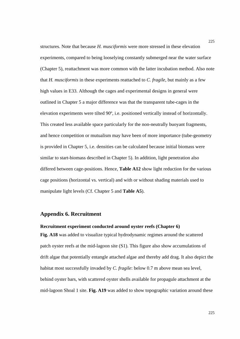
225

225

structures. Note that because H. musciformis were more stressed in these elevation

experiments, compared to being looselying constantly submerged near the water surface

(Chapter 5), reattachment was more common with the latter incubation method. Also note

that H. musciformis in these experiments reattached to C. fragile, but mainly as a few

high values in E33. Although the cages and experimental designs in general were

outlined in Chapter 5 a major difference was that the transparent tube-cages in the

elevation experiments were tilted 90º, i.e. positioned vertically instead of horizontally.

This created less available space particularly for the non-neutrally buoyant fragments,

and hence competition or mutualism may have been of more importance (tube-geometry

is provided in Chapter 5, i.e. densities can be calculated because initial biomass were

similar to start-biomass described in Chapter 5). In addition, light penetration also

differed between cage-positions. Hence, Table A12 show light reduction for the various

cage positions (horizontal vs. vertical) and with or without shading materials used to

manipulate light levels (Cf. Chapter 5 and Table A5).

Appendix 6. Recruitment

Recruitment experiment conducted around oyster reefs (Chapter 6)

Fig. A18 was added to visualize typical hydrodynamic regimes around the scattered

patch oyster reefs at the mid-lagoon site (S1). This figure also show accumulations of

drift algae that potentially entangle attached algae and thereby add drag. It also depict the

habitat most successfully invaded by C. fragile: below 0.7 m above mean sea level,

behind oyster bars, with scattered oyster shells available for propagule attachment at the

mid-lagoon Shoal 1 site. Fig. A19 was added to show topographic variation around these

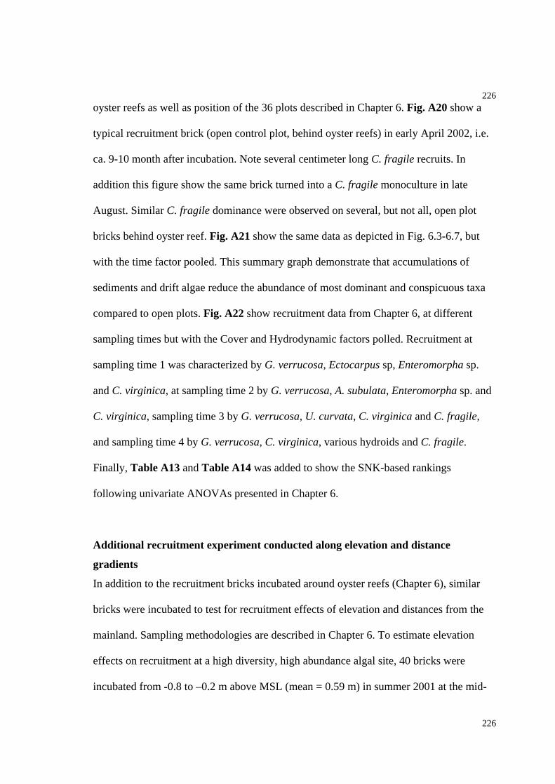
226

226

oyster reefs as well as position of the 36 plots described in Chapter 6. Fig. A20 show a

typical recruitment brick (open control plot, behind oyster reefs) in early April 2002, i.e.

ca. 9-10 month after incubation. Note several centimeter long C. fragile recruits. In

addition this figure show the same brick turned into a C. fragile monoculture in late

August. Similar C. fragile dominance were observed on several, but not all, open plot

bricks behind oyster reef. Fig. A21 show the same data as depicted in Fig. 6.3-6.7, but

with the time factor pooled. This summary graph demonstrate that accumulations of

sediments and drift algae reduce the abundance of most dominant and conspicuous taxa

compared to open plots. Fig. A22 show recruitment data from Chapter 6, at different

sampling times but with the Cover and Hydrodynamic factors polled. Recruitment at

sampling time 1 was characterized by G. verrucosa, Ectocarpus sp, Enteromorpha sp.

and C. virginica, at sampling time 2 by G. verrucosa, A. subulata, Enteromorpha sp. and

C. virginica, sampling time 3 by G. verrucosa, U. curvata, C. virginica and C. fragile,

and sampling time 4 by G. verrucosa, C. virginica, various hydroids and C. fragile.

Finally, Table A13 and Table A14 was added to show the SNK-based rankings

following univariate ANOVAs presented in Chapter 6.

Additional recruitment experiment conducted along elevation and distance

gradients

In addition to the recruitment bricks incubated around oyster reefs (Chapter 6), similar

bricks were incubated to test for recruitment effects of elevation and distances from the

mainland. Sampling methodologies are described in Chapter 6. To estimate elevation

effects on recruitment at a high diversity, high abundance algal site, 40 bricks were

incubated from -0.8 to 0.2 m above MSL (mean = 0.59 m) in summer 2001 at the mid-

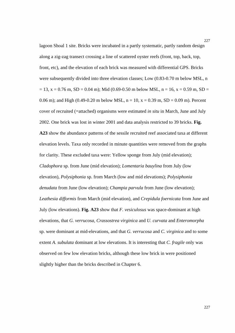
227

227

lagoon Shoal 1 site. Bricks were incubated in a partly systematic, partly random design

along a zig-zag transect crossing a line of scattered oyster reefs (front, top, back, top,

front, etc), and the elevation of each brick was measured with differential GPS. Bricks

were subsequently divided into three elevation classes; Low (0.83-0.70 m below MSL, n

= 13, x = 0.76 m, SD = 0.04 m); Mid (0.69-0.50 m below MSL, n = 16, x = 0.59 m, SD =

0.06 m); and High (0.49-0.20 m below MSL, n = 10, x = 0.39 m, SD = 0.09 m). Percent

cover of recruited (=attached) organisms were estimated in situ in March, June and July

2002. One brick was lost in winter 2001 and data analysis restricted to 39 bricks. Fig.

A23 show the abundance patterns of the sessile recruited reef associated taxa at different

elevation levels. Taxa only recorded in minute quantities were removed from the graphs

for clarity. These excluded taxa were: Yellow sponge from July (mid elevation);

Cladophora sp. from June (mid elevation); Lomentaria bauylina from July (low

elevation), Polysiphonia sp. from March (low and mid elevations); Polysiphonia

denudata from June (low elevation); Champia parvula from June (low elevation);

Leathesia difformis from March (mid elevation), and Crepidula foernicata from June and

July (low elevations). Fig. A23 show that F. vesiculosus was space-dominant at high

elevations, that G. verrucosa, Crassostrea virginica and U. curvata and Enteromorpha

sp. were dominant at mid-elevations, and that G. verrucosa and C. virginica and to some

extent A. subulata dominant at low elevations. It is interesting that C. fragile only was

observed on few low elevation bricks, although these low brick in were positioned

slightly higher than the bricks described in Chapter 6.

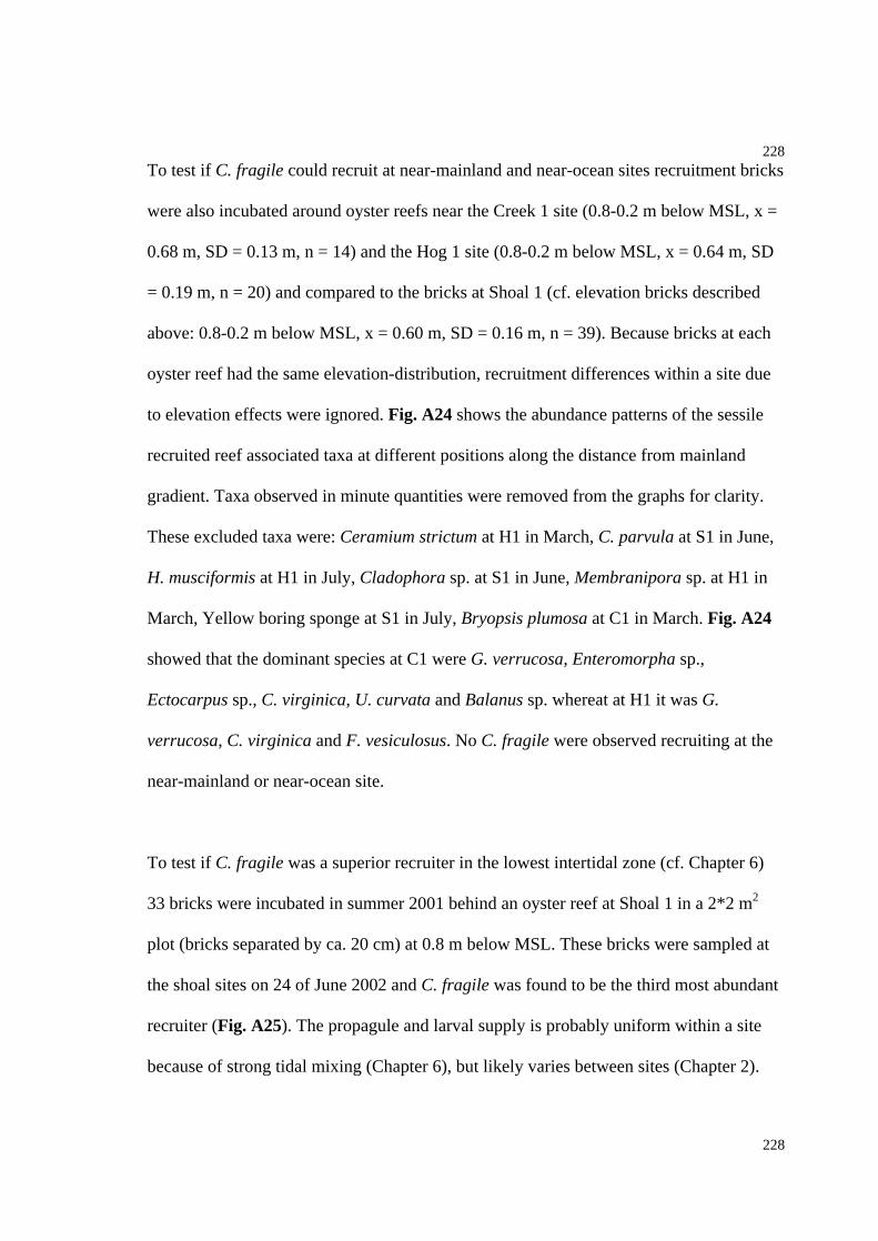
228

228

To test if C. fragile could recruit at near-mainland and near-ocean sites recruitment bricks

were also incubated around oyster reefs near the Creek 1 site (0.8-0.2 m below MSL, x =

0.68 m, SD = 0.13 m, n = 14) and the Hog 1 site (0.8-0.2 m below MSL, x = 0.64 m, SD

= 0.19 m, n = 20) and compared to the bricks at Shoal 1 (cf. elevation bricks described

above: 0.8-0.2 m below MSL, x = 0.60 m, SD = 0.16 m, n = 39). Because bricks at each

oyster reef had the same elevation-distribution, recruitment differences within a site due

to elevation effects were ignored. Fig. A24 shows the abundance patterns of the sessile

recruited reef associated taxa at different positions along the distance from mainland

gradient. Taxa observed in minute quantities were removed from the graphs for clarity.

These excluded taxa were: Ceramium strictum at H1 in March, C. parvula at S1 in June,

H. musciformis at H1 in July, Cladophora sp. at S1 in June, Membranipora sp. at H1 in

March, Yellow boring sponge at S1 in July, Bryopsis plumosa at C1 in March. Fig. A24

showed that the dominant species at C1 were G. verrucosa, Enteromorpha sp.,

Ectocarpus sp., C. virginica, U. curvata and Balanus sp. whereat at H1 it was G.

verrucosa, C. virginica and F. vesiculosus. No C. fragile were observed recruiting at the

near-mainland or near-ocean site.

To test if C. fragile was a superior recruiter in the lowest intertidal zone (cf. Chapter 6)

33 bricks were incubated in summer 2001 behind an oyster reef at Shoal 1 in a 2*2 m2

plot (bricks separated by ca. 20 cm) at 0.8 m below MSL. These bricks were sampled at

the shoal sites on 24 of June 2002 and C. fragile was found to be the third most abundant

recruiter (Fig. A25). The propagule and larval supply is probably uniform within a site

because of strong tidal mixing (Chapter 6), but likely varies between sites (Chapter 2).

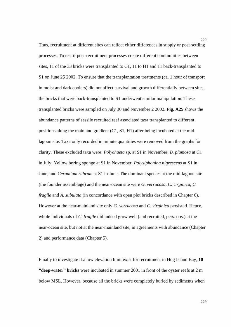
229

229

Thus, recruitment at different sites can reflect either differences in supply or post-settling

processes. To test if post-recruitment processes create different communities between

sites, 11 of the 33 bricks were transplanted to C1, 11 to H1 and 11 back-transplanted to

S1 on June 25 2002. To ensure that the transplantation treatments (ca. 1 hour of transport

in moist and dark coolers) did not affect survival and growth differentially between sites,

the bricks that were back-transplanted to S1 underwent similar manipulation. These

transplanted bricks were sampled on July 30 and November 2 2002. Fig. A25 shows the

abundance patterns of sessile recruited reef associated taxa transplanted to different

positions along the mainland gradient (C1, S1, H1) after being incubated at the mid-

lagoon site. Taxa only recorded in minute quantities were removed from the graphs for

clarity. These excluded taxa were: Polychaeta sp. at S1 in November; B. plumosa at C1

in July; Yellow boring sponge at S1 in November; Polysiphonina nigrescens at S1 in

June; and Ceramium rubrum at S1 in June. The dominant species at the mid-lagoon site

(the founder assemblage) and the near-ocean site were G. verrucosa, C. virginica, C.

fragile and A. subulata (in concordance with open plot bricks described in Chapter 6).

However at the near-mainland site only G. verrucosa and C. virginica persisted. Hence,

whole individuals of C. fragile did indeed grow well (and recruited, pers. obs.) at the

near-ocean site, but not at the near-mainland site, in agreements with abundance (Chapter

2) and performance data (Chapter 5).

Finally to investigate if a low elevation limit exist for recruitment in Hog Island Bay, 10

deep-water bricks were incubated in summer 2001 in front of the oyster reefs at 2 m

below MSL. However, because all the bricks were completely buried by sediments when

230

230

sampled in spring 2002, no sessile attached species were recorded, and not statistical data

analysis was conducted. The interpretation was straightforward: high sedimentation at

low elevations limit recruitment onto low relief hard substrate at Shoal 1.

Appendix 7. VCR/LTER water quality monitoring data

In 1992 the VCR/LTER (Hayden et al. 2000) initialized a water quality monitoring

program with 10 permanent station (Fig. A26). The 10 sites correspond to the mouth of

Phillips Creek (PCm, near-mainland creek), the head of Phillips Creek (PHh, near-

mailand creek), Green Creek (GC, near-mainland creek), Oyster Harbor (OH, near-

mainland harbor), Red Bank (RB, transition point from near-mainland creeks to open

lagoon), No name Creek (NC, back-barrier island creek, i.e. may be influenced by marsh

run-off), mouth of Cattle Shed creek (CSm, back-barrier island creek, i.e. may be

influenced by marsh run-off), Quinby Inlet (QI, near-ocean inlet), Machinpongo Inlet

(MI, near-ocean inlet) and South Hog (SH, near-ocean inlet). Some of the key variables

that are sampled on a regular basis include salinity (here presented as the mean of

refractometer and SCT-meter values), dissolved oxygen, water temperature (mean from

DO and SCT-meters), total suspended solids (each sample based on 3 sub-replicates per

site of 300 ml surface waters filtered through GC filters and oven dried at ca. 100ºC), and

secchi depth. I digitized and compiled the data from 1999-2002 (collected by Kathleen

Overman, Jason Restein, Phillips Smith and Jimmy Spitler), that temporally match most

of the data presented in Chapter 2-6. Survey dates include (d/m/y): 31/03/99, 28/04/99,

25/05/99, 30/06/99, 31/07/99, 09/09/99, 29/09/99, 03/11/99, 30/11/99, 02/12/99,

27/01/00, 24/02/00, 27/03/00, 26/04/00, 28/06/00, 08/11/00, 06/12/00, 07/02/01,

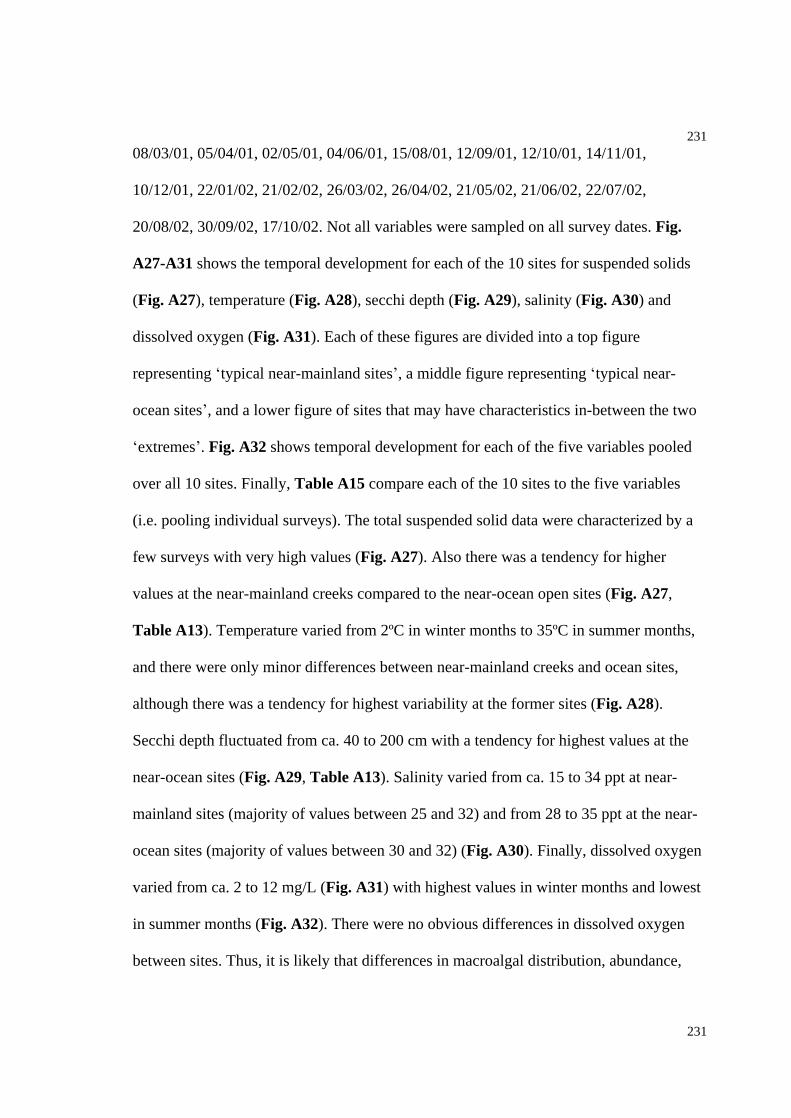
231

231

08/03/01, 05/04/01, 02/05/01, 04/06/01, 15/08/01, 12/09/01, 12/10/01, 14/11/01,

10/12/01, 22/01/02, 21/02/02, 26/03/02, 26/04/02, 21/05/02, 21/06/02, 22/07/02,

20/08/02, 30/09/02, 17/10/02. Not all variables were sampled on all survey dates. Fig.

A27-A31 shows the temporal development for each of the 10 sites for suspended solids

(Fig. A27), temperature (Fig. A28), secchi depth (Fig. A29), salinity (Fig. A30) and

dissolved oxygen (Fig. A31). Each of these figures are divided into a top figure

representing typical near-mainland sites , a middle figure representing typical near-

ocean sites , and a lower figure of sites that may have characteristics in-between the two

extremes . Fig. A32 shows temporal development for each of the five variables pooled

over all 10 sites. Finally, Table A15 compare each of the 10 sites to the five variables

(i.e. pooling individual surveys). The total suspended solid data were characterized by a

few surveys with very high values (Fig. A27). Also there was a tendency for higher

values at the near-mainland creeks compared to the near-ocean open sites (Fig. A27,

Table A13). Temperature varied from 2ºC in winter months to 35ºC in summer months,

and there were only minor differences between near-mainland creeks and ocean sites,

although there was a tendency for highest variability at the former sites (Fig. A28).

Secchi depth fluctuated from ca. 40 to 200 cm with a tendency for highest values at the

near-ocean sites (Fig. A29, Table A13). Salinity varied from ca. 15 to 34 ppt at near-

mainland sites (majority of values between 25 and 32) and from 28 to 35 ppt at the near-

ocean sites (majority of values between 30 and 32) (Fig. A30). Finally, dissolved oxygen

varied from ca. 2 to 12 mg/L (Fig. A31) with highest values in winter months and lowest

in summer months (Fig. A32). There were no obvious differences in dissolved oxygen

between sites. Thus, it is likely that differences in macroalgal distribution, abundance,

232

232

and performance along the distance from mainland gradient (Chapter 2, 3, 5, Appendix 1)

is caused by a complex set of interacting factors including nutrients (Chapter 5), grazer

abundance (Chapter 5, Rosinski 2004), salinity (this section), light regime (Chapter 5,

this section), hydrodynamic regimes and sedimentation levels.

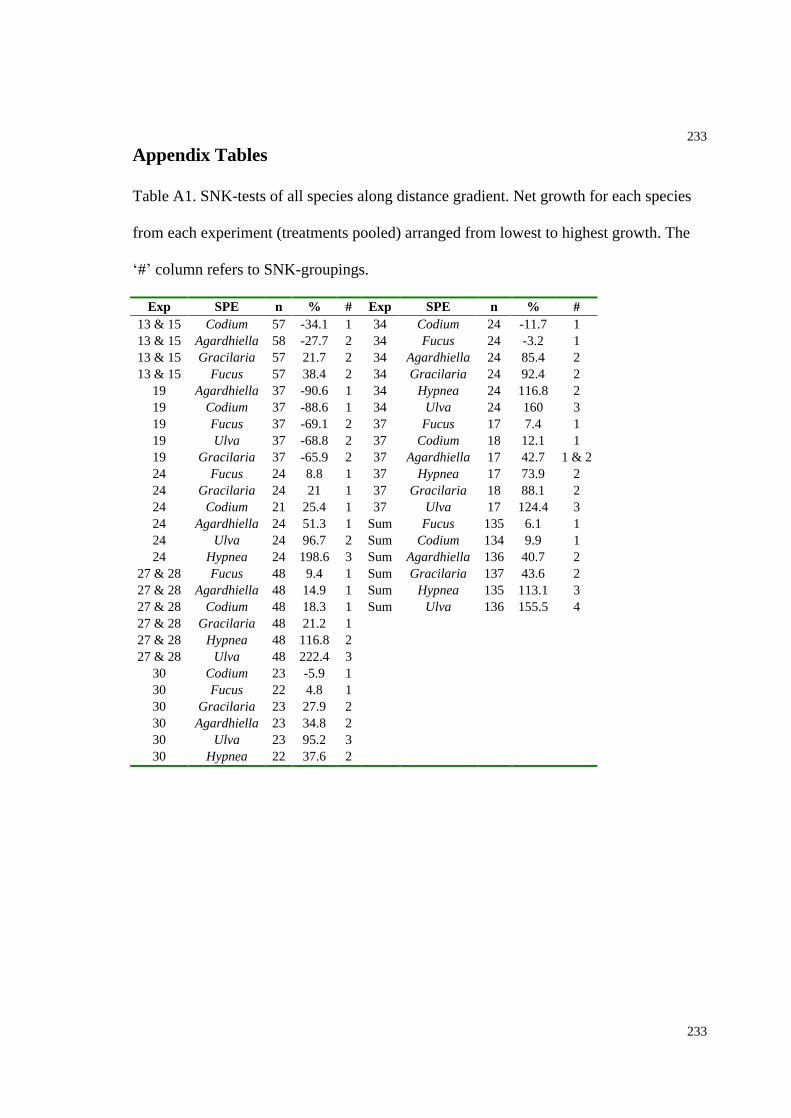
233

233

Appendix Tables

Table A1. SNK-tests of all species along distance gradient. Net growth for each species

from each experiment (treatments pooled) arranged from lowest to highest growth. The

# column refers to SNK-groupings.

Exp SPE n % # Exp SPE n % #13 & 15 Codium 57 -34.1 1 34 Codium 24 -11.7 113 & 15 Agardhiella 58 -27.7 2 34 Fucus 24 -3.2 113 & 15 Gracilaria 57 21.7 2 34 Agardhiella 24 85.4 213 & 15 Fucus 57 38.4 2 34 Gracilaria 24 92.4 2

19 Agardhiella 37 -90.6 1 34 Hypnea 24 116.8 219 Codium 37 -88.6 1 34 Ulva 24 160 319 Fucus 37 -69.1 2 37 Fucus 17 7.4 119 Ulva 37 -68.8 2 37 Codium 18 12.1 119 Gracilaria 37 -65.9 2 37 Agardhiella 17 42.7 1 & 224 Fucus 24 8.8 1 37 Hypnea 17 73.9 224 Gracilaria 24 21 1 37 Gracilaria 18 88.1 224 Codium 21 25.4 1 37 Ulva 17 124.4 324 Agardhiella 24 51.3 1 Sum Fucus 135 6.1 124 Ulva 24 96.7 2 Sum Codium 134 9.9 124 Hypnea 24 198.6 3 Sum Agardhiella 136 40.7 2

27 & 28 Fucus 48 9.4 1 Sum Gracilaria 137 43.6 227 & 28 Agardhiella 48 14.9 1 Sum Hypnea 135 113.1 327 & 28 Codium 48 18.3 1 Sum Ulva 136 155.5 427 & 28 Gracilaria 48 21.2 127 & 28 Hypnea 48 116.8 227 & 28 Ulva 48 222.4 3

30 Codium 23 -5.9 130 Fucus 22 4.8 130 Gracilaria 23 27.9 230 Agardhiella 23 34.8 230 Ulva 23 95.2 330 Hypnea 22 37.6 2

234

234

Table A2. SNK-test of C. fragile performance along distance. Net growth for C. fragile

from each experiment along DIS gradient (treatments pooled) arranged from lowest to

highest growth. The # column refers to SNK-groupings.

EXP DIS n % # EXP DIS n % #13 & 15 C1 20 -39.3 1 34 C1 8 -25.2 113 & 15 H1 15 -38.6 1 34 S1 8 -6.6 113 & 15 S1 20 -28.9 1 34 H1 8 -3.4 1

24 C1 7 23.7 1 37 C1 6 3.4 124 H1 7 26.1 1 37 H1 6 12.1 224 S1 7 26.3 1 37 S1 6 20.7 2

27 & 29 C1 16 11.5 1 30 C1 8 -12.3 127 & 29 H1 16 19.6 2 30 H1 8 -2.2 227 & 29 S1 16 23.7 2 30 S1 7 -2.8 2

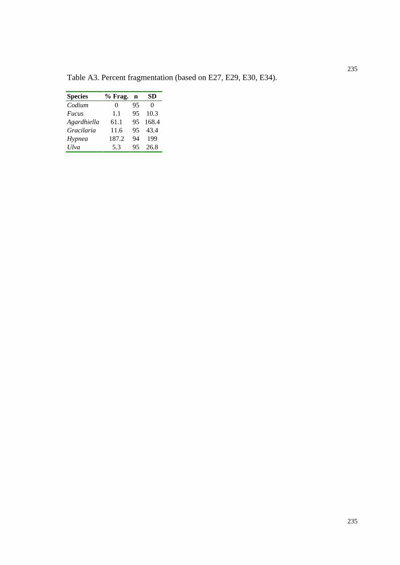
235

235

Table A3. Percent fragmentation (based on E27, E29, E30, E34).

Species % Frag. n SDCodium 0 95 0Fucus 1.1 95 10.3Agardhiella 61.1 95 168.4Gracilaria 11.6 95 43.4Hypnea 187.2 94 199Ulva 5.3 95 26.8

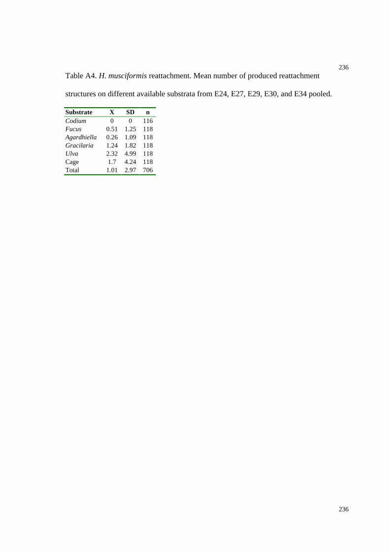
236

236

Table A4. H. musciformis reattachment. Mean number of produced reattachment

structures on different available substrata from E24, E27, E29, E30, and E34 pooled.

Substrate X SD nCodium 0 0 116Fucus 0.51 1.25 118Agardhiella 0.26 1.09 118Gracilaria 1.24 1.82 118Ulva 2.32 4.99 118Cage 1.7 4.24 118Total 1.01 2.97 706

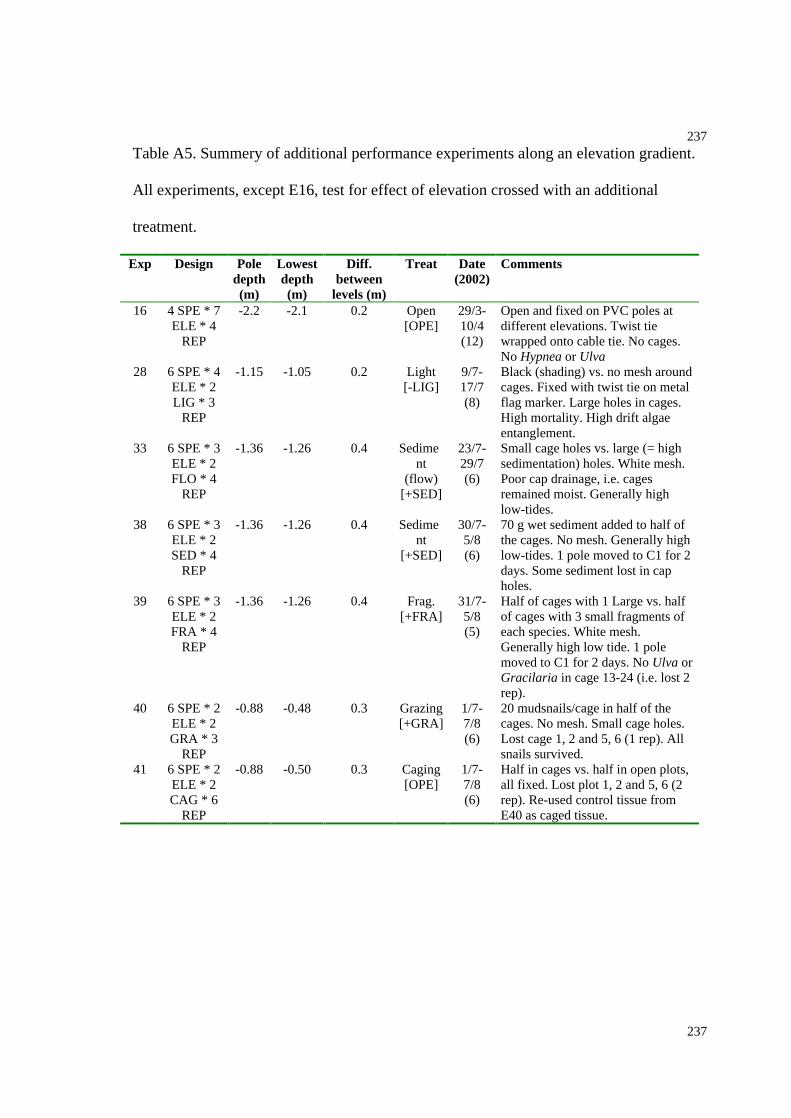
237

237

Table A5. Summery of additional performance experiments along an elevation gradient.

All experiments, except E16, test for effect of elevation crossed with an additional

treatment.

Exp Design Poledepth(m)

Lowestdepth(m)

Diff.between

levels (m)

Treat Date(2002)

Comments

16 4 SPE * 7ELE * 4

REP

-2.2 -2.1 0.2 Open[OPE]

29/3-10/4(12)

Open and fixed on PVC poles atdifferent elevations. Twist tiewrapped onto cable tie. No cages.No Hypnea or Ulva

28 6 SPE * 4ELE * 2LIG * 3

REP

-1.15 -1.05 0.2 Light[-LIG]

9/7-17/7(8)

Black (shading) vs. no mesh aroundcages. Fixed with twist tie on metalflag marker. Large holes in cages.High mortality. High drift algaeentanglement.

33 6 SPE * 3ELE * 2FLO * 4

REP

-1.36 -1.26 0.4 Sediment

(flow)[+SED]

23/7-29/7(6)

Small cage holes vs. large (= highsedimentation) holes. White mesh.Poor cap drainage, i.e. cagesremained moist. Generally highlow-tides.

38 6 SPE * 3ELE * 2SED * 4

REP

-1.36 -1.26 0.4 Sediment

[+SED]

30/7-5/8(6)

70 g wet sediment added to half ofthe cages. No mesh. Generally highlow-tides. 1 pole moved to C1 for 2days. Some sediment lost in capholes.

39 6 SPE * 3ELE * 2FRA * 4

REP

-1.36 -1.26 0.4 Frag.[+FRA]

31/7-5/8(5)

Half of cages with 1 Large vs. halfof cages with 3 small fragments ofeach species. White mesh.Generally high low tide. 1 polemoved to C1 for 2 days. No Ulva orGracilaria in cage 13-24 (i.e. lost 2rep).

40 6 SPE * 2ELE * 2GRA * 3

REP

-0.88 -0.48 0.3 Grazing[+GRA]

1/7-7/8(6)

20 mudsnails/cage in half of thecages. No mesh. Small cage holes.Lost cage 1, 2 and 5, 6 (1 rep). Allsnails survived.

41 6 SPE * 2ELE * 2CAG * 6

REP

-0.88 -0.50 0.3 Caging[OPE]

1/7-7/8(6)

Half in cages vs. half in open plots,all fixed. Lost plot 1, 2 and 5, 6 (2rep). Re-used control tissue fromE40 as caged tissue.

238

238

Table A6A. ANOVA on assemblages on additional performance experiments along

elevation gradient. Significant results are in bold (p < 0.05). Analysis procedures as in

Chapter 5.

Exp Source Df SS 2(%) F p16 SPE 3 128780 38 61.48 0.00016 ELE 8 82947 24 14.85 0.00016 SPE * ELE 24 65483 19 3.91 0.00016 Error 89 62143 1828 SPE 5 231148 69 85.18 0.00028 ELE 3 8682 3 5.33 0.00228 LIG 1 18422 6 33.94 0.00028 SPE * ELE 15 7819 2 0.96 0.50228 SPE * LIG 5 7095 2 2.61 0.02928 ELE * LIG 3 4139 1 2.54 0.06128 SPE * ELE * LIG 15 5340 2 0.66 0.82028 Error 93 50476 1533 SPE 5 316178 43 48.76 0.00033 ELE 2 98014 13 37.79 0.00033 FLO 1 4130 1 3.18 0.07733 SPE * ELE 10 149408 20 11.52 0.00033 SPE * FLO 5 12117 2 1.87 0.10033 ELE * FLO 2 11566 2 4.46 0.01433 SPE * ELE * FLO 10 5876 1 0.45 0.91633 Error 108 140058 1938 SPE 5 60095 18 7.52 0.00038 ELE 2 26547 8 8.30 0.00038 SED 1 7947 2 4.97 0.02838 SPE * ELE 10 14650 4 0.92 0.52138 SPE * SED 5 24358 7 3.05 0.01338 ELE * SED 2 15002 5 4.69 0.01138 SPE * ELE * SED 10 6019 2 0.38 0.95438 Error 108 172703 5339 SPE 5 85639 37 18.59 0.00039 ELE 2 27525 12 14.94 0.00039 FRA 1 1194 1 1.30 0.25839 SPE * ELE 10 17645 8 1.92 0.05439 SPE * FRA 5 14189 6 3.08 0.01339 ELE * FRA 2 287 0 0.16 0.85639 SPE * ELE * FRA 10 9357 4 1.02 0.43839 Error 83 76469 33

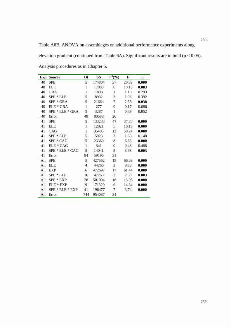
239

239

Table A6B. ANOVA on assemblages on additional performance experiments along

elevation gradient (continued from Table 6A). Significant results are in bold (p < 0.05).

Analysis procedures as in Chapter 5.

Exp Source Df SS 2(%) F p40 SPE 5 174804 57 20.82 0.00040 ELE 1 17083 6 10.18 0.00340 GRA 1 1898 1 1.13 0.29340 SPE * ELE 5 8932 3 1.06 0.39240 SPE * GRA 5 21664 7 2.58 0.03840 ELE * GRA 1 277 0 0.17 0.68640 SPE * ELE * GRA 5 3287 1 0.39 0.85240 Error 48 80588 2641 SPE 5 133283 47 37.83 0.00041 ELE 1 12821 5 18.19 0.00041 CAG 1 35405 12 50.24 0.00041 SPE * ELE 5 5923 2 1.68 0.14841 SPE * CAG 5 23360 8 6.63 0.00041 ELE * CAG 1 341 0 0.48 0.48841 SPE * ELE * CAG 5 14041 5 3.98 0.00341 Error 84 59196 21All SPE 5 427562 15 66.68 0.000All ELE 4 44266 2 8.63 0.000All EXP 6 472697 17 61.44 0.000All SPE * ELE 16 47263 2 2.30 0.003All SPE * EXP 28 501094 18 13.96 0.000All ELE * EXP 9 171329 6 14.84 0.000All SPE * ELE * EXP 41 196477 7 3.74 0.000All Error 744 954087 34

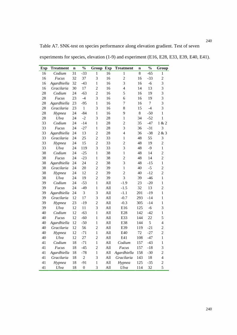
240

240

Table A7. SNK-test on species performance along elevation gradient. Test of seven

experiments for species, elevation (1-9) and experiment (E16, E28, E33, E39, E40, E41).

Exp Treatment n % Group Exp Treatment n % Group16 Codium 31 -33 1 16 1 8 -65 116 Fucus 32 37 3 16 2 16 -33 216 Agardhiella 32 -43 1 16 3 16 -6 316 Gracilaria 30 17 2 16 4 14 13 328 Codium 24 -63 2 16 5 16 19 328 Fucus 23 -4 3 16 6 16 19 328 Agardhiella 23 -95 1 16 7 16 7 328 Gracilaria 23 1 3 16 8 15 -4 328 Hypnea 24 -84 1 16 9 8 -50 128 Ulva 24 -2 3 28 1 34 -52 133 Codium 24 -14 1 28 2 35 -47 1 & 233 Fucus 24 -27 1 28 3 36 -31 333 Agardhiella 24 13 2 28 4 36 -38 2 & 333 Gracilaria 24 25 2 33 1 48 55 333 Hypnea 24 15 2 33 2 48 19 233 Ulva 24 119 3 33 3 48 -9 138 Codium 24 -25 1 38 1 48 14 238 Fucus 24 -23 1 38 2 48 14 238 Agardhiella 24 24 2 38 3 48 -15 138 Gracilaria 24 20 2 39 1 40 -5 238 Hypnea 24 12 2 39 2 40 -12 238 Ulva 24 19 2 39 3 39 -46 139 Codium 24 -53 1 All -1.9 23 -20 139 Fucus 24 -49 1 All -1.5 32 13 239 Agardhiella 24 3 3 All -1.1 201 -19 139 Gracilaria 12 17 3 All -0.7 293 -14 139 Hypnea 23 -19 2 All -0.3 305 -14 139 Ulva 12 11 3 All E16 125 -6 340 Codium 12 -63 1 All E28 142 -42 140 Fucus 12 -60 1 All E33 144 22 540 Agardhiella 12 -50 1 All E38 144 5 440 Gracilaria 12 56 2 All E39 119 -21 240 Hypnea 12 -71 1 All E40 72 -27 240 Ulva 12 27 2 All E41 108 -47 141 Codium 18 -71 1 All Codium 157 -43 141 Fucus 18 -45 2 All Fucus 157 -18 341 Agardhiella 18 -78 1 All Agardhiella 158 -30 241 Gracilaria 18 2 3 All Gracilaria 143 18 441 Hypnea 18 -91 1 All Hypnea 125 -35 241 Ulva 18 0 3 All Ulva 114 32 5

241

241

Table A8. ANOVA on C. fragile performance on additional performance experiments

along elevation gradient. Significant (p < 0.05) results are in bold.

Exp Source Df SS 2(%) F p16 ELE 9 71114 89 20.42 0.00016 Error 22 8512 1128 ELE 3 2993 12 1.84 0.18028 LIG 1 11782 48 21.78 0.00028 ELE * LIG 3 899 4 0.55 0.65328 Error 16 8653 3633 ELE 2 13184 30 8.73 0.00233 FLO 1 13464 30 17.82 0.00133 ELE * FLO 2 4419 10 2.92 0.07933 Error 18 13599 3038 ELE 2 25872 67 36.00 0.00038 SED 1 34 0 0.10 0.76138 ELE * SED 2 6218 16 8.65 0.00238 Error 18 6468 1739 ELE 2 21553 54 20.88 0.00039 FRA 1 6151 15 11.92 0.00339 ELE * FRA 2 2985 7 2.89 0.08139 Error 18 9289 2340 ELE 1 85 0 0.53 0.48740 GRA 1 18264 93 113.62 0.00040 ELE * GRA 1 85 0 0.53 0.48740 Error 8 1286 741 ELE 1 335 1 1.89 0.19141 CAG 1 20615 88 116.14 0.00041 ELE * CAG 1 9 0 0.05 0.82341 Error 14 2485 11All EXP 6 52345 18 15.83 0.000All ELE 4 24404 8 11.07 0.000All TRE 1 57006 19 103.46 0.000All EXP * ELE 9 61928 21 12.49 0.000All EXP * TRE 5 20160 7 7.32 0.000All ELE * TRE 2 2659 1 2.41 0.094All EXP * ELE * TRE 7 11705 4 3.03 0.006All Error 122 67221 23

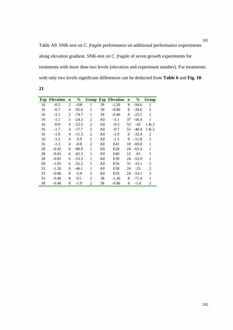
242

242

Table A9. SNK-test on C. fragile performance on additional performance experiments

along elevation gradient. SNK-test on C. fragile of seven growth experiments for

treatments with more than two levels (elevation and experiment number). For treatments

with only two levels significant differences can be deducted from Table 6 and Fig. 18-

21.

Exp Elevation n % Group Exp Elevation n % Group16 -0.5 2 -100 1 39 -1.26 8 -94.6 116 -0.7 4 -92.6 1 39 -0.86 8 -38.6 216 -2.1 2 -74.7 1 39 -0.46 8 -25.5 216 -1.1 3 -24.3 2 All -1.1 37 -56.4 116 -0.9 4 -22.5 2 All -0.3 53 -42 1 & 216 -1.7 4 -17.7 2 All -0.7 53 -40.4 1 & 216 -1.9 4 -11.3 2 All -1.9 6 -32.4 216 -1.5 4 -5.9 2 All -1.5 8 -11.8 216 -1.3 4 -0.8 2 All E41 18 -69.8 128 -0.45 6 -80.9 1 All E28 24 -63.4 128 -0.65 6 -65.3 1 All E40 12 -61 128 -0.85 6 -55.3 1 All E39 24 -52.9 128 -1.05 6 -52.2 1 All E16 31 -33.1 233 -1.26 8 -46.1 1 All E38 24 -25 233 -0.86 8 -5.8 2 All E33 24 -14.1 333 -0.46 8 9.5 2 38 -1.26 8 -71.4 138 -0.46 8 -1.9 2 38 -0.86 8 -1.6 2

243

243

Table A10. r2Pearson correlation matrix comparing performances between species from

seven additional performance experiments along elevation gradients. Significant p-values

are in bold. Only Fucus vs. Agardhiella and Fucus vs. Gracilaria had negative rPearson,

none of which were significant.

Codium Fucus Agardhiella Gracilaria Hypnea UlvaCodium r2 0.10 0.24 0.13 0.24 0.17

p 0.000 0.000 0.000 0.000 0.000n 156 157 142 125 114

Fucus r2 0.01 0.01 0.01 0.00p 0.352 0.402 0.356 0.518n 157 142 124 113

Agardhiella r2 0.11 0.40 0.13p 0.000 0.000 0.000n 143 125 114

Gracilaria r2 0.10 0.15p 0.001 0.000n 113 113

Hypnea r2 0.21p 0.000n 114

Ulva r2

pn

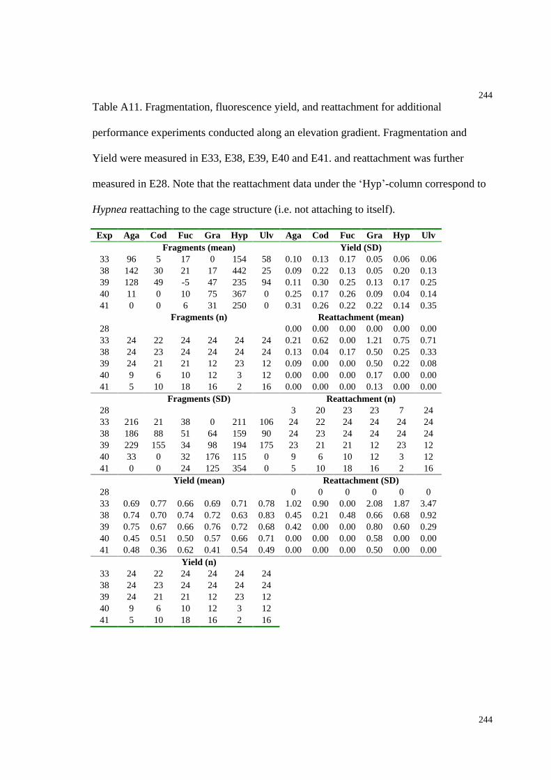
244

244

Table A11. Fragmentation, fluorescence yield, and reattachment for additional

performance experiments conducted along an elevation gradient. Fragmentation and

Yield were measured in E33, E38, E39, E40 and E41. and reattachment was further

measured in E28. Note that the reattachment data under the Hyp -column correspond to

Hypnea reattaching to the cage structure (i.e. not attaching to itself).

Exp Aga Cod Fuc Gra Hyp Ulv Aga Cod Fuc Gra Hyp UlvFragments (mean) Yield (SD)

33 96 5 17 0 154 58 0.10 0.13 0.17 0.05 0.06 0.0638 142 30 21 17 442 25 0.09 0.22 0.13 0.05 0.20 0.1339 128 49 -5 47 235 94 0.11 0.30 0.25 0.13 0.17 0.2540 11 0 10 75 367 0 0.25 0.17 0.26 0.09 0.04 0.1441 0 0 6 31 250 0 0.31 0.26 0.22 0.22 0.14 0.35

Fragments (n) Reattachment (mean)28 0.00 0.00 0.00 0.00 0.00 0.0033 24 22 24 24 24 24 0.21 0.62 0.00 1.21 0.75 0.7138 24 23 24 24 24 24 0.13 0.04 0.17 0.50 0.25 0.3339 24 21 21 12 23 12 0.09 0.00 0.00 0.50 0.22 0.0840 9 6 10 12 3 12 0.00 0.00 0.00 0.17 0.00 0.0041 5 10 18 16 2 16 0.00 0.00 0.00 0.13 0.00 0.00

Fragments (SD) Reattachment (n)28 3 20 23 23 7 2433 216 21 38 0 211 106 24 22 24 24 24 2438 186 88 51 64 159 90 24 23 24 24 24 2439 229 155 34 98 194 175 23 21 21 12 23 1240 33 0 32 176 115 0 9 6 10 12 3 1241 0 0 24 125 354 0 5 10 18 16 2 16

Yield (mean) Reattachment (SD)28 0 0 0 0 0 033 0.69 0.77 0.66 0.69 0.71 0.78 1.02 0.90 0.00 2.08 1.87 3.4738 0.74 0.70 0.74 0.72 0.63 0.83 0.45 0.21 0.48 0.66 0.68 0.9239 0.75 0.67 0.66 0.76 0.72 0.68 0.42 0.00 0.00 0.80 0.60 0.2940 0.45 0.51 0.50 0.57 0.66 0.71 0.00 0.00 0.00 0.58 0.00 0.0041 0.48 0.36 0.62 0.41 0.54 0.49 0.00 0.00 0.00 0.50 0.00 0.00

Yield (n)33 24 22 24 24 24 2438 24 23 24 24 24 2439 24 21 21 12 23 1240 9 6 10 12 3 1241 5 10 18 16 2 16

245

245

Table A12. Light reduction in cages. Treatments in cages were based on sampling at 4

different time periods during a summer day 2002. Horizontal positioned cages were

applied in Chapter 5, and vertical positioned cages in the additional performance

experiments briefly described above.

Mesh type Control None White Black None White BlackCage Position Horizontal Horizontal Horizontal Vertical Vertical VerticalPAR 1072 957 734 525 880 496 318SD 703 631 508 448 595 316 226n 50 10 10 10 5 5 5% PAR reduction 0 11 32 51 18 54 70

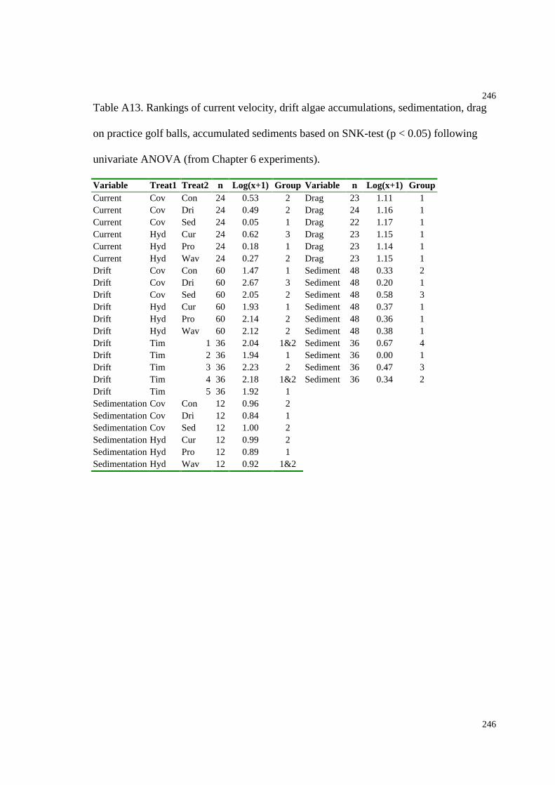
246

246

Table A13. Rankings of current velocity, drift algae accumulations, sedimentation, drag

on practice golf balls, accumulated sediments based on SNK-test (p < 0.05) following

univariate ANOVA (from Chapter 6 experiments).

Variable Treat1 Treat2 n Log(x+1) Group Variable n Log(x+1) GroupCurrent Cov Con 24 0.53 2 Drag 23 1.11 1Current Cov Dri 24 0.49 2 Drag 24 1.16 1Current Cov Sed 24 0.05 1 Drag 22 1.17 1Current Hyd Cur 24 0.62 3 Drag 23 1.15 1Current Hyd Pro 24 0.18 1 Drag 23 1.14 1Current Hyd Wav 24 0.27 2 Drag 23 1.15 1Drift Cov Con 60 1.47 1 Sediment 48 0.33 2Drift Cov Dri 60 2.67 3 Sediment 48 0.20 1Drift Cov Sed 60 2.05 2 Sediment 48 0.58 3Drift Hyd Cur 60 1.93 1 Sediment 48 0.37 1Drift Hyd Pro 60 2.14 2 Sediment 48 0.36 1Drift Hyd Wav 60 2.12 2 Sediment 48 0.38 1Drift Tim 1 36 2.04 1&2 Sediment 36 0.67 4Drift Tim 2 36 1.94 1 Sediment 36 0.00 1Drift Tim 3 36 2.23 2 Sediment 36 0.47 3Drift Tim 4 36 2.18 1&2 Sediment 36 0.34 2Drift Tim 5 36 1.92 1Sedimentation Cov Con 12 0.96 2Sedimentation Cov Dri 12 0.84 1Sedimentation Cov Sed 12 1.00 2Sedimentation Hyd Cur 12 0.99 2Sedimentation Hyd Pro 12 0.89 1Sedimentation Hyd Wav 12 0.92 1&2

247

247

Table A14. Rankings of Animal and Plant richness and abundance, and abundance of C.

fragile, C. virginia, G. verrucosa, A. subulata, U. curvata, Enteromorpha sp. based on

SNK-test (p < 0.05) following univariate ANOVA (Chapter 6 experiments).

Treat1 Treat2 n Var Log(x+1) Group Var Log(x+1) Group Var Log(x+1) GroupCov Con 48 AniR 0.48 1 PlaR 0.75 3 Ulv 0.33 2Cov Dri 48 AniR 0.45 1 PlaR 0.62 2 Ulv 0.30 2Cov Sed 48 AniR 0.44 1 PlaR 0.47 1 Ulv 0.06 1Hyd Cur 48 AniR 0.47 1 PlaR 0.63 2 Ulv 0.25 2Hyd Pro 48 AniR 0.46 1 PlaR 0.63 2 Ulv 0.25 2Hyd Wav 48 AniR 0.43 1 PlaR 0.58 1 Ulv 0.18 1Tim 1 36 AniR 0.48 2 PlaR 0.63 2 Ulv 0.07 1Tim 2 36 AniR 0.37 1 PlaR 0.66 2 Ulv 0.16 2Tim 3 36 AniR 0.47 2 PlaR 0.67 2 Ulv 0.46 3Tim 4 36 AniR 0.50 2 PlaR 0.50 1 Ulv 0.22 2Cov Con 48 AniC 0.75 2 PlaC 1.38 3 Aga 0.29 2Cov Dri 48 AniC 0.43 1 PlaC 0.94 2 Aga 0.03 1Cov Sed 48 AniC 0.43 1 PlaC 0.40 1 Aga 0.01 1Hyd Cur 48 AniC 0.54 1 PlaC 1.02 2 Aga 0.08 1Hyd Pro 48 AniC 0.56 1 PlaC 0.89 1 Aga 0.25 2Hyd Wav 48 AniC 0.51 1 PlaC 0.81 1 Aga 0.01 1Tim 1 36 AniC 0.54 1 PlaC 0.83 2 Aga 0.06 1Tim 2 36 AniC 0.46 1 PlaC 1.120 4 Aga 0.13 1Tim 3 36 AniC 0.44 1 PlaC 0.97 3 Aga 0.13 1Tim 4 36 AniC 0.70 2 PlaC 0.70 1 Aga 0.13 1Cov Con 48 Cra 0.60 2 Cod 0.49 2 Ent 0.29 2Cov Dri 48 Cra 0.12 1 Cod 0.03 1 Ent 0.62 3Cov Sed 48 Cra 0.21 1 Cod 0.01 1 Ent 0.12 1Hyd Cur 48 Cra 0.26 1 Cod 0.14 1 Ent 0.41 2Hyd Pro 48 Cra 0.35 1 Cod 0.22 1 Ent 0.27 1Hyd Wav 48 Cra 0.32 1 Cod 0.16 1 Ent 0.36 2Tim 1 36 Cra 0.25 1 Cod 0.12 1 Ent 0.35 2Tim 2 36 Cra 0.34 1 Cod 0.15 1 Ent 0.68 3Tim 3 36 Cra 0.30 1 Cod 0.23 1 Ent 0.29 2Tim 4 36 Cra 0.35 1 Cod 0.19 1 Ent 0.06 1Cov Con 48 Gra 1.02 2Cov Dri 48 Gra 0.24 1Cov Sed 48 Gra 0.21 1Hyd Cur 48 Gra 0.64 2Hyd Pro 48 Gra 0.41 1Hyd Wav 48 Gra 0.42 1Tim 1 36 Gra 0.39 1Tim 2 36 Gra 0.55 2Tim 3 36 Gra 0.55 2Tim 4 36 Gra 0.47 1&2

248

248

Table A15. Secchi depth, Temperature, Salinity, Suspended Solids and Dissolved oxygen

in Hog Island Bay. Data are mean values from nearly monthly sampling from 31-03-1999

to 17-10-2002 (data collected by Kathleen Overman, Phillips Smith and Jason Restein, as

part of the VCR/LTER Water Quality Monitoring Program).

Secchi (cm)

n SD Max Min Salt(ppt)

n SD Max Min

CSm 90 35 33 150 38 31.3 33 1.4 33.1 27.9GC 87 35 35 170 35 30.3 33 2.5 35.1 22.3MI 99 35 29 158 55 31.7 33 1.4 35.0 28.0NC 97 35 38 210 38 31.5 33 1.8 35.2 25.1OH 99 34 36 167 20 30.6 32 2.3 36.0 24.0PCh 70 35 23 119 29 27.9 33 4.7 36.3 15.8PCm 77 35 27 169 25 29.2 33 3.7 35.3 19.0QI 109 35 38 205 60 31.6 33 1.4 35.0 29.1RB 90 35 32 167 30 31.0 33 1.8 35.1 25.7SH 92 25 27 160 47 31.6 33 1.5 35.0 27.9Tot 339 34 210 20 30.7 329 2.7 36.3 15.8

T(C)

n SD Max Min TSS(gDW/L)

n SD Max Min

CSm 16.4 36 7.5 29.0 4.0 0.270 30 0.567 2.558 0.027GC 17.1 36 7.9 31.0 3.8 0.388 30 1.052 5.586 0.021MI 16.4 36 7.6 30.0 4.7 0.239 29 0.434 1.828 0.025NC 16.6 36 7.6 29.0 3.4 0.247 30 0.484 2.027 0.025OH 18.3 35 7.6 32.0 4.6 0.215 30 0.416 1.927 0.019PCh 17.5 36 7.8 31.0 3.6 0.323 30 0.754 3.822 0.022PCm 17.2 36 7.9 30.5 3.3 0.277 30 0.453 1.684 0.023QI 15.7 36 7.2 28.0 4.6 0.235 30 0.469 1.936 0.026RB 16.9 36 7.9 30.5 4.7 0.307 30 0.752 3.788 0.025SH 16.4 36 7.7 29.5 3.0 0.274 30 0.478 1.986 0.029Tot 16.9 359 7.6 32.0 3.0 0.277 299 0.610 5.586 0.019

DO(ml/L)

n SD Max Min

CSm 7.00 25 2.23 11.90 2.00GC 6.63 25 2.10 10.80 2.20MI 7.66 25 2.29 12.80 3.50NC 6.87 25 2.25 11.70 2.20OH 7.16 25 2.08 10.50 2.50PCh 6.38 25 2.47 12.20 2.10PCm 6.60 26 2.17 11.30 2.40QI 7.48 25 2.16 11.50 3.20RB 6.98 25 2.23 11.60 2.00SH 7.30 25 2.20 12.50 3.40Tot 7.01 251 2.21 12.80 2.00

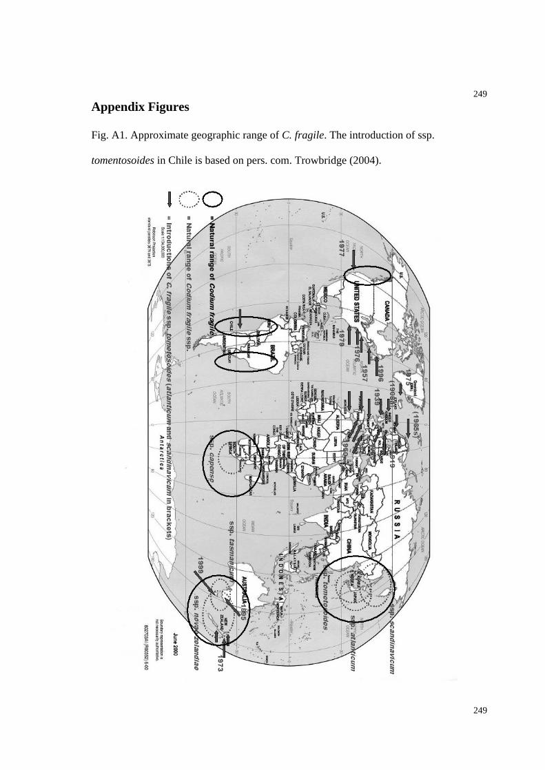
249

249

Appendix Figures

Fig. A1. Approximate geographic range of C. fragile. The introduction of ssp.

tomentosoides in Chile is based on pers. com. Trowbridge (2004).

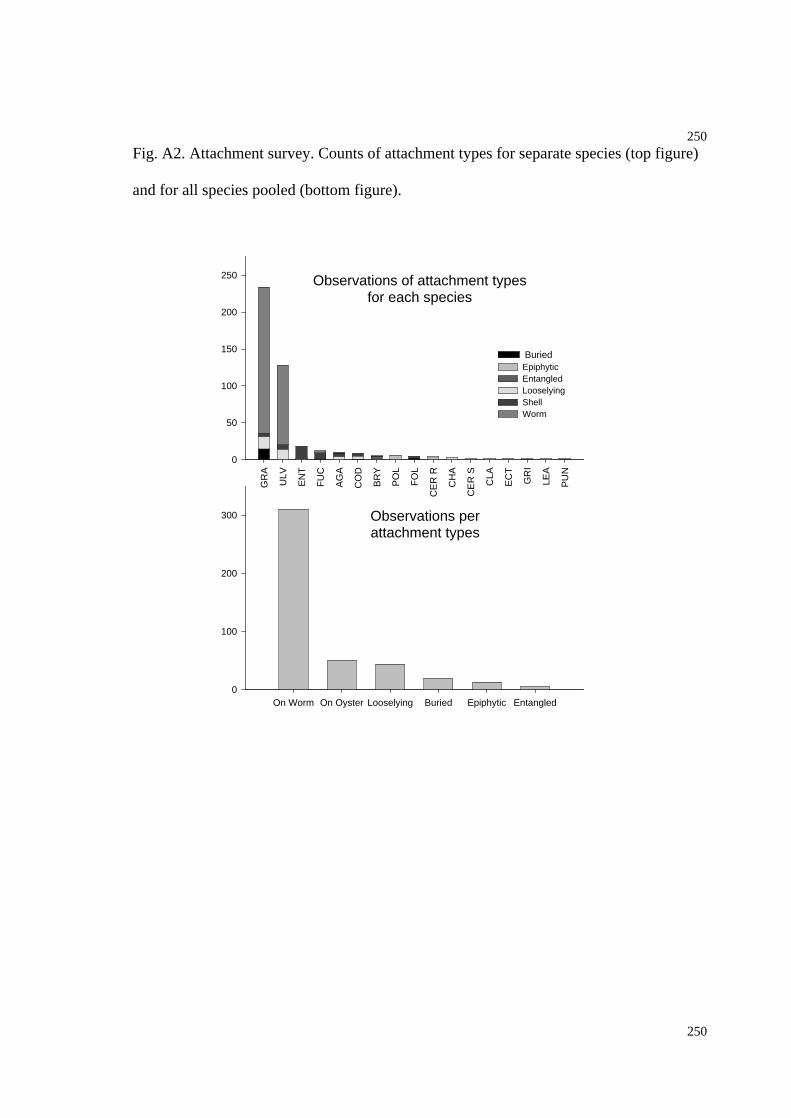
250

250

Fig. A2. Attachment survey. Counts of attachment types for separate species (top figure)

and for all species pooled (bottom figure).

Observations perattachment types

On Worm On Oyster Looselying Buried Epiphytic Entangled0

100

200

300

Observations of attachment typesfor each species

GR

A

ULV

EN

T

FU

C

AG

A

CO

D

BR

Y

PO

L

FO

L

CE

R R

CH

A

CE

R S

CLA

EC

T

GR

I

LEA

PU

N

0

50

100

150

200

250

Buried Epiphytic Entangled Looselying Shell Worm

251

251

Fig. A3. G. verrucosa dominance and D. cuprea tube caps. Top photo: A typical

intertidal mudflat dominated by scattered G. verrucosa clumps. Bottom photo: A close-

up of the G. verrucosa clumps. Each hummock is a D. cuprea tube cap with incorporated

G. verrucosa.

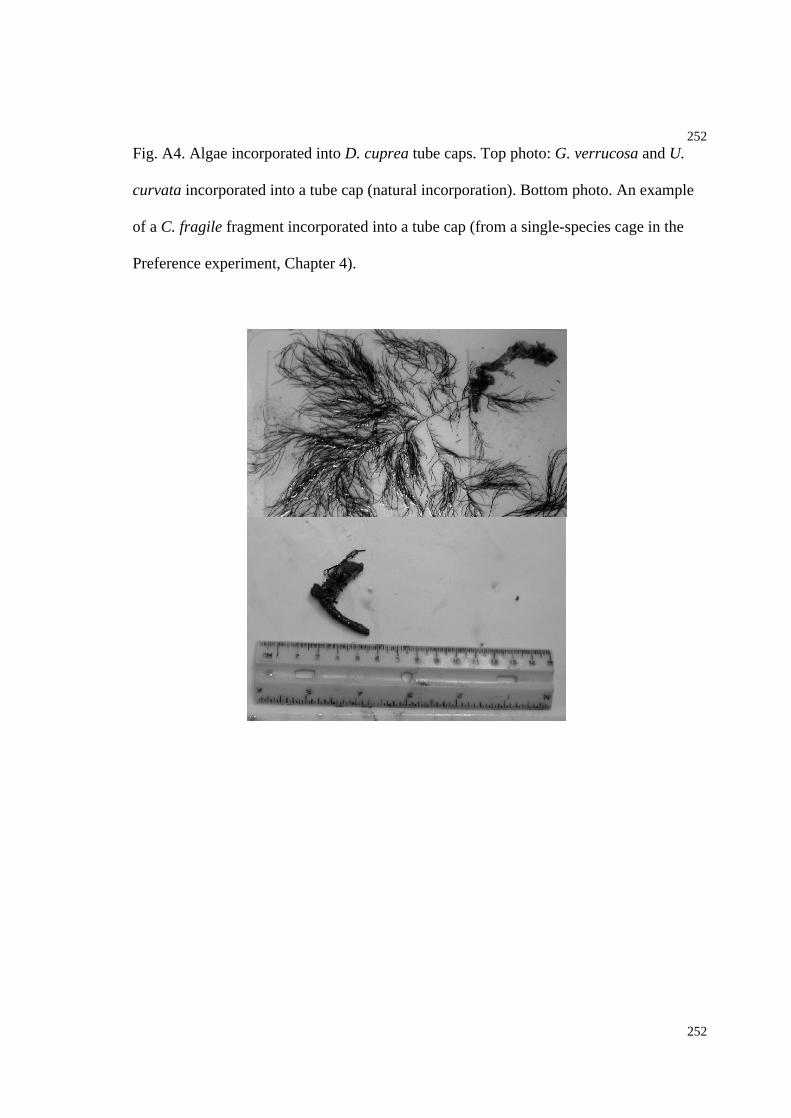
252

252

Fig. A4. Algae incorporated into D. cuprea tube caps. Top photo: G. verrucosa and U.

curvata incorporated into a tube cap (natural incorporation). Bottom photo. An example

of a C. fragile fragment incorporated into a tube cap (from a single-species cage in the

Preference experiment, Chapter 4).

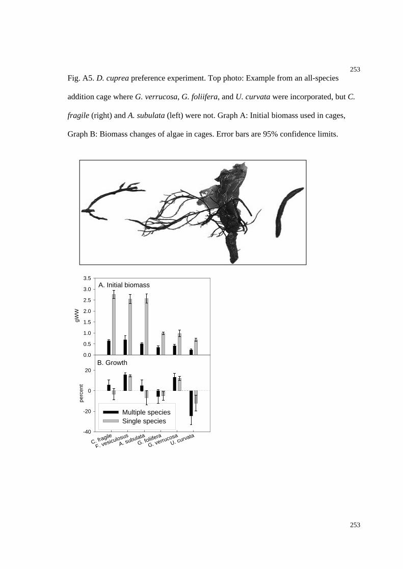
253

253

Fig. A5. D. cuprea preference experiment. Top photo: Example from an all-species

addition cage where G. verrucosa, G. foliifera, and U. curvata were incorporated, but C.

fragile (right) and A. subulata (left) were not. Graph A: Initial biomass used in cages,

Graph B: Biomass changes of algae in cages. Error bars are 95% confidence limits.

A. Initial biomass

gWW

0.0

0.5

1.0

1.5

2.0

2.5

3.0

3.5

B. Growth

C. fragile

F. vesiculosus

A. subulataG. foliifera

G. verrucosaU. curvata

perc

ent

-40

-20

0

20

Multiple speciesSingle species

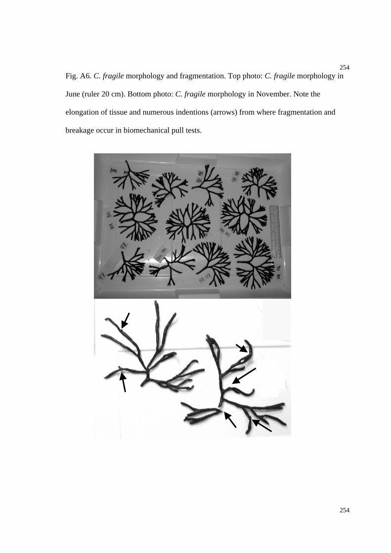
254

254

Fig. A6. C. fragile morphology and fragmentation. Top photo: C. fragile morphology in

June (ruler 20 cm). Bottom photo: C. fragile morphology in November. Note the

elongation of tissue and numerous indentions (arrows) from where fragmentation and

breakage occur in biomechanical pull tests.

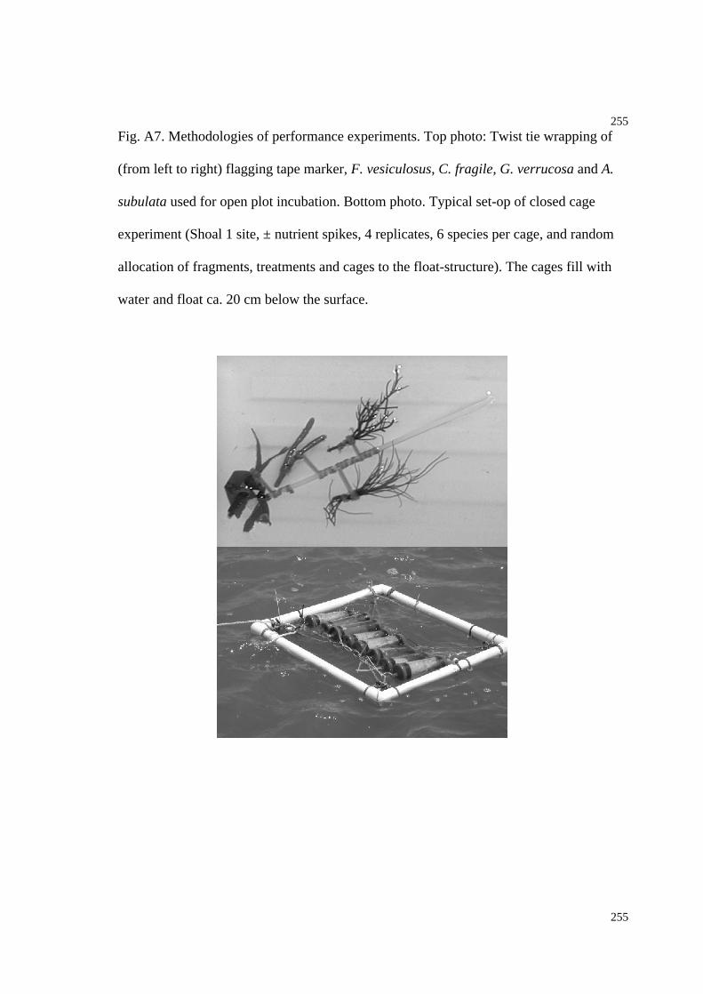
255

255

Fig. A7. Methodologies of performance experiments. Top photo: Twist tie wrapping of

(from left to right) flagging tape marker, F. vesiculosus, C. fragile, G. verrucosa and A.

subulata used for open plot incubation. Bottom photo. Typical set-op of closed cage

experiment (Shoal 1 site, ± nutrient spikes, 4 replicates, 6 species per cage, and random

allocation of fragments, treatments and cages to the float-structure). The cages fill with

water and float ca. 20 cm below the surface.

256

256

Fig. A8. Interaction plots of species, caging, distance from mainland, twist-tie wrapping

and experimental design versus algal performance. The four graphs correspond to the

significant interactions that was not depicted in Figure 5.1-5.5. Cf. Chapter 5 for

descriptions of experimental designs and abbreviation. Note that species with large S:V

ratio have small variation in cages but large variation in open plots (Exp. 37).

Exp 37: SPE*DIS*CAG interaction

Cod Fuc Aga Gra Hyp Ulv

Cha

nge

in b

iom

ass

(%)

-100

0

100

200

300

400

500

C1 OpenC1 CageS1 OpenS1 CageH1 Open H1 Cage

Exp 27: SPE*EXP interaction

Cod Fuc Aga Gra Hyp Ulv-50

0

50

100

150

200

250

300

E27E29

Exp 30: DIS*TWI interaction

C1 S1 H1

Cha

nge

in b

iom

ass

(%)

0

10

20

30

40

50

60

70

TWI-TWI+

Exp Allsummer: DIS*EXP interaction

C1 S1 H10

20

40

60

80

100

120

140

E24E27E29E30E34E37

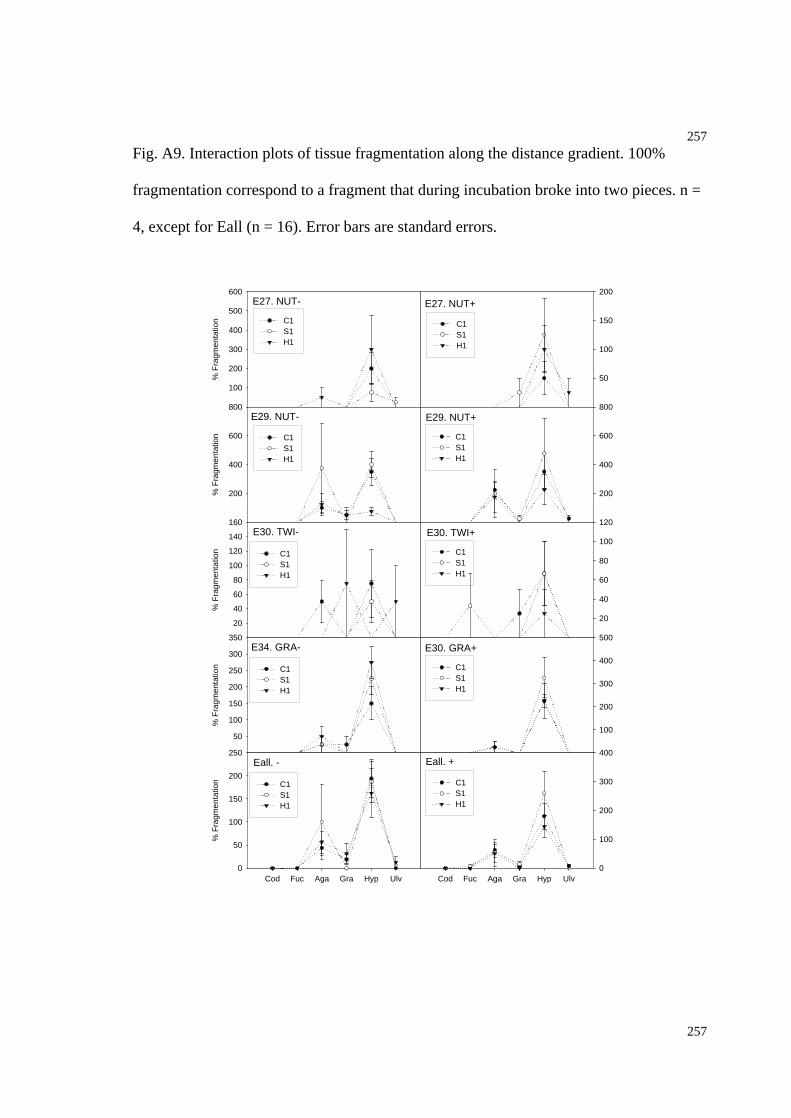
257

257

Fig. A9. Interaction plots of tissue fragmentation along the distance gradient. 100%

fragmentation correspond to a fragment that during incubation broke into two pieces. n =

4, except for Eall (n = 16). Error bars are standard errors.

E27. NUT-

Cod Fuc Aga Gra Hyp Ulv

% F

ragm

enta

tion

100

200

300

400

500

600

C1 S1H1

E27. NUT+

Cod Fuc Aga Gra Hyp Ulv

50

100

150

200

C1S1H1

E29. NUT-

Cod Fuc Aga Gra Hyp Ulv

% F

ragm

enta

tion

200

400

600

800

C1S1H1

E29. NUT+

Cod Fuc Aga Gra Hyp Ulv

200

400

600

800

C1S1H1

E30. TWI-

Cod Fuc Aga Gra Hyp Ulv

% F

ragm

enta

tion

20

40

60

80

100

120

140

160

C1S1H1

E30. TWI+

Cod Fuc Aga Gra Hyp Ulv

20

40

60

80

100

120

C1S1H1

E34. GRA-

Cod Fuc Aga Gra Hyp Ulv

% F

ragm

enta

tion

50

100

150

200

250

300

350

C1 S1H1

E30. GRA+

Cod Fuc Aga Gra Hyp Ulv

100

200

300

400

500

C1S1H1

Eall. -

Cod Fuc Aga Gra Hyp Ulv

% F

ragm

enta

tion

0

50

100

150

200

250

C1S1H1

Eall. +

Cod Fuc Aga Gra Hyp Ulv0

100

200

300

400

C1S1H1

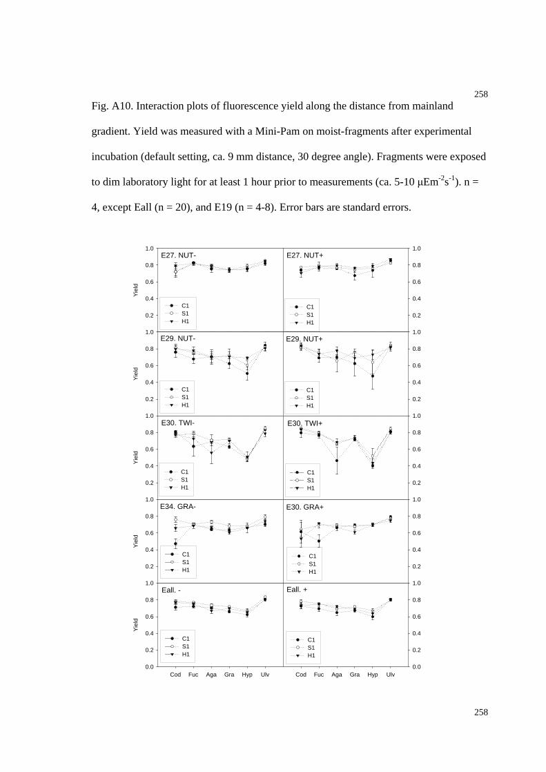
258

258

Fig. A10. Interaction plots of fluorescence yield along the distance from mainland

gradient. Yield was measured with a Mini-Pam on moist-fragments after experimental

incubation (default setting, ca. 9 mm distance, 30 degree angle). Fragments were exposed

to dim laboratory light for at least 1 hour prior to measurements (ca. 5-10 Em-2s-1). n =

4, except Eall (n = 20), and E19 (n = 4-8). Error bars are standard errors.

E27. NUT-

Cod Fuc Aga Gra Hyp Ulv

Yie

ld

0.2

0.4

0.6

0.8

1.0

C1 S1H1

E27. NUT+

Cod Fuc Aga Gra Hyp Ulv

0.2

0.4

0.6

0.8

1.0

C1S1H1

E29. NUT-

Cod Fuc Aga Gra Hyp Ulv

Yie

ld

0.2

0.4

0.6

0.8

1.0

C1S1H1

E29. NUT+

Cod Fuc Aga Gra Hyp Ulv

0.2

0.4

0.6

0.8

1.0

C1S1H1

E30. TWI-

Cod Fuc Aga Gra Hyp Ulv

Yie

ld

0.2

0.4

0.6

0.8

1.0

C1S1H1

E30. TWI+

Cod Fuc Aga Gra Hyp Ulv

0.2

0.4

0.6

0.8

1.0

C1S1H1

E34. GRA-

Cod Fuc Aga Gra Hyp Ulv

Yie

ld

0.2

0.4

0.6

0.8

1.0

C1 S1H1

E30. GRA+

Cod Fuc Aga Gra Hyp Ulv

0.2

0.4

0.6

0.8

1.0

C1S1H1

Eall. -

Cod Fuc Aga Gra Hyp Ulv

Yie

ld

0.0

0.2

0.4

0.6

0.8

1.0

C1S1H1

Eall. +

Cod Fuc Aga Gra Hyp Ulv0.0

0.2

0.4

0.6

0.8

1.0

C1S1H1

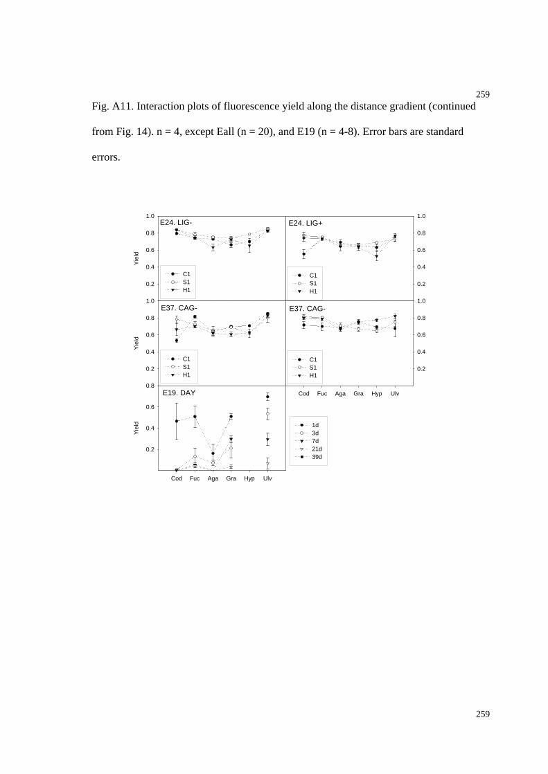
259

259

Fig. A11. Interaction plots of fluorescence yield along the distance gradient (continued

from Fig. 14). n = 4, except Eall (n = 20), and E19 (n = 4-8). Error bars are standard

errors.

E24. LIG-

Cod Fuc Aga Gra Hyp Ulv

Yie

ld

0.2

0.4

0.6

0.8

1.0

C1S1H1

E24. LIG+

Cod Fuc Aga Gra Hyp Ulv

0.2

0.4

0.6

0.8

1.0

C1S1H1

E37. CAG-

Cod Fuc Aga Gra Hyp Ulv

Yie

ld

0.2

0.4

0.6

0.8

1.0

C1 S1H1

E37. CAG-

Cod Fuc Aga Gra Hyp Ulv

0.2

0.4

0.6

0.8

1.0

C1S1H1

E19. DAY

Cod Fuc Aga Gra Hyp Ulv

Yie

ld

0.2

0.4

0.6

0.8

1d3d7d21d39d

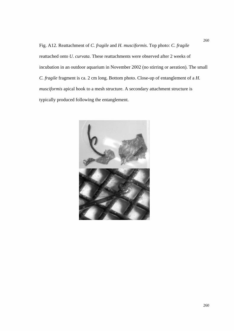
260

260

Fig. A12. Reattachment of C. fragile and H. musciformis. Top photo: C. fragile

reattached onto U. curvata. These reattachments were observed after 2 weeks of

incubation in an outdoor aquarium in November 2002 (no stirring or aeration). The small

C. fragile fragment is ca. 2 cm long. Bottom photo. Close-up of entanglement of a H.

musciformis apical hook to a mesh structure. A secondary attachment structure is

typically produced following the entanglement.

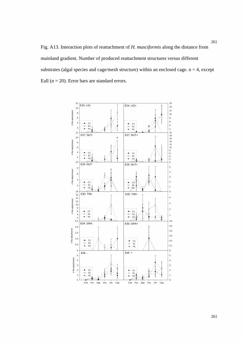
261

261

Fig. A13. Interaction plots of reattachment of H. musciformis along the distance from

mainland gradient. Number of produced reattachment structures versus different

substrates (algal species and cage/mesh structure) within an enclosed cage. n = 4, except

Eall (n = 20). Error bars are standard errors.

E24. LIG+

Cod Fuc Aga Gra Ulv Cag

2

4

6

8

10

12

14

16

C1S1H1

E24. LIG-

Cod Fuc Aga Gra Ulv Cag

# R

e-at

tach

men

t

2

4

6

8

10

12

C1S1H1

E27. NUT-

Cod Fuc Aga Gra Ulv Cag

# R

e-at

tach

men

t

2

4

6

8

10

12

C1 S1H1

E27. NUT+

Cod Fuc Aga Gra Ulv Cag

2468101214161820

C1S1H1

E29. NUT-

Cod Fuc Aga Gra Ulv Cag

# R

e-at

tach

men

t

2

4

6

8

10

C1S1H1

E29. NUT+

Cod Fuc Aga Gra Ulv Cag

1

2

3

4

5

6

C1S1H1

E30. TWI-

Cod Fuc Aga Gra Ulv Cag

# R

e-at

tach

men

t

2

4

6

8

10

12

14

16

18

C1S1H1

E30. TWI+

Cod Fuc Aga Gra Ulv Cag

1

2

3

4

5

C1S1H1

E34. GRA-

Cod Fuc Aga Gra Ulv Cag

# R

e-at

tach

men

t

0.5

1.0

1.5

2.0

2.5

C1 S1H1

E30. GRA+

Cod Fuc Aga Gra Ulv Cag

0.1

0.2

0.3

0.4

0.5

0.6

C1S1H1

Eall. -

Cod Fuc Aga Gra Ulv Cag

# R

e-at

tach

men

t

0

1

2

3

4

5

6

C1S1H1

Eall. +

Cod Fuc Aga Gra Ulv Cag0

1

2

3

4

5

6

C1S1H1

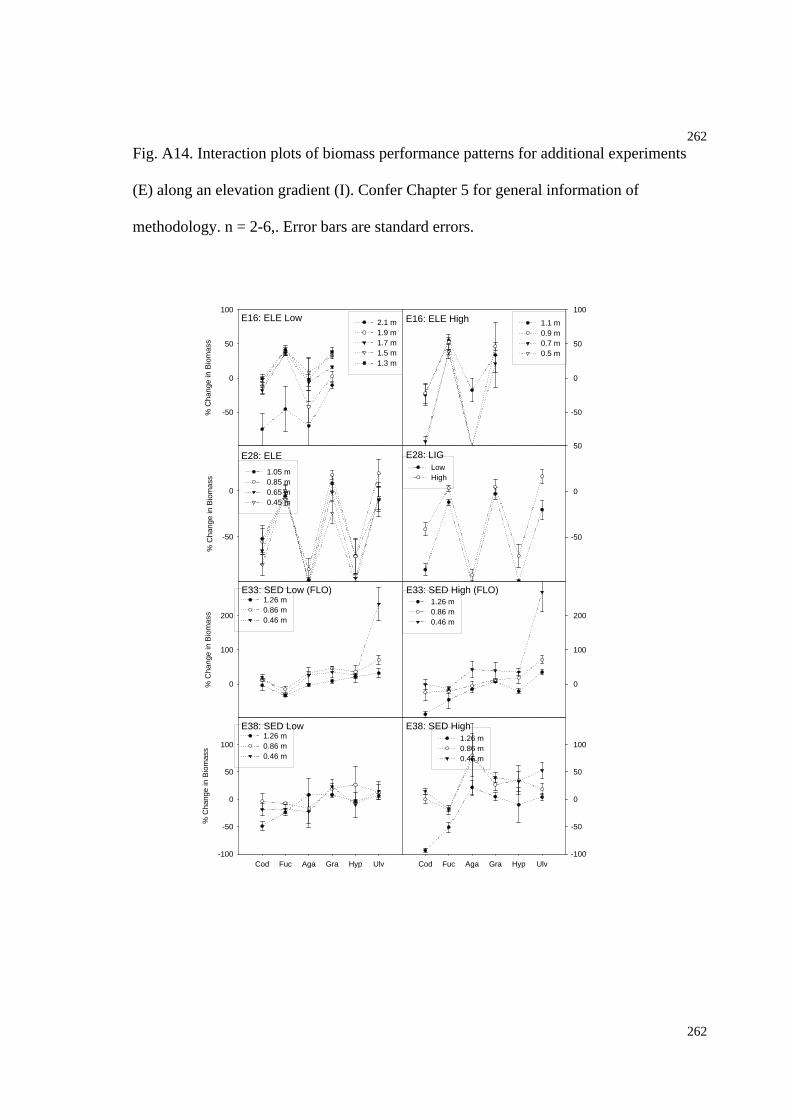
262

262

Fig. A14. Interaction plots of biomass performance patterns for additional experiments

(E) along an elevation gradient (I). Confer Chapter 5 for general information of

methodology. n = 2-6,. Error bars are standard errors.

E16: ELE Low

Cod Fuc Aga Gra Hyp Ulv

% C

hang

e in

Bio

mas

s

-50

0

50

100

2.1 m1.9 m 1.7 m1.5 m1.3 m

E28: ELE

Cod Fuc Aga Gra Hyp Ulv

% C

hang

e in

Bio

mas

s

-50

0

1.05 m0.85 m0.65 m0.45 m

E16: ELE High

Cod Fuc Aga Gra Hyp Ulv

-50

0

50

100

1.1 m0.9 m0.7 m0.5 m

E28: LIG

Cod Fuc Aga Gra Hyp Ulv

-50

0

50

LowHigh

E33: SED Low (FLO)

Cod Fuc Aga Gra Hyp Ulv

% C

hang

e in

Bio

mas

s

0

100

200

1.26 m0.86 m0.46 m

E33: SED High (FLO)

Cod Fuc Aga Gra Hyp Ulv

0

100

200

1.26 m0.86 m0.46 m

E38: SED Low

Cod Fuc Aga Gra Hyp Ulv

% C

hang

e in

Bio

mas

s

-100

-50

0

50

1001.26 m0.86 m0.46 m

E38: SED High

Cod Fuc Aga Gra Hyp Ulv-100

-50

0

50

1001.26 m0.86 m0.46 m

263

263

Fig. A15. Interaction plots of biomass performance patterns for additional experiments

(E) along an elevation gradient (II). Different interactions are emphasized compared to

Fig. A14. Confer Chapter 5 for general information of methodology. n = 2-6,. Error bars

are standard errors.

E28: LIG High

Cod Fuc Aga Gra Hyp Ulv

% g

row

th

-50

0

50

100

1.05 m0.85 m0.65 m0.45 m

E28: LIG Low

Cod Fuc Aga Gra Hyp Ulv

% C

hang

e in

Bio

mas

s

-50

0

50

100

1.05 m0.85 m0.65 m 0.45 m

E33: ELE

Cod Fuc Aga Gra Hyp Ulv

% C

hang

e in

Bio

mas

s

0

100

2001.26 m0.86 m0.46 m

E33: SED (FLO)

Cod Fuc Aga Gra Hyp Ulv

0

100

200

LowHigh

E38: ELE

Cod Fuc Aga Gra Hyp Ulv

% C

hang

e in

Bio

mas

s

-100

-50

0

501.26 m0.86 m0.46 m

E38: SED

Cod Fuc Aga Gra Hyp Ulv-100

-50

0

50LowHigh

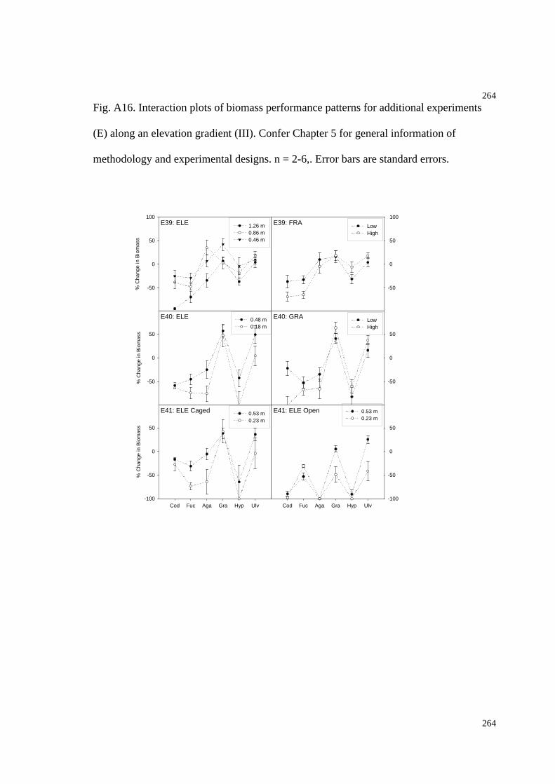
264

264

Fig. A16. Interaction plots of biomass performance patterns for additional experiments

(E) along an elevation gradient (III). Confer Chapter 5 for general information of

methodology and experimental designs. n = 2-6,. Error bars are standard errors.

E39: ELE

Cod Fuc Aga Gra Hyp Ulv

% C

hang

e in

Bio

mas

s

-50

0

50

100

1.26 m0.86 m0.46 m

E39: FRA

Cod Fuc Aga Gra Hyp Ulv

-50

0

50

100

LowHigh

E40: ELE

Cod Fuc Aga Gra Hyp Ulv

% C

hang

e in

Bio

mas

s

-50

0

50

0.48 m0.18 m

E40: GRA

Cod Fuc Aga Gra Hyp Ulv

-50

0

50

LowHigh

E41: ELE Caged

Cod Fuc Aga Gra Hyp Ulv

% C

hang

e in

Bio

mas

s

-100

-50

0

50

0.53 m0.23 m

E41: ELE Open

Cod Fuc Aga Gra Hyp Ulv-100

-50

0

50

0.53 m0.23 m

265

265

Fig. A17. Interaction plots of biomass performance patterns for additional experiments

(E) along an elevation gradient (IV). Confer Chapter 5 for general information of

methodology and experimental designs. n = 2-6. Error bars are standard errors.

E16

Distance above MSL (m)

% C

hang

e in

Bio

mas

s

-50

0

50

100

150

CodiumFucusAgardhiellaGracilaria

EAll

Distance above MSL (m)

-2.5 -2.0 -1.5 -1.0 -0.5 0.0

% C

hang

e in

Bio

mas

s

-50

0

50

100

150

CodiumFucusAgardhiellaGracilariaHypneaUlva

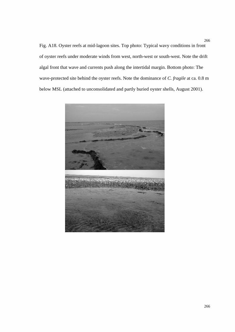
266

266

Fig. A18. Oyster reefs at mid-lagoon sites. Top photo: Typical wavy conditions in front

of oyster reefs under moderate winds from west, north-west or south-west. Note the drift

algal front that wave and currents push along the intertidal margin. Bottom photo: The

wave-protected site behind the oyster reefs. Note the dominance of C. fragile at ca. 0.8 m

below MSL (attached to unconsolidated and partly buried oyster shells, August 2001).

267

267

Fig. A19. Elevation map a mid-lagoon Shoal 1 site showing topography around oyster

reefs. The oyster reefs are the dark and scattered areas from ca. 0.0 to 0.5 m below MSL

(cf. Fig. A18). Each black dot correspond to the position of a set of three treatments: An

open control plot, a sediment-trap cage and a drift-algal trap cage. Within each plot/cage

four recruitment bricks were incubated (sub-replicates, cf. Chapter 6 for further design

description).

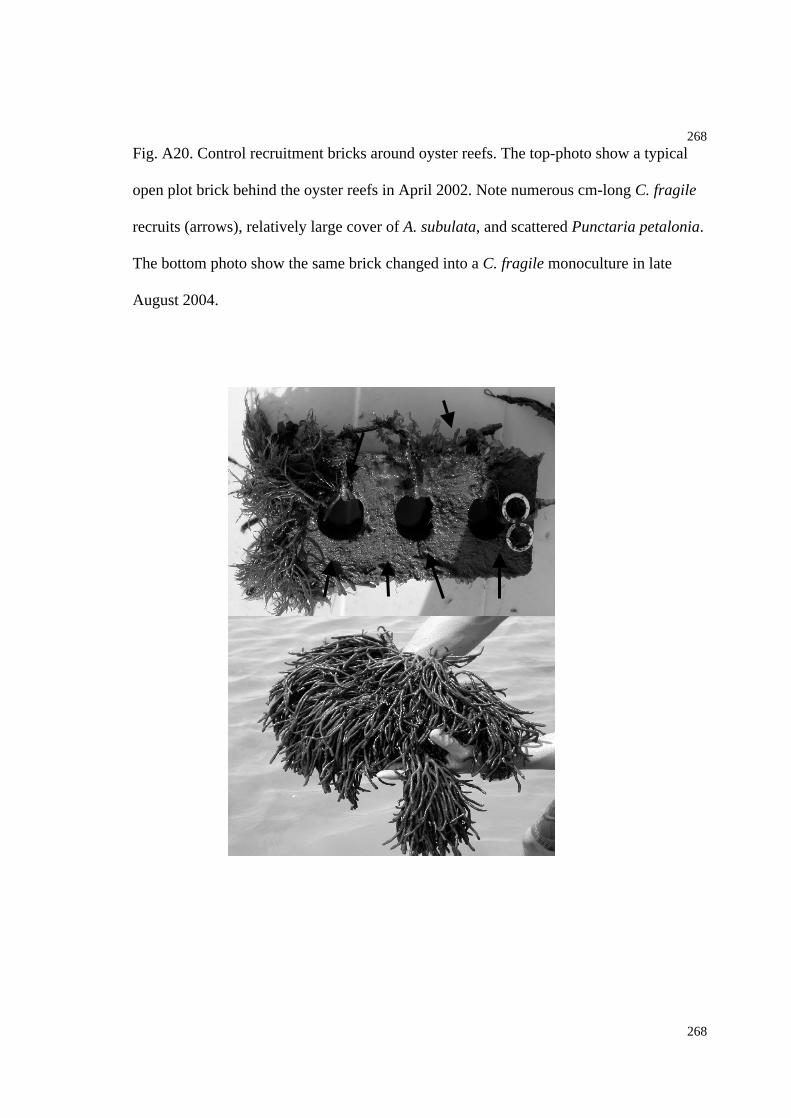
268

268

Fig. A20. Control recruitment bricks around oyster reefs. The top-photo show a typical

open plot brick behind the oyster reefs in April 2002. Note numerous cm-long C. fragile

recruits (arrows), relatively large cover of A. subulata, and scattered Punctaria petalonia.

The bottom photo show the same brick changed into a C. fragile monoculture in late

August 2004.

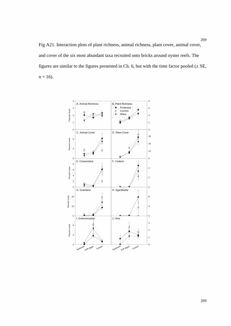
269

269

Fig A21. Interaction plots of plant richness, animal richness, plant cover, animal cover,

and cover of the six most abundant taxa recruited onto bricks around oyster reefs. The

figures are similar to the figures presented in Ch. 6, but with the time factor pooled (± SE,

n = 16).

B. Plant Richness

SedimentDrift algae Control0

2

4

6

8

A. Animal Richness

SedimentDrift algae Control

Tax

a pe

r br

ick

0

1

2

3

4

ProtectedCurrentWavy

C. Animal Cover

SedimentDrift algae Control

Per

cent

cov

er

0

4

8

D. Plant Cover

SedimentDrift algae Control0

10

20

30

E. Crassostrea

SedimentDrift algae Control

Per

cent

cov

er

0

2

4

6

8F. Codium

SedimentDrift algae Control0

2

4

G. Gracilaria

SedimentDrift algae Control

Per

cent

cov

er

0

10

20

H. Agardhiella

SedimentDrift algae Control0

4

8

I. Enteromorpha

Sediment

Drift algae

Control

Per

cent

cov

er

0

4

8

J. Ulva

Sediment

Drift algae

Control0

1

2

3

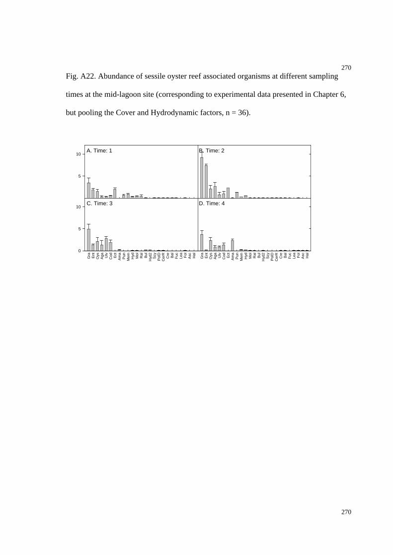
270

270

Fig. A22. Abundance of sessile oyster reef associated organisms at different sampling

times at the mid-lagoon site (corresponding to experimental data presented in Chapter 6,

but pooling the Cover and Hydrodynamic factors, n = 36).

A. Time: 1

Gra

Ent

Oys

Aga Ulv

Cod Ect

Am

aP

unM

em Hyd Mol

Ral

Bul

Hyd

2S

cyP

olD

Cer

RC

re Bal

Fuc

Lea

Fol

Asc Hal

5

10B. Time: 2

Gra

Ent

Oys

Aga Ulv

Cod Ect

Am

aP

unM

em Hyd Mol

Ral

Bul

Hyd

2S

cyP

olD

Cer

RC

re Bal

Fuc

Lea

Fol

Asc HalC. Time: 3

Gra

Ent

Oys

Aga Ulv

Cod Ect

Am

aP

unM

em Hyd Mol

Ral

Bul

Hyd

2S

cyP

olD

Cer

RC

re Bal

Fuc

Lea

Fol

Asc Hal

0

5

10D. Time: 4

Gra

Ent

Oys

Aga Ulv

Cod Ect

Am

aP

unM

em Hyd Mol

Ral

Bul

Hyd

2S

cyP

olD

Cer

RC

re Bal

Fuc

Lea

Fol

Asc Hal

271

271

Fig. A23. Abundance of sessile oyster-reef associated organisms recruited onto bricks at

different elevation levels at the mid-lagoon site (S1). Error bars are standard errors.

Low 03/02

Gra

Cra Ulv

Ent

Cer

RH

yd2

Bul

Aga Ral

Cod Fuc

Am

aH

yd Ect

Scy

Pun Mol

Bal

Cov

er (

%)

0

2

4

6

8

10

12

Low 06/02

Gra

Cra Ulv

Ent

Cer

RH

yd2

Bul

Aga Ral

Cod Fuc

Am

aH

yd Ect

Scy

Pun Mol

Bal

Cov

er (

%)

0

10

20

30

40

Low 07/02

Gra

Cra Ulv

Ent

Cer

RH

yd2

Bul

Aga Ral

Cod Fuc

Am

aH

yd Ect

Scy

Pun Mol

Bal

Cov

er (

%)

0

2

4

6

8

10

12

Mid 03/02

Gra

Cra Ulv

Ent

Cer

RH

yd2

Bul

Aga Ral

Cod Fuc

Am

aH

yd Ect

Scy

Pun Mol

Bal

5

10

15

20

25

Mid 06/02

Gra

Cra Ulv

Ent

Cer

RH

yd2

Bul

Aga Ral

Cod Fuc

Am

aH

yd Ect

Scy

Pun Mol

Bal

10

20

30

Mid 07/02

Gra

Cra Ulv

Ent

Cer

RH

yd2

Bul

Aga Ral

Cod Fuc

Am

aH

yd Ect

Scy

Pun Mol

Bal

5

10

15

20

25

High 03/02

Gra

Cra Ulv

Ent

Cer

RH

yd2

Bul

Aga Ral

Cod Fuc

Am

aH

yd Ect

Scy

Pun Mol

Bal

2

4

6

8

10

High 06/02

Gra

Cra Ulv

Ent

Cer

RH

yd2

Bul

Aga Ral

Cod Fuc

Am

aH

yd Ect

Scy

Pun Mol

Bal

0

5

10

15

20

High 07/02

Gra

Cra Ulv

Ent

Cer

RH

yd2

Bul

Aga Ral

Cod Fuc

Am

aH

yd Ect

Scy

Pun Mol

Bal

0

5

10

15

20

25

272

272

Fig. A24. Abundance of sessile oyster-reef associated organisms at recruited onto bricks

at different positions along the distance from mainland gradient (C1, S1, H1). Error bars

are standard errors.

S1, 03/02

Gra

Ent

Ect

Cra

Scy Ulv

Fuc Ral

Pun

Cod

Cer

RLe

aH

yd Bul

Mol

Bal

Pol

Hyd

2H

alA

gaLo

mP

olD

Red

FA

ma

Cre

Cov

er (

%)

0

2

4

6

8

10

12

14

16

18

S1, 06/02

Gra

Ent

Ect

Cra

Scy Ulv

Fuc Ral

Pun

Cod

Cer

RLe

aH

yd Bul

Mol

Bal

Pol

Hyd

2H

alA

gaLo

mP

olD

Red

FA

ma

Cre

0

5

10

15

20

25

S1, 07/02

Gra

Ent

Ect

Cra

Scy Ulv

Fuc Ral

Pun

Cod

Cer

RLe

aH

yd Bul

Mol

Bal

Pol

Hyd

2H

alA

gaLo

mP

olD

Red

FA

ma

Cre

Cov

er (

%)

0

2

4

6

8

10

12

14

H1, 03/02

Gra

Ent

Ect

Cra

Scy Ulv

Fuc Ral

Pun

Cod

Cer

RLe

aH

yd Bul

Mol

Bal

Pol

Hyd

2H

alA

gaLo

mP

olD

Red

FA

ma

Cre

Cov

er (

%)

0

2

4

6

8

H1, 07/02

Gra

Ent

Ect

Cra

Scy Ulv

Fuc Ral

Pun

Cod

Cer

RLe

aH

yd Bul

Mol

Bal

Pol

Hyd

2H

alA

gaLo

mP

olD

Red

FA

ma

Cre

Cov

er (

%)

0

2

4

6

8

C1, 03/02

Gra

Ent

Ect

Cra

Scy Ulv

Fuc Ral

Pun

Cod

Cer

RLe

aH

yd Bul

Mol

Bal

Pol

Hyd

2H

alA

gaLo

mP

olD

Red

FA

ma

Cre

Cov

er (

%)

0.0

0.5

1.0

1.5

C1, 07/02

Gra

Ent

Ect

Cra

Scy Ulv

Fuc Ral

Pun

Cod

Cer

RLe

aH

yd Bul

Mol

Bal

Pol

Hyd

2H

alA

gaLo

mP

olD

Red

FA

ma

Cre

Cov

er (

%)

0

1

2

3

4

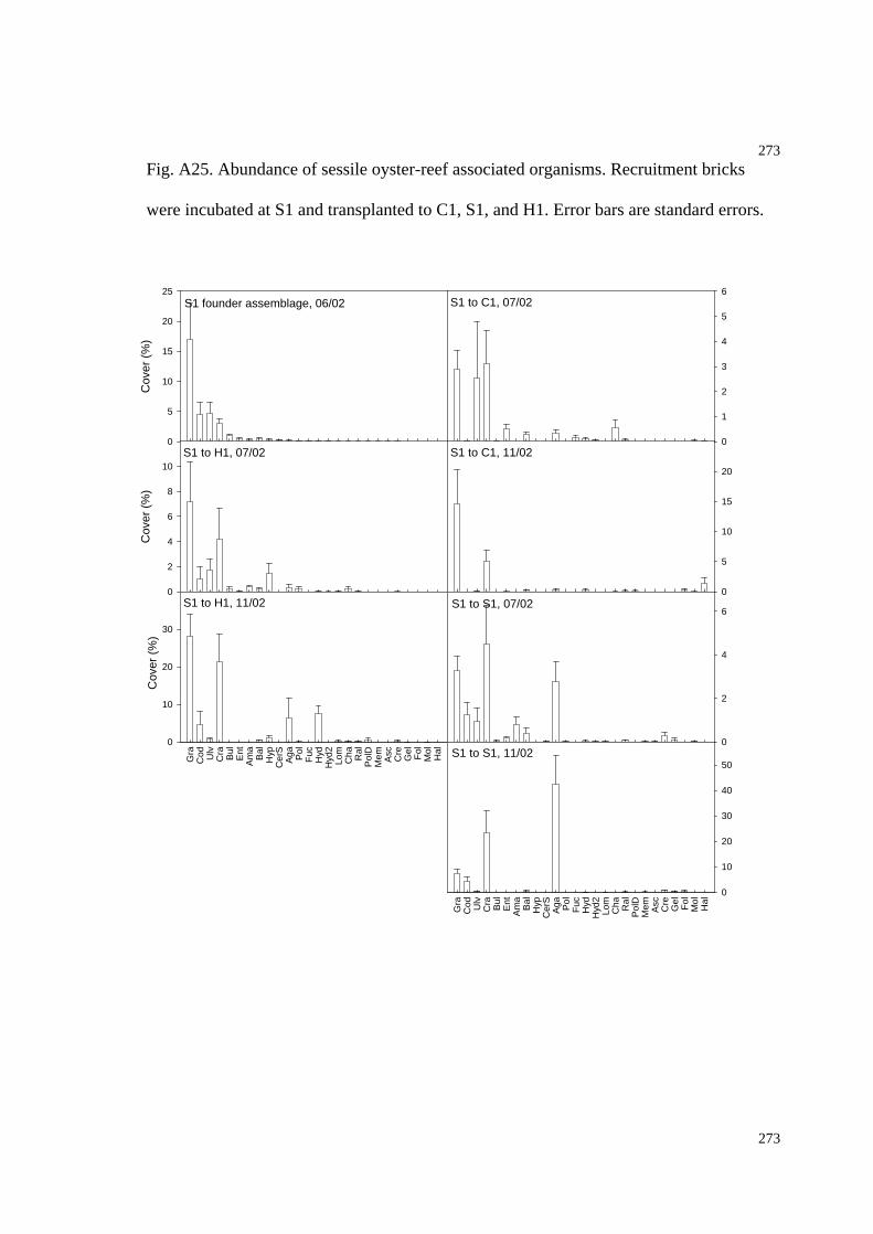
273

273

Fig. A25. Abundance of sessile oyster-reef associated organisms. Recruitment bricks

were incubated at S1 and transplanted to C1, S1, and H1. Error bars are standard errors.

S1 founder assemblage, 06/02

Gra

Cod Ulv

Cra Bul

Ent

Am

aB

alH

ypC

erS

Aga Pol

Fuc

Hyd

Hyd

2Lo

mC

ha Ral

Pol

DM

em Asc

Cre

Gel

Fol

Mol

Hal

Cov

er (

%)

0

5

10

15

20

25S1 to C1, 07/02

Gra

Cod Ulv

Cra Bul

Ent

Am

aB

alH

ypC

erS

Aga Pol

Fuc

Hyd

Hyd

2Lo

mC

ha Ral

Pol

DM

em Asc

Cre

Gel

Fol

Mol

Hal

0

1

2

3

4

5

6

S1 to H1, 07/02

Gra

Cod Ulv

Cra Bul

Ent

Am

aB

alH

ypC

erS

Aga Pol

Fuc

Hyd

Hyd

2Lo

mC

ha Ral

Pol

DM

em Asc

Cre

Gel

Fol

Mol

Hal

Cov

er (

%)

0

2

4

6

8

10S1 to C1, 11/02

Gra

Cod Ulv

Cra Bul

Ent

Am

aB

alH

ypC

erS

Aga Pol

Fuc

Hyd

Hyd

2Lo

mC

ha Ral

Pol

DM

em Asc

Cre

Gel

Fol

Mol

Hal

0

5

10

15

20

S1 to H1, 11/02

Gra

Cod Ulv

Cra Bul

Ent

Am

aB

alH

ypC

erS

Aga Pol

Fuc

Hyd

Hyd

2Lo

mC

ha Ral

Pol

DM

em Asc

Cre

Gel

Fol

Mol

Hal

Cov

er (

%)

0

10

20

30

S1 to S1, 07/02

Gra

Cod Ulv

Cra Bul

Ent

Am

aB

alH

ypC

erS

Aga Pol

Fuc

Hyd

Hyd

2Lo

mC

ha Ral

Pol

DM

em Asc

Cre

Gel

Fol

Mol

Hal

0

2

4

6

S1 to S1, 11/02

Gra

Cod Ulv

Cra Bul

Ent

Am

aB

alH

ypC

erS

Aga Pol

Fuc

Hyd

Hyd

2Lo

mC

ha Ral

Pol

DM

em Asc

Cre

Gel

Fol

Mol

Hal

0

10

20

30

40

50

274

274

Fig. A26. Location of sample stations from the VCR/LTER WQ (Water Quality)

Monitoring Program. Baseline map produced by K. Overman.

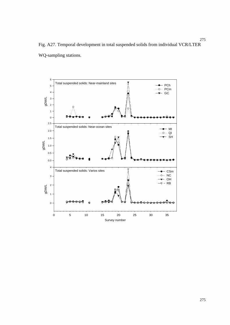
275

275

Fig. A27. Temporal development in total suspended solids from individual VCR/LTER

WQ-sampling stations.

Total suspended solids: Varios sites

Survey number

0 5 10 15 20 25 30 35

gDW

/L

0

1

2

3

4

CSmNCOHRB

Total suspended solids: Near-ocean sites

gDW

/L

0.0

0.5

1.0

1.5

2.0

2.5

MIQISH

Total suspended solids: Near-mainland sites

gDW

/L

0

1

2

3

4

5

6

PCh PCm GC

276

276

Fig. A28. Temporal development in temperature from individual VCR/LTER WQ-

sampling stations.

Temperature: Varios sites

Survey number

0 5 10 15 20 25 30 35

Cel

cius

0

10

20

30

CSmNCOHRB

Temperature: Near-ocean sites

Cel

cius

10

20

30

MIQISH

Temperature: Near-mainland sites

Cel

cius

10

20

30

PCh PCm GC

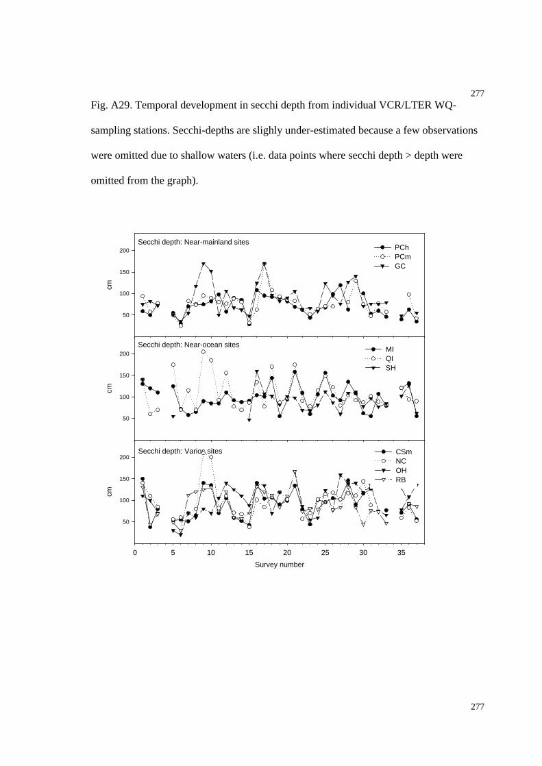
277

277

Fig. A29. Temporal development in secchi depth from individual VCR/LTER WQ-

sampling stations. Secchi-depths are slighly under-estimated because a few observations

were omitted due to shallow waters (i.e. data points where secchi depth > depth were

omitted from the graph).

Secchi depth: Varios sites

Survey number

0 5 10 15 20 25 30 35

cm

50

100

150

200CSmNCOHRB

Secchi depth: Near-ocean sites

cm

50

100

150

200MIQISH

Secchi depth: Near-mainland sites

cm

50

100

150

200 PCh PCm GC

278

278

Fig. A30. Temporal development in salinity from individual VCR/LTER WQ-sampling

stations.

Salinity: Varios sites

Survey number

0 5 10 15 20 25 30 35

ppt

15

20

25

30

35

CSmNCOHRB

Salinity: Near-ocean sites

ppt

20

25

30

35

MIQISH

Salinity: Near-mainland sites

ppt

20

25

30

35

PCh PCm GC

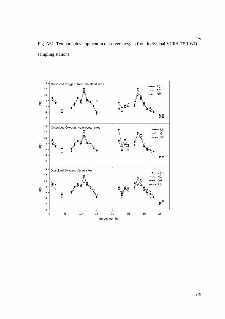
279

279

Fig. A31. Temporal development in dissolved oxygen from individual VCR/LTER WQ-

sampling stations.

Dissolved Oxygen: Varios sites

Survey number

0 5 10 15 20 25 30 35

mg/

L

0

2

4

6

8

10

12

14

CSmNCOHRB

Dissolved Oxygen: Near-ocean sites

mg/

L

2

4

6

8

10

12

14MIQISH

Dissolved Oxygen: Near-mainland sites

mg/

L

2

4

6

8

10

12

14PCh PCm GC

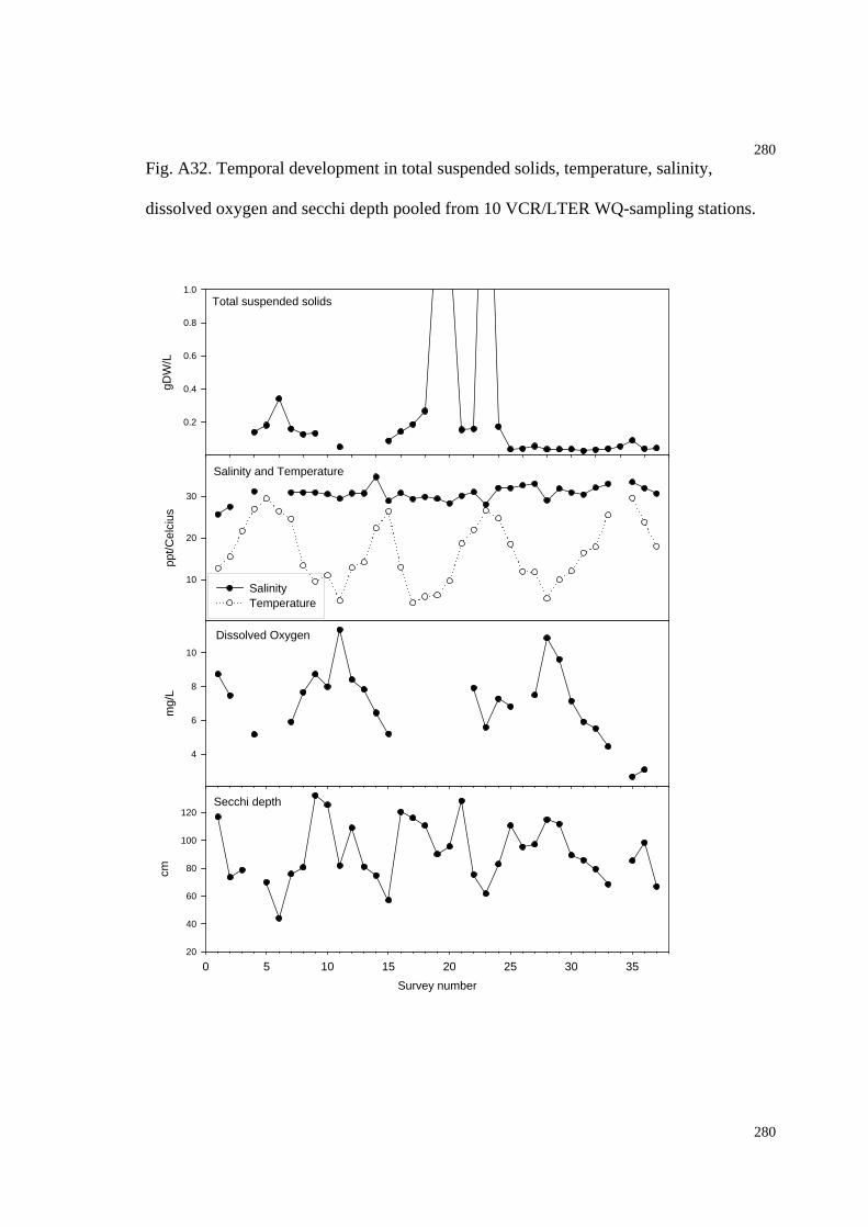
280

280

Fig. A32. Temporal development in total suspended solids, temperature, salinity,

dissolved oxygen and secchi depth pooled from 10 VCR/LTER WQ-sampling stations.

Secchi depth

Survey number

0 5 10 15 20 25 30 35

cm

20

40

60

80

100

120

Salinity and Temperature

ppt/C

elci

us

10

20

30

SalinityTemperature

Total suspended solids

gDW

/L

0.2

0.4

0.6

0.8

1.0

Dissolved Oxygen

mg/

L

4

6

8

10

281

281

References

Airoldi L (2003) The effects of sedimentation on rocky coast assemblages. Oceanography and MarineBiology: An Annual Review 41:161-236

Airoldi L, Virgilio M (1998) Responses of turf-forming algae to spatial variations in the deposition ofsediments. Marine Ecology Progress Series 165:271-282

Albrecht AS (1998) Soft bottom versus hard rock: community ecology of macroalgae on intertidal musselbeds in the Wadden Sea. Journal of Experimental Marine Biology and Ecology 229:85-109

Anderson MJ (1999a) Distinguishing direct from indirect effects of grazers in intertidal estuarineassemblages. Journal of Experimental Marine Biology & Ecology 234:199-218

Anderson MJ (1999b) Effects of patch size on colonisation in estuaries: revisiting the species-arearelationship. Oecologia 118:87-98

Anderson MJ (2000) NPMANOVA: a FORTRAN computer program for non-parametric multivariateanalysis of variance (for any two-factor ANOVA) design using permutation tests. Department ofStatistics, University of Auckland:16 pp

Anderson MJ (2001) A new non-parametric multivariate analysis of variance. Australian Ecology 32-46:32-46

Anderson MJ, Ter Braak CJF (2003) Permutation tests for multifactorial analysis of variance. Journal ofstatistical computation and simulation

Anderson MJ, Underwood AJ (1997) Effects of gastropod grazers on recruitment and succession of anestuarine assemblage - a multivariate and univariate approach. Oecologia 109:442-453

Arenas F, Fernández C, Rico JM, Fernández E, Haya D (1995) Growth and reproductive strategies ofSargassum muticum (Yendo) Fensholt and Cystoseira nodicaulis (Whit.) Roberts. Scientia Marina59:1-8

Bailey-Brock JH (1984) Ecology of the tube-building polychaete Diopatra leuckarti Kinberg, 1865(Onuphidae) in Hawaii: Community structure, and sediment stabilizing properties. ZoologicalJournal of the Linnean Society 80:191-199

Barh LM, Lanier MP (1981) The ecology of intertidal oyster reefs of the South Atlantic coast: a communityprofile. US Fish and Wildlife Service, Office of Biological Services, Washington, DC, FWS/OBS-81/15:105

Barnes H, Topinka JA (1969) Effect of the nature of the substratum on the force required to detach acommon littoral alga. American zoologist 9:753-758

Begin C, Scheibling RE (2003) Growth and survival of the invasive green alga Codium fragile ssp.tomentosoides in tide pools on a rocky shore in Nova Scotia. Botanica Marina 46:404-203

Bell EC (1999) Applying flow tank measurements to the surf zone: Predicting dislodgment of theGigartinaceae. Phycological Research 47:159-166

Bell EC, Denny MW (1994) Quantifying wave exposure - a simple device for recording maximum velocityand results of its use at several field sites. Journal of Experimental Marine Biology and Ecology181:9-29

Bell SS, Coen ID (1982a) Investigations on epibenthic meiofauna I: Abundances on and repopulation of thetube-caps of Diopatra cuprea Polychaetea Onuphidae in a subtropical system. Marine Biology673:303-310

Bell SS, Coen LD (1982b) Investigations on epibenthic meiofauna. II. Influence of microhabitat andmacroalgae on abundance of small invertebrates on Diopatra Cuprea (Bosc) (Polychaeta:Onuphidae) tube-caps in Virginia. Journal of Experimental Marine Biology and Ecology 61:175-188

Ben Avraham Z (1971) Accumulation of stones on beaches by Codium fragile. Limnology &Oceonography 16:553-554

Berchez FAS, Pereira RTL, Kamiya NF (1993) Culture of Hypnea musciformis (Rhodophyta, Gigartinales)on artificial substrates attached to linear ropes. Hydrobiologia 260/261:415-420

Berger R, Henriksson E, Kautsky L, Malm T (2003) Effects of filamentous algae and deposited matter onthe survival of Fucus vesiculosus L. germlings in the Baltic Sea. Aquatic Ecology 37:1-11

282

282

Bird CJ, Rice EL (1990) Recent approaches to the taxonomy of the Gracilariaceae (Gracilariales,Rhodophyta) and the Gracilaria verrucosa problem. Hydrobiologia 204/205:111-118

Bird N, McLachlan J (1977) Studies on Gracilaria. 5. In vitro life history of Gracilaria sp. from theMaritime Provinces. Canadian Journal of Botany 55:1282-1290

Blanchette CA (1997) Size and survival of intertidal plants in response to wave action - a case study withFucus gardneri. Ecology 78:1563-1578

Blanchette CA, Miner BG, Gaines SD (2002) Geographic variability in form, size and survival of Egregiamenziesii around Point Conception, California. Marine Ecology Progress Series 239:69-82

Borden CA, Stein JR (1969) Reproduction and early development in Codium fragile (Suringar) Harriot:Chlorophyceae. Phycologia 8:91-99

Borum JS-JK (1996) Is total primary production in shallow coastal marine waters stimulated by nitrogenloading? Oikos 76:406-410

Bouck GB, Morgan E (1957) The occurrence of Codium in Long Island waters. Bull. Torrey Bot. Club.84:384-387

Boudouresque CF, Verlaque M (2002) Biological pollution in the Mediterranean Sea: invasive versusintroduced macrophytes. Marine Pollution Bulletin 44:32-38

Bourgues S, Auby I, de Wit R, Labourg P-J (1996) Differential anaerobic decomposition of seagrass(Zostera noltii) and macroalgal (Monostroma obscurum) biomass from Arcachon Bay (France).Hydrobiologia 329:121-131

Boynton WR, Hagy JD, Murray L, Stokes C, Kemp WM (1996) A comparative analysis of eutrophicationpatterns in a temperate coastal lagoon. Estuaries 19:408-421

Brenchley GA (1976) Predator detection and avoidance: ornamentation of tube-caps of Diopatra spp.(Polychaeta: Onuphidae). Marine Biology 38:179-188

Brooks WK (1996) The oyster - a popular summary of a scientific study. The John Hopkins UniversityPress:100

Bruno JF, Bertness MD (2001) Habitat modification and facilitation in benthic marine communities inMarine Community Ecology (Bertness, M.D., Gaines, S.D., Hay, M.E.). Sinauer Associates,Inc.:201-218

Bruno JF, Stachowicz JJ, Bertness MD (in press) Inclusion of facilitation into ecological theory. TRENDSin Ecology and Evolution:pp 7

Buschmann AH (1990) The role of herbivory and dessication on early successional patterns of intertidalmacroalgae in southern Chile. Journal of Experimental Marine Biology and Ecology 139:221-230

Campbell SJ (1999) Occurence of Codium fragile subsp. tomentosoides (Chlorophyta: Bryopsidales) inmarine embayments of southeastern Australia. Journal of Phycology 35:938-940

Carlton JT (1996a) Biological invasions and crypotgenic species. Ecology 77:1653-1655Carlton JT (1996b) Invasions in the world's seas: six centuries of re-organizing earth's marine life.

Proceedings of the Norway/UN Conference on Alien Species - Trondheim, 1-5 July 1996 (editorsSandlund, T, Schei, J, Viken, Å), hosted by the Norwegian Ministry of Environment:99-102

Carlton JT (1996c) Pattern, process, and prediction in marine invasion ecology. Biological Conservation78:97-106

Carlton JT (1999) The scale and ecological consequences of biological invasions in the world's oceans inInvasive species and biodiversity management, O.T. Sandlund et al. (eds.). Kluwer AcademicPress:195-212

Carlton JT, Scanlon JA (1985) Progression and dispersal of an introduced alga: Codium fragile ssp.tomentosoides (Chlorophyta) on the Atlantic coast of North America. Botanical Marina 28:155-165

Carrington E (1990) Drag and dislodgment of an intertidal macroalga: consequences of morphologicalvariation in Mastocarpus papillatus Kützing. Journal of Experimental Marine Biology andEcology 139:185-200

Castel J, Caumette P, Herbert R (1996) Eutrophication gradients in coastal lagoons as exemplified by thebassin d'Arcachon and the Etang du Prevost. Hydrobiologia 329:9-28

Casteldelli G, Welsh DT, Flachi G, Zucchini G, Colombo G, Rossi R, Fano EA (2003) Decompositiondynamics of the bloom forming macroalga Ulva rigida C. Agardh determined using a 14C-carbonradio-tracer technique. Aquatic Botany 75:111-122

283

283

Cebrián J, Duarte CM (1994) The dependence of herbivory on growth rate in natural plant communities.Functional Ecology 8:518-525

Ceccherelli G, Piazzi L (2001) Dispersal of Caulerpa racemosa fragments in the Mediterranean: lack ofdetachment time effect on establishment. Botanical Marina 44:209-213

Cecere E, Saracino OD, Fanelli M, Petrocelli A (1992) Presence of a drifting algal bed in the Mar Piccolobasin, Taranto (Ionian Sea, Southern Italy). Journal of Applied Phycology 4:323-327

Chapman ARO (1995) Functional ecology of fucoid algae: twenty-three years of progress. Phycologia34:1-32

Chapman AS (1999) From introduced species to invader: what determines variation in the success ofCodium fragile ssp. tomentosoides (Chlorophyta) in the North Atlantic Ocean? HelgolanderMeeresuntersuchungen 52:277-289

Charters AC, Neushul M, Coon D (1973) The effect of water motion on algal spore adhesion. Limnologyand Oceanography 18:884-896

Christensen TWPLMTG (2000.) Flow and sediment transport on a tidal salt marsh surface. Estuarine,Coastal and Shelf Science 50:315-331

Churchill AC, Moeller HW (1972) Seasonal patterns of reproduction in New York populations of Codiumfragile (Sur.) Hariot subsp. tomentosoides (Van Goor) Silva. Journal of Phycology 8

Clarke KR, Warwick RM (1994) Change in marine communities - an approach to statistical analysis andinterpretation. Plymouth Marine Laboratory, Natural Environmental Research Council, UK,Bourne Press Limited:144 pages

Clements FC (1936) Nature and structure of the climax. Journal of Ecology 24:253-284Coleman M (1996) DNA analysis methods for recognizing species invasions: the example of Codium, and

generally applicable methods for algae. Hydrobiologia 326/327:29-34Collado-Vides L, DeWreede RE, Milligan KLD (1998) Biomechanical properties of Udotea (Halimedales,

Chlorophyta) in a Mexican reef lagoon. Phycologia 37:443-449Colman J (1933) The nature of intertidal zonation of plants and animals. J. Mar. Biol. Assoc. U.K. 18:435-

476Connell JH (1961a) Effects of competition, predation by Thais lapillus, and other factors on natural

populations of the barnacle Balanus balanoides. Ecological Monographs 31:61-104Connell JH (1961b) The influence of interspecific competition and other factors on the distribution of the

barnacle Chthamalus stellatus. Ecological Monographs 42:710-723Connell JH, Hughes TP, Wallace CC (1997) A 30-year study of coral abundance, recruitment, and

disturbance at several scales in space and time. Ecological Monographs 67:461-488Connell JH, Slatyer RO (1977) Mechanisms of succession in natural communities and their role in

community stability and organization. The American Naturalist 111:1119-1144Connor JL (1980) Distribution and seasonality of macroalgae on oyster communities of central Chesapeake

Bay. Botanica Marina 23:711-717Cowles HC (1899) The ecological relations of the vegetation on the sand dunes of Lake Michigan 1-4.

Botanical Gazette 27:97-391Cowper SW (1978) The drift algae community of seagrass beds in Redfish Bay, Texas. Contributions in

Marine Science 21:125-132Critchley AT, Dijkema R (1984) On the presence of the introduced brown alga Sargassum muticum

attached to commercially imported Ostrea edulis in the S.W, Netherlands. Botanica Marina27:211-216

Cromwell JE (1973) Barrier coast distribution: a world-wide survey. in: Barrier Islands (M. L. Schwartz,ed.), Dowden, Hutchinson & Ross, Stroudsburg, PA:408 pp

Dame RF, Spurrier JD, Wolaver TG (1989) Carbon, nitrogen and phosphorous processing by an oysterreef. Marine Ecology Progress series 54:249-256

Dame RFSJDZRG (1992) In situ metabolism of an oyster reef. Journal of Experimental Marine Biologyand Ecology 164:147-159

Dame RLS (1993) Oyster reefs and nutrient retention in tidal creeks. Journal of Experimental MarineBiology and Ecology 171:251-258

Dayton PK (1971) Competition, disturbance, and community organization: the provision and subsequentutilization of space in a rocky intertidal community. Ecological Monographs 43:353-389

284

284

Dayton PK (1972) Towards an understanding of community resilience and the potential effects ofenrichment to the benthos of McMurdo Sound, Antartica. Proceedings of the Colloquium onConservation Problems in Antartica:81-96

Dayton PK, Currie V, Gerrodette T, Keller BD, Rosenthal R, Ven Tresca D (1984) Patch dynamics andstability of some California kelp communities. Ecological Monographs 54:253-290

Dean RL, Connell JH (1987a) Marine invertebrates in an algal succession. I. Variations in abundance anddiversity with succession. Journal of Experimental Marine Biology and Ecology 109:195-215

Dean RL, Connell JH (1987b) Marine invertebrates in an algal succession. II. Test of hypothesis to explainchanges in diversity with succession. Journal of Experimental Marine Biology and Ecology109:217-247

Dean RL, Connell JH (1987c) Marine invertebrates in an algal succession. III. Mechanisms linking habitatcomplexity with diversity. Journal of Experimental Marine Biology and Ecology 109:249-273

Dean TA, Hurd LE (1980) Development in an estuarine fouling community: the influence of early coloniston later arrivals. Botanica Marina

Den Hartog C (1998) Is Sargassum muticum a threat to eelgrass beds? Aquatic Botany 58:37-41Denny M (1985) Water motion. In: Littler M, Littler D (eds) Handbook of Phycological Methods Vol 4:

Ecological field methods, p 8-32Denny M (1995) Predicting physical disturbance - mechanistic approaches to the study of survivorship on

wave-swept shores. Ecological Monographs 65:371-418Denny M (1999) Are there mechanical limits to size in wave-swept organisms? Journal of Experimental

Biology 202:3463-3467Denny M, Brown V, Carrington E, Kraemer G, Miller A (1989) Fracture mechanics and the survival of

wave-swept macroalgae. Journal of Experimental Marine Biology and Ecology 127:221-228Denny M, Gaines SD (1990) On the prediction of maximal intertidal wave forces. Limnology and

Oceanography 35:1-15Denny MW (1987) Life in the maelstrom: the biomechanics of wave-swept rocky shores. Trends in

Ecology and Evolution 12:61-66Denny MW (1988) Biology and the mechanics of the wave-swept environment, Vol. Princeton University

PressDenny MW, Daniel TL, Koehl MAR (1985) Mechanical limits to size in wave-swept organisms.

Ecological Monographs 55:69-102Dethier MN, Graham ES, Cohen S, Tear LM (1993) Visual versus random-point percent cover estimations:

'objective' is not always better. Marine Ecology Progress series 96:93-100Devinny JS, Volse LA (1978) Effects of sediments on the development of Macrocystis pyrifera

gametophytes. Marine Biology 48:343-348DeWreede RE, Ewanchuk P, Shaughnessy F (1992) Wounding, healing and survivorship in three kelp

species. Marine Ecology Progress Series 82:259-266Dolan R (1996) Experiences with Atlantic coast storms, barrier islands, Oregon inlet, and Douglas Inman.

Shore and Beach 13:3-7Doty MS (1946) Critical tide factors that are correlated with the vertical distribution of marine algae and

other organisms along the Pacific coast. Ecology 27:315-328Dring MJ, Brown FA (1982) Photosynthesis of intertidal brown algae during and after periods of emersion:

a renewed search for physiological causes of zonation. Marine Ecology Progress Series 8:301-308Dromgoole FI (1980) Desiccation resistance of intertidal and subtidal algae. Botanica Marina 23:149-159Dromgoole FI (1982) The buoyant properties of Codium. Botanica Marina 25:391-397Duarte CM (1992) Nutrient concentration of aquatic plants: patterns across species. Limnology and

Oceanography 37:882-889Duarte CM (1995) Submerged aquatic vegetation in relation to different nutrient regimes. Ophelia 41:87-

112Dudgeon SR, Johnson AS (1992) Thick vs. thin: thallus morphology and tissue mechanics influence

differential drag and dislodgment of two co-dominant seaweeds. Journal of Experimental MarineBiology and Ecology 165:23-43

Dudgeon SR, Steneck RS, Davison IR, Vadas RL (1999) Coexistence of similar species in a space-limitedintertidal zone. Ecological Monographs 69:331-352

Duffy JE, Hay ME (1991a) Amphipods are not all created equal: a reply to Bell. Ecology 72:354-358

285

285

Duffy JE, Hay ME (1991b) Food and shelter as determinants of food choice by an herbivorous marineamphipod. Ecology 72:1286-1298

Duggins D, Eckman JE, Siddon CE, Klinger T (2001) Interactive roles of mesograzers and current flow insurvival of kelps. Marine Ecology Progress Series 223:143-155

Eckman JE, Nowell ARM, Jumars PA (1981) Sediment destabilization by animal tubes. Journal of MarineResearch 37:437-457

Enriquez S, Duarte CM, Sand-Jensen K (1993) Patterns in decomposition rates among photosyntheticorganisms: the importance of detritus C:N:P content. Oecologia 94:457-471

Escartin J, Aubrey DG (1995) Flow structure and dispersion within algal mats. Estuarine, Coastal and ShelfScience 40:451-472

Everett RA (1994) Macroalgae in marine soft-sediment communities: effects on benthic faunalassemblages. Journal of Experimental Marine Biology and Ecology 175:253-274

Fager EW (1964) Marine sediments: effects of a tubebuilding polychaete. Science 143:356-359Fletcher RL (1975) Studies on the recently introduced brown alga Sargassum muticum (Yendo) Fensholt II.

Regenerative ability. Botanica Marina xxvii:157-162Fletcher RL (1996) The occurence of "green tides" a review. In: Marine benthic vegetation - recent changes

and the effects of eutrophication (W. Schramm & PH Nienhuis). Ecological Studies. Springer123:7-43

Flindt M, Salomonsen J, Carrer M, Bocci M, Kamp-Nielsen L (1997a) Loss, growth and transportdynamics of Chaetomorpha aerea and Ulva rigida in the Lagoon of Venice during an earlysummer field campaign. Ecological Modelling 102:133-141

Flindt MR, Kamp-Nielsen L (1997) Modelling of an eustarine eutrophication gradient. EcologicalModelling 102:143-153

Flindt MR, Kamp-Nielsen L, Margues JC, Pardal MA, Bocci M, Bendoricchio G, Salomonsen J, NielsenSN, Jørgensen SE (1997b) Description of the three shallow estuaries: Mondego River (Portogal)l,Roskilde Fjord (Denmark) and the Lagoon of Venice (Italy). Ecological Modelling 102:17-31

Fong P, Desmond JS, Zedler JB (1997) The effect of a horn snail on Ulva expansa (Chlorophyta):consumer or facilitator of growth? Journal of Phycology 33:353-359

Fralick RA, Mathieson AC (1972) Winter fragmentation of Codium fragile (Suringar) Hariot ssp.tomentosoides (van Goor) Silva (Chlorophyceae, Siphonales) in New England. Phycologia 11:67-70

Fralick RA, Mathieson AC (1973) Ecological studies of Codium fragile in New England, USA. MarineBiology 19:127-132

Franklin JF, Bledsoe C, Callahan JT (1990) Contributions of the Long-Term Ecological Research Program.BioScience 40:509-523

Friedland MT, Denny MW (1995) Surviving hydrodynamic forces in a wave-swept environment -consequences of morphology in the Feather boa kelp, Egregia menziesii (Turner). Journal ofExperimental Marine Biology and Ecology 190:109-133

Gaines SD, Denny MW (1993) The largest, smallest, highest, lowest, longest, and shortest - extremes inecology. Ecology 74:1677-1692

Galtsoff PS (1964) The American oyster Crassostrea virginica (Gmelin). U.S. Fishery and WildlifeService, Fisheries Bulletin 64:1-480

Garbary DJ, Jess CB (2000) Current status of the invasive green alga Codium fragile in eastern Canada.Journal of Phycology 36:23-24

Garbary DJ, Vandermeulen H, Kim KY (1997) Codium fragile ssp. tomentosoides (Chlorophyta) invadesthe Gulf of St. Lawrence, Atlantic coast. Botanica Marina 40:537-540

Gaylord B (2000) Biological implications of surf-zone flow complexity. Limnology and Oceanography45:174-188

Gaylord B, Blanchette CA, Denny MW (1994) Mechanical consequences of size in wave swept algae.Ecological Monographs 64:287-313

Gaylord B, Denny MW (1997) Flow and flexibility : I. Effects of size, shape and stiffness in determiningwave forces on the stipitate kelps Eisenia arborea and Pterygophora californica. Journal ofExperimental Biology 200:3141-3164

286

286

Geertz-Hansen O, Sand-Jensen K, Hansen DF, Christiansen A (1993) Growth and grazing control ofabundance of the marine macroalgae, Ulva lactuca L. in a eutrophic Danish estuary. AquaticBotany 46:101-109

Giannotti AL, McGlathery KJ (2001) Consumption of Ulva lactuca (Chlorophyta) by the omnivorous mudsnail Ilyanassa obsoleta. Journal of Phycology 37:1-7

Goshorn D, McGinty M, Kennedy C, Jordan C, Wazniak C, Schwenke K, Coyne K (2001) An examinationof benthic macroalgae communities as indicators of nutrients in middle Atlantic coastal estuaries -Maryland component. Final report 1998-1999.41

Gosner KL (1978) Peterson field guides - Atlantic seashores. Houghton Mifflin Company:329 ppGottlieb SJ, Schweighofer ME (1996) Oysters and the Chesapeake Bay ecosystem: a case for exotic species

introduction to improve environmental quality? Estuaries 19:639-650Häder DP, Lebert M, Jiménez C, Salles S, Aguilera J, Flores-Moya A, Mercado J, Vinegla B, Figueroa FL

(1999) Pulse amplitude modulated fluorescence in the green macrophyte, Codium adherens,Enteromorpha muscoides, Ulva gigantea, and Ulva rigida, from the Atlantic coast of SouthernSpain. Environmental and Experimental Botany 41:247-255

Hader DP, Porst M, Lebert M (2000) On site photosynthetic performance of Atlantic green algae. Journalof Photochemistry and Photobiology B: Biology 57:159-168

Hanisak MD (1979a) Growth patterns of Codium fragile ssp. tomentosoides in response to temperature,irradiance, salinity and nitrogen source. Marine Biology 50:319-332

Hanisak MD (1979b) Nitrogen limitation of Codium fragile ssp. tomentosoides as determined by tissueanalysis. Marine Biology 50:333-337

Hanisak MD, Stenberg RW, Ryther JH (1979) Cultivation of Gracilaria tikvahiae (Rhodophyceae) as asource for methane production. Journal of Phycology 15:18

Haring RN, Dethier MN, Williams SL (2002) Desiccation facilitates wave-induced mortality of theintertidal alga Fucus gardneri. Marine Ecology Progress Series 232:75-82

Harlin MM, Rines HH (1993) Spatial cover of eight common macrophytes and three associatedinvertebrates in Narragansett Bay and contiguous waters, Rhode Island, USA. Botanical Marina36:35-45

Harwell MC, Orth RJ (2001) Influence of a tube-dwelling polychaete on the dispersal of fragmentedreproductive shoots of eelgrass. Aquatic Botany 70:1-7

Hauxwell J, Cebrian J, Furlong C, Valiela I (2001) Macroalgal canopies contribute to eelgrass (Zosteramarina) decline in temperate estuarine ecosystems. Ecology:1007-1022

Hauxwell J, McClelland J, Behr P, Valiela I (1998) Relative importance of grazing and nutrient controls ofmacroalgal biomass i three temperate shallow estuaries. Estuaries 21:347-360

Haven DS, Whitcomb JP (1983) The origin and extent of oyster reefs in The James River, Virginia. Journalof Shellfish Research 3:141-151

Havens KE, Hauxwell J, Tyler AC, Thomas AC, McGlathery KJ, Cebrian J, Valiela I, Steinman AD,Hwang S-J (2001) Complex interactions between autotrophs in shallow marine and freshwaterecosystems: implications for community responses to nutrient stress. Environmental Pollution113:95-107

Hawes I, Smith R (1995) Effects of current velocity on the detachment of thalli of Ulva lactuca(Chlorophyta) in a New Zealand estuary. Journal of Phycology 31:875-880

Hayden BP, Dolan R (1979) Barrier islands, lagoons and marshes. J. Sediment. Petrol. 49:1061-1972Hayden BP, McGlathery K, Porter JH (2000) Long Term Ecological Research on disturbance, succession

and ecosystem state change at the Virginia Coast Reserve: LTER IV. Proposal submitted toNational Science Foundation Ecosystem Studies Program, The Department of EnvironmentalScience, Charlottesville, http://atlantic.evsc.virginia.edu/:100 pp

Heck KL, Wetstone GS (1977) Habitat complexity and invertebrate species richness and abundance intropical seagrass meadows. Journal of Biogeography 4:135-142

Heinz W (1999) Photosynthesis yield analyzer mini-PAM, Portable Chlorophyll Fluorometer, Handbook ofOperation. 2. Edition: August 1999:111

Hengeveld R (1985) Mechanisms of biological invasions. Journal of Biogeography 15:819-828Hillson CJ (1976) Codium invades Virginia waters. Bull. Torrey Bot. Club. 103:266-267Hirata T (1986) Succession of sessile organisms on experimental plates immersed in Nabeta Bay, Izu

Peninsula, Japan. I. Algal succession. Marine Ecology - Progress series 34:51-61

287

287

Hirata T (1987) Succession of sessile organisms on experimental plates immersed in Nabeta Bay, izuPeninsula, Japan. II. Succession of invertebrates. Marine Ecology - Progress series 38:25-35

Hiscock K (1983) Water movement. In: Earll R, Erwin DG (eds) Sublittoral ecology. Claredon Press, p 58-96

Holmquist JG (1994) Benthic macroalgae as a dispersal mechanism for fauna: influence of a marinetumbleweed. Journal of Experimental Marine Biology and Ecology 180:235-251

Holmquist JG (1997) Disturbance and gap formation in a marine benthic mosaic: influence of shiftingmacroalgal patches on seagrass structure and mobile invertebrates. Marine Ecology Progress series158:121-130

Hull SC (1987) Macroalgal mats and species abundance: a field experiment. Estuarine, Coastal and ShelfScience 25:519-532

Humm HJ (1944) Agar resources of the South Atlantic and East Gulf Coasts. Science 100 (2593):209-212Humm HJ (1979) The marine algae of Virginia. The University Press of Virginia:263 pagesHurd CL (2000) Water motion, marine macroalgal physiology, and production. Journal of Phycology

36:453-472Jenkins SR, Hawkins SJ, Norton TA (1999) Direct and indirect effects of a macroalgal canopy and limpet

grazing in structuring a sheltered inter-tidal community. Marine Ecology Progress Series 188:81-92

Johansson G, Eriksson BK, Pedersen M, Snoeijs P (1998) Long-term changes of macroalgal vegetation inthe Skagerrak area. Hydrobiologia 385:121-138

Johnson AS, Koehl MAR (1994) Maintenance of dynamic strain similarity and environmental stress factorin different flow habitats - thallus allometry and material properties of a giant kelp. Journal ofExperimental Biology 195:381-410

Jones WE, Demetropoulus A (1968) Exposure to wave action: measurement of an important ecologicalparameter on rocky shores on Anglesey. Journal of Experimental Marine Biology and Ecology2:46-68

Kamermans P, Malta EJ, Verschuure JM, Lentz LF, L. S (1998) The role of cold resistance and burial forsurvival and spring initiation of an Ulva spp. (Chlorophyta) bloom in a eutrophic lagoon (VeerseMeer lagoon, The Netherlands). Marine Biology 131:45-51

Karban R, Agrawal AA, Mangel M (1997) The benefits of induced defenses against herbivores. Ecology78:1351-1355

Kastler JA, Wiberg PL (1996) Sedimentation and boundary changes of Virginia salt marshes. Estuarine,Coastal and Shelf Science 42:683-700

Kawamata S (1998) Effect of wave-induced oscillatory flow on grazing by a subtidal sea urchinStrongylocentrotus nudus (Agassiz). Journal of Experimental Marine Biology and Ecology224:31-48

Kawamata S (2001) Adaptive mechanical tolerance and dislodgment velocity of the kelp LaminariaJaponica in wave-induced water motion. Marine Ecology Progress Series 211:89-104

Keddy PA (1991) Working with heterogeneity: an operator´s guide to environmental gradients. In:Ecological Studies: Quantitative methods in landscape ecology, Vol 82, p 181-201

Keddy PA (2000) Wetland ecology - principles and conservation, Vol. CambridgeKelaher BP, Levinton JS, Hoch JM (2003) Foragin by the mud snail, Ilyanassa obsoleta (Say), modulates

spatial variation in benthic community structure. Journal of Experimental Marine Biology andEcology in press

Kendrick GA, Walker DI (1991) Dispersal distances for propagules of Sargassum spinuligerum(Sargassaceae, Phaeophyta) measured directly by vital staining and venturi suction sampling.Marine Ecology Progress series 79:133-138

Kennelly SJ (1987) Physical disturbance in an Australian kelp community. I. Temporal effects. MarineEcology Progress Series 40:145-153

Kim SL (1992) The role of drift kelp in the population ecology of a Diopatra ornata More (Polychaeta:Onuphidae) ecotone. Journal of Experimental Marine Biology and Ecology 156:253-272

Kingsford MJ (1995) Drift algae: a contribution to near-shore habitat complexity in the pelagicenvironment and an attractant for fish. Marine Ecology Progress Series 116:297-301

Koch EW, Gust G (1999) Water flow in tide- and wave-dominated beds of the seagrass Thalassiatestudinum. Marine Ecology-Progress Series 184:63-72

288

288

Koehl MAR (1984) How do benthic organisms withstand moving water? American Zoology 24:57-70Koehl MAR (1986) Seaweeds in moving water: form and mechanical function. in On the economy of plant

form and function (Editor T. Givnish):603-634Koehl MAR (2000) Mechanical design and hydrodynamics of blade-like algae: Chondracanthus

exasperatus. Proceedings of the Third International Plant Biomechanics Conference, H.C., Spatzand T. Speck (ed.) Thieme Verlag, Stuttgart:295-308

Koehl MAR, Wainwright SA (1977) Mechanical adaptations of a giant kelp. Limnology and Oceanography22:1067-1071

Krause-Jensen D, McGlathery K, Rysgaard S, Christensen PB (1996) Production within dense mats of thefilamentous macroalgae Chaetomorpha Linum in relation to light and nutrient availability. MarineEcology Progress series 134:207-216

Kühl M, Glud RN, Borum J, Roberts R, Rysgaard S (2001) Photosynthetic performance of surface-associated algae below sea ice as measured with a pulse-amplitude-modulated (PAM) fluorometerand O2 microsensors. Marine Ecology Progress Series 223:1-14

Lapointe BE (1995) A comparison of nutrient-limited productivity of Sargassum natans from neritic vs.oceanic waters of the western north Atlantic ocean. Limnology and Oceanography 40:625-633

Lapointe BE, Littler MM, Littler DS (1992) Nutrient availability to marine macroalgae in siliciclasticversus vs. carbonate-rich coastal waters. Estuaries 15:75-82

Lawson S (2003) Sediment suspension as a control of light availability in a coastal lagoon. MS Thesis,University of Virginia, Department of Environmental Science:115

Lee V, Olsen S (1985) Eutrophication and management initiatives for the control of nutrient inputs toRhode Island coastal lagoons. Estuaries 8:191-202

Lenihan HS (1999) Physical-biological coupling on oyster reefs: how habitat structure influencesindividual performance. Ecological Monographs 69:251-275

Lenihan HS, Micheli F (2001) Soft-sediment communities in Marine community ecology (ed. Bertness,M.D., Gaines, S.D., Hay, M.E.). Sinauer Associates, Inc.:253-287

Lenihan HS, Peterson CH, Allen JM (1996) Does flow speed also have a direct effect on growth of activesuspension-feeder: an experimental test on oysters. Limnology and Oceanography 41:1359-1366

Leonard GH, Ewanchuk PJ, Bertness MD (1999) How recruitment, intraspecific interactions, and predationcontrol species borders in a tidal estuary. Oecologia 118:492-502

Levine TR, Hullet CR (2002) Eta squared, partial eta squared, and misreporting of effect size incommunication research. Human Communication Research 28:612-625

Lewis JR (1964) The ecology of rocky shores. English University Press:323Lippson AJ, Lippson RL (1997) Life in the Chesapeake Bay. The John Hopkins University Press:294Littler MM (1980) Morphological form and photosynthetic performance of marine macroalgae: tests of a

functional/form hypothesis. Botanica Marina 22:161-165Littler MM, Arnold KE (1982) Primary productivity of marine macroalgal functional-form groups from

southwestern North America. Journal of Phycology 18:307-311Lotze HK, Schamm W (2000) Ecophysiological traits explain species dominance patterns in macroalgal

blooms. Journal of Phycology 36:287-295Lowthion D, Soulsby PG, Houston MCM (1985) Investigation of a eutrophic tidal basin: part 1 - factors

affecting the distribution and biomass of macroalgae. Marine Environmental Research 15:263-284Luckenbach MW (1984) Biogenic structure and foraging by five species of shorebirds (Charadrii).

Estuarine, Coastal and Shelf Science 19:691-696Luckenbach MW (1986) Sediment stability around animal tubes: the role of hydrodynamic processes and

biotic activity. Limnology and Oceanography 31:779-787Luckenbach MW, O'Beirn FX, Tayler J (1999) An introduction to culturing oysters in Virginia. VIMS:24Lucy J, Ritter T, LaRue J (1986) The Chesapeake: a boating guide to weather. Educational Series Number

25, 6th printing:22Lüning K (1990) Seaweeds: their environment, biogeography and ecophysiology. Wiley-Interscience, New

York:600MacArthur RH, Wilson EO (1967) The Theory of Island Biogeography. Princeton University Press:224MacAthur R (1960) On the relative abundance of species. The American Naturalist 94:25-34

289

289

Macchiavello JE, Bulboa CR, Edding MV (2003) Vegetative propagation and spore-based recruitment inthe carrageenophyte Chodracanthus chamissoi (Gigartinales, Rhodophyta) in northern Chile.Phycological Research 51:45-50

Mack MCD, Antonio CM (1998) Impacts of biological invasions on disturbance regimes. Trends inEcology and Evolution 13:195-198

Mack RN (1996) Predicting the identity and fate of plant invaders: emergent and emerging approaches.Biological Conservation 78:107-121

Malinowski KC, Ramus J (1973) Growth of the green alga Codium fragile in a Conneticut estuary. Journalof Phycology 9:102-110

Malm T, Kautsky L, Claesson T (2003) The density and survival of Fucus vesiculosus L. (Fucales,Phaeophyta) on different bedrock types on a Baltic Sea moraine coast. Botanica Marina 46:256-262

Mangum CP, Santos SL, Rhodes WR (1968) Distribution and feeding in the onuphid polychaete, Diopatracuprea (BOSC). Marine Biology 2:33-40

Mann R (2000) Restoring the oyster reef communities in the Chesapeake Bay: a commentary. Journal ofShellfish Research 19:335-339

Martins I, Pardal MA, Lilleboe AI, Flindt MR, Marques JC (2001) Hydrodynamics as a major factorcontrolling the occurrence of green macroalgal blooms in a eutrophic estuary: a case study on theinfluence of precipitation and river management. Estuar. Coast. Mar. Sci. 52:165-177

Mathieson AC, Dawes CJ, Harris LG, Hehre EJ (2003) Expansion of the Asiatic green alga Codium fragilesubsp. tomentosoides in the Gulf of Maine. Rhodora 105:1-53

McComb AJ, Humphries R (1992) Loss of nutrients from catchments and their ecological impacts in thePeel-Harvey estuarine system, Western Australia. Estuaries 15:529-537

McCormick-Ray MG (1998) Oyster reefs in 1878 seascape pattern - Winslow revisited. Estuaries 21:784-800

McGlathery K, Anderson I, Tyler C (2001) Magnitude and variability of benthic and pelagic metabolism ina temperate coastal lagoon. Marine Ecology Progress Series 216:1-15

McGlathery KJ (1992) Physiological controls on the distribution of the macroalgae Spyridea hypnoides:patterns along a eutrophication gradient in Bermuda. Marine Ecology Progress series 87:173-182

McLachlan J (1979) Gracilaria tikvahiae sp. nov. (Rhodophyta, Gigartinales, Gracilariaceae), a newspecies from the northwestern Atlantic. Phycologia 18:19-23

McLachlan J, Bird CJ (1986) Gracilaria (Gigartinales, Rhodophyta) and productivity. Aquatic Botany26:27-49

McManus J (1998) Temporal and spatial variations in estuarine sedimentation. Estuaries 21:622-634McNeely JA (1999) The great reshuffling: how alien species help feed the global economy in Invasive

species and biodiversity management (Sandlund, et al., editor). Kluwer Academic Press:11-31Meinesz A (1999) Killer algae - the true tale of a biological invasion. The University of Chicago Press:360

pagesMenedez M, Comin F (2000) Spring and summer proliferation of floating macroalgae in a Mediterranean

coastal lagoon (Tancad Lagoon, Ebro Delta, NE Spain). Estuar. Coast. Mar. Sci. 51:215-226Menge BA (1978) Predation intensity in a rocky intertidal community - effect of an algal canopy, wave

action and desiccation on predator feeding rates. Oecologia 34:17-35Milligan KLD, DeWreede RE (2000) Variations in holdfast attachment mechanics with developmental

stage, substratum-type, season, and wave-exposure for the intertidal kelp species Hedophyllumsessile (C. Agardh) Setchell. Journal of Experimental Marine Biology and Ecology 254:189-209

Minchin D, Gollasch S (2002) Vectors - how exotics get around in Invasive Aquatic Species of Europe:Distribution, impacts and management, Leppakoski, E. et al. (eds.). Kluwer Academic Press:183-192

Möbius K (1877) Die Auster und die Austernwirtschaft, Vol. Wiegundt, Hempel and Parey, BerlinMonti MM (1993) Distribution, abundance and productivity of intertidal macroalgae on the Eastern Shore

of Virginia. MS Thesis. Department of Environmental Science, University of Virginia,Charlottesville, VA:135

Morand P, Briand X (1996) Excessive growth of macroalgae - A symptom of environmental disturbance.Botanica Marina 39:491-516

290

290

Moyle PB (1999) Effects of invading species on freshwater and estuarine ecosystems in Invasive speciesand biodiversity management, O.T. Sandlund et al. (eds.). Kluwer Academic Press:177-191

Myers AC (1972) Tube-worm-sediment relationships of Diopatra cuprea (Polychaeta: Onuphidae). MarineBiology 17:350-356

Myers JH, Bazely DR (2003) Ecology and control of introduced plants. Ecology, Biodiversity, andConcervation Series, Cambridge University Press:pp. 313

Navarrete SA (1996) Variable predation: effects of whelks on a mid-intertidal successional community.Ecological Monographs 66:301-321

Neira C, Rackemann M (1996) Black spots produced by buried macroalgae in intertidal sandy sediments ofthe wadden sea: effects on the meiobenthos. Journal of Sea Research 36:153-170

Nelson TA, Lee A (2001) A manipulative experiment demonstrates that blooms of the macroalga Ulvariaobscura can reduce eelgrass shoot density. Aquatic Botany 71:149-154

Nielsen SL, Sand-Jensen K (1990) Allometric scaling of maximal photosynthetic growht rate tosurface/volume ratio. Limnology and Oceanography 35:177-181

Norkko A (1998) The impact of loose-lying algal mats and predation by the brown shrimp Crangoncrangon (L.) on infaunal prey dispersal and survival. Journal of Experimental Marine Biology andEcology 221:99-116

Norkko A, Bonsdorff E (1996a) Altered benthic prey-availability due to episodic oxygen deficiency causedby drifting algal mats. Marine Ecology 17:355-372

Norkko A, Bonsdorff E (1996b) Population responses of coastal zoobenthos to stress induced by driftingalgal mats. Marine Ecology Progress Series 140:141-151

Norkko A, Bonsdorff E (1996c) Rapid zoobenthic community responses to accumulations of drifting algae.Marine Ecology Progress Series 131:143-157

Norkko J, Bonsdorff E, Norkko A (2000) Drifting algal mats as an alternative habitat for benthicinvertebrates: Species specific responses to a transient resource. Journal of Experimental MarineBiology and Ecology 248:79-104

Norton TA (1976) Why is Sargassum muticum so invasive. British Phycological journal 11:197Norton TA (1977) Ecological experiments with Sargassum muticum. J. Mar. Biol. Assoc. U.K. 57:33-43Norton TA (1986) The ecology of macroalgae in the Firth of Clyde. Proc. Roy. Soc. Edinburgh 90B:255-

269Norton TA (1991) Conflicting constraints on the form of intertidal algae. British Phycological Journal

26:203-218Norton TA (1992) Dispersal by macroalgae. British Phycological Journal 27:293-301Norton TA, Mathieson AC (1983) The biology of unattached seaweeds. Progress in Phycological Research

2:333-386O´Beirn PX, Walker RL, Heffernan PB (1996) Enhancement of subtidal oyster, Crassostrea virginicea,

recruitment using mesh bag enclosures. Journal of Shellfish Research 15:313-318Oertel GF (2001) Hypsographic, hydro-hypsographic and hydrological analysis of coastal bay

environments, Great Machipongo Bay, Virginia. Journal of Coastal Research 17:775-783Oertel GF, Overman K, Allen TR, Carlson CR, Porter JH (2000) Hypsographic analysis of coastal bay

environments using integrated remote sensing techniques, Great Machipongp Bay, Virginia, USA.Presented at the Sixth International Conference on Remote Sensing for Marine and CoastalEnvironments, Charleston, South Carolina, 1-3 May 2000:7

Olafsson EB (1988) Inhibition of larval settlement to a soft bottom benthic community by drifting algalmats: an experimental test. Marine Biology 97:571-574

Orris PK (1980) A revised species list and commentary on the macroalgae of the Chesapeake bay inMaryland. Estuaries 3:200-206

Osterling M, Pihl L (2001) Effects of filamentous green algal mats on benthic macrofaunal functionalfeeding groups. Journal of Experimental Marine Biology and Ecology 263:159-183

Padilla DK (1993) Rip stop in marine algae: minimizing the consequences of herbivore damage.Evolutionary Ecology 7:634-644

Paine RT (1966) Food web complexity and species diversity. The American Naturalist 100:65-75Paine RT, Levin SA (1981) Intertidal landscapes: disturbance and the dynamics of pattern. Ecological

Monographs 51:145-178

291

291

Parker T, Johnson C, Chapman ARO (1993) Gammarid amphipods and littorinid snails have significant butdifferent effects on algal succession in littoral fringe tidepools. Ophelia 38:69-88

Peckol P, Baxter D (1986) Population dynamics of the onuphid polychaeta Diopatra cuprea (Bosc) along atidal exposure gradient. Estuarine, Coastal and Shelf Science 22:371-377

Peckol P, Rivers JS (1995) Competitive interactions between the opportunistic macroalgae Cladophoravagabunda (Chlorophyta) and Gracilaria tikvahiae (Rhodophyta) under eutrophic conditions.Journal of Phycology 31:229-232

Peckol P, Rivers JS (1996) Contribution by macroalgal mats to primary production of a shallowembayment under high and low nitrogen-loading rates. Estuarine Coastal & Shelf Science 43:311-325

Pedersen MF (1995) Nitrogen limitation of photosynthesis and growth: Comparison across aquatic plantcommunities in a Danish estuary (Roskilde Fjord). Ophelia 41:261-272

Pedersen MF, Borum J (1996) Nutrient control of algal growth i estuarine waters. Nutrient limitation andthe importance of nitrogen requirements and nitrogen storage among phytoplanton and species ofmacroalgae. Marine Ecology Progress series 142:261-272

Pedersen MF, Borum J (1997) Nutrient control of estuarine macroalgae: growth strategy and the balancebetween nitrogen requirements and uptake. Marine Ecology Progress series 161:155-163

Perrone C, Cecere E (1994) Two Solieriacean algae new to the Mediterranean: Agardhiella subulata andSolieria filiformis (Rhodophyta, Gigartinales). Journal of Phycology 30:98-108

Perrone C, Cecere E (1997) Regeneration and mechanisms of secondary attachment in Solieria filiformis(Gigartinales, Rhodophyta). Phycologia 36:120-127

Peters RH (1991) A critique for ecology, Vol. Cambridge University PressPetraitis PS, Latham RE (1999) The importance of scale in testing the origins of alternative community

states. Ecology 80:429-442Phillips JC, Kendrick GA, Lavery PS (1997) A test of a functional group approach to detecting shifts in

macroalgal communities along a disturbance gradient. Marine Ecology Progress Series 153:125-138

Pihl L, Magnusson G, Isaksson I, Wallentinus I (1996) Distribution and growth dynamics of ephemeralmacroalgae in shallow bays on the Swedish west coast. Journal of Sea Research 35:169-180

Pihl L, Svenson A, Moksnes P-O, Wennhage H (1999) Distribution of green algal mats throughout shallowsoft bottoms of the Swedish Skagerrak archipelago in relation to nutrient sources and waveexposure. Journal of Sea Research 41:281-294

Pillsbury RW (1950) Natural anchoring of the red alga, Gracilaria confervoides (L.) Grev. on unstablebottom by association with an annelid worm. Canadian Journal of Research - section C 28:471-476

Poole LJ, Raven JA (1997) The biology of Enteromorpha. Progress in Phycological Research 12:1-148Pratt MC, Johnson AS (2002) Strength, drag, dislodgment of two competing intertidal algae from two wave

exposures and four seasons. Journal Experimental Marine Biology and Ecology 272:71-101Prince J (1988) Sexual reproduction in Codium fragile ssp. tomentosoides (Chlorophyceae) from the

northeast coast of North America. Journal of Phycology 24:112-114Printz H, Baardseth E (1956) Recuperation and recolonization in Ascophyllum. In: Braarud T, Sørensen NA

(eds) Second International Seaweed Symposium. Pergamon Press, p 194-197Quinn GP, Keough MJ (2002) Experimental design and data analysis for biologists, Vol. Cambridge

University PressRaffaelli D, Hull S, Milne H (1989) Long-term changes in nutrients, weed mats and shorebirds in an

estuarine system. Cahiers de Biologie Marine 30:259-270Raffaelli DG, Raven JA, Poole LJ (1998) Ecological impact of green macroalgal blooms. Oceanography

and Marine Biology: an Annual Review 36:97-125Ralph PJ, Short CA (2002) Impact of the wasting disease pathogen Labyrinthula zosterae, on the

photobiology of eelgrass Zostera marina. Marine Ecology Progress series 226:265-271Ramus J (1978) Seaweed anatomy and photosynthetic performance: the ecological significance of light

guides, heterogeneous absorption and multiple scatter. Journal of Phycology 14:352-362Ramus J (1990) A form-function analysis of photon capture for seaweeds. Hydrobiologia 204/205:65-71Ramus J, Beale SI, Mauzerall D (1976a) Changes in photosynthetic pigment concentration in seaweeds as a

function of water depth. Marine Biology 37:223-229

292

292

Ramus J, Beale SI, Mauzerall D (1976b) Correlation of changes in pigment concentration in seaweeds as afunction of water detph. Marine Biology 37:231-238

Ramus J, Venable M (1987) Temporal ammonium patchiness and growth rate in Codium and Ulva(Ulvophyceae). Journal of Phycology 23:518-523

Rees TA (2003) Safety factors and nutrient uptake by seaweeds. Marine Ecology Progress Series 263:29-42Reise K (1983) Sewage, green algal mats anchored by lugworms, and the effects on Turbellaria and small

polychaetes. Helgoländer Meeresuntersuchungen 36:151-162Reise K (1985) Tidal flat ecology - an experimental approach to species interaction. Ecological Studies

54:1-182Rejmánek M, Richardson DM (1996) What attributes make some plant species more invasive? Ecology

77:1655-1660Rhodes RG (1970) Seasonal occurrence of marine algae on an oyster reef in Burton's Bay, Virginia.

Chesapeake Science 11:61-71Ribera MA, Boudouresque CF (1995) Introduced marine plants, with special references to macroalgae:

mechanisms and impact. Progress in Phycological Research 11:187-268Roa R (1992) Design and analysis of multiple-choice feeding-preference experiments. Oecologia 89:509-

515Rogers CS (1990) Responses of coral and reef organisms to sedimentation. Marine Ecology Progress Series

62:185-202Rosinski JL (2004) Controls on benthic biodiversity and trophic interactions in a temperate coastal lagoon.

Ph.D. Thesis, Department of Environmental Science, University of Virginia:397Rowcliffe JM, Watkinson AR, Sutherland WJ, Vickery JA (2001) The depletion of algal beds by geese: a

predictive model and test. Oecologia 127:361-371Rueness J (1989) Sargassum muticum and other introduced Japanese macroalgae: biological pollution of

European coasts. Marine Pollution Bulletin 20:173-176Ruiz GM, Carlton JT, Grosholz ED, Hines AH (1997) Global invasions of marine and estuarine habitats by

non-indigenous species: mechanisms, extent, and consequences. American Zoology 37:621-632Ruiz GM, Fofonoff P, Hines AH, Grozholz ED (1999) Non-indigenous species as stressors in estuarine and

marine communities: assessing invasion impacts and interactions. Limnology and Oceanography44:950-972

Salomonsen J, Flindt M, Geertz-Hansen O, Johansen C (1999) Modelling advective transport of Ulvalactuca (L) in the sheltered bay, Møllekrogen, Roskilde Fjord, Denmark. Hydrobiologia398/399:241-252

Salomonsen J, Flindt MR, Geertz-Hansen O (1997) Significance of advective transport of Ulva lactuca fora biomass budget on a shallow water location. Ecological Modelling 102:129-132

Sand-Jensen K, Borum J (1991) Interactions among phytoplankton, periphyton, and macrophytes intemporate freshwaters and estuaries. Aquatic Botany 41:137-175

Santelices B (1990) Pattern of reproduction, dispersal and recruitment in seaweeds. Oceanography andMarine Biololgy: an Annual Review 28:177-276

Santelices B, Hoffmann AJ, Aedo D, Otaíza R (1995) A bank of microscopic forms on disturbed bouldersand stones in tide pools. Marine Ecology Progress series 129:215-228

Santelices B, Varela D (1994) Abiotic control of reattachment in Gelidium chilense (Montagne) Santelices& Montalva (Gelidiales; Rhodophyta). Journal of Experimental Marine Biology and Ecology177:145-155

Santelices B, Vasquez J, Ohme U, Fonck E (1984) Managing wild crops of Gracilaria in central Chile.Hydrobiologia 116/117:77-89

Schanz A, Polte P, Asmus H, Asmus R (2000) Currents and turbulence as a top-down regulator in intertidalseagrass communities. Biol. Mar. Medit. 7:278-281

Scheibling RE, Anthony SX (2001) Feeding, growth and reproduction of sea urchins (Strongylocentrotusdroebachiensis) on single and mixed diets of kelp (Laminaria spp.) and the invasive alga Codiumfragile ssp. tomentosoides. Marine Biology 139:139-146

Scheltema RS (1964) Feeding habits and growth in the mud-snail Nassarius obsoletus. Chesapeake Science5:161-166

Schneider CW, Searles RB (1991) Seaweeds of the southeastern United States - Cape Hatteras to CapeCaneveral. Duke University Press:554

293

293

Schoellhamer DH (1996) Anthropogenic sediment resuspension mechanisms in a shallow microtidalestuary. Estuarine Coastal & Shelf Science 43:533-548

Scrosati R (1998) Mechanisms of recolonization of the clonal intertidal alga Mazzaella cornucopiae(Rhodophyta, Gigartinaceae) after disturbances. Canadian Journal of Botany-Revue Canadiennede Botanique 76:1717-1724

Searles RB, Hommersand MH, Amsler CD (1984) The occurrence of Codium fragile subsp. tomentosoidesand C. taylorii (Chlorophyta) in North Carolina. Botanica Marina 27:185-187

Sears JR (1975) Sublittoral, benthic marine algae of southern Cape Cod and adjacent islands: seasonalperiodicity, associations, diversity, and floristic composition. Ecological Monographs 45:337-365

Sfriso A, Birkemeyer T, Ghetti PF (2001) Benthic macrofauna changes in areas of Venice lagoon populatedby seagrasses or seaweeds. Marine Environmental Research 52:323-349

Sfriso A, Pavoni B, Marcomini A, Orio AA (1992) Macroalgae, nutrient cycles, and pollutants in thelagoon of Venice. Estuaries 15:517-528

Shaughnessy F, DeWreede RE (2001) Size, survival and the potential for reproduction in transplants ofMazzaella spendens and M. linearis (Rhodophyta). Marine Ecology Progress Series 222:109-118

Shaughnessy FJ, DeWreede RE, Bell EC (1996) Consequences of morphology and tissue strength to bladesurvivorship of two closely related Rhodophyta species. Marine Ecology Progress Series 136:257-266

Smith CM, Walters LJ (1999) Fragmentation as a strategy for Caulerpa species: fates of fragments andimplications for management of an invasive seaweed. P.S.Z.N. Marine Ecology 20:307-319

Smith JMB, Bayliss-Smith TP (1998) Kelp-plucking: coastal erosion facilitated by bull-kelp Durvillaeaantartica at subantarctic Macquaria island. Antarctic Science 10:431-438

Sousa WP (1984) Intertidal mosaics: patch size, propagule availability, and spatially variable patterns ofsuccession. Ecology 65:1918-1935

Stæhr P, Pedersen MF, Thomsen MS, Wernberg T, Krause-Jensen D (2000) Invasion of Sargassummuticum in Limfjorden (Denmark) and its possible impact on the indigenous macroalgalcommunity. Marine Ecology Progress Series 207:79-88

Stanhope JW (2003) Relationships between watershed characteristics and baseflow nutrient discharges toeastern shore coastal lagoons, Virginia. M.S. Thesis, Virginia Institute of Marine Science, Collegeof William & Mary

Stephenson TA, Stephenson A (1949) The universal features of zonation between tide-marks on rockycoasts. Journal of Ecology 38:289-305

Stokke K (1956) The resistance of Gracilaria confervoides to hydrogen sulphide. In: Braarud T, SørensenNA (eds) Second International Seaweed Symposium. Pergamon Press, p 210-214

Sutherland JP (1974) Multiple stable points in natural communities. The American Naturalist 108:859-873Swanson FJ, Sparks RE (1990) Long-Term Ecological Research and the invisible place. BioScience

40:502-508Tagliapietra D, Pavan M, Wagner C (1998) Macrobenthic community changes related to eutrophication in

Palude della Rosa (Venetian Lagoon, Italy). Estuarine, Coastal and Shelf Science 47:217-226Taylor D, Nixon S, Granger S, Buckley B (1995a) Nitrogen limitation and the eutrophication of coastal

lagoons. Marine Ecology Progress series 127:235-244Taylor DI, Nixon SW, Granger SL, Buckley BA, McMahon JP, Lin HJ (1995b) Responses of coastal

lagoon plant communities to different forms of nutrient enrichment - a mesocosm experiment.Aquatic Botany 52:19-34

Thomas MLH (1986) A physically derived exposure indeks for marine shorelines. Ophelia 25:1-13Thomsen MS, Wernberg T (submitted) Comparing macroalgal break force and break velocities. Journal of

PhycologyThorne-Miller B, Harlin MM, Brady-Campbell MM, Dworetzky BA (1983) Variations in the distribution

and biomass of submerged macrophytes in five coastal lagoons in Rhode Island, U.S.A. BotanicaMarina 26:231-242

Trowbridge CD (1996a) Demography and phenology of the intertidal green alga Codium setchellii: theenigma of local scarcity on sand-influenced rocky shores. Marine Biology 127:341-351

Trowbridge CD (1996b) Introduced versus native subspecies of Codium fragile: how distinctive is theinvasive subspecies tomentosoides? Marine Biology 126:193-204

294

294

Trowbridge CD (1998) Ecology of the green macroalga Codium fragile (Suringar) Hariot 1889: invasiveand non-invasive subspecies. Oceanography and Marine Biology: An Annual Review 36:1-64

Trowbridge CD (1999) An assessment of the potential spread and options for control of the introducedgreen macroalga Codium fragile ssp. tomentosoides on Australian shores. CRIMP ConsultancyReport:51

Truitt B (2002) pers. com. Head Manager, Virginia Coast ReserveTyler AC (2002) Impact of benthic algae on dissolved organic nitrogen in a temperate, coastal lagoon.

Ph.D. Thesis, Department of Environmental Science, University of Virginia:179Tyler AC, McGlathery KJ, Anderson IC (2001) Macroalgal mediation of dissolved organic nitrogen fluxes

in a temperate coastal lagoon. Estuarine, Coastal and Shelf Science 53:155-168Tyler AC, McGlathery KJ, Anderson IC (2003) Benthic algae control sediment-water column fluxes of

organic and inorganic nitrogen compounds in a temperate lagoon. Limnology and Oceonography48:2125-2137

Underwood AJ (1981a) Structure of a rocky intertidal community in New South Wales: patterns of verticaldistribution and seasonal changes. Journal of Experimental Marine Biology and Ecology 51:57-85

Underwood AJ (1981b) Techniques of analysis of variance in experimental marine biology and ecology.Oceanography and Marine Biology: an Annual Review 19:513-605

Underwood AJ (1993) The mechanics of spatially replicated sampling programmes to detect environmentalimpacts in a variable world. Australian Journal of Ecology 18:99-116

Underwood AJ (1997) Experiments in ecology - their logical design and interpretation using analysis ofvariance, Vol. Cambridge University Press

Underwood AJ, Anderson MJ (1994) Seasonal and temporal aspects of recruitment and succession in anintertidal estuarine fouling assemblage. Journal of the Marine Biological Association of the UnitedKingdom 74:563-584

Underwood AJ, Jernakoff P (1984) The effects of tidal height, wave-exposure, seasonality and rock-poolson grazing and the distribution of intertidal macroalgae in the New South Wales. Journal ofExperimental Marine Biology and Ecology 75:71-96

Utter BD, Denny MW (1996) Wave-induced forces on the giant kelp Macrocystis pyrifera (Agardh) - fieldtest of a computational model. Journal of Experimental Biology 199:2645-2654

Valiela I, McClelland J, Hauxwell J, Behr PJ, Hersh D, Foreman K (1997) Macroalgal blooms in shallowestuaries: controls and ecophysiological and ecosystem consequences. Limnology andOceanography 42:1105-1118

van Tamelen PG, Stekoll MS (1996) The role of barnacles in the recruitment and subsequent survival of thebrown alga, Fucus gardneri (Silva). Journal of Experimental Marine Biology and Ecology208:227-238

VCR/LTER (unpublished data) Monitoring data from Long Term Ecological Research at the VirginiaCoast Reserve. http://atlantic.evsc.virginia.edu/

Vermaat JE, Sand-Jensen K (1987) Survival, metabolism and growth of Ulva lactuca under winterconditions: a laboratory study of bottlenecks in the life cycle. Marine Biology 95:55-61

Vermeij GJ (1996) An agenda for invasion biology. Biological Conservation 78:3-9Virnstein RW, Carbonara PA (1985) Seasonal abundance and distribution of drift algae and seagrasses in

the Mid-Indian River Lagoon, Florida. Aquatic Botany 23:67-82Vroom PS, Smith CM (2001) The challenge of siphonous green algae. American Scientist 89:525-531Walker DI, Kendrick GA (1998) Threats to macroalgal diversity: marine habitat destruction and

fragmentation, pollution and introduced species. Botanica Marina 41:105-112Wallentinus I (1984) Comparisons of nutrient uptake rates for Baltic macroalgae with different thallus

morphologies. Marine Biology 80:215-225Wallentinus I (2002) Introduced marine algae and vascular plants in European aquatic environments in

Invasive Aquatic Species of Europe: Distribution, impacts and management, Leppakoski, E. et al.(eds.). Kluwer Academic Press:27-52

Walters LJ, Smith CM (1994) Rapid rhizoid production in Halimeda Discoidea decaisne (Chlorophyta,Caulerpales) fragments - a mechanism for survival after separation from adult thalli. Journal ofExperimental Marine Biology & Ecology 175:105-120

Ward LG, Kemp WM, Boynton WR (1984) The influence of waves and seagrass communities onsuspended particulates in an estuarine embayment. Marine Geology 59:85-103

295

295

Wassman R, Ramus J (1973) Primary-production measurements for the green seaweed Codium fragile inLong Island Sound. Marine Biology 21:289-297

Welden CW, Slauson WL (1986) The intensity of competition versus its importance: an overlookeddistinction and some implications. The Quarterly Review of Biology 61:23-44

Wells HW (1961) The fauna of oyster beds, with special reference to the salinity factor. EcologicalMonographs 31:239-266

Wernberg T, Thomsen MS, Stæhr PA, Pedersen MF (2001) Comparative phenology of Sargassum muticumand Halidrys siliquosa (Phaeophyceae: Fucales) in Limfjorden, Denmark. Botanica Marina 44:31-39

Wheeler PA (1988) Algal productivity and hydrodynamics - a synthesis. Progress in Phycological Research6:23-58

Williams LG (1948) Seasonal alternation of marine floras at Cape Lookout, North Carolina. AmericanJournal of Botany 35:682-692

Williams SL, Carpenter RC (1988) Nitrogen-limited primary productivity of coral reef algal turfs: potentialcontribution of ammonium excreted by Diadema antillarum. Marine Ecology Progress Series47:145-154

Williamson M (1996) Biological invasions. Population and Community Biology Series, Chapman & Hall15:244

Williamson M, Fitter A (1996) The varying success of invaders. Ecology 77:1661-1666Wolfe JM, Harlin MM (1988) Tidepools in Southern Rhode Island, USA. I. Distribution and seasonality of

macroalgae. Botanica Marina 31:525-536Woodin SA (1978) Refuges, disturbance, and community structure: a marine soft-bottom example. Ecology

59:274-284Woodin SA (1981) Disturbance and community structure in a shallow water sand flat. Ecology 62:1052-

1066Worm B, Reusch TBH, Lotze HK (2000) In situ nutrient enrichment: methods for marine benthic ecology.

Internat. Rev. Hydrobiol. 85:359-375Wulff BL, Webb KL (1969) Intertidal zonation of marine algae at Gloucester Point, Virginia. Chesapeake

Science 10:29-35Wulff BL, Wulff EMT, Robison BH, Lowry JK, Humm HJ (1968) Summer marine algae of the jetty at

ocean city, Maryland. Chesapeake Science 9:56-60Yotsui T, Migita S (1989) Cultivation of a green alga Codium fragile by regeneration of medullary threads.

Nippon Suisan Gakkaishi 55:41-44Zaneweld JS, Barnes WD (1965) Reproductive periodicities of some benthic algae in lower Chesapeake

Bay. Chesapeake Science 6:17-32

This document was created with Win2PDF available at http://www.daneprairie.com.The unregistered version of Win2PDF is for evaluation or non-commercial use only.