1

Macro economy, stock market and oil prices: Do meaningful relationships exist

among their cyclical fluctuations?

GEORGE FILIS

University of Portsmouth, UK

Department of Economics

Portsmouth Business School, Richmond Building,

Portland Street, Portsmouth, PO1 3DE

george.filis@port.ac.uk

tel: 0044 (0) 2392 844828

Abstract

This paper examines the relationship among consumer price index, industrial production,

stock market and oil prices in Greece. Initially we use a unified statistical framework

(cointegration and VECM) to study the data in levels. We then employ a multivariate VAR

model to examine the relationship between the cyclical components of our series. The period

of the study is from 1996:1 – 2008:6. Findings suggest that oil prices and the stock market

exercise a positive effect on the Greek CPI, in the long run. Cyclical components analysis

suggests that oil prices exercise significant negative influence to the stock market. In addition,

oil prices are negatively influencing CPI, at a significant level. However, we find no effect of

oil prices on industrial production and CPI. Finally, no relationship can be documented

between the industrial production and stock market for the Greek market. The findings of this

study are of a particular interest and importance to policy makers, financial managers,

financial analysts and investors dealing with the Greek economy and the Greek stock market.

Keywords: Cyclical components, VAR, Oil prices, Macroeconomic indicators, Stock market

2

1. Introduction

In this study we investigate the relationship between the Consumer Price Index, Industrial

Production, Stock Market and the Brent oil prices in Greece. Initially, we study data in levels,

i.e. including both the long-run trend of our series and their short-run components and we try

to estimate whether any long run relationships exists among the series. We then proceed to

isolation of the cyclical components, trying to investigate if decomposing our series and

extracting the unobserved component of the cycle will produce additional evidence which can

be utilised from policy makers.

The relationships among the macro economy, the stock market and oil prices have been

extensively studied in the past, for countries such as US, UK, Japan and Canada, among

others. Early studies in this area support the argument that stock market returns are influenced

by economic announcements (Castanias, 1979; Hardouvelis, 1988; Ross, 1989). Additionally,

authors such as Levine and Zervos (1996), Hooker (2004) and Chiarella and Gao (2004) have

produced significant evidence that stock markets’ returns are influenced by macroeconomic

indicators such as GDP, productivity, employment and interest rates. Furthermore, authors

such as Jones and Kaul (1996), Haung et al. (1996) and Sadorsky (1999) examined the

relationship between oil prices and stock returns. They all concluded that oil price changes are

important determinants of stock market returns.

However, there has been little interest for European Union member countries, such as Greece.

It is important to investigate the relationship between macroeconomic variables, stock

markets and oil prices for small size economies, as these relationships could be significantly

different from what has been documented on large economies, such as US and UK and due to

the fact the small size economies are under-researched in the literature.

Furthermore, Greece has certain features that make it quite important to be studied. In the

early 80s the Greek government set out specific targets in order to reduce its dependency from

3

oil. This decision was triggered after the two oil crises of the 70s. However, Greece still

receives 60% of its total energy consumption from oil (Ministry of Development, 2007). This

is a very significant figure and exhibits the dependency of the Greek economy from oil.

According to Eurostat (2004) Greece has the 4th

highest percentage level of dependency from

oil, compared to the other EU15 member countries, having lower dependency only from

Portugal, Ireland and Luxemburg (Ministry of Development, 2007).

In addition, Greece plays a leading role in the area of South-East EU member countries and

the Balkans; two regions which are mainly dominated by small-medium economies and

economies that are in transition. A shared characteristic between the countries of these regions

and Greece is that some have already joined EU and others are planning to join in the future.

Another common characteristic between Greece and these economies is that they are all oil

importers. Therefore, a study in the Greek market is essential as it potentially creates the

necessary background for studying similar issues in countries such as Bulgaria, Romania and

Croatia etc. Finally, a study of the Greek market can be used for comparative analysis

between other similar, in economic terms, EU member countries, such as Portugal and

Ireland.

Furthermore, past researches were investigating the relationship between growth rates of the

series under examination. In this study we concentrate on the investigation of the relationship

of the cyclical components of our series, rather than growth rates.

Growth rates represent the progress in productivity or economic growth in the long run,

whereas business cycles represent the fluctuations around this progress (trend), i.e. they

represent a component of the short run fluctuations of a series. Specifically, Burns and

Mitchell (1946) defined a business cycle as follows:

“A cycle consists of expansions occurring at about the same time in

many economic activities, followed by similarly general recessions,

4

contractions, and revivals which merge into the expansion phase of the

next cycle; this sequence of changes is recurrent but not periodic; in

duration business cycles vary from more than one year to ten or twelve

years; they are not divisible into shorter cycles of similar character with

amplitudes approximating their own” (Burns and Mitchell, 1946, p. 3).

Business cycles cannot be considered as simple fluctuations around the long run trend of the

aggregate economic activity. Business cycles have distinct features from other short-run

fluctuations (e.g. seasonality), as they are extensively spread over the economy – they do not

have fixed length or amplitude. Thus, current research, according to Diebold and Rudebusch

(1996), seems to have refreshed its interest on the examination of the different behaviour of

the economy during expansions and contractions (i.e. in the different phases of the business

cycle).

Decomposing the series into their unobserved components and extracting the cyclical

components could yield important benefits for the research. The most important benefit on the

examination of business cycles is their implication on policy decision making. Their short

term character allows policy makers to build their strategy in an effort to minimize these

fluctuations. Diebold and Rudenbusch (2001) argued that governmental policies have

contributed significantly in the stabilisation of business cycles since the Second World War.

In addition, Rudebusch and Svensson (1999) adduced the view that business cycle’s forecasts

are essential in formulating successful policies.

The rest of the paper is organized as follows. Section 2 reviews existing work in the area

under consideration, by concentrating on the relationship between macroeconomic variables

and stock market returns (section 2.1), and documenting the relationship between oil prices,

economy and stock markets (section 2.2). In section 3, we discuss the VAR/VECM

framework (section 3.1.), we consider the cyclical component calculation (section 3.2.) and

5

we present the time series used (section 3.3.). In section 4, empirical results are outlined and

discussed, before a conclusion is reached in section 5.

2. Background of the Study

2.1. Macroeconomic factors and stock market performance

Higher capital expenditures, which can obtained be reinvesting retained earnings or by

attracting new investments, are known to lead to economic growth and to better stock market

performance (Ritter, 2005). Hence, a unidirectional relationship can be assumed to exist

between economic performance and stock market performance.

Numerous studies have attempted to provide evidence of this unidirectional relationship. Such

indicators as inflation, money supply and exchange rates, among others, have been identified

as having explanatory power over stock returns (Flannery and Protopapadakis, 2002).

Through the use of VAR and cointegration methods, it has been suggested that interest rates

and inflation have a negative relationship to stock market performance. This means that the

lower the interest rates and inflation, the higher the stock market returns and vice versa

(Pearce and Roley, 1983; Gjerde and Sættem, 1999; Omrana, 2003). Identical findings that

have been published since the early 70s by several authors, demonstrated that an inverse

relationship exists between inflation and stock market returns (Jaffe and Mandelker, 1976;

Fama and Schwert, 1977; Fama, 1981; Geske and Roll, 1983; Chen et al., 1986; Wahlroos

and Berglund, 1986; Cozier and Rahman, 1988; Lee, 1992; Solnik and Solnik, 1997; Siklos

and Kwok, 1999; Schotman and Schweitzer, 2000; Engsted and Tanggaard, 2002; Kim and

In, 2005).

Bilson et al. (2001) studied the relationship between money supply and stock market

performance in emerging stock markets. Based on their evidence, money supply and CPI

appear to have explanatory power over stock market returns.

6

Further findings show that GDP is acting as the leading indicator of the stock market

movements (Glen, 2002; Bilson et al., 2001; Ritter, 2005), meaning that growth in GDP leads

to stock market growth in subsequent periods. Vassalou (2003) showed that news related to

future GDP can explain the current market returns and the cross-section of book-to-market

and size portfolios.

Gjerde and Sættem (1999), using a VAR approach, studied several countries (Canada,

Australia, Sweden and Norway) and concluded that real activity positively affects stock

market returns. On the other hand, they pointed out that stock market response to changes in

GDP is delayed. Errunza and Hogan (1998) drew a similar conclusion regarding the European

stock return volatility. They employed a VAR model examining European stock returns

during 1959-1993 and demonstrated that money supply and industrial production can explain

changes in stock market volatility, albeit not for all European countries. No such effect was

observed in countries such as UK, Belgium and Switzerland.

However, this unidirectional relationship is not always apparent. A number of studies have

tried to explain the relationship between macroeconomic indicators and stock market

performance without producing a definite answer (Balke and Wohar, 2001; Rapach, 2001).

According to some authors (Carlstrom et al., 2002; Wongbangpo and Sharma, 2002), there

exists no clear relationship between macroeconomic indicators and stock market performance.

While stock markets may be able to predict movement in GDP, this does not always mean

that stock markets cause GDP to change.

Overall, it appears that the unidirectionality of certain relationships between macroeconomic

variables and stock market movements can be established, with 'causality' running from the

macro environment to financial markets and that, in general, economic growth leads to better

stock market performance.

7

However, according to some authors, it might not be the case that macroeconomic variables

cause changes on stock market performance, but, on the contrary, stock market movements

exert the largest influence on GDP.

Schwert (1989) for example, studied the relationship between the volatilities of inflation,

money supply and stock returns, over the period 1859-1987. He suggested that stock market

volatility can assist in predicting the volatility of future macroeconomic indicators. In

addition, Levine and Zervos (1998) argued that stock market movements can predict future

economic growth and productivity and that stock market liquidity is another determinant of

GDP growth. The same observation was reported by Mauro (2003), yet his study was

performed in emerging, rather than mature, markets. Interestingly, this suggests that there is

no difference in the predictability of macro indicators, between emerging and mature markets.

Several other authors, as well, have concluded that stock markets lead economic performance,

the main argument being that discounted-cash-flow valuation models (such as Gordon

Growth Model) for stock prices reflect the investors’ expectations regarding future economic

performance of a country (Morck et al., 1990; Choi et al., 1999).

Finally, other researchers have shown that stock price movements cannot be explained by

fundamental factors. For example, Harvey (2000) and Verma and Ozunab (2005) showed that

macroeconomic indicators do not have the ability to explain expected returns in developed

and emerging markets.

Studies that have been performed in the Greek market found evidence that macroeconomic

indicators and stock market return exhibit a long-run relationship. Dritsaki (2005) using a

Johansen cointegration approach and Granger causality concluded that industrial production,

interest rates and inflation influence the Greek stock market. However, she showed that for

industrial production and stock returns, bidirectional causality exists. Furthermore,

Theophano and Sunil (2006) using bivariate VAR models, suggested that there is a negative

8

impact of inflation and money supply on stock returns. The study was performed during the

period 1990-1999.

A study that was performed on the cyclical components of the macroeconomic indicators and

stock market was conducted by Leon and Filis (2008) on Greece for the period of 1989-2005.

Using quarterly data, VAR analysis showed that GDP and investments interact positively and

that GDP exercised a negative significant influence to the stock market, as opposed to the

stock market influences on GDP, which were low but positive nevertheless. Investments and

stock market cycles exhibited a positive relationship, albeit of relatively minor importance.

2.2. Oil price effects on macroeconomic indicators and the stock market

Oil prices can be shown to influence macroeconomic indicators and stock market returns, by

examining the effects of oil prices in industrial production and inflation (Hamilton, 1983;

Burbridge and Harrison, 1984; Gisser and Goodwin, 1986; Ferderer, 1996; Haung et al.,

1996; Ciner 2001; Miller and Ratti, 2009).

Higher oil prices result to higher costs of production and, subsequently, to lower production

or lower expected earnings (Jones et al., 2004).

Haung et al. (1996) examined the relationship between oil future price returns and US stock

returns, providing evidence that there exists a lead – lag relationship, running from oil future

prices to oil company stock returns, although no effect is observed on the overall market, in

agreement with Chen et al. (1986).

However, oil prices can influence the overall stock market performance, both directly and

indirectly. A direct negative effect can be explained by the fact that oil price upward

movements create uncertainty in the financial markets, which in turn can induce a decrease in

share prices. An indirect negative effect can be justified as well, due to the lower production

level and the higher inflation rates, as a result of higher oil prices. Evidence by Jones and

9

Kaul (1996) reveals the impact of oil price on stock markets, which occurs due to the

influence of oil price variations in real cash flows. In addition, they concluded that oil price is

a risk factor for stock markets, using an APT model.

A negative relationship between oil prices and stock returns has also been documented by

Gjerde and Sættem (1999), Ciner (2001), Nandha and Faff (2008) and O'Neill et al. (2008).

Sadorsky (1999), reaching the same conclusion, suggested that apart from oil price changes,

oil price volatility has an impact on stock returns, as well.

One of the most recent studies on the relationship between oil prices and stock markets was

presented by Miller and Ratti (2009), with data covering the period 1971 – 2008. Using a

VECM approach, they suggested that stock markets receive a negative impact from oil price

changes, in the long run. An interesting finding was that this negative impact tends to become

almost zero for the years after 1999. They reasoned that this changing relationship between

stock markets and oil prices could be explained by the fact that stock market and oil price

bubbles have made their appearance since 2000. In another recent paper by Park and Ratti

(2008) a negative impact of oil prices on stock market returns was identified for 12 European

countries, which shared the common characteristic of being oil importing countries.

Kilian and Park (2007) showed that demand driven shocks (i.e. uncertainty about future oil

availability) cause negative effects on US stock market returns. However, oil price increases,

due to global economic expansion, tend to have a significant positive effect on stock returns.

A slightly different study was performed by Haung et al. (1996) who also examined the

relationship between oil future price returns and US stock returns. There was evidenced that a

lead – lag relationship existed running from the oil future prices to oil company stock returns.

However their findings reported no effect in the overall market. No effect of oil prices on

stock market returns had been reported in an earlier study by Chen et al. (1986).

10

Finally, a study that examined the relationship between oil, economy and stock markets in

Greece, was conducted by Papapetrou (2001). Using a multivariate VAR model, the study

showed that oil price changes affect economic activity and employment, in a negative fashion

and that oil prices are important determinants in explaining stock market performance in

Greece.

An earlier, similar study (Hondroyiannis and Papapetrou, 2001) examined the dynamic

interactions between industrial production, interest rate, exchange rate, performance of the

foreign stock market, oil prices, and Greek stock returns. They concluded that stock market

returns do not lead the economic activity, economic activity and foreign stock markets

partially explain the Greek stock market movements and, finally, that oil prices influence

stock price while having a negative impact on the economic activity at the same time.

To the best of the authors' knowledge, there is one study that examined the relationship of the

cyclical components of oil prices, macroeconomic indicators and stock prices. Ewing and

Thomson (2007) performed this study for the US covering the period 1982-2005 and reported

that industrial production and stock market leads oil prices, whereas oil prices lead consumer

prices.

Although the negative effect of oil prices on the macroeconomic indicators and stock markets

has been documented by the majority of past research efforts, it is worth noting that the

relationship between macroeconomic indicators and stock market performance is rather

elusive.

Finally, no recent studies related to the Greek market exist, examining the relationship

between macroeconomic indicators, stock market and oil prices, which would take into

consideration the current market conditions. This strengthens the importance of the present

study and the value it adds to the existing literature.

11

3. Methodology and Data Description

3.1. VAR/VECM framework

In this paper we initially employ a unified statistical framework, that of cointegration and

error correction, to examine the relationship between industrial production, consumer price

index, stock market index and oil prices, in Greece. We initially use the data of our series in

levels in order to address both the long-run and short-run fluctuations, using a VEC model.

We then employ a multivariate VAR model to examine the relationship between the cyclical

components of our series. We denote the data of our series in levels as L_IP, L_CPI, L_IND

and L_OIL. We denote the cyclical components of our series as C_IP, C_CPI, C_IND and

C_OIL. We also investigate the transmission mechanism of stochastic shocks of these series.

A VAR model takes the following general form:

(1)

where ty is a m × 1 vector of endogenous variables, iA m × m coefficient matrices, tu a

m × 1 vector of stochastic disturbances, assumed to be white noise processes. In our paper

4m = . After suitable rearrangements in order to achieve stationarity we end up with

(2)

where

,

,

and I is a m × m identity matrix.

12

This reparameterized form of the initial VAR is the Vector Error Correction Model (VECM).

The rank k of matrix Π gives the statistical properties of the VAR. Full rank k = m implies

that VAR is stationary. k = 0 implies that VAR is non-stationary but with no cointegrating

equations. Reduced rank k < m means k cointegrating equations. In this case Π can be

decomposed as Π = αβ΄ where α is m × k matrix of weights and β is a m × k matrix of

parameters determining the cointegrating relationships. The columns of β are interpreted as

long-run equilibrium relationships between the variables and matrix α determines the speed of

adjustment towards these equilibria. Values of the entries of α close to unity imply high

inertia and slow convergence. The 1' t y term is the equilibrium error and is a measure of the

deviation from the long - run equilibrium. The A ’s are m × m parameters matrices,

corresponding to the lag structure of the model, determined, in practice, by an information

criterion, such as Akaike Information Criterion, which has been used in this study.

More detailed explanation on the method used can be found in Appendix 1.

3.2. Cyclical components

In this study we use the cyclical components of the variables under examination. To construct

the cyclical components we employ the Hodrick-Prescott (HP) filter (Hodrick and Prescott,

1997; Christodoulakis et al., 1995; Ewing and Thomson, 2007; Dickerson et al., 1998; Inklaar

and Haan, 2001) and the fixed-length symmetric band-pass Baxter-King filter (Baxter and

King, 1999; Ewing and Thomson, 2007), to produce the stationary cyclical deviations from

the trend of our series. We denote the cyclical components of industrial production, consumer

price index, stock market index and oil prices, as C_IP, C_CPI, C_IND and C_OIL,

respectively.

13

3.3. Data Description

We use monthly data for our series. The ATHEX General Composite Index was chosen as the

stock market index, in real prices. Industrial production and CPI are seasonally adjusted series

with the same base year (2000) and oil prices (Crude oil – Brent) represent the real oil prices.

We converted oil prices into real oil prices by taking into consideration the Eurodollar

exchange rate over the period of study and the US and Greek consumer price indices (see

appendix 2). The sources of these data are Eurostat and Datastream® database. All variables

are in logarithms and cover the period 1996:1 – 2008:6, which is translated into 150

observations in total, covering 12.5 years.

4. Empirical Results

4.1. Cointegration and VECM approach

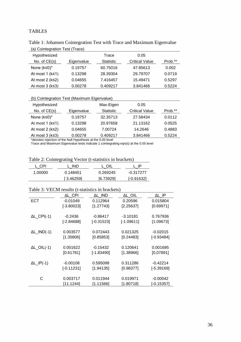
[TABLE 1 HERE]

The cointegration test, which was the prerequisite for estimating VECM(1), indicated that

there exists one significant cointegrating vector (see Table 1), i.e. that our four variables1 are

linked together by long-run equilibrium relationship, which can be seen in the following table

(Table 2 – Cointegrating Vector).

[TABLE 2 HERE]

In the long-run L_IND exercises a significant positive influence on L_CPI. The positive

relationship between the stock market and CPI in the long run, can be explained by the Fisher

hypothesis and several other studies have documented the same findings (see for example

1 All variables are I(1). Results can be obtained upon request.

14

Jaffe and Mandelker, 1976; Fama, 1981; Geske and Roll, 1983; Lee, 1992; Solnik and Solnik,

1997; Siklos and Kwok, 1999; Schotman and Schweitzer, 2000; Kim and In, 2005). Oil prices

are exercising a significant positive influence on CPI. This is explained by the fact that

increased oil prices to an oil-importing country, such as Greece, can cause cost-push inflation

(Barro, 1984; Abel and Bernanke, 2001; Hooker, 2002; LeBlanc and Chinno, 2004). On the

other hand, industrial production is not having any significant effect on L_CPI, in the long

run.

The next step is to analyse the short run parameters of the VEC model and the impulse

response functions, which are presented in Tables 3 and 4, respectively.

[TABLE 3 HERE]

[TABLE 4 HERE]

Engle and Granger (1987) demonstrated that when two variables cointegrated, then an error-

correction model necessarily describes the data-generating process (this is encapsulated

within the Granger representation theorem). Within the equations of the ECM, there are to be

found different elements, which include the lagged-first differences of the endogenous

variables and the error-correction term (ECT). The ECT indicates the extent of the deviation

from the long-run equilibrium which was present in the previous period. The coefficient

which is attached to the ECT fulfils the role of the adjustment parameter, which shows the

proportion of the disequilibrium that is recovered during the subsequent period. On the other

hand, the coefficients which are attached to the lagged first-differences provide an indication

of the short-run relationship between the endogenous variables (Enders, 1995). In other

words, we can argue that the disequilibrium error (as these expressed by the ECT) can force

variables back towards their long-run equilibrium. Miller and Russek (1990) examining the

15

relationship between government taxes and spending in US, suggested that temporal causality

can emerge from both the lagged-first differences and the error-correction term. In addition,

Masih and Masih’s (1997) interpretation of the coefficient corresponding to the ECT is one of

a long-run causal relationship between the respective variables.

Hence, starting with the error correction term (ECT), our results suggest that about 1% of

long-run disequilibrium is corrected each month by changes in the L_CPI equation. A value

of −0.01 for the coefficient of error correction term suggests that the Greek CPI will converge

towards its long run equilibrium level at a very slow speed. Continuing to the short-run

parameters, results suggest that the Greek stock market is significantly affected by oil prices

(negatively) and industrial production (positively). It can be supported that oil prices and

industrial production act as leading indicators of the Greek stock market, in the short-run. The

ECT term in the L_IND equation in not significant, suggesting that the long-run

disequilibrium error of the L_CPI equation is not influencing the L_IND equation. Similar

conclusions were expressed by other authors such as, Ritter (2005), Glen (2002),

Hondroyiannis and Papapetrou (2001) and Bilson et al. (2001).

Impulse response functions tend to suggest in the case of L_CPI that shocks from oil prices

(L_OIL) and industrial production (L_IP) require the lengthier period of time to settle down

(80 and 81 months, respectively). In the case of L_IND, almost all shocks require 50 months

to settle down. Finally, we can observe that shocks deriving from L_CPI, L_IND and L_OIL

on L_IP require the shorter period of time to reach a new equilibrium point, compared to the

other variables.

Having examined the long and short-run dynamics of our series in levels, we proceed to the

next part of our analysis, which is the examination of the relationship between the cyclical

components of our series. The extraction and analysis of cyclical components in isolation, as a

16

complementary approach to the analysis above, could be of great importance for policy

makers.

4.2. VAR approach

4.2.1. Preliminary Results

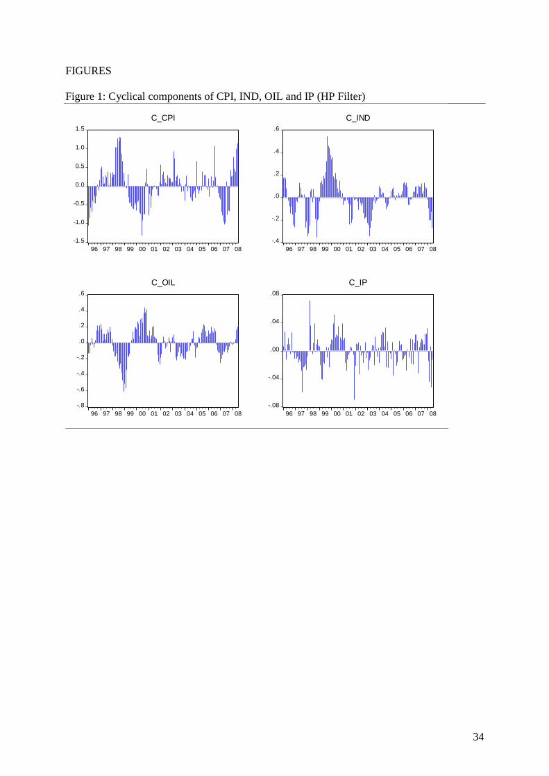
Figure 1 shows the cyclical components of our series.

[FIGURE 1 HERE]

[FIGURE 2 HERE]

It can be observed that C_IND and C_OIL are showing the higher amplitude, whereas C_IP

and C_CPI show lower one. This is due to the higher standard deviation that C_IND and

C_OIL have compared to the other two variables. This high standard deviation can also be

observed in Tables 5 and 6 below, which reports the descriptive statistics of the series.

[TABLE 5 HERE]

[TABLE 6 HERE]

All series have mean zero but the medians deviate from mean. This is an indication of non-

normally distributed series, probably due to non-linearities involved in the business cycle

fluctuations. This non-normality is also evident from the kurtosis coefficients and the

corresponding Jarque – Bera statistics. Furthermore, we find that the macroeconomic

indicators (CPI and Industrial Production) and oil prices share common length of their cycles.

For all these three series the dominant cycle is that of 50 months, i.e. almost 4 years. The

stock market index has a dominant cycle of 75 months, i.e. almost 6 years; whereas the stock

17

market’s second dominant cycle is at the length of 50 months (not reported here, though), as

well. This finding could suggest that some kind of a relationship exists among these variables.

To proceed to the VAR estimation, it is first necessary to establish the stationarity of the

model2. To do so, we employ a Johansen cointegration approach, using both trace statistic and

maximum eigenvalues, with 4 lags. The rank of matrix Π=4, so as the number of

cointegrating equations are equal to the number of variables it can be argued that the VAR

model is stationary3.

Further, using AIC, SC and HQ criteria we identify the order of the VAR model. All criteria

(AIC, SC and HQ) allow us to conclude that the order of the VAR model will be one (1)4.

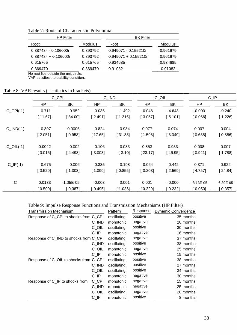
A further test on the VAR stationarity is required (Table 7), which examines the inverse roots

of the characteristic polynomial. As we can observe no root lies outside the unit circle, which

allow us to conclude that the VAR(1) model satisfies the stability condition.

[TABLE 7 HERE]

All preliminary results suggest that we can proceed to the estimation of the VAR(1) model.

The next section will report the findings of the VAR model. We will also report on the

impulse response functions and the variance decomposition to help us with the economic

interpretation of the findings.

4.2.2. VAR Results

Table 8 reports the findings from the VAR model, using both the HP and BK filters. The main

findings from this table suggest that stock market receives negative and significant influence

from oil and CPI, yet industrial production does not significantly affect stock market cycles.

2 All variables are I(0). Results can be obtained upon request.

3 Results can be obtained upon request.

4 Results can be obtained upon request.

18

Furthermore, the cyclical component of the Greek stock market exercises a negative impact

on CPI. Oil cyclical components seem to have a positive influence on industrial production

and CPI, however the HP filter suggest that this influence is not significant. Based on these

findings we could suggest that the cyclical components of oil prices lead these of the Greek

stock market and that there is a bidirectional relationship between the cyclical components of

CPI and the Greek stock market. The BK filter further suggests that there is bidirectional

relationship between the Greek macroeconomic indicators (C_CPI and C_IP) and oil prices

(C_OIL). Overall the results, using both the HP and the BK filters, are similar, which is a

finding that strengthens the validity of the results.

[TABLE 8 HERE]

Even though the majority of the results are similar, still some minor differences exist. This

was expected due to the differences in filtering methods. Such differences do not diminish the

findings of this research, as according to Spanos (1998) econometric modelling should not be

treated as a tool for statistical inference, but rather as a tool for model building. In that sense,

it is reasonable and expected that different filters could eventually provide some different

results5.

Overall, the results are almost similar to some of the previous studies, which had used growth

rates rather than the cyclical components of the variables. However, past studies showed that

industrial production is influencing stock market performance, yet again, in this study, such

conclusion cannot be supported.

The next step in the analysis is the examination of the transmission mechanism of stochastic

structural shocks by means of the impulse response functions and the variance decomposition

5 Ewing and Thomson (2007) used three different filtering methods, namely the HP, BK and CF filters,

to extract the cyclical components of oil prices, industrial production, consumer prices, unemployment and stock

prices. Their tests produced some different findings under the different filters, as well.

19

of the VAR model. The purpose of the VAR is mainly to examine the dynamic adjustments of

each of the involved variables to exogenous stochastic structural shocks.

From the transmission mechanisms referring to the response of C_CPI to shocks from

C_IND, C_OIL and C_IP we observe that there are negative responses to stock market and

industrial production shocks, whereas there is a positive response to oil shocks. Regarding

stock market responses, it can be observed that there are negative responses to CPI and oil

shocks and positive response to industrial production shocks. As for the industrial production

we can notice that there is a negative response to CPI and oil shocks, whereas the response is

positive to stock markets shocks. The results were the expected ones, yet for some of these

cases, responses are almost zero. Previous studies have documented similar findings to these,

using growth rates, instead of the cyclical components.

It is worth noting here that according to the HP filter, shocks from CPI require about 3 years

to be absorbed by the other variables, shocks from the stock market and oil need about 2-3

years, whereas shocks from industrial production will be absorbed within a period of 1.5-2

years (Table 9). The BK filter suggests that shocks from CPI require about 6 years to be

absorbed by the other variables, shocks from the stock market and oil need about 5-6 years,

whereas shocks from industrial production will be absorbed within a period of 4-6 years

(Table 10).

[TABLE 9 HERE]

[TABLE 10 HERE]

From Tables 11 and 12 we observe that the highest percentage error variance of the series

originate from themselves, as expected. Furthermore, the percentage error variance of C_CPI

is mainly influenced by the cyclical fluctuations of the stock market and oil prices. Similarly,

20

the percentage error variance of C_IND mainly originates from the cyclical components of oil

prices and CPI. Finally, the highest percentage error variance of C_IP originates from C_OIL

and C_CPI.

[TABLE 11 HERE]

[TABLE 12 HERE]

From the above findings we conclude that the Greek stock market is heavily influenced, on

aggregate, by macroeconomic variables, such as industrial production and CPI and in

addition, it is also influenced by oil prices. Additionally, the cyclical fluctuations of oil seem

to exercise some effect on the cyclical indicators of industrial production and CPI. It is worth

commenting that the Greek stock market is also influencing C_CPI at a considerably high

degree, as well.

Overall, the Greek stock market is receiving influence for national specific factors, as well as

from international specific factors, such as oil prices. In addition, industrial production is

influenced by international factors, such as oil prices; however the effect does not seem to be

transferred either on CPI or the stock market performance.

5. Concluding remarks

In this study we investigate the relationship between the Consumer Price Index, Industrial

Production, Stock Market and the Brent oil prices in Greece. Initially, we studied data in

levels and then we proceeded to the isolation of the cyclical components, trying to investigate

if decomposing our series and extracting the unobserved component of the cycle will produce

additional evidence which can be utilised from policy makers.

21

Cointegration and VECM results suggested that oil prices and the Greek stock market

exercise a significant positive effect on the Greek CPI, in the long-run. Short-run parameters

suggest that oil prices and industrial production act as leading indicators on the Greek stock

market. More specifically, oil prices shocks cause a negative effect on the Greek stock

market, whereas industrial production causes a positive effect.

According to our VAR model, findings suggest that the Greek stock market receives negative

and significant influence from oil prices and CPI and that industrial production affects stock

market cycles in a positive fashion. Furthermore, the cyclical component of the Greek stock

market exercises a negative impact of CPI. Oil cyclical components do not seem to have any

strong influence on industrial production and CPI. Based on these findings, we can assert that

the cyclical components of oil prices lead these of the Greek stock market and that there is a

bidirectional relationship between the cyclical components of CPI and the stock market.

Finally, a high percentage error variance of the Greek stock market originates from CPI and

oil prices. In addition, a high percentage error variance of CPI originates from the Greek stock

market and oil prices.

Overall, the two sets of results are not directly comparable since the VECM approach uses the

data in levels while the VAR approach uses cyclical components of the series. However, we

can observe some consistency in the results, which were produced by these two approaches.

Both VECM and VAR frameworks find evidence of a relationship among oil prices, the

Greek stock market and CPI. Nevertheless, the VAR approach enabled us to capture

additional relationships among our variables, compared to the VECM results, as these were

portrayed in section 4.2.2. This enhances the importance of the examination of the cyclical

components, as it was also suggested by Diebold and Rudebusch (1996).

A policy implication of our results suggests that Greece should pay particular attention on oil

price shocks as these shocks influence its stock market and inflation. To address both these

22

influences of oil prices, Greece should rely more on its fiscal policy for oil price shock

absorption, rather than monetary policy, since the latter is orchestrated by EMU. An

expansionary fiscal policy could be considered in order to confront supply-side inflation

pressures in the event of higher oil prices, for example.

Based on the aforementioned findings, this research adds to the existing literature, as it has a

particular focus on the cyclical components of the series under examination. In addition it

examines a small size economy, such as that of Greece, rather than a large economy, such as

US or UK, which have been extensively studied in the past. Furthermore, this study uses

recent data, which take into account the last oil crisis period.

Finally the findings of this study are of a particular interest and importance to policy makers,

financial managers, financial analysts and investors dealing with the Greek economy and the

Greek stock market.

Our results could lead to further research questions that seek answers. For example, further

research could test for potential structural breaks. Additionally, more variables could be added

to the model, such as unemployment and other energy prices, such as natural gas.

Acknowledgments: The author would like to thank one editor Prof. Richard S.J. Tol and the

two anonymous reviewers for their time and constructive suggestions. The author would like

to thank Dr. Costas Leon and Robert Gausden for their helpful comments, as well. The author

is completely responsible for any remaining errors and deficiencies.

23

References:

Abel A.B., Bernanke B.S. Macroeconomics. Addison Wesley Longman Inc, 2001.

Balke N., Wohar M. Explaining Stock price movements: Is there a case for fundamentals?.

Federal Reserve Bank of Dallas Economic Review 2001; (Third Quarter); 22–34.

Barro R.J. Macroeconomics. John Wiley & Sons, 1984.

Bilson M.C., Brailsford J.T., Hooper J.V. Selecting macroeconomic variables as explanatory

factors of emerging stock market returns. Pacific-Basin Finance Journal 2001; 9; 401-426.

Burbridge J., Harrison A. Testing for the effects of oil-price rises using vector

autoregressions. International Economic Review 1984; 25(1); 459-484.

Burns A. F., Mitchell W. C. Measuring Business Cycles. New York: National Bureau of

Economic Research, 1946.

Carlstrom T.C., Fuerst S.T., Ioannidou P.V. Stock Prices and Output Growth: An

Examination of the Credit Channel. Federal Reserve Bank of Cleveland 2002; August 15.

Castanias R.P.II. Macro Information and the variability of stock market prices. Journal of

Finance 1979; 34(2); 439-450.

Chen N.F., Roll R., Ross S. Economic forces and the stock market. Journal of Business 1986:

59; 383–403.

24

Chiarella C., Gao S. The value of the S&P 500 – A macro view of the of the stock market

adjustment process. Global Finance Journal 2004; 15; 171-196.

Choi J.J., Hauser S., Kopecky K. Does the stock market predict real activity? Time series

evidence from the G-7 countries. Journal of Banking & Finance 1999; 23; 1771–1792.

Christodoulakis N., Dimeli S., Kollintzas T. Business cycles in the EC: Idiosyncrasies and

regularities. Economica 1995; 62(245); 1-27.

Ciner C. Energy shocks and financial markets: nonlinear linkages. Studies in Nonlinear

Dynamics and Econometrics 2001; 5; 203–212.

Cozier B.V., Rahman A.H. Stock returns, inflation, and real activity in Canada. Canadian

Journal of Economics 1988; 2; 759–74.

Dickerson A.P., Gibson H.D., Tsakalotos E. Business cycle correspondence in the European

Union. Empirica 1998; 25; 51–77.

Diebold F.X., Rudebusch D.G. Five questions about business cycles. Economic Review,

Federal Reserve Bank of San Francisco 2001; 1-15

Diebold F.X., Rudebusch D.G. Measuring Business Cycles: A Modern Perspective. The

Review of Economics and Statistics 1996; 78(1); 67-77.

25

Dritsaki M. Linkage between stock market and macroeconomic fundamentals: Case study of

Athens stock exchange. Journal of Financial Management and Analysis 2005; 18(1); 38-47.

Enders W. Applied Econometric Time Series. Wiley Series in Probability and Mathematical

Statistics. 1995.

Engle F.R., Granger W.J.C. Co-integration and error correction: representation, estimation,

and testing. Econometrica 1987; 55(2); 251-276.

Engsted T., Tanggaard C. The relation between asset returns and inflation at short and long

horizons. Journal of International Financial Markets, Institutions and Money 2002; 12; 101–

118.

Errunza V., Hogan K. Macroeconomic determinants of European stock market volatility.

European Financial Management 1998; 4(3); 361-377.

Ewing B.T., Thompson M.A. Dynamic cyclical components of oil prices with industrial

production, consumer prices, unemployment and stock prices. Energy Policy 2007; 35; 5535-

5540.

Fama E. Stock return, real activity, inflation and money. American Economic Review 1981;

65; 269–82.

Fama E., Schwert G.W. Asset returns and inflation. Journal of Financial Economics 1977; 5;

115–46.

26

Favero C. Applied Macroeconometrics. Oxford University Press. 2001.

Ferderer P.J. Oil price volatility and the macroeconomy. Journal of Macroeconomics 1996;

18(1); 1-26.

Filis G., Leon C. The transmission mechanism of the cyclical components of the Greek

output, investments and stock exchange. In the proceedings of the 1st International

Conference in Accounting and Finance. August 2006.

Flannery M.J., Protopapadakis A.A. Macroeconomic factors do influence aggregate stock

returns. The Review of Financial Studies 2002; 15; 751–81.

Geske R., Roll R. The fiscal and monetary linkage between stock returns and inflation.

Journal of Finance 1983; 38; 1–32.

Gjerde Ø., Sættem F. Causal relations among stock returns and macroeconomic variables in a

small, open economy. Journal of International Financial Markets, Institutions and Money

1999; 9; 61–74.

Gisser M., Goodwin T.H. Crude oil and the macroeconomy: Tests of some popural notions.

Journal of Money, Credit and Banking 1986; 18(1); 95-103.

Glen J. Devaluations and emerging stock market returns. Emerging Markets Review 2002; 3;

409–428.

27

Hamilton J.D. Oil and the macroeconomy since World War II. Journal of Political Economy

1983; 92(2); 228-248.

Hardouvelis A.G. Stock prices: Nominal vs real shocks. Financial Markets and Portfolio

Management 1988; 2(3); 10-18.

Harvey C.R. Drivers of expected returns in international markets. Emerging Markets

Quarterly 2000; Fall; 32– 49.

Haung R.D, Masulis R.W., Stoll H.R. Energy shocks and financial markets. Journal of

Futures Markets 1996; 16(1); 1-27.

Hodrick R., Prescott E. Postwar U.S. business cycles: An empirical investigation. Journal of

Money, Credit and Banking 1997; 29; 1-16.

Hondroyiannis G., Papapetrou E. Macroeconomic influences on the stock market. Journal of

Economics and Finance 2001; 25(1); 33-49.

Hooker M.A. Are Oil Shocks Inflationary? Asymmetric and Nonlinear Specifications versus

Changes in Regime. Journal of Money, Credit and Banking 2002; 34(2); 540-561.

Hooker M. Macroeconomic factors and emerging market equity returns: A Bayesian model

selection approach. Emerging Markets Review 2004; 5; 379-387.

28

Jaffe J., Mandelker G. The Fisher effect for risky assets: an empirical investigation. Journal of

Finance 1976; 31; 447–58.

Johansen S. Statistical analysis of cointegration vectors. Journal of Economic Dynamic and

Control 1988; 12; 231-254.

Johansen S., Juselius K. Maximum likelihood estimation and inference on cointegration. With

applications to the demand of money. Oxford Bulletin of Economics and Statistics 1990; 52;

169-210.

Johansen S., Juselius K. Testing structural hypothesis in a multivariate cointegration analysis

in PPP and the UIP for UK. Journal of Econometrics 1992; 53; 169-209.

Johansen S., Juselius K. Identification of the long-run and the short-run structure. An

application of the ISLM model. Journal of Econometrics 1994; 63; 7-36.

Jones C.M., Kaul G. Oil and stock markets. Journal of Finance 1996; 51(2); 463-491.

Jones D.W., Lelby P.N., Paik I.K. Oil price shocks and the macroeconomy: what has been

learned since 1996. Energy Journal 2004; 25(2); 1-32.

Inklaar R., de Haan J. Is There Really a European Business Cycle? A Comment. Oxford

Economic Papers 2001; 53(2); 215-20.

29

Kilian L., Park C. The impact of oil price shocks on the U.S. stock market. C.E.P.R.

Discussion Papers in its series CEPR Discussion Papers with number 6166, 2007.

http://www.cepr.org/pubs/dps/DP6166.asp. [accessed 12/2/2009]

Kim S., In F. The relationship between stock returns and inflation: new evidence from

wavelet analysis. Journal of Empirical Finance 2005; 12; 435-444.

LeBlanc M., Chinn M.D. Do High Oil Prices Presage Inflation? The Evidence from G5

Countries. Business Economics 2004; 34; 38-48.

Lee B. Causal relations among stock returns, interest rates, real activity, and inflation. Journal

of Finance 1992; 47; 1591–603.

Leon C., Filis G. Cyclical fluctuations and transmission mechanisms of the GDP, investments

and the stock exchange in Greece: Evidence from spectral and VAR analysis. Journal of

Money, Investment and Banking 2008; 6(5); 54-65.

Levine R., Zervos S. Stock Markets, Banks, and Economic Growth. American Economic

Review, American Economic Association 1998; 88; 537-558.

Masih A.M.M., Masih R. On the temporal casual relationship between energy consumption,

real income and prices: Some new evidence from Asian-Energy dependent NICs based on a

multivariate cointegration/Vector Error-Correction approach. Journal of Policy Modeling

1997; 19(4); 417-440.

30

Mauro P. Stock returns and output growth in emerging and advanced economies. Journal of

Development Economics 2003; 71; 129– 153.

Miller J.I., Ratti R.A. Crude oil and stock markets: Stability, instability, and bubbles. Energy

Economics. 2009; 31(4); 559-568.

Miller S.M., Russek F.S. Co-Integration and Error-Correction Models: The Temporal

Causality between Government Taxes and Spending. Southern Economic Journal. 1990;

57(1); 221-229.

Ministry of Development. 1st Report for the Long Term Energy Planning of Greece – 2008-

2020. August 2007 (in Greek).

www.ypan.gr/docs/Ekthesi%20Makrochroniou%20Sxediasmou.doc [accessed 18/8/2009]

Morck R., Shleifer A., Vishny R. The stock market and investment: Is the market a

sideshow?. Brookings Papers on Economic Activity 1990; 1; 157–202.

Nandha M., Faff R. Does oil move equity prices? A global view. Energy Economics 2008; 30;

986–997.

Omrana M. Time Series Analysis of the Impact of Real Interest Rates on Stock Market

Activity and Liquidity in Egypt: Co-integration and Error Correction Model Approach.

International Journal of Business 2003; 8.

http://papers.ssrn.com/sol3/papers.cfm?abstract_id=420248 [accessed 23/2/2009]

31

O'Neill T.J., Penm J., Terrell R.D. The role of higher oil prices: a case of major developed

countries. Research in Finance 2008; 24; 287–299.

Park J., Ratti R.A. Oil price shocks and stock markets in the U.S. and 13 European countries.

Energy Economics 2008; 30; 2587–2608.

Papapetrou E. Oil price shocks, stock market, economic activity and employment in Greece.

Energy Economics 2001; 23(5); 511-532.

Pearce D.K., Roley V.V. The reaction of stock prices to unanticipated changes in money: A

note. Journal of Finance 1983; 38(4); 1323-1333.

Rapach D.E. Macro shocks and real stock prices. Journal of Economics and Business 2001;

53; 5–26.

Ritter R.J. Economic Growth and Equity Returns. Pacific-Basin Finance Journal 2005; 13;

489–503.

Ross S.A. Information and volatility: The no-arbitrage martingale approach to timing and

resolution irrelevancy. Journal of Finance 1989; 44(1); 1-17.

Rudebusch G. D., Svensson E.O.L. Policy Rules for Inflation Targeting. In Monetary Policy

Rules, ed. John B. Taylor. Chicago: Chicago University Press, 1999; 203-246.

Sadorsky P. Oil price shocks and stock market activity. Energy Economics 1999; 21; 449-469.

32

Schotman P.C., Schweitzer M. Horizon sensitivity of the inflation hedge of stocks. Journal of

Empirical Finance 2000; 7; 301–305.

Schwert G.W. Why does stock market volatility change over time?. Journal of Finance 1989;

44(5); 1115-1145.

Siklos P., Kwok B. Stock returns and inflation: a new test of competing hypotheses. Applied

Financial Economics 1999; 9; 567–81.

Solnik B., Solnik V., A multi-country test of the Fisher model for stock returns. Journal of

International Financial Markets, Institutions and Money 1997; 7; 289–301.

Theophano P., Sunil P. Economic variables and stock market returns: evidence from the

Athens stock exchange. Applied Financial Economics 2006; 16(13); 993-1005.

Vassalou M. News related to future GDP growth as a risk factor in equity returns. Journal of

Financial Economics 2003; 68; 47-73.

Verma R., Ozunab T. Are emerging equity markets responsive to cross-country

macroeconomic movements? Evidence from Latin America. Journal of International

Financial Markets, Institutions and Money 2005; 15; 73-87.

Wahlroos B., Berglund T. Stock returns, inflationary expectations and real activity. Journal of

Banking and Finance 1986; 10; 377–89.

33

Wongbangpo P., Sharma C.S. Stock market and macroeconomic fundamental dynamic

interactions: ASEAS-5 countries. Journal of Asian Economics 2002; 13; 27-51.

34

FIGURES

Figure 1: Cyclical components of CPI, IND, OIL and IP (HP Filter)

-1.5

-1.0

-0.5

0.0

0.5

1.0

1.5

96 97 98 99 00 01 02 03 04 05 06 07 08

C_CPI

-.4

-.2

.0

.2

.4

.6

96 97 98 99 00 01 02 03 04 05 06 07 08

C_IND

-.8

-.6

-.4

-.2

.0

.2

.4

.6

96 97 98 99 00 01 02 03 04 05 06 07 08

C_OIL

-.08

-.04

.00

.04

.08

96 97 98 99 00 01 02 03 04 05 06 07 08

C_IP

35

Figure 2: Cyclical components of CPI, IND, OIL and IP (BK filter)

-.003

-.002

-.001

.000

.001

.002

.003

.004

1996 1998 2000 2002 2004 2006 2008

C_CPI

-.10

-.05

.00

.05

.10

.15

1996 1998 2000 2002 2004 2006 2008

C_IND

-.15

-.10

-.05

.00

.05

.10

1996 1998 2000 2002 2004 2006 2008

C_OIL

-.015

-.010

-.005

.000

.005

.010

.015

1996 1998 2000 2002 2004 2006 2008

C_IP

36

TABLES

Table 1: Johansen Cointegration Test with Trace and Maximum Eigenvalue

(a) Cointegration Test (Trace)

Hypothesized Trace 0.05

No. of CE(s) Eigenvalue Statistic Critical Value Prob.**

None (k≤0)* 0.19757 60.75016 47.85613 0.002

At most 1 (k≤1) 0.13298 28.39304 29.79707 0.0719

At most 2 (k≤2) 0.04655 7.416457 15.49471 0.5297

At most 3 (k≤3) 0.00278 0.409217 3.841466 0.5224

(b) Cointegration Test (Maximum Eigenvalue)

Hypothesized Max-Eigen 0.05

No. of CE(s) Eigenvalue Statistic Critical Value Prob.**

None (k≤0)* 0.19757 32.35713 27.58434 0.0112

At most 1 (k≤1) 0.13298 20.97658 21.13162 0.0525

At most 2 (k≤2) 0.04655 7.00724 14.2646 0.4883

At most 3 (k≤3) 0.00278 0.409217 3.841466 0.5224 *denotes rejection of the Null Hypothesis at the 0.05 level Trace and Maximum Eigenvalue tests indicate 1 cointegrating eqn(s) at the 0.05 level

Table 2: Cointegrating Vector (t-statistics in brackets)

L_CPI L_IND L_OIL L_IP

1.00000 0.148451 0.269245 -0.317277

[ 3.46259] [6.73929] [-0.91632]

Table 3: VECM results (t-statistics in brackets)

ΔL_CPI ΔL_IND ΔL_OIL ΔL_IP

ECT -0.01049 0.112964 0.20596 0.015804

[-3.80023] [1.27743] [2.25637] [0.69971]

ΔL_CPI(-1) -0.2436 -0.86417 -3.10181 0.767936

[-2.84688] [-0.31523] [-1.09611] [1.09673]

ΔL_IND(-1) 0.003577 0.072443 0.021325 -0.02015

[1.35806] [0.85853] [0.24483] [-0.93484]

ΔL_OIL(-1) 0.001622 -0.15432 0.120641 0.001695

[0.61781] [-1.83490] [1.38966] [0,07891]

ΔL_IP(-1) -0.00108 0.595098 0.311286 -0.42214

[-0.11231] [1.94135] [0.98377] [-5.39169]

C 0.003717 0.011944 0.019971 -0.00042

[11.1244] [1.11566] [1.80718] [-0.15357]

37

Table 4: Impulse Response Functions and Transmission Mechanisms (VECM) Transmission Mechanism

Response

Period for converging to the new equilibrium

Response of L_CPI to shocks from L_CPI positive 45 months

L_IND negative 52 months

L_OIL positive 80 months

L_IP positive 81 months

Response of L_IND to shocks from L_CPI negative 50 months

L_IND positive 71 months

L_OIL negative 49 months

L_IP positive 50 months

Response of L_OIL to shocks from L_CPI positive 47 months

L_IND positive 58 months

L_OIL positive 75 months

L_IP negative 49 months

Response of L_IP to shocks from L_CPI positive 10 months

L_IND negative 21 months

L_OIL negative 39 months

L_IP positive 14 months

Table 5: Descriptive Statistics (HP Filter)

C_CPI C_IND C_OIL C_IP

Mean -7.30E-12 -8.30E-13 -3.38E-13 -3.80E-13

Median 0.024236 0.004576 0.020009 0.000854

Maximum 1.312880 0.546400 0.438260 0.071445

Minimum -1.319837 -0.359030 -0.610523 -0.069376

Std. Dev. 0.509892 0.156617 0.182376 0.020849

Skewness 0.241716 0.349958 -0.487155 -0.142477

Kurtosis 3.279111 4.117642 3.815919 4.064785

Jarque-Bera 1.947563 10.86879 10.09377 7.593529

Probability 0.377652 0.004364 0.006429 0.022443

Table 6: Descriptive Statistics (BK Filter)

C_CPI C_IND C_OIL C_IP

Mean 7.81E-05 0.002608 -0.00136 0.00022

Median -9.45E-06 -0.00334 0.010562 5.13E-05

Maximum 0.00331 0.115692 0.074861 0.013552

Minimum -0.00237 -0.08421 -0.13471 -0.0132

Std. Dev. 0.001069 0.042958 0.045422 0.005294

Skewness 0.673458 0.565898 -0.84599 0.046046

Kurtosis 4.162437 3.443676 3.335686 3.151336

Jarque-Bera 17.40994 8.12797 16.36499 0.172609

Probability 0.000166 0.01718 0.00028 0.917315

38

Table 7: Roots of Characteristic Polynomial

HP Filter BK Filter

Root Modulus Root Modulus

0.887484 - 0.106000i 0.893792 0.949071 - 0.155210i 0.961679

0.887484 + 0.106000i 0.893792 0.949071 + 0.155210i 0.961679

0.615765 0.615765 0.934685 0.934685

0.369470 0.369470 0.91082 0.91082 No root lies outside the unit circle. VAR satisfies the stability condition.

Table 8: VAR results (t-statistics in brackets)

C_CPI C_IND C_OIL C_IP

HP BK HP BK HP BK HP BK

C_CPI(-1) 0.711 0.952 -0.036 -1.492 -0.046 -4.643 -0.000 -0.240

[ 11.67] [ 34.00] [-2.491] [-1.216] [-3.057] [-5.101] [-0.066] [-1.226]

C_IND(-1) -0.397 -0.0006 0.824 0.934 0.077 0.074 0.007 0.004

[-2.051] [-0.953] [ 17.65] [ 31.35] [ 1.593] [ 3.349] [ 0.655] [ 0.856]

C_OIL(-1) 0.0022 0.002 -0.106 -0.083 0.853 0.933 0.008 0.007

[ 0.015] [ 4.498] [-3.003] [-3.10] [ 23.17] [ 46.95] [ 0.921] [ 1.788]

C_IP(-1) -0.675 0.006 0.335 -0.198 -0.064 -0.442 0.371 0.922

[-0.529] [ 1.303] [ 1.090] [-0.855] [-0.203] [-2.569] [ 4.757] [ 24.84]

C 0.0133 -1.05E-05 -0.003 0.001 0.001 -0.000 -8.13E-05 6.80E-05

[ 0.509] [-0.387] [-0.495] [ 1.036] [ 0.229] [-0.232] [-0.050] [ 0.357]

Table 9: Impulse Response Functions and Transmission Mechanisms (HP Filter)

Transmission Mechanism Pattern Response Dynamic Convergence

Response of C_CPI to shocks from C_CPI oscillating positive 35 months

C_IND monotonic negative 20 months

C_OIL oscillating positive 30 months

C_IP monotonic negative 16 months

Response of C_IND to shocks from C_CPI oscillating negative 37 months

C_IND oscillating positive 38 months

C_OIL monotonic negative 25 months

C_IP monotonic positive 15 months

Response of C_OIL to shocks from C_CPI oscillating positive 38 months

C_IND oscillating positive 27 months

C_OIL oscillating positive 34 months

C_IP monotonic negative 30 months

Response of C_IP to shocks from C_CPI monotonic negative 15 months

C_IND monotonic negative 25 months

C_OIL oscillating negative 20 months

C_IP monotonic positive 8 months

39

Table 10: Impulse Response Functions and Transmission Mechanisms (BK Filter)

Transmission Mechanism Pattern Response Dynamic Convergence

Response of C_CPI to shocks from C_CPI oscillating positive 71 months

C_IND oscillating negative 69 months

C_OIL oscillating positive 75 months

C_IP oscillating positive 69 months

Response of C_IND to shocks from C_CPI oscillating positive 74 months

C_IND oscillating positive 69 months

C_OIL oscillating negative 64 months

C_IP oscillating positive 71 months

Response of C_OIL to shocks from C_CPI oscillating positive 79 months

C_IND oscillating positive 78 months

C_OIL oscillating positive 78 months

C_IP oscillating negative 79 months

Response of C_IP to shocks from C_CPI oscillating positive 78 months

C_IND oscillating negative 64 months

C_OIL oscillating negative 71 months

C_IP oscillating positive 50 months

Table 11: Variance Decomposition (HP Filter)

Period C_CPI C_IND C_OIL C_IP

C_CPI 6 94.16035 5.011009 0.341387 0.487256

12 89.76675 7.857504 1.705096 0.670648

24 88.4826 8.052473 2.77453 0.690397

C_IND 6 14.76673 76.43173 7.497286 1.304247

12 15.68965 68.33327 14.5129 1.464174

24 15.77569 66.36777 16.42125 1.435283

C_OIL 6 10.24706 8.841061 80.83774 0.074141

12 22.0547 17.97148 59.53547 0.438358

24 24.94253 20.77153 53.62722 0.658712

C_IP 6 1.712449 0.755223 5.739602 91.79273

12 2.158359 1.22865 5.700322 90.91267

24 2.268711 1.341224 5.762879 90.62719

40

Table 12: Variance Decomposition (BK Filter)

Period C_CPI C_IND C_OIL C_IP

C_CPI 6 93.22985 0.137754 5.8228 0.809594

12 80.01086 0.95593 18.21055 0.82266

24 64.93392 9.072716 20.59222 5.40114

C_IND 6 0.891724 95.23854 3.445103 0.424637

12 1.114184 86.33731 12.08429 0.464223

24 10.55945 70.63635 14.95117 3.853038

C_OIL 6 10.39141 10.7809 71.85511 6.972573

12 27.63814 17.67181 37.37858 17.31147

24 28.60167 15.85836 35.42281 20.11716

C_IP 6 4.347178 0.962728 0.237333 94.45276

12 5.173669 2.675523 0.28525 91.86556

24 9.52809 4.929592 5.385148 80.15717