machine tool vibrations and violin sound fields studied...
TRANSCRIPT

DOCTORA L T H E S I SDOCTORA L T H E S I S
Luleå University of TechnologyDepartment of Applied Physics and Mechanical Engineering
Division of Experimental Mechanics
2006:27|: 02-757|: -c -- 06 ⁄27 --
2006:27
Machine tool vibrations and violin sound fields studied using laser vibrometry
Kourosh Tatar


Machine tool vibrations and violin sound fields studied using laser
vibrometry
Kourosh Tatar


ACKNOWLEDGEMENTS
This work has been carried out at the Division of Experimental Mechanics, Department of Applied Physics and Mechanical Engineering at Luleå University of Technology, Sweden. The research was performed during the years 2004-2006 in collaboration with the research groups Div. of Sound and Vibration and Div. of Manufacturing Systems Engineering, and the industrial partner SKF Nova. The Swedish Governmental Agency for Innovation System (Vinnova) supported the project “Vibrations and noise in machine tools”. The violin project and the purchase of the laser vibrometer system are financed by the Kempe foundations.
I would like to express great thanks to my two supervisors, Dr. Per Gren and Professor Mikael Sjödahl for their support, guidance and review of my work. Per Gren is also one of the co-authors of two of the papers. Great thanks to all in the research group and co-authors. I also acknowledge the efforts made by Mr Tore Silver who have worked and helped with the Liechti milling machine. I want to thank all my colleagues at the Division of Experimental mechanics for making the time at work enjoyable.
Finally I thank my family for their love and support.
Kourosh Tatar Luleå, May 2006
i


ABSTRACT
The knowledge of the dynamic behaviour of a milling process is very important for finding an optimum process window. In today’s manufacturing industry the machining parameters are often predicted using experimental data from non-rotating spindles. Many times the predicted machining parameters prove to be ineffective and inaccurate which lead to reduced quality of the machined surface, tool wear, noise or at worst spindle failure.
The best way to study the dynamics of the milling spindle is of course to measure the spindle response under actual operating conditions. Laser vibrometry is a non-contact, non-disturbing method commonly used for measurements of vibrations on static objects. The technique offers the possibility to measure vibrations on thin-walled (light), and rotating objects as well as sound fields. However, two major problems occur when measuring on rotating spindles: (1) speckle noise and (2) crosstalk between the vibration components. These two drawbacks make vibration measurements on rotating spindles difficult to interpret.
In this Licentiate thesis the principles of laser vibrometry is introduced and the speckle noise and the crosstalk between the velocity components of a rotating spindle is studied experimentally. The rotating spindle is excited by an adaptive magnetic bearing and the response is measured by laser vibrometry and non-contact inductive displacement sensors simultaneously. The work shows that by polishing the measurement surface optically smooth we are able to avoid the speckle noise and the crosstalk problem. By using this approach, the vibrations as well as the roundness of the measured target can be resolved. Hence, the laser vibrometry technique can be used for measuring the spindle dynamics under operating conditions.
Measurements on a bowed violin are performed. The chain of interacting parts of the played violin is studied: the string, the bridge and the plates as well as the generated sound field. The string is excited using a rotating bow apparatus and the vibrations from the string transmits to the violin body via the bridge and produces the sound. The measurements on the string shows stick-slip behaviour and the bridge measurements show that the string vibrations transmit to the bridge both in the horizontal and the vertical direction. Measurements on the plates show complex deflection shapes which are a combination of different eigenmodes. The sound fields emitted from the violin were measured and visualized for different harmonic partials of the played tone. However, the visualized sound field obtained by the laser vibrometer is a projection of the sound field along the laser light and the image obtained is a 2D map of the real 3D sound field. This effect is illustrated by measurements of a sound field emitted from three ultrasound transducers.
iii

iv
THESIS
This thesis consists of a summary and the following four papers:
Paper A M. Rantatalo, K. Tatar and P. Norman. “Laser doppler vibrometry measurements of a rotating milling machine spindle”. Proceedings of the Eighth International Conference in Rotating Machinery. University of Wales, Swansea, UK, 2004, 231-240.
Paper B K. Tatar, M. Rantatalo and P. Gren. “Laser vibrometry measurements of an optically smooth rotating spindle”. Submitted to “Mechanical Systems and Signal Processing” for publication.
Paper C A. Svoboda, K. Tatar, P. Norman and M. Bäckström. ”Integrated Tool for Prediction of Stability Limits in Machining”. Submitted to “International Journal for Production Research” for publication.
Paper D P. Gren, K. Tatar, J. Granström, N-E. Molin and E. V. Jansson. “Laser vibrometry measurements of vibration and sound fields of a bowed violin”. Meas. Sci. Technol. 17 2006, 635-644. Featured article in MST, see http://herald.iop.org/mst-featured/m63/crk/178594/link/226
v

vi

ContentsACKNOWLEDGEMENTS......................................................................................... i
ABSTRACT...............................................................................................................iii
THESIS....................................................................................................................... v
Part I Summary.................................................................................................... 1
1 INTRODUCTION............................................................................................... 3
2 MEASUREMENT METHOD ............................................................................ 52.1 Principle of laser vibrometry ..................................................................................... 5
2.2 Sound measurements using laser vibrometry ............................................................ 6
3 MEASUREMENTS ............................................................................................ 93.1 LDV measurements on thin-walled structures........................................................... 9
3.2 Rotating targets ........................................................................................................ 10 3.2.1 Laser Speckle effects in vibrometry measurements on rotating targets ......... 10 3.2.2 Crosstalk in laser vibrometry measurements on rotating targets.................... 11 3.2.3 An approach to solve the speckle and crosstalk problem............................... 12 3.2.4 Hammer test performed on a rotating spindle ................................................ 18
3.3 Measurements of sound fields ................................................................................. 20
4 CONCLUSIONS............................................................................................... 25
5 FUTURE WORK .............................................................................................. 27
6 SUMMARY OF APPENDED PAPERS........................................................... 29
7 REFERENCES.................................................................................................. 31
Part II Papers ................................................................................................... 33
vii


Part I
Summary
1


1 INTRODUCTION
Today’s manufacturing industry demands higher productivity, i.e. reduced production time and cost, and hence high-speed milling plays an important role. To be able to remove large material while maintaining a high quality there is need of advanced monitoring and control to prevent or limit events such as instability, tool ware, tool breakage or at worst; spindle failure. The instability of the process is a vibration phenomenon known as chatter. Vibration in machining is caused by the relative movement between the cutter and the workpiece. For a certain machine and workpiece four parameters play the most important role; tool, spindle speed, feed rate and depth of cut. Often in manufacturing processes, especially when manufacturing components for aerospace application, the workpiece is a monolith in the initial stage and the material removal is up to 90% of the original volume. In the different stages of milling the cutting parameters are changed by the operator as the workpiece rigidity and consequently the dynamic behaviour of the system changes. The critical stage is the finishing stage or when machining thin-walled structures. To optimize the cutting parameters, so-called stability lobe diagrams are used [1]. These diagrams are based on the frequency response function (FRF) of the system. An instrumented hammer is used to excite the system and the response is measured with the aid of an accelerometer. The measured response is then exported to additional software for mathematical computations to create the stability diagrams. Although stability diagrams can be helpful to understand the process, many times they are ineffective and inaccurate. The predicted stability diagram is specific for the spindle, tool and the workpiece, any changes in workpiece and or other cutting parameters will result in different response. The stability of the cutting process is much more complicated and the approach mentioned to predict the condition lack two important issues; the rotation of the cutting tool and the change of workpiece stiffness while the material is removed.
The best way of studying the dynamics of the milling spindle is of course to measure the spindle response under actual operating conditions. Since accelerometers can not be applied on the spindle shaft itself naturally the first option is to measure the vibration transmitted from the spindle into a non-rotating part. However, two problems can occur; (1) low vibration transmission making the measurements unreliable, and (2) magnetic disturbances from the motor during high spindle speeds. Non-contact position transducers such as capacitive and inductive displacement sensors are another possible measurement method, but these kinds of sensors are limited to be very close to the rotating part.
The objective of this thesis is to develop a non-contact technique to measure vibrations directly on a rotating milling machine spindle from any location. A Laser Doppler Vibrometer (LDV) offers this possibility. The LDV is a powerful tool that has now established itself as a vibration measurement instrument and is normally used on stationary vibrating objects. This instrument complements the use of accelerometers and provides the possibility of vibration measurements in situations where a non-contact measurement technique is required as in vibration measurements on, light, hot and rotating targets. However, the spectra of laser vibrometer measurements on rotating targets contain
3

4
additional surface motion information. In this thesis the principles of LDV is introduced and an approach to resolve the normal-to-surface vibrations in rotating target measurements is presented. The technique is implemented in milling machines.
As an illustration of the capacity of laser vibrometry the mechanical response of a bowed violin was studied. In most previous investigations of the violin, the different parts of the instrument are studied individually. Laser vibrometry together with a special constructed continous bowing devise offer the possibility to measure on the assembled violin and the generated sound field under conditions very close to real life. The present work is an investigation of how vibrations from the excited string transmit to the violin body via the bridge and produce the well known characteristic sound of the violin. The measured operational deflection shapes of the violin body together with the measured sound field give addition understanding of how vibrating plates emit sound.

2 MEASUREMENT METHOD
2.1 Principle of laser vibrometry Basically, the Laser vibrometer is a heterodyne interferometer based on the Doppler effect of backscattered light, as schematically presented in Figure 2.1. A laser beam is divided by a beam splitter (BS) into a reference and an object beam. The reference beam is then frequency shifted by a known amount, (fB), by a modulator, which is needed for resolving the direction of the measured vibration velocity. Systems differ by the method used for obtaining this frequency shift; our Polytec laser vibrometer uses an acousto-optic modulator (Bragg cell) with a frequency shift of 40 MHz. The object beam reflects from the target and hence is Doppler shifted, (fD), due to the target velocity and mixes with the shifted reference beam on the photo detector. Depending on the optical path difference between these two beams, they will interfere constructively or destructively. The photo detector measures the intensity of the mixed light, which will be time dependent. When the target is vibrating the frequency of the intensity variation will differ from the nominal modulation frequency by an amount, proportional to the surface velocity. Frequency demodulation of the photo detector signal by a Doppler signal processor produces a time resolved velocity of the moving target.
Laserf
f
f + fBM
BS BS
BS
f
f +
f+
D
fB+ fD
fDf
PC
Modulator(Bragg cell)
Doppler signal processor
Photo detector
Target
v(t)
f fD B|| -
Figure 2.1 Schematic of the laser vibrometer. The laser beam is divided into a reference and an object beam. These two interfere on the photo detector and the velocity of the target is obtained after demodulation of the signal. Beam splitter (BS), mirror (M), laser frequency (f), Bragg frequency shift (fB) and Doppler frequency caused by the target velocity (fD).B
5
6
The LDV is a point measuring instrument and for obtaining field measurements a sequence of single point measurements is needed. Scanning laser vibrometers offer this possibility. The Polytec PSV 300 scanning laser vibrometer used in our experiments have two small servo controlled mirrors in the scanning head, which make it possible to deflect the beam both in horizontal and vertical direction. In the application of laser vibrometry to experimental modal analysis, the surface of the vibrating object is scanned. Synchronization between the scan points is obtained through comparison with a reference signal; usually the input force signal at the driving point (excitation point) or a reference accelerometer signal. Vibration mode shapes and frequencies are then extracted from the measurements data by the vibrometer system software.
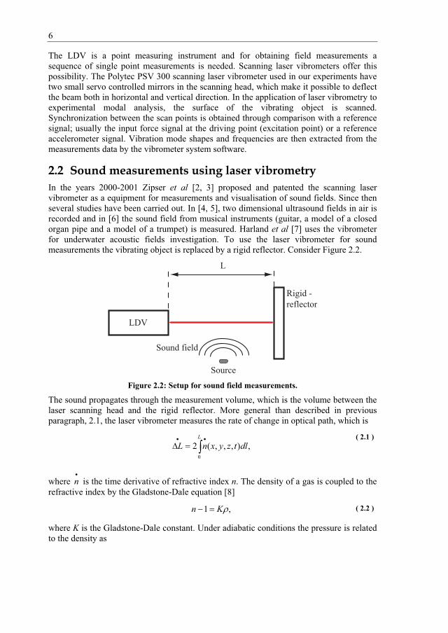
2.2 Sound measurements using laser vibrometry In the years 2000-2001 Zipser et al [2, 3] proposed and patented the scanning laser vibrometer as a equipment for measurements and visualisation of sound fields. Since then several studies have been carried out. In [4, 5], two dimensional ultrasound fields in air is recorded and in [6] the sound field from musical instruments (guitar, a model of a closed organ pipe and a model of a trumpet) is measured. Harland et al [7] uses the vibrometer for underwater acoustic fields investigation. To use the laser vibrometer for sound measurements the vibrating object is replaced by a rigid reflector. Consider Figure 2.2.
LDV
Rigid -reflector
L
Sound field
Source
Figure 2.2: Setup for sound field measurements.
The sound propagates through the measurement volume, which is the volume between the laser scanning head and the rigid reflector. More general than described in previous paragraph, 2.1, the laser vibrometer measures the rate of change in optical path, which is
( 2.1 ) ,),,,(2
0
dltzyxnLL
where is the time derivative of refractive index n. The density of a gas is coupled to the refractive index by the Gladstone-Dale equation [8]
n
,1 Kn ( 2.2 )
where K is the Gladstone-Dale constant. Under adiabatic conditions the pressure is related to the density as

7
( 2.3 ) ,
0
0
0
0
ppp
pwhere and 0p are the undisturbed pressure and density respectively. and 0represent the acoustic contribution to the overall pressure and density fields and is the specific-heat ratio. Assuming that the sound pressure fluctuations p are small compared to the undisturbed atmospheric pressure, the time derivative of the refractive index is given by
( 2.4 )
,1
0
0
ppn
n
where n0 is the undisturbed refractive index. Combining Equation ( 2.1 ) and Equation
( 2.4 ) yield
( 2.5 )
.1
20 0
0 dlppnL
L
By scanning the laser beam across the reflector we will obtain a 2-D map of the integrated 3-D sound field propagating through the measurement volume. The phase relation between each measured points are kept in track by the use of a reference signal usually obtained from a microphone at a fixed position. As an example a measurement of the sound field from a bird calling pipe is shown in Figure 2.3.
Figure 2.3: Measured sound field from a bird calling pipe.

8

3 MEASUREMENTS
3.1 LDV measurements on thin-walled structures Machine tool vibrations are the result of relative movement between the cutter and the workpiece [1]. In most situations the workpiece is considered as a solid part fixed to the machine table with no significant modal properties of its own. This assumption tends to weaken when machining components with low rigidity. In manufacturing of components for aerospace applications, for example, the material removal can be up to 90% of the original volume, hence the modal parameters of the workpiece, such as natural frequencies, natural mode shapes and stiffness changes and, consequently the behaviour of the whole system. To be able to predict reliable stable machining parameters, such as spindle speed and depth of cut, the knowledge of the workpiece response is essential during the whole milling process. The modal parameters of the workpiece may be obtained for the continuous milling process by the use of theoretical models and mathematical computations. However, these models must be verified by experiments since many times they prove to be inaccurate due to the complex geometry and boundary conditions. A detailed presentation of the theory of modal testing can be found in a book by Ewins [9]. However, the mass loading of vibration transducers such as accelerometers produce uncertainties in vibration measurements on light structures, especially at higher frequencies, hence the need for non contact measurement techniques. LDV is not the only non-contact technique for vibration measurements; other vibration transducers such as laser distance triangulation sensors (LDS) or TV-Holography may be used, though, the scanning LDV is far more stable, quick, flexible and preferable. The technique makes accurate high spatial and temporal resolution vibration measurements also if the target is positioned far from the LDV scanning head, making laser vibrometry an ideal technique for modal testing of light structures.
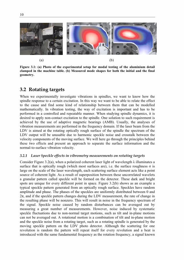
The LDV was used to study an L-shaped aluminium (7010T7451) detail for aerospace application with reduced scale. The thickness of the detail was reduced from 40 mm to 1.0 mm. The detail has shown vibration instability during machining especially at the final stage. The objective of the experimental test was to compare the measured vibration modes with the data produced by a Finite Element model (FE-model) and to calibrate the boundary conditions of the FE-model of the detail clamped in the machine table. Further, the FE-model is used in a model for predicting stability diagrams for milling, see paper C. The outputs from the test were the natural mode frequencies and mode shapes. The photo of the experimental setup is shown in Figure 3.1(a). The photo shows the detail at its initial stage clamped in the machine table. An electromechanical shaker was used to excite the detail; the input force was measured with a force transducer which was used as a reference signal. Figure 3.1(b) show the measured fundamental mode shapes for both the initial and the final geometry at 2825 Hz and 685 Hz, respectively. The fundamental natural frequency is 76% lower for the final geometry and the position at where the maximum vibration amplitude occurs is moved about 12 cm. The experimental results were used to improve the FE-model so that the outputs were closer matched to the measurements.
9
10
(a) (b)
Figure 3.1: (a) Photo of the experimental setup for modal testing of the aluminium detail clamped in the machine table. (b) Measured mode shapes for both the initial and the final geometry.
3.2 Rotating targets When we experimentally investigate vibrations in spindles, we want to know how the spindle response to a certain excitation. In this way we want to be able to relate the effect to the cause and find some kind of relationship between them that can be modelled mathematically. In vibration testing, the way of excitation is important and has to be performed in a controlled and repeatable manner. When studying spindle dynamics, it is desired to apply non-contact excitation to the spindle. One solution to such requirement is achieved by the use of adaptive magnetic bearings (AMB). Usually, the analyses of vibration measurements are performed in the frequency domain. If the laser beam from the LDV is aimed at the rotating optically rough surface of the spindle the spectrum of the LDV output will be unusable due to harmonic speckle noise and crosstalk between the velocity components of the moving surface. We will here go through the principles behind these two effects and present an approach to separate the surface information and the normal-to-surface vibration velocity.
3.2.1 Laser Speckle effects in vibrometry measurements on rotating targets Consider Figure 3.2(a), when a polarized coherent laser light of wavelength illuminates a surface that is optically rough (which most surfaces are), i.e. the surface roughness is large on the scale of the laser wavelength, each scattering surface element acts like a point source of coherent light. As a result of superposition between these uncorrelated wavelets a granular pattern called speckle will be formed on the detector. These dark and bright spots are unique for every different point in space. Figure 3.2(b) shows as an example a typical speckle pattern generated from an optically rough surface. Speckles have random amplitude and phase. The phases of the speckles are uniformly distributed between 0 and 2 , and if the speckle pattern changes during the LDV measurement, the rate of change in the resulting phase will be nonzero. This will result in noise in the frequency spectrum of the signal. Speckle noise caused by random disturbances can be averaged out by measuring a great number of measurements. However, noise induced by systematic speckle fluctuations due to non-normal target motions, such as tilt and in-plane motions can not be averaged out. A rotational motion is a combination of tilt and in-plane motion and the speckle noise from a rotating target, such as a rotating spindle is generated by the moving speckle pattern on the LDV photo detector. Although the scattering for one revolution is random the pattern will repeat itself for every revolution and a beat is introduced with the same fundamental frequency as the rotation frequency, a signal known

11
as pseudo vibrations [10]. The spectrum of the pseudo vibration signal consists of peaks at the fundamental frequency and the subsequent harmonics. These speckle harmonics aredifficult to distinguish from the true vibrations and since they contain amplitude and phase, they can also moderate or mask the true vibration pattern.
Figure 3.2: (a) Generation of speckles on the photo detector when coherent light of wavelength scatters back from an optically rough surface. (b) A typical speckle pattern.
The speckle noise in LDV measurements on rotating targets has been studied since the late 1980s and is now a well known major problem, especially if you are studying vibrations in a frequency range close to the rotation harmonics. Different methods have been proposed and investigated; Optimizing the detector size and the position relative to a rotating target, the speckle noise level can be reduced (experimentally up to 10 dB) [11]. Though, this method does not remove the speckle noise completely and is not suitable for commercial vibrometers. Speckle harmonics can be removed by braking up the repetitively of the measurement path between each revolution either by randomising the laser measurement position along the axis of rotation [12] or by changing the surface structure. The latter have been achieved by continuously applying oil to the surface during the measurement [13]. The second and the third method have only been verified experimentally by laser torsional vibrometers (LTV) and no radial measurements have been successfully presented using LDV.
Our approach to avoid the speckle harmonics is described in 3.2.3.
3.2.2 Crosstalk in laser vibrometry measurements on rotating targets The laser vibrometer is sensitive to target velocity in the direction of the laser beam and therefore when measuring on rotating targets the total surface velocity in the laser direction will be recorded. Resolving the different velocity components will not be trivial. If the desired vibration component is the axial velocity component, the crosstalk problem can be solved by aligning the laser beam with the rotation axis. This method is however not always satisfactory since it is only possible to measure at one single specific point, it must also be remembered that the speckle problem discussed in the previous section must be considered as well. A better approach is moving the laser beam synchronously with the rotation [14, 15]. In this way one can measure at different positions on the rotating surface or even a complete map of points can be measured if desired. However, for radial
12
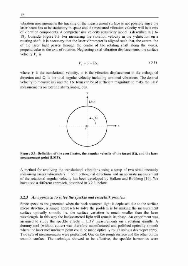
vibration measurements the tracking of the measurement surface is not possible since the laser beam has to be stationary in space and the measured vibration velocity will be a mix of vibration components. A comprehensive velocity sensitivity model is described in [16-18]. Consider Figure 3.3. For measuring the vibration velocity in the y-direction on a rotating shaft, it is necessary that the laser vibrometer is aligned such that, the centre line of the laser light passes through the centre of the rotating shaft along the y-axis, perpendicular to the axis of rotation. Neglecting axial vibration displacements, the surface velocity is yV
( 3.1 ) ,xyVy
y xwhere is the translational velocity, is the vibration displacement in the orthogonal direction and is the total angular velocity including torsional vibrations. The desired velocity to measure is and the term can be of sufficient magnitude to make the LDV measurements on rotating shafts ambiguous.
y x
LMP
x
y
z
Ω
Figure 3.3: Definition of the coordinates, the angular velocity of the target ( ), and the laser measurement point (LMP).
A method for resolving the translational vibrations using a setup of two simultaneously measuring lasers vibrometers in both orthogonal directions and an accurate measurement of the rotational angular velocity has been developed by Halkon and Rothberg [19]. We have used a different approach, described in 3.2.3, below.
3.2.3 An approach to solve the speckle and crosstalk problem Since speckles are generated when the back scattered light is dephased due to the surface micro structure, a simple approach to solve the problem is by making the measurement surface optically smooth, i.e. the surface variation is much smaller than the laser wavelength. In this way the backscattered light will remain its phase. An experiment was arranged to study the speckle effects in LDV measurements on a rotating spindle. A dummy tool (without cutter) was therefore manufactured and polished optically smooth where the laser measurement point could be made optically rough using a developer spray. Two sets of measurements were performed; One on the rough surface and the other on the smooth surface. The technique showed to be effective, the speckle harmonics were

13
avoided and also the shaft roundness was resolved. A detailed description of the experiment and the two different surfaces can be found in paper A. However, the arrangement allowed measurements during free run, i.e. no external forces were applied to the spindle. The experimental arrangement described in paper B, on the other hand offers the possibility to apply non-contact external forces to the rotating spindle. The experimental setup is shown schematically in Figure 3.4. The setup allowed LDV measurements on a dummy tool mounted in a Dynamite milling machine in the y-direction and simultaneously independent measurements with inductive displacement sensors (DS) in two orthogonal (x and y-) directions. The dummy tool was excited in a controlled manner using adaptive magnetic bearing (AMB). For a more detailed description of the experiment see paper B.
DS
AMB
EMLDV
PCy
z
x
Figure 3.4: Experimental setup. Adaptive magnetic bearing (AMB), Electro magnet (EM) and displacement sensors (DS).
Figure 3.5In a measurement on the non-rotating spindle with an optically rough laser measurement surface is shown. The dummy tool is harmonically excited at 400 Hz in the y-direction. The LDV output in (a) is as expected for a harmonically excited target. In (c) the spectrum of the LDV signal is shown, beside the peak at the excitation frequency, the harmonics are excited. The spectrum contains also a high frequency noise floor, which is in an acceptable level. In (b) the displacement sensor output is presented, differentiated once for obtaining velocity then smoothed using a moving average window with a span of seven points. The differentiation of the displacement signal is for making the comparison easier and the smoothing is the same as lowpass filtering the signal. The result is very similar to the LDV output in (a). The spectrum of the displacement sensor output is shown in (d). The noise floor is higher and some additional peaks at 940 Hz, 1400 Hz and 1900 Hz are observed. It must be remembered though that the LDV and the displacement sensors measure at different positions on the rotating dummy tool along the z-axis causing a difference in the output amplitude. In Figure 3.6, the same measurement is performed with the spindle rotating at 700 rpm corresponding to 12 Hz. In (a) and (b) the time response for one rotation and 19 cycles of translational vibration are shown obtained from the LDV and the displacement sensors, respectively. In (c), the spectrum of the LDV signal contains speckle peaks at every multiple of the rotation harmonics. The level of the speckle harmonics is about 0.1 mm s-1 with some random fluctuation. This is typical for LDV measurements on rotating targets, where the speckle noise completely masks other

14
low amplitude vibration components. In (d) the spectrum of the displacement sensor output is shown for comparison. The spectrum contains the rotation frequency, the excitation frequency with the harmonics and some other frequencies caused by the rotation. The second and the third harmonics are broader compared to the non-rotating spindle. The mentioned additional peaks found in Figure 3.5(d) turn up even here. In Figure 3.7 the measurement on the optically smooth spindle rotating at 700 rpm is presented. In (a) the LDV output is shown, very similar to Figure 3.6(b) which was obtained by the displacement sensors. The small difference in amplitude and phase is due to different measurement occasions. The spectrum of the LDV output is shown in (d) and resembles the spectrum obtained by the displacement sensor shown in Figure 3.6(d). The most difference is in the lower frequency part of the spectrum, where a number of harmonics to the rotation frequency is observed. These speckle harmonics are the roundness component of the measurement surface. For more explanation of the roundness components observed in LDV measurements, see paper A.
0 0.01 0.02 0.03 0.04 0.05
−6
−4
−2
0
2
4
6
Time [s]
Velo
city
[mm
/s]
0 0.01 0.02 0.03 0.04 0.05
−6
−4
−2
0
2
4
6
Time [s]
Velo
city
[mm
/s]
(a) (b)
0 500 1000 1500 2000
10−2
10−1
100
101
Frequency [Hz]
Velo
city
[mm
/s]
0 500 1000 1500 2000
10−2
10−1
100
101
Frequency [Hz]
Velo
city
[mm
/s]
(c) (d)
Figure 3.5: Measurements on the non-rotating spindle, harmonically excited at 400 Hz. The laser measurement surface is optically rough. (a) LDV time, (b) DS time, (c) LDV spectrum, and (d) DS spectrum.

15
0 0.01 0.02 0.03 0.04 0.05−20
−15
−10
−5
0
5
10
15
20
Time [s]
Velo
city
[mm
/s]
0 0.01 0.02 0.03 0.04 0.05−20
−15
−10
−5
0
5
10
15
20
Time [s]
Velo
city
[mm
/s]
(a) (b)
0 500 1000 1500 2000
10−2
10−1
100
101
Frequency [Hz]
Velo
city
[mm
/s]
0 500 1000 1500 2000
10−2
10−1
100
101
Frequency [Hz]
Velo
city
[mm
/s]
(c) (d)
Figure 3.6: Measurements on the spindle rotating at 700 rpm (12 Hz), harmonically excited at 400 Hz. The laser measurement surface is optically rough. (a) LDV time, (b) DS time, (c) LDV spectrum, and (d) DS spectrum.
0 0.01 0.02 0.03 0.04 0.05−20
−15
−10
−5
0
5
10
15
20
Time [s]
Velo
city
[mm
/s]
0 500 1000 1500 2000
10−2
10−1
100
101
Frequency [Hz]
Velo
city
[mm
/s]
(a) (b)
Figure 3.7: Measurements on the optically smooth spindle, rotating at 700 rpm (12 Hz), harmonically excited at 400 Hz. The laser measurement surface is optically smooth. (a) LDV time, and (b) LDV spectrum.
When the target surface is optically smooth, the LDV should be insensitive to target rotating motion as long as the cross section of the target is circular and significantly larger than the vibration amplitude. Figure 3.8 shows the crosstalk phenomenon in the LDV measurements for five different spindle speeds. The dummy tool is harmonically excited at 400 Hz perpendicular to the LDV measurement direction with displacement amplitude of about 6 μm. Two cases are illustrated; optically rough measurement surface and optically smooth measurement surface. There is a clear difference between the two

16
measurement series. The vibration velocity measured on the optically rough surface (triangle up) shows a spindle speed dependent crosstalk while the same measurements on the smooth surface (triangle down) do not. To verify that the crosstalk effect follow Equation. ( 3.1 ) calculations were performed using the displacement sensor signals y and x. The velocity is obtained by numerical differentiation of the displacement signal in the Fourier domain. Numerically there is a good agreement between the calculated velocity (circle) and the measured velocity (triangle up).
y
700 1400 2800 5600 7000
1000
2000
3000
4000
5000
Vel
ocity
[m
/s]
Spindle speed [rpm]
LDV smoothLDV roughCalculated
Figure 3.8: Crosstalk in LDV measurements on a rotating spindle.
Comparison between the velocities obtained by displacement sensors and the LDV require that the two instruments are aligned. Since it was difficult to align the LDV with the displacement sensors their outputs differed slightly. Assuming an arbitrary misalignment angle as defined in Figure 3.9, the measured displacements by the inductive displacement sensors should be compensated as following:
,sincos)( yxx ( 3.2 )
.sincos)( xyy ( 3.3 )
And the -dependent calculated velocity will therefore be
( 3.4 ) ).(sin)(cos)( yxxyVy

17
LMP
x
y
z
Ω
ϕ
Figure 3.9: The coordinates and the definition of the misalignment angle . The angular velocity of the target ( ), and the laser measurement point (LMP).
It must be remembered that the laser beam is assumed to be perpendicular to the rotation axis and a misalignment angle can result in further inaccuracies which can be corrected for in the same manner. On the other hand in our measurements the alignment of the laser beam is performed on an optically smooth surface and since the stand-off distance is about 1 m, even very small misalignments with the rotation axis results in signal dropouts.Figure 3.10 illustrate the angle misalignment effect for different spindle speeds. In (a), the velocities obtained from the displacement sensors in the y-direction are shown for different compensation angles (time derivative of Expression ( 3.3 )), these amplitudes are compared with the LDV output from the smooth surface (triangle down in Figure 3.8.). In (b), the plot shows how the amplitude of the calculated velocities changes for different compensation angles. Zero degrees compensation gives the result shown in Figure 3.8.The difference between the calculated velocities gets smaller for higher spindle speeds. This is because the x factor is much greater than y, and the translational velocities, xand for higher spindle speeds and the Expression y ( 3.4 ) can therefore be approximated to
( 3.5 ) .cos)( xVy
For small angles , the cos is close to one, hence no big variations in the calculated velocities. However, the plots indicate that the misalignment angle is something between 3.75 and 5 degrees. It has been difficult to calibrate the displacement sensors with the LDV and the angular misalignment between the two instruments has shown to affect the outputs. On the other hand, the misalignment effect does not interfere with the interpretation of the crosstalk effect and the conclusion is that it is possible to resolve the true translational vibrations in the LDV measurement direction if the measurement surface is optically smooth.
The strength of this method is that there is no need for simultaneous orthogonal measurements for resolving the normal-to-surface vibration velocity in the y-direction.

18
700 1400 2800 5600 70000
200
400
600
800
1000
1200
Spindle speed [rpm]
Vel
ocity
[m
/s]
0 deg1.25 deg2.5 deg3.75 deg5 deg
700 1400 2800 5600 7000
1000
2000
3000
4000
5000
Spindle speed [rpm]
Vel
ocity
[m
/s]
0 deg1.25 deg2.5 deg3.75 deg5 deg
(a) (b)
Figure 3.10: The angle misalignment effect. (a) Velocities obtained from the displacement sensor in the y-direction. (b) Calculated velocity Vy.
3.2.4 Hammer test performed on a rotating spindle The schematic of the setup is shown in Figure 3.11. A dummy tool, Ø20 mm with an optically smooth surface was mounted in the Liechti Turbomill ST1200 spindle. A Brüel & Kjaer type 8202 impact hammer with a force transducer was used to excite the system and the response was measured with the LDV, placed approximately 3m from the tool. The impact hammer was connected to a data acquisition system within the LDV software via a charge amplifier. The Liechti machine was capable of speeds of up to 6000 rpm. The low level of the spindle speed was due to some bearing problems which have been repaired afterwards. The hammer tests were performed at seven different spindle speeds, 0, 1000,…, 6000 rpm and the data was sampled at 25.6 kHz.
PC
LDVHammer
Amplifier
Figure 3.11: Schematic of the setup.
The laser beam was aimed at the tip of the (cylindrical) tool, arranged so that its centre line passed through the tool centre perpendicular to the axis of rotation. This arrangement was carried out by looking at the reflex of the laser light. The laser setup gave no discontinuities in the displacement signal from the LDV displacement decoder and the absence of speckle harmonics was examined in the frequency spectra of LDV output during free run, which means that no external forces where applied by the hammer. The hammer strikes were carried out manually and care was taken so that the impacts were in line with the LDV measurement direction. Also measurements with multiple impacts were

19
excluded. The force signal was set as a trigger and at every spindle speed 10 measurements were performed using a complex averaging method within the LDV software. The response signal was windowed with a negative exponential function adapted to the signal behaviour. The mobility diagram for the measurements at zero rpm and 6000 rpm is shown in Figure 3.12(a). The measured frequency response functions, FRFs, are similar in shape but differ in magnitude and also slightly in frequency. For example, the peak at about 2.2 kHz is 25% higher for the rotating spindle. The measured data is smoothed using a moving average window with a span of seven points. The smoothing procedure is the same as lowpass filtering the signal, i.e. less noise but in the same time lower resolution. However, the LDV output from the 6000 rpm measurement contains more noise compared to the measurement on the non-rotating spindle. In Figure 3.12(b), the coherence function between the input force and the measured response is presented. The coherence function is a measurement of the noise in the signal and some kind of indication of the measurement accuracy. The low coherence due to random noise can be reduced or eliminated by taking great many averages. But the reason for poor coherence at about 1.6 kHz, 2.6 kHz and 3.8 kHz can be more systematic than that. The magnitude plot of the mobility (Figure 3.12(a)) may indicate antiresonance near the mentioned frequencies.
In conclusion, the measurement should be done under more controlled manner, i.e. using an impact hammer with an automatic mechanical release. This would reduce the direction misalignment between the input force and the measured velocity. Also the test time would be reduced which would open the possibility for greater number of measurements and hence reducing the random noise. However, it is shown that it is possible to perform hammer test on a rotating spindle and that the dynamic response of the spindle changes slightly at different spindle speeds.
0 500 1000 1500 2000 2500 3000 3500 4000 4500
103
10 2
Frequency [Hz]
Mob
ility
[m/s
/ N
]
6000 rpm0 rpm
0 500 1000 1500 2000 2500 3000 3500 4000 45000
0.1
0.2
0.3
0.4
0.5
0.6
0.7
0.8
0.9
1
Frequency [Hz]
Coh
eren
ce
6000 rpm0 rpm
(a) (b)Figure 3.12: Measurements at two different spindle speeds: zero rpm and 6000 rpm (a) Mobility diagrams. (b) Coherence functions between the input force and the measured response versus frequency.

20
3.3 Measurements of sound fields As mentioned in 2.2, the optical path length is an integral of the refractive index from the entire measurement volume, i.e. along the whole light path and one must always pay attention to this projection effect. The pressure variation along the light path can not be resolved and since sound fields are not necessarily symmetric, different projection angles results in different LDV outputs. By scanning the laser beam across the reflector a 2-D map of the integrated 3-D sound field will be obtained. Transient events can of course be recorded in single point measurements but for field measurements the sound field has to be in a stationary condition. LDV measures both the amplitude and the phase of the sound and in field measurements the relative phase between each measurement point has to be kept in track. This is obtained by for example using a microphone signal as a reference.
In order to visualize the difference in projection angles an experiment was arranged for studying the acoustic field emitted from three 40 kHz ultrasound transducers in two different projection angles. Before the actual sound measurements, the vibrating membrane of the transducers were measured by the LDV which showed that they were vibrating in the fundamental mode. Hence, the transducers are assumed to be plane-piston acoustic sources. The photo of the ultrasound transducer and the measured deflection shape of the vibrating membrane are shown in Figure 3.13. The diameter of the vibrating membrane is 0.7 cm and the maximum measured velocity is 14 mm s-1 which corresponds to 56 nm in displacement.
Figure 3.13: (a) Photo of the ultrasound transducer. The diameter of the membrane is 0.7 cm. (b) The measured deflection shape of the vibrating membrane at the fundamental frequency 40 kHz. The Maximum measured velocity is 14 mm s-1.
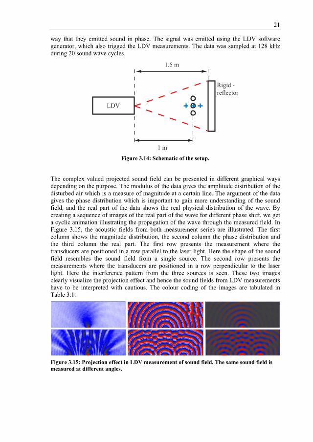
The setup of the actual sound experiment is schematically presented in Figure 3.14. The LDV scanning head was positioned about 1 m from the transducers, which were positioned either as (plus) or (circle). The distance between each transducer was 15 mm. A white painted heavy concrete block of measures 1.3×1.2×0.4 m3 was used as a reflector. A grid of 140×50 mm2 with 1 mm increments in both directions was established on a plane above the sound transducers, which gives a spatial resolution limit of 2 mm which corresponds to an upper frequency resolution of 170 kHz in air. The scanning head is fixed in space and the probing laser beam traverses the sound field at an angle changing during the measurement. Since the stand-off distance is much greater than the measured field, the influence of the angular position of the beam is minimized (0.01 sr at extremities); henceforth we assume in the following that the beam paths are parallel to each other and further, the emitted acoustic axis of each transducer perpendicular to the LDV measurement axis in every measurement point. The transducers were coupled in such a
21
way that they emitted sound in phase. The signal was emitted using the LDV software generator, which also trigged the LDV measurements. The data was sampled at 128 kHz during 20 sound wave cycles.
LDV
Rigid -reflector
1.5 m
1 m
Figure 3.14: Schematic of the setup.
The complex valued projected sound field can be presented in different graphical ways depending on the purpose. The modulus of the data gives the amplitude distribution of the disturbed air which is a measure of magnitude at a certain line. The argument of the data gives the phase distribution which is important to gain more understanding of the sound field, and the real part of the data shows the real physical distribution of the wave. By creating a sequence of images of the real part of the wave for different phase shift, we get a cyclic animation illustrating the propagation of the wave through the measured field. In Figure 3.15, the acoustic fields from both measurement series are illustrated. The first column shows the magnitude distribution, the second column the phase distribution and the third column the real part. The first row presents the measurement where the transducers are positioned in a row parallel to the laser light. Here the shape of the sound field resembles the sound field from a single source. The second row presents the measurements where the transducers are positioned in a row perpendicular to the laser light. Here the interference pattern from the three sources is seen. These two images clearly visualize the projection effect and hence the sound fields from LDV measurements have to be interpreted with cautious. The colour coding of the images are tabulated in Table 3.1.
Figure 3.15: Projection effect in LDV measurement of sound field. The same sound field is measured at different angles.

22
Position relative to laser beam Magnitude Phase Real wave
Parallel (plus) 0-5 mm s-1 -1± ± 5 mm s-1 -1Perpendicular (circle) 0-2 mm s ± ± 2 mm s
Table 3.1: Colour coding for the ultrasound measurements.
Let us now look at another example where the sound source is much more complex. A violin is such a sound source. In the appended paper D, LDV measurements have been performed on a bowed violin where the whole chain of interacting parts of the played violin and the emitted sound were studied. Here we will be content with the measurements on the sound field produced by the vibrating violin plates. The photo of the setup is shown in Figure 3.16. The violin is hanged in a specially constructed rotating bow apparatus where the violin and the rotating bow are mounted in a way that they can be rotated together around a vertical axis. In this way it is possible to measure on all sides of the violin and the generated sound without changing the bowing conditions. For a more detailed description of the experiment please see paper D.
Figure 3.16: Photo of the setup.
In Figure 3.17, the operational deflection shapes (ODS) of the front and the back plate as well as the sound field generated from these at 1130 Hz, which is the fourth partial of the played tone are illustrated. Colour coding is set within the measuring range so that the results can be visualized as good as possible (top plate: ± 4 μm, sound field: ±0.8 μm and back plate: ±1.6 μm). Vibration pattern of the violin is pretty complex; the plates are split in several antinodes. The top plate is divided in antinodes with two horizontal and one vertical nodal line. The vertical nodal line should make the measured radiated sound less efficient since the optical path difference is integrated in a line along the width of the violin and two nearby vibrations in anti-phase cancel each other. The upper part of the top plate vibrates in phase with the lower part and in anti-phase with the middle part, which probably cause the lobe shaped radiation. It must be remembered though that the radiated sound field from the top plate is also affected from the two f-shaped holes, so-called f-

23
holes and that the sound from the violin is a combination of plate vibrations and air modes. It is easier to relate the emitted sound from the back plate to the measured ODS since no vertical nodal line can be seen. The two horizontal nodal lines make the back plate resemble three sources lined in a row where the middle one is emitting in anti-phase with the two others.
Figure 3.17: LDV measurements on a bowed violin and the generated sound at 1130 Hz, the fourth harmonic of the played tone.


4 CONCLUSIONS
Laser vibrometry is today a well established technique, commonly used for vibration measurements on static objects. The method provides both qualitative and quantitative information with high spatial and temporal resolution. The non-contact nature of laser vibrometers gives four significant advantages over traditional contacting vibration transducers: (1) they are non-intrusive; no mass loading of vibration transducers, (2) they are remote vibration transducers (3) they offer full field measurements by means of scanning where the measurement grid can be set much greater in density compared to individual traditional transducers and (4) they offer the possibility to measure on rotating targets.
If the surface of the measured rotating target is optically rough, a moving speckle pattern will occur on the detector, which gives a repeatable speckle noise in the measurement signal and also the velocity component perpendicular to the intended measurement will leak in the LDV output. Without considering these two effects in a proper manner laser vibrometry measurements on rotating surfaces are not to recommend.
In the first paper, paper A, we demonstrated that by making the measurement surface optically smooth the speckle noise harmonics in LDV measurements on a rotating spindle can be eliminated. From the spectrum of the LDV output the axial misalignment and the roundness of the surface can be extracted which should be excluded in vibration testing. In the second paper, paper B, we demonstrated that the orthogonal displacements introduced by a magnetic bearing do not leak in the LDV output using our approach. This automatically implies that also the torsional vibrations are excluded from the measurement signal which means that the translational velocity in the intended direction is resolved. The presented approach has three advantages over other existing method that use laser vibrometry for vibration measurements on rotating machines:
1. Cancelling the speckle harmonics and avoiding the crosstalk.
2. No need for orthogonal measurements.
3. Possible to apply on any spindle with a circular cross section that can be polished.
In the third paper, paper C, a model for predicting stability limits in high speed machining of thin-walled structures is presented. The laser vibrometry measurements of the workpiece clamped in the machine table has been crucial for improvement of the boundary conditions of the finite element model.
In the last paper, paper D, the flexibility of laser vibrometry has been shown. Not only are the vibrations of the different parts of the violin studied but also the generated sound fields. The measurements on the string shows stick-slip behaviour and the bridge measurements show that the string vibrations transmit to the bridge both in the horizontal
25

26
and the vertical direction. Measurements on the plates show complex deflection shapes which are combinations of different eigenmodes. The sound fields emitted from the violin were measured and visualized for different harmonic partials of the played tone. However, the visualized sound field obtained by the laser vibrometer is a projection of the sound field along the laser light and the image obtained is a 2D map of the real 3D sound field, which must be considered.

5 FUTURE WORK
The relation between the maximum level of the harmonic speckle noise and the average surface roughness on rotating targets is worthy to investigate in the future. This relation can be helpful for optimizing the polishing procedure depending on the intending measured vibration levels.
The vibration tests on the milling spindle indicate angular speed dependencies. It is plausible that these nonlinearities grow at higher spindle speeds. In a planned experiment, the spindle will be studied under higher operational speeds, up to 24000 rpm. Transient and sine sweep excitations will be applied using an impact hammer with an automatic mechanical release and an adaptive magnetic bearing, respectively. A transfer function between the spindle and a non-rotating part close to the spindle shaft is desired; simultaneous measurements on the spindle and the spindle housing hopefully results in such function.
For a better understanding of the spindle behaviour under cutting operations, the spindle should be studied also under applied axial load. This may be achieved using a dummy tool consisting of a rotating shaft, bearings and a holder, simply a small spindle. Such dummy tool has been constructed and manufactured. Preliminary experiments have been conducted where the results are promising.
Rotating shafts tend to bow out at certain speeds and whirl in a complicated manner [20, 21]. This may be the case when long and slender tools are used in machining. The whirling of the tool may be in the same direction (forward whirl) or in the opposite direction of the spindle rotation (backward whirl) and the velocity may or may not be equal to the spindle speed. To be able to resolve the direction of the whirling Yamamoto et al [21] proposed a complex-FFT method where the whirling plane of the rotor is mapped to the complex plane. For this purpose two orthogonal simultaneous time histories of the tool are needed, which can be obtained from the inductive displacement sensors within the adaptive magnetic bearing. It is worth to investigate how the whirling phenomenon affects the LDV output.
Laser vibrometry has shown to be applicable to sound field measurements. The measured 2D projections open the possibility for tomographic 3D reconstructions of the sound fields if several projections can be obtained. In machining application the spectrum of the sound generated by the cutting process can be used for setting thresholds for stable machining regions. It is plausible that LDV measurements of the sound field in the close region of the tool can give addition information of the cutting process. This has yet to be investigated.
27

6 SUMMARY OF APPENDED PAPERS
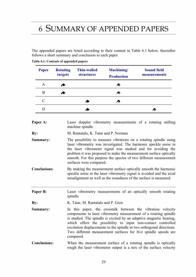
The appended papers are listed according to their content in Table 6.1 below, thereafter follows a short summary and conclusion to each paper. Table 6.1: Contents of appended papers
Paper Rotatingtargets
Thin-walled structures
Machining/ Sound field measurements Production
A
B
C
D
Paper A: Laser doppler vibrometry measurements of a rotating milling machine spindle
By: M. Rantatalo, K. Tatar and P. Norman
Summary: The possibility to measure vibrations on a rotating spindle using laser vibrometry was investigated. The harmonic speckle noise in the laser vibrometer signal was studied and for avoiding the problem it was proposed to make the measurement surface optically smooth. For this purpose the spectra of two different measurement surfaces were compared.
Conclusions: By making the measurement surface optically smooth the harmonic speckle noise in the laser vibrometry signal is avoided and the axial misalignment as well as the roundness of the surface is measured.
Paper B: Laser vibrometry measurements of an optically smooth rotating spindle
By: K. Tatar, M. Rantatalo and P. Gren
Summary: In this paper, the crosstalk between the vibration velocity components in laser vibrometry measurement of a rotating spindle is studied. The spindle is excited by an adaptive magnetic bearing, which offers the possibility to input non-contact controlled excitation displacements to the spindle in two orthogonal directions. Two different measurement surfaces for five spindle speeds are compared.
Conclusions: When the measurement surface of a rotating spindle is optically rough the laser vibrometer output is a mix of the surface velocity
29

30
components. To be able to resolve the radial velocity component the measurement surface has to be optically smooth.
Paper C: Integrated Tool for Prediction of Stability Limits in Machining
By: A. Svoboda, K. Tatar, P. Norman and M. Bäckström
Summary: In this paper, a model for the prediction of stability limits as a function of process parameters for machining of a thin-walled aluminium detail is presented. The model is based on finite element calculation of the workpiece and laser vibrometry measurements of the spindle. In order to validate and improve the model experimental modal analysis of the detail clamped in the machine table has been performed using a scanning laser vibrometer.
Conclusions: The presented model predicts stability limits in high speed machining of a thin-walled workpiece. The extensive experimental analysis of the workpiece is a limiting factor in the manufacturing industry, the developed tool base on finite element calculations of the workpiece promotes effective development of the manufacturing process.
Paper D: Laser vibrometry measurements of vibration and sound fields of a bowed violin
By: P. Gren, K. Tatar, J. Granström, N-E. Molin and E. V. Jansson.
Summary: In this paper the vibration and the sound field of a violin is studied using laser vibrometry. The string is excited using a rotating bow apparatus and the vibrations from the string transmits to the violin body via the bridge and produces the sound. The measurements on the string show stick-slip behaviour and the bridge measurements show that the string vibrations transmit to the bridge both in the horizontal and the vertical direction. Measurements on the plates show complex deflection shapes which are combinations of different eigenmodes. The sound fields emitted from the violin was measured and visualized for different harmonic partials of the played tone.
Conclusions: The designed bowing apparatus is an effective devise to excite the violin in a long and controlled manner very close to the real life condition. Vibrations of the different parts of the bowed violin as well as the emitted sound are measured. The visualized sound field obtained by the laser vibrometer is a projection of the sound field along the laser light; the image obtained is a 2D map of the real 3D sound field. The projection effect must be considered in sound field measurements using scanning laser vibrometry.
7 REFERENCES
1. Altintas, Y., Manufacturing automation: metal cutting mechanics, machine tool vibrations, and CNC design. 2000: Cambridge University Press.
2. Zipser, L., S. Lindner, and R. Behrendt, Anordnung zur Messung und visuellen Darstellung von Schalldruckfelden. 2000: DE.
3. Zipser, L. and S. Lindner. Visualisation of Vortexes and Acoustic Sound Waves. in 17th Int. Congress on Acoustics. 2001. Rome, Italy.
4. Zipser, L., et al., Reconstructing two-dimensional acoustic object fields by use of digital phase conjugation of scanning laser vibrometry recordings. Applied Optics, 2003. 42: p. 5831-5838.
5. Olsson, E., et al. Scattered ultrasound fields measured by scanning laser vibrometry. in Optical Measurements System for Industrial Inspection III. 2003: SPIE.
6. Molin, N.-E. and L. Zipser, Optical methods of today for visualizing sound fields in musical acoustics. Acta Acustica united with Acustica, 2004. 90: p. 618-628.
7. Harland, A.R., J.N. Petzing, and J.R. Tyrer, Nonperturbing measurements of spatially distributed underwater acoustic fields using a scanning laser Doppler vibrometer. J. Acoust. Soc. Am, 2004. 115(1): p. 187-195.
8. Vest, C.M., Holographic inetrferometry. 1979, New York: Wiley.
9. Ewins, D.J., Modal Testing: Theory and Practice. 1984, Taunton, Somerset: Wiley.
10. Rothberg, S.J., J.R. Baker, and N.A. Halliwell, Laser vibrometry: Pseudo-vibration. Journal of Sound and Vibration, 1989. 135: p. 516-522.
11. Denman, M., N.A. Halliwell, and S.J. Rothberg. Speckle noise reduction in laser vibrometry: experimental and numerical optimisation. in Second International Conference on Vibration Measurements by Laser Techniques: Advances and Applications. 1996. Washington, DC, USA.
12. Halliwell, N.A., The laser torsional vibrometer: a step forward in rotating machinery diagnostics. Journal of Sound and Vibration, 1996. 190: p. 399-418.
13. Drew, S.J. and B.J. Stone, Removal of speckle harmonics in laser torsional Vibrometry. Mechanical systems and Signal Processing, 1997. 11: p. 733-776.
14. C, S. and R. Montanini, Automotive components vibration measurements by tracking laser Doppler vibrometry: advances in signal processing. Measurement Science and Technology, 2002. 13: p. 1266-1279.
15. Castellini, P. and C. Santolini, Vibration measurements on blades of a naval propeller rotating in water with tracking laser vibrometer. Measurement, 1998. 24: p. 43-54.
31

16. Bell, J.R. and S.J. Rothberg, Laser vibrometers and contacting transducers, target rotation and six degree-of-freedom vibration: what do we really measure? Journal of Sound and Vibration, 2000. 237: p. 245-261.
17. Bell, J.R. and S.J. Rothberg, Rotational vibration measuring using laser Doppler Vibrometry: comprehensive theory and practical application. Journal of Sound and vibration, 2000. 238: p. 673-690.
18. Rothberg, S.J. and J.R. Bell, On the application of laser vibrometry to translational and rotational vibration measurements on rotating shafts.Measurement, 2004. 35: p. 201-210.
19. Halkon, B. and S.J. Rothberg. Automatic post-processing of laser vibrometry data for rotor vibration measurements. in Eighth International Conference on Vibrations in Rotating Machinery. 2004. University of Wales, Swansea, UK.
20. Thomson, W.T., Theory of vibration with applications. 1981, London: George Allen & Unwin.
21. Yamamoto, T. and Y. Ishida, Linear and nonlinear rotordynamics a modern treatment with applications. 2003, New York: Wiley.

Part II
Papers
33

34

Paper A Laser doppler vibrometry measurements of a rotating milling machine spindle


Laser doppler vibrometry measurements of a rotating milling machine spindle
Matti Rantatalo1
Kourosh Tatar2
Peter Norman3
Luleå University of Technology 1Div. of Sound and Vibrations 2Div. of Experimental Mechanics 3Div. of Manufacturing Systems Engineering Luleå Sweden
ABSTRACT
Finding an optimum process window to avoid vibrations during machining is of great importance; especially when manufacturing parts with high accuracy and/or high productivity demands. In order to make more accurate predictions of the dynamic modal properties of a machining system in use, a non-contact method of measuring vibrations in the rotating spindle is required. Laser Doppler Vibrometry (LDV) is a non-contact method, which is commonly used for vibration measurements. The work presented consists of an investigation into the use of LDV to measure vibrations of a rotating tool in a milling machine, and the effects of speckle noise on measurement quality. The work demonstrates how the axial misalignment and the roundness of a polished shaft can be evaluated from LDV measurements.
1 INTRODUCTION
Manufacturers of modern machine tools are increasingly implementing advanced process monitoring and supervisory process control (1) to complement the basic functionality of the machine tool control system. At there simplest, process monitoring systems are used to help prevent or limit the effects of catastrophic events such as tool breakage (2) or spindle failure. Such events can be detected by monitoring the current drawn by axis drives and spindle motor (3, 4), or by more advanced techniques such as cutting force monitoring or measurements ofvibrations using accelerometers or acoustic emission using sensitive transducers and signal conditioning software (5-9). By setting safe limits for the monitored parameter(s) based on experience or trials, unusual or unexpected events which may indicate a catastrophic failure can be used as a trigger to stop the machine.

Since vibrations are the result of relative movement between the cutter and work piece, the dynamic behaviour of both the machine structure and rotating spindle/cutter together with the behaviour of the component being machined has to be considered. In most situations, the work piece can be considered a solid part fixed to the machine table with no significant modal properties of its own. This assumption tends to weaken, however, when machining components with relatively thin walls (10).
Regenerative machine tool chatter is a fundamental type of vibration that can occur during milling. These vibrations have their origin in the closed loop nature of the cutting process and are dependent on the structural vibration modes, described by the frequency response function (FRF) of the machine tool. The FRF is normally measured on a non rotating/static system from which the limits for chatter free machining can be calculated (11). In modern machine tools, spindle speeds of 20,000 rpm and upwards are not uncommon, since the dynamic characteristics of the spindle such as damping change, this causes the FRF of the system as a whole to change.
To be able to fully investigate the behaviour of a high-speed rotating system, such as a machine tool spindle, it is necessary to use non-contact measurement methods. Several approaches to the non-contact measurement of rotating objects have been developed. These include optical techniques such as Pulsed Laser TV-Holography (12) and Laser Doppler Vibrometer techniques (LDV) (13).
LDV is a well-established technique for measuring the velocity of a moving object. It is based on the Doppler effect, which explains the fact that light changes its frequency when detected by a stationary observer after being reflected from a moving object. The vibrating object scatters or reflects light from the laser beam and the Doppler frequency shift is used to measure the component of velocity which lies along the axis of the laser beam. As the laser light has a very high frequency, direct demodulation of the light is not possible and optical interferometry is therefore used.
When a coherent light source illuminates a surface that is optically rough, i.e. the surface roughness is large on the scale of the laser wavelength, a granular pattern called speckle which has random amplitude and phase is seen. This is due to interference between the components of backscattered light. The intensity of a speckle pattern obeys negative exponential statistics and their phases are uniformly distributed over all values between -� and � (14). If the speckle pattern changes during LDV measurement the rate of change in the resulting phase will be nonzero, and the frequency spectrum will contain peaks. These kinds of speckle fluctuations are induced by non-normal target motions, such as tilt, in-plane motions or rotation (15). Speckle fluctuations due to target rotation are periodic and will repeat for each revolution. This leads to peaks in the spectrum at the fundamental rotation frequency and higher order harmonics. These modulations are difficult to distinguish from the true vibrations and in the worst case, can almost completely mask the vibration pattern. It is therefore important that the target to be measured has a surface smooth enough so that the speckle noise is avoided.

2 EXPERIMENTAL SET-UP AND PROCEDURE
2.1 Preparation of the dummy tool A dummy tool with a radius of 10 mm and a length of 100 mm was manufactured from a solid stainless steel tool blank. The shaft was mounted in a lathe and polished using emery paper with grades ranging from 400 (grains/mm) to 1200. The shaft was finally polished using diamond paste with particles ranging from 9 μm to 0.25 μm and with a chemical polishing fluid. Quality control of the polished surface was performed using non-contact optical surface profile measurement (www.veeco.com). In the actual experiment a spray which is normally used for crack detection was used to create a removable diffuse (optically rough) surface on the polished dummy tool. Both the polished tool surface and the sprayed surface were measured by the optical profiler, and a representative area of the tool of 304 x 199 μm was sampled in steps of 414 nm. The measurements showed a normally distributed surface structure with Ra = 11,29 nm, implying that the polished surface is optically smooth compared to the laser wavelength of 633 nm. The sprayed surface showed substantially higher values, Ra = 21.02μm, giving an optically raw surface.
2.2 The milling machine The LDV measurements were made on a Liechti Turbomill ST1200 ‘state-of-the-art’ machining centre offering multiple (5-axis) movement and a spindle capable of speeds of up to 24,000 rpm. The polished dummy tool was mounted in a Corogrip holder with an HSK shank which was in turn mounted in the machine and was not removed until all the measurements had been made.
2.3 Setting up the LDV For the measurements, a PSV 300 LDV system from Polytec GmbH (www.polytec.com) including a displacement decoder was used. The LDV scanning head was mounted on a sturdy tripod and placed approximately 2 m from the tip of the dummy tool on a soft damped material to reduce the influence of structural floor vibrations. Care was taken to align the laser beam so that it’s centre line passed through the centre line of the shaft and was perpendicular to the shaft’s axis of rotation. This was necessary to ensure that the true velocity vector associated with the vibrations was along the incident direction of the laser beam. The LDV system was set up to perform sampling with a frequency of 40,96 kHz. The maximum detectable frequency was set by the system to 16 kHz. The LDV system produced frequency spectra with a standard FFT algorithm using a complex averaging method with 100 averages of 800 ms each giving a frequency resolution of 1.25 Hz and a total measuring time of 12.8 s.
2.4 LDV measurements A series of experiments were carried out to establish whether vibrations of a rotating tool could be measured using the LDV system. Four different spindle speeds 2700, 4200, 6000 and 7200 rpm were studied. The LDV was used to measure the vibrations at the tip of the polished dummy tool in the radial direction at these speeds. The same set of measurements was carried out on the tool after being sprayed to give an optically raw finish.

Figure 1. LDV measurement of the rotating optically raw (sprayed) dummy tool.
Logged data was exported from the LDV as ASCII files and then imported into Matlab 6.0 where more detailed analysis and filtering of the data was carried out. The large-scale profile around the circumference of the dummy tool was measured using a mechanical roundness tester from C E Johansson (www.cej.se), with an accuracy of + 0.3μm. This was performed after that the LDV measurements were carried out.
3 RESULTS
In this section the results from the measurements at 6000 rpm are presented. The velocity spectrum of the polished and rough dummy tool measurements are displayed in the same chart for different frequency bands, Figure 2-5. The spectrum of the rough surface has been flipped down to the negative side in the charts to simplify comparison of the two spectra. In the charts it can be seen that the spectrum of the rough dummy tool contains peaks at f * n Hz where f is the rotational speed of 100 Hz (6000 rpm) and n = 1, 2, 3… These peaks are expected due to the presence of a speckle noise repeated for each dummy tool revolution in the sampled data.
A zoomed part of the spectrum covering the frequency band 8.8-10 kHz shows clearly the speckle noise in the form of peaks at integer multiples of the rotational speed of 100 Hz. These are marked with circles along the frequency axis, Figure 3. These peaks could not be seen in the graph of the polished tool. Between 1.1-1.5 kHz contains both speckle noise peaks

and ordinary vibrations, Figure 4. Note that the vibrations are present in both curves but the peaks are only present in the spectrum of the rough surface.
The frequency band covering 0-1 kHz shows harmonic peaks in both FFT graphs, see Figure 5. However; the first peak at 100 Hz in the polished measurement spectrum was detected as the dummy tool axial misalignment and the other six harmonics as the roundness profile. Figure 6 shows the signal from the displacement decoder. This signal is band-pass filtered between 0.15-0.75 kHz, thus filtering out the roundness profile. The result is shown in Figure 7, where the filtered time signal for one revolution is presented in a polar plot (dashed line), together with an independent mechanical measurement of the roundness made by the roundness tester (solid line). The difference between the curves is less than the error given by the manufacturer of the roundness tester (+ 0.3 μm). For the sprayed dummy tool the roundness could not be measured properly due to speckle noise caused by the rough surface. Similar results where achieved for measurements made at spindle speeds of 2700, 4200, and 7200 rpm.
0 1000 2000 3000 4000 5000 6000 7000 8000 9000 10000
-2
-1
0
1
2
3
Mag
nitu
de [m
m/s
]
Frequency [Hz]
Velocity FFT, 6000 rpm
Polished (upper)Rough (lower)
Figure 2. Spectra of the polished and the sprayed surface at a spindle speed of 6000 rpm. The spectrum of the rough dummy tool has been mirrored along the frequency axis
down to the negative side to simplify comparison between the two. Multiple harmonics of n*100 Hz where n= 1,2,3… can be seen in the spectrum of the sprayed surface.

8800 9000 9200 9400 9600 9800 10000-0.1
-0.05
0
0.05
0.1M
agni
tude
[mm
/s]
Frequency [Hz]
Velocity FFT, 6000 rpm
Polished (upper)Rough (lower)
Figure 3. Zoomed part of the spectrum, 8.8-10 kHz. Frequencies where peaks are expected due to speckle noise are marked with a ring on the frequency axis.
1100 1150 1200 1250 1300 1350 1400 1450 1500
-0.4
-0.2
0
0.2
0.4
0.6
Mag
nitu
de [m
m/s
]
Frequency [Hz]
Velocity FFT, 6000 rpm
Polished (upper)Rough (lower)
Figure 4. Zoomed part of the spectrum, 1.1-1.5 kHz. Frequencies where peaks are expected due to speckle noise are marked with a ring on the frequency axis. It can
clearly be seen that no peaks is present in the spectrum of the polished surface at the marked positions. Note that the vibration signal is present in both measurements.

0 100 200 300 400 500 600 700 800 900 1000-1.5
-1
-0.5
0
0.5
1
1.5M
agni
tude
[mm
/s]
Frequency [Hz]
Velocity FFT, 6000 rpm
Polished (upper)Rough (lower)
Figure 5. Zoomed part of the spectrum, 0-1 kHz. Frequencies where peaks are expected due to speckle noise are marked with a ring on the frequency axis. In this graph peaks in
both spectra are present at the marked frequency positions. For the polished case the peaks are identified as tool axial misalignment and roundness.
0 0.005 0.01 0.015 0.02 0.025 0.03 0.035-8
-6
-4
-2
0
2
4
6
8
Time [s]
Dis
plac
emen
t [µm
]
Displacement decoder, 6000 rpm
Figure 6. Displacement measurement at 6000 rpm.

2
4
6
30
210
60
240
90
270
120
300
150
330
180 0
Dummy tool circumference profile [µm]
ProfileLDV
Figure 7. Polar plot of the roundness of the dummy tool. Solid line: Measured with a mechanical roundness tester. Dashed line: Measured with LDV at a rotational speed of
6000 rpm. The distance between two circles in the plot is 2 μm.
4 DISCUSSION AND CONCLUDING REMARKS
Speckle noise interference was avoided by polishing the surface of the dummy tool (in effect a rotating shaft) until an optically smooth surface was achieved. The optically smooth surface of the rotating tool generated no repeated speckle noise and hence no unwanted peaks at integer multiples of the rotational frequency. This allowed the axial misalignment and roundness of the dummy tool to be measured at speeds of up to at least 7200 rpm using an LDV. This implies that radial vibration measurements of the tool can also be conducted; for example, when investigating dynamics of the cutting process.
The possibility of extracting roundness and alignment information is based on the fact that at a rotational speed of 6000 rpm (100Hz) any misalignment would be seen as a 100Hz signal. Since the tool is not perfectly round, harmonics of 100Hz will be present. The first component of the out of roundness is an elliptical form and results in a frequency peak at 2*100Hz (200 Hz). The second roundness component, a tri-lobed form, would be seen as a peak at 3*100Hz (300Hz) and so on. In the experiments, no significant peaks at integer multiples of the

rotational speed could be detected above the 6:th component at 7*100Hz. To eliminate the possibility of structural vibrations being misinterpreted as misalignment or out of roundness, measurements were made at a number of rotational speeds (2700, 4200, 6000 and 7200 rpm). At each of these speeds, the misalignment data would be seen as a peak at a different frequency; namely 45Hz, 70Hz, 100Hz and 120Hz. Out of roundness data would be at multiples of the primary frequency. When measuring at speeds other than 6000rpm, any structural vibration around 100Hz would become clear, and the peak due to misalignment shifted. This makes it possible to analyse the presence of structural vibrations overlaying axial misalignment and out of roundness. No significant structural vibrations overlaying the roundness and misalignment data were detected in the experimental data.
However, since some frequency components of structural vibrations are spindle speed dependant it is not possible to draw firm conclusions about misalignment and roundness based solely on the LDV measurements. This effect must be investigated further. Good correspondence was however seen between LDV measurements and direct mechanical measurements of misalignment and out of roundness made using a dial test indicator and roundness tester. This indicates that no significant structural vibrations are overlaying the pitch and roundness data at the spindle speeds investigated.
Several problems must be overcome if LDV measurements are to be made of a rotating tool when it is cutting. Firstly, the laser beam must have a clear line of sight to the target surface on the tool without interference from cooling fluid or metal chips generated by the cutting process. The target surface must also be kept free of particles such as dust or process fluids. In milling machines where the tool moves relative to the machine base it must be possible to track the moving tool either by physically mounting the LDV on the moving axis of the machine or by some other tracking system. Finally, the alignment of the laser beam relative to the optically smooth target surface on the tool is also an issue that has to be considered. Axial misalignment, roundness, in-plane vibrations or applied cutting forces can affect the direction in which the laser beam is reflected from the target surface which could lead to a poor signal level or drop outs. In plane vibrations and deflection due to cutting forces together with the geometry of the shaft can also lead to misinterpretation of vibration data due to cross sensitivity. This has not been investigated in this work.
Different spindle / cutting speeds, cutting forces and changing component geometry affect the dynamics of a machining system. Measurement techniques based on physically mounting sensors, such as accelerometers, on the machine or workpiece can also affect the system dynamics. The ability to perform non-contact measurements of vibrations will allow measurement of changes in machine dynamics to be made during the cutting process without affecting the process itself. This is the subject of ongoing work.
5 ACKNOWLEDGEMENTS
The financial and technical support for this work was provided by the Swedish Agency of Innovation Systems (Vinnova) and SKF Nova, respectively. The LDV system and auxiliary equipment have been financed by the Kempe Foundations.

6 REFERENCES
1. Bäckström, M., On monitoring and control of machining processes, in Department of Applied Physics and Mechanical Engineering. 1999, Luleå university of technology: Luleå. p. 148.
2. Huang, P.T. and J.C. Chen, Fuzzy logic-base tool breakage detecting system in end milling operations. Computers & Industrial Engineering, 1998. 35(1-2): p. 37-40.
3. Jeong, Y.-H. and D.-W. Cho, Estimating cutting force from rotating and stationary feed motor currents on a milling machine. International Journal of Machine Tools and Manufacture, 2002. 42(14): p. 1559-1566.
4. Li, X.L., A. Djordjevich, and P.K. Venuvinod, Current-sensor-based feed cutting force intelligent estimation and tool wear condition monitoring. Ieee Transactions on Industrial Electronics, 2000. 47(3): p. 697-702.
5. Byrne, G.D., D.;Inasaki, I.;Ketteler, G.;Konig, W.;Teti, R., Tool condition monitoring (TCM) - the status of research and industrial application. CIRP Annals - Manufacturing Technology, 1995. 44(5): p. p 541-567.
6. Dornfeld, D.A. Monitoring technologies for intelligent machining. in CIRP/VDI Conference on Monitoring of Machining and Forming Processes. 1995. Dusseldorf, Germany: VDI Berichte.
7. Prickett, P.W. and C. Johns, An overview of approaches to end milling tool monitoring. International Journal of Machine Tools and Manufacture, 1999. 39(1): p. 105-122.
8. Yan, D., T.I. El-Wardany, and M.A. Elbestawi, A multi-sensor strategy for tool failure detection in milling. International Journal of Machine Tools and Manufacture, 1995. 35(3): p. 383-398.
9. DimlaSnr., D.E., Sensor signals for tool-wear monitoring in metal cutting operations--a review of methods. International Journal of Machine Tools and Manufacture, 2000. 40(8): p. 1073-1098.
10. Agba, E.I., D. Ishee, and J.T. Berry, High speed machining of unsupported thin-walled structures. Technical Paper - Society of Manufacturing Engineers. MR. Proceedings of the 1999 3rd International Machining and Grinding, Oct 4-Oct 7 1999, 1999(MR99-204): p. 99-204.
11. Altintas, Y. and E. Budak, Analytical prediction of stability lobes in milling. CIRP Annals - Manufacturing Technology, 1995. 44(1): p. 357-362.
12. Gren, P., Bending wave propagation in rotating objects measured by pulsed TV holography. Applied Optics, 2002. 41(34): p. 7237-7240.
13. Williams, D.C., Optical Methods in Engineering Metrology. 1993, London: Chapman and Hall.
14. Gåsvik, K.J., Optical Metrology. 3rd ed. 2002: Wiley. 372. 15. Rothberg, S.J., J.R. Baker, and N.A. Halliwell, Laser vibrometry: Pseudo-vibrations.
Journal of Sound and Vibration, 1989. 135(3): p. 516-522.

Paper B Laser vibrometry measurements of an optically smooth rotating spindle


Laser vibrometry measurements of an optically smooth rotating spindle
Kourosh Tatar1† 2 1, Matti Rantatalo and Per GrenLuleå University of Technology, SE-97187 Luleå, Sweden 1 Div. of Experimental Mechanics 2 Div. of Sound and Vibrations
[email protected]† Corresponding author. Email:
AbstractLaser Doppler Vibrometry (LDV) is a well-established non-contact method, commonly used for vibration measurements on static objects. However, the method has limitations when applied to rotating objects. The LDV signal will contain periodically repeated speckle noise and a mix of vibration velocity components. In this paper the crosstalk between vibration velocity components in laser vibrometry measurements of a rotating dummy tool in a milling machine spindle is studied. The spindle is excited by an adaptive magnetic bearing (AMB) and the response is measured by LDV in one direction and inductive displacement sensors in two orthogonal directions simultaneously. The work shows how the LDV crosstalk problem can be avoided if the measurement surface is optically smooth, hence the LDV technique can be used when measuring spindle dynamics.
Keywords: Laser vibrometry; Crosstalk; Speckle noise; Spindle dynamics
1 Introduction To be able to fully investigate the behaviour of a rotating system, such as a milling machine spindle, it is necessary to make measurements directly on the spindle during rotation. This can be done either by electronically or optically based non-contact measurement methods such as capacitive displacement sensors [1], Laser distance sensors [2] or Laser Doppler Vibrometry (LDV) [3, 4]. The laser vibrometer is a powerful tool for measuring vibration velocities. The nature of the LDV system renders measurements without additional mass loading and allows a wide range of distances between the sensor head and the object (from millimetres up to several meters and scanning angles of about ±20°). However, two major problems occur when performing LDV measurements on rotating objects; the presence of speckle noise and crosstalk between vibration velocity components. In some cases a tracking system can be used, where the laser beam follows the rotating surface. Measurements on propellers and tiers have been demonstrated [5, 6].
Speckles are a random pattern of dark and bright spots formed in space when a diffusely reflective surface is illuminated by coherent light (laser light). This is a result of superimposing wavelets of light with different traveled path length due to the surface structure. The speckle noise from a rotating shaft is generated by the moving specklepattern on the LDV detector. This pattern is repeated for each revolution and will create a repeated noise in the measurement signal, called pseudo vibrations [7]. Larger surface structures than half the laser wavelength will result in fully developed speckles. It has
1

been shown by prior authors that the speckle noise level can be reduced or removed with different methods. By detector size optimization the noise level can be reduced but not completely removed [8]. Other methods remove the speckle noise by randomising the path that the laser light is undertaking during the revolutions, either by moving the laser along the shaft [9] or simply by adding a new surface structure. The latter can be achieved by continuously applying e.g. oil or some other substances to the surface during the measurement [10]. Another method for speckle noise removal uses recordings of the noise pattern during one revolution in the absence of target vibrations. This recording is then subtracted from the actual measurement [11].
The crosstalk problem can be described as an error-term in the measurement caused by a velocity component due to the rotation [12-14]. The measured velocities of a rotating optically rough shaft in the two orthogonal radial directions, , , can be expressed as [15]:
xv yv
)( 0xxyvy (1a) and
)( 0yyxvx , (1b) where and are radial velocities, x y x and are the vibration displacements, and
are the distances to the spin axis due to alignment errors and 0xy
0y is the total angular velocity including torsional vibrations. and are the desired velocities to measure. x y
The methods for speckle noise reduction/removal described above cope with the specific speckle noise problem but are not able to neutralize the effect of crosstalk in a single beam LDV measurement. Consequently; the signal obtained during measurements under these circumstances will be a mix of the velocities in both directions.
A method for resolving the true radial vibrations in the two x- and y-directions using a setup of two simultaneously measuring lasers in both directions and an accurate measurement of the rotational angular velocity has been developed by Halkon and Rothberg [15].
In [4] it is shown that the speckle noise in laser vibrometry can be avoided by polishing the surface optically smooth, i.e. the surface roughness is much smaller than the laser wavelength. The out of roundness was measured and showed a good agreement with a mechanical roundness measurement. However, the crosstalk was not investigated.
In this work we investigate experimentally the crosstalk between the two radial directions (x and y), in laser vibrometry measurements of a rotating spindle with a polished surface. The spindle is excited by an adaptive magnetic bearing (AMB) manufactured by SKF Revolve, and the response in the cross direction is measured by LDV and inductive displacement sensors.
2

2 Experimental setup and procedure Fig. 1(a) is a photo showing the AMB mounted in the milling machine table and Fig. 1(b) is a sketch of the AMB. The measurements were made in a Dynamite; 3-axis vertical table-top milling machine. The spindle (S) is capable of speeds of up to 7000 rpm. The dummy tool (DT) was mounted in a Collet holder (CH) with a Morse taper which was in turn mounted in the machine. The surface of the LDV measurement position (LMP) was polished optically smooth. The surface roughness was measured to Ra = 0.021 μm, using a Wyko NT1100 optical profiler (www.veeco.com). The surface could be made temporary rough by spraying it with a developer for crack testing (paint). This paint could easily be removed without scratching the surface. The spindle was harmonically excited by the AMB in the x- or y-direction with electromagnets (EM) at a cylindrical segmented part of the dummy tool consisting of a ferromagnetic material (FM). The electromagnets are arranged in two pairs opposite to each other. The radial vibrations of the spindle in the y-direction were measured by the vibrometer at LMP. Inductive displacement sensors (DS) within the AMB measured the displacements in the x- and y-directions simultaneously. The inductive displacement sensors are arranged in pairs, one pair measure the displacement in the x-direction and the other pair in the y-direction.
Figure 1. (a) Photo of the setup. Adaptive magnetic bearing (AMB), Collet holder (CH), Dummy tool (DT), LDV measurement point (LMP) and spindle (S). (b) Schematic representation of the AMB. Displacement sensor (DS), Electromagnet (EM), Ferromagnetic material (FM).
A PSV 300 LDV system from Polytec GmbH including a displacement decoder was used. The LDV scanning head was mounted on a sturdy tripod and placed 1 m from the polished dummy tool. Specular surfaces obey the law of reflection; angle of incidence = angle of reflection. When measuring on such surfaces, the optics of the LDV needs to be aligned such that the reflected light returns within the aperture of the collecting optics. Care was taken to align the laser beam so that its centre line passed through the centre line of the shaft and was perpendicular to the axis of rotation. Also the signal quality indicator of the LDV system showed a very high value at all spindle speeds so no dropout errors were present at the measurements. The LDV system was set up to perform sampling with a frequency of 32 kHz.
3
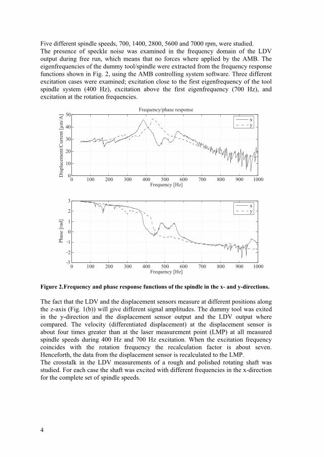
Five different spindle speeds, 700, 1400, 2800, 5600 and 7000 rpm, were studied. The presence of speckle noise was examined in the frequency domain of the LDV output during free run, which means that no forces where applied by the AMB. The eigenfrequencies of the dummy tool/spindle were extracted from the frequency response functions shown in Fig. 2, using the AMB controlling system software. Three different excitation cases were examined; excitation close to the first eigenfrequency of the tool spindle system (400 Hz), excitation above the first eigenfrequency (700 Hz), and excitation at the rotation frequencies.
0 100 200 300 400 500 600 700 800 900 10000
10
20
30
40
50
Frequency [Hz]
Dis
plac
emen
t/Cur
rent
[m
/A]
Frequency/phase response
xy
0 100 200 300 400 500 600 700 800 900 10003
2
1
0
1
2
3
Frequency [Hz]
Phas
e [r
ad]
xy
-
-
-
Figure 2. Frequency and phase response functions of the spindle in the x- and y-directions.
The fact that the LDV and the displacement sensors measure at different positions along the z-axis (Fig. 1(b)) will give different signal amplitudes. The dummy tool was exited in the y-direction and the displacement sensor output and the LDV output where compared. The velocity (differentiated displacement) at the displacement sensor is about four times greater than at the laser measurement point (LMP) at all measured spindle speeds during 400 Hz and 700 Hz excitation. When the excitation frequency coincides with the rotation frequency the recalculation factor is about seven. Henceforth, the data from the displacement sensor is recalculated to the LMP. The crosstalk in the LDV measurements of a rough and polished rotating shaft was studied. For each case the shaft was excited with different frequencies in the x-direction for the complete set of spindle speeds.
4
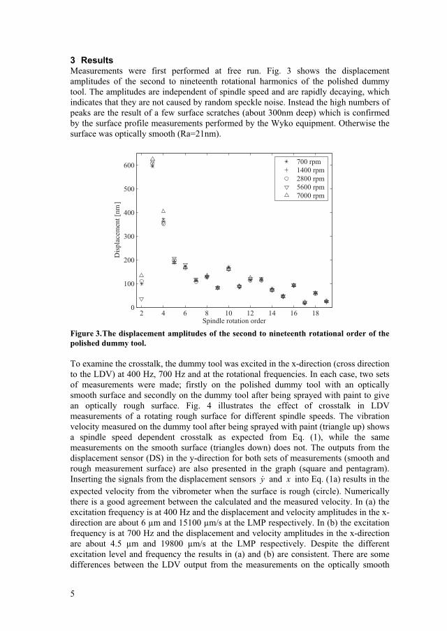
3 Results Measurements were first performed at free run. Fig. 3 shows the displacement amplitudes of the second to nineteenth rotational harmonics of the polished dummy tool. The amplitudes are independent of spindle speed and are rapidly decaying, which indicates that they are not caused by random speckle noise. Instead the high numbers of peaks are the result of a few surface scratches (about 300nm deep) which is confirmed by the surface profile measurements performed by the Wyko equipment. Otherwise the surface was optically smooth (Ra=21nm).
2 4 6 8 10 12 14 16 180
100
200
300
400
500
600
Spindle rotation order
Dis
plac
emen
t [nm
]
700 rpm1400 rpm2800 rpm5600 rpm7000 rpm
Figure 3. The displacement amplitudes of the second to nineteenth rotational order of the polished dummy tool.
To examine the crosstalk, the dummy tool was excited in the x-direction (cross direction to the LDV) at 400 Hz, 700 Hz and at the rotational frequencies. In each case, two sets of measurements were made; firstly on the polished dummy tool with an optically smooth surface and secondly on the dummy tool after being sprayed with paint to give an optically rough surface. Fig. 4 illustrates the effect of crosstalk in LDV measurements of a rotating rough surface for different spindle speeds. The vibration velocity measured on the dummy tool after being sprayed with paint (triangle up) shows a spindle speed dependent crosstalk as expected from Eq. (1), while the same measurements on the smooth surface (triangles down) does not. The outputs from the displacement sensor (DS) in the y-direction for both sets of measurements (smooth and rough measurement surface) are also presented in the graph (square and pentagram). Inserting the signals from the displacement sensors and xy into Eq. (1a) results in the expected velocity from the vibrometer when the surface is rough (circle). Numerically there is a good agreement between the calculated and the measured velocity. In (a) the excitation frequency is at 400 Hz and the displacement and velocity amplitudes in the x-direction are about 6 μm and 15100 μm/s at the LMP respectively. In (b) the excitation frequency is at 700 Hz and the displacement and velocity amplitudes in the x-direction are about 4.5 μm and 19800 μm/s at the LMP respectively. Despite the different excitation level and frequency the results in (a) and (b) are consistent. There are some differences between the LDV output from the measurements on the optically smooth
5

surface and the velocities obtained by the displacement sensor in the y-direction (triangle down and square). These differences are due to a small misalignment (few degrees) between the LDV and the displacement sensor in the y-direction. The sensitivity to misalignment has been checked by calculations. Since the excitation in the x-direction is comparatively large, even small misalignment angles do change the level of the output considerably. For example the difference in (a) can be compensated by an angle of about 4.5 degrees. In (c) the dummy tool was excited at the rotation frequencies, 11.7, 23.4, 46.7, 93.3 and 116.7 Hz. The vibrometer output from the measurements on the smooth surface shows no crosstalk and follows the differentiated displacement sensor output. The crosstalk effect lowers the vibration amplitude level in this case contrary to the previous two excitation frequencies. This shows that the crosstalk can result in either a higher vibration level or a lower one than the correct one.
6
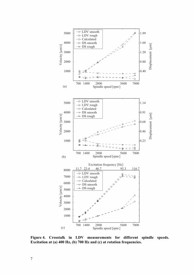
700 1400 2800 5600 7000
1000
2000
3000
4000
5000
Vel
ocity
[m
/s]
Spindle speed [rpm ]
0.40
0.80
1.20
1.60
1.99
Dis
plac
emen
t [
m]
700 1400 2800 5600 7000
1000
2000
3000
4000
5000
Vel
ocity
[m
/s]
Spindle speed [rpm ]
0.23
0.46
0.68
0.91
1.14
Dis
plac
emen
t [
m]
700 1400 2800 5600 7000
1000
2000
3000
4000
5000
6000
7000
8000
Spindle speed [rpm ]
Vel
ocity
[m
/s]
11.7 23.4 46.7 93.3 116.7Excitation frequency [Hz]
(a)
(b)
(c)
LDV smoothLDV roughCalculatedDS smoothDS rough
LDV smoothLDV roughCalculatedDS smoothDS rough
LDV smoothLDV roughCalculatedDS smoothDS rough
Figure 4. Crosstalk in LDV measurements for different spindle speeds. Excitation at (a) 400 Hz, (b) 700 Hz and (c) at rotation frequencies.
7

4 Conclusions Laser vibrometry is normally used on stationary vibrating objects, although synchronous tracking of the laser beam with the moving surface has been tried in number of cases by others. But to measure vibrations of a rotating spindle necessitates that the laser beam is stationary in space. If the rotating surface is optically rough, a moving speckle pattern will occur on the detector, which gives a repeatable speckle noise in the measurement signal and also crosstalk from other velocity components. By using a polished surface, the crosstalk in LDV measurements is avoided and the desired radial vibration can be measured. The fact that the cross vibrations applied by the AMB is removed from the LDV measurements automatically imply the removal of torsional vibration contributions. The small amount of surface scratches did not result in any detectable crosstalk. The scanning LDV also provides the possibility to measure vibrations on different parts of a rotating machine, i.e. the milling machine spindle housing and other significant components during machining, which will give an overall picture of the system.
Acknowledgements The work is supported by the Swedish Agency of Innovation System (Vinnova) and SKF Nova, respectively. The purchase of the vibrometer is financed by the Kempe-foundations. The authors wish to thanks Lars Frisk, for optimizing the polishing procedure of the dummy tool, and also Pär Marklund, for surface roughness measurements.
References[1] A. Albrecht, S.S. Park, Y. Altintas and G. Pritschow, High frequency
bandwidth cutting force measurement in milling using capacitance displacement sensors, International Journal of Machine Tools and Manufacture 45 (2005) 993-1008.
[2] R.P.H. Faassen, N.van de Wouw, J.A.J. Oosterling and H. Nijmeijer, Prediction of regenerative chatter by modelling and analysis of high speed milling. International Journal of Machine Tools & Manufacture 43 (2003) 1437-1446.
[3] LE. Drain, The Laser Doppler technique, Wiley, New York, 1980.
[4] M. Rantatalo, K. Tatar, P. Norman, Laser doppler vibrometry measurements of a rotating milling machine spindle, in: Proceedings of the Eighth International Conference on Vibrations in Rotating Machinery, University of Wales, Swansea, UK, 2004, pp. 231-240.
[5] P. Castellini and C. Santolini, Vibration measurements on blades of a naval propeller rotating in water with tracking laser vibrometer, Measurement, 24 (1998) 43-54.
[6] P. Castellini and R. Montanini, Automotive components vibration measurements by tracking laser Doppler Vibrometry: advances in signal processing, Measurement Science & Technology, 13 (2002) 1266-1279.
8
[7] S.J. Rothberg, J.R. Baker, and N.A. Halliwell, Laser vibrometry: Pseudo-vibration, Journal of Sound and Vibration, 135 (1989) 516-522.
[8] M. Denman, N.A. Halliwell and S.J. Rothberg, Speckle noise reduction in laser vibrometry: experimental and numerical optimisation, in: Second International Conference on Vibration Measurements by Laser Techniques: Advances and Applications, Washington, DC, USA 1996, pp 12-21.
[9] N.A. Halliwell, The laser torsional vibrometer: a step forward in rotating machinery diagnostics, Journal of Sound and Vibration, 190 (1996) 399-418.
[10] S.J. Drew, and B.J. Stone, Removal of speckle harmonics in laser torsional Vibrometry, Mechanical systems and Signal Processing, 11 (1997) 773-776.
[11] T.H. Wilmshurst, and N.A. Halliwell, Laser Vibrometer Speckle-Noise Cancellation, Measurements Science & Technology, 4 (1993) 479-487.
[12] J. R. Bell and S. J. Rothberg, Laser vibrometers and contacting transducers, target rotation and six degree-of-freedom vibration: what do we really measure? Journal of Sound and Vibration, 237 (2000) 245-261.
[13] J. R. Bell and S. J. Rothberg, Rotational vibration measuring using laser Doppler Vibrometry: comprehensive theory and practical application, Journal of Sound and vibration, 238 (2000) 673-690.
[14] S. J. Rothberg and J. R. Bell, On the application of laser vibrometry to translational and rotational vibration measurements on rotating shafts, Measurement, 35 (2004) 201-210.
[15] B. Halkon and S. J. Rothberg, Automatic post-processing of laser vibrometry data for rotor vibration measurements, in: Eighth International Conference on Vibrations in Rotating Machinery, University of Wales, Swansea, UK, 2004, pp. 215-229.
9

10

Paper C Integrated Tool for Prediction of Stability Limits in Machining


Integrated Tool for Prediction of Stability Limits in Machining
A. SVOBODA, K. TATAR*, P. NORMAN AND M. BÄCKSTRÖM
Department of Mechanical Engineering, Luleå University of Technology, Sweden *Corresponding author. Email: [email protected]
Abstract
High-speed machining of thin-walled structures is widely used in the aeronautical industry. Higher spindle speed and machining feed rate, combined with a greater depth of cut, increases the removal rate and with it, productivity. The combination of higher spindle speed and depth of cut makes instabilities (chatter) a far more significant concern. Chatter causes reduced surface quality and accelerated tool wear. Since chatter is so prevalent, traditional cutting parameters and processes are frequently rendered ineffective and inaccurate. For the machine tool to reach its full utility, the chatter vibrations must be identified and avoided. In order to avoid chatter and implement optimum cutting parameters, the machine tool including all components and the workpiece must be dynamically mapped to identify vibration characteristics.
The aim of the presented work is to develop a model for the prediction of stability limits as a function of process parameters. Commercial software packages used for integration into the model prove to accomplish demands for functionality and performance. In order to validate the model, the stability limits predicted by the use of numerical simulation are compared with the results based on the experimental work.
Keywords: High-speed machining; Regenerative chatter; Stability lobes; Finite element analysis; Laser Doppler Vibrometry
1 Introduction
An increasing trend in modern manufacturing industry points towards larger ranges of variation in production systems. This is a direct consequence of the effort to satisfy customer demands for fast deliveries of new products. The present situation in the manufacturing industry is that they have to adjust much of their cutting processes as a consequence of the uncertainty that exists in the influencing machining conditions. In order

to do this, techniques must be used to handle variations in the manufacturing conditions as the frequent reconfigurations and setups generate.
In manufacturing of components for aerospace applications, aluminium is one of the most frequently used materials. In machining aluminium, higher spindle speed and machining feed rate combined with a greater depth of cut, increases the removal rate and with it, productivity. The combination of higher spindle speed and depth of cut makes instabilities (chatter) a far more significant concern. In machining, chatter is perceived as an unwanted excessive vibration between the tool and the workpiece, resulting in a poor surface finish with possible initiation of micro-cracks. Chatter vibrations accelerate also tool wear which has a deteriorating effect on the tool life, and the reliability of the machining operations. Especially for the cases where long slender end mills or highly flexible thin-wall parts are involved, chatter is almost unavoidable unless special suppression techniques are used or the removal rate of material is substantially reduced. Currently working with the preparation machining process, the natural frequencies of the workpiece are measured and analysed when getting problem with the quality of the surface or cutting process. The manufacturing process is stopped just before the cutting starts in the problem area and sensors are put in the same area. The extensive experimental work is a limiting factor in application of this approach to manufacturing of aluminium aerospace components. The removal of material in aerospace applications is vast and figures up to 90% of the original volume which results in non-linear behaviour due to time variant geometry and stiffness. Due to time and costs consuming experimental work, the long-term goal is to develop a tool for the prediction of chatter vibrations that is based on a digital prototype.The first attempt to describe chatter was made by (Arnold 1946). (Tobias and Fishwick 1958) presented a comprehensive mathematical model and analysis results of chatter vibrations. The importance of predicting stability in milling has increased due to advances in high-speed milling technology. At high speeds, the stabilizing effect of process damping diminishes, making the process more prone to chatter. On the other hand, stability limits usually referred to as stability lobes exist at certain high spindle speed which can be used to substantial increase the chatter free material removal rate, provided that they are predicted accurately, see e.g. (Smith and Tlusty 1993). (Wiercigroch and Budak 2001) presented a critical review of the modelling and experimental investigations. In this work, sources of nonlinearities, chatter generation and suppression in metal cutting are studied. In the papers by (Moon and Kalmar-Nagy 2001, Balachandran 2001), the prediction of complex, unsteady and chaotic dynamics associated with cutting processes through nonlinear dynamical models is reviewed. In general, several physical mechanisms causing chatter can be distinguished. Frictional chatter due to friction between the tool and workpiece, mode-coupling chatter and thermo-mechanical chatter caused by the thermodynamics of the cutting process are often called primary chatter. Secondary chatter is caused by the regeneration of waviness on the surface of the workpiece. This phenomenon is called regenerative chatter and is considered to be one of the most important causes of instability in the cutting process. During machining as the cutter tooth enters into the cut, the cutting system (tool-holder, tool) deforms in bending due to applied cutting forces. Forces released by the tooth exiting
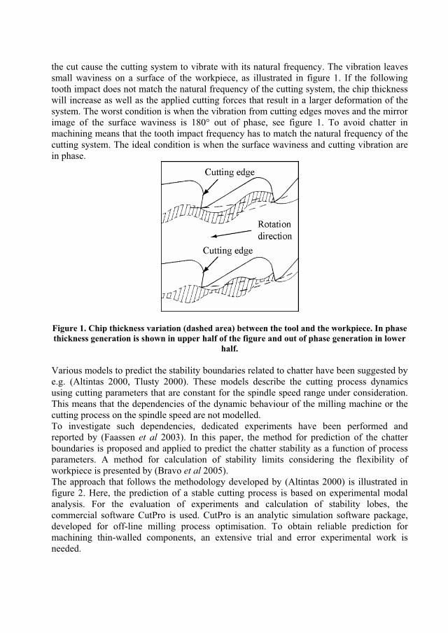
the cut cause the cutting system to vibrate with its natural frequency. The vibration leaves small waviness on a surface of the workpiece, as illustrated in figure 1. If the following tooth impact does not match the natural frequency of the cutting system, the chip thickness will increase as well as the applied cutting forces that result in a larger deformation of the system. The worst condition is when the vibration from cutting edges moves and the mirror image of the surface waviness is 180° out of phase, see figure 1. To avoid chatter in machining means that the tooth impact frequency has to match the natural frequency of the cutting system. The ideal condition is when the surface waviness and cutting vibration are in phase.
Figure 1. Chip thickness variation (dashed area) between the tool and the workpiece. In phase thickness generation is shown in upper half of the figure and out of phase generation in lower
half.
Various models to predict the stability boundaries related to chatter have been suggested by e.g. (Altintas 2000, Tlusty 2000). These models describe the cutting process dynamics using cutting parameters that are constant for the spindle speed range under consideration. This means that the dependencies of the dynamic behaviour of the milling machine or the cutting process on the spindle speed are not modelled. To investigate such dependencies, dedicated experiments have been performed and reported by (Faassen et al 2003). In this paper, the method for prediction of the chatter boundaries is proposed and applied to predict the chatter stability as a function of process parameters. A method for calculation of stability limits considering the flexibility of workpiece is presented by (Bravo et al 2005). The approach that follows the methodology developed by (Altintas 2000) is illustrated in figure 2. Here, the prediction of a stable cutting process is based on experimental modal analysis. For the evaluation of experiments and calculation of stability lobes, the commercial software CutPro is used. CutPro is an analytic simulation software package, developed for off-line milling process optimisation. To obtain reliable prediction for machining thin-walled components, an extensive trial and error experimental work is needed.
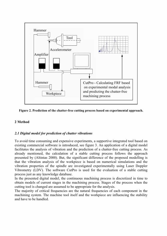
Figure 2. Prediction of the chatter-free cutting process based on experimental approach.
2 Method
2.1 Digital model for prediction of chatter vibrations
To avoid time consuming and expensive experiments, a supportive integrated tool based on existing commercial software is introduced, see figure 3. An application of a digital model facilitates the analysis of vibration and the prediction of a chatter-free cutting process. As already mentioned, the calculation of a stable cutting process follows the approach presented by (Altintas 2000). But, the significant difference of the proposed modelling is that the vibration analysis of the workpiece is based on numerical simulations and the vibration properties of the spindle are investigated experimentally using Laser Doppler Vibrometry (LDV). The software CutPro is used for the evaluation of a stable cutting process just as any knowledge database. In the presented digital model, the continuous machining process is discretized in time to obtain models of current stages in the machining process. Stages of the process when the cutting tool is changed are assumed to be appropriate for the analysis. The majority of critical frequencies are the natural frequencies of each component in the machining system. The machine tool itself and the workpiece are influencing the stability and have to be handled.

Figure 3. The model for the prediction of the chatter-free cutting process that integrates numerical simulation with experimental procedures based on LDV measurements.
2.2 Definition of tool path and geometry for the analysis
A reference geometry that is typical for an aircraft detail, see figure 4, is used for evaluation of the prediction methodology. Material removal in manufacturing this detail is large. For the illustration, the volume of the initial stock is 1.896×106 mm3 and the volume after final milling operation is 0.218×106 mm3. The thickness of the initial monolith is 40 mm, the final thickness of the bottom is 1.0 mm and the flange thickness is 1.5 mm. The structure has shown significant sensibility to vibrations during the machining. Before manufacturing, it must be first decided which operations are required to go from a stock geometry to the finished final component. A part programme for machining of the geometry is generated in a Computer Aided Manufacturing (CAM) system. The solid model of the structure that is created with nominal finished dimensions in a Computer Aided Design (CAD) system is transferred to the CAM module by selecting from the system database. In the presented work, the I-DEAS CAD/CAM system is used. Modern CAM software offers high levels of support for creating tool paths which is necessary for the definition of the component geometry from a piece of stock material. The CAM software automatically creates suitable paths for the tool to follow by the use of built-in algorithms. It is generally possible to specify how critical parts of the tool path such as entry and exit from the part or significant changes in the direction of the tool path such as machining in a corner are to be handled. To perform high speed roughing in volume milling, the scan type constant load is to be used. The milling is based on principles of constant cutting condition, constant chip load,
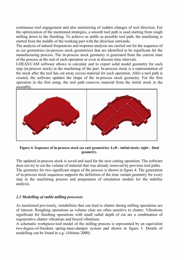
continuous tool engagement and also minimizing of sudden changes of tool direction. For the optimization of the mentioned strategies, a smooth tool path is used starting from rough milling down to the finishing. To achieve as stable as possible tool path, the machining is started from the middle of the working part with the direction outwards. The analysis of natural frequencies and response analysis are carried out for the sequence of as cut geometries (in-process stock geometries) that are identified to be significant for the manufacturing process. The in-process stock geometry is generated from the current state of the process at the end of each operation or even at discrete time intervals. I-DEAS/CAM software allows to calculate and to export solid model geometry for each step (in-process stock) in the machining of the part. In-process stock is a representation of the stock after the tool has cut away excess material for each operation. After a tool path is created, the software updates the shape of the in-process stock geometry. For the first operation in the first setup, the tool path removes material from the initial stock in the assembly.
Figure 4. Sequence of in-process stock (as cut) geometries: Left - initial stock; right – final geometry.
The updated in-process stock is saved and used for the next cutting operation. The software does not try to cut the volume of material that was already removed by previous tool paths. The geometry for two significant stages of the process is shown in figure 4. The generation of in-process stock sequences supports the definition of the time variant geometry for every step in the machining process and preparation of simulation models for the stability analysis.
2.3 Modelling of stable milling processes
As mentioned previously, instabilities that can lead to chatter during milling operations are of interest. Roughing operations as volume clear are often sensitive to chatter. Vibrations significant for finishing operations with small radial depth of cut are a combination of regenerative chatter vibrations and forced vibrations. A schematic workpiece-tool model of the milling process is represented by an equivalent two-degree-of-freedom spring-mass-damper system and shown in figure 5. Details of modelling can be found in e.g. (Altintas 2000).

Figure 5. Regenerative effect due to chip-thickness variation.
In figure 5, the feed direction and spindle rotation are shown for an up milling operation. The initial surface of the work piece is smooth without waves during the first revolution, but the tool starts leaving a wavy surface behind because of the structural modes of the machine tool-workpiece system in the feed direction. When the second revolution starts, the surface has waves both inside the cut where the tool is cutting (inner modulation (t)) and on the outside surface of the cut owing to vibrations during the previous revolution of cut (outer modulation (t – T)). Depending on the phase shift between the two successive waves, see also figure 1, the maximum chip thickness may exponentially grow while oscillating at a chatter frequency that is close but not equal to a dominant structural mode in the system. Hence, the resulting dynamic chip thickness is no longer constant but varies as a function of vibration frequency and the speed of the spindle. Generally, the dynamic thickness can be expressed as follows
tTtytytTtxtxthth cossinsin)( 0 , (1)
where h0 is the intended chip thickness, which is equal to the feed rate of the machine, and x, y are components of the dynamic chip thickness produced owing to vibrations at the present time t and one spindle revolution period (T) before. Assuming that the work piece is approximated by a two-degree-of-freedom system in two uncoupled and orthogonal directions, we obtain following equation of motion
tFtF
tytx
kk
tytx
cc
tytx
mm
y
x
y
x
y
x
y
x
00
00
00
. (2)
Here, the terms mx,y, cx,y, kx,y are the modal mass, damping and stiffness, Fx and Fy are the tangential and radial cutting forces components resolved in x, y directions. The tangential and radial components of cutting forces are proportional to the axial depth of cut a, the dynamic chip thickness h(t) and can be expressed as follows
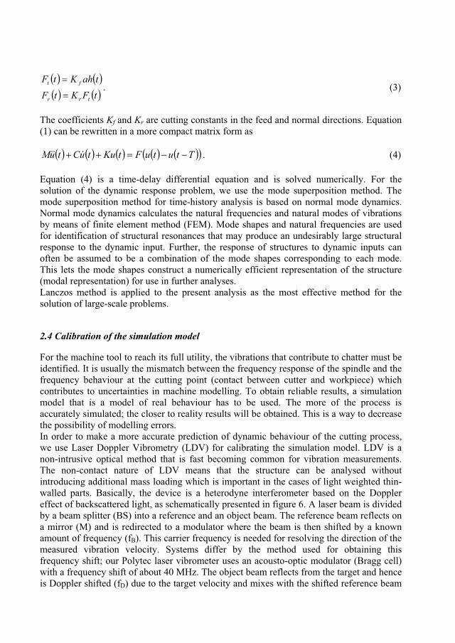
tFKtFtahKtF
trr
ft . (3)
The coefficients K and Kf r are cutting constants in the feed and normal directions. Equation (1) can be rewritten in a more compact matrix form as
TtutuFtKutuCtuM . (4)
Equation (4) is a time-delay differential equation and is solved numerically. For the solution of the dynamic response problem, we use the mode superposition method. The mode superposition method for time-history analysis is based on normal mode dynamics. Normal mode dynamics calculates the natural frequencies and natural modes of vibrations by means of finite element method (FEM). Mode shapes and natural frequencies are used for identification of structural resonances that may produce an undesirably large structural response to the dynamic input. Further, the response of structures to dynamic inputs can often be assumed to be a combination of the mode shapes corresponding to each mode. This lets the mode shapes construct a numerically efficient representation of the structure (modal representation) for use in further analyses. Lanczos method is applied to the present analysis as the most effective method for the solution of large-scale problems.
2.4 Calibration of the simulation model
For the machine tool to reach its full utility, the vibrations that contribute to chatter must be identified. It is usually the mismatch between the frequency response of the spindle and the frequency behaviour at the cutting point (contact between cutter and workpiece) which contributes to uncertainties in machine modelling. To obtain reliable results, a simulation model that is a model of real behaviour has to be used. The more of the process is accurately simulated; the closer to reality results will be obtained. This is a way to decrease the possibility of modelling errors. In order to make a more accurate prediction of dynamic behaviour of the cutting process, we use Laser Doppler Vibrometry (LDV) for calibrating the simulation model. LDV is a non-intrusive optical method that is fast becoming common for vibration measurements. The non-contact nature of LDV means that the structure can be analysed without introducing additional mass loading which is important in the cases of light weighted thin-walled parts. Basically, the device is a heterodyne interferometer based on the Doppler effect of backscattered light, as schematically presented in figure 6. A laser beam is divided by a beam splitter (BS) into a reference and an object beam. The reference beam reflects on a mirror (M) and is redirected to a modulator where the beam is then shifted by a known amount of frequency (fB). This carrier frequency is needed for resolving the direction of the measured vibration velocity. Systems differ by the method used for obtaining this frequency shift; our Polytec laser vibrometer uses an acousto-optic modulator (Bragg cell) with a frequency shift of about 40 MHz. The object beam reflects from the target and hence is Doppler shifted (fD) due to the target velocity and mixes with the shifted reference beam

on the photo detector. Depending on the optical path difference between these two beams, they will interfere constructively or destructively. When the target is moving, the intensity measured by the photo detector will be time dependent. Frequency demodulation of the photo detector signal by a Doppler signal processor produces a time resolved velocity component of the moving target.
Figure 6. Schematic of the scanning Laser Doppler vibrometer. The laser beam is divided into a reference and an object beam. These two interfere on the photo detector and the velocity of the target is obtained after demodulation of the signal. Beam splitter (BS), mirror (M), laser
frequency (f), Bragg cell frequency (fB) and Doppler frequency (fD).B
In the application of laser vibrometry to experimental modal analysis, the surface of the vibrating object is scanned. A scan is a sequence of single point measurements. Two small servo controlled mirrors in the scanning head make it possible to deflect the beam both in the horizontal and the vertical direction. The measured data in each scan point is then compared relative to a reference signal. In our case the measured object is excited by an electro dynamic shaker. A force transducer at the driving point acts as a reference. Mode shapes and frequencies are then extracted from the measurements data by the LDV system software.Here, we use LDV to calibrate the boundary conditions in the FE model and also to experimentally determine the vibration properties of the setup cutting tool–spindle. Details about measurements on the spindle are presented in (Rantatalo et al 2004). The performance of the finite elements is evaluated using the stock part that is fixed in the measuring frame by means of flexible suspensions (rubber band). The flexible fixture allows the part to reproduce all rigid body modes. A shaker is used to excite the stock by a random pulse. We choose the first non-singular mode and the corresponding natural frequency 1947 Hz to illustrate the result of the experiment, see figure 7. The finite element model with the same type of the flexible constraint allowing all rigid body modes is

analysed using eigen-problem solver. For the FE discretization, we use 10 nodes tetrahedron elements with quadratic interpolation. Material parameters for the reference part are following: Elasticity modulus 7.1×10⁴ -6 MPa, Poissons ratio 0.315, Density 2.8×10kgmm-3. The material type is: Zn-Mg-Cu-Zr-Al – aircraft grade.The simulation result – first non-singular mode with the frequency 1970 Hz is also presented in figure 7. The simulation shows good agreement with the experiment.
Figure 7. Left – FE analysis of the stock with flexible suspension. The colour scale represents normalized first mode corresponding to the first natural frequency. Right – LDV
measurements. The colour scale represents quantitative displacements corresponding to the first frequency.
The next step in the calibration of the finite element model is an accurate definition of the boundary conditions for the analysis. The workpiece is mounted on the machine table in a Liechti Turbomill machining centre by the use of stiff clamps. The setup containing the stock part and the shaker is shown in figure 8. The frequency response to a random signal is measured by means of LDV. The first mode with corresponding frequency is shown in figure 9. A sequence of numerical experiments was run to iterate to the correct stiffness of the fixing clamps. The result of the analysis is presented in figure 9. We chose again the first mode and frequency of the fixed stock to compare the numerical result with the experiment. The simulation shows again good agreement with experimental results.

Figure 8. Photo of the setup with the stock and the shaker mounted in the Liechti machine.
Figure 9. First mode and natural frequency are shown for the comparison of LDV measurements with FE analysis. Left – FE modelling. The colour scale represents the first
normalized mode corresponding to the first natural frequency 2940 Hz. Right – Experimental result. The colour scale represents quantitative displacements corresponding to the first
frequency 2835 Hz.

3. Modelling results and experimental verification
3.1 Evaluation of a stable cutting process
The digital model, constructed and calibrated in previous sections is used to pursue an analysis of stability boundaries. The sequence of as cut geometries shown in figure 4 is used for generation of FEM models. During the machining, the initial stock mass 5.31 kg is reduced to 0.61 kg after finishing operations. This factor and lack of symmetry in geometry which is very common in this type of manufacturing have large impact on the vibration properties. To show the significant changes of the vibration properties, we choose for the comparison the first natural frequency and the mode of the initial stock and of the final geometry. The simulated first frequency 2940 Hz for the stock decreases after final milling operation to 1070 Hz. Simulated and LDV experimental results are shown in figure 10.
Figure 10. The first natural frequency and mode for final geometry. Left – FEM simulation, right – the LDV experiment.
The FE model used for solving eigen value problem is also used for transient response analysis by including appropriate initial and boundary conditions. Transient analysis computes the dynamic response of a structure to a set of simultaneous transient excitations. The response at each time instant is calculated by combining the modal response obtained using time integration. The workpiece is loaded by a short force pulse in two orthogonal directions in the plane x – y which is parallel to the bottom plane of the workpiece. The frequency response functions (FRF) in mm N-1 obtained from FE analysis for a sequence of cut geometries and also obtained from LDV measurements on the spindle are exported into the CutPro software for following processing and stability lobes calculations. We use features implemented in the CutPro software for the generation of data describing a machining process. In preparatory stage, the cutter data and cutting coefficients for the current workpiece material and a cutting force model are defined. After all preparatory steps are accomplished we have necessary input data to continue with the stability lobes calculation.The stability lobe defines region of stable and unstable cutting zones as a function of maximum depth of cut and spindle speed and is used to select appropriate machining parameters. Stability lobes that are predicted for the initial stock geometry and for a 40mm CoroMill cutter are shown in figure 11. Finishing milling of the final geometry is done
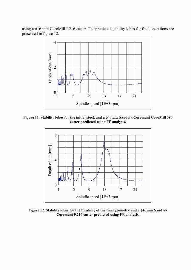
using a 16 mm CoroMill R216 cutter. The predicted stability lobes for final operations are presented in figure 12.
Figure 11. Stability lobes for the initial stock and a 40 mm Sandvik Coromant CoroMill 390 cutter predicted using FE analysis.
Figure 12. Stability lobes for the finishing of the final geometry and a 16 mm Sandvik Coromant R216 cutter predicted using FE analysis.
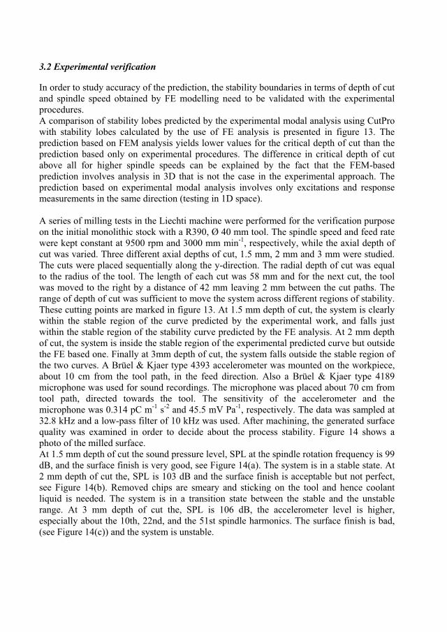
3.2 Experimental verification
In order to study accuracy of the prediction, the stability boundaries in terms of depth of cut and spindle speed obtained by FE modelling need to be validated with the experimental procedures.A comparison of stability lobes predicted by the experimental modal analysis using CutPro with stability lobes calculated by the use of FE analysis is presented in figure 13. The prediction based on FEM analysis yields lower values for the critical depth of cut than the prediction based only on experimental procedures. The difference in critical depth of cut above all for higher spindle speeds can be explained by the fact that the FEM-based prediction involves analysis in 3D that is not the case in the experimental approach. The prediction based on experimental modal analysis involves only excitations and response measurements in the same direction (testing in 1D space).
A series of milling tests in the Liechti machine were performed for the verification purpose on the initial monolithic stock with a R390, Ø 40 mm tool. The spindle speed and feed rate were kept constant at 9500 rpm and 3000 mm min-1, respectively, while the axial depth of cut was varied. Three different axial depths of cut, 1.5 mm, 2 mm and 3 mm were studied. The cuts were placed sequentially along the y-direction. The radial depth of cut was equal to the radius of the tool. The length of each cut was 58 mm and for the next cut, the tool was moved to the right by a distance of 42 mm leaving 2 mm between the cut paths. The range of depth of cut was sufficient to move the system across different regions of stability. These cutting points are marked in figure 13. At 1.5 mm depth of cut, the system is clearly within the stable region of the curve predicted by the experimental work, and falls just within the stable region of the stability curve predicted by the FE analysis. At 2 mm depth of cut, the system is inside the stable region of the experimental predicted curve but outside the FE based one. Finally at 3mm depth of cut, the system falls outside the stable region of the two curves. A Brüel & Kjaer type 4393 accelerometer was mounted on the workpiece, about 10 cm from the tool path, in the feed direction. Also a Brüel & Kjaer type 4189 microphone was used for sound recordings. The microphone was placed about 70 cm from tool path, directed towards the tool. The sensitivity of the accelerometer and the microphone was 0.314 pC m-1 s-2 and 45.5 mV Pa-1, respectively. The data was sampled at 32.8 kHz and a low-pass filter of 10 kHz was used. After machining, the generated surface quality was examined in order to decide about the process stability. Figure 14 shows a photo of the milled surface. At 1.5 mm depth of cut the sound pressure level, SPL at the spindle rotation frequency is 99 dB, and the surface finish is very good, see Figure 14(a). The system is in a stable state. At 2 mm depth of cut the, SPL is 103 dB and the surface finish is acceptable but not perfect, see Figure 14(b). Removed chips are smeary and sticking on the tool and hence coolant liquid is needed. The system is in a transition state between the stable and the unstable range. At 3 mm depth of cut the, SPL is 106 dB, the accelerometer level is higher, especially about the 10th, 22nd, and the 51st spindle harmonics. The surface finish is bad, (see Figure 14(c)) and the system is unstable.
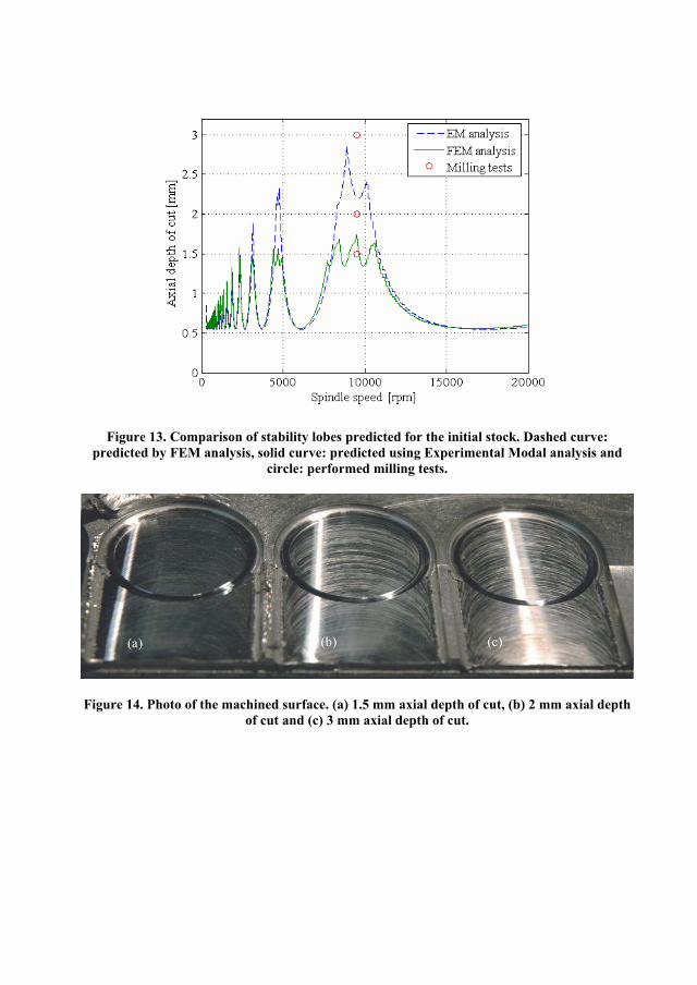
Figure 13. Comparison of stability lobes predicted for the initial stock. Dashed curve: predicted by FEM analysis, solid curve: predicted using Experimental Modal analysis and
circle: performed milling tests.
Figure 14. Photo of the machined surface. (a) 1.5 mm axial depth of cut, (b) 2 mm axial depth of cut and (c) 3 mm axial depth of cut.

4. Conclusions
Chatter is a dynamic phenomenon that can appear in a machining at any spindle speed. Stable machining cannot be achieved without investigating the influence of chatter on the cutting process. A standard way to obtain reliable prediction of a stable machining process is the application of the methodology based on the experimental modal analysis. This approach requires in the case of thin-walled structures an extensive trial and error experimental work. In this work we present an integrated tool for prediction stability boundaries. A digital model for the milling process based on integration of CAD – CAM - FEM is developed. Commercial software packages used for integration into the model prove to accomplish demands for functionality and performance. Not only do the suggested approach give safer machining it also carries promises of an overall higher productivity. To avoid the usual mismatch between the frequency response of the spindle and the frequency behaviour at the cutting point (contact between cutter and workpiece) which contributes to uncertainties in the machine modelling, we use dedicated experimental procedures which are based on LDV measurements. The non-contact nature of the LDV makes accurate and fast measurements possible with an easy setup without any mass loads. This is of crucial importance when measuring on thin-wall structures with low rigidity. It is shown to be very useful to validate and improve the dynamic FEM models, especially regarding boundary conditions. The LDV is also able to make measurements on the rotating spindle, spindle housing, tool, tool holder, workpiece, clamps and machine table in one setup and give an overall picture of the machining.
The performed milling tests showed good agreement with the predicted stability lobes (at 9500 rpm). When machining just within the stable region predicted using the FE analysis resulted in the best surface finish.
Acknowledgement
Support for this work was provided by EC 5th framework programme Growth. A part of this work is financed by the Swedish Agency of Innovative Systems VINNOVA. The purchase of the LDV system is financed by Kempe Foundations. The authors would like to express their appreciation to Tommy Gunnarsson, AB Sandvik Coromant, and to Tore Silver, Division of Manufacturing System Engineering, Luleå University for their helpful collaboration in the experimental work.

References
Altintas, Y., 2000, Manufacturing Automation, Cambridge University Press.
Arnold, R. N., 1946, Mechanism of tool vibration in cutting speed, Proc. Inst. Mech. Eng.,154, 261–276.
Balachandran, B., 2001, Nonlinear dynamics of milling processes, Phil. Trans. R. Soc. London, 359, 793–819.
Bravo, U., Altuzarra, O., Lopez de Lacalle, L., N., Sanchez, J. A. and Campa, F., J., 2005, Stability limits of milling considering the flexibility of the workpiece and the machine, International Journal of Machine Tools & Manufacture.
Faassen, R. P. H., van de Wouw, N., Oosterling, A. J. A. and Nijmeijer, H., 2003, Prediction of regenerative chatter by modelling and analysis of high-speed milling, Int. J. Machine Tools & Manufacture, 43, 1437–1446.
Moon, F. C. and Kalmar-Nagy, T., 2001, Nonlinear models for complex dynamics in cutting materials, Phil. Trans. R. Soc. London, 359, 695-711.
Rantatalo, M., Tatar, K. and Norman, P., 2004, Laser doppler vibrometry measurements of a rotating milling machine spindle, Proc. 8 Int. Conf. on Vibrations in Rotating Machinery, University of Wales, Swansea, 7-9 September, 231-240.
th
Smith, S. and Tlusty; J., 1993, An Overview of Modelling and Simulation of the Milling Process, Journal of Engineering for Industry, Transaction of the ASME, 113, 169–175.
Tarng, Y. S., , 1992, Use of model-based cutting simulation system for tool breakage monitoring in milling, International Journal of Machine Tools & Manufacture, 32, 641-649.
Lee, B.Y.
Tlusty, J., 2000, Manufacturing Processes and Equipment, Prentice Hall.
Tobias, S. A. and Fishwick, W., 1958, The chatter of lathe tools under orthogonal cutting conditions, Trans. ASME, 80, 1079–1088.
Vierck, K. C., , 1992, Adaptive thresholding for cutter breakage in milling, ASME Prod Eng Div Publ PED, 55, 17-32.
Tlusty, J.
Wiercigroh, M. and Budak, E., 2001, Sources of nonlinearities, chatter generation and suppression in metal cutting, Phil. Trans. R. Soc. London, 359, 663–693.
Wiercigroh, M. and Krivtsov, A. M., 2001, Frictional chatter in orthogonal metal cutting, Phil. Trans. R. Soc. London, 359, 713-738.


Paper D Laser vibrometry measurements of vibration and sound fields of a bowed violin


INSTITUTE OF PHYSICS PUBLISHING MEASUREMENT SCIENCE AND TECHNOLOGY
Meas. Sci. Technol. 17 (2006) 635–644 doi:10.1088/0957-0233/17/4/005
Laser vibrometry measurements ofvibration and sound fields of a bowedviolinPer Gren1, Kourosh Tatar1, Jan Granstrom1, N-E Molin1
and Erik V Jansson2
1 Division of Experimental Mechanics, Luleå University of Technology, SE-97187 Luleå,Sweden2 Department of Speech, Music and Hearing, Royal Institute of Technology (KTH),SE-10044 Stockholm, Sweden
Received 28 September 2005, in final form 4 January 2006Published 10 February 2006Online at stacks.iop.org/MST/17/635
AbstractLaser vibrometry measurements on a bowed violin are performed. Arotating disc apparatus, acting as a violin bow, is developed. It produces acontinuous, long, repeatable, multi-frequency sound from the instrumentthat imitates the real bow–string interaction for a ‘very long bow’. Whatmainly differs is that the back and forward motion of the real bow is replacedby the rotating motion with constant velocity of the disc and constantbowing force (bowing pressure). This procedure is repeatable. It is longlasting and allows laser vibrometry techniques to be used, which measureforced vibrations by bowing at all excited frequencies simultaneously. Achain of interacting parts of the played violin is studied: the string, thebridge and the plates as well as the emitted sound field. A description of themechanics and the sound production of the bowed violin is given, i.e. theproduction chain from the bowed string to the produced tone.
Keywords: laser vibrometry, violin, sound fields
M This article features online multimedia enhancements
(Some figures in this article are in colour only in the electronic version)
1. Introduction
The physics of the violin as known up to 1984 was thoroughlydescribed by Cremer [1]. The construction, properties ofseparate parts, etc are presented in a more applied wayin [2]. However, as in many earlier investigations of theviolin, the violin parts are investigated separately and not somuch as a played, assembled instrument. The holographicinterferometry investigations from the early 1970s [3, 4]used electromagnetic single frequency excitation, and notbowing. Successful experiments at that time demanded highstability. Today’s optical measuring techniques such as thelaser vibrometer are much less disturbed by rigid body motionsand have a much higher sensitivity.
The violin body is made of three main parts: the topplate, the ribs and the back plate, see figure 1. The top plate is
made of spruce and made arched (a shell), has two f-holes, isstrengthened by the bassbar and supported by the soundpost.The edges of the top plate are glued to the maple ribs with sixblocks: the upper block, the lower block and the four cornerblocks. To the other side of the ribs, the back plate of maple(also made arched, a shell) is glued. The soundpost is a smallwooden cylinder placed close to the treble foot of the bridgeand is squeezed in between the top and back plates. Its positioncan be adjusted if necessary.
Laser Doppler vibrometry (LDV) [5] is a well-establishednon-contact method normally used for measurements onvibrating surfaces. By scanning the laser beam across thesurface of the object, the resonance frequencies and thecorresponding modes can be measured and visualized. SinceLDV is an interferometric technique, changes in an opticalpath in general can be measured. Zipser et al proposed to use
0957-0233/06/040635+10$30.00 © 2006 IOP Publishing Ltd Printed in the UK 635

P Gren et al
Figure 1. Outline of the violin seen from the top, and sections seenfrom the side and the bottom end; bridge B, f-holes F, top plate TP,ribs R, soundpost SP, back plate BP and bassbar BB.
LDV to visualize and measure sound and flow fields [6, 7]. Insuch measurements the background should be stable and themedium between the laser head and the background ‘vibrates’due to pressure changes.
The present investigation differs from earlier opticalinvestigations [3, 4, 8–11] in that the violin is now excitedby a rotating bow and measured with LDV when it is bowedinstead of exciting it at a single frequency at a time. Theprime interest is now not to measure the eigenmodes but theODSs (operating deflection shapes) [12] and the sound fieldthat is excited by the bowing of the real assembled instrument.It also differs from investigations where pulsed lasers havebeen used to study the violin, often excited with impacts ortransients. Molin et al [13, 14] showed the bending wavepropagation in the body of the violin for impulses at the bridgetop when the two bridge feet moved in phase or out of phase.One observation from these experiments was the high speedwith which the back plate of the violin was set in vibrationby the waves transmitted to the back plate by the soundpost.Electro-mechanical measurement for the modal analysis ofthe violin was also performed [15–17] but such investigationswere performed either with instrumented, impact hammersor from white noise excitation, and not by bowing. In thisinvestigation, however, it is not the start or the end of a tonethat is of prime interest but rather the more continuous andconstant middle part of a played tone.
The sound radiations of three violins were measured andcompared by Wang and Buroughs [18]. They used near-fieldacoustic holography for the measurements and a haired rosinedinfinite belt for the bowing.
Linaza et al used numerical FEM analysis to studythe violin [19]. This method has many advantages sinceit allows numerical studies of the influence of thickness,curvature, material, etc, that is many numerical experimentswhich are hard or impossible to perform physically. Onthe other hand, there are a number of unknown or lessknown factors in such often quite simplified numerical FEMmodels.
Figure 2. Photo of the rotating bow and the violin. Disc (D), twobearings (B) and lever (L).
2. Experimental set-up and technique
In his study of the mechanical actions of violins, Saunders[20] constructed and used a mechanical, rosined rotating bowto obtain repeatable conditions for his experiments. Meinel[21] also constructed a bowing machine. He used an infiniterosined stripe. Our reason for developing the rotating bowwas that the LDV measurements need a repeatable, long andwell-defined vibration signal to allow the modal analysis of thesignal. Since the measuring time sometimes exceeds 10 min,ordinary bowing by hand was not possible, and it is not stableenough. A rotating bow was therefore constructed from whichthe violin string can be excited continuously and repeatedlyfor more than 15 min, see figure 2. It consists of a dc-engine(24 V) driven disc (D) of PMMA and is hinged like a pendulumin a frame supported by two bearings (B). The normal bowingforce on the string can easily be changed by moving a smallmass along the lever (L), and the rotational speed is controlledby a dc-voltage supply. The diameter and the thickness of thedisc are 110 mm and 6 mm, respectively. The edge of therotating disc was slightly rounded. It was rosined in the sameway prior to all measuring series. Any change in the soundfrom the bowed violin was not detected by the measuringmicrophone during 20 min bowing.
The violin and the rotating bow were mounted in such away that they can be rotated together around a vertical axis, seefigure 3. This makes it easy to measure on different sides of theviolin and also different projections of the sound field withoutchanging bowing conditions or moving the scanning head ofthe LDV. The rotating device is firmly bolted to the white-painted heavy concrete block (1.3 × 1.2 × 0.4 m3), seen as thebackground in figure 3. This rigid non-vibrating backgroundreflector is necessary for measuring the small changes in theoptical path length for the LDV laser beam probing throughthe sound field [6, 22].
636

Laser vibrometry measurements of vibration and sound fields of a bowed violin
Figure 3. Photo of the set-up: concrete block (CB), scanning head(SC), violin (V), accelerometer (A) and microphone (M).
The scanning head of the LDV system (Polytec PSV-300)can be seen at the lower-left corner of figure 3. It was mountedon a sturdy tripod and was placed 3 m from the concrete blockwhen measuring the sound fields and about 1 m from theviolin when measuring the top and back plate vibrations. OurPolytec LDV can be operated in two different modes: FFT andtime mode. In the FFT mode, after scanning across the fieldof interest, frequency bands corresponding to the resonancesor sound frequencies can be selected and animations of themodes can be presented. An Endevco, I-TEDS accelerometer(A) and a Bruel & Kjaer type 4189 microphone (M) were usedas reference signals and their position can be seen in figure 3.The sensitivity of the accelerometer and the microphone was10.07 mV g−1 and 46.3 mV Pa−1, respectively.
By recording in the time domain, time animations ofhow the object actually vibrates (including all modes) canbe presented. To make this possible, a repeatable triggersignal is necessary so that the recording of each scanningpoint can start at exactly the same phase of the vibration. Theslip portion of the bow–string interaction occurs once everyfundamental period and induces a sharp well-defined slope inthe microphone signal, which is used as the trigger.
The relative phase of the vibration fields of the top plateand the back plate was determined by sending the probinglaser ray through the f-holes to the inside of the back plate atthe same time as the top plate was measured. One obstaclewas that the violin label (a piece of paper) inside the violinglued to the back plate, with the violin makers name on it, didnot always work well as a reflector of laser light. It was notfirmly enough glued to the back plate.
The measurements were performed in a quite big opticslaboratory. It would have been better to put all the measuringequipment in a room with better sound absorbing walls. Atcertain frequencies, we could detect standing waves generatedby wall reflections. We tried to improve our room usingcurtains and other sound absorbing materials. On the otherhand, in sound measuring experiments, the flat, heavy concreteblock does reflect both light and sound quite well, and it isnecessary to use it in the sound measurements. So even ifwe had been in an acoustic ‘silent’ room, the heavy concreteblock would have been used. The so-called reverberationradius of the room could be estimated from room dimensionsand wall, floor and ceiling materials to 0.7 m, i.e. making
Figure 4. Horizontal (parallel to the plates) string vibrationdisplacement as a function of time, 5 mm from the bowing point inthe bowing direction.
observations over the full concrete block meaningful. Withinthe reverberation radius, the directly radiated sound is expectedto dominate over the reverberant sound of the room.
The violin used in the experiment is the same violin thatwas built and investigated during all steps in making [3]. HarrySundin made the violin in 1971 and it was named HS71. Theviolin has since then been used in several other investigations[8, 13, 14].
3. String vibrations
The bowed string has been studied extensively by many authors[23–25], and its fundamental behaviour is quite well known.The reason for our measurements of the bowed string wastwofold: to see if it was at all possible to measure on abowed violin string with LDV and if so, then to determinethe shape of the travelling waves that were excited. The sameconditions (i.e. bowing speed, position and bowing force) inthe bow–string interaction should be used as in the rest of themeasurements: on the bridge, the violin body and the soundfields. In this way, a more complete picture of the mechanicsof the violin could be obtained.
In all experiments the open D-string is bowed, somewhatlow tuned at 285 Hz (period time T = 3.5 ms). By illuminatingthe string with a stroboscope, it was easy to observe that theamplitude of vibration in the middle of the string was severalmillimetres (as high as 5 mm), both parallel and transversalto the bowing direction. Since large motions in the transversedirection to the laser beam would deteriorate the signal, itwas only possible to measure the string vibrations close to thedisc. This problem would be possible to solve if the laserbeam could follow the motion of the string. For this purpose,a sophisticated tracking system is needed. In figure 4, thedisplacement of the string in the bowing direction at a pointclose to the rotating bow is shown as a function of time. Thepeak-to-peak displacement is rather large, about 1.8 mm. Thedisplacement curve in figure 4 has the same shape as observedby Helmholtz, see figure 24(B) in [23]. The graph starts atthe left with a maximum negative slope of about 0.7 m s−1
which is quite close to the estimated bow speed of 0.75 m s−1.This corresponds to the sticking part of the period between
637

P Gren et al
Figure 5. Measurement positions on the bridge: (1) vertical,bassbar side; (2) vertical, treble side; (3) horizontal, treble side, topand (4) horizontal, treble side, bridge foot.
the bow and the string. It is much longer than the slip part,which is even more transient, where the string and the bowmove relative to each other. The radius of the rotating discis 5.5 cm and it rotates with about 2.1 rev s−1. The bowingforce was measured to be about 1 N. These numbers are inthe playable range as given by Askenfelt [24] for the violin asbeing between 0.5 and 1.5 N at a bow velocity of 1–0.1 m s−1.
The almost triangular wave in figure 4 propagates in bothdirections along (up and down) the string and is reflected atthe ends of the string. At the bridge, it is partly reflectedand it transmits part of its energy and momentum to thebridge as a series of pulses. Observe that this transmissiontakes place in both directions, parallel and at right anglesto the top plate. The pulses are traceable as a complicatedsum of allowed eigenmodes of the string. The bow–stringinteraction thus results in forced vibrations of the bridge atthe eigenfrequencies of the string in mainly two directions.This results in a bridge motion as illustrated in the followingsection. A very thorough description of the bowed string isalso given by Woodhouse [25].
4. Bridge vibrations
Time sequences of the bridge motion were measured withthe vibrometer of both horizontal and vertical components,when the violin was bowed. The LDV system was set intime mode with five averages using a sampling frequencyof 102.4 kHz. The LDV system was set to integrate thevibrometer velocity signal giving a displacement output. Themeasurement positions and directions are shown in figure 5.Figures 6 and 7 show the vibration displacement as a functionof time. It can be noted that the horizontal amplitude ofvibration (point 3 in figure 5) is about ten times larger onthe side of the bridge than the vertical component on thebassbar side (point 1 in figure 5). At the side of the bridge,the amplitude at the top is about 3.5 times larger than that atthe bottom (points 3 and 4 in figure 5), and they are vibratingin phase. The vertical motion at the top of the bridge isdifferent not only in that it is smaller, but also in that thetreble side motion is mostly negative when the bassbar sideis positive and vice versa, i.e. they move in anti-phase. Thevertical amplitude on the soundpost side is smaller than thaton the bassbar side. The shapes of the horizontal and verticalcomponents (points 1 and 3) remind us very much of eachother despite the large difference in amplitudes. This might beexplained by the rocking motion of the bridge [1, 26].
Actually, several points at the top and at the side of thebridge were measured though only two of them from each side
Figure 6. Horizontal vibration displacements as a function of timeof two points at the treble side of the bridge. Broken curve: point 3in figure 5. Full curve: point 4 in figure 5.
Figure 7. Vertical vibration displacements as a function of time oftwo points at the top of the bridge. Broken curve: point 1 in figure 5.Full curve: point 2 in figure 5.
are shown in figures 6 and 7. These measurements indicatedthat the bridge mainly moves as a ‘rigid’ body with a rockingand stamping motion. Eigenmodes of the bridge itself werenot detected in the signals.
5. Sound spectrum of the bowed violin
In the experiments, the violin HS71 was played on the openD-string by the rosined rotating bow at approximately one-tenth of the open string length. The violin was mounted 35 cmfrom the concrete block, hung upside down and held by aspecial clamp at the tailpiece button and a clamp covered byfoam plastic at the scroll. The reason for hanging it upsidedown was to minimize the covered parts of the violin front plateas seen from the LDV measuring head when bowed. Soundreflections at the concrete block and the disc of the bow giveminor disturbance to the recorded and presented sound fields.Figure 8 shows the sound spectrum obtained with amicrophone. It was placed as shown in figure 3. Frequencycomponents from the 1st up to the 17th harmonic of variablestrength starting with the fundamental one at 285 Hz can beseen. Between 2 and 3 kHz (7th to 9th harmonics) and at
638
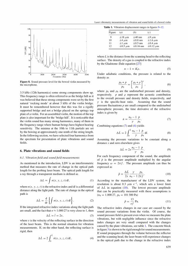
Laser vibrometry measurements of vibration and sound fields of a bowed violin
Figure 8. Sound pressure level for the bowed violin measured bythe microphone.
3.5 kHz (12th harmonics) some strong components show up.This frequency range is often referred to as the bridge hill as itwas believed that these strong components were set by the firstnatural ‘rocking mode’ at about 3 kHz of the violin bridge.It must be remembered however that this was for a rigidlysupported bridge and not a bridge placed on the springy topplate of a violin. For an assembled violin, the motion of the topplate is also important for the ‘bridge hill’. It is noticeable thatthe violin sound has many strong harmonics, many of them inthe frequency range where human beings have highest hearingsensitivity. The minima at the 10th to 11th partials are setby the bowing at approximately one-tenth of the string length.In the following section, we have selected four harmonics fromthe spectrum for presentation of plate vibrations and soundfields.
6. Plate vibrations and sound fields
6.1. Vibration field and sound field measurements
As mentioned in the introduction, LDV is an interferometricmethod that measures the rate of change in the optical pathlength for the probing laser beam. The optical path length fora ray through a transparent medium is defined as
�L =∫
n(x, y, z, t) dl, (1)
where n(x, y, z, t) is the refractive index and dl is a differentialdistance along the light path. The rate of change in the opticalpath is
�L = d
dt
{∫n(x, y, z, t) dl
}. (2)
If the integrated refractive index variations along the light pathare small, and the fact that n ≈ 1.000 27 is very close to 1, then
�L = l = 2v, (3)
where v is the velocity of the reflecting surface in the directionof the laser beam. This is the normal situation for vibrationmeasurements. If, on the other hand, the reflecting surface isrigid, then
�L = 2∫ L
0n(x, y, z, t) dl, (4)
Table 1. Vibration displacement ranges in figures 9–12.
Figure (a) (b) (c)
9 ±18 μm ±40 nm ±9 μm10 ±4 μm ±0.8 nm ±1.6 μm11 ±1 μm ±0.5 nm ±0.4 μm12 ±0.5 μm ±0.16 nm ±0.12 μm
where L is the distance from the scanning head to the reflectingsurface. The density of a gas is coupled to the refractive indexby the Gladstone–Dale equation [27]
n − 1 = Kρ. (5)
Under adiabatic conditions, the pressure is related to thedensity as
p0 + p
p0=
[ρ0 + ρ
ρ0
]γ
, (6)
where p0 and ρ0 are the undisturbed pressure and density,respectively. p and ρ represent the acoustic contributionto the overall pressure and density fields, respectively, andγ is the specific-heat ratio. Assuming that the soundpressure fluctuations p are small compared to the undisturbedatmospheric pressure, the time derivative of the refractiveindex is given by
n = n0 − 1
γ
p
p0. (7)
Combining equations (7) and (4) yields
�L = 2∫ L
0
n0 − 1
γ
p
p0dl. (8)
Assuming the pressure variations to be constant along adistance x and zero elsewhere gives
�L = 2xn0 − 1
γ
p
p0. (9)
For each frequency component of the sound, the amplitudeof p is the pressure amplitude multiplied by the angularfrequency ω = 2πf . The pressure amplitude can thus beexpressed as
p = �L
2x
γ
n0 − 1
p0
2πf. (10)
According to the manufacturer of the LDV system, theresolution is about 0.3 μm s−1, which sets a lower limitof �L in equation (10). The lowest pressure amplitudethat can be practically measured with these assumptions is(n0 = 1.000 27, p0 = 101 300 Pa)
p = 13
xfPa. (11)
The refractive index changes in our case are caused by thesound pressure variations from the violin. Of course, thesound pressure field is present even when we measure the platevibrations, but with negligible influence since the refractiveindex changes are very small compared with the changescaused by the plate vibrations, see table 1. The concrete blockin figure 3 is shown to be rigid enough for sound measurements.If sound propagates through the volume between the reflectorand the scanning head, the laser beam will experience changesin the optical path due to the change in the refractive index
639

P Gren et al
along the whole light path. By scanning the laser beam acrossthe reflector around the violin, we will obtain a 2D map of theintegrated 3D sound field [6]. The results of the plate vibrationfields and the sound fields are best presented as animations.
A comparison between microphone and LDVmeasurements was performed. The microphone wasdirected towards and quite close (a few millimetres) tothe back plate of the bowed violin. The phase differencebetween the microphone and the reference accelerometersignals of the fourth harmonic (1130 Hz) was observed in situon the computer screen. Knowing the mode shape atthis frequency from preliminary LDV measurements, themicrophone was moved across the back plate through areasvibrating in different phases. Moving from two nearbypositions vibrating in anti-phase resulted in a phase shift of180◦ in the microphone signal. From this measurement, itwas clear that the phase of the emitted near-field sound variedin the same way as the plate vibrations recorded by the LDVsystem. This qualitative check thus verifies the expected basicbehaviour of the LDV system.
In the experiments presented below, the LDV systemoperated in the FFT mode with a sampling frequency of20.48 kHz. The LDV system produced frequency spectrausing a complex averaging method with three averages of200 ms, each giving a frequency resolution of 5 Hz.
For the top and back plate measurements, the scanningpoints were spaced approximately 2 cm giving a spatialresolution of the bending waves of 4 cm. For the sound fieldmeasurements, the scanning points were spaced approximately4.5 cm giving a spatial resolution limit of about 9 cm.
6.2. Results
Figures 9–12 show the top and back plate ODSs ((a) and(c)) and the integrated sound field (b) at different frequencies(285 Hz, 1130 Hz, 1415 Hz and 2265 Hz). These figuresare ‘snapshots’ of the attached video animations. It must beunderstood that the LDV software automatically scales thecolour coding (blue–red) within the measuring range, unlessthe operator sets the scales manually. Table 1 summarizes thedisplacement ranges for figures 9–12 and the correspondinganimations. Observe the large differences between the platevibration amplitudes and the integrated sound field amplitudes(amplitude of the optical path length change caused byrefractive index changes).
The operating deflection shapes and sound field at 285 Hz(fundamental of the played tone) are shown in figure 9.The corresponding animations to these images are shown inanimated figures 9(a)–(c). Red areas vibrate in anti-phase tothe blue areas in the top and back plate images.
This frequency is close to the A0 or f-hole mode (the ‘mainair mode’ or ‘Helmholtz mode’) resonance. A nodal line runsthe length of the top plate near the treble bridge foot, whilethe back is without nodes. The plate vibrations are mainlyin the bass side of the top (left side) and the back (right side).The same colour of the top and the back means that the motionis outwards or inwards at the same time, i.e. a breathing modeof the violin body. The wavelength of sound in air at 285 Hzis about 1.2 m. The field of view in figure 9(b) is 83 ×47 cm2. This mode is characterized by considerable soundradiation through the f-holes and its radiativity is known to be
almost spherical. This is confirmed in figure 9(b), which showsalmost equal sound emission in all directions, in phase (equalcolour) both on the front side and the backside. The violin actsmainly as a monopole at this frequency. This mode can easilybe excited by a loudspeaker (since it radiates strongly), by asinusoidal force at the bridge or by a sinusoidal air pressureapplied internally [9]. By looking in more detail, the followingcan be seen. The vibrations are large (red) at the left bridgefoot and small (red-to-blue) at the right bridge foot and thesoundpost. The bridge acts mostly in a rocking motion aroundthe soundpost foot. Furthermore, the whole top plate betweenthe f-holes acts in a see-saw motion, red to the left and blue tothe right side. The vibrations of the back plate at the soundpostposition are also small. The dominant vibrating area (red) ofthe top plate is in the lower part. The maximum amplitudeis close to the left f-hole and is about 18 μm, which can becompared to the stiffer soundpost side vibrating in anti-phasewith an amplitude of about 8 μm.
The operating deflection shapes and sound field at 1130 Hz(fourth partial of the played tone) are shown in figure 10.The corresponding animations to these images are shownin animated figures 10(a)–(c). The wavelength of sound inair is now about 30 cm, close to the violin length, 36 cm.The distances between emitted wave fronts with equal colour(phase) in figure 10(b) are also about 30 cm. The pictures arenow more complex than in figure 9. The bridge feet againmove in anti-phase, i.e. mostly in a rocking motion. The areabetween the f-holes is again split into two parts moving inanti-phase and the vibrations are small at the soundpost, bothin the top and back plate. The top plate tends to split upinto six antinodes with one vertical and two horizontal nodallines. The anti-phase motions of the left and right parts shouldmake the radiation measured with the vibrometer less efficient,but still represent a symmetrical motion along the body. Thelower and upper parts of the front plate are in phase but in anti-phase with the middle part. It is plausible that this generatesa somewhat deformed radiation lobe pointing to the left asis found in figure 10(b). The back plate shows four areasvibrating in anti-phase relative to its neighbours. No verticalnodal line is seen; rather the phase of the antinodes is moreor less constant across the violin back. The radiation close tothe back plate, figure 10(b), mainly shows one part on the topand one at the bottom emitting sound in phase with one partbetween them in anti-phase. This radiation pattern remindsus somewhat of three sound sources on a line in anti-phase asin Cremer [1], p 418. The directivity [28–31] of this mode isquite strong compared to the more spherical sound distributionfound in figure 9(b). The wavelength of the sound in air is nowslightly larger than the wavelength of the bending waves of theplates.
The operating deflection shapes and sound field at 1415 Hz(fifth partial of the played tone) are shown in figure 11.The corresponding animations to these images are shown inanimated figures 11(a)–(c). The ODS of the top plate showsa similar split-up as in the previous figure 10(a). The two feetof the bridge again vibrate in anti-phase. The vibrations atthe soundpost are noticeable, also in the back plate. The ODSof the back plate now shows four areas of anti-phase motionin the lower part. In the top part, the antinodes cover almostthe whole width of the violin. The sound field in figure 11(b)
640

Laser vibrometry measurements of vibration and sound fields of a bowed violin
Figure 9. Vibration and sound fields at the first harmonic (285 Hz). (a) Top plate ODS, (b) sound field and (c) back plate ODS.
M An MPEG movie of this figure is available from stacks.iop.org/MST/17/635
Figure 10. Vibration and sound fields at the fourth harmonic (1130 Hz). (a) Top plate ODS, (b) sound field and (c) back plate ODS.
M An MPEG movie of this figure is available from stacks.iop.org/MST/17/635
(remember that it is the projected sound field that is visualized)is harder to interpret and weaker than before. It however showsradiation lobes of varying strength as can be expected. Onelobe is radiating from the upper part and one from the lowerpart of the violin. Again the wavelengths of the sound and thelongitudinal bending waves are of the same magnitudes.
The operating deflection shapes and sound field at 2265 Hz(eighth partial of the played tone) are shown in figure 12.The corresponding animations to these images are shown inanimated figures 12(a)–(c). This partial is of almost the samestrength as the fifth partial in figure 11. The ODSs are nowdivided into a larger number of antinodes. As many as sixantinodes can be seen in the lower part of the top plate and fourin the lowest part of the back plate. Several horizontal nodallines, four to five, can be seen in both plates. The radiationfrom such complicated vibration patterns will of course alsobe quite complicated, compared to the near-field distributionand the more distant radiation pattern. Radiation wavefrontsfrom the top plate, the upper part and another set from themiddle part can however be seen. The two sets of wavefrontsare of anti-phase. Still, it must be noticed that such modes areimportant to the total picture of the violin sound.
7. Discussion
The sound of a single note from a melodic musical instrumentcan be divided into a fundamental frequency tone and anumber of harmonic partials. The string has this ability; ithas a fundamental frequency plus a number of higher partials,depending upon the way it has been excited. The string itselfis however a very weak emitter of sound, and its diameter istoo thin compared to the aerial wavelength of the sound to beproduced. Ordinary wooden plates and shells normally do notgenerate harmonic partials when moderately excited, but, onthe other hand, they are efficient sound emitters. The violinuses a combination of string vibrations and plate/body modes.It operates in such a way that forced vibrations at the harmonicstring partials set the violin body into vibration to produce thesound. In this way, both harmonic partials and an efficientsound production are achieved.
Bowing the string is a very efficient way to excite thestring both vigorously and continuously. It vibrates in afundamental and a high number of partials and produces a longsustained tone. The rosined rotating bow in our experimentsmodels the bow–string interaction in an idealized way. The
641

P Gren et al
Figure 11. Vibration and sound fields at the fifth harmonic (1415 Hz). (a) Top plate ODS, (b) sound field and (c) back plate ODS.
M An MPEG movie of this figure is available from stacks.iop.org/MST/17/635
Figure 12. Vibration and sound fields at the eighth harmonic (2265 Hz). (a) Top plate ODS, (b) sound field and (c) back plate ODS.
M An MPEG movie of this figure is available from stacks.iop.org/MST/17/635
bowing velocity, bowing force and direction of bowing arekept constant. The string is excited both horizontally andvertically as well by rotation. Neither the start nor the endsof a real played note are considered in our experiments. Theset-up models the middle, constant portion of a real playednote, repeated every fundamental period. In real life, a skilledmusician can vary the bowing speed, the bowing pressure(i.e. the force by which the bow is pressed against the string)and bowing position to change the relative frequency contentof the sound in a wide range as well as the radiated soundpower. Measurements have been performed on the bowedopen D-string vibrations, close to the bowing point. Thebow–string interaction produces a triangular shaped wave, seefigure 4, which is reflected at the bridge and transmits energyand momentum into forced vibrations to the rest of theinstrument. These forced vibrations set the instrument intovibration at the fundamental string frequency and all partialfrequencies simultaneously. The bridge is constructed in aningenious way so that it efficiently transmits the vibration,mainly as a rocking and a stamping vibration, to both itsfeet which sets the rest of the violin body into vibration, seefigures 6 and 7.
The violin body may look symmetric from the outsidebut its construction is not. Close to and beneath the treble
bridge foot, the soundpost is situated. It transmits vibrationsfrom the bridge and the top plate to the back plate in a verydirect way. Beneath the bass bridge foot, there is a bar gluedto the inside of the top plate that efficiently transmits bendingwaves in the top plate along the instrument. The top plate ismade out of spruce and the back plate of maple, wooden plateswith quite different mechanical behaviour. Spruce is both avery stiff and very light anisotropic material that allows a veryhigh bending wave speed along the grains and a somewhatslower speed across the grains. The top plate, back plateand the ribs form an almost closed air volume open only atthe two f-holes in the top plate. Measurements of the topand back plate vibration fields of the bowed violin at the openD-string show that a high number of strong harmonic vibrationcomponents are generated. In the frequency range between 2and 5 kHz, where the sensitivity of human hearing is high, theviolin has a number of quite strong components. It is clear thatthe mode density (number of eigenmodes/frequency interval)of the violin body is quite low below, say, 1 kHz. This meansthat it is more likely that the fifth partial of the string is closeto an eigenmode of the violin body than the first partial. Inthe lower frequency range, the violin should be treated as abody, for instance, as an elliptical tube closed at the ends [11],
642

Laser vibrometry measurements of vibration and sound fields of a bowed violin
so that both the top and the back plate and the ribs are partsof a number of the first lower vibration modes below, say,800 Hz. For higher modes, the vibrating areas get smallerand they tend to localize inside the parts of the violin plates.Forced vibrations of the violin body at a certain frequency willset the different vibration modes into vibration, both thosebelow and those above the forced vibration frequency. Thisoften results in quite complicated sums of nearby vibrationmodes (ODSs) that operate together but not in simple phaserelations any longer.
The dimensions of the violin are small compared with theaerial wavelength at frequencies below, say, 1 kHz. Above,say, 2 kHz, the bending wavelength of the wooden violinplates is more of the same order as the aerial wavelength andconsequently the violin is an efficient radiator of sound athigher frequencies.
There are two main sound sources of the violin body: theair modes and the body (plate) modes. Both are importantfor the total performance of the violin. They are both setinto forced vibrations by the bow–string interaction, mainlytransmitted through the bridge. In figure 9, the ‘main airmode, A0’, or ‘Helmholtz mode’ is seen. It is acting as anefficient sound source, almost as a mono-source. Note alsothat the violin is small compared to the aerial wavelength at thisfrequency. The violin body, here, is vibrating as a ‘breathing’mode at this frequency so that the total sound of both the airmode and the co-vibrating walls is generated together. Theasymmetry of the violin is also noticeable. At frequenciesbelow, say, 600 Hz, the relative frequency difference betweensound generating modes is quite large (the mode density islow) and it is very crucial to the performance of the instrumentthat these modes are distributed evenly.
Measurements of the sound fields generated by the bowedviolin were performed. Interesting animated movies of thefundamental component as well as higher harmonics arevisualized. When analysing these fields it must always beremembered that it is the projected, radiated sound field acrossthe violin which is shown. If the probing laser ray is passingthrough both a high sound pressure and an equally strong soundpressure in opposite phase, the projected result may look as ifno sound was produced at all. If the measurements had beenperformed so that these two fields were beside and not behindeach other, two strong radiation centres would have been seen.Below 800 Hz, the violin acts mainly as a mono-source withalmost equal sound intensity in all directions. But already atfrequencies above, say, 800 Hz, the violin directivity starts toget important.
When looking at the fourth and fifth harmonics, figures 10and 11, the aerial wavelength is getting comparable in size tothe bending waves in the violin body. These harmonics start toshow directivity. In the eighth harmonics, figure 12, the modedensity of the violin body is quite high, and many smallervibrating areas show up. The radiation from the top plate sideis strong and is divided into directional lobes. Good violinsoften show a set of strong radiation modes at frequencies from2 to 5 kHz.
8. Conclusions
Laser vibrometry has been shown to be a versatile techniqueto study vibration fields not only of most parts of the violin
but also of the sound fields in air, generated by the vibrationfields of the violin. The technique is non-contacting andnon-disturbing. It is the middle, sustained, part of a bowedtone that is studied in this investigation. A rotating bow wastherefore developed to generate the long lasting sound thatallows scanning laser vibrometry to be used. A critical pointin the measurements is to obtain a triggering signal from amicrophone or an accelerometer that allows the measuringpoint to be moved (scanned) and still keep track of the relativephase of the signal at the different measuring points. This iscrucial for a successful modal analysis of the measurements.
Measurements of the bridge motion confirm that the stringvibrations are transferred to the bridge both in the horizontaland vertical directions. The bridge efficiently transfers thestring vibrations to the body of the instrument at the bridgefeet, mainly by a combination of a rocking and a stampingmotion of the bridge.
Both air modes of the enclosed air and body and platemodes contribute to the total generated sound. It is alsoapparent that the back plate is an equally important soundradiator as the top plate. In spite of all investigations, muchis lacking for a complete fundamental understanding of thephysics of the violin, especially at higher frequencies. Themeasured ODSs verify previous results obtained with the HS71violin [3, 8] and add understanding of how eigenmodes maycombine.
One disadvantage of using the LDV sound fieldvisualization is the fact that the sound field is integrated over aline. This means nearby vibrations in anti-phase, for example,could result in low integrated pressure values. On the otherhand, this gives a 2D image of the sound field and openspossibilities for tomographic 3D reconstructions of the soundfields if several projections can be obtained.
Another possibility is opened by the measurements; thesound field generated by the vibrating violin panels can becalculated from the measured ODSs (phase and amplitude).These calculations can be compared to measured LDV soundfields. This work is in progress. To examine the parts thatoriginate from the vibrating panels and the enclosed air, onecould try to measure with or without cotton pads in the f-holes. Indeed the projected sound fields measured with LDVopen several possibilities which are difficult to perform usingmicrophones.
In a planned subsequent paper, three violins of varyingquality—all bowed in the same way at the open E-string—will be compared, firstly, to verify if the main findings of theHS71 violin are valid for violins in general and, secondly, totest if differences can be proved between the best violins (OldItalian violins) and quite different but still good violins (Frenchviolins).
Will new acoustical factors be introduced or are the abovepresented factors differently used?
Acknowledgment
We are very grateful to the Kempe foundations for supportingthis project and also for financing the purchase of the laservibrometer.
643

P Gren et al
References
[1] Cremer L 1984 The Physics of the Violin (Cambridge, MA:MIT Press) (Original title: 1981 Physik der Geige(Stuttgart: Hirzel))
[2] Jansson E 2002 Acoustics for violin and guitar makershttp://www.speech.kth.se/music/acviguit4/index.html
[3] Jansson E, Molin N-E and Sundin H 1970 Resonances of aviolin body studied by hologram interferometry andacoustical methods Phys. Scr. 2 243–56
[4] Reinecke W and Cremer L 1970 Application of holographicinterferometry to vibrations of the bodies of stringinstruments J. Acoust. Soc. Am. 48 988
[5] Drain L E 1980 The Laser Doppler Technique (London:Wiley) pp 220–7
[6] Zipser L, Franke H, Olsson E, Molin N-E and Sjodahl M 2003Reconstructing two-dimensional acoustic object fields byuse of digital phase conjugation of scanning laservibrometry recordings Appl. Opt. 42 5831–8
[7] Molin N-E and Zipser L 2004 Optical methods of today forvisualizing sound fields in musical acoustics Acta Acusticaunited with Acustica 90 618–28
[8] Jansson E V, Molin N-E and Saldner H O 1994 Oneigenmodes of the violin—electronic holography andadmittance measurements J. Acoust. Soc. Am. 95 1100–5
[9] Roberts M and Rossing T 1998 Normal modes of vibration inviolins Catgut Acoust. Soc. J. 3 (5) 9–15
[10] Saldner H O, Molin N-E and Jansson E V 1996 Vibrationmodes of the violin forced via the bridge and action of thesoundpost J. Acoust. Soc. Am. 100 1168–77
[11] Runnemalm A, Molin N-E and Jansson E V 2000 Onoperating deflection shapes of the violin body includingin-plane motions J. Acoust. Soc. Am. 107 3452–9
[12] Richardson M H 1997 Is it a mode shape or an operatingdeflection shape? Sound Vib. 31 54–61
[13] Molin N-E, Wåhlin A O and Jansson E V 1990 Transient waveresponse of the violin body J. Acoust. Soc. Am. 88 2479–81
[14] Molin N-E, Wåhlin A O and Jansson E V 1991 Transient waveresponse of the violin body revisited J. Acoust. Soc.Am. 90 2192–5
[15] Bissinger G 2003 Wall compliance and violin cavity modesJ. Acoust. Soc. Am. 113 1718–23
[16] Bissinger G 2003 Modal analysis of a violin octet J. Acoust.Soc. Am. 113 2105–13
[17] Bissinger G 2004 Contemporary generalized normal modeviolin acoustics Acta Acustica united with Acustica 90590–9
[18] Wang L M and Burroughs C B 2001 Acoustic radiation frombowed violins J. Acoust. Soc Am. 110 543–55
[19] Bretos L J, Santamaria C and Alonso M J 1999 Vibrationalpatterns and frequency responses of the free plates and boxof a violin obtained by finite element analysis J. Acoust.Soc. Am. 85 584–6
[20] Saunders F A 1937 The mechanical actions of violinsJ. Acoust. Soc. Am. 9 87
[21] Meinel H 1937 Uber die Beziehungen zwischen Holtzdicke,Schwingungsform, Korperamplitude und Klang einesGeigenkorpers Elektrische Nachrichten-Teknik 4 120
[22] Molin N-E 2002 Visualizing instrument vibrations andsound fields—the state of the art Catgut Acoust. Soc. J.4 (5) 21–9
[23] Helmholz H 1862 Die Lehre von den Tonempfindungen(Braunschweig: Vieweg) (On the Sensations of Tone, transl.A Ellis (New York: Dover))
[24] Askenfelt A 1986 Measurement of bow motion and bow forcein violin playing J. Acoust. Soc. Am. 80 1007–15
[25] Woodhouse J 2004 The bowed string as we know it today ActaAcustica united with Acustica 90 579–89
[26] Woodhouse J 2005 On the ‘bridge hill’ of the ‘violin’ ActaAcustica united with Acustica 91 155–65
[27] Vest C M 1979 Holographic Interferometry (New York:Wiley)
[28] Meyer J 1972 Directivity of bowed stringed instruments andits effect on orchestral sound in concert halls J. Acoust. Soc.Am. 51 1994–2009
[29] Saldner H, Molin N-E and Jansson E V 1997 Sounddistribution from forced vibration modes of a violinmeasured by reciprocity and TV holography Catgut Acoust.Soc. J. 3 (4) 10–16
[30] Weinreich G 2002 Sound radiation from the violin—as we know it today Catgut Acoust. Soc. J. 4 (5)37–42
[31] Weinreich G 1997 Directional tone color J. Acoust. Soc.Am. 101 2338–46
644

