Machine Learning Projects for .NETDevelopers

Mathias Brandewinder

Machine Learning Projects for .NET Developers

Copyright © 2015 by Mathias Brandewinder

This work is subject to copyright. All rights are reserved by the Publisher, whether the whole or part of thematerial is concerned, specifically the rights of translation, reprinting, reuse of illustrations, recitation,broadcasting, reproduction on microfilms or in any other physical way, and transmission or information storageand retrieval, electronic adaptation, computer software, or by similar or dissimilar methodology now known orhereafter developed. Exempted from this legal reservation are brief excerpts in connection with reviews orscholarly analysis or material supplied specifically for the purpose of being entered and executed on a computersystem, for exclusive use by the purchaser of the work. Duplication of this publication or parts thereof ispermitted only under the provisions of the Copyright Law of the Publisher’s location, in its current version, andpermission for use must always be obtained from Springer. Permissions for use may be obtained throughRightsLink at the Copyright Clearance Center. Violations are liable to prosecution under the respectiveCopyright Law.

ISBN-13 (pbk): 978-1-4302-6767-6

ISBN-13 (electronic): 978-1-4302-6766-9

Trademarked names, logos, and images may appear in this book. Rather than use a trademark symbol withevery occurrence of a trademarked name, logo, or image we use the names, logos, and images only in aneditorial fashion and to the benefit of the trademark owner, with no intention of infringement of the trademark.

The use in this publication of trade names, trademarks, service marks, and similar terms, even if they are notidentified as such, is not to be taken as an expression of opinion as to whether or not they are subject toproprietary rights.

While the advice and information in this book are believed to be true and accurate at the date of publication,neither the authors nor the editors nor the publisher can accept any legal responsibility for any errors oromissions that may be made. The publisher makes no warranty, express or implied, with respect to the materialcontained herein.

Managing Director: Welmoed SpahrLead Editor: Gwenan SpearingTechnical Reviewer: Scott WlaschinEditorial Board: Steve Anglin, Mark Beckner, Gary Cornell, Louise Corrigan, Jim DeWolf, Jonathan

Gennick, Robert Hutchinson, Michelle Lowman, James Markham, Susan McDermott, MatthewMoodie, Jeffrey Pepper, Douglas Pundick, Ben Renow-Clarke, Gwenan Spearing, Matt Wade,Steve Weiss

Coordinating Editor: Melissa Maldonado and Christine RickettsCopy Editor: Kimberly Burton-Weisman and April RondeauCompositor: SPi GlobalIndexer: SPi GlobalArtist: SPi Global

Distributed to the book trade worldwide by Springer Science+Business Media New York, 233 Spring Street, 6thFloor, New York, NY 10013. Phone 1-800-SPRINGER, fax (201) 348-4505, e-mail orders-ny@springer-sbm.com, or visit www.springeronline.com. Apress Media, LLC is a CaliforniaLLC and the sole member (owner) is Springer Science + Business Media Finance Inc (SSBM Finance Inc).SSBM Finance Inc is a Delaware corporation.

For information on translations, please e-mail rights@apress.com, or visit www.apress.com.

Apress and friends of ED books may be purchased in bulk for academic, corporate, or promotional use. eBookversions and licenses are also available for most titles. For more information, reference our Special Bulk Sales–

eBook Licensing web page at www.apress.com/bulk-sales.

Any source code or other supplementary material referenced by the author in this text is available to readers atwww.apress.com. For detailed information about how to locate your book’s source code, go towww.apress.com/source-code/.

Contents at a Glance

About the AuthorAbout the Technical ReviewerAcknowledgmentsIntroduction

Chapter 1: 256 Shades of Gray Chapter 2: Spam or Ham? Chapter 3: The Joy of Type Providers Chapter 4: Of Bikes and Men Chapter 5: You Are Not a Unique Snowflake Chapter 6: Trees and Forests Chapter 7: A Strange Game Chapter 8: Digits, Revisited Chapter 9: Conclusion

Index

Contents

About the AuthorAbout the Technical ReviewerAcknowledgmentsIntroduction

Chapter 1: 256 Shades of GrayWhat Is Machine Learning?A Classic Machine Learning Problem: Classifying Images

Our Challenge: Build a Digit RecognizerDistance Functions in Machine LearningStart with Something Simple

Our First Model, C# VersionDataset OrganizationReading the DataComputing Distance between ImagesWriting a Classifier

So, How Do We Know It Works?Cross-validationEvaluating the Quality of Our ModelImproving Your Model

Introducing F# for Machine LearningLive Scripting and Data Exploration with F# InteractiveCreating our First F# ScriptDissecting Our First F# ScriptCreating Pipelines of FunctionsManipulating Data with Tuples and Pattern MatchingTraining and Evaluating a Classifier Function

Improving Our Model

Experimenting with Another Definition of DistanceFactoring Out the Distance Function

So, What Have We Learned?What to Look for in a Good Distance FunctionModels Don’t Have to Be ComplicatedWhy F#?

Going Further Chapter 2: Spam or Ham?Our Challenge: Build a Spam-Detection Engine

Getting to Know Our DatasetUsing Discriminated Unions to Model LabelsReading Our Dataset

Deciding on a Single WordUsing Words as CluesPutting a Number on How Certain We AreBayes’ TheoremDealing with Rare Words

Combining Multiple WordsBreaking Text into TokensNaïvely Combining ScoresSimplified Document Score

Implementing the ClassifierExtracting Code into ModulesScoring and Classifying a DocumentIntroducing Sets and SequencesLearning from a Corpus of Documents

Training Our First ClassifierImplementing Our First TokenizerValidating Our Design InteractivelyEstablishing a Baseline with Cross-validation

Improving Our ClassifierUsing Every Single WordDoes Capitalization Matter?Less Is more

Choosing Our Words CarefullyCreating New FeaturesDealing with Numeric Values

Understanding ErrorsSo What Have We Learned?

Chapter 3: The Joy of Type ProvidersExploring StackOverflow data

The StackExchange APIUsing the JSON Type ProviderBuilding a Minimal DSL to Query Questions

All the Data in the WorldThe World Bank Type ProviderThe R Type ProviderAnalyzing Data Together with R Data FramesDeedle, a .NET Data FrameData of the World, Unite!

So, What Have We Learned?Going Further

Chapter 4: Of Bikes and MenGetting to Know the Data

What’s in the Dataset?Inspecting the Data with FSharp.ChartingSpotting Trends with Moving Averages

Fitting a Model to the DataDefining a Basic Straight-Line ModelFinding the Lowest-Cost ModelFinding the Minimum of a Function with Gradient DescentUsing Gradient Descent to Fit a CurveA More General Model Formulation

Implementing Gradient DescentStochastic Gradient DescentAnalyzing Model ImprovementsBatch Gradient Descent

Linear Algebra to the RescueHoney, I Shrunk the Formula!Linear Algebra with Math.NETNormal FormPedal to the Metal with MKL

Evolving and Validating Models RapidlyCross-Validation and Over-Fitting, AgainSimplifying the Creation of ModelsAdding Continuous Features to the Model

Refining Predictions with More FeaturesHandling Categorical FeaturesNon-linear FeaturesRegularization

So, What Have We Learned?Minimizing Cost with Gradient DescentPredicting a Number with Regression

Chapter 5: You Are Not a Unique SnowflakeDetecting Patterns in DataOur Challenge: Understanding Topics on StackOverflow

Getting to Know Our Data

Finding Clusters with K-Means ClusteringImproving Clusters and CentroidsImplementing K-Means Clustering

Clustering StackOverflow TagsRunning the Clustering AnalysisAnalyzing the Results

Good Clusters, Bad ClustersRescaling Our Dataset to Improve ClustersIdentifying How Many Clusters to Search For

What Are Good Clusters?Identifying k on the StackOverflow DatasetOur Final Clusters

Detecting How Features Are RelatedCovariance and CorrelationCorrelations Between StackOverflow Tags

Identifying Better Features with Principal Component AnalysisRecombining Features with AlgebraA Small Preview of PCA in ActionImplementing PCAApplying PCA to the StackOverflow DatasetAnalyzing the Extracted Features

Making RecommendationsA Primitive Tag RecommenderImplementing the RecommenderValidating the Recommendations

So What Have We Learned? Chapter 6: Trees and ForestsOur Challenge: Sink or Swim on the Titanic

Getting to Know the DatasetTaking a Look at FeaturesBuilding a Decision StumpTraining the Stump

Features That Don’t FitHow About Numbers?What about Missing Data?

Measuring Information in DataMeasuring Uncertainty with EntropyInformation GainImplementing the Best Feature IdentificationUsing Entropy to Discretize Numeric Features

Growing a Tree from DataModeling the TreeConstructing the TreeA Prettier Tree

Improving the TreeWhy Are We Over-Fitting?

Limiting Over-Confidence with Filters

From Trees to ForestsDeeper Cross-Validation with k-foldsCombining Fragile Trees into Robust ForestsImplementing the Missing BlocksGrowing a ForestTrying Out the Forest

So, What Have We Learned? Chapter 7: A Strange GameBuilding a Simple Game

Modeling Game ElementsModeling the Game LogicRunning the Game as a Console AppRendering the Game

Building a Primitive BrainModeling the Decision Making ProcessLearning a Winning Strategy from ExperienceImplementing the BrainTesting Our Brain

Can We Learn More Effectively?Exploration vs. ExploitationIs a Red Door Different from a Blue Door?Greed vs. Planning

A World of Never-Ending TilesImplementing Brain 2.0

Simplifying the WorldPlanning AheadEpsilon Learning

So, What Have We Learned?A Simple Model That Fits IntuitionAn Adaptive Mechanism

Chapter 8: Digits, RevisitedOptimizing and Scaling Your Algorithm Code

Tuning Your CodeWhat to Search ForTuning the DistanceUsing Array.Parallel

Different Classifiers with Accord.NETLogistic RegressionSimple Logistic Regression with AccordOne-vs-One, One-vs-All ClassificationSupport Vector MachinesNeural NetworksCreating and Training a Neural Network with Accord

Scaling with m-brace.netGetting Started with MBrace on Azure with BriskProcessing Large Datasets with MBrace

So What Did We Learn? Chapter 9: ConclusionMapping Our JourneyScience!F#: Being Productive in a Functional StyleWhat’s Next?

Index

About the Author

Mathias Brandewinder is a Microsoft MVP for F# and is based in San Francisco,California, where he works for Clear Lines Consulting. An unashamed math geek, hebecame interested early on in building models to help others make better decisionsusing data. He collected graduate degrees in business, economics, and operationsresearch, and fell in love with programming shortly after arriving in the Silicon Valley.He has been developing software professionally since the early days of .NET,developing business applications for a variety of industries, with a focus on predictivemodels and risk analysis.

About the Technical Reviewer

Scott Wlaschin is a .NET developer, architect, and author. He has over 20 years ofexperience in a wide variety of areas from high-level UX/UI to low-level databaseimplementations.

He has written serious code in many languages, his favorites being Smalltalk,Python, and more recently F#, which he blogs about atfsharpforfunandprofit.com.

Acknowledgments

Thanks to my parents, I grew up in a house full of books; books have profoundlyinfluenced who I am today. My love for them is in part what lead me to embark on thiscrazy project, trying to write one of my own, despite numerous warnings that the journeywould be a rough one. The journey was rough, but totally worth it, and I am incrediblyproud: I wrote a book, too! For this, and much more, I’d like to thank my parents.

Going on a journey alone is no fun, and I was very fortunate to have three greatcompanions along the way: Gwenan the Fearless, Scott the Wise, and Petar the Rock.Gwenan Spearing and Scott Wlaschin have relentlessly reviewed the manuscript andgiven me invaluable feedback, and have kept this project on course. The end result hasturned into something much better than it would have been otherwise. You have them tothank for the best parts, and me to blame for whatever problems you might find!

I owe a huge, heartfelt thanks to Petar Vucetin. I am lucky to have him as a businesspartner and as a friend. He is the one who had to bear the brunt of my moods and darkermoments, and still encouraged me and gave me time and space to complete this. Thanks,dude—you are a true friend.

Many others helped me out on this journey, too many to mention them all in here. Toeveryone who made this possible, be it with code, advice, or simply kind words, thankyou—you know who you are! And, in particular, a big shoutout to the F# community. Itis vocal (apparently sometimes annoyingly so), but more important, it has been atremendous source of joy and inspiration to get to know many of you. Keep beingawesome!

Finally, no journey goes very far without fuel. This particular journey was heavilypowered by caffeine, and Coffee Bar, in San Francisco, has been the place where Ifound a perfect macchiato to start my day on the right foot for the past year and a half.

Introduction

If you are holding this book, I have to assume that you are a .NET developer interestedin machine learning. You are probably comfortable with writing applications in C#,most likely line-of-business applications. Maybe you have encountered F# before,maybe not. And you are very probably curious about machine learning. The topic isgetting more press every day, as it has a strong connection to software engineering, butit also uses unfamiliar methods and seemingly abstract mathematical concepts. In short,machine learning looks like an interesting topic, and a useful skill to learn, but it’sdifficult to figure out where to start.

This book is intended as an introduction to machine learning for developers. Mymain goal in writing it was to make the topic accessible to a reader who is comfortablewriting code, and is not a mathematician. A taste for mathematics certainly doesn’t hurt,but this book is about learning some of the core concepts through code by usingpractical examples that illustrate how and why things work.

But first, what is machine learning? Machine learning is the art of writing computerprograms that get better at performing a task as more data becomes available, withoutrequiring you, the developer, to change the code.

This is a fairly broad definition, which reflects the fact that machine learningapplies to a very broad range of domains. However, some specific aspects of thatdefinition are worth pointing out more closely. Machine learning is about writingprograms—code that runs in production and performs a task—which makes it differentfrom statistics, for instance. Machine learning is a cross-disciplinary area, and is atopic relevant to both the mathematically-inclined researcher and the software engineer.

The other interesting piece in that definition is data. Machine learning is aboutsolving practical problems using the data you have available. Working with data is akey part of machine learning; understanding your data and learning how to extract usefulinformation from it are quite often more important than the specific algorithm you willuse. For that reason, we will approach machine learning starting with data. Each chapterwill begin with a real dataset, with all its real-world imperfections and surprises, and aspecific problem we want to address. And, starting from there, we will build a solutionto the problem from the ground up, introducing ideas as we need them, in context. As wedo so, we will create a foundation that will help you understand how different ideaswork together, and will make it easy later on to productively use libraries orframeworks, if you need them.

Our exploration will start in the familiar grounds of C# and Visual Studio, but as we

progress we will introduce F#, a .NET language that is particularly suited for machinelearning problems. Just like machine learning, programming in a functional style can beintimidating at first. However, once you get the hang of it, F# is both simple andextremely productive. If you are a complete F# beginner, this book will walk youthrough what you need to know about the language, and you will learn how to use itproductively on real-world, interesting problems.

Along the way, we will explore a whole range of diverse problems, which will giveyou a sense for the many places and perhaps unexpected ways that machine learning canmake your applications better. We will explore image recognition, spam filters, and aself-learning game, and much more. And, as we take that journey together, you will seethat machine learning is not all that complicated, and that fairly simple models canproduce surprisingly good results. And, last but not least, you will see that machinelearning is a lot of fun! So, without further ado, let’s start hacking on our first machinelearning problem.

CHAPTER 1

256 Shades of Gray

Building a Program to AutomaticallyRecognize Images of NumbersIf you were to create a list of current hot topics in technology, machine learning wouldcertainly be somewhere among the top spots. And yet, while the term shows upeverywhere, what it means exactly is often shrouded in confusion. Is it the same thing as“big data,” or perhaps “data science”? How is it different from statistics? On thesurface, machine learning might appear to be an exotic and intimidating specialty thatuses fancy mathematics and algorithms, with little in common with the daily activities ofa software engineer.

In this chapter, and in the rest of this book, my goal will be to demystify machinelearning by working through real-world projects together. We will solve problems stepby step, primarily writing code from the ground up. By taking this approach, we will beable to understand the nuts and bolts of how things work, illustrating along the way coreideas and methods that are broadly applicable, and giving you a solid foundation onwhich to build specialized libraries later on. In our first chapter, we will dive right inwith a classic problem—recognizing hand-written digits—doing a couple of thingsalong the way:

Establish a methodology applicable across most machine learningproblems. Developing a machine learning model is subtly differentfrom writing standard line-of-business applications, and it comeswith specific challenges. At the end of this chapter, you willunderstand the notion of cross-validation, why it matters, and howto use it.

Get you to understand how to “think machine learning” and how to

look at ML problems. We will discuss ideas like similarity anddistance, which are central to most algorithms. We will also showthat while mathematics is an important ingredient of machinelearning, that aspect tends to be over-emphasized, and some of thecore ideas are actually fairly simple. We will start with a ratherstraightforward algorithm and see that it actually works pretty well!

Know how to approach the problem in C# and F#. We’ll begin withimplementing the solution in C# and then present the equivalentsolution in F#, a .NET language that is uniquely suited for machinelearning and data science.

Tackling such a problem head on in the first chapter might sound like a daunting taskat first—but don’t be intimidated! It is a hard problem on the surface, but as you willsee, we will be able to create a pretty effective solution using only fairly simplemethods. Besides, where would be the fun in solving trivial toy problems?

What Is Machine Learning?But first, what is machine learning? At its core, machine learning is writing programsthat learn how to perform a task from experience, without being explicitly programmedto do so. This is still a fuzzy definition, and begs the question: How do you definelearning, exactly? A somewhat dry definition is the following: A program is learning if,as it is given more data points, it becomes automatically better at performing a giventask. Another way to look at it is by flipping around the definition: If you keep doing thesame thing over and over again, regardless of the results you observe, you are certainlynot learning.

This definition summarizes fairly well what “doing machine learning” is about.Your goal is to write a program that will perform some task automatically. The programshould be able to learn from experience, either in the form of a pre-existing dataset ofpast observations, or in the form of data accumulated by the program itself as itperforms its job (what’s known as “online learning”). As more data becomes available,the program should become better at the task without your having to modify the code ofthe program itself.

Your job in writing such a program involves a couple of ingredients. First, yourprogram will need data it can learn from. A significant part of machine learningrevolves around gathering and preparing data to be in a form your program will be ableto use. This process of reorganizing raw data into a format that better represents theproblem domain and that can be understood by your program is called feature

extraction.Then, your program needs to be able to understand how well it is performing its

task, so that it can adjust and learn from experience. Thus, it is crucial to define ameasure that properly captures what it means to “do the task” well or badly.

Finally, machine learning requires some patience, an inquisitive mind, and a lot ofcreativity! You will need to pick an algorithm, feed it data to train a predictive model,validate how well the model performs, and potentially refine and iterate, maybe bydefining new features, or maybe by picking a new algorithm. This cycle—learning fromtraining data, evaluating from validation data, and refining—is at the heart of themachine learning process. This is the scientific method in action: You are trying toidentify a model that adequately predicts the world by formulating hypotheses andconducting a series of validation experiments to decide how to move forward.

Before we dive into our first problem, two quick comments. First, this might soundlike a broad description, and it is. Machine learning applies to a large spectrum ofproblems, ranging all the way from detecting spam email and self-driving cars torecommending movies you might enjoy, automatic translation, or using medical data tohelp with diagnostics. While each domain has its specificities and needs to be wellunderstood in order to successfully apply machine learning techniques, the principlesand methods remain largely the same.

Then, note how our machine learning definition explicitly mentions “writingprograms.” Unlike with statistics, which is mostly concerned with validating whether ornot a model is correct, the end goal of machine learning is to create a program that runsin production. As such, it makes it a very interesting area to work in, first because it isby nature cross-disciplinary (it is difficult to be an expert in both statistical methods andsoftware engineering), and then because it opens up a very exciting new field forsoftware engineers.

Now that we have a basic definition in place, let’s dive into our first problem.

A Classic Machine Learning Problem:Classifying ImagesRecognizing images, and human handwriting in particular, is a classic problem inmachine learning. First, it is a problem with extremely useful applications.Automatically recognizing addresses or zip codes on letters allows the post office toefficiently dispatch letters, sparing someone the tedious task of sorting them manually;being able to deposit a check in an ATM machine, which recognizes amounts, speeds upthe process of getting the funds into your account, and reduces the need to wait in line at

the bank. And just imagine how much easier it would be to search and exploreinformation if all the documents written by mankind were digitized! It is also a difficultproblem: Human handwriting, and even print, comes with all sorts of variations (size,shape, slant, you name it); while humans have no problem recognizing letters and digitswritten by various people, computers have a hard time dealing with that task. This is thereason CAPTCHAs are such a simple and effective way to figure out whether someoneis an actual human being or a bot. The human brain has this amazing ability to recognizeletters and digits, even when they are heavily distorted.

FUN FACT: CAPTCHA AND RECAPTCHA

CAPTCHA (“Completely Automated Public Turing test to tell Computers andHumans Apart”) is a mechanism devised to filter out computer bots from humans.To make sure a user is an actual human being, CAPTCHA displays a piece of textpurposefully obfuscated to make automatic computer recognition difficult. In anintriguing twist, the idea has been extended with reCAPTCHA. reCAPTCHAdisplays two images instead of just one: one of them is used to filter out bots,while the other is an actual digitized piece of text (see Figure 1-1). Every time ahuman logs in that way, he also helps digitize archive documents, such as backissues of the New York Times, one word at a time.

Figure 1-1. A reCAPTCHA example

Our Challenge: Build a Digit RecognizerThe problem we will tackle is known as the “Digit Recognizer,” and it is directlyborrowed from a Kaggle.com machine learning competition. You can find all theinformation about it here: http://www.kaggle.com/c/digit-recognizer

Here is the challenge: What we have is a dataset of 50,000 images. Each image is asingle digit, written down by a human, and scanned in 28 × 28 pixels resolution,encoded in grayscale, with each pixel taking one of 256 possible shades of gray, fromfull white to full black. For each scan, we also know the correct answer, that is, whatnumber the human wrote down. This dataset is known as the training set. Our goal nowis to write a program that will learn from the training set and use that information to

make predictions for images it has never seen before: is it a zero, a one, and so on.Technically, this is known as a classification problem: Our goal is to separate

images between known “categories,” a.k.a. the classes (hence the word“classification”). In this case, we have ten classes, one for each single digit from 0 to 9.Machine learning comes in different flavors depending on the type of question you aretrying to resolve, and classification is only one of them. However, it’s also perhaps themost emblematic one. We’ll cover many more in this book!

So, how could we approach this problem? Let’s start with a different question first.Imagine that we have just two images, a zero and a one (see Figure 1-2):

Figure 1-2. Sample digitized 0 and 1

Suppose now that I gave you the image in Figure 1-3 and asked you the followingquestion: Which of the two images displayed in Figure 1-2 is it most similar to?

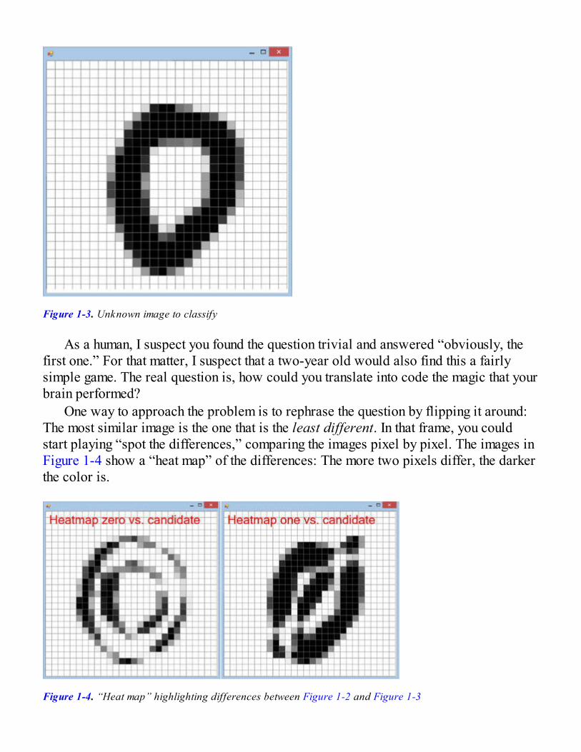
Figure 1-3. Unknown image to classify

As a human, I suspect you found the question trivial and answered “obviously, thefirst one.” For that matter, I suspect that a two-year old would also find this a fairlysimple game. The real question is, how could you translate into code the magic that yourbrain performed?

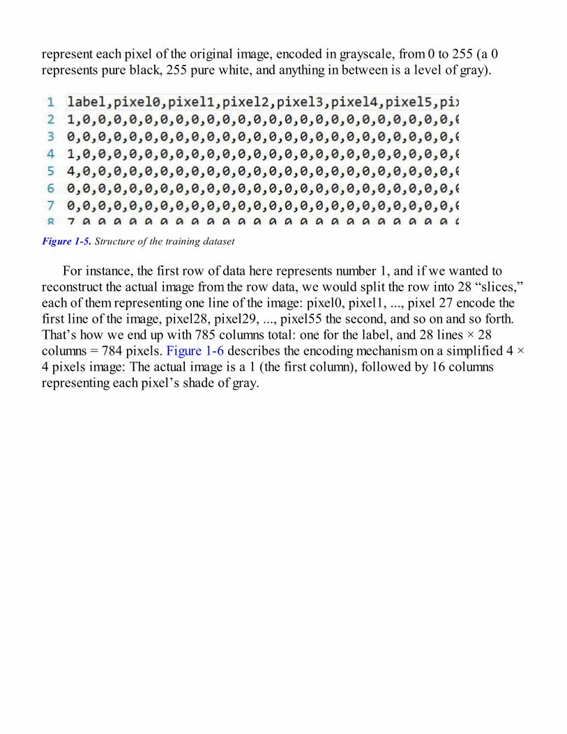
One way to approach the problem is to rephrase the question by flipping it around:The most similar image is the one that is the least different. In that frame, you couldstart playing “spot the differences,” comparing the images pixel by pixel. The images inFigure 1-4 show a “heat map” of the differences: The more two pixels differ, the darkerthe color is.

Figure 1-4. “Heat map” highlighting differences between Figure 1-2 and Figure 1-3

In our example, this approach seems to be working quite well; the second image,which is “very different,” has a large black area in the middle, while the first one,which plots the differences between two zeroes, is mostly white, with some thin darkareas.

Distance Functions in Machine LearningWe could now summarize how different two images are with a single number, bysumming up the differences across pixels. Doing this gives us a small number forsimilar images, and a large one for dissimilar ones. What we managed to define here isa “distance” between images, describing how close they are. Two images that areabsolutely identical have a distance of zero, and the more the pixels differ, the larger thedistance will be. On the one hand, we know that a distance of zero means a perfectmatch, and is the best we can hope for. On the other hand, our similarity measure haslimitations. As an example, if you took one image and simply cloned it, but shifted it(for instance) by one pixel to the left, their distance pixel-by-pixel might end up beingquite large, even though the images are essentially the same.

The notion of distance is quite important in machine learning, and appears in mostmodels in one form or another. A distance function is how you translate what you aretrying to achieve into a form a machine can work with. By reducing something complex,like two images, into a single number, you make it possible for an algorithm to takeaction—in this case, deciding whether two images are similar. At the same time, byreducing complexity to a single number, you incur the risk that some subtleties will be“lost in translation,” as was the case with our shifted images scenario.

Distance functions also often appear in machine learning under another name: costfunctions. They are essentially the same thing, but look at the problem from a differentangle. For instance, if we are trying to predict a number, our prediction error—that is,how far our prediction is from the actual number—is a distance. However, anequivalent way to describe this is in terms of cost: a larger error is “costly,” andimproving the model translates to reducing its cost.

Start with Something SimpleBut for the moment, let’s go ahead and happily ignore that problem, and follow amethod that has worked wonders for me, both in writing software and developingpredictive models—what is the easiest thing that could possibly work? Start simplefirst, and see what happens. If it works great, you won’t have to build anythingcomplicated, and you will be done faster. If it doesn’t work, then you have spent very

little time building a simple proof-of-concept, and usually learned a lot about theproblem space in the process. Either way, this is a win.

So for now, let’s refrain from over-thinking and over-engineering; our goal is toimplement the least complicated approach that we think could possibly work, and refinelater. One thing we could do is the following: When we have to identify what number animage represents, we could search for the most similar (or least different) image in ourknown library of 50,000 training examples, and predict what that image says. If it lookslike a five, surely, it must be a five!

The outline of our algorithm will be the following. Given a 28 × 28 pixels imagethat we will try to recognize (the “Unknown”), and our 50,000 training examples (28 ×28 pixels images and a label), we will:

compute the total difference between Unknown and each trainingexample;

find the training example with the smallest difference (the“Closest”); and

predict that “Unknown” is the same as “Closest.”

Let’s get cracking!

Our First Model, C# VersionTo get warmed up, let’s begin with a C# implementation, which should be familiarterritory, and create a C# console application in Visual Studio. I called my solutionDigitsRecognizer, and the C# console application CSharp— feel free to bemore creative than I was!

Dataset OrganizationThe first thing we need is obviously data. Let’s download the datasettrainingsample.csv from http://1drv.ms/1sDThtz and save itsomewhere on your machine. While we are at it, there is a second file in the samelocation, validationsample.csv, that we will be using a bit later on, but let’sgrab it now and be done with it. The file is in CSV format (Comma-Separated Values),and its structure is displayed in Figure 1-5. The first row is a header, and each rowafterward represents an individual image. The first column (“label”), indicates whatnumber the image represents, and the 784 columns that follow (“pixel0”, “pixel1”, ...)

represent each pixel of the original image, encoded in grayscale, from 0 to 255 (a 0represents pure black, 255 pure white, and anything in between is a level of gray).

Figure 1-5. Structure of the training dataset

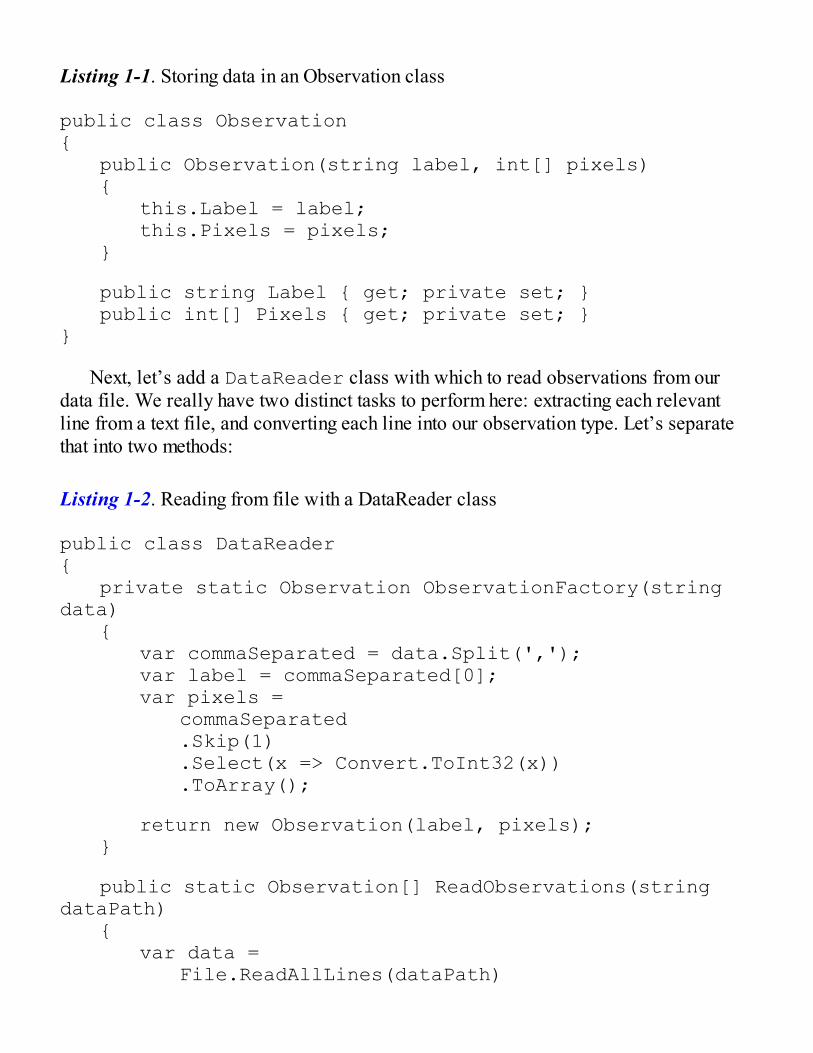
For instance, the first row of data here represents number 1, and if we wanted toreconstruct the actual image from the row data, we would split the row into 28 “slices,”each of them representing one line of the image: pixel0, pixel1, ..., pixel 27 encode thefirst line of the image, pixel28, pixel29, ..., pixel55 the second, and so on and so forth.That’s how we end up with 785 columns total: one for the label, and 28 lines × 28columns = 784 pixels. Figure 1-6 describes the encoding mechanism on a simplified 4 ×4 pixels image: The actual image is a 1 (the first column), followed by 16 columnsrepresenting each pixel’s shade of gray.

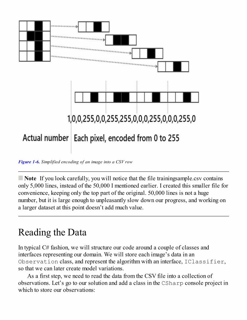
Figure 1-6. Simplified encoding of an image into a CSV row

Note If you look carefully, you will notice that the file trainingsample.csv containsonly 5,000 lines, instead of the 50,000 I mentioned earlier. I created this smaller file forconvenience, keeping only the top part of the original. 50,000 lines is not a hugenumber, but it is large enough to unpleasantly slow down our progress, and working ona larger dataset at this point doesn’t add much value.

Reading the DataIn typical C# fashion, we will structure our code around a couple of classes andinterfaces representing our domain. We will store each image’s data in anObservation class, and represent the algorithm with an interface, IClassifier,so that we can later create model variations.

As a first step, we need to read the data from the CSV file into a collection ofobservations. Let’s go to our solution and add a class in the CSharp console project inwhich to store our observations:

Listing 1-1. Storing data in an Observation class

public class Observation{ public Observation(string label, int[] pixels) { this.Label = label; this.Pixels = pixels; }

public string Label { get; private set; } public int[] Pixels { get; private set; }}

Next, let’s add a DataReader class with which to read observations from ourdata file. We really have two distinct tasks to perform here: extracting each relevantline from a text file, and converting each line into our observation type. Let’s separatethat into two methods:

Listing 1-2. Reading from file with a DataReader class

public class DataReader{ private static Observation ObservationFactory(string data) { var commaSeparated = data.Split(','); var label = commaSeparated[0]; var pixels = commaSeparated .Skip(1) .Select(x => Convert.ToInt32(x)) .ToArray();

return new Observation(label, pixels); }

public static Observation[] ReadObservations(string dataPath) { var data = File.ReadAllLines(dataPath)

.Skip(1) .Select(ObservationFactory) .ToArray();

return data; }}

Note how our code here is mainly LINQ expressions! Expression-oriented code,like LINQ (or, as you’ll see later, F#), helps you write very clear code that conveysintent in a straightforward manner, typically much more so than procedural code does. Itreads pretty much like English: “read all the lines, skip the headers, split each linearound the commas, parse as integers, and give me new observations.” This is how Iwould describe what I was trying to do, if I were talking to a colleague, and thatintention is very clearly reflected in the code. It also fits particularly well with datamanipulation tasks, as it gives a natural way to describe data transformation workflows,which are the bread and butter of machine learning. After all, this is what LINQ wasdesigned for—“Language Integrated Queries!”

We have data, a reader, and a structure in which to store them—let’s put thattogether in our console app and try this out, replacing PATH-ON-YOUR-MACHINE intrainingPath with the path to the actual data file on your local machine:

Listing 1-3. Console application

class Program{ static void Main(string[] args) { var trainingPath = @"PATH-ON-YOUR-MACHINE\trainingsample.csv"; var training = DataReader.ReadObservations(trainingPath);

Console.ReadLine(); }}

If you place a breakpoint at the end of this code block, and then run it in debugmode, you should see that training is an array containing 5,000 observations. Good—everything appears to be working.

Our next task is to write a Classifier, which, when passed an Image, will

compare it to each Observation in the dataset, find the most similar one, and returnits label. To do that, we need two elements: a Distance and a Classifier.

Computing Distance between ImagesLet’s start with the distance.What we want is a method that takes two arrays ofpixels and returns a number that describes how different they are. Distance is an area ofvolatility in our algorithm; it is very likely that we will want to experiment withdifferent ways of comparing images to figure out what works best, so putting in place adesign that allows us to easily substitute various distance definitions without requiringtoo many code changes is highly desirable. An interface gives us a convenientmechanism by which to avoid tight coupling, and to make sure that when we decide tochange the distance code later, we won’t run into annoying refactoring issues. So, let’sextract an interface from the get-go:

Listing 1-4. IDistance interface

public interface IDistance{ double Between(int[] pixels1, int[] pixels2);}

Now that we have an interface, we need an implementation. Again, we will go forthe easiest thing that could work for now. If what we want is to measure how differenttwo images are, why not, for instance, compare them pixel by pixel, compute eachdifference, and add up their absolute values? Identical images will have a distance ofzero, and the further apart two pixels are, the higher the distance between the twoimages will be. As it happens, that distance has a name, the “Manhattan distance,” andimplementing it is fairly straightforward, as shown in Listing 1-5:

Listing 1-5. Computing the Manhattan distance between images

public class ManhattanDistance : IDistance{ public double Between(int[] pixels1, int[] pixels2) { if (pixels1.Length != pixels2.Length) { throw new ArgumentException("Inconsistent image

sizes."); }

var length = pixels1.Length;

var distance = 0;

for (int i = 0; i < length; i++) { distance += Math.Abs(pixels1[i] - pixels2[i]); }

return distance; }}

FUN FACT: MANHATTAN DISTANCE

I previously mentioned that distances could be computed with multiple methods.The specific formulation we use here is known as the “Manhattan distance.” Thereason for that name is that if you were a cab driver in New York City, this isexactly how you would compute how far you have to drive between two points.Because all streets are organized in a perfect, rectangular grid, you would computethe absolute distance between the East/West locations, and North/South locations,which is precisely what we are doing in our code. This is also known as, muchless poetically, the L1 Distance.

We take two images and compare them pixel by pixel, computing the difference andreturning the total, which represents how far apart the two images are. Note that thecode here uses a very procedural style, and doesn’t use LINQ at all. I actually initiallywrote that code using LINQ, but frankly didn’t like the way the result looked. In myopinion, after a certain point (or for certain operations), LINQ code written in C# tendsto look a bit over-complicated, in large part because of how verbose C# is, notably forfunctional constructs (Func<A,B,C>). This is also an interesting example that contraststhe two styles. Here, understanding what the code is trying to do does require reading itline by line and translating it into a “human description.” It also uses mutation, a stylethat requires care and attention.

MATH.ABS( )

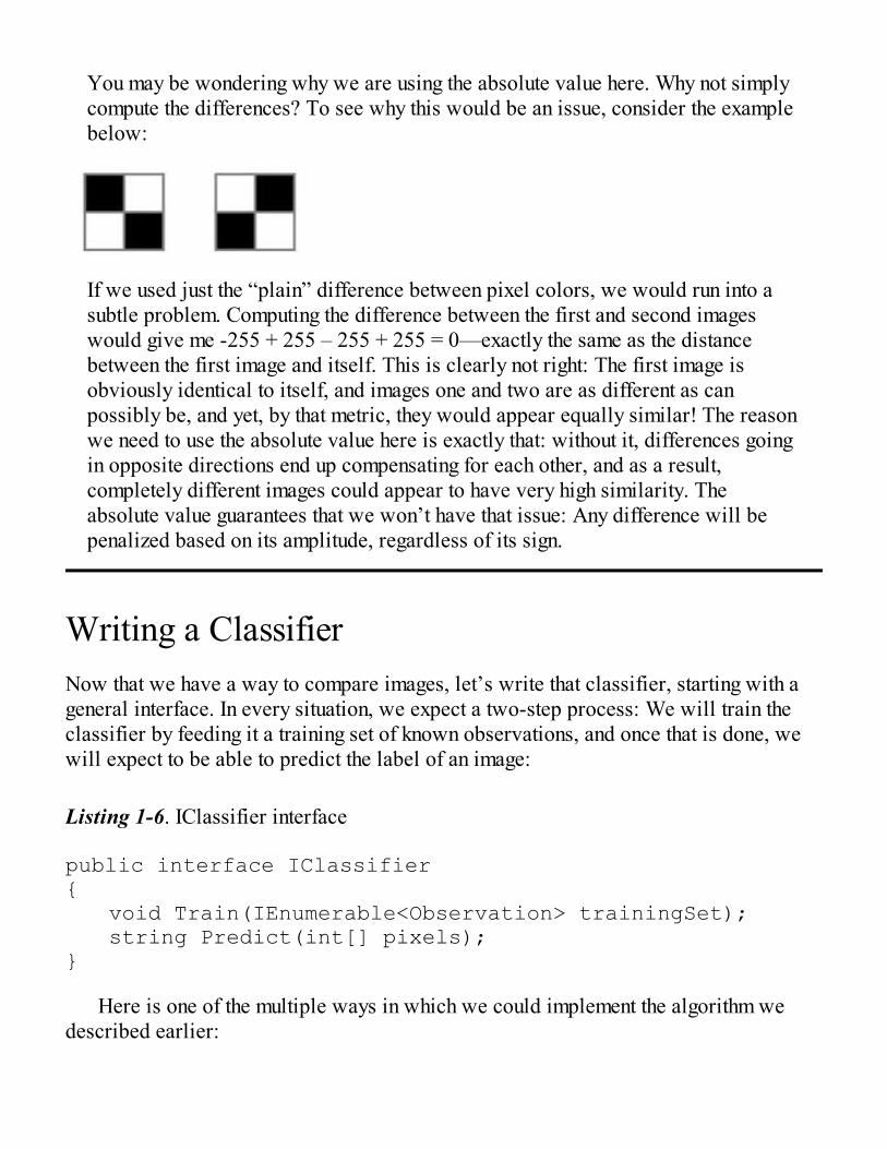
You may be wondering why we are using the absolute value here. Why not simplycompute the differences? To see why this would be an issue, consider the examplebelow:

If we used just the “plain” difference between pixel colors, we would run into asubtle problem. Computing the difference between the first and second imageswould give me -255 + 255 – 255 + 255 = 0—exactly the same as the distancebetween the first image and itself. This is clearly not right: The first image isobviously identical to itself, and images one and two are as different as canpossibly be, and yet, by that metric, they would appear equally similar! The reasonwe need to use the absolute value here is exactly that: without it, differences goingin opposite directions end up compensating for each other, and as a result,completely different images could appear to have very high similarity. Theabsolute value guarantees that we won’t have that issue: Any difference will bepenalized based on its amplitude, regardless of its sign.

Writing a ClassifierNow that we have a way to compare images, let’s write that classifier, starting with ageneral interface. In every situation, we expect a two-step process: We will train theclassifier by feeding it a training set of known observations, and once that is done, wewill expect to be able to predict the label of an image:

Listing 1-6. IClassifier interface

public interface IClassifier{ void Train(IEnumerable<Observation> trainingSet); string Predict(int[] pixels);}

Here is one of the multiple ways in which we could implement the algorithm wedescribed earlier:

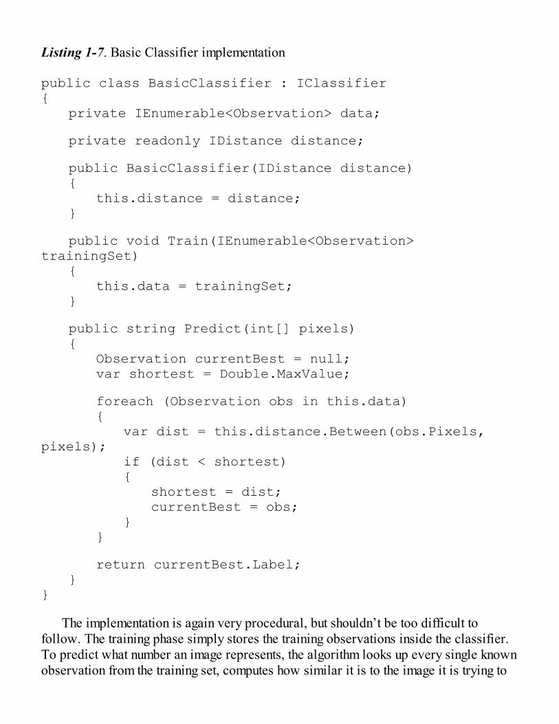
Listing 1-7. Basic Classifier implementation

public class BasicClassifier : IClassifier{ private IEnumerable<Observation> data;

private readonly IDistance distance;

public BasicClassifier(IDistance distance) { this.distance = distance; }

public void Train(IEnumerable<Observation> trainingSet) { this.data = trainingSet; }

public string Predict(int[] pixels) { Observation currentBest = null; var shortest = Double.MaxValue;

foreach (Observation obs in this.data) { var dist = this.distance.Between(obs.Pixels, pixels); if (dist < shortest) { shortest = dist; currentBest = obs; } }

return currentBest.Label; }}

The implementation is again very procedural, but shouldn’t be too difficult tofollow. The training phase simply stores the training observations inside the classifier.To predict what number an image represents, the algorithm looks up every single knownobservation from the training set, computes how similar it is to the image it is trying to

recognize, and returns the label of the closest matching image. Pretty easy!

So, How Do We Know It Works?Great—we have a classifier, a shiny piece of code that will classify images. We aredone—ship it!

Not so fast! We have a bit of a problem here: We have absolutely no idea if ourcode works. As a software engineer, knowing whether “it works” is easy. You take yourspecs (everyone has specs, right?), you write tests (of course you do), you run them, andbam! You know if anything is broken. But what we care about here is not whether “itworks” or “it’s broken,” but rather, “is our model any good at making predictions?”

Cross-validationA natural place to start with this is to simply measure how well our model performs itstask. In our case, this is actually fairly easy to do: We could feed images to theclassifier, ask for a prediction, compare it to the true answer, and compute how manywe got right. Of course, in order to do that, we would need to know what the rightanswer was. In other words, we would need a dataset of images with known labels, andwe would use it to test the quality of our model. That dataset is known as a validationset (or sometimes simply as the “test data”).

At that point, you might ask, why not use the training set itself, then? We could trainour classifier, and then run it on each of our 5,000 examples. This is not a very goodidea, and here's why: If you do this, what you will measure is how well your modellearned the training set. What we are really interested in is something slightly different:How well can we expect the classifier to work, once we release it “in the wild,” andstart feeding it new images it has never encountered before? Giving it images that wereused in training will likely give you an optimistic estimate. If you want a realistic one,feed the model data that hasn't been used yet.

Note As a case in point, our current classifier is an interesting example of how usingthe training set for validation can go very wrong. If you try to do that, you will see that itgets every single image properly recognized. 100% accuracy! For such a simple model,this seems too good to be true. What happens is this: As our algorithm searches for themost similar image in the training set, it finds a perfect match every single time, becausethe images we are testing against belong to the training set. So, when results seem too

good to be true, check twice!

The general approach used to resolve that issue is called cross-validation. Put asidepart of the data you have available and split it into a training set and a validation set.Use the first one to train your model and the second one to evaluate the quality of yourmodel.

Earlier on, you downloaded two files, trainingsample.csv andvalidationsample.csv. I prepared them for you so that you don’t have to. Thetraining set is a sample of 5,000 images from the full 50,000 original dataset, and thevalidation set is 500 other images from the same source. There are more fancy ways toproceed with cross-validation, and also some potential pitfalls to watch out for, as wewill see in later chapters, but simply splitting the data you have into two separatesamples, say 80%/20%, is a simple and effective way to get started.

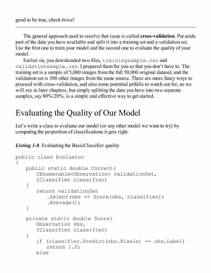
Evaluating the Quality of Our ModelLet’s write a class to evaluate our model (or any other model we want to try) bycomputing the proportion of classifications it gets right:

Listing 1-8. Evaluating the BasicClassifier quality

public class Evaluator{ public static double Correct( IEnumerable<Observation> validationSet, IClassifier classifier) { return validationSet .Select(obs => Score(obs, classifier)) .Average(); }

private static double Score( Observation obs, IClassifier classifier) { if (classifier.Predict(obs.Pixels) == obs.Label) return 1.0; else

return 0.0; }}

We are using a small trick here: we pass the Evaluator an IClassifier anda dataset, and for each image, we “score” the prediction by comparing what theclassifier predicts with the true value. If they match, we record a 1, otherwise werecord a 0. By using numbers like this rather than true/false values, we can average thisout to get the percentage correct.

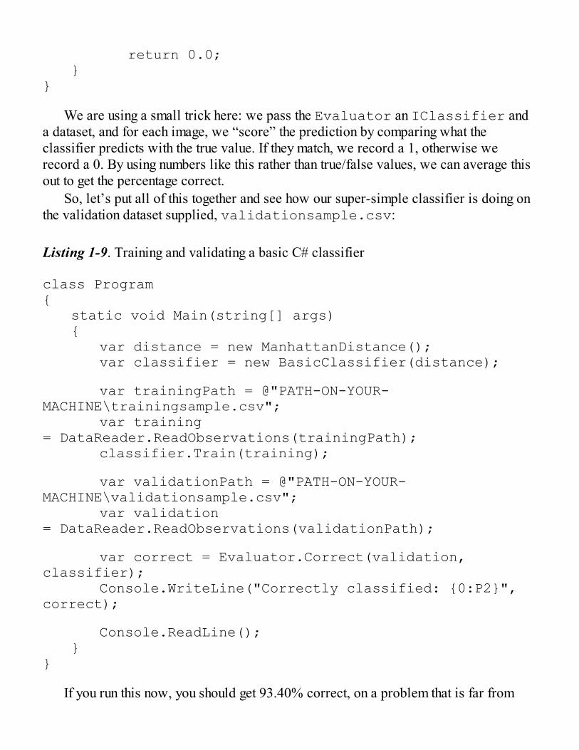
So, let’s put all of this together and see how our super-simple classifier is doing onthe validation dataset supplied, validationsample.csv:

Listing 1-9. Training and validating a basic C# classifier

class Program{ static void Main(string[] args) { var distance = new ManhattanDistance(); var classifier = new BasicClassifier(distance);

var trainingPath = @"PATH-ON-YOUR-MACHINE\trainingsample.csv"; var training = DataReader.ReadObservations(trainingPath); classifier.Train(training);

var validationPath = @"PATH-ON-YOUR-MACHINE\validationsample.csv"; var validation = DataReader.ReadObservations(validationPath);

var correct = Evaluator.Correct(validation, classifier); Console.WriteLine("Correctly classified: {0:P2}", correct);

Console.ReadLine(); }}

If you run this now, you should get 93.40% correct, on a problem that is far from

trivial. I mean, we are automatically recognizing digits handwritten by humans, withdecent reliability! Not bad, especially taking into account that this is our first attempt,and we are deliberately trying to keep things simple.

Improving Your ModelSo, what’s next? Well, our model is good, but why stop there? After all, we are still farfrom the Holy Grail of 100% correct—can we squeeze in some clever improvementsand get better predictions?

This is where having a validation set is absolutely crucial. Just like unit tests giveyou a safeguard to warn you when your code is going off the rails, the validation setestablishes a baseline for your model, which allows you to not to fly blind. You cannow experiment with modeling ideas freely, and you can get a clear signal on whetherthe direction is promising or terrible.

At this stage, you would normally take one of two paths. If your model is goodenough, you can call it a day—you’re done. If it isn’t good enough, you would startthinking about ways to improve predictions, create new models, and run them againstthe validation set, comparing the percentage correctly classified so as to evaluatewhether your new models work any better, progressively refining your model until youare satisfied with it.

But before jumping in and starting experimenting with ways to improve our model,now seems like a perfect time to introduce F#. F# is a wonderful .NET language, and isuniquely suited for machine learning and data sciences; it will make our workexperimenting with models much easier. So, now that we have a working C# version,let’s dive in and rewrite it in F# so that we can compare and contrast the two and betterunderstand the F# way.

Introducing F# for Machine LearningDid you notice how much time it took to run our model? In order to see the quality of amodel, after any code change, we need to rebuild the console app and run it, reload thedata, and compute. That’s a lot of steps, and if your dataset gets even moderately large,you will spend the better part of your day simply waiting for data to load. Not great.

Live Scripting and Data Exploration with F#

InteractiveBy contrast, F# comes with a very handy feature, called F# Interactive, in Visual Studio.F# Interactive is a REPL (Read-Evaluate-Print Loop), basically a live-scriptingenvironment where you can play with code without having to go through the whole cycleI described before.

So, instead of a console application, we’ll work in a script. Let’s go into VisualStudio and add a new library project to our solution (see Figure 1-7), which we willname FSharp.

Figure 1-7. Adding an F# library project

Tip If you are developing using Visual Studio Professional or higher, F# should beinstalled by default. For other situations, please check www.fsharp.org, the F#Software Foundation, which has comprehensive guidance on getting set up.

It’s worth pointing that you have just added an F# project to a .NET solution with an

existing C# project. F# and C# are completely interoperable and can talk to each otherwithout problems—you don’t have to restrict yourself to using one language foreverything. Unfortunately, oftentimes people think of C# and F# as competing languages,which they aren’t. They complement each other very nicely, so get the best of bothworlds: Use C# for what C# is great at, and leverage the F# goodness for where F#shines!

In your new project, you should see now a file named Library1.fs; this is theF# equivalent of a .cs file. But did you also notice a file called script.fsx? .fsxfiles are script files; unlike .fs files, they are not part of the build. They can be usedoutside of Visual Studio as pure, free-standing scripts, which is very useful in its ownright. In our current context, machine learning and data science, the usage I amparticularly interested in is in Visual Studio: .fsx files constitute a wonderful “scratchpad” where you can experiment with code, with all the benefits of IntelliSense.

Let’s go to Script.fsx, delete everything in there, and simply type the followinganywhere:

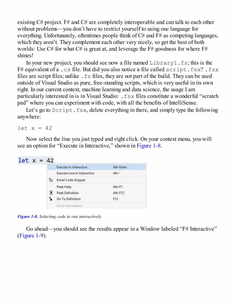
let x = 42

Now select the line you just typed and right click. On your context menu, you willsee an option for “Execute in Interactive,” shown in Figure 1-8.

Figure 1-8. Selecting code to run interactively

Go ahead—you should see the results appear in a Window labeled “F# Interactive”(Figure 1-9).

Figure 1-9. Executing code live in F# Interactive

Tip You can also execute whatever code is selected in the script file by using thekeyboard shortcut Alt + Enter. This is much faster than using the mouse and the contextmenu. A small warning to ReSharper users: Until recently, ReSharper had the nastyhabit of resetting that shortcut, so if you are using a version older than 8.1, you willprobably have to recreate that shortcut.

The F# Interactive window (which we will refer to as FSI most of the time, for thesake of brevity) runs as a session. That is, whatever you execute in the interactivewindow will remain in memory, available to you until you reset your session by right-clicking on the contents of the F# Interactive window and selecting “Reset InteractiveSession.”

In this example, we simply create a variable x, with value 42. As a firstapproximation, this is largely similar to the C# statement var x = 42; There aresome subtle differences, but we’ll discuss them later. Now that x “exists” in FSI, wecan keep using it. For instance, you can type the following directly in FSI:

> x + 100;;val it : int = 142>

FSI “remembers” that x exists: you do not need to rerun the code you have in the .fsxfile. Once it has been run once, it remains in memory. This is extremely convenientwhen you want to manipulate a somewhat large dataset. With FSI, you can load up yourdata once in the morning and keep coding, without having to reload every single timeyou have a change, as would be the case in C#.

You probably noted the mysterious ;; after x + 100. This indicates to FSI thatwhatever was typed until that point needs to be executed now. This is useful if the codeyou want to execute spans multiple lines, for instance.

Tip If you tried to type F# code directly into FSI, you probably noticed that therewas no IntelliSense. FSI is a somewhat primitive development environment comparedto the full Visual Studio experience. My advice in terms of process is to type code inFSI only minimally. Instead, work primarily in an .fsx file. You will get all the benefitsof a modern IDE, with auto-completion and syntax validation, for instance. This willnaturally lead you to write complete scripts, which can then be replayed in the future.While scripts are not part of the solution build, they are part of the solution itself, andcan (should) be versioned as well, so that you are always in a position to replicatewhatever experiment you were conducting in a script.

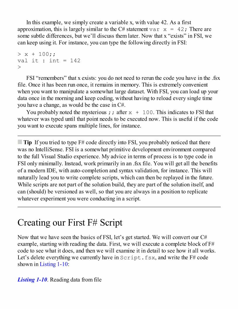
Creating our First F# ScriptNow that we have seen the basics of FSI, let’s get started. We will convert our C#example, starting with reading the data. First, we will execute a complete block of F#code to see what it does, and then we will examine it in detail to see how it all works.Let’s delete everything we currently have in Script.fsx, and write the F# codeshown in Listing 1-10:

Listing 1-10. Reading data from file

open System.IOtype Observation = { Label:string; Pixels: int[] }

let toObservation (csvData:string) = let columns = csvData.Split(',') let label = columns.[0] let pixels = columns.[1..] |> Array.map int { Label = label; Pixels = pixels }

let reader path = let data = File.ReadAllLines path data.[1..] |> Array.map toObservation

let trainingPath = @"PATH-ON-YOUR-MACHINE\trainingsample.csv"let trainingData = reader trainingPath

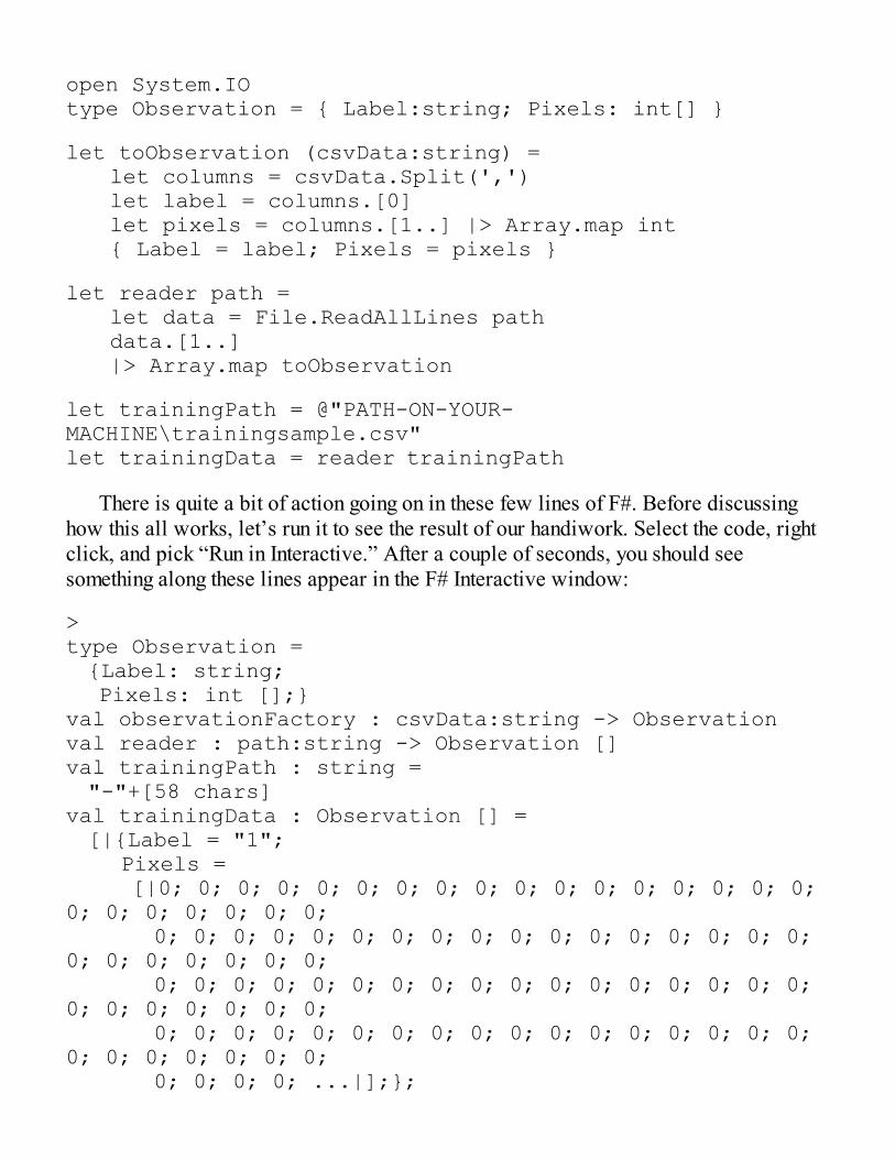
There is quite a bit of action going on in these few lines of F#. Before discussinghow this all works, let’s run it to see the result of our handiwork. Select the code, rightclick, and pick “Run in Interactive.” After a couple of seconds, you should seesomething along these lines appear in the F# Interactive window:

>type Observation = {Label: string; Pixels: int [];}val observationFactory : csvData:string -> Observationval reader : path:string -> Observation []val trainingPath : string = "-"+[58 chars]val trainingData : Observation [] = [|{Label = "1"; Pixels = [|0; 0; 0; 0; 0; 0; 0; 0; 0; 0; 0; 0; 0; 0; 0; 0; 0; 0; 0; 0; 0; 0; 0; 0; 0; 0; 0; 0; 0; 0; 0; 0; 0; 0; 0; 0; 0; 0; 0; 0; 0; 0; 0; 0; 0; 0; 0; 0; 0; 0; 0; 0; 0; 0; 0; 0; 0; 0; 0; 0; 0; 0; 0; 0; 0; 0; 0; 0; 0; 0; 0; 0; 0; 0; 0; 0; 0; 0; 0; 0; 0; 0; 0; 0; 0; 0; 0; 0; 0; 0; 0; 0; 0; 0; 0; 0; 0; 0; 0; 0; ...|];};

/// Output has been cut out for brevity here /// {Label = "3"; Pixels = [|0; 0; 0; 0; 0; 0; 0; 0; 0; 0; 0; 0; 0; 0; 0; 0; 0; 0; 0; 0; 0; 0; 0; 0; 0; 0; 0; 0; 0; 0; 0; 0; 0; 0; 0; 0; 0; 0; 0; 0; 0; 0; 0; 0; 0; 0; 0; 0; 0; 0; 0; 0; 0; 0; 0; 0; 0; 0; 0; 0; 0; 0; 0; 0; 0; 0; 0; 0; 0; 0; ...|];}; ...|]

>

Basically, in a dozen lines of F#, we got all the functionality of the DataReaderand Observation classes. By running it in F# Interactive, we could immediatelyload the data and see how it looked. At that point, we loaded an array ofObservations (the data) in the F# Interactive session, which will stay there for aslong as you want. For instance, suppose that you wanted to know the label ofObservation 100 in the training set. No need to reload or recompile anything: justtype the following in the F# Interactive window, and execute:

let test = trainingData.[100].Label;;

And that’s it. Because the data is already there in memory, it will just work.This is extremely convenient, especially in situations in which your dataset is large,

and loading it is time consuming. This is a significant benefit of using F# over C# fordata-centric work: While any change in code in a C# console application requiresrebuilding and reloading the data, once the data is loaded in F# Interactive, it’savailable for you to hack to your heart’s content. You can change your code andexperiment without the hassle of reloading.

Dissecting Our First F# ScriptNow that we saw what these ten lines of code do, let’s dive into how they work:

open System.IO

This line is straightforward—it is equivalent to the C# statement usingSystem.IO. Every .NET library is accessible to F#, so all the knowledge youaccumulated over the years learning the .NET namespaces jungle is not lost—you willbe able to reuse all that and augment it with some of the F#-specific goodies made

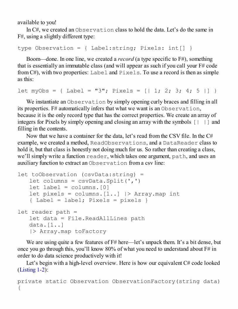
available to you!In C#, we created an Observation class to hold the data. Let’s do the same in

F#, using a slightly different type:

type Observation = { Label:string; Pixels: int[] }

Boom—done. In one line, we created a record (a type specific to F#), somethingthat is essentially an immutable class (and will appear as such if you call your F# codefrom C#), with two properties: Label and Pixels. To use a record is then as simpleas this:

let myObs = { Label = "3"; Pixels = [| 1; 2; 3; 4; 5 |] }

We instantiate an Observation by simply opening curly braces and filling in allits properties. F# automatically infers that what we want is an Observation,because it is the only record type that has the correct properties. We create an array ofintegers for Pixels by simply opening and closing an array with the symbols [| |] andfilling in the contents.

Now that we have a container for the data, let’s read from the CSV file. In the C#example, we created a method, ReadObservations, and a DataReader class tohold it, but that class is honestly not doing much for us. So rather than creating a class,we’ll simply write a function reader, which takes one argument, path, and uses anauxiliary function to extract an Observation from a csv line:

let toObservation (csvData:string) = let columns = csvData.Split(',') let label = columns.[0] let pixels = columns.[1..] |> Array.map int { Label = label; Pixels = pixels }

let reader path = let data = File.ReadAllLines path data.[1..] |> Array.map toFactory

We are using quite a few features of F# here—let’s unpack them. It’s a bit dense, butonce you go through this, you’ll know 80% of what you need to understand about F# inorder to do data science productively with it!

Let’s begin with a high-level overview. Here is how our equivalent C# code looked(Listing 1-2):

private static Observation ObservationFactory(string data){

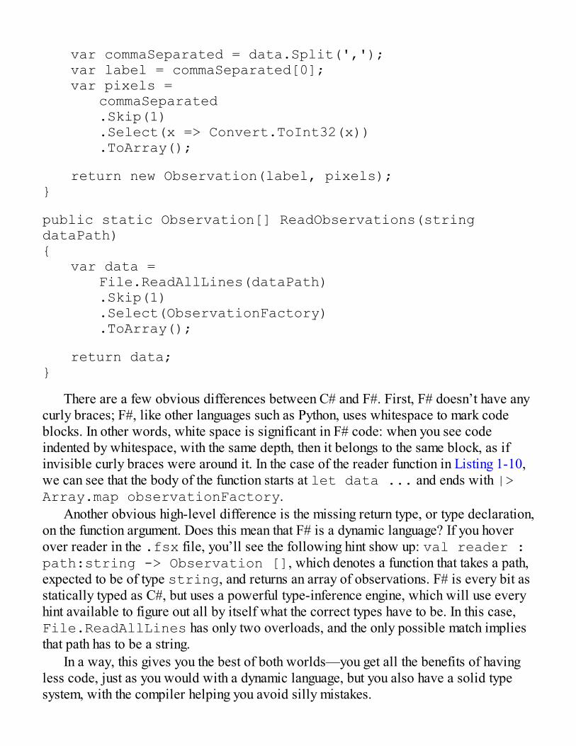
var commaSeparated = data.Split(','); var label = commaSeparated[0]; var pixels = commaSeparated .Skip(1) .Select(x => Convert.ToInt32(x)) .ToArray();

return new Observation(label, pixels);}

public static Observation[] ReadObservations(string dataPath){ var data = File.ReadAllLines(dataPath) .Skip(1) .Select(ObservationFactory) .ToArray();

return data;}

There are a few obvious differences between C# and F#. First, F# doesn’t have anycurly braces; F#, like other languages such as Python, uses whitespace to mark codeblocks. In other words, white space is significant in F# code: when you see codeindented by whitespace, with the same depth, then it belongs to the same block, as ifinvisible curly braces were around it. In the case of the reader function in Listing 1-10,we can see that the body of the function starts at let data ... and ends with |>Array.map observationFactory.

Another obvious high-level difference is the missing return type, or type declaration,on the function argument. Does this mean that F# is a dynamic language? If you hoverover reader in the .fsx file, you’ll see the following hint show up: val reader :path:string -> Observation [], which denotes a function that takes a path,expected to be of type string, and returns an array of observations. F# is every bit asstatically typed as C#, but uses a powerful type-inference engine, which will use everyhint available to figure out all by itself what the correct types have to be. In this case,File.ReadAllLines has only two overloads, and the only possible match impliesthat path has to be a string.

In a way, this gives you the best of both worlds—you get all the benefits of havingless code, just as you would with a dynamic language, but you also have a solid typesystem, with the compiler helping you avoid silly mistakes.

Tip The F# type-inference system is absolutely amazing at figuring out what youmeant with the slightest of hints. However, at times you will need to help it, because itcannot figure it out by itself. In that case, you can simply annotate with the expectedtype, like this: let reader (path:string) = . In general, I recommend usingtype annotations in high-level components of your code, or crucial components, evenwhen it is unnecessary. It helps make the intent of your code more directly obvious toothers, without having to open an IDE to see what the inferred types are. It can also beuseful in tracking down the origin of some issues, by making sure that when you arecomposing multiple functions together, each step is actually being passed the types itexpects.

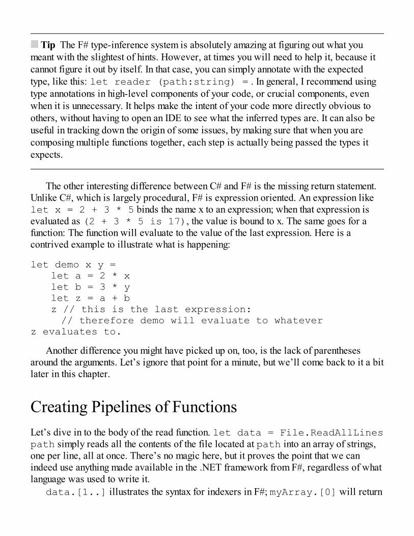
The other interesting difference between C# and F# is the missing return statement.Unlike C#, which is largely procedural, F# is expression oriented. An expression likelet x = 2 + 3 * 5 binds the name x to an expression; when that expression isevaluated as (2 + 3 * 5 is 17), the value is bound to x. The same goes for afunction: The function will evaluate to the value of the last expression. Here is acontrived example to illustrate what is happening:

let demo x y = let a = 2 * x let b = 3 * y let z = a + b z // this is the last expression: // therefore demo will evaluate to whatever z evaluates to.

Another difference you might have picked up on, too, is the lack of parenthesesaround the arguments. Let’s ignore that point for a minute, but we’ll come back to it a bitlater in this chapter.

Creating Pipelines of FunctionsLet’s dive in to the body of the read function. let data = File.ReadAllLinespath simply reads all the contents of the file located at path into an array of strings,one per line, all at once. There’s no magic here, but it proves the point that we canindeed use anything made available in the .NET framework from F#, regardless of whatlanguage was used to write it.

data.[1..] illustrates the syntax for indexers in F#; myArray.[0] will return

the first element of your array. Note the presence of a dot between myArray and thebracketed index! The other interesting bit of syntax here demonstrates array slicing;data.[1..] signifies “give me a new array, pulling elements from data starting atindex 1 until the last one.” Similarly, you could do things like data.[5..10] (giveme all elements from indexes 5 to 10), or data.[..3] (give me all elements untilindex 3). This is incredibly convenient for data manipulation, and is one of the manyreasons why F# is such a nice language for data science.

In our example, we kept every element starting at index 1, or in other words, wedropped the first element of the array—that is, the headers.

The next step in our C# code involved extracting an Observation from each lineusing the ObservationFactory method, which we did by using the following:

myData.Select(line => ObservationFactory(line));

The equivalent line in F# is as follows:

myData |> Array.map (fun line -> toObservation line)

At a very high level, you would read the statement as “take the array myData andpass it forward to a function that will apply a mapping to each array element, convertingeach line to an observation.” There are two important differences with the C# code.First, while the Select statement appears as a method on the array we aremanipulating, in F#, the logical owner of the function is not the array itself, but theArray module. The Array module acts in a fashion similar to the Enumerable class,which provides a collection of C# extension methods on IEnumerable.

Note If you enjoy using LINQ in C#, I suspect you will really like F#. In manyrespects, LINQ is about importing concepts from functional programming into an object-oriented language, C#. F# offers a much deeper set of LINQ-like functions for you toplay with. To get a sense for that, simply type “Array.” in .fsx, and see how manyfunctions you have at your disposal!

The second major difference is the mysterious symbol “|>”. This is known as thepipe-forward operator. In a nutshell, it takes whatever the result of the previousexpression was and passes it forward to the next function in the pipeline, which will useit as the last argument. For instance, consider the following code:

let double x = 2 * xlet a = 5let b = double a

let c = double b

This could be rewritten as follows:

let double x = 2 * xlet c = 5 |> double |> double

double is a function expecting a single argument that is an integer, so we can“feed” a 5 directly into it through the pipe-forward operator. Because double alsoproduces an integer, we can keep forwarding the result of the operation ahead. We canslightly rewrite this code to look this way:

let double x = 2 * xlet c = 5 |> double |> double

Our example with Array.map follows the same pattern. If we used the rawArray.map version, the code would look like this:

let transformed = Array.map (fun line -> toObservation line) data

Array.map expects two arguments: what transformation to apply to each arrayelement, and what array to apply it to. Because the target array is the last argument ofthe function, we can use pipe-forward to “feed” an array to a map, like this:

data |> Array.map (fun line -> toObservation line)

If you are totally new to F#, this is probably a bit overwhelming. Don’t worry! Aswe go, we will see a lot more examples of F# in action, and while understandingexactly why things work might take a bit, getting it to work is actually fairly easy. Thepipe-forward operator is one of my favorite features in F#, because it makes workflowsso straightforward to follow: take something and pass it through a pipeline of steps oroperations until you are done.

Manipulating Data with Tuples and Pattern MatchingNow that we have data, we need to find the closest image from the training set. Just likein the C# example, we need a distance for that. Unlike C#, again, we won’t create aclass or interface, and will just use a function:

let manhattanDistance (pixels1,pixels2) = Array.zip pixels1 pixels2 |> Array.map (fun (x,y) -> abs (x-y)) |> Array.sum

Here we are using another central feature of F#: the combination of tuples andpattern matching. A tuple is a grouping of unnamed but ordered values, possibly ofdifferent types. Tuples exist in C# as well, but the lack of pattern matching in thelanguage really cripples their usefulness, which is quite unfortunate, because it’s adeadly combination for data manipulation.

There is much more to pattern matching than just tuples. In general, pattern matchingis a mechanism with allows your code to simply recognize various shapes in the data,and to take action based on that. Here is a small example illustrating how patternmatching works on tuples:

let x = "Hello", 42 // create a tuple with 2 elementslet (a, b) = x // unpack the two elements of x by pattern matchingprintfn "%s, %i" a bprintfn "%s, %i" (fst x) (snd x)

Here we “pack” within x two elements: a string “Hello” and an integer 42,separated by a comma. The comma typically indicates a tuple, so watch out for this inF# code, as this can be slightly confusing at first. The second line “unpacks” the tuple,retrieving its two elements into a and b. For tuples of two elements, a special syntaxexists to access its first and second elements, using the fst and snd functions.

Tip You may have noticed that, unlike C#, F# does not use parentheses to define thelist of arguments a function expects. As an example, add x y = x + y is how youwould typically write an addition function. The following function tupleAdd (x,y) = x + y is perfectly valid F# code, but has a different meaning: It expects asingle argument, which is a fully-formed tuple. As a result, while 1 |> add 2 isvalid code, 1 |> tupleAdd 2 will fail to compile—but (1,2) |> tupleAddwill work.

This approach extends to tuples beyond two elements; the main difference is thatthey do not support fst and snd. Note the use of the wildcard _ below, which means“ignore the element in 2nd position”:

let y = 1,2,3,4

let (c,_,d,e) = yprintfn "%i, %i, %i" c d e

Let’s see how this works in the manhattanDistance function. We take the twoarrays of pixels (the images) and apply Array.zip, creating a single array of tuples,where elements of the same index are paired up together. A quick example might helpclarify:

let array1 = [| "A";"B";"C" |]let array2 = [| 1 .. 3 |]let zipped = Array.zip array1 array2

Running this in FSI should produce the following output, which is self-explanatory:

val zipped : (string * int) [] = [|("A", 1); ("B", 2); ("C", 3)|]

So what the Manhattan distance function does is take two arrays, pair upcorresponding pixels, and for each pair it computes the absolute value of theirdifference and then sums them all up.

Training and Evaluating a Classifier FunctionNow that we have a Manhattan distance function, let’s search for the element in thetraining set that is closest to the image we want to classify:

let train (trainingset:Observation[]) = let classify (pixels:int[]) = trainingset |> Array.minBy (fun x -> manhattanDistance x.Pixels pixels) |> fun x -> x.Label classify

let classifier = train training

train is a function that expects an array of Observation. Inside that function,we create another function, classify, which takes an image, finds the image that hasthe smallest distance from the target, and returns the label of that closest candidate;train returns that function. Note also how while manhattanDistance is not partof the arguments list for the train function, we can still use it inside it; this is known as“capturing a variable into a closure,” using within a function a variable whose scope is

not defined inside that function. Note also the usage of minBy (which doesn’t exist inC# or LINQ), which conveniently allows us to find the smallest element in an array,using any arbitrary function we want to compare items to each other.

Creating a model is now as simple as calling train training.If you hover over classifier, you will see it has the following type:

val classifier : (int [] -> string)

What this tells you is that classifier is a function, which takes in an array ofintegers (the pixels of the image you are trying to classify), and returns a string (thepredicted label). In general, I highly recommend taking some time hovering over yourcode and making sure the types are what you think they are. The F# type inferencesystem is fantastic, but at times it is almost too smart, and it will manage to figure out away to make your code work, just not always in the way you anticipated.

And we are pretty much done. Let’s now validate our classifier:

let validationPath = @" PATH-ON-YOUR-MACHINE\validationsample.csv"let validationData = reader validationPath

validationData|> Array.averageBy (fun x -> if model x.Pixels = x.Label then 1. else 0.)|> printfn "Correct: %.3f"

This is a pretty straightforward conversion of our C# code: We read the validationdata, mark every correct prediction by a 1, and compute the average. Done.

And that’s it. In thirty-ish lines of code, in a single file, we have all of the requiredcode in its full glory.

There is obviously much more to F# than what we just saw in this short crashcourse. However, at this point, you should have a better sense of what F# is about andwhy it is such a great fit for machine learning and data science. The code is short butreadable, and works great for composing data-transformation pipelines, which are anessential activity in machine learning. The F# Interactive window allows you to loadyour data in memory, once, and then explore the data and modeling ideas, withoutwasting time reloading and recompiling. That alone is a huge benefit—but we’ll seemuch more about F#, and how to combine its power with C#, as we go further along inthe book!

Improving Our Model

We implemented the Dumbest Model That Could Possibly Work, and it is actuallyperforming pretty well—93.4% correct. Can we make this better?

Unfortunately, there is no general answer to that. Unless your model is already100% correct in its predictions, there is always the possibility of making improvements,and there is only one way to know: try things out and see if it works. Building a goodpredictive model involves a lot of trial and error, and being properly set up to iteraterapidly, experiment, and validate ideas is crucial.

What directions could we explore? Off the top of my head, I can think of a few. Wecould

tweak the distance function. The Manhattan distance we are usinghere is just one of many possibilities, and picking the “right”distance function is usually a key element in having a good model.The distance function (or cost function) is essentially how youconvey to the machine what it should consider to be similar ordifferent items in its world, so thinking this through carefully is veryimportant.

search for a number of closest points instead of considering just theone closest point, and take a “majority vote.” This could make themodel more robust; looking at more candidates could reduce thechance that we accidentally picked a bad one. This approach has aname—the algorithm is called “K Nearest Neighbors,” and is aclassic of machine learning.

do some clever trickery on the images; for instance, imagine takinga picture, but shifting it by one pixel to the right. If you comparedthat image to the original version, the distance could be huge, eventhough they ARE the same image. One way we could compensatefor that problem is, for instance, by using some blurring. Replacingeach pixel with the average color of its neighbors could mitigate“image misalignment” problems.

I am sure you could think of other ideas, too. Let’s explore the first one together.

Experimenting with Another Definition of DistanceLet’s begin with the distance. How about trying out the distance you probably have seenin high school, pedantically known as the Euclidean distance? Here is the math for that

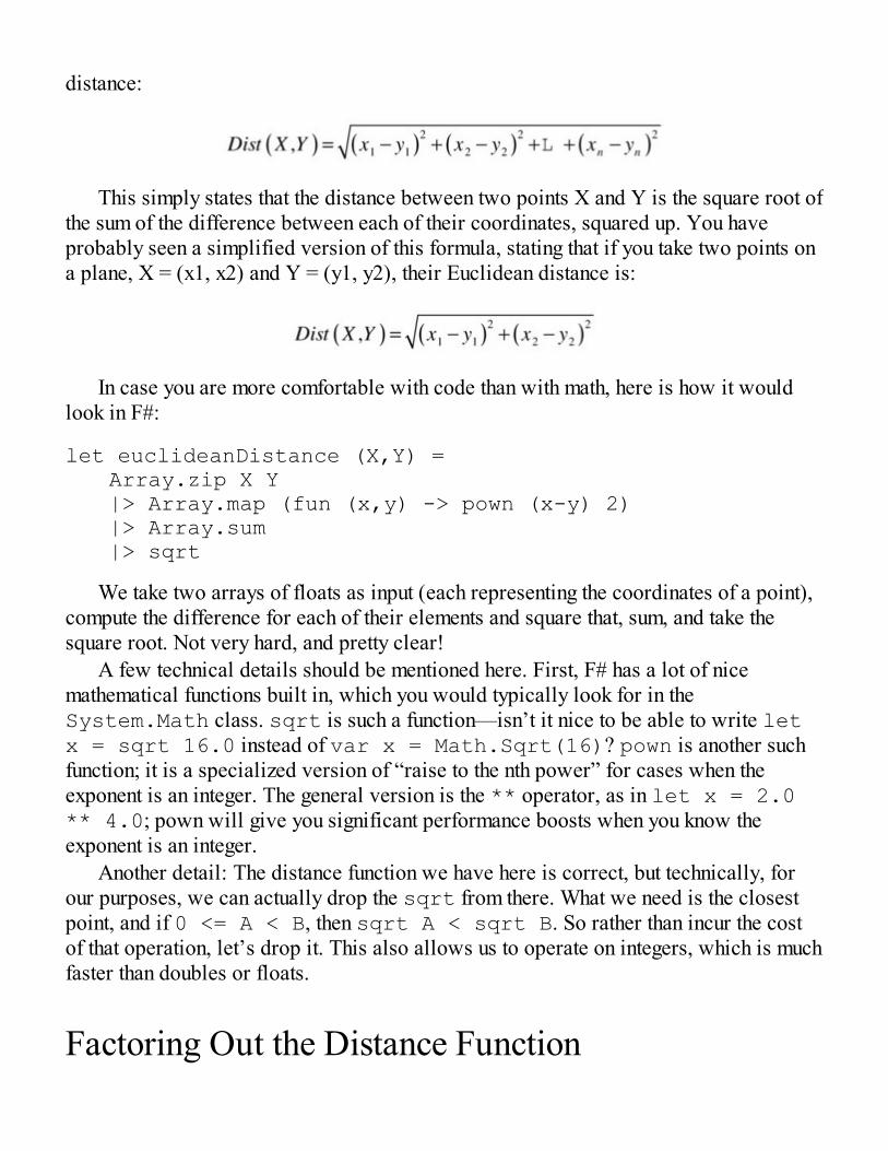
distance:

This simply states that the distance between two points X and Y is the square root ofthe sum of the difference between each of their coordinates, squared up. You haveprobably seen a simplified version of this formula, stating that if you take two points ona plane, X = (x1, x2) and Y = (y1, y2), their Euclidean distance is:

In case you are more comfortable with code than with math, here is how it wouldlook in F#:

let euclideanDistance (X,Y) = Array.zip X Y |> Array.map (fun (x,y) -> pown (x-y) 2) |> Array.sum |> sqrt

We take two arrays of floats as input (each representing the coordinates of a point),compute the difference for each of their elements and square that, sum, and take thesquare root. Not very hard, and pretty clear!

A few technical details should be mentioned here. First, F# has a lot of nicemathematical functions built in, which you would typically look for in theSystem.Math class. sqrt is such a function—isn’t it nice to be able to write letx = sqrt 16.0 instead of var x = Math.Sqrt(16)? pown is another suchfunction; it is a specialized version of “raise to the nth power” for cases when theexponent is an integer. The general version is the ** operator, as in let x = 2.0** 4.0; pown will give you significant performance boosts when you know theexponent is an integer.

Another detail: The distance function we have here is correct, but technically, forour purposes, we can actually drop the sqrt from there. What we need is the closestpoint, and if 0 <= A < B, then sqrt A < sqrt B. So rather than incur the costof that operation, let’s drop it. This also allows us to operate on integers, which is muchfaster than doubles or floats.

Factoring Out the Distance Function

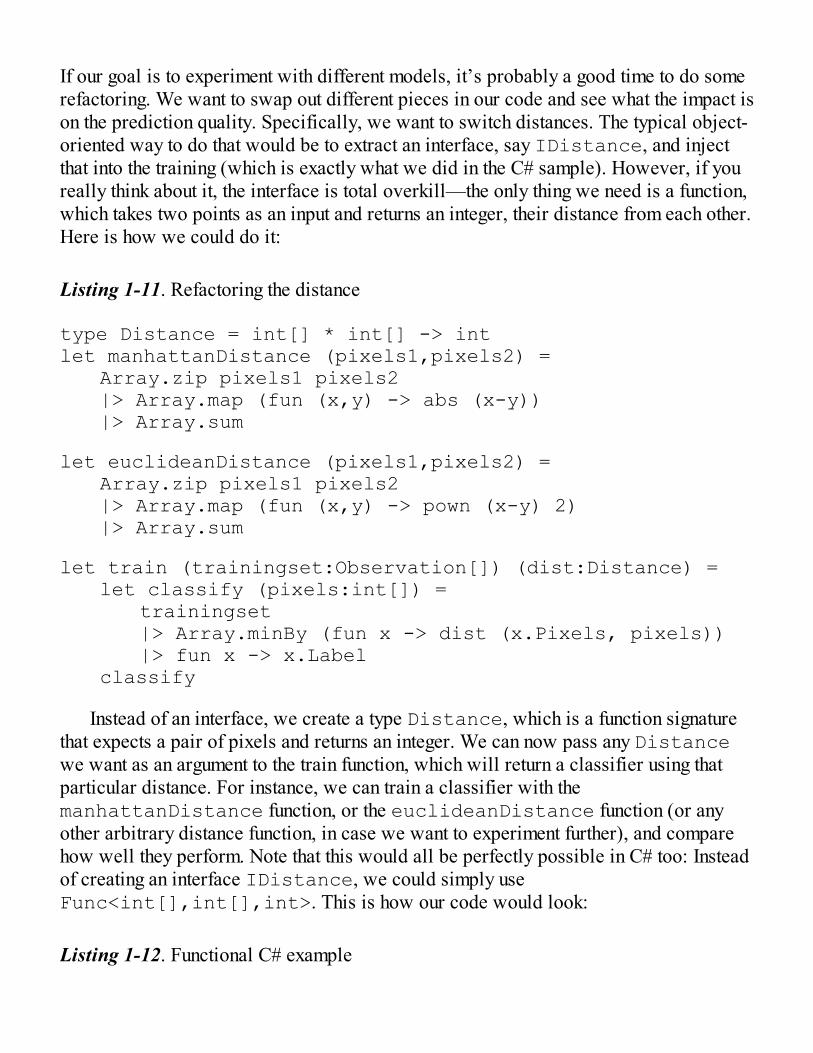
If our goal is to experiment with different models, it’s probably a good time to do somerefactoring. We want to swap out different pieces in our code and see what the impact ison the prediction quality. Specifically, we want to switch distances. The typical object-oriented way to do that would be to extract an interface, say IDistance, and injectthat into the training (which is exactly what we did in the C# sample). However, if youreally think about it, the interface is total overkill—the only thing we need is a function,which takes two points as an input and returns an integer, their distance from each other.Here is how we could do it:

Listing 1-11. Refactoring the distance

type Distance = int[] * int[] -> intlet manhattanDistance (pixels1,pixels2) = Array.zip pixels1 pixels2 |> Array.map (fun (x,y) -> abs (x-y)) |> Array.sum

let euclideanDistance (pixels1,pixels2) = Array.zip pixels1 pixels2 |> Array.map (fun (x,y) -> pown (x-y) 2) |> Array.sum

let train (trainingset:Observation[]) (dist:Distance) = let classify (pixels:int[]) = trainingset |> Array.minBy (fun x -> dist (x.Pixels, pixels)) |> fun x -> x.Label classify

Instead of an interface, we create a type Distance, which is a function signaturethat expects a pair of pixels and returns an integer. We can now pass any Distancewe want as an argument to the train function, which will return a classifier using thatparticular distance. For instance, we can train a classifier with themanhattanDistance function, or the euclideanDistance function (or anyother arbitrary distance function, in case we want to experiment further), and comparehow well they perform. Note that this would all be perfectly possible in C# too: Insteadof creating an interface IDistance, we could simply useFunc<int[],int[],int>. This is how our code would look:

Listing 1-12. Functional C# example

public class FunctionalExample{ private IEnumerable<Observation> data;

private readonly Func<int[], int[], int> distance;

public FunctionalExample(Func<int[], int[], int> distance) { this.distance = distance; }

public Func<int[], int[], int> Distance { get { return this.distance; } }

public void Train(IEnumerable<Observation> trainingSet) { this.data = trainingSet; }

public string Predict(int[] pixels) { Observation currentBest = null; var shortest = Double.MaxValue;

foreach (Observation obs in this.data) { var dist = this.Distance(obs.Pixels, pixels); if (dist < shortest) { shortest = dist; currentBest = obs; } }

return currentBest.Label; }}

This approach, which focuses on composing functions instead of objects, is typical

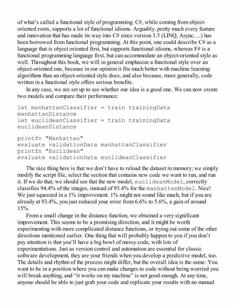
of what’s called a functional style of programming. C#, while coming from object-oriented roots, supports a lot of functional idioms. Arguably, pretty much every featureand innovation that has made its way into C# since version 3.5 (LINQ, Async, ...) hasbeen borrowed from functional programming. At this point, one could describe C# as alanguage that is object oriented first, but supports functional idioms, whereas F# is afunctional programming language first, but can accommodate an object-oriented style aswell. Throughout this book, we will in general emphasize a functional style over anobject-oriented one, because in our opinion it fits much better with machine learningalgorithms than an object-oriented style does, and also because, more generally, codewritten in a functional style offers serious benefits.

In any case, we are set up to see whether our idea is a good one. We can now createtwo models and compare their performance:

let manhattanClassifier = train trainingData manhattanDistancelet euclideanClassifier = train trainingData euclideanDistance

printfn "Manhattan"evaluate validationData manhattanClassifierprintfn "Euclidean"evaluate validationData euclideanClassifier

The nice thing here is that we don’t have to reload the dataset in memory; we simplymodify the script file, select the section that contains new code we want to run, and runit. If we do that, we should see that the new model, euclideanModel, correctlyclassifies 94.4% of the images, instead of 93.4% for the manhattanModel. Nice!We just squeezed in a 1% improvement. 1% might not sound like much, but if you arealready at 93.4%, you just reduced your error from 6.6% to 5.6%, a gain of around15%.

From a small change in the distance function, we obtained a very significantimprovement. This seems to be a promising direction, and it might be worthexperimenting with more complicated distance functions, or trying out some of the otherdirections mentioned earlier. One thing that will probably happen to you if you don’tpay attention is that you’ll have a big bowl of messy code, with lots ofexperimentations. Just as version control and automation are essential for classicsoftware development, they are your friends when you develop a predictive model, too.The details and rhythm of the process might differ, but the overall idea is the same: Youwant to be in a position where you can make changes to code without being worried youwill break anything, and “it works on my machine” is not good enough. At any time,anyone should be able to just grab your code and replicate your results with no manual

intervention. This approach is known as “reproducible research.” I strongly encourageyou to go that direction and use scripting and source control everywhere you can; I haveexperienced myself the horrible scenario in which you know you had a model yesterdaythat worked better, but because you haven’t bothered to save things cleanly, you justcan’t remember how exactly you did it, and that model is gone. Don’t be that person!Especially in this day and age when creating branches with DVCS like Git or Mercurialis so easy, there is no excuse to have that type of issue. When you have a new idea for amodel, create a branch and save the steps you execute in your script.

So, What Have We Learned?We covered quite a bit of ground in this chapter! On the machine learning front, you arenow familiar with a few key concepts, as well as with the methodology. And if you arenew to F#, you have now written your first piece of F# code!

Let’s review some of the main points, starting with the machine learning side.First, we discussed cross-validation, the process of using separate datasets for

training and validation, setting apart some of the data to evaluate the quality of yourprediction model. This is a crucial process on many levels. First, it provides you with abaseline, a “ground truth” that guides your experimentation. Without a validation set,you cannot make judgments on whether a particular model is better than another. Cross-validation allows you to measure quality scientifically. It plays a role somewhatanalogous to an automated test suite, warning you when your development efforts aregoing off the rails.

Once your cross-validation setup is in place, you can try to experiment, selectingmodels or directions to investigate on quantifiable grounds. The trial-and-errorapproach is an essential part of “doing machine learning.” There is no way to knowbeforehand if a particular approach will work well, so you will have to try it out on thedata to see by yourself, which makes it very important to set yourself up for success andembrace “reproducible research” ideas. Automate your process as much as possiblewith scripts, and use source control liberally so that at any given point you can replicateevery step of your model without human intervention. In general, set yourself up so thatyou can easily change and run code.

What to Look for in a Good Distance FunctionIn our digit-recognizer exploration, we saw that a small change in what distance weused significantly improved our model. At the heart of most (every?) machine learning

models, there is a distance function. All the learning process boils down to is thecomputer attempting to find the best way possible to fit known data to a particularproblem – and the definition of “best fit” is entirely encapsulated in the distancefunction. In a way, it is the translation of your goals from a human form into a statementthat is understandable by a machine, stated using mathematics. The distance function isalso frequently called the cost function; thinking in cost emphasizes more what makes abad solution bad, and what penalty to use so as to avoid selecting bad solutions.

In my experience, it is always worthwhile to take the time to think through your costfunction. No matter how clever an algorithm you use, if the cost function is flawed, theresults will be terrible. Imagine a dataset of individuals that includes twomeasurements: height in feet and weight in pounds. If we were to search for the “mostsimilar” individuals in our dataset, along the lines of what we did for images, here iswhat will happen: While heights are typically in the 5 to 6 feet range, weights are on awider and higher scale, say, 100 to 200 pounds. As a result, directly computing adistance based on these two measurements will essentially ignore differences in height,because a 1 foot difference will be equivalent to a 1 pound difference. One way toaddress this is to transform all features to make sure they are on consistent scales, aprocess known as “normalization,” a topic we’ll discuss in more detail later.Fortunately, all pixels are encoded on an identical scale, and we could ignore thatproblem here, but I hope this example of “Distance Gone Wrong” gives you a sense ofwhy it is worth giving your distance function some thought!

This is also one of those cases where the proper mathematical definitions areactually useful. If you dig back your math notes from way back in school, you’ll see thata distance function (sometimes also called a metric by mathematicians) is defined by afew properties:

Distance(A,B) > 0 (there is no negative distance)

Distance(A,B) = 0 if and only if A = B (the only element with 0distance to A is A itself)

Distance(A,B) = Distance(B,A) (symmetry: going from A to Bshould be the same length as going from B to A)

Distance(A,B) <= Distance(A,C) + Distance(C,B) (“Triangleinequality”: there is no shorter distance between two points thandirect travel)

We just looked at two distances in this chapter, but there is a wide variety offunctions that satisfy these properties, each of which defines similarity in a differentmanner. For that matter, the cost function in a model doesn’t need to satisfy all theseproperties, but in general, if it doesn’t, you might want to ask yourself what unintended

side effects could arise because of it. For instance, in the initial example with theManhattan distance, if we had omitted the absolute value, we would be blatantlyviolating both rule 1 (non-negative distance) and rule 3 (symmetry). In some case, thereare good reasons to take liberties and use a function that is not a metric, but when thathappens, take an extra minute to think through what could possibly go wrong!

Models Don’t Have to Be ComplicatedFinally, I hope what came through is that effective models don’t have to be complicated!Whether in C# or F#, both classifiers were small and used fairly simple math. Ofcourse, some complex models may give you amazing results, too, but if you can get thesame result with a simple model that you can understand and modify easily, then whynot go for easy?

This is known as Occam’s Razor, named after William of Ockham, a medievalphilosopher. Occam’s Razor follows a principle of economy. When trying to explainsomething, when choosing between multiple models that could fit, pick the simplest one.Only when no simple explanation works should you go for complicated models.

In the same vein, we implemented first “the simplest thing that could possibly work”here, and I strongly encourage you to follow that approach. If you don’t, here is whatwill probably happen: You will start implementing a few ideas that could work; theywill spark new ideas, so you will soon have a bunch of half-baked prototypes, and willgo deeper and deeper in the jungle, without a clear process or method. Suddenly, youwill realize you have spent a couple of weeks coding away, and you are not quite surewhether anything works or where to go from there. This is not a good feeling. Time boxyourself and spend one day (or one week, or one hour, whatever is realistic given yourproblem) and build an end-to-end model with the dumbest, simplest possible predictionmodel you can think of. It might actually turn out to be good enough, in which case youwon’t have wasted any time. And if it isn’t good enough, by that point you will have aproper harness, with data integration and cross-validation in place, and you will alsolikely have uncovered whatever unexpected nastiness might exist in your dataset. Youwill be in a great place to enter the jungle.

Why F#?If this was your first exposure to F#, you might have wondered initially why I wouldintroduce that language, and not stick with C#. I hope that the example made clear why Idid! In my opinion, while C# is a great language, F# is a fantastic fit for machinelearning and data exploration. We will see more of F# in further chapters, but I hope

some of these reasons became clear in this chapter.First, the F# Interactive and Scripting environments are absolute time savers. When

developing a machine learning model, it is crucial to be able to experiment, changecode, and see the impact, fast, and you need a scripting environment for that. My typicalF# workflow is to load whatever data I need in the Interactive environment when Ibegin the day. Once that is done, I don’t need to reload it again—the data is there, inmemory, and I can freely play with models. By contrast, testing out a new idea in C#forces me to rebuild the code and reload the data, which will end up being a big timesink.

Also, some of the language features of F# make it a great fit for data manipulation.Its focus on functions, rather than objects, works great for applying functions to data andshaping them any way you need. The pipe-forward operator |> is very convenient forcombining such transformations and creating a pipeline that represents in a veryreadable way data transformation workflows. Combine this with the ability to pack datainto tuples and unpack it with pattern matching, and the huge choice of built-in functionsin the Array, List, and Seq modules, and you’ve got something like LINQ on steroidswith which to transform and reshape your data any which way you want.

Going FurtherOne reaction I often get from people who see the algorithm for the first time is “but. . .this is pretty dumb.” What they really mean is, “but... where is the learning?” Formally,machine learning is defined as “writing a program that performs a task better when itgets more data.” Our model, the 1 Nearest Neighbor, fits that definition perfectly: Youwould expect larger samples to “work better” (or conversely, you would expect theperformance to degrade if you reduced the sample). On the other hand, it doesn’t quitefit our intuitive understanding of learning. Our model really memorizes everything it hasseen, whereas humans tend to think of learning as identifying higher-level abstractions,which provide a more compact representation of our experience. When you see thepicture of a number, you don’t go over every picture you have ever seen in your entirelife to decide whether this is a match—you know higher-level concepts that allow youto filter and recognize (“A zero looks like a circle”).

More advanced algorithms, such as Support Vector Machines or Neural Networks,could be used on our problem (we will do that in Chapter 8), and their behavior is morein line with this conception of “learning”: They process the data during the trainingphase and extract a reduced representation. The obvious downside is that the trainingphase will actually be much more involved; the upside is that the resulting model willbe both smaller and faster.

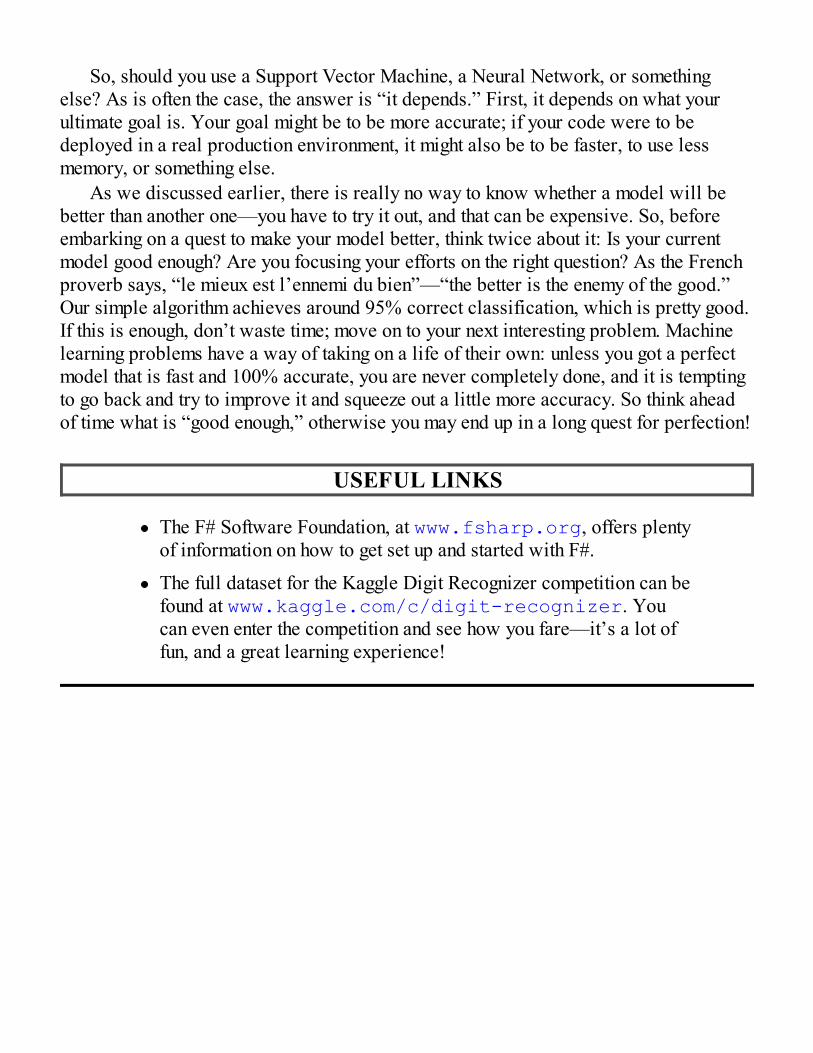
So, should you use a Support Vector Machine, a Neural Network, or somethingelse? As is often the case, the answer is “it depends.” First, it depends on what yourultimate goal is. Your goal might be to be more accurate; if your code were to bedeployed in a real production environment, it might also be to be faster, to use lessmemory, or something else.

As we discussed earlier, there is really no way to know whether a model will bebetter than another one—you have to try it out, and that can be expensive. So, beforeembarking on a quest to make your model better, think twice about it: Is your currentmodel good enough? Are you focusing your efforts on the right question? As the Frenchproverb says, “le mieux est l’ennemi du bien”—“the better is the enemy of the good.”Our simple algorithm achieves around 95% correct classification, which is pretty good.If this is enough, don’t waste time; move on to your next interesting problem. Machinelearning problems have a way of taking on a life of their own: unless you got a perfectmodel that is fast and 100% accurate, you are never completely done, and it is temptingto go back and try to improve it and squeeze out a little more accuracy. So think aheadof time what is “good enough,” otherwise you may end up in a long quest for perfection!

USEFUL LINKS

The F# Software Foundation, at www.fsharp.org, offers plentyof information on how to get set up and started with F#.

The full dataset for the Kaggle Digit Recognizer competition can befound at www.kaggle.com/c/digit-recognizer. Youcan even enter the competition and see how you fare—it’s a lot offun, and a great learning experience!

CHAPTER 2

Spam or Ham?

Automatically Detect spam in Text UsingBayes’ TheoremIf you use email (I suspect you do!), chances are that you see machine learning at workon a daily basis. Your email client probably includes some spam filter mechanism,which automatically identifies blatantly unwanted promotional materials in yourincoming messages and discreetly sends them into oblivion in a “spam folder.” It sparesyou the annoyance of having to delete these messages manually one by one; it will alsosave you from inadvertently clicking potentially harmful links. This is typical of howmachine learning, when well done, can make human life better. Computers are great atperforming repetitive tasks and being thorough about it; by automatically taking care oftedious activities and saving us from mistakes, they enable us humans to focus on moreinteresting, thought-engaging activities.

Spam detection is a great illustration of machine learning in action, and is thecanonical example of what classification is about. Given a collection of emailmessages, we need to classify them into two categories, or classes: Spam (an unwantedmessage that should go directly to the trash) or Ham (a valid message that we do want toread). It is also interesting for another reason: Unlike the digit-recognition problem wetackled in Chapter 1, where the data was in numeric form, spam detection is all abouttext. A major part of the material available in the digital universe is text rather thanwell-organized tables of numbers, so understanding how to work with it is important.

In this chapter, we will build a spam-detection engine from scratch, and then use thatexample to illustrate a couple of useful techniques and ideas. We will

establish an approach to working with text. From the computerstandpoint, a raw text document is just a random collection of

characters. We will see how we can extract features (that is,convert the original data into new and more informative or usableproperties, the “features”) from a block of text by transforming itinto tokens that can be processed by a computer.

look at Bayes’ Theorem, a simple yet powerful mathematicalformula that quantifies how new information can be incorporated soas to update our assessment of uncertain events. As a directapplication, we will implement a naïve Bayes classifier, analgorithm that uses vocabulary frequency to determine documenttypes.

discuss the importance of understanding your data for properlyinterpreting your results and their quality, and illustrate howextracting new features from a dataset can significantly enhance thepredictive power of a model, without modifying the algorithmitself.

We will focus first on implementing a general algorithm to analyze text documentsand decide what category they belong to. Once we have that tool in place, we will turnour attention back to our dataset and see how carefully inspecting the data we haveavailable will allow us to craft new features and improve the quality of our predictionsquite significantly.

Our Challenge: Build a Spam-DetectionEngineThe documents we will be working with here won’t be email. Instead, we will bedealing with text messages. Our goal will be to recognize spam, using a dataset of realSMS (Short Message Service) messages from the United Kingdom, which we found inthe wonderful University of California–Irvine Machine Learning Repository.

Side note The UCI Machine Learning Repository was started in 1987 by the Centerfor Machine Learning and Intelligent Systems at University of California Irvine. You canfind the Machine Learning Repository at http://archive.ics.uci.edu/ml/.It is a library of nearly 300 clean and well-documented datasets, searchable andorganized by criteria such as size, type of features, and more. It is a fantastic resourcefor learning machine learning, and it contains a number of “classic” datasets that are

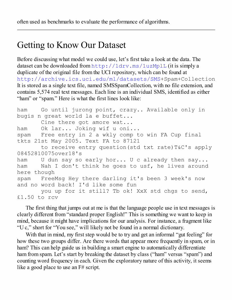
often used as benchmarks to evaluate the performance of algorithms.

Getting to Know Our DatasetBefore discussing what model we could use, let’s first take a look at the data. Thedataset can be downloaded from http://1drv.ms/1uzMplL (it is simply aduplicate of the original file from the UCI repository, which can be found athttp://archive.ics.uci.edu/ml/datasets/SMS+Spam+CollectionIt is stored as a single text file, named SMSSpamCollection, with no file extension, andcontains 5,574 real text messages. Each line is an individual SMS, identified as either“ham” or “spam.” Here is what the first lines look like:

ham Go until jurong point, crazy.. Available only in bugis n great world la e buffet... Cine there got amore wat...ham Ok lar... Joking wif u oni...spam Free entry in 2 a wkly comp to win FA Cup final tkts 21st May 2005. Text FA to 87121 to receive entry question(std txt rate)T&C's apply 08452810075over18'sham U dun say so early hor... U c already then say...ham Nah I don't think he goes to usf, he lives around here thoughspam FreeMsg Hey there darling it's been 3 week's now and no word back! I'd like some fun you up for it still? Tb ok! XxX std chgs to send, £1.50 to rcv

The first thing that jumps out at me is that the language people use in text messages isclearly different from “standard proper English!” This is something we want to keep inmind, because it might have implications for our analysis. For instance, a fragment like“U c,” short for “You see,” will likely not be found in a normal dictionary.

With that in mind, my first step would be to try and get an informal “gut feeling” forhow these two groups differ. Are there words that appear more frequently in spam, or inham? This can help guide us in building a smart engine to automatically differentiateham from spam. Let’s start by breaking the dataset by class (“ham” versus “spam”) andcounting word frequency in each. Given the exploratory nature of this activity, it seemslike a good place to use an F# script.

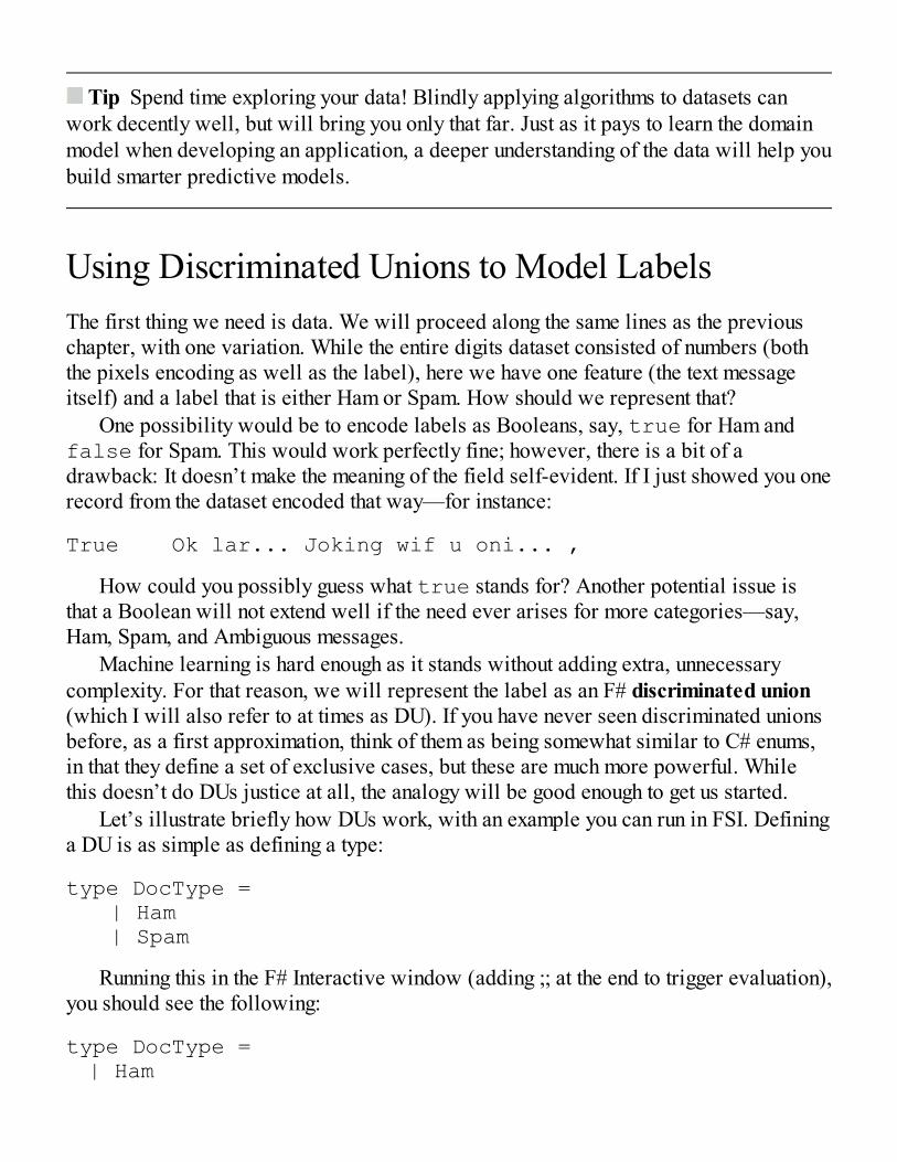
Tip Spend time exploring your data! Blindly applying algorithms to datasets canwork decently well, but will bring you only that far. Just as it pays to learn the domainmodel when developing an application, a deeper understanding of the data will help youbuild smarter predictive models.

Using Discriminated Unions to Model LabelsThe first thing we need is data. We will proceed along the same lines as the previouschapter, with one variation. While the entire digits dataset consisted of numbers (boththe pixels encoding as well as the label), here we have one feature (the text messageitself) and a label that is either Ham or Spam. How should we represent that?

One possibility would be to encode labels as Booleans, say, true for Ham andfalse for Spam. This would work perfectly fine; however, there is a bit of adrawback: It doesn’t make the meaning of the field self-evident. If I just showed you onerecord from the dataset encoded that way—for instance:

True Ok lar... Joking wif u oni... ,

How could you possibly guess what true stands for? Another potential issue isthat a Boolean will not extend well if the need ever arises for more categories—say,Ham, Spam, and Ambiguous messages.

Machine learning is hard enough as it stands without adding extra, unnecessarycomplexity. For that reason, we will represent the label as an F# discriminated union(which I will also refer to at times as DU). If you have never seen discriminated unionsbefore, as a first approximation, think of them as being somewhat similar to C# enums,in that they define a set of exclusive cases, but these are much more powerful. Whilethis doesn’t do DUs justice at all, the analogy will be good enough to get us started.

Let’s illustrate briefly how DUs work, with an example you can run in FSI. Defininga DU is as simple as defining a type:

type DocType = | Ham | Spam

Running this in the F# Interactive window (adding ;; at the end to trigger evaluation),you should see the following:

type DocType = | Ham

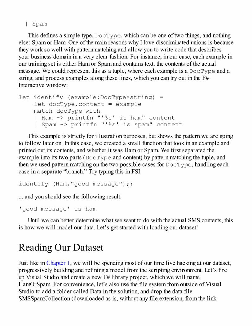
| Spam

This defines a simple type, DocType, which can be one of two things, and nothingelse: Spam or Ham. One of the main reasons why I love discriminated unions is becausethey work so well with pattern matching and allow you to write code that describesyour business domain in a very clear fashion. For instance, in our case, each example inour training set is either Ham or Spam and contains text, the contents of the actualmessage. We could represent this as a tuple, where each example is a DocType and astring, and process examples along these lines, which you can try out in the F#Interactive window:

let identify (example:DocType*string) = let docType,content = example match docType with | Ham -> printfn "'%s' is ham" content | Spam -> printfn "'%s' is spam" content

This example is strictly for illustration purposes, but shows the pattern we are goingto follow later on. In this case, we created a small function that took in an example andprinted out its contents, and whether it was Ham or Spam. We first separated theexample into its two parts (DocType and content) by pattern matching the tuple, andthen we used pattern matching on the two possible cases for DocType, handling eachcase in a separate “branch.” Try typing this in FSI:

identify (Ham,"good message");;

... and you should see the following result:

'good message' is ham

Until we can better determine what we want to do with the actual SMS contents, thisis how we will model our data. Let’s get started with loading our dataset!

Reading Our DatasetJust like in Chapter 1, we will be spending most of our time live hacking at our dataset,progressively building and refining a model from the scripting environment. Let’s fireup Visual Studio and create a new F# library project, which we will nameHamOrSpam. For convenience, let’s also use the file system from outside of VisualStudio to add a folder called Data in the solution, and drop the data fileSMSSpamCollection (downloaded as is, without any file extension, from the link

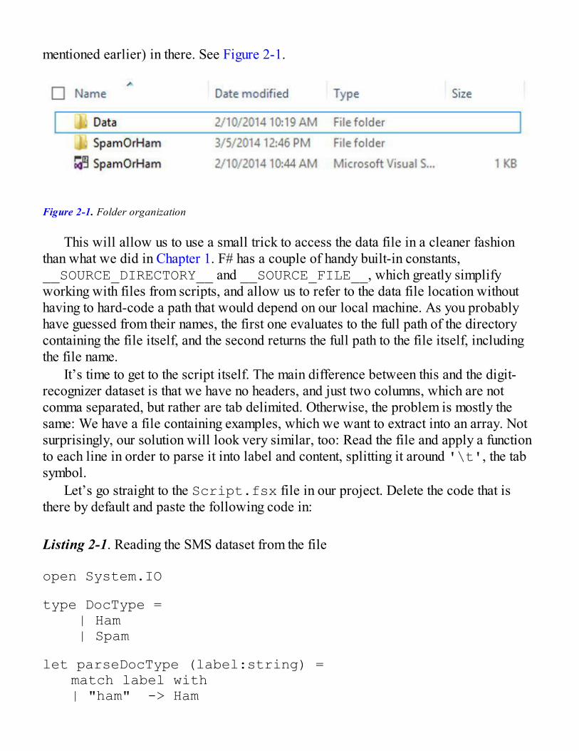
mentioned earlier) in there. See Figure 2-1.

Figure 2-1. Folder organization

This will allow us to use a small trick to access the data file in a cleaner fashionthan what we did in Chapter 1. F# has a couple of handy built-in constants,__SOURCE_DIRECTORY__ and __SOURCE_FILE__, which greatly simplifyworking with files from scripts, and allow us to refer to the data file location withouthaving to hard-code a path that would depend on our local machine. As you probablyhave guessed from their names, the first one evaluates to the full path of the directorycontaining the file itself, and the second returns the full path to the file itself, includingthe file name.

It’s time to get to the script itself. The main difference between this and the digit-recognizer dataset is that we have no headers, and just two columns, which are notcomma separated, but rather are tab delimited. Otherwise, the problem is mostly thesame: We have a file containing examples, which we want to extract into an array. Notsurprisingly, our solution will look very similar, too: Read the file and apply a functionto each line in order to parse it into label and content, splitting it around '\t', the tabsymbol.

Let’s go straight to the Script.fsx file in our project. Delete the code that isthere by default and paste the following code in:

Listing 2-1. Reading the SMS dataset from the file

open System.IO

type DocType = | Ham | Spam

let parseDocType (label:string) = match label with | "ham" -> Ham

| "spam" -> Spam | _ -> failwith "Unknown label"

let parseLine (line:string) = let split = line.Split('\t') let label = split.[0] |> parseDocType let message = split.[1] (label, message)

Let fileName = "SMSSpamCollection"let path = __SOURCE_DIRECTORY__ + @"..\..\Data\" + fileName

let dataset = File.ReadAllLines path |> Array.map parseLine

At this point, you should be able to select the entire code you just wrote in the scriptfile and execute it in F# Interactive, which will produce the following:

val dataset : (DocType * string) [] = [|(Ham, "Go until jurong point, crazy.. Available only in bugis n grea"+[50 chars]); (Ham, "Ok lar... Joking wif u oni..."); (Spam, "Free entry in 2 a wkly comp to win FA Cup final tkts 21st May"+[94 chars]); // Snipped for brevity (Ham, "Hi. Wk been ok - on hols now! Yes on for a bit of a run. Forg"+[117 chars]); (Ham, "I see a cup of coffee animation"); ...|]

We now have a dataset of examples, each of which is identified as Spam or Ham.We can start getting to work on the question we are really interested in: What featurescan we use to distinguish between Ham and Spam messages?

Tip Using File.ReadAllLines to read the contents of the dataset may notalways be the best idea. We are loading everything in memory at once into an array, andthen creating another array to store the result of the Array.map transformation. Thisparticular dataset contains around 5,000 lines, which is fairly small, but when dealing

with larger datasets, you can use a streaming version (such asSystem.IO.StreamReader.ReadLine()) to load the dataset one line at a timeinto memory.

Deciding on a Single WordNow that we have data, we can begin the analysis. Our end goal is to recognize Spamfrom Ham, but, unlike in the digit-recognizer case, we don’t have a clear set of featuresyet; the only material we have available is a raw chunk of text, the SMS itself. At thesame time, one would suspect that there is a lot of information to be leveraged in thetext. We just need to find a way to transform these strings into features we can workwith.

Using Words as CluesIf you looked through the dataset we just loaded, you probably noticed that Spammessages look a bit different from Ham. Scanning through messages, your eyes caneasily pick some clues that raise a red flag, and suggest that a message is more likely tobe Spam. As an example, the word “FREE” (all caps!) appears early on in a couple ofSpam items, and doesn’t seem to pop up often in Ham.

This suggests a possible approach: using individual words from the entire messageto recognize which category it belongs to. Let’s first try to confirm that our intuition iscorrect by counting how many Spam messages contain that particular string andcomparing it with the Ham messages. We can test this out by typing a couple of lines ofF# in our script. First, let’s filter our dataset so as to keep only Spam, then filter again,this time retaining only messages that contain “FREE,” and finally count how manyitems are left:

let spamWithFREE = dataset |> Array.filter (fun (docType,_) -> docType = Spam) |> Array.filter (fun (_,sms) -> sms.Contains("FREE")) |> Array.length

Select the code above and run it in F# Interactive—you should see the followingresult:

val spamWithFREE : int = 112

Now let’s do the same thing for Ham:

let hamWithFREE = dataset |> Array.filter (fun (docType,_) -> docType = Ham) |> Array.filter (fun (_,sms) -> sms.Contains("FREE")) |> Array.length

This should produce the following:

val hamWithFREE : int = 1

The numbers confirm our intuition: “FREE” is indeed used much more frequently inSpam than in Ham, and seems like a good flag to use for differentiating the twocategories. We could use this to build a very primitive Spam classifier, like this:

let primitiveClassifier (sms:string) = if (sms.Contains "FREE") then Spam else Ham

This is a promising start. However, if we want to build anything more serious usingthis idea, we will need to address two issues. First, we picked “FREE” as a Spamindicator, but didn’t really justify why. How do we know if a particular word is, orisn’t, a good marker for Spam or Ham? Then, making a decision based on a single wordfrom a whole message seems rather limiting. Can we somehow use multiple words atonce and combine their (potentially conflicting) information into a single decisionprocedure?

Putting a Number on How Certain We AreIt doesn’t take an advanced degree in statistics to intuitively see that messagescontaining “FREE” are very likely Spam. Can we formalize how we reached thatconclusion in a manner that doesn’t rely on intuition, and quantifies how reliably aspecific word indicates whether a message is Ham or Spam?

Personally, I often resort to decision trees as a way to better understand probabilityproblems. In our case, here is what we did: We took our corpus of 5,574 documents,split it into two groups by document type (747 Spam vs. 4,827 Ham), and, for eachdocument group, we counted how many contained the word “FREE.” This can berepresented as a decision tree, as displayed in Figure 2-2:

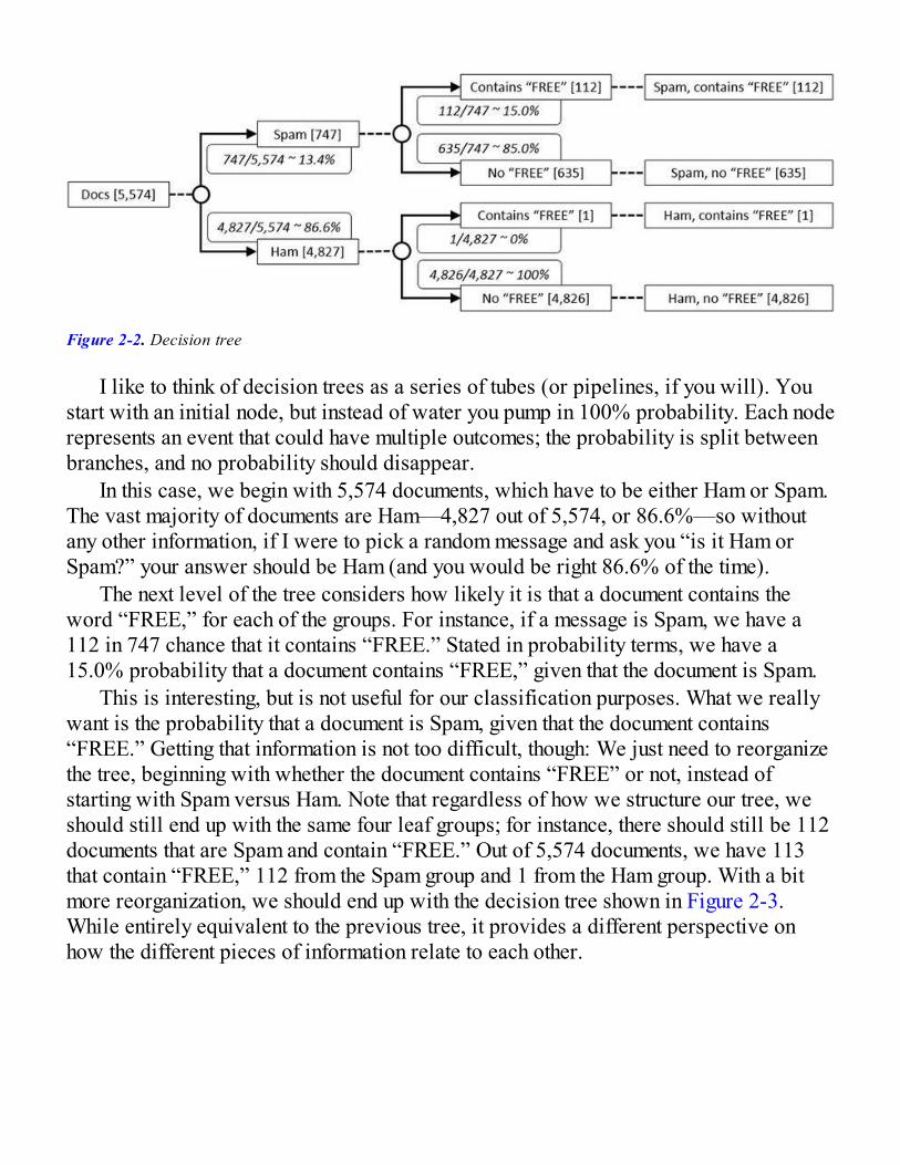
Figure 2-2. Decision tree

I like to think of decision trees as a series of tubes (or pipelines, if you will). Youstart with an initial node, but instead of water you pump in 100% probability. Each noderepresents an event that could have multiple outcomes; the probability is split betweenbranches, and no probability should disappear.

In this case, we begin with 5,574 documents, which have to be either Ham or Spam.The vast majority of documents are Ham—4,827 out of 5,574, or 86.6%—so withoutany other information, if I were to pick a random message and ask you “is it Ham orSpam?” your answer should be Ham (and you would be right 86.6% of the time).

The next level of the tree considers how likely it is that a document contains theword “FREE,” for each of the groups. For instance, if a message is Spam, we have a112 in 747 chance that it contains “FREE.” Stated in probability terms, we have a15.0% probability that a document contains “FREE,” given that the document is Spam.

This is interesting, but is not useful for our classification purposes. What we reallywant is the probability that a document is Spam, given that the document contains“FREE.” Getting that information is not too difficult, though: We just need to reorganizethe tree, beginning with whether the document contains “FREE” or not, instead ofstarting with Spam versus Ham. Note that regardless of how we structure our tree, weshould still end up with the same four leaf groups; for instance, there should still be 112documents that are Spam and contain “FREE.” Out of 5,574 documents, we have 113that contain “FREE,” 112 from the Spam group and 1 from the Ham group. With a bitmore reorganization, we should end up with the decision tree shown in Figure 2-3.While entirely equivalent to the previous tree, it provides a different perspective onhow the different pieces of information relate to each other.

Figure 2-3. Flipped decision tree

Specifically, it directly gives us the information we care about: the probability that adocument is Spam, if it contains the word “FREE,” is 112/113, or 99.1% (thusscientifically confirming our earlier intuition).

Bayes’ TheoremThe method we just used has a name: Bayes’ Theorem. In its driest textbook form, it isusually stated like this:

The | symbol should be read as “given that.” The example we just went through wasabout computing the probability that an email is Spam, given that it contains the word“FREE,” and, in Bayes’ Theorem formulation, would be writ.ke this:

If you work out the numbers mechanically, you will get the following result, whichis precisely what we arrived at with the decision tree:

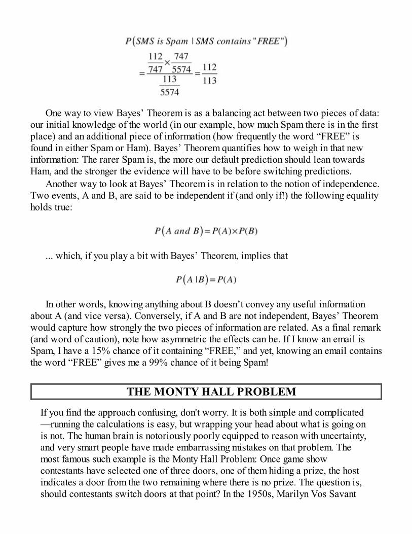
One way to view Bayes’ Theorem is as a balancing act between two pieces of data:our initial knowledge of the world (in our example, how much Spam there is in the firstplace) and an additional piece of information (how frequently the word “FREE” isfound in either Spam or Ham). Bayes’ Theorem quantifies how to weigh in that newinformation: The rarer Spam is, the more our default prediction should lean towardsHam, and the stronger the evidence will have to be before switching predictions.

Another way to look at Bayes’ Theorem is in relation to the notion of independence.Two events, A and B, are said to be independent if (and only if!) the following equalityholds true:

... which, if you play a bit with Bayes’ Theorem, implies that

In other words, knowing anything about B doesn’t convey any useful informationabout A (and vice versa). Conversely, if A and B are not independent, Bayes’ Theoremwould capture how strongly the two pieces of information are related. As a final remark(and word of caution), note how asymmetric the effects can be. If I know an email isSpam, I have a 15% chance of it containing “FREE,” and yet, knowing an email containsthe word “FREE” gives me a 99% chance of it being Spam!

THE MONTY HALL PROBLEM

If you find the approach confusing, don't worry. It is both simple and complicated—running the calculations is easy, but wrapping your head about what is going onis not. The human brain is notoriously poorly equipped to reason with uncertainty,and very smart people have made embarrassing mistakes on that problem. Themost famous such example is the Monty Hall Problem: Once game showcontestants have selected one of three doors, one of them hiding a prize, the hostindicates a door from the two remaining where there is no prize. The question is,should contestants switch doors at that point? In the 1950s, Marilyn Vos Savant

correctly answered the question, but a few famous mathematicians, like PaulErdos, incorrectly attempted to show her how mistaken she was. My personallesson from this story is to be very careful when dealing with probabilities,because human intuition doesn't have a good track record there—and of course tothink twice before publicly criticizing anyone!

Dealing with Rare WordsBayes’ Theorem gives us a convenient way to decide whether a message is Ham orSpam based on a single word. However, you might have noticed a small issue. If youpick a word that is present in only one of the categories—for instance, “uncle,”“honeybee,” or “wine,” which exist only in Ham—then our formula will assign a 100%probability for one category and 0% for the other. In other words, if we saw a messagecontaining the word “uncle,” we would automatically decide, with 100% confidence,that this message cannot be Spam, regardless of the rest of the message.

Clearly, this can’t be right; we shouldn’t have 100% confidence in anything basedon a limited training sample. One way to address this problem is by using LaplaceSmoothing. Named after the French mathematician Pierre-Simon de Laplace, this veryintimidating sounding technique can arguably be described as a “fudge factor.” We willeliminate the problem of absent words by augmenting the count of each word by one,and computing P(Spam contains “xyz”) = (1 + count of Spam containing “xyz”) / (1 +count of Spam). Essentially, we are making up a fictional message containing everytoken, and as a result, the rarest tokens will have a very low probability, but not zero.

Combining Multiple WordsUsing Bayes’ Theorem, we figured out how an SMS should be classified depending onwhether or not it contained a particular word. This is progress, but we are not done yet.There are many words in a message, each of which pushes toward Ham or Spam withvarious strength. How can we combine that information, which might be sendingconflicting signals, into a single value we can use to make our decision?

Breaking Text into TokensAs an example, consider the following hypothetical message: “Driving, cant txt.” What

is the probability it is Spam?We could try to apply Bayes’ Theorem directly and look for the entire message in

our dataset. However, I wouldn’t expect this approach to work very well. The chancesof finding an exact duplicate, let alone many, are slim. On the other hand, what we sawis that the word “FREE” carried some relevant information. What we will do is simplybreak the message into a set of words, “driving,” “cant,” and “txt,” and use thatrepresentation instead of the original text. We can then analyze individual tokens and(hopefully) combine what each of them suggests into a single value that we can rely onto make a decision.

This process of breaking up a block of text into meaningful elements (words, orpotentially other symbols), the tokens, is called tokenization. Deciding how you willtokenize is an important part of your model, and there is no unique right way to do it—itdepends on the problem at hand. For the moment, as always, we will start with theeasiest thing we could implement: If one single word, “FREE,” is informative, let’sextend that idea and break up messages into all their individual words. In effect, we aretransforming each message into a collection of features, each feature being the presenceor absence of a particular word.

For instance, if we had two strings, “Programming is Fun” and “Functionalprogramming is more fun!,” we could decompose them as “programming,” “is,” “fun,”and “functional,” “programming,” “is,” “more,” “fun.” This representation will allow usto be much more efficient. Instead of having to check whether a message contains aparticular substring, we can pre-process every document into a set of tokens and rapidlyverify if it contains a particular token we are interested in.

Note This general approach is very useful for transforming text into a form acomputer can work with. For instance, we could gather the entire set of tokens found inour corpus—[“functional”; “programming”; “is”; “more”; “fun”]—and encode eachdocument by counting how many times each token is found. In our example, the firstblock of text becomes [0; 1; 1; 0; 1], and the second one [1; 1; 1; 1; 1]. Our dataset isnow in a form that is completely unreadable by a human, but which looks a whole lotlike our digits dataset from Chapter 1: Each row is an observation, each column is afeature, and everything is encoded as numbers—and we could, for instance, use this todetermine how similar two documents are. Transforming observations in a set ofnumeric features that a computer can analyze to find patterns, in a manner no humancould, is fairly typical in machine learning.

You might be thinking at this point, “This is a gross over simplification,” and youwould be right. After all, we are converting full sentences into a raw collection of

words, ignoring things like syntax, grammar, or word order. This transformation isclearly losing information; for instance, the two sentences “I like carrots and hatebroccoli” and “I like broccoli and hate carrots” will be broken into the same set oftokens [and; broccoli; carrots; hate; i; like], and will therefore be considered identical.At the same time, we are not trying to understand the meaning of sentences here; wemerely need to identify which words are connected to a particular behavior.

Another point I want to stress here is that while our tokenization looks fairlystraightforward, it contains a lot of implicit decisions already. We decided that“Programming” and “programming” would be treated as the same word, ignoringcapitalization. Is that a reasonable assumption? Maybe, maybe not. If you have spent aminimum of time in online discussions, such as forums or YouTube comments, you willprobably agree that A HEAVY USAGE OF CAPITAL LETTERS often indicates thatthe discussion quality is going downhill. So the argument can be made that capitalizationmatters and could provide relevant information for classifying messages. Anotherimplicit decision here was to drop the “!”; is that reasonable? Punctuation could matter.

The good news is, rather than argue over whether capitalization or punctuationmatters, we can settle that question very easily with cross-validation later on. In theimmortal words of W. Edwards Deming, “In God we trust—all others must bring data.”Create alternate models for each hypothesis, compare their performance, and let the datadecide.

Naïvely Combining ScoresNow that we have decided to decompose our message into three tokens—“driving,”“cant,” and “txt”—we still need to figure out a way to compute the probability that themessage is Ham or Spam. “txt” indicates a strong chance of Spam, but “driving” pointstowards Ham. How should we put all that evidence together?

If we apply Bayes’ Theorem to determine the probability that our message is Spam,given that it contains all three tokens, we get:

This is a bit of an intimidating formula. However, if we make one simplifyingassumption, things become much nicer. Let’s assume for a minute that tokens areindependent—that is, seeing one token in a message has no bearing on what other tokensmight be present. In that case, we can compute:

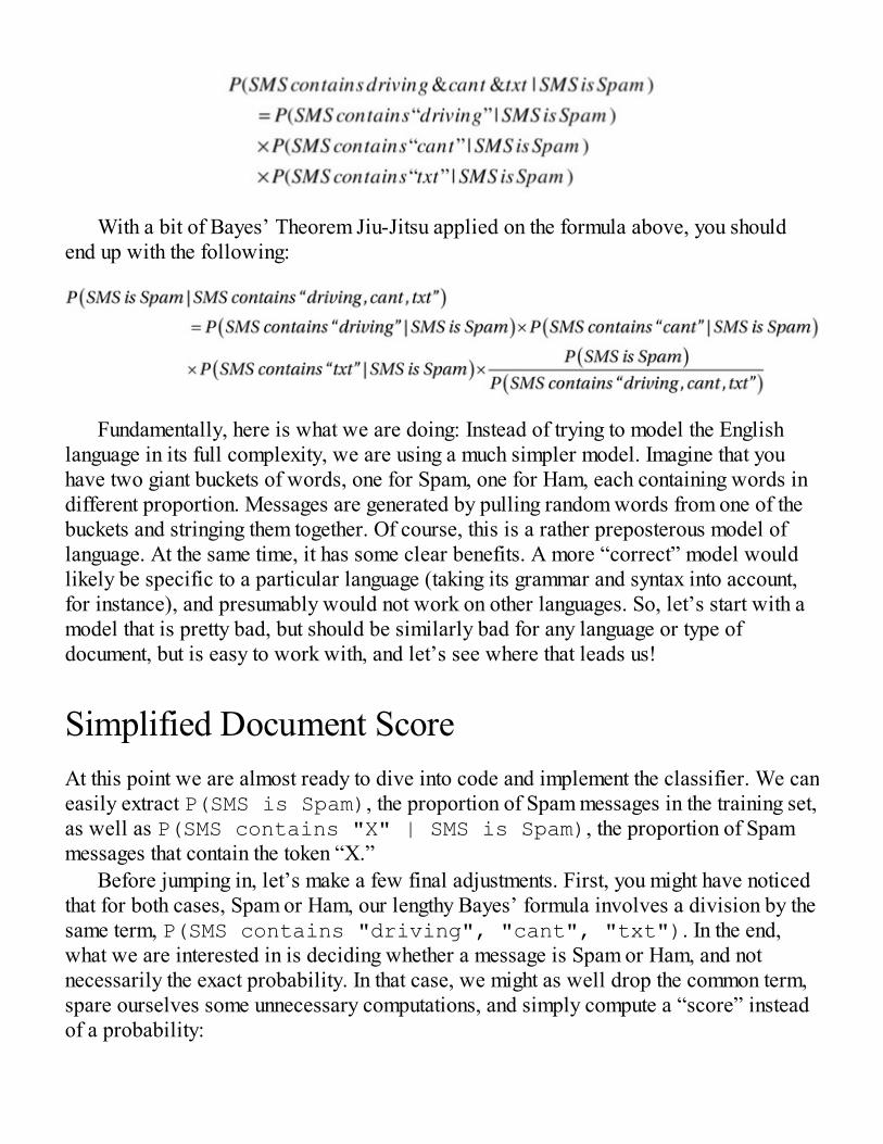
With a bit of Bayes’ Theorem Jiu-Jitsu applied on the formula above, you shouldend up with the following:

Fundamentally, here is what we are doing: Instead of trying to model the Englishlanguage in its full complexity, we are using a much simpler model. Imagine that youhave two giant buckets of words, one for Spam, one for Ham, each containing words indifferent proportion. Messages are generated by pulling random words from one of thebuckets and stringing them together. Of course, this is a rather preposterous model oflanguage. At the same time, it has some clear benefits. A more “correct” model wouldlikely be specific to a particular language (taking its grammar and syntax into account,for instance), and presumably would not work on other languages. So, let’s start with amodel that is pretty bad, but should be similarly bad for any language or type ofdocument, but is easy to work with, and let’s see where that leads us!

Simplified Document ScoreAt this point we are almost ready to dive into code and implement the classifier. We caneasily extract P(SMS is Spam), the proportion of Spam messages in the training set,as well as P(SMS contains "X" | SMS is Spam), the proportion of Spammessages that contain the token “X.”

Before jumping in, let’s make a few final adjustments. First, you might have noticedthat for both cases, Spam or Ham, our lengthy Bayes’ formula involves a division by thesame term, P(SMS contains "driving", "cant", "txt"). In the end,what we are interested in is deciding whether a message is Spam or Ham, and notnecessarily the exact probability. In that case, we might as well drop the common term,spare ourselves some unnecessary computations, and simply compute a “score” insteadof a probability:

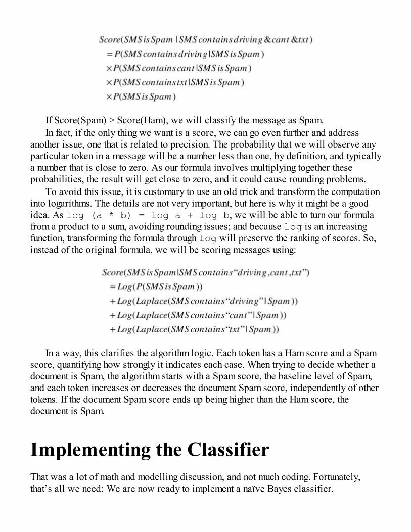
If Score(Spam) > Score(Ham), we will classify the message as Spam.In fact, if the only thing we want is a score, we can go even further and address

another issue, one that is related to precision. The probability that we will observe anyparticular token in a message will be a number less than one, by definition, and typicallya number that is close to zero. As our formula involves multiplying together theseprobabilities, the result will get close to zero, and it could cause rounding problems.

To avoid this issue, it is customary to use an old trick and transform the computationinto logarithms. The details are not very important, but here is why it might be a goodidea. As log (a * b) = log a + log b, we will be able to turn our formulafrom a product to a sum, avoiding rounding issues; and because log is an increasingfunction, transforming the formula through log will preserve the ranking of scores. So,instead of the original formula, we will be scoring messages using:

In a way, this clarifies the algorithm logic. Each token has a Ham score and a Spamscore, quantifying how strongly it indicates each case. When trying to decide whether adocument is Spam, the algorithm starts with a Spam score, the baseline level of Spam,and each token increases or decreases the document Spam score, independently of othertokens. If the document Spam score ends up being higher than the Ham score, thedocument is Spam.

Implementing the ClassifierThat was a lot of math and modelling discussion, and not much coding. Fortunately,that’s all we need: We are now ready to implement a naïve Bayes classifier.

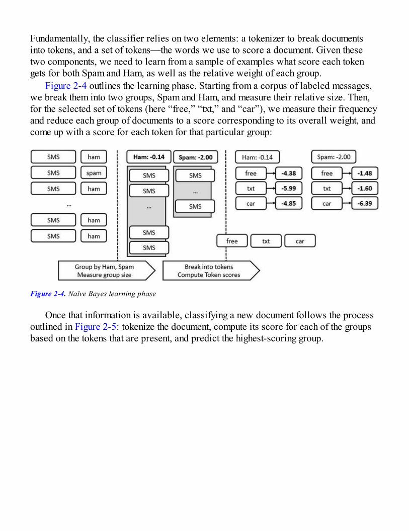
Fundamentally, the classifier relies on two elements: a tokenizer to break documentsinto tokens, and a set of tokens—the words we use to score a document. Given thesetwo components, we need to learn from a sample of examples what score each tokengets for both Spam and Ham, as well as the relative weight of each group.

Figure 2-4 outlines the learning phase. Starting from a corpus of labeled messages,we break them into two groups, Spam and Ham, and measure their relative size. Then,for the selected set of tokens (here “free,” “txt,” and “car”), we measure their frequencyand reduce each group of documents to a score corresponding to its overall weight, andcome up with a score for each token for that particular group:

Figure 2-4. Naïve Bayes learning phase

Once that information is available, classifying a new document follows the processoutlined in Figure 2-5: tokenize the document, compute its score for each of the groupsbased on the tokens that are present, and predict the highest-scoring group.

Figure 2-5. Naïve Bayes classifier outline

In this particular example, once the document has been tokenized, we look upwhether a score is available for each individual token (and ignore it otherwise),compute an overall score for each group, and decide which of the groups is the mostlikely match.

Extracting Code into ModulesTo avoid cluttering the script with too much code, let’s extract the classifier itself into amodule. In order to do that, simply right click on the solution and pick Add New Item,then choose Source File. Rename that file NaiveBayes.fs, delete any default codethat might be there, and replace it with the following:

namespace NaiveBayes

module Classifier =

let Hello name = printfn "Hello, %s" name

Finally, right click on the file and select “Move up” (or Alt + Up Arrow) untilNaiveBayes.fs appears first in the list of files in the solution (you can also add the filedirectly at the desired position by selecting a file in the Solution Explorer and using“Add Above” or “Add Below”). You have now created a module in which you can startwriting functions and calling them from your script, or consuming them from F# or C#projects. Just for the sake of illustration, here is how you would go about using theHello function from our current script:

#load "NaiveBayes.fs"open NaiveBayes.ClassifierHello "World"

Note You might wonder why you had to move up the file you just created. Unlike inC#, the order of files in an F# solution matters. The main reason for that is the type-inference system. The compiler automatically figures out for you what types you meant,by looking at what you have defined in your code file up to that point. In a similarfashion, if you want to use function f in your code, that function f needs to be definedbefore the code that uses it. This is a bit of an additional constraint, but in my opinion itis a very reasonable price to pay for the benefits of type inference; and, as an interestingside effect, it provides a natural order in F# solutions, which makes them very easy tointerpret: Start from line one and read forward, or from the last line and readbackwards!

Scoring and Classifying a DocumentNow that we have the module in place, we will write the algorithm itself in the module,then use the script file to explore data using that algorithm. Let’s follow a typical F#pattern and build from the bottom up, writing small pieces of code and composing theminto larger workflows. The key element of the model is the score computation, whichmeasures how strong the evidence is that a document belongs to a group—for instance,Spam.

The score relies on two components: how frequently the group appears in theoverall corpus (the training data), and how frequently certain tokens are found in thatgroup. Let’s start by defining a couple of types to represent our domain. Rather than

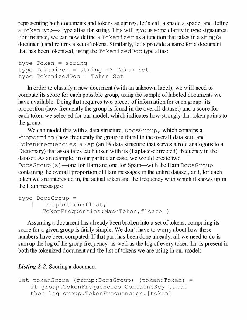
representing both documents and tokens as strings, let’s call a spade a spade, and definea Token type—a type alias for string. This will give us some clarity in type signatures.For instance, we can now define a Tokenizer as a function that takes in a string (adocument) and returns a set of tokens. Similarly, let’s provide a name for a documentthat has been tokenized, using the TokenizedDoc type alias:

type Token = stringtype Tokenizer = string -> Token Settype TokenizedDoc = Token Set

In order to classify a new document (with an unknown label), we will need tocompute its score for each possible group, using the sample of labeled documents wehave available. Doing that requires two pieces of information for each group: itsproportion (how frequently the group is found in the overall dataset) and a score foreach token we selected for our model, which indicates how strongly that token points tothe group.

We can model this with a data structure, DocsGroup, which contains aProportion (how frequently the group is found in the overall data set), andTokenFrequencies, a Map (an F# data structure that serves a role analogous to aDictionary) that associates each token with its (Laplace-corrected) frequency in thedataset. As an example, in our particular case, we would create twoDocsGroup(s)—one for Ham and one for Spam—with the Ham DocsGroupcontaining the overall proportion of Ham messages in the entire dataset, and, for eachtoken we are interested in, the actual token and the frequency with which it shows up inthe Ham messages:

type DocsGroup = { Proportion:float; TokenFrequencies:Map<Token,float> }

Assuming a document has already been broken into a set of tokens, computing itsscore for a given group is fairly simple. We don’t have to worry about how thesenumbers have been computed. If that part has been done already, all we need to do issum up the log of the group frequency, as well as the log of every token that is present inboth the tokenized document and the list of tokens we are using in our model:

Listing 2-2. Scoring a document

let tokenScore (group:DocsGroup) (token:Token) = if group.TokenFrequencies.ContainsKey token then log group.TokenFrequencies.[token]

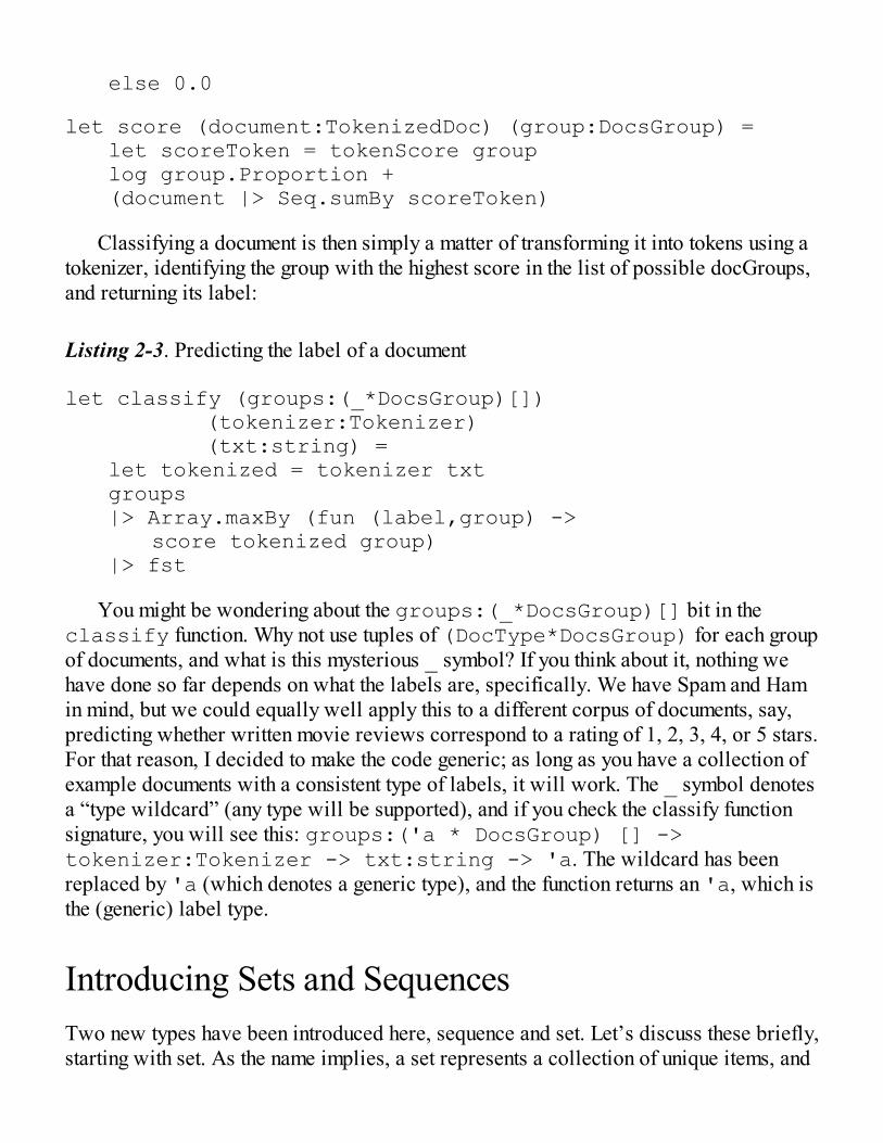
else 0.0

let score (document:TokenizedDoc) (group:DocsGroup) = let scoreToken = tokenScore group log group.Proportion + (document |> Seq.sumBy scoreToken)

Classifying a document is then simply a matter of transforming it into tokens using atokenizer, identifying the group with the highest score in the list of possible docGroups,and returning its label:

Listing 2-3. Predicting the label of a document

let classify (groups:(_*DocsGroup)[]) (tokenizer:Tokenizer) (txt:string) = let tokenized = tokenizer txt groups |> Array.maxBy (fun (label,group) -> score tokenized group) |> fst

You might be wondering about the groups:(_*DocsGroup)[] bit in theclassify function. Why not use tuples of (DocType*DocsGroup) for each groupof documents, and what is this mysterious _ symbol? If you think about it, nothing wehave done so far depends on what the labels are, specifically. We have Spam and Hamin mind, but we could equally well apply this to a different corpus of documents, say,predicting whether written movie reviews correspond to a rating of 1, 2, 3, 4, or 5 stars.For that reason, I decided to make the code generic; as long as you have a collection ofexample documents with a consistent type of labels, it will work. The _ symbol denotesa “type wildcard” (any type will be supported), and if you check the classify functionsignature, you will see this: groups:('a * DocsGroup) [] ->tokenizer:Tokenizer -> txt:string -> 'a. The wildcard has beenreplaced by 'a (which denotes a generic type), and the function returns an 'a, which isthe (generic) label type.

Introducing Sets and SequencesTwo new types have been introduced here, sequence and set. Let’s discuss these briefly,starting with set. As the name implies, a set represents a collection of unique items, and

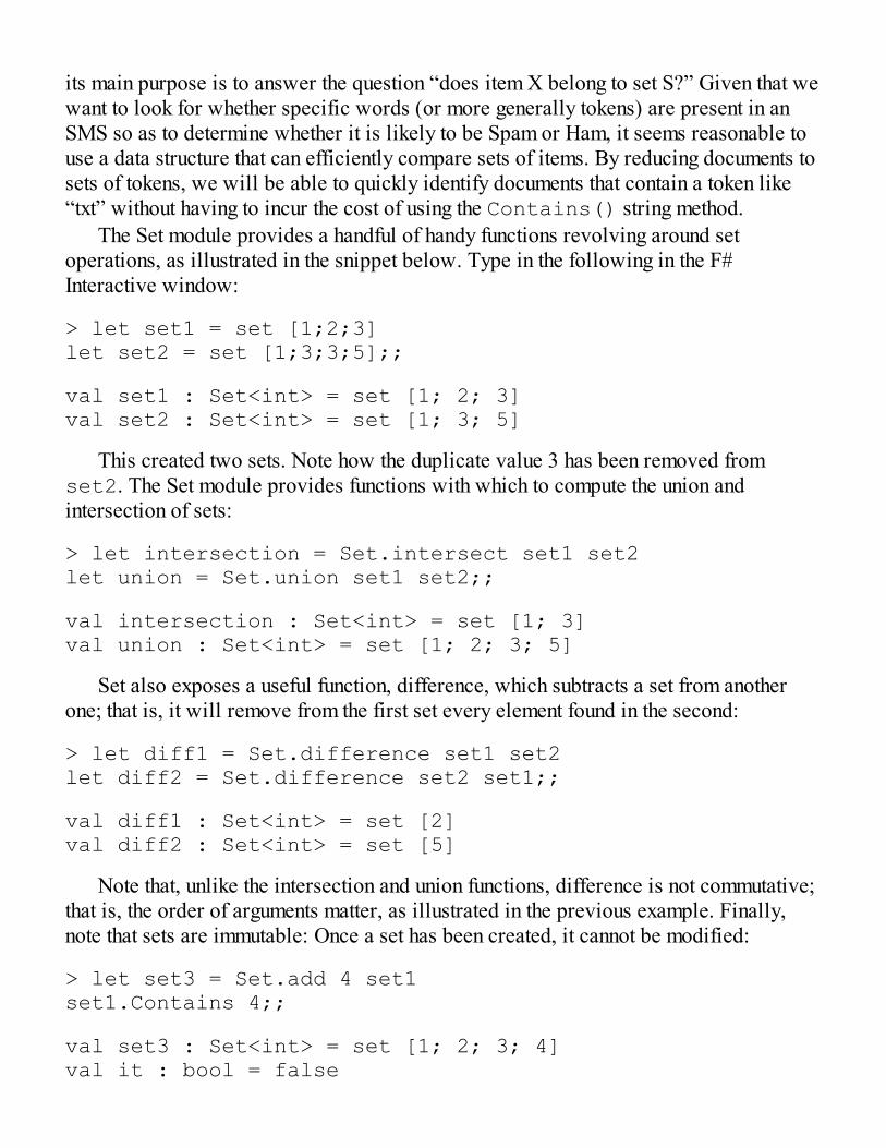
its main purpose is to answer the question “does item X belong to set S?” Given that wewant to look for whether specific words (or more generally tokens) are present in anSMS so as to determine whether it is likely to be Spam or Ham, it seems reasonable touse a data structure that can efficiently compare sets of items. By reducing documents tosets of tokens, we will be able to quickly identify documents that contain a token like“txt” without having to incur the cost of using the Contains() string method.

The Set module provides a handful of handy functions revolving around setoperations, as illustrated in the snippet below. Type in the following in the F#Interactive window:

> let set1 = set [1;2;3]let set2 = set [1;3;3;5];;

val set1 : Set<int> = set [1; 2; 3]val set2 : Set<int> = set [1; 3; 5]

This created two sets. Note how the duplicate value 3 has been removed fromset2. The Set module provides functions with which to compute the union andintersection of sets:

> let intersection = Set.intersect set1 set2let union = Set.union set1 set2;;

val intersection : Set<int> = set [1; 3]val union : Set<int> = set [1; 2; 3; 5]

Set also exposes a useful function, difference, which subtracts a set from anotherone; that is, it will remove from the first set every element found in the second:

> let diff1 = Set.difference set1 set2let diff2 = Set.difference set2 set1;;

val diff1 : Set<int> = set [2]val diff2 : Set<int> = set [5]

Note that, unlike the intersection and union functions, difference is not commutative;that is, the order of arguments matter, as illustrated in the previous example. Finally,note that sets are immutable: Once a set has been created, it cannot be modified:

> let set3 = Set.add 4 set1set1.Contains 4;;

val set3 : Set<int> = set [1; 2; 3; 4]val it : bool = false

Adding 4 to set1 creates a new set, set3, which does contain 4, but the originalset, set1, has not been affected by the operation.

The other type we introduced, sequence, is a lazily evaluated sequence of elements—that is, it is a collection that will be computed only as needed, potentially reducingmemory or compute usage. Let’s try the following code in the F# Interactive:

> let arr1 = [| for x in 1 .. 10 -> x |]let seq1 = seq { for x in 1 .. 10 -> x };;

val arr1 : int [] = [|1; 2; 3; 4; 5; 6; 7; 8; 9; 10|]val seq1 : seq<int>

The two expressions—arr1 and seq1—are very similar; they both generateintegers from 1 to 10. And yet, the array immediately shows its full contents, which havebeen eagerly evaluated; by contrast, seq1 appears as a sequence of integers, withoutfurther detail. The actual contents will be generated only when the code requires it.Let’s prove the point further with the following example, which constructs a newsequence by taking seq1 and doubling each of its elements. Note how we added a sideeffect in the sequence itself: Whenever an element of the sequence is produced, we printout the element being mapped:

> let seq2 = seq1 |> Seq.map (fun x -> printfn "mapping %i" x 2 * x) ;;

val seq2 : seq<int>

Again, the result is a sequence without actual contents yet, because nothing requiresit so far. Let’s change that by asking for the sum of the three first elements:

> let firstThree = seq2 |> Seq.take 3 |> Seq.sum;;mapping 1mapping 2mapping 3

val firstThree : int = 12

When this code executes, “mapping 1,” “mapping 2,” and “mapping 3” are printed

out, showing that the sequence is pulling out its first three elements, which are requiredin order to compute the sum. However, the remaining seven elements available, whichare still not needed, have been left unevaluated for now.

So, what is the point of sequences when we already have perfectly good collectionslike arrays available? The first benefit is lazy evaluation. Because a sequence will onlybe evaluated “as needed,” we can use them to generate infinite sequences; for instance,something that would be completely impossible to do with an array. The followingsnippet provides a somewhat contrived example: We create an infinite sequence,alternating between 1 and -1 forever. Obviously, there is no way we could instantiatesuch an infinite sequence of numbers in memory, but now that it is defined, we can useit, and, for example, compute its sum for any arbitrary number of elements:

> let infinite = Seq.initInfinite (fun i -> if i % 2 = 0 then 1 else -1)let test = infinite |> Seq.take 1000000 |> Seq.sum;;

val infinite : seq<int>val test : int = 0

The other reason F# sequences are often used is that they are equivalent to the C#IEnumerable; as such, all standard .NET collections can be treated as sequences,and, therefore, functions provided by the Seq module can be used to manipulate them,using functionality that does not appear in the actual collection itself. As an illustration,consider this example:

> let arr = [| 1;2;2;3;4;4;4|]let counts = arr |> Seq.countBy (fun x -> x) |> Seq.toArray;;

val arr : int [] = [|1; 2; 2; 3; 4; 4; 4|]val counts : (int * int) [] = [|(1, 1); (2, 2); (3, 1); (4, 3)|]

We generate an array of integers, and then want to count how many instances of eachwe have. While arrays do not directly support this functionality (at least, not until F# 4.0officially ships), sequences do, so we call Seq.countBy on the array and convertback the result to an array in order to trigger the sequence evaluation.

Tip While sequences can have a lot of advantages (who wouldn't want to computejust what is needed, and nothing more?), lazy evaluation also has its drawbacks,

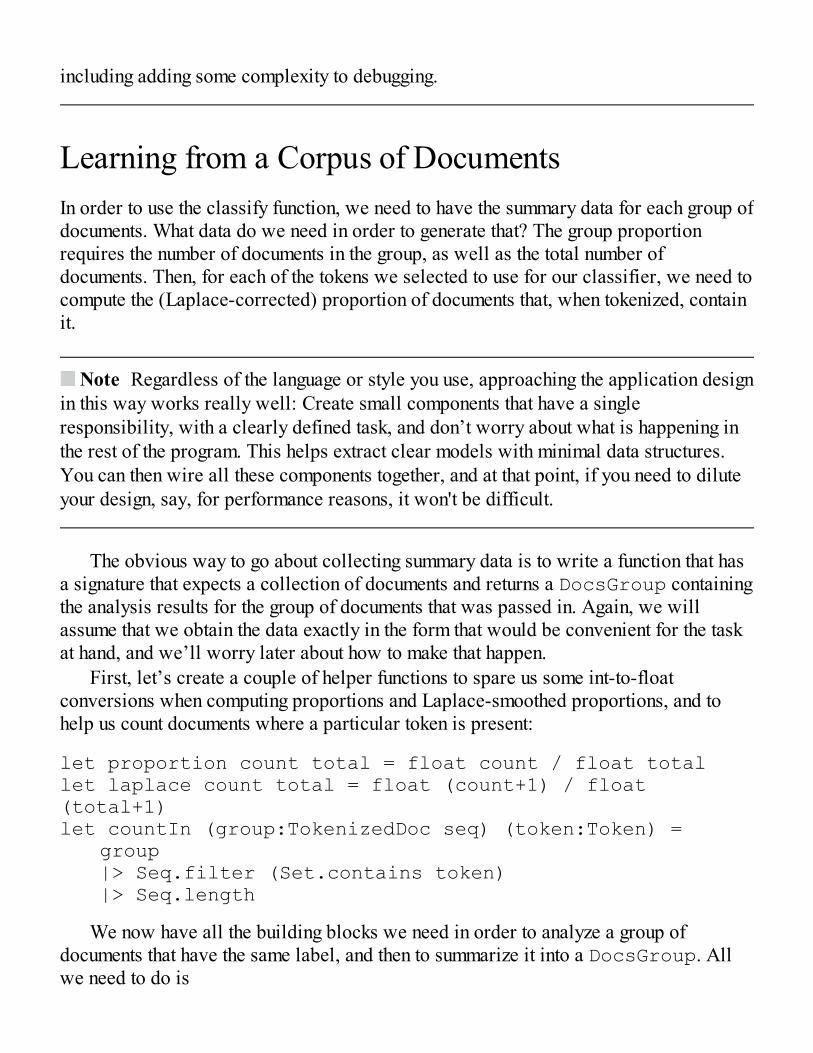
including adding some complexity to debugging.

Learning from a Corpus of DocumentsIn order to use the classify function, we need to have the summary data for each group ofdocuments. What data do we need in order to generate that? The group proportionrequires the number of documents in the group, as well as the total number ofdocuments. Then, for each of the tokens we selected to use for our classifier, we need tocompute the (Laplace-corrected) proportion of documents that, when tokenized, containit.

Note Regardless of the language or style you use, approaching the application designin this way works really well: Create small components that have a singleresponsibility, with a clearly defined task, and don’t worry about what is happening inthe rest of the program. This helps extract clear models with minimal data structures.You can then wire all these components together, and at that point, if you need to diluteyour design, say, for performance reasons, it won't be difficult.

The obvious way to go about collecting summary data is to write a function that hasa signature that expects a collection of documents and returns a DocsGroup containingthe analysis results for the group of documents that was passed in. Again, we willassume that we obtain the data exactly in the form that would be convenient for the taskat hand, and we’ll worry later about how to make that happen.

First, let’s create a couple of helper functions to spare us some int-to-floatconversions when computing proportions and Laplace-smoothed proportions, and tohelp us count documents where a particular token is present:

let proportion count total = float count / float totallet laplace count total = float (count+1) / float (total+1)let countIn (group:TokenizedDoc seq) (token:Token) = group |> Seq.filter (Set.contains token) |> Seq.length

We now have all the building blocks we need in order to analyze a group ofdocuments that have the same label, and then to summarize it into a DocsGroup. Allwe need to do is

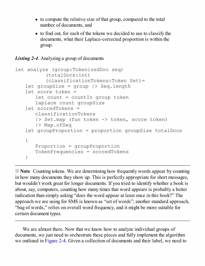
to compute the relative size of that group, compared to the totalnumber of documents, and

to find out, for each of the tokens we decided to use to classify thedocuments, what their Laplace-corrected proportion is within thegroup.

Listing 2-4. Analyzing a group of documents

let analyze (group:TokenizedDoc seq) (totalDocs:int) (classificationTokens:Token Set)= let groupSize = group |> Seq.length let score token = let count = countIn group token laplace count groupSize let scoredTokens = classificationTokens |> Set.map (fun token -> token, score token) |> Map.ofSeq let groupProportion = proportion groupSize totalDocs

{ Proportion = groupProportion TokenFrequencies = scoredTokens }

Note Counting tokens. We are determining how frequently words appear by countingin how many documents they show up. This is perfectly appropriate for short messages,but wouldn’t work great for longer documents. If you tried to identify whether a book isabout, say, computers, counting how many times that word appears is probably a betterindication than simply asking “does the word appear at least once in this book?” Theapproach we are using for SMS is known as “set of words”; another standard approach,“bag of words,” relies on overall word frequency, and it might be more suitable forcertain document types.

We are almost there. Now that we know how to analyze individual groups ofdocuments, we just need to orchestrate these pieces and fully implement the algorithmwe outlined in Figure 2-4. Given a collection of documents and their label, we need to

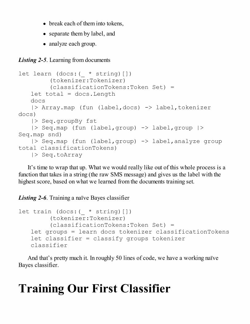
break each of them into tokens,

separate them by label, and

analyze each group.

Listing 2-5. Learning from documents

let learn (docs:(_ * string)[]) (tokenizer:Tokenizer) (classificationTokens:Token Set) = let total = docs.Length docs |> Array.map (fun (label,docs) -> label,tokenizer docs) |> Seq.groupBy fst |> Seq.map (fun (label,group) -> label,group |> Seq.map snd) |> Seq.map (fun (label,group) -> label,analyze group total classificationTokens) |> Seq.toArray

It’s time to wrap that up. What we would really like out of this whole process is afunction that takes in a string (the raw SMS message) and gives us the label with thehighest score, based on what we learned from the documents training set.

Listing 2-6. Training a naïve Bayes classifier

let train (docs:(_ * string)[]) (tokenizer:Tokenizer) (classificationTokens:Token Set) = let groups = learn docs tokenizer classificationTokens let classifier = classify groups tokenizer classifier

And that’s pretty much it. In roughly 50 lines of code, we have a working naïveBayes classifier.

Training Our First Classifier

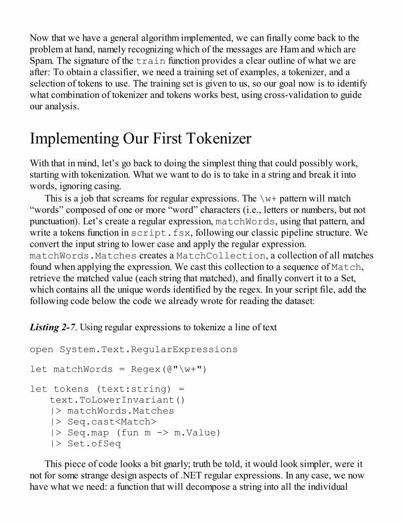
Now that we have a general algorithm implemented, we can finally come back to theproblem at hand, namely recognizing which of the messages are Ham and which areSpam. The signature of the train function provides a clear outline of what we areafter: To obtain a classifier, we need a training set of examples, a tokenizer, and aselection of tokens to use. The training set is given to us, so our goal now is to identifywhat combination of tokenizer and tokens works best, using cross-validation to guideour analysis.

Implementing Our First TokenizerWith that in mind, let’s go back to doing the simplest thing that could possibly work,starting with tokenization. What we want to do is to take in a string and break it intowords, ignoring casing.

This is a job that screams for regular expressions. The \w+ pattern will match“words” composed of one or more “word” characters (i.e., letters or numbers, but notpunctuation). Let’s create a regular expression, matchWords, using that pattern, andwrite a tokens function in script.fsx, following our classic pipeline structure. Weconvert the input string to lower case and apply the regular expression.matchWords.Matches creates a MatchCollection, a collection of all matchesfound when applying the expression. We cast this collection to a sequence of Match,retrieve the matched value (each string that matched), and finally convert it to a Set,which contains all the unique words identified by the regex. In your script file, add thefollowing code below the code we already wrote for reading the dataset:

Listing 2-7. Using regular expressions to tokenize a line of text

open System.Text.RegularExpressions

let matchWords = Regex(@"\w+")

let tokens (text:string) = text.ToLowerInvariant() |> matchWords.Matches |> Seq.cast<Match> |> Seq.map (fun m -> m.Value) |> Set.ofSeq

This piece of code looks a bit gnarly; truth be told, it would look simpler, were itnot for some strange design aspects of .NET regular expressions. In any case, we nowhave what we need: a function that will decompose a string into all the individual

words it contains.

Validating Our Design InteractivelyAt first sight, the code seems like it might be doing what we want. However, “might be”is not a great place to be; verifying that it actually works would be better. When codingin C#, my habit is to resort to test-driven development, or TDD: Write a test first andthen write the code that satisfies the requirements and passes the test. One of the benefitsof TDD is that it enables you to run small pieces of code independently of the wholeapplication, quickly making sure that it works as intended, and fleshing out your designideas as you go. In F#, I tend to have a slightly different workflow. F# Interactiveenables a more fluid style of design experimentation. Instead of immediately committingto a design and writing tests for it, potentially requiring later refactoring, you can simplyexperiment in F# Interactive, and once your design is taking shape, promote the code tounit tests.

In our case, checking that the token function works is trivial. All it takes is typingsomething like this in FSI and running it:

> tokens "42 is the Answer to the question";;

You will immediately see the results in the F# Interactive window:

val it : Set<string> = set ["42"; "answer"; "is"; "question"; "the"; "to"]

Our function looks like it is working. All the words have been isolated, includingthe number “42,” the duplicate “the” appears only once in the results, and the capital“A” in Answer is gone. At this point, if I were writing an actual library intended forproduction, I would simply lift the token function and move it from my exploratoryscript into an actual proper file in the solution, then convert that little code snippet intoan actual unit test. We are “just exploring” for the moment, so I will leave it at that, andwon’t bother with writing tests right now.

Establishing a Baseline with Cross-validationNow that we have a model, let’s see how well it does. We will be using the same scriptas before, so we have already loaded all the messages in dataset, an array of(DocType * string). As in the previous chapter, we will use cross-validation,and use one part of the dataset for training, and reserve the rest to validate how well (or

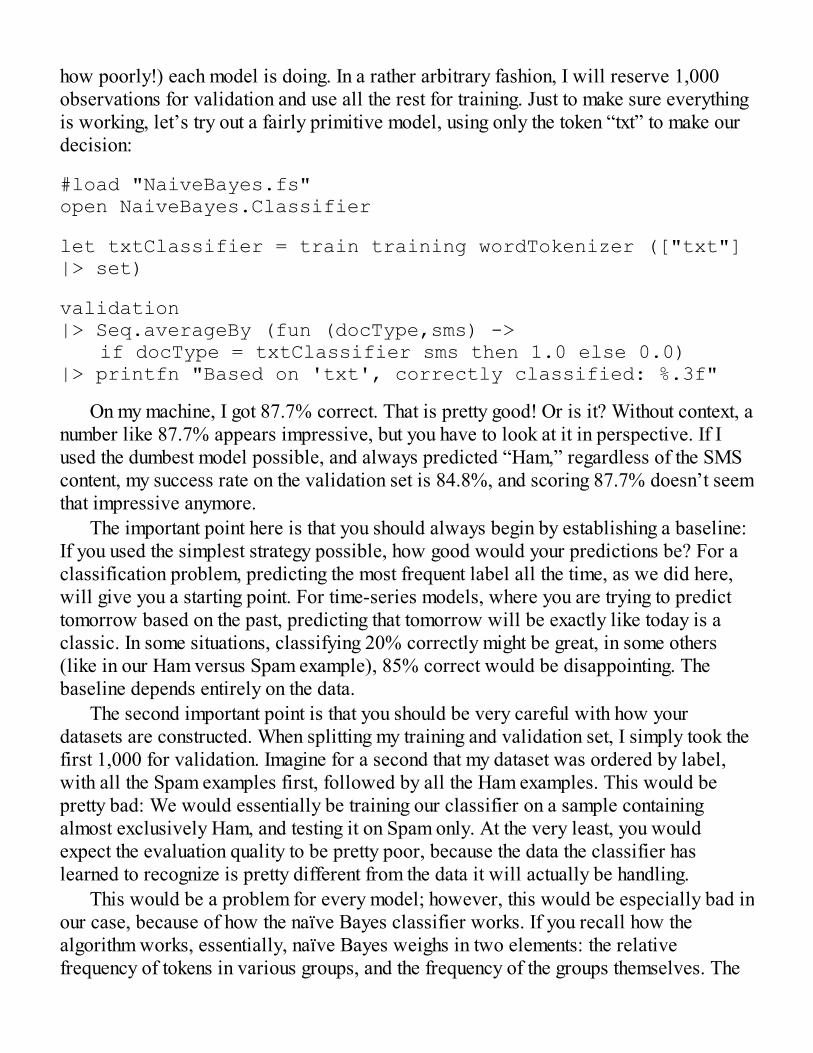
how poorly!) each model is doing. In a rather arbitrary fashion, I will reserve 1,000observations for validation and use all the rest for training. Just to make sure everythingis working, let’s try out a fairly primitive model, using only the token “txt” to make ourdecision:

#load "NaiveBayes.fs"open NaiveBayes.Classifier

let txtClassifier = train training wordTokenizer (["txt"] |> set)

validation|> Seq.averageBy (fun (docType,sms) -> if docType = txtClassifier sms then 1.0 else 0.0)|> printfn "Based on 'txt', correctly classified: %.3f"

On my machine, I got 87.7% correct. That is pretty good! Or is it? Without context, anumber like 87.7% appears impressive, but you have to look at it in perspective. If Iused the dumbest model possible, and always predicted “Ham,” regardless of the SMScontent, my success rate on the validation set is 84.8%, and scoring 87.7% doesn’t seemthat impressive anymore.

The important point here is that you should always begin by establishing a baseline:If you used the simplest strategy possible, how good would your predictions be? For aclassification problem, predicting the most frequent label all the time, as we did here,will give you a starting point. For time-series models, where you are trying to predicttomorrow based on the past, predicting that tomorrow will be exactly like today is aclassic. In some situations, classifying 20% correctly might be great, in some others(like in our Ham versus Spam example), 85% correct would be disappointing. Thebaseline depends entirely on the data.

The second important point is that you should be very careful with how yourdatasets are constructed. When splitting my training and validation set, I simply took thefirst 1,000 for validation. Imagine for a second that my dataset was ordered by label,with all the Spam examples first, followed by all the Ham examples. This would bepretty bad: We would essentially be training our classifier on a sample containingalmost exclusively Ham, and testing it on Spam only. At the very least, you wouldexpect the evaluation quality to be pretty poor, because the data the classifier haslearned to recognize is pretty different from the data it will actually be handling.

This would be a problem for every model; however, this would be especially bad inour case, because of how the naïve Bayes classifier works. If you recall how thealgorithm works, essentially, naïve Bayes weighs in two elements: the relativefrequency of tokens in various groups, and the frequency of the groups themselves. The

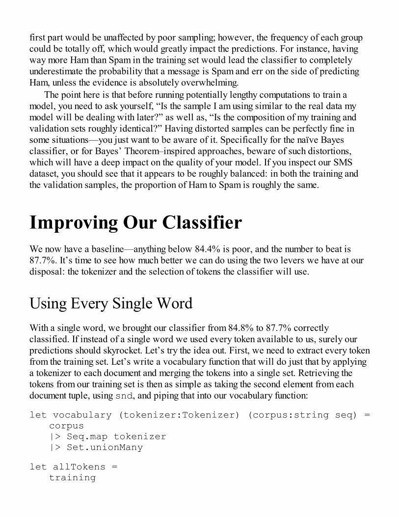
first part would be unaffected by poor sampling; however, the frequency of each groupcould be totally off, which would greatly impact the predictions. For instance, havingway more Ham than Spam in the training set would lead the classifier to completelyunderestimate the probability that a message is Spam and err on the side of predictingHam, unless the evidence is absolutely overwhelming.

The point here is that before running potentially lengthy computations to train amodel, you need to ask yourself, “Is the sample I am using similar to the real data mymodel will be dealing with later?” as well as, “Is the composition of my training andvalidation sets roughly identical?” Having distorted samples can be perfectly fine insome situations—you just want to be aware of it. Specifically for the naïve Bayesclassifier, or for Bayes’ Theorem–inspired approaches, beware of such distortions,which will have a deep impact on the quality of your model. If you inspect our SMSdataset, you should see that it appears to be roughly balanced: in both the training andthe validation samples, the proportion of Ham to Spam is roughly the same.

Improving Our ClassifierWe now have a baseline—anything below 84.4% is poor, and the number to beat is87.7%. It’s time to see how much better we can do using the two levers we have at ourdisposal: the tokenizer and the selection of tokens the classifier will use.

Using Every Single WordWith a single word, we brought our classifier from 84.8% to 87.7% correctlyclassified. If instead of a single word we used every token available to us, surely ourpredictions should skyrocket. Let’s try the idea out. First, we need to extract every tokenfrom the training set. Let’s write a vocabulary function that will do just that by applyinga tokenizer to each document and merging the tokens into a single set. Retrieving thetokens from our training set is then as simple as taking the second element from eachdocument tuple, using snd, and piping that into our vocabulary function:

let vocabulary (tokenizer:Tokenizer) (corpus:string seq) = corpus |> Seq.map tokenizer |> Set.unionMany

let allTokens = training

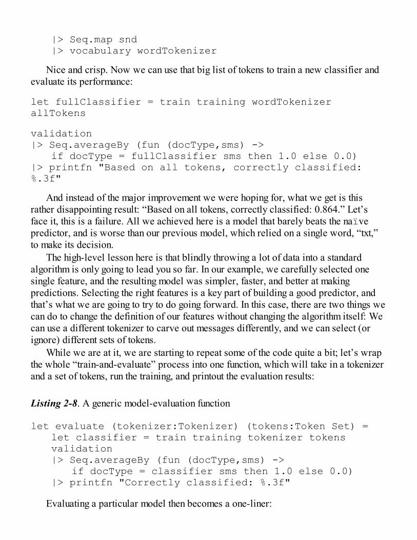
|> Seq.map snd |> vocabulary wordTokenizer

Nice and crisp. Now we can use that big list of tokens to train a new classifier andevaluate its performance:

let fullClassifier = train training wordTokenizer allTokens

validation|> Seq.averageBy (fun (docType,sms) -> if docType = fullClassifier sms then 1.0 else 0.0)|> printfn "Based on all tokens, correctly classified: %.3f"

And instead of the major improvement we were hoping for, what we get is thisrather disappointing result: “Based on all tokens, correctly classified: 0.864.” Let’sface it, this is a failure. All we achieved here is a model that barely beats the naïvepredictor, and is worse than our previous model, which relied on a single word, “txt,”to make its decision.

The high-level lesson here is that blindly throwing a lot of data into a standardalgorithm is only going to lead you so far. In our example, we carefully selected onesingle feature, and the resulting model was simpler, faster, and better at makingpredictions. Selecting the right features is a key part of building a good predictor, andthat’s what we are going to try to do going forward. In this case, there are two things wecan do to change the definition of our features without changing the algorithm itself: Wecan use a different tokenizer to carve out messages differently, and we can select (orignore) different sets of tokens.

While we are at it, we are starting to repeat some of the code quite a bit; let’s wrapthe whole “train-and-evaluate” process into one function, which will take in a tokenizerand a set of tokens, run the training, and printout the evaluation results:

Listing 2-8. A generic model-evaluation function

let evaluate (tokenizer:Tokenizer) (tokens:Token Set) = let classifier = train training tokenizer tokens validation |> Seq.averageBy (fun (docType,sms) -> if docType = classifier sms then 1.0 else 0.0) |> printfn "Correctly classified: %.3f"

Evaluating a particular model then becomes a one-liner:

> evaluate wordTokenizer allTokens;;Correctly classified: 0.864

This gives us a fairly straightforward process moving forward: Select a tokenizerand a set of tokens, and call evaluate to see if this particular combination is anybetter than whatever we tried before.

Does Capitalization Matter?Let’s start with the tokenizer. If you recall our earlier discussion, the wordTokenizer weare currently using ignores case; from its standpoint, there is no difference between “txt”or “TXT”—both will be considered to be the same token.

This is not an unreasonable thing to do. For instance, consider the two messages“Txt me now” and “txt me now.” By ignoring capitalization, we are essentially sayingthat these two messages are not different in any meaningful way. Capitalization doesn’tintroduce any relevant information here, and can be treated as noise.

On the other hand, consider these two messages: “are you free now?” and “FREESTUFF TXT NOW!”—arguably, ignoring capitalization is losing information.

So, which one is it? Let’s try it out and see if a different tokenizer, one that doesn’treduce everything to lowercase, fares any better than the wordTokenizer:

Listing 2-9. Using regular expressions to tokenize a line of text

let casedTokenizer (text:string) = text |> matchWords.Matches |> Seq.cast<Match> |> Seq.map (fun m -> m.Value) |> Set.ofSeq

let casedTokens = training |> Seq.map snd |> vocabulary casedTokenizer

evaluate casedTokenizer casedTokens

Running this in FSI produces 87.5% correct results. On the one hand, we are stillbelow our simplistic classifier that relies on the presence of “txt.” On the other hand,

we are now pretty close (87.5% versus 87.7%), and this is significantly better than theequivalent approach with the wordTokenizer using every single token (86.4%).

Less Is moreWe have what appears to be a better tokenizer; still, the fact remains that by adding alarge amount of features, we ended up with a classifier that was both worse and slower.This is obviously not great, and it is also counter-intuitive: How could adding moreinformation possibly make our model worse?

Let’s look at the question the other way around and consider why our earlier single-token model was working so well. The reason we picked “txt” as a token is that it isvery frequently found in Spam, and rarely found in Ham. In other words, it differentiateswell between the two groups, and is pretty specific to Spam.

What we are doing now is using every single token, regardless of how informative itmight be. As a result, we are potentially introducing quite a bit of noise into our model.How about being a bit more selective, perhaps by picking only the most frequentlyfound tokens in each document group?

Let’s start with a simple function that, given a collection of raw documents (plainstrings) and a tokenizer, will return the n most frequently used tokens:

let top n (tokenizer:Tokenizer) (docs:string []) = let tokenized = docs |> Array.map tokenizer let tokens = tokenized |> Set.unionMany tokens |> Seq.sortBy (fun t -> - countIn tokenized t) |> Seq.take n |> Set.ofSeq

We can now split our training sample into Ham and Spam, dropping the labels in theprocess:

let ham,spam = let rawHam,rawSpam = training |> Array.partition (fun (lbl,_) -> lbl=Ham) rawHam |> Array.map snd, rawSpam |> Array.map snd

We extract and count how many tokens we have in each group, pick the top 10%,and merge them into one token set using Set.union:

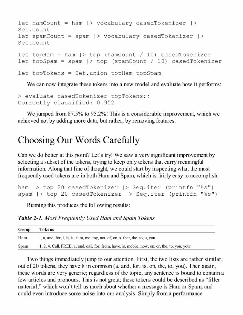
let hamCount = ham |> vocabulary casedTokenizer |> Set.countlet spamCount = spam |> vocabulary casedTokenizer |> Set.count

let topHam = ham |> top (hamCount / 10) casedTokenizerlet topSpam = spam |> top (spamCount / 10) casedTokenizer

let topTokens = Set.union topHam topSpam

We can now integrate these tokens into a new model and evaluate how it performs:

> evaluate casedTokenizer topTokens;;Correctly classified: 0.952

We jumped from 87.5% to 95.2%! This is a considerable improvement, which weachieved not by adding more data, but rather, by removing features.

Choosing Our Words CarefullyCan we do better at this point? Let’s try! We saw a very significant improvement byselecting a subset of the tokens, trying to keep only tokens that carry meaningfulinformation. Along that line of thought, we could start by inspecting what the mostfrequently used tokens are in both Ham and Spam, which is fairly easy to accomplish:

ham |> top 20 casedTokenizer |> Seq.iter (printfn "%s")spam |> top 20 casedTokenizer |> Seq.iter (printfn "%s")

Running this produces the following results:

Table 2-1. Most Frequently Used Ham and Spam Tokens

Group Tokens

Ham I, a, and, for, i, in, is, it, m, me, my, not, of, on, s, that, the, to, u, you

Spam 1, 2, 4, Call, FREE, a, and, call, for, from, have, is, mobile, now, on, or, the, to, you, your

Two things immediately jump to our attention. First, the two lists are rather similar;out of 20 tokens, they have 8 in common (a, and, for, is, on, the, to, you). Then again,these words are very generic; regardless of the topic, any sentence is bound to contain afew articles and pronouns. This is not great; these tokens could be described as “fillermaterial,” which won’t tell us much about whether a message is Ham or Spam, andcould even introduce some noise into our analysis. Simply from a performance

standpoint, it means that we are spending a lot of CPU cycles analyzing tokens that areconveying limited or no relevant information. For all these reasons, it might bebeneficial to remove these tokens from the analysis.

Before doing that, I think another interesting aspect appears in that list. Unlike Ham,the Spam list contains a couple of rather specific words, like “call,” “free,” “mobile,”and “now”—and doesn’t contain “I” or “me.” If you think about it, that makes sense:While regular text messages have a multitude of purposes, a Spam message is usually a“phishing” attempt, trying to lure you into doing something. In that context, it isn’t asurprise to see words like “now” and “free,” which reek of advertising; and becauseflattery is rarely a wrong way to get people to do what you want, it is no surprise eitherthan Spam messages would be less about “I” and more about “you.”

Note What is Phishing? Phishing is the act of using email, SMS, or the phone to stealmoney from someone. Phishing typically uses a bit of social engineering (impersonatingrespectable institutions, threat, or seduction) to get the target to take some action thescammer cannot perform by himself, like clicking a link that will install malicioussoftware on your machine.

We will come back to that point soon. In the meantime, let’s see if we can removethe “filler material.” A common approach is to rely on a predefined list of such words,which are usually called “stop words.” You can find an example of such a list here:http://norm.al/2009/04/14/list-of-english-stop-words/.Unfortunately, there is no universally correct way to go about this; obviously thisdepends on the language your documents are written in, and even the context couldmatter. For instance, in our sample, “u,” a common way to shorten “you” in textmessages, would make a great stop word. Yet, most standard lists would not contain itbecause that usage is extremely specific to SMS, and is highly unlikely to be found inany other document type.

Instead of relying on a list of stop words, we will do something simpler. OurtopHam and topSpam sets contain the most frequently used tokens in Ham and in Spam.If a token appears in both lists, it is likely simply a word that is frequently found inEnglish text messages, and is not particularly specific to either Ham or Spam. Let’sidentify all these common tokens, which correspond to the intersection of both lists,remove them from our tokens selection, and run the analysis again:

let commonTokens = Set.intersect topHam topSpamlet specificTokens = Set.difference topTokens commonTokensevaluate casedTokenizer specificTokens

With this simple change, the percentage of correctly classified SMS messages jumpsfrom 95.2% to 97.9%! This is starting to be pretty good, and as we get closer to100.0%, improvements will become harder to achieve.

Creating New FeaturesOne approach I often find useful when trying to come up with new ideas is to flip aproblem on its head in order to look at it from a different angle. As an example, when Iwrite code, I typically begin by imagining the “happy path,” the minimum steps neededfor the program to do something useful, and then I simply implement them. This is agreat approach until you want to test your code; your mind has become so focused on thesuccess path that it is difficult to think about failure. So I like to approach testing byreversing the question, asking, “What is the fastest possible way I could get thisprogram to crash?” I found this very effective, and it makes testing fun, too!

Let’s try out this method for improving our classifier. Looking at the most frequentwords in each class ended up with a very significant improvement, because the Bayesclassifier relies on frequent words in a category to recognize it. How about looking atthe least frequently found words in each document category? With a slight modificationof the code we wrote previously, we can extract the least frequently used tokens in agroup:

Listing 2-10. Extracting least frequently used tokens

let rareTokens n (tokenizer:Tokenizer) (docs:string []) = let tokenized = docs |> Array.map tokenizer let tokens = tokenized |> Set.unionMany tokens |> Seq.sortBy (fun t -> countIn tokenized t) |> Seq.take n |> Set.ofSeq

let rareHam = ham |> rareTokens 50 casedTokenizer |> Seq.iter (printfn "%s")let rareSpam = spam |> rareTokens 50 casedTokenizer |> Seq.iter (printfn "%s")

The table below summarizes the results:

Table 2-2. Least Frequently Used Ham and Spam Tokens

Group Tokens

Ham

000pes, 0quit, 100, 1120, 116, 1205, 128, 130, 140, 15pm, 16, 180, 1Apple, 1Cup, 1IM, 1Lemon,1Tulsi, 1mega, 1stone, 1thing, 2000, 21, 21st, 24th, 255, 26, 2B, 2DOCD, 2GETHA, 2GEVA,2Hook, 2I, 2MOROW, 2MORRO, 2MWEN, 2WATERSHD, 2bold, 2geva, 2hrs, 2morow,2morrowxxxx, 2mro, 2mrw, 2nhite, 2nite, 2u, 2u2, 2years, 2yrs, 30ish

Spam

0089, 0121, 01223585236, 0207, 02072069400, 02085076972, 021, 0430, 050703, 0578, 07,07008009200, 07090201529, 07090298926, 07099833605, 07123456789, 07742676969,07781482378, 077xxx, 078, 07801543489, 07808247860, 07808726822, 07821230901, 078498,0789xxxxxxx, 0796XXXXXX, 07973788240, 07XXXXXXXXX, 08, 08000407165, 08000938767,08002888812, 08002986030, 08081263000, 0825, 083, 0844, 08448350055, 08448714184, 0845,08450542832, 08452810075over18, 08700435505150p, 08700469649, 08700621170150p,08701213186, 08701237397, 0870141701216, 087016248

Do you notice a pattern here? The Spam list is full of what appears to be phonenumbers or text codes. Again, this makes sense: If I am targeted by a phishing attempt,someone wants me to do something—and on a phone, that means calling or texting anumber.

This also highlights a problem: While we as humans immediately see this list as “alot of phone numbers,” each one is treated as an individual token in our model, whichwill appear very rarely. Yet, the presence of a phone number in an SMS message seemsto be a likely flag for Spam. One way we can address the issue is by creating a newfeature that captures whether or not a message contains a phone number, regardless ofwhat specific number it is. This will let us compute how frequently phone numbers arefound in Spam, and (potentially) use that as a token in our naïve Bayes classifier.

If you examine the rare tokens list closely, you might see more-specific patternsemerge. First, the phone numbers listed have a similar structure: They begin with 07,08, or 09, followed by nine other digits. Then, there are other numbers in the list, mainlyfive-digit numbers, which are likely txt numbers.

Let’s create a feature for each case. Whenever we see something that looks like 07followed by nine digits, we will convert it to the token __PHONE__, and whenever weencounter a five-digit number, we’ll transform it into __TXT__:

Listing 2-11. Recognizing phone numbers

let phoneWords = Regex(@"0[7-9]\d{9}")let phone (text:string) = match (phoneWords.IsMatch text) with | true -> "__PHONE__" | false -> text

let txtCode = Regex(@"\b\d{5}\b")let txt (text:string) =

match (txtCode.IsMatch text) with | true -> "__TXT__" | false -> text

let smartTokenizer = casedTokenizer >> Set.map phone >> Set.map txt

The smartTokenizer simply chains three functions together. ThecasedTokenizer function takes a string and returns a set of strings, with theindividual tokens identified. Because it returns a set of strings, we can apply Set.map,running the phone function on each of the tokens and transforming each token that lookslike a phone number into the “__PHONE__” token—and then performing the same withthe txt function.

Let’s make sure it works by running the following code in F# Interactive:

> smartTokenizer "hello World, call 08123456789 or txt 12345";;val it : Set<string> = set ["World"; "__PHONE__"; "__TXT__"; "call"; "hello"; "or"; "txt"]

This is what we expected—we seem to be in business. Let’s try out our tweakedtokenizer, manually adding the two tokens we just created to the list (if we didn’t, thetoken list would still contain individual numbers, which wouldn’t match with the__PHONE__ token produced by the “smart tokenizer”):

let smartTokens = specificTokens |> Set.add "__TXT__" |> Set.add "__PHONE__"

evaluate smartTokenizer smartTokens

Drumroll, please . . . another jump up, from 96.7% to 98.3% correct! Given ourcurrent level of performance, that is a very nice boost. It’s worth taking a bit of time todiscuss what we did here. We transformed our dataset, creating a new feature byaggregating existing features. This process is a key part of what developing a goodmachine learning model entails. Starting from an original dataset, perhaps onecontaining low-quality data, and as you begin to understand the domain well and findrelationships between variables, you will progressively reshape the data into a newrepresentation that better fits the problem at hand. This cycle of conducting experimentsand refining raw data into good features is at the core of machine learning.

Dealing with Numeric ValuesLet’s finish this section on feature extraction with a quick discussion. In this chapter, wehave been considering discrete features only; that is, features that can only take adiscrete set of values. What about continuous features, or simply numeric features? Forinstance, imagine you have an intuition that message length matters. Can you use anyideas from what we have seen so far?

One possibility is to reduce the problem to a known problem and make the messagelength (which can take any value between 0 and 140 characters) into a binary feature,separating them into two categories, short messages and long messages. The questionthen becomes, “What is a good value at which to split between long and shortmessages?”

This we can address directly using Bayes’ Theorem: For a given threshold, we cancompute the probability that a message is Spam, if its length is greater than thethreshold. Identifying a “good” threshold is then simply a matter of testing variousvalues and picking the most informative one. The code below does just that, andshouldn’t be too hard to follow:

Listing 2-12. Spam probability based on message length

let lengthAnalysis len =

let long (msg:string) = msg.Length > len

let ham,spam = dataset |> Array.partition (fun (docType,_) -> docType = Ham) let spamAndLongCount = spam |> Array.filter (fun (_,sms) -> long sms) |> Array.length let longCount = dataset |> Array.filter (fun (_,sms) -> long sms) |> Array.length

let pSpam = (float spam.Length) / (float dataset.Length) let pLongIfSpam =

float spamAndLongCount / float spam.Length let pLong = float longCount / float (dataset.Length)

let pSpamIfLong = pLongIfSpam * pSpam / pLong pSpamIfLong

for l in 10 .. 10 .. 130 do printfn "P(Spam if Length > %i) = %.4f" l (lengthAnalysis l)

If you run that code, you will see that the probability that a message is Spam goes upsignificantly with length, which is not a surprise. Spammers send a lot of messages andwant to get the most bang for their buck, so they will pack as much as possible into asingle SMS. I will leave it at that for now; we will revisit this topic in Chapter 6, froma slightly different angle, but I wanted to show how Bayes’ Theorem can come in handyin a variety of situations, without much effort.

Understanding ErrorsRemember how 87.7% correctly classified sounded great, until we put it in perspectiveand compared it to a naïve baseline? We managed to bring that number up to 98.3%,which is clearly much better. However, whenever you are reducing an entire dataset toa single number, by definition you are leaving something out. People love single-numbersummaries, because they are easy to compare. My advice to you is the following:Whenever you are presented with a statistic, it pays to think twice about what thatnumber could be leaving out or hiding.

In our case, what we know is that out of 1,000 messages, we will misclassify about17 on average. One thing we don’t know is where the model is making its errors.Widely different situations could lead to that same number of 98.3%: These 17 could bemainly Spam, mainly Ham, or anything in between. Depending on the context, this canbe a crucial distinction. For instance, I suspect most people would prefer a classifierthat misses a couple of Spam messages and leaves them in their inbox, over an overlyaggressive one that sends perfectly good messages automatically to a Spam folderbecause it was incorrectly labeled as Spam.

So, how is our classifier doing? Let’s find out and measure how well it recognizesSpam and Ham. We just need to separate out Ham and Spam in our validation set, andthen compute the percentage correctly classified in each group. This is easily done—we

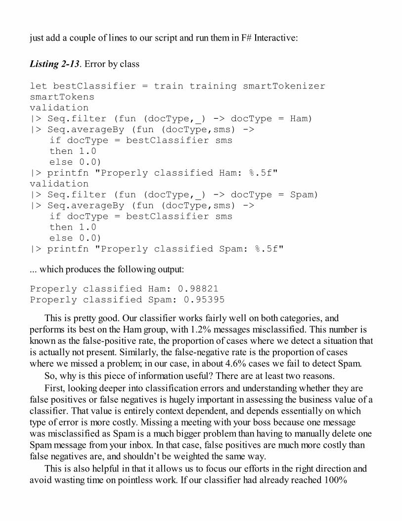
just add a couple of lines to our script and run them in F# Interactive:

Listing 2-13. Error by class

let bestClassifier = train training smartTokenizer smartTokensvalidation|> Seq.filter (fun (docType,_) -> docType = Ham)|> Seq.averageBy (fun (docType,sms) -> if docType = bestClassifier sms then 1.0 else 0.0)|> printfn "Properly classified Ham: %.5f"validation|> Seq.filter (fun (docType,_) -> docType = Spam)|> Seq.averageBy (fun (docType,sms) -> if docType = bestClassifier sms then 1.0 else 0.0)|> printfn "Properly classified Spam: %.5f"

... which produces the following output:

Properly classified Ham: 0.98821Properly classified Spam: 0.95395

This is pretty good. Our classifier works fairly well on both categories, andperforms its best on the Ham group, with 1.2% messages misclassified. This number isknown as the false-positive rate, the proportion of cases where we detect a situation thatis actually not present. Similarly, the false-negative rate is the proportion of caseswhere we missed a problem; in our case, in about 4.6% cases we fail to detect Spam.

So, why is this piece of information useful? There are at least two reasons.First, looking deeper into classification errors and understanding whether they are

false positives or false negatives is hugely important in assessing the business value of aclassifier. That value is entirely context dependent, and depends essentially on whichtype of error is more costly. Missing a meeting with your boss because one messagewas misclassified as Spam is a much bigger problem than having to manually delete oneSpam message from your inbox. In that case, false positives are much more costly thanfalse negatives are, and shouldn’t be weighted the same way.

This is also helpful in that it allows us to focus our efforts in the right direction andavoid wasting time on pointless work. If our classifier had already reached 100%

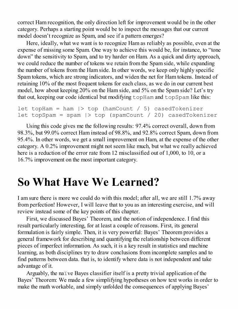
correct Ham recognition, the only direction left for improvement would be in the othercategory. Perhaps a starting point would be to inspect the messages that our currentmodel doesn’t recognize as Spam, and see if a pattern emerges?

Here, ideally, what we want is to recognize Ham as reliably as possible, even at theexpense of missing some Spam. One way to achieve this would be, for instance, to “tonedown” the sensitivity to Spam, and to try harder on Ham. As a quick and dirty approach,we could reduce the number of tokens we retain from the Spam side, while expandingthe number of tokens from the Ham side. In other words, we keep only highly specificSpam tokens, which are strong indicators, and widen the net for Ham tokens. Instead ofretaining 10% of the most frequent tokens for each class, as we do in our current bestmodel, how about keeping 20% on the Ham side, and 5% on the Spam side? Let’s trythat out, keeping our code identical but modifying topHam and topSpam like this:

let topHam = ham |> top (hamCount / 5) casedTokenizerlet topSpam = spam |> top (spamCount / 20) casedTokenizer

Using this code gives me the following results: 97.4% correct overall, down from98.3%, but 99.0% correct Ham instead of 98.8%, and 92.8% correct Spam, down from95.4%. In other words, we get a small improvement on Ham, at the expense of the othercategory. A 0.2% improvement might not seem like much, but what we really achievedhere is a reduction of the error rate from 12 misclassified out of 1,000, to 10, or a16.7% improvement on the most important category.

So What Have We Learned?I am sure there is more we could do with this model; after all, we are still 1.7% awayfrom perfection! However, I will leave that to you as an interesting exercise, and willreview instead some of the key points of this chapter.

First, we discussed Bayes’ Theorem, and the notion of independence. I find thisresult particularly interesting, for at least a couple of reasons. First, its generalformulation is fairly simple. Then, it is very powerful: Bayes’ Theorem provides ageneral framework for describing and quantifying the relationship between differentpieces of imperfect information. As such, it is a key result in statistics and machinelearning, as both disciplines try to draw conclusions from incomplete samples and tofind patterns between data. that is, to identify where data is not independent and takeadvantage of it.

Arguably, the naïve Bayes classifier itself is a pretty trivial application of theBayes’ Theorem: We made a few simplifying hypotheses on how text works in order tomake the math workable, and simply unfolded the consequences of applying Bayes’

Theorem. Perhaps more interesting than the classifier itself was the process of texttokenization. Machine learning algorithms typically require a collection of features tooperate, and a raw block of text doesn’t fit that pattern well. By breaking the text intotokens, thus identifying and counting words that are present in a document, we managedto transform text into a more convenient structure.

Finally, we spent a lot of time refining a basic model and improving it by extractingnew features. The key point here is that we used one fairly simple algorithm all the waythrough, but improved the predictive power of our model from mediocre to quite goodjust by taking the time to understand the data, then using that knowledge to reorganize ita bit. Deciding what algorithms to use is certainly an important part of machine learning,but building a good model is usually less about finding the one and only algorithm thatwill magically solve the problem, and more about gaining a better understanding of theproblem domain and using that knowledge to extract better features.

In this particular case, a few patterns emerged. First, more data is not always better.Some features contain a lot of information, and some don’t. Finding highly informativefeatures and eliminating the rest will help models by giving them information thatcarries more signal and less noise, and is easier to exploit. Then, we saw two oppositephenomena at play. We ended up using a tokenizer that kept word casing. Whathappened is that we realized that our original feature was too coarse, so we split it intomultiple, more-specific features (for instance, “FREE” and “free”). Conversely, wenoticed that we had a lot of phone numbers and aggregated them into a single over-arching feature that didn’t exist before in order to see its impact. Again, knowing yourdomain and data is absolutely crucial: A good algorithm looking at features the wrongway won’t go very far, and small changes in features are often how you can go fromhaving a decent model to having an excellent one.

USEFUL LINKS

The University of California–Irvine maintains a wonderfulrepository of machine learning datasets:http://archive.ics.uci.edu/ml/

The following web page contains a useful basic list of commonEnglish stop words: http://norm.al/2009/04/14/list-of-english-stop-words/

If you want to explore further ways to work with text, the StanfordNLP page has a wealth of resources:http://nlp.stanford.edu/

CHAPTER 3

The Joy of Type Providers

Finding and Preparing Data, fromAnywhereLet me let you in on the dirty little secret of machine learning: If you were to look solelyat the topics publicly discussed, you would think that most of the work revolves aroundcrafting fancy algorithms, the remaining time being spent on designing ways to run thesealgorithms in a distributed fashion, or some other similarly interesting engineeringchallenge. The sad truth is that this is a rather marginal part of the job; most of your timewill likely be spent on a much more prosaic activity: data janitorial tasks. If you wantthe machine to learn anything, you need to feed it data, and data has a way of comingfrom all sorts of different sources, in shapes and formats that are impractical for whatyou want to do with it. It usually has missing information, and is rarely properlydocumented. In short, finding and preparing data is both hugely important for machinelearning and potentially a source of great pain.

Besides the data itself being in a sorry state, there is another reason why masteringdata is a challenge. This reason is technical: If you think about it, what you are trying todo is to pull information—which knows nothing about your programming language—into your programming language type system so that you can actually manipulate it usingthat programming language. Two broad directions are possible here. If your language ofchoice is on the dynamic side, like Python, for instance, hacking at data is rather easy.You can write code in an optimistic manner without worrying too much about languagetypes; if it works, great! On the downside, you are getting no assistance from thecompiler. The only way to know whether your code works is to run it. If you observe noruntime error, you have to assume that it probably works. Conversely, if you are using alanguage like C#, which has a much stricter type system, getting data into your worldwill be significantly more painful and time consuming. It will probably require heavy

machinery, like an object-relational mapping system (ORM), for instance. On the plusside, though, it will save you from dumb mistakes like misspellings or obvious type-casterrors.

This is an unpleasant trade-off: Either you can get your data quickly, but you are notquite sure about what you have, or you can get solid data, at the expense of agility.Fortunately, F# provides a really interesting option by which to get all the goodness ofstatic types while sacrificing nothing, using the mechanism known as type providers. Atthe time of writing, type providers exist in no other mainstream language. A typeprovider (or TP, in short) is a component designed to target a specific type of resourceor data format, such as SQL, XML, or JSON. You can then simply point the appropriatetype provider at the data source you are interested in, and it will do the heavy lifting foryou by inspecting its schema and creating on the fly a statically typed representation thatyou can safely work with.

While the topic of type providers is arguably only tangentially related to machinelearning, data access and manipulation is such a central part of the data science activitythat I want to spend a bit of time on the general question of data exploration. In thischapter, we will illustrate how to use type providers to consume data from widelydifferent sources. We will introduce Deedle, a .NET Data Frame library that greatlysimplifies manipulating and reshaping datasets. Finally, we will also demonstrate ausage of type providers that is directly relevant to machine learning, namely using theopen-source statistical language R right from within F#.

Exploring StackOverflow dataI suspect that for most people who have written any code, StackOverflow doesn’t reallyneed an introduction. However, in the unlikely case that you have not heard about it,StackOverflow is the brainchild of Jeff Atwood and Joel Spolsky, and has quicklybecome the de facto go-to place for any programming question. Over time, a few similarsites have sprouted that focus on different specialty areas ranging from mathematics toEnglish usage or home brewing, and these are unified under the StackExchange umbrella(incidentally, the Cross-Validated site, at http://stats.stackexchange.com,is a great resource for statistics and machine learning). StackOverflow has had a veryopen, wiki-like philosophy from the beginning, and so it is no surprise that they providean open API to StackOverflow and their sister sites, allowing you to programmaticallydig into all that data. In this section, we will see how we can take advantage of F# typeproviders to explore the data made available through that API.

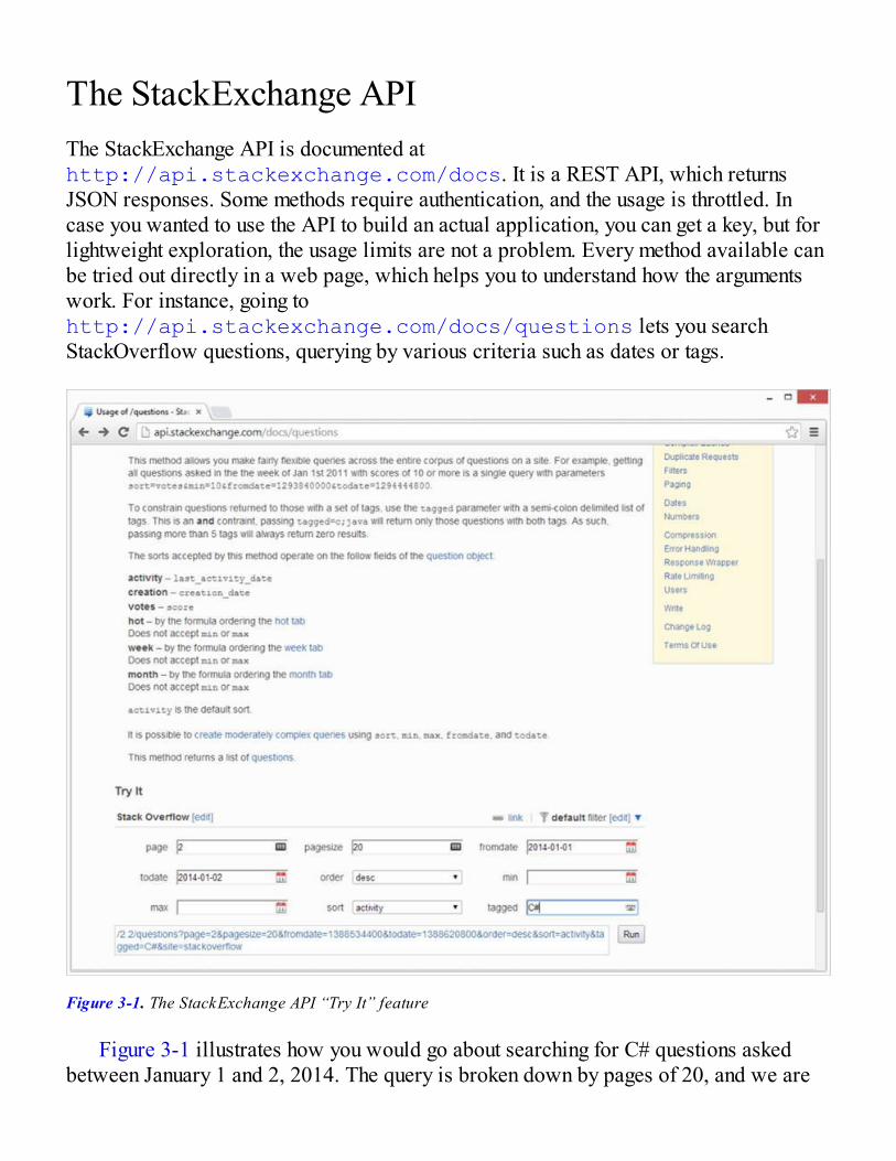
The StackExchange APIThe StackExchange API is documented athttp://api.stackexchange.com/docs. It is a REST API, which returnsJSON responses. Some methods require authentication, and the usage is throttled. Incase you wanted to use the API to build an actual application, you can get a key, but forlightweight exploration, the usage limits are not a problem. Every method available canbe tried out directly in a web page, which helps you to understand how the argumentswork. For instance, going tohttp://api.stackexchange.com/docs/questions lets you searchStackOverflow questions, querying by various criteria such as dates or tags.

Figure 3-1. The StackExchange API “Try It” feature

Figure 3-1 illustrates how you would go about searching for C# questions askedbetween January 1 and 2, 2014. The query is broken down by pages of 20, and we are

asking for the second page of results; that is, question numbers 21 to 40. If you hit the“Run” button, the current query will be executed, and its result will be displayed rightbelow, in the same window.

Note also how as you edit your query, the section to the left of the “Run” buttonchanges, reflecting your edits. What shows up is the actual query, which you can use toobtain data. As an example, if you were looking for questions tagged C#, the screenshown in Figure 3-2 would appear on the page:

Figure 3-2. A simple query

You could now simply paste that query into your browser and addhttp://api.stackexchange.com/ in front of it; for instance,https://api.stackexchange.com/2.2/questions?order=desc&sort=activity&site=stackoverflow&tagged= C%23(note how we replaced C# with C%23, thus replacing the unsafe ASCII character # withits safe encoding %23) will produce something along the lines of what is shown inFigure 3-3.

Figure 3-3. Running the query in the browser

We could now run that query from .NET using a WebRequest, for instance.However, there is still an issue to address: What we are getting back is a JSONdocument (items, which are a list of questions), and we would still need to create a.NET class to represent these, and then deserialize each item into it. While this is not aparticularly complex task, it is tedious. It would be nice if we had a mechanismavailable to us that would “just” look at that schema, do the grunt work of creating anadequate type for it, and load the response into it. The good news is that this is exactlywhat a type provider does.

Using the JSON Type ProviderType providers are an open mechanism; that is, anyone can implement one. As a result,in addition to a few type providers that were released by Microsoft when F# 3.0originally shipped, the F# community has implemented many additional type providerstargeting various resources. The majority of them have been consolidated in theFSharp.Data library; it is the de facto community reference for mainline typeproviders, and is very well maintained and documented.

NUGET PACKAGES AND F# SCRIPTS

To use a library in an F# script, you need to reference it by using the #r directive.

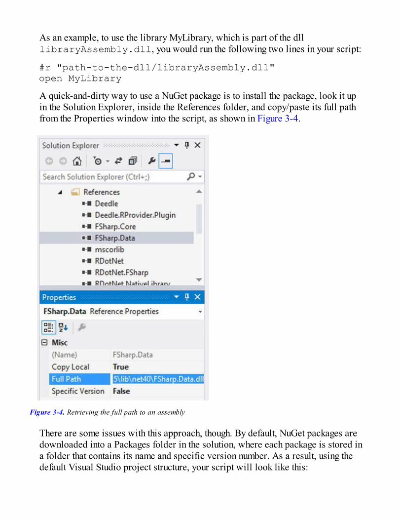
As an example, to use the library MyLibrary, which is part of the dlllibraryAssembly.dll, you would run the following two lines in your script:

#r "path-to-the-dll/libraryAssembly.dll"open MyLibrary

A quick-and-dirty way to use a NuGet package is to install the package, look it upin the Solution Explorer, inside the References folder, and copy/paste its full pathfrom the Properties window into the script, as shown in Figure 3-4.

Figure 3-4. Retrieving the full path to an assembly

There are some issues with this approach, though. By default, NuGet packages aredownloaded into a Packages folder in the solution, where each package is stored ina folder that contains its name and specific version number. As a result, using thedefault Visual Studio project structure, your script will look like this:

#r @"\Mathias\Documents\Visual Studio 2013\Projects\ProjectName\packages\PackageName.1.2.3\lib\net40-full\Assembly.dll"

This is obviously not awesome: The path depends on the local machine and on theversion number, which could both change. You can address the first issue by usingrelative paths and the #I directive, which adds a path where assemblies should besearched:

#I "..\packages"#r @"PackageName.1.2.3\lib\net40-full\Assembly.dll"

The version number problem is trickier; every time you update to a newer versionof a library, your script will break until you fix the path manually. Paket(http://fsprojects.github.io/Paket/), a dependency-managementlibrary for .NET, offers an elegant solution to that issue. We will be using version-specific paths in the rest of this book, because in this case it has the benefit ofclarifying which version was used.

Among the type providers you can find in FSharp.Data is the JSON typeprovider. Its behavior is typical of how a canonical type provider works. The followingsteps are involved:

First, create types by looking at sample data,

then load data from actual data sources into the type that has beencreated.

Let’s create a new F# solution, add a reference to FSharp.Data by installing thecorresponding NuGet package, and reference the FSharp.Data library in the defaultScript.fsx file, as shown in Listing 3-1.

Listing 3-1. Retrieving the latest StackOverflow C# questions with the JSON typeprovider

#I @"..\packages\"#r @"FSharp.Data.2.2.0\lib\net40\FSharp.Data.dll"

open FSharp.Data

type Questions = JsonProvider<"""https://api.stackexchange.com/2.2/questions?

site=stackoverflow""">

let csQuestions = """https://api.stackexchange.com/2.2/questions?site=stackoverflow&tagged=C%23"""Questions.Load(csQuestions).Items |> Seq.iter (fun q -> printfn "%s" q.Title)

Running this sample code should produce a list of 30 question titles (the defaultpage size is 30), which are the most active questions tagged C# that were asked onStackOverflow. Results will vary from machine to machine, because of the time-dependent nature of the query.

Tip F# supports two mechanisms to handle strings that contain special characters.Verbatim strings will ignore escape characters, like \, and allow you to embed quotesinside a string by using a double quote, like this: printfn @"He said""hello""!". Triple-quotes also ignore escape characters, but directly allow theusage of quotes inside, like this: printfn """He said "hello"!""".

So what’s going on here? The first piece, type Questions =JsonProvider<...>, creates a type, Questions, based on sample data. The sampledata is accessed over the wire from the URL we supplied, which, as we sawpreviously, calls the StackExchange API and returns 30 recent questions as a JSONdocument. The type provider scans that sample and creates the appropriate Propertiesand Types as needed. For instance, if you type Questions. inside your script file inVisual Studio and wait for IntelliSense to provide you with hints, you will see twothings. First, Questions contains a couple of classes that have been automaticallycreated based on what the sample contained: Item, Owner, and Root. Try clicking onItem in the drop-down menu that shows up once IntelliSense kicks in; you should seethat it exposes a bunch of Properties, such as memberAcceptedAnswerId:Option<int>. Based on the sample, the TP has generated aclass with appropriate types (the accepted answer ID should be an integer when itexists, but could also not exist, if no satisfactory answer was supplied).

Questions also exposes a Load method. This method can be used to retrievedata from a specific source, and it is expected to return something that will fit theQuestions type. This is what is taking place in the second part of the script: We pass ina query that requests the most recent questions tagged C# (encoded as C%23), and thetype provider goes over the wire, makes the request, receives a JSON document, andautomatically converts it to a full-blown type.

You can use the JSON type provider in a slightly different manner, which might helpclarify the mechanics at work here. Instead of calling the StackExchange API to generatethe Questions type, you could also directly supply it with a sample, either as a file or asan in-line string. Listing 3-2 illustrates this process: We provide a valid sample of theJSON output we expect from the API as a plain string (marked with the [<Literal>]attribute, which compiles it as a constant literal), and pass that sample to the typeprovider, which will create a new F# type based on how the data is structured in thesample.

Listing 3-2. Creating a type from a local JSON sample

[<Literal>]let sample = """{"items":[{"tags":["java","arrays"],"owner": // SNIPPED FOR BREVITY"},{"tags":["javascript","jquery","html"],"owner": // SNIPPEDFOR BREVITY"},],"has_more":true,"quota_max":300,"quota_remaining":299}"""

type HardCodedQuestions = JsonProvider<sample>

At this point, the compiler has created a type based on the sample string, and youcan use it to access data from the StackExchange API by passing in a query that isexpected to return a JSON response that follows the same structure; for instance, pullingJava-related questions:

[<Literal>]let javaQuery = "https://api.stackexchange.com/2.2/questions?site=stackoverflow&tagged=java"

let javaQuestions = HardCodedQuestions.Load(javaQuery)

In other words, the sample is used by the compiler to generate a type; whether theJSON comes from a local file or over the wire doesn’t matter. Once the type is created,it can be used to load data that has the appropriate shape. If, for instance, we were tocall a different API endpoint using this type, we would get a runtime exception.

One interesting difference between the two methods is that they have differentimplications if the schema changes over time. Imagine that, for instance, the Titleproperty was renamed to something else. In the first case, we would get a compile-timeerror, because the type is created every time we build by accessing the API, and the

compiler would catch that we are using a property that doesn’t exist anymore. Bycontrast, when using a “local sample,” we would get a runtime error: Our type is basedon a stale sample, which would still have the old property, and the mismatch would beonly caught when we try to access live data.

Building a Minimal DSL to Query QuestionsThe StackExchange API is pretty straightforward, and it would not be very difficult tosimply write queries by hand as we go. However, this would introduce a lot ofrepetition in our code, which creates potential for both typos and bugs. Let’s avoid thatand create a minimal domain-specific language, or, as they are commonly called, aDSL.

You probably noticed that the StackExchange API requests follow a pattern: From abase URL (https://api.stackexchange.com/2.2/) we append a stringencoding what entity we are interested in getting (questions), followed by a questionmark and optional parameters specifying the query further (?site=stackoverflow&tagged=C%23;F%23). One way to simplify our queryconstruction is to take advantage of that pattern, creating small functions that describehow we are modifying the base query to fit our needs, in such a way that we cancompose these operations in a nice and readable pipeline. See Listing 3-3.

Listing 3-3. Building a minimal query DSL

let questionQuery = """https://api.stackexchange.com/2.2/questions?site=stackoverflow"""let tagged tags query = // join the tags in a ; separated string let joinedTags = tags |> String.concat ";" sprintf "%s&tagged=%s" query joinedTags

let page p query = sprintf "%s&page=%i" query p

let pageSize s query = sprintf "%s&pagesize=%i" query s

let extractQuestions (query:string) = Questions.Load(query).Items

In essence, questionQuery defines the base query from which we are starting.The three functions that follow are appending optional query details to that query, and

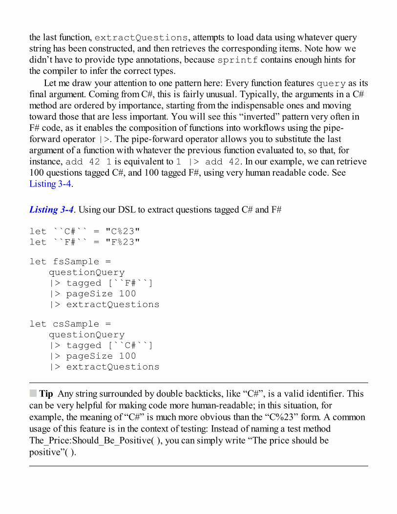
the last function, extractQuestions, attempts to load data using whatever querystring has been constructed, and then retrieves the corresponding items. Note how wedidn’t have to provide type annotations, because sprintf contains enough hints forthe compiler to infer the correct types.

Let me draw your attention to one pattern here: Every function features query as itsfinal argument. Coming from C#, this is fairly unusual. Typically, the arguments in a C#method are ordered by importance, starting from the indispensable ones and movingtoward those that are less important. You will see this “inverted” pattern very often inF# code, as it enables the composition of functions into workflows using the pipe-forward operator |>. The pipe-forward operator allows you to substitute the lastargument of a function with whatever the previous function evaluated to, so that, forinstance, add 42 1 is equivalent to 1 |> add 42. In our example, we can retrieve100 questions tagged C#, and 100 tagged F#, using very human readable code. SeeListing 3-4.

Listing 3-4. Using our DSL to extract questions tagged C# and F#

let ``C#`` = "C%23"let ``F#`` = "F%23"

let fsSample = questionQuery |> tagged [``F#``] |> pageSize 100 |> extractQuestions

let csSample = questionQuery |> tagged [``C#``] |> pageSize 100 |> extractQuestions

Tip Any string surrounded by double backticks, like “C#”, is a valid identifier. Thiscan be very helpful for making code more human-readable; in this situation, forexample, the meaning of “C#” is much more obvious than the “C%23” form. A commonusage of this feature is in the context of testing: Instead of naming a test methodThe_Price:Should_Be_Positive( ), you can simply write “The price should bepositive”( ).

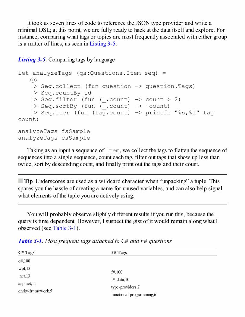
It took us seven lines of code to reference the JSON type provider and write aminimal DSL; at this point, we are fully ready to hack at the data itself and explore. Forinstance, comparing what tags or topics are most frequently associated with either groupis a matter of lines, as seen in Listing 3-5.

Listing 3-5. Comparing tags by language

let analyzeTags (qs:Questions.Item seq) = qs |> Seq.collect (fun question -> question.Tags) |> Seq.countBy id |> Seq.filter (fun (_,count) -> count > 2) |> Seq.sortBy (fun (_,count) -> -count) |> Seq.iter (fun (tag,count) -> printfn "%s,%i" tag count)

analyzeTags fsSampleanalyzeTags csSample

Taking as an input a sequence of Item, we collect the tags to flatten the sequence ofsequences into a single sequence, count each tag, filter out tags that show up less thantwice, sort by descending count, and finally print out the tags and their count.

Tip Underscores are used as a wildcard character when “unpacking” a tuple. Thisspares you the hassle of creating a name for unused variables, and can also help signalwhat elements of the tuple you are actively using.

You will probably observe slightly different results if you run this, because thequery is time dependent. However, I suspect the gist of it would remain along what Iobserved (see Table 3-1).

Table 3-1. Most frequent tags attached to C# and F# questions

C# Tags F# Tags

c#,100

wpf,13

.net,13

asp.net,11

entity-framework,5

f#,100

f#-data,10

type-providers,7

functional-programming,6

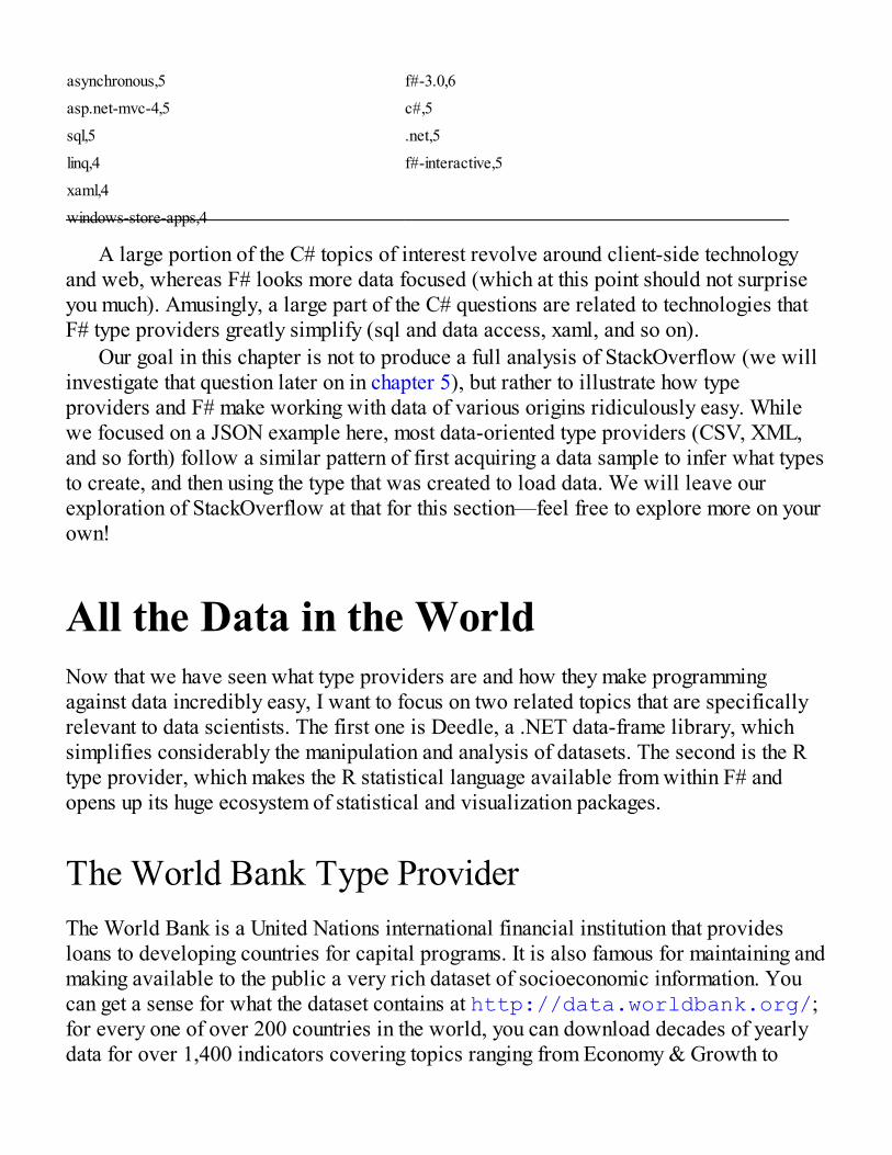
asynchronous,5

asp.net-mvc-4,5

sql,5

linq,4

xaml,4

windows-store-apps,4

f#-3.0,6

c#,5

.net,5

f#-interactive,5

A large portion of the C# topics of interest revolve around client-side technologyand web, whereas F# looks more data focused (which at this point should not surpriseyou much). Amusingly, a large part of the C# questions are related to technologies thatF# type providers greatly simplify (sql and data access, xaml, and so on).

Our goal in this chapter is not to produce a full analysis of StackOverflow (we willinvestigate that question later on in chapter 5), but rather to illustrate how typeproviders and F# make working with data of various origins ridiculously easy. Whilewe focused on a JSON example here, most data-oriented type providers (CSV, XML,and so forth) follow a similar pattern of first acquiring a data sample to infer what typesto create, and then using the type that was created to load data. We will leave ourexploration of StackOverflow at that for this section—feel free to explore more on yourown!

All the Data in the WorldNow that we have seen what type providers are and how they make programmingagainst data incredibly easy, I want to focus on two related topics that are specificallyrelevant to data scientists. The first one is Deedle, a .NET data-frame library, whichsimplifies considerably the manipulation and analysis of datasets. The second is the Rtype provider, which makes the R statistical language available from within F# andopens up its huge ecosystem of statistical and visualization packages.

The World Bank Type ProviderThe World Bank is a United Nations international financial institution that providesloans to developing countries for capital programs. It is also famous for maintaining andmaking available to the public a very rich dataset of socioeconomic information. Youcan get a sense for what the dataset contains at http://data.worldbank.org/;for every one of over 200 countries in the world, you can download decades of yearlydata for over 1,400 indicators covering topics ranging from Economy & Growth to

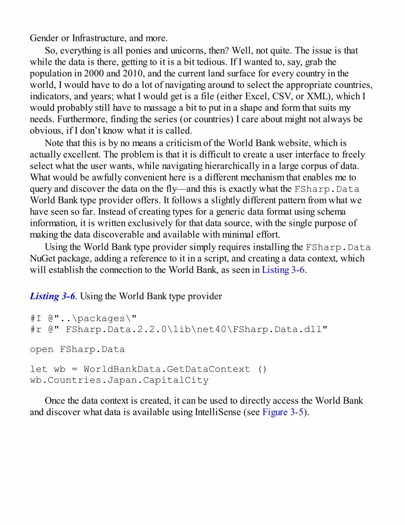
Gender or Infrastructure, and more.So, everything is all ponies and unicorns, then? Well, not quite. The issue is that

while the data is there, getting to it is a bit tedious. If I wanted to, say, grab thepopulation in 2000 and 2010, and the current land surface for every country in theworld, I would have to do a lot of navigating around to select the appropriate countries,indicators, and years; what I would get is a file (either Excel, CSV, or XML), which Iwould probably still have to massage a bit to put in a shape and form that suits myneeds. Furthermore, finding the series (or countries) I care about might not always beobvious, if I don’t know what it is called.

Note that this is by no means a criticism of the World Bank website, which isactually excellent. The problem is that it is difficult to create a user interface to freelyselect what the user wants, while navigating hierarchically in a large corpus of data.What would be awfully convenient here is a different mechanism that enables me toquery and discover the data on the fly—and this is exactly what the FSharp.DataWorld Bank type provider offers. It follows a slightly different pattern from what wehave seen so far. Instead of creating types for a generic data format using schemainformation, it is written exclusively for that data source, with the single purpose ofmaking the data discoverable and available with minimal effort.

Using the World Bank type provider simply requires installing the FSharp.DataNuGet package, adding a reference to it in a script, and creating a data context, whichwill establish the connection to the World Bank, as seen in Listing 3-6.

Listing 3-6. Using the World Bank type provider

#I @"..\packages\"#r @" FSharp.Data.2.2.0\lib\net40\FSharp.Data.dll"

open FSharp.Data

let wb = WorldBankData.GetDataContext ()wb.Countries.Japan.CapitalCity

Once the data context is created, it can be used to directly access the World Bankand discover what data is available using IntelliSense (see Figure 3-5).

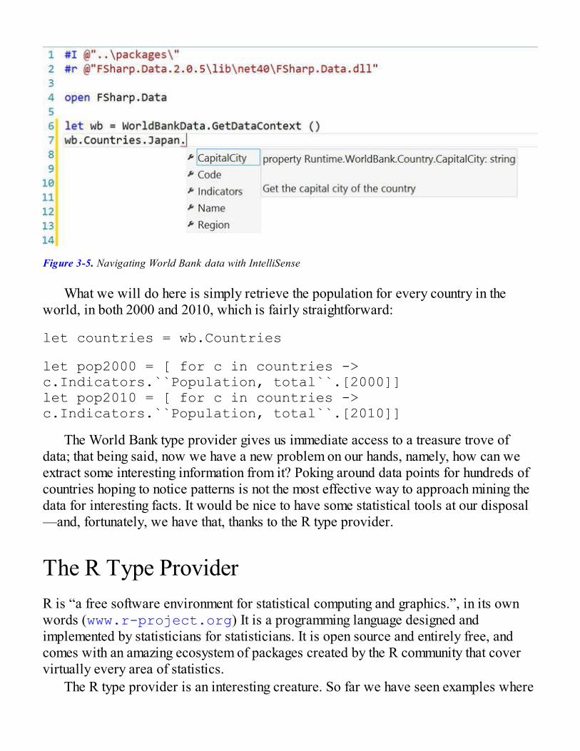
Figure 3-5. Navigating World Bank data with IntelliSense

What we will do here is simply retrieve the population for every country in theworld, in both 2000 and 2010, which is fairly straightforward:

let countries = wb.Countries

let pop2000 = [ for c in countries -> c.Indicators.``Population, total``.[2000]]let pop2010 = [ for c in countries -> c.Indicators.``Population, total``.[2010]]

The World Bank type provider gives us immediate access to a treasure trove ofdata; that being said, now we have a new problem on our hands, namely, how can weextract some interesting information from it? Poking around data points for hundreds ofcountries hoping to notice patterns is not the most effective way to approach mining thedata for interesting facts. It would be nice to have some statistical tools at our disposal—and, fortunately, we have that, thanks to the R type provider.

The R Type ProviderR is “a free software environment for statistical computing and graphics.”, in its ownwords (www.r-project.org) It is a programming language designed andimplemented by statisticians for statisticians. It is open source and entirely free, andcomes with an amazing ecosystem of packages created by the R community that covervirtually every area of statistics.

The R type provider is an interesting creature. So far we have seen examples where

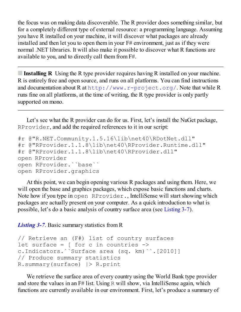
the focus was on making data discoverable. The R provider does something similar, butfor a completely different type of external resource: a programming language. Assumingyou have R installed on your machine, it will discover what packages are alreadyinstalled and then let you to open them in your F# environment, just as if they werenormal .NET libraries. It will also make it possible to discover what R functions areavailable to you, and to directly call them from F#.

Installing R Using the R type provider requires having R installed on your machine.R is entirely free and open source, and runs on all platforms. You can find instructionsand documentation about R at http://www.r-project.org/. Note that while Rruns fine on all platforms, at the time of writing, the R type provider is only partlysupported on mono.

Let’s see what the R provider can do for us. First, let’s install the NuGet package,RProvider, and add the required references to it in our script:

#r @"R.NET.Community.1.5.16\lib\net40\RDotNet.dll"#r @"RProvider.1.1.8\lib\net40\RProvider.Runtime.dll"#r @"RProvider.1.1.8\lib\net40\RProvider.dll"open RProvideropen RProvider.``base``open RProvider.graphics

At this point, we can begin opening various R packages and using them. Here, wewill open the base and graphics packages, which expose basic functions and charts.Note how if you type in open RProvider., IntelliSense will start showing whichpackages are actually present on your computer. As a quick introduction to what ispossible, let’s do a basic analysis of country surface area (see Listing 3-7).

Listing 3-7. Basic summary statistics from R

// Retrieve an (F#) list of country surfaceslet surface = [ for c in countries -> c.Indicators.``Surface area (sq. km)``.[2010]]// Produce summary statisticsR.summary(surface) |> R.print

We retrieve the surface area of every country using the World Bank type providerand store the values in an F# list. Using R will show, via IntelliSense again, whichfunctions are currently available in our environment. First, let’s produce a summary of

the surface area variable by calling R.summary, and then R.print, which generatesthe following “pretty print:”

Min. 1st Qu. Median Mean 3rd Qu. Max. NA's 2 11300 99900 630200 450300 17100000 1

Note If you run only R.summary, you might notice that it returns anRDotNet.SymbolicExpression. In order to avoid unnecessary and costlyconversions between R and .NET types, the R type provider typically sends informationto R via R Symbolic Expressions, the R representation of data and/or operations, andkeeps as much as possible in that form, converting back to .NET types only whenrequested.

There’s nothing earth shattering here, but it is very convenient. The summary returnsthe minimum and maximum values, as well as the average, the three quartiles (the valuesthat are greater than 25%, 50%, and 75% of the sample), and the number of missingvalues (NA). At a glance, we see that surface areas are wildly different, ranging from 2square kilometers for the smallest one to 17 million for the largest—and one countrywhere we found no data. That is useful, but given how dispersed the values seem to be,a chart would help us understand better how the data “looks.” This is pretty easy to dowith the R.hist(surface) function, which produces the chart seen in Figure 3-6.

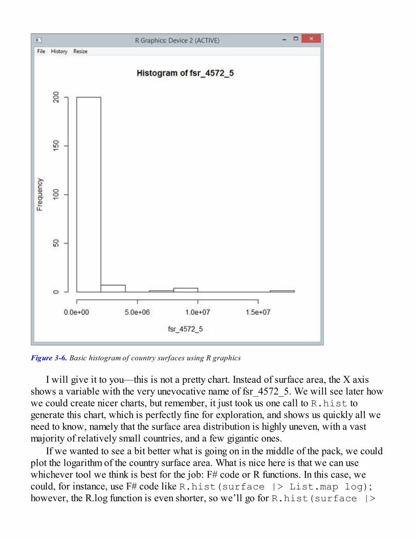
Figure 3-6. Basic histogram of country surfaces using R graphics

I will give it to you—this is not a pretty chart. Instead of surface area, the X axisshows a variable with the very unevocative name of fsr_4572_5. We will see later howwe could create nicer charts, but remember, it just took us one call to R.hist togenerate this chart, which is perfectly fine for exploration, and shows us quickly all weneed to know, namely that the surface area distribution is highly uneven, with a vastmajority of relatively small countries, and a few gigantic ones.

If we wanted to see a bit better what is going on in the middle of the pack, we couldplot the logarithm of the country surface area. What is nice here is that we can usewhichever tool we think is best for the job: F# code or R functions. In this case, wecould, for instance, use F# code like R.hist(surface |> List.map log);however, the R.log function is even shorter, so we’ll go for R.hist(surface |>

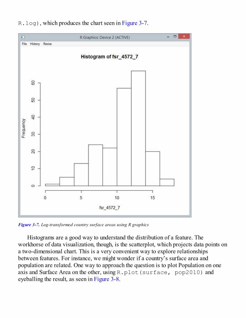
R.log), which produces the chart seen in Figure 3-7.

Figure 3-7. Log-transformed country surface areas using R graphics

Histograms are a good way to understand the distribution of a feature. Theworkhorse of data visualization, though, is the scatterplot, which projects data points ona two-dimensional chart. This is a very convenient way to explore relationshipsbetween features. For instance, we might wonder if a country’s surface area andpopulation are related. One way to approach the question is to plot Population on oneaxis and Surface Area on the other, using R.plot(surface, pop2010) andeyeballing the result, as seen in Figure 3-8.

Figure 3-8. Basic scatterplot using R.plot

From the looks of it, Surface and Population seem to have at best a limitedrelationship; the scatterplot shows no obvious pattern.

This simple scenario illustrates how R can help us understand individual featuresbetter by producing simple statistics and charts. However, working one feature at a timewill quickly end up being a nightmare if your dataset is non-trivial. When diggingthrough data, you will typically have a lot of features, and you will need to be able toexplore their relationships quickly and to rearrange them into new features bycombining existing ones. This is why data frames, the topic we will explore next, aresuch a popular tool among data scientists.

Analyzing Data Together with R Data FramesIn a nutshell, a data frame is a data structure geared toward the manipulation of acollection of observations. Each observation corresponds to an individual row in thedata frame, but individual features can also be accessed as columns. In that sense, dataframes are similar to database tables, but are geared toward in-memory manipulation.By itself, this is already very convenient: This retains type information on individualrows, but greatly simplifies operations such as “compute the average Order Quantityfeature for Customers which had a Revenue greater than 1 million,” which are notdifficult, but require repeating similar code over and over again. See Figure 3-9.

Figure 3-9. Merging various data sources into a single data frame

The other main purpose of data frames is to help in merging data sources into asingle frame. As such, data frames usually rely on keys to uniquely identify each row ofdata, so that various features can be associated with the correct rows and then joined.Another important related functionality is the management of missing values: If I amattempting to join two features—say, the surface area and population for countries—andhave incomplete data for some of them, I would want the resulting data frame to containthe union of all countries, but signal which ones have missing data, and handle thatmissing data without too much hassle when computing, for instance, the average surfacearea. Finally, data frames usually support dynamic column creation. In our previousexample, I might want to look into a new feature like country density (the populationdivided by the surface area); data frames typically allow you to add a new column and

express column combinations in a simple manner.Data frames are one of the core types of R; today, most programming languages used

by data scientists have a data-frame library. They are usually inspired by the R dataframe, but come in different flavors, depending on the language characteristics. .NET isno exception; there are a couple of good commercial products, and a great open-sourcelibrary, Deedle, which we will briefly demonstrate here.

But before looking into Deedle, let’s see for a second how we would use the nativeR data frame. The R type provider comes with a couple of utility functions that makecreating R data frames from F# easier. As an example, try out the code in Listing 3-8.

Listing 3-8. Creating and plotting an R data frame

let pollution = [ for c in countries -> c.Indicators.``CO2emissions (kt)``.[2000]]let education = [ for c in countries -> c.Indicators.``School enrollment, secondary (% gross)``.[2000]]

let rdf = [ "Pop2000", box pop2000 "Pop2010", box pop2010 "Surface", box surface "Pollution", box pollution "Education", box education ] |> namedParams |> R.data_frame

// Scatterplot of all featuresrdf |> R.plot

// Summary of all featuresrdf |> R.summary |> R.print

We retrieve a couple of additional features (pollution measured as CO2 emissions,and education measured as secondary school enrollment percentage) and create a dataframe containing five columns, each of which is associated with a name. Once the dataframe is created, we can generate a summary, which produces the following output:

> Pop2000 Pop2010 Surface Pollution Min. :9.419e+03 Min. :9.827e+03 Min. :

2 Min. : 15 1st Qu.:6.255e+05 1st Qu.:7.981e+05 1st Qu.: 11300 1st Qu.: 1050 Median :5.139e+06 Median :5.931e+06 Median : 99900 Median : 6659 Mean :2.841e+07 Mean :3.207e+07 Mean : 630216 Mean : 122608 3rd Qu.:1.631e+07 3rd Qu.:2.097e+07 3rd Qu.: 450300 3rd Qu.: 53601 Max. :1.263e+09 Max. :1.338e+09 Max. :17098240 Max. :5713560 NA's :1 NA's :20 Education Min. : 6.051 1st Qu.: 41.699 Median : 78.588 Mean : 70.782 3rd Qu.: 93.882 Max. :160.619 NA's :70

We can even visualize all features together by passing the entire data frame directlyto R.plot, as seen in Figure 3-10.

Figure 3-10. Visualizing relationships between features

Such charts are very useful. At a glance, it is immediately obvious that Pop2000 andPop2010 are related: Their scatterplot forms a nearly perfect line. Education appears tobe independent from all four other features (no clear visual pattern emerges), andSurface Area and Pollution seem somewhat related to Population (larger populationstend to go with higher values). Note also that while we had a significant number of

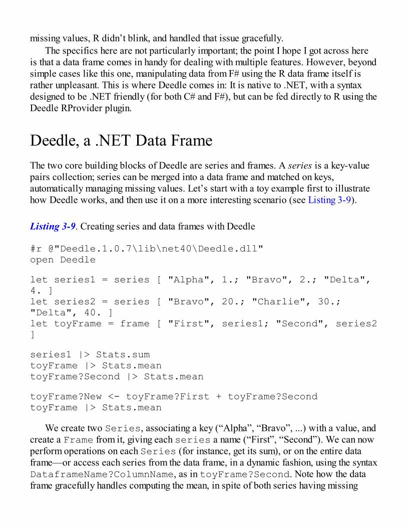
missing values, R didn’t blink, and handled that issue gracefully.The specifics here are not particularly important; the point I hope I got across here

is that a data frame comes in handy for dealing with multiple features. However, beyondsimple cases like this one, manipulating data from F# using the R data frame itself israther unpleasant. This is where Deedle comes in: It is native to .NET, with a syntaxdesigned to be .NET friendly (for both C# and F#), but can be fed directly to R using theDeedle RProvider plugin.

Deedle, a .NET Data FrameThe two core building blocks of Deedle are series and frames. A series is a key-valuepairs collection; series can be merged into a data frame and matched on keys,automatically managing missing values. Let’s start with a toy example first to illustratehow Deedle works, and then use it on a more interesting scenario (see Listing 3-9).

Listing 3-9. Creating series and data frames with Deedle

#r @"Deedle.1.0.7\lib\net40\Deedle.dll"open Deedle

let series1 = series [ "Alpha", 1.; "Bravo", 2.; "Delta", 4. ]let series2 = series [ "Bravo", 20.; "Charlie", 30.; "Delta", 40. ]let toyFrame = frame [ "First", series1; "Second", series2]

series1 |> Stats.sumtoyFrame |> Stats.meantoyFrame?Second |> Stats.mean

toyFrame?New <- toyFrame?First + toyFrame?SecondtoyFrame |> Stats.mean

We create two Series, associating a key (“Alpha”, “Bravo”, ...) with a value, andcreate a Frame from it, giving each series a name (“First”, “Second”). We can nowperform operations on each Series (for instance, get its sum), or on the entire dataframe—or access each series from the data frame, in a dynamic fashion, using the syntaxDataframeName?ColumnName, as in toyFrame?Second. Note how the dataframe gracefully handles computing the mean, in spite of both series having missing

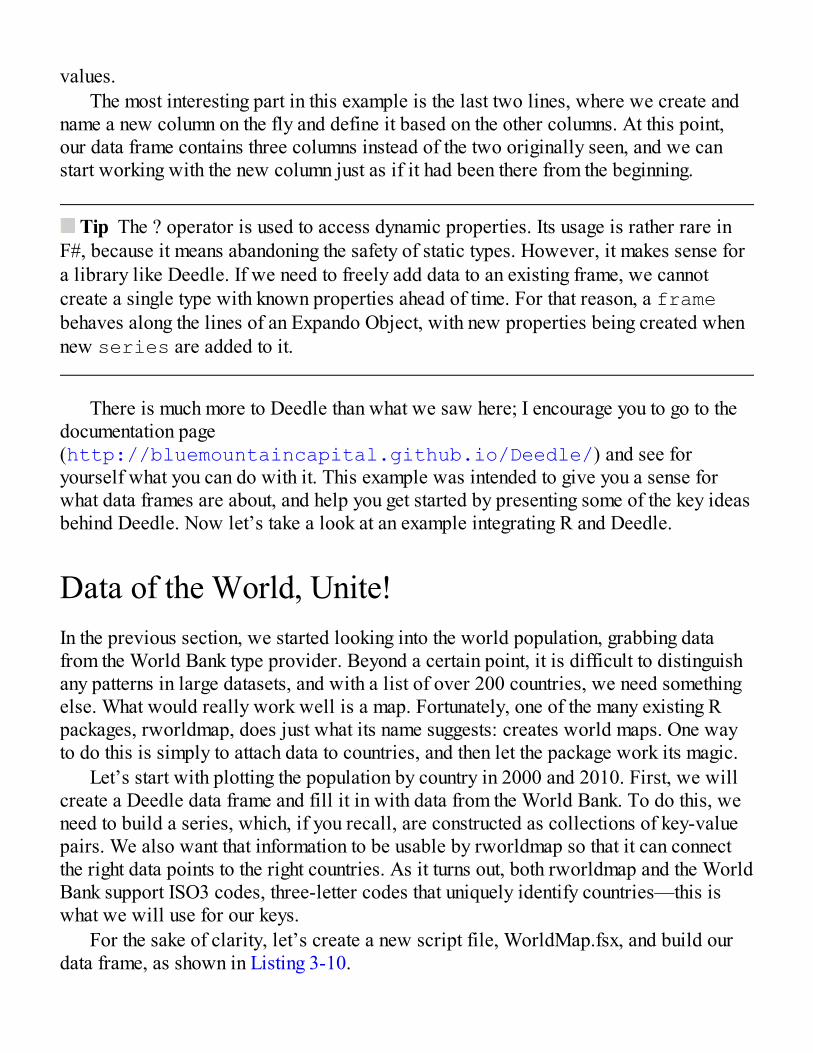
values.The most interesting part in this example is the last two lines, where we create and

name a new column on the fly and define it based on the other columns. At this point,our data frame contains three columns instead of the two originally seen, and we canstart working with the new column just as if it had been there from the beginning.

Tip The ? operator is used to access dynamic properties. Its usage is rather rare inF#, because it means abandoning the safety of static types. However, it makes sense fora library like Deedle. If we need to freely add data to an existing frame, we cannotcreate a single type with known properties ahead of time. For that reason, a framebehaves along the lines of an Expando Object, with new properties being created whennew series are added to it.

There is much more to Deedle than what we saw here; I encourage you to go to thedocumentation page(http://bluemountaincapital.github.io/Deedle/) and see foryourself what you can do with it. This example was intended to give you a sense forwhat data frames are about, and help you get started by presenting some of the key ideasbehind Deedle. Now let’s take a look at an example integrating R and Deedle.

Data of the World, Unite!In the previous section, we started looking into the world population, grabbing datafrom the World Bank type provider. Beyond a certain point, it is difficult to distinguishany patterns in large datasets, and with a list of over 200 countries, we need somethingelse. What would really work well is a map. Fortunately, one of the many existing Rpackages, rworldmap, does just what its name suggests: creates world maps. One wayto do this is simply to attach data to countries, and then let the package work its magic.

Let’s start with plotting the population by country in 2000 and 2010. First, we willcreate a Deedle data frame and fill it in with data from the World Bank. To do this, weneed to build a series, which, if you recall, are constructed as collections of key-valuepairs. We also want that information to be usable by rworldmap so that it can connectthe right data points to the right countries. As it turns out, both rworldmap and the WorldBank support ISO3 codes, three-letter codes that uniquely identify countries—this iswhat we will use for our keys.

For the sake of clarity, let’s create a new script file, WorldMap.fsx, and build ourdata frame, as shown in Listing 3-10.

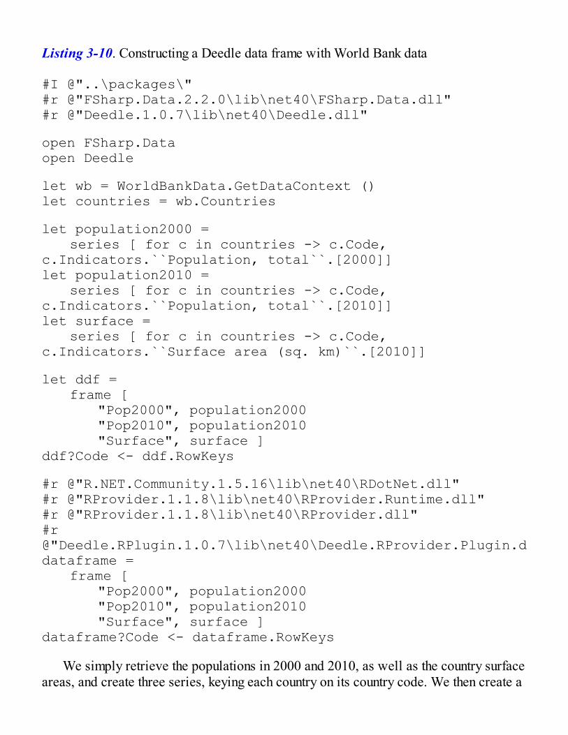
Listing 3-10. Constructing a Deedle data frame with World Bank data

#I @"..\packages\"#r @"FSharp.Data.2.2.0\lib\net40\FSharp.Data.dll"#r @"Deedle.1.0.7\lib\net40\Deedle.dll"

open FSharp.Dataopen Deedle

let wb = WorldBankData.GetDataContext ()let countries = wb.Countries

let population2000 = series [ for c in countries -> c.Code, c.Indicators.``Population, total``.[2000]]let population2010 = series [ for c in countries -> c.Code, c.Indicators.``Population, total``.[2010]]let surface = series [ for c in countries -> c.Code, c.Indicators.``Surface area (sq. km)``.[2010]]

let ddf = frame [ "Pop2000", population2000 "Pop2010", population2010 "Surface", surface ]ddf?Code <- ddf.RowKeys

#r @"R.NET.Community.1.5.16\lib\net40\RDotNet.dll"#r @"RProvider.1.1.8\lib\net40\RProvider.Runtime.dll"#r @"RProvider.1.1.8\lib\net40\RProvider.dll"#r @"Deedle.RPlugin.1.0.7\lib\net40\Deedle.RProvider.Plugin.dll"letdataframe = frame [ "Pop2000", population2000 "Pop2010", population2010 "Surface", surface ]dataframe?Code <- dataframe.RowKeys

We simply retrieve the populations in 2000 and 2010, as well as the country surfaceareas, and create three series, keying each country on its country code. We then create a

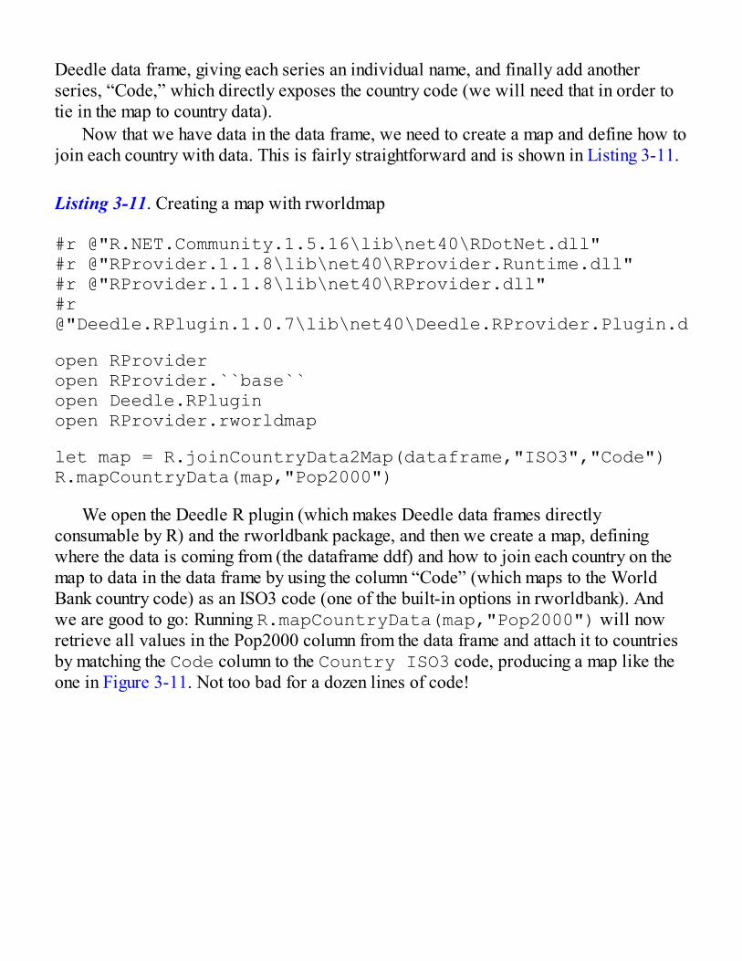
Deedle data frame, giving each series an individual name, and finally add anotherseries, “Code,” which directly exposes the country code (we will need that in order totie in the map to country data).

Now that we have data in the data frame, we need to create a map and define how tojoin each country with data. This is fairly straightforward and is shown in Listing 3-11.

Listing 3-11. Creating a map with rworldmap

#r @"R.NET.Community.1.5.16\lib\net40\RDotNet.dll"#r @"RProvider.1.1.8\lib\net40\RProvider.Runtime.dll"#r @"RProvider.1.1.8\lib\net40\RProvider.dll"#r @"Deedle.RPlugin.1.0.7\lib\net40\Deedle.RProvider.Plugin.dll"

open RProvideropen RProvider.``base``open Deedle.RPluginopen RProvider.rworldmap

let map = R.joinCountryData2Map(dataframe,"ISO3","Code")R.mapCountryData(map,"Pop2000")

We open the Deedle R plugin (which makes Deedle data frames directlyconsumable by R) and the rworldbank package, and then we create a map, definingwhere the data is coming from (the dataframe ddf) and how to join each country on themap to data in the data frame by using the column “Code” (which maps to the WorldBank country code) as an ISO3 code (one of the built-in options in rworldbank). Andwe are good to go: Running R.mapCountryData(map,"Pop2000") will nowretrieve all values in the Pop2000 column from the data frame and attach it to countriesby matching the Code column to the Country ISO3 code, producing a map like theone in Figure 3-11. Not too bad for a dozen lines of code!

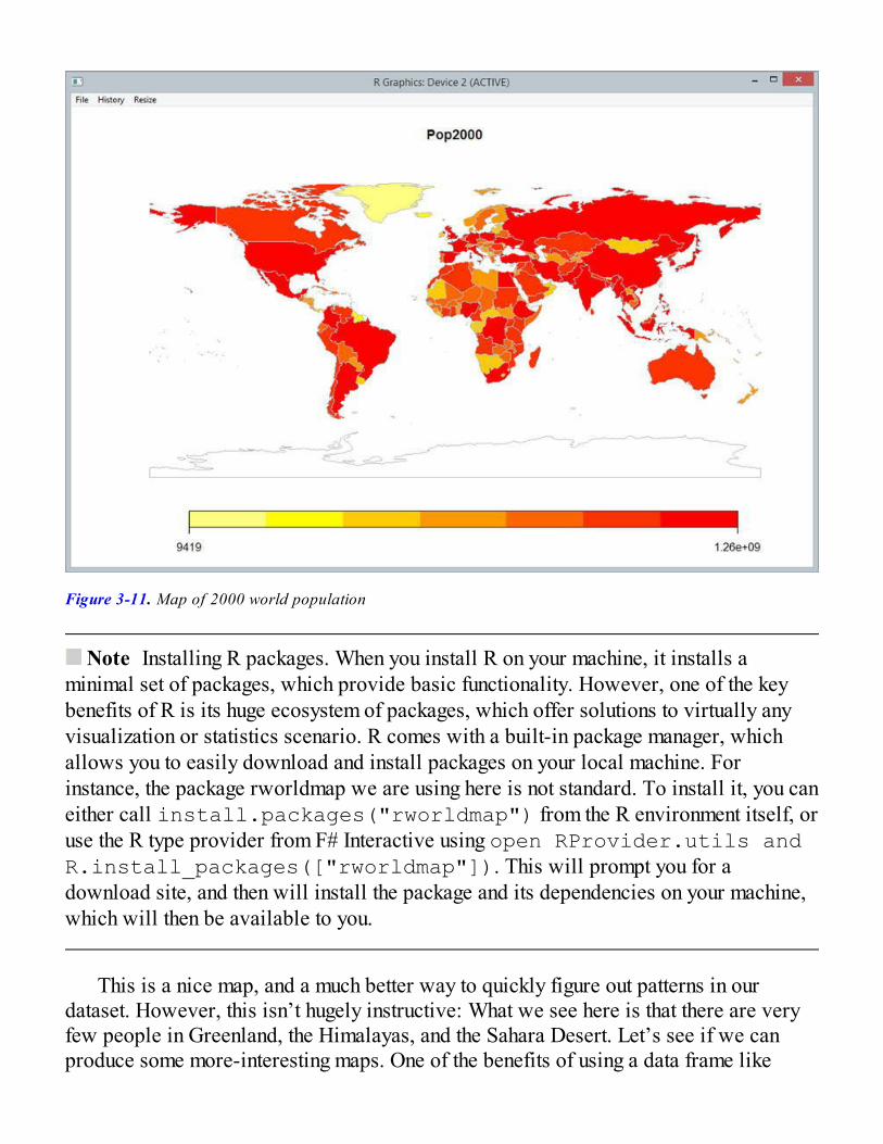
Figure 3-11. Map of 2000 world population

Note Installing R packages. When you install R on your machine, it installs aminimal set of packages, which provide basic functionality. However, one of the keybenefits of R is its huge ecosystem of packages, which offer solutions to virtually anyvisualization or statistics scenario. R comes with a built-in package manager, whichallows you to easily download and install packages on your local machine. Forinstance, the package rworldmap we are using here is not standard. To install it, you caneither call install.packages("rworldmap") from the R environment itself, oruse the R type provider from F# Interactive using open RProvider.utils andR.install_packages(["rworldmap"]). This will prompt you for adownload site, and then will install the package and its dependencies on your machine,which will then be available to you.

This is a nice map, and a much better way to quickly figure out patterns in ourdataset. However, this isn’t hugely instructive: What we see here is that there are veryfew people in Greenland, the Himalayas, and the Sahara Desert. Let’s see if we canproduce some more-interesting maps. One of the benefits of using a data frame like

Deedle, rather than manipulating raw data, is that it makes creating new features prettyeasy. As an example, let’s consider country population density; that is, how manypersons there are living per square kilometer (or mile). With Deedle, this is a breeze, asseen in Listing 3-12 and Figure 3-12.

Listing 3-12. Producing a population density map

dataframe?Density <- dataframe?Pop2010 / dataframe?Surfacelet map = R.joinCountryData2Map(dataframe,"ISO3","Code")R.mapCountryData(map,"Density")

Figure 3-12. Map of world population density

We create a new column on the fly called Density, defined as a function of twoother columns, and simply rebind the map to the updated data frame. This is a muchmore interesting map, highlighting a few very high-density areas in the world, located inWestern Europe, Southeast Asia, and Africa.

Similarly, we can visualize where the world population is growing in a couple oflines, seen in Listing 3-13 and Figure 3-13.

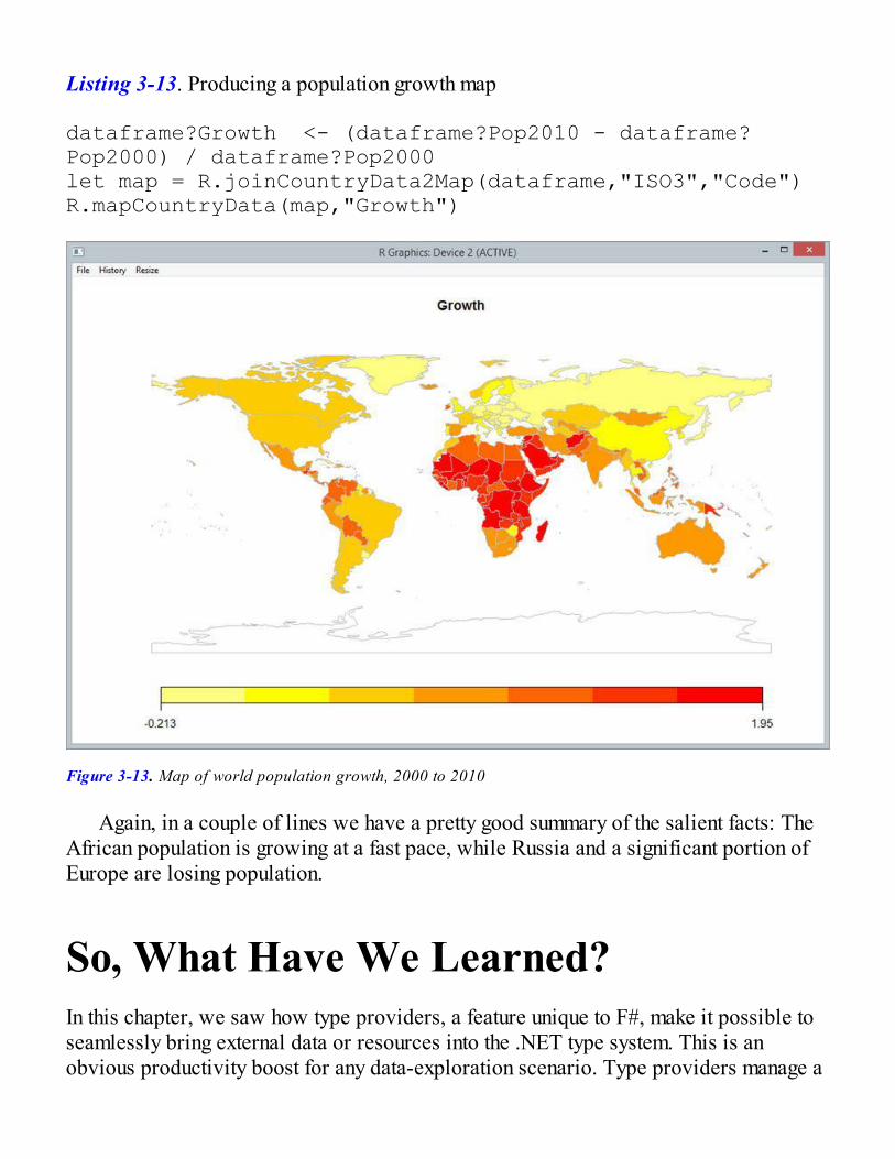
Listing 3-13. Producing a population growth map

dataframe?Growth <- (dataframe?Pop2010 - dataframe?Pop2000) / dataframe?Pop2000let map = R.joinCountryData2Map(dataframe,"ISO3","Code")R.mapCountryData(map,"Growth")

Figure 3-13. Map of world population growth, 2000 to 2010

Again, in a couple of lines we have a pretty good summary of the salient facts: TheAfrican population is growing at a fast pace, while Russia and a significant portion ofEurope are losing population.

So, What Have We Learned?In this chapter, we saw how type providers, a feature unique to F#, make it possible toseamlessly bring external data or resources into the .NET type system. This is anobvious productivity boost for any data-exploration scenario. Type providers manage a

remarkable feat: Getting to the data itself is every bit as easy as with a dynamiclanguage, but working with statically typed data gives the user additional help from thecompiler and tools, and prevents silly mistakes (such as property typos or incorrect typecasts) that would otherwise be caught only at runtime.

What is perhaps more interesting is that having typed data also provides hugebenefits in terms of data discoverability. Data is typically stored in formats that areprimarily meant to address computer I/O concerns, not human readability. As a result,coming to grips with a dataset is often an unnecessarily unpleasant experience, at leastfor humans. Type providers offer a very interesting mechanism, using tools that havebeen used for decades to help developers navigate and understand the internalorganization of large code bases (which are arguably complex data sets), and applyingthem to “normal” data via IntelliSense. This is a surprisingly powerful mechanism.Being able to discover how pieces of data are connected to each other by typing ‘.’, orhaving the computer automatically find items that partially match something I typed, is,in my experience, an extremely effective way to dive into a dataset and understand howit is organized.

The other main point in this chapter illustrated how the same mechanism can be usedto make all of the resources of R available from within the F# environment. R has itsfans and haters, but one aspect that is hard to argue with is the depth of its ecosystem. Ifyou have a statistics problem, chances are that “there’s a package for that.” R haspackages for virtually every statistical problem there is, and is also known forproducing beautiful, publication-grade charts and visualizations, and every single one ofthem is available to you in F#.

The R type provider is a great example of F# as an effective glue language. Using R-specific tools like RStudio may provide a slightly better experience using R than callingit from F# via the type provider. However, picking R as the primary developmentenvironment has large implications. R was never built with integration in mind, andrunning it in production, or talking to other systems, is not something that it isparticularly good at. On top of that, R has nothing close to type providers; gone is theability to explore and load data from everywhere.

By contrast, F# is a language that was built to run critical code in production; it justhappens to have pretty decent scripting abilities, too. In that frame, using F# as aprimary environment makes a lot of sense. A data scientist can use it to write scripts,using whatever combination of tools they please to prototype a model, along with all themight of the .NET framework; that same script can then very easily be converted to aclass or module, which will run with no problem at all in production, at scale.

Finally, we also saw how function composition with the pipe-forward operatormade it very easy to create miniature, domain-specific languages. By creating smallfunctions and thinking carefully about how to organize their arguments, we were able towrite a couple of lines code that could then be chained together in a flexible manner,

while at the same time being very human-readable. There is much more to the topic ofDSLs in F# than the simplified examples found here, but this should at least give you aninkling for why the language is a great fit for that!

Going FurtherWe saw a small sample of type providers in this chapter, but there is one available forvirtually any data format that exposes some form of schema. Type providers for XML,Soap, CSV, SQL, JSON, and so forth are an open mechanism: Anyone can write one totarget a specific type of data, and the F# community has been busy creating a wide arrayof type providers. At this point in time, fsharp.data is the largest and best-documented collection of type providers. A few other ones are worth mentioning, inparticular the SQL Command type provider(http://fsprojects.github.io/FSharp.Data.SqlClient/) forstatically typed access to input parameters and result sets of T-SQL command and theSQL type provider (https://github.com/fsprojects/SQLProvider),which enables the exploration and querying of various SQL implementations.

Beyond data, type providers targeting different languages, in a fashion similar to R,are also being developed; most interesting from a machine-learning perspective, thereare ongoing efforts to create Matlab and Python type providers. However, at the time ofwriting, these haven’t reached the same level of maturity as the R type provider.

USEFUL LINKS

FSharp.Data is a well-maintained and -documented collection ofopen-source F# type providers:http://fsharp.github.io/FSharp.Data/

The World Bank Data website:http://data.worldbank.org/

The R statistical environment: http://www.r-project.org/

The F# R Provider:http://bluemountaincapital.github.io/FSharpRProvider/

Deedle, a .NET dataframe library:http://bluemountaincapital.github.io/Deedle/

Nice tutorial on getting started with the rworldmap package:

http://cran.r-project.org/web/packages/rworldmap/vignettes/rworldmap.pdf

Paket, a dependency manager for .NET:http://fsprojects.github.io/Paket/

Fsharp.Data.SqlClient, athttp://fsprojects.github.io/FSharp.Data.SqlClient,and the SQLProvider, athttp://fsprojects.github.io/SQLProvider, aretwo complementary type providers dedicated to working with SQLdatabases.

CHAPTER 4

Of Bikes and Men

Fitting a Regression Model to Data withGradient DescentSo far, the problems we have tackled have involved classifying items between a limitedset of possible categories. While classification has applications in many practicalsituations, an arguably more common problem is to predict a number. Consider, forinstance, the following task: Given the characteristics of a used car (age, miles, enginesize, and so forth), how would you go about predicting how much it is going to sell for?This problem doesn’t really fit the pattern of classification. What we need here is amodel that differs from classification models in at least two aspects:

What the model predicts are actual numbers, which can take a widerange of values, and can be meaningfully compared.

We are interested in the functional relationship between featuresand their predicted values; that is, how a change in the featureimpacts the prediction.

In our car example, what we are looking for is a model along these lines:

Unlike the classification models we saw earlier, the predicted prices are not limitedto a fixed set of possible choices; they can take a wide range of values. Furthermore, ifyou were to plug different values for miles in the model, you could directly observehow a change in the feature impacts the predicted value, and possibly compare that tochanges in the age value, to understand how sensitive price is to various features.

This type of model is called a regression model, and it has a relatively younghistory, with significant developments beginning in the nineteenth century. Its originsstem from physics and the need to validate physical models against experimentalobservations, which lead to the foundation of modern statistics. The methods spread tobiology, economics, and other fields, evolving and adapting along the way so as tohandle questions specific to each discipline, and are an important part of machinelearning today.

In this chapter, our goal is to predict the number of people using a bicycle-sharingservice for a given day, given information such as weather conditions or day of theweek. We will start with a fairly simple model and progressively build up refinementsin order to improve accuracy, introducing important machine-learning techniques alongthe way. As we advance, we will

explain how finding a straight line that fits the data well can bestated as finding the line with the lowest overall error;

introduce gradient descent, a very powerful and general techniqueto find the minimum of a function, and then put it into action tocreate our first prediction model;

explore how linear algebra can help write much shorter models andalgorithms, and potentially speed up calculations;

present a simple approach to easily creating and modifying models,using functions to define features that select what part of the datawe want to use to make predictions; and

refine our predictions further, illustrating how to use more of thedata by handling different data types and creating more-complex,nonlinear features.

Getting to Know the DataIn this chapter, we will use another dataset from the University of California–IrvineMachine Learning Repository, the “bike-sharing dataset,” which you can find here:https://archive.ics.uci.edu/ml/datasets/Bike+Sharing+Dataset

The dataset is based off the Capital Bikeshare program. In its own words,

Capital Bikeshare puts over 2500 bicycles at your fingertips. You canchoose any of the over 300 stations across Washington, D.C., Arlington andAlexandria, VA and Montgomery County, MD and return it to any station

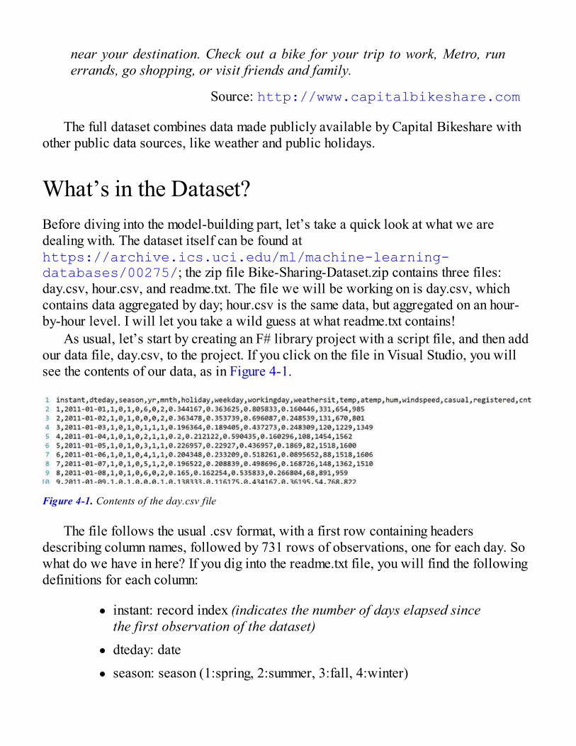
near your destination. Check out a bike for your trip to work, Metro, runerrands, go shopping, or visit friends and family.

Source: http://www.capitalbikeshare.com

The full dataset combines data made publicly available by Capital Bikeshare withother public data sources, like weather and public holidays.

What’s in the Dataset?Before diving into the model-building part, let’s take a quick look at what we aredealing with. The dataset itself can be found athttps://archive.ics.uci.edu/ml/machine-learning-databases/00275/; the zip file Bike-Sharing-Dataset.zip contains three files:day.csv, hour.csv, and readme.txt. The file we will be working on is day.csv, whichcontains data aggregated by day; hour.csv is the same data, but aggregated on an hour-by-hour level. I will let you take a wild guess at what readme.txt contains!

As usual, let’s start by creating an F# library project with a script file, and then addour data file, day.csv, to the project. If you click on the file in Visual Studio, you willsee the contents of our data, as in Figure 4-1.

Figure 4-1. Contents of the day.csv file

The file follows the usual .csv format, with a first row containing headersdescribing column names, followed by 731 rows of observations, one for each day. Sowhat do we have in here? If you dig into the readme.txt file, you will find the followingdefinitions for each column:

instant: record index (indicates the number of days elapsed sincethe first observation of the dataset)dteday: date

season: season (1:spring, 2:summer, 3:fall, 4:winter)

yr: year (0: 2011, 1:2012)

mnth: month ( 1 to 12)

holiday: whether day is holiday or not (extracted fromhttp://dchr.dc.gov/page/holiday-schedule)

weekday: day of the week

workingday: if day is neither weekend nor holiday is 1, otherwiseis 0.

weathersit:

1: Clear, Few clouds, Partly cloudy, Partly cloudy

2: Mist + Cloudy, Mist + Broken clouds, Mist + Fewclouds, Mist

3: Light Snow, Light Rain + Thunderstorm + Scatteredclouds, Light Rain + Scattered clouds

4: Heavy Rain + Ice Pellets + Thunderstorm + Mist, Snow +Fog

temp: Normalized temperature in Celsius. The values are divided to41 (max)

atemp: Normalized feeling temperature in Celsius. The values aredivided to 50 (max)

hum: Normalized humidity. The values are divided to 100 (max)

windspeed: Normalized wind speed. The values are divided to 67(max)

casual: count of casual users

registered: count of registered users

cnt: count of total rental bikes including both casual and registered

We have a couple of different features available to us: time/calendar information,whether it was a regular workday or a “special” one, multiple measurements pertainingto the weather, and finally the count of people who rented a bicycle that day, brokendown into registered and casual users.

Our focus here will be on creating a model to predict cnt, the count of people whorented a bicycle on a particular day, using the measurements we have available for thatday (excluding, of course, casual and registered, because there wouldn’t be

much fun in that, as by definition casual + register = cnt). Note that our datais not homogeneous: While some of the features are numeric— that is, actual numbers(for instance, temp, the temperature)—quite a few of them are categorical—that is,each number encodes a state (for instance, weathersit or workingday).

Inspecting the Data with FSharp.ChartingAs usual, let’s start by working in the script file and take a closer look at the data,loading it in memory using the CSV type provider from fsharp.Data, which we firstinstall from NuGet:

#I @"packages\"#r @"FSharp.Data.2.2.1\lib\net40\FSharp.Data.dll"

open FSharp.Data

type Data = CsvProvider<"day.csv">let dataset = Data.Load("day.csv")let data = dataset.Rows

Unlike some of the problems we looked at previously, this dataset has a fairlyobvious set of features to start with. In this case, it might be worth simply inspecting thedata manually to see if we can spot any patterns. Let’s start by plotting bicycle usageover time. To do this, we’ll use another F# library, fsharp.Charting, which offers acollection of classic charts. Let’s install the library with Nuget and create our firstchart, plotting the total usage as a line:

#load @"FSharp.Charting.0.90.10\FSharp.Charting.fsx"open FSharp.Charting

let all = Chart.Line [ for obs in data -> obs.Cnt ]

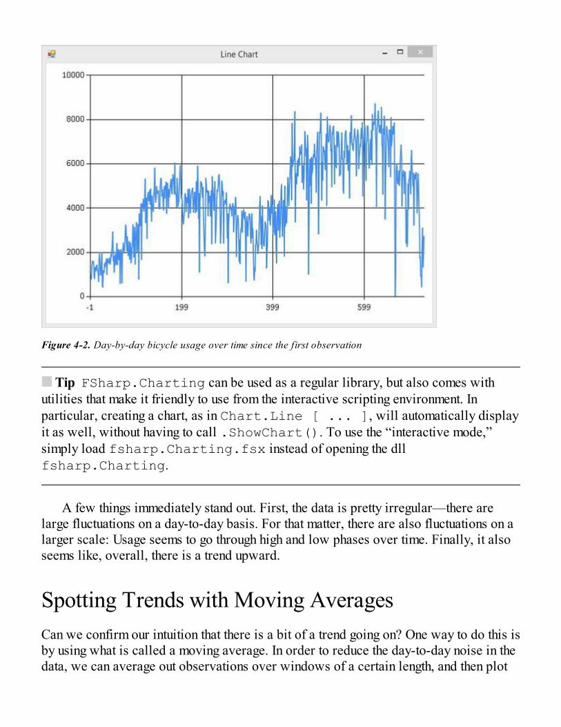
Figure 4-2. Day-by-day bicycle usage over time since the first observation

Tip FSharp.Charting can be used as a regular library, but also comes withutilities that make it friendly to use from the interactive scripting environment. Inparticular, creating a chart, as in Chart.Line [ ... ], will automatically displayit as well, without having to call .ShowChart(). To use the “interactive mode,”simply load fsharp.Charting.fsx instead of opening the dllfsharp.Charting.

A few things immediately stand out. First, the data is pretty irregular—there arelarge fluctuations on a day-to-day basis. For that matter, there are also fluctuations on alarger scale: Usage seems to go through high and low phases over time. Finally, it alsoseems like, overall, there is a trend upward.

Spotting Trends with Moving AveragesCan we confirm our intuition that there is a bit of a trend going on? One way to do this isby using what is called a moving average. In order to reduce the day-to-day noise in thedata, we can average out observations over windows of a certain length, and then plot

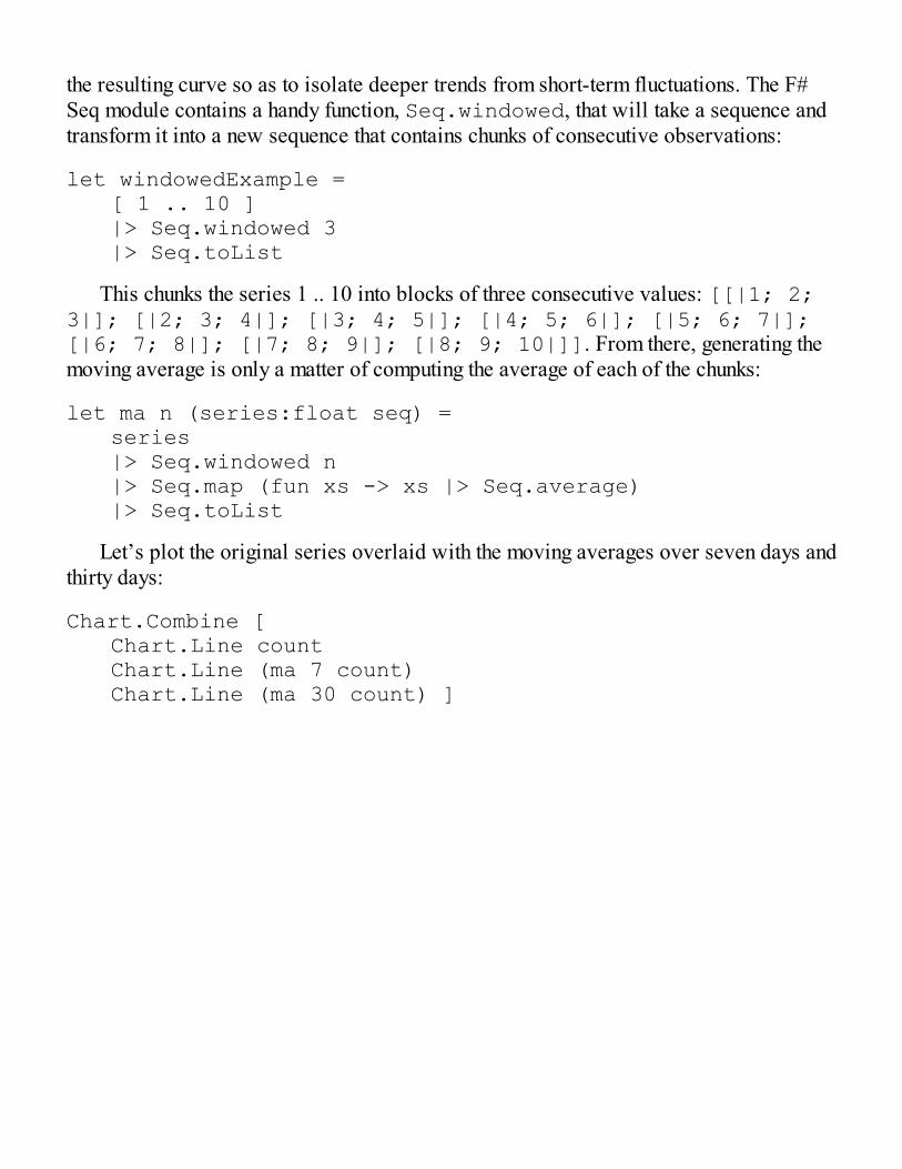
the resulting curve so as to isolate deeper trends from short-term fluctuations. The F#Seq module contains a handy function, Seq.windowed, that will take a sequence andtransform it into a new sequence that contains chunks of consecutive observations:

let windowedExample = [ 1 .. 10 ] |> Seq.windowed 3 |> Seq.toList

This chunks the series 1 .. 10 into blocks of three consecutive values: [[|1; 2;3|]; [|2; 3; 4|]; [|3; 4; 5|]; [|4; 5; 6|]; [|5; 6; 7|];[|6; 7; 8|]; [|7; 8; 9|]; [|8; 9; 10|]]. From there, generating themoving average is only a matter of computing the average of each of the chunks:

let ma n (series:float seq) = series |> Seq.windowed n |> Seq.map (fun xs -> xs |> Seq.average) |> Seq.toList

Let’s plot the original series overlaid with the moving averages over seven days andthirty days:

Chart.Combine [ Chart.Line count Chart.Line (ma 7 count) Chart.Line (ma 30 count) ]

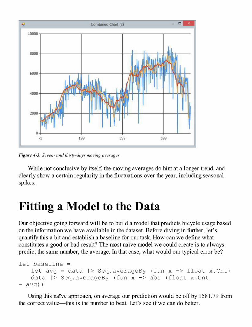
Figure 4-3. Seven- and thirty-days moving averages

While not conclusive by itself, the moving averages do hint at a longer trend, andclearly show a certain regularity in the fluctuations over the year, including seasonalspikes.

Fitting a Model to the DataOur objective going forward will be to build a model that predicts bicycle usage basedon the information we have available in the dataset. Before diving in further, let’squantify this a bit and establish a baseline for our task. How can we define whatconstitutes a good or bad result? The most naïve model we could create is to alwayspredict the same number, the average. In that case, what would our typical error be?

let baseline = let avg = data |> Seq.averageBy (fun x -> float x.Cnt) data |> Seq.averageBy (fun x -> abs (float x.Cnt - avg))

Using this naïve approach, on average our prediction would be off by 1581.79 fromthe correct value—this is the number to beat. Let’s see if we can do better.

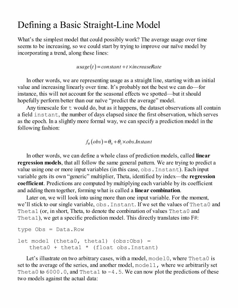
Defining a Basic Straight-Line ModelWhat’s the simplest model that could possibly work? The average usage over timeseems to be increasing, so we could start by trying to improve our naïve model byincorporating a trend, along these lines:

In other words, we are representing usage as a straight line, starting with an initialvalue and increasing linearly over time. It’s probably not the best we can do—forinstance, this will not account for the seasonal effects we spotted—but it shouldhopefully perform better than our naïve “predict the average” model.

Any timescale for t would do, but as it happens, the dataset observations all containa field instant, the number of days elapsed since the first observation, which servesas the epoch. In a slightly more formal way, we can specify a prediction model in thefollowing fashion:

In other words, we can define a whole class of prediction models, called linearregression models, that all follow the same general pattern. We are trying to predict avalue using one or more input variables (in this case, obs.Instant). Each inputvariable gets its own “generic” multiplier, Theta, identified by index—the regressioncoefficient. Predictions are computed by multiplying each variable by its coefficientand adding them together, forming what is called a linear combination.

Later on, we will look into using more than one input variable. For the moment,we’ll stick to our single variable, obs.Instant. If we set the values of Theta0 andTheta1 (or, in short, Theta, to denote the combination of values Theta0 andTheta1), we get a specific prediction model. This directly translates into F#:

type Obs = Data.Row

let model (theta0, theta1) (obs:Obs) = theta0 + theta1 * (float obs.Instant)

Let’s illustrate on two arbitrary cases, with a model, model0, where Theta0 isset to the average of the series, and another model, model1, where we arbitrarily setTheta0 to 6000.0, and Theta1 to -4.5. We can now plot the predictions of thesetwo models against the actual data:

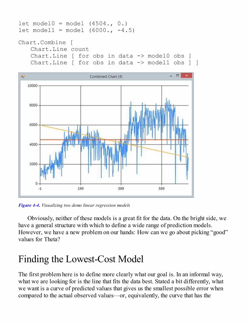
let model0 = model (4504., 0.)let model1 = model (6000., -4.5)

Chart.Combine [ Chart.Line count Chart.Line [ for obs in data -> model0 obs ] Chart.Line [ for obs in data -> model1 obs ] ]

Figure 4-4. Visualizing two demo linear regression models

Obviously, neither of these models is a great fit for the data. On the bright side, wehave a general structure with which to define a wide range of prediction models.However, we have a new problem on our hands: How can we go about picking “good”values for Theta?

Finding the Lowest-Cost ModelThe first problem here is to define more clearly what our goal is. In an informal way,what we are looking for is the line that fits the data best. Stated a bit differently, whatwe want is a curve of predicted values that gives us the smallest possible error whencompared to the actual observed values—or, equivalently, the curve that has the

smallest distance to the real data. We have seen a similar approach in Chapter 1! Wecan simply adapt the distance function; instead of computing the distance between twoimages pixel by pixel, we will compute the Euclidean distance between our predictedcurve and the actual one, comparing the true value and the forecasted one for each datapoint.

You might ask why I chose to pick the Euclidean distance, rather than somethingelse. After all, we started with the Manhattan distance in Chapter 1 because it was easyto compute. There are a couple of reasons for this choice. The first one is driven bymodelling considerations. The Euclidean distance penalizes errors by squaringdifferences; as a result, larger errors will be penalized much more heavily than smallerones, which is a good thing. When trying to minimize the distance, we will then focusprimarily on avoiding large errors, and not so much on small ones. The second reason istechnical: It makes the math considerably simpler.

As an example, let’s compute the costs of our two models:

type Model = Obs -> float

let cost (data:Obs seq) (m:Model) = data |> Seq.sumBy (fun x -> pown (float x.Cnt - m x) 2) |> sqrt

let overallCost = cost dataoverallCost model0 |> printfn "Cost model0: %.0f"overallCost model1 |> printfn "Cost model1: %.0f"

First, we create a type Model, which captures what all our models do— namely,convert an observation Obs into a float, the predicted value for Cnt, the number ofusers. Computing the cost over a particular dataset is then as simple as summing up thesquare difference between each Obs and the corresponding predicted value, and takingthe square root. We can then use partial application to create an overallCostfunction that will compute the cost over the entire dataset, and then test it out on our twomodels, which produces the following result:

>Cost model0: 52341Cost model1: 71453

In this case, model0 has a much lower cost that model1, which indicates that itfits the data better, and is consistent with Figure 4-4. At this point, we can restate ourproblem: What we are trying to achieve is to find a value for Theta such that the costfunction is minimized. Great! Now that we know what we want to do, let’s do it!

Finding the Minimum of a Function with GradientDescentThe approach we will be using is called gradient descent. The idea is to start with avalue of Theta, observe the prediction error, and gradually adjust Theta to progressivelyreduce the error. In order to do that, what we need is a way to take our current modeland move Theta0 and Theta1 in a direction that will decrease the error. Gradientdescent

Before diving into our actual problem, we’ll start with a small calculus refresher.Our goal here is to explain a bit of the mechanics of gradient descent. If you are not verycomfortable (or interested) in calculus, don’t worry about it—you’ll still be able toapply gradient descent. However, it’s interesting to understand how it works. It’s afairly general technique that is applicable in situations where you want to find themaximum value for a function. In particular, it is widely used in machine learning toidentify the best parameters that fit a dataset, which is what we will do here.

Let’s begin with a simple example:

The function f describes a straight line, and its derivative is:

What does this number represent? The derivative corresponds to the slope of faround a value x, or, stated differently, how much increase in y we should expect if weincreased x “a little” from its current value. This particular example is not extremelyinteresting: Regardless of where we are on the straight line, the slope is constant. Thisalso implies that f doesn’t have a minimum value: For any value x, we can decreasef(x) by decreasing x. However, let’s consider a more interesting example:

The function g is a polynomial of degree 2, and its derivative is:

This is much more interesting. In this case, the slope changes for every value of x.Furthermore, it changes sign: It is negative for x < 2, positive for x > 2, and zero at

x = 2. What this means is that for x > 2, the slope is oriented upward: If wedecrease x “a bit,” we will go down the slope, and g(x) should decrease. Conversely,for values of x below 2, the derivative is negative, and small increases of x will followthe slope downward and decrease g.

As an illustration, Figure 4-5 illustrates g and its derivative at x = 3. g'(3) =4: In the neighborhood of x = 3, increasing x a bit would result in a four-foldincrease in y.

Figure 4-5. Using the derivative to find the slope of a curve

How about x = 2? For that value, the slope is 0, which means we reached a flatarea, so to speak: There is nowhere obvious to go. A point where the derivative is 0 isknown as an extremum, and can be one of two things: a minimum or a maximum.

So, why is this interesting? Because we can use this to devise a general strategy tofind the minimum value of a function. Starting from an arbitrary value x, we canmeasure the derivative (or gradient) and take small steps toward the direction ofdescent:

The value alpha is known as the learning rate. The slope is only correct close to x,

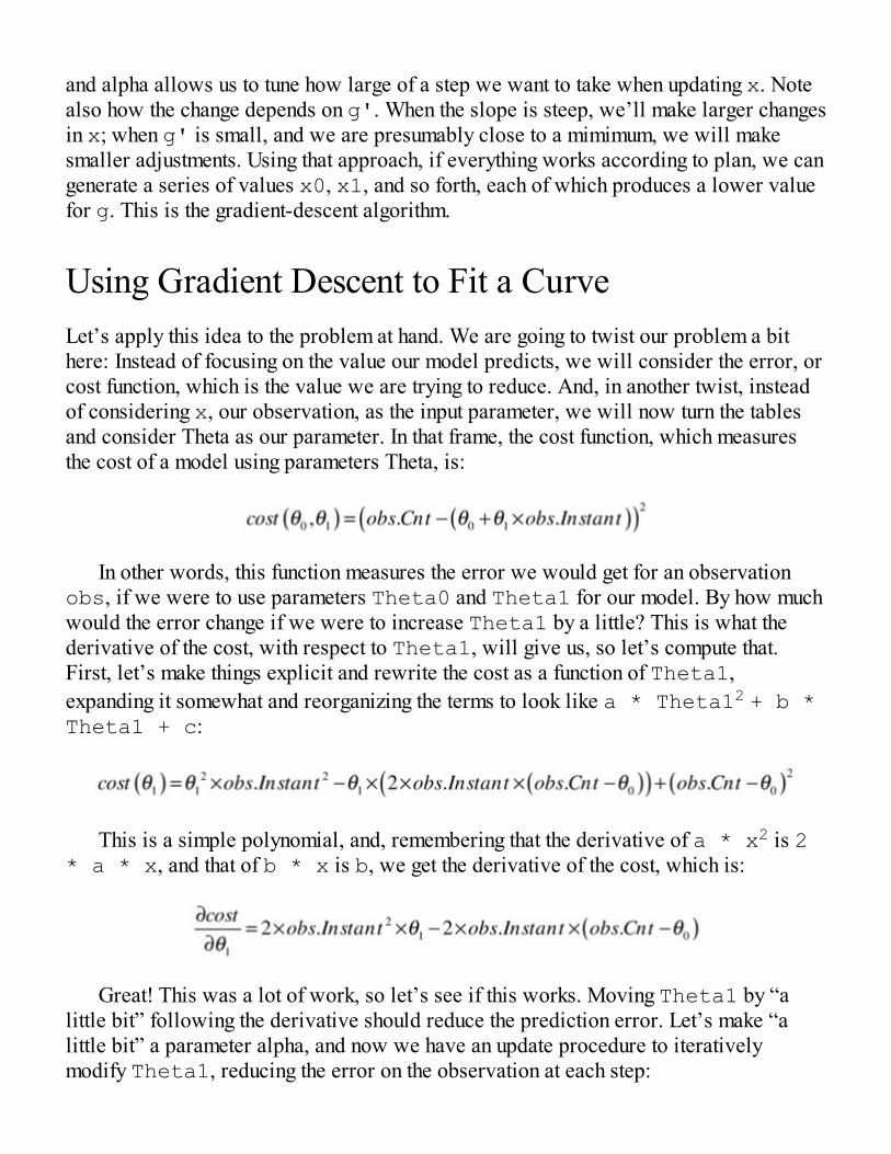
and alpha allows us to tune how large of a step we want to take when updating x. Notealso how the change depends on g'. When the slope is steep, we’ll make larger changesin x; when g' is small, and we are presumably close to a mimimum, we will makesmaller adjustments. Using that approach, if everything works according to plan, we cangenerate a series of values x0, x1, and so forth, each of which produces a lower valuefor g. This is the gradient-descent algorithm.

Using Gradient Descent to Fit a CurveLet’s apply this idea to the problem at hand. We are going to twist our problem a bithere: Instead of focusing on the value our model predicts, we will consider the error, orcost function, which is the value we are trying to reduce. And, in another twist, insteadof considering x, our observation, as the input parameter, we will now turn the tablesand consider Theta as our parameter. In that frame, the cost function, which measuresthe cost of a model using parameters Theta, is:

In other words, this function measures the error we would get for an observationobs, if we were to use parameters Theta0 and Theta1 for our model. By how muchwould the error change if we were to increase Theta1 by a little? This is what thederivative of the cost, with respect to Theta1, will give us, so let’s compute that.First, let’s make things explicit and rewrite the cost as a function of Theta1,expanding it somewhat and reorganizing the terms to look like a * Theta12 + b *Theta1 + c:

This is a simple polynomial, and, remembering that the derivative of a * x2 is 2* a * x, and that of b * x is b, we get the derivative of the cost, which is:

Great! This was a lot of work, so let’s see if this works. Moving Theta1 by “alittle bit” following the derivative should reduce the prediction error. Let’s make “alittle bit” a parameter alpha, and now we have an update procedure to iterativelymodify Theta1, reducing the error on the observation at each step:

Note that this formula has a relatively straightforward interpretation, helping usclarify what the algorithm does. The last term in the equation is exactly the error term.Assuming obs.inst is positive, if the forecasted value is lower than obs.cnt—theactual value we are trying to predict—the model is undershooting, and the algorithmwill increase the value of Theta1 by a bit, which will move us in the correctdirection. Conversely, if the opposite is true, the value of Theta1 will be reduced.Note also that the correction will be more important for larger values of obs.inst.

Finally, note also that while this approach will move Theta1 in the correctdirection, depending on the value of alpha we might end up overcompensating. As wewill see shortly, alpha is a parameter that needs to be manually tuned. If alpha is smallenough, the algorithm will progress nicely towards the optimal value of Theta1.However, smaller values also mean a slower correction, which could mean waiting fora long time for the procedure to produce a good value for Theta1.

A More General Model FormulationBefore applying this method to the problem at hand, and while the math is still fresh inour minds, let’s make two remarks that will allow us to make our algorithm moregeneral. Imagine for a minute that instead of trying to fit a simple line like we have been,we had N features X1, X2, ... XN, and were trying to fit a prediction model of the form

This is exactly the same type of model as the one we are dealing with, just withmore features. Our simple straight-line model simply happens to have N = 1. A firstconvenient trick is to introduce a “dummy” feature into our model, X0, and set X0 = 1for every single observation. The reason this is convenient is that it now allows us towrite the prediction model in a consistent fashion for all Thetas, with no specialtreatment for the constant term Theta0:

As a result, you could now rewrite the cost function, and for any values of Theta, itwill look like this:

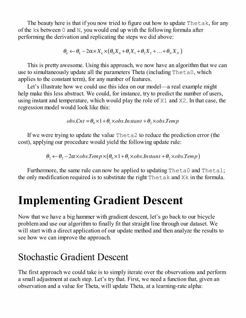
The beauty here is that if you now tried to figure out how to update Thetak, for anyof the ks between 0 and N, you would end up with the following formula afterperforming the derivation and replicating the steps we did above:

This is pretty awesome. Using this approach, we now have an algorithm that we canuse to simultaneously update all the parameters Theta (including Theta0, whichapplies to the constant term), for any number of features.

Let’s illustrate how we could use this idea on our model—a real example mighthelp make this less abstract. We could, for instance, try to predict the number of users,using instant and temperature, which would play the role of X1 and X2. In that case, theregression model would look like this:

If we were trying to update the value Theta2 to reduce the prediction error (thecost), applying our procedure would yield the following update rule:

Furthermore, the same rule can now be applied to updating Theta0 and Theta1;the only modification required is to substitute the right Thetak and Xk in the formula.

Implementing Gradient DescentNow that we have a big hammer with gradient descent, let’s go back to our bicycleproblem and use our algorithm to finally fit that straight line through our dataset. Wewill start with a direct application of our update method and then analyze the results tosee how we can improve the approach.

Stochastic Gradient DescentThe first approach we could take is to simply iterate over the observations and performa small adjustment at each step. Let’s try that. First, we need a function that, given anobservation and a value for Theta, will update Theta, at a learning-rate alpha:

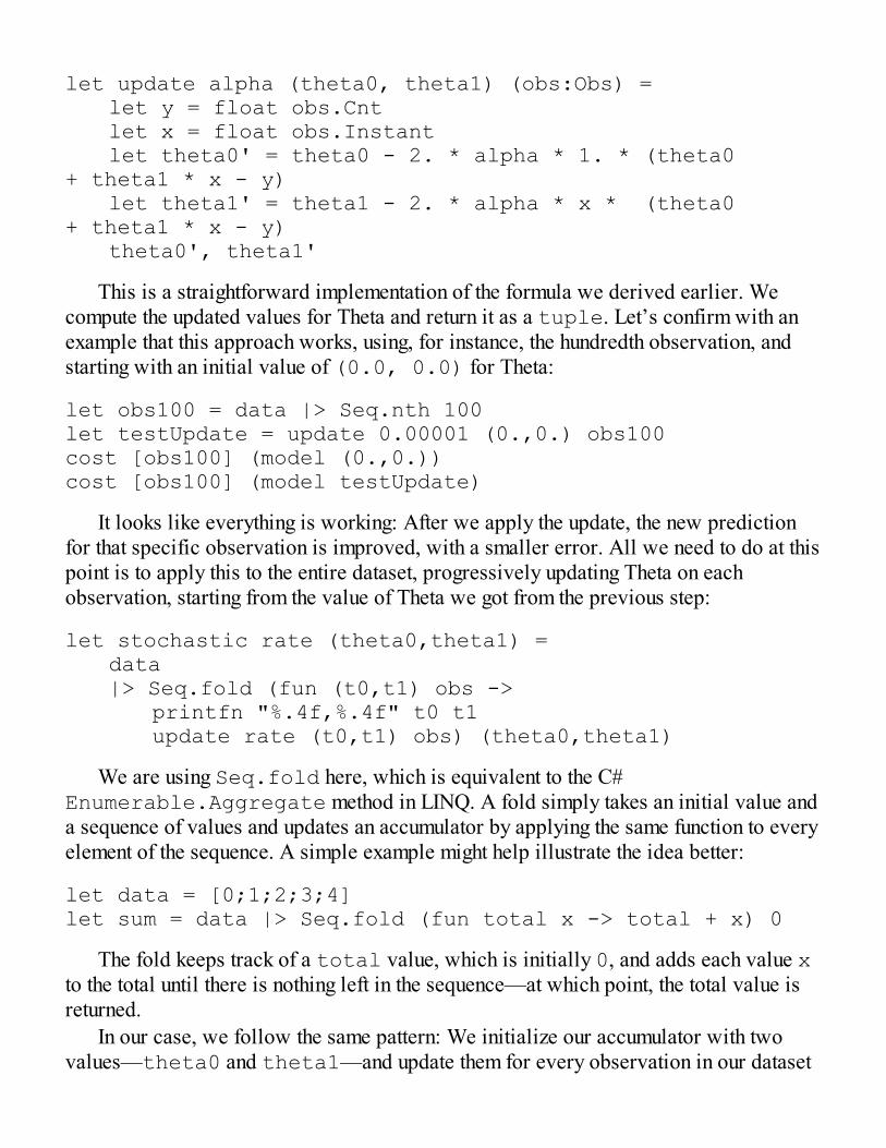
let update alpha (theta0, theta1) (obs:Obs) = let y = float obs.Cnt let x = float obs.Instant let theta0' = theta0 - 2. * alpha * 1. * (theta0 + theta1 * x - y) let theta1' = theta1 - 2. * alpha * x * (theta0 + theta1 * x - y) theta0', theta1'

This is a straightforward implementation of the formula we derived earlier. Wecompute the updated values for Theta and return it as a tuple. Let’s confirm with anexample that this approach works, using, for instance, the hundredth observation, andstarting with an initial value of (0.0, 0.0) for Theta:

let obs100 = data |> Seq.nth 100let testUpdate = update 0.00001 (0.,0.) obs100cost [obs100] (model (0.,0.))cost [obs100] (model testUpdate)

It looks like everything is working: After we apply the update, the new predictionfor that specific observation is improved, with a smaller error. All we need to do at thispoint is to apply this to the entire dataset, progressively updating Theta on eachobservation, starting from the value of Theta we got from the previous step:

let stochastic rate (theta0,theta1) = data |> Seq.fold (fun (t0,t1) obs -> printfn "%.4f,%.4f" t0 t1 update rate (t0,t1) obs) (theta0,theta1)

We are using Seq.fold here, which is equivalent to the C#Enumerable.Aggregate method in LINQ. A fold simply takes an initial value anda sequence of values and updates an accumulator by applying the same function to everyelement of the sequence. A simple example might help illustrate the idea better:

let data = [0;1;2;3;4]let sum = data |> Seq.fold (fun total x -> total + x) 0

The fold keeps track of a total value, which is initially 0, and adds each value xto the total until there is nothing left in the sequence—at which point, the total value isreturned.

In our case, we follow the same pattern: We initialize our accumulator with twovalues—theta0 and theta1—and update them for every observation in our dataset

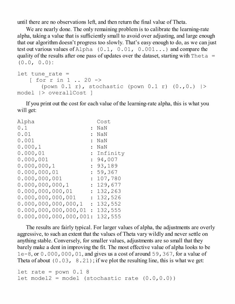
until there are no observations left, and then return the final value of Theta.We are nearly done. The only remaining problem is to calibrate the learning-rate

alpha, taking a value that is sufficiently small to avoid over adjusting, and large enoughthat our algorithm doesn’t progress too slowly. That’s easy enough to do, as we can justtest out various values of Alpha (0.1, 0.01, 0.001...) and compare thequality of the results after one pass of updates over the dataset, starting with Theta =(0.0, 0.0):

let tune_rate = [ for r in 1 .. 20 -> (pown 0.1 r), stochastic (pown 0.1 r) (0.,0.) |> model |> overallCost ]

If you print out the cost for each value of the learning-rate alpha, this is what youwill get:

Alpha Cost0.1 : NaN0.01 : NaN0.001 : NaN0.000,1 : NaN0.000,01 : Infinity0.000,001 : 94,0070.000,000,1 : 93,1890.000,000,01 : 59,3670.000,000,001 : 107,7800.000,000,000,1 : 129,6770.000,000,000,01 : 132,2630.000,000,000,001 : 132,5260.000,000,000,000,1 : 132,5520.000,000,000,000,01 : 132,5550.000,000,000,000,001: 132,555

The results are fairly typical. For larger values of alpha, the adjustments are overlyaggressive, to such an extent that the values of Theta vary wildly and never settle onanything stable. Conversely, for smaller values, adjustments are so small that theybarely make a dent in improving the fit. The most effective value of alpha looks to be1e-8, or 0.000,000,01, and gives us a cost of around 59,367, for a value ofTheta of about (0.03, 8.21); if we plot the resulting line, this is what we get:

let rate = pown 0.1 8let model2 = model (stochastic rate (0.0,0.0))

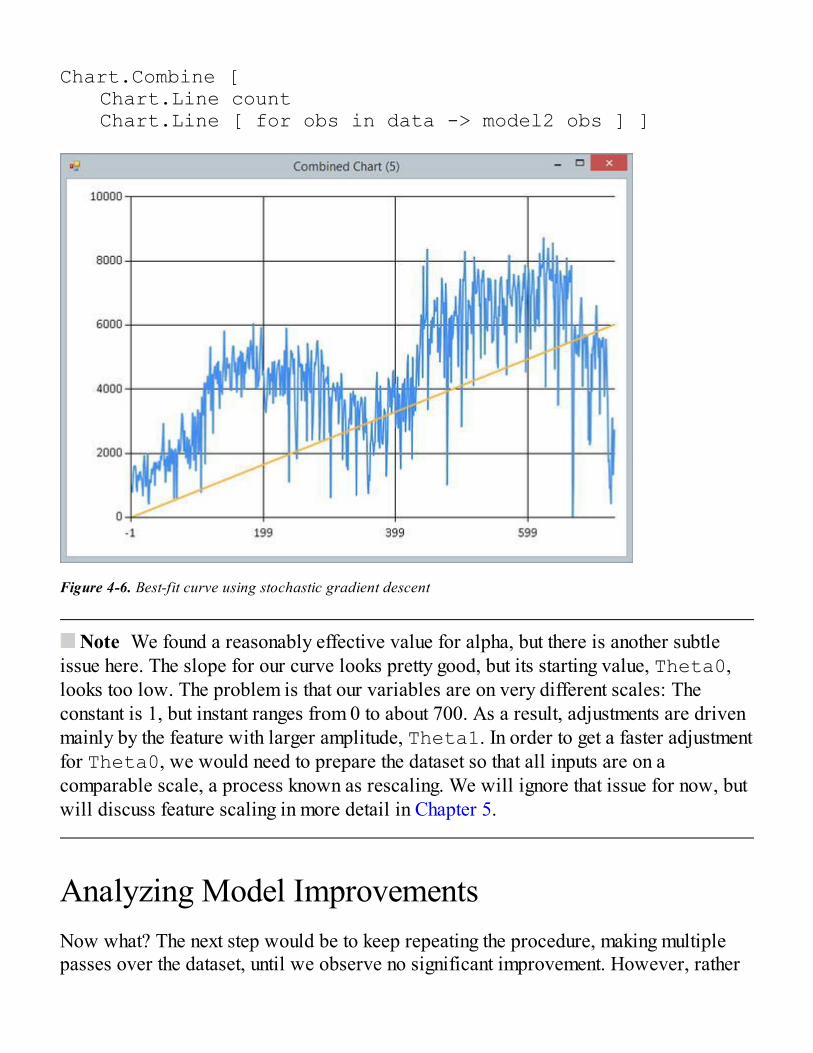
Chart.Combine [ Chart.Line count Chart.Line [ for obs in data -> model2 obs ] ]

Figure 4-6. Best-fit curve using stochastic gradient descent

Note We found a reasonably effective value for alpha, but there is another subtleissue here. The slope for our curve looks pretty good, but its starting value, Theta0,looks too low. The problem is that our variables are on very different scales: Theconstant is 1, but instant ranges from 0 to about 700. As a result, adjustments are drivenmainly by the feature with larger amplitude, Theta1. In order to get a faster adjustmentfor Theta0, we would need to prepare the dataset so that all inputs are on acomparable scale, a process known as rescaling. We will ignore that issue for now, butwill discuss feature scaling in more detail in Chapter 5.

Analyzing Model ImprovementsNow what? The next step would be to keep repeating the procedure, making multiplepasses over the dataset, until we observe no significant improvement. However, rather

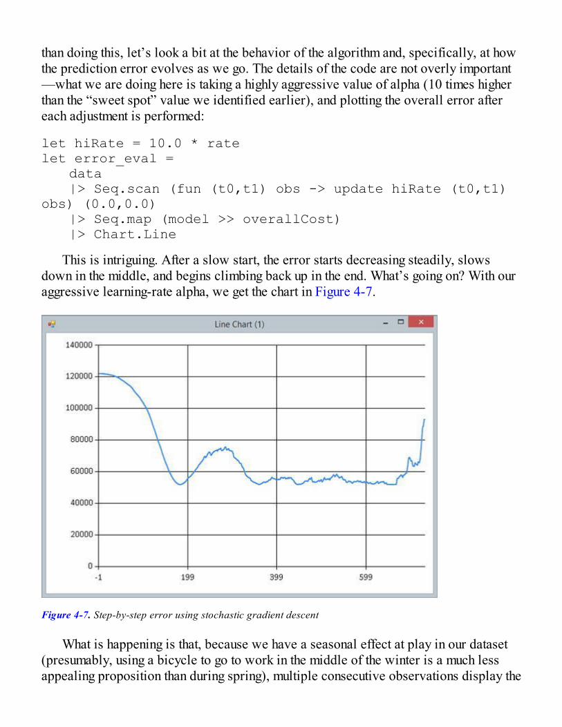
than doing this, let’s look a bit at the behavior of the algorithm and, specifically, at howthe prediction error evolves as we go. The details of the code are not overly important—what we are doing here is taking a highly aggressive value of alpha (10 times higherthan the “sweet spot” value we identified earlier), and plotting the overall error aftereach adjustment is performed:

let hiRate = 10.0 * ratelet error_eval = data |> Seq.scan (fun (t0,t1) obs -> update hiRate (t0,t1) obs) (0.0,0.0) |> Seq.map (model >> overallCost) |> Chart.Line

This is intriguing. After a slow start, the error starts decreasing steadily, slowsdown in the middle, and begins climbing back up in the end. What’s going on? With ouraggressive learning-rate alpha, we get the chart in Figure 4-7.

Figure 4-7. Step-by-step error using stochastic gradient descent

What is happening is that, because we have a seasonal effect at play in our dataset(presumably, using a bicycle to go to work in the middle of the winter is a much lessappealing proposition than during spring), multiple consecutive observations display the

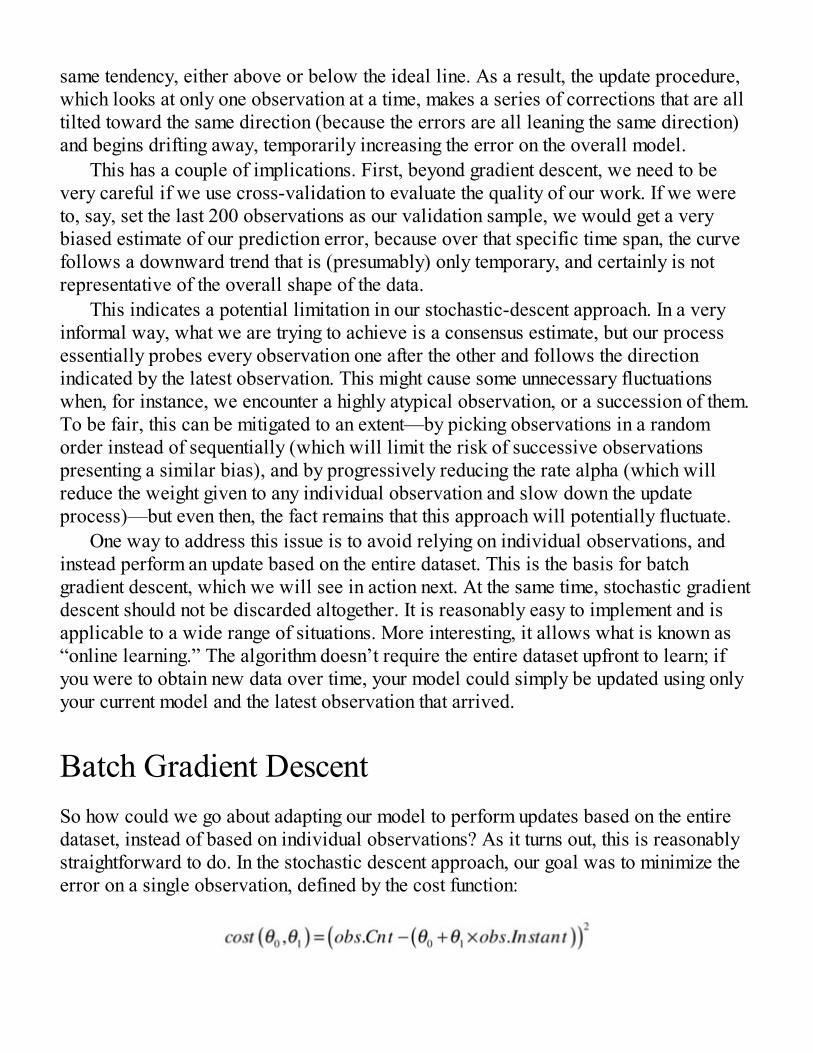
same tendency, either above or below the ideal line. As a result, the update procedure,which looks at only one observation at a time, makes a series of corrections that are alltilted toward the same direction (because the errors are all leaning the same direction)and begins drifting away, temporarily increasing the error on the overall model.

This has a couple of implications. First, beyond gradient descent, we need to bevery careful if we use cross-validation to evaluate the quality of our work. If we wereto, say, set the last 200 observations as our validation sample, we would get a verybiased estimate of our prediction error, because over that specific time span, the curvefollows a downward trend that is (presumably) only temporary, and certainly is notrepresentative of the overall shape of the data.

This indicates a potential limitation in our stochastic-descent approach. In a veryinformal way, what we are trying to achieve is a consensus estimate, but our processessentially probes every observation one after the other and follows the directionindicated by the latest observation. This might cause some unnecessary fluctuationswhen, for instance, we encounter a highly atypical observation, or a succession of them.To be fair, this can be mitigated to an extent—by picking observations in a randomorder instead of sequentially (which will limit the risk of successive observationspresenting a similar bias), and by progressively reducing the rate alpha (which willreduce the weight given to any individual observation and slow down the updateprocess)—but even then, the fact remains that this approach will potentially fluctuate.

One way to address this issue is to avoid relying on individual observations, andinstead perform an update based on the entire dataset. This is the basis for batchgradient descent, which we will see in action next. At the same time, stochastic gradientdescent should not be discarded altogether. It is reasonably easy to implement and isapplicable to a wide range of situations. More interesting, it allows what is known as“online learning.” The algorithm doesn’t require the entire dataset upfront to learn; ifyou were to obtain new data over time, your model could simply be updated using onlyyour current model and the latest observation that arrived.

Batch Gradient DescentSo how could we go about adapting our model to perform updates based on the entiredataset, instead of based on individual observations? As it turns out, this is reasonablystraightforward to do. In the stochastic descent approach, our goal was to minimize theerror on a single observation, defined by the cost function:

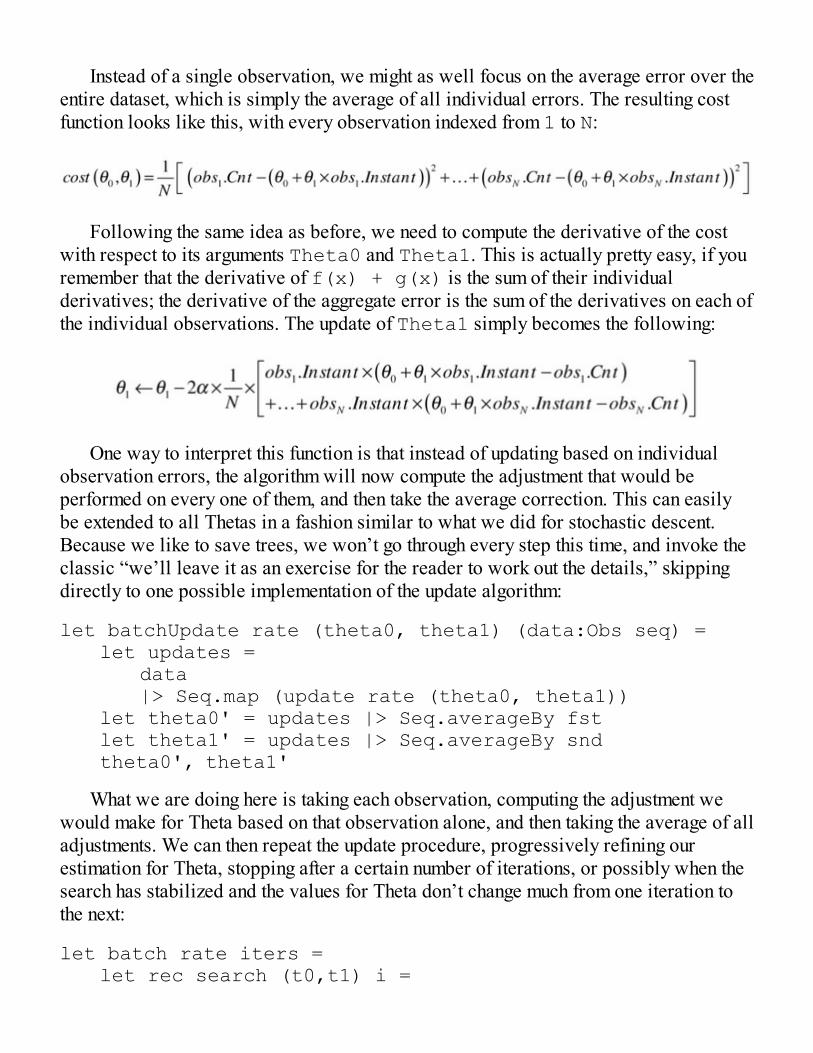
Instead of a single observation, we might as well focus on the average error over theentire dataset, which is simply the average of all individual errors. The resulting costfunction looks like this, with every observation indexed from 1 to N:

Following the same idea as before, we need to compute the derivative of the costwith respect to its arguments Theta0 and Theta1. This is actually pretty easy, if youremember that the derivative of f(x) + g(x) is the sum of their individualderivatives; the derivative of the aggregate error is the sum of the derivatives on each ofthe individual observations. The update of Theta1 simply becomes the following:

One way to interpret this function is that instead of updating based on individualobservation errors, the algorithm will now compute the adjustment that would beperformed on every one of them, and then take the average correction. This can easilybe extended to all Thetas in a fashion similar to what we did for stochastic descent.Because we like to save trees, we won’t go through every step this time, and invoke theclassic “we’ll leave it as an exercise for the reader to work out the details,” skippingdirectly to one possible implementation of the update algorithm:

let batchUpdate rate (theta0, theta1) (data:Obs seq) = let updates = data |> Seq.map (update rate (theta0, theta1)) let theta0' = updates |> Seq.averageBy fst let theta1' = updates |> Seq.averageBy snd theta0', theta1'

What we are doing here is taking each observation, computing the adjustment wewould make for Theta based on that observation alone, and then taking the average of alladjustments. We can then repeat the update procedure, progressively refining ourestimation for Theta, stopping after a certain number of iterations, or possibly when thesearch has stabilized and the values for Theta don’t change much from one iteration tothe next:

let batch rate iters = let rec search (t0,t1) i =

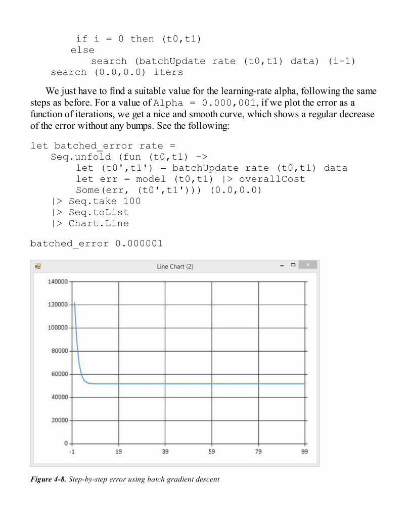
if i = 0 then (t0,t1) else search (batchUpdate rate (t0,t1) data) (i-1) search (0.0,0.0) iters

We just have to find a suitable value for the learning-rate alpha, following the samesteps as before. For a value of Alpha = 0.000,001, if we plot the error as afunction of iterations, we get a nice and smooth curve, which shows a regular decreaseof the error without any bumps. See the following:

let batched_error rate = Seq.unfold (fun (t0,t1) -> let (t0',t1') = batchUpdate rate (t0,t1) data let err = model (t0,t1) |> overallCost Some(err, (t0',t1'))) (0.0,0.0) |> Seq.take 100 |> Seq.toList |> Chart.Line

batched_error 0.000001

Figure 4-8. Step-by-step error using batch gradient descent

This is much better. On one hand, we are now using the entire dataset at once, whichin our case is not an issue, but could be problematic if it were much larger. On the otherhand, our procedure now converges steadily toward the optimal value without any bumpalong the way: The longer you wait, the better the estimate. The nice thing here is thatthe same approach is applicable to situations that extend beyond fitting a straight linethrough data. Essentially, as long as your cost function can be differentiated and isconvex, the same general approach can be taken.

However, there are still minor drawbacks to our approach. First, there is theannoyance of having to manually tune the learning-rate alpha—it would be nice if thatwasn’t required. Then, if you run the algorithm for a large number of iterations, you willnotice that the cost keeps decreasing, and the parameter Theta0 increasing, and it endsup stabilizing only after a very long time. This is due to the issue we mentioned earlier:Theta0 and Theta1 are on very different scales, and given the slow learning rate, ittakes a fairly large number of iterations for the algorithm to reach the “correct” value. Inthe next section, we will see how, for the specific problem at hand (linear regressionwithout any regularization penalty terms), we can use a bit of linear algebra to make ourlives simpler, and our algorithm much, much faster.

Linear Algebra to the RescueSo far, the direction we have followed has been to stick to our domain, representing thedataset as a collection of observations with named properties, applying transformationsusing maps and folds that were specific to the domain at hand. However, if you thinkabout it, once we start applying our update procedure, the specifics of the domain do notmatter anymore. It wouldn’t make a difference if we were trying to predict the price of acar as a function of its engine size and mileage (for instance), instead of bicycle usageas a function of wind speed. In the end, in both cases we’ll end up reducingobservations into rows of doubles and using them to try to predict another double.

In that frame, rather than focusing on the specifics of the domain, which do notmatter at that point, it would make sense to focus on the structure of the data, transformthe domain into a common structure, and apply the same general algorithm to solveproblems that share the same structure. This is where algebra comes in handy: Itprovides us with a well-established language with which to describe rows of numbers,and methods by which to perform various operations on them.

LINEAR ALGEBRA REFRESHER

The two base elements of linear algebra are vectors and matrices. A vector of size

n is simply a collection of n elements, indexed from 1 to n, such as:

A matrix is described by its dimension (or size), m x n, where m refers to itsrows and n to its columns. As an example, M is a 3 × 2 matrix:

As a loose analogy, we could describe vectors and matrices as the mathematicalequivalent of arrays and 2D arrays.

Vectors can be represented as row vectors or column vectors; this distinction isprimarily important when working with matrices. A matrix can be seen as acollection of either row vectors or column vectors, and most operations on vectorscan be seen as special cases of matrix operations.

The four core operations we need are addition, scalar multiplication, transposition,and multiplication. Adding matrices (or vectors) simply requires adding elementsby index, and it requires the two matrices to be of identical sizes:

Scalar multiplication describes multiplying a matrix (or vector) by a singlenumber, the scalar; each element is multiplied by the scalar:

Matrix transposition, denoted by a T, consists of reorienting a matrix so that rowsbecome columns, and vice-versa:

Finally, matrix multiplication is computed as the dot product (or inner product) ofevery row vector of the first matrix by every column vector of the second one. Thedot product of two vectors is a single number, computed as the sum of the productof each of their entries:

When applied to multiplying matrices, this is what we get:

Note that in order to be properly defined, this method requires the first matrix tohave the same number of columns as the number of rows in the second one.

Honey, I Shrunk the Formula!Let’s see how we could rephrase our problem in terms of algebra. Earlier on, wedefined our prediction model like this:

If we define Y as obs.cnt, and Theta and X as two vectors, with

...then our prediction model can be restated, in a much more compact form, as theproduct of the two vectors:

Similarly, the cost function we were trying to minimize in the batch gradient-descentalgorithm is the sum of the squared errors on each observation, averaged out over Nobservations:

Again, this can be restated much more compactly by denoting with Yn the outputvalue for the nth observation (that is, the nth element of the Y vector), and with Xn therow of data that describes the nth observation:

Or, even better, if we stack together all the observations, we get a matrix X, whereXn, the nth row of the matrix, contains the nth observation:

We could keep going like this and rewrite the entire batch gradient-descentalgorithm as a series of vector and matrix operations. Before getting into that, let’s firstmake sure that this actually works, and that when we use linear algebra, our results areindeed identical to the original formulation.

Linear Algebra with Math.NETWhile other options exist, the best starting point for “doing algebra” on .NET isMath.NET. Math.NET is an open-source library that is well maintained and has beenbattle tested quite a bit over its years of existence. Rather than cramming more code inthe same script we have been using so far, let’s start a new one and import Math.NETand its F# extensions via NuGet, together with the other packages we have been using sofar. First, let’s see how to perform basic algebra with Math.NET:

#I @"packages\"#r @"FSharp.Data.2.2.1\lib\net40\FSharp.Data.dll"#load @"FSharp.Charting.0.90.10\FSharp.Charting.fsx"#r @"MathNet.Numerics.Signed.3.6.0\lib\net40\MathNet.Numerics.dll"#r @"MathNet.Numerics.FSharp.Signed.3.6.0\lib\net40\MathNet.Numerics.FSharp.dll"

open FSharp.Chartingopen FSharp.Data

open MathNetopen MathNet.Numerics.LinearAlgebraopen MathNet.Numerics.LinearAlgebra.Double

Let’s create a vector A and a matrix B for illustrative purposes, and perform someoperations on them:

let A = vector [ 1.; 2.; 3. ]let B = matrix [ [ 1.; 2. ] [ 3.; 4. ] [ 5.; 6. ] ]

let C = A * Alet D = A * Blet E = A * B.Column(1)

Everything appears to be working as we would expect, and, as a nice bonus, thecode looks very similar to the mathematical formulation you would see if you opened amath book. Now, let’s rewrite our prediction and cost functions, “algebra-style”:

type Data = CsvProvider<"day.csv">let dataset = Data.Load("day.csv")let data = dataset.Rows

type Vec = Vector<float>type Mat = Matrix<float>

let cost (theta:Vec) (Y:Vec) (X:Mat) = let ps = Y - (theta * X.Transpose()) ps * ps |> sqrt

let predict (theta:Vec) (v:Vec) = theta * v

let X = matrix [ for obs in data -> [ 1.; float obs.Instant ]]let Y = vector [ for obs in data -> float obs.Cnt ]

Tip For convenience, we create two types, Vec and Mat, which correspond toVector<float> and Matrix<float>. This turns out to be very convenient forsimplifying our code: Math.NET supports algebra on numeric types other thanfloat/double, which can be very useful, but can also clutter the code and require someadditional type annotations to clarify what specific type is intended. Given that we aregoing to operate exclusively on floats, keeping everything generic doesn’t add anything,

and would create some noise, hence the simplification.

We can now compare the predictions and costs we obtained previously with theresults of our new formulation, using the same value for Theta:

let theta = vector [6000.; -4.5]

predict theta (X.Row(0))cost theta Y X

Everything matches. We are on safe ground, so let’s proceed and estimate Theta.

Normal FormWe could rewrite our batch gradient descent “algebra style.” However, we will take adifferent route here that highlights some of the benefits of using algebra. As it happens,the problem we are trying to solve (finding a value for Theta that minimizes the cost)has what math people call a closed-form solution; that is, an explicit, exact solution thatcan be computed directly from the inputs without requiring any numeric approximation.

Explaining how to derive the result would go a bit beyond the scope of this book,and wouldn’t add much value to understanding the machine-learning part, so I willsimply state the result “as is”; if you are curious about it, look in your favorite searchengine for “normal form regression.” With no justification whatsoever, the problem

has a solution Theta, which is

This is one case where having a linear algebra library available pays off big time.Matrix transposition and inversion is implemented for us, and our algorithm nowbecomes a one-liner. Better yet, we don’t have to go through the lengthy process oftuning a learning rate or running thousands of expensive iteration while hoping that weare getting close to the correct value—we get the correct solution in one shot. See thefollowing:

let estimate (Y:Vec) (X:Mat) =

(X.Transpose() * X).Inverse() * X.Transpose() * Y

Does this make our entire earlier work on gradient descent a waste of time? Mostcertainly not! Besides the pedagogical value of the exercise, which hopefully clarifiedthe general process, gradient descent is a more general algorithm that applies tosituations where, for instance, we decide to use a different, non-linear cost function,provided the appropriate modifications are done to the derivatives. By contrast, thenormal form is a solution to a very specific equation, and doesn’t generalize out of thebox. That being said, the class of problems it solves is pretty broad.

Pedal to the Metal with MKLSo far, the main advantage we highlighted for using an algebra-centric approach wasthat, for suitable problems, it enables a much more compact formulation. There isanother, completely different reason why algebra is such an important topic in machinelearning, and that is performance.

Were it used for machine learning alone, algebra would probably not be a big dealin software. Thankfully, there is another area where developers care about algebra in abig way, and that is the gaming industry. 3D graphics are all about moving polygonsaround, which is fundamentally an algebra problem. As a result, thanks to the relentlesspush for ever faster and more-detailed game universes, significant efforts have gone intomaking high-performance algebra work, including at the hardware level. The mostvisible example in that area is GPGPU (general-purpose computing on graphicsprocessing units), which, by using hardware that was originally designed with vectorgraphics in mind, can achieve huge speedups for certain types of computations.

Using GPGPUs is powerful, but also takes some work. However, Math.NET offersyou the option of leveraging something similar, with virtually no work involved. Thelibrary supports a MKL provider, a mechanism that essentially allows you to send yourcomputations to MKL, the Math Kernel Library, a set of highly-optimized mathlibraries that are built within Intel processors.

Using MKL with Math.NET is fairly straightforward. Once you add thecorresponding NuGet package to the project, two libraries will appear:MathNet.Numerics.MKL.dll and libiomp5md.dll. Right-click the MKL dll, and inProperties, set Copy to Output Directory to “Copy Always.”

Tip MKL comes in multiple flavors: 32 bits versus 64 bits, and Windows versusLinux. Make sure you select the package that is appropriate for your machine wheninstalling the NuGet package.

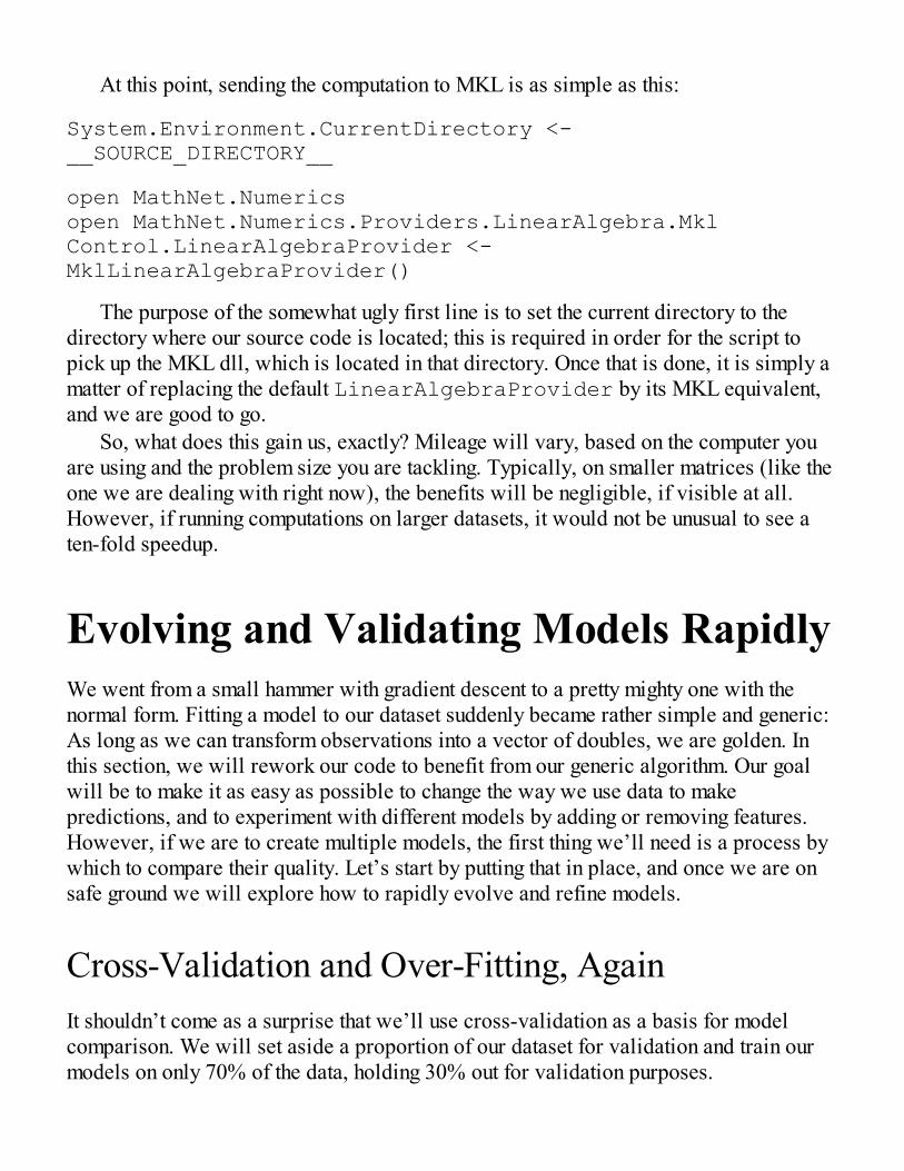
At this point, sending the computation to MKL is as simple as this:

System.Environment.CurrentDirectory <- __SOURCE_DIRECTORY__

open MathNet.Numericsopen MathNet.Numerics.Providers.LinearAlgebra.MklControl.LinearAlgebraProvider <- MklLinearAlgebraProvider()

The purpose of the somewhat ugly first line is to set the current directory to thedirectory where our source code is located; this is required in order for the script topick up the MKL dll, which is located in that directory. Once that is done, it is simply amatter of replacing the default LinearAlgebraProvider by its MKL equivalent,and we are good to go.

So, what does this gain us, exactly? Mileage will vary, based on the computer youare using and the problem size you are tackling. Typically, on smaller matrices (like theone we are dealing with right now), the benefits will be negligible, if visible at all.However, if running computations on larger datasets, it would not be unusual to see aten-fold speedup.

Evolving and Validating Models RapidlyWe went from a small hammer with gradient descent to a pretty mighty one with thenormal form. Fitting a model to our dataset suddenly became rather simple and generic:As long as we can transform observations into a vector of doubles, we are golden. Inthis section, we will rework our code to benefit from our generic algorithm. Our goalwill be to make it as easy as possible to change the way we use data to makepredictions, and to experiment with different models by adding or removing features.However, if we are to create multiple models, the first thing we’ll need is a process bywhich to compare their quality. Let’s start by putting that in place, and once we are onsafe ground we will explore how to rapidly evolve and refine models.

Cross-Validation and Over-Fitting, AgainIt shouldn’t come as a surprise that we’ll use cross-validation as a basis for modelcomparison. We will set aside a proportion of our dataset for validation and train ourmodels on only 70% of the data, holding 30% out for validation purposes.

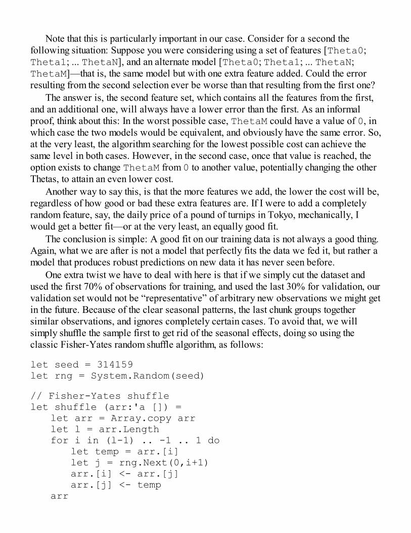
Note that this is particularly important in our case. Consider for a second thefollowing situation: Suppose you were considering using a set of features [Theta0;Theta1; ... ThetaN], and an alternate model [Theta0; Theta1; ... ThetaN;ThetaM]—that is, the same model but with one extra feature added. Could the errorresulting from the second selection ever be worse than that resulting from the first one?

The answer is, the second feature set, which contains all the features from the first,and an additional one, will always have a lower error than the first. As an informalproof, think about this: In the worst possible case, ThetaM could have a value of 0, inwhich case the two models would be equivalent, and obviously have the same error. So,at the very least, the algorithm searching for the lowest possible cost can achieve thesame level in both cases. However, in the second case, once that value is reached, theoption exists to change ThetaM from 0 to another value, potentially changing the otherThetas, to attain an even lower cost.

Another way to say this, is that the more features we add, the lower the cost will be,regardless of how good or bad these extra features are. If I were to add a completelyrandom feature, say, the daily price of a pound of turnips in Tokyo, mechanically, Iwould get a better fit—or at the very least, an equally good fit.

The conclusion is simple: A good fit on our training data is not always a good thing.Again, what we are after is not a model that perfectly fits the data we fed it, but rather amodel that produces robust predictions on new data it has never seen before.

One extra twist we have to deal with here is that if we simply cut the dataset andused the first 70% of observations for training, and used the last 30% for validation, ourvalidation set would not be “representative” of arbitrary new observations we might getin the future. Because of the clear seasonal patterns, the last chunk groups togethersimilar observations, and ignores completely certain cases. To avoid that, we willsimply shuffle the sample first to get rid of the seasonal effects, doing so using theclassic Fisher-Yates random shuffle algorithm, as follows:

let seed = 314159let rng = System.Random(seed)

// Fisher-Yates shufflelet shuffle (arr:'a []) = let arr = Array.copy arr let l = arr.Length for i in (l-1) .. -1 .. 1 do let temp = arr.[i] let j = rng.Next(0,i+1) arr.[i] <- arr.[j] arr.[j] <- temp arr

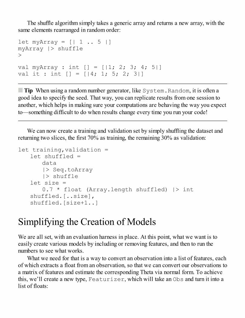
The shuffle algorithm simply takes a generic array and returns a new array, with thesame elements rearranged in random order:

let myArray = [| 1 .. 5 |]myArray |> shuffle>

val myArray : int [] = [|1; 2; 3; 4; 5|]val it : int [] = [|4; 1; 5; 2; 3|]

Tip When using a random number generator, like System.Random, it is often agood idea to specify the seed. That way, you can replicate results from one session toanother, which helps in making sure your computations are behaving the way you expectto—something difficult to do when results change every time you run your code!

We can now create a training and validation set by simply shuffling the dataset andreturning two slices, the first 70% as training, the remaining 30% as validation:

let training,validation = let shuffled = data |> Seq.toArray |> shuffle let size = 0.7 * float (Array.length shuffled) |> int shuffled.[..size], shuffled.[size+1..]

Simplifying the Creation of ModelsWe are all set, with an evaluation harness in place. At this point, what we want is toeasily create various models by including or removing features, and then to run thenumbers to see what works.

What we need for that is a way to convert an observation into a list of features, eachof which extracts a float from an observation, so that we can convert our observations toa matrix of features and estimate the corresponding Theta via normal form. To achievethis, we’ll create a new type, Featurizer, which will take an Obs and turn it into alist of floats:

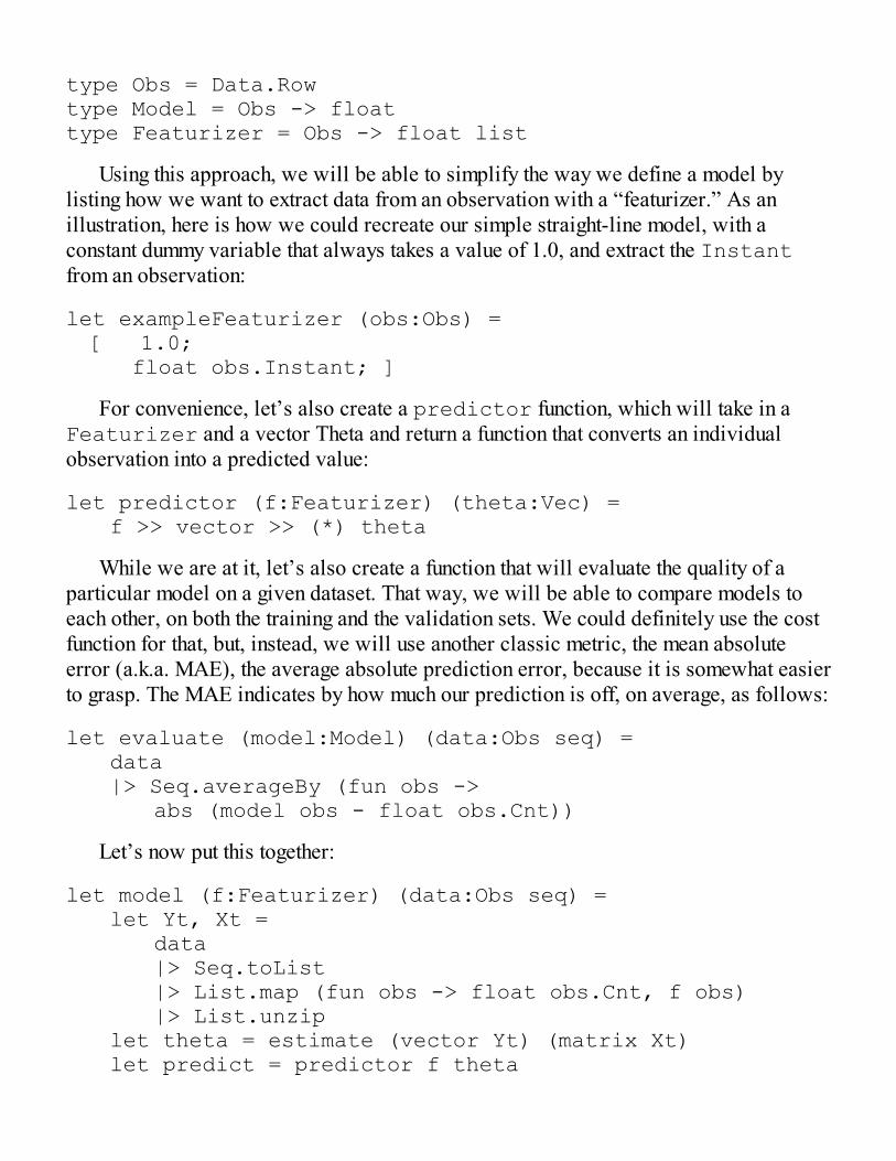
type Obs = Data.Rowtype Model = Obs -> floattype Featurizer = Obs -> float list

Using this approach, we will be able to simplify the way we define a model bylisting how we want to extract data from an observation with a “featurizer.” As anillustration, here is how we could recreate our simple straight-line model, with aconstant dummy variable that always takes a value of 1.0, and extract the Instantfrom an observation:

let exampleFeaturizer (obs:Obs) = [ 1.0; float obs.Instant; ]

For convenience, let’s also create a predictor function, which will take in aFeaturizer and a vector Theta and return a function that converts an individualobservation into a predicted value:

let predictor (f:Featurizer) (theta:Vec) = f >> vector >> (*) theta

While we are at it, let’s also create a function that will evaluate the quality of aparticular model on a given dataset. That way, we will be able to compare models toeach other, on both the training and the validation sets. We could definitely use the costfunction for that, but, instead, we will use another classic metric, the mean absoluteerror (a.k.a. MAE), the average absolute prediction error, because it is somewhat easierto grasp. The MAE indicates by how much our prediction is off, on average, as follows:

let evaluate (model:Model) (data:Obs seq) = data |> Seq.averageBy (fun obs -> abs (model obs - float obs.Cnt))

Let’s now put this together:

let model (f:Featurizer) (data:Obs seq) = let Yt, Xt = data |> Seq.toList |> List.map (fun obs -> float obs.Cnt, f obs) |> List.unzip let theta = estimate (vector Yt) (matrix Xt) let predict = predictor f theta

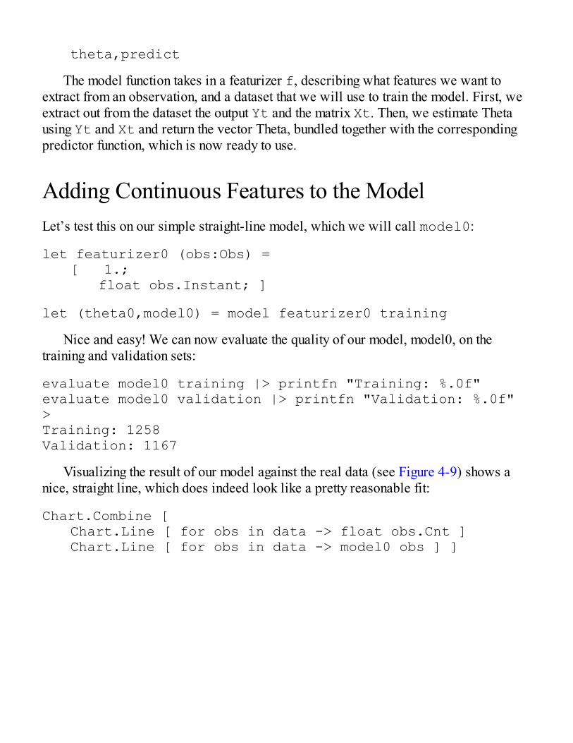
theta,predict

The model function takes in a featurizer f, describing what features we want toextract from an observation, and a dataset that we will use to train the model. First, weextract out from the dataset the output Yt and the matrix Xt. Then, we estimate Thetausing Yt and Xt and return the vector Theta, bundled together with the correspondingpredictor function, which is now ready to use.

Adding Continuous Features to the ModelLet’s test this on our simple straight-line model, which we will call model0:

let featurizer0 (obs:Obs) = [ 1.; float obs.Instant; ]

let (theta0,model0) = model featurizer0 training

Nice and easy! We can now evaluate the quality of our model, model0, on thetraining and validation sets:

evaluate model0 training |> printfn "Training: %.0f"evaluate model0 validation |> printfn "Validation: %.0f">Training: 1258Validation: 1167

Visualizing the result of our model against the real data (see Figure 4-9) shows anice, straight line, which does indeed look like a pretty reasonable fit:

Chart.Combine [ Chart.Line [ for obs in data -> float obs.Cnt ] Chart.Line [ for obs in data -> model0 obs ] ]

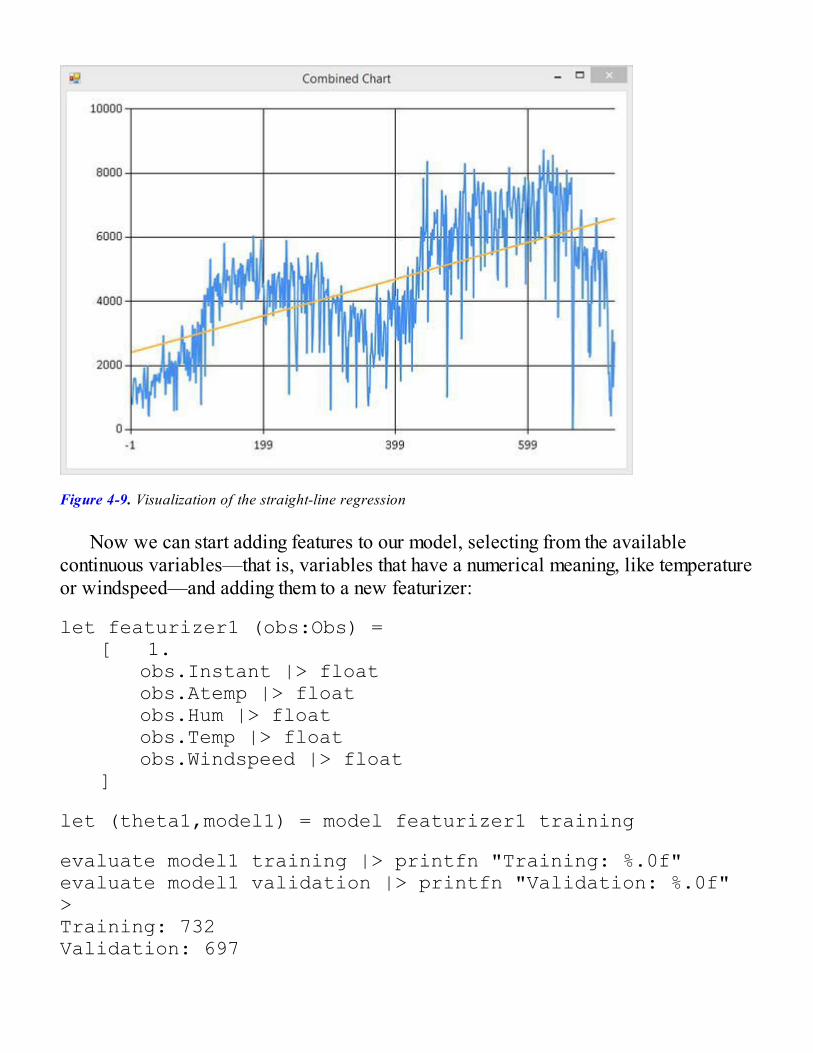
Figure 4-9. Visualization of the straight-line regression

Now we can start adding features to our model, selecting from the availablecontinuous variables—that is, variables that have a numerical meaning, like temperatureor windspeed—and adding them to a new featurizer:

let featurizer1 (obs:Obs) = [ 1. obs.Instant |> float obs.Atemp |> float obs.Hum |> float obs.Temp |> float obs.Windspeed |> float ]

let (theta1,model1) = model featurizer1 training

evaluate model1 training |> printfn "Training: %.0f"evaluate model1 validation |> printfn "Validation: %.0f">Training: 732Validation: 697

Obviously, we are doing something right: The MAE dropped significantly, both onthe training set (which is expected) and on the validation set (which is what matters).Before, we were off by about 1,200 units on average, and we are now down to around750. Not perfect, but a clear improvement! This is readily visible if we plot the newpredicted curve—the new predicted curve is beginning to stick to the target much moreclosely (see Figure 4-10).

Figure 4-10. Including more-continuous features

Let’s take a slightly different look at the data and plot the actual value against thepredicted one:

Chart.Point [ for obs in data -> float obs.Cnt, model1 obs]

Figure 4-11 confirms that our model is starting to look like the real thing. Thescatterplot, while not perfect, follows roughly a 45-degree straight line, with somenoise sprinkled on top.

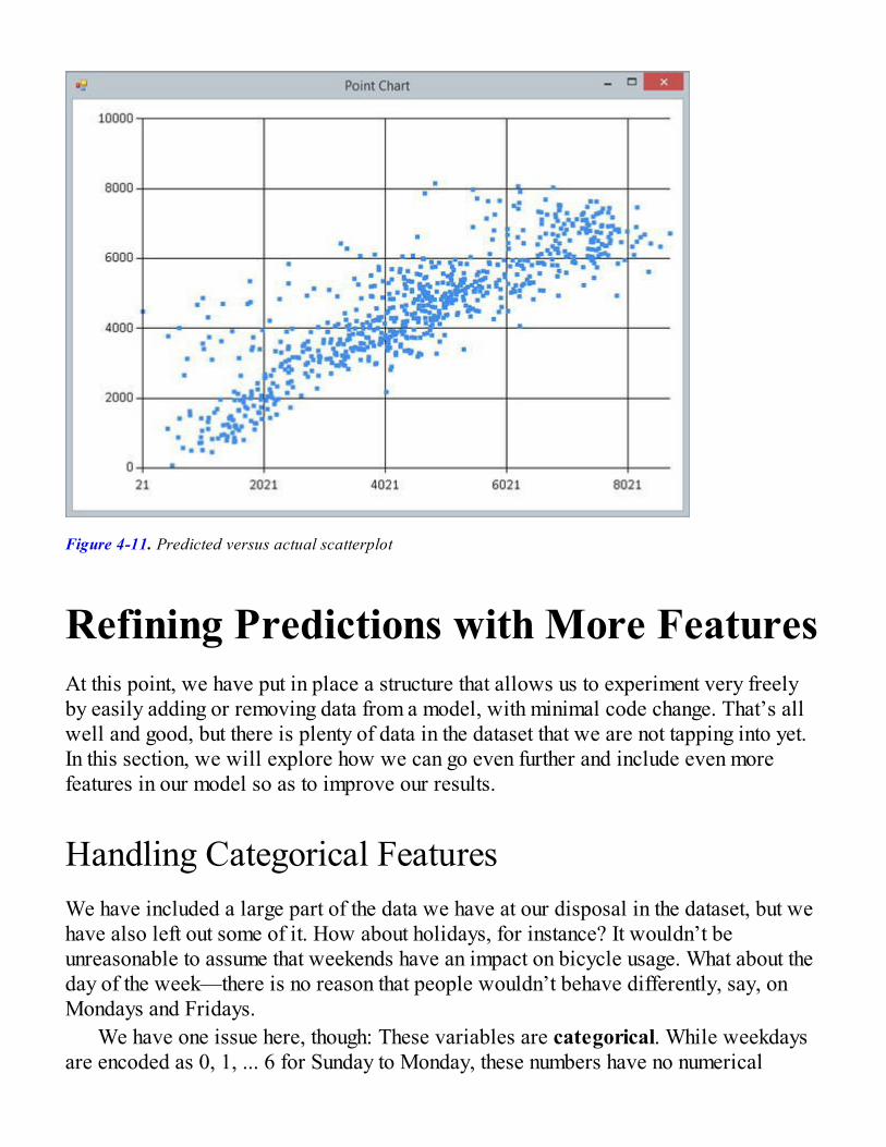
Figure 4-11. Predicted versus actual scatterplot

Refining Predictions with More FeaturesAt this point, we have put in place a structure that allows us to experiment very freelyby easily adding or removing data from a model, with minimal code change. That’s allwell and good, but there is plenty of data in the dataset that we are not tapping into yet.In this section, we will explore how we can go even further and include even morefeatures in our model so as to improve our results.

Handling Categorical FeaturesWe have included a large part of the data we have at our disposal in the dataset, but wehave also left out some of it. How about holidays, for instance? It wouldn’t beunreasonable to assume that weekends have an impact on bicycle usage. What about theday of the week—there is no reason that people wouldn’t behave differently, say, onMondays and Fridays.

We have one issue here, though: These variables are categorical. While weekdaysare encoded as 0, 1, ... 6 for Sunday to Monday, these numbers have no numerical

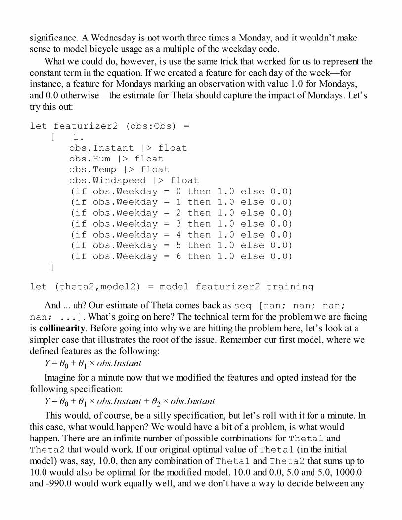
significance. A Wednesday is not worth three times a Monday, and it wouldn’t makesense to model bicycle usage as a multiple of the weekday code.

What we could do, however, is use the same trick that worked for us to represent theconstant term in the equation. If we created a feature for each day of the week—forinstance, a feature for Mondays marking an observation with value 1.0 for Mondays,and 0.0 otherwise—the estimate for Theta should capture the impact of Mondays. Let’stry this out:

let featurizer2 (obs:Obs) = [ 1. obs.Instant |> float obs.Hum |> float obs.Temp |> float obs.Windspeed |> float (if obs.Weekday = 0 then 1.0 else 0.0) (if obs.Weekday = 1 then 1.0 else 0.0) (if obs.Weekday = 2 then 1.0 else 0.0) (if obs.Weekday = 3 then 1.0 else 0.0) (if obs.Weekday = 4 then 1.0 else 0.0) (if obs.Weekday = 5 then 1.0 else 0.0) (if obs.Weekday = 6 then 1.0 else 0.0) ]

let (theta2,model2) = model featurizer2 training

And ... uh? Our estimate of Theta comes back as seq [nan; nan; nan;nan; ...]. What’s going on here? The technical term for the problem we are facingis collinearity. Before going into why we are hitting the problem here, let’s look at asimpler case that illustrates the root of the issue. Remember our first model, where wedefined features as the following:

Y = θ0 + θ1 × obs.InstantImagine for a minute now that we modified the features and opted instead for the

following specification:Y = θ0 + θ1 × obs.Instant + θ2 × obs.InstantThis would, of course, be a silly specification, but let’s roll with it for a minute. In

this case, what would happen? We would have a bit of a problem, is what wouldhappen. There are an infinite number of possible combinations for Theta1 andTheta2 that would work. If our original optimal value of Theta1 (in the initialmodel) was, say, 10.0, then any combination of Theta1 and Theta2 that sums up to10.0 would also be optimal for the modified model. 10.0 and 0.0, 5.0 and 5.0, 1000.0and -990.0 would work equally well, and we don’t have a way to decide between any

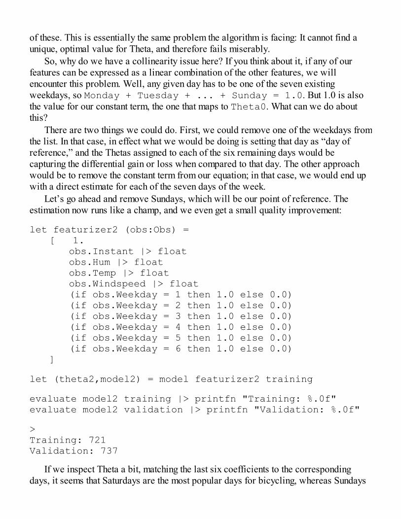
of these. This is essentially the same problem the algorithm is facing: It cannot find aunique, optimal value for Theta, and therefore fails miserably.

So, why do we have a collinearity issue here? If you think about it, if any of ourfeatures can be expressed as a linear combination of the other features, we willencounter this problem. Well, any given day has to be one of the seven existingweekdays, so Monday + Tuesday + ... + Sunday = 1.0. But 1.0 is alsothe value for our constant term, the one that maps to Theta0. What can we do aboutthis?

There are two things we could do. First, we could remove one of the weekdays fromthe list. In that case, in effect what we would be doing is setting that day as “day ofreference,” and the Thetas assigned to each of the six remaining days would becapturing the differential gain or loss when compared to that day. The other approachwould be to remove the constant term from our equation; in that case, we would end upwith a direct estimate for each of the seven days of the week.

Let’s go ahead and remove Sundays, which will be our point of reference. Theestimation now runs like a champ, and we even get a small quality improvement:

let featurizer2 (obs:Obs) = [ 1. obs.Instant |> float obs.Hum |> float obs.Temp |> float obs.Windspeed |> float (if obs.Weekday = 1 then 1.0 else 0.0) (if obs.Weekday = 2 then 1.0 else 0.0) (if obs.Weekday = 3 then 1.0 else 0.0) (if obs.Weekday = 4 then 1.0 else 0.0) (if obs.Weekday = 5 then 1.0 else 0.0) (if obs.Weekday = 6 then 1.0 else 0.0) ]

let (theta2,model2) = model featurizer2 training

evaluate model2 training |> printfn "Training: %.0f"evaluate model2 validation |> printfn "Validation: %.0f"

>Training: 721Validation: 737

If we inspect Theta a bit, matching the last six coefficients to the correspondingdays, it seems that Saturdays are the most popular days for bicycling, whereas Sundays

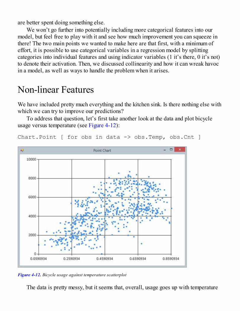
are better spent doing something else.We won’t go further into potentially including more categorical features into our

model, but feel free to play with it and see how much improvement you can squeeze inthere! The two main points we wanted to make here are that first, with a minimum ofeffort, it is possible to use categorical variables in a regression model by splittingcategories into individual features and using indicator variables (1 it’s there, 0 it’s not)to denote their activation. Then, we discussed collinearity and how it can wreak havocin a model, as well as ways to handle the problem when it arises.

Non-linear FeaturesWe have included pretty much everything and the kitchen sink. Is there nothing else withwhich we can try to improve our predictions?

To address that question, let’s first take another look at the data and plot bicycleusage versus temperature (see Figure 4-12):

Chart.Point [ for obs in data -> obs.Temp, obs.Cnt ]

Figure 4-12. Bicycle usage against temperature scatterplot

The data is pretty messy, but it seems that, overall, usage goes up with temperature

only to a certain point, and starts to decrease afterward. This is not unreasonable:Biking loses some of its appeal when it’s freezing cold or scorching hot. Unfortunately,our current model is not well suited to capturing that. All the effects are represented aslinear functions; that is, they are of the form Theta x Feature value. If Theta ispositive, all things being left equal, higher values of the feature will always result inhigher predicted values; conversely, if Theta is negative, higher values of the featurewill always produce lower predicted values.

This is not going to cut it for what we want to capture with temperature; we expectusage to go down both when temperature is getting very low or getting very high. So,what can we do?

If a linear relationship is not sufficient, we could use something else, for instance,higher-order polynomials. The simplest thing that could possibly work would be to adda square term to the mix. Instead of modelling the effect of temperature as

we could go for

Let’s try out the idea, ignoring all other features for a moment, to demonstrate whatcurve comes out of this equation:

let squareTempFeaturizer (obs:Obs) = [ 1. obs.Temp |> float obs.Temp * obs.Temp |> float ]

let (_,squareTempModel) = model squareTempFeaturizer data

Chart.Combine [ Chart.Point [ for obs in data -> obs.Temp, obs.Cnt ] Chart.Point [ for obs in data -> obs.Temp, squareTempModel obs ] ]

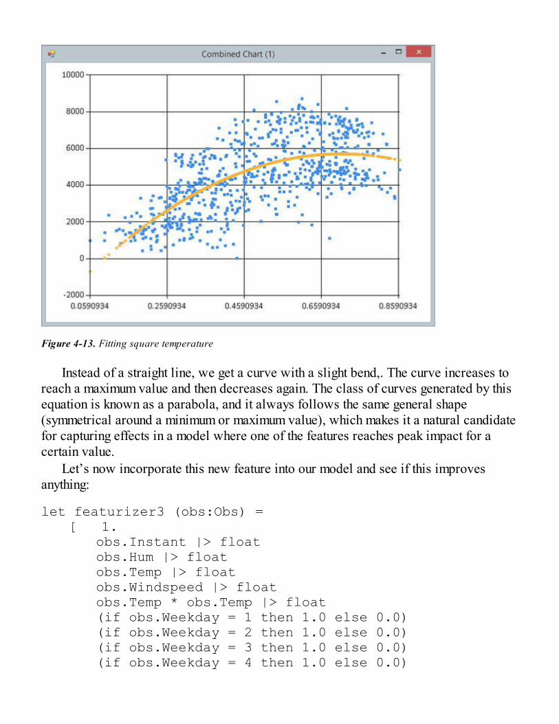
Figure 4-13. Fitting square temperature

Instead of a straight line, we get a curve with a slight bend,. The curve increases toreach a maximum value and then decreases again. The class of curves generated by thisequation is known as a parabola, and it always follows the same general shape(symmetrical around a minimum or maximum value), which makes it a natural candidatefor capturing effects in a model where one of the features reaches peak impact for acertain value.

Let’s now incorporate this new feature into our model and see if this improvesanything:

let featurizer3 (obs:Obs) = [ 1. obs.Instant |> float obs.Hum |> float obs.Temp |> float obs.Windspeed |> float obs.Temp * obs.Temp |> float (if obs.Weekday = 1 then 1.0 else 0.0) (if obs.Weekday = 2 then 1.0 else 0.0) (if obs.Weekday = 3 then 1.0 else 0.0) (if obs.Weekday = 4 then 1.0 else 0.0)

(if obs.Weekday = 5 then 1.0 else 0.0) (if obs.Weekday = 6 then 1.0 else 0.0) ]

let (theta3,model3) = model featurizer3 training

evaluate model3 training |> printfn "Training: %.0f"evaluate model3 validation |> printfn "Validation: %.0f" >Training: 668Validation: 645

Nice! Our error dropped from 750 to under 670, which is a very seriousimprovement. Even better, we now have a general direction in which to try to refine themodel further. We could introduce new features—for instance, the squares of othervariables, or the product of two variables—to capture other potential non-linear effectsin our model. We could even go further and expand to higher-level polynomials, likecubes, or other functional forms—say, exponentials or logarithms.

A small drawback of this approach is that the interpretation of results becomestrickier. In a linear model, understanding what each Theta coefficient means is fairlystraightforward. It can be read as a multiplier: Increase the value of a feature by 1.0,and the output will increase (or decrease) by Theta.

This creates a bit of a conundrum. First, this introduces a practical issue. As weexpand the number of potential features to consider, manually inspecting what featuresshould be left out or included will become quite a hassle. For instance, if we had Nvariables available, a linear model would contain N + 1 features (each variable and aconstant term). Including the interaction between each of the features and their squaresadds N x (N + 1) / 2, and a potentially staggering number of combinations toconsider. Manually inspecting each combination remains possible for a dataset with amoderate number of variables, but won’t work as the dataset width increases.

RegularizationThe larger problem is, of course, the point we discussed before. If we could just throwevery feature and the kitchen sink at the model, we would be fine. But, as we sawbefore, doing so blindly would mechanically improve the quality on the training setwithout necessarily resulting in a robust prediction model. This problem is known asover-fitting: The search algorithm uses all the features it can use to fit the dataset, andin the process ends up doing too good of a job at that task, potentially capturing artifactsin the training dataset that will not generalize beyond it.

So, how could we avoid this issue? One method commonly used is known asregularization. The idea is the following: One of the symptoms of over-fitting is that, inits attempt to fit the training set with features, the algorithm will begin to produce“wild” values for some of the Theta coefficients, whereas in a “reasonable” model,coefficients would be expected to remain within a certain range, enforcing that changesin the inputs won’t cause crazy fluctuations.

We won’t go through the whole example of regularization, and will instead simplysketch out how you would go about it in general.

If the goal is to prevent each parameter Theta from fluctuating too wildly, onepossibility is to introduce a penalty so that high individual values will be more costlythan smaller ones. For instance, we could introduce the following penalty to our costfunction:

Why would this be a good candidate? As we discussed before in the context of theoriginal cost function, because the square function increases faster as values are furtheraway from zero, larger values for each individual Theta will be penalized more heavily.As a result, by default, this penalty will tend to favor more-balanced values over highlydifferentiated ones. For instance, a Theta of [1.0; 1.0] would have a cost of 2.0,whereas [0.0; 2.0] would incur a cost of 4.0.

Putting this all together, we could now replace our original cost function with thefollowing:

This formulation has a fairly straightforward interpretation. The cost of a modelcombines two elements: how large the error is on the fit and how small the parametersare. In other words, there is now a cost to improving the fit by increasing a parameterTheta, and the algorithm will “prefer” fit improvements that use more-balancedparameters.

Before looking into how we could go about using this in an actual algorithm, thereare a couple of important technical considerations to take into account.

The first one is that in order for this to work, each of the features needs to be on acomparable scale. This matters because the penalty term we introduced assumes thatsimilar changes in the coefficients Theta can be compared with each other. One way ofstating what we are trying to achieve with this penalty is “when you can improve fitquality by increasing the coefficient of features, prefer increasing the feature that has the

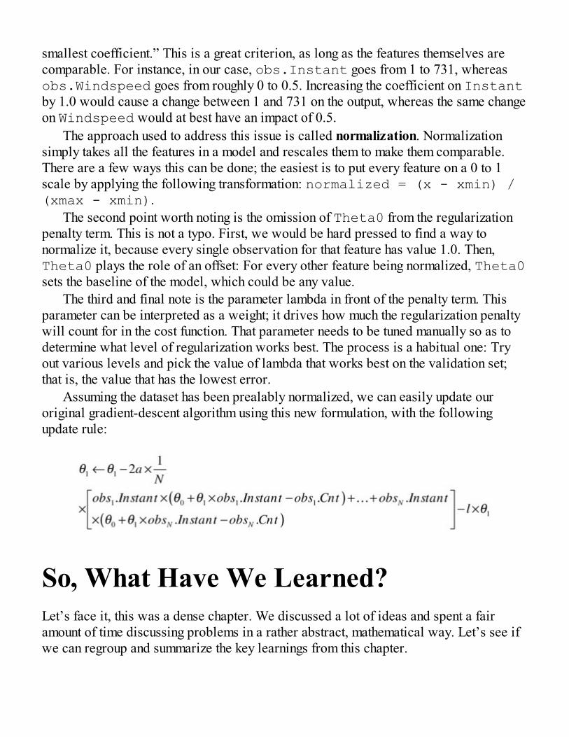
smallest coefficient.” This is a great criterion, as long as the features themselves arecomparable. For instance, in our case, obs.Instant goes from 1 to 731, whereasobs.Windspeed goes from roughly 0 to 0.5. Increasing the coefficient on Instantby 1.0 would cause a change between 1 and 731 on the output, whereas the same changeon Windspeed would at best have an impact of 0.5.

The approach used to address this issue is called normalization. Normalizationsimply takes all the features in a model and rescales them to make them comparable.There are a few ways this can be done; the easiest is to put every feature on a 0 to 1scale by applying the following transformation: normalized = (x - xmin) /(xmax - xmin).

The second point worth noting is the omission of Theta0 from the regularizationpenalty term. This is not a typo. First, we would be hard pressed to find a way tonormalize it, because every single observation for that feature has value 1.0. Then,Theta0 plays the role of an offset: For every other feature being normalized, Theta0sets the baseline of the model, which could be any value.

The third and final note is the parameter lambda in front of the penalty term. Thisparameter can be interpreted as a weight; it drives how much the regularization penaltywill count for in the cost function. That parameter needs to be tuned manually so as todetermine what level of regularization works best. The process is a habitual one: Tryout various levels and pick the value of lambda that works best on the validation set;that is, the value that has the lowest error.

Assuming the dataset has been prealably normalized, we can easily update ouroriginal gradient-descent algorithm using this new formulation, with the followingupdate rule:

So, What Have We Learned?Let’s face it, this was a dense chapter. We discussed a lot of ideas and spent a fairamount of time discussing problems in a rather abstract, mathematical way. Let’s see ifwe can regroup and summarize the key learnings from this chapter.

Minimizing Cost with Gradient DescentThe most important technique we discussed in this chapter applies to multiple areas inmachine learning, and not simply to regression. We presented the gradient-descentalgorithm, a general approach for identifying parameters that minimize the value of afunction, by iteratively adjusting the parameters following the gradient—the direction ofsteepest descent from the current state.

Gradient descent might appear a bit intimidating at first, thanks to the heavy servingof calculus that comes with it, but once the initial hurdle is passed, it is a rather simplealgorithm. More interesting, it is applicable to a broad range of situations; essentially, ifthere is a minimum value and the function is differentiable (we do need a derivative!)and not too pathological, you are in good shape. As it turns out, that makes it a great go-to tool for most machine-learning problems: If you are trying to find a model that bestfits a dataset, you are minimizing some form of distance or cost function, and gradientdescent will likely help you find it.

We also saw two variants of the algorithm, stochastic and batch gradient descent,each having their own advantages and limitations. Stochastic gradient descent updatesparameters one observation at a time. It doesn’t require operating on the entire dataset atonce, which makes it convenient for online learning. If your dataset is expanding overtime, and you are receiving new observations as time goes by, you can simply updateyour estimates using just the latest data points that arrived, and keep learning gradually.The downside, as we saw in our example, is that it’s comparatively slow andpotentially less stable: While the algorithm keeps going the right direction overall, eachindividual step is not guaranteed to produce an improvement. By contrast, batch gradientdescent operates on the entire dataset at once, producing an improved model at eachstep. The downside is that each step is computationally more intensive; also, using theentire dataset might be impractical, in particular if the dataset is large.

Predicting a Number with RegressionThe main goal we were after in this chapter was to predict the number of users for abike-sharing service on a particular day using whatever data we have available for thatday. This is known as a regression model. Unlike classification models, where theobjective is to predict what category an observation belongs to, here we are trying topredict a numeric value by finding a function that combines the features and fits the dataas closely as possible.

Starting from the simplest possible model, fitting a straight line through the data, weprogressively built up a more-complex model by including more features, illustrating a

few simple techniques along the way. In particular, we demonstrated how one can gobeyond continuous features and include categorical features in a model by breaking theminto multiple features, each indicating with a 1 or a 0 which of the states is active. Wealso saw how including non-linear terms, such as squares or higher-degree polynomials,can be used to model more-complex relationships between inputs and outputs thatcannot be properly captured by a linear model.

Adding more-complex features to a model is a double-edged sword, and thepotential for better predictions comes at a price. First, it creates an explosion in thenumber of features, and managing which ones to include or not can become a problem inand of itself. Then, it introduces a deeper issue: Adding any feature will mechanicallyimprove how well the model fits the training set, regardless of whether it has anything todo with the problem at hand. That issue is known as over-fitting: More features give thealgorithm more “freedom” to use them in creative, contorted ways, and a better fitdoesn’t necessarily translate into better predictions.

We discussed technical solutions to mitigate that issue, using cross-validation andregularization. However, as a final note, it’s perhaps useful to consider that there is aninherent tension at play here. A model can be useful for two distinct reasons: tounderstand a phenomenon, or to make predictions. Adding more data will usually helpmake better predictions, but also introduces complexity. Conversely, simpler modelsmay be less accurate, but help to understand how variables work together, and canvalidate whether things even make sense. Before building a model, ask yourself whetheryou would prefer an extremely accurate but opaque, black-box model, or a less-preciseone, but one that you can explain to a colleague. This might help guide your decisionsalong the way!

USEFUL LINKS

FSharp.Charting is a stable library, convenient for creating basiccharts while exploring data from FSI:http://fslab.org/FSharp.Charting/

Math.NET is an open-source library covering a broad range ofmathematical and numeric analysis tools. In particular it containsessential linear algebra algorithms:http://www.mathdotnet.com/

If you need higher performance from your algorithm, even if itrequires a more-complex implementation, quantalea offers a veryinteresting .NET-to-GPGPU library, which is particularly F#friendly: http://www.quantalea.net/

DiffSharp, while still evolving at the time of writing, is a promisingauto-differentiation library that can simplify gradient computationconsiderably: http://gbaydin.github.io/DiffSharp/

CHAPTER 5

You Are Not a Unique Snowflake

Detecting Patterns with Clustering andPrinciple Components AnalysisSometimes, your day of machine learning begins with a very specific problem to solve.Can you figure out if an incoming email is spam? How accurately can you predict sales?You have been given your marching orders: You start with a question, look for whatdata is available, and get to work building the best model you can to answer thatquestion.

Oftentimes, though, life is not quite that clear cut, and your day begins with a muchfuzzier problem. All you have is data, and no clear question just yet. Perhaps someonecame to you and simply asked, “Can you tell me something interesting about my data?”Perhaps you want to run some analyses on a dataset, but would like first to understandthe hand you have been dealt. Perhaps that dataset is large, with many features, making ithard to grasp if there are obvious relationships between features. Manual dataexploration is a painstaking and tedious process—it would be nice if we could offloadsome of the work to a machine and let it figure out if patterns exist in our data.

This is the domain of unsupervised learning. In supervised learning methods (suchas classification or regression), we begin with a question and labeled data—that is,examples with an answer to the question—and we use that to learn a model that fits thedata. By contrast, in unsupervised learning all we have is data, and we want thecomputer to help us find some structure in it. Hopefully that structure will be“interesting” in a human sense, and can be used to organize the individual elements in ameaningful way.

In this chapter, we will do the following:

Introduce two classic data-analysis techniques, k-means clustering

and principal component analysis, which both aim to automaticallyextract information from a dataset and to provide a simpler andmore usable representation. We will apply these techniques tohistorical data from the StackOverflow website and see if thepatterns that emerge are interesting.

Sketch out how the same general idea—detecting patterns in data—can be used to make recommendations to users based on their pastbehavior and how similar it is to patterns we observed among otherusers.

Note Some of the more complex charts from this chapter have been included in thesource code package, to allow for a larger format viewing if necessary.

Detecting Patterns in DataIf you think about it for a second, you will realize this is not an easy task. How do youdefine “something interesting” about the data? There is no clear metric for interesting,so what are we asking the computer to do for us here, exactly?

There are many ways data can be “interesting.” If we go by opposites, data that isnot interesting is data where nothing stands out. In that sense, Figure 5-1 displaysuninteresting data.

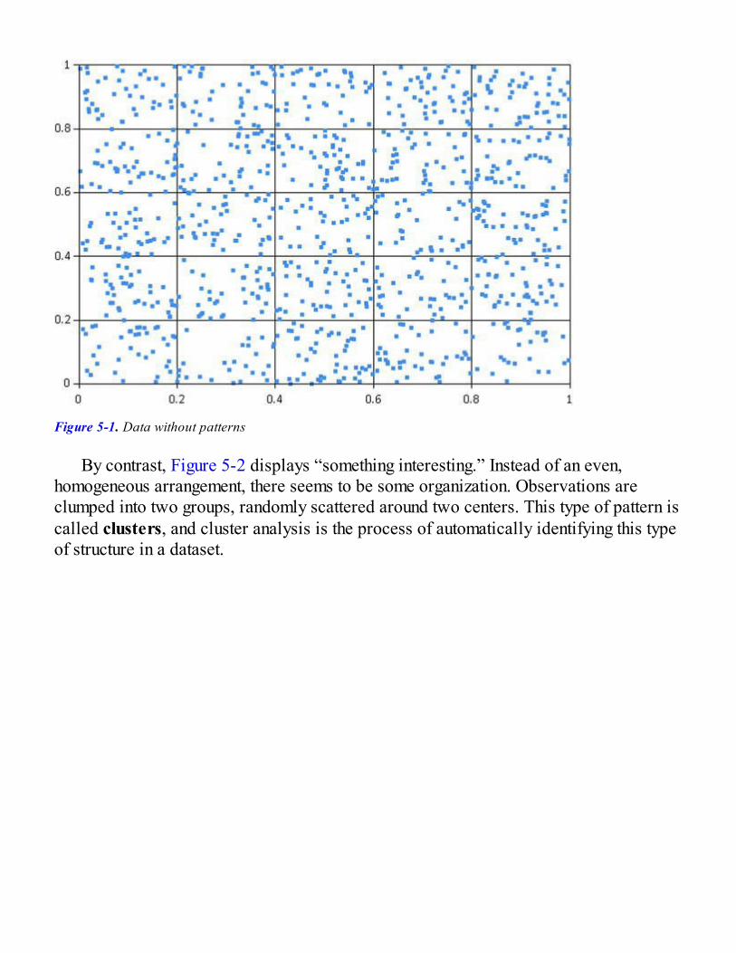
Figure 5-1. Data without patterns

By contrast, Figure 5-2 displays “something interesting.” Instead of an even,homogeneous arrangement, there seems to be some organization. Observations areclumped into two groups, randomly scattered around two centers. This type of pattern iscalled clusters, and cluster analysis is the process of automatically identifying this typeof structure in a dataset.

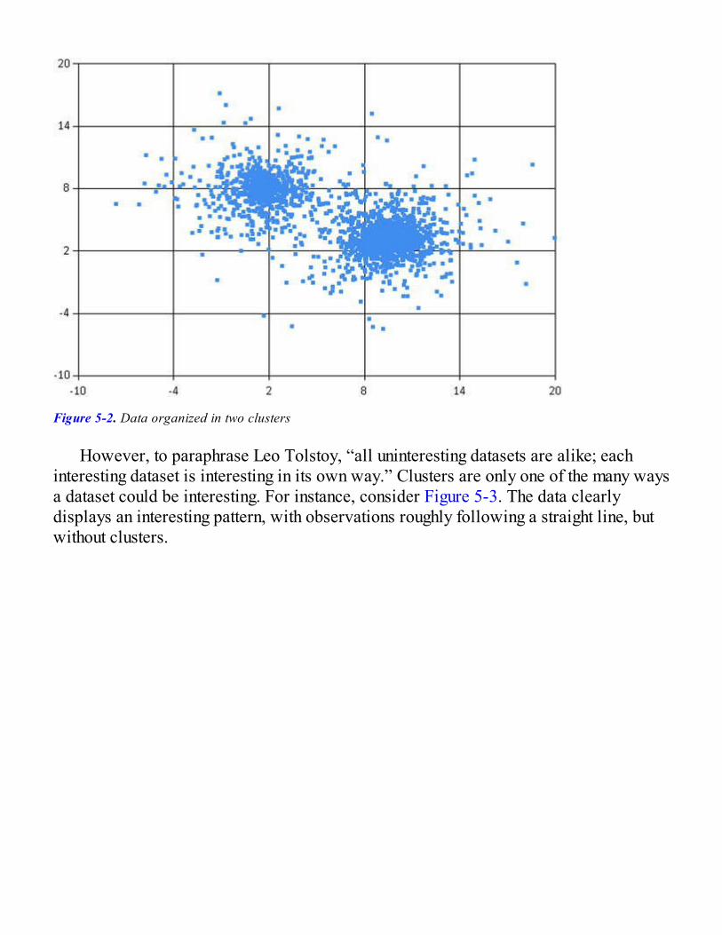
Figure 5-2. Data organized in two clusters

However, to paraphrase Leo Tolstoy, “all uninteresting datasets are alike; eachinteresting dataset is interesting in its own way.” Clusters are only one of the many waysa dataset could be interesting. For instance, consider Figure 5-3. The data clearlydisplays an interesting pattern, with observations roughly following a straight line, butwithout clusters.

Figure 5-3. Linear patterns

Clusters and linear structures are two ways a dataset can be interesting, but there arevirtually infinitely many ways data could exhibit patterns; for instance, consider Figure5-4, where data appears to be organized in rings. It’s somewhat clustered (we candistinguish three groups) and is somewhat similar to Figure 5-3 (data follows lines)—but is also pretty different.

Figure 5-4. Complex pattern

Structure can come in many forms, and, as a result, there isn’t one method that willwork in every case. Each dataset is unique, and data mining is a bit of a dark art.Figuring out what works often simply takes trying different algorithms, as well asmanipulating the data and transforming it into more appropriate features.

We humans are very good at detecting patterns. You didn’t even have to think tofigure out that there were patterns in some of the figures I just presented. In that frame,charts are your friend: Producing a scatterplot plotting one feature against another is avery cheap and effective way to eyeball structure in data.

At the same time, scatterplots will only bring you so far. Reviewing the interactionsbetween every single variable pair in a dataset becomes quite painful quite fast.Furthermore, and perhaps more important, patterns might exist in the data that will behard to pick up by just watching two variables at a time. So, while you should take thetime to look at the data when you can, you also need a systematic, mechanical approachto just sift through the dataset and find potential “interesting facts.”

Why do we care about finding “interesting patterns” in the first place? For all theexamples we presented above, we can describe the dataset in a single sentence: “Wehave two groups,” “Data follows a straight line,” “Data is organized around threerings.” In other words, we can provide a much more condensed description of the entiredataset. This is very useful, in at least two ways.

First, we now have a much better representation of the data. Instead of a random

collection of numbers, the dataset can be described in a meaningful manner, and canpotentially provide a vocabulary around it. As an example, if each of the data pointsfrom our clustered chart in Figure 5-2 represented customers, we could now startdescribing two types of customer profiles.

Second, just like we can describe each of these situations in English in a concisemanner, we can also provide a concise mathematical representation. All of thesedatasets are similar in that they follow a simple mathematical structure, with a bit ofstatistical noise on top.

Our Challenge: Understanding Topicson StackOverflowIn this chapter, we will apply some classic unsupervised learning techniques to see ifwe can mine some information out of StackOverflow usage data. It is an interestingdataset in that its domain should be familiar to most developers. As a result, we will beable to try out algorithms and modifications and judge, in a non-scientific way, whetherthe approach is producing sensible results or not.

Specifically, we will look into whether we can identify patterns in the tags used inStackOverflow questions. Every question on StackOverflow is tagged with up to fivewords describing what topic it covers. Our goal will be to see if, when we look at manyusers and questions over time, and what tags individuals were most active in, we cansee some structure and common combinations emerge.

For that purpose, I created a dataset by using the approach we discussed in Chapter3—gathering data from the StackExchange API using the JSON type provider. Thedataset, userprofiles-toptags.txt, can be downloaded from here:http://1drv.ms/1ARuLg9. I identified the 30 most common tags onStackOverflow at the time, and for each tag I retrieved the most active users, groupingtogether the users with the most answers and those with the most questions (topanswerers and top askers, all-time and current month). This gave me a list of about1,600 distinct StackOverflow users.

For each individual user, I then retrieved the top 100 tags they were active in overthe year 2015, with the corresponding level of activity, and retained only the datapertaining to the 30 main tags. Finally, I rearranged data in the final dataset, with 30columns (one for each tag), 1,600 rows (one for each user), and, for each row andcolumn, the number of times that user had been active for that tag in 2015. Note thatbecause I retrieved only the first 100 tags for a user, the information for each tag is notcomplete; if a particular user was active for, say, XML, but this was only his 101st most

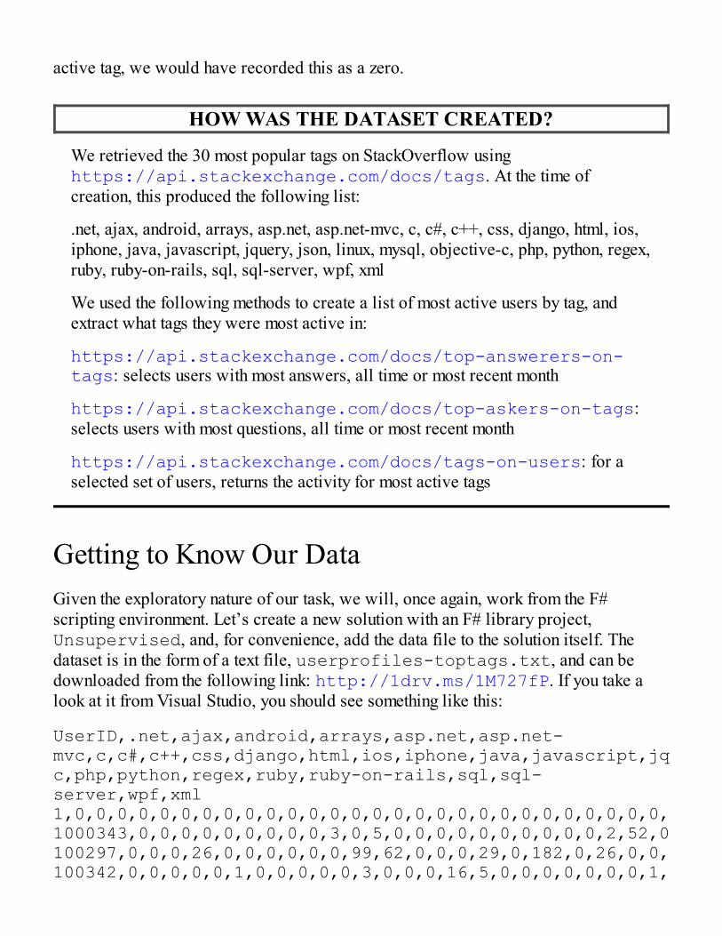
active tag, we would have recorded this as a zero.

HOW WAS THE DATASET CREATED?

We retrieved the 30 most popular tags on StackOverflow usinghttps://api.stackexchange.com/docs/tags. At the time ofcreation, this produced the following list:

.net, ajax, android, arrays, asp.net, asp.net-mvc, c, c#, c++, css, django, html, ios,iphone, java, javascript, jquery, json, linux, mysql, objective-c, php, python, regex,ruby, ruby-on-rails, sql, sql-server, wpf, xml

We used the following methods to create a list of most active users by tag, andextract what tags they were most active in:

https://api.stackexchange.com/docs/top-answerers-on-tags: selects users with most answers, all time or most recent month

https://api.stackexchange.com/docs/top-askers-on-tags:selects users with most questions, all time or most recent month

https://api.stackexchange.com/docs/tags-on-users: for aselected set of users, returns the activity for most active tags

Getting to Know Our DataGiven the exploratory nature of our task, we will, once again, work from the F#scripting environment. Let’s create a new solution with an F# library project,Unsupervised, and, for convenience, add the data file to the solution itself. Thedataset is in the form of a text file, userprofiles-toptags.txt, and can bedownloaded from the following link: http://1drv.ms/1M727fP. If you take alook at it from Visual Studio, you should see something like this:

UserID,.net,ajax,android,arrays,asp.net,asp.net-mvc,c,c#,c++,css,django,html,ios,iphone,java,javascript,jquery,json,linux,mysql,objective-c,php,python,regex,ruby,ruby-on-rails,sql,sql-server,wpf,xml1,0,0,0,0,0,0,0,0,0,0,0,0,0,0,0,0,0,0,0,0,0,0,0,0,0,0,0,0,0,01000343,0,0,0,0,0,0,0,0,0,3,0,5,0,0,0,0,0,0,0,0,0,0,2,52,0,0,0,0,0,0100297,0,0,0,26,0,0,0,0,0,0,99,62,0,0,0,29,0,182,0,26,0,0,4478,172,0,0,32,0,0,27100342,0,0,0,0,0,1,0,0,0,0,0,3,0,0,0,16,5,0,0,0,0,0,0,0,1,7,0,0,0,0

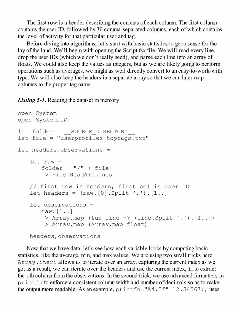
The first row is a header describing the contents of each column. The first columncontains the user ID, followed by 30 comma-separated columns, each of which containsthe level of activity for that particular user and tag.

Before diving into algorithms, let’s start with basic statistics to get a sense for thelay of the land. We’ll begin with opening the Script.fsx file. We will read every line,drop the user IDs (which we don’t really need), and parse each line into an array offloats. We could also keep the values as integers, but as we are likely going to performoperations such as averages, we might as well directly convert to an easy-to-work-withtype. We will also keep the headers in a separate array so that we can later mapcolumns to the proper tag name.

Listing 5-1. Reading the dataset in memory

open Systemopen System.IO

let folder = __SOURCE_DIRECTORY__let file = "userprofiles-toptags.txt"

let headers,observations =

let raw = folder + "/" + file |> File.ReadAllLines

// first row is headers, first col is user ID let headers = (raw.[0].Split ',').[1..]

let observations = raw.[1..] |> Array.map (fun line -> (line.Split ',').[1..]) |> Array.map (Array.map float)

headers,observations

Now that we have data, let’s see how each variable looks by computing basicstatistics, like the average, min, and max values. We are using two small tricks here.Array.iteri allows us to iterate over an array, capturing the current index as wego; as a result, we can iterate over the headers and use the current index, i, to extractthe ith column from the observations. In the second trick, we use advanced formatters inprintfn to enforce a consistent column width and number of decimals so as to makethe output more readable. As an example, printfn "%4.2f" 12.34567;; uses

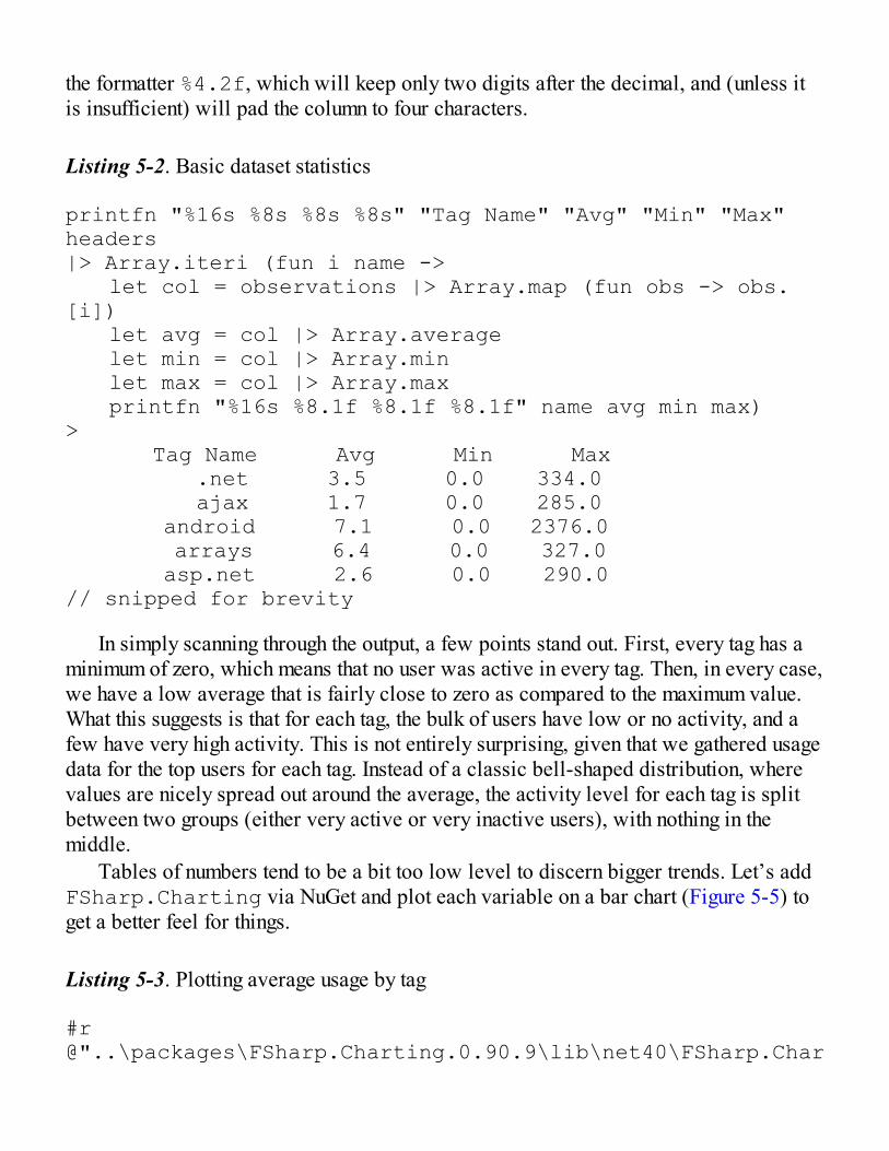
the formatter %4.2f, which will keep only two digits after the decimal, and (unless itis insufficient) will pad the column to four characters.

Listing 5-2. Basic dataset statistics

printfn "%16s %8s %8s %8s" "Tag Name" "Avg" "Min" "Max"headers|> Array.iteri (fun i name -> let col = observations |> Array.map (fun obs -> obs.[i]) let avg = col |> Array.average let min = col |> Array.min let max = col |> Array.max printfn "%16s %8.1f %8.1f %8.1f" name avg min max)> Tag Name Avg Min Max .net 3.5 0.0 334.0 ajax 1.7 0.0 285.0 android 7.1 0.0 2376.0 arrays 6.4 0.0 327.0 asp.net 2.6 0.0 290.0// snipped for brevity

In simply scanning through the output, a few points stand out. First, every tag has aminimum of zero, which means that no user was active in every tag. Then, in every case,we have a low average that is fairly close to zero as compared to the maximum value.What this suggests is that for each tag, the bulk of users have low or no activity, and afew have very high activity. This is not entirely surprising, given that we gathered usagedata for the top users for each tag. Instead of a classic bell-shaped distribution, wherevalues are nicely spread out around the average, the activity level for each tag is splitbetween two groups (either very active or very inactive users), with nothing in themiddle.

Tables of numbers tend to be a bit too low level to discern bigger trends. Let’s addFSharp.Charting via NuGet and plot each variable on a bar chart (Figure 5-5) toget a better feel for things.

Listing 5-3. Plotting average usage by tag

#r @"..\packages\FSharp.Charting.0.90.9\lib\net40\FSharp.Charting.dll"

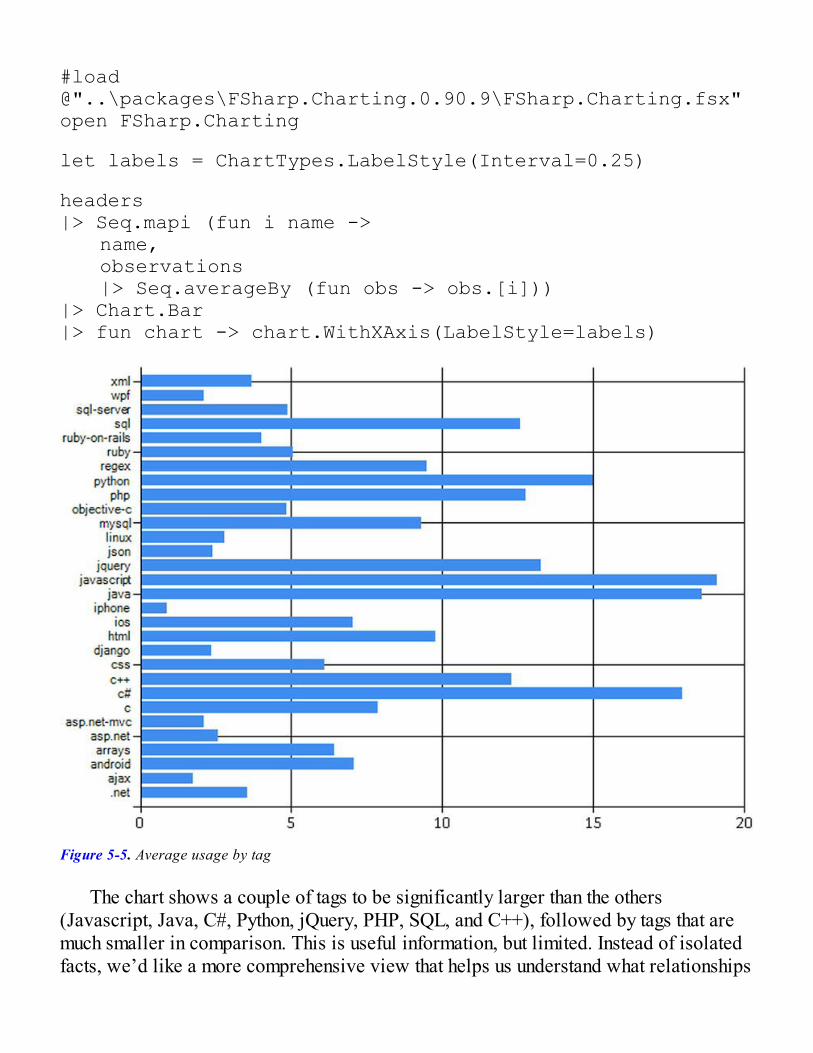
#load @"..\packages\FSharp.Charting.0.90.9\FSharp.Charting.fsx"open FSharp.Charting

let labels = ChartTypes.LabelStyle(Interval=0.25)

headers|> Seq.mapi (fun i name -> name, observations |> Seq.averageBy (fun obs -> obs.[i]))|> Chart.Bar|> fun chart -> chart.WithXAxis(LabelStyle=labels)

Figure 5-5. Average usage by tag

The chart shows a couple of tags to be significantly larger than the others(Javascript, Java, C#, Python, jQuery, PHP, SQL, and C++), followed by tags that aremuch smaller in comparison. This is useful information, but limited. Instead of isolatedfacts, we’d like a more comprehensive view that helps us understand what relationships

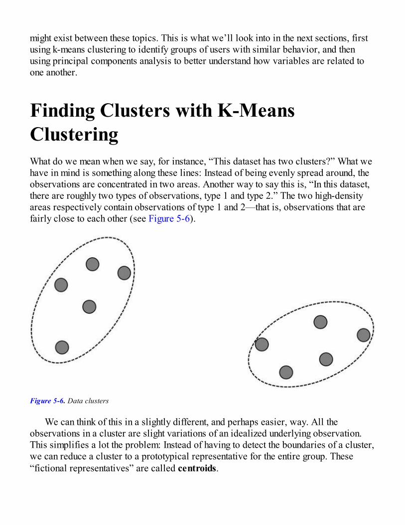
might exist between these topics. This is what we’ll look into in the next sections, firstusing k-means clustering to identify groups of users with similar behavior, and thenusing principal components analysis to better understand how variables are related toone another.

Finding Clusters with K-MeansClusteringWhat do we mean when we say, for instance, “This dataset has two clusters?” What wehave in mind is something along these lines: Instead of being evenly spread around, theobservations are concentrated in two areas. Another way to say this is, “In this dataset,there are roughly two types of observations, type 1 and type 2.” The two high-densityareas respectively contain observations of type 1 and 2—that is, observations that arefairly close to each other (see Figure 5-6).

Figure 5-6. Data clusters

We can think of this in a slightly different, and perhaps easier, way. All theobservations in a cluster are slight variations of an idealized underlying observation.This simplifies a lot the problem: Instead of having to detect the boundaries of a cluster,we can reduce a cluster to a prototypical representative for the entire group. These“fictional representatives” are called centroids.

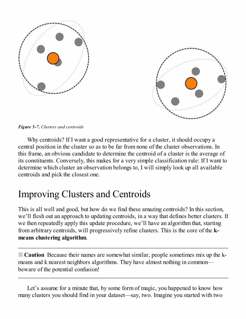
Figure 5-7. Clusters and centroids

Why centroids? If I want a good representative for a cluster, it should occupy acentral position in the cluster so as to be far from none of the cluster observations. Inthis frame, an obvious candidate to determine the centroid of a cluster is the average ofits constituents. Conversely, this makes for a very simple classification rule: If I want todetermine which cluster an observation belongs to, I will simply look up all availablecentroids and pick the closest one.

Improving Clusters and CentroidsThis is all well and good, but how do we find these amazing centroids? In this section,we’ll flesh out an approach to updating centroids, in a way that defines better clusters. Ifwe then repeatedly apply this update procedure, we’ll have an algorithm that, startingfrom arbitrary centroids, will progressively refine clusters. This is the core of the k-means clustering algorithm.

Caution Because their names are somewhat similar, people sometimes mix up the k-means and k nearest neighbors algorithms. They have almost nothing in common—beware of the potential confusion!

Let’s assume for a minute that, by some form of magic, you happened to know howmany clusters you should find in your dataset—say, two. Imagine you started with two

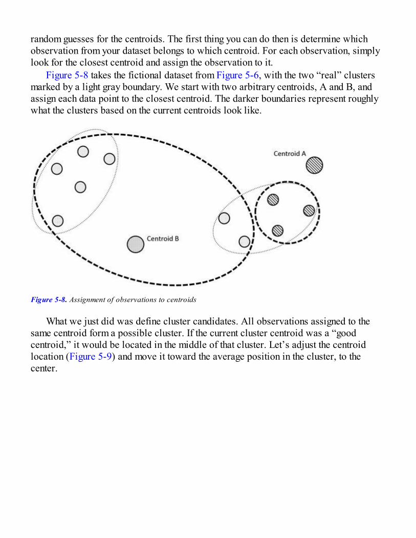
random guesses for the centroids. The first thing you can do then is determine whichobservation from your dataset belongs to which centroid. For each observation, simplylook for the closest centroid and assign the observation to it.

Figure 5-8 takes the fictional dataset from Figure 5-6, with the two “real” clustersmarked by a light gray boundary. We start with two arbitrary centroids, A and B, andassign each data point to the closest centroid. The darker boundaries represent roughlywhat the clusters based on the current centroids look like.

Figure 5-8. Assignment of observations to centroids

What we just did was define cluster candidates. All observations assigned to thesame centroid form a possible cluster. If the current cluster centroid was a “goodcentroid,” it would be located in the middle of that cluster. Let’s adjust the centroidlocation (Figure 5-9) and move it toward the average position in the cluster, to thecenter.

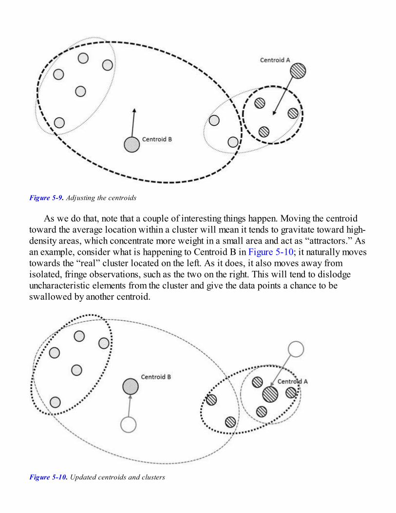
Figure 5-9. Adjusting the centroids

As we do that, note that a couple of interesting things happen. Moving the centroidtoward the average location within a cluster will mean it tends to gravitate toward high-density areas, which concentrate more weight in a small area and act as “attractors.” Asan example, consider what is happening to Centroid B in Figure 5-10; it naturally movestowards the “real” cluster located on the left. As it does, it also moves away fromisolated, fringe observations, such as the two on the right. This will tend to dislodgeuncharacteristic elements from the cluster and give the data points a chance to beswallowed by another centroid.

Figure 5-10. Updated centroids and clusters

Once that update has been performed, we can repeat the procedure and recomputewhich centroid each observation is assigned to, as well as the updated location of thecentroids.

When should we stop? Note that if the same exact observations are assigned to thesame clusters before and after the centroid locations have been updated, then thecentroids won’t move anymore. Each centroid is already occupying a location that is theaverage of its cluster, and updating it won’t change its position.

This is essentially how the k-means clustering algorithm works: to break a datasetinto k clusters, pick k arbitrary centroids, and progressively update their positions untilthey reach a stable one. Hopefully this explanation was enough to provide some insightas to why the approach could work, and could lead to stable centroids located in high-density clusters; we will leave it at that, and won’t even try to prove whether it actuallyworks.

The algorithm can be seen as an application of the fixed-point method. Theprocedure assumes that stable centroids exist, and tries to achieve self-consistency (soto speak) by progressively removing discrepancies between what cluster a centroiddefines, and what centroid a cluster defines. There are still important questions that wehave left unanswered, such as how do we figure out k or the number of clusters—butfirst, let’s keep going and start implementing the algorithm in F#, assuming we knowwhat value of k is correct, and see where that leads us.

Implementing K-Means ClusteringA few concepts emerged from the algorithm description: Given a collection ofobservations, we need to be able to assign each of them to one of k centroids, based onshortest distance, and we also need to reduce a cluster of observations into a centroid.So far nothing sounds particularly specific to our dataset, so let’s try to write a generalversion of the algorithm, in its own separate module, and use it for the problem at handby loading it in a script later.

This gives us a solid starting point. From the outside, the algorithm should look likethis: We need to provide a collection of observations and a number of clusters k. Wealso need a definition for distance, so that we can assign an observation to the closestcentroid, and a way to reduce observations from the same cluster into a single,aggregated observation, the updated centroid. In pseudo-code, here is an outline of whatwe are going to implement:

clusterize 1. initialize assign every observation an initial centroid

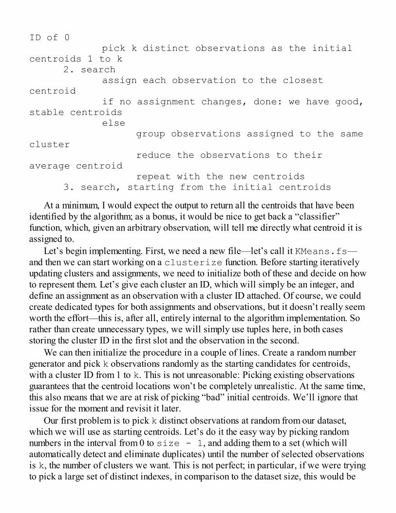
ID of 0 pick k distinct observations as the initial centroids 1 to k 2. search assign each observation to the closest centroid if no assignment changes, done: we have good, stable centroids else group observations assigned to the same cluster reduce the observations to their average centroid repeat with the new centroids 3. search, starting from the initial centroids

At a minimum, I would expect the output to return all the centroids that have beenidentified by the algorithm; as a bonus, it would be nice to get back a “classifier”function, which, given an arbitrary observation, will tell me directly what centroid it isassigned to.

Let’s begin implementing. First, we need a new file—let’s call it KMeans.fs—and then we can start working on a clusterize function. Before starting iterativelyupdating clusters and assignments, we need to initialize both of these and decide on howto represent them. Let’s give each cluster an ID, which will simply be an integer, anddefine an assignment as an observation with a cluster ID attached. Of course, we couldcreate dedicated types for both assignments and observations, but it doesn’t really seemworth the effort—this is, after all, entirely internal to the algorithm implementation. Sorather than create unnecessary types, we will simply use tuples here, in both casesstoring the cluster ID in the first slot and the observation in the second.

We can then initialize the procedure in a couple of lines. Create a random numbergenerator and pick k observations randomly as the starting candidates for centroids,with a cluster ID from 1 to k. This is not unreasonable: Picking existing observationsguarantees that the centroid locations won’t be completely unrealistic. At the same time,this also means that we are at risk of picking “bad” initial centroids. We’ll ignore thatissue for the moment and revisit it later.

Our first problem is to pick k distinct observations at random from our dataset,which we will use as starting centroids. Let’s do it the easy way by picking randomnumbers in the interval from 0 to size - 1, and adding them to a set (which willautomatically detect and eliminate duplicates) until the number of selected observationsis k, the number of clusters we want. This is not perfect; in particular, if we were tryingto pick a large set of distinct indexes, in comparison to the dataset size, this would be

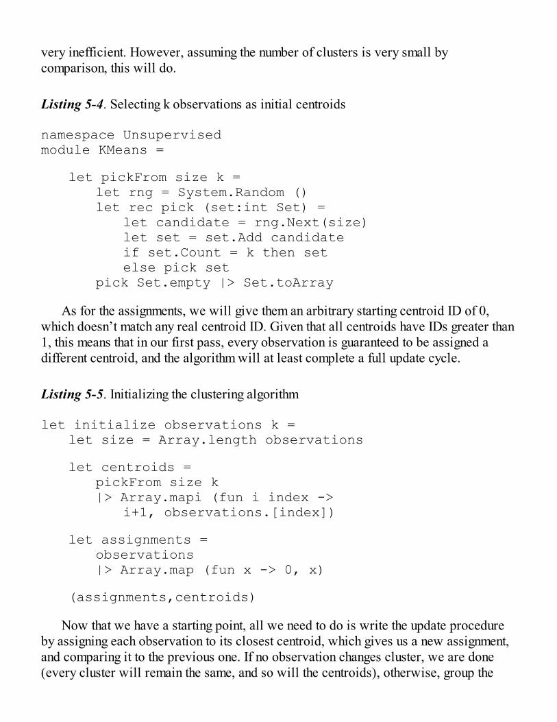
very inefficient. However, assuming the number of clusters is very small bycomparison, this will do.

Listing 5-4. Selecting k observations as initial centroids

namespace Unsupervisedmodule KMeans =

let pickFrom size k = let rng = System.Random () let rec pick (set:int Set) = let candidate = rng.Next(size) let set = set.Add candidate if set.Count = k then set else pick set pick Set.empty |> Set.toArray

As for the assignments, we will give them an arbitrary starting centroid ID of 0,which doesn’t match any real centroid ID. Given that all centroids have IDs greater than1, this means that in our first pass, every observation is guaranteed to be assigned adifferent centroid, and the algorithm will at least complete a full update cycle.

Listing 5-5. Initializing the clustering algorithm

let initialize observations k = let size = Array.length observations

let centroids = pickFrom size k |> Array.mapi (fun i index -> i+1, observations.[index])

let assignments = observations |> Array.map (fun x -> 0, x)

(assignments,centroids)

Now that we have a starting point, all we need to do is write the update procedureby assigning each observation to its closest centroid, which gives us a new assignment,and comparing it to the previous one. If no observation changes cluster, we are done(every cluster will remain the same, and so will the centroids), otherwise, group the

observations by cluster ID, reduce them into their average centroid, and keep going. Wewill now define a recursive function search inside the clusterize function, generateinitial values, and start recursively updating the centroids.

Listing 5-6. Recursive clusters update

let clusterize distance centroidOf observations k = let rec search (assignments,centroids) = // Centroid ID of the closest centroid let classifier observation = centroids |> Array.minBy (fun (_,centroid) -> distance observation centroid) |> fst // Assign each observation to closest centroid let assignments' = assignments |> Array.map (fun (_,observation) -> let closestCentroidId = classifier observation (closestCentroidId,observation)) // Check if any observation changed cluster let changed = (assignments,assignments') ||> Seq.zip |> Seq.exists (fun ((oldClusterID,_),(newClusterID,_)) -> not (oldClusterID = newClusterID))

if changed then let centroids' = assignments' |> Seq.groupBy fst |> Seq.map (fun (clusterID, group) -> clusterID, group |> Seq.map snd |> centroidOf) |> Seq.toArray search (assignments',centroids') else centroids,classifier

// start searching from initial values

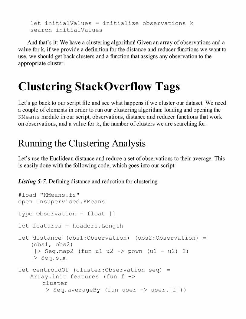
let initialValues = initialize observations k search initialValues

And that’s it: We have a clustering algorithm! Given an array of observations and avalue for k, if we provide a definition for the distance and reducer functions we want touse, we should get back clusters and a function that assigns any observation to theappropriate cluster.

Clustering StackOverflow TagsLet’s go back to our script file and see what happens if we cluster our dataset. We needa couple of elements in order to run our clustering algorithm: loading and opening theKMeans module in our script, observations, distance and reducer functions that workon observations, and a value for k, the number of clusters we are searching for.

Running the Clustering AnalysisLet’s use the Euclidean distance and reduce a set of observations to their average. Thisis easily done with the following code, which goes into our script:

Listing 5-7. Defining distance and reduction for clustering

#load "KMeans.fs"open Unsupervised.KMeans

type Observation = float []

let features = headers.Length

let distance (obs1:Observation) (obs2:Observation) = (obs1, obs2) ||> Seq.map2 (fun u1 u2 -> pown (u1 - u2) 2) |> Seq.sum

let centroidOf (cluster:Observation seq) = Array.init features (fun f -> cluster |> Seq.averageBy (fun user -> user.[f]))

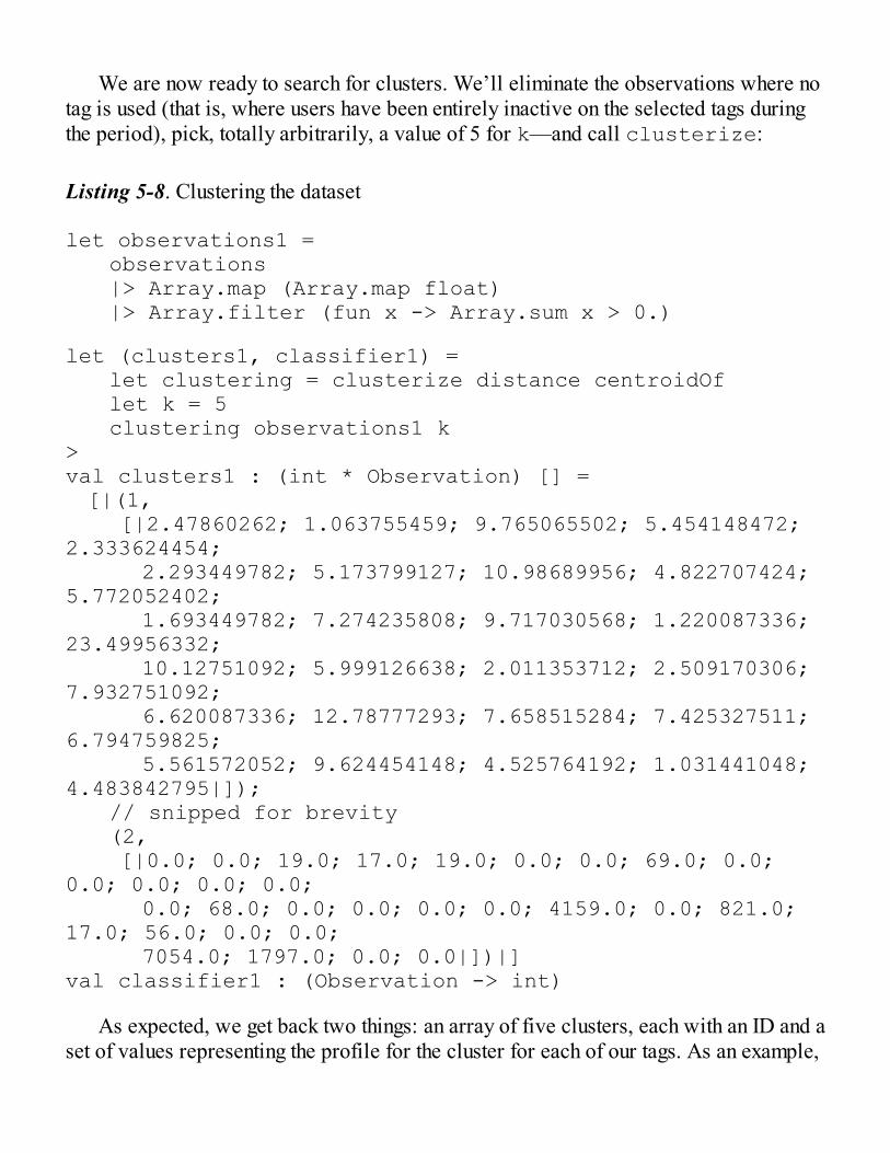
We are now ready to search for clusters. We’ll eliminate the observations where notag is used (that is, where users have been entirely inactive on the selected tags duringthe period), pick, totally arbitrarily, a value of 5 for k—and call clusterize:

Listing 5-8. Clustering the dataset

let observations1 = observations |> Array.map (Array.map float) |> Array.filter (fun x -> Array.sum x > 0.)

let (clusters1, classifier1) = let clustering = clusterize distance centroidOf let k = 5 clustering observations1 k>val clusters1 : (int * Observation) [] = [|(1, [|2.47860262; 1.063755459; 9.765065502; 5.454148472; 2.333624454; 2.293449782; 5.173799127; 10.98689956; 4.822707424; 5.772052402; 1.693449782; 7.274235808; 9.717030568; 1.220087336; 23.49956332; 10.12751092; 5.999126638; 2.011353712; 2.509170306; 7.932751092; 6.620087336; 12.78777293; 7.658515284; 7.425327511; 6.794759825; 5.561572052; 9.624454148; 4.525764192; 1.031441048; 4.483842795|]); // snipped for brevity (2, [|0.0; 0.0; 19.0; 17.0; 19.0; 0.0; 0.0; 69.0; 0.0; 0.0; 0.0; 0.0; 0.0; 0.0; 68.0; 0.0; 0.0; 0.0; 0.0; 4159.0; 0.0; 821.0; 17.0; 56.0; 0.0; 0.0; 7054.0; 1797.0; 0.0; 0.0|])|]val classifier1 : (Observation -> int)

As expected, we get back two things: an array of five clusters, each with an ID and aset of values representing the profile for the cluster for each of our tags. As an example,

in the output above, (2, [|0.0; 0.0; 19.0; // snipped // 0.0|])represents the cluster with ID 2; the average user in that cluster never used the tags.NET or ajax (the two first tags in our list), but used the Android tag 19 times. Note that,because we pick our initial centroids at random, it is very likely that you will observedifferent results for each run (we’ll get back to that in a minute).

Analyzing the ResultsLet’s face it, it is hard to interpret the output in its current form. The first thing thatwould help would be to map each of the clusters and align the tag names with thenumbers we have. Let’s do this:

clusters1|> Seq.iter (fun (id,profile) -> printfn "CLUSTER %i" id profile |> Array.iteri (fun i value -> printfn "%16s %.1f" headers.[i] value))

>CLUSTER 4 .net 2.9 ajax 1.1 android 6.1 arrays 5.0 asp.net 2.4 // snipped for brevity

This is a bit better; at least we can start scanning through each of the clusters andlooking for some sort of pattern to emerge. However, the information is still a bitoverwhelming—let’s see if a chart helps us visualize our output more clearly (seeFigure 5-11):

Chart.Combine [ for (id,profile) in clusters1 -> profile |> Seq.mapi (fun i value -> headers.[i], value) |> Chart.Bar ]|> fun chart -> chart.WithXAxis(LabelStyle=labels)

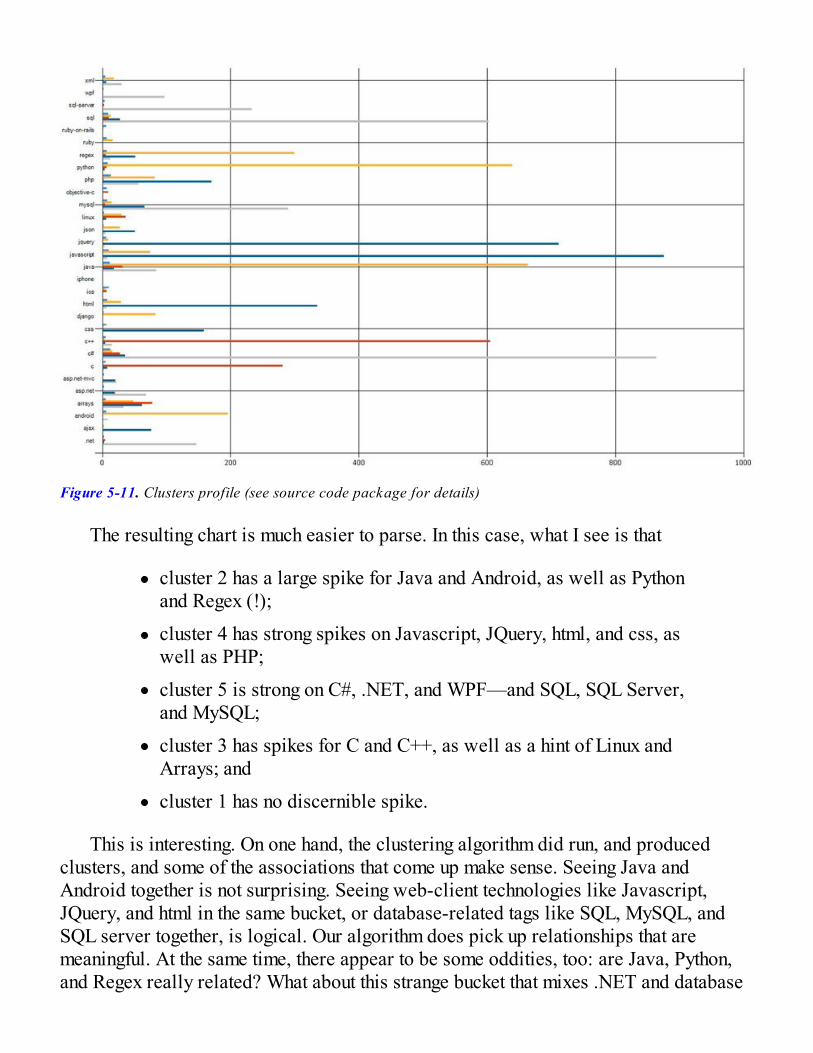
Figure 5-11. Clusters profile (see source code package for details)

The resulting chart is much easier to parse. In this case, what I see is that

cluster 2 has a large spike for Java and Android, as well as Pythonand Regex (!);

cluster 4 has strong spikes on Javascript, JQuery, html, and css, aswell as PHP;

cluster 5 is strong on C#, .NET, and WPF—and SQL, SQL Server,and MySQL;

cluster 3 has spikes for C and C++, as well as a hint of Linux andArrays; and

cluster 1 has no discernible spike.

This is interesting. On one hand, the clustering algorithm did run, and producedclusters, and some of the associations that come up make sense. Seeing Java andAndroid together is not surprising. Seeing web-client technologies like Javascript,JQuery, and html in the same bucket, or database-related tags like SQL, MySQL, andSQL server together, is logical. Our algorithm does pick up relationships that aremeaningful. At the same time, there appear to be some oddities, too: are Java, Python,and Regex really related? What about this strange bucket that mixes .NET and database

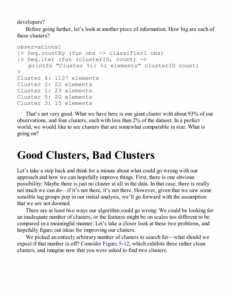
developers?Before going further, let’s look at another piece of information. How big are each of

these clusters?

observations1|> Seq.countBy (fun obs -> classifier1 obs)|> Seq.iter (fun (clusterID, count) -> printfn "Cluster %i: %i elements" clusterID count)>Cluster 4: 1137 elementsCluster 2: 22 elementsCluster 1: 23 elementsCluster 5: 20 elementsCluster 3: 15 elements

That’s not very good. What we have here is one giant cluster with about 93% of ourobservations, and four clusters, each with less than 2% of the dataset. In a perfectworld, we would like to see clusters that are somewhat comparable in size. What isgoing on?

Good Clusters, Bad ClustersLet’s take a step back and think for a minute about what could go wrong with ourapproach and how we can hopefully improve things. First, there is one obviouspossibility: Maybe there is just no cluster at all in the data. In that case, there is reallynot much we can do—if it’s not there, it’s not there. However, given that we saw somesensible tag groups pop in our initial analysis, we’ll go forward with the assumptionthat we are not doomed.

There are at least two ways our algorithm could go wrong: We could be looking foran inadequate number of clusters, or the features might be on scales too different to becompared in a meaningful manner. Let’s take a closer look at these two problems, andhopefully figure out ideas for improving our clusters.

We picked an entirely arbitrary number of clusters to search for—what should weexpect if that number is off? Consider Figure 5-12, which exhibits three rather cleanclusters, and imagine now that you were asked to find two clusters.

Figure 5-12. Searching for insufficiently many clusters

The algorithm will very probably identify two clusters, in one of three ways: One ofthe clusters will be “correct,” and the other one will aggregate the remaining twoclusters, like in Figure 5-13, for example.

This is actually fairly reasonable: If we can pick only two groups, picking one goodone and making a mediocre one from the two remaining is as good as we can get.However, given that we pick our starting centroids at random, the clusters will dependalmost entirely on which three random observations we started with. If we repeat theprocedure multiple times, we will see three different results appear, combining the“true” clusters differently. In a situation where we have more than three clusters, wewould expect to see more combinations appear.

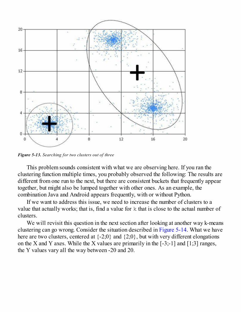
Figure 5-13. Searching for two clusters out of three

This problem sounds consistent with what we are observing here. If you ran theclustering function multiple times, you probably observed the following: The results aredifferent from one run to the next, but there are consistent buckets that frequently appeartogether, but might also be lumped together with other ones. As an example, thecombination Java and Android appears frequently, with or without Python.

If we want to address this issue, we need to increase the number of clusters to avalue that actually works; that is, find a value for k that is close to the actual number ofclusters.

We will revisit this question in the next section after looking at another way k-meansclustering can go wrong. Consider the situation described in Figure 5-14. What we havehere are two clusters, centered at {-2;0} and {2;0}, but with very different elongationson the X and Y axes. While the X values are primarily in the [-3;-1] and [1;3] ranges,the Y values vary all the way between -20 and 20.

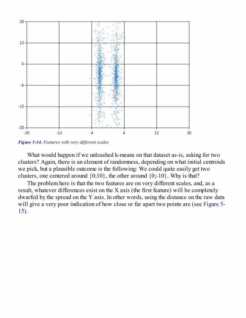
Figure 5-14. Features with very different scales

What would happen if we unleashed k-means on that dataset as-is, asking for twoclusters? Again, there is an element of randomness, depending on what initial centroidswe pick, but a plausible outcome is the following: We could quite easily get twoclusters, one centered around {0;10}, the other around {0;-10}. Why is that?

The problem here is that the two features are on very different scales, and, as aresult, whatever differences exist on the X axis (the first feature) will be completelydwarfed by the spread on the Y axis. In other words, using the distance on the raw datawill give a very poor indication of how close or far apart two points are (see Figure 5-15).

Figure 5-15. Close points

How can we address this issue? Simple: If the issue stems from features being ondifferent scales, we need to transform the data so that differences of the same magnitudeare comparable across all features. In other words, when an observation has a low orhigh value on a feature, the impact on the distance function should be comparable.

One common approach is to rescale each feature using the following formula: x'<- (x - min) / (max - min). As a result, every feature is spread on theinterval from 0 to 1, with the smallest value being 0 and the largest 1, and the others arescaled linearly in between. As an illustration, if we applied this to our previous dataset,this is how the data would look (see Figure 5-16):

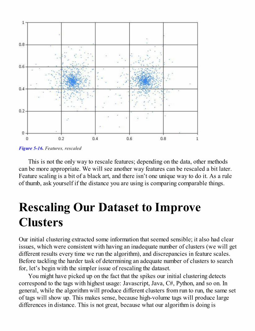
Figure 5-16. Features, rescaled

This is not the only way to rescale features; depending on the data, other methodscan be more appropriate. We will see another way features can be rescaled a bit later.Feature scaling is a bit of a black art, and there isn’t one unique way to do it. As a ruleof thumb, ask yourself if the distance you are using is comparing comparable things.

Rescaling Our Dataset to ImproveClustersOur initial clustering extracted some information that seemed sensible; it also had clearissues, which were consistent with having an inadequate number of clusters (we will getdifferent results every time we run the algorithm), and discrepancies in feature scales.Before tackling the harder task of determining an adequate number of clusters to searchfor, let’s begin with the simpler issue of rescaling the dataset.

You might have picked up on the fact that the spikes our initial clustering detectscorrespond to the tags with highest usage: Javascript, Java, C#, Python, and so on. Ingeneral, while the algorithm will produce different clusters from run to run, the same setof tags will show up. This makes sense, because high-volume tags will produce largedifferences in distance. This is not great, because what our algorithm is doing is

essentially finding high-traffic tags, and won’t be picking up more subtle differences onlower-traffic tags.

The big issue here is that the volume of activity on each tag is fairly different: Theaverage usage of JavaScript is over 20 times higher than that of the iPhone tag. Wecould rescale features along the lines of we described earlier, and remap them to spanthe interval from 0 to 1. We will take a different direction instead. Here is how wecould describe our dataset: We believe users can be categorized by a few interestprofiles, but they have a widely different level of activity on StackOverflow. Tocompare their profiles directly, regardless of how active they are on the site, what wewant is to eliminate the discrepancies due to activity levels. For instance, considerthese three hypothetical users:

JavaScript C#

User 1 100 20

User 2 10 2

User 3 50 50

By raw distance, User 1 and User 3 are the most similar, because they are muchmore active than User 2. However, arguably, User 1 and User 2 are very similar—moreso than Users 1 and 3. While User 1 is ten times more active than User 2, where theyspend their time is identical. One way we could address this is to scale by user: Foreach row, scale the largest tag to 100% and divide every other tag accordingly.

JavaScript C#

User 1 100% 20%

User 2 100% 20%

User 3 100% 100%

If we do that, suddenly User 1 and User 2 become identical, and User 3 is verydifferent. What we are really doing here is removing user activity level from theequation. The implicit model here could be stated like this: “There are a few archetypalStackOverflow users who share an interest in the same tags. However, some of themhave more time than others to spend, so their activity will be proportionally higher.”Note that this also means that we are now ignoring how active users are on the site. Isthis right? Maybe, maybe not—there is no clear-cut answer to that question.

At any rate, let’s try this out, still with a “bad” number of clusters. All we need todo, really, is to take our observations and divide each number by the largest value inthat row.

Listing 5-9. Normalizing observations to similar activity

let rowNormalizer (obs:Observation) : Observation = let max = obs |> Seq.max obs |> Array.map (fun tagUse -> tagUse / max)

let observations2 = observations |> Array.filter (fun x -> Array.sum x > 0.) |> Array.map (Array.map float) |> Array.map rowNormalizer

let (clusters2, classifier2) = let clustering = clusterize distance centroidOf let k = 5 clustering observations2 k

We still haven’t dealt with what k should be, and, as a result, we are very likelystill looking for too few clusters; results will still be unstable from run to run. However,even then, we should observe a couple of things. First, the cluster size is now muchmore balanced. Running the same code as before, here is what we get:

observations2|> Seq.countBy (fun obs -> classifier2 obs)|> Seq.iter (fun (clusterID, count) -> printfn "Cluster %i: %i elements" clusterID count)

>Cluster 4: 480 elementsCluster 5: 252 elementsCluster 2: 219 elementsCluster 1: 141 elementsCluster 3: 125 elementsval it : unit = ()

Also, some associations appear more clearly now, such as the pair C/C++, or evenpairs that didn’t register before, like Python and Django, or Ruby and Ruby on Rails,where one of the elements had too little activity to make a difference in the distance (seeFigure 5-17).

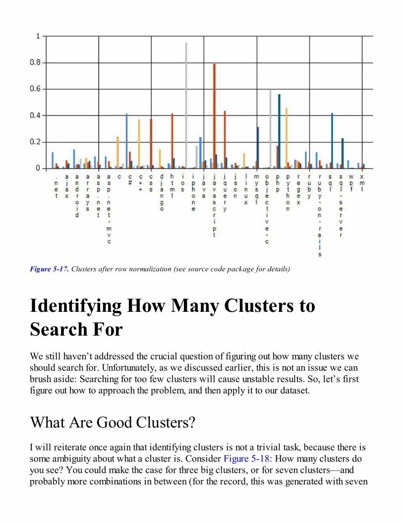
Figure 5-17. Clusters after row normalization (see source code package for details)

Identifying How Many Clusters toSearch ForWe still haven’t addressed the crucial question of figuring out how many clusters weshould search for. Unfortunately, as we discussed earlier, this is not an issue we canbrush aside: Searching for too few clusters will cause unstable results. So, let’s firstfigure out how to approach the problem, and then apply it to our dataset.

What Are Good Clusters?I will reiterate once again that identifying clusters is not a trivial task, because there issome ambiguity about what a cluster is. Consider Figure 5-18: How many clusters doyou see? You could make the case for three big clusters, or for seven clusters—andprobably more combinations in between (for the record, this was generated with seven

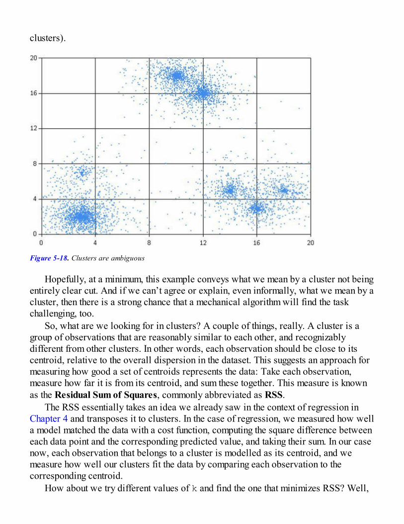
clusters).

Figure 5-18. Clusters are ambiguous

Hopefully, at a minimum, this example conveys what we mean by a cluster not beingentirely clear cut. And if we can’t agree or explain, even informally, what we mean by acluster, then there is a strong chance that a mechanical algorithm will find the taskchallenging, too.

So, what are we looking for in clusters? A couple of things, really. A cluster is agroup of observations that are reasonably similar to each other, and recognizablydifferent from other clusters. In other words, each observation should be close to itscentroid, relative to the overall dispersion in the dataset. This suggests an approach formeasuring how good a set of centroids represents the data: Take each observation,measure how far it is from its centroid, and sum these together. This measure is knownas the Residual Sum of Squares, commonly abbreviated as RSS.

The RSS essentially takes an idea we already saw in the context of regression inChapter 4 and transposes it to clusters. In the case of regression, we measured how wella model matched the data with a cost function, computing the square difference betweeneach data point and the corresponding predicted value, and taking their sum. In our casenow, each observation that belongs to a cluster is modelled as its centroid, and wemeasure how well our clusters fit the data by comparing each observation to thecorresponding centroid.

How about we try different values of k and find the one that minimizes RSS? Well,

there is a bit of a problem with that. Suppose we have a dataset with N observations—there is an obvious value that minimizes RSS, and that is k = N. If we create onecentroid for each observation, we will of course get a perfect fit. Note also that if wehave k centroids, adding one centroid will always decrease RSS (to be more precise,RSS will never increase).

This is useful in that it clarifies what we are after. What we want is an “efficient”summary of the data, once again following Occam’s Razor principle. We want clustersthat explain the data well, but are as simple as possible. Taking only RSS into accountmisses that second point: There is no penalty for complexity, and our clustering willover-fit and simply reproduce the dataset itself, without any form of summarization.

So, what should we do? The general answer is, if we had a measure for clusteringquality, it should probably include RSS (how well the model fits the data), and apenalty term for complexity. Again, this is a tricky problem, and there is no silver bullethere. There are a few popular approaches. First, imagine that you computed the RSS fora value of k. Now compute the RSS for k + 1: If you are barely improving RSS,increasing the number of clusters is not economical. This method is known as the elbowmethod—look for places where the relative improvement in RSS degrades.

This general direction can be used to compute a numeric measure for how good aparticular value of k is. The Akaike Information Criterion, or AIC, is a popularchoice. It combines in one measure the RSS and a penalty term 2 * m * k, where mis the number of features and k the number of clusters. In other words, prefer modelswith fewer clusters, and be more conservative with models with many features. Thereare a couple of other classic measures (which we won’t implement here), such as BIC(Bayesian Information Criterion) or Calinski-Harabasz, which follow roughly the samegeneral principles.

Which one is right? Unfortunately, it depends. Again, clustering is a bit of anambiguous task; all these methods are heuristics, and while they follow a similargeneral approach, they will not necessarily agree; identifying something that works willusually take a bit of trial and error. In the next section, we’ll simply use the AIC,because it’s particularly easy to implement.

Identifying k on the StackOverflow DatasetLet’s see how this works out on the dataset at hand. The first heuristic we will use tocalibrate which value of k might work is a “rule of thumb” common in the industry,which suggests the following value for k:

let ruleOfThumb (n:int) = sqrt (float n / 2.)let k_ruleOfThumb = ruleOfThumb (observations2.Length)

This approach is obviously way too simple to work well in every situation; the onlything it takes into account is how large the dataset is! On the other hand, it has thebenefit of simplicity. I would recommend using it simply to get a rough sense for whatrange of values might be reasonable. In this case, the suggested value is 25, which wewill use as an upper bound for k. Next, let’s try out the AIC.

Listing 5-10. Akaike Information Criterion (AIC)

let squareError (obs1:Observation) (obs2:Observation) = (obs1,obs2) ||> Seq.zip |> Seq.sumBy (fun (x1,x2) -> pown (x1-x2) 2)

let RSS (dataset:Observation[]) centroids = dataset |> Seq.sumBy (fun obs -> centroids |> Seq.map (squareError obs) |> Seq.min)

let AIC (dataset:Observation[]) centroids = let k = centroids |> Seq.length let m = dataset.[0] |> Seq.length RSS dataset centroids + float (2 * m * k)

In order to figure out a decent value for k, we’ll try out every single possibilitybetween k = 1 and k = 25. Because the clustering itself is going to be unstable forlow values of k, we will run the algorithm a couple of times for each value and averageout the corresponding AIC so that we can cancel out potential flukes due to, for instance,unfortunate initial value selection:

[1..25]|> Seq.map (fun k -> let value = [ for _ in 1 .. 10 -> let (clusters, classifier) = let clustering = clusterize distance centroidOf clustering observations2 k AIC observations2 (clusters |> Seq.map snd) ] |> List.average k, value)

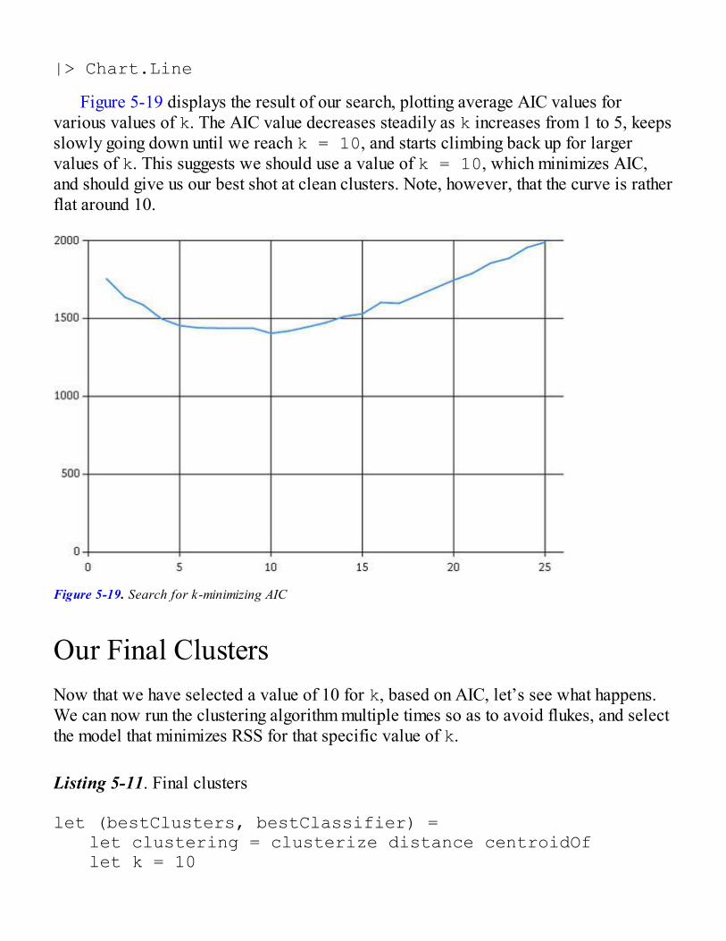
|> Chart.Line

Figure 5-19 displays the result of our search, plotting average AIC values forvarious values of k. The AIC value decreases steadily as k increases from 1 to 5, keepsslowly going down until we reach k = 10, and starts climbing back up for largervalues of k. This suggests we should use a value of k = 10, which minimizes AIC,and should give us our best shot at clean clusters. Note, however, that the curve is ratherflat around 10.

Figure 5-19. Search for k-minimizing AIC

Our Final ClustersNow that we have selected a value of 10 for k, based on AIC, let’s see what happens.We can now run the clustering algorithm multiple times so as to avoid flukes, and selectthe model that minimizes RSS for that specific value of k.

Listing 5-11. Final clusters

let (bestClusters, bestClassifier) = let clustering = clusterize distance centroidOf let k = 10

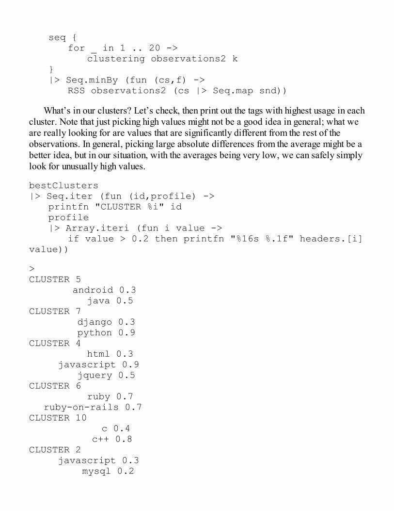
seq { for _ in 1 .. 20 -> clustering observations2 k } |> Seq.minBy (fun (cs,f) -> RSS observations2 (cs |> Seq.map snd))

What’s in our clusters? Let’s check, then print out the tags with highest usage in eachcluster. Note that just picking high values might not be a good idea in general; what weare really looking for are values that are significantly different from the rest of theobservations. In general, picking large absolute differences from the average might be abetter idea, but in our situation, with the averages being very low, we can safely simplylook for unusually high values.

bestClusters|> Seq.iter (fun (id,profile) -> printfn "CLUSTER %i" id profile |> Array.iteri (fun i value -> if value > 0.2 then printfn "%16s %.1f" headers.[i] value))

>CLUSTER 5 android 0.3 java 0.5CLUSTER 7 django 0.3 python 0.9CLUSTER 4 html 0.3 javascript 0.9 jquery 0.5CLUSTER 6 ruby 0.7 ruby-on-rails 0.7CLUSTER 10 c 0.4 c++ 0.8CLUSTER 2 javascript 0.3 mysql 0.2

php 1.0CLUSTER 8 .net 0.3 c# 0.9CLUSTER 9 mysql 0.3 sql 0.8 sql-server 0.6CLUSTER 1 ios 1.0 objective-c 0.6CLUSTER 3 css 0.9 html 0.7 javascript 0.5 jquery 0.3

This looks pretty good. I suspect you can easily conjure a mental picture for each ofthe profiles, which correspond to clear development stacks. This is great: Without mucheffort, we managed to automatically extract meaningful information out of raw data.Without any understanding of what these tags mean, just by looking at the dataset andhistorical usage patterns, k-means figured out that Ruby and Ruby on Rails are related,or that some people we call DBAs focus mainly on SQL-related technologies.

There is probably more information we could squeeze out of the dataset using k-means; however, it is likely going to become increasingly hard to get new andinteresting results if we continue in that direction, because our current results are prettygood already. What we will do instead is leave it at that for k-means, and introduce acompletely different technique, Principal Component Analysis. We will apply it to thesame problem so that we can compare and contrast the two methods.

Detecting How Features Are RelatedFor all its qualities, k-means clustering is not the end all be all. In particular, it doesn’tprovide a comprehensive picture of how the features work together. We can figure outsome relationships by inspecting each cluster profile, looking for features that aremarkedly higher or lower than is typical, but this is a tedious manual process. Theapproach we will explore now, Principal Component Analysis, or PCA in short, is ina sense the complement to k-means: Where k-means provides a clear picture ofindividual profiles, but not much information regarding how features relate to each

other, PCA is primarily about detecting some structure in features, instead of inindividuals.

Covariance and CorrelationPatterns in data can take infinitely many shapes. While detecting all of them is hopeless,some patterns are both useful and easy to spot. One such example is the following:“Whenever quantity A increases, quantity B increases, too.” This is what covarianceand correlation are about.

The covariance between two measurements X and Y is defined as:

Cov(X,Y) = average [(X-average(X)) * (Y-average(Y))]

Once you start breaking this down, you see it is a reasonable way to go. If twovalues X and Y go up and down together, then when one is above its average, the otherone should be, too, and the product will be positive. Similarly, when one goes belowthe average, so too should the other—and the product of their difference (both negativenumbers now) will still be positive. By the same line of reasoning, you would expecttwo features moving in opposite directions to have a negative covariance.

Side Note It is important to realize that a covariance (or correlation) of zero doesnot mean there is no relationship between features. It simply indicates that theirrelationship is not as simple as moving up and down together. As an example, datapoints describing a perfect circle will have a correlation of zero, even though theirrelationship is perfectly determined

Covariance is great, but it has one problem: It depends on the scale of the featuresand has no obvious scale itself, which makes interpreting it difficult. What is a highcovariance? It depends on the data. Correlation is a modification of covariance, andaddresses that problem. Formally, the correlation between features X and Y is definedas:

Corr(X,Y) = Cov(X,Y) / (stdDev(X) * stdDev(Y))

where stdDev stands for standard deviation. Depending on your level of comfortwith statistics, this might look intimidating. It should not be—let’s break this down a bit.Our issue with covariance was the scale discrepancy between X and Y. To makedifferent features comparable, what we need is to reduce the terms (X-average(X)) and (Y-average(Y)) to similar scales. Dividing (X-

average(X)) by its average value—the average distance between X and its average(quite a mouthful!)—would do just that, and that’s exactly what the standard deviation,often denoted as sigma, is.

Tip The standard deviation (and its square, the variance) is often described as ameasure for the dispersion of a feature. Personally, I found the following descriptionhelpful: The standard deviation sigma measures the average distance to the average.If you took a random observation from your sample, the standard deviation is how far itwould be from the sample average.

You can expand the covariance part and reorganize the formula a bit into thisequivalent version, which helps us better understand how correlation works:

Corr(X,Y) = average [(X-avg(X))/stdDev(X) * (Y-avg(Y))/stdDev(Y)]

The term (X-average(X))/stdDev(X) takes the differences from the averagefrom the covariance and rescales them by sigma so that the average difference is now1.0. Both the X and Y terms are now on a comparable scale, and as a result (we won’tprove it here), correlation has this pleasant property in that it goes from -1.0 to 1.0. Avalue of 1.0 indicates that X and Y always grow together in a perfect line, -1.0 indicatesa perfect line in the opposite direction, and 0.0 indicates that no such relationship hasbeen detected. The closer to 1.0 or -1.0 a correlation is, the stronger that pattern is—that is, the features move mostly together, with a certain level of uncertainty.

Incidentally, transforming a measurement X into (X-average(X))/stdDev(X) is a classic way to rescale a feature, and is known as az-score. It is a bit more involved than the method we discussed earlier, where wesimply converted values from [min;max] to [0;1], but it has some advantages aswell. The transformed feature is centered on 0, so positive or negative values can beimmediately interpreted as being high or low. If the feature is reasonably normalshaped, that is, bell-shaped around its mean, the result might be more “reasonable,” too.While the min and max values are, by definition, outliers with extreme values, thestandard deviation is typically a better metric by which to scale observations.

Correlations Between StackOverflow TagsLet’s go ahead and see how that works out on our dataset. For convenience, rather thanadding code to our current script, we’ll create a new script, PCA.fsx, and a module,

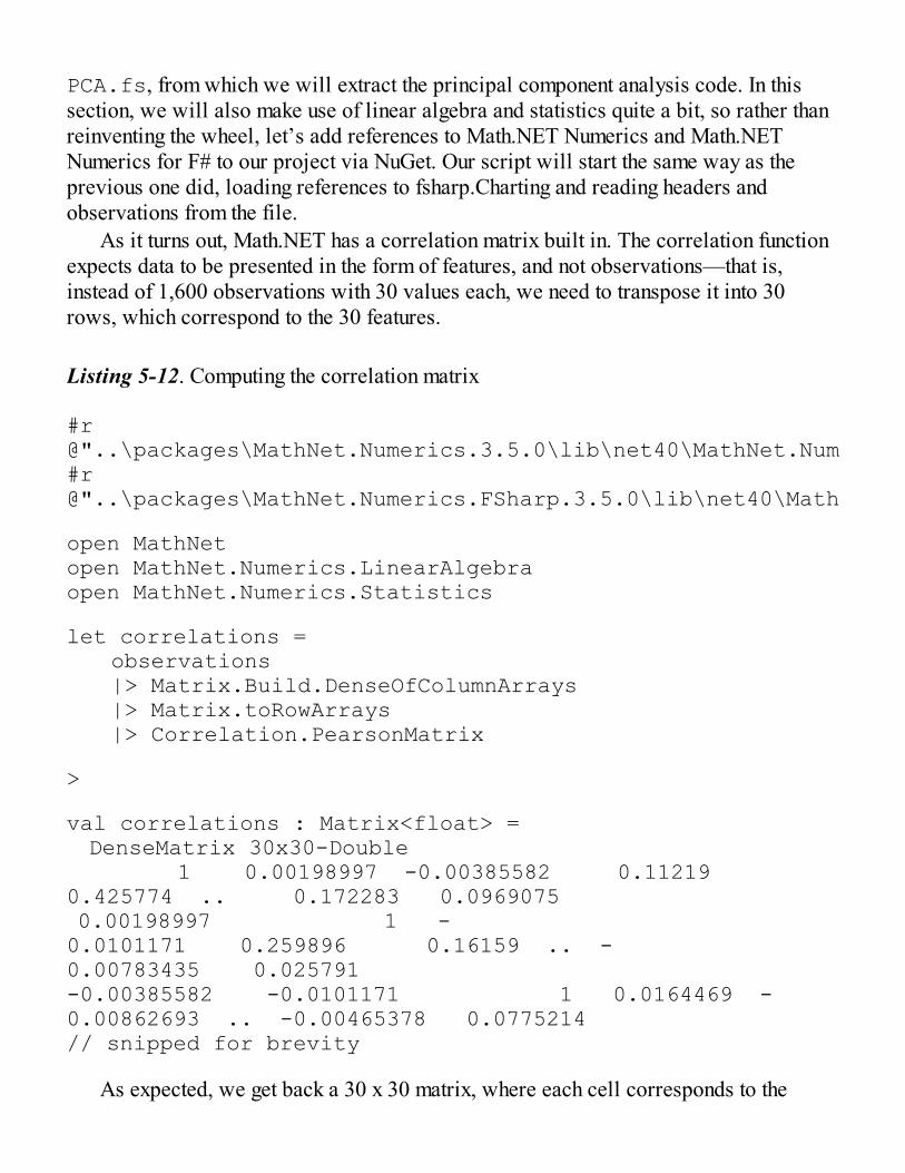
PCA.fs, from which we will extract the principal component analysis code. In thissection, we will also make use of linear algebra and statistics quite a bit, so rather thanreinventing the wheel, let’s add references to Math.NET Numerics and Math.NETNumerics for F# to our project via NuGet. Our script will start the same way as theprevious one did, loading references to fsharp.Charting and reading headers andobservations from the file.

As it turns out, Math.NET has a correlation matrix built in. The correlation functionexpects data to be presented in the form of features, and not observations—that is,instead of 1,600 observations with 30 values each, we need to transpose it into 30rows, which correspond to the 30 features.

Listing 5-12. Computing the correlation matrix

#r @"..\packages\MathNet.Numerics.3.5.0\lib\net40\MathNet.Numerics.dll"#r @"..\packages\MathNet.Numerics.FSharp.3.5.0\lib\net40\MathNet.Numerics.FSharp.dll"

open MathNetopen MathNet.Numerics.LinearAlgebraopen MathNet.Numerics.Statistics

let correlations = observations |> Matrix.Build.DenseOfColumnArrays |> Matrix.toRowArrays |> Correlation.PearsonMatrix

>

val correlations : Matrix<float> = DenseMatrix 30x30-Double 1 0.00198997 -0.00385582 0.11219 0.425774 .. 0.172283 0.0969075 0.00198997 1 -0.0101171 0.259896 0.16159 .. -0.00783435 0.025791-0.00385582 -0.0101171 1 0.0164469 -0.00862693 .. -0.00465378 0.0775214// snipped for brevity

As expected, we get back a 30 x 30 matrix, where each cell corresponds to the

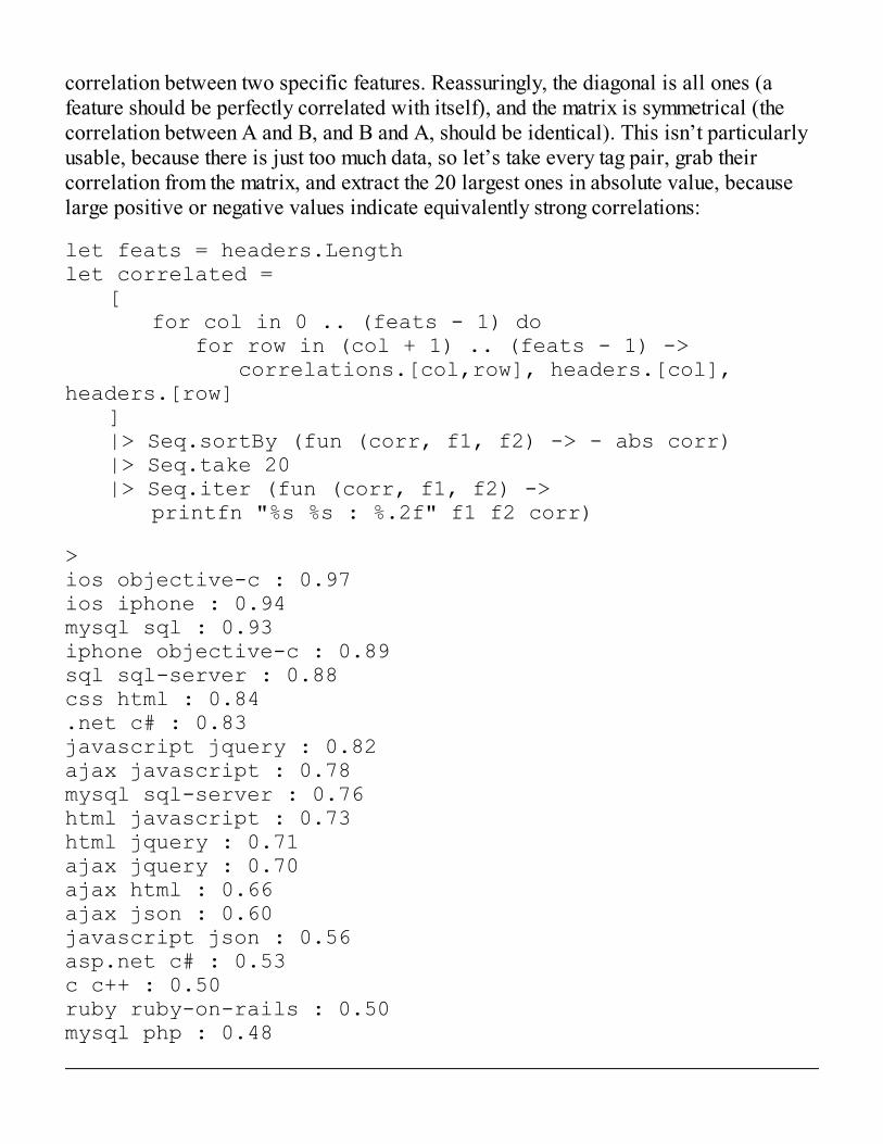
correlation between two specific features. Reassuringly, the diagonal is all ones (afeature should be perfectly correlated with itself), and the matrix is symmetrical (thecorrelation between A and B, and B and A, should be identical). This isn’t particularlyusable, because there is just too much data, so let’s take every tag pair, grab theircorrelation from the matrix, and extract the 20 largest ones in absolute value, becauselarge positive or negative values indicate equivalently strong correlations:

let feats = headers.Lengthlet correlated = [ for col in 0 .. (feats - 1) do for row in (col + 1) .. (feats - 1) -> correlations.[col,row], headers.[col], headers.[row] ] |> Seq.sortBy (fun (corr, f1, f2) -> - abs corr) |> Seq.take 20 |> Seq.iter (fun (corr, f1, f2) -> printfn "%s %s : %.2f" f1 f2 corr)

> ios objective-c : 0.97ios iphone : 0.94mysql sql : 0.93iphone objective-c : 0.89sql sql-server : 0.88css html : 0.84.net c# : 0.83javascript jquery : 0.82ajax javascript : 0.78mysql sql-server : 0.76html javascript : 0.73html jquery : 0.71ajax jquery : 0.70ajax html : 0.66ajax json : 0.60javascript json : 0.56asp.net c# : 0.53c c++ : 0.50ruby ruby-on-rails : 0.50mysql php : 0.48

Tip At the time of writing, there was no built-in descending sort in F#. As analternative, you can sort by negation; for instance, in Seq.sortBy (fun (corr,f1, f2) -> - abs corr).

The results are very reasonable. We immediately see some groups of features thatgo hand in hand: iOS, objective-c, and iPhone; SQL, MySQL, and SQL-server—and soon and so forth. With very little effort, the correlation matrix extracted a lot ofinformation from our dataset.

Identifying Better Features withPrincipal Component AnalysisWe looked at the correlation matrix as a useful summary of relationships betweenfeatures. Another way we can interpret it is as a signal that our dataset contains a lot ofredundant information. As an example, iOS, objective-C, and iPhone have a correlationthat is pretty close to 100%. What this means is that we could almost merge these threefeatures into one—say, “iOS developer. Once you know one of the three is high (orlow), you pretty much know the two others.

At the same time, some correlations are a bit trickier to handle. For instance, if youdive into the dataset a bit, you’ll see that MySQL and SQL, SQL and SQL-Server, andMySQL and PHP are highly correlated. Does this mean that, by transitivity, PHP andSQL-Server go together? I doubt it—from my personal experience, I would read this astwo different relationships, the DBAs on one side, and possibly the LAMP developerson the other. They happen to share one common interest in MySQL, but they are not one.

In this section, we will demonstrate principal component analysis (or in short,PCA), a data-mining technique that looks at the structure of the covariance orcorrelation matrix and uses it to reorganize data into a new set of features, combiningthe existing ones into composites that represent the data more efficiently and avoidredundancy.

Recombining Features with AlgebraA complete explanation on why PCA works would take us a bit far into algebra, withoutbeing all that useful in the end. We will try to convey the key points through anillustrative example, deliberately using some hand-waving at strategic moments, and

letting readers who are so inclined dig deeper on their own.What we are after here is a way to reorganize our dataset. Consider for a minute a

dataset with, say, two features only, instead of our 30. One way to represent atransformation of our features is by using a 2 x 2 matrix. If we multiply an observation(a vector of two elements) by that matrix, we will get a new vector, which still has twofeatures:

let observation = vector [ 2.0; 5.0 ]let transform = matrix [ [ 1.0; 3.0 ] [ 2.0; 1.0 ] ]transform * observation |> printfn "%A"

>seq [17.0; 9.0]

Each of the rows in the transform matrix can be seen as weights. The first row, forinstance, states that the first transformed feature combines 1.0 part of the first originalfeature and 3.0 parts of the second. If that transformation were the identity matrix (1s onthe diagonal, 0s everywhere else), the transformation would simply return the original.

What we are looking for is a matrix of that form. Obviously, we can’t pick just anyarbitrary matrix; it would just rearrange the features, but without a reason a priori toproduce anything particularly useful. So, what would we like to achieve here? In thisparticular situation, we would like the transformation to rearrange features so as to limitthe information redundancy we spotted in the correlation matrix. We would also like away to distinguish major trends in the dataset from unimportant differences.

This is the part where the heavy hand-waving takes place. As it turns out, there is alinear algebra technique that does just what we want: The factorization of a matrix intoeigenvectors and eigenvalues. At a very high level, an N x X square matrix M can beuniquely decomposed into up to N pairs of eigenvalues and eigenvectors (a float, and avector of N elements), each of which satisfies the following equation: M xeigenvector = eigenvalue x eigenvector. In other words, aneigenvector is a direction that just stretches M by an amplitude corresponding to itseigenvalue.

If we apply this technique to the covariance matrix, what should we get? First, eacheigenvector represents a new feature built by combining the existing ones. Rememberthat the covariance matrix measures differences off the average from each feature; theeigenvector with largest eigenvalue represents a feature with the most stretch. Thus, inthe case of the covariance matrix, it means the direction in which we observe the mostjoint variations from the center of the data. Stated differently, the eigenvector with thelargest eigenvalue is a feature that combines existing features in a way that explains

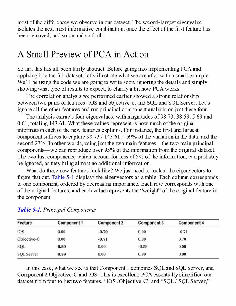
most of the differences we observe in our dataset. The second-largest eigenvalueisolates the next most informative combination, once the effect of the first feature hasbeen removed, and so on and so forth.

A Small Preview of PCA in ActionSo far, this has all been fairly abstract. Before going into implementing PCA andapplying it to the full dataset, let’s illustrate what we are after with a small example.We’ll be using the code we are going to write soon, ignoring the details and simplyshowing what type of results to expect, to clarify a bit how PCA works.

The correlation analysis we performed earlier showed a strong relationshipbetween two pairs of features: iOS and objective-c, and SQL and SQL Server. Let’signore all the other features and run principal component analysis on just these four.

The analysis extracts four eigenvalues, with magnitudes of 98.73, 38.59, 5.69 and0.61, totaling 143.61. What these values represent is how much of the originalinformation each of the new features explains. For instance, the first and largestcomponent suffices to capture 98.73 / 143.61 ~ 69% of the variation in the data, and thesecond 27%. In other words, using just the two main features—the two main principalcomponents—we can reproduce over 95% of the information from the original dataset.The two last components, which account for less of 5% of the information, can probablybe ignored, as they bring almost no additional information.

What do these new features look like? We just need to look at the eigenvectors tofigure that out. Table 5-1 displays the eigenvectors as a table. Each column correspondsto one component, ordered by decreasing importance. Each row corresponds with oneof the original features, and each value represents the “weight” of the original feature inthe component.

Table 5-1. Principal Components

In this case, what we see is that Component 1 combines SQL and SQL Server, andComponent 2 Objective-C and iOS. This is excellent: PCA essentially simplified ourdataset from four to just two features, “iOS /Objective-C” and “SQL / SQL Server,”

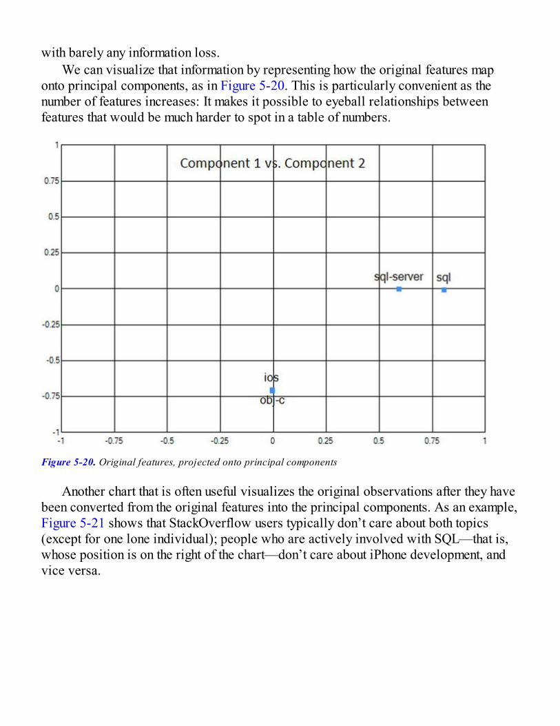
with barely any information loss.We can visualize that information by representing how the original features map

onto principal components, as in Figure 5-20. This is particularly convenient as thenumber of features increases: It makes it possible to eyeball relationships betweenfeatures that would be much harder to spot in a table of numbers.

Figure 5-20. Original features, projected onto principal components

Another chart that is often useful visualizes the original observations after they havebeen converted from the original features into the principal components. As an example,Figure 5-21 shows that StackOverflow users typically don’t care about both topics(except for one lone individual); people who are actively involved with SQL—that is,whose position is on the right of the chart—don’t care about iPhone development, andvice versa.

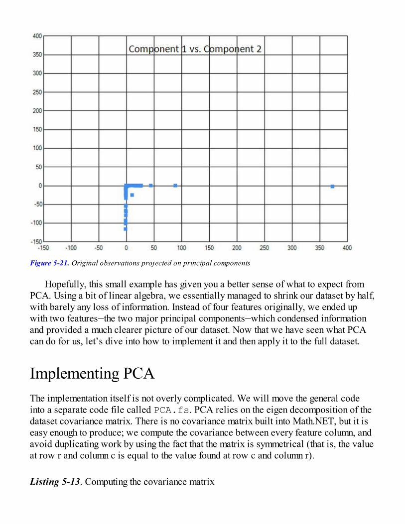
Figure 5-21. Original observations projected on principal components

Hopefully, this small example has given you a better sense of what to expect fromPCA. Using a bit of linear algebra, we essentially managed to shrink our dataset by half,with barely any loss of information. Instead of four features originally, we ended upwith two features—the two major principal components—which condensed informationand provided a much clearer picture of our dataset. Now that we have seen what PCAcan do for us, let’s dive into how to implement it and then apply it to the full dataset.

Implementing PCAThe implementation itself is not overly complicated. We will move the general codeinto a separate code file called PCA.fs. PCA relies on the eigen decomposition of thedataset covariance matrix. There is no covariance matrix built into Math.NET, but it iseasy enough to produce; we compute the covariance between every feature column, andavoid duplicating work by using the fact that the matrix is symmetrical (that is, the valueat row r and column c is equal to the value found at row c and column r).

Listing 5-13. Computing the covariance matrix

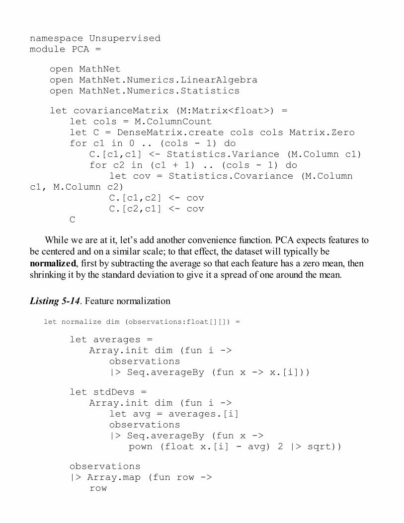
namespace Unsupervisedmodule PCA =

open MathNet open MathNet.Numerics.LinearAlgebra open MathNet.Numerics.Statistics

let covarianceMatrix (M:Matrix<float>) = let cols = M.ColumnCount let C = DenseMatrix.create cols cols Matrix.Zero for c1 in 0 .. (cols - 1) do C.[c1,c1] <- Statistics.Variance (M.Column c1) for c2 in (c1 + 1) .. (cols - 1) do let cov = Statistics.Covariance (M.Column c1, M.Column c2) C.[c1,c2] <- cov C.[c2,c1] <- cov C

While we are at it, let’s add another convenience function. PCA expects features tobe centered and on a similar scale; to that effect, the dataset will typically benormalized, first by subtracting the average so that each feature has a zero mean, thenshrinking it by the standard deviation to give it a spread of one around the mean.

Listing 5-14. Feature normalization

let normalize dim (observations:float[][]) =

let averages = Array.init dim (fun i -> observations |> Seq.averageBy (fun x -> x.[i]))

let stdDevs = Array.init dim (fun i -> let avg = averages.[i] observations |> Seq.averageBy (fun x -> pown (float x.[i] - avg) 2 |> sqrt))

observations |> Array.map (fun row -> row

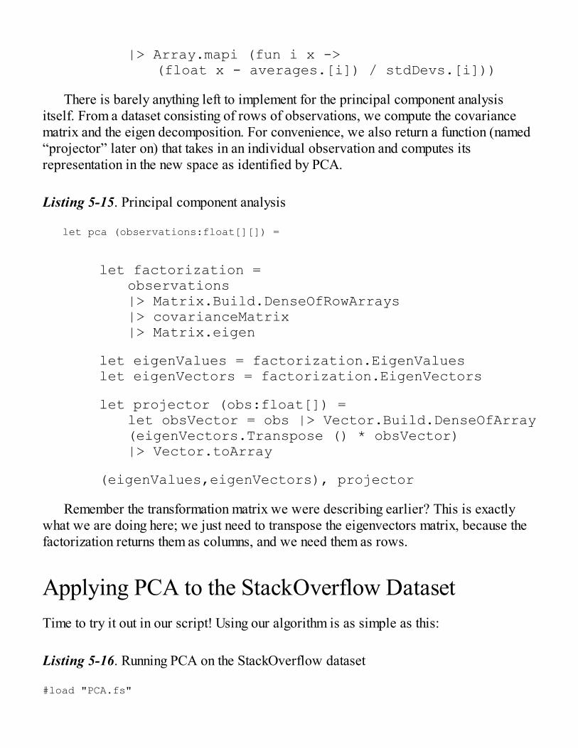
|> Array.mapi (fun i x -> (float x - averages.[i]) / stdDevs.[i]))

There is barely anything left to implement for the principal component analysisitself. From a dataset consisting of rows of observations, we compute the covariancematrix and the eigen decomposition. For convenience, we also return a function (named“projector” later on) that takes in an individual observation and computes itsrepresentation in the new space as identified by PCA.

Listing 5-15. Principal component analysis

let pca (observations:float[][]) =

let factorization = observations |> Matrix.Build.DenseOfRowArrays |> covarianceMatrix |> Matrix.eigen

let eigenValues = factorization.EigenValues let eigenVectors = factorization.EigenVectors

let projector (obs:float[]) = let obsVector = obs |> Vector.Build.DenseOfArray (eigenVectors.Transpose () * obsVector) |> Vector.toArray

(eigenValues,eigenVectors), projector

Remember the transformation matrix we were describing earlier? This is exactlywhat we are doing here; we just need to transpose the eigenvectors matrix, because thefactorization returns them as columns, and we need them as rows.

Applying PCA to the StackOverflow DatasetTime to try it out in our script! Using our algorithm is as simple as this:

Listing 5-16. Running PCA on the StackOverflow dataset

#load "PCA.fs"

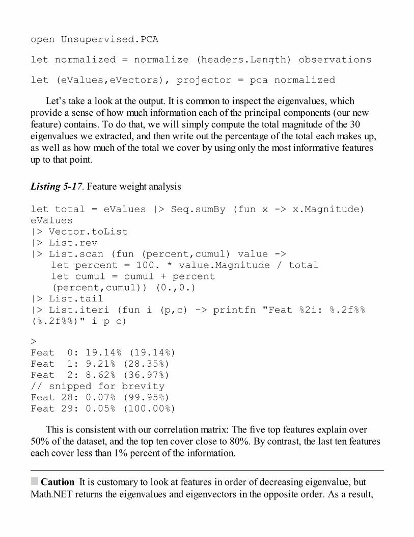
open Unsupervised.PCA

let normalized = normalize (headers.Length) observations

let (eValues,eVectors), projector = pca normalized

Let’s take a look at the output. It is common to inspect the eigenvalues, whichprovide a sense of how much information each of the principal components (our newfeature) contains. To do that, we will simply compute the total magnitude of the 30eigenvalues we extracted, and then write out the percentage of the total each makes up,as well as how much of the total we cover by using only the most informative featuresup to that point.

Listing 5-17. Feature weight analysis

let total = eValues |> Seq.sumBy (fun x -> x.Magnitude)eValues|> Vector.toList|> List.rev|> List.scan (fun (percent,cumul) value -> let percent = 100. * value.Magnitude / total let cumul = cumul + percent (percent,cumul)) (0.,0.)|> List.tail|> List.iteri (fun i (p,c) -> printfn "Feat %2i: %.2f%% (%.2f%%)" i p c)

>Feat 0: 19.14% (19.14%)Feat 1: 9.21% (28.35%)Feat 2: 8.62% (36.97%)// snipped for brevityFeat 28: 0.07% (99.95%)Feat 29: 0.05% (100.00%)

This is consistent with our correlation matrix: The five top features explain over50% of the dataset, and the top ten cover close to 80%. By contrast, the last ten featureseach cover less than 1% percent of the information.

Caution It is customary to look at features in order of decreasing eigenvalue, butMath.NET returns the eigenvalues and eigenvectors in the opposite order. As a result,

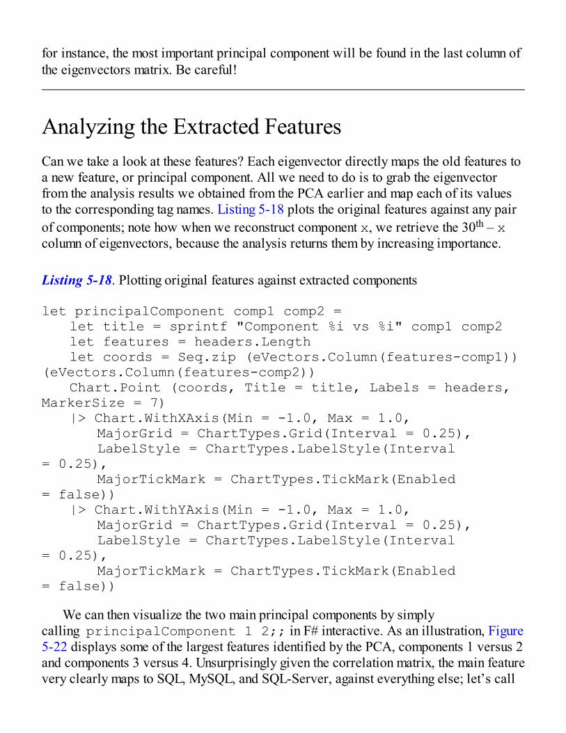
for instance, the most important principal component will be found in the last column ofthe eigenvectors matrix. Be careful!

Analyzing the Extracted FeaturesCan we take a look at these features? Each eigenvector directly maps the old features toa new feature, or principal component. All we need to do is to grab the eigenvectorfrom the analysis results we obtained from the PCA earlier and map each of its valuesto the corresponding tag names. Listing 5-18 plots the original features against any pairof components; note how when we reconstruct component x, we retrieve the 30th – xcolumn of eigenvectors, because the analysis returns them by increasing importance.

Listing 5-18. Plotting original features against extracted components

let principalComponent comp1 comp2 = let title = sprintf "Component %i vs %i" comp1 comp2 let features = headers.Length let coords = Seq.zip (eVectors.Column(features-comp1)) (eVectors.Column(features-comp2)) Chart.Point (coords, Title = title, Labels = headers, MarkerSize = 7) |> Chart.WithXAxis(Min = -1.0, Max = 1.0, MajorGrid = ChartTypes.Grid(Interval = 0.25), LabelStyle = ChartTypes.LabelStyle(Interval = 0.25), MajorTickMark = ChartTypes.TickMark(Enabled = false)) |> Chart.WithYAxis(Min = -1.0, Max = 1.0, MajorGrid = ChartTypes.Grid(Interval = 0.25), LabelStyle = ChartTypes.LabelStyle(Interval = 0.25), MajorTickMark = ChartTypes.TickMark(Enabled = false))

We can then visualize the two main principal components by simplycalling principalComponent 1 2;; in F# interactive. As an illustration, Figure5-22 displays some of the largest features identified by the PCA, components 1 versus 2and components 3 versus 4. Unsurprisingly given the correlation matrix, the main featurevery clearly maps to SQL, MySQL, and SQL-Server, against everything else; let’s call

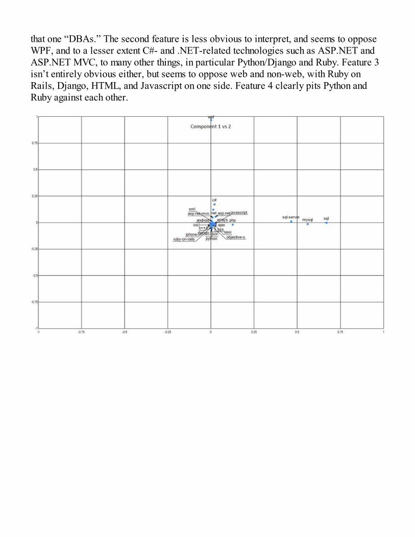
that one “DBAs.” The second feature is less obvious to interpret, and seems to opposeWPF, and to a lesser extent C#- and .NET-related technologies such as ASP.NET andASP.NET MVC, to many other things, in particular Python/Django and Ruby. Feature 3isn’t entirely obvious either, but seems to oppose web and non-web, with Ruby onRails, Django, HTML, and Javascript on one side. Feature 4 clearly pits Python andRuby against each other.

Figure 5-22. Main components (see source code package for details)

I would normally dig deeper and look into each of the top components to try tounderstand what they capture. However, this would involve producing a lot more charts,without adding much to the discussion. So I will leave it at that—feel free to investigatefurther and see what else there is to learn from this dataset!

Let’s look into another question instead: How do the original observations look,when seen through the lens of the new features? We just need to use the projectorfunction (which was part of the PCA outputs) to convert observations into the newcoordinates. Note that we precomputed the min and max values beforehand so as todisplay every chart on a comparable scale.

Listing 5-19. Plotting observations against the principal components

let projections comp1 comp2 =

let title = sprintf "Component %i vs %i" comp1 comp2 let features = headers.Length let coords = normalized |> Seq.map projector

|> Seq.map (fun obs -> obs.[features-comp1], obs.[features-comp2]) Chart.Point (coords, Title = title) |> Chart.WithXAxis(Min = -200.0, Max = 500.0, MajorGrid = ChartTypes.Grid(Interval = 100.), LabelStyle = ChartTypes.LabelStyle(Interval = 100.), MajorTickMark = ChartTypes.TickMark(Enabled = false)) |> Chart.WithYAxis(Min = -200.0, Max = 500.0, MajorGrid = ChartTypes.Grid(Interval = 100.), LabelStyle = ChartTypes.LabelStyle(Interval = 100.), MajorTickMark = ChartTypes.TickMark(Enabled = false))

Figure 5-23 displays the results for the same pairs of components we looked atearlier. These charts are not the most thrilling, but they still show some interestingpatterns. The first chart plots the “databases” component on the X axis, against theWPF/.NET component on the Y axis. First, most observations fall rather cleanly oneither axis, with a very large clump near the origin. What this indicates is that peoplewho care about one topic usually don’t care about the other (people who have largescores on SQL don’t score high on the other axis, and vice-versa), and that most peoplearen’t active in either topic. Also, observations are not evenly distributed: There are afew observations with very high scores, a large number close to zero, and few between.Given that we constructed our dataset by gathering the most active people for each tag,this isn’t surprising: We should expect to see some users with scores much larger thanthe average population.

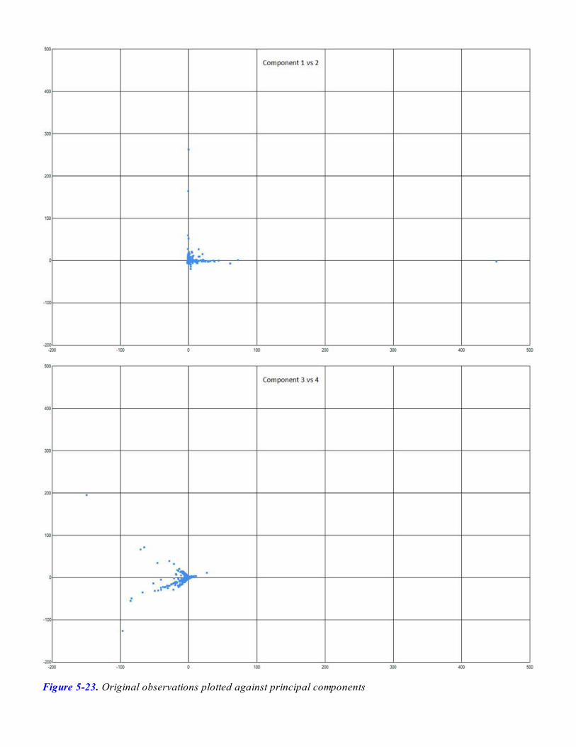
Figure 5-23. Original observations plotted against principal components

Tip The charts show a few large outliers, observations that are very far off theaverage. Outliers are a potential problem to watch out for in datasets. A couple of largeoutliers can produce distorted models, which become less representative of typical,average observations.

The second chart, which plots what seems to be web development on one axis, andRuby/Rails versus Python/Django on the other, is interesting. We still have a largeclump of people close to the origin who care about none of these topics, but then, as wemove toward the left, the population forks into two groups. My interpretation here is thatRuby and Python web app developers have some shared technologies of interest (JSON,javascript), but irreducible differences on language and framework.

Again, if we were really trying to get a solid understanding of this dataset, weshould investigate further, but we will leave it to you to do so if you are so inclined.Our main goal here was to illustrate what principal component analysis is about andwhere it can be helpful. In our situation, we managed to extract some interesting factsfrom the dataset without specifying what we were looking for. PCA spotted a topic thataligned with what we would call “databases,” and it recognized that while Rubyists andPythonistas disagree on what framework to use, many of them work on web applicationdevelopment.

PCA and cluster analysis have some similarities, in that they both create an effectivesummary of data without supervision. However, they differ profoundly in the way theyapproach the problem. Unlike cluster analysis, which extracts groups of observationswith similar behavior, PCA reorganizes the data, creating new features, recombining theoriginal ones into new ones that describe broad differences in behavior betweenobservations. In the process, it creates a high-level, comprehensive “map” of thedataset, describing the data in a more effective manner by using fewer but moreinformative features.

Rather than spend more time on PCA, we will turn next to a different topic: makingrecommendations. If you think about it, with both k-means and PCA, we simply took adataset and searched for similarities and differences between users, looking at theirhistorical behavior—and in both cases, we did find patterns. Perhaps we can use similarideas to look for patterns in data so as to make recommendations—for instance, tosuggest to users what tags they might be interested in checking out.

Making RecommendationsIf you take a step back and consider what we did with clustering and principal

component analysis, in both cases we looked at the behavior of many individuals overtime and searched for similarities between them. And, in both cases, it worked. We allhave our individual personalities, but in the end, very few people are entirely unique.Take a sufficiently large group of people, and you will find someone who is rathersimilar to you.

This is the basic idea behind collaborative filtering. In a nutshell, the idea is this: Ifyou and I have expressed the same preferences for a set of items, then there is a goodchance that we will have similar tastes for other items, too. For example, if we happento like and dislike the same ten movies, and I know you happened to enjoy anothermovie I haven’t seen yet, it’s plausible that I will enjoy that movie as well, and it wouldbe reasonable for you to recommend that I watch that movie.

Of course, there is a chance that this is just a fluke. Perhaps the ten movies wehappen to agree on have some common trait, say, action movies, and that other movie isvery different. You might enjoy romance, and I don’t. However, if instead of justcomparing your taste profile and mine, we started looking across many users, and thereis a general agreement that people who enjoy these movies also enjoy that other one, wecan feel more confident that this is a good recommendation. Conversely, if this is afluke, then no agreement would emerge: Some people who enjoy action movies willenjoy romance, some won’t, and no pattern will emerge.

Note that we could also take the question in a different direction. Instead of lookingat it from the direction of users (do these two persons have similar taste profiles?), wecould look at it from a movie perspective, and compare the movie profiles. If peoplewho rated movie A tend to rate movie B the same way, for instance, then based on whatyou thought of movie A, it would be reasonable to make a guess on what you will thinkabout B, and make a recommendation based on your predicted level of interest.

A Primitive Tag RecommenderLet’s apply this idea to our StackOverflow dataset. This example will be a bit artificial,and is intended mostly as a sketch outlining how one might approach the problem. Whatwe will do here is extract 100 “test” users from our dataset and try to predict which ofthe 10 last tags they might be interested in, based on the 20 first tags. In other words,let’s imagine that these are relatively new users, and the only thing we know is whattags they have been active in so far. Based on their history, can we suggest tags? Giventhat we also know what they actually did for the 10 remaining tags, we will be able tovalidate our guesses by comparing them to the true behavior.

Let’s try out recommendations based on user profiles. Our approach here will besimple: take a user, and, for the 20 tags we know, compare his (or her) profile with theknown users and determine how similar they are. Then, predict the level of interest for

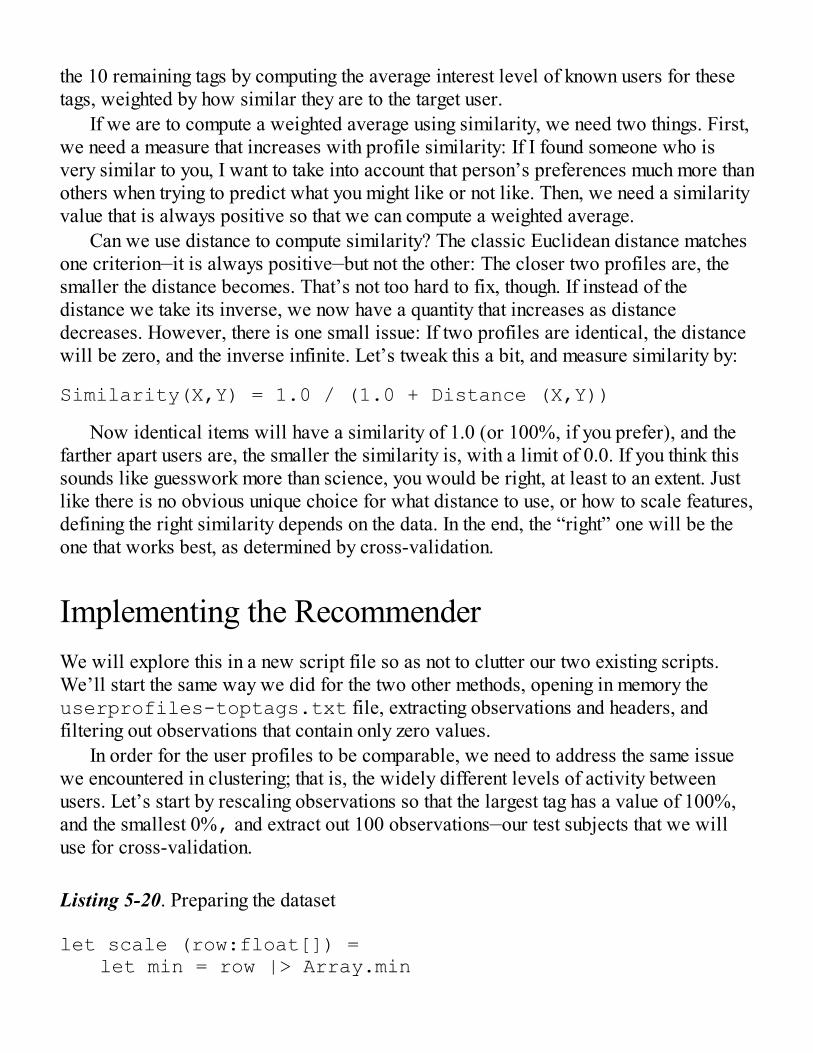
the 10 remaining tags by computing the average interest level of known users for thesetags, weighted by how similar they are to the target user.

If we are to compute a weighted average using similarity, we need two things. First,we need a measure that increases with profile similarity: If I found someone who isvery similar to you, I want to take into account that person’s preferences much more thanothers when trying to predict what you might like or not like. Then, we need a similarityvalue that is always positive so that we can compute a weighted average.

Can we use distance to compute similarity? The classic Euclidean distance matchesone criterion—it is always positive—but not the other: The closer two profiles are, thesmaller the distance becomes. That’s not too hard to fix, though. If instead of thedistance we take its inverse, we now have a quantity that increases as distancedecreases. However, there is one small issue: If two profiles are identical, the distancewill be zero, and the inverse infinite. Let’s tweak this a bit, and measure similarity by:

Similarity(X,Y) = 1.0 / (1.0 + Distance (X,Y))

Now identical items will have a similarity of 1.0 (or 100%, if you prefer), and thefarther apart users are, the smaller the similarity is, with a limit of 0.0. If you think thissounds like guesswork more than science, you would be right, at least to an extent. Justlike there is no obvious unique choice for what distance to use, or how to scale features,defining the right similarity depends on the data. In the end, the “right” one will be theone that works best, as determined by cross-validation.

Implementing the RecommenderWe will explore this in a new script file so as not to clutter our two existing scripts.We’ll start the same way we did for the two other methods, opening in memory theuserprofiles-toptags.txt file, extracting observations and headers, andfiltering out observations that contain only zero values.

In order for the user profiles to be comparable, we need to address the same issuewe encountered in clustering; that is, the widely different levels of activity betweenusers. Let’s start by rescaling observations so that the largest tag has a value of 100%,and the smallest 0%, and extract out 100 observations—our test subjects that we willuse for cross-validation.

Listing 5-20. Preparing the dataset

let scale (row:float[]) = let min = row |> Array.min

let max = row |> Array.max if min = max then row else row |> Array.map (fun x -> (x - min) / (max - min))

let test = observations.[..99] |> Array.map scalelet train = observations.[100..] |> Array.map scale

Before diving into the prediction part, we need a couple of helpers: a similarityfunction, which will use distance. For convenience, we will also write a weightsfunction, which will take an array of floats and rescale them so that they sum up to100% and can be used in a weighted average, and a split, which will separate the 20first tags from the 10 “unknown” ones.

Listing 5-21. Similarity and utility functions

let distance (row1:float[]) (row2:float[]) = (row1,row2) ||> Array.map2 (fun x y -> pown (x - y) 2) |> Array.sum

let similarity (row1:float[]) (row2:float[]) = 1. / (1. + distance row1 row2)

let split (row:float[]) = row.[..19],row.[20..]

let weights (values:float[]) = let total = values |> Array.sum values |> Array.map (fun x -> x / total)

Tip The ||> operator can be used with functions that operate on two collections atonce, such as Array.map2 or Array.zip. Instead of passing two arguments to thefunction, they can be fed in as a tuple with the “double-pipe-forward” operator, whichlooks more consistent in a pipeline of operations.

We are now ready to dive into the prediction part. Given a user history, we willretain only the part we are supposed to know (the 20 first tags), and then we will

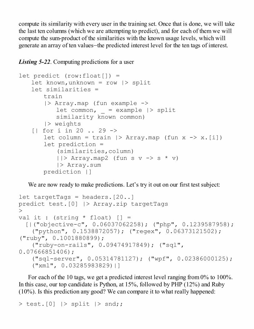
compute its similarity with every user in the training set. Once that is done, we will takethe last ten columns (which we are attempting to predict), and for each of them we willcompute the sum-product of the similarities with the known usage levels, which willgenerate an array of ten values—the predicted interest level for the ten tags of interest.

Listing 5-22. Computing predictions for a user

let predict (row:float[]) = let known,unknown = row |> split let similarities = train |> Array.map (fun example -> let common, _ = example |> split similarity known common) |> weights [| for i in 20 .. 29 -> let column = train |> Array.map (fun x -> x.[i]) let prediction = (similarities,column) ||> Array.map2 (fun s v -> s * v) |> Array.sum prediction |]

We are now ready to make predictions. Let’s try it out on our first test subject:

let targetTags = headers.[20..]predict test.[0] |> Array.zip targetTags>val it : (string * float) [] = [|("objective-c", 0.06037062258); ("php", 0.1239587958); ("python", 0.1538872057); ("regex", 0.06373121502); ("ruby", 0.1001880899); ("ruby-on-rails", 0.09474917849); ("sql", 0.07666851406); ("sql-server", 0.05314781127); ("wpf", 0.02386000125); ("xml", 0.03285983829)|]

For each of the 10 tags, we get a predicted interest level ranging from 0% to 100%.In this case, our top candidate is Python, at 15%, followed by PHP (12%) and Ruby(10%). Is this prediction any good? We can compare it to what really happened:

> test.[0] |> split |> snd;;

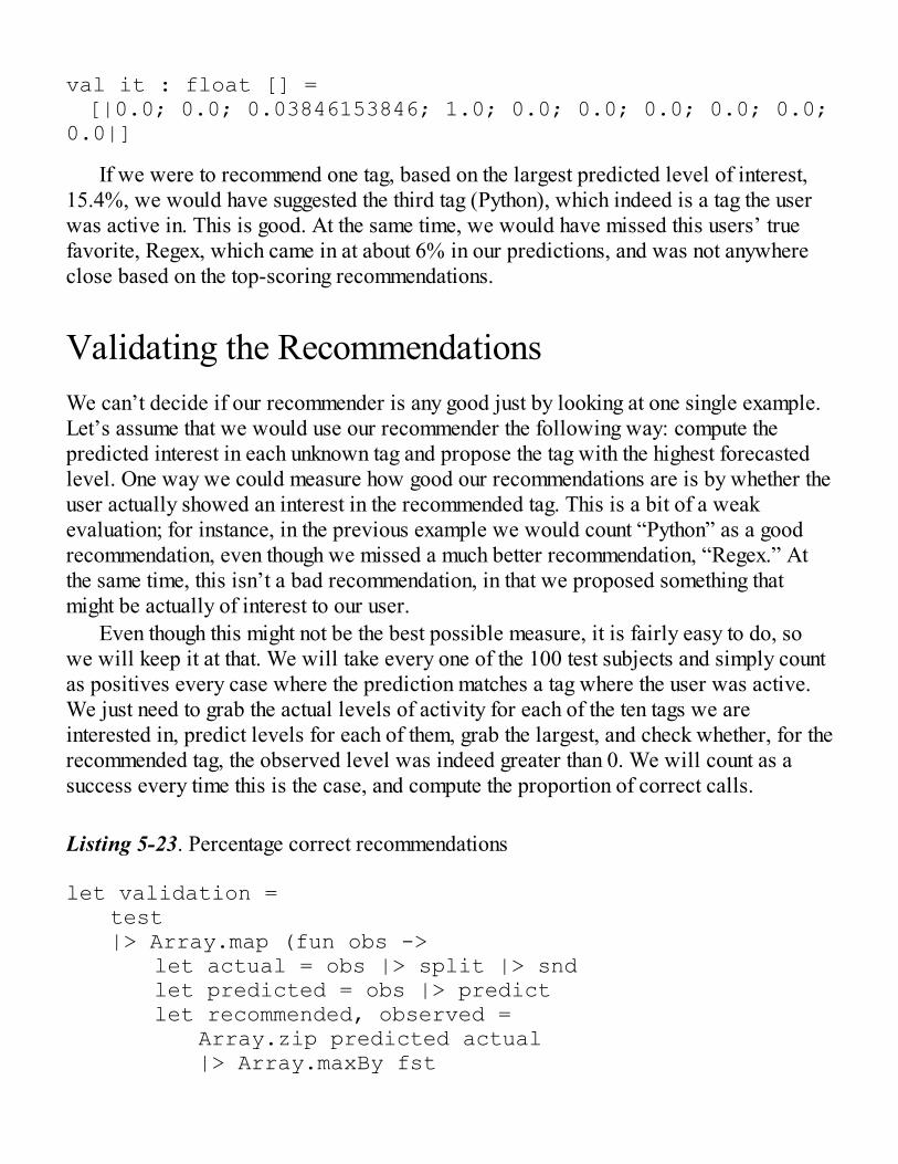
val it : float [] = [|0.0; 0.0; 0.03846153846; 1.0; 0.0; 0.0; 0.0; 0.0; 0.0; 0.0|]

If we were to recommend one tag, based on the largest predicted level of interest,15.4%, we would have suggested the third tag (Python), which indeed is a tag the userwas active in. This is good. At the same time, we would have missed this users’ truefavorite, Regex, which came in at about 6% in our predictions, and was not anywhereclose based on the top-scoring recommendations.

Validating the RecommendationsWe can’t decide if our recommender is any good just by looking at one single example.Let’s assume that we would use our recommender the following way: compute thepredicted interest in each unknown tag and propose the tag with the highest forecastedlevel. One way we could measure how good our recommendations are is by whether theuser actually showed an interest in the recommended tag. This is a bit of a weakevaluation; for instance, in the previous example we would count “Python” as a goodrecommendation, even though we missed a much better recommendation, “Regex.” Atthe same time, this isn’t a bad recommendation, in that we proposed something thatmight be actually of interest to our user.

Even though this might not be the best possible measure, it is fairly easy to do, sowe will keep it at that. We will take every one of the 100 test subjects and simply countas positives every case where the prediction matches a tag where the user was active.We just need to grab the actual levels of activity for each of the ten tags we areinterested in, predict levels for each of them, grab the largest, and check whether, for therecommended tag, the observed level was indeed greater than 0. We will count as asuccess every time this is the case, and compute the proportion of correct calls.

Listing 5-23. Percentage correct recommendations

let validation = test |> Array.map (fun obs -> let actual = obs |> split |> snd let predicted = obs |> predict let recommended, observed = Array.zip predicted actual |> Array.maxBy fst

if observed > 0. then 1. else 0.) |> Array.average |> printfn "Correct calls: %f"

According to this metric, we get 32% correct recommendations. Let’s face it—thatisn’t overly impressive. However, we don’t really have a baseline to compare itagainst. The most naïve prediction we could make would be to simply predict the tagwith the highest average rating and completely ignore any similarity between users.Let’s do a quick-and-dirty evaluation of that approach.

Listing 5-24. Naïve recommendation accuracy

let averages = [| for i in 20 .. 29 -> train |> Array.averageBy(fun row -> row.[i]) |]

let baseline = test |> Array.map (fun obs -> let actual = obs |> split |> snd let predicted = averages let recommended, observed = Array.zip predicted actual |> Array.maxBy fst if observed > 0. then 1. else 0.) |> Array.average |> printfn "Correct calls: %f"

Using a naïve recommendation, our percentage accuracy drops to 13% correct calls.While this doesn’t make our 32% great, it proves the point that our similarity-basedapproach is doing something right.

We will leave our recommendation engine as is, and won’t try to improve it further.I am fairly certain we could make it much better, but I don’t think we would gain muchinsight in the process. I’ll finish instead with a couple of considerations that might beworth keeping in mind, in case you want to explore the problem further, either on thatdataset or on another one.

First, our sample is not the most typical case for using that approach. In theprototypical scenario, you know how people rated certain items and don’t know whatthey did for others; for instance, what movies a person watched and how they ratedthem, from terrible to awesome. This is a bit different from our situation, in two ways:In that situation, we know if an item has been rated or not, and all ratings have a

consistent scale. By contrast, our dataset has vastly different scales for each userbecause we measure activity, and we don’t have a clear distinction between emptyvalues (the user has never seen this tag) or uninteresting tags (the user has hadopportunities to view that tag but isn’t interested). As a result, comparing users’ or tags’similarity is made a bit complicated.

In a more typical situation, we would face slightly different challenges. A rowwould have mostly unknown values (all the items the user hasn’t rated yet), andcomparing that user with others would require comparing them only across commonitems, which is more involved that simply computing a distance between two completerows. This also points at a limitation with the collaborative filtering approach, which isperhaps less obvious in our example. When a brand new user shows up in our system,there is no history available for that user, and therefore we have nothing usable withwhich to produce a recommendation. This is known as the “cold-start” problem. If youplay a bit further with our model, you’ll see more or less the following: By default, therecommender will predict Python, which is the most popular tag among our ten targettags. Only in situations where we have a strong, well-defined user profile does theengine produce different recommendations. This is a result you would expect in general:With limited information, engines will recommend broadly popular items, and will onlystart producing “interesting” picks for users who provided a lot of information.

A final note on this subject: In order to produce a recommendation, we had to scanthrough every single user. This is an obviously expensive operation, which hints atobvious scaling problems. First, we could have tried to approach the problem byfeature, instead of by user, and try to detect similarity between 30 tags, instead of 1,600users; we could even precompute similarities between columns, which would reducequite a bit the amount of computations.

So What Have We Learned?In this chapter, we introduced unsupervised learning. In supervised learning methods(such as classification or regression), algorithms are geared toward answering aspecific question, guided by a training set of examples to learn from. By contrast,unsupervised learning is about automatically identifying interesting features or structurein “plain” data, without explicit guidance from the user. In the process of exploringunsupervised techniques, we discussed quite a few topics. Our goal was to take adataset and see if, instead of manually exploring the data in the hopes of spottinginteresting patterns, we could apply more mechanical methods to systematically extractand summarize information from the data.

We applied two complementary techniques to the data: clustering with the k-means

algorithm, and principal component analysis. They share similar traits: both attempt toreduce the dataset into a more condensed representation by finding patterns in the dataand simplifying information, grouping similar elements together based on a certainnotion of distance. The two approaches differ in what type of patterns they are lookingfor. K-means clustering tries to group observations in clusters, so that, ideally, itemswithin the same cluster are close to each other, and clusters themselves are as differentas possible. K-means identifies centroids, which are essentially “archetypes,” and aresufficient to describe a large class of observations.

By contrast, principal component analysis doesn’t focus on similarities between theobservations themselves, but rather on what traits vary together, and how observationsdiffer from the average. By inspecting the covariance matrix, it identifies features thatmove together and attempts to provide an alternate representation, grouping togetherfeatures that either typically evolve in the same or in opposite directions, and organizingthem in a way that emphasizes the largest differentiating factors between observations.

In both cases, a key benefit is a simpler, more compact description of the dataset. Inthe case of clustering, instead of many unique observations, we can describe the datasetin terms of a few archetypes, which exhibit a consistent behavior. In the case of PCA,instead of multiple unrelated features, we get a couple of new features, the principalcomponents, which strongly differentiate observations. As a result, instead of amultitude of hard-to-interpret facts, we can start developing an understanding of thesedimensions that is more meaningful and easier to reason with than the raw data is. Thesemethods allow us to develop a vocabulary to talk about the data more efficiently, andperhaps to gain a better understanding of how the data “works” and how we can deriveinsight out of it.

At the same time, both techniques are simply searching for specific types of patternsin data. There is no guarantee that such patterns actually exist, and, even if they do, thereis no guarantee that they will be interesting to us. We might find clusters that are of nopractical interest; they could be nonactionable, or state trivially obvious facts, forinstance.

Another aspect we discussed was the notion of distance and the importance ofthinking about scale. Clustering groups observations that are close, and in that frame, itis crucial to supply the algorithm with a meaningful distance. In that context, we endedup preprocessing our observations so as to reduce them to comparable user profiles.PCA groups features that have similar variations from the average, which leads us to adiscussion on normalization and correlations, two notions that revolve around the ideaof rescaling measures so that their variations are comparable.

Finally, we sketched out how similar ideas could be used, not to extract informationfrom a dataset, but to produce recommendations. In all three cases, we looked atmultiple individuals and how they behaved, and realized that in spite of individualdifferences, collectively there existed some patterns. In the last example, starting from

the assumption that people who have behaved in a similar fashion in many situationswill likely behave similarly in others, we explored how we could approach makingrecommendations by detecting similarities and applying them in order to determine whatbehavior was likely to occur in unknown cases.

CHAPTER 6

Trees and Forests

Making Predictions from Incomplete DataOne of my nieces’ favorite games is a guessing game. One person thinks of something,and the other player tries to figure out what that something is by asking only yes or noquestions. If you have played this game before, you have probably seen the followingpattern in action: first ask questions that eliminate large categories of possible answers,such as “Is it an animal?”, and progressively narrow down the focus of the questions asyou gather more information. This is a more effective strategy than asking from the get-go, say, “Did you think about a zebra?” On the one hand, if the answer is “yes,” you aredone, as there is only one possible answer. On the other hand, if the answer is “no,” youare in a rather bad spot, having learned essentially nothing.

Decision trees are classifiers that operate in a fashion similar to that game. Theymimic the way we humans make diagnoses by asking a series of questions, trying toeliminate bad answers quickly, and deciding what question to ask next, based oneverything we have learned so far. In that context, features can be thought of asquestions one can ask about the characteristics of an observation. A decision tree willlearn from a training set, analyzing it to determine which feature provides the mostinformation, given everything that is known at that point about the observation it is tryingto classify.

In this chapter, we will work on a classic dataset and progressively learnincreasingly powerful classifiers, starting from decision stumps and expanding intodecision trees and forests. Along the way, we will do the following:

Learn how to construct flexible decision trees that can handlevirtually any type of data, including situations where data ismissing. We will also see how F# types like discriminated unionsand options can be used to model tree-like structures very

effectively.

Introduce entropy as a way to measure how much information adataset contains, and use it to compare features and decide whichones should be selected.

Discuss the risks of over-fitting, as well as ways to address it. Inparticular, we will explore more-advanced methods of cross-validation, such as k-folds, and how the same ideas can leadtoward ensemble methods, a general approach that aggregatesmultiple simple predictors into a robust one.

Our Challenge: Sink or Swim on theTitanicThe dataset we will be working with in this chapter is a classic. Using the list ofpassengers who embarked the Titanic, and some demographic information about each ofthem, our goal will be to predict their fate. Both the dataset and the problem areinteresting, for a couple of reasons. First, the question at hand is typical of a large classof problems, once you get past its somewhat macabre nature. “Will that visitor click thislink on the website?” or “Which customers will pick the small, medium, or largeorder?” are essentially the same problem: Using what information you have aboutindividuals and how they behaved in the past, you are trying to build a classificationmodel to predict one outcome from a limited set of possible ones.

Then, the data itself is quite typical of real-world situations, in that it is messy. Itcontains a mix of different types of features, from numeric (how much did the passengerpay for their ticket?) to categorical (was the passenger male or female?), witheverything in between (passenger name and title). Some of the data is missing as well.Ideally, we’d like a classifier that is flexible enough to handle all these variableswithout too much of a hassle.

Finally, the data is interesting by itself, for obvious historical reasons. The Titanicdisaster has fascinated people over time, and while there is little practical use increating a predictive model for a one-time accident that occurred nearly a century ago,the dataset provides an opportunity to see what type of insight one can gain by analyzingits data.

Getting to Know the Dataset

The specific dataset we will use comes from the Kaggle competition “Titanic: MachineLearning from Disaster”: https://www.kaggle.com/c/titanic-gettingStarted. Variants can easily be found online (, for instance,http://www.encyclopedia-titanica.org). However, we thought it wouldbe fun to use the Kaggle reference dataset; that way, you can try out your skills and seehow you fare. For convenience, we uploaded the same dataset on OneDrive here:http://1drv.ms/1HUh1ny.

The dataset is a CSV file, titanic.csv, nicely organized with a header rowdescribing what each of the 12 available columns is. Of course we could write a bit ofcode to parse it, but why not use the CSV type provider? Let’s create a solution with anF# project Titanic, add the titanic.csv file to that project, and add the fsharp.dataNuGet package to the project.

We are now ready to begin exploring the data. In the script.fsx file, let’s add areference to FSharp.Data (the specifics of the path might vary, depending on the currentlatest version of the package), create a Titanic type by looking at our sample data,and add a type alias Passenger so that we can refer to each row of the dataset in amore intuitive way. We can now read our dataset.

Listing 6-1. Using the CSV type provider to read the Titanic dataset

#r @".\packages\FSharp.Data.2.2.2\lib\net40\FSharp.Data.dll"open FSharp.Data

type Titanic = CsvProvider<"titanic.csv">type Passenger = Titanic.Row

let dataset = Titanic.GetSample ()

The CSV type provider created a nice type for us, complete with properties, givingus all the benefits of types when exploring our data. We can now get to work. If our goalis to predict who survives or dies, a first step is to get a baseline for that value. Let’sfirst count how many passengers are in each category, and then figure out the probabilityfor an individual passenger to survive, by adding the following code to our script andrunning it in the F# Interactive:

dataset.Rows|> Seq.countBy (fun passenger -> passenger.Survived)|> Seq.iter (printfn "%A")

dataset.Rows

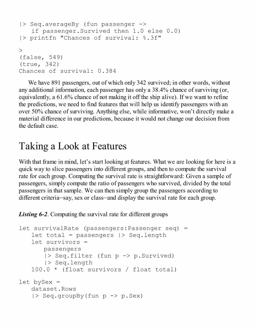
|> Seq.averageBy (fun passenger -> if passenger.Survived then 1.0 else 0.0)|> printfn "Chances of survival: %.3f"

>(false, 549)(true, 342)Chances of survival: 0.384

We have 891 passengers, out of which only 342 survived; in other words, withoutany additional information, each passenger has only a 38.4% chance of surviving (or,equivalently, a 61.6% chance of not making it off the ship alive). If we want to refinethe predictions, we need to find features that will help us identify passengers with anover 50% chance of surviving. Anything else, while informative, won’t directly make amaterial difference in our predictions, because it would not change our decision fromthe default case.

Taking a Look at FeaturesWith that frame in mind, let’s start looking at features. What we are looking for here is aquick way to slice passengers into different groups, and then to compute the survivalrate for each group. Computing the survival rate is straightforward: Given a sample ofpassengers, simply compute the ratio of passengers who survived, divided by the totalpassengers in that sample. We can then simply group the passengers according todifferent criteria—say, sex or class—and display the survival rate for each group.

Listing 6-2. Computing the survival rate for different groups

let survivalRate (passengers:Passenger seq) = let total = passengers |> Seq.length let survivors = passengers |> Seq.filter (fun p -> p.Survived) |> Seq.length 100.0 * (float survivors / float total)

let bySex = dataset.Rows |> Seq.groupBy(fun p -> p.Sex)

bySex|> Seq.iter (fun (s,g) -> printfn "Sex %A: %f" s (survivalRate g))

let byClass = dataset.Rows |> Seq.groupBy (fun p -> p.Pclass)

byClass|> Seq.iter (fun (s,g) -> printfn "Class %A: %f" s (survivalRate g))>Sex "male": 18.890815Sex "female": 74.203822Class 3: 24.236253Class 1: 62.962963Class 2: 47.282609

Clearly, both of these features are highly informative. As it turns out, with a 74%chance of surviving, being a lady on the Titanic was a very good idea. Similarly, firstclass passengers had a fair chance of making it off alive (63%), whereas the poor sodsin third class had much grimmer prospects, with a 24% chance of surviving. Toparaphrase George Orwell, “All passengers are equal, but some passengers are moreequal than others.” There are some fairly obvious sociological interpretations here, but Iwill leave that to you: After all, the data shows what is, but says nothing about why thatis.

Building a Decision StumpThis is enough information for us to implement a super simple classifier, as well as aprocedure to train it. Take sample data, break the sample into different groups along thelines of what we just did, and, for each group, predict the most frequent label. This typeof model is called a decision stump, the shortest possible tree you could build. It is thebuilding block of trees, and is a minimal classifier, which commonly appears as abuilding block in other models.

How could we go about building a stump based on passenger sex, for example?First, I would take all passengers from my sample and break them into groups accordingto the value of my chosen feature, in this case, their sex value (“male” or “female”).Then, for each group, I would look up the value of my chosen label, in our case whetherthey survived or not, and identify the most frequently appearing one for each group. We

can then build a classifier (the stump): Take a passenger as input, compute the featurevalue, look that value up in the groups, and return the groups’ most frequent label (seeFigure 6-1).

Figure 6-1. Building a decision stump for survival using sex as a feature

Note In previous chapters, we used the term class to describe the predictions of aclassifier. Here, we will use label instead, which is also common. In our case, it isconvenient, because the passenger class is a feature of our dataset, and using class forboth would introduce some potential ambiguities.

We can actually make this process entirely generic if we make both the feature andthe label into functions that extract a value from an observation. Suppose that instead ofpassengers I had a sequence of items of generic type 'a; then a feature is simply afunction that, when given an 'a, returns a value 'b; similarly the label takes an 'a andgives you back another type 'c. In our particular case, 'a will be a Passenger, 'ba string (taking value “male” or “female”), and 'c a Boolean (survived, or not). Theonly additional requirement on our types is that 'b and 'c need to support equality,because we need to group and count by both feature and label value.

So, how does our implementation look? Pretty much the way we described it:

Listing 6-3. Learning a decision stump

let mostFrequentLabelIn group = group

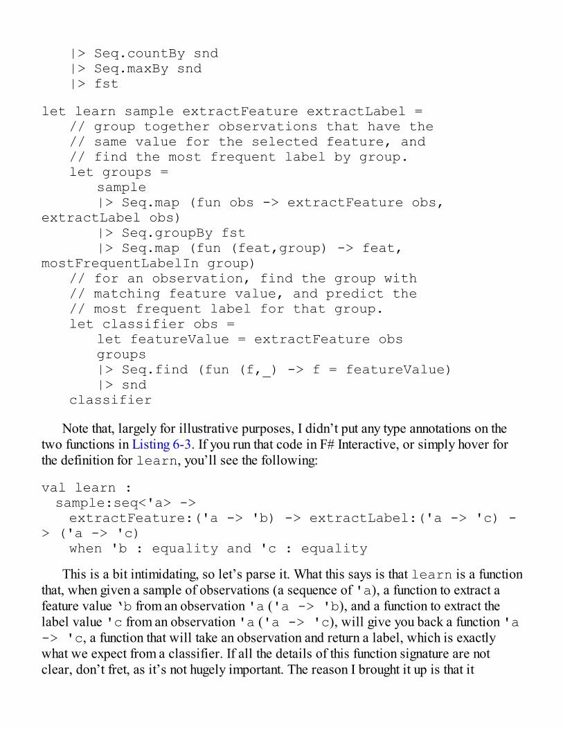
|> Seq.countBy snd |> Seq.maxBy snd |> fst

let learn sample extractFeature extractLabel = // group together observations that have the // same value for the selected feature, and // find the most frequent label by group. let groups = sample |> Seq.map (fun obs -> extractFeature obs, extractLabel obs) |> Seq.groupBy fst |> Seq.map (fun (feat,group) -> feat, mostFrequentLabelIn group) // for an observation, find the group with // matching feature value, and predict the // most frequent label for that group. let classifier obs = let featureValue = extractFeature obs groups |> Seq.find (fun (f,_) -> f = featureValue) |> snd classifier

Note that, largely for illustrative purposes, I didn’t put any type annotations on thetwo functions in Listing 6-3. If you run that code in F# Interactive, or simply hover forthe definition for learn, you’ll see the following:

val learn : sample:seq<'a> -> extractFeature:('a -> 'b) -> extractLabel:('a -> 'c) -> ('a -> 'c) when 'b : equality and 'c : equality

This is a bit intimidating, so let’s parse it. What this says is that learn is a functionthat, when given a sample of observations (a sequence of 'a), a function to extract afeature value ‘b from an observation 'a ('a -> 'b), and a function to extract thelabel value 'c from an observation 'a ('a -> 'c), will give you back a function 'a-> 'c, a function that will take an observation and return a label, which is exactlywhat we expect from a classifier. If all the details of this function signature are notclear, don’t fret, as it’s not hugely important. The reason I brought it up is that it

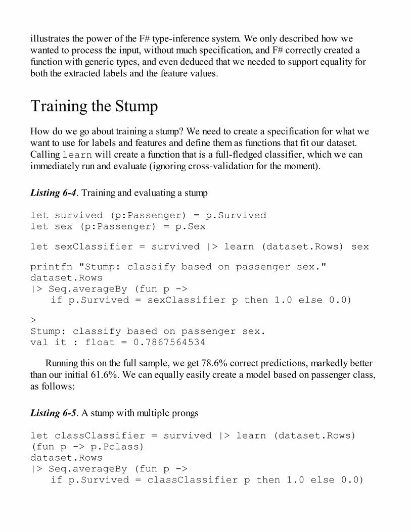
illustrates the power of the F# type-inference system. We only described how wewanted to process the input, without much specification, and F# correctly created afunction with generic types, and even deduced that we needed to support equality forboth the extracted labels and the feature values.

Training the StumpHow do we go about training a stump? We need to create a specification for what wewant to use for labels and features and define them as functions that fit our dataset.Calling learn will create a function that is a full-fledged classifier, which we canimmediately run and evaluate (ignoring cross-validation for the moment).

Listing 6-4. Training and evaluating a stump

let survived (p:Passenger) = p.Survivedlet sex (p:Passenger) = p.Sex

let sexClassifier = survived |> learn (dataset.Rows) sex

printfn "Stump: classify based on passenger sex."dataset.Rows|> Seq.averageBy (fun p -> if p.Survived = sexClassifier p then 1.0 else 0.0)

>Stump: classify based on passenger sex.val it : float = 0.7867564534

Running this on the full sample, we get 78.6% correct predictions, markedly betterthan our initial 61.6%. We can equally easily create a model based on passenger class,as follows:

Listing 6-5. A stump with multiple prongs

let classClassifier = survived |> learn (dataset.Rows) (fun p -> p.Pclass)dataset.Rows|> Seq.averageBy (fun p -> if p.Survived = classClassifier p then 1.0 else 0.0)

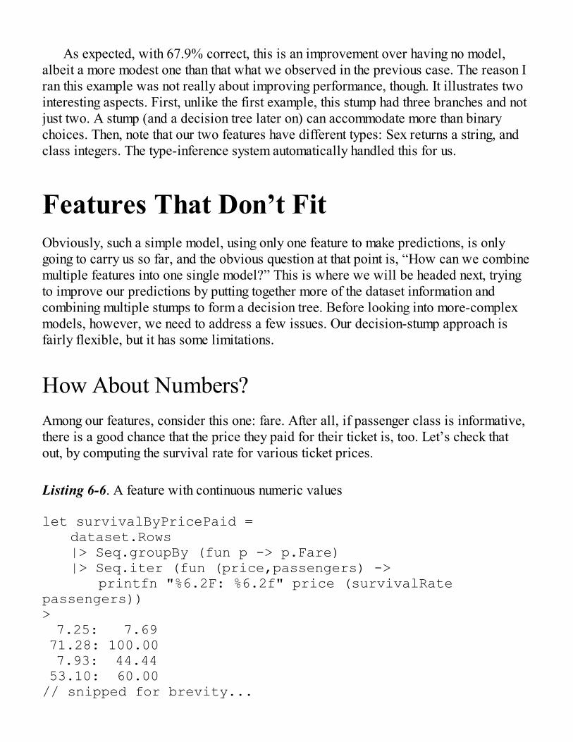
As expected, with 67.9% correct, this is an improvement over having no model,albeit a more modest one than that what we observed in the previous case. The reason Iran this example was not really about improving performance, though. It illustrates twointeresting aspects. First, unlike the first example, this stump had three branches and notjust two. A stump (and a decision tree later on) can accommodate more than binarychoices. Then, note that our two features have different types: Sex returns a string, andclass integers. The type-inference system automatically handled this for us.

Features That Don’t FitObviously, such a simple model, using only one feature to make predictions, is onlygoing to carry us so far, and the obvious question at that point is, “How can we combinemultiple features into one single model?” This is where we will be headed next, tryingto improve our predictions by putting together more of the dataset information andcombining multiple stumps to form a decision tree. Before looking into more-complexmodels, however, we need to address a few issues. Our decision-stump approach isfairly flexible, but it has some limitations.

How About Numbers?Among our features, consider this one: fare. After all, if passenger class is informative,there is a good chance that the price they paid for their ticket is, too. Let’s check thatout, by computing the survival rate for various ticket prices.

Listing 6-6. A feature with continuous numeric values

let survivalByPricePaid = dataset.Rows |> Seq.groupBy (fun p -> p.Fare) |> Seq.iter (fun (price,passengers) -> printfn "%6.2F: %6.2f" price (survivalRate passengers))> 7.25: 7.69 71.28: 100.00 7.93: 44.44 53.10: 60.00// snipped for brevity...

5.00: 0.00 9.85: 0.00 10.52: 0.00

The numbers are right, but this doesn’t seem like a good way to approach thisfeature. The fare was broken into 248 different individual cases, most of them with a0% or 100% survival rate. If we follow this model, passengers who paid 39.4000 fortheir ticket have a 100% chance of surviving; those who paid 39.6000 only 50%; andthose who paid 39.6875 have a 0% chance of making it alive. This is clearly silly.

Our problem here is that fare and, say, class, are not of the same nature. Class takesdiscrete states (you are in first, second, or third class; there are no other choices)whereas fare could, in principle, take infinitely many values. Another way these twofeatures differ is that fare represents an actual number; for instance, you can add twofares together, or subtract one from another, whereas the sum of passenger classesdoesn’t make any sense.

The issue here is that our stump can handle only categorical features; how can weincorporate continuous data? One approach is to reduce the problem to a knownproblem, and transform fare into a categorical feature. For instance, we could create anew feature, “fare level,” with two levels, Cheap or Expensive, depending on whetherthe fare was below or above the average.

Listing 6-7. Converting fare into discrete bins

let averageFare = dataset.Rows |> Seq.averageBy (fun p -> p.Fare)

let fareLevel (p:Passenger) = if p.Fare < averageFare then "Cheap" else "Expensive"

printfn "Stump: classify based on fare level."let fareClassifier = survived |> learn (dataset.Rows) fareLevel

dataset.Rows|> Seq.averageBy (fun p -> if p.Survived = fareClassifier p then 1.0 else 0.0)

>

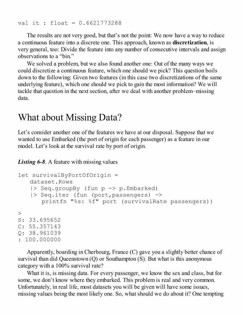
val it : float = 0.6621773288

The results are not very good, but that’s not the point: We now have a way to reducea continuous feature into a discrete one. This approach, known as discretization, isvery general, too: Divide the feature into any number of consecutive intervals and assignobservations to a “bin.”

We solved a problem, but we also found another one: Out of the many ways wecould discretize a continuous feature, which one should we pick? This question boilsdown to the following: Given two features (in this case two discretizations of the sameunderlying feature), which one should we pick to gain the most information? We willtackle that question in the next section, after we deal with another problem—missingdata.

What about Missing Data?Let’s consider another one of the features we have at our disposal. Suppose that wewanted to use Embarked (the port of origin for each passenger) as a feature in ourmodel. Let’s look at the survival rate by port of origin.

Listing 6-8. A feature with missing values

let survivalByPortOfOrigin = dataset.Rows |> Seq.groupBy (fun p -> p.Embarked) |> Seq.iter (fun (port,passengers) -> printfn "%s: %f" port (survivalRate passengers))

>S: 33.695652C: 55.357143Q: 38.961039: 100.000000

Apparently, boarding in Cherbourg, France (C) gave you a slightly better chance ofsurvival than did Queenstown (Q) or Southampton (S). But what is this anonymouscategory with a 100% survival rate?

What it is, is missing data. For every passenger, we know the sex and class, but forsome, we don’t know where they embarked. This problem is real and very common.Unfortunately, in real life, most datasets you will be given will have some issues,missing values being the most likely one. So, what should we do about it? One tempting

option would be to eliminate incomplete records. However, you might end updiscarding a lot of valuable information that way, especially if multiple features in yourdataset are missing data.

Yet we can’t keep an empty string as a valid port of embarkation! At the very least,we should clearly mark that this is missing data, so that we can decide how to deal withit later. We could create a dedicated discriminated union here, but this seems likeoverkill when we have the Option type available to us, with its two cases,Some<'T> or None.

In that frame, one option (sorry for the pun) is to slightly modify the way we define afeature and require that it explicitly define what a missing value is by returning anOption, with None indicating missing data. As a consequence, the learning functionnow needs to be explicit about the strategy used to handle that situation. The codesnippet in Listing 6-9 illustrates one way to go about it. The main changes from ourprevious version are that we filter out the examples with missing values from oursample, and then create a branch for these cases only, storing them as a Map forconvenience. In the case that a missing value comes in, we will simply predict the mostcommon label in the sample.

Listing 6-9. Incorporating missing values

let hasData extractFeature = extractFeature >> Option.isSomelet betterLearn sample extractFeature extractLabel = let branches = sample |> Seq.filter (extractFeature |> hasData) |> Seq.map (fun obs -> extractFeature obs |> Option.get, extractLabel obs) |> Seq.groupBy fst |> Seq.map (fun (feat,group) -> feat, mostFrequentLabelIn group) |> Map.ofSeq let labelForMissingValues = sample |> Seq.countBy extractLabel |> Seq.maxBy snd |> fst let classifier obs = let featureValue = extractFeature obs match featureValue with

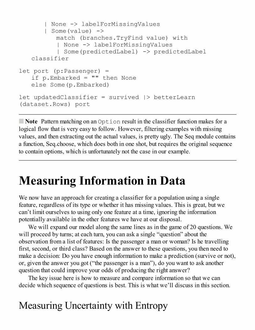
| None -> labelForMissingValues | Some(value) -> match (branches.TryFind value) with | None -> labelForMissingValues | Some(predictedLabel) -> predictedLabel classifier

let port (p:Passenger) = if p.Embarked = "" then None else Some(p.Embarked)

let updatedClassifier = survived |> betterLearn (dataset.Rows) port

Note Pattern matching on an Option result in the classifier function makes for alogical flow that is very easy to follow. However, filtering examples with missingvalues, and then extracting out the actual values, is pretty ugly. The Seq module containsa function, Seq.choose, which does both in one shot, but requires the original sequenceto contain options, which is unfortunately not the case in our example.

Measuring Information in DataWe now have an approach for creating a classifier for a population using a singlefeature, regardless of its type or whether it has missing values. This is great, but wecan’t limit ourselves to using only one feature at a time, ignoring the informationpotentially available in the other features we have at our disposal.

We will expand our model along the same lines as in the game of 20 questions. Wewill proceed by turns; at each turn, you can ask a single “question” about theobservation from a list of features: Is the passenger a man or woman? Is he travellingfirst, second, or third class? Based on the answer to these questions, you then need tomake a decision: Do you have enough information to make a prediction (survive or not),or, given the answer you got (“the passenger is a man”), do you want to ask anotherquestion that could improve your odds of producing the right answer?

The key issue here is how to measure and compare information so that we candecide which sequence of questions is best. This is what we’ll discuss in this section.

Measuring Uncertainty with Entropy

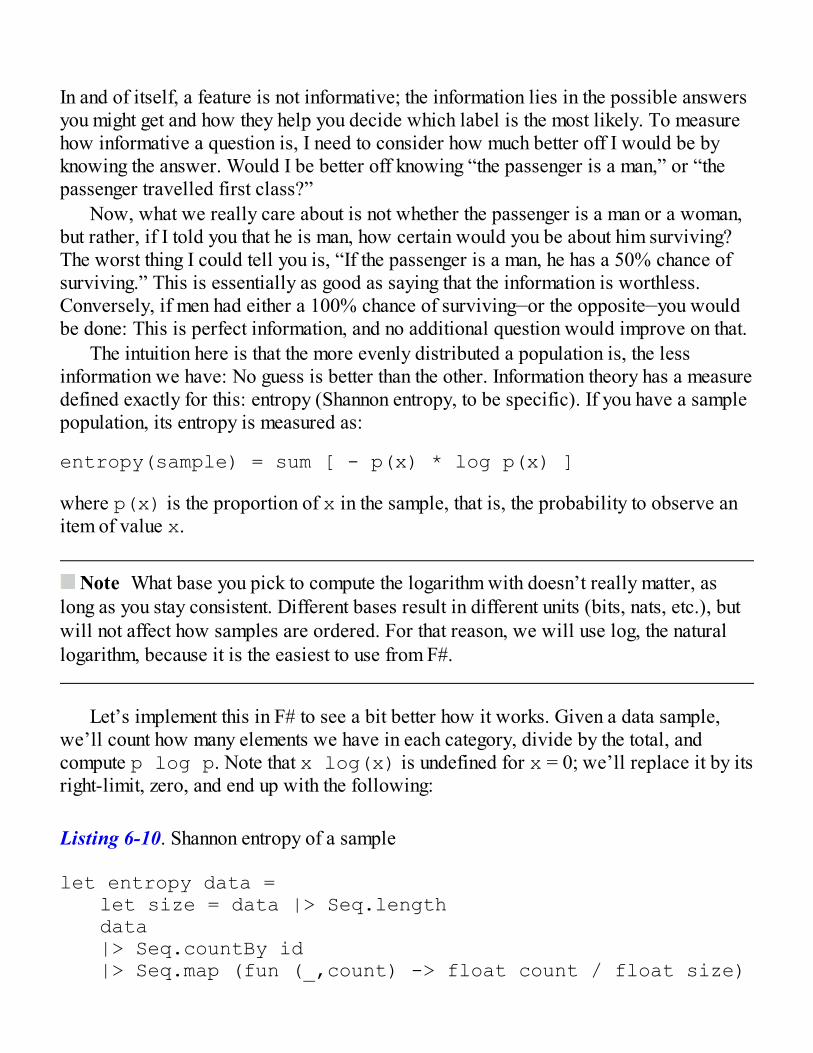
In and of itself, a feature is not informative; the information lies in the possible answersyou might get and how they help you decide which label is the most likely. To measurehow informative a question is, I need to consider how much better off I would be byknowing the answer. Would I be better off knowing “the passenger is a man,” or “thepassenger travelled first class?”

Now, what we really care about is not whether the passenger is a man or a woman,but rather, if I told you that he is man, how certain would you be about him surviving?The worst thing I could tell you is, “If the passenger is a man, he has a 50% chance ofsurviving.” This is essentially as good as saying that the information is worthless.Conversely, if men had either a 100% chance of surviving—or the opposite—you wouldbe done: This is perfect information, and no additional question would improve on that.

The intuition here is that the more evenly distributed a population is, the lessinformation we have: No guess is better than the other. Information theory has a measuredefined exactly for this: entropy (Shannon entropy, to be specific). If you have a samplepopulation, its entropy is measured as:

entropy(sample) = sum [ - p(x) * log p(x) ]

where p(x) is the proportion of x in the sample, that is, the probability to observe anitem of value x.

Note What base you pick to compute the logarithm with doesn’t really matter, aslong as you stay consistent. Different bases result in different units (bits, nats, etc.), butwill not affect how samples are ordered. For that reason, we will use log, the naturallogarithm, because it is the easiest to use from F#.

Let’s implement this in F# to see a bit better how it works. Given a data sample,we’ll count how many elements we have in each category, divide by the total, andcompute p log p. Note that x log(x) is undefined for x = 0; we’ll replace it by itsright-limit, zero, and end up with the following:

Listing 6-10. Shannon entropy of a sample

let entropy data = let size = data |> Seq.length data |> Seq.countBy id |> Seq.map (fun (_,count) -> float count / float size)

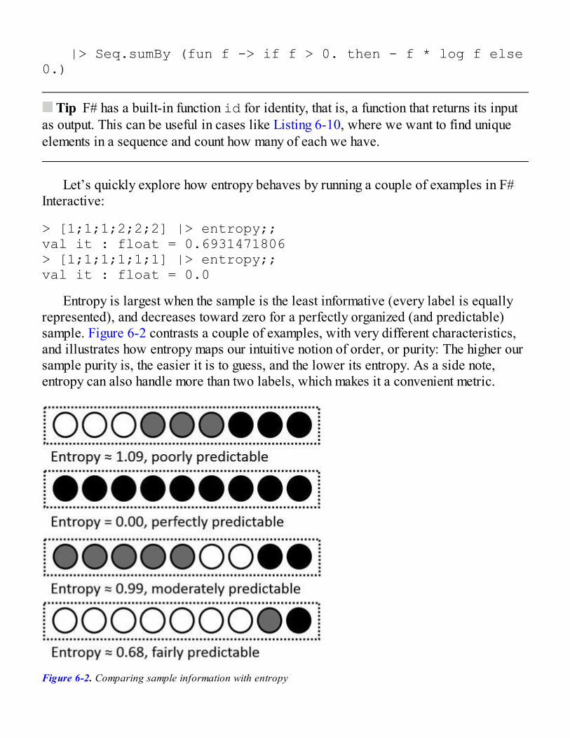
|> Seq.sumBy (fun f -> if f > 0. then - f * log f else 0.)

Tip F# has a built-in function id for identity, that is, a function that returns its inputas output. This can be useful in cases like Listing 6-10, where we want to find uniqueelements in a sequence and count how many of each we have.

Let’s quickly explore how entropy behaves by running a couple of examples in F#Interactive:

> [1;1;1;2;2;2] |> entropy;;val it : float = 0.6931471806> [1;1;1;1;1;1] |> entropy;;val it : float = 0.0

Entropy is largest when the sample is the least informative (every label is equallyrepresented), and decreases toward zero for a perfectly organized (and predictable)sample. Figure 6-2 contrasts a couple of examples, with very different characteristics,and illustrates how entropy maps our intuitive notion of order, or purity: The higher oursample purity is, the easier it is to guess, and the lower its entropy. As a side note,entropy can also handle more than two labels, which makes it a convenient metric.

Figure 6-2. Comparing sample information with entropy

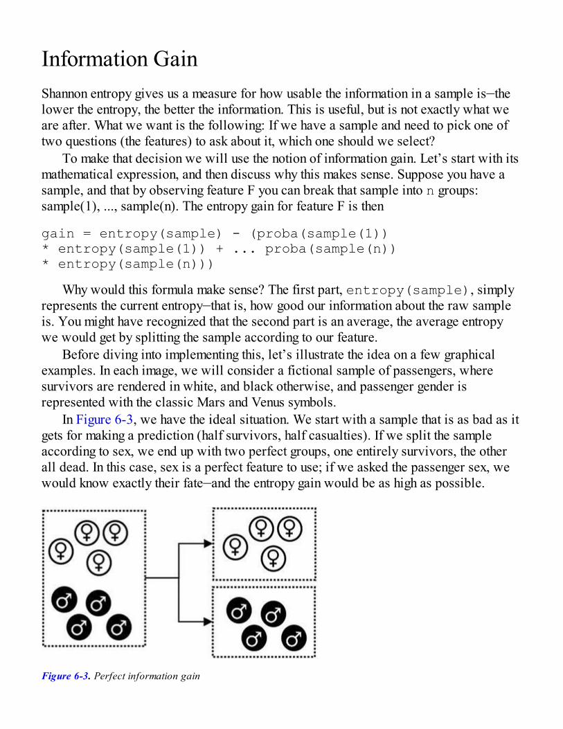
Information GainShannon entropy gives us a measure for how usable the information in a sample is—thelower the entropy, the better the information. This is useful, but is not exactly what weare after. What we want is the following: If we have a sample and need to pick one oftwo questions (the features) to ask about it, which one should we select?

To make that decision we will use the notion of information gain. Let’s start with itsmathematical expression, and then discuss why this makes sense. Suppose you have asample, and that by observing feature F you can break that sample into n groups:sample(1), ..., sample(n). The entropy gain for feature F is then

gain = entropy(sample) - (proba(sample(1)) * entropy(sample(1)) + ... proba(sample(n)) * entropy(sample(n)))

Why would this formula make sense? The first part, entropy(sample), simplyrepresents the current entropy—that is, how good our information about the raw sampleis. You might have recognized that the second part is an average, the average entropywe would get by splitting the sample according to our feature.

Before diving into implementing this, let’s illustrate the idea on a few graphicalexamples. In each image, we will consider a fictional sample of passengers, wheresurvivors are rendered in white, and black otherwise, and passenger gender isrepresented with the classic Mars and Venus symbols.

In Figure 6-3, we have the ideal situation. We start with a sample that is as bad as itgets for making a prediction (half survivors, half casualties). If we split the sampleaccording to sex, we end up with two perfect groups, one entirely survivors, the otherall dead. In this case, sex is a perfect feature to use; if we asked the passenger sex, wewould know exactly their fate—and the entropy gain would be as high as possible.

Figure 6-3. Perfect information gain

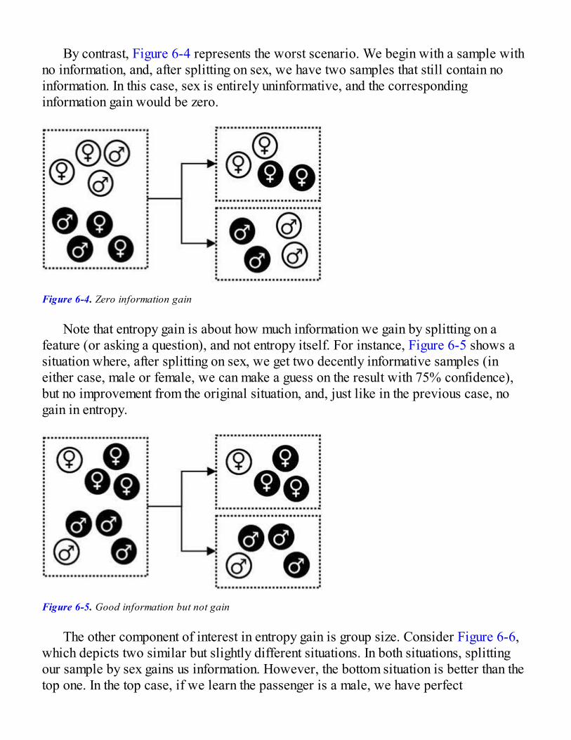
By contrast, Figure 6-4 represents the worst scenario. We begin with a sample withno information, and, after splitting on sex, we have two samples that still contain noinformation. In this case, sex is entirely uninformative, and the correspondinginformation gain would be zero.

Figure 6-4. Zero information gain

Note that entropy gain is about how much information we gain by splitting on afeature (or asking a question), and not entropy itself. For instance, Figure 6-5 shows asituation where, after splitting on sex, we get two decently informative samples (ineither case, male or female, we can make a guess on the result with 75% confidence),but no improvement from the original situation, and, just like in the previous case, nogain in entropy.

Figure 6-5. Good information but not gain

The other component of interest in entropy gain is group size. Consider Figure 6-6,which depicts two similar but slightly different situations. In both situations, splittingour sample by sex gains us information. However, the bottom situation is better than thetop one. In the top case, if we learn the passenger is a male, we have perfect

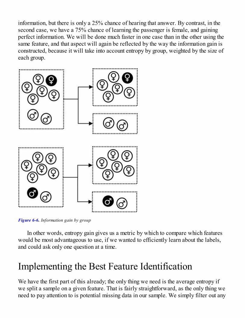
information, but there is only a 25% chance of hearing that answer. By contrast, in thesecond case, we have a 75% chance of learning the passenger is female, and gainingperfect information. We will be done much faster in one case than in the other using thesame feature, and that aspect will again be reflected by the way the information gain isconstructed, because it will take into account entropy by group, weighted by the size ofeach group.

Figure 6-6. Information gain by group

In other words, entropy gain gives us a metric by which to compare which featureswould be most advantageous to use, if we wanted to efficiently learn about the labels,and could ask only one question at a time.

Implementing the Best Feature IdentificationWe have the first part of this already; the only thing we need is the average entropy ifwe split a sample on a given feature. That is fairly straightforward, as the only thing weneed to pay attention to is potential missing data in our sample. We simply filter out any

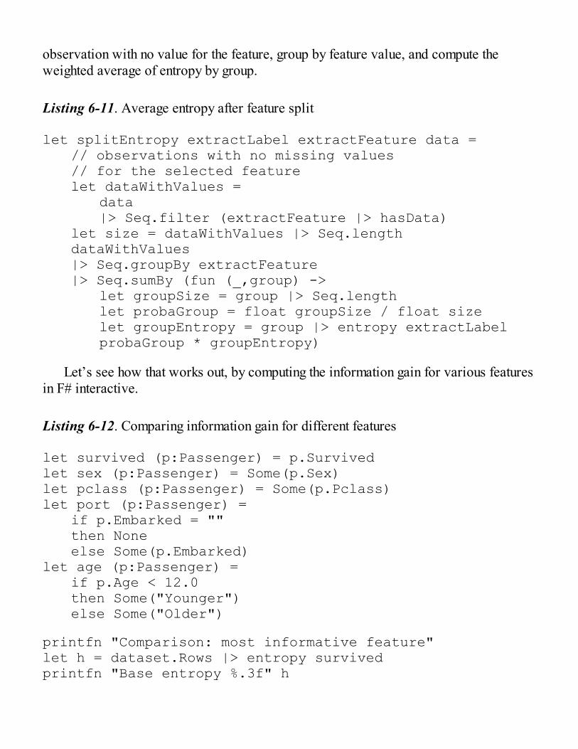
observation with no value for the feature, group by feature value, and compute theweighted average of entropy by group.

Listing 6-11. Average entropy after feature split

let splitEntropy extractLabel extractFeature data = // observations with no missing values // for the selected feature let dataWithValues = data |> Seq.filter (extractFeature |> hasData) let size = dataWithValues |> Seq.length dataWithValues |> Seq.groupBy extractFeature |> Seq.sumBy (fun (_,group) -> let groupSize = group |> Seq.length let probaGroup = float groupSize / float size let groupEntropy = group |> entropy extractLabel probaGroup * groupEntropy)

Let’s see how that works out, by computing the information gain for various featuresin F# interactive.

Listing 6-12. Comparing information gain for different features

let survived (p:Passenger) = p.Survivedlet sex (p:Passenger) = Some(p.Sex)let pclass (p:Passenger) = Some(p.Pclass)let port (p:Passenger) = if p.Embarked = "" then None else Some(p.Embarked)let age (p:Passenger) = if p.Age < 12.0 then Some("Younger") else Some("Older")

printfn "Comparison: most informative feature"let h = dataset.Rows |> entropy survivedprintfn "Base entropy %.3f" h

dataset.Rows |> splitEntropy survived sex |> printfn " Sex: %.3f"dataset.Rows |> splitEntropy survived pclass |> printfn " Class: %.3f"dataset.Rows |> splitEntropy survived port |> printfn " Port: %.3f"dataset.Rows |> splitEntropy survived age |> printfn " Age: %.3f"

>Comparison: most informative featureBase entropy 0.666 Sex: 0.515 Class: 0.608 Port: 0.649 Age: 0.660

The clear winner here is sex, which has the lowest entropy, and is therefore the mostinformative feature; class seems to have some potential, too, but port and age don’tshow any obvious improvement. This gives us a decision stump, and two groups, maleand female; we can repeat the same procedure again.

Listing 6-13. Comparing information gain in sub-groups

let bySex = dataset.Rows |> Seq.groupBy sex

for (groupName, group) in bySex do printfn "Group: %s" groupName.Value let h = group |> entropy survived printfn "Base entropy %.3f" h

group |> splitEntropy survived sex |> printfn " Sex: %.3f" group |> splitEntropy survived pclass |> printfn " Class: %.3f" group |> splitEntropy survived port |> printfn " Port: %.3f" group |> splitEntropy survived age |> printfn " Age: %.3f">Group: maleBase entropy 0.485

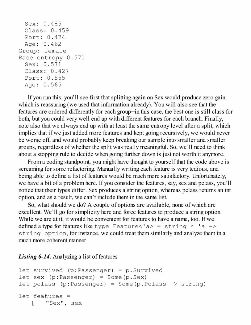
Sex: 0.485 Class: 0.459 Port: 0.474 Age: 0.462Group: femaleBase entropy 0.571 Sex: 0.571 Class: 0.427 Port: 0.555 Age: 0.565

If you run this, you’ll see first that splitting again on Sex would produce zero gain,which is reassuring (we used that information already). You will also see that thefeatures are ordered differently for each group—in this case, the best one is still class forboth, but you could very well end up with different features for each branch. Finally,note also that we always end up with at least the same entropy level after a split, whichimplies that if we just added more features and kept going recursively, we would neverbe worse off, and would probably keep breaking our sample into smaller and smallergroups, regardless of whether the split was really meaningful. So, we’ll need to thinkabout a stopping rule to decide when going further down is just not worth it anymore.

From a coding standpoint, you might have thought to yourself that the code above isscreaming for some refactoring. Manually writing each feature is very tedious, andbeing able to define a list of features would be much more satisfactory. Unfortunately,we have a bit of a problem here. If you consider the features, say, sex and pclass, you’llnotice that their types differ. Sex produces a string option, whereas pclass returns an intoption, and as a result, we can’t include them in the same list.

So, what should we do? A couple of options are available, none of which areexcellent. We’ll go for simplicity here and force features to produce a string option.While we are at it, it would be convenient for features to have a name, too. If wedefined a type for features like type Feature<'a> = string * 'a ->string option, for instance, we could treat them similarly and analyze them in amuch more coherent manner.

Listing 6-14. Analyzing a list of features

let survived (p:Passenger) = p.Survivedlet sex (p:Passenger) = Some(p.Sex)let pclass (p:Passenger) = Some(p.Pclass |> string)

let features = [ "Sex", sex

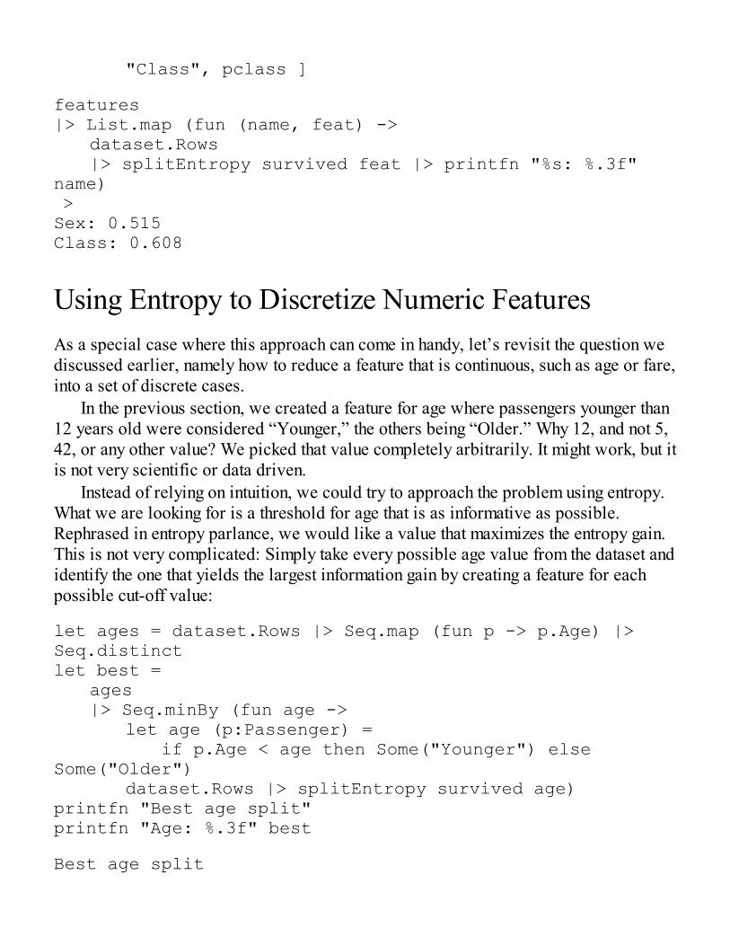
"Class", pclass ]

features|> List.map (fun (name, feat) -> dataset.Rows |> splitEntropy survived feat |> printfn "%s: %.3f" name) >Sex: 0.515Class: 0.608

Using Entropy to Discretize Numeric FeaturesAs a special case where this approach can come in handy, let’s revisit the question wediscussed earlier, namely how to reduce a feature that is continuous, such as age or fare,into a set of discrete cases.

In the previous section, we created a feature for age where passengers younger than12 years old were considered “Younger,” the others being “Older.” Why 12, and not 5,42, or any other value? We picked that value completely arbitrarily. It might work, but itis not very scientific or data driven.

Instead of relying on intuition, we could try to approach the problem using entropy.What we are looking for is a threshold for age that is as informative as possible.Rephrased in entropy parlance, we would like a value that maximizes the entropy gain.This is not very complicated: Simply take every possible age value from the dataset andidentify the one that yields the largest information gain by creating a feature for eachpossible cut-off value:

let ages = dataset.Rows |> Seq.map (fun p -> p.Age) |> Seq.distinctlet best = ages |> Seq.minBy (fun age -> let age (p:Passenger) = if p.Age < age then Some("Younger") else Some("Older") dataset.Rows |> splitEntropy survived age)printfn "Best age split"printfn "Age: %.3f" best

Best age split

Age: 7.000

This approach isn’t perfect. Binning continuous variables is a bit of a dark art, andthere is no silver bullet. This one has the benefit of being fully automated; as a result,you could generate stumps from the data without manual intervention.

Note One limitation of this method is that it assumes having two categories is a goodway to discretize the value, which may or may not be appropriate. One way to addressthis issue is by recursively applying the same procedure and inspecting whether any ofthe bins identified can be profitably split further. However, this is potentially tricky,because as the bins become smaller, the risk increases to create artificial divisions.We’ll leave it at that, but mention the search term “minimum description length” forreaders interested in exploring that question further.

Growing a Tree from DataWe have now the two key elements needed to build a decision tree. With decisionstumps, we have minimal units, which can be trained to process an observation indifferent branches, based on a feature. With entropy, we can measure how useful aparticular feature is, given a sample of observations. All we need now is to combinestumps into a full tree. Starting with a collection of features and a training set, we willidentify the most informative feature, create a stump for each outcome, and repeat theoperation for each branch.

The code we are going to write is fairly general, so, in a fashion similar to that inChapter 2, let’s extract it into its own separate module. We will add a file to oursolution, say, Tree.fs, start moving some of our general code there, and use that filein our scripts, which will be focused exclusively on the specific problem of crafting amodel for the Titanic dataset.

Modeling the TreeLet’s start with the end result, the tree. The main difference between a stump and a fulltree is that while each branch of the stump gives us a final, definite answer, a tree ismore complex: It can give us a final answer, but it can also keep going and lead usdown to another stump, with a follow-up question to ask.

Most of the time, when you hear a domain description that involves an “or”

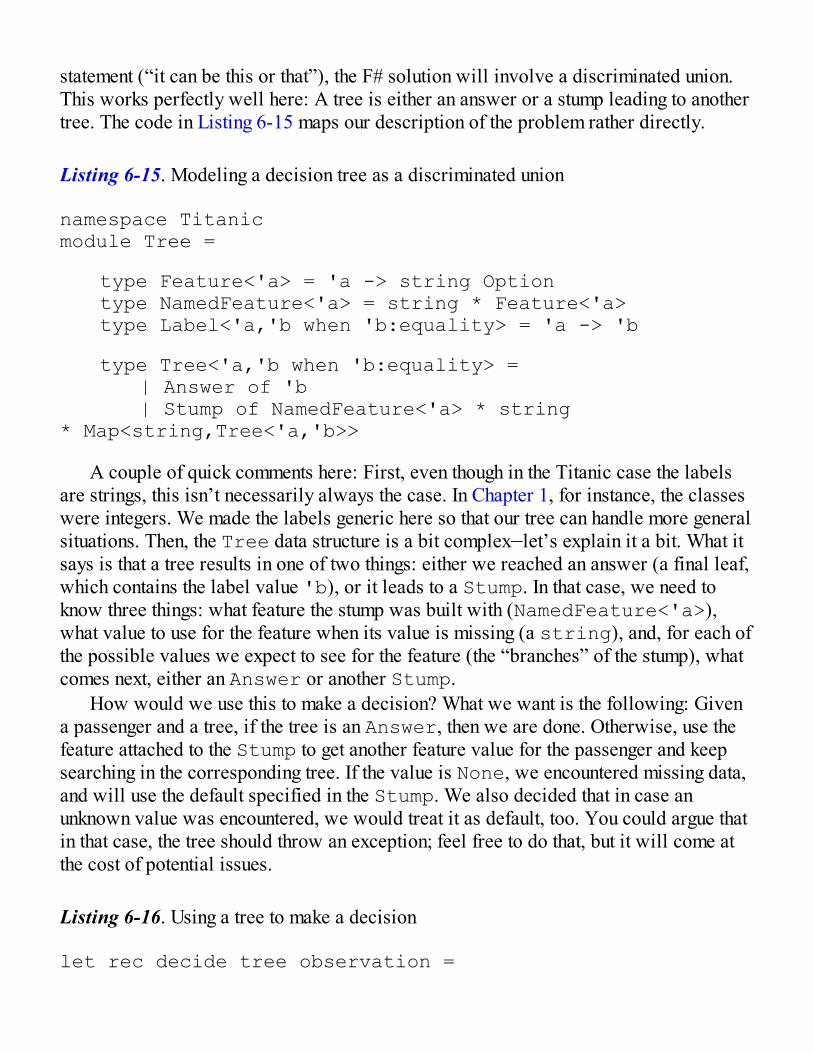
statement (“it can be this or that”), the F# solution will involve a discriminated union.This works perfectly well here: A tree is either an answer or a stump leading to anothertree. The code in Listing 6-15 maps our description of the problem rather directly.

Listing 6-15. Modeling a decision tree as a discriminated union

namespace Titanicmodule Tree =

type Feature<'a> = 'a -> string Option type NamedFeature<'a> = string * Feature<'a> type Label<'a,'b when 'b:equality> = 'a -> 'b

type Tree<'a,'b when 'b:equality> = | Answer of 'b | Stump of NamedFeature<'a> * string * Map<string,Tree<'a,'b>>

A couple of quick comments here: First, even though in the Titanic case the labelsare strings, this isn’t necessarily always the case. In Chapter 1, for instance, the classeswere integers. We made the labels generic here so that our tree can handle more generalsituations. Then, the Tree data structure is a bit complex—let’s explain it a bit. What itsays is that a tree results in one of two things: either we reached an answer (a final leaf,which contains the label value 'b), or it leads to a Stump. In that case, we need toknow three things: what feature the stump was built with (NamedFeature<'a>),what value to use for the feature when its value is missing (a string), and, for each ofthe possible values we expect to see for the feature (the “branches” of the stump), whatcomes next, either an Answer or another Stump.

How would we use this to make a decision? What we want is the following: Givena passenger and a tree, if the tree is an Answer, then we are done. Otherwise, use thefeature attached to the Stump to get another feature value for the passenger and keepsearching in the corresponding tree. If the value is None, we encountered missing data,and will use the default specified in the Stump. We also decided that in case anunknown value was encountered, we would treat it as default, too. You could argue thatin that case, the tree should throw an exception; feel free to do that, but it will come atthe cost of potential issues.

Listing 6-16. Using a tree to make a decision

let rec decide tree observation =

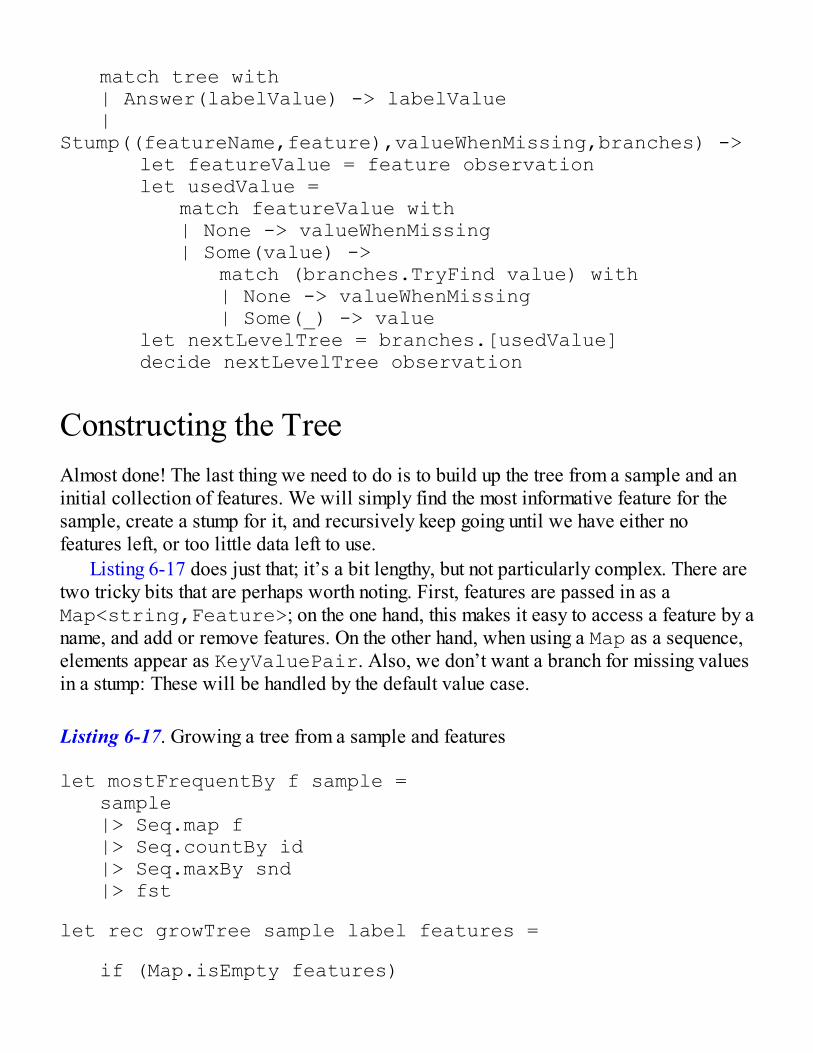
match tree with | Answer(labelValue) -> labelValue | Stump((featureName,feature),valueWhenMissing,branches) -> let featureValue = feature observation let usedValue = match featureValue with | None -> valueWhenMissing | Some(value) -> match (branches.TryFind value) with | None -> valueWhenMissing | Some(_) -> value let nextLevelTree = branches.[usedValue] decide nextLevelTree observation

Constructing the TreeAlmost done! The last thing we need to do is to build up the tree from a sample and aninitial collection of features. We will simply find the most informative feature for thesample, create a stump for it, and recursively keep going until we have either nofeatures left, or too little data left to use.

Listing 6-17 does just that; it’s a bit lengthy, but not particularly complex. There aretwo tricky bits that are perhaps worth noting. First, features are passed in as aMap<string,Feature>; on the one hand, this makes it easy to access a feature by aname, and add or remove features. On the other hand, when using a Map as a sequence,elements appear as KeyValuePair. Also, we don’t want a branch for missing valuesin a stump: These will be handled by the default value case.

Listing 6-17. Growing a tree from a sample and features

let mostFrequentBy f sample = sample |> Seq.map f |> Seq.countBy id |> Seq.maxBy snd |> fst

let rec growTree sample label features =

if (Map.isEmpty features)

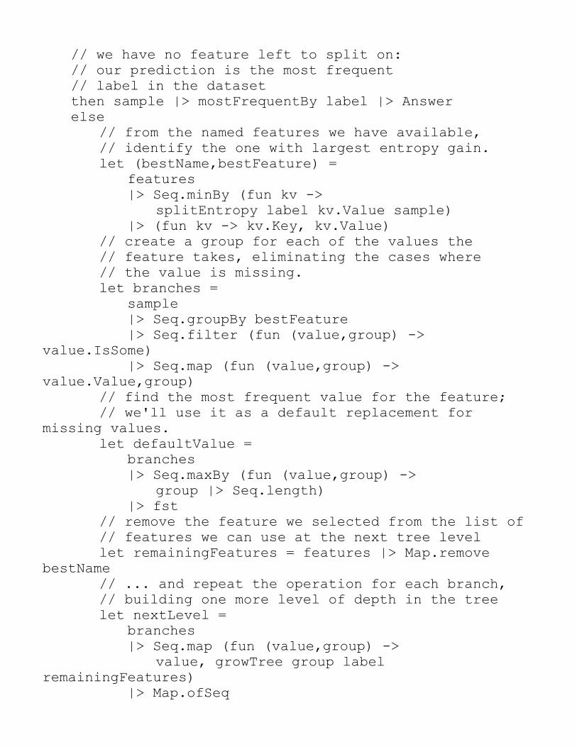
// we have no feature left to split on: // our prediction is the most frequent // label in the dataset then sample |> mostFrequentBy label |> Answer else // from the named features we have available, // identify the one with largest entropy gain. let (bestName,bestFeature) = features |> Seq.minBy (fun kv -> splitEntropy label kv.Value sample) |> (fun kv -> kv.Key, kv.Value) // create a group for each of the values the // feature takes, eliminating the cases where // the value is missing. let branches = sample |> Seq.groupBy bestFeature |> Seq.filter (fun (value,group) -> value.IsSome) |> Seq.map (fun (value,group) -> value.Value,group) // find the most frequent value for the feature; // we'll use it as a default replacement for missing values. let defaultValue = branches |> Seq.maxBy (fun (value,group) -> group |> Seq.length) |> fst // remove the feature we selected from the list of // features we can use at the next tree level let remainingFeatures = features |> Map.remove bestName // ... and repeat the operation for each branch, // building one more level of depth in the tree let nextLevel = branches |> Seq.map (fun (value,group) -> value, growTree group label remainingFeatures) |> Map.ofSeq

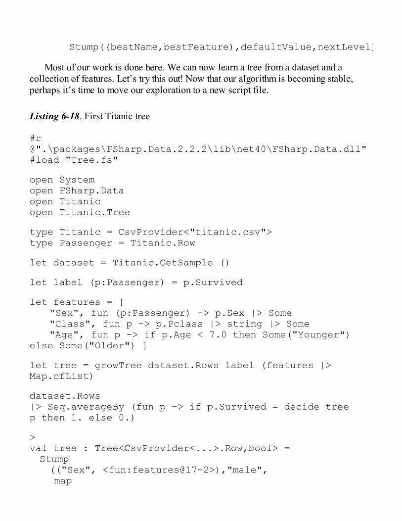
Stump((bestName,bestFeature),defaultValue,nextLevel)

Most of our work is done here. We can now learn a tree from a dataset and acollection of features. Let’s try this out! Now that our algorithm is becoming stable,perhaps it’s time to move our exploration to a new script file.

Listing 6-18. First Titanic tree

#r @".\packages\FSharp.Data.2.2.2\lib\net40\FSharp.Data.dll"#load "Tree.fs"

open Systemopen FSharp.Dataopen Titanicopen Titanic.Tree

type Titanic = CsvProvider<"titanic.csv">type Passenger = Titanic.Row

let dataset = Titanic.GetSample ()

let label (p:Passenger) = p.Survived

let features = [ "Sex", fun (p:Passenger) -> p.Sex |> Some "Class", fun p -> p.Pclass |> string |> Some "Age", fun p -> if p.Age < 7.0 then Some("Younger") else Some("Older") ]

let tree = growTree dataset.Rows label (features |> Map.ofList)

dataset.Rows|> Seq.averageBy (fun p -> if p.Survived = decide tree p then 1. else 0.)

>val tree : Tree<CsvProvider<...>.Row,bool> = Stump (("Sex", <fun:features@17-2>),"male", map

[("female", Stump (("Class", <fun:features@18-3>),"3", map [("1", Stump (("Age", <fun:features@19-4>),"Older", map [("Older", Answer true); ("Younger", Answer false)]));// snipped for brevityval it : float = 0.8058361392

The good news is that running this code produces a tree, and a clear improvement,with about 80% correct calls. There is some bad news, too. First, the output tree is uglyas hell. Also, we have completely ignored all we have preached so far, and didn’t usecross-validation at all to evaluate our work. We need to fix that.

Caution In a fashion similar to the naïve Bayes classifier we discussed in Chapter 2,what a decision tree learns is directly based on how frequently items are found in thetraining set. As a consequence, it is important to bear in mind that if the dataset issignificantly distorted from the “real” population, and doesn’t reflect its truecomposition, the predictions are likely to be entirely incorrect.

A Prettier TreeThe tree we receive back is barely readable, at best; let’s write a simple function todisplay it in a more human-friendly format. Essentially, we are going to recursivelywalk down the tree, increasing indentation every time we hit a new depth level, andprinting out feature and branch names as we go.

Listing 6-19. Rendering the tree

let rec display depth tree =

let padding = String.replicate (2 * depth) " " match tree with | Answer(label) -> printfn " -> %A" label | Stump((name,_),_,branches) -> printfn ""

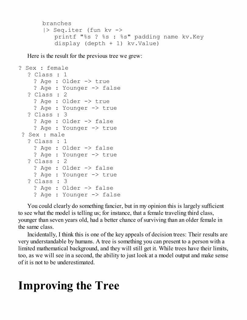
branches |> Seq.iter (fun kv -> printf "%s ? %s : %s" padding name kv.Key display (depth + 1) kv.Value)

Here is the result for the previous tree we grew:

? Sex : female ? Class : 1 ? Age : Older -> true ? Age : Younger -> false ? Class : 2 ? Age : Older -> true ? Age : Younger -> true ? Class : 3 ? Age : Older -> false ? Age : Younger -> true ? Sex : male ? Class : 1 ? Age : Older -> false ? Age : Younger -> true ? Class : 2 ? Age : Older -> false ? Age : Younger -> true ? Class : 3 ? Age : Older -> false ? Age : Younger -> false

You could clearly do something fancier, but in my opinion this is largely sufficientto see what the model is telling us; for instance, that a female traveling third class,younger than seven years old, had a better chance of surviving than an older female inthe same class.

Incidentally, I think this is one of the key appeals of decision trees: Their results arevery understandable by humans. A tree is something you can present to a person with alimited mathematical background, and they will still get it. While trees have their limits,too, as we will see in a second, the ability to just look at a model output and make senseof it is not to be underestimated.

Improving the Tree

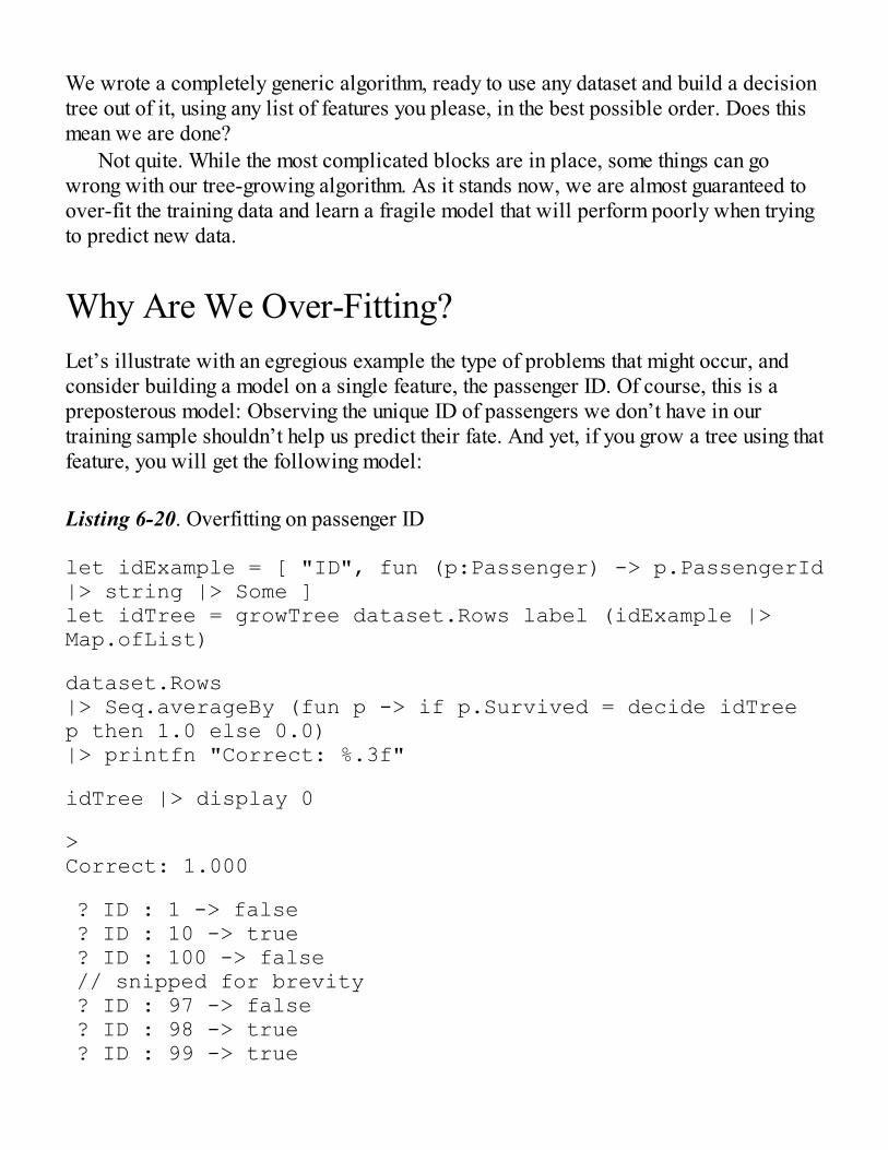
We wrote a completely generic algorithm, ready to use any dataset and build a decisiontree out of it, using any list of features you please, in the best possible order. Does thismean we are done?

Not quite. While the most complicated blocks are in place, some things can gowrong with our tree-growing algorithm. As it stands now, we are almost guaranteed toover-fit the training data and learn a fragile model that will perform poorly when tryingto predict new data.

Why Are We Over-Fitting?Let’s illustrate with an egregious example the type of problems that might occur, andconsider building a model on a single feature, the passenger ID. Of course, this is apreposterous model: Observing the unique ID of passengers we don’t have in ourtraining sample shouldn’t help us predict their fate. And yet, if you grow a tree using thatfeature, you will get the following model:

Listing 6-20. Overfitting on passenger ID

let idExample = [ "ID", fun (p:Passenger) -> p.PassengerId|> string |> Some ]let idTree = growTree dataset.Rows label (idExample |> Map.ofList)

dataset.Rows|> Seq.averageBy (fun p -> if p.Survived = decide idTree p then 1.0 else 0.0)|> printfn "Correct: %.3f"

idTree |> display 0

>Correct: 1.000

? ID : 1 -> false ? ID : 10 -> true ? ID : 100 -> false // snipped for brevity ? ID : 97 -> false ? ID : 98 -> true ? ID : 99 -> true

This is obviously wrong on many levels. There is nothing wrong with the math, mindyou; it’s just that the result, from a practical standpoint, is entirely useless. If we use thismodel against new data, those new IDs will obviously not be in the tree, and as a resultthe prediction will be the default, uninformed one—and yet, this model is 100% correcton modeling and predicting the training set.

We already have encountered this last issue, and hopefully by now you are thinkingto yourself, “Of course—he should have used cross-validation,” and you would be right.We will use cross-validation ahead, but I thought it was useful to make this point, first,because it is a very simple illustration of how things can go terribly wrong, and second,because over-fitting is a particularly important issue to keep in mind for trees.

Unlike other algorithms we considered earlier, a tree is learning recursively. As aresult, instead of learning all the features at once on the full training set, it learns onefeature at a time, on samples that are smaller and smaller as the algorithm progresses.

This is a bit problematic, when you consider how entropy works. First, informationdoesn’t disappear; in the worst possible case, splitting by a feature will gain us noinformation. As a result, in the current implementation, we will always add every singlefeature we have to the tree, even when it doesn’t add any information. Then, becauseentropy is based on proportions, it will draw the same conclusions when analyzing bothsmall and large samples, as long as their composition is identical. This is a bitproblematic, too: I would not have the same confidence in conclusions derived from asample containing 10 observations versus a sample with 100,000.

Limiting Over-Confidence with FiltersLet’s begin first by addressing the easier issues. We want to avoid learning with toomuch confidence based on insufficiently conclusive samples. One simple way to do thatis to add filters to our tree-growing algorithm so as to eliminate weak candidates as weprogress down the tree.

Let’s consider the two cases we identified already. We are currently picking thefeature that has the highest conditional entropy; we can improve the algorithm bykeeping only features that have a strictly positive entropy gain. In order to perform thatoperation, I need a few pieces of data: a feature, obviously, but also a sample and alabel, to compute the entropy and split entropy, and check that the entropy is better (thatis, strictly lower) after the split.

If I were to just hard-code this rule in the algorithm, I would modify our existingcode along these lines:

let rec growTree sample label features =

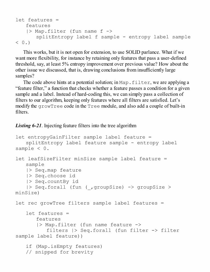
let features = features |> Map.filter (fun name f -> splitEntropy label f sample - entropy label sample < 0.)

This works, but it is not open for extension, to use SOLID parlance. What if wewant more flexibility, for instance by retaining only features that pass a user-definedthreshold, say, at least 5% entropy improvement over previous value? How about theother issue we discussed, that is, drawing conclusions from insufficiently largesamples?

The code above hints at a potential solution; in Map.filter, we are applying a“feature filter,” a function that checks whether a feature passes a condition for a givensample and a label. Instead of hard-coding this, we can simply pass a collection offilters to our algorithm, keeping only features where all filters are satisfied. Let’smodify the growTree code in the Tree module, and also add a couple of built-infilters.

Listing 6-21. Injecting feature filters into the tree algorithm

let entropyGainFilter sample label feature = splitEntropy label feature sample - entropy label sample < 0.

let leafSizeFilter minSize sample label feature = sample |> Seq.map feature |> Seq.choose id |> Seq.countBy id |> Seq.forall (fun (_,groupSize) -> groupSize > minSize)

let rec growTree filters sample label features =

let features = features |> Map.filter (fun name feature -> filters |> Seq.forall (fun filter -> filter sample label feature))

if (Map.isEmpty features) // snipped for brevity

Applying this updated algorithm using the same features as previously, but passingin [ entropyGain; leafSize 10 ] as a filter, this is the tree I get:

? Sex : female ? Class : 1 -> true ? Class : 2 -> true ? Class : 3 ? Age : Older -> true ? Age : Younger -> false ? Sex : male ? Class : 1 -> false ? Class : 2 -> false ? Class : 3 ? Age : Older -> false ? Age : Younger -> false

Our decision tree lost some depth from our previous version. This is good: Usingfilters leads to dropping some spurious branches, and as a result, we have a tree that isboth more readable and more reliable. Note also that all the branches under male leadto the same conclusion. Does this indicate an issue with our algorithm? Not necessarily:Entropy will decide to split when it finds a significant difference between branches,regardless of whether that difference is material to our decision. For instance, a 51%and a 99% chance of surviving are significantly different, but the difference is notmaterial to the conclusion, which remains the same. Depending on what you want, youcould improve the tree in two different ways, either by adding probabilities to the finalbranches or by collapsing together stumps that contain identical answers into a singleanswer.

From Trees to ForestsWe limited some of the most obvious over-fitting risks by injecting a bit of commonsense into the algorithm, but the solution was rather crude. Over-fitting is particularlyproblematic for trees because of their recursive nature; however, it is a general problemin machine learning. By learning from one training sample, there is an inherent risk oflearning that one sample too well. The filters we applied on our tree and theregularization methods we mentioned in an earlier chapter both address that issue withone strategy: limiting how much the algorithm is allowed to learn by applying a form ofpenalty.

In this section, we will introduce another way to think about this question, with a

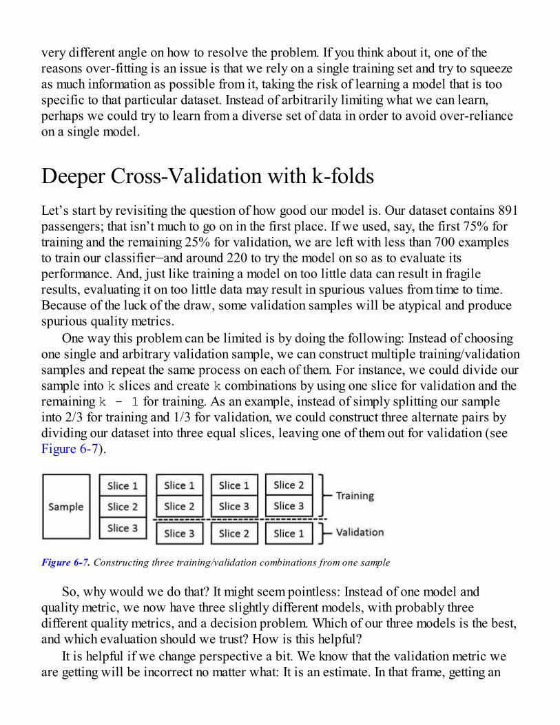
very different angle on how to resolve the problem. If you think about it, one of thereasons over-fitting is an issue is that we rely on a single training set and try to squeezeas much information as possible from it, taking the risk of learning a model that is toospecific to that particular dataset. Instead of arbitrarily limiting what we can learn,perhaps we could try to learn from a diverse set of data in order to avoid over-relianceon a single model.

Deeper Cross-Validation with k-foldsLet’s start by revisiting the question of how good our model is. Our dataset contains 891passengers; that isn’t much to go on in the first place. If we used, say, the first 75% fortraining and the remaining 25% for validation, we are left with less than 700 examplesto train our classifier—and around 220 to try the model on so as to evaluate itsperformance. And, just like training a model on too little data can result in fragileresults, evaluating it on too little data may result in spurious values from time to time.Because of the luck of the draw, some validation samples will be atypical and producespurious quality metrics.

One way this problem can be limited is by doing the following: Instead of choosingone single and arbitrary validation sample, we can construct multiple training/validationsamples and repeat the same process on each of them. For instance, we could divide oursample into k slices and create k combinations by using one slice for validation and theremaining k - 1 for training. As an example, instead of simply splitting our sampleinto 2/3 for training and 1/3 for validation, we could construct three alternate pairs bydividing our dataset into three equal slices, leaving one of them out for validation (seeFigure 6-7).

Figure 6-7. Constructing three training/validation combinations from one sample

So, why would we do that? It might seem pointless: Instead of one model andquality metric, we now have three slightly different models, with probably threedifferent quality metrics, and a decision problem. Which of our three models is the best,and which evaluation should we trust? How is this helpful?

It is helpful if we change perspective a bit. We know that the validation metric weare getting will be incorrect no matter what: It is an estimate. In that frame, getting an

idea of how wrong that estimate might be is as useful as the estimate itself. Rather thanhanging everything on one incorrect number, we can now get a sense for how changes inthe data could impact our model and how volatile the quality could be.

This approach is known as k-fold. Choosing k entails a bit of a trade-off. At theextreme, if we increase k to its largest possible value, the dataset size, we’ll end upwith k different models, validated on a single example each, which is commonlyreferred to as “leave-one-out.” Obviously, the larger k becomes, the more expensive theoperation will be, because more models need to be trained. Also, as k increases, eachof the models shares more common data, and can therefore be expected to behave morelike a model that would use the dataset in its entirety.

Let’s try it out on our model here. First, we need to generate k pairs of training andvalidation samples. The following implementation, while not pretty, does the job: Foreach of the k values, it computes the start and end index of the validation slice andreturns a list of k sample pairs, each of which contains the training and validation partsin a tuple.

Listing 6-22. Generating k training/validation pairs from a sample

let kfold k sample = let size = sample |> Array.length let foldSize = size / k

[ for f in 0 .. (k-1) do let sliceStart = f * foldSize let sliceEnd = f * foldSize + foldSize - 1 let validation = sample.[sliceStart..sliceEnd] let training = [| for i in 0 .. (sliceStart - 1) do yield sample.[i] for i in (sliceEnd + 1) .. (size - 1) do yield sample.[i] |] yield training,validation ]

Let’s try out a k-fold analysis of our basic tree, with k = 10:

Listing 6-23. Evaluating ten folds

let folds = dataset.Rows |> Seq.toArray |> kfold 10let accuracy tree (sample:Passenger seq) = sample |> Seq.averageBy (fun p -> if p.Survived = decide tree p then 1.0 else 0.0)

let evaluateFolds = let filters = [ leafSizeFilter 10; entropyGainFilter ] let features = features |> Map.ofList [for (training,validation) in folds -> let tree = growTree2 filters training label features let accuracyTraining = accuracy tree training let accuracyValidation = accuracy tree validation

printfn "Training: %.3f, Validation: %.3f" accuracyTraining accuracyValidation accuracyTraining, accuracyValidation]>Training: 0.802, Validation: 0.697Training: 0.788, Validation: 0.843Training: 0.796, Validation: 0.775Training: 0.797, Validation: 0.764Training: 0.803, Validation: 0.798Training: 0.798, Validation: 0.843Training: 0.804, Validation: 0.787Training: 0.805, Validation: 0.775Training: 0.788, Validation: 0.843Training: 0.794, Validation: 0.787 val evaluateFolds : (float * float) list = [(0.8017456359, 0.6966292135); // snipped // ; (0.7942643392, 0.7865168539)]

There are a couple of interesting results here. First, while not hugely different, theaverage accuracy on training is around 79.7%, about 0.6 points higher than onvalidation (79.1%). Then, the quality measurements on the validation samples are muchmore variable than those on the training samples. While the accuracy for training rangesfrom 78.8% to 80.5%, the validation results vary all the way from 69.7% to 84.3%.This is not surprising, because each of the validation samples is smaller, and thus morevariable. These results are very useful in that they convey a much better picture of whatwe should expect from our model. Had we performed a basic cross-validation only, wewould have seen only one of the ten results we produced with k-fold; depending on

which of the training/validation pairs we happened to select, we could have reacheddifferent conclusions—either overly optimistic, or pessimistic. By contrast, with k-fold,we can conclude that our model is likely not over-fitting (the average errors on trainingand validation are very close). We also get a much more refined sense for how good orbad our model might be: We should expect to be correct in about 79.1% of the cases,but the standard deviation—the average error around that value—is of 4.5 percentagepoints.

Hopefully, this simple example illustrates how, by simply creating multiple samplesfrom our original dataset, we managed to get a much better picture of our model quality.This technique is mainly useful for evaluating whether changes in a model are actualimprovements; in the next section, we’ll see how similar ideas can be used to improvethe model itself.

Combining Fragile Trees into Robust ForestsWith k-folds, we saw that resampling our training set allowed us to extract moreinformation from it without having to add new observations. Instead of putting all of oureggs in a single basket (or all our observations in a single training set), we generatedmultiple training samples, which gave us a better overall picture of how sensitive tochanges in data our model really was.

This is a result that I find both obvious and fascinating. Fascinating, because on thesurface it appears as if we created additional information out of thin air. Using the exactsame amount of information we initially had, we managed to squeeze out apparentlynew and better information. Obvious, because this is simply a change of focus.Fundamentally, we are dealing with uncertainty, and the best description for uncertaintyis a distribution. By constructing multiple, random samples from our original data, wecan mimic the type of variability that exists in the phenomenon we are trying to predict,and thus replicate (and measure) the resulting variability in the outputs.

This same idea can be taken further and be used to produce potentially more robustprediction models as well. Rather than trying to find the one and perfect model, wecould embrace accidents, accept that inputs are volatile, and create a multitude ofmodels based on different training sets. Some of them will be right, and some will bewrong, but if we look at all their predictions taken together, it is highly unlikely that theywill all be simultaneously incorrect. For instance, we could take a majority vote andhope for a “wisdom of the crowds” effect, where a couple of odd predictions will becanceled out by a majority of reasonable ones. This general approach is known as“ensemble methods,” an approach that studies how multiple weak prediction modelscan be combined into an overall model that is stronger than the sum of its parts.

In the specific case of decision trees, one way to go about it would be to simply

generate multiple training sets from the original dataset by uniformly samplingobservations at random, with replacement, potentially repeating the same observationmultiple times. That approach is known as “bagging” (short for bootstrap aggregating).The intuition here is that this will mitigate the risks of over-fitting, because each modelwill be trained on a different sample. Each model might still pick up artifacts from thedata, but different ones, and they will likely cancel each other out when taken together.

Decision trees, as we implemented them, have another issue that is less obvious.Because the procedure progresses one feature at the time, some features might mask theimpact of others. Imagine that a feature is heavily related to another one (say, what classyou travel in and how much you paid for your ticket), but contains a bit of informationon its own. Once the tree picks up the first one, it is quite possible that the second onewill not be selected, because the remaining information is not sufficiently strong byitself. As a result, by picking from all the features in order of entropy, we take the riskof systematically ignoring features that could convey some usable information.

In a fashion similar to bagging, we could address that issue by randomly samplingfeatures. In at least some cases, the “hidden” feature will be present without thecompeting one, and will have a chance to participate in that tree if it turns out to beinformative.

These two ideas can be combined into one. Instead of creating a single decisiontree, we will create a multitude of simpler trees, a forest, each using a randomlyselected training sample and a subset of features. Instead of relying on a single tree, wewill take a majority vote from among all of them. Each individual model will be weakerthan a decision tree using all the data at once, but, perhaps paradoxically, taken togetherthey will provide more reliable predictions.

Implementing the Missing BlocksExtending our current code to make a forest instead of a tree is rather straightforward.Basically, we only need to add three elements: randomly selecting features from a list(without repetition), randomly selecting examples from the original sample (withrepetition), and combining the predictions of multiple trees into a majority vote. Wewill add all the necessary code to the Tree.fs file, and then try it out on the specificTitanic example.

Let’s start with the second element. If we assume our initial sample is an array, thepicking with repetition is as simple as selecting a random index, as many times as weneed:

let pickRepeat (rng:Random) proportion original = let size = original |> Array.length

let sampleSize = proportion * float size |> int Array.init sampleSize (fun _ -> original.[rng.Next(size)])

Picking with no repetition is a bit trickier. One possibility is to shuffle the entirecollection and pick the first elements. Another possibility is to process the collectionrecursively, deciding one by one if an element should be selected. If I want to pick nelements out of N, the head of the list has an n/N chance of being selected. If it isselected, I now have n - 1 elements to select from N - 1 left; in the other case thechances were n over N - 1. Here we go:

let pickNoRepeat (rng:Random) proportion original =

let size = original |> Seq.length let sampleSize = proportion * float size |> int

let init = ([],size) original |> Seq.fold (fun (sampled,remaining) item -> let picked = List.length sampled let p = float (sampleSize - picked) / float remaining if (rng.NextDouble () <= p) then (item::sampled,remaining-1) else (sampled,remaining-1)) init |> fst

Finally, the prediction from a forest is simply the most frequent decision resultingfrom its trees:

let predict forest observation = forest |> Seq.map (fun tree -> decide tree observation) |> Seq.countBy id |> Seq.maxBy snd |> fst

Growing a ForestLet’s put all of this together: The only thing needed is a function that will create a user-defined number of trees. We will also wrap things tighter and directly return a functionthat can be used to make predictions. While an individual tree is useful because it can

be inspected, we are not going to look into hundreds of trees in the hopes of detectingpatterns and whatnot.

Listing 6-24. Creating a forest from decision trees

let growForest size sample label features = let rng = Random ()

let propFeatures = let total = features |> Seq.length |> float sqrt total / total

let featSample () = pickNoRepeat rng propFeatures features let popSample () = pickRepeat rng 1.0 sample let filters = [ leafSize 10; entropyGain ]

let forest = [ for _ in 1 .. size -> let sample = popSample () let features = featSample () |> Map.ofList growTree filters sample label features ]

let predictor = predict forest predictor

We simplified the function signature by pre-selecting reasonable defaults for filters;we also selected default proportions for what sample proportion to use for thepopulation (100%) and for the features (square root of the number of features).Providing a fine-grained version wouldn’t be very complicated; it just takes writing afully expanded signature of that function and calling it from the simplified “default”version.

Trying Out the ForestNow that we have the algorithm in place, let’s try it out and compare the results with thetree we ended up with earlier. We will create a list of features, and, using the same tentraining/validation pairs as before, we will train a forest of 1,000 trees (each time usinga slightly different combination of features and observations), and then compute thealgorithm’s accuracy on both the training and validation sets.

Listing 6-25. Testing out the forest

let forestFeatures = [ "Sex", fun (p:Passenger) -> p.Sex |> Some "Class", fun p -> p.Pclass |> string |> Some "Age", fun p -> if p.Age < 7.0 then Some("Younger") else Some("Older") "Port", fun p -> if p.Embarked = "" then None else Some(p.Embarked) ]

let forestResults () =

let accuracy predictor (sample:Passenger seq) = sample |> Seq.averageBy (fun p -> if p.Survived = predictor p then 1.0 else 0.0)

[for (training,validation) in folds ->

let forest = growForest 1000 training label forestFeatures

let accuracyTraining = accuracy forest training let accuracyValidation = accuracy forest validation

printfn "Training: %.3f, Validation: %.3f" accuracyTraining accuracyValidation accuracyTraining,accuracyValidation ]

forestResults ()>Training: 0.803, Validation: 0.753Training: 0.800, Validation: 0.775Training: 0.808, Validation: 0.798Training: 0.800, Validation: 0.775Training: 0.798, Validation: 0.798Training: 0.792, Validation: 0.854Training: 0.800, Validation: 0.775Training: 0.812, Validation: 0.764Training: 0.792, Validation: 0.854Training: 0.804, Validation: 0.820val it : (float * float) list = [(0.8029925187, 0.7528089888); // snipped //;

(0.8042394015, 0.8202247191)]

The results are, on average, a tiny bit better than those with the tree, but nothingparticularly impressive. However, what is more interesting here is that there is muchless of a discrepancy between the accuracy measured on the training and validation sets.Furthermore, the accuracy on the validation set is also more consistent. In the case of thetree, accuracy varied all the way from 69.7% to 84.3%; for the forest, we get a muchnarrower range, from 75.3% to 85.4%. This is great: What this means is that, typically,a forest is much less prone to over-fit, and the model will generalize well; that is, itsperformance on new data it hasn’t seen before should not be significantly different fromhow well it does on the training data.

Note One additional benefit of forests over plain trees is that they make it possibleto train on the full dataset without having to set aside a validation set. Each observationwill be used in only some of the generated trees, so one could use all the trees thatdidn’t include that example for training, and use them as a forest to predict the label ofthat example, and then check whether the prediction is correct. Repeating that procedureover every example will produce the so-called “out of bag estimates,” which is a formof cross-validation. The idea is simple, but the implementation a bit tedious, so wewon’t include it here, and will leave it as the proverbial “exercise to the reader.”

So, What Have We Learned?We covered quite a bit of territory in this chapter.

First, we presented decision trees. Part of the appeal of decision trees probably lieswith how intuitive they are. In the end, a tree is nothing more than a sequence ofquestions, designed to produce a diagnosis as quickly as possible. They mimic the wayhumans make decisions, and are also very convenient to interpret, even bynonspecialists. As silly as it might sound, this can be invaluable. Chances are, once youare finished developing a machine learning model, you will need to convince someoneelse that it works; that conversation is much easier to have when your model “makessense” on an intuitive level.

However, there are also technical reasons for why trees are a tool worth having inyour tool belt. The Titanic dataset we used as a basis is typical, in that it is messy. Itcontains different types of features, from numeric (fare) to categorical (male/female),and some of the observations have missing values—and yet, it was fairly easy to build amodel that handled all these potential issues without much of a problem. Trees are

flexible and are applicable to virtually any dataset.Beyond the cases we just mentioned, trees can be used to classify using more than

two labels, and this works without any particular tricks. It is an interesting contrast tomany classic classifiers, which are intrinsically binary and require an additional levelof complexity to handle three or more labels. For that matter, with a bit of additionaleffort, trees can even be used to handle regression problems.

As an added bonus, trees are directly based on probabilities; the ability to producenot only predictions, but the corresponding probabilities, is very convenient. The flipside is that the model quality will be sensitive to the training-sample quality. If thetraining sample doesn’t replicate the composition of the general population reasonablywell, the learning algorithm will base its conclusion on incorrect information, in afashion similar to the naïve Bayes model we discussed in Chapter 2.

Along the way, we needed a consistent way to quantify how much information therewas in a feature so that we could decide which of the features we should focus on. Weintroduced Shannon entropy, a measure for how much impurity a dataset contains (andhow reliably predictions can be made about it), and expanded into conditional entropy,which measures how likely we are to be in a better information state after asking aquestion.

We also demonstrated another way entropy can be useful, by discretizing numericalfeatures. Trees, by construction, operate on categorical features; that is, features thatdistinguish between a limited set of discrete cases. As a result, any input that isnumerical needs to be reduced to discrete bins, and entropy provides a way to decidewhat appropriate cutoff values to use so as to extract the maximum information.

Finally, we also discussed how decision trees, because of their recursive nature,have a natural tendency to over-fit. By construction, trees add features progressively,operating on smaller and smaller samples as the algorithm progresses, thus potentiallyincluding features based on insufficiently conclusive data, and ending up with a brittlemodel. This led us to an exploration of two ideas related to over-fitting: cross-validation using k-folds, and random forests. With k-folds, we saw how creatingmultiple combinations of training and validation samples allowed us to generate a rangeof values describing the quality of a model, providing us with a deeper understanding ofhow reliable a model could be, and how much it might be affected by small changes intraining data.

Building on the same ideas, we implemented a simple version of a random forest, aclassifier that belongs to a broader class of models known as ensemble methods. Insteadof relying on a single tree, we trained many of them, using randomly selected trainingdata and features for each of them, and combining their predictions into one majorityvote. That somewhat paradoxical approach, where we choose to ignore some of the dataavailable to us, is in many ways close to the idea of “wisdom of the crowds.” By

creating multiple smaller and less accurate models, each using a slightly differentsource of information, we managed in the end to create an overall model that is veryrobust, because many independent models are unlikely to all be wrong simultaneously,and this model is, in some ways, more than the sum of its individual parts.

USEFUL LINKS

You can find the Kaggle “Titanic: Machine Learning from Disaster” page here:https://www.kaggle.com/c/titanic. It is a fun opportunity to test yourskills against real competition, and there are also a couple of interesting tutorials.

If you are interested in learning more about random forests, Leo Breiman (whocreated the algorithm) has a page full of useful information here:https://www.stat.berkeley.edu/~breiman/RandomForests/cc_home.htm

CHAPTER 7

A Strange Game

Learning from Experience withReinforcement LearningImagine you are a creature in the middle of a large room. The floor is covered withcolorful tiles everywhere you look, for as far as you can see. You feel adventurous andtake a step forward onto a blue tile. Zing! You feel a burst of pain. Maybe blue tiles arebad? On your left is a red tile, on your right a blue tile. Let’s try red this time. Tada!This time, good things happen. It would seem red tiles are good, and blue are bad. Bydefault, you should probably avoid blue tiles and prefer red ones. Or maybe things areslightly more complicated, and what matters is the particular configurations of tiles.There is only one way to know—trial and error. Try things out, confirm or invalidatehypotheses, and in general, do more of the things that seem to work, and less of the onesthat seem to fail.

The real world is certainly more complicated than the universe of colored tiles I justdescribed. And yet, if you think about it, our life is not that different from that of ourfictional creature. We evolve in a vast universe, where we encounter new, unknownsituations. When such a situation arises, we try things out. Sometimes, the result isimmediate. I remember very vividly the day I put my finger into a power socket; Ilearned very promptly that this wasn’t a good decision. Some lessons take longer tolearn; for instance, usually, when you behave nicely to people, they tend to respond inkind. When you are disrespectful, it generally works poorly. But it isn’t always true, andit sometimes takes time to observe the effects of your actions, which makes drawingconclusions less obvious.

In this chapter, we will take a look at how we could actually build a brain for ourcreature, so that it learns to behave in a somewhat reasonable way as it accumulatesexperience. In and of itself, programming a creature to move around in a maze of colors

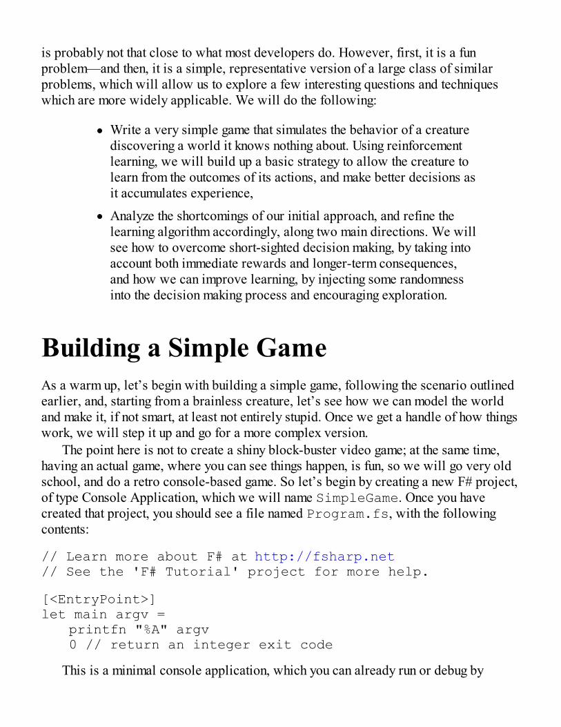
is probably not that close to what most developers do. However, first, it is a funproblem—and then, it is a simple, representative version of a large class of similarproblems, which will allow us to explore a few interesting questions and techniqueswhich are more widely applicable. We will do the following:

Write a very simple game that simulates the behavior of a creaturediscovering a world it knows nothing about. Using reinforcementlearning, we will build up a basic strategy to allow the creature tolearn from the outcomes of its actions, and make better decisions asit accumulates experience,

Analyze the shortcomings of our initial approach, and refine thelearning algorithm accordingly, along two main directions. We willsee how to overcome short-sighted decision making, by taking intoaccount both immediate rewards and longer-term consequences,and how we can improve learning, by injecting some randomnessinto the decision making process and encouraging exploration.

Building a Simple GameAs a warm up, let’s begin with building a simple game, following the scenario outlinedearlier, and, starting from a brainless creature, let’s see how we can model the worldand make it, if not smart, at least not entirely stupid. Once we get a handle of how thingswork, we will step it up and go for a more complex version.

The point here is not to create a shiny block-buster video game; at the same time,having an actual game, where you can see things happen, is fun, so we will go very oldschool, and do a retro console-based game. So let’s begin by creating a new F# project,of type Console Application, which we will name SimpleGame. Once you havecreated that project, you should see a file named Program.fs, with the followingcontents:

// Learn more about F# at http://fsharp.net// See the 'F# Tutorial' project for more help.

[<EntryPoint>]let main argv = printfn "%A" argv 0 // return an integer exit code

This is a minimal console application, which you can already run or debug by

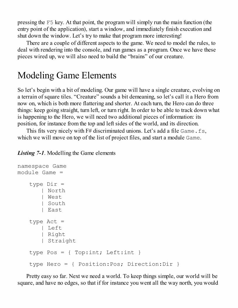
pressing the F5 key. At that point, the program will simply run the main function (theentry point of the application), start a window, and immediately finish execution andshut down the window. Let’s try to make that program more interesting!

There are a couple of different aspects to the game. We need to model the rules, todeal with rendering into the console, and run games as a program. Once we have thesepieces wired up, we will also need to build the “brains” of our creature.

Modeling Game ElementsSo let’s begin with a bit of modeling. Our game will have a single creature, evolving ona terrain of square tiles. “Creature” sounds a bit demeaning, so let’s call it a Hero fromnow on, which is both more flattering and shorter. At each turn, the Hero can do threethings: keep going straight, turn left, or turn right. In order to be able to track down whatis happening to the Hero, we will need two additional pieces of information: itsposition, for instance from the top and left sides of the world, and its direction.

This fits very nicely with F# discriminated unions. Let’s add a file Game.fs,which we will move on top of the list of project files, and start a module Game.

Listing 7-1. Modelling the Game elements

namespace Gamemodule Game =

type Dir = | North | West | South | East

type Act = | Left | Right | Straight

type Pos = { Top:int; Left:int }

type Hero = { Position:Pos; Direction:Dir }

Pretty easy so far. Next we need a world. To keep things simple, our world will besquare, and have no edges, so that if for instance you went all the way north, you would

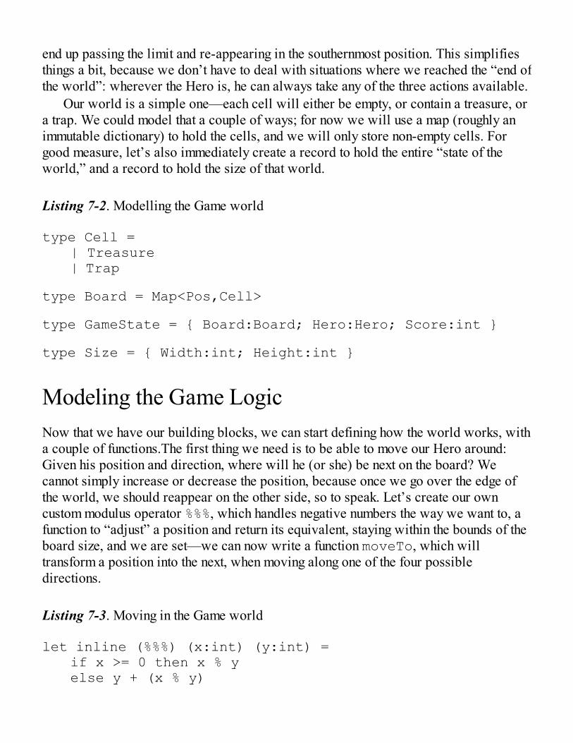
end up passing the limit and re-appearing in the southernmost position. This simplifiesthings a bit, because we don’t have to deal with situations where we reached the “end ofthe world”: wherever the Hero is, he can always take any of the three actions available.

Our world is a simple one—each cell will either be empty, or contain a treasure, ora trap. We could model that a couple of ways; for now we will use a map (roughly animmutable dictionary) to hold the cells, and we will only store non-empty cells. Forgood measure, let’s also immediately create a record to hold the entire “state of theworld,” and a record to hold the size of that world.

Listing 7-2. Modelling the Game world

type Cell = | Treasure | Trap

type Board = Map<Pos,Cell>

type GameState = { Board:Board; Hero:Hero; Score:int }

type Size = { Width:int; Height:int }

Modeling the Game LogicNow that we have our building blocks, we can start defining how the world works, witha couple of functions.The first thing we need is to be able to move our Hero around:Given his position and direction, where will he (or she) be next on the board? Wecannot simply increase or decrease the position, because once we go over the edge ofthe world, we should reappear on the other side, so to speak. Let’s create our owncustom modulus operator %%%, which handles negative numbers the way we want to, afunction to “adjust” a position and return its equivalent, staying within the bounds of theboard size, and we are set—we can now write a function moveTo, which willtransform a position into the next, when moving along one of the four possibledirections.

Listing 7-3. Moving in the Game world

let inline (%%%) (x:int) (y:int) = if x >= 0 then x % y else y + (x % y)

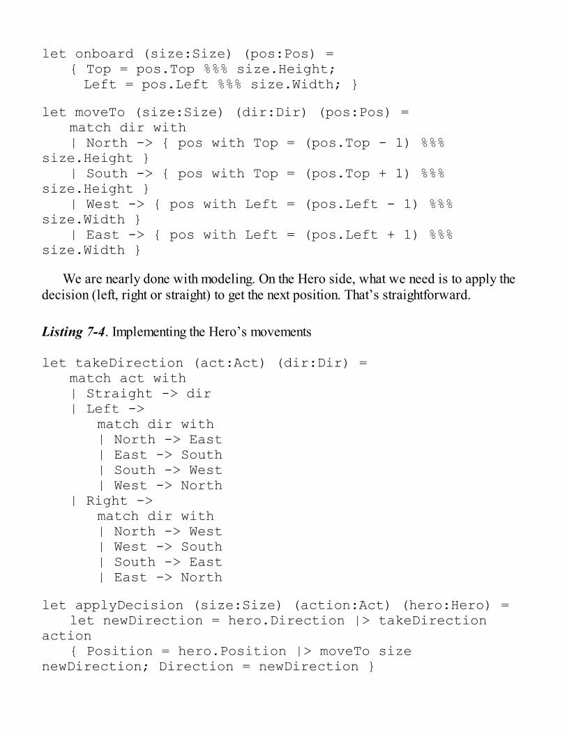
let onboard (size:Size) (pos:Pos) = { Top = pos.Top %%% size.Height; Left = pos.Left %%% size.Width; }

let moveTo (size:Size) (dir:Dir) (pos:Pos) = match dir with | North -> { pos with Top = (pos.Top - 1) %%% size.Height } | South -> { pos with Top = (pos.Top + 1) %%% size.Height } | West -> { pos with Left = (pos.Left - 1) %%% size.Width } | East -> { pos with Left = (pos.Left + 1) %%% size.Width }

We are nearly done with modeling. On the Hero side, what we need is to apply thedecision (left, right or straight) to get the next position. That’s straightforward.

Listing 7-4. Implementing the Hero’s movements

let takeDirection (act:Act) (dir:Dir) = match act with | Straight -> dir | Left -> match dir with | North -> East | East -> South | South -> West | West -> North | Right -> match dir with | North -> West | West -> South | South -> East | East -> North

let applyDecision (size:Size) (action:Act) (hero:Hero) = let newDirection = hero.Direction |> takeDirection action { Position = hero.Position |> moveTo size newDirection; Direction = newDirection }

Finally, we need to model what happens to the world. For now, whenever the Herovisits a position, if there is nothing, nothing happens; if there is a treasure, pocket 100points, if there is a trap, lose 100 points, and the trap or treasure is gone. Again, that isfairly straightforward. The function computeGain looks for a potential cell on theboard at the Hero’s position, and the corresponding gain if there is one, andupdateBoard takes the current board, and removes the cell at the Hero’s position, ifany.

Listing 7-5. Updating the world

let treasureScore = 100let trapScore = - 100

let computeGain (board:Board) (hero:Hero) = let currentPosition = hero.Position match board.TryFind(currentPosition) with | Some(cell) -> match cell with | Treasure -> treasureScore | Trap -> trapScore | None -> 0

let updateBoard (board:Board) (player:Hero) = let currentPosition = player.Position board |> Map.filter (fun position _ -> position <> currentPosition)

And... we are done with modeling. Next up, let’s get that game running!

Running the Game as a Console AppLet’s wire up the most basic things that could possibly work. The game needs to run aloop: Ask the Hero to make a decision, update the world accordingly, render it—andstart again. We also need some code to initialize the world.

In the Program.fs file, let’s modify a bit the default code, and create aProgram module, with the same namespace Game we used for the Game modelingpart:

namespace Game

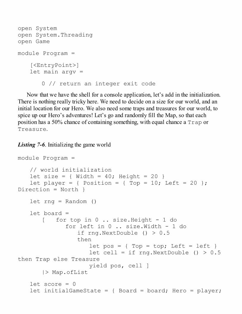
open Systemopen System.Threadingopen Game

module Program =

[<EntryPoint>] let main argv =

0 // return an integer exit code

Now that we have the shell for a console application, let’s add in the initialization.There is nothing really tricky here. We need to decide on a size for our world, and aninitial location for our Hero. We also need some traps and treasures for our world, tospice up our Hero’s adventures! Let’s go and randomly fill the Map, so that eachposition has a 50% chance of containing something, with equal chance a Trap orTreasure.

Listing 7-6. Initializing the game world

module Program =

// world initialization let size = { Width = 40; Height = 20 } let player = { Position = { Top = 10; Left = 20 }; Direction = North }

let rng = Random ()

let board = [ for top in 0 .. size.Height - 1 do for left in 0 .. size.Width - 1 do if rng.NextDouble () > 0.5 then let pos = { Top = top; Left = left } let cell = if rng.NextDouble () > 0.5 then Trap else Treasure yield pos, cell ] |> Map.ofList

let score = 0 let initialGameState = { Board = board; Hero = player;

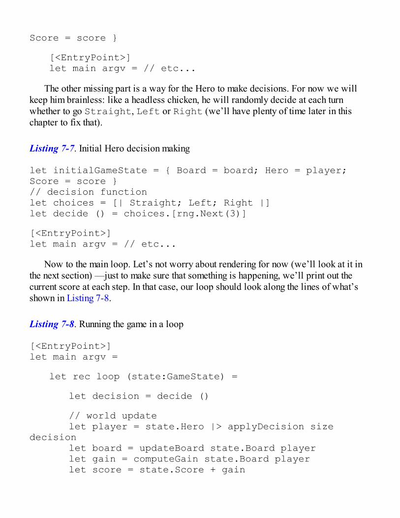
Score = score }

[<EntryPoint>] let main argv = // etc...

The other missing part is a way for the Hero to make decisions. For now we willkeep him brainless: like a headless chicken, he will randomly decide at each turnwhether to go Straight, Left or Right (we’ll have plenty of time later in thischapter to fix that).

Listing 7-7. Initial Hero decision making

let initialGameState = { Board = board; Hero = player; Score = score }// decision functionlet choices = [| Straight; Left; Right |]let decide () = choices.[rng.Next(3)]

[<EntryPoint>]let main argv = // etc...

Now to the main loop. Let’s not worry about rendering for now (we’ll look at it inthe next section) —just to make sure that something is happening, we’ll print out thecurrent score at each step. In that case, our loop should look along the lines of what’sshown in Listing 7-8.

Listing 7-8. Running the game in a loop

[<EntryPoint>]let main argv =

let rec loop (state:GameState) =

let decision = decide ()

// world update let player = state.Hero |> applyDecision size decision let board = updateBoard state.Board player let gain = computeGain state.Board player let score = state.Score + gain

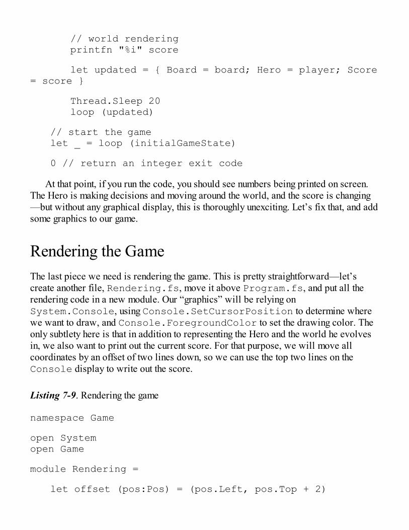
// world rendering printfn "%i" score

let updated = { Board = board; Hero = player; Score = score }

Thread.Sleep 20 loop (updated)

// start the game let _ = loop (initialGameState)

0 // return an integer exit code

At that point, if you run the code, you should see numbers being printed on screen.The Hero is making decisions and moving around the world, and the score is changing—but without any graphical display, this is thoroughly unexciting. Let’s fix that, and addsome graphics to our game.

Rendering the GameThe last piece we need is rendering the game. This is pretty straightforward—let’screate another file, Rendering.fs, move it above Program.fs, and put all therendering code in a new module. Our “graphics” will be relying onSystem.Console, using Console.SetCursorPosition to determine wherewe want to draw, and Console.ForegroundColor to set the drawing color. Theonly subtlety here is that in addition to representing the Hero and the world he evolvesin, we also want to print out the current score. For that purpose, we will move allcoordinates by an offset of two lines down, so we can use the top two lines on theConsole display to write out the score.

Listing 7-9. Rendering the game

namespace Game

open Systemopen Game

module Rendering =

let offset (pos:Pos) = (pos.Left, pos.Top + 2)

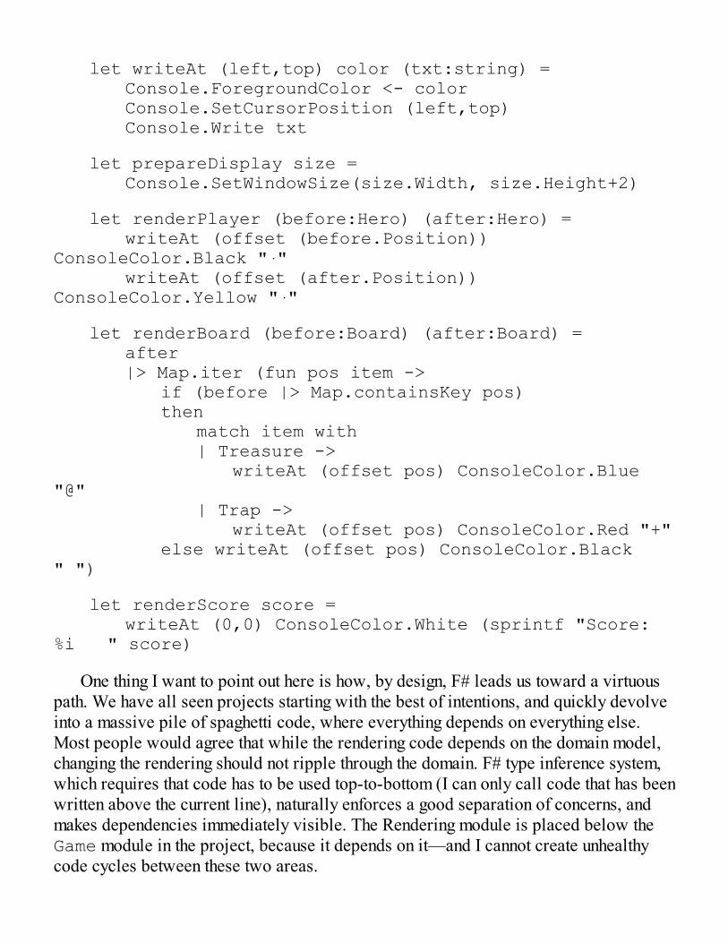
let writeAt (left,top) color (txt:string) = Console.ForegroundColor <- color Console.SetCursorPosition (left,top) Console.Write txt

let prepareDisplay size = Console.SetWindowSize(size.Width, size.Height+2)

let renderPlayer (before:Hero) (after:Hero) = writeAt (offset (before.Position)) ConsoleColor.Black "·" writeAt (offset (after.Position)) ConsoleColor.Yellow "·"

let renderBoard (before:Board) (after:Board) = after |> Map.iter (fun pos item -> if (before |> Map.containsKey pos) then match item with | Treasure -> writeAt (offset pos) ConsoleColor.Blue "@" | Trap -> writeAt (offset pos) ConsoleColor.Red "+" else writeAt (offset pos) ConsoleColor.Black " ")

let renderScore score = writeAt (0,0) ConsoleColor.White (sprintf "Score: %i " score)

One thing I want to point out here is how, by design, F# leads us toward a virtuouspath. We have all seen projects starting with the best of intentions, and quickly devolveinto a massive pile of spaghetti code, where everything depends on everything else.Most people would agree that while the rendering code depends on the domain model,changing the rendering should not ripple through the domain. F# type inference system,which requires that code has to be used top-to-bottom (I can only call code that has beenwritten above the current line), naturally enforces a good separation of concerns, andmakes dependencies immediately visible. The Rendering module is placed below theGame module in the project, because it depends on it—and I cannot create unhealthycode cycles between these two areas.

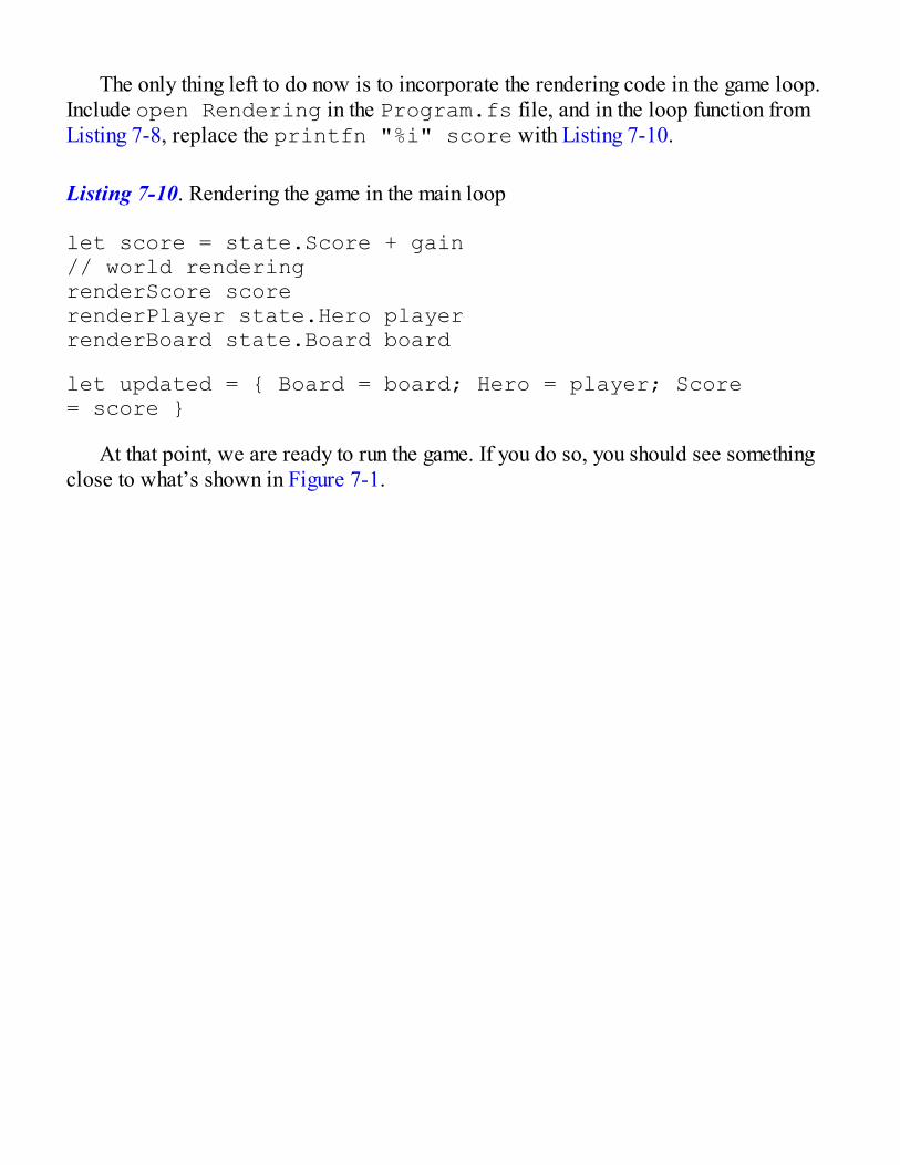
The only thing left to do now is to incorporate the rendering code in the game loop.Include open Rendering in the Program.fs file, and in the loop function fromListing 7-8, replace the printfn "%i" score with Listing 7-10.

Listing 7-10. Rendering the game in the main loop

let score = state.Score + gain// world renderingrenderScore scorerenderPlayer state.Hero playerrenderBoard state.Board board

let updated = { Board = board; Hero = player; Score = score }

At that point, we are ready to run the game. If you do so, you should see somethingclose to what’s shown in Figure 7-1.

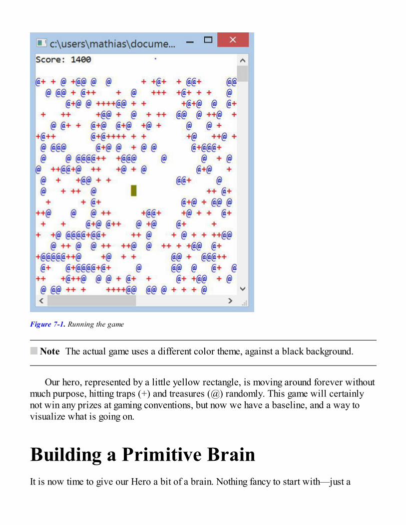
Figure 7-1. Running the game

Note The actual game uses a different color theme, against a black background.

Our hero, represented by a little yellow rectangle, is moving around forever withoutmuch purpose, hitting traps (+) and treasures (@) randomly. This game will certainlynot win any prizes at gaming conventions, but now we have a baseline, and a way tovisualize what is going on.

Building a Primitive BrainIt is now time to give our Hero a bit of a brain. Nothing fancy to start with—just a

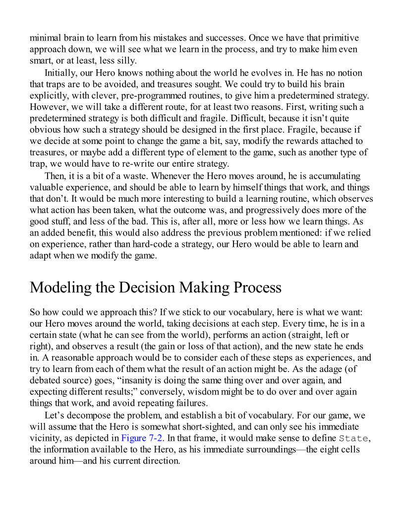
minimal brain to learn from his mistakes and successes. Once we have that primitiveapproach down, we will see what we learn in the process, and try to make him evensmart, or at least, less silly.

Initially, our Hero knows nothing about the world he evolves in. He has no notionthat traps are to be avoided, and treasures sought. We could try to build his brainexplicitly, with clever, pre-programmed routines, to give him a predetermined strategy.However, we will take a different route, for at least two reasons. First, writing such apredetermined strategy is both difficult and fragile. Difficult, because it isn’t quiteobvious how such a strategy should be designed in the first place. Fragile, because ifwe decide at some point to change the game a bit, say, modify the rewards attached totreasures, or maybe add a different type of element to the game, such as another type oftrap, we would have to re-write our entire strategy.

Then, it is a bit of a waste. Whenever the Hero moves around, he is accumulatingvaluable experience, and should be able to learn by himself things that work, and thingsthat don’t. It would be much more interesting to build a learning routine, which observeswhat action has been taken, what the outcome was, and progressively does more of thegood stuff, and less of the bad. This is, after all, more or less how we learn things. Asan added benefit, this would also address the previous problem mentioned: if we reliedon experience, rather than hard-code a strategy, our Hero would be able to learn andadapt when we modify the game.

Modeling the Decision Making ProcessSo how could we approach this? If we stick to our vocabulary, here is what we want:our Hero moves around the world, taking decisions at each step. Every time, he is in acertain state (what he can see from the world), performs an action (straight, left orright), and observes a result (the gain or loss of that action), and the new state he endsin. A reasonable approach would be to consider each of these steps as experiences, andtry to learn from each of them what the result of an action might be. As the adage (ofdebated source) goes, “insanity is doing the same thing over and over again, andexpecting different results;” conversely, wisdom might be to do over and over againthings that work, and avoid repeating failures.

Let’s decompose the problem, and establish a bit of vocabulary. For our game, wewill assume that the Hero is somewhat short-sighted, and can only see his immediatevicinity, as depicted in Figure 7-2. In that frame, it would make sense to define State,the information available to the Hero, as his immediate surroundings—the eight cellsaround him—and his current direction.

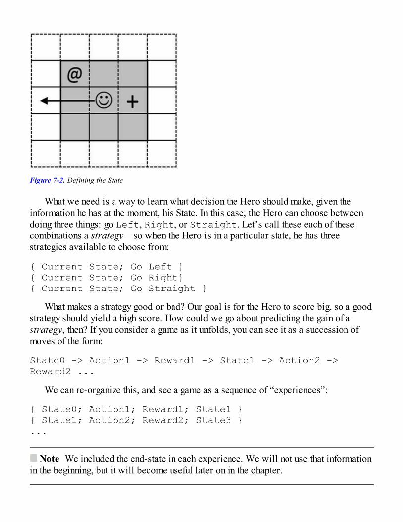
Figure 7-2. Defining the State

What we need is a way to learn what decision the Hero should make, given theinformation he has at the moment, his State. In this case, the Hero can choose betweendoing three things: go Left, Right, or Straight. Let’s call these each of thesecombinations a strategy—so when the Hero is in a particular state, he has threestrategies available to choose from:

{ Current State; Go Left }{ Current State; Go Right}{ Current State; Go Straight }

What makes a strategy good or bad? Our goal is for the Hero to score big, so a goodstrategy should yield a high score. How could we go about predicting the gain of astrategy, then? If you consider a game as it unfolds, you can see it as a succession ofmoves of the form:

State0 -> Action1 -> Reward1 -> State1 -> Action2 -> Reward2 ...

We can re-organize this, and see a game as a sequence of “experiences”:

{ State0; Action1; Reward1; State1 }{ State1; Action2; Reward2; State3 }...

Note We included the end-state in each experience. We will not use that informationin the beginning, but it will become useful later on in the chapter.

As we run the game, the Hero will be accumulating experience each time he makes adecision. Initially, some decisions will be good, some will be bad. What we would likeis to use that experience to learn a winning strategy, so that when he finds himself inconditions he has encountered before (a known state), he can predict the reward heshould expect from each of the three strategies available to him, and pick the bestdecision accordingly (the decision corresponding to the strategy with highest expectedvalue).

Learning a Winning Strategy from ExperienceThe only thing we need at that point is a learning process to evaluate strategies. Onepossibility would be to keep track of all the accumulated experience; when the Heroenters a state, we could then simply look for every situation where the same state wasencountered in the past, and compute (for instance) the average reward for each of thedecisions taken. This is clearly impractical: we would end up accumulating a lot ofdata, and the program would slowly grind to a halt.

A more effective approach would be to maintain a single record for every strategywe tried, that is, a state and decision combination, and progressively build up anestimate for how good or bad that strategy is, based on all our accumulated experienceso far. When we encounter a known state, all we have to do is look up for the threepossible matching strategies in our catalog of strategies, which we’ll call the brain,and select the strategy with highest value.

We almost have an algorithm ready to go. The only thing left is to deal with twosmall problems. The first one is rather obvious: what should the Hero do when heencounters an unknown state? What I would do in his shoes is simply take a randomaction, and see what happens.

The second is a bit more intricate: what should the Hero do when taking the sameaction twice? In our particular situation, we know that doing the same thing twice in thesame conditions will result in the same outcome—so we could just take the action once,measure the gain, and stop learning. However, the only reason we can say that isbecause we know how the game is implemented; and nothing guarantees that this willremain the case. We could, for instance, decide that treasures and traps will materializerandomly in the world, or that the reward attached to a treasure or a trap will changeover time. In that case, such an approach would be pretty bad: we would rely on onesingle experience, which might be highly unusual, to form our strategy, and stop learningaltogether afterward.

A better and more robust approach (which is advised outside of the realm of thisgame, too) is to keep learning all the time. Mimicking what we did in previous chapters,there is a simple way to do that: progressively refine our estimate for what rewards we

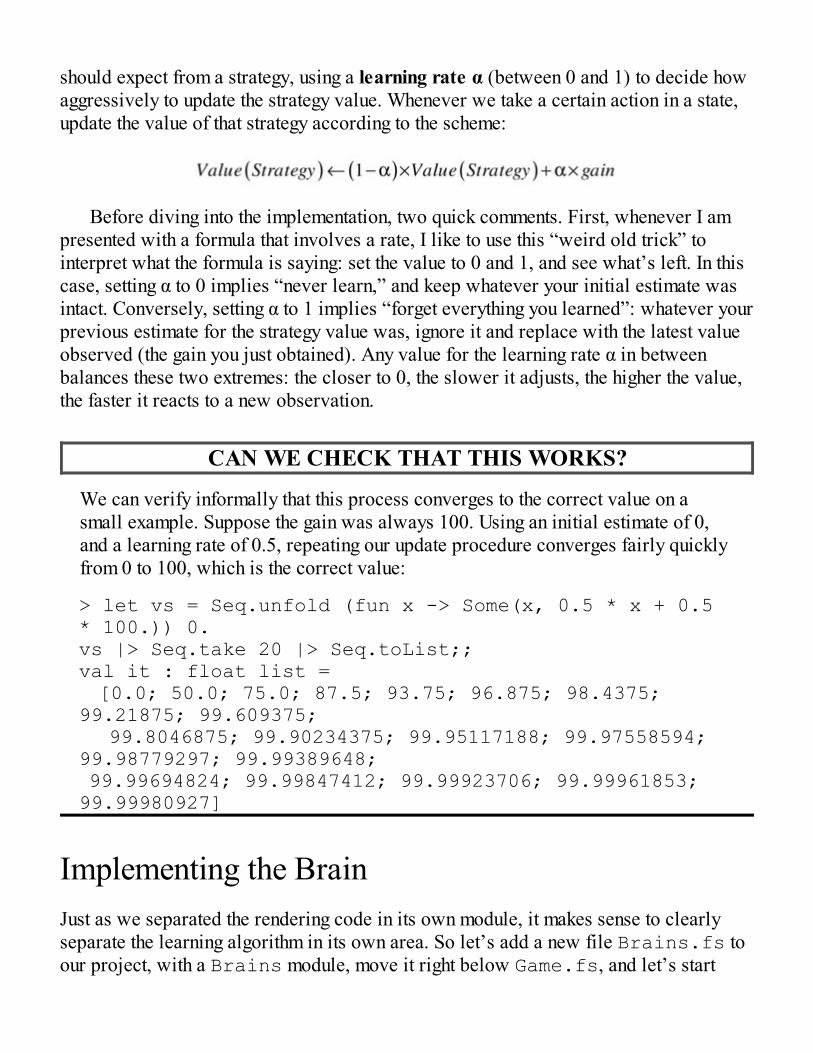
should expect from a strategy, using a learning rate α (between 0 and 1) to decide howaggressively to update the strategy value. Whenever we take a certain action in a state,update the value of that strategy according to the scheme:

Before diving into the implementation, two quick comments. First, whenever I ampresented with a formula that involves a rate, I like to use this “weird old trick” tointerpret what the formula is saying: set the value to 0 and 1, and see what’s left. In thiscase, setting α to 0 implies “never learn,” and keep whatever your initial estimate wasintact. Conversely, setting α to 1 implies “forget everything you learned”: whatever yourprevious estimate for the strategy value was, ignore it and replace with the latest valueobserved (the gain you just obtained). Any value for the learning rate α in betweenbalances these two extremes: the closer to 0, the slower it adjusts, the higher the value,the faster it reacts to a new observation.

CAN WE CHECK THAT THIS WORKS?

We can verify informally that this process converges to the correct value on asmall example. Suppose the gain was always 100. Using an initial estimate of 0,and a learning rate of 0.5, repeating our update procedure converges fairly quicklyfrom 0 to 100, which is the correct value:

> let vs = Seq.unfold (fun x -> Some(x, 0.5 * x + 0.5 * 100.)) 0.vs |> Seq.take 20 |> Seq.toList;;val it : float list = [0.0; 50.0; 75.0; 87.5; 93.75; 96.875; 98.4375; 99.21875; 99.609375; 99.8046875; 99.90234375; 99.95117188; 99.97558594; 99.98779297; 99.99389648; 99.99694824; 99.99847412; 99.99923706; 99.99961853; 99.99980927]

Implementing the BrainJust as we separated the rendering code in its own module, it makes sense to clearlyseparate the learning algorithm in its own area. So let’s add a new file Brains.fs toour project, with a Brains module, move it right below Game.fs, and let’s start

modeling.

Listing 7-11. Modeling the Brain

namespace Gameopen Systemopen Game

module Brains =

// My current direction and surrounding cells type State = Dir * (Cell option) list

type Experience = { State: State; // where I was Action: Act; // what I did Reward: float; // what reward I got NextState: State; } // where I ended

// one possible course of action I can take // when I am in that State type Strategy = { State:State; Action:Act; }

// Strategies I tried, and what reward // I should expect from them type Brain = Map<Strategy,float>

The model maps pretty much word-for-word our description of the problem. Wehave a State, putting together the current direction and a list of Cell options,denoting that some cells might be empty, Experience, and a Brain, which mapseach possible Strategy (a State and the Action that could be taken) to anestimated reward.

It makes sense to refactor a bit our code, and move the random decision function wehad in the Program itself (Listing 7-7), into the Brain as well:

let rng = Random ()let choices = [| Straight; Left; Right |]let randomDecide () = choices.[rng.Next(3)]

Let’s get into the learning process. What we want here is to incorporate a newExperience and update the Brain accordingly. This is fairly straightforward: weneed to extract out the Strategy that was taken in that Experience, look for the

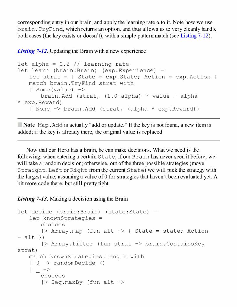
corresponding entry in our brain, and apply the learning rate α to it. Note how we usebrain.TryFind, which returns an option, and thus allows us to very cleanly handleboth cases (the key exists or doesn’t), with a simple pattern match (see Listing 7-12).

Listing 7-12. Updating the Brain with a new experience

let alpha = 0.2 // learning ratelet learn (brain:Brain) (exp:Experience) = let strat = { State = exp.State; Action = exp.Action } match brain.TryFind strat with | Some(value) -> brain.Add (strat, (1.0-alpha) * value + alpha * exp.Reward) | None -> brain.Add (strat, (alpha * exp.Reward))

Note Map.Add is actually “add or update.” If the key is not found, a new item isadded; if the key is already there, the original value is replaced.

Now that our Hero has a brain, he can make decisions. What we need is thefollowing: when entering a certain State, if our Brain has never seen it before, wewill take a random decision; otherwise, out of the three possible strategies (moveStraight, Left or Right from the current State) we will pick the strategy withthe largest value, assuming a value of 0 for strategies that haven’t been evaluated yet. Abit more code there, but still pretty tight.

Listing 7-13. Making a decision using the Brain

let decide (brain:Brain) (state:State) = let knownStrategies = choices |> Array.map (fun alt -> { State = state; Action = alt }) |> Array.filter (fun strat -> brain.ContainsKey strat) match knownStrategies.Length with | 0 -> randomDecide () | _ -> choices |> Seq.maxBy (fun alt ->

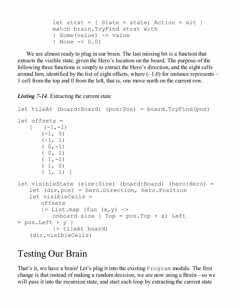
let strat = { State = state; Action = alt } match brain.TryFind strat with | Some(value) -> value | None -> 0.0)

We are almost ready to plug in our brain. The last missing bit is a function thatextracts the visible state, given the Hero’s location on the board. The purpose of thefollowing three functions is simply to extract the Hero’s direction, and the eight cellsaround him, identified by the list of eight offsets, where (–1,0) for instance represents –1 cell from the top and 0 from the left, that is, one move north on the current row.

Listing 7-14. Extracting the current state

let tileAt (board:Board) (pos:Pos) = board.TryFind(pos)

let offsets = [ (-1,-1) (-1, 0) (-1, 1) ( 0,-1) ( 0, 1) ( 1,-1) ( 1, 0) ( 1, 1) ]

let visibleState (size:Size) (board:Board) (hero:Hero) = let (dir,pos) = hero.Direction, hero.Position let visibleCells = offsets |> List.map (fun (x,y) -> onboard size { Top = pos.Top + x; Left = pos.Left + y } |> tileAt board) (dir,visibleCells)

Testing Our BrainThat’s it, we have a brain! Let’s plug it into the existing Program module. The firstchange is that instead of making a random decision, we are now using a Brain—so wewill pass it into the recursion state, and start each loop by extracting the current state

and making a decision. The other minor modification is that of course we need to dosome learning at some point; that’s easily done, by making the changes shown in Listing7-15.

Listing 7-15. Incorporating learning in the game loop

let rec loop (state:GameState,brain:Brain) = let currentState = visibleState size state.Board state.Hero let decision = Brains.decide brain currentState

// world update let player = state.Hero |> applyDecision size decision let board = updateBoard state.Board player let gain = computeGain state.Board player let score = state.Score + gain

// learning let nextState = visibleState size board player let experience = { State = currentState; Action = decision; Reward = gain |> float; NextState = nextState; } let brain = learn brain experience

Finally, when we start the game, we need to provide it a brain, which will beinitially empty:

let _ = loop (initial,Map.empty)

And we are ready to go—if you run this, you should see a similar game as before,but with a Hero who apparently is making fewer mistakes over time. So... ship it?

Hold your horses! First, where is the data? We are scientists here, and I would likea bit more evidence than a fuzzy statement like “it apparently makes less mistakes” toevaluate whether our brain is doing something right. The easiest way to perform thatevaluation is probably to run a head-to-head comparison (sorry for the pun), seeing howthe two approaches fare on games of equal length. Because both approaches involve anelement of randomness, we will want to run that comparison on a few runs. If we reliedon one game only, we would face the risk to observe unusual results, out of sheer luck.Running a bunch of games mitigates that risk.

This creates another small inconvenience, though. Obviously, the more runs we want

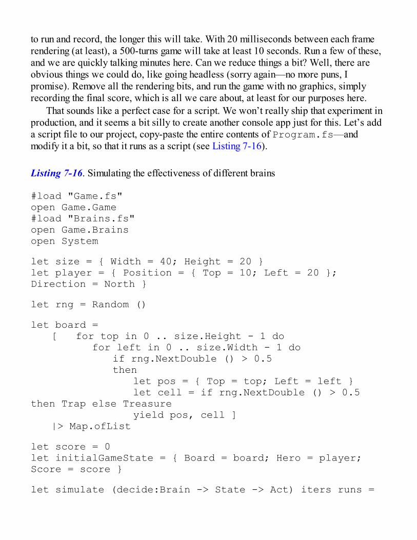
to run and record, the longer this will take. With 20 milliseconds between each framerendering (at least), a 500-turns game will take at least 10 seconds. Run a few of these,and we are quickly talking minutes here. Can we reduce things a bit? Well, there areobvious things we could do, like going headless (sorry again—no more puns, Ipromise). Remove all the rendering bits, and run the game with no graphics, simplyrecording the final score, which is all we care about, at least for our purposes here.

That sounds like a perfect case for a script. We won’t really ship that experiment inproduction, and it seems a bit silly to create another console app just for this. Let’s adda script file to our project, copy-paste the entire contents of Program.fs—andmodify it a bit, so that it runs as a script (see Listing 7-16).

Listing 7-16. Simulating the effectiveness of different brains

#load "Game.fs"open Game.Game#load "Brains.fs"open Game.Brainsopen System

let size = { Width = 40; Height = 20 }let player = { Position = { Top = 10; Left = 20 }; Direction = North }

let rng = Random ()

let board = [ for top in 0 .. size.Height - 1 do for left in 0 .. size.Width - 1 do if rng.NextDouble () > 0.5 then let pos = { Top = top; Left = left } let cell = if rng.NextDouble () > 0.5 then Trap else Treasure yield pos, cell ] |> Map.ofList

let score = 0let initialGameState = { Board = board; Hero = player; Score = score }

let simulate (decide:Brain -> State -> Act) iters runs =

// Loop now includes the iteration count let rec loop (state:GameState,brain:Brain,iter:int) =

let currentState = visibleState size state.Board state.Hero let decision = decide brain currentState

// world update let player = state.Hero |> applyDecision size decision let board = updateBoard state.Board player let gain = computeGain state.Board player let score = state.Score + gain

// learning let nextState = visibleState size board player let experience = { State = currentState; Action = decision; Reward = gain |> float; NextState = nextState; } let brain = learn brain experience

let updated = { Board = board; Hero = player; Score = score }

if iter < iters then loop (updated,brain,iter+1) else score

[ for run in 1 .. runs -> loop (initialGameState,Map.empty,0) ]

// Simulating different brainsprintfn "Random decision"let random = simulate (fun _ _ -> Game.Brains.randomDecide()) 500 20printfn "Average score: %.0f" (random |> Seq.averageBy float)

printfn "Crude brain"let crudeBrain = simulate Game.Brains.decide 500 20printfn "Average score: %.0f" (crudeBrain |> Seq.averageBy

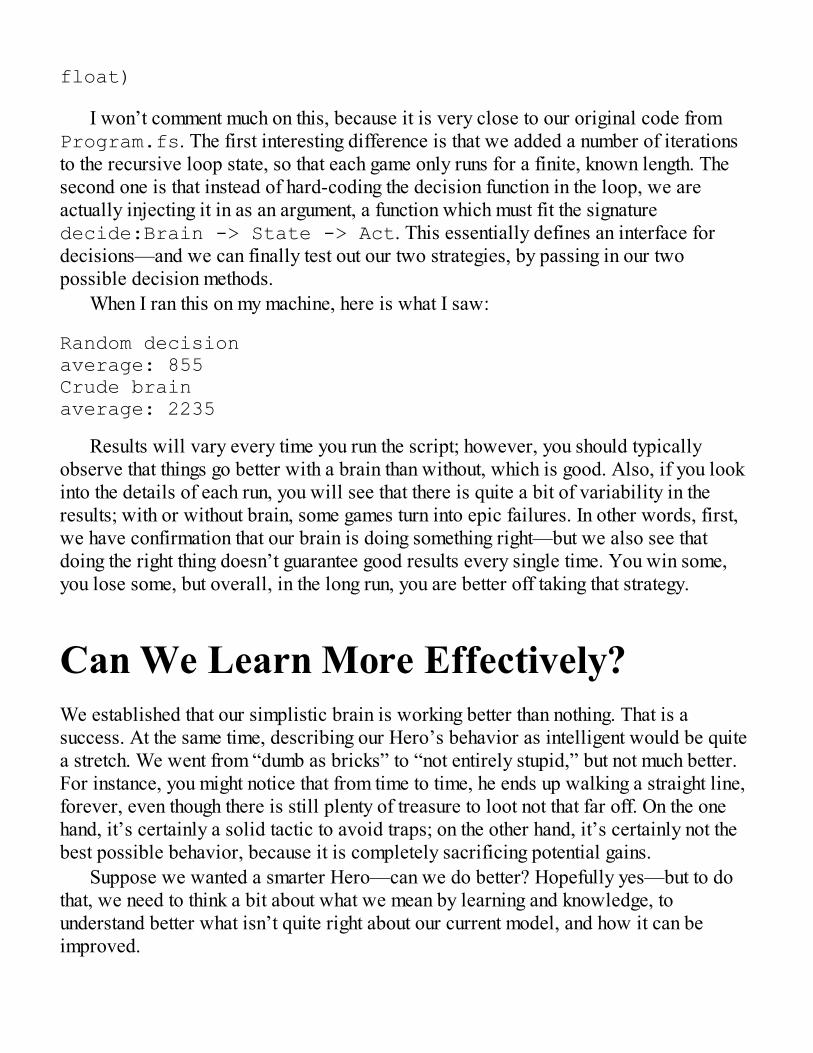
float)

I won’t comment much on this, because it is very close to our original code fromProgram.fs. The first interesting difference is that we added a number of iterationsto the recursive loop state, so that each game only runs for a finite, known length. Thesecond one is that instead of hard-coding the decision function in the loop, we areactually injecting it in as an argument, a function which must fit the signaturedecide:Brain -> State -> Act. This essentially defines an interface fordecisions—and we can finally test out our two strategies, by passing in our twopossible decision methods.

When I ran this on my machine, here is what I saw:

Random decisionaverage: 855Crude brainaverage: 2235

Results will vary every time you run the script; however, you should typicallyobserve that things go better with a brain than without, which is good. Also, if you lookinto the details of each run, you will see that there is quite a bit of variability in theresults; with or without brain, some games turn into epic failures. In other words, first,we have confirmation that our brain is doing something right—but we also see thatdoing the right thing doesn’t guarantee good results every single time. You win some,you lose some, but overall, in the long run, you are better off taking that strategy.

Can We Learn More Effectively?We established that our simplistic brain is working better than nothing. That is asuccess. At the same time, describing our Hero’s behavior as intelligent would be quitea stretch. We went from “dumb as bricks” to “not entirely stupid,” but not much better.For instance, you might notice that from time to time, he ends up walking a straight line,forever, even though there is still plenty of treasure to loot not that far off. On the onehand, it’s certainly a solid tactic to avoid traps; on the other hand, it’s certainly not thebest possible behavior, because it is completely sacrificing potential gains.

Suppose we wanted a smarter Hero—can we do better? Hopefully yes—but to dothat, we need to think a bit about what we mean by learning and knowledge, tounderstand better what isn’t quite right about our current model, and how it can beimproved.

Exploration vs. ExploitationAs a software engineer, here is a question you are probably faced with on a regularbasis: should I use the same techniques I am familiar with and know well, or should Itry this new fancy idea I have never used before, which I hear is interesting, but mightcompletely fail?

This is in a nutshell the tension between exploration and exploitation; you couldchoose to exploit a known strategy, which you have tried before, with predictableresults, or you could explore new possibilities, hoping to learn new strategies that workeven better than what you currently do, but with a risk of failure, where you wouldactually perform worse than what the conservative, “business as usual” approach wouldhave given. As software engineers, all exploitation, and we would still be coding onpunch cards; all exploration, and we would be entirely changing our stack and processall the time.

This is also why our Hero ends up chasing his tail from time to time. The onlyexploration our Hero does is when he is forced to do so, because he has neverencountered a situation, and has no default choice to fall back to. However, once hefound a strategy that had a positive outcome, he will go to it over and over again, andnever try anything else.

This suggests a first direction we can take to improve our brain: give the Hero a bitof an adventurous spirit, and make him try out from time to time random strategies, eventhough a decent one is readily available. The simplest way we can do that is called ε-learning: each turn, with a small probability ε, we will take a random decision,regardless of what we already know, and explore. This will help make sure that we arenot settling for a comfortable strategy, when a much better one might be available.

Is a Red Door Different from a Blue Door?Being silly is repeating the same mistakes, over and over again. Being smart isrecognizing that some situations are similar enough that they should be treated the same.The first time I try to open the door to my kitchen, which happens to be red, I mightfumble until I figure out how it works, and next time I see it, at a minimum, I should beable to repeat what worked the last time. However, when I see the door to the livingroom, which happens to be blue, even though the circumstances are slightly different(it’s a blue door, and a different room), I would probably try the same thing that workedin the kitchen.

Behaving in an intelligent manner involves recognizing similar states, abstractingthem, and applying what was learned to a broader context. What makes us smart is that

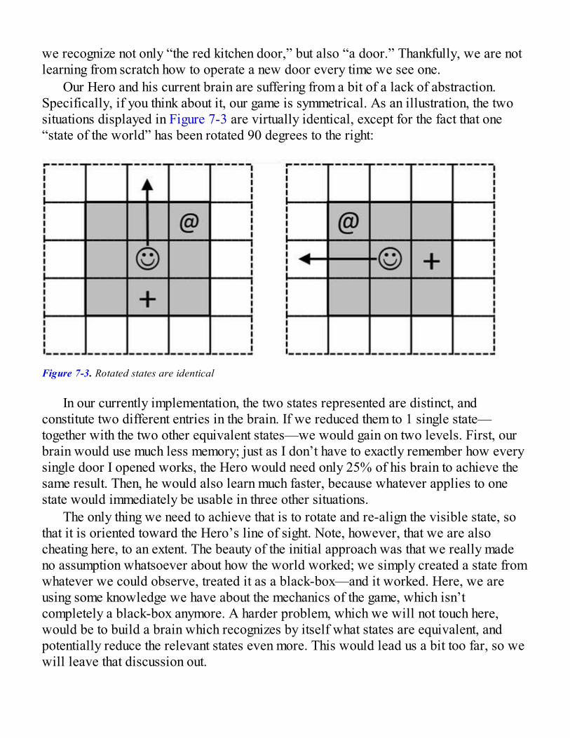
we recognize not only “the red kitchen door,” but also “a door.” Thankfully, we are notlearning from scratch how to operate a new door every time we see one.

Our Hero and his current brain are suffering from a bit of a lack of abstraction.Specifically, if you think about it, our game is symmetrical. As an illustration, the twosituations displayed in Figure 7-3 are virtually identical, except for the fact that one“state of the world” has been rotated 90 degrees to the right:

Figure 7-3. Rotated states are identical

In our currently implementation, the two states represented are distinct, andconstitute two different entries in the brain. If we reduced them to 1 single state—together with the two other equivalent states—we would gain on two levels. First, ourbrain would use much less memory; just as I don’t have to exactly remember how everysingle door I opened works, the Hero would need only 25% of his brain to achieve thesame result. Then, he would also learn much faster, because whatever applies to onestate would immediately be usable in three other situations.

The only thing we need to achieve that is to rotate and re-align the visible state, sothat it is oriented toward the Hero’s line of sight. Note, however, that we are alsocheating here, to an extent. The beauty of the initial approach was that we really madeno assumption whatsoever about how the world worked; we simply created a state fromwhatever we could observe, treated it as a black-box—and it worked. Here, we areusing some knowledge we have about the mechanics of the game, which isn’tcompletely a black-box anymore. A harder problem, which we will not touch here,would be to build a brain which recognizes by itself what states are equivalent, andpotentially reduce the relevant states even more. This would lead us a bit too far, so wewill leave that discussion out.

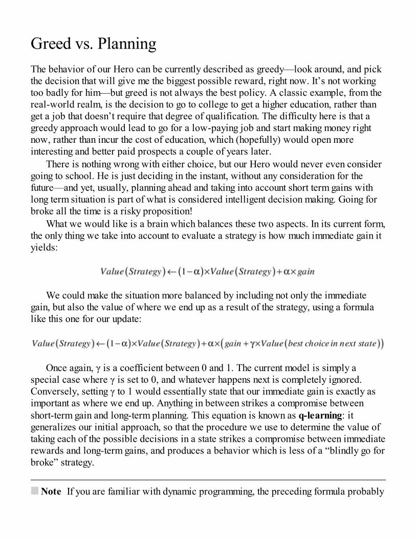
Greed vs. PlanningThe behavior of our Hero can be currently described as greedy—look around, and pickthe decision that will give me the biggest possible reward, right now. It’s not workingtoo badly for him—but greed is not always the best policy. A classic example, from thereal-world realm, is the decision to go to college to get a higher education, rather thanget a job that doesn’t require that degree of qualification. The difficulty here is that agreedy approach would lead to go for a low-paying job and start making money rightnow, rather than incur the cost of education, which (hopefully) would open moreinteresting and better paid prospects a couple of years later.

There is nothing wrong with either choice, but our Hero would never even considergoing to school. He is just deciding in the instant, without any consideration for thefuture—and yet, usually, planning ahead and taking into account short term gains withlong term situation is part of what is considered intelligent decision making. Going forbroke all the time is a risky proposition!

What we would like is a brain which balances these two aspects. In its current form,the only thing we take into account to evaluate a strategy is how much immediate gain ityields:

We could make the situation more balanced by including not only the immediategain, but also the value of where we end up as a result of the strategy, using a formulalike this one for our update:

Once again, γ is a coefficient between 0 and 1. The current model is simply aspecial case where γ is set to 0, and whatever happens next is completely ignored.Conversely, setting γ to 1 would essentially state that our immediate gain is exactly asimportant as where we end up. Anything in between strikes a compromise betweenshort-term gain and long-term planning. This equation is known as q-learning: itgeneralizes our initial approach, so that the procedure we use to determine the value oftaking each of the possible decisions in a state strikes a compromise between immediaterewards and long-term gains, and produces a behavior which is less of a “blindly go forbroke” strategy.

Note If you are familiar with dynamic programming, the preceding formula probably

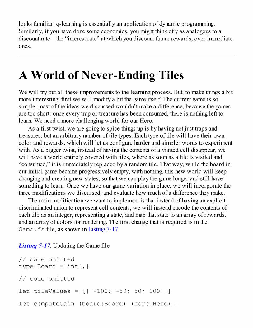
looks familiar; q-learning is essentially an application of dynamic programming.Similarly, if you have done some economics, you might think of γ as analogous to adiscount rate—the “interest rate” at which you discount future rewards, over immediateones.

A World of Never-Ending TilesWe will try out all these improvements to the learning process. But, to make things a bitmore interesting, first we will modify a bit the game itself. The current game is sosimple, most of the ideas we discussed wouldn’t make a difference, because the gamesare too short: once every trap or treasure has been consumed, there is nothing left tolearn. We need a more challenging world for our Hero.

As a first twist, we are going to spice things up is by having not just traps andtreasures, but an arbitrary number of tile types. Each type of tile will have their owncolor and rewards, which will let us configure harder and simpler words to experimentwith. As a bigger twist, instead of having the contents of a visited cell disappear, wewill have a world entirely covered with tiles, where as soon as a tile is visited and“consumed,” it is immediately replaced by a random tile. That way, while the board inour initial game became progressively empty, with nothing, this new world will keepchanging and creating new states, so that we can play the game longer and still havesomething to learn. Once we have our game variation in place, we will incorporate thethree modifications we discussed, and evaluate how much of a difference they make.

The main modification we want to implement is that instead of having an explicitdiscriminated union to represent cell contents, we will instead encode the contents ofeach tile as an integer, representing a state, and map that state to an array of rewards,and an array of colors for rendering. The first change that is required is in theGame.fs file, as shown in Listing 7-17.

Listing 7-17. Updating the Game file

// code omittedtype Board = int[,]

// code omitted

let tileValues = [| -100; -50; 50; 100 |]

let computeGain (board:Board) (hero:Hero) =

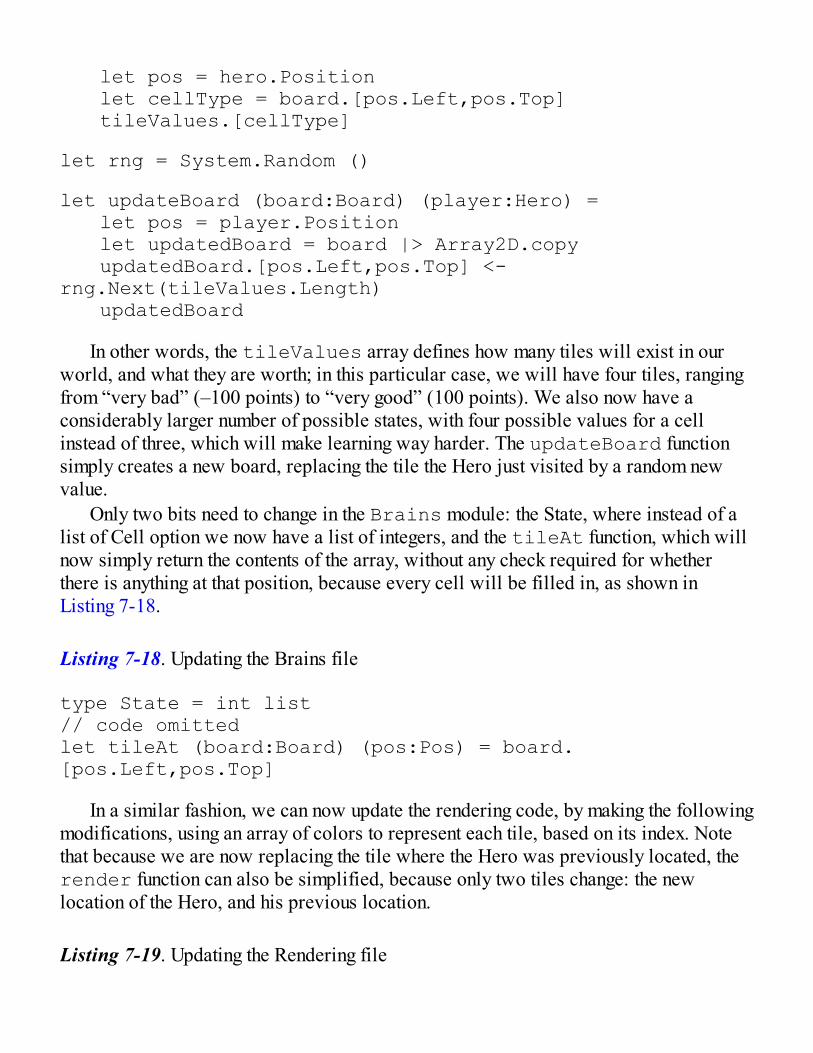
let pos = hero.Position let cellType = board.[pos.Left,pos.Top] tileValues.[cellType]

let rng = System.Random ()

let updateBoard (board:Board) (player:Hero) = let pos = player.Position let updatedBoard = board |> Array2D.copy updatedBoard.[pos.Left,pos.Top] <- rng.Next(tileValues.Length) updatedBoard

In other words, the tileValues array defines how many tiles will exist in ourworld, and what they are worth; in this particular case, we will have four tiles, rangingfrom “very bad” (–100 points) to “very good” (100 points). We also now have aconsiderably larger number of possible states, with four possible values for a cellinstead of three, which will make learning way harder. The updateBoard functionsimply creates a new board, replacing the tile the Hero just visited by a random newvalue.

Only two bits need to change in the Brains module: the State, where instead of alist of Cell option we now have a list of integers, and the tileAt function, which willnow simply return the contents of the array, without any check required for whetherthere is anything at that position, because every cell will be filled in, as shown inListing 7-18.

Listing 7-18. Updating the Brains file

type State = int list// code omittedlet tileAt (board:Board) (pos:Pos) = board.[pos.Left,pos.Top]

In a similar fashion, we can now update the rendering code, by making the followingmodifications, using an array of colors to represent each tile, based on its index. Notethat because we are now replacing the tile where the Hero was previously located, therender function can also be simplified, because only two tiles change: the newlocation of the Hero, and his previous location.

Listing 7-19. Updating the Rendering file

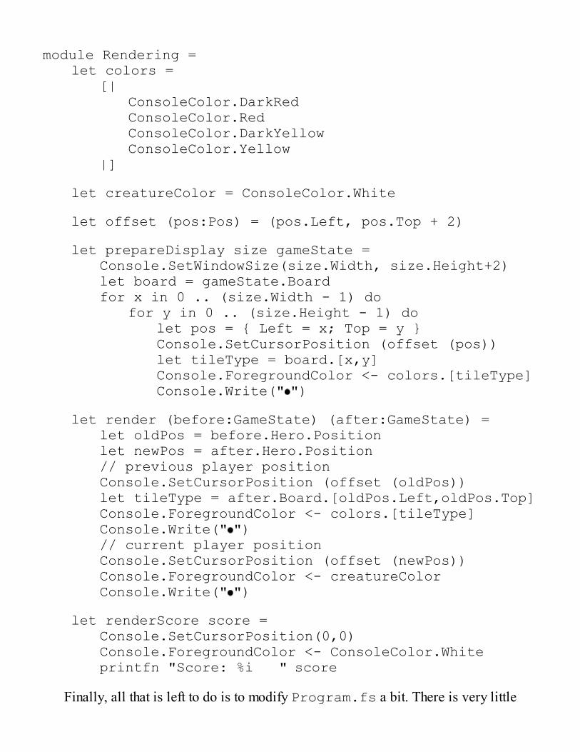
module Rendering = let colors = [| ConsoleColor.DarkRed ConsoleColor.Red ConsoleColor.DarkYellow ConsoleColor.Yellow |]

let creatureColor = ConsoleColor.White

let offset (pos:Pos) = (pos.Left, pos.Top + 2)

let prepareDisplay size gameState = Console.SetWindowSize(size.Width, size.Height+2) let board = gameState.Board for x in 0 .. (size.Width - 1) do for y in 0 .. (size.Height - 1) do let pos = { Left = x; Top = y } Console.SetCursorPosition (offset (pos)) let tileType = board.[x,y] Console.ForegroundColor <- colors.[tileType] Console.Write(" ")

let render (before:GameState) (after:GameState) = let oldPos = before.Hero.Position let newPos = after.Hero.Position // previous player position Console.SetCursorPosition (offset (oldPos)) let tileType = after.Board.[oldPos.Left,oldPos.Top] Console.ForegroundColor <- colors.[tileType] Console.Write(" ") // current player position Console.SetCursorPosition (offset (newPos)) Console.ForegroundColor <- creatureColor Console.Write(" ")

let renderScore score = Console.SetCursorPosition(0,0) Console.ForegroundColor <- ConsoleColor.White printfn "Score: %i " score

Finally, all that is left to do is to modify Program.fs a bit. There is very little

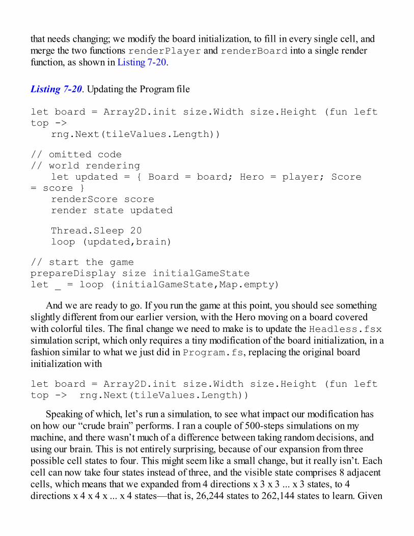
that needs changing; we modify the board initialization, to fill in every single cell, andmerge the two functions renderPlayer and renderBoard into a single renderfunction, as shown in Listing 7-20.

Listing 7-20. Updating the Program file

let board = Array2D.init size.Width size.Height (fun left top -> rng.Next(tileValues.Length))

// omitted code// world rendering let updated = { Board = board; Hero = player; Score = score } renderScore score render state updated

Thread.Sleep 20 loop (updated,brain)

// start the gameprepareDisplay size initialGameStatelet _ = loop (initialGameState,Map.empty)

And we are ready to go. If you run the game at this point, you should see somethingslightly different from our earlier version, with the Hero moving on a board coveredwith colorful tiles. The final change we need to make is to update the Headless.fsxsimulation script, which only requires a tiny modification of the board initialization, in afashion similar to what we just did in Program.fs, replacing the original boardinitialization with

let board = Array2D.init size.Width size.Height (fun left top -> rng.Next(tileValues.Length))

Speaking of which, let’s run a simulation, to see what impact our modification hason how our “crude brain” performs. I ran a couple of 500-steps simulations on mymachine, and there wasn’t much of a difference between taking random decisions, andusing our brain. This is not entirely surprising, because of our expansion from threepossible cell states to four. This might seem like a small change, but it really isn’t. Eachcell can now take four states instead of three, and the visible state comprises 8 adjacentcells, which means that we expanded from 4 directions x 3 x 3 ... x 3 states, to 4directions x 4 x 4 x ... x 4 states—that is, 26,244 states to 262,144 states to learn. Given

that our Hero has only 500 steps to learn that world, it should not be a surprise that hedoesn’t do too well. Let’s increase the length of each simulation run to, say, 100,000steps, which should give him a better shot at learning things. Obviously, this will take aconsiderably longer time to run, but that is the cost of getting a reliable result. On mymachine, this is what I got:

>Random decisionaverage: -703Crude brainaverage: 12480

Implementing Brain 2.0Now that we have a good playground to test out how well our brain is doing, andmeasured a baseline to compare against, let’s try out the three possible improvementswe discussed earlier: reducing the number of states, looking forward further than justshort-term gains, and leaving some space for exploration.

Simplifying the WorldGiven the point we just made regarding the large dimension of states, a reasonable firstpass would be to start with simplifying the states, and removing the direction,transforming the visible state into what the Hero has in his line of sight instead.

That is not very complicated. The two things that need to change are the definition ofState, which will contain only a list of eight integers (the eight surrounding cells), andthe visibleState function, which extracts the state itself. What we need is to rotatethe state: if the Hero is facing north, keep the State intact. If he is facing west, rotateeverything 90 degrees clockwise, as if the Hero was facing north—and so on and soforth.

All this takes is a transformation of our offsets. For instance, the first offset in thelist, the pair (–1,–1), represents the cell located in the top left corner of the currentposition (–1 from the top, -1 from the left). If the Hero was facing west instead of north,instead of retrieving the cell located at offset (–1,–1), we would need to grab the cell atoffset (1,–1). Similarly, the cell located on the top-right position from the Hero, whichis located at offset (–1,1) when facing north, needs to be transformed into offset (-1,-1)when facing west.

With a bit of mental gymnastics, we can figure out how the offsets need to be

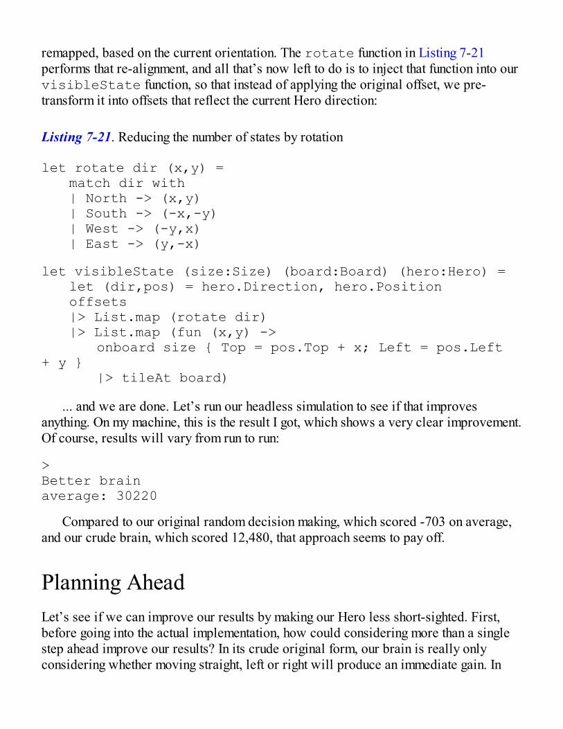
remapped, based on the current orientation. The rotate function in Listing 7-21performs that re-alignment, and all that’s now left to do is to inject that function into ourvisibleState function, so that instead of applying the original offset, we pre-transform it into offsets that reflect the current Hero direction:

Listing 7-21. Reducing the number of states by rotation

let rotate dir (x,y) = match dir with | North -> (x,y) | South -> (-x,-y) | West -> (-y,x) | East -> (y,-x)

let visibleState (size:Size) (board:Board) (hero:Hero) = let (dir,pos) = hero.Direction, hero.Position offsets |> List.map (rotate dir) |> List.map (fun (x,y) -> onboard size { Top = pos.Top + x; Left = pos.Left + y } |> tileAt board)

... and we are done. Let’s run our headless simulation to see if that improvesanything. On my machine, this is the result I got, which shows a very clear improvement.Of course, results will vary from run to run:

>Better brainaverage: 30220

Compared to our original random decision making, which scored -703 on average,and our crude brain, which scored 12,480, that approach seems to pay off.

Planning AheadLet’s see if we can improve our results by making our Hero less short-sighted. First,before going into the actual implementation, how could considering more than a singlestep ahead improve our results? In its crude original form, our brain is really onlyconsidering whether moving straight, left or right will produce an immediate gain. In

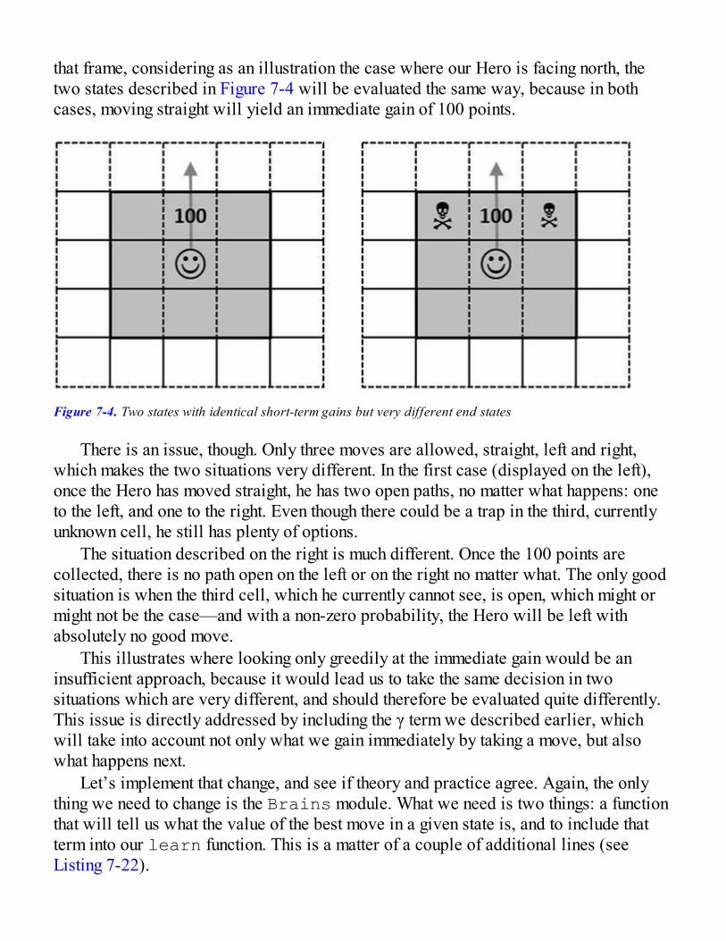
that frame, considering as an illustration the case where our Hero is facing north, thetwo states described in Figure 7-4 will be evaluated the same way, because in bothcases, moving straight will yield an immediate gain of 100 points.

Figure 7-4. Two states with identical short-term gains but very different end states

There is an issue, though. Only three moves are allowed, straight, left and right,which makes the two situations very different. In the first case (displayed on the left),once the Hero has moved straight, he has two open paths, no matter what happens: oneto the left, and one to the right. Even though there could be a trap in the third, currentlyunknown cell, he still has plenty of options.

The situation described on the right is much different. Once the 100 points arecollected, there is no path open on the left or on the right no matter what. The only goodsituation is when the third cell, which he currently cannot see, is open, which might ormight not be the case—and with a non-zero probability, the Hero will be left withabsolutely no good move.

This illustrates where looking only greedily at the immediate gain would be aninsufficient approach, because it would lead us to take the same decision in twosituations which are very different, and should therefore be evaluated quite differently.This issue is directly addressed by including the γ term we described earlier, whichwill take into account not only what we gain immediately by taking a move, but alsowhat happens next.

Let’s implement that change, and see if theory and practice agree. Again, the onlything we need to change is the Brains module. What we need is two things: a functionthat will tell us what the value of the best move in a given state is, and to include thatterm into our learn function. This is a matter of a couple of additional lines (seeListing 7-22).

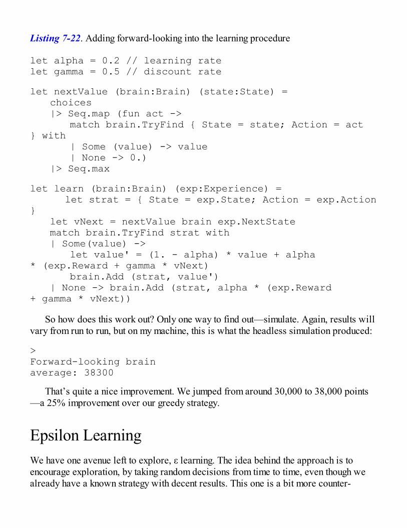
Listing 7-22. Adding forward-looking into the learning procedure

let alpha = 0.2 // learning ratelet gamma = 0.5 // discount rate

let nextValue (brain:Brain) (state:State) = choices |> Seq.map (fun act -> match brain.TryFind { State = state; Action = act } with | Some (value) -> value | None -> 0.) |> Seq.max

let learn (brain:Brain) (exp:Experience) = let strat = { State = exp.State; Action = exp.Action } let vNext = nextValue brain exp.NextState match brain.TryFind strat with | Some(value) -> let value' = (1. - alpha) * value + alpha * (exp.Reward + gamma * vNext) brain.Add (strat, value') | None -> brain.Add (strat, alpha * (exp.Reward + gamma * vNext))

So how does this work out? Only one way to find out—simulate. Again, results willvary from run to run, but on my machine, this is what the headless simulation produced:

>Forward-looking brainaverage: 38300

That’s quite a nice improvement. We jumped from around 30,000 to 38,000 points—a 25% improvement over our greedy strategy.

Epsilon LearningWe have one avenue left to explore, ε learning. The idea behind the approach is toencourage exploration, by taking random decisions from time to time, even though wealready have a known strategy with decent results. This one is a bit more counter-

intuitive—in essence, it says that it pays off to take a careful amount of risk, in order todiscover potentially better strategies, even though this will also at times result in baddecisions when a perfectly valid strategy was available.

The most straightforward way to implement this is to simply roll the dice every timewe take a decision. In a certain proportion of cases, we will completely ignoreeverything we learned so far, and take a random decision—which is quicklyimplemented, again in the Brains module (see Listing 7-23).

Listing 7-23. Adding exploration to the learning procedure

let alpha = 0.2 // learning rate

let gamma = 0.5 // discount rate let epsilon = 0.05 // random learning

// code omitted

let decide (brain:Brain) (state:State) = if (rng.NextDouble () < epsilon) then randomDecide () else let eval = choices |> Array.map (fun alt -> { State = state; Action = alt }) |> Array.filter (fun strat -> brain.ContainsKey strat) match eval.Length with | 0 -> randomDecide () | _ -> choices |> Seq.maxBy (fun alt -> let strat = { State = state; Action = alt } match brain.TryFind strat with | Some(value) -> value | None -> 0.)

Let’s run our simulation again, to see if that pays off. With all the same caveatsagain, on my machine, this is what I observed:>

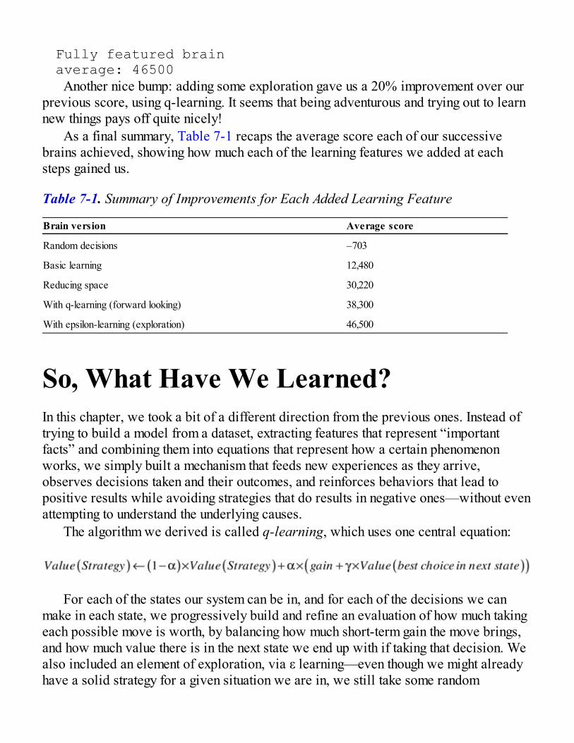
Fully featured brainaverage: 46500

Another nice bump: adding some exploration gave us a 20% improvement over ourprevious score, using q-learning. It seems that being adventurous and trying out to learnnew things pays off quite nicely!

As a final summary, Table 7-1 recaps the average score each of our successivebrains achieved, showing how much each of the learning features we added at eachsteps gained us.

Table 7-1. Summary of Improvements for Each Added Learning Feature

Brain version Average score

Random decisions –703

Basic learning 12,480

Reducing space 30,220

With q-learning (forward looking) 38,300

With epsilon-learning (exploration) 46,500

So, What Have We Learned?In this chapter, we took a bit of a different direction from the previous ones. Instead oftrying to build a model from a dataset, extracting features that represent “importantfacts” and combining them into equations that represent how a certain phenomenonworks, we simply built a mechanism that feeds new experiences as they arrive,observes decisions taken and their outcomes, and reinforces behaviors that lead topositive results while avoiding strategies that do results in negative ones—without evenattempting to understand the underlying causes.

The algorithm we derived is called q-learning, which uses one central equation:

For each of the states our system can be in, and for each of the decisions we canmake in each state, we progressively build and refine an evaluation of how much takingeach possible move is worth, by balancing how much short-term gain the move brings,and how much value there is in the next state we end up with if taking that decision. Wealso included an element of exploration, via ε learning—even though we might alreadyhave a solid strategy for a given situation we are in, we still take some random

decisions from time to time, to make sure we explore the space of all possiblestrategies.

A Simple Model That Fits IntuitionOne of the aspects I find the most interesting in q-learning is how simple it is to explainin terms that map our understanding of what knowledge and learning are about. Thebasic idea underpinning q-learning is reinforcement; reward your donkey with carrotsfor good behavior, and punish bad behavior with a stick, and your donkey willprogressively understand what you want him to do, and do the right thing. Similarly, q-learning lets the agent take decisions and adapt his behavior to maximize rewards andavoid penalties, without necessarily trying to understand what the task is really about.

Beyond that basic idea, we discussed more subtle aspects. Our initial algorithm wasessentially blindly going toward the direction of immediate reward. It worked quitewell, but we also saw how taking a less greedy approach, and taking into account notonly the immediate rewards but also long term consequences, produced quite asignificant improvement, and essentially emulated a planning behavior.

We also saw how, somewhat counterintuitively, including an element of randomnessinto our algorithm did produce another nice improvement. I find this idea particularlyappealing. Our model is all about making rational, mechanical decisions, so it is a bitunexpected that introducing some chaos would make things better. However, itresonates well when you put in the perspective of human behavior. First, learning newthings does require stepping out of your comfort zone, and trying out things which mightor might not work out. Then, every acquired behavior is both a benefit and a hindrance:while good habits are a positive, some habits we form are actually negative, and willrequire us to unlearn if we want to progress, which is exactly what ε learning does.Another remark here is that while taking chances to experiment can result in either goodor bad outcomes, the long-term consequences make it worth it, at least for controlledrisks. If you try out something and it doesn’t work out, you won’t do it again. If it worksgreat, you have now learned a lesson which can be applied over and over again,yielding a life time of positive rewards.

Finally, it might be worth pointing out that the underlying idea is somewhat relatedto the problem of over-fitting. One way of describing over-fitting is that it is the resultof being very efficient applying one approach, but developing a blind spot in theprocess—a problem which can be overcome by introducing some randomness, forinstance random bagging.

An Adaptive Mechanism

The other aspect I find interesting in this approach is its adaptive nature. We illustratedearlier on how applying a learning coefficient α to weight the previous knowledgeagainst the new experience, and progressively updating our estimates, ended upconverging to the correct value. An interesting aspect here is that this mechanism wouldalso cope pretty well in a changing world. Imagine for a minute that midway through,we changed the rule of the game, and completely switched the effect of each tile,perhaps giving them new random rewards. The beautiful thing here is that our Herowould progressively adapt to this new world: as new experiences come in, hisestimates for each state will gradually change, and so will his behavior.

In essence, if you consider how the learning rate works, what happens is, oldermemories become progressively less and less important, by comparison to the morerecent experiences. This is quite a nice feature, because it allows us to create an agentthat adapts his behavior to changes in the environment, without exactly knowing how itworks. By contrast, building a model based on one dataset will be much more fragile:the recipe will work, as long as the world remains the same—and if it doesn’t, yourmodel will systematically behave incorrectly, without any correction.

Finally, you might wonder if this is actually useful. After all, our example in thischapter was a pretty silly game, something which is probably not very close to the typeof code you write professionally. In my opinion, this is a very applicable approach to avariety of situations, and the simplicity of the underlying model makes it quite easy totweak to the problem at hand. As an example, I recently ended up using a modelextremely similar to the one we used here, in a totally different context (seehttps://vimeo.com/113597999 for more information). I needed to figure outhow many concurrent tasks a machine could handle, a problem which is a bit tricky. Itdepends on the machine itself, how many cores and how much memory it has, and so on—and it can also vary over time, if for instance some other process is started on thatmachine. Rather than trying to figure out a complicated model based on what is actuallyhappening in the machine, I simply ended up varying the number of tasks beingprocessed, and measuring the throughput for each level of activity (my states), updatingthe estimates using a learning rate α and randomly trying out to increase and decreasethe number of concurrent tasks with probability ε—which is pretty much exactly whatwe did for our game, except that instead of a silly game, I ended up with a server thatautomatically scaled itself for maximum throughput, without human intervention.

CHAPTER 8

Digits, Revisited

Optimizing and Scaling Your AlgorithmCodeIn Chapter 1, we explored together the digit recognizer problem, and wrote a classifierfrom scratch. In this final chapter, we are going to revisit that problem, from twodifferent angles: performance, and useful tools. Chapters 1 to 7 were primarily focusedon implementing algorithms to solve various problems, and discovering machinelearning concepts in the process. By contrast, this chapter is more intended as a seriesof practical tips which can be useful in various situations. We will use the digitrecognizer model we created in Chapter 1 as a familiar reference point, and use it toillustrate techniques that are broadly applicable to other situations.

In this chapter, we will do the following:

Analyze the code we wrote in Chapter 1, and search for ways totune it and improve performance, by making the code moreefficient, and exploiting opportunities for parallel processing.

Present Accord.NET, a .NET library which offers ready-to-useimplementations of numerous classic machine learning algorithms.We will illustrate how to use three of them (logistic regression,support vector machine and artificial neural networks), and discusssome of their underlying ideas.

Introduce m-brace.NET, a library geared toward runningcomputations in a distributed manner on a cluster of machines in thecloud, from the F# scripting environment. We will demonstrate howthat library can be used to process much larger datasets, while still

keeping the ability to explore and design models with the rapidfeedback FSI offers.

Tuning Your CodePerformance considerations are important in machine learning, probably more so than ineveryday line-of-business applications development. Just like for any other piece ofcode, performance is usually not the first question to focus on; the first priority shouldbe to design a model that is correct, and produces accurate results. Once that is done, ifthe model is too slow, it is time to consider tuning it.

In the words of Donald Knuth, “Programmers waste enormous amounts of timethinking about, or worrying about, the speed of noncritical parts of their programs, andthese attempts at efficiency actually have a strong negative impact when debugging andmaintenance are considered. We should forget about small efficiencies, say about 97%of the time: premature optimization is the root of all evil. Yet we should not pass up ouropportunities in that critical 3%.”

That being said, that 3% tends to be rather important in machine learning. The mainreason for it goes back to our original description of what machine learning is: aprogram that will perform better, as it is fed more data. There is empirical evidencethat, as the corpus of data used for training becomes large, simple and complexalgorithms tend to have similar predictive power (see for instance Peter Norvig’s talk“The Unreasonable Effectiveness of Data” for an example:https://www.youtube.com/watch?v=yvDCzhbjYWs). In that frame,regardless of what specific algorithm you use, you will probably want to learn from alarger volume of data if you can, which will mechanically slow things down. In thatcase, an ineffectively implementation can matter a lot, and have a direct impact on yourproductivity, or maybe even make an algorithm unusable in practice.

What to Search ForSo what are we looking for, exactly? Improving the performance of an existing piece ofcode could mean a couple of things. The obvious one is speed: we want to get the sameanswer, but in less time. Memory footprint is another aspect to keep in mind: analgorithm that works great on small datasets might behave poorly as the data it needs tohold in memory increases.

If we inspect the nearest-neighbor implementation we wrote in Chapter 1, here isroughly what is does:

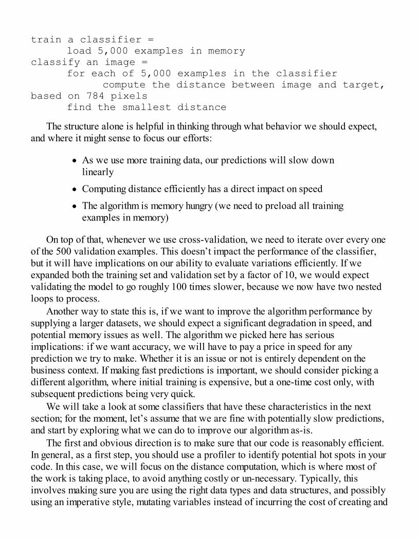
train a classifier = load 5,000 examples in memoryclassify an image = for each of 5,000 examples in the classifier compute the distance between image and target, based on 784 pixels find the smallest distance

The structure alone is helpful in thinking through what behavior we should expect,and where it might sense to focus our efforts:

As we use more training data, our predictions will slow downlinearly

Computing distance efficiently has a direct impact on speed

The algorithm is memory hungry (we need to preload all trainingexamples in memory)

On top of that, whenever we use cross-validation, we need to iterate over every oneof the 500 validation examples. This doesn’t impact the performance of the classifier,but it will have implications on our ability to evaluate variations efficiently. If weexpanded both the training set and validation set by a factor of 10, we would expectvalidating the model to go roughly 100 times slower, because we now have two nestedloops to process.

Another way to state this is, if we want to improve the algorithm performance bysupplying a larger datasets, we should expect a significant degradation in speed, andpotential memory issues as well. The algorithm we picked here has seriousimplications: if we want accuracy, we will have to pay a price in speed for anyprediction we try to make. Whether it is an issue or not is entirely dependent on thebusiness context. If making fast predictions is important, we should consider picking adifferent algorithm, where initial training is expensive, but a one-time cost only, withsubsequent predictions being very quick.

We will take a look at some classifiers that have these characteristics in the nextsection; for the moment, let’s assume that we are fine with potentially slow predictions,and start by exploring what we can do to improve our algorithm as-is.

The first and obvious direction is to make sure that our code is reasonably efficient.In general, as a first step, you should use a profiler to identify potential hot spots in yourcode. In this case, we will focus on the distance computation, which is where most ofthe work is taking place, to avoid anything costly or un-necessary. Typically, thisinvolves making sure you are using the right data types and data structures, and possiblyusing an imperative style, mutating variables instead of incurring the cost of creating and

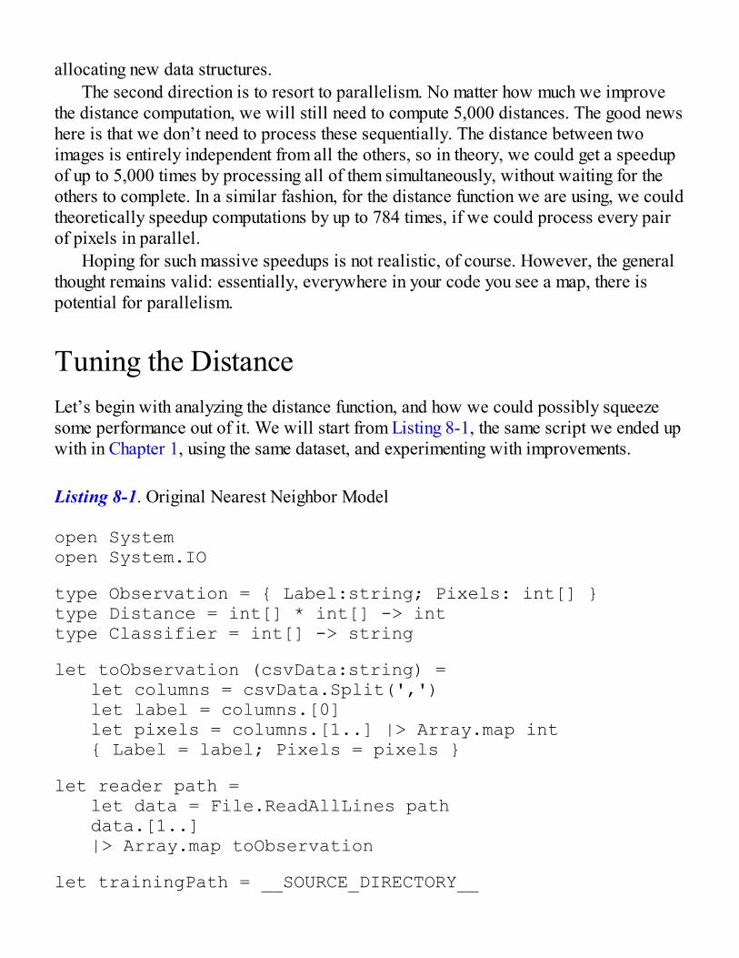
allocating new data structures.The second direction is to resort to parallelism. No matter how much we improve

the distance computation, we will still need to compute 5,000 distances. The good newshere is that we don’t need to process these sequentially. The distance between twoimages is entirely independent from all the others, so in theory, we could get a speedupof up to 5,000 times by processing all of them simultaneously, without waiting for theothers to complete. In a similar fashion, for the distance function we are using, we couldtheoretically speedup computations by up to 784 times, if we could process every pairof pixels in parallel.

Hoping for such massive speedups is not realistic, of course. However, the generalthought remains valid: essentially, everywhere in your code you see a map, there ispotential for parallelism.

Tuning the DistanceLet’s begin with analyzing the distance function, and how we could possibly squeezesome performance out of it. We will start from Listing 8-1, the same script we ended upwith in Chapter 1, using the same dataset, and experimenting with improvements.

Listing 8-1. Original Nearest Neighbor Model

open Systemopen System.IO

type Observation = { Label:string; Pixels: int[] }type Distance = int[] * int[] -> inttype Classifier = int[] -> string

let toObservation (csvData:string) = let columns = csvData.Split(',') let label = columns.[0] let pixels = columns.[1..] |> Array.map int { Label = label; Pixels = pixels }

let reader path = let data = File.ReadAllLines path data.[1..] |> Array.map toObservation

let trainingPath = __SOURCE_DIRECTORY__

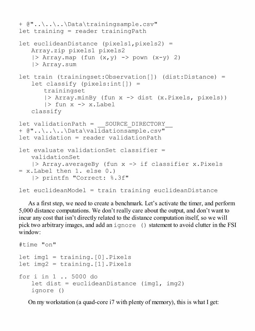
+ @"..\..\..\Data\trainingsample.csv"let training = reader trainingPath

let euclideanDistance (pixels1,pixels2) = Array.zip pixels1 pixels2 |> Array.map (fun (x,y) -> pown (x-y) 2) |> Array.sum

let train (trainingset:Observation[]) (dist:Distance) = let classify (pixels:int[]) = trainingset |> Array.minBy (fun x -> dist (x.Pixels, pixels)) |> fun x -> x.Label classify

let validationPath = __SOURCE_DIRECTORY__ + @"..\..\..\Data\validationsample.csv"let validation = reader validationPath

let evaluate validationSet classifier = validationSet |> Array.averageBy (fun x -> if classifier x.Pixels = x.Label then 1. else 0.) |> printfn "Correct: %.3f"

let euclideanModel = train training euclideanDistance

As a first step, we need to create a benchmark. Let’s activate the timer, and perform5,000 distance computations. We don’t really care about the output, and don’t want toincur any cost that isn’t directly related to the distance computation itself, so we willpick two arbitrary images, and add an ignore () statement to avoid clutter in the FSIwindow:

#time "on"

let img1 = training.[0].Pixelslet img2 = training.[1].Pixels

for i in 1 .. 5000 do let dist = euclideanDistance (img1, img2) ignore ()

On my workstation (a quad-core i7 with plenty of memory), this is what I get:

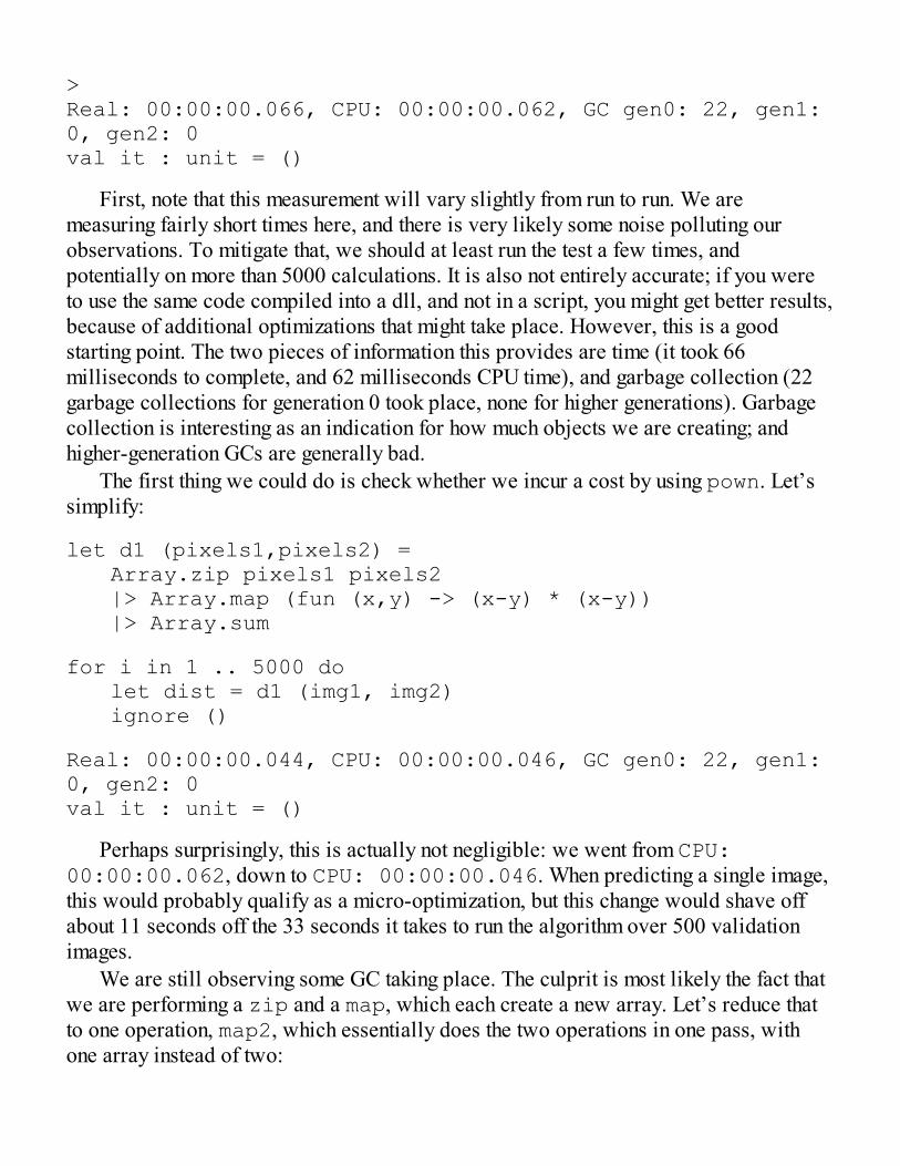
>Real: 00:00:00.066, CPU: 00:00:00.062, GC gen0: 22, gen1: 0, gen2: 0val it : unit = ()

First, note that this measurement will vary slightly from run to run. We aremeasuring fairly short times here, and there is very likely some noise polluting ourobservations. To mitigate that, we should at least run the test a few times, andpotentially on more than 5000 calculations. It is also not entirely accurate; if you wereto use the same code compiled into a dll, and not in a script, you might get better results,because of additional optimizations that might take place. However, this is a goodstarting point. The two pieces of information this provides are time (it took 66milliseconds to complete, and 62 milliseconds CPU time), and garbage collection (22garbage collections for generation 0 took place, none for higher generations). Garbagecollection is interesting as an indication for how much objects we are creating; andhigher-generation GCs are generally bad.

The first thing we could do is check whether we incur a cost by using pown. Let’ssimplify:

let d1 (pixels1,pixels2) = Array.zip pixels1 pixels2 |> Array.map (fun (x,y) -> (x-y) * (x-y)) |> Array.sum

for i in 1 .. 5000 do let dist = d1 (img1, img2) ignore ()

Real: 00:00:00.044, CPU: 00:00:00.046, GC gen0: 22, gen1: 0, gen2: 0val it : unit = ()

Perhaps surprisingly, this is actually not negligible: we went from CPU:00:00:00.062, down to CPU: 00:00:00.046. When predicting a single image,this would probably qualify as a micro-optimization, but this change would shave offabout 11 seconds off the 33 seconds it takes to run the algorithm over 500 validationimages.

We are still observing some GC taking place. The culprit is most likely the fact thatwe are performing a zip and a map, which each create a new array. Let’s reduce thatto one operation, map2, which essentially does the two operations in one pass, withone array instead of two:

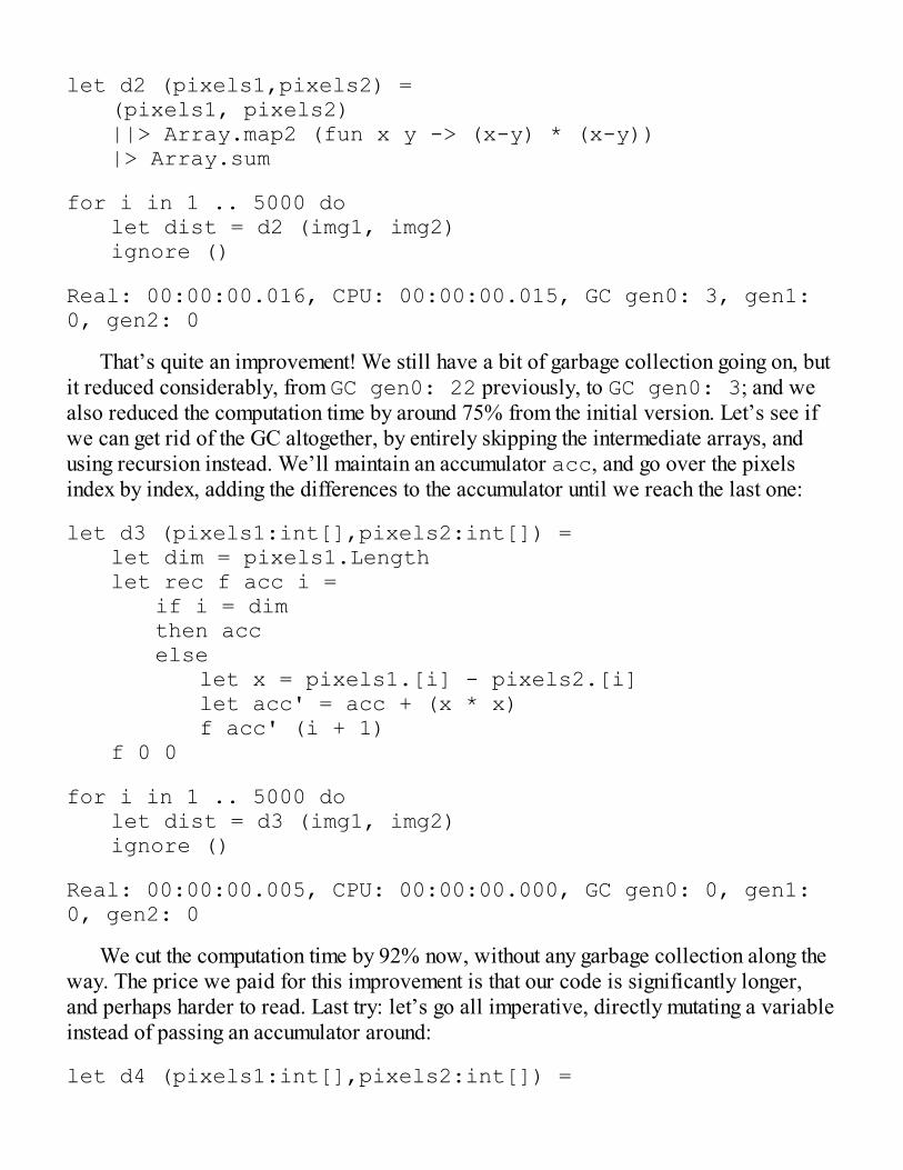
let d2 (pixels1,pixels2) = (pixels1, pixels2) ||> Array.map2 (fun x y -> (x-y) * (x-y)) |> Array.sum

for i in 1 .. 5000 do let dist = d2 (img1, img2) ignore ()

Real: 00:00:00.016, CPU: 00:00:00.015, GC gen0: 3, gen1: 0, gen2: 0

That’s quite an improvement! We still have a bit of garbage collection going on, butit reduced considerably, from GC gen0: 22 previously, to GC gen0: 3; and wealso reduced the computation time by around 75% from the initial version. Let’s see ifwe can get rid of the GC altogether, by entirely skipping the intermediate arrays, andusing recursion instead. We’ll maintain an accumulator acc, and go over the pixelsindex by index, adding the differences to the accumulator until we reach the last one:

let d3 (pixels1:int[],pixels2:int[]) = let dim = pixels1.Length let rec f acc i = if i = dim then acc else let x = pixels1.[i] - pixels2.[i] let acc' = acc + (x * x) f acc' (i + 1) f 0 0

for i in 1 .. 5000 do let dist = d3 (img1, img2) ignore ()

Real: 00:00:00.005, CPU: 00:00:00.000, GC gen0: 0, gen1: 0, gen2: 0

We cut the computation time by 92% now, without any garbage collection along theway. The price we paid for this improvement is that our code is significantly longer,and perhaps harder to read. Last try: let’s go all imperative, directly mutating a variableinstead of passing an accumulator around:

let d4 (pixels1:int[],pixels2:int[]) =

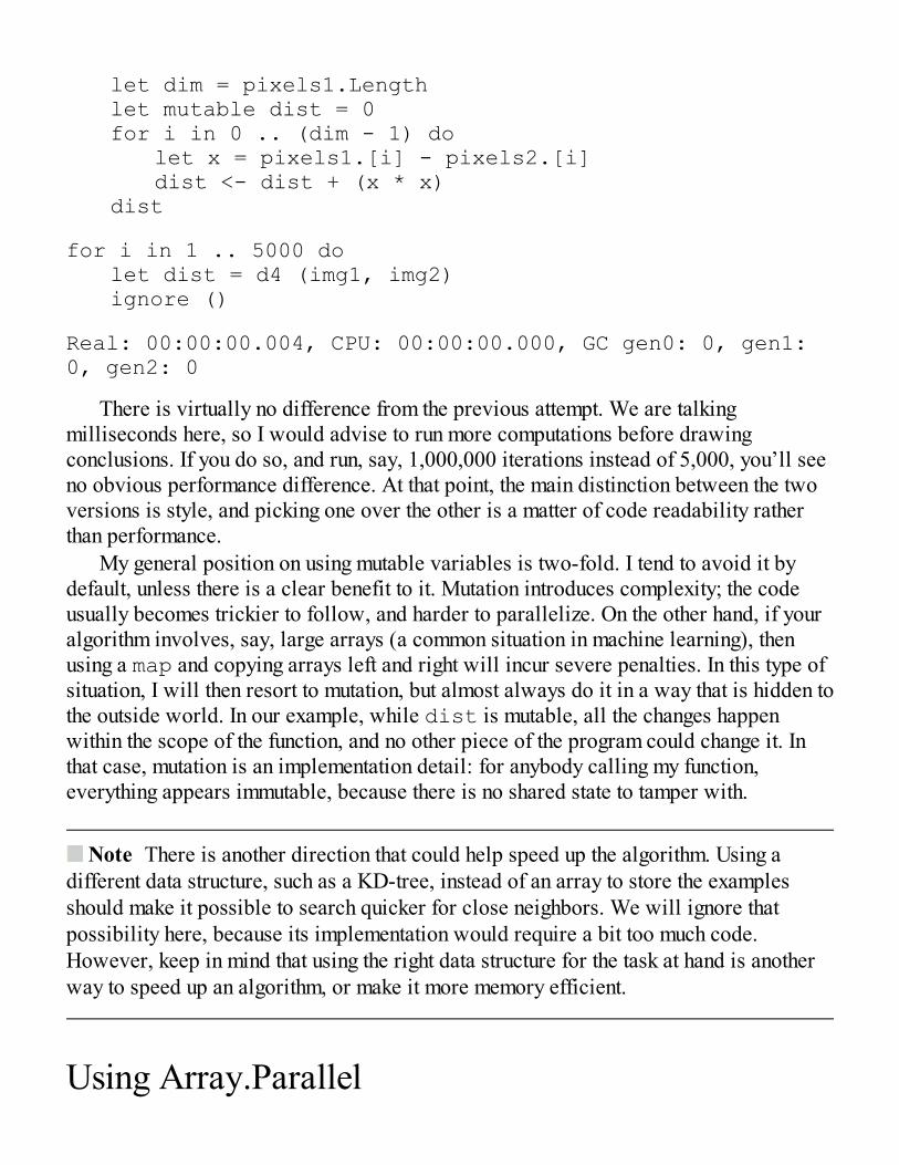
let dim = pixels1.Length let mutable dist = 0 for i in 0 .. (dim - 1) do let x = pixels1.[i] - pixels2.[i] dist <- dist + (x * x) dist

for i in 1 .. 5000 do let dist = d4 (img1, img2) ignore ()

Real: 00:00:00.004, CPU: 00:00:00.000, GC gen0: 0, gen1: 0, gen2: 0

There is virtually no difference from the previous attempt. We are talkingmilliseconds here, so I would advise to run more computations before drawingconclusions. If you do so, and run, say, 1,000,000 iterations instead of 5,000, you’ll seeno obvious performance difference. At that point, the main distinction between the twoversions is style, and picking one over the other is a matter of code readability ratherthan performance.

My general position on using mutable variables is two-fold. I tend to avoid it bydefault, unless there is a clear benefit to it. Mutation introduces complexity; the codeusually becomes trickier to follow, and harder to parallelize. On the other hand, if youralgorithm involves, say, large arrays (a common situation in machine learning), thenusing a map and copying arrays left and right will incur severe penalties. In this type ofsituation, I will then resort to mutation, but almost always do it in a way that is hidden tothe outside world. In our example, while dist is mutable, all the changes happenwithin the scope of the function, and no other piece of the program could change it. Inthat case, mutation is an implementation detail: for anybody calling my function,everything appears immutable, because there is no shared state to tamper with.

Note There is another direction that could help speed up the algorithm. Using adifferent data structure, such as a KD-tree, instead of an array to store the examplesshould make it possible to search quicker for close neighbors. We will ignore thatpossibility here, because its implementation would require a bit too much code.However, keep in mind that using the right data structure for the task at hand is anotherway to speed up an algorithm, or make it more memory efficient.

Using Array.Parallel

Let’s take a look now at the second angle, parallelism. Here, we are going to take a lookat the evaluation function, which goes over 500 validation images, classifies the image,and compares it to the true expected label. The original implementation usesArray.averageBy, which combines two steps into one: first, it maps every imageto a 1.0 or a 0.0, depending on whether the prediction is correct or not, and then, itaverages the entire array. The map function is not immediately visible, but it isimplicitly there.

Clearly, each image can be predicted independently of each other, so we should beable to perform that operation in parallel. What we would like is to divide-and-conquerthe training sample, for example, splitting it evenly based on the cores we haveavailable on our machine, running each chunk separately, and regrouping the results inone single array.

As it turns out, F# offers some interesting options out of the box, in theArray.Parallel module, which exposes a subset of the Array functions,implemented in a parallel fashion. First, let’s measure how long our initial evaluationtook, and where we are at after our distance tweaks:

let original = evaluate validation euclideanModel>Correct: 0.944Real: 00:00:31.811, CPU: 00:00:31.812, GC gen0: 11248, gen1: 6, gen2: 1

let updatedModel = train training d4let improved = evaluate validation updatedModel>Correct: 0.944Real: 00:00:02.889, CPU: 00:00:02.890, GC gen0: 13, gen1: 1, gen2: 0

Now let’s rewrite the evaluate function, breaking Array.averageBy inArray.Parallel.map first, and Array.average:

let parallelEvaluate validationSet classifier = validationSet |> Array.Parallel.map (fun x -> if classifier x.Pixels = x.Label then 1. else 0.) |> Array.average |> printfn "Correct: %.3f"

>Correct: 0.944

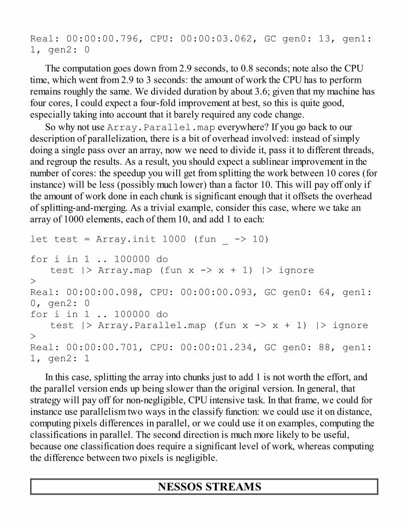
Real: 00:00:00.796, CPU: 00:00:03.062, GC gen0: 13, gen1: 1, gen2: 0

The computation goes down from 2.9 seconds, to 0.8 seconds; note also the CPUtime, which went from 2.9 to 3 seconds: the amount of work the CPU has to performremains roughly the same. We divided duration by about 3.6; given that my machine hasfour cores, I could expect a four-fold improvement at best, so this is quite good,especially taking into account that it barely required any code change.

So why not use Array.Parallel.map everywhere? If you go back to ourdescription of parallelization, there is a bit of overhead involved: instead of simplydoing a single pass over an array, now we need to divide it, pass it to different threads,and regroup the results. As a result, you should expect a sublinear improvement in thenumber of cores: the speedup you will get from splitting the work between 10 cores (forinstance) will be less (possibly much lower) than a factor 10. This will pay off only ifthe amount of work done in each chunk is significant enough that it offsets the overheadof splitting-and-merging. As a trivial example, consider this case, where we take anarray of 1000 elements, each of them 10, and add 1 to each:

let test = Array.init 1000 (fun _ -> 10)

for i in 1 .. 100000 do test |> Array.map (fun x -> x + 1) |> ignore>Real: 00:00:00.098, CPU: 00:00:00.093, GC gen0: 64, gen1: 0, gen2: 0for i in 1 .. 100000 do test |> Array.Parallel.map (fun x -> x + 1) |> ignore>Real: 00:00:00.701, CPU: 00:00:01.234, GC gen0: 88, gen1: 1, gen2: 1

In this case, splitting the array into chunks just to add 1 is not worth the effort, andthe parallel version ends up being slower than the original version. In general, thatstrategy will pay off for non-negligible, CPU intensive task. In that frame, we could forinstance use parallelism two ways in the classify function: we could use it on distance,computing pixels differences in parallel, or we could use it on examples, computing theclassifications in parallel. The second direction is much more likely to be useful,because one classification does require a significant level of work, whereas computingthe difference between two pixels is negligible.

NESSOS STREAMS

Array.Parallel implements a subset of the Array module functions in aparallel manner. If you find yourself needing more, take a look at the Streamslibrary (http://nessos.github.io/Streams/). It contains additionalfunctions in the ParStream module (for parallel streams), and offers otherinteresting possibilities. In a nutshell, the library distinguishes lazy and eageroperations in pipelines, and will fuse together lazy operations, which can yieldperformance benefits.

Different Classifiers with Accord.NETIn the previous section, we discussed a few ways you can improve the performance ofan existing algorithm. However, every algorithm has fundamental characteristics thatdefine how your program will behave. In this section, we will take an entirely differentdirection, and take a look at Accord.NET, a popular (and good!) library that contains awealth of machine learning and numeric analysis tools.

Our goal here is twofold. First, writing your own implementation is often not thathard, and comes with some benefits. In particular, you are entirely in control of thecode, which offers some opportunity for tighter integration with the application that usesit, and maybe some room for optimization at a global level. However, developing amachine learning algorithm involves a lot of experimentation and trial-and-error, andsometimes, you just need to quickly check if a particular class of models works betterthan another. In that case, implementing the algorithm from scratch might be simply toomuch effort, and using an off-the-shelf implementation can speed up the eliminationprocess. In that frame, knowing how to leverage a rich library like Accord is quiteuseful.

Then, we covered a variety of techniques in the previous chapters, but left out manyother classic and potentially useful ones, too. We cannot realistically cover everyalgorithm in detail, but we will use this section as an excuse to provide a high-levelintroduction to some of them, and demonstrate how you could use the library.

Logistic RegressionIn Chapter 4, we implemented a classic regression model, trying to predict a numericvalue from multiple input features. One of the ways that approach is different from thenearest neighbor model is that there is a clearly distinct training phase in the process.The training set is used to estimate the parameters of a classifier function, which is

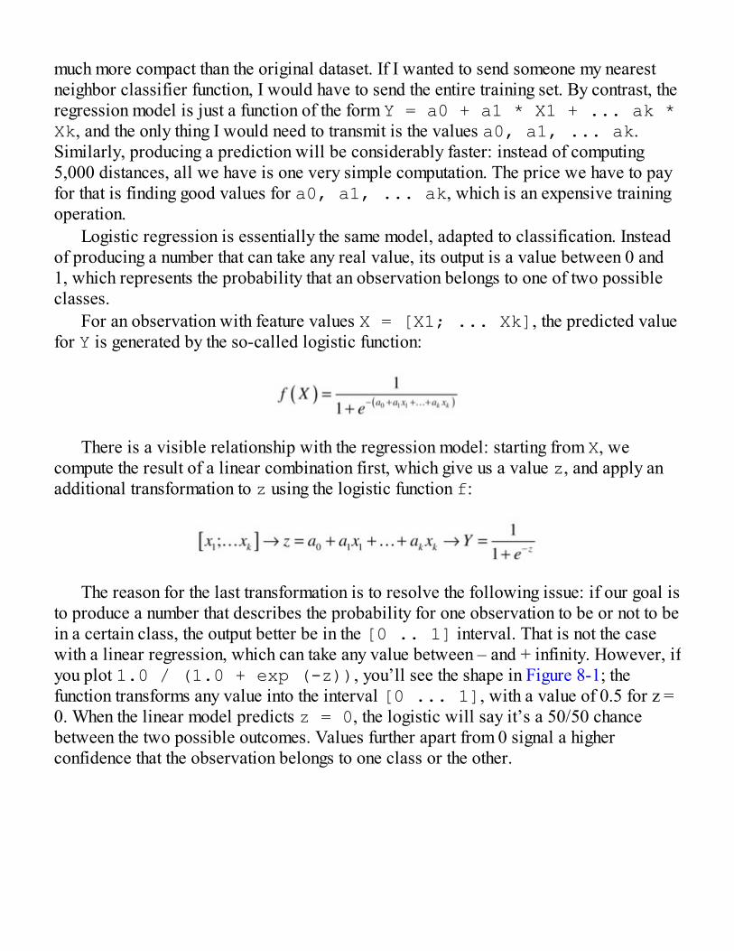
much more compact than the original dataset. If I wanted to send someone my nearestneighbor classifier function, I would have to send the entire training set. By contrast, theregression model is just a function of the form Y = a0 + a1 * X1 + ... ak *Xk, and the only thing I would need to transmit is the values a0, a1, ... ak.Similarly, producing a prediction will be considerably faster: instead of computing5,000 distances, all we have is one very simple computation. The price we have to payfor that is finding good values for a0, a1, ... ak, which is an expensive trainingoperation.

Logistic regression is essentially the same model, adapted to classification. Insteadof producing a number that can take any real value, its output is a value between 0 and1, which represents the probability that an observation belongs to one of two possibleclasses.

For an observation with feature values X = [X1; ... Xk], the predicted valuefor Y is generated by the so-called logistic function:

There is a visible relationship with the regression model: starting from X, wecompute the result of a linear combination first, which give us a value z, and apply anadditional transformation to z using the logistic function f:

The reason for the last transformation is to resolve the following issue: if our goal isto produce a number that describes the probability for one observation to be or not to bein a certain class, the output better be in the [0 .. 1] interval. That is not the casewith a linear regression, which can take any value between – and + infinity. However, ifyou plot 1.0 / (1.0 + exp (-z)), you’ll see the shape in Figure 8-1; thefunction transforms any value into the interval [0 ... 1], with a value of 0.5 for z =0. When the linear model predicts z = 0, the logistic will say it’s a 50/50 chancebetween the two possible outcomes. Values further apart from 0 signal a higherconfidence that the observation belongs to one class or the other.

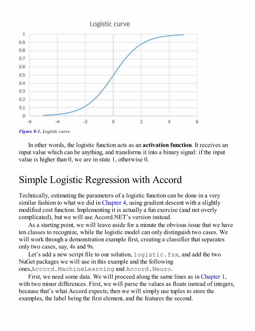
Figure 8-1. Logistic curve

In other words, the logistic function acts as an activation function. It receives aninput value which can be anything, and transforms it into a binary signal: if the inputvalue is higher than 0, we are in state 1, otherwise 0.

Simple Logistic Regression with AccordTechnically, estimating the parameters of a logistic function can be done in a verysimilar fashion to what we did in Chapter 4, using gradient descent with a slightlymodified cost function. Implementing it is actually a fun exercise (and not overlycomplicated), but we will use Accord.NET’s version instead.

As a starting point, we will leave aside for a minute the obvious issue that we haveten classes to recognize, while the logistic model can only distinguish two cases. Wewill work through a demonstration example first, creating a classifier that separatesonly two cases, say, 4s and 9s.

Let’s add a new script file to our solution, logistic.fsx, and add the twoNuGet packages we will use in this example and the followingones,Accord.MachineLearning and Accord.Neuro.

First, we need some data. We will proceed along the same lines as in Chapter 1,with two minor differences. First, we will parse the values as floats instead of integers,because that’s what Accord expects; then we will simply use tuples to store theexamples, the label being the first element, and the features the second.

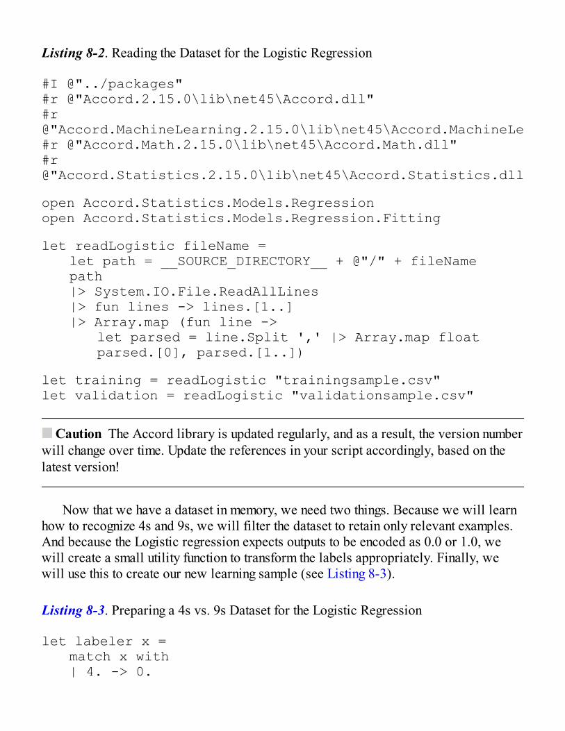
Listing 8-2. Reading the Dataset for the Logistic Regression

#I @"../packages"#r @"Accord.2.15.0\lib\net45\Accord.dll"#r @"Accord.MachineLearning.2.15.0\lib\net45\Accord.MachineLearning.dll"#r @"Accord.Math.2.15.0\lib\net45\Accord.Math.dll"#r @"Accord.Statistics.2.15.0\lib\net45\Accord.Statistics.dll"

open Accord.Statistics.Models.Regressionopen Accord.Statistics.Models.Regression.Fitting

let readLogistic fileName = let path = __SOURCE_DIRECTORY__ + @"/" + fileName path |> System.IO.File.ReadAllLines |> fun lines -> lines.[1..] |> Array.map (fun line -> let parsed = line.Split ',' |> Array.map float parsed.[0], parsed.[1..])

let training = readLogistic "trainingsample.csv"let validation = readLogistic "validationsample.csv"

Caution The Accord library is updated regularly, and as a result, the version numberwill change over time. Update the references in your script accordingly, based on thelatest version!

Now that we have a dataset in memory, we need two things. Because we will learnhow to recognize 4s and 9s, we will filter the dataset to retain only relevant examples.And because the Logistic regression expects outputs to be encoded as 0.0 or 1.0, wewill create a small utility function to transform the labels appropriately. Finally, wewill use this to create our new learning sample (see Listing 8-3).

Listing 8-3. Preparing a 4s vs. 9s Dataset for the Logistic Regression

let labeler x = match x with | 4. -> 0.

| 9. -> 1. | _ -> failwith "unexpected label"

let fours = training |> Array.filter (fun (label,_) -> label = 4.)let nines = training |> Array.filter (fun (label,_) -> label = 9.)

let labels,images = Array.append fours nines |> Array.map (fun (label,image) -> labeler label,image) |> Array.unzip

We can now start using the Accord Logistic regression model. Accord usesprimarily an object-oriented style, and as a result, it follows a pattern along these lines:

1. First you create a model, a class defining how the prediction ismade.

2. You pass it to a learner, a class that defines how to use trainingdata to fit that model.

3. You then provide data to the learner, and “learn” until the fit isgood enough,

4. You can now use the original model instance to makepredictions.

In our case, we will use a LogisticRegression model, using 28 * 28 features,corresponding to each of the pixels of our scanned images, and useLogisticGradientDescent to learn, until the changes in our model becomenegligible. This is a good fit for a recursive loop (see Listing 8-4).

Listing 8-4. Training the Logistic Model

let features = 28 * 28let model = LogisticRegression(features)

let trainLogistic (model) = let learner = LogisticGradientDescent(model) let minDelta = 0.001 let rec improve () =

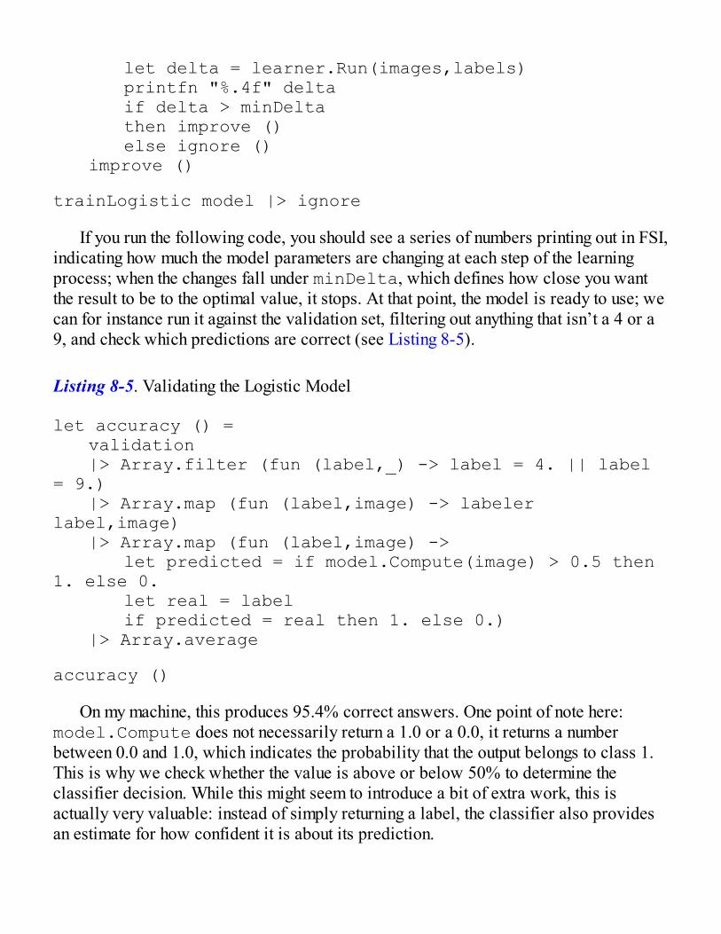
let delta = learner.Run(images,labels) printfn "%.4f" delta if delta > minDelta then improve () else ignore () improve ()

trainLogistic model |> ignore

If you run the following code, you should see a series of numbers printing out in FSI,indicating how much the model parameters are changing at each step of the learningprocess; when the changes fall under minDelta, which defines how close you wantthe result to be to the optimal value, it stops. At that point, the model is ready to use; wecan for instance run it against the validation set, filtering out anything that isn’t a 4 or a9, and check which predictions are correct (see Listing 8-5).

Listing 8-5. Validating the Logistic Model

let accuracy () = validation |> Array.filter (fun (label,_) -> label = 4. || label = 9.) |> Array.map (fun (label,image) -> labeler label,image) |> Array.map (fun (label,image) -> let predicted = if model.Compute(image) > 0.5 then 1. else 0. let real = label if predicted = real then 1. else 0.) |> Array.average

accuracy ()

On my machine, this produces 95.4% correct answers. One point of note here:model.Compute does not necessarily return a 1.0 or a 0.0, it returns a numberbetween 0.0 and 1.0, which indicates the probability that the output belongs to class 1.This is why we check whether the value is above or below 50% to determine theclassifier decision. While this might seem to introduce a bit of extra work, this isactually very valuable: instead of simply returning a label, the classifier also providesan estimate for how confident it is about its prediction.

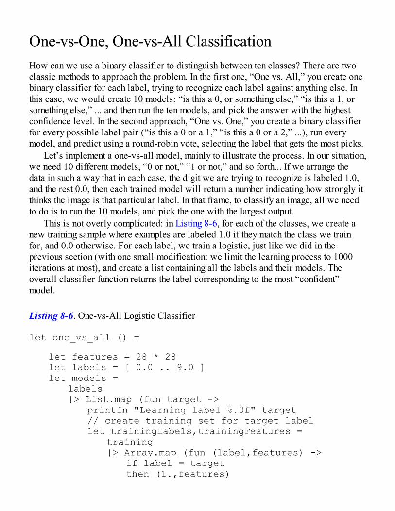
One-vs-One, One-vs-All ClassificationHow can we use a binary classifier to distinguish between ten classes? There are twoclassic methods to approach the problem. In the first one, “One vs. All,” you create onebinary classifier for each label, trying to recognize each label against anything else. Inthis case, we would create 10 models: “is this a 0, or something else,” “is this a 1, orsomething else,” ... and then run the ten models, and pick the answer with the highestconfidence level. In the second approach, “One vs. One,” you create a binary classifierfor every possible label pair (“is this a 0 or a 1,” “is this a 0 or a 2,” ...), run everymodel, and predict using a round-robin vote, selecting the label that gets the most picks.

Let’s implement a one-vs-all model, mainly to illustrate the process. In our situation,we need 10 different models, “0 or not,” “1 or not,” and so forth... If we arrange thedata in such a way that in each case, the digit we are trying to recognize is labeled 1.0,and the rest 0.0, then each trained model will return a number indicating how strongly itthinks the image is that particular label. In that frame, to classify an image, all we needto do is to run the 10 models, and pick the one with the largest output.

This is not overly complicated: in Listing 8-6, for each of the classes, we create anew training sample where examples are labeled 1.0 if they match the class we trainfor, and 0.0 otherwise. For each label, we train a logistic, just like we did in theprevious section (with one small modification: we limit the learning process to 1000iterations at most), and create a list containing all the labels and their models. Theoverall classifier function returns the label corresponding to the most “confident”model.

Listing 8-6. One-vs-All Logistic Classifier

let one_vs_all () =

let features = 28 * 28 let labels = [ 0.0 .. 9.0 ] let models = labels |> List.map (fun target -> printfn "Learning label %.0f" target // create training set for target label let trainingLabels,trainingFeatures = training |> Array.map (fun (label,features) -> if label = target then (1.,features)

else (0.,features)) |> Array.unzip // train the model let model = LogisticRegression(features) let learner = LogisticGradientDescent(model) let minDelta = 0.001 let max_iters = 1000 let rec improve iter = if iter = max_iters then ignore () else let delta = learner.Run(trainingFeatures,trainingLabels) if delta < minDelta then ignore () else improve (iter + 1) improve 0 // return the label and corresponding model target,model)

let classifier (image:float[]) = models |> List.maxBy (fun (label,model) -> model.Compute image) |> fun (label,confidence) -> label

classifier

The resulting model is not particularly good; on my machine, I got close to 83%accuracy. We won’t implement the other approach here, because the code isn’t differentenough to warrant it. On one hand, these two approaches are interesting, because theyprovide a simple technique to extend binary classifiers (which are the simplestclassifier you could create) to handle an arbitrary number of labels. On the other hand,keep in mind that both of them are just heuristics: the approach is reasonable, but notguaranteed to work well. One-vs-all has the benefit of requiring fewer models (in ourcase, 10, against 90 for one-vs-one case), but both have potential issues. In the one-vs-all situation, we are lumping together many different situations in the negative case,which can make training difficult (for instance, you would expect that recognizing a 5from a 0 or a 6 would be based on different features). Training a model to specificallyrecognize a 1 from a 6 (for instance) is easier than from nine different digits.Conversely, in the one-vs-one case, while training individual models might be easier,the final decision involves asking models trained to distinguish two specific digits torecognize something that is neither, which is arguably tricky (if you pass a 0 to a model

trained to recognize 1 from 2, what answer would you expect?).

Support Vector MachinesThe next model we’ll take a look at, Support Vector Machines (SVM afterward), isanother classic binary classifier. It has an intimidating name, and the algorithm is a bitmore involved conceptually than the previous one. We will hand-wave the details ofhow it works, and limit our explanation to a minimum.

In essence, a SVM attempts to separate the two classes by a band as wide aspossible, so that all examples of one class are on one side, all the others on the otherside. Support Vectors are the examples that lie on, or “support,” each side of theboundary. Figure 8-2 illustrates the idea on a simple example: the two dashed linesrepresent the boundaries of the separating band. Every observation that belongs to thesame class (black or white) is on the same side, and three observations, denoted assquares, are the support vectors that define where the boundary is.

Figure 8-2. Support vectors

Just like the logistic regression, SVMs are binary classifiers. One difference withthe logistic regression is that instead of 0 and 1s, the labels are encoded as –1 and 1,and the output is simply a class, and not a “confidence level.” Let’s see how we coulduse the Accord SVM to classify our digits. Conveniently, Accord has a built-inmulticlass version of the SVM, which means that we can directly use it with 10 classes,instead of having to build an extra layer: it will handle the one-vs-one process for us.

For clarity, we’ll put our SVM sample in a separate script, svm.fsx, including thesame references we used for the logistic example. First, as usual, we’ll read the dataset,but in this case we won’t convert the label to a float (see Listing 8-7).

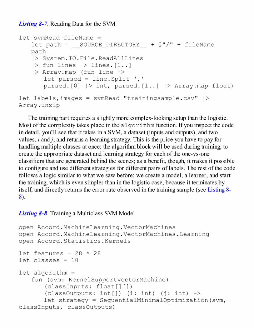
Listing 8-7. Reading Data for the SVM

let svmRead fileName = let path = __SOURCE_DIRECTORY__ + @"/" + fileName path |> System.IO.File.ReadAllLines |> fun lines -> lines.[1..] |> Array.map (fun line -> let parsed = line.Split ',' parsed.[0] |> int, parsed.[1..] |> Array.map float)

let labels,images = svmRead "trainingsample.csv" |> Array.unzip

The training part requires a slightly more complex-looking setup than the logistic.Most of the complexity takes place in the algorithm function. If you inspect the codein detail, you’ll see that it takes in a SVM, a dataset (inputs and outputs), and twovalues, i and j, and returns a learning strategy. This is the price you have to pay forhandling multiple classes at once: the algorithm block will be used during training, tocreate the appropriate dataset and learning strategy for each of the one-vs-oneclassifiers that are generated behind the scenes; as a benefit, though, it makes it possibleto configure and use different strategies for different pairs of labels. The rest of the codefollows a logic similar to what we saw before: we create a model, a learner, and startthe training, which is even simpler than in the logistic case, because it terminates byitself, and directly returns the error rate observed in the training sample (see Listing 8-8).

Listing 8-8. Training a Multiclass SVM Model

open Accord.MachineLearning.VectorMachinesopen Accord.MachineLearning.VectorMachines.Learningopen Accord.Statistics.Kernels

let features = 28 * 28let classes = 10

let algorithm = fun (svm: KernelSupportVectorMachine) (classInputs: float[][]) (classOutputs: int[]) (i: int) (j: int) -> let strategy = SequentialMinimalOptimization(svm, classInputs, classOutputs)

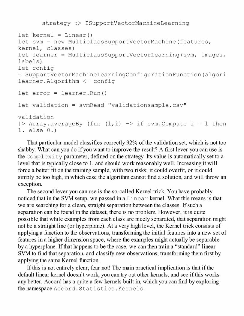
strategy :> ISupportVectorMachineLearning

let kernel = Linear()let svm = new MulticlassSupportVectorMachine(features, kernel, classes)let learner = MulticlassSupportVectorLearning(svm, images,labels)let config = SupportVectorMachineLearningConfigurationFunction(algorithm)learner.Algorithm <- config

let error = learner.Run()

let validation = svmRead "validationsample.csv"

validation|> Array.averageBy (fun (l,i) -> if svm.Compute i = l then1. else 0.)

That particular model classifies correctly 92% of the validation set, which is not tooshabby. What can you do if you want to improve the result? A first lever you can use isthe Complexity parameter, defined on the strategy. Its value is automatically set to alevel that is typically close to 1, and should work reasonably well. Increasing it willforce a better fit on the training sample, with two risks: it could overfit, or it couldsimply be too high, in which case the algorithm cannot find a solution, and will throw anexception.

The second lever you can use is the so-called Kernel trick. You have probablynoticed that in the SVM setup, we passed in a Linear kernel. What this means is thatwe are searching for a clean, straight separation between the classes. If such aseparation can be found in the dataset, there is no problem. However, it is quitepossible that while examples from each class are nicely separated, that separation mightnot be a straight line (or hyperplane). At a very high level, the Kernel trick consists ofapplying a function to the observations, transforming the initial features into a new set offeatures in a higher dimension space, where the examples might actually be separableby a hyperplane. If that happens to be the case, we can then train a “standard” linearSVM to find that separation, and classify new observations, transforming them first byapplying the same Kernel function.

If this is not entirely clear, fear not! The main practical implication is that if thedefault linear kernel doesn’t work, you can try out other kernels, and see if this worksany better. Accord has a quite a few kernels built in, which you can find by exploringthe namespace Accord.Statistics.Kernels.

Neural NetworksThe last classifier from Accord that we will take a look at is artificial neural networks(ANN afterward). The name is inspired by a loose analogy with the way a brain works.The brain is a large collection of interconnected neurons. When we receive a signalfrom the outside world, receptors send electrical impulses which activate neurons inour brain. Neurons that have received a signal strong enough will in turn send a signal toconnected neurons, and in the end, our brain will (perhaps) make sense of the signal andrecognize something.

The construction of an artificial neural network follows a similar general structure.They can come in different shapes, but the canonical ANN is a collection of neurons,organized in layers, each of them connected to every neuron in the next layer. Theneuron itself is an activation function; it receives as input the output from every neuronconnected into it, each of them with an individual weight, and if the weighted sum ofinputs it receives is high enough, it will in turn send a signal forward.

Neural networks are a huge topic, which we couldn’t possibly do justice within asingle chapter here. In a fashion similar to what we did for SVMs, we will simplyillustrate how you could go about building a classifier using the built-in tools in Accord,and highlight a couple of interesting points in the process.

In our particular situation, we have 784 pixels, our input signal, and what we expectis one of the 10 digits 0, 1, .. 9. In terms of neurons, we can represent this as a layer of784 input neurons (which can each send a signal between 0 and 255), and a final layerof 10 neurons, each of them corresponding to one of the digits. The simplest possiblenetwork we could build would be to create a direct connection between each inputneuron to each output neuron, as in Figure 8-3.

Figure 8-3. Shallow artificial neural network

What we would like is a model which takes an image, sends its input (each pixelvalue) into the network, and transforms it into a 0 or 1 value for each of the possibleoutputs. Whether we have hundreds of inputs or just two doesn’t change the nature of theproblem, so let’s look at a simpler network, with just two inputs and one output, andexplore how we could make that work. One possibility is to build a model where weactivate a node if the weighted sum of the input signals is above a certain threshold, asin Figure 8-4.

Figure 8-4. A perceptron

As it turns out, this model has a name, the perceptron. It is defined by threeelements: the weights w1 and w2 assigned to each of the incoming signals (howimportant each input is), a threshold w0 (the so-called bias term), and a linearactivation function f, which combines the input, and converts it into a 1 (a signal) if theinput signal is higher than the threshold. Training such a classifier is very simple; wejust need to find values for the weights and bias to minimize error—for instance, usingmethods similar to what we discussed in Chapter 4.

Note also that if we changed the activation function and used a logistic function inour nodes instead of a linear combination, we would have replicated our entire one-vs-all logistic model. The point here is that while a perceptron in isolation looks perhaps abit simplistic, it forms a building block that can easily be composed into interesting andcomplex models.

So what’s the problem, then, and how are artificial neural networks different? Onekey insight of ANNs is that if a simple linear model doesn’t fit your data well, insteadof using more complex components (creating new features, using nonlinear functions...),you can keep using simple perceptron-like nodes, but compose them into deeper models,

by stacking one or more hidden layers between the inputs and outputs layers, as inFigure 8-5. If you are interested in the question, there is plenty of resources discussingmodelling logic gates with a perceptron (see for instancehttp://www.cs.bham.ac.uk/~jxb/NN/l3.pdf); and as it turns out, whileyou can model AND, OR or NOT without problem, a XOR gate cannot be modelledunless you add a hidden layer.

Figure 8-5. Artificial neural network with one hidden layer

In our case, if we wanted a model that we behaves differently from our earlier one-vs-all logistic approach, we would need to insert at least one hidden layer. Every inputnode is connected to every node in the hidden layer (but not to the next), and every nodein the hidden layer is connected to every output node, as in Figure 8-5.

Creating and Training a Neural Network withAccordWith a lot of hand-waving, you are hopefully reasonably convinced that adding hiddenlayers is a promising way to compose simple perceptrons into powerful classifiers.However, this also opens a few new questions, too. First, while the size of the input andoutput layers are clearly set (one neuron per feature, and one neuron per class), howmany neurons should the hidden layer contain? For that matter, why one hidden layer,and not two, three, or more?

A second and somewhat related question is, how do you train such a model? We

have a very large number of parameters to estimate here. If you consider for instanceconnecting our 784 inputs to a layer of 10 neurons, we have to tune close to 8,000weights. This is quite a lot. We can’t train each neuron separately, because they areinterconnected; if I change the incoming weights for one neuron, its output will change,and potentially require adjusting other neurons in the same layer. Finally, there isanother subtle issue: how should we initialize the weights? If you started with weightsof zero for every connection, because every neuron is identical, you would be at risk oflearning the same parameters for every single neuron. Instead of capturing differentfeatures from the input set, every neuron would be producing the same output, and youwould have a single model replicated multiple times.

Explaining in detail how to train an artificial neural network is a topic all by itself;we will limit ourselves to a very broad outline. The main approach for that purpose iscalled back propagation. In a fashion similar to gradient descent, you feed the networkexamples, and compare the desired value with the model output, and then go backwardin the network, layer by layer, adjusting each neuron to reduce the error. To avoid theissue of identical nodes, the weights are initialized using some form of randomprocedure.

In practice, what this means is that training a neural network is a time-consumingaffair. While expanding the network depth, and the number of nodes per layer, could intheory produce a finer model, it also has direct implications in how much time it mighttake to train it, not to mention the risk of over-fitting.

With that in mind, let’s illustrate how one could create and train such a networkusing Accord, in a separate script (See Listing 8-9). As usual, we’ll start by loading therequired libraries, and writing a read function to prepare our dataset.

Listing 8-9. Preparing to Train a Neural Network with Accord

#I @"../packages"#r @"Accord.Math.2.15.0\lib\net45\Accord.Math.dll"#r @"Accord.Neuro.2.15.0\lib\net45\Accord.Neuro.dll"#r @"Accord.Statistics.2.15.0\lib\net45\Accord.Statistics.dll"#r @"AForge.2.2.5\lib\AForge.dll"#r @"AForge.Neuro.2.2.5\lib\AForge.Neuro.dll"

open Accord.Statisticsopen Accord.Neuroopen Accord.Neuro.Learningopen AForge.Neuro

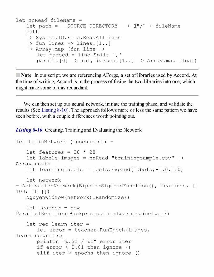
let nnRead fileName = let path = __SOURCE_DIRECTORY__ + @"/" + fileName path |> System.IO.File.ReadAllLines |> fun lines -> lines.[1..] |> Array.map (fun line -> let parsed = line.Split ',' parsed.[0] |> int, parsed.[1..] |> Array.map float)

Note In our script, we are referencing AForge, a set of libraries used by Accord. Atthe time of writing, Accord is in the process of fusing the two libraries into one, whichmight make some of this redundant.

We can then set up our neural network, initiate the training phase, and validate theresults (See Listing 8-10). The approach follows more or less the same pattern we haveseen before, with a couple differences worth pointing out.

Listing 8-10. Creating, Training and Evaluating the Network

let trainNetwork (epochs:int) =

let features = 28 * 28 let labels,images = nnRead "trainingsample.csv" |> Array.unzip let learningLabels = Tools.Expand(labels,-1.0,1.0)

let network = ActivationNetwork(BipolarSigmoidFunction(), features, [|100; 10 |]) NguyenWidrow(network).Randomize()

let teacher = new ParallelResilientBackpropagationLearning(network)

let rec learn iter = let error = teacher.RunEpoch(images, learningLabels) printfn "%.3f / %i" error iter if error < 0.01 then ignore () elif iter > epochs then ignore ()

else learn (iter + 1)

learn 0

network

let ann = trainNetwork (50)

let validate = nnRead "validationsample.csv"validate|> Array.averageBy (fun (label,image) -> let predicted = ann.Compute image |> Array.mapi (fun i x -> i,x) |> Array.maxBy snd |> fst if label = predicted then 1.0 else 0.0)

First, we need to transform the output, so that each of the digits becomes separatefeature. In order to achieve that, we use Accord.Statistics.Tools.Expand, abuilt-in utility that expands a set of labels into a new representation, where each labelbecomes an individual column, with binary outputs encoded in this case as –1 or 1. Weuse that particular encoding because of the activation function selected, theBipolarSigmoidFunction: its values go from –1 to 1, where 1 would be apositive case (“this is a 1”), and –1 a negative (“this isn’t a 1”). Alternatively,AForge.Neuro contains a couple of other built-in activation functions.

We create a network, passing in the activation function, the expected number ofinputs (in our case, the 28 × 28 pixels), and the number of nodes per layer in an array,the last element of being the expected number of labels, here 10. Note also the usage ofNguyenWidrow, which creates random but reasonable initial values for the networkweights.

On my machine, the following code produces nearly 82% correct classifications(due to the randomization of initial weights, results may vary). This is not entirelyterrible, but it is not great either. As you probably noticed if you ran it, it is also prettyslow. That being said, we limited the training to 50 iterations here, and the error (whichprints out after each pass) is still regularly decreasing when we reach the 50th iteration.When I expanded the search to 500 epochs, I saw another decrease from 1775 to 1200,with 82.6% correct. In other words, the learning process slows down quite a bit, but isstill producing improvements.

We will leave it at that on the topic of neural networks, and of Accord in general.The library contains a lot more than the algorithms we described here, as well as

interesting samples which illustrate some of it capabilities.

Scaling with m-brace.netTune your code all you want, at some point, the bottleneck will be your machine. Thereason this matters comes back full circle to our initial definition of machine learning. Agood machine learning algorithm should mechanically become better at performing itstasks, if it is fed more data.

One of the implications here is that if more data is better, then you will want more,which explains in part the recent craze around “big data.” And, as your datasets grow,both data exploration and model training using simple F# scripts will become slower,or even impossible, for instance if the dataset is too large to open or save locally. In thissection, we will provide a brief introduction to m-brace.net, a library designed toaddress that issue, by sending code from the scripting environment to be executed in acluster in the cloud.

Getting Started with MBrace on Azure with BriskIf our limiting factor is the computer itself, one direction is to throw more computers atthe problem. Just like “nine women can’t make a baby in one month” (in the words ofFred Brooks), many computers will not always speed things up, depending on theproblem. That being said, in general, any time we identify a map in our code, we shouldhave an opportunity to apply a divide-and-conquer approach: break the collection weare mapping into chunks, run the map for each chunk independently on separatecomputers, and reduce all the chunks into one final result.

This is the same pattern we saw earlier in Array.Parallel.map. Theframework we are going to discuss next, MBrace (www.m-brace.net), extends thatidea much further: instead of simply processing chunks across cores on your localmachine, it allows you to do the same, but across a cluster of machines in the MicrosoftAzure cloud.

The beauty here is that all of this is possible while still working from the scriptingenvironment. In essence, the goal of MBrace is to let you work with F# scripts in VisualStudio, so that you can keep a rapid design feedback loop, but seamlessly send that codeto be executed remotely to your cluster. You can create a cluster on-demand, just for aslong as you need large computation power or data, without being limited by your localequipment, and shut it down once you are done.

The easiest way to get started with MBrace is to follow three steps:

1. First, if you don't have one yet, get an Azure subscription. Youcan get a free trial version athttp://azure.microsoft.com.

2. Then, register for a free account at www.BriskEngine.com.Brisk is a service that allows you to easily provision a cluster onAzure, fully configured with all you need to run MBrace, anddelete it as soon as you are done. Brisk itself is free; you onlypay for your Azure cloud usage.

3. Finally, download the MBrace Starter Kit from the MBracerepository on GitHub:https://github.com/mbraceproject/MBrace.StarterKitThat project contains a preconfigured solution with numerousexamples illustrating how to use MBrace; you can simplydownload it, and add your scripts to it for an easy start.

At that point, you should have an F# project on your local machine that looks likeFigure 8-6.

Let’s deploy a cluster of machines on Azure first. To do that, simply go toBriskEngine.com, log in, and head to the Dashboard menu, where you can inspect whatclusters you recently created, and create new ones. Let’s create a new cluster, select{m} for MBrace, and choose where it should be deployed geographically. Youprobably want a location that is close to where you are, so that moving data back-and-forth between your machine and the cluster is as fast as possible; if you are going toaccess preexisting data, where it is located matters, too. Finally, let’s pick a clustersize; you can go from a tiny four-cores cluster (two medium machines), for less than$0.50 an hour, all the way up to 256 cores for around $20 an hour.

Figure 8-6. The m-brace starter project

Let’s go for 16 cores, which gives us solid horsepower, for about $1.50 an hour.The BriskEngine dashboard will indicate how far along the deployment is, and after 5 to10 minutes you should have your own cluster ready to go (see Figure 8-7).

Figure 8-7. Deploying a cluster on Azure via BriskEngine

We are now about ready to start running code on that cluster; we just need toconnect to it from our scripting session in Visual Studio. We will do that by providingMBrace with two connection strings in the credentials.fsx file. BriskEnginemakes that simple: in your dashboard, once the cluster is active, you can click thecluster name, and copy the two connection strings into the credentials file.

Finally, let’s add a new script, digits.fsx to the Starter Kit solution, withListing 8-11.

Listing 8-11. Connecting to the Cluster

#load "credentials.fsx"open MBrace.Coreopen MBrace.Azure.Client

let cluster = Runtime.GetHandle(config)

Send that code to FSI, and ... that’s it, you are now connected to the cluster. You cancheck that by running the following line of code, which will display information aboutthe workers you have running in your cluster:

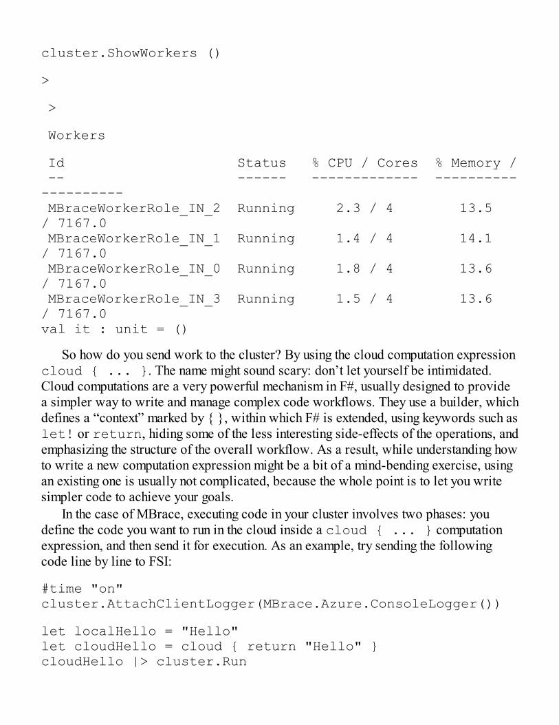
cluster.ShowWorkers ()

>

>

Workers

Id Status % CPU / Cores % Memory / -- ------ ------------- -------------------- MBraceWorkerRole_IN_2 Running 2.3 / 4 13.5 / 7167.0 MBraceWorkerRole_IN_1 Running 1.4 / 4 14.1 / 7167.0 MBraceWorkerRole_IN_0 Running 1.8 / 4 13.6 / 7167.0 MBraceWorkerRole_IN_3 Running 1.5 / 4 13.6 / 7167.0val it : unit = ()

So how do you send work to the cluster? By using the cloud computation expressioncloud { ... }. The name might sound scary: don’t let yourself be intimidated.Cloud computations are a very powerful mechanism in F#, usually designed to providea simpler way to write and manage complex code workflows. They use a builder, whichdefines a “context” marked by { }, within which F# is extended, using keywords such aslet! or return, hiding some of the less interesting side-effects of the operations, andemphasizing the structure of the overall workflow. As a result, while understanding howto write a new computation expression might be a bit of a mind-bending exercise, usingan existing one is usually not complicated, because the whole point is to let you writesimpler code to achieve your goals.

In the case of MBrace, executing code in your cluster involves two phases: youdefine the code you want to run in the cloud inside a cloud { ... } computationexpression, and then send it for execution. As an example, try sending the followingcode line by line to FSI:

#time "on"cluster.AttachClientLogger(MBrace.Azure.ConsoleLogger())

let localHello = "Hello"let cloudHello = cloud { return "Hello" }cloudHello |> cluster.Run

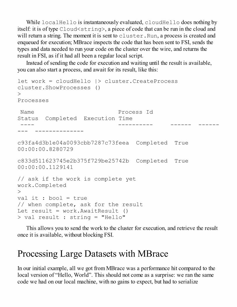
While localHello is instantaneously evaluated, cloudHello does nothing byitself: it is of type Cloud<string>, a piece of code that can be run in the cloud andwill return a string. The moment it is sent to cluster.Run, a process is created andenqueued for execution; MBrace inspects the code that has been sent to FSI, sends thetypes and data needed to run your code on the cluster over the wire, and returns theresult in FSI, as if it had all been a regular local script.

Instead of sending the code for execution and waiting until the result is available,you can also start a process, and await for its result, like this:

let work = cloudHello |> cluster.CreateProcesscluster.ShowProcesses ()>Processes

Name Process Id Status Completed Execution Time ---- ---------- ------ --------- -------------- c93fa4d3b1e04a0093cbb7287c73feea Completed True 00:00:00.8280729 c833d511623745e2b375f729be25742b Completed True 00:00:00.1129141

// ask if the work is complete yetwork.Completed>val it : bool = true// when complete, ask for the resultLet result = work.AwaitResult ()> val result : string = "Hello"

This allows you to send the work to the cluster for execution, and retrieve the resultonce it is available, without blocking FSI.

Processing Large Datasets with MBraceIn our initial example, all we got from MBrace was a performance hit compared to thelocal version of “Hello, World”. This should not come as a surprise: we ran the samecode we had on our local machine, with no gains to expect, but had to serialize

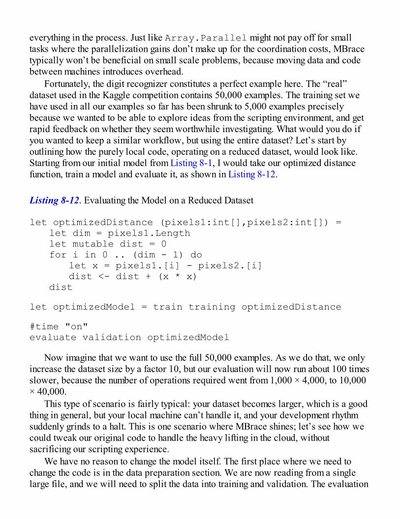
everything in the process. Just like Array.Parallel might not pay off for smalltasks where the parallelization gains don’t make up for the coordination costs, MBracetypically won’t be beneficial on small scale problems, because moving data and codebetween machines introduces overhead.

Fortunately, the digit recognizer constitutes a perfect example here. The “real”dataset used in the Kaggle competition contains 50,000 examples. The training set wehave used in all our examples so far has been shrunk to 5,000 examples preciselybecause we wanted to be able to explore ideas from the scripting environment, and getrapid feedback on whether they seem worthwhile investigating. What would you do ifyou wanted to keep a similar workflow, but using the entire dataset? Let’s start byoutlining how the purely local code, operating on a reduced dataset, would look like.Starting from our initial model from Listing 8-1, I would take our optimized distancefunction, train a model and evaluate it, as shown in Listing 8-12.

Listing 8-12. Evaluating the Model on a Reduced Dataset

let optimizedDistance (pixels1:int[],pixels2:int[]) = let dim = pixels1.Length let mutable dist = 0 for i in 0 .. (dim - 1) do let x = pixels1.[i] - pixels2.[i] dist <- dist + (x * x) dist

let optimizedModel = train training optimizedDistance

#time "on"evaluate validation optimizedModel

Now imagine that we want to use the full 50,000 examples. As we do that, we onlyincrease the dataset size by a factor 10, but our evaluation will now run about 100 timesslower, because the number of operations required went from 1,000 × 4,000, to 10,000× 40,000.

This type of scenario is fairly typical: your dataset becomes larger, which is a goodthing in general, but your local machine can’t handle it, and your development rhythmsuddenly grinds to a halt. This is one scenario where MBrace shines; let’s see how wecould tweak our original code to handle the heavy lifting in the cloud, withoutsacrificing our scripting experience.

We have no reason to change the model itself. The first place where we need tochange the code is in the data preparation section. We are now reading from a singlelarge file, and we will need to split the data into training and validation. The evaluation

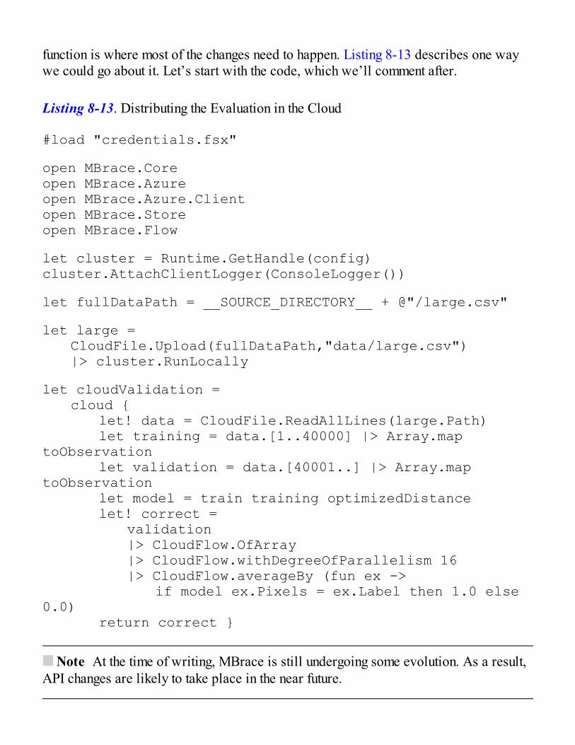
function is where most of the changes need to happen. Listing 8-13 describes one waywe could go about it. Let’s start with the code, which we’ll comment after.

Listing 8-13. Distributing the Evaluation in the Cloud

#load "credentials.fsx"

open MBrace.Coreopen MBrace.Azureopen MBrace.Azure.Clientopen MBrace.Storeopen MBrace.Flow

let cluster = Runtime.GetHandle(config)cluster.AttachClientLogger(ConsoleLogger())

let fullDataPath = __SOURCE_DIRECTORY__ + @"/large.csv"

let large = CloudFile.Upload(fullDataPath,"data/large.csv") |> cluster.RunLocally

let cloudValidation = cloud { let! data = CloudFile.ReadAllLines(large.Path) let training = data.[1..40000] |> Array.map toObservation let validation = data.[40001..] |> Array.map toObservation let model = train training optimizedDistance let! correct = validation |> CloudFlow.OfArray |> CloudFlow.withDegreeOfParallelism 16 |> CloudFlow.averageBy (fun ex -> if model ex.Pixels = ex.Label then 1.0 else 0.0) return correct }

Note At the time of writing, MBrace is still undergoing some evolution. As a result,API changes are likely to take place in the near future.

The code could be simplified a bit, but as it stands, it highlights a few interestingfeatures. First, we create a CloudFile. We upload our entire dataset to the cluster,which allows us to read its contents using CloudFile.ReadAllLines, in afashion similar to what we did previously with File.ReadAllLines. Note theusage of cluster.runLocally; the purpose is to have our local machine (wherethe original data file is located) perform the upload, rather than one of the worker roleson the cluster

The cloudValidation function is also similar to the original, purely localversion. The main modifications are that first, we wrap the evaluation in cloud {... }. As a result, the entire process will run in the cluster. Then, instead of usingArray.averageBy to evaluate the model across the validation sample, we use aCloudFlow., which behaves essentially like a sequence, but distributes workintelligently across the cluster.

So... how well does this work? On a 16-cores cluster, the evaluate part runs inabout a minute. Of course, we had to pay a cost for the initial data upload, but this is aone-time cost. At that point, we could start modifying our algorithm and testing theimpact; and each evaluation of the modified code will take a minute, instead of over 5minutes if I run it on my workstation without MBrace. This is very significant: over theduration of a day, running a dozen evaluations, I would gain an entire hour, not tomention the ability to just stay focused, instead of being distracted by 5 minutes breaksevery time I want to try something out.

There is much more to MBrace than what we just showed in this rather simpleexample; however, I hope it gave you a sense for the type of scenarios it is useful in—essentially, use cases where you want to keep an interactive and flexible workflow, butneed to significantly increase how much data you can handle. I want to specificallypoint out that while this example was entirely driven from the scripting environment, itis perfectly possible to acquire data from other sources. This is particularly important ifyou need to handle very large datasets; in that case, opening the data in the scriptingenvironment might be impractical, or even impossible. Instead, you can access the datawherever it is located, from within your cluster, do the heavy lifting there, and simplysend back the results of your analysis to your local environment.

So What Did We Learn?This final chapter was fairly different from what we have been doing up to that point.Instead of focusing on one specific problem, and building a machine learning algorithmfrom scratch to address a question, we revisited the model we developed in the firstchapter, and used it as a reference point to explore two directions: improving code

performance, and demonstrating a couple of useful modelling techniques.We started by analyzing the structure of our algorithm, to understand where

improvements would be possible, and what performance we should be expecting as weincrease the volume of data used for training and validation. In this specific case, weidentified the function responsible for computing the distance between images as abottleneck we could potentially improve. We isolated this function, and, by measuringits speed and garbage collection characteristics, we managed to adjust the code andimprove both aspects, with a ten-time speedup. The price we had to pay for thatimprovement was writing more code, and perhaps more complicated code, using eitherrecursion or mutating variables. This is not an uncommon trade-off. While coding in afunctional style, favoring immutable data structures and higher-level functions, comeswith its own benefits (clear and safe code that describes intent), it can also havedrawbacks, notably from a performance standpoint. One of the strengths of F# is itshybrid nature: by default, the language tends to favor a functional style, but it handlesperfectly well coding in an imperative style, which allows for simple localoptimizations when they are needed.

We also explored parallelism as a way to squeeze out additional performance. Oneof the benefits of a functional style is that it helps spot places where such improvementsare possible. Specifically, whenever a map is being used, we have a candidate forspeedup gains, because a map signals an operation that can be run in parallel instead ofsequentially. We illustrated that first with Array.Parallel.map, and later on withm-brace.net, which both exploit that pattern to divide-and-conquer work acrossresources, on the cores of your local machine, or across many machines in a cluster.

This is extremely useful in a machine learning context. Machine learning is aboutbuilding predictive models that become better as they are fed with more data; and whileincreasing the volume of data used by your models is an important ingredient in makingthem better, this also creates a problem, because larger datasets require morecomputation power to be processed. But in many situations, that increase can bemitigated because its translation in code happens through a map, or a similarlyparallelizable operation, which implies that the increase in volume can be dividedacross more resources. We saw a prime example here with cross validation: eventhough we needed to evaluate more observations, they can all be processedindependently of each other, and as a result, we can handle larger volumes without mucheffort, simply by provisioning a large cluster and parallelizing the map operation.

The second main direction in this chapter was a brief introduction to Accord.NET, arich .NET machine learning library. Writing your own algorithm implementation is aperfectly valid thing to do, and often easier than it seems. However, it is impractical attimes. Being able to simply try out whether a particular algorithm works, and eliminateit quickly if it doesn’t, can help avoid wasting valuable time that could be spentfocusing faster on a direction that is promising. Accord.NET offers a wealth of well-

implemented classification and regression models, and is a useful tool to master for thatpurpose. Also, while the R Type Provider offers another venue to try out off-the-shelfalgorithms, Accord.NET has the advantage of being a .NET library, which makes itsintegration with a .NET code base simpler.

Finally, we used this introduction to Accord.NET as a pretext to present, at a veryhigh level, a couple of classic classifiers which we haven’t covered in previouschapters—logistic regression, support vector machines, and artificial neural networks—and how you would go about using them. Accord contains many other tools, and Iwould recommend taking a deeper look at the library. Our introduction to the library(and the three classifiers we used as examples) was somewhat superficial; it wouldn’tbe practical to attempt to cover everything in detail in here, but we hope that our focuson usage, illustrating the general patterns Accord.NET follows, will be helpful indigging further into the library!

USEFUL LINKS

Accord.NET is a wonderful library, with numerous machinelearning algorithm, as well as tools related to computer vision andnumeric analysis: http://accord-framework.net

MBrace, a library for scalable cloud data scripting: www.m-brace.net

Brisk, a website that simplifies the deployment of MBrace clusters:www.briskengine.com

Peter Norvig’s talk “The Unreasonable Effectiveness of Data”:https://www.youtube.com/watch?v=yvDCzhbjYWs

Modelling logic gates with single-layer perceptrons:www.cs.bham.ac.uk/~jxb/NN/l3.pdf

CHAPTER 9

Conclusion

You made it through this book—congratulations! This was a long journey, and I hope itwas also an enjoyable one—one from which you picked up an idea or two along theway. Before we part ways, I figured it might be worthwhile to take a look back at whatwe have accomplished together, and perhaps also see if there are some broader themesthat apply across the chapters, in spite of their profound differences.

Mapping Our JourneyMy goal with this book was to provide an introduction to the topic of machine learningin a way that was both accessible and fun to .NET developers. Machine learning is alarge topic, which is—deservedly—attracting more attention every day. It’s also a topicthat is all too often presented in a somewhat abstract fashion, leading many to believethat it’s a complicated topic best left to mathematicians.

While mathematics play an important role in machine learning, my hope is that, afterreading this book, you realize that it isn’t quite as complex as it sounds, and that many ofthe underlying ideas are actually fairly simple and applicable to a wide range ofpractical problems.

Let’s take a step back and look at the ground we covered. At a very high level, weestablished something like a map of machine learning problems, making importantdistinctions. First, we introduced supervised and unsupervised methods. Each addressesa distinct problem, as follows:

Unsupervised methods are about helping you make sense of data,when you don’t know yet what question you might be after. Thiswas the main topic of Chapter 5, where we took a dataset ofStackOverflow questions and simply looked for patterns that would

help us make sense of otherwise hard-to-interpret, unstructureddata.

By contrast, supervised methods, where we spent most of ourefforts (Chapters 1, 2, 4, and 6), are about training a model toanswer a well-defined question that matters to us based on labeledexamples; that is, data for which the correct answer is known.

In that exploration, we covered a wide range of models, which have importantdifferences. First, we distinguished between classification and regression models,which differ in the type of answer we expect from them. A regression model aims atpredicting a continuous numeric value; in Chapter 4, we developed such a model topredict the usage level of a bicycle-sharing service based on various inputs. Bycontrast, classification models are about deciding which is the most likely out of alimited number of possible outcomes. We saw three examples of that type of model,from automatically recognizing which of ten possible digits an image represented(Chapter 1) to separating between ham and spam messages (Chapter 2), and predictingwhich passengers on the Titanic would survive their trip (Chapter 6).

We also explored a different approach using reinforcement learning in Chapter 7.The resulting model was a classifier that decided between a limited set of possibleactions, with a key difference from previous models: Instead of learning one time usingpast data, we built a model that kept learning constantly as new observations werecoming in, an approach generally known as online learning.

Throughout the book, we dug into a variety of real datasets and let the data guide ourexploration. In spite of the apparent diversity of topics (images, text, numbers, and soforth), patterns emerged across problems. In most cases, we ended up applying featuresextraction—we transformed the original data into rows of values that were moreinformative or convenient to work with. And, just as the type of answer we werelooking for in a model determined whether classification or regression was moresuitable, we ended up with different approaches depending on whether features werecontinuous or categorical. We also saw how one could potentially transform acontinuous feature into a discrete one by binning (age, in the Titanic example), orconversely how a categorical could be flattened into a series of indicator variables (dayof the week, in the regression example).

Science!Another pattern we saw emerge across the chapters involved methodology. We beginwith a question we want to answer, we gather whatever data we have available, and we

start to perform a series of experiments, progressively creating and refining a model thatagrees with the facts.

In that sense, developing a machine learning model is fairly different fromdeveloping a regular line-of-business application. When you build an application, youusually have a set of features to implement; each feature has some form of acceptancecriteria describing what it takes for it to be done. Developers decompose the probleminto smaller pieces of code, put them together, and the task is complete once things worktogether as expected.

By contrast, developing a machine learning program is closer to a research activitythat follows the scientific method. You don’t know beforehand if a particular idea willwork. You have to formulate a theory, build a predictive model using the data you haveavailable, and then verify whether or not the model you built fits with the data. This is abit tricky, in that it makes it difficult to estimate how long developing such a modelmight take. You could try a very simple idea and be done within half a day, or you couldspend weeks and have nothing to show for your work except failed experiments.

Of course, things are not entirely that clear cut. There is some uncertainty involvedwhen developing a regular application, and some failed experiments as well. However,the fact remains that with machine learning you won’t know whether your idea worksuntil you confront your model with the data. That being said, some software engineeringideas still apply, albeit in a slightly modified manner.

Just like it helps to have a clear specification for what feature you are trying to ship,it is crucial to think early on about how to measure success, and then set yourself up forthat purpose. Correct code is only a small part of what makes a good machine learningmodel; to be valuable, a model has to be useful, and that means it has to be good atmaking predictions. In that frame, we repeatedly used cross-validation throughout thebook. Put aside part of your data, don’t use it for training, and once you have a modelready, test how well it works on the validation set, which simulates what might happenwhen your model sees new input in real conditions. In some respects, cross-validationserves a purpose similar to a test suite for regular code by allowing you to checkwhether things work as intended.

A habit that has worked well for me, both for machine learning and softwaredevelopment, is to build a working prototype as quickly as possible. In the context ofmachine learning, this means creating the most naïve and quick-to-execute model youcan think of. This has numerous benefits: It forces you to put together an end-to-endprocess, from data to validation, which you can reuse and refine as you go. It helpscatch potential problems early on. It establishes a baseline, a number that sets the bar bywhich to judge whether other models are good or bad. And finally, if you are lucky, thatsimple model might just work great, in what case you’ll be done early.

Speaking of simple models, there is one point that I really hope I managed to get

across in this book. Much of the discourse around machine learning emphasizes fancymodels and techniques. Complex algorithms are fun, but in the end, it is typically muchmore important to spend time understanding the data and extracting the right features.Feeding a complex algorithm poor data will not magically produce good answers.Conversely, as we saw in a few chapters, very simple models using carefully craftedfeatures can produce surprisingly good results. And, as an added benefit, simplermodels are also easier to understand.

F#: Being Productive in a FunctionalStyleThe vast majority of the code we wrote together was written in F#, a functional-first.NET language. If this was your first exposure to F#, I hope you enjoyed it, and that itwill inspire you to explore it further! In a way, functional programming suffers from aproblem similar to machine learning; that is, it is all too often described as being atheoretical and abstract topic. The reasons F# became my primary language in the pastfew years have nothing to do with theory. I have found it to be an incredibly productivelanguage. I can express ideas with clear and simple code, and rapidly refine them andget things done faster. Plus, I simply find the language fun to work with.

In my opinion, F# qualities shine when applied to the topic of machine learning.First, the built-in scripting environment and a language with light and expressive syntaxare crucial. Developing a machine learning model involves a lot of exploration andexperimentation, and being able to load data once and continue exploring throughout theday, without the potentially distracting mental interruption of having to reload andrecompile, is key.

Then, if you look back at the models we built together, you might have noticed ageneral pattern. Starting from a data source, we read it and extract features, we apply alearning procedure that updates a model until the fit is good enough, and we computesome quality metric with cross-validation. That general process is a very good matchwith a functional style, and our implementations looked fairly similar across problems:Apply a map to transform data into features, use recursion to apply model updates andlearn, and use averages or folds to reduce predictions into quality metrics such asaccuracy. The vocabulary of functional languages fits fairly naturally with the type ofproblems machine learning is after. And, as an additional benefit, functional patterns,which emphasize immutable data, tend to be rather easy to parallelize, something thatcomes in handy when working with large amounts of data.

While this point applies to other functional languages as well, F# has a couple of

characteristics that make it particularly interesting. The first one is type providers, amechanism we explored in Chapter 3. Most languages are either dynamically orstatically typed, and each comes with its advantages or challenges. Either external datais easy to access, but we get limited assistance from the compiler, or the opposite istrue. F# type providers provide a resolution to that tension, making data (or languages,as in our example calling the R language) consumable with very limited friction, anddiscoverable in a safe manner, with all the benefits of static typing.

Another distinct benefit of F# for that particular domain is its ability to be used bothfor exploration and for production. We have been focusing mainly on the first aspectthroughout this book, exploring data in a rapid feedback loop and progressively refiningmodels. However, once ideas become stable, promoting code from a script to a moduleor a class and turning it into a full-fledged library is rather trivial, as illustrated in acouple of chapters. You can expect the same level of performance you would from.NET in general—that is, quite good. And, at that point, you can just run that code inproduction and integrate it with a .NET codebase, regardless of whether that code waswritten in C#, VB.NET, or F#. There is real value in being able to use the samelanguage from exploration to production. I have seen in many places a developmentprocess where a research team creates models using one set of tools and languages, andtransfers it to a development team that is left with the choice of either rewriting it all(with all the problems that entails) or trying their best to integrate and run exotic toolsinto a production system. F# can provide an interesting resolution to that tension, andcan serve both as an exploratory language for research and a production-ready languagefor developers.

What’s Next?So, are you a machine learning expert now? I am sorry if this comes as adisappointment, but this book barely scratches the surface, and there is much, muchmore to learn. That being said, if you enjoyed the topic, the good news is you won’t runout of interesting material to learn from (as a starting point, I would recommend taking alook at the class with Andrew Ng on Coursera, and trying out some of the Kagglecompetitions). Machine learning is developing rapidly, and that is one of the reasons Ienjoy the domain so much.

Perhaps more important, you might not be an expert just yet—but then, few peopleare, because of the sheer size of the topic. At this point, however, you are likely to knowmuch more about the topic than a majority of software engineers, and you should be ableto start productively using some of the ideas we talked about together in your ownprojects. Most important, I hope I managed to convince you that machine learning is

both less complicated than it might appear at first, full of really interesting problems formathematicians and software engineers alike, and a lot of fun. So, go try it out, do greatthings, and have fun!

Index

AAccord.NET

ANN (see Artificial neural networks (ANN))logistic regression

Accord.MachineLearning and Accord.Neurodataset, memorylogistic functionobject-oriented styleone-vs.-all classificationrecursive looptraining phasevalidation

one-vs.-all classificationR type providerSVMs

Akaike information criterion (AIC)Artificial neural networks (ANN)

constructioncreating and traininghidden layersperceptronSVMs

BBatch gradient descent

cost functiondrawbacksstep-by-step error

Bayesian information criterion (BIC)Bike-sharing dataset

Capital Bikeshare programcategorical featuresclassificationcontents, day.csvcross-validation and over-fittingcsv formatdescriptionfeaturizerFisher-Yates random shuffle algorithmfsharp.Chartinglowest-cost modelmachine-learning techniques

moving averagesnon-linear features

bicycle usage, temperature scatterplotdrawbacksfitting square temperature

normalizationreadme.txt fileregression modelregularizationstraight-line modelstraight-line regression

predicted curvepredicted vs. actual scatterplotvisualization

Bike-sharing dataset. See Gradient descentBrain 2.0

epsilon learninglearning procedure, forward-lookingrotate functionshort-term gains

CCAPTCHA. See Completely Automated Public Turing test to tell Computers and Humans apart (CAPTCHA)C# console application

classifier implementationdataset organizationdistance computation, imagesreading, data

Clustering stackOverflow tagsclusters profiledatasetEuclidean distancetag names, alignmentweb-client technologies

Code performanceArray.Parallel modulebusiness applications developmentcross-validationdistance computationempirical evidencetraining and validation

Completely Automated Public Turing test to tell Computers and Humans Apart (CAPTCHA)

DData-analysis techniques

patternsclusterscomplexlinear

scatterplot plottingwithout data

PCA (see Principal component analysis (PCA))recommendations

collaborative filteringpercentage correctprimitive tag recommenderPython and Regexuser profiles

StackOverflowbasic statisticsF# library projectJSON type providerpopular tagstags, average usage

supervised learning methodsDecision trees, Titanic dataset

classifiersconstructionCSV type providerdecision stumpdemographic informationdescriptiondiscretizationentropy (see Shannon entropy)filtersKaggle competitionmissing datamodelingover-fittingpassenger classesprettier treesurvival rate, groupsticket pricestraining and evaluation, stump

EEpsilon learning

FF#

classifier functiondata manipulation, tuplesF# interactive

code executionlibrary projectscript.fsx

language featurespattern matching

pipelines, functionsscript

creationdissection

Forests, decision treescreationcross-validation, k-foldsdescriptionfragile treesmissing blocksover-fitting riskstraining and validation

GGames

adaptive mechanismconsole application

Hero decision makinginitializationrunning, loop

creature, programmingelementsexploration vs. exploitationF# projectgreed vs. planninglogicprimitive brain

decision making processimplementationlearning processpredetermined strategytesting

q-learningred kitchen doorrenderingupdation

brains filegame fileprogram filerendering file

Gradient descentbatchcost functioncost minimizationcross-validationgeneral model formulationminimum of functiononline learningpotential limitationprediction error

stochastic

H, IHam. See Spam detection

JJSON type provider

compile-time errorFSharp.Data libraryload methodNuGet package and F# scriptsquestions type, sample dataStackExchange API

KK-means clustering

AICarbitrary numbercentroids

assignment, observationsdefinitionfixed-point methodlocation, adjustmentupdation

correlation matrix, StackOverflow tagscovariance and correlationfeature scalingfinal clustershigh-density areasimplementation

clustering algorithm, initializationk observationspseudo-coderecursive function

Java and AndroidPCA (see Principal component analysis (PCA))random observationsrescaling, datasetRSS

LLinear algebra

batch gradient-descent algorithmdata structureMath.NETMKL

normal formprediction modelvectors and matrices

M, N, OMachine learning

cost functioncross-validationC# version (see C# console application)definitiondescriptiondistance functiondumbest modelEuclidean distanceF#feature extractionimage classification

CAPTCHA and reCAPTCHAdigit recognizerdistance functionsimage recognitiontraining examples

improvementsOccam’s Razoronline learningquality evaluationregression modelrequirementscientific methodsoftware developmentsupervised methodssupport vector machineunsupervised methodswriting programs

Manhattan distanceMath Kernel Library (MKL)MBrace

Array.Parallel.mapBriskEngine dashboardcloud computationsdata exploration and model trainingdatasetsdivide-and-conquer approachprocess executionStarter Kit solutionstarter project, steps

Minimal domain-specific language (DSL)comparing tagsfrequent tags, C# and F#inverted pattern

pipe-forward operatorquery constructiontypos and bugs

MKL. See Math Kernel Library (MKL)

P, QPrincipal component analysis (PCA)

correlation analysisdatabases, observationseigenvectorsfeatures, algebraimplementationiOS, objective-C and iPhonek-means clustering.NET-related technologiesobservationsoriginal featuresplotting observations againstsource code packageStackOverflow datasetweb development

RR data frames

creating and plottingdatabase tablesfeaturesmerging data sources

Residual sum of squares (RSS)R type provider

basic functionscountry surface areadescriptionhistogram, country surfaceslog functionNuGet package and RProviderRStudioscatterplot

SShannon entropy

discretizationinformation gain

computing, F# interactivedecision stumpfeaturesmathematical expression

passenger sexsub-groupsweighted average

puritysample population

Spam detectionBayes’ theoremclassifier implementation

code extraction, modulesdocumentary collectionlearning phaseprocess outlinescore computationsequencessets

classifier improvementcapitalizationfeaturesnumeric valuessingle-token modelsingle wordword selection

computersdatasetdecision treesdecomposition, messagesdescriptiondiscriminated unionsLaplace smoothingreading, datasetsimplified document scorespam filter mechanismtext messagestokenizationtraining set

cross-validationF# interactivetokenization

understanding errorswords, clues

Stochastic gradient descentSupport vector machines (SVMs)

binary classifiersclassestraining samplevalidation

SVMs See Support vector machines (SVMs)

T, U, VType providers

benefitsdata access and manipulationDeedle datafancy algorithmsMatlab and Pythonprogramming languageSQL commandStackOverflow data

JSON (see JSON type provider)minimal DSL (see Minimal domain-specific language (DSL))StackExchange API

trade-offworld population

Deedle data framedensity mapgrowth mapmap creation

W, X, Y, ZWorld Bank type provider