machine learning neural networks and deep...
TRANSCRIPT

1
Machine Learning Neural Networks
and Deep Learning

Neural Networks
• NN is a ML algorithm belonging to the category of supervised classification models
• The learned classification model is an algebraic function (or a set of functions), rather than a boolean function, as for DTrees
• The function is linear for Perceptron algorithm, non-linear for Backpropagation algorithm
• Both features and the output class are allowed to be real valued (rather than discrete, as in Dtrees)
2

3
Neural Networks
• Analogy to biological neural systems, the most robust learning systems we know.
• Attempt to understand natural biological systems through computational modeling.
• Massive parallelism allows for computational efficiency.
• Help to understand “distributed” nature of neural computation (rather than “localist”) that allow robustness and graceful degradation.
• Intelligent behavior as an “emergent” property of large number of simple units rather than from explicitly encoded symbolic rules and algorithms.

4
Neural Speed Constraints
• Neurons have a “switching time” on the order of a few milliseconds, compared to nano/picoseconds for current computing hardware.
• However, neural systems can perform complex cognitive tasks (vision, speech understanding) in tenths of a second, computers can’t.
• Only time for performing 100 serial steps in this time frame, compared to orders of magnitude more for current computers.
• Therefore, neural computation in humans exploits“massive parallelism.”
• Human brain has about 1011 neurons with an average of 104 connections each.

5
Neural Network Learning
• Learning approach of NN algorithm based on modeling adaptation in biological neural systems.
• Two main algorithms: – Perceptron: Initial algorithm for learning simple
neural networks (single layer) developed in the 1950’s.
– Backpropagation: More complex algorithm for learning multi-layer neural networks developed in the 1980’s.

6
Real Neurons
• Cell structures – Cell body – Dendrites – Axon – Synaptic terminals
7
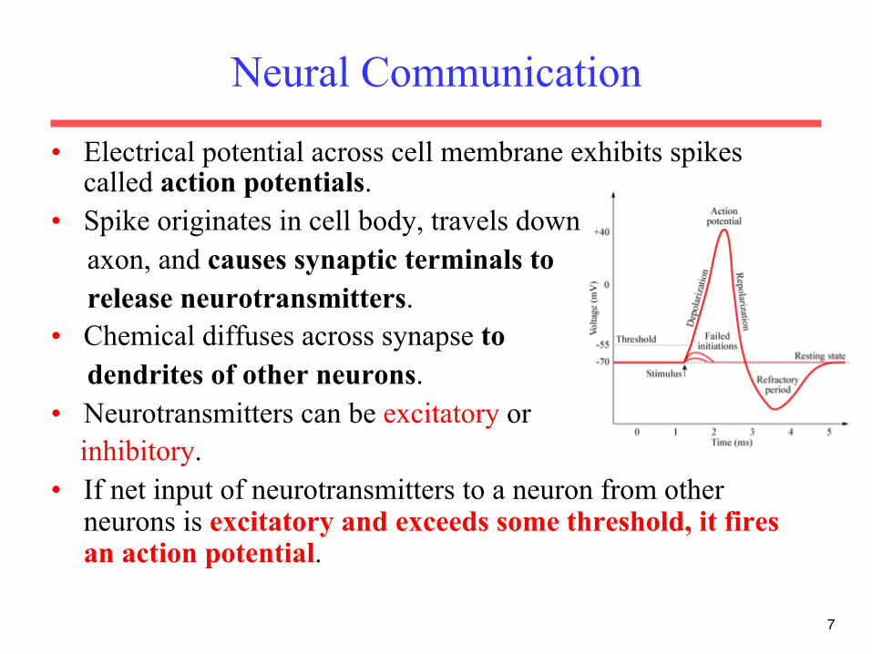
Neural Communication
• Electrical potential across cell membrane exhibits spikes called action potentials.
• Spike originates in cell body, travels down axon, and causes synaptic terminals to release neurotransmitters. • Chemical diffuses across synapse to dendrites of other neurons. • Neurotransmitters can be excitatory or inhibitory. • If net input of neurotransmitters to a neuron from other
neurons is excitatory and exceeds some threshold, it fires an action potential.
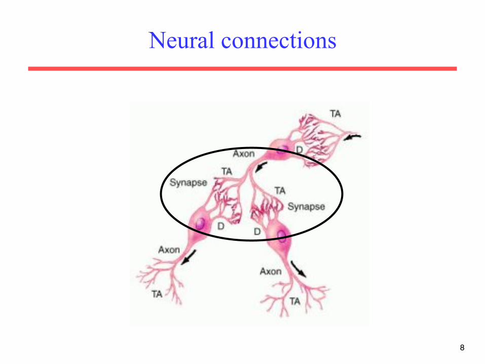
Neural connections
8
9
Real Neural Learning
• Synapses change size and strength with experience (evolving structure).
• Hebbian learning: When two connected neurons are firing at the same time, the strength of the synapse between them increases.
• “Neurons that fire together, wire together.”

10
Artificial Neuron Model
• Model network as a graph with cells as nodes, and synaptic connections as weighted edges from node i to node j, wji
• Model net input to cell as
• Cell output is:
net j = wjii∑ xi
(activation function φ is a threshold function Tj )
ji
jjj Tnet
Tneto
≥
<=
if 1 if 0
netj
oj
Tj 0
1
Tj
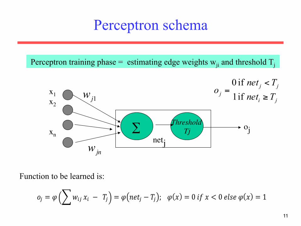
Perceptron schema
11
x1 x2 xn
Threshold Tj ∑
netj oj
ji
jjj Tnet
Tneto
≥
<=
if 1 if 0
Perceptron training phase = estimating edge weights wji and threshold Tj
wj1
wjn
Function to be learned is:
!! = ! !!" !! !− !!!! = ! !"#! − !! ; !!!! ! = 0!!"!! < 0!!"#!!! ! = 1!

Perceptron learns a linear separator
12
This is an (hyper)-line in an n-dimensional space, what is learnt are the coefficients wi
Instances X(x1,x2..x2) such that:
Are classified as positive, else they are classified as negative

13
Perceptron as a Linear Separator: example in two-dimensional space
w1x1 +w2x2 >T3
x2 > −w1w2x1 +
T3w2
x2
x1
??
Or hyperplane in n-dimensional space
x2= mx1+q
x1 x2 xn
Threshold Tj ∑
netj oj
14
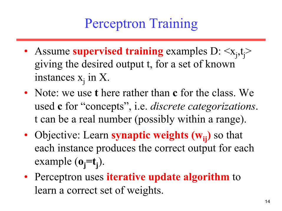
Perceptron Training
• Assume supervised training examples D: <xj,tj> giving the desired output t, for a set of known instances xj in X.
• Note: we use t here rather than c for the class. We used c for “concepts”, i.e. discrete categorizations. t can be a real number (possibly within a range).
• Objective: Learn synaptic weights (wij) so that each instance produces the correct output for each example (oj=tj).
• Perceptron uses iterative update algorithm to learn a correct set of weights.

15
Perceptron Learning Rule • Initial weights selected at random. • Update weights by:
where η is a constant named the “learning rate” tj is the “teacher” specified output for unit j, (tj -oj) is the
error in iteration t Equivalent to rules:
– If, for instance <xj,tj> in D, output is correct (tj=oj) do nothing (Errj=0) and
– If output is “high” (oj=1, tj=0, Errj=-1), lower weights on active inputs
– If output is “low” (Errj=+1), increase weights on active inputs
• Also adjust threshold to compensate:
w(t )ji = w
(t−1)ji +η(t j −oj )xi
T tj = T
t−1j −η(t j −oj )
ji
jjj Tnet
Tneto
≥
<=
if 1 if 0
wji(t ) −wji
(t−1) = Δwji =η(Errj )xi
wji(t ) = wji
(t−1)
NOTE: weights on edges are updated proportionally to the error observed on the output (Errj )AND to the intensity of the signal xi travelling
on the edges
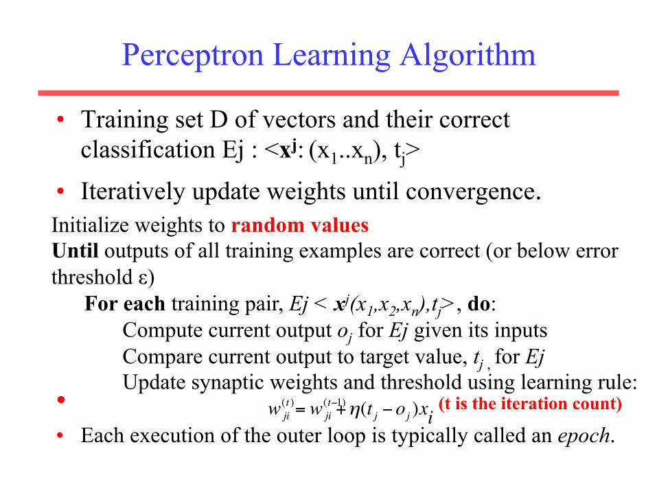
Perceptron Learning Algorithm
• Training set D of vectors and their correct classification Ej : <xj: (x1..xn), tj>
• Iteratively update weights until convergence.
• (t is the iteration count)
• Each execution of the outer loop is typically called an epoch.
Initialize weights to random values Until outputs of all training examples are correct (or below error threshold ε) For each training pair, Ej < xj(x1,x2,xn),tj>, do: Compute current output oj for Ej given its inputs Compare current output to target value, tj , for Ej Update synaptic weights and threshold using learning rule:
w(t )ji = w
(t−1)ji +η(t j −oj )xi

Concept Perceptron Cannot Learn
• Cannot learn not linearly separable functions!
• If our data (the learning set) are not separable by a line, then we need a more complex (polynomial?) function

18
Perceptron Convergence and Cycling Theorems
• Perceptron convergence theorem: If the data is linearly separable and therefore a set of weights wi exists that is consistent with the data (i.e. that identifies a line that separates positive from negative instances), then the Perceptron algorithm will eventually converge to a consistent set of weights.
• Perceptron cycling theorem: If the data is not linearly separable, the Perceptron algorithm will repeat a set of weights and threshold at the end of some epoch and therefore enter an infinite loop.
19
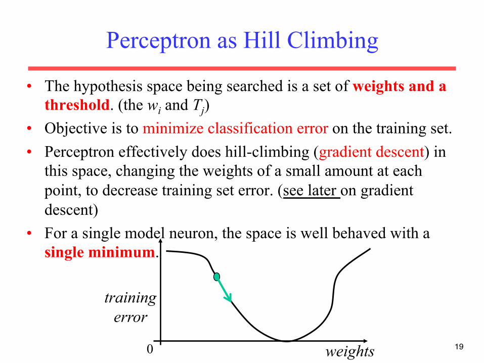
Perceptron as Hill Climbing
• The hypothesis space being searched is a set of weights and a threshold. (the wi and Tj)
• Objective is to minimize classification error on the training set. • Perceptron effectively does hill-climbing (gradient descent) in
this space, changing the weights of a small amount at each point, to decrease training set error. (see later on gradient descent)
• For a single model neuron, the space is well behaved with a single minimum.
weights 0
training
error

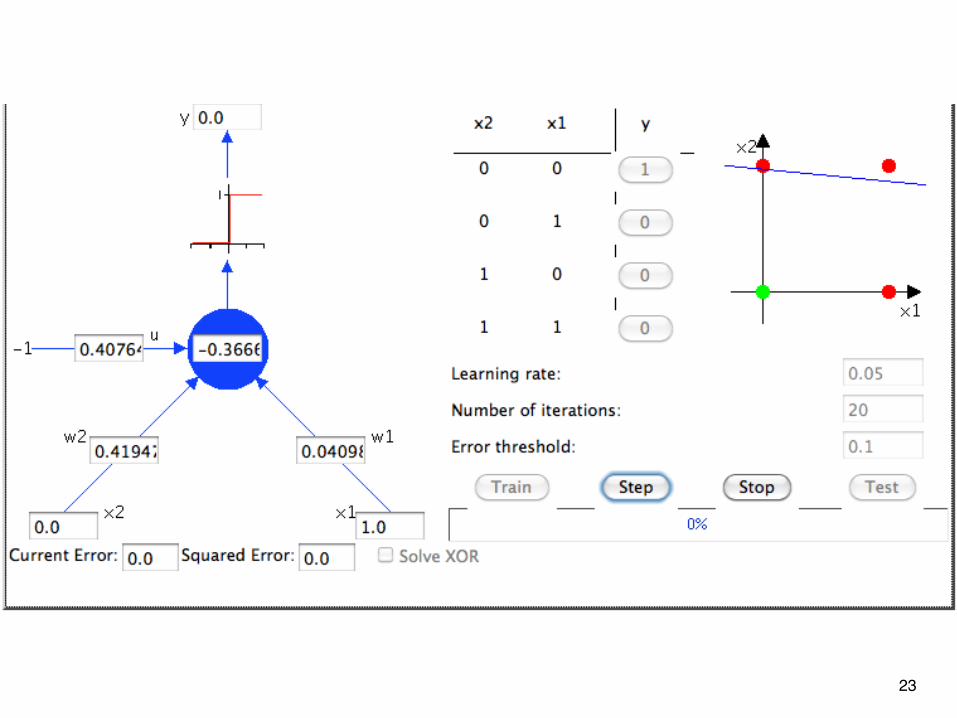
Example: Learn a NOR function
20
w1x1 +w2x2 > u(u = Threshold)
w(t )i = w(t−1)i +0.05(t j − o
(t−1)j )xi utj = u
t−1j − 0.05(t j −o
(t−1)j )
η

21

22
23

24

25

After 20 iterations
26

27
Perceptron Performance
• In practice, converges fairly quickly for linearly separable data.
• Can effectively use even incompletely converged results when only a few outliers are misclassified (outliers: data which are “exceptions”, like whales as mammals).
• Experimentally, Perceptron does quite well on many benchmark data sets.

What if data not linearly separable?
28

29
Multi-Layer Networks
• Multi-layer networks can represent arbitrary functions • A typical multi-layer network consists of an input, hidden
and output layer, each fully connected to the next, with activation feeding forward.
• Edges between nodes are weighted by wji • Instances <xi(xi
1,..xin),(ti
1,..tim)>from learning set D are
connected to input nodes in first layer • Target is to learn the weights of edges such as to
minimize the error between the output available on output nodes oj and the true class values ti
j in in training set
output
hidden
input
activation

Multilayer networks (2)
• The output function is a vector of m values ti1,..ti
m (complex output functions or multiple classifications)
• Output values can be continuous rather than discrete as for boolean learners (VS, Dtrees), therefore are indicated with t rather than c (they are not necessarily “concepts” (=boolean), though they can be concepts)
• Like for the perceptron, each node nj receives in input a weighted sum of values netj and computes a threshold function φ(netj)
30

Multilayer networks (3) • Like for the perceptron, edge weights are iteratively
updated depending on the error (difference between true output and computed output). The iterative algorithm is called Backpropagation.
• Weight updating rule is based on of hill-climbing • In a hill-climbing heuristic:
– we start with an initial solution (= a random set of weights W). – Generate one or more “neighboring” solutions (weights which are
“close” to previous values). – Pick the best and continue until there are no better neighboring
solutions.
• In the case of neural network, gradient descent is used to identify “best” neighboring solutions
Gradient and gradient descent
• The gradient of a scalar field is a vector field that points in the direction of the greatest rate of increase of the scalar field, and whose magnitude is that rate of increase.
• In simple terms, the variation of any quantity – e.g. an error function - can be represented (e.g. graphically) by a slope. The gradient represents the steepness and direction of that slope.
Gradient and gradient descent
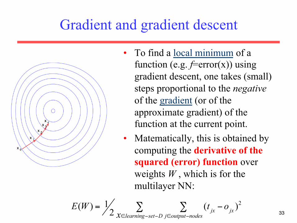
• To find a local minimum of a function (e.g. f=error(x)) using gradient descent, one takes (small) steps proportional to the negative of the gradient (or of the approximate gradient) of the function at the current point.
• Matematically, this is obtained by computing the derivative of the squared (error) function over weights W , which is for the multilayer NN:
33 E(W ) = 1
2(t jx
j∈output−nodes∑
x∈learning−set−D∑ − ojx )
2
34
Gradient descent need a differentiable threshold function
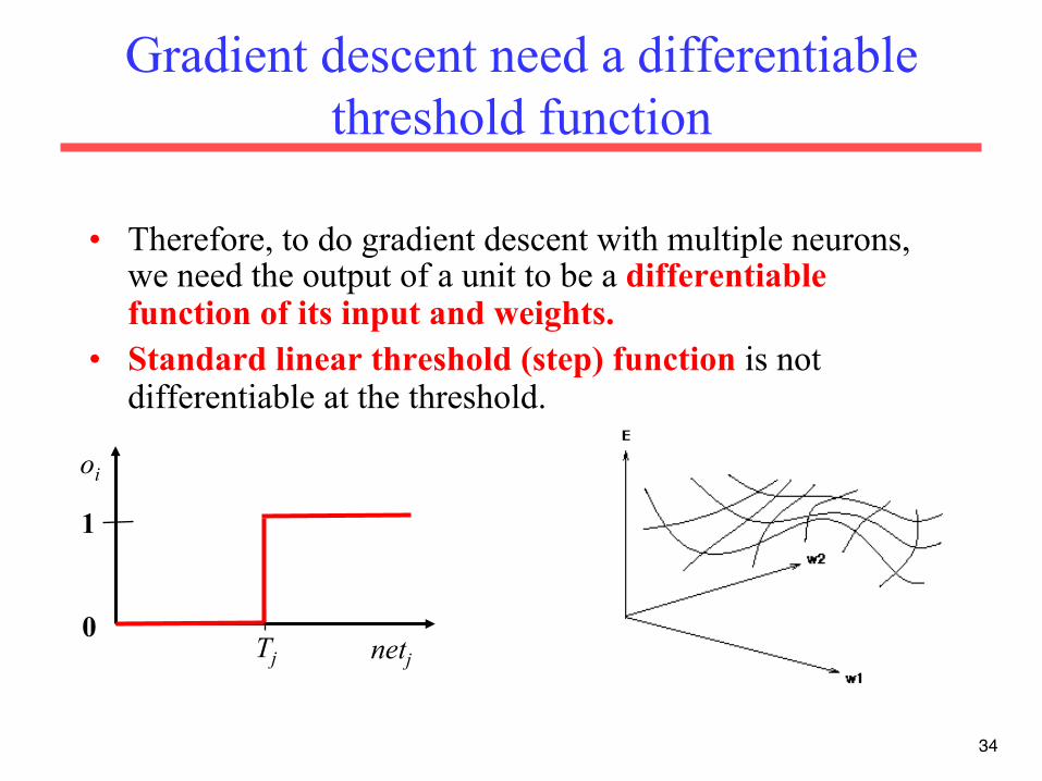
• Therefore, to do gradient descent with multiple neurons, we need the output of a unit to be a differentiable function of its input and weights.
• Standard linear threshold (step) function is not differentiable at the threshold.
netj
oi
Tj 0
1
35
Differentiable Output Function
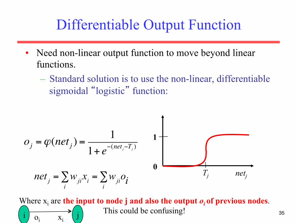
• Need non-linear output function to move beyond linear functions. – Standard solution is to use the non-linear, differentiable
sigmoidal “logistic” function:
netj Tj 0
1 oj =ϕ(net j ) =1
1+ e−(net j−Tj )
net j = wjii∑ xi = wji
i∑ oi
Where xi are the input to node j and also the output oi of previous nodes. This could be confusing! i j oi xi

36
Structure of a node in NNs
Thresholding function limits node output (Tj=0 in the example):
threshold
oj =ϕ(net j ) =1
1+ e−(net j−Tj )
oj

37
Feeding data through the net
netj= (1 × 0.25) + (0.5 × (-1.5)) = 0.25 + (-0.75) = - 0.5
11+ e0.5
= 0.3775Thresholding (with T=0):
wij 0.3775
x:<x1,x2>=<1,0.5>
38
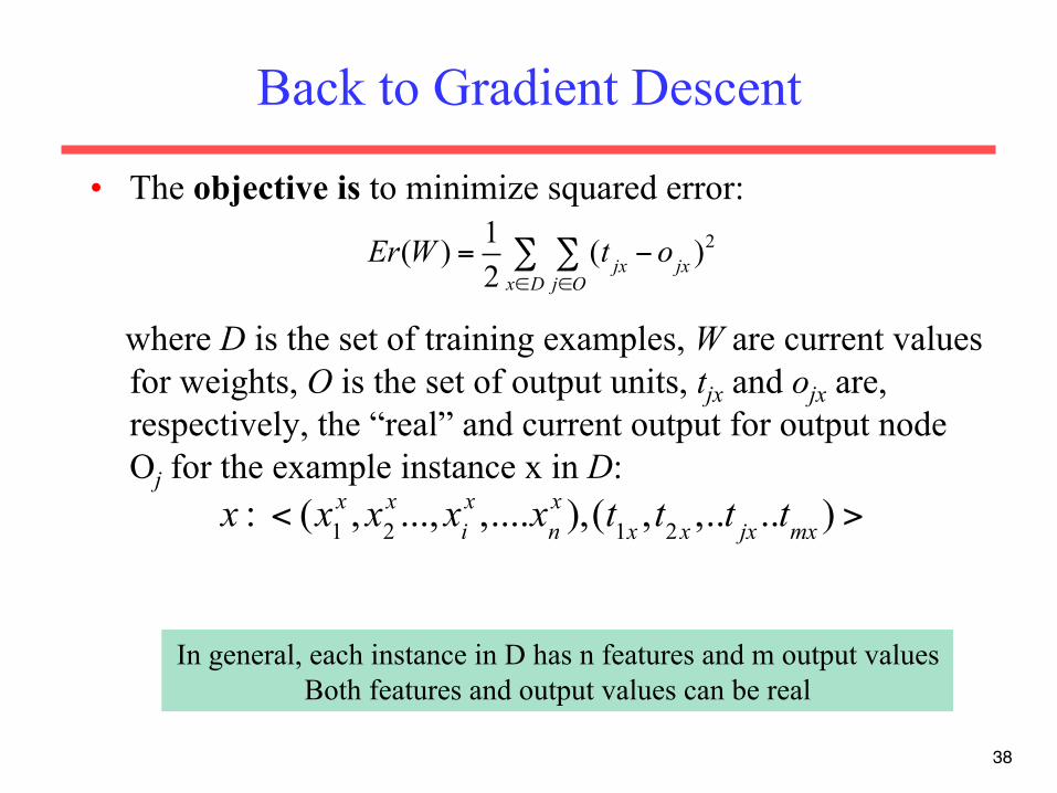
Back to Gradient Descent
• The objective is to minimize squared error:
where D is the set of training examples, W are current values for weights, O is the set of output units, tjx and ojx are, respectively, the “real” and current output for output node Oj for the example instance x in D:
Er(W ) = 12
(t jxj∈O∑
x∈D∑ − ojx )
2
x : < (x1x ,x2
x ...,xix ,....xn
x ),(t1x ,t2x ,..t jx ..tmx ) >
In general, each instance in D has n features and m output values Both features and output values can be real

Example (1 output)
39
Input instance X<(1.0,1.0),0.50>; Error(W)=1/2(0.73-0.50)2=0.0529/2

Weight update rule (hill climbing)
• Learning rule to change weights to minimize error at each iteration t is:
• Weights are updated proportionally to the
derivative of the error (move in the opposite direction of error gradient)
40
wtji −wt−1ji = Δwji = −η
∂Er∂wji
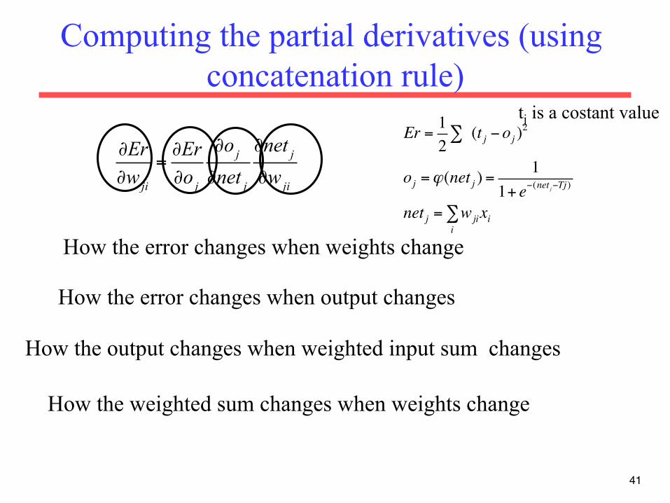
Computing the partial derivatives (using concatenation rule)
∂Er∂wji
=∂Er∂oj
∂oj∂net j
∂net j∂wji
41
How the error changes when weights change
How the error changes when output changes
How the output changes when weighted input sum changes
How the weighted sum changes when weights change
Er = 12∑ (t j − oj )
2
oj =ϕ(net j ) =1
1+ e−(net j−Tj )
net j = wjii∑ xi
tj is a costant value
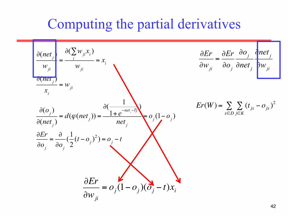
Computing the partial derivatives
42
∂(net j )wji
=∂( wjixi )
i∑
wji= xi
∂(net j )xi
= wji
∂(oj )∂(net j )
= d(ϕ(net j )) =∂( 11+ e−net j−Tj
)
net j= oj (1− oj )
∂Er∂oj
=∂∂oj(12(t − oj )
2 ) = oj − t
∂Er∂wji
= oj (1− oj )(oj − t)xi
∂Er∂wji
=∂Er∂oj
∂oj∂net j
∂net j∂wji
Er(W ) = (t jxj∈K∑
x∈D∑ − ojx )
2
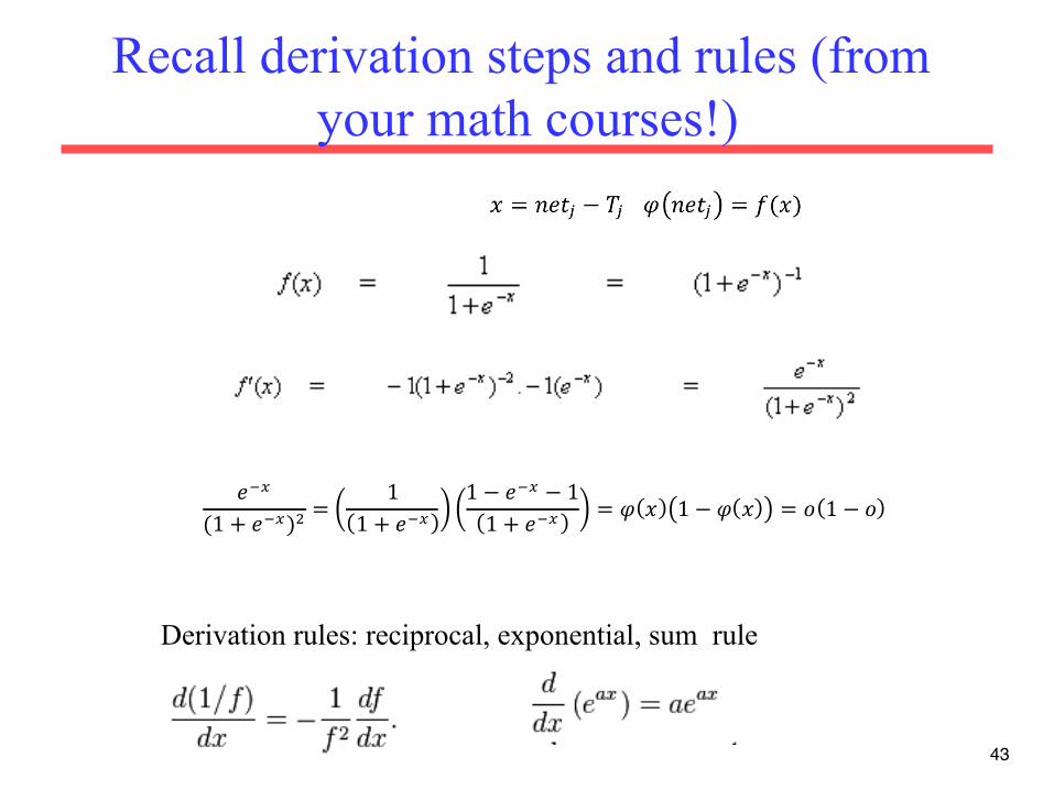
Recall derivation steps and rules (from your math courses!)
43
!!!(1+ !!!)! =
11+ !!!
1− !!! − 11+ !!! = ! ! 1− ! ! = ! 1− !
Derivation rules: reciprocal, exponential, sum rule

Summary so far
• Objective: learn oj=f(wji, x) j=1…m output functions, where x:<x1..xn> are the input instances (represented by n features) and are the wi,jweights on network edges. Target is to learn the (initially unknown) wji
• General idea: start with random values for wji and then use gradient descent and “known” output values in learning set to iteratively update the values wji, until error (difference between “true” and “computed” output values) is below a thershold or does not decrease
• We know introduce the complete algorithm, named Backpropagation
44

45
Backpropagation Learning Rule
• Each weight changed by:
where η is a constant called the learning rate tj is the correct output for unit j (as in learning set) δj is the derivative of error for unit j (see previous
slide)
Δwji =ηδ j xi =ηδ joi
δ j = oj (1− oj )(t j − oj ) if j is an output unit
δ j = oj (1− oj ) δkwkjk∑ if j is a hidden unit
i j oi=xi oj
wji
NOTE as for perceptron that weights wji are updated proportionally to error δj observed on the output of a node j AND
to the intensity of the signal (xi=oi) travelling on edge ji

Error backpropagation in the hidden nodes
46
unithidden a is if )1( jwook
kjkjjj ∑−= δδ
Notice that the error component is (tj-oj) for an output node, while in a hidden node it is the weighted sum of the errors generated by all the output nodes
to which it is connected! (the error BACKPROPAGATES)

Hidden nodes are “responsible” of errors on output nodes for a fraction depending on the weight of their connections to
output nodes
47
δ=0.2
δ=0.4
δH2=oH2(1-oH2)[0.1×0.4+1.17×0.2]
Derivative of error at nodes O1 and O2

Summary
• To learn weights, a hill-climbing approach is used
• Forward step: At each iteration and for each input, we compute the error on output nodes
• Backward step: we then update weights starting from output nodes back to input nodes using gradient descent rule (=updates are proportional to the derivative δ of the error)
48
49
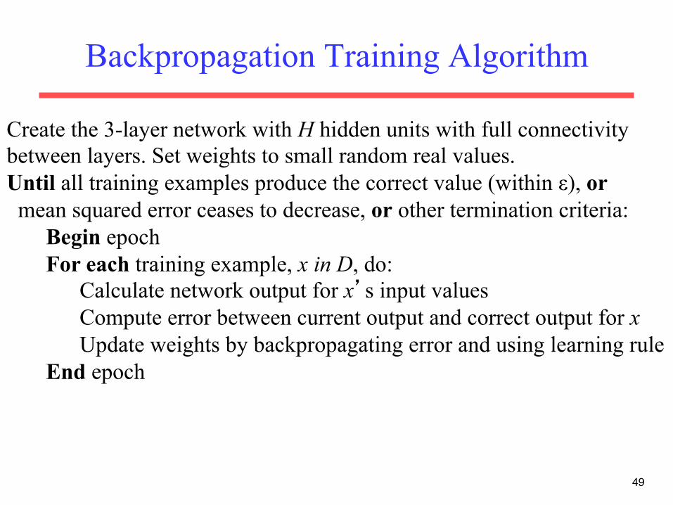
Backpropagation Training Algorithm
Create the 3-layer network with H hidden units with full connectivity between layers. Set weights to small random real values. Until all training examples produce the correct value (within ε), or mean squared error ceases to decrease, or other termination criteria: Begin epoch For each training example, x in D, do: Calculate network output for x’s input values Compute error between current output and correct output for x Update weights by backpropagating error and using learning rule End epoch

Example
oj =ϕ(x j1wj1 + x j2wj2) =ϕ(oh1wj1 + oh2wj2)oh1 =ϕ(xn1wn1h1
+ xn2wn2h1+....+ xnNwnNh1
)oh2 =ϕ(xn1wn1h2
+ xn2wn2h2+....+ xnNwnNh2
)
xn1 = on1 =ϕ(x11)....... xnN = onN =ϕ(x1N )Oj
h2 h1
oj
wj1 wj2
n1 nj nn
……. ….. …... Step 1: feed with first example x1
and compute output on all nodes with Initial (random) weights
x1: x11 x12…x1n
Oj one of the O output nodes hk the hidden nodes nj the input nodes
NOTE : inputsuccessor node = outputantecedent node

Example (cont’d)
oj
Ojout
h1hidden
h2hidden
wj1 wj2
……. ….. …...
n1in
nnin
δ j = oj (1− oj )(t1 − oj )δh1 = x j1(1− x j1)wj1δ j =
oh1(1− oh1)wj1δ jδh2 = oh2(1− oh2 )wj2δ j
Compute the error on the output node, and backpropagate computation on hidden nodes

Example (cont’d) oj
Ojout
h1hidden h2
hidden
wj1 wj2
……. ….. …...
n1in
nnin
wh1n1 wh2n1
δ(n1in ) = o1
in (1−o1in )(wh1n1δh1 +wh2n1δh2 )
......δ(nN
in ) = oNin (1−oN
in )(wh1nNδh1 +wh2nN
δh2 )
…and on input nodes

Example (cont’d): update weights and iterate
w j1← wj1 + ηδ j xj1
w j2← w j2 + ηδ j x j2wh1n1← wh1n1 + ηδh1x h1n1......
• Update all weights • Consider the second example • Compute input and output in all nodes • Compute errors on outpus and on all nodes • Re-update weights • Until all examples have been considered (Epoch) • Repeat for n Epochs, until convergence
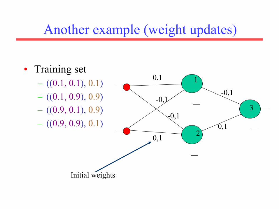
Another example (weight updates)
• Training set – ((0.1, 0.1), 0.1) – ((0.1, 0.9), 0.9) – ((0.9, 0.1), 0.9) – ((0.9, 0.9), 0.1)
0,1
0,1
-0,1
-0,1 -0,1
0,1
1
2
3
Initial weights

1. Compute output and error on output node
First example: ((0.1, 0.1), 0.1)
ϕ(1) =ϕ(w1x1+w2x2) =
11+ e−(w1x1+w2 x2)
€
Err =12(0,1− 0,5)2 = 0,08
€
δ(3) = 0,5(1− 0,5)(0.1− 0,5) = −0,5× 0,5× 0,40 = −0,1
€
δ j = o j (1− o j )(t j − o j )
0,1
0,1
0,1
0,5
0,5
0,5
1
2
3
0,1
-0,1 -0,1
0,1
-0,1
0,1

2. Backpropagate error
€
δh = oh (1− oh ) wkhδknk ∈O∑
δ(1) = 0,5(1− 0,5) 0,1(−0,1)[ ] = −0,025
δ(2) = 0,5(1− 0,5) 0,1(0,1)[ ] = 0,025
0,1
0,1
0,1
0,5
0,5
0,5
1
2
3
-0,1
-0,025
0,025

3. Update weights
€
w31 = −0,1+ 0,2× 0,5× (−0,1) = −0,11w32 = 0,1+ 0,2× 0,5× (−0,1) = 0,09w1i1 = 0,1+ 0,2× 0,1× (0,025) = 0,1005w1i2 = −0,1+ 0,2× 0,1× (0,025) = −0,0995w2i1 = −0,1+ 0,2× 0,1× (−0,025) = −0,1005w2i2 = 0,1+ 0,2× 0,1× (−0,025) = 0,0995
€
wji← wji+ ΔwjiΔw ji =ηδ j x ji
0,1
0,1
0,1
0,5
0,5
0,5
1
2
3
-0,1
-0,025
0,025
0,1
-0,1
-0,1
0,1
-0,1
0,1

Read second input from D
2. ((0,1,0,9), 0,9)
0,1005
0,0995
-0,1005
-0,0995 -0,11
0,09
1
2
3
0,1
0,9
0,9 0,48
0,52
0,501
..etc!!

59
Yet another example
• First calculate error of output units and use this to change the top layer of weights.
output
hidden
input
Current output: oj=0.2 Correct output: tj=1.0 Error δj = oj(1–oj)(tj–oj) 0.2(1–0.2)(1–0.2)=0.128
Update weights into j
ijji ow ηδ=Δ

60
Error Backpropagation
• Next calculate error for hidden units based on errors on the output units it feeds into.
output
hidden
input
∑−=k
kjkjjj woo δδ )1(

61
Error Backpropagation
• Finally update bottom layer of weights based on errors calculated for hidden units.
output
hidden
input
∑−=k
kjkjjj woo δδ )1(
Update weights into j
ijji ow ηδ=Δ

Example: Voice Recognition
• Task: Learn to discriminate between two different voices saying “Hello”
• Data – Sources
• Steve Simpson • David Raubenheimer
– Format • Frequency distribution (60 bins)

• Network architecture – Feed forward network
• 60 input (one for each frequency bin) • 6 hidden • 2 output (0-1 for “Steve”, 1-0 for “David”)

• Presenting the data Steve
David
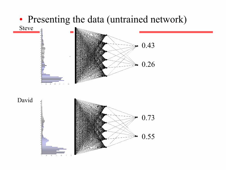
• Presenting the data (untrained network) Steve
David
0.43
0.26
0.73
0.55

• Calculate error Steve
David
0.43 – 0 = 0.43
0.26 –1 = 0.74
0.73 – 1 = 0.27
0.55 – 0 = 0.55

• Backprop error and adjust weights Steve
David
0.43 – 0 = 0.43
0.26 – 1 = 0.74
0.73 – 1 = 0.27
0.55 – 0 = 0.55
1.17
0.82

• Repeat process (sweep) for all training pairs – Present data – Calculate error – Backpropagate error – Adjust weights
• Repeat process multiple times

• Presenting the data (trained network) Steve
David
0.01
0.99
0.99
0.01
70
Comments on Training Algorithm
• Not guaranteed to converge to zero training error, may converge to local optima or oscillate indefinitely.
• However, in practice, does converge to low error for many large networks on real data.
• Many epochs (thousands) may be required, hours or days of training for large networks.
• To avoid local-minima problems, run several trials starting with different random weights (random restarts). – Take results of trial with lowest training set error. – Build a committee of results from multiple trials
(possibly weighting votes by training set accuracy).

71
Representational Power
• Boolean functions: Any boolean function can be represented by a two-layer network with sufficient hidden units.
• Continuous functions: Any bounded continuous function can be approximated with arbitrarily small error by a two-layer network. – Sigmoid functions can act as a set of basis functions for
composing more complex functions, like sine waves in Fourier analysis.
• Arbitrary function: Any function can be approximated to arbitrary accuracy by a three-layer network.
72
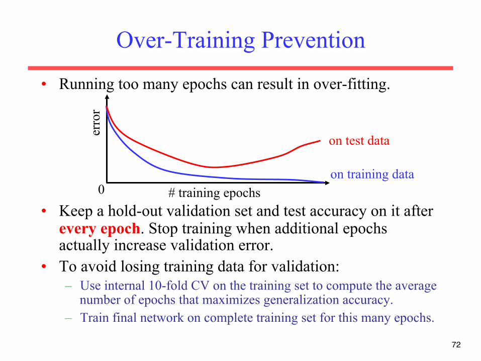
Over-Training Prevention
• Running too many epochs can result in over-fitting.
• Keep a hold-out validation set and test accuracy on it after every epoch. Stop training when additional epochs actually increase validation error.
• To avoid losing training data for validation: – Use internal 10-fold CV on the training set to compute the average
number of epochs that maximizes generalization accuracy. – Train final network on complete training set for this many epochs.
erro
r
on training data
on test data
0 # training epochs

73
Determining the Best Number of Hidden Units
• Too few hidden units prevents the network from adequately fitting the data.
• Too many hidden units can result in over-fitting.
• Use internal cross-validation to empirically determine an optimal number of hidden units.
erro
r
on training data
on test data
0 # hidden units
74
Successful Applications
• Text to Speech (NetTalk) • Fraud detection • Financial Applications
– HNC (eventually bought by Fair Isaac) • Chemical Plant Control
– Pavillion Technologies • Automated Vehicles • Game Playing
– Neurogammon • Handwriting recognition

Deep Learning
a.k.o. Neural Network
Shortcomings of Neural networks with backpropagation
• Based on iterative weight-learning • NN work by making thousands and thousands of tiny
adjustments to edge weights, each making the network do better at the most recent pattern, but perhaps a little worse on many others
• Gets stuck in local minima, especially since it starts with random initialization
• It needs labelled data (it is a trained method) but in many important problems (especially speech recognition, image understanding) data are unlabeled
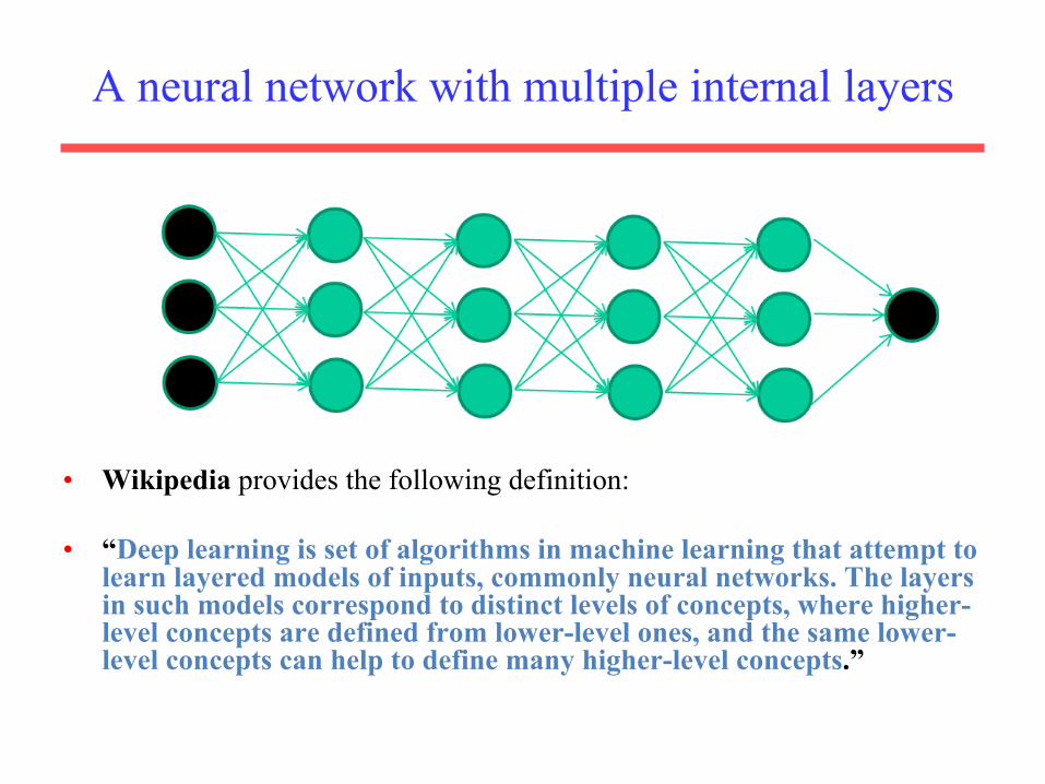
A neural network with multiple internal layers
• Wikipedia provides the following definition:
• “Deep learning is set of algorithms in machine learning that attempt to learn layered models of inputs, commonly neural networks. The layers in such models correspond to distinct levels of concepts, where higher-level concepts are defined from lower-level ones, and the same lower-level concepts can help to define many higher-level concepts.”

Multiple layers make sense
Our brain works that way

Multiple layers make sense
Many-layer neural network architectures should be capable of learning the true underlying features and ‘feature logic’, and therefore generalise very
well …

An example: image processing
• Hierarchical learning – Natural progression
from low level to higher level features as seen in many real problems
– Easier to monitor what is being lernt in each level and guide subsequent layers
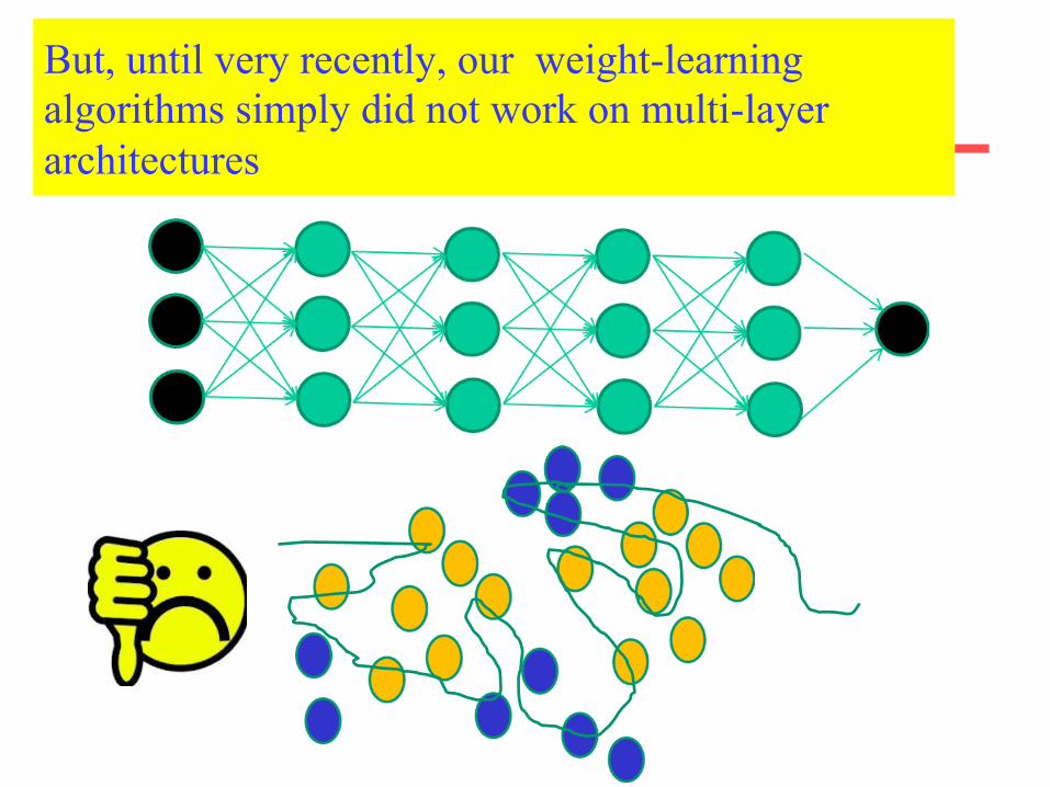
But, until very recently, our weight-learning algorithms simply did not work on multi-layer architectures

Deep Network Training
• Use unsupervised learning (greedy layer-
wise training) • With a small final trained step for fine-
tuning • Allows abstraction to develop naturally
from one layer to another • Help the network initialize with good
parameters
Many Deep Learning algorithms
• We will shortly introduce Stacking Denoising Autoencoders
• They are basically a generalization of Backpropagation, but they allow multiple layers
• More details on: Stacked Denoising Autoencoders: Learning Useful Representations in a Deep Network with a Local Denoising Criterion (Journ. of Machine Learning Research, 2010)
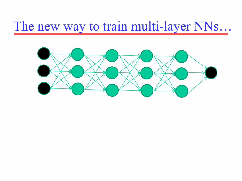
The new way to train multi-layer NNs…

The new way to train multi-layer NNs…
Train this layer first

The new way to train multi-layer NNs…
Train this layer first
then this layer

The new way to train multi-layer NNs…
Train this layer first
then this layer
then this layer

The new way to train multi-layer NNs…
Train this layer first
then this layer
then this layer then this layer

The new way to train multi-layer NNs…
Train this layer first
then this layer
then this layer then this layer
finally this layer
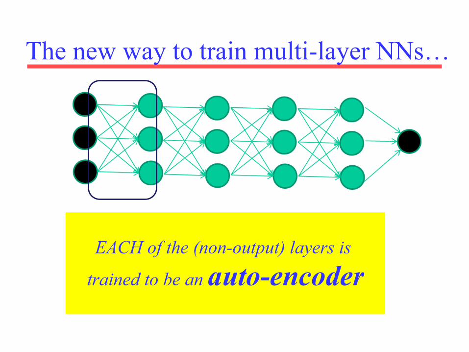
The new way to train multi-layer NNs…
EACH of the (non-output) layers is
trained to be an auto-encoder

Auto-encoders • Encoder: The deterministic (= non stocastic) mapping fθ that
transforms an input vector x into hidden representation y=fθ(x) • θ=(W,b) are the parameters of the encoder • Decoder: The resulting hidden representation y is then mapped back
to a reconstructed d dimensional vector z
• In general z is not to be interpreted as an exact reconstruction of x, but rather in probabilistic terms as the parameters (typically the mean) of a distribution p(X|Z = z) that may generate x with high probability.
• Autoencoder training consists in minimizing the reconstruction error (the difference between x and gθ’(y))
• Intuitively, if a representation allows a good reconstruction of its input, it means that it has retained much of the information that was present in that input (=identifying the relevant features).
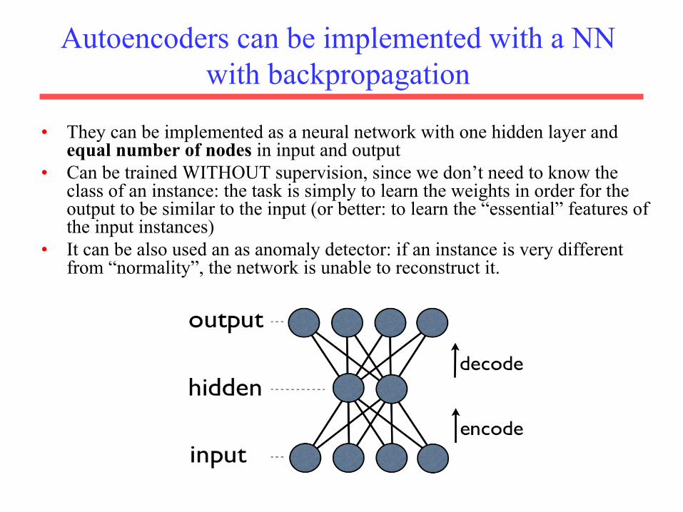
Autoencoders can be implemented with a NN with backpropagation
• They can be implemented as a neural network with one hidden layer and equal number of nodes in input and output
• Can be trained WITHOUT supervision, since we don’t need to know the class of an instance: the task is simply to learn the weights in order for the output to be similar to the input (or better: to learn the “essential” features of the input instances)
• It can be also used an as anomaly detector: if an instance is very different from “normality”, the network is unable to reconstruct it.

Denoising Autoencoders (a better method)
• The reconstruction criterion alone is unable to guarantee the extraction of useful features as it can lead to the obvious solution “simply copy the input”
• Denoising criterion: “a good representation is one that can be obtained robustly from a corrupted input and that will be useful for recovering the corresponding clean input”
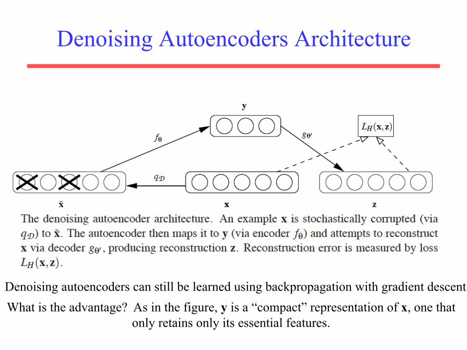
Denoising Autoencoders Architecture
What is the advantage? As in the figure, y is a “compact” representation of x, one that only retains only its essential features.
Denoising autoencoders can still be learned using backpropagation with gradient descent

Stacking Denoising Autoencoder Architecture
• After training a first level denoising autoencoder, its learnt encoding function fθ is used on “clean” input.
• The resulting representation is used to train a second level denoising autoencoder (middle) to learn a second level
encoding function f. • From there, the procedure can be repeated (right).

Intermediate layers are each trained to be auto encoders
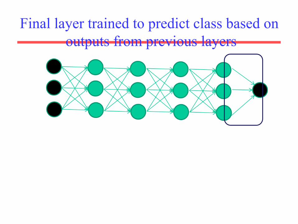
Final layer trained to predict class based on outputs from previous layers

Final layer training is supervised
• After training a stack of encoders as explained in the
previous figure, an output layer is added on top of the stack.
• The parameters of the whole system are fine-tuned to
minimize the error in predicting the supervised target
(e.g., class), by performing gradient descent.
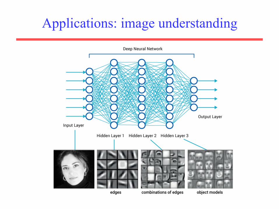
Applications: image understanding
Other applications/systems
• Video, sound, text • DNA • time series (stock markets, economic tables, the
weather) • Relevant players:
– Deep Mind (acquired by Google in 2014) àlearn playing videogames
– Deep Brain (always by Google) (used by photosearch and to build recommenders)
– May be Siri? (Apple’s Speech Interpretation and Recognition Interface)
– Microsoft’s Cortana (Intelligent Assistent)

Conclusion on Deep Learning
• That’s the basic idea • There are many many types of deep
learning, • different kinds of autoencoder, variations on
architectures and training algorithms, etc… • Very fast growing area …