Machine learning methods for vehicle predictive maintenance using off-board and on-board data

Rune Prytz

L I C E N T I A T E T H E S I S | Halmstad University Dissertations no. 9

Machine learning methods for vehicle predictive maintenance using off-board and on-board data© Rune PrytzHalmstad University Dissertations no. 9ISBN: 978-91-87045-18-9 (printed)ISBN 978-91-87045-17-2 (pdf)Publisher: Halmstad University Press, 2014 | www.hh.se/hupPrinter: Media-Tryck, Lund

Abstract

Vehicle uptime is getting increasingly important as the transport solutions becomemore complex and the transport industry seeks new ways of being competitive. Tra-ditional Fleet Management Systems are gradually extended with new features to im-prove reliability, such as better maintenance planning. Typical diagnostic and predic-tive maintenance methods require extensive experimentation and modelling duringdevelopment. This is unfeasible if the complete vehicle is addressed as it would re-quire too much engineering resources.

This thesis investigates unsupervised and supervised methods for predicting ve-hicle maintenance. The methods are data driven and use extensive amounts of data, ei-ther streamed, on-board data or historic and aggregated data from off-board databases.The methods rely on a telematics gateway that enables vehicles to communicate witha back-office system. Data representations, either aggregations or models, are sentwirelessly to an off-board system which analyses the data for deviations. These arelater associated to the repair history and form a knowledge base that can be used topredict upcoming failures on other vehicles that show the same deviations.

The thesis further investigates different ways of doing data representations anddeviation detection. The first one presented, COSMO, is an unsupervised and self-organised approach demonstrated on a fleet of city buses. It automatically comes upwith the most interesting on-board data representations and uses a consensus basedapproach to isolate the deviating vehicle. The second approach outlined is a super-vised classification based on earlier collected and aggregated vehicle statistics inwhich the repair history is used to label the usage statistics. A classifier is trainedto learn patterns in the usage data that precede specific repairs and thus can be used topredict vehicle maintenance. This method is demonstrated for failures of the vehicleair compressor and based on AB Volvo’s database of vehicle usage statistics.

Rune Prytz, Uptime & Aftermarket Solutions,Advanced Technology & Research,Volvo Group Trucks Technology, Box 9508, SE-200 39 Malmö, Sweden.mail: rune.prytz@volvo.com

i

List of attached publications

Paper I R. Prytz, S. Nowaczyk, S. Byttner, "Towards RelationDiscovery for Diagnostics" in KDD4Service ’11: Pro-ceedings of the First International Workshop on DataMining for Service and Maintenance,San Diego, Califor-nia, 2011.

Paper II T. Rögnvaldsson, S. Byttner, R. Prytz, S Nowaczyk,"Wisdom of Crowds for Self-organized Intelligent Moni-toring of Vehicle Fleets", submitted to IEEE Transactionson Knowledge and Data Engineering (TKDE), 2014.

Paper III R. Prytz, S. Nowaczyk, T. Rögnvaldsson, S. Byttner,"Analysis of Truck Compressor Failures Based onLogged Vehicle Data", in In Proceedings of the 9th In-ternational Conference on Data Mining (DMIN’13), LasVegas, NV, USA. July 2013.

Paper IV R. Prytz, S Nowaczyk, T Rögnvaldsson, S Byttner, "Pre-dicting the Need for Vehicle Compressor Repairs UsingMaintenance Records and Logged Vehicle Data" submit-ted to Engineering Applications of Artificial Intelligence,2014.

iii

Contents

1 Introduction 11.1 Background . . . . . . . . . . . . . . . . . . . . . . . . . . . . . . . 2

1.1.1 Maintenance planning . . . . . . . . . . . . . . . . . . . . . 21.1.2 Fault Detection and Isolation (FDI) . . . . . . . . . . . . . . 31.1.3 On-board data acquisition . . . . . . . . . . . . . . . . . . . 31.1.4 Off-board sources . . . . . . . . . . . . . . . . . . . . . . . . 4

1.2 Problem formulation . . . . . . . . . . . . . . . . . . . . . . . . . . 5

2 Predicting maintenance needs in vehicles 72.1 Present business solutions . . . . . . . . . . . . . . . . . . . . . . . . 72.2 State of the art . . . . . . . . . . . . . . . . . . . . . . . . . . . . . . 8

2.2.1 Learning from streams of on-board data . . . . . . . . . . . . 92.2.2 Learning from already collected records of aggregated data . . 102.2.3 Contributions . . . . . . . . . . . . . . . . . . . . . . . . . . 11

3 Methodology 133.1 Learning from historical data . . . . . . . . . . . . . . . . . . . . . . 13

3.1.1 Motivation . . . . . . . . . . . . . . . . . . . . . . . . . . . 133.1.2 Pre-processing of data . . . . . . . . . . . . . . . . . . . . . 143.1.3 Dataset . . . . . . . . . . . . . . . . . . . . . . . . . . . . . 143.1.4 Feature selection . . . . . . . . . . . . . . . . . . . . . . . . 153.1.5 The Filter method . . . . . . . . . . . . . . . . . . . . . . . . 163.1.6 Wrapper based method . . . . . . . . . . . . . . . . . . . . . 163.1.7 Unbalanced datasets . . . . . . . . . . . . . . . . . . . . . . 173.1.8 Classification . . . . . . . . . . . . . . . . . . . . . . . . . . 18

3.2 Learning from real-time data streams . . . . . . . . . . . . . . . . . . 183.2.1 Motivation . . . . . . . . . . . . . . . . . . . . . . . . . . . 183.2.2 The COSMO approach . . . . . . . . . . . . . . . . . . . . . 183.2.3 Reducing the ambient effects in on-board data streams . . . . 19

v

vi CONTENTS

4 Results 214.1 Paper I . . . . . . . . . . . . . . . . . . . . . . . . . . . . . . . . . . 214.2 Paper II . . . . . . . . . . . . . . . . . . . . . . . . . . . . . . . . . 214.3 Paper III . . . . . . . . . . . . . . . . . . . . . . . . . . . . . . . . . 224.4 Paper IV . . . . . . . . . . . . . . . . . . . . . . . . . . . . . . . . . 22

5 Discussion 255.1 Future work . . . . . . . . . . . . . . . . . . . . . . . . . . . . . . . 26

References 29

A Paper I 33

B Paper II 41

C Paper III 57

D Paper IV 65

Chapter 1

Introduction

The European Commission forecasts a 50% increase in transportation over the next20 years. This will lead to a capacity crunch as the infrastructure development willnot match the increase in traffic. It will require high efficient transportation solu-tions to maintain the transport performance of today. Together with the demand forsustainable transport solutions, more complex transport systems will evolve. Suchtransportation systems could be modal change systems for cargo and bus rapid tran-sit systems for public transportation. In these the vehicle is an integrated part of thecomplete transportation chain. High reliability and availability become increasinglyimportant as the transportation systems get more complex and depend on more actors.

High transport efficiency is also important in today’s traffic as haulage is a lowmargin business with a high turnover. Profit can easily turn into loss by unexpectedchanges in external conditions such as fuel prices, economic downturns or vehiclefailures. By continuously monitoring transport efficiency haulage companies can in-crease competitiveness and stay profitable. This is enabled with advanced Intelli-gent Transport System (ITS) solutions, such as Fleet Management Softwares (FMS),which provide efficient haulage management.

Fleet Management Software, such as DECISIV-ASIST [Reimer, 2013a,b] andCirrus-TMS [TMS, 2013] , monitors the utilisation and availability of the fleet of ve-hicles closely. These software streamline the day to day operation by offering ser-vices like route and driver planning, maintenance planning and invoice handling.This reduces waiting time at cargo bays, workshops and border crossings as the pa-perwork is automated. Thus the utilisation increases with smarter routes, increasingback-haulage and higher average speed due to less waiting time.

Vehicle reliability and thus availability, or uptime, is increasingly important tohaulers as FMS systems become more widespread. Reliability is the next area of im-provement and the demand for less unplanned stops is driven by the fierce competitionin haulage as most of the other parts of their business already is optimised. Reliabilityis partly controllable through vehicle quality and partly by preventive maintenanceactions and driver training. Preventive maintenance reduces the risk of unplannedstops, while it may increase the spending on maintenance. Other ways of handling

1

2 CHAPTER 1. INTRODUCTION

the risk of unplanned stops are by insurances and spare transport capacity, e.g. havingredundant vehicles.

A vehicle lease program with a corresponding service contract is another way ofhandling the risk of unplanned stops. Relationship based business models, such as alease program or service contract, give haulers more stability as their vehicle expenseis predictable. Vehicle uptime is likely to improve as the maintenance responsibilityis either shared with, or completely moved to, the vehicle manufactures. They benefitfrom vehicle expert knowledge and the experience of previous failures and mainte-nance strategies from other customers. This information levers manufactures aboveeven the largest hauler when it comes to experience and expertise.

Nonetheless, relationship based business models are a huge challenge to the man-ufactures. Traditionally the profit originates from sales of vehicles and spare parts.To put it simple, the more vehicles and parts sold the larger the profit. A relation-ship based business model turns this upside down. The fewer spare parts used, whilemaintaining the uptime throughout the contract time, the larger the profit.

1.1 Background

1.1.1 Maintenance planning

Maintenance can be planned and carried out in different ways. The three commonplanning paradigms are corrective, preventive and predictive maintenance.

Corrective maintenance is done after a failure has occurred and it often causesdowntime. This maintenance policy, or actually lack of policy, is common for infre-quent failures or where the repair is very expensive. Corrective maintenance is alsocommon practice in case the system has redundancy, e.g. for hard drive arrays inservers where a failing, redundant hard drive causes no downtime or loss of data.

Preventive maintenance is the common practise in the automotive industry, wherevehicle components are replaced or overhauled periodically. It is a crude policy whichenforces maintenance actions at a given vehicle age regardless of vehicle status. Somevehicles will get repairs in time while others fail prior to the scheduled repair date.

The maintenance periodicity is linked to the projected vehicle age and it is decideda priori. Common ways of estimating vehicle age is by calendar time, mileage or totalamount of consumed fuel. The latter is used to individually adjust the maintenanceinterval of passenger cars based on usage and driving style.

Predictive maintenance employs monitoring and prediction modelling to deter-mine the condition of the machine and to predict what is likely to fail and whenit is going to happen. In contrast to the individually adjusted maintenance interval,where the same maintenance is conducted but shifted backwards or forward in timeor mileage, this approach also determines what shall be repaired or maintained.

Predictive maintenance is related to on-board diagnostics featuring fault detec-tion and root cause isolation. Predictive maintenance takes this one step further bypredicting future failures instead of diagnosing already existing.

1.1. BACKGROUND 3

A vehicle, or machine, is often subject to several maintenance strategies. Differ-ent subsystems can be maintained according to different plans. That is, a vehicle isusually maintained both by preventive (fluids, brake pads, tires) and corrective (lightbulbs, turbo charger, air compressor) strategies.

1.1.2 Fault Detection and Isolation (FDI)

A vehicle is a complex mechatronic systems composed of subsystems such as brakes,engine and gearbox. A typical subsystem consists of sensors, actuators and an elec-tromechanical process which needs to be controlled. The sensors and actuators areconnected to an Electronic Control Unit (ECU) which controls and monitors the pro-cess. It is also connected to an in-vehicle Controller Area Network (CAN) throughwhich the different subsystems and the driver communicate with each other.

A fault detection system detects a change from the normal operation and providesa warning to the operator. The operator assesses the warning by analysing the ex-tracted features provided by the detection system and takes appropriate action. Nodiagnostic statement is made by the system as opposed to a diagnostics system suchas Model Based Diagnostics (MBD). Diagnostic statements are possible to derive an-alytically if the observed deviation is quantifiable and possible to associate with aknown fault, or failure mode. A deviation observed prior to a repair while not seenafter is likely to be indicative of the fault causing the repair.

The physical relationship between the inputs and outputs of the process can bemodelled and the vehicle’s health is assessed by monitoring the signals and com-paring them to a model of a faultless process. This is the basis of Model Based Di-agnostics (MBD), Condition Based Maintenance (CBM) and various fault detectionmethods, to detect and predict upcoming failures. These approaches are known asknowledge based fault detection and diagnosis [Isermann, 2006] methods and theyrequire human expert knowledge to evaluate the observed variables and deduct a di-agnosis.

Traditional FDI systems are implemented on-board the monitored machine, asthey require real-time data streams through which a subsystem can be monitored.Further, failure mode information is required to build failure mode isolation models.Typical sources are heuristic information of prior failures, fault injection experimentsor a simulation of the system under various faulty conditions.

1.1.3 On-board data acquisition

Large scale data acquisition on vehicles (on-board) is difficult as the vehicles areconstantly on the move. Data must be stored on-board for retrieval at a workshopor transmitted through a telematics gateway. As vehicles move across continents andborders, wireless downloads get expensive and hence in practice limited to smallchunks of data. In-vehicle storage of data streams is not yet feasible as they requirehuge amount of storage which still is costly in embedded systems.

4 CHAPTER 1. INTRODUCTION

The development cost aspect of large scale on-board logging solutions is alsoa major reason to why it has not been done before. The logging equipment must bedeveloped, rigorously tested and mass-produced. This does not fit well with the toughcompetition in the transport sector where vehicle manufacturers need to see a cleareconomic benefit for each function included in the vehicle.

The on-board data consists of thousands of signals from the sensors and ECUs,that are communicated through a CAN network. They are sent repeatedly with a spec-ified frequency and form streams of continuous data which are used for vehicle con-trol and status signalling between the different vehicle components.

So far, continuous vehicle on-board logging has been limited to fleets of test-vehicles and with retrofitted logging equipment. These systems are expensive andintended for product development purposes. It is probably safe to assume that anyindustrialized on-board monitoring or predictive maintenance algorithm must be lim-ited to existing hardware with respect to sensors, signals and computational resources.

1.1.4 O�-board sources

Most large corporations, like the Volvo Group, have accumulated large amounts ofdata over the years in off-board databases. The data spans from drawings and testresults to maintenance records and vehicle usage statistics. Structured right, the datacan be transformed into knowledge and prove useful in various application areas. Themaintenance records and usage statistics is of particular interest in this thesis becauseof their direct and indirect association with future vehicle maintenance.

Vehicle statistics

The usage statistics database, named the Logged Vehicle Data database (LVD), is lim-ited to aggregated data. The data is aggregated on-board every Volvo vehicle and iseither transmitted wirelessly through a telematics gateway or downloaded at a work-shop. The update frequency is at best once per month but normally every three andsix months. The frequency is unknown a priori even though vehicles regularly visitworkshops for maintenance.

The LVD database includes aggregated statistics such as mean vehicle speed andaverage fuel consumption, which have been collected during normal operation. Itprovides valuable insights in how usage, market and customer segment affect keyvehicle performance parameters. This is useful input into the development of futurevehicles.

Maintenance records

The Vehicle Maintenance database (VSR) contains records of all maintenance con-ducted at a Volvo authorised workshops. The data is used for quality statistics duringthe warranty period as well as customer invoicing. The entries are structured withstandardised repair codes and part numbers. The root cause is sometimes specified in

1.2. PROBLEM FORMULATION 5

the repair record but, in most cases, must be deducted based on the reported repairactions.

Much of the data in the VSR database are manually entered and often sufferfrom human mistakes such as typos, empty records, or missing root cause. The VSRalso contains systematic errors introduced by the process of entering new data to thedatabase. The date of repair is not the actual date of the repair but rather the date ofthe entry to the database. Further, extensive repairs are reported as consecutive repairsa few days apart. This does not cause any problems in the day to day operation as thepurpose of the system is to link invoices to repairs and give the mechanic an overviewof the history of a vehicle.

Moreover, the records do not always reveal if the problem was solved by theperformed repair. All these problems complicate the process of automatically deter-mining the root cause of a repair and matching it to found deviations in e.g. the LVDdata. Undocumented repairs, e.g. repairs done by unauthorised workshops, are also aproblem as they cause the deviations to disappear without any records of the repair.The number of these repairs is unknown but it is believed that the frequency is in-creasing as the vehicle ages. They introduce uncertainty whether a found pattern canbe linked to a given repair as the support might be low.

The aggregation of data smoothens any sudden change, which further reduces thepossibility of finding statistically valid relations between deviations and upcomingrepairs.

The database is extremely heterogeneous, as model year and vehicle specificationaffect the parameter set logged to the database. Only a small subset of parametersis common among all vehicles. In general terms, newer and more advanced vehiclesprovide more statistics. This makes it hard to find large datasets with a homogeneousset of parameters.

1.2 Problem formulation

The vehicle industry is extensively using manually engineered knowledge based meth-ods for diagnostics and prognostics. These are development resource intense and lim-its the adoption to systems which are expensive, safety critical or under legal obliga-tion of monitoring. The demand for more uptime requires less unplanned maintenancewhich in return drives maintenance predictions. This requires more universal deploy-ment of diagnostics or maintenance predictions as the systems that today are underdiagnostic monitoring only account for a small fraction of all repairs.

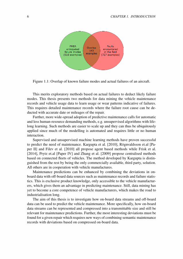
The heuristic information with regard to what failures to expect is hard to comeby. A study, based on Failure Mode Analysis (FMEA) by [Atamer, 2004], comparesanticipated failures on aircrafts to actual faults while in service. The overlap, illus-trated in figure 1.1, is surprisingly low, only about 20%. A 100% overlap means thatall faults are anticipated. This is not ideal as some faults are so severe that they shouldbe completely avoided. Non-critical faults should be anticipated and it is likely thatthey account for more than the 20% overlap that was found in the survey.

6 CHAPTER 1. INTRODUCTION

Figure 1.1: Overlap of known failure modes and actual failures of an aircraft.

This merits exploratory methods based on actual failures to deduct likely failuremodes. This thesis presents two methods for data mining the vehicle maintenancerecords and vehicle usage data to learn usage or wear patterns indicative of failures.This requires detailed maintenance records where the failure root cause can be de-ducted with accurate date or mileages of the repair.

Further, more wide-spread adoption of predictive maintenance calls for automaticand less human-resource demanding methods, e.g. unsupervised algorithms with life-long learning. Such methods are easier to scale up and they can thus be ubiquitouslyapplied since much of the modelling is automated and requires little or no humaninteraction.

Supervised and unsupervised machine learning methods have proven successfulto predict the need of maintenance. Kargupta et al. [2010], Rögnvaldsson et.al [Pa-per II] and Filev et al. [2010] all propose agent based methods while Frisk et al.[2014], Prytz et.al [Paper IV] and Zhang et al. [2009] propose centralised methodsbased on connected fleets of vehicles. The method developed by Kargupta is distin-guished from the rest by being the only commercially available, third party, solution.All others are in cooperation with vehicle manufactures.

Maintenance predictions can be enhanced by combining the deviations in on-board data with off-board data sources such as maintenance records and failure statis-tics. This is exclusive product knowledge, only accessible to the vehicle manufactur-ers, which gives them an advantage in predicting maintenance. Still, data mining hasyet to become a core competence of vehicle manufacturers, which makes the road toindustrialisation long.

The aim of this thesis is to investigate how on-board data streams and off-boarddata can be used to predict the vehicle maintenance. More specifically, how on-boarddata streams can be represented and compressed into a transmittable size and still berelevant for maintenance predictions. Further, the most interesting deviations must befound for a given repair which requires new ways of combining semantic maintenancerecords with deviations based on compressed on-board data.

Chapter 2

Predicting maintenance needs in

vehicles

2.1 Present business solutions

Solutions like remote diagnostics and monitoring are typically combined with pre-dictive maintenance and other services like vehicle positioning and remote road-sideassistance. These are often sold as an integrated part of a lager service offer, such asa FMS system.

Commercial vehicle manufacturers have not yet put any advanced predictive so-lutions on the market. Simpler predictive maintenance solutions exist, where wearand usage of brake pads, clutches and similar wear-out equipment is monitored andprojected into the future. All of these are based on data streams being aggregated on-board and transmitted to back-office system. Mercedes [Daimler, 2014] and MAN[MAN, 2014], among others, offer direct customer solutions for preventive main-tenance recommendations and remote monitoring. Volvo has chosen to incorporatepredictive maintenance as dynamic maintenance plans offered in conjunction withservice contracts.

Volvo [Volvo, 2014] has recently made advances in Remote Diagnostics by pre-dicting the most likely immediate repair given a set of diagnostic trouble codes (DTC).Active DTCs are sent wirelessly over the telematics gateway to a back-office serviceteam which, both manually and automatically, deducts the most probable cause offailure. Further, services like repair, towing and truck rental is offered to the cus-tomer. This is not predictive maintenance as such, as it does not comprehend anyfuture failures. It is still a valuable service which reduces downtime and saves money.

The passenger car industry is surprisingly ahead of the commercial vehicle manu-facturers in predicting maintenance. Commercial vehicles, i.e. trucks, buses and con-struction machines, are designed for business purposes where total cost of ownershipis generally the most important aspect. Passenger cars on the other hand, are designedand marketed to appeal the driver’s feelings for freedom, speed and so on. There areseveral published attempts of offering predictive maintenance solutions. The level of

7

8 CHAPTER 2. PREDICTING MAINTENANCE NEEDS IN VEHICLES

maturity varies from pilot studies to in-service implementations. Volkswagen [Volk-swagen, 2014], BMW [Weiss, 2014] and GM [OnStar, 2014] all have methods topredict future maintenance needs based on telematics solutions and on-board data.VW and BMW offers predictive maintenance as a maintenance solution for an owner,while GM, through the OnStar portal, publishes recommended repairs.

2.2 State of the art

On-board solutions have unrestricted, real-time, access to the data streams. This en-ables fast detection as the detection algorithms are located close to the data source.On-board solutions typically have limited computational and storage capacity sincethe hardware needs to be of automotive grade, e.g. water, shock and EMC resistant,and inexpensive as well. Generally automotive electronics usually lingers two or threegenerations behind the consumer market.

On-board solutions impose challenges in the comparison of relevant referencemodels of normal and faulty conditions as the methods need to be computationallyinexpensive and have a small memory footprint. The off-board methods have largercomputational resources and access to historical data. The data can be clustered andlabelled with failure root cause to form a knowledge base of operating modes linkedto failures and normal conditions. This enables a data driven approach which is moreprecise in fault isolation although slower in fault detection compared to the on-boardmethods.

Moreover, on-board systems have direct access to the data which it can sample asoften as necessary. It enables the detection of small deviations early in the progressof wear or failure. This leads to predictive requirements as the deviation acts as anearly warning of failure. Off-board system require wireless technology to sample theoff-board data. The sample frequency is low and it requires a predictive maintenanceapproach which relies on actual predictions rather than being reactive based on de-viations caused by already existing failures. Reactive actions are likely to be too latewhen the sampling frequency decreases.

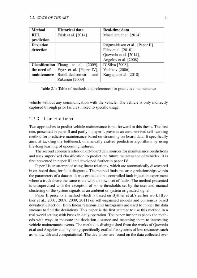
Three approaches can be used to predict vehicle maintenance; Remaining UsefulLife (RUL) prediction, Deviation Detection and supervised classification. They canuse both historical and real-time data as input. Table 2.1 illustrates the approachespresented in related work including the type of input data. Notably, no method isfound which utilises both historical and real-time data, and this leaves room for fur-ther research in this area.

The deviation detection methods are distinguished from the other methods as theydo not give specific information of what is wrong. The failing component is inherentlyknown in the RUL approach as these models are developed for a specific component.The classification approach can both be used to detect deviations and to isolate theactual failing component.

Deviation detection is an easier problem to solve since the uncertainty in linkingdeviations to failures is left out. To make deviation detection methods complete (andcomparable to RUL and Classification methods) they need to be combined with his-

2.2. STATE OF THE ART 9

torical examples of similar deviations linked to known failures. This introduces onemore uncertainty into the complete prediction, which reduces the prediction accuracy.

2.2.1 Learning from streams of on-board data

The research in predictive maintenance and prognostics using on-board data streamsin the automotive industry is small. Only a few different methods have so far beenpresented.

Filev et al. [2010] extends CBM with software agents and implements it on-board.An expert defined feature set is clustered on-board using Gaussian Mixuture Modelsand k Nearest Neighbours (kNN). The clusters are called operation modes (OM) andreflect different driving conditions like idling, driving and reversing. Every new datasample is assigned to an operating mode. New OMs are created as new and uniquefeature vectors are discovered. A health value is assigned to each OM. It is propor-tional to the number of observations assigned to it multiplied by the age of the OM.New OMs with frequent assignments of feature vectors are considered failures. Themethod works without any agent cooperation and thus without any communicationrequirements.

D’Silva [2008] presents an on-board method which assumes pair-wise correla-tions between signals of a complex system that is stationary. The cross correlationmatrix is derived and the Mahalanobis distance is used as metric to find anomalies.The complete correlation matrix is used to define the vehicle status. The normal op-eration space is defined from experimental data. The system works in an on-boardfashion with stored models of the normal operation and it has been demonstrated onsimulated data.

Similarly, Vachkov [2006] and Kargupta et al. [2010] have exploited stationarysignal relationships to find anomalies. Vachkov presents a method in which a neuralgas models is used to represent data relationships. The system comprises of an on-board part which continuously monitors the vehicle and uploads the models to an off-board counterpart. The off-line system includes a database which stores data modelsof faulty and fault free systems. The state of health is determined by an off-boardalgorithm which compares the incoming data models with the stored examples in thedatabase.

Kargupta et al. [2010] monitor the individual correlations between the on-boardsignals. A novel method of calculating the correlation matrix in a fast and efficientway enables deployment in an embedded system with scarce resources. Sudden changesin the correlation matrix are signs of wear or failures. These trigger a set of algorithmsthat collect data, calculate some statistics and transmit the result over a wireless link.The prognostic statement is made off-board.

Mosallam et al. [2014] also propose an unsupervised method that takes trainingdata labelled with RUL as input to an initial step. One RUL model per machine isderived during training and stored in a database as references of degradation patterns.The database is deployed on-board and an algorithm tries to match the degradationof the monitored system to one of the references systems stored in the database. A

10 CHAPTER 2. PREDICTING MAINTENANCE NEEDS IN VEHICLES

Bayesian approach is used to calculate the most likely RUL by looking at the similar-ities to the reference models.

Quevedo et al. [2014] propose a method for fault diagnosis where the deviationdetection is made in the model space. Quevedo et.al focuses on echo state networks(ESN) and proposes a model distance measure which is not based on the model pa-rameters, but rather on characteristics of the model. It makes the distance invariantto the parametrisation resulting in a more stable result. The approach is much likeRögnvaldsson et.al’s approach [Paper II], although he either use the model parameterspace or model space as the space for learning and does not use ESNs. Quevedo et.alfurther proposes an ensemble of one-class classifiers for learning the fault modes.

Angelov et al. [2008] present an approach to design a self-developing and self-tuning inferential soft-sensor. It is a similar research topic which shares the problemof finding a model automatically, without deeper knowledge of the underlying processstructure. His method automatically learns new operating modes and trains a separatelinear model. The operating modes are learned using a fuzzy rule set and the linearmodels are identified using weighted recursive least square (wRLS). A new fuzzy setis added each time the estimation residual suddenly increases. Fuzzy sets that havenot been used fome some time are removed to keep the number of sets low. Thismethod share the same underlying principle of Filev et al. [2010]’ Operating Modesbut differs with respect to model structure and application.

2.2.2 Learning from already collected records of aggregated data

There is not much research on the topic of using existing data sources for predictingvehicle maintenance and only three methods are known to specifically predict vehiclemaintenance using historical data. The area has a lot in common with the general datamining such as supervised classification, which is not covered here.

Zhang et al. [2009] propose a method in which a small amount of aggregated datais collected from thousands of passenger cars. The data are collected using telematicsand the material is analysed off-board using rules that have been defined by an ex-pert. The method has been demonstrated on real-world data to predict no-start eventscaused by drained starter batteries.

The starter battery is yet again considered by Frisk et al. [2014]. This time Re-maining Useful Life (RUL) is modelled from aggregated data. The main differencefrom Zhang et al. is that they model the full RUL curve instead of assessing if the ve-hicle is likely to start or not. Their dataset has been collected from heavy duty trucksand contains quantitative and qualitative data, in total about 300 variables. Further-more, the data is highly unbalanced or right censored. The important variables arediscovered using the AUC criterion and the Random Survival Forest technique isused to model the RUL.

Buddhakulsomsiri and Zakarian [2009] rely solely on warranty or maintenancerecords. By analysing the records for patterns of sequential repairs they derive simpleIF-THEN rules that capture the relationship between common repairs. This can beused to predict the most likely next repair based on what has already failed on a

2.2. STATE OF THE ART 11

Method Historical data Real-time dataRULprediction

Frisk et al. [2014] Mosallam et al. [2014]

Deviationdetection

Rögnvaldsson et.al , [Paper II]Filev et al. [2010],Quevedo et al. [2014],Angelov et al. [2008]

Classificationthe need ofmaintenance

Zhang et al. [2009],Prytz et al. [Paper IV],Buddhakulsomsiri andZakarian [2009]

D’Silva [2008],Vachkov [2006],Kargupta et al. [2010]

Table 2.1: Table of methods and references for predictive maintenance

vehicle without any communication with the vehicle. The vehicle is only indirectlycaptured through prior failures linked to specific usage.

2.2.3 Contributions

Two approaches to predict vehicle maintenance is put forward in this thesis. The firstone, presented in paper II and partly in paper I, presents an unsupervised self-learningmethod for predictive maintenance based on streaming on-board data. It specificallyaims at tackling the bottleneck of manually crafted predictive algorithms by usinglife-long learning of upcoming failures.

The second approach relies on off-board data sources for maintenance predictionsand uses supervised classification to predict the future maintenance of vehicles. It isfirst presented in paper III and developed further in paper IV.

Paper I is an attempt of using linear relations, which are automatically discoveredin on-board data, for fault diagnosis. The method finds the strong relationships withinthe parameters of a dataset. It was evaluated in a controlled fault injection experimentwhere a truck drove the same route with a known set of faults. The method presentedis unsupervised with the exception of some thresholds set by the user and manualclustering of the system signals as an ambient or system originated signal.

Paper II presents a method which is based on Byttner et al.’s earlier work [Byt-tner et al., 2007, 2008, 2009, 2011] on self-organised models and consensus baseddeviation detection. Both linear relations and histograms are used to model the datastreams to find the deviations. This paper is the first attempt to use this method in areal world setting with buses in daily operation. The paper further expands the meth-ods with ways to measure the deviation distance and matching them to interestingvehicle maintenance events. The method is distinguished from the works of Quevedoet.al and Angelov et.al by being specifically crafted for systems of low resources suchas bandwidth and computational. The deviations are found on the data collected over

12 CHAPTER 2. PREDICTING MAINTENANCE NEEDS IN VEHICLES

a week or day while the methods proposed by Quevedo and Angelov monitor thesystems more closely.

Paper III is an early attempt of using supervised classification to predict vehi-cle maintenance. Large databases of historical data are mined to find patterns andmatch them to subsequent repairs. The method uses already existing data which wereand still are collected for other purposes. This makes the method interesting as theeconomical thresholds of implementation are low, but technical problems with dataquality arise.

Paper IV develops the ideas of paper III and takes it all the way from raw data tomaintenance prediction. The concept of paper III is extended with feature selection,methods to handle unbalanced datasets and ways to properly train and test data. Themethod is complete in the sense that it makes predictions of repairs and not just devia-tion detection. Moreover, paper IV makes the process of finding the predictive modelsautomatic and without any human in the loop which is in contrast to Zhang’s expertrules. Further, the method uses both usage and warranty history whereas Buddhakul-somsiri and Zakarian [2009] only rely on warranty data. This makes the predictionmethod in paper IV susceptible to usage differences and not only to prior repairs.

Chapter 3

Methodology

3.1 Learning from historical data

3.1.1 Motivation

This method is an approach based on supervised classification and historical, off-board, sources of data. These data sources already exist and are cheap to explore as noinvestments are needed for data collection, IT-infrastructure or in-vehicle hardware.The quality of the data limits the precision in predictions and the results shall bejudged considering the implementation costs and speed of deployment.

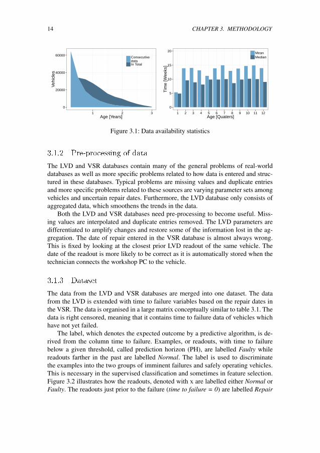
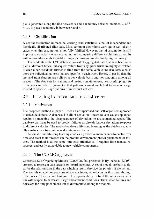
This off-board data has a very low and irregular update frequency. Figure 3.1 il-lustrates the update frequency (right panel) and how the amount of data varies withthe vehicle age. A lot of repair data are missing from older vehicles. This is unfortu-nate since it would have been very useful.

The historical data enables ubiquitous implementation of predictive maintenancein vehicles while still being cost effective as the data is already available. Further,doing classification instead of predicting RUL is likely to require less data as no con-tinuous and monotonically decreasing life-time prediction is necessary. Instead, theclassification approach can be seen as an advanced threshold which, when crossed,triggers a repair instruction. The threshold can be dynamic and vary with input con-ditions such as vehicle usage.

RUL models are desirable if the predictions are accurate and with a low spread.Otherwise, a wide safety margin must taken into account which leads to shorter actualpredicted life. A classification approach can then be beneficial as it can make betterbinary decisions on the same data. This results in lower safety margins and moreaccurate actual predictions.

As mentioned earlier, the LVD and VSR databases are combined, pre-processedand data mined for interesting patterns linked to vehicle air compressors. The methodas such is a general supervised approach with some domain specific features andeasily extended to cover other components.

13

14 CHAPTER 3. METHODOLOGY

0

20000

40000

60000

1 2 3Age [Years]

Veh

icle

sConsecutivedataIn Total

0

5

10

15

20

1 2 3 4 5 6 7 8 9 10 11 12Age [Quaters]

Tim

e [W

eeks

]

MeanMedian

Figure 3.1: Data availability statistics

3.1.2 Pre-processing of data

The LVD and VSR databases contain many of the general problems of real-worlddatabases as well as more specific problems related to how data is entered and struc-tured in these databases. Typical problems are missing values and duplicate entriesand more specific problems related to these sources are varying parameter sets amongvehicles and uncertain repair dates. Furthermore, the LVD database only consists ofaggregated data, which smoothens the trends in the data.

Both the LVD and VSR databases need pre-processing to become useful. Miss-ing values are interpolated and duplicate entries removed. The LVD parameters aredifferentiated to amplify changes and restore some of the information lost in the ag-gregation. The date of repair entered in the VSR database is almost always wrong.This is fixed by looking at the closest prior LVD readout of the same vehicle. Thedate of the readout is more likely to be correct as it is automatically stored when thetechnician connects the workshop PC to the vehicle.

3.1.3 Dataset

The data from the LVD and VSR databases are merged into one dataset. The datafrom the LVD is extended with time to failure variables based on the repair dates inthe VSR. The data is organised in a large matrix conceptually similar to table 3.1. Thedata is right censored, meaning that it contains time to failure data of vehicles whichhave not yet failed.

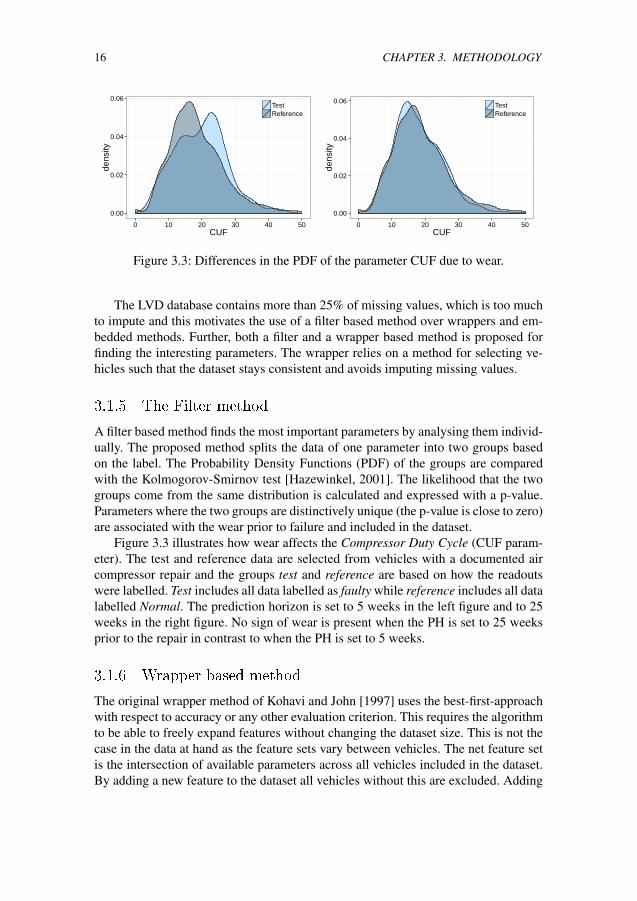
The label, which denotes the expected outcome by a predictive algorithm, is de-rived from the column time to failure. Examples, or readouts, with time to failurebelow a given threshold, called prediction horizon (PH), are labelled Faulty whilereadouts farther in the past are labelled Normal. The label is used to discriminatethe examples into the two groups of imminent failures and safely operating vehicles.This is necessary in the supervised classification and sometimes in feature selection.Figure 3.2 illustrates how the readouts, denoted with x are labelled either Normal orFaulty. The readouts just prior to the failure (time to failure = 0) are labelled Repair

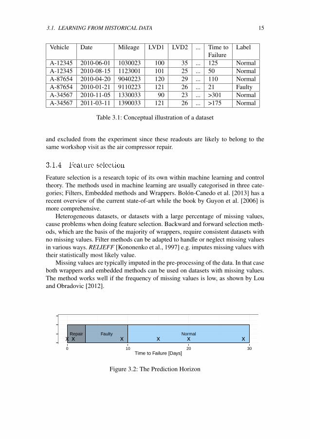
3.1. LEARNING FROM HISTORICAL DATA 15

Vehicle Date Mileage LVD1 LVD2 ... Time toFailure

Label

A-12345 2010-06-01 1030023 100 35 ... 125 NormalA-12345 2010-08-15 1123001 101 25 ... 50 NormalA-87654 2010-04-20 9040223 120 29 ... 110 NormalA-87654 2010-01-21 9110223 121 26 ... 21 FaultyA-34567 2010-11-05 1330033 90 23 ... >301 NormalA-34567 2011-03-11 1390033 121 26 ... >175 Normal

Table 3.1: Conceptual illustration of a dataset

and excluded from the experiment since these readouts are likely to belong to thesame workshop visit as the air compressor repair.

3.1.4 Feature selection

Feature selection is a research topic of its own within machine learning and controltheory. The methods used in machine learning are usually categorised in three cate-gories; Filters, Embedded methods and Wrappers. Bolón-Canedo et al. [2013] has arecent overview of the current state-of-art while the book by Guyon et al. [2006] ismore comprehensive.

Heterogeneous datasets, or datasets with a large percentage of missing values,cause problems when doing feature selection. Backward and forward selection meth-ods, which are the basis of the majority of wrappers, require consistent datasets withno missing values. Filter methods can be adapted to handle or neglect missing valuesin various ways. RELIEFF [Kononenko et al., 1997] e.g. imputes missing values withtheir statistically most likely value.

Missing values are typically imputed in the pre-processing of the data. In that caseboth wrappers and embedded methods can be used on datasets with missing values.The method works well if the frequency of missing values is low, as shown by Louand Obradovic [2012].

Repair Faulty Normalx x x x x x0 10 20 30

Time to Failure [Days]

Figure 3.2: The Prediction Horizon

16 CHAPTER 3. METHODOLOGY

0.00

0.02

0.04

0.06

0 10 20 30 40 50CUF

dens

ityTestReference

0.00

0.02

0.04

0.06

0 10 20 30 40 50CUF

dens

ity

TestReference

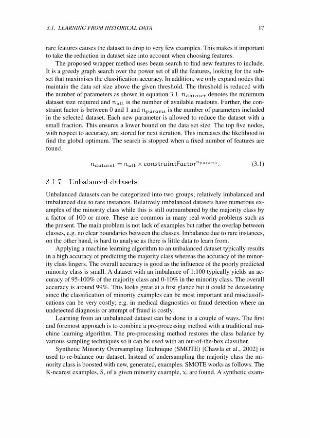
Figure 3.3: Differences in the PDF of the parameter CUF due to wear.

The LVD database contains more than 25% of missing values, which is too muchto impute and this motivates the use of a filter based method over wrappers and em-bedded methods. Further, both a filter and a wrapper based method is proposed forfinding the interesting parameters. The wrapper relies on a method for selecting ve-hicles such that the dataset stays consistent and avoids imputing missing values.

3.1.5 The Filter method

A filter based method finds the most important parameters by analysing them individ-ually. The proposed method splits the data of one parameter into two groups basedon the label. The Probability Density Functions (PDF) of the groups are comparedwith the Kolmogorov-Smirnov test [Hazewinkel, 2001]. The likelihood that the twogroups come from the same distribution is calculated and expressed with a p-value.Parameters where the two groups are distinctively unique (the p-value is close to zero)are associated with the wear prior to failure and included in the dataset.

Figure 3.3 illustrates how wear affects the Compressor Duty Cycle (CUF param-eter). The test and reference data are selected from vehicles with a documented aircompressor repair and the groups test and reference are based on how the readoutswere labelled. Test includes all data labelled as faulty while reference includes all datalabelled Normal. The prediction horizon is set to 5 weeks in the left figure and to 25weeks in the right figure. No sign of wear is present when the PH is set to 25 weeksprior to the repair in contrast to when the PH is set to 5 weeks.

3.1.6 Wrapper based method

The original wrapper method of Kohavi and John [1997] uses the best-first-approachwith respect to accuracy or any other evaluation criterion. This requires the algorithmto be able to freely expand features without changing the dataset size. This is not thecase in the data at hand as the feature sets vary between vehicles. The net feature setis the intersection of available parameters across all vehicles included in the dataset.By adding a new feature to the dataset all vehicles without this are excluded. Adding

3.1. LEARNING FROM HISTORICAL DATA 17

rare features causes the dataset to drop to very few examples. This makes it importantto take the reduction in dataset size into account when choosing features.

The proposed wrapper method uses beam search to find new features to include.It is a greedy graph search over the power set of all the features, looking for the sub-set that maximises the classification accuracy. In addition, we only expand nodes thatmaintain the data set size above the given threshold. The threshold is reduced withthe number of parameters as shown in equation 3.1. ndataset denotes the minimumdataset size required and nall is the number of available readouts. Further, the con-straint factor is between 0 and 1 and nparams is the number of parameters includedin the selected dataset. Each new parameter is allowed to reduce the dataset with asmall fraction. This ensures a lower bound on the data set size. The top five nodes,with respect to accuracy, are stored for next iteration. This increases the likelihood tofind the global optimum. The search is stopped when a fixed number of features arefound.

ndataset = nall × constraintFactornparams . (3.1)

3.1.7 Unbalanced datasets

Unbalanced datasets can be categorized into two groups; relatively imbalanced andimbalanced due to rare instances. Relatively imbalanced datasets have numerous ex-amples of the minority class while this is still outnumbered by the majority class bya factor of 100 or more. These are common in many real-world problems such asthe present. The main problem is not lack of examples but rather the overlap betweenclasses, e.g. no clear boundaries between the classes. Imbalance due to rare instances,on the other hand, is hard to analyse as there is little data to learn from.

Applying a machine learning algorithm to an unbalanced dataset typically resultsin a high accuracy of predicting the majority class whereas the accuracy of the minor-ity class lingers. The overall accuracy is good as the influence of the poorly predictedminority class is small. A dataset with an imbalance of 1:100 typically yields an ac-curacy of 95-100% of the majority class and 0-10% in the minority class. The overallaccuracy is around 99%. This looks great at a first glance but it could be devastatingsince the classification of minority examples can be most important and misclassifi-cations can be very costly; e.g. in medical diagnostics or fraud detection where anundetected diagnosis or attempt of fraud is costly.

Learning from an unbalanced dataset can be done in a couple of ways. The firstand foremost approach is to combine a pre-processing method with a traditional ma-chine learning algorithm. The pre-processing method restores the class balance byvarious sampling techniques so it can be used with an out-of-the-box classifier.

Synthetic Minority Oversampling Technique (SMOTE) [Chawla et al., 2002] isused to re-balance our dataset. Instead of undersampling the majority class the mi-nority class is boosted with new, generated, examples. SMOTE works as follows: TheK-nearest examples, S, of a given minority example, x, are found. A synthetic exam-

18 CHAPTER 3. METHODOLOGY

ple is generated along the line between x and a randomly selected member, �x, of S.xnew is placed randomly in between �x and x.

3.1.8 Classi�cation

A central assumption in machine learning (and statistics) is that of independent andidentically distributed (iid) data. Most common algorithms work quite well also incases when this assumption is not fully fulfilled.However, the iid assumption is stillimportant, especially when evaluating and comparing different solutions as resultswith non-iid data tends to yield stronger patterns and misleadingly high accuracy.

The readouts of the LVD database consist of aggregated data that have been sam-pled at different times. Subsequent values from any given truck are highly correlatedto each other. Readouts further in time from the same vehicle are also correlated asthere are individual patterns that are specific to each truck. Hence, to get iid data thetest and train datasets are split on a per vehicle basis and not randomly among allreadouts. The data sets for training and testing contain unique, non-overlapping, setsof vehicles in order to guarantee that patterns learned are linked to wear or usageinstead of specific usage patterns of individual vehicles.

3.2 Learning from real-time data streams

3.2.1 Motivation

The proposed method in paper II uses an unsupervised and self-organised approachto detect deviations. A database is built of deviations known to later cause unplannedrepairs by matching the disappearance of deviations to a documented repair. Thedatabase can later be used to predict failures as already known deviations reappearin different vehicles. The method enables a life-long learning as the database gradu-ally evolves over time and new deviations are learned.

Automatic and life-long learning enables a predictive maintenance to evolve overtime and react to unforeseen (in the product development phase) phenomena or fail-ures. The method is at the same time cost effective as it requires little manual re-sources, and easily expandable to new vehicle components.

3.2.2 The COSMO approach

Consensus Self-Organizing Models (COSMO), first presented in Byttner et al. [2008],are used to represent data streams on-board machines. A set of models are built to de-scribe the relationships in the data which in return describe the physics of the system.The models enable comparisons of the machines, or vehicles in this case, throughdifferences in their parametrisation. This is particularly useful if the vehicles are sim-ilar with respect to hardware, usage and ambient conditions. Then, wear, failures andnoise are the only phenomena left to differentiate among the models.

3.2. LEARNING FROM REAL-TIME DATA STREAMS 19

Further, the concept of COSMO includes a self-discovery of the local model rep-resentations. Each vehicle, or agent on-board the vehicle, is set out to automaticallyand independently of the other members of the fleet find the best data representations.Good models, can identify failures or wear prior to a repair. They have consistent pa-rameters over time, i.e. linear correlations close to 1, far from uniform histograms ordense clusters. A sudden parameter change is then more likely to relate to change ofthe underlying physical dynamic rather than to noise or modelling error.

The model exploration can be distributed on the fleet. Not all vehicles need tofind all interesting models as the number of possible models can be very large. Eachon-board agent is in contact with a back-office system that coordinates the search andcollects the most interesting models found by each vehicle.

Each agent of the fleet uploads the model parameters of the most interesting mod-els to the back-office. A distance measure, operating in the model parameter space,is used to compare and quantify the similarity among the models. Models, and thusvehicles, that are found to be outliers compared to the rest are flagged as deviatingand indicating a potential fault. As the model family determines the parametrisationand thus the distance measure, no distance measure can be decided upon before themodel family is chosen. Ideally, the distance measure supports proper statistical han-dling such that a hypothesis test can be performed.

So far the COSMO method only supports deviation detection. Diagnostic andfault isolation can be achieved by building a back-office database of repairs associatedwith prior observed deviations. This is then used to issue diagnostics statements assoon new and already known deviations are reported to the back-office system.

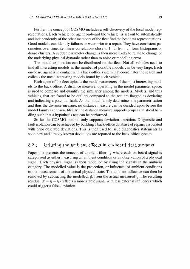
3.2.3 Reducing the ambient e�ects in on-board data streams

Paper one presents the concept of ambient filtering where each on-board signal iscategorised as either measuring an ambient condition or an observation of a physicalsignal. Each physical signal is then modelled by using the signals in the ambientcategory. The modelled value is the projection, or influence, of ambient conditionsto the measurement of the actual physical state. The ambient influence can then beremoved by subtracting the modelled, �y, from the actual measured y. The resultingresidual (r = y− �y) reflects a more stable signal with less external influences whichcould trigger a false deviation.

Chapter 4

Results

4.1 Paper I

Paper I presents the first steps towards an unsupervised method for discovering usefulrelations between measured signals in a Volvo truck, both during normal operationsand when a fault has occurred. The interesting relationships are found in a two-stepprocedure. In the first step all valid models, defined by a MSE threshold, are found.In the second step the model parameters are studies over time to determine which aresignificant.

Moreover, a method for doing ambient filtering is presented. It reduces the influ-ences of the ambient conditions which give more stable (over time) signal relations.The method is evaluated on a dataset from a controlled fault injection experimentwith four different faults. One out of the four faults was clearly found while the oth-ers werer mixed up.

4.2 Paper II

Paper II applies the COSMO algorithm in a real-world setting with 19 buses. Thealgorithm is demonstrated to be useful to detect failures related the to cooling fanand heat load of the engine. Erroneous fan control and coolant leaks were detected atseveral occasions.

Eleven cases of deviations related to the coolant fan gauge were found using his-tograms as on-board models. It means that the coolant fan was controlled in an abnor-mal way. Four occurrences could be linked to fan runaways where the cooling fan isstuck at full speed. This was the result of a failure in the control of the fan, e.g. shortcircuit in the ECU and non-functional cooling fan valve. Further, two occurrencesof coolant leaks where found as well as one jammed cylinder causing higher enginecompartment temperatures that required an extraordinary amount of cooling. Threeoccurrences of deviations were impossible to link to any repair and they were leftunexplained.

The failures discovered with the linear relations were related to the wheel speedssensors. The sensors are crucial for safety critical systems such as Anti-Lock Brake

21

22 CHAPTER 4. RESULTS

Systems and traction control and are thus under supervision of an on-board diagnosticalgorithm. However, the proposed algorithm found the upcoming failures before theexisting on-board algorithms warned. This failure was found on four of the 19 buses.

Moreover, an uptime versus downtime analysis was done on the 19 buses. Theamount of downtime was measured by studying the VSR entries combined with GPSdata. The downtime is defined as time spent in workshop, in transportation to andfrom workshop and in a broken state on the road. It was measured to 11% which,compared to operator’s goal of 5%, is too high. However, much of the downtime isspent waiting at the workshop while the actual wrench time is much less.

4.3 Paper III

Paper III introduces the off-board data sources LVD and VSR and presents earlyresults of predicting air compressor failures. Three different classifiers are evaluatedand both F-score and a cost function is used as evaluation criteria. Moreover the paperdiscusses the problem of the dataset not being iid and classifiers learning individualtruck behaviour in contrast to signs of wear. The paper concludes that using these off-board data sources is viable as input data for predicting vehicle maintenance, albeit itwill require a lot more work.

4.4 Paper IV

Paper IV introduces the presented off-board method that uses supervised machinelearning to find patterns of wear. The method is evaluated on the air compressorof a Volvo FH13 vehicles. The method evaluates a vehicle just prior to an alreadyscheduled workshop visit. The vehicle is flagged as Faulty in case the vehicle’s aircompressor is predicted to fail before the next planned workshop visit. This results inan extra air compressor check-up at the upcoming workshop visit.

The approach was evaluated using a cost function to determine the benefit ofimplementing this as a predictive maintenance algorithm. The cost function considersthe costs for the vehicle operator associated with an unplanned road-side stop alongwith the cost of replacing the air compressor during a regular workshop visit. Themethod was successful in achieving an economical benefit, albeit at the cost of arather high level of false repair claims.

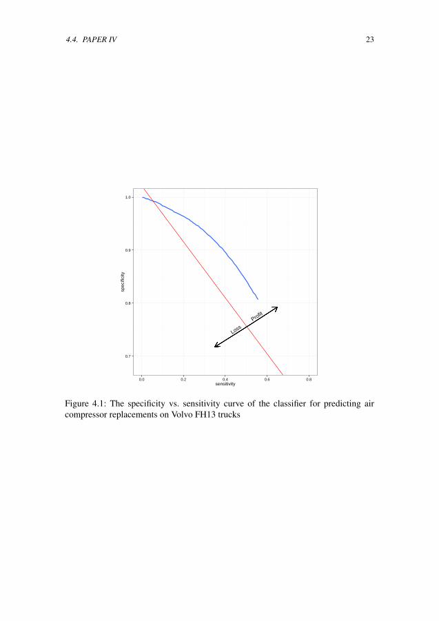
Figure 4.1 illustrates the performance of the classifier based on sensitivity andspecificity. This figure shows the trade-off of making the classifier more sensitiveto detect vehicles with an imminent failure (sensitivity). It casuses the rate of miss-classified normal vehicles (specificity) to increase as well.

The red line indicates the break-even of the business case, according to the costfunction. The approach is beneficial to the vehicle owners as long as the blue line is tothe right of the red. The optimum case is when the classifier is tuned to the sensitivityof 0.4 resulting in 0.9 specificity. This means that 40% of the failing air compressorswere correctly predicted and 10% of the normal readouts where wrongly classified asfailing.

4.4. PAPER IV 23

Profit

Loss

0.7

0.8

0.9

1.0

0.0 0.2 0.4 0.6 0.8sensitivity

spec

ifici

ty

Figure 4.1: The specificity vs. sensitivity curve of the classifier for predicting aircompressor replacements on Volvo FH13 trucks

Chapter 5

Discussion

The COSMO method presented in Paper II can be described as bottom-up where theon-board data source defines how the data is compressed, compared and transmitted.This is a deviation detection focused approach designed to find deviations and laterassociate them with a diagnosis or repair. The approach is buttom-up as it takes offfrom the source of the problem and then links the deviation to a likely repair.

All deviations are interesting since they give a clue of what could be wrong.However, to make an automatic repair recommendation algorithm deviations mustbe linked to repairs. A repair just prior to the disappearance of a deviation is interest-ing since it is likely the repair restored the vehicle status to normal.

The matching of all disappearing deviations and repairs is a potential large work.Deviations seen for the first time are linked to whatever repair just prior to it. Whilefinding new occurrences of deviations already known to the systems either confirmsthe already known deviation-repair association rule or introduces ambiguities to whatrepair actually fixed the root cause.

There are several problems and limitations to this approach. Firstly, i case morethan one repair has been conducted the problem of deciding which to merit the devia-tion needs to be addressed. In worst case this leads to miss-assigned deviation causingnoisy labels and lower prediction performance.

Secondly, not all deviations occur due to wear or vehicle failures. The vehiclesproduced constantly change as they are updated to deal with quality issues such as on-board software bugs or hardware issues. Further, suppliers and vehicle manufacturersconstantly introduce changes to reduce vehicle production cost, e.g. replacing sensorswith software estimates and replacing complete components with cheaper alternativesfrom a different supplier.

Thirdly, the method requires time for introduction and evaluation. The targetedvehicle models need to run for years at customers before the knowledge based is largeenough. Accurate statistics and good prediction accuracy is not possible to obtainbefore a statistically significant number of vehicles have failed and been saved by themethod.

25

26 CHAPTER 5. DISCUSSION

Thus, the bottom-up approach enables good deviation detection while the accu-racy of the prediction is limited to the precision of matching deviations to knownrepairs.

The maintenance classification takes off from the maintenance records and is thusa top-down approach in comparison to Paper II . Here deviations are sought and linkedto a specific repair that has already happened.

The LVD data data originates from the same sensors and networks as the approachin paper II, but has been packaged and transmitted differently. The data compressionmethod is not optimised for deviation detection but rather for visualisation or humaninterpretation. This, in combination with the data being sampled in an unknown andchanging interval, reduces the deviation detection capabilities. New parameter up-dates are not sent as new, potentially interesting, deviations are available on-board.Nor is it guaranteed that there exists any deviation in the recorded data just prior to arepair which introduces noise to the prediction labels as well.

The strength in the top-down approach lies in the initial amount of data and thefact that the data originate from customer owned vehicles in daily operation. More-over, the performance is easily obtained prior to full scale implementation, which is avaluable feature in any kind of product development, where new features are imple-mented in the order of their priority.

The clear limitations of this method is the deviation detection. It is limited byhow the data is represented in the database and the low and unknown update sam-pling frequency. The aggregation introduces smoothing effects that removes valuableinformation and the low, and independent, update frequency results in little data ona per vehicle basis. This makes it hard to make individual deviation detection andidentify anything but large and stable trends linked to usage.

Further, the quality of the maintenance records is crucial. Misslabelled repairsand repairs that have not been reported causes noisy class labels and lower accuracy.However, the most important limitation of them all, and this limitation is valid toboth approaches, is if enough parameters which are sensitive to failures are avail-able. One way of handling this is to include more data, both in on- and off-boardsources. Feature selection and distributed methods gets more and more important asthe dimensionality of the data increases.

5.1 Future work

The future work will focus on improving the off-board as industrialisation of the on-board and fleet based COSMO approach is farther away in time due to the requirementof advanced on-board logging equipment. An implementation of the proposed off-board will require higher accuracy and especially higher specificity, thus correctlyclassify normal vehicles as normal. There are several ways to go about this and thefollowing directions will be the future work.

Firstly, ways of combining the on- and off-board approaches will be investigated.The aim is to find a set of specially crafted LVD parameters which is small and yetsensitive to as many faults as possible. The COSMO approach can be introduced

5.1. FUTURE WORK 27

in closely monitored test fleet to learn upcoming failures. A search over differentmodel representations, which fit the limitations of LVD, will be used to optimise thedetection and fault isolation performance.

Further, a deeper analysis of repair information in the VSR will be conducted.The aim is to increase the precision of the repair recommendations taking previousrepairs into account. The idea of combining an IF-THEN rule approach, much likeBuddhakulsomsiri and Zakarian [2009], with the off-board repair recommendationsis intriguing and will be the second topic of my future work.

Lastly, little effort has been made in optimising the off-board classification modeland this needs to be addressed. Further a comparison between different RUL-methodsand classification algorithm will be conducted to conclude which way to go.

References

P. Angelov, A Kordon, and Xiaowei Zhou. Evolving fuzzy inferential sensors forprocess industry. In Genetic and Evolving Systems, 2008. GEFS 2008. 3rd Interna-tional Workshop on, pages 41–46, March 2008. doi: 10.1109/GEFS.2008.4484565.

A Atamer. Comparison of fmea and field-experience for a turbofan engine with ap-plication to case based reasoning. In Aerospace Conference, 2004. Proceedings.2004 IEEE, volume 5, pages 3354–3360 Vol.5, March 2004. doi: 10.1109/AERO.2004.1368142.

Verónica Bolón-Canedo, Noelia Sánchez-Maroño, and Amparo Alonso-Betanzos. Areview of feature selection methods on synthetic data. Knowledge and informationsystems, 34(3):483–519, 2013.

Jirachai Buddhakulsomsiri and Armen Zakarian. Sequential pattern mining algorithmfor automotive warranty data. Computers & Industrial Engineering, 57(1):137–147, 2009. ISSN 0360-8352. doi: 10.1016/j.cie.2008.11.006.

S. Byttner, T. Rögnvaldsson, and M. Svensson. Modeling for vehicle fleet remotediagnostics. Technical paper 2007-01-4154, Society of Automotive Engineers(SAE), 2007.

S. Byttner, T. Rögnvaldsson, and M. Svensson. Self-organized modeling for vehiclefleet based fault detection. Technical paper 2008-01-1297, Society of AutomotiveEngineers (SAE), 2008.

Stefan Byttner, Thorsteinn Rögnvaldsson, Magnus Svensson, George Bitar, andW. Chominsky. Networked vehicles for automated fault detection. In Proceed-ings of IEEE International Symposium on Circuits and Systems, 2009.

Stefan Byttner, Thorsteinn Rögnvaldsson, and Magnus Svensson. Consensus self-organized models for fault detection (COSMO). Engineering Applications of Arti-ficial Intelligence, 24:833–839, 2011.

Nitesh V. Chawla, Kevin W. Bowyer, Lawrence O. Hall, and W. Philip Kegelmeyer.Smote: Synthetic minority over-sampling technique. Journal of Artificial Intelli-gence Research, 16:321–357, 2002.

29

30 REFERENCES

Daimler. Mercedes fleetboard vehicle management. https://www.fleetboard.info/fileadmin/content/international/Brochures/VM.pdf, 2014. Accessed: 2014-08-23.

S. H. D’Silva. Diagnostics based on the statistical correlation of sensors. Technicalpaper 2008-01-0129, Society of Automotive Engineers (SAE), 2008.

Dimitar P. Filev, Ratna Babu Chinnam, Finn Tseng, and Pundarikaksha Baruah. Anindustrial strength novelty detection framework for autonomous equipment moni-toring and diagnostics. IEEE Transactions on Industrial Informatics, 6:767–779,2010.

Erik Frisk, Mattias Krysander, and Emil Larsson. Data-driven lead-acid battery prog-nostics using random survival forest. 2014.

Isabelle Guyon, Steve Gunn, Masoud Nikravesh, and Lotfi A. Zadeh. Feature Ex-traction: Foundations and Applications (Studies in Fuzziness and Soft Computing).Springer-Verlag New York, Inc., Secaucus, NJ, USA, 2006. ISBN 3540354875.

Michiel Hazewinkel, editor. Encyclopedia of Mathematics. Springer, 2001.

Rolf Isermann. Fault-Diagnosis Systems: An Introduction from Fault Detection toFault Tolerance. Springer-Verlag, Heidelberg, 2006.

Hillol Kargupta, Michael Gilligan, Vasundhara Puttagunta, Kakali Sarkar, MartinKlein, Nick Lenzi, and Derek Johnson. MineFleet®: The Vehicle Data StreamMining System for Ubiquitous Environments, volume 6202 of Lecture Notes inComputer Science, pages 235–254. Springer, 2010.

Ron Kohavi and George H. John. Wrappers for feature subset selection. Artificial In-telligence, 97(1âAS2):273 – 324, 1997. ISSN 0004-3702. doi: http://dx.doi.org/10.1016/S0004-3702(97)00043-X. URL http://www.sciencedirect.com/science/article/pii/S000437029700043X. Relevance.

Igor Kononenko, Edvard Šimec, and Marko Robnik-Šikonja. Overcoming the myopiaof inductive learning algorithms with relieff. Applied Intelligence, 1997.

Qiang Lou and Zoran Obradovic, editors. Proceedings of the Twenty-Sixth AAAIConference on Artificial Intelligence, July 22-26, 2012, Toronto, Ontario, Canada,2012. AAAI Press.

MAN. MAN TeleMatics efficient operation. http://www.truck.man.eu/global/en/services-and-parts/efficient-operation/man-telematics/overview/MAN-TeleMatics.html, 2014. Ac-cessed: 2014-08-23.

REFERENCES 31

A. Mosallam, K. Medjaher, and N. Zerhouni. Data-driven prognostic methodbased on bayesian approaches for direct remaining useful life prediction.Journal of Intelligent Manufacturing, pages 1–12, 2014. ISSN 0956-5515.doi: 10.1007/s10845-014-0933-4. URL http://dx.doi.org/10.1007/s10845-014-0933-4.

OnStar. On Star on-star services. https://www.onstar.com, 2014. Accessed:2014-08-23.

J. Quevedo, H. Chen, M. í. Cugueró, P. Tino, V. Puig, D. García, R. Sarrate, andX. Yao. Combining learning in model space fault diagnosis with data valida-tion/reconstruction: Application to the barcelona water network. Eng. Appl. Ar-tif. Intell., 30:18–29, April 2014. ISSN 0952-1976. doi: 10.1016/j.engappai.2014.01.008. URL http://dx.doi.org/10.1016/j.engappai.2014.01.008.

Michael Reimer. Service relationship management – driving uptime in commercialvehicle maintenance and repair. White paper, DECISIV, 2013a.

Michael Reimer. Days out of service: The silent profit-killer – why fleet financialand executive management should care more about service & repair. White paper,DECISIV, 2013b.

Cirrus TMS. Manage your transportation needs from the cloud. Brouchure, Cirrus,2013.

Gancho Vachkov. Intelligent data analysis for performance evaluation and fault diag-nosis in complex systems. In Proceedings of the IEEE International conference onfuzzy systems, July 2006, pages 6322–6329. IEEE Press, 2006.

Volkswagen. Volkswagen on the road to big data with predictive mar-keting in aftermarket. http://www.csc.com/auto/insights/101101-volkswagen_on_the_road_to_big_data_with_predictive_marketing_in_aftermarket, 2014. Accessed: 2014-08-23.

AB Volvo. Remote Diagnostics remote diagnostics : Volvo trucks. http://www.volvotrucks.com/trucks/na/en-us/business_tools/uptime/remote_diagnostics/Pages/Remote_Diagnostics.aspx, 2014.Accessed: 2014-08-23.

Von Harald Weiss. Ingenieur.de predictive mainte-nance: Vorhersagemodelle krempeln die wartung um.http://www.ingenieur.de/Themen/Forschung/Predictive-Maintenance-Vorhersagemodelle-krempeln-Wartung-um,2014. Accessed: 2014-08-23.

32 REFERENCES

Yilu Zhang, Gary W. Gantt Jr., Mark J. Rychlinski, Ryan M. Edwards, John J. Correia,and Calvin E. Wolf. Connected vehicle diagnostics and prognostics, concept, andinitial practice. IEEE Transactions on Reliability, 58:286–294, 2009.

Appendix A

Paper I - Towards Relation

Discovery for Diagnostics

33

Towards Relation Discovery for Diagnostics

Rune PrytzVolvo Technology

Götaverksgatan 10405 08 Gteborg

Rune.Prytz@volvo.com

Sławomir NowaczykHalmstad University

Box 823301 18 Halmstad

Slawomir.Nowaczyk@hh.se

Stefan ByttnerHalmstad University

Box 823301 18 Halmstad

Stefan.Byttner@hh.se

ABSTRACTIt is difficult to implement predictive maintenance in the au-tomotive industry as it looks today, since the sensor capabil-ities and engineering effort available for diagnostic purposesis limited. It is, in practice, impossible to develop diagnos-tic algorithms capable of detecting many different kinds offaults that would be applicable to a wide range of vehicleconfigurations and usage patterns.

However, it is now becoming feasible to obtain and anal-yse on-board data on real vehicles while they are being used.This makes automatic data-mining methods an attractivealternative, since they are capable of adapting themselvesto specific vehicle configurations and usage. In order to beuseful, however, such methods need to be able to automat-ically detect interesting relations between large number ofavailable signal.

This paper presents the first steps towards an unsuper-vised method for discovering useful relations between mea-sured signals in a Volvo truck, both during normal opera-tions and when a fault has occurred. The interesting rela-tionships are found in a two step procedure. In the first stepall valid, defined by MSE threshold, models are found. Inthe second step the model parameters are studies over timeto determine which are significant. We use two different ap-proaches towards estimating model parameters, the LASSOmethod and the recursive least squares filter. The useful-ness of obtained relations is then evaluated using supervisedlearning and classification. The method presented is unsu-pervised with the exception of some thresholds set by theuser and trivial ambient versus system signal clustering.

Categories and Subject DescriptorsI.5.4 [Pattern recognition]: Applications — Signal Pro-cessing

General TermsAlgorithms and Reliability

Permission to make digital or hard copies of all or part of this work forpersonal or classroom use is granted without fee provided that copies arenot made or distributed for profit or commercial advantage and that copiesbear this notice and the full citation on the first page. To copy otherwise, torepublish, to post on servers or to redistribute to lists, requires prior specificpermission and/or a fee.Copyright 20XX ACM X-XXXXX-XX-X/XX/XX ...$10.00.

KeywordsFault detection, Vehicle diagnostics, Machine learning

1. INTRODUCTIONMechatronic systems of today are typically associated with

a high software and system complexity, making it a chal-lenging task to both develop and, especially, maintain thosesystems. For commercial ground vehicle operators (such asbus and truck fleet owners), the maintenance strategy istypically reactive, meaning that a fault is fixed only after ithas occurred. In the vehicle industry it is difficult to movetowards predictive maintenance (i.e. telling that there isa need for maintenance before something breaks down) be-cause of limited budget for on-board sensors and the amountof engineering time it takes to develop algorithms that canhandle several different kinds of faults, but also work in awide range of vehicle configurations and for many differenttypes of operation.

If the current trend of increasing number of components invehicles continues (alongside with increased requirements oncomponent reliability and efficiency), then the only solutionwill be to move towards automated data analysis to copewith increasing costs. At the same time, with the introduc-tion of low-cost wireless communication, it is now possible todo data-mining on-board real vehicles while they are beingused. This paper presents an approach that allows discov-ery of relations between various signals that available onthe internal vehicle network. It is based on the assumptionthat while it is difficult to detect faults by looking at signals(such as road speed) in isolation, the interrelations of con-nected signals are more likely to be indicative of abnormalconditions.

One requirement for our approach is to be able to per-form relation discovery in a fully unsupervised way. This isimportant since, while an engineer may be able to predict alarge number of“good”relations between various signals, herknowledge will in most cases be global, i.e. general enough tohold for all or almost all vehicles. An automated system, onthe other hand, can be more tightly coupled to the specificsof a particular fleet of vehicles — for example, it is likelythat some of the signal relations that hold in Alaska do nothold in Mexico, or that some of the relations that are usefulfor detecting faults in long-haul trucks would be inadequatefor delivery trucks.

This paper is organised as follows. In the following sec-tion we briefly highlight some of the related research ideas.After that, in section 3, we describe the data we have beenworking with. Section 4 presents our approach towards dis-

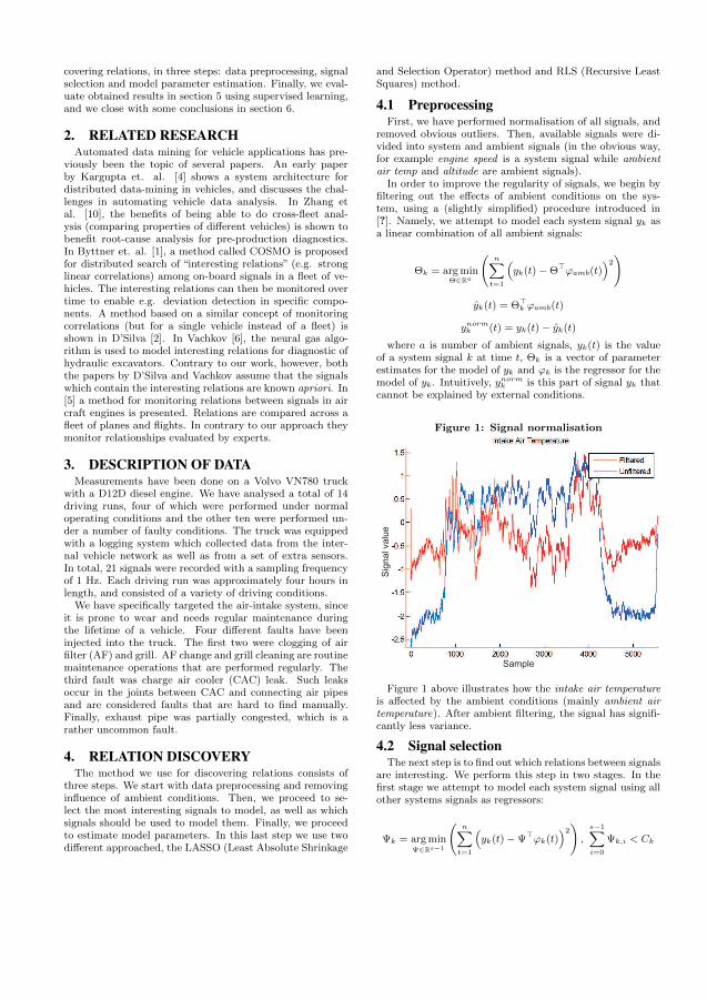
covering relations, in three steps: data preprocessing, signalselection and model parameter estimation. Finally, we eval-uate obtained results in section 5 using supervised learning,and we close with some conclusions in section 6.

2. RELATED RESEARCHAutomated data mining for vehicle applications has pre-

viously been the topic of several papers. An early paperby Kargupta et. al. [4] shows a system architecture fordistributed data-mining in vehicles, and discusses the chal-lenges in automating vehicle data analysis. In Zhang etal. [10], the benefits of being able to do cross-fleet anal-ysis (comparing properties of different vehicles) is shown tobenefit root-cause analysis for pre-production diagnostics.In Byttner et. al. [1], a method called COSMO is proposedfor distributed search of “interesting relations” (e.g. stronglinear correlations) among on-board signals in a fleet of ve-hicles. The interesting relations can then be monitored overtime to enable e.g. deviation detection in specific compo-nents. A method based on a similar concept of monitoringcorrelations (but for a single vehicle instead of a fleet) isshown in D’Silva [2]. In Vachkov [6], the neural gas algo-rithm is used to model interesting relations for diagnostic ofhydraulic excavators. Contrary to our work, however, boththe papers by D’Silva and Vachkov assume that the signalswhich contain the interesting relations are known apriori. In[5] a method for monitoring relations between signals in aircraft engines is presented. Relations are compared across afleet of planes and flights. In contrary to our approach theymonitor relationships evaluated by experts.

3. DESCRIPTION OF DATAMeasurements have been done on a Volvo VN780 truck

with a D12D diesel engine. We have analysed a total of 14driving runs, four of which were performed under normaloperating conditions and the other ten were performed un-der a number of faulty conditions. The truck was equippedwith a logging system which collected data from the inter-nal vehicle network as well as from a set of extra sensors.In total, 21 signals were recorded with a sampling frequencyof 1 Hz. Each driving run was approximately four hours inlength, and consisted of a variety of driving conditions.

We have specifically targeted the air-intake system, sinceit is prone to wear and needs regular maintenance duringthe lifetime of a vehicle. Four different faults have beeninjected into the truck. The first two were clogging of airfilter (AF) and grill. AF change and grill cleaning are routinemaintenance operations that are performed regularly. Thethird fault was charge air cooler (CAC) leak. Such leaksoccur in the joints between CAC and connecting air pipesand are considered faults that are hard to find manually.Finally, exhaust pipe was partially congested, which is arather uncommon fault.

4. RELATION DISCOVERYThe method we use for discovering relations consists of

three steps. We start with data preprocessing and removinginfluence of ambient conditions. Then, we proceed to se-lect the most interesting signals to model, as well as whichsignals should be used to model them. Finally, we proceedto estimate model parameters. In this last step we use twodifferent approached, the LASSO (Least Absolute Shrinkage

and Selection Operator) method and RLS (Recursive LeastSquares) method.

4.1 PreprocessingFirst, we have performed normalisation of all signals, and

removed obvious outliers. Then, available signals were di-vided into system and ambient signals (in the obvious way,for example engine speed is a system signal while ambientair temp and altitude are ambient signals).

In order to improve the regularity of signals, we begin byfiltering out the effects of ambient conditions on the sys-tem, using a (slightly simplified) procedure introduced in[?]. Namely, we attempt to model each system signal yk asa linear combination of all ambient signals:

Θk = arg minΘ∈Ra

(n∑

t=1

(yk(t) − Θ>ϕamb(t)

)2)

yk(t) = Θ>k ϕamb(t)

ynormk (t) = yk(t) − yk(t)

where a is number of ambient signals, yk(t) is the valueof a system signal k at time t, Θk is a vector of parameterestimates for the model of yk and ϕk is the regressor for themodel of yk. Intuitively, ynorm

k is this part of signal yk thatcannot be explained by external conditions.

Figure 1: Signal normalisation

Sample

Sig

na

l va

lue

Figure 1 above illustrates how the intake air temperatureis affected by the ambient conditions (mainly ambient airtemperature). After ambient filtering, the signal has signifi-cantly less variance.

4.2 Signal selectionThe next step is to find out which relations between signals

are interesting. We perform this step in two stages. In thefirst stage we attempt to model each system signal using allother systems signals as regressors:

Ψk = arg minΨ∈Rs−1

(n∑

t=1

(yk(t) − Ψ>ϕk(t)

)2),

s−1∑

i=0

Ψk,i < Ck

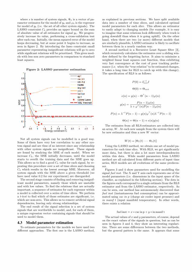
where s is number of system signals, Ψk is a vector of pa-rameter estimates for the model of yk and ϕk is the regressorfor model of yk (i.e. the set of all other system signals). TheLASSO constraint Ck provides an upper bound on the sumof absolute value of all estimates for signal yk. We progres-sively increase its value, performing a cross-validation testafter each run. Initially, the mean squared error of the modelkeeps decreasing, but at some point it begins to increase, asseen in figure 2. By introducing the lasso constraint smallparameter representing insignificant relations will go to zerowhile signficant relations will be prioritized. This gives mod-els with less non zero parameters in comparison to standardleast squares.

Figure 2: LASSO parameter estimation

Energy constraint C

MS

E

Not all system signals can be modelled in a good way.Some of them have very low correlation to any other sys-tem signal and are thus of no interest since any relationshipwith other system signals are insignificant. These signalsare found by studying the MSE of each model. When weincrease Ck, the MSE initially decreases, until the modelstarts to overfit the training data and the MSE goes up.This allows us to find a good Ck value for each signal, by re-peating this procedure over a set of time slices and choosingCk which results in the lowest average MSE. Moreover, allsystem signals with the MSE above a given threshold (wehave used value 0.2 for our experiment) are disregarded.

The second stage consists of finding and removing insignif-icant model parameters, namely those which are unstableand with low values. To find the relations that are actuallyimportant, a sequence of estimates for each regressor withina model is collected over a series of time slices. We performa t-test to find which of those estimates are significant, i.e.which are non-zero. This allows us to remove artificial signaldependencies, leaving only strong relationships.

The end result of the signal selection is a set of systemsignals that are worthwhile to model, and, for each of them,a unique regression vector containing signals that should beused to model them.

4.3 Model parameter estimationTo estimate parameters for the models we have used two

different approaches. The first one is the LASSO method,

as explained in previous sections. We have split availabledata into a number of time slices, and calculated optimalmodel parameters for each slice. This allows an estimatorto easily adapt to changing models (for example, it is easyto imagine that some relations look differently when truck isgoing downhill than when it is going uphill). On the otherhand, when there are two (or more) different models thatare similarly plausible, LASSO estimator is likely to oscillatebetween them in a nearly random way.

A second method is a Recursive Least Square filter [3],which recursively calculates the estimates over a sliding win-dow defined by the forgetting factor. It aims to minimise aweighted linear least squares cost function, thus exhibitingvery fast convergence at the cost of poor tracking perfor-mance (i.e. when the“true relation”to be estimated changes,it takes a long time for RLS to catch up with this change).The specification of RLS is as follows:

P (0) = δ−1initI

Θ(0) = Θinit

e(n) = y(n) − Θ>(n− 1)ϕ(n)

g(n) =P (n− 1)ϕ(n)

λ+ ϕ>(n)P (n− 1)ϕ(n)

P (n) = λ−1P (n− 1) − g(n)ϕ>(n)λ−1P (n− 1)

Θ(n) = Θ(n− 1) + e(n)g(n)

The estimates from all RLS-estimators are collected intoan array, W . At each new sample from the system there willbe new estimates and thus a new W vector:

W (t) = [Θ1(t) · · · Θs(t)]

Using the LASSO method, we obtain one set of model pa-rameters for each time slice. With RLS, we get significantlymore data, but there is also a lot more interdependencieswithin this data. While model parameters from LASSOmethod are all calculated from different parts of input timeseries, RLS models are all evolutions of the same predeces-sor.

Figures 3 and 4 show parameters used for modelling thesignal fuel inst. The X and Y axis each represents one of themodel parameters (i.e. dimensions in the input space of theclassifier, as explained in the following section). The dots inthe figures each correspond to a single estimate from the RLSestimator and from the LASSO estimator, respectively. Ascan be seen, our method has autonomously discovered thatfuel inst (instantaneous fuel consumption) can be approxi-mated using cac in p (charge air cooler input pressure) andin manif t (input manifold temperature). In other words,there exists a relation

fuel inst = x ∗ cac in p + y ∗ in manif t

The actual values of x and y parameters, of course, dependon the exact values of the signals in question, but as can beseen in figures 3 and 4, they show an interesting regulari-ties. There are some differences between the two methods,but the general pattern is the same. It appears that some

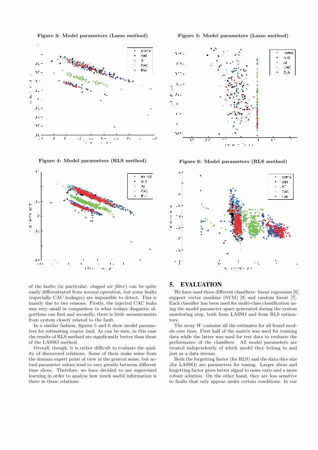
Figure 3: Model parameters (Lasso method)

Figure 4: Model parameters (RLS method)

of the faults (in particular, clogged air filter) can be quiteeasily differentiated from normal operation, but some faults(especially CAC leakages) are impossible to detect. This ismainly due to two reasons. Firstly, the injected CAC leakswas very small in comparison to what todays diagnotic al-gorthms can find and secondly, there is little measurementsfrom system closely related to the fault.

In a similar fashion, figures 5 and 6 show model parame-ters for estimating engine load. As can be seen, in this casethe results of RLS method are significantly better than thoseof the LASSO method.

Overall, though, it is rather difficult to evaluate the qual-ity of discovered relations. Some of them make sense fromthe domain expert point of view in the general sense, but ac-tual parameter values tend to vary greatly between differenttime slices. Therefore, we have decided to use supervisedlearning in order to analyse how much useful information isthere in those relations.

Figure 5: Model parameters (Lasso method)

Figure 6: Model parameters (RLS method)

5. EVALUATIONWe have used three different classifiers: linear regression [8],

support vector machine (SVM) [9] and random forest [7].Each classifier has been used for multi-class classification us-ing the model parameter space generated during the systemmonitoring step, both from LASSO and from RLS estima-tors.

The array W contains all the estimates for all found mod-els over time. First half of the matrix was used for trainingdata while the latter was used for test data to evaluate theperformance of the classifiers. All model parameters aretreated independently of which model they belong to andjust as a data stream.

Both the forgetting factor (for RLS) and the data slice size(for LASSO) are parameters for tuning. Larger slices andforgetting factor gives better signal to noise ratio and a morerobust solution. On the other hand, they are less sensitiveto faults that only appear under certain conditions. In our

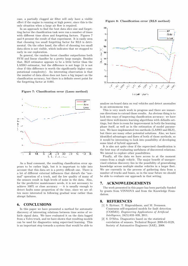
case, a partially clogged air filter will only have a visibleeffect if the engine is running at high power, since this is theonly situation when a large air flow is required.

In an approach to find the best data slice size and forget-ting factor the classification task were run a number of timeswith different time slices and forgetting factors. Figures 7and 8 present the result of that experiment. It is easily seenthat choosing too small forgetting factor for RLS is detri-mental. On the other hand, the effect of choosing too smalldata slices is not visible, which indicates that we stopped toearly in our exploration.

In general, the random forest classifier outperforms bothSVM and linear classifier by a pretty large margin. Besidesthat, RLS estimator appears to be a little better than theLASSO estimator, but the difference is not huge (it is notclear if this difference is worth the significantly higher com-putational complexity). An interesting observation is thatthe number of data slices does not have a big impact on theclassification accuracy, but there is a definite sweet point forthe forgetting factor at 0.001.

Figure 7: Classification error (Lasso method)

As a final comment, the resulting classification error ap-pears to be rather high, but it is important to take intoaccount that this data set is a pretty difficult one. There isa lot of different external influences that disturb the “nor-mal” operation of a truck, and the low quality of many ofthe sensors result in high levels of noise in the data. Also,for the predictive maintenance needs, it is not necessary toachieve 100% or close accuracy — it is usually enough todetect faults some proportion of the time, since we are of-ten more interested in following gradual wear rather thanabrupt failures.

6. CONCLUSIONSIn this paper we have presented a method for automatic

discovery of interesting relations between time series of ve-hicle signal data. We have evaluated it on the data loggedfrom a Volvo truck, and we have shown that resulting modelscan be used for diagnostics using supervised learning. Thisis an important step towards a system that would be able to

Figure 8: Classification error (RLS method)

analyse on-board data on real vehicles and detect anomaliesin an autonomous way.

This is very much work in progress and there are numer-ous directions to extend those results. An obvious thing is tolook into ways of improving classification accuracy: we haveused three well-known learning algorithms with defaults set-tings, but there is room for improvement in both the learningphase itself, as well as in the estimation of model parame-ters. We have implemented two methods (LASSO and RLS),but there are many other potential solutions. Also, we haveidentified advantages and flaws of both of those methods, soit would be interesting to look into possibility of developingsome kind of hybrid approach.

It is also not quite clear if the supervised classification isthe best way of evaluating usefulness of discovered relations.We intend to explore other possibilities.

Finally, all the data we have access to at the momentcomes from a single vehicle. The major benefit of unsuper-vised relation discovery lies in the possibility of generalisingknowledge across multiple similar vehicles in a larger fleet.We are currently in the process of gathering data from anumber of trucks and buses, so in the near future we shouldbe able to evaluate our approach in that setting.

7. ACKNOWLEDGEMENTSThe work presented in this paper has been partially funded

by grants from VINNOVA and from the Knowledge Foun-dation.

8. REFERENCES[1] S. Byttner, T. Rognvaldsson, and M. Svensson.

Consensus self-organized models for fault detection(COSMO). Engineering Applications of ArtificialIntelligence, 24(5):833–839, 2011.

[2] S. D’Silva. Diagnostics based on the statisticalcorrelation of sensors. Technical Report 2008-01-0129,Society of Automotive Engineers (SAE), 2008.

[3] M. H. Hayes. Statistical Digital Signal Processing andModeling. John Wiley & Sons, Inc., 1996.

[4] H. Kargupta, R. Bhargava, K. Liu, M. Powers,P. Blair, S. Bushra, J. Dull, K. Sarkar, M. Klein,M. Vasa, and D. Handy. VEDAS: A mobile anddistributed data stream mining system for real-timevehicle monitoring. In International SIAM DataMining Conference, 2003.

[5] J. Lacaille and E. Come. Visual mining and statisticsfor a turbofan engine fleet. In IEEE AerospaceConference, pages 1–8, March 2011.

[6] G. Vachkov. Intelligent data analysis for performanceevaluation and fault diagnosis in complex systems. InIEEE International Conference on Fuzzy Systems,pages 6322–U6329, July 2006.

[7] WWW.http://code.google.com/p/randomforest-matlab/.

[8] WWW. http://www.csie.ntu.edu.tw/∼cjlin/liblinear/.

[9] WWW. http://www.csie.ntu.edu.tw/∼cjlin/libsvm/.

[10] Y. Zhang, G. Gantt, M. Rychlinski, R. Edwards,J. Correia, and C. Wolf. Connected vehicle diagnosticsand prognostics, concept, and initial practice. IEEETransactions on Reliability, 58(2):286–U294, 2009.

Appendix B

Paper II - Wisdom of Crowds for

Self-organized Intelligent

Monitoring of Vehicle Fleets

41

- 1

Wisdom of Crowds for Self-organized IntelligentMonitoring of Vehicle Fleets

Thorsteinn Rognvaldsson, Member, IEEE, Stefan Byttner, Rune Prytz, Sławomir Nowaczyk and MagnusSvensson

Abstract—An approach is presented and experimentally demonstrated where consensus among distributed self-organized agents isused for intelligent monitoring of mobile cyberphysical systems (in this case vehicles). The demonstration is done on test data from a30 month long field test with a city bus fleet under real operating conditions. The self-organized models operate on-board the systems,like embedded agents, communicate their states over a wireless communication link, and their states are compared off-line to findsystems that deviate from the consensus. In this way is the group (the fleet) of systems used to detect errors that actually occur. Thiscan be used to build up a knowledge base that can be accumulated over the life-time of the systems.

Index Terms—Industrial automation, intelligent agents, machine learning.

F

1 INTRODUCTION

CURRENT approaches for equipment monitoring allbuild on using some form of model, see e.g. [1],

[2], [3], [4], [5], [6], [7] for reviews. These approacheshave been quite successful but they require a significantamount of “manual” expert work, e.g. trying out dif-ferent model structures, different feature sets, collectingdata, formulating suitable residuals to monitor, et cetera.These approaches are not easily scaleable and it is prob-lematic to handle complex mass-produced mechatronicsystems where the profit margins are slim. It requiresconsiderable engineering effort to construct models priorto market release and one must select carefully whichsystems to monitor.

It is necessary to look at new approaches for equip-ment health monitoring for modern mechatronic sys-tems; approaches that to a large extent are self-organizing and do not require interaction with a humanfor tuning and design, that do not require thinking ofall possible faults beforehand (of which many will neverhappen), that can do the best possible with the sensorsand signals that are available, that can easily handle “onemore system”, and that can improve over the lifetime ofthe equipment.

We have, in only a few years, become used to livingin a world of mass communication and collaborativeproduction and to using “the wisdom of crowds” [8]to filter, sort, improve and automate decision making.Surely, it should be possible to design self-organizing(self-learning) equipment monitoring systems based on

• T. Rognvaldsson, S. Byttner and S. Nowaczyk are with CAISR, HalmstadUniversity, Box 823, 301 18 Halmstad, Sweden.E-mail: denni@hh.se, stefan@hh.se and slno@hh.se

• R. Prytz and M. Svensson are with Volvo Group Trucks Technology, 40508 Goteborg, Sweden.E-mail: rune.prytz@volvo.com and magnus.svensson@volvo.com

Manuscript received May 25, 2014.

these concepts, and shift the focus from the isolatedindividual equipment, and the limitations associatedwith this view, to the fleet of equipments and buildsystems that discover and learn from the group in anautonomous way.

Modern mechatronic systems are “cyberphysical” sys-tems; they are equipped with many sensors and controlsystems, they have standardized communication proto-cols, and they typically have communication equipmentthat allows interaction with back-office systems. A fleetof such systems are a (possibly mobile) database withdata streams where data can be collected and observedin large quantities and at a low cost. We present in thispaper some ideas on how to move towards self-learningand self-monitoring systems for the case of vehicle fleetsand provide concrete examples of how this has workedin a long term field test.

2 PREVIOUS AND RELATED WORK

The idea to use consensus among self-organized modelsto detect deviations and to define an “interestingness”measure to automatically select useful features was sug-gested by Byttner et al. in 2007 [9], [10] and demon-strated on simulated data. Some experimental resultswere later presented for a heavy duty truck on a testroute with different injected faults [11], bus on a testroute and for computer hard-disk data [12]. The resultspresented in this paper are the first that in considerabledetail describe the usefulness of this approach on “off-the-shelf” vehicles (city buses) that are driven undernormal traffic conditions, by different drivers, over along time. It is also the first time it is shown howservice records can be used to match against observeddeviations.

Filev et al. [13], [14] have presented a frameworkfor using novelty detection to build an autonomous

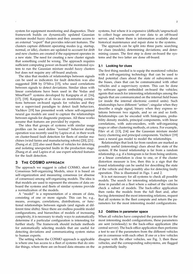
- 2

system for equipment monitoring and diagnostics. Theirframework builds on dynamically updated Gaussianmixture model fuzzy clusters and they assume access toan external “expert” that provides relevant features. Theclusters capture different operating modes (e.g. startup,normal, or idle), clusters are updated to account for driftand new clusters are created if the equipment operates ina new state. The need for creating a new cluster signalsthat something could be wrong. The approach requiressufficient computing power on-board the monitored sys-tem to run the Gaussian mixture model fuzzy clustersbut does not require any off-board analysis.

The idea that models of relationships between signalscan be used as indicators for fault detection was alsosuggested 2008 by D’Silva [15], who used correlationsbetween signals to detect deviations. Similar ideas withlinear correlations have been used in the Vedas andMineFleet R© systems developed by Kargupta et al. [16],[17], [18]. Kargupta et al. focus on monitoring correla-tions between on-board signals for vehicles and theyuse a supervised paradigm to detect fault behaviors.Vachkov [19] has presented work where self-organizedneural gas models are used to capture the relationshipsbetween signals for diagnostic purposes. All these worksassume that features are provided by experts.

The idea that groups of systems with similar usageprofiles can be used define “normal” behavior duringoperation was recently used by Lapira et al. in their workon cluster-based fault detection for fleets of similar ma-chines (wind farms and manufacturing robots) [20], [21] .Zhang et al. [22] also used fleets of vehicles for detectingand isolating unexpected faults in the production stage.Zhang et al. and Lapira et al. use expert selected featuresfor the fault detection.

3 THE COSMO APPROACHThe approach we suggest is called COSMO, short forConsensus Self-organizing Models, since it is based onself-organization and measuring consensus (or absenseof consensus) among self-organizing models. The idea isthat models are used to represent the streams of data on-board the systems and fleets of similar systems providea normalization of the models.

A “model” is a representation of a stream of data,consisting of one or more signals. This can be, e.g.,means, averages, correlations, distributions, or func-tional relationships between signals (and signals at dif-ferent time shifts). Since there are endless possible modelconfigurations, and hierarchies of models of increasingcomplexity, it is necessary to study ways to automaticallydetermine if a particular configuration is interesting forfurther study. The framework should include methodsfor automatically selecting models that are useful fordetecting deviations and communicating system statusto human experts.

The setting where the COSMO approach is applicableis where one has access to a fleet of systems that do sim-ilar things, where there are on-board data streams on the

systems, but where it is expensive (difficult/unpractical)to collect huge amounts of raw data to an off-boardserver, and where there is information available abouthistorical maintenance and repair done to the systems.

The approach can be split into three parts: searchingfor clues (models); determining deviations; and deter-mining causes. The first step is done on-board the sys-tems and the two latter are done off-board.

3.1 Looking for cluesThe first thing needed is to equip the monitored vehicleswith a self-organizing technology that can be used tofind potential clues about the state of subsystems onthe buses, clues that can be communicated with othervehicles and a supervisory system. This can be doneby software agents embedded on-board the vehicles;agents that search for interesting relationships among thesignals that are communicated on the internal field buses(or inside the internal electronic control units). Suchrelationships have different “arities”; singular when theydescribe a single signal, binary when they express re-lations between two signals, and so on and so forth.Relationships can be encoded with histograms, proba-bility density models, principal components, with linearcorrelations, with auto-encoders, with self-organizingmaps or other clustering methods, et cetera. For example,Filev et al. [13], [14] use the Gaussian mixture modelfuzzy clustering and principal components. Vachkov [19]uses a neural gas model to model the relationships.

Relationships that look far from random are marked aspossibly useful (interesting) clues about the state of thesystem. If the found relationship is far from a randomrelationship, e.g. if a histogram is far from being uniform,or a linear correlation is close to one, or if the clusterdistortion measure is low, then this is a sign that thefound relationship can be useful for describing the stateof the vehicle and then possibly also for detecting faultyoperation. This is illustrated in Figs. 1 and 2.

It is not necessary for all systems to check all possiblemodels. The search for interesting relationships can bedone in parallel on a fleet where a subset of the vehiclescheck a subset of models. The back-office applicationthen ranks the models from the full fleet and, afterhaving determined the most interesting relations, requestthat all systems in the fleet compute and return the pa-rameters for the most interesting model configurations.

3.2 Oddities in parameter spaceWhen all vehicles have computed the parameters for themost interesting model configurations, these parametersare sent (wirelessly) to the back-office application (thecentral server). The back-office application then performsa test to see if the parameters from the different vehiclesare in consensus with each other. If one or a few vehiclesdisagree with the other vehicles, see Fig. 3, then thesevehicles, and the corresponding subsystems, are flaggedas potentially faulty.

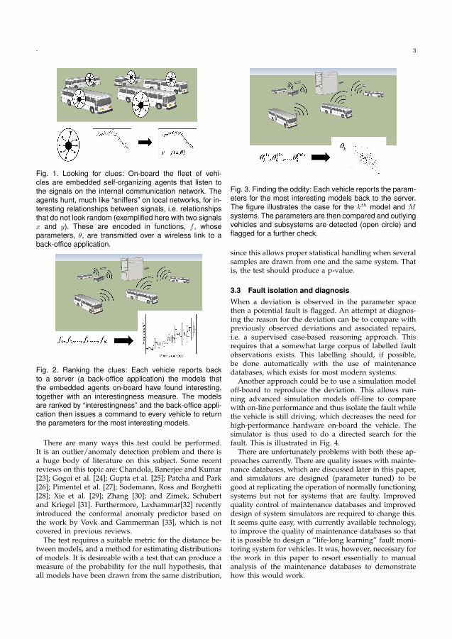
- 3

Fig. 1. Looking for clues: On-board the fleet of vehi-cles are embedded self-organizing agents that listen tothe signals on the internal communication network. Theagents hunt, much like “sniffers” on local networks, for in-teresting relationships between signals, i.e. relationshipsthat do not look random (exemplified here with two signalsx and y). These are encoded in functions, f , whoseparameters, θ, are transmitted over a wireless link to aback-office application.

Fig. 2. Ranking the clues: Each vehicle reports backto a server (a back-office application) the models thatthe embedded agents on-board have found interesting,together with an interestingness measure. The modelsare ranked by “interestingness” and the back-office appli-cation then issues a command to every vehicle to returnthe parameters for the most interesting models.

There are many ways this test could be performed.It is an outlier/anomaly detection problem and there isa huge body of literature on this subject. Some recentreviews on this topic are: Chandola, Banerjee and Kumar[23]; Gogoi et al. [24]; Gupta et al. [25]; Patcha and Park[26]; Pimentel et al. [27]; Sodemann, Ross and Borghetti[28]; Xie et al. [29]; Zhang [30]; and Zimek, Schubertand Kriegel [31]. Furthermore, Laxhammar[32] recentlyintroduced the conformal anomaly predictor based onthe work by Vovk and Gammerman [33], which is notcovered in previous reviews.

The test requires a suitable metric for the distance be-tween models, and a method for estimating distributionsof models. It is desireable with a test that can produce ameasure of the probability for the null hypothesis, thatall models have been drawn from the same distribution,

Fig. 3. Finding the oddity: Each vehicle reports the param-eters for the most interesting models back to the server.The figure illustrates the case for the kth model and Msystems. The parameters are then compared and outlyingvehicles and subsystems are detected (open circle) andflagged for a further check.

since this allows proper statistical handling when severalsamples are drawn from one and the same system. Thatis, the test should produce a p-value.

3.3 Fault isolation and diagnosisWhen a deviation is observed in the parameter spacethen a potential fault is flagged. An attempt at diagnos-ing the reason for the deviation can be to compare withpreviously observed deviations and associated repairs,i.e. a supervised case-based reasoning approach. Thisrequires that a somewhat large corpus of labelled faultobservations exists. This labelling should, if possible,be done automatically with the use of maintenancedatabases, which exists for most modern systems.

Another approach could be to use a simulation modeloff-board to reproduce the deviation. This allows run-ning advanced simulation models off-line to comparewith on-line performance and thus isolate the fault whilethe vehicle is still driving, which decreases the need forhigh-performance hardware on-board the vehicle. Thesimulator is thus used to do a directed search for thefault. This is illustrated in Fig. 4.

There are unfortunately problems with both these ap-proaches currently. There are quality issues with mainte-nance databases, which are discussed later in this paper,and simulators are designed (parameter tuned) to begood at replicating the operation of normally functioningsystems but not for systems that are faulty. Improvedquality control of maintenance databases and improveddesign of system simulators are required to change this.It seems quite easy, with currently available technology,to improve the quality of maintenance databases so thatit is possible to design a “life-long learning” fault moni-toring system for vehicles. It was, however, necessary forthe work in this paper to resort essentially to manualanalysis of the maintenance databases to demonstratehow this would work.

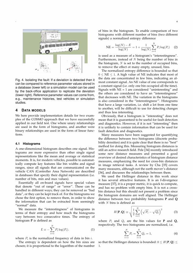
- 4

Fig. 4. Isolating the fault: If a deviation is detected then itcan be compared to reference parameter values stored ina database (lower left) or a simulation model can be usedby the back-office application to replicate the deviation(lower right). Reference parameter values can come from,e.g., maintenance histories, test vehicles or simulationstudies.

4 DATA MODELS

We here provide implementation details for two exam-ples of the COSMO approach that we have successfullyapplied in our field test. One where unary relationshipsare used in the form of histograms, and another werebinary relationships are used in the form of linear func-tions.

4.1 Histograms

A one-dimensional histogram describes one signal. His-tograms are more expressive than other single signalrepresentations like the mean and average or statisticalmoments. It is, for modern vehicles, possible to automat-ically compute key features like bin widths and signalranges, since all signals that are communicated on thevehicle CAN (Controller Area Network) are describedin databases that specify their digital representation (i.e.number of bits, min and max values).

Essentially all on-board signals have special valuesthat denote “out of range” or “error”. These can behandled in different ways; they can be removed as “baddata”, or they can be kept track of. For the histograms wechose the first option, to remove them, in order to showthe information that can be extracted from seemingly“normal” data.

We measure the “interestingness” of histograms interms of their entropy and how much the histogramsvary between two consecutive times. The entropy ofhistogram P is defined as

E ≡ −N∑

i=1

Pi log(Pi). (1)

where Pi is the normalized frequency of data in bin i.The entropy is dependent on how the bin sizes are

chosen; it is proportional to the logarithm of the number

of bins in the histogram. To enable comparison of twohistograms with different number of bins (two differentsignals) a normalized entropy difference

NE =log(N)− E

log(N)= 1 +

1

log(N)

N∑

i=1

Pi log(Pi) (2)

is used as a measure of a histogram’s “interestingness”.Furthermore, instead of N being the number of bins inthe histogram, N is set to the number of occupied bins,to remove the effect ot many empty, unused, bins.

The normalized entropy difference is bounded so that0 ≤ NE ≤ 1. A high value of NE indicates that most ofthe data are concentrated in few bins, indicating an al-most constant signal. An NE value of one corresponds toa constant signal (i.e. only one bin occupied all the time).Signals with NE = 1 are considered “uninteresting” andthe others are considered to have an “interestingness”that decreases with NE. The variation in the histogramsis also considered in the “interestingness‘”. Histogramsthat have a large variation, i.e. shift a lot from one timeto another, will be difficult to use for detecting changesand thus less interesting.

Obviously, that a histogram is “interesting” does notmean that it is guaranteed to be useful for fault detectionand diagnostics. However, if it is not “interesting” thenit is unlikely to contain information that can be used forfault detection and diagnostics.

Many measures have been suggested for quantifyingthe difference between two histograms (discrete proba-bility densities) and it is quite clear that there is no “best”method for doing this. Measuring histogram distances isstill an active research field. Pele [34] recently introducedsome new distance measures and presented a goodoverview of desired characteristics of histogram distancemeasures, emphasizing the need for cross-bin distancesin image retrieval tasks. A review by Cha [35] coversmany measures, although not the earth mover’s distance[36], and discusses the relationships between them.

We used the Hellinger distance in this work sinceit has several attractive features. It is an f-divergencemeasure [37], it is a proper metric, it is quick to compute,and has no problem with empty bins. It is not a cross-bin distance but this should not present a problem sincethe histogram domains are well aligned. The Hellingerdistance between two probability histograms P and Qwith N bins is defined as

H(P,Q) ≡

√√√√1

2

N∑

i=1

(√Pi −

√Qi

)2(3)

where Pi and Qi are the bin values for P and Q,respectively. The two histograms are normalized, i.e.

N∑

i=1

Pi =

N∑

i=1

Qi = 1, (4)

so that the Hellinger distance is bounded: 0 ≤ H(P,Q) ≤1.

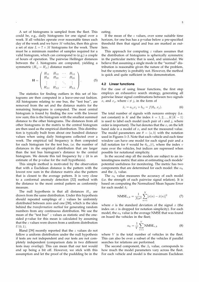
- 5

A set of histograms is sampled from the fleet. Thiscould be, e.g., daily histograms for one signal over aweek. If all vehicles operate over reasonable times eachday of the week and we have M vehicles, then this givesa set of size L = 7 ×M histograms for the week. Theremust be a minimum number of samples required for avalid histogram, which can correspond to (e.g.) a coupleof hours of operation. The pairwise Hellinger distancesbetween the L histograms are computed, yielding asymmetric (Hij = Hji) distance matrix

H =

H11 H12 · · · H1L

H21 H22 · · · H2L

......

. . ....

HL1 HL2 · · · HLL

. (5)

The statistics for finding outliers in this set of his-tograms are then computed in a leave-one-out fashion.All histograms relating to one bus, the “test bus”, areremoved from the set and the distance matrix for theremaining histograms is computed. The most centralhistogram is found by finding the row with the lowestrow sum; this is the histogram with the smallest summeddistance to the other histograms. The distances from allother histograms in the matrix to the central histogramare then used as the empirical distribution. This distribu-tion is typically built from about one hundred distancevalues when using daily histograms collected over aweek. The empirical tail frequency is then computedfor each histogram for the test bus, i.e. the number ofdistances in the empirical distribution that are largerthan the test bus histogram’s distance to the centralhistogram. We denote this tail frequency by z (it is anestimate of the p-value for the null hypothesis).

This simple method is motivated by the observationthat with a Euclidean distance is the pattern with thelowest row sum in the distance matrix also the patternthat is closest to the average pattern. It is very closeto a conformal anomaly detection [32] method withthe distance to the most central pattern as conformitymeasure.

The null hypothesis is that all distances Hij aredrawn from the same distribution. Under this hypothesisshould repeated samplings of z values be uniformlydistributed between zero and one [38], which is the ideabehind the transformation method for generating randomnumbers from any continuous distribution. We use themean of the “test bus” z values as statistic and the one-sided p-value for this mean is calculated by assumingthat the z values were drawn from a uniform distributionU(0, 1).

Bland [39] recently reported that the z values do notfollow a uniform distribution under the null hypothesisif tests are not independent and our tests are not com-pletely independent (comparison data in two differenttests may overlap). This can mean that our test wouldend up being a bit off. However, we stick with thisassumption and let the proof of the puddding be in the

eating.If the mean of the z values, over some suitable time

horizon, for one bus has a p-value below a pre-specifiedthreshold then that signal and bus are marked as out-liers.

This approach for computing z values assumes thatthe distribution of histograms is spherically symmetricin the particular metric that is used, and unimodal. Webelieve that assuming a single mode in the “normal” dis-tribution is reasonable given the nature of the problem,but the symmetry is probably not. However, the methodis quick and quite sufficient in this demonstration.

4.2 Linear functionsFor the case of using linear functions, the first stepemploys an exhaustive search strategy, generating allpairwise linear signal combinations between two signalsxi and xj , where i 6= j, in the form of

xi = aijxj + bij = f(θk, xj). (6)

The total number of signals with nonzero entropy (i.e.not constant) is K and the index k = 1, 2, ...,K(K − 1)is used to label each model (each pair of i and j, whereorder is important). The hat denotes that the xi on the lefthand side is a model of xi and not the measured value.The model parameters are θ = (a, b) with the notationused in Figures 1–3. Note that each vehicle and each timewindow can have one model for each signal pair and afull notation for θ would be θk,v(t), where the index vruns over the vehicles, but indices are supressed whenpossible for notational simplicity.

In the second step all the models are subject to an in-terestingness metric that aims at estimating each models’potential usefulness for monitoring. The metric has twocomponents that are determined for each model: the αk

and the βk value.The αk value measures the accuracy of each model

(i.e. the strength of each pairwise signal relation). It isbased on computing the Normalized Mean Square Errorfor each model k;

NMSEv,k =1

Nσ2

N∑

n=1

[x(n)− x(n)]2 (7)

where σ is the standard deviation of the signal x (theindex on x is dropped for notation simplicity). For eachmodel, the αk value is the average NMSE that was foundon board the vehicles in the fleet;

αk =1

V

V∑

v=1

NMSEv,k (8)

where V is the total number of vehicles in the fleet.This can also be over a subset of the vehicles if parallelsearches for relations are performed.

The second component, the βk value, corresponds tohow much the model parameters vary across the fleet.For each vehicle and model is the maximum Euclidean

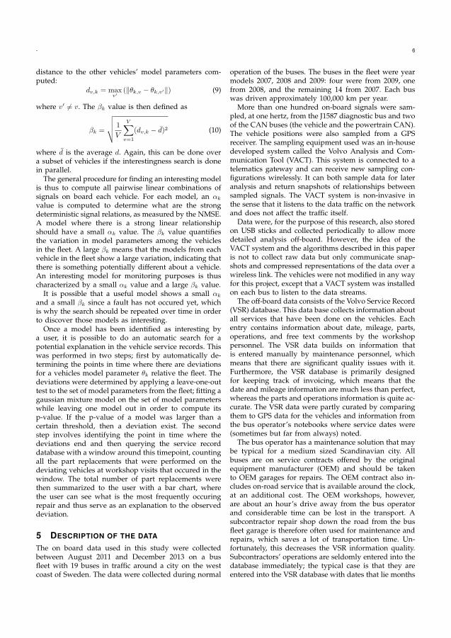
- 6

distance to the other vehicles’ model parameters com-puted:

dv,k = maxv′

(‖θk,v − θk,v′‖) (9)

where v′ 6= v. The βk value is then defined as

βk =

√√√√ 1

V

V∑

v=1

(dv,k − d)2 (10)

where d is the average d. Again, this can be done overa subset of vehicles if the interestingness search is donein parallel.

The general procedure for finding an interesting modelis thus to compute all pairwise linear combinations ofsignals on board each vehicle. For each model, an αk

value is computed to determine what are the strongdeterministic signal relations, as measured by the NMSE.A model where there is a strong linear relationshipshould have a small αk value. The βk value quantifiesthe variation in model parameters among the vehiclesin the fleet. A large βk means that the models from eachvehicle in the fleet show a large variation, indicating thatthere is something potentially different about a vehicle.An interesting model for monitoring purposes is thuscharacterized by a small αk value and a large βk value.

It is possible that a useful model shows a small αk

and a small βk since a fault has not occured yet, whichis why the search should be repeated over time in orderto discover those models as interesting.

Once a model has been identified as interesting bya user, it is possible to do an automatic search for apotential explanation in the vehicle service records. Thiswas performed in two steps; first by automatically de-termining the points in time where there are deviationsfor a vehicles model parameter θk relative the fleet. Thedeviations were determined by applying a leave-one-outtest to the set of model parameters from the fleet; fitting agaussian mixture model on the set of model parameterswhile leaving one model out in order to compute itsp-value. If the p-value of a model was larger than acertain threshold, then a deviation exist. The secondstep involves identifying the point in time where thedeviations end and then querying the service recorddatabase with a window around this timepoint, countingall the part replacements that were performed on thedeviating vehicles at workshop visits that occured in thewindow. The total number of part replacements werethen summarized to the user with a bar chart, wherethe user can see what is the most frequently occuringrepair and thus serve as an explanation to the observeddeviation.

5 DESCRIPTION OF THE DATA

The on board data used in this study were collectedbetween August 2011 and December 2013 on a busfleet with 19 buses in traffic around a city on the westcoast of Sweden. The data were collected during normal

operation of the buses. The buses in the fleet were yearmodels 2007, 2008 and 2009: four were from 2009, onefrom 2008, and the remaining 14 from 2007. Each buswas driven approximately 100,000 km per year.

More than one hundred on-board signals were sam-pled, at one hertz, from the J1587 diagnostic bus and twoof the CAN buses (the vehicle and the powertrain CAN).The vehicle positions were also sampled from a GPSreceiver. The sampling equipment used was an in-housedeveloped system called the Volvo Analysis and Com-munication Tool (VACT). This system is connected to atelematics gateway and can receive new sampling con-figurations wirelessly. It can both sample data for lateranalysis and return snapshots of relationships betweensampled signals. The VACT system is non-invasive inthe sense that it listens to the data traffic on the networkand does not affect the traffic itself.

Data were, for the purpose of this research, also storedon USB sticks and collected periodically to allow moredetailed analysis off-board. However, the idea of theVACT system and the algorithms described in this paperis not to collect raw data but only communicate snap-shots and compressed representations of the data over awireless link. The vehicles were not modified in any wayfor this project, except that a VACT system was installedon each bus to listen to the data streams.

The off-board data consists of the Volvo Service Record(VSR) database. This data base collects information aboutall services that have been done on the vehicles. Eachentry contains information about date, mileage, parts,operations, and free text comments by the workshoppersonnel. The VSR data builds on information thatis entered manually by maintenance personnel, whichmeans that there are significant quality issues with it.Furthermore, the VSR database is primarily designedfor keeping track of invoicing, which means that thedate and mileage information are much less than perfect,whereas the parts and operations information is quite ac-curate. The VSR data were partly curated by comparingthem to GPS data for the vehicles and information fromthe bus operator’s notebooks where service dates were(sometimes but far from always) noted.

The bus operator has a maintenance solution that maybe typical for a medium sized Scandinavian city. Allbuses are on service contracts offered by the originalequipment manufacturer (OEM) and should be takento OEM garages for repairs. The OEM contract also in-cludes on-road service that is available around the clock,at an additional cost. The OEM workshops, however,are about an hour’s drive away from the bus operatorand considerable time can be lost in the transport. Asubcontractor repair shop down the road from the busfleet garage is therefore often used for maintenance andrepairs, which saves a lot of transportation time. Un-fortunately, this decreases the VSR information quality.Subcontractors’ operations are seldomly entered into thedatabase immediately; the typical case is that they areentered into the VSR database with dates that lie months

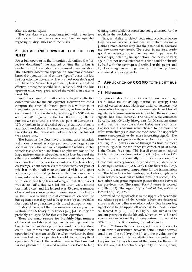
- 7

after the actual repair.The bus data were complemented with interviews

with some of the bus drivers and the bus operatorregading quality issues with the buses.

6 UPTIME AND DOWNTIME FOR THE BUSFLEET

For a bus operator is the important downtime the “ef-fective downtime”, the amount of time that a bus isneeded but not available for a planned transportation.The effective downtime depends on how many “spare”buses the operator has, the more “spare” buses the lessrisk for effective downtime. The bus fleet operator’s goalis to have one “spare” bus per twenty buses, i.e. that theeffictive downtime should be at most 5% and the busoperator takes very good care of the vehicles in order tomeet this.

We did not have information of how large the effectivedowntime was for the bus operator. However, we couldcompute the times the buses spent in a workshop, intransportation to or from a workshop, or broken downon the road. This was done by analyzing the VSR entriesand the GPS signals for the bus fleet during the 30months we observed it. The buses spent on average 11-12% of the time in or at workshops or in transportation toand from workshops. The number varied a lot betweenthe vehicles; the lowest was below 8% and the highestwas above 18%.

The buses in the fleet have a maintenance schedulewith four planned services per year; one large in as-sociation with the annual compulsory Swedish motorvehicle test, another of medium size, plus two minor. Thelarge maintenance is scheduled to take four days and theother less. Additional repairs were almost always donein connection to the service operations. The buses had,on average, about eleven visits to workshops per year, ofwhich more than half were unplanned visits, and spentan average of four days in or at the workshop, or intransportation to or from the workshop, each visit. Thevariation in visit length was also significant: the shortestwas about half a day (we did not count visits shorterthan half a day) and the longest was 35 days. A numberof on-road assistance turn-outs were needed in additionto this. It was verified in oral communication with thebus operator that they had to keep more “spare” vehiclesthan desired to guarantee undisturbed transportation.

It should be noted that the numbers are very similarto those for US heavy duty trucks [40], [41] so they areprobably not specific for this city bus operation.

There are many reasons for the fairly high numberof days at workshops. A big part is waiting time; thebus is in the workshop but no work is being doneon it. This means that the workshops optimize theiroperation, vehicles are available when work can be doneon them, but the bus operator is unable to run an optimaloperation. Some of the waiting time is the time lostfor not planning. Unplanned repairs often leads to long

waiting times while resources are being allocated for therepair in the workshop.

Thus, an ability to detect beginning problems beforethey become problems and deal with them during aplanned maintenance stop has the potential to decreasethe downtime very much. The buses in the field studyspend on average more than one month per year inworkshops, including transportation time there and backagain. It is not unrealistic that this time could be shrunkby half with the techniques described in this paper andby decreasing the waiting time, e.g. by having fewerunplanned workshop visits.

7 APPLICATION OF COSMO TO THE CITY BUSFLEET

7.1 Histograms

The process described in Section 4.1 was used. Fig-ure 5 shows the the average normalized entropy (NE)plotted versus average Hellinger distance between twoconsecutive histograms on the same vehicle and for allsignals with nonzero entropies (about half the monitoredsignals had zero entropy). The values were estimatedby collecting 100 daily histograms for 50 random timesand buses, i.e. two consecutive histograms each time.Consecutive histograms were chosen to decrease theeffect from changes in ambient conditions.The upper leftcorner corresponds to the most interesting signals. Theleast interesting signals are those in the lower right cor-ner. Figure 6 shows example histograms from differentparts in Fig. 5. In the far upper left corner, at (0.00, 0.49),is the Cooling Fan signal. This is a discrete control signalthat has the same value most of the time (more than 99%of the time) but occasionally has other values too. Thishistogram has very low entropy and is very stable. In thelower right corner, at (0.86, 0.07), is the Transm Oil Temp,which is the measured temperature for the transmissionoil. The latter has a high entropy and also a high vari-ation between consecutive histograms (not shown). Thetwo other histograms represent points that are betweenthe previous two. The signal Boost Pressure is locatedat (0.07, 0.13). The signal Engine Coolant Temperature islocated at (0.33, 0.26).

Several of the signals close to the upper left corner arethe relative speeds of the wheels, which are describedmore in relation to linear relations below. One interestingsignal close to the upper left corner is the Coolant Gauge%, located at (0.10, 0.43) in Fig. 5. This signal is thecoolant gauge on the dashboard, which shows a filteredversion of the coolant liquid temperature. It is equal to50% most of the time during normal operation.

Figure 7 shows the z statistics, which is supposed tobe uniformly distributed between 0 and 1 under normalconditions (the null hypothesis), and the p-value for thearithmetic mean for the z statistic when computed overthe previous 30 days for one of the buses, for the signalCoolant Gauge %. Sometimes, especially in the beginning

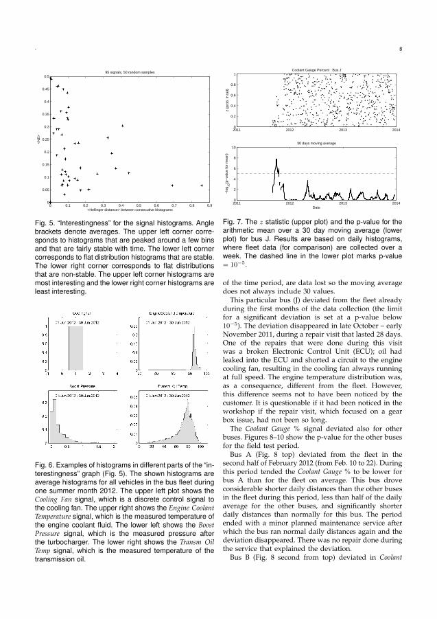
- 8

0 0.1 0.2 0.3 0.4 0.5 0.6 0.7 0.8 0.90

0.05

0.1

0.15

0.2

0.25

0.3

0.35

0.4

0.45

0.5

<Hellinger distance> between consecutive histograms

<N

E>

95 signals, 50 random samples

Fig. 5. “Interestingness” for the signal histograms. Anglebrackets denote averages. The upper left corner corre-sponds to histograms that are peaked around a few binsand that are fairly stable with time. The lower left cornercorresponds to flat distribution histograms that are stable.The lower right corner corresponds to flat distributionsthat are non-stable. The upper left corner histograms aremost interesting and the lower right corner histograms areleast interesting.

Fig. 6. Examples of histograms in different parts of the “in-terestingness” graph (Fig. 5). The shown histograms areaverage histograms for all vehicles in the bus fleet duringone summer month 2012. The upper left plot shows theCooling Fan signal, which is a discrete control signal tothe cooling fan. The upper right shows the Engine CoolantTemperature signal, which is the measured temperature ofthe engine coolant fluid. The lower left shows the BoostPressure signal, which is the measured pressure afterthe turbocharger. The lower right shows the Transm OilTemp signal, which is the measured temperature of thetransmission oil.

2011 2012 2013 20140

0.2

0.4

0.6

0.8

1

z (p

rob.

in ta

il)

Coolant Gauge Percent : Bus J

2011 2012 2013 20140

2

4

6

8

10

Date

−lo

g 10(p

−va

lue

for

mea

n)

30 days moving average

Fig. 7. The z statistic (upper plot) and the p-value for thearithmetic mean over a 30 day moving average (lowerplot) for bus J. Results are based on daily histograms,where fleet data (for comparison) are collected over aweek. The dashed line in the lower plot marks p-value= 10−5.

of the time period, are data lost so the moving averagedoes not always include 30 values.

This particular bus (J) deviated from the fleet alreadyduring the first months of the data collection (the limitfor a significant deviation is set at a p-value below10−5). The deviation disappeared in late October – earlyNovember 2011, during a repair visit that lasted 28 days.One of the repairs that were done during this visitwas a broken Electronic Control Unit (ECU); oil hadleaked into the ECU and shorted a circuit to the enginecooling fan, resulting in the cooling fan always runningat full speed. The engine temperature distribution was,as a consequence, different from the fleet. However,this difference seems not to have been noticed by thecustomer. It is questionable if it had been noticed in theworkshop if the repair visit, which focused on a gearbox issue, had not been so long.

The Coolant Gauge % signal deviated also for otherbuses. Figures 8–10 show the p-value for the other busesfor the field test period.

Bus A (Fig. 8 top) deviated from the fleet in thesecond half of February 2012 (from Feb. 10 to 22). Duringthis period tended the Coolant Gauge % to be lower forbus A than for the fleet on average. This bus droveconsiderable shorter daily distances than the other busesin the fleet during this period, less than half of the dailyaverage for the other buses, and significantly shorterdaily distances than normally for this bus. The periodended with a minor planned maintenance service afterwhich the bus ran normal daily distances again and thedeviation disappeared. There was no repair done duringthe service that explained the deviation.

Bus B (Fig. 8 second from top) deviated in Coolant

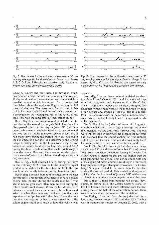
- 9

2011 2012 2013 201405

10

A

2011 2012 2013 201405

10

B

2011 2012 2013 201405

10

C

2011 2012 2013 201405

10

D

2011 2012 2013 201405

10

E

2011 2012 2013 201405

10

F

Fig. 8. The p-value for the arithmetic mean over a 30 daymoving average for the signal Coolant Gauge % for busesA, B, C, D, E and F. Results are based on daily histograms,where fleet data are collected over a week.

Gauge % exactly one year later. The deviation disap-peared after a major service and several repairs causing16 days of downtime, in association with the mandatorySwedish annual vehicle inspection. The customer hadcomplained about the engine cooling fan running at fullspeed all the time. The reason was found to be oil thathad leaked into the ECU and created a short circuit. Asa consequence the cooling fan ran at full speed all thetime. This was the same fault as seen earlier on bus J.

Bus E (Fig. 8 second from bottom) deviated from thefleet during the second half of July 2012. The deviationdisappeared after the last day of July 2012. July is amonth when many people in Sweden take vacation andthe load on the public transport system is low. Bus Ehad many days during this period when it stood still inthe bus operator’s parking lot. Furthermore, the CoolantGauge % histograms for the buses were very narrow(almost all values located in a few bins around 50%)during this time, which meant that small variations gavelarge deviations. However, there was no repair done toit at the end of July that explained the (disappearance ofthe) deviation.

Bus G (Fig. 9 top) deviated briefly during four daysin mid February 2012, when the Coolant Gauge % signaltended to be higher for this bus than the fleet. The buswas in repair, mostly indoors, during these four days.

Bus H (Fig. 9 second from top) deviated from the fleetseveral times. This particular bus tended to have a colderengine than the fleet during the colder months. It wasalso in neutral gear more often than the fleet during thecolder months (not shown). When the bus drivers wereinterviewed about their experiences with the buses andasked whether there was any particular bus that theyexperienced as “problematic” then bus H was the onlybus that the majority of bus drivers agreed on . Thecolder engine could be a result of how this vehicle was

2011 2012 2013 201405

10

G

2011 2012 2013 201405

10

H

2011 2012 2013 201405

10

I

2011 2012 2013 201405

10

K

2011 2012 2013 201405

10

L

2011 2012 2013 201405

10

M

Fig. 9. The p-value for the arithmetic mean over a 30day moving average for the signal Coolant Gauge % forbuses G, H, I, K, L and M. Results are based on dailyhistograms, where fleet data are collected over a week.

operated.Bus L (Fig. 9 second from bottom) deviated for about

five days in mid October 2011, and for about 40 daysfrom mid August to mid September 2012. The CoolantGauge % signal was higher than the fleet during the firstdeviation, which ended with a stop in the road, on-roadaction service and towing of the bus due to a coolantleak. The same was true for the second deviation, whichended with a coolant leak that had to be repaired on-siteat the bus depot.

Bus M (Fig. 9 bottom) deviated from mid August tomid September 2013, and is high (although not abovethe threshold we set) until early October 2013. The buswas sent for repair in early October because the customerhad observed that the engine cooling fan was runningat full speed all the time. This was due to a faulty ECU,the same problem as seen earlier on buses J and B.

Bus P (Fig. 10 third from top) had deviations twice,once in April 2012 and once in December 2012 to January2013. Both were short deviations, lasting 1–2 weeks. TheCoolant Gauge % signal for this bus was higher than thefleet during the first period. That period ended with oneof the engine cylinders jamming, resulting in a four weeklong unplanned stop with engine renovation. The CoolantGauge % signal tended to be lower than for the fleetduring the second period. This deviation disappearedquickly after the first week of January 2013 without anyexplanation why; there was no repair done at this time.

Bus Q (Fig. 10 third from bottom) had several devi-ations, all during 2013. The Coolant Gauge % signal onthis bus became more and more different from the fleetduring the second half of the observation period. Therewas no repair done that removed the deviation.

Bus R (Fig. 10 second from the top) deviated for along time, between August 2012 and May 2013. The buswas in maintenance service on August 27, 2012, with a

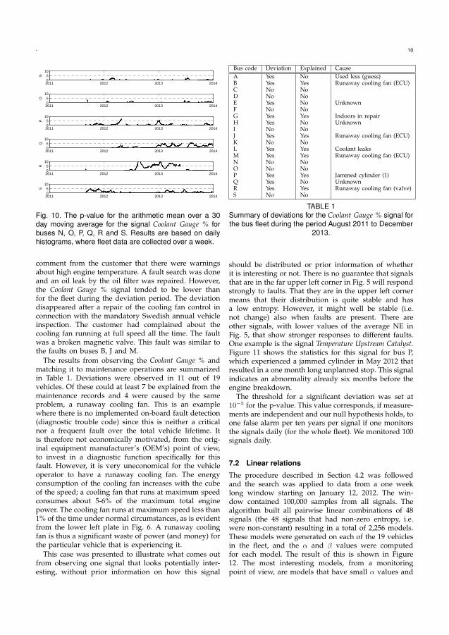
- 10

2011 2012 2013 201405

10

N

2011 2012 2013 201405

10

O

2011 2012 2013 201405

10

P

2011 2012 2013 201405

10

Q

2011 2012 2013 201405

10

R

2011 2012 2013 201405

10

S

Fig. 10. The p-value for the arithmetic mean over a 30day moving average for the signal Coolant Gauge % forbuses N, O, P, Q, R and S. Results are based on dailyhistograms, where fleet data are collected over a week.

comment from the customer that there were warningsabout high engine temperature. A fault search was doneand an oil leak by the oil filter was repaired. However,the Coolant Gauge % signal tended to be lower thanfor the fleet during the deviation period. The deviationdisappeared after a repair of the cooling fan control inconnection with the mandatory Swedish annual vehicleinspection. The customer had complained about thecooling fan running at full speed all the time. The faultwas a broken magnetic valve. This fault was similar tothe faults on buses B, J and M.

The results from observing the Coolant Gauge % andmatching it to maintenance operations are summarizedin Table 1. Deviations were observed in 11 out of 19vehicles. Of these could at least 7 be explained from themaintenance records and 4 were caused by the sameproblem, a runaway cooling fan. This is an examplewhere there is no implemented on-board fault detection(diagnostic trouble code) since this is neither a criticalnor a frequent fault over the total vehicle lifetime. Itis therefore not economically motivated, from the orig-inal equipment manufacturer’s (OEM’s) point of view,to invest in a diagnostic function specifically for thisfault. However, it is very uneconomical for the vehicleoperator to have a runaway cooling fan. The energyconsumption of the cooling fan increases with the cubeof the speed; a cooling fan that runs at maximum speedconsumes about 5-6% of the maximum total enginepower. The cooling fan runs at maximum speed less than1% of the time under normal circumstances, as is evidentfrom the lower left plate in Fig. 6. A runaway coolingfan is thus a significant waste of power (and money) forthe particular vehicle that is experiencing it.

This case was presented to illustrate what comes outfrom observing one signal that looks potentially inter-esting, without prior information on how this signal

Bus code Deviation Explained CauseA Yes No Used less (guess)B Yes Yes Runaway cooling fan (ECU)C No NoD No NoE Yes No UnknownF No NoG Yes Yes Indoors in repairH Yes No UnknownI No NoJ Yes Yes Runaway cooling fan (ECU)K No NoL Yes Yes Coolant leaksM Yes Yes Runaway cooling fan (ECU)N No NoO No NoP Yes Yes Jammed cylinder (1)Q Yes No UnknownR Yes Yes Runaway cooling fan (valve)S No No

TABLE 1Summary of deviations for the Coolant Gauge % signal forthe bus fleet during the period August 2011 to December

2013.

should be distributed or prior information of whetherit is interesting or not. There is no guarantee that signalsthat are in the far upper left corner in Fig. 5 will respondstrongly to faults. That they are in the upper left cornermeans that their distribution is quite stable and hasa low entropy. However, it might well be stable (i.e.not change) also when faults are present. There areother signals, with lower values of the average NE inFig. 5, that show stronger responses to different faults.One example is the signal Temperature Upstream Catalyst.Figure 11 shows the statistics for this signal for bus P,which experienced a jammed cylinder in May 2012 thatresulted in a one month long unplanned stop. This signalindicates an abnormality already six months before theengine breakdown.

The threshold for a significant deviation was set at10−5 for the p-value. This value corresponds, if measure-ments are independent and our null hypothesis holds, toone false alarm per ten years per signal if one monitorsthe signals daily (for the whole fleet). We monitored 100signals daily.

7.2 Linear relations

The procedure described in Section 4.2 was followedand the search was applied to data from a one weeklong window starting on January 12, 2012. The win-dow contained 100,000 samples from all signals. Thealgorithm built all pairwise linear combinations of 48signals (the 48 signals that had non-zero entropy, i.e.were non-constant) resulting in a total of 2,256 models.These models were generated on each of the 19 vehiclesin the fleet, and the α and β values were computedfor each model. The result of this is shown in Figure12. The most interesting models, from a monitoringpoint of view, are models that have small α values and

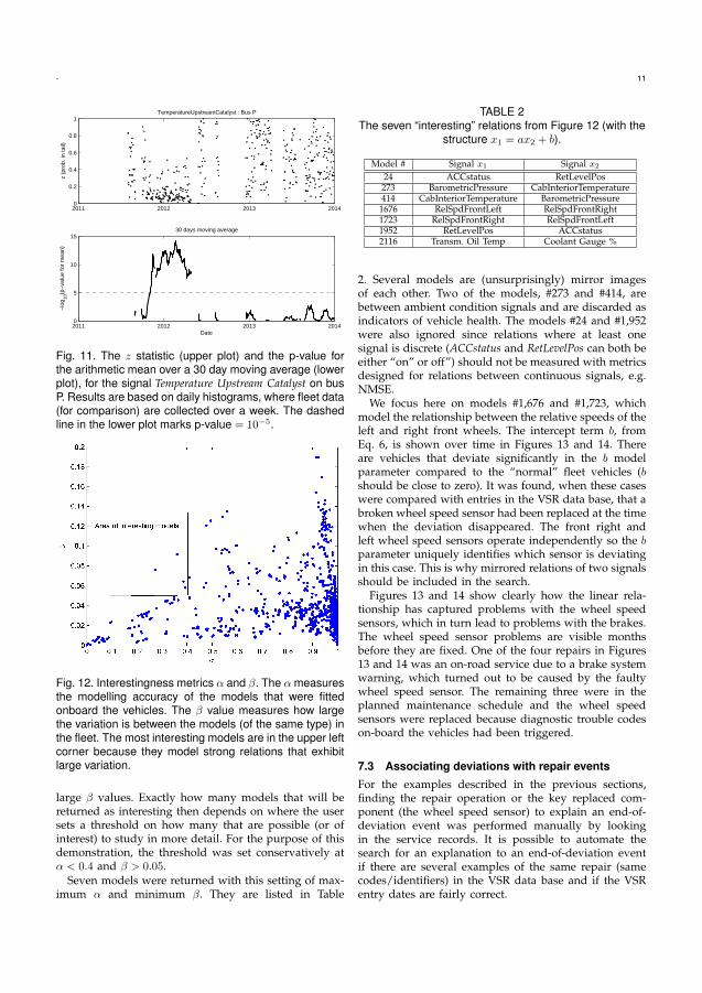
- 11

2011 2012 2013 20140

0.2

0.4

0.6

0.8

1

z (p

rob.

in ta

il)

TemperatureUpstreamCatalyst : Bus P

2011 2012 2013 20140

5

10

15

Date

−lo

g 10(p

−va

lue

for

mea

n)

30 days moving average

Fig. 11. The z statistic (upper plot) and the p-value forthe arithmetic mean over a 30 day moving average (lowerplot), for the signal Temperature Upstream Catalyst on busP. Results are based on daily histograms, where fleet data(for comparison) are collected over a week. The dashedline in the lower plot marks p-value = 10−5.

Fig. 12. Interestingness metrics α and β. The α measuresthe modelling accuracy of the models that were fittedonboard the vehicles. The β value measures how largethe variation is between the models (of the same type) inthe fleet. The most interesting models are in the upper leftcorner because they model strong relations that exhibitlarge variation.

large β values. Exactly how many models that will bereturned as interesting then depends on where the usersets a threshold on how many that are possible (or ofinterest) to study in more detail. For the purpose of thisdemonstration, the threshold was set conservatively atα < 0.4 and β > 0.05.

Seven models were returned with this setting of max-imum α and minimum β. They are listed in Table

TABLE 2The seven “interesting” relations from Figure 12 (with the

structure x1 = ax2 + b).

Model # Signal x1 Signal x2

24 ACCstatus RetLevelPos273 BarometricPressure CabInteriorTemperature414 CabInteriorTemperature BarometricPressure1676 RelSpdFrontLeft RelSpdFrontRight1723 RelSpdFrontRight RelSpdFrontLeft1952 RetLevelPos ACCstatus2116 Transm. Oil Temp Coolant Gauge %

2. Several models are (unsurprisingly) mirror imagesof each other. Two of the models, #273 and #414, arebetween ambient condition signals and are discarded asindicators of vehicle health. The models #24 and #1,952were also ignored since relations where at least onesignal is discrete (ACCstatus and RetLevelPos can both beeither “on” or off”) should not be measured with metricsdesigned for relations between continuous signals, e.g.NMSE.

We focus here on models #1,676 and #1,723, whichmodel the relationship between the relative speeds of theleft and right front wheels. The intercept term b, fromEq. 6, is shown over time in Figures 13 and 14. Thereare vehicles that deviate significantly in the b modelparameter compared to the “normal” fleet vehicles (bshould be close to zero). It was found, when these caseswere compared with entries in the VSR data base, that abroken wheel speed sensor had been replaced at the timewhen the deviation disappeared. The front right andleft wheel speed sensors operate independently so the bparameter uniquely identifies which sensor is deviatingin this case. This is why mirrored relations of two signalsshould be included in the search.

Figures 13 and 14 show clearly how the linear rela-tionship has captured problems with the wheel speedsensors, which in turn lead to problems with the brakes.The wheel speed sensor problems are visible monthsbefore they are fixed. One of the four repairs in Figures13 and 14 was an on-road service due to a brake systemwarning, which turned out to be caused by the faultywheel speed sensor. The remaining three were in theplanned maintenance schedule and the wheel speedsensors were replaced because diagnostic trouble codeson-board the vehicles had been triggered.

7.3 Associating deviations with repair events

For the examples described in the previous sections,finding the repair operation or the key replaced com-ponent (the wheel speed sensor) to explain an end-of-deviation event was performed manually by lookingin the service records. It is possible to automate thesearch for an explanation to an end-of-deviation eventif there are several examples of the same repair (samecodes/identifiers) in the VSR data base and if the VSRentry dates are fairly correct.

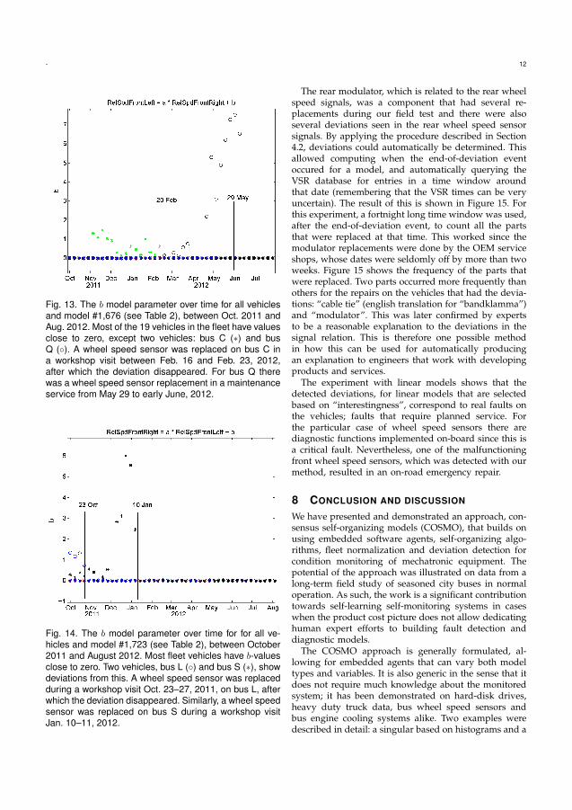
- 12

Fig. 13. The b model parameter over time for all vehiclesand model #1,676 (see Table 2), between Oct. 2011 andAug. 2012. Most of the 19 vehicles in the fleet have valuesclose to zero, except two vehicles: bus C (∗) and busQ (◦). A wheel speed sensor was replaced on bus C ina workshop visit between Feb. 16 and Feb. 23, 2012,after which the deviation disappeared. For bus Q therewas a wheel speed sensor replacement in a maintenanceservice from May 29 to early June, 2012.

Fig. 14. The b model parameter over time for for all ve-hicles and model #1,723 (see Table 2), between October2011 and August 2012. Most fleet vehicles have b-valuesclose to zero. Two vehicles, bus L (◦) and bus S (∗), showdeviations from this. A wheel speed sensor was replacedduring a workshop visit Oct. 23–27, 2011, on bus L, afterwhich the deviation disappeared. Similarly, a wheel speedsensor was replaced on bus S during a workshop visitJan. 10–11, 2012.

The rear modulator, which is related to the rear wheelspeed signals, was a component that had several re-placements during our field test and there were alsoseveral deviations seen in the rear wheel speed sensorsignals. By applying the procedure described in Section4.2, deviations could automatically be determined. Thisallowed computing when the end-of-deviation eventoccured for a model, and automatically querying theVSR database for entries in a time window aroundthat date (remembering that the VSR times can be veryuncertain). The result of this is shown in Figure 15. Forthis experiment, a fortnight long time window was used,after the end-of-deviation event, to count all the partsthat were replaced at that time. This worked since themodulator replacements were done by the OEM serviceshops, whose dates were seldomly off by more than twoweeks. Figure 15 shows the frequency of the parts thatwere replaced. Two parts occurred more frequently thanothers for the repairs on the vehicles that had the devia-tions: “cable tie” (english translation for “bandklamma”)and “modulator”. This was later confirmed by expertsto be a reasonable explanation to the deviations in thesignal relation. This is therefore one possible methodin how this can be used for automatically producingan explanation to engineers that work with developingproducts and services.

The experiment with linear models shows that thedetected deviations, for linear models that are selectedbased on “interestingness”, correspond to real faults onthe vehicles; faults that require planned service. Forthe particular case of wheel speed sensors there arediagnostic functions implemented on-board since this isa critical fault. Nevertheless, one of the malfunctioningfront wheel speed sensors, which was detected with ourmethod, resulted in an on-road emergency repair.

8 CONCLUSION AND DISCUSSION

We have presented and demonstrated an approach, con-sensus self-organizing models (COSMO), that builds onusing embedded software agents, self-organizing algo-rithms, fleet normalization and deviation detection forcondition monitoring of mechatronic equipment. Thepotential of the approach was illustrated on data from along-term field study of seasoned city buses in normaloperation. As such, the work is a significant contributiontowards self-learning self-monitoring systems in caseswhen the product cost picture does not allow dedicatinghuman expert efforts to building fault detection anddiagnostic models.

The COSMO approach is generally formulated, al-lowing for embedded agents that can vary both modeltypes and variables. It is also generic in the sense that itdoes not require much knowledge about the monitoredsystem; it has been demonstrated on hard-disk drives,heavy duty truck data, bus wheel speed sensors andbus engine cooling systems alike. Two examples weredescribed in detail: a singular based on histograms and a

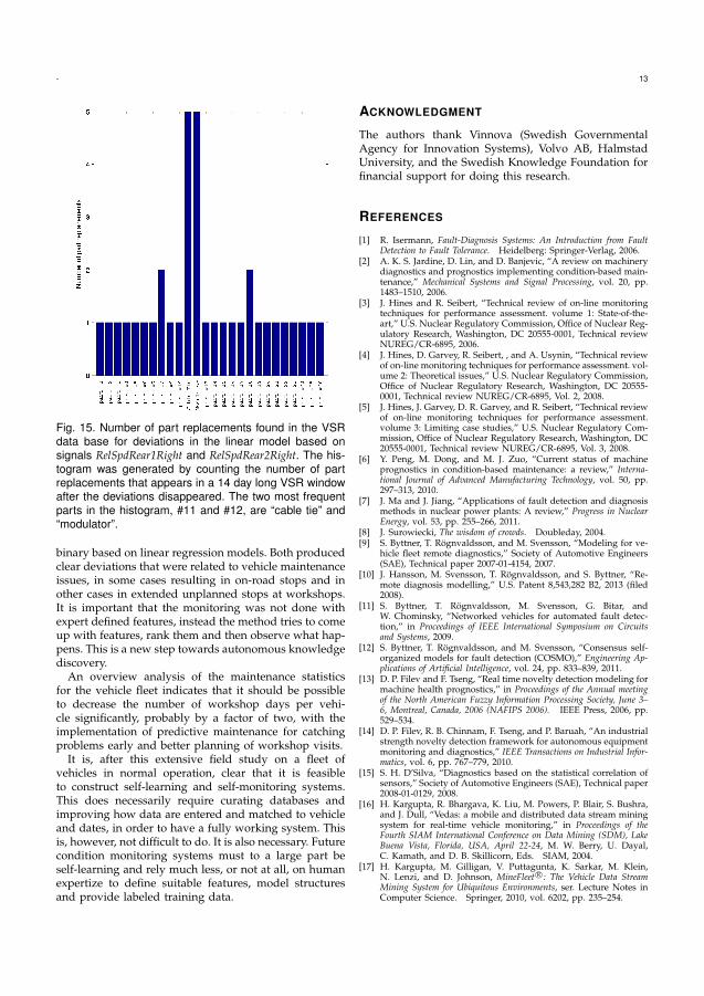
- 13

Fig. 15. Number of part replacements found in the VSRdata base for deviations in the linear model based onsignals RelSpdRear1Right and RelSpdRear2Right. The his-togram was generated by counting the number of partreplacements that appears in a 14 day long VSR windowafter the deviations disappeared. The two most frequentparts in the histogram, #11 and #12, are “cable tie” and“modulator”.

binary based on linear regression models. Both producedclear deviations that were related to vehicle maintenanceissues, in some cases resulting in on-road stops and inother cases in extended unplanned stops at workshops.It is important that the monitoring was not done withexpert defined features, instead the method tries to comeup with features, rank them and then observe what hap-pens. This is a new step towards autonomous knowledgediscovery.

An overview analysis of the maintenance statisticsfor the vehicle fleet indicates that it should be possibleto decrease the number of workshop days per vehi-cle significantly, probably by a factor of two, with theimplementation of predictive maintenance for catchingproblems early and better planning of workshop visits.

It is, after this extensive field study on a fleet ofvehicles in normal operation, clear that it is feasibleto construct self-learning and self-monitoring systems.This does necessarily require curating databases andimproving how data are entered and matched to vehicleand dates, in order to have a fully working system. Thisis, however, not difficult to do. It is also necessary. Futurecondition monitoring systems must to a large part beself-learning and rely much less, or not at all, on humanexpertize to define suitable features, model structuresand provide labeled training data.

ACKNOWLEDGMENT

The authors thank Vinnova (Swedish GovernmentalAgency for Innovation Systems), Volvo AB, HalmstadUniversity, and the Swedish Knowledge Foundation forfinancial support for doing this research.

REFERENCES

[1] R. Isermann, Fault-Diagnosis Systems: An Introduction from FaultDetection to Fault Tolerance. Heidelberg: Springer-Verlag, 2006.

[2] A. K. S. Jardine, D. Lin, and D. Banjevic, “A review on machinerydiagnostics and prognostics implementing condition-based main-tenance,” Mechanical Systems and Signal Processing, vol. 20, pp.1483–1510, 2006.

[3] J. Hines and R. Seibert, “Technical review of on-line monitoringtechniques for performance assessment. volume 1: State-of-the-art,” U.S. Nuclear Regulatory Commission, Office of Nuclear Reg-ulatory Research, Washington, DC 20555-0001, Technical reviewNUREG/CR-6895, 2006.

[4] J. Hines, D. Garvey, R. Seibert, , and A. Usynin, “Technical reviewof on-line monitoring techniques for performance assessment. vol-ume 2: Theoretical issues,” U.S. Nuclear Regulatory Commission,Office of Nuclear Regulatory Research, Washington, DC 20555-0001, Technical review NUREG/CR-6895, Vol. 2, 2008.

[5] J. Hines, J. Garvey, D. R. Garvey, and R. Seibert, “Technical reviewof on-line monitoring techniques for performance assessment.volume 3: Limiting case studies,” U.S. Nuclear Regulatory Com-mission, Office of Nuclear Regulatory Research, Washington, DC20555-0001, Technical review NUREG/CR-6895, Vol. 3, 2008.

[6] Y. Peng, M. Dong, and M. J. Zuo, “Current status of machineprognostics in condition-based maintenance: a review,” Interna-tional Journal of Advanced Manufacturing Technology, vol. 50, pp.297–313, 2010.

[7] J. Ma and J. Jiang, “Applications of fault detection and diagnosismethods in nuclear power plants: A review,” Progress in NuclearEnergy, vol. 53, pp. 255–266, 2011.

[8] J. Surowiecki, The wisdom of crowds. Doubleday, 2004.[9] S. Byttner, T. Rognvaldsson, and M. Svensson, “Modeling for ve-

hicle fleet remote diagnostics,” Society of Automotive Engineers(SAE), Technical paper 2007-01-4154, 2007.

[10] J. Hansson, M. Svensson, T. Rognvaldsson, and S. Byttner, “Re-mote diagnosis modelling,” U.S. Patent 8,543,282 B2, 2013 (filed2008).

[11] S. Byttner, T. Rognvaldsson, M. Svensson, G. Bitar, andW. Chominsky, “Networked vehicles for automated fault detec-tion,” in Proceedings of IEEE International Symposium on Circuitsand Systems, 2009.

[12] S. Byttner, T. Rognvaldsson, and M. Svensson, “Consensus self-organized models for fault detection (COSMO),” Engineering Ap-plications of Artificial Intelligence, vol. 24, pp. 833–839, 2011.

[13] D. P. Filev and F. Tseng, “Real time novelty detection modeling formachine health prognostics,” in Proceedings of the Annual meetingof the North American Fuzzy Information Processing Society, June 3–6, Montreal, Canada, 2006 (NAFIPS 2006). IEEE Press, 2006, pp.529–534.

[14] D. P. Filev, R. B. Chinnam, F. Tseng, and P. Baruah, “An industrialstrength novelty detection framework for autonomous equipmentmonitoring and diagnostics,” IEEE Transactions on Industrial Infor-matics, vol. 6, pp. 767–779, 2010.

[15] S. H. D’Silva, “Diagnostics based on the statistical correlation ofsensors,” Society of Automotive Engineers (SAE), Technical paper2008-01-0129, 2008.

[16] H. Kargupta, R. Bhargava, K. Liu, M. Powers, P. Blair, S. Bushra,and J. Dull, “Vedas: a mobile and distributed data stream miningsystem for real-time vehicle monitoring,” in Proceedings of theFourth SIAM International Conference on Data Mining (SDM), LakeBuena Vista, Florida, USA, April 22-24, M. W. Berry, U. Dayal,C. Kamath, and D. B. Skillicorn, Eds. SIAM, 2004.

[17] H. Kargupta, M. Gilligan, V. Puttagunta, K. Sarkar, M. Klein,N. Lenzi, and D. Johnson, MineFleet R©: The Vehicle Data StreamMining System for Ubiquitous Environments, ser. Lecture Notes inComputer Science. Springer, 2010, vol. 6202, pp. 235–254.

- 14

[18] H. Kargupta, V. Puttagunta, M. Klein, and K. Sarkar, “On-boardvehicle data stream monitoring using mine-fleet and fast resourceconstrained monitoring of correlation matrices,” New GenerationComputing, vol. 25, pp. 5–32, 2007.

[19] G. Vachkov, “Intelligent data analysis for performance evaluationand fault diagnosis in complex systems,” in Proceedings of the IEEEInternational conference on fuzzy systems, July 2006. IEEE Press,2006, pp. 6322–6329.

[20] E. R. Lapira, H. Al-Atat, and J. Lee, “Turbine-to-turbine prognos-tics technique for wind farms,” U.S. Patent WO 2011/143 531 A2,2011 (filed 2010).

[21] E. R. Lapira, “Fault detection in a network of similar machinesusing clustering approach,” Ph.D. dissertation, University ofCincinnati, 2012.

[22] Y. Zhang, G. W. G. Jr., M. J. Rychlinski, R. M. Edwards, J. J.Correia, and C. E. Wolf, “Connected vehicle diagnostics andprognostics, concept, and initial practice,” IEEE Transactions onReliability, vol. 58, pp. 286–294, 2009.

[23] V. Chandola, A. Banerjee, and V. Kumar, “Anomaly detection: Asurvey,” ACM Computing Surveys, vol. 41, pp. 15:1–15:58, 2009.

[24] P. Gogoi, D. Bhattacharyya, B. Borah, and J. K. Kalita, “A surveyof outlier detection methods in network anomaly identification,”The Computer Journal, vol. 54, pp. 570–588, 2011.

[25] M. Gupta, J. Gao, C. C. Aggarwal, and J. Han, “Outlier detectionfor temporal data: A survey,” IEEE Transactions on Knowledge andData Engineering, vol. 25, pp. 1–20, 2013.

[26] A. Patcha and J.-M. Park, “An overview of anomaly detectiontechniques: Existing solutions and latest technological trends,”Computer Networks, vol. 51, pp. 3448–3470, 2007.

[27] M. A. Pimentel, D. A. Clifton, L. Clifton, and L. Tarassenko, “Areview of novelty detection,” Signal Processing, vol. 99, pp. 215–249, 2014.

[28] A. A. Sodemann, M. P. Ross, and B. J. Borghetti, “A review ofanomaly detection in automated surveillance,” IEEE Transactionson Systems, Man, and Cybernetics, vol. 42, pp. 1257–1272, 2012.

[29] M. Xie, S. Han, B. Tian, and S. Parvin, “Anomaly detectionin wireless sensor networks: A survey,” Journal of Network andComputer Applications, vol. 34, pp. 1302–1325, 2011.

[30] J. Zhang, “Advancements of outlier detection: A survey,” ICSTTransaction on Scalable Information Systems, vol. 13, pp. e2:1–e2:26,2013.

[31] A. Zimek, E. Schubert, and H. P. Kriegel, “A survey on unsu-pervised outlier detection in high-dimensional numerical data,”Statistical Analysis and Data Mining, vol. 5, pp. 363–378, 2012.

[32] R. Laxhammar, “Conformal anomaly detection,” Ph.D. disserta-tion, University of Skovde, 2014.

[33] V. Vovk, A. Gammerman, and G. Shafer, Algorithmic Learning in aRandom World. New York: Springer-Verlag, 2005.

[34] O. Pele, “Distance functions: Theory, algorithms and applica-tions,” Ph.D. dissertation, The Hebrew University of Jerusalem,2011.

[35] S.-H. Cha, “Comprehensive survey on distance/similarity mea-sures between probability density functions,” International Journalof Mathematical Models and Methods in Applied Sciences, vol. 1, pp.300–307, 2007.

[36] Y. Rubner, C. Tomasi, and L. Guibas, “The earth mover’s distanceas a metric for image retrieval,” International Journal of ComputerVision, vol. 40, pp. 99–121, 2000.

[37] I. Csiszar and P. C. Shields, “Information theory and statistics: Atutorial,” Foundations and Trends

TMin Communications and Informa-

tion Theory, vol. 1, pp. 417–528, 2004.[38] W. H. Press, S. A. Teukolsky, W. T. Vetterling, and B. P. Flannery,

Numerical Recipes in C++ (2nd ed.). Cambridge University Press,2002.

[39] M. Bland, “Do baseline p-values follow a uniform distribution inrandomised trials?” PLOS ONE, vol. 8, no. e76010, pp. 1–5, 2013.

[40] M. Reimer, “Service relationship management – driving uptimein commercial vehicle maintenance and repair,” DECISIV, Whitepaper, 2013. [Online]. Available: http://www.decisiv.com/wp-content/uploads/2013/07/SRM-Driving-Uptime-in-Commercial-Fleet-Maintenance-and-Repair-FINAL-7-11-13MP.pdf

[41] ——, “Days out of service: The silent profit-killer –why fleet financial and executive management shouldcare more about service & repair,” DECISIV, Whitepaper, 2013. [Online]. Available: http://www.decisiv.com/wp-content/uploads/2013/07/DOS-White-Paper-vfinal.pdf

PLACEPHOTOHERE

Thorsteinn Rognvaldsson is professor of com-puter science at Halmstad University, Sweden.He has a PhD in theoretical physics from LundUniversity 1994 and did his post-doc at theOregon Graduate Institute 1994–1996. He haspreviously been Professor of Mechatronics atOrebro University, Sweden. He is the managerfor the CAISR research center at HalmstadUniversity. His research interests are in auto-nomic computing, machine learning and self-organizing algorithms.

PLACEPHOTOHERE

Stefan Byttner is a senior lecturer in informa-tion technology at Halmstad University, Sweden.He has a PhD in electrical engineering fromChalmers University of Technology 2005 and didhis post-doc at Halmstad University 2006. Hisresearch interests are in machine learning anddata mining.

PLACEPHOTOHERE

Rune Prytz is a research engineer and PhDcandidate in Uptime systems and services withinGlobal Trucks Technology in AB Volvo. His re-search interests lie within in predictive main-tenance and advanced data analysis, espe-cially machine learning techniques for predictingmaintenance needs.

PLACEPHOTOHERE

Sławomir Nowaczyk is assistant professor inInformation Technology at Halmstad University,Sweden. He has a MSc degree from PoznanUniversity of Technology (Poland, 2002) and aPhD degree from Lund University of Technology(Sweden, 2008), both in Computer Science. Hehas done his postdoc at AGH University of Sci-ence and Technology in Cracow, Poland. His re-search interests are knowledge representation,data mining and self-organizing systems.

PLACEPHOTOHERE

Magnus Svensson is a senior specialist in Up-time systems and services within Global TrucksTechnology in AB Volvo. He holds a Master ofScience degree from Royal Institute of Technol-ogy (Stockholm, Sweden). He has developedcontroller software for embedded systems ontrucks and has experience of innovation processdevelopment. His research interests are mainlydata mining and self-organizing systems; espe-cially on distributed systems.

Appendix C

Paper III - Analysis of Truck

Compressor Failures Based on

Logged Vehicle Data

57

Analysis of Truck Compressor Failures Based on Logged VehicleData

Rune Prytz, Sławomir Nowaczyk, Thorsteinn Rognvaldsson,Member, IEEE,and Stefan Byttner

Abstract— In multiple industries, including automotive one,predictive maintenance is becoming more and more important,especially since the focus shifts from product to service-basedoperation. It requires, among other, being able to providecustomers with uptime guarantees. It is natural to investigatethe use of data mining techniques, especially since the sameshift of focus, as well as technological advancements in thetelecommunication solutions, makes long-term data collectionmore widespread.

In this paper we describe our experiences in predictingcompressor faults using data that is logged on-board Volvotrucks. We discuss unique challenges that are posed by thespecifics of the automotive domain. We show that predictivemaintenance is possible and can result in significant cost savings,despite the relatively low amount of data available. We alsodiscuss some of the problems we have encountered by employingout-of-the-box machine learning solutions, and identify areaswhere our task diverges from common assumptions underlyingthe majority of data mining research.

Index Terms— Data Mining, Machine Learning, Fault Pre-diction, Automotive Diagnostics, Logged Vehicle Data

I. I NTRODUCTION

With modern vehicles becoming more and more sophisti-cated cyber-physical systems, increased software and systemcomplexity poses new development and maintenance chal-lenges. For commercial ground fleet operators, including busand truck companies, the maintenance strategy is typicallyreactive, meaning that a fault is fixed only after it has becomean issue affecting vehicle’s performance.

Currently, there is a desire for truck manufacturers tooffer uptime guarantees to their customers, which obviouslyrequires a shift in the paradigm. New ways of thinking aboutcomponent maintenance, scheduling and replacement need tobe introduced. Statistical lifetime predictions are no longersufficient, and workshop operations need to be planned andtheir results analysed at the level of individual vehicles.

At the same time, it is slowly becoming feasible to analyselarge amounts of data on-board trucks and buses in a timelymanner. This enables approaches based on data mining andpattern recognition techniques to augment existing, handcrafted algorithms. Such technologies, however, are not yetin the product stage, and even once they are deployed, asignificant time will be required to gather enough data toobtain consistently good results.

In the meantime, it is necessary to explore existing datasources. One example of that is Volvo’s “Logged Vehicle

Rune Prytz is with the Volvo Group Trucks Technology, AdvancedTechnology & Research Goteborg, Sweden (email: rune.prytz@volvo.com).

Sławomir Nowaczyk, Thorsteinn Rognvaldsson and Stefan Byttner arewith the Center for Applied Intelligent Systems Research, Halmstad Uni-versity, Sweden (emails follow firstname.lastname@hh.se pattern).

Database” (LVD), that collects statistics about usage andinternal workings of every vehicle. This data is stored on-board Electronic Control Units during regular operation, anduploaded to a central system during visits in authorisedworkshops.

The LVD is just one database among many that are ofinterest for predictive maintenance purposes. Others thatarebeing currently used in related projects include “VehicleData Administration” (VDA) and “Vehicle Service Records”(VSR). These databases each contain different, but comple-mentary information: usage statistics and ambient conditions,up-to-date information regarding vehicle equipment, designand configuration specifications, as well as history of allmaintenance and repair actions conducted at Volvo Autho-rised Workshops.

In a typical data mining study, the underlying assumptionis that a lot of information is available. For example, it iscommon in fault prediction research to be able to contin-uously monitor the device in question. In this regard, theautomotive domain is much more restrictive. We are onlyable to observe any given truck a couple of times per year,at intervals that are unknowna priori and difficult to predicteven during operation.

In this project we have decided to focus on analysing twocomponents: compressor and turbocharger. Due to lack ofspace, in this work we only present results related to thecompressor, but most of our discussions are valid for bothsubsystems. The main motivation of predictive maintenanceis the possibility to reduce the unplanned stops at the roadside. They can be very costly, both for the customer and forthe OEM.

If the truck is under warranty or service contract thefollowing expenses could typically be incurred: towing, dis-ruption of garage workflow, actual repair, rent of replacementtruck and loss of OEM reputation. During a service contractall maintenance and service costs are covered by a fixedmonthly fee. A secondary motivation is to minimise theamount of maintenance that is done on trucks under servicecontract while still guaranteeing required level of uptimetowards the customer.

Additionally, certain components, such as the turbochargeror timing belt, cause significant collateral damage to thevehicle when they fail. Such components are often alreadyeither designed to last the full lifetime of the vehicle orscheduled for planned maintenance. In practice, however, thisis not enough to prevent all unexpected failures. In thesecases predictive maintenance would also be very effectivein reducing the excess cost, even though the number of

breakdowns is low.Obviously, predictive maintenance not only saves money,

it also introduces additional expenses in terms of unnecessaryrepairs for the wrongly diagnosed vehicles as well as wastedcomponent life. The latter comes from the fact that the stillworking component gets exchanged.

The importance of this factor varies greatly dependingon particular application. In this study we disregard itcompletely, since both turbocharger and compressor areexchanged at most once during a vehicles lifetime.

The other cost factor, incorrectly diagnosed failures, cannever be completely avoided, but is expected to be surpassedby the savings obtained from finding vehicles before theyhave an unexpected breakdown. This expense will be themajor focus of our discussions in this work.

From classification point view, this can be directly linkedto the ratio between True Positive examples and FalsePositive ones. As mentioned previously, the cost of oneon-the-road breakdown is far greater than the cost of oneunnecessary component replacement. It is also important tonotice that the number of False Negatives is almost irrelevantin this application. They represent “wasted opportunity,”i.e.money that could potentially be saved but was not, howeverthey do not incur any direct expenses.

The predictive maintenance solution we are proposing inthis paper is designed to be used as an aid in the garage.Whenever a truck is in the workshop for whatever reason,logged data is collected and analysed. The classificationalgorithm then marks the vehicle as either normal or inneed of compressor replacement (within a specified predic-tion horizon). The workshop will then either exchange thecompressor right away, perform additional diagnostics, orschedule another visit in the near future.

This paper is organised as follows. In the next section wedescribe in more detail the type of data we are working with,as well as present the business constraints that dictate howwe state the problem and how are we trying to solve it. Wefollow by a discussion of related research in Section III. Wepresent our approach in Section IV and results of experimentswe have conducted in Section V. We close with conclusionsin Section VI.

II. DATA AND CONSTRAINTS

A typical quality measurement in the automotive industryis the fault frequency of a component. It’s percentage ofcomponents that fail within a given time: most typically,either a warranty or service contract period. However, thatisnot a representative measure for our case. Our data consistsof a number of data readouts from each truck, spread overlong time, but compressor or turbocharger gets replaced atmost once.

Most of the vehicles never have a failure of the compo-nents we are interested in. Even for those that do, many ofthe readouts come from the time when the compressor is ingood condition, and only in some cases there is a readoutfrom the workshop visit when it is exchanged.

In order to get representative data, we need to select ourexamples from three scenarios: some of the data should comefrom trucks on which compressor never failed, some shouldcome from readouts shortly before compressor failure, andsome should come from trucks on which the compressorfailed far in the future. In order to ensure that, we alsoconsider the number of readouts that is available from eachvehicle. Trucks that have too few readouts or do not containall the data parameters we are interested in are discarded atthis stage.

One of the topics of our analysis is to investigate howdoes the relative ratio of positive and negative examples intrain and test datasets influence machine learning results.It isobvious that component failures are an exception rather thana norm. However, there are different ways of measuring theprecise ratio between “faulty” and “good” cases. Neverthe-less, the fault frequency in the vehicle population does notnecessarily translate directly into exactly the same levelofimbalance between examples.

We are not able to disclose any real fault frequency data.However, as a guidance, high fault frequency is between 5-10% while a good components may have fault frequencyin the range of 0 to 3%. In this paper we will construct thedataset in such way that the baseline fault frequency is 5%. Itis important to be aware, however, that there are many factorsaffecting this and under different circumstances, the datacanlook very different. Examples include truck configuration andage, usage patterns, geographical location and many more

As a simple example, we can easily imagine a predictivemaintenance system being deployed and not applied to allvehicles, but only to those that service technicians consider“high risk”. Similarly, while compressor is an important com-ponent to monitor, the methodology itself is fully general,and there are other parts that could be targeted. Some ofthem are designed to be replaced regularly, and thus couldhave failures that occur on almost all trucks. Therefore, inseveral places in this paper, we will discuss how differentfault frequencies affect classification results.

The vehicles in our dataset are all Volvo trucks, from thesame year model, but equipped with three different com-pressor types. They also vary with respect to geographicallocation, owner, and type of operation, for instance long-haul, delivery or construction.

We have selected 80 trucks which had compressor failuresand at least 10 LVD readouts, with the right number ofparameters available. In addition we have chosen 1440 truckson which, so far at least, no compressor had failed. They allfulfil the same requirements on LVD data. We could easilyobtain more “non-faulty” vehicles, but it is the ones withcompressor failures that are the limiting factor.

A. Logged Vehicle Data

Logged Vehicle Data is a Volvo internal database whichgathers usage and ambient statistics collected from Volvovehicles. The data is downloaded from the truck when itis serviced at an authorised Volvo workshop, or wirelesslythrough a telematics gateway. The database is used for

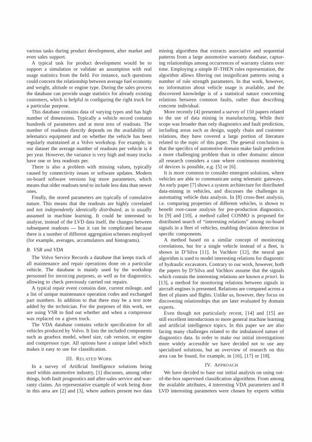
various tasks during product development, after market andeven sales support.

A typical task for product development would be tosupport a simulation or validate an assumption with realusage statistics from the field. For instance, such questionscould concern the relationship between average fuel economyand weight, altitude or engine type. During the sales processthe database can provide usage statistics for already existingcustomers, which is helpful in configuring the right truck fora particular purpose.

This database contains data of varying types and has highnumber of dimensions. Typically a vehicle record containshundreds of parameters and at most tens of readouts. Thenumber of readouts directly depends on the availability oftelematics equipment and on whether the vehicle has beenregularly maintained at a Volvo workshop. For example, inour dataset the average number of readouts per vehicle is 4per year. However, the variance is very high and many truckshave one or less readouts per.

There is also a problem with missing values, typicallycaused by connectivity issues or software updates. Modernon-board software versions log more parameters, whichmeans that older readouts tend to include less data than newerones.

Finally, the stored parameters are typically of cumulativenature. This means that the readouts are highly correlatedand not independently identically distributed, as is usuallyassumed in machine learning. It could be interested toanalyse, instead of the LVD data itself, the changes betweensubsequent readouts — but it can be complicated becausethere is a number of different aggregation schemes employed(for example, averages, accumulators and histograms).

B. VSR and VDA

The Volvo Service Records a database that keeps track ofall maintenance and repair operations done on a particularvehicle. The database is mainly used by the workshoppersonnel for invoicing purposes, as well as for diagnostics,allowing to check previously carried out repairs.

A typical repair event contains date, current mileage, anda list of unique maintenance operation codes and exchangedpart numbers. In addition to that there may be a text noteadded by the technician. For the purposes of this work, weare using VSR to find out whether and when a compressorwas replaced on a given truck.

The VDA database contains vehicle specification for allvehicles produced by Volvo. It lists the included componentssuch as gearbox model, wheel size, cab version, or engineand compressor type. All options have a unique label whichmakes it easy to use for classification.

III. R ELATED WORK

In a survey of Artificial Intelligence solutions beingused within automotive industry, [1] discusses, among otherthings, both fault prognostics and after-sales service andwar-ranty claims. An representative example of work being donein this area are [2] and [3], where authors present two data

mining algorithms that extracts associative and sequentialpatterns from a large automotive warranty database, captur-ing relationships among occurrences of warranty claims overtime. Employing a simple IF-THEN rules representation, thealgorithm allows filtering out insignificant patterns usinganumber of rule strength parameters. In that work, however,no information about vehicle usage is available, and thediscovered knowledge is of a statistical nature concerningrelations between common faults, rather than describingconcrete individual.

More recently [4] presented a survey of 150 papers relatedto the use of data mining in manufacturing. While theirscope was broader than only diagnostics and fault prediction,including areas such as design, supply chain and customerrelations, they have covered a large portion of literaturerelated to the topic of this paper. The general conclusion isthat the specifics of automotive domain make fault predictiona more challenging problem than in other domains: almostall research considers a case where continuous monitoringof devices is possible, e.g. [5] or [6].

It is more common to consider emergent solutions, wherevehicles are able to communicate using telematic gateways.An early paper [7] shows a system architecture for distributeddata-mining in vehicles, and discusses the challenges inautomating vehicle data analysis. In [8] cross-fleet analysis,i.e. comparing properties of different vehicles, is shown tobenefit root-cause analysis for pre-production diagnostics.In [9] and [10], a method called COSMO is proposed fordistributed search of “interesting relations” among on-boardsignals in a fleet of vehicles, enabling deviation detectioninspecific components.

A method based on a similar concept of monitoringcorrelations, but for a single vehicle instead of a fleet, isshown in D’Silva [11]. In Vachkov [12], the neural gasalgorithm is used to model interesting relations for diagnosticof hydraulic excavators. Contrary to our work, however, boththe papers by D’Silva and Vachkov assume that the signalswhich contain the interesting relations are knowna priori. In[13], a method for monitoring relations between signals inaircraft engines is presented. Relations are compared across afleet of planes and flights. Unlike us, however, they focus ondiscovering relationships that are later evaluated by domainexperts.

Even though not particularly recent, [14] and [15] arestill excellent introductions to more general machine learningand artificial intelligence topics. In this paper we are alsofacing many challenges related to the imbalanced nature ofdiagnostics data. In order to make our initial investigationsmore widely accessible we have decided not to use anyspecialised solutions, but an overview of research on thisarea can be found, for example, in [16], [17] or [18].

IV. A PPROACH

We have decided to base our initial analysis on using out-of-the-box supervised classification algorithms. From amongthe available attributes, 4 interesting VDA parameters and8LVD interesting parameters were chosen by experts within

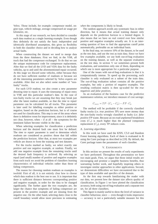
Volvo. Those include, for example: compressor model, en-gine type, vehicle mileage, average compressed air usage perkilometre, etc.

At this stage of our research, we have decided to considereach data readout as a single learning example. Even thoughthey definitely do not satisfy the basicindependent andidentically distributedassumption, this gives us flexibilityin both the classifier choice and in deciding how to analyseactual faults.

When constructing the dataset we need to merge datafrom the three databases. First we find, in the VSR, alltruck that had the compressor exchanged. To do that we usethe unique maintenance code for compressor replacement.After that we find all the LVD and VDA data for the faultyvehicles, up to and until the aforementioned repair occurred.At this stage we discard some vehicles, either because theydo not have sufficient number of readouts or because notall the interesting parameters selected by Volvo experts areavailable. After that we also select some number of “non-faulty” trucks.

For each LVD readout, we also create a new parameterdenoting time to repair. It uses the timestamp of repair entryin VSR and this particular readout’s date. In the case ofnon-faulty trucks we are assuming that they may break justafter the latest readout available, so that thetime to repairparameter can be calculated for all trucks. This parameteris later used for labelling examples as either positive ornegative, based on the prediction horizon, but is of coursenot used for classification. This step is one of the areas wherethere is definitive room for improvement, since it is definitelynot clear, however, when – if at all – the symptoms for theimminent failure become visible in the data.

When selecting examples for classification a predictionhorizon and the desired fault rate must first be defined.The time to repair parameter is used to determine whichreadouts are considered as positive: those that fall withinthe prediction horizon. After that, at most two examples pervehicle are drawn to form the training and test datasets.

For the trucks marked as faulty, we select exactly onepositive and one negative example, at random. Finally, weadd one negative example from the remaining trucks untilthe desired fault frequency is archived. By selecting anequal (and small) number of positive and negative examplesfrom each truck we avoid the problem of classifiers learningcharacteristics of individual vehicles rather than those offailing compressors.

The reason for choosing random readouts as examples istwofold. First of all, it is not entirely clear how to choosewhich data readout is the best one to use. It is important thatthere is sufficient distance between corresponding positiveand negative example, in order for the data to be changedsignificantly. The further apart the two examples are, thelarger the chance that symptoms of failing compressor arepresent in the positive example and are missing from thenegative one. On the other hand, selecting dates close to thecutoff boundary would allow more precision in estimating

whenthe components is likely to break.The random approach avoids any systematic bias in either

direction, but it means that actual training dataset onlydepends on the prediction horizon to a limited degree. Italso means that we have no real control over how similarpositive and negative examples actually are. It is an inter-esting question of how to find the appropriate cutoff pointautomatically, preferable on an individual basis.

In the final step, we remove 10% of the dataset, to be usedas the test data, and use the rest as train data. Since we havefew examples available, we use both out-of-bag evaluationon the training dataset, as well as the separate evaluationon the test data. In section V we sometimes present bothevaluations, and sometimes only one of them, depending onwhich one is more appropriate for a particular purpose.

One of the issues with out-of-bag evaluations is that it iscomputationally intense. To speed up the processing, eachclassifier is only evaluated on a subset of the train data.The out-of-bag evaluation subset contains all the positiveexamples, but only a portion of negative examples. Theresulting confusion matrix is then up-scaled for thetruenegativesand false positives.

As an evaluation of the business case for the predictivemaintenance solution, we introduce measure of cost savings:

Csave = TP · (Cu − Cp)− FP · Cp

The method will be profitable if the correctly classifiedfaulty trucks (i.e.true positives TP) save more money thanthe non-faulty trucks wrongly classified as faulty (i.e.falsepositive FPwaste. Because an on-roadunplannedbreakdowncosts (Cu) is much higher than theplanned componentreplacement (Cp), every TP reduces costs.

A. Learning algorithms

In this work we have used the KNN, C5.0 and RandomForest learning algorithms. Each of them is evaluated in Rusing the Caret package as described in [19]. By default, theCaret package tunes the parameters of each classifier.

V. EXPERIMENTS

In this section we present the results of early experimentswe have performed. Throughout this presentation we havetwo main goals. First, we argue that those initial results areencouraging and promise a tangible business benefits, thuswarranting further work, and hopefully inspiring others toinvestigate similar approaches in other applications. Second,we demonstrate difficulties we have encountered due to thetype of data available and specifics of the domain.

As the first step towards familiarising the reader withour data, we present how the dataset size affects quality ofclassification. In Figure 1 we have plotted the classificationaccuracy, both using out-of-bag evaluation and a separate testset, for all three classifiers.

This figure is mainly useful to show the level of variance inclassifier behaviour, since — even though it looks impressive— accuracy is not a particularly suitable measure for this

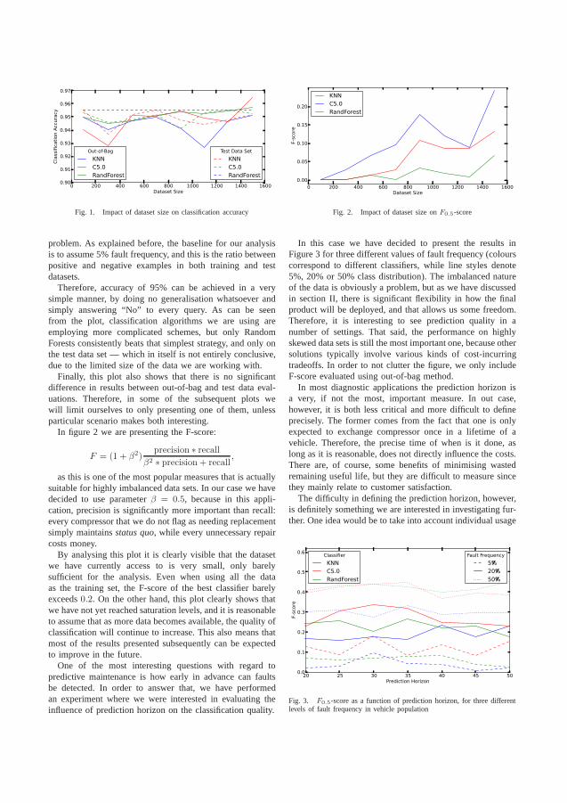
0 200 400 600 800 1000 1200 1400 1600Dataset Size

0.90

0.91

0.92

0.93

0.94

0.95

0.96

0.97

Classification Accuracy

Out-of-Bag

KNNC5.0RandForest

Test Data Set

KNNC5.0RandForest

Fig. 1. Impact of dataset size on classification accuracy

problem. As explained before, the baseline for our analysisis to assume 5% fault frequency, and this is the ratio betweenpositive and negative examples in both training and testdatasets.

Therefore, accuracy of 95% can be achieved in a verysimple manner, by doing no generalisation whatsoever andsimply answering “No” to every query. As can be seenfrom the plot, classification algorithms we are using areemploying more complicated schemes, but only RandomForests consistently beats that simplest strategy, and only onthe test data set — which in itself is not entirely conclusive,due to the limited size of the data we are working with.

Finally, this plot also shows that there is no significantdifference in results between out-of-bag and test data eval-uations. Therefore, in some of the subsequent plots wewill limit ourselves to only presenting one of them, unlessparticular scenario makes both interesting.

In figure 2 we are presenting the F-score:

F = (1 + β2)precision ∗ recall

β2 ∗ precision + recall,

as this is one of the most popular measures that is actuallysuitable for highly imbalanced data sets. In our case we havedecided to use parameterβ = 0.5, because in this appli-cation, precision is significantly more important than recall:every compressor that we do not flag as needing replacementsimply maintainsstatus quo, while every unnecessary repaircosts money.

By analysing this plot it is clearly visible that the datasetwe have currently access to is very small, only barelysufficient for the analysis. Even when using all the dataas the training set, the F-score of the best classifier barelyexceeds0.2. On the other hand, this plot clearly shows thatwe have not yet reached saturation levels, and it is reasonableto assume that as more data becomes available, the quality ofclassification will continue to increase. This also means thatmost of the results presented subsequently can be expectedto improve in the future.

One of the most interesting questions with regard topredictive maintenance is how early in advance can faultsbe detected. In order to answer that, we have performedan experiment where we were interested in evaluating theinfluence of prediction horizon on the classification quality.

0 200 400 600 800 1000 1200 1400 1600Dataset Size

0.00

0.05

0.10

0.15

0.20

F-score

KNNC5.0RandForest

Fig. 2. Impact of dataset size onF0.5-score

In this case we have decided to present the results inFigure 3 for three different values of fault frequency (colourscorrespond to different classifiers, while line styles denote5%, 20% or 50% class distribution). The imbalanced natureof the data is obviously a problem, but as we have discussedin section II, there is significant flexibility in how the finalproduct will be deployed, and that allows us some freedom.Therefore, it is interesting to see prediction quality in anumber of settings. That said, the performance on highlyskewed data sets is still the most important one, because othersolutions typically involve various kinds of cost-incurringtradeoffs. In order to not clutter the figure, we only includeF-score evaluated using out-of-bag method.

In most diagnostic applications the prediction horizon isa very, if not the most, important measure. In out case,however, it is both less critical and more difficult to defineprecisely. The former comes from the fact that one is onlyexpected to exchange compressor once in a lifetime of avehicle. Therefore, the precise time of when is it done, aslong as it is reasonable, does not directly influence the costs.There are, of course, some benefits of minimising wastedremaining useful life, but they are difficult to measure sincethey mainly relate to customer satisfaction.

The difficulty in defining the prediction horizon, however,is definitely something we are interested in investigating fur-ther. One idea would be to take into account individual usage

20 25 30 35 40 45 50Prediction Horizon

0.0

0.1

0.2

0.3

0.4

0.5

0.6

F-score

Classifier

KNNC5.0RandForest

Fault Frequency

5%20%50%

Fig. 3. F0.5-score as a function of prediction horizon, for three differentlevels of fault frequency in vehicle population

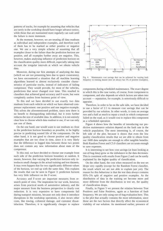
patterns of trucks, for example by assuming that vehicles thatare rarely in the workshop should have longer advance notice,while those that are maintained more regularly can wait untilthe failure is more imminent.

At the moment, however, we are treating all data readoutsas individual and independent examples, and therefore eachof them has to be marked as either positive or negativeone. We use a very simple scheme of assuming that allexamples closer to the failure than the prediction horizon arepositive, and all examples further away are negative. This,however, makes analysing influence of prediction horizon onthe classification quality more difficult, especially taking intoaccount the irregular intervals at which we obtain vehicledata.

Moreover, during our first attempts of analysing the data(which we are not presenting here due to space constraints),we have encountered a situation that all machine learningalgorithms learned to almost exclusively consider charac-teristics of particular trucks, instead of indicators of failingcompressor. They would provide, for most of the vehicles,predictions that never changed over time. This resulted inclassifiers that achieved good accuracy and F-score, but werecompletely useless from business point of view.

To this end we have decided to use exactly two datareadouts from each vehicle on which we have observed com-pressor replacement: one positive and one negative example.This solves the aforementioned problem, since now there isno benefit to distinguishing individual, but it even furtherreduces the size of available data. In addition, it is not entirelyclear how to choose which data readout to use, if we can onlyuse one of them.

On the one hand, one would want to use readouts as closeto the prediction horizon boundary as possible, to be highlyprecise in predicting wasted life of the components. On theother hand, it is not good to choose positive and negativeexamples that are too close in time, since it is very likelythat the difference in logged data between those two pointsdoes not contain any new information about state of thecompressor.

To this end, we have decided to choose one example fromeach side of the prediction horizon boundary at random. Itmeans, however, that varying the prediction horizon only in-troduces small changes in the actual training and test datasets.It may even happen that for two significantly different valuesof the horizon, we end up with the same data. This explainsthe results that can be seen in Figure 3: prediction horizonhas very little influence on the F-score.

Accuracy and F-score are important measures from re-search point of view. The inspiration for our work, however,arises from practical needs of automotive industry, and themajor measure from the business perspective is clearly costreduction. It is very expensive to have components failduring transport missions, because not only does it introducedisruptions in the workshop operations, it also incurs othercosts, like towing, collateral damage, and customer dissat-isfaction. Therefore, it is significantly cheaper to replace

5 10 15 20 25 30 35 40Fault Frequency

−200

−150

−100

−50

0

50

Cost

Savin

gs

Out-of-Bag

KNNC5.0RandForest

Test Data Set

KNNC5.0RandForest

Fig. 4. Maintenance cost savings that can be achieved for varying faultfrequency in training dataset (test set always has 5% of positive examples).

components during scheduled maintenance. The exact degreeto which this is the case varies, of course, from component tocomponent, and also depends on which factors are taken intoaccount — reputation, for example, is notoriously difficulttoappraise.

Therefore, in order to be on the safe side, we have decidedto use a factor of2.5 to measure cost savings that can beprovided by our solution. In other words, it costs on averagetwo and a half as much to repair a truck in which compressorfailed on the road, as it would cost to replace this componentas a scheduled operation.

Figure 4 shows how the benefits of introducing our pre-dictive maintenance solution depend on the fault rate in thevehicle population. The most interesting is, of course, theleft side of the plot, because it shows that even the lowquality classification results that we are able to obtain fromour 1600 data samples are enough to offer tangible benefits.Both Random Forest and C5.0 classifiers are accurate enoughto save expenses.

It is interesting to see how cost savings (at least looking atout-of-bag data) grow as the imbalance in the data decreases.This is consistent with results from Figure 2 and can be easilyexplained by the higher quality of classification.

On the other hand, the cost when measured on the test setdrops very rapidly (except for the Random Forest classifier,the result which we are not able to explain just yet). Thereason for this behaviour is that the test data always contains95%–5% split of negative and positive examples. As thedistribution of data in the training set become more andmore different from the distribution in test set, the qualityof classification drops.

Finally, in Figure 5 we present the relation between TruePositives and False Positives, again as a function of faultfrequency. We are only using out-of-bag evaluation here. Thisis the plot that actually contains the most information, sincethose are the two factors that directly affect the economicalviability of our solution. As mentioned earlier, presence of

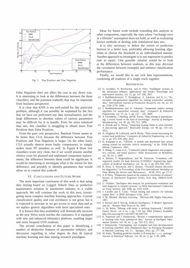
5 10 15 20 25 30Fault Frequency

0

10

20

30

40

50

Number of Vehicles

True Positive

KNNC5.0RandForest

False Positive

KNNC5.0RandForest

Fig. 5. True Positives and True Negatives

False Negatives does not affect the cost in any direct way.It is interesting to look at the differences between the threeclassifiers, and the potential tradeoffs that may be importantfrom business perspective.

It is clear that KNN is not well-suited for this particularproblem, although it can possibly be explained by the factthat we have not performed any data normalisation, and thelarge differences in absolute values of various parametersmay be difficult for it to handle. Even for more balanceddata sets, this classifier is struggling to obtain more TruePositives than False Positives.

From the pure cost perspective, Random Forest seems tobe better than C5.0, because the difference between TruePositives and True Negatives is larger. On the other hand,C5.0 actually detects more faulty compressors, in simplymakes more FP mistakes as well. In Figure 4 those twoclassifiers score very close, but if we would assume anotherrelative costs for planned and unplanned component replace-ments, the difference between them could be significant. Itwould be interesting to investigate what is the reason for thisdifference, and possibly to identify parameters that wouldallow us to control this tradeoff.

VI. CONCLUSIONS ANDFUTURE WORK

The most important conclusion of this work is that usingdata mining based on Logged Vehicle Data as predictivemaintenance solution in automotive industry is a viableapproach. We will continue the work in this area, investi-gating more complex machine learning approaches. Currentclassification quality and cost avoidance is not great, but itis expected to increase as we get access to more data and aswe replace generic algorithms with more specialised ones.

It is known that data availability will dramatically increaseas the new Volvo truck reaches the customers. It is equippedwith new and enhanced telematics platform, enabling largerand more frequent LVD readouts.

The second contribution of this paper is identifying anumber of distinctive features of automotive industry, anddiscussion regarding to what degree do they fit typicalmachine learning and data mining research paradigms.

Ideas for future work include extending this analysis toother components, especially the ones where “exchange oncein a lifetime” assumption does not hold, as well as evaluatingknown methods of dealing with imbalanced data sets.

It is also necessary to define the notion of predictionhorizon in a better way, preferably allowing learning algo-rithm to choose the threshold in an individualised manner.Another approach to investigate is to use regression to predicttime to repair. One possible solution would be to lookat the differences between readouts, as this may decreasethe correlation between examples and enhance classificationperformance.

Finally, we would like to use rich data representations,combining all readouts of a single truck together.

REFERENCES

[1] O. Gusikhin, N. Rychtyckyj, and D. Filev, “Intelligent systems inthe automotive industry: applications and trends,”Knowledge andInformation Systems, vol. 12, pp. 147–168, 2007.

[2] J. Buddhakulsomsiri, Y. Siradeghyan, A. Zakarian, and X. Li, “As-sociation rule-generation algorithm for mining automotive warrantydata,” International Journal of Production Research, vol. 44, no. 14,pp. 2749–2770, 2006.

[3] J. Buddhakulsomsiri and A. Zakarian, “Sequential pattern miningalgorithm for automotive warranty data,”Computers & IndustrialEngineering, vol. 57, no. 1, pp. 137 – 147, 2009.

[4] A. Choudhary, J. Harding, and M. Tiwari, “Data mining in manufactur-ing: a review based on the kind of knowledge,”Journal of IntelligentManufacturing, vol. 20, pp. 501–521, 2009.

[5] A. Kusiak and A. Verma, “Analyzing bearing faults in windturbines:A data-mining approach,”Renewable Energy, vol. 48, pp. 110–116,2012.

[6] A. Alzghoul, M. Lofstrand, and B. Backe, “Data stream forecasting forsystem fault prediction,”Computers & Industrial Engineering, vol. 62,no. 4, pp. 972–978, May 2012.

[7] H. Karguptaet al., “VEDAS: A mobile and distributed data streammining system for real-time vehicle monitoring,” inInt. SIAM DataMining Conference, 2003.

[8] Y. Zhang, G. Ganttet al., “Connected vehicle diagnostics and prognos-tics, concept, and initial practice,”IEEE Transactions on Reliability,vol. 58, no. 2, 2009.

[9] S. Byttner, T. Rognvaldsson, and M. Svensson, “Consensus self-organized models for fault detection (COSMO),”Engineering Appli-cations of Artificial Intelligence, vol. 24, no. 5, pp. 833–839, 2011.

[10] R. Prytz, S. Nowaczyk, and S. Byttner, “Towards relation discoveryfor diagnostics,” inProceedings of the First International Workshop onData Mining for Service and Maintenance. ACM, 2011, pp. 23–27.

[11] S. D’Silva, “Diagnostics based on the statistical correlation of sensors,”Society of Automotive Engineers (SAE), Tech. Rep. 2008-01-0129,2008.

[12] G. Vachkov, “Intelligent data analysis for performance evaluation andfault diagnosis in complex systems,” inIEEE International Conferenceon Fuzzy Systems, July 2006, pp. 6322–6329.

[13] J. Lacaille and E. Come, “Visual mining and statistics for turbofanengine fleet,” inIEEE Aerospace Conf., 2011.

[14] T. M. Mitchell, Machine Learning. McGraw-Hill Higher Education,1997.

[15] S. Russell and P. Norvig,Artificial Intelligence: A Modern Approach,2nd ed. Prentice Hall Series in AI, 2003.

[16] G. M. Weiss, “Mining with rarity: a unifying framework,” SIGKDDExplor. Newsl., vol. 6, no. 1, pp. 7–19, Jun. 2004. [Online]. Available:http://doi.acm.org/10.1145/1007730.1007734

[17] K. Napierala and J. Stefanowski, “Bracid: a comprehensive approachto learning rules from imbalanced data,”Journal of Intelligent Infor-mation Systems, vol. 39, no. 2, pp. 335–373, 2012.

[18] J. Stefanowski, “Overlapping, rare examples and classdecompositionin learning classifiers from imbalanced data,” inEmerging Paradigmsin Machine Learning, vol. 13. Springer, 2013, pp. 277–306.

[19] M. Kuhn, “Building predictive models in R using thecaret package,”Journal of Statistical Software, vol. 28, no. 5, pp. 1–26, 2008.

Appendix D

Paper IV - Predicting the Need

for Vehicle Compressor Repairs

Using Maintenance Records and

Logged Vehicle Data

65

Predicting the Need for Vehicle Compressor Repairs UsingMaintenance Records and Logged Vehicle Data

Rune Prytza, Sławomir Nowaczykb, Thorsteinn Rognvaldssonb, Stefan Byttnerb

aVolvo Group Trucks Technology, Advanced Technology & Research, Goteborg, Sweden.bCenter for Applied Intelligent Systems Research, Halmstad University, Sweden.

Abstract

Methods and results are presented for applying supervised machine learning techniquesto the task of predicting the need for repairs of air compressors in commercial trucksand buses. Prediction models are derived from logged on-board data that are down-loaded during workshop visits and have been collected over three years on large num-ber of vehicles. A number of issues are identified with the data sources, many of whichoriginate from the fact that the data sources were not designed for data mining. Nev-ertheless, exploiting this available data is very important for the automotive industryas means to quickly introduce predictive maintenance solutions. It is shown on a largedata set from heavy duty trucks in normal operation how this can be done and generatea profit.

Random forest is used as the classifier algorithm, together with two methods forfeature selection whose results are compared to a human expert. The machine learningbased features outperform the human expert features, wich supports the idea to use datamining to improve maintenance operations in this domain.

Keywords: Machine Learning, Diagnostics, Fault Detection, Automotive Industry,Air Compressor

1. Introduction

Today, Original Equipment Manufacturers (OEMs) of commercial transport vehi-cles typically design maintenance plans based on simple parameters such as calendartime or mileage. However, this is no longer sufficient in the market and there is a needfor more advanced approaches that provide predictions of future maintenance needs ofindividual trucks. Instead of selling just vehicles, the sector is heading towards sell-ing complete transport services; for example, a fleet of trucks, including maintenance,with a guaranteed level of availability. This moves some of the operational risk fromthe customer to the OEM but should lower the overall cost of ownership. The OEM

Email addresses: rune.prytz@volvo.com (Rune Prytz), slawomir.nowaczyk@hh.se(Sławomir Nowaczyk), thorsteinn.rognvaldsson@hh.se (Thorsteinn Rognvaldsson),stefan.byttner@hh.se (Stefan Byttner)

Preprint submitted to - August 27, 2014

has the benefit of scale and can exploit similarities in usage and wear between differentvehicle operators.

Predicting future maintenance needs of equipment can be approached in many dif-ferent ways. One approach is to monitor the equipment and detect patterns that signalan emerging fault, which is reviewed by Hines and Seibert (2006), Hines et al. (2008a),Hines et al. (2008b), and Ma and Jiang (2011). A more challenging one is to predictthe Remaining Useful Life (RUL) for key systems, which is reviewed by Peng et al.(2010), Si et al. (2011), Sikorska et al. (2011) and Liao and Kottig (2014). For each ofthese approaches there are several options on how to do it: use physical models, expertrules, data-driven models, or hybrid combinations of these. The models can look forparameter changes that are linked to actual degradation of components, or they canlook at vehicle usage patterns and indirectly infer the wear on the components. Data-driven solutions can be based on real-time data streamed during operation or collectedhistorical data.

We present a data-driven approach that combines pattern recognition with the RULestimation, by classifying if the RUL is shorter or longer than the time to the nextplanned service visit. The model is based on combining collected (i.e. not real-time)data from two sources: data collected on-board the vehicles and service records col-lected from OEM certified maintenance workshops. This presents a number of chal-lenges, since the data sources have been designed for purposes such as warranty anal-ysis, variant handling and financial follow-up on workshops, not for data mining. Thedata come from a huge set of real vehicles in normal operation, with different operators.The challenges include, among others, highly unbalanced datasets, noisy class labels,uncertainty in the dates, irregular readouts and unpredictable number of readouts fromindividual vehicles. In addition, multiple readouts from the same truck are highly cor-related, which puts constraints on how data for testing and training are selected. Wespecifically study air compressors on heavy duty trucks and the fault complexity isalso a challenge; air compressors face many possible types of failures, but we need toconsider them all as one since they are not differentiated in the data sources.

The paper is structured as follows. A survey of related works introduces the area ofdata mining of warranty data. This is followed by an overview of the data sets and thena methodology section where the problem is introduced and the employed methods aredescribed. This is finally followed by a results section and a conclusion section.

Related Work

There are few publications where service records and logged data are used for pre-dicting maintenance needs of equipment, especially in the automotive industry, wherewear prediction almost universally done using models that are constructed before pro-duction.

In a survey of artificial intelligence solutions in the automotive industry, Gus (2007)discuss fault prognostics, after-sales service and warranty claims. Two representativeexamples of work in this area are Buddhakulsomsiri and Zakarian (2009) and Raj-pathak (2013). Buddhakulsomsiri and Zakarian (2009) present a data mining algo-rithm that extracts associative and sequential patterns from a large automotive warrantydatabase, capturing relationships among occurrences of warranty claims over time.

2

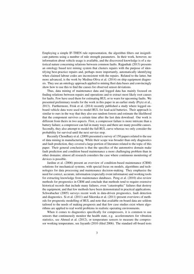
Employing a simple IF-THEN rule representation, the algorithm filters out insignifi-cant patterns using a number of rule strength parameters. In their work, however, noinformation about vehicle usage is available, and the discovered knowledge is of a sta-tistical nature concerning relations between common faults. Rajpathak (2013) presentsan ontology based text mining system that clusters repairs with the purpose of iden-tifying best-practice repairs and, perhaps more importantly, automatically identifyingwhen claimed labour codes are inconsistent with the repairs. Related to the latter, butmore advanced, is the work by Medina-Oliva et al. (2014) on ship equipment diagno-sis. They use an ontology approach applied to mining fleet data bases and convincinglyshow how to use this to find the causes for observed sensor deviations.

Thus, data mining of maintenance data and logged data has mainly focused onfinding relations between repairs and operations and to extract most likely root causesfor faults. Few have used them for estimating RUL or to warn for upcoming faults. Wepresented preliminary results for the work in this paper in an earlier study (Prytz et al.,2013). Furthermore, Frisk et al. (2014) recently published a study where logged on-board vehicle data were used to model RUL for lead-acid batteries. Their approach issimilar to ours in the way that they also use random forests and estimate the likelihoodthat the component survives a certain time after the last data download. Our work isdifferent from theirs in two aspects. First, a compressor failure is more intricate than abattery failure; a compressor can fail in many ways and there are many possible causes.Secondly, they also attempt to model the full RUL curve whereas we only consider theprobability for survival until the next service stop.

Recently Choudhary et al. (2009) presented a survey of 150 papers related to the useof data mining in manufacturing. While their scope was broader than only diagnosticsand fault prediction, they covered a large portion of literature related to the topic of thispaper. Their general conclusion is that the specifics of the automotive domain makefault prediction and condition based maintenance a more challenging problem than inother domains; almost all research considers the case where continuous monitoring ofdevices is possible.

Jardine et al. (2006) present an overview of condition-based maintenance (CBM)solutions for mechanical systems, with special focus on models, algorithms and tech-nologies for data processing and maintenance decision-making. They emphasize theneed for correct, accurate, information (especially event informaton) and working toolsfor extracting knowledge from maintenance databases. Peng et al. (2010) also reviewmethods for prognostics in CBM and conclude that methods tend to require extensivehistorical records that include many failures, even “catastrophic” failures that destroythe equipment, and that few methods have been demonstrated in practical applications.Schwabacher (2005) surveys recent work in data-driven prognostics, fault detectionand diagnostics. Si et al. (2011) and Sikorska et al. (2011) present overviews of meth-ods for prognostic modelling of RUL and note that available on-board data are seldomtailored to the needs of making prognosis and that few case studies exist where algo-rithms are applied to real world problems in realistic operating environments.

When it comes to diagnostics specifically for compressors, it is common to usesensors that continuously monitor the health state, e.g. accelerometers for vibrationstatistics, see Ahmed et al. (2012), or temperature sensors to measure the compres-sor working temperature, see Jayanth (2010 (filed 2006). The standard off-board tests

3

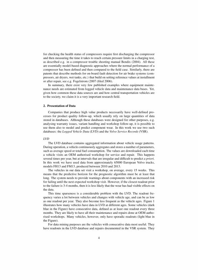
for checking the health status of compressors require first discharging the compressorand then measuring the time it takes to reach certain pressure limits in a charging test,as described e.g. in a compressor trouble shooting manual Bendix (2004). All theseare essentially model-based diagnostic approaches where the normal performance of acompressor has been defined and then compared to the field case. Similarly, there arepatents that describe methods for on-board fault detection for air brake systems (com-pressors, air dryers, wet tanks, etc.) that build on setting reference values at installmentor after repair, see e.g. Fogelstrom (2007 (filed 2006).

In summary, there exist very few published examples where equipment mainte-nance needs are estimated from logged vehicle data and maintenance data bases. Yet,given how common these data sources are and how central transportation vehicles areto the society, we claim it is a very important research field.

2. Presentation of Data

Companies that produce high value products necessarily have well-defined pro-cesses for product quality follow-up, which usually rely on large quantities of datastored in databases. Although these databases were designed for other purposes, e.g.analysing warranty issues, variant handling and workshop follow-up, it is possible touse them also to model and predict component wear. In this work we use two suchdatabases: the Logged Vehicle Data (LVD) and the Volvo Service Records (VSR).

LVDThe LVD database contains aggregated information about vehicle usage patterns.

During operation, a vehicle continuously aggregates and stores a number of parameters,such as average speed or total fuel consumption. The values are downloaded each timea vehicle visits an OEM authorised workshop for service and repair. This happensseveral times per year, but at intervals that are irregular and difficult to predict a priori.In this work we have used data from approximately 65000 European Volvo trucks,models FH13 and FM13, produced between 2010 and 2013.

The vehicles in our data set visit a workshop, on average, every 15 weeks. Thismeans that the predictive horizon for the prognostic algorithm must be at least thatlong. The system needs to provide warnings about components with an increased riskfor failing until the next expected workshop visit. However, if the closest readout priorto the failure is 3-4 months, then it is less likely that the wear has had visible effects onthe data.

This time sparseness is a considerable problem with the LVD. The readout fre-quency varies a lot between vehicles and changes with vehicle age, and can be as lowas one readout per year. They also become less frequent as the vehicle ages. Figure 1illustrates how many vehicles have data in LVD at different ages. Some vehicles (darkblue in the Figure) have consecutive data, defined as at least one readout every threemonths. They are likely to have all their maintenance and repairs done at OEM autho-rised workshops. Many vehicles, however, only have sporadic readouts (light blue inthe Figure).

For data mining purposes are the vehicles with consecutive data most useful. Theyhave readouts in the LVD database and repairs documented in the VSR system. They

4

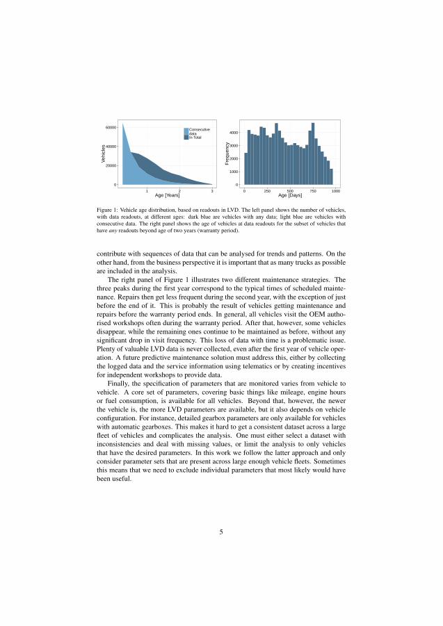
0

20000

40000

60000

1 2 3Age [Years]

Veh

icle

s

ConsecutivedataIn Total

0

1000

2000

3000

4000

0 250 500 750 1000Age [Days]

Fre

quen

cy

Figure 1: Vehicle age distribution, based on readouts in LVD. The left panel shows the number of vehicles,with data readouts, at different ages: dark blue are vehicles with any data; light blue are vehicles withconsecutive data. The right panel shows the age of vehicles at data readouts for the subset of vehicles thathave any readouts beyond age of two years (warranty period).

contribute with sequences of data that can be analysed for trends and patterns. On theother hand, from the business perspective it is important that as many trucks as possibleare included in the analysis.

The right panel of Figure 1 illustrates two different maintenance strategies. Thethree peaks during the first year correspond to the typical times of scheduled mainte-nance. Repairs then get less frequent during the second year, with the exception of justbefore the end of it. This is probably the result of vehicles getting maintenance andrepairs before the warranty period ends. In general, all vehicles visit the OEM autho-rised workshops often during the warranty period. After that, however, some vehiclesdisappear, while the remaining ones continue to be maintained as before, without anysignificant drop in visit frequency. This loss of data with time is a problematic issue.Plenty of valuable LVD data is never collected, even after the first year of vehicle oper-ation. A future predictive maintenance solution must address this, either by collectingthe logged data and the service information using telematics or by creating incentivesfor independent workshops to provide data.

Finally, the specification of parameters that are monitored varies from vehicle tovehicle. A core set of parameters, covering basic things like mileage, engine hoursor fuel consumption, is available for all vehicles. Beyond that, however, the newerthe vehicle is, the more LVD parameters are available, but it also depends on vehicleconfiguration. For instance, detailed gearbox parameters are only available for vehicleswith automatic gearboxes. This makes it hard to get a consistent dataset across a largefleet of vehicles and complicates the analysis. One must either select a dataset withinconsistencies and deal with missing values, or limit the analysis to only vehiclesthat have the desired parameters. In this work we follow the latter approach and onlyconsider parameter sets that are present across large enough vehicle fleets. Sometimesthis means that we need to exclude individual parameters that most likely would havebeen useful.

5

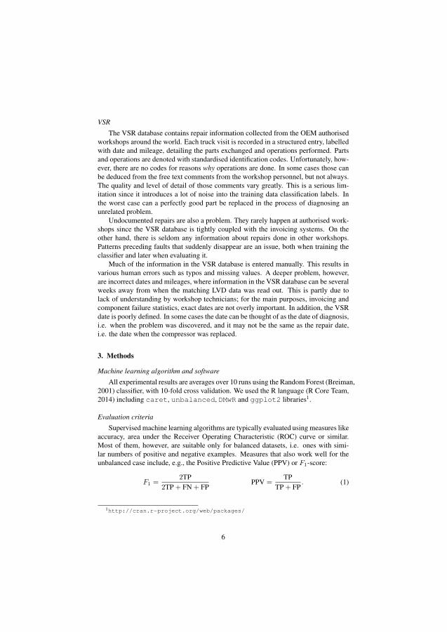
VSR

The VSR database contains repair information collected from the OEM authorisedworkshops around the world. Each truck visit is recorded in a structured entry, labelledwith date and mileage, detailing the parts exchanged and operations performed. Partsand operations are denoted with standardised identification codes. Unfortunately, how-ever, there are no codes for reasons why operations are done. In some cases those canbe deduced from the free text comments from the workshop personnel, but not always.The quality and level of detail of those comments vary greatly. This is a serious lim-itation since it introduces a lot of noise into the training data classification labels. Inthe worst case can a perfectly good part be replaced in the process of diagnosing anunrelated problem.

Undocumented repairs are also a problem. They rarely happen at authorised work-shops since the VSR database is tightly coupled with the invoicing systems. On theother hand, there is seldom any information about repairs done in other workshops.Patterns preceding faults that suddenly disappear are an issue, both when training theclassifier and later when evaluating it.

Much of the information in the VSR database is entered manually. This results invarious human errors such as typos and missing values. A deeper problem, however,are incorrect dates and mileages, where information in the VSR database can be severalweeks away from when the matching LVD data was read out. This is partly due tolack of understanding by workshop technicians; for the main purposes, invoicing andcomponent failure statistics, exact dates are not overly important. In addition, the VSRdate is poorly defined. In some cases the date can be thought of as the date of diagnosis,i.e. when the problem was discovered, and it may not be the same as the repair date,i.e. the date when the compressor was replaced.

3. Methods

Machine learning algorithm and software

All experimental results are averages over 10 runs using the Random Forest (Breiman,2001) classifier, with 10-fold cross validation. We used the R language (R Core Team,2014) including caret, unbalanced, DMwR and ggplot2 libraries1.

Evaluation criteria

Supervised machine learning algorithms are typically evaluated using measures likeaccuracy, area under the Receiver Operating Characteristic (ROC) curve or similar.Most of them, however, are suitable only for balanced datasets, i.e. ones with simi-lar numbers of positive and negative examples. Measures that also work well for theunbalanced case include, e.g., the Positive Predictive Value (PPV) or F1-score:

F1 =2TP

2TP + FN + FPPPV =

TPTP + FP

. (1)

1http://cran.r-project.org/web/packages/

6

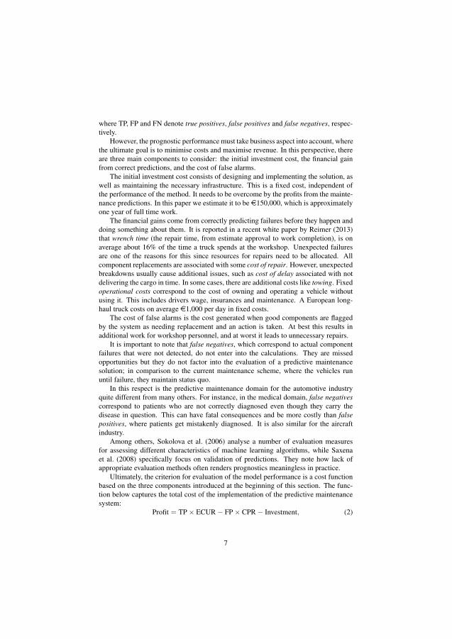
where TP, FP and FN denote true positives, false positives and false negatives, respec-tively.

However, the prognostic performance must take business aspect into account, wherethe ultimate goal is to minimise costs and maximise revenue. In this perspective, thereare three main components to consider: the initial investment cost, the financial gainfrom correct predictions, and the cost of false alarms.

The initial investment cost consists of designing and implementing the solution, aswell as maintaining the necessary infrastructure. This is a fixed cost, independent ofthe performance of the method. It needs to be overcome by the profits from the mainte-nance predictions. In this paper we estimate it to be e150,000, which is approximatelyone year of full time work.

The financial gains come from correctly predicting failures before they happen anddoing something about them. It is reported in a recent white paper by Reimer (2013)that wrench time (the repair time, from estimate approval to work completion), is onaverage about 16% of the time a truck spends at the workshop. Unexpected failuresare one of the reasons for this since resources for repairs need to be allocated. Allcomponent replacements are associated with some cost of repair. However, unexpectedbreakdowns usually cause additional issues, such as cost of delay associated with notdelivering the cargo in time. In some cases, there are additional costs like towing. Fixedoperational costs correspond to the cost of owning and operating a vehicle withoutusing it. This includes drivers wage, insurances and maintenance. A European long-haul truck costs on average e1,000 per day in fixed costs.

The cost of false alarms is the cost generated when good components are flaggedby the system as needing replacement and an action is taken. At best this results inadditional work for workshop personnel, and at worst it leads to unnecessary repairs.

It is important to note that false negatives, which correspond to actual componentfailures that were not detected, do not enter into the calculations. They are missedopportunities but they do not factor into the evaluation of a predictive maintenancesolution; in comparison to the current maintenance scheme, where the vehicles rununtil failure, they maintain status quo.

In this respect is the predictive maintenance domain for the automotive industryquite different from many others. For instance, in the medical domain, false negativescorrespond to patients who are not correctly diagnosed even though they carry thedisease in question. This can have fatal consequences and be more costly than falsepositives, where patients get mistakenly diagnosed. It is also similar for the aircraftindustry.

Among others, Sokolova et al. (2006) analyse a number of evaluation measuresfor assessing different characteristics of machine learning algorithms, while Saxenaet al. (2008) specifically focus on validation of predictions. They note how lack ofappropriate evaluation methods often renders prognostics meaningless in practice.

Ultimately, the criterion for evaluation of the model performance is a cost functionbased on the three components introduced at the beginning of this section. The func-tion below captures the total cost of the implementation of the predictive maintenancesystem:

Profit = TP × ECUR − FP × CPR − Investment, (2)

7

where ECUR stands for extra cost of unplanned repair and CPR stands for cost ofplanned repair. Each true positive avoids the additional costs of a breakdown and eachfalse positive is a repair done in vain, which causes additional costs.

It is interesting to study the ratio between the cost of planned and unplanned repairs.It will vary depending on the component, fleet operator domain and business model, etcetera. On the other hand, the cost for a breakdown for vehicles with and without pre-dictive maintenance can be used to determine the “break even” ratio required betweentrue positives and false positives.

Prediction Horizon

We define the Prediction Horizon (PH) as the period of interest for the predictivealgorithm. A replacement recommendation should be made for a vehicle for which theair compressor is expected to fail within that time frame into the future. As describedearlier, the vehicles visit the workshop on average every 15 weeks and the PH needs tobe at least that long. The system should provide warnings about components that areat risk of failing before the next expected workshop visit.

It is expected that the shorter the PH, the more likely it is that there is informationin the data about upcoming faults. It is generally more difficult to make predictionsthe further into the future they extend, which calls for a short PH. However, from abusiness perspective it is desireable to have a good margin for planning, which calls fora long PH. We experiment with setting the PH up to a maximum of 50 weeks.

Independent data sets for training and testing

A central assumption in machine learning (and statistics) it that of independent andidentically distributed (IID) data. There are methods that try to lift it to various degrees,and it is well known that most common algorithms work quite well also in cases whenthis assumption is not fully fulfilled, but it is still important, especially when evaluatingand comparing different solutions.

The readouts consist of aggregated data that have been sampled at different times.Subsequent values from any given truck are highly correlated to each other. It is evenmore profound in case of cumulative values, such as total mileage, a single event ofabnormal value will directly affect all subsequent readouts. Even without the aggrega-tion effect, however, there are individual patterns that are specific to each truck, be itparticular usage or individual idiosyncrasies of the complex cyber-physical system. Itmakes all readouts from a single vehicle dependent. This underlying pattern of the datais hard to visualize by analysing the parameter data as such. However, a classifier canlearn these patterns and overfit.

A partial way of dealing with the problem is to ensure that the test and train datasetbe split on a per vehicle basis and not randomly among all readouts. It means that if oneor more readouts from a given vehicle belong to the test set, no readouts from the samevehicle can be used to train the classifier. The data sets for training and testing mustcontain unique, non-overlapping, sets of vehicles in order to guarantee that patternsthat are linked to wear and usage are learned, instead of specific usage patterns forindividual vehicles.

8

Feature selection

The data set contains 1,250 unique features and equally many differentiated fea-tures. However, only approximately 500 of them are available for the average vehicle.It is clear that not all features should be used as input to the classifier. It is importantto find the subset of features that yields the highest classification performance. Addi-tionally, the small overlap of common features between vehicles makes this a researchchallenge. It is hard to select large sets of vehicles that each share a common set ofparameters. Every new feature that gets added to the dataset must be evaluated withrespect to the gain in performance and the decrease in number of examples.

Feature selection is an active area of research, but our setting poses some specificchallenges. Guyon and Elisseeff (2003) and Guyon et al. (2006) present a comprehen-sive and excellent, even if by now somewhat dated, overview of the feature selectionconcepts. Bolon-Canedo et al. (2013) present a more recent overview of methods.Molina et al. (2002) analyse performance of several fundamental algorithms found inthe literature in a controlled scenario. A scoring measure ranks the algorithms by tak-ing into account the amount of relevance, irrelevance and redundance on sample datasets. Saeys et al. (2007) provide a basic taxonomy of feature selection techniques, anddiscuss their use, variety and potential, from the bioinformatics perspective, but manyof the issues they discuss are applicable to the data analysed in this paper.

We use two feature selection methods: a wrapper approach based on the beamsearch algorithm, as well as a new filter method based on the Kolmogorov-Smirnovtest to search for the optimal feature set. The final feature sets are compared againstan expert dataset, defined by an engineer with domain knowledge. The expert datasetcontains four features, all of which have direct relevance to the age of the vehicle orthe usage of the air compressor.

The beam search feature selection algorithm performs a greedy graph search overthe powerset of all the features, looking for the subset that maximises the classificationaccuracy. However, at each iteration, we only expand nodes that maintain the data setsize above the given threshold. The threshold is reduced with the number of parametersas shown in equation (3). Each new parameter is allowed to reduce the dataset with asmall fraction. This ensures a lower bound on the data set size. The top five nodes,with respect to accuracy, are stored for next iteration. This increased the likelihood offinding the global optimum. The search is stopped when a fixed number of features isfound:

ndataset = nall × constraintFactornparams . (3)

Many parameters in the LVD dataset are highly correlated and contain essentiallythe same information, which can potentially lower the efficiency of the beam search.Chances are that different beams may select different, but correlated, feature sets. Inthis way the requirement for diversity on the “syntactic” level is met, while the algo-rithm is still captured in the same local maximum. We have not found this to be asignificant problem in practice.

With the Kolmogorov-Smirnov method, we are interested in features whose distri-butions vary in relation to oncoming failures of air compressors. There are two mainreasons for such variations: they are either related to different usage patterns of thevehicle, or to early symptoms of component wear. To identify these features, we define

9

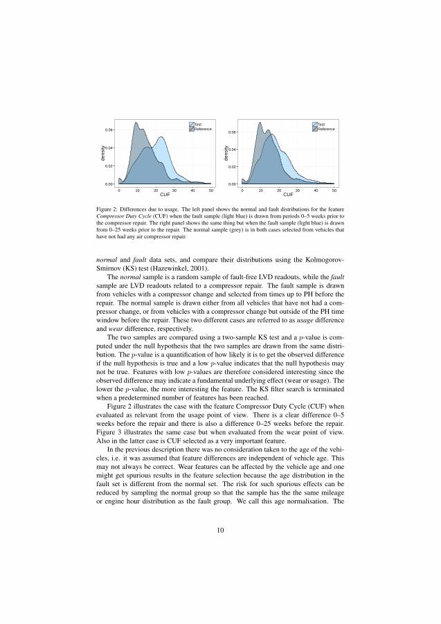
0.00

0.02

0.04

0.06

0 10 20 30 40 50CUF

dens

ity

TestReference

0.00

0.02

0.04

0.06

0 10 20 30 40 50CUF

dens

ity

TestReference

Figure 2: Differences due to usage. The left panel shows the normal and fault distributions for the featureCompressor Duty Cycle (CUF) when the fault sample (light blue) is drawn from periods 0–5 weeks prior tothe compressor repair. The right panel shows the same thing but when the fault sample (light blue) is drawnfrom 0–25 weeks prior to the repair. The normal sample (grey) is in both cases selected from vehicles thathave not had any air compressor repair.

normal and fault data sets, and compare their distributions using the Kolmogorov-Smirnov (KS) test (Hazewinkel, 2001).

The normal sample is a random sample of fault-free LVD readouts, while the faultsample are LVD readouts related to a compressor repair. The fault sample is drawnfrom vehicles with a compressor change and selected from times up to PH before therepair. The normal sample is drawn either from all vehicles that have not had a com-pressor change, or from vehicles with a compressor change but outside of the PH timewindow before the repair. These two different cases are referred to as usage differenceand wear difference, respectively.

The two samples are compared using a two-sample KS test and a p-value is com-puted under the null hypothesis that the two samples are drawn from the same distri-bution. The p-value is a quantification of how likely it is to get the observed differenceif the null hypothesis is true and a low p-value indicates that the null hypothesis maynot be true. Features with low p-values are therefore considered interesting since theobserved difference may indicate a fundamental underlying effect (wear or usage). Thelower the p-value, the more interesting the feature. The KS filter search is terminatedwhen a predetermined number of features has been reached.

Figure 2 illustrates the case with the feature Compressor Duty Cycle (CUF) whenevaluated as relevant from the usage point of view. There is a clear difference 0–5weeks before the repair and there is also a difference 0–25 weeks before the repair.Figure 3 illustrates the same case but when evaluated from the wear point of view.Also in the latter case is CUF selected as a very important feature.

In the previous description there was no consideration taken to the age of the vehi-cles, i.e. it was assumed that feature differences are independent of vehicle age. Thismay not always be correct. Wear features can be affected by the vehicle age and onemight get spurious results in the feature selection because the age distribution in thefault set is different from the normal set. The risk for such spurious effects can bereduced by sampling the normal group so that the sample has the the same mileageor engine hour distribution as the fault group. We call this age normalisation. The

10

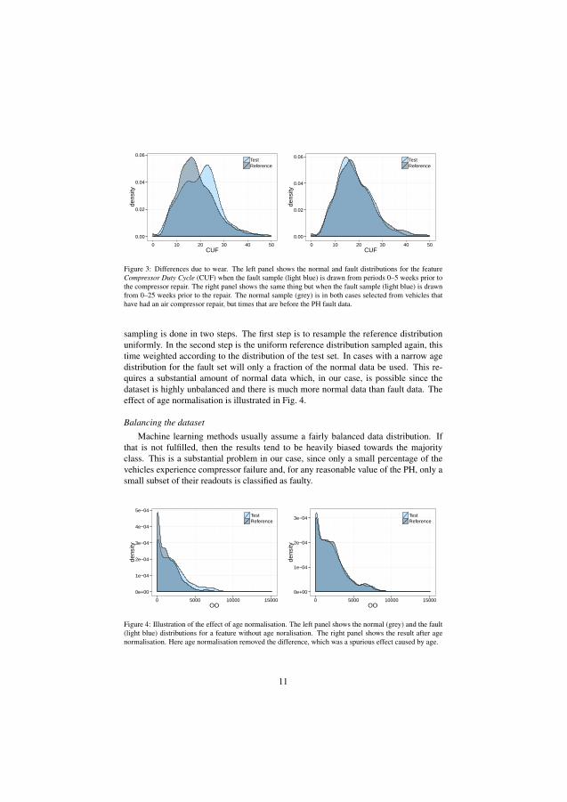
0.00

0.02

0.04

0.06

0 10 20 30 40 50CUF

dens

ity

TestReference

0.00

0.02

0.04

0.06

0 10 20 30 40 50CUF

dens

ity

TestReference

Figure 3: Differences due to wear. The left panel shows the normal and fault distributions for the featureCompressor Duty Cycle (CUF) when the fault sample (light blue) is drawn from periods 0–5 weeks prior tothe compressor repair. The right panel shows the same thing but when the fault sample (light blue) is drawnfrom 0–25 weeks prior to the repair. The normal sample (grey) is in both cases selected from vehicles thathave had an air compressor repair, but times that are before the PH fault data.

sampling is done in two steps. The first step is to resample the reference distributionuniformly. In the second step is the uniform reference distribution sampled again, thistime weighted according to the distribution of the test set. In cases with a narrow agedistribution for the fault set will only a fraction of the normal data be used. This re-quires a substantial amount of normal data which, in our case, is possible since thedataset is highly unbalanced and there is much more normal data than fault data. Theeffect of age normalisation is illustrated in Fig. 4.

Balancing the dataset

Machine learning methods usually assume a fairly balanced data distribution. Ifthat is not fulfilled, then the results tend to be heavily biased towards the majorityclass. This is a substantial problem in our case, since only a small percentage of thevehicles experience compressor failure and, for any reasonable value of the PH, only asmall subset of their readouts is classified as faulty.

0e+00

1e−04

2e−04

3e−04

4e−04

5e−04

0 5000 10000 15000OO

dens

ity

TestReference

0e+00

1e−04

2e−04

3e−04

0 5000 10000 15000OO

dens

ity

TestReference

Figure 4: Illustration of the effect of age normalisation. The left panel shows the normal (grey) and the fault(light blue) distributions for a feature without age noralisation. The right panel shows the result after agenormalisation. Here age normalisation removed the difference, which was a spurious effect caused by age.

11

Imbalanced datasets require either learning algorithms that handle this or data pre-processing steps that even out the imbalance. We chose to use the latter. There are manydomains where class imbalance is an issue, and therefore a significant body of researchis available concerning this. For example, He and Garcia (2009) provide a comprehen-sive review of the research concerning learning from imbalanced data. They provide acritical review of the nature of the problem and the state-of-the-art techniques. Theyalso highlight the major opportunities and challenges, as well as potential importantresearch directions for learning from imbalanced data. Van Hulse et al. (2007) presenta comprehensive suite of experimentation on the subject of learning from imbalanceddata. Sun et al. (2007) investigate meta-techniques applicable to most classifier learn-ing algorithms, with the aim of advancing the classification of imbalanced data, explor-ing three cost-sensitive boosting algorithms, which are developed by introducing costitems into the learning framework of AdaBoost. Napierala and Stefanowski (2012)propose a comprehensive approach, called BRACID, that combines multiple differ-ent techniques for dealing with imbalanced data, and evaluate it experimentally on anumber of well-known datasets.

We use the Synthetic Minority Over-sampling TEchnique (SMOTE), introduced byChawla et al. (2002). It identifies, for any given positive example, the k nearest neigh-bours belonging to the same class. It then creates new, synthetic, examples randomlyplaced in between the original example and the k neighbours. It uses two design pa-rameters: number of neighbours to take into consideration (k) and the percentage ofsynthetic examples to create. The first parameter, intuitively, determines how similarnew examples should be to existing ones, and the other how balanced the data shouldbe afterwards. SMOTE can be combined with several preprocessing techniques, e.g.introduced by Batista et al. (2004) and some others, aggregated and implemented in a Rlibrary by Dal Pozzolo et al.. We tried and evaluated four of them: The Edited NearestNeighbour (ENN), the Neighbourhood Cleaning Rule (NCL), the Tomek Links (TL),and the Condensed Nearest Neighbour (CNN).

4. Results

Cost function

The cost of planned repair CPR, cost of unplanned repair CUR, and extra cost ofunplanned repair ECUR can be split up into the following terms:

CPR = Cpart + CPwork + CP

downtime (4)CUR = Cpart + CU

work + CUdowntime + Cextra (5)

ECUR = CUR − CPR (6)

Here, Cpart is the cost of the physical component, the air compressor, that needsto be exchanged. We set this to e1000. It is the same for both planned and unplannedrepairs. Cwork is the labour cost of replacing the air compressor, which takes approx-imately three hours. We set CP

work to e500 for planned repairs and CUwork to e1,000

for unplanned repairs. If the operation is unplanned, then one needs to account fordiagnosis, disruptions to the workflow, extra planning, and so on.

12

Cdowntime is the cost for vehicle downtime. Planned component exchanges canbe done together with regular maintenance; CP

downtime is therefore set to zero. It isincluded in equation (4) since it will become significant in the future, once predictivemaintenance becomes common and multiple components can be repaired at the sametime. The downtime is a crucial issue for unplanned failures, however, especially road-side breakdown scenarios. Commonly at least half a day is lost immediately, beforethe vehicle is transported to the workshop and diagnosed. After that comes waiting forspare parts. The actual repair may take place on the third day. The resulting 2–3 daysof downtime plus a possible cost of towing, CU

downtime, is estimated to cost a total ofe3,500.

The additional costs, Cextra, are things like the delivery delay, the cost for damagedgoods, fines for late arrival, and so on. This is hard to estimate, since it is highlydependent on the cargo, as well as on the vehicle operator’s business model. The just intime principle is becoming more widespread in the logistics industry and the additionalcosts are therefore becoming larger. We set Cextra to e11,000.

Inserting those estimates into equations (4), (5) and (6) yields CPR = e1,500, CUR= e16,500 and ECUR = e15,000. The final Profit function, eq. (2), becomes (in Eu-ros):

Profit(TP,FP) = TP × 15, 000− FP × 1, 500− 150, 000. (7)

Obviously, the Profit function (7) is an estimate and the numbers have been chosenso that there is a simple relationship between the gain you get from true positives andthe loss you take from false positives (here the ratio is 10:1). A more exact ratio ishard to calculate since it is difficult to get access to the data required for estimatingit (this type of information is usually considered confidential). Whether the predictivemaintenance solution has a profit or loss depends much on the extra cost Cextra .

The importance of data independence

The importance of selecting independent data sets for training and testing cannot beoverstated. Using dependent data sets will lead to overly optimistic results that neverhold in the real application. Figure 5 shows the effects from selecting training and testdata sets in three different ways.

The random method refers to when samples for training and testing are chosencompletely randomly, i.e. when examples from the same vehicle can end up both in thetraining and the test data set. These data sets are not independent and the out-of-sampleaccuracy is consequently overestimated.

The one sample method refers to when each vehicle provides one positive and onenegative example to the training and test data, and there is no overlap of vehicles in thetraining and test data. This leads to independent data sets that are too limited in size.The out-of-sample performance is correctly estimated but the data set cannot be madelarge. The all sample method refers to the case when each vehicle can contribute withany number of examples but there is no overlap of vehicles between the training andtest data. This also yields a correct out-of-sample accuracy but the training data set canbe made larger.

13

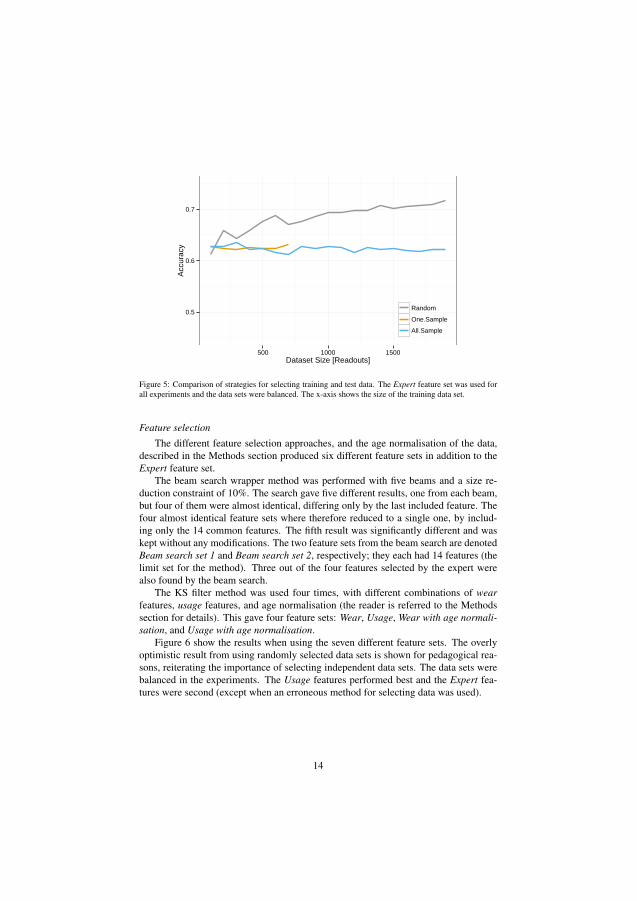
0.5

0.6

0.7

500 1000 1500Dataset Size [Readouts]

Acc

urac

y

Random

One.Sample

All.Sample

Figure 5: Comparison of strategies for selecting training and test data. The Expert feature set was used forall experiments and the data sets were balanced. The x-axis shows the size of the training data set.

Feature selection

The different feature selection approaches, and the age normalisation of the data,described in the Methods section produced six different feature sets in addition to theExpert feature set.

The beam search wrapper method was performed with five beams and a size re-duction constraint of 10%. The search gave five different results, one from each beam,but four of them were almost identical, differing only by the last included feature. Thefour almost identical feature sets where therefore reduced to a single one, by includ-ing only the 14 common features. The fifth result was significantly different and waskept without any modifications. The two feature sets from the beam search are denotedBeam search set 1 and Beam search set 2, respectively; they each had 14 features (thelimit set for the method). Three out of the four features selected by the expert werealso found by the beam search.

The KS filter method was used four times, with different combinations of wearfeatures, usage features, and age normalisation (the reader is referred to the Methodssection for details). This gave four feature sets: Wear, Usage, Wear with age normali-sation, and Usage with age normalisation.

Figure 6 show the results when using the seven different feature sets. The overlyoptimistic result from using randomly selected data sets is shown for pedagogical rea-sons, reiterating the importance of selecting independent data sets. The data sets werebalanced in the experiments. The Usage features performed best and the Expert fea-tures were second (except when an erroneous method for selecting data was used).

14

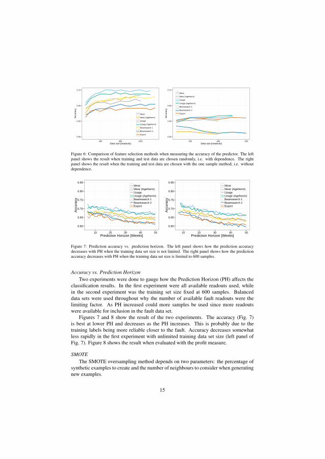
0.55

0.60

0.65

0.70

400 800 1200Data size [readouts]

Acc

urac

y

Wear

Wear (AgeNorm)

Usage

Usage (AgeNorm)

Beamsearch 1

Beamsearch 2

Expert0.55

0.60

0.65

0.70

200 400 600Data size [readouts]

Acc

urac

y

Wear

Wear (AgeNorm)

Usage

Usage (AgeNorm)

Beamsearch 1

Beamsearch 2

Expert

Figure 6: Comparison of feature selection methods when measuring the accuracy of the predictor. The leftpanel shows the result when training and test data are chosen randomly, i.e. with dependence. The rightpanel shows the result when the training and test data are chosen with the one sample method, i.e. withoutdependence.

0.60

0.65

0.70

0.75

0.80

0.85

10 20 30 40 50Prediction Horizon [Weeks]

Acc

urac

y

WearWear (AgeNorm)UsageUsage (AgeNorm)Beamsearch 1Beamsearch 2Expert

0.60

0.65

0.70

0.75

0.80

0.85

10 20 30 40 50Prediction Horizon [Weeks]

Acc

urac

y

WearWear (AgeNorm)UsageUsage (AgeNorm)Beamsearch 1Beamsearch 2Expert

Figure 7: Prediction accuracy vs. prediction horizon. The left panel shows how the prediction accuracydecreases with PH when the training data set size is not limited. The right panel shows how the predictionaccuracy decreases with PH when the training data set size is limited to 600 samples.

Accuracy vs. Prediction HorizonTwo experiments were done to gauge how the Prediction Horizon (PH) affects the

classification results. In the first experiment were all available readouts used, whilein the second experiment was the training set size fixed at 600 samples. Balanceddata sets were used throughout why the number of available fault readouts were thelimiting factor. As PH increased could more samples be used since more readoutswere available for inclusion in the fault data set.

Figures 7 and 8 show the result of the two experiments. The accuracy (Fig. 7)is best at lower PH and decreases as the PH increases. This is probably due to thetraining labels being more reliable closer to the fault. Accuracy decreases somewhatless rapidly in the first experiment with unlimited training data set size (left panel ofFig. 7). Figure 8 shows the result when evaluated with the profit measure.

SMOTEThe SMOTE oversampling method depends on two parameters: the percentage of

synthetic examples to create and the number of neighbours to consider when generatingnew examples.

15

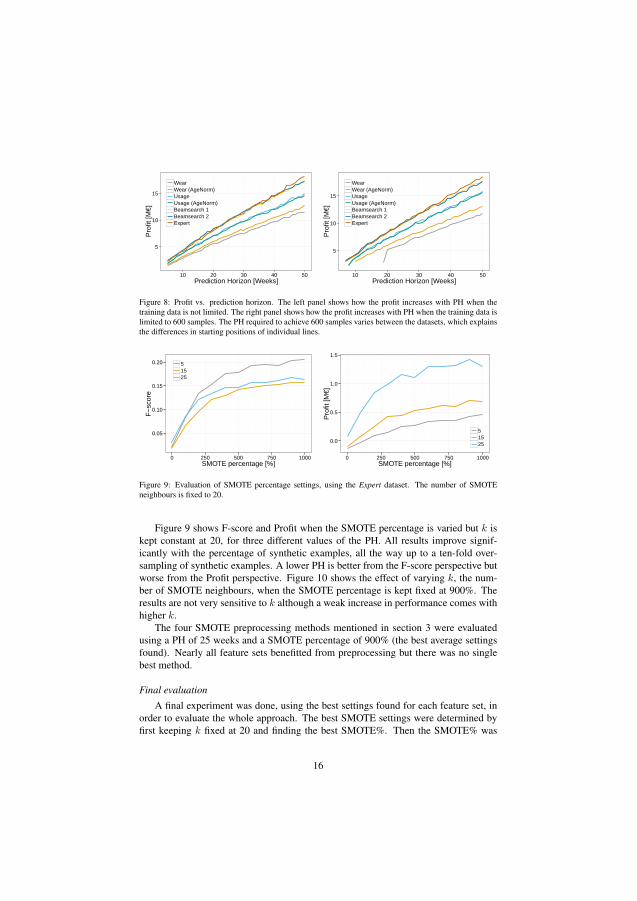
5

10

15

10 20 30 40 50Prediction Horizon [Weeks]

Pro

fit [M

€]

WearWear (AgeNorm)UsageUsage (AgeNorm)Beamsearch 1Beamsearch 2Expert

5

10

15

10 20 30 40 50Prediction Horizon [Weeks]

Pro

fit [M

€]

WearWear (AgeNorm)UsageUsage (AgeNorm)Beamsearch 1Beamsearch 2Expert

Figure 8: Profit vs. prediction horizon. The left panel shows how the profit increases with PH when thetraining data is not limited. The right panel shows how the profit increases with PH when the training data islimited to 600 samples. The PH required to achieve 600 samples varies between the datasets, which explainsthe differences in starting positions of individual lines.

0.05

0.10

0.15

0.20

0 250 500 750 1000SMOTE percentage [%]

F−

scor

e

51525

0.0

0.5

1.0

1.5

0 250 500 750 1000SMOTE percentage [%]

Pro

fit [M

€]

51525

Figure 9: Evaluation of SMOTE percentage settings, using the Expert dataset. The number of SMOTEneighbours is fixed to 20.

Figure 9 shows F-score and Profit when the SMOTE percentage is varied but k iskept constant at 20, for three different values of the PH. All results improve signif-icantly with the percentage of synthetic examples, all the way up to a ten-fold over-sampling of synthetic examples. A lower PH is better from the F-score perspective butworse from the Profit perspective. Figure 10 shows the effect of varying k, the num-ber of SMOTE neighbours, when the SMOTE percentage is kept fixed at 900%. Theresults are not very sensitive to k although a weak increase in performance comes withhigher k.

The four SMOTE preprocessing methods mentioned in section 3 were evaluatedusing a PH of 25 weeks and a SMOTE percentage of 900% (the best average settingsfound). Nearly all feature sets benefitted from preprocessing but there was no singlebest method.

Final evaluation

A final experiment was done, using the best settings found for each feature set, inorder to evaluate the whole approach. The best SMOTE settings were determined byfirst keeping k fixed at 20 and finding the best SMOTE%. Then the SMOTE% was

16

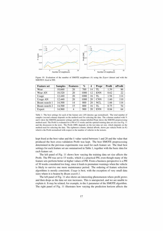
0.14

0.16

0.18

0.20

5 10 15 20Number of neighbours

F−

scor

e

51525

0.4

0.8

1.2

1.6

5 10 15 20Number of neighbours

Pro

fit [M

€]

51525

Figure 10: Evaluation of the number of SMOTE neighbours (k) using the Expert dataset and with theSMOTE% fixed at 900.

Feature set Samples Features % k Prepr Profit nProfitWear 10,660 20 700 14 TL 1.59 86Wear AN 10,520 20 1000 12 ENN 0.62 22Usage 12,440 20 1000 16 TL 1.94 114Usage AN 12,440 20 1000 20 CNN 1.60 110Beam search 1 14,500 14 800 20 NCL 1.66 116Beam search 2 14,500 15 800 16 TL 0.75 54Expert 14,960 4 900 20 ENN 0.84 64

Table 1: The best settings for each of the feature sets (AN denotes age normalised). The total number ofsamples (second column) depends on the method used for selecting the data. The columns marked with %and k show the SMOTE parameter settings and the column labelled Prepr shows the SMOTE preprocessingmethod used. The Profit is evaluated for a PH of 15 weeks and the optimal training data set size (see Fig. 11and the discussion in the text). The Profit (Me) depends on the test data set size, which depends on themethod used for selecting the data. The rightmost column, labeled nProfit, shows per vehicle Profit (in e)which is the Profit normalised with respect to the number of vehicles in the testsets.

kept fixed at the best value and the k value varied between 1 and 20 and the value thatproduced the best cross-validation Profit was kept. The best SMOTE preprocessingdetermined in the previous experiments was used for each feature set. The final bestsettings for each feature set are summarised in Table 1, together with the basic data foreach feature set.

The left panel of Fig. 11 shows how varying the training data set size affects theProfit. The PH was set to 15 weeks, which is a practical PH, even though many of thefeature sets perform better at higher values of PH. From a business perspective is a PHof 30 weeks considered too long, since it leads to premature warnings when the vehicleis likely to survive one more maintenance period. The ordering of feature selectionalgorithms is mostly consistent; Usage is best, with the exception of very small datasizes where it is beaten by Beam search 1.

The left panel of Fig. 11 also shows an interesting phenomenon where profit growsand then drops as the data set size increases. This is unexpected, and we are unable toexplain it. It may be related, for example, to the k parameter of the SMOTE algorithm.The right panel of Fig. 11 illustrates how varying the prediction horizon affects the

17

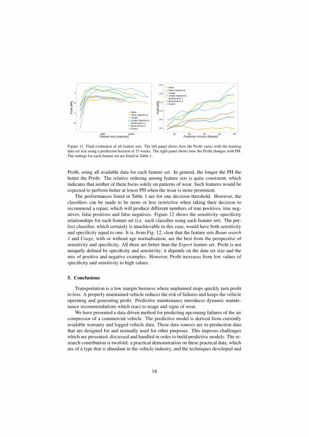
−2

−1

0

1

5000 10000Dataset size [readouts]

Pro

fit [M

€]

WearWear (AgeNorm)UsageUsage (AgeNorm)Beamsearch 1Beamsearch 2Expert 0.0

0.5

1.0

1.5

2.0

2.5

10 20 30 40 50Prediction Horizon [Weeks]

Pro

fit [M

€]

WearWear (AgeNorm)UsageUsage (AgeNorm)Beamsearch 1Beamsearch 2Expert

Figure 11: Final evaluation of all feature sets. The left panel shows how the Profit varies with the trainingdata set size using a prediction horizon of 15 weeks. The right panel shows how the Profit changes with PH.The settings for each feature set are listed in Table 1.

Profit, using all available data for each feature set. In general, the longer the PH thebetter the Profit. The relative ordering among feature sets is quite consistent, whichindicates that neither of them focus solely on patterns of wear. Such features would beexpected to perform better at lower PH when the wear is more prominent.

The performances listed in Table 1 are for one decision threshold. However, theclassifiers can be made to be more or less restrictive when taking their decision torecommend a repair, which will produce different numbers of true positives, true neg-atives, false positives and false negatives. Figure 12 shows the sensitivity–specificityrelationships for each feature set (i.e. each classifier using each feature set). The per-fect classifier, which certainly is unachievable in this case, would have both sensitivityand specificity equal to one. It is, from Fig. 12, clear that the feature sets Beam search1 and Usage, with or without age normalisation, are the best from the perspective ofsensitivity and specificity. All three are better than the Expert feature set. Profit is notuniquely defined by specificity and sensitivity; it depends on the data set size and themix of positive and negative examples. However, Profit increases from low values ofspecificity and sensitivity to high values.

5. Conclusions

Transportation is a low margin business where unplanned stops quickly turn profitto loss. A properly maintained vehicle reduces the risk of failures and keeps the vehicleoperating and generating profit. Predictive maintenance introduces dynamic mainte-nance recommendations which react to usage and signs of wear.

We have presented a data driven method for predicting upcoming failures of the aircompressor of a commercial vehicle. The predictive model is derived from currentlyavailable warranty and logged vehicle data. These data sources are in-production datathat are designed for and normally used for other purposes. This imposes challengeswhich are presented, discussed and handled in order to build predictive models. The re-search contribution is twofold: a practical demonstration on these practical data, whichare of a type that is abundant in the vehicle industry, and the techniques developed and

18

●

●

●

●

●

●

●

●●

●

●

●

●

●

●●●●

●

●

●

●

●

●

●●●

●

●

●

●

●

●●

●●

●

●

●

●

●

●●

●●

●

●

●

●

●

●●●●

●

●

●

●

●

●

●●●

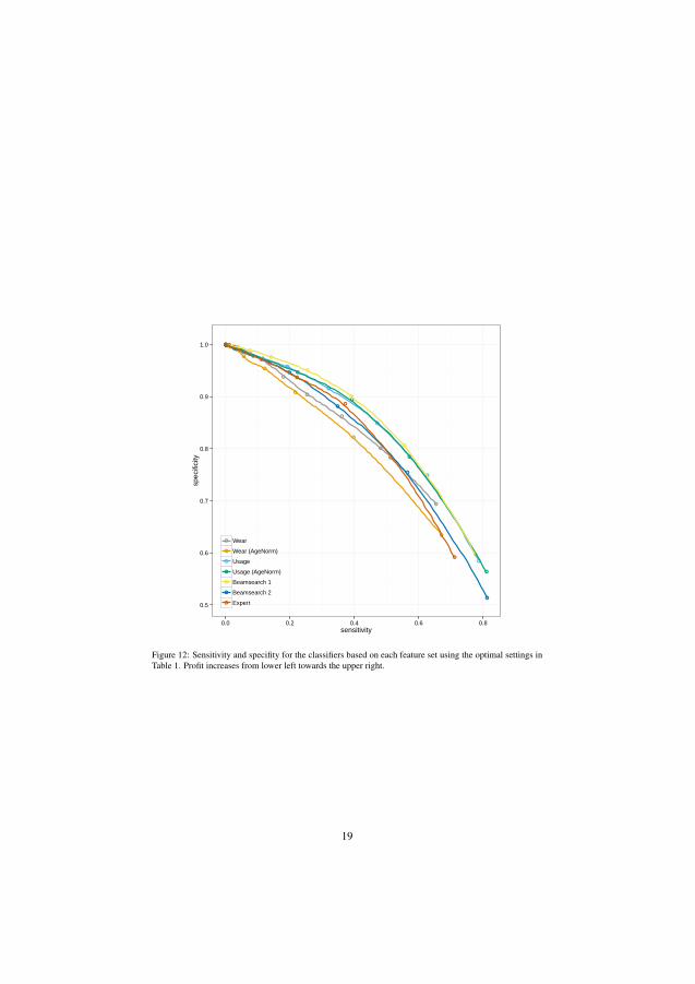
0.5

0.6

0.7

0.8

0.9

1.0

0.0 0.2 0.4 0.6 0.8sensitivity

spec

ifici

ty

●

●

●

●

●

●

●

Wear

Wear (AgeNorm)

Usage

Usage (AgeNorm)

Beamsearch 1

Beamsearch 2

Expert

Figure 12: Sensitivity and specifity for the classifiers based on each feature set using the optimal settings inTable 1. Profit increases from lower left towards the upper right.

19

tested to handle; feature selection with inconsistent data sets, imbalanced and noisyclass labels and multiple examples per vehicle.

The method generalises to repairs of various vehicle components but it is evaluatedon one component: the air compressor. The air compressor is a challenge since afailing air compressor can be due to many things and can be a secondary fault causedby other problems (e.g. oil leaks in the engine that cause coal deposits in the air pipes).Many fault modes are grouped into one label. Components with clearer or fewer faultcauses should be easier to predict, given that the information needed to predict them isavailable in the data sources, and given that the fault progresses slow enough. We havenot tested it on other components but plan to do so in the near future.

The best features are the Beam search 1 and the Usage sets, with or without agenormalisation. All three outperform the Expert feature set, which strengthens the argu-ments for using data driven machine learning algorithms within this domain. There isan interesting difference between the Wear and Usage feature sets. In the latter, there islittle effect of doing age normalisation while on the first the age normalisation removesa lot of the information. This indicates that important wear patterns are linked to age,which in turn is not particularly interesting since age is easily measured using mileageor engine hours. It is possible that trends due to wear are faster than what is detectablegiven the readout frequency. This could partly explain the low performance of the wearfeatures.

All feature sets show a positive Profit in the final evaluation. However, this dependson the estimated costs for planned and unplanned repair. There are large uncertaintiesin those numbers and one must view the profits from that perspective. The investmentcost can probably be neglected and the important factor is the ratio in cost betweenunplanned and planned repair.

Acknowledgment

The authors thank Vinnova (Swedish Governmental Agency for Innovation Sys-tems), AB Volvo, Halmstad University, and the Swedish Knowledge Foundation forfinancial support for doing this research.

20

, 2007. Knowledge and Information Systems 12.

Ahmed, M., Baqqar, M., Gu, F., Ball, A.D., 2012. Fault detection and diagnosis usingprincipal component analysis of vibration data from a reciprocating compressor, in:Proceedings of the UKACC International Conference on Control, 3-5 September2012, IEEE Press.

Batista, G.E.A.P.A., Prati, R.C., Monard, M.C., 2004. A study of the behavior of sev-eral methods for balancing machine learning training data. SIGKDD ExplorationsNewsletter 6, 20–29.

Bendix, 2004. Advanced Troubleshooting Guide for Air Brake Compressors. BendixCommercial Vehicle Systems LLC.

Bolon-Canedo, V., Sanchez-Marono, N., Alonso-Betanzos, A., 2013. A review offeature selection methods on synthetic data. Knowledge and Information Systems34, 483–519.

Breiman, L., 2001. Random forests. Machine Learning 45, 5–32.

Buddhakulsomsiri, J., Zakarian, A., 2009. Sequential pattern mining algorithm forautomotive warranty data. Computers & Industrial Engineering 57, 137–147.

Chawla, N.V., Bowyer, K.W., Hall, L.O., Kegelmeyer, W.P., 2002. SMOTE: Syntheticminority over-sampling technique. Journal of Artificial Intelligence Research 16,321–357.

Choudhary, A.K., Harding, J.A., Tiwari, M.K., 2009. Data mining in manufacturing:a review based on the kind of knowledge. Journal of Intelligent Manufacturing 20,501–521.

Dal Pozzolo, A., Caelen, O., Bontempi, G., . Comparison of balancing techniques forunbalanced datasets.

Fogelstrom, K.A., 2007 (filed 2006). Prognostic and diagnostic system for air brakes.

Frisk, E., Krysander, M., Larsson, E., 2014. Data-driven lead-acid battery prognosticsusing random survival forests, in: Proceedings of the 2:nd European Conference ofthe PHM Society (PHME14).

Guyon, I., Elisseeff, A., 2003. An introduction to variable and feature selection. Journalof Machine Learning Research 3, 1157–1182.

Guyon, I., Gunn, S., Nikravesh, M., Zadeh, L.A., 2006. Feature Extraction: Founda-tions and Applications (Studies in Fuzziness and Soft Computing). Springer-VerlagNew York, Inc.

Hazewinkel, M. (Ed.), 2001. Encyclopedia of Mathematics. Springer.

He, H., Garcia, E., 2009. Learning from imbalanced data. IEEE Transactions onKnowledge and Data Engineering 21, 1263–1284.

21

Hines, J., Garvey, D., Seibert, R., , Usynin, A., 2008a. Technical Review of On-LineMonitoring Techniques for Performance Assessment. Volume 2: Theoretical Issues.Technical review NUREG/CR-6895, Vol. 2. U.S. Nuclear Regulatory Commission,Office of Nuclear Regulatory Research. Washington, DC 20555-0001.

Hines, J., Garvey, J., Garvey, D.R., Seibert, R., 2008b. Technical Review of On-Line Monitoring Techniques for Performance Assessment. Volume 3: Limiting CaseStudies. Technical review NUREG/CR-6895, Vol. 3. U.S. Nuclear Regulatory Com-mission, Office of Nuclear Regulatory Research. Washington, DC 20555-0001.

Hines, J., Seibert, R., 2006. Technical Review of On-Line Monitoring Tech-niques for Performance Assessment. Volume 1: State-of-the-Art. Technical reviewNUREG/CR-6895. U.S. Nuclear Regulatory Commission, Office of Nuclear Regu-latory Research. Washington, DC 20555-0001.

Jardine, A.K., Lin, D., Banjevic, D., 2006. A review on machinery diagnostics andprognostics implementing condition-based maintenance. Mechanical Systems andSignal Processing 20, 1483–1510.

Jayanth, N., 2010 (filed 2006). Compressor protection and diagnostic system.

Liao, L., Kottig, F., 2014. Review of hybrid prognostics approaches for remaininguseful life prediction of engineered systems, and an application to battery life pre-diction. IEEE Transactions on Reliability 63, 191–207.

Ma, J., Jiang, J., 2011. Applications of fault detection and diagnosis methods in nuclearpower plants: A review. Progress in Nuclear Energy 53, 255–266.

Medina-Oliva, G., Voisin, A., Monnin, M., Leger, J.B., 2014. Predictive diagnosisbased on a fleet-wide ontology approach. Knowledge-Based Systems .

Molina, L., Belanche, L., Nebot, A., 2002. Feature selection algorithms: a survey andexperimental evaluation, in: Proceedings of IEEE International Conference on DataMining, pp. 306–313.

Napierala, K., Stefanowski, J., 2012. BRACID: a comprehensive approach to learningrules from imbalanced data. Journal of Intelligent Information Systems 39, 335–373.

Peng, Y., Dong, M., Zuo, M.J., 2010. Current status of machine prognostics incondition-based maintenance: a review. International Journal of Advanced Man-ufacturing Technology 50, 297–313.

Prytz, R., Nowaczyk, S., Rognvaldsson, T., Byttner, S., 2013. Analysis oftruck compressor failures based on logged vehicle data, in: Proceedings of the2013 International Conference on Data Mining (DMIN13). URL: http://worldcomp-proceedings.com/proc/p2013/DMI.html.

R Core Team, 2014. R: A Language and Environment for Statistical Computing.R Foundation for Statistical Computing. Vienna, Austria. URL: http://www.R-project.org.

22

Rajpathak, D.G., 2013. An ontology based text mining system for knowledge discoveryfrom the diagnosis data in the automotive domain. Computers in Industry 64, 565–580.

Reimer, M., 2013. Service Relationship Management – Driving Uptime in CommercialVehicle Maintenance and Repair. White paper. DECISIV.

Saeys, Y., Inza, I., Larraaga, P., 2007. A review of feature selection techniques inbioinformatics. Bioinformatics 23, 2507–2517.

Saxena, A., Celaya, J., Balaban, E., Goebel, K., Saha, B., Saha, S., Schwabacher, M.,2008. Metrics for evaluating performance of prognostic techniques, in: Proceedingsof the 2008 International Conference on Prognostics and Health Management, IEEEPress.

Schwabacher, M., 2005. A survey of data-driven prognostics, in: Infotech@Aerospace.

Si, X.S., Wang, W., Hu, C.H., Zhou, D.H., 2011. Remaining useful life estimation –a review on the statistical data driven approaches. European Journal of OperationalResearch 213, 1–14.

Sikorska, J.Z., Hodkiewicz, M., Ma, L., 2011. Prognostic modelling options for re-maining useful life estimation by industry. Mechanical Systems and Signal Process-ing 25, 1803–1836.

Sokolova, M., Japkowicz, N., Szpakowicz, S., 2006. Beyond accuracy, f-score andROC: A family of discriminant measures for performance evaluation, in: AI 2006:Advances in Artificial Intelligence. Springer Berlin Heidelberg. volume 4304 of Lec-ture Notes in Computer Science, pp. 1015–1021.

Sun, Y., Kamel, M.S., Wong, A.K., Wang, Y., 2007. Cost-sensitive boosting for classi-fication of imbalanced data. Pattern Recognition 40, 3358–3378.

Van Hulse, J., Khoshgoftaar, T.M., Napolitano, A., 2007. Experimental perspectives onlearning from imbalanced data, in: Proceedings of the 24th International Conferenceon Machine Learning, ACM, New York, NY, USA. pp. 935–942.

23