machine learning methods for rapid inspection of automated
TRANSCRIPT

University of South Carolina University of South Carolina
Scholar Commons Scholar Commons
Theses and Dissertations
Summer 2019
Machine Learning Methods for Rapid Inspection of Automated Machine Learning Methods for Rapid Inspection of Automated
Fiber Placement Manufactured Composite Structures Fiber Placement Manufactured Composite Structures
Christopher Sacco
Follow this and additional works at: https://scholarcommons.sc.edu/etd
Part of the Aerospace Engineering Commons
Recommended Citation Recommended Citation Sacco, C.(2019). Machine Learning Methods for Rapid Inspection of Automated Fiber Placement Manufactured Composite Structures. (Master's thesis). Retrieved from https://scholarcommons.sc.edu/etd/5475
This Open Access Thesis is brought to you by Scholar Commons. It has been accepted for inclusion in Theses and Dissertations by an authorized administrator of Scholar Commons. For more information, please contact [email protected].

Machine Learning Methods for Rapid Inspection of Automated Fiber Placement Manufactured Composite Structures
By
Christopher Sacco
Bachelor of Science
Presbyterian College, 2017
Submitted in Partial Fulfillment of the Requirements
For the Degree of Master of Science in
Aerospace Engineering
College of Engineering and Computing
University of South Carolina
2019
Accepted by:
Ramy Harik, Director of Thesis
Elizabeth Gregory, Reader
Zafer Gürdal, Reader
Cheryl L. Addy, Vice Provost and Dean of the Graduate School

ii
© Copyright by Christopher Sacco 2019 All Rights Reserved.

iii
ACKNOWLEDGEMENTS
I would be remised if I failed to thank the many individuals and groups that have allowed
me to participate in what has been an incredibly worthwhile period of research. Firstly, I
would like to thank my advisor, Dr. Ramy Harik, for his steadfast encouragement and
engaging instruction on this project. My project partner, Anis Baz Radwan, has likewise
contributed greatly to this research. I would like to acknowledge The Abnormal Corner.
Without their patient instruction in all manner of software development and coding, I
would not be to programmer and researcher I am today. My friend and sage advice giver,
Florentius-Johannes Van Zanten has been an excellent candidate for challenging
questions. My former mentors, Dr. Chad Rodekohr, Dr. Eli Owens, and Dr. Clinton
Harshaw were instrumental in forming my approach as a researcher and my experiences
under their instruction were beyond valuable. Lastly, the entirety of this project was
funded and supported through NASA under Award No. NNL09AA00A.

iv
ABSTRACT
The advanced manufacturing capabilities provided through the automated fiber
placement (AFP) system has allowed for faster layup time and more consistent
production across a number of different geometries. This contributes to the modern
production of large composite structures and the widespread adaptation of composites in
industry in general and aerospace in particular. However, the automation introduced in
this process increases the difficulty of quality assurance efforts and inspection. The AFP
process can induce a number of manufacturing defects including wrinkles, twists, gaps,
and overlaps. The manual identification of these defects is often laborious and requires a
measure of expert knowledge. A software package for the assistance of the inspection
process has been used in conjunction with automated inspection hardware for the
automated inspection, identification, and characterization of AFP manufacturing defects.
Image analysis algorithms were developed and demonstrated on a number of defect
types. Defects are identified in scan images and exact size and shape characteristics are
extracted for export.

v
TABLE OF CONTENTS
ACKNOWLEDGEMENTS ........................................................................................................ iii
ABSTRACT .......................................................................................................................... iv
LIST OF TABLES ................................................................................................................. vii
LIST OF FIGURES ............................................................................................................... viii
LIST OF EQUATIONS ...................................................................................................... x
LIST OF ABBREVIATIONS ............................................................................................ xi
CHAPTER 1 INTRODUCTION .................................................................................................. 1
1.1 PREAMBLE ............................................................................................................ 1
1.2 RESEARCH OBJECTIVE AND OUTLINE ................................................................... 3
CHAPTER 2 LITERATURE REVIEW ...................................................................................... 11
2.1 INTRODUCTION ................................................................................................... 11
2.2 MACHINE LEARNING ........................................................................................... 12
2.3 COMPOSITE MATERIAL INSPECTION TOOLS ......................................................... 21
2.4 ML IN INSPECTION .............................................................................................. 24
2.5 CONCLUSION ....................................................................................................... 27
CHAPTER 3 MACHINE LEARNING-BASED AFP INSPECTION ................................................. 29
3.1 INTRODUCTION ................................................................................................... 29
3.2 HARDWARE IMPLEMENTATION ............................................................................ 30
3.3 ML ALOGRITHM .................................................................................................. 32
3.4 DATA TRANSFER AND COMMUNICATION ............................................................. 44
3.5 OPERATOR INTEGRATION .................................................................................... 48

vi
CHAPTER 4 INSPECTION TRIALS ......................................................................................... 55
4.1 EXPERIMENTAL PROCEEDURE ............................................................................. 55
4.2 RESULTS ............................................................................................................. 60
4.3 NOTES ................................................................................................................ 67
CHAPTER 5 CONCLUSION ................................................................................................... 69
5.1 AN OVERVIEW OF WORK ..................................................................................... 69
5.2 A BRIEF REMARK ON ML IMAGE ANALYSIS .......................................................... 70
5.3 INSPECTION AS THE CENTERPIECE OF MODERN MANUFACTURING ..................... 71
5.4 A LONG TERM OUTLOOK ON THE INSPECTION SYSTEM ....................................... 73
5.5 FUTURE WORK .................................................................................................... 74
5.6 SITUATION OF RESEARCH .................................................................................... 79
REFERENCES ...................................................................................................................... 81

vii
LIST OF TABLES
Table 1.1: A list of common AFP Defects in (Harik et al. 2018) ....................................... 8
Table 2.1: Some ML Algorithms and Their Respective Objectives ................................. 15
Table 2.2: ML Types and Common Tasks........................................................................ 20
Table 3.1: A List of Optimization Choices for Each Hyperparameter ............................. 39
Table 3.2: GA Algorithm Parameters ............................................................................... 39
Table 3.3: Color codes for defect types ............................................................................ 42
Table 3.4: A List of Functions Demonstrated in Figure 3.15 and Figure 3.16 ................. 49
Table 4.1: Performance Metrics for Defect Network Evaluation ..................................... 66
Table 4.2: End Accuracies across Major Defects ............................................................. 67

viii
LIST OF FIGURES
Figure 1.1: A Representative Element of an FRP ............................................................... 4
Figure 1.2: An Autoclave Used for Curing FRP Prepreg ................................................... 5
Figure 1.3: NASA ISAAC AFP Machine (Harik et al. 2019) ............................................ 6
Figure 1.4: An RGB Image of a Composite Part ................................................................ 9
Figure 2.1: A schematic of a basic neural network ........................................................... 13
Figure 2.2: A Demonstration of Computations within a Single Neural Network Node ... 14
Figure 2.3: Machine Learning Comparison to Traditional Modeling Methods................ 18
Figure 2.4: Thermography Data from CFRP Part (Sert, Tas, and Alkan 2015) ............... 22
Figure 2.5: Ultrasonic Inspection Scans from Meng et al. (Meng et al. 2017) ................. 24
Figure 3.1: An Inspection-Enabled AFP System by (Bahamonde Jácome et al. 2018) ... 29
Figure 3.2: Keyence LJ-7080 Profilometers ..................................................................... 30
Figure 3.3: IMT ACSIS Inspection Platform .................................................................... 31
Figure 3.4: Operations of a Convolutional Layer ............................................................. 33
Figure 3.5: A Schematic of a CNN ................................................................................... 34
Figure 3.6: A Basic FCN Structure ................................................................................... 34
Figure 3.7: ResNet Skip Block ......................................................................................... 36
Figure 3.8: A Diagram of the Final Network Structure .................................................... 37
Figure 3.9: Examples of Labeled Training Data ............................................................... 41
Figure 3.10: A Demonstration of the Data Augmentation Scheme .................................. 43
Figure 3.11: Defect Server Platform Independence .......................................................... 45

ix
Figure 3.12: Raspberry Pi 3 b+ ......................................................................................... 45
Figure 3.13: Defect Data Structure ................................................................................... 47
Figure 3.14: Defect Characteristics from Pixel Data to Position and Classes .................. 47
Figure 3.15: Inspection System Operator User Interface (1) ............................................ 50
Figure 3.16: Operator User Interface (2) .......................................................................... 51
Figure 3.17: Operator Defined Defect Demonstration ..................................................... 51
Figure 3.18: A misidentified defect being corrected ........................................................ 52
Figure 3.19: Retraining Scheme ....................................................................................... 53
Figure 4.1: ICPS model of cylinder .................................................................................. 56
Figure 4.2: Inspection Testing Platform ........................................................................... 58
Figure 4.3: Platform Tooling Holes .................................................................................. 59
Figure 4.4: Scan of a Validation Part ................................................................................ 59
Figure 4.5: Identification on the Cylinder with Correction through Manual Tagging ..... 61
Figure 4.6: Defect Placement on Test Article ................................................................... 62
Figure 4.7: Functional Checkout Test Article ................................................................... 63
Figure 4.8: Identification of a Twist on Test Article ........................................................ 64
Figure 4.9: Identification of Defects on Test Article ........................................................ 65
Figure 4.10: The Confusion Matrix over Testing Set Defects .......................................... 66
Figure 5.1: Changes Required for Online Inspection Concept ......................................... 76
Figure 5.2: In-Situ Analysis using 1D Convolutions ........................................................ 77

x
LIST OF EQUATIONS
Equation 2.1: The Output from a Single Neuron .............................................................. 13 Equation 2.2: Sigmoid Activation Function ..................................................................... 13 Equation 2.3: ReLU Activation Function ......................................................................... 14 Equation 2.4: ELU Activation Function ........................................................................... 14
Equation 2.5: A general representation of an ML model as a function given a parameter set ...................................................................................................................................... 16 Equation 2.6: Evaluation of Gradients in with Respect to Model Parameters.................. 17 Equation 2.7: A Gradient-Based Parameter Update Rule ................................................. 17

xi
LIST OF ABBREVIATIONS
ACSIS…………………………………Advanced Composite Structure Inspection System
AFP…………………………………………………………...Automated Fiber Placement
ANN…………………………………………………………….Artificial Neural Network
BO………………………………………………………………….Bayesian Optimization
CFRP…………………………………………………...Carbon Fiber Reinforced Polymer
CNN……………………………………………………….Convolutional Neural Network
ECT…………………………………………………………………Eddie Current Testing
ELU……………………………………………………………….Exponential Linear Unit
FCN…………………………………………………………Fully Convolutional Network
FPGA……………………………………………………..Field Programmable Gate Array
FRP……………………………………………………………...Fiber Reinforced Polymer
GA………………………………………………………………………Genetic Algorithm
GFRP……………………………………………………..Glass Fiber Reinforced Polymer
GP……………………………………………………………….......Genetic Programming
GPU…………………………………………………………….Graphical Processing Unit
IMT……………………………………………………………….Ingersoll Machine Tools
JSON…………………………………………………………...JavaScript Object Notation
ML………………………………………………………………………Machine Learning
NDT………………………………………………………………Non-Destructive Testing
PSO…………………………………………………………..Particle Swarm Optimization

xii
SVM……………………………………………………………...Support Vector Machine
ReLU…………………………………………………………………Rectified Linear Unit
RTM………………………………………………………………Resin Transfer Molding
UI…………………………………………………………………………….User Interface
VARTM………………………………………..Vacuum Assisted Resin Transfer Molding

1
CHAPTER 1
INTRODUCTION
1.1 PREAMBLE
For the greater portion of engineering problems, analytic or closely approximating
solutions are both available and widely known. However, in those cases that are opaque
and not easily represented by derived formulae, finely tuned probabilistic or empiric
models, or crafted and precise algorithmic solutions, machine learning represents a clear
and successful option by representation through data. ML is able to infer models from
data in a way that few other tools are capable of. In the modern manufacturing
environment, this capability could prove invaluable as manufacturing moves to the digital
era with the adoption of Industry 4.0 concepts such as Internet of Things (IoT), Smart
Manufacturing and Virtual Manufacturing concepts. Trends towards Big Data mean that
developing insights from data is quickly becoming a key driver in every industry. There
are many indications that ML can quickly leverage this data in a constructive, and
informative manner (Cheng et al. 2018). (Kampker et al. 2018) identifies quality control,
reduction of test-timing and calibration, improving yield, and learning of processes as
relevant use cases of data in a modern manufacturing environment.
When considering the problem of determining manufacturing quality, the concept
of a hard-coded solution for determination can be a near impossible task. Suppose that
the reader was attempting to deduce a physical model or representation for the

2
identification of a defect in an image. One might consider thresholding the image,
searching for greyscale variations such as darker and lighter regions. The question then
becomes: What is the threshold? Then one may consider taking a feature such as size or
shape and building a model from this. Which shape corresponds to which defect? What
size can we expect a particular defect to exhibit itself as? These are not easy questions to
answer, and any attempt to process a large number of features through hard-coded
solutions will only result in the creation of a model that at best will be over-constrained,
and thus inaccurate, or wildly complicated and slow.
The necessary solution is capable of accounting for the soft boundaries that exist
between both different types of quality issues and their many presentations across a part.
The ability to hard-code this capability is limited, and subject to both expert judgement
error and maintenance issues. A possibly better solution uses machine learning
algorithms for the general detection and characterization of manufacturing imperfections
and quality control issues. The soft boundaries mentioned above have an attainable
solution if one looks from a deterministic model, to a statistical model that is informed
through data. In other words, ML is a prime candidate for manufacturing variance
assessment, particularly defects in the context of Automated Fiber Placement (AFP), as
well as other computer vision tasks.
This document includes a thorough outline of the use of machine learning in
computer vision tasks relevant to composites manufacturing, beginning with a number of
basic ML algorithms, and moving towards specifically the task of AFP defect detection.
In the process, research and conclusions around various difficulties surrounding a
comprehensive AFP inspection system will be presented.

3
For the continuation of this chapter presents an outline of the principal research
objective and some arguments for the validity of an ML solution.
1.2 RESEARCH OBJECTIVE AND OUTLINE
1.2.1 Composite Materials
Composite materials can be described as any non-homogeneous material that is
designed with the intention of creating a part with mechanical properties that can be
defined as non-isotropic. This can be further elaborated on by noting that composite
materials have properties dependent on direction through the material: this is referred to
as directional properties. Rather than the standard 3 material parameters denoted in an
isotropic material, composites can have as much as 22 independent material responses.
In most modern settings, particularly in the aerospace industry, advanced
composite materials refer specifically to fiber reinforced polymers (FRP). For the
construction of most aerospace structures, carbon fiber reinforced polymers (CFRP)
constitute the material of choice. For the rest of this document, the usage of the term
composite materials is equated with these FRPs. Composites principally are constituted
of a fiber material, a matrix material, and an interphase representing the boundary
between the two [Figure 1.1]. In the case of this work, fiber can be either a glass material
or carbon fiber. Matrix materials can vary with application, however common matrix
materials include epoxy resins and vinyl ester resins.
Composite materials offer a number of distinct advantages over isotropic
materials. Firstly, the material properties and load responses of a composite can be
tailored to precisely fit the application for which they are being used. This implies a more
customizable structure, and thus represents great potential for weight reduction. The use

4
of polymer resins and carbon fiber offers a level of corrosion resistance not possible in
most unaltered structural metals1. Composites are also capable of redistributing various
forms of damage in the ply direction, such as fiber breakages, by allowing matrix
properties to distribute stress to other fibers and in the matrix itself.
The multi-scale constitution of composite materials implies that manufacturing is
often a more complex process than isotropic materials such as metals. Composites require
fiber to be cured within a matrix material that both supports the fiber and protects it from
short term environmental effects.
Figure 1.1: A Representative Element of an FRP
Manufacturing of composites varies with the application. Simple open-air heat
curing in a hot press, while initially a popular technique, has given way to more
sophisticated and effective methods. Resin Transfer Moulding (RTM), and its modern
equivalent, Vacuum Assisted Resin Transfer Moulding (VARTM) infuse dry fiber with
1 However, composite materials can have their stress states affected by moisture content both pre and post cure

5
resin to impregnate the composite. If a material has been impregnated with resin, and
then cured to a transitional state where the composite remains tacky and flexible, the
composite is known as a prepreg. The latter is shaped into the final part, and then cured
completely. Curing can take place under varying conditions, including at room
temperature. The most common curing apparatus for aerospace-grade components is a
pressurized heating vessel known as an autoclave [Figure 1.2].
Figure 1.2: An Autoclave Used for Curing FRP Prepreg
A key problem with the manufacturing processes of composites mentioned above
is the limited size of parts and the need to have each layup accomplished by hand. While
this can be advantageous for limited, custom parts, industrial manufacturing of large
structures requires a greater measure of repeatability and an increase in speed.

6
1.2.2 Automated Fiber Placement
The extension of composite structures from small, custom built parts to large
consumer ready components has been aided by the development of advanced
manufacturing techniques. Principally in the aerospace industry, the use of AFP
manufacturing has enabled the manufacturing of large structural sections of aircraft. This
additional manufacturing capability has established itself as a useful tool in the aerospace
manufacturing domain.
Figure 1.3: NASA ISAAC AFP Machine (Harik et al. 2019)
AFP is enabled by the rapid movement and replicability provided by robotic
placement of collections of composite material tows, denoted as courses. These courses
are placed on a tooling surface in an additive process that builds up a complete composite
part over a number of placement passes across the tool. The part is then prepared and
cured on the tool or on a representative geometry. AFP has the capacity to run a wide

7
range of materials from thermoset to thermoplastics and dry fiber. The versatility comes
with an additional set of processing parameters that must be matched to each individual
material2. Robotic placement greatly improves the speed of layup over traditional hand-
layup techniques. In addition, the consistency of placement guarantees the error between
the intended and actual fiber angle will be far smaller than with hand layup.
The additional accuracy afforded through the AFP process has led to greater
functionality of design, and thus sped adoption of advanced composite materials in a
number of fields, primarily aerospace, but also the automotive, energy, maritime,
biomedical and sports sectors.
1.2.3 AFP Defects
However, the additional throughput and automation of the manufacturing process
inevitably leads to a lack of control in instances of imprecise manufacturing. To
compensate laborious hand inspection is used to identify the production of common
manufacturing and material related defects. Cemenska et al. notes that up to 20% of AFP
manufacturing time can be occupied by manual inspection (Cemenska, Rudberg, and
Henscheid 2015). Harik et al. identifies a number of manufacturing defects common to
the AFP process(Harik et al. 2018). The significance of each of these defects varies. Each
has unique characteristics in either appearance, creation mechanism, or effects on the
strength of the overall structure. Table 1.1 gives a description and attributed cause of
several common AFP defects.
2 These include compaction pressure, heating temperature, tow tension, and head speed.

8
Table 1.1: A list of common AFP Defects in (Harik et al. 2018)
Defect Description Cause
Gap Unoccupied space between
tows
Steering errors or layup on
a complex tool
Overlap Placement of a tow onto an
adjacent tow
Steering errors or layup on
a complex tool
Wrinkle Wavy pattern at the
boundaries of a tow
resulting on only partial
tool contact
Small steering radius;
Overfeeding material
Twist A tow rolled axially 180 on
itself and then compacted
by the roller
Friction between guide
holes or overly tacky tows;
Fold propagation
Missing Tow An entire tow falls off the
tool or is never applied
Material feed error;
Adhesion problems
Splice Two tows are joined end-
to-end so that they overlap
Result of finite length slit
tape for forming tows
Pucker Lifting up of a tow from
the tool surface along the
tow width
Overfeeding material;
Machine error

9
1.2.4 Problems with Traditional Imaging
The material anisotropy of composite materials begets a corresponding anisotropy
in electromagnetic properties. Electromagnetic anisotropy implies a corresponding series
of optical properties that would make traditional optical imaging nearly impractical.
Considering the low-contrast nature of composite parts, even close visual inspection may
lack fine resolution on defects beyond traditional large imperfects such as missing tows.
Figure 1.4 show these types of flaws. There are a number of hand-placed defects present
in the image. Determination of the location, size, or even type of defects that are present
is difficult at best.
Figure 1.4: An RGB Image of a Composite Part
Considering data capture through a visible-light spectrum camera, any analysis
algorithm that may be of use in defect identification may struggle to differentiate between
defects and the background reference surface. When considering the labelling required in
the generation of a viable training dataset, the problem becomes apparent. Thus, for
Overlap
Overlap
Overlap
Gap

10
automated AFP inspection systems to have any potential at success, one must look
beyond the visible spectrum when considering the sensing hardware to be used.
1.2.5 Overview of Study
AFP manufacturing defects pose a unique challenge in their inspection. The
principal methodology presented in the aerospace industry, manual inspection, has
several significant drawbacks. Thus, the integration of an inspection system with the
capacity to automatically classify and characterize manufacturing defects is a relevant
and worthwhile scientific endeavour.
In Chapter 2 presents a comprehensive literature review as an overview of the
composite material inspection field with special consideration for the application of
machine learning. This chapter also includes a major survey of the key concepts in the
machine learning and image processing fields. Chapter 3 gives a comprehensive
examination of the AFP inspection solution and the algorithms used for image processing
and integration within the larger manufacturing setting. Chapter 4 presents the results of
several experiments with the system and gives a quantitative analysis of algorithm
accuracy as well as demonstrations of the functional inspection process. Chapter 5 serves
as a conclusion with a look towards future work on the subject.
11
CHAPTER 2
LITERATURE REVIEW
2.1 INTRODUCTION
The general state of composite inspection systems hinges on the creation of two
separate systems: (1) Scanning systems principally composed of imaging hardware and
(2) Analysis software attempting to perform defect detection from features identified in
the scanning process. Automated analysis is includes hard-coded solutions, such as
generative or variant approaches, and machine learning approaches. While the hard-
coded software does not have a great deal of statistical dependence and has a high
interpretability, they often are challenged to account for the broad range of feature
variations in an image and typically fail to identify outliers or untypical findings. Thus, in
many of the popular image classification challenges, manual feature extraction and object
identification are not widely used in favour of machine learning techniques (Mishkin,
Sergievskiy, and Matas 2017). Machine learning solutions have a number of distinct
advantages. Firstly, ML has the capability to perform automated feature extraction,
eliminating the need for feature or knowledge-based engineering. ML can also model the
soft boundaries that often exist between classes, eliminating the potential for
misclassification due to tight tolerances defined in the manual computer vision
algorithms.
The combination of analysis algorithms and scanning hardware has a great deal of
influence on the type and frequency of defects that can be detected. Consider that certain

12
algorithms may perform better within the context of noisy data, or that sub-surface
defects are only capable of being captured with a limited number of inspection hardware
approaches. These considerations imply that in the creation of an AFP inspection system,
a thorough consideration of previous attempts in automated composite inspection, both
software and hardware, must be fully taken into account.
2.2 MACHINE LEARNING
2.2.1 Algorithms and Techniques
Machine learning is a set of processes and their respective algorithms that
automatically create relationships between sets of data. These algorithms can be extended
for use on classification tasks, clustering, and even image and signal processing.
Algorithms such as Artificial Neural Networks (ANN) (Jain, Mao, and Mohiuddin 1996;
Schmidhuber 2015), [Figure 2.1] and Support Vector Machines (SVM) (Cortes and
Vapnik 1995) have allowed greater generalization of tasks. Particularly in industry,
supervised learning processes are utilized to develop accurate and high generalization
systems. The latter are then trained on a set of input data and are expected to produce a
desired output when shown a similar data sample. The great advantage of machine
learning systems is that they can take highly dynamic and non-linear data sets spread
among a large number of features and find relations between inputs and desired outputs.
Hornik et al. showed that multilayer networks are capable of approximating any non-
linear function given enough hidden layers(Hornik, Stinchcombe, and White 1989).

13
Figure 2.1: A schematic of a basic neural network
Nerual Networks consist of general computing nodes that sum the inputs into the
nodes, pass the summation into a function, A, known as the activation funciton, to skew
the output, and then passes that output onto other nodes using a weight, w, to scale the
output [Figure 2.2]. Ocassionally an additional term know as a bias, b, will be added into
the input. In general, a single neuron of a Neural Network can be expressed in Equation
2.1. We can note that in the case where A is the unit function or provides a linear output,
then the neruon reduces to a linear regression model. Commonly, activation functions
avoid learization of outputs and seek to either scale or gate outputs. Popular activation
functions include Sigmoid [Equation 2.2], ReLU [Equation 2.3], and ELU functions
[Equation 2.4].
�� = � �� ����� + ���
Equation 2.1: The Output from a Single Neuron
�������(�) = 1
1 + ���
Equation 2.2: Sigmoid Activation Function

14
����(�) = �� ≤ 0 �ℎ�� 0
� > 0 �ℎ�� �� �ℎ��� � ∈ �
Equation 2.3: ReLU Activation Function
���(�) = �� ≤ 0 �ℎ�� �(exp(�) − 1)
� > 0 �ℎ�� ��ℎ��� � ∈ �
Equation 2.4: ELU Activation Function
Figure 2.2: A Demonstration of Computations within a Single Neural Network Node
In addition to the techniques listed above, algorithms such as the Single Hidden-
Layer Feedforward Neural Network Extreme Learning Machine (ELM) (Huang, Zhu, and
Siew 2006) , k-Nearest Neighbor (KNN) (Zhang and Zhou 2007), and decision trees have

15
also found acceptance as useful tools in the ML community. Each respective algorithm
has specific tasks for which it was constructed [Table 2.1].
Table 2.1: Some ML Algorithms and Their Respective Objectives
There are two common techniques by which ML algorithms are trained on data:
(1) supervised learning and (2) unsupervised learning. Supervised learning implies that
the ML model infers relational information through minimizing the difference between
labeled training data and network predictions. If an algorithm were to be trained to
classify pictures, an input picture would be given to the algorithm, which would make a
prediction. This prediction would be then compared to a true labeling of the image, and
the properties of the algorithm would be updated to correct the errors of the initial
prediction. In ANNs, this is usually accomplished through a gradient descent approach
Algorithm Task
KNN Classification, Regression
SVM Classification
Neural Nets Classification, Regression
Principle Component Analysis Dimensionality Reduction
Self-Organizing Map Clustering
ELM Classification, Regression
Naïve Bayes Classification, Probability Density
Maximum Likelihood Estimation Probability Density
K-Means Clustering

16
with using the backpropagation algorithm. Unsupervised learning implies that the ML
algorithm is allowed to explore a solution space until a generalized solution is reached.
This idea is connected to a number of ML tasks including reinforcement learning and
autoencoders. As a result of data labeling often being the most intensive portion of
creating a machine learning model, unsupervised learning has become an area of
enormous potential and could allow for the development of true online learning systems.
Each ML algorithm is attempting to create a model for the mapping of an input
vector I to an output vector o according to a list of model parameters θ such that
� = �(�|�)
Equation 2.5: A general representation of an ML model as a function given a parameter set
In non-parametric learning models, such as KNN, these parameters are intrinsic to
characteristics of data itself. Thus, the concept of "training", or using data to infer θ, is
simply a matter of adding additional data to the model. In these cases, the interpretation
of the model is typically straightforward, however the need to observe the properties of
each data instance can be both computationally and memory intensive.
In algorithms such as Neural Networks, the goal is to explicitly model a
probability distribution without knowing any of the priors. Thus, updating the parameters
of these models becomes an exercise in defining the error E between the observed target
distribution r and the distribution output from the model y. The latter has a fundamental
dependence on model parameters, and thus it is possible to define E in terms of θ. In
order to find the change in θ for the optimal model, one may simply observe the error

17
gradient from each training instance between targets and outputs in terms of θ [Equation
2.6].
�� = ���
��
Equation 2.6: Evaluation of Gradients in with Respect to Model Parameters
Where the total update for model parameters for the sequential step s becomes
�(� + 1) = �(�) + ��
Equation 2.7: A Gradient-Based Parameter Update Rule
Where η is the learning rate, or the size of step that is taken over the gradient in moving
towards the optimum. This technique is known as gradient descent. η does not need to be
a constant. Several variations of the algorithm have been developed to allow for an
adaptable η. These included Adagrad (Duchi, Hazan, and Singer 2011), ADADELTA
(for Computing Machinery et al. 2015), and AMSgrad (Reddi, Kale, and Kumar 2018)
algorithms.
In the case of non-differentiable evaluation functions, different update rules must be
derived. For Decision Trees, impurity measures are used to determine model complexity
and parameters.

18
Figure 2.3: Machine Learning Comparison to Traditional Modeling Methods
2.2.2 ML Objectives
ML can be used for a number of tasks. Firstly, classification has become an area
where ML has begun to dramatically change what is possible in industry. With the advent
of AlexNet in 2012 (Krizhevsky, Sutskever, and Hinton 2012), image classification
accuracy was improved to a point where it began to rival human testers in some tasks.
Classification can also be viewed as a subset of interpolation and extrapolation.
Therefore, regression similarly falls under the domain of potential ML applications. Thus,
as the reader will discover in later sections, ML can be utilized as a powerful tool for
generating additional data points without having to rely on laborious computations.
In addition to classification, representation has become a unique field that ML has
begun to broach in recent years. A Generative Adversarial Network (GAN) is a
remarkable training structure that has the capacity to produce a representation of most
datasets. In the computer vision field, GANs have been used to generate entirely new and
19
unique data that can show complex scenes (Goodfellow et al. 2014). In doing this, GANs
learn a number of low level features that can either be used as a pre-training phase for a
classification network or leveraged for understanding the key feature components of data
through feature extraction. Autoencoders (Wang and Gu 2018), a neural network
structure that embeds semi-semantic meaning of a data instance into a low-dimensional
latent space, also has application to representation. By providing inputs directly into the
latent space, one can render new original examples in the original feature space the
autoencoder was trained on.
Clustering is another task that ML can have direct application to. Neural network
strategies such as the self-organizing map (Kohonen 1998) can accomplish clustering in
an unsupervised learning task. The K-Means algorithm (Meng et al. 2018) can be utilized
as a clustering algorithm that is non-parametric.
Reinforcement learning is one of the oldest subsets of ML. Conceptually, a
network is trained to maximize a reward generated through making decisions in an
environment. This demonstrates reinforcement learning as an optimization algorithm,
capable of developing policies that generate the largest rewards possible. This structure
has been used to learn complex tasks; occasionally in a beyond human capacity
(Kaelbling, Littman, and Moore 1996; Ou, Chang, and Chakraborty 2019; Riedmiller et
al. 2018). While playing the Atari 2600 games referenced in (Zhan, Ammar, and Taylor
2016) at a grandmaster level is an interesting way to prove the viability of reinforcement
learning based task solving, one can clearly see its application in any general setting
involving choice-based optimization. There are a number of interesting attempts to

20
integrate reinforcement learning into scheduling and intelligent control of machines (Xia
et al. 2019).
Table 2.2: ML Types and Common Tasks
Supervised Learning Unsupervised Learning Reinforcement
Learning
Classification
Regression
Clustering
Dimensionality
Reduction
Decisions Under
Uncertainty
2.2.3 Notes on Hardware Implementation
One of the developments that has most recently allowed ML to come to the
forefront of data analysis is the development or incorporation of dedicated hardware into
ML training and operation. The Graphical Processing Unit (GPU) has become a notable
addition to the ML researcher’s toolkit in recent years. It allows for faster training and
operation on increasingly broad ranges of data (Franco and Bacardit 2016; Krawczyk
2016). This stems from the ease with which the common matrix algebra in ML is run in
parallel on GPU. Another hardware implementation of ML that has recently gained
traction is the Field-programmable Gate Array (FPGA). The latter are effectively
programmable silicon, allowing for individual logic gates to be moved in such a manner
that the ML architecture is physically embedded on the circuit. They have a number of
advantages in ML implementation including faster operating speed and lower power
consumption (Liang et al. 2018; Ma et al. 2018; Posewsky and Ziener 2018).

21
2.2.4 Other Artificial Intelligence Techniques
There are a number of noted statistical optimization techniques adjacent to the
ML field that are worth mentioning. Often, these techniques include a number of
properties that are distinct from pure ML, but the underlying concept of creating system
models from pure data is shared between the two methods. One of the most widely used
class of algorithms exhibiting this behavior are the evolutionary approaches. Genetic
Algorithms (Lee 2018; Tian et al. 2018; Venugopal and Narendran 1992) and Genetic
Programming (Angeline 2003; Koza 2002; Poli and Koza 2014; Safiyullah et al. 2018)
can yield complex structure through a mixing of solution properties that mimics
biological evolution. Other heuristic statistical problem solving techniques include
Particle Swarm Optimization (Chopard and Tomassini 2018; Eberhart and Yuhui Shi
2002; de Oliveira et al. 2018; Poli, Kennedy, and Blackwell 2007; Shi and Eberhart
1999), similarly mimics biological systems by simulating the behavior of flocking
animals.
2.3 COMPOSITE MATERIAL INSPECTION TOOLS
Due to their low contrast, the imaging of composite materials for defects has
proved difficult in the past. Surface and subsurface defects manifest in a number of ways,
and thus finding methods for imaging analysis must be equally as broad. Generally,
conventional visual spectrum images are not viable as an inspection technology. The low
contrast, particularly of carbon composites, makes feature identification challenging.
However, laser profiling, thermal imaging, eddy current inspection, and a number of
other additional non-conventional imaging techniques have had great success in the non-
destructive testing (NDT) process.

22
Thermographic-based composite inspection begins with the excitation of material
through a heat source. This is typically accomplished through the use of a halogen lamp,
however LED heat sources have also been used (Pickering et al. 2013). The propagation
of heat through a structure is almost entirely dependent on material properties, and thus
where those properties have changed due to damage3 heat transfer will occur differently
from the background material. As this transfer is taking place, thermal cameras capture
the differences and produce an image of the structure under inspection. Two variations of
the thermographic techniques are lock-in and long pulse thermography. Lock-in implies
that detection and excitation are happening simultaneously in a pulsed pattern, which
results in higher quality IR images (Jorge Aldave et al. 2013). Long pulse thermography
involves the extended excitation of the structure, which can be useful in poorly
conducting materials such as composites (Kalyanavalli, Ramadhas, and Sastikumar
2018). (Caminero et al. 2018) notes that thermography struggles in identifying deep
subsurface defects or defects across complex geometries.
Figure 2.4: Thermography Data from CFRP Part (Sert, Tas, and Alkan 2015)
3 Such as the production of voids or delaminations.
23
(Moustakidis et al. 2016) uses three infrared cameras operating at different
wavelengths to create a complete scan of a composite aircraft structure. (Chrysafi,
Athanasopoulos, and Siakavellas 2017) examines a number of advanced image
processing techniques to improve the inspection of a composite plate with hand-placed
cracks. (Wu, Sfarra, and Yao 2018) demonstrates the use of Sparse Principle Component
Analysis in Thermography for the structural health monitoring of a CFRP plate with
induced defects.
Profilometry is another popular NDT technique most often utilized in the 3-
dimensional rendering of a surface. A laser pattern is projected down onto a surface,
through which surface features are inferred from deviations in the pattern (Hu and
Haifeng 2011). The advantage of profilometry is the rapid profiling of a surface without
the need to take surface contrast into account. However, (Christopher Sacco et al. 2018)
observes that material type in AFP inspection can have a direct effect on data loss and
artifact production. Ultrasonic inspection has become a leading NDT technique in
composite materials. Ultrasonic project sound waves into a test article and look for
inference patterns in either the return echo4 or the sound waves propagated through to the
other side of the structure5 (Wronkowicz, Dragan, and Lis 2018). There are a number of
parameters that can affect both the resolution and penetration depth of an ultrasonic
signal such as frequency (Jolly et al. 2015).
4 Known as Pulsed Echo Technique 5 Known as Through Transmission Technique
24
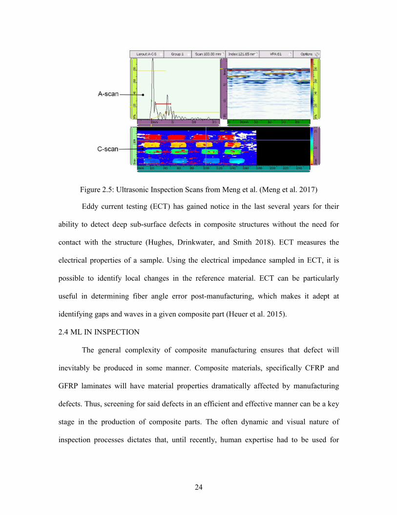
Figure 2.5: Ultrasonic Inspection Scans from Meng et al. (Meng et al. 2017)
Eddy current testing (ECT) has gained notice in the last several years for their
ability to detect deep sub-surface defects in composite structures without the need for
contact with the structure (Hughes, Drinkwater, and Smith 2018). ECT measures the
electrical properties of a sample. Using the electrical impedance sampled in ECT, it is
possible to identify local changes in the reference material. ECT can be particularly
useful in determining fiber angle error post-manufacturing, which makes it adept at
identifying gaps and waves in a given composite part (Heuer et al. 2015).
2.4 ML IN INSPECTION
The general complexity of composite manufacturing ensures that defect will
inevitably be produced in some manner. Composite materials, specifically CFRP and
GFRP laminates will have material properties dramatically affected by manufacturing
defects. Thus, screening for said defects in an efficient and effective manner can be a key
stage in the production of composite parts. The often dynamic and visual nature of
inspection processes dictates that, until recently, human expertise had to be used for
25
accurate results (Sharp, Ak, and Hedberg 2018). Thus, a number of studies have
leveraged machine learning to perform various inspection tasks on composites.
(Kuhl, Wiener, and Krauß 2013) proposes a system by which several sensor
systems are integrated with ML algorithms to detect defects resulting from the drilling of
carbon fiber composites for aircraft wing assemblies. A three step process of data
collection, feature extraction, and data analysis was constructed. Optical and thermal
systems were used for the inspection process, but the author makes note that a host of
additional sensors such as eddy current sensors could be added. (Cacciola et al. 2008) use
SVM to predict 4 defect types in ultrasonic inspection.
(Brüning et al. 2017) shows how feature extraction from thermographic
inspection and processed through an ML algorithm can be used for process parameter
optimization. (Benítez et al. 2009) examined the identification and characterization of
defects in both a flat and curved CFRP laminate using reference free thermal contrast.
They used three ML models: Multi-layer Perceptron (MLP), SVM, and Radial Basis
Function Networks. Patch classification was performed to segment the entire
thermographic image into its defect and non-defect components.
(D’Angelo and Rampone 2016) looks at using ML methods for the classification
of defects based on eddy current inspection on aircraft structures. The researchers
evaluated a number of ML algorithms including U-BRAIN algorithms that showed
promise. Feature extraction methods also had a heavy emphasis placed and a series of
feature extractors were validated through each of the ML algorithms evaluated. MLP and
U-BRAIN performed particularly well when trained using Fast Fourier Transform
extracted features.

26
(Meng et al. 2017) demonstrates ultrasonic signal classification using a
convolutional neural network (CNN) as a feature extractor to be fed into a SVM for later
classification. The system was trained to find voids and delaminations in a CFRP plate.
The CNN was used principally as a feature extraction method. Ultrasonic A-scans were
processed and used as the input data for the ML system. As the classifications were
made, C-scans were taken and used to create 2-dimension and 3-dimension renderings of
the defect areas.
Utilizing pulsed thermography, (Marani et al. 2018) trained and evaluated three
sets of classifiers to find surface and subsurface defects. Several preprocessing steps were
taken such as median filtering. Decision Trees, an Ensemble Decision Trees, and a
standard and weighted version of the k-Nearest Neighbor (KNN) classifiers were used.
(Nazarko and Ziemiański 2017) used two ANNs to determine first the novelty index of
the sensing of Lamb waves through a GFRP part, and then a classification of the type of
defect based on the second ANN. It should be noted that PCA played a principle role in
reducing dimensionality and locating major features. The specific defects investigated
were introduce by heating and chemical products.
(O’Brien et al. 2017) built an ANN to determine structural health in GFRP beams.
An impulse load was applied to the beam and a microphone recorded the resulting
acoustic signals. The input of PCA was fed into the ANN.
(Sammons et al. 2016) created a convolutional neural network and trained it to
perform patch classification on X-Ray computed tomography (CT) scans of CFRP plates.
The network produced a rough segmentation of delaminations in the composite part.
Applying similar principles, (Christopher Sacco et al. 2018) used a fully convolutional

27
neural network (FCN) proposed by (Long, Shelhamer, and Darrell 2015) with ResNet
architecture outlined in (Wu, Zhong, and Liu 2017) to segment profilometer scans of
AFP courses to detect and identify AFP defects.
2.5 CONCLUSION
One may make note of how a number of the studies examined here date from
almost 20 years ago, with a wide gap of publications through the mid-2000s. This is
indicative of the ML solutions forwarded from this time being more of a ‘buzzword’
rather than an actual tool. Dedicated training hardware had yet to be employed, and deep
learning had not emerged to offer greater generalization. Thus, while ML showed
promise, the slow training times and tedious data labeling exercises meant that such
systems were difficult to implement through traditional means.
Why the emergence of ML once again? If the author must forward a suggestion,
the great swath of data that is collected in modern manufacturing settings mean that the
ML ability to infer correlation and connection through a large feature domain can be
brought to bear. Particularly in the image analysis space, ML has made considerable
strides due to the advances of both the convolutional neural network, and the
parallelization of training with GPUs. In the span of a few years, ML algorithms went
from being one of a competing number of object recognition algorithms to a clear and
away favorite rivaling human accuracy in many challenges. Data driven decisions
become far easier when enough information is at the disposal of whichever analytics
system that one chooses to use. ML also represents an acceptable approach to online data
driven inferencing (Friedrich, Torzewski, and Verl 2018), thus extending use into a live
environment. This is particularly useful when discussing manufacturing applications.

28
When considering the applications of ML to a specific domain of composites
manufacturing, the ability to immediately use information coming from a manufacturing
apparatus can be a strong indicator of the applicability of the system.
The progress of ML and AI in the last 10 years has shown that ML is a long term
trend in the age of big data. For the greater number of cases with extremely large data can
be a first approach in generating a model with high accuracy. In the case of composite
inspection, the soft boundaries that various objects of interest are identified with coupled
with the large amount of data created in manufacturing leaves ML as the only approach
with significant potential. The numerous impressive results in numerous object
identification tasks support the use of ML in AFP based inspection. With the ability to
accurately make case-based decisions, the composites manufacturing space has begun to
take notice of how ML can be applied in the hopes of bridging a number gaps in the
knowledge base of many of the engineers controlling and developing the current
spectrum of composite inspection processes.

29
CHAPTER 3
MACHINE LEARNING-BASED AFP INSPECTION
3.1 INTRODUCTION
Figure 3.1: An Inspection-Enabled AFP System by (Bahamonde Jácome et al. 2018)
The aim of this section is to describe a potential approach to the automated
detection of AFP defects. The approach presented can be broken down into two principal
components: (1) Enabling hardware and (2) Software application. The enabling hardware
suite (1) accomplishes the majority of the data collection and measurement tasks. This
system is profilometry-based and intended to take surface height scans of an AFP
manufactured part, at the end of each layer. The software application (2) of the inspection
system processes profilometry data for the identification and characterization of AFP

30
defects. Defect information is loaded into an off-machine server for further processing
and analysis. Data from this stage can be reloaded into an operator interface giving exact
detail for defect removal or machine adjustments.
3.2 HARDWARE IMPLEMENTATION
3.2.1 ACSIS
The acquisition of the Ingersoll Machine Tools (IMT) Automated Composite
Structure Inspection System (ACSIS) [Figure 3.3] allowed for the addition of a
profilometry-based scanning system integrated with a KUKA KR120 6-axis robotic arm.
The profilometry platform is a four laser array of Keyence LJ-7080 blue light
profilometers. The physical platform is connected to both a series of devices for the
display of defect logs, and a laser projector to mark defects on the part to accelerate the
repair process.
Figure 3.2: Keyence LJ-7080 Profilometers

31
In the process of scanning a part, the profilometer is actuated by the KR120
across the part in the orientation of the fiber angle. Scans are taken per ply and across
each course in the ply. It should be noted that this form of pre-cure inspection is not an
on-line system, and thus the mandrel must be rotated away from the AFP machine after
the production of each ply. In addition, the profilometer, in its current setup, is optimized
to scan Hexcel IM7-8552 tows. Configurations can be changed based on the material
type.
Figure 3.3: IMT ACSIS Inspection Platform
The profilometer scans contain height information in relation to the surface of the
AFP part. The height profiles are collapsed into a greyscale image that can then be
processed. This process is accomplished by normalizing the height profiles on each scan,
gating values that are higher than 95% of the scan area and scaling all values between 0
and 255 for expression as an image. The spacing between the profilometers requires two

32
staggered scans with 18mm of offset over each course such that the gaps between the
profilometer heads are covered on the next scan.
3.3 ML ALOGRITHM
3.3.1 Fully Convolutional Neural Networks
The results of popular image analysis algorithms used for image classification
such as those outlined by (Krizhevsky et al. 2012; Wu et al. 2017) have demonstrated the
validity of Convolutional Neural Networks (CNNs) in image analysis. Traditional CNNs
separate into a series of convolutional layers for the input. The output tensor from the
final convolutional layer is then reshaped into a 1-dimensional vector and processed
through dense units such as those demonstrated in [Figure 2.1]. [Figure 3.5] shows a
representation of a complete CNN architecture.
CNN layers are composed of a series of filters, rather than individual processing
units such as in the hidden layers of a neural network. These filters are derived from the
collection of low level features in the dataset that are locally determined. Filters are a
generated through the multiplication of a small array with an input layer, whether that be
the input image itself, or other convolutions lower in the network. Using a sliding
window, these filters are passed along the input, creating a mapping of the activations in
each filter [Figure 3.4]. This means that the CNN creates a high-level semantic
interpretation of data through the composition of numerous automatically determined low
level features. Such a process provides two important achievements: (1) filters are only
locally connected, therefore the number of trainable parameters are quite low, and (2)
feature extraction is an active process within the network, rather than the result of

33
somewhat arbitrary feature engineering. All of these factors contribute to CNNs
becoming the state-of-the-art for image analysis and processing.
Figure 3.4: Operations of a Convolutional Layer
For the classification of individual images or patches in an image of a fixed size,
the CNN can be a powerful tool. Unfortunately, as noted in Chapter 1, the impetus on
exact characterization of an AFP defect implies that turning towards a machine learning
technique presents a unique challenge. This implies that classification must take place on
a pixel-by-pixel basis. As shown in (Long et al. 2015), Fully Convolutional Networks
(FCNs) are capable of such a process. Rather than having an array of dense neurons to
end the network as in the CNN, an FCN consist entirely of convolutional layers [Figure
3.6]. One can better understand the internal logic behind the FCN if the architecture is
considered as a “Machine Learning Filter”.

34
Figure 3.5: A Schematic of a CNN
It can also be noted that the FCN can be generalized to produce an architecture of
similar structure to the CNN. This is accomplished by reducing a given convolutional
layer to produce a 1-dimensional output vector through the manipulation of the stride,
kernel size, and filters of the preceding convolutional layer. An additional speed
advantage can be gained through the use of FCNs in pixel-by-pixel classification. A
single forward pass is needed to complete the task rather than the multiple runs required
of the traditional CNN.
Figure 3.6: A Basic FCN Structure
The AFP defect detection software outlined in this document utilized FCNs to
identify a number of common AFP defects with respect to precise size and shape. Using

35
the FCN architecture with ReLU activation functions, the software processes scan images
procured by ACSIS and segments scans into respective defect categories. The result is a
prediction map that highlights collections of pixels that correspond to AFP defects. These
results are then passed on to an operator through several additional interfaces to be
outlined in Section 483.5.
3.3.2 Network Topology
In pursuit of high accuracy systems, a number of experiments were performed
with a series of network topologies that have shown success in other image analysis
tasks. A major consideration for such a selection is the number of trainable parameters
presented in a given topology. Large parameter size can contribute to common problems
in the ML field, chiefly overfitting. A ML algorithm that can present trainable parameters
as required, i.e. adaptively, yields a great advantage in improving generalization. In
service of such a goal, the ResNet architecture (Wu et al. 2017) was utilized.
ResNet is reliant on the use of “skip functions” throughout the network. Skip
Functions are defined as a block of layers in which the output of a given layer is added to
the input of a layer later on in the network. Such a construction creates an opportunity for
the trainable parameters in the processing blocks to be “skipped over” through the
attenuation of the weights responsible for the adding operation. Hence creating a
network, while deep and complex, can present an adaptable number of trainable
parameters.

36
Figure 3.7: ResNet Skip Block
The AFP Defect Detection Network consists of 15 Skip Function blocks with 3
convolutional layers comprising each block. Batch Normalization (Mishkin et al. 2017)
and Glorot Initialization (Glorot and Bengio 2010) were used in each layer. The network
also has a scheme of down sampling tensors in the bottom half of the network and
upselling in the top half. This promotes a continuous production of low lever features
throughout the entirety of the analysis process.
3.3.3 Hyperparameter Tuning
ML algorithms are notorious for being sensitive to non-learned structural features
known as hyperparameters. These hyperparameters can include (but are not limited to)
the learning rate of an algorithm and the actual architecture of a given network.
Variations in hyperparameters can affect the overall accuracy of a system, particularly
with respect to neural networks.

37
Figure 3.8: A Diagram of the Final Network Structure

38
Optimization of hyperparameters is a well explored topic. Each evaluation step in
the optimization process is a result of the partial or complete training of an entire model,
implying a fitness function that can become extremely costly to evaluate. While
optimization approaches such as random search and grid search have been used to a great
effect, given the time necessary to train a deep network such as the one outlined in this
document such a solution is untenable.
When attempting to optimize the hyperparameters of our network, two particular
approaches are consistent with the goals of fast but effective optimization: Genetic
Algorithms (GA) and Bayesian Optimization (BO) (Frazier 2018b; Shahriari et al. 2016).
BO is a technique developed to have an optimally efficient evaluation of a search space
using stochastic choosing strategy. BO has become popular in recent years for neural
network hyperparameter optimization (Frazier 2018a; Klein et al. 2017). However, BO
has tuneable parameters of its own for managing how much the algorithm is permitted to
explore a solution space, and the lack of a significant time constraint meant that a more
thorough search could be utilized.
Therefore, GAs were used for the hyperparameter tuning due to their simple
implementation and demonstrated effectiveness in the machine learning hyperparameter
optimization task (Di Francescomarino et al. 2018). Our search space consisted of the
kernel size of each computational block of the convolutional neural network, the number
of filters in each convolutional layer, and the activation functions [
Table 3.1]. Each of the choices for each hyperparameter was encoded in the bit-
string representation of the genetic algorithm. The optimization procedure assigned these

39
hyperparameter values to each Skip Block in the network such that the entire network
structure was optimized.
Table 3.1: A List of Optimization Choices for Each Hyperparameter
Parameter Solution Space
Kernel Size (1,1), (2,2), (3,3), (5,5)
Filter Size 16, 32, 64, 80
Activation Functions Relu, Sigmoid, ELU, Tanh
Table 3.2: GA Algorithm Parameters
GA Parameters Value
Mutation Rate .7, .3
Population Size 20
Number of Generations 40
Recombination Rate .5
Solutions Selected For Recombination Best 10 Solutions
A number of addition features of the GA algorithm itself can be altered and tuned.
Aspects of the system such as population size and mutation rate can be adjusted. A
complete profile of the GA system values can be found in
Table 3.2. It should be noted that for the first 5 generations, the mutation rate is
set at .7, and then transitioned to .3 to promote solution diversity across the initial
population. All of the stochastic processes in the algorithm were generated with a
Gaussian distribution.

40
The fitness function used for the optimization process was the overall network
accuracy. While several other fitness functions that placed weights on certain defects
could potentially be used, the easy interpretability of this metric represented a distinct
advantage over other more subtle techniques while still motivating the creation of a
network structure based on the proper identification of defects.
Each individual in the population was trained on a small set of approximately 350
images in order to reduce the optimization time. This brought the network to an optimum
for a 350 image training set, but likely was not optimal for larger training sets. To
counteract this, the output from the GA optimization was used as a starting point for hand
tuning with larger datasets on the finalized network design. While the filter size or kernel
size remained unchanged, slight alterations were made to the activation function that
were observed to have positive effects on overall network accuracy, such as changing
sigmoid activation functions to ReLU and ELU.
3.3.4 Network Training
Principle training was complete with the use of an Nvidia Titan Xp GPU. The size
of the network dictated that advanced hardware was necessary for a greater majority of
the training sets. In this instance, utilizing training in serial on CPU would be too slow for
thousands of images, while the use of a smaller GPU had previously resulted in Out of
Memory Errors (OME).
A total of 900 images were used in the initial training of the system from a
number of scans to present an adequate distribution of both defects and scan quality. All
of the scans used in the training set were derived from live training environments. The
optimization of the profilometer contributes to some scattering and data loss in the scans.

41
Thus, the ML algorithms must be taught to identify the defects against a background of
occasionally limited images.
Figure 3.9: Examples of Labeled Training Data
Each defect category is assigned a given color code. When labelling training data,
that color code is used to generate an RGB image covering each defect in its respective
color [Table 3.3]. The RGB image is decoded and a 3 dimensional array with each depth
dimension corresponding to a defect type of interest [Figure 3.9].
Subsequent continuous training in use of the software [Section 3.5] was
accomplished in serial on the CPU of the inspection computer. This was due to limits in
the computational power of the original GPU in the inspection computer.

42
Table 3.3: Color codes for defect types
Defect Defect ID R G B Color
No Defect 0 0 0 0 black Twist 1 136 0 27 white Splice 2 236 28 36 red Missing Tow 3 0 168 243 blue Gap 4 14 209 69 green Overlap 5 255 157 0 orange Bridging 6 140 255 251 light blue Wrinkle 7 4 0 255 Dark blue Pucker 8 13 255 0 light green FOD 9 255 0 255 purple Boundary Coverage 10 221 162 234 light purple Angle Deviation 11 253 115 118 light red Wandering Tow 12 255 255 0 yellow Shredders 13 142 137 143 dark grey Loose Tow 14 128 96 0 brown Position Error 15 204 153 0 light brown Fold 16 247 249 165 light yellow
The stochastic nature of the analysis algorithms imply that there will be
occasional misclassifications and incomplete shapes of defects. Through the User
Interface, as the system is used and mistakes are potentially made through the Defect
Detection Network, the operator has the ability to correct and adjust predictions. These
adjustments are then used to compile a set of additional training images that adjust the
network and allow for in-the-loop control of the continued improvement of the machine
learning algorithms. Operator trained images were resized to the 800x800 pixels training
format from their original size.
3.3.5 Data Augmentation
With a finite amount of data, the ability to effectively train a network can be
limited. However, given a dataset sampled from a given distribution, slight augmentation
of each data point can effectively provide new examples to train on. This technique has

43
been proven effective in the image classification tasks popular among the ML
community. Often a rotation, resizing, or noise is added into the original image training
data to create an entirely new set of images. This can also be effective in the prevention
of overfitting in the model.
In the context of the AFP defect detection algorithm, a simple rotation might lead
to the identification of defects on a previously inspected ply in addition to the desired ply.
Noise is already present in much of our data and the compounding of more noise can in
certain circumstances can lead to the production of false features.
To utilize a data augmentation scheme while properly training the network in the
context of which the system might be use, a simple sine wave was propagated through
each of the training images [Figure 3.10]. This augmentation scheme does not have the
adverse effects discussed previously while continuing to give additional samples that
represent a close match to the original distribution they are generated from. Such a
Figure 3.10: A Demonstration of the Data Augmentation Scheme
44
procedure effectively doubled the amount of available training examples, giving
considerably greater generalization to the network.
3.4 DATA TRANSFER AND COMMUNICATION
The inherent problem with the identification of defects is the relevant
communication of said defects for additional analysis. It is vitally important to note how
inspection can easily become the lynchpin for precise process control in manufacturing.
Hence, it is not only important that defects are identified and characterized, but that this
characterization is communicated adequately to other parties along the manufacturing
chain as demonstrated in Figure 3.1.
It is the subject of this section to present a platform independent solution for the
storage and transfer of defect information. The respective toll of running the inspection
ML algorithms and analysis tools on the same machine may be too great for a given
hardware system. Thus, a multi-computer hardware execution system is implemented to
account for the processing requirements of these systems. In other words, the
communication between the inspection software and additional analysis tools must take
place irrespective of the machines that are running each software suite [Figure 3.11].
3.4.1 Server Implementation
To create a flexible and accessible implementation of AFP defects data transfers,
a server was installed in the local network along with the inspection hardware. This USC
AFP Defect Server, a Raspberry Pi B+ [Figure 3.12], is known for being cheap, easy to
operate, and has the storage capacity necessary for small scale testing of the inspection
system. Defect information is stored both locally on the inspection computer and
transferred through SSH Tunnelling into the server as a JSON file.

45
Figure 3.11: Defect Server Platform Independence
Figure 3.12: Raspberry Pi 3 b+
Additional USB flash drives are used to extend the storage capacity on the server
and hold the image of the operating system. The OS is Raspbian, a version of Linux

46
specifically intended for the Raspberry Pi hardware. Python scripts run to continually
check the server for new files or updates to old files.
3.4.2 JSON File Swapping
As mentioned, JSON files are used to store a passive version of the defect information.
JSON file formatting allows for relational data to be stored in a text format. It was chosen
over the potential alternative of a relational database due to the tree-like structure [
Figure 3.13] that our data was required to take. In addition, the firewall containerization
of the server meant that accessing a database through a python script proved nearly
impossible. Instead, the familiarity of JSON files with the analysis teams and the ability
to immediately load JSON files as Python dictionary data structures made them an
obvious second candidate for the transfer of the inspection data.
The encoding of the defects into a format that could easily be transferred into the
JSON file proved a formidable challenge. The initial output of the defect detection
network is an array of pixel values, with each value corresponding to each class. The
connectivity of each pixel has yet to be determined, and thus the defect characteristics
beyond class have yet to be determined.
To overcome this problem, the marching squares algorithm (Maple 2003) was
used to place a bounding polygon around each of the defect pixel collections. After the
separation of each of the polygons into their respective cases, classes were identified and
boundary points were extracted for each. Centroids were calculated for each of the
polygons as logged as a defined defect class in the inspection software. This translation
from pixel information to defect characteristics is demonstrated in Figure 3.14.

47
Figure 3.13: Defect Data Structure
Each of these characteristics were then transferred into a JSON file and uploaded
in the AFP Defect Server. An image with the bounding polygons overlaid were also
produced and saved locally in the event that a new algorithm could be trained at a later
point. The location of the data in each JSON file gives an indication of the course that the
defect is located on. This data transfer procedure presents fast numerical data in a manner
that is both easy to access and has low storage requirements.
Figure 3.14: Defect Characteristics from Pixel Data to Position and Classes
Gap Twist
Wandering Tow Wrinkle

48
3.5 OPERATOR INTEGRATION
One of the vitally important aspects of the software presented in this document is
the ability to integrate the operator into the inspection process in the context of control
over ML network training. It is the author’s opinion that much of the resistance to
adoption of ML techniques in industry is a result of the black-box formulation that many
ML software tools use. The integration of an inspection operator implies that the software
presented herein can be used as much as an aide in the AFP manufacturing process as a
standalone analysis tool. This can be the pre-cursor to Computer-Aided Inspection.
Human intervention, particularly in regards to training can be considered an
advantage to the overall performance of the system. ML algorithms are widely
considered sensitive to the distribution of the training set, thus guided training by an
intervening human correcting the algorithms as mistakes implies a resilient system
architecture that is self-improving and well behaved.
The functionality of the software, with an emphasis on human integration will be
demonstrated through the use of an AFP Inspection User Interface.
3.5.1 User Interface
In an attempt to keep with the themes of simplicity and control in the inspection
process, a User Interface (UI) was constructed such that the internal workings of the
analysis algorithms would not be a hindrance to the overall operation of the system. “One
button-click” functionality, while difficult to achieve, was attained in a significant
manner.
A number of crucial operations can be performed easily through the UI.

49
Table 3.4: A List of Functions Demonstrated in Figure 3.15 and Figure 3.16
Function Label
Load Image 1
Run Analysis 2
Run with ACSIS Integration 3
Manage Networks 4
Change Model 5
Display Color Codes 6
View Segmentation Map 7
Load to AFP Defect Server 8
Return Analysis of Part to Display 9
Toggle Course Images 10
Retrain On Current Images 11
3.5.2 Operator Control
The natural tendency for ML systems to become static tools rather than using
their dynamic nature to accumulate information is a particular for the inspection tools
developed in this document. Thus, with the integration of an operator, it is found to be
advantageous to place the operator in control of updating the analysis algorithms when
necessary.

50
Figure 3.15: Inspection System Operator User Interface (1)
3
8
9
11
2
1
7
5
6
10

51
The inspection software contains built in functionality to allow for the operator to
identify areas where the ML algorithm has made errors, correct those errors, and then
retrain the system. This gives the inspection software the potential to continuously
improve itself with use. With each round of inspection, the overall error within the
analysis algorithm will decrease. While this may be laborious at first, the system will
converge over time and operator interference should become less and less.
Figure 3.17: Operator Defined Defect Demonstration
Two mechanisms are offered for the correction of the inspection system. The first
is the definition of defects that were entirely missed in the inspection process. This is
represented in Figure 3.17. The second is correction in the event that the defect boundary
was defined correct, but the classification of the defect is incorrect. This functionality is
demonstrated in Figure 3.18. Figure 3.16: Operator User Interface (2)
4
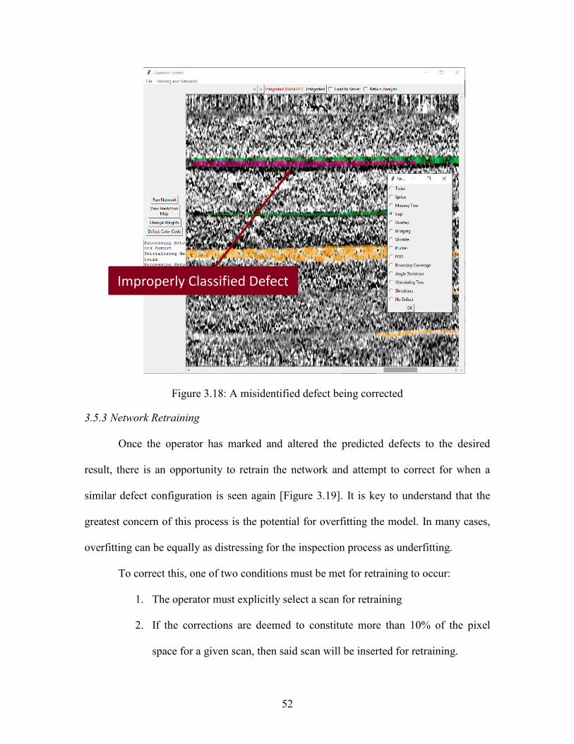
52
Figure 3.18: A misidentified defect being corrected
3.5.3 Network Retraining
Once the operator has marked and altered the predicted defects to the desired
result, there is an opportunity to retrain the network and attempt to correct for when a
similar defect configuration is seen again [Figure 3.19]. It is key to understand that the
greatest concern of this process is the potential for overfitting the model. In many cases,
overfitting can be equally as distressing for the inspection process as underfitting.
To correct this, one of two conditions must be met for retraining to occur:
1. The operator must explicitly select a scan for retraining
2. If the corrections are deemed to constitute more than 10% of the pixel
space for a given scan, then said scan will be inserted for retraining.
Improperly Classified Defect

53
These fail safes prevent the somewhat counterintuitive tendencies to retrain on every
image.
The reason such an approach would lead to overfitting is a result of the update
step taken in our network. When training, there is a global optimum that is desired and
many local optima that can represent low loss on certain defects or defect configurations,
does not give ideal results over the broad spectrum of defect classes. In retraining on
every scan, the natural imbalance existing in the distribution of defect appearance will
lead to the model becoming trained towards the local solutions rather than the preferred
global solution. The result is a model that is adept at finding a handful of the most
popular defects but completely useless on those defects that are underrepresented in the
dataset.
Figure 3.19: Retraining Scheme
3.5.4 ACSIS Integration
Much of the functionality of the software described in this document is dependent
on the rapid acquisition of profilometry scans through ACSIS. The third party nature of

54
the ACSIS software and programming systems implies that direct access to the data
stream coming into the analysis computer is difficult to the point that it is beyond the
scope of this project.
To properly integrate the USC AFP Inspection software, a threaded loop is set
running in the background of the software waiting for a new series of bitmap images to
appear in the folder that ACSIS logs scan images into. Once a new file is found, the loop
joins the thread and the images are automatically loaded, presented to the operator, and
analysed for defects using the image processing network.
This structure reduces the time demand of formatting scan images and loading by
hand, reducing the workload to selecting the “Integrated” option and running the proper
file on the KUKA robot arm.
55
CHAPTER 4
INSPECTION TRIALS
4.1 EXPERIMENTAL PROCEEDURE
With the form and function of the USC AFP Inspection software developed
throughout this document, it becomes necessary to offer examples of the systems’ usage
in a live production environment. It is the aim of this section to outline two experimental
cases for: (1) the validation of the system and (2) examples of the functionality of the
software. A general production test case of the evaluation of a cylinder with
preprogramed defects will be examined with: scans taken, defects identified, and data
exported to a remote server for collection and evaluation. In addition, a test article has
been developed such that a validation scheme can be created for the evaluation of the
overall system. The remaining portion of this chapter is dedicated to the description of
these test cases and the results thereof. The chapter will conclude with an overall
evaluation of the statistics and performance of the USC image processing software using
a confusion matrix.
4.1.1 Test Case: Analysis of an AFP Manufactured Cylinder
A 48-inch diameter cylinder was produced with an Ingersoll Machine Tools Lynx
AFP machine on a stainless steel tool. ACSIS was programmed to run scans on a section
of the cylinder such that the reach constraints were not exceeded on the KUKA KR120
robot arm.

56
Figure 4.1: ICPS model of cylinder
Programming is accomplished through ICPS. All four profilometers are used with
an 18mm stager-shift offset to account for missing data patches between the scan areas of
each profilometer. The area to be scanned is indicated in green in Figure 4.1. The large
area to be scanned was run with in-process inspection using the integration tools
developed in the inspection software.
The data from the profilometer is matched to the ICPS PF files used to program
ACSIS using a custom python code. The rosette is shared between the programming file
for both the AFP machine and ACSIS, giving a common reference point between the two
systems. This implies that the only change between the coordinate systems on ACSIS and
the AFP machine is a transformation to flip the x and y axes in order to have a common
coordinate system. This shared coordinate system is then used as the base reference for
the 2C20 data export and the 2C21-Task 6 defect-machine state correlation task.
4.1.2 Functional Checkout Procedure
A validation and checkout plan of the AFP inspection system can serve several
purposes. As a tool for the independent articulation of the inspection system free from the
lay-up of the AFP machine, validation tools can be used to do immediate verification that
system results are functioning properly, both on the hardware and the software. In the
scope of this document, the evaluation of the software tools outlined in this document are
of primary concern.

57
The procedure for validation of the inspection system is as follows:
1. Verification of Profilometer Operation
Once the ACSIS system is installed on the E1 track and both the KR120 robotic
arm is under power and the Keyence LJ-7080 profilometers are installed, begin by
verifying the connection between ACSIS computer 2 and the profilometer by opening the
Keyence LJ Viewer software and manually triggering the profilometer as explained in the
LJ-7080 manual while a second operator moves a contrast material6 towards and away
from the profilometer. When the display shows a change in the height data upon doing
this, the profilometer is active and ready to establish communication with the ACSIS
system.
2. Establish Profilometer Communication with ACSIS
Once the system hardware is verified to be functional, the inter-process
communications between the various ACSIS subsystems must be confirmed as working
properly. With the individual hardware components active, run a scan across the part on
the table. Once completed, a scan should appear in a designated folder and be forwarded
to both the native ACSIS analysis software and the USC defect detection software.
3. Prepare For Software Verification
With the scanning capabilities defined and checked, the next phase of system
verification involves the analysis software itself. With a scan image produced, run the
image analysis tools and check that each of the preprogrammed defects are both correctly
labeled, and their total area is properly bounded. In the case of the AFP Defect Detection
6 This can typically be any white object that can cover the width of all four profilometers. Though it is a simple solution, a piece of paper can adequately achieve this.
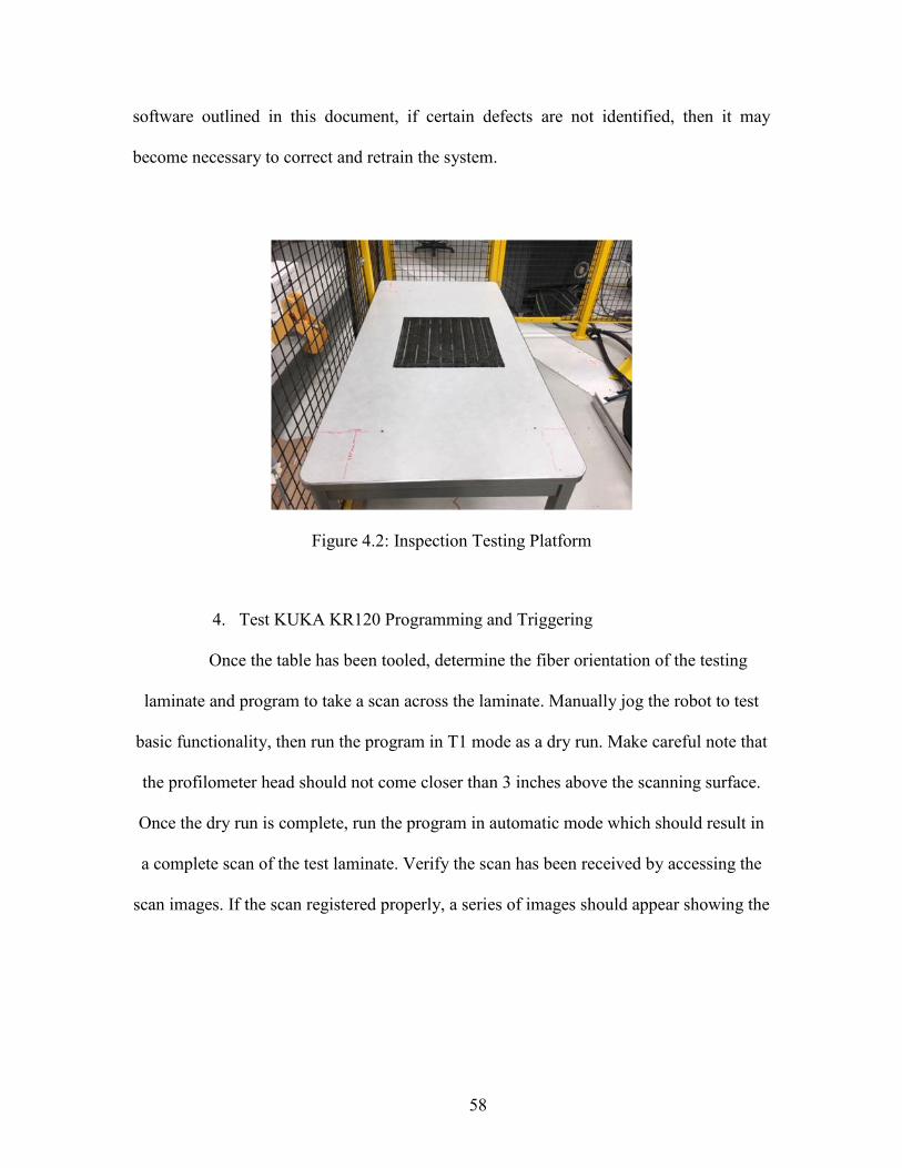
58
software outlined in this document, if certain defects are not identified, then it may
become necessary to correct and retrain the system.
Figure 4.2: Inspection Testing Platform
4. Test KUKA KR120 Programming and Triggering
Once the table has been tooled, determine the fiber orientation of the testing
laminate and program to take a scan across the laminate. Manually jog the robot to test
basic functionality, then run the program in T1 mode as a dry run. Make careful note that
the profilometer head should not come closer than 3 inches above the scanning surface.
Once the dry run is complete, run the program in automatic mode which should result in
a complete scan of the test laminate. Verify the scan has been received by accessing the
scan images. If the scan registered properly, a series of images should appear showing the

59
height profile of the test part translated into a greyscale image [Figure 4.4].
Figure 4.3: Platform Tooling Holes
Figure 4.4: Scan of a Validation Part7
5. Test ACSIS Defect Identification Software
As the scans appear in the Scaled_Courses folder, they should be processed by the
defect identification algorithms. This data should be accessible through the tablet, watch,
7 The distorted patterns at the edge of the course scan are a result of the bag material the test article was wrapped in prior to scanning and data collection.

60
defect log, or projector on ACSIS. Each of these systems can be independently verified.
If the analysis software is working correctly, the defect log should indicate both the
proper defect class and its approximate location for each of the known defects on the test
part.
4.2 RESULTS
4.2.1 Test Case: Cylindrical Part
The cylinder was scanned and evaluated through the ACSIS system. Hand placed
defects were inserted and marked on the cylinder with results to be forwarded to the
defect detection server. The result was a comprehensive survey of the cylinder ply-by-ply
with inspection informing the defect identification and repair process. The detection of
many of the non-inserted defects yielded positive results, with many of the more common
defect identified and corrected. Figure 4.5 shows the identified defects. Unfortunately,
the artificial nature of the hand-placed defects resulted in poor identification. The hand
placed defects presented themselves in a way completely unlike what existed in our
training set. To augment this, the hand-placed defects were manually tagged using the
operator correction functionality.
4.2.2 Functional Checkout with Test Article
The functional checkout of the system, as mentioned previously, is focused on the
scanning and evaluation of a test article previously developed with a number of hand
placed defects [Figure 4.7, Figure 4.6]. The test article was mounted to a platform and
scanned with the ACSIS system. The images produced were then analysed using the
Defect Detection Network and an overall sense of system performance was grasped.

61
Figure 4.5: Identification on the Cylinder with Correction through Manual Tagging
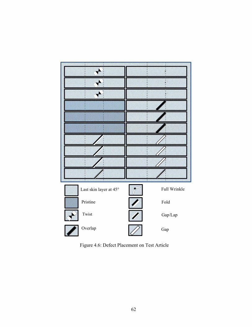
62
Last skin layer at 45°
Pristine
Twist
Full Wrinkle
Fold
Gap/Lap
Overlap Gap
Figure 4.6: Defect Placement on Test Article

63
Figure 4.7: Functional Checkout Test Article
It became clear through this testing procedure that the system was both functional
and extremely user friendly. A number of the hand placed defects were identified, and
their characteristics were extracted for later comparison to known data on the test article.
Those defects that were not identified, namely puckers and FOD, can be seen as being a
result of a limited distribution in the training set. Furthermore, the hand-placed nature of
the puckers lead to an artificial result that differed drastically from those examples that
were trained on from the natural defect production in the AFP environment.
Where the software did fail, it often was capable of discovering almost all of the
identifying characteristics save for the class. Thus, correction was simply a matter of
using the internal mechanisms of the software. Figure 4.8 shows the identification of a

64
twist on the test article. Figure 4.9 gives more examples of common defects on the test
article properly identified by the system.
Figure 4.8: Identification of a Twist on Test Article

65
Figure 4.9: Identification of Defects on Test Article
4.2.3 Evaluation of the Defect Detection Network
While images from various operations might give an overall picture of the
effectiveness of the algorithms employed for defect detection, a more succinct idea of
performance must be gained. A testing set of 50 images was collected from a scan of the
48 inch cylinder representing a wide range of defects from twists to missing tows. To
construct this testing set, the scans were hand labelled to create a true label list of pixels.

66
This testing set was evaluated by the defect detection network and a series of statistics
were produced noting the system performance across the defects present in the testing set.
For evaluation, the confusion matrix of the network will be presented, in addition
to the overall accuracies for each of the categories present in the testing set. A series of
evaluation metrics and a brief explanation for each is provided in Table 4.1.
Metric Description
Confusion Matrix An evaluation of how the model
performed over each class in relation to
other classes; Presents the true positive
and false negative cases over all classes
Accuracy Gives the weighted number of correct
classifications; Most general metric
Table 4.1: Performance Metrics for Defect Network Evaluation
Figure 4.10: The Confusion Matrix over Testing Set Defects

67
It should noted that the poor accuracy across the wrinkle and FOD classes can be
attributed to a lack of said defects in manufacturing and thus constructing the training set.
Only .5% of total pixel space in the training set was occupied by wrinkles. Likewise,
.005% of pixel space in the training set was from FOD. These issues have the potential to
be resolved through continuous use and correction of the inspection system.
Total Accuracy No Defect Twist Missing Tow Gap Overlap
98% 99% 75% 49% 77% 43%
Table 4.2: End Accuracies across Major Defects
The final accuracies are displayed in Table 4.2. The implementation of the
inspection system has been observed to be accurate in the context of a live inspection
environment. The defect accuracy demonstrated through the confusion matrix in Figure
4.10 is representative of the most common defects as defined by pixel space in our
dataset. While the capability exists to perform analysis on other defect types, the
examples in our initial training dataset are not numerous enough to currently make an
effective statement on their ease or difficult of identification through our algorithm.
4.3 NOTES
The long-term goal of this project is not to produce an immediately relevant
analysis tool. Rather, the end result should be a system that is capable of improving over
time with the ability to retrain from operator corrections. Should the size of the network
be put to the immediate optimum, then there is the potential that the network will not be
deep enough to continue to consistently learn over time.

68
This may well mean that operator corrections will be high through the first round
of system articulation. However, over time it is expected that this error will decrease, and
the result will be an overall more accurate system with the capabilities only demonstrated
through deeper network configurations. Sacrificing initial performance for long term
growth and generalization is believed by the author to be worth the trade-off.

69
CHAPTER 5
CONCLUSION
5.1 AN OVERVIEW OF WORK
A process and auxiliary techniques for the creation of an inspection software suite
for the automated identification of AFP manufacturing defects has been outlined in this
document. Machine learning algorithms were utilized to create an image processing
algorithm for the precise location and characterization of defects from within a scan
image. Fully convolutional networks were used to accomplish image analysis and were
trained such that they would segment the image into a collection of pixels corresponding
to a given defect.
The software was integrated with the Ingersoll Machine Tools ACSIS inspection
system. Profilometry scans were taken in a ply-by-ply manner through the ACSIS
platform and compressed into greyscale images for analysis. The images were
automatically loaded into the analysis algorithms after the inspection of a single ply.
The Marching Squares algorithm was used to extract a bounding polygon from
each of the collection of pixels provided by the segmentation. The bounding polygon and
defect type was collected and used to create a JSON file listing all of the defects found
across a given part. The JSON file was organized in such a manner that the defects could
be placed in the context of the overall part and ply number. A server was placed on the
local network for the JSON files to be pushed to post-analysis for 3rd party interfacing
and data analysis.

70
A user interface was created for an easier interpretation of the inspection data.
Functionality for correction was incorporated as a feature. As a corollary, the correction
of network output allowed for the creation of retraining features. Thus, the software is
capable of improvement through general use. The software was used in the scanning of a
test article in the creation of a validation scheme to verify both the hardware and software
are functional. In addition, testing of the software was conducted with the manufacturing
of cylinder structures.
5.2 A BRIEF REMARK ON ML IMAGE ANALYSIS
It is important to consider the context of any problem before applying an
algorithm or approach in an attempt to reach a solution. One cannot simply say that they
wish for a solution to a given problem. There are many potential solutions, and the
environment in which those solutions exist has as much a bearing on the viability of
implementation as the final efficacy of a given approach. In the image analysis space, this
is true as well.
ML in general image analysis is fundamentally different from the application of
ML to inspection. Accuracy, which is vitally important, is far from the only consideration
present in the space. In many cases, certain defects have a can have a more detrimental
effect on structure performance than others. Having a high false positive rate can also be
deemed more unacceptable than catching every potential flaw. All of this implies that
while the inspection processes outlined in this document are certainly a subset of the
image analysis field, the end result is something far different than what is seen at an ML
conference or the many image recognition contests.

71
The engineers responsible for implementing whatever analysis software may be
developed must be comfortable with all of the aspects of the software. Inspection
occurring at process time might be too fast for an extremely deep neural network, and the
trade-off in accuracy might be worth an increase in speed from a more light-weight
implementation. If there is no filter for the presentation of only meaningful or important
errors, then the challenges of manual inspection simply get pushed back a layer of
abstraction, effectively nullifying any progress.
In other terms, the application of ML to inspection rather than general image
analysis is the difference between a good algorithm and good software. One would be
cautioned against simply extracting the most accurate approach from the latest image
recognition competition and applying it to the detection of AFP defects. As is common in
ML, extrapolation from one domain to another can often yield less than desirable results.
Consider all aspects of the task at hand, including the extrema and edge cases that ML is
often so brilliantly good at spotting. An algorithm may be truly effective, but it adds no
value if the implementation is too unwieldy.
5.3 INSPECTION AS THE CENTERPIECE OF MODERN MANUFACTURING
The contiued digital transformation of the AFP process has produced a number of
interesting results, with the monitoring of countless metrics and better understanding of
physical processes. However, the end result of the AFP process is a fully manufactured
composites part. The many efforts of monitoring the AFP process are rendered inert
unless consistent, quantifiable data about the part and part quality can be offered.
Thus, inspection becomes the central point around which modern manufacturing
efforts can be based. It should be noted that when the author uses the term inspection, it is

72
implied that quantifiable data about part quality can be extracted an assessed. Robust
inspection, similar to the principles outlined in this document, can provide detailed
insight into the functioning of a given system.
The inspection process is an important component of the manufacturing and
design evaluation process, but the true value in the implementation of such a system
comes in the form of what can be done with the data from inspection. Exact
quantification of defect production and part quality is a direct reflection of design
features and the system state of the manufacturing process. Are there malfunctions within
the AFP machine? Are processing parameters or material properties inappropriate for a
particular part? Is the geometry of a given design more complex than what manufacturing
can appropriately handle? All of these questions can be informed from a detailed
inspection process that not only makes a statement on the global quality of the part, but
the local properties of each flaw.
This concept of inspection-influenced evaluations of manufacturing and design is
only possible through detailed examinations of inspection data. While possible for a
human inspector, the general tediousness of the process implied that automated systems
could be far more effective. This automation and augmentation of inspection through
computational tools can be termed Computer-Aided Inspection (CAI). CAI is the concept
that allows for the fast digital transformation of a part post-manufacturing and thus
allows the utilization of all of the data points identified writ large.
What are specific applications of what can be done with all of this data? In the
context of AFP, it becomes obvious that the extraction of exact size and shape
characteristics of an individual defect allows for the insertion of said information into a

73
Finite Element model for the analysis of defect influences on the overall strength of a
structure. Rapid evaluation of the effects of defects on structural properties such as
stiffness and overall strength can lead to better decisions on the scrap potential of a given
part. Rapid analysis from defect information can also indicate whether a defect is
significant enough to repair or if it can ultimately be left on the ply.
Further benefits of the data from a CAI system can be seen through a check on the
machine and system states from within the manufacturing cell. If a mechanism on the
AFP machine breaks, and that breakage presents itself as the production of a defect such
as a missing tow, a CAI system will be capable of capturing that data and analysis post-
capture can reveal points of failure on the machine.
5.4 A LONG TERM OUTLOOK ON THE INSPECTION SYSTEM
The data capture, operator interaction, and data transfer schemes within the
inspection software are purpose-built to be flexible and generalized. Should changes need
to be enacted, the software tools placed in the package allow for the maximum amount of
alteration possible. From training networks from scratch to refining how large defect
need to be before being logged, the operator is in full control of every process.
This flexibility can lead to a long term stability for any of the inspection processes
to which the inspection software is applied. Variances in material type, lighting,
reflectivity that might affect the data collection process can easily be accounted for by
capturing data, training a custom model through the software, and deploying. All of these
features lead to a natural improvement of the performance of the inspection system in the
long-term time horizon. Each manufacturer can find the proper balance of retraining
rates, defect sizes, and characterization fidelity.

74
Taken one step further, the image analysis tools are general enough that as long as
one is presenting a 2D image, it is possible to train on any imaging system, from
thermography to eddy current to ultrasonic probes. The underlying image processing
technique, semantic image segmentation, is the key concept. Any inspection task that can
be reparametrized in such a way can have the software and techniques described in this
document applied to it.
5.5 FUTURE WORK
The development of the inspection software outlined in this document represents
a novel approach to the analysis and data collection process in the inspection of AFP
manufactured composite parts. However, the culmination of this investigation has also
revealed a number of areas through which improvements could be made. From inspection
hardware to software, key areas can be modified to both create a more accurate system
and better fit what is desired in both industry and research settings.
In addition to the presentation of a number of improvements to the inspection
process, this section will identify a number of novel implementations that are possible
given the detail in defect information provided through the inspection software. Many of
these projects are the culmination of several chains of research and development.
However, all utilize the underlying concept of improvement in inspection and greater
detail in AFP defect production.
5.5.1 Improvements and Validation of Current Software Architecture
As an overall scheme, the inspection software has many of the desired features
planed from conception. However, there areas through which a more effective system

75
could be developed. Improvements in both the ML algorithms and the hardware
implementation on which the software is run could be attainable in future efforts.
A deeper exploration into the network architecture employed in this work is
almost certainly necessary in future iterations of this project. While important features
within the network were tuned using the GA optimizer discussed in Section 3.3.3, there
are several architecture features left that could benefit from optimization. The learning
rate, number of layers, down-sampling, and up-sampling rates could all have an end
effect in the performance of the network.
While the JSON file swapping to an independent server is a novel approach
within the limited third-party environment of the lab, it will be inevitable that data swap
within an industrial environment will be more complex. While a small-scale
implementation of a relational database to house defect information has been completed,
scaling this approach up may yield a more flexible option for accessing and transferring
data. Hosting a browser application for the general sharing of defect data may also
become a requirement in an age where IoT and cyber-manufacturing are becoming global
concepts with may distributed data points.
5.5.2 Online Inspection
The clear path for AFP inspection in both research and industry is towards in-situ
inspection over ply-by-ply or post-manufacturing inspection. The speed benefits of online
inspection are highly desirous, effectively eliminating machine downtime except for
defect repair. The current state of inspection systems in both software and hardware
requires several major adjustments to create an online inspection system [Figure 5.1].

76
Figure 5.1: Changes Required for Online Inspection Concept
For a functional in-situ system, a reimagining of what the AFP head must be
constituted of must be accomplished. The current model of AFP head configuration
consists of just those devices necessary for laying up material on the tool. The sensing
apparatus must be integrated with this hardware such that it is both capable of scanning
or imaging the target surface and does not interfere with the overall manufacturing
process. This becomes an even more difficult problem when considering the case of
steered tows. If the sensors are located away from the roller, then there could be a
mismatch between what the sensor is detecting and the target surface.
The speed of analysis that must occur for online inspection represents a particular
challenge. For large ML algorithms, the computation may need to be shared among
multiple computing devices in a dedicated cluster, incurring a multitude of complexities
in the scheduling and transfer of data between devices. The inclusion of FPGAs in this
concept is likely the most forward-looking of all the hardware possibilities. Even over
GPU, FPGAs can achieve massive acceleration of machine learning algorithms in general
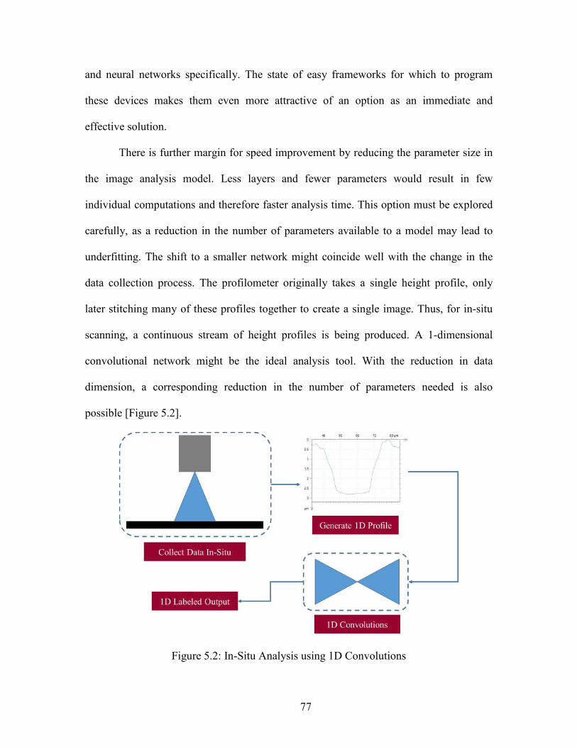
77
and neural networks specifically. The state of easy frameworks for which to program
these devices makes them even more attractive of an option as an immediate and
effective solution.
There is further margin for speed improvement by reducing the parameter size in
the image analysis model. Less layers and fewer parameters would result in few
individual computations and therefore faster analysis time. This option must be explored
carefully, as a reduction in the number of parameters available to a model may lead to
underfitting. The shift to a smaller network might coincide well with the change in the
data collection process. The profilometer originally takes a single height profile, only
later stitching many of these profiles together to create a single image. Thus, for in-situ
scanning, a continuous stream of height profiles is being produced. A 1-dimensional
convolutional network might be the ideal analysis tool. With the reduction in data
dimension, a corresponding reduction in the number of parameters needed is also
possible [Figure 5.2].
Figure 5.2: In-Situ Analysis using 1D Convolutions

78
In summary, the process time reduction made possible through online inspection
makes the concept of enormous research value. While the current implementation of both
the hardware and software present in the inspection system outlined in this document are
not ideal for an online system, small adjustments can be made to make this the case. Any
major investment into improving the inspection system must include changes in this
direction.
5.5.3 Hybrid Imaging
The height profiling capabilities given from profilometry may have drawbacks
across certain defects. A simple observation of profilometry scans of both an overlap and
a wrinkle near the tow boundary reveals similarities that make distinguishing between the
two defects difficult for a human observer, let alone ML image processing tools. This
problem is further highlighted when considering that the misidentification of these two
defects leads to a misunderstanding of the overall state of the local defect area in
question. If a wrinkle exists, then debulking cycles or the curing process may remove the
imperfection. However, an overlap represents an effective doubling of the thickness of an
affected area, which gives an entirely different repair methodology.
Combining the results of profilometry scans with additional data collection
systems may improve the overall analysis capabilities by exposing a greater number of
features for the model to identify. The advantages of thermography and eddie current
probing come with the ability to perform subsurface imaging. The latter can yield details
that a simple height profile cannot. In the case of the hypothetical overlap-wrinkle
misidentification, height profiles may be similar between the two kinds of defects, but
subsurface characterization could make a definite distinction between the two defect

79
presentations. The distinction of the doubling of material under an overlap and the void
left under a wrinkle would likely be apparent in subsurface sensing.
Combining the output of profilometry with an additional sensor output for
processing in our software requires minor modifications. The new sensors must output, or
be modified to output, a 2-dimensional array of the same resolution as the profilometry
image. Further, the pixels in each of the sensing apparatuses must correspond to the same
spatial points in each image. From this point, the defect detection network can very
quickly be modified to accept additional channels and input as well as the original
profilometry image. Thus, the feeds of each sensor can be combined into a fusion image
with multiple channels representing extra features for the network to incorporate into
training and analysis.
5.6 SITUATION OF RESEARCH
Understanding automated AFP inspection subscribes to an overall endeavor at the
McNAIR Center to push the boundary of discovery for Additive Manufacturing in
general and for Composites Manufacturing, predominately Automated Fiber Placement,
in particular. In the context of Automated Fiber Placement, this research complements
path planning studies for AFP (Halbritter et al. 2017; Rousseau et al. 2019) where finding
the optimal tool path for laying fibers is sought. One of the principal conditions is the
minimization of AFP defects (Harik et al. 2018) and the effect they can have on the
integrity of the structure (Wehbe et al. 2017; Wehbe, Harik, and Gürdal 2019) ).
Integrated design and manufacturing analysis (Noevere, Collier, and Harik 2019) ,
efficient design processes (M. A. Albazzan et al. 2019; M. Albazzan et al. 2019; Sabido
et al. 2017) , automated of process planning (Halbritter et al. 2019), heat optimization

80
(Xia et al. 2018) , automated inspection (C. Sacco et al. 2018; Sacco et al. 2019) and
rapid assessment tools can practically support a better integral lay-up quality. In the
context of Additive Manufacturing, this research complements topology optimization
(Bahamonde Jácome et al. 2018) , feature recognition (Harik, Shi, and Baek 2017; Shi et
al. 2018) , optimal part nesting (Zhang et al. 2018) and optimal build orientations (Zhang
et al. 2017, 2019).
This work actively participates in the advancement of the Additive
Manufacturing/Automated Fiber Placement research, and supports the overall goal to
thrust advanced manufacturing innovation and research.
5.7 ACKNOWLEDGMENTS
The material is based upon work supported by NASA under Award Nos. NNL09AA00A
and 80LARC17C0004.
Any opinions, findings, and conclusions or recommendations expressed in this
material are those of the author(s) and do not necessarily reflect the views of the National
Aeronautics and Space Administration.

81
REFERENCES
Albazzan, Mazen et al. 2019. “Design of Variable Stiffness Cylinder with Holes Under Bending for Maximum Buckling Load Using Lamination Parameters.” 1–18.
Albazzan, Mazen A., Ramy Harik, Brian F. Tatting, and Zafer Gürdal. 2019. “Efficient Design Optimization of Nonconventional Laminated Composites Using Lamination Parameters: A State of the Art.” Composite Structures 209(June 2018):362–74.
Angeline, Peter J. 2003. “Genetic Programming: On the Programming of Computers by Means of Natural Selection,.” Biosystems.
Bahamonde Jácome, L. G. et al. 2018. “Rapid Tools for an AFP Manufacturing Defects Assessment Framework.” International SAMPE Technical Conference 2018–May.
Benítez, Hernán D. et al. 2009. “Defect Characterization in Infrared Non-Destructive Testing with Learning Machines.” NDT and E International 42(7):630–43.
Brüning, J., B. Denkena, M. A. Dittrich, and T. Hocke. 2017. “Machine Learning Approach for Optimization of Automated Fiber Placement Processes.” Procedia CIRP 66:74–78.
Cacciola, Matteo, Salvatore Calcagno, Francesco Carlo Morabito, and Mario Versaci. 2008. “Computational Intelligence Aspects for Defect Classification in Aeronautic Composites by Using Ultrasonic Pulses.” IEEE Transactions on Ultrasonics, Ferroelectrics, and Frequency Control 55(4):870–78.
Caminero, M. A., I. García-Moreno, G. P. Rodríguez, and J. M. Chacón. 2018. “Internal Damage Evaluation of Composite Structures Using Phased Array Ultrasonic Technique: Impact Damage Assessment in CFRP and 3D Printed Reinforced Composites.” Composites Part B: Engineering.
Cemenska, Joshua, Todd Rudberg, and Michael Henscheid. 2015. “Automated In-Process Inspection System for AFP Machines.” SAE International Journal of Aerospace.
Cheng, Ying, Ken Chen, Hemeng Sun, Yongping Zhang, and Fei Tao. 2018. “Data and Knowledge Mining with Big Data towards Smart Production.” Journal of Industrial Information Integration 9(August 2017):1–13.
Chopard, Bastien and Marco Tomassini. 2018. “Particle Swarm Optimization.” in Natural Computing Series.
Chrysafi, A. P., N. Athanasopoulos, and N. J. Siakavellas. 2017. “Damage Detection on Composite Materials with Active Thermography and Digital Image Processing.” International Journal of Thermal Sciences 116:242–53.
Cortes, Corinna and Vladimir Vapnik. 1995. “Support-Vector Networks.” Machine Learning 20(3):273–97.
D’Angelo, Gianni and Salvatore Rampone. 2016. “Feature Extraction and Soft Computing Methods for Aerospace Structure Defect Classification.” Measurement: Journal of the International Measurement Confederation 85:192–209.
Duchi, John, Elad Hazan, and Yoram Singer. 2011. “Adaptive Subgradient Methods for Online Learning and Stochastic Optimization.” JMLR.

82
Eberhart and Yuhui Shi. 2002. “Particle Swarm Optimization: Developments, Applications and Resources.”
for Computing Machinery, Association et al. 2015. “ADADELTA: An Adaptive Learning Rate Method.” in Proceedings of ACL-IJNLP 2015.
Di Francescomarino, Chiara et al. 2018. “Genetic Algorithms for Hyperparameter Optimization in Predictive Business Process Monitoring.” Information Systems.
Franco, Maria A. and Jaume Bacardit. 2016. “Large-Scale Experimental Evaluation of GPU Strategies for Evolutionary Machine Learning.” Information Sciences 330:385–402.
Frazier, Peter I. 2018a. “A Tutorial on Bayesian Optimization for Machine Learning.” ArXiv Preprint.
Frazier, Peter I. 2018b. “Bayesian Optimization.” in Recent Advances in Optimization and Modeling of Contemporary Problems.
Friedrich, Jens, Jonas Torzewski, and Alexander Verl. 2018. “Online Learning of Stability Lobe Diagrams in Milling.” Procedia CIRP 67:278–83.
Glorot, Xavier and Yoshua Bengio. 2010. “Understanding the Difficulty of Training Deep Feedforward Neural Networks.” Pmlr 9:249–56.
Goodfellow, Ian et al. 2014. “Generative Adversarial Nets.” Advances in Neural Information Processing Systems 27 2672–80.
Halbritter, Joshua, Ramy Harik, A. Zuloaga, and Michael Van Tooren. 2017. “Tool Path Generation on Doubly-Curved Free-Form Surfaces.” Computer-Aided Design and Applications 14(6):855–851.
Halbritter, Joshua, Clint Saidy, Andrew Noevere, and Brian Grimsley. 2019. “Automation of AFP Process Planning Functions: Importance and Ranking.” SAMPE 2019 Conference & Exhibition (Charlotte, North Carolina, US, 20 – 23 May 2019).
Harik, Ramy, Joshua Halbritter, Dawn Jegley, Ray Grenoble, and Brian Mason. 2019. “Automated Fiber Placement of Composite Wind Tunnel Blades: Process Planning and Manufacturing.”
Harik, Ramy, Clint Saidy, S. J. Williams, Zafer Gurdal, and Brian Grimsley. 2018. “Automated Fiber Placement Defect Identity Cards: Cause, Anticipation, Existence, Significance, and Progression.” in SAMPE Conference Proceedings.
Harik, Ramy, Yang Shi, and S. Baek. 2017. “Shape Terra: Mechanical Feature Recognition Based on a Persistent Heat Signature.” Computer-Aided Design and Applications 14(2):206–18.
Heuer, H. et al. 2015. “Review on Quality Assurance along the CFRP Value Chain - Non-Destructive Testing of Fabrics, Preforms and CFRP by HF Radio Wave Techniques.” Composites Part B: Engineering 77:494–501.
Hornik, Kurt, Maxwell Stinchcombe, and Halbert White. 1989. “Multilayer Feedforward Networks Are Universal Approximators.” Neural Networks 2(5):359–66.
Hu, Eryi and Fang Haifeng. 2011. “Surface Profile Inspection of a Moving Object by Using Dual-Frequency Fourier Transform Profilometry.” Optik 122(14):1245–48.
Huang, Guang Bin, Qin Yu Zhu, and Chee Kheong Siew. 2006. “Extreme Learning Machine: Theory and Applications.” Neurocomputing 70(1–3):489–501.
Hughes, R. R., B. W. Drinkwater, and R. A. Smith. 2018. “Characterisation of Carbon Fibre-Reinforced Polymer Composites through Radon-Transform Analysis of

83
Complex Eddy-Current Data.” Composites Part B: Engineering 148(May):252–59. Jain, Anil K., Jianchang Mao, and K. M. Mohiuddin. 1996. “Artificial Neural Networks:
A Tutorial.” Computer. Jolly, Mr et al. 2015. “Review of Non-Destructive Testing (NDT) Techniques and Their
Applicability to Thick Walled Composites.” Procedia CIRP 38:129–36. Jorge Aldave, I. et al. 2013. “Review of Thermal Imaging Systems in Composite Defect
Detection.” Infrared Physics and Technology 61:167–75. Kaelbling, Leslie Pack, Michael L. Littman, and Andrew W. Moore. 1996.
“Reinforcement Learning: A Survey.” Journal of Artificial Intelligence Research. Kalyanavalli, V., T. K. Abilash. Ramadhas, and D. Sastikumar. 2018. “Long Pulse
Thermography Investigations of Basalt Fiber Reinforced Composite.” NDT and E International 100(December 2017):84–91.
Kampker, Achim, Heiner Heimes, Ulrich Bührer, Christoph Lienemann, and Stefan Krotil. 2018. “Enabling Data Analytics in Large Scale Manufacturing.” Procedia Manufacturing 24:120–27.
Klein, Aaron, Stefan Falkner, Simon Bartels, Philipp Hennig, and Frank Hutter. 2017. “Fast Bayesian Hyperparameter Optimization on Large Datasets.” Electronic Journal of Statistics.
Kohonen, Tuevo. 1998. “The Self-Organizing Map.” Neurocomputing 21(1–3):1–6. Koza, J. R. 2002. “Survey of Genetic Algorithms and Genetic Programming.” Krawczyk, Bartosz. 2016. “GPU-Accelerated Extreme Learning Machines for
Imbalanced Data Streams with Concept Drift.” Procedia Computer Science 80:1692–1701.
Krizhevsky, Alex, Ilya Sutskever, and Geoffrey E. Hinton. 2012. “ImageNet Classification with Deep Convolutional Neural Networks.” Advances In Neural Information Processing Systems 1–9.
Kuhl, M., T. Wiener, and M. Krauß. 2013. “Multisensorial Self-Learning Systems for Quality Monitoring of Carbon Fiber Composites in Aircraft Production.” Procedia CIRP 12:103–8.
Lee, C. K. H. 2018. “A Review of Applications of Genetic Algorithms in Operations Management.” Engineering Applications of Artificial Intelligence 76(May):1–12.
Liang, Shuang, Shouyi Yin, Leibo Liu, Wayne Luk, and Shaojun Wei. 2018. “FP-BNN: Binarized Neural Network on FPGA.” Neurocomputing 275:1072–86.
Long, Jonathan, Evan Shelhamer, and Trevor Darrell. 2015. “Fully Convolutional Networks for Semantic Segmentation.” Proceedings of the IEEE Computer Society Conference on Computer Vision and Pattern Recognition 07–12–June:3431–40.
Ma, Yufei, Naveen Suda, Yu Cao, Sarma Vrudhula, and Jae sun Seo. 2018. “ALAMO: FPGA Acceleration of Deep Learning Algorithms with a Modularized RTL Compiler.” Integration 62(August 2017):14–23.
Maple, C. 2003. “Geometric Design and Space Planning Using the Marching Squares and Marching Cube Algorithms.” in Proceedings - 2003 International Conference on Geometric Modeling and Graphics, GMAG 2003.
Marani, R. et al. 2018. “Modeling and Classification of Defects in CFRP Laminates by Thermal Non-Destructive Testing.” Composites Part B: Engineering 135(June 2017):129–41.
Meng, Min, Yiting Jacqueline Chua, Erwin Wouterson, and Chin Peng Kelvin Ong.

84
2017. “Ultrasonic Signal Classification and Imaging System for Composite Materials via Deep Convolutional Neural Networks.” Neurocomputing 257:128–35.
Meng, Yinfeng, Jiye Liang, Fuyuan Cao, and Yijun He. 2018. “A New Distance with Derivative Information for Functional K-Means Clustering Algorithm.” Information Sciences 463–464:166–85.
Mishkin, Dmytro, Nikolay Sergievskiy, and Jiri Matas. 2017. “Systematic Evaluation of Convolution Neural Network Advances on the Imagenet.” Computer Vision and Image Understanding 161:11–19.
Moustakidis, S., A. Anagnostis, P. Karlsson, and K. Hrissagis. 2016. “Non-Destructive Inspection of Aircraft Composite Materials Using Triple IR Imaging.” IFAC-PapersOnLine 49(28):291–96.
Nazarko, Piotr and Leonard Ziemiański. 2017. “Anomaly Detection in Composite Elements Using Lamb Waves and Soft Computing Methods.” Procedia Structural Integrity 5:131–38.
Noevere, Andrew, Chris Collier, and Ramy Harik. 2019. “Integrated Design and Manufacturing Analysis for Automated Fiber Placement Structures.” SAMPE 2019 Conference & Exhibition, Charlotte, North Carolina, US, 20 – 23 May 2019.
O’Brien, Ronald Julian, Juan Manuel Fontana, Nicolás Ponso, and Leonardo Molisani. 2017. “A Pattern Recognition System Based on Acoustic Signals for Fault Detection on Composite Materials.” European Journal of Mechanics, A/Solids 64:1–10.
de Oliveira, Mario A., Nelcileno V. S. Araujo, Daniel J. Inman, and Jozue Vieira Filho. 2018. “Kappa-PSO-FAN Based Method for Damage Identification on Composite Structural Health Monitoring.” Expert Systems with Applications 95:1–13.
Ou, Xinyan, Qing Chang, and Nilanjan Chakraborty. 2019. “Simulation Study on Reward Function of Reinforcement Learning in Gantry Work Cell Scheduling.” Journal of Manufacturing Systems 50(November 2018):1–8.
Pickering, S. G., K. Chatterjee, D. P. Almond, and S. Tuli. 2013. “LED Optical Excitation for the Long Pulse and Lock-in Thermographic Techniques.” NDT and E International 58:72–77.
Poli, R., J. Kennedy, and T. Blackwell. 2007. “Particle Swarm Optimization. An Overview.” Swarm Intelligence.
Poli, Riccardo and John Koza. 2014. “Genetic Programming.” in Search Methodologies: Introductory Tutorials in Optimization and Decision Support Techniques, Second Edition.
Posewsky, Thorbjörn and Daniel Ziener. 2018. “Throughput Optimizations for FPGA-Based Deep Neural Network Inference.” Microprocessors and Microsystems 60(June 2017):151–61.
Reddi, Sashank J., Satyen Kale, and Sanjiv Kumar. 2018. “On the Convergence of Adam and Beyond.” in ICLR 2018.
Riedmiller, Martin et al. 2018. “Learning by Playing - Solving Sparse Reward Tasks from Scratch.” (2017).
Rousseau, Guillaume, Roudy Wehbe, Joshua Halbritter, and Ramy Harik. 2019. “Automated Fiber Placement Path Planning: A State-of-the-Art Review.” Computer-Aided Design and Applications.
Sabido, Anthony, Luis Bahamonde, Ramy Harik, and Michel J. L. van Tooren. 2017. “Maturity Assessment of the Laminate Variable Stiffness Design Process.”

85
Composite Structures 160:804–12. Sacco, C., A. B. Radwan, R. Harik, and M. Van Tooren. 2018. “Automated Fiber
Placement Defects: Automated Inspection and Characterization.” in International SAMPE Technical Conference. Vol. 2018–May.
Sacco, Christopher, Anis Baz Radwan, Tyler Beatty, and Ramy Harik. 2019. “MACHINE LEARNING BASED AFP INSPECTION : A TOOL FOR CHARACTERIZATION AND INTEGRATION.” SAMPE Conference Proceedings.
Sacco, Christopher, Anis Baz Radwan, Ramy Harik, and Michael Van Tooren. 2018. “Automated Fiber Placement Defects: Automated Inspection and Characterization.” SAMPE 2018 Conference Proceeding.
Safiyullah, F., S. A. Sulaiman, M. Y. Naz, M. S. Jasmani, and S. M. A. Ghazali. 2018. “Prediction on Performance Degradation and Maintenance of Centrifugal Gas Compressors Using Genetic Programming.” Energy 158:485–94.
Sammons, Daniel, William P. Winfree, Eric Burke, and Shuiwang Ji. 2016. “Segmenting Delaminations in Carbon Fiber Reinforced Polymer Composite CT Using Convolutional Neural Networks.” AIP Conference Proceedings 1706.
Schmidhuber, Jürgen. 2015. “Deep Learning in Neural Networks: An Overview.” Neural Networks.
Sert, Eser, Deniz Tas, and Ahmet Alkan. 2015. “Three Stepped Calibration of Structured Light System with Adaptive Thresholding for 3D Measurements.” Optik 126:5176–81.
Shahriari, Bobak, Kevin Swersky, Ziyu Wang, Ryan P. Adams, and Nando De Freitas. 2016. “Taking the Human out of the Loop: A Review of Bayesian Optimization.” Proceedings of the IEEE.
Sharp, Michael, Ronay Ak, and Thomas Hedberg. 2018. “A Survey of the Advancing Use and Development of Machine Learning in Smart Manufacturing.” Journal of Manufacturing Systems.
Shi, Yang, Y. Zhang, S. Baek, W. De Backer, and Ramy Harik. 2018. “Manufacturability Analysis for Additive Manufacturing Using a Novel Feature Recognition Technique.” Computer Aided Design and Applications 15(6):941–52.
Shi, Yuhui and Russell C. Eberhart. 1999. “Empirical Study of Particle Swarm Optimization.” in Proceedings of the 1999 Congress on Evolutionary Computation, CEC 1999.
Tian, Ziyang et al. 2018. “Improved Genetic Algorithm for Optimization Design of a Three-Dimensional Braided Composite Joint.” Composite Structures 206(May):668–80.
Venugopal, V. and T. T. Narendran. 1992. “A Genetic Algorithm Approach to the Machine-Component Grouping Problem with Multiple Objectives.” Computers and Industrial Engineering 22(4):469–80.
Wang, Dongfang and Jin Gu. 2018. “VASC: Dimension Reduction and Visualization of Single-Cell RNA-Seq Data by Deep Variational Autoencoder.” Genomics, Proteomics & Bioinformatics (xxxx).
Wehbe, Roudy et al. 2017. “Tow-Path Based Modeling of Wrinkling During the Automated Fiber Placement Process.” The Composites and Advanced Materials Expo 2017 (CAMX 2017) (September 11-14, Florida, United States).

86
Wehbe, Roudy, Ramy Harik, and Zafer Gürdal. 2019. “In-Plane Tow Deformations Due to Steering in Automated Fiber Placement.” Pp. 1–13 in AIAA Scitech 2019 Forum. San Diego.
Wronkowicz, Angelika, Krzysztof Dragan, and Krzysztof Lis. 2018. “Assessment of Uncertainty in Damage Evaluation by Ultrasonic Testing of Composite Structures.” Composite Structures 203(July):71–84.
Wu, Jin Yi, Stefano Sfarra, and Yuan Yao. 2018. “Sparse Principal Component Thermography for Subsurface Defect Detection in Composite Products.” IEEE Transactions on Industrial Informatics 51(24):855–60.
Wu, Songtao, Shenghua Zhong, and Yan Liu. 2017. “Deep Residual Learning for Image Steganalysis.” Multimedia Tools and Applications 1–17.
Xia, Kaishu, Ramy Harik, J. Herrera, Josh Patel, and Brian Grimsley. 2018. “Numerical Simulation of AFP Nip Point Temperature Prediction for Complex Geometries.” in SAMPE 2018 Conference & Exhibition, Long Beach, California, US, 21 – 24 May 2018.
Xia, Kaishu, Christopher Sacco, Max Kirkpatrick, Ramy Harik, and Abdel-moez Bayoumi. 2019. “VIRTUAL COMISSIONING OF MANUFACTURING SYSTEM INTELLIGENT CONTROL.” SAMPE Conference Proceedings.
Zhan, Yusen, Haitham Bou Ammar, and Matthew E. Taylor. 2016. “Theoretically-Grounded Policy Advice from Multiple Teachers in Reinforcement Learning Settings with Applications to Negative Transfer.” IJCAI International Joint Conference on Artificial Intelligence 2016–Janua(7540):2315–21.
Zhang, Min Ling and Zhi Hua Zhou. 2007. “ML-KNN: A Lazy Learning Approach to Multi-Label Learning.” Pattern Recognition 40(7):2038–48.
Zhang, Y., A. Bernard, Ramy Harik, and George Fadel. 2018. “A New Method for Single-Layer-Part Nesting in Additive Manufacturing.” Rapid Prototyping Journal 24(5):840–54.
Zhang, Y., A. Bernard, Ramy Harik, and K. P. Karunakaran. 2017. “Build Orientation Optimization for Multi-Part Production in Additive Manufacturing.” Journal of Intelligent Manufacturing 287(6):1293–1407.
Zhang, Y., Ramy Harik, George Fadel, and A. Bernard. 2019. “A Statistical Method to Build Orientation Determination in Additive Manufacturing.” Rapid Prototyping Journal 25(1):187–207.