Machine Learning in Computer Chess:

Genetic Programming and KRK

David Gleich

Harvey Mudd College

May 13, 2003

Abstract

In this paper, I describe genetic programming as a machine learning paradigm and

evaluate its results in attempting to learn basic chess rules. Genetic programming

exploits a simulation of Darwinian evolution to construct programs. When applied

to the King-Rook-King (KRK) chess endgame problem, genetic programming shows

promising results in spite of a lack of significant chess knowledge.

Contents

Computer Chess:The Drosophila of Artificial Intelligence 2

1 Introduction to Machine Learning 5

2 Chess Problems - KRK 8

3 Genetic Programming Solutions 11

4 Conclusions and Future Work 21

References 24

Computer Chess:

The Drosophila of Artificial Intelligence

Since the inception of artificial intelligence (AI), researchers have often used chess

as an experimental method. Even before the field of AI formalized, pioneers such

as Wolfgang von Kempelen experimented with chess playing machines. Kempelen’s

mechanical automata, The Turk, fooled many into believing machines could play chess

in the 18th century.

However, it wasn’t until Claude Shannon published a paper entitled, “A Chess-

Playing Machine,” [Shannon] that the study of computer chess began in earnest. Shan-

non’s paper describes a chess program as a series of interlinked subprograms. He cor-

rectly observes that playing perfect chess is impossible, even for a machine – there are

an estimated 10120 nodes in a full-width chess tree. Even computers capable of eval-

uating 1016 positions in a second (which is eight orders of magnitude over the fastest

chess computer ever created) would need in excess of 1095 years to fully evaluate this

tree. Consequently, all chess programs are approximations.

Chess is, then, a problem of approximating, or simulating, the reasoning used by

chess masters to pick moves from an extremely large search space. The early objectives

of computer chess research were also very clear – to build a machine that would defeat

the best human player in the world. In 1997, the Deep Blue chess machine created by

IBM accomplished this goal, and defeated Gary Kasparov in a match at tournament

time controls. In tournament time controls, each player has two hours to make their

first forty moves, then one hour for the rest of the moves.

However, programs such as those described by Shannon and exemplified by Deep

Blue are essentially static. Human programmers invested massive amounts of time in

constructing the rule set of Deep Blue, in an attempt to approximate human position

evaluation. There is a vast body of literature on this problem; several references,

[Shannon], [Mar81], [Sch86], [Sch96], and [Hyatt], contain more information.

This report focuses, instead, on the problem of computer chess from a machine

2

learning perspective. One of the objectives of the machine learning field of AI is to

provide an example data set, and to have the machine “learn” the rules from the

examples along some background knowledge. One example of this type of problem

is “teaching” a computer how to distinguish even and odd numbers, based solely on

arithmetic or other properties of the numbers.

Within this paradigm, chess is an excellent problem. Investigators have constructed

massive end-game tables that specify the appropriate move for every position. One

example of these sets is the king-rook-king (KRK) set from the University of California

Irvine machine learning database [BM98]. This dataset contains all the positions where

a sole black king stands against a white king and white rook with the black king’s turn

to play. Additionally, it contains the number of moves to checkmate for all of the

positions. In Figure 1, white will mate in four moves.

80Z0Z0Z0Z7Z0Z0Z0Z060Z0Z0S0Z5Z0Z0Z0Z040Z0Z0Z0Z3Z0Z0Z0Z020Z0J0Z0Z1j0Z0Z0Z0

a b c d e f g h

Figure 1: Black to move, but White to checkmate in 4 moves.

The precise mating sequence for Figure 1 follows.

1 . . . Kb2

2 Rf3 Kb1

3 Kc3 Ka2

4 Rf1 Ka3

5 Ra1#

3

This position from Figure 1 is encoded in the database in the following format:

d,2,f,6,a,1,four

Databases such as this one serve as worth substrates for machine learning tests.

With the KRK set, one possible goal is to learn how many moves to checkmate. In the

experimental portion of this report, Section 3, I use genetic programming to solve chess

problems from this dataset. As I explain in my conclusion, Section 4, the results from

genetic programming on this database are encouraging, although much work remains.

4

1 Introduction to Machine Learning

There are many techniques and strategies used in machine learning. The following

are some of the formal machine learning systems or methods.

• Inductive Logic Programming

• Simulated Annealing

• Evolutionary Strategies (including genetic algorithms and genetic programming)

• Neural Nets

Each of these methods has slightly different advantages and disadvantages which

are outside the scope of this report. For one such analysis, see [KHFS]. Here, I will

simply focus on genetic programming.

1.1 Genetic Programming

According to Langdon and Poli, genetic programming is a type of evolutionary algo-

rithm [LP]. In general, evolutionary algorithms borrow from Darwinian evolutionary

concepts to solve search problems. The first type of evolutionary algorithms were called

genetic algorithms. Genetic programming later evolved as a generalization of genetic

algorithms.

All genetic programming (GP) experiments follow a general form. First, the GP al-

gorithm creates a random population of individuals. Next, the algorithm evaluates each

individual using a fitness function. After evaluating every individual, the algorithm

applies breeding operators to create the next generation. Together, this explanation

corresponds to the generational model from Langdon and Poli.

Since GP’s intention is to evolve programs, each individual in the population is a

program. Typically, these programs are represented as trees; an example is shown in

Figure 2.

In order to represent a program as a tree, GP requires two sets: functions and

terminals. Functions occur at every interior node in the tree and terminals occur

5

−����+����

x������ TTx����

�� T

Tx����

Figure 2: A representation of the equation (x + x)− x as a genetic program tree.In this case, the two functions are the + and − operators and the terminal is thevariable x.

at the leaves of the tree. For arithmetic problems like Figure 2 and the examples

below, the functions are the arithmetic operators and the terminals are variables and

constants.

There are three standard breeding operators.

1. crossover - two individuals exchange pieces.

2. mutation - the individual is randomly altered between generations.

3. replication - the individual is unchanged in the next generation.

These operators try to mimic the behavior of DNA exchanged between parents in

sexual reproduction.

Crossover, illustrated in Figure 3, is essentially genetic “cut-and-paste.” This op-

erator selects two pieces from different parents and exchanges them to create two

offspring.

There are two main types of mutation. The first type, point mutation, is illustrated

in Figure 4. In the point mutation operator, functions are randomly mutated into other

functions, and terminals are randomly mutated into other terminals. In the second

type of mutation, growth mutation, the operator selects terminals in an individual and

randomly adds new functions and terminals, replacing the original node. A third type,

shrinking mutation, exists, although this experiment did not use that type of mutation.

The replication operator is the simplest, this operator does not change individuals

between generations.

6

−����+����

x������ TTx����

�� T

Tx����

+����−����

x������ TTx����

�� T

Tx����

@@

@R

��

�

−����+����

x������ TTx����

,,, l

ll

−����x������ T

Tx����

+����x������ T

Tx����

Figure 3: In crossover, the two bold subtrees are exchanged between the twoparents to create the children. In the first child, the x−x subtree moves from theright tree to the place previously occupied by the x leaf of the left tree. In thesecond child, the x leaf moves from the left tree to the place previously occupiedby the x− x subtree of the right tree.

−����+����

x������ TTx����

�� T

Tx����

- +����+����

x������ TTx����

�� T

Tx����

Figure 4: The right individual mutates into the second individual when the − atthe root of the tree is switched to a +.

7

2 Chess Problems - KRK

In this paper, I look at king-rook-king (KRK) chess end game problems. As I

mentioned in the introduction, the KRK endgame consists of positions involving only

a white king, a white rook, and a black king. See Figure 1 and Figure 5 for sample

positions. More specifically, I focus on the black to move positions in the KRK endgame

from the University of California Irvine’s Machine Learning database [BM98].

80Z0Z0Z0Z7Z0ZRZ0Z060Z0Z0Z0Z5Z0Z0Z0Z040Z0Z0Z0Z3Z0ZKZ0Z020Z0Z0Z0Z1Z0ZkZ0Z0

a b c d e f g h

Figure 5: Black to move, but White to checkmate in 2 moves.

In total, the KRK dataset contains 28, 056 positions. Table 1 presents a summary

of these positions. For this problem, I only consider the non-drawn positions from the

dataset. With this restriction, there are 25, 361 positions in the seventeen depth to

checkmate classes.

2.1 The Grand KRK Problem

The grand KRK problem is ambitious. A complete solution to the problem requires

a program which takes a position from the KRK dataset and returns the number of

moves to checkmate. Equation 1 represents this program as a mathematical function.

In this equation, wkr is the integer rank of the white king where a = 1 and h = 8, wkf

is the integer file of the white king. Likewise, wrr and wrf are the rank and file of the

white rook and bkr and bkf are the rank and file of the black king. The position in

8

Summary of Positions in UCI KRK Dataset

Depth Positions Depth Positionsdraw 2796 8 1433

0 27 9 17121 78 10 19852 246 11 28543 81 12 35974 198 13 41945 471 14 45536 592 15 21667 683 16 390

Table 1: This table classifies the 28, 056 positions in the UCI KRK dataset. Withthe exception of the draw class, the other classes are the depth to checkmate.For example, there are 2796 drawn positions in the dataset and a class of 1433positions with 8 moves until checkmate.

Figure 5 corresponds with the function krkGrand(4, 3, 4, 7, 4, 1) = 2.

krkGrand(wkr, wkf , wrr, wrf , bkr, bkf ) = (1)

depth to checkmate with black to move and

white king on (wkr, wkf ),

white rook on (wrr, wrf ),

and black king on (bkr, bkf ).

Typical computer chess programs, and humans too, solve the problem using a

game tree technique. The program first enumerates all moves from the position, makes

each move, and recursively evaluates the subsequent position. These solutions require

carefully crafted algorithms to limit the size of the search tree.

In these machine learning experiments, I attempt to evolve or generate programs

or rules that solve this problem without a game tree.

9

2.2 The Petite KRK Problems

In contrast to the grand KRK problem, the petite KRK problems try to identify each

class of positions, Ci, from the KRK dataset. One of the petite KRK problems is to

identify every position where there is one move until checkmate. Thus, there are seven-

teen petite KRK problems. Solutions to these problems require programs that output a

yes value for a position in the desired class and a no value for all other positions. Using

the same notation as Equation 1, Equation 2 represents these programs mathemati-

cally. Ci denotes the class of positions with i moves until checkmate. Consequently,

the position in Figure 5 corresponds with the functions krkPetite2(4, 3, 4, 7, 4, 1) = 1

and krkPetitei(4, 3, 4, 7, 4, 1) = 0 for i 6= 2.

krkPetitei(wkr, wkf , wrr, wrf , bkr, bkf ) = (2)1 if (wkr, wkf , wrr, wrf , bkr, bkf ) ∈ Ci

0 if (wkr, wkf , wrr, wrf , bkr, bkf ) /∈ Ci

10

3 Genetic Programming Solutions

In this section, I describe the use of genetic programming (GP) to solve the grand KRK

and petite KRK problems. The first section enumerates the functions and terminals

used for the programs. I then explain the results for the grand KRK problem and a

petite KRK problem.

3.1 Function and Terminal Set

The major goal when constructing function and terminal sets is to provide enough ex-

pressive power so that there is a solution without trivializing the problem by supplying

excessive background information. To balance these objectives, I use a set of functions

which encodes very little chess knowledge.

• edge(i) - returns 1 if i = 1 or i = 8, and returns 2 otherwise.

• distance(i, j) - returns the absolute value of i − j, that is, the distance between

i and j.

• ifthen(i, j, k) - if i = 1 then ifthen returns j, else, ifthen returns k.

• compare(i, j) - returns 1 if i < j, and returns 2 otherwise.

The only chess knowledge represented in the set of functions is the edge function,

which responds if the input is an edge on a chessboard.

3.2 GP Systems

There are numerous genetic programming systems available. The web page [GPSoft]

lists 15 GP toolkits and frameworks. After initial trials using lil-gp [lilgp], which was

too slow, the jrgp system was used in the experiment [jrgp].

11

3.3 Grand KRK Problem

The evolutionary conditions for the grand KRK problem were a population size of

5000, a crossover frequency of 75%, a mutation frequency of 15%, and a replication

frequency of 10%. Each individual had three automatically defined functions. An

automatically defined function is a separate function that the program can re-use. The

evolved individuals were evaluated over each of the 25, 361 positions from the UCI

KRK database.

3.3.1 Fitness

The standard fitness function for the grand KRK problem is Equation 3. In the stan-

dard fitness evaluation, the best individual occurs at 0.0. In that equation, correcti is

the number of correct answers in class Ci; incorrecti is the number of incorrect answers

in class Ci; and numi is the total number of positions in class Ci. (Recall that class

Ci contains all of the positions where the depth to checkmate is i.)

krkGrandFit = 1−∑16

i=0correcti−incorrecti

numi

17(3)

Essentially, Equation 3 normalizes the fitness benefit of each class Ci. Consequently,

class C1 can, in total, contribute as much fitness to the individual as class C14, even

though C1 contains 78 positions and class C14 contains 4553 positions (over 50 times

as many). The normalization attempts to “smooth” the fitness function to eliminate

local optima for the large classes (e.g. C13, C14).

While the above equation calculates standard fitness, the figures in this section

plot adjusted fitness. On the adjusted fitness scale, 1.0 represents the best individual.

Adjusted fitness is calculated from standard fitness using Equation 4. StdF it is the

standard fitness value.

AdjFit =1

1 + StdF it(4)

This equation scales any StdF it value to the (0, 1] range. An individual with infinitely

12

bad fitness, StdF it → ∞, yields an AdjFit value of 0. Likewise, an individual with

perfect fitness, StdF it = 0, yields an AdjFit value of 1.

3.3.2 Results

The results from the grand KRK problem are encouraging. With a population of 5000,

jrgp could only evaluate up to 32 generations before it required too much memory to

evaluate an entire population. Consequently, the grand KRK problem requires more

investigation before it is completely successful.

Figure 6, Figure 7, and Table 2 show the results of the 32 generations. While the

evolved fitness after 32 generations is only 0.4167, the evolved programs show significant

growth. For example, if fitness continues growing at the same rate, approximately 0.04

adjusted fitness every 32 generations, then the population will reach nearly perfect

fitness in 480 generations. In addition, the population does not appear to have lost

any of the classes. In Figure 7, the best program in the population adds the “gray”

case in generation 30.

Curiously, Table 2 shows that the best individual after 32 generations does not

classify positions that the best program at the first generation did. This observation

demonstrates that the fitness function can successfully make trade-offs between the

different classes.

3.4 Petite KRK Problems

I only had time to attempt one solution to the petite KRK problem, the krkPetite1

instance. Nevertheless, the framework for evaluating the krkPetite1 problem should

solve any of the petite KRK problems.

The evolutionary conditions for the krkPetite1 problem were a population size of

1000, a crossover frequency of 75%, a mutation frequency of 15%, and a replication

frequency of 10%. The evolved individuals were evaluated over each of the 25, 361

positions from the UCI KRK database.

13

1 2 3 4 5 6 7 8 9 10 11 12 13 14 15 16 17 18 19 20 21 22 23 24 25 26 27 28 29 30 31 32

0.34

0.35

0.36

0.37

0.38

0.39

0.4

0.41

krkGrand 32 Generation Fitness

Adj

uste

d F

itnes

s

Generation

Figure 6: This figure presents the fitness of individuals in the grand KRK problempopulation over 32 generations. The upper red-colored line is the maximumfitness in the population at each generation; the middle blue-colored line is themean fitness; and the lower blue-colored line is the minimum fitness. The boxplot has a small red-colored line at the median, and shows the upper and lowerquartiles. This figure graphs the adjusted fitness where 1.0 is the best individual(see Equation 4).

14

5 10 15 20 25 300

0.5

1

1.5

2

2.5

3

3.5

4

4.5

5

Normalized Cases Correct for krkGrand 32 Generations

Generation

Nor

mal

ized

Cas

es C

orre

ct

Figure 7: This figure shows the classification ability of the best individual fromeach of the 32 generations. The colored bands show the normalized ability ofan individual to classify positions. Consequently, larger bands represent a higherpercentage of correct answers for a given problem class, Ci. The interestingfeatures on this graph are the increases in the number of classes answered correctlyby the best individual. At generation 28, the population “learns” the “blue” class,and the blue bar becomes much larger. At generation 30, the population learnsthe “gray” class, the top bar.

15

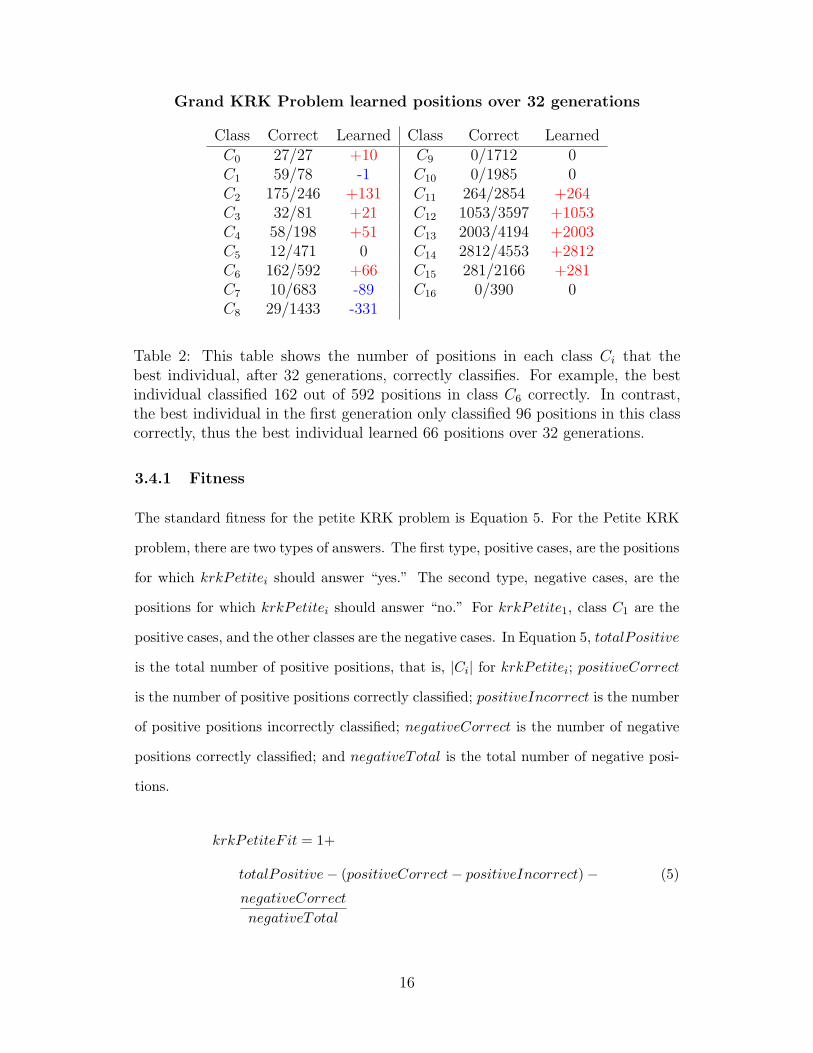
Grand KRK Problem learned positions over 32 generations

Class Correct Learned Class Correct LearnedC0 27/27 +10 C9 0/1712 0C1 59/78 -1 C10 0/1985 0C2 175/246 +131 C11 264/2854 +264C3 32/81 +21 C12 1053/3597 +1053C4 58/198 +51 C13 2003/4194 +2003C5 12/471 0 C14 2812/4553 +2812C6 162/592 +66 C15 281/2166 +281C7 10/683 -89 C16 0/390 0C8 29/1433 -331

Table 2: This table shows the number of positions in each class Ci that thebest individual, after 32 generations, correctly classifies. For example, the bestindividual classified 162 out of 592 positions in class C6 correctly. In contrast,the best individual in the first generation only classified 96 positions in this classcorrectly, thus the best individual learned 66 positions over 32 generations.

3.4.1 Fitness

The standard fitness for the petite KRK problem is Equation 5. For the Petite KRK

problem, there are two types of answers. The first type, positive cases, are the positions

for which krkPetitei should answer “yes.” The second type, negative cases, are the

positions for which krkPetitei should answer “no.” For krkPetite1, class C1 are the

positive cases, and the other classes are the negative cases. In Equation 5, totalPositive

is the total number of positive positions, that is, |Ci| for krkPetitei; positiveCorrect

is the number of positive positions correctly classified; positiveIncorrect is the number

of positive positions incorrectly classified; negativeCorrect is the number of negative

positions correctly classified; and negativeTotal is the total number of negative posi-

tions.

krkPetiteF it = 1+

totalPositive− (positiveCorrect− positiveIncorrect)− (5)

negativeCorrect

negativeTotal

16

Equation 5 pushes the population to classify the positive positions correctly first by

heavily weighting each positive position and penalizing individuals that classify positive

positions incorrectly. The total impact of the negative cases only occurs after all

positive positions are correctly classified. One positive position classified correctly

contributes twice as much fitness as classifying all negative positions correctly.

While this equation worked well for krkPetite1 (see the Results section below), it

might overweight the contribution of positive examples and certain negative classes

which could lead to a lot of locally optimal solutions. Thus, the fitness function might

need extra normalization for the larger petite KRK problems.

3.4.2 Results

After 145 generations, the best individual in the krkPetite1 population had a fitness

of 0.9749. This individual correctly classifies 97% of all positions. Figure 8 shows the

fitness of the population over 145 generations. Figure 9 presents an expanded view

of the fitness of the last 20 generations. Finally, Table 3 demonstrates the increase in

correctly classified positions from generation 1 to 145.

If the maximum fitness of the population continues to increase by the rate in Fig-

ure 9, approximately 0.006 in 20 generations, then the population will have a maximum

fitness of 0.99 in approximately 60 generations.

Based on these results, classification for the krkPetite1 problem is successful.

17

20 40 60 80 100 120 140

0.1

0.2

0.3

0.4

0.5

0.6

0.7

0.8

0.9

Generation

Adj

uste

d F

itnes

s

krkPetite1 145 Generation Fitness

Figure 8: This figure presents the fitness of individuals in the krkPetite1 problempopulation over 145 generations. The upper red-colored line shows the maximumfitness of any individual in the population; the two dashed lines show the upperand lower quartile’s of the population’s fitness (respectively); the blue-coloredline shows the mean fitness; and the bottom blue-colored line tracks the minimumfitness of the population. This figure graphs the adjusted fitness where 1.0 is thebest individual (see Equation 4).

18

1 2 3 4 5 6 7 8 9 10 11 12 13 14 15 16 17 18 19 200.9

0.91

0.92

0.93

0.94

0.95

0.96

0.97

0.98

0.99

1

Last 20 Generations of krkPetite1

Adj

uste

d F

itnes

s

Column Number

Figure 9: This figure expands the last 20 generations of the krkPetite1 problemin a box-plot view of the populations. The populations continue to increasein fitness, albeit slowly. The upper magenta-colored line follows the maximumfitness. This figure plots the adjusted fitness where 1.0 is the best individual (seeEquation 4).

19

krkPetite1learned positions over 145 generations

Class Correct Learned Class Correct LearnedC0 21/27 +21 C9 1680/1712 +1296C1 78/78 0 C10 1910/1985 +1367C2 171/246 +171 C11 2763/2854 +1977C3 53/81 +47 C12 3509/3597 +2251C4 187/198 +148 C13 4146/4194 +2133C5 428/471 +370 C14 4501/4553 +2533C6 583/592 +443 C15 2166/2166 +1253C7 649/683 +529 C16 390/390 +112C8 1377/1433 +1012

Table 3: This table shows the number of positions in each class Ci that thebest individual, after 145 generations, correctly classifies. For example, the bestindividual correctly classified 428 out of 471 positions in class C5 correctly. Incontrast, the best first generation individual only classified 58 positions in thisclass correctly, thus the best individual learned 370 positions over 145 generations.

20

4 Conclusions and Future Work

The results from the experiments with the grand KRK problem and the petite

KRK problem demonstrate that genetic programming is successful at classifying chess

positions from the KRK database. For the grand KRK problem, in 32 generations, the

evolved population showed a significant increase in the number of positions correctly

classified. For the petite KRK problem, after only 145 generations, the population suc-

cessfully identified the 78 positive positions for the krkPetite1 problem, and identified

24,612 of the 25,361 negative positions.

Nevertheless, a significant amount work remains. One interesting hypothesis to

test is whether or not the evolved populations can demonstrate separately quantifiable

chess knowledge. That is, do the evolved programs truly possess chess knowledge, or

have they simply evolved a hyper-complicated rule set to describe positions? One way

to test this might be to use the remaining, drawn, positions from the KRK dataset.

If the programs truly possess chess knowledge, then the output from the programs on

the drawn KRK positions should be reasonable. In the case of krkPetitei, the evolved

programs should, hopefully, not identify the drawn positions in class Ci.

Additionally, the grand KRK problem needs further work before it can be consid-

ered a success. The results presented in this paper are preliminary. As the populations

continue evolving, certain classes of positions might never be successfully classified.

Consequently, this problem requires more evaluation.

One unfortunate aspect of genetic programming is that the evolved individuals are

complicated and difficult to “translate.” Consequently, the programs do not constitute

easy to remember heuristics about the data and are not likely to be of much use to

chess players. However, if the chess-specific knowledge, in the form of functions and

terminals, is increased, then smaller programs might evolve.

21

4.1 Why GP on Chess?

Given the success of search based chess programs, such as Deep Blue [CHH], the idea

of applying genetic programming, or any machine learning paradigm, to create chess

programs appears odd. Machine learning strategies, however, may contribute valuable

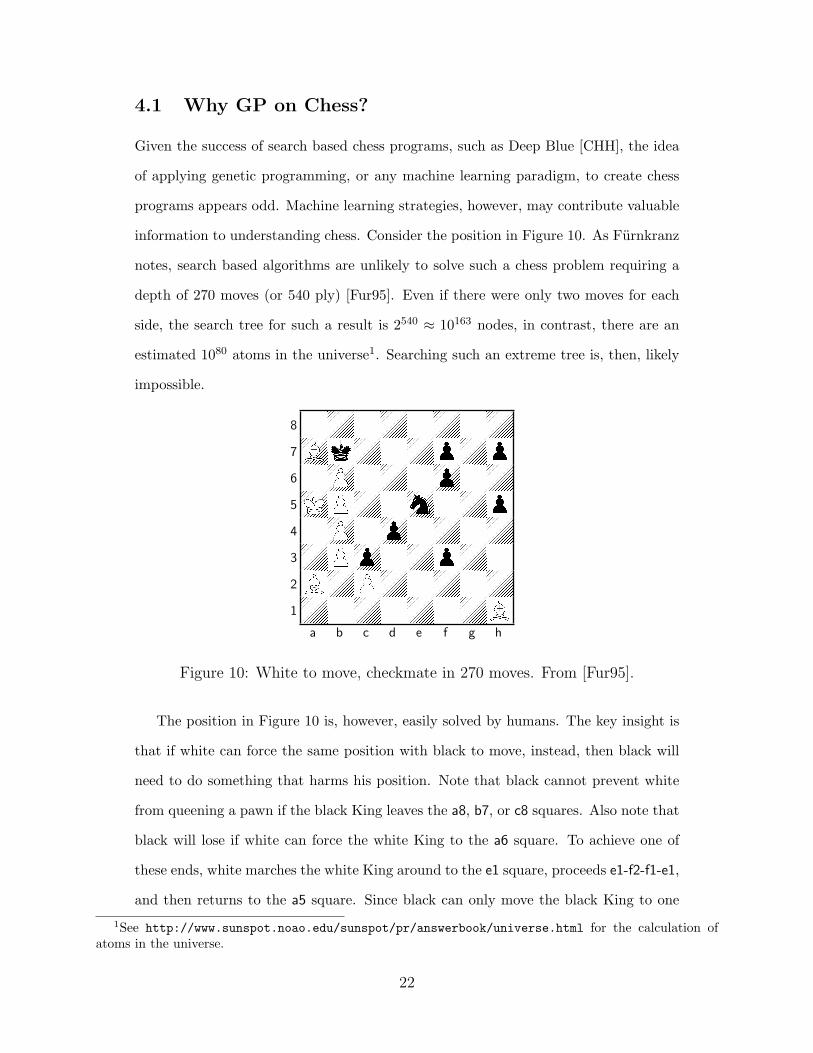
information to understanding chess. Consider the position in Figure 10. As Furnkranz

notes, search based algorithms are unlikely to solve such a chess problem requiring a

depth of 270 moves (or 540 ply) [Fur95]. Even if there were only two moves for each

side, the search tree for such a result is 2540 ≈ 10163 nodes, in contrast, there are an

estimated 1080 atoms in the universe1. Searching such an extreme tree is, then, likely

impossible.

80Z0Z0Z0Z7AkZ0ZpZp60O0Z0o0Z5JPZ0m0Zp40O0o0Z0Z3ZPo0ZpZ02BZPZ0Z0Z1Z0Z0Z0ZB

a b c d e f g h

Figure 10: White to move, checkmate in 270 moves. From [Fur95].

The position in Figure 10 is, however, easily solved by humans. The key insight is

that if white can force the same position with black to move, instead, then black will

need to do something that harms his position. Note that black cannot prevent white

from queening a pawn if the black King leaves the a8, b7, or c8 squares. Also note that

black will lose if white can force the white King to the a6 square. To achieve one of

these ends, white marches the white King around to the e1 square, proceeds e1-f2-f1-e1,

and then returns to the a5 square. Since black can only move the black King to one

1See http://www.sunspot.noao.edu/sunspot/pr/answerbook/universe.html for the calculation ofatoms in the universe.

22

position before returning to b7, white achieves the same position as Figure 10, but with

black to move. Black pushes a pawn and white repeats the maneuver. This continues

11 times until black can no longer push any pawns. Since the sequence takes 23 moves,

and is repeated 11 times white then checkmates black in the ensuing 16 moves. The key

insight makes this position trivial for a human to solve. Hopefully, machine learning

and genetic programming might allow computers to solve chess problems such as this

with the ease human chess masters do.

In summary, genetic programming is a very promising machine learning approach

to chess. Even with a modicum of chess knowledge, genetic programming evolved

populations that identified or classified a large number of positions from the UCI KRK

database.

23

References

[BM94] M. Bain and S. Muggleton. Learning Optimal Chess Strageties. In K. Fu-

rukawa, D. Michie, and S. Muggleton, editors, Machine Intelligence, volume 13,

pages 291–310. Clarendon Press, 1994.

Bain and Muggleton present some of the results from Bain’s the-

sis [Bain94]. They describe an inductive logic system that correctly iden-

tifies positions from the KRK endgame where white has won, and where

white will win in one move. Their inductive logic system allows for the

invention of new predicates to describe the chess board. They gave each

predicate a human-understandable name and had a recognized human

chess-expert verify the knowledge inducted.

[Bain94] Michael Bain. Learning Logical Exceptions in Chess. PhD thesis, Turing

Institute / Strathclyde University, Scotland, 1994.

In his PhD thesis, Bain presents a number of results using machine learn-

ing induction on chess problems. He inducts complete solutions to the

KRK illegality problem, as well as the KRK-Mate-In-Zero, and KRK-

Mate-In-One (krkPetite0, and krkPetite1) problems. The text of his

thesis is rich with theory and examples and is a good starting place for

research into computer induction of chess.

[Ber90] Hans Berliner, Danny Kopec, and Ed Northam. A taxonomy of concepts for

evaluating chess strength. In Proceedings of the 1990 conference on Supercomput-

ing, pages 336–343. IEEE Computer Society Press, 1990.

This paper describes a number of tests to evaluate the strength of a fully-

functional computer chess player. These tests are difficult positions with

only one correct move.

[BM98] C.L. Blake and C.J. Merz. UCI Repository of machine learning databases,

1998.

24

The University of California, Irvine maintains a large repository of ma-

chine learning databases for various machine learning problems. The

dataset used in this report is the chess dataset for the king-rook-king

endgame.

[Cam99] Murray Campbell. Knowledge discovery in deep blue. Communications of

the ACM, 42(11):65–67, 1999.

[CHH] Murray Campbell, Jr. A. Joseph Hoane, and Feng hsiung Hsu. Deep Blue.

Artificial Intelligence, 134(1-2):57–83, 2002.

[Coles] L. Stephen Coles. Computer Chess: The Drosophila of AI. AI Expert Magazine,

April 1994.

Coles presents a brief overview of the history of computer chess. This

article is somewhat dated since Deep Blue did beat Kasparov in 1997, as

the author predicted. However, this article is strictly about search based

chess programs, not machine learning programs.

[Fur95] Johannes Furnkranz. A Brief Introduction to Knowledge Discovery in

Databases. OGAI-Journal, 14(4):14–17, 1995.

Furnkranz explains the field of knowledge discovery. Knowledge discov-

ery is a method to discover patterns, or knowledge, within large datasets.

Furnkranz describes previous successful applications of knowledge dis-

covery in large astronomy, criminal, and telecommunications databases.

Also, he describes work on classification, association, and regression

rules.

[Fur97] Johannes Furnkranz. Knowledge Discovery in Chess Databases: A Research

Proposal. Technical Report OEFAI-TR-97-33, Austrian Research Institute for

Artificial Intelligence, 1997.

This is a research proposal by Furnkranz to study chess knowledge dis-

covery from databases. Furnkranz presents a number of reasons why

25

chess is suited to this field. Chess contains numerous features that model

real world databases, such as irrelevant pieces in certain groups of posi-

tions. Also, the growth in chess endgame databases has left chess experts

without efficient ways of extrating useful information from these mam-

moth databases. Essentially, this paper justifies chess as a good problem

for machine learning and knowledge discovery.

[GPSoft] GP related software. http://www.geneticprogramming.com/GPpages/

software.html.

A list of genetic programming software.

[GAKB] R. Gross, K. Albrecht, W. Kantschik, and W. Banzhaf. Evolving Chess

Playing Programs. In W. B. Langdon, E. Cantu-Paz, and K. Mathias, editors,

GECCO 2002: Proceedings of the Genetic and Evolutionary Computation Con-

ference, pages 740–747, New York, 9-13 July 2002. Morgan Kaufmann Publishers.

The paper explores one approach to using genetic programming to con-

struct a computer chess player. The authors develop a massively dis-

tributed genetic programming and genetic algorithm framework on the

Internet. However, they only use genetic programming to order moves

within an existing alpha-beta chess search program. Their results show

that the results of the genetic programming are superior to the standard

move ordering algorithms, and that their alpha-beta chess program uses

nearly one-fourth the nodes to reach a depth of 9-ply. In this framework,

genetic programming is used to construct an optimized portion of a larger

chess program.

[Hyatt] Robert M. Hyatt and Harry L. Nelson. Chess and supercomputers: details

about optimizing Cray Blitz. In Proceedings of the 1990 conference on Supercom-

puting, pages 354–363. IEEE Computer Society Press, 1990.

[jrgp] jrgp Home. http://jrgp.sourceforge.net/.

26

The web page for the jrgp genetic programming library. This software

was the genetic programming environment used in this experiment. Jrgp

is a GP framework written in java. The goals were an easy to use, flexible,

and efficient system.

[KHFS] R. D. King, R. Henery, C. Feng, and A. Sutherland. A Comparative Study

of Classification Algorithms: Statistical, Machine Learning, and Neural Network.

In K. Furukawa, D. Michie, and S. Muggleton, editors, Machine Intelligence, vol-

ume 13, pages 311–359. Clarendon Press, 1994.

This paper presents a preliminary comparative analysis of various ma-

chine learning systems and methods and describes their results on eight

classification problems. They describe machine learning systems as fast

and accurate on certain types of datasets.

[Kok01] G. Kokai. GeLog - A System Combining Genetic Algorithm with Inductive

Logic Programming. In Proceedings of the International Conference on Computa-

tional Intelligence, 7th Fuzzy Days, pages 326–345. Springer-Verlag, 2001.

This paper builds on previous work by Tveit [Tve97] and describes a

completed genetic algorithm and inductive logic programming hybrid

system. Building inductive logic programs is modeled using genetic op-

erations like mutation and crossover. Fitness is computed based on the

positive and negative examples provided for inductive logic program-

ming. Kokai concludes this method is promising.

[Lan98] William B. Langdon. Genetic Programming + Data Structures = Automatic

Programming! Kluwer Academic Press, 1998.

Langdon uses genetic programming to evolve data structures for a stack,

a queue, and a list. He then shows how these data structure allow ge-

netic programming to solve problems that require at least a push-down

automata model of computation.

27

[LP] William B. Langdon and Riccardo Poli. Foundations of Genetic Programming.

Springer, 1998.

In Foundations of Genetic Programming, Landgon and Poli survey the

theoretical underpinnings of genetic programming and describe various

schemata to explain why genetic programming works.

[LF] Nada Lavrac and Peter A. Flach. An extended transformation approach to in-

ductive logic programming. ACM Transactions on Computational Logic, 2(4):458–

494, October 2001.

This is a large paper on inductive logic programming. It contains a thor-

ough review of the topic and discusses limitations in existing implemen-

tations of inductive logic programming systems. They present and prove

a method to address these limitations using systematic first-order feature

construction.

[lilgp] lil-gp 1.1 Beta. http://garage.cps.msu.edu/software/lil-gp/

lilgp-index.html.

The web page for the lil-gp genetic programming library. Written by

Bill Punch and Erik Goodman, lil-gp [lilgp], is a Unix based genetic

programming framework. Lil-gp was the original GP framework used

for this experiment. It is easy to use and tremendously flexible. Lil-gp

has options for almost every aspect of the genetic programming cycles.

However, lil-gp had efficiency issues on the Harvey Mudd College Unix

server (a SPARC system with 6 350 Mhz processors running Solaris 9).

For example, a single generation of 1000 individuals took over three hours

to evaluate.

[LK] Juliet J. Liu and James T. Kwok. An extended genetic rule induction algorithm.

In Proceedings of the Congress on Evolutionary Computation (CEC), pages 458–

463, 2000.

28

This paper extends the genetic algorithm based SIA rule-induction by

adding new features, including mutation. Liu and Kwok conclude that

these extensions result in higher performance and produce smaller rule

sets.

[Mar81] T. A. Marsland and M. Campbell. A survey of enhancements to the alpha-beta

algorithm. In Proceedings of the ACM ’81 conference, pages 109–114, 1981.

[Mar73] T. A. Marsland and P. G. Rushton. Mechanisms for comparing chess pro-

grams. In Proceedings of the annual conference, pages 202–205, 1973.

[Mor97] Eduardo Morales. On Learning How to Play. In H. J. van den Herik and

J. W. H. M. Uiterwijk, editors, Advances in Computer Chess 8, pages 235–250.

Universiteit Maastricht, 1997.

Morales presents a pattern-learning analysis of the KRK endgame using

the Pal-2 system. This appears to be another way to view inductive logic

programming of chess where the human and computer construct the

final rules together. His results and approach closely model that taken

by application of inductive logic programming to chess.

[Mug90] S. Muggleton and C. Feng. Efficient induction of logic programs. In Pro-

ceedings of the 1st Conference on Algorithmic Learning Theory, pages 368–381.

Ohmsma, Tokyo, Japan, 1990.

Muggleton and Feng describe the relative-least-general-generalization

(RLGG) process and how to use it to efficiently perform inductive logic

programming. They apply their results to their inductive logic program-

ming system, GOLEM.

[Mug92] Stephen Muggleton, editor. Inductive Logic Programming. Academic Press,

1992.

Muggleton’s compendium presents an overview of the vast field of in-

ductive logic programming. Many of the papers contained within this

29

collection apply inductive logic programming to chess

[Ox99] Learning rules from chess databases. World Wide Web. http://web.comlab.

ox.ac.uk/oucl/research/areas/machlearn/chess.html, 1999.

This website is a brief summary of a project to use inductive logic pro-

gramming to learn a depth-to-win rule from a chess dataset. The site has

links to a few relevant papers and a GOLEM dataset.

[Sam59] Arthur L. Samuel. Some Studies in Machine Learning Using the Game of

Checkers. I. In David Levy, editor, Computer Games, volume 1, pages 335–365.

Springer-Verlag, 1988.

Samuel wrote one of the first papers on applying machine learning to

games; in this case, Samuel applies machine learning to checkers. This

paper is largely of historical interest and illustrates the first attempt to

make a computer automatically improve itself.

[Sam67] Arthur L. Samuel. Some Studies in Machine Learning Using the Game of

Checkers. II – Recent Progress. In David Levy, editor, Computer Games, volume 1,

pages 366–400. Springer-Verlag, 1988.

In this paper, Samuel updates his previous work [Sam59] with more

results about attempts to improve book learning in checker programs.

[Sch86] Jonathan Schaeffer. Improved parallel alpha-beta search. In Proceedings of

1986 fall joint computer conference on Fall joint computer conference, pages 519–

527. IEEE Computer Society Press, 1986.

[Sch96] Jonathan Schaeffer and Aske Plaat. New advances in Alpha-Beta searching. In

Proceedings of the 1996 ACM 24th annual conference on Computer science, pages

124–130. ACM Press, 1996.

[Shannon] Claude E. Shannon. A Chess-Playing Machine. In David Levy, editor,

Computer Games, volume 1, pages 81–88. Springer-Verlag, 1988.

30

Shannon describes a machine to play chess. He reasons that it is com-

putationally infeasible for a machine to play perfect chess based on the

size of the decision tree required, thus machines must merely play chess

“skillfully.” This is the first paper written about computer chess.

[Thr95] S. Thrun. Learning to Play the Game of Chess. In G. Tesauro, D. Touretzky,

and T. Leen, editors, Advances in Neural Information Processing Systems (NIPS)

7, Cambridge, MA, 1995. MIT Press.

This paper describes NeuroChess, a program which used a neural network

to learn the game of chess. The author uses a temporal difference method

to train the neural net on a database of games played by chess masters.

NeuroChess demonstrates that a neural net can learn the game of chess.

[Turing] Alan M. Turing. Chess. In David Levy, editor, Computer Chess Compendium,

pages 14–17. Springer-Verlag, 1953.

Turing explains some of the basics of search-based computer chess pro-

grams. He enumerates values for the different pieces and describes an

algorithm for a computer to pick moves while playing against a human.

[Tve97] A. Tveit. Genetic Inductive Logic Programming. Master’s thesis, Norwegian

University of Science and Technology, 1997.

This thesis describes a system which uses genetic programming to gener-

ate rules for inductive logic programming. It contains a useful summary

of various genetic algorithm and genetic programming stragedies and al-

gorithms. The author focuses his research on means of restricting the

search space of horn clauses, and discusses five techniques for pruning

this space. Due to time constraints, no implementation of this system

was completed, and no experimental results were presented.

[TH] A. van Tiggelen and H.J. van de Herik. ALEXS: An Optimization Approach for

the Endgame KNNKP(h). In D. F. Beal, editor, Advances in Computer Chess,

volume 6, pages 161–177. Ellis Horwood, 1991.

31

Tiggelen and Herik describe their ALEXS system to optimize a utility

weighting function for the KNNKP (white king, two white knights, black

king, and black pawn) endgame. They evaluate a series of machine learn-

ing techniques including monte-carlo methods, linear regression analysis,

and genetic algorithms. They choose to use genetic algorithms to evolve

a series of weights for eight characteristics of the positions. The results of

the genetic algorithm experiment show evolution of near-optimal weights

with a population of 16 strings over 100 generations.

[Wyman] C. Wyman. Using Genetic Algorithms to Learn Weights for Simple King-

Pawn Chess Endgames. Technical report, University of Utah, 1999.

This website describes a project to learn weighting factors for a simple

KPK chess endgame. The author’s goal is to use a genetic algorithm and

a chess database as a fitness function to compute the weights. The results

indicate that simple genetic algorithm methods can produce close to ideal

behavior on the part of one player, however, the author concludes that a

simple genetic algorithm may not be able to develop the ideal behavior

for both players.

32