machine learning for signal processing non-negative matrix...
TRANSCRIPT
Machine Learning for Signal Processing
Non-negative Matrix Factorization
Class 9. 29 Sep 2016
Instructor: Bhiksha Raj
11755/18797 1
With examples and
slides from
Paris Smaragdis

A Quick Recap
• Problem: Given a collection of data X, find a set of “bases” B, such that each vector xi can be expressed as a weighted combination of the bases
11755/18797 2
X
x1 x2 xN
w1 w2 wN
W
D
N
B
B1 BK
K
=
x
𝒙𝑖 = 𝑩𝒘𝒊 𝒙𝑖 = 𝑤11𝐵1 +⋯+𝑤1𝐾𝐵𝐾
N
D
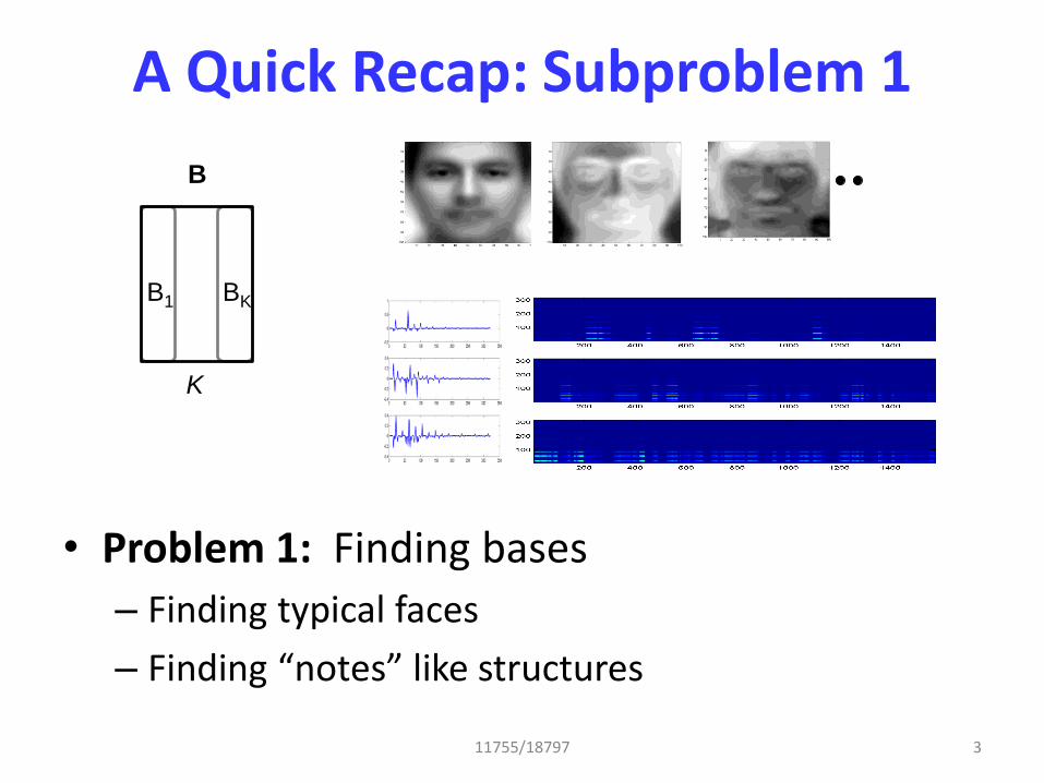
A Quick Recap: Subproblem 1
• Problem 1: Finding bases
– Finding typical faces
– Finding “notes” like structures
11755/18797 3
B
B1 BK
K
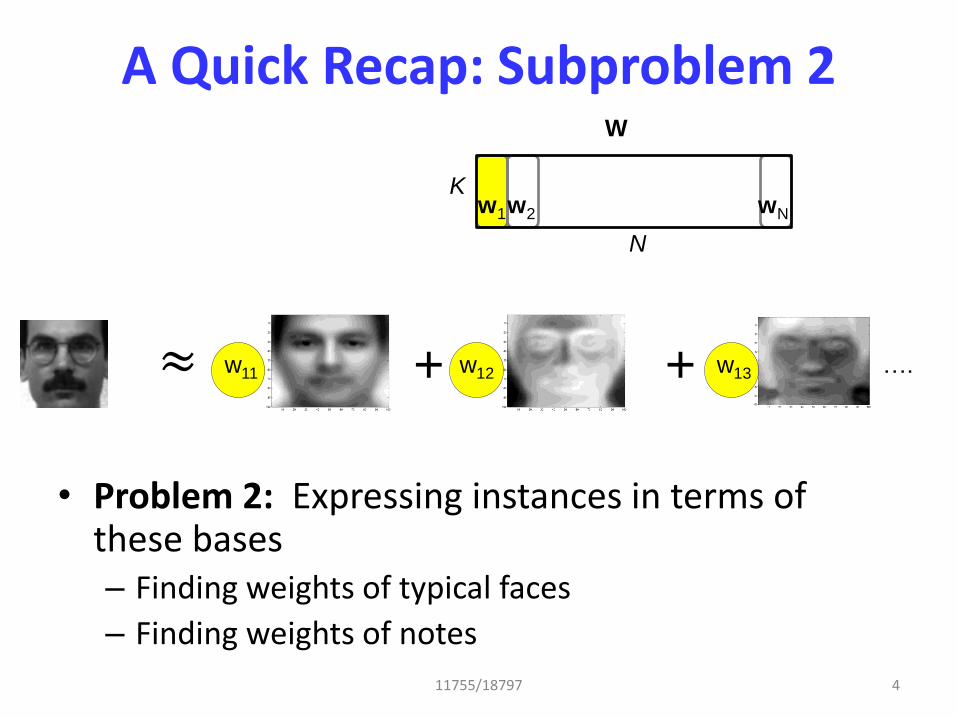
A Quick Recap: Subproblem 2
• Problem 2: Expressing instances in terms of these bases – Finding weights of typical faces
– Finding weights of notes
11755/18797 4
w1 w2 wN
W
K
N
w11 w12 w13 …. + + ≈
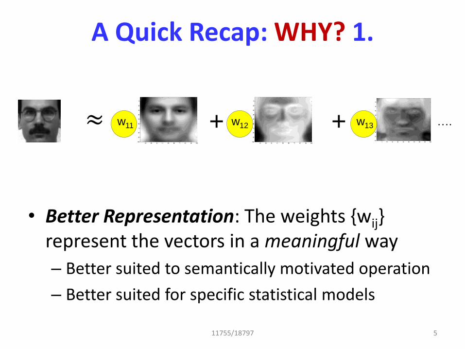
A Quick Recap: WHY? 1.
• Better Representation: The weights {wij} represent the vectors in a meaningful way
– Better suited to semantically motivated operation
– Better suited for specific statistical models
11755/18797 5
w11 w12 w13 …. + + ≈
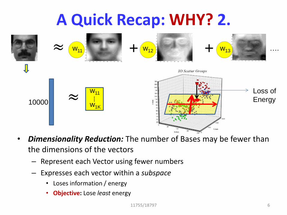
A Quick Recap: WHY? 2.
• Dimensionality Reduction: The number of Bases may be fewer than the dimensions of the vectors
– Represent each Vector using fewer numbers
– Expresses each vector within a subspace
• Loses information / energy
• Objective: Lose least energy
11755/18797 6
w11 w12 w13 …. + + ≈
10000 ≈ w11
w1K
⋮ Loss of
Energy
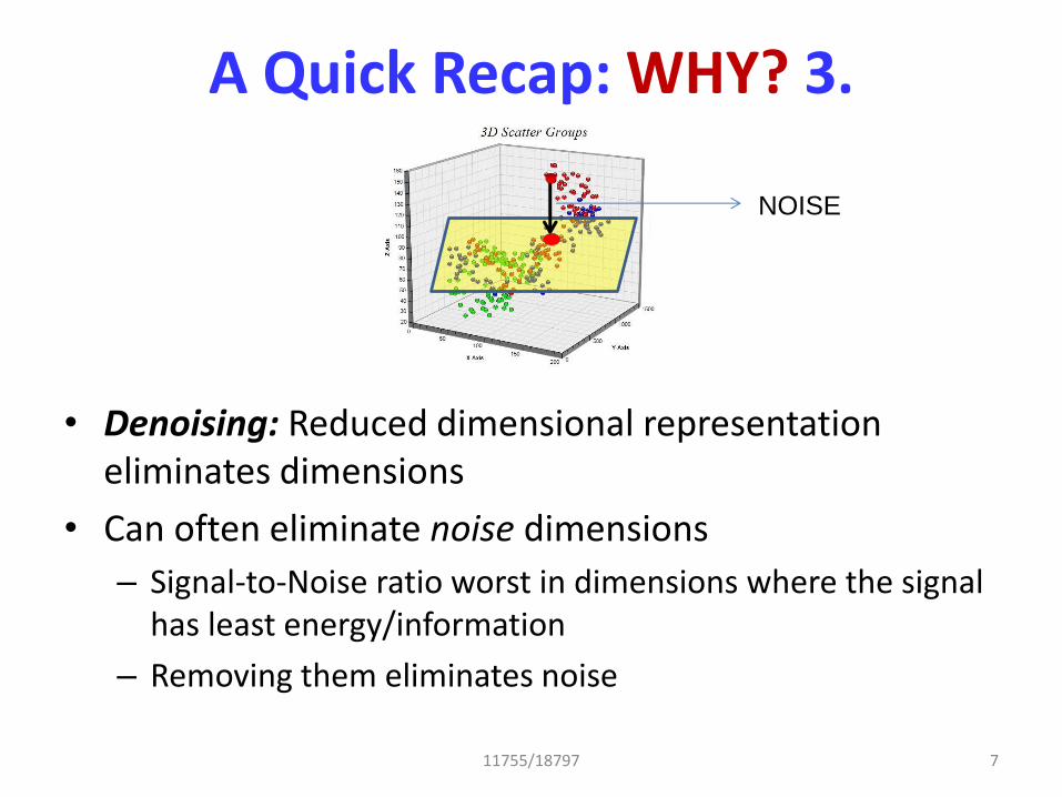
A Quick Recap: WHY? 3.
• Denoising: Reduced dimensional representation eliminates dimensions
• Can often eliminate noise dimensions
– Signal-to-Noise ratio worst in dimensions where the signal has least energy/information
– Removing them eliminates noise
11755/18797 7
NOISE
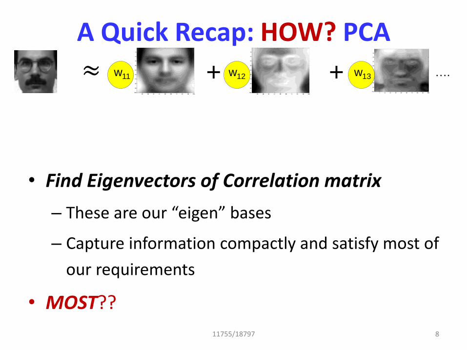
A Quick Recap: HOW? PCA
• Find Eigenvectors of Correlation matrix
– These are our “eigen” bases
– Capture information compactly and satisfy most of
our requirements
• MOST??
11755/18797 8
w11 w12 w13 …. + + ≈
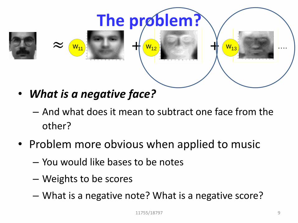
The problem?
• What is a negative face?
– And what does it mean to subtract one face from the
other?
• Problem more obvious when applied to music
– You would like bases to be notes
– Weights to be scores
– What is a negative note? What is a negative score?
11755/18797 9
w11 w12 w13 …. + + ≈
Summary
• Decorrelation and Independence are statistically meaningful operations
• But may not be physically meaningful
• Next: A physically meaningful constraint
– Non-negativity
11755/18797 10
The Engineer and the Musician
Once upon a time a rich potentate
discovered a previously unknown
recording of a beautiful piece of
music. Unfortunately it was badly
damaged.
He greatly wanted to find out what it would sound
like if it were not.
So he hired an engineer and a musician to solve the problem..
11
The Engineer and the Musician
The engineer worked for many
years. He spent much money and
published many papers.
Finally he had a somewhat scratchy
restoration of the music..
The musician listened to the music
carefully for a day, transcribed it,
broke out his trusty keyboard and
replicated the music. 12
The Prize
Who do you think won the princess?
13
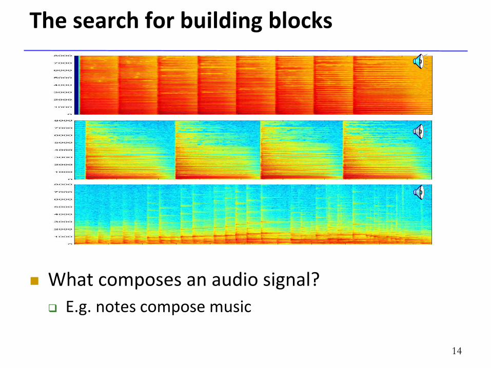
The search for building blocks
What composes an audio signal?
E.g. notes compose music
14
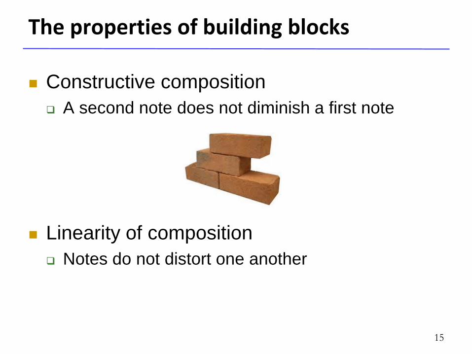
The properties of building blocks
Constructive composition
A second note does not diminish a first note
Linearity of composition
Notes do not distort one another
15
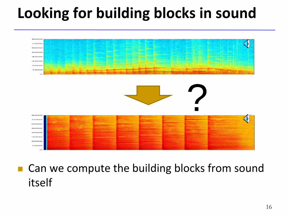
Looking for building blocks in sound
Can we compute the building blocks from sound itself
16
?
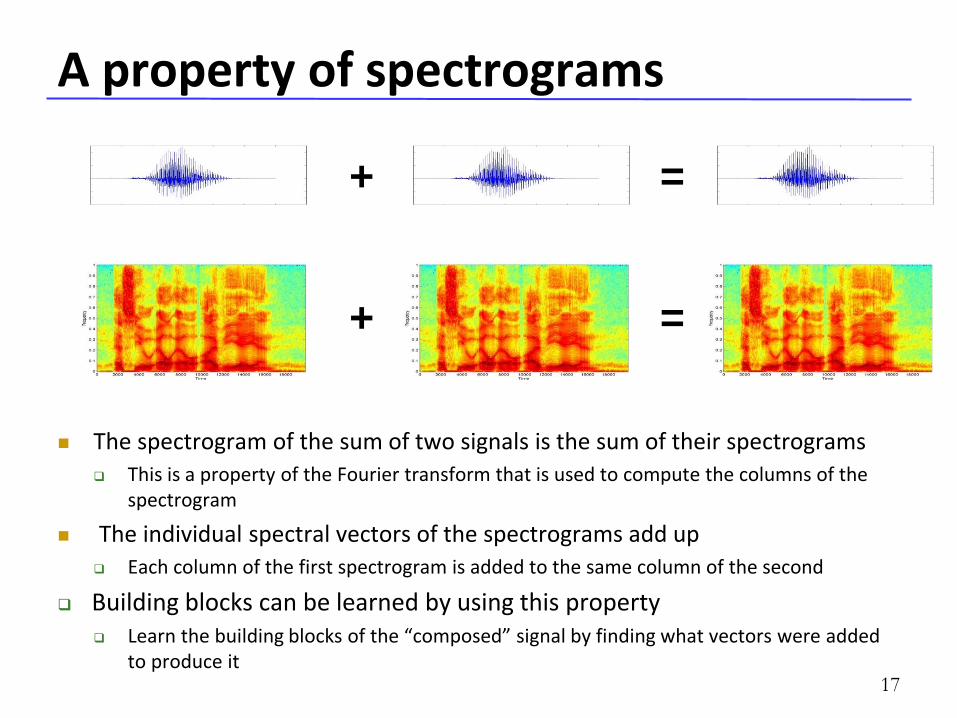
A property of spectrograms
+
+
=
=
The spectrogram of the sum of two signals is the sum of their spectrograms
This is a property of the Fourier transform that is used to compute the columns of the spectrogram
The individual spectral vectors of the spectrograms add up
Each column of the first spectrogram is added to the same column of the second
Building blocks can be learned by using this property Learn the building blocks of the “composed” signal by finding what vectors were added
to produce it 17
Another property of spectrograms
+
+
=
=
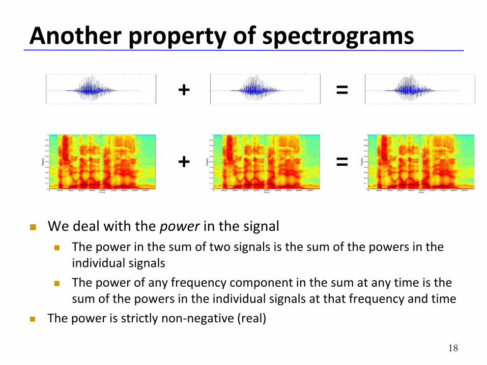
We deal with the power in the signal
The power in the sum of two signals is the sum of the powers in the individual signals
The power of any frequency component in the sum at any time is the sum of the powers in the individual signals at that frequency and time
The power is strictly non-negative (real)
18
Building Blocks of Sound
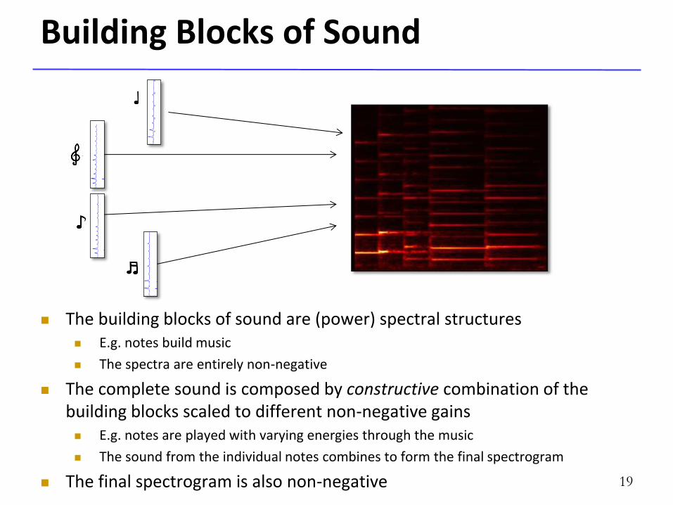
The building blocks of sound are (power) spectral structures E.g. notes build music
The spectra are entirely non-negative
The complete sound is composed by constructive combination of the building blocks scaled to different non-negative gains E.g. notes are played with varying energies through the music
The sound from the individual notes combines to form the final spectrogram
The final spectrogram is also non-negative 19
Building Blocks of Sound
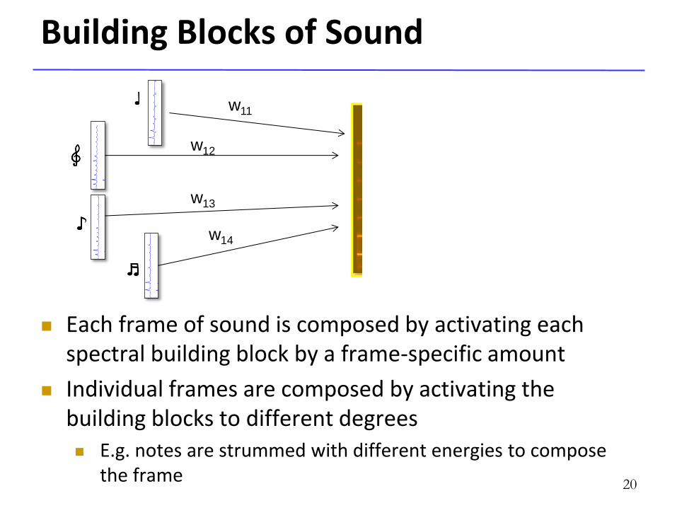
Each frame of sound is composed by activating each spectral building block by a frame-specific amount
Individual frames are composed by activating the building blocks to different degrees
E.g. notes are strummed with different energies to compose the frame
20
w11
w12
w13
w14
Composing the Sound
21
w21
w22
w23
w24
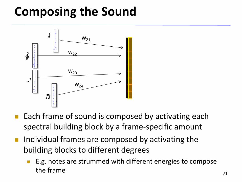
Each frame of sound is composed by activating each spectral building block by a frame-specific amount
Individual frames are composed by activating the building blocks to different degrees
E.g. notes are strummed with different energies to compose the frame
Building Blocks of Sound
22
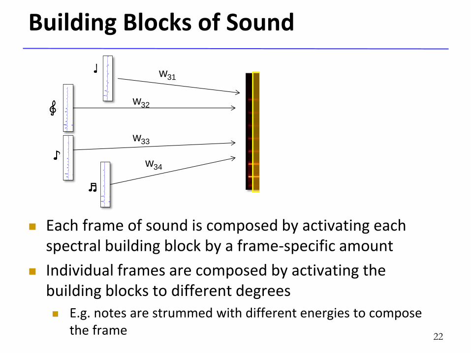
w31
w32
w33
w34
Each frame of sound is composed by activating each spectral building block by a frame-specific amount
Individual frames are composed by activating the building blocks to different degrees
E.g. notes are strummed with different energies to compose the frame
Building Blocks of Sound
23
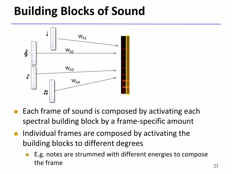
w41
w42
w43
w44
Each frame of sound is composed by activating each spectral building block by a frame-specific amount
Individual frames are composed by activating the building blocks to different degrees
E.g. notes are strummed with different energies to compose the frame
Building Blocks of Sound
24
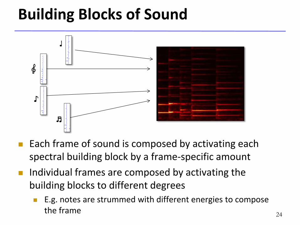
Each frame of sound is composed by activating each spectral building block by a frame-specific amount
Individual frames are composed by activating the building blocks to different degrees
E.g. notes are strummed with different energies to compose the frame
The Problem of Learning
25
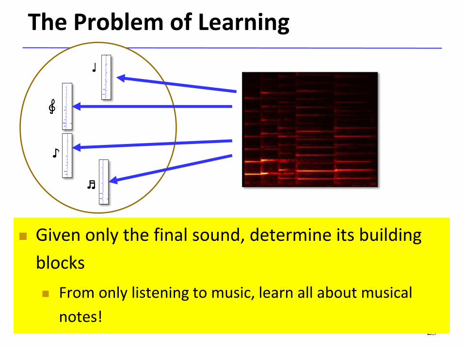
Given only the final sound, determine its building
blocks
From only listening to music, learn all about musical
notes!
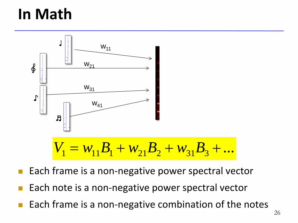
In Math
26
Each frame is a non-negative power spectral vector
Each note is a non-negative power spectral vector
Each frame is a non-negative combination of the notes
...3312211111 BwBwBwV
w11
w21
w31
w41
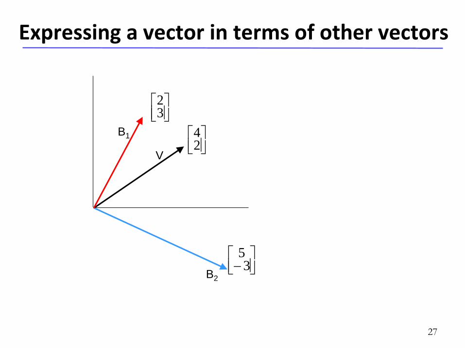
Expressing a vector in terms of other vectors
V
B1
B2
27
32
24
35
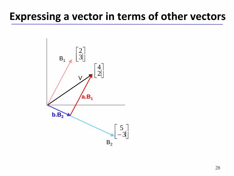
Expressing a vector in terms of other vectors
V
B1
B2
b.B2
a.B1
28
32
24
35
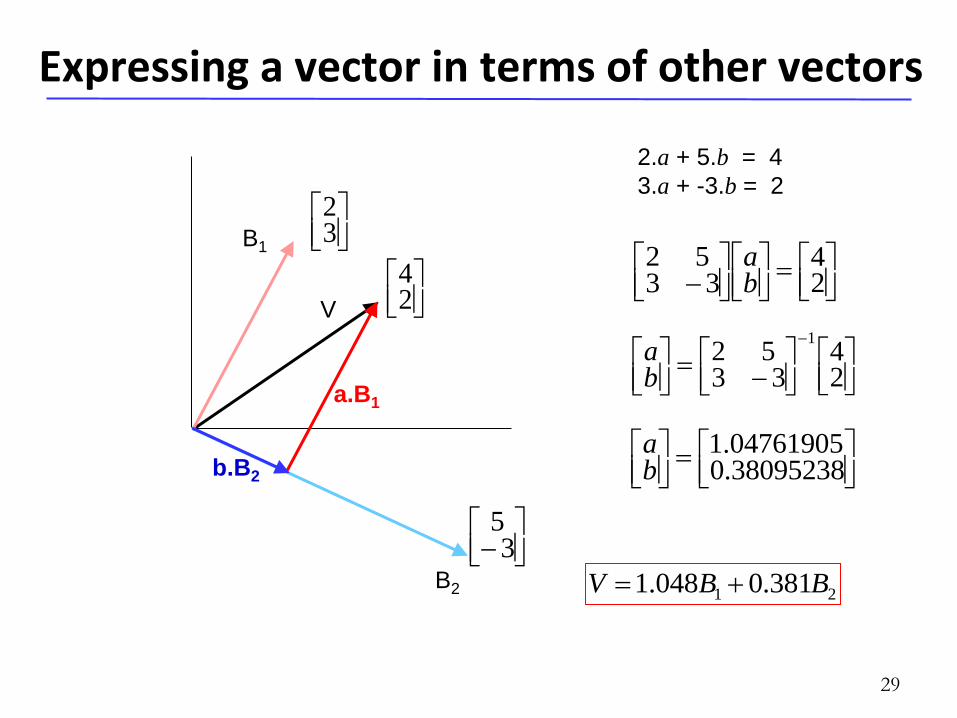
Expressing a vector in terms of other vectors
2.a + 5.b = 4
3.a + -3.b = 2
24
3352
ba
24
3352
1
ba
38095238.004761905.1
ba
21 381.0048.1 BBV
V
B1
B2
b.B2
a.B1
29
32
24
35
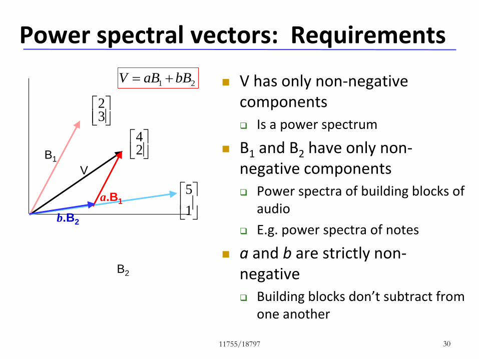
V has only non-negative components
Is a power spectrum
B1 and B2 have only non-negative components
Power spectra of building blocks of audio
E.g. power spectra of notes
a and b are strictly non-negative
Building blocks don’t subtract from one another
30
Power spectral vectors: Requirements
V
B1
B2
b.B2
a.B1
21 bBaBV
32
24
1
5
11755/18797
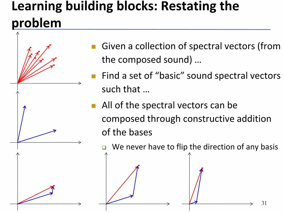
Given a collection of spectral vectors (from
the composed sound) …
Find a set of “basic” sound spectral vectors
such that …
All of the spectral vectors can be
composed through constructive addition
of the bases
We never have to flip the direction of any basis
31
Learning building blocks: Restating the problem
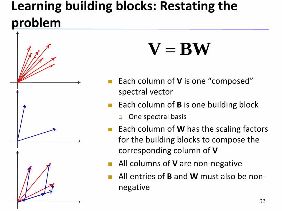
Each column of V is one “composed” spectral vector
Each column of B is one building block
One spectral basis
Each column of W has the scaling factors for the building blocks to compose the corresponding column of V
All columns of V are non-negative
All entries of B and W must also be non-negative
32
Learning building blocks: Restating the problem
BWV
Non-negative matrix factorization: Basics
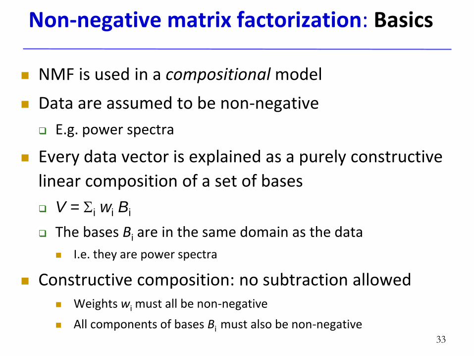
NMF is used in a compositional model
Data are assumed to be non-negative
E.g. power spectra
Every data vector is explained as a purely constructive
linear composition of a set of bases
V = Si wi Bi
The bases Bi are in the same domain as the data
I.e. they are power spectra
Constructive composition: no subtraction allowed Weights wi must all be non-negative
All components of bases Bi must also be non-negative 33
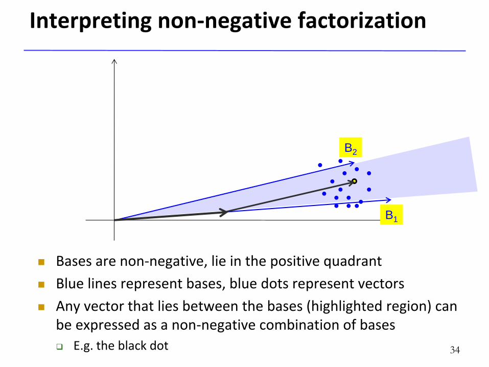
Interpreting non-negative factorization
Bases are non-negative, lie in the positive quadrant
Blue lines represent bases, blue dots represent vectors
Any vector that lies between the bases (highlighted region) can be expressed as a non-negative combination of bases
E.g. the black dot 34
B1
B2
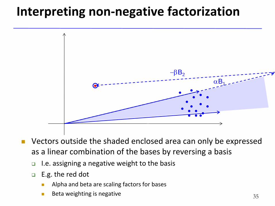
Interpreting non-negative factorization
Vectors outside the shaded enclosed area can only be expressed as a linear combination of the bases by reversing a basis
I.e. assigning a negative weight to the basis
E.g. the red dot
Alpha and beta are scaling factors for bases
Beta weighting is negative
aB1
bB2
ap
pr
o
xi
m
ati
o
n
wi
ll
d
35
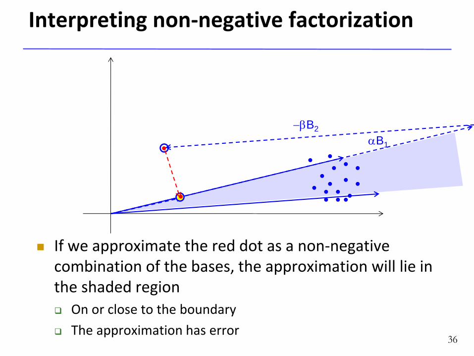
Interpreting non-negative factorization
If we approximate the red dot as a non-negative combination of the bases, the approximation will lie in the shaded region
On or close to the boundary
The approximation has error
aB1
bB2
36
The NMF representation
The representation characterizes all data as lying within
a compact convex region
“Compact” enclosing only a small fraction of the entire space
The more compact the enclosed region, the more it localizes the
data within it
Represents the boundaries of the distribution of the data better
Conventional statistical models represent the mode of the distribution
The bases must be chosen to
Enclose the data as compactly as possible
And also enclose as much of the data as possible
Data that are not enclosed are not represented correctly
37
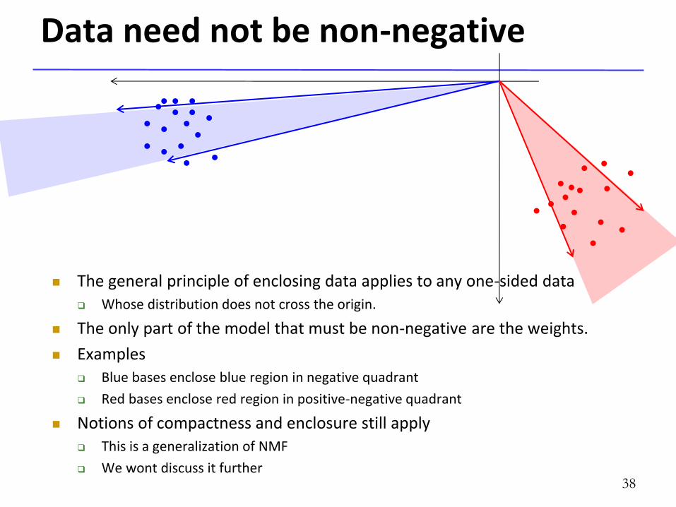
Data need not be non-negative
The general principle of enclosing data applies to any one-sided data
Whose distribution does not cross the origin.
The only part of the model that must be non-negative are the weights.
Examples
Blue bases enclose blue region in negative quadrant
Red bases enclose red region in positive-negative quadrant
Notions of compactness and enclosure still apply
This is a generalization of NMF
We wont discuss it further 38
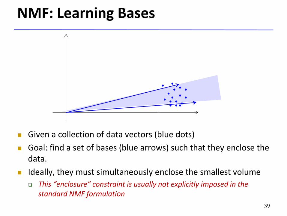
NMF: Learning Bases
Given a collection of data vectors (blue dots)
Goal: find a set of bases (blue arrows) such that they enclose the data.
Ideally, they must simultaneously enclose the smallest volume
This “enclosure” constraint is usually not explicitly imposed in the standard NMF formulation
39
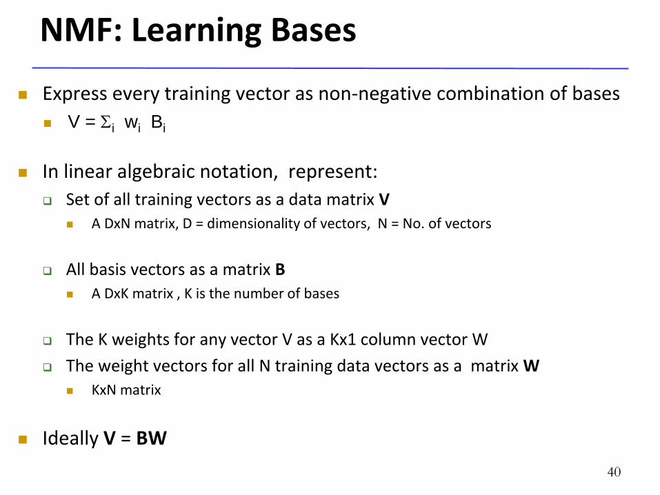
NMF: Learning Bases
Express every training vector as non-negative combination of bases
V = Si wi Bi
In linear algebraic notation, represent:
Set of all training vectors as a data matrix V
A DxN matrix, D = dimensionality of vectors, N = No. of vectors
All basis vectors as a matrix B
A DxK matrix , K is the number of bases
The K weights for any vector V as a Kx1 column vector W
The weight vectors for all N training data vectors as a matrix W
KxN matrix
Ideally V = BW
40
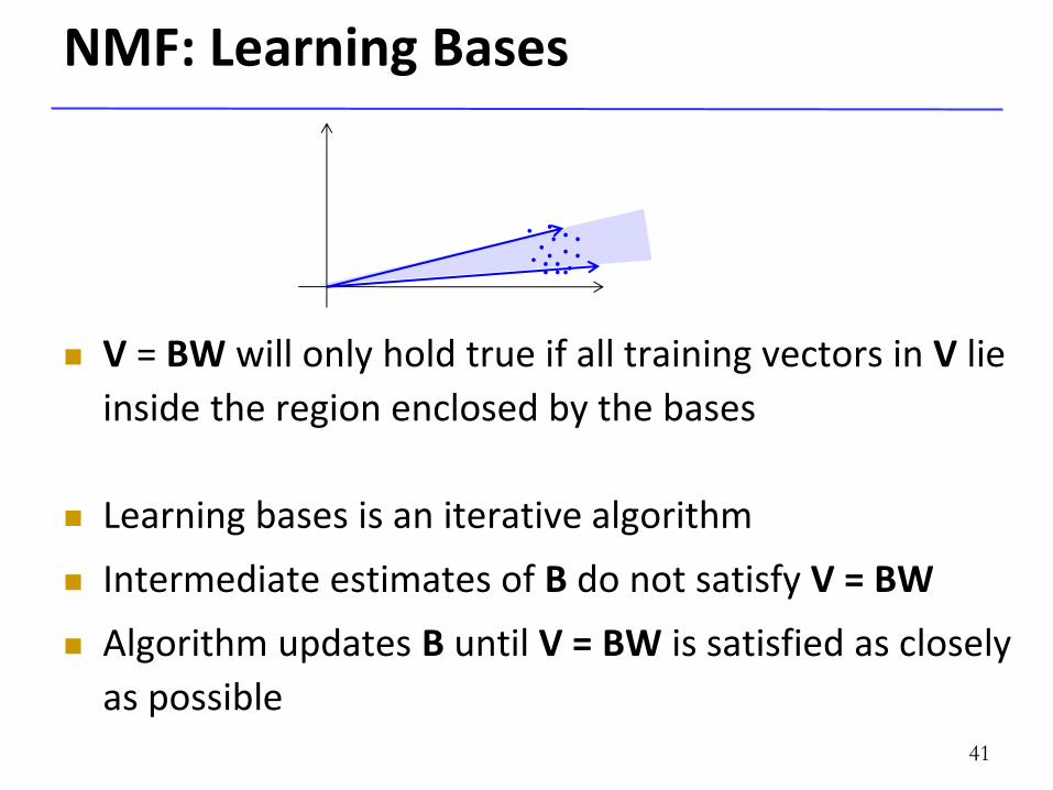
NMF: Learning Bases
V = BW will only hold true if all training vectors in V lie
inside the region enclosed by the bases
Learning bases is an iterative algorithm
Intermediate estimates of B do not satisfy V = BW
Algorithm updates B until V = BW is satisfied as closely
as possible 41
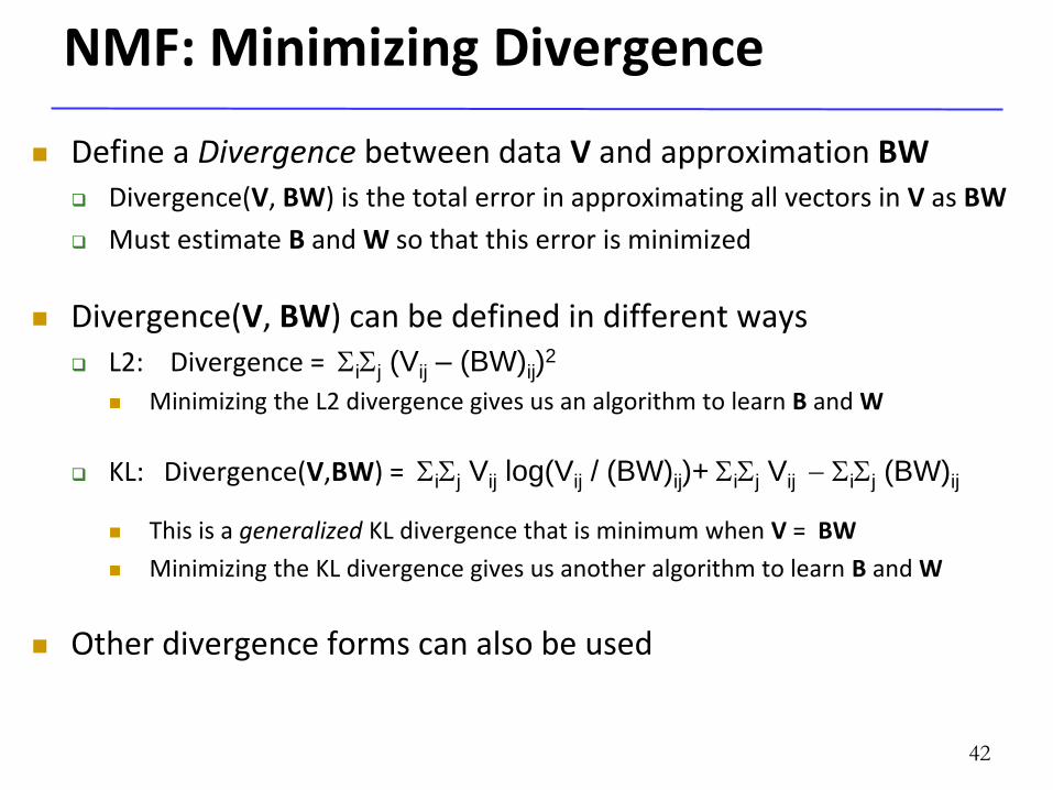
NMF: Minimizing Divergence
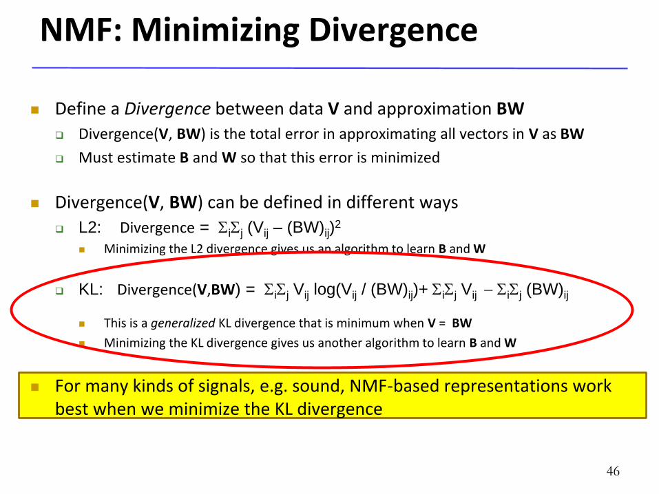
Define a Divergence between data V and approximation BW Divergence(V, BW) is the total error in approximating all vectors in V as BW
Must estimate B and W so that this error is minimized
Divergence(V, BW) can be defined in different ways
L2: Divergence = SiSj (Vij – (BW)ij)2
Minimizing the L2 divergence gives us an algorithm to learn B and W
KL: Divergence(V,BW) = SiSj Vij log(Vij / (BW)ij)+ SiSj Vij SiSj (BW)ij
This is a generalized KL divergence that is minimum when V = BW
Minimizing the KL divergence gives us another algorithm to learn B and W
Other divergence forms can also be used
42
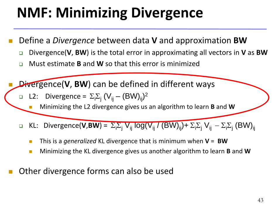
NMF: Minimizing Divergence
Define a Divergence between data V and approximation BW Divergence(V, BW) is the total error in approximating all vectors in V as BW
Must estimate B and W so that this error is minimized
Divergence(V, BW) can be defined in different ways
L2: Divergence = SiSj (Vij – (BW)ij)2
Minimizing the L2 divergence gives us an algorithm to learn B and W
KL: Divergence(V,BW) = SiSj Vij log(Vij / (BW)ij)+ SiSj Vij SiSj (BW)ij
This is a generalized KL divergence that is minimum when V = BW
Minimizing the KL divergence gives us another algorithm to learn B and W
Other divergence forms can also be used
43
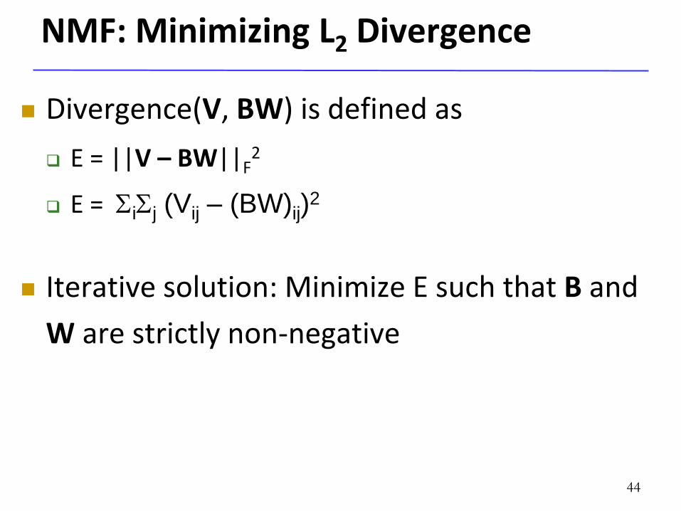
NMF: Minimizing L2 Divergence
Divergence(V, BW) is defined as
E = ||V – BW||F2
E = SiSj (Vij – (BW)ij)2
Iterative solution: Minimize E such that B and
W are strictly non-negative
44
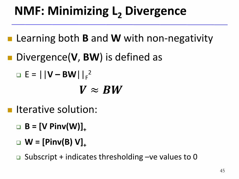
NMF: Minimizing L2 Divergence
Learning both B and W with non-negativity
Divergence(V, BW) is defined as
E = ||V – BW||F2
𝑽 ≈ 𝑩𝑾
Iterative solution:
B = [V Pinv(W)]+
W = [Pinv(B) V]+
Subscript + indicates thresholding –ve values to 0
45
NMF: Minimizing Divergence
Define a Divergence between data V and approximation BW
Divergence(V, BW) is the total error in approximating all vectors in V as BW
Must estimate B and W so that this error is minimized
Divergence(V, BW) can be defined in different ways
L2: Divergence = SiSj (Vij – (BW)ij)2
Minimizing the L2 divergence gives us an algorithm to learn B and W
KL: Divergence(V,BW) = SiSj Vij log(Vij / (BW)ij)+ SiSj Vij SiSj (BW)ij
This is a generalized KL divergence that is minimum when V = BW
Minimizing the KL divergence gives us another algorithm to learn B and W
For many kinds of signals, e.g. sound, NMF-based representations work best when we minimize the KL divergence
46
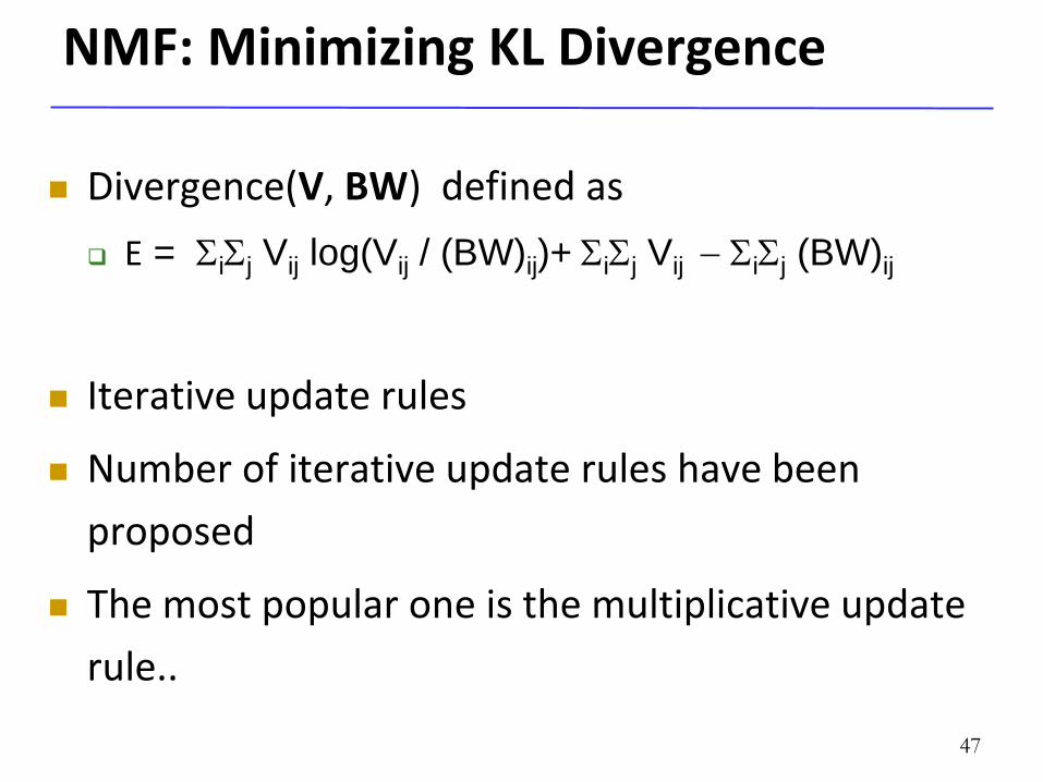
NMF: Minimizing KL Divergence
Divergence(V, BW) defined as
E = SiSj Vij log(Vij / (BW)ij)+ SiSj Vij SiSj (BW)ij
Iterative update rules
Number of iterative update rules have been
proposed
The most popular one is the multiplicative update
rule..
47
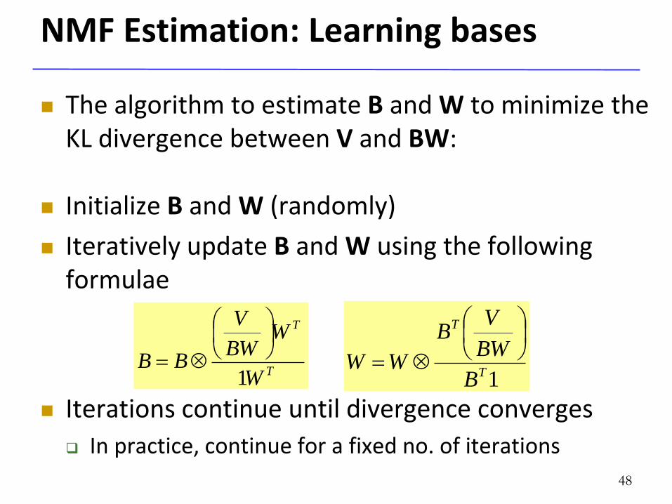
NMF Estimation: Learning bases
The algorithm to estimate B and W to minimize the KL divergence between V and BW:
Initialize B and W (randomly)
Iteratively update B and W using the following formulae
Iterations continue until divergence converges
In practice, continue for a fixed no. of iterations
T
T
W
WBW
V
BB1
1T
T
B
BW
VB
WW
48
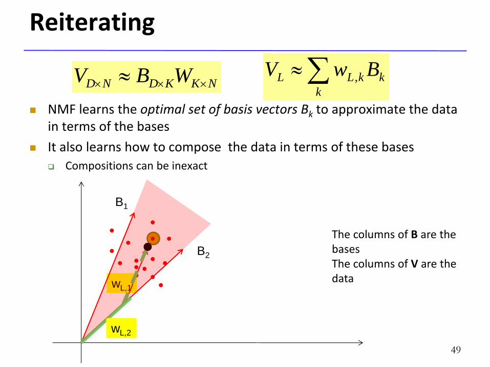
Reiterating
NMF learns the optimal set of basis vectors Bk to approximate the data in terms of the bases
It also learns how to compose the data in terms of these bases
Compositions can be inexact
NKKDND WBV k
k
kLL BwV ,
The columns of B are the bases The columns of V are the data
49
wL,1
B1
B2
wL,2
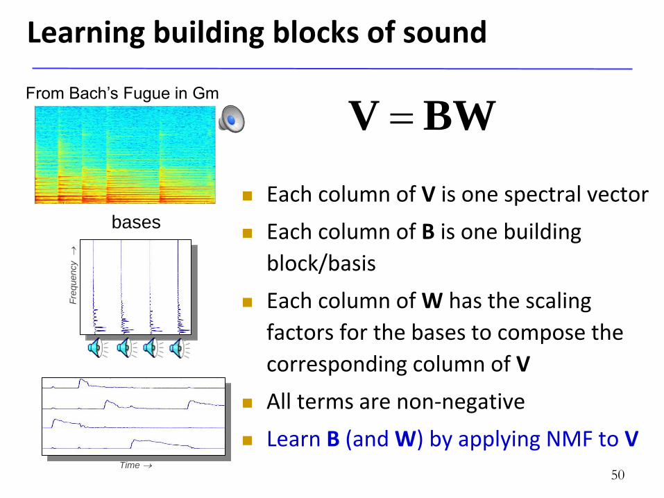
Each column of V is one spectral vector
Each column of B is one building
block/basis
Each column of W has the scaling
factors for the bases to compose the
corresponding column of V
All terms are non-negative
Learn B (and W) by applying NMF to V
50
Learning building blocks of sound
BWV From Bach’s Fugue in Gm
Fre
quency
bases
Time
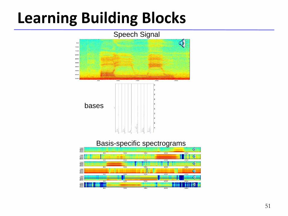
Learning Building Blocks Speech Signal
bases
Basis-specific spectrograms
51
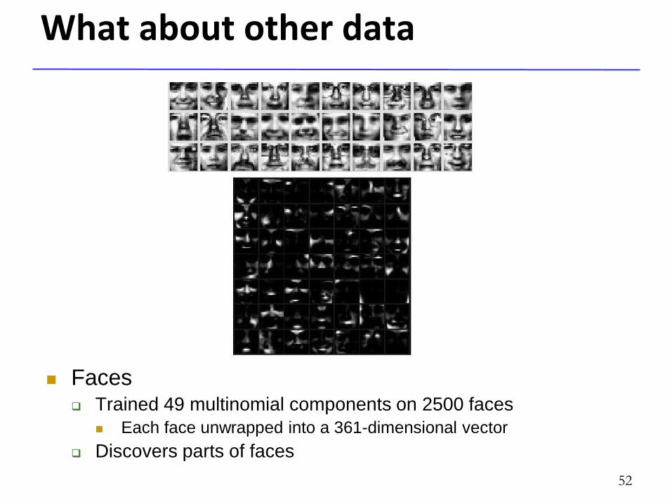
What about other data
Faces Trained 49 multinomial components on 2500 faces
Each face unwrapped into a 361-dimensional vector
Discovers parts of faces
52
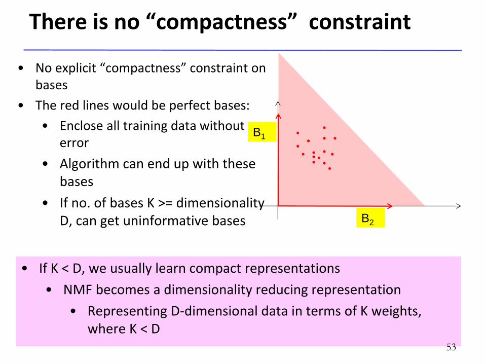
There is no “compactness” constraint
• If K < D, we usually learn compact representations
• NMF becomes a dimensionality reducing representation
• Representing D-dimensional data in terms of K weights, where K < D
B1
B2
• No explicit “compactness” constraint on bases
• The red lines would be perfect bases:
• Enclose all training data without error
• Algorithm can end up with these bases
• If no. of bases K >= dimensionality D, can get uninformative bases
53
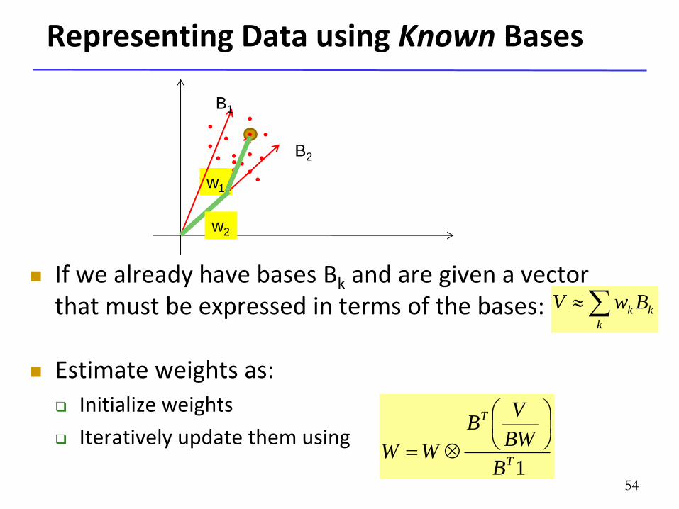
Representing Data using Known Bases
If we already have bases Bk and are given a vector that must be expressed in terms of the bases:
Estimate weights as:
Initialize weights
Iteratively update them using
k
k
k BwV
1T
T
B
BW
VB
WW
w1
B1
B2
w2
54
What can we do knowing the building blocks
Signal Representation
Signal Separation
Signal Completion
Denoising
Signal recovery
Music Transcription
Etc.
55
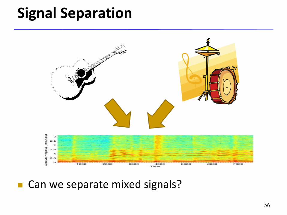
Signal Separation
Can we separate mixed signals?
56
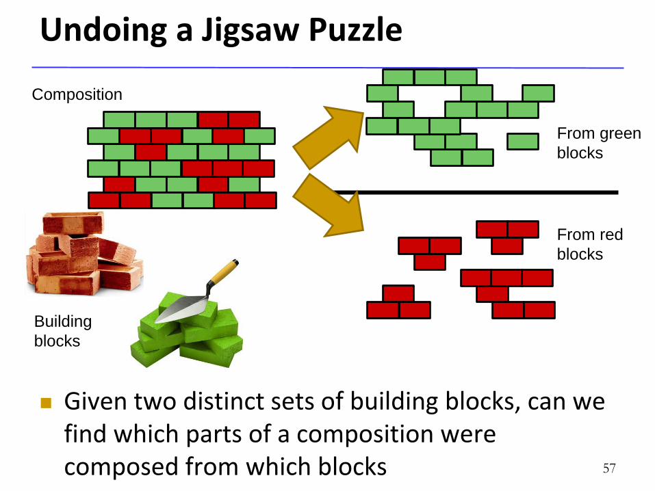
Undoing a Jigsaw Puzzle
Given two distinct sets of building blocks, can we find which parts of a composition were composed from which blocks 57
Building
blocks
Composition
From green
blocks
From red
blocks
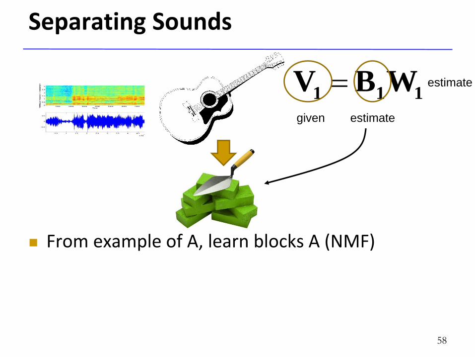
Separating Sounds
From example of A, learn blocks A (NMF)
58
111 WBV given estimate
estimate
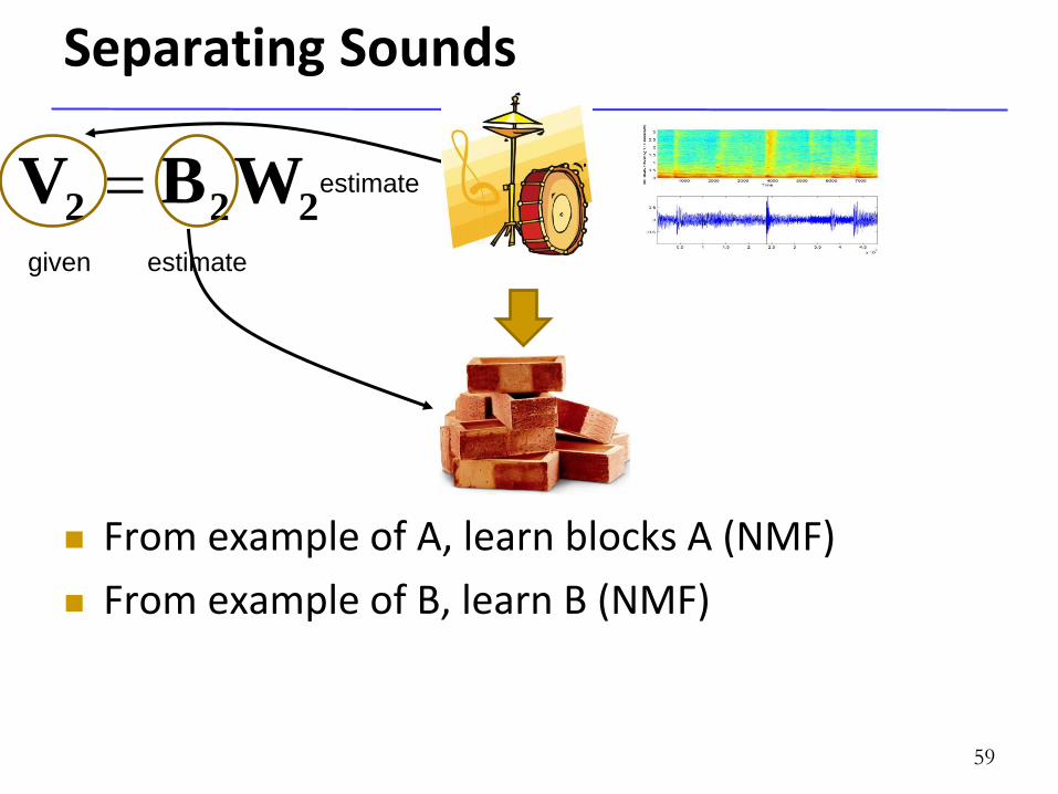
Separating Sounds
From example of A, learn blocks A (NMF)
From example of B, learn B (NMF)
59
222 WBV given estimate
estimate
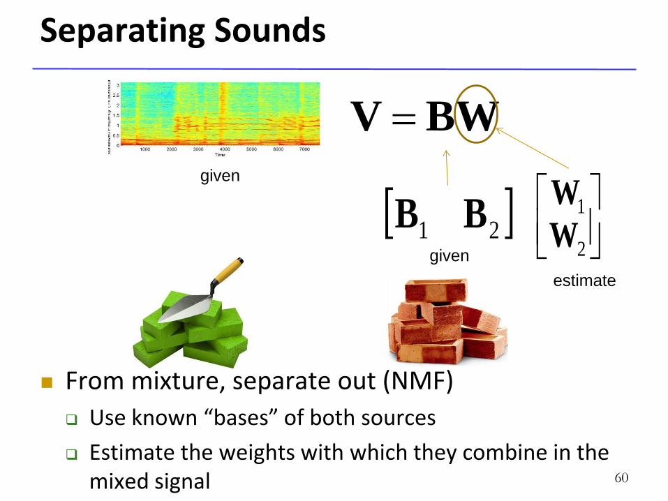
Separating Sounds
From mixture, separate out (NMF)
Use known “bases” of both sources
Estimate the weights with which they combine in the mixed signal 60
BWV
21 BB
2
1
W
Wgiven
given
estimate
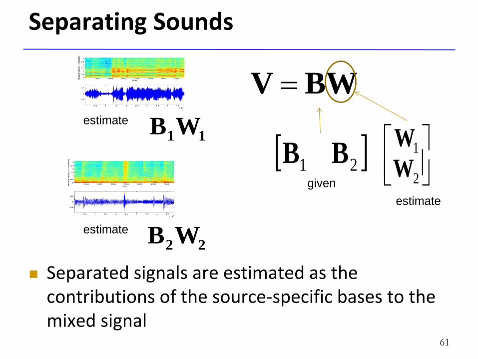
Separating Sounds
Separated signals are estimated as the contributions of the source-specific bases to the mixed signal
61
BWV
21 BB
2
1
W
Westimate
given
estimate
11WB
estimate
22WB
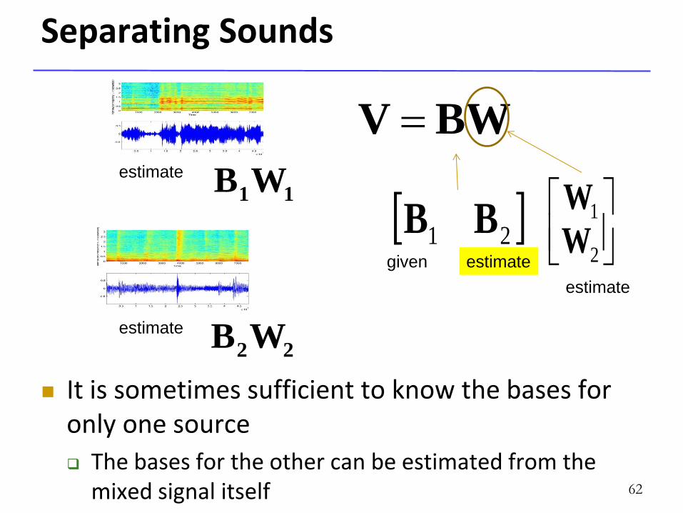
Separating Sounds
It is sometimes sufficient to know the bases for only one source
The bases for the other can be estimated from the mixed signal itself 62
BWV
21 BB
2
1
W
Westimate
given
estimate
11WB
estimate
22WB
estimate
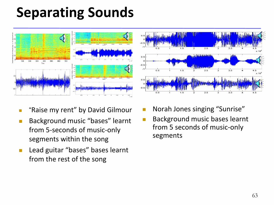
Separating Sounds
63
“Raise my rent” by David Gilmour
Background music “bases” learnt from 5-seconds of music-only segments within the song
Lead guitar “bases” bases learnt from the rest of the song
Norah Jones singing “Sunrise”
Background music bases learnt from 5 seconds of music-only segments
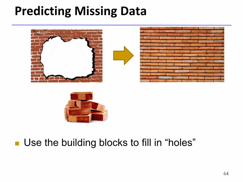
Predicting Missing Data
Use the building blocks to fill in “holes”
64
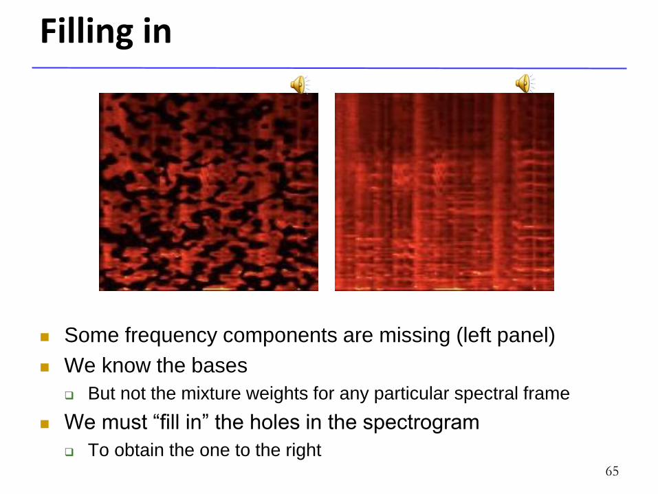
Filling in
Some frequency components are missing (left panel)
We know the bases
But not the mixture weights for any particular spectral frame
We must “fill in” the holes in the spectrogram
To obtain the one to the right 65
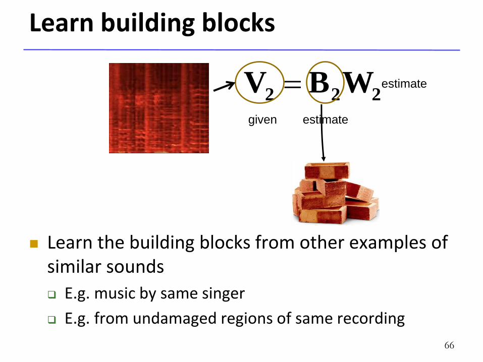
Learn building blocks
Learn the building blocks from other examples of similar sounds
E.g. music by same singer
E.g. from undamaged regions of same recording
66
222 WBV given estimate
estimate
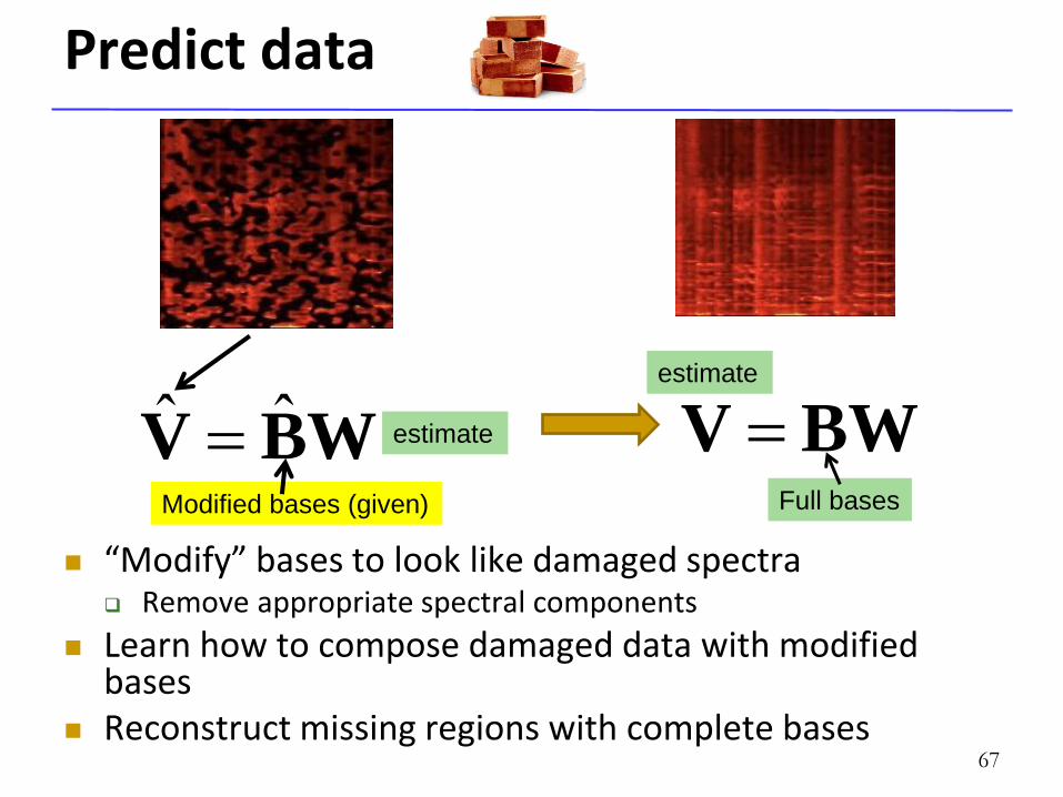
Predict data
“Modify” bases to look like damaged spectra Remove appropriate spectral components
Learn how to compose damaged data with modified bases
Reconstruct missing regions with complete bases 67
WBV ˆˆ Modified bases (given)
estimate BWV estimate
Full bases
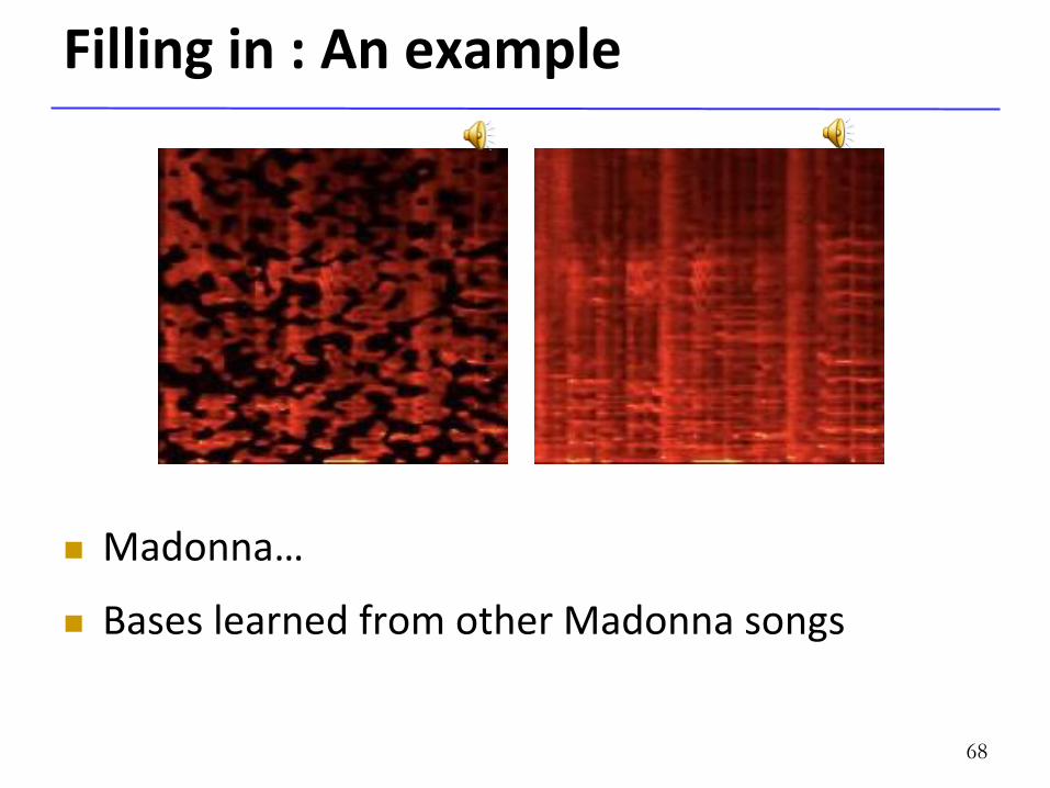
Filling in : An example
Madonna…
Bases learned from other Madonna songs
68
69
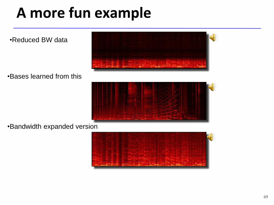
A more fun example
•Bases learned from this
•Bandwidth expanded version
•Reduced BW data
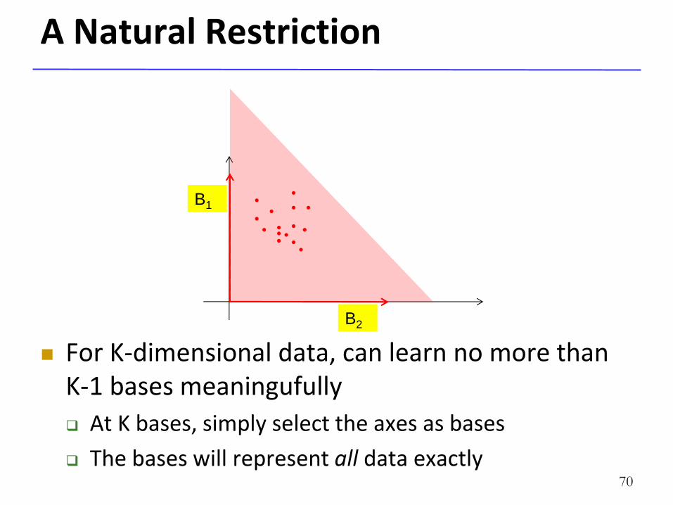
A Natural Restriction
For K-dimensional data, can learn no more than K-1 bases meaningufully
At K bases, simply select the axes as bases
The bases will represent all data exactly 70
B1
B2
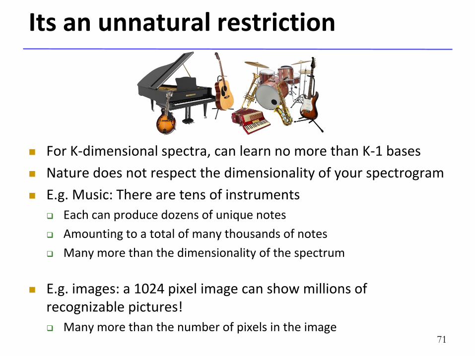
Its an unnatural restriction
For K-dimensional spectra, can learn no more than K-1 bases
Nature does not respect the dimensionality of your spectrogram
E.g. Music: There are tens of instruments
Each can produce dozens of unique notes
Amounting to a total of many thousands of notes
Many more than the dimensionality of the spectrum
E.g. images: a 1024 pixel image can show millions of recognizable pictures!
Many more than the number of pixels in the image 71
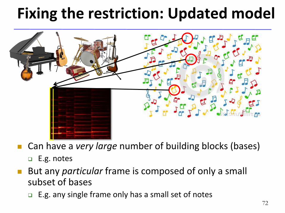
Fixing the restriction: Updated model
Can have a very large number of building blocks (bases) E.g. notes
But any particular frame is composed of only a small subset of bases E.g. any single frame only has a small set of notes
72
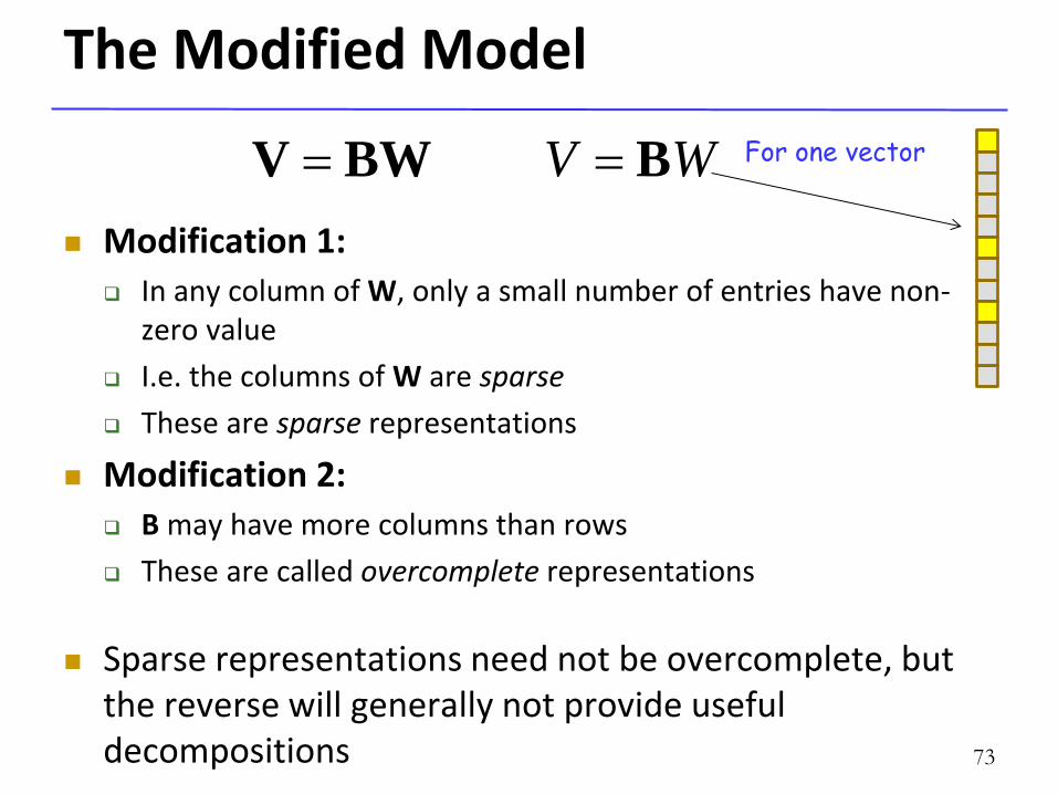
The Modified Model
Modification 1:
In any column of W, only a small number of entries have non-zero value
I.e. the columns of W are sparse
These are sparse representations
Modification 2:
B may have more columns than rows
These are called overcomplete representations
Sparse representations need not be overcomplete, but the reverse will generally not provide useful decompositions 73
BWV WV B For one vector
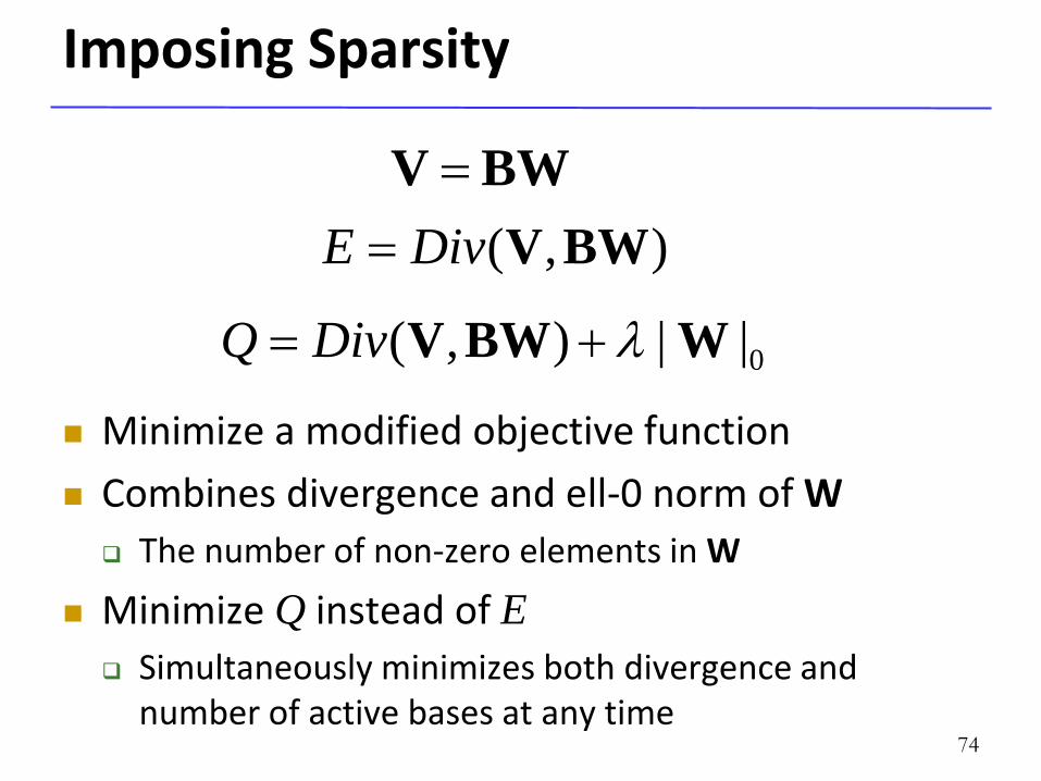
Imposing Sparsity
Minimize a modified objective function
Combines divergence and ell-0 norm of W
The number of non-zero elements in W
Minimize Q instead of E
Simultaneously minimizes both divergence and number of active bases at any time
74
BWV
),( BWVDivE
0||),( WBWV DivQ
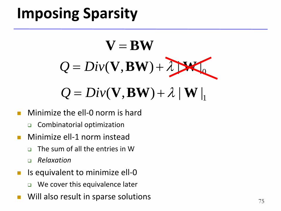
Imposing Sparsity
Minimize the ell-0 norm is hard
Combinatorial optimization
Minimize ell-1 norm instead
The sum of all the entries in W
Relaxation
Is equivalent to minimize ell-0
We cover this equivalence later
Will also result in sparse solutions 75
BWV
0||),( WBWV DivQ
1||),( WBWV DivQ
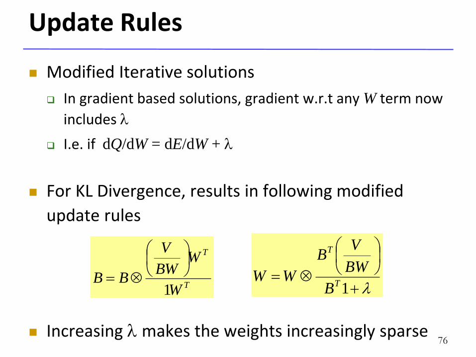
Update Rules
Modified Iterative solutions
In gradient based solutions, gradient w.r.t any W term now
includes
I.e. if dQ/dW = dE/dW +
For KL Divergence, results in following modified
update rules
Increasing makes the weights increasingly sparse 76
T
T
W
WBW
V
BB1
1T
T
B
BW
VB
WW
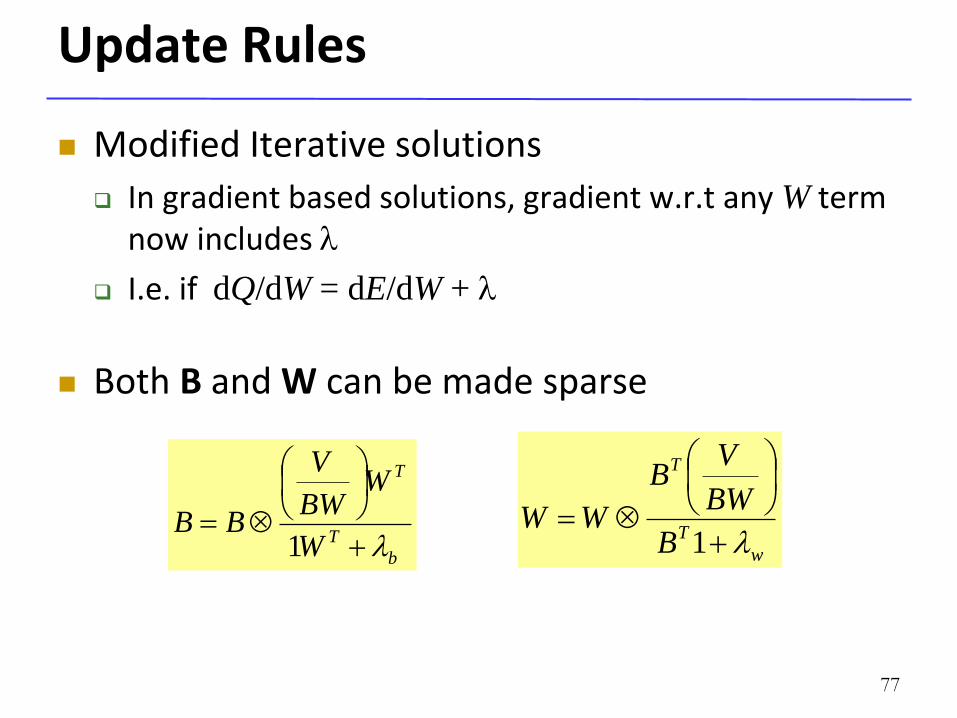
Update Rules
Modified Iterative solutions
In gradient based solutions, gradient w.r.t any W term now includes
I.e. if dQ/dW = dE/dW +
Both B and W can be made sparse
77
b
T
T
W
WBW
V
BB
1 w
T
T
B
BW
VB
WW
1
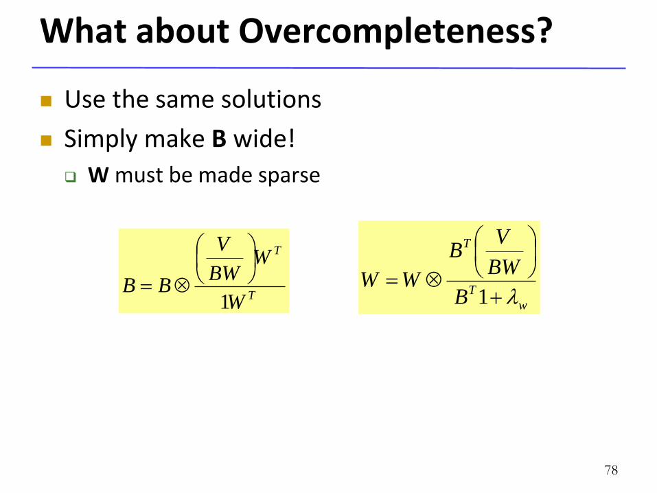
What about Overcompleteness?
Use the same solutions
Simply make B wide!
W must be made sparse
78
T
T
W
WBW
V
BB1
w
T
T
B
BW
VB
WW
1
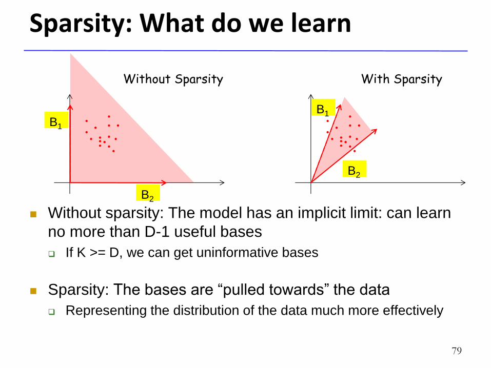
Sparsity: What do we learn
Without sparsity: The model has an implicit limit: can learn
no more than D-1 useful bases
If K >= D, we can get uninformative bases
Sparsity: The bases are “pulled towards” the data
Representing the distribution of the data much more effectively
79
B1
B2
B1
B2
Without Sparsity With Sparsity
80
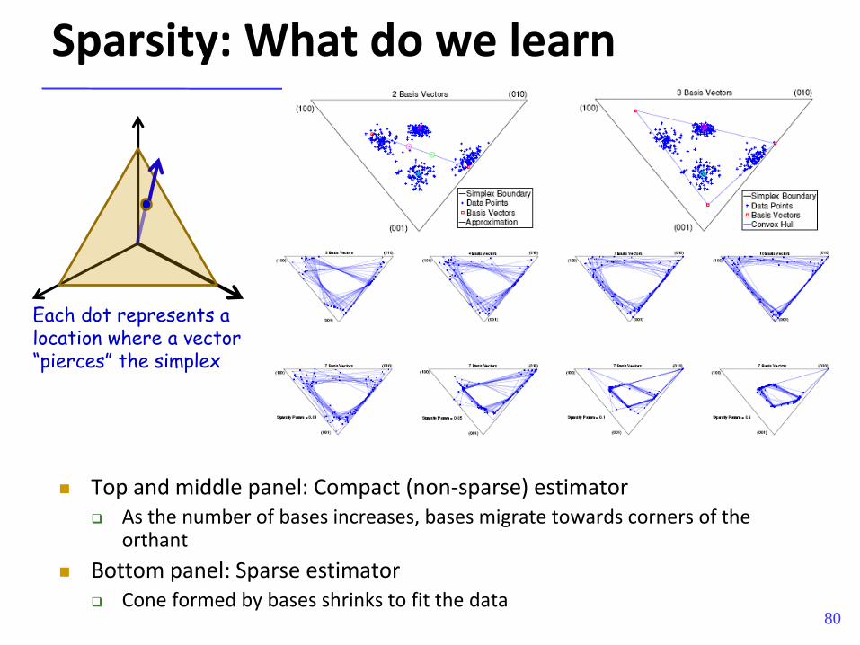
Sparsity: What do we learn
Top and middle panel: Compact (non-sparse) estimator As the number of bases increases, bases migrate towards corners of the
orthant
Bottom panel: Sparse estimator Cone formed by bases shrinks to fit the data
Each dot represents a location where a vector “pierces” the simplex
81
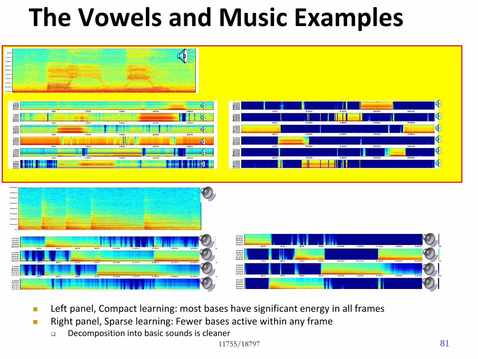
The Vowels and Music Examples
Left panel, Compact learning: most bases have significant energy in all frames Right panel, Sparse learning: Fewer bases active within any frame
Decomposition into basic sounds is cleaner 11755/18797
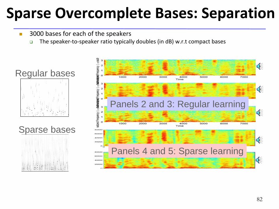
Sparse Overcomplete Bases: Separation 3000 bases for each of the speakers
The speaker-to-speaker ratio typically doubles (in dB) w.r.t compact bases
Panels 2 and 3: Regular learning
Panels 4 and 5: Sparse learning
Regular bases
Sparse bases
82
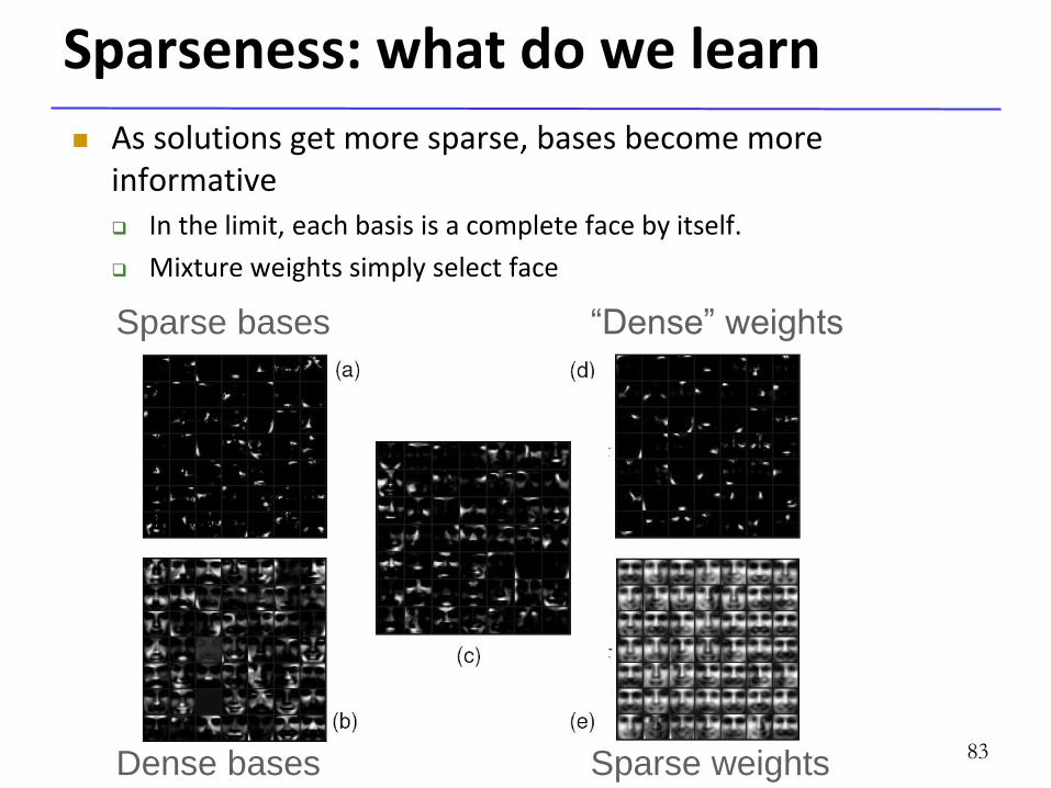
Sparseness: what do we learn
As solutions get more sparse, bases become more informative In the limit, each basis is a complete face by itself.
Mixture weights simply select face
Sparse bases
Dense bases
“Dense” weights
Sparse weights 83
84
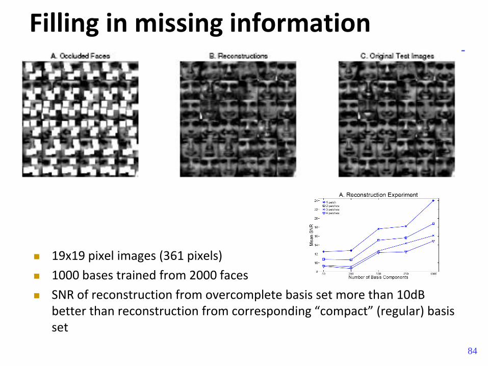
Filling in missing information
19x19 pixel images (361 pixels)
1000 bases trained from 2000 faces
SNR of reconstruction from overcomplete basis set more than 10dB better than reconstruction from corresponding “compact” (regular) basis set
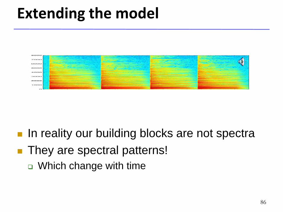
Extending the model
In reality our building blocks are not spectra
They are spectral patterns!
Which change with time
86
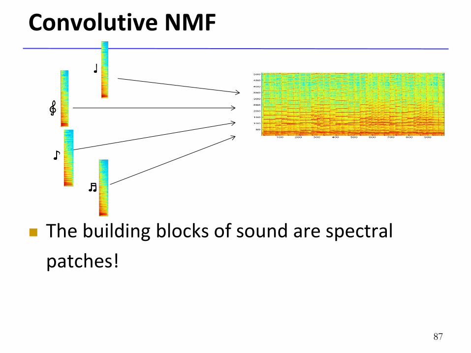
Convolutive NMF
The building blocks of sound are spectral
patches!
87
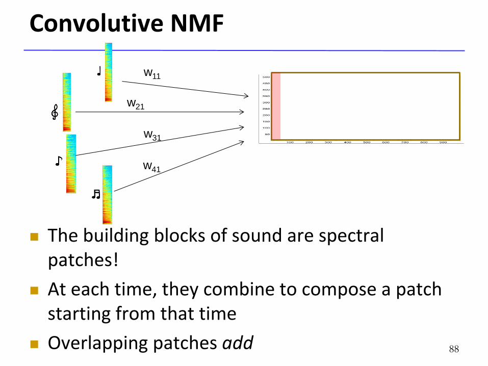
Convolutive NMF
The building blocks of sound are spectral patches!
At each time, they combine to compose a patch starting from that time
Overlapping patches add 88
w11
w21
w31
w41
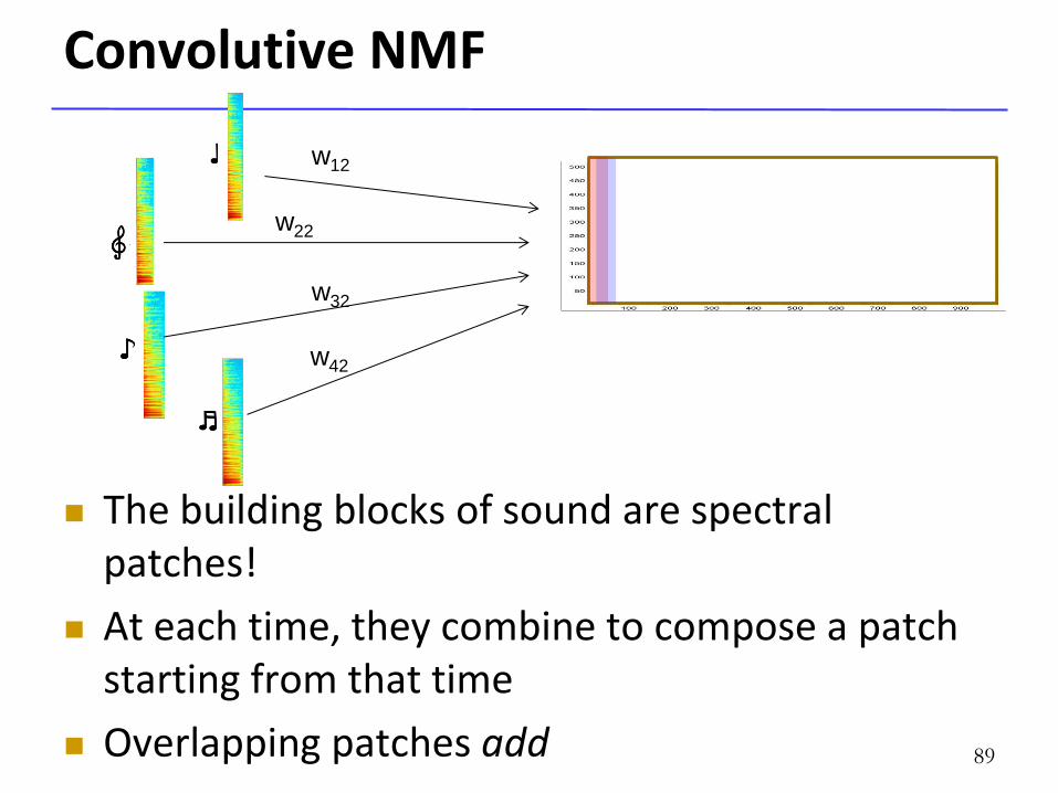
Convolutive NMF
The building blocks of sound are spectral patches!
At each time, they combine to compose a patch starting from that time
Overlapping patches add 89
w12
w22
w32
w42
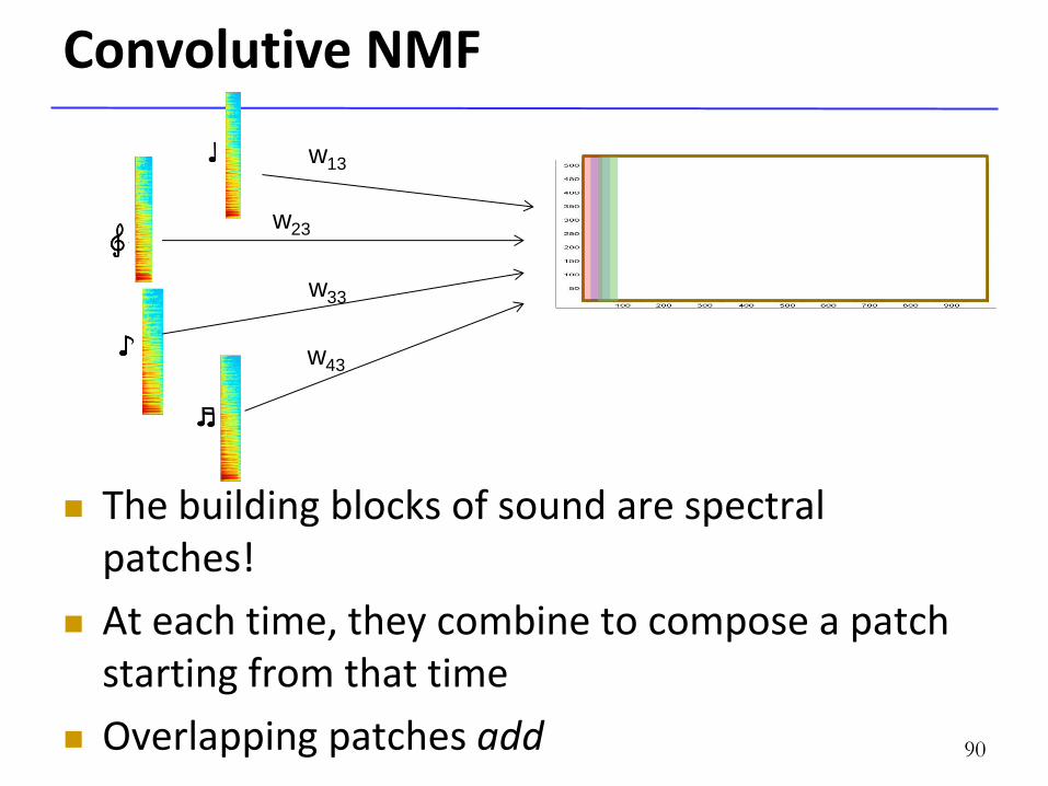
Convolutive NMF
The building blocks of sound are spectral patches!
At each time, they combine to compose a patch starting from that time
Overlapping patches add 90
w13
w23
w33
w43
Convolutive NMF
The building blocks of sound are spectral patches!
At each time, they combine to compose a patch starting from that time
Overlapping patches add 91
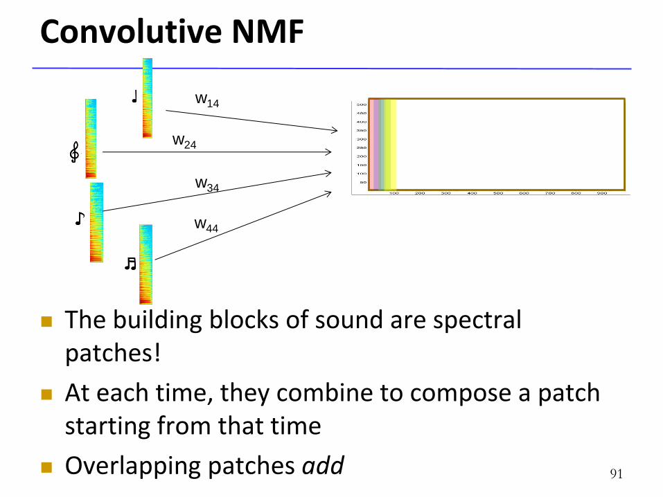
w14
w24
w34
w44
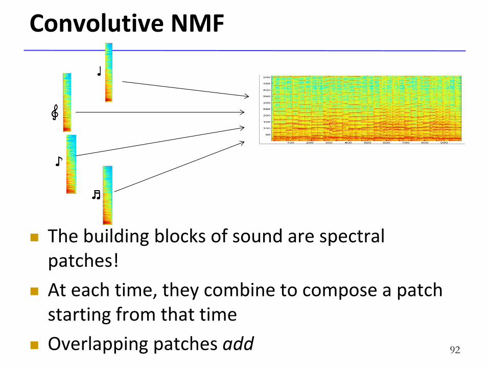
Convolutive NMF
The building blocks of sound are spectral patches!
At each time, they combine to compose a patch starting from that time
Overlapping patches add 92
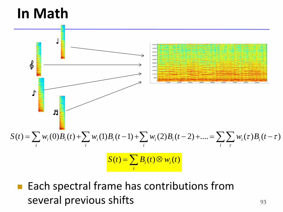
In Math
Each spectral frame has contributions from several previous shifts 93
i
ii
i
ii
i
ii
i
ii tBwtBwtBwtBwtS
)()(....)2()2()1()1()()0()(
i
ii twtBtS )()()(
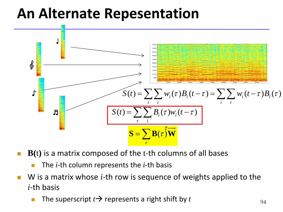
An Alternate Repesentation
B(t) is a matrix composed of the t-th columns of all bases
The i-th column represents the i-th basis
W is a matrix whose i-th row is sequence of weights applied to the i-th basis
The superscript t represents a right shift by t 94
i
ii
i
ii BtwtBwtS
)()()()()(
WBS
)(
)()()(
twBtS i
i
i
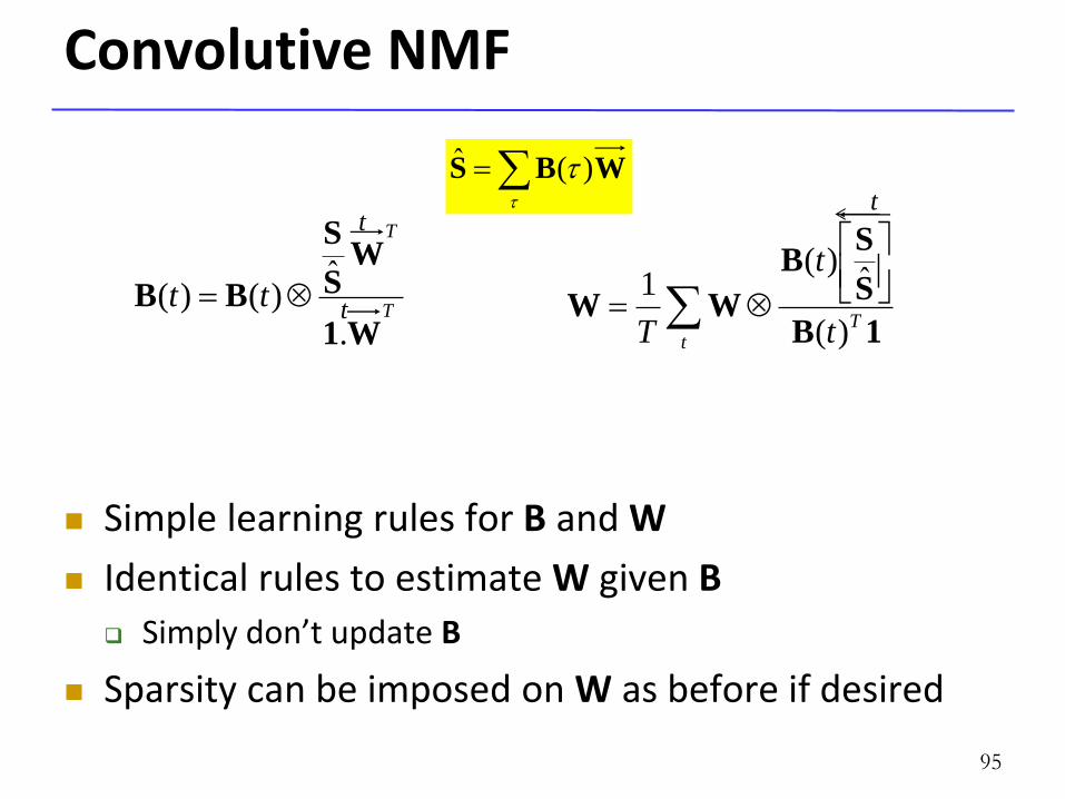
Convolutive NMF
Simple learning rules for B and W
Identical rules to estimate W given B
Simply don’t update B
Sparsity can be imposed on W as before if desired
95
T
T
ttW1
WS
S
BB
.
ˆ)()(
t
Tt
t
T 1B
S
SB
WW)(
ˆ)(
1
t t
t
WBS
)(ˆ
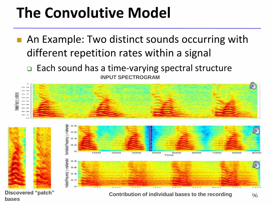
The Convolutive Model
An Example: Two distinct sounds occurring with different repetition rates within a signal
Each sound has a time-varying spectral structure INPUT SPECTROGRAM
Discovered “patch”
bases Contribution of individual bases to the recording 96
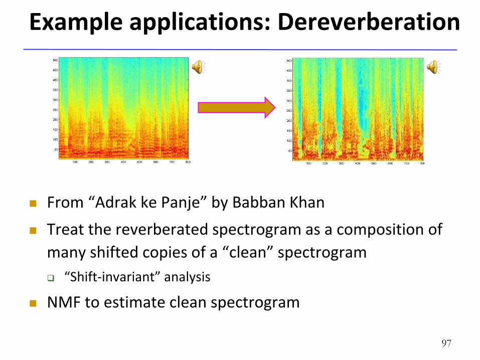
Example applications: Dereverberation
From “Adrak ke Panje” by Babban Khan
Treat the reverberated spectrogram as a composition of
many shifted copies of a “clean” spectrogram
“Shift-invariant” analysis
NMF to estimate clean spectrogram
97
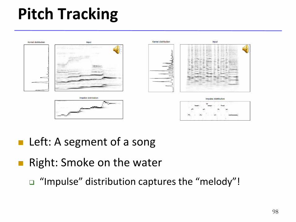
Pitch Tracking
Left: A segment of a song
Right: Smoke on the water
“Impulse” distribution captures the “melody”!
98
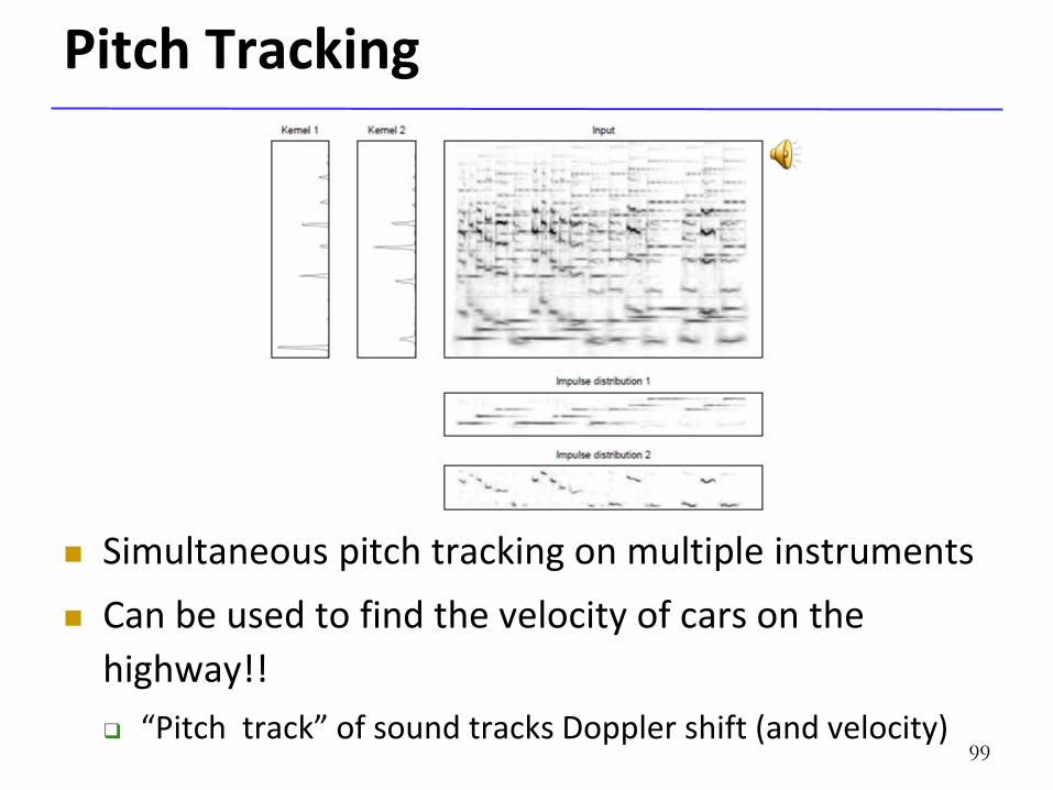
Simultaneous pitch tracking on multiple instruments
Can be used to find the velocity of cars on the
highway!!
“Pitch track” of sound tracks Doppler shift (and velocity)
Pitch Tracking
99
100
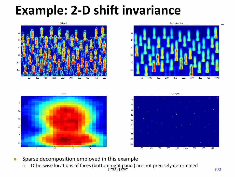
Example: 2-D shift invariance
Sparse decomposition employed in this example Otherwise locations of faces (bottom right panel) are not precisely determined
11755/18797
101
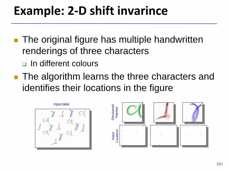
Example: 2-D shift invarince
The original figure has multiple handwritten
renderings of three characters
In different colours
The algorithm learns the three characters and
identifies their locations in the figure
Input data
Dis
covere
d
Patc
hes
Patc
h
Locations
102
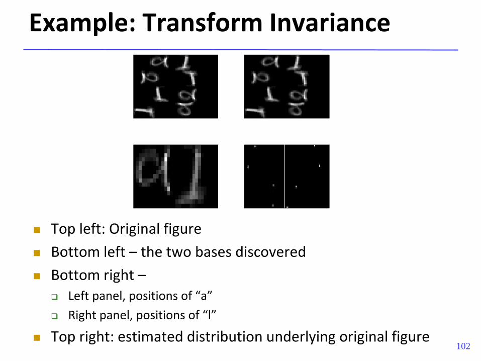
Example: Transform Invariance
Top left: Original figure
Bottom left – the two bases discovered
Bottom right – Left panel, positions of “a”
Right panel, positions of “l”
Top right: estimated distribution underlying original figure
103
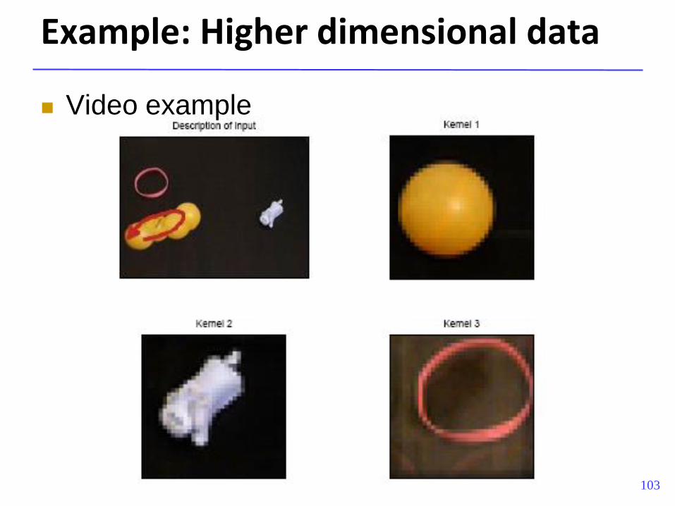
Example: Higher dimensional data
Video example
Lessons learned
Linear decomposition when constrained with semantic constraints e.g. non-negativity can result in semantically meaningful bases
NMF: Useful compositional model of data
Really effective when the data obey compositional rules..
104