machine learning for materials scientists: an introductory
TRANSCRIPT
doi.org/10.26434/chemrxiv.12249752.v1
Machine Learning for Materials Scientists: An Introductory GuideTowards Best PracticesAnthony Wang, Ryan Murdock, Steven Kauwe, Anton Oliynyk, Aleksander Gurlo, Jakoah Brgoch, KristinPersson, Taylor Sparks
Submitted date: 05/05/2020 • Posted date: 06/05/2020Licence: CC BY-NC-ND 4.0Citation information: Wang, Anthony; Murdock, Ryan; Kauwe, Steven; Oliynyk, Anton; Gurlo, Aleksander;Brgoch, Jakoah; et al. (2020): Machine Learning for Materials Scientists: An Introductory Guide Towards BestPractices. ChemRxiv. Preprint. https://doi.org/10.26434/chemrxiv.12249752.v1
This Editorial is intended for materials scientists interested in performing machine learning-centered research.We cover broad guidelines and best practices regarding the obtaining and treatment of data, featureengineering, model training, validation, evaluation and comparison, popular repositories for materials data andbenchmarking datasets, model and architecture sharing, and finally publication.In addition, we includeinteractive Jupyter notebooks with example Python code to demonstrate some of the concepts, workflows,and best practices discussed.Overall, the data-driven methods and machine learning workflows and considerations are presented in asimple way, allowing interested readers to more intelligently guide their machine learning research using thesuggested references, best practices, and their own materials domain expertise.
File list (2)
download fileview on ChemRxivBestPractices_submitted.pdf (2.22 MiB)
download fileview on ChemRxivBestPractices paper - SI.pdf (3.00 MiB)
Machine Learning for Materials Scientists:
An introductory guide towards best practices
Anthony Yu-Tung Wang,† Ryan J. Murdock,‡ Steven K. Kauwe,‡ Anton O.
Oliynyk,¶ Aleksander Gurlo,† Jakoah Brgoch,§ Kristin A. Persson,‖,⊥ and Taylor
D. Sparks∗,‡
†Fachgebiet Keramische Werkstoffe / Chair of Advanced Ceramic Materials, Technische
Universität Berlin, 10623 Berlin, Germany
‡Department of Materials Science & Engineering, University of Utah, Salt Lake City, UT,
84112, USA
¶Department of Chemistry & Biochemistry, Manhattan College, Riverdale, NY, 10471 USA
§Department of Chemistry, University of Houston, Houston, TX, 77204, USA
‖Energy Storage and Distributed Resources Division, Lawrence Berkeley National
Laboratory, Berkeley, CA, 94720, USA
⊥Department of Materials Science, University of California Berkeley, Berkeley, CA,
94720, USA
E-mail: [email protected]
Abstract
This Editorial is intended for materials scientists interested in performing machine
learning-centered research. We cover broad guidelines and best practices regarding
the obtaining and treatment of data, feature engineering, model training, validation,
evaluation and comparison, popular repositories for materials data and benchmarking
1
datasets, model and architecture sharing, and finally publication. In addition, we in-
clude interactive Jupyter notebooks with example Python code to demonstrate some of
the concepts, workflows, and best practices discussed. Overall, the data-driven methods
and machine learning workflows and considerations are presented in a simple way, allow-
ing interested readers to more intelligently guide their machine learning research using
the suggested references, best practices, and their own materials domain expertise.
Keywords
Machine learning, neural networks, materials science, materials informatics, data science,
common pitfalls, best practices, example code, Python, interactive notebooks, Jupyter
Introduction
Materials scientists are constantly striving to advance their ability to understand, predict
and improve materials properties. Due to the high cost of traditional trial-and-error methods
in materials research (often in the form of repeated rounds of material synthesis and charac-
terization), material scientists have increasingly relied on simulation and modeling methods
to understand and predict materials properties a priori. Materials informatics (MI) is a
resulting branch of materials science that utilizes high-throughput computation to analyze
large databases of materials properties to gain unique insights. More recently, data-driven
methods such as machine learning (ML) have been adopted in MI to study the wealth of
existing experimental and computational data in materials science, leading to a paradigm
shift in the way materials science research is conducted.
However, there exist many challenges and “gotchas” when implementing ML techniques in
materials science. Furthermore, many experimental materials scientists lack the know-how
to get started in data-driven research, and there is a lack of recommended best practices
for implementing such methods in materials science. As such, this Editorial is designed to
2
assist those materials science scholars who wish to perform data-driven materials research.
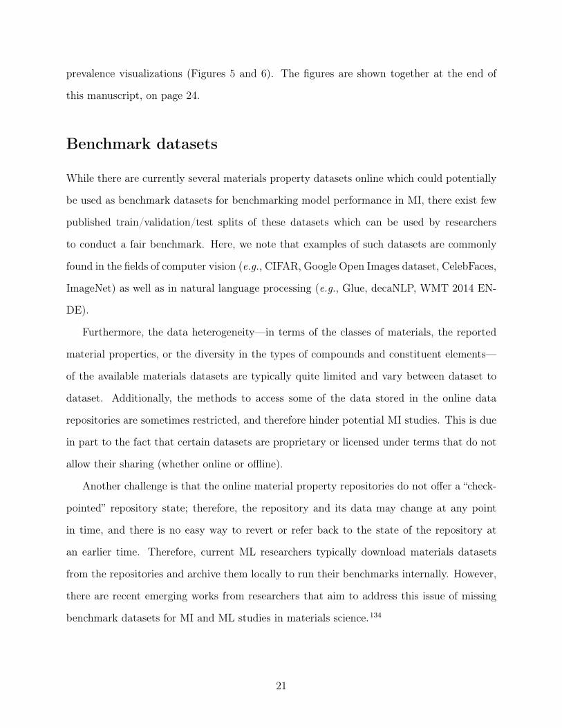
We demonstrate a typical ML project step-by-step (Figure 1 on page 24), starting with
loading and processing data, splitting data, feature engineering, fitting different ML models,
evaluating model performance, comparing performance across models, and visualizing the
results. We also cover sharing and publication of the model and architecture, with the goal
of unifying research reporting and facilitating collaboration this emerging field. Throughout
this process, we highlight some of the challenges and common mistakes encountered during
a typical ML study in materials science, as well as approaches to overcome or address them.
Highlighting the best practices will improve the research and manuscript quality, and ensure
reproducible results.
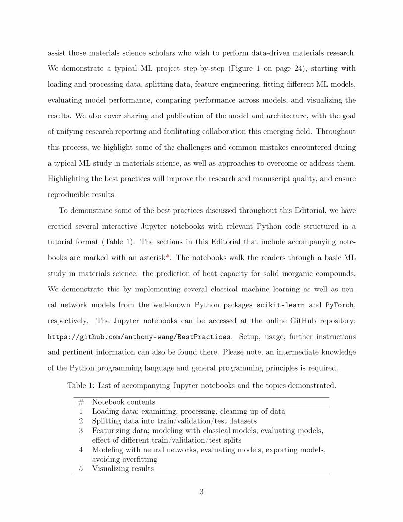
To demonstrate some of the best practices discussed throughout this Editorial, we have
created several interactive Jupyter notebooks with relevant Python code structured in a
tutorial format (Table 1). The sections in this Editorial that include accompanying note-
books are marked with an asterisk*. The notebooks walk the readers through a basic ML
study in materials science: the prediction of heat capacity for solid inorganic compounds.
We demonstrate this by implementing several classical machine learning as well as neu-
ral network models from the well-known Python packages scikit-learn and PyTorch,
respectively. The Jupyter notebooks can be accessed at the online GitHub repository:
https://github.com/anthony-wang/BestPractices. Setup, usage, further instructions
and pertinent information can also be found there. Please note, an intermediate knowledge
of the Python programming language and general programming principles is required.
Table 1: List of accompanying Jupyter notebooks and the topics demonstrated.
# Notebook contents1 Loading data; examining, processing, cleaning up of data2 Splitting data into train/validation/test datasets3 Featurizing data; modeling with classical models, evaluating models,
effect of different train/validation/test splits4 Modeling with neural networks, evaluating models, exporting models,
avoiding overfitting5 Visualizing results
3
Meaningful machine learning
Machine learning is a powerful tool, but not every materials science problem is a nail. It is
important to delineate when to use ML, and when it may be more appropriate to use other
methods. Consider what value ML can add to your project and whether there are more
suitable approaches. Machine learning is most useful when human learning is impossible,
such as where the data and interactions within the data are too complex and intractable for
human understanding and conceptualization. Contrarily, machine learning often fails to find
meaningful relationships and representations from small amounts of data, when a human
mind would otherwise likely succeed.
When developing ML tools and workflows, consider how (and with what ease) they can
be used not only by yourself, but by others in the research community. If another researcher
wants to use your method, will they be able to do so, and will it be worth it for them? For
example, if you include data from ab initio calculations such as density functional theory
(DFT), or crystal structure as one of the input features of your ML model, would it not be
simpler for other researchers to use DFT or other simulation methods themselves, instead of
using your ML model?
Another limitation to consider when using ML as a tool is the model interpretability
vs. predictive power trade-off. If you are looking for physical or chemical insights into your
materials, you are unlikely to find them when using powerful and complex models such as
neural networks: these models—while they can exhibit high model performance—are usually
too complex to be easily understood. These are so-called “black-box” models because outside
of their inputs and outputs, it is nearly impossible for a human to grasp the inner model
workings and its decision making processes. In contrast, simpler models might be easier to
understand, but tend to lack the predictive power of the more complex models.
In general, a good ML project should do one or more of the following: screen or down-
select candidate materials from a pool of known compounds for a given application or prop-
erty,1–3 acquire and process data to gain new insights,4,5 conceptualize new modeling ap-
4
proaches,6–10 or explore ML in materials-specific applications.1,11–13 Consider these points
when you judge the applicability of ML for your project.
Machine learning in materials science
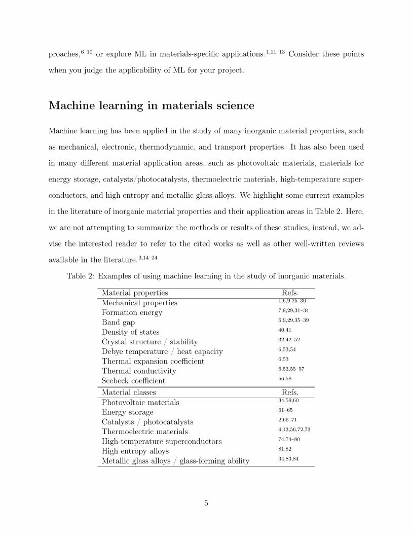
Machine learning has been applied in the study of many inorganic material properties, such
as mechanical, electronic, thermodynamic, and transport properties. It has also been used
in many different material application areas, such as photovoltaic materials, materials for
energy storage, catalysts/photocatalysts, thermoelectric materials, high-temperature super-
conductors, and high entropy and metallic glass alloys. We highlight some current examples
in the literature of inorganic material properties and their application areas in Table 2. Here,
we are not attempting to summarize the methods or results of these studies; instead, we ad-
vise the interested reader to refer to the cited works as well as other well-written reviews
available in the literature.3,14–24
Table 2: Examples of using machine learning in the study of inorganic materials.
Material properties Refs.Mechanical properties 1,6,9,25–30
Formation energy 7,9,29,31–34
Band gap 6,9,29,35–39
Density of states 40,41
Crystal structure / stability 32,42–52
Debye temperature / heat capacity 6,53,54
Thermal expansion coefficient 6,53
Thermal conductivity 6,53,55–57
Seebeck coefficient 56,58
Material classes Refs.Photovoltaic materials 34,59,60
Energy storage 61–65
Catalysts / photocatalysts 2,66–71
Thermoelectric materials 4,13,56,72,73
High-temperature superconductors 74,74–80
High entropy alloys 81,82
Metallic glass alloys / glass-forming ability 34,83,84
5

Working with materials data
Data source
Some of the more commonly-used repositories for materials property data are shown below
in Table 3.
6
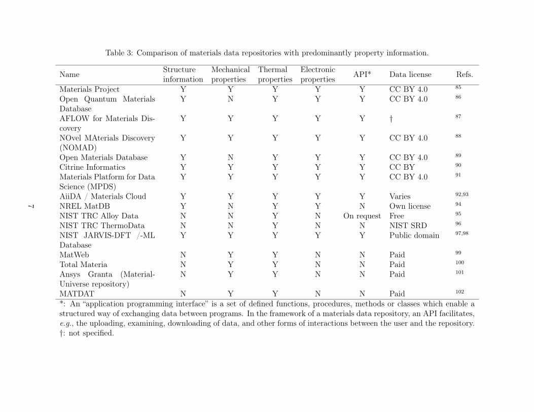
Table 3: Comparison of materials data repositories with predominantly property information.
Name Structureinformation
Mechanicalproperties
Thermalproperties
Electronicproperties API* Data license Refs.
Materials Project Y Y Y Y Y CC BY 4.0 85
Open Quantum MaterialsDatabase
Y N Y Y Y CC BY 4.0 86
AFLOW for Materials Dis-covery
Y Y Y Y Y † 87
NOvel MAterials Discovery(NOMAD)
Y Y Y Y Y CC BY 4.0 88
Open Materials Database Y N Y Y Y CC BY 4.0 89
Citrine Informatics Y Y Y Y Y CC BY 90
Materials Platform for DataScience (MPDS)
Y Y Y Y Y CC BY 4.0 91
AiiDA / Materials Cloud Y Y Y Y Y Varies 92,93
NREL MatDB Y N Y Y N Own license 94
NIST TRC Alloy Data N N Y N On request Free 95
NIST TRC ThermoData N N Y N N NIST SRD 96
NIST JARVIS-DFT /-MLDatabase
Y Y Y Y Y Public domain 97,98
MatWeb N Y Y N N Paid 99
Total Materia N Y Y N N Paid 100
Ansys Granta (Material-Universe repository)
N Y Y N N Paid 101
MATDAT N Y Y N N Paid 102
*: An “application programming interface” is a set of defined functions, procedures, methods or classes which enable astructured way of exchanging data between programs. In the framework of a materials data repository, an API facilitates,e.g., the uploading, examining, downloading of data, and other forms of interactions between the user and the repository.†: not specified.
7
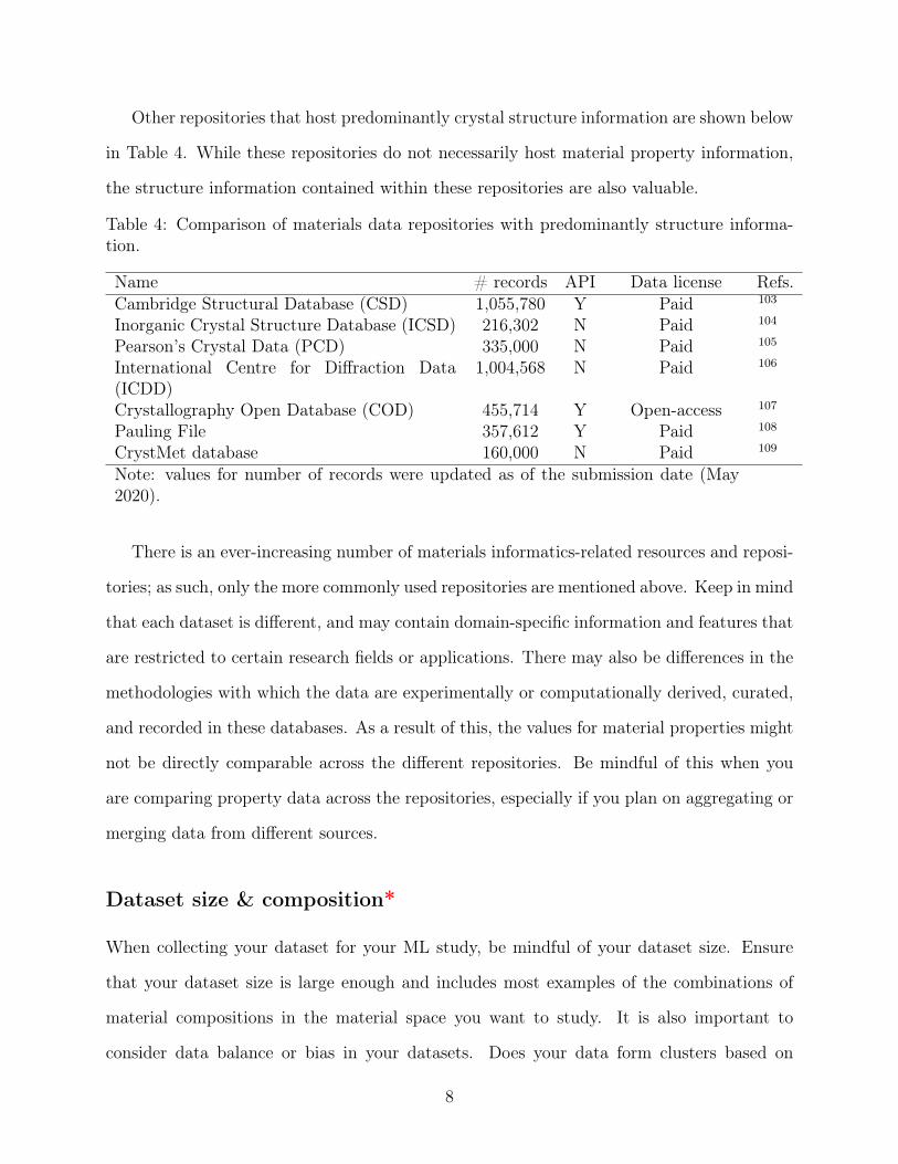
Other repositories that host predominantly crystal structure information are shown below
in Table 4. While these repositories do not necessarily host material property information,
the structure information contained within these repositories are also valuable.
Table 4: Comparison of materials data repositories with predominantly structure informa-tion.
Name # records API Data license Refs.Cambridge Structural Database (CSD) 1,055,780 Y Paid 103
Inorganic Crystal Structure Database (ICSD) 216,302 N Paid 104
Pearson’s Crystal Data (PCD) 335,000 N Paid 105
International Centre for Diffraction Data(ICDD)
1,004,568 N Paid 106
Crystallography Open Database (COD) 455,714 Y Open-access 107
Pauling File 357,612 Y Paid 108
CrystMet database 160,000 N Paid 109
Note: values for number of records were updated as of the submission date (May2020).
There is an ever-increasing number of materials informatics-related resources and reposi-
tories; as such, only the more commonly used repositories are mentioned above. Keep in mind
that each dataset is different, and may contain domain-specific information and features that
are restricted to certain research fields or applications. There may also be differences in the
methodologies with which the data are experimentally or computationally derived, curated,
and recorded in these databases. As a result of this, the values for material properties might
not be directly comparable across the different repositories. Be mindful of this when you
are comparing property data across the repositories, especially if you plan on aggregating or
merging data from different sources.
Dataset size & composition*
When collecting your dataset for your ML study, be mindful of your dataset size. Ensure
that your dataset size is large enough and includes most examples of the combinations of
material compositions in the material space you want to study. It is also important to
consider data balance or bias in your datasets. Does your data form clusters based on
8
chemical formula, test condition, structure type, or other criteria? Are some clusters greatly
over- or under-represented? Many statistical models used in ML are frequentist in nature,
and will be influenced by dataset imbalance or bias. Visualization techniques such as t-
distributed stochastic neighbor embedding (t-SNE110), uniform manifold approximation and
projection (UMAP111), or even simple elemental prevalence mapping112 may be useful in
investigating dataset imbalance and bias.
Lastly, if your dataset is too large (a rare luxury in the materials science field), you
may find yourself having to wait a long time to train and validate your models during the
prototyping phase of your project. In this case, you can sub-sample your dataset into a
small-scale “toy dataset”, and use that to test and adjust your models. Once you have tuned
your models to your satisfaction on the toy dataset, you can then carry on and apply them
to the full dataset. When sampling the original dataset to create the toy dataset, be aware
that you do not introduce any dataset biases through your sampling. Also keep in mind that
not all performance-related problems can be fixed by sub-sampling your data. If your model
can only train successfully on the toy dataset, and cannot train on the full dataset (e.g., due
to memory or time constraints), you may wish to focus on improving its performance first.
Data version control
Be sure to save an archival copy of your raw dataset as obtained, and be sure that you can
retrieve it at any time. If you make any changes to your dataset, clearly record the steps of
the changes and ensure that you are able to reproduce them on the dataset in the future if
needed. To simplify version control, consider using a version control system (such as Git,113
Mercurial114 or Subversion115) for your datasets.
Cleanup and processing*
Once you have curated your dataset, examine and explore the data on a high level to see if
there are any obvious flaws or issues. These may—and often do—include missing or unre-
9
alistic values (e.g., NaN’s, or negative values/positive values where you don’t expect them),
outliers or infinite values, badly-formatted or corrupt values (e.g., wrong text encoding, num-
bers stored in non-numeric format), non-matching data formats or data schema caused by
changes in the repository, and other irregularities. If you find any irregularities, deal with
them in an appropriate way, and be careful not to introduce any bias or irregularities of
your own. Make sure you document any data cleanup and processing steps you performed;
this is an important step in ensuring reproducibility that is often overlooked in ML studies.
In addition, during your model prototyping stage, you may find some additional problem-
atic data samples which adversarially affect your model performance. In this case, consider
performing another round of data cleanup before finalizing your model.
Train-validation-test split*
Split your data once into three datasets: train, validation, and test. The split should be
performed in a reproducible way (e.g., by assigning a random seed and shuffling the dataset);
alternatively, you can save the split datasets as files for reuse. Make sure that no same (or
similar) data appear in the test dataset, if they are already present in the train or validation
dataset. For example, if you have several measurements of a chemical compound that are
performed at different measurement conditions in the train dataset (e.g., temperature or
pressure), during the testing phase, your model would likely perform well if it is asked to
predict the property of the same compound at a different condition. This, however, gives
you an inflated estimate of how well the model will generalize in cases where it hasn’t seen
a particular chemical compound before. For a truly rigorous evaluation of your model’s
generalization performance, you should take care to avoid this data leakage when you split
your data.
During the training stage, models may only be shown the training data as part of the
learning process. Validation data may be used to assess and tune different model hyper-
parameters, and may be compared with the predictions of different model/hyperparameter
10
combinations to evaluate a model’s performance. In contrast, test data may only be used in
order to evaluate a model’s performance as a final step, after the model has been finalized.
Models must not be trained nor tuned on the test dataset. Use the same train, validation,
and test datasets for all modeling and model comparison/benchmarking steps.
The training dataset can be further partitioned to be used for cross-validation (CV). CV
is a method that is often employed to estimate the true ability of a model to predict on new
unseen data, and to catch model-specific problems such as overfitting or selection bias.116
One typical method is k-fold cross-validation. In k-fold CV, the training dataset is first
randomly partitioned into K subsets (remember to note down your partitioning details).
Then, for each k of the data subsets k = 1, 2, ..., K, the model is trained on the combined
data of the other K − 1 subsets, and then evaluated using the kth subset. The resulting K
prediction errors are then typically averaged to give a more accurate estimate of the model’s
true predictive performance compared to evaluating the model performance on one single
train/validation/test split. Typical choices for K in the literature are 5 or 10. In the case of
a small input dataset size, k-fold CV or other methods of cross-validation can also be used
as a data re-sampling technique for models that are more robust against overfitting on the
validation set (e.g., linear regression).
Modeling
Choosing appropriate models & features*
The dataset size will almost always determine your available choices of ML models. For
smaller dataset sizes, classical and statistical ML approaches (e.g., regression, support vector
machines, k-nearest neighbors, and decision trees) are more suitable. In contrast, neural
networks require larger amounts of data, and only start becoming feasible/useful when you
have training data points on the order of thousands or more. Typically, ML models such as
regression, decision tree/random forest, k-nearest neighbors, and support vector machines
11
are used on smaller datasets. These algorithms can be further improved by applying bagging,
boosting or stacking approaches. There are many existing Python libraries for implementing
the above, with perhaps the most well-known being scikit-learn.117 For larger datasets,
neural networks and deep learning methods are more commonly used. In the scholarly
community, the Python libraries PyTorch118 and TensorFlow119 are often used to implement
these architectures.
Feature engineering is important for smaller dataset sizes, and can contribute to a large
model performance increase if the features are well-engineered.1,54,120 A common way to
transform chemical compositions into usable input features for ML studies is through the
use of composition-based feature vectors (“CBFVs”). There are numerous forms of the CBFV
available, such as Jarvis,121 Magpie,34 mat2vec,4 and Oliynyk.13 These CBFVs contain val-
ues that are either experimentally-derived, calculated through high-throughput computation,
or extracted from materials science literature using ML techniques. Instead of featurizing
your data using CBFVs, you can also try a simple onehot-encoding of the elements. These
CBFV featurization schemes as well as the relevant functions and code for featurizing chem-
ical compositions are included in the online GitHub repository associated with this work.
For sufficiently large datasets and for more “capable” learning architectures like very
deep, fully-connected networks7,122 or novel attention-based architectures such as CrabNet,6
feature engineering and the integration of domain knowledge (such as through the use of
CBFVs) in the input data becomes irrelevant and does not contribute to a better model
performance compared to a simple onehot-encoding.11 Therefore, due to the effort required to
curate and evaluate domain knowledge-informed features specific to your research, you may
find it more beneficial to seek out additional sources of data, already-established featurization
schemes, or use learning methods that don’t require domain-derived features6 instead.
12
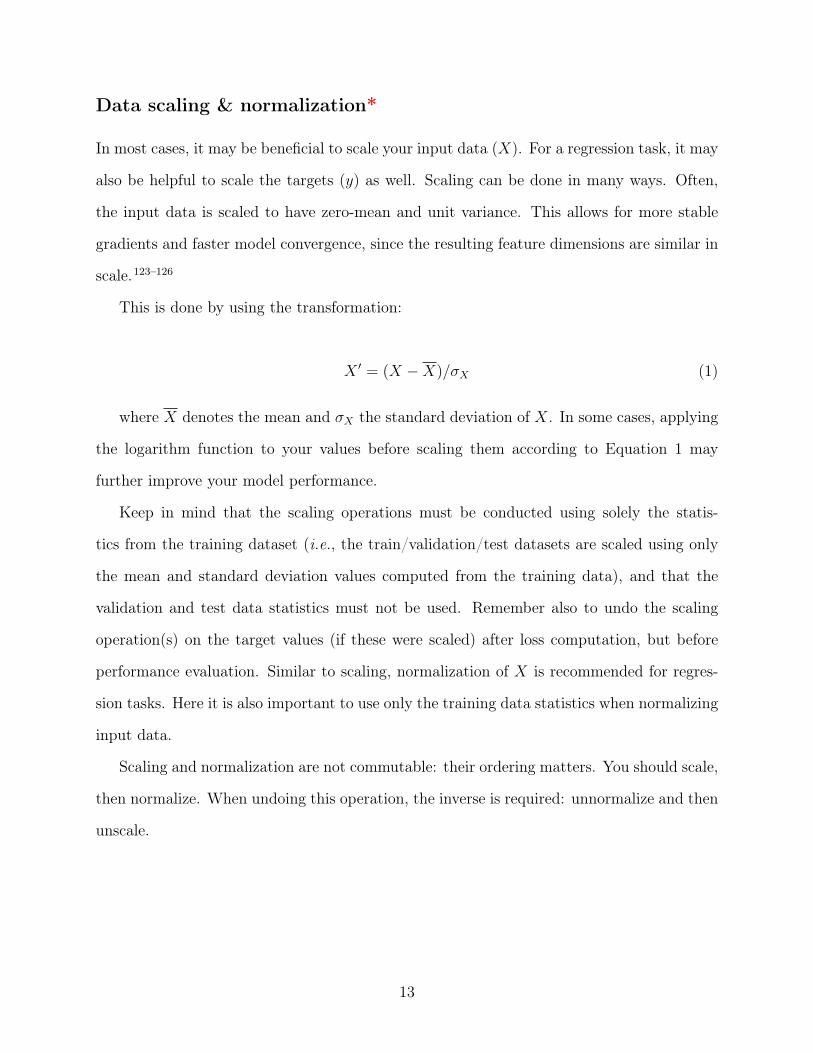
Data scaling & normalization*
In most cases, it may be beneficial to scale your input data (X). For a regression task, it may
also be helpful to scale the targets (y) as well. Scaling can be done in many ways. Often,
the input data is scaled to have zero-mean and unit variance. This allows for more stable
gradients and faster model convergence, since the resulting feature dimensions are similar in
scale.123–126
This is done by using the transformation:
X ′ = (X −X)/σX (1)
where X denotes the mean and σX the standard deviation of X. In some cases, applying
the logarithm function to your values before scaling them according to Equation 1 may
further improve your model performance.
Keep in mind that the scaling operations must be conducted using solely the statis-
tics from the training dataset (i.e., the train/validation/test datasets are scaled using only
the mean and standard deviation values computed from the training data), and that the
validation and test data statistics must not be used. Remember also to undo the scaling
operation(s) on the target values (if these were scaled) after loss computation, but before
performance evaluation. Similar to scaling, normalization of X is recommended for regres-
sion tasks. Here it is also important to use only the training data statistics when normalizing
input data.
Scaling and normalization are not commutable: their ordering matters. You should scale,
then normalize. When undoing this operation, the inverse is required: unnormalize and then
unscale.
13
Keep it simple
Sometimes, especially in the case of small dataset sizes, simpler models can perform better
than more complex models on the held-out test data. Some simpler models that you can try
are linear (or ridge / lasso) regression, random forest, or k-nearest neighbors.
Furthermore, consider the model complexity–explainability trade-off. Typically, more
complex models achieve higher model performance, but have the caveat that they are gen-
erally not easily interpretable by humans. In contrast, simpler models are typically assumed
to be more easily understood by humans, and lead to better opportunities for model intro-
spection. This an important consideration in materials science, since synthesis and charac-
terization are costly and time-consuming and the costs must be justified.
Hyperparameter optimization
Depending on your choice of ML model, there may be model hyperparameters that can be
tuned. Examples of hyperparameters are the number of neighbors (k) in k-nearest neighbors,
the number and depth of trees in a random forest, the kernel type and coefficient in support
vector machines, the maximum number of features to consider in gradient boosting, and loss
criterion, learning rate and optimizer type in neural networks. These hyperparameters are
properties of the models themselves, and can significantly affect your model’s performance,
speed (in training and inference), and complexity.
The hyperparameters are not learned by the model during the training step; rather, they
are selected by you when you create the model. The recommended way to optimize your
model hyperparameters is by training numerous models (each with a different set of hy-
perparameters) using the same training set, and then evaluating the models’ performance
using the same validation set. By doing this, you will be able to identify the set of hyper-
parameters that generally lead to good-performing models. This is commonly referred to as
a “grid search”. Imagine that your model has two continuous-variable hyperparameters, h1
and h2, and that there is a range of values for each of these parameters that you wish to
14
investigate, [h1,min, h1,max] and [h2,min, h2,max], respectively. You can then define a grid that
spans between (h1,min, h2,min) and (h1,max, h2,max). At each point on this grid, you train a
model corresponding to that set of hyperparameters using the training set, and then evaluate
its performance on the validation set. After repeating this for every point on the grid, you
obtain a mapping that you can then use to determine the best set of hyperparameters for
your specific model and data.
Once again, we stress the importance of reserving a held-out test dataset during dataset
splitting. By training and optimizing your model on the training and validation datasets, you
have effectively tuned—and possibly biased—your model to perform exceptionally well on
these data samples. Therefore, the performance metrics of your model on these datasets are
no longer good indicators of your model’s true generalization ability. In contrast, evaluating
your model’s performance on the held-out test dataset (which your model has never seen
before) will give you a much more realistic estimate.
Model evaluation and comparison
Typically, studies in materials science will compare the performance of several ML model and
hyperparameter combinations on a given task. Trained models are typically compared by
evaluating their performance on the held-out test dataset using computed test metrics such as
accuracy, logarithmic loss, precision, recall, F1-score, ROC (receiver operating characteristic
curve), and AUC (area under curve) for classification tasks, and r2 (Pearson correlation
coefficient), mean absolute error, and (root) mean squared error for regression tasks. Also
consider using cross-validation (as discussed earlier) to give a more accurate estimate of your
model’s true performance.
Show your model*
If you are reporting a new model architecture or algorithm, you must include all pertinent
information necessary to reproduce, evaluate, and apply your models. This entails providing
15
the complete source code for your implementation, the hyperparameters used, the random
seeds applied (if any), and the pre-trained weights of the models themselves. In addition,
clear descriptions and schematics of your new system should be provided, as well as instruc-
tions to reproduce your model and work. Ideally, you can show your model and results in
an interactive manner, such as through the use of Jupyter notebooks.
Fitting and testing
Avoid overfitting*
In an ML problem, the model is asked to perform two contradicting tasks: (1) minimize
its prediction error on the training dataset, and (2) maximize its ability to generalize on
unseen data. Depending on how the model, loss criterion, and evaluation methods are
set up, the model may end up memorizing the training dataset (an unwanted outcome)
rather than learning an adequate representation of the data (the intended outcome). This is
called “overfitting”, and usually leads to decreased generalization performance of the model.
Overfitting can occur on all kinds of models, although it typically occurs more often on
complex models such as random forests, support vector machines and neural networks.
During model training, observe the training metrics such as your loss output and r2 score
on the training and validation set. For example, when training a neural network, you can
use a learning curve to track validation error over each epoch during the training process.
As the model trains, the validation and training error will ideally decrease. Your training
error will approach zero, but this is not the metric we care about! Rather, you should closely
observe the validation error. When your validation error increase again while your training
error continues to decrease, you are likely memorizing your training data and thus overfitting
your data.
Overfitting can have an adverse effect on your model’s ability to generalize (that is,
returning a reasonable output prediction for new and unseen data) thus performing poorer
16
on the test dataset. If you notice that your model overfits your data very easily, consider
reducing the complexity of your model, or using regularization.
Beware of random initialization*
Many ML models require an initial guess as a starting point for their internal parameters.
In many model implementations (e.g., in scikit-learn’s linear regression, random forest,
support vector machines, boosting implementations), these initial internal model parameters
are provided by your system’s random number generator. The same applies for neural
network-based models, in the initialization of the weights and biases of the networks and some
optimizer parameters. Depending on how sensitive your model is to initialization, different
initial states of the models can lead to significant differences in your model performance.
It is therefore important that you ensure reproducible results across different model runs
and different models (both for your internal testing and for publication). To accomplish this,
you can choose a seed to use for the random number generator. Don’t forget to mention
this seed in your publication and code. Note that alternative ways of model initialization
exist, such as using different estimators for initial parameter guesses as well as different
initialization schemes for neural network weights and biases; here, you should note down
your changes if you use an alternative implementation.
Avoid p-hacking
Train your models on the training dataset only, and use the validation dataset for tuning
your model hyperparameters. Do not evaluate your model on the held-out test dataset until
you have finished tuning your model, and it is ready for publication. Looking at the test
dataset multiple times to pick ideal model hyperparameters is a form of p-hacking and is
considered cheating!127
17
Benchmarking and Testing
Reproducibly test various methods*
For comparison / ablation studies against other ML models and/or architectures, make sure
you use the same train/validation/test datasets (refer to above for best practices on dataset
splitting and management). For the most informative and fair comparison between different
published models, consider running the models yourself. If you perform any additional model-
specific data manipulation steps, make sure to document them and make them reproducible
for your readers.
During the model tuning process, train your models on the train dataset and evaluate
their performance on the validation set. After you have finalized your model architecture and
hyperparameters, train the models once more on the combined train & validation datasets,
and evaluate their performance on the test dataset.
Existing benchmarks
There are some tools and software packages online, which can be used as baselines to judge
the performance of your models.128–130 Some of these tools can perform automatic feature
engineering and testing of several different ML models. We suggest that you download these
tools and compare the performance of your models against them. If your model does not
perform better, or does not offer any advantages over these existing tools, consider other
venues of improvement.
Making publication-ready, reproducible work
Source code & documentation*
Publishing in peer-reviewed journals relies on the foundational principle that the methodol-
ogy be sufficiently described in order to ensure reproducibility. Therefore, for your ML-based
18
study, full source code for your models and architecture (if any) must be provided, including
implementation details of data processing, data cleanup, data splitting, model training, and
model evaluation. If you can, you should also publish your source code under a permissive or
an open-source license so that others may (re-)use, improve, collaborate on, and contribute
further to your work.131
Your published source code must be complete—that is, somebody should be able to take
your source code verbatim, execute it, and obtain the same results that you did. Required
libraries and other software dependencies (if any) must be listed, preferably with the per-
tinent version numbers. Ideally, these dependencies will be listed in an “environment file”
that others can use to directly create a working software environment on their local system.
If you use any code or packages developed by others, make sure to adhere to their licenses.
Also consider hosting your code in an online, version-controlled repository such as GitHub,
GitLab, Bitbucket, DLHub132 or similar.
Make sure the source code is well-documented and follows well-established code stan-
dards. Instead of writing additional comments to explain your code, considering writing code
in a way such that it is self-explanatory without the need for additional comments. This
entails using clear variable names, closely following formatting guidelines (such as PEP 8),
and writing “explicit” code. Add a “README” file as well that provides your readers with
instructions for the installation, setup, usage of your code, and for the reproduction of your
published results. To ensure large-scale deployability and consistency on any infrastructure,
consider also publishing your project as a containerized application, using tools such as
Docker.133
All data should be provided*
All results and datasets reported in the manuscript should be provided with the manuscript;
alternatively, code for the users to obtain the data themselves must be given, ideally with
clear instructions of the process. Additionally, all raw data—if their licenses allow it—
19
should be provided with the manuscript as well. In the case where the data cannot be
provided, due to licensing, legal, intellectual property protection, or other insurmountable
hurdles, an explanation should be given. You are nevertheless encouraged to find alternative
solutions for providing data within reason. Examples may be to provide a partial dataset, an
anonymized dataset, trained model weights, or instructions for users on how to obtain the
dataset themselves. Consult with the owner of the data before considering these approaches,
and as always, make sure you adhere to the data license.
Trained models & weights*
Ideally, you should provide a record of all model hyperparameters tested, as well as the best
hyperparameters reported. For neural network implementations, the trained weights from
the models should also be provided. In this case, be sure to provide the necessary code to
recreate the neural network architecture and to load the saved weights for use. Ideally, you
should also offer a friendly way to make predictions on user-supplied input data using these
saved weights.
Visualizations*
All visualizations shown in the manuscript should be reproducible by a user who accesses
your code. Ensure that you have included the required data (and ideally the code) used
to generate the visualizations, or have given the users a way to obtain the required data
themselves. If there are additional figures, such as in the supplementary information (SI),
ensure that they are understandable by themselves and do not require additional explanation.
If they do require explanation, provide this in the SI along with the figures.
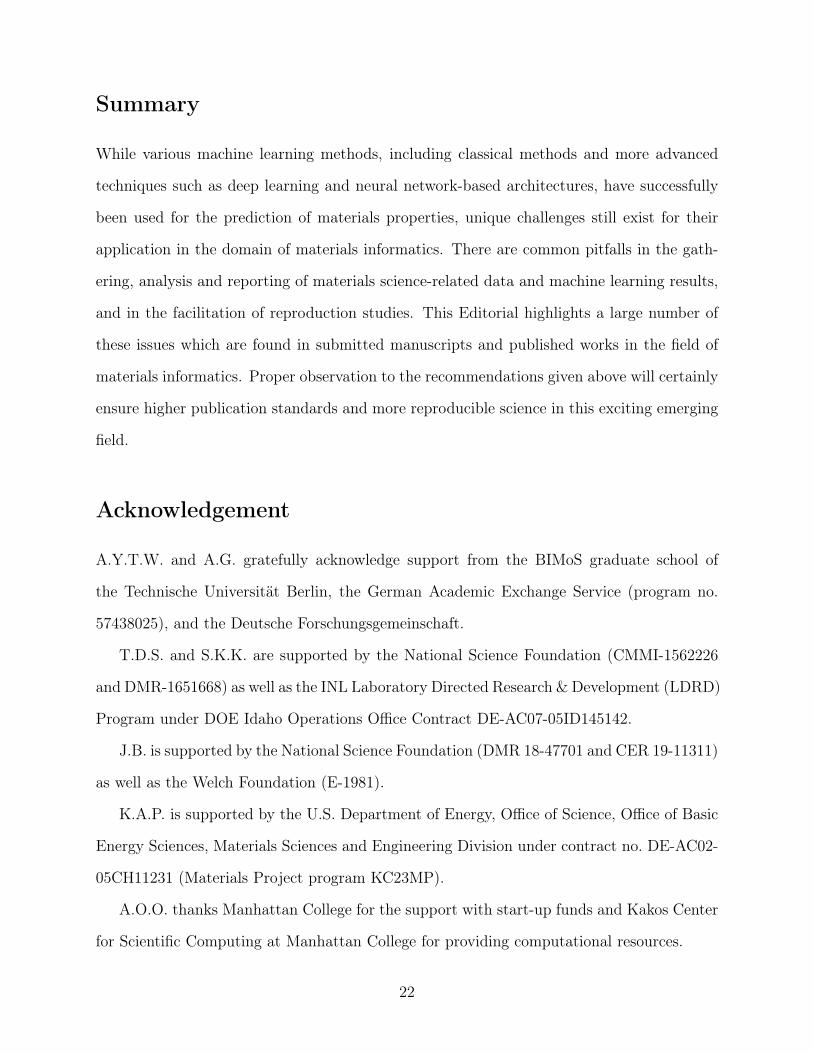
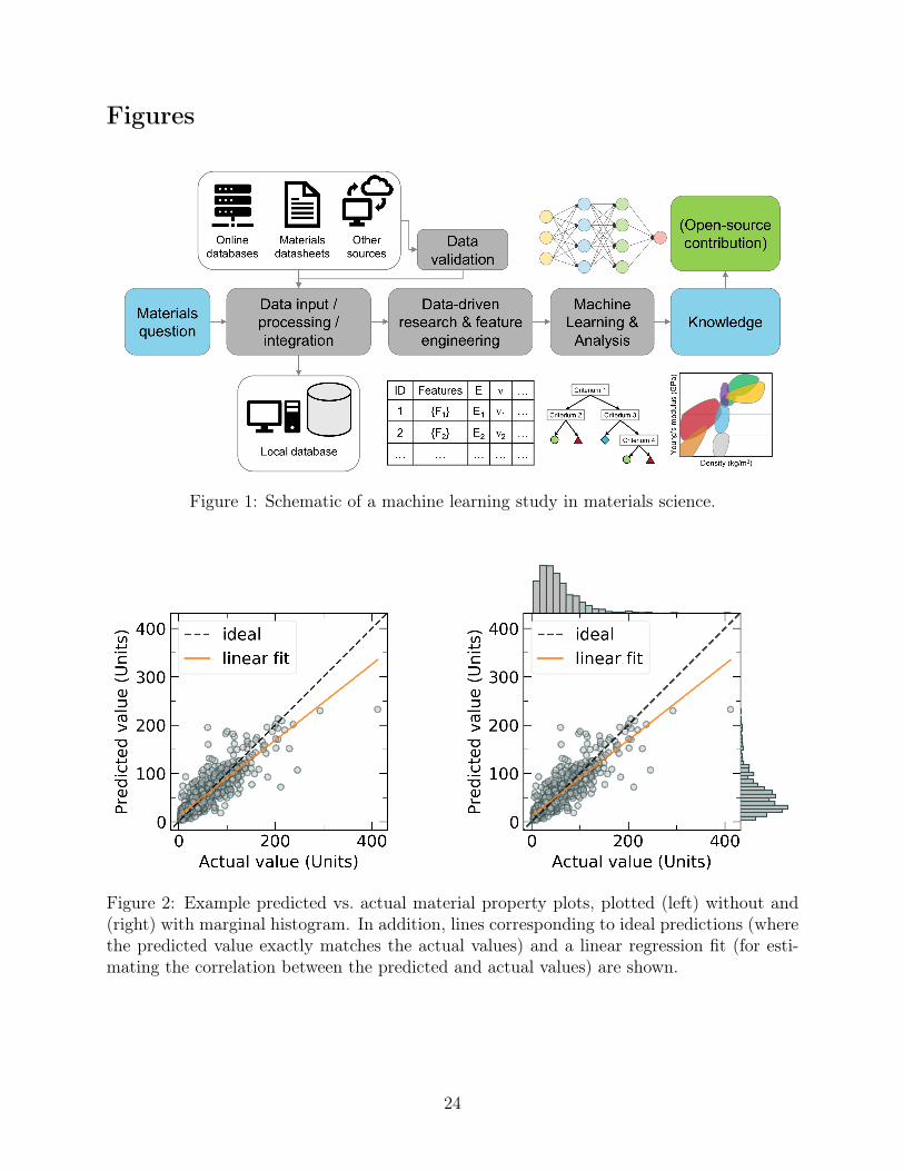
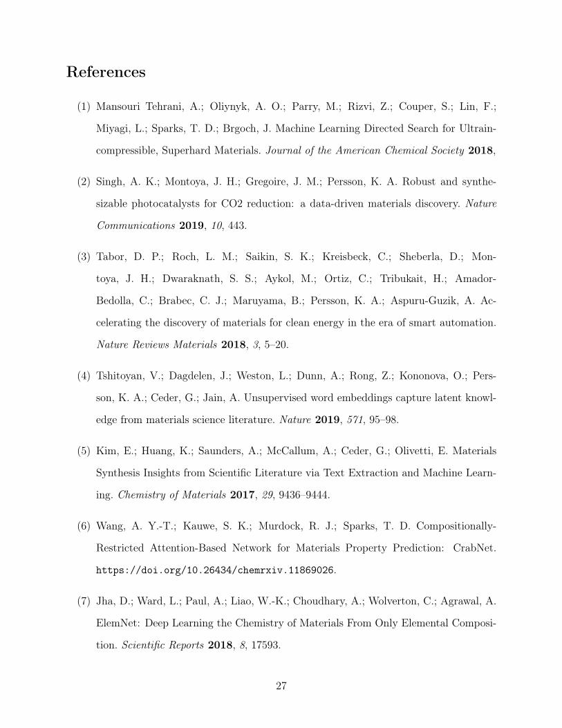
Some of the typical visualizations that have shown themselves to be generally useful—and
are thus commonly shown—in MI studies are: predicted property value vs. actual property
value plots (Figure 2), residual error plots and histograms of residual errors (Figure 3),
loss curves throughout the training process of a neural network (Figure 4), and element
20
prevalence visualizations (Figures 5 and 6). The figures are shown together at the end of
this manuscript, on page 24.
Benchmark datasets
While there are currently several materials property datasets online which could potentially
be used as benchmark datasets for benchmarking model performance in MI, there exist few
published train/validation/test splits of these datasets which can be used by researchers
to conduct a fair benchmark. Here, we note that examples of such datasets are commonly
found in the fields of computer vision (e.g., CIFAR, Google Open Images dataset, CelebFaces,
ImageNet) as well as in natural language processing (e.g., Glue, decaNLP, WMT 2014 EN-
DE).
Furthermore, the data heterogeneity—in terms of the classes of materials, the reported
material properties, or the diversity in the types of compounds and constituent elements—
of the available materials datasets are typically quite limited and vary between dataset to
dataset. Additionally, the methods to access some of the data stored in the online data
repositories are sometimes restricted, and therefore hinder potential MI studies. This is due
in part to the fact that certain datasets are proprietary or licensed under terms that do not
allow their sharing (whether online or offline).
Another challenge is that the online material property repositories do not offer a “check-
pointed” repository state; therefore, the repository and its data may change at any point
in time, and there is no easy way to revert or refer back to the state of the repository at
an earlier time. Therefore, current ML researchers typically download materials datasets
from the repositories and archive them locally to run their benchmarks internally. However,
there are recent emerging works from researchers that aim to address this issue of missing
benchmark datasets for MI and ML studies in materials science.134
21
Summary
While various machine learning methods, including classical methods and more advanced
techniques such as deep learning and neural network-based architectures, have successfully
been used for the prediction of materials properties, unique challenges still exist for their
application in the domain of materials informatics. There are common pitfalls in the gath-
ering, analysis and reporting of materials science-related data and machine learning results,
and in the facilitation of reproduction studies. This Editorial highlights a large number of
these issues which are found in submitted manuscripts and published works in the field of
materials informatics. Proper observation to the recommendations given above will certainly
ensure higher publication standards and more reproducible science in this exciting emerging
field.
Acknowledgement
A.Y.T.W. and A.G. gratefully acknowledge support from the BIMoS graduate school of
the Technische Universität Berlin, the German Academic Exchange Service (program no.
57438025), and the Deutsche Forschungsgemeinschaft.
T.D.S. and S.K.K. are supported by the National Science Foundation (CMMI-1562226
and DMR-1651668) as well as the INL Laboratory Directed Research & Development (LDRD)
Program under DOE Idaho Operations Office Contract DE-AC07-05ID145142.
J.B. is supported by the National Science Foundation (DMR 18-47701 and CER 19-11311)
as well as the Welch Foundation (E-1981).
K.A.P. is supported by the U.S. Department of Energy, Office of Science, Office of Basic
Energy Sciences, Materials Sciences and Engineering Division under contract no. DE-AC02-
05CH11231 (Materials Project program KC23MP).
A.O.O. thanks Manhattan College for the support with start-up funds and Kakos Center
for Scientific Computing at Manhattan College for providing computational resources.
22

Supporting Information Available
The following files are available with this publication:
• Online GitHub repository with the interactive Jupyter notebook files, Python source
code and example data: https://github.com/anthony-wang/BestPractices
• Supplementary Information, containing read-only versions of the Jupyter notebook files
23
Figures
Figure 1: Schematic of a machine learning study in materials science.
Figure 2: Example predicted vs. actual material property plots, plotted (left) without and(right) with marginal histogram. In addition, lines corresponding to ideal predictions (wherethe predicted value exactly matches the actual values) and a linear regression fit (for esti-mating the correlation between the predicted and actual values) are shown.
24
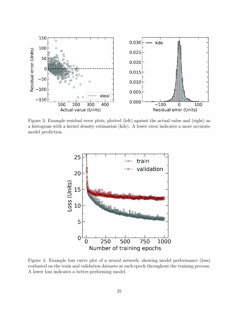
Figure 3: Example residual error plots, plotted (left) against the actual value and (right) asa histogram with a kernel density estimation (kde). A lower error indicates a more accuratemodel prediction.
Figure 4: Example loss curve plot of a neural network, showing model performance (loss)evaluated on the train and validation datasets at each epoch throughout the training process.A lower loss indicates a better-performing model.
25
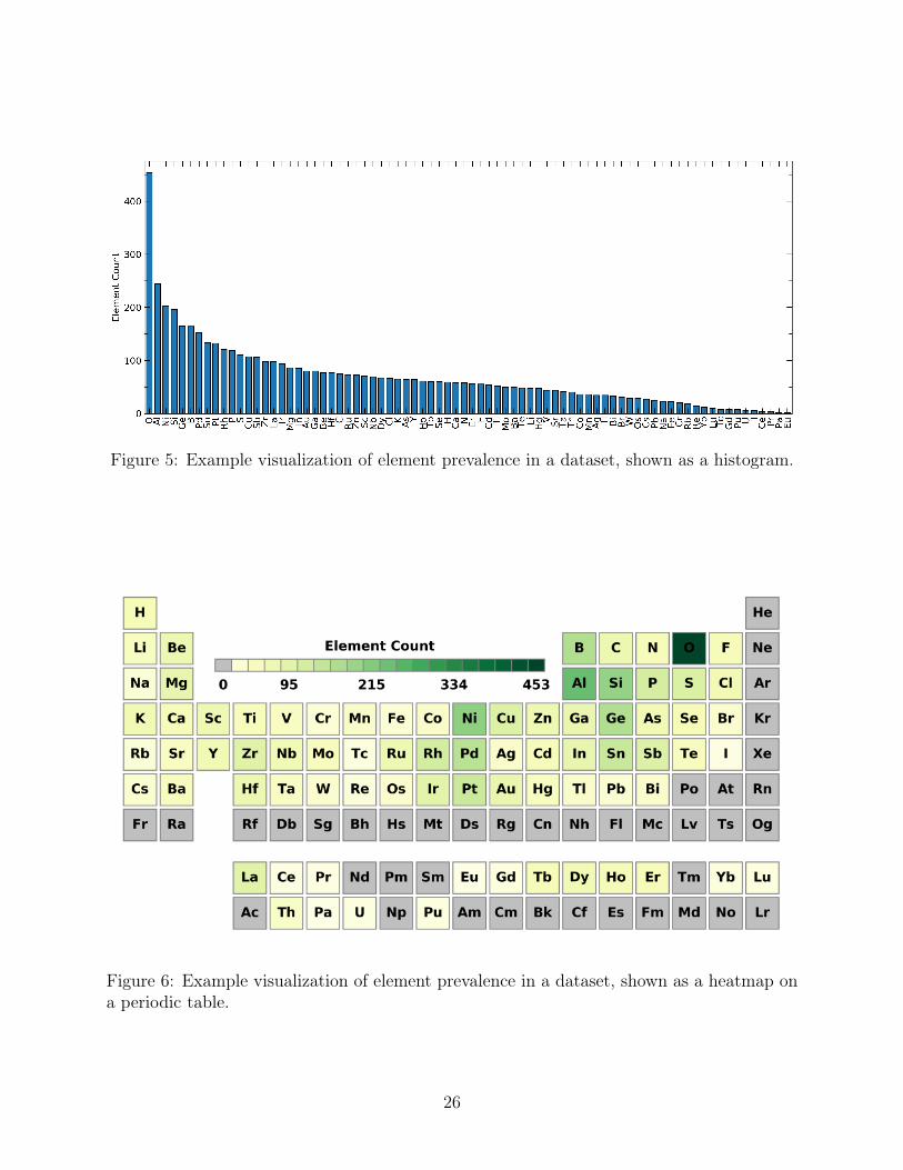
Figure 5: Example visualization of element prevalence in a dataset, shown as a histogram.
Figure 6: Example visualization of element prevalence in a dataset, shown as a heatmap ona periodic table.
26
References
(1) Mansouri Tehrani, A.; Oliynyk, A. O.; Parry, M.; Rizvi, Z.; Couper, S.; Lin, F.;
Miyagi, L.; Sparks, T. D.; Brgoch, J. Machine Learning Directed Search for Ultrain-
compressible, Superhard Materials. Journal of the American Chemical Society 2018,
(2) Singh, A. K.; Montoya, J. H.; Gregoire, J. M.; Persson, K. A. Robust and synthe-
sizable photocatalysts for CO2 reduction: a data-driven materials discovery. Nature
Communications 2019, 10, 443.
(3) Tabor, D. P.; Roch, L. M.; Saikin, S. K.; Kreisbeck, C.; Sheberla, D.; Mon-
toya, J. H.; Dwaraknath, S. S.; Aykol, M.; Ortiz, C.; Tribukait, H.; Amador-
Bedolla, C.; Brabec, C. J.; Maruyama, B.; Persson, K. A.; Aspuru-Guzik, A. Ac-
celerating the discovery of materials for clean energy in the era of smart automation.
Nature Reviews Materials 2018, 3, 5–20.
(4) Tshitoyan, V.; Dagdelen, J.; Weston, L.; Dunn, A.; Rong, Z.; Kononova, O.; Pers-
son, K. A.; Ceder, G.; Jain, A. Unsupervised word embeddings capture latent knowl-
edge from materials science literature. Nature 2019, 571, 95–98.
(5) Kim, E.; Huang, K.; Saunders, A.; McCallum, A.; Ceder, G.; Olivetti, E. Materials
Synthesis Insights from Scientific Literature via Text Extraction and Machine Learn-
ing. Chemistry of Materials 2017, 29, 9436–9444.
(6) Wang, A. Y.-T.; Kauwe, S. K.; Murdock, R. J.; Sparks, T. D. Compositionally-
Restricted Attention-Based Network for Materials Property Prediction: CrabNet.
https://doi.org/10.26434/chemrxiv.11869026.
(7) Jha, D.; Ward, L.; Paul, A.; Liao, W.-K.; Choudhary, A.; Wolverton, C.; Agrawal, A.
ElemNet: Deep Learning the Chemistry of Materials From Only Elemental Composi-
tion. Scientific Reports 2018, 8, 17593.
27
(8) Schütt, K. T.; Sauceda, H. E.; Kindermans, P.-J.; Tkatchenko, A.; Müller, K.-R.
SchNet – A deep learning architecture for molecules and materials. The Journal of
Chemical Physics 2018, 148, 241722.
(9) Xie, T.; Grossman, J. C. Crystal Graph Convolutional Neural Networks for an Ac-
curate and Interpretable Prediction of Material Properties. Physical Review Letters
2018, 120, 1929.
(10) Goodall, R. E. A.; Lee, A. A. Predicting materials properties without crystal struc-
ture: Deep representation learning from stoichiometry. http://arxiv.org/pdf/
1910.00617v2.
(11) Murdock, R. J.; Kauwe, S. K.; Wang, A. Y.-T.; Sparks, T. D. Is Domain Knowledge
Necessary for Machine Learning Materials Properties? https://doi.org/10.26434/
chemrxiv.11879193.
(12) Kauwe, S. K.; Graser, J.; Murdock, R. J.; Sparks, T. D. Can machine learning find
extraordinary materials? Computational Materials Science 2020, 174, 109498.
(13) Oliynyk, A. O.; Antono, E.; Sparks, T. D.; Ghadbeigi, L.; Gaultois, M. W.;
Meredig, B.; Mar, A. High-Throughput Machine-Learning-Driven Synthesis of Full-
Heusler Compounds. Chemistry of Materials 2016, 28, 7324–7331.
(14) Lookman, T.; Alexander, F. J.; Rajan, K. Information science for materials discovery
and design; Springer: Cham, Switzerland, 2016.
(15) Mueller, T.; Kusne, A. G.; Ramprasad, R. In Reviews in Computational Chemistry ;
Parrill, A. L., Lipkowitz, K. B., Eds.; Reviews in Computational Chemistry; John
Wiley & Sons, Inc.: Hoboken, NJ, 2016; Vol. 1; pp 186–273.
(16) Liu, Y.; Zhao, T.; Ju, W.; Shi, S. Materials discovery and design using machine
learning. Journal of Materiomics 2017, 3, 159–177.
28
(17) Gorai, P.; Stevanović, V.; Toberer, E. S. Computationally guided discovery of ther-
moelectric materials. Nature Reviews Materials 2017, 2, 17053.
(18) Butler, K. T.; Davies, D. W.; Cartwright, H.; Isayev, O.; Walsh, A. Machine learning
for molecular and materials science. Nature 2018, 559, 547–555.
(19) Ramakrishna, S.; Zhang, T.-Y.; Lu, W.-C.; Qian, Q.; Low, J. S. C.; Yune, J. H. R.;
Tan, D. Z. L.; Bressan, S.; Sanvito, S.; Kalidindi, S. R. Materials Informatics. Journal
of Intelligent Manufacturing 2018, 4, 053208.
(20) Rickman, J. M.; Lookman, T.; Kalinin, S. V. Materials informatics: From the atomic-
level to the continuum. Acta Materialia 2019,
(21) Gomes, C. P.; Selman, B.; Gregoire, J. M. Artificial intelligence for materials discovery.
MRS Bulletin 2019, 44, 538–544.
(22) Ong, S. P. Accelerating materials science with high-throughput computations and
machine learning. Computational Materials Science 2019, 161, 143–150.
(23) Schmidt, J.; Marques, M. R. G.; Botti, S.; Marques, M. A. L. Recent advances and
applications of machine learning in solid-state materials science. npj Computational
Materials 2019, 5, 484.
(24) Meredig, B. Five High-Impact Research Areas in Machine Learning for Materials Sci-
ence. Chemistry of Materials 2019, 31, 9579–9581.
(25) Bhadeshia, H. Computational design of advanced steels. Scripta Materialia 2014, 70,
12–17.
(26) Agrawal, A.; Deshpande, P. D.; Cecen, A.; Basavarsu, G. P.; Choudhary, A. N.; Ka-
lidindi, S. R. Exploration of data science techniques to predict fatigue strength of steel
from composition and processing parameters. Integrating Materials and Manufacturing
Innovation 2014, 3, 90–108.
29
(27) Furmanchuk, A.; Agrawal, A.; Choudhary, A. Predictive analytics for crystalline ma-
terials: bulk modulus. RSC Advances 2016, 6, 95246–95251.
(28) de Jong, M.; Chen, W.; Notestine, R.; Persson, K. A.; Ceder, G.; Jain, A.; Asta, M.;
Gamst, A. A Statistical Learning Framework for Materials Science: Application to
Elastic Moduli of k-nary Inorganic Polycrystalline Compounds. Scientific Reports
2016, 6, 34256.
(29) Chen, C.; Ye, W.; Zuo, Y.; Zheng, C.; Ong, S. P. Graph Networks as a Universal Ma-
chine Learning Framework for Molecules and Crystals. Chemistry of Materials 2019,
31, 3564–3572.
(30) Evans, J. D.; Coudert, F.-X. Predicting the Mechanical Properties of Zeolite Frame-
works by Machine Learning. Chemistry of Materials 2017, 29, 7833–7839.
(31) Meredig, B.; Agrawal, A.; Kirklin, S.; Saal, J. E.; Doak, J. W.; Thompson, A.;
Zhang, K.; Choudhary, A.; Wolverton, C. Combinatorial screening for new materials
in unconstrained composition space with machine learning. Physical Review B 2014,
89, 83.
(32) Ghiringhelli, L. M.; Vybiral, J.; Levchenko, S. V.; Draxl, C.; Scheffler, M. Big data of
materials science: critical role of the descriptor. Physical Review Letters 2015, 114,
105503.
(33) Deml, A. M.; O’Hayre, R.; Wolverton, C.; Stevanović, V. Predicting density functional
theory total energies and enthalpies of formation of metal-nonmetal compounds by
linear regression. Physical Review B 2016, 93 .
(34) Ward, L.; Agrawal, A.; Choudhary, A.; Wolverton, C. A general-purpose machine
learning framework for predicting properties of inorganic materials. npj Computational
Materials 2016, 2, 364.
30
(35) Dey, P.; Bible, J.; Datta, S.; Broderick, S.; Jasinski, J.; Sunkara, M.; Menon, M.;
Rajan, K. Informatics-aided bandgap engineering for solar materials. Computational
Materials Science 2014, 83, 185–195.
(36) Pilania, G.; Mannodi-Kanakkithodi, A.; Uberuaga, B. P.; Ramprasad, R.; Guber-
natis, J. E.; Lookman, T. Machine learning bandgaps of double perovskites. Scientific
Reports 2016, 6, 19375.
(37) Sparks, T. D.; Kauwe, S. K.; Welker, T. Extracting Knowledge from DFT: Experi-
mental Band Gap Predictions Through Ensemble Learning.
(38) Rajan, A. C.; Mishra, A.; Satsangi, S.; Vaish, R.; Mizuseki, H.; Lee, K.-R.; Singh, A. K.
Machine-Learning-Assisted Accurate Band Gap Predictions of Functionalized MXene.
Chemistry of Materials 2018, 30, 4031–4038.
(39) Zhuo, Y.; Mansouri Tehrani, A.; Brgoch, J. Predicting the Band Gaps of Inorganic
Solids by Machine Learning. The Journal of Physical Chemistry Letters 2018, 9,
1668–1673.
(40) Schütt, K. T.; Glawe, H.; Brockherde, F.; Sanna, A.; Müller, K.-R.; Gross, E. K. U.
How to represent crystal structures for machine learning: Towards fast prediction of
electronic properties. Physical Review B 2014, 89, 1875.
(41) Yeo, B. C.; Kim, D.; Kim, C.; Han, S. S. Pattern Learning Electronic Density of
States. Scientific Reports 2019, 9, 5879.
(42) Curtarolo, S.; Morgan, D.; Persson, K. A.; Rodgers, J.; Ceder, G. Predicting crystal
structures with data mining of quantum calculations. Physical Review Letters 2003,
91, 135503.
(43) Fischer, C. C.; Tibbetts, K. J.; Morgan, D.; Ceder, G. Predicting crystal structure by
merging data mining with quantum mechanics. Nature Materials 2006, 5, 641–646.
31
(44) Hautier, G.; Fischer, C. C.; Jain, A.; Mueller, T.; Ceder, G. Finding Nature’s Missing
Ternary Oxide Compounds Using Machine Learning and Density Functional Theory.
Chemistry of Materials 2010, 22, 3762–3767.
(45) Kong, C. S.; Luo, W.; Arapan, S.; Villars, P.; Iwata, S.; Ahuja, R.; Rajan, K.
Information-theoretic approach for the discovery of design rules for crystal chemistry.
Journal of chemical information and modeling 2012, 52, 1812–1820.
(46) Pilania, G.; Balachandran, P. V.; Gubernatis, J. E.; Lookman, T. Classification of
ABO3 perovskite solids: a machine learning study. Acta Crystallographica Section B:
Structural Science, Crystal Engineering and Materials 2015, 71, 507–513.
(47) Oliynyk, A. O.; Adutwum, L. A.; Harynuk, J. J.; Mar, A. Classifying Crystal Struc-
tures of Binary Compounds AB through Cluster Resolution Feature Selection and
Support Vector Machine Analysis. Chemistry of Materials 2016, 28, 6672–6681.
(48) Goldsmith, B. R.; Boley, M.; Vreeken, J.; Scheffler, M.; Ghiringhelli, L. M. Uncovering
structure-property relationships of materials by subgroup discovery. New Journal of
Physics 2017, 19, 013031.
(49) Balachandran, P. V.; Young, J.; Lookman, T.; Rondinelli, J. M. Learning from data
to design functional materials without inversion symmetry. Nature Communications
2017, 8, 14282.
(50) Schmidt, J.; Shi, J.; Borlido, P.; Chen, L.; Botti, S.; Marques, M. A. L. Predicting
the Thermodynamic Stability of Solids Combining Density Functional Theory and
Machine Learning. Chemistry of Materials 2017, 29, 5090–5103.
(51) Seko, A.; Hayashi, H.; Kashima, H.; Tanaka, I. Matrix- and tensor-based recommender
systems for the discovery of currently unknown inorganic compounds. Physical Review
Materials 2018, 2 .
32
(52) Li, W.; Jacobs, R.; Morgan, D. Predicting the thermodynamic stability of perovskite
oxides using machine learning models. Computational Materials Science 2018, 150,
454–463.
(53) Isayev, O.; Oses, C.; Toher, C.; Gossett, E.; Curtarolo, S.; Tropsha, A. Universal
fragment descriptors for predicting properties of inorganic crystals. Nature Commu-
nications 2017, 8, 15679.
(54) Kauwe, S. K.; Graser, J.; Vazquez, A.; Sparks, T. D. Machine Learning Prediction of
Heat Capacity for Solid Inorganics. Integrating Materials and Manufacturing Innova-
tion 2018, 7, 43–51.
(55) Carrete, J.; Li, W.; Mingo, N.; Wang, S.; Curtarolo, S. Finding Unprecedentedly Low-
Thermal-Conductivity Half-Heusler Semiconductors via High-Throughput Materials
Modeling. Physical Review X 2014, 4 .
(56) Gaultois, M. W.; Oliynyk, A. O.; Mar, A.; Sparks, T. D.; Mulholland, G. J.;
Meredig, B. Perspective: Web-based machine learning models for real-time screen-
ing of thermoelectric materials properties. APL Materials 2016, 4, 053213.
(57) Seko, A.; Hayashi, H.; Nakayama, K.; Takahashi, A.; Tanaka, I. Representation of
compounds for machine-learning prediction of physical properties. Physical Review B
2017, 95 .
(58) Furmanchuk, A.; Saal, J. E.; Doak, J. W.; Olson, G. B.; Choudhary, A.; Agrawal, A.
Prediction of seebeck coefficient for compounds without restriction to fixed stoichiom-
etry: A machine learning approach. Journal of computational chemistry 2018, 39,
191–202.
(59) Wei, L.; Xu, X.; Gurudayal,; Bullock, J.; Ager, J. W. Machine Learning Optimization
of p-Type Transparent Conducting Films. Chemistry of Materials 2019, 31, 7340–
7350.
33
(60) Davies, D. W.; Butler, K. T.; Walsh, A. Data-Driven Discovery of Photoactive Quater-
nary Oxides Using First-Principles Machine Learning. Chemistry of Materials 2019,
31, 7221–7230.
(61) Sendek, A. D.; Yang, Q.; Cubuk, E. D.; Duerloo, K.-A. N.; Cui, Y.; Reed, E. J. Holistic
computational structure screening of more than 12000 candidates for solid lithium-ion
conductor materials. Energy & Environmental Science 2017, 10, 306–320.
(62) Ahmad, Z.; Xie, T.; Maheshwari, C.; Grossman, J. C.; Viswanathan, V. Machine
Learning Enabled Computational Screening of Inorganic Solid Electrolytes for Sup-
pression of Dendrite Formation in Lithium Metal Anodes. ACS Central Science 2018,
4, 996–1006.
(63) Sendek, A. D.; Cubuk, E. D.; Antoniuk, E. R.; Cheon, G.; Cui, Y.; Reed, E. J.
Machine Learning-Assisted Discovery of Solid Li-Ion Conducting Materials. Chemistry
of Materials 2019, 31, 342–352.
(64) Bobbitt, N. S.; Snurr, R. Q. Molecular modelling and machine learning for high-
throughput screening of metal-organic frameworks for hydrogen storage. Molecular
Simulation 2019, 45, 1069–1081.
(65) Gu, G. H.; Noh, J.; Kim, I.; Jung, Y. Machine learning for renewable energy materials.
Journal of Materials Chemistry A 2019, 7, 17096–17117.
(66) Seh, Z. W.; Kibsgaard, J.; Dickens, C. F.; Chorkendorff, I.; Nørskov, J. K.;
Jaramillo, T. F. Combining theory and experiment in electrocatalysis: Insights into
materials design. Science 2017, 355 .
(67) Ulissi, Z. W.; Medford, A. J.; Bligaard, T.; Nørskov, J. K. To address surface reaction
network complexity using scaling relations machine learning and DFT calculations.
Nature Communications 2017, 8, 14621.
34
(68) Kitchin, J. R. Machine learning in catalysis. Nature Catalysis 2018, 1, 230–232.
(69) Hansen, M. H.; Torres, J. A. G.; Jennings, P. C.; Wang, Z.; Boes, J. R.; Mamun, O. G.;
Bligaard, T. An Atomistic Machine Learning Package for Surface Science and Catal-
ysis. http://arxiv.org/pdf/1904.00904v1.
(70) Schlexer Lamoureux, P.; Winther, K. T.; Garrido Torres, J. A.; Streibel, V.; Zhao, M.;
Bajdich, M.; Abild-Pedersen, F.; Bligaard, T. Machine Learning for Computational
Heterogeneous Catalysis. ChemCatChem 2019, 11, 3581–3601.
(71) Masood, H.; Toe, C. Y.; Teoh, W. Y.; Sethu, V.; Amal, R. Machine Learning for
Accelerated Discovery of Solar Photocatalysts. ACS Catalysis 2019, 9, 11774–11787.
(72) Gaultois, M. W.; Sparks, T. D.; Borg, C. K. H.; Seshadri, R.; Bonificio, W. D.;
Clarke, D. R. Data-Driven Review of Thermoelectric Materials: Performance and
Resource Considerations. Chemistry of Materials 2013, 25, 2911–2920.
(73) Sparks, T. D.; Gaultois, M. W.; Oliynyk, A. O.; Brgoch, J.; Meredig, B. Data mining
our way to the next generation of thermoelectrics. Scripta Materialia 2016, 111, 10–
15.
(74) Stanev, V.; Oses, C.; Kusne, A. G.; Rodriguez, E.; Paglione, J.; Curtarolo, S.;
Takeuchi, I. Machine learning modeling of superconducting critical temperature. npj
Computational Materials 2018, 4 .
(75) Meredig, B.; Antono, E.; Church, C.; Hutchinson, M.; Ling, J.; Paradiso, S.;
Blaiszik, B.; Foster, I.; Gibbons, B.; Hattrick-Simpers, J.; Mehta, A.; Ward, L. Can
machine learning identify the next high-temperature superconductor? Examining ex-
trapolation performance for materials discovery. Molecular Systems Design & Engi-
neering 2018, 3, 819–825.
35
(76) Konno, T.; Kurokawa, H.; Nabeshima, F.; Sakishita, Y.; Ogawa, R.; Hosako, I.;
Maeda, A. Deep Learning Model for Finding New Superconductors. http://arxiv.
org/pdf/1812.01995v3.
(77) Hamidieh, K. A data-driven statistical model for predicting the critical temperature
of a superconductor. Computational Materials Science 2018, 154, 346–354.
(78) Dan, Y.; Dong, R.; Cao, Z.; Li, X.; Niu, C.; Li, S.; Hu, J. Computational Prediction of
Critical Temperatures of Superconductors Based on Convolutional Gradient Boosting
Decision Trees. IEEE Access 2020, 8, 57868–57878.
(79) Matsumoto, K.; Horide, T. An acceleration search method of higher Tc superconduc-
tors by a machine learning algorithm. Applied Physics Express 2019, 12, 073003.
(80) Roter, B.; Dordevic, S. V. Predicting new superconductors and their critical temper-
atures using unsupervised machine learning. http://arxiv.org/pdf/2002.07266v1.
(81) Wen, C.; Zhang, Y.; Wang, C.; Xue, D.; Bai, Y.; Antonov, S.; Dai, L.; Lookman, T.;
Su, Y. Machine learning assisted design of high entropy alloys with desired property.
Acta Materialia 2019, 170, 109–117.
(82) Chang, Y.-J.; Jui, C.-Y.; Lee, W.-J.; Yeh, A.-C. Prediction of the Composition and
Hardness of High-Entropy Alloys by Machine Learning. JOM 2019, 6, 299.
(83) Ren, F.; Ward, L.; Williams, T.; Laws, K. J.; Wolverton, C.; Hattrick-Simpers, J.;
Mehta, A. Accelerated discovery of metallic glasses through iteration of machine learn-
ing and high-throughput experiments. Science Advances 2018, 4, eaaq1566.
(84) Ward, L.; O’Keeffe, S. C.; Stevick, J.; Jelbert, G. R.; Aykol, M.; Wolverton, C. A
machine learning approach for engineering bulk metallic glass alloys. Acta Materialia
2018, 159, 102–111.
36
(85) Jain, A.; Ong, S. P.; Hautier, G.; Chen, W.; Richards, W. D.; Dacek, S.; Cholia, S.;
Gunter, D.; Skinner, D.; Ceder, G.; Persson, K. A. Commentary: The Materials
Project: A materials genome approach to accelerating materials innovation. APL
Materials 2013, 1, 011002.
(86) Saal, J. E.; Kirklin, S.; Aykol, M.; Meredig, B.; Wolverton, C. Materials Design and
Discovery with High-Throughput Density Functional Theory: The Open Quantum
Materials Database (OQMD). JOM 2013, 65, 1501–1509.
(87) Curtarolo, S.; Setyawan, W.; Wang, S.; Xue, J.; Yang, K.; Taylor, R. H.;
Nelson, L. J.; Hart, G. L.; Sanvito, S.; Buongiorno-Nardelli, M.; Mingo, N.;
Levy, O. AFLOWLIB.ORG: A distributed materials properties repository from high-
throughput ab initio calculations. Computational Materials Science 2012, 58, 227–
235.
(88) Draxl, C.; Scheffler, M. The NOMAD laboratory: from data sharing to artificial in-
telligence. Journal of Physics: Materials 2019, 2, 036001.
(89) Open Materials Database. http://openmaterialsdb.se/index.php.
(90) Citrine Informatics: The AI Platform for Materials Development. https://citrine.
io/.
(91) Materials Platform for Data Science (MPDS). https://mpds.io/.
(92) Huber, S. P. et al. AiiDA 1.0, a scalable computational infrastructure for automated
reproducible workflows and data provenance. http://arxiv.org/pdf/2003.12476v1.
(93) Talirz, L. et al. Materials Cloud, a platform for open computational science. http:
//arxiv.org/pdf/2003.12510v1.
(94) Deml, A.; Lany, S.; Peng, H.; Stevanovic, V.; Yan, J.; Zawadzki, P.; Graf, P.;
Sorensen, H.; Sullivan, S. NREL MatDB. 2020; https://materials.nrel.gov/.
37
(95) National Institute of Standards and Technology (NIST), NIST TRC Alloy Data. 2017;
https://www.nist.gov/mml/acmd/trc/nist-alloy-data.
(96) National Institute of Standards and Technology (NIST), NIST TRC ThermoData
Engine. 2005; https://www.nist.gov/mml/acmd/trc/thermodata-engine.
(97) National Institute of Standards and Technology (NIST), NIST JARVIS-DFT
Database. 2017; https://www.nist.gov/programs-projects/jarvis-dft.
(98) National Institute of Standards and Technology (NIST), NIST JARVIS-ML Database.
2019; https://www.nist.gov/programs-projects/jarvis-ml.
(99) MatWeb. http://www.matweb.com/index.aspx.
(100) Total Materia. https://www.totalmateria.com/.
(101) Ansys Granta MaterialUniverse. https://grantadesign.com/.
(102) MATDAT. https://www.matdat.com/.
(103) Groom, C. R.; Bruno, I. J.; Lightfoot, M. P.; Ward, S. C. The Cambridge Structural
Database. Acta Crystallographica Section B: Structural Science, Crystal Engineering
and Materials 2016, 72, 171–179.
(104) Hellenbrandt, M. The Inorganic Crystal Structure Database (ICSD)—Present and
Future. Crystallography Reviews 2004, 10, 17–22.
(105) Pearson’s Crystal Data: Crystal Structure Database for Inorganic Compounds. https:
//www.crystalimpact.com/pcd/Default.htm.
(106) Gates-Rector, S.; Blanton, T. The Powder Diffraction File: a quality materials char-
acterization database. Powder Diffraction 2019, 34, 352–360.
(107) Gražulis, S.; Chateigner, D.; Downs, R. T.; Yokochi, A. F. T.; Quirós, M.; Lut-
terotti, L.; Manakova, E.; Butkus, J.; Moeck, P.; Le Bail, A. Crystallography Open
38
Database – an open-access collection of crystal structures. Journal of Applied Crys-
tallography 2009, 42, 726–729.
(108) PAULING FILE. https://paulingfile.com/.
(109) White, P. S.; Rodgers, J. R.; Le Page, Y. CRYSTMET: a database of the structures
and powder patterns of metals and intermetallics. Acta Crystallographica Section B:
Structural Science 2002, 58, 343–348.
(110) van der Maaten, L.; Hinton, G. Visualizing Data using t-SNE. Journal of Machine
Learning Research 2008, 9, 2579–2605.
(111) McInnes, L.; Healy, J.; Saul, N.; Großberger, L. UMAP: Uniform Manifold Approxi-
mation and Projection. Journal of Open Source Software 2018, 3, 861.
(112) Kauwe, S. K.; Yang, Y.; Sparks, T. D. Visualization Tool for Atomic Models (VITAL):
A Simple Visualization Tool for Materials Predictions. https://doi.org/10.26434/
chemrxiv.9782375.
(113) Git. https://git-scm.com/.
(114) Mercurial. https://www.mercurial-scm.org/.
(115) Apacher Subversionr. https://subversion.apache.org/.
(116) Cawley, G. C.; Talbot, N. L. On Over-Fitting in Model Selection and Subsequent Se-
lection Bias in Performance Evaluation. Journal of Machine Learning Research 2010,
11, 2079–2107.
(117) Pedregosa, F. et al. Scikit-learn: Machine Learning in Python. Journal of Machine
Learning Research 2011, 12, 2825–2830.
(118) Paszke, A. et al. PyTorch: An Imperative Style, High-Performance Deep Learning
Library. http://arxiv.org/pdf/1912.01703v1.
39
(119) Abadi, M. et al. TensorFlow: Large-Scale Machine Learning on Heterogeneous Dis-
tributed Systems. https://www.tensorflow.org/about/.
(120) Graser, J.; Kauwe, S. K.; Sparks, T. D. Machine Learning and Energy Minimization
Approaches for Crystal Structure Predictions: A Review and New Horizons. Chemistry
of Materials 2018, 30, 3601–3612.
(121) Choudhary, K.; DeCost, B.; Tavazza, F. Machine learning with force-field-inspired de-
scriptors for materials: Fast screening and mapping energy landscape. Physical Review
Materials 2018, 2, 2825.
(122) Jha, D.; Ward, L.; Yang, Z.; Wolverton, C.; Foster, I.; Liao, W.-K.; Choudhary, A.;
Agrawal, A. IRNet: A General Purpose Deep Residual Regression Framework for
Materials Discovery. Proceedings of the 25th ACM SIGKDD International Conference
on Knowledge Discovery & Data Mining - KDD ’19. New York, New York, USA, 2019;
pp 2385–2393.
(123) Juszczak, P.; Tax, D. M.; Duin, R. P. Feature scaling in support vector data de-
scription. Proceedings of the Eighth Annual Conference of the Advanced School for
Computing and Imaging. 2002; pp 95–102.
(124) Ba, J. L.; Kiros, J. R.; Hinton, G. E. Layer Normalization. http://arxiv.org/pdf/
1607.06450v1.
(125) Ioffe, S.; Szegedy, C. Batch Normalization: Accelerating Deep Network Training by
Reducing Internal Covariate Shift. http://arxiv.org/pdf/1502.03167v3.
(126) Mohamad, I. B.; Usman, D. Standardization and Its Effects on k-Means Clustering
Algorithm. Research Journal of Applied Sciences, Engineering and Technology 2013,
6, 3299–3303.
40
(127) Head, M. L.; Holman, L.; Lanfear, R.; Kahn, A. T.; Jennions, M. D. The extent and
consequences of p-hacking in science. PLoS Biology 2015, 13, e1002106.
(128) Ward, L. et al. Matminer: An open source toolkit for materials data mining. Compu-
tational Materials Science 2018, 152, 60–69.
(129) Olson, R. S.; Bartley, N.; Urbanowicz, R. J.; Moore, J. H. Evaluation of a Tree-based
Pipeline Optimization Tool for Automating Data Science. Proceedings of the 2016 on
Genetic and Evolutionary Computation Conference - GECCO ’16. New York, New
York, USA, 2016; pp 485–492.
(130) Automatminer. https://github.com/hackingmaterials/automatminer.
(131) Barnes, N. Publish your computer code: it is good enough. Nature 2010, 467, 753.
(132) Chard, R.; Li, Z.; Chard, K.; Ward, L.; Babuji, Y.; Woodard, A.; Tuecke, S.;
Blaiszik, B.; Franklin, M. J.; Foster, I. DLHub: Model and Data Serving for Science.
http://arxiv.org/pdf/1811.11213v1.
(133) Docker. https://www.docker.com/.
(134) Clement, C.; Kauwe, S. K.; Sparks, T. D. Benchmark AFLOW Data Sets for Machine
Learning. https://doi.org/10.6084/m9.figshare.11954742.
41

download fileview on ChemRxivBestPractices_submitted.pdf (2.22 MiB)
Supplementary Information for the paper “Machine Learning for Materials Scientists:
An introductory guide towards best practices”
Authors: Anthony Yu-Tung Wang, Ryan J. Murdock, Steven K. Kauwe, Anton O. Oliynyk, Aleksander Gurlo, Jakoah Brgoch, Kristin A. Persson, and Taylor D. Sparks
Overview of NotebooksThese notebooks are included to illustrate a hypothetical Machine Learning project created following bestpractices.
The goal of this ML project is to predict the heat capacity of inorganic materials given the chemical compositionand condition (the measurement temperature). We will use both classical ML models as well as neural networks.
To do this, we must:
1. Clean and process our dataset, removing obviously erroneous or empty values.2. Partition our data into train, validation, and test splits.3. Featurize our data, turning the chemical formulae into CBFVs.4. Train models on our data and assess the predictive power of the models.5. Compare the performance of the models fairly and reproducibly.6. Visualize the prediction results of the models.7. Share our models and enable others to reproduce your work and aid collaboration.
If you require more information about how to use Jupyter notebooks, you can consult:
The main README file inside this repository: https://github.com/anthony-wang/BestPractices/blob/master/README.md (https://github.com/anthony-wang/BestPractices/blob/master/README.md)The official Jupyter Notebook documentation: https://jupyter-notebook.readthedocs.io/en/stable/notebook.html (https://jupyter-notebook.readthedocs.io/en/stable/notebook.html)
To read the main publication for which these notebooks are made, please see:
link coming
Please also consider citing the work if you choose to adopt or adapt the methods and concepts shown in thesenotebooks or in the publication:
citation coming

Check that libraries are installedThis notebook checks to see if you have the correct version of Python as well as all necessary libraries installed.
Check the main README file (https://github.com/anthony-wang/BestPractices/blob/master/README.md) forinstructions if anything is missing.
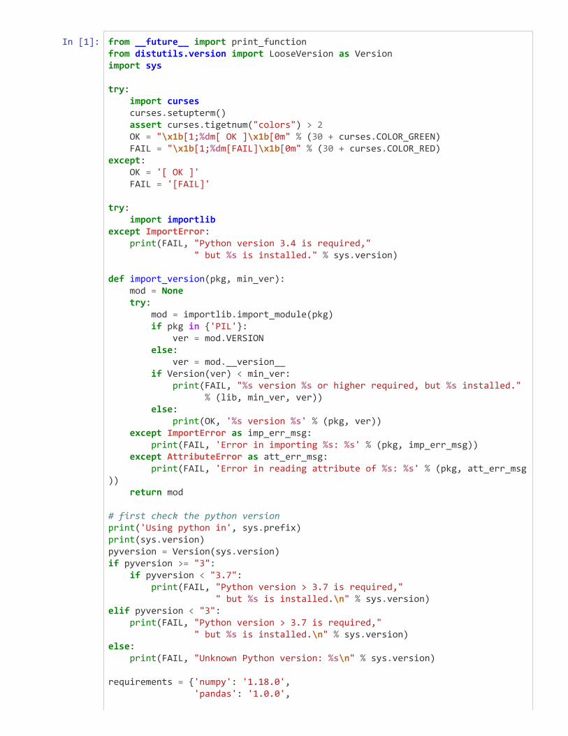
In [1]: from __future__ import print_functionfrom distutils.version import LooseVersion as Versionimport sys
try: import curses curses.setupterm() assert curses.tigetnum("colors") > 2 OK = "\x1b[1;%dm[ OK ]\x1b[0m" % (30 + curses.COLOR_GREEN) FAIL = "\x1b[1;%dm[FAIL]\x1b[0m" % (30 + curses.COLOR_RED)except: OK = '[ OK ]' FAIL = '[FAIL]'
try: import importlibexcept ImportError: print(FAIL, "Python version 3.4 is required," " but %s is installed." % sys.version)
def import_version(pkg, min_ver): mod = None try: mod = importlib.import_module(pkg) if pkg in {'PIL'}: ver = mod.VERSION else: ver = mod.__version__ if Version(ver) < min_ver: print(FAIL, "%s version %s or higher required, but %s installed." % (lib, min_ver, ver)) else: print(OK, '%s version %s' % (pkg, ver)) except ImportError as imp_err_msg: print(FAIL, 'Error in importing %s: %s' % (pkg, imp_err_msg)) except AttributeError as att_err_msg: print(FAIL, 'Error in reading attribute of %s: %s' % (pkg, att_err_msg)) return mod
# first check the python versionprint('Using python in', sys.prefix)print(sys.version)pyversion = Version(sys.version)if pyversion >= "3": if pyversion < "3.7": print(FAIL, "Python version > 3.7 is required," " but %s is installed.\n" % sys.version)elif pyversion < "3": print(FAIL, "Python version > 3.7 is required," " but %s is installed.\n" % sys.version)else: print(FAIL, "Unknown Python version: %s\n" % sys.version)
requirements = {'numpy': '1.18.0', 'pandas': '1.0.0',
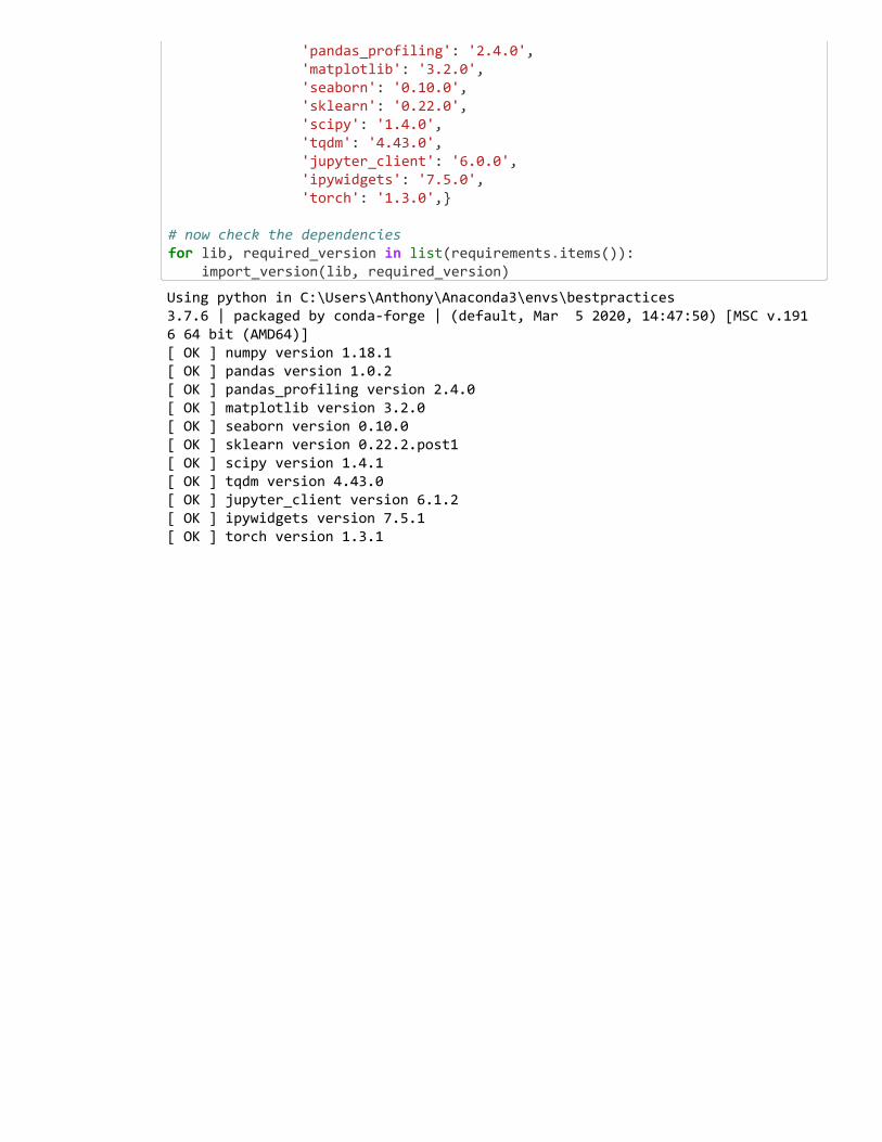
'pandas_profiling': '2.4.0', 'matplotlib': '3.2.0', 'seaborn': '0.10.0', 'sklearn': '0.22.0', 'scipy': '1.4.0', 'tqdm': '4.43.0', 'jupyter_client': '6.0.0', 'ipywidgets': '7.5.0', 'torch': '1.3.0',}
# now check the dependenciesfor lib, required_version in list(requirements.items()): import_version(lib, required_version)
Using python in C:\Users\Anthony\Anaconda3\envs\bestpractices 3.7.6 | packaged by conda-forge | (default, Mar 5 2020, 14:47:50) [MSC v.1916 64 bit (AMD64)] [ OK ] numpy version 1.18.1 [ OK ] pandas version 1.0.2 [ OK ] pandas_profiling version 2.4.0 [ OK ] matplotlib version 3.2.0 [ OK ] seaborn version 0.10.0 [ OK ] sklearn version 0.22.2.post1 [ OK ] scipy version 1.4.1 [ OK ] tqdm version 4.43.0 [ OK ] jupyter_client version 6.1.2 [ OK ] ipywidgets version 7.5.1 [ OK ] torch version 1.3.1
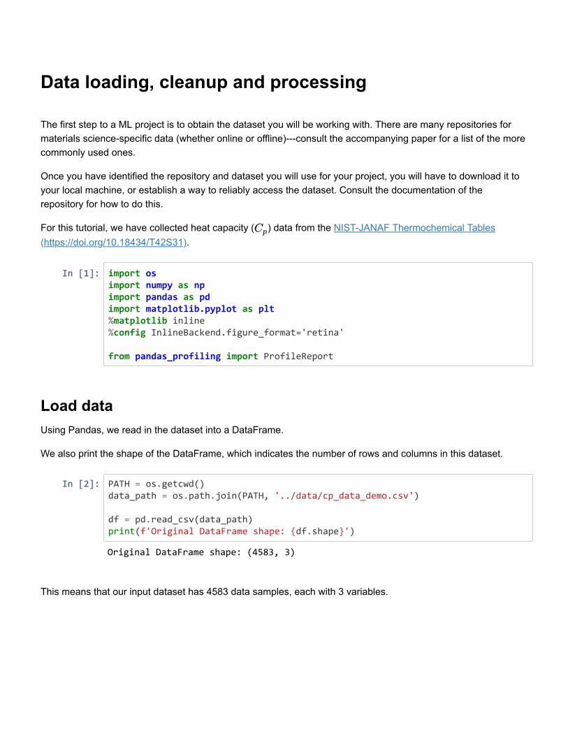
Data loading, cleanup and processing
The first step to a ML project is to obtain the dataset you will be working with. There are many repositories formaterials science-specific data (whether online or offline)---consult the accompanying paper for a list of the morecommonly used ones.
Once you have identified the repository and dataset you will use for your project, you will have to download it toyour local machine, or establish a way to reliably access the dataset. Consult the documentation of therepository for how to do this.
For this tutorial, we have collected heat capacity ( ) data from the NIST-JANAF Thermochemical Tables(https://doi.org/10.18434/T42S31).
Cp
In [1]: import osimport numpy as npimport pandas as pdimport matplotlib.pyplot as plt%matplotlib inline %config InlineBackend.figure_format='retina'
from pandas_profiling import ProfileReport
Load dataUsing Pandas, we read in the dataset into a DataFrame.
We also print the shape of the DataFrame, which indicates the number of rows and columns in this dataset.
In [2]: PATH = os.getcwd()data_path = os.path.join(PATH, '../data/cp_data_demo.csv')
df = pd.read_csv(data_path)print(f'Original DataFrame shape: {df.shape}')
This means that our input dataset has 4583 data samples, each with 3 variables.
Original DataFrame shape: (4583, 3)
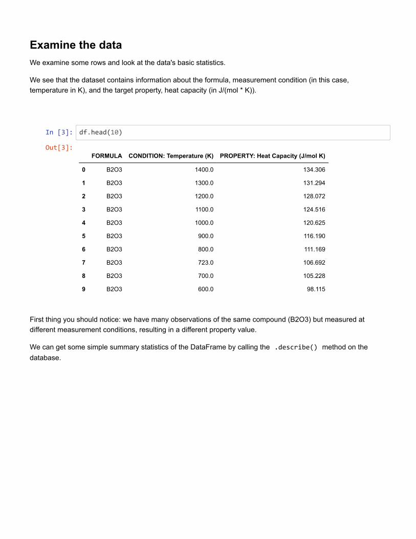
Examine the dataWe examine some rows and look at the data's basic statistics.
We see that the dataset contains information about the formula, measurement condition (in this case,temperature in K), and the target property, heat capacity (in J/(mol * K)).
In [3]: df.head(10)
First thing you should notice: we have many observations of the same compound (B2O3) but measured atdifferent measurement conditions, resulting in a different property value.
We can get some simple summary statistics of the DataFrame by calling the .describe() method on thedatabase.
Out[3]:FORMULA CONDITION: Temperature (K) PROPERTY: Heat Capacity (J/mol K)
0 B2O3 1400.0 134.306
1 B2O3 1300.0 131.294
2 B2O3 1200.0 128.072
3 B2O3 1100.0 124.516
4 B2O3 1000.0 120.625
5 B2O3 900.0 116.190
6 B2O3 800.0 111.169
7 B2O3 723.0 106.692
8 B2O3 700.0 105.228
9 B2O3 600.0 98.115
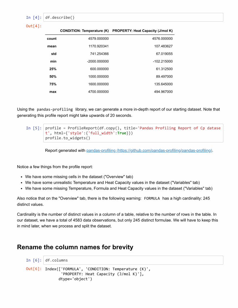
In [4]: df.describe()
Using the pandas-profiling library, we can generate a more in-depth report of our starting dataset. Note thatgenerating this profile report might take upwards of 20 seconds.
In [5]: profile = ProfileReport(df.copy(), title='Pandas Profiling Report of Cp dataset', html={'style':{'full_width':True}})profile.to_widgets()
Notice a few things from the profile report:
We have some missing cells in the dataset ("Overview" tab)We have some unrealistic Temperature and Heat Capacity values in the dataset ("Variables" tab)We have some missing Temperature, Formula and Heat Capacity values in the dataset ("Variables" tab)
Also notice that on the "Overview" tab, there is the following warning: FORMULA has a high cardinality: 245distinct values.
Cardinality is the number of distinct values in a column of a table, relative to the number of rows in the table. Inour dataset, we have a total of 4583 data observations, but only 245 distinct formulae. We will have to keep thisin mind later, when we process and split the dataset.
Rename the column names for brevity
In [6]: df.columns
Out[4]:CONDITION: Temperature (K) PROPERTY: Heat Capacity (J/mol K)
count 4579.000000 4576.000000
mean 1170.920341 107.483627
std 741.254366 67.019055
min -2000.000000 -102.215000
25% 600.000000 61.312500
50% 1000.000000 89.497000
75% 1600.000000 135.645000
max 4700.000000 494.967000
Report generated with pandas-profiling (https://github.com/pandas-profiling/pandas-profiling).
Out[6]: Index(['FORMULA', 'CONDITION: Temperature (K)', 'PROPERTY: Heat Capacity (J/mol K)'], dtype='object')
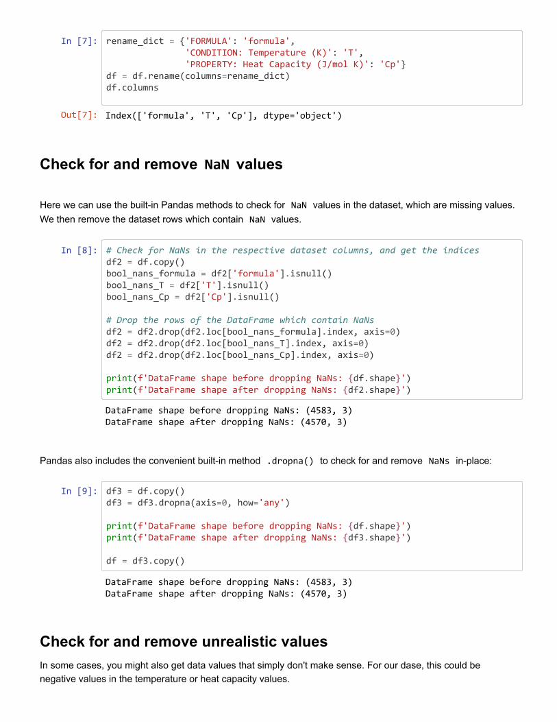
In [7]: rename_dict = {'FORMULA': 'formula', 'CONDITION: Temperature (K)': 'T', 'PROPERTY: Heat Capacity (J/mol K)': 'Cp'}df = df.rename(columns=rename_dict)df.columns
Check for and remove NaN values
Here we can use the built-in Pandas methods to check for NaN values in the dataset, which are missing values.We then remove the dataset rows which contain NaN values.
In [8]: # Check for NaNs in the respective dataset columns, and get the indicesdf2 = df.copy()bool_nans_formula = df2['formula'].isnull()bool_nans_T = df2['T'].isnull()bool_nans_Cp = df2['Cp'].isnull()
# Drop the rows of the DataFrame which contain NaNsdf2 = df2.drop(df2.loc[bool_nans_formula].index, axis=0)df2 = df2.drop(df2.loc[bool_nans_T].index, axis=0)df2 = df2.drop(df2.loc[bool_nans_Cp].index, axis=0)
print(f'DataFrame shape before dropping NaNs: {df.shape}')print(f'DataFrame shape after dropping NaNs: {df2.shape}')
Pandas also includes the convenient built-in method .dropna() to check for and remove NaNs in-place:
In [9]: df3 = df.copy()df3 = df3.dropna(axis=0, how='any')
print(f'DataFrame shape before dropping NaNs: {df.shape}')print(f'DataFrame shape after dropping NaNs: {df3.shape}')
df = df3.copy()
Check for and remove unrealistic valuesIn some cases, you might also get data values that simply don't make sense. For our dase, this could benegative values in the temperature or heat capacity values.
Out[7]: Index(['formula', 'T', 'Cp'], dtype='object')
DataFrame shape before dropping NaNs: (4583, 3) DataFrame shape after dropping NaNs: (4570, 3)
DataFrame shape before dropping NaNs: (4583, 3) DataFrame shape after dropping NaNs: (4570, 3)
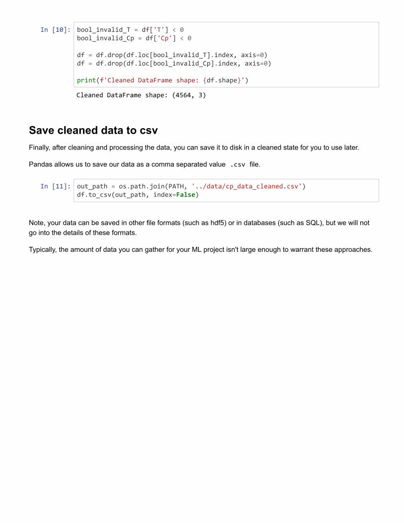
In [10]: bool_invalid_T = df['T'] < 0bool_invalid_Cp = df['Cp'] < 0
df = df.drop(df.loc[bool_invalid_T].index, axis=0)df = df.drop(df.loc[bool_invalid_Cp].index, axis=0)
print(f'Cleaned DataFrame shape: {df.shape}')
Save cleaned data to csvFinally, after cleaning and processing the data, you can save it to disk in a cleaned state for you to use later.
Pandas allows us to save our data as a comma separated value .csv file.
In [11]: out_path = os.path.join(PATH, '../data/cp_data_cleaned.csv')df.to_csv(out_path, index=False)
Note, your data can be saved in other file formats (such as hdf5) or in databases (such as SQL), but we will notgo into the details of these formats.
Typically, the amount of data you can gather for your ML project isn't large enough to warrant these approaches.
Cleaned DataFrame shape: (4564, 3)
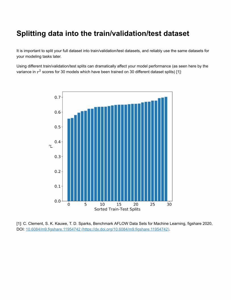
Splitting data into the train/validation/test dataset
It is important to split your full dataset into train/validation/test datasets, and reliably use the same datasets foryour modeling tasks later.
Using different train/validation/test splits can dramatically affect your model performance (as seen here by thevariance in scores for 30 models which have been trained on 30 different dataset splits) [1]:
[1]: C. Clement, S. K. Kauwe, T. D. Sparks, Benchmark AFLOW Data Sets for Machine Learning, figshare 2020,DOI: 10.6084/m9.figshare.11954742 (https://dx.doi.org/10.6084/m9.figshare.11954742).
r2
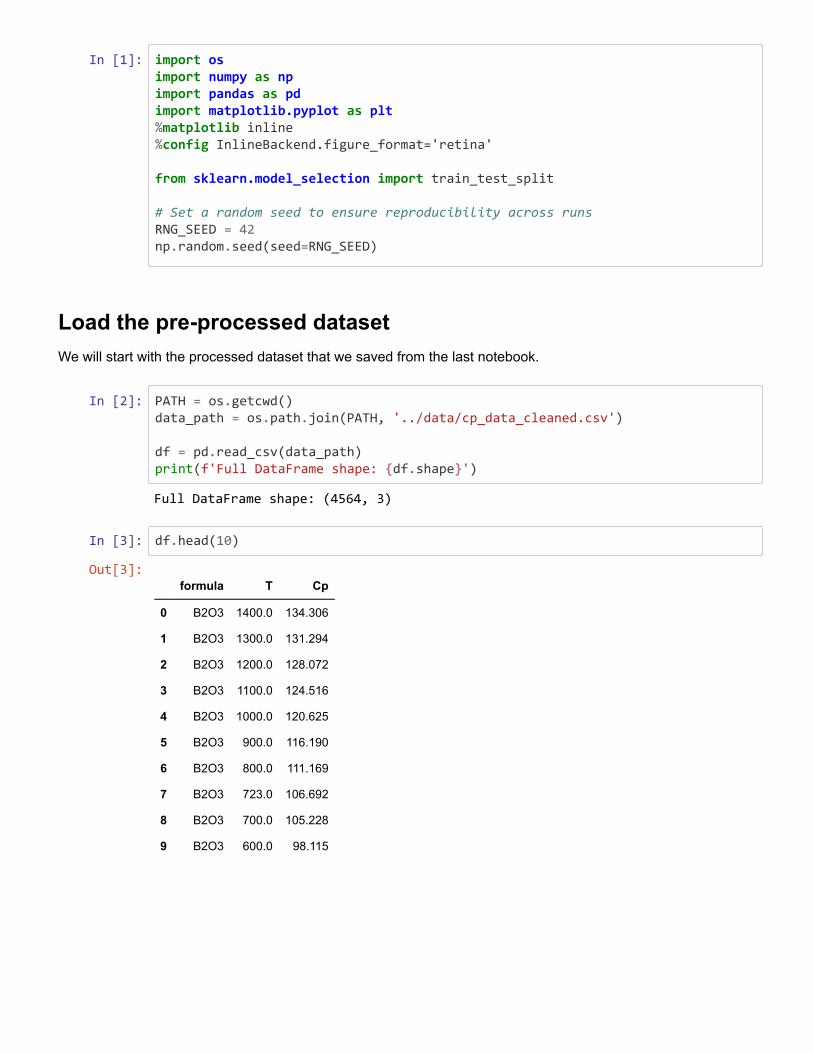
In [1]: import osimport numpy as npimport pandas as pdimport matplotlib.pyplot as plt%matplotlib inline %config InlineBackend.figure_format='retina'
from sklearn.model_selection import train_test_split
# Set a random seed to ensure reproducibility across runsRNG_SEED = 42np.random.seed(seed=RNG_SEED)
Load the pre-processed datasetWe will start with the processed dataset that we saved from the last notebook.
In [2]: PATH = os.getcwd()data_path = os.path.join(PATH, '../data/cp_data_cleaned.csv')
df = pd.read_csv(data_path)print(f'Full DataFrame shape: {df.shape}')
In [3]: df.head(10)
Full DataFrame shape: (4564, 3)
Out[3]:formula T Cp
0 B2O3 1400.0 134.306
1 B2O3 1300.0 131.294
2 B2O3 1200.0 128.072
3 B2O3 1100.0 124.516
4 B2O3 1000.0 120.625
5 B2O3 900.0 116.190
6 B2O3 800.0 111.169
7 B2O3 723.0 106.692
8 B2O3 700.0 105.228
9 B2O3 600.0 98.115
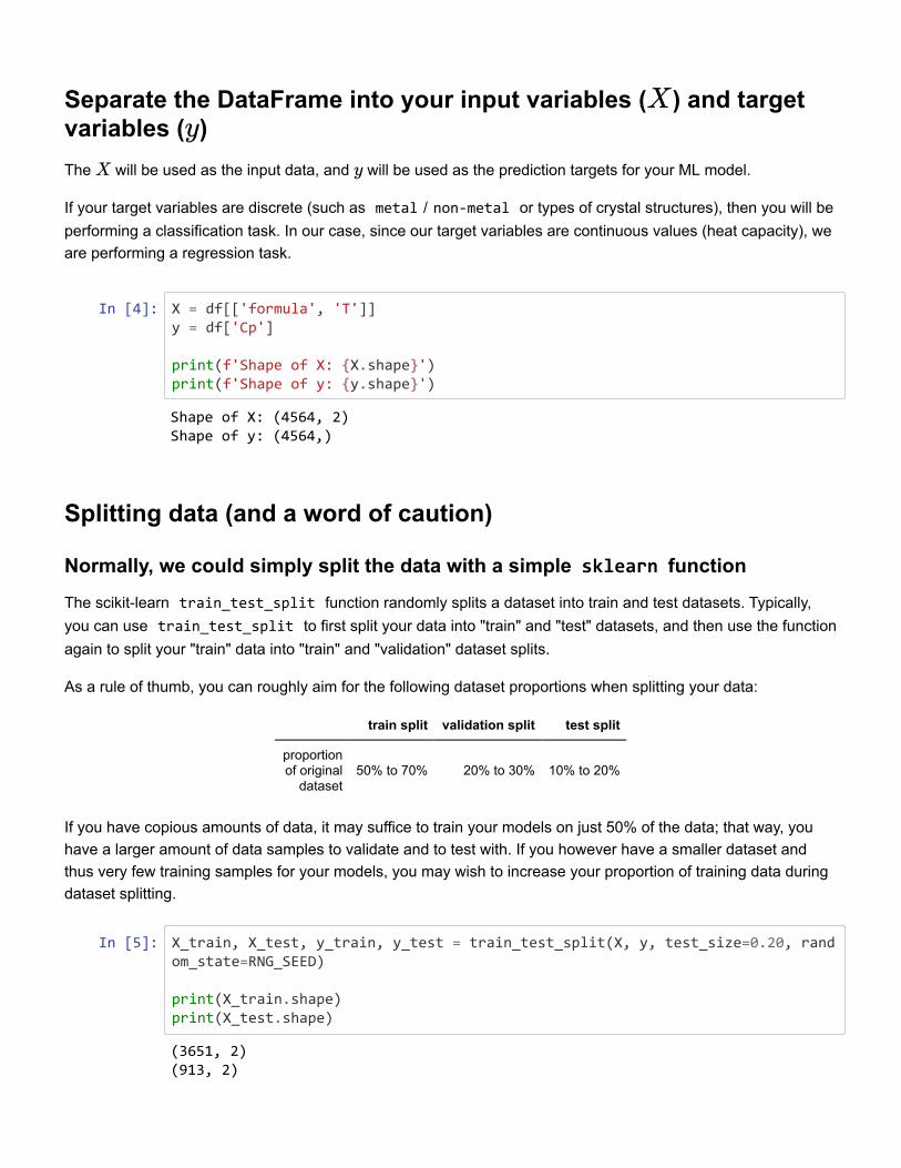
Separate the DataFrame into your input variables ( ) and targetvariables ( )The will be used as the input data, and will be used as the prediction targets for your ML model.
If your target variables are discrete (such as metal / non-metal or types of crystal structures), then you will beperforming a classification task. In our case, since our target variables are continuous values (heat capacity), weare performing a regression task.
Xy
X y
In [4]: X = df[['formula', 'T']]y = df['Cp']
print(f'Shape of X: {X.shape}')print(f'Shape of y: {y.shape}')
Splitting data (and a word of caution)
Normally, we could simply split the data with a simple sklearn functionThe scikit-learn train_test_split function randomly splits a dataset into train and test datasets. Typically,you can use train_test_split to first split your data into "train" and "test" datasets, and then use the functionagain to split your "train" data into "train" and "validation" dataset splits.
As a rule of thumb, you can roughly aim for the following dataset proportions when splitting your data:
train split validation split test split
proportionof original
dataset50% to 70% 20% to 30% 10% to 20%
If you have copious amounts of data, it may suffice to train your models on just 50% of the data; that way, youhave a larger amount of data samples to validate and to test with. If you however have a smaller dataset andthus very few training samples for your models, you may wish to increase your proportion of training data duringdataset splitting.
In [5]: X_train, X_test, y_train, y_test = train_test_split(X, y, test_size=0.20, random_state=RNG_SEED)
print(X_train.shape)print(X_test.shape)
Shape of X: (4564, 2) Shape of y: (4564,)
(3651, 2) (913, 2)
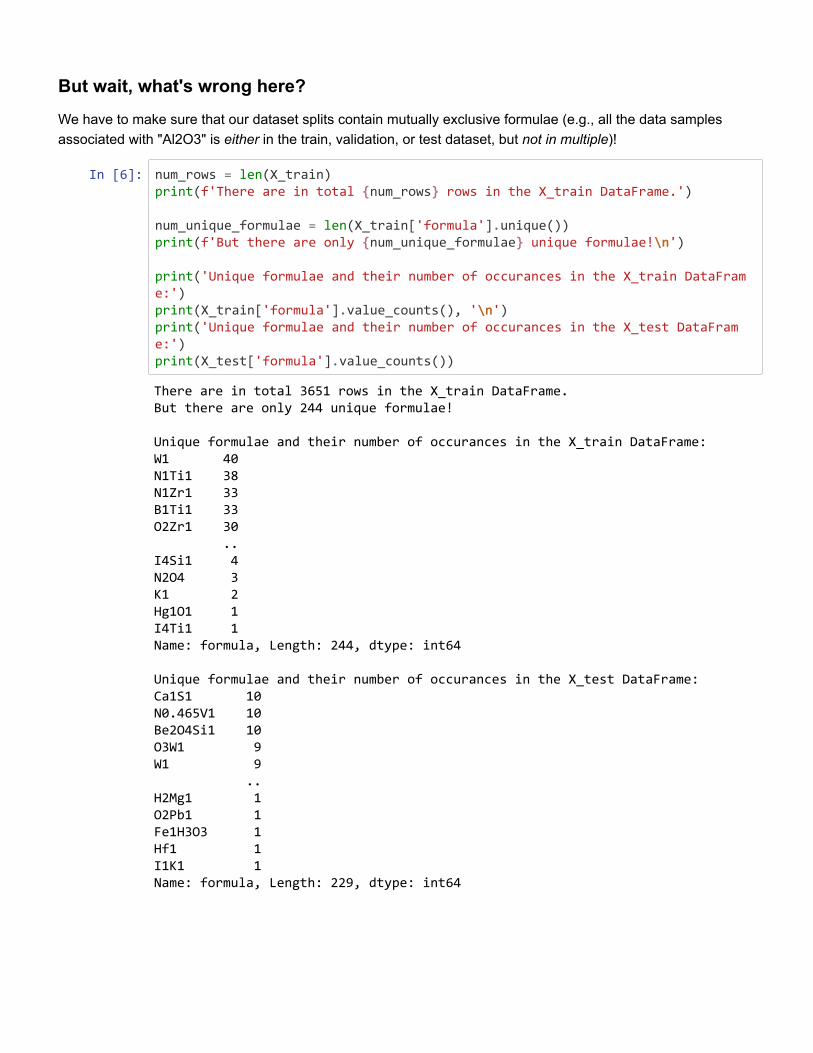
But wait, what's wrong here?We have to make sure that our dataset splits contain mutually exclusive formulae (e.g., all the data samplesassociated with "Al2O3" is either in the train, validation, or test dataset, but not in multiple)!
In [6]: num_rows = len(X_train)print(f'There are in total {num_rows} rows in the X_train DataFrame.')
num_unique_formulae = len(X_train['formula'].unique())print(f'But there are only {num_unique_formulae} unique formulae!\n')
print('Unique formulae and their number of occurances in the X_train DataFrame:')print(X_train['formula'].value_counts(), '\n')print('Unique formulae and their number of occurances in the X_test DataFrame:')print(X_test['formula'].value_counts())
There are in total 3651 rows in the X_train DataFrame. But there are only 244 unique formulae! Unique formulae and their number of occurances in the X_train DataFrame: W1 40 N1Ti1 38 N1Zr1 33 B1Ti1 33 O2Zr1 30 .. I4Si1 4 N2O4 3 K1 2 Hg1O1 1 I4Ti1 1 Name: formula, Length: 244, dtype: int64 Unique formulae and their number of occurances in the X_test DataFrame: Ca1S1 10 N0.465V1 10 Be2O4Si1 10 O3W1 9 W1 9 .. H2Mg1 1 O2Pb1 1 Fe1H3O3 1 Hf1 1 I1K1 1 Name: formula, Length: 229, dtype: int64
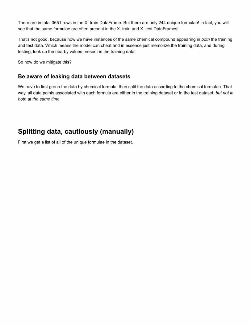
There are in total 3651 rows in the X_train DataFrame. But there are only 244 unique formulae! In fact, you willsee that the same formulae are often present in the X_train and X_test DataFrames!
That's not good, because now we have instances of the same chemical compound appearing in both the trainingand test data. Which means the model can cheat and in essence just memorize the training data, and duringtesting, look up the nearby values present in the training data!
So how do we mitigate this?
Be aware of leaking data between datasetsWe have to first group the data by chemical formula, then split the data according to the chemical formulae. Thatway, all data points associated with each formula are either in the training dataset or in the test dataset, but not inboth at the same time.
Splitting data, cautiously (manually)First we get a list of all of the unique formulae in the dataset.
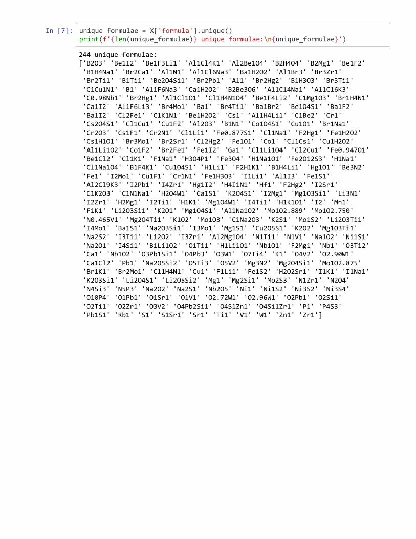
In [7]: unique_formulae = X['formula'].unique()print(f'{len(unique_formulae)} unique formulae:\n{unique_formulae}')
244 unique formulae: ['B2O3' 'Be1I2' 'Be1F3Li1' 'Al1Cl4K1' 'Al2Be1O4' 'B2H4O4' 'B2Mg1' 'Be1F2' 'B1H4Na1' 'Br2Ca1' 'Al1N1' 'Al1Cl6Na3' 'Ba1H2O2' 'Al1Br3' 'Br3Zr1' 'Br2Ti1' 'B1Ti1' 'Be2O4Si1' 'Br2Pb1' 'Al1' 'Br2Hg2' 'B1H3O3' 'Br3Ti1' 'C1Cu1N1' 'B1' 'Al1F6Na3' 'Ca1H2O2' 'B2Be3O6' 'Al1Cl4Na1' 'Al1Cl6K3' 'C0.98Nb1' 'Br2Hg1' 'Al1Cl1O1' 'Cl1H4N1O4' 'Be1F4Li2' 'C1Mg1O3' 'Br1H4N1' 'Ca1I2' 'Al1F6Li3' 'Br4Mo1' 'Ba1' 'Br4Ti1' 'Ba1Br2' 'Be1O4S1' 'Ba1F2' 'Ba1I2' 'Cl2Fe1' 'C1K1N1' 'Be1H2O2' 'Cs1' 'Al1H4Li1' 'C1Be2' 'Cr1' 'Cs2O4S1' 'Cl1Cu1' 'Cu1F2' 'Al2O3' 'B1N1' 'Co1O4S1' 'Cu1O1' 'Br1Na1' 'Cr2O3' 'Cs1F1' 'Cr2N1' 'Cl1Li1' 'Fe0.877S1' 'Cl1Na1' 'F2Hg1' 'Fe1H2O2' 'Cs1H1O1' 'Br3Mo1' 'Br2Sr1' 'Cl2Hg2' 'Fe1O1' 'Co1' 'Cl1Cs1' 'Cu1H2O2' 'Al1Li1O2' 'Co1F2' 'Br2Fe1' 'Fe1I2' 'Ga1' 'Cl1Li1O4' 'Cl2Cu1' 'Fe0.947O1' 'Be1Cl2' 'Cl1K1' 'F1Na1' 'H3O4P1' 'Fe3O4' 'H1Na1O1' 'Fe2O12S3' 'H1Na1' 'Cl1Na1O4' 'B1F4K1' 'Cu1O4S1' 'H1Li1' 'F2H1K1' 'B1H4Li1' 'Hg1O1' 'Be3N2' 'Fe1' 'I2Mo1' 'Cu1F1' 'Cr1N1' 'Fe1H3O3' 'I1Li1' 'Al1I3' 'Fe1S1' 'Al2Cl9K3' 'I2Pb1' 'I4Zr1' 'Hg1I2' 'H4I1N1' 'Hf1' 'F2Hg2' 'I2Sr1' 'C1K2O3' 'C1N1Na1' 'H2O4W1' 'Ca1S1' 'K2O4S1' 'I2Mg1' 'Mg1O3Si1' 'Li3N1' 'I2Zr1' 'H2Mg1' 'I2Ti1' 'H1K1' 'Mg1O4W1' 'I4Ti1' 'H1K1O1' 'I2' 'Mn1' 'F1K1' 'Li2O3Si1' 'K2O1' 'Mg1O4S1' 'Al1Na1O2' 'Mo1O2.889' 'Mo1O2.750' 'N0.465V1' 'Mg2O4Ti1' 'K1O2' 'Mo1O3' 'C1Na2O3' 'K2S1' 'Mo1S2' 'Li2O3Ti1' 'I4Mo1' 'Ba1S1' 'Na2O3Si1' 'I3Mo1' 'Mg1S1' 'Cu2O5S1' 'K2O2' 'Mg1O3Ti1' 'Na2S2' 'I3Ti1' 'Li2O2' 'I3Zr1' 'Al2Mg1O4' 'N1Ti1' 'N1V1' 'Na1O2' 'Ni1S1' 'Na2O1' 'I4Si1' 'B1Li1O2' 'O1Ti1' 'H1Li1O1' 'Nb1O1' 'F2Mg1' 'Nb1' 'O3Ti2' 'Ca1' 'Nb1O2' 'O3Pb1Si1' 'O4Pb3' 'O3W1' 'O7Ti4' 'K1' 'O4V2' 'O2.90W1' 'Ca1Cl2' 'Pb1' 'Na2O5Si2' 'O5Ti3' 'O5V2' 'Mg3N2' 'Mg2O4Si1' 'Mo1O2.875' 'Br1K1' 'Br2Mo1' 'Cl1H4N1' 'Cu1' 'F1Li1' 'Fe1S2' 'H2O2Sr1' 'I1K1' 'I1Na1' 'K2O3Si1' 'Li2O4S1' 'Li2O5Si2' 'Mg1' 'Mg2Si1' 'Mo2S3' 'N1Zr1' 'N2O4' 'N4Si3' 'N5P3' 'Na2O2' 'Na2S1' 'Nb2O5' 'Ni1' 'Ni1S2' 'Ni3S2' 'Ni3S4' 'O10P4' 'O1Pb1' 'O1Sr1' 'O1V1' 'O2.72W1' 'O2.96W1' 'O2Pb1' 'O2Si1' 'O2Ti1' 'O2Zr1' 'O3V2' 'O4Pb2Si1' 'O4S1Zn1' 'O4Si1Zr1' 'P1' 'P4S3' 'Pb1S1' 'Rb1' 'S1' 'S1Sr1' 'Sr1' 'Ti1' 'V1' 'W1' 'Zn1' 'Zr1']
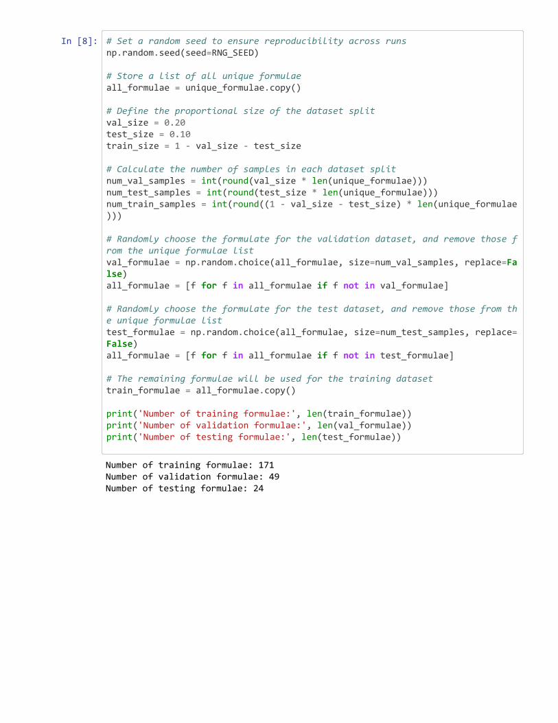
In [8]: # Set a random seed to ensure reproducibility across runsnp.random.seed(seed=RNG_SEED)
# Store a list of all unique formulaeall_formulae = unique_formulae.copy()
# Define the proportional size of the dataset splitval_size = 0.20test_size = 0.10train_size = 1 - val_size - test_size
# Calculate the number of samples in each dataset splitnum_val_samples = int(round(val_size * len(unique_formulae)))num_test_samples = int(round(test_size * len(unique_formulae)))num_train_samples = int(round((1 - val_size - test_size) * len(unique_formulae)))
# Randomly choose the formulate for the validation dataset, and remove those from the unique formulae listval_formulae = np.random.choice(all_formulae, size=num_val_samples, replace=False)all_formulae = [f for f in all_formulae if f not in val_formulae]
# Randomly choose the formulate for the test dataset, and remove those from the unique formulae listtest_formulae = np.random.choice(all_formulae, size=num_test_samples, replace=False)all_formulae = [f for f in all_formulae if f not in test_formulae]
# The remaining formulae will be used for the training datasettrain_formulae = all_formulae.copy()
print('Number of training formulae:', len(train_formulae))print('Number of validation formulae:', len(val_formulae))print('Number of testing formulae:', len(test_formulae))
Number of training formulae: 171 Number of validation formulae: 49 Number of testing formulae: 24
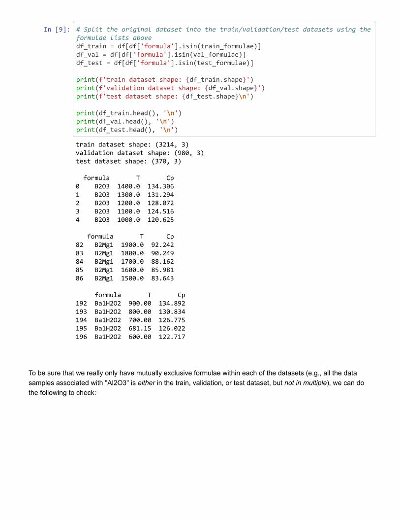
In [9]: # Split the original dataset into the train/validation/test datasets using the formulae lists abovedf_train = df[df['formula'].isin(train_formulae)]df_val = df[df['formula'].isin(val_formulae)]df_test = df[df['formula'].isin(test_formulae)]
print(f'train dataset shape: {df_train.shape}')print(f'validation dataset shape: {df_val.shape}')print(f'test dataset shape: {df_test.shape}\n')
print(df_train.head(), '\n')print(df_val.head(), '\n')print(df_test.head(), '\n')
To be sure that we really only have mutually exclusive formulae within each of the datasets (e.g., all the datasamples associated with "Al2O3" is either in the train, validation, or test dataset, but not in multiple), we can dothe following to check:
train dataset shape: (3214, 3) validation dataset shape: (980, 3) test dataset shape: (370, 3) formula T Cp 0 B2O3 1400.0 134.306 1 B2O3 1300.0 131.294 2 B2O3 1200.0 128.072 3 B2O3 1100.0 124.516 4 B2O3 1000.0 120.625 formula T Cp 82 B2Mg1 1900.0 92.242 83 B2Mg1 1800.0 90.249 84 B2Mg1 1700.0 88.162 85 B2Mg1 1600.0 85.981 86 B2Mg1 1500.0 83.643 formula T Cp 192 Ba1H2O2 900.00 134.892 193 Ba1H2O2 800.00 130.834 194 Ba1H2O2 700.00 126.775 195 Ba1H2O2 681.15 126.022 196 Ba1H2O2 600.00 122.717
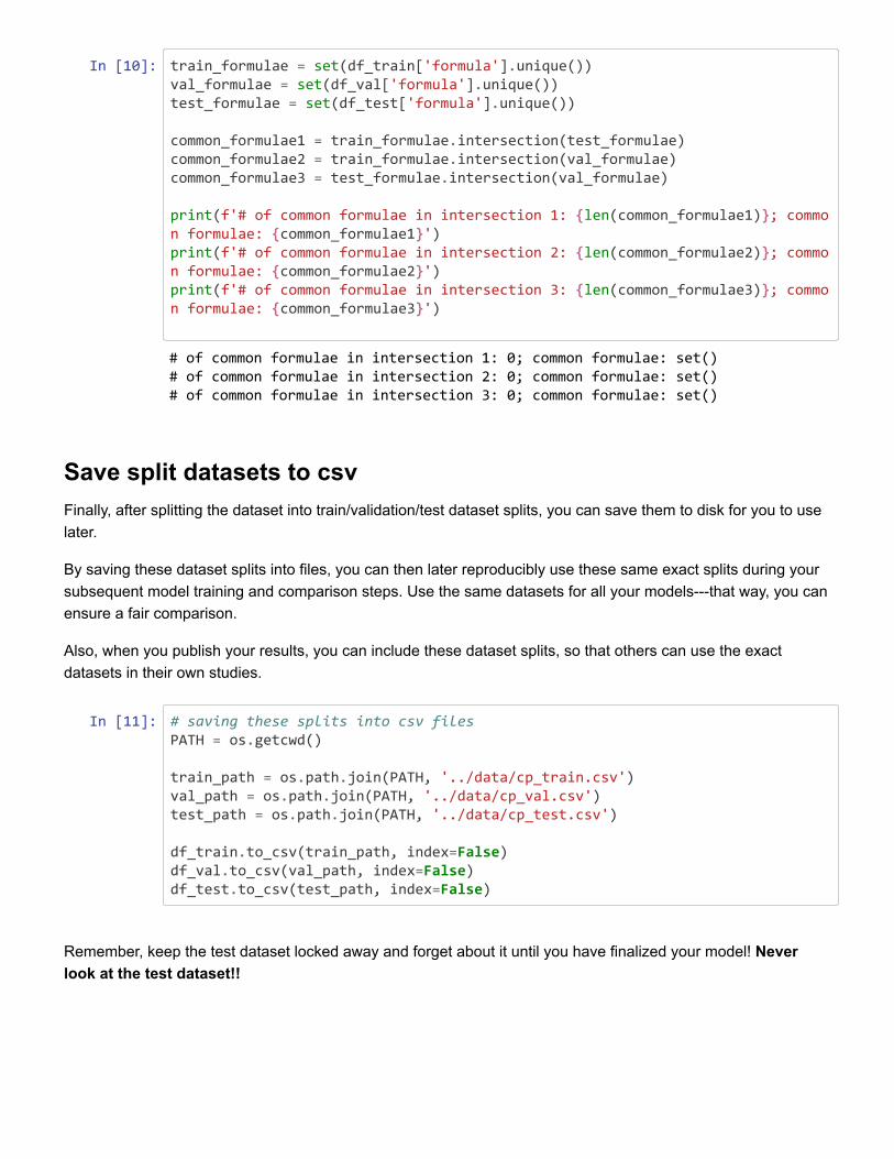
In [10]: train_formulae = set(df_train['formula'].unique())val_formulae = set(df_val['formula'].unique())test_formulae = set(df_test['formula'].unique())
common_formulae1 = train_formulae.intersection(test_formulae)common_formulae2 = train_formulae.intersection(val_formulae)common_formulae3 = test_formulae.intersection(val_formulae)
print(f'# of common formulae in intersection 1: {len(common_formulae1)}; common formulae: {common_formulae1}')print(f'# of common formulae in intersection 2: {len(common_formulae2)}; common formulae: {common_formulae2}')print(f'# of common formulae in intersection 3: {len(common_formulae3)}; common formulae: {common_formulae3}')
Save split datasets to csvFinally, after splitting the dataset into train/validation/test dataset splits, you can save them to disk for you to uselater.
By saving these dataset splits into files, you can then later reproducibly use these same exact splits during yoursubsequent model training and comparison steps. Use the same datasets for all your models---that way, you canensure a fair comparison.
Also, when you publish your results, you can include these dataset splits, so that others can use the exactdatasets in their own studies.
In [11]: # saving these splits into csv filesPATH = os.getcwd()
train_path = os.path.join(PATH, '../data/cp_train.csv')val_path = os.path.join(PATH, '../data/cp_val.csv')test_path = os.path.join(PATH, '../data/cp_test.csv')
df_train.to_csv(train_path, index=False)df_val.to_csv(val_path, index=False)df_test.to_csv(test_path, index=False)
Remember, keep the test dataset locked away and forget about it until you have finalized your model! Neverlook at the test dataset!!
# of common formulae in intersection 1: 0; common formulae: set() # of common formulae in intersection 2: 0; common formulae: set() # of common formulae in intersection 3: 0; common formulae: set()
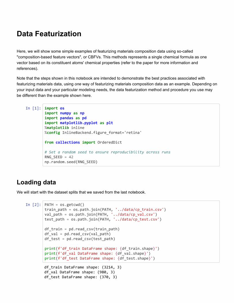
Data Featurization
Here, we will show some simple examples of featurizing materials composition data using so-called"composition-based feature vectors", or CBFVs. This methods represents a single chemical formula as onevector based on its constituent atoms' chemical properties (refer to the paper for more information andreferences).
Note that the steps shown in this notebook are intended to demonstrate the best practices associated withfeaturizing materials data, using one way of featurizing materials composition data as an example. Depending onyour input data and your particular modeling needs, the data featurization method and procedure you use maybe different than the example shown here.
In [1]: import osimport numpy as npimport pandas as pdimport matplotlib.pyplot as plt%matplotlib inline %config InlineBackend.figure_format='retina'
from collections import OrderedDict
# Set a random seed to ensure reproducibility across runsRNG_SEED = 42np.random.seed(RNG_SEED)
Loading dataWe will start with the dataset splits that we saved from the last notebook.
In [2]: PATH = os.getcwd()train_path = os.path.join(PATH, '../data/cp_train.csv')val_path = os.path.join(PATH, '../data/cp_val.csv')test_path = os.path.join(PATH, '../data/cp_test.csv')
df_train = pd.read_csv(train_path)df_val = pd.read_csv(val_path)df_test = pd.read_csv(test_path)
print(f'df_train DataFrame shape: {df_train.shape}')print(f'df_val DataFrame shape: {df_val.shape}')print(f'df_test DataFrame shape: {df_test.shape}')
df_train DataFrame shape: (3214, 3) df_val DataFrame shape: (980, 3) df_test DataFrame shape: (370, 3)
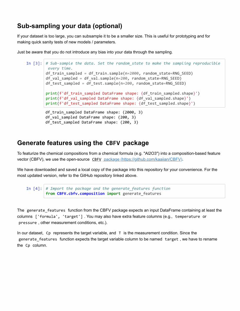
Sub-sampling your data (optional)If your dataset is too large, you can subsample it to be a smaller size. This is useful for prototyping and formaking quick sanity tests of new models / parameters.
Just be aware that you do not introduce any bias into your data through the sampling.
In [3]: # Sub-sample the data. Set the random_state to make the sampling reproducibleevery time.df_train_sampled = df_train.sample(n=2000, random_state=RNG_SEED)df_val_sampled = df_val.sample(n=200, random_state=RNG_SEED)df_test_sampled = df_test.sample(n=200, random_state=RNG_SEED)
print(f'df_train_sampled DataFrame shape: {df_train_sampled.shape}')print(f'df_val_sampled DataFrame shape: {df_val_sampled.shape}')print(f'df_test_sampled DataFrame shape: {df_test_sampled.shape}')
Generate features using the CBFV packageTo featurize the chemical compositions from a chemical formula (e.g. "Al2O3") into a composition-based featurevector (CBFV), we use the open-source CBFV package (https://github.com/kaaiian/CBFV).
We have downloaded and saved a local copy of the package into this repository for your convenience. For themost updated version, refer to the GitHub repository linked above.
In [4]: # Import the package and the generate_features functionfrom CBFV.cbfv.composition import generate_features
The generate_features function from the CBFV package expects an input DataFrame containing at least thecolumns ['formula', 'target'] . You may also have extra feature columns (e.g., temperature or pressure , other measurement conditions, etc.).
In our dataset, Cp represents the target variable, and T is the measurement condition. Since the generate_features function expects the target variable column to be named target , we have to rename
the Cp column.
df_train_sampled DataFrame shape: (2000, 3) df_val_sampled DataFrame shape: (200, 3) df_test_sampled DataFrame shape: (200, 3)
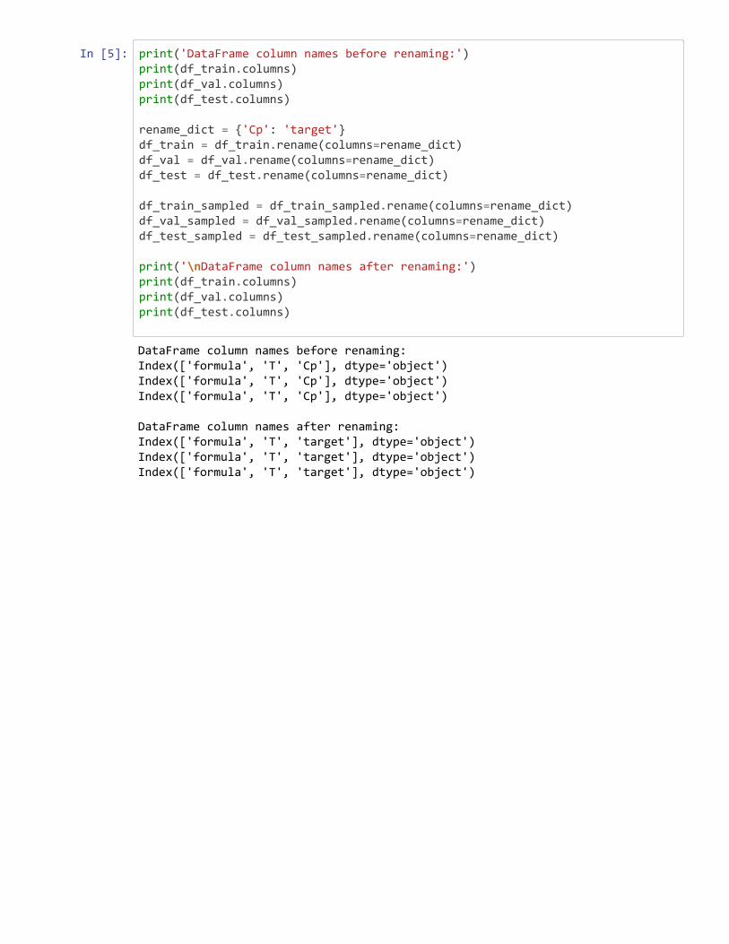
In [5]: print('DataFrame column names before renaming:')print(df_train.columns)print(df_val.columns)print(df_test.columns)
rename_dict = {'Cp': 'target'}df_train = df_train.rename(columns=rename_dict)df_val = df_val.rename(columns=rename_dict)df_test = df_test.rename(columns=rename_dict)
df_train_sampled = df_train_sampled.rename(columns=rename_dict)df_val_sampled = df_val_sampled.rename(columns=rename_dict)df_test_sampled = df_test_sampled.rename(columns=rename_dict)
print('\nDataFrame column names after renaming:')print(df_train.columns)print(df_val.columns)print(df_test.columns)
DataFrame column names before renaming: Index(['formula', 'T', 'Cp'], dtype='object') Index(['formula', 'T', 'Cp'], dtype='object') Index(['formula', 'T', 'Cp'], dtype='object') DataFrame column names after renaming: Index(['formula', 'T', 'target'], dtype='object') Index(['formula', 'T', 'target'], dtype='object') Index(['formula', 'T', 'target'], dtype='object')
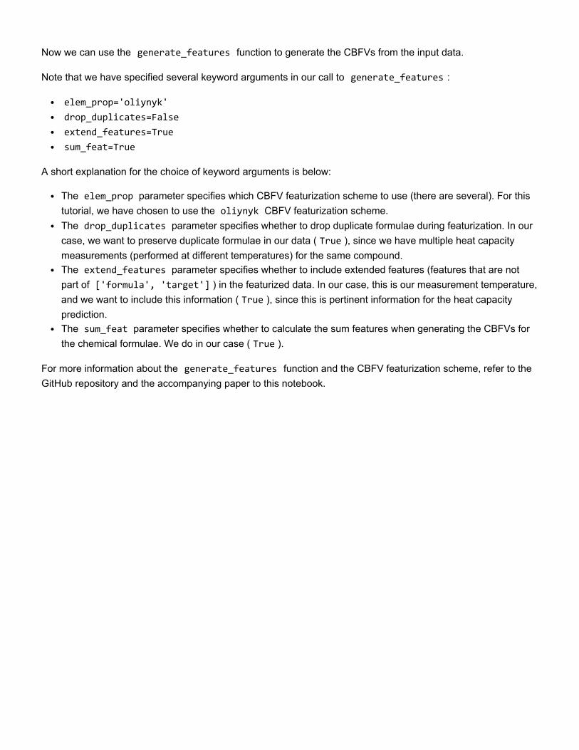
Now we can use the generate_features function to generate the CBFVs from the input data.
Note that we have specified several keyword arguments in our call to generate_features :
elem_prop='oliynyk'drop_duplicates=Falseextend_features=Truesum_feat=True
A short explanation for the choice of keyword arguments is below:
The elem_prop parameter specifies which CBFV featurization scheme to use (there are several). For thistutorial, we have chosen to use the oliynyk CBFV featurization scheme.The drop_duplicates parameter specifies whether to drop duplicate formulae during featurization. In ourcase, we want to preserve duplicate formulae in our data ( True ), since we have multiple heat capacitymeasurements (performed at different temperatures) for the same compound.The extend_features parameter specifies whether to include extended features (features that are notpart of ['formula', 'target'] ) in the featurized data. In our case, this is our measurement temperature,and we want to include this information ( True ), since this is pertinent information for the heat capacityprediction.The sum_feat parameter specifies whether to calculate the sum features when generating the CBFVs forthe chemical formulae. We do in our case ( True ).
For more information about the generate_features function and the CBFV featurization scheme, refer to theGitHub repository and the accompanying paper to this notebook.
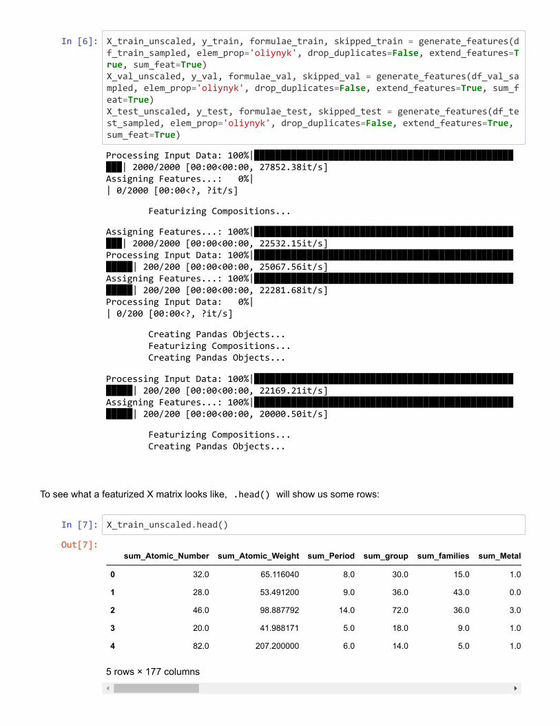
In [6]: X_train_unscaled, y_train, formulae_train, skipped_train = generate_features(df_train_sampled, elem_prop='oliynyk', drop_duplicates=False, extend_features=True, sum_feat=True)X_val_unscaled, y_val, formulae_val, skipped_val = generate_features(df_val_sampled, elem_prop='oliynyk', drop_duplicates=False, extend_features=True, sum_feat=True)X_test_unscaled, y_test, formulae_test, skipped_test = generate_features(df_test_sampled, elem_prop='oliynyk', drop_duplicates=False, extend_features=True, sum_feat=True)
To see what a featurized X matrix looks like, .head() will show us some rows:
In [7]: X_train_unscaled.head()
Processing Input Data: 100%|████████████████████████████████████████████████████| 2000/2000 [00:00<00:00, 27852.38it/s] Assigning Features...: 0%| | 0/2000 [00:00<?, ?it/s]
Featurizing Compositions...
Assigning Features...: 100%|████████████████████████████████████████████████████| 2000/2000 [00:00<00:00, 22532.15it/s] Processing Input Data: 100%|██████████████████████████████████████████████████████| 200/200 [00:00<00:00, 25067.56it/s] Assigning Features...: 100%|██████████████████████████████████████████████████████| 200/200 [00:00<00:00, 22281.68it/s] Processing Input Data: 0%| | 0/200 [00:00<?, ?it/s]
Creating Pandas Objects... Featurizing Compositions... Creating Pandas Objects...
Processing Input Data: 100%|██████████████████████████████████████████████████████| 200/200 [00:00<00:00, 22169.21it/s] Assigning Features...: 100%|██████████████████████████████████████████████████████| 200/200 [00:00<00:00, 20000.50it/s]
Featurizing Compositions... Creating Pandas Objects...
Out[7]:sum_Atomic_Number sum_Atomic_Weight sum_Period sum_group sum_families sum_Metal
0 32.0 65.116040 8.0 30.0 15.0 1.0
1 28.0 53.491200 9.0 36.0 43.0 0.0
2 46.0 98.887792 14.0 72.0 36.0 3.0
3 20.0 41.988171 5.0 18.0 9.0 1.0
4 82.0 207.200000 6.0 14.0 5.0 1.0
5 rows × 177 columns
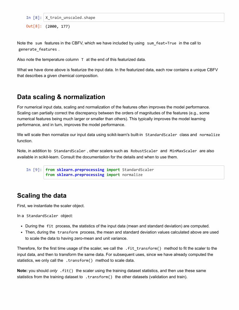
In [8]: X_train_unscaled.shape
Note the sum features in the CBFV, which we have included by using sum_feat=True in the call to generate_features .
Also note the temperature column T at the end of this featurized data.
What we have done above is featurize the input data. In the featurized data, each row contains a unique CBFVthat describes a given chemical composition.
Data scaling & normalizationFor numerical input data, scaling and normalization of the features often improves the model performance.Scaling can partially correct the discrepancy between the orders of magnitudes of the features (e.g., somenumerical features being much larger or smaller than others). This typically improves the model learningperformance, and in turn, improves the model performance.
We will scale then normalize our input data using scikit-learn's built-in StandardScaler class and normalizefunction.
Note, in addition to StandardScaler , other scalers such as RobustScaler and MinMaxScaler are alsoavailable in scikit-learn. Consult the documentation for the details and when to use them.
In [9]: from sklearn.preprocessing import StandardScalerfrom sklearn.preprocessing import normalize
Scaling the dataFirst, we instantiate the scaler object.
In a StandardScaler object:
During the fit process, the statistics of the input data (mean and standard deviation) are computed.Then, during the transform process, the mean and standard deviation values calculated above are usedto scale the data to having zero-mean and unit variance.
Therefore, for the first time usage of the scaler, we call the .fit_transform() method to fit the scaler to theinput data, and then to transform the same data. For subsequent uses, since we have already computed thestatistics, we only call the .transform() method to scale data.
Note: you should only .fit() the scaler using the training dataset statistics, and then use these samestatistics from the training dataset to .transform() the other datasets (validation and train).
Out[8]: (2000, 177)
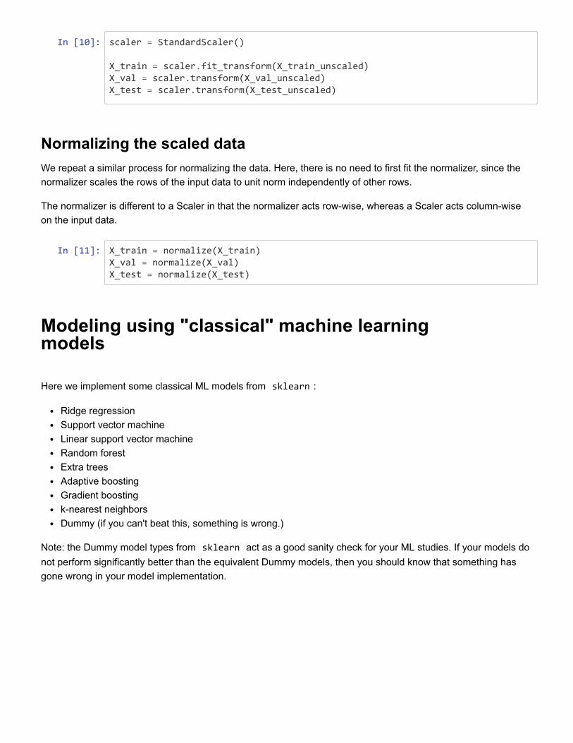
In [10]: scaler = StandardScaler()
X_train = scaler.fit_transform(X_train_unscaled)X_val = scaler.transform(X_val_unscaled)X_test = scaler.transform(X_test_unscaled)
Normalizing the scaled dataWe repeat a similar process for normalizing the data. Here, there is no need to first fit the normalizer, since thenormalizer scales the rows of the input data to unit norm independently of other rows.
The normalizer is different to a Scaler in that the normalizer acts row-wise, whereas a Scaler acts column-wiseon the input data.
In [11]: X_train = normalize(X_train)X_val = normalize(X_val)X_test = normalize(X_test)
Modeling using "classical" machine learningmodels
Here we implement some classical ML models from sklearn :
Ridge regressionSupport vector machineLinear support vector machineRandom forestExtra treesAdaptive boostingGradient boostingk-nearest neighborsDummy (if you can't beat this, something is wrong.)
Note: the Dummy model types from sklearn act as a good sanity check for your ML studies. If your models donot perform significantly better than the equivalent Dummy models, then you should know that something hasgone wrong in your model implementation.
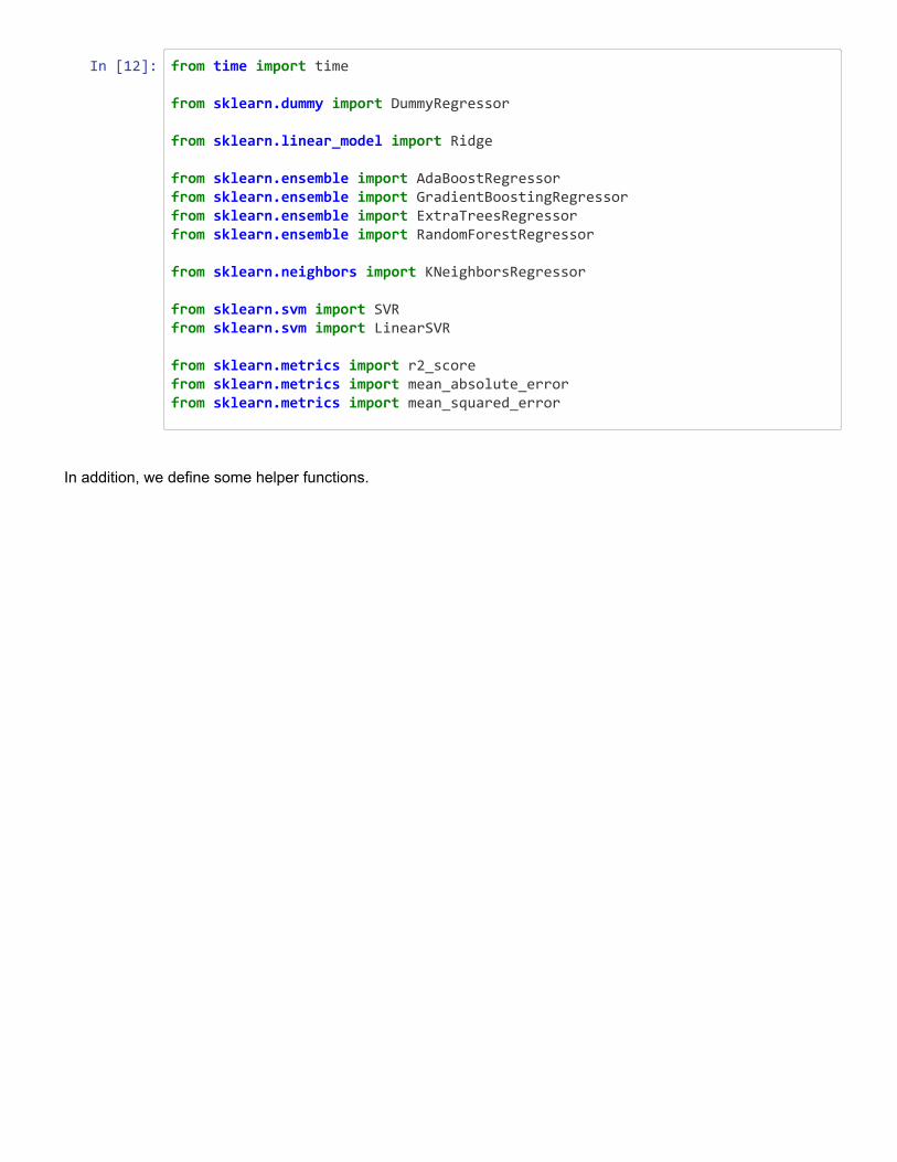
In [12]: from time import time
from sklearn.dummy import DummyRegressor
from sklearn.linear_model import Ridge
from sklearn.ensemble import AdaBoostRegressorfrom sklearn.ensemble import GradientBoostingRegressorfrom sklearn.ensemble import ExtraTreesRegressorfrom sklearn.ensemble import RandomForestRegressor
from sklearn.neighbors import KNeighborsRegressor
from sklearn.svm import SVRfrom sklearn.svm import LinearSVR
from sklearn.metrics import r2_scorefrom sklearn.metrics import mean_absolute_errorfrom sklearn.metrics import mean_squared_error
In addition, we define some helper functions.
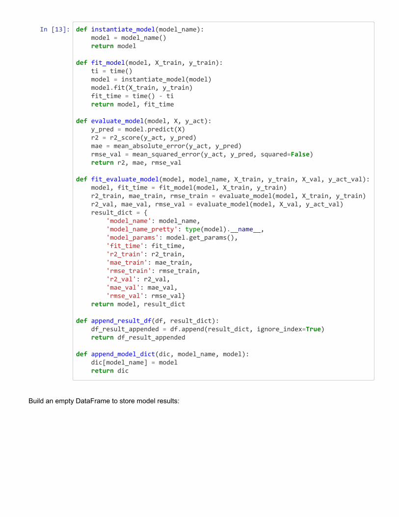
In [13]: def instantiate_model(model_name): model = model_name() return model
def fit_model(model, X_train, y_train): ti = time() model = instantiate_model(model) model.fit(X_train, y_train) fit_time = time() - ti return model, fit_time
def evaluate_model(model, X, y_act): y_pred = model.predict(X) r2 = r2_score(y_act, y_pred) mae = mean_absolute_error(y_act, y_pred) rmse_val = mean_squared_error(y_act, y_pred, squared=False) return r2, mae, rmse_val
def fit_evaluate_model(model, model_name, X_train, y_train, X_val, y_act_val): model, fit_time = fit_model(model, X_train, y_train) r2_train, mae_train, rmse_train = evaluate_model(model, X_train, y_train) r2_val, mae_val, rmse_val = evaluate_model(model, X_val, y_act_val) result_dict = { 'model_name': model_name, 'model_name_pretty': type(model).__name__, 'model_params': model.get_params(), 'fit_time': fit_time, 'r2_train': r2_train, 'mae_train': mae_train, 'rmse_train': rmse_train, 'r2_val': r2_val, 'mae_val': mae_val, 'rmse_val': rmse_val} return model, result_dict
def append_result_df(df, result_dict): df_result_appended = df.append(result_dict, ignore_index=True) return df_result_appended
def append_model_dict(dic, model_name, model): dic[model_name] = model return dic
Build an empty DataFrame to store model results:
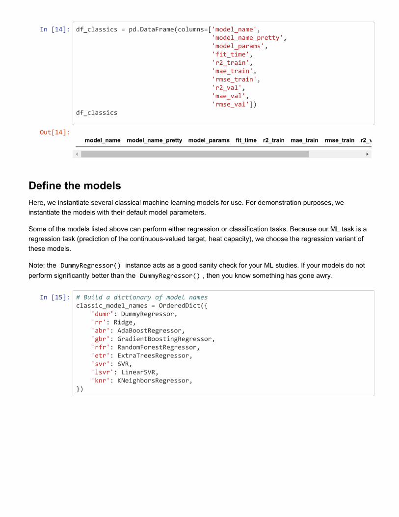
In [14]: df_classics = pd.DataFrame(columns=['model_name', 'model_name_pretty', 'model_params', 'fit_time', 'r2_train', 'mae_train', 'rmse_train', 'r2_val', 'mae_val', 'rmse_val'])df_classics
Define the modelsHere, we instantiate several classical machine learning models for use. For demonstration purposes, weinstantiate the models with their default model parameters.
Some of the models listed above can perform either regression or classification tasks. Because our ML task is aregression task (prediction of the continuous-valued target, heat capacity), we choose the regression variant ofthese models.
Note: the DummyRegressor() instance acts as a good sanity check for your ML studies. If your models do notperform significantly better than the DummyRegressor() , then you know something has gone awry.
In [15]: # Build a dictionary of model namesclassic_model_names = OrderedDict({ 'dumr': DummyRegressor, 'rr': Ridge, 'abr': AdaBoostRegressor, 'gbr': GradientBoostingRegressor, 'rfr': RandomForestRegressor, 'etr': ExtraTreesRegressor, 'svr': SVR, 'lsvr': LinearSVR, 'knr': KNeighborsRegressor,})
Out[14]:model_name model_name_pretty model_params fit_time r2_train mae_train rmse_train r2_v
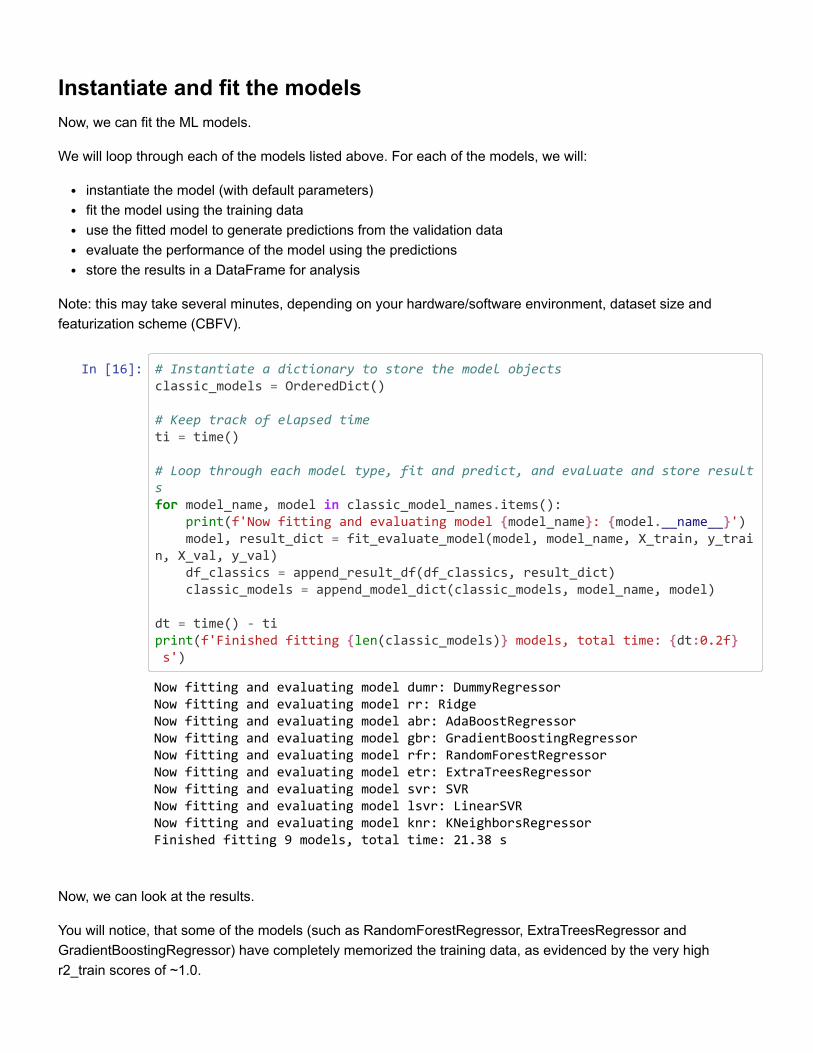
Instantiate and fit the modelsNow, we can fit the ML models.
We will loop through each of the models listed above. For each of the models, we will:
instantiate the model (with default parameters)fit the model using the training datause the fitted model to generate predictions from the validation dataevaluate the performance of the model using the predictionsstore the results in a DataFrame for analysis
Note: this may take several minutes, depending on your hardware/software environment, dataset size andfeaturization scheme (CBFV).
In [16]: # Instantiate a dictionary to store the model objectsclassic_models = OrderedDict()
# Keep track of elapsed timeti = time()
# Loop through each model type, fit and predict, and evaluate and store resultsfor model_name, model in classic_model_names.items(): print(f'Now fitting and evaluating model {model_name}: {model.__name__}') model, result_dict = fit_evaluate_model(model, model_name, X_train, y_train, X_val, y_val) df_classics = append_result_df(df_classics, result_dict) classic_models = append_model_dict(classic_models, model_name, model)
dt = time() - tiprint(f'Finished fitting {len(classic_models)} models, total time: {dt:0.2f}s')
Now, we can look at the results.
You will notice, that some of the models (such as RandomForestRegressor, ExtraTreesRegressor andGradientBoostingRegressor) have completely memorized the training data, as evidenced by the very highr2_train scores of ~1.0.
Now fitting and evaluating model dumr: DummyRegressor Now fitting and evaluating model rr: Ridge Now fitting and evaluating model abr: AdaBoostRegressor Now fitting and evaluating model gbr: GradientBoostingRegressor Now fitting and evaluating model rfr: RandomForestRegressor Now fitting and evaluating model etr: ExtraTreesRegressor Now fitting and evaluating model svr: SVR Now fitting and evaluating model lsvr: LinearSVR Now fitting and evaluating model knr: KNeighborsRegressor Finished fitting 9 models, total time: 21.38 s
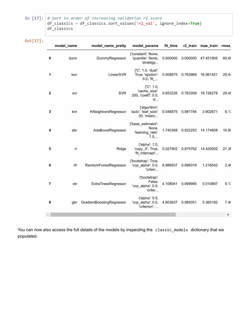
In [17]: # Sort in order of increasing validation r2 scoredf_classics = df_classics.sort_values('r2_val', ignore_index=True)df_classics
You can now also access the full details of the models by inspecting the classic_models dictionary that wepopulated.
Out[17]:model_name model_name_pretty model_params fit_time r2_train mae_train rmse_
0 dumr DummyRegressor{'constant': None,
'quantile': None,'strategy...
0.000000 0.000000 47.451805 60.60
1 lsvr LinearSVR{'C': 1.0, 'dual':True, 'epsilon':
0.0, 'fit_...0.008975 0.763989 16.961421 29.44
2 svr SVR
{'C': 1.0,'cache_size':
200, 'coef0': 0.0,'d...
0.653226 0.763306 16.726278 29.48
3 knr KNeighborsRegressor{'algorithm':
'auto', 'leaf_size':30, 'metric...
0.046875 0.981784 3.902671 8.17
4 abr AdaBoostRegressor
{'base_estimator':None,
'learning_rate':1.0,...
1.740368 0.922253 14.174608 16.89
5 rr Ridge{'alpha': 1.0,
'copy_X': True,'fit_intercept'...
0.027902 0.875762 14.425002 21.36
6 rfr RandomForestRegressor{'bootstrap': True,
'ccp_alpha': 0.0,'criteri...
8.986937 0.998316 1.216542 2.48
7 etr ExtraTreesRegressor
{'bootstrap':False,
'ccp_alpha': 0.0,'criter...
4.108041 0.999995 0.010897 0.13
8 gbr GradientBoostingRegressor{'alpha': 0.9,
'ccp_alpha': 0.0,'criterion': ...
4.803637 0.985051 5.360182 7.40

In [18]: classic_models
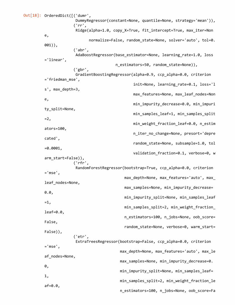
Out[18]: OrderedDict([('dumr', DummyRegressor(constant=None, quantile=None, strategy='mean')), ('rr', Ridge(alpha=1.0, copy_X=True, fit_intercept=True, max_iter=None, normalize=False, random_state=None, solver='auto', tol=0.001)), ('abr', AdaBoostRegressor(base_estimator=None, learning_rate=1.0, loss='linear', n_estimators=50, random_state=None)), ('gbr', GradientBoostingRegressor(alpha=0.9, ccp_alpha=0.0, criterion='friedman_mse', init=None, learning_rate=0.1, loss='ls', max_depth=3, max_features=None, max_leaf_nodes=None, min_impurity_decrease=0.0, min_impurity_split=None, min_samples_leaf=1, min_samples_split=2, min_weight_fraction_leaf=0.0, n_estimators=100, n_iter_no_change=None, presort='deprecated', random_state=None, subsample=1.0, tol=0.0001, validation_fraction=0.1, verbose=0, warm_start=False)), ('rfr', RandomForestRegressor(bootstrap=True, ccp_alpha=0.0, criterion='mse', max_depth=None, max_features='auto', max_leaf_nodes=None, max_samples=None, min_impurity_decrease=0.0, min_impurity_split=None, min_samples_leaf=1, min_samples_split=2, min_weight_fraction_leaf=0.0, n_estimators=100, n_jobs=None, oob_score=False, random_state=None, verbose=0, warm_start=False)), ('etr', ExtraTreesRegressor(bootstrap=False, ccp_alpha=0.0, criterion='mse', max_depth=None, max_features='auto', max_leaf_nodes=None, max_samples=None, min_impurity_decrease=0.0, min_impurity_split=None, min_samples_leaf=1, min_samples_split=2, min_weight_fraction_leaf=0.0, n_estimators=100, n_jobs=None, oob_score=Fa
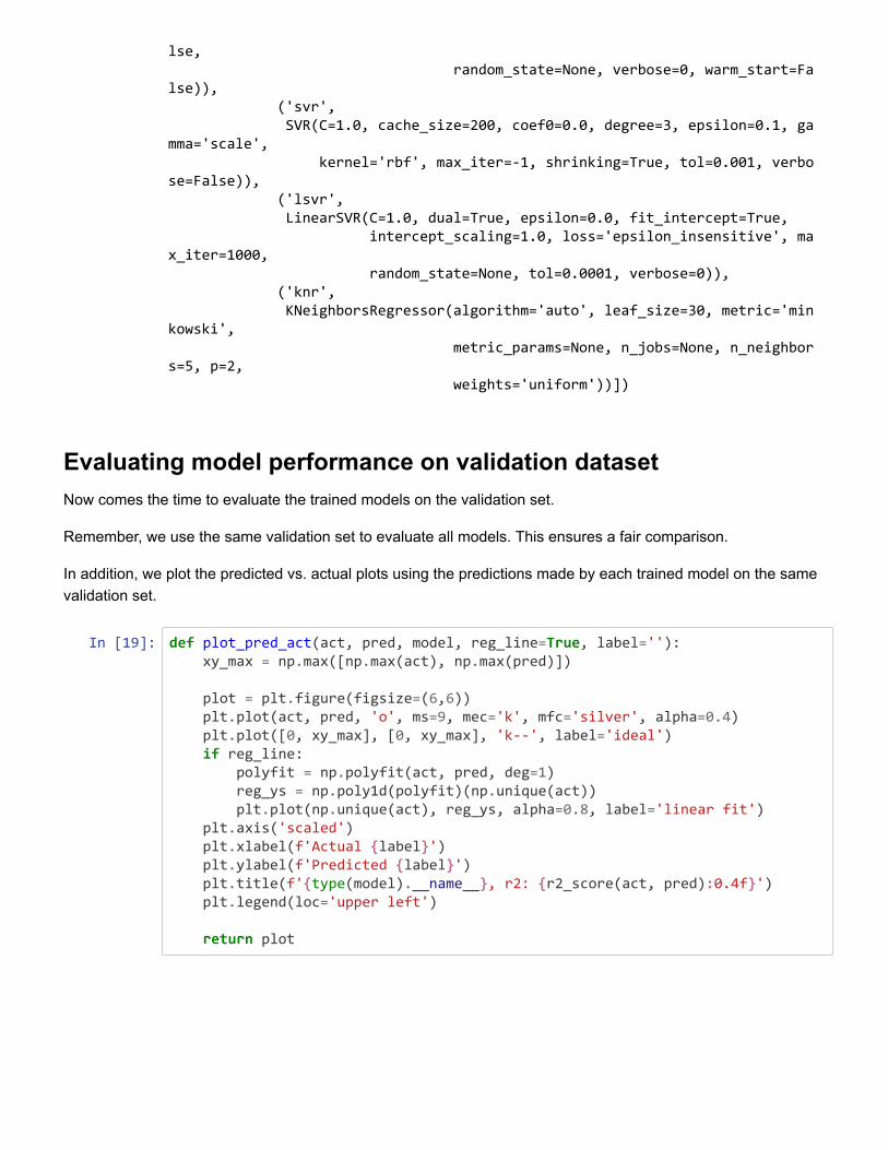
Evaluating model performance on validation datasetNow comes the time to evaluate the trained models on the validation set.
Remember, we use the same validation set to evaluate all models. This ensures a fair comparison.
In addition, we plot the predicted vs. actual plots using the predictions made by each trained model on the samevalidation set.
In [19]: def plot_pred_act(act, pred, model, reg_line=True, label=''): xy_max = np.max([np.max(act), np.max(pred)])
plot = plt.figure(figsize=(6,6)) plt.plot(act, pred, 'o', ms=9, mec='k', mfc='silver', alpha=0.4) plt.plot([0, xy_max], [0, xy_max], 'k--', label='ideal') if reg_line: polyfit = np.polyfit(act, pred, deg=1) reg_ys = np.poly1d(polyfit)(np.unique(act)) plt.plot(np.unique(act), reg_ys, alpha=0.8, label='linear fit') plt.axis('scaled') plt.xlabel(f'Actual {label}') plt.ylabel(f'Predicted {label}') plt.title(f'{type(model).__name__}, r2: {r2_score(act, pred):0.4f}') plt.legend(loc='upper left') return plot
lse, random_state=None, verbose=0, warm_start=False)), ('svr', SVR(C=1.0, cache_size=200, coef0=0.0, degree=3, epsilon=0.1, gamma='scale', kernel='rbf', max_iter=-1, shrinking=True, tol=0.001, verbose=False)), ('lsvr', LinearSVR(C=1.0, dual=True, epsilon=0.0, fit_intercept=True, intercept_scaling=1.0, loss='epsilon_insensitive', max_iter=1000, random_state=None, tol=0.0001, verbose=0)), ('knr', KNeighborsRegressor(algorithm='auto', leaf_size=30, metric='minkowski', metric_params=None, n_jobs=None, n_neighbors=5, p=2, weights='uniform'))])
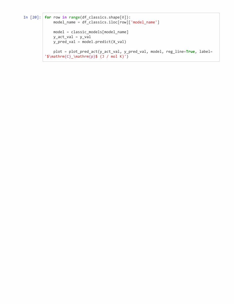
In [20]: for row in range(df_classics.shape[0]): model_name = df_classics.iloc[row]['model_name']
model = classic_models[model_name] y_act_val = y_val y_pred_val = model.predict(X_val)
plot = plot_pred_act(y_act_val, y_pred_val, model, reg_line=True, label='$\mathrm{C}_\mathrm{p}$ (J / mol K)')
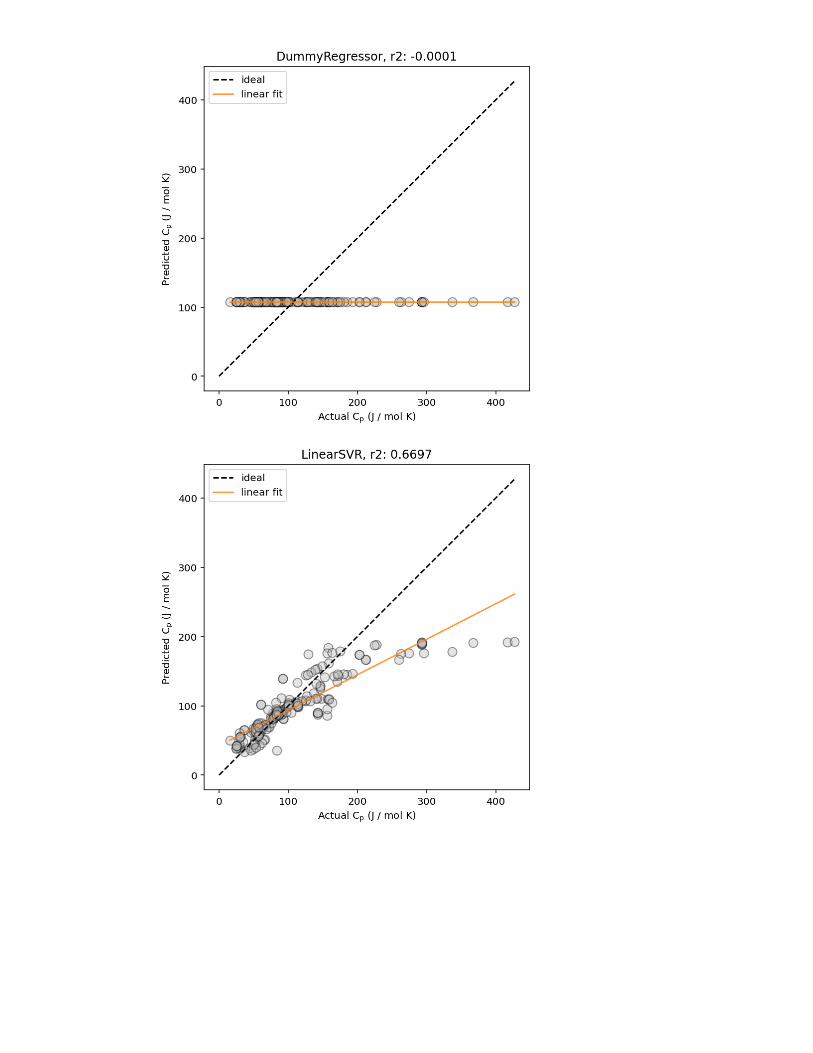
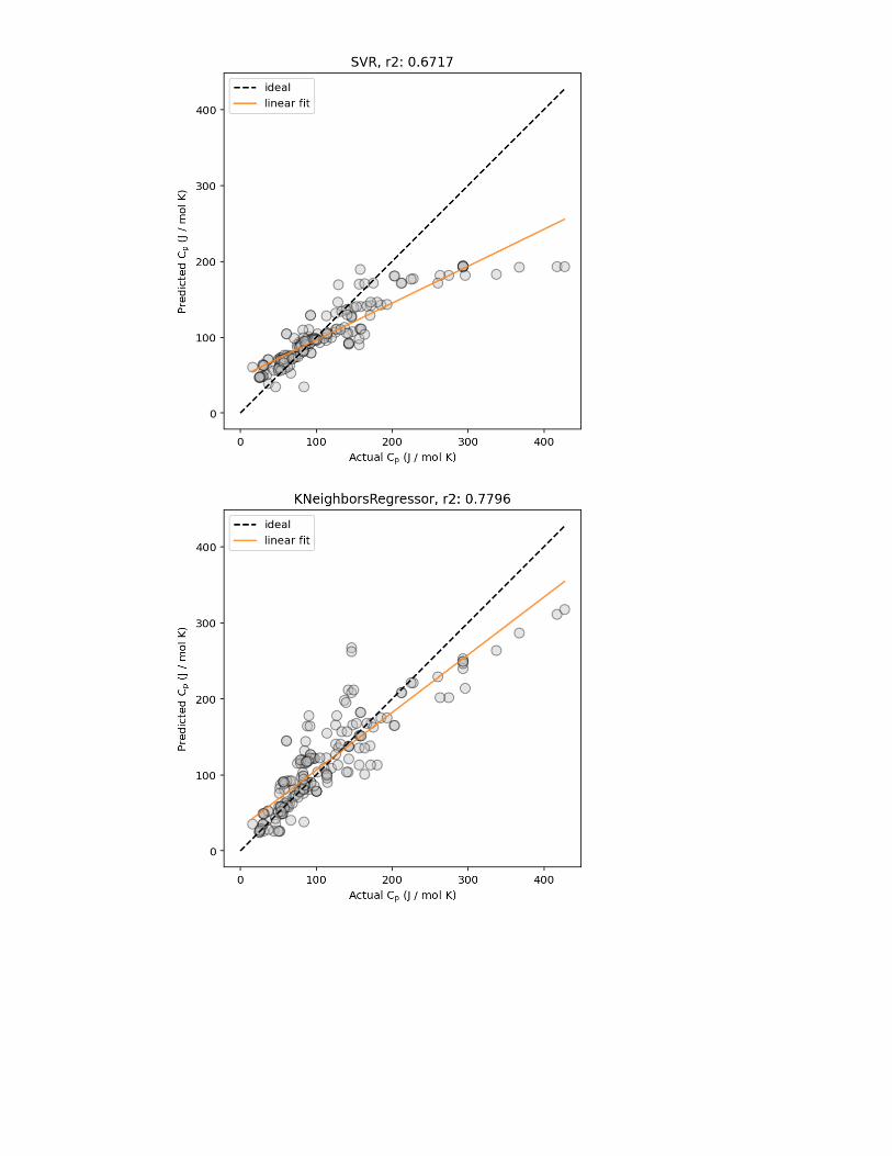
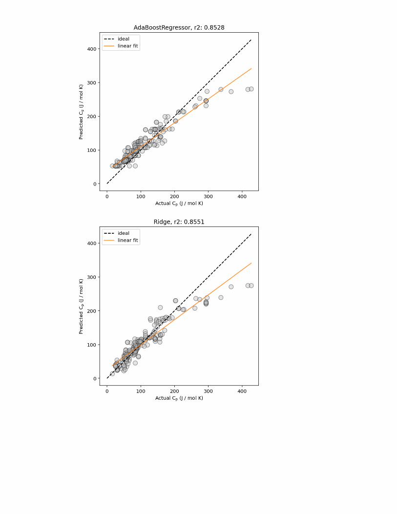
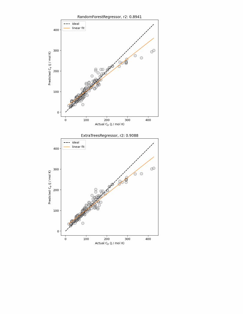
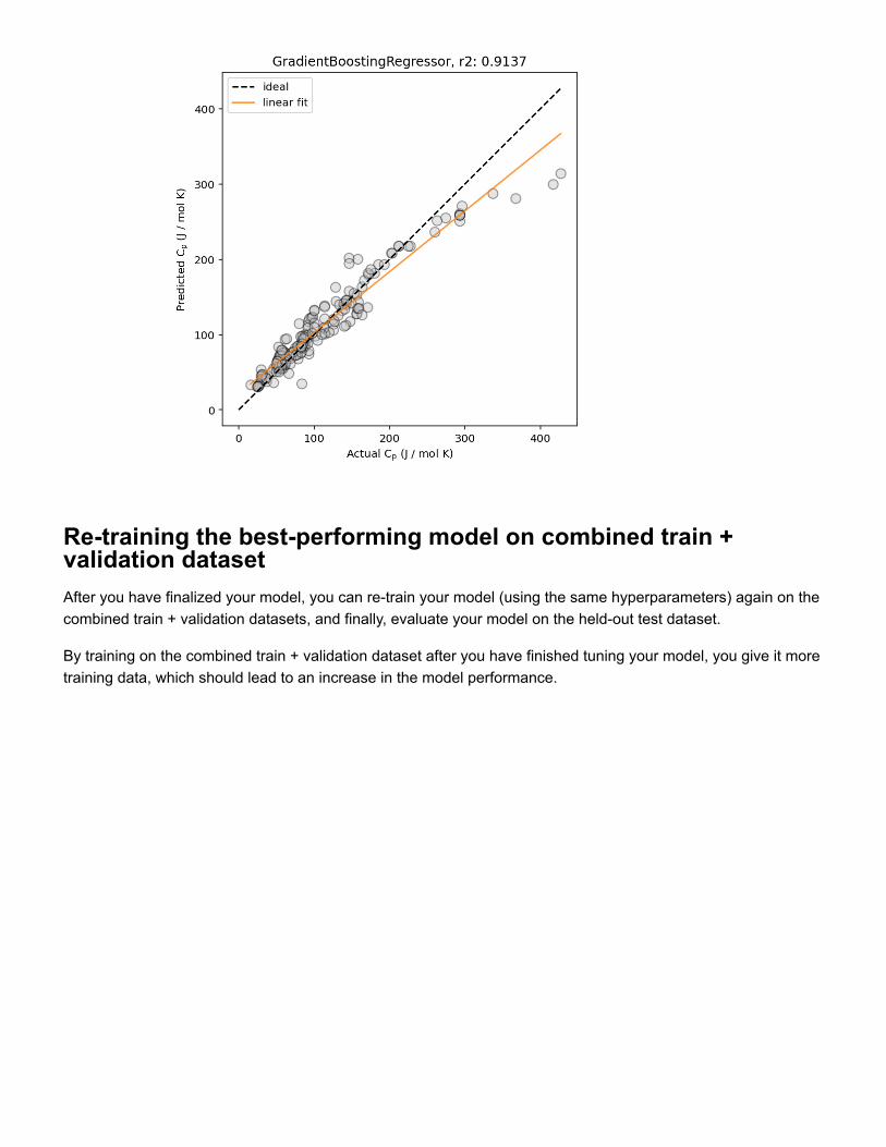
Re-training the best-performing model on combined train +validation datasetAfter you have finalized your model, you can re-train your model (using the same hyperparameters) again on thecombined train + validation datasets, and finally, evaluate your model on the held-out test dataset.
By training on the combined train + validation dataset after you have finished tuning your model, you give it moretraining data, which should lead to an increase in the model performance.
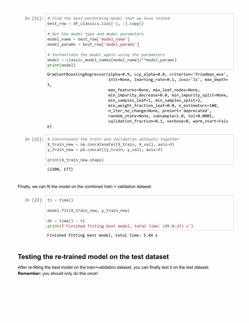
In [21]: # Find the best-performing model that we have testedbest_row = df_classics.iloc[-1, :].copy()
# Get the model type and model parametersmodel_name = best_row['model_name']model_params = best_row['model_params']
# Instantiate the model again using the parametersmodel = classic_model_names[model_name](**model_params)print(model)
In [22]: # Concatenate the train and validation datasets togetherX_train_new = np.concatenate((X_train, X_val), axis=0)y_train_new = pd.concat((y_train, y_val), axis=0)
print(X_train_new.shape)
Finally, we can fit the model on the combined train + validation dataset.
In [23]: ti = time()
model.fit(X_train_new, y_train_new)
dt = time() - tiprint(f'Finished fitting best model, total time: {dt:0.2f} s')
Testing the re-trained model on the test datasetAfter re-fitting the best model on the train+validation dataset, you can finally test it on the test dataset.Remember: you should only do this once!
GradientBoostingRegressor(alpha=0.9, ccp_alpha=0.0, criterion='friedman_mse', init=None, learning_rate=0.1, loss='ls', max_depth=3, max_features=None, max_leaf_nodes=None, min_impurity_decrease=0.0, min_impurity_split=None, min_samples_leaf=1, min_samples_split=2, min_weight_fraction_leaf=0.0, n_estimators=100, n_iter_no_change=None, presort='deprecated', random_state=None, subsample=1.0, tol=0.0001, validation_fraction=0.1, verbose=0, warm_start=False)
(2200, 177)
Finished fitting best model, total time: 5.44 s
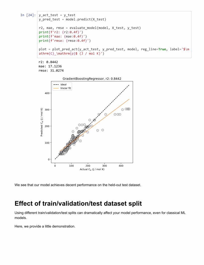
In [24]: y_act_test = y_testy_pred_test = model.predict(X_test)
r2, mae, rmse = evaluate_model(model, X_test, y_test)print(f'r2: {r2:0.4f}')print(f'mae: {mae:0.4f}')print(f'rmse: {rmse:0.4f}')
plot = plot_pred_act(y_act_test, y_pred_test, model, reg_line=True, label='$\mathrm{C}_\mathrm{p}$ (J / mol K)')
We see that our model achieves decent performance on the held-out test dataset.
Effect of train/validation/test dataset splitUsing different train/validation/test splits can dramatically affect your model performance, even for classical MLmodels.
Here, we provide a little demonstration.
r2: 0.8442 mae: 17.1236 rmse: 31.0274
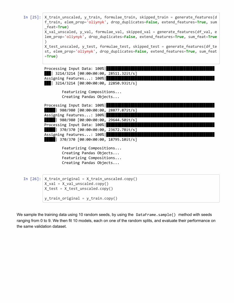
In [25]: X_train_unscaled, y_train, formulae_train, skipped_train = generate_features(df_train, elem_prop='oliynyk', drop_duplicates=False, extend_features=True, sum_feat=True)X_val_unscaled, y_val, formulae_val, skipped_val = generate_features(df_val, elem_prop='oliynyk', drop_duplicates=False, extend_features=True, sum_feat=True)X_test_unscaled, y_test, formulae_test, skipped_test = generate_features(df_test, elem_prop='oliynyk', drop_duplicates=False, extend_features=True, sum_feat=True)
In [26]: X_train_original = X_train_unscaled.copy()X_val = X_val_unscaled.copy()X_test = X_test_unscaled.copy()
y_train_original = y_train.copy()
We sample the training data using 10 random seeds, by using the DataFrame.sample() method with seedsranging from 0 to 9. We then fit 10 models, each on one of the random splits, and evaluate their performance onthe same validation dataset.
Processing Input Data: 100%|████████████████████████████████████████████████████| 3214/3214 [00:00<00:00, 28511.32it/s] Assigning Features...: 100%|████████████████████████████████████████████████████| 3214/3214 [00:00<00:00, 22850.93it/s]
Featurizing Compositions... Creating Pandas Objects...
Processing Input Data: 100%|██████████████████████████████████████████████████████| 980/980 [00:00<00:00, 28877.87it/s] Assigning Features...: 100%|██████████████████████████████████████████████████████| 980/980 [00:00<00:00, 29644.50it/s] Processing Input Data: 100%|██████████████████████████████████████████████████████| 370/370 [00:00<00:00, 23672.78it/s] Assigning Features...: 100%|██████████████████████████████████████████████████████| 370/370 [00:00<00:00, 18795.10it/s]
Featurizing Compositions... Creating Pandas Objects... Featurizing Compositions... Creating Pandas Objects...
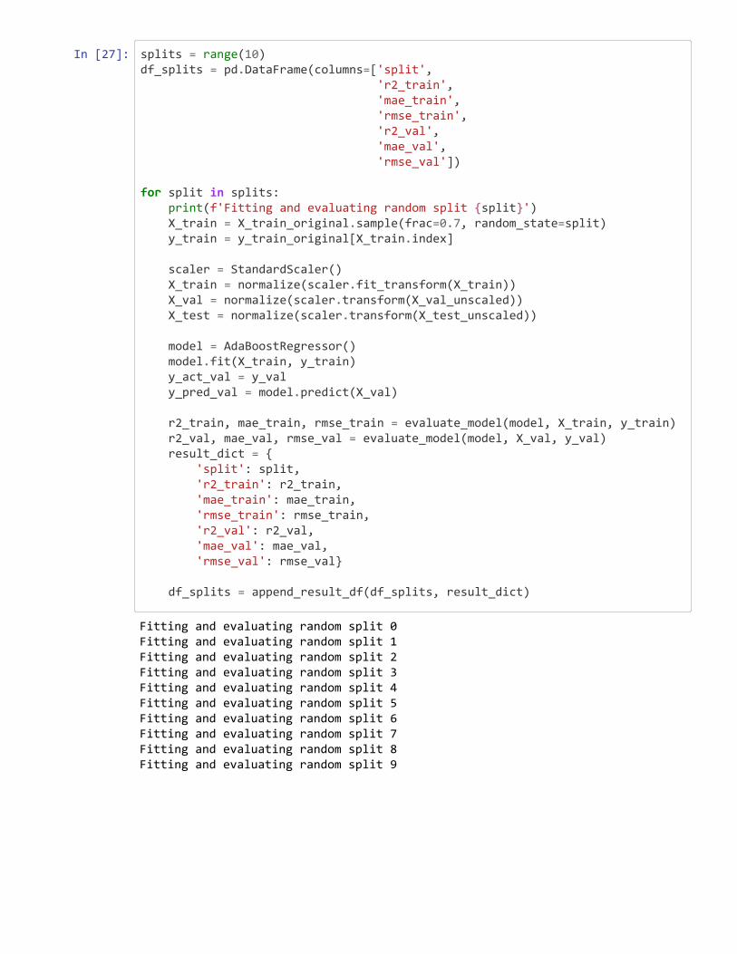
In [27]: splits = range(10)df_splits = pd.DataFrame(columns=['split', 'r2_train', 'mae_train', 'rmse_train', 'r2_val', 'mae_val', 'rmse_val'])
for split in splits: print(f'Fitting and evaluating random split {split}') X_train = X_train_original.sample(frac=0.7, random_state=split) y_train = y_train_original[X_train.index]
scaler = StandardScaler() X_train = normalize(scaler.fit_transform(X_train)) X_val = normalize(scaler.transform(X_val_unscaled)) X_test = normalize(scaler.transform(X_test_unscaled)) model = AdaBoostRegressor() model.fit(X_train, y_train) y_act_val = y_val y_pred_val = model.predict(X_val)
r2_train, mae_train, rmse_train = evaluate_model(model, X_train, y_train) r2_val, mae_val, rmse_val = evaluate_model(model, X_val, y_val) result_dict = { 'split': split, 'r2_train': r2_train, 'mae_train': mae_train, 'rmse_train': rmse_train, 'r2_val': r2_val, 'mae_val': mae_val, 'rmse_val': rmse_val} df_splits = append_result_df(df_splits, result_dict)
Fitting and evaluating random split 0 Fitting and evaluating random split 1 Fitting and evaluating random split 2 Fitting and evaluating random split 3 Fitting and evaluating random split 4 Fitting and evaluating random split 5 Fitting and evaluating random split 6 Fitting and evaluating random split 7 Fitting and evaluating random split 8 Fitting and evaluating random split 9
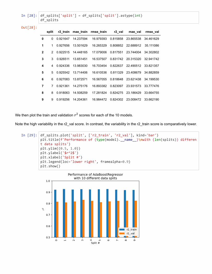
In [28]: df_splits['split'] = df_splits['split'].astype(int)df_splits
We then plot the train and validation scores for each of the 10 models.
Note the high variability in the r2_val score. In contrast, the variability in the r2_train score is comparatively lower.
r2
In [29]: df_splits.plot('split', ['r2_train', 'r2_val'], kind='bar')plt.title(f'Performance of {type(model).__name__}\nwith {len(splits)} different data splits')plt.ylim((0.5, 1.0))plt.ylabel('$r^2$')plt.xlabel('Split #')plt.legend(loc='lower right', framealpha=0.9)plt.show()
Out[28]:split r2_train mae_train rmse_train r2_val mae_val rmse_val
0 0 0.921647 14.237594 16.979393 0.815858 23.865538 34.461629
1 1 0.927656 13.501629 16.265329 0.808852 22.688912 35.111086
2 2 0.922515 14.448165 17.079006 0.817551 23.744004 34.302802
3 3 0.926511 13.651451 16.537507 0.831742 20.315320 32.941742
4 4 0.924336 13.983030 16.703454 0.822637 22.490512 33.821357
5 5 0.925542 13.714406 16.610536 0.811329 23.408679 34.882859
6 6 0.927083 13.872571 16.567055 0.818648 23.621438 34.199530
7 7 0.921361 14.275176 16.893382 0.823097 23.931573 33.777476
8 8 0.918063 14.508259 17.281824 0.824275 23.186429 33.664755
9 9 0.919256 14.204361 16.984472 0.824302 23.008472 33.662190
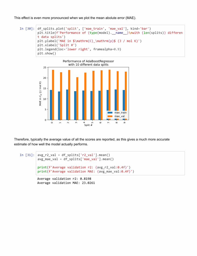
This effect is even more pronounced when we plot the mean abolute error (MAE).
In [30]: df_splits.plot('split', ['mae_train', 'mae_val'], kind='bar')plt.title(f'Performance of {type(model).__name__}\nwith {len(splits)} different data splits')plt.ylabel('MAE in $\mathrm{C}_\mathrm{p}$ (J / mol K)')plt.xlabel('Split #')plt.legend(loc='lower right', framealpha=0.9)plt.show()
Therefore, typically the average value of all the scores are reported, as this gives a much more accurateestimate of how well the model actually performs.
In [31]: avg_r2_val = df_splits['r2_val'].mean()avg_mae_val = df_splits['mae_val'].mean()
print(f'Average validation r2: {avg_r2_val:0.4f}')print(f'Average validation MAE: {avg_mae_val:0.4f}')
Average validation r2: 0.8198 Average validation MAE: 23.0261
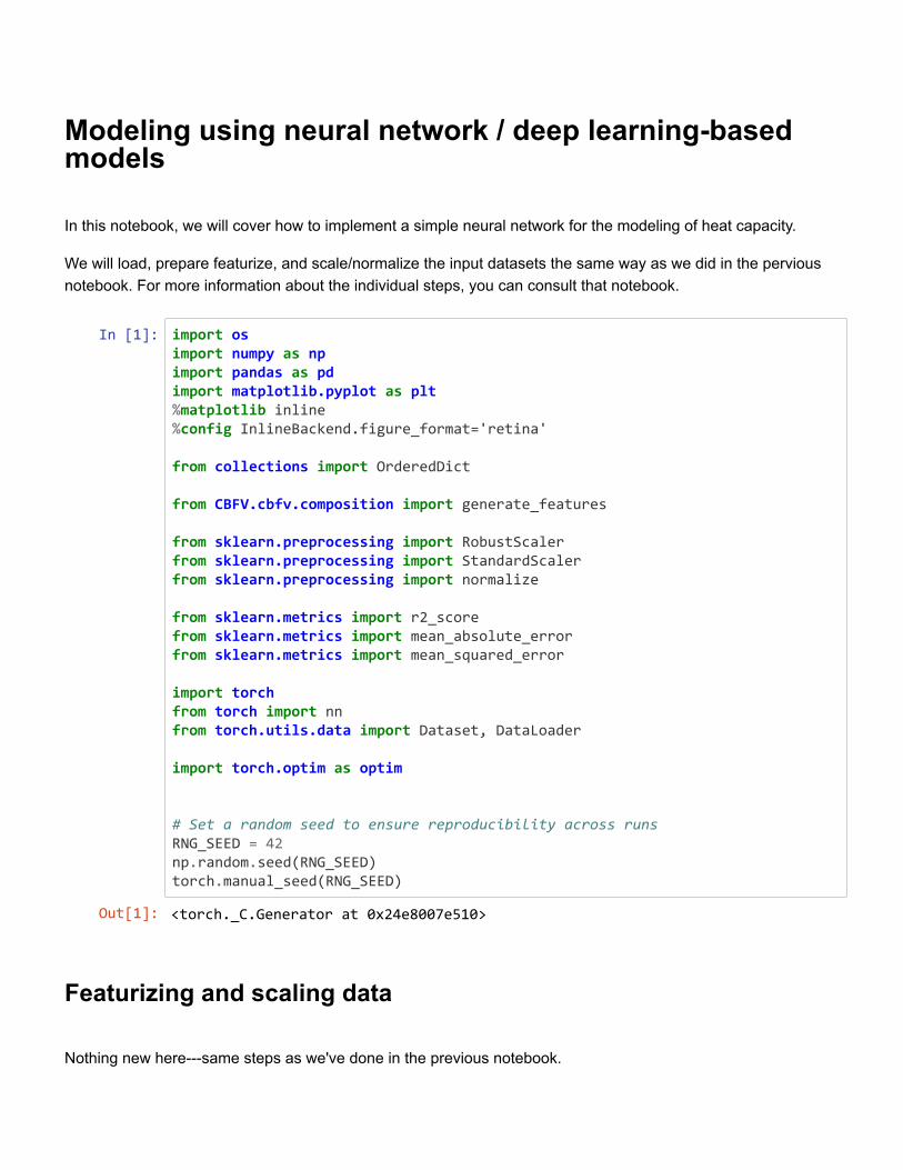
Modeling using neural network / deep learning-basedmodels
In this notebook, we will cover how to implement a simple neural network for the modeling of heat capacity.
We will load, prepare featurize, and scale/normalize the input datasets the same way as we did in the perviousnotebook. For more information about the individual steps, you can consult that notebook.
In [1]: import osimport numpy as npimport pandas as pdimport matplotlib.pyplot as plt%matplotlib inline %config InlineBackend.figure_format='retina'
from collections import OrderedDict
from CBFV.cbfv.composition import generate_features
from sklearn.preprocessing import RobustScalerfrom sklearn.preprocessing import StandardScalerfrom sklearn.preprocessing import normalize
from sklearn.metrics import r2_scorefrom sklearn.metrics import mean_absolute_errorfrom sklearn.metrics import mean_squared_error
import torchfrom torch import nnfrom torch.utils.data import Dataset, DataLoader
import torch.optim as optim
# Set a random seed to ensure reproducibility across runsRNG_SEED = 42np.random.seed(RNG_SEED)torch.manual_seed(RNG_SEED)
Featurizing and scaling data
Nothing new here---same steps as we've done in the previous notebook.
Out[1]: <torch._C.Generator at 0x24e8007e510>
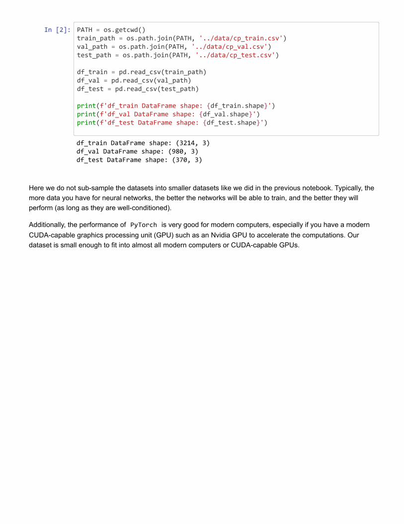
In [2]: PATH = os.getcwd()train_path = os.path.join(PATH, '../data/cp_train.csv')val_path = os.path.join(PATH, '../data/cp_val.csv')test_path = os.path.join(PATH, '../data/cp_test.csv')
df_train = pd.read_csv(train_path)df_val = pd.read_csv(val_path)df_test = pd.read_csv(test_path)
print(f'df_train DataFrame shape: {df_train.shape}')print(f'df_val DataFrame shape: {df_val.shape}')print(f'df_test DataFrame shape: {df_test.shape}')
Here we do not sub-sample the datasets into smaller datasets like we did in the previous notebook. Typically, themore data you have for neural networks, the better the networks will be able to train, and the better they willperform (as long as they are well-conditioned).
Additionally, the performance of PyTorch is very good for modern computers, especially if you have a modernCUDA-capable graphics processing unit (GPU) such as an Nvidia GPU to accelerate the computations. Ourdataset is small enough to fit into almost all modern computers or CUDA-capable GPUs.
df_train DataFrame shape: (3214, 3) df_val DataFrame shape: (980, 3) df_test DataFrame shape: (370, 3)
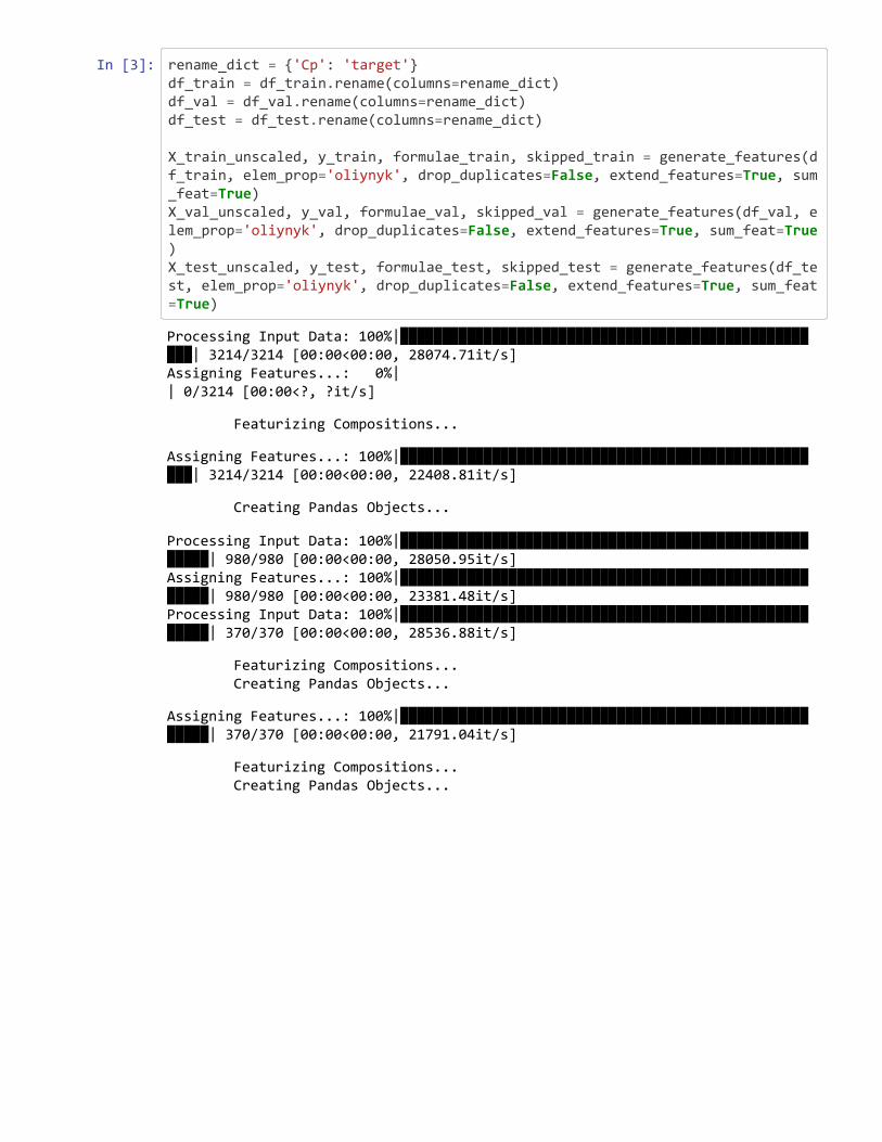
In [3]: rename_dict = {'Cp': 'target'}df_train = df_train.rename(columns=rename_dict)df_val = df_val.rename(columns=rename_dict)df_test = df_test.rename(columns=rename_dict)
X_train_unscaled, y_train, formulae_train, skipped_train = generate_features(df_train, elem_prop='oliynyk', drop_duplicates=False, extend_features=True, sum_feat=True)X_val_unscaled, y_val, formulae_val, skipped_val = generate_features(df_val, elem_prop='oliynyk', drop_duplicates=False, extend_features=True, sum_feat=True)X_test_unscaled, y_test, formulae_test, skipped_test = generate_features(df_test, elem_prop='oliynyk', drop_duplicates=False, extend_features=True, sum_feat=True)
Processing Input Data: 100%|████████████████████████████████████████████████████| 3214/3214 [00:00<00:00, 28074.71it/s] Assigning Features...: 0%| | 0/3214 [00:00<?, ?it/s]
Featurizing Compositions...
Assigning Features...: 100%|████████████████████████████████████████████████████| 3214/3214 [00:00<00:00, 22408.81it/s]
Creating Pandas Objects...
Processing Input Data: 100%|██████████████████████████████████████████████████████| 980/980 [00:00<00:00, 28050.95it/s] Assigning Features...: 100%|██████████████████████████████████████████████████████| 980/980 [00:00<00:00, 23381.48it/s] Processing Input Data: 100%|██████████████████████████████████████████████████████| 370/370 [00:00<00:00, 28536.88it/s]
Featurizing Compositions... Creating Pandas Objects...
Assigning Features...: 100%|██████████████████████████████████████████████████████| 370/370 [00:00<00:00, 21791.04it/s]
Featurizing Compositions... Creating Pandas Objects...
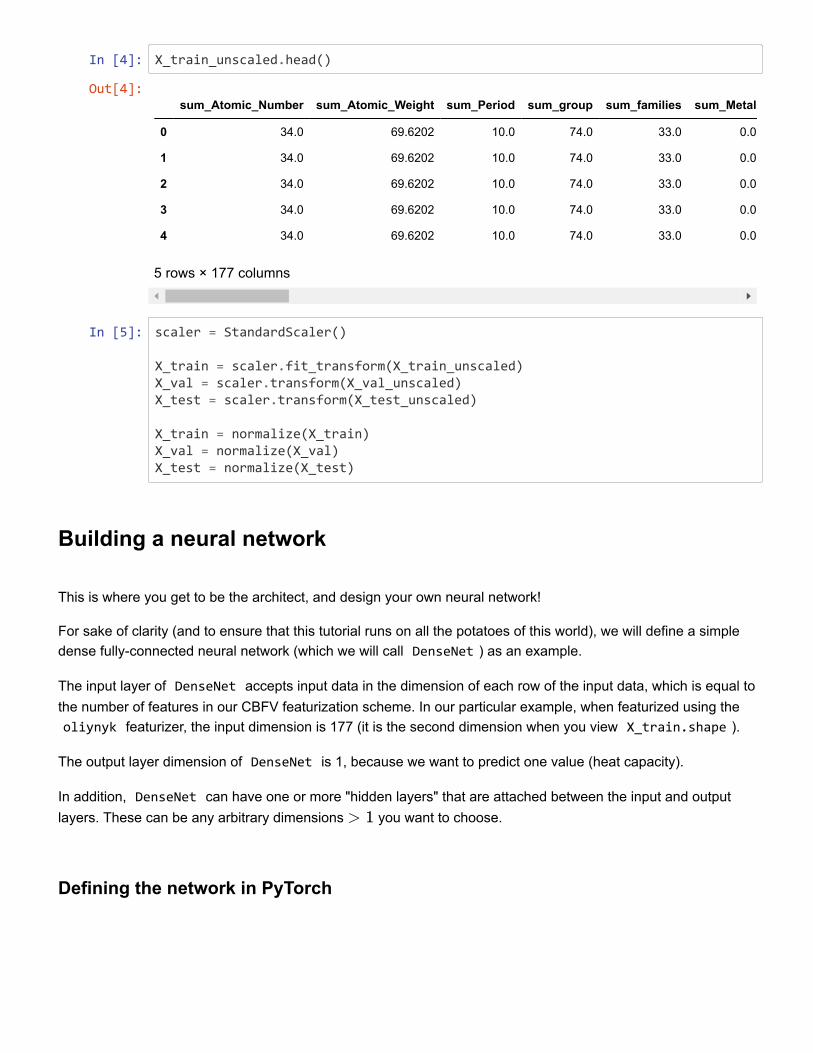
In [4]: X_train_unscaled.head()
In [5]: scaler = StandardScaler()
X_train = scaler.fit_transform(X_train_unscaled)X_val = scaler.transform(X_val_unscaled)X_test = scaler.transform(X_test_unscaled)
X_train = normalize(X_train)X_val = normalize(X_val)X_test = normalize(X_test)
Building a neural network
This is where you get to be the architect, and design your own neural network!
For sake of clarity (and to ensure that this tutorial runs on all the potatoes of this world), we will define a simpledense fully-connected neural network (which we will call DenseNet ) as an example.
The input layer of DenseNet accepts input data in the dimension of each row of the input data, which is equal tothe number of features in our CBFV featurization scheme. In our particular example, when featurized using the oliynyk featurizer, the input dimension is 177 (it is the second dimension when you view X_train.shape ).
The output layer dimension of DenseNet is 1, because we want to predict one value (heat capacity).
In addition, DenseNet can have one or more "hidden layers" that are attached between the input and outputlayers. These can be any arbitrary dimensions you want to choose.> 1
Defining the network in PyTorch
Out[4]:sum_Atomic_Number sum_Atomic_Weight sum_Period sum_group sum_families sum_Metal
0 34.0 69.6202 10.0 74.0 33.0 0.0
1 34.0 69.6202 10.0 74.0 33.0 0.0
2 34.0 69.6202 10.0 74.0 33.0 0.0
3 34.0 69.6202 10.0 74.0 33.0 0.0
4 34.0 69.6202 10.0 74.0 33.0 0.0
5 rows × 177 columns
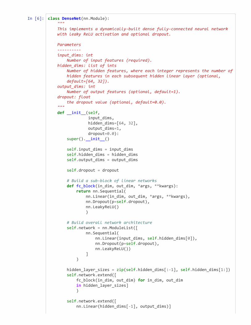
In [6]: class DenseNet(nn.Module): """ This implements a dynamically-built dense fully-connected neural network with leaky ReLU activation and optional dropout.
Parameters ---------- input_dims: int Number of input features (required). hidden_dims: list of ints Number of hidden features, where each integer represents the number of hidden features in each subsequent hidden linear layer (optional, default=[64, 32]). output_dims: int Number of output features (optional, default=1). dropout: float the dropout value (optional, default=0.0). """ def __init__(self, input_dims, hidden_dims=[64, 32], output_dims=1, dropout=0.0): super().__init__()
self.input_dims = input_dims self.hidden_dims = hidden_dims self.output_dims = output_dims
self.dropout = dropout # Build a sub-block of linear networks def fc_block(in_dim, out_dim, *args, **kwargs): return nn.Sequential( nn.Linear(in_dim, out_dim, *args, **kwargs), nn.Dropout(p=self.dropout), nn.LeakyReLU() )
# Build overall network architecture self.network = nn.ModuleList([ nn.Sequential( nn.Linear(input_dims, self.hidden_dims[0]), nn.Dropout(p=self.dropout), nn.LeakyReLU()) ] )
hidden_layer_sizes = zip(self.hidden_dims[:-1], self.hidden_dims[1:]) self.network.extend([ fc_block(in_dim, out_dim) for in_dim, out_dim in hidden_layer_sizes] )
self.network.extend([ nn.Linear(hidden_dims[-1], output_dims)]
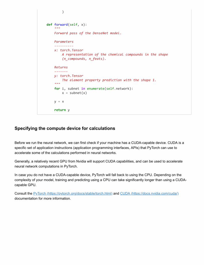
)
def forward(self, x): """ Forward pass of the DenseNet model.
Parameters ---------- x: torch.Tensor A representation of the chemical compounds in the shape (n_compounds, n_feats).
Returns ------- y: torch.Tensor The element property prediction with the shape 1. """ for i, subnet in enumerate(self.network): x = subnet(x) y = x
return y
Specifying the compute device for calculations
Before we run the neural network, we can first check if your machine has a CUDA-capable device. CUDA is aspecific set of application instructions (application programming interfaces, APIs) that PyTorch can use toaccelerate some of the calculations performed in neural networks.
Generally, a relatively recent GPU from Nvidia will support CUDA capabilities, and can be used to accelerateneural network computations in PyTorch.
In case you do not have a CUDA-capable device, PyTorch will fall back to using the CPU. Depending on thecomplexity of your model, training and predicting using a CPU can take significantly longer than using a CUDA-capable GPU.
Consult the PyTorch (https://pytorch.org/docs/stable/torch.html) and CUDA (https://docs.nvidia.com/cuda/)documentation for more information.
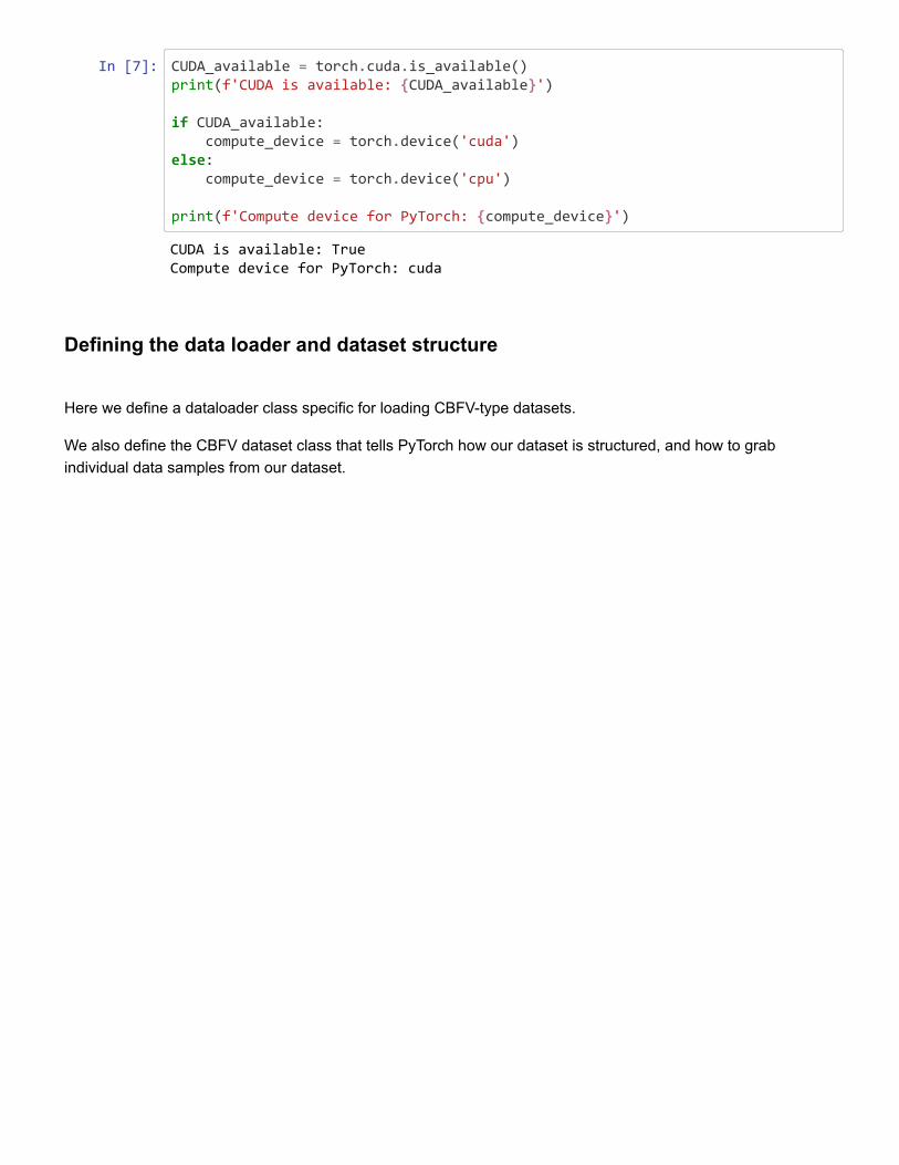
In [7]: CUDA_available = torch.cuda.is_available()print(f'CUDA is available: {CUDA_available}')
if CUDA_available: compute_device = torch.device('cuda')else: compute_device = torch.device('cpu') print(f'Compute device for PyTorch: {compute_device}')
Defining the data loader and dataset structure
Here we define a dataloader class specific for loading CBFV-type datasets.
We also define the CBFV dataset class that tells PyTorch how our dataset is structured, and how to grabindividual data samples from our dataset.
CUDA is available: True Compute device for PyTorch: cuda
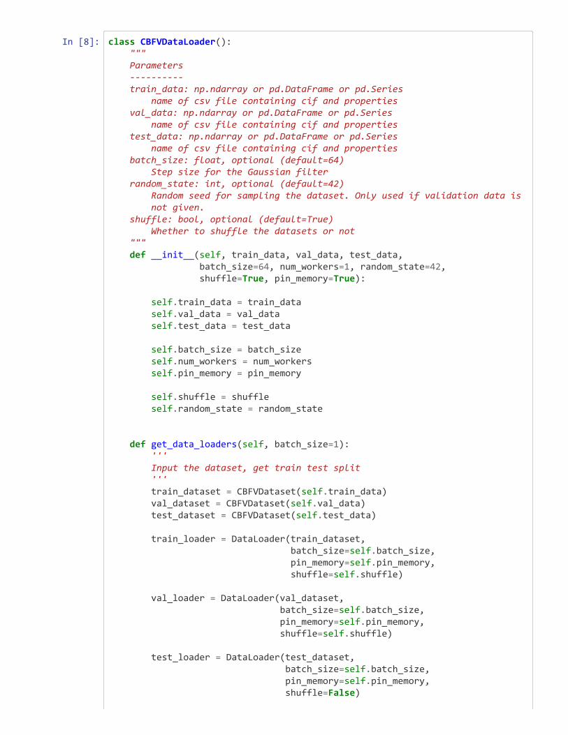
In [8]: class CBFVDataLoader(): """ Parameters ---------- train_data: np.ndarray or pd.DataFrame or pd.Series name of csv file containing cif and properties val_data: np.ndarray or pd.DataFrame or pd.Series name of csv file containing cif and properties test_data: np.ndarray or pd.DataFrame or pd.Series name of csv file containing cif and properties batch_size: float, optional (default=64) Step size for the Gaussian filter random_state: int, optional (default=42) Random seed for sampling the dataset. Only used if validation data is not given. shuffle: bool, optional (default=True) Whether to shuffle the datasets or not """ def __init__(self, train_data, val_data, test_data, batch_size=64, num_workers=1, random_state=42, shuffle=True, pin_memory=True):
self.train_data = train_data self.val_data = val_data self.test_data = test_data
self.batch_size = batch_size self.num_workers = num_workers self.pin_memory = pin_memory
self.shuffle = shuffle self.random_state = random_state
def get_data_loaders(self, batch_size=1): ''' Input the dataset, get train test split ''' train_dataset = CBFVDataset(self.train_data) val_dataset = CBFVDataset(self.val_data) test_dataset = CBFVDataset(self.test_data)
train_loader = DataLoader(train_dataset, batch_size=self.batch_size, pin_memory=self.pin_memory, shuffle=self.shuffle)
val_loader = DataLoader(val_dataset, batch_size=self.batch_size, pin_memory=self.pin_memory, shuffle=self.shuffle)
test_loader = DataLoader(test_dataset, batch_size=self.batch_size, pin_memory=self.pin_memory, shuffle=False)
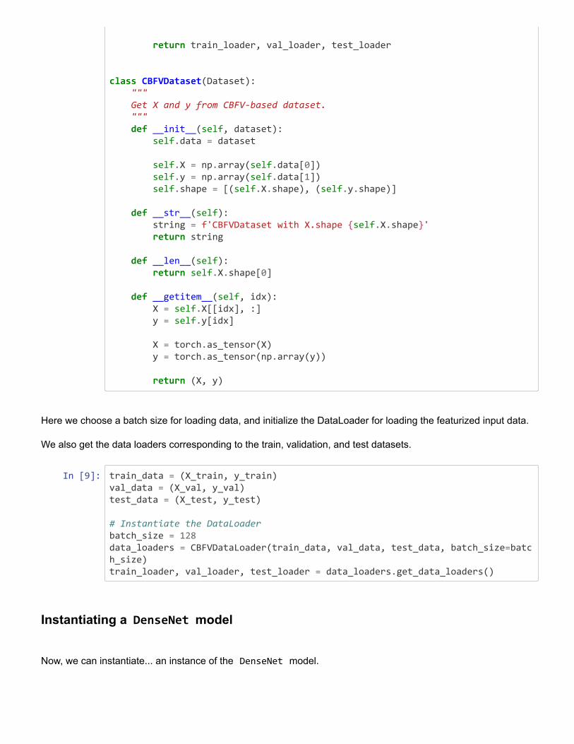
return train_loader, val_loader, test_loader
class CBFVDataset(Dataset): """ Get X and y from CBFV-based dataset. """ def __init__(self, dataset): self.data = dataset
self.X = np.array(self.data[0]) self.y = np.array(self.data[1]) self.shape = [(self.X.shape), (self.y.shape)]
def __str__(self): string = f'CBFVDataset with X.shape {self.X.shape}' return string
def __len__(self): return self.X.shape[0]
def __getitem__(self, idx): X = self.X[[idx], :] y = self.y[idx]
X = torch.as_tensor(X) y = torch.as_tensor(np.array(y))
return (X, y)
Here we choose a batch size for loading data, and initialize the DataLoader for loading the featurized input data.
We also get the data loaders corresponding to the train, validation, and test datasets.
In [9]: train_data = (X_train, y_train)val_data = (X_val, y_val)test_data = (X_test, y_test)
# Instantiate the DataLoaderbatch_size = 128data_loaders = CBFVDataLoader(train_data, val_data, test_data, batch_size=batch_size)train_loader, val_loader, test_loader = data_loaders.get_data_loaders()
Instantiating a DenseNet model
Now, we can instantiate... an instance of the DenseNet model.
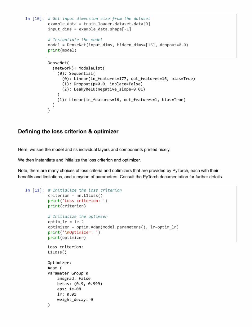
In [10]: # Get input dimension size from the datasetexample_data = train_loader.dataset.data[0]input_dims = example_data.shape[-1]
# Instantiate the modelmodel = DenseNet(input_dims, hidden_dims=[16], dropout=0.0)print(model)
Defining the loss criterion & optimizer
Here, we see the model and its individual layers and components printed nicely.
We then instantiate and initialize the loss criterion and optimizer.
Note, there are many choices of loss criteria and optimizers that are provided by PyTorch, each with theirbenefits and limitations, and a myriad of parameters. Consult the PyTorch documentation for further details.
In [11]: # Initialize the loss criterioncriterion = nn.L1Loss()print('Loss criterion: ')print(criterion)
# Initialize the optimzeroptim_lr = 1e-2optimizer = optim.Adam(model.parameters(), lr=optim_lr)print('\nOptimizer: ')print(optimizer)
DenseNet( (network): ModuleList( (0): Sequential( (0): Linear(in_features=177, out_features=16, bias=True) (1): Dropout(p=0.0, inplace=False) (2): LeakyReLU(negative_slope=0.01) ) (1): Linear(in_features=16, out_features=1, bias=True) ) )
Loss criterion: L1Loss()
Optimizer: Adam ( Parameter Group 0 amsgrad: False betas: (0.9, 0.999) eps: 1e-08 lr: 0.01 weight_decay: 0 )
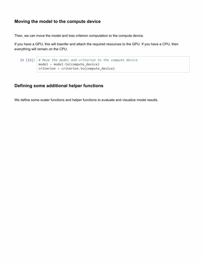
Moving the model to the compute device
Then, we can move the model and loss criterion computation to the compute device.
If you have a GPU, this will trasnfer and attach the required resources to the GPU. If you have a CPU, theneverything will remain on the CPU.
In [12]: # Move the model and criterion to the compute devicemodel = model.to(compute_device)criterion = criterion.to(compute_device)
Defining some additional helper functions
We define some scaler functions and helper functions to evaluate and visualize model results.
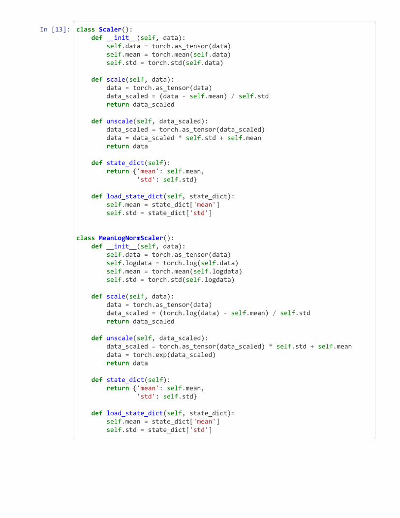
In [13]: class Scaler(): def __init__(self, data): self.data = torch.as_tensor(data) self.mean = torch.mean(self.data) self.std = torch.std(self.data)
def scale(self, data): data = torch.as_tensor(data) data_scaled = (data - self.mean) / self.std return data_scaled
def unscale(self, data_scaled): data_scaled = torch.as_tensor(data_scaled) data = data_scaled * self.std + self.mean return data
def state_dict(self): return {'mean': self.mean, 'std': self.std}
def load_state_dict(self, state_dict): self.mean = state_dict['mean'] self.std = state_dict['std']
class MeanLogNormScaler(): def __init__(self, data): self.data = torch.as_tensor(data) self.logdata = torch.log(self.data) self.mean = torch.mean(self.logdata) self.std = torch.std(self.logdata)
def scale(self, data): data = torch.as_tensor(data) data_scaled = (torch.log(data) - self.mean) / self.std return data_scaled
def unscale(self, data_scaled): data_scaled = torch.as_tensor(data_scaled) * self.std + self.mean data = torch.exp(data_scaled) return data
def state_dict(self): return {'mean': self.mean, 'std': self.std}
def load_state_dict(self, state_dict): self.mean = state_dict['mean'] self.std = state_dict['std']
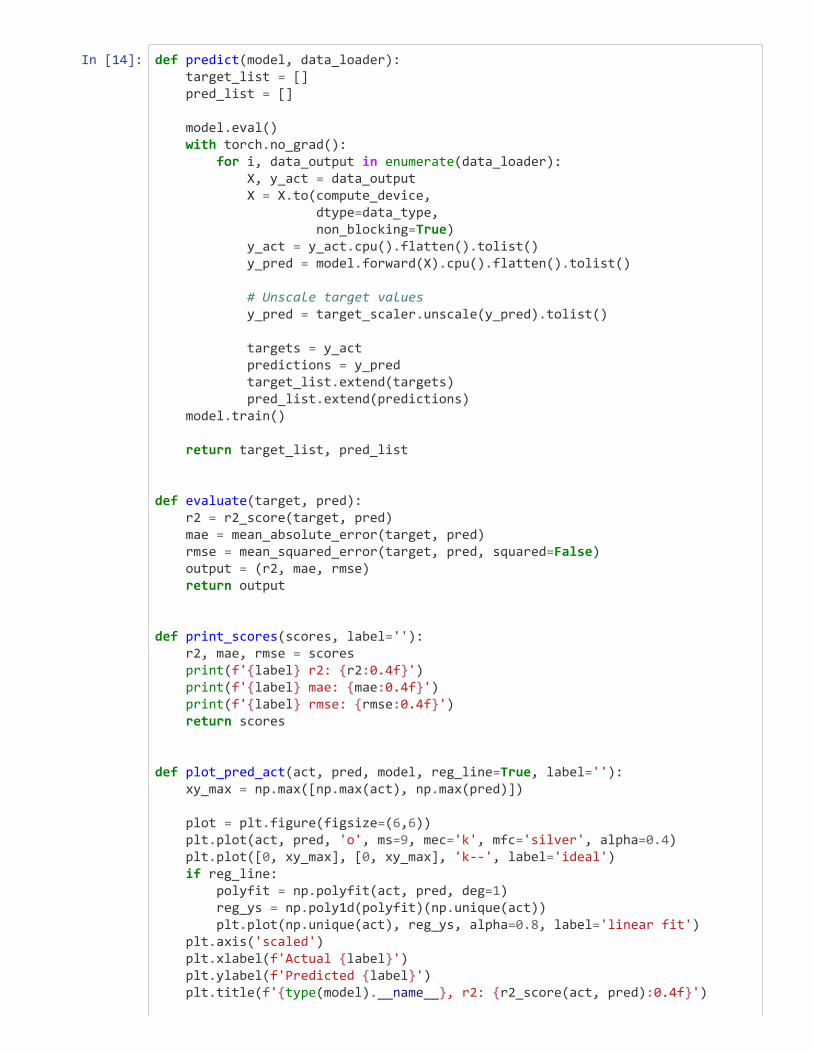
In [14]: def predict(model, data_loader): target_list = [] pred_list = []
model.eval() with torch.no_grad(): for i, data_output in enumerate(data_loader): X, y_act = data_output X = X.to(compute_device, dtype=data_type, non_blocking=True) y_act = y_act.cpu().flatten().tolist() y_pred = model.forward(X).cpu().flatten().tolist()
# Unscale target values y_pred = target_scaler.unscale(y_pred).tolist()
targets = y_act predictions = y_pred target_list.extend(targets) pred_list.extend(predictions) model.train()
return target_list, pred_list
def evaluate(target, pred): r2 = r2_score(target, pred) mae = mean_absolute_error(target, pred) rmse = mean_squared_error(target, pred, squared=False) output = (r2, mae, rmse) return output
def print_scores(scores, label=''): r2, mae, rmse = scores print(f'{label} r2: {r2:0.4f}') print(f'{label} mae: {mae:0.4f}') print(f'{label} rmse: {rmse:0.4f}') return scores
def plot_pred_act(act, pred, model, reg_line=True, label=''): xy_max = np.max([np.max(act), np.max(pred)])
plot = plt.figure(figsize=(6,6)) plt.plot(act, pred, 'o', ms=9, mec='k', mfc='silver', alpha=0.4) plt.plot([0, xy_max], [0, xy_max], 'k--', label='ideal') if reg_line: polyfit = np.polyfit(act, pred, deg=1) reg_ys = np.poly1d(polyfit)(np.unique(act)) plt.plot(np.unique(act), reg_ys, alpha=0.8, label='linear fit') plt.axis('scaled') plt.xlabel(f'Actual {label}') plt.ylabel(f'Predicted {label}') plt.title(f'{type(model).__name__}, r2: {r2_score(act, pred):0.4f}')
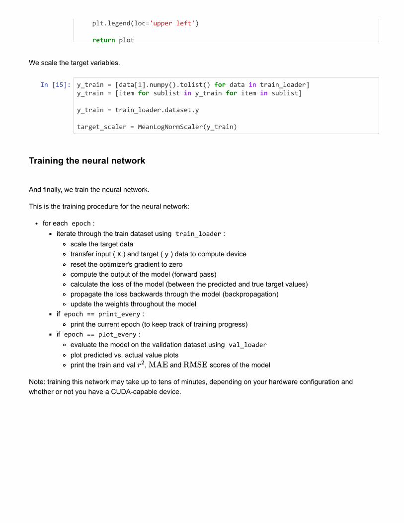
plt.legend(loc='upper left') return plot
We scale the target variables.
In [15]: y_train = [data[1].numpy().tolist() for data in train_loader]y_train = [item for sublist in y_train for item in sublist]
y_train = train_loader.dataset.y
target_scaler = MeanLogNormScaler(y_train)
Training the neural network
And finally, we train the neural network.
This is the training procedure for the neural network:
for each epoch :iterate through the train dataset using train_loader :
scale the target datatransfer input ( X ) and target ( y ) data to compute devicereset the optimizer's gradient to zerocompute the output of the model (forward pass)calculate the loss of the model (between the predicted and true target values)propagate the loss backwards through the model (backpropagation)update the weights throughout the model
if epoch == print_every :print the current epoch (to keep track of training progress)
if epoch == plot_every :evaluate the model on the validation dataset using val_loaderplot predicted vs. actual value plotsprint the train and val , and scores of the model
Note: training this network may take up to tens of minutes, depending on your hardware configuration andwhether or not you have a CUDA-capable device.
r2 MAE RMSE
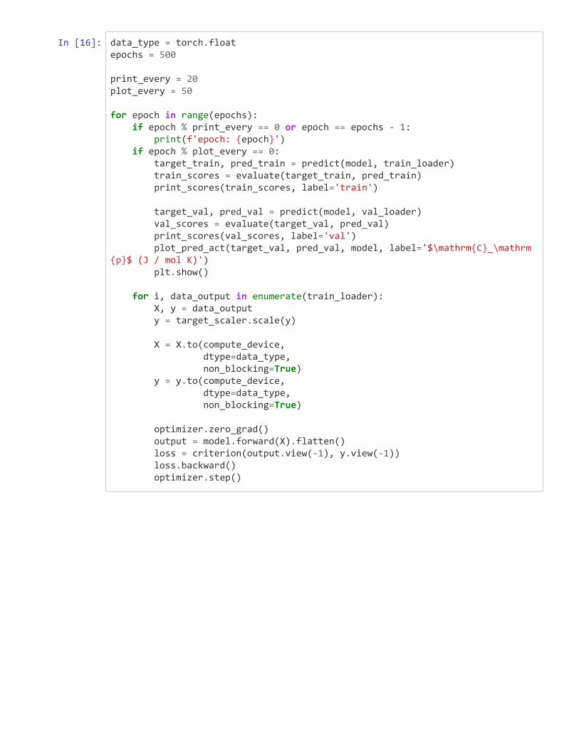
In [16]: data_type = torch.floatepochs = 500
print_every = 20plot_every = 50
for epoch in range(epochs): if epoch % print_every == 0 or epoch == epochs - 1: print(f'epoch: {epoch}') if epoch % plot_every == 0: target_train, pred_train = predict(model, train_loader) train_scores = evaluate(target_train, pred_train) print_scores(train_scores, label='train') target_val, pred_val = predict(model, val_loader) val_scores = evaluate(target_val, pred_val) print_scores(val_scores, label='val') plot_pred_act(target_val, pred_val, model, label='$\mathrm{C}_\mathrm{p}$ (J / mol K)') plt.show() for i, data_output in enumerate(train_loader): X, y = data_output y = target_scaler.scale(y) X = X.to(compute_device, dtype=data_type, non_blocking=True) y = y.to(compute_device, dtype=data_type, non_blocking=True) optimizer.zero_grad() output = model.forward(X).flatten() loss = criterion(output.view(-1), y.view(-1)) loss.backward() optimizer.step()
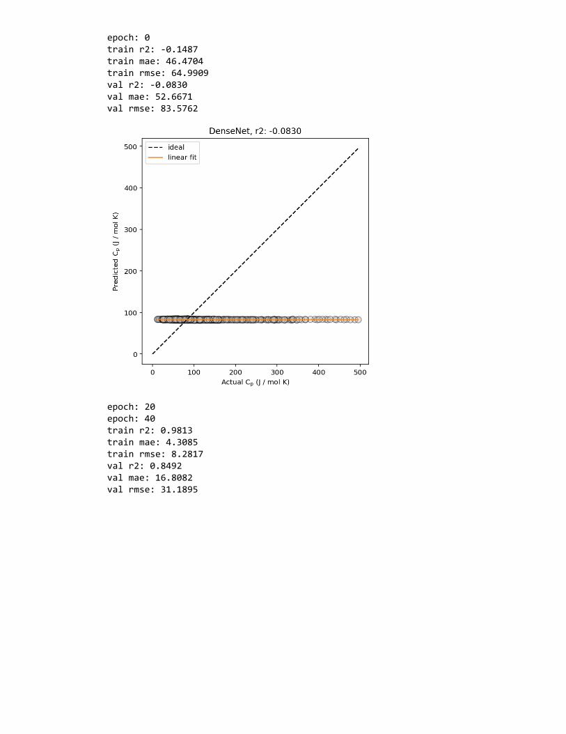
epoch: 0 train r2: -0.1487 train mae: 46.4704 train rmse: 64.9909 val r2: -0.0830 val mae: 52.6671 val rmse: 83.5762
epoch: 20 epoch: 40 train r2: 0.9813 train mae: 4.3085 train rmse: 8.2817 val r2: 0.8492 val mae: 16.8082 val rmse: 31.1895
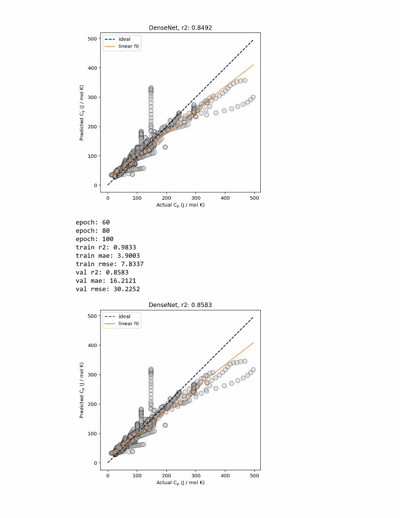
epoch: 60 epoch: 80 epoch: 100 train r2: 0.9833 train mae: 3.9003 train rmse: 7.8337 val r2: 0.8583 val mae: 16.2121 val rmse: 30.2252
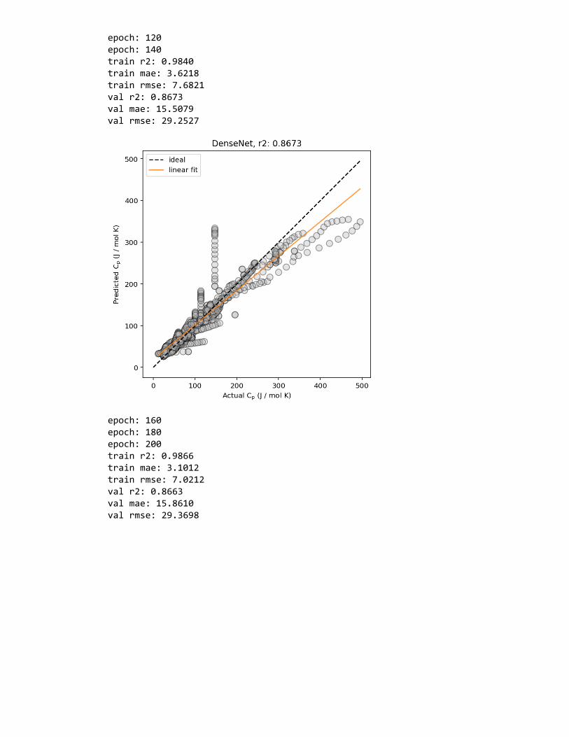
epoch: 120 epoch: 140 train r2: 0.9840 train mae: 3.6218 train rmse: 7.6821 val r2: 0.8673 val mae: 15.5079 val rmse: 29.2527
epoch: 160 epoch: 180 epoch: 200 train r2: 0.9866 train mae: 3.1012 train rmse: 7.0212 val r2: 0.8663 val mae: 15.8610 val rmse: 29.3698
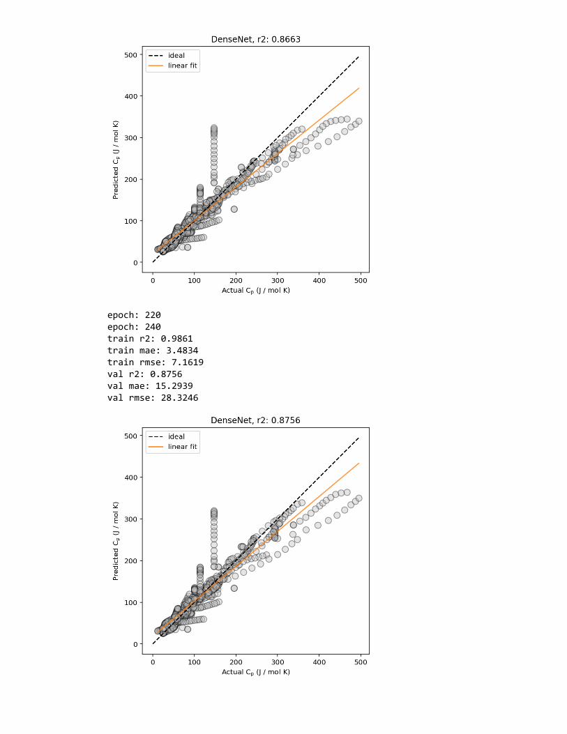
epoch: 220 epoch: 240 train r2: 0.9861 train mae: 3.4834 train rmse: 7.1619 val r2: 0.8756 val mae: 15.2939 val rmse: 28.3246
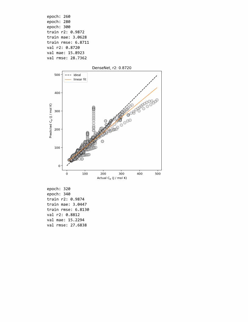
epoch: 260 epoch: 280 epoch: 300 train r2: 0.9872 train mae: 3.0628 train rmse: 6.8711 val r2: 0.8720 val mae: 15.8923 val rmse: 28.7362
epoch: 320 epoch: 340 train r2: 0.9874 train mae: 3.0447 train rmse: 6.8130 val r2: 0.8812 val mae: 15.2294 val rmse: 27.6838
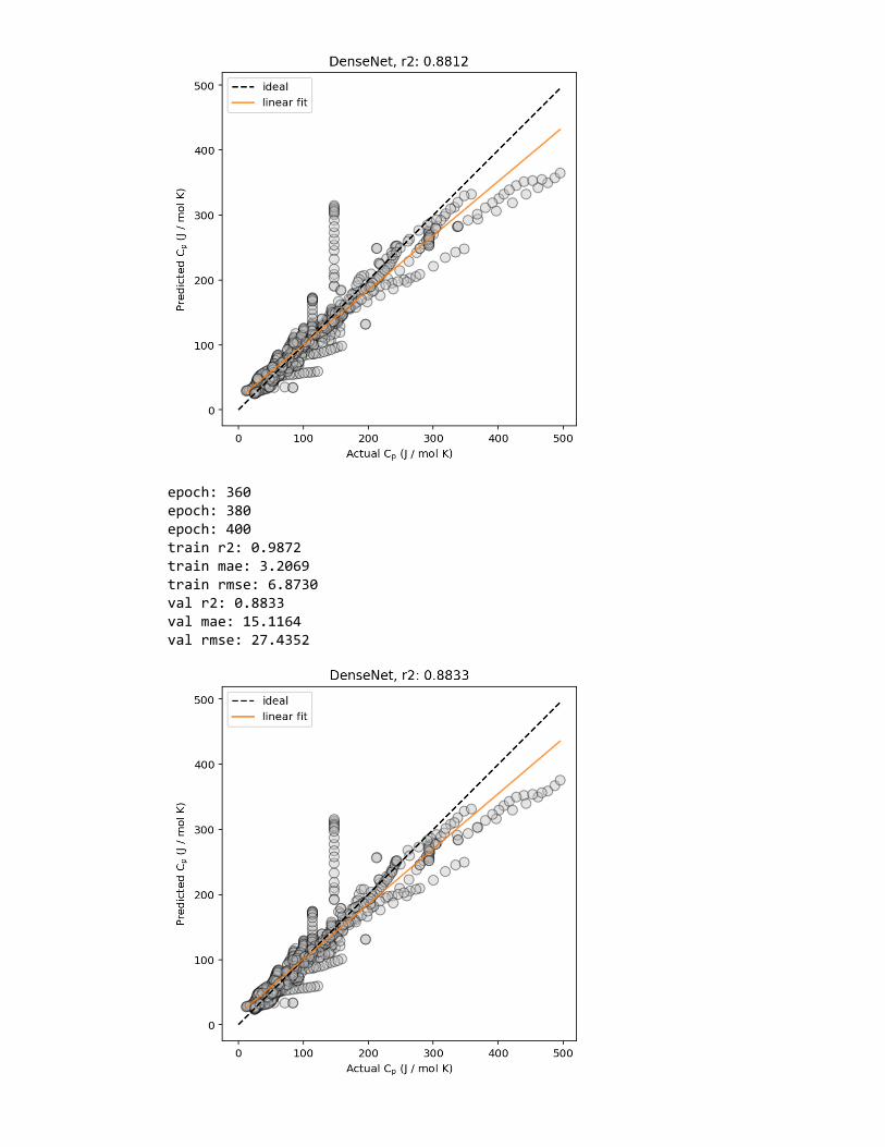
epoch: 360 epoch: 380 epoch: 400 train r2: 0.9872 train mae: 3.2069 train rmse: 6.8730 val r2: 0.8833 val mae: 15.1164 val rmse: 27.4352
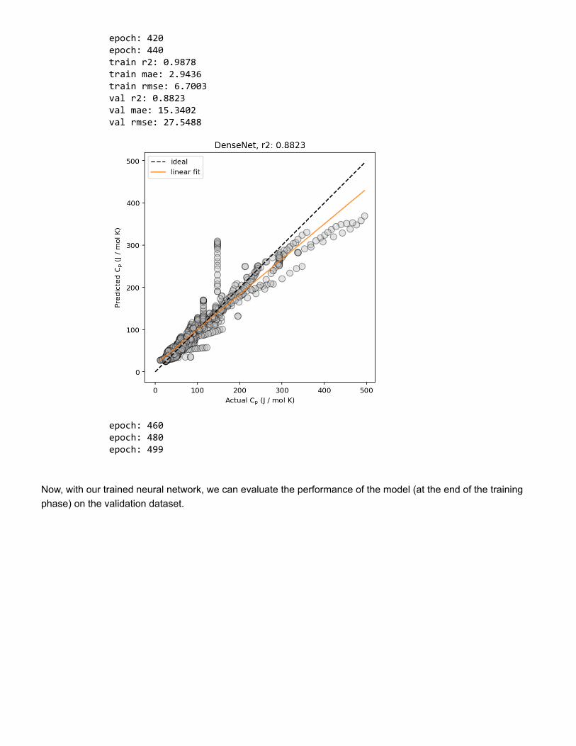
Now, with our trained neural network, we can evaluate the performance of the model (at the end of the trainingphase) on the validation dataset.
epoch: 420 epoch: 440 train r2: 0.9878 train mae: 2.9436 train rmse: 6.7003 val r2: 0.8823 val mae: 15.3402 val rmse: 27.5488
epoch: 460 epoch: 480 epoch: 499
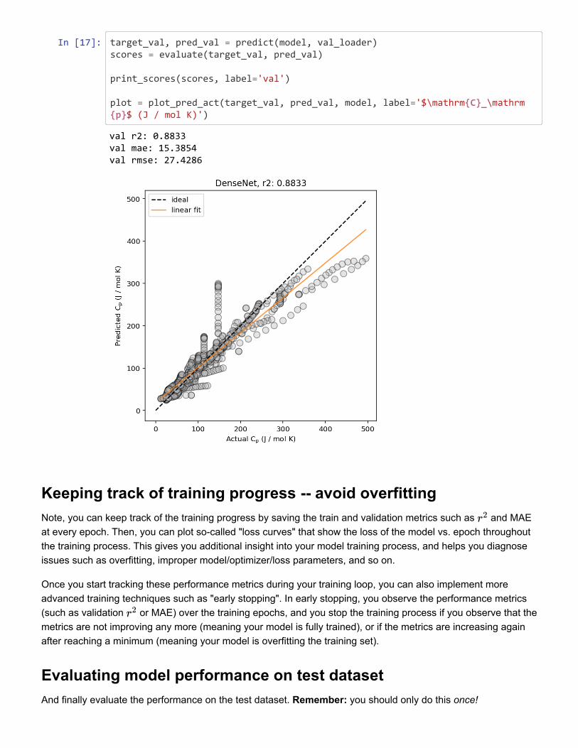
In [17]: target_val, pred_val = predict(model, val_loader)scores = evaluate(target_val, pred_val)
print_scores(scores, label='val')
plot = plot_pred_act(target_val, pred_val, model, label='$\mathrm{C}_\mathrm{p}$ (J / mol K)')
Keeping track of training progress -- avoid overfittingNote, you can keep track of the training progress by saving the train and validation metrics such as and MAEat every epoch. Then, you can plot so-called "loss curves" that show the loss of the model vs. epoch throughoutthe training process. This gives you additional insight into your model training process, and helps you diagnoseissues such as overfitting, improper model/optimizer/loss parameters, and so on.
Once you start tracking these performance metrics during your training loop, you can also implement moreadvanced training techniques such as "early stopping". In early stopping, you observe the performance metrics(such as validation or MAE) over the training epochs, and you stop the training process if you observe that themetrics are not improving any more (meaning your model is fully trained), or if the metrics are increasing againafter reaching a minimum (meaning your model is overfitting the training set).
Evaluating model performance on test datasetAnd finally evaluate the performance on the test dataset. Remember: you should only do this once!
r2
r2
val r2: 0.8833 val mae: 15.3854 val rmse: 27.4286
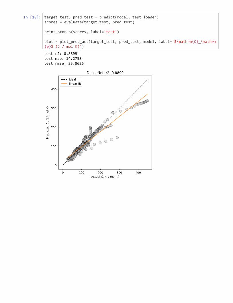
In [18]: target_test, pred_test = predict(model, test_loader)scores = evaluate(target_test, pred_test)
print_scores(scores, label='test')
plot = plot_pred_act(target_test, pred_test, model, label='$\mathrm{C}_\mathrm{p}$ (J / mol K)')
test r2: 0.8899 test mae: 14.2758 test rmse: 25.8626
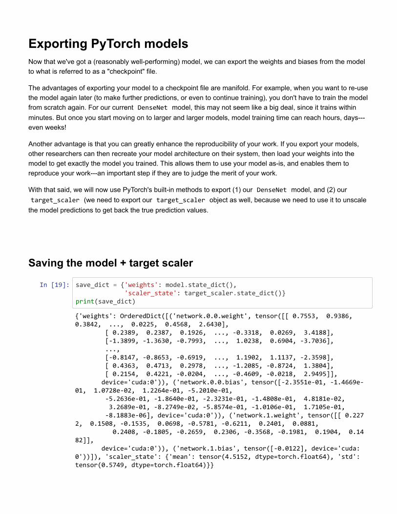
Exporting PyTorch modelsNow that we've got a (reasonably well-performing) model, we can export the weights and biases from the modelto what is referred to as a "checkpoint" file.
The advantages of exporting your model to a checkpoint file are manifold. For example, when you want to re-usethe model again later (to make further predictions, or even to continue training), you don't have to train the modelfrom scratch again. For our current DenseNet model, this may not seem like a big deal, since it trains withinminutes. But once you start moving on to larger and larger models, model training time can reach hours, days---even weeks!
Another advantage is that you can greatly enhance the reproducibility of your work. If you export your models,other researchers can then recreate your model architecture on their system, then load your weights into themodel to get exactly the model you trained. This allows them to use your model as-is, and enables them toreproduce your work---an important step if they are to judge the merit of your work.
With that said, we will now use PyTorch's built-in methods to export (1) our DenseNet model, and (2) our target_scaler (we need to export our target_scaler object as well, because we need to use it to unscale
the model predictions to get back the true prediction values.
Saving the model + target scaler
In [19]: save_dict = {'weights': model.state_dict(), 'scaler_state': target_scaler.state_dict()}print(save_dict)
{'weights': OrderedDict([('network.0.0.weight', tensor([[ 0.7553, 0.9386, 0.3842, ..., 0.0225, 0.4568, 2.6430], [ 0.2389, 0.2387, 0.1926, ..., -0.3318, 0.0269, 3.4188], [-1.3899, -1.3630, -0.7993, ..., 1.0238, 0.6904, -3.7036], ..., [-0.8147, -0.8653, -0.6919, ..., 1.1902, 1.1137, -2.3598], [ 0.4363, 0.4713, 0.2978, ..., -1.2085, -0.8724, 1.3804], [ 0.2154, 0.4221, -0.0204, ..., -0.4609, -0.0218, 2.9495]], device='cuda:0')), ('network.0.0.bias', tensor([-2.3551e-01, -1.4669e-01, 1.0728e-02, 1.2264e-01, -5.2010e-01, -5.2636e-01, -1.8640e-01, -2.3231e-01, -1.4808e-01, 4.8181e-02, 3.2689e-01, -8.2749e-02, -5.8574e-01, -1.0106e-01, 1.7105e-01, -8.1883e-06], device='cuda:0')), ('network.1.weight', tensor([[ 0.2272, 0.1508, -0.1535, 0.0698, -0.5781, -0.6211, 0.2401, 0.0881, 0.2408, -0.1805, -0.2659, 0.2306, -0.3568, -0.1981, 0.1904, 0.1482]], device='cuda:0')), ('network.1.bias', tensor([-0.0122], device='cuda:0'))]), 'scaler_state': {'mean': tensor(4.5152, dtype=torch.float64), 'std': tensor(0.5749, dtype=torch.float64)}}
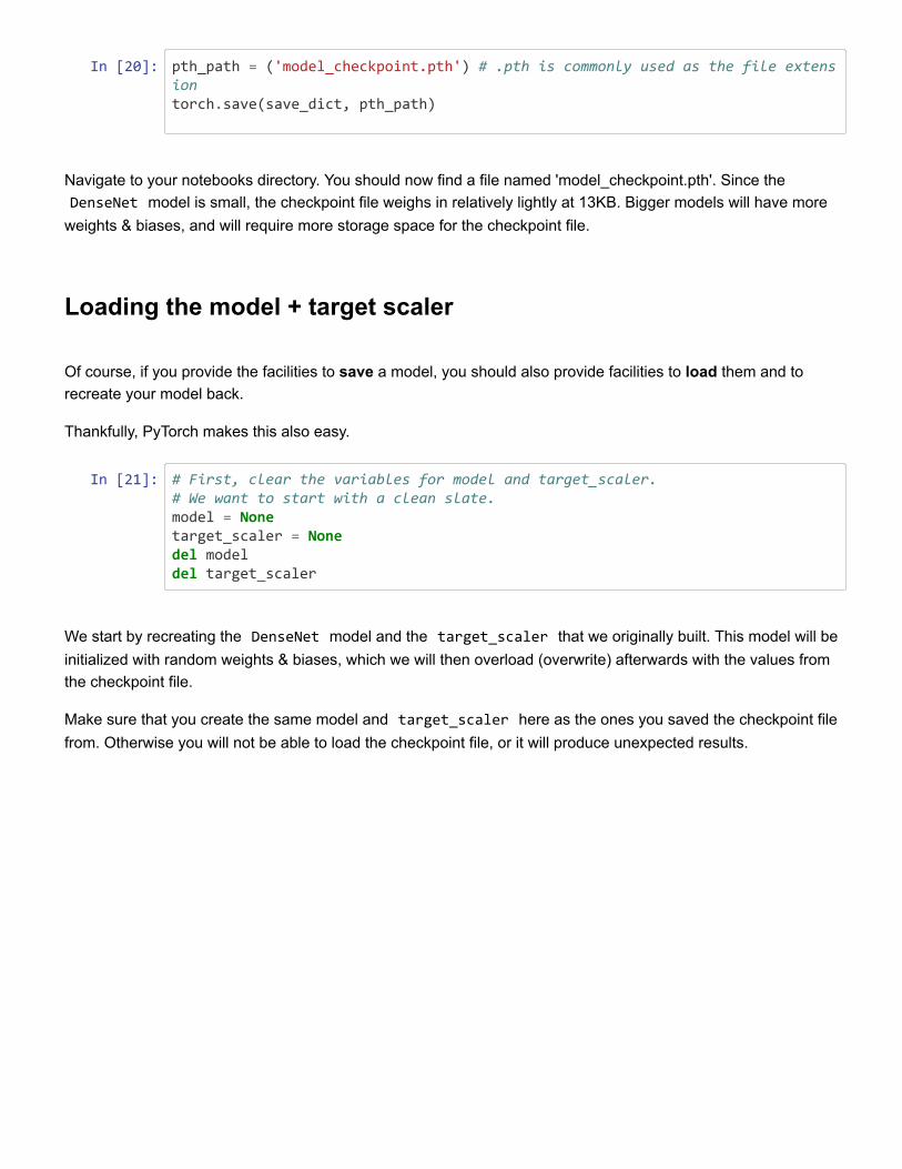
In [20]: pth_path = ('model_checkpoint.pth') # .pth is commonly used as the file extensiontorch.save(save_dict, pth_path)
Navigate to your notebooks directory. You should now find a file named 'model_checkpoint.pth'. Since the DenseNet model is small, the checkpoint file weighs in relatively lightly at 13KB. Bigger models will have more
weights & biases, and will require more storage space for the checkpoint file.
Loading the model + target scaler
Of course, if you provide the facilities to save a model, you should also provide facilities to load them and torecreate your model back.
Thankfully, PyTorch makes this also easy.
In [21]: # First, clear the variables for model and target_scaler.# We want to start with a clean slate.model = Nonetarget_scaler = Nonedel modeldel target_scaler
We start by recreating the DenseNet model and the target_scaler that we originally built. This model will beinitialized with random weights & biases, which we will then overload (overwrite) afterwards with the values fromthe checkpoint file.
Make sure that you create the same model and target_scaler here as the ones you saved the checkpoint filefrom. Otherwise you will not be able to load the checkpoint file, or it will produce unexpected results.
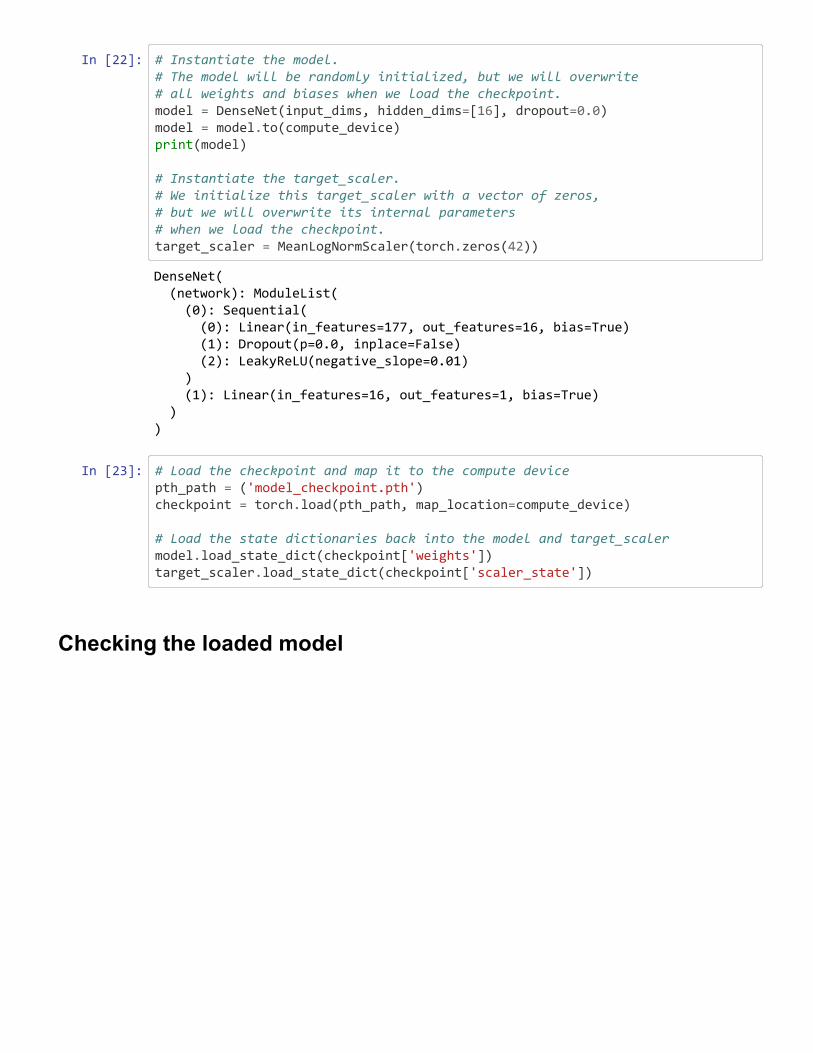
In [22]: # Instantiate the model.# The model will be randomly initialized, but we will overwrite# all weights and biases when we load the checkpoint.model = DenseNet(input_dims, hidden_dims=[16], dropout=0.0)model = model.to(compute_device)print(model)
# Instantiate the target_scaler.# We initialize this target_scaler with a vector of zeros,# but we will overwrite its internal parameters# when we load the checkpoint.target_scaler = MeanLogNormScaler(torch.zeros(42))
In [23]: # Load the checkpoint and map it to the compute devicepth_path = ('model_checkpoint.pth')checkpoint = torch.load(pth_path, map_location=compute_device)
# Load the state dictionaries back into the model and target_scalermodel.load_state_dict(checkpoint['weights'])target_scaler.load_state_dict(checkpoint['scaler_state'])
Checking the loaded model
DenseNet( (network): ModuleList( (0): Sequential( (0): Linear(in_features=177, out_features=16, bias=True) (1): Dropout(p=0.0, inplace=False) (2): LeakyReLU(negative_slope=0.01) ) (1): Linear(in_features=16, out_features=1, bias=True) ) )
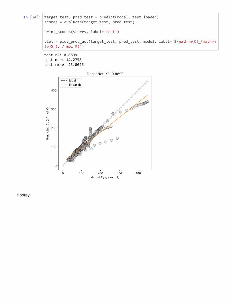
In [24]: target_test, pred_test = predict(model, test_loader)scores = evaluate(target_test, pred_test)
print_scores(scores, label='test')
plot = plot_pred_act(target_test, pred_test, model, label='$\mathrm{C}_\mathrm{p}$ (J / mol K)')
Hooray!
test r2: 0.8899 test mae: 14.2758 test rmse: 25.8626
Visualizing resultsHere, we will show some typical examples of visualizations that are used often to show results in ML studies inmaterials science.
We will use the open-source ML_figures package (https://github.com/kaaiian/ML_figures) and the exampledata provided by the package to generate these figures.
In [1]: import osimport numpy as npimport pandas as pdimport matplotlib.pyplot as plt%matplotlib inline %config InlineBackend.figure_format='retina'
# Import the ML_figures package and the figure-plotting functionsfrom ML_figures.figures import act_predfrom ML_figures.figures import residual, residual_histfrom ML_figures.figures import loss_curvefrom ML_figures.figures import element_prevalence
Predicted vs. actual value plotsThese plots, you have already seen before in the previous notebooks.
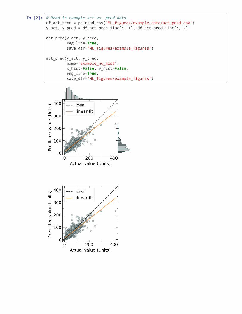
In [2]: # Read in example act vs. pred datadf_act_pred = pd.read_csv('ML_figures/example_data/act_pred.csv')y_act, y_pred = df_act_pred.iloc[:, 1], df_act_pred.iloc[:, 2]
act_pred(y_act, y_pred, reg_line=True, save_dir='ML_figures/example_figures')
act_pred(y_act, y_pred, name='example_no_hist', x_hist=False, y_hist=False, reg_line=True, save_dir='ML_figures/example_figures')
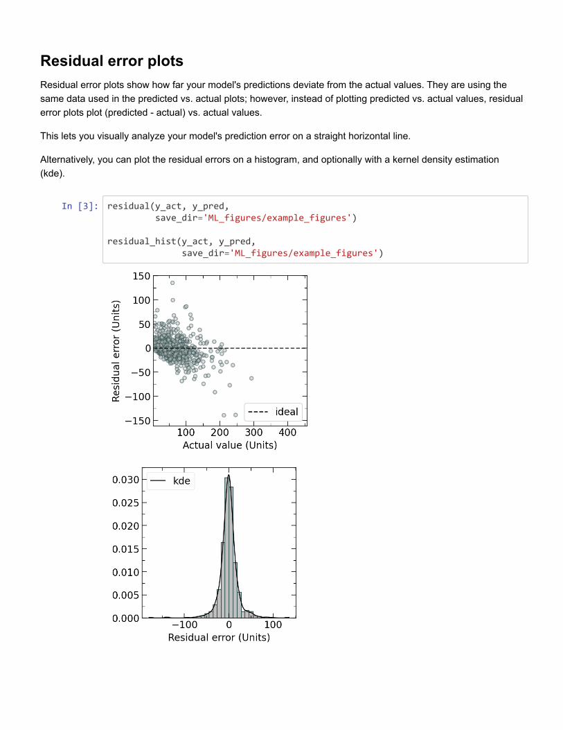
Residual error plotsResidual error plots show how far your model's predictions deviate from the actual values. They are using thesame data used in the predicted vs. actual plots; however, instead of plotting predicted vs. actual values, residualerror plots plot (predicted - actual) vs. actual values.
This lets you visually analyze your model's prediction error on a straight horizontal line.
Alternatively, you can plot the residual errors on a histogram, and optionally with a kernel density estimation(kde).
In [3]: residual(y_act, y_pred, save_dir='ML_figures/example_figures')
residual_hist(y_act, y_pred, save_dir='ML_figures/example_figures')
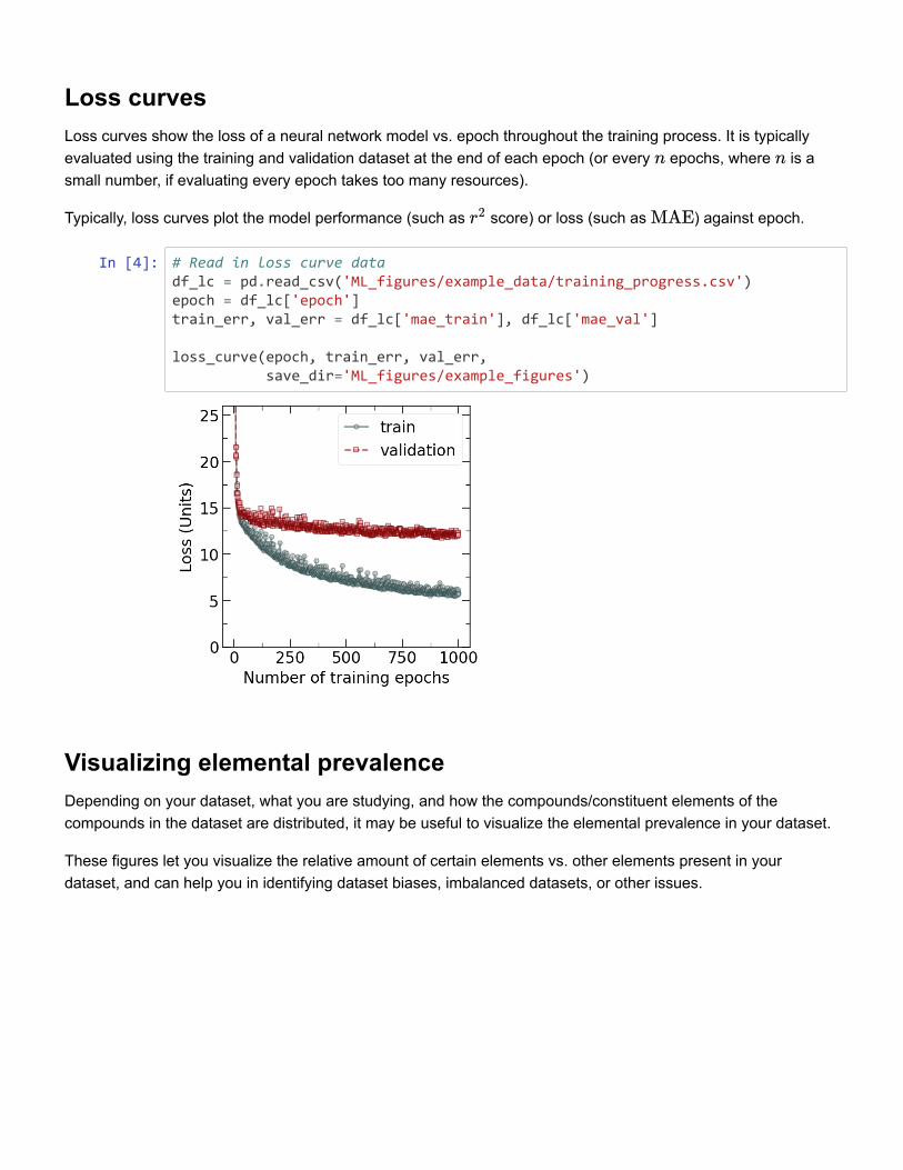
Loss curvesLoss curves show the loss of a neural network model vs. epoch throughout the training process. It is typicallyevaluated using the training and validation dataset at the end of each epoch (or every epochs, where is asmall number, if evaluating every epoch takes too many resources).
Typically, loss curves plot the model performance (such as score) or loss (such as ) against epoch.
n n
r2 MAE
In [4]: # Read in loss curve datadf_lc = pd.read_csv('ML_figures/example_data/training_progress.csv')epoch = df_lc['epoch']train_err, val_err = df_lc['mae_train'], df_lc['mae_val']
loss_curve(epoch, train_err, val_err, save_dir='ML_figures/example_figures')
Visualizing elemental prevalenceDepending on your dataset, what you are studying, and how the compounds/constituent elements of thecompounds in the dataset are distributed, it may be useful to visualize the elemental prevalence in your dataset.
These figures let you visualize the relative amount of certain elements vs. other elements present in yourdataset, and can help you in identifying dataset biases, imbalanced datasets, or other issues.
In [5]: # Visualize element prevalenceformula = df_act_pred.iloc[:, 0]
element_prevalence(formula, save_dir='ML_figures/example_figures', log_scale=False)element_prevalence(formula, save_dir='ML_figures/example_figures', name='example_log', log_scale=True)
plt.rcParams.update({'font.size': 12})element_prevalence(formula, save_dir='ML_figures/example_figures', ptable_fig=False, log_scale=False)element_prevalence(formula, save_dir='ML_figures/example_figures', name='example_log', ptable_fig=False, log_scale=True)
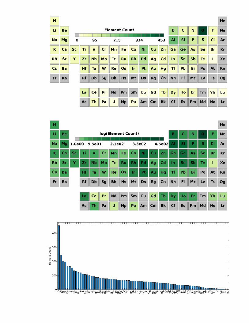
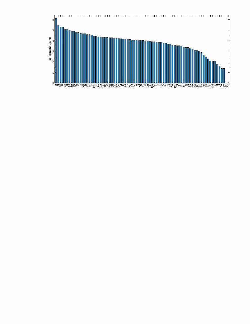

download fileview on ChemRxivBestPractices paper - SI.pdf (3.00 MiB)