machine learning for image classification ----part i: traditional … · machine learning for image...
TRANSCRIPT

Machine Learning for Image Classification----Part I: Traditional Approaches
Jianping Fan
Dept of Computer Science
UNC-Charlotte
Course Website: http://webpages.uncc.edu/jfan/itcs5152.html
Slide credit: L. Lazebnik

Pipeline for Traditional Image Classification System
Training Image Set
Feature Extraction
Classifier Training Classifier
Offline Training
Online Testing
Test Image
Feature Extraction
Classifier
Flower
Garden
Nature
……….
predictions

Machine Learning for Image Classification
• Apply a prediction function (classifier) to a feature
representation of the image to get the desired output:
f( ) = “apple”
f( ) = “tomato”
f( ) = “cow”Slide credit: L. LazebnikFeature Extraction for Image Representation
Classifier
Prediction from Classifier
according to Image Representation

Various Types of Some Classifiers
• K-nearest neighbor
• SVM
• Decision Trees
• Neural networks
• GMM & Naïve Bayes
• Boosting
• Logistic regression
• Randomized Forests
• RBMs
• Etc.
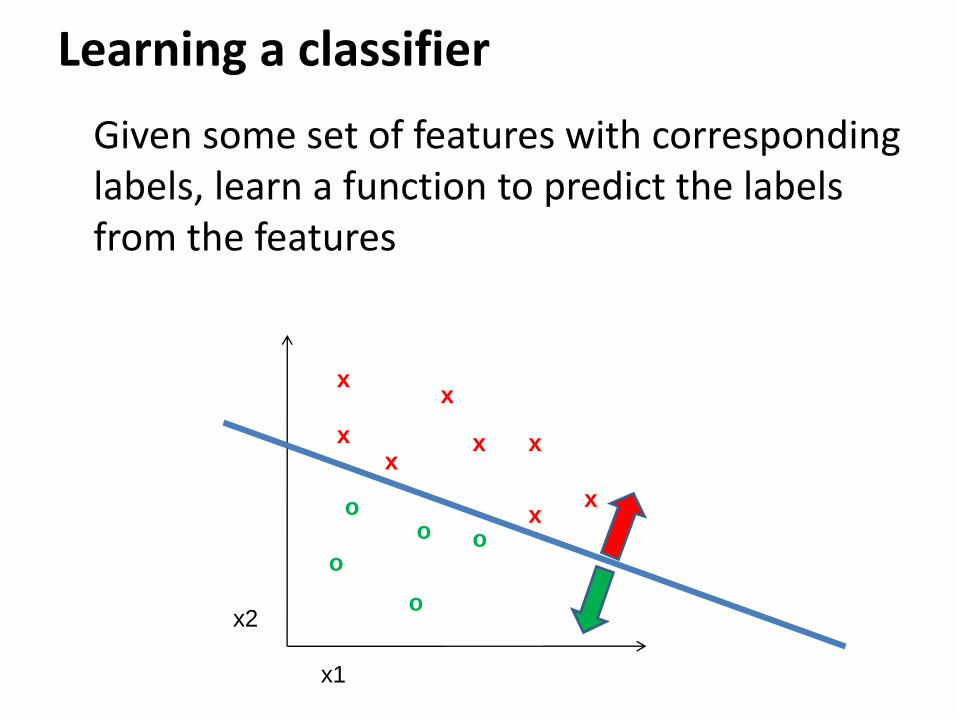
Learning a classifier
Given some set of features with corresponding labels, learn a function to predict the labels from the features
x x
xx
x
x
x
x
oo
o
o
o
x2
x1

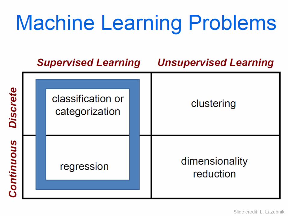
Classification
• Assign input vector to one of two or more
classes
• Any decision rule divides input space into
decision regions separated by decision
boundaries
Slide credit: L. Lazebnik

Nearest Neighbor Classifier
• Assign label of nearest training data point to each test data
point
Voronoi partitioning of feature space for two-category 2D and 3D data
from Duda et al.
Source: D. Lowe

K-nearest neighbor
x x
xx
x
x
x
x
o
oo
o
o
o
o
x2
x1
+
+

1-nearest neighbor
x x
xx
x
x
x
x
o
oo
o
o
o
o
x2
x1
+
+

3-nearest neighbor
x x
xx
x
x
x
x
o
oo
o
o
o
o
x2
x1
+
+

5-nearest neighbor
x x
xx
x
x
x
x
o
oo
o
o
o
o
x2
x1
+
+

13
Ways of rescaling for KNN
Normalized L1 distance:
Scale by IG:
Modified value distance
metric:

14
Ways of rescaling for KNN
Dot product:
Cosine distance:
TFIDF weights for text: for doc j, feature i: xi=tfi,j * idfi :
#occur. of
term i in
doc j
#docs in
corpus
#docs in corpus
that contain
term i

15
Combining distances to neighbors
Standard KNN:
Distance-weighted KNN:
|}':')','{(|)',(
))(,(maxargˆ
yyDyxDyC
xNeighborsyCy y
)',(1)',(
))',(()',(
))(,(maxargˆ
}':')','{(
xxxxSIM
xxSIMDyC
xNeighborsyCy
yyDyx
y
}':')','{(
))',(1( 1 )',(yyDyx
xxSIMDyC

Definition of Class Centroid
Where Dc is the set of all data points that belong to class c and v(d) is the vector space representation of one specific data point d.
Note that centroid will in general not be a unit vector even when the inputs are unit vectors.
16
m (c) =
1
| Dc |
v (d)
d ÎDc
å
Sec.14.2

17
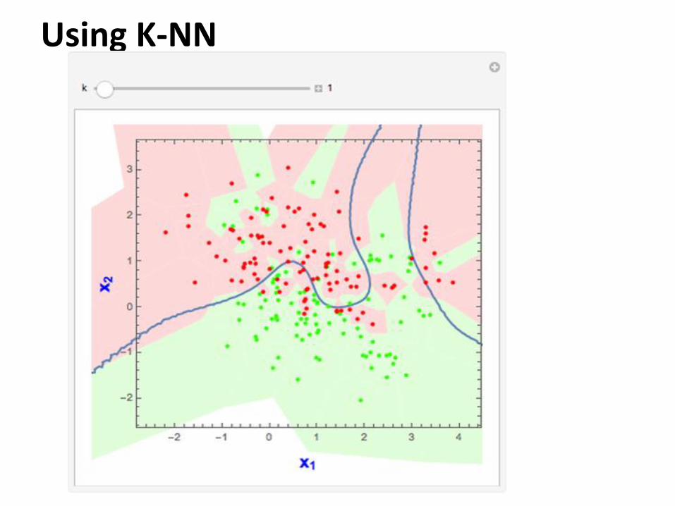
k Nearest Neighbor Classification
kNN = k Nearest Neighbor
To classify a document d:
Define k-neighborhood as the k nearest neighbors of d
Pick the majority class label in the k-neighborhood
For larger k can roughly estimate P(c|d) as #(c)/k
Sec.14.3

Using K-NN

Using K-NN

20
Nearest-Neighbor Learning
Learning: just store the labeled training examples D
Testing instance x (under 1NN): Compute similarity between x and all examples in D.
Assign x the category of the most similar example in D.
Does not compute anything beyond storing the examples
Also called: Case-based learning
Memory-based learning
Lazy learning
Rationale of kNN: contiguity hypothesis
Sec.14.3

21
k Nearest Neighbor
Using only the closest example (1NN) subject to errors due to: A single atypical example.
Noise (i.e., an error) in the category label of a single training example.
More robust: find the k examples and return the majority category of these k
k is typically odd to avoid ties; 3 and 5 are most common
Sec.14.3

22
Nearest Neighbor with Inverted Index
• Naively finding nearest neighbors requires a linear search through |D| documents in collection
• But determining k nearest neighbors is the same as determining the k best retrievals using the test document as a query to a database of training documents.
• Use standard vector space inverted index methods to find the k nearest neighbors.
• Testing Time: O(B|Vt|) where B is the average number of training documents in which a test-document word appears.
– Typically B << |D|
Sec.14.3

23
kNN: Discussion
• No feature selection necessary
• No training necessary
• Scales well with large number of classes
– Don’t need to train n classifiers for n classes
• Classes can influence each other
– Small changes to one class can have ripple effect
• Done naively, very expensive at test time
• In most cases it’s more accurate than NB or Rocchio
Sec.14.3

Using K-NN
Using K-NN

Basic Classification
!!!!$$$!!!!
Spam filtering
Input Output
BinarySpam vs. Not-Spam
)()|()()|(
)()|()|(
spamnotPspamnotxPspamPspamxP
spamPspamxPxspamp
)()|()()|(
)()|()|(
spamnotPspamnotxPspamPspamxP
spamnotPspamnotxPxspamnotp

Basic Classification
Characterrecognition
Input Output
CMulti-Class
C vs. other 25 characters
c
cPcxP
CPCxPxCP
)()|(
)()|()|(

Structured Classification
Handwritingrecognition
Input Output
3D objectrecognition
buildingtree
brace
Structured outputGraph Model

Overview of Bayesian DecisionTest patient
(a) Group assignment for test patient;
(b) Prior knowledge about the assigned group
(c) Properties of the assigned group (sick or healthy)
c
cPcxP
CPCxPxCP
)()|(
)()|()|(

Overview of Bayesian DecisionTest patient
Observations: Bayesian decision process is a data modeling
process, e.g., estimate the data distribution
K-means clustering: any relationship & difference?

Bayes’ Rule:
)(
)()|()|(
dP
hPhdPdhp
) data the seen having after hypothesis ofty (probabili posterior
data) the ofy probabilit (marginal evidence data
is hypothesis the if data the ofty (probabili likelihood
data)any seeing before hypothesis ofty (probabili belief prior
dh
h
h
:)|(
:)()|()(
true) :)|(
:)(
dhP
hPhdPdP
hdP
hP
h
Who is who in Bayes’ rule
sidesboth on
y probabilitjoint same the
),(),(
)()|()()|(
grearrangin -
(model) hypothesish
datad
rule Bayes' ingUnderstand
hdPhdP
hPhdPdPdhp
h
hPhdP
hPhdP
)()|(
)()|(
normalization

Bayes’ Rule:
)(
)()|()|(
dP
hPhdPdhp
h
hPhdP
hPhdP
)()|(
)()|(
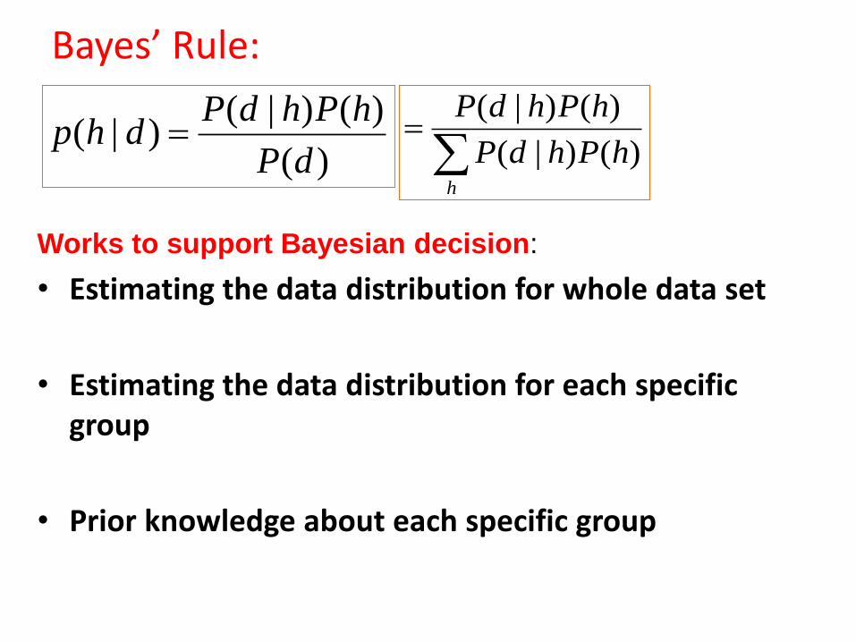
P(d|h): data distribution
of group h
P(h): importance
of group h
data distribution of whole
data set
Bayes’ Rule:
)(
)()|()|(
dP
hPhdPdhp
h
hPhdP
hPhdP
)()|(
)()|(
• Estimating the data distribution for whole data set
• Estimating the data distribution for each specific group
• Prior knowledge about each specific group
Works to support Bayesian decision:

Gaussian Mixture Model (GMM)
How to estimate the distribution for a given dataset?

Gaussian Mixture Model (GMM)

Gaussian Mixture Model (GMM)
What does GMM mean?
100 = 5*10 + 2*20 + 2*5
100 = 100*1
100 = 10*10
……………….
GMM may prefer larger K with ``smaller” Gaussians

Gaussian Mixture Model (GMM)

Gaussian Mixture Model (GMM)
Real Data Distribution
Any complex function (distribution) can be approximated by
using a limited number of other functions (distributions)
such as Gaussian functions.

Gaussian Mixture Model (GMM)
Real Data Distribution
Approximated Gaussian functions

Gaussian Function
2
2
1 ( )( | , ) exp
22
xf x
Why we select Gaussian function not others?

When one Gaussian Function is used to
approximate data distribution
a likelihood function (often simply
the likelihood) is a function of
the parameters of a statistical model
Given a dataset, how to use likelihood
function to determine Gaussian parameters?

Matching between Gaussian Function and Samples
2
2
1 ( )( | , ) exp
22
xf x
Sampling1 2( , , , )T
nx x xx
ˆ ? 2ˆ ?
2~ ( , )X N

Maximum Likelihood
Sampling1 2( , , , )T
nx x xx
2( | , )f x
/ 2 2
21
2
( )1exp
2 2
n ni
i
x
2
2
1 ( )( | , ) exp
22
xf x
Given x, it is a
function of and 2
2( , | ) xL
We want to maximize it.
1
2 2( | , ) ( | , )nf x f x

Log-Likelihood Function/ 2 2
12 2
( )1exp
2 2
n ni
i
x
2( , | ) xL
2( , | ) xl 2log ( , | ) xL2
12 2
( )1log
2 2 2
ni
i
xn
22
2 2 21
2
1
1log log
2 22
22
n n
i i
i i
n n nx x
Maximizethis instead
By setting
2( , | ) 0
xl 2
2( , | ) 0
xland

Max. the Log-Likelihood Function
22
2 2 21
2
1
1log log
2 22
22
n n
i i
i i
n n nx x
2
21
2( , 0
1| )
n
i
i
nx
xl
2( , | ) xl
1
ˆ1 n
i
i
xn

Max. the Log-Likelihood Function22
2 2 21
2
1
1log log
2 22
22
n n
i i
i i
n n nx x
22
2 2 4 41
2
14
1( , | ) 0
2 2 2
n n
i i
i i
n nx x
xl
2( , | ) xl
1
ˆ1 n
i
i
xn
2 22
1 1
2n n
i i
i i
n x x n
2 2
2
1 1 1
2 1n n n
i i i
i i i
x x xn n
1
22 21ˆˆ
n
i
i
xn

When multiple Gaussian Functions are used
to approximate data distribution
a likelihood function (often simply
the likelihood) is a function of
the parameters of a statistical model
Given a dataset, how to use likelihood
function to determine parameters for multiple
Gaussian functions?

Gaussian Mixture Model (GMM)
Parameters to be estimated:
Training Set:
We assume K is available (or pre-defined)! Algorithms
may always prefer larger K!

Gaussian Mixture Models
• Rather than identifying clusters by “nearest” centroids
• Fit a Set of k Gaussians to the data • Maximum Likelihood over a mixture model

GMM example

Mixture Models
• Formally a Mixture Model is the weighted sum of a number of pdfs where the weights are determined by a distribution,

Gaussian Mixture Models
• GMM: the weighted sum of a number of Gaussians where the weights are determined by a distribution,

Maximum Likelihood over a GMM
• As usual: Identify a likelihood function
• Log-likelihood

Maximum Likelihood of a GMM
• Optimization of means.
k=1, …..K

Maximum Likelihood of a GMM
• Optimization of covariance
k=1, …..K

Maximum Likelihood of a GMM
• Optimization of mixing term

EM for GMMs
• Initialize the parameters
– Evaluate the log likelihood
• Expectation-step: Evaluate the responsibilities
• Maximization-step: Re-estimate Parameters
– Evaluate the log likelihood
– Check for convergence

EM for GMMs
• E-step: Evaluate the Responsibilities

EM for GMMs• M-Step: Re-estimate Parameters

EM for GMMs
• Evaluate the log likelihood
and check for convergence of either the parameters or the
log likelihood. If the convergence criterion is not satisfied,
return to E-Step.

Linear SVM
Binary case

Linear SVM

Linear SVM

Linear SVM

Linear SVM

Linear SVM: Find Closest Points in Convex Hulls
c
d

Plane Bisect Closest Points
d
c
wT x + b =0
wT x + b =1
wT x + b =-1

• Binary classification can be viewed as the task of separating classes in feature space:
wTx + b = 0
wTx + b < 0wTx + b > 0
f(x) = sign(wTx + b)
Linear Discriminant Function

• How would you classify these points using a linear discriminant function in order to minimize the error rate?
Linear Discriminant Functiondenotes +1
denotes -1
x1
x2
Infinite number of answers!

• How would you classify these points using a linear discriminant function in order to minimize the error rate?
Linear Discriminant Functiondenotes +1
denotes -1
x1
x2
Infinite number of answers!

• How would you classify these points using a linear discriminant function in order to minimize the error rate?
Linear Discriminant Functiondenotes +1
denotes -1
x1
x2
Infinite number of answers!

x1
x2• How would you classify these
points using a linear discriminant function in order to minimize the error rate?
Linear Discriminant Functiondenotes +1
denotes -1
Infinite number of answers!
Which one is the best?

Large Margin Linear Classifier
“safe zone”• The linear discriminant
function (classifier) with the maximum margin is the best
Margin is defined as the
width that the boundary
could be increased by before
hitting a data point
Why it is the best?
Robust to outliners and thus
strong generalization ability
Margin
x1
x2
denotes +1
denotes -1

Large Margin Linear Classifier
• Given a set of data points:
With a scale transformation
on both w and b, the above
is equivalent to
x1
x2
denotes +1
denotes -1
For 1, 0
For 1, 0
T
i i
T
i i
y b
y b
w x
w x
{( , )}, 1,2, ,i iy i nx , where
For 1, 1
For 1, 1
T
i i
T
i i
y b
y b
w x
w x

Large Margin Linear Classifier
• We know that
The margin width is:
x1
x2
denotes +1
denotes -1
1
1
T
T
b
b
w x
w x
Margin
x+
x+
x-
( )
2 ( )
M
x x n
wx x
w w
n
Support Vectors
w . (x+-x-) = 2

What we know:
• w . x+ + b = +1
• w . x- + b = -1
• w . (x+-x-) = 2
X-
x+
ww
wxxM
2)(
M=Margin Width

Large Margin Linear Classifier
• Formulation:
x1
x2
denotes +1
denotes -1
Margin
x+
x+
x-n
such that
2maximize
w
For 1, 1
For 1, 1
T
i i
T
i i
y b
y b
w x
w x

Large Margin Linear Classifier
• Formulation:
x1
x2
denotes +1
denotes -1
Margin
x+
x+
x-n
21minimize
2w
such that
For 1, 1
For 1, 1
T
i i
T
i i
y b
y b
w x
w x
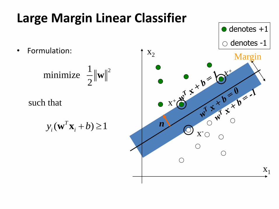
Large Margin Linear Classifier
• Formulation:
x1
x2
denotes +1
denotes -1
Margin
x+
x+
x-n( ) 1T
i iy b w x
21minimize
2w
such that

Solving the Optimization Problem
( ) 1T
i iy b w x
21minimize
2w
s.t.
Quadratic
programming
with linear
constraints
2
1
1minimize ( , , ) ( ) 1
2
nT
p i i i i
i
L b y b
w w w x
s.t.
Lagrangian
Function
0i

Solving the Optimization Problem
2
1
1minimize ( , , ) ( ) 1
2
nT
p i i i i
i
L b y b
w w w x
s.t. 0i
0pL
b
0pL
w 1
n
i i i
i
y
w x
1
0n
i i
i
y

Solving the Optimization Problem
2
1
1minimize ( , , ) ( ) 1
2
nT
p i i i i
i
L b y b
w w w x
s.t. 0i
1 1 1
1maximize
2
n n nT
i i j i j i j
i i j
y y
x x
s.t. 0i 1
0n
i i
i
y
, and
Lagrangian Dual
Problem

Solving the Optimization Problem
The solution has the form:
( ) 1 0T
i i iy b w x
From KKT condition, we know:
Thus, only support vectors have 0i
1 SV
n
i i i i i i
i i
y y
w x x
get from ( ) 1 0,
where is support vector
T
i i
i
b y b w x
x
x1
x2
x+
x+
x-
Support Vectors

Solving the Optimization Problem
SV
( ) T T
i i
i
g b b
x w x x x
The linear discriminant function is:
Notice it relies on a dot product between the test point x
and the support vectors xi
Also keep in mind that solving the optimization problem
involved computing the dot products xiTxj between all pairs
of training points

Non-ideal Situations
Data partitioning has mistakes
x1
x2
denotes +1
denotes -1
12
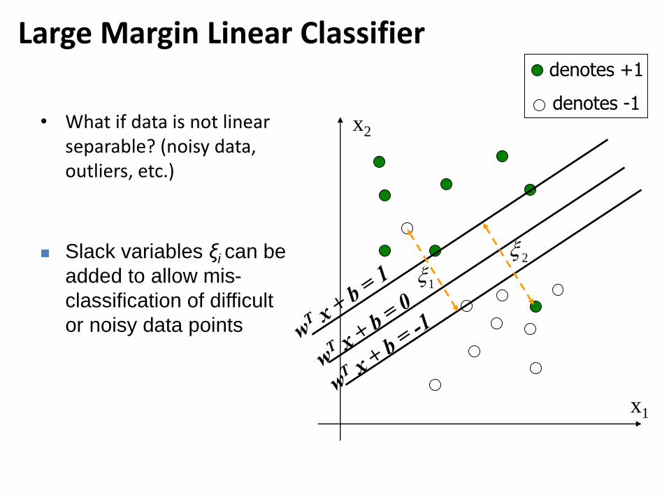
Large Margin Linear Classifier
• What if data is not linear separable? (noisy data, outliers, etc.)
Slack variables ξi can be
added to allow mis-
classification of difficult
or noisy data points
x1
x2
denotes +1
denotes -1
12

Introducing slack variables
• Slack variables are constrained to be non-negative. When they are greater than zero they allow us to cheat by putting the plane closer to the datapoint than the margin. So we need to minimize the amount of cheating. This means we have to pick a value for lamba (this sounds familiar!)
possibleassmallasand
callforwith
casesnegativeforb
casespositiveforb
c
c
c
cc
cc
2
||||
0
1.
1.
2w
xw
xw

A picture of the best plane with a slack variable

Large Margin Linear Classifier
Formulation:
( ) 1T
i i iy b w x
2
1
1minimize
2
n
i
i
C
w
such that
0i
Parameter C can be viewed as a way to control over-fitting.

Non-linear SVMs Datasets that are linearly separable with noise work out
great:
0 x
0 x
x2
0 x
But what are we going to do if the dataset is just too hard?
How about… mapping data to a higher-dimensional space:
This slide is courtesy of www.iro.umontreal.ca/~pift6080/documents/papers/svm_tutorial.ppt

Nonlinear Classification
Linear Separable
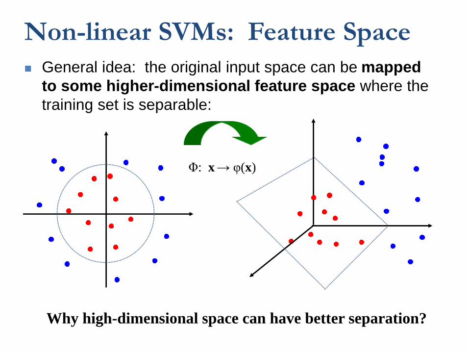
Non-linear SVMs: Feature Space
General idea: the original input space can be mapped
to some higher-dimensional feature space where the
training set is separable:
Φ: x→ φ(x)
Why high-dimensional space can have better separation?

Transforming the Data
• Computation in the feature space can be costly because it is high dimensional– The feature space is typically infinite-dimensional!
• The kernel trick comes to rescue
f( )
f( )
f( )f( )f( )
f( )
f( )f( )
f(.)f( )
f( )
f( )
f( )f( )
f( )
f( )
f( )f( )
f( )
Feature spaceInput space

Nonlinear SVMs: The Kernel Trick
With this mapping, our discriminant function is now:
SV
( ) ( ) ( ) ( )T T
i i
i
g b bf f f
x w x x x
No need to know this mapping explicitly, because we only use
the dot product of feature vectors in both the training and test.
A kernel function is defined as a function that corresponds to
a dot product of two feature vectors in some expanded feature
space:
( , ) ( ) ( )T
i j i jK f fx x x x

Nonlinear SVMs: The Kernel Trick
2-dimensional vectors x=[x1 x2];
let K(xi,xj)=(1 + xiTxj)
2,
Need to show that K(xi,xj) = φ(xi)Tφ(xj):
K(xi,xj)=(1 + xiTxj)
2,
= 1+ xi12xj1
2 + 2 xi1xj1 xi2xj2+ xi22xj2
2 + 2xi1xj1 + 2xi2xj2
= [1 xi12 √2 xi1xi2 xi2
2 √2xi1 √2xi2]T [1 xj1
2 √2 xj1xj2 xj22 √2xj1 √2xj2]
= φ(xi)Tφ(xj), where φ(x) = [1 x1
2 √2 x1x2 x22 √2x1 √2x2]
An example:
This slide is courtesy of www.iro.umontreal.ca/~pift6080/documents/papers/svm_tutorial.ppt

Nonlinear SVMs: The Kernel Trick
Linear kernel:
2
2( , ) exp( )
2
i j
i jK
x xx x
( , ) T
i j i jK x x x x
( , ) (1 )T p
i j i jK x x x x
0 1( , ) tanh( )T
i j i jK x x x x
Examples of commonly-used kernel functions:
Polynomial kernel:
Gaussian (Radial-Basis Function (RBF) ) kernel:
Sigmoid:
In general, functions that satisfy Mercer’s condition can be
kernel functions.

Nonlinear SVM: Optimization
Formulation: (Lagrangian Dual Problem)
1 1 1
1maximize ( , )
2
n n n
i i j i j i j
i i j
y y K
x x
such that0 i C
1
0n
i i
i
y
The solution of the discriminant function is
SV
( ) ( , )i i
i
g K b
x x x
The optimization technique is the same.

Support Vector Machine: Algorithm
• 1. Choose a kernel function
• 2. Choose a value for C
• 3. Solve the quadratic programming problem (many software packages available)
• 4. Construct the discriminant function from the support vectors

Some Issues
• Choice of kernel- Gaussian or polynomial kernel is default- if ineffective, more elaborate kernels are needed- domain experts can give assistance in formulating appropriate similarity measures
• Choice of kernel parameters- e.g. σ in Gaussian kernel- σ is the distance between closest points with different classifications - In the absence of reliable criteria, applications rely on the use of a
validation set or cross-validation to set such parameters.
• Optimization criterion – Hard margin v.s. Soft margin
- a lengthy series of experiments in which various parameters are tested

Strengths and Weaknesses of SVM
• Strengths– Training is relatively easy
• No local optimal, unlike in neural networks
– It scales relatively well to high dimensional data– Tradeoff between classifier complexity and error can
be controlled explicitly– Non-traditional data like strings and trees can be
used as input to SVM, instead of feature vectors– By performing logistic regression (Sigmoid) on the
SVM output of a set of data can map SVM output to probabilities.
• Weaknesses– Need to choose a “good” kernel function.

Summary: Support Vector Machine
• 1. Large Margin Classifier
– Better generalization ability & less over-fitting
• 2. The Kernel Trick
– Map data points to higher dimensional space in order to make them linearly separable.
– Since only dot product is used, we do not need to represent the mapping explicitly.

What about multi-class SVMs?
• Unfortunately, there is no “definitive” multi-
class SVM formulation
• In practice, we have to obtain a multi-class
SVM by combining multiple two-class SVMs
• One vs. others• Traning: learn an SVM for each class vs. the others
• Testing: apply each SVM to test example and assign to it the
class of the SVM that returns the highest decision value
• One vs. one• Training: learn an SVM for each pair of classes
• Testing: each learned SVM “votes” for a class to assign to
the test example
Slide credit: L. Lazebnik

Three Approaches to K-Class SVM
Three Approaches to K-Class SVM
K one-versus-residue (OVR) binary SVM
Advantages
Disadvantages

Three Approaches to K-Class SVM
Advantages
Disadvantages

Three Approaches to K-Class SVM
One K-Class SVM

K-class SVM
1
2 3

Multi-class SVM
Intuitive formulation: without
regularization / for the separable case
Primal problem: QP
Solved in the dual formulation, also Quadratic Program
Main advantage: Sparsity (but not systematic)
• Speed with SMO (heuristic use of sparsity)
• Sparse solutions
Drawbacks:
• Need to recalculate or store xiTxj
• Outputs not probabilities

Real world classification problems
Object
recognition
100
Automated protein
classification
50
300-600
Digit recognition
10
Phoneme recognition
[Waibel, Hanzawa, Hinton,Shikano, Lang 1989]
htt
p:/
/ww
w.g
lue.
um
d.e
du
/~zh
elin
/rec
og.h
tml
• The number of classes is sometimes big
• The multi-class algorithm can be heavy

Combining binary classifiers
One-vs-all For each class build a classifier for that class vs the rest
• Often very imbalanced classifiers (use asymmetric regularization)
All-vs-all For each class build a classifier for that class vs the rest
• A priori a large number of classifiers to build but…
• The pairwise classification are way much faster
• The classifications are balanced (easier to find the best regularization)
… so that in many cases it is clearly faster than one-vs-all

Confusion Matrix
• Visualize which classes are more
difficult to learn
• Can also be used to compare two
different classifiers
• Cluster classes and go hierachical [Godbole, ‘02]
[Godbole, ‘02]
Act
ua
l cl
ass
es
Predicted classes
Classification of
20 news groups
BLAST classification of
proteins in 850 superfamilies

Calibration
How to measure the confidence in a class prediction?
Crucial for:
1. Comparison between different classifiers
2. Ranking the prediction for ROC/Precision-Recall curve
3. In several application domains having a measure of
confidence for each individual answer is very important
(e.g. tumor detection)
Some methods have an implicit notion of confidence e.g. for
SVM the distance to the class boundary relative to the size of the
margin other like logistic regression have an explicit one.
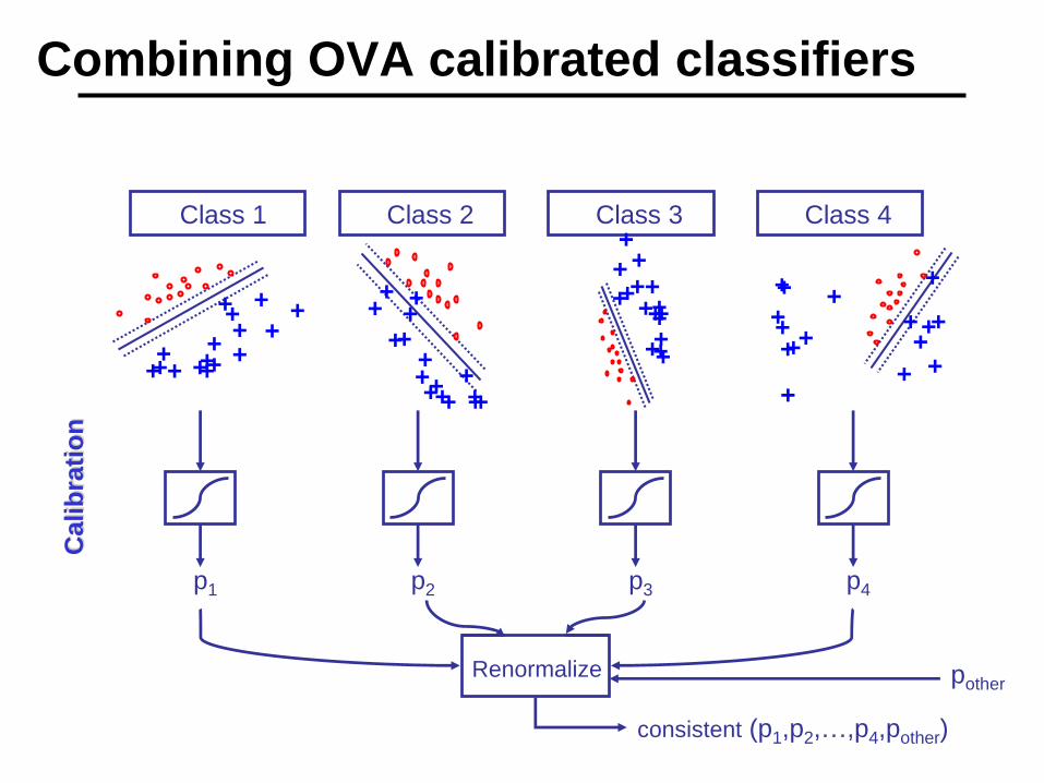
Combining OVA calibrated classifiers
Class 1 Class 2 Class 3 Class 4
+ ++++
+ ++
+++++ +++ +
+++++
+
+
++ ++++++
++
++++
++
++
+++
++ +
+
+
+ ++
+
+
+
+
+
+
+++ ++
Cali
bra
tio
n
p1 p2 p3 p4
pother
consistent (p1,p2,…,p4,pother)
Renormalize

Exponential form
Once the graph is
defined the model
can be written in
exponential form
feature vector
parameter vector
Comparing two
labellings with the
likelihood ratio

Discriminative Algorithms

Example: multiclass setting
Predict:
Update:
Feature encoding:
Predict:
Update:

Three Approaches to K-Class SVM

General SVM
Objective function = error function + regularization term

Training Samples
Learning Algorithms
Classifiery = f(x)
Test Samples x Classifiery = f(x)
Predictions y
offline
online
SVM & GMM (Bayes Rule)
cannot handle this case!
Day Outlook Temperature Humidity Wind PlayTennis
Day1 Sunny Hot High Weak No
Day2 Sunny Hot High Strong No
Day3 Overcast Hot High Weak Yes
Day4 Rain Mild High Weak Yes
Day5 Rain Cool Normal Weak Yes
Day6 Rain Cool Normal Strong No
Day7 Overcast Cool Normal Strong Yes
Day8 Sunny Mild High Weak No
Day9 Sunny Cool Normal Weak Yes
Day10 Rain Mild Normal Weak Yes
Day11 Sunny Mild Normal Strong Yes
Day12 Overcast Mild High Strong Yes
Day13 Overcast Hot Normal Weak Yes
Day14 Rain Mild High Strong No

Wish List:
Even these features or attributes x are
not comparable directly, the decisions y
they make could be comparable!
For different decisions y, we can use
different features or attributes x!
Classifier Training with Feature Selection!

Our ExpectationsOutlook
Humidity WindyP
sunnyovercast
rainy
PN
high normal
PN
yes no
How to make this happen?
Compare it with our wish list
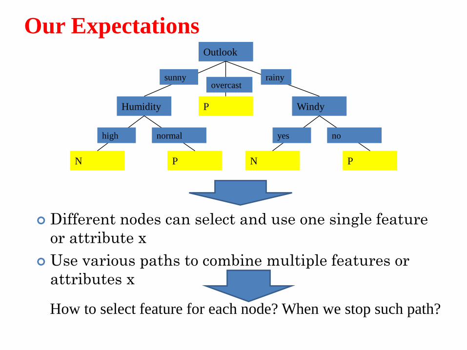
Our ExpectationsOutlook
Humidity WindyP
sunnyovercast
rainy
PN
high normal
PN
yes no
Different nodes can select and use one single feature
or attribute x
Use various paths to combine multiple features or
attributes x
How to select feature for each node? When we stop such path?

Decision Tree
• What is a Decision Tree
• Sample Decision Trees
• How to Construct a Decision Tree
• Problems with Decision Trees
• Summary

Decision tree is a classifier in the form of a tree
structure
– Decision node: specifies a test on a single
attribute or feature x
– Leaf node: indicates the value of the target
attribute (label) y
– Arc/edge: split of one attribute (could be
multiple partitions y or binary ones y)
– Path: a disjunction of test to make the final
decision (all attributes x could be used)
Decision trees classify instances or examples by
starting at the root of the tree and moving through
it until a leaf node.
Definition

Why decision tree?
• Decision trees are powerful and popular tools for classification and prediction.
• Decision trees represent rules, which can be understood by humans and used in knowledge system such as database.
Compare these with our wish list

key requirements
• Attribute-value description: object or case must be expressible in terms of a fixed collection of properties or attributes x (e.g., hot, mild, cold).
• Predefined classes (target values y): the target function has discrete output values y (binary or multiclass)
• Sufficient data: enough training cases should be provided to learn the model.

An Example Data Set and Decision Tree
yes
no
yes no
sunny rainy
nomed
yes
small big
big
outlook
company
sailboat
# ClassOutlook Company Sailboat Sail?
1 sunny big small yes
2 sunny med small yes
3 sunny med big yes
4 sunny no small yes
5 sunny big big yes
6 rainy no small no
7 rainy med small yes
8 rainy big big yes
9 rainy no big no
10 rainy med big no
Attribute

Classification
yes
no
yes no
sunny rainy
nomed
yes
small big
big
outlook
company
sailboat
# Class
Outlook Company Sailboat Sail?
1 sunny no big ?
2 rainy big small ?
Attribute

136
DECISION TREE• An internal node is a test on an attribute.
• A branch represents an outcome of the test, e.g., Color=red.
• A leaf node represents a class label or class label distribution.
• At each node, one attribute is chosen to split training examples into distinct classes as much as possible
• A new case is classified by following a matching path to a leaf node.
Each node uses one single feature to train one classifier!

Training Samples
Learning Algorithms
Classifiery = f(x)
Test Samples x Classifiery = f(x)
Predictions y
offline
online
SVM, GMM (Bayes Rule) & Decision Tree
One more weapon at hand now!

138
Decision Tree Construction
• Top-Down Decision Tree Construction
• Choosing the Splitting Attribute: Feature Selection
• Information Gain and Gain Ratio: Classifier Training
139
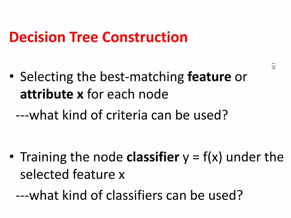
Decision Tree Construction
• Selecting the best-matching feature or attribute x for each node
---what kind of criteria can be used?
• Training the node classifier y = f(x) under the selected feature x
---what kind of classifiers can be used?

Prostate cancer recurrence
Secondary Gleason Grade
No YesPSA Level Stage
Primary Gleason Grade
No Yes
No No Yes
1,2 3 4 5
14.9 14.9 T1c,T2a,
T2b,T2c
T1ab,T3
2,3 4

Another Example
# Class
Outlook Temperature Humidity Windy Play
1 sunny hot high no N
2 sunny hot high yes N
3 overcast hot high no P
4 rainy moderate high no P
5 rainy cold normal no P
6 rainy cold normal yes N
7 overcast cold normal yes P
8 sunny moderate high no N
9 sunny cold normal no P
10 rainy moderate normal no P
11 sunny moderate normal yes P
12 overcast moderate high yes P
13 overcast hot normal no P
14 rainy moderate high yes N
Attribute

Simple Tree
Outlook
Humidity WindyP
sunnyovercast
rainy
PN
high normal
PN
yes no
Decision Tree can select different attributes for different decisions!

Complicated Tree
Temperature
Outlook Windy
cold moderate
hot
P
sunny rainy
N
yes no
P
overcast
Outlook
sunny rainy
P
overcast
Windy
PN
yes no
Windy
NP
yes no
Humidity
P
high normal
Windy
PN
yes no
Humidity
P
high normal
Outlook
N
sunny rainy
P
overcast
null
Given a data set, we could
have multiple solutions!

Attribute Selection Criteria
• Main principle– Select attribute which partitions the learning set into
subsets as “pure” as possible
• Various measures of purity– Information-theoretic– Gini index– X2
– ReliefF– ...
• Various improvements– probability estimates– normalization– binarization, subsetting

Information-Theoretic Approach
• To classify an object, a certain information is needed
– I, information
• After we have learned the value of attribute A, we only need some remaining amount of information to classify the object
– Ires, residual information
• Gain
– Gain(A) = I – Ires(A)
• The most ‘informative’ attribute is the one that minimizes Ires, i.e., maximizes Gain

Entropy
• The average amount of information Ineeded to classify an object is given by the entropy measure
• For a two-class problem:
entropy
p(c1)

Residual Information
• After applying attribute A, S is partitioned into subsets according to values v of A
• Ires is equal to weighted sum of the amounts of information for the subsets

Triangles and Squares
# Shape
Color Outline Dot
1 green dashed no triange
2 green dashed yes triange
3 yellow dashed no square
4 red dashed no square
5 red solid no square
6 red solid yes triange
7 green solid no square
8 green dashed no triange
9 yellow solid yes square
10 red solid no square
11 green solid yes square
12 yellow dashed yes square
13 yellow solid no square
14 red dashed yes triange
Attribute

Triangles and Squares
.
.
..
.
.
# Shape
Color Outline Dot
1 green dashed no triange
2 green dashed yes triange
3 yellow dashed no square
4 red dashed no square
5 red solid no square
6 red solid yes triange
7 green solid no square
8 green dashed no triange
9 yellow solid yes square
10 red solid no square
11 green solid yes square
12 yellow dashed yes square
13 yellow solid no square
14 red dashed yes triange
Attribute
Data Set:
A set of classified objects

Entropy
• 5 triangles
• 9 squares
• class probabilities
• entropy
.
.
..
.
.

Entropyreductionbydata setpartitioning
.
.
..
.
.
..
.
.
.
.
Color?
red
yellow
green

Entr
op
ija v
red
no
sti a
trib
uta .
.
..
.
.
..
..
.
.
Color?
red
yellow
green

Info
rmat
ion
Gai
n
..
..
.
.
..
..
.
.
Color?
red
yellow
green

Information Gain of The Attribute
• Attributes– Gain(Color) = 0.246
– Gain(Outline) = 0.151
– Gain(Dot) = 0.048
• Heuristics: attribute with the highest gain is chosen
• This heuristics is local (local minimization of impurity)

.
.
..
.
.
..
.
..
.
Color?
red
yellow
green
Gain(Outline) = 0.971 – 0 = 0.971 bits
Gain(Dot) = 0.971 – 0.951 = 0.020 bits

.
.
..
.
.
..
.
..
.
Color?
red
yellow
green
.
.
Outline?
dashed
solid
Gain(Outline) = 0.971 – 0.951 = 0.020 bits
Gain(Dot) = 0.971 – 0 = 0.971 bits
Conditional decision
Initial decision

.
.
..
.
.
..
.
..
.
Color?
red
yellow
green
.
.
dashed
solid
Dot?
no
yes
.
.
Outline?

Decision Tree
Color
Dot Outlinesquare
redyellow
green
squaretriangle
yes no
squaretriangle
dashed solid
.
.
..
.
.

A Defect of Ires
• Ires favors attributes with many values
• Such attribute splits S to many subsets, and if these are small, they will tend to be pure anyway
• One way to rectify this is through a corrected measure of information gain ratio.

Information Gain Ratio
• I(A) is amount of information needed to determine the value of an attribute A
• Information gain ratio

Info
rmat
ion
Gai
n R
atio
..
..
.
.
..
..
.
.
Color?
red
yellow
green

Information Gain and Information Gain Ratio
A |v(A)| Gain(A) GainRatio(A)
Color 3 0.247 0.156
Outline 2 0.152 0.152
Dot 2 0.048 0.049

Gini Index
• Another sensible measure of impurity(i and j are classes)
• After applying attribute A, the resulting Gini index is
• Gini can be interpreted as expected error rate

Gini Index
.
.
..
.
.

Gin
i In
dex
fo
r C
olo
r
..
..
.
.
..
..
.
.
Color?
red
yellow
green

Gain of Gini Index

169
Shall I play tennis today?

170

171

172

173
How do we choose the best attribute?
What should that attribute do for us?

174
Which attribute to select?
witten&eibe

175
Criterion for attribute selection
• Which is the best attribute?
– The one which will result in the smallest tree
– Heuristic: choose the attribute that produces the “purest” nodes
• Need a good measure of purity!
– Maximal when?
– Minimal when?

176
Information Gain
Which test is more informative?Split over whether
Balance exceeds 50K
Over 50KLess or equal 50K EmployedUnemployed
Split over whether applicant is employed

177
Information Gain
Impurity/Entropy (informal)– Measures the level of impurity in a group of
examples

178
Impurity
Very impure group Less impure Minimum
impurity
179
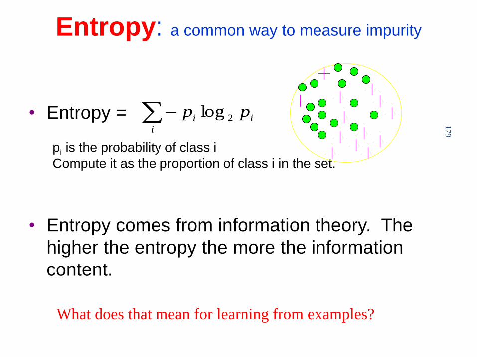
Entropy: a common way to measure impurity
• Entropy =
pi is the probability of class i
Compute it as the proportion of class i in the set.
• Entropy comes from information theory. The
higher the entropy the more the information
content.
i
ii pp 2log
What does that mean for learning from examples?

180
2-Class Cases:
• What is the entropy of a group in which all examples belong to the same class?– entropy = - 1 log21 = 0
• What is the entropy of a group with 50% in either class?– entropy = -0.5 log20.5 – 0.5 log20.5 =1
Minimum
impurity
Maximum
impurity
not a good training set for learning
good training set for learning

181
Information Gain
• We want to determine which attribute in a given set of training feature vectors is most useful for discriminating between the classes to be learned.
• Information gain tells us how important a given attribute of the feature vectors is.
• We will use it to decide the ordering of attributes in the nodes of a decision tree.

182
Calculating Information Gain
996.030
16log
30
16
30
14log
30
1422
impurity
787.017
4log
17
4
17
13log
17
1322
impurity
Entire population (30 instances)17 instances
13 instances
(Weighted) Average Entropy of Children = 615.0391.030
13787.0
30
17
Information Gain= 0.996 - 0.615 = 0.38
391.013
12log
13
12
13
1log
13
122
impurity
Information Gain = entropy(parent) – [average entropy(children)]
parent
entropy
child
entropy
child
entropy

183
Entropy-Based Automatic Decision Tree Construction
Node 1
What feature
should be used?
What values?
Training Set S
x1=(f11,f12,…f1m)
x2=(f21,f22, f2m)
.
.
xn=(fn1,f22, f2m)
Quinlan suggested information gain in his ID3 system
and later the gain ratio, both based on entropy.

184
Using Information Gain to Construct a Decision Tree
Attribute A
v1 vkv2
Full Training Set S
Set S
repeat
recursively
till when?
Information gain has the disadvantage that it prefers
attributes with large number of values that split the
data into small, pure subsets. Quinlan’s gain ratio
did some normalization to improve this.
S={sS | value(A)=v1}
Choose the attribute A
with highest information
gain for the full training
set at the root of the tree.Construct child nodes
for each value of A.
Each has an associated
subset of vectors in
which A has a particular
value.

185
Information Content
The information content I(C;F) of the class variable C
with possible values {c1, c2, … cm} with respect to
the feature variable F with possible values {f1, f2, … , fd}
is defined by:
• P(C = ci) is the probability of class C having value ci.
• P(F=fj) is the probability of feature F having value fj.
• P(C=ci,F=fj) is the joint probability of class C = ci
and variable F = fj.
These are estimated from frequencies in the training data.

186
Simple Example
• Sample Example
X Y Z C
1 1 1 I
1 1 0 I
0 0 1 II
1 0 0 II
How would you distinguish class I from class II?

187
Example (cont)
Which attribute is best? Which is worst? Does it make sense?
X Y Z C
1 1 1 I
1 1 0 I
0 0 1 II
1 0 0 II

188
Using Information Content
• Start with the root of the decision tree and the whole
training set.
• Compute I(C,F) for each feature F.
• Choose the feature F with highest information
content for the root node.
• Create branches for each value f of F.
• On each branch, create a new node with reduced
training set and repeat recursively.

189

190

Example: The Simpsons

Person Hair Length
Weight Age Class
Homer 0” 250 36 M
Marge 10” 150 34 F
Bart 2” 90 10 M
Lisa 6” 78 8 F
Maggie 4” 20 1 F
Abe 1” 170 70 M
Selma 8” 160 41 F
Otto 10” 180 38 M
Krusty 6” 200 45 M
Comic 8” 290 38 ?

Hair Length <= 5?yes no
Entropy(4F,5M) = -(4/9)log2(4/9) - (5/9)log2(5/9)
= 0.9911
np
n
np
n
np
p
np
pSEntropy 22 loglog)(
Gain(Hair Length <= 5) = 0.9911 – (4/9 * 0.8113 + 5/9 * 0.9710 ) = 0.0911
)()()( setschildallEsetCurrentEAGain
Let us try splitting
on Hair length
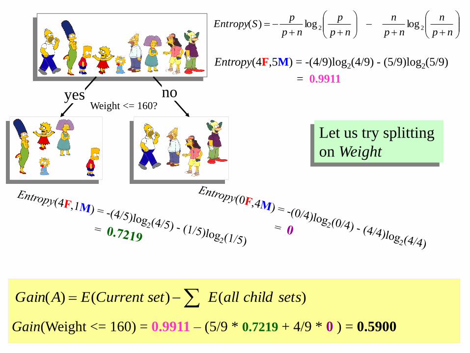
Weight <= 160?yes no
Entropy(4F,5M) = -(4/9)log2(4/9) - (5/9)log2(5/9)
= 0.9911
np
n
np
n
np
p
np
pSEntropy 22 loglog)(
Gain(Weight <= 160) = 0.9911 – (5/9 * 0.7219 + 4/9 * 0 ) = 0.5900
)()()( setschildallEsetCurrentEAGain
Let us try splitting
on Weight

age <= 40?yes no
Entropy(4F,5M) = -(4/9)log2(4/9) - (5/9)log2(5/9)
= 0.9911
np
n
np
n
np
p
np
pSEntropy 22 loglog)(
Gain(Age <= 40) = 0.9911 – (6/9 * 1 + 3/9 * 0.9183 ) = 0.0183
)()()( setschildallEsetCurrentEAGain
Let us try splitting
on Age

Weight <= 160?yes no
Hair Length <= 2?yes no
Of the 3 features we had, Weight
was best. But while people who
weigh over 160 are perfectly
classified (as males), the under 160
people are not perfectly
classified… So we simply recurse!
This time we find that we
can split on Hair length, and
we are done!

Weight <= 160?
yes no
Hair Length <= 2?
yes no
We need don’t need to keep the data
around, just the test conditions.
Male
Male Female
How would
these people
be classified?
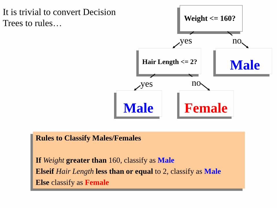
It is trivial to convert Decision
Trees to rules… Weight <= 160?
yes no
Hair Length <= 2?
yes no
Male
Male Female
Rules to Classify Males/Females
If Weight greater than 160, classify as Male
Elseif Hair Length less than or equal to 2, classify as Male
Else classify as Female

199
Building Decision Tree [Q93]
• Top-down tree construction
– At start, all training examples are at the root.
– Partition the examples recursively by choosing one attribute each time.
• Bottom-up tree pruning
– Remove subtrees or branches, in a bottom-up manner, to improve the estimated accuracy on new cases.

200
Top-Down Approach
• Top-Down Decision Tree Construction
• Choosing the Splitting Attribute
• Information Gain biased towards attributes with a large number of values
• Gain Ratio takes number and size of branches into account when choosing an attribute

201
Choosing the Splitting Attribute
• At each node, available attributes are evaluated on the basis of separating the classes of the training examples. A Goodness function is used for this purpose.
• Typical goodness functions:
– information gain (ID3/C4.5)
– information gain ratio
– gini index
witten&eibe

202
A criterion for attribute selection
• Which is the best attribute?
– The one which will result in the smallest tree
– Heuristic: choose the attribute that produces the “purest” nodes
• Popular impurity criterion: information gain
– Information gain increases with the average purity of the subsets that an attribute produces
• Strategy: choose attribute that results in greatest information gain
witten&eibe

203
Computing information
• Information is measured in bits
– Given a probability distribution, the info required to predict an event is the distribution’s entropy
– Entropy gives the information required in bits (this can involve fractions of bits!)
• Formula for computing the entropy:nnn ppppppppp logloglog),,,entropy( 221121
witten&eibe

Evaluation
• Training accuracy– How many training instances can be correctly classify based on
the available data?
– Is high when the tree is deep/large, or when there is less confliction in the training instances.
– however, higher training accuracy does not mean good generalization
• Testing accuracy– Given a number of new instances, how many of them can we
correctly classify?
– Cross validation

Strengths
• can generate understandable rules
• perform classification without much computation
• can handle continuous and categorical variables
• provide a clear indication of which fields are most important for prediction or classification

Weakness
• Not suitable for prediction of continuous attribute.
• Perform poorly with many class and small data.
• Computationally expensive to train. – At each node, each candidate splitting field must be sorted
before its best split can be found.
– In some algorithms, combinations of fields are used and a search must be made for optimal combining weights.
– Pruning algorithms can also be expensive since many candidate sub-trees must be formed and compared.
• Do not treat well non-rectangular regions.

Summary
• Decision trees can be used to help predict the future
• The trees are easy to understand
• Decision trees work more efficiently with discrete attributes
• The trees may suffer from error propagation
What to remember about classifiers
• No free lunch: machine learning algorithms are tools, not dogmas
• Try simple classifiers first
• Better to have smart features and simple classifiers than simple features and smart classifiers
• Use increasingly powerful classifiers with more training data (bias-variance tradeoff)
Slide credit: D. Hoiem

Generalization
• How well does a learned model generalize from the data it was trained on to a new test set?
Training set (labels known) Test set (labels
unknown)
Slide credit: L. Lazebnik

Generalization
• Components of generalization error – Bias: how much the average model over all training sets differ from the
true model?
• Error due to inaccurate assumptions/simplifications made by the model.
– Variance: how much models estimated from different training sets differ from each other.
• Underfitting: model is too “simple” to represent all the relevant class characteristics– High bias (few degrees of freedom) and low variance
– High training error and high test error
• Overfitting: model is too “complex” and fits irrelevant characteristics (noise) in the data– Low bias (many degrees of freedom) and high variance
– Low training error and high test error
Slide credit: L. Lazebnik

Bias-Variance Trade-off
• Models with too few parameters are inaccurate because of a large bias (not enough flexibility).
• Models with too many parameters are inaccurate because of a large variance (too much sensitivity to the sample).
Slide credit: D. Hoiem

Bias-variance tradeoff
Training error
Test error
Underfitting Overfitting
Complexity Low Bias
High Variance
High Bias
Low Variance
Err
or
Slide credit: D. Hoiem

Bias-variance tradeoff
Many training examples
Few training examples
Complexity Low Bias
High Variance
High Bias
Low Variance
Test E
rror
Slide credit: D. Hoiem

Effect of Training Size
Testing
Training
Generalization Error
Number of Training Examples
Err
or
Fixed prediction model
Slide credit: D. Hoiem

Remember…
• No classifier is inherently better than any other: you need to make assumptions to generalize
• Three kinds of error– Inherent: unavoidable
– Bias: due to over-simplifications
– Variance: due to inability to perfectly estimate parameters from limited data
Slide credit: D. Hoiem

How to reduce variance?
• Choose a simpler classifier
• Regularize the parameters
• Get more training data
Slide credit: D. Hoiem

Generative vs. Discriminative Classifiers
Generative Models
• Represent both the data and the labels
• Often, makes use of conditional independence and priors
• Examples– Naïve Bayes classifier
– Bayesian network
• Models of data may apply to future prediction problems
Discriminative Models
• Learn to directly predict the labels from the data
• Often, assume a simple boundary (e.g., linear)
• Examples– Logistic regression
– SVM
– Boosted decision trees
• Often easier to predict a label from the data than to model the data
Slide credit: D. Hoiem

Other Issues for Image Classification


OBJECTS
ANIMALS INANIMATEPLANTS
MAN-MADENATURALVERTEBRATE…..
MAMMALS BIRDS
GROUSEBOARTAPIR CAMERA

Specific recognition tasks
Svetlana Lazebnik

Scene categorization or classification
• outdoor/indoor
• city/forest/factory/etc.
Svetlana Lazebnik

Image annotation / tagging / attributes
• street
• people
• building
• mountain
• tourism
• cloudy
• brick
• …
Svetlana Lazebnik

Object detection
• find pedestrians
Svetlana Lazebnik

Image parsing / semantic segmentation
mountain
building
tree
banner
market
people
street lamp
sky
building
Svetlana Lazebnik

Scene understanding?
Svetlana Lazebnik