Machine Learning for Healthcare HST.956, 6.S897

Lecture 5: Risk stratification (continued)

David Sontag

1

Outline for today’s class

1. Risk stratification (continued) – Deriving labels – Evaluation

– Subtleties with ML-based risk stratification

2. Survival modeling

2

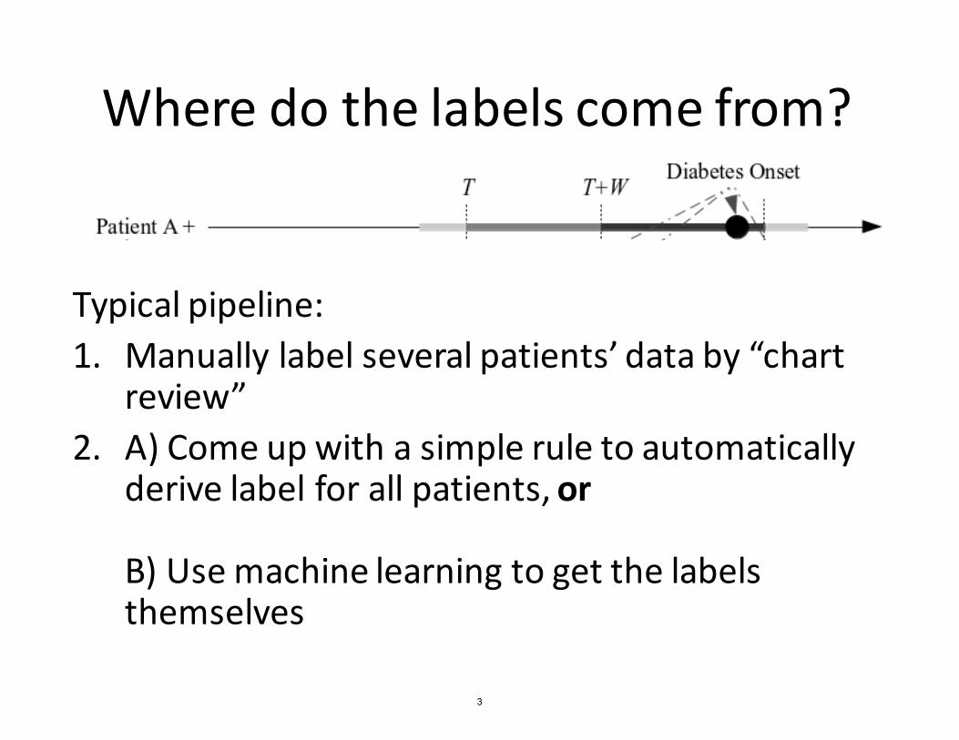
Where do the labels come from?

Typical pipeline: 1. Manually label several patients’ data by “chart

review” 2. A) Come up with a simple rule to automatically

derive label for all patients, or

B) Use machine learning to get the labelsthemselves

3

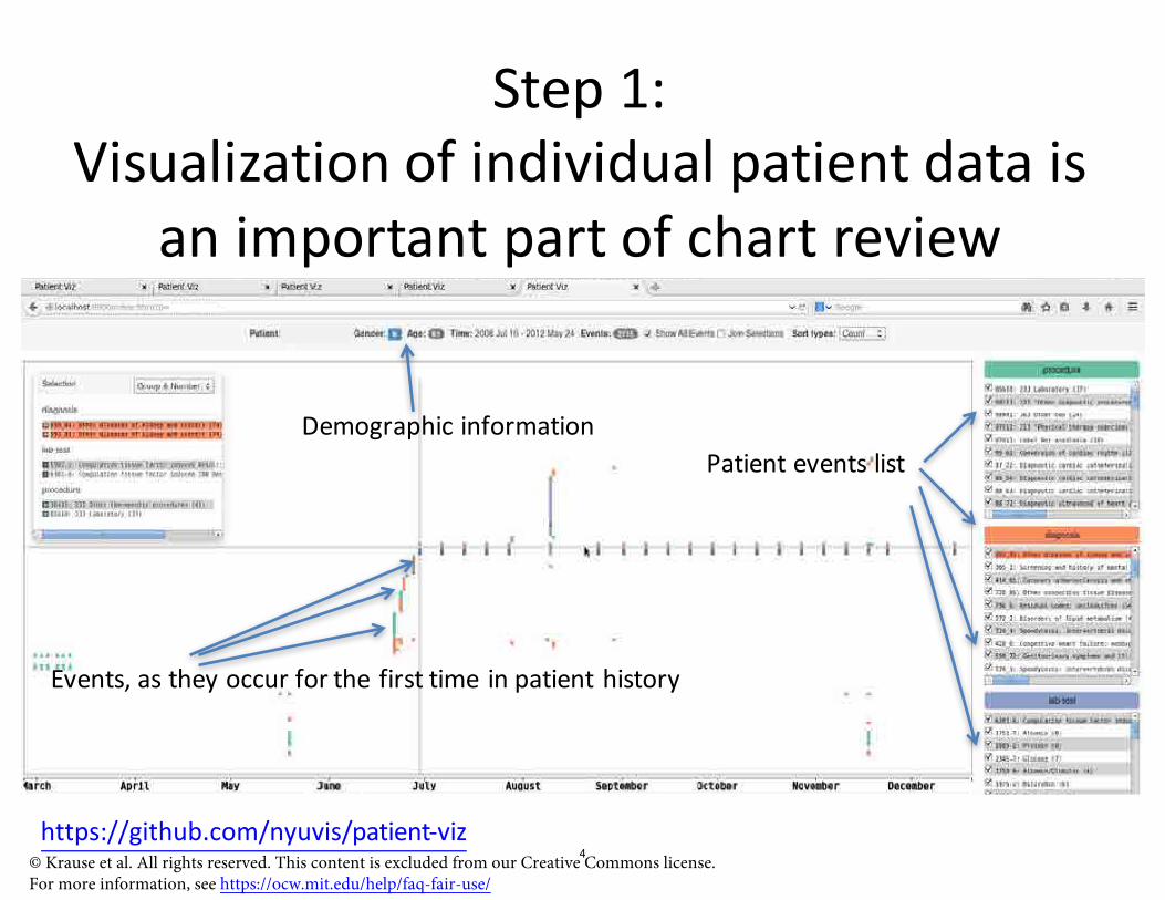
Step 1: Visualization of individual patient data is

an important part of chart review

Demographic information Patient events list

Events, as they occur for the first time in patient history

https://github.com/nyuvis/patient-viz © Krause et al. All rights reserved. This content is excluded from our Creative Commons license. For more information, see https://ocw.mit.edu/help/faq-fair-use/

4

Figure 1: Algorithm for identifying T2DM cases in the EMR.

Step 2: Example of a rule-based phenotype

5© Pacheco and Thompson. All rights reserved. This content is excluded from our Creative Commons license. For more information, see https://ocw.mit.edu/help/faq-fair-use/

Outline for today’s class

1. Risk stratification (continued) – Deriving labels – Evaluation

– Subtleties with ML-based risk stratification

2. Survival modeling

6

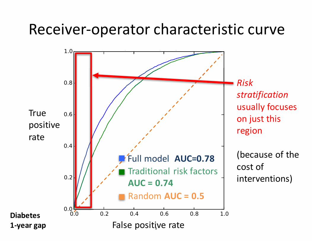
Receiver-operator characteristic curve

Full model Traditional risk factors

True positive rate

Want to be here Obtained by varying prediction threshold

Diabetes 1-year gap False positive rate 7

Receiver-operator characteristic curve

True positive rate

Diabetes 1-year gap

Full model Traditional risk factors

Area under the ROC curve (AUC)

False positive rate

AUC = Probability that algorithm ranks a positive patient over a negative patient

Invariant to amount of class imbalance

8

C0LL)B9<-L));<=>?@AB #17<4/49:7L)1456)87./915 ;<=(>(?@AC

C7L5-)F954/4?-)17/-

F954/4?-)

37:<9B);<=(>(?@D

3-.-4?-1H9F-17/91).N717./-145/4.).01?-

#10-)

17/-

4%"5'0'6 789'"*(+":

!"#$% #&'(&")"*(&"+, 0507LLD)89.05-5) 9:)c05/)/N45) 1-@49:

;R-.705-)98)/N-) .95/)98) 4:/-1?-:/49:5=

9

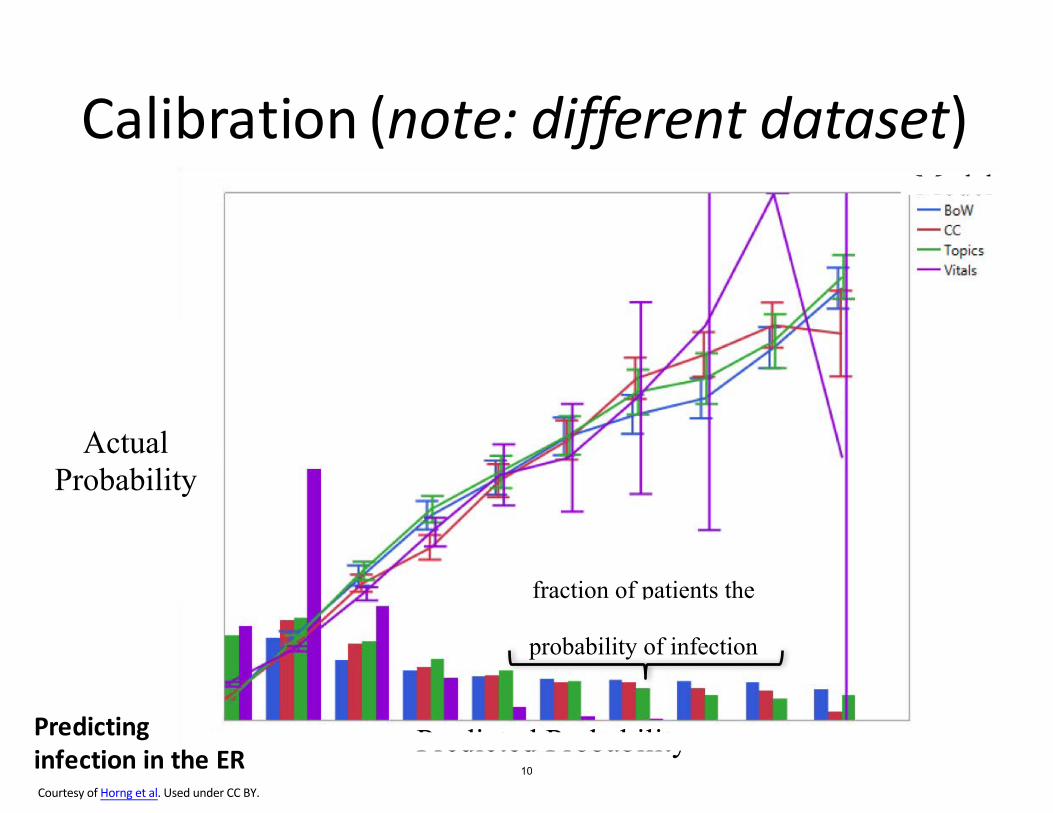
Predicted Probability 0

1

0.5

1

fraction of patients the model predicts to have this

probability of infection

Model

Calibration (note: different dataset)

Actual Probability

Predicting infection in the ER Courtesy of Horng et al. Used under CC BY.

10

Outline for today’s class

1. Risk stratification (continued) – Deriving labels – Evaluation

– Subtleties with ML-based risk stratification

2. Survival modeling

11

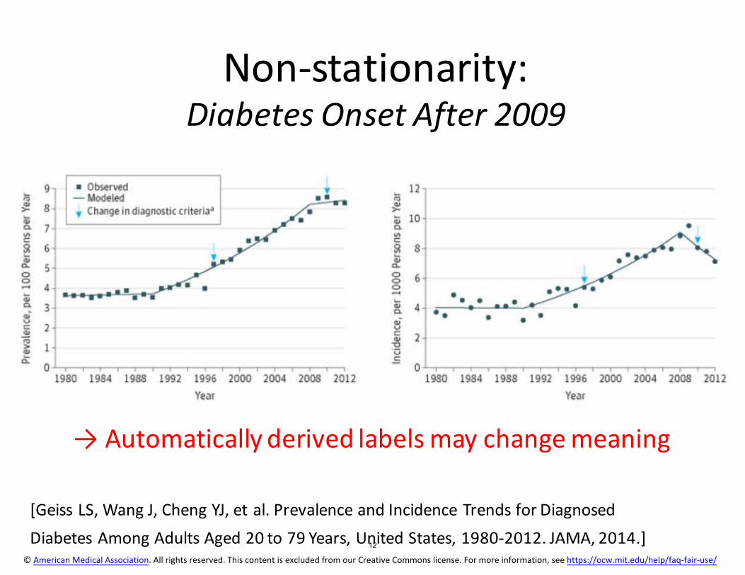
Non-stationarity: Diabetes Onset After 2009

→ Automatically derived labels may change meaning

[Geiss LS, Wang J, Cheng YJ, et al. Prevalence and Incidence Trends for Diagnosed Diabetes Among Adults Aged 20 to 79 Years, United States, 1980-2012. JAMA, 2014.] 12

© American Medical Association. All rights reserved. This content is excluded from our Creative Commons license. For more information, see https://ocw.mit.edu/help/faq-fair-use/

Non-stationarity: Top 100 lab measurements over time

Labs

Time (in months, from 1/2005 up to 1/2014)

→ Significance of features may change over time© Narges Razavian. All rights reserved. This content is excluded from our Creative Commons license. For more information, see https://ocw.mit.edu/help/faq-fair-use/

[Figure credit: Narges Razavian] 13

Non-stationarity: ICD-9 to ICD-10 shift

Coun

t of d

iagnosis codes

2000 2005 2010 2015

→ Significance of features may change over time© Mike Oberst. All rights reserved. This content is excluded from our Creative Commons license. For more information, see https://ocw.mit.edu/help/faq-fair-use/[Figure credit: Mike Oberst] 14

ICD-10

ICD-9

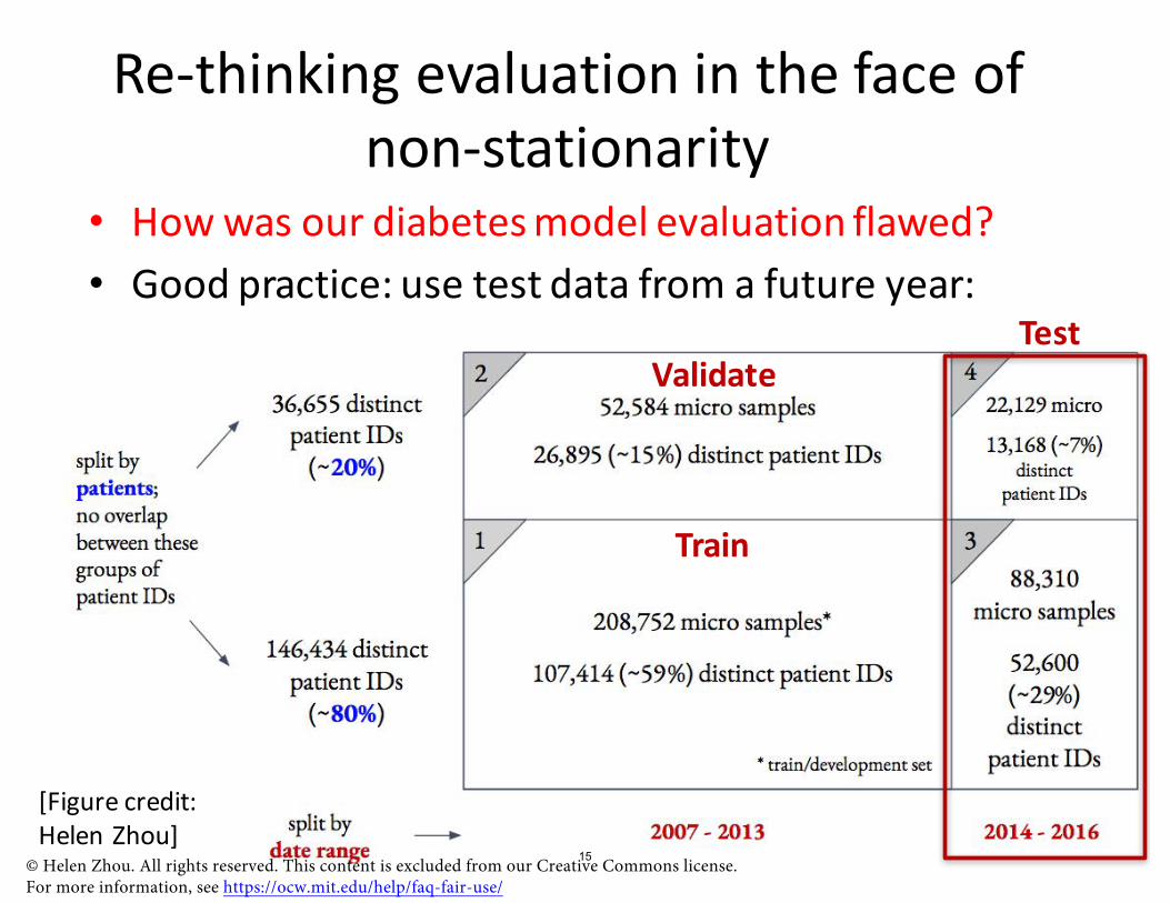
Re-thinking evaluation in the face of non-stationarity

• How was our diabetes model evaluation flawed?

• Good practice: use test data from a future year: Test

Train

Validate

[Figure credit: Helen Zhou]

© Helen Zhou. All rights reserved. This content is excluded from our Creative Commons license. For more information, see https://ocw.mit.edu/help/faq-fair-use/

15

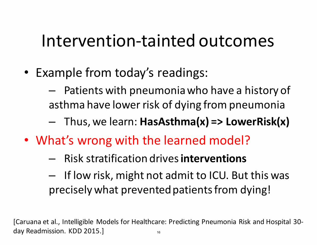
Intervention-tainted outcomes • Example from today’s readings:

– Patients with pneumoniawho have a history of asthma have lower risk of dying from pneumonia

– Thus, we learn: HasAsthma(x) => LowerRisk(x) • What’s wrong with the learned model?

– Risk stratification drives interventions – If low risk, might not admit to ICU. But this was preciselywhat preventedpatients from dying!

[Caruana et al., Intelligible Models for Healthcare: Predicting Pneumonia Risk and Hospital 30-day Readmission. KDD 2015.] 16

Intervention-tainted outcomes • Formally, this is what’s happening:

� �

ED triage Death Time

“Mary”

Treatment

A long survival time may be because of treatment!

• How do we address this problem?

• First and foremost,must recognize it is happening – interpretable models help with this

17

Intervention-tainted outcomes • Hacks:

1. Modify model, e.g. by removing the HasAsthma(x) => LowerRisk(x) rule I do not expect this to work with high-dimensionaldata

2. Re-define outcome by finding a pre-treatmentsurrogate (e.g., lactate levels)

3. Consider treated patients as right-censored by treatment

Example: Henry, Hager, Pronovost, Saria. A targeted real-time early warningscore (TREWScore) for septic shock. Science Translation Medicine, 2015

18

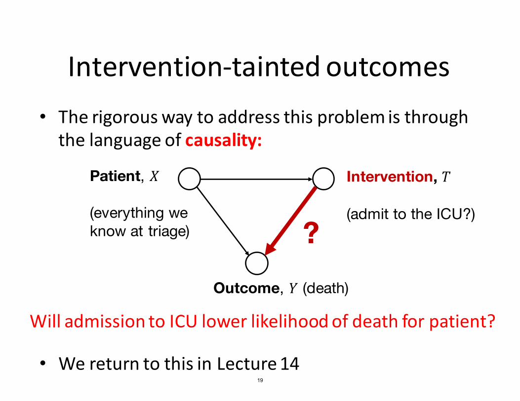
Intervention-tainted outcomes • The rigorous way to address this problem is through the language of causality:

Patient, � Intervention, �

(everything we know at triage)

(admit to the ICU?)

Outcome, � (death)

Will admission to ICU lower likelihood of death for patient?

?

• We return to this in Lecture 14 19

No big wins from deep models on structured data/text

Rajkomar et al., Scalable and accurate deep learning with electronic health records. Nature Digital Medicine, 2018

Recurrent neural network & attention-based models trained on 200K hospitalized patients

Courtesy of Rajkomar et al. Used under CC BY. 20

Inpatient Mortality, (95% CI)Deep learning 24 hours after admission 0.95(0.94-0.96) 0.93(0.92-0.94)Full feature enhanced baseline at 24 hours after admission 0.93 (0.92-0.95) 0.91 (0.89-0.92)Full feature simple baseline at 24 hours after admission 0.93 (0.91-0.94) 0.90 (0.88-0.92)

No big wins from deep models on structured data/text

Supplemental Table 1: Prediction accuracy of each task of deep learning model compared to baselines

Hospital A Hospital BAUROC1

Comparison to Razavian

Baseline (aEWS2) at 24 hours after admission 0.85 (0.81-0.89) 0.86 (0.83-0.88)et al. ‘15

30-day Readmission, AUROC (95% CI)Deep learning at discharge 0.77(0.75-0.78) 0.76(0.75-0.77)Full feature enhanced baseline at discharge 0.75 (0.73-0.76) 0.75 (0.74-0.76)Full feature simple baseline at dischargeBaseline (mHOSPITAL3) at discharge

0.74 (0.73-0.76)0.70 (0.68-0.72)

0.73 (0.72-0.74)0.68 (0.67-0.69)

Length of Stay at least 7 days AUROC (95% CI)Deep learning 24 hours after admissionFull feature enhanced baseline at 24 hours after admissionFull feature simple baseline at 24 hours after admissionBaseline (mLiu4) at 24 hours after admission

0.86(0.86-0.87)0.85 (0.84-0.85)0.83 (0.82-0.84)0.76 (0.75-0.77)

0.85(0.85-0.86)0.83 (0.83-0.84)0.81 (0.80-0.82)0.74 (0.73-0.75)

Courtesy of Rajkomar et al. Used under CC BY. 21

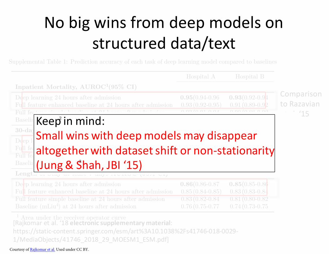
No big wins from deep models on structured data/text

Courtesy of Rajkomar et al. Used under CC BY.

[Rajkomar etal.‘18electronicsupplementarymaterial:ttps://static-content.springh er.com/esm/art%3A10.1038%2Fs41746-018-0029-/MediaObjects/411 746_2018_29_MOESM1_ESM.pdf]

Supplemental Table 1: Prediction accuracy of each task of deep learning model compared to baselines

Hospital A Hospital BInpatient Mortality, AUROC1(95% CI)Deep learning 24 hours after admission (0.94-0.960.95( -0.94(0.920.93(Full feature enhanced baseline at 24 hours after admission 0.93 (0.92-0.95) 0.91 -0.92(0.89(Full feature simple baseline at 24 hours after admission 0.93 (0.91-0.94( 0.90 (0.88( -0.92Baseline (aEWS ) at 24 hours after admission 0.85 (0.81( -0.89 0.86 -0.88(0.83(30-day Readmission, AUROC (95% CI)Deep learning at discharge 0.77((0.75-0.78 (0.750.76( -0.77Full feature enhanced baseline at discharge 0.75 (0.73-0.76( 0.75 ((0.74-0.76Full feature simple baseline at discharge 0.74 -0.76((0.73 0.73 -0.74(0.72(Baseline (mHOSPITAL ) at discharge 0.70 (0.68( -0.72 0.68 (0.67-0.69(Length of Stay at least 7 days AUROC (95% CI)Deep learning 24 hours after admission -0.870.86((0.86 -0.86(0.850.85(Full feature enhanced baseline at 24 hours after admission 0.85 (0.84-0.85) 0.83 ( -0.84(0.83

0.83 (0.82-0.84( 0.81 -0.82(0.80(Full feature simple baseline at 24 hours after admissionBaseline (mLiu4) at 24 hours after admission 0.76 -0.77((0.75 0.74 ((0.73-0.751 Area under the receiver operator curve

ComparisontoRazavianetal.‘15

Keep2inmind:Smallwinswithdeepmodelsmaydisappearaltogetherwithdatasetshiftornon-stationarity(Jung&S3hah,JBI‘15)

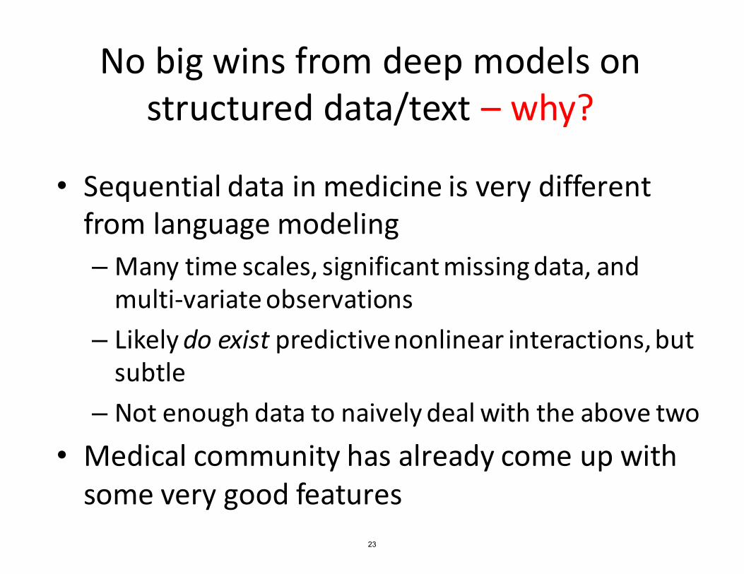
No big wins from deep models on structured data/text – why?

• Sequential data in medicine is very different from language modeling – Many time scales, significant missing data, and multi-variate observations

– Likely do exist predictivenonlinear interactions,but subtle

– Not enough data to naively deal with the above two

• Medical community has already come up with some very good features

23

Outline for today’s class

1. Risk stratification (continued) – Deriving labels – Evaluation

– Subtleties with ML-based risk stratification

2. Survival modeling

24

Survival modeling

• We focus on right-censored data:Event occurrence e.g., death, divorce, college graduation

Censoring

T

[Wang, Li, Reddy. Machine Learning for Survival Analysis: A Survey. 2017] © ACM. All rights reserved. This content is excluded from our Creative Commons license. For more information, see https://ocw.mit.edu/help/faq-fair-use/

25

Survival modeling

• Why not use classification, as before?– Less data for training (due to exclusions)– Pessimistic estimates due to choice of window

• What about regression, e.g. minimizing mean-squared error?– T is non-negative,may want long tails– If we just naively removed censoredevents,wewould be introducing bias

26

�

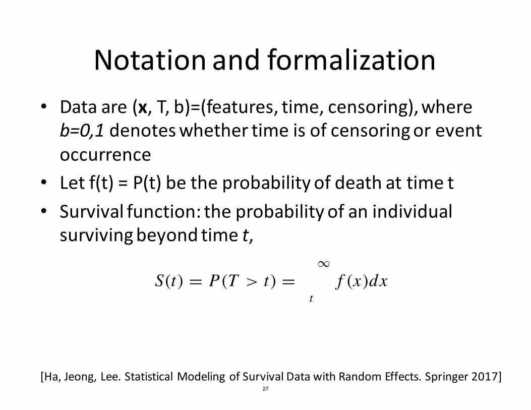
Notation and formalization • Data are (x, T,b)=(features,time,censoring),whereb=0,1 denotes whether time is of censoring or eventoccurrence

• Let f(t) = P(t) be the probability of death at time t• Survival function: the probability of an individualsurviving beyond time t,

∞S(t) = P(T > t) = f (x)dx .

t

[Ha, Jeong, Lee. Statistical Modeling of Survival Data with Random Effects. Springer 2017] 27

Notation and formalization

Time in years

Fig. 2: Relationship among different entities f(t), F (t) and S(t).

[Wang, Li, Reddy. Machine Learning for Survival Analysis: A Survey. 2017] © ACM. All rights reserved. This content is excluded from our Creative Commons license. For more information, see https://ocw.mit.edu/help/faq-fair-use/

28

�� � �

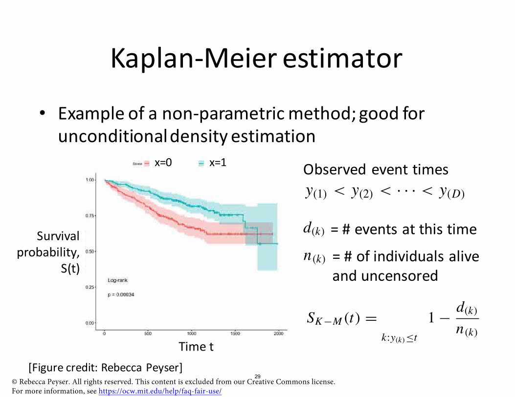
Kaplan-Meier estimator

• Example of a non-parametric method; good for unconditionaldensity estimation

x=0 x=1 Observed event times y(1) < y(2) < · · · < y(D)

Survival d(k) = # events at this time probability,

S(t) n(k) = # of individuals alive

and uncensored

Time t

SK −M (t) = k:y(k)≤t

d(k)1 − n(k)

[Figure credit: Rebecca Peyser] © Rebecca Peyser. All rights reserved. This content is excluded from our Creative Commons license. For more information, see https://ocw.mit.edu/help/faq-fair-use/

29

�

�

�

Hazard rate λ(t)

λ

λφtφ−1

f (t)/S(t)

(λφtφ−1)/(1+ λtφ)

f (t)/S(t)

λeφt

Maximum likelihood estimation

• Commonly parametric densities for f(t): Table 2.1 Useful parametric distributions for survival analysis Distribution Survival function

S(t) Density function f (t)

Exponential (λ > 0) exp(−λt) λ exp(−λt)

Weibull (λ, φ > 0) exp(−λtφ) λφtφ−1 exp(−λtφ)

Log-normal (σ > 0, µ ∈ R)

(parameters can be a

1 − {(lnt − µ)/σ} ϕ{(lnt − µ)/σ}(σt)−1

Log-logistic (λ > 0, φ > 0)

function of x) 1/(1 + λtφ) (λφtφ−1)/(1 + λtφ)2

Gamma (λ, φ > 0) 1 − I (λt, φ) {λφ/ (φ)}tφ−1 exp(−λt)

Gompertz (λ, φ > 0)

exp{ λ (1 − eφt )}φ λeφt exp{ λ (1 − eφt )}φ

[Ha, Jeong, Lee. Statistical Modeling of Survival Data with Random Effects. Springer 2017] © Springer. All rights reserved. This content is excluded from our Creative Commons license. For more information, see https://ocw.mit.edu/help/faq-fair-use/

30

�

Z 1

tp✓ (a |x)da

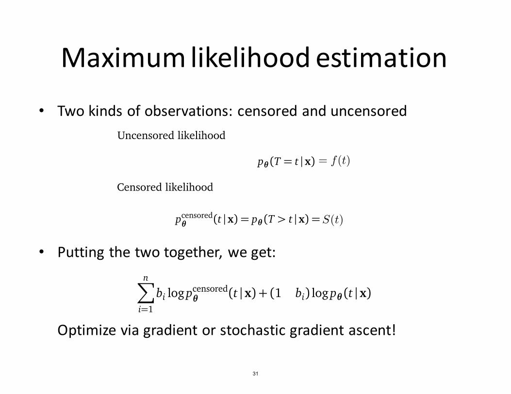
Maximum likelihood estimation

• Two kinds of observations: censored and uncensored

Uncensored likelihood

p✓ (T = t | x) = f(t)

Censored likelihood

censoredp (t | x) = p✓ (T > t | x) = S(t)✓

• Putting the two together, we get: nX

censoredbi log p (t | x) + (1 bi) log p✓ (t | x)✓ i=1

Optimize via gradient or stochastic gradient ascent!

31

i

=1

Evaluation for survival modeling

• Concordance-index (also called C-statistic): look atmodel’s ability to predict relative survival times:

X X c =

1 I[S(y

j |Xj ) > S(yi

|Xi

)]num

i:�bi = 0j:yi

<y

j

•

Black = uncensored Red = censored

• Equivalent to AUC for binary variables and no censoring

[Wang, Li, Reddy. Machine Learning for Survival Analysis: A Survey. 2017] © ACM. All rights reserved. This content is excluded from our Creative Commons license. For more information, see https://ocw.mit.edu/help/faq-fair-use/

Illustration – blue lines denote pairwise comparisons:

1y 2y 3y 4y 5y

32

Final thoughts on survival modeling

• Could also evaluate: – Mean-squared error for uncensored individuals – Held-out (censored) likelihood

– Derive binary classifier from learnedmodel and check calibration

• Partial likelihood estimators (e.g. for cox-proportional hazards models) can be much more data efficient

33

MIT OpenCourseWare https://ocw.mit.edu

6.S897 / HST.956 Machine Learning for Healthcare Spring 2019

For information about citing these materials or our Terms of Use, visit: https://ocw.mit.edu/terms

34