machine learning for ecological science and environmental
TRANSCRIPT

Machine Learning for Ecological
Science and Environmental Policy
Tom Dietterich, Rebecca Hutchinson, Dan Sheldon
Oregon State University
JCC 2012 Tutorial 1

The Distinguished Speakers Program
is made possible by
For additional information, please visit http://dsp.acm.org/
JCC 2012 Tutorial 2

Introduction
JCC 2012 Tutorial 3
Ecological Science
Processes governing the function
and structure of ecosystems
Flows of energy and nutrients
Sunlight, water, carbon, nitrogen,
phosphorus
Species distribution and interaction
Reproduction, Dispersal, Migration,
Invasion
Competition, Food Webs, Mutualism
Non-equilibrium systems: Continual
disturbance and system resilience
Many species depend on disturbances
Wikipedia; http://www.plantbio.uga.edu/~chris/wind.html
Introduction
JCC 2012 Tutorial 4
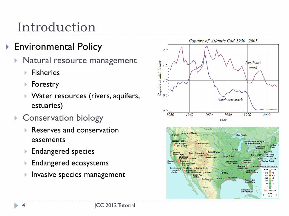
Environmental Policy
Natural resource management
Fisheries
Forestry
Water resources (rivers, aquifers,
estuaries)
Conservation biology
Reserves and conservation
easements
Endangered species
Endangered ecosystems
Invasive species management
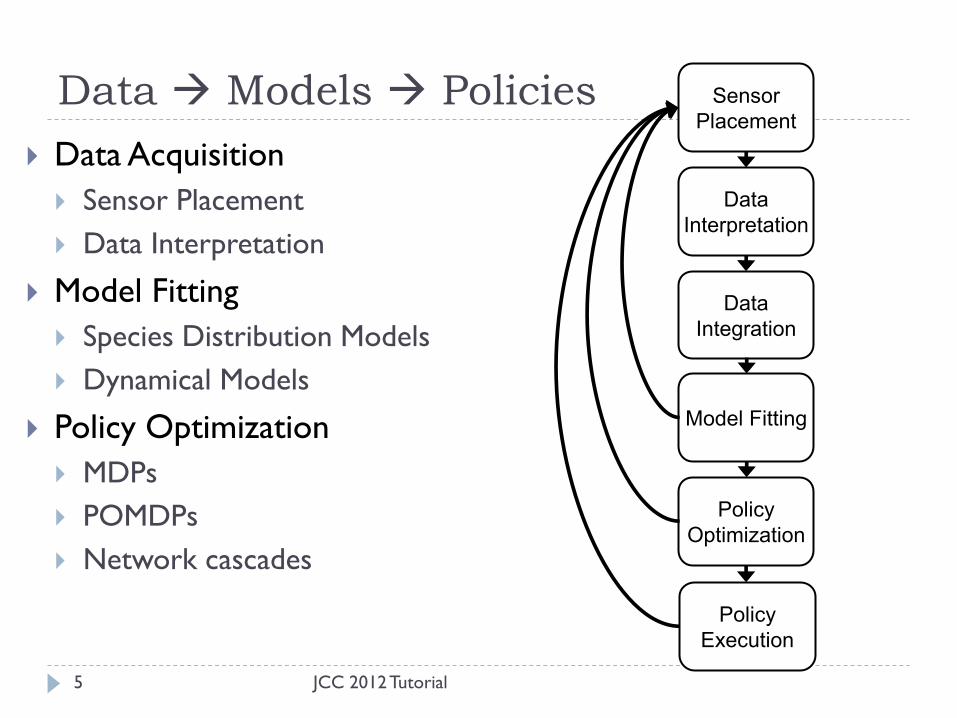
Data Models Policies
JCC 2012 Tutorial 5
Data Acquisition
Sensor Placement
Data Interpretation
Model Fitting
Species Distribution Models
Dynamical Models
Policy Optimization
MDPs
POMDPs
Network cascades
Data
Integration
Data
Interpretation
Model Fitting
Policy
Optimization
Sensor
Placement
Policy
Execution

Unique Aspects
JCC 2012 Tutorial 6
Heterogeneity Physical quantities (nutrients, temperature, wind)
Organisms and species (viruses, bacteria, fungi, plants, animals)
Spatial Scale (inside a single organism, watershed, continent, planet)
Hidden dynamics Virtually all interactions are not directly observed
Observations are noisy and incomplete
Most movement (dispersal, migration) is not directly observed
Non-stationary dynamics: climate change, land-use change, evolution
Optimization wrt learned dynamic models Large spatio-temporal MDPs
Essential POMDPs
Need for robust solutions poorly-modeled dynamics
politics

Goals for the Tutorial
JCC 2012 Tutorial 7
Review the primary data sources, model types, and
machine learning and optimization problems that arise in
ecological science and environmental policy
Provide examples of current optimization and machine
learning work in each of these areas
Point out open problems and opportunities for additional
research
Provide pointers to data sets and relevant literature

Outline
JCC 2012 Tutorial 8
Data Acquisition Sensors: Physical sensors, human
observers, repurposing data from other sources
Data interpretation: Extracting signals from data
Ecological Models Species Distribution Models
Dynamical Models: Dispersal, Migration, Invasion, Climate Change
Policy Optimization Conservation: Reserve design,
Network design
Invasive species: Eradication, restoration, monitoring
Fisheries: Managing harvest levels
Data
Integration
Data
Interpretation
Model Fitting
Policy
Optimization
Sensor
Placement
Policy
Execution
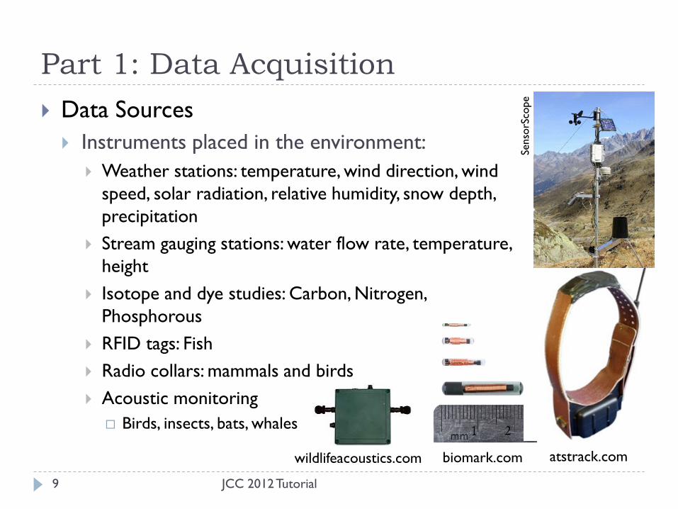
Part 1: Data Acquisition
JCC 2012 Tutorial 9
Data Sources
Instruments placed in the environment:
Weather stations: temperature, wind direction, wind
speed, solar radiation, relative humidity, snow depth,
precipitation
Stream gauging stations: water flow rate, temperature,
height
Isotope and dye studies: Carbon, Nitrogen,
Phosphorous
RFID tags: Fish
Radio collars: mammals and birds
Acoustic monitoring
Birds, insects, bats, whales
atstrack.com biomark.com
Senso
rSco
pe
wildlifeacoustics.com
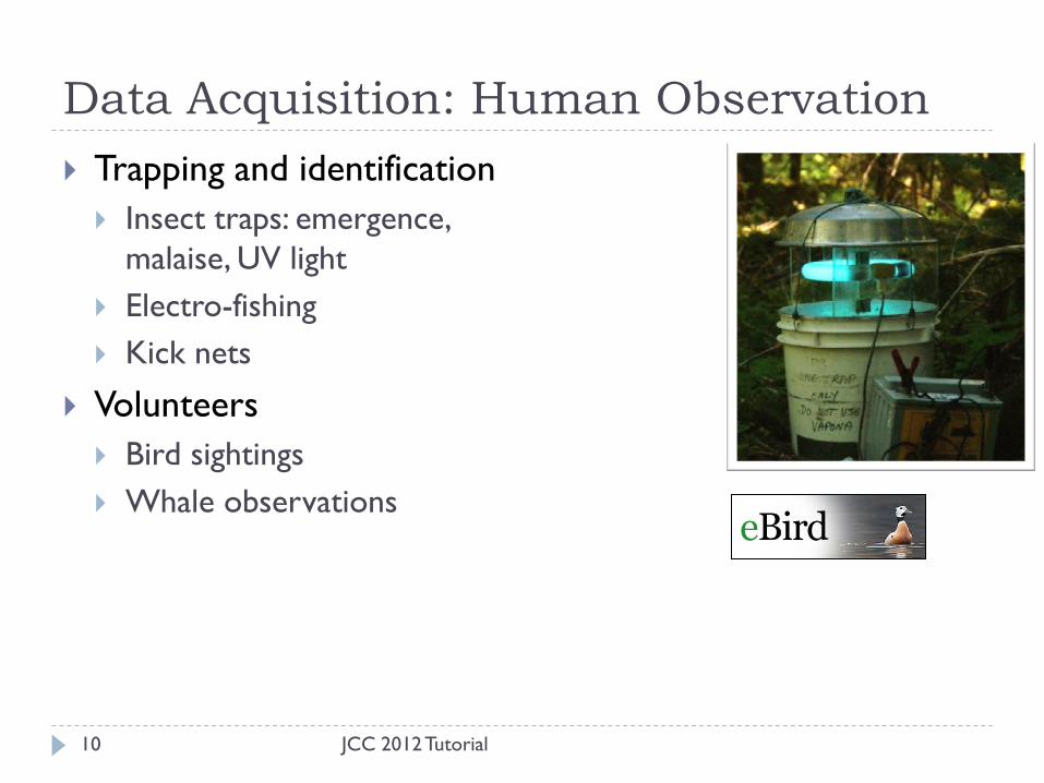
Data Acquisition: Human Observation
JCC 2012 Tutorial 10
Trapping and identification
Insect traps: emergence,
malaise, UV light
Electro-fishing
Kick nets
Volunteers
Bird sightings
Whale observations

Data Acquisition: Repurposing Data
Gathered for Other Purposes
JCC 2012 Tutorial 11
Repurposing information gathered
for other purposes
Fish catch data
Doppler weather radar

Data Acquisition: Remote Sensing
JCC 2012 Tutorial 12
Satellite-borne Sensors
Landsat 7
15m resolution; whole planet coverage every 16 days
MODIS
250m-1km resolution; whole planet coverage every 1-2 days
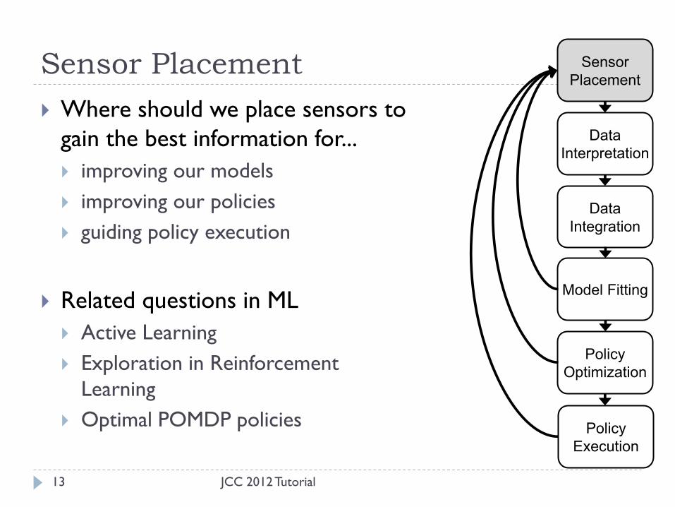
Sensor Placement
JCC 2012 Tutorial 13
Where should we place sensors to
gain the best information for...
improving our models
improving our policies
guiding policy execution
Related questions in ML
Active Learning
Exploration in Reinforcement
Learning
Optimal POMDP policies
Data
Integration
Data
Interpretation
Model Fitting
Policy
Optimization
Sensor
Placement
Policy
Execution
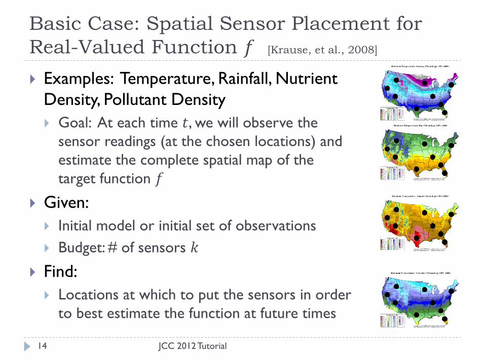
Basic Case: Spatial Sensor Placement for
Real-Valued Function 𝑓 [Krause, et al., 2008]
JCC 2012 Tutorial 14
Examples: Temperature, Rainfall, Nutrient
Density, Pollutant Density
Goal: At each time 𝑡, we will observe the
sensor readings (at the chosen locations) and
estimate the complete spatial map of the
target function 𝑓
Given:
Initial model or initial set of observations
Budget: # of sensors 𝑘
Find:
Locations at which to put the sensors in order
to best estimate the function at future times

Approach
15
Discretize space: Let S be a set of points (𝑠1, … , 𝑠𝑁)
where sensors can be placed
where we will make predictions
Assume joint Gaussian
(𝑓 𝑠1 , … , 𝑓 𝑠𝑁 )~Norm 𝝁, 𝚺
where 𝝁 has dimension 𝑁 and
𝚺 has dimension 𝑁 × 𝑁
Use the initial observations to estimate 𝚺
Choose an objective function 𝐽(𝐴) for evaluating the quality of a set of sensor locations 𝐴
Formulate an optimization problem to choose a set 𝐴 ⊂ 𝑆 of size 𝑘 that optimizes 𝐽(𝐴).
Place sensors at points 𝐴
JCC 2012 Tutorial

What Criterion to Optimize?
JCC 2012 Tutorial 16
Estimate the amount of
information that the chosen
points tell us about the not-
chosen points
𝐼 𝑋𝐴; 𝑋𝑆\A = “mutual
information”
𝐽 𝐴 = 𝐼 𝑋𝐴; 𝑋𝑆\A will be
our “objective function”
Choose 𝐴 to maximize 𝐽(𝐴)
𝐴 𝑆\𝐴

What Criterion to Optimize?
17
Rationale:
empirical: gives good results
computational: easy to compute for Gaussian distributions
analytical: objective is sub-modular
Greedy Algorithm with provable bounds
Submodularity:
𝐽 is submodular if for all 𝐴 ⊆ 𝐴′ and all 𝑎 ∈ 𝑆\A′, 𝐽 𝐴 ∪ 𝑎 − 𝐽 𝐴 ≥ 𝐽 𝐴′ ∪ 𝑎 − 𝐽(𝐴′)
“diminishing returns of adding 𝑎”
𝐴
𝐴′
{𝑎}
{𝑎}
𝐽
JCC 2012 Tutorial

Greedy Algorithm
18
Input:
Sites: 𝑆
Number of sensors: 𝑘
Estimated covariance matrix of joint Gaussian: 𝚺
Output: sensor locations 𝐴 ⊂ 𝑆, 𝐴 = 𝑘
begin
𝐴 ← ∅
for 𝑗 = 1 to 𝑘 do
𝑎∗ ← argmax𝑎∈𝑆\A
𝐽(𝐴 ∪ 𝑎 )
𝐴 ← 𝐴 ∪ 𝑎∗
end
JCC 2012 Tutorial

Analytical Bound
19
Monotonicity assumption: ∀ 𝑎 ∈ 𝑆\A 𝐽 𝐴 ∪ 𝑎 > 𝐽 𝐴 + 𝜖
Let 𝐴 be the greedy solution and 𝐴∗ be
the optimal solution
𝐽 𝐴 ≥ 1 −1
𝑒𝐽 𝐴∗ − 𝑘𝜖
1 −1
𝑒≈ 0.632
Assumption will hold if 𝑆 is discretized
sufficiently finely
JCC 2012 Tutorial

Experimental Accuracy
20
Theoretical bound is 63.2%
of optimal
Greedy algorithm is closer
to 95% of optimal in this
case
Intel Berkeley Temperature Sensors
JCC 2012 Tutorial

Data Interpretation
JCC 2012 Tutorial 22
Extracting high level
interpretation from low-level
sensor data
Example I: Arthropod Population
Counting
Example 2: Finding Swallow Roosts
in Doppler Weather Radar
Data
Integration
Data
Interpretation
Model Fitting
Policy
Optimization
Sensor
Placement
Policy
Execution
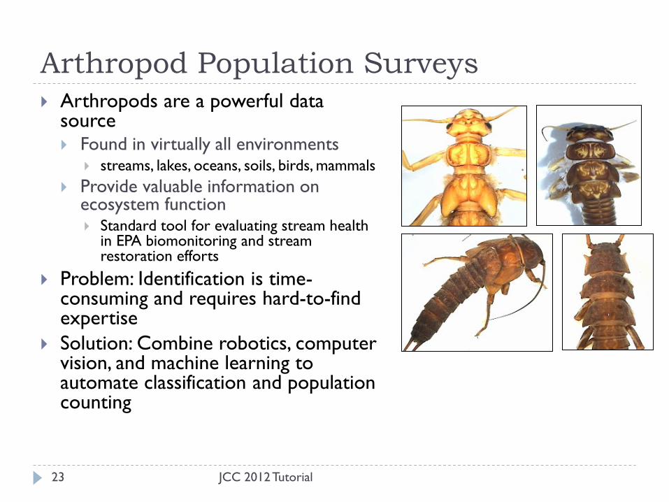
Arthropod Population Surveys
JCC 2012 Tutorial 23
Arthropods are a powerful data source Found in virtually all environments
streams, lakes, oceans, soils, birds, mammals
Provide valuable information on ecosystem function Standard tool for evaluating stream health
in EPA biomonitoring and stream restoration efforts
Problem: Identification is time-consuming and requires hard-to-find expertise
Solution: Combine robotics, computer vision, and machine learning to automate classification and population counting

OSU BugID Project
JCC 2012 Tutorial 24
Human technician gathers
field sample
Semi-automated image
capture
Automated classification
ww
w.e
pa.
gov
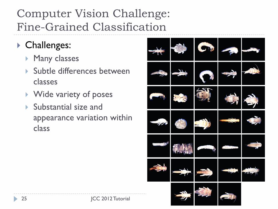
Computer Vision Challenge:
Fine-Grained Classification
JCC 2012 Tutorial 25
Challenges:
Many classes
Subtle differences between
classes
Wide variety of poses
Substantial size and
appearance variation within
class

Hypotheses
JCC 2012 Tutorial 26
Fine-grained classification requires
High-resolution images
Non-uniform extraction of information from the image
Existing object recognition methods
Break image into set of patches
Extract a fixed number of bits from each patch
e.g., via vector quantization, filter banks, PCA, etc.
Classify image using extracted information

Patch
Classifier
A “Variable Resolution” Method for Object
Recognition
JCC 2012 Tutorial 27
Stacked Patch Classifiers
Learn a classifier that tries to classify the whole image using
detailed information from a single patch
Combine the single-patch classifications into a classification for
the whole image
[Martinez, et al, 2009]
𝑦 = 2
0
0
0
0
0
0
0
0
0
1
𝑦 = 3
1
𝑦
2
8
1
3
0
0
6
4
2
Stacked
Classifier 𝑦 = 2

Results on STONEFLY9 Dataset
JCC 2012 Tutorial 28
Variable resolution method is much more accurate
Configuration Error Rate
Fixed resolution method 16.1%
Stacked Patch Classifier 5.6%

EPT54: 54 Species of Freshwater
Macroinvertebrates
JCC 2012 Tutorial 29
Stacked Patch Classifier: 74.3% Correct
0%
10%
20%
30%
40%
50%
60%
70%
80%
90%
100%
% C
orr
ect
Cla
ssif
icati
on
Taxon
mean

0%
10%
20%
30%
40%
50%
60%
70%
80%
90%
100%
0 0.1 0.2 0.3 0.4 0.5 0.6 0.7 0.8 0.9
Macro
-avera
ged
Pre
cis
ion
Rejection Rate
Open Problems
JCC 2012 Tutorial 30
Rejection:
Maximize recall subject to high
precision
Detect and reject novel (i.e.,
unknown to the classifier)
species
Scale to thousands of species
Hierarchical loss functions
Order, Family, Genus, Species
Classify as finely as possible
while bounding error rate

Tracking Tree Swallow Roosts
Using NEXRAD Radar
31 JCC 2012 Tutorial

Dover, DE, 10/2/2010@6:52AM 32
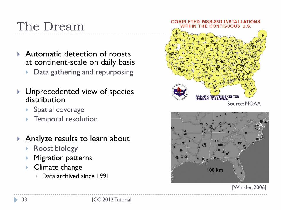
The Dream
Automatic detection of roosts at continent-scale on daily basis Data gathering and repurposing
Unprecedented view of species distribution Spatial coverage
Temporal resolution
Analyze results to learn about Roost biology
Migration patterns
Climate change Data archived since 1991
Source: NOAA
33
[Winkler, 2006]
JCC 2012 Tutorial

Machine Learning Pipeline (1)
JCC 2012 Tutorial 34
Primary goal: data reduction
High recall
Many false positives
Step 1: Fast
Unsupervised
Detector
Radar scans
(terabytes)
Candidate
roosts
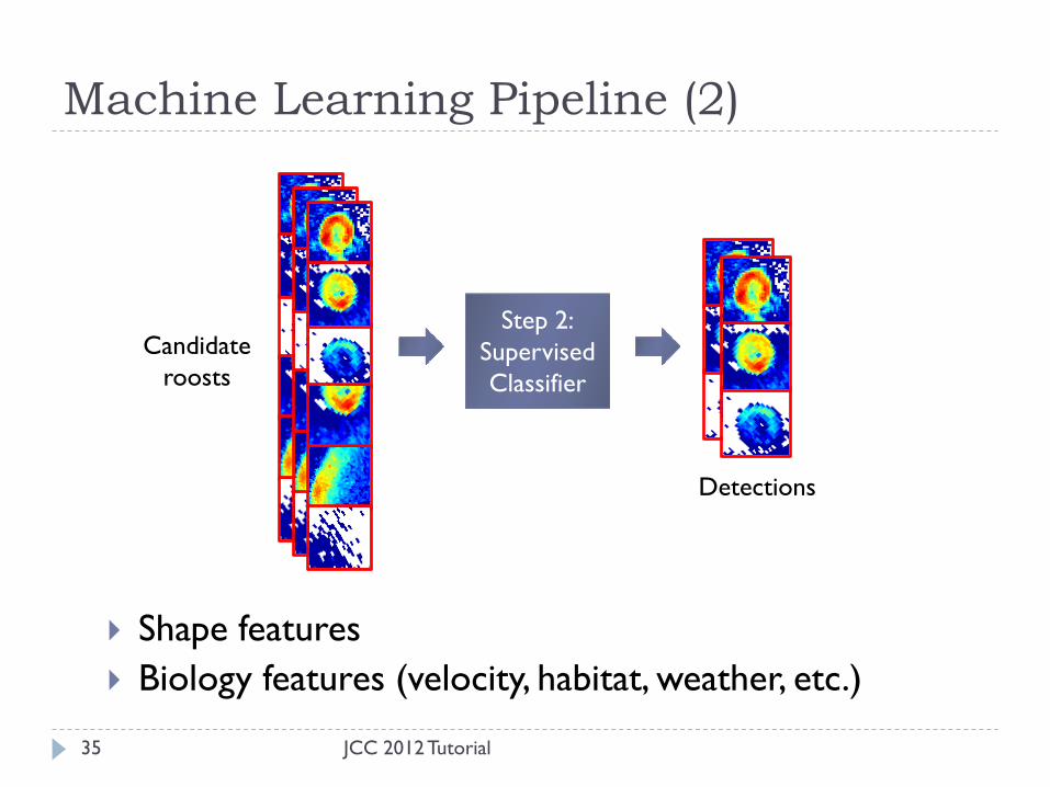
Machine Learning Pipeline (2)
JCC 2012 Tutorial 35
Step 2:
Supervised
Classifier
Shape features
Biology features (velocity, habitat, weather, etc.)
Candidate
roosts
Detections

Machine Learning Pipeline (3)
JCC 2012 Tutorial 36
Step 3:
Sequence
assembly
(Multiple Target
tracking)
Roost 1
Roost n
Detections
(all frames) Sequences
…
Motivation:
Improve detection by using temporal context
Extract high-level information such as duration, maximum size, etc.

Progress: Machine Learning
JCC 2012 Tutorial 37
Steps 1 and 2 Primarily shape features to-date
High precision for roosts with “perfect appearance”
Variability in appearance is challenging low recall
100 positive examples Top 100 predicted roosts
(shape features + SVM)
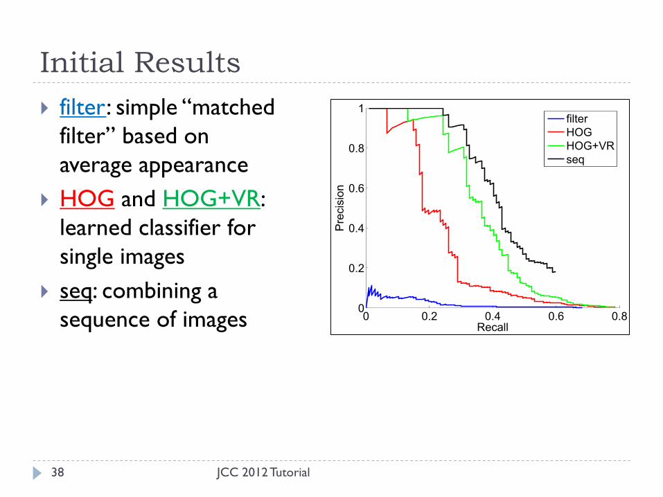
Initial Results
JCC 2012 Tutorial 38
filter: simple “matched
filter” based on
average appearance
HOG and HOG+VR:
learned classifier for
single images
seq: combining a
sequence of images 0 0.2 0.4 0.6 0.80
0.2
0.4
0.6
0.8
1
RecallP
recis
ion
filter
HOG
HOG+VR
seq
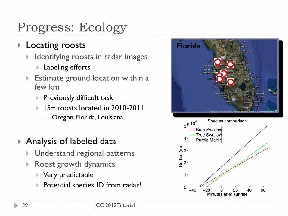
Progress: Ecology
39
Locating roosts
Identifying roosts in radar images
Labeling efforts
Estimate ground location within a few km
Previously difficult task
15+ roosts located in 2010-2011
Oregon, Florida, Louisiana
Analysis of labeled data
Understand regional patterns
Roost growth dynamics
Very predictable
Potential species ID from radar!
JCC 2012 Tutorial
Florida

Summary
JCC 2012 Tutorial 40
Ongoing project
A lot of work remains to reach “the dream”
Significant opportunity for ML and ecology to develop in
parallel
Data Integration
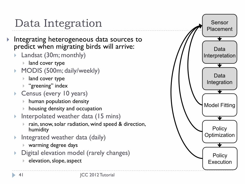
Integrating heterogeneous data sources to predict when migrating birds will arrive: Landsat (30m; monthly)
land cover type
MODIS (500m; daily/weekly) land cover type
“greening” index
Census (every 10 years) human population density
housing density and occupation
Interpolated weather data (15 mins) rain, snow, solar radiation, wind speed & direction,
humidity
Integrated weather data (daily) warming degree days
Digital elevation model (rarely changes) elevation, slope, aspect
JCC 2012 Tutorial 41
Data
Integration
Data
Interpretation
Model Fitting
Policy
Optimization
Sensor
Placement
Policy
Execution

Questions on Part 1?
JCC 2012 Tutorial 42

Part 2: Ecological Models
JCC 2012 Tutorial 43
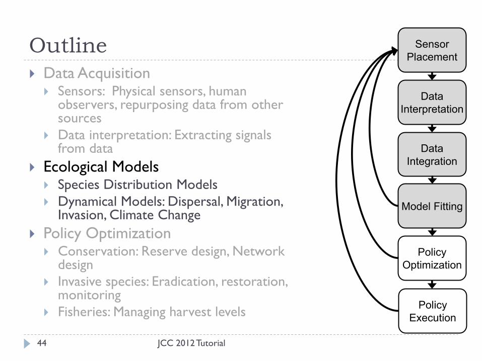
Outline
JCC 2012 Tutorial 44
Data Acquisition Sensors: Physical sensors, human
observers, repurposing data from other sources
Data interpretation: Extracting signals from data
Ecological Models Species Distribution Models
Dynamical Models: Dispersal, Migration, Invasion, Climate Change
Policy Optimization Conservation: Reserve design, Network
design
Invasive species: Eradication, restoration, monitoring
Fisheries: Managing harvest levels
Data
Integration
Data
Interpretation
Model Fitting
Policy
Optimization
Sensor
Placement
Policy
Execution

Ecological Models
Species Distribution Models
Static descriptions of the geographic distribution of a species.
Address the fundamental ecological question of why species
are found where they are.
Dynamical Models
Account for dynamic ecological processes like dispersal,
migration, population growth, etc.
45 JCC 2012 Tutorial
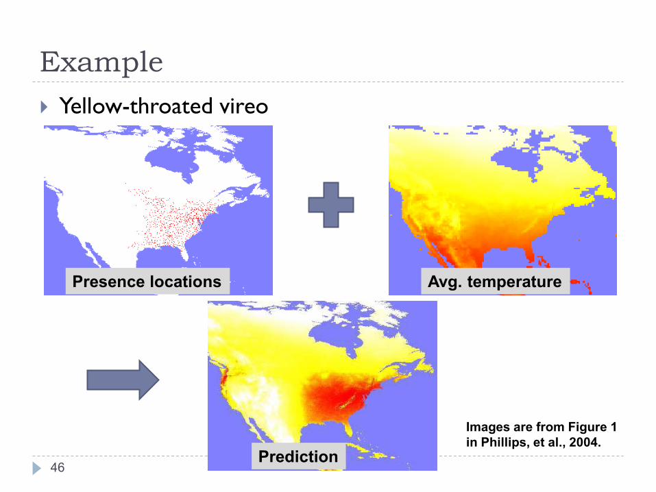
Yellow-throated vireo
Example
46
Images are from Figure 1
in Phillips, et al., 2004.
Presence locations Avg. temperature
Prediction

Species Distribution Models (SDM)
47
Prediction Task: Given a feature vector 𝒙 describing a site, predict whether the
species occurs there 𝑦 ∈ {0,1}
Standard Supervised Learning Given training examples 𝑥1, 𝑦1 , … , 𝑥𝑁, 𝑦𝑁 Learn a predictive model 𝑓 such that 𝑦 = 𝑓(𝑥)
Purposes: Mapping the current distribution of a species
Understanding habitat requirements for the species
Predicting distribution in places where there is no data
available
JCC 2012 Tutorial
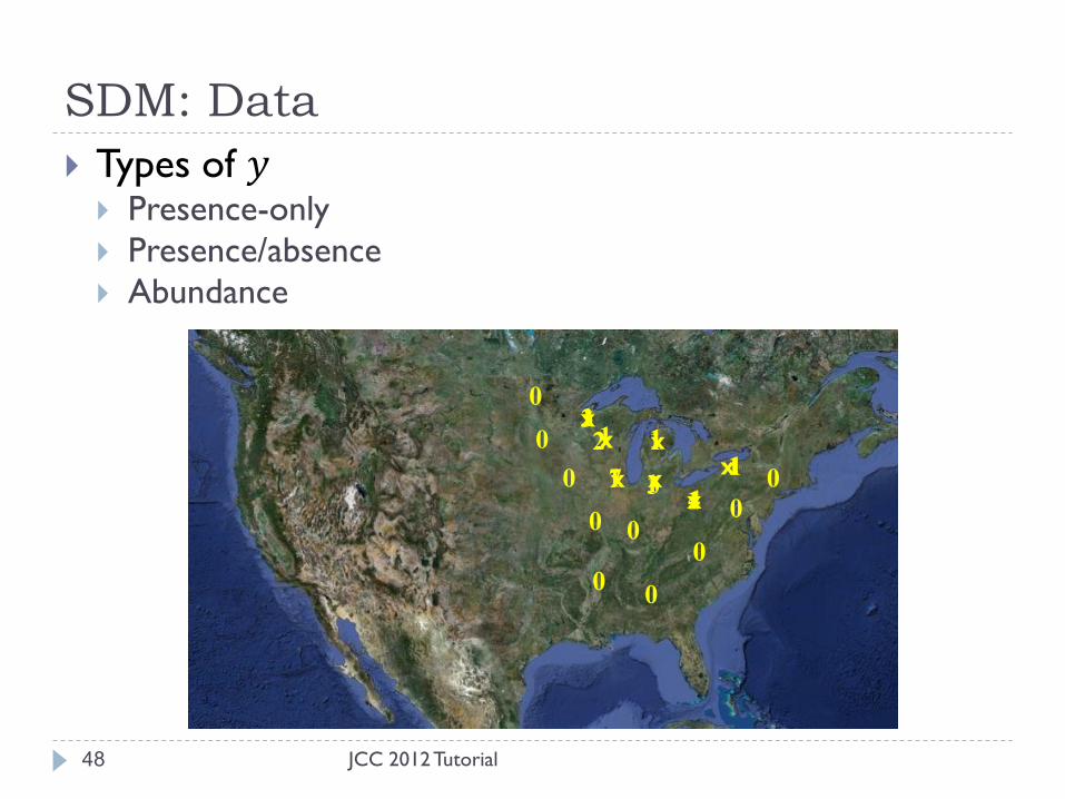
SDM: Data
48
Types of 𝑦 Presence-only
Presence/absence
Abundance
x
x x
x x
x
x 1
0
1 1
1
1
1 1
0
0
0
0
0 0 0
0
0
4
1 3
1
7
2 3
JCC 2012 Tutorial
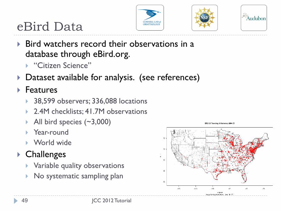
eBird Data
Bird watchers record their observations in a database through eBird.org.
“Citizen Science”
Dataset available for analysis. (see references)
Features 38,599 observers; 336,088 locations
2.4M checklists; 41.7M observations
All bird species (~3,000)
Year-round
World wide
Challenges Variable quality observations
No systematic sampling plan
49 JCC 2012 Tutorial

SDM: Methods
50
Envelope Models
Bioclim
Statistical and Machine Learning Models Maxent
Generalized Linear Models
Generalized Additive Models
Multivariate Adaptive Regression Splines
Hierarchical Bayesian modeling
Boosted regression trees
Random forests
Genetic algorithms
…and more! JCC 2012 Tutorial

ML is already having an impact in SDM
51
16 methods
226 species
6 regions
General result: new(er) statistical and/or machine learning methods outperformed older envelope/distance style models.
JCC 2012 Tutorial

52 Elith et al, 2006
Older,
envelope-style
models
Statistical, regression-style models
Newer,
machine
learning-style
models
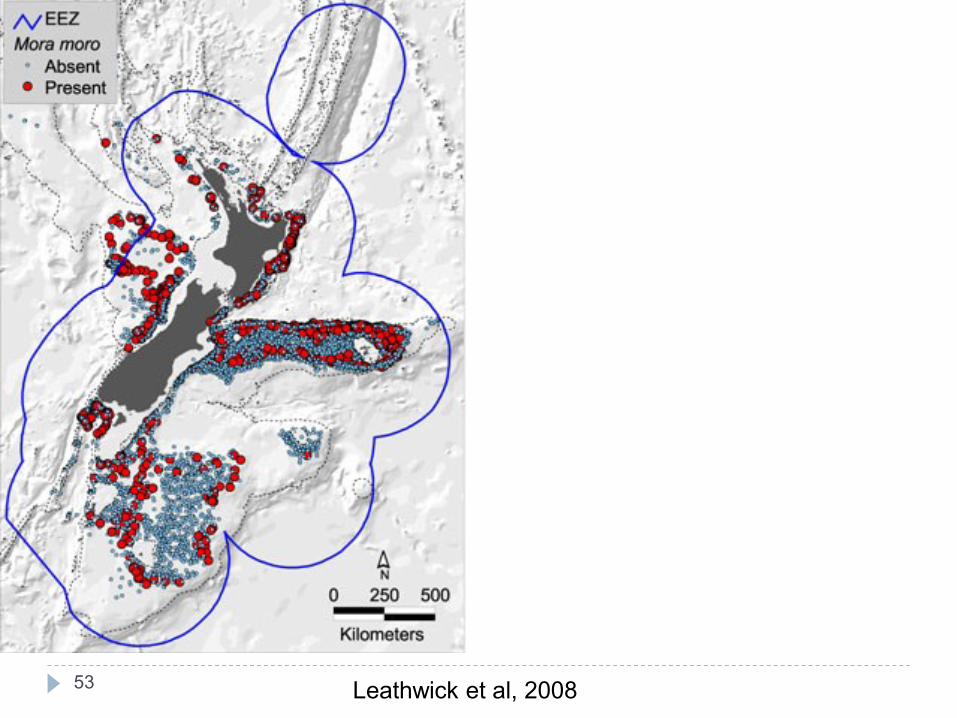
53
Leathwick et al, 2008

54
Disregarding costs
to fishing industry
Full consideration of costs
to fishing industry
Leathwick et al, 2008

Three SDM Challenges
55
Presence-only data
Extrapolation beyond the training data
Imperfect detection of the species on surveys
Often lack prior knowledge of the system for model building
Observers have variable expertise/biases
JCC 2012 Tutorial
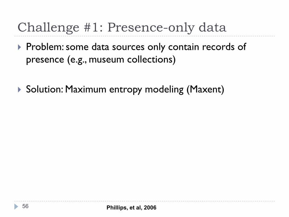
Challenge #1: Presence-only data
56
Problem: some data sources only contain records of
presence (e.g., museum collections)
Solution: Maximum entropy modeling (Maxent)
Phillips, et al, 2006
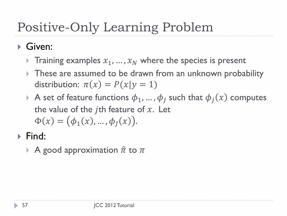
Positive-Only Learning Problem
JCC 2012 Tutorial 57
Given:
Training examples 𝑥1, … , 𝑥𝑁 where the species is present
These are assumed to be drawn from an unknown probability
distribution: 𝜋 𝑥 = 𝑃(𝑥|𝑦 = 1)
A set of feature functions 𝜙1, … , 𝜙𝐽 such that 𝜙𝑗 𝑥 computes
the value of the 𝑗th feature of 𝑥. Let
Φ 𝑥 = 𝜙1 𝑥 , … , 𝜙𝐽 𝑥 .
Find:
A good approximation 𝜋 to 𝜋
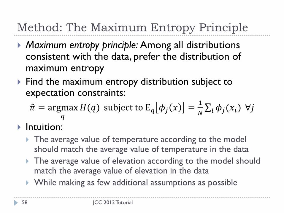
Method: The Maximum Entropy Principle
JCC 2012 Tutorial 58
Maximum entropy principle: Among all distributions consistent with the data, prefer the distribution of maximum entropy
Find the maximum entropy distribution subject to expectation constraints:
𝜋 = argmax𝑞
𝐻(𝑞) subject to E𝑞 𝜙𝑗 𝑥 =1
𝑁 𝜙𝑗(𝑥𝑖)𝑖 ∀𝑗
Intuition:
The average value of temperature according to the model should match the average value of temperature in the data
The average value of elevation according to the model should match the average value of elevation in the data
While making as few additional assumptions as possible

Solving the Maxent Optimization
59
Step 1: Relax the constraints: 𝜋 = argmax
𝑞𝐻(𝑞) subject to
Eq 𝜙𝑗 𝑥 −1
𝑁 𝜙𝑗(𝑥𝑖)
𝑖
≤ 𝛽𝑗 ∀𝑗
Step 2: Assume a parametric form for 𝜋 :
𝜋 𝑥 =1
𝑍 𝒘exp[𝒘 ⋅ Φ 𝒙 ]
Step 3: Apply duality methods to show this is equivalent
to an 𝐿1-regularized linear optimization
𝒘 = argmax𝒘
𝒘 ⋅ Φ 𝑥𝑖
𝑖
− 𝛽𝑗|𝑤𝑗|
𝑗
JCC 2012 Tutorial
Obtaining an SDM
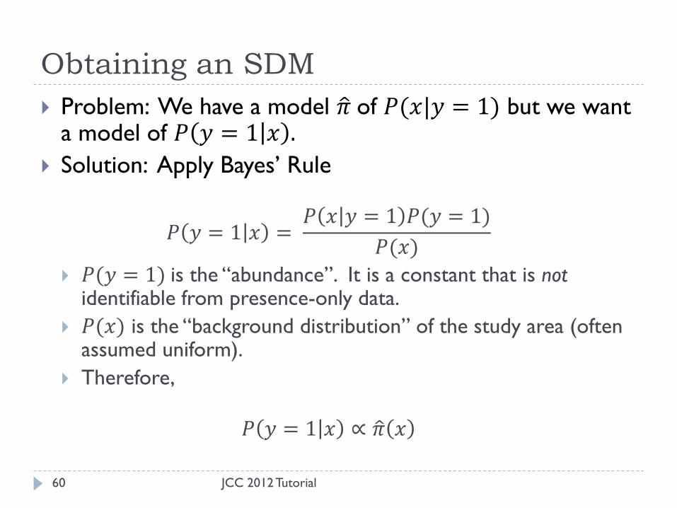
JCC 2012 Tutorial 60
Problem: We have a model 𝜋 of 𝑃(𝑥|𝑦 = 1) but we want a model of 𝑃 𝑦 = 1 𝑥 .
Solution: Apply Bayes’ Rule
𝑃 𝑦 = 1 𝑥 = 𝑃 𝑥 𝑦 = 1 𝑃(𝑦 = 1)
𝑃(𝑥)
𝑃(𝑦 = 1) is the “abundance”. It is a constant that is not identifiable from presence-only data.
𝑃(𝑥) is the “background distribution” of the study area (often assumed uniform).
Therefore,
𝑃 𝑦 = 1 𝑥 ∝ 𝜋 𝑥

Creating a Usable Tool
JCC 2012 Tutorial 61
Free software package for SDM
http://www.cs.princeton.edu/~schapire/maxent/
Has had a huge impact in the ecology literature
Provides a rich set of feature types 𝜙𝑡
linear
quadratic
thresholds
ramps
pairwise products of these
Provides default settings for the 𝛽s
The method requires tuning a separate 𝛽𝑗 for each feature, which is
hard to do via cross-validation.
Defaults are based on tuning for 6 datasets from Elith, et al. [2006]

Yellow-throated vireo
Example
62
Images are from Figure 1
in Phillips, et al., 2004.
Presence locations Avg. ann. temperature
Maxent prediction

Challenge #2: Extrapolation
63
Problem: at continental scale, learned models may
extrapolate too far and make mistakes
Fink, et al., 2010: “Spatiotemporal exploratory models for
broad-scale survey data”
Fink, et al, 2010

64
Winter Distribution
Tree Swallow
Winter Distribution Analysis
(Tachycineta bicolor)
eBird Bagged Decision Trees
Wetland Coverage > 5%
“Wetland” should really be “Wetland at time 𝑡”
Lack of data for northern US in winter time (people don’t go bird
watching in the snow)
slide courtesy of Daniel Fink

STEM: Ensemble Method
65
Idea:
Slice space and time into
hyperrectangles:
latitude x longitude x time
called “stixels”
Train a classifier on the data
inside each stixel
To predict at a new point 𝑥
at a given place 𝑙𝑜𝑐(𝑥) and
time 𝑡(𝑥), vote the
predictions of all classifiers
whose stixel contains
(𝑙𝑜𝑐 𝑥 , 𝑡 𝑥 )
Fink, et al, 2010
𝑙𝑜𝑐(𝑥)
𝑡(𝑥)

Key Idea
JCC 2012 Tutorial 66
Because each classifier is only asked to predict within its
stixel, it will never extrapolate beyond the stixel

STEM SDM: Solitary Sandpiper
slide courtesy of Daniel Fink 67
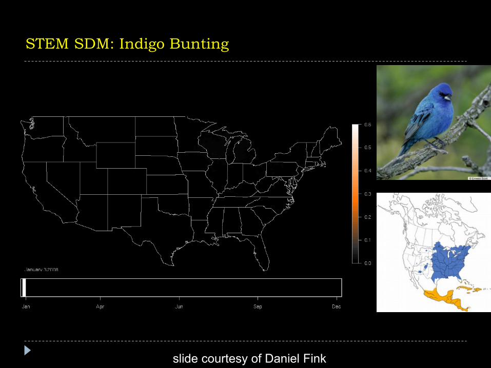
STEM SDM: Indigo Bunting
slide courtesy of Daniel Fink
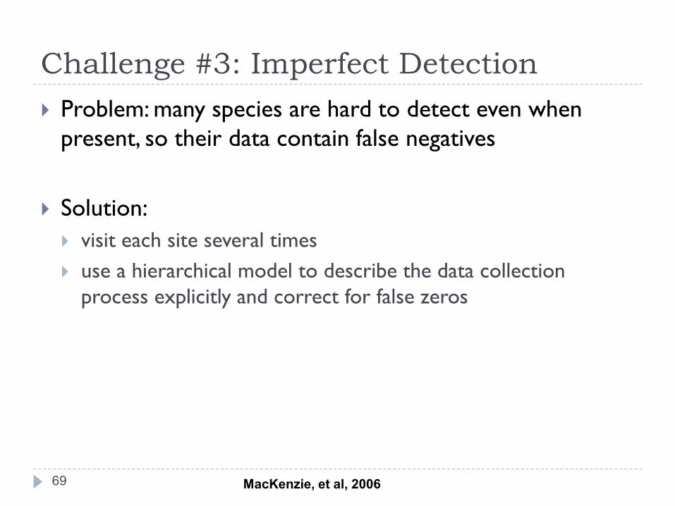
Challenge #3: Imperfect Detection
69
Problem: many species are hard to detect even when
present, so their data contain false negatives
Solution:
visit each site several times
use a hierarchical model to describe the data collection
process explicitly and correct for false zeros
MacKenzie, et al, 2006
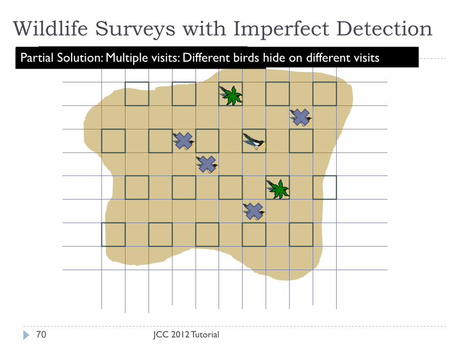
Wildlife Surveys with Imperfect Detection
70
Problem 1: We don’t observe everywhere Problem 2: Some birds are hidden Partial Solution: Multiple visits: Different birds hide on different visits
JCC 2012 Tutorial
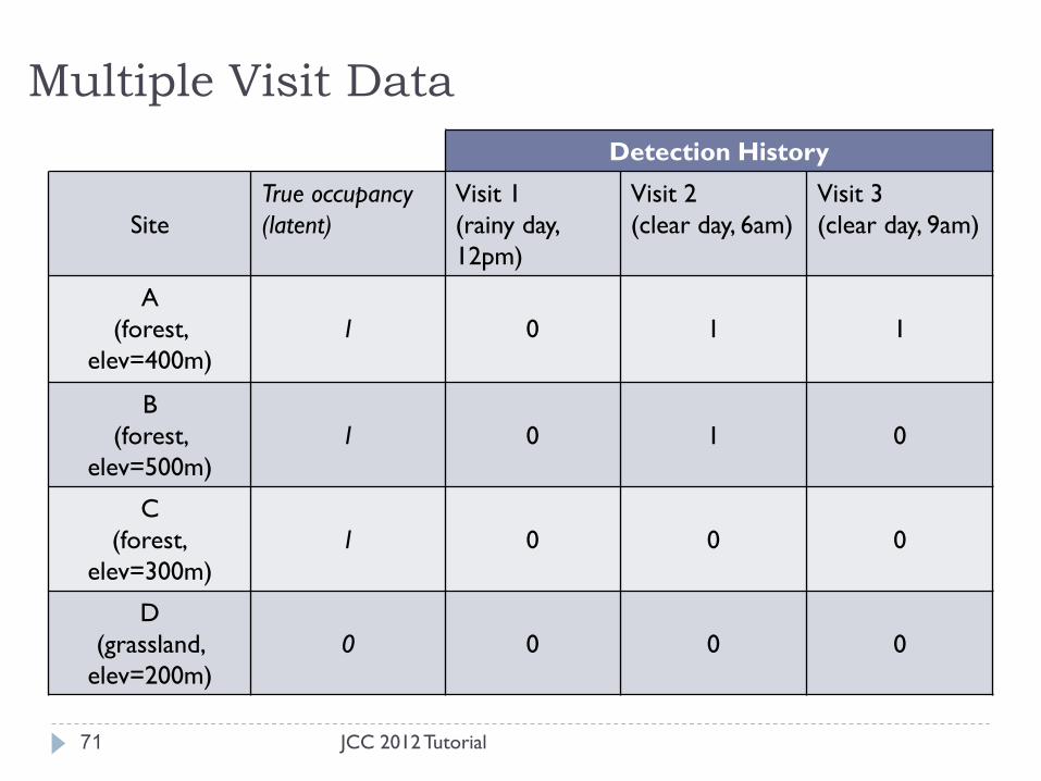
Multiple Visit Data
71
Detection History
Site
True occupancy
(latent)
Visit 1
(rainy day,
12pm)
Visit 2
(clear day, 6am)
Visit 3
(clear day, 9am)
A
(forest,
elev=400m)
1
0
1
1
B
(forest,
elev=500m)
1
0
1
0
C
(forest,
elev=300m)
1
0
0
0
D
(grassland,
elev=200m)
0
0
0
0
JCC 2012 Tutorial

𝑑13 𝑑12
Probabilistic Model with Latent Variable 𝑍
72
𝑋1
𝑍1= 1
𝑤11 𝑤12 𝑤13
𝑦11= 0 𝑦12= 1 𝑦13= 1
(rain, 12pm) (clear, 6am) (clear, 9am)
(forest, 400m)
𝑜1
𝑑11
𝑋4
𝑍4= 0
𝑤41 𝑤42 𝑤43
𝑦41= 0 𝑦42= 0 𝑦43= 0
(rain, 12pm) (clear, 6am) (clear, 9am)
(grassland, 200m)
... 𝑜4
𝑑41 𝑑42 𝑑43
MacKenzie, et al, 2006

73
Occupancy Model
Yit Zi
i=1,…,M
t=1,…,T
Xi Wit
oi dit
Covariates of occupancy (e.g. elevation, vegetation)
Covariates of detection (e.g. time of day, effort)
Observed presence/absence Yit | Zi ~ Bern(Zidit)
True (latent) presence/absence Zi ~ Bern(oi)
Probability of occupancy (function of Xi, a)
Probability of detection (function of Wit, b)
Sites
Visits
MacKenzie, et al, 2006
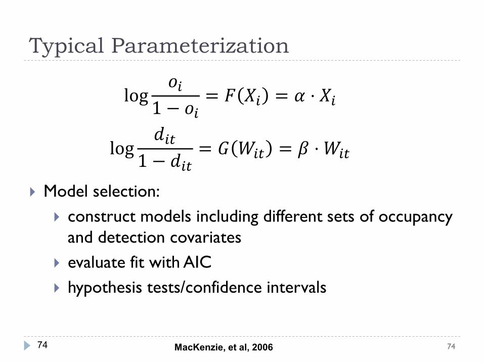
Typical Parameterization
74 74 74
MacKenzie, et al, 2006
Model selection:
construct models including different sets of occupancy
and detection covariates
evaluate fit with AIC
hypothesis tests/confidence intervals
log𝑜𝑖
1 − 𝑜𝑖= 𝐹 𝑋𝑖 = 𝛼 ⋅ 𝑋𝑖
log𝑑𝑖𝑡
1 − 𝑑𝑖𝑡= 𝐺 𝑊𝑖𝑡 = 𝛽 ⋅ 𝑊𝑖𝑡

Imperfect Detection +
Lack of Prior Knowledge
75
Problem: occupancy models require parametric
assumptions too rigid for exploratory modeling of big
data sets
Solution: incorporate flexible models into the model
while maintaining hierarchical structure to account for
imperfect detection
Hutchinson, et al, 2011
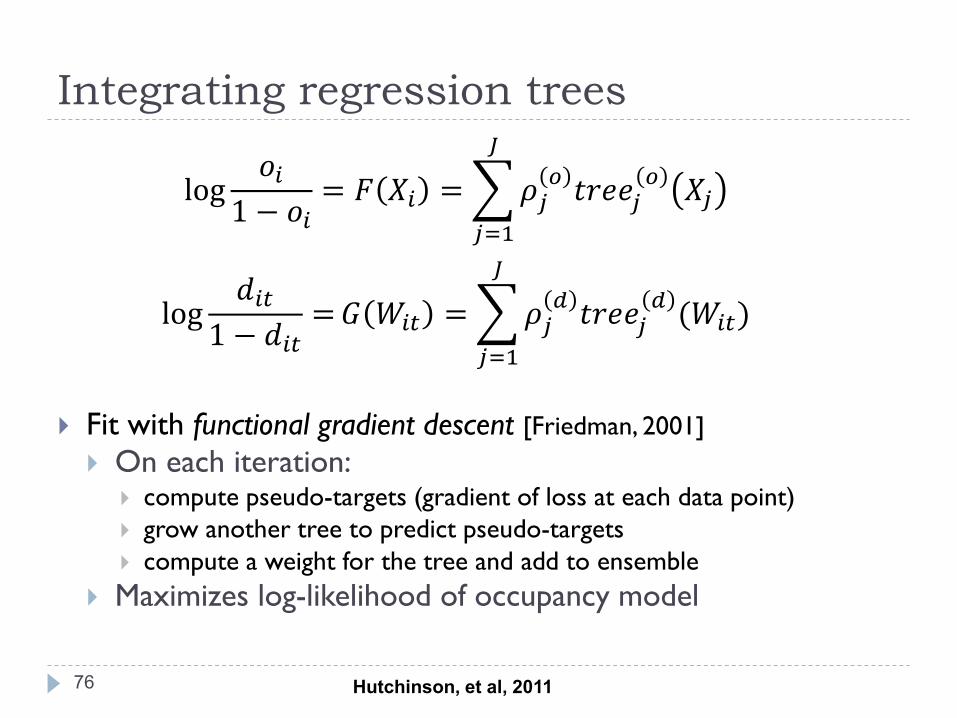
Integrating regression trees
76
Fit with functional gradient descent [Friedman, 2001]
On each iteration: compute pseudo-targets (gradient of loss at each data point)
grow another tree to predict pseudo-targets
compute a weight for the tree and add to ensemble
Maximizes log-likelihood of occupancy model
Hutchinson, et al, 2011
log𝑜𝑖
1 − 𝑜𝑖= 𝐹 𝑋𝑖 = 𝜌𝑗
𝑜𝑡𝑟𝑒𝑒𝑗
𝑜𝑋𝑗
𝐽
𝑗=1
log𝑑𝑖𝑡
1 − 𝑑𝑖𝑡= 𝐺 𝑊𝑖𝑡 = 𝜌𝑗
𝑑𝑡𝑟𝑒𝑒𝑗
𝑑(𝑊𝑖𝑡)
𝐽
𝑗=1
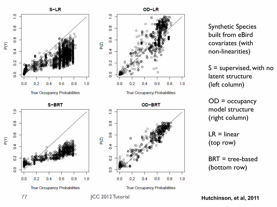
77
Synthetic Species
built from eBird
covariates (with
non-linearities)
S = supervised, with no
latent structure
(left column)
OD = occupancy
model structure
(right column)
LR = linear
(top row)
BRT = tree-based
(bottom row)
Hutchinson, et al, 2011 JCC 2012 Tutorial

Imperfect Detection + Variable Expertise
78
Problem: expert and novice observers contributing
observations to citizen science data generate different
mistakes/biases
Solution: extend occupancy models so that observer
expertise affects the detection model
Yu, et al, 2010

Extending Occupancy Models
79
Yit Zi
i=1,…,M
Xi Wit
oi dit,fit
t=1,…,T
j=1,…,N
vj Observer
covariates
Expert/novice observer Expertise probability (function of U)
Observers
d’it,f’it
Ej Uj
Yu, et al, 2010

-0.05
0.00
0.05
0.10
0.15
0.20
Average Difference in True Detection Probability
Expert vs Novice Differences
80
Hard-to-detect
birds
Common birds
Yu, et al, 2010

A few SDM Challenges
81
Presence-only data
Predictor-response relationships are non-stationary
Imperfect detection of the species on surveys
Often lack prior knowledge of the system for model building
Observers have variable expertise/biases
Sampling bias
Extrapolation (e.g. under climate change)
Evaluation strategies
Estimating temporal trends directly
More biologically-realistic models
Multi-species models
Models of abundance (instead of presence/absence)
JCC 2012 Tutorial

Sampling Bias
eBird participants tend to stay close to home.
How can we make good predictions uniformly across the U.S.?
82
Cardinals
JCC 2012 Tutorial

Inappropriate Extrapolation
83 http://data.prbo.org/cadc2/index.php?page=climate-change-distribution
Model
learned
with data
from
1992-2007
Applied to
conditions
projected
for 2070,
according
to IPCC
scenarios

A few SDM Challenges
84
Presence-only data
Predictor-response relationships are non-stationary
Imperfect detection of the species on surveys
Often lack prior knowledge of the system for model building
Observers have variable expertise/biases
Sampling bias
Extrapolation (e.g. under climate change)
Evaluation strategies
Estimating temporal trends directly
More biologically-realistic models
Multi-species models
Models of abundance (instead of presence/absence)
JCC 2012 Tutorial

Ecological Models (part 2):
Dynamical Models
JCC 2012 Tutorial 85
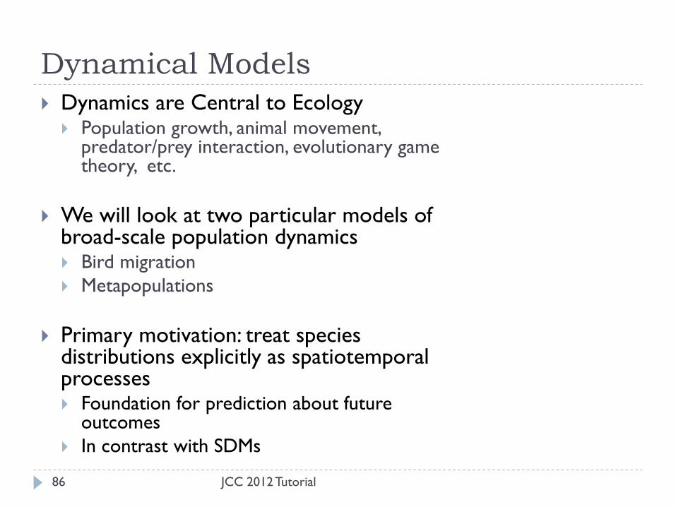
Dynamical Models
Dynamics are Central to Ecology Population growth, animal movement,
predator/prey interaction, evolutionary game theory, etc.
We will look at two particular models of broad-scale population dynamics Bird migration
Metapopulations
Primary motivation: treat species distributions explicitly as spatiotemporal processes Foundation for prediction about future
outcomes
In contrast with SDMs
86 JCC 2012 Tutorial
Dynamical Model #1: Bird Migration
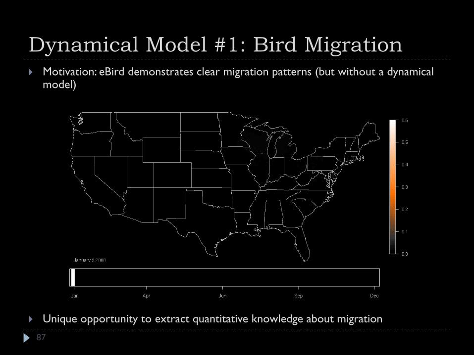
87
Motivation: eBird demonstrates clear migration patterns (but without a dynamical model)
Unique opportunity to extract quantitative knowledge about migration
Challenges Extracting Migration Knowledge
Migration is a latent process
eBird data and SDM predictions are static
Each observation/prediction for particular place and time
We see a sequence of snapshots
Observations are noisy and incomplete
Migration most naturally described at level of individual
behavior, but we can only observe population-level statistics
Lack of modeling techniques to link the two
88 JCC 2012 Tutorial
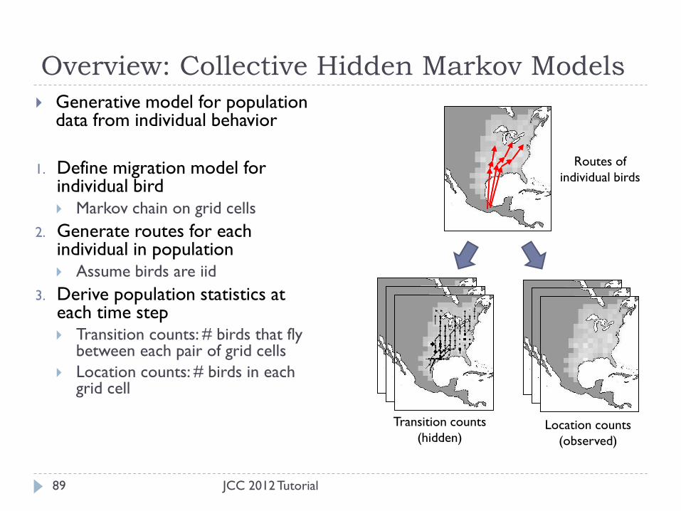
Overview: Collective Hidden Markov Models
JCC 2012 Tutorial 89
Generative model for population data from individual behavior
1. Define migration model for individual bird Markov chain on grid cells
2. Generate routes for each individual in population Assume birds are iid
3. Derive population statistics at each time step Transition counts: # birds that fly
between each pair of grid cells
Location counts: # birds in each grid cell
Transition counts
(hidden) Location counts
(observed)
Routes of
individual birds

Overview: Collective Hidden Markov Models
90 JCC 2012 Tutorial
𝑋1 𝑋2 𝑋𝑇 … Individual model:
Markov chain on grid cells
𝑋1𝑚 𝑋2
𝑚 𝑋𝑇𝑚 …
𝑚 = 1, … , 𝑀
Population model:
iid copies of individual model
𝐧1,2 𝐧2,3 𝐧𝑇−1,𝑇 … Marginalize out individuals:
chain-structured model on
sufficient statistics
Transition
counts
… 𝐧1 𝐧2 𝐧3 𝐧𝑇
Add observations: location counts

Results
91
Reconstruction by network flow techniques
Use to visualize bird migration
E.g. Ruby-throated Hummingbird
Northbound
March 5
Southbound
October 1
JCC 2012 Tutorial
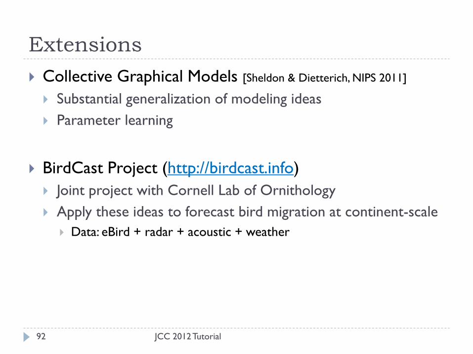
Extensions
Collective Graphical Models [Sheldon & Dietterich, NIPS 2011]
Substantial generalization of modeling ideas
Parameter learning
BirdCast Project (http://birdcast.info)
Joint project with Cornell Lab of Ornithology
Apply these ideas to forecast bird migration at continent-scale
Data: eBird + radar + acoustic + weather
92 JCC 2012 Tutorial

Dynamical Model #2: Metapopulations
Dynamics of spatially disjoint populations
Butterflies in alpine meadows
Birds in a fragmented forest
93
Metapopulation = population of populations
htt
p://w
ww
.bio
.uni-pots
dam
.de/
JCC 2012 Tutorial

Basic Components
A network of habitat patches
Dynamics models
Local population dynamics in each patch
Interaction between patches (dispersal/colonization)
94
JCC 2012 Tutorial

Metapopulation Background
Extremely important models in ecology
Thousands of articles dating from1960s with many
modeling variations
Originally mathematical models for idealized landscapes
E.g. equidistant patches
Move to applied models, real landscapes
Importance: formal basis for reasoning about the effects
of habitat configuration on species persistence
95 JCC 2012 Tutorial

SPOM: Stochastic Patch Occupancy Model
Patches are occupied or unoccupied
Two types of stochastic events:
Local extinction: occupied unoccupied
Colonization: unoccupied occupied (from neighbor)
Independence among all events
Time 1 Time 2
96 JCC 2012 Tutorial

SPOM Probability Model
𝑘
𝑗
𝑖
𝑗
𝑝𝑖𝑗
1 − 𝛽𝑗
𝑡 − 1 𝑡
𝑙
𝑖
𝑘
𝑙
97
To determine occupancy of patch 𝑗 at time 𝑡 For each occupied patch 𝑖 ≠ 𝑗 from time
𝑡 − 1, flip coin with probability 𝑝𝑖𝑗 to see if 𝑖 colonizes 𝑗
If 𝑗 is occupied at time 𝑡 − 1, flip a coin with probability 1 − 𝛽𝑗 to determine survival (non-extinction)
If any of these events occurs, 𝑗 is occupied
Parameters: 𝑝𝑖𝑗 : colonization probability
𝛽𝑗 : extinction probability
functions of patch-size, inter-patch distance, etc.
JCC 2012 Tutorial
𝑝𝑖𝑗

SPOM as Dynamic Bayes Net (DBN)
Xjt
𝑡 = 1 𝑡 = 2 𝑡 = 3 𝑡 = 4 𝑡 = 5
98
Let 𝑋𝑗𝑡 = 0 or 1 be occupancy of patch 𝑗 at time 𝑡
Pr 𝑋𝑗𝑡 = 1 𝐗1, … , 𝐗t−1 = Pr (𝑋𝑗
𝑡 = 1|𝐗𝑡−1)
JCC 2012 Tutorial

SPOM Fitting Major advance in practical utility of SPOMs was ability to fit to survey data
Given: Occupancy vectors 𝐗1, 𝐗2, … , 𝐗𝑇
Find: Parameters Θ for colonization and extinction models
Hanski [1994] gave heuristic approach based on equilibrium properties of metapopulation
Moilanen [1999] Maximum likelihood approach
𝐿 Θ = 𝑝 𝐗1; Θ 𝑝(𝐗𝑡|𝐗𝑡−1; Θ)
𝑇
𝑡=2
Easy in principle
Likelihood easy to evaluate
Small parameter space
99 JCC 2012 Tutorial

Challenge: Missing Data
Field data is sparse and messy Surveys conducted in non-consecutive time steps
Some patches are not surveyed
= observed values
(either present
or absent)
100 JCC 2012 Tutorial

Fitting by Data Augmentation
JCC 2012 Tutorial 101
Key step: fill in missing data by sampling from distribution
of missing data given observed data
Maximum-likelihood approach of Moilanen [1999]
Bayesian approach of Ter Braak and Etienne [2003]

ML Opportunity
102
Improved methods for fitting?
Key step is inference in P(missing | observed) I.e., inference in DBN with metapopulation structure
Approximate inference techniques
Importance of inference:
...
Fitting Prediction
??
JCC 2012 Tutorial

Connections to Network Cascades
Models for diffusion in (social) networks Spread of information, behavior, disease, etc.
Independent cascade model Each individual passes information to friends independently with
specified probability
[Goldenberg, Libai, Muller 2001][Kempe, Kleinberg, Tardos 2003]
103 JCC 2012 Tutorial
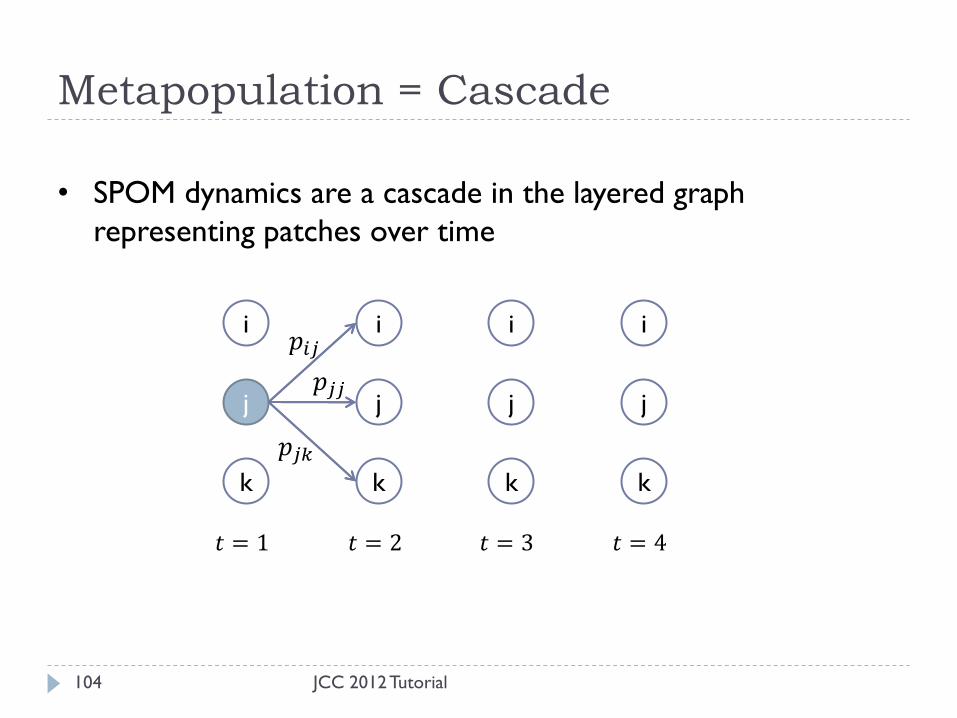
Metapopulation = Cascade
k
j
i
k
j
i
k
j
i
k
j
i 𝑝𝑖𝑗
𝑝𝑗𝑗
𝑝𝑗𝑘
𝑡 = 1 𝑡 = 2 𝑡 = 3 𝑡 = 4
104
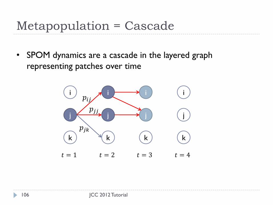
• SPOM dynamics are a cascade in the layered graph
representing patches over time
JCC 2012 Tutorial
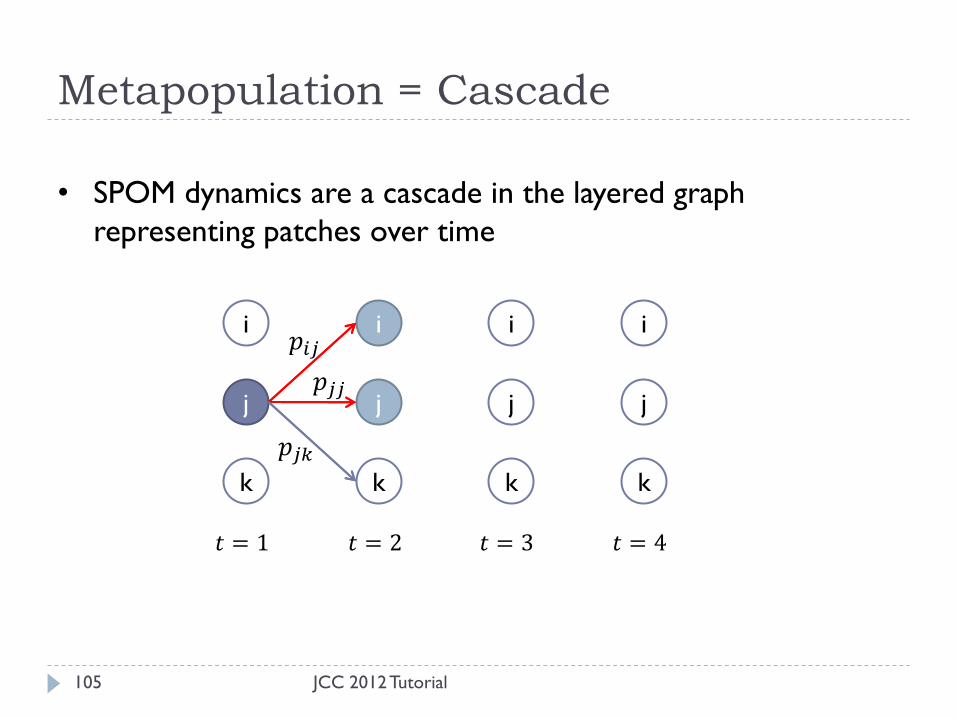
Metapopulation = Cascade
k
j
i
k
j
i
k
j
i
k
j
i
• SPOM dynamics are a cascade in the layered graph
representing patches over time
105
𝑝𝑖𝑗
𝑝𝑗𝑗
𝑝𝑗𝑘
𝑡 = 1 𝑡 = 2 𝑡 = 3 𝑡 = 4
JCC 2012 Tutorial
Metapopulation = Cascade
k
j
i
k
j
i
k
j
i
k
j
i
• SPOM dynamics are a cascade in the layered graph
representing patches over time
106
𝑡 = 1 𝑡 = 2 𝑡 = 3 𝑡 = 4
𝑝𝑖𝑗
𝑝𝑗𝑗
𝑝𝑗𝑘
JCC 2012 Tutorial

Metapopulation = Cascade
k
j
i
k
j
i
k
j
i
k
j
i
• SPOM dynamics are a cascade in the layered graph
representing patches over time
107
𝑡 = 1 𝑡 = 2 𝑡 = 3 𝑡 = 4
𝑝𝑖𝑗
𝑝𝑗𝑗
𝑝𝑗𝑘
JCC 2012 Tutorial

ML connection: Social Network Inference
Recent work in ML community to learn cascade models
Network is hidden
Observe infection times of nodes
Maximum-likelihood estimation by convex optimization
[Myers and Leskovec, 2010]
[Gomez-Rodriguez et al., 2011]
Applicability to SPOM fitting?
Model differences
Layered vs. non-layered graph
Time model
Much different parameterization
JCC 2012 Tutorial 108

Coffee Break
JCC 2012 Tutorial 109

Part 3: Policy Optimization
JCC 2012 Tutorial 110

Outline
JCC 2012 Tutorial 111
Data Acquisition
Sensors: Physical sensors, human observers, repurposing data from other sources
Data interpretation: Extracting signals from data
Ecological Models
Species Distribution Models
Dynamical Models: Dispersal, Migration, Invasion, Climate Change
Policy Optimization
Conservation: Reserve design, Network design
Invasive species: Eradication, restoration, monitoring
Fisheries: Managing harvest levels
Data
Integration
Data
Interpretation
Model Fitting
Policy
Optimization
Sensor
Placement
Policy
Execution

Optimal Policies for Environmental
Management
JCC 2012 Tutorial 112
One-shot problems
Network design
Reserve design
Sequential decision-making problems (known as “Active
Management”)
Fisheries management
Fire management
Invasive species management
Reserve design and conservation easements over time
Most problems are really sequential decision-making problems

Distinctive Aspects
JCC 2012 Tutorial 113
Optimizing an objective computed using a learned model of the system
Generalization of reinforcement learning
Models are typically very bad
Doak, et al. 2008: Ecological Surprises
“Surprises are common and extreme”
Costs and benefits may be highly uncertain and non-stationary
Multiple objectives: Harvest + Species Viability
Need solutions that are robust to misspecified models
Large state and action spaces
Spatial models

Plan
JCC 2012 Tutorial 114
Reserve Design for the Endangered Red Cockaded
Woodpecker
One-shot design problem
Optimal Policies for Managing Fisheries
Markov Decision Problem with analytical characterization of
the optimal policy
Managing Wildfire in Eastern Oregon
Large Spatial Markov Decision Problem (MDP)
Optimal Management of Difficult-to-Observe Invasive
Species
Small Partially-Observable MDP (POMDP)
SPOM Optimization:
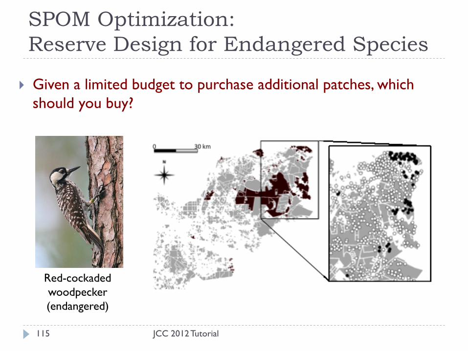
Reserve Design for Endangered Species
Given a limited budget to purchase additional patches, which
should you buy?
Red-cockaded
woodpecker
(endangered)
115 JCC 2012 Tutorial
Key Observation
By viewing SPOM dynamics as a network cascade in the
layered graph, we can formulate the conservation
problem as a cascade optimization problem
116 JCC 2012 Tutorial
Insight #1: Objective as Network Connectivity
Conservation objective: maximize expected # occupied patches at time T
i
j
k
l
m
i
j
k
l
m
i
j
k
l
m
i
j
k
l
m
i
j
k
l
m targets
Live edges
Occupied patches = nodes reachable by live edges
117 JCC 2012 Tutorial
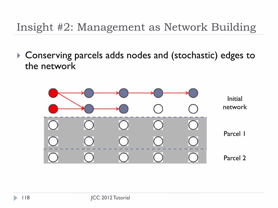
Insight #2: Management as Network Building
Conserving parcels adds nodes and (stochastic) edges to the network
Parcel 1
Parcel 2
Initial
network
118 JCC 2012 Tutorial

Insight #2: Management as Network Building
Conserving parcels adds nodes to the network
Parcel 1
Parcel 2
Initial
network
119 JCC 2012 Tutorial
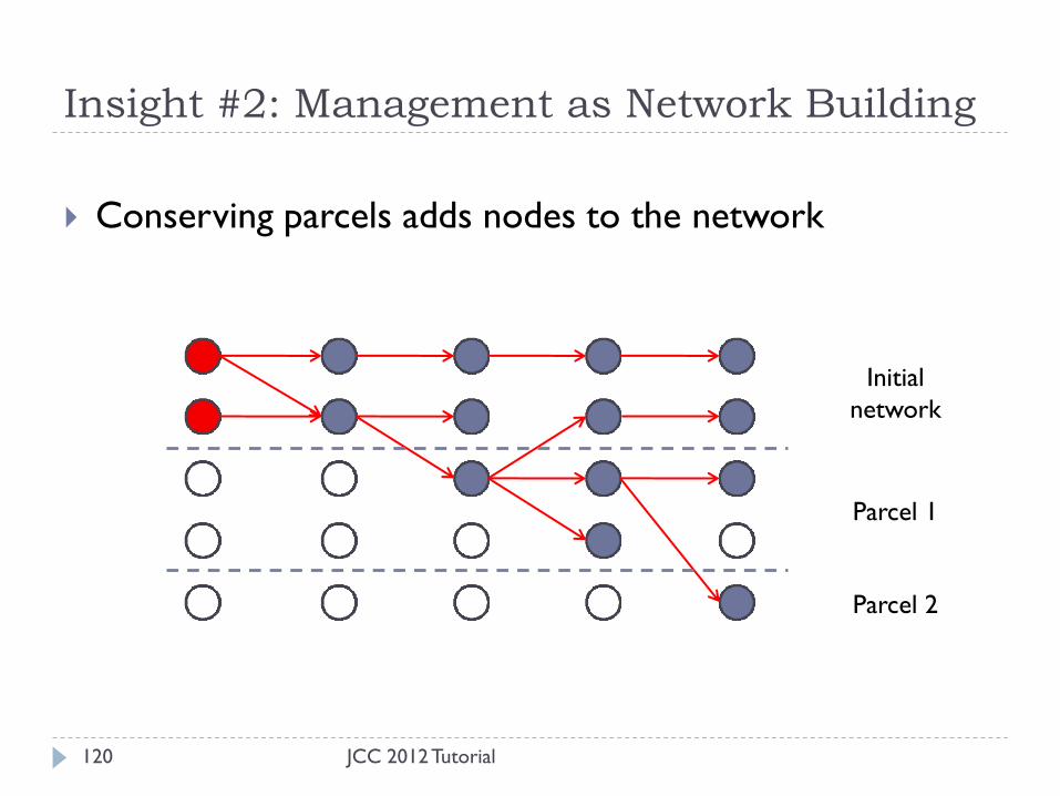
Insight #2: Management as Network Building
Conserving parcels adds nodes to the network
Parcel 1
Parcel 2
Initial
network
120 JCC 2012 Tutorial

Solution Strategy
121
1. Assume we own all parcels. Run multiple simulations of bird propagation
2. Join all of those simulations into a single giant graph
Goal of maximizing expected # of occupied patches at time 𝑇 is approximated by # of reachable patches in the giant graph
3. Define a set of variables 𝑥1, 𝑥2 … , one for each parcel
that we can buy
4. Solve a mixed integer program to decide which 𝑥 variables are 0 and which are 1
JCC 2012 Tutorial
𝑥1
𝑥1
𝑥1
𝑥2
𝑥2
𝑥2

Why This Works
JCC 2012 Tutorial 122
Using the simulation on the whole graph, it is easy to
compute the results for any purchased subgraph
𝑥1 = 1
𝑥2 = 1
Initial
network

Sample Average Approximation (SAA)
JCC 2012 Tutorial 123
Generic approach to convert stochastic problem to deterministic problem:
max𝑋
𝐸𝑌 𝑓 𝑋, 𝑌
max𝑋
1
𝑁 𝑓 𝑋, 𝑌𝑖
𝑁
𝑖=1
𝑋: decision variable
𝑌: random variable
𝑌1, … , 𝑌𝑁: realizations of 𝑌
Nice properties Converges to true optimum as 𝑁 → ∞
Error bounds
Can we solve the sample average problem?

Results
126
Upper bound!
JCC 2012 Tutorial

Results
Upper bound!
127 JCC 2012 Tutorial
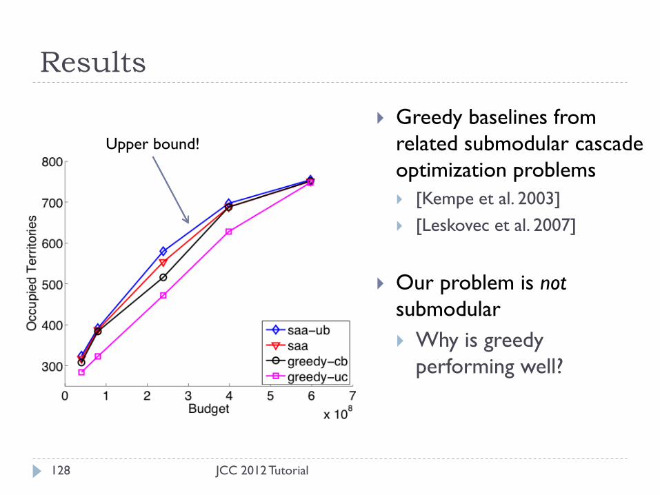
Results
128
Upper bound!
Greedy baselines from
related submodular cascade
optimization problems
[Kempe et al. 2003]
[Leskovec et al. 2007]
Our problem is not
submodular
Why is greedy
performing well?
JCC 2012 Tutorial

Conservation Strategies
129
Both approaches build
outward from source
Greedy buys best patches next
to currently-owned patches
Optimal solution builds toward
areas of high conservation
potential
In this case, the two
strategies are very similar Conservation
Reservoir
Source population
JCC 2012 Tutorial
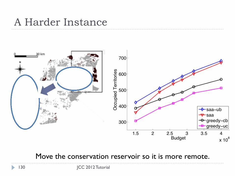
A Harder Instance
Move the conservation reservoir so it is more remote.
130 JCC 2012 Tutorial

Conservation Strategies
Greedy
Baseline
SAA Optimum
(our approach)
$150M $260M $320M
Build outward
from sources
Path-building (goal-setting) 131 JCC 2012 Tutorial

Future Challenges
The real world is complex
Competing objectives
Multiple species
Competing uses of the land
Model dynamics
Learn the SPOM
Include interactions among multiple species
competition for nesting sites
predation
Markov Decision Processes (MDPs)
Buy some patches each year based on annual budgets
Make future purchases depending on where the birds actually go
132 JCC 2012 Tutorial

Fishery Management [Ermon et al. 2010]
How to sustainably exploit a renewable and economically
valuable resource such as forest or fishery?
JCC 2012 Tutorial
International commission decides each year’s harvest (total allowable catch)
Pacific Halibut Fishery
133

MDP Formulation
State variable
𝑥: stock (population size)
Actions
Harvest amount ℎ in each year
Reward model
Fixed cost 𝐾 when ℎ > 0
Per-unit harvest cost
More $$ when fish are scarce
Per-unit market price 𝑝
Discount rate for future reward
JCC 2012 Tutorial 134
𝑥 (stock)
Unit
harvest
cost
MDP Formulation (2)
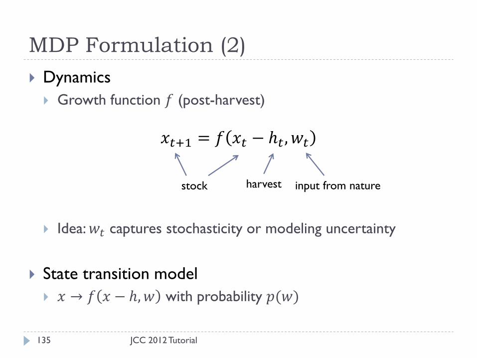
Dynamics
Growth function 𝑓 (post-harvest)
𝑥𝑡+1 = 𝑓 𝑥𝑡 − ℎ𝑡 , 𝑤𝑡
Idea: 𝑤𝑡 captures stochasticity or modeling uncertainty
State transition model
𝑥 → 𝑓 𝑥 − ℎ, 𝑤 with probability 𝑝(𝑤)
stock harvest input from nature
JCC 2012 Tutorial 135
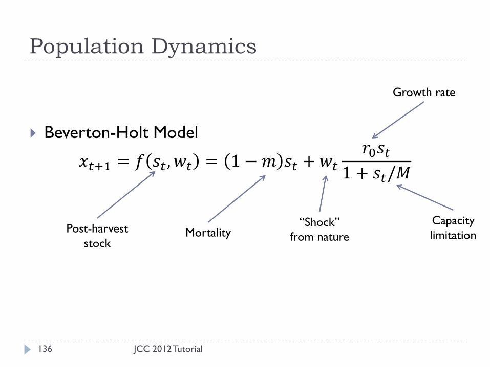
Population Dynamics
Beverton-Holt Model
𝑥𝑡+1 = 𝑓 𝑠𝑡 , 𝑤𝑡 = 1 − 𝑚 𝑠𝑡 + 𝑤𝑡
𝑟0𝑠𝑡
1 + 𝑠𝑡/𝑀
Post-harvest
stock Mortality
“Shock”
from nature
Growth rate
Capacity
limitation
JCC 2012 Tutorial 136

Population Dynamics
Fit to historical data (𝑤 = 1)
JCC 2012 Tutorial 137

Robust Optimization
Traditional MDP approach
Maximize expected total discounted reward
Their approach: “Game against Nature”
Nature chooses 𝑤 adversarially
Maximize worst-case total discounted reward
Advantages:
Avoid catastrophic outcomes such as collapse of fishery
Don’t need fine-grained model for 𝑝(𝑤)
Only specify allowable range of 𝑤
JCC 2012 Tutorial 138
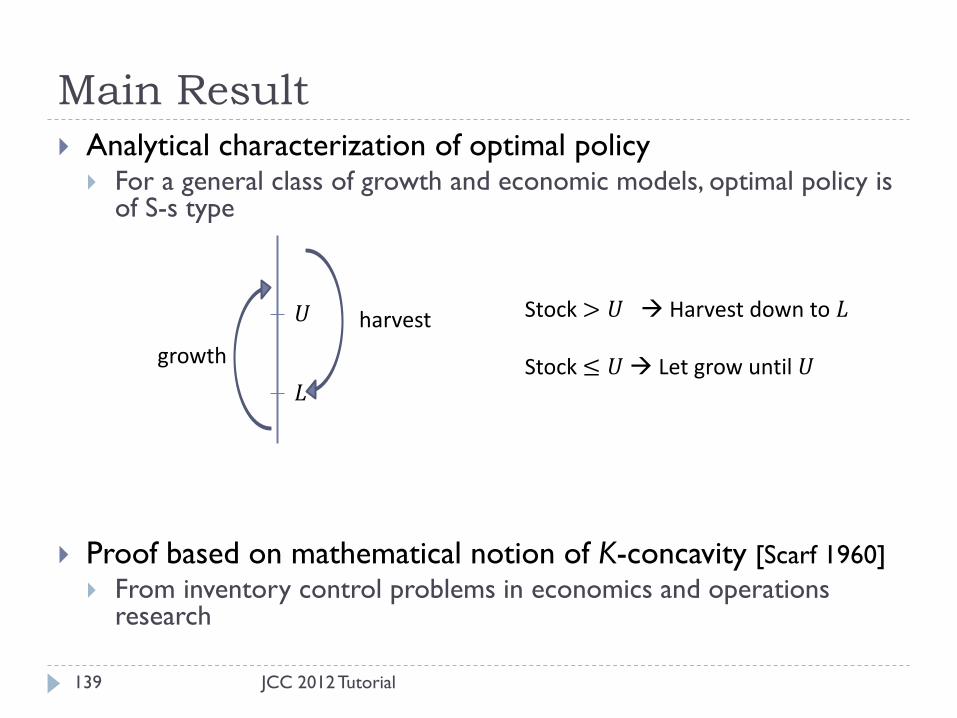
Main Result
Analytical characterization of optimal policy For a general class of growth and economic models, optimal policy is
of S-s type
Proof based on mathematical notion of K-concavity [Scarf 1960]
From inventory control problems in economics and operations research
𝑈
𝐿
harvest
growth
Stock > 𝑈 Harvest down to 𝐿 Stock ≤ 𝑈 Let grow until 𝑈
JCC 2012 Tutorial 139

Pacific Halibut Results
Reanalysis of 1975-2007 data
Fitted growth model
Worst-case environmental inputs
Optimal policy involves periodic
closures of fishery
Maintain supply by rotating
closures
More revenue than baselines
Historical revenue
Current IPHC policy (Constant
Proportional Policy; CPP)
JCC 2012 Tutorial 140
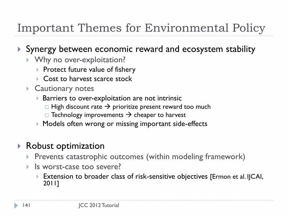
Important Themes for Environmental Policy
Synergy between economic reward and ecosystem stability Why no over-exploitation?
Protect future value of fishery
Cost to harvest scarce stock
Cautionary notes Barriers to over-exploitation are not intrinsic
High discount rate prioritize present reward too much
Technology improvements cheaper to harvest
Models often wrong or missing important side-effects
Robust optimization Prevents catastrophic outcomes (within modeling framework)
Is worst-case too severe? Extension to broader class of risk-sensitive objectives [Ermon et al. IJCAI,
2011]
JCC 2012 Tutorial 141
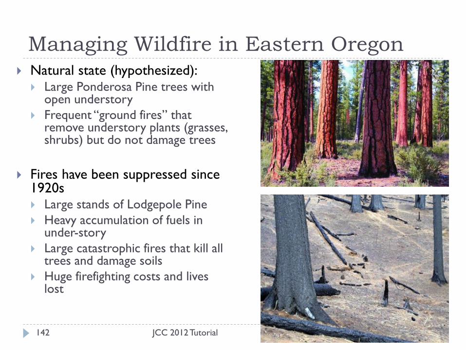
Managing Wildfire in Eastern Oregon
JCC 2012 Tutorial 142
Natural state (hypothesized): Large Ponderosa Pine trees with
open understory
Frequent “ground fires” that remove understory plants (grasses, shrubs) but do not damage trees
Fires have been suppressed since 1920s Large stands of Lodgepole Pine
Heavy accumulation of fuels in under-story
Large catastrophic fires that kill all trees and damage soils
Huge firefighting costs and lives lost
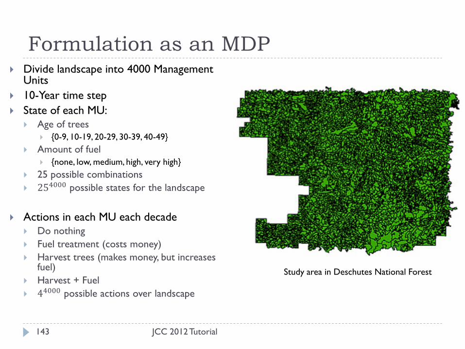
Formulation as an MDP
JCC 2012 Tutorial 143
Divide landscape into 4000 Management Units
10-Year time step
State of each MU:
Age of trees
{0-9, 10-19, 20-29, 30-39, 40-49}
Amount of fuel
{none, low, medium, high, very high}
25 possible combinations
254000 possible states for the landscape
Actions in each MU each decade
Do nothing
Fuel treatment (costs money)
Harvest trees (makes money, but increases fuel)
Harvest + Fuel
44000 possible actions over landscape
Study area in Deschutes National Forest
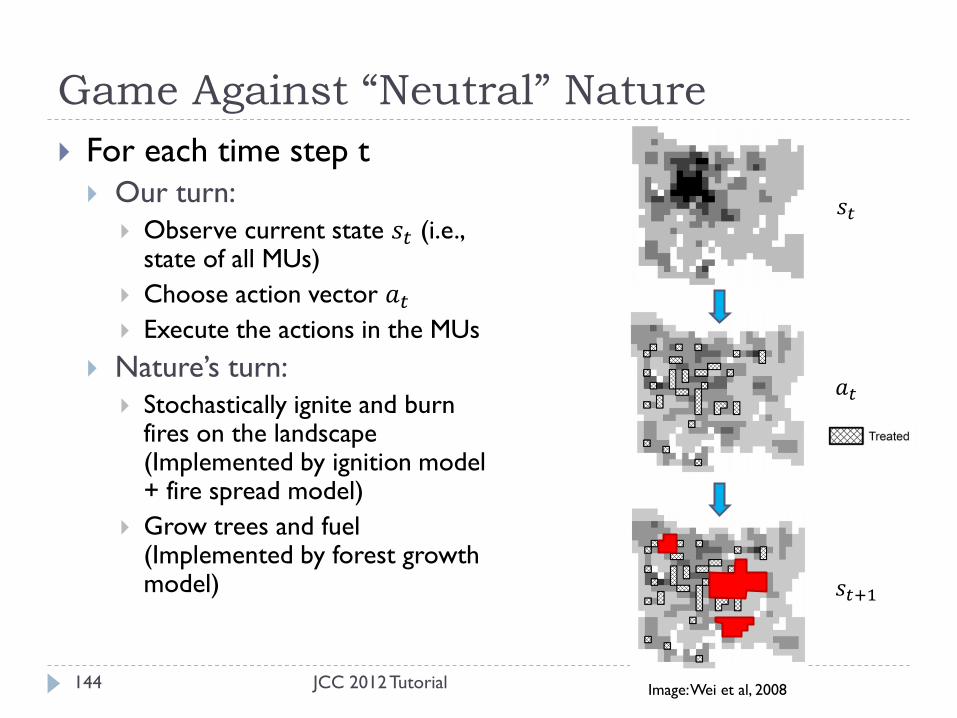
Game Against “Neutral” Nature
JCC 2012 Tutorial 144
For each time step t
Our turn:
Observe current state 𝑠𝑡 (i.e., state of all MUs)
Choose action vector 𝑎𝑡
Execute the actions in the MUs
Nature’s turn:
Stochastically ignite and burn fires on the landscape (Implemented by ignition model + fire spread model)
Grow trees and fuel (Implemented by forest growth model)
𝑠𝑡
𝑎𝑡
𝑠𝑡+1
Image: Wei et al, 2008

Open Problem: Solving This MDP
JCC 2012 Tutorial 145
One-shot Method [Wei, et al., 2008]
Run 1000s of simulated fires to generate fire risk map and fire
propagation graph
Formulate and solve Mixed Integer Program to compute
optimal one-shot solution
Challenge:
Develop methods that can solve the MDP over long time
horizons

Optimal Management of Difficult-to-Observe
Invasive Species [Regan et al., 2011]
JCC 2012 Tutorial 146
Branched Broomrape (Orobanche ramosa)
Annual parasitic plant
Attaches to root system of host plant
Results in 75-90% reduction in host biomass
Each plant makes ~50,000 seeds
Viable for 12 years
Quarantine Area in S. Australia
375 farms; 70km x 70km area
Transition from eradication to management
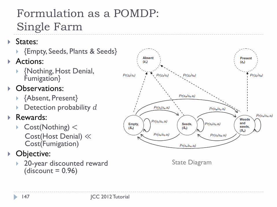
Formulation as a POMDP:
Single Farm
147
States: {Empty, Seeds, Plants & Seeds}
Actions: {Nothing, Host Denial,
Fumigation}
Observations: {Absent, Present}
Detection probability 𝑑
Rewards: Cost(Nothing) <
Cost(Host Denial) ≪ Cost(Fumigation)
Objective: 20-year discounted reward
(discount = 0.96) State Diagram
JCC 2012 Tutorial

Optimal MDP Policy
148
If plant is detected, Fumigate; Else Do Nothing
Assumes perfect detection
www.grdc.com.au
JCC 2012 Tutorial
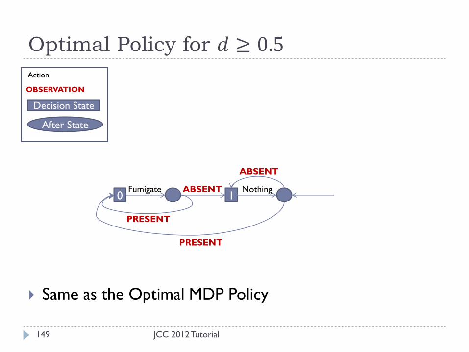
Optimal Policy for 𝑑 ≥ 0.5
149
Same as the Optimal MDP Policy
Action
OBSERVATION
Decision State
After State
JCC 2012 Tutorial
0 1 Fumigate ABSENT
PRESENT
Nothing
ABSENT
PRESENT

Optimal Policy for 𝑑 = 0.3
150
Deny Deny 0 1
Fumigate ABS
PRESENT
ABS
PRESENT
2 ABS 16
PRESENT
... Nothing
ABS
PRESENT
Deny Host for 15 years before switching to Nothing
For 𝑑 = 0.1, Deny Host for 17 years before switching to
Nothing
JCC 2012 Tutorial

Discussion
152
POMDP is exactly solvable because the state space is
very small
Real problem is a spatial meta-population at two scales
Within a single farm
Among the 375 farms in the quarantine area
3375 states
Exact solution of large POMDPs is beyond the state of the art
JCC 2012 Tutorial
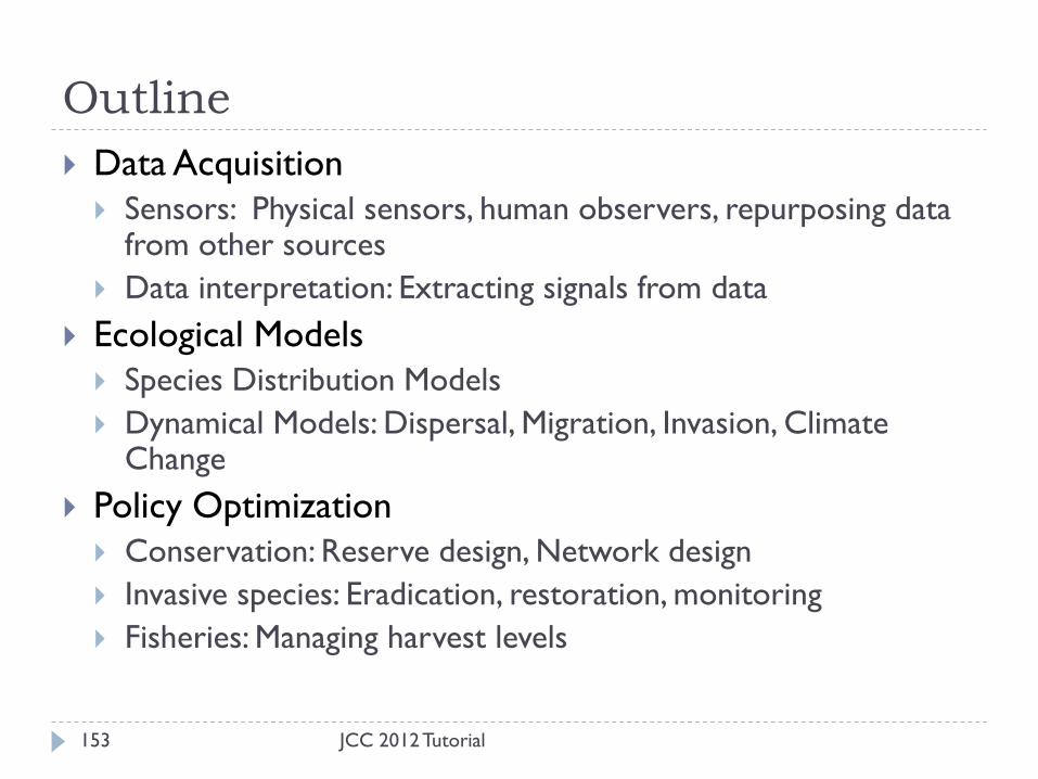
Outline
JCC 2012 Tutorial 153
Data Acquisition
Sensors: Physical sensors, human observers, repurposing data from other sources
Data interpretation: Extracting signals from data
Ecological Models
Species Distribution Models
Dynamical Models: Dispersal, Migration, Invasion, Climate Change
Policy Optimization
Conservation: Reserve design, Network design
Invasive species: Eradication, restoration, monitoring
Fisheries: Managing harvest levels

Challenges for Machine Learning:
Sensor Placement/Active Learning
JCC 2012 Tutorial 154
We have...
Algorithms for one real-valued quantity
assuming stationary correlations, perfect
observations
We need...
Algorithms for multiple quantities
real-valued: nutrients, temperature, precipitation
counts: species abundance for multiple species
discrete: species presence/absence for multiple
species
Algorithms that consider dynamics,
detectability, patchiness (meta-populations)
Data
Integration
Data
Interpretation
Model Fitting
Policy
Optimization
Sensor
Placement
Policy
Execution
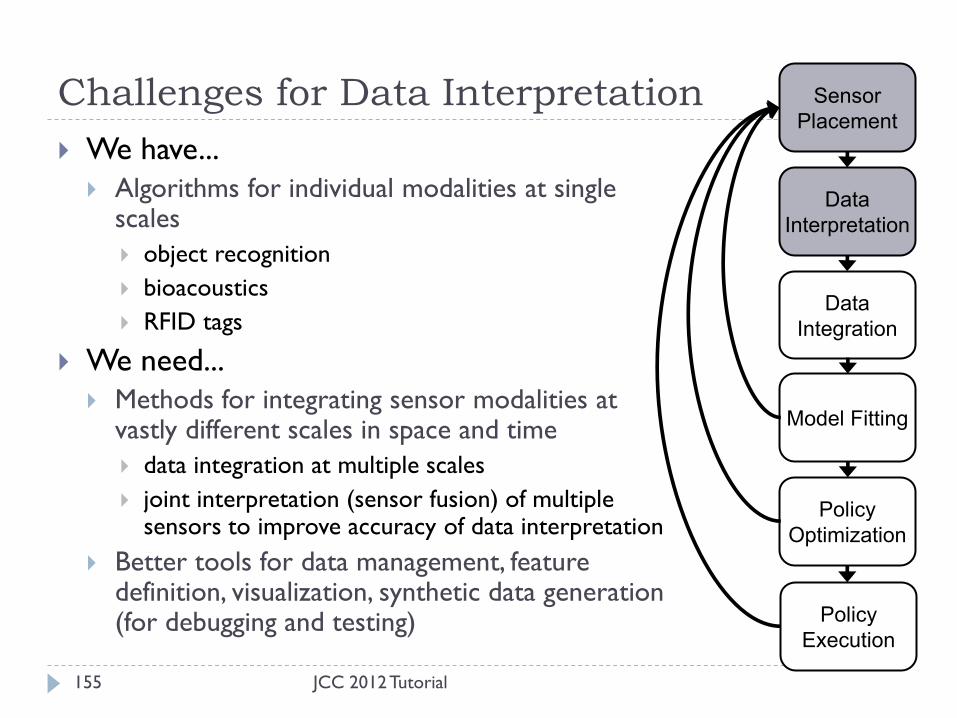
Challenges for Data Interpretation
JCC 2012 Tutorial 155
We have...
Algorithms for individual modalities at single scales
object recognition
bioacoustics
RFID tags
We need...
Methods for integrating sensor modalities at vastly different scales in space and time
data integration at multiple scales
joint interpretation (sensor fusion) of multiple sensors to improve accuracy of data interpretation
Better tools for data management, feature definition, visualization, synthetic data generation (for debugging and testing)
Data
Integration
Data
Interpretation
Model Fitting
Policy
Optimization
Sensor
Placement
Policy
Execution

Challenges for Data Integration
JCC 2012 Tutorial 156
How do we integrate data from
multiple temporal and spatial scales
while retaining all of the detail?
Joint modeling of the ecological process
and the data collection process?
Integrate at a small number of scales?
Are there general-purpose strategies?
Can there be general tools?
Data
Integration
Data
Interpretation
Model Fitting
Policy
Optimization
Sensor
Placement
Policy
Execution
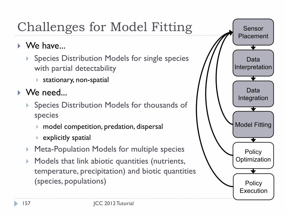
Challenges for Model Fitting
JCC 2012 Tutorial 157
We have...
Species Distribution Models for single species
with partial detectability
stationary, non-spatial
We need...
Species Distribution Models for thousands of
species
model competition, predation, dispersal
explicitly spatial
Meta-Population Models for multiple species
Models that link abiotic quantities (nutrients,
temperature, precipitation) and biotic quantities
(species, populations)
Data
Integration
Data
Interpretation
Model Fitting
Policy
Optimization
Sensor
Placement
Policy
Execution
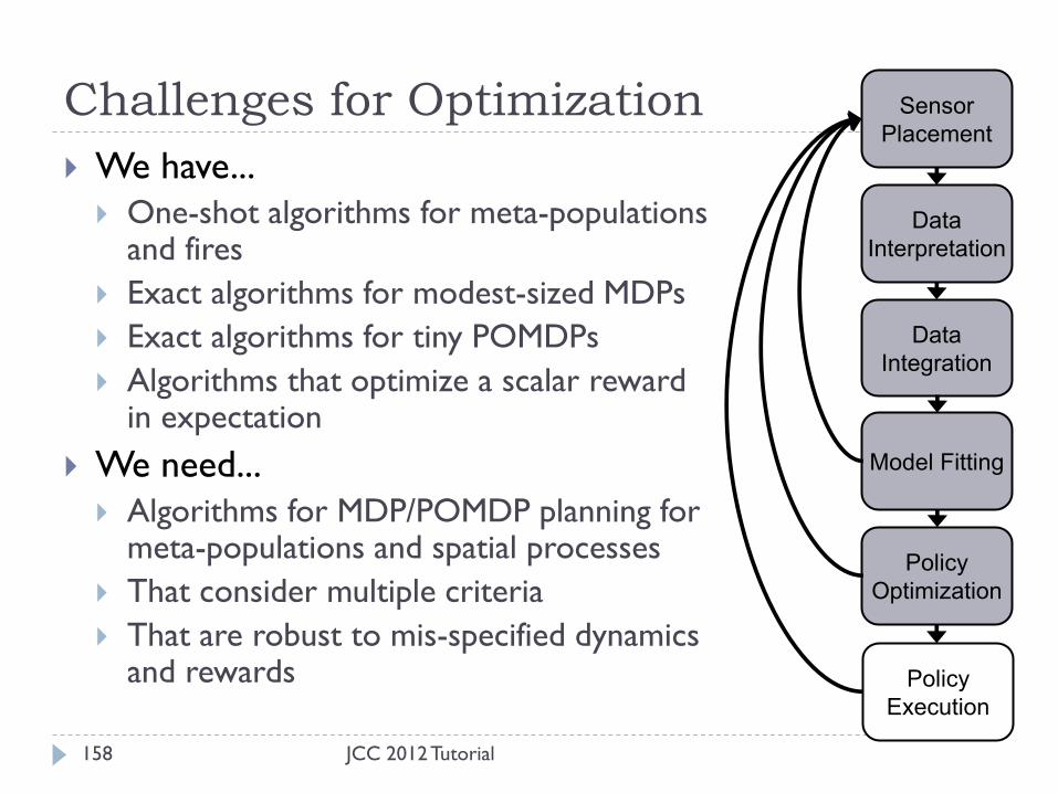
Challenges for Optimization
JCC 2012 Tutorial 158
We have...
One-shot algorithms for meta-populations and fires
Exact algorithms for modest-sized MDPs
Exact algorithms for tiny POMDPs
Algorithms that optimize a scalar reward in expectation
We need...
Algorithms for MDP/POMDP planning for meta-populations and spatial processes
That consider multiple criteria
That are robust to mis-specified dynamics and rewards
Data
Integration
Data
Interpretation
Model Fitting
Policy
Optimization
Sensor
Placement
Policy
Execution

Data Models Policies:
Overall Challenges
JCC 2012 Tutorial 159
It isn’t a pipeline
We need algorithms that
integrate/couple all parts of the
process
Learning algorithms should be
integrated with policy optimization
Sensor placement should be sensitive
to all goals
Data
Integration
Data
Interpretation
Model Fitting
Policy
Optimization
Sensor
Placement
Policy
Execution

Closing
JCC 2012 Tutorial 160
Links to data, software, and papers available in the electronic version of these slides
Thank-you’s
Dan Sheldon and Rebecca Hutchinson
BugID team, especially Wei Zhang, Natalia Larios, Junyuan Lin, Gonzalo Martinez
David Winkler
Jane Elith and Steven Phillips
Lab of Ornithology collaborators: Daniel Fink, Steve Kelling and the thousands of eBirders
National Science Foundation support under grants 0705765, 0832804, and 0905885
ACM Distinguished Lecturers Program

Questions?
JCC 2012 Tutorial 161

Data Resources
JCC 2012 Tutorial 162
Species Distribution Models eBird Reference Dataset 3.0
http://www.avianknowledge.net/content/features/archive/ebird-reference-dataset-3-0-released
eBird checklist data along with an excellent set of covariates
set of suggested analysis problems
Fine-Grained Image Classification Oregon State STONEFLY9 dataset
http://web.engr.oregonstate.edu/~tgd/bugid/stonefly9/
Oregon State EPT29 dataset http://web.engr.oregonstate.edu/~tgd/bugid/ept29/
Caltech/UCSD CUB-200 bird dataset http://www.vision.caltech.edu/visipedia/CUB-200.html
Oxford Flower dataset (102 classes) http://www.robots.ox.ac.uk/~vgg/data/flowers/102/index.html
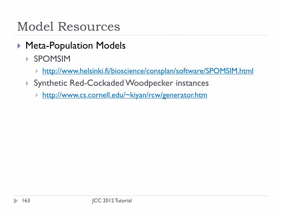
Model Resources
JCC 2012 Tutorial 163
Meta-Population Models
SPOMSIM
http://www.helsinki.fi/bioscience/consplan/software/SPOMSIM.html
Synthetic Red-Cockaded Woodpecker instances
http://www.cs.cornell.edu/~kiyan/rcw/generator.htm

Machine Learning Algorithms
JCC 2012 Tutorial 164
Phillips’ Maxent Package
http://www.cs.princeton.edu/~schapire/maxent/
References
JCC 2012 Tutorial 165
Crowley M, Nelson J, Poole D. Seeing the Forest Despite the Trees: Large Scale Spatial-Temporal
Decision Making. In: AAAI 2011.; 2011.
Doak DF, Estes JA, Halpern BS, et al. Understanding and predicting ecological dynamics: are major
surprises inevitable? Ecology. 2008; 89(4):952-961.
Elith J, Graham CH, Anderson RP, et al. Novel methods improve prediction of species’ distributions
from occurrence data. Ecography. 2006;29(2):129-151.
Elith J, Phillips SJ, Hastie T, et al. A statistical explanation of MaxEnt for ecologists. Diversity and
Distributions. 2011;17:43-57.
Ermon, S., Conrad, J., Gomes, C., & Selman, B. (2010). Playing games against nature: optimal policies for
renewable resource allocation. Proc. of The 26th Conference on Uncertainty in Artificial Intelligence.
Ermon, S., Conrad, J., Gomes, C., & Selman, B. (2011). Risk-sensitive Policies for Sustainable Renewable
Resource Allocation. To appear in IJCAI 2011.
Fink D, Hochachka WM, Zuckerberg B, et al. Spatiotemporal exploratory models for broad-scale
survey data. Ecological applications : a publication of the Ecological Society of America. 2010;20(8):2131-47
Friedman J. Greedy function approximation: a gradient boosting machine. Annals of Statistics.
2001;29(5):1189-1232.
References (2)
JCC 2012 Tutorial 166
Gomez-Rodriguez, M., Balduzzi, D., & Schölkopf, B. (2011). Uncovering the Temporal Dynamics of
Diffusion Networks. ICML 2011.
Hanski, I. (1994). A practical model of metapopulation dynamics. Journal of Animal Ecology, 63(1), 151–162.
Hutchinson RA, Liu L-P, Dietterich TG. Incorporating Boosted Regression Trees into Ecological Latent
Variable Models. In: Proceedings of the Twenty-fifth Conference on Artificial Intelligence.; 2011.
Kempe, D., Kleinberg, J., & Tardos, É. (2003). Maximizing the spread of influence through a social
network. Proceedings of the ninth ACM SIGKDD international conference on Knowledge discovery and data mining (p.
137–146).
Krause A, Singh A, Guestrin C. Near-Optimal Sensor Placements in Gaussian Processes: Theory ,
Efficient Algorithms and Empirical Studies. Journal of Machine Learning Research. 2008;9:235-284.
Leathwick JR, Moilanen A, Francis M, et al. Novel methods for the design and evaluation of marine
protected areas in offshore waters. Conservation Letters. 2008;1:91-102.
Leskovec, J., Krause, A., Guestrin, C., Faloutsos, C., VanBriesen, J., & Glance, N. (2007). Cost-effective outbreak
detection in networks. Proceedings of the 13th ACM SIGKDD international conference on Knowledge discovery and
data mining (p. 420–429).
MacKenzie DI, Nichols JD, Royle JA, et al. Occupancy estimation and modeling: inferring patterns and
dynamics of species occurrence. Elsevier, San Diego, USA; 2006.
References (3)
JCC 2012 Tutorial 167
Martinez G, Zhang W, Payet N, et al. Dictionary-Free Categorization of Very Similar Objects via
Stacked Evidence Trees. In: IEEE Conference on Computer Vision and Pattern Recognition (CVPR2009). IEEE; 2009:
1-8.
Moilanen, A. (1999). Patch occupancy models of metapopulation dynamics: efficient parameter
estimation using implicit statistical inference. Ecology, 80(3), 1031–1043.
Myers, S. A., & Leskovec, J. (2010). On the convexity of latent social network inference. NIPS 2010.
Phillips SJ, Anderson R, Schapire R. Maximum entropy modeling of species geographic distributions.
Ecological Modelling. 2006;190(3-4):231-259.
Phillips SJ, Dudik M, Schapire RE. A maximum entropy approach to species distribution modeling.
Twenty-first international conference on Machine learning - ICML ’04. 2004:83.
Regan TJ, Chadès I, Possingham HP. Optimally managing under imperfect detection: a method for
plant invasions. Journal of Applied Ecology. 2011;48(1):76-85.
Scarf, H. (1960). The Optimality of (S,s) policies in the dynamic inventory problem. Stanford
mathematical studies in the social sciences, p. 196.
Sheldon, D., Elmohamed, M. A. S., & Kozen, D. (2008). Collective inference on Markov models for
modeling bird migration. Advances in Neural Information Processing Systems 2007, 20, 1321–1328.
References (4)
JCC 2012 Tutorial 168
Sheldon, D. (2010). Manipulation of PageRank and Collective Hidden Markov Models. Ph.D. Thesis,
Cornell University.
Sheldon, D., Dilkina, B., Elmachtoub, A., Finseth, R., Sabharwal, A., Conrad, J., Gomes, C., Shmoys, D., Allen, W.,
Amundsen, O., & Vaughaun, B. (2010.). Maximizing the Spread of Cascades Using Network Design. UAI-
2010: 26th Conference on Uncertainty in Artificial Intelligence (p. 517–526).
Ter Braak, C. J. F., & Etienne, R. S. (2003). Improved Bayesian analysis of metapopulation data with an
application to a tree frog metapopulation. Ecology, 84(1), 231–241.
Wei Y, Rideout D, Kirsch A. An optimization model for locating fuel treatments across a landscape to
reduce expected fire losses. Canadian Journal of Forest Research. 2008;38(4):868-877.
Winkler, D. W. (2006). Roosts and migrations of swallows. El hornero, 21, 85–97.
Yu J, Wong W-K, Hutchinson RA. Modeling Experts and Novices in Citizen Science data for Species
Distribution Modeling. In: Proceedings of the 10th IEEE International Conference on Data Mining (ICDM 2010).;
2010.
Zhang W, Surve A, Fern X, Dietterich T. Learning Non-Redundant Codebooks for Classifying Complex
Objects. In: Proceedings of the International Conference on Machine Learning, ICML-2009.; 2009:1241-1248.