machine learning for biologie · 19.1 1.64 0.6 0.1 0.03 1.75 1.04 0.007 0.018 5 v. monbet (ufr...

Machine Learning for biologie

V. Monbet

UFR de MathématiquesUniversité de Rennes 1

V. Monbet (UFR Math, UR1) Machine Learning for biologie (2019) 1 / 29

Introduction

Outline

1 Introduction

2 Dimension Reduction


Dimension Reduction

Outline

1 Introduction

2 Dimension ReductionIntroductionPrincipal Component AnalysisPCA for multiple imputationOther methods for dimension reductionNon-negative Matrix FactorizationStochastic neighbor embedding


Dimension Reduction Introduction

Outline



Dimension Reduction Introduction

When dealing with huge volumes of data, problems naturally arise. How do youwhittle down a dataset of hundreds or even thousands of variables into an optimalmodel? How do you visualize data with countless dimensions?

Dimension reduction techniques- Principal Component Analysis (PCA) or Empirical Orthogonal Function (EOF)- Multidimensional Scaling (MDS) and Isomap- t-Distributed Stochastic Neighbor Embedding (t-SNE)


Dimension Reduction Principal Component Analysis

Outline




Principal Component Analysis, introduction

When only 2 quantitative variables are observed, it is easy to plot them. Each axis ofthe plan represents a variable. The relationships between the variables or thesamples are visible.

Taille Pointure Genre155.1 36.5 F167.6 40.0 F

......

182.9 44.0 H

How to deal with more than 2 variables?

PAl2O3 Fe2O3 MgO CaO Na2O K2O TiO2 MnO BaO Four18.8 9.52 2 0.79 0.4 3.2 1.01 0.077 0.015 116.9 7.33 1.65 0.84 0.4 3.05 0.99 0.067 0.018 1

......

......

......

......

......

19.1 1.64 0.6 0.1 0.03 1.75 1.04 0.007 0.018 5



Principal Component Analysis or Empirical Orthogonal Functions

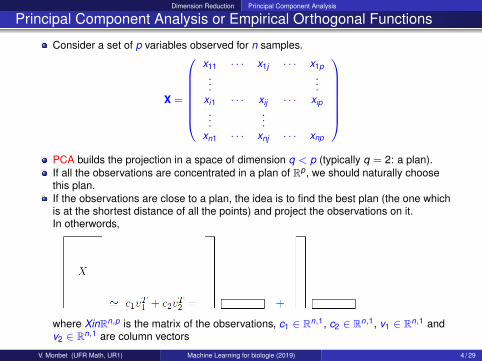
Consider a set of p variables observed for n samples.

X =

x11 · · · x1j · · · x1p...

...xi1 · · · xij · · · xip...

...xn1 · · · xnj · · · xnp

PCA builds the projection in a space of dimension q < p (typically q = 2: a plan).If all the observations are concentrated in a plan of Rp , we should naturally choosethis plan.If the observations are close to a plan, the idea is to find the best plan (the one whichis at the shortest distance of all the points) and project the observations on it.In otherwords,

where XinRn,p is the matrix of the observations, c1 ∈ Rn,1, c2 ∈ Rn,1, v1 ∈ Rn,1 andv2 ∈ Rn,1 are column vectors



Principal Component Analysis or Empirical Orthogonal Functions

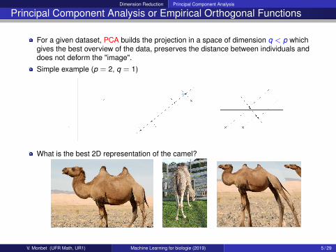
For a given dataset, PCA builds the projection in a space of dimension q < p whichgives the best overview of the data, preserves the distance between individuals anddoes not deform the "image".

Simple example (p = 2, q = 1)

What is the best 2D representation of the camel?



Data

Consider a set of p variables observed for n samples.

x =

x11 · · · x1j · · · x1p...

...xi1 · · · xij · · · xip...

...xn1 · · · xnj · · · xnp

In the sequel, columns xj reprensent the variables. They are supposed to have 0mean.They don’t have 0 mean, a transformation can be applied to the data.Standardization: transformation of the data such that all variables of the sample havea zero mean and a unit variance.

x̄j =1n

n∑i=1

xij , s2j =

1n

n∑i=1

(xij − x̄j

)2

x (st)ij =

xij − x̄j

sj



Inertie

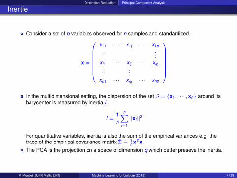
Consider a set of p variables observed for n samples and standardized.

x =

x11 · · · x1j · · · x1p...

...xi1 · · · xij · · · xip...

...xn1 · · · xnj · · · xnp

In the multidimensional setting, the dispersion of the set S = {x1, · · · , xn} around itsbarycenter is measured by inertia I.

I =1n

n∑i=1

||xi ||2

For quantitative variables, inertia is also the sum of the empirical variances e.g. thetrace of the empirical covariance matrix Σ̂ = 1

n xT x.

The PCA is the projection on a space of dimension q which better preseve the inertia.



Principal Component Analysis

PCA provides axes vj and coordinates αj such that

x = c1vT1 + · · ·+ cqvT

q + ε (1)

where vj ∈ Rp are the factors, vj ⊥ v` and ||vj || = 1,where cj ∈ Rn are the principal componentswhere ε is a residual.

x predicted as a linear combination of the latent factors vj .

Factors vj are the q eigenvectors of the covariance matrix Σ̂ = 1n xT x associated with

the q largest eigenvalues.It means that the space generated by v1, · · · , vq is the space of dimension q forwhich the inertia of the projection of x is largest.

Coordinates ( = principal components) of individual i

cij = xTi vj



Example with images of digits

Original images

Factors (5 first)

Reconstruction

= c1v1 + c2v2 + ca3v3 + c4v4 + c5v5



PCA reconstruction

PCA 5 first factors

Reconstructed images (based on 5 factors)

with weightsimage 0 2.44 -0.74 -0.60 0.02 0.01image 1 -1.38 -0.62 -1.18 0.96 -0.05image 2 -0.68 0.13 0.43 1.66 0.36image 3 -0.23 -0.95 0.27 -1.55 0.63image 4 0.25 1.03 0.12 -1.88 0.23



Principal Component Analysis, visualization example

PCA is often used to help plot data in high dimensions. For the digits example, ithelps to "discriminate" the numbers.For q = 2, the 1s are on the right side of the first axis while numbers 0, 2, 3, 4 and 5are on the left side. The 2s are on the bottom of the second axis and the 4s at the top.Similar-shaped numbers are close to each others: if 7s were added they would beclose to the 1s.



Back to poteries

PCA is a good tool for vizualization of multivariate datasets.

The left plot, also called "individuals plot" allows to highlight the proximities betweenindividuals.

The right plot, also called "correlations circle plot" allows to highlight the dependancebetween the variables.



Principal Component Analysis, visualization example

Discrimination of AML (27 patients) and ALL (11 patients)

About 7000 genes (too much to plot the correlations circle.)

Gene expression

5 10 15 20 25 30 35

1000

2000

3000

4000

5000

6000

7000

Samples

Genes E

xpre

ssio

n

−4

−2

0

2

4

6

PCA

−60 −40 −20 0 20 40 60 80

050

100

PC 1, 14.99 %

PC

2, 11.9

8 %

NoYes

Running PCA, classes are unknown.

Golub et al. (1999), Science.V. Monbet (UFR Math, UR1) Machine Learning for biologie (2019) 13 / 29


Principal Component Analysis vs other projection methods

PCA is a projection on a basis of orthogonal vectors (see example below).

Analogy with Fourier, wavelets, etc.

Particularities of PCA: the basis is data driven.

Used for visualization, description, dimension reduction.


Dimension Reduction PCA for multiple imputation

Outline



Dimension Reduction PCA for multiple imputation

PCA for multiple imputation

An iterative PCA algorithm can be used to impute missing data.

It allows to take into account the multivariate correlations.

AlgorithmInitialization: replace missing values by the mean of the variablesand compute X̄(0)

Repeat until convergence(a) Compute a PCA on X(`−1) to find Q(`) and α(`)

(b) Missing values are replaced by

X(`) = Q(`)(α(`)

)T+ X̄(`−1)

X(`) = WX + (1−W )X(`)

where wij = 0 if observation is missing and 1 otherwise.(c) Compute X̄(`)

Ref: Josse, J., Pages, J., & Husson, F. (2011). Multiple imputation in principal componentanalysis. Advances in data analysis and classification, 5(3), 231-246.


Dimension Reduction Other methods for dimension reduction

Outline




Other methods: multidimensional scaling (MDS)

There are other methods for dimension reduction based on the searches oforthogonal/independent basis or factors.

MDSMulti-Dimension Scaling is a distance-preserving manifold learning method.

Given a matrix of distances D between the n observations, MDS searches foreuclidean coordinates Xmds ∈ Rq such that if Dij is small, Xmds(i) is close to Xmds(j).

In practice, it is obtained by minimizing the following cost function

J(Xmds) =∑i<j

ωij (dij (Xmds)− Dij )2

where dij (Xmds) denotes the distance in the small dimension space and ωij areweights.

When D is defined by the euclidean distance, MDS is equivalent to PCA.



Optimization algorithm

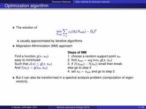
The solution ofminXmds

∑i<j

ωij (dij (Xmds)− Dij )2

is usually approximated by iterative algorithms

Majoration-Minimization (MM) approach

Find a function g(x , xm)easy to minimizedSuch that J(x) ≤ g(x , xm)And f (xm) = g(xm, xm)

Steps of MM1. choose a random support point xm2. find xmin = arg minx g(x , xm)3. if |f (xmin)− f (xm)| small then breakelse go to step 44. set xm = xmin and go to step 2

But it can also be transformed in a spectral analysis problem (computation of eigenvectors).



Optimization algorithm

https://blog.paperspace.com/dimension-reduction-with-multi-dimension-scaling/





MDS, digits data

MNIST digits, PCA (left) and MDS (right)



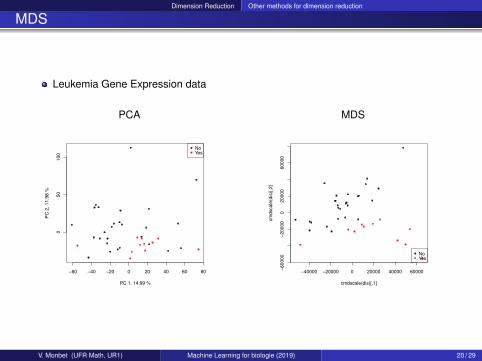
MDS

Leukemia Gene Expression data

PCA

−60 −40 −20 0 20 40 60 80

050

100

PC 1, 14.99 %

PC

2, 11.9

8 %

NoYes

MDS

−40000 −20000 0 20000 40000 60000

−60000

−20000

020000

60000

cmdscale(dis)[,1]

cm

dscale

(dis

)[,2

]

NoYes



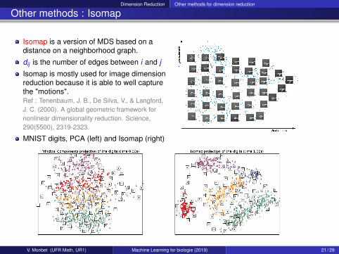
Other methods : Isomap

Isomap is a version of MDS based on adistance on a neighborhood graph.

dij is the number of edges between i and j

Isomap is mostly used for image dimensionreduction because it is able to well capturethe "motions".Ref : Tenenbaum, J. B., De Silva, V., & Langford,J. C. (2000). A global geometric framework fornonlinear dimensionality reduction. Science,290(5500), 2319-2323.

MNIST digits, PCA (left) and Isomap (right)


Dimension Reduction Non-negative Matrix Factorization

Outline




Non-negative Matrix Factorization

Non-negative matrix factorization (NNMF) is a tool for dimensionality reduction of datasetsin which the values, like the rates in the rate matrix are constrained to be non-negative.

NNMF

X ' HW

(or Xj ' h1j W1 + · · ·+ hqj Wq)where V ∈ Rn,p ,W ∈ Rn,q → basis (components)H ∈ Rq,p → weightsconstraints : W ≥ 0,H ≥ 0.

(H,W ) solution of

minW≥0,H≥0

||X −WH||2F

PCA

X ' Qα

(or Xi ' ci1v1 + · · ·+ ciqvq)where X ∈ Rn,p ,V ∈ Rn,q → basisC ∈ Rq,p → weightsno constraints



NMF loadings

Comparison of NMF and PCA for the handwritten digits

NMF 5 first factors

One of the advantages of NMF is that the components may be interpretable in the originalspace.

PCA 5 first components



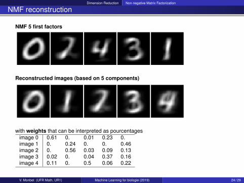
NMF reconstruction

NMF 5 first factors

Reconstructed images (based on 5 components)

with weights that can be interpreted as pourcentagesimage 0 0.61 0. 0.01 0.23 0.image 1 0. 0.24 0. 0. 0.46image 2 0. 0.56 0.03 0.09 0.13image 3 0.02 0. 0.04 0.37 0.16image 4 0.11 0. 0.5 0.06 0.22



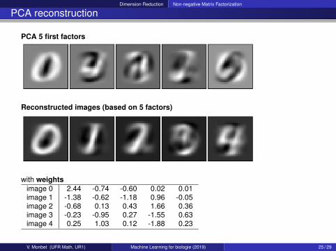
PCA reconstruction

PCA 5 first factors

Reconstructed images (based on 5 factors)

with weightsimage 0 2.44 -0.74 -0.60 0.02 0.01image 1 -1.38 -0.62 -1.18 0.96 -0.05image 2 -0.68 0.13 0.43 1.66 0.36image 3 -0.23 -0.95 0.27 -1.55 0.63image 4 0.25 1.03 0.12 -1.88 0.23


Dimension Reduction Stochastic neighbor embedding

Outline




Stochastic neighbor embedding

SNE is a method of dimension reduction.SNE leads to a representation of the data in a low dimension space (typically 2). Inthis space, two samples with a high similarity will be close to each other.SNE is different from PCA because- the similarity is not measured through correlation- t-SNE performs different transformation on different regions.In the original space of the data, the similarity between two samples xj and xi isdefined by the conditional density of xj given xi

pj|i =exp

(−‖xi − xj‖2/2σi

)∑k 6=j exp

(−‖xi − xk‖2/2σi

)where σi is a parameter to be chosen. By convention, pi|i = 0.In the reduced space, the similarity is measured by a conditional density as well

qj|i =exp

(−‖yi − yj‖2)∑

k 6=j exp(−‖yi − yk‖2

)with qi|i = 0 by convention.

Ref : Van der Maaten, L., & Hinton, G. (2008). Visualizing data using t-SNE. Journal ofMachine Learning Research, 9(2579-2605), 85.Animations :https://www.oreilly.com/learning/an-illustrated-introduction-to-the-t-sne-algorithm



t-distributed stochastic neighbor embedding (t-SNE)

Digits MNIST, PCA (left) vs t-SNE (right)

t-SNE allows to better gather similar observations.But, a key parameters may be hard to chooseThe tuneable parameter σi which says (loosely) how to balance attention betweenlocal and global aspects of the data.It is referred implicitly to as the "perplexity" in the solftwares and it is link the thenumber of close neighbors each point has.It may be hard to choose!For more detailled examples and discussion seehttps://distill.pub/2016/misread-tsne/Computation time is large.

Number of citations of the seminal paper : 2600V. Monbet (UFR Math, UR1) Machine Learning for biologie (2019) 27 / 29


Other methods: t-SNE, leukemia gene’s data

To capture the structure, it is usually useful to plot the t-SNE result for various values ofthe perplexity (perp<n).Top panel: all the genesBottom panel: 89 genes with the highest SNR



Concluding remarks

There are many algorithms for dimension reduction: PCA, MDS, t-SNE, etc.

They are used for- vizualization of data of high dimension- Dimension reduction (pre-processing)

The most common is to use PCA (or one of its extension).PCA leads to a linear approximation of the initial dataset.

MDS and Isomap are usefull for data on a graph where distances are defined as aneighborhood.

t-SNE is a local method which is powerfull but with parameters to choose.


machine learning for biologie · 19.1 1.64 0.6 0.1 0.03 1.75 1.04 0.007 0.018 5 v. monbet (ufr...

Documents