machine learning and graph theory approaches for
TRANSCRIPT

Georgia State University Georgia State University
ScholarWorks @ Georgia State University ScholarWorks @ Georgia State University
Computer Science Dissertations Department of Computer Science
4-22-2008
Machine Learning and Graph Theory Approaches for Machine Learning and Graph Theory Approaches for
Classification and Prediction of Protein Structure Classification and Prediction of Protein Structure
Gulsah Altun
Follow this and additional works at: https://scholarworks.gsu.edu/cs_diss
Part of the Computer Sciences Commons
Recommended Citation Recommended Citation Altun, Gulsah, "Machine Learning and Graph Theory Approaches for Classification and Prediction of Protein Structure." Dissertation, Georgia State University, 2008. https://scholarworks.gsu.edu/cs_diss/31
This Dissertation is brought to you for free and open access by the Department of Computer Science at ScholarWorks @ Georgia State University. It has been accepted for inclusion in Computer Science Dissertations by an authorized administrator of ScholarWorks @ Georgia State University. For more information, please contact [email protected].

MACHINE LEARNING AND GRAPH THEORY APPROACHES FOR
CLASSIFICATION AND PREDICTION OF PROTEIN STRUCTURE
by
GULSAH ALTUN
Under the direction of Dr. Robert W. Harrison
ABSTRACT
Recently, many methods have been proposed for the classification and prediction
problems in bioinformatics. One of these problems is the protein structure prediction.
Machine learning approaches and new algorithms have been proposed to solve this problem.
Among the machine learning approaches, Support Vector Machines (SVM) have attracted a
lot of attention due to their high prediction accuracy. Since protein data consists of sequence
and structural information, another most widely used approach for modeling this structured
data is to use graphs. In computer science, graph theory has been widely studied; however it
has only been recently applied to bioinformatics. In this work, we introduced new algorithms
based on statistical methods, graph theory concepts and machine learning for the protein
structure prediction problem. A new statistical method based on z-scores has been introduced
for seed selection in proteins. A new method based on finding common cliques in protein
data for feature selection is also introduced, which reduces noise in the data. We also
introduced new binary classifiers for the prediction of structural transitions in proteins. These

new binary classifiers achieve much higher accuracy results than the current traditional
binary classifiers.
INDEX WORDS: algorithm, machine learning, graph theory, support vector machines, feature selection, protein structure prediction

MACHINE LEARNING AND GRAPH THEORY APPROACHES FOR
CLASSIFICATION AND PREDICTION OF PROTEIN STRUCTURE
by
GULSAH ALTUN
A Dissertation Submitted in Partial Fulfillment of the Requirements of the Degree of
Doctor of Philosophy
in the College of Arts and Science
Georgia State University
2008

Copyright by Gulsah Altun
2008

MACHINE LEARNING AND GRAPH THEORY APPROACHES FOR
CLASSIFICATION AND PREDICTION OF PROTEIN STRUCTURE
by
GULSAH ALTUN
Committee Chair: Robert. W. Harrison Co-Chair: Yi Pan Committee: Alexander Zelikovsky
Phang C. Tai
Electronic Version Approved: Office of Graduate Studies College of Arts and Science Georgia State University May 2008

iv
DEDICATION
To my father Zikri Altun, my mother Aynur Altun
and my sister Gokcen Altun Ciftcioglu

v
ACKNOWLEDGEMENTS
This dissertation would not have been possible without the help of so many people and I
would like to take this opportunity to express my deep appreciation to them.
First of all, I would like to thank my advisor, Dr. Robert Harrison, for all his help,
support, guidance and for his unending patience. He was always there and never once
hesitated for a second to answer any of my questions. I will never forget our discussions and
how he challenged me to do better. He always encouraged me and given advice and provided
endless help whenever I needed it. I have been very lucky to work with Dr. Robert Harrison.
I would like to thank my co-advisor Dr. Yi Pan. He has helped me so many times in
many ways during my PhD study. I will never forget his advice, encouragement and
guidance on how to be a good graduate student and how he always tells students to do their
best. I am very grateful to have worked with Dr. Yi Pan during the past years.
I would like to thank Dr. Alexander Zelikovsky for all his help to me. I will never forget
his guidance, advice and our discussions on many different things with him. I will always
remember how he everyday encourages students to do better. I have been very lucky to work
with Dr. Alexander Zelikovsky.
I would like to thank Dr. Phang C. Tai. I greatly appreciate his support. It has been a
great pleasure to work with him and I feel very grateful to have him on my dissertation
committee.
I want to thank my friends whom I spent almost everyday together at the Computer
Science department for their friendship and support; Hae-Jin Hu, Dumitru Brinza, Stefan
Gremalschi, Irina Astrovskaya, Kelly Westbrooks, Diana Mohan, Navin Viswanath, Qiong

vi
Cheng, Eun-Jung Cho, Patra Volarath, Akshaye Dhawan, Bernard Chen, Amit Sabnis and
Stephen Pellicer. We have had a great time all together while taking classes, going to
conferences, traveling and sharing offices. I will never forget how we strived for coffee that
led to us forming the first coffee club of our department which was occupied by the three
graduate student offices that were right next to each other. I will also never forget our parties
and barbeques, which were always so much fun! Also, I want to thank my friends; Arzu Ari,
Nimarta Arora, Prajakta Pradhan and Vanessa Bertollini for their friendship and support. I
feel very lucky to have known them.
I greatly appreciate the Computer Science Department at the Georgia State University
(GSU) and the Molecular Basis of Disease (MBD) fellowship at GSU, GSU Physics and
Astronomy department, NIH, NSF, Georgia Cancer Coalition and Turkpetrol Vakfi (TPV)
for their support during my graduate studies. I thank all my friends and instructors at GSU
for making these years an enjoying experience. Especially, I would like to thank Dr. Raj
Sunderraman who has helped me and so many other students in our department in many
different ways. He has never hesitated to go out of his way to help a student. I will never
forget his support and advice during my studies.
Finally, I would like to thank my mother Aynur Altun, my father Zikri Altun and my
sister Gokcen Altun Ciftcioglu for their love, encouragement and support. They have been
the greatest support to me during all my life and have always been there for me. I feel so
lucky and happy to have such a great family. Without my family’s support, I couldn’t have
been able to achieve any of this today.

vii
TABLE OF CONTENTS
ACKNOWLEDGEMENTS ....................................................................................................v
TABLE OF CONTENTS ..................................................................................................... vii
LIST OF FIGURES ............................................................................................................... ix
LIST OF TABLES ...................................................................................................................x
LIST OF ACRONYMS ......................................................................................................... xi
Introduction..............................................................................................................................1
Problem Definitions and Related Work.................................................................................7
2.1. Prediction of protein structure .................................................................................. 7 2.2. Protein secondary structure prediction problem formulation ................................. 10 2.3. Previous work on protein secondary structure prediction....................................... 11 2.4. Random forests ....................................................................................................... 12 2.5. Random forest software .......................................................................................... 13 2.6. Support Vector Machines ....................................................................................... 13 2.7. SVM software ......................................................................................................... 16 2.8. Feature selection ..................................................................................................... 17 2.9. Graph Theory .......................................................................................................... 19
A New Seed Selection Algorithm that Maximizes Local Structural Similarity in
Proteins ...................................................................................................................................20
3.1 Experimental setup.................................................................................................. 21 3.2 Sequence vs. Profile Algorithm .............................................................................. 23 3.3 Profile vs. Profile Algorithm................................................................................... 24 3.4 Profile vs. Clustered Profile Algorithm .................................................................. 25 3.5 Experimental Results .............................................................................................. 26
3.5.1. Seed selection results for the Sequence vs. Profile and Profile vs. Profile
Algorithms .......................................................................................................................26
3.5.2. Dissimilarity search .........................................................................................28
3.5.3. Profile vs. Clustered Profile seed selection results ..........................................29
3.6 Conclusion .............................................................................................................. 32 Hybrid SVM Kernels for Protein Secondary Structure Prediction..................................33
4.1. Hybrid kernel: SVMSM+RBF ..................................................................................... 34 4.2. Hybrid kernel: SVMEDIT+RBF................................................................................... 36 4.3. Experimental Results .............................................................................................. 38 4.4. Conclusion .............................................................................................................. 40

viii
A Feature Selection Algorithm based on Graph Theory and Random Forests for
Protein Secondary Structure Prediction..............................................................................41
5.1. Encoding Schemes of the Data ............................................................................... 42 5.2. Feature Reduction Based on Cliques ...................................................................... 43 5.3. Training and Testing ............................................................................................... 47 5.4. Parameter Optimization .......................................................................................... 48 5.5. Binary Classifiers.................................................................................................... 48 5.6. Results..................................................................................................................... 49
5.6.1. Parameter Optimization ...................................................................................49
5.6.2. Encoding Scheme Optimization ......................................................................49
5.6.3. Time comparison .............................................................................................51
5.6.4. Random forest vs. SVM...................................................................................52
5.7. Conclusion .............................................................................................................. 53 New Binary Classifiers for Protein Structural Boundary Prediction...............................55
6.1. Problem Formulation .............................................................................................. 57 6.1.1. Traditional problem formulation for the secondary structure prediction.........57
6.1.2. New problem formulation for the transition boundary prediction...................58
6.2. Method .................................................................................................................... 59 6.2.1. Motivation........................................................................................................59
6.2.2. A new encoding scheme for the prediction of starts of H, E and C.................60
6.2.3. A new encoding scheme for the prediction of ends of H, E and C..................61
6.3. New binary classifiers............................................................................................. 62 6.4. SVM kernel............................................................................................................. 63 6.5. Choosing the window size ...................................................................................... 64 6.6. Test results of the binary classifiers........................................................................ 67 6.7. Accuracy as a function of helix sizes...................................................................... 68 6.8. Comparison of traditional binary classifiers to the new binary classifiers ............. 69
6.8.1. Estimate of the Q3 from QT and QT from Q3 ................................................70
6.8.2. Traditional binary classifiers vs. new binary classifiers .................................71
6.9. Test results on individual proteins outside the dataset............................................ 73 6.10. Test results on randomly chosen subsets of data ................................................ 75 6.11. New binary classifiers tested with the feature selection algorithm..................... 79 6.12. Test results on randomly chosen subsets of data ................................................ 80 6.13. Conclusion .......................................................................................................... 83
Future work............................................................................................................................85
Conclusion ..............................................................................................................................88
BIBLIOGRAPHY..................................................................................................................91
APPENDIX...........................................................................................................................100

ix
LIST OF FIGURES
FIGURE 2.1 CASPASE 7 PROTEIN ...................................................................................................................8 FIGURE 2.2 RANDOM FORESTS....................................................................................................................12 FIGURE 2.3 NON-LINEAR SVM MAPPING...................................................................................................15 FIGURE 3.1 SLIDING WINDOW REPRESENTATION..................................................................................22 FIGURE 3.2 HSSP REPRESENTATION OF SEQUENCE PROFILES ...........................................................23 FIGURE 3.3 SEQUENCE VS. PROFILE METHOD RESULTS ......................................................................27 FIGURE 3.4 PROFILE VS. PROFILE METHOD RESULTS...........................................................................27 FIGURE 3.5 STRUCTURAL DISSIMILARITY FOR THE MOST DISSIMILAR SEQUENCES USING
SEQUENCE-PROFILE METHOD. ...........................................................................................................29 FIGURE 3.6 STRUCTURAL DISSIMILARITY FOR THE MOST DISSIMILAR SEQUENCES USING
PROFILE-PROFILE METHOD.................................................................................................................29 FIGURE 3.7 SEED SELECTION RESULTS OF ALL THREE ALGORITHMS .............................................31 FIGURE 4.1 RBF KERNEL VS. SUBSTITUTION KERNEL ..........................................................................34 FIGURE 4.2 DISTANCE BETWEEN TWO SEQUENCE WINDOWS ...........................................................35 FIGURE 4.3 SVMSM+RBF ALGORITHM............................................................................................................36 FIGURE 4.4 SVMEDIT+RBF ALGORITHM..........................................................................................................37 FIGURE 5.1 NEW MODEL FOR PROTEIN SECONDARY STRUCTURE PREDICTION...........................42 FIGURE 5.2 COMMON CLIQUE SEARCH ALGORITHM ............................................................................45 FIGURE 6.1 STRUCTURAL TRANSITIONS OF A PROTEIN.......................................................................56 FIGURE 6.2 A 9-MER WITH HELIX JUNCTION ...........................................................................................59 FIGURE 6.3 NEW ENCODING SCHEME FOR HELIX START ....................................................................60 FIGURE 6.4 A 9-MER WITH HELIX END ......................................................................................................61 FIGURE 6.5 NEW ENCODING SCHEME FOR HELIX START ....................................................................61 FIGURE 6.6 ACCURACY OF HEND, EEND AND CEND BINARY CLASSIFIERS FOR RS126 DATASET.....65 FIGURE 6.7 ACCURACY OF HEND, EEND AND CEND BINARY CLASSIFIERS FOR CB513 DATASET ....66 FIGURE 6.8 ACCURACY LEVELS OF HSTART AND HEND.............................................................................69

x
LIST OF TABLES
TABLE 4.1 6-FOLD CROSS-VALIDATION OF THE BINARY CLASSIFIERS............................................38 TABLE 4.2. 6-FOLD CROSS-VALIDATION OF THE BINARY CLASSIFIERS...........................................39 TABLE 5.1 PHYSICO-CHEMICAL PROPERTY SET .....................................................................................46 TABLE 5.2 FINDING OPTIMAL CLIQUE SIZE (RESULTS BETWEEN SIZE 3-10) ...................................47 TABLE 5.3 FINDING OPTIMAL CLIQUE SIZE (RESULTS BETWEEN SIZE 11-18) .................................47 TABLE 5.4 FINDING OPTIMAL CLIQUE SIZE (RESULTS BETWEEN SIZE 19-20) .................................47 TABLE 5.5 COMPARISON OF DIFFERENT MTRY VALUES.........................................................................49 TABLE 5.6 COMPARISON OF DIFFERENT ENCODING SCHEMES FOR H/~H .......................................50 TABLE 5.7 ACCURACY RESULTS WITH BLOSUM+PSSM ENCODING ..................................................51 TABLE 5.8 COMPARISON OF EXECUTION TIMES FOR REDUCED PSSM VS. PSSM+BLOSUM ........52 TABLE 5.9 RANDOM FOREST VS. SVM COMPARISON FOR DIFFERENT ENCODING SCHEMES ....53 TABLE 6.1 PREDICTION ACCURACIES OF THE NEW BINARY CLASSIFIERS .....................................68 TABLE 6.2 ESTIMATED Q3 RESULTS............................................................................................................72 TABLE 6.3 ESTIMATED QT RESULTS ..........................................................................................................72 TABLE 6.4 PROTEIN ID: CBG .........................................................................................................................73 TABLE 6.5 PROTEIN ID: CELB .......................................................................................................................74 TABLE 6.6 PROTEIN ID: BAM ........................................................................................................................74 TABLE 6.7 PROTEIN ID: AMP-1 .....................................................................................................................74 TABLE 6.8 PROTEIN ID: ADD-1 .....................................................................................................................75 TABLE 6.9 TEST-1, RANDOM SUBSET-1......................................................................................................75 TABLE 6.10 TEST-2, RANDOM SUBSET-2....................................................................................................76 TABLE 6.11 TEST-3, RANDOM SUBSET-3....................................................................................................76 TABLE 6.12 TEST-4, RANDOM SUBSET-4....................................................................................................76 TABLE 6.13 TEST-5, RANDOM SUBSET-5....................................................................................................77 TABLE 6.14 TEST-6, RANDOM SUBSET-6....................................................................................................77 TABLE 6.15 TEST-7, RANDOM SUBSET-7....................................................................................................77 TABLE 6.16 TEST-8, RANDOM SUBSET-8....................................................................................................78 TABLE 6.17 TEST-9, RANDOM SUBSET-9....................................................................................................78 TABLE 6.18 TEST-10, RANDOM SUBSET-10................................................................................................78 TABLE 6.19 PREDICTION ACCURACIES OF THE NEW BINARY CLASSIFIERS WITH FEATURE
SELECTION...............................................................................................................................................79 TABLE 6.20 TEST-1, RANDOM SUBSET-1....................................................................................................80 TABLE 6.21 TEST-2, RANDOM SUBSET-2....................................................................................................80 TABLE 6.22 TEST-3, RANDOM SUBSET-3....................................................................................................81 TABLE 6.23 TEST-4, RANDOM SUBSET-4....................................................................................................81 TABLE 6.24 TEST-5, RANDOM SUBSET-5....................................................................................................81 TABLE 6.25 TEST-6, RANDOM SUBSET-6....................................................................................................82 TABLE 6.26 TEST-7, RANDOM SUBSET-7....................................................................................................82 TABLE 6.27 TEST-8, RANDOM SUBSET-8....................................................................................................82 TABLE 6.28 TEST-9, RANDOM SUBSET-9....................................................................................................83 TABLE 6.29 TEST-10, RANDOM SUBSET-10................................................................................................83

xi
LIST OF ACRONYMS
1. SVM - Support Vector Machines
2. PSSM - Position-Specific Scoring Matrix
3. NMR - Nuclear Magnetic Resonance
4. BLAST - The Basic Local Alignment Search Tool
5. CASP - Critical Assessment of Techniques for Protein Structure Prediction
6. PSI-BLAST - Position Specific Iterative BLAST
8. PISCES - Protein Sequence Culling Server
9. HSSP - Homology-derived Secondary Structure of Proteins
10. PDB - Protein Data Bank
11. DSSP - Dictionary of Secondary Structure of Proteins
12. BLOSUM - Blocks of Amino Acid Substitution Matrix substitution matrix

1
CHAPTER 1
Introduction
Recently, many methods have been proposed for the classification and prediction
problems in bioinformatics [9][38][43]. One these problems is the protein structure
prediction problem. Solving the protein structure prediction problem is one of the ten most
wanted solutions in protein bioinformatics [65]. Proteins are the major components of living
organisms and are considered to be the working and structural molecules of cells and they are
composed of building-block units called amino acids [34][45]. These amino acids dictate the
structure of a protein [72].
Many machine learning approaches and new algorithms have been proposed to solve the
protein structure prediction problem [5][8][16][14][41][60]. Among the machine learning
approaches, Support Vector Machines (SVM) have attracted a lot of attention due to its high
prediction accuracy. Since protein data consists of sequence and structural information,
another widely used approach for modeling this structured data is to analyze it as graphs. In
computer science, graph theory has been widely studied; however it has been recently
applied to bioinformatics. In this work, we introduced new algorithms based on statistical
methods, graph theory concepts and machine learning for the protein structure prediction
problem.
In this work, we introduced new algorithms based on statistical methods, graph theory
concepts and machine learning for the protein structure prediction problem. We introduced a

2
new statistical method based on z-scores has been introduced for seed selection in protein
data. We also developed a new method based on finding common cliques in protein data for
feature selection. This method reduces noise in the data. We also introduced new binary
classifiers for the prediction of structural transitions in proteins. Our new binary classifiers
achieve much higher accuracy results than the current traditional binary classifiers.
In the following, a short description of the methods and results that are described in each
chapter of this dissertation is given:
In chapter 2, the problem definitions and related work is presented. This chapter gives a
general background for the methods that we propose in this work. In this chapter, proteins are
introduced in detail. Then, the formal problem formulation for protein structure prediction is
given. We also give background of two machine learning approaches; support vector
machines and random forests. The mathematical theories behind these two approaches are
explained in detail. A brief introduction to feature selection is given and some related work is
explained. Then, a brief background to graph theory is given.
In chapter 3, we propose a new algorithm based on a statistical approach using z-scores
that maximizes the likelihood of seeds sharing the same local structure in both the query and
known protein sequences. A seed is a short contiguous or patterned match of amino acids of
two or more protein sequences that can be extended to find alignments between these
proteins. We evaluated our algorithms on the 2290 protein sequences in the PISCES (Protein
sequence culling server) database [69]. Our new algorithm results in an effective a priori
estimate of seed structural quality which results in finding better query seeds in a BLAST
(The Basic Local Alignment Search Tool) search [3].

3
In this study, the factors involved in the accurate selection of seeds for protein sequence
alignments were explored. It is possible to identify seeds that are likely to share structural
similarity with a meaningful a priori assessment of accuracy by using a profile-clustered
profile approach. We used high order information identified by clustering and showed that it
is reliable in small scales. We found that look-up of this clustered sequence-based seeds for
the best match works much better than look-up of individual frequency profile of each seed
in the database. The predictive ability of these clusters suggests that there are distinct
sequence-structure seeds. The dramatic improvement found by using high quality clustered
profiles shows that higher order descriptions of sequence similarity are required for accurate
results in the prediction of protein structure. This suggests that PHI-BLAST like algorithms
can be substantially improved if the database is clustered first. Our results show that it is
possible to select seeds when sequence windows are clustered and average profiles of these
clusters are used for calculating similarity measure.
In chapter 4, we propose two hybrid kernels SVMSM+RBF and SVMEDIT+RBF. The goal of
this work is to find the best kernel function that can be applied to different types of problems
and application domains. We propose two hybrid kernels SVMSM+RBF and SVMEDIT+RBF [5].
SVMSM+RBF is designed by combining the best performed radial basis function (RBF) kernel
with substitution matrix (SM) based kernel developed by Vanschoenwinkel and Manderick
[66]. SVMEDIT+RBF is designed by combining the edit kernel devised by Li and Jiang [47] with
the RBF kernel. In our approach, two hybrid kernels are devised by combining the best
performed RBF kernel with substitution matrix (SM) based kernel [66] and with edit kernel
[47]. We tested these two kernels on the CB513 and RS126 protein datasets for the protein
secondary structure problem. Two data sets were used in evaluating our system. The RS126

4
dataset consists of 126 protein chains, was presented by Rost and Sander [61]. The CB513
dataset by Cuff and Barton contains 513 proteins [22]. Our results were 91% accuracy on
H/E binary classifier. In this case, the information in the substitution matrix reinforces the
information in the RBF on PSSM profiles. However, this is not true with the edit distance.
These results show us that the data are consistent when substitution matrix is used and not
consistent when edit distance is used. The edit distance kernel gives good results in [47], but
not when used with our dataset in this work. Our results show that it is critically important to
use mutually consistent data when merging different distance measures in support vector
machines.
In chapter 5, we propose a new algorithm that uses a graph theoretical approach which
finds cliques in the non-position specific evolutionary profiles of proteins obtained from
BLOSUM62. Even though, graph theory concepts have been around for more than a century,
its concepts are just newly being explored for applying to biology [13][67]. The clique search
algorithm was applied to find all the cliques with the different threshold values. In this work,
we propose an algorithm that used a graph theory approach for feature selection. First, we
apply this algorithm on BLOSUM62 matrix and then based on the feature set produced by
the algorithm; we use this feature set for condensing the PSSM matrix. Next, based on the
newly designed algorithm, final cliques were determined. By merging the vertices within the
same clique into one, the original feature space is reduced. Finally, this reduced feature set
was applied to random forests and the performance was compared with the unreduced
counterpart. These cliques the features selected by this algorithm are used for condensing the
position specific evolutionary information obtained from PSI-BLAST. Our results show that

5
we are able to save significant amount of space and time and still achieve high accuracy
results even when the features of the data are 25% reduced.
In chapter 6, we introduce a novel encoding scheme and a computational method using
machine learning for prediction starts and ends of secondary structure elements. Most
computational methods have been developed with the goal to predict the secondary structure
of every residue of a given protein sequence. However, instead of targeting to predict the
structure of each and every residue, a method that can correctly predict where each secondary
structure segment (such as alpha-helices, beta-sheets or coils) in a protein starts and ends
could be much more reliable since less number of predictions are required. Our system
makes only one prediction to determine whether a given sequence segment is the start or end
of any secondary structure H, E or C, whereas the traditional methods must be able to predict
each and every residue’s structure correctly in the segment to be able to make that decision.
We compared the traditional existing binary classifiers, to the new binary classifiers
proposed in this work and achieved a much higher accuracy than the traditional approach.
In chapter 7, we give future work. As a future work, our clique finding algorithm can be
enhanced for the newly proposed encoding scheme in chapter 6. Finding common amino acid
patterns in transition boundaries could be useful in making our feature selection algorithm
more robust and accurate. These common patterns will be searched when a prediction is
being made. Where in the protein these common patterns occur is also important. Depending
on whether at the beginning of a sequence or end of a sequence is, the transition boundary
could be changed drastically. A new encoding scheme will be developed to represent this
information as well. This is one of the future problems that can be explores in the future.

6
In chapter 8, we give a conclusion where we summarize our work. The expected
contribution of this dissertation work involves two aspects: first, we developed new
algorithms drawing from graph theory and machine learning for structured data prediction. In
protein structure prediction, we encountered too many negative data and just a few positive
examples. The datasets are huge and these problems are shared by the data in many
applications. We tested our methods on protein structure data; our methods, however, are
more general and were tested for different data and applications such as micro array and gene
data. We propose methods for predicting protein secondary structure and detecting transition
boundaries of secondary structures of helices (H), coils (C) and sheets (E). Detecting
transition boundaries instead of the structure of individual residues in the whole sequence is
much easier. Thus, our problem is reduced to the problem of finding these transition
boundaries.

7
CHAPTER 2
Problem Definitions and Related Work
In this chapter, problem definitions, motivation and related work are presented. This
chapter gives a general background for the methods that we propose in chapters 3, 4, 5 and 6.
2.1. Prediction of protein structure
Proteins are polymers of amino acids containing a constant main chain (linear polymer of
amino acids) or backbone of repeating units with a variable side chain (sets of atoms attached
to each alpha-carbon of the main chain) attached to each [44]. Proteins play a variety of roles
that define particular functions of a cell [44]. They are a critical component of all cells and
are involved in almost every function performed by them. Proteins are building blocks of the
body controls; they help communicating with cells and transport substances. Biochemical
reactions which are done by enzymes also contain protein. The transcription factors that turn
genes on and off are proteins as well.
A protein is primarily made up of amino acids, which determine its structure. There are 20
amino acids that can produce countless combinations of proteins [34][55]. There are four
levels of structure in a protein: the first level is the primary structure of the protein, which is
its amino acid sequence. A typical protein contains 200-300 amino acids. The second level is
the secondary structure, which is formed of recurring shapes called helices, strands, and coils

8
as shown in Figure 2.1. Many proteins contain helices and strands. The third level is the
tertiary structure of a protein which is the spatial assembly of helices and sheets and the
pattern of interactions between them. This is also called the folding pattern of a protein.
Many proteins contain more than one polypeptide chain; the combinations two or more
polypeptide chains in a protein make up its quaternary structure [10][20]. The protein in
Figure 2.1 is a CASPase 7 protein borrowed from the Weber lab in the Georgia State
University (GSU) Biology department.
Figure 2.1 CASPASE 7 protein
Proteins interact with DNA (Deoxyribonucleic acid), RNA (Ribonucleic acid) and other
proteins in their tertiary and quaternary state. Therefore, knowing the structure of a protein is
crucial for understanding its function.

9
Recently, large volumes of genes have been sequenced. Therefore, the gap between
known protein sequences and protein structures that have been experimentally determined is
growing exponentially. Today, in Protein Data Bank (PDB) [11] there are over 1 million
proteins whose amino acid sequence are known; however, only a very little fraction
(~50,000) of these protein structures are known [8][11]. The reason for this gap is that
Nuclear Magnetic Resonance (NMR) and x-ray crystallography techniques take years to
determine the structure of one protein. Therefore, having computational tools to predict the
structure of a protein is very important and necessary. Even though most of the
computational methods proposed for protein structure prediction do not give 100% accurate
results, even an approximate model can help experimental biologists guide their experiments.
Predicting the secondary and tertiary structure of a protein from its amino acid sequence is
one of the important problems in bioinformatics. However, with the methods available today,
protein tertiary structure prediction is a very hard task even when starting from the exact
knowledge of protein backbone torsion angles [12]. It is also suggested that protein
secondary structure delimits the overall topology of the proteins [50]. It is believed that
predicting the protein secondary structure provides insight into and an important starting
point for the prediction of the tertiary structure of the protein, which leads to understanding
the function of the protein. Recently, there have been many approaches to reveal the protein
secondary structure from the primary sequence information [19][27][56][57][58][59]
[75][76].

10
2.2. Protein secondary structure prediction problem formulation
In this work, we adopted the most generally used DSSP secondary structure assignment
scheme [39]. The DSSP classifies the secondary structure into eight different classes: H (α-
helix), G (310-helix), I (π-helix), E (β-strand), B (isolated β-bridge), T (turn), S (bend), and -
(rest). These eight classes were reduced for the purposes of this dissertation into three
regular classes based on the following method: H, G and I to H; E to E; all others to C. In this
work, H represents helices; E represents sheets and C represents coils.
The problem formulation is stated as:
Given: A protein sequence a1a2…aN, secondary structure prediction
Find: The state of each amino acid ai as being either H (helix), E (beta strand), or C
(coil).
The quality of secondary structure prediction is measured with a “3-state accuracy” score
called Q3. The Q3 formula is the percent of residues that match reality as shown below in
equation 2.1.
{ }
{ }∑
∑
∈
∈=
CEHi
CEHii
iclassinresiduesof
predictedcorrectlyresiduesofQ
,,
,,
#
#
3 (2.1)
Q3 is one of the most commonly used performance measures in protein secondary
structure prediction. Q3 refers to the three-state overall percentage of correctly predicted
residues.

11
2.3. Previous work on protein secondary structure prediction
The protein secondary structure prediction problem has been studied widely for almost a
quarter of a century. Many methods have been developed for the prediction of the secondary
structure of proteins. In the initial approaches, secondary structure predictions were
performed on single sequences rather than families of homologous sequences [26]. The
methods were shown to be around 65% accurate. Later, with the availability of large families
of homologous sequences, it was found that when these methods were applied to a family of
proteins rather than a single sequence, the accuracy increased well above 70%. Today, many
proposed methods utilize evolutionary information such as multiple alignments and PSI-
BLAST profiles [2]. Many of these methods that are based on Neural networks, SVM and
hidden Markov models have been very successful [5][8][16][14][41][60]. The accuracy of
these methods reaches around 80%. An excellent review on the methods for protein
secondary structure prediction has been published by Ross [60].
Recently, there has been an increase in pattern-based approaches for protein secondary
structure prediction due to their high accuracy values, which are mostly above 80%. Among
these, machine learning methods SVM, decision trees and random forests have been
attracting a lot of attention. In this work, we propose a new algorithm that adapts a graph
theory approach combined with random forests for the secondary structure prediction
problem and feature selection. In section 2.4 we give a brief introduction to random forests.

12
2.4. Random forests
Random forests were proposed by Leo Breiman [14]. Random forests are a combination of
decision trees; each tree is grown from a randomly sampled set of the training data as shown
in Figure 2.2.
Figure 2.2 Random forests
Each of the classification trees (k classifiers) is built using a bootstrap sample of the data.
Each tree outputs a class for a given set of test data, and the test data is labeled with the class
that has the majority of the votes from these trees. Given M features in a training set, the best
splitting feature is determined for each decision tree in the random forest from a randomly
selected subspace of m features at each decision node. The optimal value of m is usually the
square root of M; however, this m value also depends on the strength and correlation of the
trees. The user has to specify the m value accordingly.
Random forests use both bagging and random variable selection for tree building. There
is no pruning. Bagging and random variable selection result in low correlation of the

13
individual trees, which yields better classification [14][25]. Random forests do not overfit
and show comparable results to other machine learning approaches such as SVM. It is a
robust method concerning the noise and the number of attributes. Generated forests in
random forests can be saved for future use on other data.
2.5. Random forest software
The random forests software used in this work is an implementation of random forests [15]
written in extended Fortran 77.
2.6. Support Vector Machines
The Support Vector Machines (SVM) algorithm is a modern learning system designed by
Vapnik and Cortes [68]. Based on statistical learning theory which explains the learning
process from a statistical point of view, the SVM algorithm creates a hyperplane that
separates the data into two classes with the maximum margin. Originally, it was a linear
classifier based on the optimal hyperplane algorithm. However, by applying the kernel
method to the maximum-margin hyperplane, Vapnik and his colleagues proposed a method
to build a non-linear classifier. In 1995, Cortes and Vapnik suggested a soft margin classifier,
which is a modified maximum margin classifier that allows for misclassified data. If there is
no hyperplane that can separate the data into two classes, the soft margin classifier selects a
hyperplane that separates the data as cleanly as possible with maximum margin [17].
SVM learning is related to recognizing patterns from the training data [1][23]. Namely, we

14
estimate a function f: RN → {±1}, based on the training data which have an N-dimensional
pattern xi and class labels yi. By imposing the restriction called Structural Risk Minimization
(SRM) on this function, it will correctly classify the new data (x, y) which has the same
probability distribution P(x,y) as the training data. SRM determines the learning machine that
yields a good trade-off between low empirical risk (mean error over the training data) and
small capacity (a set of functions that can be implemented by the learning machine).
In the linear soft margin SVM which allows some misclassified points, the optimal
hyperplane can be found by solving the following constrained quadratic optimization
problem.
∑=
+l
iibw
Cw1
2
,, 21min ε
ε (2.2)
libxwyts iiii ,....,101)(.. =>−≥+• εε
Where, xi is an input vector, yi = +1 or -1 based on whether xi is in a positive class or
negative class, ‘l’ is the number of training data, ‘w’ is a weight vector perpendicular to the
hyperplane and ‘b’ is a bias which moves the hyperplane parallel to itself. Also ‘C’ is a cost
factor (penalty for misclassified data) and ε is a slack variable for misclassified points. The
resulting hyperplane decision function is
∑=
+•=SV
iiii bxxysignxf
1))(()( α (2.3)
where, αi is a Lagrange multiplier for each training data. The points αi > 0 lie on the boundary
of the hyperplane and are called ‘support vectors’. In Eq. (2.2) and (2.3), it is observed that
both the optimization problem and the decision function rely on the dot products between
each pattern.
In the non-linear SVM, the algorithm first maps the data into high-dimensional feature

15
space (F) via the kernel function φ(•):X→F and constructs the optimal separating hyperplane
there using the linear algorithm as can be seen in Figure 2.3.
Figure 2.3 Non-linear SVM mapping
According to Mercer’s theorem, any symmetric positive definite matrix can be regarded as
a kernel function. The positive definite kernel is defined as follows [23]:
Definition 1. Let X be a nonempty set. A function k(•, •):
X x X → R is called a positive definite kernel if k(•, •) is symmetric and for all n ∈N,
x1,...., xn ∈ X and a1, ..., an ∈ R.
The traditional positive definite kernel functions are the following:
pyxyxK )1(),( +•= (2.4)
2
),( yxeyxK −−= γ (2.5)
)tanh(),( δ−•= ykxyxK (2.6)
Eq. (2.4) is a polynomial, Eq. (2.5) is a Gaussian radial basis function (RBF), and Eq. (2.6)
is a two-layer sigmoidal neural network kernel. Based on one of the above kernel functions,
(a) Not separable by linear boundary
x2
x1
x2
x
(b) Linearly separable
x3
K(xi,xj)

16
the final non-linear decision function has the form
∑=
+•=SV
iiii bxxKysignxf
1))(()( α (2.7)
The choice of proper kernel is critical to the success of the SVM. In the previous protein
secondary structure prediction studies, a radial basis function worked best [32][33].
2.7. SVM software
SVMlight is an implementation of Support Vector Machines (SVM) in C [36]. In this work,
we adopt the SVMlight software, which is an implementation of Vapnik's Support Vector
Machines [67]. This software also provides methods for assessing the generalization
performance efficiently.
SVMlight consists of a learning module (svm_learn) and a classification module
(svm_classify). The classification module can be used to apply the learned model to new
examples.
The format of training data and test data input file is as follows:
<line> .=. <target> <feature>:<value> <feature>:<value> ...
<target> .=. +1 | -1 | 0 | <float>
<feature> .=. <integer> | "qid"
<value> .=. <float>

17
For classification, the target value denotes the class of the example. +1 and -1 as the
target values denote positive and negative examples, respectively.
2.8. Feature selection
Analysis with a large number of variables requires a large amount of memory and
computation time. The problem of selecting a subset of relevant features in a large quantity
of data is very important. Feature selection is a process commonly used in machine learning,
where a subset of the features available from the data is selected for the learning algorithm.
Feature selection is often necessary where it is computationally infeasible to use all available
features. One of the main benefits of feature selection is that it reduces training and storage
requirements. Also, a good feature selection mechanism can improve the classification by
eliminating noisy or non-representative features.
There has been a lot of research on feature selection. Birzele and Kramer [12] have used
a new representation for protein secondary structure prediction based on frequent patterns,
which gives competitive results with the current techniques. Shi and P. N. Suganthan [63]
investigated feature analysis for the prediction of the secondary structure of protein
sequences using support vector machines (SVM) and the K-nearest neighbors algorithm
(KNN). They applied feature selection and scaling techniques to obtain a number of distinct
feature subsets. Their experimental results show that the feature subset selection improves
the performance for both SVM and KNN.
Kurgan and Homaeian [44] describe a new method for predicting protein secondary
structure content based on feature selection and multiple linear regression. The application of

18
feature selection and the novel representation result in a 14-15% error rate reduction when
compared to results where normal representation is used. Their prediction tests also show that
a small set of 5-25 features is sufficient to achieve accurate predictions for the helix and
strand content of non-homologous proteins. Karypis proposes a new encoding scheme and
better kernels for the protein secondary structure problem [40]. In the proposed new coding
scheme, both position-specific and non-position-specific information are combined for the
representation of each protein sequence. In this work, we compare this new encoding scheme
with many different encoding schemes and present the results.
Su et al. [64] have used a condensed position-specific scoring matrices with respect to
physicochemical properties (PSSMP), where the matrices are derived by merging several
amino acid columns of a PSSM matrix sharing a certain property into a single column. Their
experimental results show that the selected feature set improves the performance of a
classifier built with Radial Basis Function Networks (RBFN) when compared with the
feature set constructed with PSSMs or PSSMPs that simply adopt the conventional
physicochemical properties. In order to get an effective and compact feature set for this
problem, they propose a hybrid feature selection method that inherits the efficiency of
univariant analysis and the effectiveness of the stepwise feature selection that explores
combinations of multiple features. They decompose each conventional physicochemical
property of amino acids into two disjoint groups which have a propensity for order and
disorder, respectively. Then, they show that some of the new properties perform better than
their parent properties in predicting protein disorder.

19
2.9. Graph Theory
In mathematics and computer science, graph theory is the study of graphs –mathematical
structures used to model pair-wise relations between objects from a certain collection. Graph
algorithms are good for data mining and modeling; additionally, it is powerful to have a
graphic statistic model [29][70].
Many problems today can be stated in terms of a graph. Since the properties of graphs are
well-studied in computer science, many algorithms exists to solve problems that are posed as
graphs. Recently many bioinformatics problems have been studied using graph theory
.Usually biological data is represented as mathematical objects (strings, sets, graphs,
permutations, etc.), then biological relations are mapped into mathematical relations, and
then the biological question is formulated. An excellent survey on graph theory and protein
structures can be found in [61]. Although the topic is more than two centuries old, only
recently has it gained momentum and been routinely used in various branches of science and
engineering.

20
CHAPTER 3
A New Seed Selection Algorithm that Maximizes Local Structural Similarity in
Proteins
All homology methods and many ab initio methods assume that similar sequences have
similar structures [18][53][59]. Recent work suggests that finding short contiguous or
patterned matches, called seeds or words, can be extended to find alignments [52]. Similarity
searches based on the strategy of finding short seed matches have been widely studied, and
many programs have been developed using this approach. One of the most popular programs
is BLAST (Basic Local Alignment Search Tool), which has been cited over 10000 times over
the last decade; the BLAST server currently receives about 100000 hits per day [3][56].
Given a query protein or DNA sequence along with a pattern (query sequence) occurring
within the sequence, the Pattern Hit Initiated BLAST (PHI-BLAST) program searches a
protein database for other instances of the query sequence in order to build local alignment
[2][74]. This is because of the assumption that a good alignment is likely to contain high-
scoring pairs of seeds. Many methods have been proposed to find more optimal seeds by
using gapped alignments or position-specific scoring matrices [2][18][21][24][28][30]
[46][48][60][69][73]. However, some of these methods select seeds by scanning each
sequence window of a given size k in the database one by one, which can result in many false
positives due to the large number of sequence windows in a protein database.
Therefore, it is crucial to evaluate the factors in selecting seeds to minimize the number

21
of false positives. In this work, we explore the reliability of z-score statistics when used on
sequence vs. profile, profile vs. profile and profile vs. clustered profile approaches to define
seeds.
Sequence vs. profile methods use a single profile for the first sequence and the second
sequence to select scores from the profile. For example, PSI-BLAST derives profile sequence
alignments and then uses the query sequence to find the score [2]. In profile vs. profile
methods, the two profiles are compared. For example, the Fold and Function Assignment
System (FFAS) server uses the dot product of the two profiles when aligning protein
sequences [35]. Neither sequence vs. profile nor profile vs. profile methods has any means of
assessing the statistical significance of the profile. Clustering the profiles as a preprocessing
step extracts profiles that are conserved in sequence space and that are, thus, likely to
correspond to conserved structure or function in the proteins. The Profile vs. Clustered
profile algorithm, suggested in this work, can take advantage of this statistical significance.
The sequence clusters can be assigned a quality based on their internal statistical consistency;
this quality strongly correlates with the structural similarity in the proteins that contain them.
3.1 Experimental setup
The dataset used in this work includes 2290 protein sequences obtained from the Protein
Sequence Culling Server (PISCES) [62][69]. Protein sequences in this database do not share
more than 25% sequence similarity in this database. We also used the sliding window
scheme. When predicting or analyzing some characteristics of an amino acid, a window that
is centered with that particular amino acid is used. In the sliding window scheme, every
amino acid in the protein becomes a center and a window becomes one training pattern for

22
predicting the structure of that residue. All the sliding windows with nine successive and
continuous residues are generated from protein sequences. The width of nine residues was
chosen to be representative of the size of protein-folding motifs. While the optimal sizes are
not constant and may be either larger or smaller than nine residues, this is a useful
approximation and removes sample size bias from the analysis. The frequency profile from a
database of homology-derived secondary structures of proteins (HSSP) is constructed based
on the alignment of each protein sequence from the Protein Data Bank (PDB) in which all the
sequences are considered homologous in the sequence database [54][51]. Using the sliding
window technique, 500,000 sequence windows are generated. Each sequence window is
represented by either the amino acid residue or the 9x20 HSSP profile matrix, depending on
the method applied. Twenty columns represent the 20 amino acids and 9 rows represent each
position of the sliding window.
Figure 3.1 Sliding window representation

23
Figure 3.2 HSSP representation of sequence profiles
3.2 Sequence vs. Profile Algorithm
In the Sequence vs. Profile algorithm, each sequence window in the database is represented
by its frequency profile produced by the multiple sequence alignment. However, the query
sequence is represented solely by its amino acid residues. The scores were calculated for a
window width of 9 residues. Z-scores were used to place the results in a constant scale with
respect to the standard deviation. Thus two samples with similar z-scores have similar
statistical significance. The formula to calculate the score for a sequence window of size 9 is
given in the following equation:
∑∑==
−=−
=−9
1
9
1 ii i
ii scorezindividualStd
AvgFreqscorez (3.1)
Freqi : The frequency of the ith amino acid of the sequence window in the sequence profile
database
Avgi : The average value of the the ith amino acid in the entire database.
Stdi : The standard deviation value of the ith amino acid in the entire database.

24
After each sequence window in the database is assigned a z-score, the sequence window
which receives the highest z-score after the comparison process is considered to be the best
match for the given query.
3.3 Profile vs. Profile Algorithm
In the Profile vs. Profile algorithm, a given query amino acid sequence window is
represented by the frequency profile rather than its amino acid sequence representation, as
was done in the Sequence vs. Profile method. The sequence window in the database having a
frequency profile closest to the frequency profile of a given amino acid sequence window is
considered to be the best match for the Profile vs. Profile method.
(3.2)
(3.3)
StdAvgscore
scorez i−=− (3.4)
N
scoreAvg
N
ii∑
== 1
N
AvgscoreStd
N
ii∑
=
−= 1
2)(scorei : The score assigned to the ith sequence segment in the sequence profile database.

25
3.4 Profile vs. Clustered Profile Algorithm
In the Profile vs. Clustered Profile algorithm, we propose a cluster-based approach which
is different from the previous two methods. In this algorithm, initially all the sequence
windows in the database are classified into different sequence-based clusters by the K-means
clustering algorithm [75]. We used the K-means algorithm because it produces many high
quality clusters and because it is an efficient way to cluster a huge dataset such as PISCES
[75]. After all sequence windows are clustered based on their sequence similarity using
HSSP profiles, each cluster was assigned an average profile that represents that cluster.
After finding the clusters, each cluster was ranked based on the secondary structure
similarity of each sequence window that they contain. Based on this ranking the clusters were
divided into high quality clusters, average quality clusters and low quality clusters. A cluster
was ranked as high quality if at least 70% of the sequence windows that the cluster contains
shared more than 70% secondary structure similarity. Similarly, if at most 70% of the
sequence windows had 70% secondary structure similarity, the cluster was ranked as average
cluster. If no more than 30% of the sequence windows shared more than 70% secondary
structure similarity, the cluster was ranked as a bad cluster.
For a given query sequence window, when a cluster had an average frequency profile
closest to the profile of the given query, then that cluster’s frequency profile was considered
to be the best match of the given query sequence.

26
3.5 Experimental Results
Using the sliding window technique, we generated 6507 sequence windows
(approximately %1 of the PISCES) to search for seeds from randomly selected proteins.
These windows were removed from the database to prevent any bias when sequences were
alike. We determined that this was a good proportion for searching for seeds because having
more sequence windows would generate many matches in the database. For all our tests,
these 6507 sequence and profile windows were used as the search queries. Seeds were
selected by using the algorithms described above. These seeds were scanned against the 2290
protein sequences in the PISCES in order to find their best match out of 500,000 unique 9-
mers (sequence window of size 9) in the PISCES database.
3.5.1. Seed selection results for the Sequence vs. Profile and Profile vs. Profile
Algorithms
The results for the Sequence vs. Profile and the Profile vs. Profile methods are almost
similar as can be seen in Fig. 3.3 and Fig. 3.4, respectively. In both of the methods, when the
optimal alignment over the entire database was found, the probability of a significant
structural similarity was low. This would correspond to the probability of a seed used by
PHI-BLAST which was a structurally accurate homolog. It is clear that most of the seeds
found have less than 70% structural similarity with their best match. These results indicate
that the Sequence vs. Profile and the Profile vs. Profile methods cannot find seeds that would
lead to a good sequence alignment.

27
Figure 3.3 Sequence vs. Profile method results
Figure 3.4 Profile vs. Profile method results

28
3.5.2. Dissimilarity search
The Sequence-Profile and Profile-Profile methods were also tested for their ability to find
the most dissimilar structures in the database. We performed this test because we used an
extreme value distribution measurement such as maximum and minimum z-scores in this
work. The assumption is that the best matches found by the minimum and maximum z-scores
of the sequence segments could correspond to most dissimilar structures as well. Searching
for dissimilarity is important because it is possible that, if the structures of two proteins are
dissimilar, then the words that form these structures are dissimilar.
All the given sequence segments are assigned a minimum z-score by using the Sequence-
Profile method. The segments with minimum scores are compared with their best match in
order to find the dissimilarity between them. The results are given in Figure 3.5, where each
segment’s minimum z-score and the secondary structure similarity with its best match are
shown. The low secondary structure predictions correspond to most dissimilar structures. As
can be seen from Figure 3.5 a, there is no relation between a segment’s minimum z-score and
its secondary structure similarity with its best match.
For the Profile-Profile method, all the given sequence segments are assigned a maximum
z-score. The segments with maximum scores are compared with their best match in order to
find the dissimilarity between them. The results are given in Figure 3.6, where each
segment’s maximum z-score and the secondary structure similarity with its best match are
shown. The low secondary structure predictions correspond to most dissimilar structures. As
can be seen from Figure 3.6a, there is no relation between a segment’s maximum z-score and
its secondary structure similarity with its best match.

29
.
0
0.2
0.4
0.6
0.8
1
1.2
-0.5 -0.45 -0.4 -0.35 -0.3 -0.25 -0.2 -0.15 -0.1 -0.05 0Minimum z-score
Seco
ndar
y st
ruct
ure
sim
ilarit
y
(A) Scatter Plot
15.00% 16.00%
10.00%7.00%
3.00% 2.00% 1.00%
14.00% 13.00%
20.00%
0.00%
5.00%
10.00%
15.00%
20.00%
25.00%
0%--10% 10%--20% 20%-30% 30%--40% 40%--50% 50%--60% 60%--70% 70%--80% 80%--90% 90%--100%
Range of secondary structure similarity
Perc
enta
ge o
f se
quen
ce
segm
ents
(B) Histogram of the scatter plot in (A).
= Figure 3.5 Structural dissimilarity for the most dissimilar sequences using Sequence-Profile
Method.
Neither approach could accurately predict that two sequences have different structures
because the best scores and worst scores of most sequence segments in the database have
similar prediction accuracy.

29
0
0.2
0.4
0.6
0.8
1
1.2
0 0.5 1 1.5 2 2.5 3 3.5 4 4.5Maximum z-score
Seco
ndar
y st
ruct
ure
sim
ilarit
y
(A) Scatter Plot
9.00%
13.00% 14.00% 14.00%
8.00%5.00%
3.00% 4.00%
15.00%12.00%
0.00%2.00%4.00%6.00%8.00%
10.00%12.00%14.00%16.00%
0%--10% 10%--20% 20%-30% 30%--40% 40%--50% 50%--60% 60%--70% 70%--80% 80%--90% 90%--100%
Range of secondary structure similarity
Perc
enta
ge o
f se
quen
ce
segm
ents
(B) Histogram of the scatter plot in (A).
Figure 3.6 Structural dissimilarity for the most dissimilar sequences using Profile-Profile Method.
3.5.3. Profile vs. Clustered Profile seed selection results
Neither the Sequence vs. Profile nor the Profile vs. Profile methods could select seeds that
reflected local structural similarities. However, when the profiles are clustered prior to the
search, significant structural similarity between the seeds and their best match are found
when the Profile vs. Clustered Profile algorithm is used. Based on previous work, [75] we
used 800 clusters and ranked each cluster as specified in the algorithm. Out of these 800
clusters, 345 clusters were ranked as high quality clusters and average quality clusters.
Figure 3.7(a) and 3.7(b) show the results for the Sequence vs. Profile and the Profile vs.
Profile methods, respectively. Fig. 3.7(c) and Fig. 3.7(d) show that only 9% and 52% of
sequence windows share above 70% structural similarity in bad sequence clusters and in
average clusters, respectively.

30
On the other hand, as can be seen from Fig. 3.7(e), high quality clusters were able to select
sequence windows with very high structural similarity where 84% of sequence windows
share above 70% structural similarity with the average cluster structure. These results show
that the Profile vs. Clustered Profile algorithm can select seeds that have high structural
similarity with the average cluster structure when high quality clusters are used.

31
9.00% 10.00% 12.00% 11.00% 10.00% 8.00% 7.00% 6.00%12.00%15.00%
0%
20%
40%
60%
0%--10% 10%--20%
20%-30% 30%--40%
40%--50%
50%--60%
60%--70%
70%--80%
80%--90%
90%--100%
Secondary structure accuracy(a) Quality of seeds found in Sequence vs. Profile algorithm
% o
f see
ds
11.00% 15.00% 15.00% 11.00% 8.00% 8.00% 5.00% 3.00%14.00%10.00%
0%
20%
40%
60%
0%--10% 10%--20%
20%-30%
30%--40%
40%--50%
50%--60%
60%--70%
70%--80%
80%--90%
90%--100%
Secondary structure accuracy(b) Quality of seeds found in Profile vs. Profile algorithm
% o
f see
ds
9% 14.00% 11% 17% 21%13%
6.00% 4% 4% 1%0%
20%
40%
60%
0%-10% 10%-20% 20%-30% 30%-40% 40%-50% 50%-60% 60%-70% 70-80% 80-90% 90%-100%
Secondary structure accuracy(c) Quality of seeds found in bad quality clusters in Profile vs. Clustered profile algotihm.
% o
f see
ds
7% 3.00% 3% 6% 8% 9% 12.00% 14% 18% 20%
0%
20%
40%
60%
0%-10% 10%-20% 20%-30% 30%-40% 40%-50% 50%-60% 60%-70% 70-80% 80-90% 90%-100%
Secondary structure accuracy(d) Quality of seeds found in average quality clusters in Profile vs. Clustered profile algorithm
% o
f see
ds
1% 2% 1% 1% 2% 4% 5% 10% 15%
59%
0%
20%
40%
60%
0%-10% 10%-20% 20%-30% 30%-40% 40%-50% 50%-60% 60%-70% 70-80% 80-90% 90%-100%
Secondary structure accuracy(e) Quality of seeds found in high quality clusters in Profile vs. Clustered profile algorithm
% o
f see
ds
Figure 3.7 Seed selection results of all three algorithms
84% of the sequence windows share more than 70% structural similarity

32
3.6 Conclusion
In this study, the factors involved in the accurate selection of seeds for protein sequence
alignments were explored [4]. It is possible to identify seeds that are likely to share structural
similarity with a meaningful a priori assessment of accuracy by using a profile-clustered
profile approach. We used high order information identified by clustering and showed that it
is reliable in small scales. We found that the look-up of these clustered sequence-based seeds
for the best match works much better than the look-up of the individual frequency profile of
each seed in the database. The predictive ability of these clusters suggests that there are
distinct sequence-structure seeds. The dramatic improvement found by using high quality
clustered profiles shows that higher order descriptions of sequence similarity are required for
accurate results in the prediction of protein structure. This suggests that PHI-BLAST-like
algorithms can be substantially improved if the database is clustered first. Our results show
that when sequence windows are clustered and average profiles of these clusters are used for
calculating similarity measure, it is possible to select seeds.

33
CHAPTER 4
Hybrid SVM Kernels for Protein Secondary Structure Prediction
The SVM model is a powerful methodology for solving problems in nonlinear
classification, function estimation and density estimation. When the data are not linearly
separable, they are mapped to a high dimensional future space using a nonlinear function,
which can be computed through a positive definite kernel in the input space. Different kernel
functions can change the prediction results remarkably. The goal of this work is to find the
best kernel function that can be applied to different types of problems and application
domains. We propose two hybrid kernels: SVMSM+RBF and SVMEDIT+RBF [5]. SVMSM+RBF is
designed by combining the best performing radial basis function (RBF) kernel with a
substitution matrix (SM)-based kernel developed by Vanschoenwinkel and Manderick [66].
SVMEDIT+RBF is designed by combining the edit kernel devised by Li and Jiang [46] with the
RBF kernel. In our approach, two hybrid kernels are devised by combining the best
performing RBF kernel both with the substitution matrix (SM)-based kernel [66] and with
the edit kernel [46][68].

34
4.1. Hybrid kernel: SVMSM+RBF
The SM-based kernel was developed by Vanschoenwinkel and Manderick [66]. The
authors introduced a pseudo inner product (PI) between amino acid sequences based on the
Blosum62 substitution matrix values [31]. PI is defined in [66] as follows:
Definition 1. Let M be a 20 × 20 symmetric substitution matrix with entries M(ai, aj) = mij
where ai, aj are components of the 20-tuple A = (A, C, D, E, F, G, H, I, K, L, M, N, P, Q, R,
S, T, V, W, Y ) = (a1, . . . , a20). Then for two amino acid sequences x, x’ ∈ ∑n with x = (ai1
, . . . , ain) and x’ = (aj1 , . . . , ajn), with aik , ajk ∈A, i, j ∈{1, . . . , 20} and k = 1, . . . , n,
their inner product is defined as:
),('|1 jkik
n
kaaMxx ∑
==>< (4.1)
Based on the PI above, the substitution matrix-based distance function between amino acid
sequences is defined in [66] as follows:
Definition 2. Let x, x’ ∈ ∑n be two amino acid sequences with x = (ai1 , . . . , ain) and x’ =
(aj1 , . . . , ajn) and let <x | x’> be the inner product as defined in equation (4.1) [66], then the
substitution distance dsub between x and x’ is defined as:
><+><−><= '|''|2|)',( xxxxxxxxd sub (4.2)
Figure 4.1 shows how the rbf kernel is replaced with the substiturion kernel.
Figure 4.1 RBF Kernel vs. Substitution kernel

35
Figure 4.2 Distance between two sequence windows
In our approach, we combined the SM kernel with the RBF kernel. A diagram of the
algorithm of SVMSM+RBF is given in Fig. 4.3, which shows how a sequence segment is used
in the hybrid kernel for finding distances with different kernel functions.

36
Figure 4.3 SVMSM+RBF algorithm
The data encoding given to the SVMSM+RBF is shown in detail in Figure 4.2. The data input
for each sequence is the position-specific scoring matrix (PSSM) encoding of the sequence
combined together with the sequence itself [37]. The same data encoding is used for
SVMEDIT+RBF.
4.2. Hybrid kernel: SVMEDIT+RBF
The edit kernel was devised by Li and Jiang [47] to predict translation initiation sites in
Eukaryotic mRNAs with SVM. It is based on the string edit distance, which contains
biological and probabilistic information. The edit distance is the minimum number of edit
operations (insertion, deletion, and substitution) that transform one sequence to the other.
These edit operations can be considered as a series of evolutionary events. In nature, the
evolutionary events happen with different probabilities. Li and Jiang [47] defined the edit
Input 1: Sequence pattern of window size 11
ABNHVBNKLEE
Substitution kernel
Decision function
PSSM encoding
+
Blosum62 RBF
kernel

37
kernel as follows:
),(),( yxediteyxK •−= γ
(4.3)
( ))|(log)|(log21),( ∑∑ +−=
i iii ii xyPyxPyxedit (4.4)
where the edit distance is the average of the negative log of the probability of mutating x into
y and the negative log of the probability of mutating y into x. The authors modified the 1-
PAM matrix to get the asymmetric substitution cost matrix (SCM) for the edit kernel above.
In our approach, we combined the edit kernel with the RBF kernel. An example of
SVMEDIT+RBF is given in Fig. 4.4, which shows how a sequence segment is used in the hybrid
kernel for finding the distances.
Figure 4.4 SVMEDIT+RBF algorithm
Input 1: Sequence pattern of window size 11 ABNHVBNKLEE
EDIT kernel kernel
Decision function
PSSM encoding
+
Cost Matrix
RBF kernel

38
4.3. Experimental Results
The dataset used in this work includes 126 protein sequences obtained from Rost and
Sander [59]. Sliding windows with eleven successive residues are generated from protein
sequences. Each window is represented by a vector of 20x11. Twenty represents 20 amino
acids and eleven represents each position of the sliding window. In Table 4.1, we show the
results of the binary classifiers of the 6-fold cross-validation test for the protein secondary
structure prediction. SVMfreq are from Hua and Sun [33] and the SVMpsi results are obtained
by PSI-BLAST profiles from Kim and Park [41]. SVMRBF is the profile which adopts the
PSSM by Hu et al. [32]. As the result in [32] show, since PSSM encoding achieves the best
results in the previous studies, we adopted the PSSM encoding scheme for the RBF kernel
part of our hybrid kernel approaches.
Table 4.1 6-fold cross-validation of the binary classifiers
RS126 Binary
Classifier SVMfreq SVMpsi SVMRBF
H/~H 80.4 87.5 87.4
E/~E 81.3 86.3 86.8
C/~C 73.2 77.9 77.5
H/E 80.9 90.2 91.1
E/C 76.7 81.9 82.4
C/H 77.6 85.0 85.1
In Table 4.2, 6-fold cross-validation results of the binary classifiers obtained by using
different kernels in SVM are shown. The hybrid SVM method SVMSM+RBF proposed in this
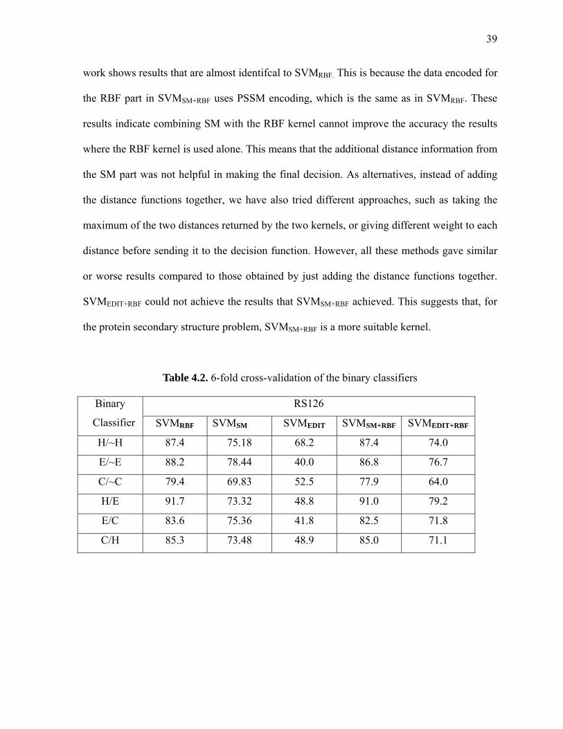
39
work shows results that are almost identifcal to SVMRBF. This is because the data encoded for
the RBF part in SVMSM+RBF uses PSSM encoding, which is the same as in SVMRBF. These
results indicate combining SM with the RBF kernel cannot improve the accuracy the results
where the RBF kernel is used alone. This means that the additional distance information from
the SM part was not helpful in making the final decision. As alternatives, instead of adding
the distance functions together, we have also tried different approaches, such as taking the
maximum of the two distances returned by the two kernels, or giving different weight to each
distance before sending it to the decision function. However, all these methods gave similar
or worse results compared to those obtained by just adding the distance functions together.
SVMEDIT+RBF could not achieve the results that SVMSM+RBF achieved. This suggests that, for
the protein secondary structure problem, SVMSM+RBF is a more suitable kernel.
Table 4.2. 6-fold cross-validation of the binary classifiers
RS126 Binary
Classifier SVMRBF SVMSM SVMEDIT SVMSM+RBF SVMEDIT+RBF
H/~H 87.4 75.18 68.2 87.4 74.0
E/~E 88.2 78.44 40.0 86.8 76.7
C/~C 79.4 69.83 52.5 77.9 64.0
H/E 91.7 73.32 48.8 91.0 79.2
E/C 83.6 75.36 41.8 82.5 71.8
C/H 85.3 73.48 48.9 85.0 71.1

40
4.4. Conclusion
In chapter 4, we propose two hybrid kernels SVMSM+RBF and SVMEDIT+RBF. We tested these
two hybrid kernels on one of the most widely studied problems in bioinformatics -the protein
secondary structure prediction problem. For the protein secondary structure problem, our
results achieved 91% accuracy in predicting the H/E binary classifier. In this case, the
information in the substitution matrix reinforces the information in the RBF-on-PSSM
profiles. However, this is not true with the edit distance. These results show that the data are
consistent when the substitution matrix is used, but are not consistent when the edit distance
is used. The edit distance kernel gives good results in [47], but not when used with our
dataset in this work. Our results show that it is critically important to use mutually consistent
data when merging different distance measures in support vector machines.

41
CHAPTER 5
A Feature Selection Algorithm based on Graph Theory and Random Forests for Protein
Secondary Structure Prediction
In this work, we propose an algorithm that uses a graph-theory approach for feature
selection. First, we apply this algorithm to the BLOSUM62 matrix; and then, based on the
feature set produced by the algorithm, we use this feature set for condensing the PSSM
matrix. This work attempted to reduce the feature space of the dataset using a graph-
theoretical approach. Even though graph theory concepts have been around for more than a
century, its concepts are just newly being explored for biological applications [12][66]. The
clique search algorithm was applied to find all the cliques with different threshold values. We
used Niskanen’s and Ostergard’s original implementation of Cliquer version 1.1 [49]. The
code Cliquer is a set of C routines for finding cliques in an arbitrary weighted graph. It uses
an exact branch-and-bound algorithm recently developed by Östergård [50]. Next, based on
the newly designed algorithm, final cliques were determined. By merging the vertices within
the same clique into one, the original feature space is reduced. Finally, this reduced feature
set was applied to random forests and the performance was compared with the unreduced
counterpart. In Fig. 5.1, the whole picture of this model is presented.

42
Figure 5.1 New model for protein secondary structure prediction
5.1. Encoding Schemes of the Data
Two matrices such as Blosum62 and PSSM were applied alone or combined with a feature
reduction scheme. The BLOSUM62 matrix is a measure of differences between two distantly
related proteins. The values in the BLOSUM62 matrix represent the possibility that two
given amino acids will interchange with each other in the evolutionary process. The position-
specific scoring matrix (PSSM) generated by PSI-BLAST; uses position-specific scores for
each position in the alignment. Highly conserved positions have high scores and weakly
conserved positions have low scores close to zero. Since each of these coding schemes
captures different aspects of the properties of the amino acids, the combinations of these two
different encodings would be more informative.
Data Set
Bootstrapped sample
Clique Search Algorithm
Data Set with Reduced Features
…Bootstrapped sample Bootstrapped sample
Random Forest

43
The above encoding profiles were generated based on the sliding window scheme. In the
sliding window scheme, a window becomes one training pattern for predicting the structure
of the residue at the center of the window. The optimal window size of the sliding window
scheme was set as 13 based on previous research [32]. To reduce the noise in the training
data and to minimize the memory requirement for training, the feature set was reduced based
on the clique search algorithm. This approach is described in detail in the next section.
5.2. Feature Reduction Based on Cliques
A clique in an undirected graph G is a set of vertices V such that, for every two vertices in
V, there exists an edge connecting the two. The subgraph induced by V is a complete graph.
The size of a clique is the number of vertices it contains. The maximum clique problem is to
find the largest clique in a given graph.
The BLOSUM62 matrix used in this study can be represented as a graph which consists of
20 different vertices. The edges among these 20 vertices can be introduced by applying
different threshold values to the BLOSUM62 matrix. This study attempted to reduce the
feature size by obtaining the cliques which occur commonly in different threshold values and
by merging the vertices within the same clique. This process can be divided into the
following three steps. The first step is converting the matrix into the adjacency matrix based
on different threshold values ranging from -2 to 2. Each cell of the adjacency matrix has a
value ‘1’ if there is an edge between two vertices or a value ‘0’ if there is no edge between
them based on different threshold values. The second step is applying the clique search
algorithm to each of these adjacency matrices. The third step is scanning through all the

44
cliques obtained from each matrix and finding the common cliques. The cliques of size 2, 3
or 4 vertices (n-mer) which share at least one physico-chemical property (polarity,
hydrophobicity, or aromaticity, etc.) were considered for final decision. The common cliques
were determined by counting the same vertices (n-mer) in each clique. Based on this
algorithm, three most commonly occurring n-mers were found. These were merged into one-
mers as follows:
Q E → E
I L M → L
H F Y → Y
The pseudocode of this algorithm is given in Fig. 5.2 The physico-chemical property sets P
in the pseudocode are described in Table 5.1.

45
Input: Blosum62 matrix B
Threshold set T T = {-2, -1, 0, 1, 2}
Physico-chemical property sets P P= {P1, P2, …, P8, P9}
Output: Common_Clique_Set C
Process:
FOR each threshold i of T
Adj_Matrixi = Create_adjacency_matrix (B)
END FOR
FOR each adjacency matrix Adj_Matrixi
Clique_Seti = Find_all_cliques (Adj_Matrixi )
END FOR
FOR each clique set Clique_Seti
FOR each clique j j ∈ Clique_Set i
if size_of(j) equals to 2 or 3 or 4
FOR each Pi ∈ P
if j ⊆ Pi
count++
END FOR
Save the count into count_array
END FOR
END FOR
Common_Clique_Set C = Vote_and_Find_Top_Three(count_array)
Figure 5.2 Common clique search algorithm

46
Table 5.1 Physico-chemical property set
Set P Physico-chemical properties Amino acids in each set
P1 Small A, C, D, G, N, P, S, T, V P2 Hydrophobic A, C, F, G, H, I, K, L, M, T, V, W, Y P3 Polar C, D, E, H, K, N, Q, R, S, T, W, Y P4 Tiny A, C, G, S P5 Aliphatic I, L, V P6 Aromatic F, W, Y P7 Charged D, E, H, K, R P8 Positive H, K, R P9 Negative D, E
The BLOSUM62 matrix is reduced to the size of 15x15 based on the above compression.
By applying the same reduction, the dimensions of the PSSM can also be compressed to
Lx15. Here, L is the sequence length of the protein.
We also tested all other possible clique sizes between 1-20 in order to choose an optimal
clique size. The test results are given in tables 5.2, 5.3 and 5.4. The highest accuracy was
achieved when a clique size of 5 is used. These results indicate that the output of the
algorithm already gives the optimal clique size which is 5.

47
Table 5.2 Finding optimal clique size (results between size 3-10)
Clique sizes Binary classifiers
3 4 5 6 7 8 9 10
H/~H 87.3 86.2 93.6 86.8 87.0 85.9 83.9 75.1
Table 5.3 Finding optimal clique size (results between size 11-18)
Clique sizes Binary classifiers
11 12 13 14 15 16 17 18
H/~H 74.2 68.8 67.3 67.3 68.0 64.1 63.5 66.6
Table 5.4 Finding optimal clique size (results between size 19-20)
Clique sizes Binary classifiers
19 20
H/~H 67.7 65.9
5.3. Training and Testing
The commonly used RS126 set was applied to compare our results with previous studies.
The RS126 data set was proposed by Rost and Sander and is known to be a non-homologous
set which shares less than 25% sequence identity [59]. The random forests algorithm
performs a bootstrap test with the training data. In other words, one third of the instances are

48
left out in the construction of the kth tree; are applied for classification. Therefore, in random
forests, we do not need to perform a cross-validation. Nor do we need to save a separate test
set to obtain unbiased accuracy values. However, the current study applied two thirds of the
original data for training and one third for testing to confirm the results obtained from the
training data.
5.4.Parameter Optimization
In the random forests program, the only parameter which is optimized is the number of
features, called mtry, that are randomly selected at each node [15]. As a rule of thumb, the
author suggested that it could be set to the square root of the number of whole features.
Including this value, this study tested 4 different mtry values to find the optimum value.
5.5. Binary Classifiers
Six binary classifiers, such as three one-versus-rest classifiers (H/~H, E/~E and C/~C),
and three one-versus-one classifiers (H/E, E/C and C/H) were created based on the previous
study [32]. Here, the name ‘one’ in the one-versus-rest classifier refers to a positive class and
the name ‘rest’ means a negative class. In the term one-versus-one classifier, the former
“one” refers to a positive class and the latter “one” to a negative class. For example, the
classifier H/~H classifies the testing sample as helix or not helix and the classifier E/C
classifies the testing sample as sheet or coil. This paragraph is unclear. You introduce the
one-versus-rest and one-versus-one notations, but then your example illustrates a different
nomenclature: V and ~V.

49
5.6. Results
5.6.1. Parameter Optimization
Table 5.5 presents the result of applying different mtry values (the number of features
randomly selected) based on the Blosum62 and the reduced PSSM concatenated encoding
scheme. In the second column of the table, the value 22 is obtained from the approximate
square root of the whole dimension of the feature: the whole dimension is (20+15) * 13 =
455. As can be seen from the table, the accuracy values are almost same even though we
chose the larger mtry values. This means that the square root value is almost the optimal
value.
Table 5.5 Comparison of different mtry values
Accuracy (%) for different mtry values Binary classifier 22 50 100 200
H/~H 82.2 85.1
82.1 85.6
83.3 85.6
82.1 85.1
5.6.2. Encoding Scheme Optimization
Table 5.6 shows the result obtained by applying different encoding schemes to the random
forests. Two different accuracy values are displayed. The first row is obtained by doing a
bootstrap test on the training data and the second row by using the test data. As can be
observed from the table, both the reduced Blosum62 matrix and the reduced PSSM

50
encodings present equal level of accuracy values when compared with the unreduced
counterparts whether applied alone or applied in a concatenated form. This result proves that
there is no information loss from the feature reduction and that our algorithm for this
reduction works properly. Among all the different encoding schemes, the reduced PSSM
encoding shows the best performance. The reduced PSSM encoding performs similarly to the
concatenated encoding of the reduced PSSM and the BLOSUM62 matrix. The reduced
PSSM shown in the last column has 13*15=195 features whereas the unreduced PSSM
13*20=260 features. This means that an approximate 25% feature reduction is achieved by
using our algorithm while still achieving high accuracy.
Table 5.6 Comparison of different encoding schemes for H/~H
PSSM Reduced PSSM BLOSUM Reduced
BLOSUM
PSSM+ BLOSU
M
Reduced PSSM+
BLOSUM
Reduced PSSM+ Reduced
BLOSUM
H/~H 82.3 85.5
82.5 85.7
76.9 80.7
77.2 80.8
82.3 85.1
82.2 85.1
81.7 85.0
In Table 5.7, all six binary classifiers are tested based on the BLOSUM and PSSM
combined encodings. Once again, it can be observed that the reduced PSSM encoding has
almost the same performance as the unreduced counterpart against all six binary classifiers.

51
Table 5.7 Accuracy results with BLOSUM+PSSM encoding
5.6.3. Time comparison
Table 5.8 shows the execution times of the reduced PSSM encoding scheme versus the
PSSM+BLOSUM encoding scheme with different number of trees. Our proposed encoding
scheme using reduced PSSM has a faster execution time. Also, when using 2000 trees,
PSSM+BLOSUM encoding scheme did not run after a few hours due to its high
dimensionality whereas reduced the PSSM encoding could run. These results show that the
reduced PSSM encoding could be used to reduce the space and time complexity drastically
where the data dimensionality is very high.
Binary classifiers
Accuracy for PSSM+BLOSUM
Accuracy for reduced
PSSM+BLOSUM
Accuracy for reduced PSSM
H/~H 82.3 85.1
82.2 85.1
82.5 85.7
E/~E 83.9 81.1
83.7 81.1
84.0 81.0
C/~C 76.1 75.5
75.7 74.9
76.3 75.6
H/E 85.2 83.1
85.3 82.7
86.5 84.0
E/C 79.5 78.7
78.9 78.6
80.6 80.3
C/H 82.0 83.2
82.1 82.9
82.2 83.3
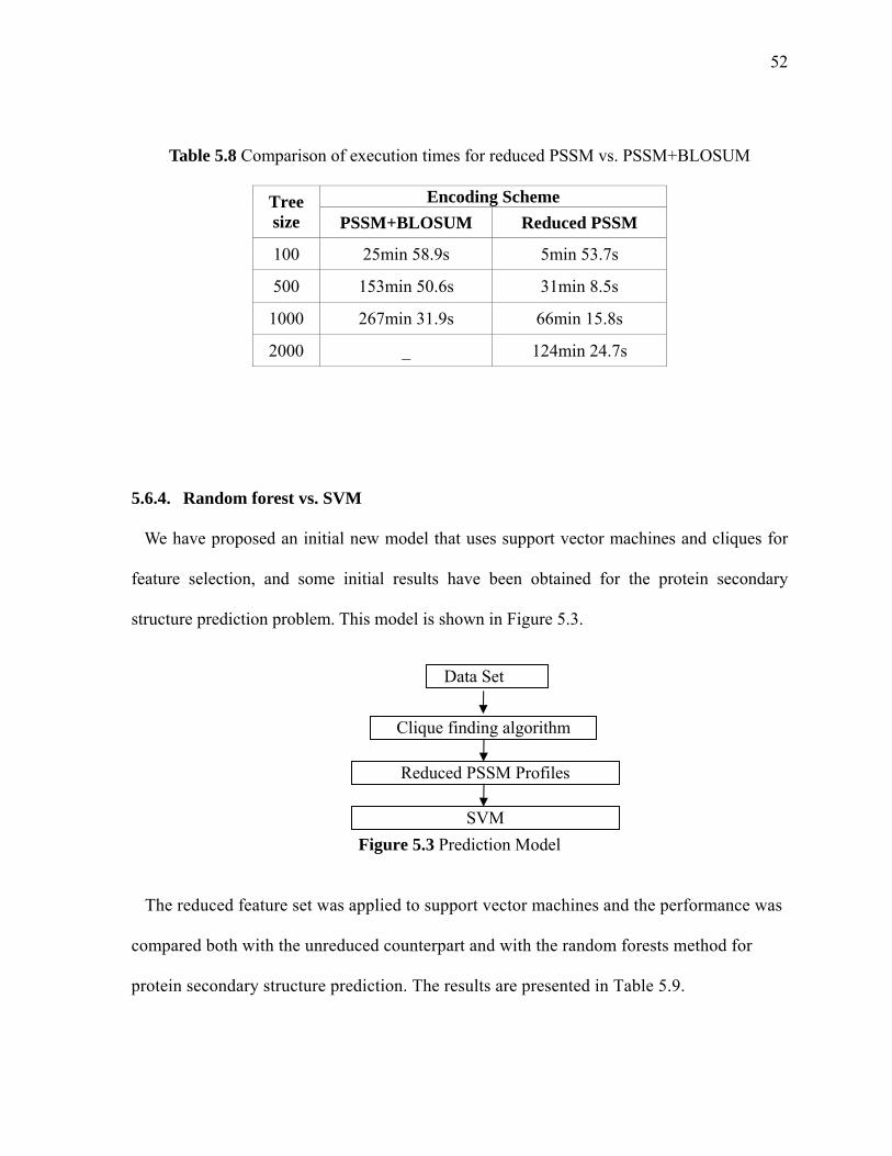
52
Reduced PSSM Profiles
Clique finding algorithm
SVM
Data Set
Table 5.8 Comparison of execution times for reduced PSSM vs. PSSM+BLOSUM
Encoding Scheme Tree size PSSM+BLOSUM Reduced PSSM
100 25min 58.9s 5min 53.7s
500 153min 50.6s 31min 8.5s
1000 267min 31.9s 66min 15.8s
2000 _ 124min 24.7s
5.6.4. Random forest vs. SVM
We have proposed an initial new model that uses support vector machines and cliques for
feature selection, and some initial results have been obtained for the protein secondary
structure prediction problem. This model is shown in Figure 5.3.
Figure 5.3 Prediction Model
The reduced feature set was applied to support vector machines and the performance was
compared both with the unreduced counterpart and with the random forests method for
protein secondary structure prediction. The results are presented in Table 5.9.

53
Table 5.9 Random forest vs. SVM comparison for different encoding schemes
Random forest SVM Binary
classifiers Accuracy for PSSM+BLOSU
M
Accuracy for reduced PSSM
Accuracy for PSSM+BLOSU
M
Accuracy for reduced PSSM
H/~H 85.1 85.7 92.8 93.6 E/~E 81.1 81.0 83.3 87.1 C/~C 75.5 75.6 72.4 77.6 H/E 83.1 84.0 88.2 90.8 E/C 78.7 80.3 79.8 82.4 C/H 83.2 83.3 83.9 84.5
As can be seen from the table, SVM produces much better accuracy than the random forests
which improved our previous accuracy results.
5.7. Conclusion
In this work, we proposed a novel algorithm for feature selection based on cliques and
evolutionary information of proteins. We tested our algorithm using random forests and
different encoding schemes for the secondary structure problem in proteins. These algorithms
were tested on both condensed and non-condensed data sets. We found out that the prediction
accuracies for both data sets were similar. These results show that a significant amount of
space and time can be saved while still achieving the same high accuracy results by using a
subset of the features when these features are carefully selected.
These results show that it is important to select features from the data that are more
significant for training and testing instead of using the entire feature set. Also, using our
novel algorithm, we achieved an approximate 25% reduction in space and time. We tested

54
our algorithm using SVM as a machine learning method instead of random forests and
achieved high accuracy. Finally, we propose that, as a subject for further research, SVM can
be used instead of random forests in order to increase prediction accuracy.
55
CHAPTER 6
New Binary Classifiers for Protein Structural Boundary Prediction
Proteins are primarily made up of amino acids which determine the structure of a protein.
Protein structure has three states called primary structure, secondary and tertiary structure.
The primary structure of the protein is its amino acid sequence. The secondary structure of a
protein is formed from recurring shapes called the alpha-helix, the beta sheet, and the coil.
The tertiary structure of the protein is the spatial assembly of helices and sheets and the
pattern of interactions between them. Predicting the secondary and tertiary structure of
proteins from their amino acid sequences is an important problem; knowing the structure of a
protein aids in understanding how the functions of proteins in metabolic pathways map for
whole genomes, in deducing evolutionary relationships, and in facilitating drug design.
It is strongly believed that protein secondary structure delimits the overall topology of the
proteins [26] Therefore, during the past 25 years, many researchers have tried to understand
how to predict the secondary structure of a protein from its amino acid sequence. Many
algorithms and machine learning methods have been proposed for this problem [2][6]
[40][42]. The algorithms for predicting secondary structure of proteins have reached a
plateau of roughly 90%. Much more success has occurred with motifs and profiles [16].
The common approach to solve the secondary structure prediction problem has been to
develop tools that predict the secondary structure for each and every amino acid (residue) of
a given protein sequence. In this work, we propose new binary classifiers which do not

56
require the correct prediction of each and every residue in a given protein segment. The new
binary classifiers predict only the start or end of a helix, sheet or coil. In figure 6.1, this
concept is illustrated. Fig 6.1 represents the tertiary structure of a protein with its secondary
structure regions colored in different shades. The point where one secondary structure
element ends and another one begins is called a “structural transition” throughout this
chapter.
Figure 6.1 Structural transitions of a protein
Protein sequences may have specific residue preferences at the end or start of secondary
structure segments. For example, it has been shown that specific residue preferences exist at
the end of helices, which is called helix capping. Recent research has suggested that it is
possible to detect helix-capping motifs [7]. However, these results reflect a linear decision
function based on amino acid frequencies. It is well known that non-linear decision
functions, for example those implemented with the Support Vector Machines (SVM),
dramatically outperform linear decision functions when the underlying data are nonlinear
[68]. In this work, we use a machine learning approach based on SVM to predict the helix
Structural transitions
Start of a helix
End of a helix

57
capping regions of a given protein sequence. These helix capping regions indicate where a
helix ends. The same method is also used for predicting the starting points of helices and to
predict the end and starting points of coils and sheets. The end and starting points of
secondary structures are also called structural transition boundaries.
6.1. Problem Formulation
In this study, we adopted the most generally used DSSP secondary-structure-assignment
scheme [39]. The DSSP classifies the secondary structure into eight different classes: H (α-
helix), G (310-helix), I (π-helix), E (β-strand), B (isolated β-bridge), T (turn), S (bend), and -
(rest). These eight classes were reduced into three regular classes based on the following
method: H, G and I were reduced to H; E to E; and all others to C.
6.1.1. Traditional problem formulation for the secondary structure prediction
The traditional problem formulation is stated as:
Given a protein sequence a1a2…aN, find the state of each amino acid ai as being either:
• H (helix) or
• E (beta strand) or
• C (coil).
The quality of the secondary structure prediction is measured with a “3-state accuracy”
score called Q3. Q3 is the percent of residues that match reality. Most of the previous research
adopted Q3 as an accuracy measurement.

58
6.1.2. New problem formulation for the transition boundary prediction
The new problem formulation is stated as follows:
Given a protein sequence profile, find the state of each amino acid ai as being either:
• The start of a H (helix), E (beta strand), or C (coil) or
• The end of a H (helix), E (beta strand), or C or
• Neither of the above (named as ‘X’: doesn’t matter)
Here, we used a new scoring scheme that we call QT (Transition) which is similar to Q3. QT
is the percent of residues that match reality. We had to change the scoring scheme to QT
because Q3 scoring scheme takes into account all the residues whereas QT takes into account
only the residues that are necessary for prediction.
{ }
{ }∑
∑
∈
∈=
CEHi
CEHii
T iresiduestransitionof
residuestransitionpredictedcorrectlyofQ
,,
,,
#
#(6.1)
In QT scoring scheme the number of correctly predicted transition residues of class H, E, o C
are divided by the number of all transition residues of class H, E or C.

59
6.2. Method
6.2.1. Motivation
Figure 6.2 A 9-mer with helix junction
Given a protein sequence of a 9-mer, let the middle element of this 9-mer be the starting
position of a helix as it shown in Figure 6.2. Our goal is to determine whether the middle
residue is the start or end of a helix. If we use the traditional binary classifiers (such as
H/~H), first we must correctly identify all the residues in the whole segment. We need to
correctly predict 3 consecutive residues as H (at least 4 residues are needed for a helix) and
the rest of the residues should be ~H. In this case, we have to make 9 predictions, and ideally
we should be correct all 9 times. However, the probability that we can predict all 9 residues
correctly in the protein segment is at maximum .35 if we assume that our chance of making
each prediction correctly is 0.9 and that this probability of success is independent of the other
predictions.
In the next section, we explore how to overcome the problem of making 9 predictions for
a given 9-mer and how to reduce it to a problem of making only one prediction per 9-mer.
EAN L D A V D A
HHH H H E H C E
0.9 0.9 0.9 0.9 0.9 0.9 0.9 0.9 0.9=(0.9)9=0.35
Corresponding secondary structure of the protein sequence segment

60
6.2.2. A new encoding scheme for the prediction of starts of H, E and C.
The goal of our new encoding scheme is shown in Fig 6.3 where a new binary classifier has
to make only one guess instead of 9 guesses. Here, the new encoding scheme for representing
the starting points of helices is shown as an example. The same encoding is applied to both
sheets and coils.
Figure 6.3 New encoding scheme for Helix start
In Figure 6.3, the illustration of the new encoding scheme is presented.
The rules of the new encoding scheme are as follows:
In order for the middle residue to be classified as the start of a helix, the conditions are:
1. The residues corresponding to X’s can be C, H or E, but no two consecutive H’s are
allowed.
2. The secondary structure of the middle residue must be H. 3. All residues after the middle residue must be H.
E AN L A V D A
D
H HH H H X X XX
A helix starts here
Corresponding secondary structure of the protein sequence segment

61
If all three rules are satisfied, the protein segment is represented by the new encoding as
the start of a helix (Hstart). If not, the protein segment is represented as ~Hstart (not the start of
a helix).
6.2.3. A new encoding scheme for the prediction of ends of H, E and C.
Similar to the the method in section 6.2.2 the new encoding scheme for representing the
ends of helices is shown as an example is shown in Fig 6.5. The same encoding is applied to
sheets and coils.
Figure 6.4 A 9-mer with helix end
In the new encoding scheme, the protein sequences are classified as the following:
Figure 6.5 New encoding scheme for Helix start
The rules of the new encoding scheme are as follows. These are similar to the rules in section
6.2.2, however used for predicting the ends of secondary structures:
In order for the middle residue to be classified as a helix end, the conditions are:
E EH C H H H H H
Only one prediction is sufficient
X XX X H H H HH
A Helix ends here

62
1. The residues corresponding to X’s can be C, H or E, but no two consecutive H’s are
allowed.
2. The secondary structure of the middle residue must be H.
3. All residues before the middle residue must be H.
If all three rules are satisfied, the protein segment is represented by the new encoding as the
end of a helix (Hend). If not, the protein segment is represented as ~Hend (not the end of an
helix).
6.3. New binary classifiers
In the traditional secondary structure prediction approach, usually six binary classifiers,
such as three one-versus-rest classifiers (H/~H, E/~E and C/~C) and three one-versus-one
classifiers (H/E, E/C and C/H) are used. Here, the name ‘one’ in one-versus-rest classifier
refers to a positive class and the name ‘rest’ means a negative class. Likewise, the name
‘one’s in one-versus-one classifier refers to positive class and negative class respectively. For
example, the classifier H/~H classifies the testing sample as helix or not helix and the
classifier E/C classifies the testing sample as sheet or coil.
The six new binary classifiers that are proposed are the following:
Binary Classifier 1:
Hstart/~Hstart: This binary classifier classifies the positive samples as the start of a helix
and negative samples as not being the start of a helix.

63
Binary Classifier 2:
Estart/~Estart: This binary classifier classifies the positive samples as the start of a sheet and
negative samples as not being the start of a sheet.
Binary Classifier 3:
Cstart/~Cstart: This binary classifier classifies the positive samples as the start of a coil and
negative samples as not being the start of a coil.
Binary Classifier 4:
Hend/~Hend: This binary classifier classifies the positive samples as the end of a helix and
negative samples as not being the end of a helix.
Binary Classifier 5:
Eend/~Eend: This binary classifier classifies the positive samples as the end of a sheet and
negative samples as not being the end of a sheet.
Binary Classifier 6:
Cend/~Cend: This binary classifier classifies the positive samples as the end of a coil and
negative samples as not being the end of a coil.
6.4. SVM kernel
We used a radial basis kernel (RBF) since it was optimal when used for secondary
structure prediction:
2
),( yxeyxK −−= γ (6.2)
Here, x and y are two input vectors containing different feature values and γ is the radial
basis kernel parameter. Radial basis kernels depend on a numerical representation of the
input data.

64
6.5. Choosing the window size
In order to choose an optimal window size for the proposed encoding scheme for a given
protein segment, we tried different window sizes on the smaller dataset RS126. We used the
PSSM profiles of the dataset RS126 during the tests. As a prediction method, the SVM RBF
kernel was used. Using the sliding window scheme, first each k-mer from a protein sequence
is extracted. Each k-mer is classified as a positive or negative sample. If the middle residue
satisfies the encoding scheme as described in section 6.2, it is marked as a positive sample:
Hstart, Estart, or Cstart. Otherwise it is marked as a negative sample ~Hstart, ~Estart, or ~Cstart,
Fig 6.6 shows the QT prediction accuracy results of all the six new binary classifiers used
with the SVM RBF kernel and the RS126 dataset. The prediction accuracy of SVM varied
for different window sizes. The best overall prediction accuracy was achieved when the
window size was 9.
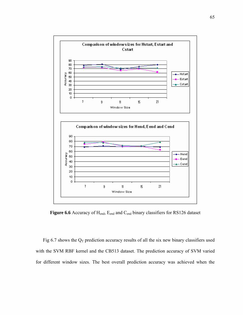
65
Figure 6.6 Accuracy of Hend, Eend and Cend binary classifiers for RS126 dataset
Fig 6.7 shows the QT prediction accuracy results of all the six new binary classifiers used
with the SVM RBF kernel and the CB513 dataset. The prediction accuracy of SVM varied
for different window sizes. The best overall prediction accuracy was achieved when the

66
window size was 9 for CB513 data which is similar to the results of RS126 data shown in
Fig. 6.6.
Comparison of w indow sizes for Hstart, Estart and Cstart
0102030405060708090
0 5 10 15 20Window size
Accu
racy
Hstart
Estart
Cstart
Comparison of w indow sizes for Hend, Eend and Cend
0102030405060708090
0 5 10 15 20Window size
Accu
racy
Hend
Eend
Cend
Figure 6.7 Accuracy of Hend, Eend and Cend binary classifiers for CB513 dataset
For the later experiments and for the larger dataset CB513 dataset a window size of 9 was
used for testing the new binary classifiers.

67
6.6. Test results of the binary classifiers
Table 6.1 shows the QT prediction accuracy results of all six binary classifiers
Hstart/~Hstart, Estart/~Estart , Cstart/~Cstart and Hend/~Hend , Eend/~Eend and Cend/~Cend used with the
SVM RBF kernel with a window size of 9. We used the PSSM profiles of the dataset CB513
during these tests. Since there were many negative samples, we balanced the negative and
positive samples in the dataset by randomly choosing from the negative samples for training
the SVM. The results are given in Table 6.1. The probability of SVM correctly predicting the
start of helices is 81.5%, which is much higher than the 35% theoretical bound for per-
residue prediction. The probability of successfully predicting the end of a helix is also high--
approximately 71.33%. This shows that there is more of a signal in the data indicating the
start of helices than there is a stop signal. The start and end positions of strands and coils are
predicted with approximately 75% accuracy.
These results show that, by training a classifier such as SVM to predict the secondary
structure transition boundaries, it is possible to detect where helices, strands and coils begin
and end with high accuracy. Furthermore, the detection of these secondary structure
transition boundaries is performed on the basis of one prediction rather than trying to predict
correctly all the residues in a given sequence segment, the probability of which would
theoretically be only roughly 35%.

68
Table 6.1 Prediction accuracies of the new binary classifiers
Binary Classifier
Accuracy (TP+TN)/
(TP+TN+FN+FP)*
Recall (TP/TP+FN)
Specifity (TN/TN+FP)
Precision (TP/(TP+FP)
Hstart/~Hstart 81.5 78.5 84.16 83.33
Estart/~Estart 73.16 73.33 73.16 73.16
Cstart/~Cstart 75.33 78.33 72 74.33
Hend/~Hend 71.33 86.16 66.66 69.5
Eend/~Eend 78.66 82 75.33 77.66
Cend/~Cend 77.66 79 76 77.5
* TP: TRUE POSITIVE TN: TRUE NEGATIVE FP: FALSE POSITIVE FN: FALSE NEGATIVE
6.7. Accuracy as a function of helix sizes
Fig 6.8 shows the comparison between the prediction accuracy levels of helix starting and
end points as a function of the number of turns in the helix. One can see that the prediction
accuracies of the binary classifiers Hstart/~Hstart and Hend/~Hend reach a maximum value when
the helix has 2.25 turns. Since a helix has about 4 residues per turn, this corresponds to a
window size of 9 residues. At different number of turns of a helix, the accuracies are lower.
This also proves that choosing a window size of 9 residues is optimal for the transition
boundary prediction problem.

69
Hstart vs. Hend
687072747678808284
0 2 4 6Observed size of helix in turns
Acc
urac
yhelix start
helix f inish
Figure 6.8 Accuracy levels of Hstart and Hend
6.8. Comparison of traditional binary classifiers to the new binary classifiers
There are several studies that focus on finding where the structural segments start and
end. Aydin et al. have shown that new dependency models and training methods bring
further improvements to single-sequence protein secondary structure prediction [8]. Their
results improve most Q3 accuracy results by 2%, which shows that considering amino acid
patterns at segment borders increases the prediction accuracy. Some other approaches are
focused on finding the end of helices. The reason for this is that the helices (alpha-helices)
are the most abundant regular secondary structure and that a certain residue preference exists
at the ends of helices [71]. However, current secondary structure prediction programs can not
identify the ends of helices correctly in most cases. The same rule applies to strands although
the residue preferences for strand termini are not as strong as in helices. Wilson et. al. used
cumulative pseudo-free energy calculations to predict helix start positions and achieved 38%
prediction accuracy. We achieved around 80% QT accuracy using SVM, which is of course
significantly higher.

70
One could question what our Q3 overall prediction accuracy is. Most of the current
secondary structure prediction methods try to solve the problem at a per-residue level,
whereas we try to solve the prediction at a per-segment level. In this work, we proposed
binary classifiers that target the prediction of the start and end positions of helices, strands
and coils. Therefore, in order to be able to compare our prediction accuracy to the current
prediction methods, we derived a method that converts our QT accuracy results to the
standard Q3 and vice versa.
6.8.1. Estimate of the Q3 from QT and QT from Q3
When, traditional binary classifiers such as one-versus-rest classifiers (H/~H, E/~E and
C/~C), and one-versus-one classifiers (H/E, E/C and C/H) are used, their prediction
accuracies are measured using a Q3 measurement. In the Q3 measurement, a prediction for
each and every residue of a protein sequence is done. In order to determine whether a given
protein sequence is the start or end of a secondary structure with the traditional binary
classifiers, each residue’s secondary structure must be predicted first. However, it is clear
that, even with the 90% accuracy per residue, the probability of independently predicting k
residues correctly is 0.9 to the kth order. In order to calculate a Q3 measurement of a given a
protein sequence window (of size k), a prediction for each and every residue in that window
must be made using the traditional binary classifiers. However, with the proposed new binary
classifiers, only one prediction per window is enough to tell whether that window represents
the end or start of a helix, sheet or coil. Besides, the overall prediction probability is slightly
pessimistic because the estimates may not be fully independent.

71
Based on the above reasoning, in order to be able to compare our results to the traditional
binary classifiers which calculate the prediction accuracy per residue, we derived a method
using the following assumption. Given a protein segment of window size k, we assumed that
the prediction of each residue in that window is truly independent of the other residues in that
window. Then, we converted the traditional Q3 accuracy measurement to our accuracy
measurement QT, using the following equation:
QT=Q3
(window size) (6.3)
The formula above basically states that, the fewer number of predictions made for a
given protein window, the higher the chances are that the prediction is correct. Using the
traditional binary classifiers, given a protein window of size k, k predictions must be made in
order to see what that protein sequence segment is. Using the binary classifiers proposed in
this work, only one prediction is enough. The inverse of the formula above is:
(6.4) The inverse of the formula gives us the corresponding Q3 accuracy as a function of QT. 6.8.2. Traditional binary classifiers vs. new binary classifiers
In order to make a fair comparison, we took Q3 measurements for the H/~H, E/~E and
C/~C binary classifiers from [32][33] which are one of the highest Q3 measurements for
these binary classifiers, and estimated their QT measurements. We also converted the QT
results in Table 6.1 to Q3 measurements and listed the results in Table 6.2 and Table 6.3.
)/kln(Q3
TeQ =

72
Table 6.2 Estimated Q3 results
QT converted to Q3 Binary classifiers QT Q3
H/~H 83.17 96.31 E/~E 80.5 95.67 C/~C 76.5 94.65
Table 6.3 Estimated QT results
Q3 converted to QT Binary classifiers Q3* QT
H/~H 87.18 50.35 E/~E 86.02 47.09 C/~C 77.47 36.01
*Q3 measurements from Hu et al, 2004 and Hua and Sun, 2001
Table 6.2 shows our QT accuracy calculations converted to the corresponding Q3
accuracies. When Q3 accuracies are converted to QT measurements as shown in table 6.3, the
accuracies are low. (Note, these estimates are based on the assumption that each residue
prediction is independent of all the others.) These results show that using the new binary
classifiers gives higher prediction accuracy than the traditional binary classifiers. These
results also prove that it is better to make predictions using a per-segment window rather than
a making them per residue. In other words, we should split the data in big chunks (segments)
and make predictions using these segments instead of trying to predict each and every piece
of data (residues).

73
6.9. Test results on individual proteins outside the dataset
In order to prove that the new proposed encoding scheme works, we have run blind tests
on individual proteins. The test results are given in Table 6.4. In all the test cases, the
accuracy, recall, specifity and precision values are high as expected. However, the precision
values are low. The reason for this is the unbalanced nature of the dataset. In our training
datasets, we have many negative samples whereas the positive samples are roughly 1% of the
number of the negative sets. This is a major problem with these kinds of datasets. The false
positives (FPs) are high because we are dealing with 100 times more examples of negative
cases than positive cases. These results imply that it is very hard to get a high precision due
to the unbalanced nature of the datasets. The false positives overwhelm the correct matches.
This is the truly difficult aspect of using minority classes. The good accuracy shows that
there is a signal in the data that we can extract. However, because there are so many more
negatives matches, we get large number FPs. What we discover by this analysis is that there
is a signal that SVM selects because we have high accuracy; however, we can not get high
precision values because there are very few examples of the minority classes. Therefore, we
give he results for both balanced data and unbalanced data.
Table 6.4 Protein ID: CBG Binary
Classifier Accuracy Recall Specifity Precision
Hstart/~Hstart 0.77 0.62 0.77 0.13 Estart/~Estart 0.80 0.53 0.81 0.9 Cstart/~Cstart 0.71 0.59 0.72 0.17 Hend/~Hend 0.79 0.54 0.80 0.13 Eend/~Eend 0.81 0.59 0.82 0.11 Cend/~Cend 0.72 0.57 0.73 0.17

74
Table 6.5 Protein ID: CELB
Binary Classifier Accuracy Recall Specifity Precision
Hstart/~Hstart 0.89 0.2 0.99 0.03 Estart/~Estart 0.75 0.39 0.78 0.13 Cstart/~Cstart 0.58 0.27 0.62 0.07 Hend/~Hend 0.91 0.70 0.92 0.17 Eend/~Eend 0.79 0.42 0.82 0.17 Cend/~Cend 0.63 0.51 0.64 0.13
Table 6.6 Protein ID: BAM
Table 6.7 Protein ID: AMP-1
Binary Classifier Accuracy Recall Specifity Precision
Hstart/~Hstart 0.79 0.57 0.79 0.09 Estart/~Estart 0.69 0.50 0.69 0.06 Cstart/~Cstart 0.66 0.75 0.65 0.16 Hend/~Hend 0.76 0.86 0.76 0.11 Eend/~Eend 0.78 0.62 0.78 0.11 Cend/~Cend 0.72 0.56 0.73 0.16
Binary Classifier Accuracy Recall Specifity Precision
Hstart/~Hstart 0.70 0.64 0.70 0.08 Estart/~Estart 0.79 0.11 0.82 0.02 Cstart/~Cstart 0.73 0.65 0.73 0.15 Hend/~Hend 0.84 0.55 0.85 0.12 Eend/~Eend 0.83 0.67 0.83 0.11 Cend/~Cend 0.72 0.67 0.72 0.16

75
Table 6.8 Protein ID: ADD-1 Binary
Classifier Accuracy Recall Specifity Precision
Hstart/~Hstart 0.86 0.77 0.87 0.28 Estart/~Estart 0.84 0.88 0.84 0.11 Cstart/~Cstart 0.65 0.66 0.65 0.16 Hend/~Hend 0.74 0.59 0.75 0.14 Eend/~Eend 0.86 0.88 0.86 0.13 Cend/~Cend 0.80 0.37 0.84 0.18
6.10. Test results on randomly chosen subsets of data
In order to test that we did not simply select a subset of the negative data for balancing
the dataset that optimized our method’s prediction probabilities, we tested our method using
10 different randomly chosen different subsets of the data. These test results show that our
proposed method works and that it is possible to train an SVM algorithm to learn where the
helices, strands and coils begin and end.
Table 6.9 Test-1, random subset-1
Binary Classifier Accuracy Recall Specifity Precision
Hstart/~Hstart 80 80 80 80 Estart/~Estart 73 77 68 71 Cstart/~Cstart 73 72 73 73 Hend/~Hend 70 77 64 68 Eend/~Eend 81 84 78 80 Cend/~Cend 76 80 72 76

76
Table 6.10 Test-2, random subset-2
Table 6.11 Test-3, random subset-3
Table 6.12 Test-4, random subset-4
Binary Classifier Accuracy Recall Specifity Precision
Hstart/~Hstart 81 79 83 83 Estart/~Estart 72 78 67 70 Cstart/~Cstart 70 73 68 69 Hend/~Hend 73 76 70 72 Eend/~Eend 78 82 74 77 Cend/~Cend 75 79 71 75
Binary Classifier Accuracy Recall Specifity Precision
Hstart/~Hstart 87 84 91 90 Estart/~Estart 75 74 77 76 Cstart/~Cstart 72 73 71 72 Hend/~Hend 74 84 64 70 Eend/~Eend 80 83 77 79 Cend/~Cend 81 84 77 79
Binary
Classifier Accuracy Recall Specifity Precision
Hstart/~Hstart 84 83 84 84 Estart/~Estart 73 71 75 74 Cstart/~Cstart 73 79 68 71 Hend/~Hend 76 80 73 75 Eend/~Eend 78 84 71 75 Cend/~Cend 78 79 77 79
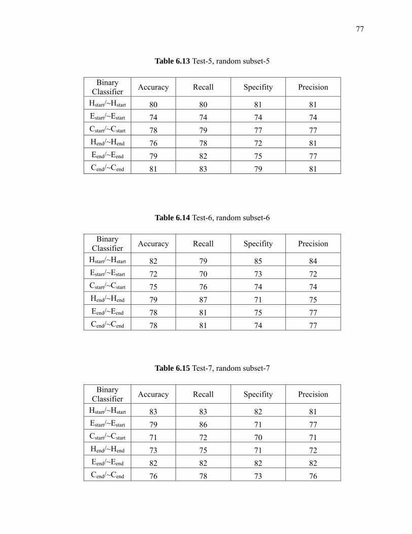
77
Table 6.13 Test-5, random subset-5
Table 6.14 Test-6, random subset-6
Table 6.15 Test-7, random subset-7
Binary Classifier Accuracy Recall Specifity Precision
Hstart/~Hstart 80 80 81 81 Estart/~Estart 74 74 74 74 Cstart/~Cstart 78 79 77 77 Hend/~Hend 76 78 72 81 Eend/~Eend 79 82 75 77 Cend/~Cend 81 83 79 81
Binary Classifier Accuracy Recall Specifity Precision
Hstart/~Hstart 82 79 85 84 Estart/~Estart 72 70 73 72 Cstart/~Cstart 75 76 74 74 Hend/~Hend 79 87 71 75 Eend/~Eend 78 81 75 77 Cend/~Cend 78 81 74 77
Binary Classifier Accuracy Recall Specifity Precision
Hstart/~Hstart 83 83 82 81 Estart/~Estart 79 86 71 77 Cstart/~Cstart 71 72 70 71 Hend/~Hend 73 75 71 72 Eend/~Eend 82 82 82 82 Cend/~Cend 76 78 73 76

78
Table 6.16 Test-8, random subset-8
Binary
Classifier Accuracy Recall Specifity Precision
Hstart/~Hstart 84 82 85 85 Estart/~Estart 81 84 77 81 Cstart/~Cstart 72 78 66 70 Hend/~Hend 74 79 70 72 Eend/~Eend 81 85 77 79 Cend/~Cend 80 83 76 79
Table 6.17 Test-9, random subset-9
Table 6.18 Test-10, random subset-10
Binary Classifier Accuracy Recall Specifity Precision
Hstart/~Hstart 85 83 88 87 Estart/~Estart 79 84 74 78 Cstart/~Cstart 74 78 69 72 Hend/~Hend 74 82 71 66 Eend/~Eend 80 84 76 79 Cend/~Cend 78 85 71 76
Binary Classifier Accuracy Recall Specifity Precision
Hstart/~Hstart 83 80 86 85 Estart/~Estart 73 73 73 73 Cstart/~Cstart 75 78 73 74 Hend/~Hend 73 80 67 70 Eend/~Eend 80 84 75 78 Cend/~Cend 79 83 75 79

79
6.11. New binary classifiers tested with the feature selection algorithm
In this section, we apply the feature selection algorithm described in chapter 5 to the
boundary detection problem with the new binary classifiers proposed in chapter 6. Table 6.19
shows the QT prediction accuracy results of all six binary classifiers--Hstart/~Hstart, Estart/~Estart,
Cstart/~Cstart and Hend/~Hend, Eendt/~Eemd and Cend/~Cend--used with the SVM RBF kernel and a
window size of 9. We used the PSSM profiles of the dataset CB513 during these tests.
As in chapter 5, first, based on the feature set produced by the algorithm, we used this
feature set for condensing the PSSM matrix. Our goal was to reduce the feature space of the
dataset using the proposed graph-theoretical approach. By merging the vertices within the
same clique into one, the original feature space is reduced. Finally, this reduced feature set
was applied to a support vector machine algorithm. We were able to achieve similar accuracy
results as given in Table 6.1 with less number of features.
Table 6.19 Prediction accuracies of the new binary classifiers with feature selection
Binary Classifier
Accuracy (TP+TN)/
(TP+TN+FN+FP)*
Recall (TP/TP+FN)
Specifity (TN/TN+FP)
Precision (TP/(TP+FP)
Hstart/~Hstart 83 81 85 85
Estart/~Estart 79 84 74 79
Cstart/~Cstart 73 74 72 72
Hend/~Hend 78 84 72 76
Eend/~Eend 79 85 73 76
Cend/~Cend 77 79 75 78

80
6.12. Test results on randomly chosen subsets of data
In order to test that we did not simply select a subset of the data that optimized our
method’s prediction probabilities when we balanced the dataset, we tested our method using
10 different randomly chosen different subsets of the data. These test results show that our
proposed method works and that it is possible to train an SVM algorithm to learn where the
helices, strands and coils begin and end when features are reduced based on the clique
algorithm.
Table 6.20 Test-1, random subset-1
Table 6.21 Test-2, random subset-2
Binary Classifier Accuracy Recall Specifity Precision
Hstart/~Hstart 82 80 83 83 Estart/~Estart 81 86 74 80 Cstart/~Cstart 73 78 71 68 Hend/~Hend 80 85 75 79 Eend/~Eend 80 82 77 79 Cend/~Cend 77 82 72 76
Binary Classifier Accuracy Recall Specifity Precision
Hstart/~Hstart 83 80 85 84 Estart/~Estart 79 85 72 77 Cstart/~Cstart 73 80 73 70 Hend/~Hend 79 86 71 77 Eend/~Eend 80 85 74 77 Cend/~Cend 81 84 76 80

81
Table 6.22 Test-3, random subset-3
Table 6.23 Test-4, random subset-4
Table 6.24 Test-5, random subset-5
Binary Classifier Accuracy Recall Specifity Precision
Hstart/~Hstart 84 82 85 85 Estart/~Estart 82 88 75 80 Cstart/~Cstart 76 77 75 75 Hend/~Hend 78 86 70 76 Eend/~Eend 80 84 75 78 Cend/~Cend 77 82 72 76
Binary
Classifier Accuracy Recall Specifity Precision
Hstart/~Hstart 83 80 86 85 Estart/~Estart 83 86 79 83 Cstart/~Cstart 76 73 79 78 Hend/~Hend 81 88 72 80 Eend/~Eend 81 82 80 81 Cend/~Cend 79 78 79 80
Binary Classifier Accuracy Recall Specifity Precision
Hstart/~Hstart 85 82 87 86 Estart/~Estart 78 82 74 78 Cstart/~Cstart 72 76 68 71 Hend/~Hend 77 81 72 77 Eend/~Eend 83 84 81 82 Cend/~Cend 80 82 77 79

82
Table 6.25 Test-6, random subset-6
Table 6.26 Test-7, random subset-7
Table 6.27 Test-8, random subset-8
Binary Classifier Accuracy Recall Specifity Precision
Hstart/~Hstart 83 83 84 84 Estart/~Estart 80 85 75 79 Cstart/~Cstart 77 78 75 76 Hend/~Hend 79 85 72 76 Eend/~Eend 79 83 75 77 Cend/~Cend 80 82 76 80
Binary Classifier Accuracy Recall Specifity Precision
Hstart/~Hstart 83 80 86 85 Estart/~Estart 81 83 78 81 Cstart/~Cstart 74 76 72 73 Hend/~Hend 85 89 80 84 Eend/~Eend 82 87 78 80 Cend/~Cend 78 83 72 77
Binary Classifier Accuracy Recall Specifity Precision
Hstart/~Hstart 82 79 84 84 Estart/~Estart 80 85 74 79 Cstart/~Cstart 71 78 65 69 Hend/~Hend 79 85 73 78 Eend/~Eend 81 83 79 80 Cend/~Cend 77 82 71 76

83
Table 6.28 Test-9, random subset-9
Table 6.29 Test-10, random subset-10 6.13. Conclusion
In this work, we proposed a new way to look at the protein secondary prediction problem.
Most of the current methods use the traditional binary classifiers such as H/~H and require
the correct prediction of every residue’s secondary structure. This approach gives an
overview of the secondary structure of a sequence. However, in order to determine whether a
sequence segment is a Helix, Sheet or Coil using the traditional binary classifier, most of the
Binary Classifier Accuracy Recall Specifity Precision
Hstart/~Hstart 81 81 82 82 Estart/~Estart 79 88 70 76 Cstart/~Cstart 74 71 77 76 Hend/~Hend 81 88 74 80 Eend/~Eend 82 84 81 82 Cend/~Cend 80 83 76 79
Binary Classifier Accuracy Recall Specifity Precision
Hstart/~Hstart 85 83 87 86 Estart/~Estart 81 84 77 81 Cstart/~Cstart 74 76 72 73 Hend/~Hend 82 85 78 81 Eend/~Eend 79 83 76 78 Cend/~Cend 79 85 73 77

84
residues in the sequence segment must be classified correctly. Even with a 90% probability
that each residue is correctly predicted independently, the cumulative probability of being
correct for all the residues in the sequence segment is low (around 35%). We propose six
new binary classifiers that could be used to overcome the problem of classifying all the
residues in a given protein sequence segment when we attempt to determine whether the
sequence segment is a helix, strand of coil. In our binary classifiers, only one classification is
made per segment. In order to use these binary classifiers, we proposed a new encoding
scheme for data representation. Our results show that it is possible to train an SVM to learn
where the helices, strands and coils begin and end.

85
CHAPTER 7
Future work
There are many things that can be done to further the research in this dissertation. In
chapter 3, we explored the factors involved in the accurate selection of seeds for protein
sequence alignments. Our results show that if the proteins in a database are clustered first and
a seed search is made, higher quality seeds are found than when an individual database
search is made. In the future, PHI-BLAST like algorithms can be improved based on this
finding. These algorithms currently do not cluster any of the data and run a search
individually for each protein in the whole database. This is not only time consuming, but also
it makes it harder for quality seeds to be found.
In chapter 4, we proposed two hybrid kernels SVMSM+RBF and SVMEDIT+RBF. Both of these
hybrid kernels can be further improved by using different substitution matrices. Also, in both
the models, the decision from two kernels are simply added and sent to SVM. However,
instead of simply adding these, a different function such a Boolean of two values can be
used.
For the feature selection algorithm introduced in chapter 5, the clique-finding approach
could be enhanced by using different size cliques for each binary classifier. Our current
algorithm uses a fixed size of 5 for all binary classifiers. However, it is possible to achieve
higher accuracy if this number is optimized for each classifier individually. Also, different
threshold values in the clique-finding algorithm could be applied and tested. Currently we are

86
using threshold values between -2 and +2 and our algorithm uses a fixed threshold value for
all classifiers. Again this value can be adapted to each classifier.
Also, the current feature selection algorithm takes into account only the BLOSUM
(BLOcks of Amino Acid SUbstitution Matrix substitution matrix however, many other
matrix representations of the protein data could be replaced in our algorithm. Even, these
different representations could be combined optimally in the future.
We proposed six new binary classifiers that are used for predicting the starts and end of
secondary structures of protein. For these binary classifiers, we also proposed a new
encoding scheme. Our current encoding scheme takes only into account the information
whether a protein window is the end or start of a secondary structure. It does not take into
account where in the protein that sequence window belongs to. Depending on whether it
occurs at the beginning or end of a sequence, the occurrence of a transition boundary could
be changed drastically. The new binary classifiers currently do not use the information that
states a sequence window to be at the start or end of protein; however, they can be improved
in the future to represent this information.
Another future improvement could be finding common amino acid patterns that make up
the transition boundaries. If there are common amino acid patterns (motifs), this information
could be added to the encoding scheme and an SVM could be additionally trained with these
patterns to make better prediction. These common patterns could lead to rules as in which
order of amino acids represent transition boundaries. These rules can later be embedded into
the encoding scheme or put into a new kernel function of SVM.
The correct detection of transition boundaries could be used for predicting the tertiary
structure of a protein. For instance, each transition boundary could also be a possible domain

87
boundary. Proteins are usually made up of several domains or independent functional units
which have their own shape and function. All these remain as promising topics for future
research.

88
CHAPTER 8
Conclusion
In this study, first we explored the factors involved in the accurate selection of seeds for
protein sequence alignments. We found that it is possible to identify seeds that are likely to
share structural similarity with a meaningful a priori assessment of accuracy by using a
profile-clustered profile approach. In this approach we proposed that instead of searching
individual frequency profile of each seed in a database, we should first cluster the database
and search for seeds in a clustered database. Based on this finding PHI-BLAST-like
algorithms can be substantially improved if the database is clustered first. Our results show
that it when sequence windows are clustered and average profiles of these clusters are used
for calculating a similarity measure, it is possible to select high quality seeds that share many
of the structural properties of a protein.
We also proposed a novel algorithm for feature selection based on cliques and
evolutionary information of proteins. We tested our algorithm using random forests, SVM
and different encoding schemes for the secondary structure problem in proteins. When we
selected only a subset of the features given in the dataset, we found out that the prediction
accuracies for both data sets were similar. These results show that our algorithm carefully
selects important features whereas unnecessary features were thrown away. Based on the
new algorithm we were able to save space and time while still achieving the same accuracy
when feature set of the data is not reduced. Using our novel algorithm, we achieved an

89
approximate 25% reduction in space and time. We tested our algorithm using SVM as a
machine learning method instead of random forests and achieved a higher accuracy.
We also propose six new binary classifiers that are used for predicting the starts and end
of secondary structures of protein. With these binary classifiers, it is easier to train an SVM
since only one prediction per protein segment is necessary for concluding whether it is a
helix, strand or coil. In order to use these binary classifiers, we also proposed a new encoding
scheme for data representation. Our results show that it is possible to train an SVM to learn
where the helices, strands and coils begin and end. We have achieved close to 90% accuracy
whereas traditional binary classifiers can only reach to a maximum of 35% accuracy for a
window size of 9.
The expected contribution of this dissertation involves two aspects: we develop new
methods and algorithms based on statistics, machine-learning and graph-theory approaches
for protein structure prediction. In the protein structure prediction problem, we encounter too
many negative matches/examples in the data because there are always too many negative
samples in the biological dataset compared to positive samples. We tested our methods
primarily on protein structure data; however, our methods can be used and tested for different
data and applications, such as for gene data.
We also propose methods for predicting protein secondary structure and detecting
transition boundaries between the helix, coil and sheet secondary structures. Detecting
transition boundaries instead of the structure of individual residues in the whole sequence is
much easier. Thus, our problem is reduced to the problem of finding these transition
boundaries. Our work provides new insights on accurately predicting protein secondary
structure and may help determine the tertiary structure as well; this could be used by

90
biologists to help solve the critically important problem of how proteins fold. A protein’s
tertiary structure is critical to its performing its biological functions correctly and efficiently.

91
BIBLIOGRAPHY
[1] Abe S., “Support Vector Machines for Pattern Classification”, Springer-Verlag, 2005.
[2] Altschul S. F., Madden T.L., Schaffer AA, Zhang J., Zhang Z., Miller W. and Lipman
D.J, “Gapped BLAST and PSI-BLAST: a new generation of protein database search
programs”, Nucleic Acids Research, Vol. 25, No.17, pages 3389-3402, 1997.
[3] Altschul S. F., Gish W., Miller W., Myers E.W. and Lipman D. J., “Basic local alignment
search tool”, Journal of Molecular Biology, Vol.215, No.3, pages 403-410, 1990.
[4] Altun G., Zhong W., Pan Y., Tai P.C, Harrison R.W., “A New Seed Selection
Algorithm that Maximizes Local Structural Similarity in Proteins” Proc. International
Conf. of the IEEE Engineering in Medicine and Biology (EMBC'06) pages 5822-5825,
August 2006.
[5] Altun G., Hu H-J., Brinza D., Harrison R.W., Zelikovsky A. and Pan Y. ,“Hybrid SVM
kernels for protein secondary structure prediction”, Proc. IEEE Intl Conf on Granular
Computing (GRC 2006) , pages 762-765, May 2006.
[6] Altun G., Hu H., Gremalschi S., Harrison R.W., Pan Y. A Feature Selection Algorithm
based on Graph Theory and Random Forests for Protein Secondary Structure Prediction,
Proc. International Symposium on Bioinformatics Research and Applications
(ISBRA'07), Lecture Notes in Computer Science, 4463, Springer, pages 590-599, May
2007.
[7] Aurora, R. and G. Rose, “Helix Capping”, Prot. Sci., Vol. 7, pages 21-38, 1998.

92
[8] Aydin Z., Altunbasak Y., and Borodovsky M., “Protein secondary structure prediction for
a single-sequence using hidden semi-Markov model, BMC Bioinformatics. Vol. 7, No.1
178, 2006.
[9] Baxevanis A.D, Ouellette B. F., "Bioinformatics: A Practical Guide to the Analysis of
Genes and Proteins", Wiley, 2005.
[10] Berg, J. M., Tymoczko J. L. and Stryer L, “Biochemistry”, 5th edition, W.H. Freeman
and Company New York, 2002.
[11] Berman, H., Henrick K., Nakamura H. and Markley J.L, “The worldwide Protein Data
Bank (wwPDB): ensuring a single, uniform archive of PDB data”, Nucleic Acids Res. 35,
January 2007.
[12] Birzele F. and Kramer S., “A new representation for protein secondary structure
prediction based on frequent patterns”, Bioinformatics, Vol. 22, No.21, 2628-2634, 2006.
[13] Butenko, S., Wilhelm, W., “Clique-detection models in computational biochemistry
and genomics”, European Journal of Operational Research, Vol. 17, No.1, pages 1-17,
2006.
[14] Breiman, L., “Random Forests”, Machine Learning. Vol. 45, No.1, pages 5-32, 2001.
[15] Breiman, L. and Cutler, A., Random Forest, http://www.stat.berkeley.edu/~breiman
/RandomForests/cc_software.htm
[16] Bystroff, C., Thorsson, V., Baker, D., “HMMSTR: a Hidden Markov Model for Local
Sequence Structure Correlations in Proteins”, J Mol Biol. Vol. 301, pages 173-190, 2000.
[17] Burges C., “A Tutorial on Support Vector Machines for Pattern Recognition,” Data
Mining and Knowledge Discovery, Vol. 2, No.2, pages 121-167, 1998.

93
[18] Burkhardt S. and Kärkkäinen, J., “Better Filtering with Gapped q-Grams”, Proceedings
of the 12th Annual Symposium on Combinatorial Pattern Matching, pages 73-85, 2001.
[19] Casbon J., “Protein secondary structure prediction with support vector machines,”
M.Sc. thesis, Univ. Sussex, Brighton, U.K., 2002.
[20] Chou, P.Y, Fasman, G.D.: Prediction of protein conformation. Biochemistry. Vol. 13,
No.2, 222–245, 1974.
[21] Claverie J.M and Bougueleret L., “Heuristic informational analysis of sequences”,
Nucleic Acids Research. Vol. 14, No.1, pages 179-196, 1986.
[22] Cuff, J.A., Barton, G.J., "Evaluation and improvement of multiple sequence methods
for protein secondary structure prediction", Proteins: Struct. Funct. Genet. Vol. 34, pages
508-519, 1999.
[23] Cristianini N. and Shawe-Taylor J., “An introduction to Support Vector Machines”,
Cambridge University Press, 2000.
[24] Deonier R. C., Tavare S. and Waterman M. S., “Computational Genome Analysis: An
Introduction”, Springer Verlag, New York, 2005.
[25] Efron, B. Tibshirani, R., “An Introduction to the Bootstrap”, Chapman and Hall, New
York, 1993.
[26] Fleming, P.J., Gong, H. and Rose, G.D., “Secondary structure determines protein
topology”, Protein Science, Vol. 15, pages 1829-1834, 2006.
[27] Garnier J, Osguthorpe DJ, Robson B., “Analysis of the accuracy and implications of
simple methods for predicting the secondary structure of globular proteins”, J. Mol. Biol.,
Vol. 120, pages 97-120, 1978.

94
[28] Gribskov M., Veretnik S., “Identication of sequence patterns with profile analysis”,
Methods in Enzymology, Vol. 266 No. 13. pages. 198-212, 1996.
[29] Gross J. L., Yellen J., "Graph theory and its applications", CRC Press, 1999.
[30] Gotea V., Veeramachaneni V., Makalowski W., “Mastering seeds for genomic size
nucleotide BLAST searches”, Nucleic Acids Research, Vol. 31, No.23, 2003.
[31] Henikoff, S. and Henikoff, J. G., “Amino acid substitution matrices from protein
blocks”, Proc. Natl. Acad. Sci., Vol. 89, pages 10915-10919, 1992.
[32] Hu H., Pan Y., Harrison R. and Tai P. C., "Improved Protein Secondary Structure
Prediction Using Support Vector Machine with a New Encoding Scheme and an
Advanced Tertiary Classifier" IEEE Transactions on NanoBioscience,Vol. 3, No. 4,
pages. 265- 271, 2004.
[33] Hua S. and Sun Z. “A Novel Method of Protein Secondary Structure Prediction with
High Segment Overlap Measure: Support Vector Machine Approach”, J. Mol. Biol Vol.
308, pages 397-407, 2001.
[34] Ignacimuthu S., “Basic Bioinformatics”, Narosa Publishing House, 2005.
[35] Jaroszewski L., Rychlewski L., Li Z., Li W. and Godzik A., “FFAS03: a server for
profile-profile sequence alignments”, Nucl. Acids Res. Vol. 33, pages 284-288, 2005.
[36] Joachims J., “SVMlight Support Vector Machine”, Department of Computer Science,
Cornell University
[37] Jones D., “Protein Secondary Structure Prediction Based on Position-specific Scoring
Matrices”, Journal of Molecular Biology, Vol. 292, pages 195-202, 1999.
[38] Jones N. C, Pevzner P. A, “An Introduction to Bioinformatics Algorithms” MIT Press,
Cambridge, Massachusetts.

95
[39] Kabsch W, Sander C, , “Dictionary of protein secondary structure: pattern recognition
of hydrogen-bonded and geometrical features", Biopolymers, Vol. 22, No.12, pages
2577-637, 1983.
[40] Karypis, G., “YASSPP: better kernels and coding schemes lead to improvements in
protein secondary structure prediction”, Proteins, Vol. No. 64(3):575-86, 2006.
[41] Kim H. and Park H., “Protein secondary structure prediction based on an improved
support vector machines approach”, Protein Engineering, Vol. 16 No. 8, pages 553-560,
2003.
[42] Kloczkowski, A., Ting KL, Jernigan RL, Garnier J., “Combining the GOR V algorithm
with evolutionary information for protein secondary structure prediction from amino acid
sequence”, Proteins, Vol. 49, pages 154-166, 2002.
[43] Konopka A.K., Crabbe M.J., "Compact Handbook of Computational Biology" CRC
Press, August 2004
[44] Kurgan, L. and Homaeian, L., “Prediction of Secondary Protein Structure Content from
Primary Sequence Alone-A Feature Selection Based Approach”, Machine Learning and
Data Mining in Pattern Recognition, Vol. 3587, pages 334-345, 2005.
[45] Lesk A. M. “Introduction to Protein Science-Architecture, Function and Genomics”,
Oxford University Press 2004.
[46] Li M., Ma B., Kisman D. and Tromp J., “PatternHunter II: Highly Sensitive and Fast
Homology Search”, Journal of Bioinformatics and Computational Biology, Vol. 2, No.3,
pages 417-440, 2002.

96
[47] Li H. and Jiang T., “A Class of Edit Kernels for SVMs to Predict Translation Initiation
Sites in Eukaryotic mRNAs”, Journal of Computational Biology, Vol.12, pages 702-718,
2004.
[48] Ma B., Tromp J. and Li M., “PatternHunter: Faster and More Sensitive Homology
Search”, Bioinformatics, Vol. 18. pages 440-445, 2002.
[49] Niskanen, S. and Östergård, P.R.J.: Cliquer User's Guide, Version 1.0,
Communications Laboratory, Helsinki University of Technology, Espoo, Finland, Tech.
Rep. T48, 2003.
[50] Ostergard, P. R. J., “A fast algorithm for the maximum clique problem”, Discrete
Applied Mathematics, Vol.120, No.1-3, pages 197-207, 2002.
[51] Ohsen N. V., Sommer I. and Zimmer R., “Profile-Profile Alignment: A Powerful Tool
for Protein Structure Prediction”, Pacific Symposium on Biocomputing, Vol. 8. pages
252-263, 2003.
[52] Panchenko A. R. and Bryant S., “A comparison of Position-Specific Score Matrices
based on sequence and structure alignments”, Protein Science, Vol. 11, pages 361-370,
2002.
[53] Pol A. and Kahveci T., “Highly Scalable and Accurate Seeds for Subsequence
Alignment”, IEEE International Conference on Bioinformatics and Bioengineering, pages
27-31, 2005.
[54] Przybylski D. and Rost B., “Alignments grow, secondary structure prediction
improves”, Proteins, Vol. 46, No. 2, pages 197-205, 2002.
[55] Przytycka, T., Aurora, R., Rose, G.D., “A protein taxonomy based on secondary
structure”, Nature Structural Biol. Vol. 6 (1999) 672-682.

97
[56] Przytycka T., Srinivasan R. and Rose G.D., “Recursive domains in proteins”, J. Biol.
Chem., Vol. 276, No. 27, pages 25372-25377, 2001.
[57] Qian N. and Sejnowski T. J., "Predicting the secondary structure of globular proteins
using neural network models", Journal of Molecular Biology, Vol. 202, pages 865-884,
1988.
[58] Riis S. K. and A. Krogh, “Improving Prediction of Protein Secondary Structure Using
Structured Neural Networks and Multiple Sequence Alignments”, Journal of
Computational Biology, Vol. 3, No.1, pages 163-184, 1996.
[59] Rost B. and Sander C., “Prediction of secondary structure at better than 70% accuracy,”
Journal of Molecular Biology, Vol. 232, pages 584-599, 1993.
[60] Rost B., Sander C. and Schneider R., “Evolution and neural networks - protein
secondary structure prediction above 71% accuracy”, 27th Hawaii International
Conference on System Sciences, Vol. 5, pages 385-394, Wailea, Hawaii, U.S.A. Los
Alamitos, CA, 1994.
[61] Rost, B., “Rising accuracy of protein secondary structure prediction” In: Chasman
D.,editor., Protein structure determination, analysis, and modeling for drug discovery.
New York: Dekker, pages 207-249, 2003.
[62] Sander C. and Schneider R., “Database of similarity-derived protein structures and the
structural meaning of sequence alignment”, Proteins: Struct. Funct. Genet.. Vol. 9 No. 1
pages 56-68, 1991.
[63] Shi, S. Y. M. and Suganthan, P. N., “Feature Analysis and Classification of Protein
Secondary Structure Data”, In Lecture Notes in Computer Science, Vol. 2714, pages
1151-1158, Springer-Verlag Berlin, Germany, 2003.

98
[64] Su C.-T., Chen C.-Y. and Ou Y.-Y., “Protein disorder prediction by condensed PSSM
considering propensity for order or disorder”, BMC Bioinformatics, Vol. 7., 319, 2006.
[65] Tramontano, A.,“The ten most wanted solutions in protein bioinformatics”,
Chapman&Hall/CRC Mathematical Biology and Medicine Series.
[66] Vanschoenwinkel B. and Manderick B., “Substitution Matrix based Kernel Functions
for Protein Secondary Structure Prediction”, In the proceedings of ICMLA, 2004.
[67] Vishveshwara, S., Brinda, K.V., Kannan, N.: Protein Structure: Insights from Graph
Theory Jl Th Comp Chem. Vol. 1., 187-211, 2002.
[68] Vapnik V. and Cortes C., “Support vector networks”, Machine Learning vol 20, no 3,
pages 273-293, 1995.
[69] Wang G. and Dunbrack Jr. R.L., “PISCES: a protein sequence-culling server”,
Bioinformatics, Vol. 19, No. 12, pages 1589-1591, 1993.
[70] West D. B., "Introduction to Graph Theory", Prentice Hall, Second edition, 2001.
[71] Wilson C.L, Boardman P.E, Doig A.J. and Hubbard S.J., "Improved prediction for N-
termini of a-helices using empirical information" Proteins: Structure, Function and
Bioinformatics, Vol.57, No. 2, pages 322-330, 2004.
[72] Xiong J., "Essential Bioinformatics" Cambridge University Press, 2006.
[73] Xu J., Brown D., Li M. and Ma B., “Optimizing Multiple Spaced Seeds for Homology
Search”, Journal of Computational , Vol. 13, No.7, pages 1355-1368, 2006.
[74] Zhang Z., Schäffer A.A., Miller W., Madden T.L, Lipman D. J., Koonin E.V., Altschul
S.F., “Protein sequence similarity searches using patterns as seeds", Nucleic Acids
Research, Vol. 26, No. 17, pages 3986–3990, 1998.

99
[75] Zhong W., Altun G., Harrison R., Tai P.C., Pan Y., “ Improved K-means Clustering
Algorithm for Exploring Local Protein Sequence Motifs Representing Common
Structural Property”, IEEE Transactions on Nanobioscience, Vol. 4, No. 3, pages 255-
265, 2005.
[76] Zhong W., Altun G., Tian X., Harrison R., Tai P.C., Pan Y., "Parallel Protein
Secondary Structure Prediction Schemes using Pthread and OpenMP over Hyper-
Threading Technology," The Journal of Supercomputing, Vol. 41, No.1, pages 1-16, July
2007.

100
APPENDIX
1. Related papers:
[1] Altun G., Hu H., Gremalschi S., Harrison R.W., Pan Y. A Feature Selection Algorithm
based on Graph Theory and Random Forests for Protein Secondary Structure Prediction,
Proc. International Symposium on Bioinformatics Research and Applications (ISBRA'07),
Lecture Notes in Computer Science, 4463, Springer, pages 590-599, May 2007.
[2] Zhong W., Altun G., Tian X., Harrison R., Tai P.C, and Pan Y., "Parallel Protein
Secondary Structure Prediction Schemes using Pthread and OpenMP over Hyper-Threading
Technology," The Journal of Supercomputing, Vol. 41, No.1, pages 1-16, July 2007.
[3] Weeks M. and Altun G., “Efficient, Secure, Dynamic Source Routing for Ad-hoc
Networks”, Journal of Network and Systems Management, Volume 14 , Issue 4 Pages: 559-
581, December 2006.
[4] Altun G., Zhong W., Pan Y., Tai P. C, Harrison R. W, “A New Seed Selection Algorithm
that Maximizes Local Structural Similarity in Proteins” Proc. International Conf. of the IEEE
Engineering in Medicine and Biology (EMBC'06) pages 5822-5825, August 2006.
[5] He J., Zhang J., Altun G., Zelikovsky A. and Zhang Y., “Haplotype Tagging using
Support Vector Machines,” Proc. IEEE Intl Conf on Granular Computing (GRC 2006),
pages 758-761, May 2006.

101
[6] Altun G., Hu H.-J., Brinza D., Harrison R. W., Zelikovsky A. and Pan Y., “Hybrid SVM
kernels for protein secondary structure prediction”, Proc. IEEE Intl Conf on Granular
Computing (GRC 2006) , pages 762-765, May 2006.
[7] Zhong W., Altun G., Harrison R., Tai P.C., and Pan Y., "Improved K-means Clustering
Algorithm for Exploring Local Protein Sequence Motifs Representing Common Structural
Property," IEEE Transactions on NanoBioscience, Vol. 4, No. 3, pages 255-265, September
2005.
[8] Zhong W., Altun G., Harrison R., Tai P.C., and Pan Y., “Discovery of Local Protein
Sequence Motifs using Improved K-means Clustering Technique”, Proceedings of
International Conference on Bioinformatics and its Applications (ICBA2004), Florida,
December 2004.
[9]. Zhong W., Altun G., Harrison R., Tai P. C., and Pan Y., “Factoring Tertiary
Classification into Binary Classification Improves Neural Network for Protein Secondary
Structure Prediction,” Proceedings of IEEE Symposium on Computational Intelligence in
Bioinformatics and Computational Biology (CIBCB2004), pages 175-181, 2004.

102
2. Related posters:
[1] Altun G., Gremalschi S., Harrison R.W., and Zelikovsky A., “Linear Programming for
Protein-Protein Interaction Prediction”, 2007 Georgia Tech-ONRL International Conference
on Bioinformatics, (BINF 2007).
[2] Altun G., Hu H.-J., Gremalschi S., Harrison R. W., Pan Y., “Support Vector Machine and
Clique Based Approach for Feature Selection in Protein Profiles”, RECOMB'07, San
Francisco, April 2007.
[3] Altun G., Hu H.-J. Hu, Brinza D., Harrison R.W., Zelikovsky A. and Pan Y., “Hybrid
SVM kernels for protein secondary structure prediction”, Molecular Basis of Disease
Symposium (MBD'06), 2006.
[4] Zhong W., Altun G., Harrison R., Tai P.C., and Pan Y., “Mining Relationship between
Structural Homology and Frequency Profile for Structure Clusters,” Poster Paper of the
Ninth Annual International Conference on Research in Computational Molecular Biology
(RECOMB 2005), Boston, May 2005.
[5] Zhong W., Altun G., Harrison R., Tai P. C. and Pan Y., “Protein Secondary Structure
Prediction by Neural Network ”, Biotech Symposium sponsored by Southeast Collaborative
Alliance Biocomputing Center, Atlanta, May 2004