Global J. Environ. Sci. Manage. 5(4): 515-534, Autumn 2019

*Corresponding Author:Email: adven.masikh@urfu.ruPhone: +79655100302 Fax: +79655100302

Global Journal of Environmental Science and Management (GJESM)

Homepage: https://www.gjesm.net/

REVIEW PAPER

Machine learning algorithms in air quality modeling

A. Masih

Department of System Analysis and Decision Making, Ural Federal University, Ekaterinburg, Russian Federation

Modern studies in the field of environment science and engineering show that deterministic models struggle to capture the relationship between the concentration of atmospheric pollutants and their emission sources. The recent advances in statistical modeling based on machine learning approaches have emerged as solution to tackle these issues. It is a fact that, input variable type largely affect the performance of an algorithm, however, it is yet to be known why an algorithm is preferred over the other for a certain task. The work aims at highlighting the underlying principles of machine learning techniques and about their role in enhancing the prediction performance. The study adopts, 38 most relevant studies in the field of environmental science and engineering which have applied machine learning techniques during last 6 years. The review conducted explores several aspects of the studies such as: 1) the role of input predictors to improve the prediction accuracy; 2) geographically where these studies were conducted; 3) the major techniques applied for pollutant concentration estimation or forecasting; and 4) whether these techniques were based on Linear Regression, Neural Network, Support Vector Machine or Ensemble learning algorithms. The results obtained suggest that, machine learning techniques are mainly conducted in continent Europe and America. Furthermore a factorial analysis named multi-component analysis performed show that pollution estimation is generally performed by using ensemble learning and linear regression based approaches, whereas, forecasting tasks tend to implement neural networks and support vector machines based algorithms.

©2019 GJESM. All rights reserved.

ARTICLE INFO

Article History:Received 11 March 2019Revised 07 June 2019Accepted 17 July 2019

Keywords:Air Pollution ModelingEnsemble Learning TechniquesMachine Learning TechniquesSupport Vector MachineSystematic Review

ABSTRAC T

DOI: 10.22034/gjesm.2019.04.10

NUMBER OF REFERENCES

93NUMBER OF FIGURES

5NUMBER OG TABLES

0

Note: Discussion period for this manuscript open until January 1, 2020 on GJESM website at the “Show Article.

516

A. Masih

INTRODUCTION

Due to serious health concerns, atmospheric pollution has become a major basis of premature mortality among general public by causing millions of deaths each year (WHO, 2014). Almost no urban area completely follows air quality guidelines set by World Health Organization WHO (Limb, 2016; WHO, 2016). Apart from those who suffer from asthma, cardiovascular problems and respiratory issues, children and elderly people are at high risk of being prone to negative effects of atmospheric pollution (Masih, 2018a). In order to abate the effects of elevated pollutants, there is a need to spread awareness among citizens to limit their outdoor activities in case of poor air conditions (Salnikov and Karatayev, 2011). At the same time, development of statistical models that can efficiently estimate and predict the pollutant concentration is also crucial. Atmospheric pollution modeling deals with pollutant concentrations, their characteristics and connection with regional meteorological conditions for further research inquiries and scientific applications (Daly and Zannetti, 2007). With air pollution modeling one can estimate the level of air pollution and assess its impact on environment and human health (Brunekreef and Holgate, 2002). Moreover considering the relationship of emission sources with air pollutants as well as with regional and meteorological parameters, the role of such models is indispensable (Cohen et al., 2017; Pannullo et al., 2017; Lelieveld et al., 2015; Kinney, 2008). Besides determining actual emission sources, future mitigation solutions is the other major contribution of air pollution modeling. Atmospheric pollution modeling techniques are mainly divided into three types: 1) atmospheric chemistry; 2) dispersion; and 3) machine learning. However, there are some other pollution models widely adopted in the field of atmospheric sciences such as Gaussian models, Lagrangian models, Eulerian models etc. Complex Gaussian dispersion models such as AERMOD and PLUME are mainly adopted by environmental protection organizations and industries to investigate the emission sources based on emission data and regional meteorological conditions (Lutman et al., 2014). Lagrangian models e.g. Numerical Atmospheric dispersion Modeling Environment (NAME), on the other hand study the position, characteristics and movement of air parcel based on wind data over time

(Lutman et al., 2014). Whereas Eulerian model named ‘Unified’ is applied to study atmospheric properties such as concentration of gases, temperature and atmospheric pressure over time (Met, 2004). Emission process, its chemical mixing transportation of atmospheric gases with meteorology is dealt by Chemical Transport models (CTM) (Prank et al., 2005; Seigneur and Moran, 2010). These atmospheric science models are based on multi-processing approaches involving real time updated emission records and meteorological data (Feng et al., 2015). The implementation of these models is further hindered by the lack of primary emission data and meteorological parameters in some areas for initial boundary conditions (Jiménez and Dudhia, 2013). To resolve the issue Computer Fluid Dynamics methods are proposed (Baklanov, 2000). Studies revealed that traditional deterministic models suffer from a problem of capturing the non-linearity between air pollutants and the sources of their emission and dispersion (Chen et al., 2017; Liu et al., 2017; Shimadera et al., 2016) especially in regions with complex terrain (Ritter et al., 2013). In order to tackle the limitations of traditional models, machine learning approaches based on statistical algorithms seem promising. Instead of considering physical and chemical processes, statistical models strictly rely on historical data to make pollution predictions. Regression; Time Series; and Autoregressive Integrated Moving Average (ARIMA) are the most common statistical approaches applied in the field of environment science and engineering (Lee et al., 2017; Nhung et al., 2017; Zafra et al., 2017). They work on a principle of describing an association between input and output variables based on statistical averages. The training of these models is based on emission inventory inputs and other predictive features such as regional meteorological conditions, land use, boundary layer, anthropogenic activity, etc. to calculate the concentration level of atmospheric pollutants for future predictions (Russo and Soares, 2014; Singh et al., 2012). Although regression based models can provide reasonable results, however, the non- linear behavior of air pollutants and other influential reginal features leads to a very complex system of air pollutant formation (Brunelli et al., 2007; Morabito and Versaci, 2003; Chaloulakou et al., 2003). For that, advanced statistical approaches based on machine

517

Global J. Environ. Sci. Manage., 5(4): 515-534, Autumn 2019

learning algorithms e.g. neural network (NN) (Capilla, 2014), support vector machine (SVM) (Suárez Sánchez et al., 2011), and Ensemble Learning algorithms (Cannon and Lord, 2000) are well known due to their ability to efficiently overcome the issue of capturing non-linearity trend in air pollution modeling. In general, statistical learning algorithms show a superior predictive performance as compared to CTMs, without knowing the details about chemical processes occurring in the atmosphere (Adam-Poupart et al., 2014; Hoek et al., 2008; Marshall et al., 2008). Due to wide applications in air quality modeling, NNs are considered one of the most common, reliable, widely adopted and cost effective machine learning tools to predict air pollutant concentrations (Russo and Soares, 2014; Shaban et al., 2016; Capilla, 2014; Singh et al., 2012; Rahimi, 2017). In these studies NN based algorithms are preferred over classic statistical techniques for their ability to yield improved performances and handle non-linearity and complexity of the emission inventory records. However, their practical application show that NN based prediction models suffer from several drawbacks such as local minima, overfitting, poor generalization, and the need to determine the appropriate network architecture. Couple of attempts were made by Lu et al. (2003) and Wang and Lu, (2006) to overcome these issues, but, unfortunately, both couldn’t succeed in solving these problems simultaneously. Finally, the performance of SVM algorithm was assessed against Multilayer perceptron (MLP) by Lu and Wang, (2014) which illustrate that on structural issues SVM performs better than MLP. The study is considered a landmark in the field of atmospheric pollution prediction for solving overfitting and instability problems. Interestingly, until 2000, no study in field of atmospheric modeling considered meta-learning technique Bagging for prediction purpose, when for the first time Cannon and Lord, (2000) attempted a model using bagging to predict the maximum concentration of ground level O3 during daytime. The work is divided into two phases. During first, MLP and Multiple Linear Regression (MLR) were tested as an independent classifiers, whereas in second phase both were adopted within bagging as base classifiers. The result obtained suggest that, as independent classifiers both MLP and MLR suffered from overfitting and instability problems, however, later adopting them

within Bagging as base classifiers enhanced their stability and accuracy performance. Later, a study based on Athens Greece (Riga et al., 2009) developed multiple models and established that Tree and Rule classification algorithms perform significantly better than SVM and linear regression. Similarly, the application of Tree classifiers – Random Forest (RF) for atmospheric prediction were recently explored in a study conducted by Jiang and Riley (2015). For this study classification model based on RF was developed, whereas for validation, the result were compared against Classification and Regression Tree (CART). This Sydney based work concluded that the accuracy obtained by using RF is superior to CART. Knowing that several machine learning approaches have recently been employed to predict variety of air pollutants by using predictive parameters in different combination, however, it still remains confusing why one algorithm performs better than the other under certain conditions. Keeping in view these observations, the work aims at a systematic review of machine learning techniques applied in the field of air pollution research in recent years. The work involves the perusing of a number of recent studies regarding machine learning techniques to model air pollutants. It discusses the strategies adopted for analysis, results obtained as well as the future challenges faced by machine learning techniques in air pollution modeling. This study has been carried out in Ekaterinburg, Russian Federation in 2019.

RESEARCH MAIN BODY

The search was conducted in a widely known research highly indexed database SCOPUS and Web of Science journals publications. The reason for considering only the two citation databases were that, they are among few databases which compile the most significant engineering databases such as IEEE Xplore and ACM. As a first step under this literature review a document search on SCOPUS website was made using the following key: (‘machine learning’) AND (‘air pollution modeling’). The main focus of the work is on recent studies as these databases consider the most credible, concise, and achieved work. The enquiry covers a time period of 6 years i.e. 2013 – 2018. As a result of this enquiry 100 articles were identified. A further filtration was performed by reading the title and abstract of all articles. Based on this filtration 56 papers were

518

Air quality machine learning algorithms

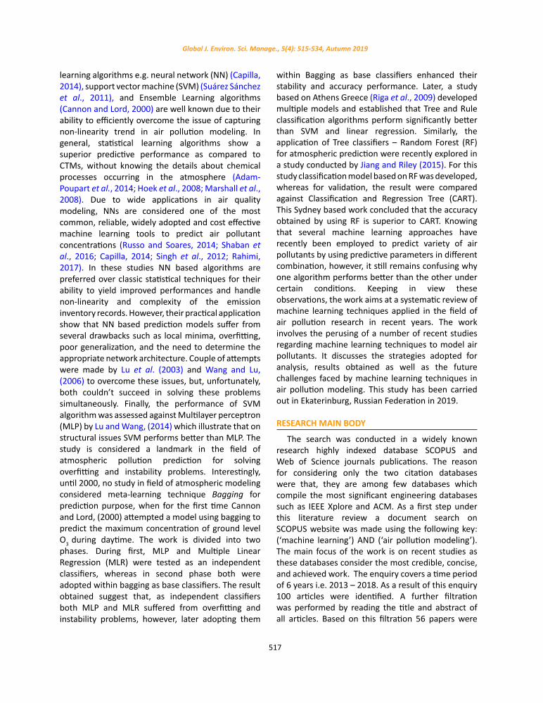
excluded from the selection list of 100 because; 1) they didn’t address the topic; 2) the work was based on physical sensors instead of computational models; 3) many studies from biology, social and health sciences used predictive models to calculate the health impact of air pollutant and did not estimate or forecast their concentrations. Following the above discussed criteria, the documents were reduced to 44. Before finalizing the list, all research works were read carefully during final step. Out of these 44, another 6 were vetoed after a full document review due to the similarity of work with studies carried out in past by the same authors. Finally, a total of 38 journal articles were considered for review. A complete summery of article selection method is presented in Fig.1.

For this review, the work considers the following aspects of the selected studies; 1) motivation of the work; 2) type of modeling i.e. forecast or estimation; 3) historical data of predictive features; 4) type of the machine learning algorithms employed e.g. Regression, ANNs, SVM, ensemble learning techniques, or hybrid models; 5) nature of prediction i.e. if a specific pollutant (PM10, PM2.5, NOx, O3, SO2etc.)

is predicted or air quality index (AQI) in general is calculated to learn pollution level; 6) geographic location where the study is performed; 7) time span and the number of data stations used; 8) evaluation methods to assess the model performance. The assessment is based on a comparison between model accuracy and the prediction of the actual value. The most popular evaluation criteria are the correlation coefficient (R2), Mean Absolute Error (MAE), Root Mean Square Error (RMSE) and Relative Absolute Error (RAE). The R2 value shows the fitting degree of regression, MAE represents the difference between predicted and actual values, RMSE focuses on the impact of extreme values based on MAE, while RAE calculates the variance of a model when comparing the performance of different models. As MAE and RMSE depend on the scale of the data that’s why RAE can be extremely helpful when comparing different data with different scales. The R2, MAE, RMSE and RAE are calculated by using Eqs. 1 to 4, respectively.

( )( )

( ) ( )2

1/22 2

i ii

i ii i

x x y yR

x x y y

− − = − −

∑∑ ∑

(1)

Fig. 1: Flowchart of systematic selection of articles for qualitative and quantitative analysis  

Fig. 1: Flowchart of systematic selection of articles for qualitative and quantitative analysis       

519

Global J. Environ. Sci. Manage., 5(4): 515-534, Autumn 2019

1

1 n

i ii

MAE y xn =

= −∑ (2)

( )2

1

1 n

i ii

RMSE y xn =

= −∑ (3)

ni ii

nii

y xRAE

y x

−=

−

∑∑

(4)

Where, yi and xi are predicted and observed values respectively, x is the average predicted value and n is total number of instances. In this study, the results obtained after reviewing the journal articles are described in two ways; 1) general statistical description and 2) detailed description. The first part discusses about the total number of studies based on machine learning tools have been conducted in the field of air quality modeling to estimate or predict the concentration of air pollutants over the period of 6 years. Furthermore, it enquires about the geographic distribution of these studies. Whereas the other part provides a detailed description about the statistical models, their evolution and modeling performance to predict the principal pollutants over the period of 6 years. Considering the number of parameters for selected articles, as a final point the study performs a factorial analysis called multiple component analysis. It uses nominal categorical data to draw a relationship among qualitative parameters that characterize each study and represent it in terms of low dimensional Euclidean space.

General descriptionDue to serious health concerns of pollutants

present in troposphere, globally air quality monitoring and prediction modeling have become a key focus for a number of researchers. As a result, recently the number of studies using machine learning approaches in air pollution modeling have significantly increased. However their distribution around the world doesn’t look uniform. Fig. 2 depicts that the number of research articles based in Europe and America are higher than that of Asia. Only Europe counts for nearly 40% of total work, followed by 33% and 24% in America and Asia respectively. As a country United States of America (USA) takes the lead by publishing the 27% (i.e. 10 articles) of the total studies considered during 6 years period followed by China (24%), United Kingdom (10%) and Spain (10%).

While, Fig. 3 represents the number of works which applied machine learning algorithms in air pollution modeling during 2013 to 2018. Besides showing a consistent increasing trend in the number of studies published during last three years (2016-18), its stability during 2017 and 2018 is of greater importance.

A complete document review of 38 studies suggested that the most common and widely adopted algorithms for air pollutant estimation and prediction since 2013 are: Linear Regression; NNs; SVMs; and Ensemble Learning Algorithms as shown in Fig. 3. Only one study used a peculiar approach related to Lazy methods. Among these 5, Ensemble learning is the most advanced machine learning approach

 Fig. 2: Geographic distribution of pollution studies 

   

US27%

China24%Spain

10%

France8%

United Kingdom10%

Canada6%

Itlay 5%

Switzerland 4%

Germany3%

Greece3% US

China

Spain

France

United Kingdom

Canada

Itlay 

Switzerland 

Germany

Fig. 2: Geographic distribution of pollution studies

520

A. Masih

applied in the field of air pollution prediction followed by SVM and NNs. Ensemble learning approach is a set of algorithms in which multiple predictors are trained to address the same problem by combining the results produced by all predictors (Beckerman et al., 2013). While its final output is based either on the average of all predictions or on majority voting. Ensemble learning techniques combine weak and strong predictors which are less sensitive to overfitting and better at generalization (Mckeen et al., 2004). These techniques work on a principle of introducing stochasticity either into the dataset to produce different sample sets and predictors or through prediction algorithms to solve the issue. These techniques overall perform better than that of single base learners such as ANNs and SVMs (Masih, 2019; Masih, 2018b; Nawahda, 2016; Van Loon et al., 2007). Bagging is the simplest ensemble learning technique in which stochasticity is introduced into the original dataset to create several datasets by taking random samples with replacement. Each specific dataset is used to generate predictive learner. Later for model output, all predictors are combined (Windeatt et al., 2008). In Boosting – another ensemble learning technique, the randomness is introduced into weak classifiers through sequential training to produce predictors, which later are weighted in such a way that all incorrectly predicted observations are given more weightage that usually results in a better accuracy (Singh et al., 2013). Due to its ability to critically observe the incorrectly classified instances, boosting is considered one of the best prediction algorithm. While the ensemble methods that use multiple algorithms

for prediction are called Voting and Stacking (Masih, 2019). Keeping in mind that each model is given a fair weightage according to its performance, ensemble methods are generally evaluated by cross validation. The review conducted suggest that RF is one of the most popularly known ensemble learning technique due to its wide applications in various fields such as Bioinformatics, Marketing, environmental science etc. (Alfaro et al., 2008; Gabralla and Abraham, 2014; Fathima et al., 2014; Yang et al., 2010; Tüfekci, 2014).RF is a flexible and supervised algorithm that can generate great results without hyper parameter tuning. The term “forest” has been coined to RF because numerous trees are built, compiled and trained by using bagging method which helps in improving the accuracy of the predictor. In RF each tree is built from a sample drawn with replacement from training set results in a slightly increased bias and decreased variance of the forest, however, it enhances the overall performance of the model. RF is considered one of the most efficient, powerful, and accurate learning approach due to its ability of extracting important variables, handling internal unbiased of the generalization error and most importantly the competency of maintaining accuracy even if a large portion of data is missing. NN are the other major approaches applied in environmental sciences recently (Abdul-Wahab and Al-Alawi, 2002; Zhang et al., 2012; Rahimi, 2017). These approaches take inspiration from human nervous system. NN works on a principle of classifying input observations by using linear combination of the datasets using Eq. 5.

 Fig. 3: Number of studies based on different machine learning algorithms from 2013 to 2018 

   

0

2

4

6

8

10

12

14

2013 2014 2015 2016 2017 2018

Num

ber o

f pub

lications

Ensemble learning Regression NN SVM Lazy

Fig. 3: Number of studies based on different machine learning algorithms from 2013 to 2018

521

Global J. Environ. Sci. Manage., 5(4): 515-534, Autumn 2019

0

i

i ii

X W O=

=∑ (5) Where, O is an observation characterized by several

features (from 0 to i) and W is the weight applied to each feature. It starts with all weights set to 0, later with the help of a loop it keeps on modifying the incorrectly classified instances to a point until all instances are classified correctly (Gardner and Dorling, 1998). It consists of a minimum of three layers i.e. Input, hidden and output layer. The input layer is a layer of predictive features such as pollutant concentrations, meteorological parameters, regional land features etc. The output layer represents the predictor variables such as pollutant predictors (PM10, NO2) and AQI, while hidden layer comprises nodes which enable multiple connections between input and output layers (Gardner and Dorling, 1999). Example of ANN having small number of hidden neurons is called MLP, whereas Deep Learning Neural Network contains large number of hidden layers. These nodes act as a weighted sum between input and output layers. The next popular advanced machine learning tool is SVM (Zhu et al., 2012). It is sometimes considered as the popular alternative to NN. It’s a discriminative algorithm used for classification purpose by finding the hyperplane that maximizes the boundary between two classes. It requires the selection of critical points also called support vectors to obtain the boundary line, that describe the channel and perpendicular bisectors of the line which in case of 2-dimensional dataset are joined by two support vectors and in case of multidimensional dataset by a hyperplane (Vong et al., 2012). To attain a maximum margin, hyperplane does not depend on observations but largely rely upon the value of the support vectors as described in Eq. 6.

( )0

n

i ii

X b y a i aα=

= + ×∑ (6)

Where, a(i) are the support vectors and i is the number of these vectors.

Whereas to deal with classes that are linearly inseparable, a function is applied to transform the original dataset, whereas to reduce the computational cost of the transformation, a kernel trick is adopted. Hence, for a fair performance of SVM, the selection of right kernel and correct tuning of its parameters is vital. The most common kernel types are linear kernel, polynomial kernel, and radial basis function kernel in

Eqs. 7, 8, and 9, respectively.

( ),K a b a b= × (7)

( ) ( ), 1 dK a b a b= × + (8)

( ) 2

, a bK a b e γ− −= (9)

Last but not the least, it was quite interesting to know that a fair number of articles (5) have applied classic statistical regression model for pollution prediction. Features extracted from dataset were treated as input variables, whereas, for prediction, the relationship between input and output is learned through weights which fit a linear or nonlinear curve to data points. To correctly fit a curve, in regression modeling, an optimization technique named goodness of the fit matric is used in order to find a curve that better fits as compared to others. For example gradient descent algorithm is a popular optimization technique adopted both in regression as well as in machine learning models to minimize the cost function using Eq. 10.

( ) ( )( )2

0

1 ni i

i

f h x yn θθ

=

= −∑ (10)

Where, n is the number of observations, y is the actual output and hθ (x) is the predicted output.

Detailed descriptionIn this section a comprehensive discussion has

been conducted over the selected studies. Based on the motivation and objective of the work, the section explores five key group of studies in details; 1) Role of input parameters in a successful air pollutant estimation and forecasting; 2) hybrid and deep learning approaches; 3) contribution of satellite image and sensor based monitoring techniques to enhance pollution prediction accuracy; (4) relationship between air pollution and land use; (5) application based approaches.

Group 1: Role of input parameters for successful air pollutant estimation and forecasting

This section focuses on the role of input variables adopted by modeling approaches to successfully predict the atmospheric concentration of pollutants.

522

Air quality machine learning algorithms

Results suggest that a total of 14 articles out of 38 accounted for estimation and forecasting purposes. RF – a tree based ensemble learning approach was found to be the most common machine learning technique recently employed for prediction of air pollutants, followed by regression approaches, ANNs, SVM and lazy learning. Further in depth details revealed that various tests namely Pearson Correlation, Principle Component Analysis (PCA) have also been considered by the studies to learn how dimensionality reduction can influence predictors’ performance. Starting with the most recent work conducted by Zhan et al. (2018) is based in China. The study makes use of RF algorithm to construct a spatiotemporal model that can efficiently predict the concentration of ground level O3 all across the country. The list of input features adopted include: planetary boundary height, vegetation index, meteorology, anthropogenic emission inventory, land use, population density, time, road density and elevation. The dataset was gathered from 1601 stations over a period of one year. The model develops 500 regression trees for prediction. Whereas for evaluation purpose, two widely accepted evaluation parameters namely R2 and RMSE were considered. For a proficient assessment model performance was compared against CMTs. Result obtained recommend that the performance of proposed model (R2=0.69) is better than that of obtainable by CTMs. It also reports that, model performance mainly relies upon meteorological parameters namely humidity, solar radiation and temperature, while its connection with anthropogenic emissions such as CO, Organic Carbon, and NOx etc. was not strong enough, and sparsity of monitoring stations results in a lower accuracy. Another recent work by Grange et al. (2018) used RF as a classification technique to build a model by using meteorological conditions, atmospheric pollutant data and temporal factors to analyze the trend of PM10 as well to make a long term prediction. The methodology of the study involves the creation and training of many out of the bag (OOB) samples to grow Decision Tree, which later were combined to make a prediction. The study makes use of daily input variables named: wind speed, wind direction, temperature, time, boundary layer height and synoptic scale, were obtained from 31 monitoring stations of Switzerland for a period of 20 years. The average accuracy calculated in terms of correlation

coefficient (R2) at all 31 stations was found to be 0.62, with wind speed and boundary layer being the best input predictors and synoptic scale the worst. The prediction performance obtained under the model at different location varied from R2 = 0.53 to R2 = 0.71. The lower values were mostly recorded at stations located near rural mountainous areas. In order to learn about the conditions which lead to high pollution in Athens, Greece, Bougoudis et al. (2016) built a hybrid system by using ANN, RF, fuzzy logic along with unsupervised clustering for the prediction of various pollutants. The experiment conducted makes use of 12 years’ hourly dataset of air pollutants (CO, NO, NO2, SO2) and meteorological parameters (temperature, relative humidity, pressure, solar radiation, wind speed, wind direction). Unsupervised clustering was aimed at re-sampling the initial data vectors, while the modeling performance of each experiment was evaluated in terms of R2 value, Mamdani rule based on fuzzy inference system (FIS) was applied to enquire about factors affecting the quality of air. The model performed well to estimate the concentration of CO and NO with R2 =0.95 when FIS ensemble with RF and ANN respectively, while using RF alone it could predict NO and O3 with accuracy equal to 0.91. To learn more about the robustness of machine learning tools Martínez-España et al. (2018) conducted a work in Murcia, Spain. The study aimed at the prediction accuracy of ground level O3 by using 5 different classification models namely Bagging, RF, Decision Tree, k-Nearest Neighbor, and Random Committee. The work applied two years’ air pollution dataset of NO, NOx, PM10, O3, SO2, C6H6, C7H8, XIL, and environmental parameters such as pressure, solar radiations, temperature, relative humidity, wind speed and direction. The experimental design has been divided into two phases. During first, the prediction accuracy of all the models were tested out and compared against each other, whereas to study the number of models required for O3 modeling in Murcia region, during second phase the work adopted a hierarchical clustering approach. Results obtained in terms of correlation coefficient are as follow: the performance of RF has been superior having R2 value equal to 0.85 as compared to Random Committee (0.83), Bagging (0.82) and Decision Tree (0.82). Among 5 models kNN performed the worst (0.78), whereas NOx, temperature, wind direction, wind speed, relative

523

Global J. Environ. Sci. Manage., 5(4): 515-534, Autumn 2019

humidity, SO2, NO, and PM10 were found to be the best predictors. In the end, using clustering approach suggested that study region only requires two models for a thorough modeling of O3. While another study by Sayegh et al., (2014) aimed at capturing the variability of PM10 by employing several statistical and machine learning models such as Boosted Regression Tree (BRT), Generalized Additive Model, Linear and Quantile Regression models (QRMs). It is worth noting that QRM was used to assess the contribution of predictors at different percentiles, unlike LR which only considers feature distribution as a whole. For this study hourly dataset of NOx, CO, SO2, PM10, temperature, relative humidity, wind speed and direction were recorded at Makkah, Saudi Arabia for a period of one year. The performance was evaluated in terms of coefficient of determination (observed/predicted values). Considering the role of different quantiles instead of central tendency of PM10, it was observed that QRM has performed better as compared to other data mining tools to predict the hourly concentrations PM10. Nieto et al. (2015) conducted a research using 3 years dataset of NOx, CO, SO2, O3, and PM10 from Oviedo (Spain) to predict three different air pollutants NO2, SO2 and PM10. The experimental setup employs MLP and Multivariate Adaptive Regression Splines as modeling tools. The proficient assessment of modeling results inferred that the estimation of NO2 (R

2 = 0.85) has been pretty good, followed by a slightly lower accuracy obtained for SO2 (R

2 =0.82) and PM10 (R2 =0.75). Meanwhile, to

predict the concentration of a greenhouse gas N2O, another study adopts RF algorithm (Philibert et al., 2013). It makes use of global meteorological and crop data such as; type of crop, country, fertilization, etc. Prior to data modeling, during data preprocessing several measures were taken into consideration to improve the prediction accuracy including: the removal of extreme values in the dataset; exclusion of boreal ecosystem; ranking of important features in dataset; and supply of controlled number input variables. For a fair assessment the results were compared against linear and nonlinear regression models. The result show that accuracy performance of RF based model was 20-24% higher than that of both regression models. Whereas another RF based model (Yu et al., 2016) have lately been constructed to predict the AQI by using urban public data based on road information, air quality and meteorological

datasets of all the regions of Shenyang, China. Over proficient assessment of the model, it was verified that RF with its highest precision (R2 = 0.81) and lowest error value (RAE = 36.9%) have outperformed the state of the art classifiers such as Naïve Bayes, Logistic Regression, single decision tree and ANN. A simplified regression technique based on Quito, Ecuador introduced by Kleine Deters et al. (2017) was aimed understanding the effects of meteorological factors on the precise prediction of PM2.5. The data preparation under this study include 6 years meteorological data for training and testing purposes, while for evaluation the model adopts 10-fold cross validation and coefficient of determination R2. The most interesting aspects of this model is that, it can be considered a fair and an economic option for the cities without air quality equipment, to estimate the PM2.5 concentration in air by just using meteorological parameters. Beside a fair performance during a regular days, it was interesting to see that improved results were recorded during extreme weather conditions. A lazy learning technique was tested out to draw an association between the PM10 emissions and AQI. Hourly dataset of SO2, NOx, CO, PM10, and Ammonia (NH3) was gathered from an area called Lombard in Italy for one year period (Carnevale et al., 2016). Other specifications of the study include: application of Dijkstra algorithm for large scale data processing. The data were split at a ratio of 80% and 20% for training and validation purposes respectively. The validation phase results were compared with deterministic models instead of comparing it with the targeted values. The results obtainable through this approach in the form of R2were nearly the same as achieved by Transport Chemical Aerosol Model (TCAM) i.e. R2=0.99. By the way TCAM is a costly computational method commonly used in decision making. One of most reliable predictive model based on SVM was employed by (Liu et al., 2018). The predictive features of the model were trained using two years emission data of 6 atmospheric pollutant concentrations (PM2.5, PM10, SO2, CO, NO2, O3), AQI value and 3 meteorological parameters (temperature, wind direction and velocity) from three cities of China namely Tianjin, Beijing, and Shijiazhuang. 4- Fold cross validation technique was adopted to split the data into training and testing sets, whereas for model validation the model output was compared against the observed data. It was observed that the model

524

A. Masih

performance fairly improves especially if emission information of the nearby cities is considered. Contrary to that, Singh et al., (2013) proposed an air quality model using tree based ensemble algorithms – Single decision tree, Decision tree boost, and Decision tree forest against SVM, for AQI prediction. In addition it makes use of Principal Component Analysis for dimensionality reduction to identify pollution sources. The study uses air pollutant and meteorological data of 5 years collected from Lucknow (India). The model performance shows a significant improvement in results as all three approaches namely Decision tree boost ( 2R 0.96= ), Decision tree forest ( 2R 0.95= ) and Single decision tree ( 2R 0.9= ) have outperformed SVM ( 2R 0.89= ). While in forecasting category only two studies were found, out of which one article applied ensemble neural network technique to forecast AQI one day ahead by using three years pollutants and meteorological dataset of 16 cities in China (Chen et al., 2018). The model uses Partial Mutual Information (PMI) to select the best predictors, to precisely forecast the daily AQI value by using PEK-based machine learning approach and previous day’s emission and meteorological data. PEK is an ensemble artificial neural network based general purpose function approximator. With PM2.5, PM10, and SO2 as the best predictors the proposed model on average have achieved an accuracy of 2R = 0.58. The other article by Oprea et al., (2016) take a dig at forecasting the level of PM10 concentration in atmosphere by using Tree based data mining algorithms i.e. REPTree – Reduced Error Pruning Tree and M5P – an inductive learning approach based on regression tree using M5 algorithm. To extract the best input features (PM10, NO2, SO2, relative humidity and temperature) from emission and meteorological data, the model uses PCA. This Romania based study used 27 months records for training, and 8 previous days’ data for a short term prediction of PM10 concentration. The comparison drawn between two models suggested that the performance of M5P is better and can forecast PM10 concentration one and two days ahead with an accuracy value 0.81 and 0.79 respectively.

Group 2: Extreme learning and hybrid approachesThis category registered the second spot with

10 articles. Interestingly it is the only class in which forecasting approaches (8) are way more

than estimations models (2). The first estimation technique using Extreme Learning Machine (ELM) is proposed by Zhang and Ding, (2017). ELM was aimed at handling low convergence and local minima which NN algorithms suffer from. The proposed ELM was based on only 2 NN layers, first (hidden) layer was random and fixed, whereas second involved training. The study uses meteorological and time parameters to predict the concentration of number of pollutants such as NO2, NOx, O3, PM2.5, and SO2. The results obtained indicate that ELM based model is highly feasible because it doesn’t just provide a better prediction accuracy than MLR and NN, but offers a low computational cost as well. Whereas the other study builds a model to precisely predict NO2 and NOx with a high spatiotemporal resolution (Li et al., 2017). The work was mainly divided into three stages. To characterize the spatiotemporal variability of NOx and NO2, first stage incorporates nonlinear, fixed and spatial input variable. In second stage ensemble learning technique was employed with an aim to reduce variance and uncertainty in prediction. While third was an optimization stage which handles incomplete time dependent variables such as traffic, meteorology etc. to get a continuous time series dataset. The prediction accuracy of the model in polluted areas was quite good (R2=0.85) however, its performance was poor in areas with low level pollution. Peng et al., (2017) are the latest to introduce an advanced machine learning based approach for an air quality forecasting up to 48 h. The model was based on ELM and is updateable in real time by using linear solution applied to new data. Under this study performance of 5 different algorithms (MLR, Multi-Layer Neural Network (MLNN), ELM, updated-MLR, and updated-ELM) was assessed and compared. The model predicts three air pollutants namely O3, PM2.5, and NO2 in two stages. First controls the initial training of the algorithm, whereas the other is a sequential learning stage which considers daily online update of MLR and ELM. The results obtained suggest that updated-ELM have the characteristics of predicting O3, PM2.5, and NO2 with high accuracy and low error values as compared to other four models. In order to improve atmospheric pollution forecasting, few studies have applied Deep Learning approach. Recently, Zhao et al., (2018) built a Deep Recurrent Neural Network (DRNN) model for daily air quality forecasting. The method consists of two steps. In first,

525

Global J. Environ. Sci. Manage., 5(4): 515-534, Autumn 2019

data pre-processing of six pollutants was performed to categorize them into four groups i.e. Individual AQI. While in second step Long Short Term Memory (LSTM) algorithm was employed for forecasting. LSTM is a Recurrent Neural Network (RNN) based algorithm. It has a memory that allows the algorithm to learn the input sequence with longer time steps. The predictive performance of the model was not up to authors’ expectations, as it couldn’t perform significantly better than other tested algorithms such as SVM and ensemble learning techniques. The other limitation was its high computational cost and low interpretability. Another hybrid approach using big data, LSTM and NN to forecast the atmospheric concentrations of PM2.5 (1 h ahead) was proposed by Huang and Kuo, (2018). The study makes use of Convolutional Neural Network because it reduces training time. The model performance was superior to state of the art machine learning techniques such as RF, SVM and MLP. However, the model is yet to be validated over a longer time forecast. A hybrid model discussed the short and long term forecasting of O3, NO2, and PM10 concentrations in air was presented by Tamas et al., (2016). The model was based on NN and clustering, whereas for validation, the results were compared against MLP. Which show that, to predict PM10 and O3 in particular, the performance of the model was significantly better than MLP. While Ni et al., (2017) offered a different combination of NN and ARIMA in the form of a hybrid model to predict the concentration of PM2.5 in Beijing (China). Knowing that, forecasting combines with a time span (e.g. 1 h ahead), the study considered microblog data, chemical variables, and meteorological parameters as input features. The approach was proficient for a few hours ahead forecast, however, error values increased with bigger time lag. Another hybrid approach making future prediction was proposed by Wang et al., (2015). The model is based on ANN and SVM methods and can be described in two stages. During first stage, the authors apply traditional ANN or SVM to make future predictions of PM10 and SO2 concentration by using two years historical pollutant and meteorological data collected from 4 monitoring stations of Taiyuan, China. Whereas in second, forecasting targets by Taylor expansion forecasting method were revised using previous stage’s residual information. The experimental results show that by revising error terms of traditional ANN and SVM

methods can significantly enhance their forecasting accuracy. Couple of studies have implemented fuzzy logics to forecast air contaminants. In first, Li et al., (2018) composed Fuzzy logic with ELM, and heuristic algorithms to forecast AQI level. For this study the pollution data of PM10, PM2.5, SO2, NO2, CO, and O3 was collected from six cities of China. Fuzzy logic was aimed at feature selection, whereas, ELM and heuristic algorithms were employed for a deterministic prediction of AQI. The Fuzzy based pollution model resulted in a better prediction accuracy as compared to NN and ARIMA based algorithms, nevertheless the proposed approach was slightly slower than NN and ARIMA. Whereas the other fuzzy approach was implemented by Eldakhly et al., (2018) to make 1 hour ahead forecast of PM10 concentrations. The study uses fuzzy logic, and chance weight value to handle fuzziness of the data, target minimize an outliner point, while support vector point was used during training process. The unique results obtained is one of the rare examples, as the study establishes that the proposed approach can outperform ensemble learning algorithms.

Group 3: Satellite image and sensor based monitoring techniques to enhance pollution prediction accuracy

Six articles made to this group. Fascinatingly, all were based on pollution estimation instead of future forecasting, possibly because, for all 6, the aim was to enhance the spatial resolution of pollution dispersion. The first paper in this regard Liu et al., (2018) discussed a method using an integrated approach of adding geostatistical model (Random Forest Regression Kriging- RFRK) to traditional CTM. It not just improved the spatial resolution of ground level PM2.5 derived via satellite but results in an enhanced model accuracy. This USA based study using 14 years dataset, was basically performed in two steps. During first step, nonlinear relationship between PM2.5 and the geographic variables was modeled using RF technique, whereas kriging was further applied to estimate the error values. The predictive input features used for this study include: meteorological data; emission data; brightness of night time lights; elevation and normalized difference vegetation index as a part of geographic and satellite based variable, while PM2.5 was the only predicted feature. To validate the model, results of RFRK were compared against CTM derived traditional geophysical model.

526

A. Masih

It suggest that, RFRK is superior to other models, its computational cost is relatively low and flexibility to incorporate supplementary variables is high, but, the work has a limitation of its great reliance on satellite images. A similar approach subjected to enhance the prediction accuracy of PM2.5 applied a correction measure based on three ensemble learning techniques namely Gradient Boosting, Extreme Gradient Boosting (XGBoost) and RF (Just et al., 2018). In spite of using Aerosol Optical Depth (AOD) alone, under the proposed correction, for this study additional predictive features such as land use and meteorology were considered. The proposed approach used 14 years PM2.5 concentration records collected in Northeastern USA. The proficiency of the model was assessed by comparing the correlation coefficient value of the three different algorithms chosen for the study. Apart from the slightly better performance of XGBoost algorithm as compared to other two, results obtained demonstrate the significance of using land use and meteorological records to improve the accuracy when compared with raw AOD. However, the approach was considered limited due to the fact that it involves a total of 52 predictive features. Later, an exactly similar approach proposed by Zhan et al., (2017) was based on an improved version of Gradient Boosting algorithm to draw a relationship considering the nonlinearity between predicted output (PM2.5) and input predictors (AOD and meteorological parameters). Under this work, a geographically weighted gradient boost machine involving spatial smoothing kernels was developed to weight the optimized loss function. This China based case study used one year AOD, land use and meteorological dataset to achieve better accuracy as compared to traditional GB machine. While, day of the year, AOD, pressure, temperature, wind direction, relative humidity were found to be the best predictive features. While de Hoogh et al. (2018) proposed a method to predict PM2.5 concentrations in Switzerland by using AOD and PM2.5/ PM10 ratio data. The dataset used to build the model is a sequence of broad spectrum of features such as planetary boundary layers, meteorological factors, sources of pollution, AOD, elevation, and land use. Whereas the prediction of PM2.5 concentrations were based on SVM algorithm. The model result obtained considering the local (100 m × 100 m) as well global (1 km × 1 km) boundaries show that, it

can accurately predict PM2.5 concentrations by using data collected from sparse monitoring stations. A slightly different satellite based study was tried by Xu et al. (2017). It was aimed at estimating ozone profile shapes. In this work the author developed a NN based algorithm namely Physics Inverse Learning Machine. The working principle of the model involves 5 major steps: 1) application of k-mean clustering to group different ozone profiles based on its concentration values; 2) generation of simulated UV spectra from each cluster of respective ozone profiles; 3) input predictive feature selection by using PCA to enhance classification effectiveness; 4) application of classification models to assign an ozone profile with respect to a given UV spectrum; and (5) scaling the ozone profile shape by considering the total ozone columns. The model results were tested by using predicted and observed values. Results obtained indicate that, altogether a total of 11 clusters were prepared with an estimation error lower than 10%. Lastly, a very different technique based on less reliable dense mobile sensors data collected from sparse monitoring stations was aimed at getting a fine granularity (Hu et al., 2017). For this Sydney, Australia based study, seven regression models were developed to predict the concentration of CO. Prior to modeling and validation the study involves 3 main steps. During first, regression models were developed by using 10 years data including 7 years historical data from 15 static monitoring stations and 3 years of mobile monitoring data. A proficient model comparison and validation was performed during the second and third step respectively. Out of seven modeling techniques, Support Vector machine for regression (SVR), RF and Decision Tree regression achieved the best results, with SVR having the highest spatial resolution and precise demarcation of pollution boundaries as compared to other models.

Group 4: Role of land use and spatial dependence in pollution prediction

There are 5 articles in this group. It considers the role of land use and spatial dependence to predict the atmospheric pollution concentrations. Abu Awad et al., (2017) build a general model based on land use to predict the PM2.5 concentrations. The two steps approach, first applied nu-SVR to enhance land use regression model and then used generalized additive model to refit residuals from nu-SVR. The study was

527

Global J. Environ. Sci. Manage., 5(4): 515-534, Autumn 2019

carried out in New England States (USA). It uses 12 years data, collected at 368 monitoring stations. For model validation the results were tested in warm and cold seasons. On average the model achieved a high correlation coefficient ( 2R =0.80), however, specifically the model accuracy was significantly higher in winter than in summer season. There is another spatiotemporal approach based on land use subjected to learn the nonlinear relationship between air pollutants and land use (Araki et al., 2018). This Amagasaki (Japan) based study estimated the atmospheric concentration level of NO2 by applying two algorithms namely Land Use Random Forest (LURF) and Land Use Regression (LUR). The list of input features data recorded for a period of 4 years include; land use, population, emission intensities, meteorology, satellite-derived NO2, and time. The results reported suggest that LURF outperformed LUR with a slight margin. Because LUR can only perform linear modeling, whereas besides finding nonlinear relationship, LURF have an advantage of automatic selection of most important features. The issue of feature selection related to LUR was well tackled through a hybrid model proposed by Beckerman et al., (2013). In this model LUR was mixed with deletion, substitution, and addition machine learning for pollution prediction. To evaluate the prediction performance of PM2.5 and NO2 the input dataset of 12 variables were recorded for a period of 3 and 4 years respectively at California USA. Though the overall performance of the hybrid model was fair, however, its accuracy was significantly better to predict NO2 as compared to PM2.5. To further extend the idea of Beckerman et al., (2013) a similar but deeper model comparing LURF and LUR was developed by Brokamp et al., (2017). The main objective of the work was to predict the chemical composition of PM2.5. For this Cincinnati (USA) based study the input measurements were taken from 24 monitoring stations during 2001–2005. The dataset is a sequence of over 50 spatial parameters including land cover, physical features, greenspace, socioeconomic characteristics, emission sources and transportation. The novelty of the work is to develop prediction models that cannot just predict the level of PM2.5, but can also estimate the concentration of other metal components in air. Out of five papers classified in this group, the only model that deals with future forecasting was proposed by Yang et al. (2018). The model is based on three steps.

First step involves clustering analysis to handle the spatial heterogeneity of air pollutants. During second, important spatial features are measured by using Gauss vector weight function. Whereas in third step spatial features are combined with meteorological parameters to be used as input variables of the proposed approach – Space-Time Support Vector Regression (STSVR). The model performance was validated by comparing its results with ARIMA, traditional SVR, and NN based models. The ability of STSVR to forecast PM2.5 concentration was partially better than other models. Because its performance was superior to other models from 1 h to 12 h ahead forecast, whereas to forecast 13 h to 24 h ahead, its performance was slightly shorter than global SVR. The study concluded that there is strong correlation between air pollutants and spatial features however, it changes over spatial areas. And model accuracy depends upon the forecasting span.

Group 5: Application system based studiesMajority of published work (discussed above) in

the field of pollution modeling is theoretical. However, group 5 focuses on studies which encourage the development of application systems to regulate the pollution level in urban areas. Out of 3, the first air forecast application was aimed at reducing pollution level through regulated traffic flow by recommending the drivers a best path in terms of shortest but least polluted route (Sadiq et al., 2016).The application is based on a hybrid model using Hadoop framework to manage multi-agent system and NN for modeling. The technique uses meteorology, pollutant emissions and traffic data as predictive features to predict the concentration of O3 in Marrakech-City (Morocco). The model accuracy was validated by comparing the predicted values with the observed measurements taken at the monitoring station. Another advance approach introduced by Shaban et al. (2016) involves the installation of low cost pollution sensors network. The proposed model captures raw data, first stores it and then processes it to make near future forecasts. While the results are presented on different forums such as mobile application and web portal. For this study Regression, Model Trees, SVM and NN were tested with an aim to determine the best algorithm that can precisely forecast the concentration of O3, NO2, and SO2 in air. Model trees provided the accuracy with lowest RMSE. The authors suggested that the

528

A. Masih

approach can be helpful for developing countries that suffer from high level of air pollution. The last work of this category is based on an operational forecasting platform named “Prev’Air” (Debry and Mallet, 2014). The platform is known for daily based forecasting maps of O3, NO2, and PM10. The study indicated that using Ridge Regression method can significantly reduce forecast errors (RMSE) of O3 by 35%, NO2 by 26% and PM10 by 19%. However, the limitation of the technique is its ineffectiveness to predict pollution peaks. Hence it is not applicable in cities especially because air quality standards here are frequently violated.

Multiple component analysisConsidering the different aspects of selected

studies, Multiple Component Analysis (MCA) was performed to further elaborate the results. In MCA, the qualitative variables are summarized with respect to quantitative variables i.e. MCA dimensions, to draw a linkage between qualitative variables through cloud based representation as shown in Fig. 4. The analysis performed suggest that the total percentage of inertia is slightly over 30% that an acceptable value considering that studies are located in an upper dimension space. Dimension 1 (x-axis) shows a split

between estimation and forecast models, whereas dimension 2 (y-axis) reflects an association between qualitative variables and prediction models. It can be seen in Fig. 4 that, from 2013-2018 estimation models have been applied to predict the O3, NOx, CO and particular matter (PM2.5) concentrations by using ensemble learning and regression approaches. These models have generally relied on land use (land: yes) and satellite images (image: yes) because such models estimate the concentration of pollutants contributed by different contamination and dispersion sources. Whereas, on the other hand, forecasting models are mainly based on system applications and hybrid approaches to predict the prediction parameter AQI (PP-AQI) by using algorithms such as NN (algorithm: NN) and SVM (algorithm: SVM). Unlike estimation, these models have weak association with predictive features like land use (land: No) and satellite images (image: No). Although dimension 2 doesn’t explain much as compared to dimension 1, however, it highlights a clear split between two different modeling approaches i.e. spatial resolution and nanoparticles. It seems as both methods are distinct and deals only with the specific type of predictive parameters (CO, PM10 and PM2.5). The paper using lazy algorithm to forecast the concentration of PM10 is an exception.

 Fig. 4: Cloud point results obtained by using MCA characterizing all group articles 

   Fig. 4: Cloud point results obtained by using MCA characterizing all group articles

529

Global J. Environ. Sci. Manage., 5(4): 515-534, Autumn 2019

Overall the number of studies based on pollutant estimation (23) are nearly 1.5 times more than forecasting (14). Two out of five classes (i.e. number 2 and 5) have more studies dedicated to forecasting models. Class 2 is based on hybrid solutions using deep and extreme learning algorithms, the other focuses on the practical significance of modeling tools by developing Apps or Web portals. In class 3 forecast modeling has not performed at all, possibly because, the main goal of such works is to improve the spatial resolution by assessing pollution level. While estimation models dominate in other classes. Class 1 and 4 are other notable set of studies because more than 80% of their work is based on estimation models.

Lastly, the study assesses each algorithm’s performance (e.g. ensemble learning, NN, SVM etc.) in terms of correlation coefficient achieved for estimation and forecasting models. Fig. 5a represents that around 80% of total studies considered under these classes have either applied ensemble learning or NN algorithms. It also shows that ensemble learning and regression techniques are the most commonly adopted for estimation modeling whereas NN and SVM based techniques are mainly applied for forecasting purposes. On the other hand, the average accuracy achieved per algorithm in Fig. 5b shows that ensemble learning are highly reliable techniques with an average correlation coefficient value 0f 0.79, followed by classical regression technique (R2=0.74). The average prediction accuracy of SVM is also fair

(R2=0.67), while NN based algorithms frequently used for forecasting, had the lowest correlation coefficient equal to 0.64. The success of estimations models (ensemble learning and regression techniques) is largely dependent upon on their low variability, conversely, the variation of the results is significantly higher in the forecasting models which is why the accuracy obtained by forecasting models is comparatively lower than estimation models.

CONCLUSION

The systematic review conducted reveals that since 2017 the application of machine learning techniques to predict atmospheric pollution has significantly increased. However, due to non-uniform distribution the majority of studies are restricted to continent Europe and America. The studied work is divided into two main classes namely estimation and forecasting of air pollutant concentrations. The work indicate that ensemble learning and linear regression algorithms are suitable for pollution estimation, whereas for air pollution forecasting, NN and SVM based approaches are preferred. MCA further explains that predictive features such as land use and satellite images have a strong association with estimation models, but their correlation with forest models is weak. Finally the performance assessment of algorithms revealed the superiority of ensemble learning and regression approaches over NN, lazy, and SVM due to their low variability and standard deviation as compared

Fig. 5.a): Total number of articles dedicated to estimation and forecast modeling; b): Average prediction performance of major algorithms (Ensemble learning, regression, SVM and NN). 

 

12

3 4 4

2

8

31

0

2

4

6

8

10

12

14

16

Ensemble NN SVM Regression

Num

ber o

f articles

a

Estimation Forecasting0.79

0.740.67

0.64

0

0.1

0.2

0.3

0.4

0.5

0.6

0.7

0.8

0.9

Ensemble Regression SVM NN

Correlation coefficient 

b

Fig. 5: a): Total number of articles dedicated to estimation and forecast modeling; b): Average prediction performance of major algorithms (Ensemble learning, regression, SVM and NN).

530

A. Masih

to forecast models. The high accuracies achieved with machine learning algorithms explains it all why these algorithms are appropriate and should be preferred over traditional approaches. Although machine learning algorithms have registered one of the highest values of correlation coefficient, however, forecasting is still remained very much limited to certain models (NN and SVM) and air pollutants (AQI, PM10 and PM2.5). Therefore, to improve the prediction accuracy, model development considering other critical pollutants (NOx and SO2) and machine learning techniques (ensemble learning techniques) constitute the next challenge.

ACKNOWLEDGEMENT

The Author expresses its gratitude to the Management of Graduate School of Economics and Management, Ural Federal University, Ekaterinburg Russian Federation for providing necessary facilities to complete this study successfully.

CONFLICT OF INTEREST

The author declares that there is no conflict of interests regarding the publication of this manuscript. In addition, the ethical issues, including plagiarism, informed consent, misconduct, data fabrication and/or falsification, double publication and/or submission, and redundancy have been completely observed by the authors.

ABBREVIATIONS

ACM Association for computing machineryAERMOD Atmospheric dispersion modeling systemANN Artificial neural networkAOD Aerosol optical depthAQI Air quality indexARIMA Additive regressionBRT Boosted regression treeCART Classification and Regression TreeC6H6 Benzene C7H8 TolueneCO Carbon monoxideCTM Chemical transport modelDRNN Deep recurrent neural networkELM Extreme learning machine

FIS Fuzzy inference systemHCl Hydro chloric acid

IEEE Institute of Electrical and Electronics Engineers

kNN K- nearest neighborLR Linear regressionLSTM Long short term memoryLUR Land use regressionLURF Land use random forestM5P Regression Tree using M5 algorithmMAE Mean absolute errorMCA Multiple component analysisMLNN Multi-layer neural networkMLP Multilayer perceptron MLR Multiple linear regression

NAME Numerical Atmospheric dispersion Modeling Environment

NH3 AmmoniaNN Neural networksNO2 Nitrogen dioxideNOx Oxides of NitrogenN2O Nitrous oxidenu-SVR Nu-support vector regressionO3 OzoneOOB Out of the bagPCA Principle component analysisPLUME Gaussian dispersion model

PM2.5Particles less than or equal to 2.5 micrometers in diameter

PM10Particles less than or equal to 10 micrometers in diameter

PMI Partial mutual informationQRM Quantile Regression modelsR2 Correlation of determinationRAE Relative absolute errorREP Tree Reduced error pruning treeRF Random forestRFRK Random forest regression krigingRMSE Root mean squared error RNN Recurrent neural networkRSS Random subspaceSO2 Sulphur dioxideSTSVR Space-time support vector regression

531

Global J. Environ. Sci. Manage., 5(4): 515-534, Autumn 2019

SVM Support vector machineSVR Support Vector machine for regressionTCAM Transport chemical aerosol modelUSA United States of AmericaUV spectrum Ultraviolet spectrumXIL TrihydroxyoxanXGBoost Extreme gradient boosting

REFERENCES Abu-Awad, Y.; Koutrakis, P.; Coull, B.A.; Schwartz, J., (2002). A

spatio-temporal prediction model based on support vector machine regression: Ambient Black Carbon in three New England States. Environ. Res., 159: 427- 434 (8 pages).

Abdul-Wahab, S.A.; Al-Alawi, S.M., (2002). Assessment and prediction of tropospheric ozone concentration levels using artificial neural networks. Environ Modell Software, 17: 219-228 (10 pages).

Adam-Poupart, A.; Brand, A.; Fournier, M.; Jerrett, M.; Smargiassi, A. (2014). Spatiotemporal modeling of ozone levels in Quebec (Canada): a comparison of kriging, land-use regression (LUR), and combined Bayesian maximum entropy--LUR approaches. Environ. Health Perspect., 122: 970-976 (7 pages).

Alfaro, E.; Garcıa, N.; Gámez, M.; Elizondo, D., (2008). Bankruptcy forecasting: An empirical comparison of AdaBoost and neural networks. Decis. Support Syst., 45: 110-122 (13 pages).

Araki, S.; Shima, M.; Yamamoto, K. (2018). Spatiotemporal land use random forest model for estimating metropolitan NO 2 exposure in Japan. Sci. Total Environ., 634: 1269-1277 (8 pages).

Awad, Y. A.; Koutrakis, P.; Coull, B. A.; Schwartz, J. (2017). A spatio-temporal prediction model based on support vector machine regression: Ambient Black Carbon in three New England States. Environ. Res., 159: 427-434 (8 pages).

Baklanov, A. (2000). Application of CFD methods for modeling in air pollution problems: possibilities and gaps. In Urban Air Quality: Measurement, Model. Manage., 181-189 (8 pages). Springer

Beckerman, B. S.; Jerrett, M.; Martin, R. V.; Donkelaar, A.; Ross, Z.; Burnett, R. T. (2013). Application of the deletion/substitution/addition algorithm to selecting land use regression models for interpolating air pollution measurements in California. Atmos Environ., 77: 172-177 (6 pages).

Bougoudis, I.; Demertzis, K.; Iliadis, L. (2016). HISYCOL a hybrid computational intelligence system for combined machine learning: the case of air pollution modeling in Athens. Comput. Appl., 27: 1191-1206 (15 pages).

Brokamp, C.; Jandarov, R.; Rao, M. B., LeMasters, G.; Ryan, P. (2017). Exposure assessment models for elemental components of particulate matter in an urban environment: A comparison of regression and random forest approaches. Atmos. Environ., 151, 1-11 (11 pages).

Brunekreef, B.; Holgate, S. T. (2002). Air pollution and health. The lancet., 360(9341): 1233-1242 (10 pages).

Brunelli, U.; Piazza, V.; Pignato, L.; Sorbello, F.; Vitabile, S., (2007). Two-days ahead prediction of daily maximum concentrations of SO2, O3, PM10, NO2, CO in the urban area of Palermo, Italy. Atmos. Environ., 41, 2967-2995 (29 pages).

Cannon, A. J.; Lord, E. R., (2000).. Forecasting summertime surface-

level ozone concentrations in the Lower Fraser Valley of British Columbia: An ensemble neural network approach. J. Air Waste Manage. Assoc., 50: 322-339 (18 pages).

Capilla, C., (2014). Multilayer perceptron and regression modelling to forecast hourly nitrogen dioxide concentrations. WIT Trans. Ecol. Environ., 183: 39-48 (10 pages).

Chaloulakou, A.; Saisana, M.; Spyrellis, N., (2003). Comparative assessment of neural networks and regression models for forecasting summertime ozone in Athens. Sci. Total Environ., 313: 1-13 (13 pages).

Carnevale, C.; Finzi, G.; Pederzoli, A.; Turrini, E.; Volta, M. (2016). Lazy Learning based surrogate models for air quality planning. Environm. Model. software, 83: 47-57 (11 pages).

Chen, S.; Kan, G.; Li, J.; Liang, K.; Hong, Y. (2018). Investigating China’s Urban Air Quality Using Big Data, Information Theory, and Machine Learning. Pol. J. Environ. Stud., 27(2): 1-14 (14 pages).

Chen, J.; Chen, H.; Wu, Z.; Hu, D.; Pan, J. Z. (2017). Forecasting smog-related health hazard based on social media and physical sensor. Inf. Syst., 64: 281–291 (11 pages).

Cohen, A. J.; Brauer, M.; Burnett, R.; Anderson, H. R.; Frostad, J.; Estep, K.; Balakrishnan, K.; Brunkreef, B.; Dandona, L.; Dandona, R.; Feigen, V.; Freedman, G.; Hubbel, B.; Jobling, A.; Kan, H.; Knibbs, L.; Liu, Y.; Martin, R.; Forouzanfar, M. H. (2017). Estimates and 25-year trends of the global burden of disease attributable to ambient air pollution: an analysis of data from the Global Burden of Diseases Study 2015. The Lancet, 389: 1907-1918 (12 pages).

Daly, A.; Zannetti, P. (2007). Air pollution modeling--An overview. Ambient air pollut., 15-28 (14 pages).

Debry, E.; Mallet, V. (2014). Ensemble forecasting with machine learning algorithms for ozone, nitrogen dioxide and PM10 on the Prev’Air platform. Atmos. Environ., 91: 71-84 (14 pages).

Eldakhly, N. M.; Aboul-Ela, M.; Abdalla, A. (2018). A Novel Approach of Weighted Support Vector Machine with Applied Chance Theory for Forecasting Air Pollution Phenomenon in Egypt. Int. J. Comput. Intell. Appl., 17(1), 1850001 (29 pages).

Fathima, A.; Mangai, J.A.; Gulyani, B.B., (2014). An ensemble method for predicting biochemical oxygen demand in river water using data mining techniques. Int. J. River Basin Manage., 12: 357-366 (10 pages).

Feng, X.; Li, Q.; Zhu, Y.; Hou, J.; Jin, L.; Wang, J. (2015). Artificial neural networks forecasting of PM2. 5 pollution using air mass trajectory based geographic model and wavelet transformation. Atmos. Environ., 107, 118-128 (11 pages).

Gabralla, L.A.; Abraham, A., (2014). Prediction of oil prices using bagging and random subspace. Proceedings of the Fifth International Conference on Innovations in Bio-Inspired Computing and Applications IBICA, 2014, 343-354 (12 pages).

Gardner, M. W.; Dorling, S. R. (1998). Artificial neural networks (the multilayer perceptron)—a review of applications in the atmospheric sciences.. Atmos. Environ., 32: 2627-2636 (10 pages).

Gardner, M. W.; Dorling, S. R. (1999). Neural network modelling and prediction of hourly NOx and NO2 concentrations in urban air in London. Atmos. Environ., 33: 709-719 (11 pages).

Grange, S. K.; Carslaw, D. C.; Lewis, A. C.; Boleti, E.; Hueglin, C. (2018). Random forest meteorological normalisation models for Swiss PM 10 trend analysis. Atmos. Chem.Phys., 18(9), 6223-6239 (17 pages).

Hoek, G.; Beelen, R.; De Hoogh, K.; Vienneau, D.; Gulliver, J.; Fischer,

532

A. Masih

P.; Briggs, D. (2008). A review of land-use regression models to assess spatial variation of outdoor air pollution. Atmos. Environ., 42: 7561-7578 (18 pages).

Hoogh, K.; Héritier, H.; Stafoggia, M.; Künzli, N.; Kloog, I. (2018). Modeling daily PM2. 5 concentrations at high spatio-temporal resolution across Switzerland. Environ. Pollut., 233: 1147-1154 (8 pages).

Hu, K.; Rahman, A.; Bhrugubanda, H.; Sivaraman, V. (2017). HazeEst: Machine learning based metropolitan air pollution estimation from fixed and mobile sensors. IEEE Sensors J., 17: 3517-3525 (9 pages).

Huang, C. J.; Kuo, P. H. (2018). A deep cnn-lstm model for particulate matter (PM2.5) forecasting in smart cities. Sensors, 18: 2220 (22 pages).

Jiménez, P. A.; Dudhia, J. (2013). On the ability of the WRF model to reproduce the surface wind direction over complex terrain. J. Appl. Meteorol. Climatol., 52: 1610-1617 (7 pages).

Just, A.; De Carli, M.; Shtein, A.; Dorman, M.; Lyapustin, A.; Kloog, I. (2018). Correcting Measurement Error in Satellite Aerosol Optical Depth with Machine Learning for Modeling PM2.5 in the Northeastern USA. Remote Sens., 10: 803 (17 pages).

Kinney, P. L. (2008). Climate change, air quality, and human health. American journal of preventive medicine, 35: 459-467 (8 pages).

Kleine Deters, J.; Zalakeviciute, R.; Gonzalez, M.; Rybarczyk, Y. (2017). Modeling PM2. 5 urban pollution using machine learning and selected meteorological parameters. J. Electr. Comp. Eng., 2017 (14 pages).

Lee, M.; Brauer, M.; Wong, P.; Tang, R.; Tsui, T. H.; Choi, C.; Chang, W.; Lai, P. C.; Tian, L.;Thach, T. Q.; Allen, R.; Barret, B. (2017). Land use regression modeling of air pollution in high density high rise cities: A case study in Hong Kong. Sci. Total Environ., 592: 306-315 (10 pages).

Lelieveld, J.; Evans, J.S.; Fnais, M.; Giannadaki, D.; Pozzer, A., (2015). The contribution of outdoor air pollution sources to premature mortality on a global scale. Nature, 525, 367 (14 pages).

Li, C.; Zhu, Z. (2018). Research and application of a novel hybrid air quality early-warning system: A case study in China. Science of the Total Environ., 626: 1421-1438 (18 pages).

Li, L.; Lurmann, F.; Habre, R.; Urman, R.; Rappaport, E.; Ritz, B.; Chen, J.; Gilliland, F. D.; Wu, J. (2017). Constrained mixed-effect models with ensemble learning for prediction of nitrogen oxides concentrations at high spatiotemporal resolution. Environ. Sci. Tech., 51: 9920-9929 (10 pages).

Limb, M. (2016). Half of wealthy and 98% of poorer cities breach air quality guidelines. BMJ: Br. Med. J., 353 (15 pages).

Liu, B.C.; Binaykia, A.; Chang, P.C.; Tiwari, M.; Tsao, C.C. (2017). Urban air quality forecasting based on multidimensional collaborative Support Vector Regression (SVR): A case study of Beijing-Tianjin-Shijiazhuang. PLoS ONE, 12, e0179763 (11 pages).

Liu, Y.; Cao, G.; Zhao, N.; Mulligan, K.; Ye, X. (2018). Improve ground-level PM2. 5 concentration mapping using a random forests-based geostatistical approach. Environ. Pollut., 235: 272-282 (11 pages).

Lu, W. Z.; Wang, W. J.; Wang, X. K.; Xu, Z. B.; Leung, A. Y., (2003). Using improved neural network model to analyze RSP, NO x and NO 2 levels in urban air in Mong Kok, Hong Kong. Environ. Monit. Assess., 87: 235-254 (20 pages).

Lutman, E. R.; Jones, S. R.; Hill, R. A.; McDonald, P.; Lambers, B. (2004). Comparison between the predictions of a Gaussian

plume model and a Lagrangian particle dispersion model for annual average calculations of long-range dispersion of radionuclides. J. Environ. Radioact., 75: 339-355 (17 pages).

Marshall, J. D.; Nethery, E.; Brauer, M. (2008). Within-urban variability in ambient air pollution: comparison of estimation methods. Atmos. Environ., 42, 1359-1369 (11 pages).

Martınez-España, R.; Bueno-Crespo, A.; Timon-Perez, I. M.; Soto, J.; Muñoz, A.; Cecilia, J. M. (2018). Air-Pollution Prediction in Smart Cities through Machine Learning Methods: A Case of Study in Murcia, Spain. J. UCS, 24: 261-276 (16 pages).

Masih, A. (2018b). Modelling the atmospheric concentration of carbon monoxide by using ensemble learning algorithm. CEUR Workshop Procedings., 2298: 12 (7 pages).

Masih, A. (2018a). Thar coalfield: Sustainable development and an open sesame to the energy security of Pakistan. J. Physics: Conf. Ser., 989(1): 012004 (7 pages).

Masih, A. (2019). Application of Ensemble learning techniques to model the atmospheric concentration of SO2. Global J. Environ. Sci., 5(3): 309-318 (10 pages).

Mckeen, S.; Wilczak, J.; Grell, G.; Djalalova, I.; Peckham, S.; Hsie, E. Y.; Gong, W.; Bouchet, V.; Menard, S.; Moffet, R.; McHenry, J.; McQueen, J.; Tang, Y.; Carmichael, G. R.; Pogawski, M.; Chan, A.; Dye, T.; Frost, G.; Lee, P.; Mathur, R. (2005). Assessment of an ensemble of seven real-time ozone forecasts over eastern North America during the summer of 2004. J. Geophys. Res. Atmos., 110 (16 pages).

Met Office 2004. Numerical Atmospheric-Dispersion Modeling Environment (NAME) Model.

Morabito, F. C.; Versaci, M. (2003). Fuzzy neural identification and forecasting techniques to process experimental urban air pollution data. Neural Networks, 16: 493-506 (13 pages).

Nawahda, A., (2016). An assessment of adding value of traffic information and other attributes as part of its classifiers in a data mining tool set for predicting surface ozone levels. Process Saf. Environ. Prot., 99: 149-158 (13 pages).

Nhung, N. T.; Amini, H.; Schindler, C.; Joss, M. K.; Dien, T. M.; Probst-Hensch, N.; Perez, L.; Künzli, N. (2017). Short-term association between ambient air pollution and pneumonia in children: A systematic review and meta-analysis of time-series and case-crossover studies. Environ. Pollut., 230: 1000-1008 (9 pages).

Ni, X. Y.; Huang, H.; Du, W. P. (2017). Relevance analysis and short-term prediction of PM2. 5 concentrations in Beijing based on multi-source data. Atmos. Environ., 150: 146-161 (16 pages).

Nieto, P. J.; Antón, J. C.; Vilán, J. A.; Garcıa-Gonzalo, E. (2015). Air quality modeling in the Oviedo urban area (NW Spain) by using multivariate adaptive regression splines. Environ. Sci. Pollut. Res., 22, 6642-6659 (18 pages).

Oprea, M.; Dragomir, E. L.; Popescu, M. A..; Mihalache, S.A., (2016). Particulate matter air pollutants forecasting using inductive learning approach. Rev. Chim, 67: 2075-2081 (7 pages).

Pannullo, F.; Lee, D.; Neal, L.; Dalvi, M.; Agnew, P.; O’Connor, F. M.;Mukhopadhyay, S.; Sahu, S.; Sarran, C. (2017). Quantifying the impact of current and future concentrations of air pollutants on respiratory disease risk in England. Environ. Health, 16: 29 (14 pages).

Peng, H.; Lima, A. R.; Teakles, A., Jin, J.; Cannon, A. J.; Hsieh, W.W., (2017). Evaluating hourly air quality forecasting in Canada with nonlinear updatable machine learning methods. Air Qual. Atmos. Health, 10: 195-211 (17 pages).

Philibert, A.; Loyce, C.; Makowski, D. (2013). Prediction of N2O

533

Global J. Environ. Sci. Manage., 5(4): 515-534, Autumn 2019

emission from local information with Random Forest. Environ. Pollut., 177: 156-163 (8 pages).

Prank, M.; Sofiev, M.; Tsyro, S.; Hendriks, C.; Semeena, V.; Francis, X. V.; Butler, T.; Van Der Gon, H. D.; Friedrich, R.; Hendricks, J.; Kong, X.; Lawrence, M.; Righi, M.; Samaras, Z.; Sausen, R.; Kukkonen, J.; Sokhi, R. (2005). Evaluation of the performance of four chemical transport models in predicting the aerosol chemical composition in Europe in 2005. Atmos. Chem. Phys., 16, 6041–6070 (30 pages).

Rahimi, A., (2017). Short-term prediction of NO2and NOx concentrations using multilayer perceptron neural network: a case study of Tabriz, Iran. Ecol Processes., 6(4) (9 pages).

Riga, M.; Tzima, F.A.; Karatzas, K.; Mitkas, P.A., (2009). Development and evaluation of data mining models for air quality prediction in Athens, Greece. Inf. Technol. Environ. Eng., 331-344 (14 pages).

Ritter, M.; Müller, M. D.; Tsai, M.Y.; & Parlow, E., (2013). Air pollution modeling over very complex terrain: An evaluation of WRF-Chem over Switzerland for two 1-year periods. Atmos. Res., 132: 209-222 (14 pages).

Russo, A.; Soares, A.O., (2014). Hybrid model for urban air pollution forecasting: A stochastic spatio-temporal approach. Math. Geosci., 46: 75-93 (19 pages).

Sadiq, A.; El Fazziki, A.; Ouarzazi, J.; Sadgal, M., (2016). Towards an agent based traffic regulation and recommendation system for the on-road air quality control. SpringerPlus., 5: 1604 (19 pages).

Salnikov, V.G.; Karatayev, M.A., (2011). Impact of air pollution on human health: Focusing on Rudnyi Altay industrial area. Am. J. Environ. Sci., 7(3): 286-294 (9 pages).

Sayegh, A. S.; Munir, S.; & Habeebullah, T. M. (2014). Comparing the performance of statistical models for predicting PM10 concentrations. Aerosol Air Qual. Res., 14: 653-665 (13 pages).

Shaban, K. B.; Kadri, A.; Rezk, E. (2016). Urban air pollution monitoring system with forecasting models. IEEE Sensors J., 16: 2598-2606 (9 pages).

Seigneur, C.; Moran, M. (2010) Chapter 8. Chemical-Transport Models, NASTRO Better Air Quality for North America (42 Pages).

Shimadera, H.; Kojima, T.; Kondo, A. (2016). Evaluation of Air Quality Model Performance for Simulating Long-Range Transport and Local Pollution of PM2.5 in Japan. Adv. Meteorol., 2016 (13 pages).

Singh, K. P.; Gupta, S.; Rai, P. (2013). Identifying pollution sources and predicting urban air quality using ensemble learning methods. Atmos. Environ., 80: 426-437 (12 pages).

Singh, K. P.; Gupta, S.; Kumar, A.; Shukla, S. P. (2012). Linear and nonlinear modeling approaches for urban air quality prediction. Sci. Total Environ., 426: 244-255 (12 pages).

Suárez Sánchez, A.; García Nieto, P. J.; Riesgo Fernández, P.; del Coz Díaz, J. J.; Iglesias-Rodríguez, F. J. (2011). Application of an SVM-based regression model to the air quality study at local scale in the Avilés urban area (Spain). Math. Comput. Model. 2011, 54, 1453–1466 (14 pages).

Tamas, W.; Notton, G.; Paoli, C.; Nivet, M.L.; Voyant, C., (2016). Hybridization of air quality forecasting models using machine learning and clustering: An original approach to detect pollutant peaks. Aerosol Air Qual. Res, 16: 405-416 (12 pages).

Tüfekci, P., (2014). Prediction of full load electrical power output of a base load operated combined cycle power plant using

machine learning methods. Int. J. Electr. Power Energy Syst., 60: 126-140 (15 pages).

Van Loon, M.J.W.; Vautard, R.; Schaap, M.; Bergström, R.; Bessagnet, B.; Brandt, J.; Builtjes, P.J.H.; Christensen, J.H.; Cuvelier, C.; Graff, A.; Jonson, J.E.; Krol, M.; Langner, J.; Roberts, P.; Rouil, L.; Stern, R.; Tarrasón, L.; Thunis, P.; Vignati, E.; White, L.; Wind, P., (2007). Evaluation of long-term ozone simulations from seven regional air quality models and their ensemble. Atmos. Environ., 41, 2083-2097 (15 pages).

Vong, C. M.; Ip, W. F.; Wong, P. K.; Yang, J. Y. (2012). Short-term prediction of air pollution in Macau using support vector machines. J. Control Sci. Eng., 2012 (11 pages).

Wang, D.; Lu, W.Z., (2006). Interval estimation of urban ozone level and selection of influential factors by employing automatic relevance determination model. Chemosphere, 62: 1600-1611 (12 pages).

Wang, P.; Liu, Y.; Qin, Z.; Zhang, G., (2015). A novel hybrid forecasting model for PM10 and SO2 daily concentrations. Sci. Total Environ., 505: 1202-1212 (11 pages).Windeatt, T., (2008). Ensemble MLP classifier design. Comput. Intell. Paradigms., 133-147 (15 pages).

WHO, (2014). WHO’s ambient air pollution database Update 2014.WHO, (2016) Air Pollution Levels Rising in Many of the World’s

Poorest Cities.Xu, J.; Schüssler, O.; Rodriguez, D. G.; Romahn, F.; Doicu, A. (2017).

A novel ozone profile shape retrieval using full-physics inverse learning machine (FP-ILM). IEEE J. Sel. Top. Appl. Earth Obs. Remote Sens., 10: 5442-5457 (16 pages).

Yang, W.; Deng, M.; Xu, F., Wang, H. (2018). Prediction of hourly PM2. 5 using a space-time support vector regression model. Atmos. Environ., 181: 12-19 (8 pages).

Yu, R.; Yang, Y.; Yang, L.; Han, G.; Move, O.A., (2016). Raq--a random forest approach for predicting air quality in urban sensing systems. Sensors, 16: 86 (18 pages).

Zafra, C.; Ángel, Y.; Torres, E. (2017). ARIMA analysis of the effect of land surface coverage on PM10 concentrations in a high-altitude megacity. Atmos. Pollut. Res., 8: 660-668 (9 pages).

Zhan, Y.; Luo, Y.; Deng, X.; Chen, H.; Grieneisen, M. L.; Shen, X.; Zhu, L.; Zhang, M. (2017). Spatiotemporal prediction of continuous daily PM2. 5 concentrations across China using a spatially explicit machine learning algorithm. Atmos. Environ., 155: 129-139 (11 pages).

Zhan, Y.; Luo, Y.; Deng, X.; Grieneisen, M. L.; Zhang, M.; Di, B. (2018). Spatiotemporal prediction of daily ambient ozone levels across China using random forest for human exposure assessment. Environ. Pollut., 233: 464-473 (10 pages).

Zhang, J.; Ding, W. (2017). Prediction of air pollutants concentration based on an extreme learning machine: the case of Hong Kong. Int. J. Environ. Res. Public health, 14: 114 (19 pages).

Zhang, Y.; Bocquet, M.; Mallet, V.; Seigneur, C.; Baklanov, A. (2012). Real-time air quality forecasting, part I: History, techniques, and current status. Atmos. Environ., 60: 632-655 (24 pages).

Zhao, X.; Zhang, R.; Wu, J. L.; Chang, P.C. (2018). A deep recurrent neural network for air quality classification. J. Inf. Hiding Multimed. Signal Process, 9, 346-354 (9 pages).

Zhu, W.; Wang, J.; Zhang, W.; Sun, D. (2012). Short-term effects of air pollution on lower respiratory diseases and forecasting by the group method of data handling. Atmos. Environ., 51: 29-38 (10 pages).

534

A. Masih

AUTHOR (S) BIOSKETCHES

Masih, A., Department of System Analysis and Decision Making, Ural Federal University, Ekaterinburg, Russian Federation. Email: adven.masikh@urfu.ru

HOW TO CITE THIS ARTICLE

Masih, A., (2019). Machine learning algorithms in air quality modeling. Global J. Environ. Sci. Manage., 5(4): 515-534.

DOI: 10.22034/gjesm.2019.04.10

url: https://www.gjesm.net/article_35967.html

COPYRIGHTS

Copyright for this article is retained by the author(s), with publication rights granted to the GJESM Journal.This is an open-access article distributed under the terms and conditions of the Creative Commons AttributionLicense (http://creativecommons.org/licenses/by/4.0/).