Machine Learning 10-601 Tom M. Mitchell

Machine Learning Department Carnegie Mellon University

January 14, 2015

Today: •  The Big Picture •  Overfitting •  Review: probability

Readings: Decision trees, overfiting •  Mitchell, Chapter 3

Probability review •  Bishop Ch. 1 thru 1.2.3 •  Bishop, Ch. 2 thru 2.2 •  Andrew Moore’s online

tutorial

Function Approximation:

Problem Setting: •  Set of possible instances X

•  Unknown target function f : XàY

•  Set of function hypotheses H={ h | h : XàY }

Input: •  Training examples {<x(i),y(i)>} of unknown target function fOutput: •  Hypothesis h ∈ H that best approximates target function f

Function Approximation: Decision Tree Learning

Problem Setting: •  Set of possible instances X

–  each instance x in X is a feature vector x = < x1, x2 … xn>

•  Unknown target function f : XàY–  Y is discrete valued

•  Set of function hypotheses H={ h | h : XàY }–  each hypothesis h is a decision tree

Input: •  Training examples {<x(i),y(i)>} of unknown target function fOutput: •  Hypothesis h ∈ H that best approximates target function f

Function approximation as Search for the best hypothesis

•  ID3 performs heuristic search through space of decision trees

Function Approximation: The Big Picture

Which Tree Should We Output? •  ID3 performs heuristic

search through space of decision trees

•  It stops at smallest acceptable tree. Why?

Occam’s razor: prefer the simplest hypothesis that fits the data

Why Prefer Short Hypotheses? (Occam’s Razor)

Arguments in favor: Arguments opposed:

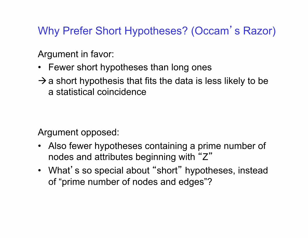
Why Prefer Short Hypotheses? (Occam’s Razor)

Argument in favor: •  Fewer short hypotheses than long ones à a short hypothesis that fits the data is less likely to be

a statistical coincidence Argument opposed: •  Also fewer hypotheses containing a prime number of

nodes and attributes beginning with “Z” •  What’s so special about “short” hypotheses, instead

of “prime number of nodes and edges”?

Overfitting Consider a hypothesis h and its •  Error rate over training data: •  True error rate over all data:

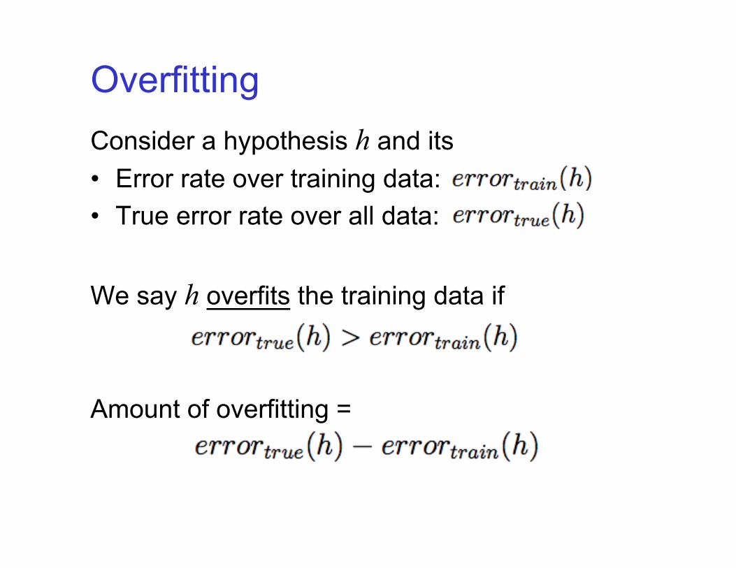
Overfitting Consider a hypothesis h and its •  Error rate over training data: •  True error rate over all data: We say h overfits the training data if Amount of overfitting =

Split data into training and validation set

Create tree that classifies training set correctly

Decision Tree Learning, Formal Guarantees

Labeled Examples

Supervised Learning or Function Approximation

Learning Algorithm

Expert / Oracle

Data Source

Alg.outputs

Distribution D on X

c* : X ! Y

(x1,c*(x1)),…, (xm,c*(xm))

h : X ! Y x1 > 5

x6 > 2

+1 -1

+1

Labeled Examples

Learning Algorithm Expert/Oracle

Data Source

Alg.outputs c* : X ! Y h : X ! Y

(x1,c*(x1)),…, (xm,c*(xm))

•  Algo sees training sample S: (x1,c*(x1)),…, (xm,c*(xm)), xi i.i.d. from D

Distribution D on X

err(h)=Prx 2 D(h(x) ≠ c*(x))

•  Does optimization over S, finds hypothesis h (e.g., a decision tree).

•  Goal: h has small error over D.

Supervised Learning or Function Approximation

Two Core Aspects of Machine Learning

Algorithm Design. How to optimize?

Automatically generate rules that do well on observed data.

Confidence Bounds, Generalization

Confidence for rule effectiveness on future data.

Computation

•  Very well understood: Occam’s bound, VC theory, etc.

(Labeled) Data

•  Decision trees: if we were able to find a small decision tree that explains data well, then good generalization guarantees.

•  NP-hard [Hyafil-Rivest’76]

Top Down Decision Trees Algorithms

•  Decision trees: if we were able to find a small decision tree consistent with the data, then good generalization guarantees.

•  NP-hard [Hyafil-Rivest’76]

•  Very nice practical heuristics; top down algorithms, e.g, ID3

•  Natural greedy approaches where we grow the tree from the root to the leaves by repeatedly replacing an existing leaf with an internal node.

•  Key point: splitting criterion.

•  ID3: split the leaf that decreases the entropy the most.

•  Why not split according to error rate --- this is what we care about after all?

•  There are examples where we can get stuck in local minima!!!

𝑓(𝑥)= 𝑥↓1 ∧𝑥↓2 

0 0 0 −0 0 1 −0 1 0 −0 1 1 −1 0 0 −1 0 1 −1 1 0 +1 1 1 +

𝑥↓1 

𝑞=1/4

𝑝=0 𝑟=1/2

Initial error rate is 1/4 (25% positive, 75% negative)

Error rate after split is 0.5∗0+0.5∗0.5=1/4 (left leaf is 100% negative; right leaf is 50/50)

Overall error doesn’t decrease!

Entropy as a better splitting measure

𝑓(𝑥)= 𝑥↓1 ∧𝑥↓2 

0 0 0 −0 0 1 −0 1 0 −0 1 1 −1 0 0 −1 0 1 −1 1 0 +1 1 1 +

𝑥↓1 

𝑞=1/4

𝑝=0 𝑟=1/2

Initial entropy is 1/4 ( log↓2  4)+ 3/4 ( log↓2  4/3 )=0.81  

Entropy after split is 1/2 ∗0+1/2 ∗1=0.5

Entropy decreases!

Entropy as a better splitting measure

•  Natural greedy approaches where we grow the tree from the root to the leaves by repeatedly replacing an existing leaf with an internal node.

•  Key point: splitting criterion. •  ID3: split the leaf that decreases the entropy the most.

•  Why not split according to error rate --- this is what we care about after all?

•  There are examples where you can get stuck!!!

Top Down Decision Trees Algorithms

•  [Kearns-Mansour’96]: if measure of progress is entropy, we can always guarantees success under some formal relationships between the class of splits and the target (the class of splits can weakly approximate the target function).

•  Provides a way to think about the effectiveness of various top down algos.

Top Down Decision Trees Algorithms •  Key: strong concavity of the splitting crieterion

h

Pr[c*=1]=q

Pr[c*=1| h=0]=p Pr[c*=1| h=1]=r

0 1 Pr[h=0]=u Pr[h=1]=1-u

v

v1 v2

•  q=up + (1-u) r.

p q r

Want to lower bound: G(q) – [uG(p) + (1-u)G(r)]

•  If: G(q) =min(q,1-q) (error rate), then G(q) = uG(p) + (1-u)G(r)

•  If: G(q) =H(q) (entropy), then G(q) – [uG(p) + (1-u)G(r)] >0 if r-p> 0 and u ≠1, u ≠0 (this happens under the weak learning assumption)

Two Core Aspects of Machine Learning

Algorithm Design. How to optimize?

Automatically generate rules that do well on observed data.

Confidence Bounds, Generalization

Confidence for rule effectiveness on future data.

Computation

(Labeled) Data

What you should know: •  Well posed function approximation problems:

–  Instance space, X –  Sample of labeled training data { <x(i), y(i)>} –  Hypothesis space, H = { f: XàY }

•  Learning is a search/optimization problem over H –  Various objective functions

•  minimize training error (0-1 loss) •  among hypotheses that minimize training error, select smallest (?)

–  But inductive learning without some bias is futile !

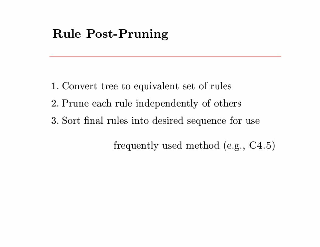
•  Decision tree learning –  Greedy top-down learning of decision trees (ID3, C4.5, ...) –  Overfitting and tree post-pruning –  Extensions…

Extra slides

extensions to decision tree learning

Questions to think about (1) •  ID3 and C4.5 are heuristic algorithms that

search through the space of decision trees. Why not just do an exhaustive search?

Questions to think about (2) •  Consider target function f: <x1,x2> à y,

where x1 and x2 are real-valued, y is boolean. What is the set of decision surfaces describable with decision trees that use each attribute at most once?

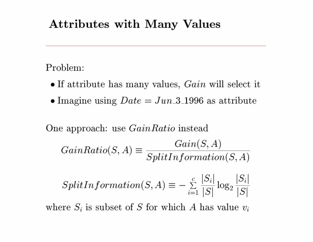
Questions to think about (3) •  Why use Information Gain to select attributes

in decision trees? What other criteria seem reasonable, and what are the tradeoffs in making this choice?

Questions to think about (4) •  What is the relationship between learning

decision trees, and learning IF-THEN rules

Machine Learning 10-601 Tom M. Mitchell

Machine Learning Department Carnegie Mellon University

January 14, 2015

Today: •  Review: probability

Readings: Probability review •  Bishop Ch. 1 thru 1.2.3 •  Bishop, Ch. 2 thru 2.2 •  Andrew Moore’s online

tutorial

many of these slides are derived from William Cohen, Andrew Moore, Aarti Singh, Eric Xing. Thanks!

Probability Overview •  Events

–  discrete random variables, continuous random variables, compound events

•  Axioms of probability –  What defines a reasonable theory of uncertainty

•  Independent events •  Conditional probabilities •  Bayes rule and beliefs •  Joint probability distribution •  Expectations •  Independence, Conditional independence

Random Variables

•  Informally, A is a random variable if –  A denotes something about which we are uncertain –  perhaps the outcome of a randomized experiment

•  Examples A = True if a randomly drawn person from our class is female A = The hometown of a randomly drawn person from our class A = True if two randomly drawn persons from our class have same birthday

•  Define P(A) as “the fraction of possible worlds in which A is true” or “the fraction of times A holds, in repeated runs of the random experiment” –  the set of possible worlds is called the sample space, S –  A random variable A is a function defined over S

A: S à {0,1}

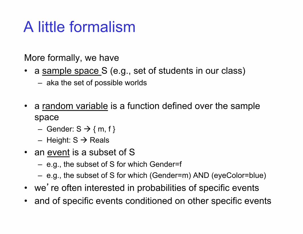
A little formalism

More formally, we have •  a sample space S (e.g., set of students in our class)

–  aka the set of possible worlds

•  a random variable is a function defined over the sample space –  Gender: S à { m, f } –  Height: S à Reals

•  an event is a subset of S –  e.g., the subset of S for which Gender=f –  e.g., the subset of S for which (Gender=m) AND (eyeColor=blue)

•  we’re often interested in probabilities of specific events •  and of specific events conditioned on other specific events

Visualizing A

Sample space of all possible worlds

Its area is 1

Worlds in which A is False

Worlds in which A is true

P(A) = Area of reddish oval

The Axioms of Probability

•  0 <= P(A) <= 1 •  P(True) = 1 •  P(False) = 0 •  P(A or B) = P(A) + P(B) - P(A and B)

[di Finetti 1931]: when gambling based on “uncertainty formalism A” you can be exploited by an opponent iff your uncertainty formalism A violates these axioms

Elementary Probability in Pictures •  P(~A) + P(A) = 1

A

~A

A useful theorem

•  0 <= P(A) <= 1, P(True) = 1, P(False) = 0, P(A or B) = P(A) + P(B) - P(A and B)

è P(A) = P(A ^ B) + P(A ^ ~B)

A = [A and (B or ~B)] = [(A and B) or (A and ~B)]

P(A) = P(A and B) + P(A and ~B) – P((A and B) and (A and ~B))

P(A) = P(A and B) + P(A and ~B) – P(A and B and A and ~B)

Elementary Probability in Pictures •  P(A) = P(A ^ B) + P(A ^ ~B)

B

A ^ ~B

A ^ B

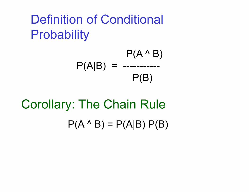
Definition of Conditional Probability

P(A ^ B) P(A|B) = ----------- P(B)

A B

Definition of Conditional Probability

P(A ^ B) P(A|B) = ----------- P(B)

Corollary: The Chain Rule P(A ^ B) = P(A|B) P(B)

Bayes Rule

•  let’s write 2 expressions for P(A ^ B)

B

A

A ^ B

P(B|A) * P(A)

P(B) P(A|B) =

Bayes, Thomas (1763) An essay towards solving a problem in the doctrine of chances. Philosophical Transactions of the Royal Society of London, 53:370-418

…by no means merely a curious speculation in the doctrine of chances, but necessary to be solved in order to a sure foundation for all our reasonings concerning past facts, and what is likely to be hereafter…. necessary to be considered by any that would give a clear account of the strength of analogical or inductive reasoning…

Bayes’ rule

we call P(A) the “prior” and P(A|B) the “posterior”

Other Forms of Bayes Rule

)(~)|~()()|()()|()|(

APABPAPABPAPABPBAP

+=

)()()|()|(

XBPXAPXABPXBAP

∧

∧∧=∧

Applying Bayes Rule

P(A |B) = P(B | A)P(A)P(B | A)P(A)+P(B |~ A)P(~ A)

A = you have the flu, B = you just coughed Assume: P(A) = 0.05 P(B|A) = 0.80 P(B| ~A) = 0.2 what is P(flu | cough) = P(A|B)?

what does all this have to do with function approximation?

The Joint Distribution

Recipe for making a joint distribution of M variables:

Example: Boolean variables A, B, C

The Joint Distribution

Recipe for making a joint distribution of M variables:

1.  Make a truth table listing all

combinations of values of your variables (if there are M Boolean variables then the table will have 2M rows).

Example: Boolean variables A, B, C

A B C 0 0 0

0 0 1

0 1 0

0 1 1

1 0 0

1 0 1

1 1 0

1 1 1

The Joint Distribution

Recipe for making a joint distribution of M variables:

1.  Make a truth table listing all

combinations of values of your variables (if there are M Boolean variables then the table will have 2M rows).

2.  For each combination of values, say how probable it is.

Example: Boolean variables A, B, C

A B C Prob 0 0 0 0.30

0 0 1 0.05

0 1 0 0.10

0 1 1 0.05

1 0 0 0.05

1 0 1 0.10

1 1 0 0.25

1 1 1 0.10

The Joint Distribution

Recipe for making a joint distribution of M variables:

1.  Make a truth table listing all

combinations of values of your variables (if there are M Boolean variables then the table will have 2M rows).

2.  For each combination of values, say how probable it is.

3.  If you subscribe to the axioms of probability, those numbers must sum to 1.

A B C Prob 0 0 0 0.30

0 0 1 0.05

0 1 0 0.10

0 1 1 0.05

1 0 0 0.05

1 0 1 0.10

1 1 0 0.25

1 1 1 0.10

A

B

C 0.05

0.25

0.10 0.05 0.05

0.10

0.10 0.30

Using the Joint Distribution

One you have the JD you can ask for the probability of any logical expression involving your attribute

∑=E

PEP matching rows

)row()(

Using the Joint

P(Poor Male) = 0.4654 ∑=E

PEP matching rows

)row()(

Using the Joint

P(Poor) = 0.7604 ∑=E

PEP matching rows

)row()(

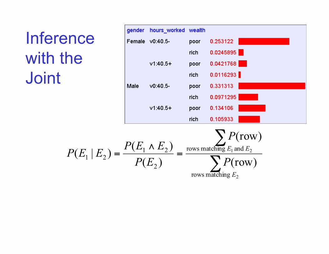
Inference with the Joint

∑

∑=

∧=

2

2 1

matching rows

and matching rows

2

2121 )row(

)row(

)()()|(

E

EE

P

P

EPEEPEEP

Inference with the Joint

∑

∑=

∧=

2

2 1

matching rows

and matching rows

2

2121 )row(

)row(

)()()|(

E

EE

P

P

EPEEPEEP

P(Male | Poor) = 0.4654 / 0.7604 = 0.612

You should know •  Events

–  discrete random variables, continuous random variables, compound events

•  Axioms of probability –  What defines a reasonable theory of uncertainty

•  Conditional probabilities •  Chain rule •  Bayes rule •  Joint distribution over multiple random variables

–  how to calculate other quantities from the joint distribution

Expected values Given discrete random variable X, the expected value of

X, written E[X] is We also can talk about the expected value of functions

of X

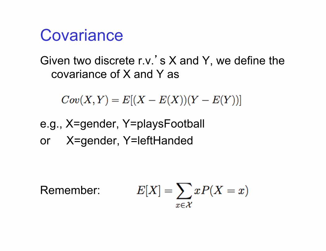
Covariance Given two discrete r.v.’s X and Y, we define the

covariance of X and Y as e.g., X=gender, Y=playsFootball or X=gender, Y=leftHanded Remember: