m. wu: enee631 digital image processing (spring'09) lattice sampling spring ’09 instructor:...
TRANSCRIPT

M. Wu: ENEE631 Digital Image Processing (Spring'09)
Lattice SamplingLattice Sampling
Spring ’09 Instructor: Min Wu
Electrical and Computer Engineering Department,
University of Maryland, College Park
bb.eng.umd.edu (select ENEE631 S’09) [email protected]
ENEE631 Spring’09ENEE631 Spring’09Lecture 26 (5/6/2009)Lecture 26 (5/6/2009)

M. Wu: ENEE631 Digital Image Processing (Spring'09) Lec26 – Lattice Sampling [2]
Overview and LogisticsOverview and Logistics
Last Time: – Radon and inverse Radon transform for medical app.
Inverting Radon transform data based on Fourier properties vs. Filtered Back projections
– Sampling theory: extending 1-D to 2-D
Today:– Sampling on non-rectangular grid via the Lattice Theory
Course evaluation (online)
Project feedback
UM
CP
EN
EE
63
1 S
lide
s (c
rea
ted
by
M.W
u ©
20
04
)

M. Wu: ENEE631 Digital Image Processing (Spring'09) Lec26 – Lattice Sampling [3]
Recall: 2-D SamplingRecall: 2-D Sampling
2-D impulse function (a.k.a. 2-D comb)
comb(x,y; x, y) = m,n ( x - mx, y - ny ) ~ separable function
FT: COMB(x, y) = comb(x, y; 1/x, 1/y) / xy
Sampling vs. Replication (tiling)– Nyquist rates (2x0 and 2y0) Aliasing
Jain’s Fig.4.7
UM
CP
EN
EE
63
1 S
lide
s (c
rea
ted
by
M.W
u ©
20
01
)

M. Wu: ENEE631 Digital Image Processing (Spring'09) Lec26 – Lattice Sampling [4]
2-D Sampling: Beyond Rectangular Grid2-D Sampling: Beyond Rectangular Grid
Sampling at nonrectangular grid – May give more efficient sampling
density when spectrum region of support is not rectangular
Sampling density measured by #samples needed per unit area
– E.g. interlaced grid for diamondshaped region of support equiv. to rotate 45-degree
of rectangular grid spectrum rotate by the
same degree
From Wang’s book preprint Fig.4.2
UM
CP
EN
EE
63
1 S
lide
s (c
rea
ted
by
M.W
u ©
20
01
/20
04
)

M. Wu: ENEE631 Digital Image Processing (Spring'09) Lec26 – Lattice Sampling [5]
General Sampling LatticeGeneral Sampling Lattice
Lattice in K-dimension space R K – A set of all possible vectors represented as integer weighted
combinations of K linearly independent basis vectors
Generating matrix V (sampling matrix)V = [v1, v2, …, vk] => lattice points x = V n
e.g., identity matrix V ~ square lattice
Voronoi cell of a lattice– A “unit cell” of a lattice, whose translations cover the whole space– Enclose all points that are closer to the origin than to other lattice points
cell boundaries are equidistant lines between surrounding lattice points
K
jkjj
K nn1
,| ZR vxx
From Wang’s book preprint Fig.3.1U
MC
P E
NE
E6
31
Slid
es
(cre
ate
d b
y M
.Wu
© 2
00
1/2
00
4)

M. Wu: ENEE631 Digital Image Processing (Spring'09) Lec26 – Lattice Sampling [6]
Sampling Density:d1 = 1d2 = 2 / 3
)(hexagonal 12/1
02/3
ar)(rectangul 10
01
2
1
V
V
From Wang’s book preprint Fig.3.1
Examples of LatticesExamples of Lattices
UM
CP
EN
EE
63
1 S
lide
s (c
rea
ted
by
M.W
u ©
20
04
)
M. Wu: ENEE631 Digital Image Processing (Spring'09) Lec26 – Lattice Sampling [7]
Periodicity in Lattice RepresentationsPeriodicity in Lattice Representations
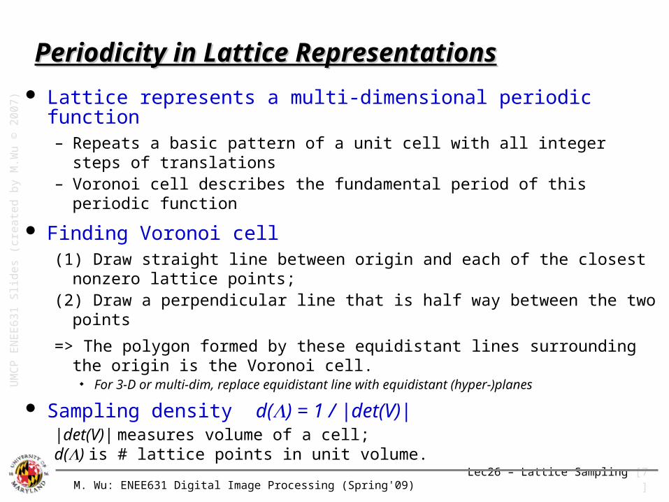
Lattice represents a multi-dimensional periodic function – Repeats a basic pattern of a unit cell with all integer steps of
translations– Voronoi cell describes the fundamental period of this periodic function
Finding Voronoi cell(1) Draw straight line between origin and each of the closest nonzero
lattice points; (2) Draw a perpendicular line that is half way between the two points
=> The polygon formed by these equidistant lines surrounding the origin is the Voronoi cell. For 3-D or multi-dim, replace equidistant line with equidistant
(hyper-)planes
Sampling density d() = 1 / |det(V)||det(V)| measures volume of a cell; d() is # lattice points in unit volume.
UM
CP
EN
EE
63
1 S
lide
s (c
rea
ted
by
M.W
u ©
20
07
)

M. Wu: ENEE631 Digital Image Processing (Spring'09) Lec26 – Lattice Sampling [8]
Frequency Domain View & Reciprocal LatticeFrequency Domain View & Reciprocal Lattice
Reciprocal lattice # for a lattice (with generating matrix V)– Generating matrix of # is U = (VT)-1 – Basis vectors for and # are orthonormal to each other: VT U = I
– Denser lattice has sparser reciprocal lattice # : det(U) = 1 / det(V)
Frequency domain view of sampling over lattice– Sampling in spatial domain Repetition in frequency domain– Repetition grid in freq. domain can be described by reciprocal lattice– Intuition for “reciprocal”
[e.g.] rectangular grid that sample faster horizontally than vertically=>the repetition in frequency domain is slower horizontally than vertically
Aliasing and prefiltering to avoid aliasing– Aliasing happens when signal spectrum extends outside the Voronoi
cell of reciprocal lattice
UM
CP
EN
EE
63
1 S
lide
s (c
rea
ted
by
M.W
u ©
20
01
/20
04
)
M. Wu: ENEE631 Digital Image Processing (Spring'09) Lec26 – Lattice Sampling [10]
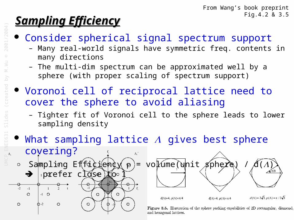
Sampling EfficiencySampling Efficiency Consider spherical signal spectrum support
– Many real-world signals have symmetric freq. contents in many directions– The multi-dim spectrum can be approximated well by a sphere (with proper
scaling of spectrum support)
Voronoi cell of reciprocal lattice need to cover the sphere to avoid aliasing– Tighter fit of Voronoi cell to the sphere leads to lower sampling density
What sampling lattice gives best sphere covering? Sampling Efficiency = volume(unit sphere) / d() prefer close to 1
From Wang’s book preprint Fig.4.2 & 3.5U
MC
P E
NE
E6
31
Slid
es
(cre
ate
d b
y M
.Wu
© 2
00
1/2
00
4)
M. Wu: ENEE631 Digital Image Processing (Spring'09) Lec26 – Lattice Sampling [11]
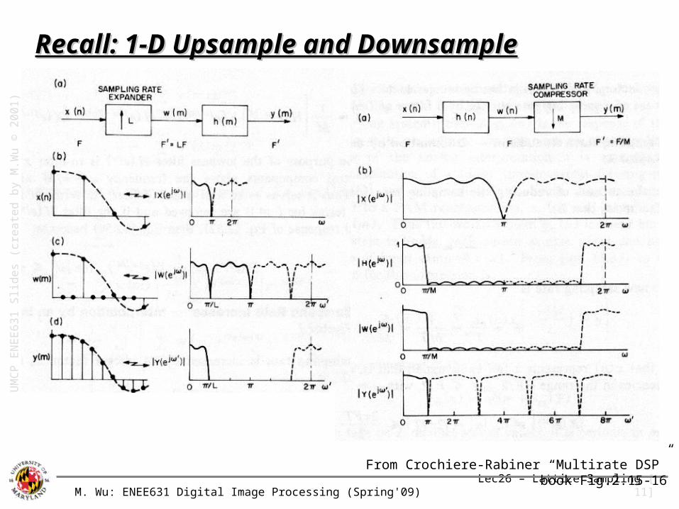
Recall: 1-D Upsample and DownsampleRecall: 1-D Upsample and Downsample
From Crochiere-Rabiner “Multirate DSP” book Fig.2.15-16
UM
CP
EN
EE
63
1 S
lide
s (c
rea
ted
by
M.W
u ©
20
01
)

M. Wu: ENEE631 Digital Image Processing (Spring'09) Lec26 – Lattice Sampling [12]
General Procedures for Sampling Rate ConversionGeneral Procedures for Sampling Rate Conversion
From Wang’s book preprint Fig.4.1
UM
CP
EN
EE
63
1 S
lide
s (c
rea
ted
by
M.W
u ©
20
01
)

M. Wu: ENEE631 Digital Image Processing (Spring'09) Lec26 – Lattice Sampling [13]
Sampling Lattice ConversionSampling Lattice Conversion
From Wang’s book preprint Fig.4.4
Intermediate
Original
Targeted
UMCP ENEE631 Slides (created by M.Wu © 2001)

M. Wu: ENEE631 Digital Image Processing (Spring'09) Lec26 – Lattice Sampling [14]
Case Studies on Sampling and Resampling Case Studies on Sampling and Resampling
in Video Processingin Video Processing
Reference Readings: Wang’s book Chapter 4Reference Readings: Wang’s book Chapter 4
e.g. Interlaced 50 fields/sec e.g. Interlaced 50 fields/sec 60 fields/sec 60 fields/secUM
CP
EN
EE
63
1 S
lide
s (c
rea
ted
by
M.W
u ©
20
04
)
M. Wu: ENEE631 Digital Image Processing (Spring'09) Lec26 – Lattice Sampling [15]
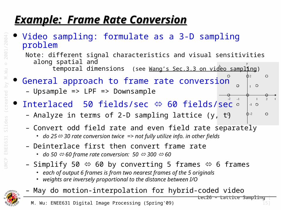
Example: Frame Rate ConversionExample: Frame Rate Conversion Video sampling: formulate as a 3-D sampling problem
Note: different signal characteristics and visual sensitivities along spatial and temporal dimensions (see Wang’s Sec.3.3 on video sampling)
General approach to frame rate conversion– Upsample => LPF => Downsample
Interlaced 50 fields/sec 60 fields/sec– Analyze in terms of 2-D sampling lattice (y, t)
– Convert odd field rate and even field rate separately do 25 30 rate conversion twice => not fully utilize info. in other
fields
– Deinterlace first then convert frame rate do 50 60 frame rate conversion: 50 300 60
– Simplify 50 60 by converting 5 frames 6 frames each of output 6 frames is from two nearest frames of the 5 originals weights are inversely proportional to the distance between I/O
– May do motion-interpolation for hybrid-coded video
UM
CP
EN
EE
63
1 S
lide
s (c
rea
ted
by
M.W
u ©
20
01
/20
04
)

M. Wu: ENEE631 Digital Image Processing (Spring'09) Lec26 – Lattice Sampling [16]
From Wang’s book preprint Fig.4.3
UM
CP
EN
EE
63
1 S
lide
s (c
rea
ted
by
M.W
u ©
20
01
)

M. Wu: ENEE631 Digital Image Processing (Spring'09) Lec26 – Lattice Sampling [17]
Video Format Conversion for NTSC Video Format Conversion for NTSC PAL PAL
Require both temporal and spatial rate conversion– NTSC 525 lines per picture, 60 fields per second– PAL 625 lines per picture, 50 fields per second
Ideal approach (direct conversion)– 525 lines 60 field/sec 13125 line 300 field/sec
625 lines 50 field/sec
4-step sequential conversion– Deinterlace => line rate conversion
=> frame rate conversion => interlace
UM
CP
EN
EE
63
1 S
lide
s (c
rea
ted
by
M.W
u ©
20
01
)

M. Wu: ENEE631 Digital Image Processing (Spring'09) Lec26 – Lattice Sampling [19]
From Wang’s book preprint Fig.4.9
UM
CP
EN
EE
63
1 S
lide
s (c
rea
ted
by
M.W
u ©
20
01
)

M. Wu: ENEE631 Digital Image Processing (Spring'09) Lec26 – Lattice Sampling [20]
Simplified Video Format ConversionSimplified Video Format Conversion
50 field/sec 60 field/sec– After deinterlacing, simplify to 5 frames 6 frames– Conversion involves two adjacent frames only
625 lines 525 lines– Simplify to 25 lines 21 lines– Conversion involves two adjacent lines only
UM
CP
EN
EE
63
1 S
lide
s (c
rea
ted
by
M.W
u ©
20
01
)

M. Wu: ENEE631 Digital Image Processing (Spring'09) Lec26 – Lattice Sampling [21]
UM
CP
EN
EE
63
1 S
lide
s (c
rea
ted
by
M.W
u ©
20
01
)
From Wang’s book preprint

M. Wu: ENEE631 Digital Image Processing (Spring'09) Lec26 – Lattice Sampling [22]
Interlaced Video and DeinterlacingInterlaced Video and Deinterlacing Interlaced video
Odd field at 0 Even field at t Odd field at 2t Even field at
3t …
Deinterlacing– Merge to get a complete frame with odd and even field
Examples from http://www.geocities.com/lukesvideo/interlacing.html
UM
CP
EN
EE
63
1 S
lide
s (c
rea
ted
by
M.W
u ©
20
01
)

M. Wu: ENEE631 Digital Image Processing (Spring'09) Lec26 – Lattice Sampling [23]
De-interlacing: Practical ApproachesDe-interlacing: Practical Approaches
Spatial interpolation– Vertical interpolation within
same field (1-D upsample by 2)– Line averaging ~ average the line
above and below D=(C+E)/2
Temporal interpolation– 2-frame field merging => artifacts– 3-frame field averaging D=(K+R)/2
fill in the missing odd field by averaging odd fields before and after
Spatial-temporal interpolation– Line-and-field averaging D=(C+E+K+R)/4
UM
CP
EN
EE
63
1 S
lide
s (c
rea
ted
by
M.W
u ©
20
01
)
From Wang’s book preprint
M. Wu: ENEE631 Digital Image Processing (Spring'09) Lec26 – Lattice Sampling [25]
Motion-Compensated De-interlacing Motion-Compensated De-interlacing
Stationary video scenes– Temporary deinterlacing approach yield good result
Scenes with rapid temporal changes– Artifacts incurred from temporal interpolation– Spatial interpolation alone is better than involving temporal
interpolation
Switching between spatial & temporal interpolation modes– Based on motion detection result– Hard switching or weighted average– Motion-compensated interpolation
UM
CP
EN
EE
63
1 S
lide
s (c
rea
ted
by
M.W
u ©
20
01
)

M. Wu: ENEE631 Digital Image Processing (Spring'09) Lec26 – Lattice Sampling [26]
Example: Example:
De-interlacingDe-interlacing
From Woods’ book resource

M. Wu: ENEE631 Digital Image Processing (Spring'09) Lec26 – Lattice Sampling [27]
Example: Temporal Example: Temporal
Upsampling Upsampling (5 to 30 fps)(5 to 30 fps)
From Woods’ book resource
M. Wu: ENEE631 Digital Image Processing (Spring'09) Lec26 – Lattice Sampling [28]
Texture AnalysisTexture Analysis
UM
CP
EN
EE
63
1 S
lide
s (c
rea
ted
by
M.W
u ©
20
04
)

M. Wu: ENEE631 Digital Image Processing (Spring'09) Lec26 – Lattice Sampling [30]
TextureTexture
Observed in structural patterns of objects’ surfaces – [Natural] wood, grain, sand,
grass, tree leaves, cloth– [Man-made] tiles, printing patterns
“Texture” ~ repetition of “texels” (basic texture element)– Texels’ placement may be
periodic, quasi-periodic, or random
From http://texlib.povray.org/textures.html and Gonzalez 3/e book online resource

M. Wu: ENEE631 Digital Image Processing (Spring'09) Lec26 – Lattice Sampling [31]
Properties and Major Approaches to Study TextureProperties and Major Approaches to Study Texture
Texture properties: smoothness, coarseness, regularity
Structural approach– Describe arrangement of basic image primitives
Statistical approach– Examine histogram and other features derived from it– Characterize textures as smooth, coarse, grainy
Spectral and random field approach– Exploit Fourier spectrum properties– Detect global periodicity

M. Wu: ENEE631 Digital Image Processing (Spring'09) Lec26 – Lattice Sampling [32]
Statistical Measures on TexturesStatistical Measures on Textures
x ~ r.v. of pixel value
R = 1 – 1 / ( 1 + x2 )
~ 0 for constant region; 1 for large variance
E[ (X – x)K ]
3rd moment:~ histogram’s skewness
4th moment:~ relative flatness
Uniformity or Energy~ squared sum of hist. bins
Figures from Gonzalez’s book resource

M. Wu: ENEE631 Digital Image Processing (Spring'09) Lec26 – Lattice Sampling [33]
Characterizing TexturesCharacterizing Textures Structural measures
– Periodic textures Features of deterministic texel: gray levels, shape, orientation,
etc. Placement rules: period, repetition grid pattern, etc.
– Textures with random nature Features of texel: edge density, histogram features, etc.
Stochastic/spectral measures– Mainly for textures with random nature; Model as a random field
2-D sequence of random variables
– Autocorrelation function: measuring the relations among those r.v.R(m,n; m’,n’) = E[ U(m,n) U(m’,n’) ]“wide-sense stationary”: R(m,n;m’n’) = RU(m-m’,n-n’) and constant
mean
– Fit into random field models ~ analysis and synthesis Focus on second order statistics for simplicity Two textures with same 2nd order statistics often appear similar

M. Wu: ENEE631 Digital Image Processing (Spring'09) Lec26 – Lattice Sampling [34]
Examples:Examples:Spectral Approaches Spectral Approaches to Study Textureto Study Texture
Figures from Gonzalez’s 2/e book resource
M. Wu: ENEE631 Digital Image Processing (Spring'09) Lec26 – Lattice Sampling [35]
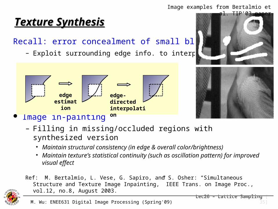
Texture SynthesisTexture Synthesis
Recall: error concealment of small blocks– Exploit surrounding edge info. to interpolate
Image in-painting– Filling in missing/occluded regions with synthesized version
Maintain structural consistency (in edge & overall color/brightness)
Maintain texture’s statistical continuity (such as oscillation pattern) for improved visual effect
Ref: M. Bertalmio, L. Vese, G. Sapiro, and S. Osher: “Simultaneous Structure and Texture Image Inpainting,” IEEE Trans. on Image Proc., vol.12, no.8, August 2003.
edge estimation
edge-directed interpolation
Image examples from Bertalmio et al. TIP’03 paper

M. Wu: ENEE631 Digital Image Processing (Spring'09) Lec26 – Lattice Sampling [36]
Summary of Today’s LectureSummary of Today’s Lecture
Multi-dimension Lattice sampling– Sampling lattice and frequency-domain interpretation– Sampling rate conversion
Texture analysis
Next Lecture: – Continue on texture analysis and synthesis
Readings– Lattice Sampling: Wang’s book Sec. 3.1-3.3, 3.5; Chapter 4
– Texture: Gonzalez’s book 11.3.3 (see also Jain’s 9.11)
UM
CP
EN
EE
63
1 S
lide
s (c
rea
ted
by
M.W
u ©
20
04
)

M. Wu: ENEE631 Digital Image Processing (Spring'09) Lec26 – Lattice Sampling [37]

M. Wu: ENEE631 Digital Image Processing (Spring'09) Lec26 – Lattice Sampling [38]
Image InpaintingImage Inpainting:: Basic Approach Basic Approach and Exampleand Example
Figures from Bertalmio et al. TIP’03 paper

M. Wu: ENEE631 Digital Image Processing (Spring'09) Lec26 – Lattice Sampling [40]
Recall: Characterize the Ensemble of 2-D SignalsRecall: Characterize the Ensemble of 2-D Signals
Specify by a joint probability distribution function– Difficult to measure and specify the joint distribution for images of
practical size=> too many r.v. : e.g. 512 x 512 = 262,144
Specify by the first few moments– Mean (1st moment) and Covariance (2nd moment)
may still be non-trivial to measure for the entire image size
By various stochastic models– Use a few parameters to describe the relations among all pixels
E.g. 2-D extensions from 1-D Autoregressive (AR) model
Important for a variety of image processing tasks– image compression, enhancement, restoration, understanding, …
UM
CP
EN
EE
63
1 S
lide
s (c
rea
ted
by
M.W
u ©
20
04
)

M. Wu: ENEE631 Digital Image Processing (Spring'09) Lec26 – Lattice Sampling [41]
Recall: Discrete Random FieldRecall: Discrete Random Field
We call a 2-D sequence discrete random field if each of its elements is a random variable– when the random field represents an ensemble of images, we often
call it a random image
Mean and Covariance of a complex random fieldE[u(m,n)] = (m,n)
Cov[u(m,n), u(m’,n’)] = E[ (u(m,n) – (m,n)) (u(m’,n’) – (m’,n’))* ] = ru( m, n; m’, n’)
For zero-mean random field, autocorrelation function = cov. function
Wide-sense stationary (or wide-sense homogeneity)
(m,n) = = constant
ru( m, n; m’, n’) = ru( m – m’, n – n’; 0, 0) = r( m – m’, n – n’ )
also called shift invariant, spatial invariant in some literature
UM
CP
EN
EE
63
1 S
lide
s (c
rea
ted
by
M.W
u ©
20
04
)

M. Wu: ENEE631 Digital Image Processing (Spring'09) Lec26 – Lattice Sampling [42]
Recall: Special Random Fields of InterestsRecall: Special Random Fields of Interests
White noise field– A stationary random field– Any two elements at different locations x(m,n) and x(m’,n’)
are mutually uncorrelated
rx( m – m’, n – n’) = x2
( m, n ) ( m – m’, n – n’
)
Gaussian random field– Every segment defined on an arbitrary finite grid is Gaussian
i.e. every finite segment of u(m,n) when mapped into a vector have a joint Gaussian p.d.f. of
UM
CP
EN
EE
63
1 S
lide
s (c
rea
ted
by
M.W
u ©
20
04
)

M. Wu: ENEE631 Digital Image Processing (Spring'09) Lec26 – Lattice Sampling [43]
Recall: Spectral Density FunctionRecall: Spectral Density Function Spectral density function (SDF) is defined as the Fourier
transform of the covariance function rx
Also known as the power spectral density (p.s.d.)
– Example: SDF of stationary white noise field with r(m,n)= 2 (m,n) S(
1, 2) = 2
SDF Properties:
– Real and nonnegative: S(1, 2) = S*(1, 2); S(1, 2) 0 By conjugate symmetry of covariance function: r(m, n) = r *(-m, -n) By non-negative definiteness of covariance function
– SDF of the output from a LSI system w/ freq response H(1, 2)
Sy(1, 2) = | H(1, 2) |2 Sx(1, 2)
m n
x nmjnmrS )](exp[),(),( 2121
UM
CP
EN
EE
63
1 S
lide
s (c
rea
ted
by
M.W
u ©
20
04
)

M. Wu: ENEE631 Digital Image Processing (Spring'09) Lec26 – Lattice Sampling [44]
More on Image ModelingMore on Image Modeling Good image model can facilitate many image proc. tasks
– Coding/compression; restoration; estimation/interpolation; …
Image models we’ve seen/used so far– Consider pixel values as realizations of a r.v.
Color/grayscale histogram
– Predictive models Use linear combination of (causal) neighborhood to estimate
– Random field u(m,n) Characterized by 2-D correlation function or p.s.d.
Generally can characterize u(m,n) = u’(m,n) + e(m,n)– u’(m,n) is some prediction of u(m,n); e(m,n) is another random field
Minimum Variance representation(MVR): e(m,n) is error of min. var. prediction
White noise Driven representation: e(m,n) is chosen as a white noise field ARMA representation: e(m,n) is a 2-D moving average of a white noise
field.

M. Wu: ENEE631 Digital Image Processing (Spring'09) Lec26 – Lattice Sampling [45]
Recall: Linear PredictorRecall: Linear Predictor
Causality required for coding purpose– Can’t use the samples that decoder hasn’t got as reference
Use last sample uq(n-1): equiv. to coding the difference (DPCM)
pth–order auto-regressive (AR) model – Linear predictor from past samples
Prediction neighborhood– Line-by-line DPCM
predict from the past samples in the same line
– 2-D DPCM predict from past samples in the same line and from previous lines
– Non-causal neighborhood Use samples around as prediction/estimation => for filtering,
restoration, etc
Predictor coeff. in MMSE sense: get from orthogonality condition (from Wiener filtering discussions)
)()()(1
neinuanup
ii
UM
CP
EN
EE
63
1 S
lide
s (c
rea
ted
by
M.W
u ©
20
01
)

M. Wu: ENEE631 Digital Image Processing (Spring'09) Lec26 – Lattice Sampling [46]
Commonly Used Image ModelCommonly Used Image Model Gaussian model and Gaussian mixture model
Every segment defined on an arbitrary finite grid is Gaussian-or- follows a distribution of linear combining several Gaussian Reduce the modeling to estimate mean(s), variance(s), and
weightings
(Ref: Prof. R. Gray’s IEEE talk S’07 http://www-ee.stanford.edu/~gray/umcpqcc.pdf)
Markov random field– Markovianity: conditional independence
Define past, present, future pixel set for each pix location Given the present, the future is independent of the past
– 2-D/spatial causal AR model (under Gaussian noise or MVR)
Gauss-Markov random field model– For Gaussian: conditional indep. => conditional uncorrelateness
Bring in multi-scale and wavelet/multi-resolution ideasRef: Section 4.1-4.5 of Bovik’s Handbook

M. Wu: ENEE631 Digital Image Processing (Spring'09) Lec26 – Lattice Sampling [48]
Recursive Estimation: Basic IdeasRecursive Estimation: Basic Ideas
Kalman filter: recursive Linear MMSE estimator
1-D example: provide linear estimation for an AR signal
– System model AR(M): x(n)=c1x(n-1)+… cM x(n-M) + w(n) State equation: x(n) = C x(n-1) + w(n) for n = 0, 1, …, x(-1)=0 ~
AR sig Observation equation: y(n) = hT x(n) + v(n) M-dimension state vector x(n); model noise w(n) and observation
noise v(n) are white & orthogonal
– Signal model is Mth-order Markov under Gaussian noise w – Linear MMSE estimator is globally optimal if model and
observation noise w and v are both Gaussian– C can be time-variant and physics motivated by applications
General MMSE solution: equiv. to find conditional mean Filtering estimate: E[ x(n) | y(n), y(n-1), … y(0) ] xa (n) One-step predictor estimate: E[ x(n) | y(n-1), … y(0) ] xb(n)

M. Wu: ENEE631 Digital Image Processing (Spring'09) Lec26 – Lattice Sampling [49]
Recursive Estimation (cont’d)Recursive Estimation (cont’d)
1-D Kalman filter equations Prediction: xb(n) = C xa(n-1) Update: xa(n) = xb(n) + g(n) [ y(n) – hT xb(n) ]
– Error variance equationsPb(n) = C Pa(n-1) CT + Qw initialize x(0) = [w(0), 0, … 0 ]T,
xb(0) = 0
Pb(n) = (I – g(n) hT ) Pb(n) Pb(n) = Qw all zero except 1st entry w2
– Kalman gain vector: g(n) g(n) = Pb(n) (hT Pb(n) h + v
2) -1
2-D Kalman filtering: define proper state vector Raster scan observations & map to equiv. 1-D case Restrict Kalman gain terms to be just surround current
observation to reduce computational complexity
past
present state
future

M. Wu: ENEE631 Digital Image Processing (Spring'09) Lec26 – Lattice Sampling [50]
Summary of Today’s LectureSummary of Today’s Lecture
Readings– Texture: Gonzalez’s book 11.3.3 (see also Jain’s 9.11)
– Image modeling: Wood’s book Chapter 7 & 9.4 See also Jain’s Chapter 6 and Bovik’s Handbook 4.1-4.5 Recursive/Kalman estimation:
Woods’ book Chapter 7; EE621 (Poor’s book)
UM
CP
EN
EE
63
1 S
lide
s (c
rea
ted
by
M.W
u ©
20
04
)