m-files

As we have seen before, it is generally convenient to save programs in some sort of file (script, macro, batch, etc.) for program

development and reuse.

Matlab offers this feature through m-files, which are ascii text files containing a set of

Matlab commands.

m-files

There are two kinds of m-files:

Scripts, which do not accept input arguments or return output arguments. They operate on data in the workspace.

Functions, which can accept input arguments and return output arguments. Functions have internal variables are local to the function.

The filename has to end in “.m”

You have probably been using scripts already in your previous matlab homework.

These files are the same things that you would type in when running interactively.

They can have for and while loops, if-elseif-else-end.

They are executed by entering the file name in the matlab command window.

Functions Functions are M-files that can accept input

arguments and return output arguments. (Comments in Matlab are denoted using the % symbol.)

This function, loadsac, calls another function, sac, with the filename to read. It then works with the 3 matrices returned by sac, returning a data matrix, and 3 scalars

dt, beg, pt.

We see here that functions can call other

functions.

Global Variables

If you want more than one function to share a single copy of a variable, simply declare the

variable as global in all the functions.

Do the same thing at the command line if you want the base workspace to access the

variable.

The global declaration must occur before the variable is actually used in a function. Although it is not required, using capital letters for the names of global

variables helps distinguish them from other variables.

In an .m file called falling.m function h = falling(t) global GRAVITY h = 1/2*GRAVITY*t.^2;

In the workspace, enter the statements >>global GRAVITY >>GRAVITY = 32; >>y = falling((0:.1:5)');

The two global statements make the value assigned to GRAVITY at the command

prompt available inside the function. You can then modify GRAVITY interactively and obtain new solutions without editing any

files.

function tsting global c c=4 b=2 [a d]=tstfn(b) whos return function [out1 out2]=tstfn(in) global c out1=in.^2 out2=c*out1 whos return

>> tstingfuns c = 4 b = 2 out1 = 4 out2 = 16 Name Size Bytes Class Attributes c 1x1 8 double global in 1x1 8 double out1 1x1 8 double out2 1x1 8 double a = 4 d = 16 Name Size Bytes Class Attributes a 1x1 8 double b 1x1 8 double c 1x1 8 double global d 1x1 8 double

Can put multiple functions in one m file. “b” and “c” declared global in both, but only assigned in one of them.

Rethinking code for taking advantage of matlab vectorization.

More than just defining vectors and matricies using matlab definitions.

x = rand(1,100); %In place of : for k=1:100 y(k) = sin(x(k)); End % We can use : y = sin(x);

Given an=n and bn=(1000-an) , n=1,2,…1000, calculate

�

ssum = anbnn=1

1000

∑

Solution: It might be tempting to implement the above calculation as

a = 1:1000; b = 1000 - a; ssum=0; for n=1:1000 %poor style... ssum = ssum +a(n)*b(n); End

Recognizing that the sum is the inner product of the vectors a and b, abT , we can

do better:

ssum = a*b' %Vectorized, better!

Say we have a number of seismograms and we would like to “window” and scale each one.

First – what is the “window” process? (Blue trace is original signal, red trace is “window”, dashed red trace is negative of window to show “envelope” – use it to scale the original signal. Green trace is the final result after applying the “window” to the blue trace. In this case the windowing is done by a point by point multiply of the blue and red vectors, b.*r, [64 pts]).

What if we want to do this to a number of seismograms?

We could use a loop, doing the vectorized multiply on each seismogram.

But can we do better than that?

We would not be asking leading questions if not!

So how do we do it? (Now we want to do point by point multiplies of each trace by the window – T1.*w and T2.*w, etc. How can we do this in one shot?

What if we make a diagonal matrix of the window vector [elements of the vector on the diagonal and all else zero]?)

Looking at what happens when we do matrix multiplication, we see that this does what we

need.

% length %Number traces N = 64; M=1:4; TH=1:N; X = sin(TH'*M*… pi*2/(N-1)); plot(X)

% Make a window w = hamming(N); W = diag(w); % Windowed signals %without loops XW = W * X

To do the point by point multiply we need to match the length of the seismograms (64

points in this case). >> whos Name Size Bytes Class Attributes M 1x4 32 double N 1x1 8 double TH 1x64 512 double W 64x64 32768 double X 64x4 2048 double XW 64x4 2048 double g 1x4 32 double w 64x1 512 double

So we have a 64x64 * 64x4 producing a 64x4 result.

Say we want to scale each seismogram (there are 4 of them). We have to multiply each

point in the seismogram by the same number).

(Now we want to multiply each trace by its scale – T1*w1 and T2*w2, etc. How can we do this in one shot?

What if we make a diagonal matrix of the weights [elements of the vector on the diagonal and all else zero]?)

% Make a vector of gain factors g = 1./M; G = diag(g);

% scale each seismogram by corresponding gain factor XG = X * G;

Do both windowing and gain scaling together. % Windowing and gain scaling is just left and right % multiplication with appropriate diagonal matrices. XWG = W * X * G;

Notice that vectorization requires a different algorithmic thought pattern in the

approach to solving problems.

It will initially take longer to develop the program.

But with practice (effort!, and seeing/looking for examples), it will become more

natural and faster to code. (If doing the previous example “for real” one would use the sparse matrix

feature for the diagonal matrices

W = diag(sparse(w));

This will save on both memory use and execution time.)

Why Use Vectorized Code? Advantages

Increased Speed:

Vectorized code runs significantly faster.

How much faster?

This depends on the commands used and the application. And although Matlab has made great strides in accelerating low-level code,

vectorized code still runs faster. But in general, vectorized code is faster than it’s

low-level counterpart.

Why Use Vectorized Code? Advantages

Compact: Vectorized code is more compact and can be easier to read and

understand.

Why Use Vectorized Code? Disadvantages

Difficulty:

Most people with programming experience are used to doing things in a low-level manner

(i.e. FOR loops). Vectorizing code can be a challenge because of the different thinking that is required. In addition, there is no set formula on how to

vectorize code. A good working knowledge of the available functions within Matlab is

certainly helpful when it comes to vectorization.

Why Use Vectorized Code? Disadvantages

Compact:

Being compact is both a blessing and a curse.

Vectorized code can be difficult to understand because it is so compact.

If the code is undocumented and does not have any comments, it can be a real pain to

figure what the code does.

Although vectorization can make your code simpler at times, it can also make your code

archaic and difficult to understand.

In addition, it can be difficult to vectorize your code at times, so it may not be worth

the time and effort to do so.

Thus, you may be wondering if it is really worth your time to vectorize your code.

If you find it too difficult to vectorize your code, you may be better off just using a low

level method.

The most important thing is to make sure that your code works!

After you get your code working, you can consider optimizing it through vectorization.

In conclusion, vectorization is not required, but it can certainly be beneficial.

Unless the arrays you are dealing with are quite large (and depending on the operations

performed), it can be difficult to see the benefits of vectorization.

But in general, I believe that it’s good practice to get into the habit of using vectorized code as it is more efficient.

Graphics

Basics

Types of Graphics

Predefined graph types, or Create your own graphics

Creating a Graph

Use plotting tools to create graphs interactively.

Use the command interface to enter commands in the Command Window or create

plotting programs.

Creating a plot

The plot function has many different forms, depending on the input arguments.

If y is a vector, plot(y) produces a piecewise linear graph of the elements of y versus the

index of the elements of y.

If you specify two vectors as arguments, plot(x,y) produces a graph of y versus x.

>>x = 0:pi/100:2*pi; >>y = sin(x); >>plot(x,y)

>>xlabel('x = 0:2\pi') >>ylabel('Sine of x') >>title('Plot of the Sine Function','FontSize',12)

(Notice that the fontsize specification is sort of verbose. This aspect of setting plot parameters is worse than GMT! It will improve you typing.)

>> seis=loadsac('BJT.BHZ_00.Q.2005:01:23:41'); >> plot(seis) >> ylabel('Digital Counts') >> xlabel('Number of points') >> title('BJT BHZ Seismogram')

Plotting multiple data sets

Multiple x-y pair arguments create multiple graphs with a single call to plot, which

automatically cycles through a predefined (but customizable) list of colors

>>x = 0:pi/100:2*pi; >>y = sin(x); >>y2 = sin(x-.25); >>y3 = sin(x-.5); >>plot(x,y,x,y2,x,y3) >>legend('sin(x)',… 'sin(x-.25)','sin(x-.5)')

>> size(seis) 25138 1

>> x=1:25138; >> plot(x,seis,x,seis2) >> legend('Raw','Mean Removed’)

Specifying line colors/styles

It is possible to specify color, line styles, and markers (such as plus signs or circles)

when you plot your data using the plot command:

>>plot(x,y, 'specify_color_linestyle_markertype')

Change color

>> plot(x,seis,'r',x,seis2,'b') >> plot(x,seis,'r',x,seis2,'b:')

Color 'c' 'm' 'y' 'r' 'g' 'b' 'w' 'k'

cyan magenta yellow red green blue white black

Line style '-' '--' ':' '.-' no character

solid dashed dotted dash-dot no line

Specifying lines and markers If you specify a marker type but not a line

style, only the marker is drawn.

>>plot(x,y,'ks')

plots black squares at each data point, but does not connect the markers with a line

>>plot(x,y,'r:+')

plots a red-dotted line and places plus sign markers at each data point

>>x1 = 0:pi/100:2*pi; >>x2 = 0:pi/10:2*pi; >>plot(x1,sin(x1),'r:',x2,sin(x2),'r+')

Second part only plots the + every 10 points. So does.

>>plot(x1,sin(x1),'r:',x1(1:10:end),sin(x1(1:10:end)),'r+’)

Marker Type '+' 'o' '*' 'x' 's' 'd' '^' 'v' '>' '<' 'p' 'h' no character

plus mark unfilled circle asterisk letter x filled square filled diamond filled upward triangle filled downward triangle filled right-pointing triangle filled left-pointing triangle filled pentagram filled hexagram no marker

Graphing imaginary and complex data

Reminder: complex numbers can be represented by the expression a+bi where a and b are real numbers and i is a symbol with

the property i2=-1

Complex numbers can be plotted using Real and Imaginary axes.

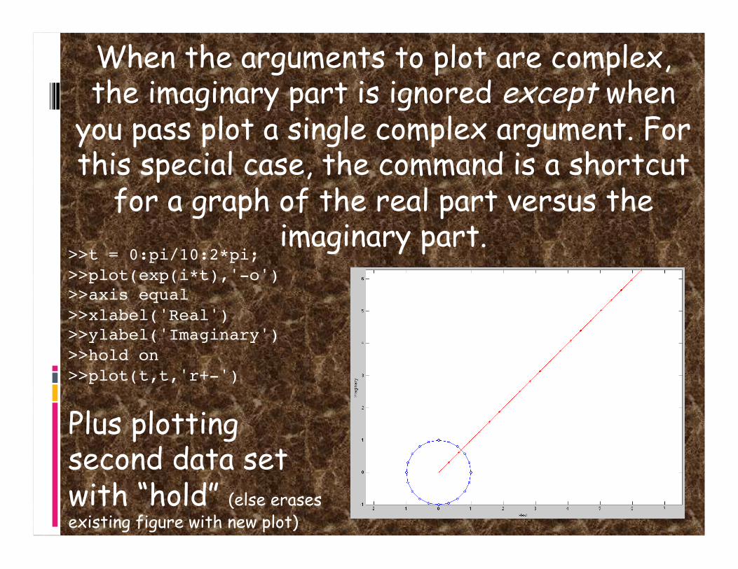
When the arguments to plot are complex, the imaginary part is ignored except when

you pass plot a single complex argument. For this special case, the command is a shortcut

for a graph of the real part versus the imaginary part.

>>t = 0:pi/10:2*pi; >>plot(exp(i*t),'-o') >>axis equal >>xlabel('Real') >>ylabel('Imaginary') >>hold on >>plot(t,t,'r+-')

Plus plotting second data set with “hold” (else erases existing figure with new plot)

Figure Handling

Graphing functions automatically open a new figure window if there are no figure windows

already on the screen.

If a figure window exists, it is used for graphics output (and clobbers what’s there if

hold is off).

The default is to graph to the current figure (usually the last active figure)

To create a new figure without overwriting the old, use the figure command

When multiple figures already exist, you can set one of them to the current figure with

the command figure(n) where n is the number at the top of the figure window.

>> plot(x,seis,x,seis2) >> legend('Raw','Mean Removed') >> figure %creates 2 >> plot(seis,'r') >>figure(1) %makes 1 current

1 2

3 4

Creating subplots

The subplot command enables you to display multiple plots in the same window or print

them on the same piece of paper. t = 0:pi/10:2*pi; [X,Y,Z] = cylinder(4*cos(t)); subplot(2,2,1); mesh(X) subplot(2,2,2); mesh(Y) subplot(2,2,3); mesh(Z) subplot(2,2,4); mesh(X,Y,Z)

%creates a 2 x 2 matrix of %subplots

>> help cylinder CYLINDER Generate cylinder. [X,Y,Z] = CYLINDER(R,N) forms the unit cylinder based on the generator curve in the vector R. Vector R contains the radius at equally spaced points along the unit height of the cylinder. The cylinder has N points around the circumference. SURF(X,Y,Z) displays the cylinder. [X,Y,Z] = CYLINDER(R), and [X,Y,Z] = CYLINDER default to N = 20 and R = [1 1]. Omitting output arguments causes the cylinder to be displayed with a SURF command and no outputs to be returned.

Controlling axes

The axis command provides a number of options for setting the scaling, orientation,

and aspect ratio of graphs.

Set the axis limits axis auto

axis([xmin xmax ymin ymax zmin zmax])

Set the axis aspect ratio axis auto normal

axis square; axis equal

The axis command provides a number of options for setting the scaling, orientation,

and aspect ratio of graphs.

Set axis visibility axis on; axis off

Set grid lines grid on; grid off

axis vs axes >> help axis AXIS Control axis scaling and appearance. >> help axes AXES Create axes in arbitrary positions.

>> figure(2) >> plot(seis2) >> axis([6500 10500 -4000 4000])

>> axis auto >> plot(seis2(6500:10500,:),'r')

Overlaying new graphs Use the command hold on to overlay different types of plots on one another >>[x,y,z] = peaks; >>pcolor(x,y,z) >>shading interp >>hold on >>contour(x,y,z,20,'k') >>hold off

>> surf(x,y,z) >> clf >> [x y z]=peaks; >> surf(x,y,z) >> shading interp

Saving & Exporting Graphics

The default graphics file is a MATLAB Figure or .fig formatted file.

This format retains the most data about how it was created within matlab it is not

particularly portable

you can also save as eps (encapsulated postscript), which can be read by Illustrator

or you can save in one of the picture formats like tiff and jpg which do not allow additional

editing but maintain good resolution

Cool Feature

After creating the perfect figure, you can generate an m-file so that the figure can be recreated using different data in the future.

This feature is found under the File drop down

menu in the Figure toolbar.

Advanced graphics: Handle graphics.

Handle graphics provides a rich set (i.e. powerful,

difficult and confusing) of functions and properties for generating imagery using Matlab.

>> x=1:10; >> y=x; >> h=plot(x,y,'*-’) h = 171.0034 >>

Notice the output, saved in “h”, from the plot command. “h” is a number that identifies the “handle” for the graphics object created

by the plot command.

>> get(h) DisplayName: '' Annotation: [1x1 hg.Annotation] Color: [0 0 1] LineStyle: '-' LineWidth: 0.5000 Marker: '*' MarkerSize: 6 MarkerEdgeColor: 'auto' MarkerFaceColor: 'none' XData: [1 2 3 4 5 6 7 8 9 10] YData: [1 2 3 4 5 6 7 8 9 10] ZData: [1x0 double] BeingDeleted: 'off' ButtonDownFcn: [] Children: [0x1 double] Clipping: 'on' CreateFcn: [] DeleteFcn: []

BusyAction: 'queue' HandleVisibility: 'on' HitTest: 'on' Interruptible: 'on' Selected: 'off' SelectionHighlight: 'on' Tag: '' Type: 'line' UIContextMenu: [] UserData: [] Visible: 'on' Parent: 170.0012 XDataMode: 'manual' XDataSource: '' YDataSource: '' ZDataSource: ''

>>

To view the information associated with the handle for the plot, use the get function.

This displays all of the properties of the line we just plotted.

>> help get GET Get object properties. V = GET(H,'PropertyName') returns the value of the specified property for the graphics object with handle H. If H is a vector of handles, then get will return an M-by-1 cell array of values where M is equal to length(H). If 'PropertyName' is replaced by a 1-by-N or N-by-1 cell array of strings containing property names, then GET will return an M-by-N cell array of values.

GET(H) displays all property names and their current values for the graphics object with handle H.

V = GET(H) where H is a scalar, returns a structure where each field name is the name of a property of H and each field contains the value of that property.

Most of the properties can be changed using the set function (a few are read-only).

>> set(h,'color',[1 0 0])

If you need to change a lot of values, this will improve your typing skills even more than

GMT

Assigning a graphic’s object to a variable simplifies modifying the object after

creation, but there are also ways to access a graphics object even if you forget.

Access to recently plotted/accessed objects is provided through pre-defined variables

gcf (handle to current figure (get current figure)),

gca (handle to current axis (get current axis)) and

gco (handle to current object (get current object), which is almost always graphics object

created as result of last graphics command).

>> f=get(gcf) f = Alphamap: [1x64 double] BeingDeleted: 'off' BusyAction: 'queue' ButtonDownFcn: '' Children: 170.0044 Clipping: 'on' CloseRequestFcn: 'closereq' Color: [0.8000 0.8000 0.8000] Colormap: [64x3 double] CreateFcn: '' CurrentAxes: 170.0044 CurrentCharacter: '' CurrentObject: [] CurrentPoint: [0 0] DeleteFcn: '' DockControls: 'on' FileName: '' HandleVisibility: 'on' HitTest: 'on' IntegerHandle: 'on' Interruptible: 'on' InvertHardcopy: 'on' KeyPressFcn: '' KeyReleaseFcn: '' MenuBar: 'figure' Name: '' NextPlot: 'add' NumberTitle: 'on' PaperOrientation: 'portrait' PaperPosition: [0.2500 2.5000 8 6] PaperPositionMode: 'manual' PaperSize: [8.5000 11]

PaperType: 'usletter' PaperUnits: 'inches' Parent: 0 Pointer: 'arrow' PointerShapeCData: [16x16 double] PointerShapeHotSpot: [1 1] Position: [1029 583 560 420] Renderer: 'painters' RendererMode: 'auto' Resize: 'on' ResizeFcn: '' Selected: 'off' SelectionHighlight: 'on' SelectionType: 'normal' Tag: '' ToolBar: 'auto' Type: 'figure' UIContextMenu: [] Units: 'pixels' UserData: [] Visible: 'on' WindowButtonDownFcn: '' WindowButtonMotionFcn: '' WindowButtonUpFcn: '' WindowKeyPressFcn: '' WindowKeyReleaseFcn: '' WindowScrollWheelFcn: '' WindowStyle: 'normal' XDisplay: '/tmp/launch-GGBpjE/:0' XVisual: '0x24 (TrueColor, depth 24, RGB mask 0xff0000 0xff00 0x00ff)' XVisualMode: 'auto’ >>

Use get function with predefined variables to get parameters.

And set function with predefined variables to set parameters.

>> set(gcf, 'Units', 'Inches');

As with GMT you have to know all the values (you can get the property names from the get function), no cheating with menus, etc.

Modified from mathworks matlab documentation web pages

MATLAB assigns a handle to every graphics object it creates. All object creation

functions optionally return the handle of the created object.

If you want to access the object's properties (e.g., from an M-file), assign its

handle to a variable at creation time to avoid searching for it later.

If you forget to assign the handle when you plot the figure, you can always obtain the

handle of an existing object with the findobj function or by listing its parent's Children

property.

Special Object Handles

The root object's handle is always zero.

The handle of a figure is either:

- An integer

- A floating point number requiring full MATLAB internal precision

The figure property IntegerHandle controls the type of handle the figure receives.

All other graphics object handles are floating-point numbers.

You must maintain the full precision of these numbers when you reference handles.

(The “full precision” condition means means you cannot read handles off the screen [usually

an approximation to the actual floating point value in memory] and retype them, you must store the value in a variable and pass that variable whenever

MATLAB requires a handle).

The Current Figure, Axes, and Object

An important concept in the Handle Graphics technology is that of being current.

The current figure is the window designated to receive graphics output.

Likewise, the current axes is the target for commands that create axes children.

The current object is the last graphics object created or clicked on by the mouse.

MATLAB stores the three handles corresponding to these objects in the

ancestor's property list.

Relationship between various objects is hierarchical.

As you work with higher-dimensional plots, or figures with lots of plots on top of each

other, the set of handles can seem a little unwieldy.

Fortunately, the set of handles for each figure are nicely organized in a parent-child

hierarchy.

The figure handle is at the top.

It’s child is the axes.

To see this, type the command get(gcf,’Children’) and compare the result to just typing gca.

We could also discover that the figure is the parent by typing get(gca,’Parent’) and

comparing the result to just typing gcf.

The axes are in turn the parent of each plot, and also of the xlabel, ylabel,

and title.

At this point one is tempted to wonder why all this matters... the important result here

is that we can find handles that we did not store in variables

when the object was created.

clear all % clears the variable space close all % closes all figures x1 = linspace(0,2*pi,1000); y1 = sin(x1); y2 = sin(x1)./x1; x2 = linspace(0,2*pi,9); y3 = sin(x2); y4 = sin(x2)./x2; figure(2) % opens a new figure with %ID 2, or goes to figure 2 if open p1 = plot(x1,y1,'color','b'); hold on; p2 = plot(x1,y2,'color','r'); p3 = plot(x2,y3,'-o','color','c'); p4 = plot(x2,y4,'-s','color','m'); hold off; set(gca,'XLim',[0 2*pi],'XTick',[0:pi/2:2*pi],'XGrid','on'); set(gca,'XTickLabel',{'0','p/2','p','3p/2','2p'},'FontName','Symbol','FontSize',12) xlabel('$\theta$ [rad]','FontSize',14,'Interpreter','latex') ylabel('$f(\theta)$','FontSize',14,'Interpreter','latex') title('Plots of $f_1(\theta) = sin(\theta)$ and $f_2(\theta) = \frac{sin(\theta)}{\theta}$',... 'FontSize',16,'FontWeight','b','Interpreter','latex'); l1 = legend([p1,p2,p3,p4],'f_1','f_2','f_1 undersampled','f_2 undersampled',1); set(l1,'FontName','Helvetica')

[AX,H1,H2]=plotyy(rt,gt,r,pofr); grid set(get(AX(1),'Ylabel'),'String','g(r) m/sec^2') set(get(AX(2),'Ylabel'),'String','p(r) km/m^3') xlabel('distance from center of earth, km') title('density and gravity of earth’)

Plotting and labeling multiple

axes. Two sets x and y vectors.

[AX,H1,H2]=plotyy( rt, [gt; rt.*([g(end)/… r(end)*ones(1,length(r)) repmat(NaN,1,length(ro))])],r,… [m; mpave]); set(get(AX(1),'Ylabel'),'String','g(r) m/sec^2 as function of radius for uniform density sphere and earth') set(get(AX(2),'Ylabel'),'String','m in kg as function of radius for uniform density sphere and earth') xlabel('distance from center of earth, km') title('mass distribution and gravity of uniform density sphere versus earth') set(H1,'LineStyle','--') set(H2,'LineStyle',':')

Plotting multiple functions on same axes. Multiple y

vectors for each x.