lyapunov optimizing sliding mode control for robot ... … · lyapunov optimizing sliding mode...

Applied Mathematical Sciences, Vol. 7, 2013, no. 63, 3123 - 3139HIKARI Ltd, www.m-hikari.com

Lyapunov Optimizing Sliding Mode Control

for Robot Manipulators

Chutiphon Pukdeboon

Department of MathematicsFaculty of Applied Science

King Mongkut’s University of TechnologyNorth Bangkok, Thailand

[email protected]

Abstract

This paper studies the robust optimal control problem for robottracking system. An optimal sliding mode control law is designed tosolve this problem. Integral sliding mode control is employed to combinethe first-order sliding mode with optimal control approach and is appliedto robust control of robot manipulators. For the optimal control part,the Lyapunov optimizing control method is used to solve the finite-timenonlinear optimal control problem. The second method of Lyapunov isused to show that tracking is achieved globally. A case study of two-linkrobot model is presented to demonstrate the usefulness of the developedapproach.

Mathematics Subject Classification: 93D05; 93D09; 49K99

Keywords: Robot tracking control, Lyapunov optimizing sliding modecontrol, minimum cost descent control, descent function, integral sliding modecontrol

1 Introduction

Optimal control theory involves the design of controllers that can satisfy someobjective while simultaneously minimizing some cost. It has shown that astandard dynamic programming approach reduces the optimal control prob-lem to the Hamilton-Jacobi-Bellman (HJB) partial differential equation. Inother word, to solve optimal control problems is equivalent to solve the HJBequation. However it is very complicate to solve the HJB equation for nonlin-ear dynamic systems. A common technique to develop an optimal control for a

3124 Chutiphon Pukdeboon

nonlinear system is to suppose that the nonlinear dynamics are exactly knownand then feedback linearization can be performed. Optimal control techniqueswere applied to the linearized system as in [1]-[3]. A review of the optimalityof nonlinear design schemes and general results involving feedback lineariza-tion, Jacobian linearization and other nonlinear design approaches are givenin [4], [5]. In [6]-[8] dynamic programming method was employed to obtain theminimum-time optimal trajectories. In [9]-[10] control algorithms for the ro-bust control of robot manipulators were also designed. Johansson [11] appliedthe special coordinate transformation for quadratic optimal control of robotmanipulators. In [12] the Hamiltonian optimization method was employedto deal with robot manipulators. Inverse optimal control is an alternative ap-proach to solve the nonlinear optimal control problem without the need to solvethe HJB equation [13]-[14]. By finding a control Lyapunov function (CLF),which can be shown to also be a value function, an optimal control can be de-signed that optimizes a derived cost. However, for practical implementationswe have to prove that there exists a CLF for a individual nonlinear system.This is usually the most difficult step in the whole design process.

Another effective method to solve the nonlinear optimal control problem bycircumventing the need to solve the HJB equation is based on Lyapunov theory.It is well-known that Lyapunov’s second method has been extended to developcontrollers for linear and nonlinear systems. One such controller is Lyapunovoptimizing control (LOC) that offers feedback controls by selecting a candi-date Lyapunov function and choosing the control to minimize this Lyapunovfunction as much as possible along system trajectories [15]-[17]. Supposingthat the target is the origin, if the candidate Lyapunov function is decreasedeverywhere outside the origin, a sufficient condition for asymptotic stabilityis satisfied [15]. In addition, the LOC approach provides an algorithm to de-sign feedback controllers where cost accumulation is considered explicitly. Onthe other hand, a trajectory-following optimization (TFO) method is based onsolving continuous differential equations, whose equilibrium solutions satisfythe necessary conditions for a minimum or maximum. Any problems that aredifficult to solve by other methods can be solved by trajectory following ap-proaches [15]. However, this technique has not been investigated for nonlinearmodels of real-life problems.

In this research the LOC approach and the TFO concept [18]- [20] aremerged to develop a novel optimal controller. A new optimal sliding modecontrol is also obtained by using integral sliding mode (ISM) concept [21], [22]to combine the first-order sliding mode with the developed optimal controller.The aim is to zero the state of the system, while considering some state depen-dent cost. A variant of LOC known as minimum cost descent control (MCDC)presented in [15] is used to derive a suboptimal controller for rigid robot sys-tems. This control algorithm offers the asymptotic stability of the origin and

Lyapunov optimizing sliding mode control 3125

minimizes the given cost functional.This paper is organized as follows. In Section 2 the manipulator dynamics

([23], [24]) and problem formulation are described. In Section 3 the controlobjective is given. Section 4 presents basic concepts of the LOC approach todevelop the optimal controller. The MCDC approach and TFO concept areemployed to produce an optimal tracking control law of robot manipulators.Section 5 proposes a robust optimal controller design based on the ISM con-cept. The sliding manifold is chosen and a control law is designed such that thestability of closed-loop system is achieved. In Section 6 a numerical example ofa two-link robot manipulator is presented and simulation results are includedto demonstrate the performance of the developed controller. In Section 7 wepresent conclusions.

2 Description of the robot manipulator

Consider the following general robot system model [23], [24]

M(q)q + C(q, q)q + G(q) = τ + τd, (1)

where q, q, q ∈ Rn are the vectors of joint angular position, velocity andacceleration, respectively. M(q) ∈ Rn×n denotes the generalized inertia ma-trix, C(q, q) ∈ Rn×n and C(q, q)q are the vectors of centrifugal and Coriolistorques, G(q) ∈ Rn is the vector of gravitational torques, τ ∈ Rn is the vectorof applied joint torque.

For the subsequent development we assume that q(t) and q(t) are mea-surable and that M(q), C(q, q), G(q) and τd are unknown. Furthermore, thefollowing assumptions are required in the further development.

Assumption 2.1. The inertia matrix M(q) is symmetric and uniformlypositive definite, and satisfies the following inequality ∀ϑ(t) ∈ Rn:

m1‖ϑ‖2 ≤ ϑT M(q)ϑ ≤ m(q)‖ϑ‖2, (2)

where m1 ∈ R is a known positive constant, m(q) ∈ R is a known positivefunction, and ‖ · ‖ denotes the standard Euclidean norm.

Assumption 2.2. The following skew-symmetric relationship is satisfied:

ϑT (M(q) − 2C(q, q))ϑ = 0, ∀ϑ(t) ∈ Rn. (3)

Assumption 2.3. Let qd(t), qd(t) and qd(t) be the desired position, de-sired velocity and desired acceleration, respectively. The vectors qd(t), qd(t), qd(t) ∈Rn are exist and bounded.

Assumption 2.4. The nonlinear disturbance term τd satisfies ‖τd‖ ≤ D,where D is a positive constant.


3 Control objective

The control objective is to guarantee that the robot system in the presence ofa general disturbance tracks a desired trajectory qd ∈ Rn, while minimizing agiven performance index. Let us define a position tracking error e1(t) ∈ Rn as

e1 = qd − q. (4)

To facilitate the subsequent analysis, a filtered tracking error, denoted by e2(t)is also defined as

e2 = e1 + αe1, (5)

where α ∈ Rn×n denotes a subsequently defined positive definite, constant,gain matrix.

We next use the method in [25] to develop a state-space model based ontracking errors (4) and (5). The inertia matrix is premultiplied by the timederivative of (5), and substitutions are made from (1) and (4) obtain

Me2 = −C(q, q)e2 − τ + h + τd, (6)

where the nonlinear function h(q, q, qd, qd, qd) ∈ Rn is defined as

h = M(qd + αe1) + C(qd + αe1) + G (7)

Under the assumption that the dynamics in (1) are known, the control inputcan be designed as

τ = h + τd − u, (8)

where u ∈ Rn is an auxiliary control input that will be designed to minimizea subsequent performance index. By substituting (8) into (6) the closed-looperror system for e2 can be obtained as

Me2 = −C(q, q)e2 + u. (9)

A state-space model for (5) and (6) can be written as

z = A(q, q)z + B(q)u, (10)

where A(q, q) ∈ R2n×2n, B(q) ∈ R2n×n and z(t) ∈ R2n are defined as

A(q, q) =

[ −α In×n

0n×n −M−1C

], B(q) =

[0n×n

M−1

]and z(t) =

[e1

e2

]. (11)

Here, In×n and 0n×n denote an n × n identity matrix and matrix of zeros,respectively.


4 Lyapunov optimizing controller

In this section the LOC approach using TFO [15] is used to solve the finite-timenonlinear optimal control problem. For the LOC method, feedback controls areproduced by selecting a candidate Lyapunov function and choosing the con-trol to minimize this Lyapunov function as much as possible along the systemtrajectories [15]. The advantage of LOC algorithms is that they offer feedbackcontrol laws where cost accumulation is explicitly considered. However, themain drawback in utilizing LOC methods is that it may be difficult to guar-antee that the candidate Lyapunov function decreases everywhere outside theorigin. If this is the case, the necessary conditions for asymptotic stability arenot satisfied.

For the optimal controller design the control strategy design [16] for non-linear systems is presented. This control combines LOC with TFO and is usedto zero the state of the system, while considering some state dependent cost.In [16] the state-augmented control descent (SACD) algorithm was developedand an adaptation of the Newton optimization method [16] was used for thecontroller design for nonlinear systems, when a proper necessary condition issatisfied.

Next, some fundamental theories of LOC and TFO in [15] are restated.

4.1 Minimum cost descent control

Consider the general nonlinear control system

x = f(x, u), (12)

where x(t) ∈ Rn, u ∈ Rm and f(·) ∈ Rm is assumed to be C1 (continuous andcontinuously differentiable). Let a specific target set χ be defined by a systemof z equalities

χ = {x|g(x) = 0},with g(x) = [g1(x) . . . gz(x)]T assumed to be continuous and continuouslydifferentiable. With a control u ∈ U ⊆ Rm, the controllable set C to thetarget set χ is defined as the set of all initial states that can be transferredto the target in finite time using some admissible control law. The feedbackcontrollers require that the state of the system (12) be driven to a target setχ and minimize a cumulative cost functional

J [u(·)] =

∫ tf

0

f0(x, u)dt, (13)

where tf is the time at which the state reaches the target x(tf ) ∈ χ. NowLyapunov optimizing feedback controls that consider a cost associated with


transferring the state to a target are investigated. At time t let

x0(t) =

∫ t

0

f0(x, u)dt (14)

denote the accumulated cost along a trajectory of (12) and the initial conditionis x0(0) = 0. Let W (x) be a descent function for the target χ and let

W0 = x0 + W (x)

be an augmented descent function. It follows that

W0 =∂W

∂x0x0 +

∂W (x)

∂xx = f0(x, u) +

∂W (x)

∂xf(x, u). (15)

A control u ∈ U is a minimum cost descent control [15] if at each state x inthe controllable set C to the target χ, the control minimizes W0.

A continuous-time trajectory-following algorithm may be implemented byusing Newton’s method [15]. In Newton’s method we have

∂2Ψ

∂u2u = −

[∂Ψ

∂u

]T

, (16)

which implies

u = −(

∂2Ψ

∂u2

)−1 [∂Ψ

∂u

]T

(17)

provided ∣∣∣∣∂2Ψ

∂u2

∣∣∣∣ �= 0. (18)

Note that an implementation of Newton’s method for designing LOC in [16]will be given later.

4.2 State-augmented control descent algorithm

The SACD algorithm [16] was developed to design a suboptimal controller fornonlinear systems. Let the descent function for the general optimal controlproblem be denoted by W (x). Using the concepts in [16] suboptimal controlupdates are specified by selecting a descent function W (x), corresponding to anapproximate function W0 = x0 + W (x), and minimizing the function W0 withrespect to u. Consider the control minimizing W0. It satisfies the necessarycondition [

∂W0

∂u

]T

= 0 (19)


at each point along the state trajectory, if u is interior to U . Any u-equilibriumresulting from trajectory-following control updates should satisfy (19) [16].The control strategy and W0 must include a term such that the state is trans-ferred to the target set. This requires that an augmented descent function W0

decreases along the system trajectories, i.e.

W (x) → 0 as t → ∞. (20)

In addition W0 now will contain a possibly nonlinear cost term f0.

4.3 Implementation of Newton’s method

Here an implementation of Newton’s method by McDonald [16] is presented.An update u was derived by applying Newton’s method to (19) yielding theSACD algorithm. Next the algorithm in [16] to obtain the formula for gener-ating u is stated. In view of (19) and (20)

σ =

[∂W0

∂u

]T

(21)

goes to zero as t → ∞.We next apply Newton’s method to obtain an update u. By letting Ψ = W0

and substituting into (17), we have

u = −(

∂2W0

∂u2

)−1 [∂W0

∂u

]T

. (22)

The time derivative of σ can be written as

σ =∂σ

∂uu

=

(∂2W0

∂u2

)u. (23)

Using (23) and (21), (22) becomes

σ = −σ. (24)

We have

σ =∂σ

∂xx +

∂σ

∂uu, (25)

where we let

∂σ

∂x=

∂2W0

∂x∂u(26)


and

Ψu =∂σ

∂u=

∂2W0

∂u2. (27)

Using (24) u can be written as [17]

u = −Ψ−1u [σ + σ]. (28)

If Ψu(x, u) is nonsingular along the state trajectory, the equilibrium will occurwhen the necessary condition (19) is satisfied, i.e., σ = 0.

4.4 Control law

We consider a feedback controller minimizing the performance index

I =

∫ tf

0

(zT Qz + uTRu)dt (29)

where

z = f(z, u), z(0) = z0 (30)

and

f(z, u) =

[ −αz1 + z2

−M−1Cz2 + M−1u

]. (31)

Using the same idea of the descent function presented in [17], the candidatedescent function is selected as

W (z) =1

2

[c1z

T1 Kz2 + 2c2z

T1 Mz2 + c3z

T2 Mz2

], (32)

where K ∈ Rn×n denotes a positive definite symmetric gain matrix. Takingthe first time derivative of W (z), we obtain

W (z) =∂W

∂zf(z, u)

=

[c1z

T1 K + c2z

T2 M

c2zT1 M + c3z

T2 M

]T [ −αz1 + z2

−M−1Cz2 + M−1u

],

which yields

W (z) = (c1zT1 K + c2z

T2 M)(−αz1 + z2)

+(c2zT1 M + c3z

T2 M)(−M−1Cz2 + M−1u). (33)


Thus the time derivative of the augmented descent function W0 can bewritten as

W0 = f0(z, u) +∂W

∂zf(z, u)

=1

2(zT Qz + uT Ru) + W (z)

=1

2

([z1

z2

]T

Q

[z1

z2

]+ uT Ru

)+ W (z). (34)

With W0 we calculate

σ =

[∂W0

∂u

]T

= Ru + [zT1 c2 + zT

2 c3]T

= c2z1 + c3z2 + Ru. (35)

It follows that

σ =∂σ

∂zz +

∂σ

∂uu

=

[c2

c3

]T [ −αz1 + z2

−M−1Cz2 + M−1u

]+ Ru

= −c2αz1 + c2z2 − c3M−1Cz2 + c3M

−1u + Ru (36)

and

Ψ−1u =

[∂σ

∂u

]−1

= R−1. (37)

Using (28), the resulting SACD control strategy is

u = −R−1[c2z1 + c3z2 + Ru − c2αz1 + c2z2

−c3M−1Cz2 + c3M

−1u + Ru]

= −R−1[c2z1 + c3z2 + Ru − c2αz1 + c2z2

−c3M−1Cz2 + c3M

−1u] − u,

which yields

u = −0.5R−1[c2z1 + c3z2 + Ru − c2αz1 + c2z2

−c3M−1Cz2 + c3M

−1u]. (38)

Evidently with the necessary condition (19) the resulting suboptimal con-trol law can be obtained from (38). Substituting this control law into (40), weobtain LOISMC.


5 Robust optimal controller design

To exactly suppress the disturbance and uncertainties of the system (6) andguarantee that control objectives are fulfilled, the developed LOC controller iscombined with sliding mode control by using the ISM concept. The proposedcontrol is expressed as the sum of an optimal controller and a compensatedcontroller. Using the ISM control technique, the control law consists of twoparts. The first one is optimal control, which is continuous and is used tostabilize the closed-loop system of the spacecraft in finite time. For the secondpart a first-order SMC is applied to yield system robustness against parametervariations and external disturbances for t > 0 and to ensure that controlobjectives are achieved. We use the ISM concept to obtain the sliding manifoldand a new robust optimal control law is then developed. The second methodof Lyapunov is used to show that reaching and sliding on the manifold areguaranteed.

Consider a nonlinear dynamic system

x = f(x) + b(x)u + ξ (39)

where x ∈ n is the state, u ∈ m denotes the control input, f(x) and b(x)are sufficiently smooth vector fields. ξ represents an unknown function, whichrepresents the system uncertainties. For the robot model (6), let δ = h+τd andAssumptions 2.1-2.4 hold. Then, we know that there exists an unknown δ suchthat ξ can be written as ξ = b(x)δ and γi = supt≥0(|δi(t)|), i = 1, 2, 3, . . .m.

The objective of this paper is to design a robust optimal sliding modecontroller so that the uncertain nonlinear system has both optimal performanceand robustness to the system uncertainties. Applying the integral sliding modecontrol concept we obtain an optimal sliding mode controller [21]

u = υ∗ − μϑi (40)

where υ∗ is the optimal control input that was defined in Section 4, μ =diag[μ1 μ2 . . . μm]T ∈ Rm×m is a positive definite diagonal matrix, andthe ith component of ϑ is given by

ϑi = sat(si, εi), i = 1, 2, 3, . . .m (41)

and

sat(si, εi) =

⎧⎨⎩

1 for si > εi

si/εi for |si| ≤ εi

−1 for si < −εi

Using the method in [22] we now define the function g(x) : n → m asa linear combination of the system state. The time derivative of g(x) can bewritten as

g(x) = gx(x)x, (42)


where gx(x) = ∂g(x)∂x

∈ m×n represents the Jacobian matrix. The system is inthe sliding manifold at the initial time instant. In this paper, we assume thatgx(x) is defined such that gx(x)b(x) is nonsingular.

Based on the ISM control approach, the sliding manifold is designed as [22]

s = g(x) − φ, (43)

where the integral term φ is

φ = g(x0) +

∫ t

t0

gx(x)(f(x) + b(x)υ∗)dτ (44)

Now we show that the control law (40) is designed such that the reachingand sliding mode conditions are satisfied. The candidate Lyapunov is selectedas

V =1

2sT s (45)

and the time derivative of V is

V = sT s

= sT (gx(x)x − φ) (46)

With the substitution of x and φ we obtain

V = sT gx(x)[f(x) + b(x)u] − sT [gx(x)(f(x) + b(x)υ∗] (47)

With external disturbances and the optimal control υ∗, the control law (40)can be written as

u = u1 + υ∗ + δ (48)

Substituting (48) into (47), the time derivative of V can be written as

V = sT gx(x) (f(x) + b(x)u)

−sT [gx(x) (f(x) + b(x)u − b(x)u1 − b(x)δ)]

= sT (gx(x)b(x)[δ + u1]) (49)

Let the discontinuous control input u1 have the following form

u1 = −μsign(s) (50)

where sign(s) = [sign(s1) sign(s2) . . . sign(sm)]T . We now obtain

V = sT (gx(x)b(x)[δ − μsign(s)]) (51)

which can be further written as

V ≤ −m∑

i=1

(μi − γi)‖si‖‖gx(x)b(x)‖ (52)

Obviously if μi is chosen such that μi > γi then V < 0. This guaranteesreaching and sliding on the manifold.


6 Simulation Results

An example of a two-link robot manipulator [26] is presented with numericalsimulations to verify the performance of the developed controller. The equationof motion of this robot system is defined as

[a11(q2) a12(q2)a12(q2) a22

] [q1

q2

]+

[−β(q2)q1 −2β(q2)q1

0 β(q2)q2

] [q1

q2

]

+

[ζ1(q1, q2)gζ2(q1, q2)g

]= τ + τd (53)

where

a11(q2) = (m1 + m2)r21 + m2r

22 + 2m1r1r2 cos(q2) + J1

a12(q2) = m2r22 + m2r1r2 cos(q2), a22 = m2r

22 + J2

β(q2) = m2r1r2 sin(q2)

ζ1(q1, q2) = (m1 + m2)r1 cos(q2) + m2r2 cos(q1 + q2)

ζ2(q1, q2) = m2r2 cos(q1 + q2). (54)

The parameter values are assigned as r1 = 1 m, r2 = 0.8 m, J1 = 5 kg-m,J2 = 5 kg-m, m1 = 0.5 kg, and m2 = 1.5 kg. The desired joint position signalsare given as

qd(t) =

[1.25 − 1.4e−t + 0.35e−4t

1.25 + e−t − 0.25e−4t.

]rad.

For the switching function (43) we choose the matrix g(x) = [I3×3 λI3×3]T

with λ = 1.2. The proposed control law is designed by using (40) with anoptimal control obtained from (38). The weighting matrices are chosen tobe Q = diag(1, 1, 5, 5) and R = diag(1, 1), For the descent function (32) thepositive scalars are chosen as c1 = 5.0, c2 = 1.5 and c3 = 5.0.

The initial conditions for the state are q(0) = [0.8 2.0]T and q(0) =[0 0]T . The external disturbance is

τd =

[0.2 sin(3t) + 0.02 sin(26π

t)

0.2 sin(3t) + 0.02 sin(26πt

)

]N-m.

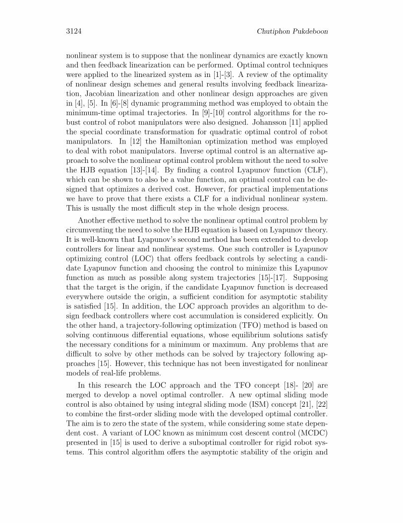
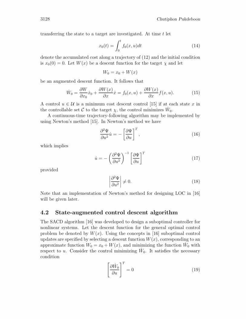
Figs. 1 and 2 shows tracking responses of joint 1 and 2 respectively. Thejoints are driven to their positions after 5 seconds. Obviously, the effect ofexternal disturbances on both responses is totally removed. As shown in Fig.3 the sliding vector is on the sliding manifold s = 0 at time zero and very closeto zero thereafter. From Fig. 4 it can be seen that the proposed controllerapproximates the harmonic curves which are limited to a steady state level.


Figure 1: Response of joint 1

Figure 2: Response of joint 2

7 Conclusion

A novel robust optimal feedback controller design based on the LOC methodand SMC concept has been successfully applied to the tracking control of robotmanipulators. To obtain this controller design, the sliding mode controller hasbeen combined with the optimal controller derived by using the LOC approach.For the optimal controller design, the LOC scheme has been employed to solve


Figure 3: Components of the sliding vector

Figure 4: Input torques of joint 1 and joint 2

the finite-time optimal control problem. The second method of Lyapunov isused to show that tracking is achieved and the asymptotic stability of theclosed-loop system is guaranteed. An example of a two-link robot manipulatoris presented and simulation results are included to verify the usefulness of theproposed controller.


Acknowledgements

This research was supported by Faculty of Applied Science, King Mongkut’sUniversity University of Technology North Bangkok under Grant No. 5642107.

References

[1] R. Freeman and P. Kokotovic, Optimal nonlinear controllers for feedbacklinearizable systems, in Proc. of the American Controls Conf., pp. 2722-2726, Jun. 1995.

[2] Q. Lu, Y. Sun, Z. Xu, and T. Mochizuki, Decentralized nonlinear optimalexcitation control, IEEE Trans. Power Syst., vol. 11, no. 4, pp. 1957-1962,Nov. 1996.

[3] M. Sekoguchi, H. Konishi, M. Goto, A. Yokoyama, and Q. Lu, Nonlinearoptimal control applied to STATCOM for power system stabilization, inProc. IEEE/PES Transmission and Distribution Conference and Exhibi-tion, pp. 342-347, Oct. 2002.

[4] V. Nevistic and J. A. Primbs, Constrained nonlinear optimal control: aconverse HJB approach, California Institute of Technology, Pasadena, CA91125, Tech. Rep. CIT-CDS 96-021, 1996.

[5] J. A. Primbs and V. Nevistic, Optimality of nonlinear design techniques:Aconverse HJB approach, California Institute of Technology, Pasadena, CA91125, Tech. Rep. CIT-CDS 96-022, 1996.

[6] K. G. Shin and N. D. Mckay, A dynamic programming approach to trajec-tory planning of robotic manipulators, IEEE Transactions on AutomaticControl, vol. 6, pp. 491-500, 1986.

[7] T. Balkan, A dynamic programming approach to optimal control ofrobotic manipulators, Mechanics Research Communication, vol. 25, pp.225-230, 1998.

[8] C. R. Dohrmann and R. D. Robinett, Robot trajectory planning via dy-namic programming, Proc. of the Fifth International Symp. on Roboticsand Manufacturing and Application, vol. 25, pp. 75-81, 1994.

[9] B. S. Chen and Y. C. Chang, Nonlinear mixed control for robust trackingdesign of robotic systems, International Journal of Control, vol. 67, no. 6,pp. 837-857, 1997.


[10] B. S. Chen, T. S. Lee and J. H. Feng , A nonlinear control design inrobotic systems, under parameter uncertainties and external disturbances,International Journal of Control, vol. 59, no. 2, pp. 439-461, 1994.

[11] R. Johansson, Quadratic optimization of motion coordination and control,IEEE Transactions on Automatic Control, vol. 35, no. 11, pp. 1197-1208,1990. vol. 12, no. 2-3, pp. 97-115, 2002.

[12] Y. J. Choi, W. K. Chung and Y. Youm, Robust control of manipula-tors using Hamiltonian optimization, Proc. IEEE Trans. Inter. Conf. onRobotics and automation, pp. 2358-2346, 1997.

[13] M. Krstic and H. Deng, Stabilization of Nonlinear Uncertain Systems.Springer, 1998.

[14] M. Krstic, and Z. H. Li, Inverse optimal design of input-to-state stabilizingnonlinear controllers, IEEE Transactions on Automatic Control, vol. 43,no. 3, pp. 336-350, 1998.

[15] T. L. Vicent and W. J. Grantham, Nonlinear and Optimal Control Sys-tem, Wiley, N.Y. 1997.

[16] D. B. McDonald, Feedback control algorithms through Lyapunov opti-mizing control and trajectory following optimization, Ph.D. Dissertation,Mechanical and Material Engineering, Washington State University, Pull-man, WA, 2007.

[17] McDonald, D. B., Quickest descent control of nonlinear systems withsingular control chatter elimination, Proceedings of the 2008 IAJC-IJMEConference, Nashville, TN, USA, 17-19 November, 2008.

[18] Grantham, W. J., Trajectory following optimization by gradient trans-formation differential equations, Proc. 42nd IEEE Conf. on Decision andControl, Maui, HI, December 2003;5496-5501.

[19] A. Jameson, Gradient Based Optimization Methods, MAE Technical Re-port No. 2057, Princeton University, 1995.

[20] J. T. Betts, Survey of numerical methods for trajectory optimization,Journal of Guidance, Control, and Dynamics, vol. 21, no. 2 pp. 193-207,1998.

[21] V. I. Utkin and J. Shi, Integral sliding mode in systems operating un-der uncertainty conditions, Proceedings of the 35th IEEE Conference onDecision and Control, Kobe, Japan, 1996.


[22] M. Rubagotti, A. Estrada, F. Castanos, A. Ferrara and L. Fridman, Op-timal disturbance rejection via integral sliding mode control of uncertainsystem in regular form, International Workshop on Variable StructureSystems, Mexico City, Mexico, 26-28 June, 2010.

[23] M. W. Spong, and Vidyasagar M., Robot Dynamics and Control, Wiley ,New York, 1989

[24] H. G. Sage, D.M.F Mathelin and E. Ostertag, Robust control of robotmanipulators: a survey, Int. J. Control, Vol. 72, No. 16, pp. 1948-1522,1999.

[25] K. Dupree, P. M. Patre, Z. D. Wilcox and W E. Dixon, Asymptotic opti-mal control of uncertain nonlinear Euler-Lagrange systems, Automatica,vol. 47, no. 1, pp. 99-107, 2011.

[26] Y. Feng, X. Yu and Z. Man, Adaptive fast terminal sliding mode trackingcontrol of robotic manipulator, Proceedings of the 40th IEEE Conferenceon Decision and Control, Orlando, Florida USA, December, 2001.

Received: March 14, 2013

lyapunov optimizing sliding mode control for robot ... … · lyapunov optimizing sliding mode...

Documents