lyapunov-basedcontrolstrategiesforthe ......right: deployed from hmas newcastle. 1.1. thesis...
TRANSCRIPT

Lyapunov-based Control Strategies for theGlobal Control of Symmetric VTOL UAVs
RohinWood
school of mechanical engineeringThe University of Adelaide
South Australia 5005Australia
A thesis submitted in fulfillment of the requirements for the degreeof Ph.D. in Mechanical Engineering on the 28th of June 2007.
Qualified on the 3rd of December 2007.

CHAPTER 1
Introduction
Vertical take-off and landing (VTOL) vehicles offer significant advantages overtheir conventional take-off and landing counterparts. In particular, the operation ofsuch vehicles are not restricted by runway space. Furthermore, such vehicles havethe ability to travel arbitrarily slowly, and in many cases maintain hover. It is thispart of the VTOL flight envelope that is most advantageous as it enables observationand interaction with stationary objects. Typical examples of such vehicles includehelicopters and VTOL jets. More recently, much effort has been focused toward thedevelopment of small scale VTOL, unmanned aerial vehicles (UAVs) commonly re-ferred to as mini and micro-VTOL UAVs. As these vehicles are unmanned, satisfac-tory operation often requires that their control be fully autonomous.
The autonomous control of VTOL vehicles is a nontrivial task, due to the com-plexity of the systems’ dynamics. Specifically, the differential equations describing thedynamics of such vehicles are heavily nonlinear and under-actuated. Furthermore, in-put coupling present in most vehicles results in the dynamics being non-minimumphase. Aerodynamic models of such vehicles also tend to be heavily nonlinear, com-plex and poorly known due to the exotic geometries, typical of such vehicles. Themost common control design approach for VTOL vehicles involves the design of twocascaded control loops. Firstly, a control loop providing high-speed tracking of atti-tude and heading commands is designed. This control-loop is commonly referred to asthe innerloop. Subsequent to this, a slower speed outerloop is designed for the controlof translational demands. Stability of the overall system relies a time-scale separa-tion between these control loops. In other words, the bandwidth of the innerloopmust be significantly greater than that of the outerloop. Consequently, such designarchitectures place an upper limit on the overall aggressiveness of these controllers,restricting the maneuverability of the vehicle. This limitation is a property of thedesign technique, and not of the system itself. Inner-outer loop designs are generallysufficient for the autonomous control of helicopters and VTOL jets as translationaldemands for such vehicles tend to be slow. However, micro-VTOL UAVs are designedfor use in clustered environments, and thus require high performance tracking controlof aggressive maneuvers.
Recently, much interest has surrounded the global stabilisation and tracking con-trol of VTOL vehicles via the use of nonlinear design methodologies. This has directlyfollowed the maturation of a number of Lyapunov-based nonlinear design tools, mostnotably feedback linearisation and backstepping. Early research on the topic focusedon a simplified, three degree of freedom (3DOF) representation of the system dubbedthe planar VTOL (PVTOL) vehicle. In many cases, the controllers developed for the
1

2 1. INTRODUCTION
3DOF system have then been extended for the control of full six degree of freedom
(6DOF) vehicle models. Most published PVTOL control designs focus on
overcoming the system’s non-minimum phase characteristics. Such approaches
include the use of minimum phase approximations, robust techniques and digital
model based methods. However, the most popular method involves the application of
a diffeomorphism to transform the system into an equivalent, minimum phase
representation. This idea was first discovered by demonstrating that changing the
outputs (or states) from translation at the PVTOL vehicle’s centre of gravity to its
center of percussion decoupled the system, making it differentially flat and
consequently minimum phase. This concept may be extended to decouple the 6DOF
system, in the special case where the vehicle has an axis of symmetry in the direction
of primary thrust. We refer to these systems as symmetric VTOL vehicles. A
significant number of symmetric VTOL vehicles currently exist. For example, a
growing number of VTOL UAVs are utilising a ducted fan-type arrangement
exhibiting such symmetry (see for example, Figure 1.1). Once decoupled, the
resulting triangular, cascade structure leads naturally to backstepping control designs.
One popular control technique that maintains the conceptual separation between inner
and outer control loops is to use a model-based backstepping control design for the
innerloop. The overall closed-loop dynamics consist of a cascade nonlinear system
describing vehicle translation (the outerloop) with an exponentially stable subsystem
describing vehicle orientation (the innerloop). This control architecture removes the
time-scale separation requirement, and cascade stability theory may be employed to
demonstrate global stability of the controlled system. Consequently, the controlled
system may perform arbitrarily aggressive maneuvers, the aggressiveness of which
are only bounded by physical actuator limitations.
NOTE: This figure is included on page 2 of the print copy of the thesis held in the University of Adelaide Library.
Figure 1.1. Symmetric VTOL UAV examples. Left: Bertin Technology’s LAAS-CNRS hovereye [60]. Right: Georgia Institute of Technology’s GTSpy [33]. The research documented within this thesis was commissioned by BAE Systems
Australia with the aim of investigating advanced flight control systems for the Nulka

1.1. THESIS OVERVIEW 3 Active Missile Decoy system (as pictured in Figure 1.2). The Nulka decoy system
protects naval ships from the threat of anti-ship missiles. The decoy system uses a
unique combination of hovering rocket flight vehicle and sophisticated electronic
warfare payload to attract enemy missiles away from the target ship [1]. This hovering
rocket flight vehicle is a prime example of a symmetric VTOL UAV*.
NOTE: This figure is included on page 3 of the print copy of the thesis held in the University of Adelaide Library.
Figure 1.2. The Nulka active missile decoy system. Left: Mid-flight. Right: Deployed from HMAS Newcastle.
1.1. Thesis overview The aim of this thesis is to explore nonlinear design techniques for symmetric VTOL
UAVs. In particular, focus is placed on Lyapunov-based control techniques that
produce globally stable, cascade, closed-loop structures. The following section
provides a brief outline of chapters presented in this thesis:
Chapter 2 presents the fundamental aspects of backstepping control, and reviews
current literature regarding Lyapunov-based control techniques for VTOL vehicles.
A detailed description of the system’s dynamics is also presented.
In Chapter 3, a nonlinear control technique for cascaded nonlinear systems with inputs
entering at different dynamic orders is presented. This control approach is inspired by
previously published work for the global stabilisation of the PVTOL system.
However, an additional innovation is proposed, involving the minimisation of a
weighted interconnection term between closed-loop subsystems. The idea is first
presented for a general class of systems, and then applied to the specific example of
the PVTOL system. Monte-Carlo simulations are used to demonstrate that minimising
the interconnection term results in faster convergence, yet less control action of the
closed-loop response. Furthermore, it is demonstrated that this idea is a generalisation
of previously published work involving the use of dynamic linearisation to decouple
the vehicle’s vertical dynamics. *Although motivated by the Nulka decoy system, all quantitative values specified throughout this thesis have no correlation
whatsoever to those of the Nulka Active Missile Decoy system. This is true with regard to both vehicle and trajectory parameters.
Where possible, dimensionless results are presented for generality.

4 1. INTRODUCTION
In Chapter 4, the nonlinear cascade control technique presented in Chapter 3 forthe PVTOL system is revisited. It is demonstrated that if care is not taken in de-sign, such cascade control laws will contain a singularity. This singularity is a directconsequence of feeding forward information into the innerloop, and has the potentialto cause unbound roll control demands. The most common approach to mitigate thisproblem is to embed saturation functions within the controller such that the singu-larity is never encountered. However, as this approach artificially saturates controlsignals it has the potential to limit controller aggressiveness. The primary innovationof Chapter 4 is to present an alternative technique that overcomes this singularityissue. Here, additional nonlinear dynamics are embedded within the control law suchthat the singularity may never occur. However, as saturation functions are avoided,controller aggressiveness is not compromised.
In Chapter 5 the ideas presented in Chapters 3 and 4 for the control of the 3DOFPVTOL system are extended for the control of 6DOF VTOL vehicles. To achievethis, control laws are formulated using an approximate backstepping approach. Thisapproach leads more naturally to tracking control designs that are presented in laterchapters. Rather than minimising an interconnection term between closed-loop sub-systems, the control law is designed to minimise a perturbation to an otherwise neg-ative definite control Lyapunov function derivative. The idea is however equivalentto that presented in Chapter 3, and parallels are drawn to demonstrate this. Con-sequently, the controlled system contains a singularity equivalent to that discussedin Chapter 4. However, the ideas presented in Chapter 4 for the mitigation of thissingularity are also extended to 6DOF.
Chapter 6 addresses trajectory tracking for VTOL UAVs. Whereas previous chap-ters only consider stabilisation at hover and thus ignore aerodynamic effects, thischapter addresses trajectory tracking at velocities where the influence of aerodynam-ics on the vehicle’s dynamics is significant. This chapter addresses the question ofhow the cascade control techniques discussed in previous chapters may be extendedto account for vehicle aerodynamics. The primary difficulty that the introduction ofaerodynamics introduces, is in the design of the outerloop. In particular, the atti-tude and heading demands that are to be fed from the outerloop to the innerlooprequire the inversion of a complex nonlinear set of equations. Two approaches areproposed to achieve this. The first involves an approximation of the vehicle’s aerody-namic model, while the second uses numerical techniques. A comparison of the twoapproaches is presented regarding control law complexity, memory requirements andtracking performance.
In Chapter 7, the standard backstepping technique is first used to design a highperformance trajectory tracking controller for VTOL vehicles with arbitrary aerody-namic models. For a backstepping technique to be employed, all system inputs mustenter at the same dynamic order. Dynamic extension is thus employed to achievethis, and consequently, the closed-loop dynamics do not have the cascade structureinvestigated in previous chapters. As aerodynamic effects influence the VTOL dy-namics two integrators from the roll control inputs, the controller uses explicit firstand second order differentiation of the relevant aerodynamic model. This poses twomajor problems; firstly, the first and second derivatives of the aerodynamic model

1.2. PUBLICATIONS ARISING FROM THIS THESIS 5
are far more algebraically complex that the model itself. The resulting control lawis thus unmanageably large. Of more concern however, it is hypothesized that theuse of such second order aerodynamic model derivatives may give rise to sensitiv-ity issues. Although a complex nonlinear model may be a good local representationof a phenomena, the nonlinearities are still approximations of real world dynam-ics. When derivatives are taken of such models, there exists significant potential forthe introduction of large errors due to the potential sensitivity of nonlinear models.To overcome this, a Lyapunov-based, backstepping-type control design procedure isproposed that does not use explicit second-order differentiation of the aerodynamicmodel. The design procedure achieves this via two coupled filters, designed alongsidethe backstepping framework. Control expressions resulting from this design procedureare also shown to be significantly less algebraically complicated than those obtainedusing the conventional backstepping approach. Furthermore, it is anticipated thatthis approach should lead to high performance control with greater robustness tohigh frequency modelling errors. Results are presented from a Monte-Carlo compar-ison technique that suggest this to be the case.
The thesis concludes with Chapter 8; a brief summary of work done and an outlineof various potential future research questions and directions.
In summary, this thesis presents various nonlinear control design techniques forthe global stabilisation and trajectory tracking control of symmetric VTOL vehicles.Particular focus is placed on nonlinear design techniques that result in a globallystable cascade structures. Advances to previously published control laws are presentedthat significantly improve the closed-loop response of these vehicles. Various nonlinearcontrol approaches are also developed for the trajectory tracking control of VTOLvehicles at velocities with significant aerodynamic effects.
1.2. Publications arising from this thesis
The majority of contributions made by this thesis have been published in variousconference and journal publications. Each of these publications directly relates to aspecific chapter within the thesis, although thesis chapters contain a more detaileddocumentation of the work. These publications and their respective chapters arelisted below:
Chapter 3: Wood, R., Cazzolato, B.S., (2007) “An Alternative Non-Linear ControlLaw for the PVTOL Vehicle”, to be published in the IEEE Transactionson Automatic Control, July, 2007.
Chapter 4: Wood, R., Cazzolato, B.S., (2007) “Aggressive Nonlinear Stabilisationfor VTOL Vehicles”, to be presented at the European Control Conference2007.
Chapter 5: Wood, R., Cazzolato, B.S., (2007) “An Approximate Backstepping Con-trol Law for the Global Stabilisation of Symmetric VTOL Vehicles”, Pro-ceedings of the Information, Decision and Control Conference 2007, Ade-laide, Australia, 12-14 February, p142-147.

6 1. INTRODUCTION
Chapter 6: Wood, R., Cazzolato, B.S., Halim, D., (2005) “A Global Non-linear Con-trol Design for a PVTOL Vehicle with Aerodynamics”, Proceedings of the44th IEEE Conference on Decision and Control, Seville, Spain, 12-15 De-cember, p7478-7483.
Wood, R., Cazzolato, B.S., Halim, D., (2007) “Control of a cylindricalPVTOL vehicle: Global non-linear velocity tracking control”, to be pub-lished in the International Journal of Control.
Chapter 7: Wood, R., Mahoney, R., Cazzolato, B.S., (2007) “High performance con-trol for trajectory tracking of symmetric VTOL vehicles with significantaerodynamic effects”, to be presented at the European Control Conference2007.

CHAPTER 2
Background
2.1. Introduction
The following chapter serves as a precursor to the research outcomes presented inlater chapters. The chapter begins with a brief introduction to control concepts fre-quently referenced throughout this thesis. This is followed by an introduction to thedynamics of the motivating system: the vertical take-off and landing (VTOL) vehicle.Firstly, a reduced order approximation of the VTOL vehicle dynamics is presented.This simplified model is commonly used throughout the published literature for con-troller development. A more thorough review of the complete vertical take-off andlanding (VTOL) system dynamics is then outlined, including a discussion regardingthe system’s non-minimum phase dynamics. The specific class of symmetric VTOLvehicles is then introduced. This is accompanied by a discussion addressing charac-teristics of the vehicle’s aerodynamic model. The final section provides a review ofworks published to date with relevance to this thesis.
2.2. Background control theory
In this section, several nonlinear control design methodologies and concepts areintroduced for reference in later chapters. Core to much of present-day nonlinear con-trol theory are the concepts of Lyapunov stability theory. Hence, this section beginswith a review of this theory. The basic ideas of feedback linearisation are then pre-sented as a means to introducing the concepts of relative degree, zero dynamics andminimum and non-minimum phase. This is followed by a brief outline of Lyapunovbased control design and the theory of integrator backstepping. Finally, a brief dis-cussion on differential flatness and some of its consequences is presented. This sectionis intended to provide only a brief introduction to concepts that will be used in laterchapters. A complete discussion of these concepts is lengthy, and the subject of nu-merous, excellent text books to which the reader is referred for further detail (e.g. see[31], [35], [39] and [69]). The reader adept with the basic theory of backstepping,feedback linearisation and flatness will not be disadvantaged by skipping directly tothe next section.
2.2.1. Lyapunov stability theory
Consider the class of nonlinear, time-invariant autonomous systems defined by:
x = f (x) , (2.1)
where x ∈ Rn are the system states, f : Rn → Rn is a smooth vector function andn is the order of the system. Assume without loss of generality that all solutions to
7

8 2. BACKGROUND
this system begin at t = 0, and may be denoted by x (t, x0), where x0 ∈ Rn are theinitial states of the system (i.e. x0 = x (0, x0)). Lyapunov stability theory describesproperties of these solutions. Before proceeding further, we introduce the notion ofboundedness; the solution x (t, x0) to the system (2.1) is:bounded: if there exists a K (x0) ∈ R+ such that:
‖x (t, x0)‖ ≤ K (x0) , ∀t ≥ 0. (2.2)
A solution is thus bounded if a measure of its absolute magnitude (in this case theL2 norm) is finite for all time. That is, it will not escape a closed set surrounding theequilibrium, the size of which is a function of the initial value of the solution. Denotexe as an equilibrium to this system, that is f (xe) = 0 such that x (t, xe) = 0, ∀t.Lyapunov theory categorizes such equilibria via properties of solutions beginningwithin a local set. Without loss of generality, we assume xe = 0∗. The equilibriumxe = 0 is:stable: if for each ε > 0 there exists some δ (ε) such that:
‖x0‖ < δ ⇒ ‖x (t, x0)‖ < ε, ∀t ≥ 0, (2.3)
globally stable: if it is stable and all of its solutions are bounded,attractive: if there exists an r (x0) > 0 such that:
‖x0‖ < r (x0) ⇒ limt→∞ ‖x (t, x0)‖ = 0, (2.4)
asymptotically stable: if it is stable and attractive,exponentially stable: if there exists positive constants r, γ and α such that:
‖x0‖ < r ⇒ ‖x (t, x0)‖ ≤ γe−αt ‖x0‖ , (2.5)
unstable: if it is not stable.Notice that if a system is exponentially stable, it is also asymptotically stable bydefinition. The converse is however not true. Exponential stability is a stronger formof asymptotic stability. Associated with each stable equilibria is a region of attraction,a set Ω of initial states x0 such that x → 0 as t →∞. When this set encompasses theentire space of x (i.e. Ω ≡ Rn), the system is said to be globally asymptotically stable(GAS). Much of present day nonlinear control is built upon a set of theory used todemonstrate the above stability properties. At the center of this theory is Lyapunovstability theory. Before reviewing this, we require some additional definitions; A scalarfunction V : Rn → R is:positive definite: if V (0) = 0 and V (x) > 0, ∀x 6= 0,positive semi-definite: if V (0) = 0 and V (x) ≥ 0, ∀x 6= 0,negative (semi-)definite: if −V (x) is positive (semi-)definiteradially unbound: if V (x) →∞ as ‖x‖ → ∞.
∗If xe 6= 0, the change of coordinates z = x− xe will transform the system representation intoz = f (z). This transformed system will have an equilibrium at z = 0.

2.2. BACKGROUND CONTROL THEORY 9
Theorem 2.2.1. (Lyapunov stability) Let V : Rn → R+ be some positive semi-definite, radially unbound, class C1 differentiable scalar function (a Lyapunov func-tion). If:
V =dV (x)
dxf (x) ≤ 0, ∀x ∈ Rn, (2.6)
the equilibrium xe = 0 of (2.1) is globally stable and all solutions converge to the setE =
x|V (x) = 0
. Furthermore, if V is negative definite, then xe = 0 is globally
asymptotically stable.
For an English translation of the original proof of this theorem, as published inRussian, the reader is referred to [45]. Notice that this theorem provides only asufficient condition for system stability. That is, if one can find a Lyapunov functionsuch that Theorem 2.2.1 is satisfied then one is assured the system (2.1) is eitherglobally stable, or asymptotically stable. However, it is not often immediately obvioushow such a function should be chosen. Thus, it is quite possible that a system isglobally asymptotically stable, regardless of ones inability to find a Lyapunov functiondemonstrating this. Several converse theorems have been developed however thatestablish at least the existence of a Lyapunov function if a system’s stability is knownto satisfy some conditions (e.g. see [25]). Such theorems provide no further cluesregarding the appropriate choice of a Lyapunov function, however they do assure usthat the search for a Lyapunov function is not an impossible task if the system isstable.
In contrast to linear systems, nonlinear systems may be stable but not asymp-totically so. In such cases we refine the description of such systems by invoking thenotion of invariant sets. A set M is called an invariant set of (2.1) if any solutionx (t, x0) existing in M at some time t1, exists in M for all past and future time. Aset P is positively invariant if this is true for all positive time only. Having statedthese definitions, we are ready to state the next most important theorem in nonlinearsystem theory, La Salle’s invariance principle:
Theorem 2.2.2. (La Salle’s invariance principle) Let P be a compact set of (2.1)that is positively invariant. Let V : Rn → R be a class C1 differentiable function suchthat V (x) ≤ 0 in P . Let E be the set of points in P such that V (x) = 0. Let M bethe largest invariant set in E. Then every solution starting in P approaches M ast →∞.
In many cases, it is difficult if not impossible to find an equilibrium’s region ofattraction analytically. In these cases, Theorem 2.2.2 provides us with a means of atleast determining an upper limit on the size of this region.
2.2.2. Existing nonlinear control design tools
In this section, two of the major nonlinear design methodologies are presented,namely backstepping and feedback linearisation. Firstly, we introduce the general class

10 2. BACKGROUND
of nonlinear, non-autonomous, time-invariant systems of the form:
x = f (x, u)
y = h (x) , (2.7)
where f : Rn × R → Rn and h : Rn → R are smooth vector and scalar functionsrespectively, x ∈ Rn are the system states, u ∈ R the system input, y ∈ R thesystem output and n is the system order. For brevity, controller design techniquesare introduced for single-input single-output (SISO) systems. However, the techniquesare readily extended to cope with the multiple-input multiple-output (MIMO) case.
2.2.2.1. Feedback linearisation
Feedback linearisation (or dynamic linearisation as it is often referred to) usesnonlinear state feedback to cancel out system nonlinearities. The input-output be-haviour of the modified system will thereafter be linear, enabling well understoodlinear control design tools to be used. The purpose of this section is to provide onlya brief introduction to the concept of exact feedback linearisation, as it is not explic-itly used in this thesis for controller design. Here, we discuss feedback linearisationonly as a means of introducing the concepts of relative degree, zero dynamics andminimum and non-minimum phase. As such, these concepts are presented only forsingle input systems, affine in the input of the form†:
x = f (x) + g (x) u
y = h (x) , (2.8)
where f : Rn → Rn and g : Rn → Rn are smooth vector functions, h : Rn → Rn isa smooth scalar function and f (0) = h (0) = 0. Although feedback linearisability ofa system is often defined locally, in the neighbourhood of an equilibrium, for brevitywe restrict discussion here to global feedback linearisation. For a more thoroughtreatment of the subject, the reader is referred to one of the many existing texts onthe subject (e.g. [31]).
To apply feedback linearisation, one must first transform the system represen-tation (2.8) into a feedback linearisable form. Consider the diffeomorphism T (x) (abijective map defining a change of coordinates) of the form:
z = T (x) =
φ (x)...
φn−r (x)ψ1 (x)
...ψr (x)
,[
ηξ
]. (2.9)
†Any system that is not affine with respect to its inputs, may be converted into one by cascadingthe input with a simple integrator via a process known as dynamic extension.

2.2. BACKGROUND CONTROL THEORY 11
The states η are used to parameterise the internal dynamics of the linearised system(to be discussed shortly), and the states ξ are defined by:
ξ1 = y = h (x)
ξ2 = y = Lfh (x)...
...
ξr = y(r−1) = Lr−1f h (x) , (2.10)
where r is defined as the smallest integer value such that LgLrfh (x) 6= 0 and is known
as the relative degree of the system‡. Stated alternatively, the relative degree is equalto the number of times one must differentiate the system output until the controlinput appears. It may also be interpreted of as the number of integrators betweenthe input and the output of the system. Applying this change of coordinates to (2.8)one has:
ξ1 = ξ2
ξ2 = ξ3
...
ξr = Lrfh (x) + LgL
(r−1)f h (x) u, (2.11)
and thus (2.8) may be re-written as:
η = f0 (η, ξ)
ξ = Acξ + Bc1
β (x)[u− α (x)]
y = Ccξ, (2.12)
where (Ac, Bc, Cc) is the canonical form representation of a chain of r integrators.The nonlinear functions α and β are defined such that the dynamics of (2.11) and(2.12) are matched. The function f0 defines the internal dynamics of the system, tobe discussed shortly. The nonlinear feedback:
u = α (x) + β (x) u (2.13)
will thus result in dynamics of the form:
η = f0 (η, ξ)
ξ = Acξ + Bcu
y = Ccξ. (2.14)
The dynamics between the augmented input u and the output y are now perfectlylinear; a simple chain of integrators. The system representation (2.12) is commonlyreferred to as a system’s normal form. The dynamics η = f0 (η, ξ) have an order ofn − r and describe the internal dynamics of the linearised system; a component ofthe closed-loop system dynamics that has been made unobservable by the linearising
‡Operators Lf and Lg are Lie derivatives with respect to functions f and g respectively.

12 2. BACKGROUND
feedback. Setting ξ = 0 in the internal dynamics results in: η = f0 (η, 0). These areknown as the zero dynamics of the system as they represent the internal behaviour ifthe outputs are stabilised at y = 0. If these dynamics have an asymptotically stableequilibrium, the system is said to be minimum phase. However, if these dynamics areunstable the system is non-minimum phase. This is undesirable as it means that theinternal states of the system will not behave well and may grow unbound, regardless ofthe fact that the controller achieves perfect output stabilisation. The zero dynamicsof a system may be derived directly from (2.8) by setting y = 0 (i.e. holding theoutputs at zero).
2.2.2.2. Lyapunov based control designs: Backstepping
Feedback linearisation based control laws attempt to cancel all system nonlin-earities, regardless of their structure. However, such nonlinearities may be helpfulfor achieving stabilisation. For example, consider the simple system x = −x3 + u.The −x3 component of this system is heavily nonlinear, however it provides strongstabilisation at x = 0. Cancelling such nonlinearities is not always the best approach,and will likely result in excessive control action. The war cry of backstepping basedcontrol designs is that they provide a technique to stabilise a nonlinear systems bycancelling unhelpful nonlinearities through feedback, while retaining those that assistin stabilisation. Backstepping control is built on Lyapunov based control, which wewill review first.
Lyapunov based control. In Section 2.2.1, Lyapunov stability theory was intro-duced as a means of demonstrating stability properties of an autonomous system viathe definition of an appropriate Lyapunov function. Lyapunov control design reversesthis idea, defining a Lyapunov function first, and then designing a feedback controllaw such that the stability of the closed-loop system is guaranteed via this Lyapunovfunction. Before proceeding further, we introduce the notion of a control Lyapunovfunction (CLF); The positive definite, radially unbound, class C1 differentiable func-tion V : Rn → R+ is a control Lyapunov function for (2.7) if:
infu
dV (x)dx
f (x, u) < 0, ∀x 6= 0. (2.15)
That is to say, given a CLF it is possible to find a globally stabilising control lawu such that Theorem 2.2.1 is satisfied. In fact, it may be demonstrated that theexistence of a globally stabilising control law is equivalent to the existence of a CLF[7]. However, this idea provides us with no help regarding an appropriate choice fora CLF or how one may go about determining a control law that satisfies it. Suchchoices are left up to the control designer, although some suggestions do exist (e.g.Sontag’s formula provides a stabilising control input for input affine systems, givena CLF [75]).
Backstepping. The fundamental idea of backstepping may be demonstrated asfollows: Consider the system:
x = f (x, ξ)
ξ = u, (2.16)
2.2. BACKGROUND CONTROL THEORY 13
where x ∈ Rn and ξ ∈ R are state variables, u ∈ R is a control input and f :Rn×R→ Rn is a smooth vector function. Assume that if it were possible to directlyset ξ = ξd (x), then the function ξd is such that it renders the system GAS at x = 0,as demonstrated by Theorem 2.2.1 and the Lyapunov function W (x) . In otherwords, consider the state ξ as a virtual control and design a virtual control law ξd
for this using a Lyapunov control design. The question is thus; how may we use thisknowledge to design a feedback law for u that will render (2.16) GAS? This questionis answered by the following theorem, taken from [69]:
Theorem 2.2.3. (Integrator backstepping) Consider the system (2.16). Assumethat a CLF W (x) and a virtual control ξ = ξd (x) are known such that:
W (x)∣∣∣ξ=ξd(x)
=dW (x)
dxf (x, ξd (x)) < 0 ∀x 6= 0. (2.17)
Then, defining the error variable z = ξ − ξd (x), a CLF for the augmented system(2.16) is given by:
V (x, ξ) = W (x) +12z2. (2.18)
Furthermore, the control law:
u = −z +∂ξd (x)
∂xf (x, ξ)− dW (x)
dx
f (x, ξ)− f (x, ξd (x))z
(2.19)
results in:
V =dW (x)
dxf (x, ξd (x))− z2 < 0, ∀x 6= 0, ξ 6= α (0) . (2.20)
and renders system (2.16) GAS at the equilibrium x = 0, ξ = ξd (0).
The proof of this theorem is a relatively straightforward application of Lyapunovstability theory and may be found in numerous references (e.g. [39]). The feedbacklaw proposed in Theorem 2.2.3 is not the only stabilising feedback law for (2.16).However, providing this control law is not the sole purpose of the theorem. Integratorbackstepping provides us with a technique whereby one may use augmentation of aCLF to backstep over an integrator, and design a control law that guarantees globalstability. If the system (2.16) were cascaded with additional n integrators, providedthe CLF W is Cn differentiable, global stability is achievable via the applicationof Theorem 2.2.3 recursively. In fact, it is relatively straightforward to extend thistheorem to deal with any system of the form:
x = f (x, ξ1)
ξ1 = g1 (x, ξ1, ξ2)
ξ2 = g2 (x, ξ1, ξ2, ξ3)...
ξm = gm (x, ξ1, ξ2, ...., ξm, u) . (2.21)
This class of systems is known as pure-feedback systems and are said to have a lowertriangular form.

14 2. BACKGROUND
Integrator backstepping is closely related to the cascade control concepts thatwill be used heavily throughout later chapters. The cascade control technique itselfis not discussed here however, as its introduction is delayed until Chapter 3 where itis introduced in greater detail.
2.2.3. Differential flatness
A concept that will be touched upon in later chapters is that of differentialflatness. A system is said to be differentially flat if a set of system outputs knownas flat outputs may be found. Such outputs are flat, if the system inputs and allsystem states at any instant in time may be expressed as an analytic function ofthese outputs and a finite number of their derivatives. That is, for the flat outputsy ∈ Rn, there exist functions h1 and h2 for which:
x = h1
(y, y, y, ...., yj
)(2.22)
and:
u = h2
(y, y, y, ...., yj
), (2.23)
where j is a scalar variable defining the highest order flat output derivative requiredby these functions. An an important property of flat outputs is that there will be adirect mapping from output trajectories to system states and input demands. Thisproperty is of particular interest in trajectory planning problems. The concept offlatness was first introduced in [20] and has since found a number of applications inthe control of many systems including multibodied robots [40], solenoid valves [12],VTOL vehicles [51] and an entire class of underactuated mechanical systems [65]. Itshould be noted that for an nth order system to be differentially flat, it must haverelative degree n. Hence, differentially flat systems have no zero dynamics and arethus minimum phase by default. A reader-friendly introduction to differentially flatsystems may be found in the introductory chapter of [64].
2.3. 3DOF VTOL rigid body dynamics: The PVTOL system
Early research on the application of nonlinear control techniques for the stabili-sation of VTOL vehicles used a simplified, three degree of freedom (3DOF) vehiclemodel, dubbed the planar vertical take-off and landing vehicle (PVTOL). In general,this system model is considered as belonging to a VTOL jet, however the modeldescribes the reduced order dynamics of any VTOL system. The PVTOL systemmodel constrains translation of the vehicle to a single plane, and rotation about asingle axis. Regardless of these simplifications however, this model retains most of thecharacteristics of the full six degree of freedom (6DOF) model. That is, it is highlynonlinear, under-actuated and non-minimum phase. These system properties, alongwith other characteristics of such vehicles are discussed more generally in the nextsection for the 6DOF VTOL vehicle model. Therefore, this section serves only as abrief introduction to the PVTOL system for reference in later chapters.

2.3. 3DOF VTOL RIGID BODY DYNAMICS: THE PVTOL SYSTEM 15
Figure 2.1. The PVTOL vehicle.
2.3.1. Non-minimum phase PVTOL model representation
A free body diagram of the PVTOL aircraft is shown in Figure 2.1. A simplifi-cation of the system’s rigid body dynamics as introduced in [26] is:
x1 = x2
x2 = −u1 sin (θ) + εu2 cos (θ)y1 = y2
y2 = u1 cos (θ) + εu2 sin (θ)− g
θ = ω
ω = u2. (2.24)
Here x1, y1 ∈ R are horizontal and vertical displacements, and x2, y2 ∈ R horizontaland vertical velocities of the vehicle’s center of gravity (CG) respectively. The variableθ is the roll angle, ω the roll rate, g gravitational acceleration, u1 primary thrustinput and u2 roll control input. Here ε ∈ R+ represents an input coupling betweenthe roll control input and translational dynamics. This coupling is a consequence ofroll control inputs being generated via forces that do not form a perfect couple (i.e.do not produce a pure moment). The non-minimum phase property of (2.24) may beattributed directly to this input coupling.
2.3.2. Decoupled, minimum phase PVTOL model representation
Most of the early PVTOL literature focused on overcoming the system’s non-minimum phase characteristics. A wide variety of techniques have been proposed toachieve this, however the most popular approach is to design a controller using adecoupled, minimum phase representation of the system’s dynamics. Such an ideahas been published by many different authors, however all proposed techniques canbe interpreted as a nonlinear change of coordinates with some relation to the vehicle’scenter of percussion (CP). A more detailed discussion regarding this may be found

16 2. BACKGROUND
in Section 2.6.3. In this thesis, we employ the change of coordinates:
λx = x1 + ε cos (θ)
σx = x2 − ε sin (θ) ω
λy = y1 − ε sin (θ)
σy = y2 − ε cos (θ) ω, (2.25)
where λx, λy ∈ R are horizontal and vertical displacements, and σx, σy ∈ R horizon-tal and vertical velocities of the vehicle’s CP respectively. Applying this change ofcoordinates to the system dynamics (2.24), we arrive at the system representation:
λx = σx
σx = − sin (θ) u1
λy = σy
σy = cos (θ) u1 − g
θ = ω
ω = u2. (2.26)
The input u1 is obtained via augmentation of primary thrust; u1 = u1 + εω2. Themost important observation is that the translational dynamics of the vehicle’s centreof percussion are decoupled from the roll control input. This decoupled representationis now minimum phase and has the triangular structure required for a Lyapunov basedcontrol design. Furthermore, the dynamics are also differentially flat, a property thatmakes the system of particular interest to the control community.
2.4. 6DOF VTOL rigid body dynamics
In this section, a thorough outline of the 6DOF VTOL vehicle dynamics is pre-sented. In the previous section, the PVTOL dynamics were presented in scalar form.However, the additional degrees of freedom required by the 6DOF model increase sys-tem complexity substantially. Consequently, a vectorial representation is employedfor this system. Following the introduction of the general 6DOF VTOL model, amore specific class of VTOL vehicles is presented; the symmetric VTOL vehicle. It isshown that the characteristics of this system are such that the decoupling techniquepresented for the PVTOL may be extended to decouple this system. The aerody-namic characteristics of such vehicles arising from vehicle symmetry, along with aframework in which to represent aerodynamic models are then presented.
2.4.1. Reference frames and orientation angle set
To provide a framework in which to represent vehicle dynamics we define theinertial reference frame E , Ex, Ey, Ey, and body fixed reference frame B ,ex, ey, ez, located at the vehicle’s center of gravity (CG). Variables Ex, ex etc.are unit vectors that denote the coordinate axis of their respective frames, as shownin Figure 2.2. With reference to this figure, the relative displacement between theseframes is denoted by the vector x ,
[xx xy xz
]T ∈ R3, and the relative velocity

2.4. 6DOF VTOL RIGID BODY DYNAMICS 17
by the vector x = v ,[
vx vy vz
]T ∈ R3. We define the relative orientationbetween these frames using the rotation matrix R : B → E . This matrix is a functionof the orientation angle set η , (φ, θ, ψ). Here, rather than using the conventional‘yaw ψ - pitch θ - roll φ’ Euler angles, we define these angles as being applied in theorder ‘roll φ - pitch θ - yaw ψ’. Choosing this unconventional angle set significantlysimplifies expressions arising in controller design and analysis for VTOL vehicles.The reason for this will become clear in chapters to follow, however it may be at-tributed to the fact that the orientation of the z axis of the body fixed frame will beindependent of yaw angle. The corresponding rotation matrix is§:
R(η) = Rx (φ)Ry (θ)Rz (ψ)
=
1 0 00 cφ −sφ0 sφ cφ
cθ 0 sθ0 1 0−sθ 0 cθ
cψ −sψ 0sψ cψ 00 0 1
=
cθcψ −cθsψ sθsθsφcψ + cφsψ cφcψ − sθsφsψ −cθsφ−sθcφcψ + sφsψ cψsφ + sθcφsψ cθcφ
, (2.27)
where the matrices Rx, Ry and Rz define the individual roll φ, pitch θ and yaw ψtransformations about the x, y and z axis respectively. The angular velocity of frameB with respect to E is denoted by Ω ,
[ωx ωy ωz
]T ∈ R3. The relationshipbetween the time derivative of the angle set η and the angular velocity may be shownto be:
η = T (η)Ω, (2.28)
where T (η) ∈ R3 is the velocity Jacobian, defined for the given angle set as:
T (η) =1
cos (θ)
cψ −sψ 0sψcθ cψcθ 0−cψsθ sψsθ cθ
. (2.29)
For an explicit derivation of this Jacobian, the reader is referred to any introductorytext discussing rotational dynamics. A suitable example of such a text is [21].
2.4.2. General dynamics of a 6DOF VTOL vehicle
An abundance of example VTOL systems currently exist. These vehicles include,but are not limited to; helicopters, VTOL jets and VTOL unmanned aerial vehicles(UAVs). A number of commonalities are shared by all of these systems, allowing themto be grouped into a single category of aerospace vehicles. In this section, we explorethe dynamics common to all vehicles within the VTOL category.
2.4.2.1. Differential equations
With regard to their rigid body dynamics, all VTOL vehicles may be describedby the free body diagram shown in Figure 2.4. With reference to the figure, a generalVTOL vehicle has a primary thrust input Tz ∈ R and an orientation control torqueτ ,
[τx τy τz
]T ∈ R3. Primary thrust force is directed through the vehicle’s
§For brevity, we use the notation cθ , cos θ and sθ , sin θ.

18 2. BACKGROUND
Figure 2.2. Reference frames in which vehicle dynamics are de-scribed. Frame E is the inertial reference frame. Frame B is the bodyreference frame, fixed to the vehicle CG. Unit vectors Ex, ex etc. de-fine the coordinate axis of their respective frames. Vectors x and vdenote the position and velocity of frame B with respect to frame Erespectively.
Figure 2.3. Angle set defining orientation of frame B with respectto frame E . The orientation of frame E may be made to coincide withB by first rotating it an angle of φ about the x axis (roll), followedby a rotation of θ about the y axis (pitch) and finally a rotation of ψabout the z axis (yaw).
CG, along the z axis of the body fixed reference frame¶. The control torque τ isa control input used to influence the orientation of the vehicle and the directionof the primary thrust vector Tzez. Primary thrust, along with the weight of the
¶Primary thrust force is directed along the z axis of the body fixed frame, as this is the orienta-tion chosen for the frame. In reality, this frame may be defined with arbitrary orientation, providedit is fixed to the vehicle. However, defining the orientation in this manner results in differentialequations that are easily interpreted and relatively simple to work with.

2.4. 6DOF VTOL RIGID BODY DYNAMICS 19
Figure 2.4. Free body diagram of a general VTOL vehicle. Vari-ables Tz and τ are primary thrust and control torque respectively.The matrix E defines coupling between the control torque τ and thetranslational dynamics.
vehicle are the primary influences on the translational acceleration of the vehicle.However, as with the PVTOL system, most 6DOF VTOL systems suffer from inputcoupling. This coupling exists between the torque input τ , intended to influencevehicle orientation, and the vehicle’s translational dynamics. In Figure 2.4 this isrepresented by the force vector Eτ , where E is the input coupling matrix. This matrixis equivalent to the coupling parameter ε introduced for the PVTOL vehicle in Section2.3. Input coupling arises in vehicles that produce torque control inputs via forcesapplied at some eccentricity from the vehicle CG. In the helicopter control literature,the coupling force Eτ is commonly referred to as the body force. The magnitude of thiscoupling force is in general small compared to the weight of the vehicle. However,input coupling has important consequences with regard the zero dynamics of thesystem.
From Newtonian mechanics, the differential equations describing the system are:
x = v
mv = TzR(η)ez − gEz + R (η)Eτ
η = T (η) Ω
IΩ = τ − Ω× IΩ, (2.30)
where m ∈ R is the vehicle mass, and I ∈ R3 the inertia tensor. To assist in controldesign, we define the state vector variable as X ,
[λT σT ηT ωT
]T ∈ R12.From (2.30), we may make the following remarks regarding the dynamics of 6DOFVTOL systems; firstly, they are heavily nonlinear. Furthermore, as the system has

20 2. BACKGROUND
Figure 2.5. Block diagram of a general VTOL vehicle model’s dy-namics. Dashed arrow indicates signal flow due to input coupling.
six degrees of freedom and only four independent control inputs, they are also under-actuated. A block diagram of these dynamics is shown in Figure 2.5. With referenceto this figure, the VTOL dynamics are generally viewed as being composed of twosubsystems, describing rotational and translational dynamics. These two systems areconnected together via the orientation states η. The intended operation of the vehicleis as follows: the torque input is used to control the orientation of the vehicle, directingthe primary thrust vector TzR(η)ez appropriately to produce a desired translationalresponse. Thus, the input coupling R (η)Eτ is undesirable as it causes the torque inputto directly influence the translational dynamics of the system. Furthermore, as withthe PVTOL system, this input coupling results in the system being non-minimumphase, as demonstrated in the following two sections.
2.4.2.2. Normal form of VTOL vehicle dynamics
To analyse the zero dynamics of the general VTOL system, we first transform itinto its normal form. The dynamics (2.30) may be written in an input affine form asfollows:
˙
xvηΩ
︸ ︷︷ ︸X
=
v1m (TzR(η)ez − gEz + R (η)Eτ)
T (η)ΩI−1 (τ − Ω× IΩ)
︸ ︷︷ ︸f(X)+gτ (X)τ+gT (X)Tz
, (2.31)
where f , gτ and gT are smooth vector fields. To convert these equations into theirnormal form, system outputs must be defined. As the plant has four independentinputs, the maximum number of outputs that may be chosen for input-output lin-earisation is four [31]. In general we may chose any four of the twelve scalar variablesgiven by the state vector X ∈ R12 as these outputs. However, in practice we chosevehicle translation x as three of the outputs and one of the orientation angles as theother (in general yaw angle ψ, as will be chosen here). However, feedback linearisa-tion may be applied to any of the C12
4 possible combinations of square input-outputpairs [37]. Differentiating each output until an input appears, the dynamics may be

2.4. 6DOF VTOL RIGID BODY DYNAMICS 21
written in normal form as:¨
λx
λy
λz
ψ
︸ ︷︷ ︸ζ
=[
1mRE 1
mRez[0 0 1
]T(η) I−1 0
]
︸ ︷︷ ︸,A
τx
τy
τz
Tz
︸ ︷︷ ︸u
+
00−g[
0 0 1] (
T (η)Ω− T(η) I−1Ω× IΩ)
︸ ︷︷ ︸b
. (2.32)
Provided the matrix A is invertible, the dynamics have been transformed into feed-back linearisable from. It is straightforward to show that the matrix A is non-singularfor all X ∈ R12. From this, we see that the system has relative degree 2, 2, 2, 2 forall X ∈ R12 [31]. Thus, one may use the linearising feedback control law:
u = A−1 (u− b) (2.33)
to transform the system dynamics into the linear from:
ζ = u. (2.34)
A stabilising control law for the input u may then be designed using a variety ofexisting linear design tools. The resulting closed-loop system will be input-outputstable.
2.4.2.3. Zero Dynamics
The linearising controller presented in the previous section will result in a stableoutput response. However, as the sum of the system’s relative degrees (the order ofthe linearised system) is 8, and the open-loop system has order 12, the linearised sys-tem will have internal dynamics of order 12− 8 = 4. In this section, we demonstratethat the internal response of the system will be undesirable due to these dynamicsbeing unstable. Such non-minimum phase behaviour of VTOL vehicles is well un-derstood and has been demonstrated separately for the helicopter [37], VTOL jet[26] and VTOL UAV [60]. Here we show that this non-minimum phase behaviour iscommon to all VTOL vehicles that produce their control torques via a force appliedperpendicularly to a point along the body fixed z axis.
Without significant loss of generality, assume the inertia tensor has the form‖:
I =
Ixx 0 00 Iyy 00 0 Izz
, (2.35)
where Ixx, Iyy and Izz are the principle moments of inertia of the vehicle in thebody x, y and z directions respectively. If control torques are generated via a force
‖That is, assume the body axis are orientated in the direction of the vehicle’s principle momentsof inertia.

22 2. BACKGROUND
perpendicular to ez denoted: Fc ,[
Fcx Fcy 0]T , applied at a point along the
body fixed z axis of the vehicle, then:
τ = lez × Fc, (2.36)
where l is the distance from the point of application of the force and the vehicle’sCG. As the force Fc is the cause of the input coupling we have:
Fc = Eτ, (2.37)
and thus:
E =
0 −1l 0
1l 0 00 0 0
. (2.38)
To analyse the internal stability of the system, one must examine the system’s zerodynamics (the internal dynamics of the system subject to the constraint that theoutputs and all of there derivatives are set to zero for all time). As these dynamics
are 4th order, we will parameterise them by the state vector[θ, θ, φ, φ
]T. Subject to
the constraint[ψ, ψ, λx, λy, λz, σx, σy, σz
]= 0, from (2.35) and (2.38) it is straight-
forward to show that (2.32) becomes:
0000
=
0 1mlc (θ) 0 1
ms (θ)1
mlc (φ) 1mls (θ) s (φ) 0 − 1
mc (θ) s (φ)1
ml s (φ) − 1mls (θ) c (φ) 0 1
mc (θ) c (φ)− tan(θ)
Ixx0 1
Izz0
τx
τy
τz
Tz
+
00−g
θφ((
Iyy−Ixx
Izz
)c (θ)− s (θ) +
(Izz−Iyy
Ixx
)s (θ) tan (θ)
)
. (2.39)

2.4. 6DOF VTOL RIGID BODY DYNAMICS 23
Solving this for [τx, τy, τz, Tz]T one has:
τx
τy
τz
Tz
= −
0 1mlc (θ) 0 1
ms (θ)1
mlc (φ) 1ml s (θ) s (φ) 0 − 1
mc (θ) s (φ)1
ml s (φ) − 1ml s (θ) c (φ) 0 1
mc (θ) c (φ)− tan(θ)
Ixx0 1
Izz0
−1
×
00−g
θφ((
Iyy−Ixx
Izz
)c (θ)− sec (θ) +
(Izz−Iyy
Ixx
)s (θ) tan (θ)
)
=
lmgs (φ)lmgs (θ) c (φ)
lmgIzz tan(θ)s(φ)Ixx
− Izz θφ((
Iyy−Ixx
Izz
)c (θ)
− sec (θ) +(
Izz−Iyy
Ixx
)s (θ) tan (θ)
)
mgc (θ) c (φ)
. (2.40)
Combining this with (2.31), we arrive at the zero dynamics of the system:
φ =lmg
Ixxsec (θ) s (φ)−
((Izz − Iyy
I2xx
)s (θ)− tan (θ)
)φθ
θ =lmg
Iyys (θ) c (φ)−
(Ixx − Izz
I2yy
)c (θ) s (θ) φ2. (2.41)
It is straightforward to show that these dynamics have equilibria at φ = 0, θ = 0, φ =±kφπ, θ = ±kθ ∀kφ, kθ ∈ Z+. Using Jacobian linearisation, we may approximatethe zero dynamics at its equilibria as:
φ
θ
φ
θ
=
0 0 1 00 0 0 1
lmgIxx
(−1)kφ+kθ 0 0 00 lmg
Iyy(−1)kφ+kθ 0 0
φθ
φ
θ
. (2.42)
From this, the eigenvalues of the zero dynamics at its equilibria can be shown to
be ±√
lmgIxx
(−1)kφ−kθ
2 ,±√
lmgIyy
(−1)kφ+kθ
2 . Thus, assuming l > 0, at equilibria wherekφ +kθ is even (i.e. the vehicle is upright), the linearised zero dynamics will have twosets of completely imaginary, conjugate poles. In this case, the equilibrium is a centre[35]. At equilibria where kφ + kθ is odd (i.e. the vehicle is inverted), the linearisedzero dynamics will have four completely real poles; two stable and two unstable. Inthis case, the equilibrium is a saddle point [35]. Thus, any controller designed usingdynamic linearisation will suffer from undesirable behaviour of the orientation anglesφ and θ. This behaviour is shown in the next section for the case of the symmetricVTOL vehicle. It has thus been demonstrated that the VTOL system with inputcoupling is non-minimum phase.

24 2. BACKGROUND
Figure 2.6. Geometric configuration of a symmetric VTOL vehicle.Vectors ex, ey, ez and Ex, Ey, Ez define the coordinate axes of thebody fixed and inertial reference frames respectively. Vectors Tx, Ty
and Tz are control thrusts and τz is control torque. Variable m isvehicle mass, g acceleration due to gravity, and l the eccentricity ofTx and Ty with respect to the CG.
2.4.3. The symmetric VTOL vehicle
A special class of symmetric VTOL vehicles are those with an axis of symmetryin the direction of primary thrust (i.e. where the principle moments of inertia aboutaxes perpendicular to the direction of primary thrust are equal: Ixx = Iyy). It hasbeen shown that in this case, the decoupling change of coordinates discovered for thePVTOL system in [50] can be generalised to decouple the 6 DOF VTOL system. Thiswas first demonstrated in [49] by proposing that the weight of a model helicopterbe distributed such that it is symmetric. The idea has since been used by manyother authors. After decoupling, the resulting representation of system dynamicshas a pure-feedback form and can thus be globally stabilised using linearisation orbackstepping techniques (see Section 2.6.3 for further discussion). Many examplesof symmetric VTOL vehicles exist, including the Bertin LAAS-CNRS hovereye [60],the Honeywell MAV [6] and the Allied Aerospace iSTAR [18], just to name a few. Inthe following section, the dynamics of symmetric VTOL vehicles are presented, andthe decoupling technique is reviewed.
2.4.3.1. System dynamics
A typical ducted fan type VTOL UAV arrangement is shown in Figure 2.7. Thisclass of VTOL vehicle controls its orientation and displacement via thrust vectoring,typically using a series of vanes at the exhaust exit. A torque about the longitudinalaxis may be produced via differentially pitching the exhaust vanes or differentiallyvarying the speed of a vehicle’s counter rotating fans. Using the same notation as inSection 2.4.2, the rigid body dynamics of this system may be written as:

2.4. 6DOF VTOL RIGID BODY DYNAMICS 25
x = v
mv = R (η) (Tzez + Txex + Tyey)−mgEz
η = T (η)Ω
IΩ = −Ω× IΩ + lTyex − lTxey + τzez. (2.43)
It should be noted that these dynamics may be derived from the general ones (2.30)using the variable values:
τ =[
lTy −lTx τx
], I =
Ixx 0 00 Ixx 00 0 Izz
andE =
−
0 1l 0
1l 0 00 0 0
. (2.44)
2.4.3.2. Zero dynamics
The zero dynamics of the symmetric VTOL vehicle are as described in Section2.4.2.3, for the general VTOL vehicle. The time domain response of a symmetricVTOL vehicle with non-zero initial conditions, stabilised using a linearising con-troller is shown in Figure 2.7. Note that for this simulation we have set τz = 0 as theyaw dynamics are decoupled due to vehicle symmetry (see Section 2.4.3.3). Althoughthe CG of the vehicle is exactly stabilised, the system response is clearly impracti-cal. Aside from the undesirable rotational behaviour, the response is unrealistic as itrequires negative values of primary thrust Tz and large values of orientation controlthrusts Tx and Ty. The linearising controller suffers from these zero dynamics be-cause it attempts to control the translational dynamics of the system via the inputcoupling (the dashed line shown in Figure 2.5). However, torque inputs only enter thetranslational dynamics via undesired coupling. Their intended purpose is to controlvehicle orientation, not translation. If this input coupling did not exist (i.e. E = 0into (2.30)), it is readily shown that the dynamics are differentially flat and thusminimum phase by default. The non-minimum phase behaviour of the VTOL vehiclemay thus be directly attributed to this input coupling.
2.4.3.3. Decoupling technique
Before proceeding with the Lyapunov based controller designs to follow in laterchapters, it is necessary to find a representation of vehicle dynamics with the requiredtriangular form, or at the very least is minimum phase. Fortunately, it can be shownthat there exists a representation that is differentially flat with respect to vehicledisplacement, and is thus minimum phase by default. This is demonstrated in thefollowing section.
Decoupling of yaw dynamics. Here, we follow the lead of [60], and firstly analysethe yaw dynamics of this symmetric vehicle. Due to the symmetry of the inertiatensor (i.e. Ixx = Iyy), it is trivial to show that:
Ω× IΩ =
(Izz − Ixx) ωyωz
(Ixx − Izz) ωxωz
0
. (2.45)

26 2. BACKGROUND
Figure 2.7. Zero dynamics of a symmetric VTOL vehicle, capturedat 0.1 s intervals. Dark grey arrow denoted vehicle weight −mgEz.Light grey arrows denote control thrusts Tx, Ty and Tz.
Combining this with (2.43), the yaw dynamics of the vehicle may be written asωz = 1
Izzτz. Thus, the yaw dynamics are decoupled from the rest of the vehicle
dynamics. Assuming ωz (0) = 0, and applying τz = 0, we ensure ωz = 0 for all t > 0.Consequently, the inertial cross coupling term Ω × IΩ will disappear. In practiceit is more sensible to chose τz = −kωz such that any non-zero initial condition ordisturbance to ωz will be rejected.
Decoupling change of coordinates. Following the work of [51], it appears reason-able that a differentially flat output may exist for the system at some point along thebody fixed z axis. Thus, the change of coordinates:
λ = x + cez
σ = v + Ω× cez (2.46)

2.4. 6DOF VTOL RIGID BODY DYNAMICS 27
Figure 2.8. Geometric configuration of a symmetric VTOL vehicle.: Center of gravity: Control point
is proposed where c ∈ R is to be defined. The variables λ ,[
λx λy λz
]and
σ ,[
σx σy σz
]as thus the position and velocity of a point cez from the vehicle’s
CG, which we will refer to as the control point (CP - see Figure 2.8). Combining thischange of coordinates with ωz = 0, the system’s dynamics (2.43) may be re-writtenas:
λ = σ
mσ =(Tz − c
(ω2
x + ω2y
))ez +
(1− mlc
Ixx
)Tyey +
(1− mlc
Iyy
)Txex −mgEz
η = T(η)Ω
IΩ = lTyex − lTxey + τzez. (2.47)
Due to the symmetry of the vehicle (i.e. Ixx = Iyy) we may choose c = Ixxml such that
the input coupling disappears. Combining this with the linearising input augmenta-tion Tz = Tz − c
(ω2
x + ω2y
), the dynamics become:
λ = σ
mσ = Tzez −mgEz
η = T (η) Ω
IΩ = lTyex − lTxey + τzez. (2.48)
Input coupling has thus been removed and the system exhibits the triangular struc-ture required for Lyapunov-based control designs. A block diagram demonstratingthe structure of this decoupled system is exactly as that shown in Figure 2.5, withthe input coupling signal (denoted by the dashed line) removed.

28 2. BACKGROUND
2.4.4. Aerodynamic models for symmetric VTOL vehicles
In Chapters 6 and 7, we address issues associated with how to include aerody-namic effects into tracking controller design. Aerodynamic models for VTOL vehiclesdescribe the drag experienced by the vehicle at a given velocity and orientation. Suchmodels are generally available either via first principles or empirical means (e.g. see[16] and [24] respectively). The primary difficulty in accounting for aerodynamic ef-fects in controller design arises from the normal component of aerodynamic drag (i.e.the component of drag in the plane defined by ex and ey). The axial component ofaerodynamic drag (i.e. that in the ez direction) and aerodynamic pitching momentsenter the system in the same manner as the control inputs Tz and τ respectively.Hence, these components of vehicle aerodynamics may be directly compensated forvia input augmentation. Thus, in this thesis only the normal aerodynamic compo-nent of vehicle drag is included in the system model. For Lyapunov-based controllerdesign, a smooth function representing this aerodynamic model is required. In thefollowing section, a framework for such a model is developed and the characteristics ofthis model arising due to vehicle symmetry are defined. Some of these characteristicswill be exploited in later chapters for controller design.
2.4.4.1. Aerodynamic model of a symmetric VTOL vehicle
We will denote the aerodynamic model for symmetric VTOL vehicles by:
A (v, η) = ‖A‖Adir, (2.49)
where ‖A‖ is the magnitude of the aerodynamic force and Adir is a unit vector definingits direction. Due to the symmetry of the vehicle, the aerodynamic force must lie ona plane coincident with the vectors v and ez, as shown in Figure 2.9. Noting that weare only interested in modelling the normal component of this force, the direction ofthe aerodynamic drag is completely define as:
Adir = − v − (v · Rez) ez
‖v − (v · Rez) ez‖ = − RI2RT v
‖I2RT v‖ , (2.50)
where I2 =
1 0 00 1 00 0 0
. Thus, for a symmetric VTOL vehicle, the direction of the
normal component of aerodynamic drag is completely defined by vehicle velocity vand orientation η. It is thus independent of any geometric features other than vehiclesymmetry.
The magnitude of a drag force experienced by a body in a fluid flow may beexpressed as [23]:
‖A‖ = CNPD, (2.51)
where CN is the drag coefficient (in this case, the the normal drag coefficient). Thevariable PD is the dynamic pressure:
PD = S 12ρ ‖v‖2 . (2.52)
where ρ is air density and S is a reference area. The normal drag coefficient CN ofa three dimensional body of arbitrary geometry must in general be parameterised

2.4. 6DOF VTOL RIGID BODY DYNAMICS 29
Figure 2.9. Normal aerodynamic component of a symmetric VTOLvehicle. Grey plane is constructed from the velocity vector v and thebody fixed z axis ez. Variables α and β denote vehicle attitude andheading respectively.
by three variables (e.g. the three velocity components, or alternatively the speed,attitude and heading). However, from Figure 2.9, it is clear that the magnitude ofaerodynamic drag does not depend on the heading angle β, due to the symmetryof the vehicle. Thus, the normal drag coefficient may be parameterised by only twovariables, namely speed ‖v‖ and attitude α. The variable CN may thus be definedby a function CN (‖v‖ , α) : R2 → R , geometrically interpreted as a surface in 3Dspace. In practice, this function may be determined either from first principles, orvia a surface fit to some experimental data.
2.4.4.2. Aerodynamic model of a symmetric VTOL vehicle: A first order approx-imation
In Section 2.4.4.1, it was demonstrated that the aerodynamic model of any sym-metric VTOL vehicle is represented by the drag coefficient CN , which will depend onthe speed ‖v‖ and attitude α. Let us assume that this representation takes the formof a function denoted by CN : R2 → R. For many geometric bodies, there exists pub-lished data on the drag coefficient as a function of axial flow. For a symmetric VTOLvehicle with such geometry, this data will define the contour CN (‖v‖ , 0), defining

30 2. BACKGROUND
the drag on the vehicle when α = 0. That is:
‖A‖|α=0 = 12CN (‖v‖ , 0)Sρ ‖v‖2 . (2.53)
A simple first order approximation for the magnitude of aerodynamic drag at anyattitude, may be obtained by assuming this force will be as given by (2.53), with ‖v‖replaced by the magnitude of the component of v in the axial direction of the vehicle(i.e. ‖v‖ cos (α), see Figure 2.9). That is:
‖A‖| = 12CN (‖v‖ , 0)Sρ (‖v‖ cos (α))2 = 1
2CN (‖v‖ , 0) cos (α)2 Sρ ‖v‖2 . (2.54)
From (2.53) and (2.54), a first order approximation for the function, denoted CN (‖v‖ , α)is thus:
CN (‖v‖ , α) = CN (‖v‖ , 0) cos (v)2 . (2.55)
An example of this is shown in Section 2.4.5 for a VTOL vehicle with cylindricalgeometry.
2.4.4.3. Aerodynamic model of a symmetric VTOL vehicle: Regularisation net-works
In many cases, empirical aerodynamic data for a symmetric VTOL vehicle willbe available. This data will represent values of CN at discrete values of ‖v‖ and α.However, a Lyapunov based controller requires a smooth function CN (‖v‖ , α) rep-resenting the values of CN for all ‖v‖ ∈ R+ and α ∈ [−π
2 , π2
]. In this section, we
propose the approximation of CN (‖v‖ , α) via a regularisation network. Regularisa-tion networks are chosen as they are a universal approximator∗∗. Here, we proposethe use of a radial basis function network (RBFN) [59].
Before proceeding, we first note the following preliminaries: It is straightforwardto show:
α = sin−1
(σ · Rez
‖σ‖)
. (2.56)
However, in this section we parameterise CN by sin (α) rather than α as it simplifiesexpressions relating to the partial derivatives of the aerodynamic model required bycontroller designs to follow††. For generality, aerodynamic data is most commonlyexpressed as a function of Reynolds number:
Re =ρ ‖v‖D
µ(2.57)
rather than free-stream velocity. Here, the variable µ is fluid viscosity and D somereference length associated with the geometry of the vehicle. Subsequently, here wewill parameterise CN by Re rather than ‖v‖.
∗∗A universal approximator is capable of approximating a function arbitrarily well given enoughinput data.
††For example, controller designs presented in Chapters 6 and 7, require the partial derivative∂CN∂σ
. The expression for this derived by ∂CN∂σ
= ∂CN∂ sin(α)
∂ sin(α)∂σ
is far simpler than ∂CN∂σ
= ∂CN∂α
∂α∂σ
,
as ∂ sin(α)∂σ
is simpler algebraically than ∂α∂σ
.

2.4. 6DOF VTOL RIGID BODY DYNAMICS 31
The construction of the radial basis function network proceeds as follows; Definethe input space as:
x ,[
sinα Re] ∈ R2, (2.58)
and the set of points in this space as:
xCi, i ∈ 1, .., N. (2.59)
These points are known as center locations, and have associated weights:
wi, i ∈ 1, .., N. (2.60)
These center locations and their weights completely define the radial basis functionnetwork (RBFN), which takes the form:
CN (x) =N∑
i=1
wigi (x) (2.61)
gi (x) = exp
(−‖x− xCi‖2
2κ2
). (2.62)
The variable κ defines the width of the radial basis functions and is chosen to beroughly equal to the average spacing between center points. Clearly, these centerlocations must span the entire operating envelope of the vehicle. It is more convenientto rewrite (2.61) in the form:
CN (x) = gT (x)w, (2.63)
where:
w = [w1, ...., wN ]T (2.64)
and:
g (x) = [g1 (x) , ...., gN (x)]T . (2.65)
Having specified the center locations (most easily as a uniform grid over x), theoptimal weights may be determined as follows: Define the vector of measured datapoints:
Y = [CN (x1) , ....., CN (xM )] , (2.66)
where xi, i = 1, ..., M are points at which measured data exists. Evaluating the RBFNat these points we have:
Y =[CN (x1) , ....., CN (xM )
]
=[gT (x1)w, ....., gT (xM )w
]
= Gw, (2.67)
where
G =
gT (x1)...
gT (xM )
∈ RN×M . (2.68)

32 2. BACKGROUND
From this, it is a straightforward application of linear algebra to show that theweights:
wopt =(GT G
)−1GT Y (2.69)
will minimise the cost function J = 12εT ε, where ε = Y − Y is the error between the
value of CN predicted by the RBFN and the measured data points. That is, theseweights are optimal with respect to a minimisation of the sum of squared errors.
2.4.4.4. Decoupled representation of symmetric VTOL vehicle dynamics with aero-dynamics
The aerodynamic models presented in previous sections were derived for dragforces applied at the vehicle’s CG. However, the decoupling technique presented inSection 2.4.3.3 expresses the dynamics of the vehicle at the CP, located at a displace-ment of lez from the CG. Recalling the corresponding change of coordinates:
λ = x + cez
σ = v + Ω× cez, (2.70)
we see that the velocity at the CP is equal to the velocity at the CG, plus thevelocity of the CP relative to the CG due to the angular velocity of the vehicle:Ω × cez. Applying this change of coordinates to a system with the aerodynamicmodel presented in Section 2.4.4.1 will thus couple the rotational dynamics to thetranslational through Ω. Consequently, the desired triangular structure will not beachieved. However, at velocities where aerodynamic effects are significant, the relativevelocity of the CP with respect to the CG will be very small compared to the velocityof the vehicle’s CG (i.e. throughout the normal operating envelope of most VTOLvehicles, when ‖v‖ is large, ‖v‖ >> ‖Ω× cez‖). The approximation:
A (σ, η) = A (v + Ω× cez, η) ' A (v, η) (2.71)
is thus justified, and will be used in controller designs to follow.
2.4.5. An example system: The cylindrical VTOL vehicle
In Chapters 6 and 7, issues associated with how to include aerodynamic effectsinto tracking controller designs are addressed. Although design techniques are pre-sented for arbitrary symmetric vehicle geometries and aerodynamic models, specificcase studies are presented for a VTOL vehicle with a cylindrical geometry, as shownin Figure 2.10. In this section, we present the aerodynamic model used for this vehi-cle. The exact accuracy of this model is of little concern, as its purpose is to act asan example for demonstration purposes only.
A model for the normal drag coefficient CN vs. Reynolds number Re for axialflow over an infinite cylinder is shown in Figure 2.11. This model was generated tomatch trends shown in [23]. Figure 2.12 (a) shows a surface plot of an aerodynamicmodel defined by the function CN (‖v‖ , α), derived using a cubic spline fit to thedata plotted in Figure 2.11, along with first order approximation outlined in Section2.4.4.2. Figure 2.12 (b) shows a surface plot of an aerodynamic model defined by aradial basis function network. This network has been generated as a fit to data pointssampled from the model shown in Figure 2.12 (a). Data points were distributed in


34 2. BACKGROUND
00.2
0.40.6
0.81
−1
−0.5
0
0.5
10
0.2
0.4
0.6
0.8
1
Resin α
CN
(a) CN (‖ v ‖, α) derived using a first order ap-proximation.
00.2
0.40.6
0.81
−1
−0.5
0
0.5
10
0.2
0.4
0.6
0.8
1
Resin α
CN
(b) CN (‖ v ‖, α) modelled with a radial basisfunction network.
Figure 2.12. Surface plots of functions defining relationship betweennormal drag coefficient CN , attitude α and Reynolds number Re.
2.5. Previous works on the control of VTOL vehicles
The control of VTOL vehicles has been the subject of many thousands of pub-lications over the past several decades. In particular, over the past fifteen years, theVTOL vehicles have become regarded as a test bed for many emerging control systemtechnologies. Hence, a complete review of all literature pertaining to the control ofVTOL systems would be a monumental task in itself. The following section is in-tended to provide only a brief introduction regarding the historical development ofcontrol systems for VTOL vehicles. Following this, the literature review narrows tofocus on recent nonlinear control designs, specifically those related to this thesis.
2.5.1. The autonomous control of VTOL vehicles: From linear to non-linear
Throughout history, the development of VTOL vehicles has been accompanied byadvances in control system technology. The earliest example of VTOL systems wererotary wing vehicles (helicopters), which have been in existence since 1923 [62]. Dueto the complicated dynamics of such vehicles, the application of electronic feedbackcontrol was recognized early as an integral part of their development [73]. The earli-est helicopter control systems were designed simply to stabilise vehicle orientation. Ingeneral this was achieved via two SISO, gyroscope feedback loops stabilising pitch androll [52]. By the mid 1950s, this technology had matured to the point that it enabledthe development of remotely piloted helicopters [58]. These unmanned drones werearguably the world first VTOL UAVs. As technology advanced, helicopter controlsystems were developed that regulated vehicle translation in addition to orientation.An example of such a design is shown in Figure 2.13. With reference to this figure,SISO control loops were designed for a very basic, linearized model of vehicle dy-namics. Such designs were typically formulated for the orientation and translationdynamics separately, forming the inner and outer control loops respectively. This

2.5. PREVIOUS WORKS ON THE CONTROL OF VTOL VEHICLES 35
conceptual separation between control of these two subsystems has been retained bymany control designs to date, and is discussed in further detail in Section 2.5.2).All these control designs provided only very low bandwidth control. High bandwidthcontrol was enabled in the 1980s via the use of digital computing technology [79].Fly-by-wire helicopter control systems were developed that not only reduced pilotworkload by improving helicopter stability, but also enabled the execution of ma-neuvers that could not be achieved manually [80]. By the 1990s, advanced MIMOcontroller strategies were being investigated. In particular, the emergence of H∞loop-shaping control techniques throughout the 1980s (see [83]) enabled advancedVTOL MIMO controller designs. These designs were formulated for helicopters andVTOL jets (e.g. see [82] and [29] respectively), culminating in the first flight of aH∞ control law, on a DRA Bedford Harrier in December of 1993 [30]. H∞ controllaws were later implemented for the control of helicopters [61].
A fundamental limitation of all controllers mentioned to this point is that theyare based on linear models of the VTOL vehicle’s dynamics. However, as noted inprevious sections, the dynamics of such vehicles are heavily nonlinear. Consequently,controllers developed for such models are only valid in a finite region of the system’sstate space, limiting the aggressiveness of controllable maneuvers. This problem maybe alleviated to some degree via gain scheduling, and some success has been reportedusing µ-synthesis techniques to increase controllers’ robustness to system nonlinear-ities [70]. Regardless, controllers designed using linear techniques are not capable ofcontrolling a VTOL vehicle over its entire state space.
The late 1990s and early 2000s has seen substantial work in the development ofmicro-VTOL UAVs. These vehicles are designed for use in clustered environments,and thus require high performance tracking control of very aggressive maneuvers.The corresponding large operating envelope of such vehicles has pushed the devel-opment of nonlinear control laws for these systems. Fortunately, this time periodhas also seen explosive developments in the field on nonlinear control. Consequently,the past decade has seen the publication of hundreds of works applying nonlinearcontrol theory to VTOL vehicles. Such control strategies include the use of fuzzylogic [76], neural networks [53], model predictive control [36], and Lyapunov-basedbackstepping and dynamic linearisation designs.
2.5.2. Inner-outer loop control designs
Due to the cascaded nature of the VTOL vehicle dynamics, it is common amongstcontrol systems to use separate control designs for the orientation and translationdynamics. These control laws are often referred to as the inner and outer controlloops respectively. A block diagram representation of such a control law is shownin Figure 2.14. The outerloop controller is designed assuming vehicle orientation tobe a control input. A high bandwidth (fast) innerloop is then designed to force thevehicle orientation to track this desired orientation. Such designs rely on a time-scaleseparation between subsystems. That is, the bandwidth of the outer control loopmust be significantly lower than that of the innerloop, such that interaction betweenthe overall closed-loop response does not suffer from interaction between the loops.The primary disadvantage of such designs is thus an upper limit on the closed-loop


NONLINEAR CONTROL OF THE PVTOL VEHICLE 37
in Section 2.3, the PVTOL system is a reduced order model of the 6DOF VTOLvehicle that retains the majority of the full model’s characteristics. Consequently,many nonlinear control designs have been proposed for this system, the concepts ofwhich have gone on to directly inspire control laws for the full 6DOF system.
The PVTOL system was first introduced in 1992 by the authors of [26]. Theprimary contribution of this work was to demonstrate that the system was non-minimum phase, as it had unstable zero dynamics that could be directly attributedto the system’s input coupling (ε 6= 0, see Section 2.3). It was demonstrated thatneglecting this input coupling (i.e. using a minimum phase approximation of the sys-tem’s dynamics with ε = 0) resulted in a system that was minimum phase and couldbe stabilised using dynamic linearisation. Furthermore, it was shown that for suffi-ciently small values of input coupling, the system could be stabilised by a controllerformulated for the minimum phase approximation. However, controller performancedegraded rapidly with increasing input coupling. This work led to the definition ofslightly non-minimum phase systems‡‡. In addition to the dynamic linearisation de-sign, a control design was also presented that achieved perfect vertical tracking at theexpense of horizontal performance. This was achieved by first decoupling the verticaldynamics via a linearising input augmentation.
The work in [26] sparked a multitude of publications regarding the nonlinearcontrol of the PVTOL vehicle. The focus of these works were primarily how theyovercame the non-minimum phase problem. Thus, throughout this review works arecategorized as such.
2.6.1. Control designs using minimum phase approximation
The first, and most simple method published to tackle the non-minimum phaseproblem was to use the minimum phase approximation proposed in [26]. The follow-ing section reviews these works.
In [13], a digital controller was developed using the minimum phase approach. Byfeedback linearising the system’s vertical dynamics using a technique equivalent tothat proposed in [26], and applying a diffeomorphism, it was shown that the minimumphase approximation could be transformed into finite-discretisable form. That is, adiscrete representation of the dynamics could be determined. A simple dead beatcontrol strategy was then proposed. Simulation results showed good performancewhen applied to the minimum phase approximation, however performance degradedrapidly with increasing input coupling. This was exacerbated by the fact that thecontroller was implemented open-loop.
In [69], a Lyapunov-based control design was proposed for the minimum phaseapproximation of the PVTOL system. This design exploited the cascade structure ofthe system’s dynamics, using an approximate backstepping technique. In essence, thecontroller was composed of inner and outer control loops, however backstepping wasused to feed forward information relating to the desired roll angle into the innerloop.This resulted in closed-loop dynamics with a stable cascade structure. The require-ment of time scale separation between the loops was thus removed. The controller
‡‡Specifically, this term refers to a system who’s phase properties, but not degree are dependenton some real value ε.

38 2. BACKGROUND
structure did however contain a singularity with the potential to cause unboundedroll control demands. A high-gain equivalent of this controller was also presented in[69]. This technique is reviewed in detail in Chapter 3.
Controllers designed for the minimum phase approximation of the PVTOL ve-hicle functioned well when input coupling was small. However, large values of inputcoupling was shown to significantly reduce performance.
2.6.2. Control designs directly accounting for input coupling
To overcome the degradation in performance arising from the minimum phaseapproximation of the PVTOL system, several approaches were developed to directlyaccount for the input coupling. These approaches can be further categorized into twostreams: those that directly compensate for input coupling; and those that treat it asa disturbance and design a controller robust to its influence. The following sectionsreview these works.
2.6.2.1. Direct compensation approaches
In [13], an extension to the digital technique discussed in Section 2.6.1 was pro-posed to account for nonzero input coupling. Upon each iteration, the diffeomorphismwas altered to include a second order approximation of the neglected dynamics. Al-though simulation results showed far better performance when input coupling waspresent, the method was still an open-loop digital dead beat controller, retaining allthe shortcomings of the original design.
In [2], an alternative approach to the stabilisation of the PVTOL vehicle wasproposed. Firstly, the system was input-output linearised. The unstable internal dy-namics were then transformed using a change of coordinates defined such that theywere not directly influenced by the control inputs. Interestingly, this change of coor-dinates could be interpreted as replacing the roll-rate state with the velocity of thevehicle’s CP with respect to its CG. It is thus directly related to the change of coordi-nates discussed in Section 2.3.2. The vertical dynamics, dubbed the “minimum phasecomponent” of the system were then decoupled using the technique proposed in [26],and stabilised using a high gain controller. The remainder of the system’s dynamics,dubbed the “non-minimum phase component” of the system were then approximatedusing Jacobian linearisation and locally stabilised using an LQR approach. Simula-tion results showed favorable performance, however the controller was only valid forslow demands due to the linearisation approach used. It was shown in [4] that thetracking performance of the controller was particularly limited as it attempted toregulate roll angle to zero.
In [28], another approach for the stabilisation of the PVTOL vehicle was pro-posed. This technique used the same nonlinear change of coordinates proposed in [2].The resulting system was then decomposed into its linear and nonlinear components.The linear component was stabilised using an LQR approach. An auxiliary input wasthen designed to stabilise the nonlinear component using a Lyapunov-based tech-nique. The controller was shown to track demand trajectories well, however inputdemands exhibited large, undesirable spikes that were likely due to the controllerstructure.

NONLINEAR CONTROL OF THE PVTOL VEHICLE 39
2.6.2.2. Robust Approach
In [43] a controller was designed for the approximate, minimum phase PVTOLmodel. However, the controller was designed to be robust with respect to the neglectedinput coupling. This was achieved using a theorem whereby a robust problem wascast as an optimal control problem [42]. Simulation results demonstrated closed-loop stability for a large value of input coupling. However, convergence speed wassignificantly penalised as a result of robustness. Consequently, the method wouldnot be suitable as a trajectory tracking controller when aggressive maneuvering isrequired.
2.6.3. Control designs overcoming input coupling via a coordinate trans-form
The PVTOL model as specified in [26] described the vehicle’s rigid body motionwith respect to its CG. However, as with any state space representation, these stateequations are not unique. Thus, the question naturally arises as to whether thereexists an alternative dynamic representation that is minimum phase. This questionwas answered in [50].
The focus of the work presented in [50], and later refined in [51] was to deter-mine a differentially flat output of the PVTOL vehicle. All literature reviewed tothis point has considered translation at the vehicle’s center of gravity (CG) as theoutput of the system, however this need not be the case. In fact, any static functionof the system states may be viewed as an output. It was reasoned that if the systemwere to have a flat output, then it would likely have some physical meaning. Thus,the displacement of all points fixed to the PVTOL body axis were investigated aspotential outputs. It was found that the system could be made differentially flat bychanging its output from displacement at the CG, to a point at a fixed distance abovethe vehicle’s CG (see Section 2.3.2). This point had been known historically, but forother reasons as the center of percussion (CP). As the dynamics were differentiallyflat at the CP, they were also minimum phase by default. The system was then sta-bilised using conventional linear theory, resulting in a tracking controller capable offorcing the vehicle’s CP to track a desired path. However, it was reasoned that de-sired trajectories would most likely be in terms of CG motion. The proposed solutionto this was to design a “state tracker” to indirectly control CG motion, by makingappropriate demands on the CP. This was achieved via the flat nature of the outputsand a nonlinear inversion approach similar to the method proposed in [27] for non-minimum phase systems. The resulting state trajectory was shown to be non-causalrather than unstable, resulting in a possible initial condition mismatch of the roll androll-rate states. However, trajectories were only considered with zero translational ac-celeration at the beginning and end to avoid this. Simulation results were shown forthe controlled system’s response to horizontal step demands. Favorable performancewas demonstrated when compared to the method proposed in [26], specifically wheninput coupling values were large. The principle disadvantage of the controller pre-sented in [51] was its non-causal nature. The controller required knowledge of allfuture output demands to generate appropriate CP trajectories. This knowledge maynot always be known a priori. Many other authors have since proposed coordinate

40 2. BACKGROUND
changes to side step the non-minimum phase problem. Although they may arrive attheir decoupling coordinate changes using a different methodology, they all rely onequivalent physical principles (involving motion at the vehicle’s CP). These worksare reviewed in the remainder of this section.
In [15] and [14] a PVTOL controller was proposed that built on the digitaldesign proposed in [13]. The same input augmentation was used, however the diffeo-morphism was determined by ensuring nilpotency of the Lie algebra generated by thevector fields describing the dynamics. However, this diffeomorphism was equivalent tothe original one, with the states describing position and velocity of the CG replacedwith position and velocity of the CP. Hence, the diffeomorphism essentially trans-formed the system into a minimum-phase representation, similar to that presentedby [51]. The remainder of the design used the same method as the earlier digitalapproach, with the exception that feedback was introduced to stabilise the system.A good comparison between this method, and those presented in [51] and [26] canbe found in [8].
In [54], a solution to the PVTOL control problem was presented that achievedglobal stability, regardless of the level of input coupling. This method extended theideas presented in [69]. The crux of the design was a seemingly abstract change ofcoordinates that removed input coupling. However, it is straightforward to show thatthis coordinate change is equivalent to replacing the states describing translationat the CG with those describing translation at a “control point” located at a fixedoffset from the vehicle’s CP (such that the control point is coincident with the CGat steady state). Appropriate input augmentation of primary thrust resulted in atransformed representation of the dynamics having the same structure as the mini-mum phase approximation of the system. Hence, the non-minimum phase system wasessentially transformed into its minimum phase approximation, with the exceptionthat the outputs were now at the control point, rather than the CG. Following this,any of the afore-mentioned methods proposed for the minimum phase approxima-tion of the system could have been employed to complete the design. In [54], theLyapunov-based method proposed in [69] was used. However, saturation functionswere embedded within the controller to avoid the singularity present in [69]. Simu-lation results showed aggressive stabilisation of the controlled vehicle from a difficultinitial condition. However, as with most controllers using a decoupling method, track-ing demands were defined at a point other than the CG. Later, asymptotic stabilityof this method was proven using a Lyapunov approach [56]. The decoupling methodwas later generalised in [57] to cover a class of non-minimum phase systems.
In [68] a controller was proposed for the PVTOL vehicle via a process dubbed“A Two-Step Linearisation”. This method used the ideas of [54] with minor modifi-cation. The only difference was the manner in which the controller was formulated.Specifically, in [68] it was explicitly stated that the change of variables changed thesystem representation from translation at its CG to translation at its CP.
In [44], an alternative control design was proposed to stabilise the PVTOL ve-hicle. Firstly, the system was decoupled using the nonlinear change of coordinatespresented in [54]. Then, the vertical dynamics were decoupled from the plant usingthe input augmentation proposed in [26]. The resulting two components of the system

NONLINEAR CONTROL OF THE PVTOL VEHICLE 41
were then stabilised using nonlinear feedback of nested saturation functions designedusing an iterative, forwarding Lyapunov-based technique. The method was relativelystraight-forward, and its stability proof was inferred by its design. The controller wasapplied experimentally to one axis of a 4-rotor mini helicopter. Although suitable forstabilisation, it was likely that the proposed method would be overly conservativefor tracking as it inadvertently placed upper and lower bounds on roll rate and rollcontrol input.
All control techniques mentioned so far assume full state feedback. The controlof VTOL platforms without direct measurements of all states has since been studiedin [17], with the proposition of a control design to stabilise the vehicle in the absenceof velocity measurements. The proposed controller used a nonlinear observer, twocoordinate transforms directly related to the vehicle’s CP and an extension to thebackstepping technique that resulted in a cascade structure, similar to that proposedin [69].
Decoupling approaches utilising changes of coordinates or outputs relating tothe PVTOL vehicle’s CP have become the most popular method of sidesteppingthe non-minimum phase problem. Once this decoupling has been performed, thetransformed system can be controlled by any method that works for the minimumphase approximation, and is not limited to low levels of input coupling. However, theprice paid for this is that trajectory demands are tracked by a point other than thevehicle’s CG.
2.6.3.1. Output tracking at points other than the center of percussion
Most decoupling controllers will track output trajectories at the vehicle’s CPrather than the CG. This is not always desired, and thus work has been done toremedy this problem. The basic idea is to control some point on the vehicle (such asthe CG) indirectly, by making appropriate demands on CP motion. As discussed inSection 2.6.3, this was achieved in [51] using a nonlinear inversion approach. Howeverthe results were limited to non-causal trajectory demands.
In [72], a technique was proposed to move control from the CP, to the CG. Thesame tracking controller as designed by [51] was used. However, instead of using theinversion based trajectory generator, a static relationship was determined betweenthe equilibria of the flat output, and the CG position (a simple vertical offset). Thisrelationship enabled trajectories defined at the CG, to be mapped to trajectoriesat the CP. It is interesting to note that this idea was contained within the changeof coordinates proposed in [54]. This approach was shown to function well for slowtrajectories, however trajectories departing far from the vehicle’s equilibria were notaccurately tracked.
In [71], an improvement to the technique outlined in [72] for the indirect controlof CG motion was proposed. The method followed similar lines to the earlier work,however an expression was derived for the position of the CP as an infinite series ofterms relating to the position of the CG and its first two time derivatives. This wasmade possible as a consequence of the differentially flat nature of the system outputs.It is interesting to note that the method proposed in [72] was equivalent to a firstorder truncation of this series. This series was truncated to produce an approximate

42 2. BACKGROUND
relationship between motion at the CG and that at the CP. CG trajectories werethen converted off-line to appropriate demands on the CP. Simulation results showedaccurate CG trajectory tracking, even with a truncation order as low as two. Thisapproach offers a relatively simple and intuitive method to obtain tracking controlat the CG, regardless of input coupling level. The method was presented using off-line trajectory generation, as knowledge of the demand derivatives was required.However, the controller could be implemented without pre-processing trajectories,provided demands were smooth and the controller had knowledge of their first twoderivatives.
2.6.3.2. Works concerned with bounded inputs/ accelerations
It may be desirable to design a stabilising controller with guaranteed bounds onaircraft acceleration or actuator demands. Bounds on acceleration are desirable tolimit inertial forces on the vehicle, while actuator demands will always be bound byphysical limitations. Some work has been done to address this problem. All work pub-lished to date overcomes the non-minimum phase problem via the nonlinear changeof coordinates proposed in [54].
In [10] a controller was presented that guaranteed upper bounds on accelera-tions and velocities. A stabilising feedback law was designed using a Lyapunov-basedapproach and nested saturation functions. Global stability was proven and boundson vertical acceleration and velocity was guaranteed by the controller. Horizontalacceleration bounds could not be guaranteed however.
Working alongside the authors of [10], in [19] a controller was presented that glob-ally stabilised the PVTOL vehicle with guaranteed bounds on actuator demands. Itis interesting to note that if saturation is present, no linear feedback can globallystabilise a chain of integrators of order greater than three [77]. Thus, a nonlinearapproach is required. The control design used was a combination of the cascade ap-proach proposed in [69], and the nested saturation approach proposed in [78]. Globalstability of the controller was proven, and an upper limit on primary thrust demandswas guaranteed. The controller was later extended in [84] to ensure additional boundson roll control inputs.
2.6.4. Control designs overcoming input coupling via dynamic inver-sion
An alternative approach to overcoming the PVTOL non-minimum phase prob-lem has been investigated based on the following proposition; if it were possible tosolve the open-loop control problem (i.e. determine feed-forward inputs resulting in astable state trajectory and a desired output), then control would be reduced to reg-ulation about this trajectory. Provided perturbations have reasonable bounds, localrather than global stabilisation will be adequate, and achievable via linear control. Inaddition to overcoming non-minimum phase problems, control involving dynamic in-version will have the added benefit of aggressive maneuvering. To this point, all meth-ods reviewed have cast trajectory tracking as a stabilisation problem. Consequently,outputs will always lag input demands, as controllers only respond to tracking er-rors. In contrast, the feed-forward structure offered by dynamic inversion techniques

NONLINEAR CONTROL OF THE PVTOL VEHICLE 43
will mean tracking errors only arise as a consequence of output perturbations (un-der the assumption of a perfect system model). However, as the PVTOL system isnon-minimum phase, open-loop inversion will suffer issues of instability and causality[27]. Work has been done to address these problems and is reviewed in the followingsection.
The first dynamic inversion based controller for the PVTOL system was presentedin [4] and [5] . By expressing the dynamics in normal form, it was shown that for anyoutput trajectory there existed an infinite number of corresponding control signalsand roll trajectories, parameterised by the initial roll angle θ0. To determine the initialroll angle resulting in a bounded roll trajectory, an iterative, non-causal inversionapproach was employed [11]. This method required knowledge of all future outputdemands. To satisfy this, periodic circular motion was chosen as the demonstrationtrajectory. Linear stabilising feedback was then designed using an LQR methodology,based on Jacobian linearisation. The controller was shown to function well for smallinitial condition mismatches. However it was noted that if the vehicle was perturbedtoo far from the reference trajectory, instability would result due to the finite region ofattraction of the linear stabilising component of the controller. This was alleviated tosome degree by the design of a “Relaxed path following controller”. For this controller,requirements were relaxed such that the vehicle was required to track a specifiedpath with a specified velocity, but not at a specified time. However, the relaxedpath following controller still suffered from the non-causal constraints of the originaldesign.
In [3], the control approach presented in [2] (see Section 2.6.2.1) was combinedwith the dynamic inversion ideas published in [4] and [5]. The method was exactlythat proposed in [3], with the exception that the internal dynamics were solved open-loop using the iterative approach proposed by proposed in [11]. The LQR controllerfor the “non-minimum phase component” of the system therefore regulated the open-loop internal dynamics about this reference trajectory, rather than forcing them tozero. Hence, the output tracking was more aggressive than the original approach, atthe cost of causality constraints (i.e. trajectories must be computed off-line, prior toflight). This method was also extended using the “relaxed path following” approach.
In [85] and [63], a method was presented to alleviate the problem of having toknow all future output demands when performing the dynamic inversion of a non-minimum phase system. It was reasoned that the effect of distant-future desired out-put values on current feed-forward inputs would be small. Thus, feed-forward termsof reasonable accuracy should be able to be computed with finite future knowledge.This work quantified the length of future desired trajectory required (forward projec-tion time) and showed that the associated error decreased exponentially with forwardprojection time (the decay rate being directly related to the magnitude of the un-stable zero). A controller was designed for the PVTOL plant using this method.With a forward projection time of eight seconds, the tracking error was unobservablein simulation results shown. Thus, causality issues were relaxed, but not overcomealtogether.

44 2. BACKGROUND
2.7. Previous works on the Lyapunov-based control of the 6DOF VTOLvehicle.
From the very late 1990s until the present, much work has been published, propos-ing various nonlinear control designs for the 6DOF VTOL vehicle. Much of this workhas been directly inspired by that done earlier, for the control of the PVTOL system.In particular, focus had tended towards Lyapunov-based backstepping techniques asthey readily handle the additional degrees of freedom. The purpose of this section isto provide a review of these works.
2.7.1. The 6DOF VTOL vehicle: A non-minimum phase system
As with the PVTOL system, most 6DOF VTOL vehicles suffer from input cou-pling between orientation control inputs and translational dynamics (see Section 2.4).It was first demonstrated in [37] that this input coupling resulted in the 6DOF heli-copter model being non-minimum phase. A nonlinear controller using dynamic inver-sion was designed using a minimum phase approximation of the system by neglectinginput coupling (analogous to the work presented in [26] for the PVTOL system).It was later shown in [55] that in general, no flat outputs existed for the helicoptersystem. Consequently, in general there exists no decoupling change of coordinatesfor the 6DOF VTOL vehicle equivalent to those discovered for the PVTOL systemin [51]. Many designs have been proposed for the minimum phase approximation ofthe 6DOF helicopter model. In [48] a Lyapunov-based control design was proposed.This approach employed inner and outer control loops, designed using backsteppingapproaches. Gains for the innerloop were chosen sufficiently high such that the re-quired time scale separation was achieved. This controller could be interpreted asan extension of the high gain version of the PVTOL control law proposed in [69].This control architecture was later repeated in [22], however the robustness of thecontroller to the neglected input coupling was quantified. A full backstepping con-troller using dynamic extension (equivalent to a dynamic linearisation approach) waslater presented in [47]. Robustness of the controller with respect to neglected inputcoupling was also quantified.
2.7.1.1. Decoupling the 6DOF VTOL vehicle
It has been shown that in general, no flat outputs exist for the 6DOF helicoptermodel [55]. However, for a special class of vehicles, the decoupling change of coordi-nates discovered for the PVTOL system in [50] can be generalised to decouple the6 DOF VTOL system. This special class of VTOL vehicles are those with an axis ofsymmetry in the direction of primary thrust, introduced in Section 2.4.3 as symmet-ric VTOL vehicles. This was first demonstrated in [49] by proposing that the weightof a model helicopter be distributed such that it is symmetric. In such a case, thereexists flat outputs, corresponding to the motion of a point fixed to the vehicle bodyaxis (see Section 2.4.3.3). After decoupling, the resulting representation of systemdynamics is differentially flat and can thus be globally stabilised using linearisationor backstepping techniques. No specific controller was proposed in [49], however abackstepping approach using this decoupling technique was later proposed in [60] fora symmetric VTOL UAV.

2.8. RESEARCH EXPOSITION 45
2.7.2. Control of 6DOF VTOL vehicles considering aerodynamic ef-fects
Recently, researchers have begun to address the question of how aerodynamiceffects may be incorporated into a nonlinear control architecture. The majority ofthese works focus on the fact that such aerodynamic effects are in general, poorlyknown. Consequently, the most published works use an adaptive approach. In [46],an adaptive backstepping controller was formulated for helicopters to compensate forthe ground effects during take-off and landing. Later, in [60] an adaptive backstep-ping controller was formulated for a symmetric VTOL UAV. This controller usedadaptation to determine the magnitude and point of application of aerodynamicforces on the vehicle body. Such adaptive techniques attempt to estimate instanta-neous aerodynamic forces on the vehicle body using information from the measuredsystem states. Consequently, perfect tracking is not possible as the estimate of theaerodynamic load will always lag the true value. Furthermore, the stability of suchcontrollers is contingent on the rate of change of aerodynamic forces being bound.
An alternative technique regarding the incorporation of uncertain aerodynamicforces into a backstepping framework has been proposed in [32] and [34]. The pro-posed technique uses a Lyapunov based controller to design inner and outer controlloops, resulting in a cascaded closed-loop structure. The primary difficulty in design-ing such an inner-outer loop controller for VTOL vehicles when aerodynamic forcesare present is in the design of the outerloop. Algebraic complexity arising from theuncertain and heavily nonlinear aerodynamic forces make it difficult when designingappropriate orientation demands for the innerloop. In [34], this was overcome usingan adaptive neural network approach, whereby a neural network was implemented inthe outerloop to determine appropriate demands for the innerloop. The neural net-work was made adaptive to account for aerodynamic uncertainty. This design couldtheoretically outperform an adaptive backstepping approach, if the neural networkhad been trained perfectly prior to flight. However, because an inner-outer loop designwas used, the design required a time scale separation between control loops. Thus,an upper limit existed on controller aggressiveness. Nevertheless, a successful flightof a VTOL UAV using this control architecture was demonstrated recently [33].
2.8. Research Exposition
In light of the reviewed literature, a brief outline of the research contained withinthis thesis is provided below.
The first half of this thesis (Chapters 3-5) is dedicated to the development ofnonlinear, Lyapunov-based control strategies for VTOL vehicles. In particular, focusis placed on the control strategies that attempt to cast the closed-loop dynamics intoa stable cascade structure, such as the cascade structure proposed in [69]. Such cas-caded structures have been heavily utilised throughout the VTOL nonlinear controlliterature, as outlined in previous sections.
The second half of this thesis (Chapters 6 and 7) is dedicated to answering thequestion of how aerodynamic effects may be best incorporated into Lyapunov-basedcontrol designs. This is first addressed for the cascade control architecture investi-gated in earlier chapters and later addressed for full backstepping designs. Here, we

46 2. BACKGROUND
are interested in the case where an accurate model of aerodynamic effects is obtain-able either via first principles or empirical means.

CHAPTER 3
Nonlinear cascade control design with application to thePVTOL vehicle
3.1. Introduction
In this chapter, a nonlinear cascade control technique for the global stabilisationof the planar vertival take-off and landing (PVTOL) vehicle is presented. Here, weretain the same conceptual separation of roll and translation subsystems as withinner-outer loop controller structures (see Section 2.5.2). However, using a Lyapunovbased control architecture, we ‘feedforward’ information into the innerloop such thatthe vehicle orientation is guaranteed to converge to that demanded by the outer-loop. The resulting closed-loop dynamics exhibit a cascaded structure in the formof a nonlinear subsystem describing translational dynamics, with a stable, cascadedlinear subsystem describing orientation error. In this way, we overcome the require-ment of time scale separation between inner and outer control-loops. Consequently,limitations on outerloop bandwidth are removed, enabling highly aggressive stabili-sation maneuvers. This cascade architecture was first proposed in [69], however theproposed controller ignored singularity issues. This singularity was later overcome in[54] and [57], using a slightly modified cascade approach. In this chapter, we proposean additional innovation to the cascade control of the PVTOL vehicle, involving aminimisation of the interconnection term between closed-loop subsystems. It is ex-pected that this idea may be used for the cascade control of other systems.
The chapter proceeds as follows; To demonstrate how the innovation of this chap-ter may be generalised, we first outline the cascade control architecture proposed in[69] for a general class of systems. The modified control architecture resulting from aminimisation of the resulting closed-loop interconnection term is then presented forthis class of systems. Herein, these controllers are referred to as the conventional andmodified controllers respectively. Cascade controllers are then designed for the PV-TOL system using both the conventional and modified techniques. For the purposesof clarity, singularity issues are ignored and treated separately in Chapter 4. Globalstability is proven for both controllers. Numerical simulations are then presented,demonstrating the modified cascade controller in general achieves faster convergence,while using less control action than the conventional technique. An additional in-novation is then proposed that enables a trade-off between horizontal and verticalperformances. It is shown that this innovation is a generalisation of dynamic lineari-sation to decouple the vertical dynamics, as proposed in [26] and since used by manyother authors. Simulation results are then presented demonstrating this trade-off fora given non-zero initial condition. The chapter concludes with a brief summary.
47

48 3. NONLINEAR CASCADE CONTROL FOR THE PVTOL VEHICLE
3.2. Cascade control for a class of nonlinear systems
Consider the class of systems:
z = g (z, θ1) u1 + h (z, θ1)
θ1 = θ2
...
θm = u2, (3.1)
where z ∈ Rn and θi ∈ R, i = 1, 2, .., m are the system states, g : Rn × R → Rn
and h : Rn × R → Rn are smooth vector functions and u1, u2 ∈ R are the systeminputs. Note that these inputs enter the system at different dynamic orders. Thisclass of systems has the structure of nonlinear a z-subsystem, cascaded with a chainof m integrators. Input u1 directly influences the z-subsystem, while u2 influencesthe z-subsystem via the integrator chain. This class of systems includes, or is closelyrelated to, many systems of interest such as the decoupled PVTOL, as well as theplanar hovercraft system, amongst others.
3.2.1. Conventional cascade control
Here we outline a cascade control architecture for the class of systems definedby (3.1). Firstly, define the smooth function f : Rn → Rn such that the system z =f (z) is globally asymptotically stable (GAS). Assume there exists smooth functionsk1 : Rn → R and k2 : Rn → R such that:
g (z, k2 (z)) k1 (z) + h (z, k2 (z)) , f (z) . (3.2)
Comparing (3.2) and (3.1), we see that if it were possible to directly set u1 = k1 andθ1 = k2, the z-subsystem would behave with the desired GAS dynamics z = f (z).Hence, k1 and k2 may be thought of as desired values of u1 and θ1 respectively. Asu1 is a control input, it is possible to directly set:
u1 = k1. (3.3)
However, θ1 is not a control input. We thus proceed by backstepping over the inte-grator chain, resulting in a control law for u2 that ensures θ1 converges to k2. Ratherthan follow the conventional backstepping approach, we use the method proposed in[57] and firstly introduce the change of coordinates:
ζi , θi − di−1
dti−1k2, i = 1, 2, ..,m. (3.4)
It is straightforward to show that provided k2 ∈ Cm−1 and k1 ∈ Cm−2 (i.e. k2 and k1
have finite m−1 and m−2 derivatives with respect to z respectively), di
dtik2 exists for
i = 1, 2, .., m, and may be expressed as analytic functions of state variables. Applying

3.2. CASCADE CONTROL FOR A CLASS OF NONLINEAR SYSTEMS 49
this change of variables to the system’s dynamics (3.1) we may write:
z = g (z, k2 (z) + ζ1) k1 (z) + h (z, k2 (z) + ζ1)
ζ1 = ζ2
...
ζm = u2 − dm
dtmk2. (3.5)
Introducing the control law:
u2 =dm
dtmk2 − c1ζ1 − c2ζ2 − ......− ciζi, i = 1, 2, .., m, (3.6)
where cm, i = 1, 2, ..,m are coefficients of a stable polynomial, we ensure ζi, i =1, 2, .., m converge exponentially to zero. In particular, ζ1 converges to zero, and thusθ1 converges to k2. Combining the feedback control laws (3.3), (3.6) and the change ofcoordinates (3.4) with the system’s dynamics (3.1), the overall closed-loop dynamicsmay be expressed in standard cascade form as:
z = f (z) + ψ1 (z, ζ1)
ζ1 = ζ2
...
ζm = −c1ζ1 − c2ζ2 − ......− cmζm, i = 1, 2, ..,m, (3.7)
where:
ψ1 (z, ζ) = g (z, k2 (z) + ζ1) k1 (z) + h (z, k2 (z) + ζ1)− f (z) (3.8)
is the interconnection term; a smooth vector function with ψ1 (z, 0) = 0. An in-spection of (3.7) reveals that the closed-loop dynamics take the form of a nonlinearz-subsystem, cascaded with an exponentially stable linear ζ-subsystem. After ζ1 hasconverged to zero, the interconnection term ψ1 disappears and the z-subsystem willhave the desired GAS dynamics z = f (z). The interconnection term is thus viewedas an unwanted, vanishing perturbation to the z-subsystem’s dynamics. These obser-vations are sufficient in demonstrating local asymptotic stability of the closed-loopdynamics. However, these observations alone are not enough to guarantee globalstability of the overall cascaded system. It is possible that z may grow unbound‘faster’ than ζ1 converges to zero. Global stability of such cascaded systems is gen-erally proven by first showing boundedness of the upper subsystem (in this casethe z-subsystem). This may be achieved by either demonstrating that the stabil-ising term f (z) dominates the interconnection term ψ1 (z, ζ1), or that the systemz = f (z) + ψ1 (z, ζ1) remains bound for all vanishing ζ1. If boundedness may bedemonstrated, GAS follows from a theorem in [74]. We demonstrate this for thespecific case of the PVTOL system in Section 3.3.2.
3.2.2. Modified cascade control
Here, we define an alternative control architecture by redesigning the u1 feedbacklaw. The motivation for this is as follows; The variable k1 is interpreted as the required

50 3. NONLINEAR CASCADE CONTROL FOR THE PVTOL VEHICLE
value of u1 such that when θ1 = k2, the z-subsystem has the GAS dynamics z = f (z).However, as it takes a finite time for θ1 to converge to k2, in general θ1 (t) 6= k2 (t).It follows that u1 = k1 may not be the best feedback law for u1. Consequently,we propose the following; Consider the control law u1 = q (z, ζ1) yet to be defined.Applying this control law along with the change of coordinates (3.4) and the controllaw (3.6) to the system’s dynamics (3.1), the overall closed-loop dynamics become:
z = f (z) + ψ2 (z, ζ1)
ζ1 = ζ2
...
ζm = −c1ζ1 − c2ζ2 − ......− cmζm, i = 1, 2, .., m, (3.9)
where:
ψ2 (z, ζ1) = g (z, k2 (z) + ζ1) q (z, ζ1) + h (z, k2 (z) + ζ1)− f (z) (3.10)
is the resulting interconnection term. Provided q (z, 0) = k1 (z), we ensure ψ2 (z, 0) =0 and the closed-loop cascade structure will be preserved. With the exception of thisconstraint, we have the freedom to choose u1 = q (z, ζ1) arbitrarily. With referenceto (3.9), we view z = f (z) as the desired dynamics of the z-subsystem, and ψ2 (z, ζ1)as an unwanted perturbation to this. With this in mind, we propose an appropriatechoice for q (z, ζ1) is that which minimises the L2 norm of the weighted interconnec-tion term Wψ2 with respect to this control input q. Here W ∈ Rn is a weightingmatrix, defined such that the influence of the resulting interconnection term on thez-subsystem may be further controlled. As Wψ2 is affine with respect to q, ‖Wψ2‖ isconvex with respect to q, in addition to being non-negative. We may thus minimise‖Wψ2‖ with respect to q by first noting:
∂ ‖Wψ2 (z, ζ1)‖2
∂q= 2W (g (z, k2 + ζ1) q (z, ζ) + h (z, k2 + ζ1)
−f (z)) · Wg (z, k2 + ζ1) . (3.11)
Setting this to 0 and solving for q, we arrive at:
q (z, ζ1) =W (f (z)− h (z, k2 + ζ1)) · Wg (z, k2 + ζ1)
‖Wg (z, k2 + ζ1)‖2 . (3.12)
With the choice of W = I such that we minimise the L2 norm of the unweightedinterconnection term, this reduces to:
q (z, ζ1) =(f (z)− h (z, k2 + ζ1)) · g (z, k2 + ζ1)
‖g (z, k2 + ζ1)‖2 . (3.13)
Defining the unit vector g (z, θ) = g(z,θ)‖g(z,θ)‖ , the interconnection term of the modified
control design becomes:
ψ2 (z, ζ1) = g (z, k2 + ζ1) (f (z)− h (z, k2 + ζ1)) · g (z, k2 + ζ1)
+ h (z, k2 + ζ1)− f (z) . (3.14)

3.2. CASCADE CONTROL FOR A CLASS OF NONLINEAR SYSTEMS 51
Figure 3.1. Graphical interpretation of z-subsystem’s dynamics ofboth the conventional and modified controllers at an instant wherethe states of their controlled systems coincide.
It is straightforward to show:
‖ψ2 (z, ζ1)‖ ≤ ‖ψ1 (z, ζ1)‖ ∀z ∈ Rn, ζ1 ∈ R. (3.15)
As the interconnection terms ψ1 and ψ2 are viewed as perturbations to the desiredGAS z-subsystem’s dynamics of z = f (z), it follows that a stability proof formulatedfor the conventional control method presented in Section 3.2.1 may be easily modifiedsuch that it also applies to the modified control method presented here. Furthermore,as the interconnection terms ψ1 and ψ2 are viewed as unwanted perturbations totheir respective z-subsystems, it follows from (3.15) that improved performance ofthe modified control law, as compared to the conventional control law is likely. Thisof course may not always be the case, and the reality depends on both the choiceof f , and the nonlinear functions g and h. However, an alternative nonlinear designmethodology for the class of systems (3.1) has been presented that is likely to improveperformance.
Figure 3.1 shows an interesting graphical interpretation of the two control laws.The interconnection term ψ for both controllers is the difference between the desiredvalue of z given by f (z) and that currently achieved: z = g (z, θ1) u1 + h (z, θ1). Thevalue of z currently achieved lies along the dashed line (in the direction of g (z, θ1)),with the exact position defined by the value of u1. By designing u1 as an appropriatefunction of ζ1, the resulting interconnection term ψ2 is always perpendicular to thedirection of g (z, θ1) such that ‖ψ2‖ is minimised with respect to u1.

52 3. NONLINEAR CASCADE CONTROL FOR THE PVTOL VEHICLE
3.3. Cascade control for the PVTOL system
3.3.1. System dynamics
Recall the decoupled dynamics of the PVTOL system introduced in Section 2.3,expressed in the form of (3.1):
˙
λx
σx
λy
σy
=
0− sin (θ)
0cos (θ)
u1 +
σx
0σy
−g
θ = ω
ω = u2, (3.16)
where variable definitions are as in Section 2.3. To assist in control design, we definethe translational state vector: µ ,
[λx σx λy σy
]T . To aid in discussions tofollow, it is useful to consider a physical interpretation of these dynamics. As shownin Figure 3.2 (b), these dynamics are derived by considering the net translational ac-celeration of the vehicle
[σx σy
]T achieved by gravity, and the primary thrust u1.Clearly, gravitational acceleration is always directed downward, while the orientationof the primary thrust vector is dictated by the vehicle roll angle θ.
(a) The decoupled PVTOL vehicle. (b) Vector diargam of decoupledPVTOL vehicle acceleration.
Figure 3.2. The decoupled PVTOL system.
3.3.2. Conventional cascade control of the PVTOL system
Here we design a control law for the PVTOL system by application of the conven-tional technique presented in Section 3.2.1. This design methodology is equivalent tothat presented in [69] and later used in various forms by other authors (see Section

3.3. CASCADE CONTROL FOR THE PVTOL SYSTEM 53
2.6). Firstly, we define the function:
f (µ) =
0 1 0 0−c11 −c12 0 0
0 0 0 10 0 −c21 −c22
µ, (3.17)
where c11, c12, c21, c22 ∈ R+. It is straightforward to show that the system defined byµ = f (µ) describes two second order, decoupled, stable, linear subsystems describingvertical and horizontal motion. The dynamics µ = f (µ) thus describes the desiredtranslational dynamics of the system. Proceeding as in Section 3.2.1, we define thefunctions k1 (µ) and k2 (µ) such that:
0− sin (k2 (µ))
0cos (k2 (µ))
k1 (µ) +
σx
0σy
−g
, f (µ) . (3.18)
Solving (3.18) for k1 (µ) and k2 (µ):
k1 (µ) =√
a2dx + (ady + g)2 (3.19)
k2 (µ) = atan2 (−adx, ady + g) , (3.20)
where:
adx = −c11λx − c12σx (3.21)
ady = −c21λy − c22σy. (3.22)
Variables axd and ayd may be thought of as the desired horizontal and vertical accel-eration respectively, corresponding to the values of σx and σy given by µ = f (µ). Itis insightful to think of variables k1 and k2 as desired thrust and roll angle (u1 andθ) respectively∗. As u1 is a control input, we directly set:
u1 = k1. (3.23)
From (3.19), k1 ≥ 0 and thus, values of primary thrust demanded by this controllaw are guaranteed to be non-negative. This is desirable, as the majority of VTOLplatforms are unable to produce negative primary thrust. If roll angle θ were a controlinput, we would simply set it equal to k2 and the translational subsystem wouldbehave with the desired dynamics µ = f (µ). However roll angle is clearly not acontrol input. We thus use a backstepping controller to force roll angle θ to convergeto the desired value k2. Defining the change of coordinates ζ1 , θ−k2 and ζ2 , ω−k2,from Chapter 3 we have:
ζ1 = ζ2
ζ2 = u2 − k2. (3.24)
∗Desired roll k2 is calculated using a version of the atan2 function which remembers the imme-diate past value of k2 such that it does not ‘wrap’ (i.e., undergo a discontinuity at k2 = ±π). Thus,k2 ∈ R rather than being restricted to k2 ∈ [−π, π]. Physically, this means that the vehicle mayexecute a 2π roll, and be stabilised at any θ = k2π, k ∈ Z.

54 3. NONLINEAR CASCADE CONTROL FOR THE PVTOL VEHICLE
Variable ζ1 is interpreted as the roll angle error; the difference between the currentand desired roll angle of the vehicle. It is straightforward to show the control law:
u2 = k2 − d1ζ1 − d2ζ2, d1, d2 ∈ R+ (3.25)
ensures ζ1 and ζ2 converge exponentially to zero. In particular, as the roll angle errorζ1 converges to zero, we ensure roll angle θ converges exponentially to the desiredvalue k2. Analytic expressions for k2 and k2 required by the u2 feedback control lawmay be obtained as:
k2 =adxady − adx (ady + g)
a2dx + (ady + g)2
=adxady − adx (ady + g)
k21
(3.26)
and:
k2 =((adxady − adx (ady + g)) k2
1 − 2 (adxady
−adx (ady + g))× (adxadx + (ady + g) ady)) /k41, (3.27)
where:
adx = −c11σx − c12σx, (3.28)
ady = −c21σy − c22σy, (3.29)
adx = −c11σx − c12σx, (3.30)
ady = −c21σy − c22σy, (3.31)
σx = −k1 sin (θ) , (3.32)
σy = −k1 cos (θ)− g, (3.33)
σx = −k1 sin (θ)− k1 cos (θ) ω, (3.34)
σy = −k1 cos (θ) + k1 sin (θ) ω (3.35)
and:
k1 =adxadx + (ady + g) ady
k1. (3.36)
The proposed feedback law is thus:
u1 = k1
u2 = k2 − d2ζ2 − d1ζ1 d1, d2 ∈ R+. (3.37)
Applying this feedback law to the system dynamics (3.16), the overall closed-loopdynamics may be written as:
µ = f (µ) + ψ1 (µ, ζ1)
ζ1 = ζ2
ζ2 = −d1ζ1 − d2ζ2, (3.38)

3.3. CASCADE CONTROL FOR THE PVTOL SYSTEM 55
where:
ψ1 (µ, ζ1) =
0− sin (k2 (µ) + ζ1)
0cos (k2 (µ) + ζ1)
k1 +
σx
0σy
−g
− f (µ) (3.39)
is the resulting interconnection term, a smooth vector function with ψ1 (µ, 0) = 0.The closed-loop dynamics thus take the form of a nonlinear µ-subsystem describingtranslational dynamics, cascaded with an exponentially stable linear ζ-subsystemdescribing roll error dynamics. After ζ1 has converged to zero, the interconnectionterm ψ1 disappears and the translational µ-subsystem will have the desired GASdynamics µ = f (µ).
It is worthwhile comparing this closed-loop dynamic structure with the inner-outer loop designs discussed in Section 2.5.2. Here, the desired dynamics µ = f (µ) isequivalent to an outerloop control design. An accompanying innerloop design wouldbe a high gain controller that attempts to force θ to an invariant manifold definedby k2. Overall stability would rely on this innerloop having a significantly greaterbandwidth than the outerloop. Here, instead of using a high gain approach we havefed forward information into the roll subsystem such that we ensure θ converges tok2. In this manner, we remove the time-scale separation requirement and achieveglobal stability, demonstrated as follows;
Proposition 3.3.1. The feedback law (3.37) globally stabilises the PVTOL sys-tem (3.16).
Proof. The following proof relies on the fact that the interconnection termψ1 (µ, ζ1) grows linearly with the translational state vector µ and the fact that thesystem µ = f (µ) decays exponentially. Firstly, we demonstrate linear growth of theinterconnection term by determining an affine function of ‖µ‖ which upper bounds‖ψ1 (µ, ζ1)‖. We then use this, along with a quadratic Lyapunov function demonstrat-ing exponential convergence of µ = f (µ) to show boundedness of the translationalstate vector µ. Global asymptotic stability follows from a theorem in [74].
Recall the closed-loop dynamics (3.38):
µ = f (µ) + ψ1 (µ, ζ1)
ζ1 = ζ2
ζ2 = −d1ζ1 − d2ζ2. (3.40)

56 3. NONLINEAR CASCADE CONTROL FOR THE PVTOL VEHICLE
From (3.18) and (3.39), the interconnection term ψ1 (µ, ζ1) may be written as:
ψ1 (µ, ζ1) =
0− sin (k2 + ζ1)
0cos (k2 + ζ1)
k1 +
σx
0σy
−g
− f (µ)
= k1
0− sin (k2 + ζ1) + sin (k2)
0cos (k2 + ζ1)− cos (k2)
. (3.41)
From this, it follows:
‖ψ1 (µ, ζ1)‖ = k1
√2− 2 cos (ζ1)
= 2k1 sin(
ζ1
2
)
≤ ‖ζ1‖√
σ2xd + (σyd + g)2
≤ ‖ζ1‖(√
σ2xd + σ2
yd + g)
≤ ‖ζ1‖(√
(−c11λx − c12σx)2 + (−c21λy − c22σy)2 + g
)
≤ ‖ζ1‖(√
2√
c211λ
2x + c2
12σ2x + c2
21λ2y + c2
22σ2y + g
)
≤ ‖ζ1‖
√
2
∥∥∥∥∥∥∥∥
c11 0 0 00 c12 0 00 0 c21 00 0 0 c22
∥∥∥∥∥∥∥∥
∥∥∥∥∥∥∥∥
λx
σx
λy
σy
∥∥∥∥∥∥∥∥+ g
≤ ‖ζ1‖(√
2max (c11, c22, c21, c22) ‖µ‖+ g)
. (3.42)
Thus, we have shown the growth of ‖ψ1 (µ, ζ1)‖ to be bound by an affine functionof ‖µ‖. The remainder of the proof closely follows the standard method for demon-strating the stability of cascaded systems, as outlined in [69]. Consider the quadraticpositive definite Lyapunov function:
W (µ) =12c11λ
2x +
12σ2
x +12c21λ
2y +
12σ2
y , (3.43)
with the property:
∥∥∥∥∂W
∂µ
∥∥∥∥ =
∥∥∥∥∥∥∥∥
c11λx
σx
c21λy
σy
∥∥∥∥∥∥∥∥≤ max (c11, c21, 1) ‖µ‖ , (3.44)

3.3. CASCADE CONTROL FOR THE PVTOL SYSTEM 57
and:
W (µ) ≥ 12
min (1, c11, c21)(λ2
x + σ2x + λ2
y + σ2y
)
≥ 12
min (1, c11, c21) ‖µ‖2 (3.45)
such that: ∥∥∥∥∂W
∂µ
∥∥∥∥ ‖µ‖ ≤ 2max (c11, c21, 1)min (1, c11, c21)
W (µ). (3.46)
Taking the time derivative of W (µ) and using (3.42), it can be shown:
W (µ) = LfW (µ) + Lψ1W (µ)
= −σ2x − σ2
y + Lψ1W (µ)
≤ Lψ1W (µ)
≤∥∥∥∥∂W
∂µ
∥∥∥∥ ‖ψ1 (µ, ζ2)‖
≤∥∥∥∥∂W
∂µ
∥∥∥∥ ‖ζ1‖(√
2max (c11, c22, c21, c22) ‖µ‖+ g)
, (3.47)
where Lf and Lψ1 are Lie derivatives with respect to functions f and ψ1 respectively.As ‖ζ1‖ converges to zero exponentially fast:
W (µ) ≤∥∥∥∥∂W
∂µ
∥∥∥∥ γ (‖ζ (0)‖) e−at(√
2max (c11, c22, c21, c22) ‖µ‖+ g)
≤ 2√
2∥∥∥∥∂W
∂µ
∥∥∥∥ ‖µ‖ γ (‖ζ (0)‖) e−at max (c11, c22, c21, c22)
for ‖µ‖ >g√
2max (c11, c22, c21, c22), (3.48)
for some a ∈ R+, and γ a non-decreasing function with γ (0) = 0. Substituting (3.46)into (3.48), we arrive at:
W (µ) ≤ 4√
2max (c11, c21, 1)max (c11, c22, c21, c22)
min (1, c11, c21)W (µ) γ (‖ζ (0)‖) e−at
for ‖µ‖ >g√
2max (c11, c22, c21, c22), (3.49)
and thus:
W (µ (t)) ≤ W (µ (0)) e4√
2max(c11,c21,1) max(c11,c22,c21,c22)
min(1,c11,c21)
∫ t0 γ(‖ζ(0)‖)e−asds
≤ Γ (‖ζ (0)‖)W (µ (0)) . (3.50)
for Γ a non-decreasing function with Γ (0) = 0. As W (µ) is radially unbound, theboundedness of W (µ (t)) implies boundedness of ‖µ (t)‖. Global asymptotic stabilityfollows from a theorem in [74]. ¤

58 3. NONLINEAR CASCADE CONTROL FOR THE PVTOL VEHICLE
3.3.3. Modified cascade control of the PVTOL system
Here, we follow the innovation presented in Section 3.2.2 and define an alterna-tive control architecture for the PVTOL system by redesigning the u1 feedback law.The motivation for this in the context of cascade control of the PVTOL vehicle isas follows; The conventional cascade controller presented in Section 3.2.2 uses theprimary thrust feedback u1 = k1 such that when the roll angle θ converges to k2, thesystem’s translational dynamics will behave with the desired linear, GAS dynamics:µ = f (µ). However, as the backstepping controller takes some time to force the rollangle error ζ1 to zero, in general θ (t) 6= k2 (t). It follows that u1 = k1 may not bethe best feedback law for primary thrust. The proposal here is to make the primarythrust feedback not only a function of the translational state variables µ, but alsothe error term ζ1. Intuitively, this feedback should be chosen such that it minimisesthe interconnection term of the resulting cascade structure, as this represents anunwanted perturbation to the translational dynamics. Replacing the feedback law(3.23) in Section 3.3.2 with u1 = q (µ, ζ1), where q : R4×R→ R is a smooth functionyet to be defined, the closed-loop dynamics become:
µ = f (µ) + ψ2 (µ, ζ1)
ζ1 = ζ2
ζ2 = −d1ζ1 − d2ζ2, (3.51)
where:
ψ2 (µ, ζ1) =
0− sin (k2 (µ) + ζ1)
0cos (k2 (µ) + ζ1)
q +
σx
0σy
−g
− f (µ) (3.52)
is the new interconnection term. Substituting (3.18) into (3.52), the L2 norm of thisinterconnection term may be written as:
‖ψ2 (µ, ζ1)‖ =
∥∥∥∥∥∥∥∥
0−q sin (k2 + ζ1) + k1 sin (k2)
0q cos (k2 + ζ1)− k1 cos (k2)
∥∥∥∥∥∥∥∥
=
√(−q sin (k2 + ζ1) + k1 sin (k2))
2
+(q cos (k2 + ζ1)− k1 cos (k2))2 . (3.53)
As this expression is quadratic in q, it is convex and may thus be minimised bysetting:
∂ ‖ψ2 (µ, ζ1)‖2
∂q= 2 (q − k1 cos ζ1) = 0 (3.54)
and solving for q, resulting in:
q = k1 cos ζ1. (3.55)

3.3. CASCADE CONTROL FOR THE PVTOL SYSTEM 59
An interesting observation is that |q| ≤ |k1| holds for all state configurations. Theproposed feedback law is thus:
u1 = k1 cos (ζ1)
u2 = k2 − d2ζ2 − d1ζ1 d1, d2 ∈ R+. (3.56)
An interesting graphical comparison between the modified and conventional controllaws is shown in Figure 3.3. This figure may be interpreted as an analysis of thetranslational acceleration of two vehicles controlled by alternative controllers, at aninstant where their states coincide. Recall that adx (µ) and ady (µ) may be thoughtof as the desired horizontal and vertical acceleration respectively, governed by thedesired dynamics: µ = f (µ). A comparison of Figure 3.2 (b) and Figure 3.3 revealshow k1 and k2 represent the required primary thrust u1 and roll angle θ to achievethe desired translational dynamics. However, at the instance shown in Figure 3.3,θ (t) 6= k2 (t). An analysis of the interconnection terms ψ1 and ψ2 reveals that theymay be written as the difference between the desired and current vehicle accelerationψ =
[0 σx − axd 0 σy − ayd
]T , and thus interpreted as an acceleration error.The current value of vehicle acceleration will lie on the dashed line denoting vehicleorientation, with the exact position defined by the value of u1. Figure 3.3 demon-strates that the feedback law u1 = q, ensures that the norm of the interconnectionterm ‖ψ2‖ is minimised with respect to u1 (i.e., the acceleration error ψ2 is perpen-dicular to the direction defined by the current roll angle θ). From this observation,it can be seen that when k1 6= q, ‖ψ2 (µ, ζ1)‖ < ‖ψ1 (µ, ζ1)‖ is assured.
Proposition 3.3.2. The feedback law (3.56) globally stabilises the PVTOL sys-tem (3.16).
Proof. The proof of this proposition follows the same argument as that forProposition 3.3.1. As demonstrated here, a stability proof formulated for a conven-tional cascade control design may easily be extended to demonstrate stability of themodified control design.
Recall the closed-loop dynamics:
µ = f (µ) + ψ2 (µ, ζ1)
ζ1 = ζ2
ζ2 = −d1ζ1 − d2ζ2. (3.57)
As the feedback law (3.56) has been designed to minimise ‖ψ2 (µ, ζ1)‖, it is straight-forward to show:
‖ψ2 (µ, ζ1)‖ ≤ ‖ψ1 (µ, ζ1)‖ ∀µ ∈ R4, ζ1 ∈ R. (3.58)
From (3.42), we have:
‖ψ2 (µ, ζ1)‖ ≤ ‖ζ1‖(√
2max (c11, c22, c21, c22) ‖µ‖+ g)
. (3.59)
Thus, we have shown the growth of ‖ψ2 (µ, ζ1)‖ to be bound by an affine functionof ‖µ‖. The remainder of the proof closely follows that of Proposition 3.3.1, and isomitted for brevity. ¤

60 3. NONLINEAR CASCADE CONTROL FOR THE PVTOL VEHICLE
Figure 3.3. Vector diagram comparing conventional and modifiedcascade control designs, as applied to the PVTOL vehicle. All vectorsmay be interpreted in terms of vehicle acceleration. Labels indicatevector magnitudes.
3.3.4. Modified cascade control of the PVTOL system with guaranteednon-negative thrust
Inspection of the primary thrust feedback law for the modified cascade controlmethod (3.55) reveals that if ζ1 ∈
[−π,−π2
),(
π2 , π
], then u1 = q ≤ 0. Consequently,
under some circumstances, the control law presented in Section 3.3.2 will demandnegative values of primary thrust. As the majority of VTOL platforms are unable toproduce such negative thrust, we propose an alternative feedback law that minimisesthe resulting interconnection term, subject to the constraint that u1 ≥ 0. We denotethis new feedback law as u1 = q, where q : R4 → R+ is a function to be defined, andψ3 (µ, ζ1) as the resulting interconnection term. Following the argument proposed inSection 3.3.3, we may write:
∂ ‖ψ3 (µ, ζ1)‖2
∂q= 2 (q − k1 cos ζ1) . (3.60)
The non-negative feedback law minimising ‖ψ3 (µ, ζ1)‖ will be the solution to ∂‖ψ3(µ,ζ1)‖2∂q =
0, provided the resulting q is non-negative. From this, it is clear that:
q = k1 cos ζ1 if ζ1 ∈[−π
2,π
2
]. (3.61)

3.3. CASCADE CONTROL FOR THE PVTOL SYSTEM 61
From (3.60):
∂ ‖ψ3 (µ, ζ1)‖2
∂q≥ 0, ∀ζ1 ∈
[−π,−π
2
],[π
2, π
], q ∈ (0,∞] .
Consequently, ∂‖ψ3(µ,ζ1)‖2∂q
∣∣∣ζ1∈[−π,−π
2 ],[π2,π]
is a non-decreasing function of q on q ∈(0,∞]. From this, we have:
q =
k1 cos ζ1 if ζ1 ∈[−π
2 , π2
]0 if ζ1 ∈
[−π,−π2
),(
π2 , π
] . (3.62)
As both q and k1 are non-negative, and q minimises ‖ψ3 (µ, ζ1)‖ subject to the con-straint q ≥ 0, it follows that the inequality ‖ψ3 (µ, ζ1)‖ ≤ ‖ψ1 (µ, ζ1)‖ ∀µ ∈ R4, ζ1 ∈ Rstill holds. A stability proof of for this control law is thus exactly the same as thatfor Proposition 3.3.2.
3.3.5. Simulation results
A comparison of the conventional and modified cascade control techniques asapplied to the PVTOL system was conducted via numerical simulations. These sim-ulations and their respective outcomes are described in the following section.
3.3.5.1. Controller gain selection
From (3.38) and (3.51), the closed-loop dynamics of both cascade controllers maybe written as:
˙[λx
σx
]=
[0 1
−c11 −c12
] [λx
σx
]+
[1 0 0 00 1 0 0
]ψ (µ, ζ1)
˙[λy
σy
]=
[0 1
−c21 −c22
] [λy
σy
]+
[0 0 1 00 0 0 1
]ψ (µ, ζ1)
˙[ζ1
ζ2
]=
[0 1−d1 −d2
] [ζ1
ζ2
]. (3.63)
Hence, the closed-loop dynamic structure is that of two stable, linear subsystemsdescribing desired horizontal and vertical motion, represented by the first two expres-sions of (3.63) respectively. These subsystems are cascaded via the interconnectionterm ψ to a stable, linear subsystems describing vehicle roll angle error. For the pur-pose of simulation, control gains of c11 = c21 = d1 = 1 and c12 = c22 = d2 = 2 werechosen such that the eigenvalues of both the desired translational dynamics, and theroll error dynamics were located at s = −1. Consequently, both the desired transla-tional dynamics and the roll error dynamics had the same convergence speed. It isthus demonstrated that a cascaded control design for the PVTOL system removesthe need for time scale separation between inner and outer control loops.
3.3.5.2. Typical controlled responses
In the following section, simulation results for three nonzero initial conditionsare presented to demonstrate the differing response of the conventional controller

62 3. NONLINEAR CASCADE CONTROL FOR THE PVTOL VEHICLE
and modified controller with non-negative thrust (see Sections 3.3.2 and 3.3.4 respec-tively). For ease of comparison, we consider the case where the coupling parameterε = 0 such that u1 = u1. All simulations are normalised against gravity (i.e., g = 1).
Figures 3.4 and 3.5 show the response of both controllers, controlling vehiclesinitially upright and stationary, but displaced by λx (0) = 1, λy (0) = −1 andλx (0) = 1, λy (0) = 1 respectively. These figures demonstrate both controllers ag-gressively stabilising the vehicle to the position λx = λy = 0. The behaviour of bothcontrollers shown in Figure 3.4 differ little from one another. However, Figure 3.5shows the modified controller converging significantly faster than the conventionalone. This may be explained as follows; The closed-loop dynamics of both controllershave almost identical structure (see (3.63)). Both have the same exponentially stablelinear ζ-subsystem, and the same desired translational dynamics: µ = f (µ). Thus,the only difference between the two controllers is that of the interconnection termsψ1 (µ, ζ1) 6= ψ3 (µ, ζ1) which act to perturb the desired translational dynamics. Bothinterconnection terms grow with ζ1 and vanish when ζ1 = 0. Consequently, when ζ1 issmall, ψ1 (µ, ζ1) and ψ3 (µ, ζ1) will differ little, and both controllers will behave simi-larly. This is the case with the responses shown in Figure 3.4. However, for the initialconditions shown in Figure 3.5, the initial value of ζ1 is significant. A plot of the L2
norm of the interconnection term against time for both controllers indicates that itis significantly lower for the modified controller at all values of time (see Figure 3.5(g)). Since the interconnection terms act to perturb the desired translational dynam-ics, it follows that the modified controller tracks closer to the trajectory describedby the desired translational dynamics: µ = f (µ), than the conventional controller.Consequently, the translational states converge significantly faster for the modifiedcascade controller than for the conventional one (see Figure 3.5 (a)).
Figure 3.6 demonstrates the global stabilising properties of both controllers. Re-sponses to an extreme initial condition of an initially stationary and inverted vehicle,displaced downward by one unit are shown. Both controllers aggressively stabilise thevehicle, however the modified controller achieves this significantly faster, and withsignificantly less primary thrust. The explanation for this faster convergence is akinto that for the differing responses in Figure 3.5, however the initial value of ζ1 isgreater, and thus the difference is more pronounced. In addition to this improvementin performance, the proposed controller uses less primary thrust. This is expected, asminimising the interconnection term will result in less energy being fed into undesireddirections of vehicle translation. For example, at time t = 0 the vehicle is one unitbelow the equilibrium and the desired acceleration governed by the desired dynamicsµ = f (µ) is one unit upward. At this instant, the conventional control law demandsthe control action u1 = 1. However, as the vehicle is initially inverted, it is intuitivelyobvious that the best value of u1 ≥ 0 to use at this instant is u1 = 0, as used by themodified controller.
Figure 3.6 (e) exhibits a sharp spike in the modified controller’s roll control de-mand u2. This spike is due to the presence of a singularity within the controller. Thissingularity is a consequence of the system’s dynamics, and thus exists within both theconventional and cascade control designs. However, for the initial conditions chosen,only the trajectory of the modified controller passes close to it. This singularity will

3.3. CASCADE CONTROL FOR THE PVTOL SYSTEM 63
0 2 4 6 8 100
0.5
1
1.5
time (s)‖
µ‖
(a)
0 2 4 6 8 100
0.3
0.6
0.9
1.2
time (s)
λx
(b)
0 2 4 6 8 10−1.2
−0.9
−0.6
−0.3
0
time (s)
λy
(c)
0 2 4 6 8 100
0.5
1
1.5
2
2.5
time (s)
u1
(d)
0 2 4 6 8 10−1
0
1
2
time (s)
u2
(e)
0 2 4 6 8 10−0.6
−0.4
−0.2
0
0.2
time (s)
ζ1
(f)
0 2 4 6 8 100
0.3
0.6
0.9
1.2
time (s)
‖ψ
1‖,‖ψ
3‖
(g)
Figure 3.4. Closed loop response for initial conditions: θ (0) =ω (0) = 0,
[λx (0) σx (0) λy (0) σy (0)
]=
[1 0 −1 0
].
Modified cascade control with guaranteed non-negative thrustConventional cascade controlDesired translational dynamics: µ = f (µ)

64 3. NONLINEAR CASCADE CONTROL FOR THE PVTOL VEHICLE
0 2 4 6 8 100
0.5
1
1.5
time (s)
‖µ‖
(a)
0 2 4 6 8 100
0.3
0.6
0.9
1.2
time (s)
λx
(b)
0 2 4 6 8 100
0.3
0.6
0.9
1.2
time (s)
λy
(c)
0 2 4 6 8 100
0.3
0.6
0.9
1.2
time (s)
u1
(d)
0 2 4 6 8 10−2
−1
0
1
2
time (s)
u2
(e)
0 2 4 6 8 10−2
−1.5
−1
−0.5
0
0.5
time (s)
ζ1
(f)
0 2 4 6 8 100
0.5
1
1.5
time (s)
‖ψ
1‖,‖ψ
3‖
(g)
Figure 3.5. Closed loop response for initial conditions: θ (0) =ω (0) = 0,
[λx (0) σx (0) λy (0) σy (0)
]=
[1 0 1 0
].
Modified cascade control with guaranteed non-negative thrustConventional cascade controlDesired translational dynamics: µ = f (µ)

3.3. CASCADE CONTROL FOR THE PVTOL SYSTEM 65
Cost Function Conventional ModifiedImprovedResponses
∫∞0‖µ‖ dt 27.67 8.65 70.8%
∫∞0
(‖u1‖ − 1) dt 37.21 1.14 81.4%∫∞0‖u2‖ dt 12.68 11.05 53.7%
∫∞0
(‖µ‖+ ‖u1‖ − 1 + ‖u2‖) dt 77.56 20.84 91.0%
Table 3.1. Monte Carlo analysis of conventional and modified cas-cade controller techniques. Values shown are mean values for 103 simu-lations, and the percentage of simulations that the modified controlleroutperformed the conventional with respect to the relevant cost func-tion.
not destabilise the system, provided unbound demands on u2 are achievable. How-ever, this is clearly impractical. A technique to overcome this problem is presentedin Chapter 4.
3.3.5.3. Monte Carlo analysis
The trends documented in Section 3.3.5.2 suggest improved response of the mod-ified controller, as compared to the conventional. However, these observations aloneare insufficient to conclude that this is the indeed case. Due to the nonlinear closed-loop dynamics of both controller designs, it is unclear how their performances maybe assessed analytically. Consequently, we evaluate and compare controller designsusing a Monte Carlo approach. To achieve this, 103 simulations were conducted us-ing a variety of cost functions relating to convergence speed and control effort. Initialconditions were chosen at random, with a uniform distribution over the set:
µ (0) , θ (0) , ω (0) | 0 ≤∥∥∥∥[
λx (0)λy (0)
]∥∥∥∥ ≤ 1, 0 ≤∥∥∥∥[
σx (0)σy (0)
]∥∥∥∥ ≤ 1
, 0 ≤ ‖θ (0)‖ ≤ π, 0 ≤ ‖ω (0)‖ ≤ 1 .(3.64)
Results are summarised in Table 3.1, where it can be seen that the modified controltechnique outperformed the conventional one with respect to all cost functions. Thisis true in terms of the average value of these cost functions over all 103 simulations,and in terms of the number of individual cases where the modified controller outper-formed the conventional one. Most notably, the modified controller outperformed theconventional one in 91.0% of simulations conducted with respect to a cost function pe-nalising both convergence speed and controller effort:
∫∞0 (‖µ‖+ ‖u1‖ − 1 + ‖u2‖) dt.
These results agree with the trends presented in Section 3.3.5.2. From this analysis,it may be concluded that the modified controller design, in general uses less controlaction, yet achieves faster convergence.
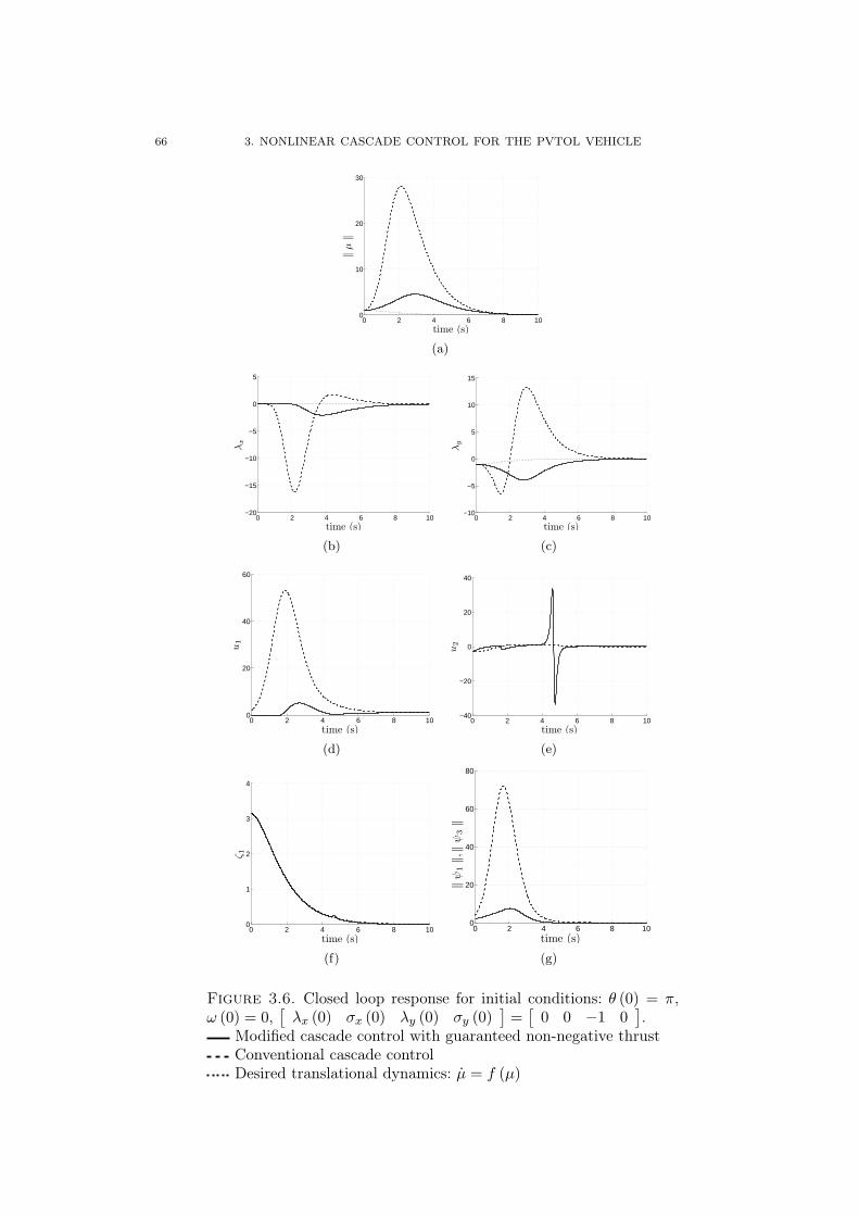
66 3. NONLINEAR CASCADE CONTROL FOR THE PVTOL VEHICLE
0 2 4 6 8 100
10
20
30
time (s)
‖µ‖
(a)
0 2 4 6 8 10−20
−15
−10
−5
0
5
time (s)
λx
(b)
0 2 4 6 8 10−10
−5
0
5
10
15
time (s)
λy
(c)
0 2 4 6 8 100
20
40
60
time (s)
u1
(d)
0 2 4 6 8 10−40
−20
0
20
40
time (s)
u2
(e)
0 2 4 6 8 100
1
2
3
4
time (s)
ζ1
(f)
0 2 4 6 8 100
20
40
60
80
time (s)
‖ψ
1‖,‖ψ
3‖
(g)
Figure 3.6. Closed loop response for initial conditions: θ (0) = π,ω (0) = 0,
[λx (0) σx (0) λy (0) σy (0)
]=
[0 0 −1 0
].
Modified cascade control with guaranteed non-negative thrustConventional cascade controlDesired translational dynamics: µ = f (µ)

3.4. MODIFIED CASCADE CONTROL OF THE PVTOL WITH VARYING WEIGHTS 67
3.4. Modified cascade control of the PVTOL with varying weights
In Section 3.2.2, it was suggested that it may be desirable to design a feedback lawfor the input u1 that minimised the L2 norm of the weighted, resulting interconnectionterm. The argument for this weighting was that it would enable further control ofthe influence of the interconnection term on the upper subsystem in the resultingclosed-loop dynamics. In this section, we explore this idea, as applied to the PVTOLvehicle.
3.4.1. Control design
From (3.63), for the chosen desired dynamics: µ = f (µ), the closed-loop transla-tional dynamics take the form of:
˙[λx
σx
]=
[0 1
−c11 −c12
] [λx
σx
]+
[1 0 0 00 1 0 0
]ψ (µ, ζ1)
˙[λy
σy
]=
[0 1
−c21 −c22
] [λy
σy
]+
[0 0 1 00 0 0 1
]ψ (µ, ζ1) . (3.65)
regardless of the primary thrust feedback law. From (3.65), the closed-loop horizontaland vertical dynamics behave as two GAS, linear subsystems, perturbed and coupledvia the interconnection term ψ. From (3.65), it is clear how the individual componentsof the interconnection term influence these subsystems. With this in mind, we proposethe weighting matrix:
W =[
wxI2×2 02×2
02×2 wyI2×2
]. (3.66)
Here wx, wy ∈ R+ are scalar weights that trade off the influence of the interconnectionterm on the closed-loop translational sub-systems. Defining the new feedback law asu1 , q (µ, ζ1), from (3.53), the norm of the resulting, weighted interconnection term,denoted ψ4 (µ, ζ1) may be written as:
‖Wψ4 (µ, ζ1)‖ =
∥∥∥∥∥∥∥∥
0−wxq sin (k2 + ζ1) + wxk1 sin (k2)
0wy q cos (k2 + ζ1)− wyk1 cos (k2)
∥∥∥∥∥∥∥∥
=
√w2
x (−q sin (k2 + ζ1) + k1 sin (k2))2
+w2y (q cos (k2 + ζ1)− k1 cos (k2))
2 . (3.67)
As in Section 3.3.3, q is determined by first writing:
∂ ‖Wψ4 (µ, ζ1)‖2
∂q= 2
(q(w2
x sin2 (k2 + ζ1) + w2y cos2 (k2 + ζ1)
)
− k1
(w2
x sin (k2) sin (k2 + ζ1)
+w2y cos (k2) cos (k2 + ζ1)
))= 0, (3.68)
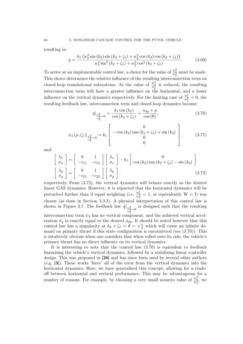
68 3. NONLINEAR CASCADE CONTROL FOR THE PVTOL VEHICLE
resulting in:
q =k1
(w2
x sin (k2) sin (k2 + ζ1) + w2y cos (k2) cos (k2 + ζ1)
)
w2x sin2 (k2 + ζ1) + w2
y cos2 (k2 + ζ1). (3.69)
To arrive at an implementable control law, a choice for the value of w2x
w2ymust be made.
This choice determines the relative influence of the resulting interconnection term onclosed-loop translational subsystems. As the value of w2
xw2
yis reduced, the resulting
interconnection term will have a greater influence on the horizontal, and a lesserinfluence on the vertical dynamics respectively. For the limiting case of w2
xw2
y= 0, the
resulting feedback law, interconnection term and closed-loop dynamics become:
q|w2x
w2y
=0=
k1 cos (k2)cos (k2 + ζ1)
=ady + g
cos (θ), (3.70)
ψ4 (µ, ζ1)|w2x
w2y
=0= k1
0− cos (k2) tan (k2 + ζ1) + sin (k2)
00
, (3.71)
and:˙[
λx
σx
]=
[0 1
−c11 −c12
] [λx
σx
]− k1
[0
cos (k2) tan (k2 + ζ1)− sin (k2)
]
˙[λy
σy
]=
[0 1
−c21 −c22
] [λy
σy
]. (3.72)
respectively. From (3.72), the vertical dynamics will behave exactly as the desiredlinear GAS dynamics. However, it is expected that the horizontal dynamics will beperturbed further than if equal weighting (i.e. w2
xw2
y= 1, or equivalently W = I) was
chosen (as done in Section 3.3.3). A physical interpretation of this control law isshown in Figure 3.7. The feedback law q|w2
xw2
y=0
is designed such that the resulting
interconnection term ψ4 has no vertical component, and the achieved vertical accel-eration σy is exactly equal to the desired ady. It should be noted however that thiscontrol law has a singularity at k2 + ζ1 = θ = ±π
2 which will cause an infinite de-mand on primary thrust if this state configuration is encountered (see (3.70)). Thisis intuitively obvious when one considers that when rolled onto its side, the vehicle’sprimary thrust has no direct influence on its vertical dynamics.
It is interesting to note that the control law (3.70) is equivalent to feedbacklinearising the vehicle’s vertical dynamics, followed by a stabilising linear controllerdesign. This was proposed in [26] and has since been used by several other authors(e.g. [3]). These works ‘force’ all of the error from the vertical dynamics into thehorizontal dynamics. Here, we have generalised this concept, allowing for a trade-off between horizontal and vertical performance. This may be advantageous for anumber of reasons. For example, by choosing a very small nonzero value of w2
xw2
y, we

3.4. MODIFIED CASCADE CONTROL OF THE PVTOL WITH VARYING WEIGHTS 69
Figure 3.7. Vector diagram outlining the modified cascade controldesign as applied to the PVTOL vehicle, with weighting w2
xw2
y= 0. All
vectors may be interpreted in terms of vehicle acceleration. Labelsindicate vector magnitudes.
will approximately linearise the vertical dynamics, but the singularity at θ = π2 will
be avoided.For the alternative limiting case of w2
xw2
y= ∞, the resulting feedback law becomes:
q|wy=0 =k1 sin (k2)
sin (k2 + ζ1)=
adx
sin (θ). (3.73)
This is equivalent to feedback linearising the vehicle’s horizontal dynamics, followedby a linear controller design. However, an inspection of (3.73) reveals a singularityoccurs at θ = 0. Again, this is intuitively obvious when one considers that the vehicle’sprimary thrust has no direct influence on its horizontal dynamics when directedupright. As the vehicle’s equilibrium occurs at θ = 0, the control law (3.73) is clearlyimpractical.
3.4.2. Simulation results
Figure 3.8 shows the effect of differing penalty ratios on the controller’s responseto a unit horizontal disturbance. As expected, when w2
xw2
y= 0, the vehicle’s vertical
dynamics are completely decoupled from the horizontal and roll dynamics. Conse-quently, the vehicle does not deviate in the vertical direction. However, as the valueof w2
xw2
yis increased, the vertical dynamics become more perturbed, and the horizontal

70 3. NONLINEAR CASCADE CONTROL FOR THE PVTOL VEHICLE
dynamics behave closer to the desired dynamics. Furthermore, the control signals be-come larger and far less smooth. This observation is consistent with the singularitythat occurs at θ = 0 for the limiting case of w2
xw2
y= ∞.
3.5. Conclusion
In this chapter, cascade control for the stabilisation of the PVTOL system hasbeen presented. It has been demonstrated that by feeding forward derivative informa-tion of desired vehicle orientation into the inner control-loop, a cascade closed-loopstructure may be achieved, resulting in global stability of the controlled system. Theprimary innovation of this chapter was to present an alternative cascade control ar-chitecture that minimised the interconnection term between closed-loop subsystems.This idea was generalised by first demonstrating how it may be applied to a generalclass of systems. Application of this technique to the PVTOL system demonstratedfaster convergence, yet less control action of the closed-loop response. Furthermore,we have shown how this technique may be used to trade-off horizontal and verticalperformance for the PVTOL system. It was demonstrated that this idea is a gen-eralisation of dynamic linearisation to decouple the vehicle’s vertical dynamics, asproposed in [26].

3.5. CONCLUSION 71
0 2 4 6 8 100
0.3
0.6
0.9
1.2
time (s)
λx
(a)
0 2 4 6 8 10−0.5
−0.25
0
0.25
0.5
time (s)
λy
(b)
0 2 4 6 8 100
1
2
3
4
time (s)
u1
(c)
0 2 4 6 8 10−8
−4
0
4
8
12
time (s)
u2
(d)
−0.2 0 0.2 0.4 0.6 0.8 1 1.2−0.4
−0.2
0
0.2
0.4
λx
λy
(e)
Figure 3.8. Controlled response to initial condition: θ (0) = ω (0) =σx (0) = σy (0) = 0, λx (0) = 1, λy (0) = 0 with differing penaltyratios w2
xw2
y.
w2x
w2y
= 0w2
xw2
y= 1
w2x
w2y
= 2Desired translational dynamics: µ = f (µ)

CHAPTER 4
Singularity issues in the nonlinear cascade control of thePVTOL vehicle
4.1. Introduction
In this chapter we revisit the methodology presented in Chapter 3 for the cascadecontrol of the planar vertical take-off and landing (PVTOL) vehicle. If care is nottaken in design, such cascade control laws will contain a singularity. This singularityis a direct consequence of feeding forward information into the orientation controlloop, and has the potential to cause unbound roll control demands. An approachto mitigate this problem was first proposed in [57] through the use of saturationfunctions embedded within the controller. This approach, along with a decouplingchange of coordinates, formulated the first truly globally stable control law publishedfor the PVTOL system. Subsequently, this technique has since been used by manyother authors (see Section 2.6.3). However, the approach presented in [57] artificiallysaturates control signals and thus has the potential to limit controller aggressiveness.The primary innovation of this chapter is to present an alternative technique toovercome this singularity issue. Here, we embed additional nonlinear dynamics withinthe control law such that the singularity may never occur. However, as saturationfunctions are avoided, controller aggressiveness is not compromised.
The chapter proceeds as follows; Firstly, the singularity issue is identified anddiscussed via a review of the control technique presented in Chapter 3. A numericalsimulation is then used to demonstrate the potential influence of this singularity onclosed-loop responses. The control law proposed in [57], that avoids this singularityusing saturation is then reviewed. This is followed by an outline of the approachovercoming singularity issues via additional nonlinear dynamics embedded withinthe controller. Proofs demonstrating that this new controller avoids the singularityand is globally bounded are then presented. All three controllers are then comparedvia numerical simulation. The chapter concludes with a brief summary.
4.2. Singularity issue in the cascade control of VTOL vehicles
In this section, the singularity occurring within the cascade control of VTOL ve-hicles is identified and discussed. A numerical simulation is then used to demonstratethe impact that this singularity can have on the closed-loop response.
73

74 4. SINGULARITY ISSUES IN THE CASCADE CONTROL OF THE PVTOL VEHICLE
4.2.1. System Dynamics
Recall the decoupled dynamics of the PVTOL system as introduced in Section2.3, written in the form:
λ = σ
σ = r (θ) u1 + g , a
θ = ω
ω = u2, (4.1)
where r (θ) =[ − sin (θ) cos (θ)
]T , λ =[
λx λy
]T , σ =[
σx σy
]T and g =[0 −g
]T are vectors representing the direction of primary thrust, position, veloc-ity and gravitational acceleration respectively. For the purpose of clarity throughoutthe following section, we have defined the additional variable a = σ, denoting trans-lational acceleration of the vehicle’s center of percussion (CP). To assist in controldesign, we also define the translational state vector: µ ,
[λx σx λy σy
]T
4.2.2. Cascade control design overview
In this section we briefly review the cascade control architecture outlined in Chap-ter 3, and identify a singularity existing within such cascaded control laws. Slightlydifferent notation is used from that presented earlier to highlight this issue. In partic-ular, we formulate controller design using the concept of a virtual control. We definethis virtual control as:
ad , −C1λ− C2σ ,[
adx
ady
]T
, (4.2)
where C1 =[
c11 00 c21
], c11, c21 ∈ R+ and C2 =
[c12 00 c22
], c12, c22 ∈ R+
are control gains. This virtual control may be thought of as desired translationalacceleration a. Upon inspection of the vehicle dynamics (4.1), it is clear that if itwere possible to set σ = ad, the translational dynamics of the vehicle would belinear, and exponentially stable. The definition of this virtual control is equivalent tothe desired translational dynamics of µ = f (µ) discussed in Section 3.3.2. Proceedingas in Section 3.3.2 we define k1 and k2 such that:
r (k2) k1 + g , ad. (4.3)
Variables k1 and k2 are thought of as desired thrust and desired roll angle (u1 andθ) respectively. Solving (4.3) for k1 and k2 it follows that:
k1 =√
a2dx + (ady + g)2 (4.4)
and:
k2 = atan2 (−adx, ady + g) . (4.5)

4.2. SINGULARITY ISSUE IN THE CASCADE CONTROL OF VTOL VEHICLES 75
Defining the feedback law: u1 = k1 and backstepping over the roll dynamics to forceθ to converge to k2, we arrive at the overall control law:
u1 = k1
u2 = k2 − d1 (θ − k2)− d2
(ω − k2
), d1, d2 ∈ R+. (4.6)
Analytic expressions for k2 and k2 required by this feedback control law may beobtained as:
k2 =adxady − adx (ady + g)
a2dx + (ady + g)2
=adxady − adx (ady + g)
k21
(4.7)
and:
k2 =((adxady − adx (ady + g)) k2
1 − 2 (adxady
−adx (ady + g))× (adxadx + (ady + g) ady)) /k41, (4.8)
where:
ad =[
adx ady
]T = −C1σ − C2a, (4.9)
ad =[
adx ady
]T = −C1a− C2a, (4.10)
a =∂r (θ)
∂θωk1 + r (θ) k1 (4.11)
and:
k1 =axdaxd + (ayd + g) ayd
k1. (4.12)
The closed-loop dynamics take the form a nonlinear subsystem describing vehicletranslation, with an exponentially stable cascaded linear subsystem describing ve-hicle orientation. Applying the control law (4.6) to the system dynamics (4.1) andintroducing the error variable ζ , θ − k2, we may write this as:
λ = σ
σ = −C1λ− C2σ + ψ1 (ζ, λ, σ)
ζ = −d1ζ − d2ζ. (4.13)
Again, ψ1 (ζ, λ, σ) is an interconnection term with ψ1 (0, λ, σ) = 0. Global asymptoticstability may be demonstrated by showing linear growth of the interconnection termwith respect to the state vector describing translational motion: µ (see Section 3.3.2).However it may be shown that a singularity exists within the closed-loop system. Itis clear from (4.3) that if the virtual control ad takes the value ad = g =
[0 −g
]T ,we have k1 = 0, and the value of k2 becomes undefined. Furthermore, an inspectionof (4.7) and (4.8) reveals that as k1 → 0, k2 → ∞ and k2 → ∞. Consequently,closed-loop solutions that pass close to this singularity will result in exceptionallylarge values of k2, k2 and ultimately u2. This phenomenon was observed earlier, inFigure 3.6 of Section 3.3.5.2.

76 4. SINGULARITY ISSUES IN THE CASCADE CONTROL OF THE PVTOL VEHICLE
Figure 4.1. Graphical interpretation of singularity existing withina cascade controller for the PVTOL system. Singularity denoted bycross at ad =
[0 −1
]T . Quantities scaled against gravitational ac-celeration.
A graphical interpretation of this singularity is shown in Figure 4.1. From thedefinition of k1 (t) and k2 (t) shown in this figure, it is clear that at instances wherethe virtual control ad (t) passes close to the singularity located at g, the rate ofchange of the angle k2 (t) will be large. The closer the trajectory of ad (t) passes tothis singularity, the more pronounced this becomes. In the limiting case, when thead trajectory passes over the singularity, a discontinuity of π radians will exist inthe k2 (t) signal and its derivative will thus be unbound. Information regarding k2 (t)is fed forward into the backstepping controller for vehicle roll in the form of k2 (t)and k2 (t). Consequently, closed-loop trajectories encountering this singularity willrequire exceptionally large values of roll control u2.
4.2.3. Simulation
Figure 4.2 shows the response of the PVTOL system controlled by the cascadecontroller discussed in the previous section. This simulation was conducted using theinitial conditions: λ (0) = [−1.285, 1.285] , σ [0, 0] , θ (0) = ω (0) = 0. These initial

OVERCOMING SINGULARITY IN CASCADE CONTROL DESIGNS 77
conditions were purposely chosen such that the closed-loop trajectory passed closeto the singularity discussed in the previous section. As in Chapter 3, control gainsof c11 = c21 = d1 = 1 and c12 = c22 = d2 = 2 were selected and the couplingparameter ε was set to zero such that primary thrust augmentation is not requiredto decouple the system (i.e., u1 = u1). All results are normalised against gravity (i.e.,g = 1). From Figure 4.2 it is clear that the singularity has had little negative impacton the translational response of the system. However, this is not the case for thesystem’s internal dynamics and control signals. Figure 4.3 (a) shows the trajectoryof the virtual control ad (t) passing close to the singularity at t ≈ 1.3 s. As expected,this results in a sharp transient in desired roll angle at this time (see Figure 4.3 (b)).As information regarding this signal is fed forward into the backstepping controllerfor vehicle roll, roll angle also undergoes this sharp transient (see Figure 4.3 (d)).However, Figure 4.3 (e) shows the exceptionally large roll control demand u2 requiredto achieve this.
−1.5 −1.25 −1 −0.75 −0.5 −0.25 0 0.25−0.25
0
0.25
0.5
0.75
1
1.25
1.5
1.75
λx
λy
Figure 4.2. Translational response of PVTOL system stabilised us-ing a nonlinear cascade control law. Closed-loop trajectory passes closeto the controller singularity. Vehicle shown at 0.5 second increments.Initial conditions: λ (0) = [−1.285, 1.285] , σ [0, 0] , θ (0) = ω (0) = 0.
4.3. Methods for overcoming singularity in cascade control designs
In this section, two techniques are presented for overcoming singularity issuesassociated with the cascade control of VTOL vehicles. The first of these, proposedin [57] is to use saturation within the controller such that the singularity may notoccur. However, we later show that this approach has the potential to limit controller

78 4. SINGULARITY ISSUES IN THE CASCADE CONTROL OF THE PVTOL VEHICLE
(a) Virtual control trajectory ad(t). Singularitydenoted by cross. Points on curve indicate time.
0 2 4 6 8 10−3
−2.5
−2
−1.5
−1
−0.5
0
0.5
1
time (s)
k2
(b) Desired roll angle k2.
0 2 4 6 8 100
0.5
1
1.5
time (s)
u1
=k
1
(c) Primary thrust u1 = k1.
0 2 4 6 8 10−2
−1.5
−1
−0.5
0
0.5
1
1.5
2
time (s)
θ
(d) Vehicle roll θ.
0 2 4 6 8 10−2000
−1000
0
1000
2000
time (s)
u2
(e) Roll control u2.
Figure 4.3. Control signal and roll angle responses for the PVTOLsystem. Closed-loop trajectory passes close to the controller singular-ity.

OVERCOMING SINGULARITY IN CASCADE CONTROL DESIGNS 79
performance when rejecting large non-zero initial conditions. The second techniquepresented encompasses the primary innovation of this chapter; We propose an al-ternative controller structure whereby additional dynamics are embedded into thecontroller. These dynamics are designed such that the singularity may never occur.A numerical simulation is then used to compare these control techniques.
4.3.1. Overcoming singularity using saturation
The solution to the singularity problem proposed in [57], is equivalent to bound-ing an element of the virtual control ad using a saturation function. This is done insuch a way that the singularity may never occur. We review this technique as follows;Firstly, the new virtual control is defined as:
ad =[
adx
b0ϕ (ady)
],
[adx
ady
], (4.14)
where 0 < b0 < g and ϕ is a smooth saturation function; a strictly increasing functionwith ϕ (s) ∈ (−1, 1) ∀s ∈ R. A commonly used choice for ϕ is the hyperbolic tangent“tanh” function. The corresponding desired values of thrust and roll (k1 and k2) arethen defined such that:
r(k2
)k1 + g , ad (4.15)
and consequently:
k1 =√
a2dx + (ady + g)2 (4.16)
and:
k2 = atan( −adx
ady + g
). (4.17)
The remainder of control design follows Section 4.2.2. From (4.14) it can be seenthat the saturation function has ensured |ady| < g . Consequently, ad is restrictedto a set that does not include g, and the singularity is thus avoided. However, asthe virtual control ad has been restricted using saturation, it follows that controlleraggressiveness to large non-zero initial conditions will be reduced. This is demon-strated in Section 4.3.3. In addition to this, it can be shown that such an approachhas the potential to cause undesirable transients as the magnitude of initial conditionsincreases.
4.3.2. Overcoming singularity using additional dynamics
Here we propose an alternative technique to overcoming the singularity associatedwith the cascade control of VTOL vehicles. Rather than using saturation, additionalnonlinear dynamics are embedded within the controller such that the singularity maynever occur. We first define the new virtual control as:
ad = −C1λ− C2σ + δ
= ad + δ ,[
adx
ady
], (4.18)

80 4. SINGULARITY ISSUES IN THE CASCADE CONTROL OF THE PVTOL VEHICLE
where δ , [δx, δy]T , δx, δy ∈ R is interpreted as a perturbation, to be designed shortly.
The corresponding desired values of thrust and roll (k1 and k2) are defined such that:
r(k2
)k1 + g , ad (4.19)
and consequently:
k1 =√
a2dx + (ady + g)2 (4.20)
and:
k2 = atan2 (−adx, ady + g) . (4.21)
We now design dynamics for δ such that δ 6= 0 when ad = g (i.e. from (4.18), ad = gmay never occur). We have the additional restriction that δ must have continuousfirst and second derivatives such that the first and second derivatives of k2 are finiteand available to the controller. To achieve this, we design second order dynamics forδ of the form:
δ = −D1δ −D2δ + F (ad, ˙ad) , D1, D2 ∈ R+, (4.22)
where:
F (ad, ˙ad) ,
0 if ‖ad − g‖ ≥ c0g(h1 (ad) + h2 (ad, ˙ad)) f (‖ad − g‖) if ‖ad − g‖ < c0g
. (4.23)
Here c0 ∈ (0, 1) and f : R → R+ is a continuous function with f (c0g) = 0 andlims→0
∫ c0gs f (x) dx = ∞. The function h1 (ad) , ad−g
‖ad−g‖ , and h2 (ad, ˙ad) : R2 → R2
is continuous with h2 (ad, ˙ad)T ˙ad = 0. An example of specific functions f and h2
satisfying these constraints are given in Section 4.3.3. The remainder of the controldesign closely follows that presented in Section 4.2.2, and arrives at the control law:
u1 = k1
u2 = ¨k2 − c1
(θ − k2
)− c2
(ω − ˙k2
), (4.24)
where ¨k2 and ˙k2 are obtained as in Section 4.2.2.Upon inspection of (4.22) and (4.23) we note that when ad ∈ x| ‖x− g‖ ≥ c0g,
(4.22) becomes simply that of an exponentially stable, second order linear systemand δ will converge to zero. From (4.18), ad will converge to ad and the system willbehaves as a stable cascade equivalent to that presented in Section 4.2.1. However,when ad ∈ x| ‖x− g‖ < c0g (i.e. ad enters a region surrounding the singularity atg) the nonlinear function F ensures δ will grow such that ad = g can not occur. Thefunction F is comprised of the three functions: f , h1 and h2 serving the followingpurposes; The scalar function f may be thought of as the magnitude of a ‘force’surrounding the singularity, the potential of which grows unbound at the singularity.The vector function h1 ensures this ‘force’ is applied in the appropriate direction suchthat ad may never reach g. The vector function h2 is designed such that ad passessmoothly around the singularity. We formalise all this as follows;
Proposition 4.3.1. Consider the control law (4.24) applied to system (4.1). Forall bounded solutions, the state configuration corresponding to ad = g can never occurprovided ad (0) 6= g (0) .

OVERCOMING SINGULARITY IN CASCADE CONTROL DESIGNS 81
Proof. Consider the storage function:
E , 1
2˙aTd
˙ad if ‖ad − g‖ ≥ c0g∫ c0g‖ad−g‖ f (s) ds + 1
2˙aTd
˙ad if ‖ad − g‖ < c0g(4.25)
with the derivative:
E =
˙aTd
(ad −D1δ −D2δ
)if ‖ad − g‖ ≥ c0g
−f (‖ad − g‖) (ad−g)T ˙ad
‖ad−g‖ + ˙aTd
(ad −D1δ −D2δ
+(h1 (ad) + h2 ( ˙ad)) ×f (‖ad − g‖)) if ‖ad − g‖ < c0g
(4.26)
Noting that:˙aTd (h1 (ad) + h2 ( ˙ad)) = ˙aT
d h1 (ad)
=(ad − g)T ˙ad
‖ad − g‖ (4.27)
(4.26) reduces to:
E = ˙aTd
(ad −D1δ −D2δ
). (4.28)
Thus, along solutions of the closed-loop system we have:
E (t)−E (0) =∫ t
0
˙aTd
(ad −D1δ −D2δ
)dt. (4.29)
As these solutions are bounded, it follows that for all initial conditions there existsfunctions α, β, γ, κ : R → R+ such that; ‖ ˙ad (t)‖ ≤ α (χ (0)), ‖¨ad (t)‖ ≤ β (χ (0)),‖δ (t)‖ ≤ γ (χ (0)) and
∥∥∥δ (t)∥∥∥ ≤ κ (χ (0)) , ∀t ≥ 0, where χ ,
[λ, σ, θ, ω, δ, δ
]. Ex-
plicit arguments demonstrating these inequalities are lengthy, algebraic, and thusomitted due to space limitations. Defining the function:
Λ (χ (0)) , α (χ (0)) [β (χ (0)) + c1γ (χ (0)) + c2κ (χ (0))] (4.30)
from (4.29) we have:∫ c0g
‖ad(t)−g‖f (s) ds− 1
2˙aTd (t) ˙ad (t)−
∫ c0g
‖ad(0)−g‖f (s) ds
+12˙aTd (0) ˙ad (0) ≤ Λ (χ (0)) t, (4.31)
and thus:∫ c0g
‖ad(t)−g‖f (s) ds−
∫ c0g
‖ad(0)−g‖f (s) ds ≤ Λ (χ (0)) t + 2α (χ (0)) . (4.32)
We see that as ad (t) → g, the left hand side (LHS) of this equation →∞. Thus, forthe above inequality to hold, ad (t) = g may not occur for all t ≤ ∞. ¤
Criterion 4.3.2. Consider the control law (4.24) applied to system (4.1). Forall solutions, ‖δ‖ remains upper bounded by some ∆(χ (0)).

82 4. SINGULARITY ISSUES IN THE CASCADE CONTROL OF THE PVTOL VEHICLE
Upon inspection of the dynamics describing δ (4.22), this assumption is not un-reasonable provided the function F is designed appropriately. Specifically, F shouldbe designed such that ad may not become ‘stuck’ in the region surrounding the sin-gularity while ad grows unbound.
Proposition 4.3.3. Consider the control law (4.24) applied to system (4.1). IfCriterion 4.3.2 is satisfied, then all closed-loop solutions will be bounded.
Proof. Recalling (4.2):
ad = −C1λ− C2σ
= −[
C1 00 C2
]
︸ ︷︷ ︸,C
[λσ
](4.33)
it follows that ‖ad‖ > Cσmin
∥∥∥[
λT σT]T
∥∥∥, where Cσmin is the minimum singularvalue of the matrix C. Considering this, and recalling:
ad = ad + δ (4.34)
it follows from Criterion 4.3.2 that if after some time t1, we have∥∥∥[
λT σT]T
∥∥∥ >
(1+c0g)+∆(χ(0))Cσmin
, we must have ‖ad‖ > (1 + c0g) + ∆ (χ (0)) and ‖ad‖ ≥ (1 + c0) g.In particular, after time t1, we are assured that ad /∈ x| ‖x− g‖ ≥ c0g such thatF (ad, ˙ad) = 0. Introducing the error variable ζ , θ − k2, it follows from the controllaw given by (4.24) applied to the system dynamics (4.1) that after time t1, theclosed-loop dynamics may be expressed in a cascaded form as:
λ = σ
σ = −C1λ− C2σ + δ + ψ(λ, σ, δ, ζ
)
δ = −D1δ −D2δ
¨ζ = −c1ζ − c2˙ζ, (4.35)
where:
ψ(λ, σ, δ, ζ
)= a− ad
=[ − sin
(k2 + ζ
)k1
cos(k2 + ζ
)k1 − g
]−
[ − sin(k2
)k1
cos(k2
)k1 − g
]
=[ − sin
(k2 + ζ
)+ sin
(k2
)cos
(k2 + ζ
)− cos(k2
)]
k1 (4.36)
is the nonlinear interconnection term with ψ (λ, σ, δ, 0) = 0. From (4.35) it follows thatif δ = ζ = 0, the translational states λ and σ will behave with linear, exponentially
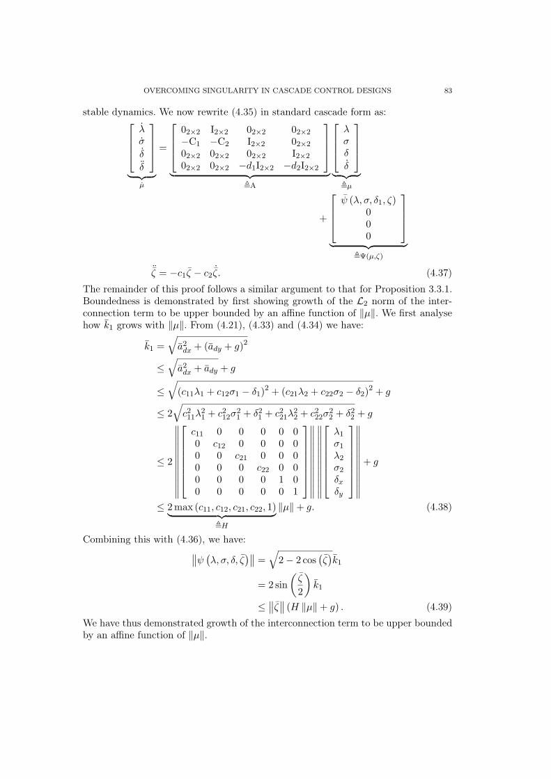
OVERCOMING SINGULARITY IN CASCADE CONTROL DESIGNS 83
stable dynamics. We now rewrite (4.35) in standard cascade form as:
λσ
δ
δ
︸ ︷︷ ︸µ
=
02×2 I2×2 02×2 02×2
−C1 −C2 I2×2 02×2
02×2 02×2 02×2 I2×2
02×2 02×2 −d1I2×2 −d2I2×2
︸ ︷︷ ︸,A
λσδ
δ
︸ ︷︷ ︸,µ
+
ψ (λ, σ, δ1, ζ)000
︸ ︷︷ ︸,Ψ(µ,ζ)
¨ζ = −c1ζ − c2˙ζ. (4.37)
The remainder of this proof follows a similar argument to that for Proposition 3.3.1.Boundedness is demonstrated by first showing growth of the L2 norm of the inter-connection term to be upper bounded by an affine function of ‖µ‖. We first analysehow k1 grows with ‖µ‖. From (4.21), (4.33) and (4.34) we have:
k1 =√
a2dx + (ady + g)2
≤√
a2dx + ady + g
≤√
(c11λ1 + c12σ1 − δ1)2 + (c21λ2 + c22σ2 − δ2)
2 + g
≤ 2√
c211λ
21 + c2
12σ21 + δ2
1 + c221λ
22 + c2
22σ22 + δ2
2 + g
≤ 2
∥∥∥∥∥∥∥∥∥∥∥∥
c11 0 0 0 0 00 c12 0 0 0 00 0 c21 0 0 00 0 0 c22 0 00 0 0 0 1 00 0 0 0 0 1
∥∥∥∥∥∥∥∥∥∥∥∥
∥∥∥∥∥∥∥∥∥∥∥∥
λ1
σ1
λ2
σ2
δx
δy
∥∥∥∥∥∥∥∥∥∥∥∥
+ g
≤ 2max (c11, c12, c21, c22, 1)︸ ︷︷ ︸,H
‖µ‖+ g. (4.38)
Combining this with (4.36), we have:∥∥ψ
(λ, σ, δ, ζ
)∥∥ =√
2− 2 cos(ζ)k1
= 2 sin(
ζ
2
)k1
≤ ∥∥ζ∥∥ (H ‖µ‖+ g) . (4.39)
We have thus demonstrated growth of the interconnection term to be upper boundedby an affine function of ‖µ‖.

84 4. SINGULARITY ISSUES IN THE CASCADE CONTROL OF THE PVTOL VEHICLE
With reference to (4.37), the dynamics µ = Aµ are stable as they represents twostable, linear, cascaded sub-systems. Consider the Lyapunov function V = µT Pµ,where P ∈ R8×8 is the positive definite solution to the Lyapunov equation AT P +PA = −Q, with Q some positive definite matrix. Noting that this Lyapunov functionis quadratic we may write:
V ≥ λPmin ‖µ‖2 (4.40)
where λPmin 6= 0 is the magnitude of the minimum eigenvalue of P. Differentiatingthis Lyapunov function with respect to time and using (4.39) and (4.40), we maywrite:
V = −2µT Qµ + 2ΨT Pµ
≤ 2ΨT Pµ
≤ 2 ‖ψ‖ ‖P‖ ‖µ‖≤ 2 ‖P‖ ‖µ‖∥∥ζ
∥∥ (H ‖µ‖+ g)
≤ 4 ‖P‖ ‖µ‖2∥∥ζ
∥∥ for ‖µ‖ >g
H
≤ 4 ‖P‖λPmin
V∥∥ζ
∥∥ for ‖µ‖ >g
H. (4.41)
From (4.37), ζ converges exponentially fast. Consequently, we may write:
V ≤ 4 ‖P‖λPmin
V γ(∥∥ζ (0)
∥∥)e−nt for ‖µ‖ >
g
H, (4.42)
for some n ∈ R+, and γ : R → R some non-decreasing function with γ (0) = 0.Integrating this over time we have:
V (µ (t)) ≤ V (µ (t1)) e4‖P‖γ(‖ζ(0)‖)
λPmin
∫ tt1
e−nsds
≤ Γ(∥∥ζ (0)
∥∥)V (µ (t1)) , (4.43)
for Γ : R → R some non-decreasing function with Γ (0) = 0. As V (µ) is radiallyunbound, boundedness of V (µ (t)) implies boundedness of ‖µ (t)‖. ¤
4.3.3. Simulation results
In the following section, a numerical simulation is presented demonstrating thecharacteristics of all three controllers as they relate to the singularity issue. Forbrevity, the controller with singularity (see Section 4.2.2), controller avoiding thesingularity using saturation (see Section 4.3.1), and the controller using additionaldynamics (see Section 4.3.2) are herein referred to as controllers A, B and C respec-tively.
4.3.3.1. Controller gain/ function selection
As in Chapter 3, control gains of c11 = c21 = d1 = 1 and c12 = c22 = d2 = 2 wereselected, and the coupling parameter ε was set to zero. Other controller gains andfunctions used were:
b0 = 0.5, c0 = 0.8,

OVERCOMING SINGULARITY IN CASCADE CONTROL DESIGNS 85
D1 = 100, D2 = 20,
f (s) =(
1s
+s
(c0g)2− 2
c0g
), (4.44)
and:
h2 (ad, ˙ad) = K
[0 1−1 0
] ˙ad
‖ ˙ad‖sign
((ad − g) ·
[0 1−1 0
] ˙ad
‖ ˙ad‖)
, (4.45)
where K = 50.
4.3.3.2. Controlled response comparison
Numerical simulations were conducted for all three controllers using the initialconditions: λ (0) = [−1.285, 1.285], σ (0) = [0, 0], θ (0) = 0 and ω (0) = 0. Theseinitial conditions were used such that the response of controller A was as shown inSection 4.2.3 (i.e., passed close to the singularity).
Figure 4.4 shows the trajectories of the virtual controls for all three proposedcontrol designs. As observed in Section 4.2.3, the virtual control for controller A: ad
passes very close to the singularity point at g. Again, the output trajectory for thiscontroller appears reasonable (see Figure 4.5), however Figure 4.6 (e) demonstratesthe unrealistic roll control input arising from the singularity.
Figure 4.4 demonstrates the bounds on the virtual control for controller B: ad
such that it can never reach the singularity point g. Consequently, this virtual controlcan not pass close to the singularity, and the unrealistic roll control demand in theresponse of controller A is not observed (see Figure 4.6 (e)). However, upon inspectionof Figures 4.5 and 4.6 (a) it can be seen that controller B is less aggressive thancontroller A. In particular, the L2 norm of the state vector describing translationalmotion
∥∥∥[
λT σT]T
∥∥∥ decays more rapidly for controller A than for controller B(see Figure 4.6 (a)). This observation becomes more pronounced as the magnitude ofinitial conditions are increased.
Figure 4.4 demonstrates how the virtual control for controller C: ad avoids passingclose to the singularity point. At time t = 0, δ (0) = 0, and the virtual control forcontrollers A and C are coincident (i.e. ad = ad, see (4.18)). This is true up until thepoint at which the virtual control enters a region surrounding the singularity, definedby the set ad| ‖ad − g‖ ≥ c0g. At this point, the additional dynamics embeddedwithin controller C causes δ to grow such that the virtual control ad diverges fromad, and ad does not pass close to the singularity. Consequently, the sharp transientexisting in the k2 signal for controller A is not observed. Rather, ad is deflectedaround the singularity, and the vehicle undergoes a full 2π rotation (see Figures 4.6(b) and (d)). As a consequence of this, the problem regarding unrealistic roll controlinput observed for controller A is significantly reduced for controller C (see Figure4.6 (e)). From Proposition 4.3.1 we are assured that the virtual control ad can notpass over the singularity. Consequently, the roll control demands for controller Care guaranteed to be bound. However, Figures 4.5 and 4.6 (a) demonstrate that theaggressive nature of the controller has been preserved, with the translational responseof controllers A and C differing little. It should be noted that the peak roll control

86 4. SINGULARITY ISSUES IN THE CASCADE CONTROL OF THE PVTOL VEHICLE
Figure 4.4. Virtual control trajectories.: ad for controller with singularity (A): ad for controller with bounded virtual control (B): ad for controller with dynamic virtual control (C): ad for controller with dynamic virtual control (C): Region defining ‖ad − g‖ < c0g: Region bounding ad
: Singularity point g
input for controller C is significantly greater than that for controller B. However, itis possible that this may be reduced via alternative choices for functions f and h1.

4.4. CONCLUSION 87
−1.5 −1 −0.5 0
0
0.5
1
1.5
2
λx
λy
Figure 4.5. Comparison of controller responses to initial conditions:λ (0) = [−1.285, 1.285], σ (0) = [0, 0], θ (0) = ω (0) = 0.
- Controller with singularity (A)- Controller with bounded virtual control (B)- Controller with dynamic virtual control (C)
4.4. Conclusion
In this chapter, a singularity issue that may arise within cascade controllers de-signed for the PVTOL vehicle has been identified and discussed. It has been demon-strated that this singularity has the potential to cause unbound roll-control demands.It has been shown that this is a direct consequence of feeding forward informationinto the control-loop for vehicle roll. A previously published approach using embed-ded saturation within the controller to overcome this issue has been reviewed. It

88 4. SINGULARITY ISSUES IN THE CASCADE CONTROL OF THE PVTOL VEHICLE
0 5 10 150
0.5
1
1.5
2
2.5
time (s)
‖[λ
T,σ
T]T
‖
(a) L2 norm of the translational state vector [λT , σT ]T
0 5 10 15−8
−6
−4
−2
0
2
time (s)
k2,k2,k2
(b) Desired roll k2
0 5 10 150
0.4
0.8
1.2
1.6
time (s)
u1
(c) Primary thrust u1 = k1
0 5 10 15−8
−6
−4
−2
0
2
time (s)
θ
(d) Vehicle roll θ
0 5 10 15−80
−40
0
40
80
time (s)
u2
(e) Roll control u2
Figure 4.6. Vehicle roll and control signals.: Controller with singularity (A): Controller with bounded virtual control (B): Controller with dynamic virtual control (C)

4.4. CONCLUSION 89
has been shown that this artificial saturation has the potential to reduce controlleraggressiveness to large non-zero initial conditions. A new approach to mitigate thissingularity issue has been presented. This approach embeds additional nonlinear dy-namics within the controller such that the singularity can not occur. In this mannersingularity issues were avoided, however the controller remained capable of executinghighly aggressive stabilisation maneuvers.