Automatically Generating Novel and Epic Music Tracks

Exploring Computational Creativity using Deep Structures against Music

Luıs Carlos de Almeida Espırito Santo

Thesis to obtain the Master of Science Degree in

Information Systems and Computer Engineering

Supervisors: Prof. Helena Sofia Andrade Nunes Pereira PintoProf. David Manuel Martins de Matos

Examination Committee

Chairperson: Prof. Francisco Joao Duarte Cordeiro Correia dos SantosSupervisor: Prof. Helena Sofia Andrade Nunes Pereira PintoMembers of the Committee: Prof. Fernando Amılcar Cardoso

June 2019

Acknowledgments

I would like to thank everyone that assisted my continuously learning process, over all this years.

I would like to thank my supervisor Sofia Pinto and co-supervisor David Matos, not only for the

guidance both provided during this work, but also for helping me build and improve my knowledge

during these last years. In the same way, I would like to thank to all the other teachers that shaped me

into what I am today.

I would like to thank everyone that answered my survey and all those people that in one way or

another demonstrated interest in my project. In addition, I wish to acknowledge the help provided by all

those that contributed directly with some feedback or improvement proposals.

I would also like to write a word of gratitude to all my friends and colleagues, from all different contexts

and areas, for providing me a variety of safe places where I could relax, laugh and learn different things,

everyday, which helped me growing as a person and allowed me to develop the ideas on this work.

Finally, I express my very great appreciation to my parents and my sister for teaching me friendship,

tolerance, balance, patience and caring just as so confidence and resilience over all my years of exis-

tence. I would also like to extend my gratitude to the rest of my family for their support and friendship

throughout all these years.

Last but not least, I would like to offer my special thanks to my girlfriend, for sharing with me so many

years and for teaching me how to manage every aspect of me, during the good and bad times in my life,

in order to always achieve one better version of myself, for always being there for me through thick and

thin and without whom this project would not be possible..

To each and every one of you – Thank you.

Abstract

Computational Creativity is an applied field of study focused on algorithms that allow a better under-

standing of the creativity processes or simply perform some task usually considered creative. Among

these models we can find some Deep Learning models, such as the Restricted Boltzmann Machines

and the Generative Adversarial Networks, also widely studied outside of Computational Creativity scope.

In addition, we can distinguish different application areas within Computational Creativity, such as music

or visual arts. With the purpose of exploring the capability of these models to work with music dynamics,

this work focuses on the application of neural models for multitrack epic music generation, trying to fol-

low a general approach and a complying vision with the field of Computational Creativity. Three different

models were developed, adapted and compared: the HRBMM, the MuseGAN and the MuCyG. After

conducting a survey, and analyzing the results obtained, we conclude that none of the computational

models consistently outperformed the other ones. The results also point out that the used methodology

led to problems of mode collapsing and possibly prevented the models to produce products capable of

causing a similar effect that epic human composed samples are capable of.

Keywords

Music; Deep Learning; Creativity; Epic; Generative Models.

iii

Resumo

A Criatividade Computacional e uma area aplicada que estuda algoritmos que permitem compreender

a criatividade ou que desempenham tarefas usualmente consideradas criativas. Entre estes modelos

encontram-se alguns modelos de Deep Learning, nomeadamente as Restricted Boltzmann Machines

e as Generative Adversarial Networks, tambem vastamente estudados fora da area de Criatividade

Computacional. Tambem dentro desta area podemos distinguir diferentes areas de aplicacao, como a

musica ou as artes visuais. Com o proposito de explorar a capacidade destes modelos trabalharem

com dinamicas musicais, este trabalho pretende focar-se na aplicacao de modelos neuronais a tarefa

de geracao de musica multitrack epica, seguindo uma abordagem geral e uma visao concordante com

a area da Criatividade Computacional. Tres modelos foram desenvolvidos, adaptados e posteriormente

comparados: o HRBMM, o MuseGAN e o MuCyG. Depois de conduzir um questionario e de analisar

os resultados obtidos, concluımos que nenhum destes modelos obteve avaliacoes consistentemente

melhores que os outros. Os resultados tambem indicam que a metodologia usada conduziu a problemas

de mode collapsing e que os produtos gerados nao foram capazes de afetar o ouvinte da mesma forma

que excertos epicos compostos por humanos.

Palavras Chave

Musica; Redes Neuronais; Criatividade; Epico; Modelos Gerativos.

v

Contents

1 Introduction 1

1.1 Terminology Concerns . . . . . . . . . . . . . . . . . . . . . . . . . . . . . . . . . . . . . . 4

1.2 Document Structure . . . . . . . . . . . . . . . . . . . . . . . . . . . . . . . . . . . . . . . 5

2 Related Work 7

2.1 Creativity Related Work . . . . . . . . . . . . . . . . . . . . . . . . . . . . . . . . . . . . . 9

2.1.1 Models for Human Creativity . . . . . . . . . . . . . . . . . . . . . . . . . . . . . . 9

2.1.2 Models for Computational Creativity . . . . . . . . . . . . . . . . . . . . . . . . . . 12

2.2 Deep Learning Related Work . . . . . . . . . . . . . . . . . . . . . . . . . . . . . . . . . . 16

2.2.1 General Concepts . . . . . . . . . . . . . . . . . . . . . . . . . . . . . . . . . . . . 16

2.2.2 Convolutional Neural Networks (CNN) and Recurrent Neural Networks (RNN) . . . 19

2.2.3 Generative Deep Models . . . . . . . . . . . . . . . . . . . . . . . . . . . . . . . . 20

2.2.4 Cyclical Generative Models . . . . . . . . . . . . . . . . . . . . . . . . . . . . . . . 24

2.3 Automatic Music Composition Related Work . . . . . . . . . . . . . . . . . . . . . . . . . . 25

2.3.1 General Concepts . . . . . . . . . . . . . . . . . . . . . . . . . . . . . . . . . . . . 25

2.3.2 Using Deep Learning . . . . . . . . . . . . . . . . . . . . . . . . . . . . . . . . . . 28

2.4 Summary . . . . . . . . . . . . . . . . . . . . . . . . . . . . . . . . . . . . . . . . . . . . . 29

3 Dataset 31

3.1 Representations . . . . . . . . . . . . . . . . . . . . . . . . . . . . . . . . . . . . . . . . . 33

3.2 Data Sources . . . . . . . . . . . . . . . . . . . . . . . . . . . . . . . . . . . . . . . . . . . 36

3.3 Preprocessing . . . . . . . . . . . . . . . . . . . . . . . . . . . . . . . . . . . . . . . . . . 37

3.4 Datasets Characterization . . . . . . . . . . . . . . . . . . . . . . . . . . . . . . . . . . . . 39

3.5 Summary . . . . . . . . . . . . . . . . . . . . . . . . . . . . . . . . . . . . . . . . . . . . . 40

4 Models 43

4.1 Environment and Tools . . . . . . . . . . . . . . . . . . . . . . . . . . . . . . . . . . . . . . 45

4.2 HRBMM . . . . . . . . . . . . . . . . . . . . . . . . . . . . . . . . . . . . . . . . . . . . . . 46

4.3 MuseGAN . . . . . . . . . . . . . . . . . . . . . . . . . . . . . . . . . . . . . . . . . . . . . 48

4.4 MuCyG . . . . . . . . . . . . . . . . . . . . . . . . . . . . . . . . . . . . . . . . . . . . . . 50

vii

4.5 Tuning . . . . . . . . . . . . . . . . . . . . . . . . . . . . . . . . . . . . . . . . . . . . . . . 52

4.6 Summary . . . . . . . . . . . . . . . . . . . . . . . . . . . . . . . . . . . . . . . . . . . . . 53

5 Results and Evaluation 55

5.1 Final Experiment . . . . . . . . . . . . . . . . . . . . . . . . . . . . . . . . . . . . . . . . . 57

5.2 Survey . . . . . . . . . . . . . . . . . . . . . . . . . . . . . . . . . . . . . . . . . . . . . . . 62

5.2.1 Word Description . . . . . . . . . . . . . . . . . . . . . . . . . . . . . . . . . . . . . 64

5.2.2 Impacts on Creativity . . . . . . . . . . . . . . . . . . . . . . . . . . . . . . . . . . . 65

5.2.3 Evaluating Confronting Pairs . . . . . . . . . . . . . . . . . . . . . . . . . . . . . . 66

5.3 Summary . . . . . . . . . . . . . . . . . . . . . . . . . . . . . . . . . . . . . . . . . . . . . 73

6 Conclusion 75

6.1 Conclusions . . . . . . . . . . . . . . . . . . . . . . . . . . . . . . . . . . . . . . . . . . . . 77

6.2 Future Work . . . . . . . . . . . . . . . . . . . . . . . . . . . . . . . . . . . . . . . . . . . . 77

7 Epic Dataset Reference List 85

8 Confrontations Results 93

9 Survey Example in English 114

viii

List of Figures

2.1 Artificial neuron scheme, adapted from [1] . . . . . . . . . . . . . . . . . . . . . . . . . . . 16

2.2 Commonly used activation functions’ plots . . . . . . . . . . . . . . . . . . . . . . . . . . . 17

2.3 Convolution filter operation . . . . . . . . . . . . . . . . . . . . . . . . . . . . . . . . . . . 19

2.4 Variational Auto-Encoder architecture . . . . . . . . . . . . . . . . . . . . . . . . . . . . . 22

2.5 Generative Adversarial Networks architecture . . . . . . . . . . . . . . . . . . . . . . . . . 22

2.6 Cyclical models common architecture . . . . . . . . . . . . . . . . . . . . . . . . . . . . . 24

3.1 Most commonly used rhythmic figures . . . . . . . . . . . . . . . . . . . . . . . . . . . . . 34

3.2 Schematic illustration of representation . . . . . . . . . . . . . . . . . . . . . . . . . . . . 35

3.3 Evolution of the volume along an average epic song in the new epic dataset . . . . . . . . 40

4.1 Hierarchical Restricted Boltzmann Musical Machine (HRBMM) architecture . . . . . . . . 47

4.2 Convolutional network architecture used in MuseGAN and MuCyG for the epic dataset . . 51

4.3 Deconvolutional network architecture used in MuseGAN and MuCyG for the epic dataset 51

4.4 Resulting plots for learning rate study . . . . . . . . . . . . . . . . . . . . . . . . . . . . . 54

5.1 Pianoroll representation of Human composed samples used in survey . . . . . . . . . . . 58

5.2 Pianoroll representation of HRBMM’s samples used in survey . . . . . . . . . . . . . . . . 59

5.3 Pianoroll representation of MuseGAN’s samples used in survey . . . . . . . . . . . . . . . 60

5.4 Pianoroll representation of Musical CycleGAN (MuCyG)’s samples used in survey . . . . 61

5.5 Resulting Directed Acyclic Graph (DAG)’s from analysis of confrontation graphs on ”Cre-

ativity” . . . . . . . . . . . . . . . . . . . . . . . . . . . . . . . . . . . . . . . . . . . . . . . 68

5.6 Resulting DAG’s from analysis of confrontation graphs on ”Inspiring” . . . . . . . . . . . . 69

5.7 Resulting DAG’s from analysis of confrontation graphs on ”Novelty” . . . . . . . . . . . . . 70

5.8 Resulting DAG’s from analysis of confrontation graphs on ”Epic” . . . . . . . . . . . . . . 71

5.9 Resulting DAG’s from analysis of confrontation graphs on ”Cinematography” . . . . . . . . 72

8.1 Number of confrontations between each pair of samples on ”Creativity” . . . . . . . . . . 94

ix

8.2 Number of confrontations between each pair of samples on ”Inspiring” . . . . . . . . . . . 95

8.3 Number of confrontations between each pair of samples on ”Novelty” . . . . . . . . . . . . 96

8.4 Number of confrontations between each pair of samples on ”Epic” . . . . . . . . . . . . . 97

8.5 Number of confrontations between each pair of samples on ”Cinematography” . . . . . . 98

8.6 Number of won and lost confrontations for each pair of samples on ”Creativity” . . . . . . 99

8.7 Number of won and lost confrontations for each pair of samples on ”Inspiring” . . . . . . . 100

8.8 NNumber of won and lost confrontations for each pair of samples on ”Novelty” . . . . . . 101

8.9 Number of won and lost confrontations for each pair of samples on ”Epic” . . . . . . . . . 102

8.10 Number of won and lost confrontations for each pair of samples on ”Cinematography” . . 103

8.11 Percentage of won and lost confrontations for each pair of samples on ”Creativity” . . . . 104

8.12 Percentage of won and lost confrontations for each pair of samples on ”Inspiring” . . . . . 105

8.13 Percentage of won and lost confrontations for each pair of samples on ”Novelty” . . . . . 106

8.14 Percentage of won and lost confrontations for each pair of samples on ”Epic” . . . . . . . 107

8.15 Percentage of won and lost confrontations for each pair of samples on ”Cinematography” 108

8.16 Number of tied confrontations for each pair of samples on ”Creativity” . . . . . . . . . . . 109

8.17 Number of tied confrontations for each pair of samples on ”Inspiring” . . . . . . . . . . . . 110

8.18 Number of tied confrontations for each pair of samples on ”Novelty” . . . . . . . . . . . . 111

8.19 Number of tied confrontations for each pair of samples on ”Epic” . . . . . . . . . . . . . . 112

8.20 Number of tied confrontations for each pair of samples on ”Cinematography” . . . . . . . 113

x

List of Tables

3.1 Characterization of the new datasets . . . . . . . . . . . . . . . . . . . . . . . . . . . . . . 41

4.1 Comparison between tools for Machine Learning (ML) models development . . . . . . . . 46

5.1 Summary of time spent in music related hobbies . . . . . . . . . . . . . . . . . . . . . . . 63

5.2 Summary of our sample’s age, knowledge on the project and relationship with music . . . 63

5.3 Four most used words used per model . . . . . . . . . . . . . . . . . . . . . . . . . . . . . 64

5.4 Summary of the results about the impact on creativity . . . . . . . . . . . . . . . . . . . . 65

5.5 Confrontations results summary . . . . . . . . . . . . . . . . . . . . . . . . . . . . . . . . 67

5.6 Confrotations ranking based in percentage of gained games . . . . . . . . . . . . . . . . . 67

5.7 Confrontation ranking based in DAG’s topological order . . . . . . . . . . . . . . . . . . . 67

7.1 Full list of epic music samples . . . . . . . . . . . . . . . . . . . . . . . . . . . . . . . . . . 85

xi

xii

Acronyms

Adam Adaptive Moment Estimation

AI Artificial Intelligence

AMG Automatic Music Generation

ANN Artificial Neural Networks

BVSR Blind Variation and Selective Retention

BPM Beats per Minute

CC Computational Creativity

CNN Convolutional Neural Networks

CT Convergent Thinking

DAG Directed Acyclic Graph

DT Divergent Thinking

DL Deep Learning

Emmy Experiments in Music Intelligence

GA Genetic Algorithm

GAN Generative Adversarial Networks

GSN Generative Stochastic Networks

GPU Graphics Processing Unit

GUI Graphical User Interface

HMM Hidden Markov Models

xiii

HRBMM Hierarchical Restricted Boltzmann Musical Machine

INESC-ID Instituto de Engenharia de Sistemas e Computadores - Investigacao e Desenvolvimento

LSTM Long-Short Term Memory

MIDI Musical Instrument Digital Interface

MIR Music Information Research

MuCyG Musical CycleGAN

ML Machine Learning

LReLU Leaky Rectified Linear Unit

ReLU Rectified Linear Unit

RNN Recurrent Neural Networks

RBM Restricted Boltzman Machines

SGD Stochastic Gradient Descent

SVM Support Vector Machine

VAE Variational Auto-Encoder

WGAN-GP Wasserstein Generative Adversarial Networks with Gradient Penality

xiv

1Introduction

Contents

1.1 Terminology Concerns . . . . . . . . . . . . . . . . . . . . . . . . . . . . . . . . . . . . 4

1.2 Document Structure . . . . . . . . . . . . . . . . . . . . . . . . . . . . . . . . . . . . . . 5

1

2

During the last years, we have been witnessing the emergence of start-ups focusing on Automatic

Music Generation (AMG) such as Alysia1, Amper2, Hexachords3 and Jukedeck4. Some big compa-

nies also started to demonstrate interest and to invest in these technologies by creating, financing and

showing projects and partnerships such as Magenta5 from Google, that presented BachDoodle6 on

21st March of 2019, Watson Beat7 from IBM, Flow Machines8 and Sony, Aiva9 with NVIDIA and the

TransProse10 project involvement with Accenture, to name a few.

Nowadays, most of these projects about ”machine-made” songs are only used for advertising and

most of them are either based on human specified rules or suffered a strong human-based reviewing

process. Moreover, scientific research on this area usually focuses on a specific task such as melody

generation [2,3] scope of music such as Baroque music [4], Jazz [5,6] or Pop-Rock [7,8], in order to scale

down the music generation problem. We consider that both the fact that the quality of these machine

generated music products still strongly depends on human intervention and this over-specialization gen-

erally verified in research studies about music generation illustrate in a truthful way the actual landscape

of AMG and help to clarify how far we are from creating a totally automatic composer. However, the

emergence of some new data-driven technologies is dramatically changing this landscape, promising

important developments in generative models in a near future.

Generative Adversarial Networks (GAN) [9] are a Deep Learning (DL) model presented in 2014

that have been generating very interesting products mostly in visual field [10–12]. Since this model

was presented, adaptations of this model to the music domain have been proposed [13–15] but many

different aspects of music creativity are yet to be explored. Widmer in his Con Espressione Manifesto

in 2016, points out that: “[m]usic is expressive and affects us”, then good computer generated music

products should affect people as well. In order to explore the potential of these models to affect people,

we focused our study in one style of music that deeply relies on the effect it causes: epic music.

As pointed out by van Elferen, “the ’epic’ soundtrack idiom is based on the recognizable idiom of

classic orchestral film scoring” [16]. This definition highlights two different qualities of this style: the

importance of the symphonic timbres (specially strings, brass and percussion) as well as the recurrent

usage of the symbolism and semiotics defined and reproduced over and over again in multimedia con-

tents. However, this point of view can be very restrictive and as Hans Zimmer, a well known and widely

considered as an epic composer, states:

1https://www.withalysia.com2https://www.ampermusic.com3https://www.hexachords.com4https://www.jukedeck.com/5https://magenta.tensorflow.org6https://www.google.com/doodles/celebrating-johann-sebastian-bach7https://www.ibm.com/case-studies/ibm-watson-beat8https://www.flow-machines.com9https://www.aiva.ai

10https://www.musicfromtext.com

3

It’s usually not the size of the orchestra or the production that makes things sound epic, it’s

usually the commitment of the players. A great string quartet can sound louder when they

play with fire and heart, than a boring orchestra, and a single note by [rock guitarist and

collaborator] Jeff Beck can slice right through your heart.

(Hans Zimmer, 2013, in [17])

This new opinion breaks the previous strict bond between epic music and the symphonic orchestra,

by stating that even an electric guitar can play epic music. In addition, both music dynamics and the

expression of feelings are also referred as important aspects for epic music. We can summarize this

style as commonly characterized by repetitive rhythmic movements as well as decisive variations of

harmony, intensity and tension capable of expressing emotions to those people who are familiar with the

musical symbols and signs commonly used in multimedia content.

With this definition in mind, we looked for some fresh insights into DL’s capability of modeling music in

multi-instrument symbolic representations by exploring the generation capacities of three different mod-

els, trained against an original epic music dataset: Hierarchical Restricted Boltzmann Music Machine

(HRBMM), MuseGAN [8] and Music CycleGAN (MuCyG).

Thus, the main aim of this work is to explore DL models and their capacity of creating new epic music,

based on small examples of epic music and possibly inspired by one or more melodic lines. There are

some properties that a good model must verify: the products generated must be considered creative

(both novel and useful [18]) epic music excerpts and, at the same time, it should, in theory, represent a

reusable methodology for different musical categories (recursively enumerable sets of musical content).

As a secondary goal, this work aims at increasing our understanding on DL in general and on how DL

models can be used to study the human creativity.

The models were evaluated using an online survey encompassing three different kinds of questions:

one single-word description question; one question where products were confronted against each other

in a two ”player” game arbitrated by the user (representing an audience) that decides the winner; and

one question about the impact of knowledge on music creativity perception.

The results showed that the models were not able to express sentiments with the generated products,

but that a randomly selected sample composed by a human is not able to consistently outperform the

products of the models.

1.1 Terminology Concerns

When something is created it is said that it has come into being as a new whole entity. However, a

new entity may be similar to other entities that already exist, and in this case the new entity is considered

4

not novel. The disparate usage of the terms “new” and “novel” as words with different meanings requires

special attention when talking about creativity, which will be taken into account in this document.

Moreover, when a new, novel and different entity does not fulfill the expectations that fostered its own

creation, it will be considered not ”useful”. Creativity related authors propose different terminologies

for this dimension of creative artifacts, although the term ”value” is the most frequently used when

referring to music and other arts. Yet this term has the inconvenient that its common usage is strongly

positively connected to the artifact’s novelty. Therefore, in order to better reflect the independence of

these orthogonal and possibly antagonic components of creative artifacts (”novelty” and ”utility”), we

preferred to use the term ”utility” to refer to every aspect that contribute to the ”value” of an artifact apart

from the ”novelty”. In addition, although “all art is quite useless” [19] for the common concept of ”utility”,

as pointed out by Oscar Wilde, we may consider that art’s ”utility” is to fulfill one or more criterion of

aesthetics or beauty. So, in this work, we will accept that music and art are useful in some way.

In this document, we also terminologically differentiate the music produced by a computer and a

human by adopting distinct verbs. A music artifact is ”composed” by a human while it is ”generated”

by a computer. This distinction does not aim to separate human composition from computer-generation

procedures in what concerns creativity, serving only to improve on text clarity and provide a better

understanding of this work.

1.2 Document Structure

This thesis is organized as follows:

• Chapter 2 overviews three distinct but intersecting areas: Section 2.1 presents a summary about

creativity models for human and computer creative tasks, Section 2.2 goes from basic knowledge

on DL until state of the art recently presented DL models and Section 2.3 presents some general

concepts on music generating systems, focusing in DL models;

• Chapter 3 describes the processes of acquiring, processing and storing data for the new datasets;

• Chapter 4 presents, in detail, the development environment, the training methodology and the

three models implemented and explored: HRBMM, MuseGAN and MuCyG;

• in Chapter 5, we sumarize and discuss the results;

• Finally, in Chapter 6, we systematize this work, presenting also possible future developments.

5

6

2Related Work

Contents

2.1 Creativity Related Work . . . . . . . . . . . . . . . . . . . . . . . . . . . . . . . . . . . . 9

2.2 Deep Learning Related Work . . . . . . . . . . . . . . . . . . . . . . . . . . . . . . . . . 16

2.3 Automatic Music Composition Related Work . . . . . . . . . . . . . . . . . . . . . . . 25

2.4 Summary . . . . . . . . . . . . . . . . . . . . . . . . . . . . . . . . . . . . . . . . . . . . 29

7

8

2.1 Creativity Related Work

2.1.1 Models for Human Creativity

Since the beginning of ages, humans have created tools and concepts to help modify and understand

the real world. However, the first usage of different words for the concepts “to make” and “to create” is

nowadays dated back from Ancient Roman roots with the words “facere” and “creare” [7]. The concept

“to create” has suffered several shifts in its meaning during time: it was divine until Renaissance, it was

considered purely innate in 19th century and in 20th century it gained even more different meanings. The

use of the noun “creativity” became popular only in the 1920s replacing the expression “creative imag-

ination”. Further, when, in 1950, Guilford [20] announces creativity as a “human” capacity liable to be

measured, a chase for new studies about this new ”power” began. Creativity has been explained through

different metaphors and using different concepts [21]: from madness and possession to evolution and

organism, from incubation and illumination to divergence and algorithms, from investment to democratic

attunement... Despite this long journey through these different and conflicting points of view, creativity

continues to have antagonic meanings for different people. Therefore, we are forced to conclude that,

using d’Inverno and Still’s words, “Creativity needs Creativity to explain itself” [22].

Moving away from the search for the origin of creativity and getting more involved in what is needed

to consider one manifestation or product as creative, different authors have been proposing different

important dimensions in creative artifacts such as novelty, utility, value, beauty, surprise. . . Nowadays,

according to Mumford, “we seem to have reached a general agreement that creativity involves the pro-

duction of novel, useful products” [18].

One of the main problems which emerges when we talk about creativity, is that this term may be used

to refer too many different degrees of novelty. It seems absurd to compare Salvador Dali’s work with a

child’s drawing, but both may be considered creative works. In order to separate this different kinds of

creative acts, Beghetto and Kaufman [23] distinguish four different types of creativity and propose “the

four C model of creativity”:

• Big-C: this class includes most of the cases when people casually talk about creativity. It refers to

creative acts that are historically known as creative and represent an important change in people’s

mentality. Beghetto and Kaufman were not the first ones to identify this class, which corresponds

to Boden’s H-creativity concept.

• Little-C: corresponds to creative acts that happen in everyday life. This category is similar to

P-creativity proposed by Boden and it was also not first distinguished by these two authors.

• Mini-C: this new class, proposed by Beghetto and Kaufman in 2007, contains every subjective

experience of creativity when we learn something new.

9

• Pro-C: described by the same authors only in 2009, this degree tries to recognize the creativity

acts between the little-c and big-c, when professionals develop creative ideas that never get to be

historically remembered.

Since Guilford [20], most of the creativity studies focus exclusively on the creative products. These

kind of approaches have been criticized, for being unable to explore the full picture of creativity. D’Inverno

and Still [22] propose to model creativity by building one closed system where autonomous agents act

on their social world and where creativity emerges from this interaction, without actively trying to produce

tangible products. When we try to analyze creativity besides the creative product itself, we may find that

in a creative act, according to Rhodes [24], there are four different main components that interact with

each other, known as “the four P’s of creativity”:

• the Product: also known as the “creation”, that may be a concept, an idea, a story, a joke, a song,

a performance, a cooking recipe, or just simply a phrase;

• the Person: the entity behind the creative act;

• the Press: this term refers to the environment where the creative act took place, including the

cultural and social factors;

• the Process: the method by which the Person achieved the Product.

In what concerns to the creative process, one of the most studied aspects of creativity, countless

different models to explain it have been proposed. Graham Wallas [25], in early 20th century, proposes

a four stage model for the creative process:

1. Preparation: the creative entity consciously starts to explore and understand the problem and its

properties;

2. Incubation: the unconscious process where the problem is extensively explored;

3. Insight: action by which the solution found in incubation jumps into the individual’s consciousness;

4. Verification: corresponds to the final examination of this new idea.

Wallas was an economist and this is one of the reasons why this model has been considered as

mainly focused in the economic value of creative products. After almost a century, this model was

expanded by Sawyer [26] up to eight stages:

1. Ask: in this stage one finds problems that the creative entity will try to solve;

2. Learn: in this stage is acquired relevant knowledge related with the problem;

10

3. Look: in this stage is important to keep aware about new results and information about this new

problem;

4. Play: in this stage is used this information in informal activities like games;

5. Think: in this stage a large variety of possibilities is generated;

6. Fuse: in this stage these ideas are combined in unexpected ways;

7. Choose: in this stage the best ideas are selected from all that were generated;

8. Make: in the final stage the best solution is externalized.

One topic about creativity that we consider of most importance is the discussion about the role of

freedom and constraints in the creative process. Naturally, we may think total freedom is necessary in

order to achieve a pure creative act but Patridge and Rowe [27] consider that the need of constraints in

order to create something creative is “one of the paradoxes of creativity”. These authors argue that in a

free domain it is easy to create novel and complexity increasing ideas, while when there are restrictions

it is much more difficult to find simple novel products, making these latter more likely to be considered

as creative. The authors refer five criteria to classify these constraints:

• Sharp vs Blurry: the former one is precisely checkable while the other is not;

• Explicit vs Implicit: the first one is a conscious restriction and the second is implicitly provided;

• Strong vs Weak: the latter may be violated while the first type must not be disrupted.;

• External vs Self-imposed: depending on the constraint’s origin, it is considered self-imposed if it

came from the creative entity itself, it is considered external otherwise;

• Elastic vs Rigid: the latter corresponds to a predicate, which means that it only has two differ-

ent states: fulfilled or not; while an elastic constraint has one spectrum between broken and the

completely satisfied.

Dali, in an interview in 1974, said that “[f]reedom of any kind is the worst thing for creativity” [28].

Whether he is being ironic or not, we cannot tell and, according to the painter, neither can he, but this

discussion about freedom and its role in creative acts does not seem to finish any time soon. We believe

that a broad study about the relationship between constraints and creativity would bring a new look to

this kind of theories, since constraints are play a very important role in Convergent Thinking (CT).

When we talk about creativity, Convergent Thinking (CT) corresponds to the intellectual methodology

used to trim a huge number of different possibilities to only one solution, while Divergent Thinking (DT)

refers to the different mental processes by which one is able to generate different hypothesis going

11

in different directions. DT, by definition, requires freedom because we need different possibilities to

explore. Constraints are much more important for CT, once that they will help to confine our possibilities.

There are many other different theories about creative processes, focusing various aspects. The

exhaustive exploration of all these models would not be a realistic goal for this work. However, we

consider important to refer some pointers for future research on the topic: in the beginning of the 60s,

based in DT and CT theory, Campbell presents Blind Variation and Selective Retention (BVSR) model

[29]; in 1964, Koestler publishes a matrix based bisociation theory to explain creativity [30]; in 1990,

Boden publishes an exploratory vision of creativity based in conceptual spaces [31]; Sternberg and

Lubart in 1991 publish the beginning of an investment theory of creativity [32]; Fink, Smith and Ward

present the Geneplore Model in 1992 [33]; Turner and Fauconnier, based on Koestler’s work, develop

the initial notion of Conceptual Blending in 1995 [34]; Csikszentmihalyi expands Wallas model to five

steps in 1997 [35]; Propulsion Theory is presented in 1999 by Sternberg [36]; in 2006, Wiggins [37]

proposes a formalization of Boden’s exploratory creativity model.

Summing up, creativity is a complex, subjective and difficult to define concept and that’s the main

reason why there are so many different models trying to explain the different aspects of this capacity.

Creativity happens in several different contexts from science to art and it relates different abstract con-

cepts regarding consciousness and human mind. That is one of the reasons why creativity is so complex

and so difficult to study. After this summary and reflection on creativity, we still have intentionally left out

several other topics about creativity such as: the relationship between creativity and emotions; the role

of intention in creativity; the correlation between motivation and creativity; author versus tool duality; the

value of creator’s capacity to explain it’s work; and the relevance of time in creativity. We hope that with

the creation of new tools, the scientific community will be able to address these kind of questions in a

near future.

2.1.2 Models for Computational Creativity

Nowadays we have a steady collection of different means to study human cognition: neuroimaging

techniques, deep brain stimulation, psychoanalysis, stem cells and organoids, artificial intelligence and

robotics, autopsy, auto-reflection, among others. Some of these tools study the brain functionally, while

others focus on the brain’s structure. Some of them study the brain by dissecting, others do it by ana-

lyzing how it reacts to different stimuli and others by trying to imitate how the brain behaves. Artificial

Intelligence (AI) techniques might help to understand our brain functionally. The main hypothesis con-

sidered in this kind of approaches is that if we replicate human behavior using a computer, we may

assume that the computable process which originates those results and the mental process that occurs

in the brain responsible for that behavior share some similarities. This kind of approaches are known as

analysis by synthesis and the studies on computer techniques that may be used to specifically simulate

12

creative behavior are usually included in the area known as Computational Creativity (CC). CC is an

interdisciplinary area where art, philosophy and cognitive sciences meet computer science and AI, that

aims at studying the relationship between computers and creativity, trying to discover if it is possible to

endow computers with creative capacities; if human creativity has algorithmic nature; or even if we can

enhance human creativity using computers.

There are different classifications of the techniques and models used in CC using different criteria.

The first classification we consider relevant is to distinguish between discriminative models and gener-

ative models. The former support most of AI applications nowadays and correspond to a classification

problem, while the latter ones focus on the production of new data. Both are extremely important for CC

area and are used to complement each other, similarly to art analysis and art production.

This classification helps to organize these techniques but it does not take into account other prop-

erties of the algorithms. One complete and general algorithm-based classification of these approaches

would have numerous advantages: it would allow to explain similar approaches in a systematic way

and teach CC in an easier way; it would allow to compare these generalized approaches with creativity

models, and advance the state of art of creativity psychology and the knowledge of the human mind;

and it would also allow to implement and expand similar systems, making it possible to create complexity

increasing systems with possibly better results.

In 2017, Ackerman et al. [38], focusing pedagogic issues, presented what they call the CC-continuum,

a spectrum between two opposites views on the CC area. On one side of the spectrum, we have what

the authors consider a more engineering related approach, where the main purpose of the systems is to

simulate the creative behavior. On the other side, there is a more theoretical and more cognitive focused

approach where the system is only used to verify the quality of one creativity model. In the engineering

approach the systems’ creation is usually motivated by the final products that the system will create,

while in the cognitive approach the major motivation is the initial model. The authors argue that all CC

systems can be located in this continuum, allowing the comparison of different systems.

Besides this classification, Ackerman et al. [38] also propose an arrangement of the different CC

approaches in 5 categories: state space search, Markov chains, knowledge-based systems, genetic

algorithms and learning or adapted systems.

State space search

The idea of creativity as a search problem is not recent. According to D’Inverno and Still [22], Hobbes

and Leibniz, early in the 17th century, tried to explain the creation process using search metaphors

and a combinatorial search space of possibilities. But only in 2006, Wiggins [37] formalized Boden’s

conceptual spaces exploration model that complies directly with this idea but that is far from being only

limited to computational purposes. He defines the trajectory of a creative agent through the conceptual

13

space as a set of four different components: an universe, U , of possibilities to explore; a set of rules,

R, that define the acceptable conceptual space; an evaluation set of rules, E, that assigns a value to

each concept in U ; and finally, a set of rules, TR,E , that define the strategy to explore U , taking into

consideration R and E.

This point of view about creativity is simple, mechanical and demystifying. We see artists trying

and failing, which is concordant with this theory and emphasizes the iterative nature of the art creation

process. However, this model does not provides hints on what is the best strategy TR,E for searching

the possibility space.

Markov chains

These models use probabilistic approaches and are usually implemented as probabilistic state ma-

chines where the Markov property is assumed. This property was named after the homonym Russian

mathematician and refers to memoryless sequential random variables. A sequence of related random

variables, X1, X2, . . . , Xn, . . ., is said to verify the Markov property if the value of one random variable

Xn is enough to characterize the behavior of next random variable Xn+1, then we may just ignore the

rest of the sequence, as represented in equation 2.1.

P (Xn+1 = x|Xn = xn, Xn−1 = xn−1, . . . , X1 = x1) = P (Xn+1 = x|Xn = xn) (2.1)

This type of systems have been quite popular in text and music generation but, as Widmer [39] ar-

gues, music has a lot of long-term relationships and a memoryless process such as a Markov process is

not able to remember and recreate these relations. This is the reason why the usage of these techniques

has been criticized and considered not appropriate for music composition. One early example of these

models is the Analogique developed by Iannis Xenakis in 1958, which used Markov chains.

Knowledge-based systems

In this approach we use mechanisms of reasoning, known as inference engines, and a knowledge

representation structure: the knowledge base. The former allows us to deduce indirect information from

the knowledge base, while the latter is one symbolic representation of the world state. Rules systems,

frame based systems or even constraint satisfaction systems are examples of this kind of systems. One

big disadvantage of these kind of systems is that the knowledge needs to be acquired from experts, and

then standardized, which might be very long process.

14

Genetic algorithms

The Genetic Algorithm (GA), also known as evolutionary algorithm, is a search algorithm inspired

in the evolutionary and genetics theories. In a short, it takes some random samples, selects the best

artifacts and tries to get more somehow similar samples by crossing the good ones. We believe that

Ackerman et al. [38] considered that this algorithm deserved a distinct class due to its importance for

the CC area: it has many parallels with different creativity theories and it has been used in different

domains achieving good results. According to Floreano et al. [40], this algorithm requires seven steps:

choose a genetic representation; build a population; design a fitness function; choose a selection op-

eration; choose a recombination operator; choose a mutation operator and at the end devise a data

analysis procedure. These steps involve four different components that interact with each other: one

representation, one population, some operators (recombination and mutation) and the fitness function.

The overall algorithm consists in modifying the population of represented elements using the operators

and selecting the best elements, using the fitness function to score them.

Both the representation and the operators have the possibility to constrain or expand the search

space: by exploring less/more different possibilities in exchange of time. The representation defines

what kind of possibilities are acceptable and one representation is said to be more flexible if it allows

to represent more possibilities. The operators receive one or more possibilities from the population and

return one new possibility. If these operators have domain specific knowledge they will only produce

plausible possibilities. In order to clarify the distinction between blind and domain specific operators, let

us compare the latter with one math expert while comparing the former with one child. Let both solve an

equation. While the math expert turns the equation into another well-formed formula by applying known

operations, the child will randomly play with the symbols, thus possibly achieving the solution.

GA has many different spaces where randomness can be added to: the operators may contain

stochastic processes; we may choose random elements of the population to apply the operators to; and

the fitness function may define a probability of survival. Since the fitness function is measuring the utility

of the possibilities and acts like an heuristic, the GA is able to mix the randomness and the heuristically

directed search in a very elegant way.

Learning and adapted systems

Learning systems are systems that use some kind of ML techniques that aim to define a function

using examples and are considered data-driven approaches as opposed to model-driven approaches.

ML encompasses an enormous diversity of algorithms, but one of the most famous, controversial, but

recently considered promising family of techniques is Deep Learning (DL). Therefore, although Acker-

man et al. [38] presented this wide class of techniques without emphasizing none of them specifically, in

the next section, we will focus on presenting exclusively DL concepts.

15

Figure 2.1: Artificial neuron scheme, adapted from [1]

2.2 Deep Learning Related Work

2.2.1 General Concepts

During the last 70 years, different words, such as cybernetics and connectionism, have been used

to refer the approaches that nowadays are included in DL. According to Goodfellow et al. [41], “DL

enables the computer to build complex concepts out of simpler concepts” by “introducing representations

that are expressed in terms of other”. This representation learning process usually is implemented

using structures famously known as neural networks. Neural networks were originally inspired in the

structure of the neural system and process data by connecting artificial neurons. Similarly to the brain’s

synapses plasticity, this structure learns by adapting the strength of the links between neurons and thus

the knowledge is coded in these links.

In 1943, McCullock and Pitts [42] presented a simplified model of the neurons, the ”Threshold Logic

Unit”, that supported the implementation of what we may assume as the first artificial neurons, at the

time with adjustable but not learned weights. These neurons received signals, or inputs, X = [x0, x1...xt]

through weighted links, with weights W = [w0, w1...wt] respectively; a threshold value was applied to the

pondered sum of the signals plus one bias, φ(∑t

i=0 wixi + b); finally the resulting signal or output y

was propagated to the next neurons. This process is schematically represented in Figure 2.1. In 1957,

Frank Rosenblatt presents the Perceptron which was used for linear classification tasks and where the

value of the weights, bias and threshold were learned from a dataset. This model was so surprising that

newspapers at the time described it as “the embryo of an electronic computer [. . . ] that [. . . ] will be able

to walk, talk, see, write, reproduce itself and be conscious of its existence” [43] .

From a first simple analysis of this system we understand that we are applying a function (the ac-

tivation function) to a linear operator. Since these first models do not used non-linear functions, at the

end of the 60’s, researchers proved that it was theoretically impossible for Perceptron to learn non-

linear functions, even simple ones such as XOR function, which lead to an alienation of research in

16

(a) Sigmoid (b) Hyperbolic tangent plot

(c) ReLU function plot (d) LReLU function plot

Figure 2.2: Commonly used activation functions’ plots

neural networks. Therefore, in order to model real data (usually non-linear data), models grew, started

connecting more and more neurons and included non-linear activation functions, also known as non-

linearities, in neural networks’ structure. Different activation functions are currently used such as the

sigmoid function, σ(x) = 11+e−x (Figure 2.2(a)); the hyperbolic tangent, tanh(x) = 2

1+e−2x − 1 (Fig-

ure 2.2(b)), Rectified Linear Unit (ReLU), R(x) = max(0, x) (Figure 2.2(c)) or the Leaky Rectified Linear

Unit (LReLU) LR(x) = max(0.1× x, x) (Figure 2.2(d)) to name the most usual ones.

In Feedforward Neural Networks, in order to organize these neurons we use layers and neurons

only link to neurons in the right next layer. There are two special layers: the input layer, the one that

first receives the data, and the output layer that exports the final result. All other layers that might exist

between these two are named hidden layers. The fact that in these networks the information only moves

in one direction (without cycles) explains their name.

The core concept of this technique is the Back-Propagation algorithm, proposed in 1986 by Geoffrey

Hinton et al. [44], which is responsible for the learning process. This algorithm receives a network and a

series of examples and returns the neural network with the updated weights, according to the examples

given. This process is refereed as “training the network”. For each pair, input (x) and expected output

17

(d), two steps take place in the learning process: the forward phase and the backward phase. In forward

phase, the input signal x is propagated through the fixed network until we get the output value calculated

by the network, y. At the end we calculate an error measure, L(d, y), which is usually called the loss

function or cost function and it represents a critical part of the entire process.

During the Backward Phase, this loss is used to correct network’s weights and bias, starting at the

end of the network and propagating the error to the beginning of it. Using derivative properties, it will

calculate the way each weight in the network influences our loss measure, ∂L∂wt

and minimize it. In

mathematical terms, we will calculate the gradient of the loss function ∇L(w0, w1...wn) and, considering

we want to minimize our loss function, we will update our weights taking a small step, defined by a

learning rate η, in the opposite direction of this gradient: W t+1 = W t−∇L(W ). This iterative process of

moving against the gradient is commonly referred as gradient descent. Bibliography usually also refers

some kinetics-inspired meta-parameters that might have a great impact in convergence and efficiency

of the algorithm:

• Batch size: if we update the weights taken into account all of the instances in the dataset then error

variation may be monotonic but it may not be computably treatable, when we only have access to

bounded memory or time resources. To overcome these limitations, we may update our weights

using only a fixed number, n, of instances (the so called mini-batch gradient descent with batch

size of n) or even, when n = 1, we will have the well known Stochastic Gradient Descent (SGD),

that migh lead to a loss measure with a high variance;

• Learning Rate: this represents how much we will learn from each batch and it may be constant,

or vary in different ways: from iteration to iteration (Ex: exponentially decay), from input to input or

even from weigth to weigth (e.g. AdaGrad, explained in [41]);

• Momentum: similarly to what happens in physical systems, we can endow our training process

with an inertial property and update the weights also taking into account the direction in which the

weights have been evolving during the last iterations;

• Other: different models and techniques can make use of additional hyperparameters such as the

threshold c for weight clipping in gradient penalties, for instance.

One optimizing technique that worth to point out is Adaptive Moment Estimation (Adam) [45] which is

a method that uses exponentially decaying momenta and parameter specific learning rate and is widely

used for different purposes, making it suitable for both sparse and noisy data. Moreover, although this

optimizer is widely used the best optimizing technique can deeply depend on the architecture of the

network.

18

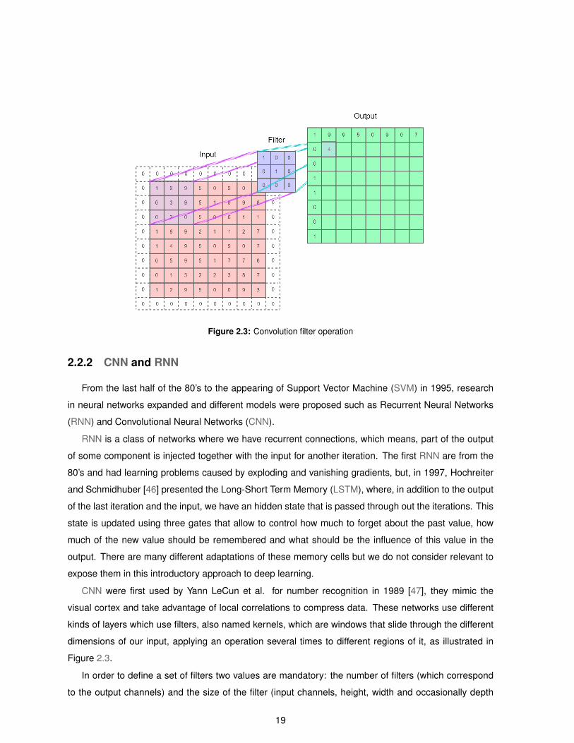
Figure 2.3: Convolution filter operation

2.2.2 CNN and RNN

From the last half of the 80’s to the appearing of Support Vector Machine (SVM) in 1995, research

in neural networks expanded and different models were proposed such as Recurrent Neural Networks

(RNN) and Convolutional Neural Networks (CNN).

RNN is a class of networks where we have recurrent connections, which means, part of the output

of some component is injected together with the input for another iteration. The first RNN are from the

80’s and had learning problems caused by exploding and vanishing gradients, but, in 1997, Hochreiter

and Schmidhuber [46] presented the Long-Short Term Memory (LSTM), where, in addition to the output

of the last iteration and the input, we have an hidden state that is passed through out the iterations. This

state is updated using three gates that allow to control how much to forget about the past value, how

much of the new value should be remembered and what should be the influence of this value in the

output. There are many different adaptations of these memory cells but we do not consider relevant to

expose them in this introductory approach to deep learning.

CNN were first used by Yann LeCun et al. for number recognition in 1989 [47], they mimic the

visual cortex and take advantage of local correlations to compress data. These networks use different

kinds of layers which use filters, also named kernels, which are windows that slide through the different

dimensions of our input, applying an operation several times to different regions of it, as illustrated in

Figure 2.3.

In order to define a set of filters two values are mandatory: the number of filters (which correspond

to the output channels) and the size of the filter (input channels, height, width and occasionally depth

19

when dealing with 3D data). However, there are two additional ways we can modify the filter behaviour:

the stride and the padding. The stride controls the size of the shifting when the filter is sliding, while the

padding indicates if we should add extra volume around our input in order to preserve the dimension of

our data. In Figure 2.3, the 8 × 8 input with only one channel is filtered by only one 3 × 3 convolution

filter using a stride and a padding both set to 1× 1, resulting in a 8 × 8 output. We can use the formula

in Equation 2.2 to calculate the output size O of one dimension with input size I, filter size K, a stride S

and a symmetric padding P , assuming that the fraction bar represents the integer division.

O =I −K + 2P

S+ 1 (2.2)

There are different operations we can do with kernels, but the most common are: pooling operations

and the convolution operation. Pooling operations are non-linear down-sampling techniques that usually

use strides that allow non-overlapping sub-regions. Among these operations the max pooling is the

most commonly used and uses a max filter, choosing the higher value of the sub-region. On the other

hand, the convolution operations commonly keep the dimensions of the input by using a stride of 1 and

making use of padding. In one convolution operation for a two dimensional input, a matrix M(m×m),

using a filter K(k×k), the result will be a new matrix N(m×m) where the Equation 2.3 is used to calculate

the value in position i, j and v = k/2 using integer division.

Ni,j =Mi−v,j−v.K0,0 +Mi−v,j−v+1.K0,1 + . . .+

Mi−v+1,j−v.K1,0 + . . .+

Mi−v+k,j−v+k.Kk,k

(2.3)

2.2.3 Generative Deep Models

With the dawn of the 21th century, the software and hardware developments in parallel computation,

the easy access to big data and to gradient-computation based platforms (e.g. Theano1, TensorFlow2

. . . ) and some new training ideas (unsupervised pre-training, the Adam optimizer [45], dropout [48] as

well as other optimizers and regularization techniques) allowed the blossom of a new era of research in

neural networks now with access to quite complex and deep structures. Deep Artificial Neural Networks,

networks with many hidden layers, are mostly used as black boxes because, despite its simplicity in

terms of model and implementation, it turns out they are very challenging to understand. It is specially

difficult to keep track of what is happening in the hidden layers.

One of the most formidable advantages of these models is that, besides the already known ca-

pacity to evaluate data, they have been recently discovered to obtain very good results in generative1http://deeplearning.net/software/theano2https://www.tensorflow.org

20

approaches. Many generative models and frameworks using Artificial Neural Networks (ANN) have

been presented in the last years: the PixelCNN and PixelRNN [49]; the Generative Stochastic Net-

works (GSN) [50]; and the interest in Restricted Boltzman Machines (RBM) [51] reappeared.

RBM were among the first deep generative models and, according to Goodfellow et al. [41], were

presented under the name ”Harmonium” by Smolensky [51] during the 80’s. These are Boltzman Ma-

chines, binary stochastic undirected graph-based models, where neurons are organized in two layers,

the visible and hidden one, and where, unlike to common Boltzman Machines, intra-layer connection are

not allowed. These machines use stochastic neurons and are energy-based models, meaning that we

define the probability of each state for these neurons using an energy function, E(v, h).

For a machine with nv visible neurons, V, and nh hidden ones, H, with weights defined by the matrix

Wnv×nhand bias bv and bh for visible and hidden neuron respectively, we can calculate the energy, E,

and probability, P , functions for one state (v, h) using the formulas defined in Equations 2.4 and 2.5,

respectively. In these equations, V and H are random vectors, Vi represents the ith random variable in

V and while v and h are concrete states, V ∗ and H∗ represent the set of all possible states for each

of the random vectors. Besides, W is a nv × nh matrix, bv and bh are nv and nh sized vectors. In

Equation 2.6, we prove that, when dealing with binary data and thanks to the special restriction of RBM

that makes neurons in the same layer conditionally independent given the full state of the other layer, we

can calculate the activation probability of one neuron in a layer given the full state of the opposite using

the sigmoid function, σ, shown in Figure 2.2(a).

E(v, h) = −v>Wh− b>v v − b>h h (2.4)

P (V = v,H = h) =e−E(v,h)∑

v∈V ∗

∑h∈H∗

e−E(v,h)(2.5)

P (Vi = 1|H = h) =P (Vi = 1,H = h)

P (H = h)

=

∑v∈V ∗

e−E(v,h), where Vi = 1∑v∈V ∗

e−E(v,h)

=ebvi+Wih

ebvi+Wih + 1

=1

1 + e−(bvi+Wih)

= σ(bvi +Wih)

(2.6)

21

Figure 2.4: Variational Auto-Encoder architecture

Figure 2.5: Generative Adversarial Networks architecture

In 2013 and 2014, two very promising new generative frameworks using deep structures have been

introduced: the Generative Adversarial Networks (GAN) [9] and Variational Auto-Encoder (VAE) [52].

The classic auto-encoder model starts with one encoder that is responsible for turning one instance

into a code (also known as the latent variable) which represents this instance in a different space.

The decoder, the next phase, receives this code and creates a new instance. The learning process

consists in comparing the instance created by the decoder and the initial instance and propagate the

errors through the network. In one VAE [52], the result of the encoder is the description of a Gaussian

distribution, one pair: mean value and standard deviation (µ, σ). For this case, the input for the decoder

is one random sample from this distribution, as represented in Figure 2.4.

GAN [9] is a generative framework where two networks, the generator and the discriminator, dispute

against each other and evolve together. While the role of the generator is to produce instances to

trick the discriminator, this last one must distinguish between fake and real instances. A schematic

representation of the components of GAN is presented in Figure 2.5. The generator G takes random

noise (usally gaussian) z ∼ prandom and turns it into potentially good instances D(z) that are evaluated

by the discriminator D while it also evaluates real data x ∼ preal to continually improve. In this zero-sum

non-cooperative game between the discriminator and the generator, we are looking for a state where

the generator is so good at generating data that the discriminator is not able to find a way to distinguish

between real and generated data. Equation 2.7 presents the minimax equation we want to optimize.

The model converges when neither of the players can achieve a better score by locally improving its

22

strategy, i.e., when they reach a Nash equilibrium point, in terms of game theory, or when both gradients

are very small.

minG

maxD

V (D,G) = Ex∼preal[logD(x)] + Ez∼prandom

[log(1−D(G(z)))] (2.7)

However, there are several major problems that we may run into during the training process:

• Non-convergence: when using gradient descent, there are no guaranties the model will converge.

then, it can oscillate around some stable point(s) and never converge;

• Mode collapse: this case happens when we get an over-specialized generator that only gener-

ates a small number of examples, causing a generation with low variability and an output that is

completely independent from the seed, z;

• Vanishing Gradient: deeply related with the exploding gradient problem, it is a very common

problem in other deep models as well, including RNN, and it is characterized by an accentuated

decrease in gradient’s magnitude, resulting in a very slow training process;

• Overfitting: when the generator and discriminator overfit, we end up with a short variability of

results with the additional problem that the collapsing points are point from the real data, i.e., no

new data is generated;

All these problems are the target of innumerous studies, nowadays, and thanks to these studies, all

of them have already some possible solutions and some insights on how to solve them. Furthermore,

all of them are suspected to be mostly caused by sensitive and inappropriate hyperparameter values,

unsuitable lost functions, meager datasets or unbalanced training processes that side with one of the

components giving it some unwanted advantage. Despite the fact that currently no general procedure

to solve all these problems is known, some commonly used strategies include adding noise to the train-

ing process, using more robust cost functions such as Wasserstein distance with gradient penalties

(WGAN-GP) [53], searching for new hyperparameter values, using dynamic and complex hyperparam-

eters, component specific hyperparameters (e.g. use different learning rates for discriminator and gen-

erator), normalizing or even clipping weights and/or results along the network (batch normalization [54],

spectral normalization [55] and weight clipping) or even pre-trainning some components.

In short, training GAN is a non trivial task and it still is an heuristic guided process that usually

involves a lot of empirical experimentation. Actually, all these training problems represent the biggest

drawback of this approach. Yet GAN have been successfully used for generation and style transferring

in visual data, recently providing sharp high quality results [11,12].

23

Figure 2.6: Cyclical models common architecture

2.2.4 Cyclical Generative Models

Besides all the problems mentioned before, GAN were not originally designed to provide control over

the features of the generated objects. Therefore, some new ways of mixing these training frameworks

have been introduced, such as CycleGAN [56] and DiscoGAN [57], that make use of different loss

functions to find one-to-one mappings between two domains A and B both defined by representative

datasets of non-paired samples. These have been studied and applied for style transferring, achieving

great results in image to image translation. Conversely, to the best of our knowledge, applications of

these models to non-visual data are limited and cross-domain, for example visual to audio, use cases

are almost nonexistent.

Figure 2.6 represents the general components we may find in a cyclical model: two discriminators

(DA, DB) and two generators, one that maps instances of one domain A into instances of B, GAB , and

one that does the opposite GBA. In one of the two streams, the network maps instances a ∈ A into

an intermediate representation b and, afterwards, decode it back a, while trying to ensure that these

transitional codes fool the discriminator DB . The other stream is responsible for the corresponding

process starting with one instance from b ∈ B. The adversarial, also called classical-GAN, loss, LAadvers,

works precisely in the same way it does in usual GAN, pushing b into domain B. At the same time, to

minimize the reconstruction or cycle consistency loss, LArecons, which measures the differences between

the original instance a and the one we were able to recover a, forces the relevant information to flow into

b. The way these loss functions are implemented and used during the training process can vary from

model to model.

24

2.3 Automatic Music Composition Related Work

2.3.1 General Concepts

The marriage between technology and music was desired even before the emergence of computers

as we know them today. Ada Lovelace3 in 1843 already talks about the usage of the Analytical Engine

for music composition:

Supposing, for instance, that the fundamental relations of pitched sounds in the science of

harmony and of musical composition were susceptible of such expressions and adaptations,

the engine might compose elaborate and scientific pieces of music of any degree of com-

plexity or extent.

(Ada Lovelace, 1843, Note A, p. 696)

In the 18th century, Wolfgang Amadeus Mozart composed using one algorithmic composition tech-

nique in Musikalisches Wurfelspiel where songs were created using dices to randomize the order of a

set of already composed parts. In the middle of the 20th century, the dawn of computer brings differ-

ent composers like Iannis Xenakis, Karlheinz Stockhausen and John Cage, to name just a few, to use

these new sound technologies in their art work. David Cope in the beginning of the 1980s starts de-

veloping the Experiments in Music Intelligence (Emmy) and, at the end of the same decade, according

to Eck and Schmidhuber [59], Todd publishes one attempt to generate music using Recurrent Neu-

ral Networks (RNN), technique explored later in the CONCERT system presented by Mozer in 1994.

Since then, several authors have been developing music related systems and new events (conferences,

concerts and workshops among others) focused specifically on this area have been organized.

The usage of generative models to create musical products is known as Automatic Music Generation

(AMG) or as Algorithmic Composition. Since both partial and total automations of the compositional

process are considered in this area, to organize these systems into categories turned out a challenging

task. In 2013, Eigenfeldt et al. [60] propose one taxonomy based on the relationship between the system

and the human user, and its relation with musical gestures:

Level 0 - Not Metacreative Systems: systems that can not be considered as metacreative nor inde-

pendent are placed in this level.

Level 1 - Independence: the systems in this category are simple systems that expand composer/per-

former’s musical gesture without his control.

Level 2 - Compositionality: these systems determine relationships between musical gestures.

3In translator’s notes for Menabrea’s article [58] on Babbage’s Analytical Engine

25

Level 3 - Generativity: the generation of musical gestures is what characterizes this type of systems.

Level 4 - Proactivity: these are systems that are able to initiate their own musical gesture, and may

already be considered as agents.

Level 5 - Adaptability: agents that may influence each other or behave in different ways over time are

known as adaptable.

Level 6 - Versatilty: here we consider agents that can determine their own content with almost no

stylistic limits.

Level 7 - Volition: finally, these agents decide when, what and how to compose/perform; they are

considered as totally autonomous.

It is important to clarify that this taxonomy does not aim to hierarchize systems neither by creativity

nor complexity. It is a scale of autonomy. A system that plays random sounds at random times may be

at the top of this taxonomy and yet it does not seem much complex nor creative. The authors argue that

only when a system is placed in one of these categories, it is possible to discuss about its complexity

and/or musicality, by comparing with others in the same level.

Music is, indeed, different from almost all other areas of creativity (visual arts, humor, sculpture or

even science). It needs to take the time dimension into account; it has several more or less independent

layers of complexity (tracks); and it is, most of the times, preformed. The area of AMG began isolated,

by looking for techniques in other areas that could generate music. Due to the small number of projects

and the isolation of these early small research communities, some problems have been pointed out

to these early works. The poor specification of the practical and theoretical aims, the non-existence

of a methodology to achieve these aims and the usage of inappropriate evaluation methods are some

common problems we may find in most of these early AMG systems.

Merz [61] considers that, nowadays, most of automatic music systems try to get the best results,

without taking into account the algorithm’s and/or approach’s purity. The author defends that this is

appropriate when the main goal is to have musical products. When we want to study the creative pro-

cess that allows the creation of music, we should try not to include what is designated as “ad hoc”

elements. Ad hoc modifications are alterations that are concerned with one specific case, domain de-

pendent changes that are not appropriate for other areas. Three aspects are taken into account by

Merz [61] to decide if a change of the “pure” algorithm may be considered as one ad hoc modification:

• In order to operate with musical information, it is unavoidable to have some kind of non-general

change that defines our work representation.

• Some alteration in one context may be considered as an ad hoc modification and may not be ad

hoc when they are applied in a different context.

26

• Most “pure” algorithms do not have a single and unique definition. Most of the times they are

expandable.

Ad hoc modification analysis is one way to study and measure how much a solution may be gen-

eralized to different kinds of music or different areas of CC. Merz mentioned that methods that have

too many ad hoc modifications “are used to model a specific task rather than the general functioning

of the brain” [61]. In addition to this analysis we must try to find the limitations of these systems, like

contents that may be interesting but can not be generated or the differences between the generated

musical products from each other. At the end, the author questions the need of algorithmic “purity” in

this area arguing that the reason behind the common usage of ad hoc modifications is that music is

social and intrinsically tied to culture and tradition, perhaps, making it impossible to have good results

without these modifications.

In 2016, Widmer [39] presents what he considers to be six well known facts about Western music

that are being “ignored” by the area of Music Information Research (MIR), including AMG:

1. Music is time dependent, therefore approaches based in bag-of-frames, where the frame order is

ignored, should be dropped and temporal models should start to be more used.

2. Music is fundamentally non-Markovian, meaning that usually music does not have the Markov

property; that it is filled with long-term dependencies not captured by most temporal models like

Hidden Markov Models (HMM) or even RNN.

3. Music main goal is to be perceived by human listeners therefore, besides the digital representation,

the emotional effect, tension and anticipation in complex musical structures need to be explored in

AMG systems.

4. Music perception and appreciation are learned, a great argument to use unsupervised artificial

learning systems in AMG and to create good quality data corpora to train these systems.

5. Music is usually performed and there are several different creative choices that are performer’s

responsibilities. These aspects have been neglected in AMG area and the Con Espressione

Project [39] tries to change this.

6. Music is expressive. It affect us. Most of music systems do not take into account none of the three

levels of expressiveness identified: basic, intrinsic and associative

In short, as a recent and applied area the main goals of the AMG community should be to find a

general methodological approach that would provide better analytical and comparison tools; to focus on

new emerging technologies to overcome old obstacles and to unlock new possibilities; to create open

resources in order to expand the community; and finally to explore the merging of completely different

techniques in order to get the best of each one of them.

27

2.3.2 Using Deep Learning

The number of deep learning articles in MIR has increased last years which reflects the new interest

in these techniques, according Choi et al. in their introductory article on deep learning in MIR [62].

In September of 2017, Briot et al. [63], from the Flow Machines project, presented a survey on mu-

sic generation systems using deep learning methods. In this study, the authors propose an analytical

methodology based in four dimension that are not entirely orthogonal:

• Objective: there are different AMG systems that aim different objectives of music generation.

According to Briot et al. [63] the creation of a melody (monophonic or polyphonic) must be consid-

ered as a different task from a multi-track generation or the generation of an harmony for a given

melody. Also the autonomy of the system must be taken into consideration while analyzing deep

AMG systems.

• Representation: when dealing with generative systems we must consider training and generating

phases separately. The training input, the generating input and the generating output representa-

tions might be different. The authors divided the different representations in signal (e.g. waveform,

audio spectrum) which represent more directly the sound waves and symbolic representations

(e.g. Musical Instrument Digital Interface (MIDI), pianoroll, text, chords, lead sheet) much more

similar to a score or even to the act of playing an instrument. They also talk about two different

encodings: one-hot encoding and value-encoding. The first one is suited for finite discrete dimen-

sions, while the former is usually used for continuous dimensions that may be defined as a function

of the other dimensions.

• Architecture: in this dimension we explore: the number of layers; the number of neurons in each

layer; which nonlinearities should be used; how should the artificial neurons be connected; if we

should use attention layers; if we should use some already well known deep structures such as

CNN, RNN, RBM, GAN...

• Strategy: one architecture can be used in different ways, providing different outputs and solv-

ing different tasks. One direct way to use the model starts by feeding it with the beginning of

one song and predict the rest. However, many other different strategies are possible: sampling

from the generated distribution, including input manipulation, making networks play against each

other, concatenating cherry-picked results of different models or even any combination of these

strategies.

28

2.4 Summary

Creativity is a very complex, subjective and difficult to define concept. Usually a creative act involves

four different components, ”the fours P’s of creativity”: a creative person inserted in some creative en-

vironment (press) creates a creative product through a creative process. All these components are

currently target of several studies and have several complementary and sometimes apparently contra-

dictory theories. However, nowadays, researchers have reached the agreement that both novelty and

utility have some big role in creative tasks.

Computational Creativity (CC) is an interdisciplinary field that aims at exploring the relationship be-

tween creativity and algorithms. In this area, researchers develop computational systems to perform

creative tasks or simulate the mental processes that occur in the brain during a creative task, using a

varied range of algorithms. In this work we focused on Deep Learning (DL) algorithms.

DL is a family of ML algorithms that use structures with several layers, commonly known as neural

networks, to extract features from data. Nowadays there are a set of commonly used network architec-

tures such as the Convolutional Neural Networks (CNN), that pay special attention to features related

with spacial locality, and Recurrent Neural Networks (RNN) or Long-Short Term Memory (LSTM) suitable

for sequence processing and time realted features. On generative models we can pointed out the RBM

a energy-based stochastic model, the Variational Auto-Encoder (VAE) and the Generative Adversarial

Networks (GAN). In GAN, we have a generator network that tries to fool a discriminator network that

distinguishes between real and fake examples. Both networks are trainned against each other which can

lead to some already well known but not easily solvable problems such as mode collapse and vanishing

gradient. Cyclical generative models such as CycleGAN [56] and DiscoGAN [57] use GAN loss and

an additional reconstruction loss function in order to learn a one-to-one mapping between two domains

defined by representative non-paired datasets. With this kind of models, two different generators and

two discriminators can be trained to find for instance a translation between two styles of music.

About the Automatic Music Generation (AMG) task, Widmer [39] criticized, in 2016, the way some

well known facts have been ignored by the area of Music Information Research (MIR) such as that music

is usually performed for humans to listen and that those humans socially learned how to appreciate the

expressiveness of it. In 2017, Briot et al. [63] presented four main components of any solution of music

automatic generation using deep learning: the objective, the representation, the architectures and the

strategy.

29

30

3Dataset

Contents

3.1 Representations . . . . . . . . . . . . . . . . . . . . . . . . . . . . . . . . . . . . . . . . 33

3.2 Data Sources . . . . . . . . . . . . . . . . . . . . . . . . . . . . . . . . . . . . . . . . . . 36

3.3 Preprocessing . . . . . . . . . . . . . . . . . . . . . . . . . . . . . . . . . . . . . . . . . 37

3.4 Datasets Characterization . . . . . . . . . . . . . . . . . . . . . . . . . . . . . . . . . . 39

3.5 Summary . . . . . . . . . . . . . . . . . . . . . . . . . . . . . . . . . . . . . . . . . . . . 40

31

32

3.1 Representations

Although nowadays the advantages of data-driven approaches are clear, one must also take into

account all their disadvantages. Data-driven approaches are only possible because there is data to

drive our model and, although nowadays we have easy access to a massive amount of data, more than

at any other time thanks to the internet, data retrieving, cleaning, processing, converting and all the

other data management tasks are not as easy as they may seem in theory.

Searching and gathering data is one of the first tasks in a modern data-driven approach and one of

the most complex. This task encompasses three sub tasks which we are going to present separately: to

choose one representation; to search and gather data from data sources; to preprocess data.

In this work we used DL to learn how to generate epic music. In order to achieve that, we used a

representative dataset, i.e., a dataset of examples, to represent our definition of epic music, which was

used to teach our model the common characteristics of epic music. One distinct representative dataset

exclusively dedicated to melodies was also built and used in our experiments.

As exposed before, Briot et al. [63] consider representation one important component of any DL ap-

proach to music composition. Actually, this is an important aspect of any data-driven approach. If we

think only of the size of the search space generated by the representation, an overly flexible represen-

tation can generate such a vast search space that any search process becomes inefficient, whereas a

too rigid representation may end up excluding too many potentially interesting artifacts. Therefore, trivial

problems may seem very difficult if one uses the wrong representation.

In section 2.3.2, we explained that music representations can classified as signal representations,

such as waveforms, or symbolic representations, such as MIDI and pianoroll representations. The

pianoroll representation receives its name from the homonym storage media used in music boxes or old

automatic pianos.

We used the pianoroll representation as output representation (generated songs) as well as training

and input representations, both for melodies and epic songs. The translation process from pianoroll to

audio allows us to efficiently use different sound libraries (or even human players) to render different

audio results, while the translation from MIDI (commonly used online) to pianoroll is also very efficient.

In addition, the similarities between this representation and some visual representations commonly used

in DL makes it suitable for the use of CNN and GAN models.

In our pianoroll representation we have time, pitch, tracks and velocity (musical intensity) dimensions.

While, the first three dimensions use one hot encoding, i.e., as explained in section 2.3.2, there is one

cell for each one of 3-tuple (timestep,pitch,track), the last one is value-encoded which means that

is represented by a value in each one of those cells. We can visualize this structure as a three-order

tensor (or a cube of cells) where cell cs,p,t stores the value of the velocity of track t at timestep s for the

note p.

33

Figure 3.1: Most commonly used rhythmic figures

To fully understand our representation, we present a deeper analysis of each one of our musical

dimensions:

• Intensity: in our approach, it is represented by a real value in a range from 0, that means not

playing at all, up to 1, which means playing as loud as possible. Usually, this dimension is repre-

sented on a musical score using Italian words such as piano and forte, which mean low and loud

respectively, while in MIDI it is represented by an integer value between 0 and 127.

• Pitch: a scale is a musical structure that defines both the amount of different pitches and the rela-

tionships between them. Different music styles use different musical scales, for instance, Eastern

music, renaissance music and microtonal music all use different pitch scales. The chromatic scale

is the standard for western music because it includes all the most used scales in this culture and

it is used in MIDI where each pitch maps into one integer between 0 and 127. In this mapping, for

example, an A3 corresponds to 57. We also used a 128 sized array to represent the 128 chromatic

notes used in MIDI while allowing to have multiple notes played at the same time.

• Timesteps: the resolution of time (also referred as tick) can be absolute, if it represents a fixed du-

ration time interval, or relative, if it is measured in relation to a symbolic figure and needs a tempo

value to be converted into an absolute time. Regarding relative time, although beat and quarter

are different concepts, the expressions ”beat resolution” and ”quarter resolution” have been fre-

quently used interchangeably, which may become misleading in cases not limited to simple time

signatures, i.e., when a beat does not correspond to a quarter note. For simplicity purposes, in our

approach, we chose to have a 24 beat resolution and a fixed tempo of 120 Beats per Minute (BPM).

This resolution value means that, 4 bars of 4 beats each (assuming a quaternary time signature)

totals 4× 4× 24 = 384 timesteps. These values have been commonly used in pianoroll represen-

tation and allow to represent the most common rhythmic figures, represented in Figure 3.1, from

the whole note, on the left, until a set of sixteenth note triplets on the right. The value of 24 was

calculated by finding the least common multiple for 1, 2, 3, 4 and 6 representing the full, half, third,

quarter and sixth of a beat and then doubling it to make sure we can always represent the end of

one rhythmic figure by inserting an empty timestep.

34

Figure 3.2: Schematic illustration of representation

• Tracks: tracks usually represent instruments or groups of instruments. MIDI represents instru-

ments using programs, using once again integer values between 0 and 127, and allows dynamic

instrumentation, i.e., changing the program of one track in the middle of the piece. On the other

hand, our implementation uses static instrumentation, a fixed program for each track. We de-

cided to use only one track for melody representation (usually rendered in a piano sound). For

epic songs, we used a fixed set of 8 tracks, to represent different groups of instruments: woods

(rendered using the clarinet), brass (rendered using the french horn), percussion set, timpani,

pitched percussion (rendered using tubular bells), voices, strings and keyboards (using piano).

These groups were chosen based on: organological knowledge also reflected in MIDI’s program

mapping; the instrumentation of the epic examples we have collected and the classical symphonic

orchestra configuration.

With one of these cubes or blocks of cells, we can represent one segment of epic music by calculating

the intensity of all the 128 chromatic pitches in each one of the 384 time intervals and for each one of our

8 instruments. The limited fixed time scope is a particularity of this representation, which, at first glance,

may seem as a disadvantage but that actually simplifies our deep learning solution architecture thanks

to its fixed dimension. Moreover, we can have a sequence of these blocks in order to represent longer

music tracks, knowing that with this approach we may lose some structural information.

On the whole, as illustrated in Figure 3.2, the final representation of one epic song is a finite sequence

of 128× 384× 8 sized blocks (notes, timesteps and track), with values between 0 and 1, i.e., a tensor of

4 dimensions, T 4[0,1].

35

3.2 Data Sources

A very natural way to define a concept is throughout stating examples. However this practice is very

prone to bias factors, even more if we are dealing with subjective concepts such as ”epic”. There are

many different ways to create a representative dataset, but when dealing with subjective concepts most

of them include two steps: gathering data and labeling it. During the analysis of the different possible

approaches, we identified two dimensions that may impact both the time it takes to create the dataset

and its overall quality.

The first of these dimensions is the temporal relationship between the processes of gathering and

labeling data. By gathering pre-labeled data we are able to spend less time in labeling data afterwards.

However, to find pre-labeled data often means using costly expert knowledge or conducting a time

consuming search process. On the other side, to conduct a post-labeling process on an heterogeneous

amount of gathered data provides us the flexibility and control we may need in some contexts, in return

for a much more longstanding labeling process. Hybrid approaches that join advantages from both are

also a possibility and were also considered.

The second dimension we should consider is the format of the gathered data. When we are dealing

with real data, we can not expect to receive the data from the source already formatted and using the

intended final representation. A preprocessing phase is often needed and depending on the source

representation, this phase can become very time consuming or even produce low quality results. For

instance, nowadays, the task of decoding signal data into a symbolic representation is a complex, very

prone to fault task while, conversely, the translation between symbolic representations is most of the

times simple to program. This means that, to extract pianorolls from MIDI files is easy whereas extracting

them from WAV files is much more complex. However, while the latter are relatively easy to find available

online, the former are not and most of the times are not pre-labeled with the terms we desire nor have

enough heterogeneity to allow us to use the desired labels afterwards.

Besides these two, there are many other dimensions which we can pay attention to, when defining cri-

teria for choosing the best data source and methodology. As guidelines for our pursuit for data sources,

we focused on pre-labeled symbolic data sources, in order to prevent great loses during preprocessing

and to avoid the time consuming task of post-labeling the data.

After analyzing the perks and realities of some of the approaches, we included in our representative

dataset of epic music some samples available in an open score library created and managed by the

enterprise responsible for MuseScore1, an open source score editing software. From this library of

original and adapted pieces, available for downloading in MIDI format, we considered exclusively those

samples that were provided in a specific group uniquely dedicated to ”Epic Orchestral Music”2. We

1https://musescore.com2https://musescore.com/groups/epicorchestralmusic

36

used the assumption that the content (orchestral pieces) present in this group could represent well the

concept of epic music, and, in this sense, this group represents a pre-labeled MIDI data source which

supported a simple way to retrieve data for our representative dataset. Moreover, the high availability of

the service and the existence of other groups dedicated to other music styles, provides a free and easy

way to create new and distinct datasets. On the other hand, there are also some disadvantages. One

is copyrights, that may partially or integrally forbid us to freely distribute our dataset and to share it with

the rest of the scientific community. Besides that, we must take into account that most of this content

was inserted in the ”Epic Orchestral Music” group by content creators, which may have some impact in

the overall quality of the dataset. Summing up, we considered this solution achieved a good balance

between the dataset quality and the time dispensed for data management and processing.

For our dataset of melodies, we opted to use a very practical and brief approach. Since ”melody”

is a much less subjective concept, we used an automatic melody generator3 available online to create

a dataset of heterogeneous MIDI melodies. This generator used some parameters such as the tonality

factor, which regulates how tonal should the melody be; the proximity factor, that fosters smaller intervals;

or even repeated notes to allow the repetition of notes.

3.3 Preprocessing

Music dedicated tools usually are not as popular as those used in other domains. When searching

for python libraries for MIDI and pianoroll preprocessing and visualization, although we were able to

find some, they were very dispersed and were not uniformed. Consequently, during the whole devel-

opment of this work, we used different libraries and different representations such as midi.Pattern4,

pretty midi.PrettyMIDI5, pypianoroll.Multitrack6 and mido.MidiFile7. All these representa-

tions were finally integrated in one unified library, the Gmidi8 (General MIDI) library, along with a new

one midiarray.MidiArray and some new functionalities. This new library works as a facade for all the

representations, transparently translating from one to another when we want to use specific methods or

access to certain attributes. Inside the Gmidi library, we also included some new methods for visualiza-

tion, storing and preprocessing MIDI data such as for chopping a MIDI file in blocks or for re-orchestrating

a MIDI.

Our preprocessing procedure is summarized in the next steps:

1. Re-orchestrate: the MIDI files gathered, had different numbers of tracks and used different sets

3https://www.link.cs.cmu.edu/melody-generator4https://github.com/vishnubob/python-midi5https://github.com/craffel/pretty-midi6https://salu133445.github.io/pypianoroll7https://mido.readthedocs.io8https://github.com/LESSSE/gmidi

37

of instruments, therefore, in order to uniformize them, we mapped each MIDI program into one of

our 8 tracks, based on this we assigned a destination track to each one of the original tracks and

finally copied every note in each one of the original tracks to its correspondent destination track;

2. Translate into Pianoroll: the MIDI files are transformed into pianoroll, walking through the list of

events and filling all the cells of the matrix that correspond to the timesteps between the start and

stop note events;

3. Chop: after considering several chopping techniques, we opted to use a non-informed chopping

technique that chops one song in contiguous non-overlapping fixed size blocks;

4. Transpose: thanks to the equal temperament, i.e., all semitones are equal, we can move the pitch

of each note n semitones above or bellow without damaging the relationship between those, thus

we transposed each one of the pieces for each one of the pitches between −6 and +5 semitones,

in one attempt to create more variety in our dataset;

5. Thresholds: we discarded notes that were being played to low or too loud;

6. Normalize: all value-encoded velocities were mapped into a value between 0 and 1;

Data augmentation techniques are methods by which one can expand the size of one dataset by

exploiting known symmetries (or other kinds properties) of the data. During the creation of the dataset,

several augmentation techniques were considered: transposing (an epic music using a different key still

sounds epic), doubling or halving rhythmic values (the sonority of one song does not depend on the

relative time of the notes), track switch (switching parts of two instruments should not make one epic

song not epic, but can make it very difficult to be played by human musicians). Some initial experiments

were conducted using data augmentation by transposition and following one adaptation of the SGD

process where all the batch instances were augmented from the same original instance, technique which

we called Augmented Stochastic Grandient Descent. However, in the end, no augmentation method was

used, since we verified that it added no clear value to the overall approach.

During early development, we verified that to store all the data as a full already preprocessed matrix

would require more memory than we had available. Supposing that it uses 32-bit float precision format

to store 12 different transpositions of one block with the dimensions defined in section 3.1 (128 pitches,

384 timesteps and 8 tracks), a single block of one epic song would occupy 128 × 384 × 8 × 4 × 12 =

18MB. Knowing that the 335 songs gathered in our dataset have in average 17 blocks, we would need

over than 335 × 17 × 18 > 100GB of available storing space just to store only one of the datasets.

MIDI files are a much more efficient way to store our data, with an average file size of 20.17KB and

a maximum of 118.91KB, then we adopted an online preprocessing method, where one instance is

entirely preprocessed just before running the training with that particular instance and never storing

38

the results of preprocessing. However, this approach has proved to be very time inefficient. Finally, to

address this last issue, we returned to an offline approach and developed a sparse representation, that

we also included in Gmidi library, that take advantage of the sparsity of our data, allowing us to store

already preprocessed data with an average size of 1.20MB per file, while liberating the training phase

from all preprocessing overheads.

3.4 Datasets Characterization

From the 561 songs available inside ”Epic Orchestral Music” group on 30th May of 2018, we filtered

those that: used strange programs that our representation could not support; used no strings or were

composed for solo instruments; were to big to load in memory as a matrix; keeping only 335 of those

songs in the final version of the Epic Dataset. The complete list of references for the resulting set of epic

songs is available at Appendix 7.

The Melody Dataset includes 300 melodies using various keys, that were generated using different

values for the proximity and tonal factors, allowing an heterogeneous set fo melodies. Table 3.1 compiles

some statistics and metrics to characterize our new datasets: the Epic Dataset and the Melody Dataset.

In the first parts of the table we hove some statistics about the users that uploaded content that was

included in the final Epic Dataset, including those that contributed the most. As expected in any scale-

free network, the number of songs is not uniformly distributed over the users, it follows a power law, i.e.,

there are few authors contributing a lot for the dataset while there are many composers contributing with

only one piece. For instance, the user 10712571 is responsible for uploading more than one third of the

blocks included in the dataset 233216.91×335 ≈ 0.4, and the four users that contributed the most cover more

than 50% of the dataset.

The second and third parts of the table show some information about the dimensions and musical

features of the songs and melodies in our datasets. The methods to calculate these musical metrics were

adapted from the MuseGAN project [8] and were included in the Gmidi library. The data shows us that

although the strings dominate in epic songs, which means that, in average, they have more volume than

any other instrument, usually one epic song uses 6 of the 8 tracks we have in our representation. Both

epic songs and melodies have little spots of silent and usually use no more than 6 from the 12 possible

classes of pitches (all the C notes belong to the same class, regardless of the octave). The diatonic,

harmonic and pentatonic metrics provide a way to measure how the pitch classes used in a sample

correspond to the diatonic, harmonic and pentatonic scales, while the harmonicity metric represents the

inter tonality between different tracks.

39

Figure 3.3: Evolution of the volume along an average epic song in the new epic dataset

In Figure 3.3 we can see that both the average and the standard deviation of the sound volume

increase along one epic song. This graph was achieved by aligning the beginning and ending of the

songs and using linear interpolation to align the rest of the points between two lines. This sound volume

measure is affected not only by how loud the instruments are playing but also how many of them are

playing in one moment, and it is calculated by summing up all the velocity values and dividing by the

number of timesteps in our block.

3.5 Summary

Concluding, in this chapter we present the two new datasets created for this work: the Epic Dataset

and the Melody Dataset. The first one contains samples of epic songs originally obtained from an

online group exclusively dedicated to orchestral epic music, that were preprocessed and translated into

a sequence of pianoroll blocks with 8 tracks, 128 pitches and 384 timesteps. The data in our Melody

Dataset was created by applying the same preprocessing procedure to some MIDI files generated by

an automatic melody generator. During the creation of the data sets we developed the Gmidi library in

order to gather, compile and integrate all the tools we used.

40

Table 3.1: Characterization of the new datasets

Epic Dataset Melody DatasetNumber of songs 335 songs 300 songs

Users and ContributionsDistinct Users 78 users -Users with only one song 45 users -User with Greatest Contribution user 10712571 -Greatest Contribution (Songs) 100 songs -Greatest Contribution (Blocks) 2332 blocks -Second User with Greatest Contribution user 2544941 -Second Greatest Contribution (Songs) 18 songs -Second Greatest Contribution (Blocks) 274 blocks -

DimensionsAverage Number of Original Tracks per Song 24.6 tracks 1 trackAverage MIDI File Size per Song 20.14KB 3.11KBAverage Number of Blocks per Song 16.91 blocks 12.38 blocksAverage Number of Ticks per Song 6781.33 ticks 4755.20 ticksAverage Number of Notes per Song 1876.48 notes 347.50 notesAverage Duration per Song 02m57s 01m43sTotal MIDI Size 6.59MB 933.07KBTotal Number of Blocks 5665 blocks 3715 blocksTotal Duration 16h30m56s 08h35m52s

Musical MetricsStatistical Mode of Dominant Instrument Strings PianoStatistical Mode of Number of Instruments Used per Song 6 1Average Empty Timesteps Ratio per Song 0.042263 0.097024Average Volume per Sounding Tick 4.134 0.503Statistical Mode of Number of Pitch Classes Used 6 5Statistical Mode of Pitch Extension 65 34, 36Highest Pitch Used 111 78Lowest Pitch Used 0 42Average Reused Notes Index 43.216 25.288Average Ratio of Qualified Notes (≥ than a sixteenth note triplet) 0.920664 0.999812Average Ratio of Long Notes (≥ than an eighth note) 0.607416 0.534424Average Ratio of Long Notes (≥ than a quarter note) 0.338370 0.159075Average Diatonic Similarity Metric 0.582159 0.627548Average Harmonic Similarity Metric 0.545730 0.584224Average Pentatonic Similarity Metric 0.369851 0.298396Average Harmonicity Metric 1.403273 −Average Polyphonic Ratio per Song (> than 2 notes) 0.774234 −Average Polyphonic Ratio per Song (> than 3 notes) 0.618742 −

41

42

4Models

Contents

4.1 Environment and Tools . . . . . . . . . . . . . . . . . . . . . . . . . . . . . . . . . . . . 45

4.2 HRBMM . . . . . . . . . . . . . . . . . . . . . . . . . . . . . . . . . . . . . . . . . . . . . 46

4.3 MuseGAN . . . . . . . . . . . . . . . . . . . . . . . . . . . . . . . . . . . . . . . . . . . . 48

4.4 MuCyG . . . . . . . . . . . . . . . . . . . . . . . . . . . . . . . . . . . . . . . . . . . . . 50

4.5 Tuning . . . . . . . . . . . . . . . . . . . . . . . . . . . . . . . . . . . . . . . . . . . . . . 52

4.6 Summary . . . . . . . . . . . . . . . . . . . . . . . . . . . . . . . . . . . . . . . . . . . . 53

43

44

4.1 Environment and Tools

Choosing the right tools to tackle a problem is a decisive issue that can define the success or failure

of any project. Therefore, before developing any kind of piece of software, one must always have a look

into what tools and resources are available. To find the right tools, we need to find a balance between

the learning curve, the time spent on configuring and maintaining the development environment and the

time spent developing the final software, while taking into account other issues such as the fault recovery

capability, code reviewing and the flexibility of the tools.

Nowadays, there is a wide range of tools for developing ML models, providing various degrees of

abstraction and different levels of flexibility: some allow to create new models by writing the code of the

different stages of the model, others provide drag and drop interfaces to built the data flow; some were

developed for on-permise development, others run on the cloud for scalability; some are for general use,

others focus specific branches of ML. In Table 4.1 we compare some basic machine learning developing

tools.

We decided that using a Python 31 based tool was the best choice due to its simplicity, flexibility and

familiarity. Python is a simple, flexible and easy to learn object-oriented language that, during these last

years, has been widely used for all kind of applications, including for DL, thanks to the great availability

of DL related libraries such as Tensorflow. Tensorflow is a strong and flexible dataflow programming

framework widely used for general ML. In this dataflow programming paradigm, the programmer writes

the code to create and manipulate a set of objects which represent data operations. These objects

define a graph of operations through out which the data will flow. Tensorflow have a big, very active and

helpful support community online. There is also a big online collection of already implemented models

using Tensorflow on Python, including some of the models we wanted to adapt.

We used a local Windows machine to work on, from which we manage and access all the other

development environments. Firstly, using Vagrant2, we created a local Linux virtual machine, that, using

Ansible3, automatically configured a Jupyter Notebook4 server and all the Python libraries we needed for

quick testing small parts of code, visualizing results and semi-automate reporting. This environment al-

lowed us to test new ideas and to start working on the models, even without any internet connection, and

in case of a problem with the local machine it could be easily setted up in a different machine with virtual-

ization tools and a Vagrant instance installed, by cloning a git repository5 available on GitHub. However,

the models grew up and it became practically impossible to run them in a local machine. Therefore,

we used servers provided by the L2F group from Instituto de Engenharia de Sistemas e Computadores

- Investigacao e Desenvolvimento (INESC-ID) at Lisbon. These machines provided enough Graphics1https://www.python.org2https://www.vagrantup.com3https://www.ansible.com4https://jupyter.org5https://github.com/LESSSE/music-cage-machine

45

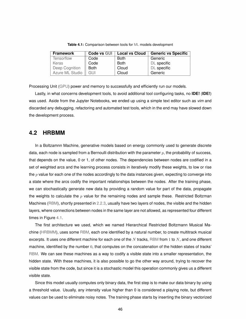
Table 4.1: Comparison between tools for ML models development

Framework Code vs GUI Local vs Cloud Generic vs SpecificTensorflow Code Both GenericKeras Code Both DL specificDeep Cognition Both Cloud DL specificAzure ML Studio GUI Cloud Generic

Processing Unit (GPU) power and memory to successfully and efficiently run our models.

Lastly, in what concerns development tools, to avoid additional tool configuring tasks, no IDE! (IDE!)

was used. Aside from the Jupyter Notebooks, we ended up using a simple text editor such as vim and

discarded any debugging, refactoring and automated test tools, which in the end may have slowed down

the development process.

4.2 HRBMM

In a Boltzamnn Machine, generative models based on energy commonly used to generate discrete

data, each node is sampled from a Bernoulli distribution with the parameter p, the probability of success,

that depends on the value, 0 or 1, of other nodes. The dependencies between nodes are codified in a

set of weighted arcs and the learning process consists in iteratively modify these weights, to low or rise

the p value for each one of the nodes accordingly to the data instances given, expecting to converge into

a state where the arcs codify the important relationships between the nodes. After the training phase,

we can stochastically generate new data by providing a random value for part of the data, propagate

the weights to calculate the p value for the remaining nodes and sample these. Restricted Boltzman

Machines (RBM), shortly presented in 2.2.3, usually have two layers of nodes, the visible and the hidden

layers, where connections between nodes in the same layer are not allowed, as represented four different

times in Figure 4.1.

The first architecture we used, which we named Hierarchical Restricted Boltzmann Musical Ma-

chine (HRBMM), uses some RBM, each one identified by a natural number, to create multitrack musical

excerpts. It uses one different machine for each one of the N tracks, RBM from 1 to N , and one different

machine, identified by the number 0, that computes on the concatenation of the hidden states of tracks’

RBM. We can see these machines as a way to codify a visible state into a smaller representation, the

hidden state. With these machines, it is also possible to go the other way around, trying to recover the

visible state from the code, but since it is a stochastic model this operation commonly gives us a different

visible state.

Since this model usually computes only binary data, the first step is to make our data binary by using

a threshold value. Usually, any intensity value higher than 0 is considered a playing note, but different

values can be used to eliminate noisy notes. The training phase starts by inserting the binary vectorized

46

Figure 4.1: HRBMM architecture

pianoroll (also called flatten) of each one of the 8 tracks in the visible layer of the respective machine.

With this in mind, one can easily conclude that the visible layer of each one of these 8 machines has

128 × 384 = 49 152 nodes, the number of notes times the number of timesteps in our representation.

These are connected to 128 hidden nodes using (128× 384)× 128 arcs and using one extra bias arc for

each one of the nodes, resulting in a total of (128×384)×128+(128×384)+128 = 6 340 736 arc weights

per track machine that we need to optimize. The hidden states of each one of the RBM from 1 to 8 are

concatenated in a 128 × 8 = 1024 sized visible state for machine number 0 which uses a new hidden

states also with 128 nodes. This last machine adds more (1024 × 128) + 1024 + 128 = 132 224 arcs to

train, including the arcs between the layers and bias arcs. Counting everything, we end up with the wide

number of 8× 6 340 736 + 132 224 = 50 858 112 parameters to optimize during the training process.

During the training process, after inserting the input in machine i, we propagate the visible values

vi to the hidden nodes by multiplying them by the weights matrix W i, adding hidden bias bih, applying

the sigmoid function σ to this sum, as shown in Equation 2.6 and finally sampling using the resulting

value to parameterize a Bernoulli experiment. After getting all the hidden states for 1 to N machines,

we concatenate them and inject it in the visible layer of machine number 0 and we do the same step to

propagate the values to the hidden layer.

Once we arrived to this state we go backwards using transposed matrices to sample new visible

states for each one of the machines, i.e., 8 new segments for each one of the 8 tracks. The process

that goes from one visible state to another is called a Gibbs step and a Gibbs sample uses one or more

Gibbs steps. Due to time efficiency constraints, it is common to perform only one Gibbs step during the

training process. After having one sample of the hidden and visible states we can use the differences

47

between these states and the states first propagated from our data to update the biases and weights.

The sampling process is similar, using only one Gibbs step on a full 0 initial visible state and a full song

is created by concatenating of several sampled blocks.

After a quick analysis of this model, one of the first things that caught our attention was that it only

generates binary data which leads to music without any dynamics. Knowing that epic music takes

advantage of dynamics to create an impact on the listener, this approach may not fit to our goals.

Another problem with this approach, is that it is not easy to control the output, i.e., include features from

one input into the final product, which can make unclear how the melody inspiration mechanism could or

should be included. Yet, it was a very straight forward and easy to implement model with the capability

of providing great results, specially in what concerns the novelty.

4.3 MuseGAN

MuseGAN6, first presented in November of 2017 by Dong et al. [8] was, to the best of our knowledge,

the first application of GAN, discussed in 2.2.3, to the task of multitrack symbolic music generation. This

project also used pianoroll to represent the training and output samples, it was also implemented using

Tensorflow over Python and it explores three different ways of generating tracks inspired in different

contexts for music creation:

• the jamming model: where each track uses an independent generator and discriminator;

• the composer model: which uses only one generator and single discriminator for all the tracks;

• an hybrid model: that combines features of both models, having one private generator for each

one of the tracks but only one discriminator that evaluates the credibility of the joined tracks.

One basic possible sampling strategy was to concatenate several results from the bar generator(s),

but, since these bars are totally independent, this strategy does not allow to model some important

temporal relations in music, possibly resulting in a very incoherent final product. In order to address this

problem, the authors include a vector that represents the temporal structure, a sequence of codes that

can be used to generate a sequence of coherent bars, which are afterwards complemented with some

per-track and per-bar specific random seeds to promote the variety of the results.

In the end, to simplify the task, Dong et al. [8] decided to generate binary pianorolls (ignoring note

velocity) and in order to make the overall process more stable the authors used different techniques:

• Wasserstein Generative Adversarial Networks with Gradient Penality (WGAN-GP) [53] as the cost

function;

6https://github.com/salu133445/musegan

48

• batch normalization [54] in the generator, which learns the mean and variance of the values in

each layer and use these values to normalize the hidden states;

• LReLU as the activation function;

• an unbalanced training, updating the generators only once every five updates of the discriminator.

We adapted the hybrid model to work against our Epic Dataset and limited the modifications to those

that were imperative to do in order to work with this new data. Since now one instance consists in 4

bars of 8 tracks of 128 different pitches, these changes consisted mostly in changing the size of some

variables and the size of some convolution filters. In the training process, we only choose a different

learning rate, explained in 4.5 and dismissed the unbalancing factor, making both the discriminator and

generator update at the same time, keeping all the rest.

Both the generators and discriminators use CNN, introduced in 2.2.2, to compress each one of the

blocks used to represent one song, presented in section 3.1, into a smaller representation. In the

discriminator, the model uses the convolutional network represented in Figure 4.2. Starting with one

block of shape (386, 127, 8), the first step is to divide it into 4 different bars of 96 timesteps and extend

the pitch dimension by padding the data, to get a multiple of 12 semitones, i.e., an integer number of

octaves (recalling that a perfect octave has 12 semitones). The block is then inserted into four different

streams:

• the timestep-first stream: where, using convolutional filters in non overlapping areas of the data,

we reduce the dimensions of the data, starting by the timesteps;

• the pitch-first stream: that perform the same operations as the timestep-first stream but in a

different order, starting by compressing the pitch first;

• the onset stream: which firstly identifies the beginning of each note and uses convolutional filters

over the result;

• the chroma stream: that starts by folding the pianoroll in a single octave representation and

performing convolutions over that.

After these streams the resulting tensors are concatenated and reduced into a 512 vector. On the

other hand, the generator uses a deconvolutional network which expands a new block from a compact

representation, as shown in Figure 4.3. In this network we have two streams that are similar to the

pitch-fist and timestep-first streams but that expand the dimensions instead of reducing them.

Contrarily to the binary sampling method originally used in the paper, we decided not to discretize

the results and make use of the values to define the velocity of the notes. This way we can create

dynamics fluctuations along the music. Therefore, when compared to HRBMM, this model has the

49

advantage of making use of dynamics and the usage of convolution networks allows a smaller number

of weights to optimize, dropping the total number of parameters to 9 821 081. However, as we have seen

in section 2.2.3, GAN are complex models that are really difficult to train, that are not easy to optimize

and that may suffer from too many different problems for which we do not have yet one general solution.

4.4 MuCyG

We present the Musical CycleGAN (MuCyG) that is the first implementation of CycleGAN applied

to multitrack symbolic music that takes into account velocities, to the best of our knowledge. With our

main objectives in mind, we conceived what we considered a general model, inspired by the process

of musical composition with mechanisms of inspiration, that uses cyclical models which have been

achieving great results in one-to-one mapping across visual domains.

As in any generic cyclical model, such as the one presented in section 2.2.4, the MuCyG uses two

discriminators and two generators. Taking into account the main aims of this work, we attempt to use

the model to translate melodies into epic music and the other way around. To minimize the complexity

of the project, we used generators and discriminators based on the architecture used in MuseGAN,

using CNN. In Figures 4.2 and 4.3, we have a detailed schematic representation of the operations and

different states our 8-track data flows through inside our convolutional and deconvolutional architectures,

respectively.

When compared to other CNN, these networks present two peculiarities: pooling layers are not used;

and, when a convolutional filter is applied, usually there is no overlapping areas, i.e., most of the times

the stride corresponds to the size of the filter.

In our convolutional network the data is compress into a 512 sized representation. The first step is

to expand the pitch dimension to the next multiple of 12 greater than 128, in order to always represent

complete octaves (each one including twelve semitones). After that, different streams compress the

data in different ways, exploring different features, but always converging into a concatenation step. On

the contrary, the deconvolutional network expands the representation, generating a new instance. At the

end of the process we drop the pitches that were synthetically added to our data.

Both these networks are used to build our generators, starting with a convolutional network followed

by a deconvolutional network. The discriminators are made up of only one convolutional network that

compresses our blocks into 512 sized representations and feeds those to one LSTM, which is responsi-

ble to evaluate the pattern structure of these compressed codes. As adversarial loss function, we used

WGAN without gradient penalties, instead of WGAN-GP used in MuseGAN, because this was not sup-

ported by the Tensorflow version we were using. To measure the reconstruction loss we used a simple

mean difference.

50

Figu

re4.

2:C

onvo

lutio

naln

etw

ork

arch

itect

ure

used

inM

useG

AN

and

MuC

yGfo

rthe

epic

data

set

Figu

re4.

3:D

econ

volu

tiona

lnet

wor

kar

chite

ctur

eus

edin

Mus

eGA

Nan

dM

uCyG

fort

heep

icda

tase

t

51

When training simultaneously with two non-aligned datasets of different sizes, some questions may

arise: should we balance the datasets? How to make both datasets the same size? What is an epoch,

when the sizes are different? Should we train one of the domains with more examples? In our definition,

one epoch corresponds to train the model with all the data one time and one time only. This way, in one

epoch no instance is repeated nor wasted, thanks to the implemented mechanism that only optimizes

what it is possible with the given data. Yet, very unbalanced datasets lead to an inappropriate training

process, which may cause some problems such as mode collapsing or overfitting.

The sampling process firstly consisted in getting the result from the epic generator by feeding it one

melody.

This model aims at overcoming the lack of an inspiration mechanism. Yet, it is an experimental model

with a high complexity which can take a very long time to optimize, possibly beyond our time constraints.

For example one point particularly difficult to manage is the balance between the adversarial losses

and reconstruction losses. To the best of our knowledge this problem was not addressed yet, probably

because it only becomes visible when dealing with non balanced loss measurements, such as the mean

difference.

4.5 Tuning

Using these models and environments we conduct several experiments on music generation in order

to tune some aspects of the models. We chose the name MuCaGEX (Music Categories Generation

Experiments) to identify all the software we developed in order to conduct these experiments, and the

code is integrally available in https://github.com/LESSSE/public_MuCaGEx. In order to compare these

three models in a fair way we needed to make sure that all are in a state that can be comparable, since

the choice of the right hyperparameters can have a huge impact in performance.

During the initial experiments, with training, the results of our models converged into completely

empty tensors, full zero matrices, representing completely silent samples. After checking for semantic

bugs, we decided to focus our study in one of the most important hyperparameters: the learning rate.

Learning rate is “reliably one of the most difficult to set hyperparameters because it significantly affects

model performance”, as noted by Goodfellow et al. [41]. However, the same authors also state that “[to

choose the right learning rate] is more of an art than a science”, making clear that, currently, there is no

good general way to tune this value.

In our method to tune the learning rate, we trained each model on three random small subsets of the

Epic Dataset with an exponential growing learning rate, and plotted the difference between the densities

of the original o and the generated instance g, as defined in Eq. 4.1. In Figure 4.4 we see the resulting

plots and verify that the three models behave differently when set with the same learning rate.

52

density(Tm×n×t) =

∑mi=0

∑nj=0

∑tk=0 Tijk

n×m× tloss =density(o)− density(g)

(4.1)

Choosing a learning rate value associated with high variances should allow the training to move

quickly towards the goal. In fact, it allows steps too big, resulting in an erratic training trajectory. We

considered that this erratic movement had some creative potential, therefore we searched for spikes in

the standard deviation and in the first derivative and used the corresponding learning rate. The final

values used for the learning rates of each model are: 1 × 10−1 for HRBMM, 2.51 × 10−4 for MuseGan

and 5× 10−4 for MuCyG.

4.6 Summary

During this work, three models in Tensoflow were adapted or implemented to work against our Epic

Dataset. MuCaGEx is the name of the repository that includes all the code we used to conduct several

experiments on automatic music generation using these three models.

The HRBMM uses one dedicated RBM for each one of the tracks and an additional one that computes

on the concatenation of the hidden states of the track-dedicated machines. Since it is a binary stochastic

model, it did not allow us to explore dynamics.

We adapted the hybrid MuseGAN model, presented by Dong et al. [8], that uses dedicated genera-

tors for each one of the tracks, that play against an unique discriminator in a GAN-like environment. This

model was able to model dynamics and some long term structure.

The last model, MuCyG, was an original model based on the idea of cycle consistency, explored in

other models such like CycleGAN [56] and DiscoGAN [57]. This model intended to translate melodies

into epic music excerpts and it was the only one from the three, that used both the Epic Dataset and the

Melody Dataset. Using two streams, two generators, two discriminators and two types of loss functions,

it generates a product from a melody and generates a second melody from this product, making sure

that this generated product was indistinguishable from real epic music samples and that the second

melody was the same as the original one. In the second stream, the process started with an epic music

that was translated into a melody.

We tuned the learning rate of our models by studying the variation of density of the generated sam-

ples when the models were trained with exponentially increasing learning rate. After this study, we chose

learning rate values associated with big variations of density.

53

Figure 4.4: Resulting plots for learning rate study

54

5Results and Evaluation

Contents

5.1 Final Experiment . . . . . . . . . . . . . . . . . . . . . . . . . . . . . . . . . . . . . . . . 57

5.2 Survey . . . . . . . . . . . . . . . . . . . . . . . . . . . . . . . . . . . . . . . . . . . . . 62

5.3 Summary . . . . . . . . . . . . . . . . . . . . . . . . . . . . . . . . . . . . . . . . . . . . 73

55

56

5.1 Final Experiment

The final experiments used a methodology inspired in the way humans learn music composition:

in the beginning, one starts studying some ”classic” examples in detail, and only then one gradually

introduces more and more complex examples, taking less time to learn, in each iteration. The training

process adopted the following steps:

1. firstly, using one subset of only 15 elements of each one of the datasets, we trained each model

for one full day of CPU time;

2. after this we took our first 32 seconds long sample, which corresponds to 4 blocks;

3. then we trained the models one more time using sub-datasets of 30 random samples for only half

a day;

4. sampled the second excerpt also with a duration of 32 seconds.

The resulting 8 samples1 (including two samples composed by humans, randomly selected from

the dataset), hereinafter referred to as Human 1, Human 2, HRBMM 1, HRBMM 2, MuseGAN 1,

MuseGAN 2, MuCyG 1 and MuCyG 2, have their pianorolls represented in Figure 5.1(a), Figure 5.1(b),

Figure 5.2(a), Figure 5.2(b), Figure 5.3(a), Figure 5.3(b), Figure 5.4(a) and Figure 5.4(b), respectively.

We can draw some conclusions about the characteristics of our samples, from these figures.

HRBMM’s samples look very chaotic, without any kind of order nor long notes. However, we can

see that strings, represented in orange, dominate in HRBMM 1, Figure 5.2(a), while they share the

dominance with brass instruments in HRBMM 2, Figure 5.2(b).

In MuseGAN’s samples, represented in Figure 5.3(a) and Figure 5.3(b), we can see that there is

a pattern that is repeated 16 times, with some variations, associated with the 16 bars we have in our

samples. We can also see patterns repeated 4 times inside a bar, 64 time in total along our sample,

that represent 4 beats inside the quaternary time signature. According to Simchy-Gross and Margulis,

”repetition musicalizes [...] sounds” [64]. This effect makes repetition to provide musical coherence and

makes samples to sound like minimal music. On the other hand this not completely identical repetition

is a symptom of a bigger problem in our model: mode collapse. Besides this, we can see longer notes

and a dominance of the strings in both these samples.

Finally, we can see that similar repetition effects and symptoms are present in MuCyG samples, rep-

resented in Figure 5.3(a), Figure 5.3(b). Possibly also due to the collapse mode problem, the melodies

generated by MucyG were empty and all the epic songs that were generated with some fixed learned

parameters sounded identical disregarding the input. These samples also make a strong use of strings

but possibly due to the additional reconstruction restriction both samples feature less notes.1http://web.tecnico.ulisboa.pt/~ist178303/mucagex/Final_Samples/

57

(a) Human 1

(b) Human 2

Figure 5.1: Pianoroll representation of Human composed samples used in survey

58

(a) HRBMM 1

(b) HRBMM 2

Figure 5.2: Pianoroll representation of HRBMM’s samples used in survey

59

(a) MuseGAN 1

(b) MuseGAN 2

Figure 5.3: Pianoroll representation of MuseGAN’s samples used in survey

60

(a) MuCyG 1

(b) MuCyG 2

Figure 5.4: Pianoroll representation of MuCyG’s samples used in survey

61

5.2 Survey

In order to compare the results of the experiments using our three models, we conducted an online

survey2. In Appendix 9, we provide one example of the survey presented to the users, with the difference

that we present the names of the samples bellow each audio controller. This responsive web page was

implemented using PHP and SurveyJS3, a JavaScript library, and the final results after being stored in

JSON files were analyzed using Pandas4 and NetworkX5 and visualized using Matplotlib6 libraries for

Python in a Jupyter Notebook.

The final samples were compared in three different contexts:

• word description, one open question where the respondent could insert up to three words to de-

scribe each one of the excerpts presented;

• one exercise where the sentence ”This epic music is creative.” referring to two specific excerpts,

namely MuCyG 1 and Human 2, is evaluated on a Likert scale from 1 to 10, several times while

provided with new information about the inspiration, explanation and nature of the excerpt;

• one relative direct confrontation, where excerpts confronted each other in an evaluation focused in

one of 5 specific characteristics, and where the user explicitly chose the winner.

The information retrieved from all the 100 responses we received, is from one population character-

ized as presented in both Table 5.1 and Table 5.2. As we may see, most of the people were between

18 and 34 years old and had no prior information about the project and its main objectives. The sample

was very rich with a wide variety of relationships with music: performers, musicologists, composers and

even featuring some producers, music teachers and conductors. 13 people that answered the question-

naire have some knowledge in music technologies and only 5 people had no relationship with music at

all. On a weekly basis, most of these people answered that they spend roughly 1 to 6 hours watching

films, playing games and watching videos and 6 to 12 hours listening to music. Moreover, while 77%

spend less than 1 hour in music concerts only 7% spend less than 1 hour listening to music. The survey

was provided in both Portuguese and English seeking some richness and variety of nationalities in our

sample.

2http://web.tecnico.ulisboa.pt/~ist178303/mucagex3https://surveyjs.io4https://pandas.pydata.org5https://networkx.github.io6https://matplotlib.org

62

Table 5.1: Summary of time spent in music related hobbies

Music Related Hobbies Listeningto music

Watchingfilms

Playing videogames

Attendinglive concerts

Watchingvideos

(%) (%) (%) (%) (%)None 1 0.010 2 0.020 33 0.330 33 0.330 7 0.070Less than 1 hour 6 0.060 12 0.120 17 0.170 44 0.440 12 0.1201-6 hours 17 0.170 42 0.420 27 0.270 19 0.190 39 0.3906-12 hours 27 0.270 23 0.230 14 0.140 0 0.000 17 0.17012-18 hours 17 0.170 8 0.080 2 0.020 1 0.010 9 0.09018-24 hours 14 0.140 7 0.070 3 0.030 0 0.000 9 0.090More than 24 hours 17 0.170 4 0.040 2 0.020 0 0.000 5 0.050

Table 5.2: Summary of our sample’s age, knowledge on the project and relationship with music

Frequency Percentage (%)Total 100 1.000

Age groupUnder 18 years old 10 0.10018-34 years old 68 0.6835-54 years old 18 0.18055-74 years or older 4 0.040

Knowledge About the ProjectNever heard of it 77 0.770I don’t know its goals 12 0.120I know the main goals 8 0.080I know implementation details 3 0.030

Music RelationshipBusiness 2 0.020Composition 17 0.170Conducting 5 0.050Critic 2 0.020Instruments Sale 1 0.010Musicology 26 0.260None 5 0.050Other (Cinema) 1 0.010Performing 41 0.410Production 13 0.130Teaching 15 0.150Technology 12 0.120Therapy 2 0.020

63

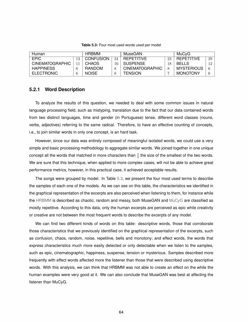
Table 5.3: Four most used words used per model

Human HRBMM MuseGAN MuCyGEPIC 13 CONFUSION 34 REPETITIVE 23 REPETITIVE 29CINEMATOGRAPHIC 11 CHAOS 16 SUSPENSE 18 BELLS 12HAPPINESS 6 RANDOM 8 CINEMATOGRAPHIC 8 MYSTERIOUS 6ELECTRONIC 6 NOISE 8 TENSION 7 MONOTONY 6

5.2.1 Word Description

To analyze the results of this question, we needed to deal with some common issues in natural

language processing field, such as mistyping, translation due to the fact that our data contained words

from two distinct languages, time and gender (in Portuguese) tense, different word classes (nouns,

verbs, adjectives) referring to the same radical. Therefore, to have an effective counting of concepts,

i.e., to join similar words in only one concept, is an hard task.

However, since our data was entirely composed of meaningful isolated words, we could use a very

simple and basic processing methodology to aggregate similar words. We joined together in one unique

concept all the words that matched in more characters than 23 the size of the smallest of the two words.

We are sure that this technique, when applied to more complex cases, will not be able to achieve great

performance metrics, however, in this practical case, it achieved acceptable results.

The songs were grouped by model. In Table 5.3, we present the four most used terms to describe

the samples of each one of the models. As we can see on this table, the characteristics we identified in

the graphical representation of the excerpts are also perceived when listening to them, for instance while

the HRBMM is described as chaotic, random and messy, both MuseGAN and MuCyG are classified as

mostly repetitive. According to this data, only the human excerpts are perceived as epic while creativity

or creative are not between the most frequent words to describe the excerpts of any model.

We can find two different kinds of words on this table: descriptive words, those that corroborate

those characteristics that we previously identified on the graphical representation of the excerpts, such

as confusion, chaos, random, noise, repetitive, bells and monotony; and effect words, the words that

express characteristics much more easily detected or only detectable when we listen to the samples,

such as epic, cinematographic, happiness, suspense, tension or mysterious. Samples described more

frequently with effect words affected more the listener than those that were described using descriptive

words. With this analysis, we can think that HRBMM was not able to create an effect on the while the

human examples were very good at it. We can also conclude that MuseGAN was best at affecting the

listener than MuCyG.

64

Table 5.4: Summary of the results about the impact on creativity

Impact Human 2 MuCyG 1mean std mean std

Base 6.03 2.52 5.77 2.23Melody 6.4 2.61 5.92 2.41Explanation 6.28 2.52 5.92 2.44Computer 6.40 2.54 5.84 2.48

Melody - Base 0.37 1.49 0.15 1.13Explanation - Melody −0.12 1.12 0.00 0.94Computer - Explanation 0.12 0.77 −0.08 0.76

5.2.2 Impacts on Creativity

We believe that some knowledge about a product can deeply influence the perception of creativity.

Therefore, in this question we aimed to study the impact of three different aspects:

• the first one is the impact of knowing that one song was inspired in one melody, hereinafter called

the melody factor;

• the second aspect we wanted to study is how does explaining the creative product using external

concepts impact the way our audience evaluates the overall creativity of the product, which we

named explanation factor ;

• The last and most important aim of this question, intrinsically related with our main goal in this

work, is to study the existence of bias in favor or against computer generated music, factor which

we named the computer factor.

As mentioned before, only two samples participated in this study: Human 2 and MuCyG 1, which

appeared in a random order during the survey, that included the exact same questions for both samples.

In Table 5.4, we present the means and standard deviations of the answers for each one of the questions

as well as the differences, i.e., the impacts of each one of the pieces of information.

From our analysis, we could quickly see that Human 2 is consistently evaluated as more creative

than MuCyG 1. It is also important to notice that, while, for both these two examples, the melody factor

caused an increasing on the perception of creativity, the explanation factor provoked a slight decrease.

In what concerns to the automatic nature of the product, it had a different effect in both examples. In

order to identify a bias factor, we were expected to observe that the computer factor would cause a

consistent increase or decrease. Yet, we can interpret this difference effect as a sign that MuCyG model

was easily spotted by the users. We mean that possibly, the respondents became surprised by the fact

that Human 2 was generated by a computer which contributed to a higher value of creativity, while it had

the opposite effect in the MuCyG sample.

65

5.2.3 Evaluating Confronting Pairs

One really natural way to evaluate subjective concepts is to use a jury in a binary confrontation

between two parts. This idea is used in commonly different contexts in day-to-day life. With these

questions, instead of asking for an absolute score or asking to choose between dichotomic states (for

instance, epic versus not epic), we asked for choice between two opposing samples, saying that the

picked one represents a better example than the other one for some provided characteristic.

We explored 5 different characteristics of our products, related to the words: creative, inspiring, novel,

epic and cinematographic. The first aim of this question was to order our samples based on the results

to have an idea of which sample is the best in each one of these dimensions. A secondary aim was to

verify if there is a direct correlation between the concepts of novelty and creativity as well as between

epic and creativity. We used two different approaches to order the samples. In Appendix 8, we have

fully described all the confrontations we gathered in this sample and the respective results.

Table 5.5 presents us the number of played games, as well as the percentage of wins, losses and

ties. This is a possible way to order our samples. With the hypothesis that the game is fair, which means

that the probability of confrontation is the same for any pair of samples, we can suppose that better

samples win more times. Therefore, in Table 5.6, we present, for each one of the dimensions, the order

that results from this reasoning process.

If we suppose an unbalanced way to choose opponents, some models could avail from this last

ordering approach. For instance, in the case that some advantageous sample confronts many times

a weak sample, then the percentage of winning games of the former can overcome all the other fair

playing samples. Therefore, another completely different idea, and our first idea, was to create a DAG

based on winning games.

To create our DAG’s, as a first step, if the sample A won in a confrontation with the sample B, the

edge (B,A) will be inserted into the directed graph G, meaning that A is potentially better than B. Since

we want an acyclic graph, we introduced a mechanism to cancel opposite edges, so if A wins B only

once and after a while B wins A also only one time, then neither (A,B) nor (B,A) will be present in the

final graph G. After this step, for each pair A and B of nodes, G will only have one edge between those,

pointing to the most likely to be the better and the weight of the arc corresponds to how many more

times did the best node won. For instance, supposing that A wins B 4 times while B only wins 1 time,

then, after this step we will have in graph G the edge (B,A) with weight: w(B,A) = 3.

However, this mechanism only prevents direct cycles or cycles of two nodes. To destroy bigger cycles

we use two different heuristics: the edge with smaller weight first and the edge present in more cycles

first. After identifying a cycle, we check if there is one edge with a weight value below the weights of all

the other edges in the cycle and remove it if it exists. If there are more than one, from those, we chose

the edge that has part in the most number of cycles, destroying as many cycles we can by removing

66

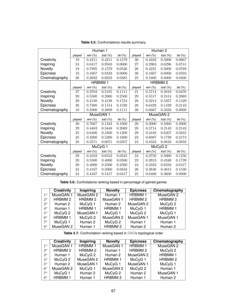
Table 5.5: Confrontations results summary

Human 1 Human 2played win (%) lost (%) tie (%) played win (%) lost (%) tie (%)

Creativity 19 0.4211 0.4211 0.1579 30 0.4333 0.5000 0.0667Inspiring 24 0.0417 0.9583 0.0000 27 0.2963 0.6296 0.0741Novelty 19 0.7895 0.1579 0.0526 26 0.4231 0.5000 0.0769Epicness 18 0.1667 0.8333 0.0000 30 0.1667 0.8000 0.0333Cinematography 26 0.2692 0.6923 0.0385 25 0.1600 0.8000 0.0400

HRBMM 1 HRBMM 2played win (%) lost (%) tie (%) played win (%) lost (%) tie (%)

Creativity 27 0.3704 0.5185 0.1111 21 0.5714 0.3810 0.0476Inspiring 20 0.5500 0.2000 0.2500 29 0.5517 0.2414 0.2069Novelty 29 0.4138 0.4138 0.1724 28 0.3214 0.5357 0.1429Epicness 26 0.7308 0.1154 0.1538 28 0.6429 0.1429 0.2143Cinematography 18 0.5000 0.3889 0.1111 30 0.6667 0.3333 0.0000

MuseGAN 1 MuseGAN 2played win (%) lost (%) tie (%) played win (%) lost (%) tie (%)

Creativity 30 0.7667 0.1333 0.1000 20 0.3000 0.5000 0.2000Inspiring 29 0.4483 0.3448 0.2069 28 0.5714 0.2143 0.2143Novelty 25 0.6400 0.2400 0.1200 29 0.3448 0.6207 0.0345Epicness 25 0.3200 0.5200 0.1600 23 0.6087 0.1739 0.2174Cinematography 28 0.3571 0.6071 0.0357 24 0.8333 0.0833 0.0833

MuCyG 1 MuCyG 2played win (%) lost (%) tie (%) played win (%) lost (%) tie (%)

Creativity 29 0.3103 0.6552 0.0345 24 0.3750 0.5000 0.1250Inspiring 20 0.5500 0.4000 0.0500 23 0.3913 0.4348 0.1739Novelty 20 0.4000 0.3500 0.2500 24 0.3333 0.6250 0.0417Epicness 24 0.4167 0.5000 0.0833 26 0.3846 0.4615 0.1538Cinematography 24 0.4167 0.5417 0.0417 25 0.6400 0.3600 0.0000

Table 5.6: Confrotations ranking based in percentage of gained games

Creativity Inspiring Novelty Epicness Cinematography1o MuseGAN 1 MuseGAN 2 Human 1 HRBMM 1 MuseGAN 22o HRBMM 2 HRBMM 2 MuseGAN 1 HRBMM 2 HRBMM 23o Human 2 MuCyG 1 Human 2 MuseGAN 2 MuCyG 24o Human 1 HRBMM 1 HRBMM 1 MuCyG 1 HRBMM 15o MuCyG 2 MuseGAN 1 MuCyG 1 MuCyG 2 MuCyG 16o HRBMM 1 MuCyG 2 MuseGAN 2 MuseGAN 1 MuseGAN 17o MuCyG 1 Human 2 MuCyG 2 Human 1 Human 18o MuseGAN 2 Human 1 HRBMM 2 Human 2 Human 2

Table 5.7: Confrontation ranking based in DAG’s topological order

Creativity Inspiring Novelty Epicness Cinematography1o MuseGAN 1 HRBMM 1 MuseGAN 1 HRBMM 1 MuseGAN 22o HRBMM 2 HRBMM 2 Human 1 HRBMM 2 MuCyG 23o Human 1 MuCyG 2 Human 2 MuseGAN 2 HRBMM 14o MuCyG 2 MuseGAN 2 HRBMM 1 MuCyG 1 HRBMM 25o Human 2 MuseGAN 1 MuCyG 1 MuseGAN 1 MuCyG 16o MuseGAN 2 MuCyG 1 MuseGAN 2 MuCyG 2 Human 17o MuCyG 1 Human 2 MuCyG 2 Human 2 MuseGAN 18o HRBMM 1 Human 1 HRBMM 2 Human 1 Human 2

67

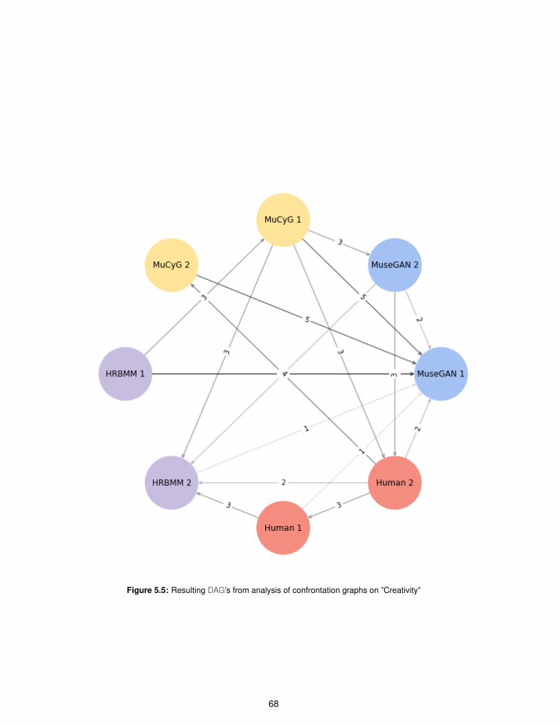
Figure 5.5: Resulting DAG’s from analysis of confrontation graphs on ”Creativity”

68

Figure 5.6: Resulting DAG’s from analysis of confrontation graphs on ”Inspiring”

69

Figure 5.7: Resulting DAG’s from analysis of confrontation graphs on ”Novelty”

70

Figure 5.8: Resulting DAG’s from analysis of confrontation graphs on ”Epic”

71

Figure 5.9: Resulting DAG’s from analysis of confrontation graphs on ”Cinematography”

72

only one edge. If in one cycle, there are several edges with the same small weight, that participates in

the same number of cycles, then we chose one randomly between those and remove it from the graph

G. After breaking all cycles, we are left with one DAG. In Figures 5.5, 5.6, 5.7, 5.8 and 5.9 we may see

the generated DAG’s and Table 5.7 shows the order calculated based on the DAG’s.

Our results demonstrate that, in this context, novelty and epicness might be kind of inversely related,

while epic and cinematographic may be positively related. Considering this and our definition of creativity

as both novel and epic products, we were expecting to have those samples that better balance epicness

and novelty scoring better in creativity, but the data do not reflect this definition. Also we were not able

to identify any clear relation between creativity and novelty nor epicness. In our interpretation of these

results, this data reflects that this simplistic definition of creativity do not comply in general with the

common use of the word in this context.

Another interesting aspect to notice is that even though human samples were the only ones described

as epic in the open question, in this question human samples were evaluated as not being epic nor

inpiring at all, but as being novel. Also according to our results, different samples were classified the

best in different categories: MuseGAN 1 was considered the most creative sample; the HRBMM 1 was

the most epic; MuseGAN 2 was the most cinematographic; while MuseGAN 1 and Human 1 were both

considered novel. Moreover, there was no model that consistently produced the best results for all the

categories.

5.3 Summary

Using a process with two sequential training phases, we gathered two different 32 seconds long

samples from each one of the models. From the graphical representation of these pianorolls, we could

conclude that RBM-based model’s products were very chaotic and featured only very short notes while

both GAN-based models ended up suffering from the mode collapse problem that opportunely provided

some repetitive musical coherence to the final products. Additionally to this 6 samples, we randomly

picked two 32 seconds long epic excerpts that were composed by humans, and all of these 8 samples

were evaluated in three different types of questions, using an online survey.

In the first question, an open question where the respondent could insert up to three words to de-

scribe each one of the excerpts presented, we used a very basic way to aggregate words with similar

meanings: we considered that words that matched on 23 of the size of the smallest word had similar

meanings. With this strategy we got the list of most frequent terms that were used to describe the sam-

ples of each one of the models. These words corroborate the conclusions we visually inferred from the

pianorolls and allowed us to order our models by the impact their products caused on the listener. From

the greater impact down to no impact the models followed the order: Human, MuseGAN, MuCyG and

73

HRBMM.

In one second question, that evaluated only MuCyG 1 and Human 2, we used Likert scales from 1

to 10 to evaluate the impact some factor may have on the perception of creativity. Our results point out

that, knowing that an excerpt is based on a melody will make the listener consider it as more creative,

while the explanation factor will impact negatively this perception. On our results we were not able to

detect any kind of bias nor in favor nor against automatic generated music.

Our last question consisted in a game where two excerpts confronted each other from which the

user explicitly chose the winner while focusing in one specific characteristic. We studied 5 characteris-

tics: creative, inspiring, novel,epic and cinematographic; and we used two different strategies to order

our samples: using the percentage of winning games and using DAG’s based on the winning matches

between each pair of samples. In the end, we conclude that no model was able to consistently outper-

form all the other ones in every category, but some randomly picked human composed samples were not

able to outperform all the models in all the categories. In addition, the data did not reflect any observable

relationship between creativity and novelty or creativity and epicness.

74

6Conclusion

Contents

6.1 Conclusions . . . . . . . . . . . . . . . . . . . . . . . . . . . . . . . . . . . . . . . . . . 77

6.2 Future Work . . . . . . . . . . . . . . . . . . . . . . . . . . . . . . . . . . . . . . . . . . 77

75

76

6.1 Conclusions

Our project consisted in exploring the CC field using DL technologies and generating symbolic epic

music. We created two new pianoroll representative datasets: the Epic Dataset and the Modely Dataset;

and explored three different DL models: HRBMM, MuseGAN and MuCyG. We used an pianoroll repre-

sentation and collected two representative datasets in this representation: one dedicated to epic music

and one of melodies.

Two different software products resulted from the development process: the Gmidi library1, that

includes a set of tools to process music, and the MuCaGEx2, a collection of deep learning models and

complementary libraries to perform experiments on music generation.

To train deep learning models is still a very empirical process and, currently, expert knowledge and

previous experience are the best guides, which are one of the main contributions of this works to our

personal experience. Defining our task, choosing the best representation, choosing the best architec-

ture, choosing the tools, balancing between generality and performance, tuning hyperparameters... all

these are very hard tasks that need informed testing and prototyping in order to achieve the best results.

According to our results, none of the models consistently outperformed the others. However, human

creations, according to the survey answers, also did not overcome the models. The generated final

products revealed both visually and audibly that our GAN-based models suffered from the mode collapse

problem, that was probably caused by some choices on the architecture or on the procedure such as

the learning rate associated with a high variance and the training method using small subsets. The

computational models were worse than human in affecting the listener but were considered more epic

when direct confronted with human samples. Finally, our results also do not comply with the definition

of creativity as utility and novelty.

6.2 Future Work

Since the beginning of our thesis, many new developments on this area have been published which

we were not able to follow up, in order to focus on the practical development and implementation of this

project. The datasets can be cleaned up, the preprocessing needs to be reviewed and we would like to

get the authorization to distribute the datasets we created.

In what concerns to the representation, the representation we used is limited to a fixed number of

tracks, a fixed number of timesteps and do not generate other musical dimensions such as stacatto,

tenuto, tempo and time signature. Those musical aspects and many others may be very important in

order to get good products in epic music.

1https://github.com/LESSSE/gmidi2https://github.com/LESSSE/public_MuCaGEx

77

In HRBMM, we should test different sampling techniques such as performing gibbs steps until the

sample stabilizes. We should also try different sizes for the hidden states and compare this hierarchical

version with a simple full RBM. There are some versions of RBM that are able to compute real values,

thus maybe adapt one of these models could bring some value to this approach.

To improve MuCyG several approaches were considered but not performed due to time constraints.

Both MuCyG and MuseGAN might benefit from a review of the architecture to include some overlapping

convolutions. The implementation of a mechanism of self-attention has been proved to achieve good

results in visual field, and maybe this can improve the way MuCyG model generates melodies. Other

improvements include implementing WGAN-GP for RNN, and add bi-directional LSTM to model the final

parts of the structure and generate time structure. On a technical level, we can migrate the models to

the new version of Tensorflow and the code should be refactorized, while joining new efforts to solve the

balancing losses and the collapsing mode problems.

78

Bibliography

[1] S. J. Russell and P. Norvig, Artificial Intelligence - A Modern Approach (3. internat. ed.). Pearson

Education, 2010.

[2] Magenta: A recurrent neural network music generation tutorial. [accessed at: 2017-12-11]. [Online].

Available: https://magenta.tensorflow.org/2016/06/10/recurrent-neural-network-generation-tutorial

[3] Magenta: Generating long-term structure in songs and stories. [accessed at: 2017-12-11].

[Online]. Available: https://magenta.tensorflow.org/2016/07/15/lookback-rnn-attention-rnn

[4] D. Cope, Virtual Music: Computer Synthesis of Musical Style. The MIT Press, 2004.

[5] J. A. Biles, “Genjam: A genetic algorithm for generating jazz solos,” in Proceedings of the 1994

International Computer Music Conference, ICMC, 1994.

[6] G. Bickerman, S. Bosley, P. Swire, and R. Keller, “Learning to create jazz melodies using deep

belief nets,” Proceedings of the International Conference on Computational Creativity, ICCC-10,

Jan 2010.

[7] J. Teixeira, “Cross domain analogy: From image to music,” Master’s thesis, Instituto Superior

Tencico, Universidade de Lisboa, Lisbon, Portugal, May 2017.

[8] H. W. Dong, W. Y. Hsiao, L. C. Yang, and Y. H. Yang, “Musegan: Multi-track sequential generative

adversarial networks for symbolic music generation and accompaniment,” ArXiv e-prints, Sep 2017.

[9] I. Goodfellow, J. Pouget-Abadie, M. Mirza, B. Xu, D. Warde-Farley, S. Ozair, A. C. Courville, and

Y. Bengio, “Generative adversarial networks,” CoRR, vol. abs/1406.2661, 2014.

[10] A. Radford, L. Metz, and S. Chintala, “Unsupervised representation learning with deep

convolutional generative adversarial networks,” 2015, cite arxiv:1511.06434 Comment: Under

review as a conference paper at ICLR 2016. [Online]. Available: http://arxiv.org/abs/1511.06434

[11] T. Karras, T. Aila, S. Laine, and J. Lehtinen, “Progressive growing of gans for improved

quality, stability, and variation,” CoRR, vol. abs/1710.10196, 2017. [Online]. Available:

http://arxiv.org/abs/1710.10196

79

[12] H. Zhang, I. Goodfellow, D. Metaxas, and A. Odena, “Self-attention generative adversarial

networks,” in Proceedings of the 36th International Conference on Machine Learning, ser.

Proceedings of Machine Learning Research, K. Chaudhuri and R. Salakhutdinov, Eds., vol. 97.

Long Beach, California, USA: PMLR, 09–15 Jun 2019, pp. 7354–7363. [Online]. Available:

http://proceedings.mlr.press/v97/zhang19d.html

[13] A. van den Oord, S. Dieleman, H. Zen, K. Simonyan, O. Vinyals, A. Graves, N. Kalchbrenner,

A. W. Senior, and K. Kavukcuoglu, “Wavenet: A generative model for raw audio,” CoRR, vol.

abs/1609.03499, 2016.

[14] O. Mogren, “C-RNN-GAN: continuous recurrent neural networks with adversarial training,” CoRR,

vol. abs/1611.09904, 2016. [Online]. Available: http://arxiv.org/abs/1611.09904

[15] C. Donahue, J. McAuley, and M. Puckette, “Synthesizing audio with generative adversarial

networks,” CoRR, vol. abs/1802.04208, 2018. [Online]. Available: http://arxiv.org/abs/1802.04208

[16] I. van Elferen, “Fantasy music: Epic soundtracks, magical instruments, musical metaphysics,”

Journal of the Fantastic in the Arts, vol. 24, no. 1 (87), pp. 4–24, 2013. [Online]. Available:

http://www.jstor.org/stable/24352902

[17] S. Meyer, Music in Epic Film: Listening to Spectacle. Taylor & Francis, 2016. [Online]. Available:

https://books.google.fr/books?id=JVH0DAAAQBAJ

[18] M. D. Mumford, “Where have we been, where are we going? taking stock in creativity research,”

Creativity Research Journal, vol. 15, no. 2-3, pp. 107–120, 2003.

[19] O. Wilde, The Picture of Dorian Gray. Floating Press, 2009. [Online]. Available: https:

//books.google.cz/books?id=J9cnJ21pKNgC

[20] J. P. Guilford, “Creativity,” American Psychologist, vol. 5, no. 9, pp. 444–454, 1950.

[21] A. McKerracher, “Understanding creativity, one metaphor at a time.” Creativity Research Journal,

vol. 28, no. 4, pp. 417–425, 2016.

[22] M. d’Inverno and A. Still, “A history of creativity for future AI research,” in Proceedings of the Seventh

International Conference on Computational Creativity (ICCC 2016). Sony CSL Paris, France, 2016,

pp. 147–154.

[23] J. C. Kaufman and R. A. Beghetto, “Beyond big and little: The four c model of creativity,” Review of

General Psychology, vol. 13, no. 1, pp. 1–12, 2009.

[24] M. Rhodes, “An analysis of creativity,” Phi Delta Kappan, vol. 42, no. 7, pp. 305–310, 1961.

80

[25] G. Wallas, The Art of Thought. Harcourt, Brace, 1926.

[26] R. Sawyer, Explaining Creativity: The Science of Human Innovation. Oxford University Press,

USA, 2012.

[27] D. Partridge and J. Rowe, Computers and Creativity, ser. Intellect Books. Intellect, 1994.

[28] Salvador Dali - Quotes. [accessed: 2019-05-30]. [Online]. Available: https://en.wikiquote.org/wiki/

Salvador Dal%C3%AD

[29] D. T. Campbell, “Blind variation and selective retention in creative thought as in other knowledge

processes,” Psychological Review, vol. 67, no. 6, pp. 380–400, 1960.

[30] A. Koestler, The Act of Creation. Arkana, 1964.

[31] M. A. Boden, The Creative Mind: Myths and Mechanisms. New York, NY, USA: Basic Books, Inc.,

1991.

[32] R. J. Sternberg and T. I. Lubart, “An investment theory of creativity and its development,” Human

Development, vol. 34, no. 1, pp. 1–31, 1991.

[33] R. A. Finke, T. B. Ward, and S. M. Smith, Creative Cognition: Theory, Research, and Application

(Bradford Books). The MIT Press, 1992.

[34] M. Turner and G. Fauconnier, “Conceptual integration and formal expression,” Journal of Metaphor

and Symbolic Activity, vol. 10, pp. 183–204, 1995.

[35] M. Csikszentmihalyi, Creativity: Flow and the Psychology of Discovery and, ser. Harper Perennial

Modern Classics. HarperCollins, 2009.

[36] R. J. Sternberg, The Propulsion Theory of Creative Contributions. Cambridge University Press,

2003, pp. 124–144.

[37] G. A. Wiggins, “Searching for computational creativity,” New Generation Computing, vol. 24, no. 3,

pp. 209–222, Sep 2006.

[38] M. Ackerman, A. Goel, C. G. Johnson, A. Jordanous, C. Leon, R. P. y Perez, H. Toivonen, and

D. Ventura, “Teaching computational creativity,” in Proceedings of the Eigth International Confer-

ence on Computational Creativity (ICCC 2017). Sony CSL Paris, France, 2017, pp. 9–16.

[39] G. Widmer, “Getting closer to the essence of music: The con espressione manifesto,” CoRR, vol.

abs/1611.09733, 2016.

[40] D. Floreano and C. Mattiussi, Bio-Inspired Artificial Intelligence: Theories, Methods, and Technolo-

gies (Intelligent Robotics and Autonomous Agents series). The MIT Press, 2008.

81

[41] I. Goodfellow, Y. Bengio, and A. Courville, Deep Learning. MIT Press, 2016. [Online]. Available:

http://www.deeplearningbook.org

[42] W. Mcculloch and W. Pitts, “A logical calculus of ideas immanent in nervous activity,” Bulletin of

Mathematical Biophysics, vol. 5, pp. 127–147, 1943.

[43] “The navy revealed the embryo of an electronic computer today that it expects will be

able to walk, talk, see, write, reproduce itself and be conscious of its existence,” The

New York Times, Jul 1986. [Online]. Available: https://www.nytimes.com/1958/07/08/archives/

new-navy-device-learns-by-doing-psychologist-shows-embryo-of.html

[44] D. E. Rumelhart, G. E. Hinton, and R. J. Williams, “Learning representations by back-propagating

errors,” Nature, vol. 323, Oct 1986.

[45] D. P. Kingma and J. Ba, “Adam: A method for stochastic optimization,” 2014, cite

arxiv:1412.6980Comment: Published as a conference paper at the 3rd International Conference

for Learning Representations, San Diego, 2015. [Online]. Available: http://arxiv.org/abs/1412.6980

[46] S. Hochreiter and J. Schmidhuber, “Long short-term memory,” Neural computation, vol. 9, pp. 1735–

80, Dec 1997.

[47] Y. Lecun, B. Boser, J. Denker, D. Henderson, R. E. Howard, W. Hubbard, and L. Jackel, “Backprop-

agation applied to handwritten zip code recognition,” Neural Computation, vol. 1, pp. 541–551, Dec

1989.

[48] N. Srivastava, G. Hinton, A. Krizhevsky, I. Sutskever, and R. Salakhutdinov, “Dropout: A simple

way to prevent neural networks from overfitting,” J. Mach. Learn. Res., vol. 15, no. 1, pp.

1929–1958, Jan 2014. [Online]. Available: http://dl.acm.org/citation.cfm?id=2627435.2670313

[49] A. van den Oord, N. Kalchbrenner, and K. Kavukcuoglu, “Pixel recurrent neural networks,” CoRR,

vol. abs/1601.06759, 2016.

[50] G. Alain, Y. Bengio, L. Yao, J. Yosinski, E. Thibodeau-Laufer, S. Zhang, and P. Vincent, “Gsns :

Generative stochastic networks,” CoRR, vol. abs/1503.05571, 2015.

[51] P. Smolensky, “Information processing in dynamical systems: Foundations of harmony theory,”

in Parallel Distributed Processing: Explorations in the Microstructure of Cognition, Vol. 1, D. E.

Rumelhart, J. L. McClelland, and C. PDP Research Group, Eds. MIT Press, 1986, pp. 194–281.

[52] D. P. Kingma and M. Welling, “Auto-encoding variational bayes,” CoRR, vol. abs/1312.6114, 2013.

82

[53] I. Gulrajani, F. Ahmed, M. Arjovsky, V. Dumoulin, and A. C. Courville, “Improved

training of wasserstein gans,” CoRR, vol. abs/1704.00028, 2017. [Online]. Available: http:

//arxiv.org/abs/1704.00028

[54] S. Ioffe and C. Szegedy, “Batch normalization: Accelerating deep network training by

reducing internal covariate shift,” CoRR, vol. abs/1502.03167, 2015. [Online]. Available:

http://arxiv.org/abs/1502.03167

[55] T. Miyato, T. Kataoka, M. Koyama, and Y. Yoshida, “Spectral normalization for generative adversarial

networks,” CoRR, vol. abs/1802.05957, 2018. [Online]. Available: http://arxiv.org/abs/1802.05957

[56] J. Zhu, T. Park, P. Isola, and A. A. Efros, “Unpaired image-to-image translation using

cycle-consistent adversarial networks,” CoRR, vol. abs/1703.10593, 2017. [Online]. Available:

http://arxiv.org/abs/1703.10593

[57] T. Kim, M. Cha, H. Kim, J. K. Lee, and J. Kim, “Learning to discover cross-domain relations

with generative adversarial networks,” CoRR, vol. abs/1703.05192, 2017. [Online]. Available:

http://arxiv.org/abs/1703.05192

[58] L. F. Menabrea, “Sketch of the analytical engine invented by charles babbage,” in Scientific mem-

oirs: selected from the transactions of foreign Academies of Science and learned societies, and

from foreign journals. Richard and John E. Taylor, London, 1842, vol. 3, pp. 666–731.

[59] D. Eck and J. Schmidhuber, “A first look at music composition using lstm recurrent neural networks,”

Istituto Dalle Molle Di Studi Sull Intelligenza Artificiale, Tech. Rep., 2002.

[60] A. Eigenfeldt, O. Bown, P. Pasquier, and A. Martin, “Towards a taxonomy of musical metacreation:

Reflections on the first musical metacreation weekend,” in Proceedings of the Second International

Workshop on Musical Metacreation (MUME 2013). The AAAI Press, Palo Alto, California, 2013,

pp. 40–47.

[61] E. X. Merz, “Implications of ad hoc artificial intelligence in music,” in Proceedings of the Third

International Workshop on Musical Metacreation (MUME 2014), Philippe Pasquier, Arne Eigenfeldt,

and Oliver Bown. The AAAI Press, Palo Alto, California, 2014, pp. 35–39.

[62] K. Choi, G. Fazekas, K. Cho, and M. B. Sandler, “A tutorial on deep learning for music information

retrieval,” CoRR, vol. abs/1709.04396, 2017. [Online]. Available: http://arxiv.org/abs/1709.04396

[63] J. Briot, G. Hadjeres, and F. Pachet, “Deep learning techniques for music generation - A survey,”

CoRR, vol. abs/1709.01620, 2017.

83

[64] R. Simchy-Gross and E. H. Margulis, “The sound-to-music illusion: Repetition can musicalize

nonspeech sounds,” Music & Science, vol. 1, p. 2059204317731992, 2018. [Online]. Available:

https://doi.org/10.1177/2059204317731992

84

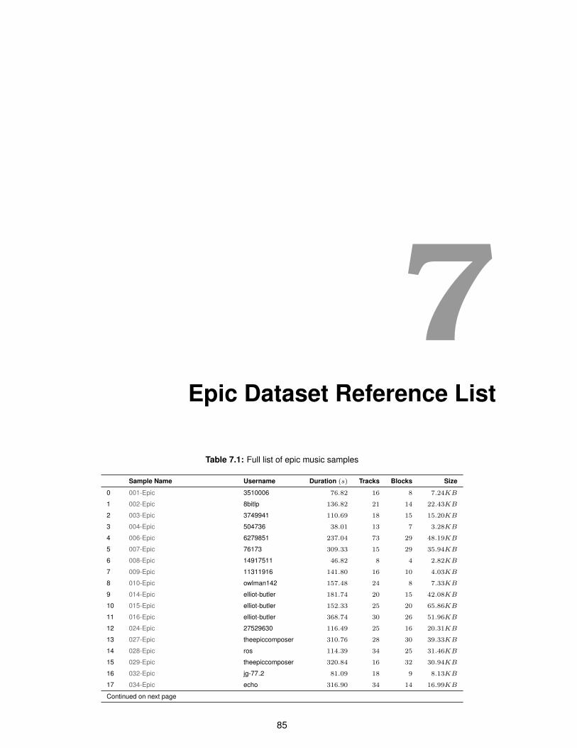
7Epic Dataset Reference List

Table 7.1: Full list of epic music samples

Sample Name Username Duration (s) Tracks Blocks Size

0 001-Epic 3510006 76.82 16 8 7.24KB

1 002-Epic 8bitlp 136.82 21 14 22.43KB

2 003-Epic 3749941 110.69 18 15 15.20KB

3 004-Epic 504736 38.01 13 7 3.28KB

4 006-Epic 6279851 237.04 73 29 48.19KB

5 007-Epic 76173 309.33 15 29 35.94KB

6 008-Epic 14917511 46.82 8 4 2.82KB

7 009-Epic 11311916 141.80 16 10 4.03KB

8 010-Epic owlman142 157.48 24 8 7.33KB

9 014-Epic elliot-butler 181.74 20 15 42.08KB

10 015-Epic elliot-butler 152.33 25 20 65.86KB

11 016-Epic elliot-butler 368.74 30 26 51.96KB

12 024-Epic 27529630 116.49 25 16 20.31KB

13 027-Epic theepiccomposer 310.76 28 30 39.33KB

14 028-Epic ros 114.39 34 25 31.46KB

15 029-Epic theepiccomposer 320.84 16 32 30.94KB

16 032-Epic jg-77 2 81.09 18 9 8.13KB

17 034-Epic echo 316.90 34 14 16.99KB

Continued on next page

85

Table 7.1 – continued from previous page

Sample Name Username Duration (s) Tracks Blocks Size

18 035-Epic solacedescending 218.75 23 25 28.28KB

19 038-Epic 8003276 225.14 36 22 66.71KB

20 039-Epic 14917511 75.32 14 7 4.23KB

21 040-Epic lizzapie 232.99 51 15 40.26KB

22 041-Epic maja-pechanach 125.63 25 9 8.24KB

23 042-Epic 1793111 131.26 28 15 27.85KB

24 043-Epic 2391956 113.36 23 12 17.69KB

25 044-Epic 9283941 194.00 31 20 67.66KB

26 047-Epic 4776246 185.34 18 13 14.89KB

27 048-Epic mollymawk 42.02 29 5 10.37KB

28 049-Epic 167892 42.02 29 5 10.37KB

29 051-Epic 2903486 450.90 16 23 7.94KB

30 052-Epic bntibbetts 94.22 29 9 15.29KB

31 053-Epic rookwizard 234.03 20 19 8.00KB

32 054-Epic rookwizard 216.03 33 22 35.97KB

33 055-Epic rookwizard 242.16 31 6 52.80KB

34 056-Epic 4918891 223.22 34 11 27.40KB

35 058-Epic rookwizard 249.05 17 13 5.67KB

36 059-Epic kalle-edh 222.84 24 18 18.89KB

37 061-Epic kalle-edh 196.39 21 13 15.04KB

38 063-Epic fabiolaw 239.42 12 24 20.00KB

39 065-Epic kalle-edh 188.93 19 16 14.57KB

40 066-Epic kalle-edh 234.45 28 16 40.57KB

41 067-Epic kalle-edh 271.96 32 27 35.50KB

42 068-Epic kalle-edh 162.62 24 8 12.85KB

43 069-Epic kalle-edh 164.28 25 11 24.03KB

44 070-Epic robin m butler 70.19 19 4 2.51KB

45 072-Epic-Prelude-for elliot-butler 126.44 15 7 2.35KB

46 073-Epic-Pastoralia-mid 18361371 441.94 27 29 21.24KB

47 074-Epic-Medieval-Times joshuaai 153.85 41 19 57.16KB

48 076-Epic-Blackheart-Full 28264345 266.21 56 14 61.71KB

49 077-Epic-March-for kalle-edh 260.52 29 32 42.22KB

50 079-Epic-Celthyan-In 2544941 124.91 36 14 33.16KB

51 080-Epic-To-a elliot-butler 190.09 16 7 11.92KB

52 081-Epic-Love-theme kalle-edh 136.52 17 9 5.04KB

53 084-Epic-Yeomen-Of kalle-edh 138.63 30 18 34.09KB

54 085-Epic-Intermezzo-Summer robin m butler 104.04 15 6 1.01KB

55 087-Epic-Adagio-A robin m butler 258.77 26 12 18.13KB

56 089-Epic-Feuillemort-HQ rookwizard 268.08 18 8 2.45KB

57 090-Epic-Running-Away robin m butler 92.76 20 7 14.37KB

58 093-Epic-Tian-Shan kalle-edh 162.50 22 11 18.87KB

59 095-Epic-INTERGALACTIC-Theme robin m butler 126.04 21 7 2.96KB

60 096-Epic-Superhero-theme kalle-edh 101.07 37 6 37.33KB

61 097-Epic-In-The lizzapie 53.39 12 0 4.00KB

62 098-Epic-Left-to 10712571 226.70 12 17 12.77KB

63 099-Epic-Two-Steps 2544941 167.76 36 20 26.91KB

64 101-Epic-An-adventure kalle-edh 123.02 40 12 28.53KB

65 102-Epic-Anton-Coladecci 10712571 306.69 23 28 38.43KB

66 104-Epic-Kingdom-of kalle-edh 219.56 29 19 22.85KB

67 105-Epic-The-Haunting kalle-edh 182.54 28 17 24.70KB

Continued on next page

86

Table 7.1 – continued from previous page

Sample Name Username Duration (s) Tracks Blocks Size

68 106-Epic-A-life kalle-edh 183.12 37 14 15.27KB

69 107-Epic-Celthyan-I 2544941 303.54 41 23 79.73KB

70 108-Epic-Zap-Nick 10712571 198.42 10 31 30.07KB

71 109-Epic-A-Virtual 18361371 384.79 12 7 31.30KB

72 110-Epic-Celthyan-Ode 2544941 215.51 20 12 15.45KB

73 111-Epic-Artist-Rendition 10712571 132.02 8 16 7.47KB

74 112-Epic-Jim-Saves lizzapie 149.65 48 22 26.79KB

75 114-Epic-Duel-of cherylthegoat 160.61 30 25 24.98KB

76 115-Epic-Theme-of 10712571 230.04 8 14 4.01KB

77 117-Epic-We-Run tristanwillcox 63.27 50 10 17.53KB

78 118-Epic-The-Circus 10712571 264.54 18 35 20.27KB

79 120-Epic-O-HOLY owlman142 104.79 54 7 13.35KB

80 122-Epic-Klap-Sahali 123002 180.57 27 17 24.53KB

81 123-Epic-O-Holy 1332076 97.88 39 7 21.94KB

82 124-Epic-Overture-in 5270096 137.17 20 18 19.75KB

83 125-Epic-John-Adams johnwd 53.30 73 8 38.71KB

84 126-Epic-Samurai-of robin m butler 67.40 31 9 2.73KB

85 127-Epic-Planet-Of robin m butler 72.02 27 9 4.76KB

86 128-Epic-Tempo-di rookwizard 136.51 13 25 10.61KB

87 131-Epic-Perspective-A johnwd 87.64 35 11 32.48KB

88 133-Epic-Celthyan-You 2544941 84.80 17 5 2.66KB

89 134-Epic-Ghost-The ronaldspotomusic 132.22 28 7 7.55KB

90 135-Epic-Phantom-Of ronaldspotomusic 120.89 16 4 13.89KB

91 137-Epic-Dreams-of 10712571 146.11 4 4 5.88KB

92 138-Epic-Ethereal-Sci lizzapie 189.19 62 10 20.26KB

93 139-Epic-Bergan-Village 10712571 453.39 10 43 24.35KB

94 140-Epic-Lycia-Kingdom 10712571 258.69 9 24 5.72KB

95 141-Epic-Music-of johnwd 85.39 44 13 47.26KB

96 142-Epic-Take-What 10712571 224.03 14 21 10.05KB

97 145-Epic-The-Freedom 10712571 147.09 16 13 13.60KB

98 146-Epic-Tears-remain 18361371 379.34 10 0 18.41KB

99 148-Epic-Incedendo-Epic johnwd 240.66 58 38 61.47KB

100 149-Epic-Opening-Titles johnwd 143.70 37 13 33.17KB

101 151-Epic-Boss-Battle 10712571 273.50 19 28 23.79KB

102 152-Epic-Space-Movie johnwd 156.68 39 12 21.90KB

103 154-Epic-Iris-The 10712571 144.87 14 10 8.68KB

104 155-Epic-The-Wild 9528871 189.03 21 15 17.78KB

105 157-Epic-King-Norrix 10712571 160.00 16 12 7.52KB

106 158-Epic-Jungle-Ruins lizzapie 119.77 32 9 10.42KB

107 162-Epic-BlackheartGame-of owlman142 125.31 18 22 27.55KB

108 163-Epic-The-Life lizzapie 285.13 46 21 15.45KB

109 164-Epic-Ninja-s 10712571 266.02 16 33 20.34KB

110 165-Epic-Hymn-mid dun-ought 212.50 22 13 3.96KB

111 166-Epic-Rhapsody-by 18361371 665.21 8 0 23.25KB

112 167-Epic-Drava-The 10712571 240.02 12 25 9.20KB

113 168-Epic-ZeroBlade-Run 107032 129.58 24 24 25.68KB

114 169-Epic-The-King 10712571 240.02 13 24 9.85KB

115 170-Epic-AOR-Battle 10712571 163.22 14 17 10.61KB

116 171-Epic-Midnight-600 rookwizard 204.05 30 10 22.42KB

117 172-Epic-AOR-World 10712571 268.82 10 28 17.88KB

Continued on next page

87

Table 7.1 – continued from previous page

Sample Name Username Duration (s) Tracks Blocks Size

118 173-Epic-Dreams-Of 10712571 182.42 5 16 1.66KB

119 174-Epic-Leonard-Cohen owlman142 135.06 44 7 15.82KB

120 177-Epic-The-Time lizzapie 276.59 45 26 29.22KB

121 178-Epic-Dark-Depths 107032 30.03 23 1 2.86KB

122 179-Epic-How-To tristanwillcox 67.78 67 5 12.07KB

123 180-Epic-Lulu-and cherylthegoat 141.59 33 19 27.70KB

124 181-Epic-Celthyan-A 2544941 210.89 53 13 55.80KB

125 182-Epic-HikariSimple-and piesafety 191.78 46 15 76.26KB

126 183-Epic-Electric-Deity 10712571 256.02 18 40 27.33KB

127 184-Epic-Main-Theme cherylthegoat 140.58 32 17 22.13KB

128 185-Epic-Sonic-The 10712571 281.48 18 32 33.50KB

129 188-Epic-End-Credits rookwizard 43.75 18 5 5.83KB

130 189-Epic-Quiet-Town 10712571 208.03 15 19 11.28KB

131 191-Epic-We-Will 10712571 245.27 15 25 26.34KB

132 194-Epic-The-Vault 4118671 166.39 20 26 15.17KB

133 195-Epic-By-the rookwizard 87.45 33 12 12.05KB

134 197-Epic-Celthyan-Downcast 2544941 151.90 47 14 28.21KB

135 198-Epic-FLOWER-TIME 10712571 118.17 8 16 10.00KB

136 201-Epic-Celthyan-First 2544941 126.45 52 15 31.01KB

137 202-Epic-The-Story lizzapie 179.53 40 16 14.29KB

138 203-Epic-A-Room rookwizard 143.12 34 11 10.52KB

139 204-Epic-Zues-Lord 10712571 169.86 19 23 13.61KB

140 205-Epic-Medusa-The 10712571 289.82 13 30 24.46KB

141 206-Epic-Rondo-Purcell 10712571 234.02 16 29 12.92KB

142 207-Epic-AOR-Cutscene 10712571 204.82 12 28 20.96KB

143 208-Epic-Central-Intelligence 10712571 260.42 14 24 20.00KB

144 210-Epic-A-New lizzapie 228.00 43 16 29.21KB

145 212-Epic-Theme-Of 10712571 290.61 9 21 18.56KB

146 213-Epic-Celthyan-Unseen 2544941 170.28 18 20 10.55KB

147 214-Epic-The-Land lizzapie 232.42 41 23 27.92KB

148 215-Epic-Fairy-Sprites 10712571 218.77 14 18 16.90KB

149 216-Epic-The-Battle lizzapie 187.36 52 14 26.80KB

150 217-Epic-Morning-Star 4118671 220.68 4 34 11.45KB

151 218-Epic-Fairy-Sprites 10712571 248.75 16 28 28.27KB

152 219-Epic-Fairy-Sprites 10712571 150.03 6 12 5.37KB

153 220-Epic-The-Voyage ronaldspotomusic 177.47 19 20 14.46KB

154 221-Epic-Celthyan-The 2544941 159.01 45 18 70.79KB

155 222-Epic-The-Old 10712571 167.13 8 16 2.95KB

156 223-Epic-Rise-of 10712571 194.64 18 32 14.27KB

157 224-Epic-Dark-Castle lizzapie 109.30 62 8 9.75KB

158 225-Epic-Fantasia-1 lizzapie 181.71 38 15 36.15KB

159 226-Epic-Beyond-The lizzapie 227.83 38 20 20.45KB

160 227-Epic-e-Minor 1388021 169.22 24 17 20.14KB

161 229-Epic-Chinchila-s 10712571 326.42 15 34 25.16KB

162 230-Epic-Promenade-in 18361371 577.75 11 38 31.37KB

163 231-Epic-Naru-s 10712571 220.52 12 27 14.21KB

164 232-Epic-Dira-The 10712571 198.02 8 24 13.95KB

165 233-Epic-The-Night rookwizard 96.17 29 10 17.04KB

166 234-Epic-Celthyan-I 2544941 135.07 47 18 39.75KB

167 235-Epic-Zoosters-Breakout ronaldspotomusic 93.51 37 15 18.42KB

Continued on next page

88

Table 7.1 – continued from previous page

Sample Name Username Duration (s) Tracks Blocks Size

168 236-Epic-Owain-Glyndwr 5270096 388.89 26 33 30.92KB

169 237-Epic-Last-Stop 10712571 192.02 18 28 5.83KB

170 238-Epic-Forever-HQ rookwizard 165.22 32 13 34.93KB

171 239-Epic-Cari-the 10712571 117.36 6 11 4.85KB

172 240-Epic-Remember-ANZAC rookwizard 211.06 43 16 29.90KB

173 241-Epic-Suite-for rookwizard 155.20 18 6 7.69KB

174 242-Epic-Fanfare-for 19173711 170.78 37 16 20.14KB

175 243-Epic-Cari-s 10712571 297.02 8 34 8.48KB

176 245-Epic-Celthyan-Pearl 2544941 328.81 26 22 17.21KB

177 246-Epic-Caris-Castle 10712571 123.02 19 15 4.65KB

178 247-Epic-Celthyan-From 2544941 105.55 54 6 25.54KB

179 249-Epic-War-on 10712571 264.02 21 41 26.27KB

180 251-Epic-The-First rookwizard 89.38 32 13 19.29KB

181 252-Epic-Star-Trek robin m butler 113.98 33 13 27.12KB

182 253-Epic-Intensity-Remix 10712571 163.66 19 27 28.93KB

183 254-Epic-The-Last jmusic1600 125.36 37 11 31.21KB

184 255-Epic-Temple-of 10712571 122.42 14 19 10.27KB

185 256-Epic-Temple-of 10712571 150.94 11 20 6.01KB

186 257-Epic-Temple-of 10712571 276.03 5 23 8.06KB

187 259-Epic-Epic-2 pandorasbox123 179.98 38 15 40.43KB

188 261-Epic-Naru-s 10712571 88.02 5 11 5.38KB

189 262-Epic-Cari-s 10712571 153.62 7 16 6.81KB

190 263-Epic-Blizzerd-Battle 10712571 238.17 14 32 10.09KB

191 264-Epic-I-Cant 10712571 213.37 13 8 2.79KB

192 265-Epic-V-S 10712571 162.73 18 24 19.08KB

193 266-Epic-Dira-s 10712571 156.82 14 24 6.23KB

194 267-Epic-Plains-Shop 10712571 172.82 4 27 18.03KB

195 268-Epic-Plains-Lv 10712571 228.02 17 23 9.26KB

196 269-Epic-Boss-Forest 10712571 264.08 12 33 22.67KB

197 270-Epic-Boss-Caves 10712571 288.03 10 27 18.60KB

198 271-Epic-Caves-Lv 10712571 293.36 4 27 9.80KB

199 272-Epic-Forest-Lv 10712571 171.80 5 34 11.71KB

200 273-Epic-Slow-and 10712571 185.19 7 18 5.47KB

201 274-Epic-The-Dictators knightsofarrethtrae 117.09 23 11 13.59KB

202 275-Epic-Shop-Mart 10712571 145.36 6 13 11.35KB

203 277-Epic-Ninja-Skills 10712571 266.42 5 27 18.29KB

204 278-Epic-Rigged-School 10712571 163.25 10 8 7.70KB

205 279-Epic-The-Treasure lizzapie 173.16 43 19 29.95KB

206 280-Epic-The-United 10712571 222.59 12 15 18.49KB

207 281-Epic-World-Theme 10712571 220.03 12 20 3.57KB

208 282-Epic-Naru-s 10712571 132.02 7 16 5.24KB

209 283-Epic-Car-Chase 10712571 187.22 14 28 36.22KB

210 284-Epic-The-United 10712571 317.56 21 43 13.81KB

211 286-Epic-The-White 10712571 320.03 18 30 16.54KB

212 287-Epic-Tails-Of 10712571 240.04 9 11 6.10KB

213 288-Epic-Queen-of 10712571 240.02 13 37 13.70KB

214 289-Epic-Bribing-The 10712571 250.69 6 12 13.66KB

215 290-Epic-The-String 10712571 142.01 9 16 5.72KB

216 291-Epic-March-of 10712571 316.85 10 16 3.58KB

217 292-Epic-Meadows-Film rookwizard 78.06 14 3 2.66KB

Continued on next page

89

Table 7.1 – continued from previous page

Sample Name Username Duration (s) Tracks Blocks Size

218 293-Epic-The-US 10712571 224.82 13 35 11.18KB

219 294-Epic-Battle-of robin m butler 38.79 32 5 9.86KB

220 295-Epic-Coronation-mid sapphirefloutist 141.28 38 23 45.41KB

221 296-Epic-Agent-Diezo 10712571 124.02 19 15 9.23KB

222 297-Epic-Against-The 10712571 184.02 10 23 6.75KB

223 298-Epic-The-Castle 10712571 144.03 15 13 4.94KB

224 299-Epic-March-of 10712571 264.03 15 24 7.90KB

225 300-Epic-The-Jungle 10712571 123.02 10 15 6.08KB

226 301-Epic-Two-Steps 2544941 265.09 63 14 55.65KB

227 302-Epic-Castle-Theme 10712571 614.42 19 64 70.26KB

228 304-Epic-To-the origamidos 128.22 16 12 9.44KB

229 307-Epic-Electroman-Theme robin m butler 101.35 30 12 26.17KB

230 309-Epic-Strings-Esemble 10712571 319.67 12 35 9.56KB

231 310-Epic-Building-of robin m butler 166.79 32 19 21.09KB

232 311-Epic-The-Encampment robin m butler 68.02 38 8 24.36KB

233 312-Epic-T-e robin m butler 94.43 18 7 5.37KB

234 313-Epic-Epic-Movie robin m butler 32.66 22 4 9.35KB

235 314-Epic-Newt-Says cherylthegoat 195.16 20 13 8.32KB

236 316-Epic-Lawrence-s 10712571 277.71 25 35 42.46KB

237 317-Epic-Starship-Explorer robin m butler 91.83 33 9 31.37KB

238 320-Epic-Leo-s 10712571 186.82 6 14 21.88KB

239 322-Epic-THE-MIGHTY robin m butler 67.99 27 5 11.78KB

240 323-Epic-Irons-Theme 10712571 174.02 15 23 7.86KB

241 324-Epic-Broken-Hero 10712571 144.03 19 13 13.54KB

242 325-Epic-Alyssa-s 10712571 166.01 18 27 9.54KB

243 326-Epic-Thinking-Music 10712571 189.02 12 23 8.91KB

244 327-Epic-The-Agency 10712571 132.24 12 16 4.43KB

245 328-Epic-Icy-Wastland 10712571 149.36 9 14 4.50KB

246 329-Epic-Battle-Theme 10712571 336.02 14 52 19.09KB

247 330-Epic-Make-The 10712571 268.63 23 35 21.32KB

248 332-Epic-Under-Attack 10712571 195.57 17 29 29.49KB

249 334-Epic-Imprisoned-mid 10712571 192.16 12 19 6.47KB

250 335-Epic-Token-God 10712571 120.02 12 15 3.09KB

251 336-Epic-Insert-creative origamidos 58.02 14 7 5.64KB

252 337-Epic-Light-in 10712571 379.07 26 27 6.53KB

253 339-Epic-Kill-The 10712571 124.85 8 6 3.92KB

254 341-Epic-Adestes-Fidelis owlman142 123.16 45 14 23.74KB

255 342-Epic-Please-help 6877881 159.90 29 24 17.08KB

256 345-Epic-Celthyan-In 2544941 195.00 39 13 68.41KB

257 346-Epic-Celthyan-Conquest 2544941 128.45 68 9 110.73KB

258 347-Epic-The-Colony origamidos 78.30 26 10 18.14KB

259 348-Epic-BATTLE-OF robin m butler 82.21 32 6 12.52KB

260 350-Epic-Celthyan-A 2544941 238.48 54 22 56.81KB

261 351-Epic-The-Last origamidos 99.92 29 10 17.72KB

262 352-Epic-Also-Untitled 6877881 230.02 25 28 8.98KB

263 353-Epic-The-End origamidos 68.04 14 3 3.47KB

264 354-Epic-The-Chariots 4118671 64.63 12 8 5.96KB

265 355-Epic-Super-Hero jmusic1600 47.83 38 8 22.10KB

266 357-Epic-Russian-March 142190 181.18 28 17 32.39KB

267 358-Epic-The-Trial origamidos 84.02 21 12 12.87KB

Continued on next page

90

Table 7.1 – continued from previous page

Sample Name Username Duration (s) Tracks Blocks Size

268 360-Epic-Eitz-Chayim isaacweiss 96.26 8 3 2.58KB

269 361-Epic-Oceans-Twilight 4118671 144.04 15 10 1.92KB

270 362-Epic-Carol-of 12165716 172.45 36 16 64.97KB

271 363-Epic-Papyruss-Mansion origamidos 252.98 14 41 27.04KB

272 364-Epic-Blue-Team austin harning 307.27 28 22 13.10KB

273 365-Epic-Time-Warp origamidos 110.23 25 11 45.46KB

274 366-Epic-Undertale-Spider piesafety 201.17 47 22 118.91KB

275 367-Epic-The-Closing origamidos 159.20 26 6 19.98KB

276 369-Epic-A-dark qqqant 177.32 47 21 32.85KB

277 370-Epic-Mammoths-mid 2644126 81.50 46 8 13.49KB

278 371-Epic-SSE-7 owlman142 121.04 24 11 11.55KB

279 372-Epic-Final-Boss thepopstardude 201.31 16 32 31.57KB

280 374-Epic-Dedication-200 owlman142 114.08 24 14 18.00KB

281 375-Epic-Sword-Valley thepopstardude 246.21 25 39 26.73KB

282 377-Epic-Release-From 11742266 222.20 14 20 3.00KB

283 378-Epic-Fugue-VI rpbouman 186.95 27 20 23.10KB

284 379-Epic-Simple-Wartime tristanwillcox 34.69 28 3 10.77KB

285 380-Epic-Lament-in rpbouman 176.39 27 11 12.52KB

286 381-Epic-Blue-Team austin harning 268.28 25 21 10.22KB

287 384-Epic-Encanto-Gitano 3857556 114.98 45 12 8.74KB

288 385-Epic-Gravity-Falls origamidos 54.00 40 3 12.41KB

289 387-Epic-Users-Documents origamidos 93.37 43 7 10.64KB

290 388-Epic-Siman-TovChassen isaacweiss 147.04 12 18 10.08KB

291 389-Epic-SSE-6 owlman142 119.38 26 15 18.14KB

292 391-Epic-I-Dont 6278966 212.44 37 14 14.76KB

293 393-Epic-Celthyan-Towards 2544941 274.22 43 16 87.87KB

294 394-Epic-Sun-For tristanwillcox 154.21 32 10 27.25KB

295 396-Epic-Trojan-Wildfire johnwd 163.46 33 23 56.81KB

296 397-Epic-Jupiter-the 6278966 177.90 40 11 14.43KB

297 398-Epic-F-a solacedescending 178.23 9 21 7.60KB

298 399-Epic-Not-for 2644126 196.25 42 33 52.02KB

299 402-Epic-SSE-4 owlman142 120.04 24 15 23.57KB

300 404-Epic-Revelation-EPIC tristanwillcox 185.61 43 13 18.51KB

301 406-Epic-Jabba-the 5549196 40.03 13 3 1.67KB

302 407-Epic-The-Southern thenightreader 202.48 34 23 29.22KB

303 408-Epic-SSE-3 owlman142 92.02 24 11 10.58KB

304 409-Epic-Mesa-Shewie owlman142 84.02 22 10 7.10KB

305 413-Epic-Expressivo-mid 4118671 115.15 2 0 9.63KB

306 414-Epic-Victoria-Altissimi tehdoctorr 186.70 46 15 28.85KB

307 415-Epic-Pokemon-Super 7135916 91.75 61 14 18.66KB

308 417-Epic-The-Majestic 4118671 108.70 18 10 6.18KB

309 418-Epic-Pot-O 4118671 108.43 22 13 20.57KB

310 419-Epic-Star-Fox vgoscore 39.39 22 5 15.92KB

311 420-Epic-From-the 5104821 191.27 24 11 24.88KB

312 421-Epic-The-Cascadant 4118671 259.80 18 20 12.58KB

313 422-Epic-Undertale-Medley vgoscore 60.72 18 6 8.38KB

314 425-Epic-Bravery-Honor rodcosta 25.44 18 2 3.09KB

315 427-Epic-Stand-mid 1388021 125.28 23 26 26.74KB

316 429-Epic-Nyan-Cat vgoscore 14.56 18 2 6.52KB

317 430-Epic-SimCity-Theme vgoscore 46.17 22 5 6.55KB

Continued on next page

91

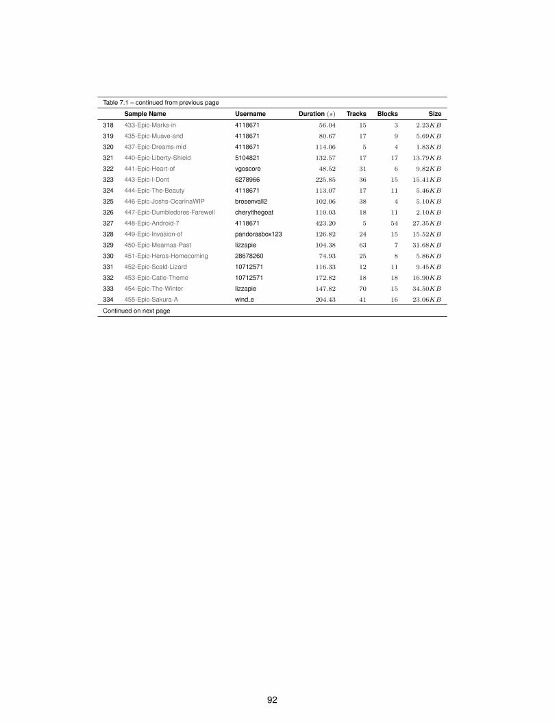
Table 7.1 – continued from previous page

Sample Name Username Duration (s) Tracks Blocks Size

318 433-Epic-Marks-in 4118671 56.04 15 3 2.23KB

319 435-Epic-Muave-and 4118671 80.67 17 9 5.69KB

320 437-Epic-Dreams-mid 4118671 114.06 5 4 1.83KB

321 440-Epic-Liberty-Shield 5104821 132.57 17 17 13.79KB

322 441-Epic-Heart-of vgoscore 48.52 31 6 9.82KB

323 443-Epic-I-Dont 6278966 225.85 36 15 15.41KB

324 444-Epic-The-Beauty 4118671 113.07 17 11 5.46KB

325 446-Epic-Joshs-OcarinaWIP brosenvall2 102.06 38 4 5.10KB

326 447-Epic-Dumbledores-Farewell cherylthegoat 110.03 18 11 2.10KB

327 448-Epic-Android-7 4118671 423.20 5 54 27.35KB

328 449-Epic-Invasion-of pandorasbox123 126.82 24 15 15.52KB

329 450-Epic-Mearnas-Past lizzapie 104.38 63 7 31.68KB

330 451-Epic-Heros-Homecoming 28678260 74.93 25 8 5.86KB

331 452-Epic-Scald-Lizard 10712571 116.33 12 11 9.45KB

332 453-Epic-Catle-Theme 10712571 172.82 18 18 16.90KB

333 454-Epic-The-Winter lizzapie 147.82 70 15 34.50KB

334 455-Epic-Sakura-A wind e 204.43 41 16 23.06KB

Continued on next page

92

8Confrontations Results

93

Figure 8.1: Number of confrontations between each pair of samples on ”Creativity”

94

Figure 8.2: Number of confrontations between each pair of samples on ”Inspiring”

95

Figure 8.3: Number of confrontations between each pair of samples on ”Novelty”

96

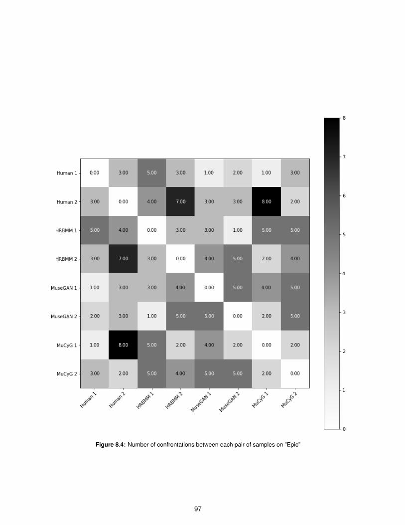
Figure 8.4: Number of confrontations between each pair of samples on ”Epic”

97

Figure 8.5: Number of confrontations between each pair of samples on ”Cinematography”

98

Figure 8.6: Number of won and lost confrontations for each pair of samples on ”Creativity”

99

Figure 8.7: Number of won and lost confrontations for each pair of samples on ”Inspiring”

100

Figure 8.8: NNumber of won and lost confrontations for each pair of samples on ”Novelty”

101

Figure 8.9: Number of won and lost confrontations for each pair of samples on ”Epic”

102

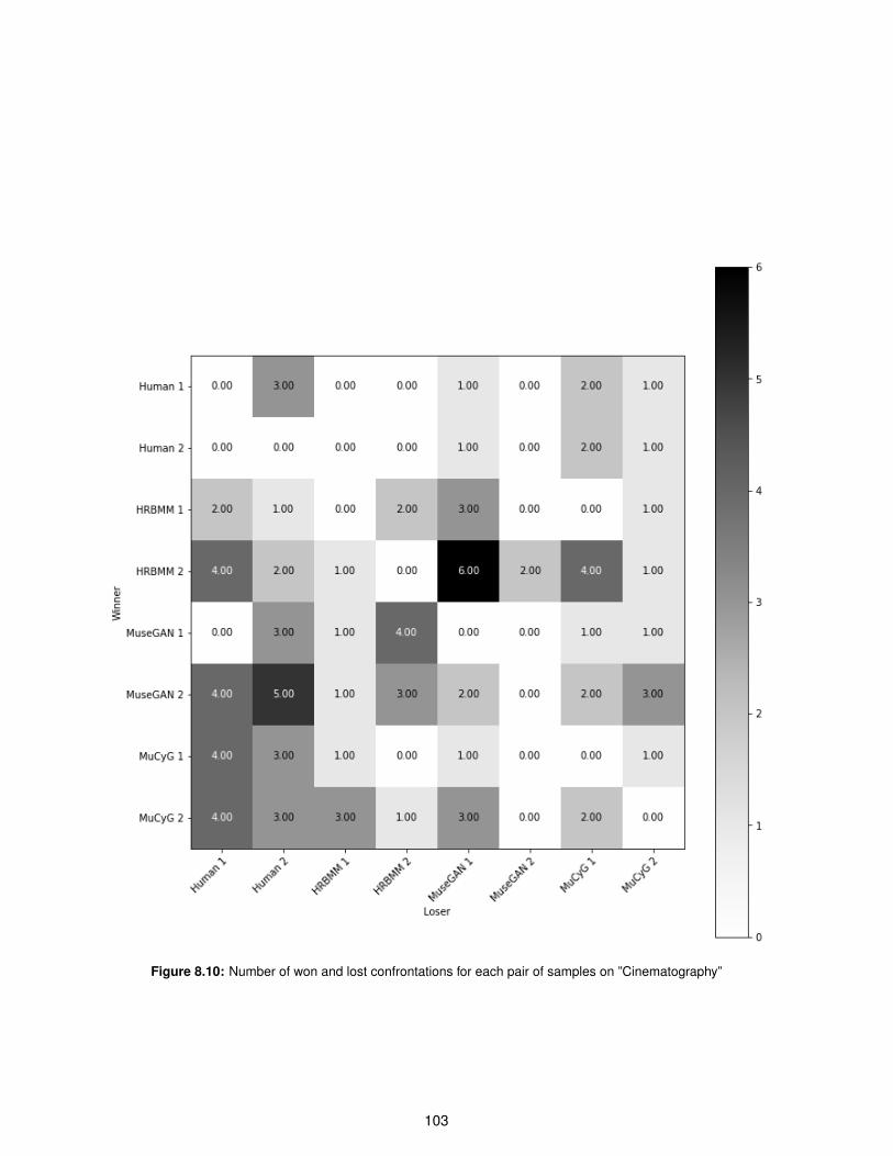
Figure 8.10: Number of won and lost confrontations for each pair of samples on ”Cinematography”

103

Figure 8.11: Percentage of won and lost confrontations for each pair of samples on ”Creativity”

104

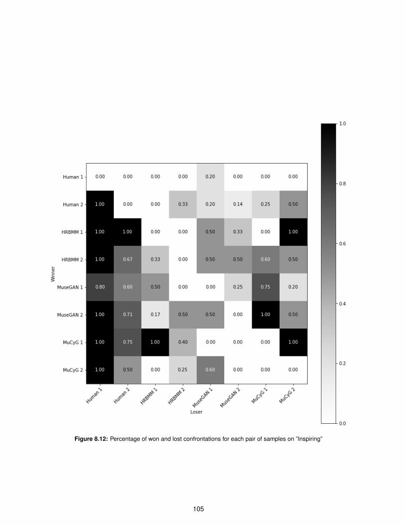
Figure 8.12: Percentage of won and lost confrontations for each pair of samples on ”Inspiring”

105

Figure 8.13: Percentage of won and lost confrontations for each pair of samples on ”Novelty”

106

Figure 8.14: Percentage of won and lost confrontations for each pair of samples on ”Epic”

107

Figure 8.15: Percentage of won and lost confrontations for each pair of samples on ”Cinematography”

108

Figure 8.16: Number of tied confrontations for each pair of samples on ”Creativity”

109

Figure 8.17: Number of tied confrontations for each pair of samples on ”Inspiring”

110

Figure 8.18: Number of tied confrontations for each pair of samples on ”Novelty”

111

Figure 8.19: Number of tied confrontations for each pair of samples on ”Epic”

112

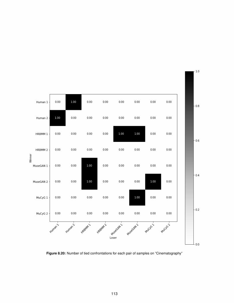
Figure 8.20: Number of tied confrontations for each pair of samples on ”Cinematography”

113

9Survey Example in English

114

115

116

117

118

119

120

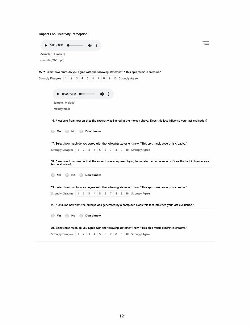
121

122