Lumpy Labor Adjustment as a Propagation

Mechanism of Business Cycles

Fang Yao*

SFB 649 Discussion Paper 2008-056

SFB

6

4 9

E

C O

N O

M I

C

R

I S

K

B

E R

L I

N

* Humboldt-Universität zu Berlin, Germany

This research was supported by the Deutsche Forschungsgemeinschaft through the SFB 649 "Economic Risk".

http://sfb649.wiwi.hu-berlin.de

ISSN 1860-5664

SFB 649, Humboldt-Universität zu Berlin Spandauer Straße 1, D-10178 Berlin

Humboldt-Universitat zu Berlin

Wirtschaftswissenschaftliche Fakultat

Institut fur Wirtschaftstheorie II

Lumpy Labor Adjustment as a Propagation

Mechanism of Business Cycles

Fang Yao1

Affiliation: Institute for Economic Theory

Humboldt University of Berlin

E-mail: yaofang@rz.hu-berlin.de

Date: August 11, 2008

1 I am grateful to Michael Burda, Tom Krebs, Dirk Kruger, Salvador Ortigueira, Harald Uhlig, KlausWalde, Yi Wen and seminar participants in Berlin, Florence, Deutsche Bundesbank and Oslo forhelpful comments and I acknowledge the support of the Deutsche Forschungsgemeinschaft throughthe SFB 649 ”Economic Risk”. All errors are my sole responsibility.

Abstract

I explore the aggregate effects of micro lumpy labor adjustment in a prototypical RBC

model, which embeds a stochastic labor duration mechanism in the spirit of Calvo(1983),

and it extends this approach by introducing a Weibull-distributed labor adjustment pro-

cess to capture the increasing hazard function corroborated by the micro data. My prin-

cipal findings are: The aggregate labor demand equation derived from the baseline Calvo-

style model corresponds to the same reduced form as the quadratic-adjustment-cost model

and deep parameters have a one-to-one mapping. However, this result does not hold in

general. When introducing the Weibull labor adjustment, the aggregate dynamics vary

with the extent of increasing hazard function, e.g., the volatility of aggregate labor is in-

creasing, but the persistence is decreasing in degree of the increasing hazard of the labor

adjustment.

JEL Classification: E32; E24; C68

Keywords: business cycles; heterogeneous labor rigidity; increasing hazard function;

Weibull distribution

1

Introduction

Micro evidence shows that, at the plant level, non-convex adjustment costs cause firms to

discretely adjust their production factor at infrequent intervals of stochastic length, i.e.,

labor adjustment at the firm level exhibits lumpy, asynchronous pattern. Earlier evidence

has been presented by Hamermesh (1989). Recently, Letterie, Pfann, and Polder (2004)

investigate the dynamic interrelation between factor demand with plant-level data for

the Dutch manufacturing sector. They find that both adjustments of capital and labor

are lumpy, and they are coordinated with each other in time. In addition, Varejao and

Portugal (2006) find that large employment adjustments (larger than 10% of the plant’s

labor force) account for about 66% of the total job turnover, and on average around 75%

of all observed Portuguese employer do not change employment over an entire quarter.

In macroeconomics, the (S,s) model is frequently used to investigate the aggregate ef-

fects of the lumpy factor adjustment2. The major theme discussed in the literature is

whether the micro-level lumpy factor adjustment has a significant impact on the aggre-

gate dynamics. The earlier partial equilibrium (S,s) models of labor adjustment (See:

e.g. Caballero and Engel, 1993, Caballero, Engel, and Haltiwanger, 1997) found that

employment growth depends on the cross-sectional distribution of the employment devi-

ation from optimal target. In particular, Caballero, Engel, and Haltiwanger (1997) found

that the adjustment hazard rises with large shocks and thus amplifies the shock’s effect

in aggregate adjustment. These findings were taken as evidence that lumpy adjustment

pattern at firm’s level matters for aggregate economy. However, the recent development of

the general equilibrium (S,s) models show that this considerable effect of lumpiness at the

plant level disappears with changes in the equilibrium prices. King and Thomas (2006)

construct a general equilibrium (S,s) model of discrete employment adjustment and find

that simulation results are ’observationally’ equivalent to the quadratic-adjustment-cost

model3.

In this paper, I pursue the business cycle implications of the lumpy labor adjustment

from a new perspective. It is motivated by the evidence of the empirical hazard function

of labor adjustment4. Varejao and Portugal (2006) estimated parameters of a Weibull

hazard function with the Portuguese employer survey data on labor adjustments, they

found that the shape parameter lies in the range between 1.174 and 1.309, indicating an

2 Caplin and Spulber (1987) was the early work applying the (S,s) approach to macro models.3 Similar results have been also found in the capital adjustment context. See, e.g., Veracierto (2002)

and Thomas (2002).4 To quantify the concept of lumpy labor adjustment, Caballero, Engel, and Haltiwanger (1997) used a

hazard function in terms of economic deviations from optimal targets.

2

increasing hazard function in the elapsed time.

Motivated by this evidence, I tackle the issue in a novel way, in which I embeds a general

stochastic labor duration mechanism in a prototypical RBC model. The essence of the

model is that, when making the firm’s adjustment probability depend on the amount

of time that has elapsed since the last adjustment, the labor dynamics in different vin-

tage groups are heterogeneous with respect to both persistence and volatility. In these

circumstances, aggregation mechanism (the distribution of labor vintages) matters for

the aggregate behavior, so that the propagation mechanism of the model is significantly

enriched.

To formalize this idea, in the benchmark model I introduce the firm’s stochastic labor

adjustment in the spirit of Calvo (1983), which implies that the underlying labor adjust-

ment process is characterized by a constant hazard function. As a result, even though the

’front-loading’ effect helps amplify the volatility of labor at the micro level, the large labor

adjustment is neutralized by the restrictive aggregation mechanism implied by the Calvo-

style labor adjustment. To this end, I show analytically that the aggregate labor demand

equations derived from the Calvo-adjustment model and the quadratic-adjustment-cost

model correspond to the same reduced form, and deep parameters have a one-to-one map-

ping of each other. With these results I confirm the finding by King and Thomas (2006)

discussed above.

In the second part of the paper, I extend the baseline model to a more general case, in

which I implement a Weibull-distributed labor adjustment process to capture features of

increasing hazard rates corroborated by micro evidence. This extension has a significant

impact on both the persistence and the magnitude of business cycles. When calibrating

the model with the empirically plausible hazard function, adjustment probabilities vary

across labor vintages. The longer a firm remains inactive, the more likely it adjusts its

labor in the current period. As a result, heterogeneous labor dynamics emerge naturally

from the underlying labor adjustment process, and as shown in the numerical results,

the model matches several important aspects of the U.S. business cycles. In particular,

the model can jointly account for persistent aggregate labor, smoothing real wages and

features observed in both micro and macro labor adjustment data: i.e. at the micro level,

labor adjustment exhibits a lumpy pattern in response to the technology shock, while the

aggregate employment reacts smoothly and sluggishly. In addition, sensitivity analysis

shows that aggregate dynamics vary with the extent of increasing hazard function, e.g.,

the volatility of aggregate labor is increasing, but the persistence is decreasing in degree

of the increasing hazard of the labor adjustment.

3

My model is intrinsically related to the (S,s) approach with respect to many modeling

concepts, it contributes to the literature, however, in the sense that it uses a more tractable

framework to generate the findings of the general equilibrium (S,s) models, and then it

extends the approach in an empirically plausible direction, showing that the micro lumpy

labor adjustment could play an important role in propagating business cycles.

The remainder of the paper is organized as follows: Section 1 introduces the baseline

model with a staggered employment adjustment at the firm’s level ; In section 2, I show

some analytical results to reveal the key mechanism underlying the model; Section 3

extends the basic model to the Weibull-adjustment model; and in section 4 I introduce

the calibration of model parameters and present simulation results; Section 5 contains

some concluding remarks.

1 The Baseline Model

In this section, I set up the baseline model in a RBC framework. The main feature of

this basic model is to introduce the lumpy labor adjustment in the spirit of Calvo(1983).

Even though this modeling idea has been existing for a long time and it is familiar to

most researchers in macroeconomics, I formulate it here formally in the context of the

statistical duration model, which also serves as the solid theoretical base for the extension

in the next section.

1.1 Household

There is a continuum of identical households, who are endowed with K0 units of capital

at t = 0 and then with one additional unit for each subsequent period of time, which

can be spent on either working or leisure. The infinitely-lived representative household

chooses consumption, labor supply and investment to maximize the expected discounted

utility:

U = maxCt,Lt,It

E0

∞∑

t=0

βt (U(Ct)− V (Lt))

. (1)

The instantaneous utility U(.) and V (.) are bounded, continuously differentiable, strictly

increasing and strictly concave in consumption and leisure. I take the following function

4

form for instantaneous utility:

U(Ct)− V (Lt) =C1−η

t

1− η− χ

L1+φt

1 + φ(2)

In each period, households receive wage income, rental payment for their capital stock

and a lump-sum transfer of net profits resulting from firm ownership, which can be spent

on consumption and investment in capital stocks. Due to the assumption of complete

financial markets, all households can perfectly share their idiosyncratic income risk, so

that they consume and invest the same amount. Consequently, the sequence of aggregate

budget constraints is given by:

Ct + It ≤ WtLt + RtKt + Tt (3)

The capital stock evolves according to the following law of motion:

Kt+1 = (1− δ)Kt + It (4)

Finally, I impose the transversality condition for the capital stock:

limT→∞

E0

[T∏

t=0

R−1t,t+1

]KT+1 = 0, (5)

Based on this setup, the following first order conditions must hold in an equilibrium:

χLφt C

ηt = Wt, (6)

1 = Et

[β

(Ct+1

Ct

)−η

(rt+1 + 1− δ)

], (7)

1.2 Firms

The economy is populated by a continuum of firms, which is normalized to one. Firms

operate in a rigid labor market, where some unspecified frictions cause a fixed ratio of

firms not to adjust their labor input in each period. In effect, the more rigid the labor

market is, the lower the adjustment ratio is, as expected by agents in the market. Due to

this rigid labor adjustment process, firms are differentiated with respect to the amount

5

of time that has elapsed since the last adjustment and hence by their stocks of labor

force. I index firms by j, corresponding to the ”time-since-last-adjustment”. I call them

hereafter “labor vintages”. Furthermore, given the complete financial market, adjusting

firms choose a common target labor adjustment at each period. Firms in any labor

vintage share an equal amount of employment, and hence the state of the economy can

be summarized by the vintage index j with the corresponding labor stock (lj,t).

1.2.1 Stochastic Labor Adjustment Process and Distribution of Firms

Now I formally introduce the staggered labor adjustment process in the context of the

statistical duration model.

Here I consider a process in which the firm’s employment adjustment occurs randomly

over time. It turns out that under some basic assumptions with respect to independence

and uniformity in time, this random process is governed by the Poisson process5. This

assumption simplifies the real-world continuous factor adjustment decisions in terms of a

sequence of generic trials that satisfy the following assumptions:

• Each trial has two possible outcomes, called adjustment and non-adjustment.

• The trials are memoryless, i.e. the outcome of one trial has no influence over the

outcome of another trial.

• For every firm, the probability of adjusting is 1 − α and the probability of non-

adjusting is α.

Formally I define the labor adjustment process as a Bernoulli process as follows:

Definition: Given a probability space (Ω, P r) together with a random variable X over

the set 0, 1, so that for every ω ∈ Ω, Xi(ω) = 1 with probability α and Xi(ω) = 0 with

probability 1−α, where Ω = adjusting, non-adjusting, a Bernoulli process is a sequence

of integers Zω = n ∈ Z : Xn(ω) = 1.

Given the factor adjustment process follows the Bernoulli process, the probability of

receiving zero adjusting signal in an interval of j periods is:

Pr(0) =

(j

0

)(1− α)0αj = αj for j = 0, 1, 2, ... (8)

5 In this paper, as I write the model in the discrete-time, the discretized adjustment process follows theBernoulli trials process, which is the discrete version of the Poisson process.

6

And, the probability that a duration spell terminates at the period j is

Pr(j) = (1− α)αj−1 for j = 0, 1, 2, ... (9)

Define Θ = θ(j)∞j=0 as the distribution of firm over labor vintages. It can be easily

shown that θ(j) = (1− α)αj for j = 0, 1, 2, ...6.

The hazard function corresponding to the Bernoulli process is:

H(j) =θ(j)

1− F (j)= 1− α (10)

The hazard function embeded in the Bernoulli distribution is constant. It implies that the

probability of adjusting is independent of the period time elapsed. The aggregate stock of

labor can be summed up with respect to the distribution of firms over labor vintages, i.e.

the aggregate labor is the weighted sum of all past optimal labor demands, and weights

are equal to the probability density function over vintages j.

Finally aggregate labor is obtained by7:

Lt =∞∑

j=0

θ(j)lj,t =∞∑

j=0

(1− α)αjlj,t (12)

Since the fraction of firms that adjust their employment is randomly drawn across the

population, it follows that the recursive law for aggregate employment is obtained by:

Lt = (1− α)l0,t + αLt−1 (13)

or equivalently,

∆Lt = Lt − Lt−1 = (1− α)(l0,t − Lt−1) (14)

6 Because, by assumption there is 1− α fraction of firm in the group zero, and α percent of them goesto group one, this gives the density of group one to be (1−α)α. Similarly, α percent of untis in groupone goes to group two, so the density of group two is (1− α)α2, and so on.

7 Note that equation 18 implies that firms in the vintage j group must also use same amount of capital.Thus the distribution of plants over labor is the same as over capital stocks. As a result, we canaggregate capital in the same way.

Kt =∞∑

j=0

(1− α)αjkj,t (11)

7

This equation reveals the partial adjustment nature of this model, that the actual job

turnover is only a fraction of the optimal adjustment. The speed of adjustment depends

on the extent of market rigidity (1−α). If no friction exists in the labor market (α = 0),

all firms re-optimize their labor by l0,t, where this model is then reduced to the standard

RBC case.

1.2.2 Capital Market and Technology

Furthermore I assume that firms can access an instantaneous rental market for capital,

which is supplied by households in any given period. This assumption is desirable because

the firm’s first order condition requires the capital and labor ratio to be identical in the

entire economy8, the instantaneous capital market makes possible for those firms that

can not change their employment to fulfill this requirement. The aggregate capital stock,

however, is still predetermined by the household.

Firms use a decreasing-return-to-scale technology to produce output9.

yt = Ztlat k

bt − ι and a + b < 1 (15)

Where (ι) denotes the fixed cost of operation, which is equal to the profits earned in

the steady state. Consequently, firms expect zero profit and thus the number of firms is

constant in the long run.

Zt summarizes the aggregate productivity shock, which consists of a trend component Zt

and a realization of a stochastic process zt. The trend component Zt evolves at a constant

growth rate g, while zt follows an AR(1) process in logs:

Zt = Ztzt, (16)

where zt = zςt−1e

vt , and vt ∼ i.i.d.N(0; σ2)

8 This is the case when the production function is constant-return-to-scale, however, when assumingdecreasing-return-to-scale, as shown in equation(18), a power function of labor and capital dependsonly on the rental rate and aggregate shocks, hence it should be identical for all firms in the economy.

9 In the equation (21), it shows that some extent of DRTS is needed to show the lumpy effect at thefirm level. However, my main numerical results do not crucially depend on this assumption.

8

1.2.3 Firm’s optimization Problem

In spite of heterogeneous nature of the problem, the firms’ maximization problem can be

written in a representative fashion: a typical firm maximizes the expected discounted real

value of all future profits by choosing nonnegative values for current optimal labor l0,t and

a sequence of optimal capital stocks kj,t∞j=0, taking the real wage wt and real rental rate

rt as given.

maxl0,t,kj,t∞j=0

Vt =∞∑

j=0

Etβt,t+j αj[F (l0,t, kj,t)− wt+jl0,t − rt+jkj,t+j]|Ωt (17)

where βt,t+j is the stochastic discount factor, which is defined according to equation (7).

Since, at the steady state, all real variables except for labor grow at rate g along the

balanced growth path, I will work with detrended variables without changing the notions

from now on.

First order conditions for the firm’s optimization problem are:

rt = fk(j, t) = b zt

laj,t

k1−bj,t

(18)

∞∑j=0

αjEt[βt,t+j(azt+jla−10,t kb

j,t+j)] =∞∑

j=0

αjEt[βt,t+j(wt+j)] (19)

Eqation (19) shows that the optimal labor demand is determined by balancing all future

discounted marginal benefits of adding one more worker (marginal product of labor)

and the marginal costs of having a worker (real wage). This condition contrasts to the

standard RBC case, where real wage is equal to labor productivity period by period.

Due to the labor adjustment friction the optimal labor demand in this model becomes a

forward-looking condition.

To reveal the model’s implication for the optimal labor demand at the firm level, I derive

the firm’s optimal employment demand by combining first order conditions and solving

for the plant’s optimal labor demand l0,t at period t:

l1−a−b1−b

0,t =

abb/1−b∞∑

j=0

αjEt[βt,t+iz1/1−bt+j /r

b/1−bt+j ]

∞∑j=0

αjEt[βt,t+iwt+j], (20)

9

Equation(20) shows that, at the firm level, the optimal labor demand reacts to all future

shocks and the equilibrium prices. In the case of the first-order-approximation, it is

increasing in all expected future shocks zt+j and decreasing in all expected future prices

wt+j and rt+j. In the partial equilibrium, where prices are constant, it is easy to show

that a positive persistent shock will make the individual labor adjustment higher than

that in the frictionless economy. Firms hire more labor than they currently need to hedge

the risk they might not be able to re-optimize it in the near future and vice verse for the

negative shocks. It is the ’front-loading’ effect of the labor demand under the uncertainty

in the labor adjustment process. Note that the magnitude of the front-loading effect is

dependent on the labor rigidity parameter α. The larger the value of α is, the higher weight

is attached on the expectations of future variables. In another words, when frictions in the

labor market are more severe, the labor demand is more sensitive to the future economic

state.

1.3 Equilibrium

Given an exogenous stochastic process for aggregate technology shocks and the common

knowledge of the firms’ distribution across vintage groups Θ, I define the competitive equi-

librium as a set of stochastic processes of endogenous variables Yt, Ct, Lt, lj,t, kj,t, It, Kt,

wt, rt∞t=0 such that:

1. Given Kt and the market prices wt, rt∞t=0, the sequences Cst , L

st , I

st ∞t=0

10solve the

representative household’s maximization problem (1) subject to (2)-(5).

2. Given wt, rt∞t=0, lj,t, kj,t∞t=0solve the Firms’ profits maximization problem (17)

subject to production technology (15) and exogenous technology shock process (16).

3. Aggregate demands for employment Ldt and capital Kd

t are determined by (12) and

(11) respectively.

4. Markets clear: Lst = Ld

t = Lt in labor market, Kst = Kd

t = Kt in capital market and

Ct + It = Yt in the goods market.

5. Finally, market’s equilibrium determines the equilibrium real wage and rental rate

wt, rt∞t=0

10 Here, superscript s denotes “supply”; Similar notation d for “demand”

10

2 Analysis

2.1 Dynamic Labor Demand Equations

To gain further intuition of the firm’s behavior, I log-linearizing the FOCs (18) and (19)

around the non-stochastic steady state11. In contrast to the other partial adjustment

model, the Calvo-adjustment model implies different labor demand behaviors at different

aggregation levels.

l0,t = αβEt[l0,t+1]−b(1− αβ)

1− a− brt −

(1− b)(1− αβ)

1− a− bwt +

1− αβ

1− a− bzt (21)

Equation (21) reveals that at the firm level optimal adjustment is forward-looking and

a trade-off exists between the weights assigned to the current shock and future shocks.

When α is large, firms put more weight on future shocks than on current shocks.

Together with equation (13), the aggregate labor demand equation is obtained by:

αβκEt[lt+1]− (1 + α2β)κlt + ακlt−1 − b rt − (1− b)wt + zt = 0 (22)

where κ = (1−a−b)(1−α)(1−αβ)

. The aggregate labor demand (22) exhibits more complex dynamics,

which are not only dependent on the forward-looking component, but also on the lagged

labor. Moreover, it demonstrates that equilibrium prices work here as a counter factor to

the technology shock. In this equation, one can explicitly see that, when the aggregate

technology shock, real wage and interest rate all rise by 1%, then the total effect of those

changes on the aggregate labor are exactly cancelled.

Note that both equations require some degree of decreasing-returns-to-scale (1−a−b > 0)

to ensure that the size of labor demand is determined.

2.2 Equivalence to the Quadratic-adjustment-cost Models

The quadratic-adjustment-cost model has lost footing in macroeconomic literature be-

cause economists have grown disenchanted with its smoothing and synchronous impli-

cation relating to the firm-level factor adjustment. As discussed in the introduction,

mounting micro evidence shows that firms adjust their labor in a discrete and asyn-

chronous fashion. Despite this fact, the quadratic adjustment cost model has been used

11 Variables with hat are denoted as log deviation from the non-stochastic steady state, such as xt =logXt − logX; and the derivation is shown in a technical appendix, which is available upon request.

11

widely in theoretical and empirical work, because they are easily solved and produce ag-

gregate equations in a form suitable for estimation. By contrast, as I have shown in the

equation (20), the Calvo-adjustment model can capture lumpy and asynchronous features

in firm’s labor adjustment, while aggregate labor demand in this model is characterized

by a smoothing AR(2) dynamic process (see: Equation 22). The key question addressed

in this subsection is whether the quadratic-adjustment-cost model is equivalent to the

Calvo-adjustment model concerning the aggregate dynamics. If this is true, it can be

treated as a reduced form model and is still valid in the empirical work using aggregate

data.

In Appendix (A), I derive the aggregate labor demand equation from a textbook quadratic-

adjustment-cost model (See e.g. Hamermesh, 1993). As Rotemberg (1987) has shown

that the equivalence between the Calvo model and the quadratic cost model in the price

adjustment context, it can also be shown analytically that aggregate labor demand equa-

tions derived from both models conform to the same reduced form. In addition, the deep

parameters of the two models have a one-to-one mapping of each other.

Equation (34) is the dynamic labor demand equation derived from the quadratic-adjustment-

cost model:

γβEt[lt+1]− [(1− a− b) + γ(1 + β)] lt + γlt−1 − b rt − (1− b)wt + zt = 0

where I denote γ = dnw

(1− b).

And it is the dynamic labor demand equation derived from the Calvo-adjustment model:

αβκEt[lt+1]− (1 + α2β)κlt + ακlt−1 − b rt − (1− b)wt + zt = 0

where κ = (1−a−b)(1−α)(1−αβ)

Comparing these two equations, I find that these two equations can be put into the

following reduced form equation, so that the aggregate data alone can not differentiate

between them.

ϕ1Et[lt+1] + ϕ2lt + ϕ3lt−1 − brt − (1− b)wt + zt = 0

When I set ακ = γ, For example, the correspondence among parameters in both models

is expressed by equation (23). Then the Calvo-adjustment model is equivalent to the

quadratic-adjustment-cost model with respect to the aggregation relations and they con-

12

sequently generate the exact same aggregate dynamics, given that all other aspects of

both models are equal.

dn

w=

α(1− a− b)

(1− α)(1− αβ)(1− b)(23)

Note that both parameters d and α govern the rigidity of the labor adjustment process

in both models and this equation gives the exact mapping between these two rigidity

parameters.

3 Extension

In this section, I extend the baseline model to a more general case in which the labor

adjustment process is characterized by an increasing hazard function. In particular, I

apply the Weibull distribution12 to model the firm’s labor adjustment process. Because of

its flexibility, the Weibull distribution is frequently used in statistical analysis of duration

phenomena. In fact, it enables the incorporation of a wide range of hazard functions by

using various values of the shape parameter.

3.1 The Weibull-adjustment Model

To integrate the Weibull-labor-adjustment into the RBC framework, I only have to modify

the firm’s problem, while keeping the household’s optimal conditions (6) and (7) as they

are in the baseline model.

I consider an economy with a continuum of perfectly competitive firms, which are dif-

ferentiated with respect to the time elapsed since their last labor adjustments, indexed

by j ∈ 0, J13. I assume that the stochastic labor duration follows a Weibull distribu-

tion. According to the statistical duration theory, the distribution of firms with respect

to time-since-last-adjustment (vintage groups) is summarized by the density function of

the Weibull distribution, and the hazard rate in the vintage group j is obtained by:

h(j) =τ

λ

(j

λ

)τ−1

∀j ≤ J (24)

12 For detailed discussion on Weibull distribution, see technical appendix (B)13 J = λ

(λτ

)1/τ−1is the maximum number of vintage groups, which is obtained through equaling the

hazard rate of the group J to one (H(J) = 1).

13

where τ and λ are the parameters of the Weibull distribution and j is the amount of time

that has elapsed since the last adjustment. Note that this hazard function is increasing

when τ is greater than one, thereby the adjustment probability in each vintage is depen-

dent on the vintage index j. The longer a firm remains inactive, the more likely it adjusts

its labor in the current period.

When resetting its labor l∗0,t at time t, a firm uses the survival function of the Weibull

distribution to access the probabilities that its reseted labor input will remain unchanged

in the future, and the firm chooses an optimal labor adjustment to maximize:

maxl∗0,t,kj,t+iJ

j=0

Vt =J∑

i=0

S(i)Etβt,t+i[f(l∗0,t, kj,t+i

)−Wt+il0,t −Rt+ikj,t+i]|Ωt

where S(i) denotes the probability that firm’s newly adjusted labor force will survive for

i periods in the future, which is obtained by the formula S(i) = 1−F (i) = exp(−(

iλ

)τ).

The first order necessary condition gives us the optimal labor demand:

l∗0,t

1−a−b1−b = abb/1−b

J∑i=0

S(i)Et[βt,t+iz1/1−bt+i /r

b/1−bt+i ]

J∑i=0

S(i)Et[βt,t+iwt+i]

, (25)

Equation(25) has the same form as in the baseline model, except that the survival func-

tion is now a more complex function of the elapsed inactive time. This change enriches

the labor dynamics of the model, but as the same time it also puts a challenge to the

computation of the solution.

I log-linearize equation(25) for the labor demand as follows14:

l∗0,t = αβEt[l∗0,t+1]−

b

Ψ(1− a− b)rt −

1− b

Ψ(1− a− b)wt +

1

Ψ(1− a− b)zt (26)

Analog to the Calvo-adjustment model, α governs dynamic properties of the labor de-

mand. Given my calibration values of the model’s parameters, α is equal to 0.75, which is

slightly less than its counterpart (0.77) in the Calvo-adjustment model. As in the baseline

model, the optimal labor adjustment is increasing in all expected future shocks zt+j and

decreasing in all expected future prices wt+j and rt+j, and thus the ’front-loading’ effect

is also at work here. It is important to note that the parameters in this equation nest

14 The derivation of this equation is shown in the Appendix (C).

14

those in the corresponding equation (21), where the hazard function is constant.

To aggregate the labor demand, I use a two-stage aggregation scheme. First I define a

dummy sectoral labor demand as lj,t, which is the sum of labor demand in a labor vintage

before reshuffling firms into the new vintage groups, and let αj = 1 − h(j) denote the

probability of non-adjusting.

lj,t = (1− α(j)) l∗0,t + α(j) lj,t−1 (27)

In equation (27), we can see that the heterogeneous sectoral labor demands arise as a result

of the non-constant hazard function. Because the hazard rates α(j) are disparate across

vintages due to the increasing-hazard function, each vintage labor group is composed of

the optimal labor adjustments (l∗0,t) and the lagged sectoral labor demand with different

compositions. As a result, heterogeneity in labor emerges naturally from the underlying

labor adjustment process in this economy. Given the increasing hazard rate in the time-

since-last-adjustment, the labor demand in the younger labor vintage is more persistent,

but less volatile than those in the older labor vintage.

At last, the aggregate labor demand can be derived by using the sectoral labor demand

and the Weibull density function:

lt =

∫ J

0

θ(j)lj,t dj. (28)

Equation (28) reveals that, given the heterogeneous nature of the economy, the aggrega-

tion mechanism plays an important role in forming aggregate dynamics. In this model

dynamics properties in the different labor vintages are divergent, and their contributions

to the aggregate behavior depend on their weights that are given by the distribution of

labor vintages θ(j).

4 Calibration and Simulation Results

In this paper, I investigate quantitative significance of lumpy labor adjustment as a prop-

agation mechanism for business cycles. In order to address this question properly, I follow

the tradition of RBC literature and calibrate my optimal growth model such that it is

consistent with long-run growth facts in U.S. data, and then study its short-run dynamics

by investigating the statistical properties of simulated time series and impulse responses

15

functions. In the following sections, I address the calibration method for this model and

then present the quantitative results and impulse response functions.

4.1 Calibration

For most parameters in the model, I take the standard values in the RBC literature. As

for special parameters of the Weibull distribution, I refer to evidence of empirical studies

using micro employment data.

For the quarterly discount rate β I use 0.9902 to reflect that the real rate of interest in

the U.S. economy is around 4% per annum. The depreciation rate δ is 0.025, indicating

an annual rate of 10%. Given these two values, I select the capital share b to be 0.329 to

match the average capital-output ratio of 2.353 (Thomas and Khan, 2004), and the labor

share of output a is set to be 0.58, which is consistent with direct estimates for the U.S.

economy. (King, Plosser, and Rebelo, 1988).

As to the preference parameters, I choose φ = 0.25 implying that the average household

allocates one quarter of the time to productive activities (Benhabib and Farmer, 1992),

and σ = 1, which gives rise to a log utility function for consumption.

The labor adjustment parameter is calibrated according to empirical work estimating the

hazard function using aggregate net flow data. Caballero and Engel (1993) used U.S.

manufacturing employment and job flow data (1972:1-1986:4) to estimate the constant

hazard function. Their results suggest that on average, 22.9% of firms in the U.S. adjust

their employment per quarter. As a result, I choose 0.77 as the value for α in the baseline

model, which implies that the mean duration of employment is 4.35 quarters.

The Weibull parameters are set as follows: In the standard case, I set the shape parameter

τ to be 1.2, implying an increasing hazard function. This value is based on Varejao and

Portugal (2006), in which they found that the shape parameter is in the range between

1.174 to 1.30915. Since there is yet no standard value for this parameter in the literature,

I will test the sensitivity of my results to the value of τ in the later part of this section. To

calibrate the scale parameter λ, I apply the equation (37), implying that the characteristic

life of the Weibull distribution is equal to 4.62 quarters, given τ = 1.2 and the average

duration of 4.35 quarters.

Finally, I select the values of ς and σε for aggregate technology shocks. I choose ς = 0.95

15 Since Portuguese labor market emerges as the most regulated in Europe in all existing rankings ofindexes of employment protection (OECD,1999), this evidence may be thought of as lower-bounds forthe slope of the hazard function.

16

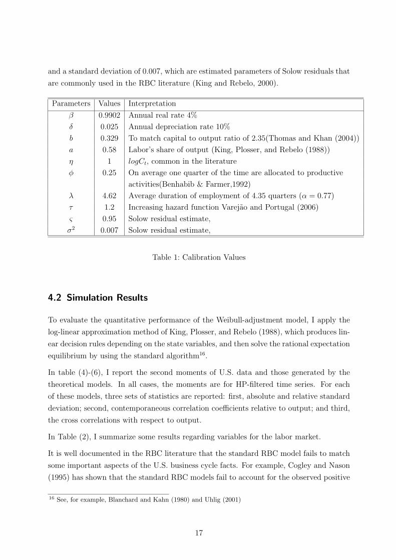
and a standard deviation of 0.007, which are estimated parameters of Solow residuals that

are commonly used in the RBC literature (King and Rebelo, 2000).

Parameters Values Interpretation

β 0.9902 Annual real rate 4%

δ 0.025 Annual depreciation rate 10%

b 0.329 To match capital to output ratio of 2.35(Thomas and Khan (2004))

a 0.58 Labor’s share of output (King, Plosser, and Rebelo (1988))

η 1 logCt, common in the literature

φ 0.25 On average one quarter of the time are allocated to productive

activities(Benhabib & Farmer,1992)

λ 4.62 Average duration of employment of 4.35 quarters (α = 0.77)

τ 1.2 Increasing hazard function Varejao and Portugal (2006)

ς 0.95 Solow residual estimate,

σ2 0.007 Solow residual estimate,

Table 1: Calibration Values

4.2 Simulation Results

To evaluate the quantitative performance of the Weibull-adjustment model, I apply the

log-linear approximation method of King, Plosser, and Rebelo (1988), which produces lin-

ear decision rules depending on the state variables, and then solve the rational expectation

equilibrium by using the standard algorithm16.

In table (4)-(6), I report the second moments of U.S. data and those generated by the

theoretical models. In all cases, the moments are for HP-filtered time series. For each

of these models, three sets of statistics are reported: first, absolute and relative standard

deviation; second, contemporaneous correlation coefficients relative to output; and third,

the cross correlations with respect to output.

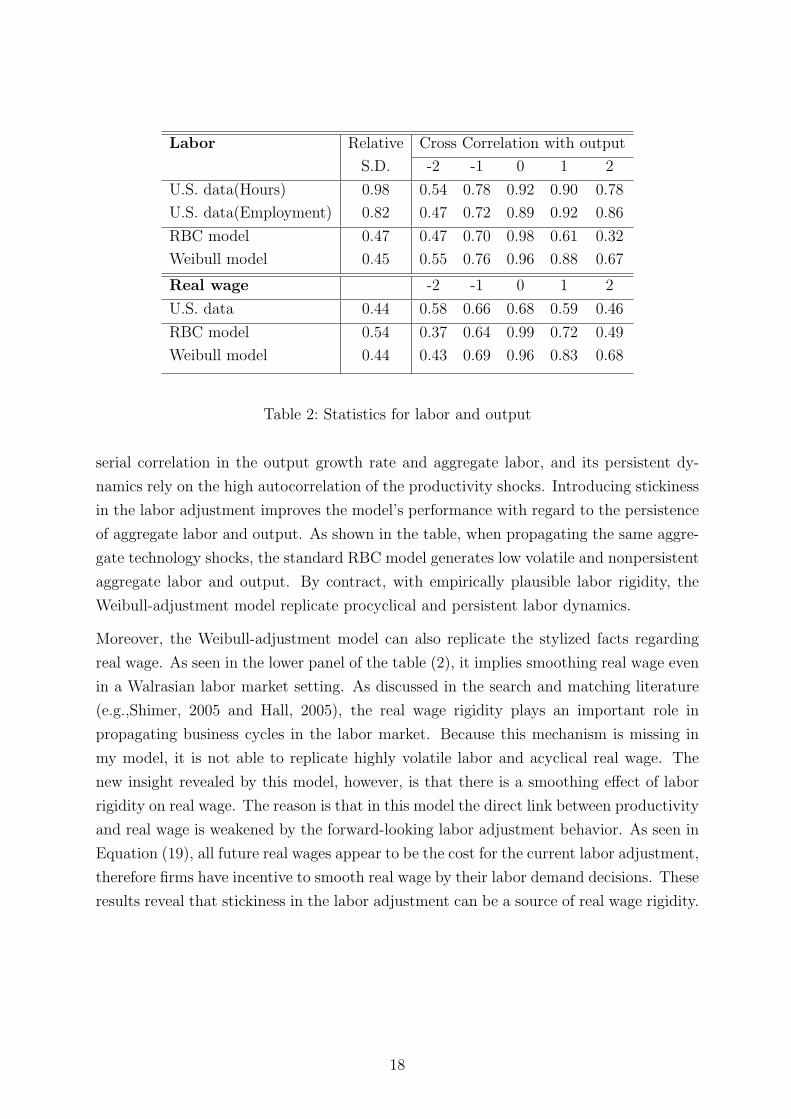
In Table (2), I summarize some results regarding variables for the labor market.

It is well documented in the RBC literature that the standard RBC model fails to match

some important aspects of the U.S. business cycle facts. For example, Cogley and Nason

(1995) has shown that the standard RBC models fail to account for the observed positive

16 See, for example, Blanchard and Kahn (1980) and Uhlig (2001)

17

Labor Relative Cross Correlation with output

S.D. -2 -1 0 1 2

U.S. data(Hours) 0.98 0.54 0.78 0.92 0.90 0.78

U.S. data(Employment) 0.82 0.47 0.72 0.89 0.92 0.86

RBC model 0.47 0.47 0.70 0.98 0.61 0.32

Weibull model 0.45 0.55 0.76 0.96 0.88 0.67

Real wage -2 -1 0 1 2

U.S. data 0.44 0.58 0.66 0.68 0.59 0.46

RBC model 0.54 0.37 0.64 0.99 0.72 0.49

Weibull model 0.44 0.43 0.69 0.96 0.83 0.68

Table 2: Statistics for labor and output

serial correlation in the output growth rate and aggregate labor, and its persistent dy-

namics rely on the high autocorrelation of the productivity shocks. Introducing stickiness

in the labor adjustment improves the model’s performance with regard to the persistence

of aggregate labor and output. As shown in the table, when propagating the same aggre-

gate technology shocks, the standard RBC model generates low volatile and nonpersistent

aggregate labor and output. By contract, with empirically plausible labor rigidity, the

Weibull-adjustment model replicate procyclical and persistent labor dynamics.

Moreover, the Weibull-adjustment model can also replicate the stylized facts regarding

real wage. As seen in the lower panel of the table (2), it implies smoothing real wage even

in a Walrasian labor market setting. As discussed in the search and matching literature

(e.g.,Shimer, 2005 and Hall, 2005), the real wage rigidity plays an important role in

propagating business cycles in the labor market. Because this mechanism is missing in

my model, it is not able to replicate highly volatile labor and acyclical real wage. The

new insight revealed by this model, however, is that there is a smoothing effect of labor

rigidity on real wage. The reason is that in this model the direct link between productivity

and real wage is weakened by the forward-looking labor adjustment behavior. As seen in

Equation (19), all future real wages appear to be the cost for the current labor adjustment,

therefore firms have incentive to smooth real wage by their labor demand decisions. These

results reveal that stickiness in the labor adjustment can be a source of real wage rigidity.

18

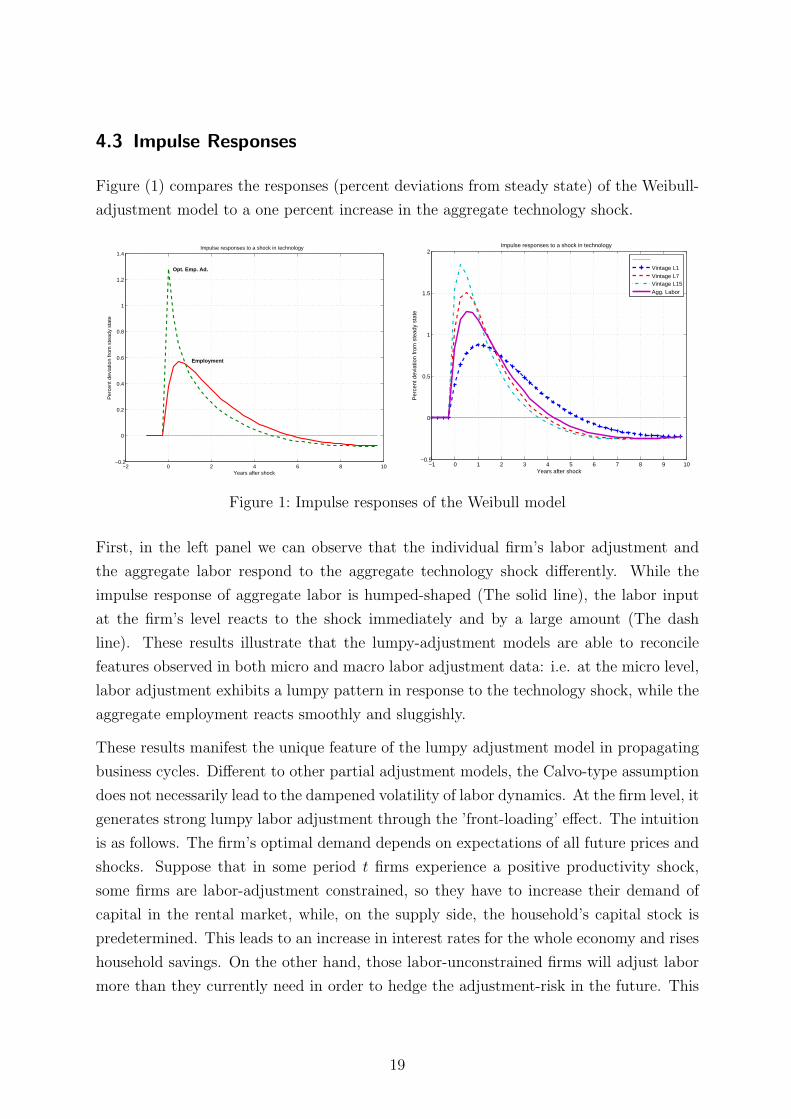
4.3 Impulse Responses

Figure (1) compares the responses (percent deviations from steady state) of the Weibull-

adjustment model to a one percent increase in the aggregate technology shock.

−2 0 2 4 6 8 10−0.2

0

0.2

0.4

0.6

0.8

1

1.2

1.4Impulse responses to a shock in technology

Years after shock

Per

cent

dev

iatio

n fr

om s

tead

y st

ate

Opt. Emp. Ad.

Employment

−1 0 1 2 3 4 5 6 7 8 9 10−0.5

0

0.5

1

1.5

2Impulse responses to a shock in technology

Years after shock

Per

cent

dev

iatio

n fr

om s

tead

y st

ate

Vintage L1Vintage L7Vintage L15Agg. Labor

Figure 1: Impulse responses of the Weibull model

First, in the left panel we can observe that the individual firm’s labor adjustment and

the aggregate labor respond to the aggregate technology shock differently. While the

impulse response of aggregate labor is humped-shaped (The solid line), the labor input

at the firm’s level reacts to the shock immediately and by a large amount (The dash

line). These results illustrate that the lumpy-adjustment models are able to reconcile

features observed in both micro and macro labor adjustment data: i.e. at the micro level,

labor adjustment exhibits a lumpy pattern in response to the technology shock, while the

aggregate employment reacts smoothly and sluggishly.

These results manifest the unique feature of the lumpy adjustment model in propagating

business cycles. Different to other partial adjustment models, the Calvo-type assumption

does not necessarily lead to the dampened volatility of labor dynamics. At the firm level, it

generates strong lumpy labor adjustment through the ’front-loading’ effect. The intuition

is as follows. The firm’s optimal demand depends on expectations of all future prices and

shocks. Suppose that in some period t firms experience a positive productivity shock,

some firms are labor-adjustment constrained, so they have to increase their demand of

capital in the rental market, while, on the supply side, the household’s capital stock is

predetermined. This leads to an increase in interest rates for the whole economy and rises

household savings. On the other hand, those labor-unconstrained firms will adjust labor

more than they currently need in order to hedge the adjustment-risk in the future. This

19

in turn drives real wage up. Put them together, all those rises in productivity and prices

can be expected by rational agents, so that the adjusting firms will, in addition to their

risk-hedging motive, demand even more workers. Moreover, if labor supply is elastic, rise

in the interest rate triggers the intertemporal substitution effect in the labor supply side,

because real wage is higher today and wage tomorrow is discounted at a higher rate, the

household is willing to enjoy less leisure today thus supply more labor. Consequently, both

labor and investment rise sharply at the micro level. However, at the aggregate level, this

strong effect is to a large extent neutralized by the underlying aggregation mechanism.

To further illustrate the important role played by the heterogeneous labor and the aggre-

gation mechanism in this model, I show in the right panel of the figure (1) the impulse

response functions of aggregate labor along with the responses of labor in different vin-

tage groups. Recalling the aggregate labor demand equation (28), the aggregate labor is

a weighted average of vintage labor demands, where the weights correspond to the prob-

ability density function of the Weibull distribution. This can be visualized in this figure.

The aggregate labor (the solid thick line) is composed of the sectoral labor from different

vintages (Dashed lines). As discussed in the previous section, given the increasing hazard

rates, the labor demand in the younger labor vintage is more persistent, but less volatile

than those in the older labor vintage. IRFs of the sectoral labor vary from the persistent

but less volatile younger vintage labor (The vintage L1) to the volatile but less persistent

older vintage labor (e.g. the vintage L15).

4.4 Sensitivity Analysis

Now I use numerical results to test how sensitive my results are in response to the key

parameter τ , which measures the shape of the Weibull distribution. In Table (3), I report

the relative volatility of aggregate labor to output and the first-order autocorrelations of

aggregate labor that are generated by a wide range of values of the shape parameter17.

In general, I find that the value of the shape parameter exerts an important influence on

the aggregate labor dynamics. As the shape parameter increases, the relative volatility of

labor to output rises, while the persistence of labor decreases. These results confirm the

intuition of the model, in which the higher is τ , the less likely firms sustain a fix amount of

labor for a long period of time, and hence the labor market is less rigid. On the other hand,

17 Here I check the range in which the hazard function of the Weibull distribution is increasing and 2.2is the maximum value that guarantees an unique stable solution of this dynamic system, given otherparameters’ value that I specify in the calibration section.

20

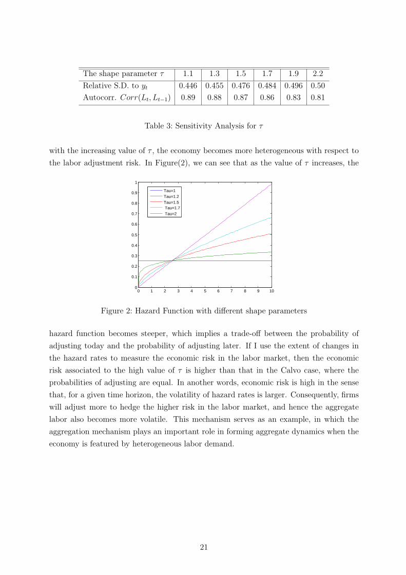
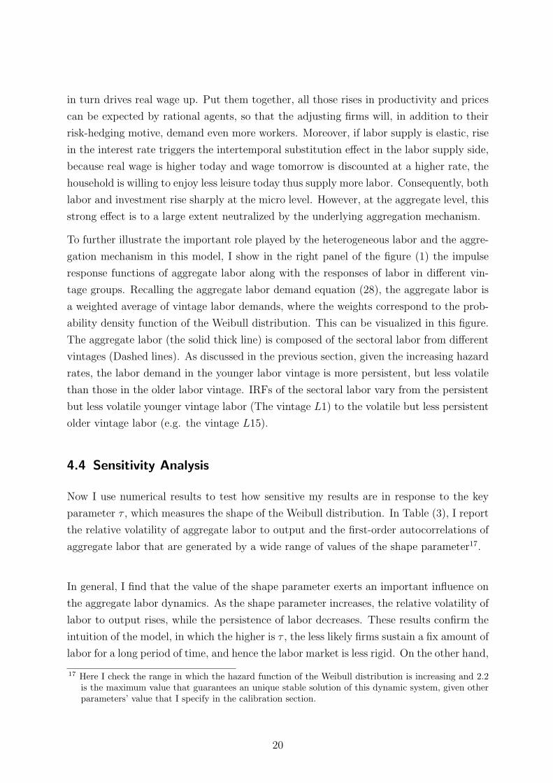
The shape parameter τ 1.1 1.3 1.5 1.7 1.9 2.2

Relative S.D. to yt 0.446 0.455 0.476 0.484 0.496 0.50

Autocorr. Corr(Lt, Lt−1) 0.89 0.88 0.87 0.86 0.83 0.81

Table 3: Sensitivity Analysis for τ

with the increasing value of τ , the economy becomes more heterogeneous with respect to

the labor adjustment risk. In Figure(2), we can see that as the value of τ increases, the

0 1 2 3 4 5 6 7 8 9 100

0.1

0.2

0.3

0.4

0.5

0.6

0.7

0.8

0.9

1

Tau=1Tau=1.2Tau=1.5 Tau=1.7 Tau=2

Figure 2: Hazard Function with different shape parameters

hazard function becomes steeper, which implies a trade-off between the probability of

adjusting today and the probability of adjusting later. If I use the extent of changes in

the hazard rates to measure the economic risk in the labor market, then the economic

risk associated to the high value of τ is higher than that in the Calvo case, where the

probabilities of adjusting are equal. In another words, economic risk is high in the sense

that, for a given time horizon, the volatility of hazard rates is larger. Consequently, firms

will adjust more to hedge the higher risk in the labor market, and hence the aggregate

labor also becomes more volatile. This mechanism serves as an example, in which the

aggregation mechanism plays an important role in forming aggregate dynamics when the

economy is featured by heterogeneous labor demand.

21

5 Concluding Remarks

In this paper general equilibrium is generated in markets where the household’s consumption-

leisure choice meets the firm’s factor demand decision under a stochastic labor adjustment

process. The innovation of the model is to apply the statistical duration analysis to extend

the well-established time-dependent adjustment scheme in the spirit of Calvo (1983) in a

DSGE framework. Using the increasing-hazard Weibull distribution, the model generates

heterogeneous labor vintages, which are different not only in the time of adjustment, but

also in terms of the volatility and the persistence of dynamics.

The key message conveyed in this paper is that impediment in the labor adjustment

process induces firms to make precautionary labor adjustments, and non-constant hazard

adjustment process brings about heterogeneity in the economy. In addition, given the het-

erogeneous nature of the economy, the underlying aggregation mechanism play a crucial

role in forming the aggregate dynamics. Serial studies by Hamermesh (e.g. Hamermesh,

1989, Hamermesh, 1993 and Hamermesh and Pfann, 1996) have shown that information

about the distribution of sub-units is crucial to linking micro-level features with implica-

tions for macro behavior deduced by determining the correct mechanism for aggregation.

Thus my model is an endeavor to illustrate how this mechanism works in propagating

realistic business cycle fluctuations.

22

A Equivalence of the Partial Adjustment Models

I first derive the aggregate labor demand equation from a textbook quadratic-adjustment-

cost model(See e.g. Hamermesh, 1993).

In this economy, each firm is assumed to maximize the expected discounted real value of

all future profits by choosing nonnegative values for optimal sequence of labors lt+i and

optimal sequence of capital stocks kt+i, subject to the quadratic labor adjustment costs.

The objective function of firm is:

maxlt+i,kt+i

Vt =∞∑i=0

Etβt+i[F (lt+i, kt+i)− wt+ilt+i − rt+ikt+i −d

2(lt+i − lt+i−1)

2] (29)

where d is denoted as the adjustment cost parameter.

subject to

yt = Ztlat k

bt (30)

and the total productivity shock Zt and the household’s problem are the same as in the

Calvo adjustment model.

The first order conditions are:

rt+i = FK(t + i) = bZt+i

lat+i

k1−bt+i

(31)

βt+i[FL(t + i)− wt+i − d(lt+i − lt+i−1)] + Et[βt+i+1d(lt+i − lt+i−1)] = 0 (32)

It follows:

a Zt+ila−1t+i kb

t+i − wt+i + β d lt+i+1 − d(1 + β)lt+i + d lt+i−1 = 0 (33)

If I log-linearize these FOCs around the steady state, I get the following dynamic labor

demand equation:

γβEt[lt+1]− [(1− a− b) + γ(1 + β)] lt + γlt−1 −bR

rRt − (1− b)wt + zt = 0 (34)

Where I denote γ = dnw

(1− b).

23

B Weibull Distribution

The PDF of Weibull distribution is given by the following expression:

Pr(j) =τ

λ

(j

λ

)τ−1

exp

(−(

j

λ

)τ)(35)

and the cumulative probability function is:

F (j) = 1− exp

(−(

j

λ

)τ)(36)

The parameters that characterize the Weibull distribution are the scale parameter λ and

the shape parameter τ . The shape parameter determines the shape of the Weibull’s pdf

function, e.g. when τ = 1, it reduces to an exponential case; while τ = 3.4, the Weibull

amounts to the normal distribution. The scale parameter defines the characteristic life of

the random process that amounts to the time, at which 63.2% of the firm will adjust their

labor. This can be seen with the evaluation of the cdf function of the Weibull distribution

at j equaling the scale parameterλ. Then we have, F (λ) = 1− e(−1) = 0.632.

Note that it relates to the mean duration j according to the following equation:

j =1

α= λΓ(

1

τ+ 1), (37)

where Γ() is the Gamma function.

It follows that the hazard function of Weibull distribution is:

h(j) =τ

λ

(j

λ

)τ−1

(38)

Note that this hazard is constant when the shape parameter τ equals one, and increasing

when τ is greater than one.

24

C Derivation of the Dynamic Labor Demand Equation

First, log-linearize Equation 25:

J∑i=0

S(i) βiEt[(a− 1)l∗0,t + bkj,t+i − wt+i + zt+i] = 0 (39)

J∑i=0

S(i) βiEt[bkj,t+i − wt+i + zt+i] + (a− 1) l∗0,t

J∑i=0

S(i) βi = 0

Let Ψ =J∑

i=0

S(i)βi and rearrange this equation:

(1− a)Ψ l∗0,t =J∑

i=0

S(i) βiEt[bkj,t+i − wt+i + zt+i]

Then, substitute out kj,t+i with the log-linearized Equation (18):

(1− a)Ψ l∗0,t =J∑

i=0

S(i) βiEt[ab

1− blj,t+i −

b

1− brt+i − wt+i +

1

1− bzt+i]

Note that l∗0,t = lj,t+i ∀ j ∈ (0, J), we obtain:

1− a− b

1− bΨ l∗0,t =

J∑i=0

S(i) βi Et[1

1− bzt+i −

b

1− brt+i − wt+i]︸ ︷︷ ︸

Xt+i

(40)

= S(0)Xt + S(1) βXt+1 + S(2) β2Xt+2 + S(3) β3Xt+3 + ...

And, iterate Equation 40 one period forward, we obtain:

1− a− b

1− bΨ l∗0,t+1 =

J∑i=0

S(i) βiEt[1

1− bzt+i+1 −

b

1− brt+i+1 − wt+i+1]

= S(0)Xt+1 + S(1) βXt+2 + S(2) β2Xt+3 + ...

=S(0)

S(1)S(1) Xt+1 +

S(1)

S(2)S(2) βXt+2 +

S(2)

S(3)S(3) β2Xt+3 + ...

25

Multiply both sides of this equation by β:

β1− a− b

1− bΨ l∗0,t+1 =

S(0)

S(1)S(1)β Xt+1 +

S(1)

S(2)S(2) β2Xt+2 +

S(2)

S(3)S(3) β3Xt+3 + ...

where S(i)S(i+1)

= exp(

(i+1)τ−iτ

λτ

). Given my calibration values of the Weibull parameters,

these values can be approximated to be a constant (α).

β1− a− b

1− bΨ l∗0,t+1 =

1

αS(1)β Xt+1 +

1

αS(2) β2Xt+2 +

1

αS(3) β3Xt+3 + ...

αβ1− a− b

1− bΨ l∗0,t+1 = S(1)β Xt+1 + S(2) β2Xt+2 + S(3) β3Xt+3 + ... (41)

Substitute (41) into (40), we obtain:

1− a− b

1− bΨ l∗0,t = Xt + αβ

1− a− b

1− bΨ l∗0,t+1 (42)

And, it follows the equation 26, which is introduced in the text.

l∗0,t = αβEt[l∗0,t+1]−

b

Ψ(1− a− b)rt −

1− b

Ψ(1− a− b)wt +

1

Ψ(1− a− b)zt

where α−1 = 1J+1

J∑i=0

exp(

(i+1)τ−iτ

λτ

)

26

References

Benhabib, J., and R. E. Farmer (1992): “Indeterminacy and Increasing Returns,”

Ucla economics working papers, UCLA Department of Economics.

Blanchard, O. J., and C. M. Kahn (1980): “The Solution of Linear Difference

Models under Rational Expectations,” Econometrica, 48(5), 1305–11.

Caballero, R. J., and E. M. Engel (1993): “Microeconomic Adjustment Hazards

and Aggregate Dynamics,” The Quarterly Journal of Economics, 108(2), 359–83.

Caballero, R. J., E. M. Engel, and J. Haltiwanger (1997): “Aggregate Employ-

ment Dynamics: Building from Microeconomic Evidence,” American Economic Review,

87(1), 115–37.

Calvo, G. (1983): “Staggered Prices in a Utility Maximizing Framework,” Journal of

Monetary Economics, 12, 383–398.

Caplin, A. S., and D. F. Spulber (1987): “Menu Costs and the Neutrality of Money,”

The Quarterly Journal of Economics, 102(4), 703–25.

Cogley, T., and J. M. Nason (1995): “Output Dynamics in Real-Business-Cycle

Models,” American Economic Review, 85(3), 492–511.

Cooley, T. F. (1995): Frontiers of Business Cycle Research. Princeton University Press.

Hall, R. E. (2005): “Employment Fluctuations with Equilibrium Wage Stickiness,”

American Economic Review, 95(1), 50–65.

Hamermesh, D. S. (1989): “Labor Demand and the Structure of Adjustment Costs,”

American Economic Review, 79(4), 674–89.

Hamermesh, D. S. (1993): Labor Demand. Princeton University Press.

Hamermesh, D. S., and G. A. Pfann (1996): “Adjustment Costs in Factor Demand,”

Cepr discussion papers, C.E.P.R. Discussion Papers.

King, R. G., C. I. Plosser, and S. Rebelo (1988): “Production, Growth and Busi-

ness Cycles: The Basic Neoclassical Model,” Journal Monetary Economics, 21(2/3),

195–232.

King, R. G., and S. T. Rebelo (2000): “Resuscitating Real Business Cycles,” Nber

working papers, National Bureau of Economic Research, Inc.

27

King, R. G., and J. K. Thomas (2006): “Partial Adjustment Without Apology,”

International Economic Review, 47(3), 779–809.

Letterie, W. A., G. A. Pfann, and J. M. Polder (2004): “Factor adjustment spikes

and interrelation: an empirical investigation,” Economics Letters, 85(2), 145–150.

Rotemberg, J. (1987): “The New Keynesian Microfoundations,” NBER Macroeco-

nomics Annual, December(2), 69–104.

Shimer, R. (2005): “The Cyclical Behavior of Equilibrium Unemployment and Vacan-

cies,” American Economic Review, 95(1), 25–49.

Thomas, J. K. (2002): “Is lumpy investment relevant for the business cycle?,” Discussion

paper.

Thomas, J. K., and A. Khan (2004): “Idiosyncratic shocks and the role of noncon-

vexities in plant and aggregate investment dynamics,” Discussion paper.

Uhlig, H. (2001): “A Toolkit for Analyzing Nonlinear Dynamic Stochastic Models Eas-

ily,” Discussion paper.

Varejao, J., and P. Portugal (2006): “Employment Dynamics and the Structure

of Labor Adjustment Costs,” Iza discussion papers, Institute for the Study of Labor

(IZA).

Veracierto, M. L. (2002): “Plant-Level Irreversible Investment and Equilibrium Busi-

ness Cycles,” American Economic Review, 92(1), 181–197.

28

D Tables

Standard Relative Cross Correlation with output

Variables Deviation% S.D. -3 -2 -1 0 1 2 3

Hours* 1.69 0.98 0.38 0.54 0.78 0.92 0.90 0.78 0.63

Employment* 1.41 0.82 0.22 0.47 0.72 0.89 0.92 0.86 0.73

Real wage 0.76 0.44 0.47 0.58 0.66 0.68 0.59 0.46 0.29

Consumption 1.27 0.74 0.57 0.72 0.82 0.83 0.67 0.46 0.22

Output 1.72 1.00 0.38 0.63 0.85 1.00 0.85 0.63 0.38

Investment 5.34 3.10 0.43 0.63 0.82 0.90 0.81 0.60 0.35

Labor productivity 0.73 0.42 0.44 0.45 0.34 0.34 0.10 -0.09 -0.30

Notes: all statistics are reported in Cooley (1995) Table(1.1)*: Based on establishment survey.

Table 4: Business Cycle Statistics for the U.S. Economy

Standard Relative Cross Correlation with output

Variables Deviation% S.D. -3 -2 -1 0 1 2 3

Hours 0.59 0.47 0.29 0.47 0.70 0.98 0.61 0.32 0.10

Capital 0.32 0.26 -0.31 -0.16 0.06 0.36 0.54 0.63 0.65

Real wage 0.67 0.54 0.15 0.37 0.64 0.99 0.72 0.49 0.31

Consumption 0.38 0.31 0.02 0.24 0.53 0.90 0.75 0.60 0.46

Output 1.24 1.00 0.22 0.42 0.68 1.00 0.68 0.42 0.22

Interest rate 0.04 0.04 0.32 0.49 0.70 0.96 0.57 0.27 0.05

Investment 3.84 3.10 0.27 0.46 0.70 0.99 0.63 0.35 0.14

Labor productivity 0.67 0.54 0.15 0.37 0.64 0.99 0.72 0.49 0.31

Table 5: Business Cycle Statistics for the Standard RBC Model

29

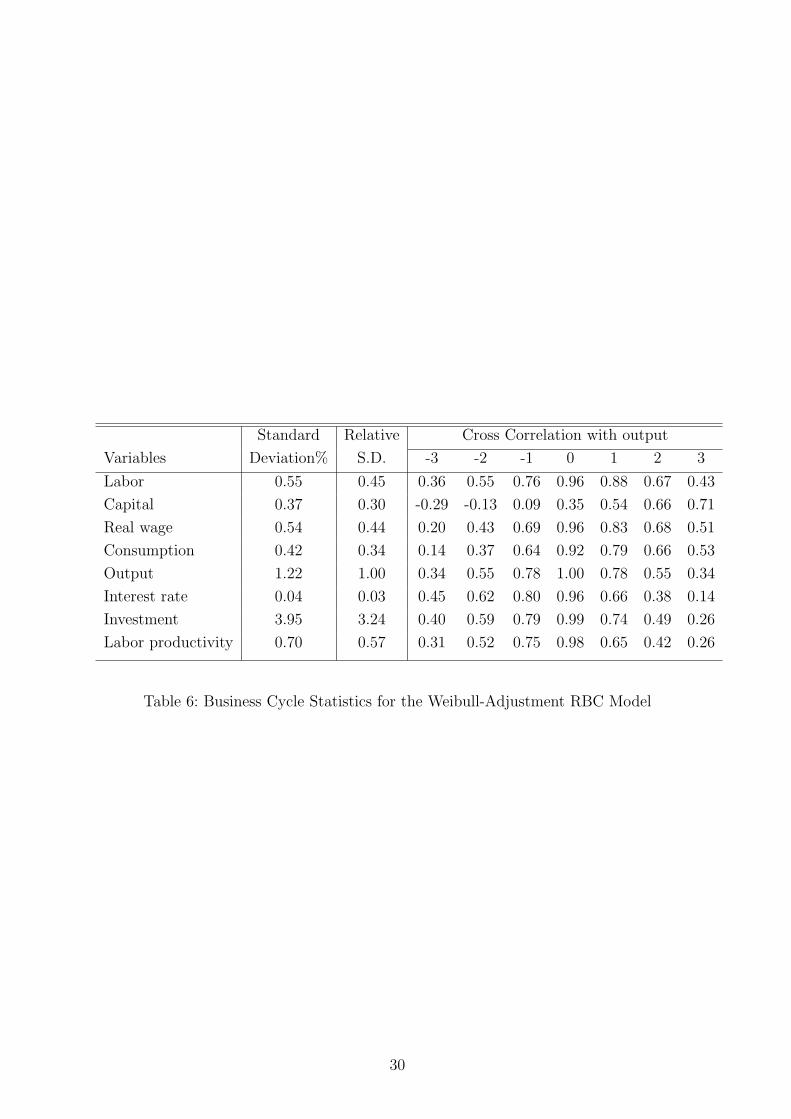
Standard Relative Cross Correlation with output

Variables Deviation% S.D. -3 -2 -1 0 1 2 3

Labor 0.55 0.45 0.36 0.55 0.76 0.96 0.88 0.67 0.43

Capital 0.37 0.30 -0.29 -0.13 0.09 0.35 0.54 0.66 0.71

Real wage 0.54 0.44 0.20 0.43 0.69 0.96 0.83 0.68 0.51

Consumption 0.42 0.34 0.14 0.37 0.64 0.92 0.79 0.66 0.53

Output 1.22 1.00 0.34 0.55 0.78 1.00 0.78 0.55 0.34

Interest rate 0.04 0.03 0.45 0.62 0.80 0.96 0.66 0.38 0.14

Investment 3.95 3.24 0.40 0.59 0.79 0.99 0.74 0.49 0.26

Labor productivity 0.70 0.57 0.31 0.52 0.75 0.98 0.65 0.42 0.26

Table 6: Business Cycle Statistics for the Weibull-Adjustment RBC Model

30

SFB 649 Discussion Paper Series 2008

For a complete list of Discussion Papers published by the SFB 649, please visit http://sfb649.wiwi.hu-berlin.de.

001 "Testing Monotonicity of Pricing Kernels" by Yuri Golubev, Wolfgang Härdle and Roman Timonfeev, January 2008.

002 "Adaptive pointwise estimation in time-inhomogeneous time-series models" by Pavel Cizek, Wolfgang Härdle and Vladimir Spokoiny, January 2008. 003 "The Bayesian Additive Classification Tree Applied to Credit Risk Modelling" by Junni L. Zhang and Wolfgang Härdle, January 2008. 004 "Independent Component Analysis Via Copula Techniques" by Ray-Bing Chen, Meihui Guo, Wolfgang Härdle and Shih-Feng Huang, January 2008. 005 "The Default Risk of Firms Examined with Smooth Support Vector Machines" by Wolfgang Härdle, Yuh-Jye Lee, Dorothea Schäfer and Yi-Ren Yeh, January 2008. 006 "Value-at-Risk and Expected Shortfall when there is long range dependence" by Wolfgang Härdle and Julius Mungo, Januray 2008. 007 "A Consistent Nonparametric Test for Causality in Quantile" by Kiho Jeong and Wolfgang Härdle, January 2008. 008 "Do Legal Standards Affect Ethical Concerns of Consumers?" by Dirk Engelmann and Dorothea Kübler, January 2008. 009 "Recursive Portfolio Selection with Decision Trees" by Anton Andriyashin, Wolfgang Härdle and Roman Timofeev, January 2008. 010 "Do Public Banks have a Competitive Advantage?" by Astrid Matthey, January 2008. 011 "Don’t aim too high: the potential costs of high aspirations" by Astrid Matthey and Nadja Dwenger, January 2008. 012 "Visualizing exploratory factor analysis models" by Sigbert Klinke and Cornelia Wagner, January 2008. 013 "House Prices and Replacement Cost: A Micro-Level Analysis" by Rainer Schulz and Axel Werwatz, January 2008. 014 "Support Vector Regression Based GARCH Model with Application to Forecasting Volatility of Financial Returns" by Shiyi Chen, Kiho Jeong and Wolfgang Härdle, January 2008. 015 "Structural Constant Conditional Correlation" by Enzo Weber, January 2008. 016 "Estimating Investment Equations in Imperfect Capital Markets" by Silke Hüttel, Oliver Mußhoff, Martin Odening and Nataliya Zinych, January 2008. 017 "Adaptive Forecasting of the EURIBOR Swap Term Structure" by Oliver Blaskowitz and Helmut Herwatz, January 2008. 018 "Solving, Estimating and Selecting Nonlinear Dynamic Models without the Curse of Dimensionality" by Viktor Winschel and Markus Krätzig, February 2008. 019 "The Accuracy of Long-term Real Estate Valuations" by Rainer Schulz, Markus Staiber, Martin Wersing and Axel Werwatz, February 2008. 020 "The Impact of International Outsourcing on Labour Market Dynamics in Germany" by Ronald Bachmann and Sebastian Braun, February 2008. 021 "Preferences for Collective versus Individualised Wage Setting" by Tito Boeri and Michael C. Burda, February 2008.

SFB 649, Spandauer Straße 1, D-10178 Berlin

http://sfb649.wiwi.hu-berlin.de

This research was supported by the Deutsche Forschungsgemeinschaft through the SFB 649 "Economic Risk".

022 "Lumpy Labor Adjustment as a Propagation Mechanism of Business Cycles" by Fang Yao, February 2008. 023 "Family Management, Family Ownership and Downsizing: Evidence from S&P 500 Firms" by Jörn Hendrich Block, February 2008. 024 "Skill Specific Unemployment with Imperfect Substitution of Skills" by Runli Xie, March 2008. 025 "Price Adjustment to News with Uncertain Precision" by Nikolaus Hautsch, Dieter Hess and Christoph Müller, March 2008. 026 "Information and Beliefs in a Repeated Normal-form Game" by Dietmar Fehr, Dorothea Kübler and David Danz, March 2008. 027 "The Stochastic Fluctuation of the Quantile Regression Curve" by Wolfgang Härdle and Song Song, March 2008. 028 "Are stewardship and valuation usefulness compatible or alternative objectives of financial accounting?" by Joachim Gassen, March 2008. 029 "Genetic Codes of Mergers, Post Merger Technology Evolution and Why Mergers Fail" by Alexander Cuntz, April 2008. 030 "Using R, LaTeX and Wiki for an Arabic e-learning platform" by Taleb Ahmad, Wolfgang Härdle, Sigbert Klinke and Shafeeqah Al Awadhi, April 2008. 031 "Beyond the business cycle – factors driving aggregate mortality rates" by Katja Hanewald, April 2008. 032 "Against All Odds? National Sentiment and Wagering on European Football" by Sebastian Braun and Michael Kvasnicka, April 2008. 033 "Are CEOs in Family Firms Paid Like Bureaucrats? Evidence from Bayesian and Frequentist Analyses" by Jörn Hendrich Block, April 2008. 034 "JBendge: An Object-Oriented System for Solving, Estimating and Selecting Nonlinear Dynamic Models" by Viktor Winschel and Markus Krätzig, April 2008. 035 "Stock Picking via Nonsymmetrically Pruned Binary Decision Trees" by Anton Andriyashin, May 2008. 036 "Expected Inflation, Expected Stock Returns, and Money Illusion: What can we learn from Survey Expectations?" by Maik Schmeling and Andreas Schrimpf, May 2008. 037 "The Impact of Individual Investment Behavior for Retirement Welfare: Evidence from the United States and Germany" by Thomas Post, Helmut Gründl, Joan T. Schmit and Anja Zimmer, May 2008. 038 "Dynamic Semiparametric Factor Models in Risk Neutral Density Estimation" by Enzo Giacomini, Wolfgang Härdle and Volker Krätschmer, May 2008. 039 "Can Education Save Europe From High Unemployment?" by Nicole Walter and Runli Xie, June 2008. 040 "Solow Residuals without Capital Stocks" by Michael C. Burda and Battista Severgnini, August 2008. 041 "Unionization, Stochastic Dominance, and Compression of the Wage Distribution: Evidence from Germany" by Michael C. Burda, Bernd Fitzenberger, Alexander Lembcke and Thorsten Vogel, March 2008 042 "Gruppenvergleiche bei hypothetischen Konstrukten – Die Prüfung der Übereinstimmung von Messmodellen mit der Strukturgleichungs- methodik" by Dirk Temme and Lutz Hildebrandt, June 2008. 043 "Modeling Dependencies in Finance using Copulae" by Wolfgang Härdle, Ostap Okhrin and Yarema Okhrin, June 2008. 044 "Numerics of Implied Binomial Trees" by Wolfgang Härdle and Alena Mysickova, June 2008.

SFB 649, Spandauer Straße 1, D-10178 Berlin http://sfb649.wiwi.hu-berlin.de

This research was supported by the Deutsche

Forschungsgemeinschaft through the SFB 649 "Economic Risk".

045 "Measuring and Modeling Risk Using High-Frequency Data" by Wolfgang Härdle, Nikolaus Hautsch and Uta Pigorsch, June 2008. 046 "Links between sustainability-related innovation and sustainability management" by Marcus Wagner, June 2008. 047 "Modelling High-Frequency Volatility and Liquidity Using Multiplicative Error Models" by Nikolaus Hautsch and Vahidin Jeleskovic, July 2008. 048 "Macro Wine in Financial Skins: The Oil-FX Interdependence" by Enzo Weber, July 2008. 049 "Simultaneous Stochastic Volatility Transmission Across American Equity Markets" by Enzo Weber, July 2008. 050 "A semiparametric factor model for electricity forward curve dynamics" by Szymon Borak and Rafał Weron, July 2008. 051 "Recurrent Support Vector Regreson for a Nonlinear ARMA Model with Applications to Forecasting Financial Returns" by Shiyi Chen, Kiho Jeong and Wolfgang K. Härdle, July 2008. 052 "Bayesian Demographic Modeling and Forecasting: An Application to U.S. Mortality" by Wolfgang Reichmuth and Samad Sarferaz, July 2008. 053 "Yield Curve Factors, Term Structure Volatility, and Bond Risk Premia" by Nikolaus Hautsch and Yangguoyi Ou, July 2008. 054 "The Natural Rate Hypothesis and Real Determinacy" by Alexander Meyer- Gohde, July 2008 055 "Technology sourcing by large incumbents through acquisition of small firms" by Marcus Wagner, Juny 2008 056 "Lumpy Labor Adjustment as a Propagation Mechanism of Business Cycle" by Fang Yao, August 2008

SFB 649, Spandauer Straße 1, D-10178 Berlin http://sfb649.wiwi.hu-berlin.de

This research was supported by the Deutsche

Forschungsgemeinschaft through the SFB 649 "Economic Risk".