luddites 12 june 2011

7/29/2019 Luddites 12 June 2011

http://slidepdf.com/reader/full/luddites-12-june-2011 1/43

Luddites, the Industrial Revolution,

and the Demographic Transition∗

Kevin H. O’Rourke, Ahmed S. Rahman, and Alan M. Taylor†

June 2011

∗We acknowledge funding from the European Community’s Sixth Framework Programme through itsMarie Curie Research Training Network programme, contract numbers MRTN-CT-2004-512439 and HPRN-CT-2002-00236. We also thank the Center for the Evolution of the Global Economy at the University of California, Davis, for financial support. O’Rourke would like to thank the European Research Council forits financial support, under its Advanced Investigator Grant scheme, contract number 249546. Some of thework on the project was undertaken while O’Rourke was a Government of Ireland Senior Research Fellowand while Taylor was a Guggenheim Fellow; we thank the Irish Research Council for the Humanities andSocial Sciences and the John Simon Guggenheim Memorial Foundation for their generous support. For theirhelpful criticisms and suggestions we thank Gregory Clark, Oded Galor, Philippe Martin, David Mitch,Joel Mokyr, Andrew Mountford, Joachim Voth, two anonymous referees, and participants in workshopsat Royal Holloway, University of London; London School of Economics; Universidad Carlos III; UniversityCollege, Galway; Paris School of Economics; and Brown University; and at the CEPR conferences “Europe’s

Growth and Development Experience” held at the University of Warwick, 28–30 October 2005, “Trade,Industrialisation and Development” held at Villa Il Poggiale, San Casciano Val di Pesa (Florence), 27–29 January 2006, and “Economic Growth in the Extremely Long Run” held at the European UniversityInstitute, 27 June–1 July, 2006; at the NBER International Trade and Investment program meeting, held atNBER, Palo Alto, Calif., 1–2 December 2006; and at the NBER Evolution of the Global Economy workshop,held at NBER, Cambridge, Mass., 2 March 2007. The latter workshop was supported by NSF grant OISE05-36900 administered by the NBER. All errors are ours.

†O’Rourke: Trinity College, Dublin, CEPR, and NBER ([email protected]). Rahman: United StatesNaval Academy ([email protected]). Taylor: University of California, Davis, NBER, and CEPR ([email protected])

7/29/2019 Luddites 12 June 2011


Luddites, the Industrial Revolution,

and the Demographic Transition

Abstract

Technological change was unskilled-labor-biased during the early Industrial Revolution,but is skill-biased today. This represents a rich set of non-monotonic macroeconomicdynamics which is not embedded in extant unified growth models. We present historicalevidence and develop a model which can endogenously account for these facts, wherefactor bias reflects profit-maximizing decisions by innovators. In a setup with directedtechnological change, initial endowments dictate that the early Industrial Revolutionbe unskilled-labor-biased. Increasing basic knowledge then causes a growth takeoff, anincome-led demand for fewer but more educated children, and this ultimately ensuresa transition to skill-biased technological change in the long run.

Keywords : skill bias, directed technological change, endogenous growth, demography, unifiedgrowth theory.

JEL Codes : O31, O33, J13, J24, N10.

7/29/2019 Luddites 12 June 2011


On March 11, 1811, several hundred framework knitters gathered in the Nottingham mar-

ketplace, not far from Sherwood Forest, to protest their working conditions. Having been

dispersed by the constabulary and a troop of Dragoons, they reassembled that evening in

nearby Arnold, and broke some sixty stocking frames. On November 10 of the same year,

another Arnold mob gathered in Bulwell Forest, under the command of someone stylinghimself “Ned Lud,” and the rapidly growing Luddite movement would suffer its first fatality

that night when John Westley was shot dead during an attack on the premises of Edward

Hollingsworth, a local hosier.

Today, the term Luddite often refers to opponents of technological progress for its own

sake. At the time, however, Luddites were engaged in what Hobsbawm (1952, p. 59) has

termed “collective bargaining by riot.” “In none of these cases . . . was there any question of

hostility to machines as such. Wrecking was simply a technique of trade unionism” (ibid.)

on the part of skilled textile workers whose living standards were being eroded by new

machinery. This new machinery was making it possible for employers not just to produce

cloth more efficiently, but to use cheaper unskilled workers—women, and even children—in

the place of highly paid artisans. Not surprisingly, skilled workers objected to this.

Luddism emerged during what Galor and Weil (2000) have termed the “post-Malthusian

regime.” During this phase of British economic history, technological change was enabling

the economy to gradually escape the Malthusian trap. However, living standards only rose

slowly during this period, as population grew at an accelerating rate. But by the late

19th century, technological change was accelerating and living standards were growing more

rapidly (Figure 1). Much of this acceleration was due to a dramatic and well-documenteddemographic transition, whereby fertility rates fell and educational standards rose (Figure

2). Many new technologies were by then beginning to emerge which were skill-using rather

than skill-saving, for example in modern chemical and metallurgical industries.

A standard assumption in unified growth theory (UGT) is that modern economic growth

(MEG) is characterized by the development of skill-using technologies. That this is a sensible

assumption for the 20th century has been abundantly documented in Goldin and Katz (2008)

for the United States, for example, but this is certainly not only an American story (see for

example Berman, Bound, and Machin 1998). So, in the sufficiently recent past, technological

progress has been skill-using. However, as the example of the Luddites shows, we cannot

assume that this has always been the case. Indeed, Acemoglu (2002), surveying the literature,

concludes that the notion that technical change is skill-biased is appropriate for the 20th

century, but not for earlier periods. And there are good grounds for believing that in

the sufficiently early stages of the British Industrial Revolution, technological progress in

industries like textiles was skill-saving rather than skill-using.

1

7/29/2019 Luddites 12 June 2011


Figure 1: Growth Rates of GDP per Capita and Population in Western Europe, 1500–2000

The figure shows two key long-run stylized facts: the permanent acceleration in output per capitagrowth rates, and the temporary boom in population growth rates which accompanied the IndustrialRevolution.

0.0

0.2

0.4

0.6

0.8

1.0

1.2

1.4

1.6

1.8

2.0

1500 1600 1700 1800 1900 2000

Growth of output per person (% per year)

Growth of population (% per year)

Source : Galor (2005), based on Maddison (2001).

For example, by way of initial conditions, preindustrial textile production needed highly

skilled labor such as spinners and weavers. Similarly, other preindustrial manufactures re-

lied on their own skilled artisans of various sorts. But implementing the technologies of the

Industrial Revolution (in textile production, iron smelting and refining, mining and agricul-

ture) required large labor forces with little to no specialized training. In some cases it is

very easy to see the motivation as well as the impact of innovation. For example, Richard

Roberts’s invention of the self-acting mule came about as a result of a plea for help on

the part of Manchester cotton manufacturers, faced with a mule spinners strike (Rosenberg

1969, p. 13), and this was not the only example of a skilled-labor-saving invention brought

about as a result of the efforts of skilled workers to maintain their relative economic position

(ibid.). Nor was this a uniquely British phenomenon, as unskilled labour, capital and natural

resources were substituted for skilled labour in mid-nineteenth century American industryas well (this is a core tenet of American macroeconomic history: see, e.g., the seminal work

by James and Skinner 1985). Furthermore, this process continued during the rest of the

nineteenth century in other industries. As Mokyr (1990, p. 137) puts it, after the U.S. Civil

War, first in the U.S., and then in Europe, mass production methods gradually displaced

skilled workers in a broad range of sectors: “First in firearms, then in clocks, pumps, locks,

2

7/29/2019 Luddites 12 June 2011


Figure 2: Fertility and Schooling in Four Advanced Countries

The figures show two important correlates of the Industrial Revolution: fertility decreased (theDemographic Transition) and education increased. However, the transtions did not occur untillater in the 19th century.

0

10

20

30

40

50

60

70

80

1850 1860 1870 1880 1890 1900 1910

(a) England and Wales

Crude birth rate (per thousand)

Primary enrollment (5–14 years, percent)

20

30

40

50

60

70

80

90

100

1865 1870 1875 1880 1885 1890 1895 1900 1905 1910

(b) Germany



3

7/29/2019 Luddites 12 June 2011


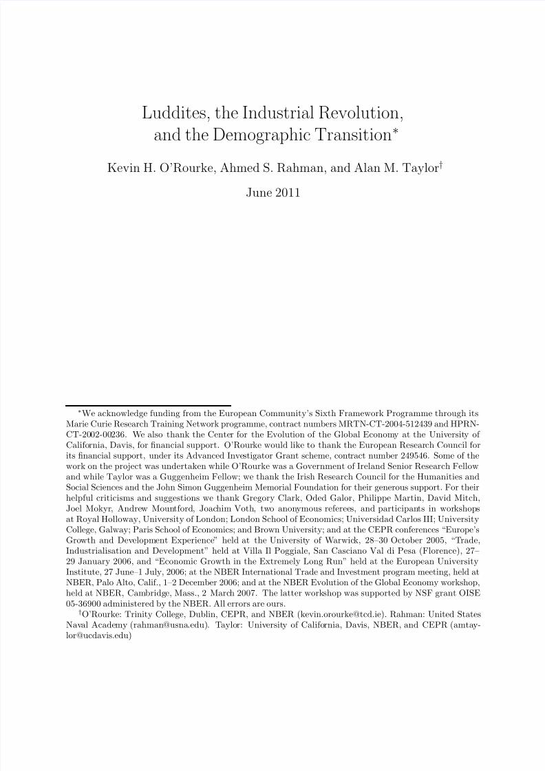
Figure 2 (continued): Fertility and Schooling in Four Advanced Countries

0

10

20

30

40

50

60

70

80

1800 1820 1840 1860 1880 1900

(c) Sweden

Crude birth rate (per thouand)


20

30

40

50

60

70

80

90

100

1800 1820 1840 1860 1880 1900 1920

(d) United States



Source : Tan and Haines (1984). Trend lines are 2-period moving averages.

4

7/29/2019 Luddites 12 June 2011


mechanical reapers, typewriters, sewing machines, and eventually in engines and bicycles,

interchangeable parts technology proved superior and replaced the skilled artisans working

with chisel and file.” Through these kinds of long-run processes happy, highly-valued skilled

craftsmen became angry, machine-breaking Luddites.

Much later, fortunes changed: the techniques developed in the latter half of the 19thcentury (for example in chemicals, electrical industries and services) raised the demand

for a new labor force with highly specialized skills (Mokyr 1999). The industries of the

Second Industrial Revolution were not only based on an increasingly formal interaction

between science and industry, but required an increased supply of well-trained chemists,

engineers, and other high-skill workers as well. According to Goldin and Katz (2008), in

the early 20th century (or from as early as the 1890s onwards, in certain sectors) American

manufacturers began to adopt continuous-process or batch production methods, associated

with new electricity- and capital-intensive technologies. These new technologies increased

the relative demand for skilled workers, who were required to operate the new machinery,

and ceteris paribus raised the return to skills. Again the story is not confined to one country.

For example, an inability to match Germany in the training of high-skill workers essential

for new industries has long been thought to be a factor in relative British decline during this

period (e.g., see the references in Mokyr 2002, p. 274).

If in the sufficiently distant past, technological progress was skill-saving, but in the suffi-

ciently recent past it has become skill-using, then it logically follows that at some point there

was a transition from skill-saving to skill-using technical change. This transition presumably

happened over a long period of time, with turning points occurring in different periods indifferent countries, and at different times in different sectors.

The challenge to history and theory is then to explain how and why this happened. The

main purpose of this paper is to show how such a transition could have occurred, within the

context of a UGT model. Since in reality the transition was not abrupt, but took place over

a protracted period of time, we will want our model to generate a long-drawn-out transition

period, during which both skill-saving and skill-using technological change occurred, but

with the relative share of the former decreasing, and of the latter increasing, over time.

In order to achieve this this, we need to go beyond the current UGT literature (e.g.,

Galor and Weil 2000; Jones 2001; Hansen and Prescott 2002; Lucas 2002; Weisdorf 2004;

Galor 2011a) in several respects.

Most obviously, we need to incorporate two types of workers, skilled and unskilled, so that

technological change can be biassed in either direction. Second, we need to allow for factor-

biased technological change. Third, and most importantly, we need to allow the direction of

factor bias to differ at different points in time, since we want to explain why the Industrial

5

7/29/2019 Luddites 12 June 2011


Revolution was initially so bad for skilled workers, rather than simply assume this was the

case. Similarly, we want to explain why, by the end of the 19th century, new technologies

that were skill-using were being invented, rather than just assume this was happening. We

are thus going to have to explicitly model the choices facing would-be innovators. If the

direction of technological change differed over time, this presumably reflected the differentincentives facing these inventors.1

In this paper, we thus delve into the microeconomics of technological change to a greater

extent than previous unified growth theory papers, which have tended to model technological

change in a reduced form manner as a function of scale affects (cf. Romer 1990, Kremer

1993) and/or human capital endowments. We propose a fully-specified research and devel-

opment model driving technological change, which is appropriate for this period since Allen

(2006) has recently pointed out that British firms were investing significant resources in the

search for technological breakthroughs during the Industrial Revolution. Building on the

foundations of the benchmark Galor-Weil (2000) and Galor-Mountford (2008) models, we

thus make several key changes to previous specifications.

The first key feature of our model, and the paper’s main contribution, is that it en-

dogenizes the direction of technological change. There are two ways to produce output,

using either a low-skill technique (based on raw labor L) or a high-skill technique (based

on educated labor or human capital H ). For simplicity, these techniques are each linear in

their sole input, and are characterized by their own, endogenous, productivity coefficients or

technology levels.

Research by firms, which is patentable or otherwise excludable in the short run, can raisethese technology levels and generate short-run monopoly profits. In the spirit of Acemoglu

(1998), we allow potential innovators to look at the supply of skilled and unskilled labor

in the workforce, and tailor their research efforts accordingly. The direction as well as the

pace of technological change thus depends on demography. At the same time, demography

is explicitly modeled as depending on technology, as is common in the literature (e.g., Galor

and Weil 2000). Households decide the quality and quantity of their children (that is, the

future supply of L and H ) based directly on anticipated future wages, and thus (indirectly)

on recent technological developments. As such the model allows for the co-evolution of both

factors and technologies.

1Some existing models, notably Galor and Weil (2000), do allow for an endogenous link between tech-nological change and skill premia, in that they assume that technological change is in itself skill-biased (inthe sense that educated agents have an advantage in adapting to changed technological environments). Wedo not incorporate this short run link between technological change and skill-biasedness in our model, so asto focus on the long run skill-biased or skill-saving nature of new technologies. Naturally, a more completemodel could incorporate both mechanisms.

6

7/29/2019 Luddites 12 June 2011


The second key feature of our approach is that we distinguish between two different types

of technological progress: basic knowledge (B) and applied knowledge (A). In our model, the

former grows according to the level of human capital in the economy and is a public good;

the latter describes firms’ techniques, which are subject (for a time) to private property

rights, generate private profits, and hence create incentives for research. In our model, Ais driven by research which generates benefits (increases in A) but also has costs (that are

decreasing in B); thus basic knowledge drives the development of applied knowledge.

This distinction between basic and applied knowledge is inspired by Mokyr (2002, 2005a),

who distinguishes between two knowledge types: the “propositional” episteme (“what”) and

the “prescriptive” techne (“how”). An addition to the former is for Mokyr a discovery,

and an addition to the latter an invention. These categories can be thought of as close

parallels to our B-knowledge (which we also call “Baconian” knowledge) and A-knowledge

(our sector-specific productivity levels, or TFP). We propose the term Baconian knowledge

to honor Francis Bacon, since if Mokyr (2002, p. 41) is correct, then “the amazing fact

remains that by and large the economic history of the Western world was dominated by

materializing his ideals.” Our model can provide a rationale for one of Mokyr’s key claims,

namely that “the true key to the timing of the Industrial Revolution has to be sought in

the scientific revolution of the seventeenth century and the enlightenment movement of the

eighteenth century” (p. 29). As will be seen, basic knowledge has to advance in our model for

some time before applied knowledge starts to improve. This helps the model match reality:

we find that Baconian knowledge B can increase continuously, but applied knowledge or

productivity A only starts to rise in a discontinuous manner once B passes some threshold.The third key feature of our model is that it embodies a fairly standard demographic

mechanism, in which parents have to trade off between maximizing current household con-

sumption and the future skilled income generated by their children. We get the standard

result that, ceteris paribus, a rising skill premium implies rising educational levels and falling

fertility levels, while a falling skill premium implies the reverse. However, we further assume

that rising wages makes education more affordable for households, an effect which accords

with documented evidence on schooling costs in the mid-19th century. Thus our model sug-

gests that robust technological growth during the late 19th century fostered the dramatic

rise in education and fall in fertility, and could do so even without skill premia rising.

The next section of the paper presents the key aspects of the model, which endogenizes

both technologies and demography. We then simulate this model to show how the theory

can track the key features of the industrialization of Western Europe during the 18th and

19th centuries.

7

7/29/2019 Luddites 12 June 2011


1 The Model

In this section we build a theoretical version of an industrializing economy in successive steps,

keeping the points enumerated in the introduction firmly in mind. Section 1.1 goes over

the production function and technologies. Here we develop a method for endogenizing thescope and direction of technical change, keeping endowments fixed. Section 1.2 then merges

the model with an overlapping generations framework in order to endogenize demographic

choices, and hence endowments, taking technology as given. These two parts will then form

an integrated dynamic model which we use to analyze the industrialization of England during

the 18th and 19th centuries.

1.1 Technology and Production

We begin by illustrating the static general equilibrium of a hypothetical economy. Theeconomy produces a final good Y out of two “intermediate inputs” using a CES production

function

Y =

(AlL)σ−1σ + (AhH )

σ−1σ

σσ−1

, (1)

where Al and Ah are technology terms, L is unskilled labor, H is skilled labor, and σ is

the elasticity of substitution between the two intermediate inputs. Heuristically, one might

think of the final good Y as being “GDP” which is simply aggregated up from the two

intermediates.By construction, Al is L-augmenting and Ah is H-augmenting. We will assume throughout

the paper that these intermediates are grossly substitutable , and thus assume that σ > 1.2

With this assumption of substitutability, a technology that augments a particular factor is

also biased towards that factor. Thus we will call Al unskilled-labor-biased technology, and

Ah skill-biased technology.

Economic outcomes heavily depend on which sectors enjoy superior productivity perfor-

mance. Some authors use loaded terms such as “modern” and “traditional” to label the

fast and slow growing sectors, at least in models where sectors are associated with types of

goods (e.g., manufacturing and agriculture). We employ neutral language, since we contend

that growth can emanate from different sectors at different times, where ‘sectors’ in our

model are set up to reflect factor biases in technology. We argue that the unskilled-intensive

sector was the leading sector during the early stages of the Industrial Revolution, while the

2This has become a rather standard assumption in the labor literature, and is an important one for ouranalysis later.

8

7/29/2019 Luddites 12 June 2011


skilled-intensive sector significantly modernized only from the mid-1800s onwards.

We assume that markets for both the final good and the factors of production are per-

fectly competitive. Thus, prices are equal to unit costs, and factors are paid their marginal

products. We can then describe wages as

wl =


σ−1σ

1σ−1

L− 1σ A

σ−1σ

l , (2)

wh =


σ−1σ

1σ−1

H −1σ A

σ−1σ

h . (3)

which in turn implies that the skill premium, wh/wl, can be expressed as

wh

wl

=

L

H

1σ

Ah

Al

σ−1σ

. (4)

From the above we can see that, so long as the maintained assumption σ > 1 holds,

and holding fixed the supply of factors H and L, a rise (fall) in Ah relative to Al implies

a rise (fall) in the demand for skilled labor relative to unskilled labor, and in our model

this will generate a rise (fall) in the skill premium, all else equal. Similarly, holding Ah

and Al constant, a rise (fall) in H/L will lead to a fall (rise) in the skill premium, all else

equal. Later, however, as we develop our model, we will see how supplies of factors change

endogenously in the long run in response to the skill premium, and how changes in the

technology parameters Ah and Al depend, among other things, on factor supplies and wage

rates.In order to endogenize the evolution of factor-specific technology levels Al and Ah, we

model technological development as improvements in the quality of machines, as in Acemoglu

(1998). Specifically, we assume that researchers expend resources to improve the quality of a

machine, and receive some positive profits (due to patents or first-mover advantage) from the

sale of these new machines for only one time period .3 We then define the productivity levels

Al and Ah to be amalgamations of quality-adjusted machines that augment either unskilled

labor, or skilled labor, but not both.

In our model, costly innovation will be undertaken to improve some machine j (designed

to be employed either by skilled or unskilled labor), get the blueprints for this newly im-

proved machine, use these blueprints to produce the machine, and sell these machines to the

producers of the intermediate good. After one period, however, new researchers can enter

3Conceptually one could assume either that patent rights to innovation last only one time period, orequivalently that it takes one time period to reverse-engineer the development of a new machine. In anycase, these assumptions fit the historical evidence that profits from inventive activity were typically short-lived during the Industrial Revolution (Clark 2007).

9

7/29/2019 Luddites 12 June 2011


the market, and we find that newer, better machines will drive out the older designs. In

this fashion we simplify the process of “creative destruction” (Schumpeter 1934, Aghion and

Howitt 1992) whereby successful researchers along the quality dimension tend to eliminate

the monopoly rents of their predecessors.

Intermediate Goods Production

Let us now make technology levels explicit functions of these quality-adjusted machines. Al

and Ah at time t are defined as the following:

Al ≡1

1 − β

10

q l( j)

M l( j)

L

1−β

dj, (5)

Ah ≡1

1 − β

1

0

q h( j)M h( j)

H

1−β

dj, (6)

where 0 < β < 1. M l are machines that are strictly employed by unskilled workers, while

M h are machines that are strictly employed by skilled workers. q z( j) is the highest quality

of machine type j used in sector z . The index j runs over [0, 1], and z ∈ l, h. Note that

these technological coefficients may thus be interpreted simply as functions of different types

of ‘capital per worker’ in each sector z ; however, the capital in this case is specialized and

quality-adjusted. The specifications here imply constant returns to scale in the production

of the skilled- and unskilled-intensive intermediate goods.

In the end, we care less about micro differences in machine qualities than about macro

effects on total factor productivity. To draw conclusions about the latter we note that our

problem will have a symmetric equilibrium at the sector level, implying that aggregation

is straightforward. In particular, all machines indexed by j in the (0,1) continuum will on

average be of symmetric quality, as inventors will be indifferent as to which particular ma-

chines along the continuum they will improve. As such we can alternatively write equations

(5) and (6) as

Al ≡

1

1 − β

Ql

10

M l( j)

L

1−β

dj, (7)

Ah ≡

11 − β

Qh

10

M h( j)

H

1−β

dj, (8)

where Qz simply denotes the uniform and symmetric quality of all machine types j used

in sector z ∈ l, h. The term Qz can therefore be taken outside the integral. Increases in

this index directly increase the total factor productivity of sector z . We also assume that

machines last one period, and then depreciate completely.

Now consider a representative firm that competitively produces the unskilled interme-

10

7/29/2019 Luddites 12 June 2011


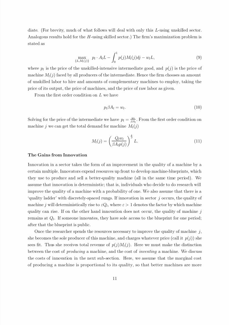
diate. (For brevity, much of what follows will deal with only this L-using unskilled sector.

Analogous results hold for the H -using skilled sector.) The firm’s maximization problem is

stated as

maxL,M l( j) pl · AlL −

10

p( j)M l( j)dj − wlL, (9)

where pl is the price of the unskilled-intensive intermediate good, and p( j) is the price of

machine M l( j) faced by all producers of the intermediate. Hence the firm chooses an amount

of unskilled labor to hire and amounts of complementary machines to employ, taking the

price of its output, the price of machines, and the price of raw labor as given.

From the first order condition on L we have

plβAl = wl. (10)

Solving for the price of the intermediate we have pl = wl

βAl. From the first order condition on

machine j we can get the total demand for machine M l( j)

M l( j) =

Qlwl

βAl p( j)

1β

L. (11)

The Gains from Innovation

Innovation in a sector takes the form of an improvement in the quality of a machine by a

certain multiple. Innovators expend resources up front to develop machine-blueprints, whichthey use to produce and sell a better-quality machine (all in the same time period). We

assume that innovation is deterministic; that is, individuals who decide to do research will

improve the quality of a machine with a probability of one. We also assume that there is a

‘quality ladder’ with discretely-spaced rungs. If innovation in sector j occurs, the quality of

machine j will deterministically rise to εQl, where ε > 1 denotes the factor by which machine

quality can rise. If on the other hand innovation does not occur, the quality of machine j

remains at Ql. If someone innovates, they have sole access to the blueprint for one period;

after that the blueprint is public.

Once the researcher spends the resources necessary to improve the quality of machine j,

she becomes the sole producer of this machine, and charges whatever price (call it p( j)) she

sees fit. Thus she receives total revenue of p( j)M l( j). Here we must make the distinction

between the cost of producing a machine, and the cost of inventing a machine. We discuss

the costs of innovation in the next sub-section. Here, we assume that the marginal cost

of producing a machine is proportional to its quality, so that better machines are more

11

7/29/2019 Luddites 12 June 2011


expensive to make—a form of diminishing returns. Indeed, we can normalize this cost, so

that total costs are simply QlM l( j).

Thus the producer of a new unskilled-using machine will wish to set the price p( j) in

order to maximize V l( j) = p( j)M l( j) − QlM l( j), where V l( j) is the value of owning the

rights to the new blueprints of machine j at that moment in time. The question for us iswhat this price will be. Note that it will not be possible for the owner to charge the full

monopoly markup over marginal cost unless the quality increase ε is very large. This is

because all machines in sector j are perfect substitutes (they are simply weighted by their

respective qualities); by charging a lower price, producers of older lower-quality machines

could compete with producers of newer higher-quality machines.

To solve the problem, we assume that producers of new machines engage in Bertrand

price competition, in the spirit of Grossman and Helpman (1991) and Barro and Sala-i-

Martin (2003). In this case the innovator and quality leader uses a limit-pricing strategy,

setting a price that is sufficiently below the monopoly price so as to make it just barely

unprofitable for the next best quality to be produced. This limit pricing strategy maximizes

V l and ensures that all older machine designs are eliminated from current production. The

Appendix describes how we solve for this price; our solution yields

p( j) = plimit = ε1

1−β Ql. (12)

Note that this price is higher than the marginal cost of producing new machines, and so

there is always a positive value of owning the blueprint to a new machine. Plugging this

price into machine demands and these machine demands into our expressions of V l and V h

gives us

V l =

ε1

1−β+( 1

β )( 1β−1) − ε( 1

β )( 1β−1)

Ql

wl

βAl

1β

L = ΨQl

wl

βAl

1β

L, (13)

V h =

ε1

1−β+( 1

β )( 1β−1) − ε( 1

β )( 1β−1)

Qh

wh

βAh

1β

H = ΨQh

wh

βAh

1β

H (14)

for unskilled-using and skilled-using machines, respectively. Notice that Ψ is simply a con-stant greater than zero.

The Costs of Innovation

Before an innovator can build a new machine, she must spend resources on R&D to first get

the blueprints. Let us denote these costs as cl (for a new unskilled-labor using machine).

12

7/29/2019 Luddites 12 June 2011


The resource costs of research will evolve due to changing economic circumstances. Specif-

ically, the “price” of a successful invention should depend on things like how complicated

the invention is and how “deep” general knowledge is. To capture some of these ideas, let us

assume that the resource costs of research to improve machine j in the unskilled-intensive

sector are given bycl = Qα

l B−φ, (15)

and that the resource costs of research to improve machine j in the skilled-intensive sector

are given by

ch = QαhB−φ. (16)

where φ > 0 and α > 1. α can be considered a “fishing-out” parameter—the greater is the

complexity of existing machines, the greater is the difficulty of improving upon them (see

Jones 1998 on the idea of fishing out). The variable B is our measure of current general

knowledge that we label Baconian knowledge . The general assumptions in each sector are

that research is more costly the higher is the quality of machine one aspires to invent (another

sort of diminishing returns), and the lower is the stock of general knowledge.

Growth of Baconian Knowledge

Baconian knowledge B thus influences the level of technology A. But what are the plausible

dynamics of B? We allow general knowledge to grow throughout human history, irrespective

of living standards and independent of the applied knowledge embedded in technology levels.

According to Mokyr (2005b, pp. 291–2), Bacon regarded “knowledge as subject to constant

growth, as an entity that continuously expands and adds to itself.” Accordingly, we assume

that the growth in basic knowledge depends on the existing stock. Furthermore, we assume

that Baconian knowledge grows according to how much skilled labor exists in the economy.4

Specifically, we assume the simple form:

Bt+1 = H t · Bt. (17)

Thus we assume that increases in general knowledge (unlike increases in applied knowledge)

do not arise from any profit motive, but are rather the fortuitous by-product of the existence

of a stock of skilled workers, as well as of accumulated stocks of Baconian knowledge. But

in our model, as we shall see, a skilled worker is just an educated worker, so it is here that

the link between productivity growth and human capital is made explicit.

We now have a mechanism by which growth in general knowledge (B) can influence the

4Galor and Mountford (2008) make a rather similar assumption.

13

7/29/2019 Luddites 12 June 2011


subsequent development of applied knowledge (Al and Ah). Our functional forms (15) and

(16) assume that low Baconian knowledge produces large costs to machine improvement,

while high Baconian knowledge generates lower costs. In our model, B never falls since (17)

ensures that changes in B are nonnegative. Hence, general knowledge always expands. This

is not a historically trivial assumption, although it is accurate for the episode under scrutiny:Mokyr (2005b, 338–9) comments on the fact that knowledge had been lost after previous

“efflorescences” (Goldstone 2002) in China and Classical Antiquity, and states that “The

central fact of modern economic growth is the ultimate irreversibility of the accumulation of

useful knowledge paired with ever-falling access costs.”

Modeling the Beginnings of Industrialization

Turning to the decision to innovate in the first place, we assume that any individual can spend

resources on research to develop and build machines with one quality-step improvement. Of course they will innovate only if it is profitable to do so. Specifically, if πi = V i − ci ≥ 0,

research activity for i-type machines occurs, otherwise it does not. That is,

Ql,t =

εQl,t−1 if Ψ

wl

βAl

1β

L ≥ Qαl B−φ,

Ql,t−1 otherwise,(18)

Qh,t =

εQh,t−1 if Ψ

wh

βAh

1β

H ≥ QαhB−φ,

Qh,t−1 otherwise.

(19)

As these expressions make clear, applied innovations will not be profitable until Baconian

knowledge reaches a certain critical threshold where benefits exceed costs. The natural world

needs to be sufficiently intelligible before society can begin to master it (Mokyr 2002). Thus

our model embodies the idea that growth in general Baconian knowledge is a necessary but

not sufficient condition for output growth.

Finally, which type of applied innovations happen first? It turns out that due to a “market

size” effect, the sector that innovates first will be the one using the abundant factor, since

it is there that there is the greatest potential demand for new machines. We can state this

result in the following proposition:

Proposition 1. If Ql = Qh and L > H , initial technological growth will be unskilled-labor

biased if and only if σ > 1.

Proof. Given Ql = Qh, the costs of innovation are the same for skilled and unskilled-labor-

using machines, and are falling at the same rate. Hence, to show that initial growth will be

14

7/29/2019 Luddites 12 June 2011


unskill-intensive, we must demonstrate that initial conditions are such that V l > V h.

First, note that we can plug the limit price from (12) into our machine demand equation

(11), and plug this expression into our technology coefficient expressions (7) and (8) to get

Al =

11 − β β

1β 1−β

Qβl w1−βl , (20)

Ah =

1

1 − β

β 1

β

1−β

Qβhw1−β

h . (21)

We plug these into the value expressions (13) and (14). After simplifying a bit, we get

V l = Ψ

1

Ql

1 − β

β

wlL, (22)

V h = Ψ

1

Qh

1 − β

β

whH. (23)

Computing the ratio of these last two expressions, we see that our condition for innovation

to occur first in the L sector is

V h < V l ⇐⇒V hV l

< 1 ⇐⇒V hV l

=whH

wlL< 1,

given the maintained assumption that Ql = Qh.

From this we can see that the relative gains for the innovator are larger when the factor

capable of using the innovation is large (the “market-size” effect) and when the price of the

factor is large (the “price” effect). To get everything in terms of relative factor supplies, we

can use (4), (20) and (21), to get a new expression for relative wages:

wh

wl

=

L

H

1σ

Ah

Al

σ−1σ

=

L

H

1(1−β)(1−σ)+σ

Qh

Ql

β(σ−1)(1−β)(1−σ)+σ

. (24)

Finally, by plugging this relative wage into the above inequality, and again using the fact

that Ql = Qh, and then simplifying, we have

V hV l

=whH

wlL=

L

H

(1−β)(σ−1)−σ+1(1−β)(1−σ)+σ

< 1.

Given that L/H > 1, this can only hold if the exponent is negative, which (since 0 < β < 1)

is true only when σ > 1.

15

7/29/2019 Luddites 12 June 2011


In other words, provided that labor types are grossly substitutable, the initial stages

of industrialization had to be unskilled-labor-intensive simply because there were so many

more unskilled laborers in the workforce than skilled laborers. So, to grossly simplify the

history of innovation, we maintain that for most of human existence the inequalities πl < 0

and πh < 0 held strictly. Once πl ≥ 0, industrialization could occur. Once both πl ≥ 0and πh ≥ 0, robust modern economic growth could occur. As we will suggest below, this

sequence was precisely how we believe history played out.

1.2 Endogenous Demography

With the dynamics of technology defined, we can now close the model by specifying the dy-

namics of endowments. Here we adopt a variant of a fairly standard overlapping generations

model of demography suited to unified growth theory (cf. Galor and Weil 2000).

In a very simplified specification, we assume that ‘adult’ agents maximize their utility,which depends both on their current household consumption and on their children’s expected

future income. In an abstraction of family life, we assume that individuals begin life naturally

as unskilled workers, accumulate human capital, and then employ that human capital as

adults. An agent begins life as an unskilled worker; as an adult she is both an unskilled

worker (supplying one unit of unskilled labor inelastically) and a skilled worker (supplying

whatever human capital she accumulated as a child). Thus her welfare will be affected by

both types of wages; and given these wages, her adult income will be higher, the higher is

her endowment of human capital.

Only ‘adults’ are allowed to make any decisions regarding demography. Specifically, the

representative household is run by an adult who decides two things: how many children to

have (denoted nt) and the level of education each child is to receive (denoted et). The number

of children must be nonnegative and to keep things simple all households are single-parent,

with n = 1 being the replacement level of fertility. The education level is constrained to the

unit interval, e ∈ [0, 1], and is the fraction of time the adult devotes to educating the young.

Our modeling of demography is as follows. An individual born at time t spends fraction

et of her time in school (chosen by her parent), while spending the rest of her time as an

unskilled laborer. At t + 1, the individual (who is by this time a mature adult) still works asan unskilled laborer but also uses whatever human capital she had accumulated as a child.

In passing, we should note that assuming instead that all adults are strictly skilled workers

does not alter any of the qualitative results.

16

7/29/2019 Luddites 12 June 2011


The Adult Household Planner

Allowing for the costs of child-rearing, we assume that the household consumes all the

income that the family members have generated. At time t there are popt adults, each of

whom is an individual household planner. These planners wish to maximize the sum of

current household consumption and the future skilled income generated by their children.

That is, the representative agent born at time t − 1, who is now an adult at time t, faces the

problem

max log (ct) + log (wh,tntht+1) , (25)

where ct is current consumption per household, nt is the fertility rate, and ht+1 is each child’s

level of education. We will use a very simple function for human capital:

ht = Ωekt−1 (26)

. where Ω > 0 and 0 < k < 1. (26) reflects a very simple education technology with

diminishing returns. Note that here we assume that agents base their expectations of future

wages wh,t+1 on current wages wh,t in myopic fashion.

We now must specify more precisely how household consumption, and the endowments

of unskilled and skilled labor, are functions of rates of fertility (nt) and education (et).

These variables are related to each other via the following budget constraints and assumed

production relations:

ct = wh,tht (1 − τ nt − x1ntet) + wl,t [1 + (1 − et) nt] − x2ntet (27)

Lt = nt (1 − et) popt + popt (28)

H t = Ωekt−1 (1 − τ nt − x1ntet) popt (29)

where 0 ≤ τ ≤ 1, 0 ≤ x1 ≤ 1, and x2 ≥ 0. The first term in (27) is the skilled income

generated by the parent (after subtracting the parent’s opportunity cost of child-rearing and

education). The second term in (27) is unskilled income (this is generated both by the adult

who provides one unit of unskilled labor inelastically, and by the children who spend 1 − e of

their childhood as unskilled workers). Thus we see that when children are not being educated

for a fraction of time 1 − e, they increase the family’s unskilled income, but this will reduce

their own future skilled income because they will receive a lower endowment of H .

The final term in (27) is the overall resource costs of the childen’s education. Note

that while having more children involves only an opportunity cost of time (since these costs

depend on the skilled wages of the parent), each unit of education per child involves both

17

7/29/2019 Luddites 12 June 2011


an opportunity cost (captured by x1) and a resource cost (of some amount x2). The first

of these effects is now totally standard. Having more children typically requires parents to

spend more time on child rearing, and having educated children requires more time still.

The second of these effects reflects the costs of educating the offspring to make them

more skilled. It is also increasing in the number of children. That property appears, forexample, in Galor and Mountford (2008), where, under a discrete choice, unskilled or skilled

offspring may be created at exogenously fixed time costs τ u and τ s, where the latter exceeds

the former (generating an exogenous, fixed skill premium on the supply side when both types

of offspring are present).

Our set up is slightly different in that we have both time and resource costs in education

per child. We treat both x1 and x2 as exogenous unit costs. In principle these might shift

in response to changes in school productivity, input costs, or public policies that subsidize

the cost of education. As long as the education cost contains some non-wage elements, and

is therefore not linear in wh, the general assumption that higher wages will lead to more

affordable education will be preserved.

Public education policies played an increasing role in Britain towards the end of the

nineteenth century, and that story and its political economy origins are discussed in Galor

and Moav (2006). Although we do not examine the effects of shifts in x2 in this paper, the

presence of this term generates sharp income effects which are important for our account

of the growth process, as for a given level of x2, growth implies increased affordability of

education. Allowing x2 to fall would a fortiori encourage a switch towards skill-biased

growth, further enhancing our story. For the purposes of being conservative, and since thiseffect has been explored elsewhere, we keep x2 constant.

The income-elasticity of education is a potentially important effect in this period, despite

its omission from prevailing theories. For example, as noted by Mitch (1982, 1992), influential

historians such as Roger Schofield (1973) and E. G. West (1975), who might not agree on

broader questions, thought rising incomes were important causally, allowing poorer families

(with no access to credit) to be able to afford human capital investments. In his own empirical

analysis, Mitch (1992, 84–86) finds mixed support for the hypothesis.5

5

Strong results on schooling (parental income elasticities near 1) emerge from raw data, but not forregressions that include “regional” dummies (e.g., village or county), suggesting that these effects are mostclearly visible across locales. In regressions of child literacy on income, regressions for specific towns (London,Macclesfield, Hanley) were unable to detect within-town variation (p. 86). But a national sample usingoccupational proxies for wages found an parental income elasticity of literacy of 0.72. This last result couldbe undermined by the inclusion of parental literacy, but the latter is of course highly collinear with income.Mitch also found that income elasticities were falling as incomes rose, suggesting the possibility of thresholdeffects. In accounts by contemporaries, poor parents themselves were found to cite poverty as the mainreason they did not send their kids to school, although their upper-class neighbors were apt to disagree. Forthe United States, Go (2008) finds a strong correlation between father’s wealth and school attendance by the

18

7/29/2019 Luddites 12 June 2011


Finally, on the equations defining factor endowments, (28) reflects the idea that both

children and adults work as unskilled laborers. (29) illustrates the usable human capital

in the economy. This is the total stock of human capital after reflecting the opportunity

cost for parents in child-rearing and educating their children. We note that, in this setup,

increases in fertility rates will immediately translate into increased levels of unskilled labor,while increases in education will eventually translate into increased levels of skilled labor next

period. Thus given our discussion above, wage changes will immediately change the overall

population level, and will eventually change the level of human capital in the economy.

Given (27), the individual born at t − 1 will choose a pair of nt, et that maximizes (25),

taking perceived wages as given. The first-order condition for the number of children is:

wl,t(1 − et) +ctnt

= wh,tht (τ + x1et) + x2et. (30)

The left-hand side illustrates the marginal benefit of an additional child, while the right-hand

side denotes the marginal cost. At the optimum, the gains from an extra unskilled worker in

the family and more skilled income for children in the future precisely offsets the opportunity

and resource costs resulting from additional child-rearing.

The first order condition for education is:

ctk

et= (wl,t + wh,thtx1 + x2) nt. (31)

Again the left-hand side is the marginal benefit and the right-hand side is the marginal cost,

this time of an extra unit of education per child. At the optimum, the gains received from

more skilled income by children offset the foregone unskilled-labor income and the extra

time and resource costs associated with an extra educational unit for all children at t.

2 A Tale of Two Revolutions

Sections 1.1 and 1.2 summarize the long-run co-evolution of factors and technologies in the

model. Once innovation occurs and levels of Ql and Qh are determined, the complete general

equilibrium can be characterized by simultaneously solving (2), (3), (20), (21), (28), (29),(30) and (31) for wages, productivity-levels, fertility, education, and factor supplies.

We are now ready to see how well our model can account for what happened in England

(and other northwestern European economies) in the eighteenth and nineteenth centuries.

child in 1850; this correlation disappears in later years after the introduction of free public schools. Go andLindert (2010) suggest that one of the main reasons why school enrollments in the U.S. North were higherthan those in the U.S. South was the fact that the northern schools had lower direct costs relative to income.

19

7/29/2019 Luddites 12 June 2011


2.1 The Industrial Revolution

An economy before its launch into the Industrial Revolution may be described by the features

discussed in section 1.1, only with technological coefficients Al and Ah constant. Here wages

are fixed, and thus the levels of raw labor and human capital remain fixed as well. Both

output and output per capita remain stagnant. Baconian knowledge B is low.6

If we assume that the evolution of technological coefficients Al and Ah are described

by the relationships in section 1.1, then the economy must wait until Baconian knowledge

grows to a sufficient level before applied innovation becomes possible. Further, technological

growth will initially be unskilled-labor biased (that is, there is growth in Al) so long as

it becomes profitable to improve machines used in the unskilled sector before it becomes

profitable to improve machines used in the skilled sector. Thus if the economy begins such

that Ql = Qh (as we maintain in the simulations that follow), initial technological growth

will be unskilled labor biased so long as there is relatively more unskilled labor than skilledlabor in the economy (by Proposition 1), as was surely the case in the eighteenth century.

Next, the onset of technological developments changes the wage structure, and by impli-

cation the evolution of factor endowments. The growth of Al lowers the skill premium, as

can be seen in our expression (4), increasing the future ratio of unskilled wages to skilled

wages. As wl rises faster than wh, the marginal gains of having more children (the left hand

side of equation 30) rise faster than the marginal costs (the right hand side of 30); households

respond by raising fertility.

This story of unbalanced growth in early industrialization seems consistent with history.

Well-known studies such as Atack (1987) and Sokoloff (1984) describe the transition of the

American economy from reliance on highly-skilled artisans to the widespread mechanization

of factories. This paper further argues that the boom in fertility that the industrializing areas

experienced was both the cause and consequence of these technological revolutions arising,

in the British case, in the late 1700s and early 1800s. According to Folbre (1994), the

development of industry in the late eighteenth and early nineteenth centuries led to changes

in family and household strategies. The early pattern of rural and urban industrialization

in this period meant that children could be employed in factories at quite a young age.

The implication is that children became an asset, whose labor could be used by parents to6Although not Malthusian in nature, the initial static phase in our model is broadly consistent with

Malthusian dynamics in the following way. If we consider the pre-Industrial world, one where L is much largerthan H , and maintain the assumption that these factors are grossly substitutable, then any technologicalchange that could have a meaningful influence on average incomes would necessarily be unskilled-laborbiased. As the model demonstrates, this will induce a rise in fertility and influence education only modestly.Thus, our model is entirely consistent with the pre-Industrial correlation between brief and temporary burstsof technologically-induced income gains and increases in population.

20

7/29/2019 Luddites 12 June 2011


contribute income to the household. In English textile factories in 1835, for example, 63%

of the work force consisted of children aged 8–12 and women (Nardinelli 1990). This is not

to say that attitudes toward children were vastly different in England then compared with

now; rather economic incentives were vastly different then compared with now (Horrell and

Humphries 1995). As a result of these conditions, fertility rates increased during the periodof early industrialization.

While our approach may help explain the population growth that coincided with the

initial stages of the Industrial Revolution,7 we are still faced with the challenge of explaining

the demographic transition that followed it.

2.2 The Demographic Transition

Figure 2 documented rising education and falling fertility rates in four advanced countries—

but only late in the 19th century—a shift which was replicated in many rich countries at thetime. Part of our argument is that biases inherent in technological innovation fostered this

reversal. As Baconian knowledge rose further and skill-biased production grew in importance,

the labor of children became less important as a source of family income, and this was

reflected in economic behavior. It is true that legislation limited the employment possibilities

for children (Folbre 1994), and introduced compulsory education. However,the underlying

economic incentives were leading in the same direction.

The incentives for households to reverse fertility trends and dramatically expand edu-

cation came about through changes in wages. As evident from (30) and (31), households

will want to invest in greater education and limit fertility not only when skilled wages rise

relative to unskilled wages (since educated children provide a greater relative return than

unskilled children), but also when overall wages rise (since the resource costs of education

grow less onerous with wage growth).

Modest wage growth and falling relative returns to skilled labor, characteristic of early

industrialization, allows fertility to rise while keeping education growth modest. But once

overall wages have risen sufficiently, the benefits of education begin to dramatically outweigh

the costs, and the transition in household demand from child quantity to child quality is truly

launched.87Of course there are a host of other explanations, including falling death rates related to health improve-

ments, and the passage of various Poor Laws. Naturally we are abstracting from these possibilities withoutdismissing them as inconsequential.

8Recent studies make a variety of related points which can also explain the demographic transition.Hazan and Berdugo (2002) suggest that technological change at this stage of development increased the wagedifferential between parental labor and child labor, inducing parents to reduce the number of their childrenand to further invest in their quality, stimulating human capital formation, a demographic transition, anda shift to a state of sustained economic growth. In contrast, Doepke (2004) stresses the regulation of child

21

7/29/2019 Luddites 12 June 2011


2.3 Simulations

How well does the model track these general historical trends? To answer this we numerically

simulate the model.

For each time period, we solve the model as follows:

1) Baconian knowledge grows according to (17).

2) Based on this new level of Baconian knowledge, if πl > 0, Ql rises by a factor of ε; if

not Ql remains the same. Similarly, if πh > 0, Qh rises by a factor of ε; if not Qh remains

the same.9

3) Given levels of Ql and Qh, we solve the equilibrium. This entails solving the system

of equations (2), (3), (20), (21), (28), (29), (30) and (31) for wl, wh, Al, Ah, n, e, L, and H .

In our baseline case, parameters are set equal to the following: σ = 2, β = 0.66, α =

1.5, ε = 1.05, φ = 2, Ω = 3, k = 0.75, τ = 0.5, x1 = 0.01, x2 = 0.01. Many other

parameterizations will produce qualitatively similar results, and we shall explore this in somesensitivity analysis that follows; for now we focus on our baseline simulation. The critical

assumptions here are that σ > 1 (the skilled- and unskilled-labor-intensive intermediates

have enough substitutability to satisfy Proposition 1),10 0 < k < 1 (diminishing marginal

returns to education), and x2 > 0 (positive resource cost to raising educated children).11

For our initial equilibrium, we set n1 = 1.04 (to capture the positive population growth

rate experienced in Britain in the mid-18th century, before the onset of the Industrial Rev-

olution), and pop1 = 1.12 We then solve the 9 × 9 system of (2), (3), (20), (21), (28), (29),

(30), (31), and an expression for Ql = Qh for initial values of wl, wh, Al, Ah, L, H , e, Ql, and

Qh.13 Given Ql = Qh and ensuring that wh/wl > 1, it must be that L > H . By Proposition

labor. Alternatively, the rise in the importance of human capital in the production process may have inducedindustrialists to support laws that abolished child labor, inducing a reduction in child labor and stimulatinghuman capital formation and a demographic transition (Doepke and Zilibotti 2003; Galor and Moav 2006;Galor 2011b).

9We can relax this assumption to allow for multiple-step quality improvements each period. Simulationresults (not shown) display the same patterns for fertility, education, and relative wages as our main results.

10The degree of substitutability between skilled and unskilled labor has been much explored by laboreconomists. Studies of contemporary labor markets in the U.S. (Katz and Murphy 1992, Peri 2004), Canada(Murphy et al. 1998), Britain (Schmitt 1995), Sweden (Edin and Holmlund 1995), and the Netherlands(Teulings 1992) suggest aggregate elasticities of substitution in the range of one to three. See Katz and

Autor (1999) for a detailed review of this literature.11Other parameters simply scale variables (such as Ω) or affect the speed of growth (such as α, ε and φ).Changing the values of these parameters however would not shift the direction of technology, nor would itaffect the responsiveness of households. Thus these specific values are not crucial for the qualitative resultsand our underlying story.

12Each period in our model is equivalent to roughly five years, so this is equivalent to assuming thatinitially population grows by 4 per cent in 5 years.

13This produces initial values of wl = 0.0014, wh = 0.0046, Al = 0.001, Ah = 0.0015, L = 1.85, H = 0.29,e = 0.15, Ql = Qh = 0.02.

22

7/29/2019 Luddites 12 June 2011


1, this implies that the first stage of the Industrial Revolution must be unskilled in nature .

To see this we turn to modeling the economy as it evolves in time.

We simulate our hypothetical northwestern European economy through 25 time periods,

roughly accounting for the time period 1750–1910. The results are given in Figures 3–8,

using the parameterizations summarized above.14

Figure 3 illustrates the market for innovation. Initial Baconian knowledge B is set low

enough that the costs of innovation are larger than the benefits in the beginning. As a result

technology levels remain stagnant at first. But through Baconian knowledge growth costs

fall, first catching up with the benefits of research for technologies designed for unskilled

labor; hence, at t = 4, we see that Ql begins to grow (that is, πl becomes positive). By

contrast, πh < 0 early on, so Qh remains fixed. Note that this results solely because L is

larger than H through Proposition 1. In other words, endowments dictate that the Industrial

Revolution will initially be unskilled-biased. As Ql rises the costs of subsequent unskilled

innovation rise because it gets increasingly more expensive to develop new technologies the

further up the quality ladder we go (due to the “fishing-out” effect from the α term); however,

the benefits of research rise even faster due to both rising unskilled wages and unskilled labor

supplies (see equation 22). And further growth in Baconian knowledge keeps research costs

from rising too fast (see equation 15). As a result unskilled-intensive growth persists.

Skill-biased technologies, on the other hand, remain stagnant during this time. Their

eventual growth is however inevitable; Baconian knowledge growth drives down the costs to

develop them, and rising skilled wages (due to the growth of unskilled technologies) drives

up the value of developing them, as seen in equation (3). By t = 10, πh becomes positive aswell, allowing Qh to climb. At this point growth occurs in both sectors, with advance in all

periods given by the constant step size on the innovation ladders. Note that this induces an

endogenous demographic transition; population growth rates begin to fall, while education

rates rise, as we can see in Figures 4 and 5.

Figures 4 through 8 depict historical and simulated time series for population growth

rates, education rates, wages, skill premia and income per capita. The skill premia data

are taken from Clark (2007), but we readily admit that it is difficult, if not impossible,

to identify data which can unambiguously track “the skill premium” during this period.

Clark’s data track the relative earnings of skilled and unskilled workers over time, but one

can argue that what really mattered during this period was the obsolescence of old skills,

and the emergence of new skills paying new premia.15 As can be seen, our model reproduces

the early rise in population growth rates, followed by falling population growth and rising

14The initial level of B is chosen such that growth starts after a few periods.15See Mokyr and Voth (2010) for a recent criticism of Clark’s skill premium data.

23

7/29/2019 Luddites 12 June 2011


Figure 3: Incentives for Innovation in Each SectorThe figure shows the value of innovating and the cost of innovating in each period for each sectorin our simulated model. The economy is initially endowed with much more unskilled labor L thanskilled labor H . Hence, unskilled-intensive technologies are the first to experience directedtechnological change.

0

0.5

1

1.5

2

2.5

2 7 12 17 22

period

(a) L intensive sector

value of innovation

cost of innovation

0

0.2

0.4

0.6

0.8

1

1.2

1.4

1.6

1.8

2

2 7 12 17 22

period

(b) H intensive sector

value of innovation

cost of innovation

24

7/29/2019 Luddites 12 June 2011


Figure 4: Population Growth Rates: Data versus ModelThe figure shows the population growth rates in the English data and in the simulated model.

0

1

2

3

4

5

6

7

8

9

10

1750 1800 1850 1900

(b) Population growth rate (%): data, 5 year moving average

period

-2

0

2

4

6

8

10

12

2 7 12 17 22

period

(b) Population growth rate (%): model

Source : The data are for England (excluding Monmouthshire) until 1801, and England and Walesthereafter, and are taken from Mitchell (1988).

25

7/29/2019 Luddites 12 June 2011


Figure 5: Education: Data versus ModelThe figure shows the education levels in the English data and in the simulated model.

(a) Education: data (% of 5–14 year olds in school)

0

10

20

30

40

50

60

70

80

90

100

1750 1800 1850 1900

period

0

0.05

0.1

0.15

0.2

0.25

0.3

0.35

0.4

0.45

2 7 12 17 22

period

(b) Education: model

Source : The data are 10-year moving averages from Flora et al. (1983).

26

7/29/2019 Luddites 12 June 2011


Figure 6: Wages: Data versus ModelThe figure shows wage levels in the English data and in the simulated model.

0

200

400

600

800

1000

1200

1400

1600

1750 1800 1850 1900

period

(a) Real wages: data (index)

0

0.001

0.002

0.003

0.004

0.005

0.006

0.007

0.008

2 7 12 17 22

period

(b) Real wages: model (skilled and unskilled)

Skilled

Unskilled

Source : The data are 10-year moving averages from Wrigley and Schofield (1981).

27

7/29/2019 Luddites 12 June 2011


Figure 7: Skill Premium: Data versus Model

The figure shows wage levels in the English data and in the simulated model.

1.3!

1.4!

1.5!

1.6!

1.7!

1750! 1800! 1850! 1900!

(a) Skilled/unskilled wage: data

period

1

1.5

2

2.5

3

3.5

2 7 12 17 22

period

(b) Skilled/unskilled wage: model

Source : The data are from Clark (2007).

28

7/29/2019 Luddites 12 June 2011


Figure 8: GDP per Person: Data versus ModelThe figure shows GDP per person in the U.K. data and in the simulated model.

(a) GDP per person: data

0

1000

2000

3000

4000

5000

6000

1750 1770 1790 1810 1830 1850 1870 1890 1910

period

0

0.001

0.002

0.003

0.004

0.005

0.006

0.007

0.008

2 7 12 17 22

period

(b) GDP per person: model

Source : The data are from Broadberry and van Leeuwen (2008) and Maddison (2003).

29

7/29/2019 Luddites 12 June 2011


education. Education rates rise very modestly during the early stages of the Industrial

Revolution, and accelerate only after growth occurs in both sectors. To understand the

fertility and education patterns depicted in Figures 4 and 5, one must observe the absolute

and relative wage patterns depicted in Figures 6 and 7. The early stages of industrialization

are associated with very limited wage growth and a modestly declining skill premium. Thismakes sense: what growth in applied knowledge does occur is confined to the unskilled sector.

The evolution of wages that this produces then has implications for education and

fertility—while the modestly falling skill premium puts some downward pressure on edu-

cation (education limits the children’s ability to earn unskilled income), rising wages overall

put upward pressure on education (since education becomes more affordable).

These countervailing forces keep growth in education during this period modest. Fertility

however is free to rise: since slow-rising education keeps the resource costs of each child low,

parents can take advantage of rising unskilled wages by having more children. Of course

this produces more L and keeps H fairly low. Thus the model can replicate the rapid

fertility growth and low education growth observed during the early stages of the Industrial

Revolution.

Once skill-biased technologies grow as well, the patterns of development change dramat-

ically. Growth in both Al and Ah allows both wl and wh to rise more rapidly, even as the

skill premium starts to fall rapidly. Education rates rise faster as education becomes more

affordable. More affordable education, together with a rising opportunity cost of having

children, incites adults to lower their fertility. There is thus an endogenous switch from child

quantity to child quality consistent with history (Galor 2011b). The demographic transitionof the mid to late 19th century is launched.

Figures 3 through 8 thus depict an integrated story of western European development

fairly consistent with the historical record. The theory of endogenous technical change can

indeed motivate a unified growth theory. Increases in income induce increases in education,

which then through the quality-quantity tradeoff eventually induce a fall in fertility. And

increases in H/L put downward pressure on the premium through supply-side forces. Thus,

as implied by (24), continued supply increases can keep pace with demand-side forces (Goldin

and Katz 2008): a modern economy can have both high relative skilled labor supplies and a

low skill premium even in the context of directed endogenous technological change.

Our simulations show skill-biased technology starting to be used, and rising in impor-

tance, quite early on, even at the time of the fertility peak. This is not the same thing as

saying that skill biased sectors became dominant at that point, in absolute, macro terms

(although they did later on). This is the standard argument that nascent sectors start from

a very low base (which was famously the case of cotton textiles, for example, during the

30

7/29/2019 Luddites 12 June 2011


First Industrial Revolution). They only win out in the longer run. The fact that our model

incorporates both types of technological change simultaneously (rather than, say, switching

in a discontinuous manner from one type of innovation to another) is, we believe, a positive

feature of the paper in that it corresponds better with historical reality.

Finally, Figure 8 shows the evolution of output per person in the data and the model. Inboth theory and reality, the population growth spurred by initial technological growth kept

per capita income growth very modest—making the ‘Industrial Revolution’ appear to be a

fairly un -revolutionary event. But later on, with technological advance occurring in more

sectors, incomes rose faster; this in turn provoked fertility decreases and made per capita

growth faster still, heralding a more marked trend breakout into “modern economic growth.”

3 Robustness checks

One might wonder if our results are sensitive to our assumed time and resource costs of

child-rearing. That is, what if x1 and/or x2 had different values? Here we demonstrate that

the patterns of industrialization implied by our model are robust to different child-rearing

costs.

Figure 9 illustrates the results of our simulation when we increase resource costs to rearing

educated children by a factor of five. All other parameters are the same as in the baseline

case, and again we set n1 = 1.04 and pop1 = 1. What we discover is that the patterns

for fertility, education, and absolute and relative wages are exactly the same. However, the

timing of both industrialization and the demographic transition have been pushed back.The reason for this is that changes in x2 simply induce scale changes in certain variables.

Specifically, imposing initial fertility at 1.04 implies an initial equilibrium with the same

education rates, but with higher resource costs families must start with higher wages to

afford this education. The result is a wealthier economy, with higher wages and productivity

levels. Higher productivity levels push up initial costs of research, which ultimately delays

development. Note however that changes in resource costs to child rearing affect only the

timing of industrialization, not its nature.

Figure 10 displays the evolution of the economy with time costs to education increased

by a factor of five (specifically, x2 is set back to its original value). Again, patterns of

fertility, education and wages echo those in the baseline case. Notice however that here the

demographic transition is more dramatic. The reason is that a higher opportunity cost of

educating children makes having children a more expensive proposition. Thus increases in

education are matched by even lower rates of fertility.

Finally, Figure 11 displays the case where both x1 and x2 are raised by a factor of five.

31

7/29/2019 Luddites 12 June 2011


Figure 9: Robustness Check 1

The figure shows the model simulation when x1 = 0.01 and x2 = 0.05.

0

0.5

1

1.5

2

2.5

3

2 7 12 17 22

period


value of innovation

cost of innovation

0

0.5

1

1.5

2

2.5

2 7 12 17 22

period


value of innovation

cost of innovation

0

2

4

6

8

10

12

2 7 12 17 22

period

(c) Population growth rate (%): model

0

0.05

0.1

0.15

0.2

0.25

0.3

2 7 12 17 22

period

(d) Education: model

0

0.005

0.01

0.015

0.02

0.025

2 7 12 17 22

period

(e) GDP per person: model

1

1.5

2

2.5

3

3.5

2 7 12 17 22

period

(f) Skilled/unskilled wage: model

32

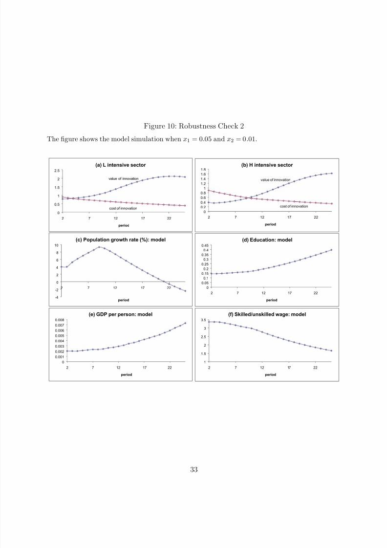
7/29/2019 Luddites 12 June 2011




0

0.5

1

1.5

2

2.5

2 7 12 17 22

period


value of innovation

cost of innovation

0

0.2

0.4

0.6

0.8

1

1.2

1.4

1.6

1.8

2 7 12 17 22

period


value of innovation

cost of innovation

-4

-2

0

2

4

6

8

10

2 7 12 17 22

period


0

0.05

0.1

0.15

0.2

0.25

0.3

0.35

0.4

0.45

2 7 12 17 22

period


0

0.001

0.002

0.003

0.004

0.005

0.006

0.007

0.008

2 7 12 17 22

period


1

1.5

2

2.5

3

3.5

2 7 12 17 22

period


33

7/29/2019 Luddites 12 June 2011




0

0.5

1

1.5

2

2.5

3

2 7 12 17 22

period


value of innovation

cost of innovation

0

0.5

1

1.5

2

2.5

2 7 12 17 22

period


value of innovation

cost of innovation

0

1

2

3

4

5

6

7

8

9

10

2 7 12 17 22

period


0

0.05

0.1

0.15

0.2

0.25

0.3

2 7 12 17 22

period


0

0.005

0.01

0.015

0.02

0.025

2 7 12 17 22

period


1

1.5

2

2.5

3

3.5

2 7 12 17 22

period


34

7/29/2019 Luddites 12 June 2011


Again, a consistent pattern of development emerges. In general, adjusting other parameters

similarly affects either the speed or the timing of growth, but not the general patterns. The

bottom line is that our model is able to capture the key features of industrialization given

the reasonable assumptions of gross substitutability in labor-types and some resource costs

for education.

4 Conclusion

We believe that by explicitly modeling research and development, thus endogenizing the

direction of technical change, we have been able to shed some valuable light on the transition

to modern economic growth. Like most unified growth models, our model is subject to the

criticism that it makes a take-off “inevitable,” a proposition to which many historians, more

comfortable with notions of chance and contingency, might object. Our model makes anotherclaim, however, which seems much more robust: if a take-off took place, it most likely should

have first involved unskilled-labor-using technologies, for the simple reason that unskilled

labor was the abundant factor of production at this time. Eventually, however, continuing

growth in Baconian knowledge led to the growth of the science-based, skill-intensive sectors

of the Second Industrial Revolution. While this could have caused skill premia to start rising,

massive endogenous increases in education kept the relative wages of skilled labor in check,

and actually led them to fall, at an accelerating rate. Furthermore, in addition to these forces

which are endogenous to our model, there were other factors at work keeping skill premia

down. For example, Galor and Moav (2006) highlight the fact that governments embarkedon a large-scale programme of public education, raising skill endowments and lowering skill

premia. Furthermore, public primary education programmes were later followed by two

world wars, rising union strength, and public secondary and tertiary education programmes,

all of which served to further reduce skill premia—in the U.S. case at least through the

“Great Compression” of the 1940s (Goldin and Margo 1992; Goldin and Katz 2008).

It seems possible that these factors leading to greater equality were actually endogenously

influenced by growth, even though powerful endogenous technological factors were pushing

economies towards greater inequality. This is striking, since as Acemoglu (1998) points out,

in the context of a model like this one, long run exogenous increases in skill endowments

lead to more rapid skill-biased technical change, thus increasing the upward pressure on

skill premia in the long run. What is remarkable, therefore, is that western labor markets

remained on an egalitarian path until well into the twentieth century. In this context, current

inegalitarian trends in the U.S. and elsewhere can be seen as late nineteenth century chickens

finally coming home to roost.

35

7/29/2019 Luddites 12 June 2011


References

Acemoglu, Daron. 1998. Why Do New Technologies Complement Skills? Directed Technical

Change and Wage Inequality. Quarterly Journal of Economics 113 (November): 1055–89.

Acemoglu, Daron. 2007. Equilibrium Bias of Technology. Econometrica 175 (September): 1371–

1410.

Aghion, Philippe, and Peter Howitt. 1992. A Model of Growth through Creative Destruction.

Econometrica 60 (March): 323–51.

Allen, Robert C. 2006. The British Industrial Revolution in Global Perspective: How Commerce

Created the Industrial Revolution and Modern Economic growth. Unpublished, Nuffield Col-

lege, Oxford.

Andorka, Rudolph. 1978. Determinants of Fertility in Advanced Societies. New York: The Free

Press.

Atack, Jeremy. 1987. Economies of Scale and Efficiency Gains in the Rise of the Factory in

America, 1820–1900. In Quantity and Quiddity: Essays in U.S. Economic History edited by P.

Kilby. Middletown, Conn.: Wesleyan University Press, pp. 286–335.

Barro, Robert J., and Xavier Sala-i-Martin. 2003. Economic Growth, 2nd Edition . Cambridge,

Mass.: MIT Press.

Becker, Gary S., and H. Gregg Lewis. 1973. On the Interaction between the Quantity and Quality

of Children. The Journal of Political Economy 81: S279–S288.

Becker, Gary S., and Nigel Tomes. 1976. Child Endowments and the Quantity and Quality of

Children. Journal of Political Economy 84 (August): S143–S162.

Broadberry, Stephen N., and Bas van Leeuwen. 2008. British Economic Growth and the Business

Cycle, 1700–1850: Annual Estimates. University of Warwick (March). Photocopy.

Ciccone, Antonio, and Giovanni Peri. 2005. Long-Run Substitutability Between More and Less

Educated Workers: Evidence from U.S. States, 1950-1990. The Review of Economics and

Statistics , 87(4): 652–663.

Clark, Gregory. 1987. Why Isn’t the Whole World Developed? Lessons from the Cotton Mills.

Journal of Economic History 47 (March): 141–173.

Clark, Gregory. 2007. A Farewell to Alms: A Brief Economic History of the World. Princeton,

N.J.: Princeton University Press.

Doepke, Matthias. 2004. Accounting for Fertility Decline during the Transition to Growth. Journal

of Economic Growth 9 (September): 347–83.

Doepke, Matthias, and Fabrizio Zilibotti. 2003. Voting with your Children: A Positive Analysis of

Child Labour Laws. CEPR Discussion Papers no. 3733.

Edin, Per Anders, and Bertil Holmlund. 1995. The Swedish Wage Structure: The Rise and Fall of

Solidarity Wage Policy?, in R. Freeman and L. Katz, eds., Differences and Changes in Wage

Structures . Chicago: University of Chicago Press and NBER.

36

7/29/2019 Luddites 12 June 2011


Folbre, Nancy. 1994. Who Pays for the Kids: Gender and the Structure of Constraint . New York:

Routledge.

Galor, Oded. 2005. From Stagnation to Growth: Unified Growth Theory. In Handbook of Economic

Growth , volume 1, part 1, edited by P. Aghion and S. N. Durlauf, pp. 171–293. Amsterdam:

North Holland.Galor, Oded. 2011a. Unified Growth Theory . Princeton & Oxford: Princeton University Press.

Galor, Oded. 2011b. The Demographic Transition: Causes and Consequences. NBER working

paper 17057, National Bureau of Economic Research, Cambridge, MA.

Galor, Oded, and Omer Moav. 2002. Natural Selection and the Origin of Economic Growth.

Quarterly Journal of Economics 117 (November): 1133–92.

Galor, Oded, and Omer Moav. 2006. Das Human-Kapital: A Theory of the Demise of the Class

Structure. Review of Economic Studies 73 (January): 85–117.

Galor, Oded, and Andrew Mountford. 2008. Trading Population for Productivity. Review of

Economic Studies 75: 1143–1179.

Galor, Oded, and David Weil. 2000. Population, Technology and Growth: From Malthusian Stag-

nation to the Demographic Transition and Beyond. American Economic Review 90 (Septem-

ber): 806–28.

Go, Sun. 2008. Schools in America, 1850–1870: Who Voted for Them, Who Got Them, and Who

Paid. UC Davis, photocopy.

Go, Sun, and Peter Lindert. 2010. “The Uneven Rise of American Public Schools to 1850.” The

Journal of Economic History 70: 1–26.

Goldin, Claudia D., and Lawrence F. Katz. 2008. The Race Between Education and Technology .

Cambridge, Mass.: Belknap Press.

Goldin, Claudia D., and Robert A. Margo 1992. The Great Compression: The Wage Structure in

the United States at Mid-century. Quarterly Journal of Economics 107 (February): 1–34.

Goldstone, Jack. 2002. Efflorescence and Economic Growth in World History: Rethinking the

“Rise of the West” and the Industrial Revolution. Journal of World History 13 (Fall): 323–89.

Grossman, Gene M., and Elhanan Helpman. 1991. Innovation and Growth in the Global Economy ,

Cambridge, Mass.: MIT Press.

Hansen, Gary D., and Edward C. Prescott. 2002. Malthus to Solow. American Economic Review

92 (September): 1205–17.

Hazan, Moshe, and Berdugo, Binyamin. 2002. Child Labour, Fertility, and Economic Growth.

Economic Journal 112: 810–828.

Hobsbawm, E. J. 1952. The Machine Breakers. Past and Present 1 (February): 57–70.

Horrell, Sara, and Jane Humphries. 1995. “The Exploitation of Little Children”: Child Labor

and the Family Economy in the Industrial Revolution. Explorations in Economic History 32

(October): 485–516.

Jones, Charles I. 1998. Introduction to Economic Growth . New York: W.W. Norton & Company.

37

7/29/2019 Luddites 12 June 2011


Jones, Charles I. 2001. Was the Industrial Revolution Inevitable? Economic Growth over the Very

Long Run. Advances in Macroeconomics 1(2): 1028–28.

Katz, Lawrence F., and David H. Autor. 1999. Changes in the Wage Structure and Earnings

Inequality. In Handbook of Labor Economics , volume 3A, edited by O. Ashenfelter and D.

Card. Amsterdam: North Holland.Katz, Lawrence F., and Kevin M. Murphy. 1992. Changes in Relative Wages, 1963–87: Supply

and Demand Factors. Quarterly Journal of Economics 107:35–78.

Kremer, Michael. 1993. Population Growth and Technological Change: One Million B.C. to 1990.

Quarterly Journal of Economics 108 (August): 681–716.

Kuczynski, Robert R. 1969. The Measurement of Population Growth . Revised edition. New York:

Gordon and Breach Science Publishers, Inc.

Lucas, Robert E. 2002. The Industrial Revolution: Past and Future. In Lectures on Economic

Growth . Cambridge, Mass.: Harvard University Press.

Maddison, Angus. 1995.Monitoring the World Economy 1820–1992

. Paris: OECD.Maddison, Angus. 2001. The World Economy: A Millennial Perspective . Paris: OECD.

Mitch, David. 1982. The Spread of Literacy in Nineteenth-Century England. Ph.D. dissertation,

University of Chicago.

Mitch, David. 1992. The Rise of Popular Literacy in Victorian England: The Influence of Private

Choice and Public Policy. Philadelphia, Penn.: University of Pennsylvania Press.

Mitch, David. 1999. The Role of Education and Skill in the First Industrial Revolution. In The

British Industrial Revolution: An Economic Perspective edited by Joel Mokyr. 2nd edition.

Boulder, Colo.: Westview Press, pp. 241–79.

Mitchell, B.R. 1988. British Historical Statistics . Cambridge: Cambridge University Press.

Mokyr, Joel. 1999. The British Industrial Revolution: An Economic Perspective. 2nd edition.

Boulder, Colo.: Westview Press.

Mokyr, Joel. 2002. The Gifts of Athena . Princeton, N.J.: Princeton University Press.

Mokyr, Joel. 2005a. Long-Term Economic Growth and the History of Technology. In Philippe

Aghion and Steven Durlauf (eds.), Handbook of Economic Growth , volume 1, pp. 1113–80.

Amsterdam: Elsevier.

Mokyr, Joel. 2005b., The Intellectual Origins of Modern Economic Growth. Journal of Economic

History 65 (June): 285–351.

Mokyr, Joel and Hans-Joachim Voth. 2010. Understanding Growth in Europe, 1700-1870: Theory

and Evidence. In The Cambridge Economic History of Modern Europe , volume 1, pp. 7-42.

Cambridge: Cambridge University Press.

Murphy, Kevin M., W. Craig Riddell, and Paul M. Romer. 1998. Wages, Skills and Technology in

the United States and Canada. In General Purpose Technologies and Economic Growth edited

by E. Helpman. Cambridge, Mass.: MIT Press.

Nardinelli, Clark. 1990. Child Labor and the Industrial Revolution , Bloomington, Ind.: Indiana

38

7/29/2019 Luddites 12 June 2011


University Press.

North, Douglass, and Barry Weingast. 1989. Constitutions and Commitment: Evolution of Institu-

tions Governing Public Choice in Seventeenth Century England. Journal of Economic History

49 (December): 803–32.

Romer, Paul. 1990. Endogenous Technological Change. Journal of Political Economy 98 (October):S71–S102.

Schmitt, John. 1995. The Changing Structure of Male Earnings in Britain, 1974–1988. In Differ-

ences and Changes in Wage Structures edited by R. Freeman and L. Katz. Chicago: University

of Chicago Press and NBER.

Schofield, Roger S. 1968. The Measurement of Literacy in Pre-Industrial England. In Literacy in

Traditional Societies edited by J. Goody. Cambridge: Cambridge University Press.

Schofield, Roger S. 1973. Dimensions of Illiteracy, 1750–1850. Explorations in Economic History

10: 437–54.

Schumpeter, Joseph A. 1934.The Theory of Economic Development

. Cambridge, Mass.: HarvardUniversity Press.

Sokoloff, Kenneth L. 1984. Was the Transition from the Artisan Shop to the Non-Mechanized

Factory Associated with Gains in Efficiency? Evidence from U.S. Manufacturing Censuses of

1820 and 1850. Explorations in Economic History 21 (October): 351–82.

Tan, Jee-Peng, and Michael Haines. 1984. Schooling and Demand for Children: Historical Per-

spectives. World Bank Staff Working Paper no. 695.

Teulings, Coen. 1992. The Wage Distribution in a Model of Matching between Skills and Jobs.

unpublished paper, University of Amsterdam.

van Zanden, Jan Luiten. 2009. The Skill Premium and the “Great Divergence.” European Review

of Economic History 13 (April): 121–153.

Voth, Hans-Joachim. 2003. Living Standards During the Industrial Revolution: An Economist’s

Guide. American Economic Review 93 (May): 221–26.

Weisdorf, Jacob. 2004. From Stagnation to Growth: Revisiting Three Historical Regimes. Journal

of Population Economics 17 (August): 445–74.

West, E. G. 1975. Education and the Industrial Revolution. London: Batsford.

Williamson, Jeffrey G. 1982. “The Structure of Pay in Britain, 1710–1911.” Research in Economic

History 7: 1–54.

Williamson, Samuel H. 2004. An Index of the Wage of Unskilled Labor from 1774 to the Present.

Economic History Services, December. http://eh.net.

Wrigley, E. A., and R. S. Schofield. 1981. The Population History of England 1541–1871. Cam-

bridge: Cambridge University Press.

39

7/29/2019 Luddites 12 June 2011


Appendix: Limit Pricing and the Gains from Innovation

Here we solve for the price new innovators would charge for newly invented machines in the face of

competition from producers of older machines. First, let us describe the producers of the unskilled-

intensive good, AlL; analogous results will hold for the skill-intensive good. The production function

for these goods are 1

1 − β

QlL

β

10

M l( j)1−βdj.

Producers wish to maximize profits or, equivalently, to minimize unit costs. The unit costs for

producers who buy new machines, denoted as uc, can be written as

uc = β −β (1 − β )β

1

εQl

wβl

10

p( j)1−βdj,

where p( j) is the price of machine j and wl is the wage of L.

The question for us is, what maximum price could an innovator charge and drive out thecompetition at the same time? The “competition” in this case are those who hold the blueprints of

the next highest-quality machines of quality Ql. The lowest price they can charge is their marginal

cost, Ql; if all old machine-producers charge this, unit costs can be written as

ucold = β −β (1 − β )β

1

Ql

wβl Q

1−βl .

Traditional endogenous growth theories that use quality ladders typically have producers of

new machines charge a monopolistic mark-up over marginal cost. In our case producers of new

machines would charge a price pmonop =εQl

(1−β) for a machine of quality εQl. However, in order forthis to be a profitable strategy, unit costs for producers of AlL must be at least as low when they

buy new machines compared with when they buy the older, cheaper machines. In other words,

ucold ≥ ucmonop, which requires that

β −β (1 − β )β

1

Ql

wβl Q

1−βl ≥ β −β (1 − β )β

1

εQl

wβl

εQl

(1 − β )

1−β

.

This simplifies to the condition ε ≥ (1 − β )β−1β . Thus, in order for monopoly pricing to prevail,

quality improvements must be large enough for goods-producers to be willing to pay the higher

price. If this condition does not hold, the monopoly-priced machine will be too expensive, and

producers will opt for the older machines.

However, producers of newer machines can charge a price lower than this and still turn a profit.

How low would they have to go to secure the market? They certainly could go no lower than εQl,

which is their own marginal cost of machine production. Fortunately they would not have to go

that low; they could charge a price plimit low enough such that ucold ≥ uclimit (see Barro and

Sala-i-Martin 2003 and Grossman and Helpman 1991 for similar limit-pricing treatments). That

40

7/29/2019 Luddites 12 June 2011


is, producers of new machines could undercut their competition so that goods-producers would

prefer the higher-quality machines to the older lower-quality machines. And to maximize prices,

new machines producers would charge a price such that this held with equality:

β

−β

(1 − β )

β 1

Ql

w

β

l Q

1−β

l = β

−β

(1 − β )

β 1

εQl

w

β

l p

1−β

limit.

Solving for this limit price gives us

plimit = ε1

1−β Ql > εQl.

Thus, producers will always opt for newer machines, no matter the size of quality steps. So

our approach would be valid for any values of ε > 1 and 0 < β < 1. Given our paramerization

described in section 2.3, we assume this limit pricing strategy is used.

luddites 12 june 2011

Documents