low-noise, low-sensitivity active-rc allpole filters using ...cdn.intechweb.org/pdfs/18564.pdf ·...

10

Low-Noise, Low-Sensitivity Active-RC Allpole Filters Using MATLAB Optimization

Dražen Jurišić University of Zagreb, Faculty of Electrical Engineering and Computing, Zagreb,

Croatia

1. Introduction

The application of Matlab, combining its symbolic and numeric calculation capabilities, to

calculate noise and sensitivity properties of allpole active-RC filters is shown. Transfer

function coefficients calculations, as well as plotting of amplitude-frequency and phase-

frequency characteristics (Bode plots) have been performed using Matlab. Thus, using

Matlab a comparison of different design strategies of active-RC filters is done. It is shown

that active-RC filters can be designed to have low sensitivity to passive components and at

the same time possess low output thermal noise. The classical methods were used to

determine output noise of the filters. It was found that low-sensitivity filters with minimum

noise have reduced resistance levels, low Q-factors, low-noise operational amplifiers

(opamps) and use impedance tapering design. The design procedure of low-noise and low-

sensitivity, positive- and negative-feedback, second- and third-order low-pass (LP), high-

pass (HP) and band-pass (BP) allpole filters, using impedance tapering, is presented. The

optimum designs, regarding both performances of most useful filter sections are

summarized (as a cookbook programmed in Matlab) and demonstrated on examples. The

relationship between the low sensitivity and low output noise, that are the most important

performance of active-RC filters, is investigated, and optimum designs that reduce both

performances are presented.

A considerable improvement in sensitivity of single-amplifier active-RC allpole filters to

passive circuit components is achieved using the design technique called 'impedance

tapering' (Moschytz, 1999), and as shown in (Jurisic et al., 2010a) at the same time they will

have low output thermal noise. The improvement in noise and sensitivity comes free of

charge, in that it requires simply the selection of appropriate component values. Preliminary

results of the investigation of the relation between low sensitivity and low thermal noise

performances using impedance tapering on the numeric basis using Matlab have been

presented in (Jurisic & Moschytz, 2000; Jurisic, 2002).

For LP filters of second- and third-order the complete analytical proofs for noise properties of the desensitized filters are given in (Jurisic et al., 2010a). By means of classical methods as in (Jurisic et al., 2010a) closed-form expressions are derived in (Jurisic et al., 2010c), providing insight into noise characteristics of the LP, HP and BP active-RC filters using different designs. LP, HP and BP, low-sensitivity and low-noise filter sections using positive and negative feedback, that have been considered in (Jurisic et al., 2010c) are presented here. These filters are

www.intechopen.com

Applications of MATLAB in Science and Engineering

198

of low power because they use only one opamp per circuit. The design of optimal second- and third-order sections referred to as 'Biquads' and 'Bitriplets', regarding low passive and active sensitivities has been summarized in the table form as a cookbook in (Jurisic et al., 2010b). For common filter types, such as Butterworth and Chebyshev, design tables with normalized component values for designing single-amplifier LP filters up to the sixth-order with low passive sensitivity to component tolerances have been presented in (Jurisic et al., 2008). The filter sections considered in (Jurisic et al., 2010c) and repeated here have been recommended in (Moschytz & Horn, 1981; Jurisic et al., 2010b) as high-quality filter sections. It was shown in (Jurisic & Moschytz, 2000; Jurisic, 2002; Jurisic et al., 2008, 2010a, 2010b, 2010c), that both noise and sensitivity are directly proportional to the pole Q’s and, therefore, to the pass band ripple specified by the filter requirements. The smaller the required ripple, the lower the pole Q’s. Besides, it is wise to keep the filter order n as low as the specifications will permit, because the lower the filter order, the lower the pole Q’s. Also, it was shown that positive-feedback filter blocks are useful for the realization of the LP and HP filters (belonging to class 4, according to the classification in (Moschytz & Horn, 1981), the representatives are SAK: Sallen and Key filters). Filters with negative feedback (class 3 SAB: Single-amplifier Biquad) are better for the BP filters, where the BP-C Biquad is preferable because it has lower noise than BP-R. A summary of figures and equations that investigate sensitivity and noise performance of active RC filters, and have been calculated in (Jurisic & Moschytz, 2000; Jurisic, 2002; Jurisic et al., 2008, 2010a, 2010b, 2010c), by Matlab, will be presented here. Numeric and symbolic routines that were used in those calculations are shown here in details. In Section 2 a brief review of noise and sensitivity is given and the most important equations

are defined. These equations will be used by Matlab in Section 3 to analyze a second-order

LP filter as representative example. In Section 4 the results of analysis using Matlab of the

LP, HP and BP sections of second- and third-order filters are summarized. Those results

were obtained with the same Matlab algorithms as in Section 3 for the second-order LP

filter, and are presented in the form of optimum-design procedures. The chapter ends with

the conclusion in Section 5.

2. A brief review of noise and sensitivity of active-RC filters

2.1 Output noise and dynamic range Thermal (or Johnson) noise is a result of random fluctuations of voltages or currents that

seriously limit the processing of signals by analog circuits. Because this noise is caused by

random motion of free charges and is proportional to temperature, it is referred to as

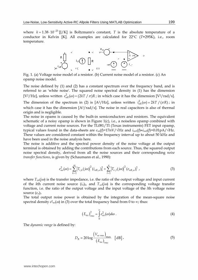
thermal noise (Jurisic et al., 2010a). The most important sources of noise in active-RC filters are resistors and opamps. For the purpose of noise analysis, appropriate noise models for resistors and opamps must be used. Resistors are represented by the well-known Nyquist voltage or current noise models shown in Figure 1(a) and (b), consisting of noiseless resistors and noise sources whose values are

defined by the squared noise voltage density within the narrow frequency band f, i.e.,

2 ( ) 4nRe f kTR , (1)

or the squared noise current density given by

2 ( ) 4 /nRi f kT R , (2)

www.intechopen.com


199

where 231.38 10k [J/K] is Boltzmann's constant, T is the absolute temperature of a

conductor in Kelvin [K]. All examples are calculated for 22C (T=295K), i.e., room temperature.

Fig. 1. (a) Voltage noise model of a resistor. (b) Current noise model of a resistor. (c) An opamp noise model.

The noise defined by (1) and (2) has a constant spectrum over the frequency band, and is referred to as 'white noise'. The squared noise spectral density in (1) has the dimension

[V2/Hz], unless written 2 ( ) (2 / )nRe kT R ; in which case it has the dimension [V2/rad/s].

The dimension of the spectrum in (2) is [A2/Hz], unless written 2 ( ) 2 /( )nRi kT R ; in

which case it has the dimension [A2/rad/s]. The noise in real capacitors is also of thermal origin and is negligible. The noise in opams is caused by the built-in semiconductors and resistors. The equivalent schematic of a noisy opamp is shown in Figure 1(c), i.e., a noiseless opamp combined with voltage and current noise sources. For the TL081/TI (Texas instruments) FET input opamp, typical values found in the data-sheets are ena(f)=17nV/Hz and ina1(f)ina2(f)=0.01pA/Hz. These values are considered constant within the frequency interval up to about 50 kHz and have been used in the noise analysis here. The noise is additive and the spectral power density of the noise voltage at the output terminal is obtained by adding the contributions from each source. Thus, the squared output noise spectral density, derived from all the noise sources and their corresponding noise transfer functions, is given by (Schaumann et al., 1990):

2 22 2 2

, , , ,1 1

( ) ( ) ( ) ( ) ( )m n

no i k nR a k l nR a lk l

e T j i T j e

, (3)

where Ti,k(j) is the transfer impedance, i.e. the ratio of the output voltage and input current of the kth current noise source (in)k, and T,l(j) is the corresponding voltage transfer function, i.e. the ratio of the output voltage and the input voltage of the lth voltage noise source (en)l. The total output noise power is obtained by the integration of the mean-square noise spectral density e2no() in (3) over the total frequency band from 0 to ∞; thus:

2 2

0

( )no normsE e d . (4)

The dynamic range is defined by:

max20log dBso rms

Rno rms

VD

E , (5)

www.intechopen.com


200

where max

so rmsV represents the maximum undistorted rms voltage at the output, and the

denominator is the noise floor defined by the square root of (4). max

so rmsV is determined by

the opamp slew rate, power supply voltage, and the corresponding THD factor of the filter. In our examples we use a 10Vpp signal which yields

max

so rmsV =5/2 [V]. (6)

2.2 Sensitivity to passive component variations Sensitivity analysis provides information on network changes caused by small deviations of passive component values. Given the network function F(s, x1,, xN), where s is a complex variable and xk (k=1 ,, N) are real parameters of the filter, the relative deviation of F, F/F, due to the relative deviations xk/xk (k=1 ,, N) is given to the first approximation by:

k

F kx

k

xFS

F x

, (7)

where k

FxS represents the relative sensitivity of the function F to variations of a single

parameter (component) xk, namely:

k

F kx

k

x dFS

F dx . (8)

If several components deviate from the nominal value, a criterion for assessing the deviation of the function F due to the change of several parameters must be used. With xk/xk considered to be an independent random variable with zero mean and identical standard deviation x, the squared standard deviation 2F of the relative change F/F is given by:

2

( )2 2

1k

NF j

F x xk

S

. (9)

F is therefore dependent on the component sensitivities k

FxS , but also on the number of

passive components N. The more components the circuit has, the larger the sensitivity. Equation (9) defines multi-parametric measure of sensitivity (Schoeffler, 1964; Laker & Gaussi, 1975; Schaumann et al., 1990). In the following Section, all Matlab calculations regarding noise and sensitivity performance will be demonstrated on the second-order LP filter circuit with positive feedback (class-4 or Sallen and Key). All Matlab commands and variables will appear in the text using Courier New font.

3. Application to second-order LP filter

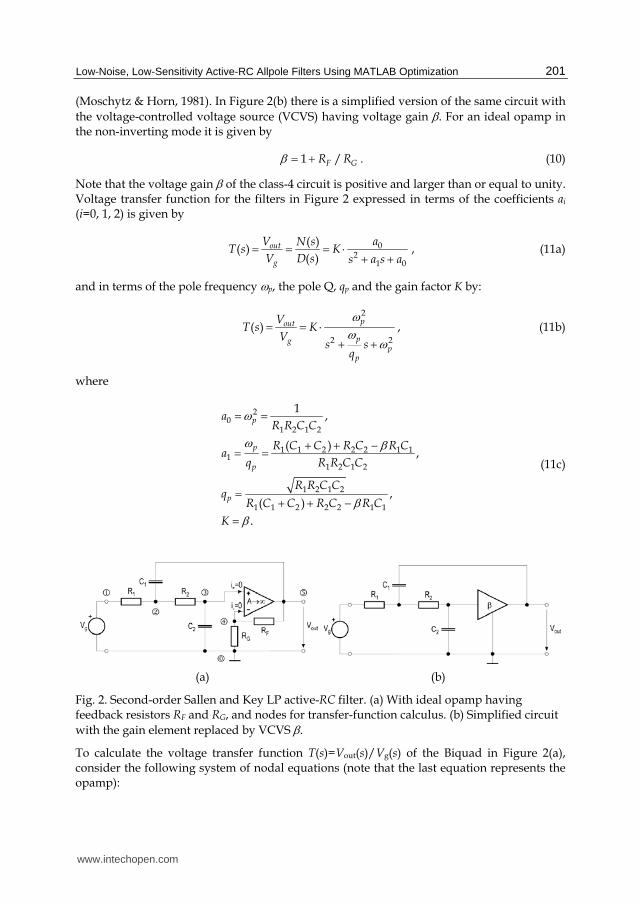
3.1 Calculating transfer function coefficients and parameters using 'symbolic toolbox' in Matlab Consider the second-order low-pass active-RC allpole filter circuit (Biquad) shown in Figure 2(a). This circuit belongs to the positive feedback or class-4 (Sallen and Key) filters

www.intechopen.com


201

(Moschytz & Horn, 1981). In Figure 2(b) there is a simplified version of the same circuit with

the voltage-controlled voltage source (VCVS) having voltage gain . For an ideal opamp in the non-inverting mode it is given by

1 /F GR R . (10)

Note that the voltage gain of the class-4 circuit is positive and larger than or equal to unity. Voltage transfer function for the filters in Figure 2 expressed in terms of the coefficients ai (i=0, 1, 2) is given by

02

1 0

( )( )

( )out

g

V aN sT s K

V D s s a s a , (11a)

and in terms of the pole frequency p, the pole Q, qp and the gain factor K by:

2

2 2

( )pout

pgp

p

VT s K

Vs s

q

, (11b)

where

20

1 2 1 2

1 1 2 2 2 1 11

1 2 1 2

1 2 1 2

1 1 2 2 2 1 1

1,

( ),

,( )

.

p

p

p

p

aR R C C

R C C R C R Ca

q R R C C

R R C Cq

R C C R C R C

K

(11c)

(a) (b)

Fig. 2. Second-order Sallen and Key LP active-RC filter. (a) With ideal opamp having feedback resistors RF and RG, and nodes for transfer-function calculus. (b) Simplified circuit

with the gain element replaced by VCVS .

To calculate the voltage transfer function T(s)=Vout(s)/Vg(s) of the Biquad in Figure 2(a), consider the following system of nodal equations (note that the last equation represents the opamp):

www.intechopen.com


202

1

1 2 1 3 5 11 1 2 2

2 3 22 2

3 5

3 5 5

(1)

1 1 1 1(2) 0

1 1(3) 0

1 1 1(4) 0

(5) ( ) , , 0, 0.

g

F G F

out

V V

V V sC V V sCR R R R

V V sCR R

V VR R R

A V V V V A i i

(12)

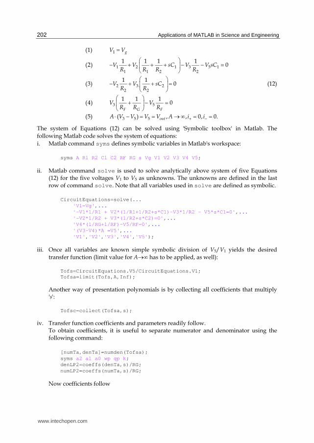
The system of Equations (12) can be solved using 'Symbolic toolbox' in Matlab. The

following Matlab code solves the system of equations:

i. Matlab command syms defines symbolic variables in Matlab's workspace:

syms A R1 R2 C1 C2 RF RG s Vg V1 V2 V3 V4 V5;

ii. Matlab command solve is used to solve analytically above system of five Equations (12) for the five voltages V1 to V5 as unknowns. The unknowns are defined in the last row of command solve . Note that all variables used in solve are defined as symbolic.

CircuitEquations=solve( ... 'V1=Vg' , ... '-V1*1/R1 + V2*(1/R1+1/R2+s*C1)-V3*1/R2 - V5*s*C1=0' , ... '-V2*1/R2 + V3*(1/R2+s*C2)=0' , ... 'V4*(1/RG+1/RF)-V5/RF=0' , ... '(V3-V4)*A =V5' , ... 'V1' , 'V2' , 'V3' , 'V4' , 'V5' );

iii. Once all variables are known simple symbolic division of V5/V1 yields the desired

transfer function (limit value for A∞ has to be applied, as well):

Tofs=CircuitEquations.V5/CircuitEquations.V1; Tofsa=limit(Tofs,A,Inf);

Another way of presentation polynomials is by collecting all coefficients that multiply 's':

Tofsc=collect(Tofsa,s);

iv. Transfer function coefficients and parameters readily follow. To obtain coefficients, it is useful to separate numerator and denominator using the

following command:

[numTa,denTa]=numden(Tofsa); syms a2 a1 a0 wp qp k; denLP2=coeffs(denTa,s)/RG; numLP2=coeffs(numTa,s)/RG;

Now coefficients follow

www.intechopen.com


203

a0=denLP2(1)/denLP2(3); a1=denLP2(2)/denLP2(3); a2=denLP2(3)/denLP2(3);

And parameters

k=numLP2; wp=sqrt(a0); qp=wp/a1;

Typing command whos we obtain the following answer about variables in Matlab workspace:

>> whos Name Size Bytes Class A 1x1 126 sym object C1 1x1 128 sym object C2 1x1 128 sym object CircuitEquations 1x1 2828 struct array Tofs 1x1 496 sym object Tofsa 1x1 252 sym object Tofsc 1x1 248 sym object R1 1x1 128 sym object R2 1x1 128 sym object RF 1x1 128 sym object RG 1x1 128 sym object V1 1x1 128 sym object V2 1x1 128 sym object V3 1x1 128 sym object V4 1x1 128 sym object V5 1x1 128 sym object Vg 1x1 128 sym object a0 1x1 150 sym object a1 1x1 210 sym object a2 1x1 126 sym object denTa 1x1 232 sym object denLP2 1x3 330 sym object k 1x1 144 sym object numTa 1x1 134 sym object numLP2 1x1 144 sym object qp 1x1 254 sym object s 1x1 126 sym object wp 1x1 166 sym object Grand total is 1436 elements using 7502 bytes

It can be seen that all variables that are defined and calculated so far are of symbolic type. We can now check the values of the variables. For example we are interested in voltage transfer function Tofsa . Matlab gives the following answer, when we invoke the variable:

>> Tofsa Tofsa = (RF+RG)/(s*C2*R2*RG+R2*s^2*C1*R1*C2*RG-s*C1*R1*RF+RG+R1*s*C2*RG)

www.intechopen.com


204

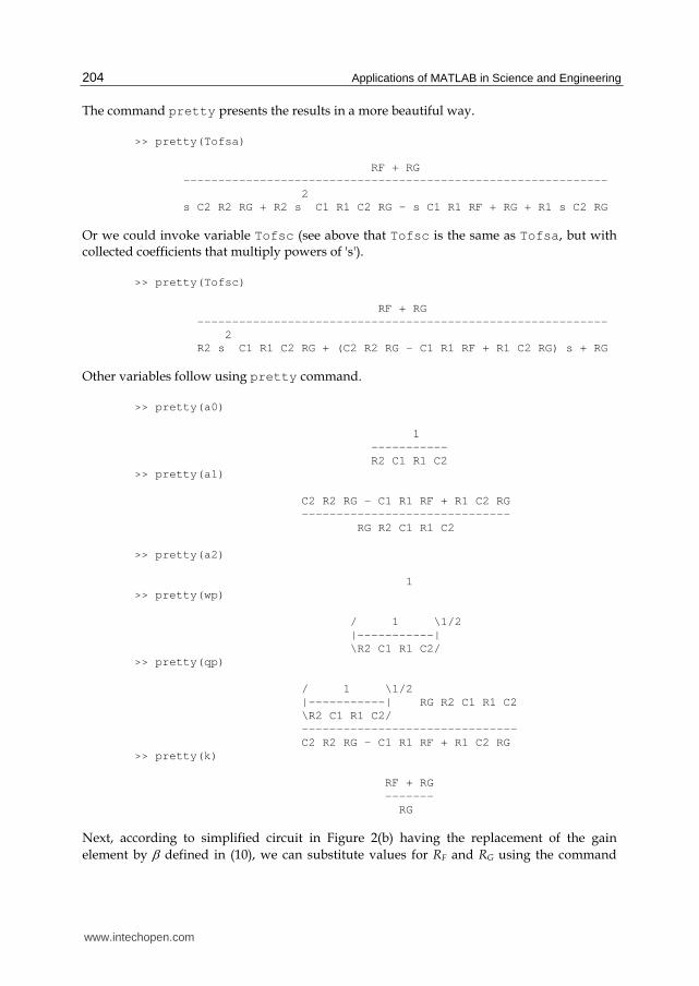
The command pretty presents the results in a more beautiful way.

>> pretty(Tofsa) RF + RG ------------------------------------------------------------- 2 s C2 R2 RG + R2 s C1 R1 C2 RG - s C1 R1 RF + RG + R1 s C2 RG

Or we could invoke variable Tofsc (see above that Tofsc is the same as Tofsa , but with collected coefficients that multiply powers of 's').

>> pretty(Tofsc) RF + RG ----------------------------------------------------------- 2 R2 s C1 R1 C2 RG + (C2 R2 RG - C1 R1 RF + R1 C2 RG) s + RG

Other variables follow using pretty command.

>> pretty(a0) 1 ----------- R2 C1 R1 C2 >> pretty(a1) C2 R2 RG - C1 R1 RF + R1 C2 RG ------------------------------ RG R2 C1 R1 C2 >> pretty(a2) 1 >> pretty(wp) / 1 \1/2 |-----------| \R2 C1 R1 C2/ >> pretty(qp) / 1 \1/2 |-----------| RG R2 C1 R1 C2 \R2 C1 R1 C2/ ------------------------------- C2 R2 RG - C1 R1 RF + R1 C2 RG >> pretty(k) RF + RG ------- RG

Next, according to simplified circuit in Figure 2(b) having the replacement of the gain

element by defined in (10), we can substitute values for RF and RG using the command

www.intechopen.com


205

subs and obtain simpler results [in the following example we perform substitution RF

RG(–1)]. New symbolic variable is beta

>> syms beta >> a1=subs(a1,RF,'(beta-1)*RG'); >> pretty(a1) C2 R2 RG - C1 R1 (beta - 1) RG + R1 C2 RG ----------------------------------------- RG R2 C1 R1 C2

Note that we have obtained RG both in the numerator and denominator, and it can be abbreviated. To simplify equations it is possible to use several Matlab commands for simplifications. For example, to rewrite the coefficient a1 in several other forms, we can use commands for simplification, such as:

>> pretty(simple(a1)) 1 beta 1 1 ----- - ----- + ----- + ----- C1 R1 R2 C2 R2 C2 R2 C1 >> pretty(simplify(a1)) -C2 R2 + C1 R1 beta - C1 R1 - R1 C2 - ----------------------------------- R2 C1 R1 C2

The final form of the coefficient a1 is the simplest one, and is the same as in (11c) above. Using the same Matlab procedures as presented above, we have calculated all coefficients and parameters of the different filters' transfer functions in this Chapter. If we want to calculate the numerical values of coefficients ai (i=0, 1, 2) when component

values are given, we simply use subs command. First we define the (e.g. normalized) numerical values of components in the Matlab’s workspace, and then we invoke subs :

>> R1=1;R2=1;C1=0.5;C2=2; >> a0val=subs(a0) a0val = 1 >> whos a0 a0val Name Size Bytes Class a0 1x1 150 sym object a0val 1x1 8 double array Grand total is 15 elements using 158 bytes

Note that the new variable a0val is of the double type and has numerical value equal to 1, whereas the symbolic variable a0 did not change its type. Numerical variables are of type double .

www.intechopen.com


206

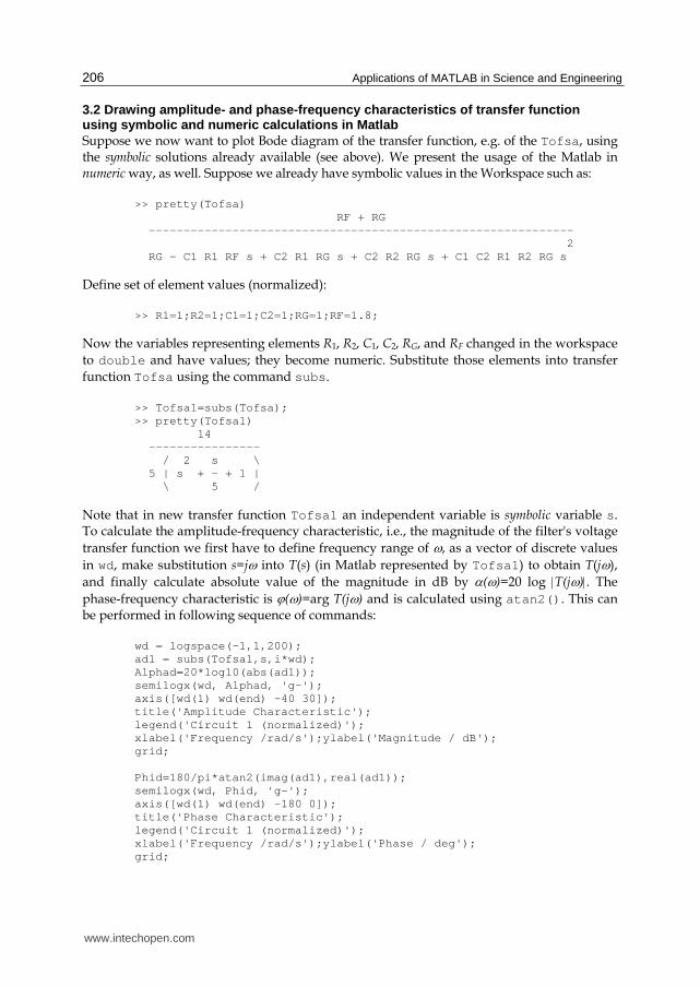
3.2 Drawing amplitude- and phase-frequency characteristics of transfer function using symbolic and numeric calculations in Matlab Suppose we now want to plot Bode diagram of the transfer function, e.g. of the Tofsa , using the symbolic solutions already available (see above). We present the usage of the Matlab in numeric way, as well. Suppose we already have symbolic values in the Workspace such as:

>> pretty(Tofsa) RF + RG ------------------------------------------------------------- 2 RG - C1 R1 RF s + C2 R1 RG s + C2 R2 RG s + C1 C2 R1 R2 RG s

Define set of element values (normalized):

>> R1=1;R2=1;C1=1;C2=1;RG=1;RF=1.8;

Now the variables representing elements R1, R2, C1, C2, RG, and RF changed in the workspace

to double and have values; they become numeric. Substitute those elements into transfer

function Tofsa using the command subs .

>> Tofsa1=subs(Tofsa); >> pretty(Tofsa1) 14 ---------------- / 2 s \ 5 | s + - + 1 | \ 5 /

Note that in new transfer function Tofsa1 an independent variable is symbolic variable s . To calculate the amplitude-frequency characteristic, i.e., the magnitude of the filter's voltage

transfer function we first have to define frequency range of , as a vector of discrete values

in wd, make substitution s=j into T(s) (in Matlab represented by Tofsa1 ) to obtain T(j),

and finally calculate absolute value of the magnitude in dB by ()=20 log T(j). The

phase-frequency characteristic is ()=arg T(j) and is calculated using atan2() . This can be performed in following sequence of commands:

wd = logspace(-1,1,200); ad1 = subs(Tofsa1,s,i*wd); Alphad=20*log10(abs(ad1)); semilogx(wd, Alphad, 'g-'); axis([wd(1) wd(end) -40 30]); title('Amplitude Characteristic'); legend('Circuit 1 (normalized)'); xlabel('Frequency /rad/s');ylabel('Magnitude / dB'); grid; Phid=180/pi*atan2(imag(ad1),real(ad1)); semilogx(wd, Phid, 'g-'); axis([wd(1) wd(end) -180 0]); title('Phase Characteristic'); legend('Circuit 1 (normalized)'); xlabel('Frequency /rad/s');ylabel('Phase / deg'); grid;

www.intechopen.com


207

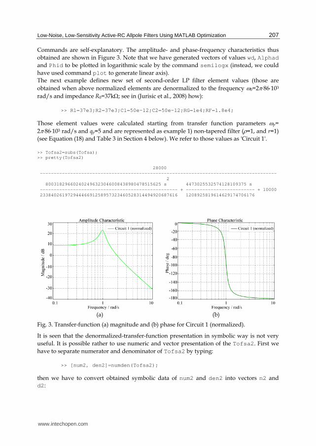
Commands are self-explanatory. The amplitude- and phase-frequency characteristics thus

obtained are shown in Figure 3. Note that we have generated vectors of values wd, Alphad

and Phid to be plotted in logarithmic scale by the command semilogx (instead, we could

have used command plot to generate linear axis).

The next example defines new set of second-order LP filter element values (those are

obtained when above normalized elements are denormalized to the frequency 0=286103

rad/s and impedance R0=37k; see in (Jurisic et al., 2008) how):

>> R1=37e3;R2=37e3;C1=50e-12;C2=50e-12;RG=1e4;RF=1.8e4;

Those element values were calculated starting from transfer function parameters p=

286103 rad/s and qp=5 and are represented as example 1) non-tapered filter (=1, and r=1)

(see Equation (18) and Table 3 in Section 4 below). We refer to those values as 'Circuit 1'.

>> Tofsa2=subs(Tofsa); >> pretty(Tofsa2) 28000 -------------------------------------------------------------------------------------- 2 800318296602402496323046008438980478515625 s 4473025532574128109375 s -------------------------------------------------- + ------------------------- + 10000 23384026197294446691258957323460528314494920687616 1208925819614629174706176

(a) (b)

Fig. 3. Transfer-function (a) magnitude and (b) phase for Circuit 1 (normalized).

It is seen that the denormalized-transfer-function presentation in symbolic way is not very

useful. It is possible rather to use numeric and vector presentation of the Tofsa2 . First we

have to separate numerator and denominator of Tofsa2 by typing:

>> [num2, den2]=numden(Tofsa2);

then we have to convert obtained symbolic data of num2 and den2 into vectors n2 and d2 :

www.intechopen.com


208

>> n2=sym2poly(num2) n2 = 6.5475e+053 >> d2=sym2poly(den2) d2 = 1.0e+053 * 0.0000 0.0000 2.3384

and finally use command tf to write transfer function which uses vectors with numeric values:

>> tf(n2,d2) Transfer function: 6.548e053 --------------------------------------- 8.003e041 s^2 + 8.652e046 s + 2.338e053

If we divide numerator and denominator by the coefficient of s2 in the denominator, i.e., d2(1) , we have a more appropriate form:

>> tf(n2/d2(1),d2/d2(1)) Transfer function: 8.181e011 ----------------------------- s^2 + 1.081e005 s + 2.922e011

Obviously, the use of Matlab (numeric) vectors provides a more compact and useful representation of the denormalized transfer function. Finally, note that when several (N) filter sections are connected in a cascade, the overall transfer function of that cascade can be very simply calculated by symbolic multiplication of sections' transfer functions Ti(s) (i=1, , N), i.e. T=T1* *TN, if Ti(s) are defined in a symbolic way. On the other hand, if numerator and denominator polynomials of Ti(s) are defined numerically (i.e. in a vector form), a more complicated procedure of multiplying vectors using (convolution) command conv should be used.

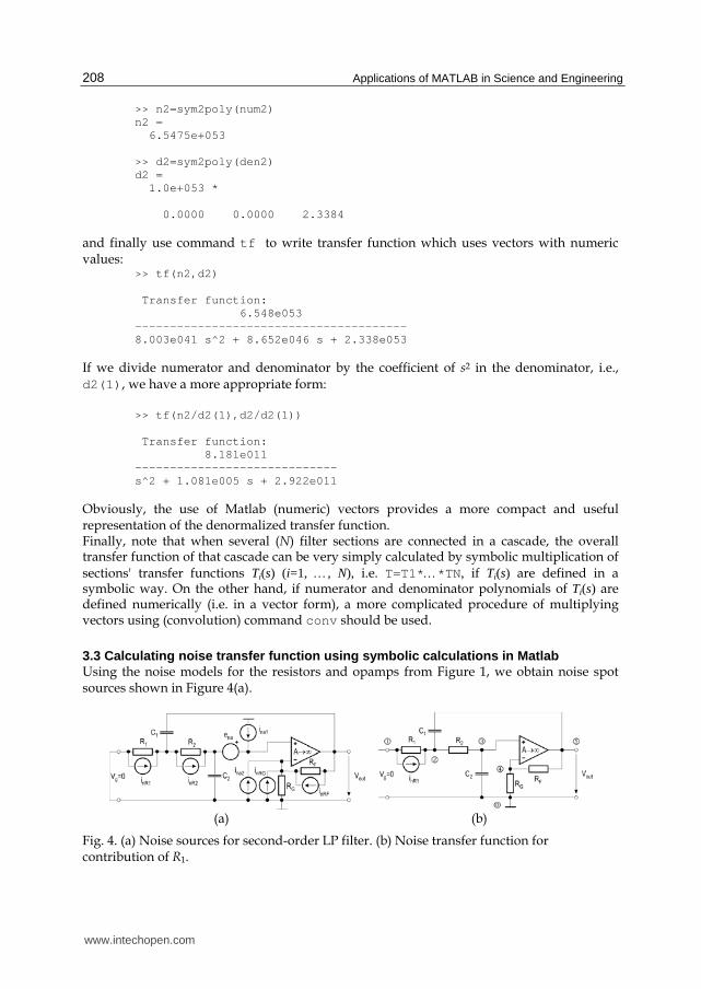
3.3 Calculating noise transfer function using symbolic calculations in Matlab Using the noise models for the resistors and opamps from Figure 1, we obtain noise spot sources shown in Figure 4(a).

(a) (b)

Fig. 4. (a) Noise sources for second-order LP filter. (b) Noise transfer function for contribution of R1.

www.intechopen.com


209

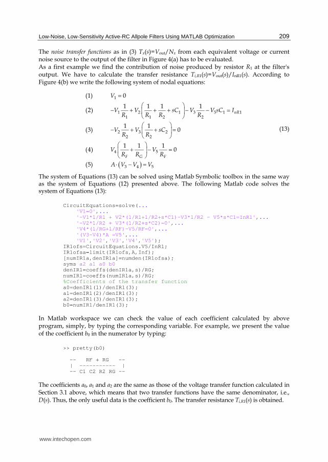
The noise transfer functions as in (3) Tx(s)=Vout/Nx from each equivalent voltage or current noise source to the output of the filter in Figure 4(a) has to be evaluated. As a first example we find the contribution of noise produced by resistor R1 at the filter's output. We have to calculate the transfer resistance Ti,R1(s)=Vout(s)/InR1(s). According to Figure 4(b) we write the following system of nodal equations:

1

1 2 1 3 5 1 11 1 2 2

2 3 22 2

4 5

3 4 5

(1) 0

1 1 1 1(2)

1 1(3) 0

1 1 1(4) 0

(5)

nR

F G F

V

V V sC V V sC IR R R R

V V sCR R

V VR R R

A V V V

(13)

The system of Equations (13) can be solved using Matlab Symbolic toolbox in the same way as the system of Equations (12) presented above. The following Matlab code solves the system of Equations (13):

CircuitEquations=solve( ... 'V1=0' , ... '-V1*1/R1 + V2*(1/R1+1/R2+s*C1)-V3*1/R2 - V5*s*C1=InR1' , ... '-V2*1/R2 + V3*(1/R2+s*C2)=0' , ... 'V4*(1/RG+1/RF)-V5/RF=0' , ... '(V3-V4)*A =V5' , ... 'V1' , 'V2' , 'V3' , 'V4' , 'V5' ); IR1ofs=CircuitEquations.V5/InR1; IR1ofsa=limit(IR1ofs,A,Inf); [numIR1a,denIR1a]=numden(IR1ofsa); syms a2 a1 a0 b0 denIR1=coeffs(denIR1a,s)/RG; numIR1=coeffs(numIR1a,s)/RG; %Coefficients of the transfer function a0=denIR1(1)/denIR1(3); a1=denIR1(2)/denIR1(3); a2=denIR1(3)/denIR1(3); b0=numIR1/denIR1(3);

In Matlab workspace we can check the value of each coefficient calculated by above program, simply, by typing the corresponding variable. For example, we present the value of the coefficient b0 in the numerator by typing:

>> pretty(b0) -- RF + RG -- | ----------- | -- C1 C2 R2 RG --

The coefficients a0, a1 and a2 are the same as those of the voltage transfer function calculated in Section 3.1 above, which means that two transfer functions have the same denominator, i.e., D(s). Thus, the only useful data is the coefficient b0. The transfer resistance Ti,R1(s) is obtained.

www.intechopen.com


210

The noise transfer functions of all noise spot sources in Figure 4(a) have been calculated and presented in Table 1 in the same way as Ti,R1(s) above. We use current sources in the resistor noise model. Nx is either the voltage or current noise source of the element denoted by x.

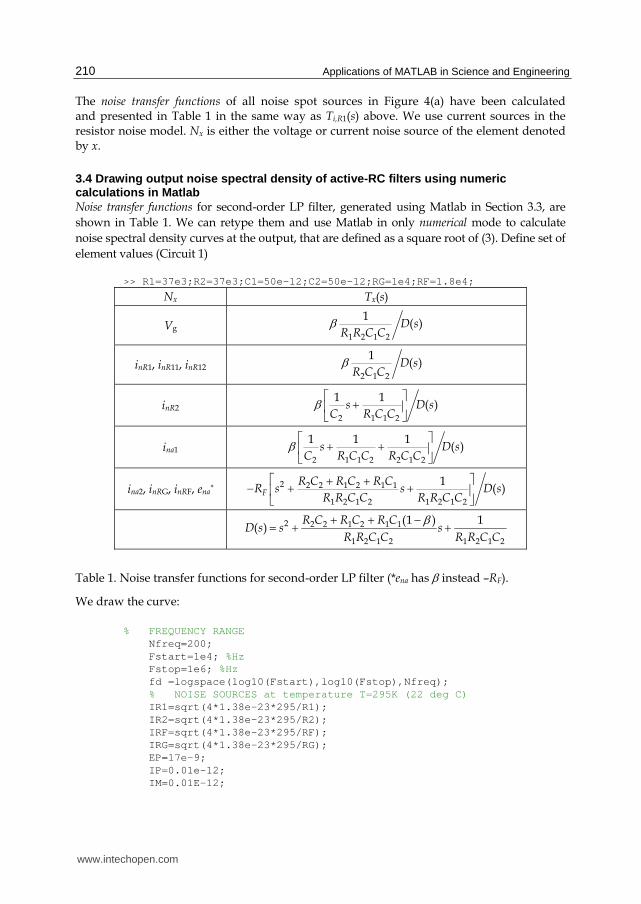
3.4 Drawing output noise spectral density of active-RC filters using numeric calculations in Matlab Noise transfer functions for second-order LP filter, generated using Matlab in Section 3.3, are

shown in Table 1. We can retype them and use Matlab in only numerical mode to calculate

noise spectral density curves at the output, that are defined as a square root of (3). Define set of

element values (Circuit 1)

>> R1=37e3;R2=37e3;C1=50e-12;C2=50e-12;RG=1e4;RF=1.8e4;

Nx Tx(s)

Vg 1 2 1 2

1( )D s

R R C C

inR1, inR11, inR12 2 1 2

1( )D s

R C C

inR2 2 1 1 2

1 1( )s D s

C R C C

ina1 2 1 1 2 2 1 2

1 1 1( )s D s

C R C C R C C

ina2, inRG, inRF, ena* 2 2 2 1 2 1 1

1 2 1 2 1 2 1 2

1( )F

R C R C R CR s s D s

R R C C R R C C

2 2 2 1 2 1 1

1 2 1 2 1 2 1 2

(1 ) 1( )

R C R C R CD s s s

R R C C R R C C

Table 1. Noise transfer functions for second-order LP filter (*ena has instead –RF).

We draw the curve:

% FREQUENCY RANGE Nfreq=200; Fstart=1e4; %Hz Fstop=1e6; %Hz fd =logspace(log10(Fstart),log10(Fstop),Nfreq); % NOISE SOURCES at temperature T=295K (22 deg C) IR1=sqrt(4*1.38e-23*295/R1); IR2=sqrt(4*1.38e-23*295/R2); IRF=sqrt(4*1.38e-23*295/RF); IRG=sqrt(4*1.38e-23*295/RG); EP=17e-9; IP=0.01e-12; IM=0.01E-12;

www.intechopen.com


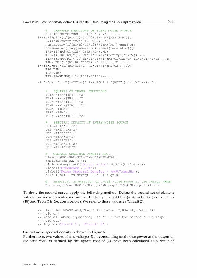
211

% TRANSFER FUNCTIONS OF EVERY NOISE SOURCE D=1/(R1*R2*C1*C2) - (fd*2*pi).^2 + ... i*(fd*2*pi)*(1/(R1*C1)+1/(R2*C1)-RF/(R2*C2*RG)); H=(1/(R1*R2*C1*C2)*(1+RF/RG))./D; numerator=(1/(R1*R2*C1*C2)*(1+RF/RG))*conj(D); phase=atan(imag(numerator)./real(numerator)); TR1=(1/(R2*C1*C2)*(1+RF/RG))./D; TR2=((1+RF/RG)*(1/(R1*C1*C2)+i*(fd*2*pi)*1/C2))./D; TIP=((1+RF/RG)*(1/(R1*C1*C2)+1/(R2*C1*C2)+i*(fd*2*pi)*1/C2))./D; TIM=-RF*(1/(R1*R2*C1*C2)-(fd*2*pi).^2 + ... i*(fd*2*pi)*(1/(R1*C1)+1/(R2*C1)+1/(R2*C2)))./D; TRG=TIM; TRF=TIM; TEP=(1+RF/RG)*(1/(R1*R2*C1*C2)-...

(fd*2*pi).^2+i*(fd*2*pi)*(1/(R1*C1)+1/(R2*C1)+1/(R2*C2)))./D;

% SQUARES OF TRANS. FUNCTIONS TR1A =(abs(TR1)).^2; TR2A =(abs(TR2)).^2; TIPA =(abs(TIP)).^2; TIMA =(abs(TIM)).^2; TRGA =TIMA; TRFA =TIMA; TEPA =(abs(TEP)).^2; % SPECTRAL DENSITY OF EVERY NOISE SOURCE UR1 =TR1A*IR1^2; UR2 =TR2A*IR2^2; UIP =TIPA*IP^2; UIM =TIMA*IM^2; UEP =TEPA*EP^2; URG =TRGA*IRG^2; URF =TRFA*IRF^2;

% OVERALL SPECTRAL DENSITY PLOT U2=sqrt(UR1+UR2+UIP+UIM+URF+UEP+URG); semilogx(fd,U2,'k-'); titletext=sprintf( 'Output Noise' );title(titletext); xlabel( 'Frequency / kHz' ); ylabel( 'Noise Spectral Density / \muV/\surdHz' ); axis ([fd(1) fd(Nfreq) 0 3e-6]); grid; % Numerical integration of Total Noise Power at the Output (RMS) Eno = sqrt(sum(U22(1:Nfreq))/(Nfreq-1)*(fd(Nfreq)-fd(1)));

To draw the second curve, apply the following method. Define the second set of element values, that are represented as example 4) ideally tapered filter (=4, and r=4), (see Equation (18) and Table 3 in Section 4 below). We refer to those values as 'Circuit 2'. >> R1=23.1e3;R2=92.4e3;C1=80e-12;C2=20e-12;RG=1e4;RF=1.05e4; >> hold on; >> redo all above equations; use 'r--' for the second curve shape >> hold off; >> legend( 'Circuit 1' , 'Circuit 2' );

Output noise spectral density is shown in Figure 5. Furthermore, two values of rms voltages Eno (representing total noise power at the output or the noise floor) as defined by the square root of (4), have been calculated as a result of

www.intechopen.com


212

numerical integration in Matlab code given above, and they are as follows: Eno1=176.0 V (Circuit 1 or example #1 in Table 3) and Eno2=127.7 V (Circuit 2 or example #4 in Table 3). They are shown in the last column of Table 3, in Section 4. For all filter examples the rms total output noise Eno was calculated numerically using

Matlab and presented in the last column of Tables.

To plot output noise spectral density and calculate total output noise voltage it was easy

to retype the noise transfer function expressions from Table 1 in Matlab code. In the

following Section 3.5 it is shown that retyping of long expressions is sometimes

unacceptable (e.g. to calculate the sensitivity). Then we have another option to use Matlab in

symbolic mode.

Fig. 5. Output noise spectral density of Circuit 1 and Circuit 2 (denormalized).

3.5 Sensitivity characteristic of active-RC filter using both symbolic and numeric calculations in Matlab To efficiently calculate multi-parametric sensitivity in (9), we use a mixture of symbolic and

numeric capabilities of Matlab.

Suppose F in (7)–(9) is our transfer function T(s)=N(s)/D(s) defined by (11), where xk are

elements R1, R2, C1, C2, RF and RG. We will use previous symbolic results of transfer functions

numerator numLP2 and denominator denLP2 , and Matlab operation of symbolic

differentiation diff to produce relative sensitivity in (8). To calculate the transfer function

sensitivity as defined by (8) we will also apply the following rule:

( ) ( ) ( )

k k k

T j N j D jx x xS S S

. (14)

To construct (14), we proceed as follows. The following code reveal numerator and

denominator as function of components. (Division of both numerator and denominator by

RG is just to have nicer presentation.) First we make the substitution s=j into N(s) and D(s).

Then we have to produce absolute values of N(j) and D(j). In the subsequent step we

perform symbolic differentiation using Matlab command diff or the operator D.

www.intechopen.com


213

>> den=simplify(denTa/RG); >> pretty(den) 2 C1 R1 RF s C2 R1 s + C2 R2 s + C1 C2 R1 R2 s - ---------- + 1 RG >> denofw = subs(den,s,i*wd) denofw = C2*R2*wd*i - C1*C2*R1*R2*wd^2 + 1 - (C1*R1*RF*wd*i)/RG + C2*R1*wd*i

(To calculate all components and frequency values as real variables we have to retype real

and imaginary parts of denofw .)

>> syms wd; >> redenofw= - C1*C2*R1*R2*wd^2 + 1; >> imdenofw= C2*R2*wd - (C1*R1*RF*wd)/RG + C2*R1*wd; >> absden=sqrt(redenofw^2+imdenofw^2); >> pretty(absden) / / C1 R1 RF wd \2 2 2 \1/2 | | C2 R1 wd + C2 R2 wd - ----------- | + (C1 C2 R1 R2 wd - 1) | \ \ RG / /

>> SDR1=diff(absden,R1)*R1/absden; >> pretty(SDR1)

/ / C1 RF wd \ / C1 R1 RF wd \ 2 2 \ R1 | 2 | C2 wd - -------- | | C2 R1 wd + C2 R2 wd - ----------- | + 2 C1 C2 R2 wd (C1 C2 R1 R2 wd - 1) | \ \ RG / \ RG / / ---------------------------------------------------------------------------------------------------------- / / C1 R1 RF wd \2 2 2 \ 2 | | C2 R1 wd + C2 R2 wd - ----------- | + (C1 C2 R1 R2 wd - 1) | \ \ RG / /

The same calculus (with simpler results) can be done for the numerator:

>> num=simplify(numTa/RG); >> pretty(num) RF -- + 1 RG >> numofw = subs(num,s,i*wd) numofw = RF/RG + 1 >> renumofw= RF/RG + 1; >> imnumofw= 0; >> absnum=sqrt(renumofw^2+imnumofw^2);

www.intechopen.com


214

>> pretty(absnum) / / RF \2 \1/2 | | -- + 1 | | \ \ RG / / >> SNR1=diff(absnum,R1)*R1/absnum; >> pretty(SNR1) 0

Sensitivity of the numerator to R1 is zero. We have obviously obtained too long result to be

analyzed by observation. We continue to form sensitivities to all remaining components in

symbolic form.

>> SDR2=diff(absden,R2)*R2/absden;

>> SDC1=diff(absden,C1)*C1/absden;

>> SDC2=diff(absden,C2)*C2/absden;

>> SDRF=diff(absden,RF)*RF/absden;

>> SDRG=diff(absden,RG)*RG/absden;

>> SNR2=diff(absnum,R2)*R2/absnum;

>> SNC1=diff(absnum,C1)*C1/absnum;

>> SNC2=diff(absnum,C2)*C2/absnum;

>> SNRF=diff(absnum,RF)*RF/absnum;

>> SNRG=diff(absnum,RG)*RG/absnum;

By application of rule (14), we form sensitivities to each component, whose squares we finally have to sum, and form (9).

>>SCH=(SNR1-SDR1)^2+(SNR2-SDR2)^2+(SNC1-SDC1)^2+(SNC2-SDC2)^2+... (SNRF-SDRF)^2+(SNRG-SDRG)^2;

The resulting analytical form of multi-parametric sensitivity is as follows:

>> SigmaAlpha=sqrt(SCH)*0.01*8.68588964;

The multiplication by 0.01 defines the standard deviation of all passive elements x in (9) to

be 1%. The multiplication by 8.68588965 converts the standard deviation F in (9) into decibels. When typing SigmaAlpha in Matlab's workspace, a very large symbolic expression is

obtained. We do not present it here (it is not recommended to try!). Because it is too large

neither is it useful for an analytical investigation, nor can it be retyped, nor presented in

table form. Instead we will substitute in this large analytical expression for SigmaAlpha

component values and draw it numerically. This has more sense.

Define first set of element values (Circuit 1 with equal capacitors and equal resistors):

>> R1=37e3;R2=37e3;C1=50e-12;C2=50e-12;RG=1e4;RF=1.8e4;

www.intechopen.com


215

By equating to values, elements changed in the workspace to double and they have become numeric. Substitute those elements into SigmaAlpha .

>> Schoefler1=subs(SigmaAlpha);

Note that in new variable Schoefler1 independent variable is symbolic wd. To calculate

its magnitude, we have to define first the frequency range of , as a vector of discrete values

in wd. When the frequency in Hz is defined, we have to multiply it by 2. The frequency assumed ranges from 10kHz to 1MHz.

>> fd = logspace(4,6,200);

>> wd = 2*pi*fd;

>> Sch1 = subs(Schoefler1,wd);

>> semilogx(fd, Sch1, 'g-.');

>> title( 'Multi-Parametric Sensitivity' );

>> xlabel( 'Frequency / kHz' ); ylabel( '\sigma_{\alpha} / dB' );

>> legend( 'Circuit 1' );

>> axis([fd(1) fd(end) 0 2.5])

>> grid;

This is all needed to plot the sensitivity curve of Circuit 1. To add the second example, we set the element values of Circuit 2 in the Matlab workspace:

>> R1=23.1e3;R2=92.4e3;C1=80e-12;C2=20e-12;RG=1e4;RF=1.05e4;

Then we substitute symbolic elements (components) in the SigmaAlpha with the numeric values of components in the workspace to obtain new numeric vales for sensitivity

>> Schoefler2=subs(SigmaAlpha);

>> Sch2 = subs(Schoefler2,wd);

Finally, to draw both curves we type >> semilogx(fd, Sch1, 'k-', fd, Sch2, 'r--');

>> title( 'Multi-Parametric Sensitivity' );

>> xlabel( 'Frequency / kHz' ); ylabel( '\sigma_{\alpha} / dB' );

>> legend( 'Circuit 1' , 'Circuit 2' );

>> axis([fd(1) fd(end) 0 2.5])

>> grid;

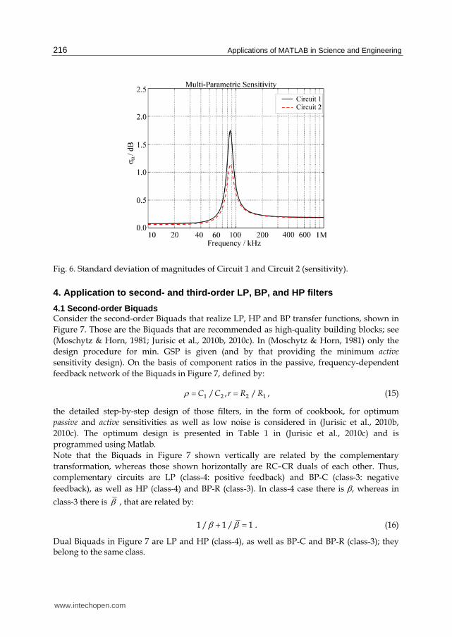
Sensitivity curves of Circuit 1 and Circuit 2 are shown in Figure 6. Recall that both circuits realize the same transfer-function magnitude which is shown in Figure 3(a) above. Note that only several lines of Matlab instructions have to be repeated, and none of large analytical expressions have to be retyped. In the following Chapter 4, we will use Matlab routines presented so far to construct examples of different filter designs. According to the results obtained from noise and sensitivity analyses we prove the optimum design.

www.intechopen.com


216

Fig. 6. Standard deviation of magnitudes of Circuit 1 and Circuit 2 (sensitivity).

4. Application to second- and third-order LP, BP, and HP filters

4.1 Second-order Biquads Consider the second-order Biquads that realize LP, HP and BP transfer functions, shown in

Figure 7. Those are the Biquads that are recommended as high-quality building blocks; see

(Moschytz & Horn, 1981; Jurisic et al., 2010b, 2010c). In (Moschytz & Horn, 1981) only the

design procedure for min. GSP is given (and by that providing the minimum active

sensitivity design). On the basis of component ratios in the passive, frequency-dependent

feedback network of the Biquads in Figure 7, defined by:

1 2 2 1/ , /C C r R R , (15)

the detailed step-by-step design of those filters, in the form of cookbook, for optimum

passive and active sensitivities as well as low noise is considered in (Jurisic et al., 2010b,

2010c). The optimum design is presented in Table 1 in (Jurisic et al., 2010c) and is

programmed using Matlab.

Note that the Biquads in Figure 7 shown vertically are related by the complementary

transformation, whereas those shown horizontally are RC–CR duals of each other. Thus,

complementary circuits are LP (class-4: positive feedback) and BP-C (class-3: negative

feedback), as well as HP (class-4) and BP-R (class-3). In class-4 case there is , whereas in

class-3 there is , that are related by:

1 / 1 / 1 . (16)

Dual Biquads in Figure 7 are LP and HP (class-4), as well as BP-C and BP-R (class-3); they belong to the same class.

www.intechopen.com


217

RC–CR Duality

Po

sitive fe

edba

ck

C

om

plem

entary T

ran

sform

atio

n

(a) Low pass (b) High pass

Neg

ative

feedb

ack

(c) Band pass -Type C (d) Band pass -Type R

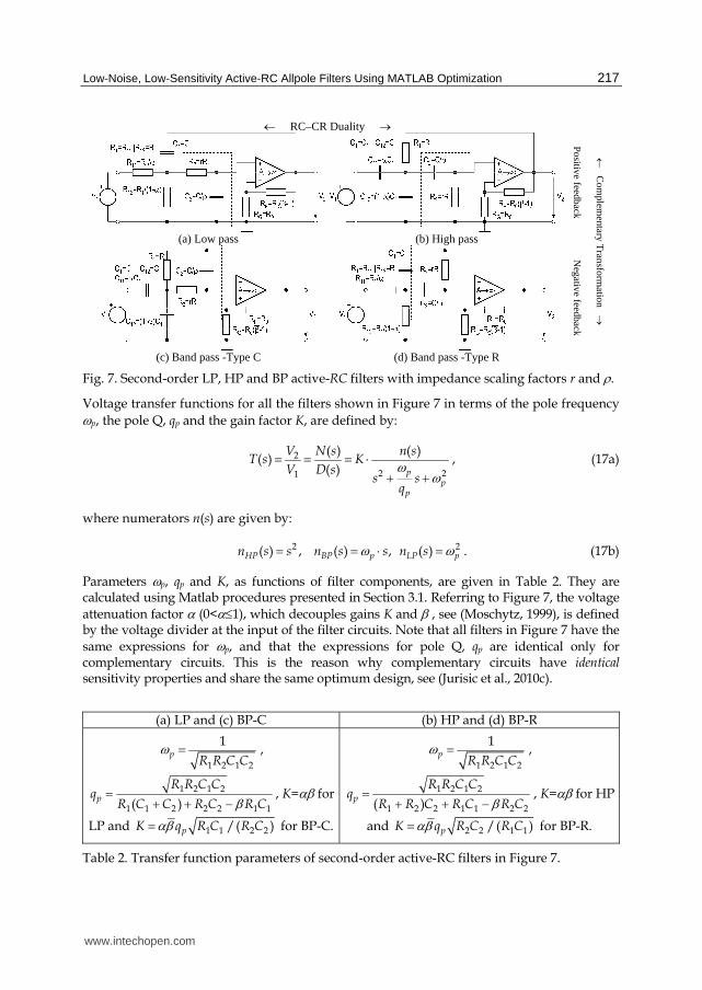
Fig. 7. Second-order LP, HP and BP active-RC filters with impedance scaling factors r and .

Voltage transfer functions for all the filters shown in Figure 7 in terms of the pole frequency p, the pole Q, qp and the gain factor K, are defined by:

2

2 21

( ) ( )( )

( ) pp

p

V N s n sT s K

V D ss s

q

, (17a)

where numerators n(s) are given by:

2 2( ) , ( ) , ( )HP BP p LP pn s s n s s n s . (17b)

Parameters p, qp and K, as functions of filter components, are given in Table 2. They are calculated using Matlab procedures presented in Section 3.1. Referring to Figure 7, the voltage

attenuation factor (0<1), which decouples gains K and , see (Moschytz, 1999), is defined by the voltage divider at the input of the filter circuits. Note that all filters in Figure 7 have the same expressions for p, and that the expressions for pole Q, qp are identical only for complementary circuits. This is the reason why complementary circuits have identical sensitivity properties and share the same optimum design, see (Jurisic et al., 2010c).

(a) LP and (c) BP-C (b) HP and (d) BP-R

1 2 1 2

1p

R R C C ,

1 2 1 2

1 1 2 2 2 1 1( )p

R R C Cq

R C C R C R C , K= for

LP and 1 1 2 2/( )pK q R C R C for BP-C.

1 2 1 2

1p

R R C C ,

1 2 1 2

1 2 2 1 1 2 2( )p

R R C Cq

R R C R C R C , K= for HP

and 2 2 1 1/( )pK q R C R C for BP-R.

Table 2. Transfer function parameters of second-order active-RC filters in Figure 7.

www.intechopen.com


218

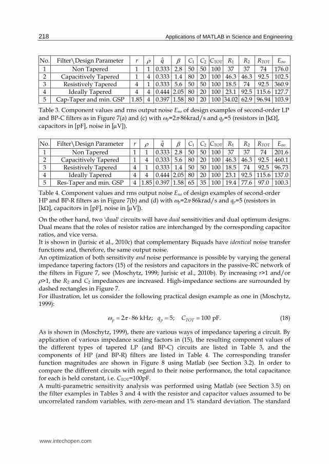
No. Filter\Design Parameter r q̂ C1 C2 CTOT R1 R2 RTOT Eno

1 Non Tapered 1 1 0.333 2.8 50 50 100 37 37 74 176.0 2 Capacitively Tapered 1 4 0.333 1.4 80 20 100 46.3 46.3 92.5 102.5 3 Resistively Tapered 4 1 0.333 5.6 50 50 100 18.5 74 92.5 360.9 4 Ideally Tapered 4 4 0.444 2.05 80 20 100 23.1 92.5 115.6 127.7 5 Cap-Taper and min. GSP 1.85 4 0.397 1.58 80 20 100 34.02 62.9 96.94 103.9

Table 3. Component values and rms output noise Eno of design examples of second-order LP

and BP-C filters as in Figure 7(a) and (c) with p=286krad/s and qp=5 (resistors in [k],

capacitors in [pF], noise in [V]).

No. Filter\Design Parameter r q̂ C1 C2 CTOT R1 R2 RTOT Eno

1 Non Tapered 1 1 0.333 2.8 50 50 100 37 37 74 201.6 2 Capacitively Tapered 1 4 0.333 5.6 80 20 100 46.3 46.3 92.5 460.1 3 Resistively Tapered 4 1 0.333 1.4 50 50 100 18.5 74 92.5 96.73 4 Ideally Tapered 4 4 0.444 2.05 80 20 100 23.1 92.5 115.6 137.0 5 Res-Taper and min. GSP 4 1.85 0.397 1.58 65 35 100 19.4 77.6 97.0 100.3

Table 4. Component values and rms output noise Eno of design examples of second-order HP and BP-R filters as in Figure 7(b) and (d) with p=286krad/s and qp=5 (resistors in [k], capacitors in [pF], noise in [V]).

On the other hand, two 'dual' circuits will have dual sensitivities and dual optimum designs. Dual means that the roles of resistor ratios are interchanged by the corresponding capacitor ratios, and vice versa. It is shown in (Jurisic et al., 2010c) that complementary Biquads have identical noise transfer functions and, therefore, the same output noise. An optimization of both sensitivity and noise performance is possible by varying the general impedance tapering factors (15) of the resistors and capacitors in the passive-RC network of the filters in Figure 7, see (Moschytz, 1999; Jurisic et al., 2010b). By increasing r>1 and/or >1, the R2 and C2 impedances are increased. High-impedance sections are surrounded by dashed rectangles in Figure 7. For illustration, let us consider the following practical design example as one in (Moschytz, 1999):

2 86 kHz; 5; 100 pF.p p TOTq C (18)

As is shown in (Moschytz, 1999), there are various ways of impedance tapering a circuit. By application of various impedance scaling factors in (15), the resulting component values of the different types of tapered LP (and BP-C) circuits are listed in Table 3, and the components of HP (and BP-R) filters are listed in Table 4. The corresponding transfer function magnitudes are shown in Figure 8 using Matlab (see Section 3.2). In order to compare the different circuits with regard to their noise performance, the total capacitance for each is held constant, i.e. CTOT=100pF. A multi-parametric sensitivity analysis was performed using Matlab (see Section 3.5) on the filter examples in Tables 3 and 4 with the resistor and capacitor values assumed to be uncorrelated random variables, with zero-mean and 1% standard deviation. The standard

www.intechopen.com


219

deviation ()[dB] of the variation of the logarithmic gain =8.68588|T()|/|T()| [dB] was calculated, with respect to all passive components, and plotted for the cases in Tables 3 and 4 in Figure 9. There exist four different plots for all four Biquads in Figure 7. In Figures 9(a) and (c) it is shown that the LP and BP-C filters no. 2, i.e. the capacitively-

tapered filters with equal resistors (=4 and r=1) have the minimum sensitivity to passive component variations (Moschytz, 1999). The next best result is obtained with filter no. 5, i.e. the capacitively-tapered filter with minimum Gain-Sensitivity-Product (GSP). It is shown in Figure 9(b) and (d) that the HP and BP-R filters no. 3, i.e. the resistively

tapered filters with equal resistors (having component values in the third row in Table 4)

have the minimum sensitivity to passive component variations. The next best result is the

'optimum' design no. 5.

To conclude, the sensitivity curves in Figure 9 confirm that complementary Biquads have

identical optimum design, whereas dual Biquads have dual optimum designs. All

complementary and dual Biquads in Figure 7 have identical sensitivity figure of merit (all

corresponding Schoeffler sensitivity curves in Figure 9 are equally high).

Fig. 8. Transfer function magnitudes of LP, HP and BP second-order filter examples [with (18) and K=1].

The output noise spectral density eno defined by square roof of (3) has been calculated using

Matlab (see Sections 3.3 and 3.4) and for these filters is shown in Figure 10. Note that there

are only two figures; one for both the (complementary) LP and BP-C filters, i.e. Figure 10(a),

because they have identical noise properties, and the other for HP and BP-R filters, i.e.

Figure 10(b). The total rms output noise voltage Eno defined by square root of (4) are

presented in the last columns of Tables 3 and 4 (Jurisic et al., 2010c).

Considering the noise spectral density in Figure 10(a) and the Eno column in Table 3, we

conclude that the LP and BP-C filters, with the lowest output noise and maximum

dynamic range, are again filters no. 2. The second best results are obtained with filters no.

5, and these results are the same as those for minimum sensitivity shown above (see

Figures 9a and c).

www.intechopen.com


220

(a) (b)

(e)

(c) (d) Fig. 9. Schoeffler sensitivities of second-order (a) LP, (c)BP-C filter examples in Table 3 and

(b) HP, (d) BP-R filter examples given in Table 4. (e) Legend.

(a) (b)

Fig. 10. Output noise spectral densities of second-order (a) LP/BP-C and (b) HP/BP-R filter

examples given in Tables 3 and 4.

Analysis of the results in Figure 10(b) and the Eno column in Table 4 leads to conclusion that

designs no. 3 and no. 5 of the HP and BP-R filters have best noise performance, as well as

minimum sensitivity (see Figures 9b and d).

www.intechopen.com


221

The noise analysis above confirms that complementary circuits have identical noise properties and, on the other hand, those related by the RC–CR duality have different noise properties. Thus, there is a difference between LP and its dual counterpart HP filter in an output noise value. From inspection of Figure 10 it results that the noise of the HP filter is larger than that of the LP filter, for all design examples. Consequently, we propose to use the LP and BP-C Biquads in Figure 7(a) and (c) as recommended second-order active filter building blocks, because they have better noise figure-of-merit, and the HP Biquad in Figure 7(b) as a second-order active filter building block for high-pass filters, if low noise and sensitivity properties are wanted. Unfortunately, it is unavoidable, that HP realizations will have a little bit worse noise performance.

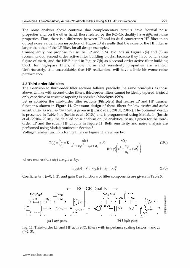
4.2 Third-order Bitriplets The extension to third-order filter sections follows precisely the same principles as those above. Unlike with second-order filters, third-order filters cannot be ideally tapered; instead only capacitive or resistive tapering is possible (Moschytz, 1999). Let us consider the third-order filter sections (Bitriplets) that realize LP and HP transfer functions, shown in Figure 11. Optimum design of those filters for low passive and active sensitivities, as well as low noise, is given in (Jurisic et al., 2010b, 2010c). The optimum design is presented in Table 6 in (Jurisic et al., 2010c) and is programmed using Matlab. In (Jurisic et al., 2010a, 2010c), the detailed noise analysis on the analytical basis is given for the third-order LP and the (dual) HP circuits in Figure 11. Both sensitivity and noise analysis are performed using Matlab routines in Section 3. Voltage transfer functions for the filters in Figure 11 are given by:

23 2

1 2 1 0 2 2

( ) ( )( )

( )p

pp

V n s n sT s K K

V s a s a s as s s

q

(19a)

where numerators n(s) are given by:

3 20( ) , ( )HP LP pn s s n s a . (19b)

Coefficients ai (i=0, 1, 2), and gain K as functions of filter components are given in Table 5. RC–CR Duality

Po

sitive fe

edba

ck

(a) Low pass (b) High pass Fig. 11. Third-order LP and HP active-RC filters with impedance scaling factors ri and i (i=2, 3).

www.intechopen.com


222

Coefficient (a) LP 2

0 pa 11 2 3 1 2 3R R R C C C

21

pp

p

aq

1 1 1 2 3 3 2 1 2

1 2 3 1 2 3

( ) (1 ) ( )R C R R R C C R R

R R R C C C

2p

p

aq

1 2 1 3 1 3 3 1 2 2 3 2 3 1 2 1 2

1 2 3 1 2 3

( ) (1 )R R C C R R C C C R R C C R R C C

R R R C C C

K

Coefficient (b) HP

0a 11 2 3 1 2 3R R R C C C

1a 1 1 2 2 2 3 3 3

1 2 3 1 2 3

( ) ( ) (1 )R C C R C C R C

R R R C C C

2a 1 2 1 2 3 2 2 3 1 3 1 3 3 1 2

1 2 3 1 2 3

( ) ( ) ( )(1 )R R C C C R C C R R R R C C C

R R R C C C

K

Table 5. Transfer function coefficients of third-order active-RC filters with positive feedback in Figure 11.

An optimization of both sensitivity and noise performance is possible by varying the general impedance scaling factors of the resistors and capacitors in the passive network of the filters in Figure 11, see (Moschytz, 1999):

1 2 2 3 3 1 2 2 3 3, , , , / , / .R R R r R R r R C C C C C C (20)

The quantity referred to as 'design frequency' is defined by 0=1/(RC) (Moschytz, 1999). The third-order LP and HP filters with the minimum sensitivity to component tolerances as well as the lowest output noise and maximum dynamic range are the circuits designed in the optimum way as presented in Table 6 in (Jurisic et al., 2010c). The LP filter circuit was

designed by capacitive impedance tapering with 2=, 3=2; >1 and 0 chosen to provide r2r3. In the case of the third-order HP filter, the optimum design is dual: circuit has to be designed by resistive impedance tapering with r2=r, r3=r2; r>1 and 0 chosen to provide 23. Thus, the minimum-noise and minimum-sensitivity designs coincide. Comparing the output noise of two third-order dual circuits we see again that HP filter has larger noise than LP filter, although their sensitivities are identical, see (Jurisic et al., 2010c).

5. Conclusion

In this paper the application of Matlab analysis of active-RC filters performed regarding noise and sensitivity to component tolerances performance is demonstrated. All Matlab routines used in the analysis are presented. It is shown in (Jurisic et al., 2010c) and repeated here that LP, BP and HP allpole active-RC filters of second- and third-order that are designed in (Jurisic et al., 2010b) for minimum sensitivity to component tolerances, are also

www.intechopen.com


223

superior in terms of low output thermal noise when compared with standard designs. The filters are of low power because they use only one opamp. What is shown here is that the second-order, allpole, single-amplifier LP/HP filters with positive feedback, designed using capacitive/resistive impedance tapering in order to minimize sensitivity to component tolerances, also posses the minimum output thermal noise. The second-order BP-C filter with negative feedback is recommended filter block when the low noise is required. The same is shown for low-sensitivity, third-order, LP and HP filters of the same topology. Using low-noise opamps and metal-film small-valued resistors together with the proposed design method, low-sensitivity and low-noise filters result simultaneously. The mechanism by which the sensitivity to component tolerances of the LP, HP and BP allpole active-RC filters is reduced, also efficiently reduces the total noise at the filter output. Designs are presented in the form of optimum design tables programmed in Matlab [see Tables 1 and 6 in (Jurisic et al., 2010c)]. All curves are constructed by the presented Matlab code, and all calculations have been performed using Matlab.

6. References

Jurišić, D., & Moschytz, G. S. (2000). Low Noise Active-RC Low-, High- and Band-pass

Allpole Filters Using Impedance Tapering. Proceedings of MEleCon 2000, Lemesos,

Cyprus, (May 29-31, 2000.), pp. 591–594

Jurišić, D. (April 17th, 2002). Active RC Filter Design Using Impedance Tapering. Zagreb,

Croatia: Ph. D. Thesis, University of Zagreb, April 2002.

Jurišić, D., Moschytz, G. S., & Mijat, N. (2008). Low-Sensitivity, Single-Amplifier, Active-RC

Allpole Filters Using Tables. Automatika, Vol. 49, No. 3-4, (Nov. 2008), pp. 159–173,

ISSN 0005-1144, Available from http://hrcak.srce.hr/automatika

Jurišić, D., Moschytz, G. S., & Mijat, N. (2010). Low-Noise, Low-Sensitivity, Active-RC

Allpole Filters Using Impedance Tapering. International Journal of Circuit Theory and

Applications, doi: 10.1002/cta.740, ISSN 0098-9886

Jurišić, D., Moschytz, G. S., & Mijat, N. (2010). Low-Sensitivity Active-RC Allpole Filters

Using Optimized Biquads. Automatika, Vol. 51, No. 1, (Mar. 2010), pp. 55–70, ISSN

0005-1144, Available from http://hrcak.srce.hr/automatika

Jurišić, D., Moschytz, G. S., & Mijat, N. (2010). Low-Noise Active-RC Allpole Filters Using

Optimized Biquads. Automatika, Vol. 51, No. 4, (Dec. 2010), pp. 361–373, ISSN 0005-

1144, Available from http://hrcak.srce.hr/automatika

Laker, K. R., & Ghausi, M. S. (1975). Statistical Multiparameter Sensitivity—A Valuable

Measure for CAD. Proceedings of ISCAS 1975, April 1975., pp. 333–336.

Moschytz, G. S., & Horn, P. (1981). Active Filter Design Handbook. John Wiley and Sons, ISBN

978-0471278504, Chichester, UK.: 1981, (IBM Progr. Disk: ISBN 0471-915 43 2)

Moschytz, G. S. (1999). Low-Sensitivity, Low-Power, Active-RC Allpole Filters Using

Impedance Tapering. IEEE Trans. on Circuits and Systems—Part II, Vol. CAS-46, No.

8, (Aug 1999), pp. 1009–1026, ISSN 1057-7130

Schaumann, R., Ghausi, M. S., & Laker, K. R. (1990) Design of Analog Filters, Passive, Active

RC, and Switched Capacitor, Prentice Hall, ISBN 978-0132002882, New Jersey 1990

www.intechopen.com


224

Schoeffler, J. D. (1964). The Synthesis of Minimum Sensitivity Networks. IEEE Trans. on

Circuits Theory, Vol. 11, No. 2, (June. 1964), pp. 271–276, ISSN 0018-9324

www.intechopen.com

Applications of MATLAB in Science and EngineeringEdited by Prof. Tadeusz Michalowski

ISBN 978-953-307-708-6Hard cover, 510 pagesPublisher InTechPublished online 09, September, 2011Published in print edition September, 2011

InTech EuropeUniversity Campus STeP Ri Slavka Krautzeka 83/A 51000 Rijeka, Croatia Phone: +385 (51) 770 447 Fax: +385 (51) 686 166www.intechopen.com

InTech ChinaUnit 405, Office Block, Hotel Equatorial Shanghai No.65, Yan An Road (West), Shanghai, 200040, China

Phone: +86-21-62489820 Fax: +86-21-62489821

The book consists of 24 chapters illustrating a wide range of areas where MATLAB tools are applied. Theseareas include mathematics, physics, chemistry and chemical engineering, mechanical engineering, biological(molecular biology) and medical sciences, communication and control systems, digital signal, image and videoprocessing, system modeling and simulation. Many interesting problems have been included throughout thebook, and its contents will be beneficial for students and professionals in wide areas of interest.

How to referenceIn order to correctly reference this scholarly work, feel free to copy and paste the following:

Draz ̌en Juris ̌ić (2011). Low-Noise, Low-Sensitivity Active-RC Allpole Filters Using MATLAB Optimization,Applications of MATLAB in Science and Engineering, Prof. Tadeusz Michalowski (Ed.), ISBN: 978-953-307-708-6, InTech, Available from: http://www.intechopen.com/books/applications-of-matlab-in-science-and-engineering/low-noise-low-sensitivity-active-rc-allpole-filters-using-matlab-optimization

low-noise, low-sensitivity active-rc allpole filters using ...cdn.intechweb.org/pdfs/18564.pdf ·...

Documents