ABSTRACT

Tropospheric angle-of-arrival and amplitude scintillation measurements

were made at X-band (7.3 GHz) and at UHF (0.4 GHz). The measurements

were made using sources on satellites with 42-day orhits. The angle of

arrival of the ray path to a satellite changed slowly allowing observations

of fluctuations caused by atmospheric irregularities as they slowly drifted

across the ray path. The fluctuations were characterized by the rms vari-

ations of elevation angle and the logarithm of received power (log power).

Over a one-year period, 458 hours of observation were amassed spanning

every season, time of day, and weather conditions. The results show strong

scintillation occurrences below 1 to 20 elevation angles characterized by a

number of random occurrences of multipath events that produce deep fades,

a@e-Of-aprival fluctuations, and depolarization of the received signal. The

log power fluctuations ranged from i to iO dB rms at elevation angles below

2- to less than 0.1 dB at elevation angles above iO”. The elevation angle

fluctuations ranged from 1 to i 00 mdeg at elevation angles below 2” to less

than 5 mdeg at a i O” elevation angle. Comparable fluctuations in elevation

angle are expected for bias refraction correction models based upon the use

of surface values of the refractive index.

iii

—- . . .. —.a?=-e

I.

n.

m.

Iv.

v.

CONTENTS.

AbstractList of Illustrations

INTRODUCTION

INSTRUMENTATION

A. Haystack

B. Millstone

OBSERVATIONS

A. Amplitude Fluctuations

B. Elevation Angle Fluctuations

C. Orthogonal Polarization Fluctmtions

ANALYSIS

A. Statistical Summary

B. Comparison with Scintillation Theoq

CONCLUSIONS

iii

v

i

5

5

8

i9

49

25

3i

,,

References32

iv

LIST OF ILLUSTRATIONS

Figure Title Page

,

I-i

n-i

11-2

111-%

111-2

111-3

III-4

111-5

111-6

111-7

111-8

111-9

111-10

Ill-ii

111-12

111-+3

111-i4

IH-i5

111-i6

111-i7

Iv-i

Iv-2

IV-3

IV-4

IV-5

IV-6

IV-7

IV-8

IV-9

Iv-io

Iv-ii

Iv-iz

Elevation andtraverse angle fluctiuations; i3-i5 September i975;weather, cloudy.

X-band receiver system.

X-band tracker.

Received signal levelsat high elevation angles.

Received eignal levels at lowelemtion angles.

RMS fluctuations in log power at X-band.

RMS fluctuations in log power at UHF.

Apparent elevation angle at X-band, high-angle data.

Apparent elevation angle at UHF, high-angle data.

Normalized elevation angle error voltages, high-angle data.

Elevation and traverse angle residuals, high-angle data.

Apparent elevation angle at X-band, low-angle data.

Apparent elevation angle at URF, low-angle data.

Normalized elevation angle error voltages, low -angle data.

Elevation and traverse angle residuals, low -angle data.

Comparkon of received signal level and quadratureelevation angle error voltage fluctuations, low -angledata.

RMS fluctuations in elevation angle at X-band.

RMS fluctuations in traverse angle at X-band.

Received sigml fluctuations in the principal and orthogonalpolarization sum channels and the elevation and traversedifference channels, low-angle data at X-band.

Received signal fluctuations in the principal and orthogonalpolarization sum channe16, low-angle data W UHF.

Satellite rise, 2330 UT, 29 April i975.

Satellite rise continued, 0!00 UT, 30 April i975.

L-band radar observations of a rise and set of a 1-m2 calibrationsphere (LCS-4, Object No. 5398).

Elevation angle and rms log cross section values for calibrationsphere track depicted in Fig. IV-3.

Three satellite rises witbin 12 hours, 29 April i975,

RMS fluctuations in log power at X-band.

RMS fluctuations in log power at X-band, spring season.

RMS fluchratiom in log power at X-band, summer season.

RMS fluctuations in log power at X-band. fall season.

RMS fluctuations in log power at X-band, winter season.

RMS fluctuations in elevation angle at X-band, spring season.

RMS fluctuations in elevation angle at X-band, summer season.

i5

i6

16

i7

i8

20

2i

22

22

23

24

24

24

24

26

26

26

v

Figure TiUe Page

Iv-i3 RMS fluctuations in elevation angle at X-band. faU seas On. 26

IV-14 RMS fluctuations in elevation angle at X-band, winter season. 27

Iv-i5 RMS fluctuations in log power, fu33 year. 27

IV-46 RMS fluctuations in elevation angle, full year. 27

IV-47 RMS fluctuations in log power at X-band and UHF, 29-30 April i975. 29

v-i Median rms fluctuations in elevation angle by season. 31

\

I i[

d“‘....._

.../ ,.,~,{

,!:,

LOW ELEVATION ANGLE MEASU~~NTS IMPOSED BY THE TROPOSP~RE:

AN ANALYSIS OF SCINTILLATION OBSERVATIONS

MADE AT HAYSTACK AND MILLSTONE

1. INTRoDUCTION

Radar systems operating within the troposphere experience measurement errors caused hy

spatial and temporal variations in the index of ref~actiim. Tropospheric propagation errors oc-

cur at all elevation angles but are of major concern only at elevation angles below 5 to 10”. The

Millstone Hill Radar Propagation Studyi was undertaken to investigate the effects of the propaga-

tion medium on radar measurements. A joint Lincoln Laboratory and Bell Telephone Laboratory

study was sponsored at Millstone by the U.S. Army through the Advanced Ballistic Missile De-

fense Agency (ABM.DA) and the SAFEGUARD System Command during the February i969 to

July 1973 time periwl to investigate the effects of the ionosphere on radar measurement accu-

racy. This report describes a follow-m program conducted at the Millstone Hill Radar Facility

for ABMDAto investigate the effects of the troposphere.

The gross effects of tropospheric refraction–elevation angle errors and range errors –have

been studied in the past, andrefraction” correction models can he found in handbooks. 2>3>4 These

models provide an estimate of refraction errors based upon a limited amount of data on the state

of the atmosphere. The model described by Crane 4$5 was generated specifically for the Mill-

stone Hill Radar Propagation Study. Residual refraction errors remain after the model correc -

tions have been app3ied. The magnitude of these residuals depends upon the sophistication of the

correction procedure and on the random fluctuations of the refraction errors that occur during

an observation (or correction) pericd.

The residual errors are often modeled as belonging toti?=o classes: bias errors and scintil-

lation. The bias errors correspond to residual refraction errors that are constant or slowly

varying during an observation period; scintillation corresponds to random fluctuations about the

bias values. Unfortunately, a clear separation between bias effects and scintillation does not

exist. Residuals that maybe considered to be bias values for short observation periods maybe

included ae scintillation for longer duration intervals. This difficulty arises from the non-

stationary behavior of refraction errors: range and angle-o f-arrival variances increase with

increasing observation time. Additional complications occur in the estimation of bias errors

due both to long-term (large-scale) variations in the atmosphere and to possible inadequacies

in the correction mafel. Ideally, correction can be made for the bias component of the refrac -

tion error but not for the random component (scintiDation). A study of refraction effects must

consider both components.

To s+mdy this problem futiher, and to establish the limitations it imposes on the metric ac -

curacy of a radar operating at low elevation angles, the program of propagation studies reported

here was devised. In this etudyangle-of-arrival andamplihlde scintillation were observed at

0.4 and 7.3 GHzbyobserving transmissions from the fnterim DefenseC ommunicationS atellite

Program [IDCSP) satellites. For reception, a 0.4-GHz monoptdse beacon tracker at the Mill-

stone Hill Radar Facility6 and a 7.3-GHz beacon tracker at the Haystack Observatory, operated

bythe Northeast Radio Observatory CorWration(NEROC), were .s~. MadditiOn, bias errOr

residuals were observed using L-band radar sphere tracks. Radar observations were made of

multiple passes of i-, 0.2-, and O.I-mz calibration spheres. Best fit orbits were constmcted

for each of the spheres foruseaa position references forobservations atlowelevation =gles

,..

on each of tie passes. Bias error estimation requires extreme target position measurement

accuracy to separate the errors caused by the instrument from the errors caused by the atmo-

sphere. Considerable effort has been expended for the calibration of the Millstone facility.7

Using multipass orbit fits, the position of a sphere at any instant within the time used for the

orbit fit is known with an angular accuracy of better than 4 mdeg at elevation angles below 10”

(an accuracy of better than 70 pad).

L-band radar observations were made during 16 tracking sessions between i October i 973

and 30 September i 974 for the study of low elevation angle propagation effects. At first, most

observations were of large cross section objects, but during the last four tracking sessions

sphere tracks were emphasized. Coherent data recordings were also made during the last four

tracking sessions to provide information on cross-section (amplitide) scintillation and phase

fluctuations in addition to the position measurement data. State vectors have been generated for

each of the objects tracked to provide accurate position esti’rnates for bias error estimation.

Unfortunately, due to a sudden termination of funding for this program, an analysis of the re-

sidual errors has not been performed. Except for examples of scintillation, further reference

to the L-band radar data will not be made in this report.

Scintillation observations using the IDCSP satellites were made at Haystack and Millstone

during i975. Nineteen sets of measurements were made between 27 January and i i December.

The durations of the observations within a set ranged from 6 to 40 hours, and a total of 458 hours

of observations was amassed during the year. The satellites were observed at elevation angles

from 43” down to the horizon under all weather conditions. An extensive analysis program was

planned, but due to the termination of funding only root mean square (rms) fluctuations in the

logarithm of received power (log power) and angle of arrival will be reported. The rms values

were calculated over 5-rein. and f -hr intervals about quadratic curves fitted by least squares to

tbe data within an observation interval to remove the mean trend. No attempt has been made to

study the angle b% errors: only scintillation is considered in this report.

Observations were made simultaneously at O.4 and 7.3 GHZ. The antennas used for these

observations are separated by a distance of 0.7 km, i.e., significantly larger than the correla-

tion distance for amplitude fluctuations at either frequency. Tbe simultaneous observations are

not useful for studying the correlation between the fluctuations at both frequencies but are useful

for examining the frequency dependence of the rms fluctuation values.~rane8, 9, i O

has reported a theoretical amlysis and observations of the frequency depen-

dence of rms fluctuations in the logarithm of received power (log power), doppler, and angle of

arrival caused by ionospheric scintillation. The same weak scintillation theory (Rytov approxi-

mation) is valid for tropospheric scintillation when the results given in Refs. 8, 9. and i O are

modified to account for the differences in wavelength dependence between ionospheric and tropo-

spheric indices of refraction. Weak scintillation theory coupled with an assumed . ‘* ’13 three-

dimensional (3-d) power spectral density for tropospheric refractivity fluctuations ( K = wave-

number yields an estimated A-7/12

wavelength dependence for rms variations in log power (ox).

The wavelength dependence for angle-of-arrival and Doppler fluctuations is given by 1° and~-i.

respectively. The last results do not depend upon the exponent of tbe assumed refractive

index spectrum. The Haystack and Millstone observations are in agreement with tbe predicted

wavelength dependence for Cx fm. measurements at low elevaticm angles.

2

)

I

I

co - I I

:!:R:E;::*z:%?l::RFAcE

:x\

-u@m -.

\“ ..

.

\

4

RMs RESIDUALS ABOUT SURFACEREFRACTIVITY CORRECTION MADEWITH 3 N UNIT RM5 REFRACTIVITYMEAWREMEN7 ERROR

,0 L“”\t.

\ - Ice

\“”” :

Y’ . 3

TX*”

‘1 \

@

‘ ‘ -.x

x?R.% e

“a ‘\’;~

5mi” I hr

&

ii’- ‘“

I ‘-BAND “-’““L.,..[”,”NOISE UMIT

IELEVA7WN : . 0

TRAVERSE, x ak

.-.., . .

~~

APPARENT ELEVATION ANGLE ldeo

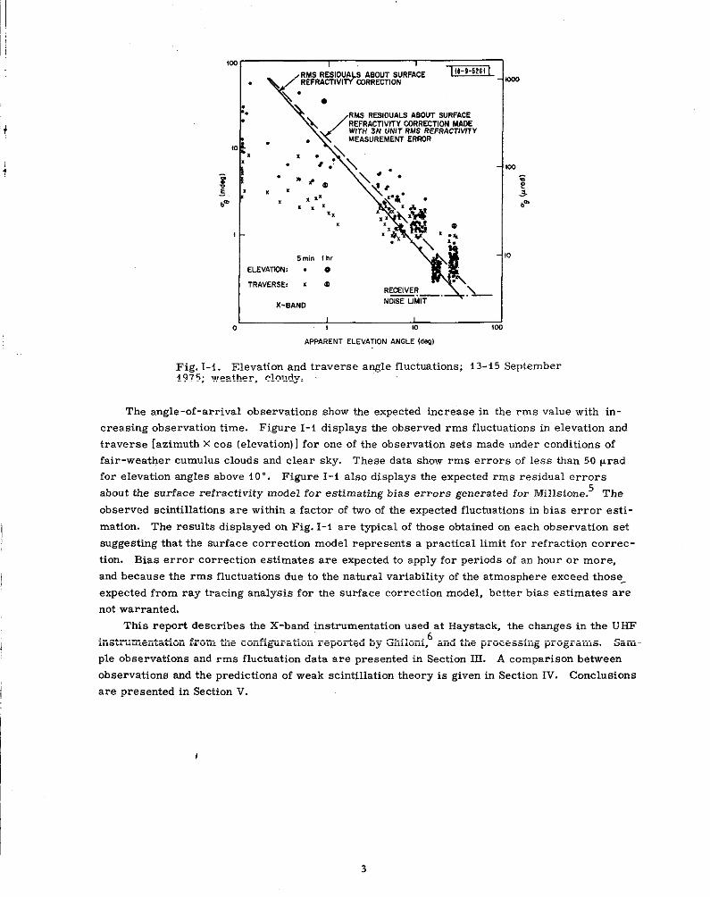
Fig. 1-!. Elevation and traverse angle fluctuations; 13-$5 Septemberi975; weather, cloudy.

The angle -of -arrival observations show the expected increase in the rms value with in-

creasing observation time. Figure I-i displays the observed rms fluctuations in elevation and

traverse [azimuth X cos (elevation) 1 for one of the observation sets made under conditions of

fair-weather cumulus clouds and clear sky. These data show rms errors of less than 50 prad

for elevation angles above i O”. Figure I-i also displays the expected rms residual errors

about the surface refractivity model for estimating bias errors generated for Millstone.5 The

observed scintillations are within a factor of two of the expected fluctuations in hiss em-m. esti-

mation. The results displayed on Fig. 1-i are typical of those obtained on each observation set

suggesting that the surface correction model represents a practical limit for refraction correc -

tion. Bias error correction estimates are expected to apply for periods of an hour or mm-e,

and because the rms fluctuations due to the natural variability of the atmosphere exceed thosez

expected from ray tracing analysis for the surface correction model, better bias estimates are

not warranted.

This report describes the X-band instrumentation used at Haystack, the changes in the U ED?

instrumentation Crom the configuration reported by GhiIoni,6 and the processing programs. Sam-

ple observations and rrns fluctuation data are presented in Section f.ff. A comparison between

observations and the predictions of weak scintillation theory is given in Section IV. Conclusions

are presented in Section V.

I

,

1

,. _.. . .

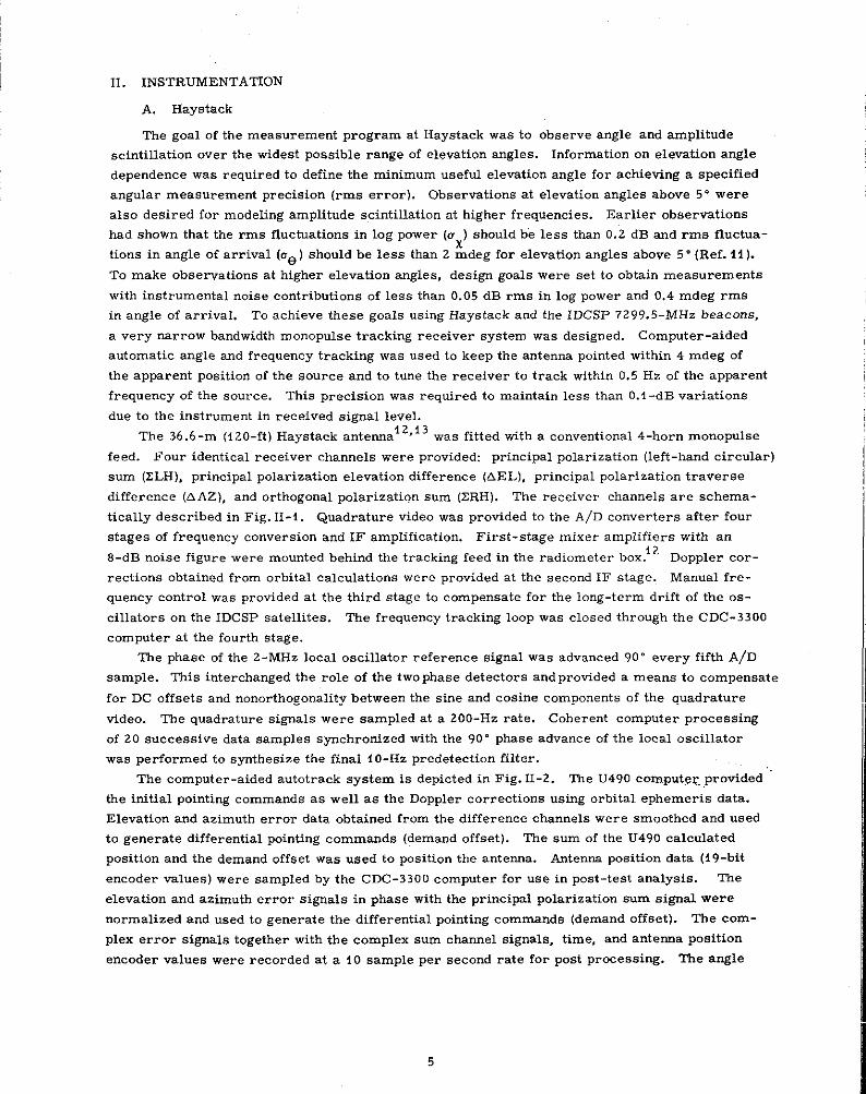
IL 1NSTRUMENTATION

A. Haystack

The goal of the measurement program at Haystack was to observe angle and amplitude

scintillation over the widest possible range of elevation angles. Information on elevation angle

dependence was required to de finetbe minimum useful elevation angle for achieving a specified

angular measurement precision (rms error). Observations at elevation angles above 5“ were

also desired for modeling amplitude scintillation at higher frequencies. Earlier observations

had shown that the rms fluctuations in log power (ox) should be less than 0.2 dBa.ndrms fluctua-

tions in angle of arrival (oe) should be less than 2 mdegfor elevation angles above 5“(Ref. ii).

To make observations at higher elevation angles, design goals were set to obtain measurements

with instrumental noise contributions of less than 0.05 dB rms in log power and 0.4 mdeg rms

in angle of arrivaL To achieve these goals using Haystack and the lDCSP 7299.5-MHz beacons,

a very narrow bandwidth monopulse tracking receiver system was designed. Computer-aided

automatic angle and frequency tracking was used to keep the antenna pointed within 4 mdeg of

the apparent position of the source and to tune the receiver to track within 0.5 Hz of the apparent

frequency of the mu-cc. This precision was required to maintain less than O.i-dB variations

due to theinstrmnent in received signal level.

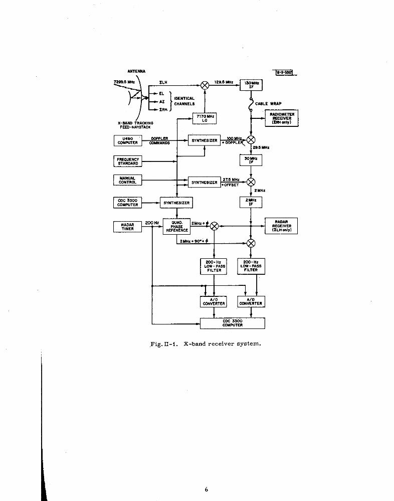
The 36.6-m (i ZO-ft) Haystack antennai2, i3

was fitted with a conventional 4-horn monopulse

feed. Four identical receiver channels were provided: principal polarization (left-hand circular)

sum (zLH), principal polarization elevation difference (AEL), principal polarization traverse

difference (AAZ), andorthogonal polarization sum (ZRH). The rezeiver channels are schema-

tically described in Fig. 11-l. Quadrature video was provided to the A/D converters after four

stages of frequency conversion and IF amplification. First-stage mixer amplifiers with an

8-dB noise figure were mounted behind the tracking feed in the radiometer box.i2

Doppler cor-

rections obtained from orbital calculations were provided at the second IF stage. Manual fre-

quency control was provided at the third stage to compensate for the long-term drift of the os-

cillators on the IDCSP satellites, The frequency tracking loop was closed through the CDC-3300

computer at the fourth stage.

The phase oftbe2-MHz local oscillator reference signal was advanced 90” every fifth A/D

sample. This interchanged the role of the twophase detectors andprovided a means to compensate

for DC offsets and nonorthogonality between the sine and cosine components of the quadrature

video. The quadrature signals were sampled at a 200-Hz rate. Coherent computer processing

of 20 successive data samples synchronized with the 90” phase advance of the local oscillator

was performed to synthesize the final 40-Hz predetection filter.

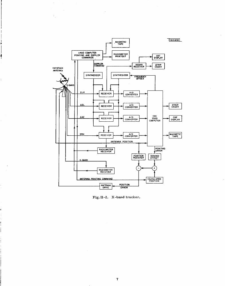
The computer-aided autotrace system is depicted in Fig.11-2. ‘me u490 comput.e~. provided

the initial pointing commands as well as the Doppler corrections using orbital ephemeris data.

Elevation and azimuth error data obtained from the difference channels were smoothed and used

to generate differential pointing commands (demand offset). The sum of the U490 calculated

position and the demand offset was used to positicm the antenna. Antenna position data (i9-bit

encoder values) were sampled by the CDC-3300 computer for use in post-test analysis. The

elevation and azimuth error signals i“ phase with the principal polarization sum sigmd were

normalized and used to generate the differential pointing commands (demand offset). The Com-

plex error signals together with thecmnplex sum channel signals, time, and antenna position

encoder values were recorded at a 10 sample per second rate for post processing. The angle

5

,,;

,,

ANTENNA -EmEL.

t

‘2MHz+S0-++

t2C0- H, m-m

LflL;~SS UW:ss

11 dA/O A(D

WWFRTER MRTER

1 1

,Fig. II-i. X-band receiver system.

6

—.. . . ....-

HI,YSTLCKANTE MA

Fig.11-Z. X-bared tracker.

--EE1-El

-@El

)ij,,!

,, 4,,

I

7

..—-,..-.-. . . .-. ., . ..

encoder values were sampled at the ZOO-HZ rate and averaged prior to recording and to generat-

ing the pointing commands.

The recorded complex signal data were detected, averaged, and used to generate scintilla-

tion statistics in a subsequent analysis program. Using this tracking system and i O-sample

post-detection averaging, the signal-to-noise-ratio for the IDCSP satellites ranged from 40 to

45 dB. The corresponding minimum detectable rms fluctuations in log power due to receiver

noise ranged between 0,04 and 0.06 dB. The signal-to-noise ratio varied within this range due

to differences between the eight IDCSP satellites that were still operating during the i975 season,

due to changes i“ signal level caused by variations in the distance between the satellite and re-

ceiver station and in tbe mmmnt of atmospheric absorption at low elevation angles ae the satellite

rose or set, and as a result of transponder usage on the satellites. However, only one instance

of signal level change due to transponder use was noted during the observations. The receiver

noise limitations on angle measurement ranged from O.Z to ~.4 mdeg rms. The X-band receiver

system plus i O-sample post-detection processing achieved the desired measurement precision.

Radiometer receivers available at the Haystack Observatory were used with the X-band

system to provide additional information about the atmosphere along the observation path. A

20-MHz total power X-band radiometer was used with the orthogonal polarization sum channel.

This radiometer was available for use on any channel by cable changes, and was used to observe

the bright radio stars Cassiopeia A and Cygnus for antenna pointing calibration. The monopulse

feed was mounted off axis in the elevation plane. The pointing corrections obtained from the

radio star observations were —0.075 * 0.005” in elevation and +0.005 ● 0.005” in traverse. These

offsets were added to the reported encoder position values prior to analysis. A t 5-GHz, 500-MHz -

bandwidth Dicke switched mdiometer was also used during the measurement program. Tbe feed

for this radiometer system was on axis and no pointing correction was required.

B. Millstone

The UHF beacon tracker at Millstone was used to track the 40i -MHz telemetry signal trans-

mitted by the IDCSP satellites. Because the satellites are no longer in active use, the telemetry

signal was stable in amplitude and provided an adequate source for scintillation observations.

The receiver system was used as configured for the earlier Millstone Radar Propagation Study!

Data obtained from the receiver were sampled at a i O-Hz rate and transferred to the CDC-3300

computer at Haystack via the Millstone/Haystack intersite link. At first, only the AGC level

was sampled and recorded. As the experiment progressed, the data transfer system was mod-

ified to provide complex difference channel signals, complex orthogonal polarization signal, and

the Millstone antenna encoder values. The IDCSP transmission at UHF had highly elliptical polar-

izations. Nearly equal amplitude signals were available on the principal (right-hand circular)

and orthogonal polarization channels. The elevation and traverse difference channels were right-

hand circular polarization.

8

—.. - . . . . . .

\

III. OBSERVATIONS

A. Amplitude Fluctuations

The lDCSP satellites were tracked as they rose or set. The satellites were in near-

synch ronoue orbits moving slowly with respect to a ground station. The orhit aI period for

each satellite was approximately i 2 days with each satellite visible for about 5 days. At Hay-

stack, the apparent angular motion was typically only two beamwidths in five minutes. At this

slow angle tracking rate, the satellite -to -ground station geometry was essentially fixed while

the atmosphere drifted across the path.

‘“ ~z

X- 8AN0

3“ . . .

:

s

z 30 — .x .0,05569~

;J: m~

3

g ,0 .

;.

0 ! 1 1 1 !

Fig. III- i. Received signal levels at high ,0elevation angles.

G ““,:: .0—

:2 ,. - .x .0.0.9d,d>5: m—“z

g ,0_

;.

! I 1 t 10 m m so 40 5. 6

35.25. APPARENT TIME (ml.) ,4.XELWATION ANGLE

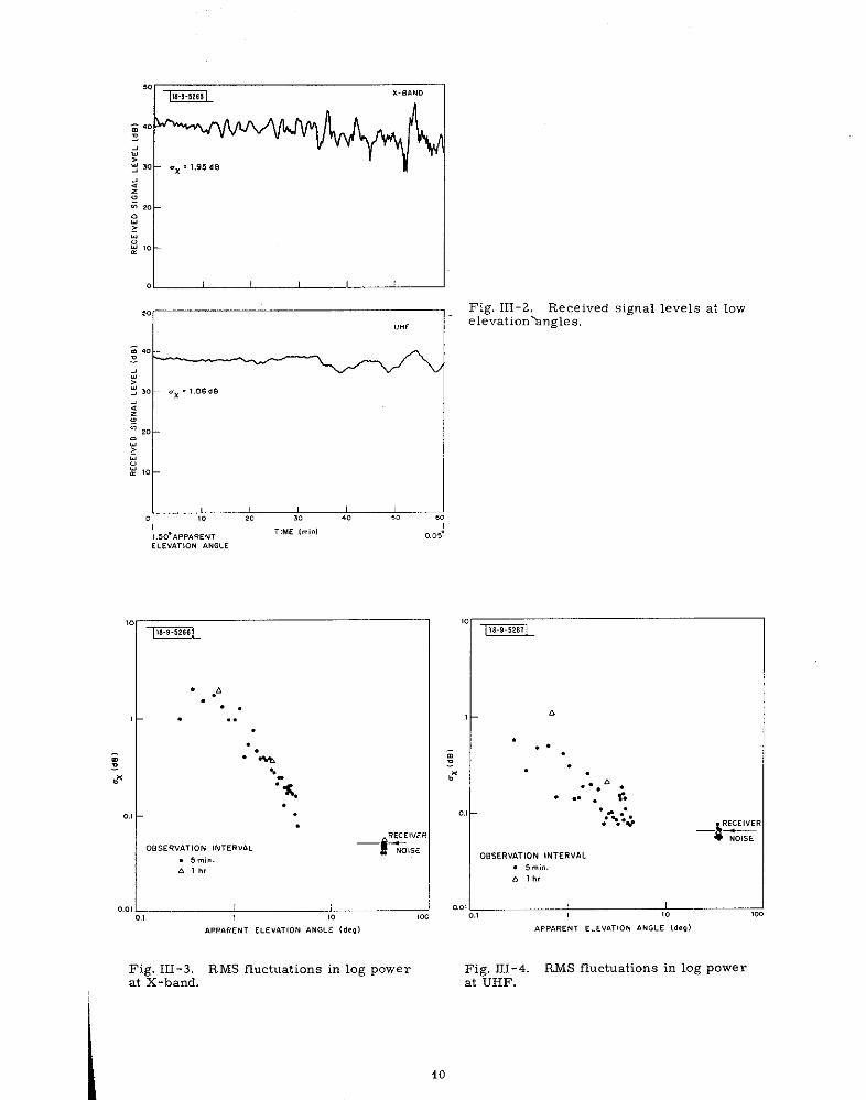
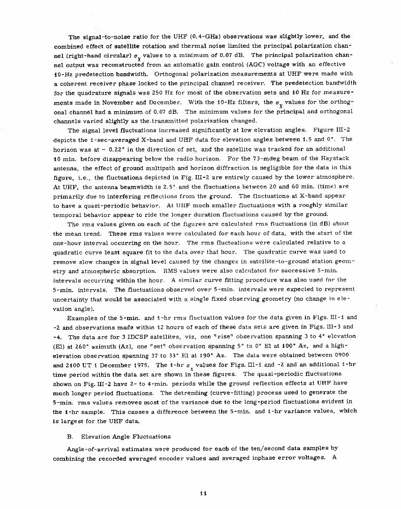
,Examples of observed received eignal level fluctuations are given in Figs. III-i and -2 for

high and low elevation angles, respectively. The high-angle data are for elevation angles

between 35.25 and 34.20’ and display fluctuations near the thermal noise limit. For this sat-

ellite, at X-band (7.3 GHz) the signal-to-noise ratio was 42 dB in a 1-Hz band; at UHF (O.4 GHz)

the signal-to -noise ratio was 39 dB in a i -H. band. The meamred rms fluctuations at X-band

were slightly higher than the values expected due to thermal noise because of small additimaal

fluctuations caused by satellite spi% the satellites were spinning at i 50 rpm, ‘and O.i to 0.2 dB

peak-to-peak modulation at the spin rate was usually evident. The combined effect of spin and

thermal noise increased the X-band received signal level fluctuations to the O.06-dB level.

Slight changes in the minimum detectable WYvalue were observed but the minimum value never

exceeded O.07 dB.

9

—...——_ .,. ..%W-,=,,., -

——.. ,0 <

0.0

. #“..

. . ..

..-

“%..

.

08 SERV’ITIOM IN,,, ”,,

. 5.,”..,”,

1 1). ,,

Fig. III-3.at X-band,

W,A.ENT ELEVATION ANGLE (d!, )

RMS fluctuations in log power

L-l

Fig. 111-2. Received signal levels at low“ elevationlmgles.

‘0Tm!m-

.

. . .; .:,. . “.

. . . . .. . ..r.

0.,

I....”.. . ...+

+-

O8SERVATIONINTERVAL. 5.,”.

b Ihr

..o~,,W.RENT ELEVAT (ON ANGLE 14<,1

Fig. DI-4.at UHF.

RMS fluctuations in log power

The signal-to-noise ratio for the UHF (O.4-GHz) observations was slightly lower, and the

combined effect of satellite rotation and thermal noise limited the principal polarization chan-

nel (right -hand circular) ox values to a mf~mum of 0.07 dB. .The principal polarization chan-

nel output was reconstructed from an automatic gain control (AGC ) voltage with an effective

IO-HZ predetection bandwidth. Orthogonal polarization measurements at UHF were made with

a coherent receiver phase locked to the principal channel receiver. The predetect ion bandwidth

for the quadrature signals was 250 Hz for most of the observation sets and iO HZ for measure-

ments made in November and December. With the i O-Hz filters, the ox values for the Orthog-

onal channel had a minimum of 0.07 dB. The minimum values for the principal and orthogonal

channels varied slightly as the .t ransm itted polarization changed.

The signal level fluctuations increased significantly at low elevation angles. Figure III-2

depicts the i-see-averaged X-band and UHF data for elevation angles between 1.5 and 0“. The

horizon was at – 0.22” in the direction of set, and the satellite was tracked for an additional

40 min. before disappearing below the radio horizom For the 73-mdeg beam of the Haystack

antenna, the effect of ground multipath and horizon diffraction is negligible for the data in this

figure, i.e., tbe fluctuations depicted in Fig. HI-2 are entirely caused by tbe lower atmosphere.

At UHF, the antenna beamwidth is 2. 5“ and the fluctuations between 20 and 60 min. (time) are

primarily due to interfering reflections from the ground. The fluctuations at X-band appear

to have a quasi-periodic behavior. At UHF much smaller fluctuations with a roughly similar

temporal behavior appear to ride the longer duration fl”ct”ations caused by the ground.

The rms values given on each of the figures are calculated rms fluctuations (in dB) ahout

tbe mean trend. These rms values were calculated for each hour of data, with the start of the

one -hour interval occurring on the hour. The rms fluctuations were calculated relative to a

quadratic curve least square fit to the data over that hour. The quad rat ic curve was used to

remove slow changes in signal level caused by the changes in satellite-to-ground station geom

et ry and atmospheric absorption. RIMS values were also calculated for successive 5-min.

intervals occurring within the hour. A similar curve fitting procedure was also used for the

5-rein. intervals, The fluctuations observed over 5-rein. intervals were expected to represent

uncertainty that would be associated with a single fixed observing geomet W (no change in ele -

vation angle).

Examples of tbe 5-min. and 4-hr rms fluctuation values for tbe data given in Figs. fU -f and

-2 amd observations made within i2 hours of each of these data sets are given in Figs. 111-3 and

-4. The data are for 3 IDCSP satellites, viz, one ‘1rise” observation spanning 3 to 4“ elevation

(El) at 26o” azimuth (A.), one “ set” observation spanning 5“ to 0“ El at 100” A., and a high-

elevation observation spanning 37 to 33° El at i90” Az, The data were obtained between 0900

and 2iO0 UT i December i975. The i-hr ax values for Figs. 111-1 and -2 and an additional ! -hr

time period within the data set are shown in these figures. Tbe quasi-periodic fluctuations

shown on Fig. 111-2 have 2- to 4-min. periods while the ground reflection effects at UHF have

much longer period fluctuations. The det rending (curve-fitting) process used to generate the

5-min. rms values remo”es most of the wmirmce due to the long-period fluctuations evident in

the i -hr sample. This causes a difference between the 5-min. and i -br variance values, which

is largest for the UHF data.

B. Elevation Angle Fluctuations

Angle -of -arrival estimates were produced for each of the ten/second data samples by

combining the recorded averaged encoder values and averaged inphase error voltages. A

ii

3’”’1-EEL

t

Fig. III-5. Apparent elevation angle atX-bred, high-angle data.

Fig. UI-7. Normalized elevation angleerror voltages, high-angle data.

I I I3*D I I I

o ,0 2040 m -

T!~E3k

Fig. III-6. Apparent elevation angle atUHF, high-angle data.

~ ‘: .-g

q:Q It?l~ -. 0.‘5: .m_<.-4.s-Q5C4- -0.0.6mm

~. w_

“’ -, m I I I I !

i:~

Fig. III-8. Elevation and traverse ~gle

residuals, high-angle data.

,! ,

predetermined calibration constant was used to convert the normalized error voltage (error

channel voltage inphase with the sum charnel signal divided by the magnitude of the sum channel

voltage) into an angle deviation relative to the position encoder value. Error voltage-to-angle

calibration curves were obtained occasionally at X-band and during each observation set at UHF.

(The calibration constants and phases of the difference channels relative to the sum channel

were very stable at X-band. The calibration constants had to be modified only once during the

observation program after the wavegufde connections to the X-band feed were disturbed.) The

UHF system was manually adjusted prior to each set of observations, and new calibration

curves were required for each data set. Unfortunately, the calibration curves could only be

determined after initial data processing and, at the current level of data reduction, the available

UEF angle-of-arrival values had to be generated using a nominal rather than the correct cali -

bration curves.

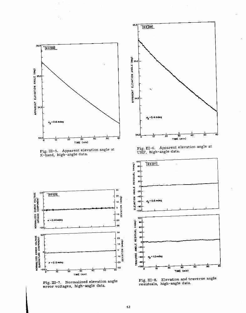
Elevation angle estimates averaged over one second are depicted for the high elevation angle

observations (Fig. III- 1) in Figs. 111-5 and -6. The signal level fluctuations were near the re -

ceive r noise limit. For the 73 -mdeg Haystack beam and the 42-dB signal-to-noise ratio achieved

in a i -Hz band, the theoretical angle measurement limit is 0, 3 mdeg (Ref. 2). The angle encoder

system at Haystack suffered one to two 5- to 10-mdeg random errors or ‘Iglitche s“ within each

tenth of a second sampling interval due to an encoder system malfunction. Efforts to remedy

this defect by detecting the improper reported positions in the computer proved difficult, and

for data reported here the encoder readings taken at 200 values per second were averaged to

reduce the effect of these “glitches.” The net effect of the “glitches!’ was to cause an additional

rms fluctuation of less than 0.3 mdeg. The combined expected rms measurement error is less

than 0.4 mdeg. The observed i -hr rms measurement error was 0.6 mdeg. The difference

between the expected and observed rms errors is due to the curve fitting procedure used to

detrend the data (estimate biases). The theoretical angle-of-arrival measurement limitation

due to receiver noise was 20 mdeg for the 2.5“ Millstone beam. The theoretical estimate is

based upon a 39-dB signal-to-noise ratio and a i-33z bandwidtb. Due to the requirement of

using only a nominal em-or voltage -to-angle calibration curve, the error voltage cent ribut ion

to the angle-of-arrival fluctuation was significantly unclere stimated for the data pre sented in

Fig. Ifl-6. The autotrack system has a time constant larger than i see, causing the observed

rms fluctuation value to be less than the theoretically predicted value.

The X-band inphase and quadrature elevaticm angle error voltages and corresponding

angular deviations are displayed in Fig. fI1-7. The closed-loop computer-aided t racker had a

7-see time constant. The inphase error voltage was used to cent rol the antenna position, and

the observed fluctuations were in part caused by tracker system oscillation. The quadrature

error data are also displayed in the figure. These data were not used in real time for tracking.

A small non-zero quadrature error voltage is apparent in these data. The quadrature voltages

generally exhibited small non-zero long-period fluctuations that depended upon the polarization

of the satellite transmission.

The residual elevation angle errors that remained after curve fitting to one hour of data

are shown in Fig. f31-8. The tracker oscillation is not evident in these data since the use of

both angle encoder data and error voltage data in constmcting angle -of -arri”al estimates

removes any antenna positioning uncertaintiess. The residual error data show slow deviations

from the quadratic curve which are cawed by using only a second-order. equation to represent

the bias errors. Traverse angle residual errors are also displayed in Fig. U1-8.

$3

——... -----————’-—-.--—..---—-

\1 I I

o m *O 30 . . 5.

TIME (.(”)

Fig. III- 9. Apparent elevat iOn angled X-band, low-angle data.

‘“”l -i!mmL

I ! 1 1 , !

o m 20 3. 4. 5.

TcME [.!”1

Fig. 111-’10. Apparent elevation angleat UHF, low-angle data.

lii~0 ,0 20

m’%.)

Fig. III- i 2. Elevation and traverse angleresiduals, low-angle data.

‘1J

At low elevation angles, fluctuations due to the atmosphere were evident at X-band as shown

in Fig. 111-9 and fluctuations due to the ground were evident at UHF as shown in Fig. III-f O. The

X-band inphase and quadrature error voltages are displayed in Fig. J31-i%, and the X-hand eleva-

tion and traverse angle residuals are displayed in Fig. III-12. These observations reveal ele -

vation angle fluctuations that are significantly greater than the noise. “glitch,” and cuwe fitt~g

errors displayed in Fig. III-8, The elevation angle residuals increase as the elevation angle

decreases; the traverse angle residuals appear to exceed measurement noise for only the last

40 min. or for elevation angles below 0.25”. The X-band observations are at angles Sufficiently

high above the horizon to exclude ground reflection effects. The inphase angle deviations

(Fig. ID-i 1) are all less than i O mdeg. Although at times the angle deviations exceed 4 mdeg,

the signal ievel fluctuations are far larger than can be attributed to antenna gain changes caused

by the apparent angle-of-arrival deviation. These observations show that the X-band system

successfully maintained track during severe scintillation and that any signal level changes that

may have occurred due to angle-of-arrival deviations were negligible.

The quadrature component of the normalized error voltage shows relatively large quasi-

periodic fluctuations that are similar to the received signal level fluctuations displayed in

Fig. UI-2. A close comparison between the two curves shows that the quasi-periodic fluctua-

tions are displaced hy a quarter of a period as shown in Fig, III-13. Both UHF and X-band

data are displayed in Fig. III-i 3, and both show this apparent quarter-period displacement

between the received signal and quadrature error curves. This relationship is characteristic

of a complex monopulse receiver system response to rnult ipath.!4

At X-band the characteristic

complex monopulse system response is evident in the figure for times between $0 and 20 min.

The peak-to-peak signal level change is 4 dB. Two signals with a i 2-dB difference in level can

combine to produce this effect. Since the elevation angle for this multipath event is CIOse to

$”, i.e., more than ‘t6 beamwidths above the horizon, and the antenna gain in the direction of

the horizon is more than 40 dB below tbe mainlobe peak, the multipath signal could not have

originated from a ground reflection but must have been generated within the atmosphere. At

-mm .-BAND

— FKCEIVED SIGNAL LEVEL

. NORMAL\ZEO O“ADRb7UREERROR vOLTAGE

I $ 1 1 1 I IFig. L31-13. Comparison of received signallevel and quadrature elevation angle errorvoltage fhctuations, low-angle data.

UHF

..

I — RECEIVED SIGNAL LEVEL I

II , 1 I , Io m 20 3. 40 50 .,

11.6 [.1”1

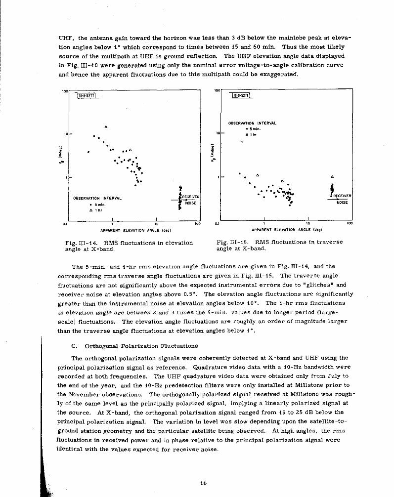
UHF, the antenna gafn toward the horizon was less than 3 dB below the mainlobe peak at eleva-

tion angles below i o which correspond to times between i5 and 60 min. Thus the most likely

source of the multipath at UHF is ground reflection. The UHF elevation angle data displayed

in Fig. 111-40 were generated using only the nominal error voltage-to-angle calibration curve

and hence the apparent fluctuations due to this multipath could be exaggerated.

-

. ..

. . . ,.6

. . . . ““. .. .

I..e

. . ,

“.8.

.

OBSERVATION,NTERV.L. 5 ml”,

A,h, -i=

~,,~

APPARENT ELEVATION ANGLE [,,91

Fig. III- i 4. RMS fluctuations in elevationangle at X-band.

I1“OBSERVATIONINTERVAL.F,”,,..

,0 A,h,

1l“. A

. A

. . . .

. . . .o%-:.& ;,,,,,.,,“. “> ~.*

~,~

&PP&RENT ELEVATION ANGLE [d., )

Fig. 111-i5. RMS fluctuations in traverseangle at X-band.

The 5-min. and i -hr rms ele”at ion angle fluctuations are given in Fig. If I -14, and the

corresponding rms traverse angle fluctuations are given in Fig. 13-i 5. The traverse angle

fluctuations are not significantly above the expected instrument al errors due to “glitches” and

receiver noise at elevation angles above O.5”. Tbe elevation angle fluctuations are significantly

greater than the instrumental noise at elevation angles below 10”. The i -hr rms fluctuations

in elevation angle are between Z and 3 times the 5-min. values due to longer period (large-

scale) fluctuations. The elevation angle fluctuations are roughly an order of magnitude larger

than the traverse angle fluctuations at elevation angles below i”.

c. 0rthogona3 Polarization Fluctuations

The orthogonal polarization signals were coherently detected at X-band and UHF using the

principal polarization signal as reference. Quadrature video data with a i O-Hz bandwidth were

recorded at both frequencies. The UHF quadrature video data were obtained only from July to

the end of the year, and the i O-Hz predetection filters were only installed at Millstone prior to

the November observations. The orthogonally polarized signal received at Millstone was rough-

ly of tbe same level as the principally polarized signal, implying a linearly polarized signal at

the source. At X-band, the orthogonal polarization signal ranged from i5 to 25 dB below the

principal polarization signal. The variation i“ level was slow depending upon the satellite-to-

ground station geometry and the particular satellite being observed. At high angles, the rms

fluctuations in received power and in phase relative to the principal polarization signal were

identical with the values expected for receiver noise.

16

.—-. .—.__ . . . .._-

“1-ImELpRtNCIPAL sum

,ORT”CIGONAL-PRINCIPAL

o

I-w ! 1 1 I !

“... .Q-EL

o —

.. . -

I 1 1 I 1 1 I

l-TR

o

-0.2 ! 1 1 1 1 I.2

O-7R

-0.2 1 I I I I

o ,0 ,0 ,0 40 ,. m

TIME (ml. )

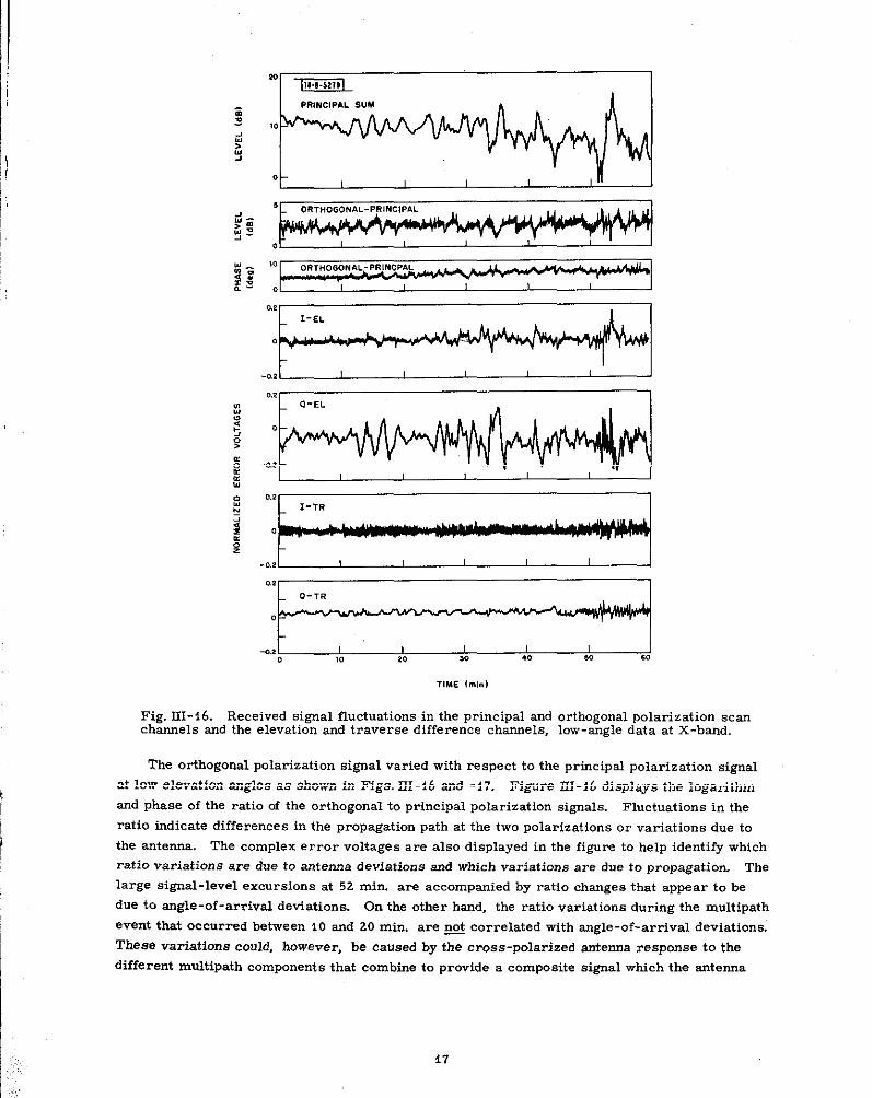
Fig. 221-i6. Received signal fluctuations in the principal and orthogonal polarization scanchannels and the elevation and traverse difference channels, low-angle data at X-band.

The orthogonal polarization signal varied with respect to the principal polarization signal

at low elevation angles as shown in Figs. III-96 and -i 7. Figure 211-46 displays the logarithm

and phase of the ratio of the orthogonal to principal polarization signals. Fluctuations in the

ratio indicate differences in the propagation path at the two polarizations or variations due to

the antenna. The complex em-or voltages are also displayed in the figure to help identify which

ratio variation are due to antenna deviations and which variations are due to propagation The

large signal-level excursions at 52 min. are accompanied by ratio changes that appear to be

due to angle-of-arrival deviations. On the other hand, the ratio variations dm-ing the mult ipath

event that occurred between ICI and 20 min. are @ correlated with angle-of-arrival deviations.

These variations could, however, be caused by the cross-polarized antema response to the

different multipath components that combine to provide a composite signal which the antenna

‘0 -i!EE!L I

ORTHOGONAL POLARIZATION,. —

o I I ! I r I20

PRINCIPAL POLARIZATION

,.

I,50 —

!ta —

w —

.0 —

m —

,~

T,ME [ml.)

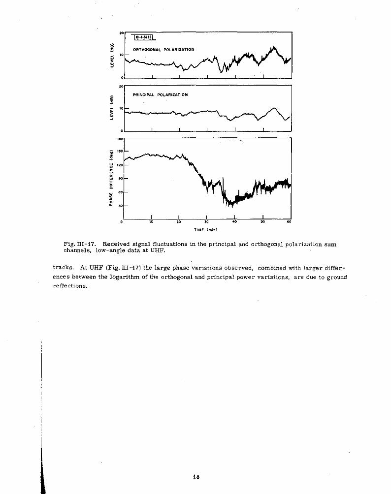
Fig. III - i7. Received signal fluctuations in the principal and orthogonal polarization sumchannels, low-angle data at UHF.

tracks. At UHF (Fig. III-17) the large phase variations observed, combined with larger differ-

ences between the logarithm of the orthogonal and principal power variations, are due to ground

reflections.

18

i

i

,

IV. ANALYSIS

A. Statistical Summary

The fluctuation time histories depicted above are for two hours of observations at high,

-35”, and low, <i.5-, elevation angles. During, the entire measurement series, 458 hours Of

observations were made on 37 days at different times of the day under different meteorological

conditions. Roughly equal numbers of hours of observations were made during each season.

The data all showed ele”aticm. angle and signal-level fluctuations that were large at elevation

angles near the horizon and decreased to very small values hy iOS elevation angle. The data

showed a slight seasonal dependence and a variation with time of day.

Observations of a single satellite rise or set provide a time history that is a single sample

from a random process. An examination of a limited number of time histories is “sef”l in ob-

taining a physical understanding of the fluctuation process. A quantitative measure of the pro-

cess can only be acquired from the statistical moments of fhe process. These in turn are use-

ful only if the process is stationary. The 5-rein. and i.hr rms fluctuation values depicted in

Figs. IV-3, -4, -44, and -i 5 differed significantly suggesting that the process is not stationary.

These problems will be examined in tum starting with a limited rmmber of time-history exam-

ples.

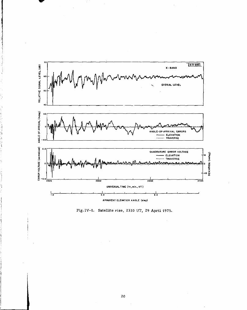
A dependence of the magnitude of signal level a“d angle -of arrival fl”ctwdions on elevation

angle is evident from the time history of a satellite rise observed under clear sky conditions

and displayed in Figs. IV-1 and -Z. These data show large fluct”atiom in the X-band signal

level, elevation angle, and quadrature component of the ele”ation angle error voltage at t to 2-

elevation angles. The signal -lem?l variations decrease from 11 dB peak-to-peak (p-p) at 2° El.

to 3 dB p-p at 3“ El, and i.5 dB p-p at 5° El. The elevation angle variations do not decrease as

rapidly, changing from 40 mdeg p-p at 2“ El to iO mdeg p-p at 5“ El. The difference in the eleva-

tion angle dependence of signal le”el a“d elewt ion angle fluctuations is evident in the rms values

pIotted in Figs. Iv-3 and - f4. The elewation angle quadrature error voltage fluctuations appear

to decay more rapidly with increasing elewat ion angle than do the s igrml le”el fhctu at ions. Sig-

nificant quadrature error voltage variations occur only in combination with the quasi-periodic

fluctuations typical of two-ray mult ipath. No significant error voltage fluctuations or signal

level fluctuations are evident which correspond with the i O- to 2O-mdeg point ing angle var iat ions

abcme 40.

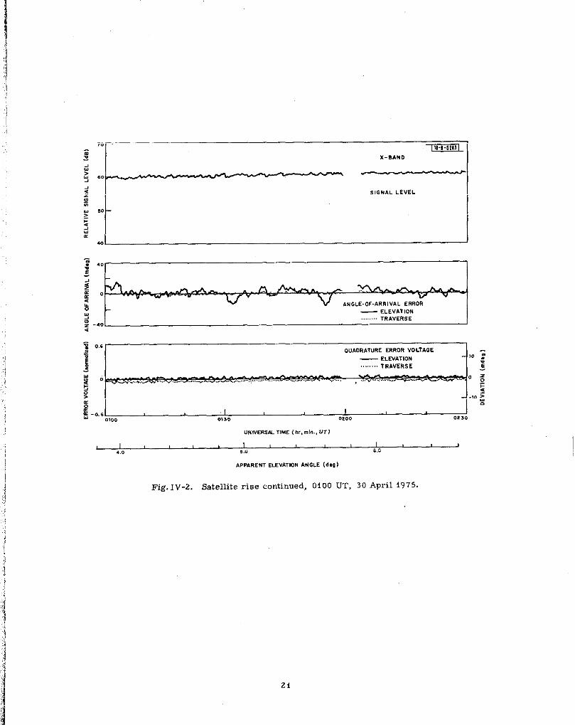
The data displayed in Figs. IV- I and -2 can be interpreted as representing bias error fluc-

tuations that depend only on the initial ele”ation angle (satellite-to-ground station) and not on

time. ff, as is usuaIIy assumed for ray-tracing analysis of bias errors due to refraction, tbe

bias errors arise from the stratification of refractive index, the fluct”atiom d“e to the stratifi-

cation should be identical for different azimuth directions.

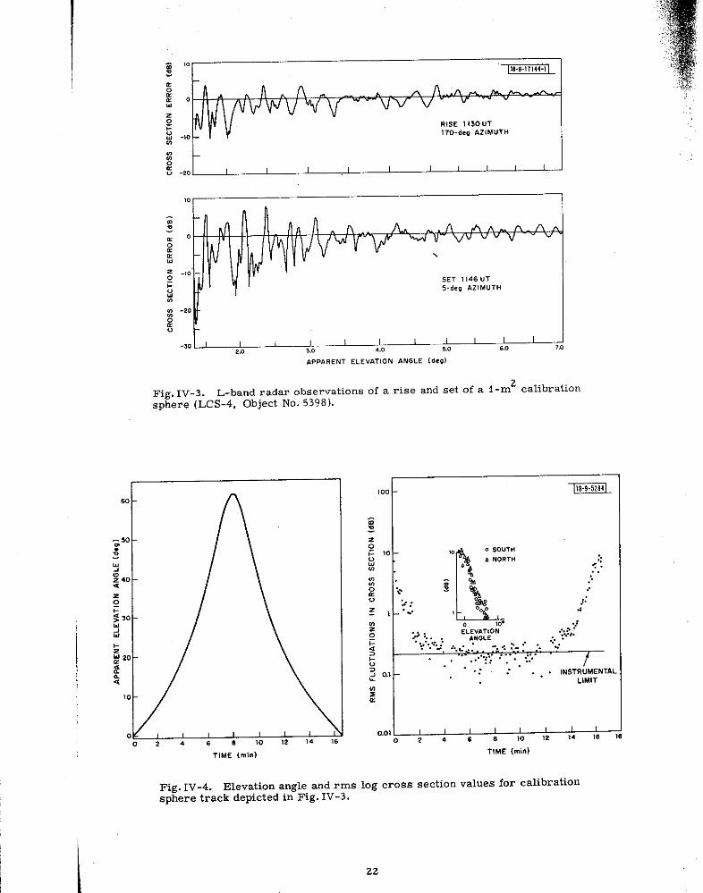
L-band radar observations of the cross section of a calibration sphere are shown in Fig. IV-3.

The observations were made toward the south then north a“d were separated in time by less than

i6 min. The cross-section fluctuations represent signal level changes for the two-way path

through the atmosphere, hence, are larger than the fluctuations for the one-way satellite beacon

observations. For the l-m2 calibration sphere, LCS-4, the signal-to-noise ratio exceeded 30 dB

for the i -see averages displayed i“ this figure. The error in measuring the rms log cross sec-

tion resulting from receiver noise was less than 0.2 dB. The peak-to-peak cross-section varia-

tion between 2 and 30 elevation angle steering set exceeded 20 dB. The detailed fluctuation

I

I

60

b~ .SIQNALLEVEL

m

.

.NGLE-OF-. RR, VAL ERRORS

— ELEVATION

. .------- TRAVERSE

s 0.6.6 QUADRATURE ERROR VOLTAGE

— ELEV,ir(ON:- ,0 .

:------ TRAVERSE g

~og ~:~.

-!0 :0

R -0.6 ! I2,3, .000 00,0 0!0,

uNivERSL TIME [h,, min., ur 1

I 1 1,.. 2,0 ,,.

APPARENT ELEVaTIO. ANGLE (dog)

Fig. IV-I. Satellite rise, 233o UT, 29 April i975.

20

—

m-EEm_

X-BAND

..

SIGNAL LEVEL

$0

t

..~

,0

0

ANGLE-OF-ARRIVAL ERROR

Y — ELEVATIONTRAVERSE

: -40<

!

0.6QUADRATURE ERROR VOLTAGE

— ELEvATION - m j

TRAVERSE :

0

!=

.,. :a

0.6 I I.!0. 0,,. 0,0, 02,0

uNwERs#L TIME (w, m;.., .7)

, I I 1..0 ,.0 s .0

Fig. IV-2.

APP&RENT ELEVATION ANGLE (W)

Satellite rise continued, OiOO UT, 30 April 1975.

21

..-—-–—-———.,.s

.

:,,

,,,,.

,.IIW11144.I I

o I * . II Avwrv”v~

A

R!SE 1130uT

-,0 -170-de, AZIMUTH

!.20 1 1 1 1 1 ! I 1 1

.

-m

.20

Fig. IV-3. L-band radar observations of a rise and set of a %-mz calibrationsphere (LCS-4, Object No. 5398).

TIME (ml.)

L ‘:,.0 SOUTH

. NORTH

“t .<.”...g <w.: .i,.. , “.0

o ,0.MVAT;ON .. . . :!

2:.. , y.. .. +... .:....J.-......~. : ., .. ~. .

. .+ .“:“ . :..”.”.“.

. .. .. . . . IN STRUMEN TA

LIMIT

1 1 I I 1 , 1 ,

,468,012 t~lsTIME (rein)

Fig. IV-4. Elevation angle and rms log cross section values for calibrationsphere track depicted in Fig. IV-3.

22

$,

time histOries fOr observations tO the nOrth and wuth are different. Even the peak-to peak

~“ values differ. These data show that large-scale stratification alone is not responsible for the

ffluctuations. Figure IV-4 displays both the apparent elevation” angle and rms cross section

valuee for the same pass of LCS-4. The 0.2 -dB noise limit is evident for elevation angles

above 45”. The rms values in this plot were calculated for 8. 5-see intervals using the same

detrending process as described above. Each 8.5-see interval spanned less than 0.6” at eleva-

E,

t ion angles below i O” encompassing a sufficient number of fluctuations to provide a useful esti-

mate of the variance of the process. The insert in Fig. Iv-4 shows the rms values vs elevation

angle and these are found to be identical toward the north and south. The rms values provide

~

a good description of the fluctuation process because they are reasonably identical at the same

elevation angles. Because the variance depends on elevation angle, larger observation inter-

vals will have larger variances due to the change in elevation angle. Smaller observation in-

tervals, however, would also produce a larger spread in the rms values due to a decrease in

the number of fluctuations (samples) used in computing the value.,,;

A time-of-day dependence in the fluctuations is also evident a8 shown in Fig. IV-5. Thesei

data are for three mtellite rises observed six hours apart on the same day (same day as for

-,.g ~1

--q60 ,- l.,Jv-lJw

.s: ,0

1 I 1 ! I ( I ! I,,1” ,,03

T,ME (“, )

[

, I , I 1 1 ,m %0

ELEvATION .NGLE (,.”1

I ) , 1 I 1 1 I ! 1 I 1 1 1 1m w

ELEVATION .NGLE (d*O)

FM. IV-5. Three satellite rises within i2 hours. 29 ADril i975.

23

—.--.—.—

-

L-1

Tixm

., :... ,, .. .

‘$

i.; ““.:,..

‘ ~:’?

,8-,9 NovEMBER 1975 W. THER: CLEAR

I I,0

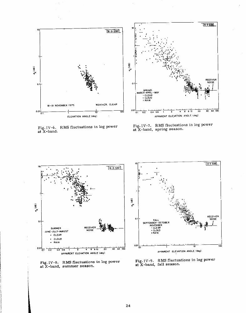
Fig. IV-6.at X-band.

ELEVATION ANGLE (4.,1

R MS fluctuations in log power

. . -imma-. . . . . ....

00! L ‘ ~~ ‘ Jo, 0., 0.40.6 I z 4 6s10 ‘0 ““’m

APPARENT ELEVATION .NGLECdeQ)

Fig. IV-7. RMS fluctuations in log powerat x-band, spring season.

0.1I:,

SUMMERJUNE- d“LY-AuwsT ‘waHit--.CLMR

Fig. IV-8. RMS fluctuations in log powerat X-band, summer season.

1’-----’-:--’... ....; ,....’<, ‘ , ,:.:,

_::-:~’

. .

0.010.!

,0

M-mm, ELEvbT (ON ANGLE ld.gl

Fig. IV-9. R MS fluctuations in log power

at X-band, fall season.

24

I . C1.ouo. RA4N I0.07 1 I I

0., 0,2 0.4 06 1 2 + 6 .10 ,. ~o so j~APPARENT ELEVATION ANGLE (d.ql

,,

:(”

!.

,,

:

Figs. IV-4 and -2). The character of the fluctuations is markedly different for each rise. In

the morning, low-frequency fluctuations with small peak-to-peak variations are evident. By

afternoon, larger fluctuations are evident which have superimposed on them a high-frequency

component. fn the evening, the fluctuations remained large but the high-frequency component

had disappeared. The rms variations at a given time of day span a relatively narrow dB range

at a given elevation angle as shown in Fig. IV-4. The data displayed at elevation angles below

iO” in Figs. IV-3, -4, -i4, and -i 5 were all obtained within four hours. Although these data

were obtained at azimuth angles near i 00- and 260-, the spread in rms values at a given eleva-

tion angle is small. When the low elevation angle data are obtained from two sets of observa-

tions spaced by more than six hours, the data often fall into two different groups as shown in

Fig. IV-6. Data for an entire season display a significant variation in rms values for a given

elevation angle as shown in Figs. IV-7 through -i4. Figures lv-i5 and -16 summarize the ex-

tremes in the rms values for elevation angles between 1 and 100.

The seasonal summaries encompass all the observations including days with clear skies,

days with clouds (scattered fair-weather cumulus to complete overcast), and days with rain.

Days with showery and widespread rain were encountered. A single observation get often en-

countered several weather types. Sets displayed as clear weather observations may have in-

cluded thin scattered cirrus clouds. Data sets that encompassed clear sky and cloudy conditions

were included in the ‘Iclo”d *1cat egory. If rain occurred at any time within an observation set it

was classified as !Irain.l! No clear dependence on weather type was ohserved. In the spring

the ‘*cloud” data set showed lower fluctuations than for clear sky; in the fall the reverse

occurred. In general, the summer data showed the largest fluctuations; the rest of the

seasons were roughly the same. The elevation-angle fluctuations displayed a wider range of

rms “alues than did the signal-level variations.

The 5-rein.’ rms signal level variations ranged between 0.5 and i 4 dB at elevation angles

below i ‘, and were less than O.2 dB at elevation angles above f O”. NO variations larger than

the measurement error introduced by the receiver noise and satellite spin were evident at

elevation angles above i 50. The 5-min. rms elevation angle fluctuations ranged between 1 and

i 00 mdeg for elevation angles below i”. The summer values were significantly higher than for

the other seasons at elevation angles below i ~. RMS values as high as 2 mdeg were observed

at elevation angles as high as 30”. The clear-sky elevation angle fluctuation data were all be-

low %mdeg rms for elevation angles above i 0-. The elevation-angle fluctuations w ere measur-

able above the receiver noise for elevation angles “p to 40”. The elevation-angle fluctuations

are nearly identical to the predicted hiss-error fluctuations expected using a surface correc-

tion model as shown in Fig. IV-i 6.

Fluctuations in traverse angle and in the ratio of the orthogonal-to-principal polarization

signals are not discussed further because they did not show significant increases above instru-

ment measurement noise at elevation angles above i o.

B. Comparison with Scintillation Theory

Scintillation theory attempts to describe the random fluctuations in signal level and angle of

arrival a“d relate the rms valw%’ to either the spectrum or correlation function describing the

refractive index fluctuations along the ray path. At the present time, an adequate theoretical

model exists only for weak scintillation when ax < 5 dB [(Ref. 9)1. The theOw cm be used tO de-

scribe the dependence of the rms fl”ct”ation values m frequency, propagation geometry, and on

. ... .

. . .

. . ... .

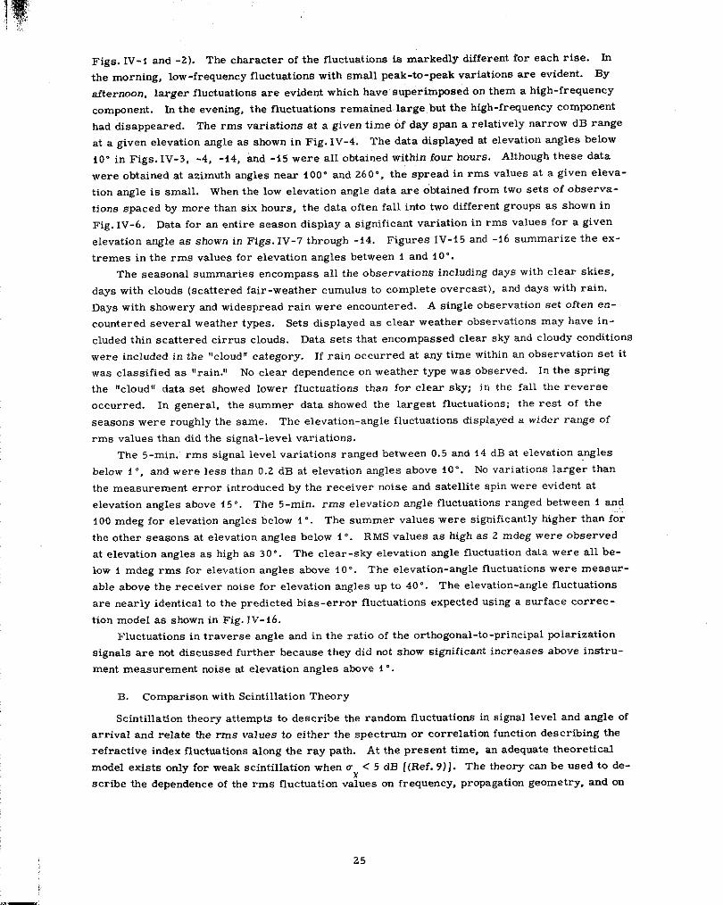
. CLEAR

. CLOUD

. RAIN

I-

,0 1

APPARENT ELEVATION ANGLE (d*Q)

Fig. IV-IO. RMS fluctuations in log Wwerat x-band, winter season.

I,,

,,1 ...’..’

0.,x

APPb..&ELEvATI..AN;LE(e+ol

1;.0>

APPAFSNT ELEVATION ANBLE wag)

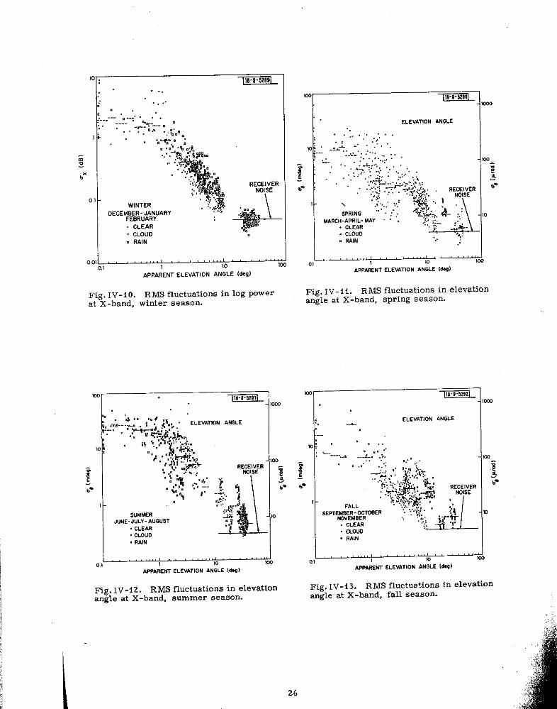
Fig. IV-i i. R MS fluctuations in elevatiOnangle at X-band, spring season.

o

-D@m_

ELEVAT,ONANGLE.-

,,. ,

. RAIN

.

APPA.& ELEVATION bNGLE @+U)

Fig. IV-12. RMS fluctuations in elevation Fig. IV-43. RMS fluctuations in elevation

angle at X-band, summer season. angle at X-band, fall season.

4,i

$.;:

26;:,f,,..,,,,,

; ?,...!,:.!>,?-

1,

I

.

Fig. IV- 44. RMS fluctuations in elevationangle at X-band, winter season.

!!, ,0

,. ; :-. : .,”, . .

& “.. .

OECEM#?EER-~A#ARY :: j,,.. CLEAR. CLOUD —. RAIN

A,,ARENTELEVATION ANGLE (@l

Fig. IV-i 5. RMS fluctuations in log power.full year.

1. J01 ,m

APPARENT ELEVATION AN:LCi~d

1 ,

0,, m ,0AF.PA.EN,ELEVATION ANGLE (’44’9)

Fig. IV-i6. RMS fluctuations in elevationangle, full year.

27

..-.——

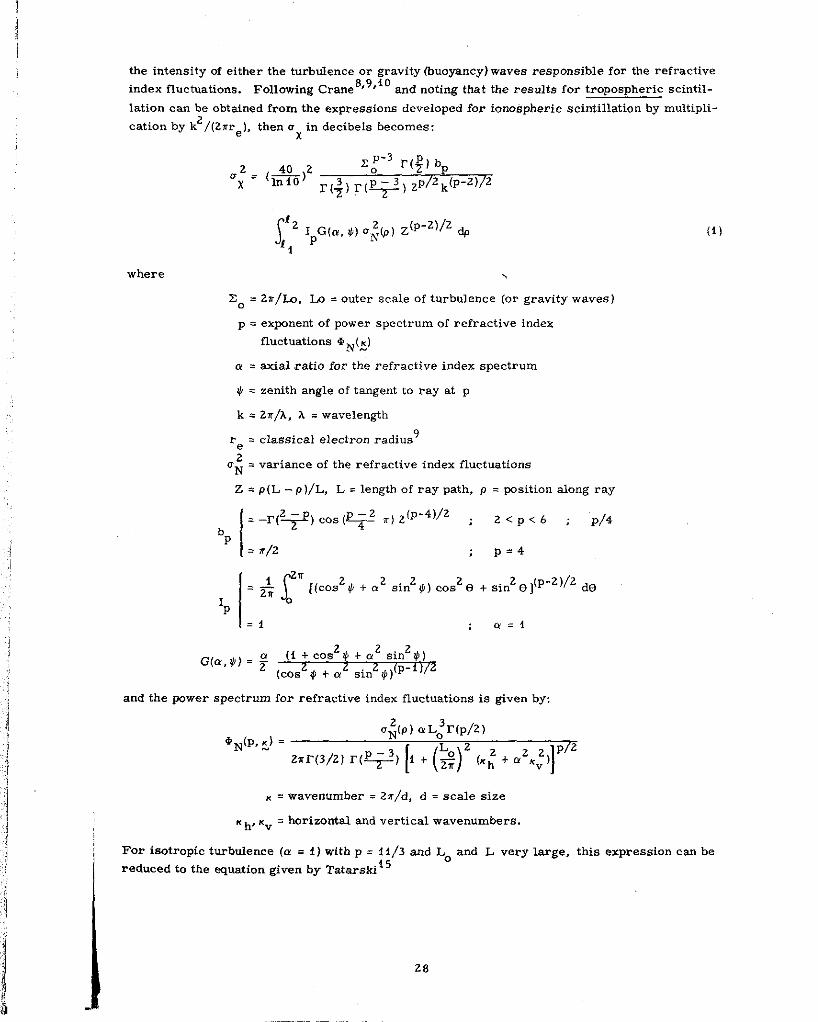
the intensity of either the turbulence or gravity (buoyancy) waves responsible for the refractive8,9,+0index fluctuations. Following Crane and noting that the results for tropospheric scintil-

lation can be obtained from the expreasicms developed for icmotipheric scintillation hy multipli-

cation by k2/(2rr e), then UX in decibels becomes:

where \

Z. = 2u/f.o, u = outer scale of turbulence (or gravity waves)

(i)

p . expnent of power spectrum of refractive index

fluctuations *N(:)

u . axial ratio for the refractive index spectrum

$ = zenith angle of tangent to ray at p

k . 2T/A, A . wavelength

re = classical electron radims9

2- variance of the refractive index fluctuations‘N -

Z = P(L - p)/L, L = length of ray path, p . position along ray

I

= –r(z+) Cos (+2 .1 2’P-4)’2 ; 2<p<6 ;b

p/4

P. x/2 p=4

G(@,4)= ;(i + cosz~ + az sinz~)

(cosz * + az sinz *)(p-1)/2

and the power spectrum for refractive index fluctuations is given by:

U;(P) aL:r(p/2)*N(P> ~) = L2

[()z~r(3/2) r(~) i + ~ 122P12

(K; +c! .“)

K = =wemrnber = 2T/d, d = scale size

Sh, Sv = ~rimntal and vertical wavenumberif.

For isotropic turbulence (CT. i ) with p . 1i/.3and Lo and L very large, this expression can be

Ireduced to the equation given by Tatarski i5

.3; =(*)2 &56k’qLc’(p,p’/6N *0

(2)

where c; replaces u: as a measure of the intensitY Of turbulence.

A reasonable expression for the angle-of-arrival varimce requires a better understanding

of tbe values to be used in describing the power spectrum for the refractive-index fluctuations.

For ionospheric scintillation, Lo exceeds any scale, size associated with atmospheric drift10

across the path during a measurement interval. In that case, a reasonably simple approxi -

mate expression for u: ban be generated. From analyses of tropospheric scintillation data re -i 5 it is e~dent that L is larger than the Fresnel zone sizes typical Of mi -ported by Tatarsla,

0crowave and optical propagation through the lower atmosphere. For tropospheric turbulence

at scale sizes smaller than Lo, the spectrum is isotropic.i6 Anisotropy (a <1 ) occurs at scale

sizes larger than Lo. Since, for the Haystack measures, the elevation-angle fluctuations

greatly exceed the traverse-angle fluctuations, Lo must be smaller than tbe scale sizes as so -

ciated with atmospheric drift by the line of sight and a 5-rein. observation period. For a nom-

inal 10-m/eec drift by the line of sight. Lo << 3 km.

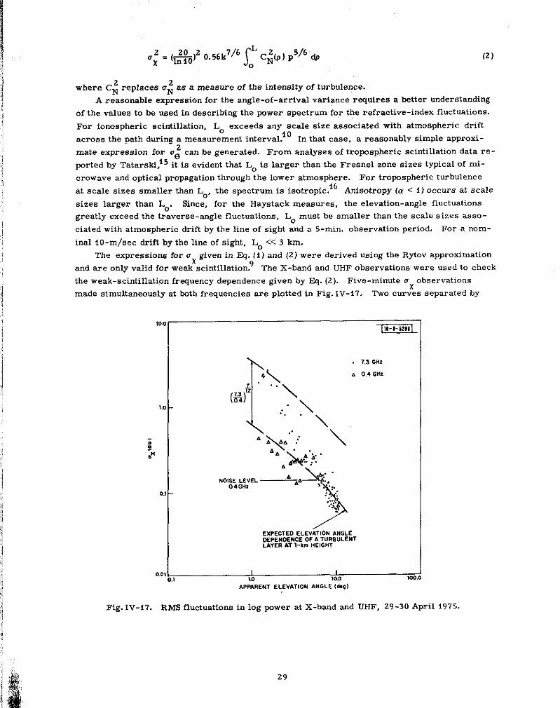
The expressions for ax given in Eq. (i) and (2) were derived using the Rytov approximation

and are only valid for weak scintillation.9 The X-band and UHF observations were used to check

the weak-scintillati~n frequency dependence given by Eq. (2 ). Five-minute ox observations

made simultaneously at kcdb frequencies are plotted in Fig. IV-17. TWO curves separated by

EXPECTED ELEVillON ANGLEOEPENOENCE OF A TURBULENTLAYER AT l-km HEIGHT

7,3 6!!,

0,4 G14Z

0,0, ~,, I 120.0 ,@.!

AP;RENT ELEVATION ANGLE (t+q)

Fig. lV-i7. RMS fluctuations in log power at X-band and URF. 29-30 April i975.

A -7/i2 were plotted on this figure to represent the expected freTJencY dependence. These

curves were generated for a hypothetical turbulent layer at a t km height. The UHF data can

be interpreted as being in reasonable agreement with this expected elevation-angle dependence.

The X-band data are not in agreemerit and exhibit a significant decrease in ox as the elevation

angle increases. This discrepancy may be due in part to a reduction in the X-band fluctuations

caused by averaging over the 36.6-m antenna aperture.

Tatarski?3

This latter effect was discussed by

He showed that the rms fluctuations are reduced by 20 percent for a uniformly

weighted circular aperture when the diameter is one-half of the size of the first Fresnel zone

~. The distance between the layer and the antenna rapidly decreases below the value required

for the firs t Fresnel zone size to equal the diameter of the aperture as the elevation angle in-

creases producing the apparently steeper slope for the X-band data. The angle -of -arrival fluctu-

ations are dominated by the large scale sizes, d >> ~Z, which are not severely attenuated by

aperture averaging. As a result, the elevation angle-of-arrival data have an elevation angle

dependence similar to that for the UHF data (see Figs. IV-3, -4, and -i4).

The weak scintillation theory model is not valid when the signal-level fluctuations become

lar-ge.g For large fluctuations or strong scintillation, the time histories reveal a number of

randomly occmring multipath events. These e“ents appear to be characteristic of strong

scintillation. Currently, a viable strong scintillation model is not available.

The weak-scintillation results gi”en above were derived using a power spectrum for the

refractive index perturbations that is often observed for atmospheric turbulence.i4

The be-

havior of the spectrum at the larger scale sizes of importance to angle-of-arrival fluctuations

is not known. The theoretical analysis used to derive ~. (t) only assumed the existence of a

spectrum and its general shape, hut not its cause. The fluctuations could be due to gravity

waves m- to tm-bulence. Although a distinction is usually drawn between waves and turbulence,

for scintillation the differences between the two phenomena are not important; the shape of the

spectrum. however, is of importance.

The angle-of-arrival fluctuations are dominated by the large scale size refractive index

perturbations. At large scale sizes, the propagation phenomena are adequately described by

geometrical optics (ray tracing ). In the limit of geometrical optics (the Rytov approximation

at large scale sizes), tbe angle-of-arrival fluctuations are independent of frequency. At high

frequencies, the signal-level fluctuations, a , increase as f7/f2 ~a~ ~ ‘7/32). For a fixed aper-

ture size, v , however, decreases due to th~increase in D/~Z where D is aperture diameter.

Again for axfixed aperture size, the elevation-angle fluctuations increase as a percentageof the

beamwidth as the frequency increases (increase is linear with frequency).

30

v. CONCLUSIONS

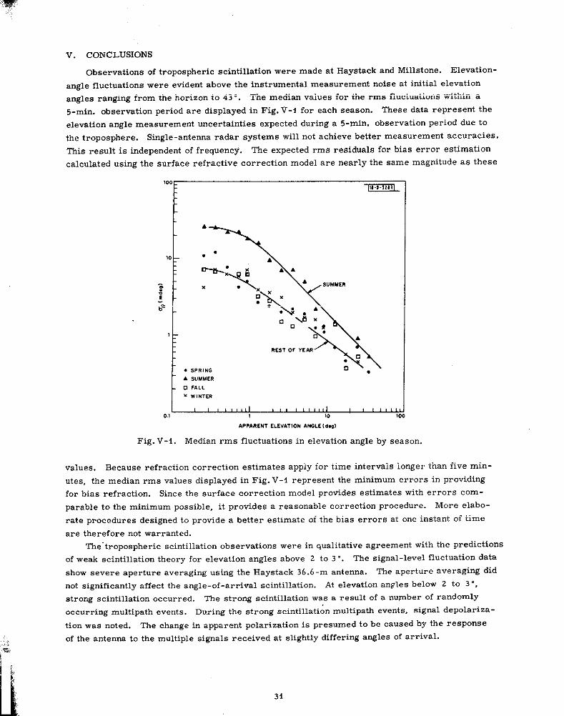
Observations of tropospheric scintillation were made at Haystack and Millstone. Elevation-

angle fluctuations were evident above the instrumental measurement noise at initial elevation

angles ranging from the horizon to 43”. The median values for the rms fluctuations within a

5-rein. observation period are displayed in Fig. V-i for each season. These data represent the

elevation angle measurement uncertainties expected during a 5-rein. observation period due to

the troposphere. Single-antenna radar systems will not achieve better measurement accuracies.

This result is independent of frequency. The expected rms residuals for bias error estimation

calculated using the surface refractive correction model are nearly the same magnitude as these

t

SUMMER

F.SPRING ~. ,A SUMMER

t ~ 818, 1 t u

0 FALL

. wImm

0.1 !0 !0

APPARENT ELEVATION ANGLE (d.,)

Fig. V-i. Median rms fluctuations in elevation angle by season.

values. Because refraction correction estimates apply for time intervals longer than five min-

utes, the median rms values displayed in Fig. V-i represent the minimum errors in providing

for bias refraction. Since the sin-face cm.rection model provides estimates with errors com-

parable to the minimum possible, it provides a reasonable correction procedure. More elabo-

rate procedures designed to provide a better estimate of the hiss errors at one instant of time

are therefore not warranted.

The-tropospheric scintillation observations were i“ qualitative agreement with the predictions

of weak scintillation theory for elevation angles above 2 to 30. The signal-level fluctuation data

show severe aperture averaging using tbe Haystack 36.6 -m antenna. The aperture averaging did

not significantly affect the angle-of-arrival scintillation. At elevation angles below 2 to 3”,

strong scintillation occm-red. The strong scintillation was a result of a number of randomly

occurring multipath events. During the strong scintillation multipatb events, signal depolariza-

tion was noted. The change in apparent polarization is presumed to be caused by the response

of the antenna to the multiple signals yeceived at slightly diffe=ing angles of arrival.

*,

2

3,

4,

5,

6.

7,

8.

9.

10.

il.

<2.

13.

%4.

i5.

16.

REFERENCES

J. V. Evans, editor, ,,Millstone Hill Radar Propagation Study: scientificResults, Parts I, 32, and 131j’ Technical Report 509, Lincoln Laboratory,Nf.1.l’. (i3 November i973), DDC Nos.: Part 1, AD-78 ii79/7; Part 11,AD-782748/8; Part 111, AtJ-7805<9/5.

D. K. Barton, Chapter 15 in Radar Svstem Analy~ (Prentice Hall,Englewood Cliffs, N. J., i964).

B. R. Bean, E. J. Dutton, and B. D. Warner, Chapter 24, “Weather Effectson Radar:t in Radar Handbook, M. I. Skolnik, editor (McGraw-Hill,New York, i970).

EL K. crane, SeC. 2.5, ,,Refraction Effects in th$ Neutral Atmosphere,” inMethods of Experimental Pby.&s, Vol. 13B, M. L. Meeks, editOr (Aca-demic Press, New York, i 976).

J. V. Evans, editor, ‘tMillstone Hill Radar Propagation Study; TechnicalNote i969-5i, Lincoln Laboratory, M.l. T. (26 September i969),DDC AD-701939.

J, C, GbilOni, editor, ,,Millstone Hill Radar propagation Study: InSt ru -mentation;’ Technical Report 507, Lincoln Laboratory, M. I.T. (20 Sep-tember 1973), DDC AD-775 i40/7.

J. V. EVanS, editor, ,1Millstone Hill Radar Propagation Study: Calibra -tion, “Technical Report 508, Lincoln Laboratory, M. I.T. (3 Octo-ber f973, DDC AD-77968919.

R. K. Crane, “Spectra of Ionospheric Scintillation, J. Geopbys. Res.~, 204i (i976),

R. K. Crane, 1’Ionospheric Scintillation!’ Proc. IEEE (accepted forpublication, i97 7).

R. K. Crane, ‘1Variance and Spectra of Angle-of-Arrival and DopplerFluctuations Caused by Ionospheric Scintillation; J. Geopbys. Res. (sub-mitted for publication, t 976).

R. K. Crane, “ Propagation Phenomena Affecting Satellite CommunicationSystems Operating in the Centimeter and Millimeter Wavelength Bands:’Proc. IEEE ~9, 173 (i971), DDC AD-728i87.

M. L. Meeks and J. Ruze, ,,Eval”atio” of tbe Haystack Antenna and Radome,”IEEE Trans. Antennas and Propag. -9, 723 (i971), DDC AD-737t66.

H. G. Weiss, 11The Haystack Microwave Research FacilityU IEEE Spec -tr”mz, NO. 2, 50 (t965), DDC AD-6i4734.s, ~. Sherman, ,,COmpIe X ~dica ted Angles Applied to Unre sO1ved Radar

Targets and Multipath:’ IEEE Trans. Aerospace Electron. Systems ~7,i60 (i97i).

V. 1. Tatarskii, Tbe Effects of the Turbulent Atmosphere On Wave prOPA-gan (Nauka, Moscow, t967j. (Translation available U. S. Depatimentof Commerce, National Technical Information Service, Springhill,Virginia, i97i.)

A. S. Monin and Y. M. Yaglom, Statistical Fluid Mechanics, Vol. 2 (M. LT.Press, Cambridge, Mass., i975).

32

uNCLASSIFIEDJJRITY CLASSI FICATIQN OF THIS PAGE (When Dal. Entered)

REPORT DOCUMENTATION PAGEREPORT NUMBER I 2. GOVT ACCESSION N

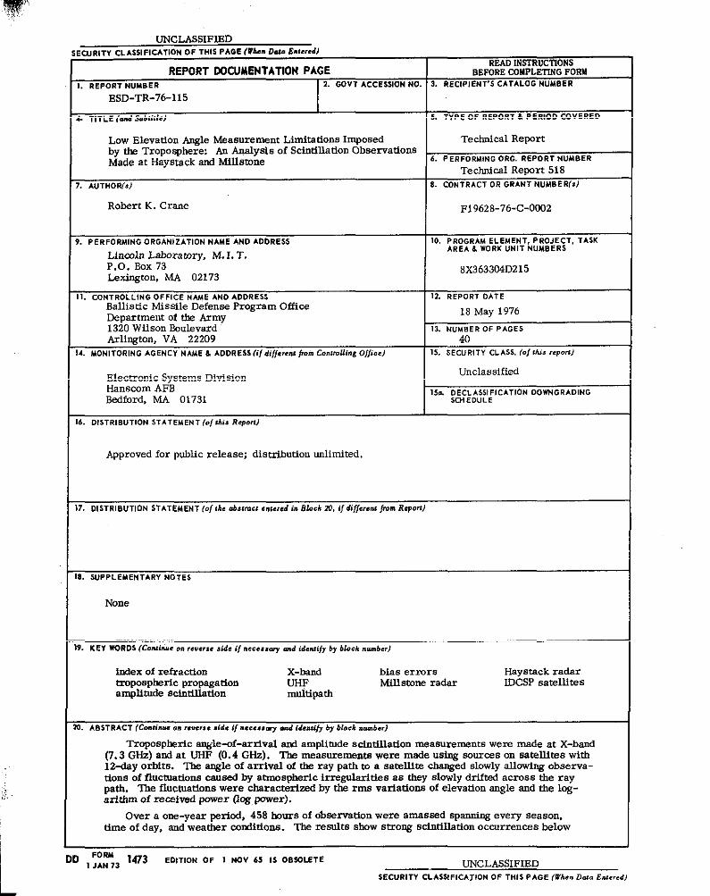
ESD-TR-76-115

TITLE [and Sub*itle)

Low Elevation Angle Measurement Limitations Imposedby fhe Troposphere: An Analysis of Scintillation Observation!Made at Haystack and Millsmne

AU THO R(s)

Robert K. Crane

PERFORMING ORGANIZATION NAME ANO ADDRESS

Lincaf.n Labcwatory, M. 1.T.P.O. Box 73Lexington, M 02173

CONTROLLING OFFICE NbW ANO ADDRESS

Ballimic Missile Defense Program OfficeDepartment of * Army1320 Wif son EmlevardArlington, VA 22209

MONITORING AGENCY NAME 6 ADDRESS (i/ di//ereU from ConlwUing Of/ice)

Elecmonic Systems DivisionHanscom AFBBedford, MA 01731

DISTRIBUTION STATEMENT (./ thisRqort)

Approved for public release; dimrib.tion unlimited.

READ INSTRUCTIONSBEFDRE CDUPLETING FOSS!

3. RECIPIENT’S CATALOG NUMBER

5. TYPE OF REPORT & PER1OD COVERED

Technical Report

6. PERFORMING ORG. REPORT NUMOER

Teclu!lcal Report 5188. CONTRACT OR GRANT NUMBER(S)

F19628-76-C-0002

10, PROGRAM ELEMENT, PROJEcT, TAsKAREA h WORK uNIT NUMBERS

8x363304D215

12. REPORT DATE

18 May 1976

13.N“ldBER OF PAGES

4015. SECURITY CLASS, (0/ Ibis rePorl)

Unclassified

15c- ~~C;;;;l[lCATlON DOWNGRADING

DISTRIBUTION STATEMENT (.{ th. abcract enwed in E1.mk Z3, if different /lore Report)

SUPPLEMENTARY NOTES

None

KEY WORDS (Continue on reverse side if naesmry md {daui/~ by blook number)

fmiex of refraction x-band bizw errors Haystack radartropospheric propagation UHF Miflstone radar IDCSPsatellitesampltmde scimflhion muitipati

ABSTRACT (Continua .?. wwr. e ride if .SG.S.V amd i&nti/~ by bkmk wmb.r)

Tropospkrfc .an$Je-of-arrfval axd amplitude mimflhdon measurements wem made at X-band(7. 3 GHz) and at UHF (0.4 GNz). Tbe measurements were made using sources on safdlffes with12-day O1bft.9. The ~le of arrivat of tbe ray Path m a satellite changed slowly alfowing observa-tions of flucmadons caused by atmospheric irregularities as they slowly drifted across tie raypath ‘fbe fluctuations were cbaracterfzad by the rms variations of elevation angle and the log-arfthm of received prover (fog power).

Over a one-yeax period, 458 twurs of obee-ation were amassed spanning every season,time of day, and weather conditions. The leSIdtB show SUOW sclntflfation Occurrences below

DD,%3 1473 EDITION OF 1 NOV 6S IS 00 S0i.EIEUNCLASSIFIED

SECURITY CLAS$IFICAJ1ON OF THIS PAOE (When D.,ta .?”ler,d,

UNCLASSIFIED

SECURITY CLASSIFICATION OF TtIIS PAGE @h.. Data Entered)

Q. ABSTU ACT (Con,lwd)

1 M 2“ elevation twgles cbaracferized by a number of random occurrexums of mtdtipaftt events thatproduce deep fades, angle-of-arrival flttctuationa, and depolarization of fk received s@tal. Thelog power fbtcmatlons ranged from 1 m 10 ds rms at elevation angles below 2° to less than 0.1 dsat elevation angles shve 10°. The elevation angle fluctuations ranged from 1 to 100 mdeg at ele-vation angles below 2° to less than 5 ntdeg at a 10” elevation angle. Comparable fluctuations helevaUon angle are expected for bias refraction correction mcdels based upon tbe use of surfacevalues of the refractive in&x.

uNCLASSIFIED

5EcuR17Y cLAs$l FlcATlON OF nils pAoe 6%. Dote E.teredl

.. . .. . ... . ”- w