Fluid Dynamics Research 1 (1986) 257-282

North-Holland

251

Low dimensional chaos in Boussinesq convection

Kenji URATA

Department of Astronomy, Faculty of Science, UnicersitJ of Tokyo, Bunkyo-ku, Tokyo I 13, Jupan

Received 18 July 1986

Abstract. Three-dimensional time-dependent Boussinesq convection has been simulated numerically and analyzed based on the theory of the dynamical system. The dynamical development of the system is simulated

numerically with Rayleigh number Ra = 2.104 and the aspect ratio I’, = r,, = 2; a chaotic solutions is obtained

for the Prandtle number Pr = 1, whereas the case Pr = 3 gives a periodic solution. The chaotic solution has an

initial transient state of quasi-periodicity which turns into a non-periodic state characterized by a large degree of

asymmetry in the flow pattern and a large vertical vorticity compared with that of the periodic solution. It is

found that the total heat flux averaged over the time is somewhat smaller in the non-periodic state than in

quasi-periodicity. Using the velocities and temperatures at a few particular points, the phase space has been

constructed for studying the dynamical behavior of the system. The dimension of the chaotic attractor is found

to be 3.3 with two positive and one possibly zero Lyapunov exponents. These chaos characteristics are

considered to be consistent with the appearance of the asymmetry of the flow pattern and of the vertical

vorticity in the chaotic flow.

1. Introduction and overview

The characteristics of time-dependent three-dimensional convection of high Rayleigh num- ber are so complicated that the mechanism and the dynamics have not been fully understood. The state of convective stability seems to bifurcate in a sequence of steady, periodic, quasi-peri- odic and non-periodic (chaotic) states as the control parameters are varied. Gollub et al. (1982) conducted convection experiments with water in a box and found various bifurcation sequences leading to chaos by changing the Prandtle number Pr. When the Rayleigh number Ra is just a little over the critical Ra,, the observed flow is time-dependent for a long time, showing a broad horizontal wave number spectrum.

Three-dimensional Boussinesq convection has been studied by a number of workers using numerical simulation. One of the most detailed studies of time-dependent convection is that of Lipps (1976). In his study, however, numerical simulation of thermal convection in large Rayleigh number was not carried out for a long enough time to study non-periodic solution in

detail. Graham (1975, 1976) found in his study on two dimensional compressible convection in a polytropic atmosphere that the realized horizontal wavelength differs from that which maximizes the total heat flux and that flow is subsonic in the parameter range he investigated. In his three-dimensional simulation, he discovered the existence of vertical vorticity o3 without imposing an initial angular momentum, but the dynamics of vorticity generation were not studied in detail. Lopez and Murphy (1985) studied the effect of w3 using the modal expansion technique and indicated its important role in the time-dependent behavior of thermal convec- tion. But the number of modes was not sufficiently large in these numerical analyses. Little has been fully understood of three-dimensional time-dependent convection. In particular, the physics of the transition from quasi-periodic convection to chaos needs to be clarified.

0169/5983/86/$7.50 0 1986, The Japan Society of Fluid Mechanics

Compressible convection can be well approximated by Boussinesq equations provided that the pressure or density scale height is much larger than the depth of the convective layer and the motion-induced fluctuations in density or pressure do not exceed the total static variations of these quantities in order of magnitude (Spiegel 1960). These conditions are not satisfied in the sun and stars, but for simplicity Boussinesq equations are used in this paper with fixed temperature and free boundaries.

Curry et al. (1984) and Mclaughlin and Orszag (1982) conducted numerical experiments on three-dimensional Boussinesq convection using Fourier and Chebychev expansions over the wide range of Rayleigh number Ra in order to study the transition to turbulence. They found the bifurcation sequences following Ruelle-Takens, a scenario in which three oscillatory excited modes cause broad band spectrum-that is, there are non-periodic solutions in moderate Ra. Yahata (1984, 1986) studied numerically the transition to chaos in Boussinesq convection with the Galerkin method and obtained non-periodic solutions. We are interested in what kind of properties these non-periodic solutions have from the viewpoint of the theory of dynamical systems. Expanding the solution of the Boussinesq equations in the series of proper functions and truncating the series, we obtain low dimensional ordinary equations, of which the simplest dynamical system leading to chaos is that of Lorenz (1963). Lorenz system has three Fourier modes, obtained from two-dimensional Boussinesq equations and leaving one mode for velocity and two modes for temperature. When the control parameter corresponding to the Rayleigh number is increased properly, a strange attractor emerges with topological dimension two, and the behavior of the system becomes non-periodic. It is important that such chaos exists without recourse to infinite degrees of freedom. Chaos is understood in this paper as deterministic non-periodic behavior with finite low dimensional degrees of freedom. Chaos can appear in relatively low dimensional systems and has been considered mainly in low dimen-

sional systems. But, in reality, fluid motion can have infinite degrees of freedom, and it is important to detect and identify the low dimensional strange attractors in realistic high dimensional systems using the result of numerical simulations.

Lyapunov characteristic exponents and generalized dimensions of the system which char-

acterize strange attractors are treated in this paper. If positive Lyapunov exponents exist, the distance between nearby trajectories expands exponentially and the attractor is called strange. A turbulent state composed of infinite oscillatory modes, as Landau (1954) once proposed, has

no positive Lyapunov exponents. Thus the idea of chaos is a new one in interpretating non-periodicity in dynamical systems. A dynamical system with positive Lyapunov exponents is sensitivity dependent on initial conditions. Benettin (1976) and Shimada and Nagashima (1979) have proposed numerical methods for calculating Lyapunov exponents in low dimen- sional dynamical systems, but their methods are not so practical in high dimensional systems. and the way to calculate Lyapunov exponents from a single temporal sequence of data was not known. Recently Wolf et al. (1985). Eckmann and Ruelle (1985) and Sano and Sawada (1985) proposed novel methods to calculate the Lyapunov exponents from numerical and experimen- tal data.

Quantities which characterize the geometrical fine structure of the attractor are called generalized dimensions: examples are Hausdorff dimension d,, pointwise dimension d, and characteristic dimension d,, (Farmer et al. 1983). It is difficult and impractical to calculate the Hausdorff dimension because the phase space needs to be partitioned into infinitesimal boxes. Another dimension used in our calculation is the pointwise dimension d, which will be discussed in Chapter 5.1.

The attractors with positive Lyapunov exponents should form Cantor sets because the attractors are in the finite area in the phase space. These attractors are what is called fractal, therefore, d,, d,, and d, are non-integers. These three dimensions are not the same in the mathematical sense (Grassberger and Procattia 1983) but are identical in the practical sense

K. Urafu / Low dimensional chaos in Boussrnesq convection 259

because errors arising from instrumental noises or insufficiency of data are larger than the differences among them. Only d, is treated in this paper. The integer part of these dimensions

denotes the least degree of freedom in the chaotic behavior, and the non-integer part denotes the intensity of disorder.

Detection of chaos has recently been investigated using various experimental and observa- tional data (Abraham et al. 1984). Original phase space can be reconstructed easily from single time series data (Takens 1981). It is possible to analyze experimental data from the dynamical system point of view. Roux et al. (1983) identified two-dimensional strange attractors using time series data of Bromine concentration in B-Z chemical reaction and determined the largest Lyapunov exponent by a one-dimensional map. Brandstater et al. (1983) detected the low (less than five) dimensional strange attractor in the CouetteeTaylor system. Methods of the dynamical system seem to be very useful for analysis of non-periodic data. Application to astrophysical data has been developed recently (Masaki et al. 1985) but analysis of experimen- tal data is not treated in this paper.

We simulate three dimensional Boussinesq convection for the cases of Rayleigh number Ra = 20000 and Prandtle numbers Pr = 1 and 3, and analyze the numerical data from the dynamical system point of view. The Rayleigh number Ra = 20000 turns out to be in the interesting range of the transition between quasi-periodic and non-periodic solution. Boundary conditions and parameter ranges are different from those of stars and the sun, but the results in this paper are thought to be useful for basic understanding of the three dimensional convection.

We describe the method of numerical simulation in Section 2, its results and interpretations

in Section 3, and the analysis of chaos in Sections 4, 5 and 6.

2. Basic equations and numerical methods

We examine three dimensional Boussinesq convection in a box heated from below. Cartesian coordinates are defined, with x, and x2 horizontal and x1 directed upwards. Gravity acts in the negative .x3 direction. The flow is confined in 0 < x, < T,d, 0 < x2 < &d and 0 < x3 < d. The normal velocity and tangential stress both vanish on all the plates, while the temperatures are fixed on the horizontal plates and are insulated on the vertical.

2. I. Basic equations

The density or pressure scale height is assumed to be much larger than d so that we can use the Boussinesq approximation, and the basic fields without flow are as follows:

dPB(X3) dx,

= -Pa(x,)g,

d2Tdxd = o

dx: >

PB(X3) = PO{1 - 4Gh) - T,)L (3)

where P,, pB and TB are the conductive solutions for pressure, density and temperature, respectively. The density and temperature at the top of the box are p0 and T,, g is gravity acceleration and a is the thermal expansion coefficient. Substituting P = P, + P’, p = pB + p’ and T = TB + 8’ into Boussinesq equations and using eqs. (l)-(3), we obtain the governing equations for P’, p’, 8’ and u,!. The prime denotes the variation caused by the flow. Using the

temperature difference AT and the distance d between two horizontal plates, and also thermal conductivity K. we can non-dimensionalize the basic equations:

au, ab,U,) 8P

at+-=--- ax, ax, + PrRat98,, + Pr3

ax; -

au -=o. (i. ,j=l.2.3) ax,

(5)

where the prime is omitted. Ra (= ~yg& AT/KU) and Pr (= V/K) denote the Rayleigh number and the Prandtle number, respectively. where v is the kinematic viscosity. Note that the

temperature T = 0 - x3 + constant from eq. (2). where the constant is chosen to be 2.

2.2. Numericd methods

Though the temperature boundary condition on the vertical plates is assumed to be insulated, it can be considered to be a periodic one with strong symmetry in the horizontal directions, so that Fourier expansion might be used in x, and x2 directions and finite meshes in x3 direction. Velocity and temperature fields are expanded:

U,(X,. X1. Xi. f)

U>(X,. X1. X3. f) I

24,(/. nr, _yj_ t) sin(k ,,,, .r) cos(k,,;v),

u3(x,, _X’-, x;. t) \=c c I

u,( 1. m. x3. t) cos( k,,,, r) sin( k,,,, r),

I

(7) \/i&I. ~rn~<M u,(l. m, Xj, t) cos(k[,,I.r) cos(k,,;r).

8(X,. X1, .X3. I) e( I, III, x3. t ) cos( k,,,, . I-) cos( k,,,, Y),

where k ,,,, = (71/T,, nm/rz). r = (.x1, x2 ). From divergence of eq. (6) and eq. (4). a Poisson equation for pressure is obtained as follows.

(8)

We expand the above equation with Fourier series and set its component of r.h.s. to

S(I. m, x3, t).

This equation is solved explicitly as:

P(,. m, X3, t)=f,,,,(.Yj)P(I. m. 0. t)+g,,~,(x,)P(I, I?I, 1. t)

I-,,,, ( x 3 ) ~. I kit,, I J “S( I, nz. i, t) sinh( ) k,,,, I i) dl

o

g/m ( -x 3 1 _~. I kin, I / ‘S(I. m. l. r) sinh( Ik ,,,, I.(1 -1)) dS. (TO)

\J where

fi,,(-X.3) = sinh{ I k,,, I(1 - x3)} sinh{ I k,,,, I x3 )

sinh I k,,, / ’ g/m ( x 3 ) = sinh 1 k,,,, (

K. Uruta / Low dimensional chaos in Boussrnesq c’onwc’t~on 261

The pressure components on the horizontal plates, P(1, m, 0, t) and P(I, m, 1, t), are de- termined by the boundary condition for velocities aur,Qx, = i3u2/i3.xi = 0. The { derivatives in

S(I, m, l. t) should be eliminated by integration by parts before numerical integration is

performed. The pressure is integrated smoothly using Spline functions so that incompressible condition (6) is well satisfied during the run.

We integrate Fourier components of eqs. (4) (5) and (8) using the DuforttFrankel difference scheme. The derivatives of space in _xj direction and time are replaced by center-dif- ferences.

Eddy viscosity coefficients vE(x3. t) = 0.08\i”u2( L, M, x3, t) /I k,,, 1 are introduced in order to take into account sub-grid scale motions, but this effect results in 3 or 4 percent

molecular viscosity and is found to be unimportant in our parameter range. The number of Fourier components, L and M, are both 12, and that of meshes is 26. Time

step At is set to 2 ’ 10e4, C.P.U. time per step is 0.6 second using an S-810 (super-computer).

3. Numerical results and its interpretation

A general linear stability analysis for the conductive solution of eqs. (l)-(3) is given by Chandrasekhar (1961). The critical Rayleigh number is Ra, = 27~~/4 and its horizontal wave

number is 1 k,,, 1 ’ = $T’. Gollub et al. (1980) found in one of their experiments with water that the flow bifurcates from quasi-periodic into non-periodic as Rayleigh number Ra is increased towards 29 Ra,. Referring to their results, we chose the value of parameters Ra = 30 Ra, + 20000 and r, = I’, = 2, and integrate eqs. (4)-(6) over the long time about two cases, that is, Pr = 1 and Pr = 3. In this case the most unstable horizontal mode (I, m) is (1. 1). The numbers of Fourier modes. L and M, are both chosen to be 12, and are sufficient to exclude the effect on the truncation of Fourier modes because the unstable modes having the largest wave numbers are (7, 0) or (0, 7).

(;I (;I (f) (;:) ‘f’

I I ) ) I I ) ) I r -II-l 2.00 3.00 4.00 5.co 6.00 7.00 8.00 9.00 10.00

TIME

Fig. 1. Time series of horizontally averaged total heat flux in Pr =l. The times indicated by the arrows (a)-(f) correspond to those in Fig. 2.

” .

t,, ..--~

~_--“-__*__,__“-.

i ) . __---i_-.-___________. ,

“__-_.~.~

_*)_~~

__1”~“__

(P)

3.1. In the case of Pr = I

263

Initial conditions are chosen to be u,(l, m, x3, 0) = f?(l, m, x3, 0) = lo-‘. Since the time step is restricted to the Courant condition AxJu? 2 At, we chose At = 2. 10p4.

The results of numerical simulations in Pr = 1 are shown in Figs. 1-5. Fig. 1 plots time series of total heat flux N averaged over horizontal directions at .x:, = 4. Time is non-dimensionalized

by the vertical thermal diffusion time Q( = d*/~). Two interesting things are found. The first is that a drastic change of variability occurs at t + 4.9. Non-linear terms come to play an important role in I> 0.6. The total flux N seems to be almost stationary at first but begins to oscillate (its period is 0.09). The oscillation is grown and damped and becomes quasi-stationary in 4.4 < f < 4.9. Then drastically the heat flux N begins to oscillate non-periodically from f = 4.9. Its amplitude varies from 2 to 9. Though the solution in the range of t < 4.9 is transient, it is remarkable that qualitatively different solutions (steady, quasi-periodic, steady, non-peri- odic) emerge in sequence with time. This result seems to indicate a typical three dimensional characteristic of convection. Lopez and Murphy (1985) found a similar behavior by allowing the motion with vertical vorticity wg in the method of modal expansion in cellular planforms. The growth of ti3 may provide the key mechanism for behavior like the above.

The second finding is that the flux N averaged over t < 4.9 is different from that averaged over t > 4.9. The mean value of N over 0.6 < t < 4.4 is 6.3, while that over 4.9 i t -=z 9.8 is 4.7. Convection does not always take place in such way as to maximize the heat transport as was widely believed, The irreguIar flow is less efficient in transporting heat than the laminar one. This result can be interpreted as follows. Convective flow transports too much heat at one time so that the thermal inversion layer in horizontally averaged temperature (YQ xj. t)) is formed in the middle (see Fig. 4 and Fig. 5). Therefore convective modes corresponding to the scale of this layer are damped, and the corresponding flux N is smaller in the middle than at the boundary. Then the stable layer disappears. In this way, the convective modes start growing again but remain small for some time because time is needed for growth. A too large convective flux causes the rapid formation of the temporarily stable layer, which decreases the efficiency

of heat transport in the time scale of the growing and damping time of the inherent convective modes.

Figure 2 shows time variations of the flow pattern on the horizontal plane at X? = 2. The time of (a)-(e) in Fig. 2 corresponds to the time indicated by the arrow in Fig. 1. Regardless of non-linear effect, the most linearly unstable mode (I, m) = (1, 1) dominates in Fig. 2(a). but

0.8

I,, 3*

0.6

0.4

0.2

0

l

Fig. 3. Time variations of the vertical 0.0 l 0 8

I I I I I t I vorticity. The ordinate w: is the ratio of 0 2 4 6 8 10 the maximum of the v&cal vorticity to

TTHE that of the horizontal.

264

2

t 8 0;

t 8 m’

I 8 m

265

:: dl I I 1 I I I , I 1 I I I I I I

8.57 8.61 8.65 6.69 8.73 a.77 5.81 8.85

TIME

Fig. 5. Time variations of the thermal inversion layr of (T) in Pr = 1.

comes to damp slowly (Fig. 2(b)), and at last is inferior to (1, 0) mode (Fig. 2(c)). This mode

transition corresponds to the qualitative change of properties as seen in Fig. 1 and to generation of the vertical vorticity w3 as we found in Fig. 3. Graham (1975) calculated numerically the two dimensionai compressible convection in full equations without approxima- tions to simulate the polytropic atmosphere and found that the horizontal scale of convection is

71 7.30 7.3a 7.46 7.14 7.62 ‘I,70 7.78 7.86 7.94 8.02 e.ra

TIME

Fig. 6. Time series of horizontally averaged total heat flux at x3 = : in Pr = 3

266 K. Uratu / Low dimensionul chaos in Boussinesy conr‘ectrvn

not that which maximizes the heat flux N. From Fig. 1 and Fig. 2, we found that N averaged over time for (1, 1) mode is 6.3 while that for (1, 0) mode is 4.7. Therefore it is concluded, as Graham found. that the typical horizontal scale of convection, which maximizes N, is not always realized.

Figure 4 represents time variations about the vertical profiles of horizontally averaged temperature (T) = (0) - xj + 2 and convective fluxes (~~8) (right figure) in the irregular motion over t > 4.9. As soon as too much heat flux is transported upwards, the inversion layer

is formed in the middle (Fig. 4(a)); thus convective flux is decreased (Fig. 4(b)) and (T) approaches the linear in x3 (Fig. 4(c)), but again large convection occurs (Fig. 4(d)), and at last the gradient of (T) as before is recovered (Fig. 4(e)). Lopez and Murphy introduced the vertical vorticity w7 in the modal expansion method and found that kinetic energy in the vertical turns into the horizontal, the vertical profile of (T) begins to approach a linear gradient and thus N is decreased. Figure 3 plots time variations of the ratio of the maximum of the vertical vorticity to that of the horizontal one. From this figure and Fig. 1 it is found that w3 plays an important role in the phase of irregular motions. As Lopez and Murphy say, convective solutions are divided into two types depending on the significance of the vertical vorticity w3. These two types of solutions have appeared in our calculation. Time variation of the temporary stable layer is also a good indication of a non-periodic behavior of convection as shown in Fig. 5 over 8.57 < t < 8.85. The time scales for formation, maintenance and disap- pearance of the stable layer are found to be the dynamical time d/u, - 0.01, the damping time of the convective mode and its growth time. respectively.

3.2. In the case of Pr = 3

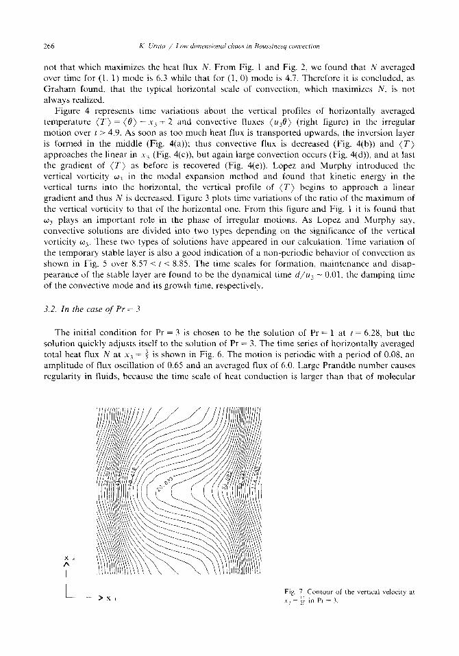
The initial condition for Pr = 3 is chosen to be the solution of Pr = 1 at t = 6.28, but the solution quickly adjusts itself to the solution of Pr = 3. The time series of horizontally averaged total heat flux N at x3 = : is shown in Fig. 6. The motion is periodic with a period of 0.08, an amplitude of flux oscillation of 0.65 and an averaged flux of 6.0. Large Prandtle number causes regularity in fluids, because the time scale of heat conduction is larger than that of molecular

Fig. 7. Contour of the vertical velocity at .x3 = i; in Pr = 3.

K. Urae2 / S.orv ~~rn~~~~i#na~ charts in Boussinesq coiwec~io~~ 267

viscosity for large Prandtle number, and its dissipation of energy is governed mainly by molecular viscosity.

Figure 7 represents the iso-contour of ui at x3 = @, and we have a nearly two dimellsiona~

268

x.3

Fig. 9. (T) versus xyi at I = 9.02 in Pr = 3.

convection. In spite of isotropy of external conditions in the X, and x2 directions, the solution results in a roll because of a small asymmetry in the initial condition.

Time variations of velocity fields on the vertical plane at x z = E are shown in Fig. 8. From

these figures, we see that the center of the circulating streamline moves around the vertical plane and returns to the original place. The periodic behavior caused by the circulation of the centroid is found to be a buoyant oscillation in the thermal inversion layer formed in the middle.

Figure 9 plots the depth xi versus the horizontally averaged temperature (7’) at t = 8.02. A thermal inversion layer exists, although the gradient of this layer is more gentle than that in the case of Pr = 1. This gradient oscillates with time, but the inversion layer never vanishes. With the equation of state, the buoyant frequency of this stable layer can be expressed as

fsvC /m (11)

rrrv( = 27T/fsv) can be expressed in units of the vertical thermal diffusion time

(12)

From Fig. 9 we see that d(T)/dx, + 0.04/0.4, and r Bv + 0.08, when Pr = 3 and Ra = 20000. This period agrees with the value 0.08 read from Fig. 8. The periodic solution in Pr = 3 is similar to that of the model by Moore and Spiegel (1966). Molecular viscosity cannot damp out the buoyant oscillation because the time scale (Pr-‘) of the former is larger than that of the latter.

4. Reconstruction of phase space

Infinite numbers of Fourier modes are needed in principle to solve eqs. (4)-(6) using expansion methods. Since the phase space of this system is constructed by Fourier modes, its

K. Urata / Low dimensional chuos in Boumnesq conwct~on 269

dimensions should be infinite in principle, In this paper, velocity and temperature fields are expanded using Fourier modes in horizontal directions and meshes in a vertical direction.

Therefore, u,(I, 172, x3. t) and e(l, m, x3. t) construct the phase space instead of

u,(x,, x2. x3. t) and 0(x,, x2, x3, t). Suppose a d-dimensional figure in a phase space constructed by u,( 1, m, x3, t) and 0(/, m, x3, t). It is known that this figure is embedded in reconstructed phase space of dimension equal to or larger than 2d + 1 (Takens 1980). This dimension is called embedded dimension. Arbitrary variables, such as velocity, temperature and heat flux at several particular mesh points, can reconstruct the phase space when a sufficiently large embedded dimension is requested.

In the case of observational or experimental data, the situation is quite different. We obtain usually a time series observation of a single quantity, such as X-ray counts or photon counts in astrophysical phenomena or the concentration of a particular species in chemical reactions, or the temperature at one particular point in fluids. Several kinds of simultaneous time series are rarely obtained. The way phase space is reconstructed from a ginel time series is as follows: Suppose a single time series { X(t,)} (i = 1.. . . , n). Make the d-dimensional vector D( t,) =

{ X(t,). X(t, + T’). X(t, + 27”) ,..., X(t, + (d- l)Z-‘)}. where T’ is arbitrary. This vector reconstructs the phase space of the observed system. Thus, this method enables us to calculate the quantities, such as non-integer dimensions, Lyapunov exponents and entropy of the embedded attractor and to link observations or experiments with the theory of chaos.

The time variations of velocity u1 at a particular point (+, 8, i) are shown in Fig. 10 when Pr = 1 and Pr = 3. Figure 11 represents 2-dimensional phase space reconstructed by u1 and U, at the same point. The attractor of a periodic solution (Fig. 11(b)) is found to be a limit cycle. In Pr = 1, the attractor is so complicated that we cannot know from Fig. 11(a) what properties it has. In section 5. we investigate its geometrical property (dimension) and its time variation (Lyapunov exponents). We can reconstruct the same two-dimensional phase space as Fig. 11 by using time series of a single quantity u,(*, &, $, t). Figure 12 plots (u,($, &, $, t), u,($, &, 1 3> t + T’)), where T’ = 0.01. We see that the phase spaces in Fig. 11 and Fig. 12 are topologically equivalent. However, T’ should be chosen to be an order of typical time scale of

(a)

(b) 14-

6-

2 1 I 7.3

I 7.5

I I I 7.1

‘a TIME *’

Fig. 10. Time series of u1 at (x 1._)iz,~~i)=(:,~.:):(a)Pr=1;(b)Pr=3.

270

15.00 3:.00 47.00 63.00

Fig. 11. Two dimensional pro.iectinn of the phase space reconstructed by ~1 and u2: (a) Pr = I. 6.18 < I cl 9.17: (b)

Pr = 3, 7.4 c: I <: X.0.

271

a

b

'1 -!X.UO -104.00 -88.00 -72.00 -56.00 -40.00

ua>

Fig. 12. Two dimensional projection of the phase space reconstructed only by uj; (a) Pr = 1, 7“ = 5.10-“; (b) Pr = 3, j-‘=5.1() 2.

the system (Spiegel 1985). When T’ is too small or too large, the structure of an attractor cannot be analyzed because of the loss of spatial correlations in large or small scales.

Since molecular or turbulent viscosities exist in fluids, the volume in the phase space contracts and tends to be zero so that the trajectories necessarily fall into the attractor. It is, however, not known that the topological dimension of this attractor is generally finite, because the dimension of the phase space in fluids is originally infinite (Eckmann and Ruelle 1985). But

in the special case of weak turbulence, the dimension of an attractor is expected to be very low. Since we do not know the topological dimension of the attractor in advance, we have to investigate the properties of the attractor by taking a reasonably high dimension for the phase space.

5. Properties of attractors

5.1. Dimension

Orbits in a strange attractor are sensitive in initial conditions and have at least one positive Lyapunov exponent. Since attractors are compact in general, strange attractors are fractals having structures like Cantor sets. Thus, the generalized dimension of a strange attractor is considered to be a non-integer.

Consider a point x0 in M-dimensional phase space. The probability with which points on the attractor are contained in the M-dimensional hypersphere with radius R centered at 1,) is proportional to R dl,(rsl) Pointwise dimension d, . is defined as d,(x,,) averaged over the attractor. Characteristic dimension d,, is defined by the fact that the probability with which the distance between arbitrary two points on the attractor is less than R is proportional to R”,. The dimensions d, and d, are more practical than the Hausdorff dimension because we do not have to partition the phase space and have only to treat data directly. Characteristic and pointwise dimensions are almost the same, so we consider the pointwise dimension d,.

Suppose a hyper-sphere BK( x,) with radius R centered at X, (i = 1. n(R)) on an attractor. where n(R) is the number of hyper-spheres. The probability P( BK(x,)) that a hyper-sphere BR(x,) contains points on an attractor is considered to be proportional to Rdpcx~); thus dp( x,) is defined as

d,>(x,) = lim log P(M.?))

R-O log R (13)

When d,(x,) is independent of x,, the pointwise dimension of an attractor can be defined. Averaging d,(x,) in all BR(x,), we set its value to d6:

n(R)

dk= 1 P(B,(x,)).d,(x,)== lim IcR) ,=I R-O log(l/R) ’

(14)

where P is assumed to be normalized, that is C:‘/:‘P(B,(x,)) = 1 and I(R) = - Cy’T’P( BR(x,)) . log(P( BR( x,))). The quantity Z(R) is the information when the scale less than R is indistinguishable; therefore lim x _ ,, I( R)/log(l /R) denotes information dimension. It is found from eq. (14) that the pointwise dimension db averaged in all hyper-spheres is equal to the information dimension. When P( BR(x,)) is independent of x,, we find that I(R) = log(n( R)), and then the information dimension is equal to the Hausdorff (fractal) dimension. In general, the inequality I(R) c log( n( R)) leads to the inequality d, (information dimension) < dn(fracta1 dimension) (Farmer et al. 1983).

As mentioned above, various dimensions exist and are related to one another. In this paper. we calculate the modified and simplified pointwise dimension di’. The dimension d6’ is

K. Urara / Low drmensmnal chaos in Boussinesq convection 273

defined by the running mean of d,(x,). We count the number of data QR(x,) in BR(x,) and average its logarithm denoted by (log QR):

(log Q,) = ; . 5 log Q,(T)> I=1

(15)

where n is the total number of data. Plot (log Q,) as a function of log R. The gradient of its line is di. The dimension d: is an average exponent which indicates the decreasing rate of the number of data in a hyper-sphere as its radius is decreased.

Since the dimension of the attractor is not known in advance, we have to set its phase space dimension m sufficiently large. If dz is not increased as m is increased, we conclude that m is sufficiently large. In contrast, if we know the topological dimension d of the attractor, (2d + 3)

dimension of the phase space is large enough to embed the attractor in.

5.2. Results of dimension measurements

We calculate non-integer dimension d, ” in the non-periodic case of Pr = 1 as shown in Fig.

10(a). The total number of data is 3600 and their time interval is O.OOlr,, where 7d is the vertical thermal diffusion time. The phase space is reconstructed by ul, ui and B at

(ax,, x2. ?3) = (& , &, :), (:, &, :), (A, &, i), (&. ii, ?), (A, A, 4). When m= I, only u,(&, &, 4) is used, an in other cases, the set of ui, uj and 0 are used. For example, when

m = 3, the phase space is reconstructed by uI, u3 and 8 at (&, &, i). The result is shown in Fig. 13. We find that the gradient in the region of small R

(0 -c log R < 1.2) is smaller than that of intermediate R (1.2 < log R < 1.7). This is caused by

trajectory passing through the center of the hyper-sphere because, in a small scale, the number of data is small and thus the number of trajectories passing through a hyper-sphere is small. In the region of large R, when the attractor is seen from a far, this compact set looks like a point

I I

-. c , I I I I

t’ ’ ’ ’ ,”

j

m -1

n; +++sfss

++++ v

++++ ++ ++++ ++

++++*f& fl 0 ++

++ &f+ _i+ ,h9,, N

2 u 2

=: ‘i . 1

++ II- 1-t

++ ++

+p +F ++ ++

-1 A+

+’ ,+I+ +t+

L + h ,++I +:+

“+“+’ +.+ ++ +++15

0 ++’ m d

++++ A$!!+

1 I I I I , r I I 0.60 I .20 1.60 2.00 2.40

LBGCR 1

Fig. 13. Probability (QR) that points on an attractor fall into the hyper-sphere with radius R. m denotes the dimension of the reconstructed phase space.

Table 1

Non-integer dimension d; read from Fig. 12. The gradients of the lines can be determined by the best fitted line in the

intermediate interval of R

m 1 3 6 9 12 15

dimension 0.99 2.31 3.00 3.24 3.31 3.36

and its dimension tends to be zero. It is found that the constant gradients exist in the intermediate R. Its gradient is a dimension of the attractor. From Fig. 13 we determine the best fit of the line and its gradients. Table 1 shows its gradient in each m. In the case of m = 1 or 3, since the dimension of the attractor is found to be almost the same as that of the phase space, it is not embedded. As m is increased from 9, the dimension is not increased and tends to be constant. We conclude d: = 3.3 + 0.06, as seen in Fig. 13. When m is sufficiently large, we find

in large R a different value of the non-constant grad&t from 3.3, but it is considered to be caused by the global structure of the attractor. not the local one.

5.3. Lyapunov characteristic exponents

Strange attractors have at least one positive Lyapunov exponent. Consider an infinitesimal hyper-sphere in the phase space. This sphere transforms itself into a hyper-ellipsoid with time. The exponential growth or contraction rates per unit time of the principal axes are Lyapunov exponents X, (i=l...., m), and we arrange them in the following order;

x, > x, 3 ‘. 3 A.,.

where m is the dimension of the phase space. Wolf et al. (1985) Eckmann and Ruelle (1985) and Sano and Sawada (1985) proposed a

method of calculating Lyapunov exponents when governing equations are not known and only time series data are available. In this paper, we simplify Wolf et al.‘s method and calculate the Lyapunov exponent using our numerical data with Pr = 1. Let us consider the problem of calculating k non-negative Lyapunov exponents. The volume V, of k-dimensional parallele- piped, which consists of (k + 1) data points in the phase space. varies with time like exp(X, + X, + . . * + A,) ’ t. Thus the exponential growth rates of a line (k = 1). an area (k = 2) and a volume (k = 3) lead to X,, h, + XZ, X, + h2 + X,, respectively, and Lyapunov exponents are actually determined. But there are generally three difficulties:

(1) Since the linearized equation of the system is not considered, we cannot treat the infinitesimal volume.

(2) In positive Lyapunov exponents, the volume of V, becomes too large and then overflows.

(3) The parallelepiped collapses into X, direction and the calculation becomes impossible. To avoid these difficulties, we continue to calculate them as follow (see Fig. 14 and see Wolf

et al.)

(a) We choose a fiducial point x(t,) at time t, and calculate the hypervolume along with a trajectory passing through this point. We also choose y,( to), y2( to), . . . , and yk( I,) near x( to).

(b) After a time 7, x(t,_,) and ~?,(t,_,) (j=l, k) move into x(t,) and JJ,‘(~,) (j= 1. k) respectively, where t, = ir (i = 1, TV,). We calculate the volume of a k-dimensional parallele- piped consisting of these points and denote them at t,-, and t, by V, (t,_,) and V[(t,) respectively.

(c) We search for s;( t,) satisfying the condition that the length of a vector { y,(t,) - x( t,)} is smaller than that of { J,‘( t,) - x( t,)} and that their angle c is smaller than E,~ which is taken here to be 0.3 radian. We choose y,(t,) as the smallest in angle E. When no vector satisfies these conditions, let J;‘(?,) = ~,(t,_,). The time 7 is the replacement interval.

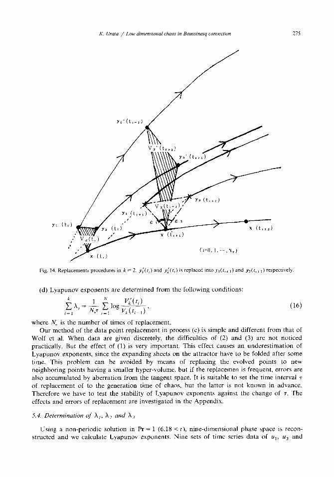
K. Urata / Low dimensional chaos in Boussinesq conveciion

Fig. 14. Replacements procedures in k = 2. y;(r,) and y;(r,) is replaced into y,(fz+,) and y2 (1, + 1 ) respectively.

(d) Lyapunov exponents are determined from the following conditions:

(16)

where N, is the number of times of replacement. Our method of the data point replacement in process (c) is simple and different from that of

Wolf et al. When data are given discretely, the difficulties of (2) and (3) are not noticed practically. But the effect of (1) is very important. This effect causes an underestimation of Lyapunov exponents, since the expanding sheets on the attractor have to be folded after some time. This problem can be avoided by means of replacing the evolved points to new neighboring points having a smaller hyper-volume, but if the replacemen is frequent, errors are also accumulated by aberration from the tangent space. It is suitable to set the time interval 7 of replacement of to the generation time of chaos, but the latter is not known in advance. Therefore we have to test the stability of Lyapunov exponents against the change of 7. The effects and errors of replacement are investigated in the Appendix.

5.4. Determination of A,, A, and A,

Using a non-periodic solution in Pr = 1 (6.18 < t), nine-dimensional phase space is recon- structed and we calculate Lyapunov exponents. Nine sets of time series data of u,, uj and

100.8 at three points, (x,. s2, x3) = (&, &. i), (k, &. G), ($5. &. 3) are used in this recon-

struction. We found the 3.3 dimensional attractor in Section 5.3 and thus regard the topological dimension as 4. Then the embedded dimension is 9 so that trajectories do not intersect each

other in the reconstructed phase space. Time interval At’ of data is 0.001 thermal diffusion time, and the total number of data is 3600.

Figure 15 shows exponential growth rates of V,, V, and V3 per unit time as a function of

TIHE(count number)

Fig. 15. Convergence of Lyapunov expo- rtents. The dimension of raxwstructed

phase space is 9.

K. Urata / Low dimensional chaos m Boussmesq convection 277

Table 2

Time interval 7 of replacements and Lyapunov exponents. c M = 0.3 (radian) and Ar’ = lo--‘. Data in the case where

Pr = 1 (6.18 -C t) are used

7 40.At' 60.At’ 80.Ar’ 120.At’

Line 1.7kO.3 1.3i0.2 1.3 * 0.4 0.7 * 0.2

Area 3.3 * 0.7 2.3 +0.2 2.3 f0.2 1.2kO.5

Volume 4.3kl.O 2.9 i 0.5 2.1+0.3 1.6 i 0.7

time. It is found that the values almost converge with time. It is read from these figures that h, = 1.1, h, +X, = 2.0 and h, +X, + h, = 2.5, and thus it is determined that X, = 1.1, X2 = 0.9 and X, = 0.5.

Results in changing r are shown in Table 2. When r = 60. At’ or 80. At’, Lyapunov exponents are stable so that we conclude that X, = 1.3 k 0.2, X, = 1.0 & 0.4 and h, = 0.4 _t 0.4. The value of X, is considered to be zero, which is the value in the direction along the trajectory. These results indicate that the attractor has two stretching directions and one neutral direction. and are consistent with its dimension.

6. Summary and brief discussion

6. I. Summary

Main results are summarized as follows.

1)

2)

3) 4)

5)

6)

Using Fourier expansions in a horizontal direction, we simulate three dimensional Boussinesq convection in a rectangular box with aspect ratio 2 in cases of Pr = 1 and Pr = 3 (Ra = 20000). We have obtained a non-periodic solution in Pr = 1 and a solution with buoyant oscillation with period 0.08 in Pr = 3. In Pr = 1, after a long period of transient behavior, sudden chaotic behavior appears. The three dimensional convection is more complicated than hitherto expected. In Pr = 1, by comparing a chaotic state with a transient, we find that the horizontal wavelength in this case differs from what would maximize the heat flux. In comparison with Pr = 1 and Pr = 3, we find that advection terms cause irregularity. Phase spaces in fluid systems are reconstructed by velocities and temperature at a few selected mesh points. The dimension of the attractor in an irregular solution is found to be 3.3 + 0.6. Lyapunov exponents h,, X, and X, are found to be 1.3 * 0.2, 1.0 + 0.4 and 0.4 _t 0.4, respectively. These values are consistent with the dimension 3.3.

From 4) and 5), the non-periodic behaviors in Pr = 1 are concluded to be chaotic, and its attractor is strange.

6.2. Brief discussion

It is interesting, particularly in the fields of the sun and the atmosphere, to investigate the relation between the horizontal wavelength and the total heat flux. For clear understanding, we have to make more numerical simulations by changing aspect ratios. Since the horizontal length is considered to be highly dependent on the vertical boundary conditions, we have to choose as large an aspect ratio as possible. Then more Fourier modes are needed so that in the three dimensional convection the simulation becomes more difficult because of large C.P.U. time.

As considered in Section 4, it is thought here that the phase space of fluid systems with

partial derivatives is constructed by velocities and temperature at particular points or Fourier modes. In our results obtained here, Fourier coefficients corresponding to large scales are dominant and that of small scales can be neglected, so that the phase space constructed by Fourier modes seems to be different from that reconstructed by velocities or temperatures at particular mesh points. We need to take into account what kind of variables should be used in reconstructing the phase space.

The two dimensional Lorenz attractor has one positive Lyapunov exponent, while the strange attractor obtained here in Pr = 1 has two positive Lyapunov exponents, but their values are smaller than that of the Lorenz. The relation between the dimension or Lyapunov exponents and the development of turbulence should be studied in future.

The integer part of non-integer dimension denotes the least degrees of freedom in non-peri- odic or chaotic behavior. A 3.3 dimensional attractor (three degrees of freedom) was obtained in Pr = 1. We conjecture from Figs. 8 and 9 that three degrees of freedom correspond to three modes in fluids, that is. a convective mode (vertical circulation), a horizontal circulation and a gravity wave in the thermal inversion layer.

Appendix

A.1. Definition of the lurgest Lyupunor: exponent A,

We consider two points x(t’) and y,( t’) on the attractor in the M dimensional phase space R,“. We suppose that the governing ordinary equation can be made discrete using a time increment At and the mapping f govern the system.

x(t:+,)=f(x(t;)) (i=O. l,..., (L-l’).k4), (1)

where time t,’ = i At. L and k’ are positive integer and L 1 k’ are the number of data points on the attractor. Equation (1) govern v,( t(‘). too. If k ’ time steps are combined, eq. (1) results in

x(t,+,)=f”‘(x(t,)) (i=O,l...., L-l), (2)

where t, = i( k’ At) = i7.

The largest Lyapunov exponent h, can be defined by

x, = i I J?Ct,) - X(lL) I

,.,(f(i)+x(I,,) EL tlr log\ l’*(f,) - x(t,,) 1 lim

. (3)

Let Jacobian of fh’ at t, be J,.

J,- g(x(t,),

Since ~+,(t,_,) - x(t,_,) can be considered to be infinitesimal, y,(t,) - x(t,) is expanded from eqs. (2) and (4).

Y,(t,) -x(t,> =f”‘{(s&. 1) -x(U) +x(&)) -fh’M-l))

= J, , ( yl(t,_,) - x(t,-,)) + (higher order). (5)

From eq. (5) using a vector 6 -y,(to) - x(to) at t = t(,, eq. (3) can be represented as follows:

We regard eq. (6) as the definition of h, hereafter.

K. I/rata / Low dimensiond chaos in Boumnesq conoect~~n 279

A.2. Effects of replacement

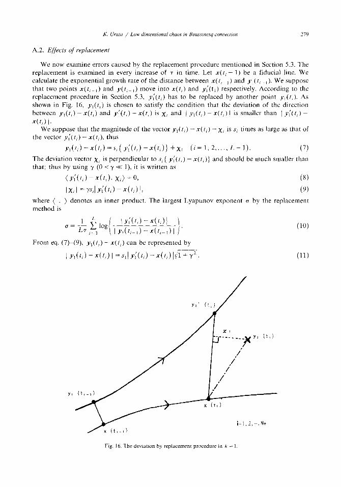
We now examine errors caused by the replacement procedure mentioned in Section 5.3. The replacement is examined in every increase of r in time. Let x( t, - 1) be a fiducial line. We calculate the exponential growth rate of the distance between x( t, 1) and Y, (t, _ ,). We suppose that two points x(t,_l) and y(t,_,) move into x(t,) and Y;(t,) respectively. According to the replacement procedure in Section 5.3, y;(t,) has to be replaced by another point y,(r,). As shown in Fig. 16, y,(t,) is chosen to satisfy the condition that the deviation of the direction between y,(t,) - x(t,) and y;(t,) - x(t,) is x, and ( y,(t,) - x(f,) ( is smaller than [ y;(t,) -

x(t,> 1. We suppose that the magnitude of the vector yr( t,) - x( t,) - x, is S, times as large as that of

the vector Y,‘( t,) - x(t,), thus

y,(t,)-x(t,)=s,{y,‘(t,)-x(t,)} +x, (i=1,2 ,..., L-l). (7)

The deviation vector x, is perpendicular to s, { y;(t,) - x(t,)} and should be much smaller than that; thus by using y (0 < y -=x l), it is written as

(Y;(t,) -xkL xc> =o, lx,1 =Ys,lY;(4-4t,)l~

where ( , ) denotes an inner product.

method is

(8) (9)

The largest Lyapunov exponent u by the replacement

L

u = + ,x log :

lYlw-44)l

?- r=l I Yr(t,?l> -4rl-I> I

From eq. (7)-(9), yI(t,) - x(t,) can be represented by

(10)

I Yl(f,) - x(t,) I = St1 Ylw - x(t,> 167. (11)

Fig. 16. The deviation by replacement procedure in k = 1

280 K. (/rata / Low, dimensional chaos tn Bouminesq conuectron

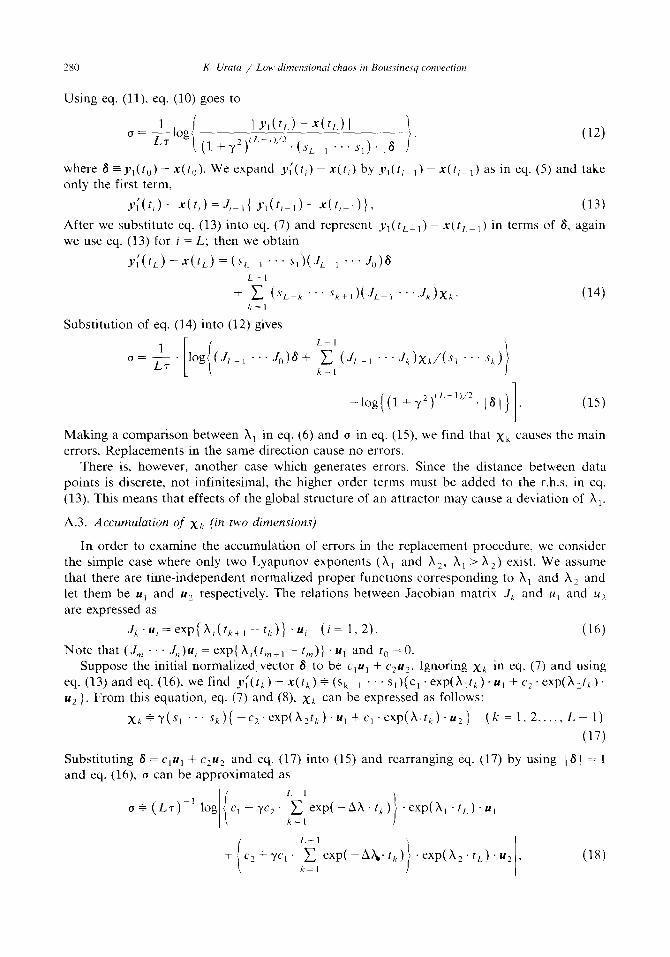
Using eq. (ll), eq. (10) goes to

/ I v,(t1.> - X(lL) I t u = J-log

Lr \ (l+y2)(L-1),‘2.(,gL_, .‘. s,). (81 ) ’ (12)

where S -y,(t,) - x(t,). We expand y;(r,) - x(t,) by y,(t,_,) - x(t,_,) as in eq. (5) and take only the first term.

Y;(t,) -x(t,) =4-l{ Yl(t,-1) -x(t,-I)}. (13)

After we substitute eq. (13) into eq. (7) and represent y,(t,_,) - x(t,,_,) in terms of S, again we use eq. (13) for i = L; then we obtain

Y;(tr.) - X(tL) = ($I./ 1 ‘. . s,)(J, -1 ‘. . 4,)s L-l

+ c (XL-h ... ~k+l)(JI_/l . . ..Jk>X.. (14) /,=I

Substitution of eq. (14) into (12) gives

1 (T= -.

LT

-log((l +y2)(‘--‘)‘2. 181) . I

(15)

Making a comparison between h, in eq. (6) and u in eq. (15) we find that xk causes the main errors. Replacements in the same direction cause no errors.

There is, however, another case which generates errors. Since the distance between data points is discrete, not infinitesimal, the higher order terms must be added to the r.h.s. in eq.

(13). This means that effects of the global structure of an attractor may cause a deviation of X,.

A.3. Accumulation of xk (in two dimensions)

In order to examine the accumulation of errors in the replacement procedure, we consider the simple case where only two Lyapunov exponents (X, and X2, X, > h2) exist. We assume that there are time-independent normalized proper functions corresponding to Xi and X2 and let them be u, and uZ respectively. The relations between Jacobian matrix .Jk and u, and uL are expressed as

Jh.u,=exp{X,(t,+,-f,)}.u, (i=1,2). (16)

Note that (J,, . . J,l)u, = exp{ Xl(tm+, - t,,)} . u, and t0 = 0. Suppose the initial normalized vector 6 to be c,ui + czu2. Ignoring x/, in eq. (7) and using

eq. (13) and eq. (16) we find y;(tk)-~(tX)i (sk_, ... s,){cI .exp(X,t,).u, + c,~e~p(~~t~)~ uz}. From this equation, eq. (7) and (8). xk can be expressed as follows:

xkfy(.s, . ..s.){--“2.exp(X,rh).u,+c, .exp(h,tl,).u2} (k=l,2 ,.... L-l)

(17)

Substituting 6 = c,ui + cZuZ and eq. (17) into (15) and rearranging eq. (17) by using ) 6 ( = 1 and eq. (16). u can be approximated as

II

L-1

a+ (LT)_’ log c,-yc,. c exp(-Ah-i,j)-cnp(h,.t,_).u, k=l

L-l

c,+yc,. c exp(-Ab.tk) .exp(X,+t,).u, k=l

(18)

K. I/rata / LOW’ dwnensional chaos in Boursrnesq conwction 2x1

where AX = A, -h, > 0) and $1 + y2 is set equal to 1. When t, = k7, we can calculate the

summation; thus

-(2L7)_’ . log(1 - A)2, (19)

where A = exp( - AX. T). If X, # X2 we find that errors caused by x,, do not accumulate and u tends to X,. But if h, + h?. u does not tend to X,. Eq. (19) shows dependence of u on the initial separation vector 6. If A +z 1, eq. (19) is

u converges h, irrespective of the deviation vector, whereas in the paper of Wolf et al. the error in h, is dependent on an angular change in replacements.

Acknowledgements

I would like to thank Dr. W. Unno for his guidance and valuable advice, and thank Dr. M. Kondo for his encouragements. Dr. T. Nakano was kind enough to discuss our numerical

results. I am very grateful to Dr. I. Masaki and Dr. T. Yoneyama for Sections 4 and 5. The numerical calculations were made with Facom M-380 in Nobeyama Radio Observatory and

S-810 in the Computer Center of University of Tokyo.

References

Abraham, N.B.. Gollub. J.P. and Swinney, H.L. (1984) Testing nonlinear dynamics, Physica Dll, 252.

Benettin, G., Galgani, L. and Strelcyn, J.M. (1976) Kolmogolov entropy and numerical experiments, Ph~,:r. Rec. A/4.

2338.

Brandstater. A.. Swift, J., Swinney. H.L., Wolf, A., Farmer, J.D., Jen. E. and Crutchfield, P.J. (1983) Low dimensional

chaos in a hydrodynamic system, Phys. Rev. Lett. 51, 1442.

Chandrasekhar, S. (1961) Hydrodynamic and Hydromagnetrc Stability (Dover, New York) 35.

Curry, J.H., Herring, J.R., Loncaric, J. and Orszag, S.A. (1984) Order and disorder in two- and three-dimensional

Benard convection, J. Fluid. Mech. 147, 1.

Eckmann, J.P. and Ruelle, D. (1985) Ergodic theory of chaos and strange attractors, Rev. Mod. Phys. 57, 617.

Farmer, D., Ott, E. and Yorke, J.A. (1983) The dimension of chaotic attractors, Physica 70. 153.

Gollub, J.P. and Benson, S.V. (1980) Many routes to turbulent convection, J. Fluid. Mech. 100, 449.

Gollub, J.P., McCarriar, A.R. and Steinman, J.F. (1982) Convective pattern evolution and second instabilities, J. Nurd.

Mech. 125, 259.

Graham, E. (1975) Numerical simulation of two-dimensional compressible convection, J. F/uid. Mech. 70, 689.

Graham, E. (1976) Compressible convection, Lecture Notes in Physics 71, 151.

Grassberger, P. and Procaccia. 1. (1983) Measuring the strangeness of strange attractors. Phl>sica 90, 189.

Landau. L.D.. Lifshitz, E.M. (1959) Fluid Dynamics (Pergamon Press, New York), 106.

Lipps, F.B. (1976) Numerical simulation of three-dimensional Benard convection in air. J. Fluid. Mech. 75, 113.

Lopez, J.M. and Murphy, J.O. (1985) Non-steady time dependent Rayleigh-Benard convection, Monash Univ.,

preprint.

Lorenz, E.N. (1963) Deterministic nonperiodic flow, J. Atoms. SCL 20, 130. Masaki, K.. Yoneyama, T., Unno, W., Urata, K. and Kondo, M. (1985) Time series analysis of Cygnus X-l, Proc.

Cosmo-sphere Symp. 54.

McLaughlin, J.B. and Orszag, S.A. (1982) Transition from periodic to chaotic thermal convection, J. Fluid. Mech. 122.

123.

Moore, D.W. and Spiegel, E.A. (1966) A thermally excited non-linear oscillator, Astrophys. J. 143, 871.

282 K. Urata / Low dmensional chaos in Boussinesq convecmn

Roux, J.C., Simoyi, R.H. and Swinney, H.L. (1983) Observation of a strange attractor, Physica 80, 257.

Sano, M. and Sawada. Y. (1985) Measurement of the Lyapunov spectrum from a chaotic time series, Phys. Rev. Letr.

55, 1082.

Shimada. I. and Nagashima, T. (1979) A numerical approach to ergodic problem of dissipative dynamical systems.

Prog. Them. Phys. 61, 1605.

Spiegel, E.A. and Veronis, G. (1960) On the Boussinesq approxtmation for a compressible fluid, Asrrophys. J. 131. 442.

Spiegel, E.A. (1985) Cosmic arrythmias. Proc. NATO Workshop on Chaos UI Astrophysics. R. Buchler. J. Perdang and

E.A. Spiegel, eds. (Reidel, Boston).

Takens, F. (1981) Detecting strange attractors in turbulence, Lecture Notes in Math. 898, 366.

Wolf, A.. Swift, J.B., Swinney, H.L. and Vastano, J.A. (1985) Determining Lyapunov exponents from a time series.

Physica 160. 285.

Yahata. H. (1984) Onset of chaos in the Rayleigh-Benard convection, Prog. Theor. Phys. Suppl. 79, 26.

Yahata. H. (1986) Evolution of the convection rolls in low Prandtl number fluids, Prog. Theor. Ph.vs. 75, 790.