UNIVERSITY OF GRONINGEN

FACULTY OF MATHEMATICS AND NATURAL SCIENCIES

KAPTEYN INSTITUTE

BACHELOR’S THESIS

Looking for sulfur in the Sculptordwarf spheroidal galaxy

Author:Michael ZURAVLOVS

Supervisor:Prof. Eline TOLSTOY

A thesis submitted in fulfillment of the requirementsfor the degree of Bachelor of Astrophysics

in the

Kapteyn Astronomical Institute

August 23, 2016

iii

UNIVERSITY OF GRONINGEN

AbstractFaculty of Mathematics and Natural Sciences

Kapteyn Astronomical Institute

Bachelor of Astrophysics

Looking for sulfur in the Sculptor dwarf spheroidal galaxy

by Michael ZURAVLOVS

Sulfur is a poorly studied element in individual red giant branch starsoutside the Milky Way. In the Galactic halo red giant branch stars the el-ement has been shown to behave like other α-elements. High-resolutionESO VLT/FLAMES/UVES spectra was used to look for the S I triplet at9213, 9228, and 9238 Å for 8 individual stars in the Sculptor dSph. This in-volved significant data reduction, namely sky removal, telluric corrections,helio-centric corrections and co-adding same stars spectra. Convincing ev-idence of the presence of sulfur in the stars was not found.

1

Chapter 1

Introduction

We are living on the Planet Earth. Our planet is turning around a star thatwe call the Sun. Sun is the central object of our solar system. Among 200billion stars in our Milky Way galaxy our solar system is not the only one,despite that, it is impossible to see any other solar systems with a naked eye.Behind the Milky Way a great amount of different types of galaxies exist:spirals, ellipticals, irregulars, where each of them has their own brightness,size, mass, opacity, velocity, age. No galaxies are the same. Galaxy type ofinterest in this project is a Dwarf Spheroidal Galaxy (dSph).

dSphs are one of the simplest galaxies that are known by now. Spectraof individual dSph red giant branch (RGB) stars can be studied and metalcontent can be determined that gives the information on the chemical evo-lution that in turn provides the understanding of a galactic formation andevolution. Typically, dSphs has very metal poor stars and unique ability ofloosing gas instead of attracting it (Mateo, 1998), thus amount of HI gas isnegligible. Also, dSphs characterize roughly spheroidal shape and old starsin it. Usually, these galaxies are found in the vicinity of large galaxies, suchas ours.

Nearby galaxies like dSph can be studied star by star, which belong tothe Local Group (Figure 1.1) that is a group of galaxies that covers a di-ameter about 2 Mpc. Milky Way and Andromeda are the most massivegalaxies in the Local Group. Since the majority of galaxies not just in theLocal Group but in the whole Universe are Dwarf Galaxies there is a greatinterest in examining them in detail (McConnachie, 2012). The number ofstars in a dSph could be calculated to be around 4 millions. This numberis very small in comparison with the number of stars in galaxies such asMilky way. At greater distances individual stars cannot be observed andespecially high resolution spectra cannot be taken. dSphs are being exam-ined in the Local Group, a good laboratory for astronomers.

The interest in dSphs has raised after the pioneer work of (Aaronson,1983). In the same year in a theoretical work of (Faber, 1983) large amountof non-luminous matter in the dSphs due to the high mass-to-light ratio(even higher than in globular clusters) was discussed, of individual RGBstars was first. Measurements of metallic abundances were done by (Shetrone,2001; Shetrone, 2003; Geisler, 2001). Chemical evolution of the dSphs hasnot been affected by very massive star judging by α-element abundance(Tolstoy, 2003).

2 Chapter 1. Introduction

FIGURE 1.1: The approximate observed locations and sizesof a few galaxies in the Local Group. Milky way is on theright, Andromeda is on the left. It is just a representationof the scale of the Local Group. Image from (Hammonds,

2013).

CMDs constructed from dSph’s stars were analyzed that lead to the con-clusion that dSphs are composed of composite stellar populations. Exam-ination of different stars in the RGB have shown that Sphs have internalmetallicity dispersion (Suntzeff, 1993; Smecker-Hane, 1999). More preciseinformation about stars metallicity can be found by analyzing stars high-resolution spectra. But first, it is important to consider the possible originof dSphs stars.

Cold gas clouds that overcome, so called, Jeans limit collapse into astars, where all the chemical elements in the Universe that are heavier thanlithium are being created. In some time, "metals" (elements heavier thanHe) are dispersed into the stars surroundings mostly due to energetic su-pernovae explosions and stellar winds. It is known, that Type II supernovaemostly produce so-called α-elements (O, Ca, Mg, S, Si and Ti), when TypeIa supernovae synthesize Fe group (Fe, Co, Ni and Zn). Thus, a new gener-ations of stars with a fraction of metals that increases with time are formedfrom enriched gas. Since photospheres retain the most of chemical compo-sition of the stars birth environment, spectral analysis (star’s spectrum is aspectrum of its photosphere) can give a clue about the chemical enrichmenthistory of the stars and systems they are in.

One remarkable tool, that efficiently obtains spectra is a multi-objecthigh resolution (HR) spectrograph FLAMES/UVES of the ESO Very LargeTelescope (VLT) in Chile (Pasquini, 2002). FLAMES/UVES has resolutionof about 40,000. The spectrograph can cover from 3000 to 11000 Å, however

1.1. The Sculptor dSph galaxy 3

it can cover a few thousand Ångström per spectrum. Such an instrumentcan collect a useful data that can be reduced by an automatic pipeline, thatsimplifies the reduction process.

The first results on stars in dSph from the UVES spectrograph wereobtained during the commissioning the instrument in the 2000 (Bonifacio,2000). After this more studies were published, but with low number of starsprobed (Shetrone, 2003; Bonifacio, 2004; Geisler, 2005). Worth mention-ing that not only UVES instrument was used for dSph observations, alsothe Keck I telescope and the High Resolution Echelle Spectrometer (HIRES)was involved in the observations of dSph galaxies (Shetrone, 2001). It wasproblematic to observe faint dSphs stars because up to 5 hours of exposuretime per star is required. The problem with low number of observationswas solved when HR spectrographs with multiplex capabilities come insight (FLAMES multi-fiber facility for UVES (Pasquini, 2002)). Larger sam-ples of stars measured in the same period of time boosted the productivity(Monaco, 2005; Sbordone, 2007; Monaco, 2007; Letarte, 2007; Skuladottir,2016).

In this thesis the data from the Sculptor dSph galaxy collected by theFLAMES/UVES was used.

1.1 The Sculptor dSph galaxy

The dSph galaxy studied here is the Sculptor dSph. This well studied lowsurface brightness galaxy is located in the constellation of Sculptor rela-tively close by in the Local Group. The Sculptor dSph is located at highGalactic latitude b = -83◦ and longitude l=287.5◦ (Figure 1.2). The discoveryof the galaxy was made by (Shapley, 1938). Despite the fact that the galaxywas discovered almost a century ago, new technological advances and im-provements regarding the resolution of observations help to discover moreand more stars, and analyze them.

The basic properties of the dSph Sculptor galaxy are summarized in Ta-ble 1.1, data was taken from the NASA/IPAC Extragalactic Database. Apicture of the Sculptor dSph in optical that was obtained from SIMBADdatabase is shown on Figure 1.3, in fact, even if a collective structure ofstars is hardly seen, this constellation of stars is the Sculptor dSph since astars in the galaxy have a measurable bound.

Since the dSph Sculptor galaxy is close enough to us it is possible toobserve the brightest individual stars, infer their magnitudes and createCMDs. The first studies of star formation history (SFH) of the galaxy hasbeen carried by using CMD. The first interpretations after analyzing firstCMDs by observing the RGB stars of the dSph Sculptor galaxy has led tothe interpretation that the galaxy has small star formation, mainly old, butwith main-sequence turn-off stars as young as 5 Gyr (Da Costa, 1984). Thephotometric analysis of the Sculptor galaxy taken with the Hubble SpaceTelescope WFPC2 tells that the absence of faint stars V=21 mag. rules outthe possibility of star formation more recent than 2 Gyr ago (Monkiewicz,

4 Chapter 1. Introduction

FIGURE 1.2: Milky Way’s dwarf galaxy satellites in Galacticcoordinates. Blue circles are classical dwarf galaxies, andred circles are the SDSS ultra-faint satellites. The imagingfootprint of SDSS DR8 is shown in grey. The Sculptor dSphat longitude l=287.5◦ and latitude b = -83◦. From Belokurov

et al. (2014).

TABLE 1.1: Properties of the Sculptor dSph (NASA/IPACExtragalactic Database). Mass and mass-to-light ratioare taken from (Battaglia, 2013). Distance is taken from

(Pietrzynski, 2008).

Property Value

Radial velocity (km/s) 110 ± 1Major Diameter (arcmin) 39.8Absolute magnitude and filter -10.97 ± 0.51 VMass (inside 1.8 kpc)(M�) 3.4 ± 0.7 · 108

Mass-to-light ratio (inside 1.8 kpc)((M/L)�) 158 ± 33Distance (kpc) 86 ± 5

1.1. The Sculptor dSph galaxy 5

FIGURE 1.3: The Sculptor dSph galaxy negative picture inoptical was taken from SIMBAD database by Aladin Litesoftware. A red cross is the center of the galaxy. Angular

size is 25.7 arcmin.

1999).

The star formation history (SFH) was qualitatively determined by thework of (Boer, 2012). Figure 1.4 shows star formation rate (SFR) at each ageof the galaxy and the metallicity distribution function (MDF) for numberof stars. Turns out that the Sculptor dSph is not experiencing any signif-icant star formation for about 6 Gyr from now. But before, between 14and 7 Gyr ago 7.8×106 M� was formed within a radius of 1.5 kpc. Themost metal-rich, young galactic stars are more centrally concentrated, whenmetal-poor are present at all radii. The most of the galaxy stars have metal-licities [Fe/H] equal to -2 +/- 0.5 dex. It means that the metallic content ofthese stars is much less than in the Sun and stars are much older. Thus, theSculptor dSph could be very helpful in studying ancient stellar populations.

Dwarf Abundance and Radial-velocity Team (DART) (Tolstoy, 2006) madea good progress towards understanding that the kinematic and evolution-ary processes of the Sculptor dSph are not as simple as it was thought andthe Sculptor dSph is not a "building block" of the largest galaxies in the Lo-cal Group. The galaxy kinematics has been well studied on a sample of 470stars from low resolution spectra (R-6500) (Battaglia, 2008). Over more than15 years DART has been presenting results of abundances of different ele-ments in the galaxy. The latest work of (Skuladottir, 2016) was dedicated tosulfur, zink and carbon abundances measurement, also this work was thefirst comprehensive study of the sulfur abundances in the galaxy. The maingoal of this thesis is to expand Asa’s work by looking for an abundances of

6 Chapter 1. Introduction

FIGURE 1.4: Left graph: Star formation history of the Sculp-tor dSph galaxy. Right graph: The best matching simulatedMDF (green) solid histogram and observed MDF (red) his-togram from spectroscopic observations. From (Boer, 2012).

TABLE 1.2: Overall number of observations of each star indifferent wavelength ranges.

Star 4770 - 5800 Å 5820-6830 Å 6730-8540 Å 8650-10420 Å

UET0248 8 8 10 10Ut125 2 2 10 10UET0235 5 5 10 10UXET0324 8 8 10 10UET0381 8 8 10 10UET0360 8 8 10 10UET0409 8 8 10 10UCET0136 6 6 0 0

sulfur in different stars.

In total 36 different observations in different bands (4770, 5820, 6730,8650 Å) in the period between 2012-07-15 and 2013-11-18 were obtained. 8different bright and relatively cool RGB stars from the Sculptor dSph galaxywere observed and analyzed. This 8 stars were chosen randomly except theUt125 star, since this is a telluric star (very bright source star). Random se-lection of RGB stars is a good choose for obtaining good sampling of thewhole population. Repetitive observation of the same stars were made,since it helps to get rid of bad pixels, distinguish cosmic rays, tackle verynoisy data and achieve more accurate results. Number of observations ofeach star in different wavelengths are summarized in the Table 1.2. Notethat I was provided with the stars data already pipeline processed and Iwasn’t observing by using VLT by my own.

The importance of having accurate stars data ensures qualitative andfruitful data analysis. In spectroscopic analysis lines may or may not befound. It can give an ideas about the evolution of the stars and its origin.Also, knowing the origin of a Local Group galaxy stars the evolution of

1.2. Sulfur 7

Milky Way could be determined.

1.2 Sulfur

Sulfur is an α-element, means that it is one of the most abundant isotopesthat is made out of the He-nuclei. Sulfur is one of the most challenging el-ement among all α-elements in the Local Group to study and the very firstsurvey of sulfur abundances in individual stars in dSph was made by (Sku-ladottir, 2016). Previously, sulfur abundances were examined only withinthe Milky Way. The paper of (Jenkins, 2009) tells that sulfur most likely isnot bound onto interstellar dust, therefore, sulfur abundances in stars couldbe compared to measurements in ISM, like damped Lyman-α absorptionsystems. It makes more interesting to inspect the element more attentively.

The first clues of α-element scarcity in dSph galaxies compared to theMilky Way halo or disc was recorded by (Shetrone, 1998; Shetrone, 2001;Tolstoy, 2003; Tolstoy, 2009). At low [Fe/H], the ratio [α/Fe] is the same ineach galaxy (Figure 1.5). As [Fe/H] starts to increase, the ratio [α/Fe] indSphs evolve down to lower values.

The star-formation timescale in a system is traced by [α/Fe]. Super No-vae Type II (SNe II) that occur after the explosion of massive stars in 107

yr after formation is believed to be the most important production site forthe α-elements like Si, Ca, S and Ti. The ratio of Type II Supernovae mas-sive stars to Type Ia supernovae intermediate mass binary systems withmass transfer (SNIa) change [α/Fe]. Because SNI live longer than SNII andas soon as they start to contribute they dominate the iron enrichment and[α/Fe] decreases.

α-elements can easily be measured in Red Giant Branch (RGB) stars se-lected from a CMD. However, there are contraries in different studies thatquestion whether sulfur is a typical α-element. Some studies find no cor-relation between [S/Fe] and [Fe/H], when other found increase of [S/Fe]towards lower [Fe/H] (Takeda, 2011). All contraries were summed up inthe work of (Ryde, 2014). From the same work [S/Fe] vs. [Fe/H] valueswere demonstrated on the Figure 1.6, where the results from different pa-pers were collected. Judging by the blue line (Kobayashi, 2011), at lowmetallicities [S/Fe] values doesn’t change gradually. At higher metallici-ties [Fe/H]>1 values of [S/Fe] decrease more steeply with the increase of[Fe/H], such a trend can be caused by the yields from SNe Type I.

Usually, Local Thermodynamic Equilibrium (LTE) is assumed when stel-lar abundances are analyzed, but sulfur is sensitive to the deviations fromLTE. Thus, non-LTE corrections need to be taken into account (Takeda,2005). LTE assumption is valid for S I 8683, 8694 Å lines, when for com-monly used S I lines of multiplet 1, namely 9212, 9228, 9237 Å non-LTEeffect need to be assumed. Also, multiplet 1 lines are located in the regioncovered with telluric absorption lines, which need to be removed before the

8 Chapter 1. Introduction

FIGURE 1.5: α-element abundance ratios of RGB stars infour nearby dwarf spheroidal galaxies (coloured dots) and

the Milky Way (grey dots). From (Tolstoy, 2009)

spectra can be analyzed.

So, the key moment in measuring Sulfur lines is that a hint could befound towards exploring the chemical enrichment history.

1.3 This Thesis

HR spectra of 8 individual RGB stars from the Sculptor dSph observed byFLAMES/UVES was used. Cleaning of the stars spectra was done, namely,sky was removed, telluric lines were removed in the region where sulfurlines from S I triplet could be found (9000-9500 Å), heliocentric velocity cor-rections was made and the same stars different time data was combined. Inthe end, sulfur line regions on the spectrum of the each star were inspectedfor extending the knowledge of chemical enrichment history of the Sculp-tor galaxy. All the technical part was done in Python and IRAF.

1.3. This Thesis 9

FIGURE 1.6: Taken from (Matrozis, 2013) that was repro-duced by (Ryde, 2014) by adding the data (solid and openred squares). Crosses are from (Takada-Hidai, 2002), starsare from (Caffau, 2005), rhombi are from (Nissen, 2007),circles are from (Caffau, 2010), triangles are from (Spite,2011). Blue dotted, solid and dashed lines are models from(Kobayashi, 2011), the red solid line (Timmes, 1995) and reddashed shows the model where iron yields are reduced bya factor of two, the green line is prediction of (Kobayashi,2006) for the solar neighborhood, dashed and black lines arefrom (Brusadin, 2013) double-infall model with and with-

out outflow, respectively.

11

Chapter 2

Sky removal

2.1 Introduction

Observing an astronomical object’s spectra is not enough to analyze it straightaway. Usually, there are some disturbing factors that should be taken intoaccount and can’t be avoided. One of this factors is a sky light. It is a lightthat comes from everywhere, but not from the star. The light comes fromnatural light sources in the night sky include moonlight (especially whenthe Moon is above the horizon), starlight, and airglow. The dependencyof the emission features in the sky spectrum on the sunspot cycle was firstpointed out by (Rayleigh, 1928). Also, light from distant galaxies, interstel-lar medium, cosmic microwave background (CMB) and ambient city lightcontributes to the sky. The factors depend greatly on time and location, andsky can vary more than on one magnitude (Patat, 2008).

The solar ultraviolet radiation ionizes the upper Earth’s atmosphereatomic and molecular components, which induce the airglow line and con-tinuum emission that dominate near-UV, optical and near-IR sky emission(Khomich, 2008). Much weaker, but not less important due to it’s constantpresence, component is scattered starlight (Mattila, 1980; Leinert, 1998).A zodiacal light (solar radiation reflecting off interplanetary dust grainsmainly distributed in the inner solar system) is a significant component atoptical wavelengths (Levasseur-Regourd and Dumont, 1980; Leinert, 1998).The extinction of radiation from astronomical objects by Rayleigh scatter-ing off of air molecules and Mie scattering off of aerosols (they are wave-length dependent) was characterized at different telescope sites (Gutiérrez-Moreno, 1982; Gutiérrez-Moreno, 1986; Patat, 2011). All this sky compo-nents are shown in Figure 2.1.

Sky can be removed from stars spectra in a few ways, but the most im-portantly sky lines should go away and S/N needs to improve or at leastnot decrease. The simplest way is to measure a spectrum of the closest re-gion to the object of interest, where brightness is the least. This is the skyspectrum. Best, if the sky and the object spectra are measured in the sametime. Then, the sky spectrum can be subtracted from the object spectrum.The example of a measured star spectrum, sky spectrum and its good re-moval is shown on Figure 2.2

However, as was mentioned in Chapter 1, VLT’s FLAMES/UVES has 8fibers that measure separate objects in the same time. So, for convenienceeach observation provides different stars data from 7 fibers and a sky data

12 Chapter 2. Sky removal

FIGURE 2.1: Components of the sky model in logarithmicradiance units for wavelengths between 0.3 and 4.2 µm.This example, with the Moon above the horizon, showsscattered moonlight, scattered starlight, zodiacal light, ther-mal emission by the telescope and instrument, molecularemission of the lower atmosphere, airglow emission linesof the upper atmosphere, and airglow/residual continuum.

From (Noll, 2012).

FIGURE 2.2: Example of a sky removal from a spec-trum. With a star+sky and sky data given, star datacan be obtained. Taken from https://www.lsw.uni-heidelberg.de/projects/instrumentation/Feros/Installation.html.

2.2. Results 13

FIGURE 2.3: Sky region between 9210 and 9242 Å obtainedby VLT FLAMES/UVES. Peaks are cosmic rays.

from one fiber, an example of a data is shown on a Figure 2.3. Hence, 2different ways of the sky subtraction could be done:

• median of all sky data (total 36) can be obtained and subtracted from theevery single object data

• single sky data can be subtracted from the objects data within the frame-work of the each observation.

Second sky reduction method was used in this work, because the ob-tained spectra were taken over a long time frame and the night-to-nightvariations are quite strong.

If we take a close look at Figure 2.3 high peaks can be noticed. Thesepeaks are not intrinsic for the dSph stars spectra or sky spectra, and ineach data set these peaks occur randomly in different places. These arecosmic rays (CR). If the sky with a CR in the spectra will be subtracted fromthe stars spectra an unwelcome and non-existent absorption line would beadded to the data spectra. To avoid this, CR needed to be removed fromeach sky spectra.

A Python code was written to remove CRs and the sky.

2.2 Results

First of all, each sky spectrum was checked. It was noted that for differentobservation bands sky intensities are different. In the red band CR havelower values in comparison with the blue band.

CR was removed from a sky spectra as follows. CR were found in thespectra and the median of a 40 pixels (less than 1 Å) around the CR werecomputed. Such a number of pixels were chosen because a good medianvalue can be computed from this sample and some CRs are wider than theothers (better to have some spare pixels to remove CRs definitely). Thenthe pixels with CR were changed with computed median values Figure 2.4.

When CR were removed from sky spectra, one more procedure wasmade before removing sky from stars spectra. Since sky spectra are too

14 Chapter 2. Sky removal

FIGURE 2.4: Two different sky spectra on the top have CR inthe region between 9210 and 9242 Å. On the bottom spectra

CR are removed by taking the median around them.

noisy having low signal-to-noise there is a risk of adding an excess noiseto the stars spectra. Therefore, sky spectra need to be smoothed. The skyemission lines were kept in sky spectra after normalizing and smoothing itas these peaks are also found in star spectra and they are part of the skyspectrum.

After taking CR into consideration normalizing and smoothing the skyspectra, the sky were subtracted from the normalized stellar spectra (Fig-ure 2.5a, 2.5b, 2.6a, 2.6b).

2.2. Results 15

(A)

(B)

FIGURE 2.5: Resulting star spectrum (black) after smoothedsky spectrum with sky emission lines (blue) removal fromthe raw star spectrum (green). In comparison, star spectrumreduced from non-smoothed sky spectrum is more noisy(gray). Red lines are sky emission lines positions. All lines

are artificially shifted on y-axis for convenience sake.

16 Chapter 2. Sky removal

(A)

(B)

FIGURE 2.6: Similarly as at Figure 2.5a, 2.5b.

17

Chapter 3

Telluric’s and heliocentricvelocities

3.1 What are Telluric’s

Ground-based astronomical spectroscopy has to face troubles related tothe earth atmosphere. Any light coming from an astronomical object passthrough the Earth atmosphere before it is detected by a telescope. Some ofthe frequencies of radiation (especially in the near-infrared) are absorbedby the Earth’s atmosphere and in addition molecules, and emit their ownradiation. This atmospheric absorption lines are known as telluric lines.

In the red and near-IR region telluric lines are mainly the result of ab-sorption by the ozone (O3), oxygen (O2), and water vapor (H2O) (Adelman,2002). Other telluric lines include Carbon dioxide (CO2), methane (CH4),nitrous oxide (N2O) (Seifahrt, 2010) and sodium-D lines (Lundstrom, 1991).Among all different absorption lines H2O is the most unpredictable andvariable line. It was found that H2O line does notably vary within a year(Lundstrom, 1991), but it is still hard to predict the line variation on thesmaller time scale. Hence, telluric spectrum is not identical in different re-gions and at different times. Thus, the driest place with the lowest air-mass(high altitudes) for ground-based telescopes is required to minimize con-tamination of data by telluric lines and simplify the telluric reduction.

Telluric lines can be modeled by Doppler profile, Lorentz profile or by acombination of the two, a Voigt profile. A Doppler profile models a distri-bution of velocities of the atoms and molecules that cause the Doppler ef-fect and the spectral lines broadening. Doppler broadening becomes domi-nant in the upper atmosphere, where the pressure is low. A Lorentz profilemodels collisions between atoms and molecules that causes pressure broad-ening. Pressure broadening becomes dominant in the lower atmosphere,where pressure is high. At the altitudes between 20 and 50 km Voigt pro-file is used. The example of synthetic telluric spectrum (taken from TAPAS)(Bertaux, 2014) is shown on Figure 3.1.

3.2 Telluric’s removing method

Sometimes, telluric lines are not touched in the spectra because the regionsof interest could be not contaminated by them. In our case telluric linesremoval can’t be skipped, because our main region of interest is S I triplet

18 Chapter 3. Telluric’s and heliocentric velocities

FIGURE 3.1: Normalized telluric spectrum taken fromTAPAS (Bertaux, 2014) for a region 4500-10500 Å. If fluxvalues are at 1 it means that no radiation is absorbed by theatmosphere, if flux values at 0 - all radiation is absorbed by

the atmosphere in this region.

region and it is full of telluric lines.

(Honeycutt, 1977; McCord, 1979; Cochran, 1981) has presented methodsin which the telluric bands were treated as if they contained a linear termand a constant. After the removal of the linear component, the remainingpart were thought as it was an instrumental noise. Alternatively, in searchof the atmospheric extinction in the near infrared (Manduca, 1979) usedIRTRANS (Traub, 1976). The empirical method was presented by (Galkin,1981) that allows to determine magnitudes within the telluric bands withan 3-5% error. Nevertheless, it is still not known if it is possible to obtain aperfect correction of spectrum from telluric lines.

Beforehand, a telluric spectrum should be obtained. A various databasescould be used to acquire the Earth’s atmosphere spectrum, for example,TAPAS (Transmissions Atmosphériques Personnalisées pour l’AStronomie,or Transmissions of the AtmosPhere for AStromomical data) database (Bertaux,2014). Telluric spectrum needs to be modified, such that the center of thetelluric lines match lines of the object’s spectrum. It is easier to calibratethe spectrum by using the strong, deep lines. Since the synthetic telluric’sspectra resolution is unbelievably high due to it’s origin (it is an idealizedmodel, synthetic spectrum), the telluric spectrum needs to be convolvedwith a Gaussian and multiplied by a normalization factor in order to lowerthe spectral resolution. As soon as these steps are done, an object spectrumneeds to be divided by the telluric spectrum in order to finally get rid of thetelluric lines.

Another method of telluric reduction is to use a telluric standard star, aone whose spectrum is featureless and precisely known (for example slowrotating hot stars, A stars or Horizontal Branch stars or white dwarfs) and

3.3. Results 19

use it for cleaning the object of interest spectrum. Such a stars usually havesignal-to-noise ratio S/N ≥ 100. A reduction method based on this idea wasdiscussed by (Vacca, 2003) following almost the same process as (Maiolino,1996). A-type telluric standard star needs to be observed close to and inthe same time when the star of interest is observed. Theoretical model ofVega (the brightest star in the Lyra constellation with a well known spec-trum, also an A-type star) spectrum is used to remove intrinsic H lines inthe telluric standard star spectrum. In short, construction a telluric correc-tion spectrum is this: normalizing the A star, shifting the Vega spectrumto the determined radial velocity of the A star, scaling and reddening theVega spectrum to match the A star observed magnitudes, convolving thekernel, constructed from a small region around an absorption feature in theA star and Vega spectra, with the processed model of Vega and scaling theequivalent widths of the different H lines to match the A star lines. Theconvolved model is then divided by the A star spectrum. Finally, multiply-ing the result by the observed target spectrum removes the telluric featuresin the spectra.

One more useful tool for the telluric reduction is a recently developedMolecfit software (Smette, 2015). This software is versatile but data’s FITSfiles need to be managed in a required by program way to make it work.The GUI interface of this software simplifies work and graphically showsevery reduction step.

Method used in this work was a simplified one. I was provided withthe telluric spectrum that covers the spectral range of 9000-9500 Å (it is theregion of interest, where S I triplet is located) already scaled to match the tel-luric lines in observed stars spectra same as in the (Skuladottir, 2016) work.Normalized tellurics were subtracted from normalized stars data and re-turned to normalized scale by adding 1.

Telluric lines was removed with means of the Python code.

3.3 Results

Resolution of the modeled telluric spectrum was reduced to the resolutionof the stars spectra by convolution with the Gaussian with σ = 70 and nor-malizing it (Figure 3.2). This sigma value was used as a good match. Lowersigma values would not be enough to lower the synthetic telluric spectrumresolution to match the stars spectra, higher sigma values would widentelluric lines so much they affect regions on the stars spectra during the re-duction.

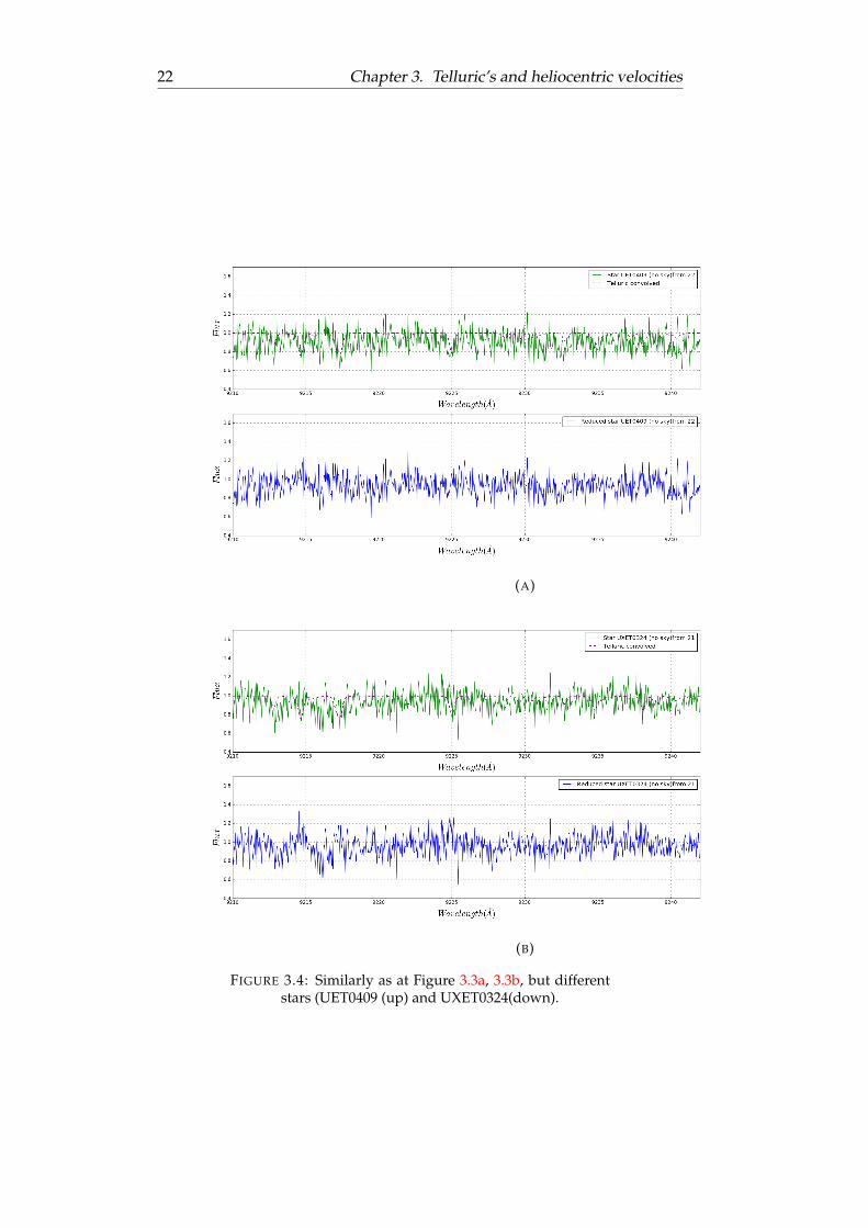
Next, telluric spectra was subtracted from the sky removed normalizedstar spectra after centering the star spectra around unity (Figure 3.3a, 3.3b, 3.4a, 3.4b).Formula used is: newpoint = 1+(centeredstarflux−convolvedtelluricflux).

20 Chapter 3. Telluric’s and heliocentric velocities

FIGURE 3.2: Telluric convolved with Gaussian (σ=70) isshown as a dotted purple line. Gray line is non-convolved

synthetic telluric

3.3. Results 21

(A)

(B)

FIGURE 3.3: UET0248 star sky removed spectra (green) isshown with convolved telluric’s spectrum (dotted purple)on the top graph. The star with removed telluric’s (blue) is

shown on the bottom graph.

22 Chapter 3. Telluric’s and heliocentric velocities

(A)

(B)

FIGURE 3.4: Similarly as at Figure 3.3a, 3.3b, but differentstars (UET0409 (up) and UXET0324(down).

23

Chapter 4

Heliocentric corrections andcombining spectra

4.1 Heliocentric velocities

After any observations the correct use of reference frame must be takeninto account. In this work, data was collected from the Earth that is mov-ing relative to the Sun and the objects of interest are moving relative toSun. When coordinates are Earth-centered they are called geocentric. Formore accurate velocity determination the object’s coordinates should beconverted to the more convenient reference frame, namely, Sun referenceframe. Sun-centered observations are called heliocentric. The data that iskept in geocentric coordinate frame can make the calculations problematicdue to the constant changes of the object velocity relative to the Earth due tothe Earth’s motion around the sun (Figure 4.1). Therefore, the most handycoordinate system to keep the data is the heliocentric system.

4.2 Combining spectra

The last step before all individual stars spectra can be analyzed, the spectrathat was observed in different times and removed from sky, telluric linesand heliocentrically corrected need to be combined. Faint star spectrum istoo uncertain to be totally analyzed from single observation. Usually, spec-tra are combined by taking a median in order to increase signal-to-noiseratio and avoid spurious data points that can occur.

Spectra can be median co-added as follows. All the same stars spec-tra need to be summed up. In the most cases, because of the heliocentriccorrections, wavelengths are shifted implies that interpolation needs to bedone in order to use correct fluxes for the certain wavelengths. As soon asspectra corresponding to the certain wavelengths are summed up, it needsto be normalized, in other words the continuum needs to be set to unity.In the end the summed spectra need to be divided by the total number ofspectra.

24 Chapter 4. Heliocentric corrections and combining spectra

FIGURE 4.1: Earth motion around the sun that producedDoppler Shifts in the object of interest. From (Wood, 2003).

4.3 Results

The Earth rotation around the sun is producing Doppler shifts in the spec-trum. The object lines are blue shifted when earth is moving towards theobject, and red shifted when it moves away. The Doppler shift formula isEq.4.1. Here, λnew is the heliocentrically corrected wavelength.

λnew = λold

√1 + vhelio

c

1− vhelioc

(4.1)

Once the telluric removal was done, the stars spectra were shifted withrespect to the heliocentric velocities. IRAF function "rvcorrect" was used forcalculating the heliocentric velocities. Heliocentrically corrected spectrumis shown on the Figure 4.2.

The resulting co-added spectra from one of the stars in the S I tripletregion is shown on the Figure 4.3a, 4.3b. Indeed, signal-to-noise raised andimperfections in the spectra, such as accidentally remaining emission linesand too deep emission lines gone.

4.3. Results 25

FIGURE 4.2: Heliocentric velocity corrected spectrum of theUET0409 star. Blue - star spectrum, green - heliocentrically

corrected star spectrum.

26 Chapter 4. Heliocentric corrections and combining spectra

(A)

(B)

FIGURE 4.3: Green is co-added star spectrum, blue is notco-added star spectrum. Lines are artificially shifted on the

y-axis in convenience sake.

27

Chapter 5

Results

Before final stars spectra was obtained, several spectra cleaning steps hadbeen taken. First of all, the sky emission lines were deleted, the atmosphericcontamination was removed, wavelengths were heliocentrically correctedand the same stars spectra were combined for improving S/N level. Theobtained results are compared with the example results from (Skuladottir,2016) shown on the Figure 5.1.

7 out of 8 stars have spectrum in the S I triplet region. One of the stars,namely UT125 is the telluric star, therefore, it was not analyzed. Thus, 6stars were analyzed. Figure 5.2a, 5.2b are the resulting spectra of the regionof interest (9210-9245Å is shown). The green marked regions shows possi-ble sulfur absorption lines location.

In the first green region in all the stars, where the first line from the S Itriplet might be, is seen quite definite absorption line. The central line fromthe S I triplet is located in the wing of the Paschen ζ line, a bit to the rightfrom the central green region. In comparison with the Paschen ζ line, sulfurline is harder to detect, but it is not seen at all. The last third S I triplet lineis the weakest on the Figure 5.1. On our stars the last S I line can’t be seen.But, from all the stars spectra the UXET0324 is the star in which sulfur mostprobably could be found.

It can be concluded since all three S I triplet lines need to be detected inorder to claim the sulfur existence on the stars - the stars got no sulfur (onestar may has sulfur) or sky, or telluric lines removal went wrong. Surely,an undetected mistake in data reduction could be made, but i believe thatthe given stars are too faint to be easily analyzed. So, more data samplesneeded to be taken or the stars are not subject to analysis until the reliableresolution of the ground-based telescopes will not be set up.

28 Chapter 5. Results

FIGURE 5.1: One of the dSph Sculptor star (ET0048) spectra,in the rest frame of the earth, before (red) and after (black)telluric correction. Blue dotted lines are the synthetic tel-luric spectra. The final telluric-corrected, co-added spec-trum, in the rest frame of the sun is shown on the bottom

panel. From (Skuladottir, 2016).

Chapter 5. Results 29

(A)

(B)

FIGURE 5.2: Blue lines are the final stars spectra (with nosky radiation, telluric lines, heliocentrically corrected andco-added spectra). Green region are the regions where S Itriplet were found on Figure 5.1. Dotted purple lines aretelluric’s that were removed before spectra were heliocen-

trically shifted.

31

Bibliography

Aaronson, M. (1983). “Accurate radial velocities for carbon stars in Dracoand Ursa Minor: The first hint of a Dwarf Spheroidal mass-to-light ra-tio”. In: The Astrophysical Journal 266, p. 11. URL: https://books.google.nl/books?hl=en&lr=&id=XI59041hwfMC&oi=fnd&pg=PA70&dq=Aaronson+1983,+ApJL,+266,+11&ots=SdsU1tjqUn&sig=0hI5xRLncOF5lpnTHcIRqVN2J2k#v=onepage&q&f=false.

Adelman S. J., Bikmaev I. Gullive A. F. Smalley B. (2002). “Round Table onInstrumentation and Data Processing”. In: AU Symposium, Modelling ofStellar Atmospheres, p. 13. URL: http://www.astro.keele.ac.uk/~bs/publs/roundtable.pdf.

Battaglia G., Helmi A. Tolstoy E. Irwin M. Hill V. Jablonka-P. (2013). “Thekinematic status and mass content of the Sculptor Dwarf SpheroidalGalaxy”. In: The Astrophysical Journal 2. URL: https://arxiv.org/pdf/0802.4220v2.pdf.

Battaglia G., Tolstoy E. Helmi A. Irwin M. J. Jablonka P.-Hill V. PasquiniL. (2008). “The DART imaging and CaT survey of the Sculptor DwarfSpheroidal Galaxy”. In: URL: http://www.rug.nl/research/portal/files/14452219/c4.pdf.

Bertaux J. L., Lallement R. Ferron S. Boonne C. Bodichon R. (2014). “TAPAS,a web-based service of atmospheric transmission computation for as-tronomy”. In: Astronomy and Astrophysics 564, p. 12. URL: http : / /www.pole-ether.fr/tapas/resources/doc/Bertaux_tapas_2014_aa.pdf.

Boer T. J. L., Tolstoy E. Hill V. Saha A.-Olsen K. Starkenburg E. LemasleB. Irwin M. J. Battaglia G. de (2012). “The star formation and chemi-cal evolution history of the sculptor dwarf spheroidal galaxy”. In: A&A539.765. URL: http://www.aanda.org/articles/aa/pdf/2012/03/aa18378-11.pdf.

Bonifacio P., Hill V. Molaro P. Pasquini L. Di Marcantonio P.-Santin P. (2000).“First results of UVES at VLT: abundances in the Sgr dSph”. In: Astron-omy & Astrophysics 359. URL: http://articles.adsabs.harvard.edu/cgi- bin/nph- iarticle_query?2000A%26A...359..663B&data_type=PDF_HIGH&whole_paper=YES&type=PRINTER&filetype=.pdf.

Bonifacio P., Sbordone L. Marconi G. Pasquini L. Hill V. (2004). “The SgrdSph hosts a metal-rich population”. In: Astronomy & Astrophysics 414.URL: http://www.aanda.org/articles/aa/pdf/2004/05/aa3930.pdf.

Brusadin G., Matteucci F. Romano D. (2013). “Modeling the chemical evo-lution of the Galaxy halo”. In: Astronomy and Astrophysics 554, p. 10.URL: http://www.aanda.org/articles/aa/pdf/2013/06/aa20884-12.pdf.

32 BIBLIOGRAPHY

Caffau E., Bonifacio P. Faraggiana R. François P. Gratton R. G.-Barbieri M.(2005). “Sulphur abundance in Galactic stars”. In: Astronomy and Astro-physics 441.2. URL: http://www.aanda.org/articles/aa/pdf/2005/38/aa2905-05.pdf.

Caffau E., Sbordone L. Ludwig H.-G. Bonifacio P. Spite M. (2010). “Sulphurabundances in halo stars from multiplet 3 at 1045 nm”. In: AstronomicalNotes 331. URL: http://onlinelibrary.wiley.com/doi/10.1002/asna.201011353/epdf.

Cochran A. L., Barnes III T. G. (1981). “Spectrophotometry with a self-scannedsilicon photodiode array. I - Instrumentation and reductions”. In: Astro-physical Journal Supplement Series 45. URL: http://adsabs.harvard.edu/full/1981ApJS...45...73C.

Da Costa, G. S. (1984). “The age of the Sculptor dwarf galaxy”. In: Astro-physical Journal 285, pp. 483–494. URL: http://articles.adsabs.harvard.edu/cgi-bin/nph-iarticle_query?1984ApJ...285..483D&data_type=PDF_HIGH&whole_paper=YES&type=PRINTER&filetype=.pdf.

Faber S. M., Lin D. N. C. (1983). “Is there nonluminous matter in dwarfspheroidal galaxies?” In: The Astrophysical Journal 266. URL: http://adsabs.harvard.edu/full/1983ApJ...266L..17F.

Galkin V. D., Arkharov A. A. (1981). “Determination of Extra AtmosphericMonochromatic Stellar Magnitudes in the Region of Telluric Bands”. In:Soviet Astronomy 25. URL: http://adsabs.harvard.edu/full/1981SvA....25..361G.

Geisler D., Smith V. V. Wallerstein G. Gonzalez G. Charbonnel C. (2001).“"Sculptor-ing" the Galaxy? The Chemical Compositions of Red Giantsin the Sculptor Dwarf Spheroidal Galaxy”. In: Astrophysical Journal 129.3,p. 17. URL: http://iopscience.iop.org/article/10.1086/427540/pdf.

— (2005). ““Sculptor-ing” the Galaxy? The Chemical Compositions of RedGiants in the Sculptor Dwarf Spheroidal Galaxy”. In: Astronomy & As-trophysics 129.3. URL: http://iopscience.iop.org/article/10.1086/427540/pdf.

Gutiérrez-Moreno A., Moreno H. Cortés G. (1982). “A study of atmosphericextinction at Cerro Tololo Inter-American observatory”. In: Publicationsof the Astronomical Society of the Pacific 94. URL: http://www.jstor.org/stable/40678027?seq=1#page_scan_tab_contents.

— (1986). “A study of atmospheric extinction at Cerro Tololo Inter-Americanobservatory. II”. In: Publications of the Astronomical Society of the Pacific98. URL: http://iopscience.iop.org/article/10.1086/131923/pdf.

Hammonds, M. (2013). “Andromeda and the 13 Dwarfs”. In: Australian Sci-ence. URL: http://www.australianscience.com.au/space/andromeda-and-the-13-dwarfs/.

Honeycutt R. K., Ramsey L. W. Warren W. H. Ridgway Jr.-S. T. (1977). “Spec-trophotometry of cool angular-diameter stars”. In: Astrophysical Journal215. URL: http://adsabs.harvard.edu/full/1977ApJ...215..584H.

Jenkins, E. B. (2009). “A unified representation of gas-phase element de-pletions in the interstellar medium”. In: The Astronomical Journal 700.

BIBLIOGRAPHY 33

URL: http://iopscience.iop.org/article/10.1088/0004-637X/700/2/1299/pdf.

Khomich V. Y., Semenov A. I. Shefov N. N. (2008). “Airglow as an Indica-tor of Upper Atmospheric Structure and Dynamics (Berlin: Springer)”.In: URL: https://books.google.lv/books?hl=en&lr=&id=vlg64lnz70sC & oi = fnd & pg = PA1 & dq = Khomich , +V . +Y . , +Semenov,+A.+I.,+%26+Shefov,+N.+N.+2008,+Airglow+as+an+Indicator+of+Upper+Atmospheric+Structure+and+Dynamics&ots=1n1BtFPW2d&sig=qsX5tPmhwEkdKwNn8N-gSRatZ_c&redir_esc=y#v=onepage&q&f=false.

Kobayashi C., Karakas A. I. Umeda H. (2011). “The evolution of isotoperatios in the Milky Way Galaxy”. In: Monthly Notices of the Royal Astro-nomical Society 414. URL: http://mnras.oxfordjournals.org/content/414/4/3231.full.pdf+html.

Kobayashi C., Umeda H. Nomoto K. Tominaga N. Ohkubo T. (2006). “Galac-tic Chemical Evolution: Carbon through Zinc”. In: The Astrophysical Jour-nal 653, p. 27. URL: http://iopscience.iop.org/article/10.1086/508914/pdf.

Leinert Ch., Bowyer S. Haikala L.K. Hanner M.S. Hauser M.G. Levasseur-Regourd A.-Ch. Mann I. Mattila K. Reach W.T. Schlosser W. Staude H.J.Toller G.N. Weiland J.L. Weinberg J.L. Witt A.N. (1998). “Synthetic spec-trum of the integrated starlight between 3,000 and 10,000 A. I - Methodof calculation and results”. In: Astronomy and Astrophysics SupplementSeries 127. URL: http://aas.aanda.org/articles/aas/pdf/1998/01/ds1449.pdf.

Letarte, B. (2007). “Chemical analysis of the Fornax dwarf galaxy”. In: PhDThesis.

Levasseur-Regourd, A. C. and R. Dumont (1980). “Absolute photometryof zodiacal light”. In: Astronomy and Astrophysics 84. URL: http://adsabs.harvard.edu/full/1980A%26A....84..277L.

Lundstrom L., Ardeberg A. Maurice E. Lindgren H. (1991). “A synthetictelluric spectrum in the wavelength region surrounding the D1 and D2lines of sodium”. In: Astronomy and Astrophysics Supplement Series 91.2.URL: http://articles.adsabs.harvard.edu/cgi-bin/nph-iarticle_query?1991A%26AS...91..199L&data_type=PDF_HIGH&whole_paper=YES&type=PRINTER&filetype=.pdf.

Maiolino R., Rieke G. H. Rieke M. J. (1996). “Correction of the AtmosphericTransmission in Infrared Spectroscopy”. In: The Astronomical Journal 111.1.URL: http://adsabs.harvard.edu/full/1996AJ....111..537M.

Manduca A., Bell R. A. (1979). “Atmospheric extinction in the near infrared”.In: The Astronomical Society of the Pacific 91. URL: http://iopscience.iop.org/article/10.1086/130598/pdf.

Mateo, M. (1998). “Detection of H i Associated with the Sculptor DwarfSpheroidal Galaxy”. In: Annual Review of Astronomy and Astrophysics 36,pp. 435–506. URL: http://www.annualreviews.org/doi/pdf/10.1146/annurev.astro.36.1.435.

Matrozis E., Ryde N. Dupree A. K. (2013). “Galactic chemical evolution ofsulphur. Sulphur abundances from the [SI ] λ1082 nm line in giants”. In:

34 BIBLIOGRAPHY

Astronomy and Astrophysics 559, p. 13. URL: http://www.aanda.org/articles/aa/pdf/2013/11/aa22317-13.pdf.

Mattila, K. (1980). “Synthetic spectrum of the integrated starlight between3,000 and 10,000 A. I - Method of calculation and results”. In: Astron-omy and Astrophysics Supplement Series 39. URL: http://articles.adsabs.harvard.edu//full/1980A%26AS...39...53M/0000053.000.html.

McConnachie, A. W. (2012). “The Observed Properties of Dwarf Galaxiesin and around the Local Group”. In: The Astronomical Journal 144.1, p. 4.URL: http://iopscience.iop.org/article/10.1088/0004-6256/144/1/4/meta.

McCord T. B., Clark R. N. (1979). “Atmospheric extinction 0.65-2.50 µmabove Manua Kea”. In: The Astronomical Society of the Pacific 91. URL:http://iopscience.iop.org/article/10.1086/130538/pdf.

Monaco L., Bellazzini M. Bonifacio P. Buzzoni A. Ferraro F. R.-Marconi G.-Sbordone L. Zaggia S. (2007). “High-resolution spectroscopy of RGBstars in the Sagittarius streams. I. Radial velocities and chemical abun-dances”. In: Astronomy and Astrophysics 464.1. URL: http : / / www .aanda.org/articles/aa/pdf/2007/10/aa6228-06.pdf.

Monaco L., Bellazzini M. Bonifacio P. Ferraro F. R. Marconi G.-Pancino E.-Sbordone L. Zaggia S. (2005). “The Ital-FLAMES survey of the Sagit-tarius dwarf spheroidal galaxy. I. Chemical abundances of bright RGBstars”. In: Astronomy and Astrophysics 441.1. URL: http://www.aanda.org/articles/aa/pdf/2005/37/aa3333-05.pdf.

Monkiewicz J., Mould J. R. Gallagher J. S. III Clarke J. T. Trauger-J. T. Grill-mair C. Ballester G. E. Burrows C. J. Crisp D. Evans R. Griffiths R. Hes-ter J. J. Hoessel J. G. Holtzman J. A. Krist J. E. Meadows V. Scowen P.A. Stapelfeldt K. R. Sahai R. Watson A. (1999). “The Age of the SculptorDwarf Spheroidal Galaxy from Imaging with WFPC2”. In: The Publica-tions of the Astronomical Society of the Pacific 111.765, pp. 1392–1397. URL:http://iopscience.iop.org/article/10.1086/316447/pdf.

Nissen P. E., Akerman C. Asplund M. Fabbian D. Kerber F. Käufl H. U. Pet-tini M. (2007). “Sulphur and zinc abundances in Galactic halo stars re-visited”. In: A&A 469.1. URL: http://www.aanda.org/articles/aa/pdf/2007/25/aa7344-07.pdf.

Noll S., Kausch W. Barden M. Jones A. M. Szyszka C. Kimeswenger S.Vinther J. (2012). “An atmospheric radiation model for Cerro Paranal”.In: Astronomy and Astrophysics 543, p. 23. URL: http://www.aanda.org/articles/aa/pdf/2012/07/aa19040-12.pdf.

Pasquini L., Avila G. Blecha A. Cacciari C. Cayatte V. Colless M. DamianiF. de Propris R. Dekker H. di Marcantonio P. Farrell T. Gillingham P.Guinouard I. Hammer F. Kaufer A. Hill V. Marteaud M. Modigliani A.Mulas G. North P. (2002). “Installation and commissioning of FLAMES,the VLT Multifibre Facility”. In: The Messenger 110. URL: http://articles.adsabs.harvard.edu/cgi-bin/nph-iarticle_query?2002Msngr.110....1P&data_type=PDF_HIGH&whole_paper=YES&type=PRINTER&filetype=.pdf.

BIBLIOGRAPHY 35

Patat, F. (2008). “The dancing sky: 6 years of night-sky observations at CerroParanal”. In: Astronomy and Astrophysics 481. URL: http://www.jstor.org/stable/95013?seq=1#page_scan_tab_contents.

Patat F., Moehler S. O’Brien K. Pompei E. Bensby T. Carraro G. de UgartePostigo A. Fox A. Gavignaud I. James G. Korhonen H. Ledoux C. Ran-dall S. Sana H. Smoker J. Stefl S. Szeifert T. (2011). “Optical atmosphericextinction over Cerro Paranal”. In: Astronomy and Astrophysics 527, p. 14.URL: http://www.aanda.org/articles/aa/pdf/2011/03/aa15537-10.pdf.

Pietrzynski G., Gieren W. Szewczyk O. Walker A. Rizzi L. Bresolin F. Ku-dritzki R. P. Nalewajko K. Storm J. Dall’Ora M. (2008). “The ARAU-CARIA project: The distance to the Sculptor dwarf spheroidal galaxyfrom infrared photometry of RR Lyrae stars”. In: The Astronomical Jour-nal 135, p. 5. URL: http://iopscience.iop.org/article/10.1088/0004-6256/135/6/1993/pdf.

Rayleigh, F. R. S. (1928). “The Light of the Night Sky: Its Intensity Variationswhen Analysed by Colour Filter. III”. In: Proceedings of the Royal Societyof London. Series A 119. URL: http://www.jstor.org/stable/95013?seq=1#page_scan_tab_contents.

Ryde N., Jonsson H. Matrozis E. (2014). “Is sulphur a typical α element?”In: Memorie della Societa Astronomica Italiana 85. URL: http://sait.oat.ts.astro.it/MmSAI/85/PDF/269.pdf.

Sbordone L., Bonifacio P. Buonanno R. Marconi G. Monaco L. Zaggia S.(2007). “The exotic chemical composition of the Sagittarius dwarf spheroidalgalaxy”. In: Astronomy and Astrophysics 465.3. URL: http://www.aanda.org/articles/aa/pdf/2007/15/aa6385-06.pdf.

Seifahrt A., Käufl H. U. Zängl G. Bean J. L. Richter M. J. Siebenmorgen R.(2010). “Accurate radial velocities for carbon stars in Draco and UrsaMinor: The first hint of a Dwarf Spheroidal mass-to-light ratio”. In: As-tronomy and Astrophysics 524, p. 10. URL: http://www.aanda.org/articles/aa/pdf/2010/16/aa13782-09.pdf.

Shapley, H. (1938). “A Stellar System of a New Type”. In: Harvard College Ob-servatory Bulletin 908. URL: http://articles.adsabs.harvard.edu/full/1938BHarO.908....1S/0000001.000.html.

Shetrone M. D., Bolte M. Stetson P. B. (1998). “Keck HIRES Abundancesin the Dwarf Spheroidal Galaxy Draco”. In: The Astronomical Journal115.5. URL: http://iopscience.iop.org/article/10.1086/300341/pdf.

Shetrone M. D., Côté P. Sargent W. L. W. (2001). “Abundance Patterns in theDraco, Sextans, and Ursa Minor Dwarf Spheroidal Galaxies”. In: TheAstrophysical Journal 548.2, p. 17. URL: http://iopscience.iop.org/article/10.1086/319022/pdf.

Shetrone M., Venn K. A. Tolstoy E. Primas F. Hill F. Kaufer A. (2003). “VLT/UVESAbundances in Four Nearby Dwarf Spheroidal Galaxies. I. Nucleosyn-thesis and Abundance Ratios”. In: Astrophysical Journal 125.2, p. 23. URL:http://iopscience.iop.org/article/10.1086/345966/pdf.

Skuladottir, A. (2016). “Sulphur, Zink and Carbon in the Sculptor DwarfSpheroidal Galaxy”. In: PhD Thesis.

36 BIBLIOGRAPHY

Smecker-Hane T., McWilliam A. (1999). “Ages and Chemical Abundancesin Dwarf Spheroidal Galaxies”. In: URL: http://arxiv.org/pdf/astro-ph/9910211v1.pdf.

Smette A., Sana H. Noll S. Horst H. Kausch W. Kimeswenger S. BardenM. Szyszka C. Jones A. M. Gallenne A. Vinther J. Ballester P. Taylor J.(2015). “Molecfit: A general tool for telluric absorption correction”. In:Astronomy and Astrophysics 576.A77, p. 17. URL: http://www.aanda.org/articles/aa/pdf/2015/04/aa23932-14.pdf.

Spite M., Caffau E. Andrievsky S. M. Korotin S. A. Depagne E. Spite F. Boni-facio P. Ludwig H.-G. Cayrel R. François P. Hill V. Plez B. Andersen J.Barbuy B. Beers T. C. Molaro P. Nordström B. Primas F. (2011). “Firststars. XIV. Sulfur abundances in extremely metal-poor stars”. In: As-tronomy and Astrophysics 528, p. 8. URL: http://www.aanda.org/articles/aa/pdf/2011/04/aa15926-10.pdf.

Suntzeff N. B., Mateo M. Terndrup D. M. Olszewski E. W. Geisler D. WellerW. .. (1993). “Spectroscopy of Giants in the Sextans Dwarf SpheroidalGalaxy”. In: The Astrophysical Journal 418. URL: http://adsabs.harvard.edu/full/1993ApJ...418..208S.

Takada-Hidai M., Takeda Y. Sato S. Honda S. Sadakane K. Kawanomoto S.Sargent W. L. W. Lu-L. Barlow T. A. (2002). “Behavior of Sulfur Abun-dances in Metal-poor Giants and Dwarfs”. In: The Astrophysical Journal573, p. 17. URL: http://iopscience.iop.org/article/10.1086/340748/pdf.

Takeda Y., Hashimoto O. Taguchi H. Yoshioka K. Takada-Hidai M. Saito Y.Honda S. (2005). “Non-LTE Line-Formation and Abundances of Sulfurand Zinc in F, G, and K Stars”. In: Astronomical Society of Japan 57. URL:http://pasj.oxfordjournals.org/content/57/5/751.full.pdf+html.

Takeda Y., Takada-Hidai M. (2011). “Exploring the [S/Fe] Behavior of Metal-Poor Stars with the S I 1.046 µm Lines”. In: Astronomical Society of Japan63. URL: http://pasj.oxfordjournals.org/content/63/sp2/S537.full.pdf+html.

Timmes F. X., Woosley S. E. Weaver T. A. (1995). “Galactic Chemical Evolu-tion: Hydrogen Through Zinc”. In: The Astrophysical Journal 617, p. 114.URL: http://arxiv.org/pdf/astro-ph/9411003v1.pdf.

Tolstoy E., Hill V. Irwin M. Helmi A. Battaglia-G. Letarte B. Venn K. A.Jablonka P. Shetrone-M. Arimoto N. Abel T. Primas F Kaufer A. SzeifertT. Francois P. Sadakane K. (2006). “The Dwarf galaxy Abundances andRadial-velocities Team (DART) Large Programme – A Close Look atNearby Galaxies”. In: The Messenger 133. URL: https://www.researchgate.net/profile/F_Primas/publication/252564810_The_Dwarf_galaxy_Abundances_and_Radial-velocities_Team_(DART)_Large_Programme_-_A_Close_Look_at_Nearby_Galaxies/links/0a85e53bd176ed16ed000000.pdf.

Tolstoy E., Hill V. Tosi M. (2009). “Star-Formation Histories, Abundances,and Kinematics of Dwarf Galaxies in the Local Group”. In: Annual Re-view of Astronomy & Astrophysics 47.1. URL: http://www.annualreviews.org/doi/pdf/10.1146/annurev-astro-082708-101650.

Tolstoy E., Venn K. A. Shetrone M. Primas F.-Hill V. Kaufer A. SzeifertT. (2003). “VLT/UVES Abundances in Four Nearby Dwarf SpheroidalGalaxies. II. Implications for Understanding Galaxy Evolution”. In: The

BIBLIOGRAPHY 37

Astrophysical Journal 125.2, p. 17. URL: http://iopscience.iop.org/article/10.1086/345967/pdf.

Traub W. A., Stier M. T. (1976). “Theoretical atmospheric transmission inthe mid- and far-infrared at four altitudes”. In: Optical Society of America91. URL: https://www.osapublishing.org/ao/abstract.cfm?uri=ao-15-2-364.

Vacca W. D., Cushing M. C. Rayner J. T. (2003). “A Method of CorrectingNear-Infrared Spectra for Telluric Absorption”. In: Publications of theAstronomical Society of the Pacific 115. URL: http://irtfweb.ifa.hawaii.edu/~spex/Telluric.pdf.

Wood, E. (2003). “Telluric Line Removal in Astrophysical Spectroscopy”.In: ASEN/ATOC 5235, p. 15. URL: http://irina.eas.gatech.edu/ATOC5235_2003/Erin_Wood-paper.pdf.