NBER WORKING PAPER SERIES

LOOKING FOR LOCAL LABOR MARKET EFFECTS OF NAFTA

John McLarenShushanik Hakobyan

Working Paper 16535http://www.nber.org/papers/w16535

NATIONAL BUREAU OF ECONOMIC RESEARCH1050 Massachusetts Avenue

Cambridge, MA 02138November 2010

This research was supported by the Bankard Fund for Political Economy. For useful comments wethank seminar participants at the University of Virginia and Johns Hopkins University, as well as conferenceparticipants at the NBER International Trade and Investment Group, March 2011, the Empirical Investigationsin Trade and Investment Conference, Tokyo, March 2011, and the ILO Globalization and Labor MarketOutcomes Workshop, Geneva, June 2011. A special vote of thanks is owed to Kala Krishna and AndrewBernard and to our discussants Carolyn Evans and Avraham Ebenstein. All remaining errors are ours.The views expressed herein are those of the authors and do not necessarily reflect the views of theNational Bureau of Economic Research.

NBER working papers are circulated for discussion and comment purposes. They have not been peer-reviewed or been subject to the review by the NBER Board of Directors that accompanies officialNBER publications.

© 2010 by John McLaren and Shushanik Hakobyan. All rights reserved. Short sections of text, notto exceed two paragraphs, may be quoted without explicit permission provided that full credit, including© notice, is given to the source.

Looking for Local Labor Market Effects of NAFTAJohn McLaren and Shushanik HakobyanNBER Working Paper No. 16535November 2010, Revised January 2012JEL No. F13,F16,J31

ABSTRACT

Using US Census data for 1990-2000, we estimate effects of NAFTA on US wages. We look for effectsof the agreement by industry and by geography, measuring each industry’s vulnerability to Mexicanimports, and each locality’s dependance on vulnerable industries. We find evidence of both effects,dramatically lowering wage growth for blue-collar workers in the most affected industries and localities(even for service-sector workers in affected localities). These distributional effects are much largerthan aggregate welfare effects estimated by other authors. In addition, we find strong evidence of anticipatoryadjustment in places whose protection was expected to fall but had not yet fallen; this adjustment appearsto have conferred an anticipatory rent to workers in those locations.

John McLarenDepartment of EconomicsUniversity of VirginiaP.O. Box 400182Charlottesville, VA 22904-4182and NBERjmclaren@virginia.edu

Shushanik HakobyanDepartment of EconomicsMiddlebury College505 Warner HallMiddlebury, VT 05753shakobyan@middlebury.edu

1 Introduction

Perhaps the most passionately debated issue in trade policy within the United States ina generation has been the signing and implementation of the North American Free TradeAgreement (NAFTA), signed by the governments of the US, Canada and Mexico in 1993.Opponents believe that it has devastated some parts of the country by encouraging multina-tionals to shift operations to Mexico, while proponents argue that it has boosted US exportsand thus job growth. Despite the age of the agreement, as recently as 2008 it became thesubject of intense political debate, with Democratic presidential candidates competing witheach other in denunciations of the agreement in Ohio, a state in which many voters blamethe agreement for local economic difficulties (Austen, 2008). Brown (2004, Ch. 6) presentsa passionate example of the liberal non-economist’s case against the NAFTA, arguing thatit has destroyed millions of US jobs as well as causing environmental problems.

One aspect of popular opposition to the NAFTA has been the claim that it has hada disparate impact geographically, that it has devastated particularly vulnerable townseven as others have prospered. Leonhardt (2008) describes the anti-NAFTA sentiment inYoungstown, Ohio, which had suffered a long economic decline that many residents blamedpartly on NAFTA. In particular, residents had recently seen the shuttering of the YoungstownSteel Door plant, which had been the leading supplier of steel doors for railway cars in NorthAmerica for decades; the capital was purchased by a foreign firm and shipped to a plant inMexico. Brown (2004, pp.156-7) argues that the agreement was a devastating blow to thetowns of Nogales, Arizona and El Paso, Texas. At the same time, the town of Laredo,Texas enjoyed a dramatic economic boom based on traffic to and from Mexico following theagreement (Duggin, 1999). Kumar (2006) argues that the Texas economy as a whole hasbenefitted from exports to the Mexico as a result of the agreement.

Unfortunately, economists to date have not provided an answer to the question of whetheror not NAFTA has indeed had the effects ascribed to it by its opponents. This paper is anattempt to do so. We ask whether or not we can identify subsets of US workers whoseincomes were seriously diminished by the agreement, and if so, do they follow an identifiablegeographic pattern.

Our approach is to do what seems like the simplest possible exercise to look for signs ofthe effects that NAFTA opponents claim. We try to identify local labor-market effects ofthe tariff reductions brought about by the NAFTA, using publicly available US Census data

2

from 1990 and 2000, taken from the IPUMS project at the Minnesota Population Center(www.ipums.org; see Ruggles et. al. (2010)). This data has enough richness to enable us tocapture the features we need to capture.

Three features in particular that we need to capture should be highlighted.(i) We need to be able to control for a worker’s industry of employment, in order to allow

for the likelihood that workers in industries that compete with imports from Mexico1 willbe affected differently than workers in other industries. The census data has a very coarsedivision of workers into industries that allows us to do so adequately.

(ii) The issue that has been foremost in much of the political debate is a geographicone: The claim that workers in some vulnerable locations have been harmed, relative toworkers in other places. Thus, we need detailed geographic data, and a measure of howvulnerable a given location is likely to be to the effects of the NAFTA. The IPUMS datadivide the country into 543 similar-sized, non-overlapping pieces, called Consistent Public-Use Microdata Areas, or conspumas, whose boundaries are the same for both 1990 and 2000.Every worker in the data is identified as living in one of these conspumas, and so this allowsus to control for geography. In particular, in addition to controlling for what industry inwhich a worker is employed, we can control for how many of the other workers within aworker’s conspuma are employed in industries that will compete directly with imports fromMexico. This will be interpreted as the ‘local vulnerability’ of the labor market to the effectsof NAFTA.

(iii) The agreement was framed as a gradual phase-in of tariff elimination between thethree countries, starting in 1994 and continuing for 10 years (with a few tariffs continuingto 15 years). The negotiated schedule of liberalization was different for each sector of theeconomy. As a result, for some industries, the period from 1990 to 2000 would represent theperiod of an announcement of tariff reductions, most of which occurred after 2000. For otherindustries, the same period would be a period of rapid elimination of tariffs. Consider twohypothetical industries. Industry A benefitted from a 12% tariff in 1990; by 2000, the tariffon imports of that industry’s products from Mexico had fallen to 9%, with the remaining9% scheduled to be eliminated between 2000 and 2004. Industry B benefitted from a 3%tariff as of 1990, which was completely eliminated on imports from Mexico by 2000. Bothof these industries saw a drop in their respective Mexico tariffs of 3 percentage points in the

1Note that we are not interested in imports from Canada, since tariffs between the US and Canada hadalready been eliminated by the Canada-US Free Trade Agreement.

3

sample period 1990-2000, but we would not expect the same economic effects in these twocases since in the case of Industry A, most of the tariff reduction is anticipated, rather thanbeing realized over the period of the data. In any model of dynamic adjustment, anticipatedtariff changes can have important effects over and above realized tariff changes. To dealwith this, we measure the extent of anticipated tariff reduction by the initial tariffs (since allintra-NAFTA tariffs needed to be eliminated over the course of the agreement), and controlfor this in regressions in addition to the actual realized tariff reduction between 1990 and2000.

To anticipate results, we find that NAFTA-vulnerable locations that lost their protectionquickly experienced significantly slower wage growth compared to locations that had noprotection against Mexico in the first place, particularly for blue-collar workers. For the mostheavily NAFTA-vulnerable locations, a high-school dropout would have up to 8 percentagepoints slower wage growth from 1990 to 2000 compared to the same worker in a location withno initial protection. There is, however, an even larger industry effect, with wage growth inthe most protected industries that lose their protection quickly falling 16 percentage pointsrelative to industries that were unprotected to begin with.

To put it in concrete terms, the effect of the NAFTA on most workers and on the averageworker is likely close to zero, but for an important minority of workers the effects are verynegative. A high-school dropout living in an apparel and footwear dependent small town inSouth Carolina, even if she is employed in the non-traded sector such as in a diner where shewould appear to be immune to trade shocks, would see substantially lower wage growth from1990 to 2000 than if she were in, for example, College Park, Maryland, as the local workers intradable sectors that do compete with Mexico start seeking jobs in the non-traded sectors. Atthe same time, if the same worker had actually been employed in those vulnerable tradablessectors when the agreement was signed, she would be hurt twice, with a much lower wagegrowth than fellow workers who were already working in the diner. These effects, however,are much smaller – and statistically insignificant – for college-educated workers.

In addition, we find evidence of anticipatory effects. Comparing two locations that ex-perience the same drop in weighted average tariff over the sample period, if one of themstill has high tariffs on Mexican imports and thus expects further drops in protection soon,while the other is now unprotected, the location expecting further tariff drops on averagesees wage increases as less-educated workers leave the area, making less-educated workers

4

scarcer, as in Artuç, Chaudhuri and McLaren (2008).

2 Previous work

Post-NAFTA, much work on the economic effects of the agreement has focussed on tradecreation and trade diversion. Romalis (2007) studies changes in trade flows following NAFTAand finds that trade diversion effects of the agreement were substantial, and swamped anybenefits from trade creation, leaving a net aggregate welfare benefit for the US of about zero.Caliendo and Parro (2009) calibrate and simulate an Eaton-Kortum-type model of NorthAmerican trade to estimate the effects of NAFTA. Taking full account of enhanced tradein intermediate inputs and inter-industry input-output linkages, they find small increasesin welfare for each NAFTA country as a result of the agreement. Neither of these papersaddresses within-country income distribution, which is the focus of this paper.

A few papers have looked at aggregate effects on US labor markets, summarized inBurfisher et. al. (2001), and have found only small effects. Hanson (2007) finds that inthe most globalization-affected regions of Mexico over the introduction of NAFTA bothinequality and poverty fell relative to the rest of the country. Prina (2009a,b) finds thatMexican small farmers tended to benefit from the agreement on balance, and that theredoes not seem to have been much of an effect on rural landless workers.

An important related study is Trefler (2004), who studied firm- and industry-level dataon Canadian manufacturing to find effects of the earlier Canada-US Free Trade Agreement.That study found substantial employment reductions in Canadian industries whose tariffagainst US imports fell the fastest, but no reduction in wages and a substantial improvementin productivity growth. The study did not look for local labor-market effects.

We here borrow ideas from a number of sources. A number of studies identify effectsof a national trade shock on local labor markets, most notably the pioneering paper byTopalova (2007), who constructed an employment-weighted average tariff for each Indiandistrict to identify the differential effects of local labor-market shocks on different locations.Kovak (2010) uses a similar technique for Brazil. These studies indicate significant location-specific effects of trade shocks on wages, which of course implies mobility costs of some sortfor workers that prevent them from arbitraging wage differences across locations. A richliterature examines the correlation of changes in industry tariffs or other industry-specific

5

trade shocks with industry wages. Revenga (1992) finds effects of an industry’s import priceon that industry’s wages in the US. Pavcnik, Attanasio and Goldberg (2004) find such effectsfor Columbia. Here, we allow for both local labor market effects and industry effects.

A number of studies have isolated effects of imports from a specific geographic origin ondomestic labor markets. Bernard, Jensen, and Schott (2006) find that imports from low-wage countries have much more pronounced effects on the survival probabilities of US plantsin the same product category than imports from other locations. Ebenstein et. al. (2009)show that offshoring to low-wage countries is associated with reductions in US employmentin the same industry, while offshoring to high-wage countries has the opposite effect. Autor,Dorn and Hanson (2011) show that a rise in China’s share of imports reduces wages in USlocalities where employment is concentrated in the affected industries. Although Mexico isnot a low-wage country by the definition used in these papers, we do isolate Mexico-specificeffects of imports on US workers in a similar manner.

In addition, Kennan and Walker (2011) and Artuç, Chaudhuri and McLaren (2010)estimate structural models of labor mobility, the former focussing on geographic mobilityand the latter on inter-industry mobility. Both studies find large costs to moving, but notenough to keep a substantial number of workers from moving when economic shocks call forit. Our reduced-form regression can be interpreted as providing confirming evidence for suchmoving costs.

We also draw ideas from Artuç, Chaudhuri and McLaren (2008) on the effects of antici-pated changes in trade policy on current labor-market outcomes, although in this paper wedo not estimate a structural empirical model.

3 Empirical approach

The approach described above requires a measure of protection by industry and also bygeographic location. Note that for each industry j of the 89 Census traded-goods industries,we have an average tariff, τ jt , assessed on goods from industry j entering the US from Mexico.To turn this into a measure of protection in geographic terms, we compute the initial averagetariff in a given location, c, which we interpret as the ‘vulnerability’ of the location to theNAFTA. We define this similarly to the local average tariff in Topalova (2007), but we takeinto account that Mexico is not good at producing everything; a high tariff on imports of

6

good j from Mexico makes no difference if Mexico has no comparative advantage in j and willnot export it regardless of the tariff. We thus form an average local tariff, averaged acrossindustries weighted by local employment in each industry and also by Mexico’s revealedcomparative advantage in each industry.

Weighted local average tariff (‘vulnerability,’ or anticipated local tariff drop) is definedas:

locτ c1990 ≡∑Nindj=1 Lcj1990RCA

jτ j1990∑Nindj=1 Lcj1990RCA

j, (1)

where Lcjt is the number of workers employed in industry j at conspuma c at date t, Nind isthe number of industries, and

RCAj =

(xMEX

j,1990xROW

j,1990

)(∑

ixMEX

i,1990∑ixROW

i,1990

)is Mexico’s revealed comparative advantage in j, a slight adaptation of Balassa’s (1965)familiar formulation. Here, xMEX

j,1990 is Mexico’s exports of good j to the rest of the worldexcluding the US (ROW) and xROWj,1990 is total exports of good j from countries excluding theUS and Mexico to each other. Therefore, RCAj is Mexico’s share of ROW trade in goodj, divided by Mexico’s share in total ROW trade. The interpretation is that if RCAj > 1,Mexico has more of a tendency to export j than the average product, and thus has a revealedcomparative advantage in good j.

This gives rise to the realized local tariff change: loc4τ c ≡∑Nind

j=1 Lcj1990RCA

j4τ j∑Nindj=1 Lcj

1990RCAj

, where

4τ j is the change in the tariff on good j imports from Mexico from 1990 to 2000.Now, to show how we attempt to deal with the dynamic issues mentioned as point (iii)

above, for the moment set aside geography and focus on industry-level effects (which wouldbe an appropriate approach if, for example, we were certain that geographic mobility costswere zero). Then we could run a regression as follows:

wi = αXi +∑j

αindj indi,j +{θ1yr2000iτ j(i)1990 + θ2yr2000i4τ j(i)

}+ εi, (2)

where i indexes workers; Xi is a set of individual characteristics; j(i) is the index of workeri’s industry; indi,j is a dummy variable that takes a value of 1 if individual i is employed

7

in industry j; yr2000i is a dummy that takes a value of 1 if individual i is observed in theyear 2000; 4τ j = τ j2000 − τ j1990; εi is a random disturbance term; and the α’s and θ’s areparameters to be estimated.2

In this specification, there are two factors that allow for wages to grow at different ratesbetween 1990 and 2000 in different industries, both captured by the two terms in bracebrackets. The more obvious of these is that the tariff on industry i’s products imported fromMexico may fall at different rates for different industries; this is captured by the change intariff in the second term in brace brackets. However, we also need to take into account thatfor some industries the tariff elimination was virtually complete by 2000, while for othersit was ongoing, and so would generate expectations of future liberalization that would alsoaffect wages. To capture this, we include the initial tariff separately from the change intariff, in the first of the two terms in the brace brackets. The year-1990 tariff captures thescale of the anticipated total tariff reduction (since all tariffs on Mexican goods must bebrought down to zero over the adjustment period of the agreement). Holding constant therealized change in tariff from 1990 to 2000, a higher value of the 1990 tariff indicates a largeranticipated reduction in tariffs following 2000.

Anticipated liberalization of this sort can have a wide range of effects. Artuç, Chaudhuriand McLaren (2008) show that in a model with costly labor adjustment, an anticipatedliberalization of trade in one industry can lead to a steady stream of exiting workers, creatinga labor shortage and rising wages in that sector. The way this works is illustrated in Figures1 and 2, which illustrate the time path of employment and wages for a pair of hypotheticalindustries. Suppose that they both have the same level of τ j1990. In 1994, the agreementis made public and ratified, and the industry in Figure 1 loses its tariff right away. Thisleads to a sudden drop in wages in industry i, and a flow of workers out of the industry.As workers leave the industry, the equilibrium moves up and to the left along the industrylabor-demand curve, increasing wages progressively toward the new steady state as shownin the second panel of Figure 1. The new steady state wage could be above or below theold one, and so the difference in wages between the sampled wages at 1990 and 2000 couldbe positive, negative or zero. Contrast this situation with the case of the delayed tariffelimination of Figure 2. Here, suppose that the tariff is scheduled in the agreement to be

2Note that our Census data, which we will describe in detail shortly, take the form of two cross sectionsrather than a panel. Each individual i in the sample is observed once; some are observed in 1990 and somein 2000.

8

eliminated in 2004. Between 1994 and 2000, workers will be gradually leaving the industryin anticipation of this tariff elimination, moving the equilibrium up and to the left along theindustry labor-demand curve, and therefore steadily increasing the wage. In this case, thesampled industry wage in 2000 will definitely be higher than the sampled industry wage in1990. Note that in Figure 2, τ i1990 > 0 and 4τ i = 0, and the wage increases over the sampleperiod. Compare that with another industry j that never had a tariff, and so expects nolosses from NAFTA: τ j1990 = 4τ j = 0. Over the sample period, clearly industry i’s wagesrise relative to wages in industry j.

Clearly, in a model of that sort, θ1 would be positive: Holding constant the realized tariffreduction during the sample period, the larger the tariff reduction anticipated during thesample period, the more workers will stream out of the industry and the more rapidly willwages in the industry rise during the sample period. A model with heterogeneous workersor firms might generate a similar effect, as workers or firms that are only marginally suitedto the liberalizing industry leave it in anticipation, leaving only the higher-productivityproducers and hence higher average wages. On the other hand, in a model with frictionaljob search and costly creation of vacancies as in Hosios (1990), anticipated liberalizationwill have the effect of curtailment of vacancies, which could occur more rapidly than workerexodus, leading to rising unemployment and falling wages in the industry. In this case, wewould see θ1 < 0. We can parsimoniously say that θ1 captures the ‘anticipatory effect’ of theliberalization, while θ2 captures the ‘impact effect.’ Of course, in the event that an industryloses its tariff entirely during the sample period so that 4τ j = −τ j1990, the effect on the wageduring the sample period is then θ1 − θ2.

Equation (2) summarizes the essence of our approach to dynamics, but in practice weare interested in capturing more detail than it entails. In particular, we wish to allow theeffects on wages to differ by educational class. We break the sample down into four classes:less than high school; high-school graduate; some college; and college graduate, and allowboth the initial wage and the wage growth to vary by these categories. This yields the richerregression equation:

9

log(wi) = αXi +∑j

αindj indi,j (3)

+∑k 6=col

γ1keducik +∑k

γ2keducikyr2000i

+∑k 6=col

θ1keducikτj(i)1990 +

∑k

θ2keducikyr2000iτ j(i)1990

+∑k 6=col

θ3keducik4τ j(i) +∑k

θ4keducikyr2000i4τ j(i) + εi,

where educij is a dummy variable taking a value of 1 if worker i is in educational category k.The variables of interest here, corresponding to the anticipatory effect and the impact effectdiscussed in the context of equation (2), are θ2k and θ4k.3

Equation (3) allows for a rich characterization of dynamic response that varies by industryand education, but it does not yet allow for geography. To incorporate that, we include termsthat treat local average tariffs as in (1), in a way that is parallel to the treatment of industrytariffs. In addition, to be consistent, in controlling for the level of protection by industry,we use the product of industry tariff with the revealed comparative advantage, RCAjτ j1990.We also allow for a different rate of wage growth for locations on the US-Mexico border,producing our main regression equation:

log(wi) = αXi +∑j

αindj indi,j +∑c

αconspumac conspumai,c (4)

+∑k 6=col

γ1keducik +∑k

γ2keducikyr2000i

+∑k 6=col

δ1keduciklocτc(i)1990 +

∑k

δ2keducikyr2000ilocτ c(i)1990

+∑k 6=col

δ3keducikloc4τ c(i) +∑k

δ4keducikyr2000iloc4τ c(i)

+∑k 6=col

θ1keducikRCAjτj(i)1990 +

∑k

θ2keducikyr2000iRCAjτ j(i)1990

+∑k 6=col

θ3keducikRCAj4τ j(i) +

∑k

θ4keducikyr2000iRCAj4τ j(i)

+ µBorderc(i)yr2000i + εi,

3The term with θ3k is included only for consistency; it does not seem to have much economic meaning,and does not make much difference whether or not it is included in the regression.

10

where conspumai,c is a dummy variable that takes a value of 1 if worker i resides in conspumac, c(i) is the index of worker i’s conspuma, and loc4τ c(i) is the change in tariff for locationc, as defined at the beginning of this section.

The parameters of primary interest here are δ2,k and δ4,k, which measure the anticipatoryeffect and the impact effect, respectively, for the local average tariff change; and θ2,k and θ4,k,which measure the anticipatory effect and the impact effect, respectively, for the industrytariff. If there is no dynamic adjustment, so that the labor market simply responds to currenttariffs regardless of expectations, then we will observe δ2,k = θ2,k = 0.

If it is easy for workers to move geographically, so that local wage premiums are arbitragedaway, but difficult for workers to switch industry, we will observe δ1,k, . . . , δ4,k = 0 whileθ1,k, . . . , θ4,k 6= 0. In that case, industry matters, but location does not. This, together withthe assumption that δ2,k = 0 is how the model in a number of studies such as Pavcnik,Attanasio and Goldberg (2004) are set up. On the other hand, if it is difficult for workersto move geographically but easy to switch industries within one location, we will see theopposite: δ1,k, . . . , δ4,k 6= 0 while θ1,k, . . . , θ4,k = 0. A ‘pure Youngstown’ effect would beindicated by δ4,k > 0 while δ2,k = θ2,k = θ4,k = 0. This would imply that an export-sectorworker in Youngstown (with its industries that compete with Mexican imports) would suffera wage reduction due to NAFTA, while an import-competing worker in Arlington, VA (withonly very few workers employed in industries that compete with Mexican imports) wouldnot. This is how the model in Kovak (2010) is set up.

Finally, for a location that loses all of its protection within the sample period, the effecton wages within the sample period is equal to δ2,k − δ4,k, while for an industry that loses allof its protection within the sample period, the effect on wages within the sample period isequal to θ2,k − θ4,k.

4 Data

We use a 5% sample from the US Census for 1990 and 2000, collected from usa.ipums.org,selecting workers from age 25 to 64 who report a positive income in the year before thecensus.4 We include the personal characteristics age, gender, marital status, whether ornot the worker speaks English, race, and educational attainment (less than high school,

4The sample includes individuals who report being employed, unemployed or not in labor force in thecensus year. We use the last industry of employment for the unemployed and those not in labor force.

11

high school graduate, some college, college graduate). In addition, we have the industry ofemployment and conspuma of residence for each worker as well as the worker’s pre-tax wageand salary income. Our sample size is 10,320,274 workers.

We use data on US tariffs on imports from Mexico collected by John Romalis and de-scribed in Feenstra, Romalis, and Schott (2002). We constructed a concordance to mapthe 8-digit tariff data into the 89 traded-goods industry categories of the Census in orderto construct industry tariffs τ jt .5 We used Mexican trade data from the US InternationalTrade Commission to obtain a trade-weighted average tariff for each Census industry.6 Toconstruct Mexico’s revealed comparative advantage, RCAj, we used data on exports byreporting countries from the UN Comtrade.

Table 1 shows descriptive statistics for the main control variables. The sample is 53%male and 80% white, with an average age of 41 years. High-school dropouts are 11% ofthe total, with the remainder about evenly split between high-school graduates, those withsome college, and college graduates. The tariff in 1990 on Mexican goods ranged acrosstraded-goods industries from 0 to 17%, with a mean of 2%. These tariffs are generally belowthe US Most-Favored-Nation (MFN) tariffs which are charged on imports from World TradeOrganization (WTO) members as a default (see Figure 3). The difference is due to theGeneralized System of Preferences (GSP), under which rich countries extend discretionarytariff preferences to lower-income countries (see Hakobyan (2010)). After multiplying thetariff by RCAj to correct for Mexico’s pattern of comparative advantage, we obtain a productthat ranges from 0 to 8.8% (for footwear). The initial average local tariff ranges acrossconspumas from approximately 0.09 to 4.74%, with a mean just above one percent.

We actually have computed two versions of the local average tariff. In one, all industriesare treated in the same way; in the second, we omit agriculture by setting its tariff equalto zero. The reason for doing this is that aggregation of industries is a particularly largeproblem for agriculture, as the Census makes no distinction between different crops. We knowthat corn, in particular, benefitted greatly from NAFTA due to elimination of Mexican cornquotas, while other crops, such as some vegetables, were likely hurt. However, with Censusaggregation we are forced to apply the same tariff to all agriculture. This resulted in various

5Note that only 89 out of the 238 Census industry categories produce tradable goods and can be mappedto trade data. The tariffs for the remaining non-traded-goods industries are treated as zeros.

6Trade data are obtained from the US International Trade Commission Trade and Tariff DataWeb athttp://dataweb.usitc.gov.

12

farming areas of the great plains, where corn is king, appearing, implausibly, in the top tenmost vulnerable conspumas (see Figure 6). To eliminate this problem, throughout, we haveperformed parallel regressions with agriculture omitted by artificially setting the agriculturetariff equal to zero, and reported the two sets of regressions side by side. The results are closeto identical, but we refer to the version without agriculture as our preferred specification.

Table 2 shows which industries received the most protection against Mexican imports,and Table 3 shows those with the highest value of the product of tariff and RCAj andthus potentially the most vulnerable to NAFTA. The top two are footwear and oil andgas extraction, followed by carpets and rugs and plastics, all in the range of 7 to 8.8%.Comparison of Tables 2 and 3 shows that the correction for Mexican comparative advantagemakes a fair amount of difference.7 Figure 4 shows that the relationship between the 1990tariff levels and the decline in tariffs between 1990 and 2000 mostly follows a linear pattern,but with plenty of deviations. Industries whose tariffs fell more slowly than average includeFootwear (initial tariff is 17%; the 2000 tariff is 11.2%) and Structural clay products (initialtariff is 14.5%; the 2000 tariff is 6.8%). After adjusting for Mexico’s revealed comparativeadvantage, tariffs in these industries still fell the slowest (see Figure 5). Four industries(Dairy products; Cycles and miscellaneous transportation equipment; Printing, publishing,and allied industries; Agricultural chemicals) experienced tariff increases between 1990 and2000.

Table 4 shows the conspumas with the highest and lowest 1990 local average tariffs onMexican goods, and hence the most and least potential vulnerability to NAFTA (the localaverage tariffs with agriculture omitted is used). The list is dominated by manufacturingareas of the Carolinas and southern Virginia. The least vulnerable locations include Wash-ington, D.C. and its suburbs in northern Virginia and Maryland. Figure 5 shows a mostlylinear relationship between the 1990 local tariff levels and the decline in local tariffs, butwith plenty of variation. The largest differences between the initial local tariff and changein local tariff are observed in a conspuma in the state of Indiana (initial tariff is 3.32%; thechange in tariff is −2.26%). As will be seen, the variance of the differences between initiallocal tariffs and local tariff changes is sufficient to identify differential effects quite well.

7An earlier draft did not correct for Mexican comparative advantage at all. The results were qualitativelysimilar, but for the location variables the impact and anticipatory effects were larger, and the net effect wasmuch smaller. Those details are available on request.

13

5 Results

Table 5 shows the results for the main regression with all right-hand-side variables andindustry and conspuma fixed effects. This is the estimation of equation (4), with clusteringof standard errors by conspuma, industry, and year, following Cameron, Gelbach and Miller(2006). The worker controls have unsurprising coefficients. Married white men enjoy a wagepremium; there is a concave age curve; and workers with more education earn higher wages,ceteris paribus. For each educational class k, the coefficients of interest are the equivalent ofthe key parameters in (4): δ2,k, which are listed in the table as the ‘Anticipation Effect’ forthe Location-Specific Controls; δ4,k, listed as the ‘Impact Effect’ for the Location-SpecificControls; θ2,k, listed as the ‘Anticipation Effect’ for the Industry-Specific Controls; and θ4,k,listed as the ‘Impact Effect’ for the Industry-Specific Controls. In addition, the values ofδ2,k − δ4,k and θ2,k − θ4,k for the case with agriculture excluded are reported in Table 6,together with the results of the test of the hypothesis that these differences are equal to0. Throughout, we present results with and without agriculture excluded for comparison;the results are very similar, and we will focus on our preferred specification with agricultureexcluded.

Looking first at the local variables, we find point estimates of 10.28 for δ2,lhs and 12.12for δ4,lhs. Note first that the impact effect is larger than the anticipatory effect, and Table 6shows that δ2,lhs−δ4,lhs takes a value of -1.84, with a high level of significance. In other words,among conspumas that lost their protection quickly under NAFTA, those that appeared tobe very vulnerable had substantially lower wage growth for high-school dropouts than thosewith low initial tariffs. Recalling that the most vulnerable conspumas had an initial localaverage tariff in the neighborhood of 4 or 5, this implies a drop in wage growth of around 8percentage points in such a conspuma, a very substantial difference. Second, note that eachof these terms individually is also very different from zero. The positive sign on the coefficientfor the tariff change (12.12) indicates that for a given initial level of protection, locationsthat lost protection more quickly had more sluggish wage growth over the sample period– the impact effect. The positive sign on the coefficient for the initial level of protectionlocτ c1990 indicates that for a given realized tariff change during the sample period, the higheris the initial tariff (and thus the larger is the anticipated total tariff reduction), the higher isthe wage growth over the sample period – the anticipation effect, just as described in Figure2. The magnitudes are large. For a conspuma with a 4% initial local average tariff, this

14

anticipatory effect amounts to an increase in wage growth for high-school dropouts relativeto the rest of the economy equal to 40 percentage points.

Similar comments apply for high-school graduates and for workers with some college butwith smaller magnitudes, while college graduates show much smaller coefficients, as well asanticipatory and impact effects of opposite sign.

Briefly, the effect of the dummy for location on the Mexican border is both statisticallyinsignificant and economically minuscule, implying half a percentage point of additional wagegrowth over a ten-year period. Evidently, the experience of towns like Laredo and towns likeNogales cancel each other out on average.

Turning now to the coefficients on the industry effects, the first feature to point out isthat, from Table 5, the industry effects θ2,k, θ4,k are not nearly as precisely estimated asthe corresponding δ2,k, δ4,k coefficients for the location effects were. However, from Table 6,the differences θ2,k − θ4,k are precisely estimated (apart from college graduates, for whomthe difference is not significantly different from zero). Recall that the most highly-protectedindustries had an initial value of tariff times RCA in the neighborhood of 8%; high-schooldropouts in such an industry, if it lost its protection right away, would see wage growth16 percentage points lower than similar workers in an industry that had had no protection.Again, the effect is much smaller for those with some college, and negligible (as well asstatistically insignificant) for college graduates.

The fact that the industry effects hit blue-collar workers, especially high-school dropouts,but not college graduates suggests the possibility that the costs of switching industries arelarger for less-educated workers, so that more-educated workers can arbitrage industry wagedifferences away.8 This contrasts with the local labor-market effects, which suggest thatblue-collar workers are quite mobile geographically.

To sum up, both locational variables and industry variables are highly statistically sig-nificant after controlling for a wide range of personal characteristics. This suggests thatboth costs of moving geographically and costs of switching industries are important. In ad-dition, we find, for blue collar workers, a significant ‘Youngstown’ effect in the data: Morevulnerable locations that lost their tariffs quickly had smaller wage growth compared withlocations that had no NAFTA vulnerability at all, controlling for a broad range of personal

8It should be noted that Artuç, Chaudhuri and McLaren (2010) looked for differences in inter-industrymobility costs and found no significant differences. However, they used only two skill categories (some collegeand no college), had a much smaller data set, and were not controlling for geographical mobility.

15

characteristics. In addition, both by locality and by industry, anticipatory effects are in evi-dence, but the effect is more robust for the results by locality. Locations that were expectedto lose protection but had not lost it yet saw wages rise relative to the rest of the country,possibly because of workers leaving the area and making labor more scarce. This appliesacross industries, so that even workers in a non-traded industry – waiting on tables in adiner, for example – benefitted from the (temporary) rise in wages.

6 Migration

The fact that wages rose more quickly in locations that anticipated a future drop in tariffssuggests the possibility that workers tend to leave such locations or to avoid moving tothem, in anticipation of the future liberalization, thus driving up local wages temporarilymuch as in Artuç, Chaudhuri and McLaren (2008). We explore that possibility in Table 7.In the regression reported there, the dependent variable is the change in the log of the totalnumber of workers of educational class k employed full time in conspuma c between 1990and 2000. We regress this on locτ c1990 and loc4τ c to see if movements in workers are drivento a significant degree by the anticipated or realized tariff changes.

It should be pointed out that this exercise is illustrative; the employment growth figuresare very volatile. This is likely due to the IPUMS sampling method; we draw a 5% samplefrom the Census, but there is no guarantee that 5% of the individuals from each conspumaare in the sample. Random variation in the location of sampled individuals creates largevariations in the apparent size of conspumas over time. For example, the change between1990 and 2000 in the log of employed high-school dropouts within a conspuma ranges from−0.661 to 0.5728. It is hard to believe that the number of such workers rose or fell by twothirds in any location over 10 years.

Nonetheless, for our purposes this is nothing more than noise in the left-hand side vari-able, and although it makes it more difficult to measure a statistically significant relationship,it does not necessarily generate any bias in the regression. The regression does provide someinformation on the overall pattern of worker movements. The only significant coefficientsare for high-school dropouts, and the main message is that a conspuma with a high level ofprotection tended to lose high-school dropouts over the 1990’s relative to other conspumaswhether the conspuma lost its protection right away (since −43.20 + 38.49 < 0) or merely

16

anticipated losing it (since −43.20 < 0). This can be also seen in Figure 8, which plotsthe change in employment shares for each education class against initial local tariff. Thefigure shows that highly vulnerable conspumas tended to shed high-school dropouts over the1990’s.

We interpret this as weak evidence in favor of the migration story, since anticipation of adrop in the local tariff leads to a drop in the number of local blue-collar workers. However,a different dataset will be needed to explore this question in a more credible way.

7 Alternative approaches

We have explored some alternative ways of approaching the regression in order to check forrobustness of the main results.

7.1 Import shares in place of tariffs

A natural concern is that NAFTA changed not only tariff but non-tariff barriers, borderprocedures, and dispute-resolution mechanisms, all of which can have a large effect on trade.As a result, our tariff measure is an imperfect measure of the policy changes brought about byNAFTA. In addition, there is the possibility that the tariff changes we track are correlatedwith other aspects of globalization, and so the effects that they are picking up are notspecific to trade with Mexico. For instance, US MFN tariffs also saw decline over this periodaccording to staged duty reductions under the Uruguay Round Agreements Act.9

To address these issues, we have tried an alternative approach similar in spirit to Bernard,Jensen, and Schott (2006)’s use of import penetration by low-wage countries (with parallelsin Ebenstein et. al. (2009) and Autor, Dorn and Hanson (2011)). Specifically, we performa simple regression using changes in Mexican import shares as a proxy for the whole rangeof policy changes embodied in NAFTA that affect trade flows. For industry j, at date t, wecompute Mexico’s share, M j

t , in US imports of industry-j goods. For each conspuma c, wefind the local average value of M j

t , with weights given by employment shares in 1990 withinthe conspuma, and denote that local average as M c

t . Analogous to the Mexican tariff, wecalculate this measure with and without agriculture by setting the change in Mexican import

9The Uruguay Round Agreements Act was signed into law on December 8, 1994, as Public Law No.103-465.

17

share to zero for agricultural products. Figure 9 shows considerable variation in the industryMexican import shares between 1990 and 2000, with Leather tanning and finishing andRailroad locomotives and equipment experiencing the largest increase (35 and 31 percentagepoints, respectively). The largest drop in Mexican import share is observed for industriesNonmetallic mining and quarrying, except fuels and Agricultural production, livestock, 11.5and 10.3 percentage points, respectively. From Table 1, the average change in Mexicanimport share across 89 traded-goods industries is 2.9 percentage points, and the averagechange in local Mexican import share across all conspumas is 0.7 percentage points.

We run a wage regression with the following right-hand side variables: the individualcontrols, industry and conspuma fixed effects as in the main regression; plus the change,4M j, in the industry Mexican import share interacted with education class and year-2000dummies; and the change, 4M c, in the local-average Mexican import share interacted witheducation class and year-2000 dummies. In effect, in a simplified form, the Mexican importshares take over the role of the Mexican tariffs in the main regression. Descriptive statisticsare included in Table 1, and the main results are shown in Table 8 (we suppress all coefficientestimates except for the interactions with the change in import share and year-2000 dummy,since those are the coefficients of interest).

In this regression the location effects essentially disappear. The location coefficients aremostly statistically insignificant, and the point estimates multiplied by even the largestchange in location-average import share are economically negligible (−0.46 × 3.44% =−1.58% for high-school dropouts, for example, meaning less than 2 percentage points ofreduced wage growth over 10 years for the most heavily-affected worker). The industry re-sults, however, come out more strongly than in the tariff regression. For each education classexcept for college graduates, a rise in the Mexican share of imports of the workers’ industryresults in a statistically significant drop in wages relative to workers in other industries. Theeffects are of significant magnitude as well. For an industry whose Mexico share went from10% to 20% (an increase of 10 percentage points, about one standard deviation above themean increase; see Table 1), they imply a drop in the cumulative growth of high-schooldropout wages of 11 percentage points over the decade. For the maximum rise in an in-dustry’s Mexican import share, 35 percentage points, the implied drop in cumulative wagegrowth for a high-school dropout is 35.5 percentage points – an enormous deficit for a workerwhose wages are already low.

18

7.2 Controlling for trade with China

Autor, Dorn and Hanson (2011) show that increases in imports from China are correlatedwith reductions in employment and wages in the local US labor markets that are dependenton the industries whose imports are increasing. The effects of trade with China are sub-stantial. A reader might be concerned that these increases in trade with China might becorrelated with increases in trade or reductions in tariffs with Mexico. We therefore re-runthe regression to control for Chinese imports. We add two variables to our basic regression:the share of imports for each industry that comes from China, and the employment-weightedlocal average of this share for each conspuma. We interact the first difference of both of thesevariables with the education class and year-2000 dummies. The results for the main coeffi-cients of interest are listed in Tables 9 and 10. These correspond to Tables 5 and 6; again,only coefficients of interest are included. (The coefficients on Chinese import shares gener-ally show that a higher rate of increase in that import share is correlated with lower wagegrowth. Full results are available from the authors on request.)

It is clear from Tables 9 and 10 that the results are barely affected by including trade withChina. Trade with China and the NAFTA appear to have had quite separate, distinguishableeffects.

7.3 Limiting the sample to service-sector workers

In interpreting the main regression results, we have interpreted the coefficients on the locationvariables as telling us about what happens to a worker who is not in the tradable sector butemployed in close proximity to workers who are. In Table 11, we scrutinize that interpretationby limiting our sample only to workers in the service sector and running the main regressionagain. Of course, the industry-specific variables cannot be used in this exercise (apart fromindustry fixed effects), since those are all derived from tariffs, which do not apply to services.Again, standard errors are clustered by industry, conspuma and year.

Comparing the last four lines of Table 11 with Table 6 shows almost identical coefficients.The table therefore confirms that local labor market effects do indeed apply to workers whoare not employed in the tradable sector. Thus, a worker waiting on tables in a town heavilydependent on NAFTA-vulnerable jobs, although he or she is not employed in an industryproducing tradable output, is nonetheless harmed indirectly by NAFTA, plausibly due toworkers who are in a contracting tradables industry and seek employment in local non-traded

19

industries, pushing those wages down.

7.4 Employment effects

To this point, we have focussed on the wage effects of NAFTA. Here we explore effects onemployment status. Table 12 reports the results from a linear probability model (Columns 1and 2) and a logistic regression (Columns 3 and 4) for the determinants of the probability thata worker is unemployed (Columns 1 and 3) or not in the labor force (NILF; Columns 2 and 4).The right-hand-side variables are the same as in the main regression, and are arranged in thesame way as in Table 5, so the first four rows can be interpreted as the ‘anticipatory’ effect,with the following four rows the ‘impact’ effect, and so on. Unfortunately, our data do nothave as clear a story to tell on these employment issues as on wages. Ideally, we would havepanel data for these questions, to see how each worker’s employment status changes from1990 to 2000, conditional on the worker’s industry and location in 1990, but for a worker in2000, we can condition only on year-2000 industry and location. Since it is likely that manyworkers have switched industry or moved in the intervening years, a decision influenced bytrade policy as confirmed in Table 7, we are likely to be missing much of the story.

The NILF results are the most informative. Focussing on the estimated coefficientsfrom the logistic model, the NILF coefficients in the top panel are all negative, with thecoefficient for the ‘anticipatory’ effect for each educational category smaller in magnitudethan the corresponding coefficient for the ‘impact’ effect (this is not true, however, for high-school dropout results in the linear probability model). The findings are the same for theother educational classes, and the pattern is broadly similar for unemployment (except forcollege graduates), but generally not statistically significant.

However, these estimates imply a truly negligible marginal effect of the tariff on theprobability of being in the labor force, and a very small effect on unemployment. To illustratethis, we set the values of all right-hand side variables equal to their sample averages, andfocus on the case of high-school dropouts for concreteness. Define a ‘high’ local tariff as theaverage local tariff (1.03% from Table 1) plus one standard deviation (0.67%, from Table 1).Call a conspuma ‘high-impact’ (‘average impact’) if it had a high (an average) initial tariffand lost all of its tariff by 2000. We can then use the estimated parameters to compute theprobability of being NILF or unemployed at each date. The outcome of this calculation isthat the change between 1990 and 2000 in the probability of being out of the labor force is

20

only 0.07 percentage points higher in a high-impact conspuma than in an average conspuma(for the linear probability model, the corresponding figure is 0.08 of a percentage point in theother direction). The change between 1990 and 2000 in the probability of being unemployedis only 0.32 percentage points higher in a high-impact conspuma than in an average conspuma(for the linear probability model, the figure is 0.34 of a percentage point). These figures aresmall enough to treat as zero for practical purposes.

The industry effects are listed in the bottom half of the table. The overall story for thenot-in-labor-force column is similar (while not precisely estimated) in that the impact effectdominates the anticipatory effect in each case, implying that workers in highly-protectedindustries that lost protection were more likely to leave the labor force. Defining the ‘high’industry tariff to be the average industry tariff plus one standard deviation (as always,multiplying with the revealed comparative advantage term), we can compute the marginaleffects of the tariffs. Call an industry ‘high-impact’ (‘average impact’) if it had a high(average) initial tariff and lost it all by 2000. The change between 1990 and 2000 in theprobability of a high-school dropout being out of the labor force is 2.1 percentage pointshigher in a high-impact industry than in an average industry (for the linear probabilitymodel, the corresponding figure is 0.72 of a percentage point). By contrast, for all buthigh-school dropouts, the effect works in the opposite direction for unemployment, but themagnitudes are very small. For example, for the linear probability model, the change between1990 and 2000 in the probability of being unemployed for a high-school graduate is 0.30 ofa percentage point less for a high-tariff industry than for an average-tariff one (conditionalon the worker still being in the same conspuma and not having switched industries).

Overall, no strong message regarding employment effects emerges from these data, whichis not surprising due to our inability to follow workers over time. The exception is modestevidence that high-impact industries saw a substantial rise in the likelihood that workerswould leave the labor market.

7.5 Some additional qualifications

A few issues that are beyond our control should be mentioned. First, our measures of locationand industry are both coarse, because of the nature of Census data. We would ideallyprefer to have information on the county of residence for each worker, since a conspuma

21

typically encompasses multiple counties.10 By the same token, we have only 89 traded-goodsindustries, and so cannot make use of the rich variation in tariff changes across tariff codes.Because of these issues, we are likely to underestimate the effects of trade on wages in bothgeographic and industry dimensions.

Second, it should be remembered that a change in wages brought about by trade policywill tend to overestimate the welfare change for the workers in question, because the wel-fare change depends on lifetime utility, which includes option value (Artuç, Chaudhuri andMcLaren (2010)). To assess those welfare changes, we would need a structural model, whichis beyond the scope of this paper.

8 Conclusions

We have tried to identify the distributional effect of NAFTA using US Census data. Ourfocus is on the effects of reductions in US tariffs on Mexican products under NAFTA on thewages of US workers.

Limitations on mobility of workers both geographically and across industries appear to bevery important, because we find statistically and economically significant effects of both localemployment-weighted average tariffs and industry tariffs on wages. We find that reductionsin the local average tariff are associated with substantial reductions in the locality’s blue-collar wages, even for workers in the service sector, while a reduction in the tariff of theindustry of employment generates additional substantial wage losses. In other words, foundboth a ‘Youngstown’ effect and ‘textile’ effect or a ‘footwear’ effect. The blue-collar dinerworker in the footwear town is hurt by the agreement, as is the blue-collar footwear-factoryworker in a town dominated with insurance companies. Worst hit of all is the blue-collarfootwear worker in a footwear town, particularly if that worker never finished high school.College-educated workers skate away mainly unharmed.

In addition, we find strong evidence of anticipatory effects, at least for local average tariffs.When a location is about to receive a major tariff drop that has not occurred yet, wagesthere rise relative to locations with no current protection, possibly because of anticipatorymovements of labor.

Perhaps the main finding is that the distributional effects of the NAFTA are large.10The Census does record county information, but the Publicly Available Microsamples do not consistently

report it because of rules to protect confidentiality.

22

Whether we define highly affected industries as industries that had been protected by ahigh tariff against Mexican imports, or as industries whose Mexican share of imports rosequickly, the result is the same: Blue-collar workers in highly-affected industries saw verysubstantially lower wage growth than workers in other industries. Since studies of aggregatewelfare effects of the NAFTA such as Romalis (2007) and Caliendo and Parro (2009) find atmost very small aggregate US welfare gains from NAFTA (the most optimistic estimate is0.2% in Caliendo and Parro (2009)), these distributional effects suggest strongly that blue-collar workers in vulnerable industries suffered large absolute declines in real wages as aresult of the agreement. This case study provides another example of the observation madeby Rodrik (1994) that trade policy tends to be characterized by large redistributional effectsand modest aggregate welfare effects, and hence emphasizes once again the importance ofidentifying the effects of trade on income distribution (see Harrison, McLaren and McMillan(2010) for a recent survey).

23

References

[1] Artuç, Erhan, Shubham Chaudhuri, and John McLaren (2008). “Delay and Dynamicsin Labor Market Adjustment: Simulation Results.” Journal of International Economics75:1, pp. 1-13.

[2] (2010). “Trade Shocks and Labor Adjustment: A Structural Empirical Ap-proach.” American Economic Review 100:3 (June), pp. 1008-1045.

[3] Austen, Ian (2008). “Trade Pact Controversy in Democratic Race Reaches Into Cana-dian Parliament.” The New York Times, March 7.

[4] Autor, David H., David Dorn, and Gordon H. Hanson (2011). “The China Syndrome:Local Labor Market Effects of Import Competition in the United States.” Mimeo, Febru-ary 2011.

[5] Balassa, Bela (1965). “Trade Liberalization and ‘Revealed’ Comparative Advantage.”The Manchester School 33, pp. 99-123.

[6] Bernard, Andrew B., J. Bradford Jensen, and Peter K. Schott (2006). “Survival of theBest Fit: Exposure to Low-wage Countries and the (Uneven) Growth of U.S. Manufac-turing Plants.” Journal of International Economics 68, pp. 219-37.

[7] Brown, Sherrod (2004). Myths of Free Trade: Why American Trade Policy has Failed.New York: The New Press.

[8] Burfisher, Mary E., Sherman Robinson, and Karen Thierfelder (2001). “The Impact ofNAFTA on the United States.” Journal of Economic Perspectives 15:1 (Winter), pp.125-144.

[9] Caliendo, Lorenzo and Fernando Parro (2009). “Estimates of the Trade and WelfareEffects of NAFTA.” Working Paper, University of Chicago.

[10] Cameron, A. Colin, Gelbach, Jonah B., Miller, Douglas L. (2006). “Robust inferencewith multi-way clustering.” NBER Technical Working Paper 0327.

[11] Duggan, Paul (1999). “NAFTA a Mixed Blessing for Laredo.” Washington Post, Sunday,April 18, p. A17.

24

[12] Ebenstein, Avraham, Ann Harrison, Margaret McMillan, and Shannon Phillips (2009).“Estimating the Impact of Trade and Offshoring on American Workers Using the Cur-rent Population Surveys.” NBER Working Paper 15107.

[13] Feenstra, Robert C., John Romalis, and Peter K. Schott (2002). “U.S. Imports, Exports,and Tariff Data, 1989-2001.” NBER Working Paper 9387.

[14] Fukao, Kyoji, Toshihiro Okubo, and Robert Stern (2003). “An Econometric Analysis ofTrade Diversion under NAFTA.” North American Journal of Economics and Finance14:1 (March), pp. 3-24.

[15] Gould, D. (1998). “Has NAFTA Changed North American Trade?” Federal ReserveBank of Dallas Economic Review, First Quarter, pp. 12-23.

[16] Hakobyan, Shushanik (2010). “Accounting for Underutilization of Trade Preference Pro-grams: U.S. Generalized System of Preferences.” Mimeo, University of Virginia.

[17] Hanson, Gordon H. (2007). “Globalization, Labor Income, and Poverty in Mexico,” inAnn Harrison (ed.), Globalization and Poverty. Chicago: University of Chicago Press.

[18] Harrison, Ann, John McLaren, and Margaret S. McMillan (2010). “Recent Findings onTrade and Inequality.” NBER Working Paper 16425.

[19] Hosios, Arthur J. (1990). “Factor Market Search and the Structure of Simple GeneralEquilibrium Models.” Journal of Political Economy 98:2 (April), pp. 325-355.

[20] Hufbauer, Gary Clyde and Jeffrey J. Schott (2005). NAFTA Revisited: Achievementsand Challenges. Washington, D.C.: Institute for International Economics.

[21] Kennan, John and James R. Walker (2011). “The Effect of Expected Income on Indi-vidual Migration Decisions.” Econometrica 79:1 (January), pp. 211-251.

[22] Kovak, Brian K. (2010). “Regional Labor Market Effects of Trade Policy: Evidencefrom Brazilian Liberalization.” Working Paper, Carnegie Mellon University.

[23] Kumar, Anil (2006). “Did NAFTA Spur Texas Exports?” Southwest Economy (FederalReserve Bank of Dallas), March/April, pp. 3-7.

25

[24] Leonhardt, David (2008). “The Politics of Trade in Ohio.” The New York Times, Febru-ary 27.

[25] Pavcnik, Nina, Orazio Attanasio and Pinelopi Goldberg (2004). “Trade Reforms andIncome Inequality in Colombia." Journal of Development Economics 74 (August), pp.331-366.

[26] Prina, Silvia (2009(a)). “Who Benefited More from NAFTA: Small or Large Farmers?Evidence from Mexico.” Working Paper, Department of Economics, Case Western Re-serve University.

[27] (2009(b)). “Effects of NAFTA on Agricultural Wages and Employment inMexico.” Case Western Reserve University.

[28] Revenga, Ana L. (1992). “Exporting Jobs?: The Impact of Import Competition onEmployment and Wages in U.S. Manufacturing.” Quarterly Journal of Economics 107:1(February), pp. 255-284.

[29] Rodrik, Dani (1994). “The Rush to Free Trade in the Developing World: Why So Late?Why Now? Will It Last?” in Stephan Haggard and Steven B. Webb, (eds.), Votingfor Reform: Democracy, Political Liberalization, and Economic Adjustment. New York,NY: Oxford University Press.

[30] Romalis, John (2007). “NAFTA’s and CUSFTA’s Impact on International Trade.” Re-view of Economics and Statistics 89:3 (August), pp. 416-435.

[31] Ruggles, Steven, J. Trent Alexander, Katie Genadek, Ronald Goeken, Matthew B.Schroeder and Matthew Sobek (2010). Integrated Public Use Microdata Series: Version5.0 [Machine-readable database]. Minneapolis: University of Minnesota.

[32] Sethupathy, Guru (2009). “Offshoring, Wages, and Employment: Theory and Evidence.”Working Paper, Johns Hopkins University.

[33] Topalova, Petia (2007). “Trade Liberalization, Poverty and Inequality: Evidence fromIndian Districts.” Chapter 7 in Ann Harrison (ed.) Globalization and Poverty. Chicago:University of Chicago Press, pp. 291-336.

26

[34] Trefler, Daniel (2004). “The Long and Short of the Canada-U.S. Free Trade Agreement.”American Economic Review 94:4 (September), pp. 870-895.

27

Figure 1: An Unanticipated Tariff Elimination

28

Figure 2: An Anticipated Tariff Elimination

29

Figure 3: Evolution of Tariffs

01

23

4T

ariff

Rat

e (p

erce

nt)

1990 1991 1992 1993 1994 1995 1996 1997 1998 1999 2000

Mexican MFN

Note: MFN and Mexican tariffs are weighted by world and Mexican imports, respectively.(Harmonized System 8-digit level)

30

Figure 4: Industry Tariff in 1990 and Tariff Decline

-.2

-.15

-.1

-.05

0C

hang

e in

Tar

iff b

etw

een

1990

and

200

0

0 .05 .1 .15 .2Mexican Tariff, 1990

downward-sloping 45% line industry

Figure 5: RCA-adjusted Industry Tariff in 1990 and Tariff Decline

-.08

-.06

-.04

-.02

0C

hang

e in

Tar

iff b

etw

een

1990

and

200

0

0 .02 .04 .06 .08RCA-adjusted Mexican Tariff, 1990

downward-sloping 45% line industry

31

Figure 6: Local Tariff in 1990 and Local Tariff Decline

-.05

-.04

-.03

-.02

-.01

0Lo

cal t

ariff

cha

nge

(exc

l agr

ic)

0 .01 .02 .03Local Vulnerability (excl agric)

downward-sloping 45% line conspuma

Note: Only conspumas with locτc1990 − |loc4τ

c| > 0.0012 are plotted. Excludes agriculture.

32

Figure 7: Variation in Local Vulnerability

(includes agriculture)

(excludes agriculture)

33

Figu

re8:

Cha

ngein

Employ

mentSh

ares

byEd

ucationGroup

-.15-.1-.050.05Change in LHS employment share

0.0

1.0

2.0

3.0

4.0

5Lo

cal V

ulne

rabi

lity

-.1-.050.05Change in HS employment share

0.0

1.0

2.0

3.0

4.0

5Lo

cal V

ulne

rabi

lity

-.050.05.1Change in SCOL employment share

0.0

1.0

2.0

3.0

4.0

5Lo

cal V

ulne

rabi

lity

-.050.05.1.15Change in COL employment share

0.0

1.0

2.0

3.0

4.0

5Lo

cal V

ulne

rabi

lity

Not

e:So

lidlin

erepresents

fittedvalues

from

alocally

weigh

tedsm

oothingregressio

n(ban

dwidth

=0.8).

34

Figure 9: Change in Mexican Import Share and Initial Share in 1990

-.1

0.1

.2.3

.4C

hang

e in

Mex

ican

Impo

rt S

hare

0 .05 .1 .15 .2 .25Mexican Import Share in 1990

35

Table 1: Summary StatisticsVariable Mean St. Dev. Min Max

Individual-levelAge 41 10 25 64Male 0.53 0.50 0 1Married 0.66 0.47 0 1English speaking 0.99 0.09 0 1White 0.80 0.40 0 1High school dropouts 0.11 0.31 0 1High school graduates 0.31 0.46 0 1Some college 0.30 0.46 0 1College graduates 0.28 0.45 0 1Border 0.04 0.20 0 1Industry-levelτ j

1990 (%) 2.1 3.9 0 174τ j (%) -1.8 3.4 -16.5 0.9RCA1990 0.8 2.5 0 22.1RCAτ j

1990 (%) 1.0 2.0 0 8.8RCA4τ j (%) -0.9 1.7 -7.0 0.044M j (%) 2.9 6.5 -11.5 34.9Conspuma-level (excludes agriculture)locτ c

1990(%) 1.03 0.67 0.09 4.74loc4τ c (%) -0.92 0.61 -4.30 -0.084M c(%) 0.75 0.56 -0.40 3.44

36

Table 2: Top 20 Most Protected Industries in 1990Rank Industry Name τ j

1990 (%) 4τ j

1 Footwear, except rubber and plastic 17.0 -11.22 Apparel and accessories, except knit 16.6 -16.53 Canned, frozen, and preserved fruits and vegetables 15.9 -15.14 Knitting mills 15.7 -15.75 Structural clay products 14.5 -6.86 Yarn, thread, and fabric mills 9.3 -9.37 Leather products, except footwear 7.4 -4.68 Dyeing and finishing textiles, except wool and knit goods 7.4 -7.49 Carpets and rugs 6.9 -5.210 Grain mill products 5.5 -5.511 Agricultural production, crops 5.5 -5.312 Pottery and related products 5.1 -5.013 Blast furnaces, steelworks, rolling and finishing mills 4.2 -2.814 Electrical machinery, equipment, and supplies, n.e.c. 3.9 -3.915 Plastics, synthetics, and resins 3.6 -3.616 Miscellaneous textile mill products 3.6 -3.617 Motor vehicles and motor vehicle equipment 3.3 -3.318 Paints, varnishes, and related products 3.1 -3.119 Engines and turbines 2.3 -2.320 Cycles and miscellaneous transportation equipment 2.3 0.2

37

Table 3: Top 20 Most Protected Industries in 1990 (adjusted for RCA)Rank Industry Name RCAτ j

1990 (%) RCA4τ j

1 Footwear, except rubber and plastic 8.8 -5.82 Oil and gas extraction 8.3 -6.63 Carpets and rugs 7.7 -5.94 Plastics, synthetics, and resins 7.0 -7.05 Canned, frozen, and preserved fruits and vegetables 6.6 -6.36 Dyeing and finishing textiles, except wool and knit goods 6.5 -6.57 Structural clay products 3.9 -1.88 Agricultural production, crops 3.9 -3.89 Leather products, except footwear 3.3 -2.010 Blast furnaces, steelworks, rolling and finishing mills 3.2 -2.111 Knitting mills 2.8 -2.812 Yarn, thread, and fabric mills 2.7 -2.713 Nonmetallic mining and quarrying, except fuels 2.3 -2.314 Engines and turbines 2.3 -2.315 Glass and glass products 2.0 -1.216 Beverage industries 1.9 -1.617 Apparel and accessories, except knit 1.7 -1.718 Industrial and miscellaneous chemicals 1.4 -1.019 Pottery and related products 1.4 -1.320 Motor vehicles and motor vehicle equipment 1.3 -1.3

38

Table 4: Most and Least Vulnerable Conspumas (excludes agriculture)Rank State Counties/Cities locτ c

1990 (%) loc4τ c

Panel A: Top 20 Most Vulnerable Conspumas1 Georgia Catoosa, Dade, Walker 4.74 -4.042 North Carolina Alamance, Randolph 4.41 -4.303 South Carolina Oconee, Pickens 4.24 -4.124 South Carolina including Cherokee, Chester, Chesterfield, Clarendon 3.67 -3.525 South Carolina Anderson 3.62 -3.456 North Carolina Cabarrus, Rowan 3.54 -3.457 North Carolina Alexander, Burke, Caldwell 3.51 -3.308 South Carolina including Abbeville, Edgefield, Fairfield 3.47 -3.339 North Carolina Cleveland, McDowell, Polk, Rutherford 3.46 -3.3210 Indiana Gary 3.32 -2.2611 Virginia Danville, Pittsylvania 3.27 -3.1412 North Carolina Catawba 3.23 -3.1513 South Carolina Spartanburg 3.19 -3.0714 Missouri including Douglas, Howell, Oregon, Ozark, Shannon 2.98 -2.1715 Indiana Hammond, Whiting, East Chicago 2.79 -1.9316 Georgia including Appling, Baldwin, Banks, Barrow, Bartow 2.78 -2.3917 Michigan Flint 2.71 -2.6718 North Carolina including Alleghany, Ashe, Avery, Mitchell 2.64 -2.5119 South Carolina including Greenville, Greer, Mauldin, Simpsonville 2.60 -2.4520 Pennsylvania Schuylkill 2.57 -2.35

Panel B: Top 20 Least Vulnerable Conspumas1 D.C. Washington 0.09 -0.082 Washington Kitsap 0.19 -0.173 Virginia Arlington 0.21 -0.184 Maryland Calvert, Charles, St. Mary’s County 0.23 -0.195 Montana including Flathead, Lincoln, Missoula, Ravalli 0.27 -0.246 Maryland including College Park, Hyattsville, Prince George’s 0.28 -0.257 Virginia Alexandria 0.29 -0.268 Montana including Big Horn, Blaine, Carter, Chouteau 0.30 -0.249 South Dakota including Aurora, Beadle, Bennett, Brule, Buffalo 0.30 -0.2810 Iowa Calhoun, Hamilton, Humboldt, Pocahontas, Webster 0.30 -0.2811 Washington Whatcom 0.32 -0.2812 Montana Yellowstone 0.32 -0.2613 Oregon Clatsop, Columbia, Lincoln, Tillamook 0.32 -0.2814 California Humboldt 0.33 -0.2815 Kansas including Clark, Finney, Ford, Grant, Gray, Wichita 0.33 -0.2616 Kansas including Cheyenne, Decatur, Graham, Russell 0.33 -0.2617 Virginia Fairfax County, Fairfax city, Falls Church city 0.33 -0.3118 Oregon Jackson 0.33 -0.2919 South Dakota including Brookings, Clark, Codington, Hamlin 0.33 -0.3120 North Dakota including Adams, Barnes, Benson, Billings, Burke 0.34 -0.28

39

Table 5: Regression ResultsIndividual Characteristics

Dependent Variable: Log Wage IncludingAgriculture

ExcludingAgriculture

Age 0.08*** 0.08***(0.004) (0.004)

Age squared -0.001*** -0.001***(4.05e-05) (4.08e-05)

Male 0.51*** 0.51***(0.062) (0.063)

Married 0.069*** 0.069***(0.02) (0.021)

White 0.16*** 0.16***(0.016) (0.016)

English speaking 0.30*** 0.30***(0.021) (0.022)

Less than high school -0.78*** -0.78***(0.031) (0.039)

High school -0.51*** -0.51***(0.032) (0.039)

Some college -0.35*** -0.36***(0.030) (0.036)

Less than high school * (Year = 2000) 0.36*** 0.38***(0.016) (0.017)

High school * (Year = 2000) 0.36*** 0.37***(0.008) (0.008)

Some college * (Year = 2000) 0.38*** 0.39***(0.012) (0.012)

College graduate * (Year = 2000) 0.40*** 0.40***(0.016) (0.019)

Standard errors in parentheses, clustered by conspuma, industry and year.

*** indicates significance at the 1% level.

40

Regression Results (continued)

Anticipationeff

ect

Impa

cteff

ect

Location-Specific ControlsDependent Variable: Log Wage Including

AgricultureExcluding

AgricultureLess than high school * locτ c

1990 * (Year = 2000) 8.49*** 10.28***(1.598) (1.594)

High school * locτ c1990 * (Year = 2000) 4.07*** 5.91***

(0.778) (0.752)Some college * locτ c

1990 * (Year = 2000) -1.016 1.50**(0.652) (0.656)

College * locτ c1990 * (Year = 2000) -5.74* -5.30

(3.024) (3.368)Less than high school * loc4τ c * (Year = 2000) 8.97*** 12.12***

(1.574) (1.525)High school * loc4τ c * (Year = 2000) 3.96*** 7.05***

(0.843) (0.950)Some college * loc4τ c * (Year = 2000) -1.23* 3.15***

(0.679) (0.824)College * loc4τ c * (Year = 2000) -5.09* -4.34

(3.052) (3.359)Less than high school * locτ c

1990 -20.55*** -19.95***(3.751) (3.999)

High school * locτ c1990 -19.29*** -18.92***

(3.387) (3.534)Some college * locτ c

1990 -14.02*** -15.50***(2.767) (3.024)

Less than high school * loc4τ c -21.15*** -20.16***(3.623) (4.105)

High school * loc4τ c -18.90*** -18.29***(3.017) (3.442)

Some college * loc4τ c -12.95*** -15.62***(2.260) (2.896)

Border * (Year = 2000) 0.005 0.001(0.016) (0.017)

Standard errors in parentheses, clustered by conspuma, industry and year.

***, ** and * indicate significance at the 1%, 5% and 10% level.

41

Regression Results (continued)

Anticipationeff

ect

Impa

cteff

ect

Industry-Specific ControlsDependent Variable: Log Wage Including

AgricultureExcluding

AgricultureLess than high school * RCAτ j

1990 * (Year = 2000) -3.90 2.21(2.956) (1.540)

High school * RCAτ j1990 * (Year = 2000) -2.19 -0.27

(2.146) (1.856)Some college * RCAτ j

1990* (Year = 2000) -2.09 0.15(1.933) (1.603)

College * RCAτ j1990 * (Year = 2000) -2.93 -1.21

(2.280) (2.345)Less than high school * RCA4τ j * (Year = 2000) -4.68 4.28**

(4.133) (1.700)High school * RCA4τ j * (Year = 2000) -2.14 0.67

(2.685) (2.140)Some college * RCA4τ j * (Year = 2000) -1.87 1.36

(2.487) (1.906)College * RCA4τ j * (Year = 2000) -3.21 -0.98

(2.803) (3.024)Less than high school * RCAτ j

1990 0.60 3.15(2.473) (2.411)

High school * RCAτ j1990 1.69 5.20*

(2.774) (2.724)Some college * RCAτ j

1990 -1.58 2.01(2.147) (1.868)

Less than high school * RCA4τ j 1.29 4.50(3.290) (3.287)

High school * RCA4τ j 1.94 6.61*(3.522) (3.429)

Some college * RCA4τ j -1.98 2.78(2.982) (2.603)

Standard errors in parentheses, clustered by conspuma, industry and year.

** and * indicate significance at the 5% and 10% level.

42

Table 6: Differences Between Anticipation and Impact EffectParameter difference Point estimate F Value Pr > F

δ2,lhs − δ4,lhs -1.843 10.39 0.001δ2,hs − δ4,hs -1.139 13.31 <0.001δ2,scol − δ4,scol -1.646 10.79 0.001δ2,col − δ4,col -0.957 1.23 0.27θ2,lhs − θ4,lhs -2.066 16.46 <0.001θ2,hs − θ4,hs -0.939 4.40 0.036θ2,scol − θ4,scol -1.206 6.12 0.013θ2,col − θ4,col -0.228 0.07 0.791

Table 7: Employment Growth Regression ResultsDependent Variable: Including Excluding4 in Log Employment of Agriculture AgricultureHigh School Dropoutslocτ c1990 -50.20*** -43.20***

(8.667) (8.696)loc4τ c -50.68*** -38.49***

(9.494) (9.236)High School Graduateslocτ c1990 -3.069 -1.473

(4.009) (4.232)loc4τ c -6.701 -3.302

(4.256) (4.529)Some College Educationlocτ c1990 8.312 10.56

(6.649) (6.973)loc4τ c 3.254 8.094

(7.009) (7.355)College Graduateslocτ c1990 -8.176 -7.969

(7.923) (8.056)loc4τ c -11.65 -10.79

(8.402) (8.631)Robust standard errors in parentheses. *** indicates significance at the 1% level.

43

Table 8: Robustness Check: Change in Mexican Import SharesDependent Variable: Log Wage Including

AgricultureExcluding

AgricultureLocation-specific controlsLess than high school * 4M c * (Year = 2000) -2.05*** -0.45

(0.48) (0.48)High school * 4M c * (Year = 2000) -0.01 1.20***

(0.13) (0.17)Some college * 4M c * (Year = 2000) -0.99*** 0.23

(0.15) (0.15)College * 4M c * (Year = 2000) -0.36 -0.14

(0.33) (0.42)Industry-specific controlsLess than high school * 4M j * (Year = 2000) -1.01*** -1.07***

(0.10) (0.09)High school * 4M j * (Year = 2000) -0.56*** -0.60***

(0.10) (0.08)Some college * 4M j * (Year = 2000) -0.50*** -0.52***

(0.10) (0.10)College * 4M j * (Year = 2000) -0.10 -0.07

(0.20) (0.16)Standard errors in parentheses, clustered by conspuma, industry and year.

*** indicates significance at the 1% level.

44

Table 9: Robustness Check: Control for Changes in Chinese Import ShareDependent Variable: Log Wage Excluding

AgricultureLocation-Specific ControlsLess than high school * locτ c

1990 * (Year = 2000) 9.92***(1.641)

High school * locτ c1990 * (Year = 2000) 4.82***

(0.806)Some college * locτ c

1990 * (Year = 2000) 0.693(0.679)

College * locτ c1990 * (Year = 2000) -5.90*

(3.257)Less than high school * loc4τ c * (Year = 2000) 11.60***

(1.548)High school * loc4τ c * (Year = 2000) 6.24***

(0.918)Some college * loc4τ c * (Year = 2000) 2.67***

(0.861)College * loc4τ c * (Year = 2000) -4.494

(3.283)

Industry-Specific ControlsLess than high school * RCAτ j

1990 * (Year = 2000) 4.75***(1.806)

High school * RCAτ j1990 * (Year = 2000) 1.328

(2.194)Some college * RCAτ j

1990* (Year = 2000) 0.631(1.774)

College * RCAτ j1990 * (Year = 2000) -1.026

(2.430)Less than high school * RCA4τ j * (Year = 2000) 6.99***

(1.978)High school * RCA4τ j * (Year = 2000) 2.331

(2.432)Some college * RCA4τ j * (Year = 2000) 1.722

(2.020)College * RCA4τ j * (Year = 2000) -0.826

(3.069)Standard errors in parentheses, clustered by conspuma, industry and year.

*** and * indicate significance at the 1% and 10% level.

45

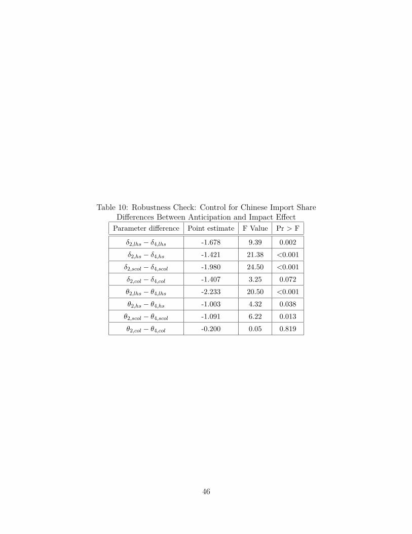
Table 10: Robustness Check: Control for Chinese Import ShareDifferences Between Anticipation and Impact EffectParameter difference Point estimate F Value Pr > F

δ2,lhs − δ4,lhs -1.678 9.39 0.002δ2,hs − δ4,hs -1.421 21.38 <0.001δ2,scol − δ4,scol -1.980 24.50 <0.001δ2,col − δ4,col -1.407 3.25 0.072θ2,lhs − θ4,lhs -2.233 20.50 <0.001θ2,hs − θ4,hs -1.003 4.32 0.038θ2,scol − θ4,scol -1.091 6.22 0.013θ2,col − θ4,col -0.200 0.05 0.819

46

Table 11: Sample sensitivity: Workers in Services (excludes agriculture)Dependent Variable: Log WageLocation-Specific ControlsLess than high school * locτ c1990 * (Year = 2000) 21.82***

(2.12)High school * locτ c1990 * (Year = 2000) 11.57***

(1.29)Some college * locτ c1990 * (Year = 2000) 4.03***

(0.59)College * locτ c1990 * (Year = 2000) -4.00

(3.33)Less than high school * loc4τ c * (Year = 2000) 24.23***

(2.03)High school * loc4τ c * (Year = 2000) 12.87***

(1.56)Some college * loc4τ c * (Year = 2000) 5.65***

(0.79)College * loc4τ c * (Year = 2000) -2.98

(3.34)Number of Observations 7,489,403

Differences Between Anticipation and Impact EffectParameter difference Point estimateδ2,lhs − δ4,lhs -2.41***

(20.11)δ2,hs − δ4,hs -1.30***

(11.06)δ2,scol − δ4,scol -1.62***

(13.00)δ2,col − δ4,col -1.03

(1.49)Standard errors or F values in parentheses.

*** indicates significance at the 1% level.

Standard errors are clustered by conspuma, industry and year.

47

Table 12: Other employment outcomes (excludes agriculture)Linear probability model Logistic modelUnemployed NILF Unemployed NILF

(1) (2) (3) (4)Location-Specific ControlsLess than high school * locτ c

1990 * (Year = 2000) 0.06 -6.71*** -1.07 -60.22***(0.605) (1.679) (10.70) (7.54)

High school * locτ c1990 * (Year = 2000) -1.11*** -3.26*** -25.04*** -32.75***

(0.155) (0.981) (7.29) (5.27)Some college * locτ c

1990 * (Year = 2000) -0.27 -2.11*** -8.41 -29.31***(0.171) (0.622) (10.21) (6.93)

College * locτ c1990 * (Year = 2000) 0.15 -1.56*** -7.81 -24.56***

(0.230) (0.452) (17.81) (9.30)Less than high school * loc4τ c * (Year = 2000) -0.44 -6.59*** -8.14 -63.58***

(0.600) (1.894) (11.58) (8.15)High school * loc4τ c * (Year = 2000) -1.27*** -3.93*** -27.75*** -42.78***

(0.145) (1.069) (7.94) (5.72)Some college * loc4τ c * (Year = 2000) -0.37** -2.71*** -11.04 -39.87***

(0.184) (0.689) (11.03) (7.48)College * loc4τ c * (Year = 2000) 0.16 -1.99*** -7.13 -32.56***

(0.236) (0.502) (19.02) (10.01)Industry-Specific ControlsLess than high school * RCAτ j

1990 * (Year = 2000) -0.62 -0.34 -8.92* 2.38(0.455) (0.425) (4.89) (3.36)

High school * RCAτ j1990 * (Year = 2000) 0.18 -0.39 -2.14 -0.95

(0.326) (0.503) (4.12) (3.05)Some college * RCAτ j

1990* (Year = 2000) 0.97*** -0.80** 21.20*** -13.42***(0.353) (0.403) (6.49) (4.85)

College * RCAτ j1990 * (Year = 2000) 0.99*** -0.37 39.13*** -9.99

(0.263) (0.299) (10.58) (7.44)Less than high school * RCA4τ j * (Year = 2000) -0.69 -0.70 -10.45* -0.65

(0.642) (0.573) (5.53) (3.91)High school * RCA4τ j * (Year = 2000) 0.33 -0.86 -0.76 -7.84**

(0.437) (0.649) (4.75) (3.58)Some college * RCA4τ j * (Year = 2000) 1.23*** -1.32*** 26.12*** -22.91***

(0.468) (0.505) (7.50) (5.69)College * RCA4τ j * (Year = 2000) 1.18*** -0.65 44.70*** -17.50**

(0.345) (0.412) (12.50) (8.87)Number of Observations 9,474,678 10,320,274 9,474,678 10,320,274Robust standard errors in parentheses. In Column 1 and 2, standard errors are clustered by

conspuma, industry and year. Column 3 and 4 report the estimated coefficients from the logistic

model. ***, ** and * indicate significance at the 1%, 5% and 10% level.

48