Atmos. Chem. Phys., 14, 1095–1105, 2014www.atmos-chem-phys.net/14/1095/2014/doi:10.5194/acp-14-1095-2014© Author(s) 2014. CC Attribution 3.0 License.

Atmospheric Chemistry

and PhysicsO

pen Access

Longitudinal hotspots in the mesospheric OH variations due toenergetic electron precipitation

M. E. Andersson1, P. T. Verronen1, C. J. Rodger2, M. A. Clilverd 3, and S. Wang4

1Earth Observation, Finnish Meteorological Institute, Helsinki, Finland2Department of Physics, University of Otago, Dunedin, New Zealand3British Antarctic Survey (NERC), Cambridge, UK4Jet Propulsion Laboratory, California Institute of Technology, California, USA

Correspondence to:M. E. Andersson (monika.andersson@fmi.fi)

Received: 13 June 2013 – Published in Atmos. Chem. Phys. Discuss.: 26 July 2013Revised: 5 December 2013 – Accepted: 20 December 2013 – Published: 29 January 2014

Abstract. Using Microwave Limb Sounder (MLS/Aura)and Medium Energy Proton and Electron Detector(MEPED/POES) observations between 2005–2009, westudy the longitudinal response of nighttime mesosphericOH to radiation belt electron precipitation. Our analysisconcentrates on geomagnetic latitudes from 55–72◦ N/S andaltitudes between 70 and 78 km. The aim of this study isto better assess the spatial distribution of electron forcing,which is important for more accurate modelling of its atmo-spheric and climate effects. In the Southern Hemisphere, OHdata show a hotspot, i.e. area of higher values, at longitudesbetween 150◦ W–30◦ E, i.e. poleward of the Southern At-lantic Magnetic Anomaly (SAMA) region. In the NorthernHemisphere, energetic electron precipitation-induced OHvariations are more equally distributed with longitude. Thislongitudinal behaviour of OH can also be identified usingEmpirical Orthogonal Function analysis, and is found to besimilar to that of MEPED-measured electron fluxes. Themain difference is in the SAMA region, where MEPEDappears to measure very large electron fluxes while MLSobservations show no enhancement of OH. This indicatesthat in the SAMA region the MEPED observations are notrelated to precipitating electrons, at least not at energies>100 keV, but rather to instrument contamination. Analysisof selected OH data sets for periods of different geomagneticactivity levels shows that the longitudinal OH hotspotsouth of the SAMA (the Antarctic Peninsula region) ispartly caused by strong, regional electron forcing, althoughatmospheric conditions also seem to play a role. Also, aweak signature of this OH hotspot is seen during periods

of generally low geomagnetic activity, which suggests thatthere is a steady drizzle of high-energy electrons affectingthe atmosphere, due to the Earth’s magnetic field beingweaker in this region.

1 Introduction

An important source of variability of mesospheric OH at highlatitudes comes from energetic particle precipitation eventsthat originate from explosions on the surface of the Sun(Thorne, 1977; Heaps, 1978; Verronen et al., 2006, 2007;Damiani et al., 2008, 2010b; Jackman et al., 2011; Verronenet al., 2011). In contrast to solar protons, which propagate di-rectly from the Sun into Earth’s atmosphere, energetic elec-trons are first stored and energised in the radiation belts. Dur-ing geomagnetic storms, strong acceleration and loss pro-cesses occur (Reeves et al., 2003), which can both boostthe trapped population and lead to significant loss of elec-trons into the atmosphere. Energetic electron precipitation(EEP) from the radiation belts affects the neutral atmosphereat magnetic latitudes of about 55–72◦ and results in the en-hancement of HOx through water cluster ion chemistry. Thisprocess is only effective below about 80 km, where enoughwater vapour is available (Solomon et al., 1981; Sinnhu-ber et al., 2012; Verronen and Lehmann, 2013). The atmo-spheric penetration depth depends on the energy of the parti-cles, e.g. electrons with 100 keV and 3 MeV energy can reach80 km and 50 km, respectively (see, e.g.Turunen et al., 2009,Fig. 3).

Published by Copernicus Publications on behalf of the European Geosciences Union.

1096 M. E. Andersson et al.: Electron precipitation and longitudinal OH variations

The primary driver of the radiation belt variability is ge-omagnetic activity, which can come either from the coronalmass ejections (CMEs) during solar maximum or the high-speed solar wind streams (HSSWS,> 500 km/s) which aremost common during the declining and minimum phase ofsolar activity. The energy input to the magnetosphere duringHSSWS events is comparable to or can be higher than theenergy input during CMEs (Richardson et al., 2000, 2001).Such storms tend to be weaker than CME storms in termsof geomagnetic index values, last longer, and involve moreradiation belt dynamics in the production of electron precip-itation (Borovsky et al., 2006).

EEP can occur on different timescales with varying signif-icance for the atmospheric chemistry, but our understandingof the nature of the precipitation as well as the variation of theelectron flux lost to the atmosphere is limited. This is mostlydue to spatial and temporal limitation of the measurements aswell as contamination issues in the space-based instrumenta-tion (Rodger et al., 2010a; Clilverd et al., 2010). Therefore,detailed study of the EEP effects in the atmosphere can sig-nificantly improve our understanding of the EEP variabilitywhich is important for atmospheric modelling (Funke et al.,2011).

Recent studies provided evidence of the connection be-tween precipitating radiation belt electrons and mesospherichydroxyl (Andersson et al., 2012; Verronen et al., 2011). Byanalysing zonal mean time series of MLS/Aura OH mixingratios and MEPED/POES radiation belt electron fluxes dur-ing the period August 2004–December 2009, they demon-strated strong correlation between experimentally observed100–300 keV electron count rates and nighttime OH concen-trations below 80 km. These studies provided a lower-limitestimation of the importance of energetic electron precipita-tion on HOx, showing that for the considered time period,EEP has measurable effects in about 30 % of cases.

In this paper, we combine MLS OH and MEPED EEPsatellite measurements to study the longitudinal OH varia-tions caused by precipitating radiation belt electrons betweenJanuary 2005–December 2009. We go on to utilise empiri-cal orthogonal function (EOF) analysis to identify OH spa-tial and temporal patterns of variability. Finally we provideclear evidence that the SAMA region influences the longitu-dinal variation of OH at geomagnetic latitudes 55–72◦ in theSouthern Hemisphere (SH), as expected from the location ofthe radiation belts and the weaker magnetic field region. Notethat the time period 2005–2009 analysed here coincided withdeclining phase of solar activity and an extended solar mini-mum, and thus consists mainly of HSSWS-driven storms.

2 Data

2.1 MLS/Aura observations

The MLS instrument onboard NASA’s Aura satellite, placedinto a Sun-synchronous orbit (about 705 km), samples the at-mosphere up to 82◦ N/S (Waters et al., 2006). MLS observesthermal microwave emission, scanning from the ground to90 km every 25 s with daily global coverage of about 14.6orbits per day.

In this study, we use Version 3.3 Level 2 nighttime (solarzenith angle>100◦) OH for the time period of January 2005–December 2009 between 70 and 78 km altitude (correspond-ing to pressure levels between 0.046 and 0.015 hPa). The al-titude selection was based on previous studies, i.e. (Anders-son et al., 2012), which showed that between 70 and 78 kmthe response of OH to electron precipitation is the highest.The vertical resolution of OH observations is about 2.5 kmand the systematic error is typically less than 10 %. The datawere screened according to the MLS data description andquality document (Livesey et al., 2011). The OH observa-tions taken during solar proton events (SPE), which domi-nate the ionization in the middle atmosphere, were excludedhere and from all further considerations using a flux limitof 4 protons cm−2 s−1 sr−1 as observed by GOES-11 at 5–10 MeV energies.

In addition, to support our discussion about OH variations,we also use MLS water vapour (H2O) and temperature ob-servations. The H2O and temperature data were sampled thesame way as the OH measurements and screened accordingto the MLS data quality document. The vertical resolutionof H2O/temperature observations is coarser than that of OHat considered altitudes, i.e. about 5 km, and therefore, we usemeasurements between 70 and 76 km (corresponding to pres-sure levels between 0.046 and 0.025 hPa). The systematic er-ror of the H2O/temperature data is typically less than about0.8 ppmv (25 %)/3 K (5 %). Details on the validation of theMLS OH, H2O and temperature are given inPickett et al.(2008), Lambert et al.(2007) and Schwartz et al.(2008),respectively. Note that due to the selection criteria we havemore observations during the wintertime.

3 MEPED/POES observation

The Space Environment Monitor (SEM-2) instrument pack-age onboard the Sun-synchronous (800–850 km) NOAAPOES satellites, provides long-term global measurement ofprecipitating electron fluxes with some limited energy spec-tra information. SEM-2 includes the Medium Energy Pro-ton and Electron Detector (MEPED) which consists of twoelectron telescopes and two proton telescopes. The pairs oftelescopes are pointed approximately perpendicular to eachother. Both electron telescopes provide three channels of en-ergetic electron data:> 30 keV,> 100 keV, and> 300 keV,

Atmos. Chem. Phys., 14, 1095–1105, 2014 www.atmos-chem-phys.net/14/1095/2014/

M. E. Andersson et al.: Electron precipitation and longitudinal OH variations 1097

Fig. 1. World maps showing medians of>30 keV precipitating electrons observed by the 0◦ directed MEPED telescopes onboard POES in2005, 2006, 2008 and 2009.

sampled simultaneously. For a detailed description of theSEM-2 instruments, seeEvans and Greer(2004).

We utilise data from the MEPED 0◦ electron telescope(field-of-view is outward along the local zenith, parallel tothe Earth-center-to-satellite radial vector). The electron tele-scopes are observing fluxes located inside the bounce losscone, and thus electrons which are being lost locally towardthe spacecraft direction (Rodger et al., 2010a; Rodger et al.,2010b). At this point NOAA is undertaking major new datare-processing, which will produce new data sets with deriveduncertainty values. Until these have been produced we sug-gest a reasonable value for the measurement uncertainties is20%, followingTan et al.(2007).

4 Results

Figure 1 shows the distribution of> 30 keV electrons pre-cipitating into the atmosphere observed by the 0◦ directedMEPED telescopes in 2005, 2006, 2008 and 2009. Becausethe year 2007 is very similar to 2008, considering electronprecipitation and OH, we omitted it from the Fig. 1 (and alsofrom Fig. 2 later) for clarity reasons. However, our analy-sis is conducted for the whole period between 2005–2009.These maps were produced from the 2 s resolution electrontelescope data, which were corrected for proton contamina-tion (Yando et al., 2011) using the algorithm described inAppendix A of Lam et al.(2010). For each day of the yearselected, a 1◦ spatial resolution map of the median> 30 keVfluxes was produced for each POES spacecraft in subsatel-lite coordinates. The median of each of these daily maps pro-duces the median world maps shown in Fig.1. While theLamet al.(2010) method can generally correct for proton contam-

ination, this is not possible when the electron observationsare dominated by proton counts, as expected during SPEs orin the SAMA region. The data inside the SAMA region, i.e.around 30◦ E–90◦ W and 0◦–45◦ S, appears to contain an in-creased particle background due to a local minimum of thegeomagnetic field. This however, is more likely due to con-tamination of the particle detectors than electron precipita-tion (we will discuss this in the next paragraph). In Fig.1 theelectron precipitation is confined to the geomagnetic latitu-dinal bands 55–72◦ N and 55–72◦ S and can occur at all geo-graphic longitudes. However, in the SH the observed electronfluxes are consistently higher poleward of the SAMA region,i.e. the Antarctic Peninsula (AP) hotspot, which ranges inlongitudinal extent from 180◦ W–60◦ E. There is less elec-tron precipitation at longitudes between 90◦ E–180◦ E. Themaximum difference in longitudinal EEP distribution withinthe range of the radiation belt in the SH is of about 150 %.In the Northern Hemisphere (NH) precipitation is more ho-mogenous through the whole longitude range with higherelectron fluxes observed between 150◦ W–30◦ W, i.e. NorthAmerica (NAm) hotspot. The maximum difference in longi-tudinal EEP distribution within the range of the radiation beltin the NH is of about 70 %. A similar geographic distributionof the precipitating electrons is observed for all consideredyears, with a decreasing trend of electron fluxes in the radi-ation belts from 2005 to 2009, related to the decline in solaractivity. As noted above, Fig.1 shows a clear pattern with alocal hotspot in precipitating fluxes in the AP region. This isexpected, due to the changing strength of the geomagneticfield. In the AP region the magnetic field is weaker, suchthat the angular width of the bounce loss cone increases andelectrons which were mirroring just above the atmosphere at

www.atmos-chem-phys.net/14/1095/2014/ Atmos. Chem. Phys., 14, 1095–1105, 2014

1098 M. E. Andersson et al.: Electron precipitation and longitudinal OH variations

2005

Longitude

Lat

itu

de

0 60 120 −180 −120 −60 0 −80

−40

0

40

802006

Longitude

Lat

itu

de

0 60 120 −180 −120 −60 0 −80

−40

0

40

800.6 0.8 1 1.2 1.4 1.6

2008

Longitude

Lat

itu

de

0 60 120 −180 −120 −60 0 −80

−40

0

40

802009

Longitude

Lat

itu

de

0 60 120 −180 −120 −60 0 −80

−40

0

40

80

OH [ppbv]

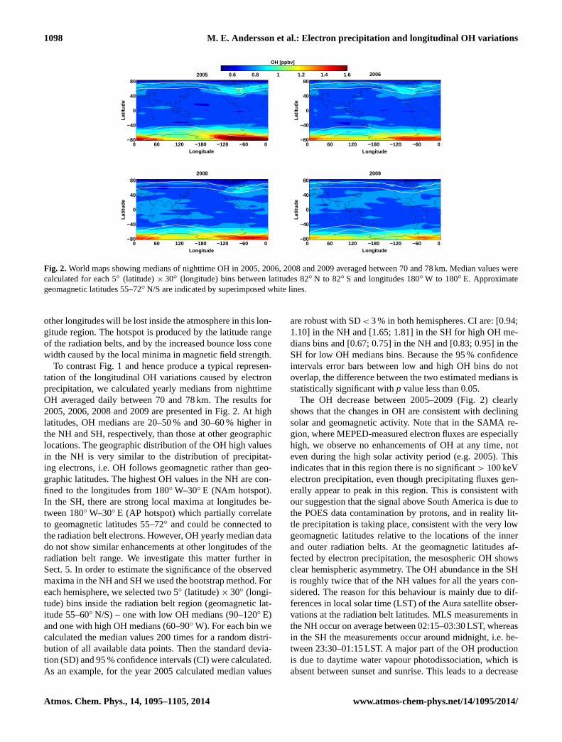
Fig. 2. World maps showing medians of nighttime OH in 2005, 2006, 2008 and 2009 averaged between 70 and 78 km. Median values werecalculated for each 5◦ (latitude)× 30◦ (longitude) bins between latitudes 82◦ N to 82◦ S and longitudes 180◦ W to 180◦ E. Approximategeomagnetic latitudes 55–72◦ N/S are indicated by superimposed white lines.

other longitudes will be lost inside the atmosphere in this lon-gitude region. The hotspot is produced by the latitude rangeof the radiation belts, and by the increased bounce loss conewidth caused by the local minima in magnetic field strength.

To contrast Fig.1 and hence produce a typical represen-tation of the longitudinal OH variations caused by electronprecipitation, we calculated yearly medians from nighttimeOH averaged daily between 70 and 78 km. The results for2005, 2006, 2008 and 2009 are presented in Fig.2. At highlatitudes, OH medians are 20–50 % and 30–60 % higher inthe NH and SH, respectively, than those at other geographiclocations. The geographic distribution of the OH high valuesin the NH is very similar to the distribution of precipitat-ing electrons, i.e. OH follows geomagnetic rather than geo-graphic latitudes. The highest OH values in the NH are con-fined to the longitudes from 180◦ W–30◦ E (NAm hotspot).In the SH, there are strong local maxima at longitudes be-tween 180◦ W–30◦ E (AP hotspot) which partially correlateto geomagnetic latitudes 55–72◦ and could be connected tothe radiation belt electrons. However, OH yearly median datado not show similar enhancements at other longitudes of theradiation belt range. We investigate this matter further inSect. 5. In order to estimate the significance of the observedmaxima in the NH and SH we used the bootstrap method. Foreach hemisphere, we selected two 5◦ (latitude)× 30◦ (longi-tude) bins inside the radiation belt region (geomagnetic lat-itude 55–60◦ N/S) – one with low OH medians (90–120◦ E)and one with high OH medians (60–90◦ W). For each bin wecalculated the median values 200 times for a random distri-bution of all available data points. Then the standard devia-tion (SD) and 95 % confidence intervals (CI) were calculated.As an example, for the year 2005 calculated median values

are robust with SD< 3 % in both hemispheres. CI are: [0.94;1.10] in the NH and [1.65; 1.81] in the SH for high OH me-dians bins and [0.67; 0.75] in the NH and [0.83; 0.95] in theSH for low OH medians bins. Because the 95 % confidenceintervals error bars between low and high OH bins do notoverlap, the difference between the two estimated medians isstatistically significant withp value less than 0.05.

The OH decrease between 2005–2009 (Fig. 2) clearlyshows that the changes in OH are consistent with decliningsolar and geomagnetic activity. Note that in the SAMA re-gion, where MEPED-measured electron fluxes are especiallyhigh, we observe no enhancements of OH at any time, noteven during the high solar activity period (e.g. 2005). Thisindicates that in this region there is no significant> 100 keVelectron precipitation, even though precipitating fluxes gen-erally appear to peak in this region. This is consistent withour suggestion that the signal above South America is due tothe POES data contamination by protons, and in reality lit-tle precipitation is taking place, consistent with the very lowgeomagnetic latitudes relative to the locations of the innerand outer radiation belts. At the geomagnetic latitudes af-fected by electron precipitation, the mesospheric OH showsclear hemispheric asymmetry. The OH abundance in the SHis roughly twice that of the NH values for all the years con-sidered. The reason for this behaviour is mainly due to dif-ferences in local solar time (LST) of the Aura satellite obser-vations at the radiation belt latitudes. MLS measurements inthe NH occur on average between 02:15–03:30 LST, whereasin the SH the measurements occur around midnight, i.e. be-tween 23:30–01:15 LST. A major part of the OH productionis due to daytime water vapour photodissociation, which isabsent between sunset and sunrise. This leads to a decrease

Atmos. Chem. Phys., 14, 1095–1105, 2014 www.atmos-chem-phys.net/14/1095/2014/

M. E. Andersson et al.: Electron precipitation and longitudinal OH variations 1099

23 00 01 02 03 04

0.5

1

1.5

Time [hh]

OH

[p

pb

v]

5−6 March 2005

LST of SH−MLS measurements

LST of NH−MLS measurements

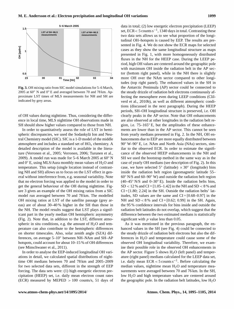
Fig. 3.OH mixing ratio from SIC model simulations for 5–6 March,2005 at 60◦ N and 0◦ E and averaged between 70 and 78 km. Ap-proximate LST times of MLS measurements for NH and SH areindicated by grey areas.

of OH values during nighttime. Thus, considering the differ-ence in local time, MLS nighttime OH observations made inSH should show higher values compared to those from NH.

In order to quantitatively assess the role of LST in hemi-spheric discrepancies, we used the Sodankylä Ion and Neu-tral Chemistry model (SIC). SIC is a 1-D model of the middleatmosphere and includes a standard set of HOx chemistry. Adetailed description of the model is available in the litera-ture (Verronen et al., 2005; Verronen, 2006; Turunen et al.,2009). A model run was made for 5–6 March 2005 at 60◦ Nand 0◦ E, using MLS/Aura monthly mean values of H2O andtemperature. This setup (single location instead of contrast-ing NH and SH) allows us to focus on the LST effect in gen-eral without interference from, e.g. seasonal variability. Notethat no electron forcing was applied to the model in order toget the general behaviour of the OH during nighttime. Fig-ure3 gives an example of the OH mixing ratios from a SICmodel run averaged between 70 and 78 km. The modelledOH mixing ratios at LST of the satellite passage (grey ar-eas) are of about 30–40 % higher in the SH than those inthe NH. The model results suggest that LST plays a signif-icant part in the yearly median OH hemispheric asymmetry(Fig. 2). Note that, in addition to the LST, different atmo-spheric in situ conditions, e.g. the amount of H2O and tem-perature can also contribute to the hemispheric differenceson shorter timescales. Also, solar zenith angle (SZA) dif-ferences, on average 5–10◦ between NH–NAm and SH–APhotspots, could account for about 10–15 % of OH differences(seeMinschwaner et al., 2011).

In order to analyse the EEP-induced longitudinal OH vari-ations in detail, we calculated spatial distributions of night-time OH medians between 70 and 78 km and 2005–2009for two selected data sets, different in the strength of EEPforcing. The data sets were: (1) high energetic electron pre-cipitation (HEEP) set, i.e. daily mean electron count rates(ECR) measured by MEPED> 100 counts/s, 51 days of

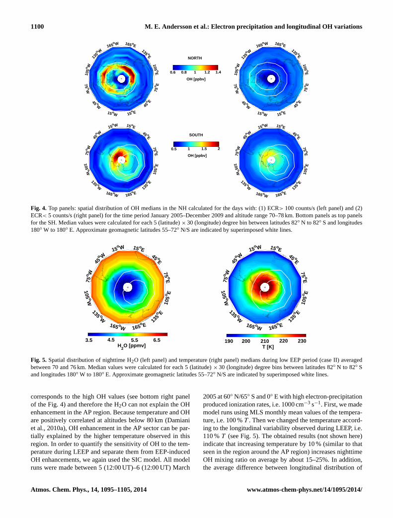
data in total; (2) low energetic electron precipitation (LEEP)set, ECR< 5 counts s−1, 1340 days in total. Contrasting thesetwo data sets allows us to see what proportion of the longi-tudinal OH–hotspots is caused by EEP. The results are pre-sented in Fig.4. We do not show the ECR maps for selectedcases as they show the same longitudinal structure as mapspresented in Fig. 1, with more homogeneously distributedfluxes in the NH for the HEEP case. During the LEEP pe-riod, high OH values are centered around the geographic polewith maximum OH inside the radiation belt in the AP sec-tor (bottom right panel), while in the NH there is slightlymore OH over the NAm sector compared to other longi-tudes (top right panel). The enhanced values in the SH inthe Antarctic Peninsula (AP) sector could be connected tothe steady drizzle of radiation belt electrons continuously af-fecting the mesosphere even during LEEP conditions (Clil-verd et al., 2010b), as well as different atmospheric condi-tions (discussed in the next paragraph). During the HEEPperiods, SH–OH longitudinal structure is preserved, i.e. OHclearly peaks in the AP sector. Note that OH enhancementsare also observed at other longitudes in the radiation belt re-gion, i.e. 75–165◦ E, but the amplitudes of these enhance-ments are lower than in the AP sector. This cannot be seenfrom yearly medians presented in Fig.2. In the NH, OH en-hancements due to EEP are more equally distributed between90◦ W–90◦ E, i.e. NAm and North Asia (NAs) sectors, sim-ilar to the observed ECR. In order to estimate the signifi-cance of the observed HEEP enhancements in the NH andSH we used the bootstrap method in the same way as in thecase of yearly OH medians (see description of Fig.2). In thiscase, we have selected 5◦ (latitude)× 30◦ (longitude) binsinside the radiation belt region (geomagnetic latitude 55–60◦ N/S and 60–90◦ W) and outside the radiation belt region(40–45◦ N/S and 0–30◦ E). Inside the radiation belts bins,SD< 12 % and CI = [1.05–1.42] in the NH and SD< 8 % andCI = [1.80; 2.24] in the SH. Outside the radiation belts’ lat-itudes, SD values are the same and CI = [0.68–0.97] in theNH and SD< 8 % and CI = [0.62; 0.99] in the SH. Again,the 95 % confidence intervals for bins inside and outside theradiation belt latitudes do not overlap, which suggest that thedifference between the two estimated medians is statisticallysignificant withp value less than 0.05.

As it was mentioned in the previous paragraph, the en-hanced values in the SH (see Fig.4) could be connected tothe steady drizzle of radiation belt electrons but also the dif-ferences in H2O and temperature could cause some of theobserved OH longitudinal variability. Therefore, we exam-ine their possible role in the observed OH enhancements inthe AP sector. Figure5 shows H2O (left panel) and temper-ature (right panel) medians calculated for the LEEP data set,i.e. daily mean ECR< 5 counts s−1. Before calculating themedian values, nighttime mean H2O and temperature mea-surements were averaged between 70 and 76 km. In the SH,low H2O and high temperature values are centered aroundthe geographic pole. In the radiation belt latitudes, low H2O

www.atmos-chem-phys.net/14/1095/2014/ Atmos. Chem. Phys., 14, 1095–1105, 2014

1100 M. E. Andersson et al.: Electron precipitation and longitudinal OH variations

165o W

135o W

105

o W

75 oW

45 oW

15 o

W 15o E

45o E

75

o E

105 oE

135 oE

165 oE

165o W

135o W

105

o W

75 oW

45 oW

15 o

W 15o E

45o E

75

o E

105 oE

135 oE

165 oE

165 oW

135 oW

105 oW

75

o W

45o W

15

o W 15 oE

45 oE

75 oE

105

o E

135o E

165o E

165 oW

135 oW

105 oW

45o W

15

o W 15 oE

45 oE

75 oE

105

o E

135o E

165o E

75

o W

OH [ppbv]

0.5 1 1.5 2

0.6 1 1.2 1.4

SOUTH

OH [ppbv]

NORTH

0.8

Fig. 4. Top panels: spatial distribution of OH medians in the NH calculated for the days with: (1) ECR> 100 counts/s (left panel) and (2)ECR< 5 counts/s (right panel) for the time period January 2005–December 2009 and altitude range 70–78 km. Bottom panels as top panelsfor the SH. Median values were calculated for each 5 (latitude)× 30 (longitude) degree bin between latitudes 82◦ N to 82◦ S and longitudes180◦ W to 180◦ E. Approximate geomagnetic latitudes 55–72◦ N/S are indicated by superimposed white lines.

165 oW

135 oW

105 oW

75

o W

45o W

15o W 15 o

E 45 oE

75 oE

105

o E

135o E

165o E

165 oW

135 oW

105 oW

75

o W

45o W

15o W 15 o

E 45 oE

75 oE

105

o E

135o E

165o E

190 200 210 220 230T [K]

3.5H

2O [ppmv]

6.55.54.5

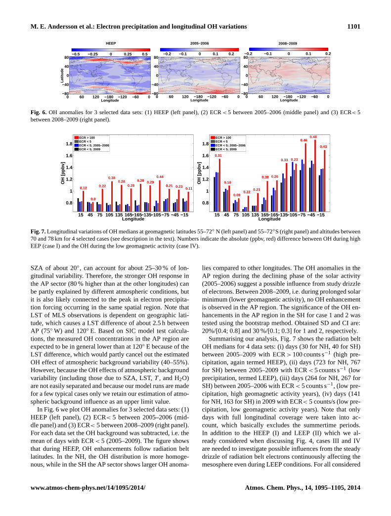
Fig. 5. Spatial distribution of nighttime H2O (left panel) and temperature (right panel) medians during low EEP period (case II) averagedbetween 70 and 76 km. Median values were calculated for each 5 (latitude)× 30 (longitude) degree bins between latitudes 82◦ N to 82◦ Sand longitudes 180◦ W to 180◦ E. Approximate geomagnetic latitudes 55–72◦ N/S are indicated by superimposed white lines.

corresponds to the high OH values (see bottom right panelof the Fig.4) and therefore the H2O can not explain the OHenhancement in the AP region. Because temperature and OHare positively correlated at altitudes below 80 km (Damianiet al., 2010a), OH enhancement in the AP sector can be par-tially explained by the higher temperature observed in thisregion. In order to quantify the sensitivity of OH to the tem-perature during LEEP and separate them from EEP-inducedOH enhancements, we again used the SIC model. All modelruns were made between 5 (12:00 UT)–6 (12:00 UT) March

2005 at 60◦ N/65◦ S and 0◦ E with high electron-precipitationproduced ionization rates, i.e. 1000 cm−3 s−1. First, we mademodel runs using MLS monthly mean values of the tempera-ture, i.e. 100 %T . Then we changed the temperature accord-ing to the longitudinal variability observed during LEEP, i.e.110 %T (see Fig.5). The obtained results (not shown here)indicate that increasing temperature by 10 % (similar to thatseen in the region around the AP region) increases nighttimeOH mixing ratio on average by about 15–25%. In addition,the average difference between longitudinal distribution of

Atmos. Chem. Phys., 14, 1095–1105, 2014 www.atmos-chem-phys.net/14/1095/2014/

M. E. Andersson et al.: Electron precipitation and longitudinal OH variations 1101

2005−2006

Longitude

0 60 120 −180 −120 −60 0 −80

−40

0

40

80−0.2 −0.1 0 0.1 0.2

2008−2009

Longitude

0 60 120 −180 −120 −60 0 −80

−40

0

40

80−0.2 −0.1 0 0.1 0.2

HEEP

Longitude

Lat

itu

de

0 60 120 −180 −120 −60 0 −80

−40

0

40

80−0.5 −0.25 0 0.25 0.5

Fig. 6. OH anomalies for 3 selected data sets: (1) HEEP (left panel), (2) ECR< 5 between 2005–2006 (middle panel) and (3) ECR< 5between 2008–2009 (right panel).

15 45 75 105 135 165−165−135−105−75 −45 −15

0.8

1

1.2

1.4

1.6

1.8

Longitude

OH

[p

pb

v]

15 45 75 105 135 165−165−135−105−75 −45 −15

0.8

1

1.2

1.4

1.6

1.8

Longitude

OH

[p

pb

v]

ECR > 100ECR < 5ECR < 5; 2005−2006ECR < 5; 2009

ECR > 100ECR < 5ECR < 5; 2005−2006ECR < 5; 2009

0.12 0.22 0.280.29

0.110.230.21

0.440.280.28

0.38

0.0

0.31

0.10

0.080.22

0.21

0.38 0.26

0.33 0.23

0.460.48

0.43

Fig. 7.Longitudinal variations of OH medians at geomagnetic latitudes 55–72◦ N (left panel) and 55–72◦S (right panel) and altitudes between70 and 78 km for 4 selected cases (see description in the text). Numbers indicate the absolute (ppbv, red) difference between OH during highEEP (case I) and the OH during the low geomagnetic activity (case IV).

SZA of about 20◦, can account for about 25–30 % of lon-gitudinal variability. Therefore, the stronger OH response inthe AP sector (80 % higher than at the other longitudes) canbe partly explained by different atmospheric conditions, butit is also likely connected to the peak in electron precipita-tion forcing occurring in the same spatial region. Note thatLST of MLS observations is dependent on geographic lati-tude, which causes a LST difference of about 2.5 h betweenAP (75◦ W) and 120◦ E. Based on SIC model test calcula-tions, the measured OH concentrations in the AP region areexpected to be in general lower than at 120◦ E because of theLST difference, which would partly cancel out the estimatedOH effect of atmospheric background variability (40–55%).However, because the OH effects of atmospheric backgroundvariability (including those due to SZA, LST,T , and H2O)are not easily separated and because our model runs are madefor a few typical cases only we retain our estimation of atmo-spheric background influence as an upper limit value.

In Fig.6 we plot OH anomalies for 3 selected data sets: (1)HEEP (left panel), (2) ECR< 5 between 2005–2006 (mid-dle panel) and (3) ECR< 5 between 2008–2009 (right panel).For each data set the OH background was subtracted, i.e. themean of days with ECR< 5 (2005–2009). The figure showsthat during HEEP, OH enhancements follow radiation beltlatitudes. In the NH, the OH distribution is more homoge-nous, while in the SH the AP sector shows larger OH anoma-

lies compared to other longitudes. The OH anomalies in theAP region during the declining phase of the solar activity(2005–2006) suggest a possible influence from study drizzleof electrons. Between 2008–2009, i.e. during prolonged solarminimum (lower geomagnetic activity), no OH enhancementis observed in the AP region. The significance of the OH en-hancements in the AP region in the SH for case 1 and 2 wastested using the bootstrap method. Obtained SD and CI are:20%/[0.4; 0.8] and 30 %/[0.1; 0.3] for 1 and 2, respectively.

Summarising our analysis, Fig.7 shows the radiation beltOH medians for 4 data sets: (i) days (30 for NH, 40 for SH)between 2005–2009 with ECR> 100 counts s−1 (high pre-cipitation, again termed HEEP), (ii) days (723 for NH, 767for SH) between 2005–2009 with ECR< 5 counts s−1 (lowprecipitation, termed LEEP), (iii) days (264 for NH, 267 forSH) between 2005–2006 with ECR< 5 counts s−1, (low pre-cipitation, high geomagnetic activity years), (iv) days (141for NH, 163 for SH) in 2009 with ECR< 5 counts/s (low pre-cipitation, low geomagnetic activity years). Note that onlydays with full longitudinal coverage were taken into ac-count, which basically excludes the summertime periods.In addition to the HEEP (I) and LEEP (II) which we al-ready considered when discussing Fig.4, cases III and IVare needed to investigate possible influences from the steadydrizzle of radiation belt electrons continuously affecting themesosphere even during LEEP conditions. For all considered

www.atmos-chem-phys.net/14/1095/2014/ Atmos. Chem. Phys., 14, 1095–1105, 2014

1102 M. E. Andersson et al.: Electron precipitation and longitudinal OH variations

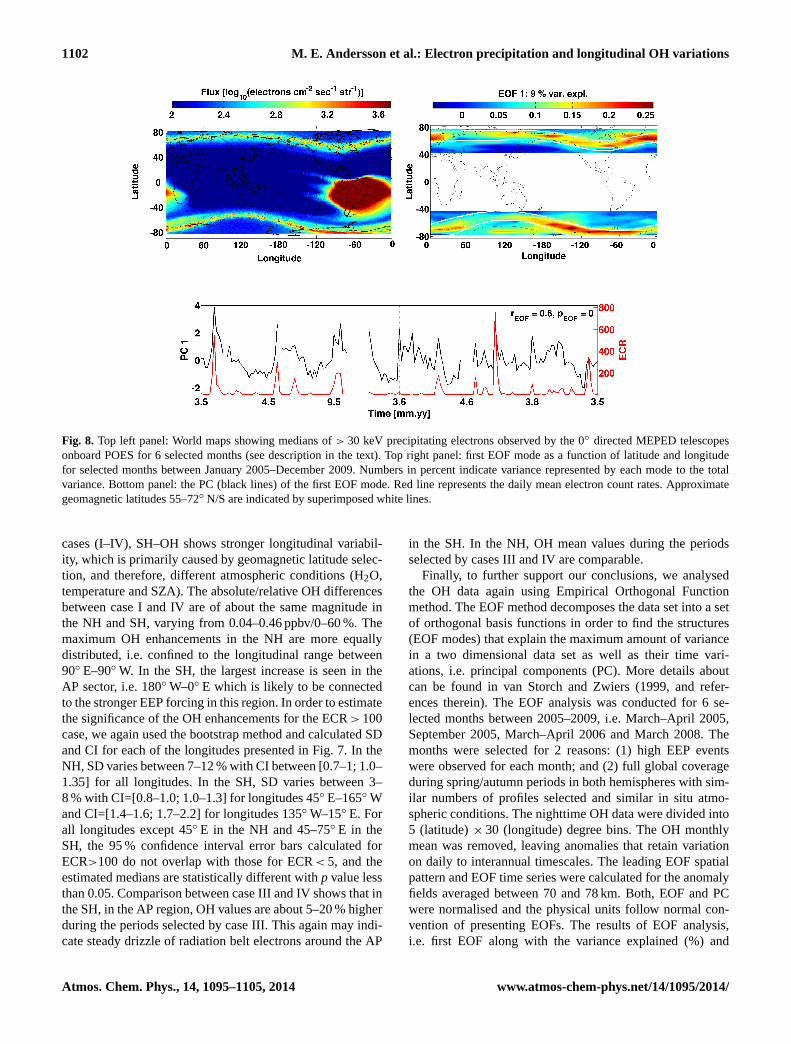
Fig. 8. Top left panel: World maps showing medians of> 30 keV precipitating electrons observed by the 0◦ directed MEPED telescopesonboard POES for 6 selected months (see description in the text). Top right panel: first EOF mode as a function of latitude and longitudefor selected months between January 2005–December 2009. Numbers in percent indicate variance represented by each mode to the totalvariance. Bottom panel: the PC (black lines) of the first EOF mode. Red line represents the daily mean electron count rates. Approximategeomagnetic latitudes 55–72◦ N/S are indicated by superimposed white lines.

cases (I–IV), SH–OH shows stronger longitudinal variabil-ity, which is primarily caused by geomagnetic latitude selec-tion, and therefore, different atmospheric conditions (H2O,temperature and SZA). The absolute/relative OH differencesbetween case I and IV are of about the same magnitude inthe NH and SH, varying from 0.04–0.46 ppbv/0–60 %. Themaximum OH enhancements in the NH are more equallydistributed, i.e. confined to the longitudinal range between90◦ E–90◦ W. In the SH, the largest increase is seen in theAP sector, i.e. 180◦ W–0◦ E which is likely to be connectedto the stronger EEP forcing in this region. In order to estimatethe significance of the OH enhancements for the ECR> 100case, we again used the bootstrap method and calculated SDand CI for each of the longitudes presented in Fig.7. In theNH, SD varies between 7–12 % with CI between [0.7–1; 1.0–1.35] for all longitudes. In the SH, SD varies between 3–8 % with CI=[0.8–1.0; 1.0–1.3] for longitudes 45◦ E–165◦ Wand CI=[1.4–1.6; 1.7–2.2] for longitudes 135◦ W–15◦ E. Forall longitudes except 45◦ E in the NH and 45–75◦ E in theSH, the 95 % confidence interval error bars calculated forECR>100 do not overlap with those for ECR< 5, and theestimated medians are statistically different withp value lessthan 0.05. Comparison between case III and IV shows that inthe SH, in the AP region, OH values are about 5–20 % higherduring the periods selected by case III. This again may indi-cate steady drizzle of radiation belt electrons around the AP

in the SH. In the NH, OH mean values during the periodsselected by cases III and IV are comparable.

Finally, to further support our conclusions, we analysedthe OH data again using Empirical Orthogonal Functionmethod. The EOF method decomposes the data set into a setof orthogonal basis functions in order to find the structures(EOF modes) that explain the maximum amount of variancein a two dimensional data set as well as their time vari-ations, i.e. principal components (PC). More details aboutcan be found invan Storch and Zwiers(1999, and refer-ences therein). The EOF analysis was conducted for 6 se-lected months between 2005–2009, i.e. March–April 2005,September 2005, March–April 2006 and March 2008. Themonths were selected for 2 reasons: (1) high EEP eventswere observed for each month; and (2) full global coverageduring spring/autumn periods in both hemispheres with sim-ilar numbers of profiles selected and similar in situ atmo-spheric conditions. The nighttime OH data were divided into5 (latitude)× 30 (longitude) degree bins. The OH monthlymean was removed, leaving anomalies that retain variationon daily to interannual timescales. The leading EOF spatialpattern and EOF time series were calculated for the anomalyfields averaged between 70 and 78 km. Both, EOF and PCwere normalised and the physical units follow normal con-vention of presenting EOFs. The results of EOF analysis,i.e. first EOF along with the variance explained (%) and

Atmos. Chem. Phys., 14, 1095–1105, 2014 www.atmos-chem-phys.net/14/1095/2014/

M. E. Andersson et al.: Electron precipitation and longitudinal OH variations 1103

corresponding PC 1, are shown in Fig.8. Figure8 also showsthe median distribution of> 30 keV electrons precipitatinginto the atmosphere observed by the 0◦ directed MEPEDfor the same months EOF analysis was conducted. Note thatthe OH measurements from the equatorial regions, i.e. 45◦S–45◦ N were excluded from analysis in order to avoid possibleimpact from other factors (for example tides) that could af-fect the OH variation.

The observed electron precipitation seen in the upper left-hand panel of this figure is similar to the yearly medianspresented in Fig.1 except that is has a more pronouncedlongitudinal structure. EEP is clearly higher in the AP re-gion and slightly higher between 150◦ E–0◦ W in the NHin the magnetic latitudinal band 55–72◦ N/S. The first EOF(right top panel of Fig.8) also has pronounced structures atgeomagnetic latitudes connected to the radiation belts (55–72◦ N/S) and appears to be associated with the spatial vari-ations in electron precipitation. The spatial patterns of theOH changes do not extend to other latitudes and follow theradiation belt areas much more closely than the yearly me-dian presented in Fig.2. EOF 1 constitutes 9% of the totalvariance, and this mode clearly dominates the OH variationafter a strong global seasonal component was removed. Theprincipal component (PC 1) related to the first EOF followsthe ECR variability (bottom panel of Fig.8). The correla-tion between amplitude of the PC 1 and ECR isrEOF = 0.6.The statistical robustness of the correlation was determinedby calculating thep value (t test). The resultingp < 0.01, i.e.the random chance probability of getting such correlation forthe data sets when the true correlation is zero is less than1 %. Note that the enhanced PC 1 values at the beginning ofMarch 2006 are connected to the enhanced OH values at lati-tudes> 70◦ N and longitudes 0–120◦ W, i.e. outside radiationbelt latitudes. Similar OH enhancement, again outside the ra-diation belt latitudes, is observed in March 2008 at latitudes>70◦ S and longitudes 90◦ E–120◦ W. In the SH, the reasonfor such OH enhancement is unclear. In the NH, it could beconnected to the descent of OH maximum layer, which oc-curred in 2006 after a sudden stratospheric warming event(Damiani et al., 2010a).

These results indicate that first EOF is associated withEEP. EOF 1 not only reflects an enhancement of OH at lati-tudes affected by EEP but also captures its longitudinal vari-ations, i.e. maximum increases confined to the longitudinalband 150◦ E–30◦ W in the NH and 180◦ W–60◦ E in the SH(see Fig.4). We analysed also the second and third EOF pat-terns (not shown). However, these sum up to less than 4% ofthe total variance and the patterns do not correlate with EEP.They are more likely connected to the noise.

5 Conclusions

Using measurements from the MLS/Aura andMEPED/POES between 2005–2009, we have studiedlongitudinal variations of nighttime OH and their link toenergetic electron precipitation. The time period analysedhere coincided with a declining phase of solar activityand an extended solar minimum, and thus consists mainlyof HSSWS-driven storms. Our analysis shows, that atgeomagnetic latitudes 55–72◦ N/S and altitudes between 70and 78 km, there are spatial hotspots in the mesospheric OHvariations due to energetic electron precipitation.

In the SH, an OH hotspot is located in the AP region, i.e.in a longitudinal band between 150◦ W–60◦ E. At those lon-gitudes, EEP observed by POES, as well as the OH enhance-ment are the highest. Because the atmospheric in situ con-ditions can explain only part of the total 80 % of OH longi-tudinal variations (15–25 % H2O and temperature, 25–30 %SZA), the OH hotspot in this sector is likely to be connectedto stronger electron forcing. Also, increased OH values inthis region during the period of low EEP but higher geomag-netic activity suggest the effect of a steady drizzle of radi-ation belt electrons during the quiet time conditions. EOFanalysis has shown similar pronounced structures at geomag-netic latitudes connected to the radiation belts (55–72◦ S).The first EOF mode constitutes 9 % of the total variance, andclearly reflects an enhancement of OH at latitudes affectedby EEP as well as its longitudinal variations, i.e. a maximumamplitude confined to the longitudinal band 150◦ W–60◦ E.Note that even though MEPED measures very high electroncount rates inside SAMA, this does not seem to correspondto any significant precipitation, i.e. no OH enhancement isobserved in that region.

In the NH, EEP is more homogenous over the whole lon-gitude range with slightly higher electron fluxes observed be-tween 180◦ W–0◦ E, i.e. over the NAm sector. The distribu-tion of OH yearly medians is roughly confined to the samelongitudinal band 150◦ W–30◦ E, but the OH medians duringHEEP show different spatial behaviour, i.e. an OH hotspotextends from NAm to the NAs sector (90◦ E–90◦ W). Thefirst EOF mode clearly reflects the OH enhancement withthe maximum amplitude roughly confined to the longitudi-nal band 150◦ W–30◦ E.

Our analysis has shown a significant role of the particleprecipitation in the OH distribution at latitudes connected tothe radiation belt, which is especially important in the SHdue to the local weakness in the Earth’s magnetic field. Tak-ing into account the OH longitudinal variations due to theenergetic electrons precipitation is important from the pointof view of the atmospheric modelling in order to better rep-resent polar regions.

www.atmos-chem-phys.net/14/1095/2014/ Atmos. Chem. Phys., 14, 1095–1105, 2014

1104 M. E. Andersson et al.: Electron precipitation and longitudinal OH variations

Acknowledgements.M. E. Andersson would like to thank MarkoLaine for helpful comments. The work of M. E. Andersson andP. T. Verronen was supported by the Academy of Finland throughthe projects #136225, #140888, and #272782 (SPOC: Significanceof Energetic Electron Precipitation to Odd Hydrogen, Ozone, andClimate). The work of C. J. Rodger was supported by the NewZealand Marsden fund. The work of S. Wang was supported by theNASA Aura Science Team program.

Edited by: G. Stiller

References

Andersson, M. E., Verronen, P. T., Wang, S., Rodger, C. J., Clil-verd, M. A., and Carson, B.: Precipitating radiation belt electronsand enhancements of mesospheric hydroxyl during 2004-2009, J.Geophys. Res., 117, D09304, doi:10.1029/2011JD017246, 2012.

Borovsky, J. E. and Denton, M., H.: Differences between CME-driven storms and CIR-driven storms, J. Geophys. Res., 111,A07S08, doi:10.1029/2005JA011447, 2006.

Clilverd, M. A., Rodger, C. J., Moffat-Griffin, T., Spanswick, E.,Breen, P., Menk, F. W., Grew, R. S., Hayashi, K., and Mann,I. R.: Energetic outer radiation belt electron precipitation dur-ing recurrent solar activity, J. Geophys. Res., 115, A08323,doi:10.1029/2009JA015204, 2010.

Clilverd, M. A., Rodger, C. J., Gamble, R. J., Ulich, Th., Raita, T.,Seppälä, A., Green, J. C., Thomson, N. R., Sauvaud, J.-A., andParrotet, M.: Ground-based estimates of outer radiation belt en-ergetic electron precipitation fluxes into the atmosphere, J. Geo-phys. Res., 115, A12304, doi:10.1029/2010JA015638, 2010b.

Damiani, A., Storini, M., Laurenza, M., and Rafanelli, C.: Solarparticle effects on minor components of the Polar atmosphere,Ann. Geophys., 26, 361–370, doi:10.5194/angeo-26-361-2008,2008.

Damiani, A., Storini, M., Santee, M. L., and Wang, S.: Vari-ability of the nighttime OH layer and mesospheric ozone athigh latitudes during northern winter: influence of meteorology,Atmos. Chem. Phys., 10, 14583–14610, doi:10.5194/acpd-10-14583-2010, 2010a.

Damiani, A., Storini, M., Santee, M. L., and Wang, S.: Thehydroxyl radical as an indicator of SEP fluxes in the high-latitude terrestrial atmosphere, Adv. Space Res., 46, 1225–1235,doi:10.1016/j.asr.2010.06.022, 2010b.

Evans, D. S. and Greer, M. S.: Polar Orbiting environmental satel-lite space environment monitor – 2 instrument descriptions andarchive data documentation, NOAA Technical Memorandumversion 1.4, Space Environment Laboratory, Colorado, 2004.

Funke, B., Baumgaertner, A., Calisto, M., Egorova, T., Jackman,C. H., Kieser, J., Krivolutsky, A., López-Puertas, M., Marsh,D. R., Reddmann, T., Rozanov, E., Salmi, S.-M., Sinnhuber, M.,Stiller, G. P., Verronen, P. T., Versick, S., von Clarmann, T.,Vyushkova, T. Y., Wieters, N., and Wissing, J. M.: Composi-tion changes after the ”Halloween” solar proton event: the High-Energy Particle Precipitation in the Atmosphere (HEPPA) modelversus MIPAS data intercomparison study, Atmos. Chem. Phys.,11, 9089–9139, doi:10.5194/acp-11-9089-2011, 2011.

Heaps, M. G.: The effect of a solar proton event on the minor neu-tral constituents of the summer polar mesosphere, Tech. Rep.

ASL-TR0012, US Army Atmos. Sci. Lab., White Sands MissileRange, N. M., 1978.

Jackman, C. H., Marsh, D. R., Vitt, F. M., Roble, R. G., Ran-dall, C. E., Bernath, P. F., Funke, B., López-Puertas, M., Ver-sick, S., Stiller, G. P., Tylka, A. J., and Fleming, E. L.: NorthernHemisphere atmospheric influence of the solar proton events andground level enhancement in January 2005, Atmos. Chem. Phys.,11, 6153–6166, doi:10.5194/acp-11-6153-2011, 2011.

Lam, M. M., Horne, R. B., Meredith, N. P., Glauert, S. A., Moffat-Griffin,T., and Green, J. C.: Origin of energetic electron pre-cipitation> 30 keV into the atmosphere, J. Geophys. Res., 115,A00F08, doi:10.1029/2009JA014619, 2010.

Lambert, A., Read, W. G., Livesey, N. J., Santee, M. L., Manney,G. L., Froidevaux, L., Wu, D. L., Schwartz, M. J., Pumphrey,H. C., Jimenez, C., Nedoluha, G. E., Cofield, R. E., Cuddy, D. T.,Daffer, W. H., Drouin, B. J., Fuller, R. A., Jarnot, R. F., Knosp,B. W., Pickett, H. M., Perun, V. S., Snyder, W. V., Stek, P. C.,Thurstans, R. P., Wagner, P. A., Waters, J. W., Jucks, K. W., Toon,G. C., Stachnik, R. A., Bernath, P. F., Boone, C. D., Walker,K. A., Urban, J., Murtagh, D., Elkins, J. W., and Atlas, E.: Vali-dation of the Aura Microwave Limb Sounder middle atmospherewater vapor and nitrous oxide measurements, J. Geophys. Res.,112, D24S32, doi:10.1029/2007JD008724, 2007.

Livesey, N. J., Read, W. G., Froidevaux, L., Lambert, A., Manney,G. L., Pumphrey, H. C., Santee, M. L., Schwartz, M. J., Wang,S., Cofield, R. E., Cuddy, D. T., Fuller, R. A., Jarnot, R. F., Jiang,J. H., Knosp, B. W., Stek, P. C., Wagner, P. A., and Wu, D. L.:EOS MLS Version 3.3 Level 2 data quality and description docu-ment, JPL D-33509, Jet Propulsion Laboratory, Version 3.3x-1.0,18 January, 2011.

Minschwaner, K., Manney, G. L., Wang, S. H., and Harwood, R. S.:Hydroxyl in the stratosphere and mesosphere – Part 1: Diurnalvariability, Atmos. Chem. Phys., 11, 955–962, doi:10.5194/acp-11-955-2011, 2011.

Pickett, H. M., Drouin, B. J., Canty, T., Salawitch, R. J., Fuller,R. A., Perun, V. S., Livesey, N. J., Waters, J. W., Stachnik,R. A., Sander, S. P., Traub, W. A., Jucks, K. W., and Min-schwaner, K.: Validation of Aura Microwave Limb SounderOH and HO2 measurements, J. Geophys. Res., 113, D16S30,doi:10.1029/2007JD008775, 2008.

Reeves, G. D., McAdams, K. L., Friedel, R. H. W., andO’Brien, T. P.: Acceleration and loss of relativistic electronsduring geomagnetic storms, Geophys. Res. Lett., 30, 1529,doi:10.1029/2002GL016513, 2003.

Richardson, I. G., Cliver, E. W., and Cane, H. V.; Sources of ge-omagnetic activity over the solar cycle: Relative importance ofcoronal mass ejections, high-speed streams, and slow solar wind,J. Geophys. Res., 105, 18203–18213, 2000.

Richardson, I. G., Cliver, E. W., and Cane, H. V.: Sources of geo-magnetic storms for solar minimum and maximum conditionsduring 1972–2000, Geophys. Res. Lett., 28, 13, 2569–2572,2001.

Rodger, C. J., Clilverd, M. A., Green, J. C., and Lam, M. M.: Useof POES SEM-2 observations to examine radiation belt dynamicsand energetic electron precipitation into the atmosphere, J. Geo-phys. Res., 115, A04202, doi:10.1029/2008JA014023, 2010a.

Rodger, C. J., Carson, B. R., Cummer, S. A., Gamble, R. J.,Clilverd, M. A., Sauvaud, J.-A., Parrot, M., Green, J. C., andBerthelier, J.-J.: Contrasting the efficiency of radiation belt

Atmos. Chem. Phys., 14, 1095–1105, 2014 www.atmos-chem-phys.net/14/1095/2014/

M. E. Andersson et al.: Electron precipitation and longitudinal OH variations 1105

losses caused by ducted and non-ducted whistler mode wavesfrom ground-based transmitters, J. Geophys. Res., 115, A12208,doi:10.1029/2010JA015880, 2010b.

Schwartz, M. J., Lambert, A., Manney, G. L., Read, W. G., Livesey,N. J., Froidevaux, L., Ao, C. O., Bernath, P. F., Boone, C. D.,Cofield, R. E., Daffer, W. H., Drouin, B. J., Fetzer, E. J., Fuller,R. A., Jarnot, R. F., Jiang, J. H., Jiang, Y. B., Knosp, B. W.,Krüger, K., Li, J.-L. F., Mlynczak, M. G., Pawson, S., RussellIII, J. M., Santee, M. L., Snyder, W. V., Stek, P. C., Thurstans,R. P., Tompkins, A. M., Wagner, P. A., A., W. K., Waters, J. W.,and Wu, D. L.: Validation of the Aura Microwave Limb Soundertemperature and geopotential height measurements, J. Geophys.Res., 113, D15S11, doi:10.1029/2007JD008783, 2008.

Sinnhuber, M., Nieder, H., and Wieters, N.: Energetic particle pre-cipitation and the chemistry of the mesosphere/lower thermo-sphere, Surv. Geophys., 33, 1281–1334, doi:10.1007/s10712-012-9201-3, 2012.

Solomon, S., Rusch, D. W., Gérard, J.-C., Reid, G. C., and Crutzen,P. J.: The effect of particle precipitation events on the neutraland ion chemistry of the middle atmosphere: II. Odd hydrogen,Planet. Space Sci., 8, 885–893, 1981.

Tan, L. C., Fung, S. F., and Shao, X.: NOAA/POES MEPED DataDocumentation: NOAA-5 to NOAA-14 Data Reprocessed atGSFC/SPDF, NASA, Space Physics Data Facility, 2007.

Thorne, R. M.: Energetic radiation belt electron precipitation - Anatural depletion mechanism for stratospheric ozone, Science,195, 287–289, 1977.

Turunen, E., Verronen, P. T., Seppälä, A., Rodger, C. J., Clilverd,M. A., Tamminen, J., Enell, C.-F., and Ulich, T.: Impact ofdifferent precipitation energies on NOx generation during ge-omagnetic storms, J. Atmos. Sol.-Terr. Phys., 71, 1176–1189,doi:10.1016/j.jastp.2008.07.005, 2009.

van Storch, H. and Zwiers, F. W.: Statistical Analysis in Climate Re-search, Cambridge University Press, New York, 289–316, 1999.

Verronen, P. T.: Ionosphere-atmosphere interaction during solarproton events, no. 55 in Finnish Meteorological Institute Con-tributions, Finnish Meteorological Institute, Helsinki, Finland,ISBN:952-10-3111-5, 2006.

Verronen, P. T. and Lehmann, R.: Analysis and parameterisa-tion of ionic reactions affecting middle atmospheric HOx andNOy during solar proton events, Ann. Geophys., 31, 909–956,doi:10.5194/angeo-31-909-2013, 2013.

Verronen, P. T., Seppälä, A., Clilverd, M. A., Rodger, C. J.,Kyrölä, E., Enell, C.-F., Ulich, T., and Turunen, E.: Diur-nal variation of ozone depletion during the October-November2003 solar proton events, J. Geophys. Res., 110, A09S32,doi:10.1029/2004JA010932, 2005.

Verronen, P. T., Seppälä, A., Kyrölä, E., Tamminen, J., Pickett,H. M., and Turunen, E.: Production of odd hydrogen in the meso-sphere during the January 2005 solar proton event, Geophys. Res.Lett., 33, L24811, doi:10.1029/2006GL028115, 2006.

Verronen, P. T., Rodger, C. J., Clilverd, M. A., Pickett, H. M., andTurunen, E.: Latitudinal extent of the January 2005 solar pro-ton event in the Northern Hemisphere from satellite observationsof hydroxyl, Ann. Geophys., 25, 2203–2215, doi:10.5194/angeo-25-2203-2007, 2007.

Verronen, P. T., Rodger, C. J., Clilverd, M. A., and Wang, S.: Firstevidence of mesospheric hydroxyl response to electron precipi-tation from the radiation belts, J. Geophys. Res., 116, D07307,doi:10.1029/2010JD014965, 2011.

Waters, J. W., Froidevaux, L., Harwood, R. S., Jarnot, R. F., Pickett,H. M., Read, W. G., Siegel, P. H., Cofield, R. E., Filipiak, M. J.,Flower, D. A., Holden, J. R., Lau, G. K., Livesey, N. J., Man-ney, G. L., Pumphrey, H. C., Santee, M. L., Wu, D. L., Cuddy,D. T., Lay, R. R., Loo, M. S., Perun, V. S., Schwartz, M. J., Stek,P. C., Thurstans, R. P., Boyles, M. A., Chandra, K. M., Chavez,M. C., Chen, G.-S., Chudasama, B. V., Dodge, R., Fuller, R. A.,Girard, M. A., Jiang, J. H., Jiang, Y., Knosp, B. W., Labelle,R. C., Lam, J. C., Lee, A. K., Miller, D., Oswald, J. E., Patel,N. C., Pukala, D. M., Quintero, O., Scaff, D. M., Vansnyder, W.,Tope, M. C., Wagner, P. A., and Walch, M. J.: The Earth Ob-serving System Microwave Limb Sounder (EOS MLS) on theAura satellite, IEEE Trans. Geosci. Remote Sens., 44, 1075–1092, doi:10.1109/TGRS.2006.873771, 2006.

Yando, K., Millan, R. M., Green, J. C., and Evans, D. S.: A MonteCarlo simulation of the NOAA POES Medium Energy Pro-ton and Electron Detector instrument, J. Geophys. Res., 116,A10231, doi:10.1029/2011JA016671, 2011.

www.atmos-chem-phys.net/14/1095/2014/ Atmos. Chem. Phys., 14, 1095–1105, 2014