long-term hourly peak demand and energy forecast...long-term hourly peak demand and energy forecast...

© 2018 Electric Reliability Council of Texas, Inc. All rights reserved.

2019 ERCOT System Planning

Long-Term Hourly Peak Demand and Energy Forecast

December 21, 2018

2019 ERCOT Planning December 21, 2018

Long-Term Hourly Peak Demand and Energy Forecast of 22

Executive Summary

The 2019 Long-Term Demand and Energy Forecast (LTDEF) for the ERCOT region is presented in this report,

which includes information about the methodology, assumptions, and data used to create the forecast. This

forecast is based on a set of econometric models describing the hourly load in the region as a function of the

number of premises in various customer classes (e.g., residential, business, and industrial), weather variables

(e.g., temperature, heating and cooling degree days, cloud cover, and wind speed), and calendar variables (e.g.,

day of week and holidays). The premise forecasts that drive growth in the LTDEF are created using a set of

econometric autoregressive models (AR1) and are based on certain economic (e.g., non-farm payroll

employment, housing stock, and population) data. A county-level forecast of economic and demographic data

was obtained from Moody’s. Fifteen years of historical weather data was provided by Schneider Electric/DTN

for 20 weather stations.

As shown in Figure 1, the 2019 LTDEF depicts system peak demand increasing at an average annual growth

rate (AAGR) of approximately 2.1% from 2019-2028. Historically, summer peak demand has grown at an

AAGR of 1.6% from 2009-2018.



As shown in Figure 2, historical annual energy for the calendar years 2009-2018 grew at an AAGR of 2.3%.

The forecasted AAGR for energy from 2019-2028 is 2.9%.



Introduction

This report gives a high-level overview of the 2019 LTDEF. The forecast methodology is described,

highlighting its major conceptual and statistical underpinnings. The 2019 forecast results are presented in a

manner comparing them to the 2018 LTDEF to allow for a direct comparison of results. Finally, an examination

is presented describing the six major sources of forecast uncertainty: weather, economics, energy efficiency,

demand response, on-site distributed generation, and electric vehicles.



2019 Modeling Framework

ERCOT consists of eight distinct weather zones (Figure 3). Weather zones1 represent a geographic region in

which climatological characteristics are similar. Each weather zone has two or three weather stations that

provide data for the assigned weather zone. In order to reflect the unique weather and load characteristics of

each zone, separate load forecasting models were developed for each of the weather zones.

Figure 3: ERCOT Weather Zones

The 2019 LTDEF was produced with a set of linear regression models that combine weather, premise data, and

calendar variables to capture and project the long-term trends extracted from the historical load data. Premise

forecasts were also developed.

All of the model descriptions included in this document should be understood as referring to weather zones. The

ERCOT forecast is calculated as the sum of all of the weather zone forecasts.

1 See ERCOT Nodal Protocols, Section 2.



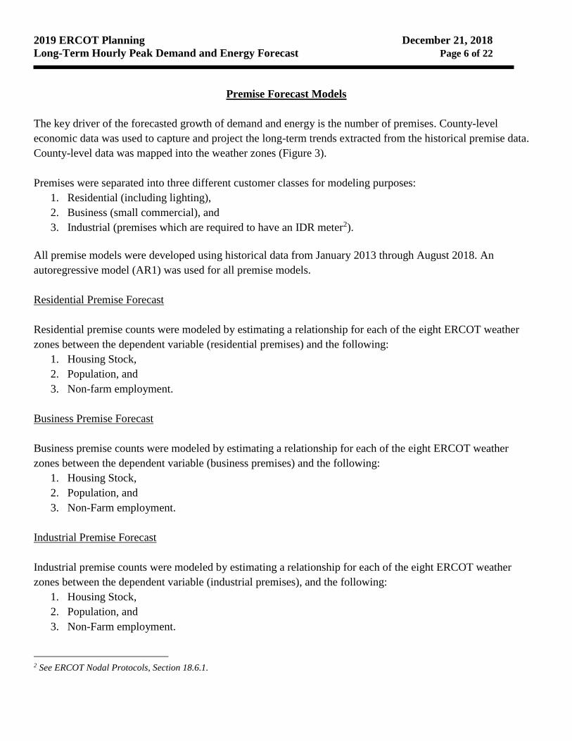
Premise Forecast Models

The key driver of the forecasted growth of demand and energy is the number of premises. County-level

economic data was used to capture and project the long-term trends extracted from the historical premise data.

County-level data was mapped into the weather zones (Figure 3).

Premises were separated into three different customer classes for modeling purposes:

1. Residential (including lighting),

2. Business (small commercial), and

3. Industrial (premises which are required to have an IDR meter2).

All premise models were developed using historical data from January 2013 through August 2018. An

autoregressive model (AR1) was used for all premise models.

Residential Premise Forecast

Residential premise counts were modeled by estimating a relationship for each of the eight ERCOT weather

zones between the dependent variable (residential premises) and the following:

1. Housing Stock,

2. Population, and

3. Non-farm employment.

Business Premise Forecast

Business premise counts were modeled by estimating a relationship for each of the eight ERCOT weather

zones between the dependent variable (business premises) and the following:

1. Housing Stock,

2. Population, and

3. Non-Farm employment.

Industrial Premise Forecast

Industrial premise counts were modeled by estimating a relationship for each of the eight ERCOT weather

zones between the dependent variable (industrial premises), and the following:

1. Housing Stock,

2. Population, and

3. Non-Farm employment.

2 See ERCOT Nodal Protocols, Section 18.6.1.



Premise Model Issues

During the review process for the previously mentioned premise models, a problem was identified that impacted

two weather zones.

During the historical timeframe used to create the models, in the Far West and West weather zones, there was a

significant increase in the number of premises. This increase was due to an entity opting in to ERCOT’s

competitive market in those two regions in the middle of 2014 and due to an expansion of ERCOT’s service

territory.

As a result of this problem, it was problematic to create accurate premise forecast models for the Far West and

West weather zones. These two weather zones instead used economic variables as the key driver of forecasted

growth of demand and energy.



Hourly Demand Models

The long-term trend in hourly demand was modeled by estimating a relationship for each of the eight ERCOT

weather zones between the dependent variable (hourly demand) and the following:

1. Month,

2. Day of Week,

3. Hour,

4. Weather Variables,

a. Temperature,

b. Temperature Squared,

c. Temperature Cubed,

d. Dew Point,

e. Cloud Cover,

f. Wind Speed,

g. Cooling Degree Days3 (base 65),

h. Heating Degree Days3 (base 65),

i. Lag Cooling Degree Days3 (1, 2, or 3 previous days),

j. Lag Heating Degree Days3 (1, 2, or 3 previous days), and

k. Lag Temperature (1, 2, 3, 24, 48, or 72 previous hours).

5. Interactions,

a. Hour and Day of Week,

b. Hour and Temperature,

c. Hour and Dew Point,

d. Temperature and Dew Point, and

e. Hour and Temperature and Dew Point,

6. Number of premises4, and

7. Non-Farm Employment / Housing Stock / Population5

All of the variables listed above are used to identify the best candidates for inclusion in the forecast models and

to provide details on the types of variables that were evaluated in the creation of the models. Not every variable

listed above was included in each model. Unique models were created for each weather zone to account for the

different load characteristics of each area.

Model Building Process

The model building data set was comprised of a randomly selected 70% of the data from January 1, 2013

through August 10, 2018, with the remaining 30% of the data withheld. The model building data set

3 All Degree Day variables are calculated versus 65 degrees F. 4 For Coast, East, North, North Central, South, and South Central weather zones. 5 For Far West and West weather zones.



was used to create various forecast models. The model building process was an iterative process that was

conducted multiple times.

The validation data set consisted of the randomly selected 30% of data from the January 1, 2013 through

August 10, 2018 timeframe that was withheld from the model building data set. After model building was

complete, the validation data set was used to determine the accuracy of the various forecast models. Each

model’s performance was calculated based on its forecasting performance on the validation data set. The most

accurate models were selected based on their performance.

The last step in the model building process was to update the selected model for each weather zone by using

data from January 1, 2013 through August 10, 2018 in order to update the variable coefficients. Using only five

years of historical data and as much of the current year’s data as possible enables the model to reflect recent

appliance stock, energy efficiency measures, price responsive load impacts, etc.

Weather Zone Load Forecast Scenarios

Actual weather data from calendar years 2003 through 2017 was used to create each weather zone’s forecast by

applying the weather data from each historical year one-by-one to the load forecasting model. The process

began by using actual weather data from 2003 as weather input into the model for all forecasted years (2019-

2028). The actual weather data from all days in 2003 was copied into the same day and hour for each of the

forecasted years (2019-2028). For example, the actual weather data for 1/1/2003 was copied into 1/1/2019,

1/1/2020, … , 1/1/2028. Using 2003’s weather as input into each weather zone’s forecast model results in what

is referred to as the 2003 weather load forecast scenario. The 2003 weather load forecast scenario is a forecast

that assumes 2003’s weather would occur for each forecasted calendar year (2019-2028). This process was

completed for each of the historical weather years (2003-2017) individually and resulted in fifteen weather load

forecast scenarios for each weather zone for the forecasted years 2019-2028. It should be noted that the premise

and economic forecasts are the same in each of these fifteen weather scenarios.

The following notation can be used to denote the weather load forecast scenarios:

𝐻𝐹(𝑥,𝑦,𝑧)

Where:

HF = hourly demand forecast,

x = weather zone (Coast, East, Far West, North, North Central, South, South Central, and West),

y = historical weather date and time, and

z = forecast date and time.

For example, 𝐻𝐹 (𝑊𝑒𝑠𝑡, 7/24/2008 1700, 7/24/2019 1700), would denote the forecast for 7/24/2019 at 5:00 pm,

which was based on weather from 7/24/2008 at 5:00 pm, for the West weather zone.



Weather Zone Normal Weather (P50) Hourly Forecast

The fifteen weather zone load forecast scenarios are used as the basis for creating the weather zone normal

weather 50th percentile (denoted as the P50) hourly forecast. Each of the fifteen hourly weather zone load

forecast scenarios were separated into individual calendar year forecasts (covering calendar years 2019-2028).

The calendar year forecasts were then divided by calendar month. Forecasted hourly values for each individual

calendar month were ordered from the highest value to the lowest value. Then, for each ordered value, the

average was calculated. This process is commonly referred to as the Rank and Average methodology.

For example, to determine the normal weather (P50) forecasted peak value for May 2019, take the highest

forecasted value from each of the fifteen weather load forecast scenarios for May 2019 and average them. To

determine the second highest value for May 2019, take the second highest forecasted value for each of the

fifteen weather load forecast scenarios for May 2019 and average them. Repeat this process for all hours in May

2019. See Table 1 below for a summary of these calculations.

Table 1: Coast Weather Zone May 2019 Forecast Scenarios

Historical Weather Year

After this process has been completed for all hours in May, a P50 forecast will have been calculated for all 744

hours of May. At this point, the forecast is ordered from the highest value (indicated as rank 1) to the lowest

value (indicated as rank 744). Note that the forecasted values have not yet been assigned to a day or hour. The

values associated with a rank of 1 are the monthly forecasted peak demand values. The forecasted monthly

peak values for August and January, however, are subject to an adjustment which is covered in the two sections

immediately below.

Weather Zone Normal Weather (P50) Summer Peak Demand Forecast

The fifteen weather load forecast scenarios are used as the basis for creating the weather zone normal weather

50th percentile (denoted as the P50) summer peak forecast. Each of the fifteen hourly weather load forecast

scenarios are separated into individual calendar year forecasts (covering calendar years 2019-2028). The

maximum forecasted hourly value occurring during the summer season (defined as June through September) is



determined for each individual calendar year. The summer peak demand values from all of the fifteen weather

scenarios for a particular calendar year are averaged to determine the normal weather P50 forecasted summer

peak value. For example, to determine the normal weather (P50) forecasted summer peak value for calendar

year 2019, take the highest forecasted value in months June through September from each of the fifteen weather

load forecast scenarios for calendar year 2019 and average them. The forecasted summer peak demand is then

assigned to August and replaces the previously calculated peak (rank 1) forecasted value for the month of

August.

Example:

Table 2 (below) shows the forecasted summer peak demand for the Coast weather zone for 2019 based on the

historical weather years of 2003-2017. The P50 column is the average of the fifteen forecasts in the row. The

P50 forecasted summer peak demand for Coast is 21,144 MW.

Table 2: Coast Weather Zone 2019 Summer Peak Forecast Scenarios


Weather Zone Normal Weather (P50) Winter Peak Demand Forecast

The fifteen weather load forecast scenarios are used as the basis for creating the weather zone normal weather

50th percentile (denoted as the P50) winter peak forecast. Each of the fifteen hourly weather load forecast

scenarios are separated into individual calendar year forecasts (covering calendar years 2019-2028). The

maximum forecasted hourly value occurring during the winter season (defined as December through March) is

determined for each year. The winter peak demand values from each weather scenario for a particular year are

averaged to determine the normal weather P50 forecasted winter peak value. For example, to determine the

normal weather (P50) forecasted winter peak value for 2019, take the highest forecasted value from each of the

fifteen weather load forecast scenarios for December 2018 – March 2019 and average them. The forecasted

winter peak demand is then assigned to January and replaces the previously calculated peak (rank 1) forecasted

value for the month of January.

Example:

Table 3 (below) shows the forecasted winter peak demand for the Coast weather zone for the winter of 2019

based on the historical weather years of 2003-2017. The P50 column is the average of the fifteen forecasts in

the row. The P50 forecasted winter peak demand for Coast is 15,054 MW.

Table 3: Coast Weather Zone 2019 Winter Peak Forecast Scenarios




Weather Zone Normal Weather (P50) Hourly Forecast Mapping to Calendar

The next step is to map the weather zone P50 hourly forecasts into a representative calendar. Remember that

the P50 hourly forecast is ranked from highest to lowest value within each forecasted month. The sorted hourly

forecasted values need to be mapped into a representative time-sequenced shape. This was accomplished by

looking at historical load data from calendar years 2007-2017. For each month in each historical year, the rank

of all of the observations for each day and hour was determined. Then, the corresponding forecasted P50 hourly

values were mapped to the day and hour from the historical year with the same month and the same rank.

Example:

The Coast P50 Summer Peak Forecast is 21,144 MW. Also remember that the forecasted summer peak value is

assigned to the month of August. In 2016, Coast’s Summer Peak occurred on 8/09/2016 @ 1600. Using the

2016 mapping factors, the Coast P50 Summer Peak value is assigned to 8/09 @ 1600 for all forecasted years

(2019-2028). This means that the Coast P50 Summer Peak will always occur on 8/09 @ 1600 for all forecasted

years when mapped to 2016.

Example:

In 2015, Coast’s Summer Peak occurred on 8/11/2015 @ 1600. Using the 2015 mapping factors, the Coast P50

Summer Peak value is assigned to 8/11 @ 1600 for all forecasted years (2019-2028). This means that the Coast

Summer Peak will always occur on 8/11 @ 1600 for all forecasted years when mapped to 2015.

This mapping process was completed using calendar years 2007-2017. This produced eleven different hourly

P50 forecasts based on each of the eleven calendar years 2007-2017. Note, though, that the monthly peak

demand and monthly energy values are exactly the same in each of the eleven hourly weather zone P50

forecasts. The only difference is the day and time that the forecasted hourly values occur when mapped to the

different historical years.

Example:

There are 744 (31 days times 24 hours per day) P50 hourly forecasted demand values for the Coast weather

zone for August. They are mapped into a day and time (in August) based on the historical ranking of actual

load values from August 2007, August 2008, August 2009, ... , August 2016, and August 2017. Each forecasted

value was assigned a day and hour based on the historical ranking. But the monthly peak demand and monthly

energy values are the same no matter which historical mapping year is used.

ERCOT Zone Normal Weather (P50) Hourly Forecast

Each of the eleven different mapped hourly P50 forecasts based on the historical calendar years of 2007-2017

for each weather zone are summed for each forecasted year, month, day, and hour. This results in eleven

different ERCOT P50 hourly coincident forecasts. The differences among these forecasts are caused by the

different timing of weather conditions across the ERCOT region. It bears repeating that all of the underlying

weather zone load forecasts have the same exact monthly peak demand and energy values.



In order to determine which hourly P50 ERCOT coincident forecast to use as our primary and official P50

ERCOT coincident forecast, an analysis was performed on these eleven different P50 hourly coincident

forecasts. The distribution of ERCOT summer peak demand was determined. Seeing that it is very difficult to

determine how weather conditions will align or not at the time of ERCOT’s summer peak, the forecast using

historical factors from 2007 was deemed the ERCOT official P50 forecast. Using the 2007 historical factors

resulted in the least amount of diversity between weather zone demand and ERCOT-wide demand at the time of

ERCOT’s summer peak. Stated differently, using the 2007 historical factors resulted in the highest ERCOT

coincident summer peak forecast.

Load Forecast Scenarios (ERCOT system)

The weather zone load forecast scenarios are used as the basis for creating load forecast scenarios for the

ERCOT system. The hourly values from each weather zone are summed for each year, month, day, and hour to

get the ERCOT total forecasted hourly demand.

The following notation can be used to denote ERCOT system weather load forecast scenarios:

∑ 𝐻𝐹(𝑦,𝑧)

8

𝑥=1

Where:

HF = hourly demand forecast,

x = weather zone (Coast, East, Far West, North, North Central, South, South Central, and West),

y = historical weather date and time, and

z = forecast date and time.

For example, 𝐻𝐹 ( 7/24/2008 1700, 7/24/2019 1700), would denote the forecast for 7/24/2019 at 5:00 pm, which

was based on weather from 7/24/2008 at 5:00 pm, for the ERCOT system.

Weather Zone (P90) Summer Peak Demand Forecast

Another forecast of interest is the 90th percentile (P90) weather zone summer peak demand forecast. The

process for determining the 90th percentile weather zone summer peak demand forecast is identical to the

process used for calculating the P50 forecast, except that instead of using the average of the fifteen weather year

load forecast scenarios, the 90th percentile of the values is used.

Example:

Table 2 (above) shows the forecasted summer peak demand for the Coast weather zone for 2019 based on

historical weather years of 2003-2017. The P90 column is the 90th percentile of the fifteen forecasts. The P90

forecasted summer peak demand for the Coast weather zone in 2019 is 21,822 MW.



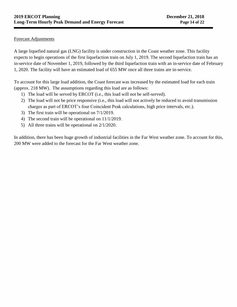
Forecast Adjustments

A large liquefied natural gas (LNG) facility is under construction in the Coast weather zone. This facility

expects to begin operations of the first liquefaction train on July 1, 2019. The second liquefaction train has an

in-service date of November 1, 2019, followed by the third liquefaction train with an in-service date of February

1, 2020. The facility will have an estimated load of 655 MW once all three trains are in-service.

To account for this large load addition, the Coast forecast was increased by the estimated load for each train

(approx. 218 MW). The assumptions regarding this load are as follows:

1) The load will be served by ERCOT (i.e., this load will not be self-served).

2) The load will not be price responsive (i.e., this load will not actively be reduced to avoid transmission

charges as part of ERCOT’s four Coincident Peak calculations, high price intervals, etc.).

3) The first train will be operational on 7/1/2019.

4) The second train will be operational on 11/1/2019.

5) All three trains will be operational on 2/1/2020.

In addition, there has been huge growth of industrial facilities in the Far West weather zone. To account for this,

200 MW were added to the forecast for the Far West weather zone.



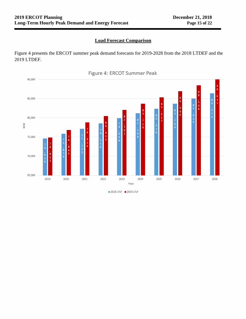
Load Forecast Comparison

Figure 4 presents the ERCOT summer peak demand forecasts for 2019-2028 from the 2018 LTDEF and the

2019 LTDEF.



Figure 5 presents the ERCOT annual energy forecast for 2019-2028 from the 2018 LTDEF and the 2019

LTDEF.



Load Forecast Uncertainty

A long-term load forecast can be influenced by a number of factors. The volatility of these factors can have a

major impact on the accuracy of the forecast. This document will cover the following eight areas.

1. Weather,

2. Economics,

3. Energy Efficiency,

4. Price Responsive Loads,

5. On-site Distributed Generation,

6. Electric Vehicles.

7. Large Industrial Loads, and

8. Change in ERCOT’s Service Territory.



Weather Uncertainty

Figure 6 suggests the significant impact of weather in forecasting. This figure shows what the 2019 forecasted

peak demand would be using the actual weather from each of the past fifteen years as input into the model. As

shown, there is considerable variability ranging from 72,291 MW using 2004’s weather to 77,739 MW using

2011’s weather. This equates to approximately a 7.5% difference in the forecast based on historical weather

volatility. The variation seen in the figure below is due to differences in weather and calendar factors between

the fifteen historical weather years.

76,434

72,291

73,317

74,254

72,759

73,490

75,232

76,271

77,739

76,673

75,098

73,323

75,017 74,908

72,547

74,853

69,000

70,000

71,000

72,000

73,000

74,000

75,000

76,000

77,000

78,000

79,000

2003 2004 2005 2006 2007 2008 2009 2010 2011 2012 2013 2014 2015 2016 2017 P50

MW

Year

Figure 6: Weather Scenarios - 2019 Summer Peak Forecast



Figure 7 depicts weather volatility out to 2028. Assuming 2004 weather (identified as the mild weather

scenario) in 2028, we would expect a peak of 86,607 MW. Assuming 2011 weather (identified as the extreme

weather scenario) in 2028, results in a forecasted peak demand of 92,055 MW. This equates to approximately a

6.3% difference in the forecast based on weather extremes.

Economic Uncertainty

Economic uncertainty impacts the premise forecasts. Stated differently, significant changes in economic

forecasts will have impacts on the premise forecasts which, in turn, will be reflected in the peak demand and

energy forecasts. Premise forecasts were based on the base economic scenario from Moody’s Analytics.

Energy Efficiency

Energy efficiency is a much more difficult uncertainty to quantify. First, it must be recognized that the 2019

LTDEF was a “frozen efficiency” forecast. That means the forecast model employs statistical techniques that

estimate the relationships between load, weather, and economics based on historical data from January 2013

through August 2018. The implicit assumption in the forecast is that there will be no significant change in the

level of energy efficiency during the forecasted timeframe when compared to what occurred during the

historical period used in the model building process. Such an assumption has significant implications. Among

other things, it means that the models assume the thermal characteristics of the housing stock and the

72,291

86,607

77,739

92,055

74,853

90,021

65,000

70,000

75,000

80,000

85,000

90,000

95,000

2019 2020 2021 2022 2023 2024 2025 2026 2027 2028

MW

Year

Figure 7: Forecast Uncertainty Due to Weather

Mild Weather (2004) Extreme Weather (2011) P50 Forecast



characteristics of the mix of appliances will remain relatively the same. If thirty percent of the residential central

air conditioners in the South Central weather zone had Seasonal Energy Efficiency Ratios (SEER—a measure

of heat extraction efficiency) of twelve during the historical time period, then the model assumes that same

proportion in all forecasted years. In the future, ERCOT will create energy efficiency scenarios which adjust the

load forecast based on data from the Energy Information Administration (EIA)6. It is somewhat likely that an

Energy Efficiency adjustment will be applied in the 2020 LTDEF.

Price Responsive Loads

Price responsive load programs are in their infancy for much of ERCOT. Determining the impact of these

programs is challenging, especially when you consider that over the last few years, ERCOT’s price caps have

increased from $1,000/MWh to $9,000/MWh. Discussions are underway to explore ways to enable loads to

participate in ERCOT’s real-time energy market by submitting demand response offers to be deployed by the

Security Constrained Economic Dispatch. There remains much uncertainty as to what future levels these

programs may achieve. Similar to Energy Efficiency, it must be recognized that the 2019 LTDEF is a “frozen”

forecast with respect to price responsive loads. Price responsive loads are reflected in the forecast at the level

that was observed during the historical period of January 2013 – August 2018. In the future, ERCOT may create

price responsive load scenarios, which would adjust the forecasted peak demands.

On-site Distributed Generation (DG)

Another area of uncertainty is on-site distributed generation. Included are technologies such as the following:

1. Distributed Generation (non-renewable),

2. Distributed On-site Wind,

3. Photovoltaic (PV), and

4. Solar Water Heating.

On-site distributed generation technologies are also characterized by much uncertainty about what future levels

may be achieved. The 2019 LTDEF was a “frozen” forecast with respect to on-site renewable generation

technologies. On-site renewable generation technologies are reflected in the forecast at the level that was

observed during the historical period of January 2013 – August 2018. In the future, ERCOT may create

scenarios for On-site Renewable Energy Technologies.

Electric Vehicles Uncertainty

The growth of Electric Vehicles (EVs) has been accelerating. As an example, industry forecasts indicate that the

number of electric vehicles in Texas will grow from 5,000 to approximately 100,000 by 2023. Still, the number

of electric vehicles represents a very small percentage of the new car market in the United States. The 2019

6 For a discussion of the EIA scenarios, see the “Buildings Sector Case” at http://www.eia.gov/forecasts/aeo/appendixe.cfm

http://www.eia.gov/forecasts/aeo/appendixe.cfm



LTDEF was a “frozen” forecast with respect to EVs. EVs are reflected in the forecast at the level that was

observed during the historical period of January 2013 - August 2018 which was used to build the 2019 LTDEF

models. ERCOT will continue to watch the growth of electric vehicles in order to monitor their impact on the

load forecast.

Large Industrial Loads

A key challenge in creating a load forecast is to determine if the model is adequately capturing the impact of

future large industrial loads. Examples include liquefied natural gas facilities, oil and gas exploration, chemical

processing plants, Tesla battery plants, etc. In addition, ERCOT had discussions with Transmission Service

Providers (TSPs) and gathered information on the expected growth of industrial load within their service

territories. ERCOT carefully reviews the historical performance of long-term load forecasts to determine how

well large industrial growth has been captured. Based on the results of this evaluation and on data gathered from

the TSPs, ERCOT may use this information to adjust the long-term load forecast. The 2019 LTDEF was

adjusted for large industrial loads in the Coast and Far West weather zones.

Change in ERCOT’s Service Territory

Another challenge in creating a load forecast is the potential for ERCOT’s service territory to change. As an

example, the City of Lubbock is joining ERCOT in 2021. Lubbock’s peak load is approximately 500 MW. The

2019 LTDEF includes an hourly forecast for Lubbock (based on the City of Lubbock’s forecast of its growth)

which was added to the North weather zone forecast.

Looking Ahead

As more information becomes available and additional data analysis is performed on each of these highlighted

areas of forecast uncertainty, ERCOT will begin developing models which quantify their impacts on future

long-term demand and energy forecasts. These themes will likely be revisited in the 2020 LTDEF.



Appendix A

Peak Demand and Energy Forecast Summary

Year

Summer Peak

Demand (MW)

Energy (TWh)

2019

74,853

384

2020

76,845

401

2021

78,824

413

2022

80,455

426

2023

82,101

438

2024

83,716

450

2025

85,327

461

2026

86,940

473

2027

88,508

484

2028

90,021

496

long-term hourly peak demand and energy forecast...long-term hourly peak demand and energy forecast...

Documents