long-term effects of free primary education on educational

Policy Research Working Paper 9404

Long-Term Effects of Free Primary Education on Educational Achievement

Evidence from Lesotho

Ramaele Moshoeshoe

Africa RegionOffice of the Chief EconomistSeptember 2020

Pub

lic D

iscl

osur

e A

utho

rized

Pub

lic D

iscl

osur

e A

utho

rized

Pub

lic D

iscl

osur

e A

utho

rized

Pub

lic D

iscl

osur

e A

utho

rized

Produced by the Research Support Team

Abstract

The Policy Research Working Paper Series disseminates the findings of work in progress to encourage the exchange of ideas about development issues. An objective of the series is to get the findings out quickly, even if the presentations are less than fully polished. The papers carry the names of the authors and should be cited accordingly. The findings, interpretations, and conclusions expressed in this paper are entirely those of the authors. They do not necessarily represent the views of the International Bank for Reconstruction and Development/World Bank and its affiliated organizations, or those of the Executive Directors of the World Bank or the governments they represent.

Policy Research Working Paper 9404

Many Sub-Saharan African countries have instituted free primary education policies, and this has led to a significant increase in the primary school enrollment rate. However, many children who are in school are not learning. It is not clear whether free primary education policies have contrib-uted to the decline in the quality of education and whether these learning effects are long-lasting. This paper addresses the latter question and estimates the long-term effects of free primary education on educational achievement in Leso-tho where the program was phased-in on a grade-by-grade basis, beginning with grade one in 2000. The timing of the

implementation created changes in program coverage across age (and grade) groups over time. A semiparametric differ-ence-in-differences strategy is employed that exploits these variations to identify the long-term effects of the free pri-mary education policy on educational achievement, using university examinations records data for student cohorts with and without free primary education. The results indi-cate that the effect of free primary education on academic performance is bounded between 2 and 19 percentage points, implying that the program increased enrollment without hurting education quality.

This paper is a product of the Office of the Chief Economist, Africa Region. It is part of a larger effort by the World Bank to provide open access to its research and make a contribution to development policy discussions around the world. Policy Research Working Papers are also posted on the Web at http://www.worldbank.org/prwp. The author may be contacted at [email protected].

Long-Term Effects of Free Primary Education on

Educational Achievement: Evidence from Lesotho∗

Ramaele Moshoeshoe

National University of Lesotho

The World Bank

Keywords: Free Primary Education, Educational achievement, Long-term effects, Lesotho

JEL Classification: H52, I22, I28, 015

∗I thank Kehinde Ajayi, Moussa Blimpo, Justine Burns, David Evans, Deon Filmer, Markus Goldstein, AbbiKedir, Germano Mwabu, Patrick Plane, the audiences of the AERC December 2018 and June 2019 bi-annualconferences, and participants at the World Bank and National University of Lesotho seminars for helpful commentsand suggestions. Pedro Sant’Anna generously helped me to implement his DRDID R code. I am grateful to the WorldBank-AERC Visiting Scholars program which financed my stay at the World Bank where parts of this paper weredeveloped. Financial support from African Economic Research Consortium (AERC), through grant No. RT18537,is also gratefully acknowledged. All remaining errors are my own. The views expressed in this paper are entirelymine, and do not necessarily represent those of the World Bank or its Board of Directors.Contact emails: [email protected] or [email protected]

1 Introduction

The Dakar Framework for Action (DFA), adopted by World Education Forum in 2000, called for

complete, free, and compulsory quality education, with the aim to redress global educational in-

equalities (UNESCO, 2000, p.8). Since then, several Sub-Saharan African countries have instituted

free primary education (FPE) programs1 by abolishing all primary school user fees. Several stud-

ies have quantified the short-term effects of the FPE programs in Sub-Saharan Africa on school

enrollment, drop-out, and grade progression (see Deininger 2003; Al-Samarrai and Zaman 2007;

Nishimura et al. 2008; Grogan 2009; Lucas and Mbiti 2012; Hoogeveen and Rossi 2013; Moshoeshoe

et al. 2019). These studies find that FPE increased enrollment, reduced school drop-out, and re-

duced grade-progression. Therefore, largely owing to FPE programs, the primary school enrollment

rate in the developing world has reached 91 percent (UNDP, 2016), with 94 percent and 74 percent

of children worldwide completing primary education and lower secondary education, respectively

(World Bank, 2016, 2018).

However, school attendance is different from learning. The main problem now is that millions

of children finish primary school without acquiring functional literacy and numeracy skills, and

this is more pronounced in Sub-Saharan Africa (World Bank, 2018; Filmer et al., 2020). There-

fore, achieving inclusive and equitable quality education by 2030 is the fourth most important

Sustainable Development Goal (SDG) under the 2030 Agenda.

Since the Millennium Development Goals, the SDGs’ predecessor, focused mainly on increasing

access to schooling, it is generally believed that the current learning crisis is partly due to school

fees’ elimination programs. However, a few studies that quantify the short-term effects of these

FPE programs, and similar fee elimination policies in Africa, on education quality (i.e. test scores)

find mixed evidence. Lucas and Mbiti (2012), for example, apply a difference-in-differences (DID)

strategy, exploiting the variation in pre-program primary school drop-out rates across districts in

Kenya to estimate the effect of FPE on primary school completion rate and test scores. They find

marginal negative effects of FPE on test scores, but large and positive effects on primary school

completion rate. Blimpo et al. (2016), on the other hand, find positive effects of the Gambian

Girls’ Scholarship program (a secondary school fee elimination program for girls) on student access

and learning, using a DID strategy. In as much as this question remains open, data availability

remains a hinderance in answering it, and this paper does not attempt to address it for the same

reasons.

All else held constant, the negative (or positive) effects of FPE on learning may still show up

later on in a child’s academic life. According to Cunha et al. (2006), achievement test scores are

determined by skills or abilities (both cognitive and noncognitive)2 that are malleable to environ-

1Including but not limited to Burundi, Cameroon, Eswatini, Ghana, Kenya, Lesotho, Mozambique, Namibia,Rwanda, Tanzania, and Zambia.

2Cognitive skills are malleable to environmental factors up to age 10 or so, while noncognitive skills are malleablefor a much longer time (Cunha et al., 2006)

1

mental (e.g. family and school) influences. These skills are self-productive and complementary.

That is, skills acquired at primary school may augment skills attained at the secondary and uni-

versity levels, and that skills acquired at primary school may raise the productivity of education

investments at the secondary and university levels. Therefore, it is reasonable to assume that FPE,

through its influence on school inputs and environments, will have lasting effects of education qual-

ity. This paper tests this hypothesis.

Further, the paper examines whether FPE effects differ by gender of the student. Because

of gender stereotypes in many cultures, girls’ education is mostly considered of a lesser value,

resulting in girls getting less education, at least in terms of access. However, the question of

whether, conditional on attendance, boys and girls receive the same quality education still remains

unanswered. If we are to build a productive, talented, and diverse labor force, it is essential to

know well in time the effects of the implemented policies so that they can either be scaled up (if

the effects are positive) and/or changed (if the effects are negative).

Therefore, this paper estimates the long-term effects of FPE on education performance and

establishes whether these effects, if any, differ by student’s gender. Apart from the fact that this

paper is among the first studies to estimate the long-term effects of FPE policies in Sub-Saharan

Africa, it contributes to several strands of literature. First, it contributes to the literature that looks

at the long-term impacts of schooling inputs on educational outcomes. For example, Fredriksson

et al. (2013) look at the long-term effects of class size on human capital development. They find that

smaller class sizes improve cognitive and noncognitive abilities at age 13, and improve achievement

test scores at age 16. Second, it adds to the literature that looks at the short- term impacts of

fee eliminations on educational outcomes in developing countries (Grogan, 2009; Lucas and Mbiti,

2012; Hoogeveen and Rossi, 2013; Chyi and Zhou, 2014; Blimpo et al., 2016; Moshoeshoe et al.,

2019). Lastly, it adds to the small, but growing, literature on the long-term effects of schooling

subsidy programs (including tuition fee eliminations) on human capital development. For example,

Xiao et al. (2017) estimate the long-term effects a free compulsory education reform in rural China

on educational attainment, cognitive skills and health. They find that the reform had long lasting

positive effects on educational attainment and cognitive achievement.

I estimate the long term effects of FPE on education quality in Lesotho mainly for the following

two reasons. First, unlike in many Sub-Saharan African countries, the FPE program in Lesotho

was phased-in grade by grade, starting with grade one in 2000, until it covered the entire primary

schooling system in 2006. This implementation strategy makes it possible to follow two cohorts of

children (the FPE treated and the FPE untreated cohorts) from primary school through university

level, and hence account for the underlying trends in achievement test scores of the cohorts through

a difference-in-differences estimation strategy. Second, Lesotho has only one big (and premier)

public university, the National University of Lesotho (NUL), and two smaller (and new) private

universities, which only opened in 2007 and 2016, respectively. Therefore, it is possible to get

2

data for a sizeable proportion of the FPE treated and untreated cohorts that have written similar

standardized achievement tests.

The results indicate that the FPE program has lasting positive effects on educational quality: it

increased university students’ academic performance by between 2 and 19 percentage points. But

there are no discernible FPE effect heterogeneities by student gender. This implies that, conditional

on university attendance, boys and girls receive the same quality education. The robustness checks

results indicate that the increase in educational quality cannot be attributed to some positive time

trend, and that these effects are stronger when the sample is narrowed to 18-22 years old, the age

range appropriate for the undergraduate level. The results are also robust to model specification

errors.

The reminder of the paper proceeds as follows. Section 2 presents the institutional context and

policy background. Section 3 briefly provides the theoretical framework while Section 4 discusses

the data and presents some descriptive statistics. In Section 5, I explain the identification strategy,

and present the main results in Section 6. Section 7 concludes the paper.

2 Institutional context and policy background

2.1 Institutional context

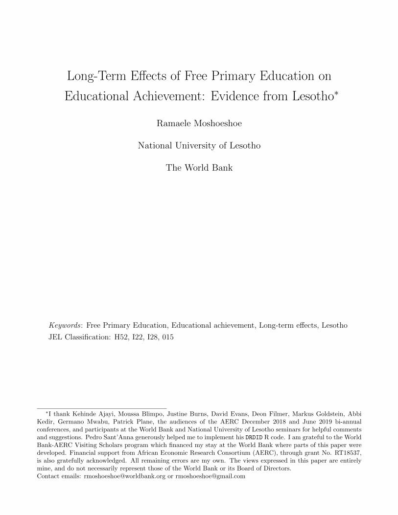
In Lesotho education follows a 7-3-2-4 system, with seven years of primary education, three years

of junior secondary education, two years of senior secondary education, and four years of university

education (see Figure 1). The official age of entry into primary schooling is six years, such that by

age 12, children should be in grade seven. This implies that the official primary school-age is 6 to

12 years old, and that for secondary education is 13 to 17 years old.

At the end of primary school, students take the national exit exam, the Primary School Leaving

Exam (PSLE), in order to enter the lower (junior) secondary school. After 3 years of junior sec-

ondary education, students take the Junior Certificate (JC) exam to progress to senior secondary,

at the end of which they take the Cambridge Overseas School Certificate Exam (COSC).3 Students

can also enroll in different Technical and Vocational Education and Training (TVET) after taking

either the PSLE, JC, and/or COSC exams. Given that secondary education is not free in Lesotho,

enrollment into TVET is largely dictated by a child’s academic performance (low performance)

and/or household wealth.

Unlike many other countries, most primary schools in Lesotho (about 85 percent) are owned and

controlled by different churches (see Moshoeshoe et al., 2019), and these churches are represented

in the national education advisory board by their appointed education secretaries (Ambrose, 2007).

Non-religious private schools constitute about 1 percent of primary schools, and are not covered by

3This is now called Lesotho General Certificate of Secondary Education (LGCSE). Through out this paper,COSC and LGCSE are used interchangeably.

3

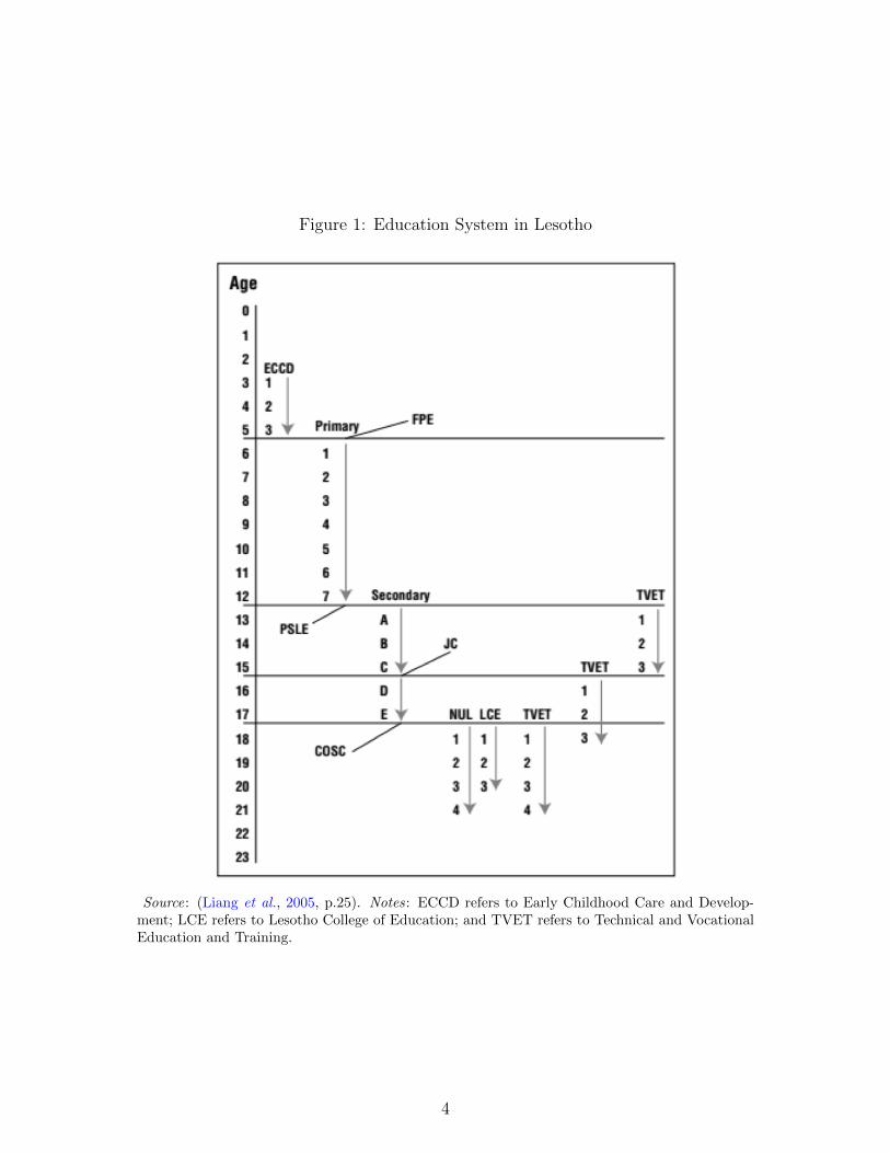
Figure 1: Education System in Lesotho

Source: (Liang et al., 2005, p.25). Notes: ECCD refers to Early Childhood Care and Develop-ment; LCE refers to Lesotho College of Education; and TVET refers to Technical and VocationalEducation and Training.

4

the FPE policy. The picture is very much similar even at the secondary or high school level because

most church-owned primary schools have their secondary schools nearby. However, the share of

non-religious private secondary schools is slightly higher than that at primary level. As of 2014,

there were about 1.4 percent non-church private high schools (Bureau of Statistics, 2015), and these

are concentrated in four districts of the country, namely, Berea, Botha-Bothe, Leribe and Maseru.

Notwithstanding this co-ownership structure, and except for non-church private schools, all schools

follow the same national curriculum provided by the Ministry of Education and Training (MOET).

Further, the government has an overall authority in pronouncing education policies, management

and regulation of education, training of teachers, and teachers’ placements, and deployments within

government and church-owned schools. But some church-owned schools do at times privately hire

contract teachers at their own costs.

With regard to students’ progression within the system, the de jure government policy since

1967 is that of automatic grade promotion at primary school level but, de facto, schools still

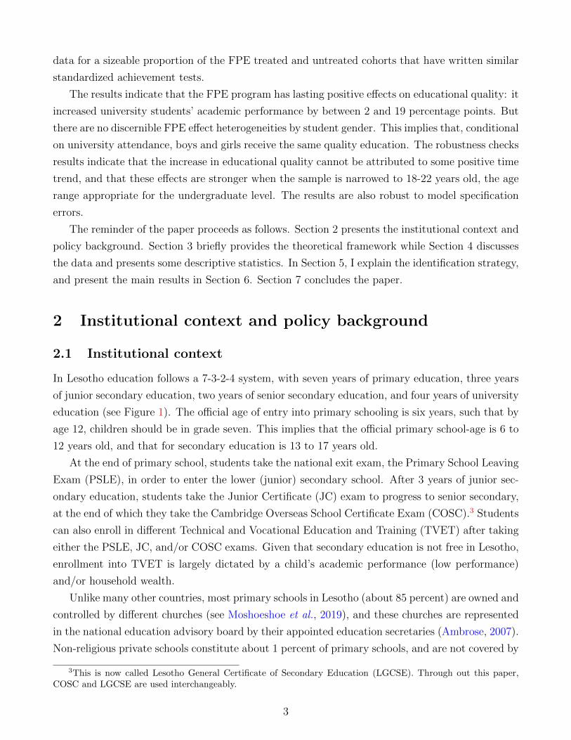
practice grade retention (Ambrose, 2007).4 Figure 2 indicates that, between 2000 and 2015, the

primary school repetition rate was about 20 percent until 2010, after which it dropped to about

14 percent in 2015. During this period, the primary education repetition rate averaged about 17.3

percent and the PSLE exam failure rate fluctuated between 12 percent and 17 percent. Thus,

coupled with delayed school enrollment, the high grade retention rate implies that in any given

year (or grade) there are children of different cohorts Moshoeshoe et al. (2019).

There is grade retention policy at secondary school level. Figure 2 further shows that, while

the transition rate between primary and secondary education is high (about 81 percent), the

repetition rate in secondary education is also high, averaging about 12.6 percent between 2000 and

2015. Further, the JC exams failure rate is high; it fluctuated between 24 percent (recorded in

2004) and 32 percent (recorded in 2009 when the first FPE students wrote JC exams) (Bureau of

Statistics, 2015). This high failure rate could explain the high dropout rate, of 16 percent at

secondary school level. Therefore, those who ultimately get into university are a select group of

motivated and high ability students who potentially come from high income households.

Beyond physical and monetary costs, there are no regulatory restrictions on school choice in

Lesotho. Thus, school choice is largely determined by school availability, school’s past pass rates,

parental wealth, and parental tastes for education. High performing high schools generally attract

students from across the country and have stricter entry requirements. Hence, to cope with the

high demand, such high schools normally administer entry exams, and often do not re-admit their

students whose JC exam’s performance is considered poor (usually second class pass and below).

This implies that different schools largely cater for different types of students with regard to

performance.

4However, since 2010, there has been an increased push for automatic grade promotion at the primary schoollevel. But this latest policy call does not affect the cohorts which this paper studies (i.e. those that were in primaryschool during the years 2000 to 2006).

5

Figure 2: Primary-to-Secondary education Transition rate, and Repetition rates,1997-2016

0

20

40

60

80

1997 2006 20121995 2000 2005 2010 2015 2020

Year

Primary−to−Secondary school Transition rate Primary school repetition Rate

Secondary school repetition rate

Primary & Secondary education Transition and Repetition Rates

Source: Own representation using data from UN Institute of Statistics.

As of 2013, there were about 13 higher education institutions, 8 (i.e. 62 percent) of which

are public institutions. The National University of Lesotho (NUL) is the main tertiary institution

in Lesotho, and remained the only local bachelor’s and master’s degree-awarding institution until

2007. The university admits about 44 percent5 and 89 percent of Lesotho’s undergraduate and

postgraduate students’ population, respectively (Council on Higher Education, 2013).

2.2 Policy background

Lesotho instituted the FPE program in 2000 in order to meet the Millennium Development Goal

(MDG) of ensuring that primary education is free and available to all (UNESCO, 2000). As

mentioned earlier, Lesotho’s implementation strategy was different from that followed by other

African countries. School fees were eliminated sequentially on a grade-by-grade basis starting with

grade one in 2000 such that by 2006, all seven primary school grades were under FPE. The main

reason for this implementation strategy was to cushion FPE’s financial impact on the public budget

(Urwick, 2011).

The FPE policy is an amalgamation of several program components that address both demand-

and supply-side constraints to schooling. On the demand-side, the policy involves elimination of

some private schooling costs such as school fees, stationery and textbooks’ costs. On the supply-

5This is as a percent of all those enrolled in local colleges and foreign universities, mainly in South Africa.

6

side, the government recruited more teachers,6 built additional classrooms in existing schools, and

new government schools where none existed before. For example, between 2002 and 2011, the

number of primary schools in Lesotho increased by about 10 percent, and the primary school

pupil-teacher ratio dropped from 48 to 34 pupils per teacher (MOET, 2011). This increase in in-

frastructure also helped to reduce the average distance to schools, and hence transportation costs.

In addition to school infrastructure, the government provides annual capitation grants, furniture

and teaching materials to all schools, including church/private schools (Jopo et al., 2011; Lekhetho,

2013). Except for the differences in years of exposure, the supply-side program components be-

nefited everyone at school while fee eliminations and free stationery and textbooks exclusively

benefited those covered by FPE.

Figure 3: Changes in Pupil-Teacher Ratio and enrollment

20

30

40

50

60

En

rolm

en

t R

ate

2000 2005 2010 2015

Year

Gross Enrolment Rate

Net Enrolment Rate

Trends in Secondary School Enrolments Rates

20

30

40

50

60

Pu

pil

Te

ach

er

Ra

tio

(P

TR

)

2000 2005 2010 2015

Year

Primary school

Secondary school

Trends in Pupil−Teacher Ratios

Source: Own representation using data from various Education Statistics Reports (MOET, 2010,2011, 2016).

Figure 3 shows changes in secondary school enrollment (demand for education), on the left

panel, and pupil-teacher ratio (supply of education), on the right panel, since the introduction of the

FPE program. From the left panel of the figure, we can see that, while the secondary school gross

enrollment rate was on the increase between 2001 and 2011, the increase was much faster between

2006 and 2010. The figure further shows that, while the net enrollment rate increased through out

the period, the gross enrollment rate plateaued between 2011 and 2015, and then began the upward

trend. The year 2007 is when the first cohort of FPE children entered secondary school level.

6More young and qualified teachers were recruited. Between 2000 and 2007, the proportion of teachers withtertiary qualifications increase from 6 percent to 14 percent, but teacher quality, as measured by teacher performanceon SACMEQ reading test, declined (see Moshoeshoe, 2015).

7

Moshoeshoe et al. (2019) find that, within the first three years of the FPE policy implementation,

enrollment of primary school-aged children increased by about 29 percent. Therefore, the increase

in secondary school enrollment between 2007 and 2011 is partly due to the increased demand for

education from the first three FPE cohorts. This first FPE cohort, which potentially had many

over-aged children, completed secondary education in 2011. And this partly explains the plateauing

of the gross enrollment rate, and the continued increase in net enrollment, between 2011 and 2015.

According to MOET (2011), the government increased the number of secondary schools and

recruited more teachers in anticipation of the increased demand. This is evident in the right panel

of Figure 3 that shows that secondary schools’ student-teacher ratio was on the increase until 2005,

and then began to decline to about 1 teacher per 24 students in 2009. It is clear from this analysis,

therefore, that Lesotho’s FPE program had multiple components targeted at primary schools, and

it also had a knock-on effect on school resources at the secondary school level. This paper examines

the long-term effects of this policy package, not its individual elements.

3 Conceptual Framework

Understanding the process of a child’s cognitive development has remained the preoccupation of

economists since the early works of Leibowitz (1974) and Becker and Tomes (1986). According

to Haveman and Wolfe (1995), a child’s development is principally determined by three factors,

namely: government choices regarding the amount of resources invested in education; parental

investment decisions in the form of quantity and quality of resources devoted; and the child’s own

choices (but only past age 13 or 15). In this setting, the government moves first by making direct

investment in the child and setting the economic environment, within which parents, and then

children, operate. Here the view is that investment in children cannot happen outside government

involvement and that this investment takes place only after the child is born.

However, Cunha, Heckman, Lochner and Masterov (2006) argue that skill (or ability) formation

is a life cycle process that starts much earlier in life, from the womb, and that abilities, cognitive

and non-cognitive, are malleable to environmental influences. They postulate that early and late

investments in a child’s development are complementary. Thus, early high quality child investments

increase the productivity of later child investments (i.e. skill begets skill), and this effectively

places parents as very important first movers under the Haveman-Wolfe sequential framework.

But equally important is the role played by the society or government in the second stage of

human capital development (after birth) because early investments are only productive if there is

follow-up investment.

Indeed Behrman (2010) propounds that, for children aged 6 or 7 to 15, educational achieve-

ment is partly determined by formal schooling and its characteristics, including out-of-school ex-

periences such as homework conditional on preschool investments, individual, family, market and

8

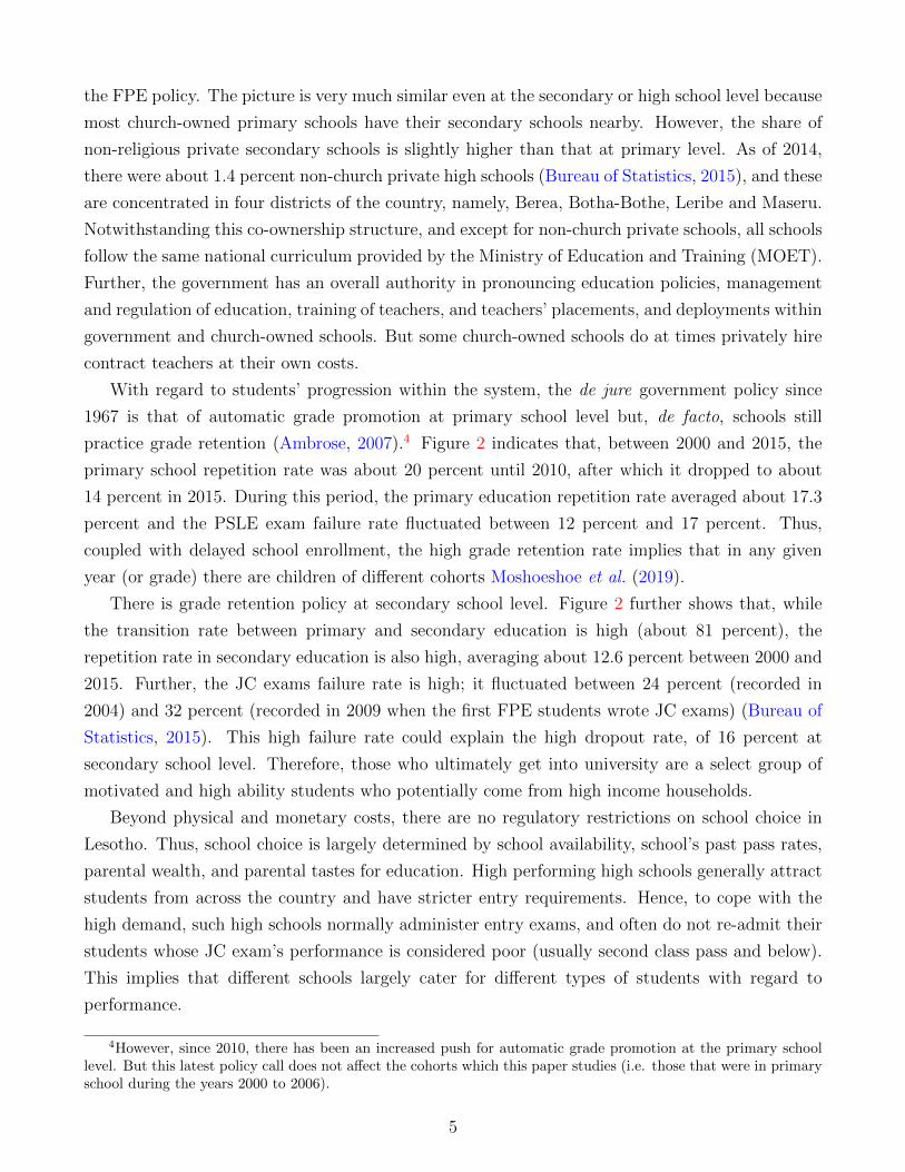
Figure 4: The Directed Acyclic Graph (DAG) of causal effect of FPE on academic performance

Fee Elimination

Textbooks

Teacherrecruitment

Access orenrollment

Schoolbuilding

PTRAcademic

performancet

SES

Academicperformancet+6

Source: Own representation. Notes: PTR is the Pupil Teacher Ratio; SES is socioeconomic status. Thedirection of the arrow (A→ B) indicates the direction of the cause from node A to node B.

institutional characteristics. Hence, early quality childhood investment, both at home and at

school, manifests itself in the form of high achievement and low grade retention. It is clear that

achievement is a function of not only abilities but also school inputs, thereby placing family and

government at the center of the child’s development.

Figure 4 is the directed acyclic graph (DAG) of the causal path ways from FPE program

components (i.e. fee eliminations, textbooks, teacher-recruitment, and school building) to academic

achievement. We can see from this figure that, because elimination of schools fees, building of

more schools, and provision of textbooks reduce the costs of schooling, they are expected to affect

access to schooling positively. The increase in enrollment will lead to an increase in the pupil-

teacher ratio (PTR), all else held constant, and this will in turn affect (current or primary school)

academic achievement. Recruiting more teachers will reduce PTR and, hence, improve academic

achievement.

Further, textbooks availability and teacher recruitment have a direct influence on academic

achievement, and students’ socioeconomic status (SES) affects academic achievement directly and

through its influence on access and PTR, holding all else constant. There is a positive relationship

between SES and achievement. Therefore, fee eliminations will lead to an influx of low SES

children into the schooling system and lower achievement. Lastly, (current or primary) academic

achievement can also influence current enrollment and academic achievement in the next period,

say six years later.

I therefore model knowledge acquisition as a cumulative process that combines a full history of

family, community and school inputs with the child’s innate ability to produce child’s achievement

9

as measured by test scores at a point in time (Todd and Wolpin, 2003). Let Ait be student i’s

academic achievement (or test scores), and Sit and Xit denote vectors of school-supplied inputs

(e.g. student i’s class size, school infrastructure, quality of teachers, etc) and family-supplied

inputs at time t, respectively. Allowing for the idiosyncratic error, which includes all omitted

inputs (observed and unobserved) and measurement error, εit, and inherited ability, ai0, the general

achievement production function is given as:

Ait = f(Xit,Xit−1, . . .Xi0,Sit,Sit−1, . . . ,Si0, ai0, εit) (1)

In this framework, a student’s performance at the university level is influenced not only by her

current individual and household characteristics, but also by current and previous school/university-

supplied inputs. Because skill begets skill, the influence of past school-supplied inputs is partly

reflected in the child’s performance in JC and COSC/LGCSE examinations.

4 Data and Descriptive Statistics

This paper uses the National University of Lesotho’s students’ administrative records data for

years 2010 up to 2014. It makes use of first-year and second-year students’ data. As the largest

and oldest undergraduate degree-awarding university in Lesotho, the NUL admits the largest share

of all students who achieve the minimum score for university entry in the senior high school exit

examinations. It therefore admits the largest proportion of students who have gone through the

FPE system. Given that the first cohort that has gone through the FPE program first entered

university level in 2012, the second-year students are a control group, while the first years are a

treatment group. I discuss this group categorization in detail in Section 5.

The data contains information on each student’s gender, date of birth, academic year, the

senior high school exit (or Cambridge Overseas School Certificate (COSC)) examination pass

grade, the NUL Admission Point System (APS) score7 for each student, the high school attended,

faculty, department or program of study, the overall weighted mean or year mean performance,

and whether a student is local or international. The overall weighted mean (OWM) is the main

outcome variable. It is calculated as the weighted sum of the final scores of core, pre-requisite,

and/or elective subject courses that make a maximum of 36 credit hours, where the weights are

7APS score (commonly known as the aggregate score) is the sum of grade points/ranks for 6 COSC subjects,including English language. For example, grade A* (or A+) is given point/rank 1, grade A is equivalent to 2 points,grade B is equivalent to 3 points, etc. Therefore, the lower the APS score the higher the performance in COSCexams. The lowest achievable APS score is 6 and indicates the highest level of performance in all six subjects.

10

Table 1: Summary Statistics

Pre-FPE (2010-2011) Post-FPE (2012-2014)p−value for diff.

Variable N Mean Std.Dev N mean Std.Dev

OWM 5654 59.88 9.605 7795 59.25 9.094 0.0001Standardized OWM 5654 0.0268 1.034 7795 -0.0204 0.970 0.0068Female 5776 0.563 0.496 8016 0.601 0.490 0.0000Age 5764 21.10 3.915 8004 20.89 3.588 0.0016

COSC passFirst class 4765 0.300 0.458 7713 0.314 0.464 0.0991Second class 4765 0.551 0.497 7713 0.571 0.495 0.0245Third class 4765 0.149 0.356 7713 0.115 0.319 0.0000APS 5221 14.92 5.242 7343 15.43 5.413 0.0000

Distribution of Students by (School) District (%)Berea 5776 0.0734 0.261 8016 0.109 0.312 0.0000Botha-Bothe 5776 0.0682 0.252 8016 0.0828 0.276 0.0015Leribe 5776 0.199 0.399 8016 0.178 0.382 0.0017Mafeteng 5776 0.101 0.301 8016 0.112 0.316 0.0321Maseru 5776 0.352 0.478 8016 0.340 0.474 0.1401Mohale’s Hoek 5776 0.0829 0.276 8016 0.0639 0.245 0.0000Mokhotlong 5776 0.0303 0.171 8016 0.0308 0.173 0.8623Qacha’s Nek 5776 0.0156 0.124 8016 0.0147 0.120 0.6823Quthing 5776 0.0298 0.170 8016 0.0250 0.156 0.0842Thaba-Tseka 5776 0.00606 0.0776 8016 0.0126 0.112 0.0001Foreign 5776 0.0424 0.202 8016 0.0314 0.175 0.0006

Distribution of Students by Faculty (%)Agriculture 5776 0.0571 0.232 8016 0.0586 0.235 0.7101Education 5776 0.254 0.436 8016 0.246 0.431 0.2653Health Sciences 5776 0.0703 0.256 8016 0.0750 0.263 0.2969Humanities 5776 0.115 0.319 8016 0.130 0.337 0.0052Law 5776 0.0452 0.208 8016 0.0485 0.215 0.3610Science & Technology 5776 0.144 0.351 8016 0.124 0.329 0.0006Social Sciences 5776 0.315 0.465 8016 0.318 0.466 0.7142

Source: Own calculations using NUL students’ records data for 2010, 2011, 2012, 2013, and 2014. Notes: OWM isthe overall weighted mean, calculated as the weighted sum of final scores of core, pre-requisite, and/or elective subjectcourses that make a maximum of 36 credit hours, where the weights are each course’s credit hours divided by 36. TheN for some variables is smaller due to missing values.

11

each course’s credit hours divided by 36.8 I construct the student’s district information based on

the location of the high school attended9.

Table 1 gives the summary statistics for the sample, first and second year students not exposed

to FPE, 2010 to 2011, and those exposed to FPE, 2012 to 2014. There are 6,613 students who

are in the first and second years of their undergraduate studies (diploma and degree programs)

pre-FPE, and 9,610 of them post-FPE. If I exclude diploma students, there are 5,776 and 8,016

students from 230 high schools, pre- and post-FPE, respectively.

From Table 1, we can see that the pre-FPE and post-FPE periods, the OWM dropped by

about 1 percentage point from 60 percent to 59 percent. The average age dropped slightly from

21.1 years old pre-FPE to 20.9 post-FPE, indicating that more young students were enrolled in

the university post-FPE. This decline in average age of students could be the result of early or

on-time school entry due to FPE program.

On average, post-FPE students were of poor quality: the APS score increased from 14.9 to

15.4 points, indicating a decline in academic performance. The percentage of students passing

the COSC exams with first-class statistically remained constant at about 30 percent, and that of

second-class students increased 55 percent to 57 percent between these periods. The proportion of

students passing with a third class dropped by about 3 percentage points. Therefore, the decline in

academic performance is largely attributed to the increase in the proportion of those attaining the

second-class COSC pass from 19.5 percent to 21 percent. Furthermore, this drop in performance

potentially implies that, while some students attained the same pass categories pre- and post-FPE,

their pass marks were towards the lower end of each pass category.

The decline in performance can also be deduced from the faculty student shares. The three

faculties of Agriculture, Health Sciences, and Science and Technology have the strictest entry

requirements: candidates must score high in mathematics, sciences, and english language, and

have low APS score. The share of students in the faculty of Science and Technology (FOST)

declined by 2 percentage points between periods. While part of the decline in FOST student

share could be due to differences in student career or course tastes, it is also more likely that

most students could not meet the admission requirements due to their relatively poor performance

at COSC level. To further support this interpretation, data also reveals that the proportion of

students admitted into diploma courses at the NUL’s Institute of Extra-Mural Studies (IEMS)

increased by 4 percentage points. We know that high performing students would normally go for

degree programs. Hence the increase in the proportion of students going for a diploma program

8Suppose that a student has registered for 12 courses, each with 3 credit hours (or contact hours per week).These courses make a total of 36 credit hours, and will all be used in the calculation of the OWM. If the studentscores 60% in each course, then her OWM is the weighted sum of all the 60s, where the weights are 3

36 = 112 , which

equals 60%. If the student has taken courses with more than 36 credit hours, then only courses making at least 36credit hours, starting with core and pre-requisite (i.e. required) courses, are included in the OWM calculation.

9Even though some students attend schools outside their home districts, a large proportion of them do attendschools within their home districts.

12

is indicative of the students’ poor COSC performance post-FPE relative to pre-FPE. In sum, the

table shows that there has been a drop in student performance between pre- and post-FPE.

5 Identification Strategy

In this section, I explain the semiparametric difference-in-differences (DID) identification strategy

that the paper employs to tease out the long-term treatment effect of the FPE program on academic

performance (Abadie, 2005; Chang, 2020). In order to fix ideas, I begin by explaining the standard

DID method (Angrist and Pischke, 2009; Blundell and Dias, 2009; Imbens and Wooldridge, 2009),

assess the plausibility of its assumptions, and then explain the semiparametric DID strategy.

5.1 Standard Difference-in-Differences method

Here I explain the standard DID strategy when repeated cross-sections data are available. Suppose

student i belongs to group Gi = g ∈ {0, 1} (where Gi = 1 is the treatment cohort), and is observed

in period Ti = t ∈ {0, 1} (where Ti = 1 is post-program period). Let Yi(0) and Yi(1) be her potential

outcomes (e.g. achievement test score) before and after the program, respectively. Therefore, the

DID estimand (or the average treatment effect on the treated (ATT)), δDID, is given by

ATT = δDID = E[Yi(1)− Yi(0)]

= (E[Yi|Gi = 1, Ti = 1]− E[Yi|Gi = 1, Ti = 0]) (2)

−(E[Yi|Gi = 0, Ti = 1]− E[Yi|Gi = 0, Ti = 0])

where E[Yi|Gi = 1, Ti = 1] = E[Yit=1|Di = 1, T = 1] is the average outcome for the treatment

group unit in post-program period. This double differencing procedure removes the bias due to

permanent pre-existing differences between the two groups, and that due to common time trends

unrelated to the program. Therefore, the DID method requires that the control group should not

be influenced by the program, and should be comparable to the treatment group. In practice, the

following two-way fixed effects (TWFE) linear regression model is used to estimate the ATT10

Yi = α + γTi + λGi + δDIDDi + Xiβ + εi (3)

where Di = Ti × Gi = d ∈ {0, 1} is the treatment indicator, γ is the year-specific effect common

to both control and treatment cohorts; λ is a cohort-specific, time-invariant coefficient; δDID is

the DID effect parameter, Xi is a vector of controls (current and past school- and family-supplied

10Equation 3 is an estimable version of the production function in Equation 1, where Yi ≡ Ai.

13

inputs), and εi is an unobserved individual error term.11 Interacting Di with an indicator for

gender will identify the gender effects of the program.

As mentioned earlier, the FPE program was progressively implemented from grade 1 in year

2000 such that the first FPE cohort that successfully passed senior high school exit examinations

entered the university in 2012. Given the school entry age of 6 years, the age-appropriate cohort for

first, and second year(s) of university education are 18, and 19, respectively. Thus, the treatment

group is defined in two ways. First, the treatment group is defined by age-group (i.e. the age-

appropriate cohort for university year 1). Second, it is defined by grade-group (i.e. whether

a university student wrote primary school exit exams in 2006 or after, irrespective whether she

ought to have written it earlier and be in the second year of university education). Table A.1

summarizes the composition of the control and treatment groups over time.

Given that the FPE did not have age restrictions, it is inevitable that the control group under

the age-appropriate cohort treatment group definition also includes the FPE treated students either

because of delayed school enrollment and/or grade repetition. Higher age of school entry increases

academic performance and the effect is long-lasting (Black et al., 2011; Ponzo and Scoppa, 2014;

Caceres-Delpiano and Giolito, 2019). Thus, the control group’s performance is likely inflated.

Further, the control group could be contaminated by the potential presence of intra-household

spill-over effects, whereby a younger sibling who directly benefited from FPE may have freed up

some household resources to pay fees and textbooks for an older sibling in secondary education and

help her to concentrate better at school. While Moshoeshoe et al. (2019) find no evidence of these

intra-household spill over effects at the primary school level, it is possible that these spill-overs

might be present at this level. The main advantage of the age-group definition is, however, that

it cannot be manipulated for one to fall into any particular group. For these reasons, the DID

estimand is likely biased downward, and identifies the lower bound effect of FPE.

With respect to the grade-group (year of study) treatment group definition, the treatment group

is much broader as it likely includes those who delayed school enrollment, and those who repeated

grades in primary school level, secondary level, and/or at university level. All those who were

not covered by the no-fee policy at primary school level, but ended up being in the same grades

with the FPE-treated cohort at the secondary school level and at university level are thought to

be indirectly FPE-treated due to class peer effects. The control group in this case is largely clean

of contamination because students are less likely skip grades. It includes all second year students,

including those who are repeating the year and excluding all those who are repeating the first

year. The later group, first-year repeaters, contaminate the treatment group and will likely bias

upwards the performance of first years. Since the composition of the control group is similar pre-

and post-FPE, there is likely to be an upward bias in FPE effect. Therefore, under this treatment

11This TWFE model implicitly imposes further assumptions that treatment effects are homogeneous acrosssubpopulations, and that there are no covariate-specific trends in both the treatment and control groups (Sant’Annaand Zhao, 2020).

14

group definition, the DID method likely identifies the upper bound effect of FPE.

5.2 Assessing the plausibility of the parallel trends assumption

From the previous section, we know that the most important identifying assumption for the DID

method is the parallel trends assumption that, in the absence of the FPE policy, the change in

academic performance of the treatment group would have been equal to the to the change in

academic performance of the control group. I discuss the plausibility of this assumption in this

subsection. First, I assess the assumption plausibility when treatment group is defined by year of

study, and then discuss it when treatment group is defined age appropriate for years 1 and 2 at

university level. Lastly, I look at the compositional differences between the control and treatment

groups.

5.2.1 Parallel trends in academic performances of first and second year undergradu-

ate students

Figure 5 shows the trends in students’ academic performance for the period 2010–2014. As we

can see from the figure, academic performance of both first- and second-years increased between

2010 and 2011, but plummeted in 2012, the year when the first FPE cohort entered university.

Since then, academic performance of first-years has recovered, surpassing the pre-FPE levels in the

following years. While the gap in average performance between first- and second-years remained

almost constant between 2010 and 2011, the first years’ average performance dropped significantly

in 2012 relative to that of the second- years (see also Table A.2 ). Taken together, this analysis

points out that the trends in first- and second-years’ academic performances were parallel before

treatment (i.e. that is before the FPE cohort entered university level). This, therefore, implies that

academic performance of second year students is a credible counterfactual for academic performance

of first year students.

5.2.2 Parallel trends in academic performances of 16-18 year old and 19-23 year old

student groups at the undergraduate level

I now turn to the assessment of the parallel trends assumption when the treatment group is defined

as the age-appropriate cohort for the first year of university. Because of early school entry, some

children do reach university before the age of 18 years. In the data, there is a small fraction of

students aged below 18 years in their first year of university. While it is possible that age (i.e.

date of birth) was captured incorrectly for some students in this category, there is a small fraction

of students who enter the schooling system before the age of 6 years. According to MOET (2016),

about 7 percent and 17 percent of children aged 16 years and 21 years and older, respectively, were

in their last grade of secondary school in 2016. Therefore, I define the treatment cohort as those

15

Figure 5: Trends in Students’ average Academic Performance by Year of Study: 2010–2014

56

58

60

62

Stu

dent O

ve

rall

Weig

hte

d M

ean (

OW

M)

2010 2011 2012 2013 2014

Academic Year

95% CI

First Years

95% CI

Second Years

Source: Own calculations using the NUL students records data for the academic years 2010, 2011, 2012,2013, and 2014. Notes: OWM is the overall weighted mean.

aged 16-18 years because they are of the appropriate age for first year of university, and those aged

19-23 years as the control cohort.

Figure 6 presents trends in students’ academic performance between 2010 and 2014 by treatment

cohort. We can see from the figure that the trends in academic performance of the 16-18 year olds

and the 19-23 year olds are parallel throughout the period. As mentioned earlier, the control group

(i.e. the 19-23 year cohort) possibly includes children directly affected by FPE. Hence, it is more

than likely that the observed drop in average performance of this cohort in 2012 is largely driven by

the decline in performance of fraction of old but FPE-treated children. This further supports the

idea that our DID method under this treatment group definition will only identify the lower-bound

effect of FPE on academic performance.

5.2.3 Compositional differences

Notwithstanding the above evidence establishing the second years and the 19-23 year old univer-

sity students as the plausible counterfactuals for the respective treatment groups, compositional

differences between the control and treatment groups can cause the violation of the parallel trends

assumption. That is, the identifying assumption may be implausible if pre-treatment individual

characteristics that are correlated with the dynamics of the outcome variable are not balanced

16

Figure 6: Trends in Students’ average Academic Performance by Cohort: 2010–2014

57

58

59

60

61

Stu

dent O

ve

rall

Weig

hte

d M

ean (

OW

M)

2010 2011 2012 2013 2014

Academic Year

16−18 years old cohort

19−23 years old cohort

Source: Own calculations using the NUL students records data for the academic years 2010, 2011, 2012,2013, and 2014. Notes: OWM is the overall weighted mean.

between the FPE-treated and FPE-untreated groups (Abadie, 2005). In such a case, therefore, the

FPE effect identified by the standard DID would be biased. It is, therefore, important to check

whether the pre-PFE characteristics are balanced between the control and treatment groups.

Table 2 presents the pre-FPE compositional differences between the control and treatment

groups. Specifically, the table shows pre-FPE mean differences, by treatment group, in the main

outcome variable (OWM) and the individual characteristics (APS, age, gender, and location).

Column (3) shows the p−value of the t−test for differences in mean characteristics of the control

and treatment groups pre-FPE. Looking at these p−values, we can see that there are statistic-

ally significant differences between the control and treatment group with respect to their age,

pre-university (i.e. COSC) academic performance, gender and location (e.g. Berea and Botha-

Bothe district).12 Undoubtedly, these characteristics are associated with the changes in student’s

academic performance over time. For example, because early and current investments in human

12Column (5) of the table presents the normalized difference in characteristics between groups. The normalizeddifference between means is a scale-free measure of the difference in the distribution of characteristics by treatmentstatus, and is given as Norm-diff ≡ 4X = X1−X0√

S20+S2

1

, where S2G is the sample variance of Xi in sub-sample with

treatment Gi = {0, 1}. If the normalized difference is less than one quarter in absolute value, the unconfoundednessassumption is likely satisfied and the model is less sensitive to functional form (Imbens and Wooldridge, 2009).Using this indicator, we can see that pre-FPE performance at the COSC exams (pre-university entry exams) isdifferent between groups.

17

Table 2: Pre-FPE Compositional Differences between Control and Treatment groups

VariableTreatment Control p-value Diff (X1 −X0) Norm-diff

(1) (2) (3) (4) (5)OWM 58.5060 61.0930 0.0000 -2.5869 -0.1866

(10.9261) (8.5287)APS 19.2063 11.2710 0.0000 7.9353 1.5799

(3.9627) (3.0859)Child Age 21.3088 22.1000 0.0000 -0.7912 -0.1239

(4.7751) (4.2376)Gender (female) 0.5920 0.5651 0.0270 0.0269 0.0384

(0.4915) (0.4958)School or Home DistrictBerea 0.0699 0.0817 0.0694 -0.0118 -0.0315

(0.2550) (0.2740)Botha-Bothe 0.0717 0.0573 0.0177 0.0144 0.0413

(0.2580) (0.2324)Leribe 0.1863 0.1963 0.3017 -0.0100 -0.0180

(0.3894) (0.3973)Mafeteng 0.0991 0.1005 0.8549 -0.0013 -0.0031

(0.2989) (0.3007)Maseru 0.3729 0.3579 0.2040 0.0151 0.0221

(0.4837) (0.4794)Mohale’s Hoek 0.0801 0.0801 0.9988 -0.000 -0.0000

(0.2716) (0.2715)Mokhotlong 0.0304 0.0288 0.6990 0.0016 0.0067

(0.1718) (0.1673)Qacha’s Nek 0.0158 0.0169 0.7214 -0.0011 -0.0062

(0.1247) (0.1289)Quthing 0.0298 0.0316 0.6736 -0.0018 -0.0073

(0.1701) (0.1750)Thaba-Tseka 0.0088 0.0066 0.3069 0.0022 0.0178

(0.0933) (0.0808)FacultyAgriculture 0.0374 0.0632 0.0000 -0.0258 -0.0836

(0.1899) (0.2434)Education 0.1778 0.2696 0.0000 -0.0917 -0.1566

(0.3824) (0.4438)Health Sciences 0.0541 0.0692 0.0107 -0.0151 -0.0444

(0.2262) (0.2538)Humanities 0.0758 0.1265 0.0000 -0.0507 -0.1194

(0.2646) (0.3324)Law 0.0430 0.0356 0.1275 0.0073 0.0266

(0.2029) (0.1856)Science & Technology 0.1272 0.1234 0.6346 0.0039 0.0083

(0.3333) (0.3289)Social Sciences 0.2401 0.3125 0.0000 -0.0723 -0.1147

(0.4272 (0.4636)Observations 3419 3194

Source: Own calculations using NUL students’ records data for the academic years 2010, 2011, 2012,2013, and 2014. Notes: OWM is the overall weighted mean. The treatment group is all students intheir first year of university studies. Standard deviations are in parentheses. The reported p-values arefor tests of equality of means between the treatment and control groups (independent samples). Diffstands for difference in means by treatment status. Norm-diff means normalized differences betweentreatment and control means computed as 4X = X1−X0√

S20+S2

1

, where S2G is the sample variance of Xi in

subsample with treatment Gi = {0, 1}. G = 1 if a student is in second year.

18

capital development are complementary, a child’s high school academic performance influences her

performance at university level. Given these compositional differences, Abadie (2005) proposes

that the treatment effect be estimated by the semiparametric DID strategy, which allows for the

distribution of both observed and unobserved characteristics to differ by treatment group. Further,

the semiparametric DID method relaxes the implicit assumption in the standard DID specification

that treatment effects are not heterogeneous, and it is robust to functional form misspecification

as it treats the covariates nonparametrically (Sant’Anna and Zhao, 2020; Chang, 2020). Below I

present this strategy as implemented in the paper.

5.3 Semiparametric DID strategy

Under the semiparametric DID strategy, the main identifying assumption is that, conditional on in-

dividual pre-FPE characteristics, the average performance of the FPE-treated and FPE-untreated

students would have followed parallel trends in the absence of the FPE policy (Assumption 3.1,

Abadie (2005)). Therefore, taking the average of the differences in change in academic performance

over time between FPE-treated and FPE-untreated with similar pre-FPE characteristics allows us

to identify an unbiased estimate of the ATT (δSDID) (Abadie, 2005; Houngbedji, 2018; Sant’Anna

and Zhao, 2020; Chang, 2020). This estimator requires that individuals first be matched based

on their propensity score (i.e. the probability of being under FPE conditional on their pre-FPE

characteristics, π0(Xi) ≡ P (D = 1|Xi)), before averaging the differences in outcome changes over

time. In a repeated cross-sections setting, as in this study, Abadie (2005) shows that the ATT is

given by

δSDID = EM

[P (D = 1|Xi)

P (D = 1|)· ϕ0 · Y

](4)

if P (D = 1) > 0 and π0(Xi) < 1, where

ϕ0 =Ti − λ

λ · (1− λ)· D − π0(Xi)

π0(Xi) · (1− π0(Xi))(5)

Substituting ϕ into equation 4 gives

δSDID = EM

[D − π0(Xi)

(1− π0(Xi)· Y

P (D = 1)

](6)

where Y = Ti−λλ·(1−λ) · Y , and λ is the proportion of post-treatment individuals in the sample.13

Therefore, δSDID is an inverse probability weighted average of temporal changes in Y . It weighs

the FPE-untreated individuals by their probability of being under FPE given their characteristics.

13Subscript M in the expectation sign indicates that the expectation is taken on data coming from the followingmixture distribution PM (Y = y,D = d,X = x, T = t) = λ ·t ·P (Y (1) = y,D = d,X = x)+(1−λ) ·(1−t) ·P (Y (0) =y,D = d,X = x), where λ ∈ (0, 1).

19

According to Abadie (2005), if the parallel trends assumption holds unconditionally, and also

conditional on the predetermined variables of interest like gender, the conditional identification

can still be used to tease out the effect of treatment for different population groups. Given that

the object of this paper is also to evaluate the heterogeneous effects of FPE by gender, I use the

semiparametric estimator in this paper to examine the FPE policy effects on academic performance.

6 Results

This section presents the estimation results of the long-run effect of FPE on student achievement.

First, in Section 6.1, I present results from the non-parametric estimation of ATT (δDID) dir-

ectly from equation 2. These non-parametric results are important because they are based on a

framework that (1) does not impose, a priori, any functional form assumptions on the data, and

(2) allows us to visualize the effect (without any controls). Second, I present, in Section 6.2, the

semiparametric DID results having controlled for observed differences in individual characteristics

between the control and treatment groups, and for cohort effects using age fixed effects models.

6.1 Non-parametric estimation results

Table 3 presents the non-parametric results of the long-term effects of FPE on educational achieve-

ment. Panel A shows the (lower-bound effect) results when the treatment group is defined by the

age appropriate for year one of university, and panel B shows the (upper-bound effect) results when

the treatment group is defined by year of study.

Looking at Panel A of Table 3, we can see that, pre-FPE policy, the average academic perform-

ance in the control group (E[Yi|Gi = 0, Ti = 0]) and the treatment group (E[Yi|Gi = 1, Ti = 0]) was,

respectively, 59.97 percent and 58.94 percent. After the FPE policy implementation, the average

academic performance dropped slightly to 59.95 percent in the control group (E[Yi|Gi = 0, Ti = 1]),

and 58.57 percent in the treatment group (E[Yi|Gi = 1, Ti = 1]). However, the decline in per-

formance over time, for the two groups respectively, is both economically and statistically in-

significant. The non-parametric estimate of the average treatment effect on the treated (ATT:

δDID = ∆G=1 −∆G=0) is equal to 0.34 percentage points drop in academic performance, which is

not statistically significant. This, therefore, implies that the non-parametric lower bound effect of

FPE on student achievement is statistically equal to zero.

Now turning to Panel B of Table 3, we can see that, pre-FPE policy, the average academic

performance in the control group was 61.09 percent, while in the treatment group it was 58.51

percent. Post-FPE policy introduction, the average academic performance dropped slightly by 0.31

percentage points in the control group to stay at 60.78 percent. In the treatment group, however,

student performance increased by 0.41 percentage points to 58.92 percent. While these time

changes in performance within each group are both economically and statistically insignificant, the

20

Table 3: Effect of FPE on Student achievement: Non-parametric res-ults by Treatment group definition

Pre-FPE Post-FPE ∆G=g

A: Group defined by Age-appropriate cohortControl group 59.9683 59.9494 -0.0189

(0.1358) (0.1019) (0.1667)Treatment group 58.9376 58.5742 -0.3634

(0.2943) (0.2233) (0.3628)

ATT: δDID = ∆G=1 −∆G=0 -0.3445(0.3992)

B: Group defined by year of studyControl group 61.0930 60.7804 -0.3126

(0.1527) (0.1332) (0.2019)Treatment group 58.5060 58.9179 0.4118

(0.1898) (0.1266) (0.2197)

ATT: δDID = ∆G=1 −∆G=0 0.7244**(0.2984)

Source: Own calculations. Notes: ∆G=g = E[Yi|Gi = g, Ti = 1] − E[Yi|Gi =g, Ti = 0] is time change in OWM for group Gi = g ∈ {0, 1}. Standard errors inparentheses and significance levels are indicated as follows: *** p<0.01, ** p<0.05,* p<0.1.

non-parametric estimate of the average treatment effect on the treated (ATT: δDID = ∆G=1−∆G=0)

is statistically significant. The ATT is equal to 0.72 percentage points, which implies that FPE

increased academic performance by 0.72 percentage points. Taken together, these results indicate

that the FPE effect is bounded between zero and 0.72 percentage points, at least in this non-

parametric setting.

While these non-parametric results are intuitive, they may be biased by the differences in the

composition of the treatment and control groups over time. One of the obvious differences between

the control and treatment groups is age (see Table 2). Those in the treatment group are significantly

younger than those in the control group, implying that they are from different age cohorts. If the

younger cohort was in primary school during times of good economic performance, they possibly

enjoyed better familial resources during their formative years compared to the older cohort. To

the extent that human capital investments are more productive when made at an early stage (see

Cunha and Heckman, 2009; Heckman and Mosso, 2014), the observed better performance of the

treatment group is potentially due to the differences in investments (family wealth) enjoyed while

young. Further, it is possible that the younger cohort was taught by young and motivated teachers

in both primary and secondary school, hence their better performance in high school exit or COSC

examinations (see Table 2). Therefore, the observed increase in academic performance post-FPE

could actually be attributed to these factors, and not FPE. In the next Section, I estimate the

FPE effect after controlling for these potential confounders. For example, I control for age fixed

21

effects to approximate the cohort effects on performance (Cabus and De Witte, 2011).14

6.2 Semiparametric DID estimation results

In this section, I present the semiparametric estimates of the FPE effect after controlling for

compositional differences between groups. The results are shown in Table 4, which shows both the

overall and heterogeneous effects of FPE by gender and faculty (or program of study). Columns (1)

and (2) show results when the treatment group is those in their first year of university (identifying

the upper-bound effect), and columns (3) and (4) show results when the treatment is those aged

16-18 years old (identifying the lower-bound effect). Columns (1) and (3), report the estimates

of the average effect of FPE when the treatment group is defined by year of study, and by age

appropriate for year one of university studies, respectively. Columns (2) and (4) present results

showing how the average effect of FPE varies across different groups of students (i.e. gender and

faculty of study groups).

Looking at column (1) of Table 4, we can see that the, having controlled for groups’ com-

positional imbalances, the upper bound effect the FPE policy on academic achievement is 15.79

percentage points, which is statistically significant at 1 percent level. This implies that the FPE

policy increased university academic performance of the beneficiaries by about 15.79 percentage

points. Given the pre-FPE average performance of 59.76 percent, this increase represents a 26

percent increase in academic performance at the university level, which is economically significant.

If we look at column (3), however, we can see that the lower bound effect of FPE on academic

performance is 2.94 percentage points (or 0.5 percent), which is economically and statistically in-

significant. Therefore, these results indicate that the FPE effect is effectively bounded between

zero and 16 percentage points. It is important to note that, apart from the differences in the effect

size, these semiparametric results are consistent with the non-parametric results presented above.

This gives us assurance that the FPE policy did not cause a decline, but an increase, in academic

performance. The results are consistent with those of Xiao et al. (2017) who found long lasting

positive effects of a free and compulsory education program in China.

In standard deviations form, the FPE lower bound effect is 0.13 standard deviations, while the

FPE upper bound effect is 0.82 standard deviations. To put these results into perspective, the

short-run class size effect estimated by Fredriksson et al. (2013) is 0.23 standard deviations and

the estimated long-run effect of free and compulsory education on math performance by Xiao et al.

(2017) is 0.101 standard deviations. Therefore, the lower bound effect is comparable to these other

estimates in the literature, while the upper bound is almost eight times larger than Xiao et al.

(2017)’s estimate, for example.

Turning to the columns (2) and (4) on the heterogeneous effects of FPE by gender and faculty

14The standard DID results are presented in Table A.3, and are largely consistent with the nonparametric resultsexcept that they are not statistically significant (see columns (1) and (2)).

22

Table 4: Long-term Effect of FPE on Educational Achievement

VARIABLES

Treatment group:First year students.

Treatment group:16-18 year olds

(1) (2) (3) (4)

Total ATT of FPE

ATT (δSDID) 15.7940*** 19.3648*** 2.9394 2.3894(2.3166) (5.5198) (3.0303) (8.4694)[3.4080] [6.4826] [7.8675] [18.5473]

Heterogenieties of FPE effectfemale 0.9700 4.8939

(4.9266) (6.7208)[5.6126] [11.5040]

Agriculture -6.3270 -56.5824***(9.3363) (17.3100)[11.4092] [26.0263]

Health Sciences 11.5125 -18.5925(8.6084) (13.2479)[9.2857] [27.0102]

Humanities 6.1071 46.2779(9.8383) (11.4773)[10.6054] [32.7043]

Law -11.2598 7.0008(9.9782) (13.1108)[11.8654] [21.3546]

Science & Technology -15.1297** -10.4212(7.8899) (10.4535)[7.4746] [19.2751]

Social Sciences -9.5815 -4.8977(5.8828) (8.4315)[7.0641] [16.1814]

Observations 9,274 9,274 6,127 6,127

Notes: The point estimates of the FPE effect on achievement (OWM) and standard errors inparentheses are produced using asdid Stata command by Houngbedji (2016). Bootstrapped stan-dard errors, clustered by high school attended, in brackets with 1000 replications, and significancelevels are indicated as follows: *** p<0.01, ** p<0.05, * p<0.1. Models (1) and (3) report estim-ates of the average ATT. Models (2) and (4) show how the ATT varies across different groups ofstudents. All models are estimated using a linear polynomial function of degree 4 to approximatethe propensity score. The covariates used in the estimation of the propensity score are APS,gender, district, and age dummies to approximate the cohort effects.

23

(or program of study), we can see from Table 4 that the effect of FPE on student achievement

is bounded between zero effect to 19.36 percentage points increase on students achievement. The

upper bound slightly increases in this case, but not by a significant margin. More importantly, there

are no noticeable heterogeneities by gender. This implies that FPE policy has affected academic

performance of females and males equally. However, the effect of FPE varies by program of study.

For instance, looking at column (2) results, we notice that, post-FPE, academic performance of

students doing science and technology programs is 4 percentage points (i.e. 19.36 − 15.13) lower

than that of a typical student, this effect is significant at 5 percent. Further, we can see from

column (4) results that the program decreased academic performance of those in the faculty of

agriculture.

The faculties of agriculture, health sciences, and science and technology have exactly the same

entry requirements, the most important being a good COSC pass in mathematics and sciences.

Therefore, while these results seem to suggest that FPE-treated students are less prepared on math-

ematics and science subjects, they likely reflect the effect of discontinuing the bridging program

for students into these faculties (or programs), known as the pre-entry science program (PESP),

in 2012.15 In the next section, I test the sensitivity of the results against this potential confounder.

6.3 Robustness checks

In this section, I present a number of robustness checks’ results. First, I show that the results are

less likely to have been driven by selection bias. Second, I present the placebo test results, using

the pre-FPE data, assuming that FPE was introduced in 1999, such that the first FPE-treated

cohort entered university in 2011. Third, I narrow the age window to include only students aged

between 18 and 22 years old. Fourth, I present the semiparametric DID results controlling for some

confounding factors, particularly the discontinuity of PESP at NUL, which affected all students

doing physical science-based programs. Lastly, I present the doubly robust DID estimates that are

robust to misspecification in either the propensity score (π0(Xi) ≡ P (D = 1|Xi)) or the outcome

regression models for E[Yit|D = d, T = t,Xi],16 following Sant’Anna and Zhao (2020).

6.3.1 Who entered the university post FPE?

Given that I use university administrative data, which are not representative of the population,

one basic concern could be that the students who got admitted into university post FPE program

are different from those admitted pre-FPE in a number of ways. First, it could be that post FPE

program, the number of those completing secondary school and qualifying for university entrance

15I explain the PESP program in detail below.16Sant’Anna and Zhao (2020) shows that the outcome regression DID estimator is given as δDID = Y1,1 −[

Y1,0 + n−1treat

∑i|Di=1 (µ0,1(Xi)− µ0,0(Xi))

], where Yd,t = n−1

d,t ·∑

i|Di=d,Ti=t Yit is the sample average outcome for

treatment group d units in time t, and µd,t(Xi) is the estimator for md,t = E[Yit|D = d, T = t,Xi].

24

Figure 7: School attendance and Secondary School or Higher Education Completion

0

.1

.2

.3

.4

Pro

port

ion w

ith s

econdary

or

hig

her

education

17 245 10 15 20 25

Age

2008

2014

95% CI

Secondary School Completion

0

.2

.4

.6

.8

1

Pro

port

ion a

ttendin

g s

chool

17 245 10 15 20 25

Age

2008

2014

95% CI

School attendance

Source: Own calculations using the 2008 and 2014 Lesotho Demographic Health Survey data. Notes: House-hold survey weights have been used to get the age-specific proportions.

increased. Therefore, without an increase in its capacity, the university may have admitted the

best students from a larger pool of qualifying students compared to the pre-FPE period. This

would overstate the real impact of the FPE program on achievement. Second, it could be that

the pre- and post-FPE cohorts that got admitted into the university differ by household wealth.

Specifically, the post-FPE cohort could be poorer than the pre-FPE cohort, which would likely

attenuate the FPE program effect. Therefore, I use a nationally representative data from the 2008

(pre-FPE period) and 2014 (post-FPE period) Lesotho Demographic Health Surveys (LDHS) in

order to make sense of who actually got into university pre- and post-FPE.

The left panel of figure 7 shows the proportion of individuals who have completed secondary or

higher education by age, pre- and post-FPE, and the right panel of the figure shows the enrollment

rates by age, pre- and post-FPE. In 2014, the first age-appropriate FPE cohort to enter the

university was aged 20 years old. We can see from the left panel of figure 7 that, pre- and post-

FPE, the age-specific probability of completing secondary or higher education is statistically equal

for those aged 21 and below. The right panel of the figure further shows that the enrollment rates

of those aged between 14 and 24 years are statistically equal pre- and post-FPE. Taken together,

this implies that the pool of potential university applicants did not increase significantly post-FPE.

It is, therefore, less likely that the university could have admitted students from the very top end

of the achievement distribution of all qualifying students post-FPE compared to those admitted

25

Table 5: Secondary school completion and Completed years of education

(1) (2)VARIABLES Secondary Completion Years of Education

year2014 0.0058 0.4973**(0.0282) (0.2398)

Household-poor (omitted = poorer) 0.0081 1.3286***(0.0083) (0.1570)

Household-middle 0.0469*** 2.4016***(0.0101) (0.1597)

Household-rich 0.0808*** 3.4853***(0.0125) (0.1700)

Household-richer 0.2359*** 5.0930***(0.0208) (0.1992)

Household size -0.0028** -0.0305**(0.0014) (0.0122)

female 0.0379*** 2.9445***(0.0086) (0.1397)

year2014×Household-poor 0.0046 -0.0849(0.0123) (0.1629)

year2014×Household-middle 0.0103 -0.3457**(0.0140) (0.1641)

year2014×Household-rich 0.0176 -0.6085***(0.0211) (0.2011)

year2014×Household-richer 0.0323 -0.5967**(0.0325) (0.2546)

female×Household-poor 0.0016 -0.7557***(0.0108) (0.1621)

female×Household-middle 0.0122 -1.0507***(0.0126) (0.1500)

female×Household-rich 0.0220 -1.4964***(0.0144) (0.1639)

female×Household-richer -0.0035 -2.1604***(0.0215) (0.1866)

year2014×female 0.0291*** -0.1402(0.0112) (0.1038)

Constant -0.0455 3.9527***(0.0407) (0.3609)

Observations 16,259 16,259R-squared 0.193 0.327

Notes: Linearized (svy) standard errors in parentheses and significance levels are indicated asfollows: *** p<0.01, ** p<0.05, * p<0.1. Other included controls are age dummies, location andits interaction with household wealth, gender of household head, marital status, and householdrelationship structure. The sample is those aged 16 to 24 years.

26

pre-FPE.

Further, I present evidence in table 5 to show that the pre- and post-FPE cohorts do not come

from different wealth groups, and even if they do, such differences would attenuate rather than

overstate the FPE effect. Column (1) of the table presents the determinants of the probability

of completing secondary or higher education, while column (2) presents the determinants of com-

pleted years of education. From column (1), we can see that, all else constant, the probability

of completing secondary or higher education did not increase post-FPE. And the interaction of

year and household wealth dummies indicates that, while household wealth increases the chances

of completing secondary or higher education, the influence of household wealth did not change

post-FPE. That is, pre- and post-FPE cohorts come from the same wealth groups.

From column (2), we can see that, everything held constant, 16-24 year-old children completed

0.5 more years of schooling post-FPE and those from wealthier households completed more years of

schooling. However, the influence of household wealth on completed years of schooling attenuated

post-FPE as indicated by the negative coefficients on year-wealth interaction dummies. The gap

in completed years of education between those from rich and poor households was reduced. Con-

sequently, if those who completed more years of education are the ones more likely to proceed to

acquire higher education, the pool of students admitted into university post FPE is relatively poor

compared to that admitted pre-FPE. This may have downward biased the FPE effect. Thus, taken

together, the estimated effect could not have been an artefact of pre- and post-FPE differences in

student composition.

6.3.2 Pre-FPE effect of FPE on student academic performance

Here I estimate the placebo FPE effect using the pre-FPE data (i.e. 2010-2011), assuming that the

FPE-treated first enrolled in university in 2011. Because the FPE-treated students were not at the

university in those years, we do not expect to see any positive placebo FPE effect on performance

because, if there is, it would imply that the observed increase in academic performance post-FPE

presented in Table 4 cannot be attributed to FPE. It would imply that academic performance

is simply continuing its upward trend post-FPE. The results are reported in Table 6. Looking

at column (1) results, we can see that, pre-FPE, there was no statistically significant increase in

academic performance. The results in column (2) indicate that, in fact, academic performance

was on the decline pre-FPE, although the decline is statistically insignificant. Taken together,

these results, therefore, indicate that the observed significant increase in academic performance

post-FPE is indeed attributable to FPE, not some positive time trend.

6.3.3 Narrow age range (18-22 years old sample)

Given the school entry age of 6 years, the 18 to 22 year olds are the age appropriate cohort

for undergraduate university level. Further, narrowing the age range of the sample increases the

27

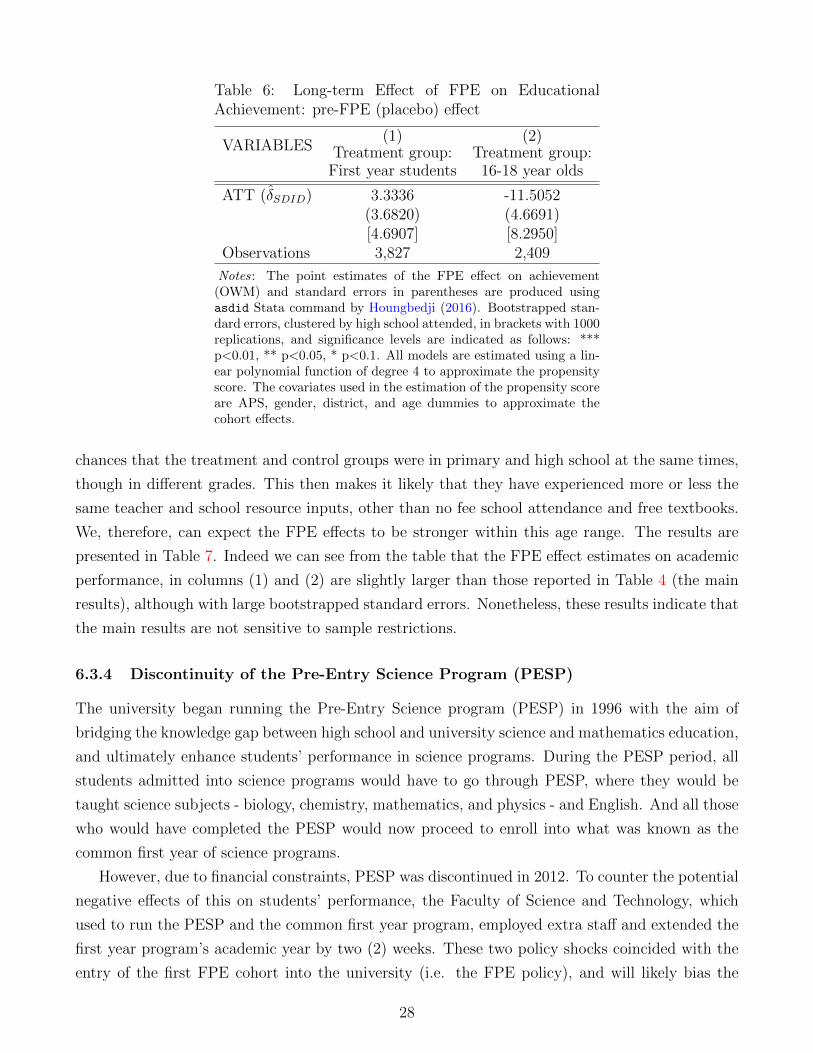
Table 6: Long-term Effect of FPE on EducationalAchievement: pre-FPE (placebo) effect

VARIABLES(1) (2)

Treatment group:First year students


ATT (δSDID) 3.3336 -11.5052(3.6820) (4.6691)[4.6907] [8.2950]

Observations 3,827 2,409

Notes: The point estimates of the FPE effect on achievement(OWM) and standard errors in parentheses are produced usingasdid Stata command by Houngbedji (2016). Bootstrapped stan-dard errors, clustered by high school attended, in brackets with 1000replications, and significance levels are indicated as follows: ***p<0.01, ** p<0.05, * p<0.1. All models are estimated using a lin-ear polynomial function of degree 4 to approximate the propensityscore. The covariates used in the estimation of the propensity scoreare APS, gender, district, and age dummies to approximate thecohort effects.

chances that the treatment and control groups were in primary and high school at the same times,

though in different grades. This then makes it likely that they have experienced more or less the

same teacher and school resource inputs, other than no fee school attendance and free textbooks.

We, therefore, can expect the FPE effects to be stronger within this age range. The results are

presented in Table 7. Indeed we can see from the table that the FPE effect estimates on academic

performance, in columns (1) and (2) are slightly larger than those reported in Table 4 (the main

results), although with large bootstrapped standard errors. Nonetheless, these results indicate that

the main results are not sensitive to sample restrictions.

6.3.4 Discontinuity of the Pre-Entry Science Program (PESP)

The university began running the Pre-Entry Science program (PESP) in 1996 with the aim of

bridging the knowledge gap between high school and university science and mathematics education,

and ultimately enhance students’ performance in science programs. During the PESP period, all

students admitted into science programs would have to go through PESP, where they would be

taught science subjects - biology, chemistry, mathematics, and physics - and English. And all those

who would have completed the PESP would now proceed to enroll into what was known as the

common first year of science programs.

However, due to financial constraints, PESP was discontinued in 2012. To counter the potential

negative effects of this on students’ performance, the Faculty of Science and Technology, which

used to run the PESP and the common first year program, employed extra staff and extended the

first year program’s academic year by two (2) weeks. These two policy shocks coincided with the

entry of the first FPE cohort into the university (i.e. the FPE policy), and will likely bias the

28

Table 7: Long-term Effect of FPE on EducationalAchievement: Narrow age range (18-22)

VARIABLES(1) (2)



ATT (δSDID) 19.8659 3.7067(3.8932) (2.1174)

[100.3128] [15.0155]Observations 10,032 3,943


overall FPE effect on academic achievement.

Therefore, as a robustness check, I control for this potential confounding factor by removing

all PESP affected students from the Faculties of Agriculture, Health Sciences, and Science and

Technology, and estimate the FPE effect on academic achievement. The results are reported in

table 8. We can see from this table that, similar to the main results, the upper bound effect of

FPE is positive and the lower bound effect of FPE is negative but are statistically insignificant

with large bootstrapped standard errors. It is clear, therefore, that the effect of FPE program

is not driven by the PESP discontinuity, and the resulting increase in employment and teaching

time.17

6.3.5 Doubly Robust DID estimates

If the propensity score is mis-specified, the semiparametric (inverse probability weighted) DID

estimates are biased (Sant’Anna and Zhao, 2020). Therefore, to check the sensitivity of the results

to potential misspecification of the propensity score, I use the Doubly Robust (DR) DID estimator

proposed by Sant’Anna and Zhao (2020). Under repeated cross-section framework, as in the current

case, Sant’Anna and Zhao (2020) provide the following two DR DID estimands that are consistent

and locally semiparametrically efficient;

δdr,rc1 = E

D · 1 {T = t}E [D · 1 {T = t}]

−π(Xi)(1−D)·1{T=t}

1−π(Xi)

E[π(Xi)(1−D)·1{T=t}

1−π(Xi)

](Y − µrc0,Y (T,Xi

) (7)

17The standard DID results presented in table A.3- see columns (3) and (4) - are consistent with the resultspresented here.

29

Table 8: Long-term Effect of FPE on EducationalAchievement: Without PESP-affected students

VARIABLES(1) (2)



ATT (δSDID) 16.7749 -3.5147(3.7257) (3.1510)[10.5722] [15.3209]

Observations 9,946 3,893


and

δdr,rc2 = δdr,rc1 +(E[µrc1,1(Xi)− µrc0,1(Xi)|D = 1

]− E

[µrc1,1(Xi)− µrc0,1(Xi)|D = 1, T = 1

])−(E[µrc1,0(Xi)− µrc0,0(Xi)|D = 1

]− E

[µrc1,0(Xi)− µrc0,0(Xi)|D = 1, T = 1

])(8)

where 1 {T = t} is an indicator function that equals 1 event in the braces is true, µrcd,Y (T,Xi) =

T · µrcd,1(Xi) + (1 − T ) · µrcd,0(Xi), and µrcd,t(Xi) is the outcome regression in repeated cross-section

settings.

Table 9 presents the results. Panel A reports traditional DR DID estimates that are DR

consistent and locally semiparametrically efficient. Panel B reports DR DID estimates that are

DR consistent, locally semiparametrically efficient, and DR efficient (i.e. they are efficient under

misspecification in either the outcome model, µrcd,t(Xi), or the propensity score, π(Xi)).

We can see from panel A of the table that DR estimates are positive and statistically significant

when the treatment group is defined as the first year students (the upper bound effect). We

observe the same in panel B. For example, the results from column (1) of panel A indicate that

the FPE program increased students academic performance by between 0.77 percentage points (or

1 percent) and 2.89 percentage points (or 5 percent). In standard deviations, the FPE effect is

bounded between 0.03 and 0.15 standard deviations. While these effects are economically smaller

than those reported in the main results table, they are consistent in terms of the direction of the

effect.

30

Table 9: Long-term Effect of FPE on Educational Achieve-ment: DR DID estimates

VARIABLES(1) (2)



Panel A: Traditional DR DID estimates

ATT (δDRDID) 2.8628*** 0.7666(0.8439) (0.5148)

[1.1369, 4.5888] [-0.3085, 1.8416]Observations 14,095 14,095Panel B: Improved DR DID estimates

ATT (δDRDID) 5.7425***(0.8318)

[1.4052, 10.0798]Observations 14,095

Notes: The point estimates of the FPE effect on achievement (OWM)and standard errors in parentheses are produced using DRDID R code bySant’Anna and Zhao (2020). Bootstrapped standard errors with 1000replications are in parentheses. 95% Confidence intervals in brackets.Significance levels are indicated as follows: *** p<0.01, ** p<0.05, *p<0.1. The covariates used in the estimation of the propensity scoreare APS, gender, district, and age (age dummies in the first column toapproximate the cohort effects, and age and age squared in the secondcolumn). Panel A reports traditional DR DID estimates that are DRconsistent and locally semiparametrically efficient. Panel B reports DRDID estimates that are DR consistent, locally semiparametrically efficient,and DR efficient (i.e. they are efficient under misspecification in eitherthe outcome model or the propensity score).

6.4 Potential mechanisms

So far, I have not specified any possible channels through which FPE program generates these

positive effects. This section attempts to narrow down on the possible causal channels through

which the observed positive effects the program could have emerged based on figure 4 and previous

research.

It is well documented in the literature that elimination of user-fees leads to an increase in

access to schooling and, conditional on teacher recruitment, increases pupil teacher ratio (PTR)

(see Grogan, 2009; Chyi and Zhou, 2014; Moshoeshoe et al., 2019). And high PTR, especially

due to an influx of poor children coming to school, leads to a decline, or at the most no change,

in academic performance, holding all else constant (see Case and Deaton, 1999; Lucas and Mbiti,

2012). Similarly, building more schools, holding teacher recruitment constant, leads to an increase

in access and PTR, and hence a decrease in academic achievement.

Furthermore, conditional on enrollment and teacher quality, increasing access to textbooks

leads to an increase, at least not a decline, in academic achievement (see Glewwe et al., 2009;

31

Frolich and Michaelowa, 2011; Kuecken and Valfort, 2013). And the increase in teacher quality

(i.e. teacher level of qualification and years of experience) can increase, but not decrease, academic

achievement (Glewwe et al., 2011; Harris and Sass, 2011; Chetty et al., 2014).

Following the introduction of the FPE program, there was a decline in PTR, an increase in

students’ textbook ownership, and an increase in teacher qualification and years of professional

training (Moshoeshoe, 2015). Further, Moshoeshoe (2019) shows that academic achievement of

six graders increased between 2000 (pre-FPE) and 2007 (post-FPE), and this increase was partly

attributable to the fall in PTR. Therefore, the increase in teacher employment likely contributed

to the increase in academic achievement at primary school level.

Taken together, therefore, it is less likely that the positive FPE program effects documented in

this paper are due to fee eliminations. The progressive implementation of the fee eliminations al-

lowed the government to plan for the influx by recruiting more teachers and building more schools,

which potentially enabled teachers to adjust their teaching strategies, as they learn, to effectively

reach low-ability and/or poor students. These additional program components, individually and in

complementarity with each other, are the likely drivers of the positive FPE program effect on aca-

demic achievement. For instance, while the school building component of the FPE program is less

likely to have contributed to the increase in academic achievement individually, it was potentially

complemented by teacher recruitment and textbook provision to positively affect achievement.

And because skill begets skill, this led to an increase in academic achievement at university level.

7 Conclusion

This paper examines the long-term effect of Free Primary Education policy on educational achieve-

ment, and how this varies by gender. The results indicate that the effect of FPE on educational

achievement at university level is bounded between 2 percentage (which is statistically insignific-

ant) and 20 percentage points (which is statistically significant at 1 percent). I do not find any

FPE effect heterogeneities by student gender, but the effect varies by faculty or program of study.

In countries where the FPE policy was introduced simultaneously for all grades, it was found

that education quality declined, at least in the short run (see Lucas and Mbiti, 2012). However,

in countries where no user-fees programs have been implemented progressively across the country,

like the rural China’s free and compulsory education reform program, there are positive long-

run effects on education quality (Xiao et al., 2017). The results suggest that other Sub-Saharan

African countries that are yet to implement free education programs can potentially increase their

chances of meeting the SDG goal of inclusive and equitable education quality for all if they replicate

Lesotho’s FPE implementation approach. Further, these results provide important policy lessons

to many countries (e.g. Tanzania) that are implementing (or contemplating to implement) free

secondary or lower secondary education programs.

32

This paper is not without limitations. As highlighted earlier, the FPE program in Lesotho is a

true package of supply and demand side programs all geared towards achieving quality education

for all. Therefore, while these results are interesting, they must be interpreted with caution: they

do not show the effects of just fee eliminations. As we have seen in figure 3, maybe in anticipation

of the influx into the secondary schooling system, secondary school resources increased from 2005.

These results are partly attributable to resource increase at the secondary school level. Second,

the study sample is a very select group of smart students who are potentially from rich households.

Nonetheless, these results are informative in that they show how the program has affected this

group.

Furthermore, I cannot completely rule out the possibility that the FPE treated group worked

harder than they would have in order to compensate for the perceived lower education quality they

received under FPE. That is, there could have been a Hawthorne effect. In addition to this, it is

also possible that secondary school teachers may have doubled their effort when teaching the FPE

cohort for the same reasons of perceived primary school education. While these are real threats to

the validity of the results, nothing indicates that there has been any of these coordinated responses

by students and/or teachers that could have biased the results this way. Further research is still

needed to tease out the pathways through which the FPE policy increased students academic

performance.

33

References

Abadie, A. (2005) Semiparametric difference-in-differences estimators, The Review of Economic

Studies, 72, 1–19.

Al-Samarrai, S. and Zaman, H. (2007) Abolishing School Fees in Malawi: The Impact on Education

Access and Equity, Education Economics, 15, 359–375.

Ambrose, D. (2007) The History of Education in Lesotho: Six Brief Subsectoral Studies, Lesotho

Miscelaneous Documents, No. 23.

Angrist, J. D. and Pischke, J.-S. (2009) Mostly harmless econometrics: An empiricist’s companion,

Princeton University Press, New Jersey.

Becker, G. S. and Tomes, N. (1986) Human Capital and the Rise and Fall of Families, Journal of

labor economics, pp. S1–S39.

Behrman, J. R. (2010) Investment in education – inputs and incentives, in Handbook of Develop-

ment Economics (Eds.) D. Rodrik and M. Rosenzweig, Elsevier, vol. 5, pp. 4883 – 4975.

Black, S. E., Devereux, P. J. and Salvanes, K. G. (2011) Too young to leave the nest? The effects

of school starting age, The Review of Economics and Statistics, 93, 455–467.

Blimpo, M. P., Gajigo, O. and Pugatch, T. (2016) Financial constraints and girls’ secondary

education: Evidence from school fee elimination in the gambia, The World Bank Economic

Review, p. lhw051.

Blundell, R. and Dias, M. C. (2009) Alternative Approaches to Evaluation in Empirical Microeco-

nomics, Journal of Human Resources, 44, 565–640.

Bureau of Statistics (2015) 2014 Education Sstatistics Report Force Survey, Statistics Report, No.

28.

Cabus, S. J. and De Witte, K. (2011) Does school time matter? - on the impact of compulsory

education age on school dropout, Economics of Education Review, 30, 1384–1398.

Caceres-Delpiano, J. and Giolito, E. P. (2019) The impact of age of entry on academic progression,

in Data-Driven Policy Impact Evaluation, Springer, pp. 249–267.

Case, A. and Deaton, A. (1999) School inputs and educational outcomes in South Africa, The

Quarterly Journal of Economics, 114, 1047–1084.

Chang, N.-C. (2020) Double/debiased machine learning for difference-in-differences models, The

Econometrics Journal, forthcoming.

34

Chetty, R., Friedman, J. N. and Rockoff, J. E. (2014) Measuring the impacts of teachers ii: Teacher

value-added and student outcomes in adulthood, American economic review, 104, 2633–79.

Chyi, H. and Zhou, B. (2014) The effects of tuition reforms on school enrollment in rural china,

Economics of Education Review, 38, 104–123.

Council on Higher Education (2013) Report on the state of Higher Education in Lesotho, Tech.

rep., Council on Higher Education.

Cunha, F. and Heckman, J. J. (2009) The economics and psychology of inequality and human

development, Journal of the European Economic Association, 7, 320–364.

Cunha, F., Heckman, J. J., Lochner, L. and Masterov, D. V. (2006) Interpreting the Evidence on

Life Cycle Skill Formation, in Handbook of the Economics of Education (Eds.) E. Hanushek and

F. Welch, Elsevier, vol. 1, pp. 697 – 812.

Deininger, K. (2003) Does cost of schooling affect enrollment by the poor? Universal primary

education in Uganda, Economics of Education Review, 22, 291–305.

Filmer, D., Rogers, H., Angrist, N. and Sabarwal, S. (2020) Learning-adjusted years of schooling

(LAYS): Defining a new macro measure of education, Economics of Education Review, p. 101971.

Fredriksson, P., Ockert, B. and Oosterbeek, H. (2013) Long-term effects of class size, The Quarterly

Journal of Economics, 128, 249–285.

Frolich, M. and Michaelowa, K. (2011) Peer effects and textbooks in African primary education,

Labour Economics, 18, 474–486.

Glewwe, P., Kremer, M. and Moulin, S. (2009) Many children left behind? Textbooks and test

scores in Kenya, American Economic Journal: Applied Economics, 1, 112–135.

Glewwe, P. W., Hanushek, E. A., Humpage, S. D. and Ravina, R. (2011) School resources and

educational outcomes in developing countries: A review of the literature from 1990 to 2010,

NBER Working Paper, No. 17554.

Grogan, L. (2009) Universal primary education and school entry in Uganda, Journal of African

Economies, 18, 183–211.

Harris, D. N. and Sass, T. R. (2011) Teacher training, teacher quality and student achievement,

Journal of public economics, 95, 798–812.

Haveman, R. and Wolfe, B. (1995) The determinants of children’s attainments: A review of meth-

ods and findings, Journal of Economic Literature, 33, 1829–1878.

35

Heckman, J. J. and Mosso, S. (2014) The Economics of Human Development and Social mobility,

NBER Working Paper 19925.

Hoogeveen, J. and Rossi, M. (2013) Enrolment and Grade Attainment following the Introduction

of Free Primary Education in Tanzania, Journal of African Economies, 22, 375–393.

Houngbedji, K. (2016) Abadie’s semiparametric difference-in-differences estimator, The Stata

journal, 16, 482–490.

Houngbedji, K. (2018) Property rights and labour supply in ethiopia, Annals of Economics and

Statistics/Annales d’Economie et de Statistique, pp. 137–179.

Imbens, G. W. and Wooldridge, J. M. (2009) Recent Developments in the Econometrics of Program

Evaluation, Journal of Economic Literature, 47, 5–86.

Jopo, H., Maema, M. and Ramokoena, M. (2011) Quality of primary school inputs in Lesotho,

SACMEQ Policy Brief, No. 2.

Kuecken, M. and Valfort, M.-A. (2013) When do textbooks matter for achievement? Evidence

from African primary schools, Economics Letters, 119, 311–315.

Leibowitz, A. (1974) Home investments in children, The Journal of Political Economy, 82, S111–

S131.

Lekhetho, M. (2013) The Impact of Free Primary Education on Access and Quality of Primary

Education in Lesotho, International Journal of Educational Science, 5, 397–405.

Liang, X., Tan, J.-P. and Mutumbuka, B., Dzingai (2005) Primary and Secondary Education

in Lesotho - a Country Status Report for Education. africa education country status report.

washington, dc: World bank., Tech. rep., World Bank; Africa Region Human Development

Working Paper Series, No. 101.

Lucas, A. M. and Mbiti, I. M. (2012) Access, Sorting, and Achievement: The Short- Run Effects

of Free Primary Education in Kenya, American Economic Journal: Applied Economics, 4, 226–

253.

MOET (2010) Education Statistics Report), Tech. rep.

MOET (2011) Presentation on Education Management Information System (EMIS): 1999-2011,

Tech. rep.

MOET (2016) 2016 Education Statistics Report), Tech. rep.

36

Moshoeshoe, R. (2015) Essays in economics of education: free primary education, birth order and

human capital development in Lesotho, Ph.D. thesis, University of Cape Town.

Moshoeshoe, R. (2019) Changes in Educational Achievement after the Free Primary Education

programme in Lesotho: A Relative Distribution Analysis, Working Paper.

Moshoeshoe, R., Ardington, C. and Piraino, P. (2019) The Effect of the Free Primary Education

Policy on School Enrolment and Relative Grade Attainment in Lesotho, Journal of African

Economies, 28, 511–532.

Nishimura, M., Yamano, T. and Sasaoka, Y. (2008) Impacts of the universal primary education

policy on educational attainment and private costs in rural Uganda, International Journal of

Educational Development, 28, 161–175.

Ponzo, M. and Scoppa, V. (2014) The long-lasting effects of school entry age: Evidence from Italian

students, Journal of Policy Modeling, 36, 578–599.

Sant’Anna, P. and Zhao, J. B. (2020) Doubly robust difference-in-differences estimators, Journal

of Econometrics, Forthcoming.

Todd, P. E. and Wolpin, K. I. (2003) On the specification and estimation of the production function

for cognitive achievement, The Economic Journal, 113, F3–F33.

UNDP (2016) Sustainable Development Goals Booklet, Tech. rep., UNDP.

UNESCO (2000) The Dakar Framework for Action: Education for All, Meeting our Collective

Commitments, Tech. rep., UNESCO.

Urwick, J. (2011) ”Free Primary Education in Lesotho” and the disadvantages of the highlands,

International Journal of Educational Development, 31, 234–243.

World Bank (2016) World Development Indicators: Featuring the Sustainable Development Goals,

Tech. rep., World Bank.

World Bank (2018) World Development Report: Learning to Realize Education’s Promise, Tech.

rep., World Bank.

Xiao, Y., Li, L. and Zhao, L. (2017) Education on the Cheap: The Long-run Effects of a Free

Compulsory Education Reform in Rural China, Journal of Comparative Economics, 45, 544–562.

37

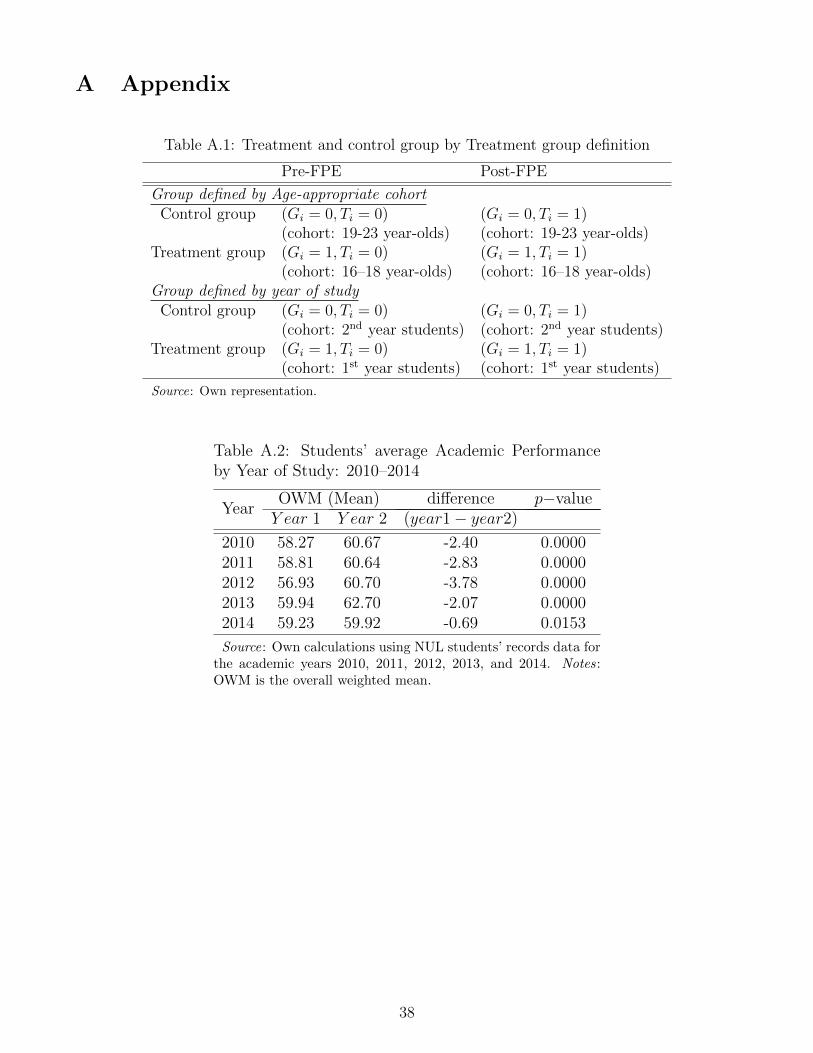
A Appendix

Table A.1: Treatment and control group by Treatment group definition

Pre-FPE Post-FPE

Group defined by Age-appropriate cohortControl group (Gi = 0, Ti = 0) (Gi = 0, Ti = 1)

(cohort: 19-23 year-olds) (cohort: 19-23 year-olds)Treatment group (Gi = 1, Ti = 0) (Gi = 1, Ti = 1)

(cohort: 16–18 year-olds) (cohort: 16–18 year-olds)Group defined by year of study

Control group (Gi = 0, Ti = 0) (Gi = 0, Ti = 1)(cohort: 2nd year students) (cohort: 2nd year students)

Treatment group (Gi = 1, Ti = 0) (Gi = 1, Ti = 1)(cohort: 1st year students) (cohort: 1st year students)

Source: Own representation.

Table A.2: Students’ average Academic Performanceby Year of Study: 2010–2014

YearOWM (Mean) difference p−valueY ear 1 Y ear 2 (year1− year2)

2010 58.27 60.67 -2.40 0.00002011 58.81 60.64 -2.83 0.00002012 56.93 60.70 -3.78 0.00002013 59.94 62.70 -2.07 0.00002014 59.23 59.92 -0.69 0.0153

Source: Own calculations using NUL students’ records data forthe academic years 2010, 2011, 2012, 2013, and 2014. Notes:OWM is the overall weighted mean.

38

Table A.3: Long-term Effect of FPE on Educational Achievement: Standard DID results

VARIABLES(1) (2) (3) (4)

All students Without FOA, FOHS, and FOST studentsTreatment group:

First Year studentsTreatment group:16-18 year olds

Treatment group:First Year students


ATT (δDID) -0.1986 0.3077 0.0505 0.8722*(0.4127) (0.5161) (0.3935) (0.5225)

First Year of study orAge-Appropriate (16-18 years) 1.9499*** 0.7100 1.2837** 0.5104

(0.5661) (0.4347) (0.4985) (0.4252)Period (Post-FPE) -0.8578*** -0.9312*** -0.6356** -0.7282***

(0.2593) (0.2140) (0.2774) (0.2371)Female 1.5807*** 1.4871*** 2.0025*** 1.9139***

(0.2179) (0.2155) (0.2349) (0.2345)APS score -0.5217*** -0.3983*** -0.2898*** -0.2072***

(0.0535) (0.0271) (0.0374) (0.0216)Constant 68.3291*** 66.7340*** 61.0506*** 59.5750***

(0.9359) (0.8588) (0.9132) (0.8310)Observations 12,239 12,239 9,021 9,021R-squared 0.075 0.073 0.037 0.037

Notes: FOA means Faculty of Agriculture, FOHS means Faculty of Health Sciences, and FOST means Faculty of Science and Technology.All regressions control for district, faculty, nationality of the student, age and age squared. Clustered standard errors are in parentheses, andsignificance levels are indicated as follows: *** p<0.01, ** p<0.05, * p<0.1.

39